Knight_Ch1and2.pdf - Effingham County Schools

LOOKING AHEAD ..

The goals of Chapter 1 are to introduce the fundamental concepts of motion and to review the related basic mathematical principles.

The Chapter Preview Each chapter will start wi th an overview of the material to comc. You should read these chapter previews carefully to gel a sense of the conten t and structu re of the chapter.

Looo_ ... [ .... •

Arrows wi ll show the connections and flow between different topics in the preview.

... -~- , -~-----.- ... ~------

~==~ -,-..... • ,-_.,---=-...:.:t=----... __ .-..... _-

:"-:, .. ::::''',::: .. ''!:.., ---... _----- .--.-. -----A chapter preview is a visual presentat ion that outlines the big ideas and the organization of the chapte r to come.

The chapter previews not only let you know what is coming, but also help you make connections with materia l you have already seen.

Looking Back .. We'll tell you what material from prev ious chapters is especially important to review to best understand the new materia l.

Describing Motion Pictures like the one above or the one at right give us val uable clues about motion.

This picture shows successive images of a frog jumping. The images of the f rog are getting farther apart, so the frog must be speeding up.

You will learn to make much simpler pictures to describe the key features of motion.

f = 0 s i s • • 2 s 3s 4 s 5 s 6 s 7 58s This diagram tel ls

us everything we need to know about the mot ion of a ca r.

• • • • ••• / Car starts brak ing here

Numbers and Units For a full desc ription of motion, we need to ass ign num bers to physical quantities such as speed .

This speedometer gives speed in both m iles per hour and kilometers per hour. You w ill learn how to use and convert units and how to describe large and small numbers.

Vectors Num bers alone aren ' t enough, somet imes the direction is important too. We ' ll use vectors to represent such quantiti es.

When you push a swing. the direction of the force makes a difference.

You wi ll see how to do simple math wi th vectors.

1.1 Motion: A First Look The concept of motion is a theme that will appear in one form or another throughout thi s entire book. You have a well-developed intuition about motion , based on your experiences, but you ' ll see that some of the most important aspects of motion can be rather subtle. We need to develop some tools to help us explain and understand motion , so rather than jumping immediately inro a lot of mathematics and calculations, this first chapter focuses on visualizing motion and becoming farruliar with the concepts needed to describe a moving object.

One key difference between phys ics and other sciences is how we set up and solve problems. We' ll often use a two-step process to solve motion problems. The first step is to develop a simplified represelllalioH of the motion so that key elements stand out. For exampl e, the photo of the skier at the start of the chapter allows us to observe his position at many successive times. It is precisely by considering thi s sort of picture of motion that we will begin our study of thi s topic. The second step is to analyze the motion with the language of mathematics. The process of putting numbers on nature is often the most challenging aspect of the problems you will solve. In thi s chapter, we will ex plore the steps in thi s process as we introduce the basic concepts of motion.

Types of Motion As a starting point , let's defin e motion as the change of an object's position or orientation with time . Examples of motion are easy to li st . Bicycles, baseball s, cars, airplanes, and rockets are all objects that move. The path along whi ch an object moves, which might be a straight line o r might be curved, is called the object's trajectory.

FIGURE 1.1 shows four basic types of motion that we will study in thi s book. In thi s chapter, we will start with the first type of motion in the fi gure, motion along a straight line. In later chapters, we will learn about circular motion, whi ch is the Illation of an object alon g a c ircular path ; proj ectil e motion , the Illation of an object through the air; and rotational motion, the spinnin g of an object about an aX1S.

FIGURE 1.1 Four basic types of motion.

Projectile motion Rotational motion

1.1 Motion: A First Look 3

4 CHAPTER 1 Representing Motion

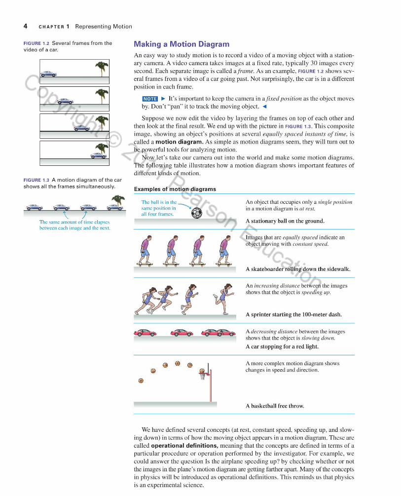
FIGURE 1.2 Several frames from the video of a ca r.

FIGURE 1.3 A motion diagram of the ca r shows all the frames simultaneously.

.~. • ~ / t ...

Tht.:: samc amount of time elapscs bclwcen each image and the nex!.

Making a Motion Diagram

An easy way to study motion is to record a video of a moving object with a stati onary camera. A video camera takes images at a fi xed rate, typically 30 images every second. Each separate image is caJled aframe. As an example, FIGURE 1.2 shows severaJ fram es from a video of a car going past. Not surprisingly, the car is in a different position in each frame.

III!JD .. It 's important to keep the camera in ajixed position as the object moves by. Don't "pan" it to track the moving object. ...

Suppose we now edit the video by layering the frames on top of each other and then look at the final result. We end up with the picture in FIGURE 1.3 . This composite image, showing an object 's positions at several equally spaced installts of time, is calJed a motion diagram. As simple as motion diagrams seem, they will turn out to be powerful tools for analyzing motion.

Now let's take our camera out into the world and make some motion diagrams. The followin g table illustrates how a motion diagram shows important features of different kinds of motion.

Examples of motion diagrams

The ba ll is in Ihe same posi lion in ~ ~ all four frames. ~

An object that occupies only a single po:,·ition in a motion diagram is af rest .

A stationary ball on the ground.

Images that are equally spaced indicate an object moving with cOllstant speed.

A skateboarder roUing down the sidewalk.

An increasing distance between the images shows that the object is speeding III'.

A sprinter starting the lOO-meter dash.

A decreasing distance between the images shows lhat the object is slowing do wl!.

A car stopping for a red light.

A more complex motion diagram shows changes in speed and direclion.

A basketball free throw.

We have defined several concepts (at rest, constant speed, speeding up, and slowing down) in terms of how the moving object appears in a motion di agram. These are called operational definitions. meaning that the concepts are defi ned in terms of a parti cular procedure or operation performed by the in ves tigator. For example, we could answer the question ]s the airplane speeding up? by checki ng whether or not the images in the plane's motion diagram are getting farther apru1. Many of the concepts in physics will be introduced as operational defi nitions. This reminds us that physics is an experimental science.

1.1 Motion: A First Look 5

STOP TO THINK 1 1 Which car is going faster, A or B? Assume there are equal intervals of time between the frames of both videos.

Car A Car B

ImJD .. Each chapter in this textbook has several Slap to Think questions. These questions are designed to see if you've understood the basic ideas that have just been presented. The answers are given at the end of the chapter, but you should make a serious effort to think about these questions before turning to the answers. If you answer correctly and are sure of your answer rather than just guessing, you can proceed to the next section with confidence. But if you answer incorrectly, it would be wise to reread the preceding sections carefully before proceeding onward . ...

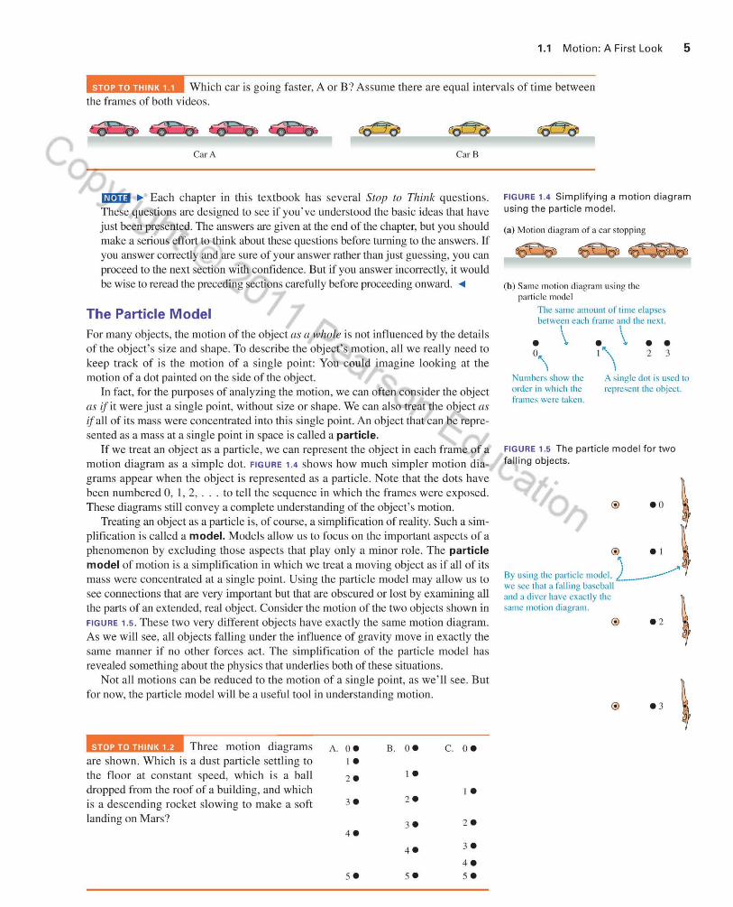
The Particle Model For many objects, the motion of the object as [f whole is not infiuenced by the details of the object's size and shape. To describe the object's motion , all we really need to

keep track of is the motion of a si ngle point: You could imagine looking at the motion of a dot painted on the side of the object.

In fact , for the purposes of analyzing the motion, we can often consider the object liS flit were just a si ngle point, without size or shape. We can also treat the object as ifaU of its mass were concentrated into this single point. An object that can be represented as a mass at a single point in space is called a particle.

If we treat an object as a particle, we can represent the object in each frame of a motion diagram as a simple dot. FIGURE 1.4 shows how much simpler motion diagrams appear when the object is represented as a particle. Note that the dots have been numbered 0, I, 2,. . to tell the sequence in which the frames were exposed. These diagrams still convey a complete understanding of the object's motion.

Treating an object as a particle is, of course, a simplification of reality. Such a simpLification is called a model. Models allow us to focus on the important aspects of a phenomenon by excluding those aspects that play only a minor role. The particle model of motion is a simplification in which we treat a moving object as if all of its mass were concentrated at a single point. Using the particle model may allow us to see connections that are very important but that are obscured or lost by examining aU the parts of an extended, real object. Consider the motion of the two objects shown in FIGURE 1.5. These two very different objects have exactly the same motion diagram. As we will see, all objects falling under the influence of gravity move in exactly the same manner if no other forces act. The simplification of the particle model has revealed somethjng about the physics that underljes both of these situations.

Not all motions can be reduced to the motion of a single point, as we'll see. But for now, the particle model will be a useful tool in understanding motion.

Three motion diagrams A. o. B. o. C. o. are shown. Which is a dust particle settling to ,. the floor at constant speed, which is a ball 2 .

,. dropped from the roof of a building, and which ,. is a descending rocket slowing to make a soft 3 . 2 .

landing on Mars? 3 . 2 . 4.

4 . 3 .

4 . 5 . 5 · 5 .

FIGURE 1.4 Simplifying a motion diagram using the particle model.

(a) Molion d iagram of a car stoppi ng

(b) Same motion diagram usi ng the particle model

The same :HTlOunl o f time elapses between each frame and the nex t.

\ \ • \. . \.

\ '\ • 2 • 3

Numbers show (he order in which the frames were lal\cll.

A single d Ol is used 10 represent the object.

FIGURE 1.5 The particle model for two falling objects.

.0 i """"' ""~,,,,-,G~ we sec lhal a f'liling baseba ll and a diver have exactly the same Illotion diagram.


FIGURE 1.6 Describing your position.

Origin (post office)

nnb Direction Your position

"" W-E

4 miles

Sometimes measurements have a natural origin. This snow depth gauge has its origin set at road level.

FIGURE 1.7 The coordinate system used to describe objects along a country road.

The post offi ce defi nes the zero, or origi n. of the coordinutc !.ystcm. )

,~'" ,~, - 6 1 5 - 4 - 3 - 2 - 1 0

Th is cow is at posi ti on - S miles.

, ,'!?', , 2 3 /' 4 Smiles

Your car is at position + 4 mi les.

1.2 Position and Time: Putting Numbers on Nature

To develop our understanding of motion further, we need to be able to make quantitative measurements: We need to use numbers. As we analyze a motion diagram, it is useful to know where the object is (its positioll) and when the object was at that position (the time) . We' ll start by considering the motion of an object that can move only along a straight line. Examples of this one-dimensional or " 1-0" motion are a bicyclist moving along the road, a train moving on a long straight track, and an elevator moving up and down a shaft.

Position and Coordinate Systems Suppose you are driving along a long, straight country road, as in FIGURE 1.6, and your friend calls and asks where you are. You might reply that you are 4 miles east of the post office, and your friend would then know just where you were. Your location at a particular in stant in time (when your friend phoned) is called your position. Notice that to know your position along the road, your friend needed three pieces of information. First, you had to give her a reference point (the post office) from which all di stances are to be measured. We call this fixed reference point the origin. Second, she needed to know how far you were from that reference point or origjn~in thi s case, 4 miles, Finally, she needed to know which side of the origin you were on: You could be 4 miles to the west of it or 4 miles to the east.

We will need these same three pieces of information in order to specify any object's position along a line. We first choose our origin, from which we measure the position of the object. The position of the origin is arbitrary, and we are free to place it where we li.ke. Usually, however, there are certain points (such as the well-known post office) that are more convenient choices than others.

In order to specify how far our object is from the origin, we lay down an imaginary axi s along the line of the object's motion . Like a ruler, thi s axis is marked off in equal ly spaced divi sions of distance, perhaps in inches, meters, or miles, dependjng on the problem at hand. We place the zero mark of th.i s ruJer at the origin, aLlowing us to locate the position of our object by reading the ruler mark where the object is.

Finally, we need to be able to specify which side of the origin our object is on. To do this, we imagine the axis extending from one side of the origin with increasing positive markings; on the other side, the axi s is marked with increasing I/.egative

numbers. By reporting the position as either a positive or a negative number, we know on what side of the origin the object is.

These elements~all origin and an axis marked in both the positive and negative di.rections~can be used to unambiguously locate the position of an object. We call this a coordinate system. We will use coordinate systems throughout this book, and we will soon develop coordinate systems that can be lIsed to describe the positions of objects moving in more complex ways than just along a line. FIGURE 1.7

shows a coordinate system that can be used to locate various objects along the country road discussed earlier.

Although our coordinate system works well for desc ribing the position s of objects located along the axis, our notation is somewhat cumbersome. We need to keep say ing things like "the car is at pos ition +4 miles." A better notation, and one that will become particularly important when we study motion in two djmensions, is to use a symbol such as x or y to represent the position along the axis. Then we can say "the cow is at x = -5 miles." The symbol that represents a position along an axis is called a coordinate. The introduction of symbo ls to represen t position s (and, later, velocities and accelerations) also allows us to work with these quantities mathematically.

1.2 Position and Time: Putting Numbers on Nature 7

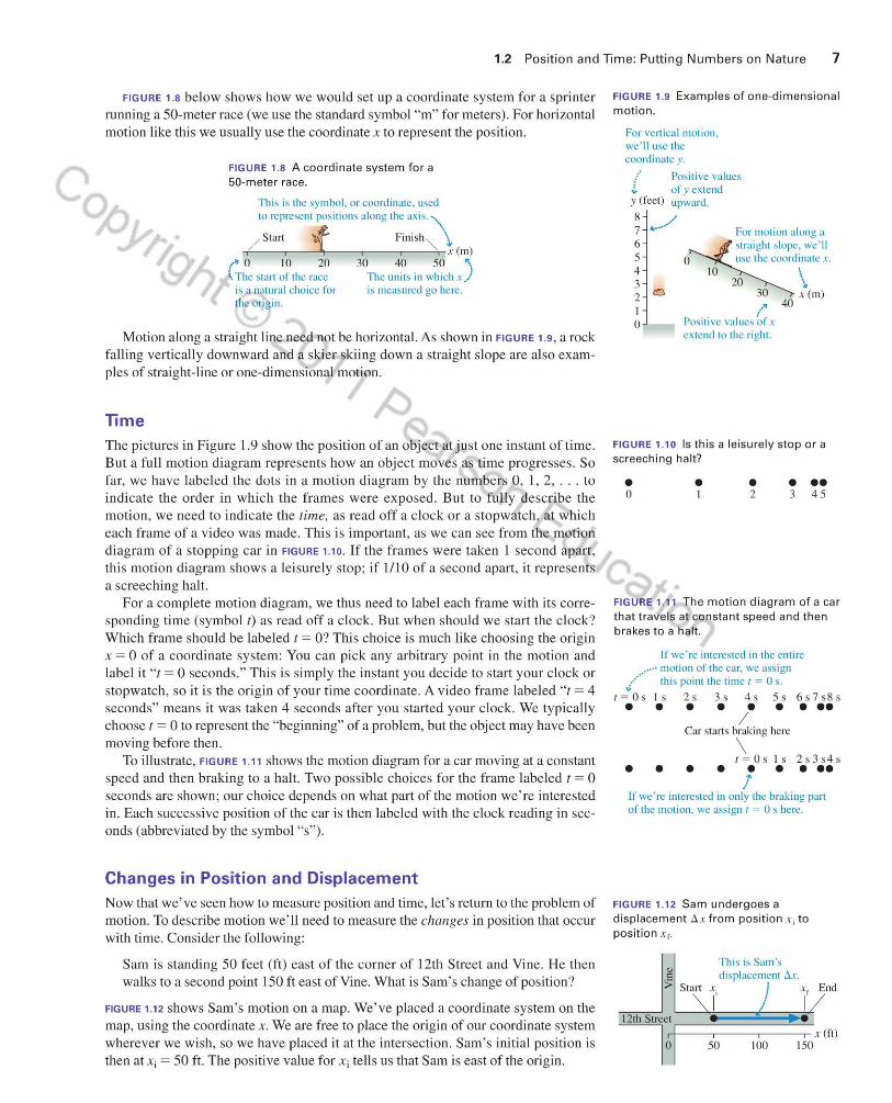
FIGURE 1.8 below shows how we would set up a coordinate system for a sprinter mnning a 50-meter race (we use the standard symbol "m" for meters). For hori zontal motion like this we usuaJJy use the coordinate x to represent the position.

FIGURE 1.8 A coordinate system for a 50-meter race.

Th is is the symbol. or coordinate . used to represent pos it ions along the axis "\

,/ Stan, f , ~1ilI Sh~f \ (In)

I' 0 10 20 30 40 50 i \. The start of the race The un its in which x .J

is a natura l choice for is measured go here. the origin .

Motion along a straight line need not be horizontal. As shown in FIGURE 1.9, a rock falling vertically downward and a skier skiing down a straight slope are al so examples of straight-Line or one-dimensional motion.

Time

The pictures in Figure 1.9 show the position of an object at just one instant of time . But a full motion diagram represents how an object moves as time progresses. So far, we have labeled the dots in a motion diagram by the numbers 0, 1,2, ... to indicate the order in which the frames were ex posed. But to fully describe the motion , we need to indicate the rime, as read off a clock or a stopwatch, at which each frame of a video was made. Thi s is important, as we can see from the motion diagram of a stopping car in FIGURE 1.10. If the fram es were taken 1 second apart, thi s motion diagram shows a leisurely stop; if 1/ 10 of a second apart, it represents a screeching halt.

For a complete motion diagram , we thus need to label each frame with its corresponding time (symbol f) as read off a clock . BUI when should we start the clock? Which frame should be labeled I = 07 This choice is much like choosing the origin x = 0 of a coordinate system: You can pick any arbitrary point in the motion and label it "{ = 0 seconds." This is simply the instant you dec ide to start your clock or stopwatch, so it is the origin of your time coordinate. A video frame labeled " I = 4 seconds" means it was taken 4 seconds after you started your clock . We typically choose I = 0 10 represent the "beginning" of a problem, but the object may have been moving before then.

To illustrate, FIGURE 1.11 shows the motion diagram for a car moving at a constant speed and then braking to a hall. Two possible choices for the fram e labeled 1= 0 seconds are shown; our choice depends on what part of the motion we're interested in. Each successive position of the car is then labeled with the clock reading in seconds (abbrev ialed by the symbol "s").

Changes in Position and Displacement Now that we've seen how to measure position and time, let's return to the problem of motion. To describe motion we' Ll need to measure the changes in position that occur with time. Consider the followin g:

Sam is standing 50 feet (ft) east of the corner of 12th Street and Vine. He then walks to a second point 1.50 ft east of Vine. What is Sam's change of position ?

FIGURE 1.12 shows Sam's motion on a map. We've placed a coordinate system on the map, using the coordinate x. We are free to place the origin of our coordinate system wherever we wish, so we have placed it at the intersection. Sam's initial position is then at Xi = 50 ft. The positive value for Xi tell s us that Sam is east of the origin.

FIGURE 1.9 Examples of one-dimensional motion.

For ven ica! motion. we' ]] use the coord inate y .

.' Positi ve values .;.. of y ex tend y (feel) upward .

~ .../ 6 5 4 3 2 c I o

o 10

For 111otion along a strai ght slope, we'll usc the coord inate x .

20 \ 30 .t (111)

/' 40 Positi ve values of x extend to the ri ght.

FIGURE 1.10 Is this a leisurely stop or a screech ing halt?

• o • I • 2 • •• 3 45

FIGURE 1 .11 The motion diagram ofa car that travels at constant speed and then brakes to a halt.

Ifwc' re interested in the entire ..... motion of the car. we ass ign

."" this point the time 1 = 0 s.

I ="'OS I s 2s 3s 4s 5s 6 s7s8s • • • • • • ••• / Car starts braking here

\ I = OS I s 2s3s4s • • • • • • ••• 1

Ifwc're interested in only the braking pan of the motion . we assign I = 0 s here.

FIGURE 1.12 Sam undergoes a displacement Ax from position Xi to position X f.

J This is Sam 's

.~ di splacement dx. > Stan x. 1 x End

I' I i' ~::~:~I ====;5~~0~~~1~6~0~~·~I~:~O· x cft)

8 CHAPTER 1 Represe nting Motion

The size and the direction of the displacement both matter. Roy Riegels (pu rsued above by team mate Benny Lam) found thi s out in dramatic fashion in the 1928 Rose Bowl when he recovered a fumble and ran 69 yardstowa rd his own tea m's end zone. An impressive distance, but in the w ro ng di rection!

FIGURE 1.13 A displacement is a signed quantity. Here ll X is a negative number.

A fi nal position to the le ft of the initial position gives a negative di splaccment.

lJtl 1 6

1

, 50

12th Street ,

100 , x (fl)

150

FIGURE 1. 14 The motion diagram of a bicycle mov ing to the right at a constant speed.

Os I , 2,

• • • , , , 0 20 40 \

In itial posi tion Xi

EXAMPLE 1 1

3s

• , 60

4 s

• , 80

5 s 6 s

• • I I x (ft ) 100 120

/ Final pos ition x

f

How long a ride?

III.!ID .... We will label special va lues of x or y with subscripts. The value at the start of a problem is usually labeled with a subscript Hi," for initial, and the value at the end is labeled with a subscript "f, " for final. For cases having several special values, we wiJlusually use subscripts" I," "2," and so on . ....

Sam's final position is Xf = 150 ft, indi cating that he is 150 ft eas t of the ori gin . You can see that Sam has changed positi on, and a challge of positio n is called a displacement. His displ acement is the di stance labeled d x in Figure 1.12. The Greek letter delta (d ) is used in math and science to indicate the change in a quantity. Thus d x indicates a change in the position x.

ImlD .... .6. x is a sillgle symbol. You cannot cancel out or remove the .6. in algebraic operations . ....

To get from the 50 ft mark to the J 50 ft mark, Sam clearl y had to walk JOO ft, so the change in hi s position- hi s displacement- is 100 ft. We can think about di splacement in a more general way, however. Displacement is the difference between a fin a] position Xf and an initial position Xi' Thus we can write

~ x = xr - X; = J 50 ft - 50 ft = lOa ft

ImID .... A general principle, used throughout thi s book, is that the change in any quantity is the fjnal value of the quantity minus its injtia l vaJue . ....

Displacement is a siglled quaHliry; that is, it can be either positi ve or negative. If, as shown in FIGURE 1.13 , Sam's final position Xf had been at the origin instead of the 150 ft mark, his di splacement would have been

~x = xl' - X ; = a ft - 50 ft = - 50 ft

The negative sign tells us that he moved to the left along the x-ax is, or 50 ft lVesl.

Change in Time

A displacement is a change in positio n. In order to quantify motion, we' ll need to also consider changes in time, which we call time intervals. We've seen how we can label each frame of a motion diagram with a specific time, as determined by our stopwatch. FIGURE 1.14 shows the motion diagram of a bicycle moving at a constant speed, with the times of the measured poi nts indicated.

The displacement between the initial position Xi and the final position Xf is

~ x = Xr - x ; = 120 ft - a ft = J 20 ft

Simjlarly, we defi ne the time interval between these two points to be

~I = Ir - I; = 6 s - a s = 6 s

A time interval t.t measures tbe elapsed time as an object moves from an initial position Xi at time ti to a final position Xf at time t f o Note that , unlike .6.x, .6.1 is always positive because If is a lways greater than I i'

Carol is enjoy ing a bicycle r ide on a country road that runs eas(- FIGURE 1.15 A drawing of Carol's motion.

west past a water tower. Define a coordinate system so that inc reasing x means moving east. At noon, Carol is 3 miles (mi) east of the waler tower. A half-hour later, she is 2 mi west of the water tower. What is her displacement during that half-hour?

PREPARE Allhough it may seem like overki ll for s lich a s imple problem, you should start by making a drawing, like the one in FIGURE 1.15, with the x-axi s along the road. Distances are measured with respect to the water tower, so it is a natural origin for the

End x , •• ,

- 2 ,

- I

! dx

Stan X,

• , , , x(mi) 0 2 3

1.3 Velocity 9

coordinate system. Once the coordinate system is established, we can show Carol's initial and final positions and her displacement between the two.

SOLVE We've specified values for Carol's initiaJ and final positions in our drawing. We can thus compute her displacement:

ASSESS Once we've completed the solution to the problem, we need to go back to see if it makes sense. Carol is moving to the west, so we expect her displacement to be negative-and it is. We can see from Ollr drawing in Figure 1.15 that she has moved 5 miles from her starting position, so our answer seems reasonable.

6.x =Xr-Xj = (-2 mi) - (3 mi ) = - 5 mi

ImD] .... All of the numerical examples in the book are worked out with the same three-step process: Prepare, Solve, Assess. It's tempting to cut corners, especiaLly for the simple problems in these early chapters, but you should take the time to do all of these steps now, to practice your problem-solving technique. We' ll have more to say about our general problem-solving strategy in Chapter 2 . ....

STOP TO THINK 1 3 Sarah starts at a positive position along the x-axis. She then undergoes a negative di splacement. Her final position

A. Is positive. B. Is negative. C. Could be either positive or negative.

1.3 Velocity We aU have an intuitive sense of whether something is moving very fast or just cruising slowly along. To make this intuitive idea more precise, let 's start by examining the motion diagrams of some objects moving along a st raight line at a constant speed, objects that are neither speeding up nor slowing down. This motion at a constant speed is called uniform motion. As we saw for the skateboarder in Section 1.1 , for an object in uniform motion, successive frames of the motion diagram are equally spaced. We know now that this means that the object's displacement d x is the same between successive frames.

To see how an object's displacement between successive frames is related to its speed, consider the motion diagrams of a bicycle and a car, traveling along the same street as shown in FIGURE 1.16. Clearly the car is moving faster than the bicycle: In any I-second time interval , the car undergoes a displacement dx = 40 ft, while the bicycle's displacement is ollly 20 ft.

The distances traveled in ] second by the bicycle and the car are a measure of their speeds. The greater the distance traveled by an object in a given time interval , the greater its speed. Thi s idea leads us to define the speed of an object as

distance traveled in a given time interval speed = ----------"------

time interval

Speed of a moving object

For the bicycle, this equation gives

while for the car we have

20 ft ft speed = -- = 20-

Iss

40 ft ft speed = -- = 40-

1 s s

The speed of the car is twice that of the bicycle, which seems reasonable.

(1.1)

ImD] .... The division gives units that are a fraction: ft/s. This is read as "feet per second," just Like the more familiar "miles per hour." ....

~.

FIGURE 1.16 Motion diagrams for a car and a bicycle.

During each second, (he car moves tw ice as far as the bicycle. Hence (he car is moving at a greater speed.

0 ,

• \ I , \ h 3,

\ . . . • Car

Os l s\ 2s 3s • ..... • Bicycle .;., ---;,;.--.:---;-, ---;,---"CC{-, =,,-~, -x (ft) o 20 40 60 80 100 f20


FIGURE 1.17 Two bicycles travel ing at the same speed, but w ith diffe rent ve lociti es.

Bike 1 is moving Bi ke 2 is moving to the righl. to the left .

Os 1 I , 2 , 3, 4, 5 s l 6 s -- • • • - 1- Bike I

6, 5 , 4 , 3, 2, I s .i- 0 s • • • • • -- Bike 2 , , , , , , , x ( fI) 0 20 40 60 80 100 120

@

To fully charac terize the motion of an object, it is important to specify not o n.l y the object's speed but also the directioll in which it is moving. For example, FIGURE 1.17

shows the motio n di agrams of two bicycles trave li ng at the same speed of 20 ft /s. The two bicycles have the same speed, but something about their motion is differentthe direction of their motio n.

The problem is that the "di stance traveled" in Equation L I does n' t capture any information about the di rec tion of travel. But we've seen that the disp/acemellf of an obj ect does contain this information. We can then introduce a new quantity, the velocity, as

displacement .6. x velocity = -'------

time interval .6.1 ( 1.2)

Ve loc ity or a moving objec t

The velocity of bicycle I in Figure 1.17, computed usi.ng the I second time interval between the 1 = 2 sand t = 3 s positions, is

.6. x X3 - X2 v= - =

M 3s-25

60 ft - 40 ft

I 5

ft + 20-

s

while the velocity for bicycle 2, during the same time interval , is

Ll x X, -x, 60 ft - 80 ft v= - =

Ll t 3 s - 2 s i s

ft - 20-

s

lmID ... We have used X2 for the position at time t = 2 seconds and X3 for the positio n at time t = 3 seconds. The subscripts serve the same ro le as beforeidenti fy ing parti cular positions-but in thi s case the positions are iden ti fied by the time at which each position is reached . .....

The two veloci ties have opposite signs because the bicycles are trave li ng in opposite directions. Speed measures only how fast an object moves, but velocity tells us both an object's speed and its direction. A positi ve velocity indicates motion to the right or, for vertical motion, upward . Similarly, an obj ect movi ng to the left , or down, has a negati ve velocity.

lmID ... Learn.ing to d istingui sh between speed, which is a lways a positi ve number, and velocity, which can be e ither positive or negative, is one of the most importan t tasks in the analys is of motion . .....

The velocity as defined by Equati on 1.2 is actuall y what is called the average velocity. On average, over each I. s interval bicycle I. moves 20 ft , but we don' t know if it was moving at exactly the same speed at every moment during this time interval. In Chapter 2, we' ll develop the idea of instantalleolls velocity, the velocity of an obj ect at a particul ar instan t in time. S ince our goal in thi s chapter is to visualize motion with motion diagrams, we ' U somewhat blur the distinction between average and instantaneous quantities, refining these defi nitions in Chapter 2, where our goal will be to develop the mathemati cs of mot jon .

EXAMPLE 1 2 Finding the speed of a seabird

Albatrosses are seabirds that spend most of their li ves fl ying over the ocean looking for food. Wi th a stiff tailwi nd. an albatross can fly at high speeds. Satell ite data on one panicula rl y speedy a lbatross showed it 60 miles eas t of its roost at 3:00 PM and then, at 3:20 PM, 86 miles east of its roost. What was its veloc ity?

PREPARE The statement or the problem prov ides us with a nat ural coord inate system: We can measure di stances with respect to the roost, with distances to the east as

1.4 A Sense of Scale: Significant Figures, Scientific Notation, and Units 11

positive. With this coordinate system, the motion of the albatross appears as in FIGURE

1.18. The motion takes place between 3:00 and 3:20, a time interva l of 20 minutes, or 0.33 hour.

FIGURE 1.18 The motion of an albatross at sea.

Stan End

Roost x j ............... ax ~ -' f . ......... -"--T'--T' --r, --,,--x (mi) o 25 50 75 100

SOLVE W e know the initial and final positions, and we know the time interval, so we can calculate the velocity:

6.x Xf - Xi 26 mi v = t;; = 0.33 h = 0.33 h = 79 mph

ASSESS The velocity is positive, which makes sense because Figure 1.18 shows that the motion is to the right. A speed of 79 mph is certainly fast, but the problem said it was a " particularly speedy" albatross, so our answer seems reasonable. (Indeed, albatrosses have been observed to fly al such speeds in the very fast winds of the Southern Ocean. This problem is based on real observations, as will be our general practice in this book.)

The "Per" in Meters Per Second

The units for speed and velocity are a un.it of di stance (feet, meters, miles) divided by a unit of time (seconds, hours). Thus we could measure velocity in units of m/s or mph , pronounced "meters per second" and "mjles per hour." The word "per" wiiJ often arise in physics when we consider the ratio of two quantities . What do we mean, exactly, by "per"?

If a car moves with a speed of 23 mIs , we mean that it travels 23 meters for each I second of e lapsed time. The word "per" thus associates the number of units in the numerator (23 m) with one unit of the denominator (I s) . We' ll see many other examp les of thi s idea as the book progresses. You may already know a bit about dellsity; you can look up the density of gold and you'll find that it is 19.3 glcm' ("g rams per cub ic cent imeter"). Thi s mean s that there are 19.3 grams of gold/or each 1 cubic centimeter of the metal. Thinking about the word "per" in thi s way will help you better understand physical quantities whose units are the ratio of two other units.

1.4 A Sense of Scale: Significant Figures, Scientific Notation, and Units

Physics attempts to explain the natural world, from the very small to the exceedingly large. And in order to understand our world, we need to be able to measure quantities both minuscule and enormous. A properly reported measurement has three elements. First, we can measure our quantity with only a cerlain precision. To make this precision clear, we need to make sure that we report our measurement with the correct number of signijicallt figures.

Second, writing down the really big and small numbers that often come up in physics can be awkward. To avoid writing all those zeros, scientists use scieHt~fic Hotation to express numbers both big and small.

Finally, we need to choose an agreed-upon set of ttl/irs for the quantity. For speed, common units include meters per second and miles per hour. For mass, the kilogram is the most commonly used unit. Every physical quantity that we can measure has an associated set of units.

120 um = 1.2 x 10- 4 III

From galaxies to cells ... BID In science, we need to express numbers both very large and very small . The top image is a computer simulation of the structure of the universe. Bright areas represent regions of clustered galax ies . The boltom image is cortical nerve cells. Nerve cells re lay signals to each other through a complex web of dendrites. These images, though si milar in appearance. differ in scale by a factor of about 2 X I028 !


FIGURE 1.19 The precis ion of a measurement depends on the instrument used to make it.

These cal ipers have a precision or O.OI mill .

Walter Davis's best long jump on this day was reported as 8.24 m . This implies that the actual length of the jump was between 8.235 m and 8.245 m , a spread of only 0.01 m, w hich is 1 cm. Does thi s clai med accuracy seem reasonable?

TRY IT YOURSELF

How tall are you really? U you measure your height in the moming,just after you wake up, and then in the evening, after a full day of activi ty, you' ll find that your even ing height is shorfer by as much as 3/4 inch. Your height decreases over the course of the day as gravity compresses and reshapes your spine. lf you give your he ight as 66 3/16 in, you are claiming more significant figures than are truly warranted; the 3/ 16 in isn' t really reliably known because your height can vary by more than this. Expressi ng your he ight to the nearest inch is plenty!

Measurements and Significant Figures When we measure any quantity, such as the length of a bo ne o r the weight of a spec imen, we can do so with onl y a certain precision. The di gital calipe rs in FIGURE 1.19 can make a measurement to within ± 0.01 mm, so they have a precisio n of 0.0 1 111111. If you made the measurement with a ruler, you probably couldn ' t do bette r than about ± I mm, so the prec ision of the rule r is about I mm . The precision of a measurement can also be affected by the skill or judgmen t of the person performing the measurement. A stopwatch might have a precision of 0.001 s, but, due to your reaction time, your measureme nt o f the time of a sprinte r would be much less precise.

It is important that your measurement be reported in a way that reflec ts its actual precisio n. Suppose you use a ruler to measure the length of a parti cular specimen of a newl y di scovered species of frog. You judge that you can make this measurement with a precisio n of about I mm, or 0.1 cm. In thi s case, the frog's length should be reported as , say, 6.2 cm. We inte rpret this to mean that the actual value fall s between 6.15 em and 6.25 em and thus rounds to 6.2 em. Reporting the frog's length as simpl y 6 cm is saying less than you know ; you are withholding information. On the other hand , to repo rt the number as 6.213 cm is wrong. Any person reviewing your work wou ld interpret the number 6.2 13 cm as meaning that the actual length faUs between 6.2125 em and 6.2135 em, thus rounding to 6.21 3 em. In thi s case, you are claiming to have knowledge and information that you do not reall y possess .

The way to state your knowledge precisely is through the proper use of significant figures . You can think of a significant figure as a dig it that is re liably known. A measurement such as 6.2 cm has fwo signjfi cant fi gures, the 6 and the 2. The next decimal place-the hundredths-is not re liabl y known and is thus not a significant figure. Similarly, a time measurement of 34.62 s has four significant fi gures, implying that the 2 in the hundredths place is reliably known .

When we perform a calculation sLlch as adding or muJtipl y ing two or more measured numbers, we can' t c laim more accuracy for the result than was present in the in.itial measurements. N ine out of ten numbers used in a calcul ation might be known with a precision of 0.0 I %, but if the tenth number is poorly known, with a precision of on ly 10%, then the result of the calculation cannot possibly be more precise than 10%.

Determining the proper number o f significant fi gures is straightforward, but there are a few definite rules to follow. We will often spe ll out such technical details in what we call a "Tactics Box." A Tactics Box is designed to teach you particu lar skills and technjques . Each Tactics Box will use the il icon to designate exercises in the Student Workbook that you can use to practice these skills.

TACTICS BOX 1. 1

Using significant figures

o When you multiply or divide several numbers, or when you take roots, the number of significant figures in the answer should match the number of significant figures of the least precisely known number used in the calculation:

Three significant figures

"-3.73 X 5.7 = 21

/ 1'". An~wcr should have Ihe lower of Two significan t figures .......... the (WO, or two significalH fi gure~ .

Contilllled

1.4 A Sense of Scale: Significant Figures, Scientific Notation , and Units 13

f} When you add or subtract severaJ numbers, the number of decimal places in the answer should match the smallest number of decimal places of any number used in the calculation:

18.54 -Two decimal places

+ I06.6-0ne decimal place

125.1 Co"

.......... Answer should have the (ower of thc two. or one deci ma l place.

€) Exact numbers have no uncertainty and, when used in calculations, do not change the number of significant figures of measured numbers. Examples of exact numbers are 7T and the number 2 in the relation d = 2r between a circle's diameter and radius.

There is one notable exception to these rules:

• It is acceptable to keep one or two extra digits during illfermediate steps of a calculation. The goal here is to minimize round-off errors in the calculation. But the/inal answer must be reported with the proper number of significant figures.

EXAMPLE 1 3 Measuring the velocity of a car

To measure the ve locity of a car, clocks A and B are set up at two points along the road, as shown in FIGURE 1.20 . Clock A is precise to 0.0 1 s, while B is precise to on ly 0. 1 s. The di stance between these two clocks is carefu lly measured to be .1 24.5 m. The two clocks are automatically started when the car passes a trigger in the road; each clock SLOpS automaticall y when the car passes that clock. After the car has passed both clocks, clock A is fo und to read fA = 1.22 s, and clock B to read Is = 4 .5 s. The time from the lessprec ise c lock B is correctly reported wiLh fewer sign ifican t fi gures than that from A. What is the ve locity of the car, and how should it be reported with the cOlTect number of signifi cant fi gures?

FIGURE 1.20 Measuri ng the ve locity of a ca r.

A (l1

~ 't5 '\

Both clocks Sian whcn the car cro~ses thi s trigger.

6.x - 124 .5 m

B

Q

PREPARE To calculate the veloc ity, we need the displacement 6.x and the time in te rval 6. 1 as the car moves between the two clocks. The di splacement is given as 6.x = 124.5 m; we can calculate the time in terval as the di ffe rence between the two mea~

sured times.

Scientific Notation

Exercise 15 II

SOLVE The time interval is:

'fh il> number ha!> Thi s num ber has one decim:.ll pl ace. two decima l places.

\ / tl l ~ IB - IA ~ (4.5 s) - ( 1.22 s) ~ 3.3 s

;' By rule 2 of Tactics Box 1.1 . the result should have one deci mal place.

We can now calculate the veloc ity with the di splacement and the time in terva l:

The displaceme nt has fo ur significant figures .~

tl.x 124.5 Tn v ~ - ~

tl l 3.3 s ~ 38 Tn/s

;' The time interval has / By rule I of Tactics Box 1 1. the result two significant figures. should have fl\ '() significant fi gures .

ASSESS Our fi nal value has two signifi cant fi gures. Suppose you had been hired to measure the speed of a car thi s way, and you reported 37.72 m/s. It would be reasonable for someone looking at your result to assume that the measurements you used to arri ve at thi s value were correct to four sign ificant fi gures and th us that you had measured time to the nearest 0.001 second. Our calTect result of 38 tnls has all of the accuracy that you can claim, but no more!

It 's easy to write down measurements o f ordinary-sized objects: Your height might be 1.72 meters, the weight of an apple 0 .34 pound. But the radius of a hydrogen atom is 0.000000000053 m, and the distance to the moon is 384000000 m. Keeping track of all those zeros is quite cumbersome.


Beyond requiring yo u to deal with all th e zeros, writing quantities thi s way makes it unc lear how many significant figures are involved. In the di stance to the moon g iven above, how many of those digits are sign ifi cant ? Three? Four? All nine?

Writing numbers using scientific notation avoids both these probl ems. A value in scientifi c notation is a number with one digi t to the left of the decimal point and zero or more to the right of it , multiplied by a power of ten. This solves the problem of all the zeros and makes the number of significant figures immed iately apparent. In scientific notation , writing the distance to the sun as 1.50 X 1011 m implies that three digits are signifi cant ; writing it as 1.5 X 1011 m implies Ihat only two digits are.

Even for smaller values, sc ientific notation can clarify the number of significant figures. Suppose a di stance is reported as 1200 m. How many s ignificant figures does thi s measurement have? It 's ambiguous , but us ing scie ntific notation can remo ve any ambiguity. If this di stance is known to within I m, we can write it as 1.200 X 103 m, showing that all four digits are s ignificant ; if it is accurate to only 100 m or so, we can report it as 1.2 X 103 m, indicating two s ignifi cant fi gures.

Tactics Box 1.2 shows how to convert a number to scientific notation, and how to correctly indicate the number of significant figures.

TACTICS B O X 1 . 2 Using scientific notation

To convert a number into scientific notation:

o For a number greater than 10, move the decimal point to the left until only one digit remain s to the left of the decimal point. The remaining number is then multiplied by 10 to a power; thi s power is given by the number of spaces the decimal point was moved. Here we convert the diameter of the earth to scientific notation:

We move the decimal poi nt unti l there is only Since we moved the decimal point one digit to its lef~ , counti ng the number of steps . 6 steps, the power of ten is 6.

\·. ~ ilZe8ee In = ~ X 10";;;-,-TIle number of d igits here equals

the number of s ignificant figu res.

6 For a number less than I, move the decimal point to the right until it passes the first digit that isn't a zero. The remaining number is then multip'-ied by IO to a negative power; the power is given by the number of spaces the decimal point was moved. For the diameter of a red blood cell we have:

We move the decimal poi nt until it passes the first Since we moved the deci nKII poi nt digi t lhat i!> not a zero. counting the number of steps. 6 steps. the power of ten is -6.

'\ .. ~ gg~g~~ 5 In = 7J X w, l;( "-- The nl1mber of d igits here equal s

the number of s ignificant figures.

Exercise 16 II

Proper use of significant figures is part o f the "culture" of science . We will frequently emphasize these "cultural issues" because you must learn to speak the same language as the natives if you wish to communicate effecti vely ! Most students know the rules of significant figures, having learned them in high school, but many fail to

1.4 A Sense of Scale: Significant Figures, Scientific Notation, and Units 15

apply them. It is important that you understand the reasons for significant figures and that you get in the habit of using them properly.

Units

As we have seen, in orderto measure a quantity we need to give it a numerical value. But a measurement is more than just a number-it requires a lIlIil to be given. You canlt go to the deli and ask for " three quarters of cheese." You need to use a unithere, one of weight, such as pounds-in addition to the number.

In your daily life, you probably use the English system of units, in which distances are measured in inches, feet, and miles. These units are well adapted for daily life. but they are rarely used in scientific work. Given that science is an international discipLine, it is also important to have a system of units that is recognized around the world . For these reasons, scientists use a system of units called Ie Systeme Illternarial/ale d'Ullites. commonly referred to as 51 units. S1 units were originally developed by the French in the late 1700s as a way of standardizing and regularizing numbers for commerce and science. We often refer to these as metric ullits because the meter is the basic standard of length.

The three basic SI quantities, shown in Table 1.1, are time, length (or distance), and mass. Other quantities needed to understand motion can be expressed as combinations of these basic units. For example, speed and velocity are expressed in meters per second or m/s. This combination is a ratio of the length unit (the meter) to the time unit (the second).

Using Prefixes

We will have many occasions to use lengths, times, and masses that are either much less or much greater than the standards of I meter, I second, and I kilogram. We will do so by using prefixes to denote various powers of ten. For instance, the prefix "kilo" (abbreviation k) denotes /03, or a factor of 1000. Thus I km equals 1000 OJ ,

I MW equals 106 wallS, and I 11-V equals 10-6 V. Table 1.2 lists the common prefixes that wilJ be used frequently throughout this book. A more extensive li st of prefixes is shown inside the cover of the book.

Allhough prefixes make it easier to talk about quantities, the proper SI units are meters, seconds, and kilograms. Quantities given with prefixed units must be converted to base SI units before any calculations are done. Thus 23.0 em must be converted to 0.230 m before starting calcu lations. The exception is lhe kilogram, which is already the base SJ unit.

Unit Conversions

Although SI units are our standard, we cannot entirely forget that the United Slates still uses Engl ish units. Even after repeated exposure to metric units in classes, most of us "think" in English units. Thus it remains important to be able to convert back and forth between SI units and English units. Table 1.3 shows some frequently used conversions that will come in handy.

One effective method of performing un.it conversions begins by noticing that since, for example, I mi = 1.609 km, the ratio of these two di stances-illcludillg their units-is equal to I , so that

I mi

1.609 km

1.609 km ~~"' = 1

I mi

The importance of units In 1999, (he $ 125 million Mars Climate Orbiter burned up in rhe Martian atmosphere instead of entering a safe orbit from which it could perfo rm observations. The problem was faulty units ! An engineering tcam had provided critical data on spacec raft performance in English units, but the navigation learn assumed these data were in metric units. As a consequence, the navig'lti on team had the spacecrafl fly too close to the planet. and it burned up in the atmosphere.

TABLE 1.1 Common $1 units

Quantity Unit Abbreviation

lime second s

length meter m

mass ki logram kg

TABLE 1.2 Common prefixes

Prefix Abbreviation Power of 10

mega- M 106

kilo- k 10' centi- c 10- 2

milli - m 10-3

micro- Ii- 10-6

nano- n 10-'

TABLE 1.3 Useful unit conversions

I inch (in) = 2.54 em

I foot (ft) = 0.305 In

I mile (mi) = 1.609 kill

I mile per hour (mph) = 0.447 m/s I In = 39.37 in

I km = 0.62 1 mi

A ratio of values equal to I is called a conversion factor. The fo llowing Tactics Box I Ill/s = 2.24 mph shows how to make a unit conversion .


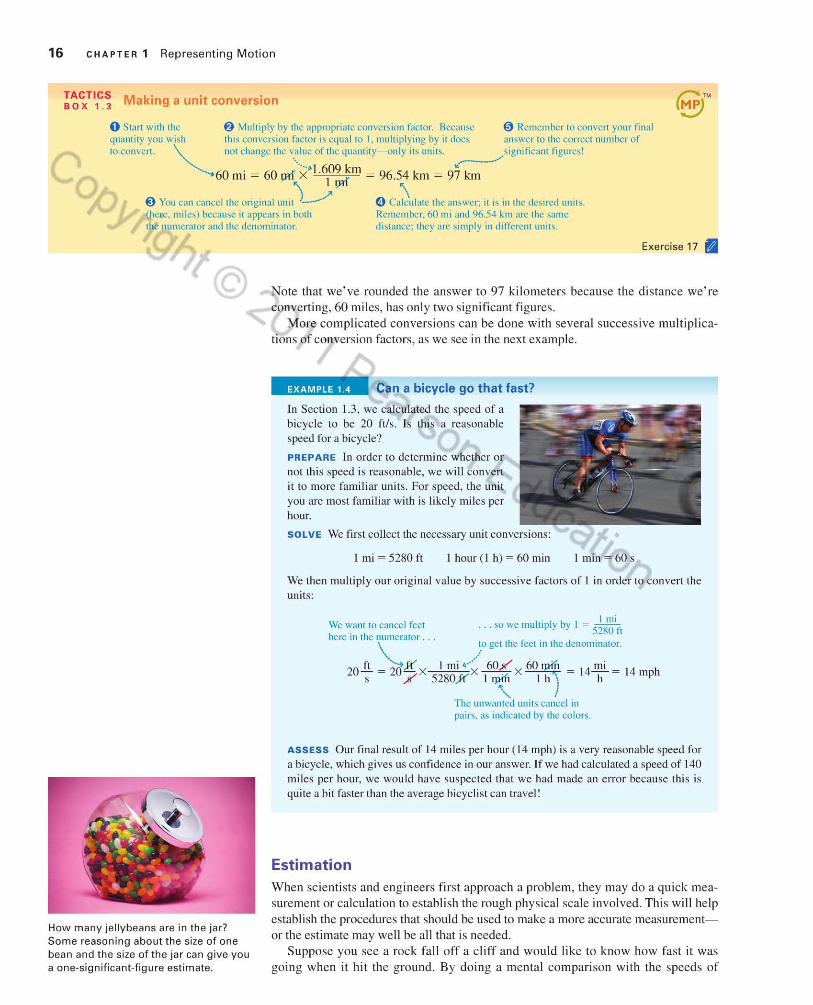
TACTICS BOX 1 . 3 Making a unit conversion

o Stan wi th the 6 Mult iply by the appropriate conversion fac(Or. Because 0 Remember (0 convert your fi nal quantifY you wish Ihis conversion factor is equal fO I, mult ip lying by it does an<i wer (0 the correct number of (0 convert. \ not change the val ue of the quantity-only iL<i unit<i. <iignificum figures!

"-.... .. ---------. -60 mi = 60 prl··X · 1.6?~Jan = 96.54 Jan = 97 km

'\ ? \ 9 You can cancel the origi nal uni t 1_" 6 Calculate the answer: it is in the desired uni ts. (here. miles) because it appears in bOlh Remember, 60 mi and 96.54 km are the same [he numerator and the denominator. distance; they arc simply in differen t units.

How many je llybeans are in the jar? Some reason ing about the size of one bean and the size of the jar can give you a one-signif ica nt-f igu re est imate.

Exercise 17 ill

Note that we've rou nded the answer to 97 kilometers because the di stance we' re converting, 60 miles, has only two significant figures .

More complicated convers ions can be done with several successive multipl.ications of conversion factors, as we see i.n the next example.

EXAMPLE 1 4 Can a bicycle go that fast?

In Sec tion 1.3. we calculated the speed of a bicycle to be 20 ft/s. Is thi s a reasonable speed for a bicycle?

PREPARE In order to de termine whether or not thi s speed is reasonable, we wi ll convert it to more fami liar uni ts. For speed. the uni t you are mosl fam iliar with is li kely miles per hour.

SOLVE We fi rst collec t the necessary unit conversions:

1 mi = 5280 ft I hour ( I h) = 60 min 1 min = 60s

We then mul tip ly our ori ginal value by successive fac tors of I in order to convert the units:

We want 10 cancel feet . l mi

... so we mu ll1 ply by I = 5280 ft hcre in the ll Ulllcrator . ~ t.o get the feet in the denominator.

20.!l = 20K X I mi •.. ~ .. 60/ X 60 ,»iii = 1 4~ = 14 mph s / 5280)( I'~ Ih) h

The unwanted units cal1cel in pairs. as indicated by the colors.

ASSESS Our final resull of 14 mi les per hour (14 mph) is a very reasonable speed for a bicycle, which gives us confidence in our answer. If we had calculated a speed of 140 miles per hour, we would have suspected that we had made an error because thi s is qu ite a bit fasle r than the average bicycl ist can trave l!

Estimation When sc ientists and engineers first approach a probl em, they may do a qui ck measurement or calcul ation to establish the rough physicaJ scaJe i.nvolved. This will help establish the procedures that should be used to make a more accurate measurementor the estimate may well be all that is needed.

Suppose you see a rock fa ll off a cliff and woul d li ke to know how fast it was going when it hit the ground. By doing a mental comparison with the speeds of

1.5 Vectors and Motion: A First Look 17

familiar objects, such as cars and bicycles, you might judge that the rock was traveling at about 20 mph . This is a one-s ignificant-figure est imate. With so me luck, you can probably di st inguish 20 mph from either 10 mph or 30 mph , but you certainly cannot distinguish 20 mph from 2 1 mphjust from a visual appearance. A one-significantfigure esti mate or calculatio n, such as this estimate of speed, is ca ll ed an order-ofmagnitude estimate. An order-of-magnitude estimate is indicated by the symbol "', which indicates even less precision than the "approxi mately equal" symbol ~ . You would report your estimate of the speed of thefalling rock as v - 20 mph.

A useful sk iU is to make reliable order-of-m agnitude estimates on the basis of known information, simple reasoning, and common sense. This is a ski U that is acquired by practice. Tables 1.4 and 1.5 have informat io n that will be useful for doing estimates.

EXAMPLE 1 5 How fast do you walk?

Est imate how fast you walk, in meters per second.

PREPARE In order to compu te speed, we need a d istance and a time. If yo u walked a mile to campus, how long would thi s take? You ' d probably say 30 minutes or s(}-hal f an hour. Let's use this rough num ber in our estimate.

SOLVE Given thi s estimate, we compute speed as

dista nce I mile mi speed = --- - 2 -

time 112 hour h

But we want the speed in meters per second. Since our calculation is only an estimate , we use an approx imate form of the conversion factor from Table 1.3:

mi m 1- "' 0.5 -

h s

This g ives an approx imate walking speed of I m/s.

ASSESS Is thi s a reasonab le value? Let 's do another est imate. Your stride is probably about I yard long- abou t I meter. And you take about one step per second; next time you are walking, you can count and see. So a walk ing speed of I meter per second sounds pretty reasonable .

This sort of estimation is very valuable. We wi ll see many cases in which we need to know an approximate value fo r a quantity before we start a problem or after we finish a problem, in order to assess our results .

STOP TO THINK 1 4 Rank in order, from the most to the fewest , the number of signifi cant figures in the following numbers. For example, if B has more than C, C has the same number as A, and A has more than D, give your answer as B > C = A > D.

A. 0.43 B. 0.0052 C. 0.430 D. 4.321 X 10- 10

1.5 Vectors and Motion: A First Look Many physical quantities, such as time, temperature, and weight , can be described completely by a number with a unit. For example, the mass of an object might be 6 kg and its temperature 30° C. When a physical quantity is described by a single number (with a unit), we call it a scalar quantity. A scalar can be positive, negative, or zero.

TABLE 1.4 Some approximate leng ths

Length (m)

Circumference of the earth

Distance from New York to Los Angeles

Distance you can drive in I hour

Alti tude o r jet planes

Distance across a college campus

Length of a football field

Length of a classroom

Length of your arm

4 X 10'

5 x 10'

I X 10'

I X 10'

1000

100

10

Width of a textbook 0. 1

Length of your litt le fingernail 0.0 1

Diameter of a pencil lead I X 10 3

Thickness of a sheet of paper I X 10-4

Diameter of a dust particle I X 10- 5

TABLE 1.5 Some approximate masses

Mass (kg)

Large airliner I X 10'

Small car 1000

Large human 100

Medillm~s i ze dog 10

Science textbook I

Apple 0.1

Pencil 0.01

Raisin I X 10- 3

Fly I X 10- '


Vectors and scalars

Scalars

Time, temperature and weight are all sca/ar quan ti ties. To specify your weight} the temperature outside, or the cU lTent time, you only need a single num ber.

Vectors

The veloc ity of the race car is a vector. To fu lly specify a veloc ity, we need to give its magnitude (e.g., 120 mph) alld its direction (e.g., west).

The force with which the boy pushes on hi s fr iend is another example of a vector. To completely specify thi s force, we must know not only how hard he pushes (the magnitude) but also in which direct ion.

The boat 's displacement is the st raig ht~

line connect io n f rom its in itia l to its f inal positi on.

Many other quantities, however, have a directional quality and cannot be described by a single number. To describe the moti on of a car, for example, you must specify not onl y how fast it is moving, but also the direcTion in which it is moving. A vector quantity is a quantity that has both a size (How far? or How fas t?) and a direction (Which way?). The size or length of a vector is called its magnitude. The magn.itude of a vector can be positive or zero, but it cannot be negati ve.

Some examples of vector and scalar quantities are shown on the left. We graphically represent a vector as a n arrow, as illu strated for the velocity

and force vectors. The arrow is drawn to point in the direction of the vector quantity, and the length of the arrow is proportional to the magnitude of the vector quantity.

When we want to represent a vector quantity with a symbol, we need so mehow to indi cate that the sy mbol is for a vector rather th an for a scalar. We do th is by drawing an arrow over the letter that represents the quantity. Thus r and A are symbols for vectors, whereas r and A, without the arrows, are symbols fo r scalars. In handwritten work you must draw arrows over all sy mbo ls th at represent vectors . T hi s may seem strange until you get used to it , but it is very important because we will often use both rand r, or both A and A, in the same problem, and they mean d ifferent thin gs!

I1l'!'Iil ... The arrow over the symbol always points to the right, regardless of which di rection tbe actual vector points. Thus we write r or A, never r or A, ....

Displacement Vectors For motion along a line, we found in Section 1.2 that the displacement is a quantity that specifies not onl y how far an object moves but also the directioll-to the left or to the right- that the object moves. S ince displacement is a quantity that has both a magnitude (How far?) and a d irection, it can be represented by a vector, the displacement vector. FIGURE 1.21 shows the displacement vector for Sam's trip that we discussed earlier. We ' ve simpl y drawn an arrow-the vector-from his initial to hi s fin al pos ition and ass igned it the symbol ds. Because ds has both a magnitude and a direc tion, it is conveni ent to write Sam's d isplacement as {is = (l00 ft, east). The first val ue in the paren theses is the magnitude of the vector (Le., the size of the displ acement), and the second value specifies its d irecti on.

FIGURE 1.21 Two displacement vectors.

Jane end

Also show n in Figure 1.2 1 is the di splacement vec tor dJ for Jane, who started on 12th Street and e nded up on Vin e. As with Sam, we draw her d ispl acement vecto r as an arrow fro m her ini tial to her final position. In this case, dJ = 100 ft . 30 0 east of n0l1h).

Jane's trip illustrates an important point about di spl acement vectors. Jane started her trip on 12th Street and ended up on Vine. leading to the di splacement vec tor show n. But to get from her initial to her final positi on, she needn ' t have walked along the straight- li ne path denoted by d,. If she walked east along 12th Street to the intersection and th en headed no rth on Vine, her di splacement would still be the vector show n. An object's displacement vector is drawn from the object's initial position to its final position, regardless of the actual path followed between these two points.


Vector Addition

Let's consider one more trip for the peripatetic Sam. In FIGURE 1.22 , he starts at the intersecti on and walks east 50 ft ; then he walks 100 ft to the northeast through a vacant lot. Hi s di splacement vectors for the two legs ofhjs trip are labeled d, and d2

in the figure. Sam 's trip consists of two legs that can be represented by the two vectors dl and

d2• but we can represent his trip as a whole, from his initial starting position to his overall final pos iti on, with the He t di splace me nt vector labeled dlle! . Sam 's net di splacement is in a sense the sum of the two di splacements that made it up, so we can write

Sam 's net di splacement thus requires the addition of two vectors, but vector addition obeys different rules from the addition of two scalar quantities. The directions of the two vectors, as well as thejr magnitudes, must be taken into account. Sam 's trip suggests that we can add vectors together by putting the " tail" of one vec tor at the tip of the other. Thi s idea, which is reasonabJe for di splacement vectors, in fact is how allY two vectors are added. Tactics Box 1.4 shows how to add two vectors A and B.

TACTICS Adding vectors BO X 1 . 4

To add BtoA: o Draw A.

6 Place the tail of B at the tip of A.

e Draw an arrow from~-the tai~ of A to the Ii tip of B. This is vector A + B. A+B

Exercise 21 II

Vectors and Trigonometry

When we need to add displacements or other vectors in more than one dimension , we' ll end up computing lengths and angles of triangles. This is the job of trigonometry. Trigonometry will be our primary mathematical tool for vector addition; let's review the basic ideas.

FIGURE 1.22 Sam undergoes two displacements.

Sam end

Suppose we have a right triangle with hypotenuse H , angle e, side opposite the FIGURE 1.23 A right triangle. angle 0 , and side adjacent to the angle A, as shown in FIGURE 1.23 . The sine, cosine, and tangent (wh.ich we write as "sin," "cos," and "tan") of angle e are defined as ratios of the sides of the triangle:

A cos e = H o

tane = A (1.3)

If you know the angle e and the length of one side, you can use the sine, cosine, or tangent to find the lengths of the other sides. For example, if you know e and the length A of the adjacent side, you can find the hypotenuse H by rearranging the middle Equa~on 1.3 to give H = A/cosO.

The longest side. opposite the right angle, is the hypotenuse.

"'-. H

A i ,

This is the side opposite the angle.

/

This is lhe side adjuccnt to the angle.


Conversely, if you know two sides of the triangle, you can fi nd the angle e by us ing inverse trigonometric functi ons:

0.4)

We will make regular use of these relationships in the following chapters.

EXAMPLE 1 6 How far north and east?

Suppose Alex is nav igating using a compass. She starts walking at an angle 60° nort h of east and walks a total of 100 m. I-Iow far north is she from her starting point? How far east?

PREPARE A sketch of Alex's motion is shown in FIGURE 1.24a .

We've shown north and east as they would be on a map, and we've noted Alex's displacement as a vector, giving its magnitude and direction. FIGURE 1.24b shows a triangle with thi s displacement as the hypotenuse. Alex's distance nonh of her starting point and her distance east of her start ing poin t are the sides of thi s triangle.

SOLVE The sine and cos ine functions are rat ios of sides of ri ght tri angles, as we saw above. Wi th the 60° angle as noted, the distance north of the starti ng poin t is the opposite side of the tri angle; the distance east is the adjacent side. Thus:

distance north of start = ( 100 m) sin (60°) = 87 m

distance east of start = (100 m) cos (60°) = 50 m

ASSESS Both of the distances we calculated are less than 100 m, as they must be, and the distance east is less than the distance north , as our diagram in Figure 1.24b shows it should be. Our

EXAMPLE 1 7 How far away is Anna 7

Anna walks 90 m due east and then 50 m due north . What is her displacement from her starting po in t?

PREPARE Let's start wi th the sketch in FIGURE 1.25a . We set up a coord inate system with Anna 's original pos ition as the ori gin, and then we drew her two subsequent motions as the two di splacement vectors dl and d2•

FIGURE 1.25 Analyzing Anna's motion.

(a) (b)

Nonh

50

LJ 42 o SOm

0 East 0 50 100 90 m

SOLVE We drew the two vector di splacements with the ta il of one vector start ing at the head of the previous one-exactl y what is needed to form a vector sum. The vector dne1 in Figure 1.25a is the vector sum of the success ive displacements and thus represents Anna's net di splacement from the origin.

An na's distance from the origin is the length of thi s vector dllet • FIGURE 1.25b shows that thi s vector is the hypo tenuse of a right triang le with sides 50 m (because An na walked 50 m

answers seem reasonab le. In find ing the solution to this problem, we "broke down" the displacement into two different distances, one north and one east. This hints at the idea of the components of a vec tor, somethi ng we ' ll explore in the nex t chapter.

FIGURE 1.24 An analysis of Alex's motion.

(b) (al

North

d = ( 100 m, 60° nort h or eas!)

The displacement is the hypotenuse of the !rijng1c.

Di stance ........... north of

start

/1--"----- East

Distance ~ast of start

north ) and 90 m (because she wa lked 90 m east). We can compute the magni tude of thi s vector, her net di splacement, using the Pythagorean theorem (the square of the lengt h of the hypotenuse of a tri angle is equal to the sum of the squares of the lengths o f the sides):

d,~c t = (50 m)2 + (90 m)2

d,", = V(50 m)' + (90 m)' - 103 m '" 100 m

We have rounded off to the appropriate number of sign ificant fi gures, giving us LOO m for the magni tude of the displacement vector. How about the direct ion? Figure 1.25b identifies the angle that gives the angle north of east of An na 's displacement. In the right triangle, 50 m is the opposite side and 90 m is the adjacent side, so the angle is given by

8 = tan I -- = tan 1 - = 29° (50 m) (5) 90 m 9

PUll ing it all together, we get a net displacement of

d net = (100 m, 29° north of east)

ASSESS We can use our drawing to assess our result. If the two sides of the triangle are 50 m and 90 m, a length of 100 m for the hypotenuse seems about right. The angle is certain ly less than 45°, but not too much less, so 29° seems reasonab le.


Velocity Vectors We've seen that a bas ic quantity describing the motion of an object is its velocity. Velocity is a vector quantity because its specification involves not only how fast an object is moving (its speed) but al so the direction in which the object is moving. We thu s represent the velocity of an object by a velocity vector \i that points in the direction of the object's motion , and whose magnitude is the object's speed.

FIGURE 1.26a shows the motion diagram of a car accelerating from res t. We've drawn vectors showing the car's displacement between successive positions of the motion diagram. How can we draw the velocity vectors on this diagram? First, note that the direction of the displacement vector is the direction of motion between successive points in the motion diagram. But the velocity of an object also points ill the direction of motion , so an object's velocity vector points in the same direction as its di splacement vector. Second, we've already noted that the magnitude of the velocity vector-How fast?-is the object's speed. Because higher speeds imply greater displacements in the same lime interval , you can see that the length of the velocity vector should be proportional to the length of the displacement vector between successive points on a motion diagram. Consequently, the vectors connecting each dot of a motion diagram to the next, which we previously labeled as displacement vectors, could equally well be identified as velocity vectors. This is shown in FIGURE 1.26b .

From now on, we'll show and label velocity vectors on motion diagrams rather than displacement vectors.

rmm ... The ve locity vectors shown in Figure 1.26b are actually (Iverage

velocity vectors. Because the velocity is steadily increasing, it 's a bit less than thi s average at the start of each time interval , and a bit more at the end. In Chapter 2 we'll refine these ideas as we develop the idea of in stantaneous velocity . ....

EXAMPLE 1 8 Drawing a ball's motion diagram

FIGURE 1.26 The motion diagram for a car starting from rest.

The di splacement vectors arc lengthening. This means Ihe car is speeding up.

I I _0 sis 2 s \, 3 s " 4 s

(a) d . lt . It • • • • •

(b)

I Start

\ , ... - """"::""- --:;----<-

r \ The longer veloc ity vectors al so indicate Ihat the car is speeding up.

Jake hits a ball at a 600 angle from the horizontal. It is caught by Jim. Draw a motion diagram of the ball that shows ve locity vectors rather than di splacement vectors.

PREPARE This example is typical of how many problems in sc ience and engineering are worded. The problem does not give a clear statement of where the motion begins or ends. Are we interested in the motion or the ball only during the time it is in the air between Jake and Jim? What about the motion a .~· Jake hits it (ball rapidly speeding up) or as Jim catches it (ball rapidly slowing down)? Should we include Jim dropping the ball after he catches it? The point is that you will often be called on to make a reasonable inlerpretation or a problem statement. In thi s problem, the detail s of hitting and catching the ball are complex. The motion of the balllhrough the air is easier to describe, and it' s a motion you might expect to learn about in a physics class. So our interpretation is that the motion diagram should start as the ball leaves Jake's bat (ball already moving) and should end the instant it tOllches Jim 's hand (ball still moving). We will model the ba ll as a partic le.

connec ting the dots with arrows. You can see that the velocity vectors get shorter (ball slowing down), get longer (ball speeding up) , and change direction. Each v is different, so this is I/O/

constant.velocity motion.

SOLVE With thi s interpretation in mind, FIGURE 1.27 shows the mot ion diagram of the ball. Notice how, in contrast to the car of Figure 1.26, the ball is already moving as the motion diagram movie begins. As before, the ve locity vectors are shown by

FIGURE 1.27 The motion diagram of a ball traveling from Jake to Jim.

/

L eJim

" ASSESS We haven't learned enough to make a detai led analys is of the mot ion of the ball , but it's still worthwhile to do a quick assessment. Does our diagram make sense? Think about the ve locity of the ball- we show it moving upward at the start and downward allhe end. This does malch what happens when you toss a ball back and forth , so our answer seems reasonable.


STOP TO THINK 1.5 P and Q are two vectors of equal length but different direction. Which vector shows the sum 15 + Q?

A. B. c. D.

1.6 Where Do We Go from Here? Thi s first chapter has been an introduct ion to some of the fundamental ideas about motion and so me of the basic techniques that yo u will use in the rest of the course. You have seen some examples of how to make models of a physical si tuation, thereby focusing in on the essential elements of the situation. You have learned so me practical ideas, such as how to convert quantities from one kind of units to another. The rest of thi s book-and the rest of your coursewiLl extend these themes. You wiJllearn how to model many kinds of physical sys te ms, and learn the technical s kill s needed to se t up and so lve probl ems using these model s.

In each chapter of this book, you'll learn both new principles and more tools and techniques. We are starting with motion, but, by the end of the book, you'll have learned about more abstract concepts such as magnetic fields and the structure of the nucleus of the atom. As you proceed, you'lJ find that each new chapter depends on those that preceded it. The principles and the problem-solving strategies you learned in this chapter will still be needed in Chapter 30.

We' U give you some assistance integrating new ideas with the material of pre vious chapters. When you start a chapter, the chapter preview will let you know which topics are especially important to review. And the last e lement i.n each chapter will be an integrated example that brings together the principles and techniques you have just learned with those you learned previously. The integrated nature of these examples will also be a helpful reminder that the problems of the real world are similarly complex. and solving such problems requires you to do just thi s kind of integration .

Our first integrated example is reasonably straightforward because there 's not much to integrate yet. The examples in future chapters wiLl be much richer.

<II( Chapter 28 ends w ith an integrated example that explores the basic physics of magnetic resonance imaging (MRIl, explaining how the interaction of magnetic fields with the nuclei of atoms in the body can be used to create an image of the body's interior.

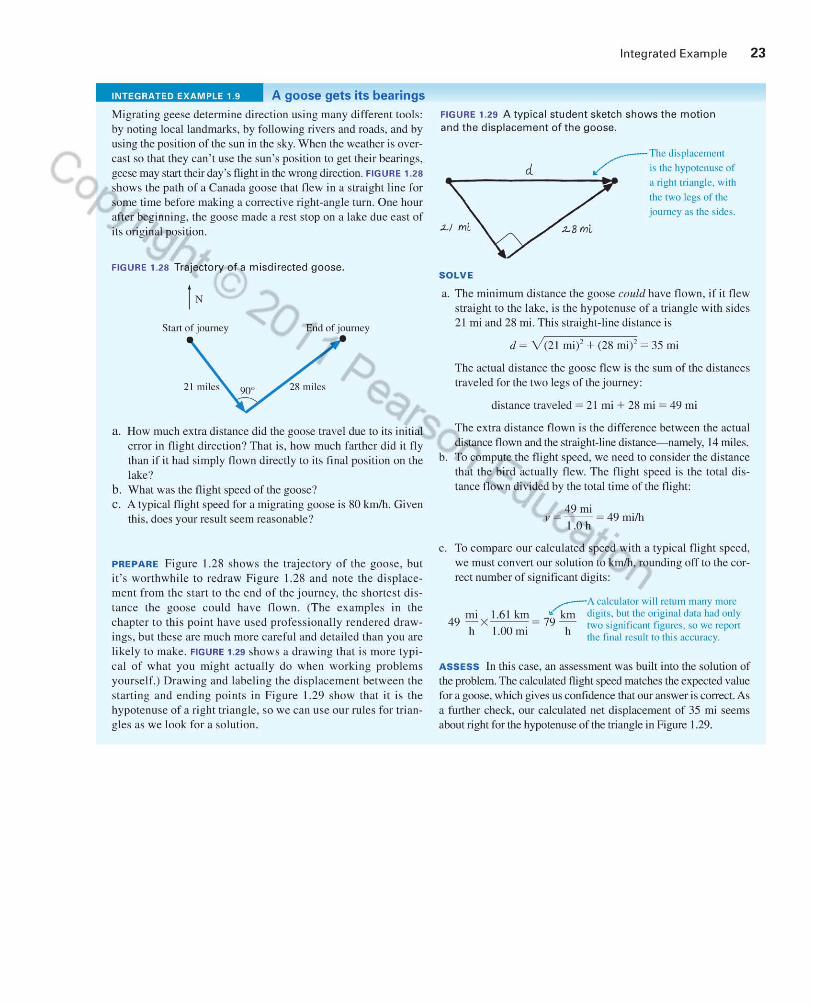
c INTEGRATED EXAMPLE 1 9 A goose gets its bearings

Mi grating geese dete rmine direct ion using many different tools: by noting local landmarks, by followin g rivers and roads, and by using lhe position of the sun in the sky. When Ihe weather is overcast so that they can' t use the sun's pos ition to get their bearings, geese may start their day's flight in the wrong direction. FIGURE 1.28 shows the path of a Canada goose that fl ew in a straight line for some time before making a correcti ve ri ght-angle turn . One hour afte r beginning, the goose made a rest stop on a lake due east of its original position.

FIGURE 1.28 Trajectory of a misdirected goose.

Start of joumey End of joumey

a. How much extra distance did the goose travel due to its initial error in fli ght direction? That is, how much farth er did it fly than if it had simply flown direct ly to its final position on the lake?

b. What was the fli ght speed of the goose? C. A typical flight speed for a migrating goose is 80 km/h. Given

thi s, does your result seem reasonab le?

PREPARE Figure 1.28 shows the trajec tory o f the goose, but it' s worthwhi le to redraw Figure 1.28 and note the disp lacement from the start to the end of the journey, lhe shofl est d istance the goose could have fl own. (The examples in the chapter to thi s point have used professiona lly re nde red drawings, but these are much more careful and detailed than you are likely to make. FIGURE 1.29 shows a drawing that is more typi ca l o f what yo u mi ght actua ll y do when working problems yo urself.) Drawing and labeling the disp lacement between the starting and endi ng points in Figure 1.29 show that it is the hypotenuse of a ri ght triangle, so we can use our rules for triangles as we look for a solution.

Integrated Examp le 23

FIGURE 1.29 A typical student sketch shows the motion and the displacement of the goose.

~ The displacement

d ,,(' is the hypotenuse of

\)/Z aright triangle. wi th

Ihe two legs of the journey as lhe sides .

:L/ mL :La mL

SOLVE

a. The minimum distance the goose could have fl own, if it flew straight to the lake, is the hypotenuse of a triangle with sides 21 mi and 28 mi . This straight-line distance is

d ~ V(2 1 mi )' + (28 mi l ' ~ 35 mi

The actual distance the goose fle w is the sum of the distances traveled for the two legs of the journey:

distance traveled = 2 1 mi + 28 mi = 49 mi

The extra distance flown is the difference between the actual di stance flown and the straight-line distance- namely, 14 miles.

b. To compute the fli ght speed, we need to consider the distance that the bird actually fl ew. The flight speed is the total di stance flown di vided by the total time of the flight:

49mi v ~ -- = 49 milh

I.Oh

c. To compare our calculated speed with a typical fli ght speed, we must convert our solution to kmlh, Jounding off to the correct number of signifi cant digits:

_-A calculator will retum many more mi 1.6 1 km / km di gi t ~. but the original data had onl y

49 - X ---. = 79 - two significant figures, so we repOrt h 1.00 ml h the tina! rcsultlO thi s llCCUr:lCY.

ASSESS In this case, an assessment was built into the solution of the problem. The calculated fligh t speed matches the expected value for a goose, which gives us confidence that our answer is correct. As a further check, ollr calculated net displacement of 35 mi seems about ri ght for the hypotenuse of the triangle in Figure 1.29.


SUMMARY The goals of Chapter 1 have been to introduce the fundamental concepts of motion and to review the related basic mathematical principles.

IMPORTANT CONCEPTS

Motion Diagrams The particle model represents a moving object as if all its mass were concentrated at a si ngle point. Using this model, we can represent motion with a motion diagram, where dots indicate the object's positions at success ive times. In a motion diagram, the time interval between success ive dots is always the same.

Each dot rcprcsents thc position of the obJcct. Each position i~ labeled with the time at which the dot wa, ther~

I = Os

• . ..

I ,

• . ..,/

2 s J 3s

• • 111C time imerval betwcen succes~ive position~ is the same.

Scalars and Vectors Scalar quantities have only a magnitude and can be represented by a single number.

4 ,

• 5 s 6 s

• •

Temperature, time, and mass ~ are scalars. A~ Direction

A vector is a quantity / '--- ~c lengt~ of a vc.ctor described by both a magnitude 1S propon10nai LO 1b;

magni tude. and a direction. Velocity and displacement are vectors.

Velocity vectors can be drawn on a motion diagram by connecting successive points with a vector.

Velocity vectors span succe\sive points in _ _ a mOlion diagram. ':lI

Start

\ ......... . ... The velocity

vectors arc gelling longer, so the object is ~peeding up.

APPLICATIONS

Working with Numbers In scientific notation, a number is expressed as a decimal number between I and 10 multiplied by a power of ten. In sc ientific notation , the diameter of the earth is 1.27 X 107 m.

A prefix can be used before a unit to indicate a multiple of 10 or 1/ 10. Thus we can write the diameter of the earth as 12,700 km, where the k in km denotes 1000.

We can perfonn a unit conversion to convert the diameter of the earth to a different unit, such as miles. We do so by multiplying by a convers ion factor equal to 1, such as I = I mill .6 1 km.

Describing Motion Position locates an object with respect to a chosen coordinate system. It is described by a coordinate.

The C(lortlillllfe is the variable u~ed to deM'ribe the po\ition.

1 ':t 1 i i 1 1 1 1 i ~ 1 ~x(mi) - 6 1 5 - 4 - 3 - 2 - 1 0 I 2 3 ( 4 5

This cow i~ at f = - 5 miles. Thi\ car i~ at .( = + 4 mi les.

A change in position is called a displacement. For motion along a line, a displacement is a signed quantity. The displacement from Xi to X f is ilx = Xf - Xi'

Time iSJneasured from a particular instant to which we ass ign f = O. A time interval is the elapsed time between two specific instants Ii and If. It is given by ill = Ir - 'i'

Velocity is the ratio of the displacement of an object to the time interval during which this displacement occurs:

Ax )I=~

AI

Units Every measurement of a quantity must include a unit.

The standard system of units used in sc ience is the SI system. Common SI units include:

Length: meters (m)

Time: seconds (s)

Mass: kilograms (kg)

Significant figures are reliably known digits. The number of significant fi gures for:

Multiplication, division, and powers is set by the value with the fewest significant figures.

Addition and subtraction is set by the value with the smallest number of decimal places.

An order-of-magnitude estimate is an esti mate that has an accuracy of about one sign ificant figure. Such estimates are usually made using rough numbers from everyday experience.

tMP)TM For homeWO~k assig~ed on MasteringPhysics, go to

;,:,.:,/ www.mastenngphyslcs.com

Problem difficulty is labeled as ! (straightforward) to IJlIl (challenging).

Q UESTIONS

Conceptual Questions

I. a. Write a paragraph describing the particle model. What is it, and why is it import ant?

b. Give two examples o f situations, di fferent from those descri bed in !.he text, for which the panicle model is appropriate.

c. Give an example of a s ituation, di ffere nt from those described in the text, for whic h it would be inappropriate.

2. A softball player slides in to second base. Use the particle model to draw a motion d iagram of the player from the lime he beg ins to sl ide unt il he reac hes the base. Number the dots in order, starting with zero.

3. A car travels to the left at a steady speed for a few seconds, then brakes for a stop s ign. Use the particle model to draw a mot ion di agram of the car for the entire moti on desc ri bed here. Number the dots in order. start ing with zero.

4. A ball is dropped from the roo f o f a tall build ing and students in a phys ics class are as ked to sketch a motion di agram for thi s s ituation. A student submits the di agram shown in Figure QI A. Is the di agra m correct? Ex plain .

FIGURE 01.4

• 0

• I

• 2 • 3 . 4

5. Write a sente nce or two descri b ing the d ifference between pos ition and di splacement. Give one example of each.

6. Give an example of a trip you mi ght take in your car for which the d istance traveled as measured on your car's odometer is not equal to the d isplacement between your initi al and final positions.

7. Wri te a sentence or two desc ri b ing the d iffere nce between speed and veloc ity. Give one example of each.

8. The mot ion of a skateboard along a hori zontal ax is is obse rved for 5 s. The initi al pos ition of the skateboard is negati ve with respect to a chosen orig in, and its ve loc ity throughout the 5 s is also negati ve. At the end of the observation time, is the skateboard closer to or farther fro m the orig in than initi all y? Ex plain .

9. Can the veloc ity of an object be pos itive duri ng a time interval in which its pos ition is always negat ive? Can its veloc ity be pos itive during a time interval in which its d isplacemen t is negat ive?

10. Two Frie nds watch a jogger complete a 400 m lap around the track in 100 s. One of the fri ends states, "The jogger's veloc ity was 4 mls during thi s lap." The second fri e nd objec ts, say ing, "No, the jogger's speed was 4 m/s." Who is correc t? Justi fy your answer.

11. A softball player hits the ball and starts running toward first base. Draw a mot ion d iagram, using the parti cle model , showing he r veloc ity vec tors during the firs t few seconds of her run.

12. A child is sledd ing on a smooth, level patch of snow. She encoun ters a rocky patc h and s lows to a sto p. Draw a motion di agram, using the particle model, showing her veloc ity vectors .

Questions 25

Problems labeled BID are of biolog ical o r medical interest.

13. A skydi ver jumps ou t o f an airplane. Her speed steadi ly increases unt il she deploys her parac hu te, at which po int her speed quic kly decreases. She subsequentl y fa ll s to earth at a constan t rate, stopping when she lands on the g round. Draw a motion diagram, using the particle mode l, that shows her pos iti on at successive times and incl udes veloc ity vectors.

14. Your roommate drops a tenni s ball from a third-story bak ony. It hi ts the sidewalk and bounces as high as the second story. Draw a motion d iagram, using the particle model , showing the ball 's veloc ity vectors from the lime it is released until it reaches the max imum he ight on its bounce.

15. A car is dri ving north at a steady speed. It makes a gradual 90° left tu rn without los ing speed, then conti nues driving to the west. Draw a mo ti on d iagram, using the particle model , showing the car 's veloc ity vectors as seen from a he licopter hovering over the highway.

16. A toy car ro ll s down a ramp, then across a smooth, horizontal fl oor. Draw a mot ion d iagram, using the particle model. showing the car 's veloc ity veclOrs.

17. Estimate the average speed with which you go from home to campus (or another trip you common ly make) via whatever mode of transport ati on you usc most commonly. Give your answer in both mph and m/s . Desc ribe how yo u arrived at thi s estimate.

18. Estimate the num ber of times you sneezed during the paSI year. Desc ri be how you arrived at thi s est imate.

19. Dens ity is the ratio o f an object's mass to its volume. Would you expect de nsity to be a vector or a scalar quantity? Ex plain .

Multiple-Choice Questions

20. I A studen t walks 1.0 mi west and then 1.0 mi north . Afterward, how far is she from her start ing po in t? A. 1.0 mi 8 . IA mi C. 1.6 mi D. 2.0 mi

2 1. I Which of the following mot ions is described by the motion di agram of Figure Q 1.2 1 ? A. An ice skater gliding across the ice. 8 . An airplane braking to a stop after landing. C. A car pulli ng away from a stop s ign. D. A pool ball bouncing off a cushion and revers ing di rection.

o 1 2 FIGURE 01 .2 1 •• •

3 •

4 •

5 •

22. I A bird flies 3.0 km due west and then 2.0 km due north . What is the mag nitude of the bird 's d isplaceme nt? A. 2.0 km B. 3.0 km C. 3.6 km D. 5.0 km


23. II A bird fli es 3.0 km due west and then 2.0 km due no rth. Another bird fl ies 2.0 km due west and 3.0 km due north. What is the ang le between the net displacement vec tors for the two birds? A. 23° B. 34° C. 56° D. 90°

24. I A woman walks bri skly at 2.00 m/s . How much time will it take her to walk one mile? A. 8.30 min B. 13.4 mi n C. 2 1.7 mi n D. 30.0 min

25. 1 Compute 3.24 m + 0.532 m to the correc t number of sign ificant fi gures. A. 3.7 m B. 3.77 m C. 3.772 01 D. 3.7720 01

26. I A rectangle has length 3.24 m and height 0.532 m. To the correct number of significant fi gures, what is its area? A. 1.72 m' B. 1.723 m' C. 1.7236 m' D. '1 .72368 01 '

PROBLEMS

Section 1.1 Motion: A First Look

1. I You' ve made a video of a car as it skids to a halt to avoid hi tti ng an objec t in the road. Use the images from the video to draw a motion diagram of the car from the time the skid begins until the car is stopped.

2. I A man rides a bike along a straight road for 5 mi n, then has a nat ti re. He stops fo r 5 mi n to repair the flat , but then realizes he cannot fi x it. He conti nues hi s journey by walking the rest of the way, which takes him another 10 min. Use the parti cle model to draw a motion diagram of the man for the entire mot ion described here. Number the dots in order, starti ng with zero.

3. I A jogger running east at a steady pace suddenl y develops a cramp. He is lucky: A westbound bus is sitting at a bus stop just ahead. He gets on the bus and enjoys a qu ick ride home. Use the part icle model to draw a moti on diagram of the jogger for the entire motion descri bed here. Number the dots in order, starti ng with zero.

Section 1.2 Position and Time: Putting Numbers on Nature

4. I Figure PI .4 shows Sue between her home and the cinema. What is Sue's posit ion x if a. Her home is the origin? b. The cinema is the origin?

Home Sue Ci nema g B

FIGURE P1.4 2 mi 3 mi

5. I Keira starts at position x = 23 m along a coordinate axis. She then undergoes a displacement of -45 m. What is her final position?

6. I A car trave ls along a stra ight east-west road. A coordinate system is establ ished on the road, with x increasing to the east. The car ends up 14 mi west of the inte rsec tion with Mulberry Road. If its disp lacement was -23 mi , how far from and on which side of Mul berry Road did it start?

7. I Foraging bees often move in straight li nes away fro m and BID toward their hi ves. Suppose a bee starts at its hi ve and fli es 500 m

due east, then fli es 400 m west, then 700 m east. How far is the bee from the hive?

27. I The earth fo rmed 4.57 X 109 years ago. What is thi s time in seconds?

28.

A. 1.67 X 10 12 s C. 2.40 X 10" S

B. 4.0 1 X 10" s D. 1.44 X 10 17 s

III An object's ave rage density p is defin ed as the ratio of its mass to its volume: p = M /Y. The earth's mass is 5.94 X 1024 kg, and its vo lume is 1.08 X J0 12 km3. What is the earth's average density? A. 5.50 X 103 kg/m3

C. 5.50 X 10' kg/m3 B. 5.50 X 10' kg!m3

D. 5.50 X 10 12 kg/m3

Section _1.3 Velocity

8. I A security guard walks 110 m in one trip around the perimeter of the bu ilding. It takes him 240 s 10 make thi s trip. What is hi s speed?

9. II List the following items in order of decreas ing speed, from greatcst to least: (i) A wind-up toy car that moves 0. 15 m in 2.5 s. (ii ) A soccer ball that .ro ll s 2.3 m in 0.55 s. ( iii ) A bicycle that travels 0.60 m in 0.075 s. (iv) A cat that runs 8.0 m in 2.0 s.

10. II Figure PI . IO shows the mot ion diagram for a horse galloping in onc di rection along a straight path. Not every dot is labeled, but the dots are at equally spaced instanls of time. What is the horse's veloc ity a. During the fi rst len seconds of its galJop? b. During the in terva l from 30 s to 40 s? c. During the interva l from 50 s to 70 s?

70s 50s 30s lOs • • •••• • • x(m)

50 150 250 350 450 550 650

FIGURE Pl .l0

II . II It takes Harry 35 s to walk from x = - 12 m to x = - 47 m. What is hi s ve locity?

12. I A dog trots from x = - 12 m to x = 3 m in 10 s. What is its veloc ity?

13. I A ball rol lin g along a stra ight line with veloc ity 0.35 mls goes from x = 2. 1 m to x = 7.3 m. How much t ime does this take?

Section 1.4 A Sense of Scale: Significant Figures, Scientific Notation, and Units

14 . Convert the following to SI uni ts: a. 9. 12/Ls b. 3.42 km c. 44 cm/ms d. 80 kmfhour

IS. Convert the following 10 SI unit s: a. 8.0 in b. 66 ftls c. 60 mph

16. Convert the following to Siuni ts: a. l.0 hour b. 1.0 day c. 1.0 year

17. List the following three speeds in order, from smaLl es l to largest: I mm per /-Ls , 1 km per ks, I cm per ms.

18. I How many signifi cant figures does each of the following numbers have? a. 6.21 b. 62.1 c. 0.620 d. 0.062

19. I How many significant figures does each of the following numbers have? a. 0.62 1 b. 0.006200 c. 1.0621 d. 6.2 1 X 103

20. I Compute the following numbers to 3 significant figures.

2 1.

22.

a. 33.3 X 25 .4 b. 33 .3 - 25.4 c. V3D d. 333.3';- 25.4 JlIII The Empi re State Building has a height of 1250 ft. Express thi s he ight in meters, giving your resu lt in sc ientific notation with three significant figures. I Estimate (don' t measure !) the length of a typical car. Give yo ur answer in both feet and meters. Briefly desc ribe how YOll

arrived at this est imate. 23. III Blades of grass grow from the bottom, so, as growth occurs, BlO the top of the blade moves upward. During the summer, when

yo ur lawn is growing quickly, estimate thi s speed in m/s. Explain how you made thi s est imate, and express your resu lt in scientific notation.

24. II Estimate the average speed with which the hair on your head 810 grows. Give your answer in both mls and ,umlh. Briefly

describe how you arri ved at thi s est imate. 25. II Estimate the average speed at which your fin ge rnail s grow, in BlO both mls and ,um/h. Brieny describe how yo u arrived at thi s

estimate.

Section ].5 Vectors and Motion: A First Look

26. I Carol and Robin share a house. To get to work, Carol walks north 2.0 km while Robin drives west 7.5 km. How far apart are their workplaces?

27. 1 Joe and Max shake hands and say goodbye. Joe walks east 0.55 km to a coffee shop, and Max n ags a cab and rides north 3.25 km to a bookstore. How far apart are the ir dest inat ions?

28. II A city has streets laid out in a square grid, with each block 135 m long. IF yo u dri ve north for three blocks, then west for two blocks, how far are you from your starting point?

29. II A butterfly nies from the top of a tree in the center of a garden to rest on top of a red fl ower at the garden 's edge. The tree is 8.0 m taller than the flower, and the garden is 12 m wide. Determine the magnitude of the butterfly 's di splacement.

30. III A garden has a c ircular path of radius 50 m. John starts at the easternmost point on thi s path, then wa lks counterclockwise around the path until he is at its southernmost point. What is John 's displacement? Use the (magnitude, direction) notat ion for your answer.

3 1. I Migrating geese tend to travel in straight-line paths at approxBIO imately constant speed. A goose flies 32 km south , then turns 10

fly 20 km west. How far is the goose from its original position? 32. Ilill A baU on a porch roUs 60 cm to the porch' s edge, drops 40 em,

continues rolling on the grass, and eventually stops 80 cm from the porch's edge. What is the magnitude of the ball 's net di splacement, in centimeters?

33. II A ki cker punts a footbaU from the very center of the fie ld to the sideline 43 yards down field . What is the net displacement of the ball? (A football field is 53 yards wide. )

Problems 27

General Problems

Problems 34 through 40 are motion problems similar to those you will learn 10 sol ve in Chapter 2. For now, simply interpret the problem by drawing a motion diagram showing the object's position and its veloc ity vec tors. Do not solve these problems or do any mathematics. 34. Il In a typical greyhound race , a dog accelerates to a speed of BID 20 mls over a di stance of 30 m. It then maintains thi s speed.

What would be a greyhound ' s lime in the 100 m dash? 35. Il BiUy drops a wate rmelon from the top of a three-slory build

ing, 10 In above the sidewalk. How fast is the watermelon go ing when il hits?

36. Il Sam is reckless ly dri ving 60 mph in a 30 mph speed zone when he suddenly sees the police. He steps on the brakes and slows to 30 mph in th ree seconds, looking nonchalant as he passes the officer. How far does he Lravel while braking?

37. II A speed skate r moving across fricti o nl ess ice at 8.0 mls hit s a 5.0-m-wide patch of rough ice. She slows steadil y, Ihen conlinues on at 6.0 m/s. What is her accele ralion on the rough ice?

38. Il The giant eland, an African ante lope, is an exceptional BID jumper, able 10 leap 1.5 m off the ground. To jump thi s high, with

what speed must the eland leave the ground? 39. II A ball roll s along a smooth horizontal floor at 10 mis, then

starts lip a 20° ramp. How high doe.. ... it go before rolling back down?

40. Il A motorist is traveling at 20 m/s. He is 60 m from a stop light when he sees illurn yellow. His react ion time, before stepp ing on the brake , is 0.50 s. What steady deceleration while braking will bring him to a SLOp right at the light?

Problems 41 through 46 show a motion diagram. For each of these problems, write a one or two sentence "slory" about a real object that has thi s motion diagram. Your slories should talk about people or objects by name and say what they are doing. Problems 34 through 40 are examples of motion short stories.

41. I

Stop

FIGURE Pl .41 -rO.-.."MO.-_.' ----..-.... .......... ~

42. I

FIGURE Pl .42

43.

II • .. . II . .. Til! ' Stop

II •

•

Top view of motion i) :1 horizontal plane

jj -----. ...............

FIGURE P1 .43 Circular arc

II • II •

28 CHAPTER 1 Repres enting Motion

44. I SIan

The two pans of Ihe motion diagram <Ire displaced for clarity. but the motion <lctually occurs along a single line.

FIGURE P1 .44

Same point

/ "

Stop

45. I Side view or mot ion Circular arc

i"'"'"i7--..(

-~ , FIGURE P1 .45

46. I

FIGURE P1.46

47. 11111 How many inches does li ght travel in one nanosecond? T he speed ofli ghl is 3.0 X lOll m/s.

48. I Joseph watches the roadside mile markers during a long car trip on an interslate hi ghway. He not ices that at 10:45 A.M. they are pass ing a marker labe led 10 1. and at II :00 A.M. the car reaches marker J 19. What is the car's speed, in mph?

49 . II Alberta is go ing to have din ner at her grandmother's house, but she is run ning a bit behind schedule. As she gets onto the highway, she knows that she must ex it the highway withi n 45 min if she is not going to arri ve late. Her ex it is 32 mi away. What is the slowest speed at which she could drive and still ill-rive in time? Express your answer in mi les per hour.

50. II The end of Hubbard Glac ier in Alaska advances by an average of 105 fee t per year. What is the speed of advance of the glacier in mls?

5 1. I The earth completes a circular orbit around the sun in one year. The orbit has a radius of 93,000,000 miles. W hat is the speed of the earth around the sun in m/s? Report your res ult using scientifi c notat ion.

52. III Shan non dec ides to check the accuracy of her speedometer. She adj usts her speed to read exactly 70 mph on her speedometer and holds thi s steady, measuri ng the ti me between successive mile markers separated by exactly 1.00 mile . If she measures a time of 54 s, is her speedometer accurate? If not, is the speed it shows too high or too low?

53. II Motor neurons in mammals transmi t signals from the brain to

BID skeletal muscles at approx imately 25 m/s. Estimate how much time in ms (10- 3 s) it will take for a signal to ge t from yo ur bra in to your hand.

54. III Sate llite data taken several times per hour on a panicular BID albatross showed travel of 1200 km over a time of 1.4 days.

a. Gi ven these data, what was the bird 's average speed in mph? b. Data on the bird 's pos ition were recorded only intermit

ten tly. Explain how this means that the bi rd's actual average speed was higher than what you calculated in part a.

55. I Your bra in communicates with yo ur body using lieI've

BID impulses. electri cal signals propagated along axo ns. Axons come in two variet ies: insu lated axons with a sheath made of mye lin , and uninstll ated axons with no stich sheath. Myel inated (sheat hed) axons conduc t ne rve imp ul ses much fas te r than unm ye li nated (unsheathed) axons . The impulse speed de pends on the di amete r of the axo ns and the sheath, but a typical myel inated axon transmi ts ne rve impulses at a speed o f aboul 25 mis, muc h fas ler than the Iypi cal 2 .0 mls for an unmye li na ted axo n. Figure PI.55 shows three equal.length nerve fibers consisting of e ight axons in a row. Nerve impulses enter at the left side simultaneous ly and travel to the ri ght. a. Draw motion diagrams for the nerve impulses travel ing

along fibers A, B, and C. b. Which nerve impulse arri ves at the ri ght side fi rst? c. Which will be last?

Unmyelinated fiber A:

""- Individual Panly myelinated fiber Bj axons

Fully myelinated fiber C:

FIGUREP1 .55 = = = =

56. II The bacterium E:icherichia coli (or E. coli) is a single-ce ll ed BID organism that li ves in the gut of healthy humans and animals.

Its body shape can be modeled as a 2-,um- long cylinder with a I t-Lm diameter, and it has a mass of I X 10- 12 g. Its chro mosome cons ists of a sing le double-stranded chain of DNA 700 times longer than its body length . The bacterium moves at a cons tant speed of 20,um/s, though not always in the same di rection. Answer the fo Ll owing questi ons about E. coli using SI uni ts (unless specifically req uested othe rwise) and correct sign ificant fi gures. a. What is its length? b. Diameter? c . Mass? d. What is the length of its

DNA, in mill imeters? e. If the organ ism were to

move along a straight path , how many meters would it travel in one day?

57 . II The bacterium Escherichia BID coli (or E. coli) is a sing le

ce lled organ ism that lives in the gut of healthy humans and an imals. When grown in a uni form medi um ri ch in sallS and ami no ac ids, it swims along zig-zag paths at a constant speed. Fi gure PI .57 shows

A

the pos itions of an £. coli as it FIGURE Pl .57 moves from point A to point

E

J. Each segment of the mot ion can be identifi ed by two letters, such as segment Be. During which segments, if any, does the bacterium have the same a . Displacement? b. Speed? c. Veloc ity?

58. III In 2003, the population of the United States was 291 million people. The per-capita income was $3 1 ,459. What was the total income of everyone in the United States? Express your answer in sc ientific notation, with the correct number of significant figures.

59. 111 The sun is 30° above the hori zon. It makes a 52-m-long shadow of a tall tree. How high is the tree?

60. II A large passenger aircraft accelerates down the runway for a di stance of 3000 m before leaving the ground. It then climbs at a steady 3.0° angle. Arter the plane has traveled 3000 m along this new trajectory, (a) how high is it , and (b) how far horizontally is it, from its initial position?

61. III Start ing from its nes t, an eagle flies at constant speed for 3.0 min due eas t, then 4.0 min due north. From there the eag le flies directly to its nest at the same speed. How long is the eagle in the air?

62. 111 John walks 1.00 km north, then turns right and walks 1.00 km east. His speed is 1.50 m/s during the entire stroll . a. What is the magnitude or hi s displacement , rrom beginning

to end? b. Ir Jane start s at the same time and place as John , but walks

in a straight line to the endpoint of John 's strolJ , at what speed should she walk to arrive at the endpoint just when John does?

Stop to Think 1.1: B. The images or Bare rarther apart, so B travels a greater distance than does A during the same intervals of time.

Stop to Think 1.2: A. Dropped ball. B. Dust particle. C. Descending rocket.

Stop to Think 1.3: C. Depending on her initial positi ve position and how far she moves in the negative direction , she could end up on either side or the origin.

Passage Problems

Growth Speed

Problems 29

The images or trees in Figure P I.63 come from a catalog adverti sing fast-growing trees. Ifwe mark the position of the top of the tree in the sllccess ive years, as shown in the graph in the figure, we obtain a motion diagram much like ones we have seen for other kinds of motion. The motion isn't steady, of course. In some months the tree grows rapidly; in other months, quite slowly. We can see, though, that the average speed of growth is fairly constant for the first few years.

v( ft ) 30' e t = 3 years

21 e t=2years

12 e t = I year • o Is! 2nd 3<d

FIGURE Pl .63 year year year

63. I What is the tree's speed of growth, in feet per year, from (= I yrto{ =3 yr? A. Ilftlyr B. 9 ftlyr C. 6 ftlyr D. 3 ft/yr

64. I What is thi s speed in m/s? A. 9 X 10- 11 m/s B. 3 X 10-9 m/s C. 5 X 10 6 m/s D. 2 X 10 6 m/s

65. I At the end of year 3, a rope is tied to the very top of the tree to steady it This rope is staked into the ground 15 feet away from the tree. What angle does the rope make with the ground? A. 63° B. 60° C. 30° D. 27°

01)

Stop to Think 1.4: D > C > B = A.

Stop to Think 1.5: B.The vector sum is found by placing the tailor one vector at the head of the other.

LOOKING AHEAD .. The goal of Chapt er 2 is to describe a nd a na lyze linea r motion.

Describing Motion We began discussing mOlion in Chapter I. In Chapter 2, you' lIlearn more ways to represent mot ion. You will a lso learn general strategies for so lving problems.

From lime 1110 I~. the car continue\ at a conMant \peed. h om l ime I, to /1' Ihe

(mJ ) • : car i\ brJk in·" . and the "" s .,/ 1 C"

(1'<)0' I l~'" . i-l/ (s) II '2 I)

Motion diagrams and graphs are key parts of the problem-solving strategies that we will develop in thi s chapter.

looking Back .. 1.5 Velocity vectors and motion diagrams

Analyzing Motion Once you know how to describe motion, you' ll be ready to do some ana lysis.

The main engines of a Saturn V fire for 21/2 minutes. How high will the rocket be and how fa st w ill it be going when the engines shut off?

Position Position is defined in terms of a coordi nate system and uni ts of our choos ing.

:3 0-I~ ,. .

, I I ,' I I I I

A game of football is really about motion in one dimension with a welldefined coordinate system .

looking Back .. ' .2 Position and displacement

Constant Velocity One imponanl case we wi ll consider is motion in a straight line at a constanl vclocity- unifonn motion.

". /

f .. / .,.._ ._ 1~

.. - . -" - "

, ... '" '. ~

Each minute, the ship moves the same distance in the same direction.

Velocity Velocity is the rale of change of pos ition.

A small change in position during an interval of time means a small velocity; a larger change means a larger velocity.

looking Back .. 1.3 Velocity

Constant Acceleration Another special case is motion with constant accelerat ion.

We think of acceleration as "speeding up, " but braking to a stop involves a change in velocity-an acceleration-as well.

Acceleration Accelerat ion is the rate of change of ve loc ity.

A cheetah is capable of a rapid change in ve locitythat is a large acceleration. We'll see how to solve problems of changing velocity by using the concept of acceleration.

Free Fall Free fall is a special case of constan t accele rat ion.

Once the coin leaves your hand, it's in free fall, and its motion is similar to that of a falling ball or a jumping Razelle.

2.1 Describing Motion The modern name for the mathematical description of motion, without regard to causes, is kinematics. The term comes from the Greek word kinema, meaning "movement." You know thi s word through its English variation cinema-motion pictures! This chapter will focu s on the kjnematics of motion in one dimension , motion along a straight line.

Representing Position

As we saw in Chapter I , kinematic variables such as position and velocity are measured with respect to a coordinate system, an axis that YO ll impose on a system. We will use an x-axis to analyze both horizontal motion and motion on a ramp; a y-axis will be used for vertical motion. We will adopt the convention that the positive end of an x-axis is to the right and the positive end of a y-axis is up. Thi s convention is illustrated in FIGURE 2 .1.

Now, let's look at a practical problem of the sort that we first saw in Chapter I. FIGURE 2 .2 is a motion diagram, made at 1 frame per minute, of a straightforward situation: A student walking to school. She is moving hori zontally, so we use the variable x to describe her motion. We have set the origin oftlle coordinate system, x = 0, at he r starting position, and we measure her position in meters. We have included velocity vectors connecting successive positions on the motion diagram, as we saw we could do in Chapter I. The motion diagram shows that she leaves home at a time we choose to call t = 0 min, and then makes steady progress for a while. Beginning at t = 3 min there is a period in which the distance traveled during each time interval becomes shorter-perhaps she slowed down to speak with a friend. T.hen, at t = 6 min, the distances traveled within each interval are longer- perhaps, realizing she is running late, she begins walking more quickly.

FIGURE 2 .2 The motion diagram of a student walking to school and a coordinate axis for making measurements.

1 = Omin / • • , o

, 100

I frame per minute ..... .. 200

, 300

, 400

• • • • i x (m)

500

Every dot in the motion diagram of Figure 2.2 represents the student's position at a particular time. For example, the student is at position x = 1.20 m at f = 2 min. Table 2. 1 li sts he r position for every point in the motion diagram.

The motion diagram of Figure 2.2 is one way to represent the student's motion. Presenting the data as in TabJe 2.1 is a second way to represent this motion. A third way to represent the motion is to make a graph. FIGURE 2 .3 is a graph ofthe positions of the student at different times; we say it is a graph of x versus {for the student. We have merely taken the data from the table and plotted these particular points on the graph.

ImID ... A graph of "a versus b" means that a is graphed on the vertical axis and b on the horizontal axis . ....

We can flesh out the graph of Figure 2.3, though. Common sense tell s us that the student was somewhere specific at all times: There was never a time when she failed to have a well-defined position, nor could she occupy two position s at one time. (As reasonable as this belief appears to be, we'Ll see that it's not entirely accurate when we get to quantum physics!) We also can assume that, from the start to the end of her motion, the student moved cOlltilllfOtiS/y through all intervening points of space, so

2.1 Describing Motion 31

FIGURE 2 .1 Sign conventions for position.

• --T'--X

o Position to right of origi n.

x > O

Position above ori gi n.

y> O

• ---,,--X o

Position 10 left of origin.

x < O

Position below origin.

y< O

TABLE 2.1 Measured positions of a student walking to school

Time Position Time Position ( (min) x(m) ( (min) x(m)

a a 5 220 60 6 240

2 120 7 340

3 180 8 440 4 200 9 540

FIGURE 2 .3 A graph of the student's motion.

X (m) 600

400

200

The dOis show the stude m's positions at all times in the table .

t •••• •

• •

• o +-'::·~--'----'--'----'--I (m in)

o 2 4 6 8 10

32 CHAPTER 2 Motion in One Dimension

FIGURE 2 .4 Extending the graph of Figure 2.3 to a position-versus-time graph.

The continuous curve ~hows thc student's posi tions lit all

x (m) instants of timc. 600

400

200 , ! 0 ¥"----,----,----,----,---~f (min) \ a 2 4 6 8 10 '" \ /

Posi tion is graphcd Timc i.5 graphed on on the vcnical axis. thc horizontal axis.

we can represent he r motion as a continuous curve that passes through the measured

points , as s hown in FtGURE 2 .4 . Such a continuous curve that shows an object's pos i

tion as a function of time is called a position-versus-time graph or, sometimes,

just a posiTion graph.

ImJD ... A graph is not a "picture" of the motion. The student is walking along a

straight line, but the graph itself is not a straight line. Further, we've graphed her

pos ition on the vertical axis even though he r mo tion is horizontal. A graph is an

abstract represenlatioll of motion. We will place s ig nifi cant emphasis on the

process of interpreting graphs, and many of the exercises and problems will give

you a chance to practice these ski.l1 s . ....

CONCEPTUAL EXAMPLE 2 1 Interpreting a car's position-versus-time graph

The graph in FIGURE 2 .5 represents the motion of a car along a straight road. Describe (in words) the motion of the car.

FIGURE 2 .6 looking at the position-versus-time graph in detail.

1. At ( = 0 min , thc 2. Thc value of x decreases for

FIGURE 2 .5 Position-versus-time graph for the car. ear is 10 km to the / 30 mi n. indicating thai the ear right of the ori gin. is moving to the le ft.

X (km) 20

10

x (knl)\/ 20 ./

...to ,,:'

j

5. The car reaches the origin at f = 80 min.

o +--\-,.-~r--'---?r~ I (min) \ o +--\-~-~--~-*"~t (min)

20 40 60 80 20 40 60 80

- 10 - 10

- 20 \ - 20 / ?'

REASON The vertical axis in Figure 2.5 is labe led "x (km)"; position is measured in kilometers. Our convention for motion along the x-ad s given in Figure 2.1 tells LI S that x increases as the car moves to the right and x decreases as the car moves to the left. The graph thus shows that the car travels to the left for 30 minutes, stops for 10 minutes, then travels to the right for 40 minutes. It ends up 10 km to the left of where it began. FIGURE 2 .6 g ives a ful.l explanation of the reasoning.

3. The car stops for to min at a position 20 km 10 the Jefl of the origin.

4. The car starts moving back 10 the right aU =- 40 mi n.

ASSESS The car travels to the left for 30 minutes and to the right for 40 minutes. Nonetheless, it ends up to the left of where it started. This means that the car was moving faster when it was moving (0 the left than when it was moving to the ri ght. We can deduce this fact from the graph as well, as we will see in the next sect ion.

FIGURE 2.7 Sign conventions for velocity.

• Direction of mOlion is to Ihe right.

1' ... > 0

Direction of motion is up.

1',.> 0

• Direction of motion is to the left.

\, ... < 0

Direction of motion is down.

I'. < 0

Representing Velocity Velocity is a vector; it has both a magnitude and a di.rection . When we draw a veloc

ity vector on a diagram, we use an arrow labeled with the symbol v to represent the

magnitude and the direction. For motio n in o ne dimens ion, vectors are restricted to

point only "forward" or "backward" for hori zon tal motion (or "up" or "down" for

vertical motion). This res triction le ts u s s implify our notation for vectors in one

dimen sion. When we solve problems for motion along an x-a.xis, we will re present

velocity with the symbol 1\ . 1\ wilJ be positive or negative, corresponding to motion

to the right or the left, as shown i.n FIGURE 2.7. For motion along a y-cu:is, we will use

the symbol v)' to represent the velocity; the sig n conventions are also ilJustrated in

Figure 2.7. We will use the symbol v, with no subscript, to represent the speed of an

object. Speed is the magllitude of the velocity vector aDd is always positive. For motion along a line , the definition of velocity from Chapter I can be written as

Ll.x vx = -

Ll.t (2. 1)

This agrees with the sign conventions in Figure 2.7. If a x is positi ve, x is increasing, the object is moving to the right , and Equation 2. L gives a positi ve value for velocity. If a x is negative, x is decreasing, the object is moving to the left , and Equat ion 2. 1 gives a negati ve value for veloc ity.

Equation 2. 1 is the fi rst of many kinemati c equations we' U see in thi s chapter. We' ll often specify equations in terms of the coordinate x, but if the motion is vertical , in whi ch case we use the coordinate y, the equations can be easil y adapted. For example, Equation 2. 1 for motion along a vertical axis becomes

From Position to Velocity

~y v,. = t;; (2.2)

Let's take another look at the motion diagram of the student walking to school. As we see in FIGURE 2 .8 , where we have repeated the motion diagram of Figure 2.2, her motion has three clearly defined phases. In each phase her speed is constant (because the velocity vectors have the same length) but the speed varies from phase to phase.

FIGURE 2.8 Revis iti ng th e m o tion d iag ra m o f th e student w al king to scho o l.

In the first phase of the motion , the student walks <II a constant speed.

tn the next phase. her speed is s lowe r.

In the Iina1 phase. she moves at a constant faster speed.

r~--~~--~\~--------~----~~\

r = Om in I

I fmlne per mi nute ....... .. • • • • , o

, 100

, 200

, 300

, 400

I x (m) 500

Throughout the motion. she moves toward the right. ill the directi on o f increas ing x. Her velocity is al ways posi ti ve.

Her motion has three di ffe rent phases; similarly, the pos ition-versus- time graph redrawn in FIGURE 2.9a has three clearly defi ned segments with three different slopes. Looki ng at the different segments of the graph, we can see that there's a relationship between her speed and the slope of the graph: A faster speed corresponds to a steeper slope.

FIGURE 2 .9 Revis iti ng th e g ra ph o f th e m o tion o f th e s tu de nt wa lking to school.

(a) When the student When she slows down. the speeds up, the

x (m) slope of the graph slope incrc(lses 600 clecreases. j/ . .

400 1 200

o ¥"'--~-~~--.---r ( (min) o 2 4 6 8 10

(b)

x(m) 600

400

200

The slope is dctennined by the ri se and the run for

this scg~ the g,::~ ~ 300 m

At = 3 min

O¥~~-~-~~---rl (mi n) o 2 4 6 8 10

The correspondence is actually deeper than this. Let's look at the slope of the third segment of the position-versus-time graph, as shown in FIGURE 2.9b . The slope of a graph is defined as the ratio of the "rise," the vertical change, to the "run," the hori zontaJ change. For the segment of the graph shown, the slope is:

rise ax slope of graph = - = -

run Il f

Thi s ratio has a physical meaning-it 's the veloci ty, exactly as we defined it in Equation 2. 1. We' ve shown thi s correspondence for one particular graph, but it is a

2 .1 Desc ribing M o tion 33


Time lines BIO This se(;tion of the crunk of a pine tree shows the light bands of sp ring growth and the dark bands of summer and fall growth in successive years. If you focus on the spacing of successive dark bands, you can think of this picrure as a motion diagmlll for the tree, representing its growth in diameter. The years of mpid growth (large distance between dark bands) during wet years and slow growth (small di stance between dark bands) during years of drought are readily apparent.

FIGURE 2.10 Deducing the velocityversus-time graph from the positionversus-time graph.

X (m) 600

400

200 .v~-----L_-1

o (min)

4 ~ 8 10

During the fi rst segment During thi s segment of the mot ion, the s lope of the motion . the is posit ive. a constant 60 tn/mi n = 1.0 m/s .

... so tile vel oc ity is positive. a constant 1.0 m/s . .

I'x (rn/s) 2.0

1.5

1.0+--~

0.5

.. , •

, , , , ,

slope decreases but is still pos itive .

. . . so the veloc ity is posi tive. but with a

.... smaller magnitude.

8 O+--,~T=~-.--r ( (min) o 2 4 6 8 10

general principle: The slope of an object's position·versus·time graph is the object's velocity at that point in the motion. This principle al so holds for negative slopes, which correspond to negative velocities. We can associate the slope of a position-versustime graph, a geometrical quantity, with velocity, a physical quantity. This is an important aspect of interpreting position-versus-time graphs, as outlined in Tactics Box 2.1.

TACTICS BOX 2 . 1

Interpreting position·versus·time graphs E?J" lnformation about motion can be obtained from position-versus- time graphs as follows:

o Determine an object's positioll at time I by reading the graph at that instant of time.

@ Determine the object's velocity at time t by finding the slope of the position graph at that point. Steeper slopes correspond to faster speeds.

o Determine the direction. o/motioll by noting the sign of the slope. Positive slopes correspond to positive velocities and, hence, to motion to the right (or up) . Negative slopes correspond to negative velocities and, hence, to motion to the left (or down).

Exercises 2,3 III

IlI!.ID ... The slope is a ratio ofjntervals, ax/dr, not a ratio of coordinates; that is, the slope is 110t simply X/I . ...

I:mD) .... We are distingui shing between tbe actual slope and the physically meallingjitl slope. If you were to use a ruler to measure the ri se and the run of the graph, you could compute the actual slope of the line as drawn on the page. That is not the slope we are referring to when we equate the velocity with the slope of the line. Instead, we find the physically meallingful slope by measuring the ri se and run using the scales along the axes. The "ri se" ax is some number of meters; the " run" fl.t is some number of seconds. The physically meaningful ri se and run include units, and the ratio of these units gives the units of the slope . ...

We can now use the approach of Tactics Box 2.1 to analyze the student's positionversus-time graph that we saw in Figure 2.4. We can determine her velocity during the first phase of her motion by measuring the slope of the Line:

Ll.x 180m m I min v =slope = - = --=6Q-- x -- = 1.0m/s

x at 3 min min 60 s

In completing this calculation, we've converted to more usual units for speed, m/s. During this phase of the motion, her velocity is constant, so a graph of velocity versus time appears as a horizontal line at LO mIs, as shown in FIGURE 2.10. We can do simiJar calculations to show that her velocity during the second phase of her motion (i.e. , the slope of the position graph) is + 0.33 mIs, and then increases to + 1.7 m/s during the final phase. We combine all of thi s information to create the velocityversus-time graph shown in Figure 2.10 .

An inspect jon of the velocity-versus-time graph shows that it matches our understanding of the student 's motion: There are three phases of the motion, each with constant speed. In each phase, the velocity is positive because she is always moving 10 the righl. The second phase is slow (low velocily) and the third phase fast (high velocity.) AU of th.is can be clearly seen on the velocity-versus-time graph, which is yet another way to represent her motion.

GI!Ji) .... The velocity-versus-time graph in Figure 2.10 includes vertical segments in which the velocity changes instantaneously. Such rapid changes are an ideal.ization ; it actually takes a small amount of time to change velocity . ...

c

2.1 Desc ribing Motion 35

EXAMPLE 2 2 Analyzing a car's position graph

FIGURE 2.1' gives the position-versus- time graph of a car.

a. Draw the car's veloc ity-versus- time graph.

between 1 = 4 sand 1 = 6 S ( fi 1 = 2 s) is fi x = 10 m. T hus the veloc ity duri ng this in terval is

b. Describe the car 's mot ion in words . 10 m

v ~ -- = 5 m/s -~ 2 s FIGURE 2.11 The position-versus-time graph of a car.

x(m) These veloc ities are represented graphically in FIGURE 2 .12.

6 ----------------

4 FIGURE 2.12 The ve loci ty-versus-time g raph fo r the car.

2

- 2 234 , ,

6

)Ix (m/s) 6

4

2

Value = 5 m/s

" Va lue = 0 m/s

- 4

PREPARE Figure 2. 11 is a graphical representat ion of the molion. The car 's pos ition-versus-time graph is a sequence of three stra ight lines. Each of these stra ight lines represe nts uni form motion at a constant velocity. We can determine the car 's velocity during each interval of time by measuring the slope of the line.

SOLVE

o +-~-~-'-\~--+-~_'-I (,) t 3 4 5 6

- 2-!--" .......... Value = - 2 m/s

a. From 1 = 0 s to 1 = 2 S (fi l = 2 s) the car 's di splacement is fi x = - 4 m - 0 m = - 4 m. The veloc ity during thi s in terval is

b. T he veloc ity-versus- time graph of Figure 2. 12 shows the motion in a way that we can desc ri be in a straightforward manner: The car backs up for 2 s at 2 mIs, sits at rest for 2 s, then dri ves forward at 5 mls for 2 s.

fi x - 4 m v ~- ~--=-2 m/s

x fi l 2 s

The car 's pos ition does not change from I = 2 s to 1 = 4 s (fi x = 0 m), so Vx = 0 m/s. Finall y, the di splacement

ASSESS Notice that the veloci ty graph and the position graph look complete ly differen l. They should! The value of the ve loc ity graph at any instantof time equals the slope of the posit ion graph . S ince the position graph is made up of segments of constant s lope, the ve loc ity graph should be made up of segme nts of constant vallie, as it is. Th is g ives us confidence that the graph we have drawn is correc l.

From Velocity to Position We've now seen how to move between di ffe rent representations of uniform motion. There's one last issue to address: If you have a graph of velocity versus time, how can you determjne the position graph?

Suppose you leave a lecture hall and begin walking toward your next class, whjch is down the hall to the west. You then reali ze that you left your textbook (which you always bring to class with you!) at your seat. You turn around and run back to the lecture haLl to retrieve it. A veloc ity-versus- time graph for thi s mot jon appears as the top graph in FIGURE 2.13 . There are two clear phases to the motion: walking away from class (velocity + 1.0 m/s) and running back (velocity - 3.0 m/s.) How can we deduce your position-versus-time graph ?

As before, we can analyze the graph segment by segment. This process is shown in Figure 2. 13, in wll ich the upper velocity-versus-time graph is used to deduce the lower position-versus-time graph. For each of the two segments of the motion, the sign of the velocity tell s us whether the slope of the graph is positi ve or negative; the magnitude of the velocity tell s how steep the slope is. The fin aJ result makes sense; it shows 15 seconds of slowly increasing position (walk.ing away) and then 5 seconds of rapidly decreasing position (running back.) And you end up back where you started.

There's one important detail that we didn ' t talk about in the preceding paragraph : How did we know that the position graph started at x ~ 0 m? The velocity graph tells us the slope of the position graph, but it doesn' t tell us where the pos ition graph should start . Although you' re free to select any point you choose as the ori gin of the coordinate system, here it seems reasonable to set x = 0 m at your starting point in the lecture hall ; as you walk away, your position increases.

FIGURE 2 .13 Deducing a posi t ion graph f rom a ve locity-ve rsus-time gra ph .

I'~ (m/s) 1.0 +---c • .----,

I o +-_,+~---r-~_,-I (5)

- 1.0 5 I 10

- 2.0

15 I I I

20 , , , , , ,

25

/ - 3 0 I 1 __ '

. / . As you move away, your \A~ you renlnl , ve locity is + 1.0 m/s . your veloci ty is

- 3.0 m/s.

. . . so the s lope of your pos ition graph i:. + 1.0 tTl /s . x(m)\\

15

10

5

.. so the :.lope of your position graph is - 3.0 m/s .

J o 1(5)

o 5 10 15 20 25


Which position-versus-time graph best describes the motion diagram at left?

A ship on a constant heading at a steady speed is a practical example of uniform motion.

FIGURE 2.14 Motion diagram and position-versus-time graph for uniform motion.

Uniform motion , --~,~~,,,--,,,--,.~, .

... ~ The displacements between Sllccess ive framcs are the same . Dots are equally spaced. I'.t is constant.

x The posit ion-verslls-time graph is a strai ght line. The slope of the li ne is I ' . ~

\ t ~6.x- Equal

displacements ~-.---,--.--,---,-l

FIGURE 2.15 Position-versus-time graph for an object in uniform motion.

x Thc slope of the tine is v .. = ¥,.

X, - } ------ \ ----Ax

x, - - : ........ Initial

I position il l

x x x X

~l ~l ~l ~l A. B. c. D.

2.2 Uniform Motion If you drive your car on a straight road at a perfectly steady 60 miles per hour (mph), you wi.ll cover 60 mi during the first hour, another 60 mi during the second hour, yet another 60 Illi during the third hour, and so on. Thi s is an example of what we call uniform mOfiol/. Straight-line motion in which equal displacements occur during any successive equal-time intervals is called uniform motion or constant-velocity motion.

milD ~ The qualifier "any" is important. U during each hour you drive 120 mph for 30 min and stop for 30 min, you will cover 60 Illi during each successive I hour interval. But you will flOl have equal di splacements during successive 30 min interval s, so this motion is not uniform. Your constant 60 mph driving is uniform motion because you will find equal displacements no matter how you choose your successive time intervals . ....

FIGURE 2.14 shows a motion diagram and a graph for an object in un.iform motion. Notice that the position-versus-time graph for uniform motion is a straight Line. This follow s from the requirement that all values of.6.x corresponding to the same value of .6.1 be equal. Tn fact, an alternative definition of uniform motion is: An object's motion is uniform if and only if its position-versus-time graph js a straight line.

Equations of Uniform Motion An object is in uniform motion along the x-aris with the linear position-versus-time graph shown in FIGURE 2.15. Recall from Chapter 1 that we denote the object's initial position as Xi at time f i . The lenn "initial" refers to the starting point of our analysis or the starting point i.n a problem. The object mayor may not have been in motion prior to f i • We use the teml "final" for the ending poi.nt of our analysis or the ending point of a problem, and denote the object's final position Xf at the time If. As we've seen, the object's velocity 1\ along the x-axis can be detennined by finding the slope of the graph:

rise .6. X Xr - X ; v =--=-=---

.r run .6.t If-Ii (2.3)

Equation 2.3 can be rearranged to give

(24)

Pos ition equation for an object in uniform motion (~\ is constan t)

where .6.1 = If - Ii is the interval of time in which the object moves from position Xi to position x f. Equation 2.4 applies to any time intervaJ .6.t during which the velocity is constant. We can also write this in terms of the object's displacement, .6.x = Xf - Xi:

(2.5)

The velocity of an object in uniform motion tells us the amount by which its position changes during each second. An object with a velocity of 20 mts changes its position by 20 m during every second of motion: by 20 m during the first second of its motion, by

another 20 m during the next second, and so on. We say that position is changing at the rate of 20 m/s. If the object starts at Xi = 10m, it will be aU: = 30 m after I s of motion and atx = 50 m after 2 s of motion. Thinking of velocity like this will help you develop an intuitive understanding of the connection between velocity and position.

Physics may seem densely populated with equations, but most equations follow a few basic forms. The mathematical form of Equation 2.5 is a type that we will see again: The displacement ax is proportiollal to the time interval dt.

ImJD .... The important features of a proportional relationship are described below. 1n this text , the first time we use a particular mathematical form we will provide such an overview. In future chapters, when we see other examples of this type of relationship, we will refer back to this overview . ....

y y = Cx

IL Proportional relationships

We say that y is proportional to .x if they are related by an equation of this form: 4C - ---- -- - - -- I \

: When we double x. y doubles as well.

y= Cx

y is propo rtio nal lO X

We call C the proportionality constant. A graph of y versus x is a straight line that passes through the origin.

2C

o,jL-~-jr-~-+-X o 2 3 4

SCALING If x has the initial value XI, then y has the initial value YI = CXI'

Changing x from X I to X2 changes Y from Yl to Y2. The ratio of Y2 to Yl is

Y2 CX2 X2

Yl CXI Xl

The ratio of Y2 to YI is exactly the same as the ratio of X2 to x I ' [f y is proportional to x, which is often written Y ex: x, then X and y change by the same factor:

• If you double x, you double y. • If you decrease x by a factor of 3, you decrease y by a factor of 3.

If two variables have a proportional relationship, we can draw important conclusions from ratios without knowing the value of the proportionality constant C. We can often solve problems in a very straightforward manner by looking at such ratios. This is an important skill called ratio reasonillg.

Exercise 11 II

EXAMPLE 2.3 If a train leaves Cleveland at 2:00 ...

A train is moving due west at a constant speed. A passenger notes that it takes 10 minutes to travel 12 km. How long will it take the train to trave l 60 km?

PREPARE For an object in uniform motion, Equation 2.5 shows that the distance traveled ~x is proportional 10 the time interval ~t, so thi s is a good problem to solve us ing ratio reason ing.

SOLVE We are comparing two cases: the time to travell2 km and the time to travel 60 km. Because ~x is proporlionallo ~t, the ratio or the times will be equal to the ratio or the distances. The ratio of the distances is

~x, 60 km --~--~5

~Xl l2km

CUlllinued

y 100

80

60

40

20

0 0.0

f( (J)

100

80

60

40

20

0 0.0

U(J) 100

80

60

40

20

2.2 Uniform Motion 37

y = 4x2

The mathemat iCal equat ion y = 4r

~ 1.0 2.0 3.0

K = tm/ The kinetic energy of an 8 kg object

'"". 1.0 2.0 3.0

The potential energy of 3. spring

x 4.0 5.0

)I (m/s) 4.0 5.0

o ~x(m) 0.0 1.0 2.0 3.0 4.0 5.0

Mathematical Forms These three figures show graphs of a mathematical equation, the kinetic energy of a moving object versus its speed, and the potential energy of a spring versus the displacement of the end of the spring. All three graphs have the same overall appearance. The three expressions differ in thei r variables, but all three equations have the same mathematical form. There are only a handful of different mathematical forms that we'll use in this text. As we meet each form for the first time, we will give an overview. When you see it again, we' ll insert an icon that refers back to the overview so that you can remind yourself of the key detail s.


FIGURE 2.16 Disp lacem ent is the area under a velocity-versus-time graph.

The velocity), is constant at 12 ~n/s .

v, (m/s) J

16 / 12

8

4

o

•

o

" il.,

2

The area of the h d d Ie is: S a e rect:lng

Area = \I tlr I '

V ""

I (s) 3 4

This is equal to the rat io of the times:

il.h --~5

tol ,

All = time to travel 60 km = SAt l = 5 X (10 min) = 50 min

It takes 10 minutes to travel 12 km ; it will take 50 minutcs-5 times as long-to travel 60km.

ASSESS For an objec t in steady mot ion, it makes sense that 5 times the d istance req uires 5 limes the time. We can see that using ratio reasoning is a straightforward way to so lve thi s problem. We don ' t need to know the proportionality constant (in thi s case, the ve locity); we just used rat ios of di stances and times.

From Velocity to Position, One More Time We' ve seen that we can deduce an object's velocity by measuring the slope of its posi tion graph . Conversely, if we have a velocity graph, we can say something about position- not by looking at the slope of the graph, but by looking at what we call the area under the graph. Let's look at an example.

Suppose a car is in uniform motion at 12 m/s . How far does it travel-that is, what is its displacement-during the time interval between I = 1.0 sand t = 3.0 s?

Equation 2.5, ~x = \Ix Il l, describes the di splacement mathematicall y; for a graphical interpretation, consider the graph of velocity versus time in FIGURE 2.16 . In the figure , we've shaded a rectangle whose height is the velocity \Ix and whose base is the time interval D.I. The area of thi s rectangle is Vx 6. t. Looking at Equation 2.5, we see that thi s quantity is also equal to the displacement of the car. The area of thi s rectangle is the area between the axis and the line representing the velocity; we call it the "area under the graph ." We see that the displacement /!"X is equal to the area under the velocity graph during interval/!" t.

Whether we lise Equation 2.5 or the area under the graph to compute the displacement, we get the same result:

/!" x = v, III ~ (12 O1/s) (2.0 s) ~ 24 m

Although we've shown that the displacement is the area under the graph onl y for uniform motion, where the velocity is constant , we'Ll SOO D see that this result applies to anyone-dimensional motion.

In'!lD .... Wait a minute! The di splacement 6.x = x f - Xi is a length. How can a length equal an area? Recall that earlier, when we found that the velocity is the slope of the position graph, we made a distinction between the aclual slope and the physically meanillgful slope? The same distinction applies here. The velocity graph does indeed bound a certain area on the page. That is the actual area, but it is 1101 the area to which we are referring. Once again, we need to measure the quantities we are using, Vx and Ill, by referring to the scales on the axes. Ilt is some number of seconds, while Vx is some number o f meters per second . When these are multiplied together. the physically meanil/gfu l area has units of meters, appropriate for a di splacement. <III

STOP TO THINK 2 2 Four objects move with the velocity-verslls-time graphs shown. Which object has the largest displacement between I = 0 s and I = 2 s?

v" (m/s)

:6 ,(s) o I 2

A.

11..- (m/s)

~C' o I r (s) o 1 2

B.

I'x (m/s) 2U--. I 1 I

o I 1($) o 1 2

C.

v., (m/s) 2h 1 I

o I r (s) o I 2

D.

2.3 Instantaneous Velocity The obj ects we've studied so far have moved with a constant , unchanging velocity or, like the car in Example 2. 1, changed abruptly from o ne constant velocity to

another. Thi s is not very reali stic. Reaimoving objects speed up and slow down , challging their velocity. As an extreme ex ample, think about a drag racer. In a typical race, the car begins at rest but , I second later, is moving at over 25 miles per hour!

For one-dimensional motion, an object changi ng its velocity is e ither speeding up or slowing down. When you drive your car, as you speed up or slow down---changing your velocity-a glance at your speedometer tells you how fast you ' re going a1rhar illstallf. An object's velocity- a speed alld a direction- at a specific instaflf of time t is called the object's instantaneous velocity.

But what does it mean to have a velocity "at an instant"? An instantaneous velocity of magnitude 60 mph means that the rate at which your car's position is changi ng-at that exact instant-is such that it would travel a distance of 60 miles in 1 hour if it continued at that rate without change. Said another way, if just for WI instant your car matches the velocity of another car driving at a steady 60 mph, then your instantaneous velocity is 60 mph. From now on, the word "velocity" will always mean instantaneous velocity.

For uniform motion, we found that an object 's position-versus-time graph is a straight line and the object's velocity is the slope of that line. In contrast, FIGURE 2 .17

shows that the position-versus-time graph for a drag racer is a curved line. The displacement .6. x during equal intervals of time gets greater as the car speeds up. Even so, we can use the slope of the position graph to measure the car' s velocity. We can say that

instantaneous velocity Vol at time r = slope of position graph at time t (2.6)

But how do we determine the slope of a curved line at a particular point? The following table gives the necessary details.

Finding the instantaneous velocity

.r(m)

16

12

8

4 &.- r

O t----~~~~--~-J===~,t~,),_--o 0.5 1.0 1.5 2.0

If the velocity changes, the position graph is a curved line. But we can still compute a slope by considering a small segment of the graph . Let' s look at the motion in a very small time interval right around 1 = 0.75 s. This is highlighted with a circle, and we show a close-up in the next graph , at right.

Now that we have magnified a small part of the position graph, we see that the graph in thi s small parl appears to have a constant slope. It is always possible to make the graph appear as a straight line by choosing a small enough time interval. We can find the slope of the line by calculating the rise over run , just as be fore :

1.6 m v = --= 8.0 mls • 0.20 s

Thi s is the slope of the graph at I = 0.75 s and thus the velocity at thi s instant of time.

2.3 Instantaneous Velocity 39

A drag racer moves with rapidly changing velocity.

FIGURE 2.17 Position-versus-time graph for a drag racer.

rem)

IS

16

The displacement in later ti me intervlli s is greater: the velocity is increasing .

14 In early time 12 interval s. the

\

10 d isp];lcement 8 is smllll: the 6 ve loc ity is 4 small as well. 2 :; o ___ --:=~cO-~--~--~r(s)

o 0.5 1.0 1.5 2.0

.r (m)

16

12

8

4

. .-... ....

Ax = 8.0 III

IJ.I = 1.0 s o +---"""'----=:c..---'--'-"--l--~I (5)

o 0.5 1.0 1.5 2.0

Graphically, the slope of the curve at a particular point is the same as the slope of a straight line drawn rangelli to the curve at that point. The slope of the tangent line is the instantaneous velocity at that instant of time.

Calculating ri se over run for the tangent line, we get

8.0 m v = --=8.0 m/s

of 1.0 s

This is the same val ue we obtained from cons idering the close-up view.


CONCEPTUAL EXAMPLE 2 4 Analyzing an elevator's position graph FIGURE 2 .18 shows the pos itioll-versus-time graph of all elevator.

a. Sketch all approx imate ve loc ity-versus-time graph. b. At which point or poi nts is the elevator moving the fastest? c. Is the elevator ever at rest? H so, at which poillt or poillts?

FIGURE 2 .18 The position-versus-time graph for an elevator.

y

c

o+-------~~--~~-

A

REASON a. Notice that the pos itioll graph shows y versus t, rather than x versus f. indicating that the motion is vert ical rather than horizon tal. Our analysis of one-dimensional motion has made no assumptions about the direction of motion , so it appl ies equaUy we ll to both horizon tal and vertical motion . As we just found , the velocity at a particular instant of time is the slope of a tangent line to the position-versus- time graph at that time. We can move pointby-point along the positioll-versus-time graph , noting the slope of the tangent at each point. Thi s will give us the velocity at that point.

Initiall y, to the left of point A, the slope is negati ve and thus the veloc ity is negative (i. e., the elevator is moving downward). BUI the slope decreases as the curve flattens OUl, and by the time the grap h gets to poi nl A, the slope is zero. The slope then increases to a maximum value at point B, decreases back to zero a little before point C, and remains at zero thereafter. This reasoning process is outlined in FIGURE 2 .19a , and FIGURE 2 .19b shows the approximate veloc ity-versus-time graph that resul ts.

The other questions were answered during the constructi on of the graph:

b. The elevator moves the fastest at point B where the slope of the position graph is the steepest.

FIGURE 2.19 Findi ng a ve loci ty graph from a position graph.

y The slope is maximu m at B. 'n tis is the poi nt C of maxim um veloci ty. /_ ... _ "" .. ,/ I

Or-------~~--+-----

"

llle s lope is zero :1t A and C,

/ so the velocity is zero. ""_,,_£ llle elevator is at rest.

The slope is negative before A. so 1\ < O.

.' B

c

c. A particle at rest,has 1',. = O. GraphicaHy, thi s occurs at points

where the tangent line to the position-versus-t ime graph is horizontal and thus has zero slope. Figure 2. 19 shows that the slope is zero at points A and C. At point A, the velocity is onl y instantaneously zero as the particle reverses direction from dow nward mot ion (negati ve veloc ity) to upward motion (positi ve veloc ity) . At poi nt C, the e levator has actuall y stopped and remains at rest.

ASSESS The best way to check our work is to look at different segments of the motion and see if the veloc ity and position graphs match. Until point A, y is decreasing. The elevator is going down, so the velocity should be negat ive, which am graph shows. Between points A and C, y is increasi ng, so the velocity should be positive, which is also a feature of our graph. The steepest slope is at point B, so thi s should be the high point of our velocity graph. as it is.

Fo r uniform motio n we showed that the di splaceme nt ax is the area under the

ve locity-versu s- time graph during ti me inte rval 601 . We can generali ze th.i s idea to

the case of an object whose ve loc ity varies. FIGURE 2 .20a o n the nex t page is the

ve loc ity-versus- time g raph for an object whose velocity changes w ith time. Suppose

we know the object's position to bexi at an initiaJ time Ii' Our goal is to find its posi

tio n x f at a later time If.

Because we know how to handle constant ve locities, let' s approximale the ve loc

ity function of Figure 2.20a as a series of constant-veloc ity steps of width 601 a s

shown in FIGURE 2 .21b . The veloci ty during each step is constant (unif0l111 motio n), so

we can calculate the displacement during each step as the area of the rectang le under

the curve. The total di spl aceme nt of the object between Ii and I f can be found as the

sum o f all the indi vidua l di splaceme nts during each of the constant-velocity steps. We

can see in Figure 2.20b that the total di splace ment is approximate ly equal to the area

under the g raph , even in the case where the velocity varies. Although the approxima

tio n shown in the fi g ure is rathe r rough, with o nly nine step s, we can imag ine that it

could be made as accurate as desired by having more and more ever-na rrower steps.

2.3 Instantaneous Velocity 41

FIGURE 2.20 Approximating a ve locity-versus-time graph with a series of constant-velocity steps.

(a)

" The veloc ilY varies wilh lime.

The vclocity curve is approximatcd by constantvelocity steps o f widt h .1.1 .

t, H 6t

The d isplacement during this limc interval is equ:l l io the area of the rectangle.

Consequently, an object 's displacement is related to its velocity by

(c)

t,

X f - Xi = ~ X = area under the velocity graph I'x between I i and I f (2.7)

EXAMPLE 2.5 The displacement during a rapid start

FIGURE 2.21 shows the veloc ity-versus-time graph of a car pulling away from a stop. How far does the car move during the fi rst 3.0 s?

PREPARE Figure 2 .2 1 is a graphica l representat ion of the motion. The question How far? indicates that we need to find a displacement 6.x rather than a position x. According to Equati on 2 .7, the car's di splacement 6. x = Xf - Xi between I = 0 sand r = 3 s is the area under the curve from f = 0 s to t = 3 s.

FIGURE 2.21 Ve loc ity-versus-time graph for the ca r o f Example 2.5.

1' .. (m/s) The veloci ty is steadil y 16

12

8

4

11lC di splacement .1...\. is the area of the

/ I . shal ed tnangle.

o ¥"=-------r--r--+--,-t (s) o 2 3 4

SOLVE The curve in thi s case is an angled line, so the area is that of a tri angle:

6. x = area of triangle between t = 0 sand 1 = 3 s

= ~ X base X height = ~ X 3 s X 12 mls = 18 m

The car moves 18 m during the flrst 3 seconds as its ve locity changes from 0 to 12 m/s.

ASSESS The physically meaningful area is a product of s and mIs, so 6.x has the proper units of m. Let's check the numbers to see if they make physical sense. The final velocity, 12 mIs, is about 25 mph. Pulling away from a stop, you might expect to reach thi s speed in abou t 3 s-at least if yoll have a reasonably sporty vehicle! IJ the car had moved at a constan t 12 mls (the final velocity) during these 3 s, the distance would be 36 m. The actual di stance traveled during the 3 s is 18 m- halr of 36 m. This makes sense, as lhe velocity was 0 mls at the start of the problem and increased steadily to 12 m/s.

STOP TO THINK 2 3 Which velocity-versus-time graph goes with the positionversus-time graph on the left?

A. 8. c. D.

The tOlal di splacement ax is the sum of the arcas o f all the rec tangles. which is approximate ly equal to the area under the graph.


TABLE 2 .2 Performance data for vehicles

Time to go from Vehicle 0 to 60 mph

1997 Porsche 911 Turbo S 3.6 s

1973 Volkswagen Super Beetle Convert ible 24 s

Cushion kinematics When a car hits an obstacle head-on , the damage to the car and its occupants can be reduced by making the acceleration as small as possible. As we can see from Equat ion 2.8, accelerat ion can be reduced by making the time for a change in ve locity as long as possible. Th is is the purpose of the ye llow crash cus hion barrels you may have seen in work zones on highways-to lengthen the lime of a coll ision with a barrier.

2.4 Acceleration The goal of this chapter is to describe motion. We've seen that veloc ity describes the rate at which an object changes position . We need one more motion concept to complete the description, one that will describe an object whose velocity is changing.

As an example, let's look at a frequently quoted measurement of car performance, the time it takes the car to go from 0 to 60 mph . Table 2.2 shows thi s time fo r two different cars.

Let's look at motion diagrams for the Porsche and the Volkswagen in FIGURE 2.22 .

We can see two important facts about the motion. First, the lengths of the velocity vectors are increasing, showing that the speeds are increasing. Second, the velocity vectors for the Porsche are inc reas ing in length more rapidly than those of the VW. The quantity we seek is one that measures how rapidl y an object's velocity vectors change in length.

FIGURE 2.22 Motion diagrams for the Porsche and Volkswagen.

Volkswagen ... •

Porsche ",-~,.""-------•• ".""------------",,,.,,,.

When we wanted to measure changes in positi on, the ratio 6.xl6.1 was useful. Thi s ratio, which we defined as the velocity, is the rate of dumge of positioll. Similarl y. we can measure how rapidly an object's velocity changes with the ratio a vxl dt . Given our expe rience with velocity, we can say a couple of things about this new ratio:

• The ratio d v.\J dr is the rare 0/ challge o/velocity . • The ratio d v.J dr is the slope 0/ a velocity-versus-time graph.

We will define this ratio as the acceleration, for which we use the symbol ax:

d "x a = -x at

Defi nilion of acceleration as the rale o f change of velocily

Similarly. (ly = d vyf dt for vertical motion.

(2.8)

As an example, let' s calculate the acceleration for the Porsc he and the Volkswagen. For both, the initial velocity (vJ; is zero and the final velocity (vx)f is 60 mph. Thus the change in velocity is d Vx = 60 mph. In mIs, our SI unit of velocity, d Vol = 27 mis.

Now we can use Equation 2.8 to compute acceleration. Le t' s start with the Porsche, wh ich speeds up to 27 m/s in at = 3.6 s:

d Vx 27 mis mls aporschcx = -- = --- = 7.5 --at 3.68 s

Here's the meaning of this final fi gure: Every second. the Porsche's velocity changes by 7.5 m/s. [n the first second of motion , the Porsche's velocity increases by 7.5 m/s; in the nex t second, it increases by another 7.5 mIs, and so on. After I second, the velocity is 7.5 m/s; after 2 seconds, it is 15 m/s . This increase continues as long as the Porsche has th.i s acceleration. We thus interpret the un.its as 7.5 meters per second, per second-7.5 (m /s)/s.

The Volkswagen's acceleration is

a \Ix 27 m/s m/s {/vw = -- = --- = 1.J--

x at 24 s s

In eaeh second, the Volkswagen changes its speed by 1.1 m/s. Thi s is only 117 the acceleratio n of the Porsche! The reasons the Porsche is capable of greater accelerati on has to do wi th what c{/uses the motion. We will explore the reasons for acceleration in Chapter 4 . For now, we will simply note that the POTsche is capable of much greater acceleration, something you would have suspected.

lmID ... It is customary to abbreviate the acceleration units (m/s)/s as m/s2• For

example, we' l! write that the Vo Lkswagen has an acceleratio n of 1.1 m/s2. When you use thi s notation, keep in mind the mealling of the notation as "(meters per second) per second." ...

Representing Acceleration Let's use the values we have computed for acceleration to make a table of velocities for the Porsche and the Volkswagen we cons idered earli e r. Table 2.3 uses the idea tha t the VW 's velocity increases by 1.1 mls every second while the Porsche's ve locity increases by 7.5 mls every second. The d ata in Table 2 .3 are the basjs for the

veloci ty-versus-time graphs in FIGURE 2 .23 . As you can see, an object undergoing constant accelera tio n has a straight- line velocity graph.

The s lope o f ei ther of these lines-the ri se over run-is ~ v_,1 ~ t. Comparing this w ith Equatio n 2.8, we see tha t the eq uatio n fo r the s lo pe is the same as tha t fo r the acceleratio n . That is, a n object's a cceleration is the s lope of its velocity-versus

time gra ph:

acceleratio n (Ix at time t ;;;; slope of ve locity graph at time f (2.9)

T he VW has a sma lle r accelera tio n, so its ve locity graph has a smalle r slope.

CONCEPTUAL EXAMPLE 2 6 Analyzing a car's velocity graph

2.4 Acce leration 43

TABLE 2 .3 Ve locity data for the Vo lkswagen and the Po rsche

Velocity of Velocity of Time (s) VW(m/s) Porsche (m /s)

0 0 0

1.1 7.5

2 2.2 15.0

3 3.3 22.5

4 4.4 30.0

FIGURE 2 .2 3 Ve loc ity-versus-time g ra phs for the two ca rs.

" .. (m/s)

30

20

10

The veloc ity-versus- time graph is a stra ight li ne. The slope can becompllted using the rise and the run .

Porsche

fill .. = 7.5 m/s

~---;-;;-' fit = 1.0 s

FIGURE 2 .24a is a graph of ve locity versus time for a car. Sketch a graph of the car's acceleration versus time.

fi nal segment has constant , negative acceleration. The acceleration graph appears in FtGURE 2 .24b .

REASON The graph can be divided into three sections:

• An initial segment, in which the ve locity increases at a steady rate.

• A middle segment, in which the velocity is constant. • A fin al segment, in which the veloc ity decreases at a steady

rate.

In each section, the accelerati on is the slope of the velocityversus- time graph. Thus the initial segment has constant, positive acceleration, the midd le segment has zero acceleration, and the

ASSESS Thi s process is ana logous to finding a veloc ity graph from the slope of a pos ition graph. The middle segment hav ing zero acceleration does IIot mean that the veloc ity is zero. The velocity is constant, which means it is /lot cflanging and thus the car is not accelerat ing. The car does accelerate duri ng the ini tial and fin al segments. The magnitude of the acceleration is a measure of how quickl y the velocity is changing. How about the sign? This is an issue we will address in the nex t section.

FIGURE 2 .24 Find ing an acceleration graph fro m a ve loc ity graph.

A ,)y " During the init ial segment 0 Constant VelOC Lty Negati ve s lope on

(a)

(b) of the motion, the slope i<; ~ mean ') zc~o slope on the velocity graph constant. so the '~., \. the VelOC Lty graph and means ncg:lt ive acceleration is con ~lanl. I zero accelerat ion. accele rati on.

1 o +---1---'!,-- ,---.-!'---r-~


FIGURE 2.25 Determining the sign of the acceleration.

The object is mov ing to thc right (I' > 0) and <;peeding ~p .

" ,

Posi tive ~ tope , positive (/

a_ ';J

1',> 0

The object is mov ing to the right (I" > 0) and slow ing down.

'. \ /

Ncgativc 'slopc. ncgat ivc (I ,

..... ..... li

The object is moving to the le ft (v < 0) and slowing'dowll .

posit ive (I

a ...... .-J ' .• _ ......... . I'~ < 0

The objec t is moving to the le ft (I' < 0) and speedi ng lip.

" \

nC"ali ve (I o , "'_ ;; -,.._._'.. . __ ._,_ .. FIGURE 2.26 The red dots show the positions of the top of the Saturn V rocket at equally spaced intervals of time during liftoff.

FIGURE 2.27 A graph of the rocket's velocity versus time.

I\. (m/s)

40

35

30

25

20 f), 1'.1 = 27 m/s

15

10

5

0 0.0 0.5 ¥--~-~c--~-~-~C- I(S)

1.0 1.5 2.0 2.5

The Sign of the Acceleration

h 's a natural tendency to think that a positive value of ax or (1)' describes an object that is speeding up while a negative value describes an object that is slowing down (decelerating). Unfortunately, this simple interpretation does 1l00lVork.

Because an object can move right or left (o r, equivalently, up and down) while either speeding up or slowing down, there are four situations to consider. FIGURE 2.25

shows a motion diagram and a velocity graph for each of these situations. As we've seen, an object's acceleration is the slope of its velocity graph, so a positive slope implies a positive acceleration and a negative slope implies a negative acceleration.

Acceleration, like velocity, is reaJ.ly a vector quantity, a concept that we will explore more fully in Chapter 3. Figure 2.25 shows the acceleration vectors for the four si tuations. The acceleration vector points in the same direction as the velocity vector Ii for an object that is speeding up and opposite to v for an object that is slowing down.

An object that speeds up as it moves to the right (positive IIx) has a positive acceleration, but an object that speeds up as it moves to the left (negative vx) has a negative acceleration. Whether or not an object that is slowing down has a negative acceleration depends on whether the object is moving to the right or to the left. This is admittedly a bit more complex than thinking that negative acceleration always means slowing down, but our definition of acceleration as the slope of the velocity graph forces us to pay careful attention to the sign of the acceleration.

A particle moves with the velocity-versus-time graph shown here. At which labeled point is the magnitude of the acceleration the greatest?

A

B

c

2.5 Motion with Constant Acceleration

D

For uniform motion- motion with constant velocity-we found in Equation 2.3 a simple relationship between position and time. It 's no surprise that there are also simple re lationships that connect the various kinematic variables in constant-acceleration motion. We will start with a concrete example, the launch of a Saturn V rocket like the one that carried the Apollo astronauts to the moon in the 1960s and 1970s. FIGURE 2.26

shows one frame from a video of a rocket l.ifti.ng off the launch pad. The red dots show the positions of the top of the rocket at equaJJy spaced interval s of time in earlier frames of the video. This is a motion d.iagram for the rocket, and we can see that the velocity i s increasing. The graph of velocity versus time in FIGURE 2.27 shows that the velocity is increasing at a fairly constant rate. We can approximate the rocket's motion as constant acceleration.

We can use the slope of the graph in Figure 2.27 to determine the acceleration of the rocket:

8,\1,. 27 m/s (J , = -- = --- = 18 mis'

) t:;r I .5 s

This acceleration is more than double the acceleration of the Porsche, and it goes on for quite a long time- the first phase of the launch lasts over 2 minutes~ How fast is the rocket moving at the end of thi s acce leration, and how far has it traveled? To answer questions Like these, we first need to work out some basic kinematic formulas for motion with constant acceleration.

2.5 Motion with Constant Acceleration 45

.... Solar sailing A rocket achieves a high speed by hav ing a very high acceleration. A different approac h is represented by a so lar sail. A spacecraft with a solar sai l accelerates due to the pressure of sunlight from the sun on a large. mirrored surface. The acceleration is minuscu le, but it can continue fo r a long. long time. After an accelerati on period or a few yea rs, the spacecraft wi ll reach a respectable speed!

Constant-Acceleration Equations Consider an object whose acceleration ax remain s constant during the time interval !l.1 = If - I i' At the beginning of this interval, the object has initial velocity (Vx)i and injtial position Xi' Note that I i is often zero, but it need not be. FIGURE 2.28a shows the acceleration-versus-t ime graph . It is a hori zontal line between Ii and If, indicating a cOllstalll acceleration.

The object's velocity is changing because the object is accelerati ng. We can use the acceleration to find (Vx)f at a later time If. We deti ned acceleration as

!l. vx (Vx)f-(Vx)i a,= t:; = tJ.[ (2. 10)

which is rearranged to g ive

Velocity equation for an obj ect w ith constant acce leration

ImID .... We have expressed thi s equation for motion along the x-axis, but it is a general result that will apply to any axis . ...

The velocity-versus- time graph for this constant-acceleration motion, shown in FIGURE 2 .28b, is a straight line with value (Vx)i at time Ii and with slope ax-

We would also like to know the object's position Xf at time If. As you learned eartier, the displacement fl.x during a lime interval !l.1 is the area under the velocity-versllstime graph. The shaded area in Figure 2.28b can be subdi vided into a rectangle of area (v,); tJ.[ and a triangle of area 4(".,. tJ.[)( tJ.[) = 4ax( tJ.[ )2 Adding these gives

(2. 12)

Position equation for an object with constant accelerat ion

where fl.r = If - Ii is the elapsed time. The fact that the time interval fl.t appears in the equatjon as ( !l.t)2 causes the position-verslls-time graph for constant-acceleration motion to have a parabolic shape. For the rocket launch of Figure 2.26, a graph of the position of the top of the rocket versus time appears as in FIGURE 2.29 .

Equations 2.11 and 2.12 are two of the basic kinematic equations for motion with constant acceleration. They al.low us to predict an object's position and velocity at a future instant of time. We need one more equation to complete our set, a direct relationship between displacement and veloci ty. To derive this relationship, we first use Equation 2. 11 to write tJ.[ = ((I'x)' - (vxl;)lax. We can substitute this into Equation 2.12 to obtain

(2.13)

Re lating veloc ity and d isplaceme nt fo r constant-acce leratio n motio n

Tn Equation 2. 13 !l. x = Xf - Xi is the displacemenl (not the di stance!). Notice that Equation 2.U does not require knowing the time interval fl.l . This is an important equation in problems where you ' re not given information about times. Equations 2. 11 , 2. 12, and 2. 13 are the key equation s fo r motion with constant acceleration. These results are summarized in Table 2.4.

FIGURE 2.28 Acceleration and veloc ity graphs fo r motion with constant acceleration.

(a ) Acceleration

":L-I ~_~,_ " "

I

(b) Veloci ty

(V")f

111e displacement tl.x is the area under thi s curve: the sli m of the area or a t r ian.~le .

... and a rcctungJc. \ , . ,

(',), O~~-r--------~~('~)'

T,

FIGURE 2.29 Position-versus-time graph for the Saturn V rocket launch.

y(m)

180 The posi tion-versus-time graph 170 for Ihe rockel's venicalmotion

160

150

140

130

is a parabola. a shape that implies mOlion al constant acceleration.

\ '----

1 20+--~--~-~--~-~1 (s) 0.0 0.5 1.0 1.5 2.0 2.5

TABLE 2 .4 Kinemati c equations for motion w ith constant acceleration

(Vx)f = (vx)i + (1.1' fj.{

Xf = Xi + (V ~) i fj. / + }(lJ fj. t)2 . - .


EXAMPLE 2 7 Coming to a stop

As you drive in your car at 15 m/s (just a bit under 35 mph), you see a child 's ball roll into the street ahead of you . YOll hit the brakes and stop as quickly as you can. In this case, you come to rest in 1.5 s. How far does your car travel as you brake to a stop?

PREPARE The problem statement gives us a description of motion in words. To help us visuali ze the s ituatio n, FIGURE 2.30 illustrates the key features of the motion with a motion diagram and a

FIGURE 2.30 Motion diagram and velocity graph for a car coming to a stop.

We ' ll assume that the car moves to the righl.

\.

" (m/s)

15

10

The veloc ity vectors get sha ner. a so the accelerati on vector poi nts

...- '-" to the left .

As the car brakes, it ~

velocity steadily decreases.

I At 1.5 s, the car

7

5 has come to rest.

o+----,--~-~/-- I (s) o 0.5 1.0 1.5

ve locity graph . The graph is based on the car slowing from 15 mls to 0 m/s in 1.5 s.

SOLVE We've assumed that your car is moving to the right , so its initial velocity is (Vx)i = + 15 mls. After you come to rest, your final ve loci ty is (V~)f = 0 m/s. The acceleration is given by Equation 2.JO:

Om/s - 15m/s

1.5 s

An acceleration of - I 0 m/s2 (really - \ 0 m/s per second) means the car slows by 10 m/s every second.

Now that we know the acceleration , we can compute the distance that the car moves as it comes to rest using Equation 2.12:

x f - Xi = (Vx)i 81 + 4ai .6.t )2

~( 15m/s)( 1.5 s)+t(- lOln/s')( 1.5s)'~ " In

ASSESS II m is a little over 35 feel. That 's a reasonable distance for a qui ck stop while traveling at about 35 mph. The purpose of LheAssess step is not to prove that your so lution is correct but to use common sense to recognize answers that arc clearly wrong. Had you made a calculation en'or and ended up with an answer of 1.1 m- Iess than 4 feet-a moment's reflection should indicate lhat this couldn ' t possibly be correct.

1.1.1.2. 1.3 Ad'IV physc's Graphs will be an important component of our problem solutions, so we want to

consider the types of graphs we are likely to encounter in more detail. FIGURE 2 .31 is a graphicaJ compari son of motion with constant velocity (unjform motio,n) and motion with constant acceleration. Notice that uniform motion is reaJly a special case of constant-acceleration motion in which the acceleration happens to be zero.

FIGURE 2.31 Motion with constant velocity and constant acceleration. These graphs assume X i = 0, (vx); > 0, and (for constant acceleration) ax> 0.

(a) Motion at constant veloci ry

20m \

", Horizontal line (")·+1---=-,---I

The veloci ty is constant.

x

-', -'"'=----i----

The slope is v"

(b) Motion at constant acceleration

(I HorizonlUllinc

o 11-' ---\ '-;;-' \ ---

T he acceleration is const'lll t.

()'.,l;

The slope is ll ,

x

J;:V

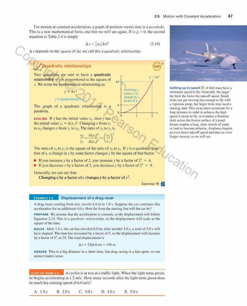
2.5 Motion with Constant Acceleration 47

For motion at constant acceleration, a graph of position versus time is a parabola. This is a new mathematical form , one that we will see again. If (Vx)i = 0, the second eq ualion in Table 2.4 is simply

I A ' ~ x = ,aJu t) - (2. 14)

6. x depends on the square of 6.t; we calJ this a quadratic relatiollship.

l.L Quadratic relationships

Two quantities are said to have a quadratic relationship if y is proportional to the square of x. We write the mathematical relationship as

y = AX2

Y is proportional [O X2

The graph of a quadratic relationship is a parabola.

SCALING If x has the initial vaJue x l, then y has the initiaJ vaJue YI = A(X,)2. Changing x from x , to X2 changes y from YI to Y2. The ratio of Y2 to YI is

y, = A(X1P = (x,)' Y, A(x ,)' X,

y y = Ax" 4A -------------

\ Doublingx causes y 10

change by a factor of 4.

A - - ----

O+-"""-- -+---+-x o

o The ratio of Y2 to y , is the square of the ratio of X2 to X I ' If Y is a quadratic function of x, a change in x by some factor changes y by the square of that factor:

• If you increase x by a factor of 2, you increase y by a factor of 22 = 4. • If you decrease X by a faclor of 3, you dccrease Y by a faclor of 3' = 9.

GeneraJJy, we can say that: Changing x by a factor of c changes y by a factor of c'.

EXercise 19 II

EXAMPLE 2 8 Displacement of a drag racer

A drag racer, starting from rest, travels 6.0 m in 1.0 s. Suppose the car continues thi s acceleration for an add itional 4.0 s. How far from the starting line will the car be?

PREPARE We assume that the accelerat ion is constant, so the displacement will follow Equation 2 .1 4. This is a quadratic relaTionship. so the displacement will scale as the square of the time.

SOLVE After 1.0 s, the car has traveled 6.0 m; after another 4.0 s, a total of 5.0 s will have elapsed. The time has increased by a factor of 5, so the displacement will increase by a factor of 52, or 25. The total d isplacement is

Il x~25(6.0 m)~ 150 m

ASSESS This is a bi g di stance in a short t ime, but drag racing is a fast sport, so our answer makes sense.

A cyclist is at rest at a traffic light. When the light turns green, he begins accelerating at 1.2 m/s!. How many seconds after the light turns green does he reach hi s cruising speed of 6.0 m/s?

A . 1.0 s B. 2.0s C. 3.0 s D. 4.0 8 E. 5.0 s

Getting up to speed BIO A bird must have a minimum speed to fl y. Generally, the larger the bird, the faster the takeoff speed. Small birds can gel moving fast enough to fl y wi th a vigorous jump, but larger birds may need a running start. This swan must acce lerate for a long di stance in order to ach ieve the high speed il needs 10 fly. so it makes a frenzied dash across Ihe frozen surface of a pond. Swans require a long, clear stretch of water or [and to become airborne. Airp lanes require an even fas ter takeoff speed and thus an even longer run way, as we wi ll see.


Dinner at a distance BID A oh:llneleon's tongue is a powerful tool for catching prey. Certain spec ies can extend the tongue to a distance of over I ft in less than 0.1 s! A study of the kinematics of the motion of the chameleon tongue, using techniques like those in this chapter, reveals that the tongue has a period of ntpid accelenttion followed by a period of constant velocity. This knowledge is a very val uable clue in the analysis of the evolutionary relationships between chameleons and other an imals.

Building a co mplex structure requires careful planning. The architect's visualization and drawings have to be complete before the detailed procedures of construction get under way. The same is true for solving problems in physics.

2.6 Solving One-Dimensional Motion Problems

The big challenge when solving a physics problem is to translate the words into symbols that can be manipulated, calculated, and graphed. This translation from words to symbols is the heart of problem solving in physics. Ambiguous words and phrases must be clarified, the imprecise must be made precise, and you must arrive at an understanding of exactly what the question is asking.

In this section we will ex plore some general problem-solving strategies that we wiU use throughout the text, applying them to problems of motion along a line.

A Problem-Solving Strategy

The first step in solving a seemingly complicated problem is to break it down into a series of smaller steps. In worked examples in the text, we use a problem-solving strategy that consists of three steps: prepare. solve. and assess. Each of these steps has important elements that you should foLlow when you sol ve problems on your own.

le f Problem-Solving Strategy

PREPARE The Prepare step of a solution is where you identify important elements of the problem and collect information you will need to solve it. It 's tempting to jump right to the Solve step, but a skilled prob lem solver wi ll spend the most time on this step, the preparation. Preparation includes:

• Drawing a picture. In many cases, thi s is the most important part of a problem. The picture lets you model the problem and identify the important elements. As you add information to your picture, the outline of the solution will take shape. For the probl ems in this chapter, a picture could be a motion diagram or a graph-or perhaps both.

• Collecting necessary information. The problem's statement may give you some values of variables. Other important information may be impli ed or must be looked up in a table. Gather everything you need to solve the problem and compi le it in a list.

• Doing preliminary calculations. There are a few caJculations, such as unit conversions, that are best done in advance of the main part of the solution.

SOLVE The Solve step of a solution is where you actually do the mathematics or reasoning necessary to arrive at the answer needed. This is the part of the problem-solving strategy that you likely think of when you think of "solving problems." But don ' t make the mi stake of starting here! The Prepare step will help you be certain you understand the problem before you start putting numbers in eq uations.

ASSESS The Assess step of your solution is very important. When you have an answer, you should check to see whether it makes sense. Ask yourself:

• Does my solution answer the question that was asked? Make sure you have addressed all parts of the question and clearly written down your solutions.

• Does my answer have the correct units and number of significant figures? • Does the value I computed make physical sense? In thi s book all calcula

tion s use physically reasonable numbers. You will not be given a problem to solve in which the final velocity of a bicycle is 100 miles per hour! If your answer seems unreasonable, go back and check your work.

• Can I estimate what the answer should be to check my solution? • Does my final solution make sense in the context of the material I am

learning?

2.6 Solving One-Dimensional Motion Problems 49

The Pictorial Representation Many physics problems, including I-D motion probl ems, often have several vari ables and other pieces of information to keep track of. The best way to tackle such problems is to draw a picture, as we noted when we introduced a general problemsolving strategy. But what lUnd of picture should you draw?

In this section, we will begin to draw pictorial representations as an aid to solving problems. A pictorial representation shows all of the important detail s that we need to keep track of and will be very important in solving motion problems.

TACTICS BOX 2.2 Drawing a pictorial representation er o Sketch the situation. Not just any sketch: Show the object at the beginning

of the motion, at the end, and at any point where the character of the motion changes. Very simple drawings ~U"e adequate.

@ Establish a coord inate system. Select your axes and origin to match the motion.

€) Define symbols. Use the sketch to define symbols representing quantities such as position, velocity, acceleration, and time. Every variable used later in the mathematical solution should be defined on the sketch.

We will generally combine the pictorial representation with a list of values, which will include:

• Known information. Make a table of the quantities whose values you can determine from the problem statement or that you can find quickly widl simple geometry or unit conversions .

• Desired unknowns. What quantity or quantities will allow you to answer the question?

EXAMPLE 2.9 Drawing a pictorial representation

Complete a pictorial representation and a list of values for the fol lowing problem: A rocket sled accelerates at 50 m/s:! for 5 s. What are the total distance traveled and the fin al velocity?

PREPARE FIGURE 2.32a shows a pictorial representation as drawn by an arti st in the style oflhe figures in thi s book. This is

FIGURE 2.32 Constructing a pictorial representation and a list of values.

(a) Artist ' s version Pictorial representation

a ~

~~I::::z;:~.....l::::Q~x

(b) Student sketch

SI.\! lch .......•... ..... Coordin:ue

. ........ , ~ • ..........• \YSIC!ll

~ , ~ Xi. (IItrhdl ~ .•... ~ .... '> Il.f} (~)F . fl ... :.:.,;.

De fine symbol-..

.•.••......

" ,

List of values

Known

Xi - Om

(1'), = 0 Ill/s I i = 0 s

a. = 50 Ill/s2

I f = 5 s

Find

Xl' (V)f

KncldIl "Find Xi-()m X, (~) .... 0 m.6 (\"" .. )p

f , "() J l' LJI .. 51) nr.S- 2 ./

f,-S.$

l' ./

Lis! !.. nown

Id\!l1 !i fy dc .. ired ull l.no ..... n~ .

inronna!ion .

Exercise 21 ,. •

certainly neater and more artistic than the sketches you will make when solving problems yourse lf! FIGURE 2.32b shows a sketch like one you might actually do. It 's less formal , but it contains all of the important information you need to solve the problem.

ImIiJ .... Throughout thi s book we will illustrate select examples with actual hand-drawn figures so that you bave them to refer to as you work on your own pictures for homework and practi ce. ....

Let's look at how these pictures were constructed. The motion has a clear beginning and end; these are the points sketched. A coordinate system has been chosen with the origin at the starting poin!. The quantities x, Vt' and I are needed at both points, so these have been defined on the sketch and distinguished by subscripts. The acceleration is associated with an interva l between these points. Values for two of these quantities are given in the problem sta tement. Others, such as Xi = 0 m and tj = 0 s, are inferred from our choice of coordinate system. The value (Vx)i = 0 m/s is parl of our inlerprefation of the problem. Finally, we identify X r

and (Vx)f as the quant ities that will answer the question. We now understand quite a bit about the problem and would be ready to start a quantitative analysis.

ASSESS We didn't solve the problem; that was not our purpose. Constructing a pictorial representation and a list of va lues is part of a systematic approach to interpreting a problem and getting ready for a mathemat ical solution .


The Visual Overview The pictorial representation and the list of values are a very good complement to the motion diagram and other ways of looking at a problem that we have seen. As we translate a problem into a form we can solve, we wiJI combine these elements into what we will term a visual overview. The visual overview will consist of some o r all of the following e lements:

• A motion diagram. A good strategy for solving a motion problem is to start by drawing a motion diagram.

• A pictorial represellwtioll, as defined above. • A graphical represelltation. For motion problems, it is often quite useful to

include a graph of position and/or velocity. • A Iisl olvalues. This list should sum up all of the important values in the problem.

Future chapters will add other elements to this visual overview of the physics.

EXAMPLE 2 10 Kinematics of a rocket launch

A Saturn V roc ket is launched straight up with a constant acceleration of 18 mls2

. After 150 s, how fast is the rocket mov ing and how far has it traveled?

interval, so we can use the first kinemat ic equati on of Table 2.4 to find the fin al veloc ity:

(v,), ~ (v,,); +", 11 , ~ 0 m/s + ( 18 m/s' )( ISO 5)

~ 2700 m/s PREPARE FIGURE 2.33 shows a visual overview of the rocket launch thaI includes a mOl ion diagram, a pictorial representation , and a li st of val ues. The v isual overv iew shows the whole problem in a nutshell . The mot ion diagram illustrates the mot ion of the rocket. The pictorial representati on (produced accord ing to Tactics Box 2.2) shows axes, ident ifies the important points o f the motion, and defines variables. Finally, we have incl uded a li st of val ues that g ives the known and unknown quantities. In the visual overview we have taken the statement of the problem in words and made it much more prec ise ; it con tains everything you need to know about the problem.

The di stance traveled is found using the second eq uati on in Table 2.4:

)'f = Yi + (vy)i 6.( + ~ayC ~t)2

~ 0 m + (0 m/s)(JSO s) + t (l8 m/s')( ISO s)'

~ 2.0 X 10' m ~ 200 I.om

SOLVE Our first task is to tind the final veloc ity. Our li st of values includes the initial ve loc ity, the accelerat ion , and the time

ASSESS The acceleration is very large, and it goes on for a long time, so the large final ve loc ity and large distance traveled seem reasonable.

FIGURE 2.33 Visual overview of the rocket launch.

Motion diagram

The motion diagram for the rocket .. hows the full range of the motion.

1.4- 1.6, 1.8, 1.9, 1.11 - 1.14

Act"IV Physcs

Pictorial representation

; 0 The pictorial rcprescm<ltion ident ifies the two important poims of the mOl ioll . the start and the cnd. and shows that the rocket accelerates between them.

List of values

Known

Yj = Om

( I')i = 0 m/s

'i = 0 S

tl, = 18 m/s2

I f = 150 s

Find \ -:-(,",)"','-a'-":-I y-,- \

The li st of value~ rnukes everything concrete. We defi ne the start of the problem to be at t ime 0 s, when the rocket has a pos ition of 0 III and a velocity of o m/s . T he end of the problem is at lime 150 s. We are to fi nd the position and ve locity at Ih is time .

Problem-Solving Strategy for Motion with Constant Acceleration Earlier in tltis section, we introduced a general problem-solving strategy. Now we wiLl adapt this general strategy to solving problems of motion with constant acceleration. We wi.ll introduce such specific problem-solving strategies in future chapters as well.

c

2.6 Solv ing One-Dimensional Motion Probl ems 51

PROBLEM · SOLVING

STRATEGY 2 . 1 Motion with constant acceleration er PREPARE Draw a visual overview of the problem. This should incl ude a motion diagram, a pictorial representation, and a list of values ; a graphical representation may be useful for certain problems.

SOLVE The mathematical solution is based on the three equations in Table 2.4.

• Though the equations are phrased in terms of the variable x, it' s customary to use y for motion in the vertical direction.

• Use the equation that best matches what you know and what you need to find . For example, if you know acceleration and time and are looking for a change in velocity, the first equation is the best one to use.

• Uniform motion with constant velocity has a = O.

ASSESS Is your result believable? Does it have proper units? Does it make sense?

Exercise 25 II

EXAMPLE 2 11 Calculating the minimum length of a runway

A fully loaded Boeing 747 with all engines at ful l thrust accele r- (Vx)r = (Vx)i + ax 6 1

ates at 2.6 m/s2. lts minimum takeoff speed is 70 m/s. How much time will the plane take to reach its takeoff speed? What mini-mum length of runway does the plane req ui re for takeoff?

PREPARE The visuaJ overview of FIGURE 2.34 summarizes the important deta il s of the problem. We set Xi and Ii equal to zero at the start ing point of the mot ion, when the plane is at res t and the accelerat ion begins. The fin al point of the mot ion is when the plane achieves the necessary takeoff speed of 70 m/s. The plane is acce lerating to the ri ght . so we will compute the ti me for the plane to reach a velocity of 70 m/s and the pos ition of the plane at thi s time, giving us the minimum length of the ru nway.

FIGURE 2.34 Visual overview for an accelerat ing plane.

;; KM"", •• ... •• ••

*' .. )ii-Olll t;-O.r

~"P?" (v,);" 0 nt/.s - A.~" .1.., 111/.$1-

0 (v, ),- 7D m/.$

~,(1',),-> ti ".(~)I' I, Find

" SOLVE First we solve fo r the time req uired for the plane to reach takeoff speed. We can use the first equation in Table 2.4 to compute thi s time:

EXAMPLE 2.12 Finding the braking distance

A car is trave ling al a speed of 30 mIs, a typ ical highway speed. on wet pavement. The driver sees an obstacle ahead and dec ides to stop. From this instant, it takes him 0.75 s to begin apply ing the brakes. Once the brakes are applied, the car experiences an accele ration of - 6.0 m/s2

. How far does the car trave l fro m the instant the driver notices the obstac le un til stopping?

70 m/s = 0 m/s + (2.6 Ill/52) 6J

70 mls il l = --- = 269 s

2.6 m/s2 •

We keep an ex tra signi ficant fi gure here because we wil l use thi s result in the nex t step of the calc ulat ion.

Given the time that the plane takes to reach takeoff speed, we can compute the pos ition of the plane when it reaches this speed us ing the second equation in Table 2.4:

Xr = Xi + (v,.); 81 + ta..(6 t)2

= 0 m + (0 mls)(26.9 s) + 1(2.6 m/s2)(26.9 S)2

= 940m

Our tinal answers are thus that the plane wi ll take 27 s to reach takeoff speed, with a minimum runway length of940 m .

ASSESS Thi nk about the las t time you new; 27 s seems like a reasonable time for a plane to acce lerate on takeoff. Actual ru nway lengths at major a irports are 3000 m or more, a few times greater than the minimum length, because they have to allow for emergency stops during an aborted takeoff. (If we had calculated a di stance fa r greater than 3000 m, we would know we had done something wrong!)

PREPARE This problem is more involved than previous problems we have solved, so we will take more care with the visual overview in FIGURE 2.35 . In addition to a mot ion diag ram and a pictorial represen tation, we include a graphical representat ion. Noti ce that there are two diffe rent phases of the motion: a constant-velocity phase before braking beg ins, and a steady slowing

COlllilllled


FIGURE 2.35 Visual overview fo r a car braking to a stop.

Known

'j - 0 S

XI = Om (1')1 = 30 m/s '2= 0.75s (1')2 = 30 m/s (1')3 = 0 m/s Between '2 and 13, {Ix = - 6.0 m/s2

Find

dow n once the brakes are appl ied. We will need to do two differen t calculati ons, one for each phase. Consequently, we've used numerical subscripts rather than a simple i and f.

The position at time 13 is computed using the second equati on in Table 2.4; we take point 2 as the initial point and point 3 as the final point for thi s phase of the motion and use D. I = 13 - 12:

SOLVE From II to 12 the veloc ity stays constant at 30 m/s. This is uniform motion , so the pos ition at time t2 is computed us ing Equation 2.4:

X3 = X2 + (Vx)2 !J. l + !ai!J. l)2

= 22.5 m + (30 mls)(S .O s) + 1(-6.0 mis' )(S.O s)'

= 98 m x, = x, + (v,MI, - I,) = 0 In + (30 O1ls)(0.7S s)

= 22.5 m X3 is the position of the car at the end of the problem- and so the car LTavels 98 m before coming to rest. At 12, the veloci ty beg ins to decrease at a steady - 6.0 m/s2

until the car comes to rest at t ) . This time interval can be computed using the first equation in Table 2.4, (vxh = (vxh + ax D. (:

ASSESS The numbers for the reaction time and the acceleration on wet pavement are reasonable ones for an alert driver in a car with good tires . The final di stance is quite large- it is more than the length of a football field.

o mls - 30 mls

- 6.0 mis' 5.0 s

1.7, 1.10 Act·IV Physcs

"Looks like Mr. Galileo was correct . . • " was the commenl made by Apollo 15 aslronaul Dav id Scott, who dropped a hammer and a feather all the mOOI1. The objects were dropped from the same height al the same lime and hit the ground simultaneously-something that would not happen in the atmosphere of the earth!

2.7 Free Fall A particularl y important example of constant acceleration is the motion of an object moving under the influence of gravity only, and no other forces. This motion is called free fall . Strictly speaking, free fa l.! occurs onl y in a vacuum, where there is no air resistance. But if you drop a hammer, air resistance is nearly neglig ible, so we'll make only a very sLi ght error in treating it as if it were in free fall. If you drop a feather, air resistance is 110t neg ligible, and we can' t make this approximation. Motion with air resistance is a problem we will study in Chapter 5. Until then, we wi.1l restrict our attention to situations in which air resistance can be ignored, and we will make the reasonable assumption that fallin g objects are in free fall.

As part of his early studies of motion, Galileo did the first careful ex periments on free fall and made the surpri sing observation that two objects of different weight dropped from the same height will, if air resistance can be neglected, hit the ground at the same time and with the same speed. In fact-as Galileo surmised, and as a famous demon stration on the moon showed-in a vacuum , where there is no air resistance, this holds true for any two objects.

Galileo's di scovery about free fall means that any two objects in free fall, regardless of their mass, have the same acceleration. This is an especiaUy important conclusion. FIGURE 2.36a shows the motion diagram of an object that was released from rest and faUs freely. The motion diagram and graph would be identical for a falling baseball or a falling boulder! FIGURE 2.36b shows the object's velocity graph. As we can see, the veloci ty changes at a steady rate. The slope of the velocityversus-t ime graph is the free-fall acceleration afrccf<lll .

Instead of dropping the object, suppose we throw it upward. What happens then? You know that the object will move up and that its speed will decrease as it rises.

FIGURE 2.36 Motion of an object in free fall.

(a) For an object dropped fro m

",::,

/ res\, the veloci ty v veclOrs poi nt

down and gct longer. The

~ ;accelerat ion I ..:oints down.

t "

(b)

v,, (m/s)

The graph has a constant slope ; thus the free-fa ll acceleration is constant.

i O +---~--~---f~-1 (5)

2 ... ",,/ 3

- 9.8 .. : ... .... - 19.6 /

a" = - 9.8 m/s2 - 29.4

(c) I f the object is in itiu ll y movi ng

.. ' up, thc veloc ity

" .... ,/. vectors point up but get sha ner. The acceleration

.. still points down.

~ a

This is illustrated in the motion diagram of FIGURE 2.36c , which shows a surprising result: Even though the object is moving up, its acceleration still points down. In fact , the free-fall acceleration always points down, no matter what direction an object is moving.

milD ... Despite the name, free faLl is not restrjcted to objects that are literally falling. Any object moving under the influence of gravity only, and no other forces , is in free fall. Thi s includes objects falling straight down, objects that have been tossed or shot straight up. objects in projectile motion (such as a passed footbaJl), and, as we will see, satellites in orbit. In thi s chapter we consider only objects that move up and down along a vertical line; projectile motion will be studied in Chapter 3 . ...

The free-fall acceleration is always in the same direction, and on earth, it always has approximately the same magn.itude. Careful measurements show that the value of the free-fall acceleration varies slightly at different places on the earth, but for the cakulations in this book we will use the the following average value:

Gfreefnll = (9.80 m/s1, vertically downward)

Standard value ror [he acce leration or an objecl in free fall

The magnilude of Ihe free-fall acceleration has the special symbol g:

g = 9.80 mis'

(2. 15)

We will generaLly work with two significant figures and so will useg = 9.8 m/s2.

Several points about free fall are worthy of note:

• g, by definition, is a/ways positive. There will never be a problem that uses a negative value for g.

• The velocity graph in Figure 2.36b has a negative slope. Even though a falling object speeds up, it has negative acceleration. Alternatively, notice that the acceleration vector Gfrccfnll points down. Thus g is nO! the object's acceleration, simply the magnitude of the acceleration. The one-dimensional acceleration is

It is a)' that is negative, not g. • Because free fall is motion with constant acceleration, we can use the kinematic

equations of Table 2.4 with the acceleration being due to gravity, (I)' = -g . • g is not called "gravity." Gravity is a force, not an accelerat.ion. g is the free-fall

acceleration. • g = 9.80 mis' only on earth. Other planets have different values of g. You will

learn in Chapter 6 how to detennine g for other planets.

2.7 Free Fall 53

Some of the children are moving up and some are moving down, but all are in free fall-and so are accelerating downward at 9.8 Ill/S

2.

TRY IT YOURSELF

A reaction time challenge Hold a $1 (or larger!) bill by an upper corner. Have a friend prepare to grasp a lower corner, putting her fingers Ileal' bllt l10t touching [he bill. Tell her to try to catch the bill when you drop it by simply c losing her fingers withoul moving her hand downward- and Ihal if she can calch it, she can keep il. Don ' t worry; the bill's free fall will keep your money safe. rn the few tenths of a second that it takes your friend to react, free fall will take the bill beyond her grasp.


• We will sometimes compute acceleration in units of g. An acceleration of9.8 m/s2

is an acceleration of Ig; an acceleration of 19.6 m/s2 is 2g. Generally. we can compute

acceleration (in units of m/s2) acceleration (in units of g) = 2

9.8 mls (2.16)

This allows us to ex press accelerations in units that have a definite physical reference.

EXAMPLE 2.13 Analyzing a rock's fall

A heavy rock is dropped from rest at the top of a cl iff and fall s 100 m before hitting the ground. How long does the rock take to fall to the ground, and what is its velocity when it hi LS?

PREPARE FIGURE 2.37 shows a visual overview with all necessary data. We have placed the origin at the ground, which makes Yj = 100m.

FIGURE 2.37 Visual overview of a falling rock.

!Ji -/COm Yr- 0", r.,l;. Om/J f l - OJ "':1' -j " -qeom/"

Find.

SOLVE Free faU is motion with the specific constant acceleration Q y = -g. The first question in volves a relation between time and distance, a relation expressed by the second equation in Table 2.4. Using (Vy)i = D mls and ti = 0 s, we find

().\ 1.\ ., 1.\., I.,

Yr = Yi + Vy i uf + 'F'y U. r = Yi -"2g u r = Yi -"1g t{

We can now solve for ' r:

2( 100 III - 0 Ill)

9.80 m/s2 4.52 s

Now that we know the faU time, we can use the firsl kinematic

equation to find (v.,.)r:

(v).)r = (v, ); - g fir = -grr = -(9.80 m/s')(4.52 s)

= - 44.3 mls

ASSESS Are the answers reasonable? Well , 100 m is about 300 feet , which is about the height of a 3D-floor building. How long does it take something to faU 30 floors? Four or five seconds seems pretty reasonable. How fast would it be going at the bottom? Using an approximate ve rs ion of our conversion factor I mls ~ 2 mph, we find that 44.3 mls ~ 90 mph. That also seems like a prelly reasonable speed for something thaI has fallen 30 floors. Suppose we had made a mistake. If we misplaced a dec imal point we could have calculated a speed of 443 mIs, or about 900 mph ! This is clearly flot reasonable. Lf we had mi splaced the dec imal point in the other direction, we would have calculated a speed of 4.3 mls ~ 9 mph. This is another unreasonable result, because thi s is slower than a typical bicycl ing speed.

CONCEPTUAL EXAMPLE 2 14 Analyzing the motion of a ball tossed upward

Draw a motion diagram and a ve locity-versus- lime graph for a ball tossed straight up in the air from the point that it leaves the hand until just before it is caught.

REASON You know what the motion of the ball looks like: The ball goes up, and then it comes back down again. Thi s complicates the drawing of a motion diagram a bit , as the ball retraces its route as it fall s. A literal motion diagram would show the upward motion and downward motion on top of each other, leading to confusion. We can avoid this difficulty by hori zon tall y separating the upward motion and downward motion diagrams. This will not affect our conclusions because it does not change any of the vecto rs. The mOlion diagram and veloc ity-versus- time graph appear as in FIGURE 2.38 on the next page.

ASSESS The highest point in the ball's motion , where it reverses direction, is called a fIlming poinl. What are the velocity and the acceleration at thi s point? We can see from the motion diagram that the velocity vectors are pointing upward but getting shorter

as the bal.1 approaches the top. As it starts to faU, the ve locity vectors are pointing downward and getting longer. There must be a moment- just an instant as v switches from pointing up to pointing down- when the velocity is zero . Indeed, the ball's velocity is zero for an instant at the precise top of the mOlion ! We can also see on the velocity graph that there is one instant of time when Vy = O. This is the turning point.

But what about the acce leration at the top? Many people expec t the acceleration to be zero at the highest point. But recall that the velocity at the top point is changing-from up to down. If the velocity is changing, there musf be an acceleration. The slope of Ihe ve locity graph at the instant when Vy = O-that is, al the highest point- is no different than at any other point in the motion. The ball is still in free fall with acceleration Qy = -g !

Another way to think about thi s is to note that zero acceleration would mean no change of veloc ity. When the ball reached zero ve loc ity at the top, it would hang there and not fall if the acceleration were also zero!

2.7 Free Fall 55

FIGURE 2.38 Motion diagram and velocity graph of a ball tossed straight up in the air.

Thi s is the same point shown [wicc.

Last veloci ty-upward

The upward and downward motions arc separated in Ihi s mOlion diagram for clarity. They really a I occur along Ihe Same , line.

Start of 111otion _______

,.

--First downward velocity

The upward and downward velocity vectors arc of equal magnitude but opposite directi on. The bull is caught

.•....... .. ·····"wilh (he same speed as it le ft (he hand. .----End of

. ............... mOlion

v v

EXAMPLE 2.15 Finding the height of a leap

A springbok is a n antelope found in sOUlhern Africa lhat gels its name from it s remarkable j ump. ing ability. When a springbok is startled, it will leap straight up in to the air- a maneuver called a "pronk." A springbok goes into a crouch to perform a pronk. It then ex tends its legs forcefully, accelerating at 35 I11/S2 for 0.70 m as its legs straighten. Legs fully extended, it leaves the ground and ri ses into the a ir.

a. At what speed does the springbok leave the ground? b. How high does it go?

FIGURE 2.39 A v isual overv iew of the springbok's leap.

The ball starts with l.I When the ball positive (upward) velocity Ihat s te adi ly decreases.

" I rcaehes it:. hi ghest point , its veloci ty is instantaneously zero. Th is i" the turning poi lli or the Illotion.

•

Now rhe ball is moving do wnward. The velocity is negati ve .

I, /a,~ - 9.8m/s· •

During the entire motion, the acceleration is that of free fall. The slope of the veloci ty graph is constant and negat ive.

PREPARE We begin with the visual overview shown in FIGURE

2.39 , whe re we've idenlifi ed two different phases o f the motion: the springbok pushing off the gro und and the springbok ri sing inlO the air. We' U treat these as two separa te problems that we

solve in turn. We will "re-use" the variables Yj, Yf, (v.I.)j , and (vy)r for the two phases of the motion.

For the first part of o ur so lution, in Figure 2.39a we choose the ori g in o f the y-axis at the position of the springbok deep in the crouch. The final pos ition is the top ex tent o f the push, at the instant the springbok leaves the ground . We want lO find the veloc ity at thi s pos ition because that 's how fast the springbok is movi ng as it leaves the ground . Figure 2.39b essent ially starts over- we have defined a new vertical ax is with it s ori gin at the ground , so the highest point of the springbok's motion is a

(a) Pushing off {he g round (h) Risi ng illlo (he ai r

Known

Y1 = Om

Yr= O.70m

(II,); = 0 Ill/S

Yr ay = 35 m/s '1

(II), Fi nd ~'-----

If (v)\

y

~Y"(")" I' Known

y. = Om

(v), is equal to (v)r from part a

( lI)r = 0 Ill/s

a" = - 9.8 tn/S2

F ind

COl/til/ued

56 CHAPTER 2 Motion in One Dime ns ion

distance above the ground. The table of values shows the key piece of information for thi s second part of the problem: The initi al veloc ity for part b is the final veloc ity from pillt a.

After the spri ngbok leaves the ground, thi s is a free-fall problem because the spri ngbok is moving under the in fl uence of gravity onl y. We want to know the height of the leap, so we are looking fo r the he ight at the top point of the motion. This is a turni ng poinr of the moti on, with the insta ntaneous velocity equal to zero. Thus Yr. the height of the leap, is the springbok 's pos ilion at the instan t (v.\.)r = O.

SOLVE a. For the first ph,lse, pushing off the ground, we have in formation about displacement, ini tial veloc ity, and acce lerati on. but we don ' t know anything about the time interval. The thi rd equat ion in Table 2.4 is perfecl fo r thi s type of situation. We can rearrange it to solve for the velocity with which the spri ngbok lifts off the ground:

(v.,.)f = v? + 2{/.', ~y = (0 m/s)2 + 2(35 m/s2)(0.70 111) = 49 m2/s2

(vy)r= V49 m2/s2 -7.0 m/s

The springbok leaves the ground with a speed of 7.0 m/s.

b. Now we are ready for the second phase of the mot ion, the vert ical mot ion after leaving the ground. The th ird equation in Table 2.4 is again appropri ate because aga in we don' t know the lime. BecauseYi = 0, the spri ngbok's displacement is ~y = Yf - Yi = Yr, the height of the vertical leap. Frolll part a, the initial velocity is (V~.) i = 7.0 mis, and the fi na l veloc ity is (Vy)f = 0. This is free- fall motion, with ay = -g; thus

(v)')f = 0 = (Vy)~ - 2g ~y = (vy)f - 2gYf

which gives

(Vy)~ = 2gYf

Solving for Yf. we get aj ump he ight of

(7.0 m/s)' Yf~ , 2.5 m

2(9.8 m/s-)

ASSESS 2.5 m is a remarkable leap- a bit over 8 ft- but these an imals are known for the ir jumping ab ility, so thi s seems reasonable.

FIGURE 2.40 Velocity-versus-time an d posi ti on-versus-time graphs fo r a spri nt between a man and a horse.

The capti on accompanying the photo at the start of the chapter asked a questi on about animals and their athletic abilities: Who is the wi nner in a raCe between a horse and a man? The surprising answer is " It depends." Specifically, the winner depends on the length of the race. T hc velocity-vcNus

time graph for the

)' (m/s) man starts with a 2' steeper slope.

S In itiall y, the man is running at a higher veloci ty, but ..

20

15 ,

.. . the horse has a higher maximulII velocity.

1 Horse

I ...... ?--------Man 10 • 5

0 +--~r_-___r--~--~, (s) 0

x (m)

100

80

60

40

20

2.0 4.0

The man will be in the lead up 10 a disl.mce of about 40 m.

6.0 8.0

Horse

Man

o+-"""=--~--~--~--r' (s) o 2.0 4.0 6.0 8.0

Some animals are capable of hjgh speed; others are capable of great acceleration. Horses can run much faster than humans, but, when starting from rest, humans are capable of much greater initi al acceleration. FIGURE 2.40 shows velocity and positi on graph s for an elite male sprinter and a thoroughbred racehorse. The horse's max imum veloc ity is about twice that of the man, but the man's initial acceleration- the slope of the ve locity graph at early times-is about twice that of the horse. As the second graph shows, a man could win a very short race. For a longer race, the horse's higher max imum velocity will put it in the lead; the men's world-record time for the mile is a bit under 4 min , but a horse can eas i.Jy run thi s di stance in less than 2 min .

For a raCe of many mi.Jes, another factor comes into play: energy. A very long race is less about velocity and acceleration than about endurance-the ability to continue expendin g energy for a long time. In such endurance trials, humans often win . We will ex plore such energy issues in Chapter I L

STOP TO THINK 2 6 A volcano ejects a chun k of rock straight up at a velocity of v)' = 30 m/s. Ignoring air resistance, what will be the velocity II)' of the rock when it faUs back into the volcano's crater?

A. > 30 m/s B. 30 m/s c. 0 m/s D. - 30 mls E. < - 30 m/s

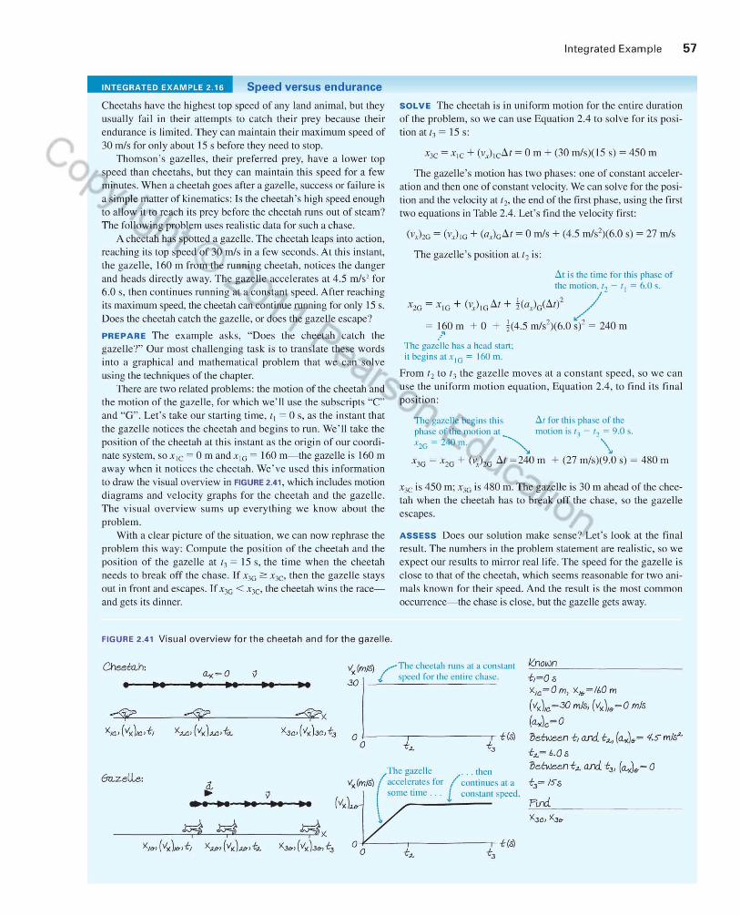
c

Integrated Example 57

INTEGRATED EXAMPLE 2 16 Speed versus endurance

Cheetahs have the highest top speed of any land animal, but they SOLVE The cheetah is in uniform mot ion for the ent ire duration usually fa il in the ir attempts to catch the ir prey because their endurance is limited. They can maintain their maximum speed of 30 mls for only about 15 s before they need to stop.

Thomson's gaze lles, the ir preferred prey, have a lower top speed than cheetahs, but they can maintain thi s speed for a few minules. When a cheetah goes after a gazelle, success or failure is a simple matter of kinematics: Is the cheetah's high speed enough to allow it to reach its prey before the cheetah nms out of steam? The following problem uses real isti c data for such a chase.

A cheetah has spotted a gazelle. The cheetah leaps into act ion, reaching its top speed of 30 mls in a few seconds. At thi s instant, the gazelle, 160 m from the running cheetah, not ices the danger and heads directly away. The gazeUe accelerates at 4.S mls2 for 6.0 s, then continues running at a constant speed. After reaching its max imum speed, the cheetah can continue running for only IS s. Does the cheetah catch the gazeUe, or does the gaze lle escape?

PREPARE The example asks, "Does the cheetah catch the gaze lle?" Our most challeng ing task is to translate these words into a graphical and mathemati cal problem that we can solve using the techniques of the chapter.

There are two related problems: the motion of the cheetah and the motion of the gaze lle, for which we' ll use the subscripts "C" and "G". Let's take our starting time, II = 0 s, as the instant that the gazelle notices the cheetah and begins to run. We'll take the position of the cheetah at thi s instant as the origin of our coordi nate system, sox1c = 0 m and xlG = 160 m-the gaze lle is 160 m away when it nOlices the cheetah. We 've used thi s inFormat ion to draw the visual overview in FIGURE 2.41, which includes moti on diagrams and ve locity graphs for the cheetah and the gaze lle. The visual overview sums up everything we know about the problem.

With a clear picture of the situat ion, we can now rephrase the problem thi s way: Compute the position of the cheetah and the position of the gaze lle at 13 = IS s, the time when the cheetah needs to break off the chase. If X3G =:: X 3C, then the gaze lle stays out in front and escapes. If X3G < X3C ' the cheetah wins the raceand gets its dinner.

of the problem, so we can lise Equation 2.4 to solve for its pos ition at'3 = 15 s:

X3C =XIC + (Vt)lc~ 1 = 0 m + (30 m/s)( IS s) = 4S0 111

The gazelle'S motion has two phases: one of constant accelerali on and then one of constant veloc ity. We can solve for the position and the velocity at 12, the end of the first phase, using the first two equations in Table 2.4. Let 's find the velocity first:

(v,hG - (v.}'G + (aJG8 r - 0 mls + (4.5 mls')(6.0 s) - 27 mls

The gazelle's pos ition at 12 is:

.6. t is the time for this phase of the motion. '2 - r J = 6.0 s.

, 2 / x2G = x lG + (~t)IG.6.t + 2(a.r)G(.6.I) /

- 160 m + 0 + 1(4.5 m/s' )(6.0 s)' - 240 m ....... -

The gazelle has a head start; it begins al x lG = 160 m.

From 12 to '3 the gazelle moves at a constant speed, so we can use the uniform mot ion equation . Equation 2.4, to find its final position :

The gazelle' begins this 6, for this phase of the phase of the 1110lion at mot ion is IJ - 12 = 9.0 s. x2G = 240 m. ~ \

x3G = x 2G + (~t)2G !!J.t = 240 m + (27 m/s)(9.0 s) = 4RO m

X3C is 450 m; X3G is 480 m. The gazelle is 30 m ahead of the cheetah when the cheetah has to break off the chase, so the gaze lle escapes.

ASSESS Does our so lution make sense? Let 's look at the final result. The numbers in the problem statement are real istic, so we expect our results to mirror real life. The speed for the gazelle is close to that of the cheetah , which seems reasonable for two ani mals known for their speed. And the result is the most common occurrence-the chase is close, but the gazelle gets away.

FIGURE 2.41 Visual overview for the cheetah and for the gazelle.

ChedtLh, ",,-0 v

• •• •• • • 1? --<¥'

'X/C) (vl()/C,f, <..." (lIx)..." f~

~ ..... ..

•• .. . f<

<3C, (lIxhc,f3

vl«(m/<S) ~The cheetah runs at a constant

3

0

0 I .:. speed for the entIre chase

} , f[s) o r~ f3

The gazel le ... then vl(Cmls) (acce le~alcs for ( continues al a

(vl(b \ some lime. 1 constant speed. ... ... \,

$< )(.36') (vl().J&,f,J o-lL--,-------,- f[s)

o f,1.. f,J

Known f,=Os 'X,c=O m) 'XI(, =11.0 m

(lIx)",-.30 mis, (lIx),.-O mls

("")c- O

lle~n f, and. f~, (a,J.- 4.0 mls~ 1:,;..=1,.05

lle~n f~ and. fJ' (a,J. - 0

1:,3= iSs

Pl.l'ld.


SUMMARY The goal of Chapter 2 has been to describe and analyze linear motion.

GENERAL STRATEGIES

Proble m-Solving Strategy Visual Overview Our general problem-solving strategy has three parts:

A visual overview consists of several pieces that completely specify a problem. This may include any or all of the elements below:

PREPARE Set lip the problem: l\Iotion diagram Pictorial representation Graphicall't!presentation List or values

Draw a picture.

Collect necessary information.

Do preliminary calculat ions.

SOLVE Do the necessary mathematics or reasoning.

ASSESS Check your answer to see if it is complete in all detail s and makes physical sense.

IMPORTANT CONCEPTS

Velocity is the rate of change of position:

~x II = , ~f

Acceleration is the rate of change of veloc ity:

~ " (/ = --' , ~f

The units of acceleration are m/s2.

y ~ YI' (1',)1' If

ij

, ta ta

0 Yi' (v)",;

A position-versus-time graph plots position on the vertical ax is against time on the horizontal axis.

x(m)

6

4

2

An object is speeding up if V.I and ax have the same sign, slowing down if they have opposite signs.

o +"-~~-~-~-~ I (s) 0246810

APPLICATIONS

Uniform motion An object in uniform motion has a constant velocity. Its velocity graph is a horizontal line; its position graph is linear.

Kinematic equation for uniform motion:

Xf= Xi + VA' 61

Uniform motion is a special case of constantacceleration motion, with a.l , = O.

Motion with constant acceleration An object with constant acceleration has a constantly chang ing velocity. Its velocity graph is linear; its position graph is a parabola.

Kinematic equations for motion with constant accelerat ion:

(V,)r = (V)i + (/x 61

Xf = Xi + (v,,), D.I + ta,( D.t )2

(vJl = (v.T)? + 2ax D. X

Known ,. , Yi= Om

(I',)f (r,)i = 0 m/s

I; = Os

(I , = !8 m/sl

I f = 150 s

Find

" (V,)I andYr

A velocity-versus-time graph plots velocity on the vertical axis against time on the hori zontal axis.

Vt

(m/s)

30

10

Acce)emliQn j, the slope or The velOCiTY graph.

0+--_-_-_-="- , (s) o 2 3 4

Free fall Free fall is a special case of constan tacceleration moti on; the acceleration has magnitude g = 9.80 m/s 2 and is always directed vert ical ly downward whether an object is moving up or down.

, . .

", , ", The vc!oci ty grJph is a straight line with a slope of - 9.80 m/sl.

./

tMP)TM For homework assigned on MasteringPhysics, go to

!:!!/ www.masteringphysics.com

Problem difficulty is labeled as I (straightforward) to 11111 (challenging),

QUESTIONS

Conceptual Ouestions

1. A person gets in an elevator on the ground floor and rides it to the lOp floor or a building. Sketch a veloc ity-versus-time graph for t.hi s motion.

2. a. Give an example of a ve rtical molion with a pos itive velocity and a negati ve acce leration.

b. Give an example of a vertical motion with a negative ve locity and a negative acceleration.

3. Sketch a ve loc ity-versus-timc graph for a roclnhat is thrown straight upward, from the instant it leaves the hand until the instant it hits the ground.

4. You <rre dri ving down the road at a constant speed. Another car go ing a bit faster catches up with you and passes you. Draw a position graph for both vehicles on the same set of axes, and note the point on the graph where the other vehicle passes yo u.

S. A ca r is travel ing north . Can its acceleration vector ever point sOlllh? Ex plain.

6. Certain an imals are capable of run ning at great speeds; o ther BID animals are capable of tremendolls accelerations. Speculate on

which would be more benefic ial to a predator-large maximum speed or l<rrge acceleration .

7. A ball is thrown straight up into the air. At each of the following instants, is the baJJ 's acceleration Cly equa l to g, -g, 0, < g, or > g? a. Just after leaving your hand? b. At the very top (maximum height)? c. Just before hitting the ground?

8. A rock is (hrollln (not dropped) straight down from a bridge into the ri ver below. a. Immediately after being released, is the magnitude of the

rock's acceleration greater than g, less than g, or equal to g? Explain .

b. Immediately before hitting the water, is the magnitude of the the rock's acceleration grealer than g, less than g, or equal to g? Expla in .

9. Figure Q2.9 shows an object's position-verslis- time graph . The letters A to E correspond to various segments of the mot ion in which the graph has constant slope.

x(rn) B

2

A

2 4 6 8 - I

E

FIGURE 02.9 - 2

a. Write a reali st ic motion short story for an objec t that would have thi s position graph.

b. In which segment(s) is the object at rest?

Questions 59

Prob lems labeled INT integrate significant material from earlier

chapters; BID are of biological or medical interest.

c. In which segment(s) is the object moving to the ri ght? d. Is the speed of the object during segment C greate r than ,

equal to, or less than its speed during segment E? Explain. 10. Figure Q2.IO shows the position graph for an object moving

along the hori zontal ax is. a. Write a real istic motion short story for an objecl that would

have thi s position graph. b. Draw the corresponding velocity graph.

x

\ FIGURE 02.10

~ \'-------II. Figure 02.11 shows the pos ition

versus-t ime graphs for two objec ts, A and B, that are moving along the same ax is. a. At the instant (= L s, is the

speed of A greater than , less than , or equal to the speed of B? Explain.

b. Do objects A and B ever have

x

0 2 3

FIGURE 02.11

B

4

thesClme speed? If so, at what time or limes? Explain. 12. Figure Q2. 12 shows a position- x 8

versus-time graph. At which lettered point or points is the object a. Moving the fastest?

D

A

t (s) 5

b. Moving to the le ft ? E '-__

c. Speeding up? F

d. Slowing down? FIGURE 02.12

e. Turning around? 13. Figure Q2.1 3 is the veloc ity-versus-t ime graph for an objec t

moving along the x-axis. a. During which segment(s) is the veloc ity constant? b. During which segment( s) is the object speeding up? c. During which segment(s) is the object slowing down? d. During which segment(s) is the object standing still ? e . During which segment(s) is the object moving to the right?

I'~ (m/s)

3

2 A

B

0 F

I (s) 2 3 4 10

- I

- 2 D

FIGURE 02.13 - 3


14. A car traveling at veloc ity v takes distance d to stop after the brakes are appl ied. W hat is the stopping distance if the car is ini tiaUy trave ling at veloc ity 2v? Assume that the acce leration due to the braking is the same in both cases.

Multiple-Choice Questions

IS. 1 Figure Q2.L5 shows the pos ition graph of a car traveling on a straight road. At which labeled instant is the speed of the car greatest?

FIGURE OZ.15

x

E

16. I Figure Q2. 16 shows the pos ition graph of a car traveling on a stra ight road. The veloc ity at instant I is __ -,-_ and the veloc ity at instan t 2 is ___ _ A. positi ve, negat ive ~,

B. posi tive, posit ive FIGURE OZ.16 C. negative. negative D. negative, zero E. positive, zero

17. 1 Figure 02.1 7 shows an x(m)

40 object 's pos ition-versus-time

30 graph. W hat is the ve loc ity of the object at t = 6 s? 20

A. 0.67 ml' 10 B. 0.83 ml, C. 3.3 m/s

O+----_---~I (s) o 5 10

D. 4.2 mls FIGURE OZ.17 E. 25 mls

18. I The fo llowing options desc ri be the mot ion of four cars A- D. Which car has the largest accelerat ion? A. Goes from 0 mls to 10 mls in 5.0 s 8 . Goes from 0 mls to 5.0 mls in 2.0 s C. Goes from 0 mls to 20 mls in 7.0 s D. Goes from 0 mls to 3.0 mls in 1.0 s

19. I A car is trave ling at Vx = 20 m/s. The dr iver applies the brakes, and the car slows with a.~ = - 4.0 m/s 2

. What is the stopping di stance? A. S.Om B. 25 m C. 40 m D. 50 m

20. II Ve loc ity-ve rsus-t ime graphs for three drag racers are shown in Figure Q2.20. At t = 5.0 s, which car has traveled the furthest? A. Andy B. Belly C. Carl D. All have traveled the same distance

I'~ (m/s)

4:W ,(,) 1', (m/s)

4:k===L,) ~or') / O~I(S)

o Andy 5.0 o Betty 5.0 o Carl 5.0

FIGURE Q2.20

2 1. I Which of the three drag race rs in Question 20 had the greatest acceleration at I = 0 s?

22.

A. Andy B. Belly C. Carl D. All had the same acceleration II Ball 1 is thrown straight up in the air and, at the same instant. ball 2 is released fro m rest and allowed to fall. Which veloc ity graph in Figure Q2.22 best represents the motion of the two ball s?

FIGURE 02 .22

23 . II Figure Q2.23 shows a motion diagram with the clock reading (in seconds) shown al each pos ition. From I = 9 s to I = 15 s the object is at the same pos ition . After that, it returns along the same track. The pos itions of the dots for f ;::= 16 s are offset for clarity. Which graph best" represents the object's velocity?

o • •

• 23

FIGURE 02 .23

2 •

• • 21 21

3 •

4

• 5 ~ : ! . /9to 15 •

• • • • • 20 19 18 17 16

C. I'x D. I'x

h, ~, 24. II A car can go from 0 to 60 mph in 7.0 s. Assumi ng that it

could maintain the same acceleration at higher speeds, how long would it take the car to go from 0 to 120 mph ? A. lOs B. 14 s C. 2 1 , D. 28 s

25. 11 A car can go from 0 to 60 mph in 12 s. A second car is capable of twice the accelera ti on of the fi rst car. Assuming that it could maintain the same acceleration at highe r speeds, how much time will thi s second car take to go from 0 to 120 mph? A. 12 s B. 9.0s C. 6.0 s D. 3.0s

PROBLEMS

Section 2. t Describing Motion

I . II I Figure P2. l shows a m Ol ion diagram of a car travel ing down a street. The camera took one frame every second. A distance scale is prov ided. a. Measure the x-value of the car at each dot. Place your data in

a table, simi lar to Table 2. 1, showing each pos ition and the instanroftime at which it occurred.

b. Make a graph of x versus I, using the data in your table. Because you have data only at certain instants of lime, your graph should consist of dots that arc not connected together.

I frame per second

o 2()() 4flO 600 800 I flO()

FIGURE P2.1

2. I For each motion diagram in Figure P2.2, determine the sign (positi ve or negat ive) of the pos ition and the velocity.

(a) (bJ ('J • ~ I •• 0

t 0

t FIGURE P2.2 0

3. I Write a short desc ription of the mot ion of a real object for which Figure P2.3 would be a realist ic pos ition-versus- time graph .

x(m)

300

200

100

o ~~~~-c~~-+:I (s) o 200 400 600

FIGURE P2 .3

x(mi)

40

20

O +-~+C-~~~ I (h)

- 20

FIGURE P2.4

4. I Write a short desc ription of the motion of a real object fo r which Figure P2.4 would be a reaJi sti c pos ition-versus- time graph .

5. II The pos ition graph of Figure P2.5 shows a dog slowly sneaki ng up on a squi rrel, then putting on a burst of speed. a. For how many seconds does the dog move at the slower

speed? b. Draw the dog's ve loc ily-ve rsus-ti me graph. Include a

numerical scale on both axes.

x(m)

~D"., o 2 4 6 8 10

FIGURE P2.5

Probl ems 61

6. II The pos ition graph of Figure P2.6 represents the mot ion of a ball being roUed back and forth by two children. a. At what positions are the two children sitti ng? b. Draw the ba ll' s veloc ity-versus- time graph . Include a

numerical scale on both axes.

4

2

0 I (s) 16 20

- 2

- 4

FIGURE P2.6 - 6

7. II A rural ma il carri er is driving slowly, putting ma il in ma il boxes near the road. He overshoots one mailbox.s tops.shi fts into reverse, and then backs up until he is at the right spot. The veloc ity graph of Figure P2.7 represents hi s mot ion. a. Draw the mail carrier 's pos ition-versus-time graph. Assume

that x = 0 m at f = 0 s. b. What is the pos ition of the mailbox?

I', (Ill /s) 1'.< (Ill/S)

3 3 r--,

2 2 I I I I

I I I I

0 1(8) 0 I (s) 2 4 6 'f - I 2 4 6 8 10 " - I I 1

L-.J - 2 I - 2 I

-3 - 3

FIGURE P2 .7 FIGURE P2.8

8. For the ve loc ity-versus-time graph of Figure P2.8: a. Draw the corresponding position-versus-time graph. Assume

that x = 0 m at f = 0 s. b. What is the object's posit ion at f = 12 s? c. Desc ri be a moving objec t that could have these graphs.

9. II A bicycl ist has the pos ition-versus- time graph shown in Figure P2.9. What is the bicycl ist's veloc ity at 1 = 10 s, at t = 25 s, and at f = 35 s?

FIGURE P2.9

x(m)

100

50 -

o +--~---c~-:--+-t (s) o 10 20 30 4{)

Section 2.2 Uniform Motion

10. I In co ll ege softball , the di stance from the pitcher' s mound to the balle r is 43 fee l. If the ba ll leaves the bat at 100 mph, how muc h time elapses between the hi t and the ball reac hi ng the pitcher?


11. II Alan leaves Los Ange les at 8:00 A .M. to d ri ve to San Franc isco, 400 mi away. He trave ls at a steady 50 mph. Beth leaves Los Angeles at 9:00 A.M. and dri ves a steady 60 mph. a. Who gets to San Francisco first? b. How long does the first to arri ve have to wa it for the sec

ond? 12. II Richard is driving home to vis it his parents. 125 mi of the tri p

.u e on the interstate highway where the speed limit is 65 mph . Normally Richard drives a1 the speed li mit, but today he is running late and decides to take hi s chances by dri ving at 70 mph. How many mi nutes doeS' he save?

13. III In a 5.00 km race, one ru nner ru ns at a steady 12.0 kmlh and another runs at 14.5 km/h. "How long does the faster runner have to wait at the fi nish li ne to see the slower runner cross?

14. llil In an S.OO km race, one runner runs at a steady 11 .0 kmlh and anot her runs at 14.0 kmfh. How far from the fini sh line is the slower ru nner when the faster runner fini shes the race?

15. Il A car moves with constant velocity along a straight road. Its posi ti on is XI = 0 m at '1 = 0 s and is X2 = 30 III at 12 = 3.0 s . Answer the fo llowing by considering rat ios, withou t computi ng the car 's veloc ity. a. What is the car 's pos ition at 1 = 1.5 s? b. What will be its pos ition at I = 9.0 s?

16. II While run ning a marathon, a long-d istance run ner uses a stopwatch to time herse lf over a distance of 1.00 Ill. She finds that she runs thi s distance in IS s. Answer the following by consider ing rati os, without computing her ve locity. a. If she mainta ins her speed, how much time will it take her to

ru n the nex t 400 m? b. How long will it take her to ru n a mile at thi s speed?

Section 2.3 Instantaneous Velocity

17. 1 Figure P2. 17 shows the x (m)

pos ition graph of a particle. 20 a. Draw the parti cle's veloc ity

graph for the interval 10 Oss:t S: 4s.

b. Does thi s particle have a o +---I--~-~--'\- I (s) 0 24

turni ng point or po ints? If FtGURE P2 .17

so, at what time or times? 18. II A somewhat ideali zed graph of the speed of the blood in the BID ascend ing aorta during one beat of the heart appears as in

Figure P2. 1S. a. Approximately how far, in cm, does the blood move duri ng

one beat? b. Assume similar data for the mot ion of the blood in yo ur

aorta. Esti mate how many beats of the heart it wil.l it take the blood to get from your heart to your bra in.

I' (m/s)

1.0

0.5

o +---+--~I--~- f (s) FIGURE P2 .18 0 0.20 0.40 0.60

19. III A car starts from Xi = \0 m at Ii = 0 sand moves with the veloc ity graph shown in Figure P2. 19.

I'~ (m/s)

" 8

4

o +--~-2'---"3"~4c- 1 (s) a. W hat is the object'S

posit ion at 1 = 2 s, 3 s, and 4 s?

- 4

FIGURE P2 .19

b. Does thi s car ever change di.recti on? If so, at what time? 20. Figure P2.20 shows a graph of actual pos ition-versllstime

data for a particular type of drag racer known as a "funny car. " a. Estimate the car 's veloc ity at 2.0 s. b. Estimate the car's veloc ity at 4.0 s.

r(m)

400

300

200

100

0 I (s) FIGURE P2 .20 0 2 4 6

Section 2.4 Acceleration

2 1. II Figure P2.2 1 Shows the veloc ity graph of a bicycle. Draw the bicycle's acceleration graph for the in terval 0 s :5 1 :5 4 s. Give both axes an appropriate numeri cal scale.

1' ... (m/s)

4 --v, (m/s)

2

2 1

0 I (s) 8 10

- I

0 I (s) - 2 0 2 4

FIGURE P2.21 FIGURE P2 .22

22.

23.

24. BID

25.

III Figure P2 .22 shows the veloc ity graph of a train that starts from the ori gin at I = 0 s. a. Draw pos ition and accelerat ion graphs for the train . b. Find the accelerat ion of the train at ( = 3.0 s. I For each moti on diagram shown earli er in Figure P2.2, determi ne the sign (positive or negative) of the acce lerat ion. II Figure P2. 18 showed data for the speed of blood in the aorta . Determine the magn itude of the acceleration for both phases, speeding up and slowing down. II Figure P2.25 is a somewhat simplified veloci ty graph for O lympic spr inter Carl Lewis starting a 100 III dash. Est imate hi s acce lerat ion duri ng each of the intervals A, B, and C.

L' ... (m/s)

12 10

8 6

4 A 2

c

B

O¥--~-~-~-~I (s) FIGURE P2 .2S 0 2 3 4

Section 2.5 Motion with Constant Acceleration

26. I A Thomson's gazelJ e can reach a speed of 13 mls in 3.0 s. A BID lion can reach a speed of 9.5 mls in 1.0 s. A lrout can reach a speed

of 2.8 mls in 0 .1 2 s. Which animal has the largest acce leration?

27. III When striking, the pike. a BID predatory fish, can acce lerate

from rest to a speed of 4 .0 m/s in 0. 11 s. a. What is the acceleration of

the pike during thi s str ike? b. How far does the pike move

during this strike? 28. II a. What constant acce lerat ion, in SI units, must a car have to

go from ze ro to 60 mph in IDs? b. What fraction of g is thi s? c. How far has the car trave led when it reaches 60 mph ?

Give your answer both in SI units and in feet. 29. Light-rail passenger trains that provide transportatio n within

30.

31.

32.

and between ci ties are capable o f modes t accelerati o ns. T he magni tude of the maximum acceleration is typica lly 1.3 m/s2, but the driver will usually maintain a constant acce leration that is less than the maximum. A train travel s through a congested part of town at 5.0 m/s. Once free of thi s area, it speeds up to 12 m/s in 8.0 s. At the edge of town, the driver aga in acce lerates, with the same accelerat io n, for a nother 16 s to reach a higher crui sing speed. What is the final speed? III A speed skater moving across frictionless ice at 8.0 m/s hits a 5.0-m-wide patch of rough ice. She slows stead ily. then continues on at 6.0 m/s. What is her acceleration on the rough ice? JI A small propeller ai rpl ane can comfortably achieve a hi gh enough speed to take off on a runway that is 1/4 mile long. A large, fully loaded passenger jet has about the same accelerati on from rest, but it needs to achieve twice the speed to take off. What is the minimum runway length that will serve? Hint: You can solve this problem using ratios without hav ing any additional infonnati on. II Figure P2.32 shows a veloc-ity-versus-t ime graph for a particle moving along the x-aris. At t = 0 s. assume that x = 0 m. a. What are the particle's posi

ti on , veloc ity, and acceleration at t = 1.0 s?

b. What are the parti cle's position , ve locity, and accelerati on at t = 3.0 s?

v~ (mJs)

4+---,

2

O+--~-~~--+-I (s) o 2 3 4

FIGURE P2 .32

Section 2.6 Solving One· Dimensional Motion Problems

33. II A driver has a reac tion time of 0.50 s, and the maximum deceleration o f her car is 6.0 m/s2

. She is driving at 20 m/s when suddenly she sees an obstacle in the road 50 m in front of her. Can she stop the car in time to avo id a colli s ion?

34. II Chameleons catch insects with their tongues, whi ch they can BID rapidly ex tend to great lengths. In a typical strike, the chameleo n's

to ngue accelerates at a remarkable 250 m/s2 for 20 ms, then travels at constant speed for another 30 ms. During thi s total time of 50 ms, 1/20 o f a second, how far does the tongue reac h?

35. !II Yo u' re dr iving dow n the hig hway late one nig ht at 20 m/s when a deer steps on to the road 35 m in front o f you. Your reaction time before stepping on the brakes is 0.50 s , and the maximum deceleration of your car is 10 m/s2

.

a. How much di stance is be tween you and the deer whe n you come to a stop?

b. What is the max imum speed you could have and still not hit the deer?

Problems 63

36. Jl I A light-ra il trai n go ing from one stati o n to the next o n a straight section of track accelerates from rest at 1.1 m/s2 for 20 S.

It the n proceeds at constant speed fo r 11 00 m before slowing dow n at 2.2 m/s2 until it stops at the station. a. What is the di stance between the stations? b. How much time does it take the train to go between the

stati ons? 37. III A simple model for a person runni ng the 100 m dash is to

assu me the spri nter runs with cons tant acce leration unt il reaching top speed, then mai ntains that speed throug h the fini sh line. If a sprinter reaches hi s top speed of I L. 2 m/s in 2. 14 s, what will be hi s total time?

Section 2.7 Free Fall

38. III BaLI bear ings can be made by letting spheri ca l drops of mol ten metal fall ins ide a tall tower--called a sliot tower-and so lidify as they fall. a. If a bearing needs 4.0 s to solidify eno ugh for impact, how

high must the tower be? b. What is the bearing's impact veloc ity?

39. III In the chapter, we saw that a person' s react ion time is generBID all y not quick enough to allow the person to catch a dollar bill

dropped be tween the fingers. If a typ ical reaction time in thi s case is 0.25 s, how long would a bill need to be for a person to have a good chance of catching it ?

40. II A ball is thrown verti cally upward with a speed of 19.6 m/s. a. What are the ball 's ve locity and he igh t after 1.00,2 .00,3.00,

and 4.00 s? b. Draw the ball 's ve loc il y-versus- time graph. G ive both axes

an appropriate numerical scale. 4 1. A student at the top of a building of heig ht Ii throws ball A

stra ight upward with speed Vo and throws ball B straight downward with the same initi al speed. a. Compare the balls' accelerat ions. both direction and mag ni

tude, immediately after they leave her hand. Is one acceleration larger than the other? Or are the magn itudes equal?

b. Compare the final speeds of the ball s as they reac h the ground. Is one larger than the other? Or are they equal?

42. II Excellent human jumpers can leap straight up to a height of 110 cm o ff the gro und. To reach thi s he ight , with what speed would a person need to leave the grou nd?

43. II A footba ll is kicked straight up into the air; it hits the ground 5.2 s lale r. a. What was the greatest height reached by the ball? Assume it

is kicked from grou nd level. b. With what speed d id it leave the ki cker 's foot?

44. 11111 In an acti o n movie, the viU a in is rescued from the ocean by grabb ing onto the ladder hanging from a helicopter. He is so intent on g rippi ng the ladder that he lets go of hi s briefcase of counterfe it money when he is 130 m above the water. If the briefcase hits the water 6.0 s later, what was the speed at which the heli copter was ascend ing?

45. 11 11 A rock cli mber stands on top o f a 50-m-high cliff overhanging a pool of wa ter. He throws two stones vert ically downward 1.0 s apart and observes that they cause a single splash. The ini ti al speed of the firsl stone was 2.0 m/s. a. How long after the release of the first stone docs the second

stone hit the water? b. What was the initial speed of the second stone? C . What is the speed of each stone as they hit the water?


General Problems

46. III Actual ve loc ity data fo r a li on pu rs ui ng prey are shown in BIO Figure P2.46. Estimate:

a. The initial accelerat ion of the lion. b. The acce leration of the lion at 2 s and at 4 s. c. The di stance traveled by the lion between 0 sand 8 s.

I'~ (m/s)

15

O+---~----,~ I (s) 048

FIGURE P2 .46

Prob lems 47 and 48 concern Ilen'e Unmyelinated fiber A:

impulses, electrical signals propagated alo ng nerve fi bers cons ist ing of many axol/s (fiberlike extensions of nerve ceLis) connected end-to-end.

" Individual Panly myelinated fi ber B:/ awns

== == Axo ns come in two varieties: insu- Fully myelinated fiber C:

lated axons with a sheath made of mye lin , and uninsulated axons with

FIGURE P2 .41

no such sheath. Myel inated (sheathed) axons conduct nerve impulses much faste r than unmyelinated (unsheathed) axons. The impulse speed depends on the diameter o f the axons and the sheath, but a typical mye linated axon transmi ts nerve impulses at a speed of about 25 mis , much faster than the typical 2.0 mls for an unmyeli nated axo n. Figure P2.47 shows small porti ons of three nerve fibers consisti ng of axons of equal size. Two-thirds of the axons in fi ber B are myel inated.

47. I Suppose nerve impulses s imultaneously enter the left side of BIO the nerve fi bers sketched in Figure P2.47, then propagate to the

ri ght. Draw quali tati vely accurate pos ition and veloc ity graphs fo r the nerve impulses in all th ree cases. A nerve fiber is made up of many axons, but show the propagat ion of the impulses only over the six axons shown here.

48. I Suppose that the nerve fibers in Figure P2.47 con nect a finBIO ger to your brain , a di stance of 1.2 m.

a. What are the travel times of a nerve impul se from fi nger (0

brain alo ng fi bers A and C? b. Fo r fiber B, 2/3 of Ihe length is composed of myeli nated

axons, 1/3 unm yelinated axo ns. Compute the travel time for a nerve impulse on thi s fiber.

c. When you touch a hot stove with your finger, the sensat ion of pain must reac h your bra in as a nerve s ignal along a nerve fibe r before your muscles can react. Which of the three fibers g ives you the bes t protec ti on aga inst a bu rn? Are any of these fi bers unsui table for transmitting urgent sensory infonnation?

49. II A truck d ri ve r has a shipment of apples to del iver to a destination 440 mi les away. The tr ip usuaLl y takes him 8 hours. Today he fi nds himself daydreami ng and reali zes 120 miles in to hi s trip that he is running 15 mi nutes la te r than hi s usual pace at thi s po int. At what speed must he dri ve for the remainder o f the tr ip to complete the tr ip in the usual amoun t of time?

50. II When you sneeze, the air in your lungs accelerates from rest BIO to approx imately ISO kmlh in about 0 .50 seconds .

a. What is the accelerat ion of the air in m/s2?

b. What is thi s accelerati on, in uni ts of g?

51.

52.

53.

54.

II Figure P2.5 1 shows the mo ti on d iagram. made at two frames of film per second, of a ball rolli ng along a trac k. The track has a 3 .0-m-long sticky section .

2 fram es per second

1 = 0 s

Sticky section of track ~

0+ o o DOOOQO

- 4 - 3 - 2 - ! 0 2 3 4 6

Meters

FIGURE P2 .51

a. Use the sca le to dete rmine the pos itions o f the center o f the bal l. Place your data in a tab le, s imi lar to Table 2. 1, show ing each pos ition and the ins ta nt o f time at whic h it occurred.

b. Make a graph of x versus t fo r the bal l. Because you have data only at certain instants of time, yo ur graph should consist o f dots that are not connec ted together.

c. What is the cha llge in the ball 's pos ition from 1 = 0 s to 1 = 1.0 s?

d. What is the change in the ball's pos ition from t = 2.0 s to ( = 4.0 s7

e. What is the ball's velocity before reaching the sticky sec ti on? f. What is the ball 's veloc ity after passing the stick"), sec ti on? g . Detemline the ball 's acceleration on the sticky secti on of the

track. Juli e drives LOO mi to Grand mother 's house. On the way to

Grandmother' s, Ju lie dri ycs half the distance at 40 mph and half the di stance at 60 mph. On her return trip, she dri ves half the time at 40 mph and half the time at 60 mph. a. How long does it take Juli e to complete the trip to Grand-

mother 's house? b. How long does the return trip take? II The takeoff speed for an Airbus A320 jetliner is 80 m/s. Veloc ity data measured during takeoff are as shown in the table. a. What is the takeoff speed in miles per

hour? b. What is the jet liner's acce leration during

takeoff? c. At what time do the whee ls leave the

ground?

I (s)

o o 10 23

20 46 30 69

d. For safety reasons, in case of an aborted takeoff, the runway must be three times the takeoff di stance. Can an A320 take off sa fely on a 2.5-mi -long runway?

1111 Does a real automobile have cons tant accelerat ion? Measured data fo r a Porsche 944 Turbo at max imum acce lerati on are as shown in the table. a. Convert the veloc ities to mis, then make

a graph of ve loc ity ve rsus time. Based on your graph, is the accelerati on con-stan t? Ex plain.

b. Draw a smooth curve through the points on your graph, the n use your graph to esrinw(e the car 's accele rati on at 2.0 s

I (s) vA mph)

0 0

2 28

4 46 6 60 8 70

10 78

and 8.0 s. Give yo ur answer in SI unit s. Hint: Remember that accelerat ion is the slope of the veloc ity graph .

55. II People hoping to travel to other worlds are faced with huge challenges. One of thc biggest is the time requi rcd for a journcy. The nearest star is 4. 1 X 10Ib m away. Suppose you had a spacec rart that could accelerate at 1.0g for half a year, then continue at a constant speed. (This is far beyond what can be ac hieved with any known technology.) How long wou ld it take you to reach the nearest star to earth?

56. III You are driving to the grocery store at 20 m/s. You are 11 0 m from an inte rsection when thc traffi c light turns red. Assume that your react ion time is 0.70 s and that your car brakes with constant acce leration. a. How Far are you from the inte rsec tion when you begin to

apply the brakes? b. What acceleration will bri ng you to rest right at the in tersec

tion? c. How long does it take you to stop?

57. J When you blink your eye, the upper lid goes From rest with your BID cye open to completely cove ri ng your eye in a time of 0.024 s.

a. Estimate the di stance that the top lid of your eye moves during a bli nk.

b. What is the acceleration of your eyelid? Assume it to be constant.

c. What is your upper eyel id 's fin al speed as it hi ts the bottom eyel id?

58. III A bush baby, an African BID primate, is capablc of leap

ing vert ica lly to the remarkable hcight of 2.3 m. To jump thi s high, the bush baby accelerates over a distance of 0. 16 m whi le rapidly ex tending it s legs. The acceleration during the jump is approx imately constant. What is the acce lera ti on in m/s2 and in g's?

59. 1111 When jumping, a flea reaches a takeoff speed of 1.0 mls over BID a di stance of 0.50 mm .

a. What is the flea's accelerat ion during the jump phase? b. How long does the acceleration phase last? c. If the flea jumps strajght up, how high will it go? (Ignore air

res istance for thi s problem; in real ity, air res istance plays a large ro le , and the fl ca will not reach thi s height.)

60. 1II Certain insects can achieve BID seemi ngly imposs ible accel

erations while j umping. The c li ck bee tlc accelerates at an aston ishing 400g over a distance of 0.60 em as it rapidly bends its thorax, making the "cl ick" that gives it its name. a. Assumi ng the beetle jumps straight up, at what speed does it

leave the ground? b. How much time is required for the beetle to reach thi s speed? c. Ignori ng air res istance, how high would it go?

61 . 1111 Di vers compete by diving in to a 3.0-m-deep pool from a platform 10 m above the water. What is the magnitude of the mini mum acce lerat ion in the wate r needed to keep a diver from hitting the bottom of the pool? Assume the acceleration is constant.

Problems 65

62. 11 11 A studen t stand ing on the ground throws a ball straight up. The ball leaves the studen t's hand with a speed of 15 mls when the hand is 2.0 m above the grou nd. How long is the baU in the air before it hit s the ground? (The student moves her hand out of the way.)

63. 1111 A rock is tossed stra ight up with a speed of 20 m/s. When it returns, it fall s into a hole 10 m deep. a. What is the rock's velocity as it hits the bottom of the hole? b. How long is the rock in the air, from the instant it is released

until it hilS the bottom of the hole? 64 . 11111 A 200 kg weather rocket is loaded with 100 kg of fue l and

fi red stra ight up. It accelerates upward at 30.0 m/s2 for 30.0 s, then runs out of fuel. Ignore any air resistance effects. a. What is thc rocket's maximum altitude? b. How long is the rocket in the air? c. Draw a veloc ity-ve rsus-time graph for the rocket from

liftoff un til it hi ts the ground. 65. 11111 Ajuggler throws a baU straight up into the air with a speed of

10 m/s. With what speed would she need to throw a second ball half a second later, starting from the same pos ition as the first, in order to hi t the fi rst ball at the top of its trajectory?

66. 1111 A hotel e levator ascends 200 m with a max imum speed of 5.0 m/s. Its acceleration and deceleration both have a magni tude of 1.0 m/s2. a. How far does the elevator move while accelerating to full

speed from rest? b. How long does it take to make the complete trip from bot

tom to top? 67. 1111 A car starts from rest at a stop sign. It accelerates at 2.0 m/s2

for 6.0 seconds, coasts For 2.0 s, and then slows down at a rate of 1.5 m/s2 for the next stop sign. How far apart are the stop signs?

68. 11 11 A toy train is pushed Forward and released at Xi = 2.0 m with a speed of 2.0 m/s. It ro ll s at a steady speed for 2.0 s, then one wheel beg ins to stick. The tra in comes to a stop 6.0 m from the point at which it was released. Whal is the tra in 's acce leration after its wheel begins to stick?

69. III Heather and Jerry are standing on a bridge 50 m above a river. Heather throws a rock stra ight down with a speed of 20 mls. Jerry, at exactly the same instant of time, throws a rock straight up with the same speed. Ignore air resistance. a. How much time elapses between the first splash and the sec

ond splash? b. Which rock has the faster speed as it hi ts the water?

70. 1111 A motori st is dri ving at 20 mls when she sees that a traffic light 200 m ahead has j ust turned red. She knows that thi s li ght stays red for 15 s, and she wants to reach the light j ust as it turns green aga in. It takcs her 1.0 s to step on the brakes and begin slowing at a constant deceleration . What is her speed as she reaches the light at the instant it turns green?

7 1. 11 111 A "rocket car" is launched along a long straight track at ( = 0 s. It moves with cons tant acceleration GI = 2.0 mls2

. At ,= 2.0 s, a second car is launched along a paralle l track, from the same start ing point, with constan t accelerati on G2 = 8.0 I11/s2.

a. At what time does the second car catch up with the first one? b. How far have the cars traveled when the second passes the fi rst?

72. III A Parse he challenges a Honda to a 400 m race. Because the Porsche 's acceleration of 3.5 m/s 2 is larger than the Honda's 3.0 m/s2

, the Honda gets a 50-m head start. Assume, somewhat unreal isticall y, that bo th cars can maintai n these accelerations the enti re di stance. Who wins, and by how much time?


73. 1111 1 The minimum stopping distance for a car traveling at a speed of 30 m/s is 60 m, including the distance traveled during the dri ver's react ion time of 0.50 s. a. What is the mini mum slOpping distance for the same car

travel ing at a speed of 40 m1s? b. Draw a pos ition-versus-time graph for the mot ion of the car

in part a. Assume the car is at Xj = 0 m when the driver first sees the emergency situation ahead that call s for a rapid halt.

74. 1111 1 AJocket is launched straight up with constant acceleration. Four seconds after liftoff, a bolt faUs off the side of the rocket. The bolt hits the ground 6.0 s later. What was the rocket's acceleration?

Passage Problems

Free Fall on Different Worlds

Objects ill free fall on the earth have acceleration ay = -9.8 m/s2. On the moon, free-fall acceleration is approx imately 116 of the acceleration on earth. This changes the scale of problems involv ing free fall. For instance, suppose you jump straight upward, leaving the ground with ve loc ity Vi and then stead il y slowing un til reaching zero ve locity

Stop to Think 2.1: D. The moti on consists of two constant-velocity phases; the second one has a greater ve locity. The correct graph has two straight-l ine segments, with the second one hav ing a steeper slope.

Stop to Think 2.2: B. The displacement is the area under a ve locityve rsus-t ime curve. In all four cases, the graph is a straight line, so the area under the curve is a rectangle. The area is the product of the length times the height, so the largest disp lacement belongs to the graph with the largest product of the leng th (the time interva l, in s) times the height (the velocity, in m/s).

Stop to Think 2.3: C. Consider the slope of the pos ition-versus-time graph ; it starts ou t positive and constant, then decreases to zero. Thus the veloc ity graph must start with a constan t pos itive value, then decrease to zero.

at your highest point. Because your initial velocity is determi ned mostly by the strength of your leg musctes, we can assume your ini t ial ve locity would be the same on the moon. But conside ri ng the final equation in Table 2.4 we can see that, with a smaller free- fall accelerat ion, your max imum height would be greater. The following quest ions ask you to think about how certa in athletic feats might be performed in thi s reduced-gravity environment.

75. I If an astronaut can jump straight up to a height of 0.50 m on earth, how high could he jump on the moon? A. 1.2 m B. 3.0 m C. 3.6 m D. 18 m

76. I On the earth, an astronaut can safely jump (0 the ground from a height of 1.0 m; her velocity when reaching the ground is slow enough to not cause inj ury. From what height could the astronaut safe ly jump to the ground on the moon? A. 2.4 m B.6.0 m C. 7.2 m D.36 m

77 . I On the earth , an astronaut throws a ball straight upward; it stays in the air for a total time of3.0 s before reachi ng the ground again. If a ball were to be thrown upward with the same initial speed on the moon, how much time would pass before it hi t the ground? A. 7.3s B.1 8s C. 44s D. 108s

Stop to Think 2.4: C. Acceleration is the slope of the veloc ityversus- time graph. The largest magni tude of the slope is at poin t C.

Stop to Think 2.5: E. An accelerat ion of 1.2 m1s2 corresponds to an increase of 1.2 m/s every second. At thi s rate, the cruising speed of 6.0 m/s will be reached after 5.0 s.

Stop to Think 2.6: D. The fi nal veloc ity wi ll have the same magnitude as the ini tial veloc ity, but the veloc ity is negati ve because the rock will be moving downward.

Knight_Ch1and2.pdf - Effingham County Schools

Documents

Transcript of Knight_Ch1and2.pdf - Effingham County Schools