ISE EBook Online Access for Fundamentals of Electric Circuits

ELECTRIC CIRCUITS

Fundamentals of

Seventh Edition

Charles AlexanderMatthew Sadiku

This International Student Edition is for use outside of the U.S.

ELECTRIC CIRCUITS

Fundamentals of

Seventh Edition

Charles AlexanderMatthew Sadiku

s e v e n t h e d i t i o n

Fundamentals of

Electric Circuits

Charles K. AlexanderProfessor Emeritus of Electrical Engineering and Computer Science

Cleveland State University

Matthew N. O. SadikuDepartment of Electrical and Computer Engineering

Prairie View A&M University

FUNDAMENTALS OF ELECTRIC CIRCUITS

Published by McGraw-Hill Education, 2 Penn Plaza, New York, NY 10121. Copyright © 2021 by McGraw-Hill Education. All rights reserved. Printed in the United States of America. No part of this publication may be reproduced or distributed in any form or by any means, or stored in a database or retrieval system, without the prior written consent of McGraw-Hill Education, including, but not limited to, in any network or other electronic storage or transmission, or broadcast for distance learning.

Some ancillaries, including electronic and print components, may not be available to customers outside the United States.

This book is printed on acid-free paper.

1 2 3 4 5 6 7 8 9 LWI 24 23 22 21 20

ISBN 978-1-260-57079-3MHID 1-260-57079-7

Cover Image: NASA, ESA, and M. Livio and The Hubble 20th Anniversary Team (STScI)

All credits appearing on page or at the end of the book are considered to be an extension of the copyright page.

The Internet addresses listed in the text were accurate at the time of publication. The inclusion of a website does not indicate an endorsement by the authors or McGraw-Hill Education, and McGraw-Hill Education does not guarantee the accuracy of the information presented at these sites.

mheducation.com/highered

Dedicated to our wives, Kikelomo and Hannah, whose understanding and support have truly made this book possible.

MatthewandChuck

v

ContentsPreface xi

Acknowledgments xv

About the Authors xxiii

PART 1 DC Circuits 2

Chapter 1 Basic Concepts 3

1.1 Introduction 41.2 Systems of Units 51.3 Charge and Current 61.4 Voltage 91.5 Power and Energy 101.6 Circuit Elements 141.7 Applications 16

1.7.1 TV Picture Tube1.7.2 Electricity Bills

1.8 Problem Solving 191.9 Summary 22

Review Questions 23Problems 24Comprehensive Problems 26

Chapter 2 Basic Laws 29

2.1 Introduction 302.2 Ohm’s Law 302.3 Nodes, Branches, and Loops 352.4 Kirchhoff’s Laws 372.5 Series Resistors and Voltage

Division 432.6 Parallel Resistors and Current

Division 442.7 Wye-Delta Transformations 512.8 Applications 57

2.8.1 Lighting Systems2.8.2 Design of DC Meters

2.9 Summary 63Review Questions 64Problems 65Comprehensive Problems 77

v

Chapter 3 Methods of Analysis 79

3.1 Introduction 803.2 Nodal Analysis 803.3 Nodal Analysis with Voltage Sources 863.4 Mesh Analysis 913.5 Mesh Analysis with Current Sources 963.6 Nodal and Mesh Analyses

by Inspection 983.7 Nodal Versus Mesh Analysis 1023.8 Circuit Analysis with PSpice 1033.9 Applications: DC Transistor Circuits 1053.10 Summary 110

Review Questions 111Problems 112Comprehensive Problem 124

Chapter 4 Circuit Theorems 125

4.1 Introduction 1264.2 Linearity Property 1264.3 Superposition 1294.4 Source Transformation 1334.5 Thevenin’s Theorem 1374.6 Norton’s Theorem 1434.7 Derivations of Thevenin’s

and Norton’s Theorems 1474.8 Maximum Power Transfer 1484.9 Verifying Circuit Theorems

with PSpice 1504.10 Applications 153

4.10.1 Source Modeling4.10.2 Resistance Measurement


Chapter 5 Operational Amplifiers 173

5.1 Introduction 1745.2 Operational Amplifiers 174

vi Contents

5.3 Ideal Op Amp 1785.4 Inverting Amplifier 1795.5 Noninverting Amplifier 1815.6 Summing Amplifier 1835.7 Difference Amplifier 1855.8 Cascaded Op Amp Circuits 1895.9 Op Amp Circuit Analysis with PSpice 1925.10 Applications 194

5.10.1 Digital-to-Analog Converter5.10.2 Instrumentation Amplifiers


Chapter 6 Capacitors and Inductors 213

6.1 Introduction 2146.2 Capacitors 2146.3 Series and Parallel Capacitors 2206.4 Inductors 2246.5 Series and Parallel Inductors 2286.6 Applications 231

6.6.1 Integrator6.6.2 Differentiator6.6.3 Analog Computer


Chapter 7 First-Order Circuits 251

7.1 Introduction 2527.2 The Source-Free RC Circuit 2537.3 The Source-Free RL Circuit 2577.4 Singularity Functions 2637.5 Step Response of an RC Circuit 2717.6 Step Response of an RL Circuit 2787.7 First-Order Op Amp Circuits 2827.8 Transient Analysis with PSpice 2877.9 Applications 291

7.9.1 Delay Circuits7.9.2 Photoflash Unit7.9.3 Relay Circuits7.9.4 Automobile Ignition Circuit


Chapter 8 Second-Order Circuits 311

8.1 Introduction 3128.2 Finding Initial and Final Values 3138.3 The Source-Free Series

RLC Circuit 3178.4 The Source-Free Parallel

RLC Circuit 3248.5 Step Response of a Series RLC

Circuit 3298.6 Step Response of a Parallel RLC

Circuit 3348.7 General Second-Order Circuits 3378.8 Second-Order Op Amp Circuits 3428.9 PSpice Analysis of RLC Circuits 3448.10 Duality 3488.11 Applications 351

8.11.1 Automobile Ignition System8.11.2 Smoothing Circuits


PART 2 AC Circuits 366

Chapter 9 Sinusoids and Phasors 367

9.1 Introduction 3689.2 Sinusoids 3699.3 Phasors 3749.4 Phasor Relationships for

Circuit Elements 3839.5 Impedance and Admittance 3859.6 Kirchhoff’s Laws in the Frequency

Domain 3879.7 Impedance Combinations 3889.8 Applications 394

9.8.1 Phase-Shifters9.8.2 AC Bridges


Chapter 10 Sinusoidal Steady-State Analysis 411

10.1 Introduction 41210.2 Nodal Analysis 41210.3 Mesh Analysis 415

Contents vii


Chapter 13 Magnetically Coupled Circuits 553

13.1 Introduction 55413.2 Mutual Inductance 55513.3 Energy in a Coupled Circuit 56213.4 Linear Transformers 56513.5 Ideal Transformers 57113.6 Ideal Autotransformers 57913.7 Three-Phase Transformers 58213.8 PSpice Analysis of Magnetically

Coupled Circuits 58413.9 Applications 589

13.9.1 Transformer as an Isolation Device13.9.2 Transformer as a Matching Device13.9.3 Power Distribution


Chapter 14 Frequency Response 611

14.1 Introduction 61214.2 Transfer Function 61214.3 The Decibel Scale 61514.4 Bode Plots 61714.5 Series Resonance 62714.6 Parallel Resonance 63214.7 Passive Filters 635

14.7.1 Low-Pass Filter14.7.2 High-Pass Filter14.7.3 Band-Pass Filter14.7.4 Band-Stop Filter

14.8 Active Filters 64014.8.1 First-Order Low-Pass Filter14.8.2 First-Order High-Pass Filter14.8.3 Band-Pass Filter14.8.4 Band-Reject (or Notch) Filter

14.9 Scaling 64614.9.1 Magnitude Scaling14.9.2 Frequency Scaling14.9.3 Magnitude and Frequency Scaling

10.4 Superposition Theorem 41910.5 Source Transformation 42210.6 Thevenin and Norton

Equivalent Circuits 42410.7 Op Amp AC Circuits 42910.8 AC Analysis Using PSpice 43110.9 Applications 435

10.9.1 Capacitance Multiplier10.9.2 Oscillators

10.10 Summary 439Review Questions 439Problems 441

Chapter 11 AC Power Analysis 455

11.1 Introduction 45611.2 Instantaneous and Average Power 45611.3 Maximum Average Power Transfer 46211.4 Effective or RMS Value 46511.5 Apparent Power and

Power Factor 46811.6 Complex Power 47111.7 Conservation of AC Power 47511.8 Power Factor Correction 47911.9 Applications 481

11.9.1 Power Measurement 11.9.2 Electricity Consumption Cost


Chapter 12 Three-Phase Circuits 501

12.1 Introduction 50212.2 Balanced Three-Phase Voltages 50312.3 Balanced Wye-Wye Connection 50712.4 Balanced Wye-Delta Connection 51012.5 Balanced Delta-Delta

Connection 51212.6 Balanced Delta-Wye Connection 51412.7 Power in a Balanced System 51712.8 Unbalanced Three-Phase

Systems 52312.9 PSpice for Three-Phase Circuits 52712.10 Applications 532

12.10.1 Three-Phase Power Measurement12.10.2 Residential Wiring

viii Contents

14.10 Frequency Response Using PSpice 650

14.11 Computation Using MATLAB 65314.12 Applications 655

14.12.1 Radio Receiver14.12.2 Touch-Tone Telephone14.12.3 Crossover Network


PART 3 Advanced Circuit Analysis 672

Chapter 15 Introduction to the Laplace Transform 673

15.1 Introduction 67415.2 Definition of the Laplace

Transform 67515.3 Properties of the Laplace

Transform 67715.4 The Inverse Laplace Transform 688

15.4.1 Simple Poles15.4.2 Repeated Poles15.4.3 Complex Poles

15.5 The Convolution Integral 69515.6 Application to Integrodifferential

Equations 70315.7 Summary 706

Review Questions 706Problems 707

Chapter 16 Applications of the Laplace Transform 713

16.1 Introduction 71416.2 Circuit Element Models 71516.3 Circuit Analysis 72016.4 Transfer Functions 72416.5 State Variables 72816.6 Applications 735

16.6.1 Network Stability16.6.2 Network Synthesis


Chapter 17 The Fourier Series 757

17.1 Introduction 75817.2 Trigonometric Fourier Series 75917.3 Symmetry Considerations 766

17.3.1 Even Symmetry17.3.2 Odd Symmetry17.3.3 Half-Wave Symmetry

17.4 Circuit Applications 77617.5 Average Power and RMS Values 78017.6 Exponential Fourier Series 78317.7 Fourier Analysis with PSpice 789

17.7.1 Discrete Fourier Transform17.7.2 Fast Fourier Transform

17.8 Applications 79517.8.1 Spectrum Analyzers17.8.2 Filters


Chapter 18 Fourier Transform 811

18.1 Introduction 81218.2 Definition of the Fourier Transform 81218.3 Properties of the Fourier

Transform 81818.4 Circuit Applications 83118.5 Parseval’s Theorem 83418.6 Comparing the Fourier and

Laplace Transforms 83718.7 Applications 838

18.7.1 Amplitude Modulation18.7.2 Sampling


Chapter 19 Two-Port Networks 851

19.1 Introduction 85219.2 Impedance Parameters 85319.3 Admittance Parameters 85719.4 Hybrid Parameters 86019.5 Transmission Parameters 86519.6 Relationships Between

Parameters 870

Contents ix

Appendix A Simultaneous Equations and Matrix Inversion A

Appendix B Complex Numbers A-9

Appendix C Mathematical Formulas A-16

Appendix D Answers to Odd-Numbered Problems A-21

Selected Bibliography B-1

Index I-1

19.7 Interconnection of Networks 87319.8 Computing Two-Port Parameters

Using PSpice 87919.9 Applications 882

19.9.1 Transistor Circuits 19.9.2 Ladder Network Synthesis

19.10 Summary 891Review Questions 892Problems 892Comprehensive Problem 903

xixi

PrefaceIn keeping with our focus on space for the covers for our book, we have chosen a picture from the NASA Hubble Space Telescope for the seventh edition. The reason for this is that like any satellite, many electrical circuits play critical roles in their functionality. Conceived in the 1940s as the Large Space Telescope, the Hubble Space Telescope became the most significant development in astron-omy! Why was it needed? No matter how big and accurate a terrestrial telescope could be made, it would always be severely limited because of the earth’s atmosphere. Building a telescope to operate above the atmosphere would open up the things that could be seen to essentially the whole universe. Finally, we can see deeper into space than ever before. After decades of research and planning, the Hubble Space Telescope was finally launched into space on April 24, 1990. This incredible telescope has expanded the field of astronomy and our knowledge of the universe well beyond our very limited knowledge prior to its launch. It led to determining the age of the universe, a much better understanding of our own solar system, as well as our being able to peer into the deepest recesses of the universe. Our cover is a Hubble picture of the “Pillars of Creation!” It is a picture taken deep within the galaxy and is of the Carina Nebula. Rising from the wall of the nebula, dust and towers of cool hydrogen mix to create this beautiful and dramatic image! For more about Hubble, go to NASA’s website: www.nasa.gov/.

FeaturesA course in circuit analysis is perhaps the first exposure students have to electrical engineering. This is also a place where we can enhance some of the skills that they will later need as they learn how to design. An important part of this book is our 121 design a problem problems. These problems were developed to enhance skills that are an important part of the design process. We know it is not possible to fully develop a student’s design skills in a fundamental course like circuits. To fully develop design skills a student needs a design experience normally reserved for their senior year. This does not mean that some of those skills cannot be developed and exercised in a circuits course. The text already included open-ended questions that help students use creativity, which is an important part of learning how to design. We already have some questions that are open-ended but we desired to add much more into our text in this important area and have developed an approach to do just that. When we develop problems for the student to solve our goal is that in solving the problem the student learns more about the theory and the problem solving process. Why not have the students design problems like we do? That is exactly what we do in each chapter. Within the normal problem set, we have a set of problems where we ask the student to design a problem to

xii Preface

help other students better understand an important concept. This has two very important results. The first will be a better understanding of the basic theory and the second will be the enhancement of some of the student’s basic design skills. We are making effective use of the principle of learning by teaching. Essentially we all learn better when we teach a subject. Designing effective problems is a key part of the teaching pro-cess. Students should also be encouraged to develop problems, when appropriate, which have nice numbers and do not necessarily overempha-size complicated mathematical manipulations. A very important advantage to our textbook, we have a total of 2,481 Examples, Practice Problems, Review Questions, and End-of-Chapter Problems! Answers are provided for all practice problems and the odd numbered end-of-chapter problems. The main objective of the seventh edition of this book remains the same as the previous editions—to present circuit analysis in a manner that is clearer, more interesting, and easier to understand than other circuit textbooks, and to assist the student in beginning to see the “fun” in engineering. This objective is achieved in the following ways:

∙ Chapter Openers and SummariesEach chapter opens with a discussion about how to enhance skills which contribute to successful problem solving as well as success-ful careers or a career-oriented talk on a subdiscipline of electrical engineering. This is followed by an introduction that links the chap-ter with the previous chapters and states the chapter objectives. The chapter ends with a summary of key points and formulas.

∙ Learning Objectives Each chapter has learning objectives that reflect what we believe are the most important items to learn from that chapter. These should help you focus more carefully on what you should be learning.

∙ Problem-Solving MethodologyChapter 1 introduces a six-step method for solving circuit problems which is used consistently throughout the book and media supple-ments to promote best-practice problem-solving procedures.

∙ Student-Friendly Writing StyleAll principles are presented in a lucid, logical, step-by-step man-ner. As much as possible, we avoid wordiness and giving too much detail that could hide concepts and impede overall understanding of the material.

∙ Boxed Formulas and Key TermsImportant formulas are boxed as a means of helping students sort out what is essential from what is not. Also, to ensure that students clearly understand the key elements of the subject matter, key terms are defined and highlighted.

∙ Margin NotesMarginal notes are used as a pedagogical aid. They serve multiple uses such as hints, cross-references, more exposition, warnings, reminders not to make some particular common mistakes, and problem-solving insights.

Preface xiii

∙ Worked ExamplesThoroughly worked examples are liberally given at the end of ev-ery section. The examples are regarded as a part of the text and are clearly explained without asking the reader to fill in missing steps. Thoroughly worked examples give students a good understanding of the solution process and the confidence to solve problems them-selves. Some of the problems are solved in two or three different ways to facilitate a substantial comprehension of the subject mate-rial as well as a comparison of different approaches.

∙ Practice ProblemsTo give students practice opportunity, each illustrative example is immediately followed by a practice problem with the answer. The student can follow the example step-by-step to aid in the solution of the practice problem without flipping pages or looking at the end of the book for answers. The practice problem is also intended to test a student’s understanding of the preceding example. It will reinforce their grasp of the material before the student can move on to the next section. Complete solutions to the practice problems are avail-able to students on the website.

∙ Application SectionsThe last section in each chapter is devoted to practical application aspects of the concepts covered in the chapter. The material covered in the chapter is applied to at least one or two practical problems or devices. This helps students see how the concepts are applied to real-life situations.

∙ Review QuestionsTen review questions in the form of multiple-choice objective items are provided at the end of each chapter with answers. The review questions are intended to cover the little “tricks” that the examples and end-of-chapter problems may not cover. They serve as a self test device and help students determine how well they have mas-tered the chapter.

∙ Computer ToolsIn recognition of the requirements by ABET ® on integrating computer tools, the use of PSpice, Multisim, MATLAB, and de-veloping design skills are encouraged in a student-friendly man-ner. PSpice is covered early on in the text so that students can become familiar and use it throughout the text. Tutorials on all of these are available on Connect. MATLAB is also introduced early in the book.

∙ Design a Problem ProblemsDesign a problem problems are meant to help the student develop skills that will be needed in the design process.

∙ Historical TidbitsHistorical sketches throughout the text provide profiles of important pioneers and events relevant to the study of electrical engineering.

∙ Early Op Amp Discussion The operational amplifier (op amp) as a basic element is intro-

duced early in the text.

xiv Preface

∙ Fourier and Laplace Transforms Coverage To ease the transition between the circuit course and signals and

systems courses, Fourier and Laplace transforms are covered lucidly and thoroughly. The chapters are developed in a manner that the interested instructor can go from solutions of first-order circuits to Chapter 15. This then allows a very natural progression from Laplace to Fourier to AC.

∙ Extended Examples Examples worked in detail according to the six-step problem solv-

ing method provide a road map for students to solve problems in a consistent fashion. At least one example in each chapter is devel-oped in this manner.

∙ EC 2000 Chapter Openers Based on ABET’s skill-based CRITERION 3, these chapter open-

ers are devoted to discussions as to how students can acquire the skills that will lead to a significantly enhanced career as an engi-neer. Because these skills are so very important to the student while still in college as well after graduation, we use the heading, “Enhancing your Skills and your Career.”

∙ Homework Problems There are 580 new or revised end-of-chapter problems and changed

practice problems which will provide students with plenty of prac-tice as well as reinforce key concepts. We continue to try to make the problems as practical as possible.

∙ Homework Problem Icons Icons are used to highlight problems that relate to engineering

design as well as problems that can be solved using PSpice, Multisim, or MATLAB.

OrganizationThis book was written for a two-semester or three-quarter course in linear circuit analysis. The book may also be used for a one-semester course by a proper selection of chapters and sections by the instructor. It is broadly divided into three parts.

∙ Part 1, consisting of Chapters 1 to 8, is devoted to dc circuits. It covers the fundamental laws and theorems, circuits techniques, and passive and active elements.

∙ Part 2, which contains Chapter 9 to 14, deals with ac circuits. It introduces phasors, sinusoidal steady-state analysis, ac power, rms values, three-phase systems, and frequency response.

∙ Part 3, consisting of Chapters 15 to 19, are devoted to advanced techniques for network analysis. It provides students with a solid introduction to the Laplace transform, Fourier series, Fourier trans-form, and two-port network analysis.

The material in the three parts is more than sufficient for a two-semester course, so the instructor must select which chapters or

Preface xv

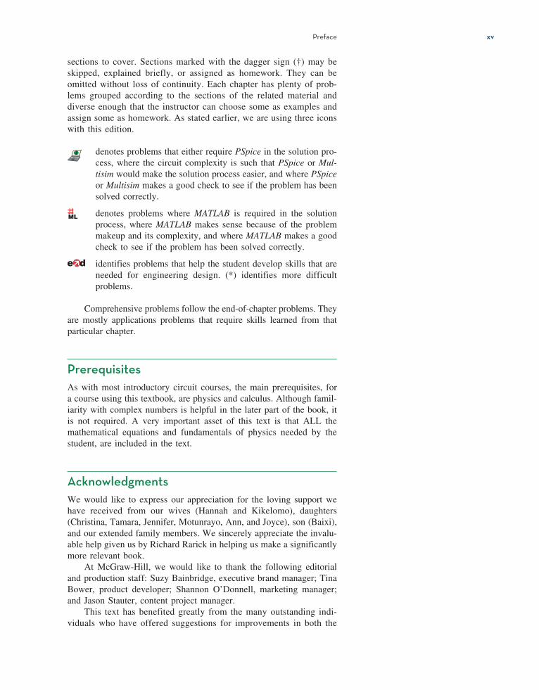
sections to cover. Sections marked with the dagger sign (†) may be skipped, explained briefly, or assigned as homework. They can be omitted without loss of continuity. Each chapter has plenty of prob-lems grouped according to the sections of the related material and diverse enough that the instructor can choose some as examples and assign some as homework. As stated earlier, we are using three icons with this edition.

denotes problems that either require PSpice in the solution pro-cess, where the circuit complexity is such that PSpice or Mul-tisim would make the solution process easier, and where PSpice or Multisim makes a good check to see if the problem has been solved correctly.

denotes problems where MATLAB is required in the solution process, where MATLAB makes sense because of the problem makeup and its complexity, and where MATLAB makes a good check to see if the problem has been solved correctly.

identifies problems that help the student develop skills that are needed for engineering design. (*) identifies more difficult problems.

Comprehensive problems follow the end-of-chapter problems. They are mostly applications problems that require skills learned from that particular chapter.

PrerequisitesAs with most introductory circuit courses, the main prerequisites, for a course using this textbook, are physics and calculus. Although famil-iarity with complex numbers is helpful in the later part of the book, it is not required. A very important asset of this text is that ALL the mathematical equations and fundamentals of physics needed by the student, are included in the text.

AcknowledgmentsWe would like to express our appreciation for the loving support we have received from our wives (Hannah and Kikelomo), daughters (Christina, Tamara, Jennifer, Motunrayo, Ann, and Joyce), son (Baixi), and our extended family members. We sincerely appreciate the invalu-able help given us by Richard Rarick in helping us make a significantly more relevant book. At McGraw-Hill, we would like to thank the following editorial and production staff: Suzy Bainbridge, executive brand manager; Tina Bower, product developer; Shannon O’Donnell, marketing manager; and Jason Stauter, content project manager. This text has benefited greatly from the many outstanding indi-viduals who have offered suggestions for improvements in both the

xvi Preface

text as well as the various problems. In particular, we thank Nicholas Reeder, Professor of Electronics Engineering Technology, Sinclair Community College, Dayton, Ohio, and Douglas De Boer, Professor of Engineering, Dordt College, Sioux Center, Iowa, for their detailed and careful corrections and suggestions for clarification which have contributed to making this a better edition. In addition, the following have made important contributions to this textbook (in alphabetical order):

Zekeriya Aliyazicioglu, California State Polytechnic University— PomonaRajan Chandra, California State Polytechnic University—PomonaMohammad Haider, University of Alabama—BirminghamJohn Heathcote, Reedley CollegePeter LoPresti, University of TulsaRobert Norwood, John Brown UniversityAaron Ohta, University of Hawaii—ManoaSalomon Oldak, California State Polytechnic University—PomonaHesham Shaalan, U.S. Merchant Marine AcademySurendra Singh, University of Tulsa

Finally, we sincerely appreciate the feedback received from instructors and students who used the previous editions. We want this to continue, so please keep sending us e-mails or direct them to the publisher. We can be reached at [email protected] for Charles Alexander and [email protected] for Matthew Sadiku.

C. K. Alexander and M. N. O. Sadiku

SupplementsInstructor and Student Resources Available on Connect are a number of additional instructor and student resources to accompany the text. These include complete solutions for all practice and end-of-chapter problems, solutions in PSpice and Multisim problems, lecture PowerPoints®, and text image files. Problem Solving Made Almost Easy, a companion workbook to Fundamentals of Electric Circuits, is available for students who wish to practice their problem-solving techniques. The workbook can be found at mhhe.com/alexander7e and contains a discussion of problem-solving strategies and 150 additional problems with complete solutions provided.

McGraw-Hill Create®Craft your teaching resources to match the way you teach! With McGraw-Hill Create, http://create.mheducation.com, you can easily rearrange chapters, combine material from other content sources, and quickly upload content you have written like your course syllabus or teaching notes. Find the content you need in Create by searching through thousands of leading McGraw-Hill textbooks. Arrange your book to fit your teaching style. Create even allows you to personalize

Preface xvii

your book’s appearance by selecting the cover and adding your name, school, and course information. Order a Create book and you’ll receive a complimentary print review copy in three to five business days or a complimentary electronic review copy (eComp) via e-mail in minutes. Go to http://create.mheducation.com today and register to experience how McGraw-Hill Create empowers you to teach your students your way.

Affordability & Outcomes = Academic Freedom!You deserve choice, flexibility and control. You know what’s best for your students

and selecting the course materials that will help them succeed should be in your hands.

Thats why providing you with a wide range of options that lower costs and drive better outcomes is our highest priority.

They’ll thank you for it.Study resources in Connect help your students be better prepared in less time. You can transform your class time from dull definitions to dynamic discussion. Hear from your peers about the benefits of Connect at www.mheducation.com/highered/connect/smartbook

Make it simple, make it affordable.Connect makes it easy with seamless integration using any of the major Learning Management Systems— Blackboard®, Canvas, and D2L, among others—to let you organize your course in one convenient location. Give your students access to digital materials at a discount with our inclusive access program. Ask your McGraw-Hill representative for more information.

Learning for everyone.McGraw-Hill works directly with Accessibility Services Departments and faculty to meet the learning needs of all students. Please contact your Accessibility Services office and ask them to email [email protected], or visit www.mheducation.com/about/accessibility.html for more information.

Students—study more efficiently, retain more and achieve better outcomes. Instructors—focus on what you love—teaching.

®

Rent ItAffordable print and digital rental options through our partnerships with leading textbook distributors including Amazon, Barnes & Noble, Chegg, Follett, and more.

Go DigitalA full and flexible range of affordable digital solutions ranging from Connect, ALEKS, inclusive access, mobile apps, OER and more.

Get PrintStudents who purchase digital materials can get a loose-leaf print version at a significantly reduced rate to meet their individual preferences and budget.

Learn more at: www.mheducation.com/realvalue

Laptop: McGraw-Hill Education

xx

A Note to the StudentThis may be your first course in electrical engineering. Although elec-trical engineering is an exciting and challenging discipline, the course may intimidate you. This book was written to prevent that. A good textbook and a good professor are an advantage—but you are the one who does the learning. If you keep the following ideas in mind, you will do very well in this course.

∙ This course is the foundation on which most other courses in the electrical engineering curriculum rest. For this reason, put in as much effort as you can. Study the course regularly.

∙ Problem solving is an essential part of the learning process. Solve as many problems as you can. Begin by solving the practice prob-lem following each example, and then proceed to the end-of-chapter problems. The best way to learn is to solve a lot of problems. An asterisk in front of a problem indicates a challenging problem.

∙ Spice and Multisim, computer circuit analysis programs, are used throughout the textbook. PSpice, the personal computer version of Spice, is the popular standard circuit analysis program at most universities. PSpice for Windows and Multisim are described on our website. Make an effort to learn PSpice and/or Multisim, because you can check any circuit problem with them and be sure you are handing in a correct problem solution.

∙ MATLAB is another software that is very useful in circuit analysis and other courses you will be taking. A brief tutorial on MATLAB can be found on our website. The best way to learn MATLAB is to start working with it once you know a few commands.

∙ Each chapter ends with a section on how the material covered in the chapter can be applied to real-life situations. The concepts in this section may be new and advanced to you. No doubt, you will learn more of the details in other courses. We are mainly interested in gaining a general familiarity with these ideas.

∙ Attempt the review questions at the end of each chapter. They will help you discover some “tricks” not revealed in class or in the textbook.

∙ Clearly a lot of effort has gone into making the technical details in this book easy to understand. It also contains all the mathemat-ics and physics necessary to understand the theory and will be very useful in your other engineering courses. However, we have also focused on creating a reference for you to use both in school as well as when working in industry or seeking a graduate degree.

A Note to the Student xxi

∙ It is very tempting to sell your book after you have completed your classroom experience; however, our advice to you is DO NOT SELL YOUR ENGINEERING BOOKS! Books have always been expensive; however, the cost of this book is virtually the same as I paid for my circuits text back in the early 60s in terms of real dollars. In fact, it is actually cheaper. In addition, engineering books of the past are nowhere near as complete as what is available now.

When I was a student, I did not sell any of my engineering textbooks and was very glad I did not! I found that I needed most of them throughout my career. A short review on finding determinants is covered in Appendix A, complex numbers in Appendix B, and mathematical formulas in Appendix C. Answers to odd-numbered problems are given in Appendix D. Have fun! C. K. A. and M. N. O. S.

xxiiixxiii

About the AuthorsCharles K. Alexander Professor Emeritus of Electrical Engineering and Computer Science in the Washkewicz College of Engineering, Cleveland State University, Cleveland, Ohio. He was a Professor of Electrical Engineering and Computer Science at Cleveland State University from 2002 until 2018. He was the director of The Center for Research in Electronics and Aerospace Technology (CREATE) from 2004 until 2018. From 2002 until 2006 he was Dean of the Fenn College of Engineering. He has held the position of dean of engineer-ing at Cleveland State University, California State University, North-ridge, and Temple University (acting dean for six years). He has held the position of department chair at Temple University and Tennessee Technological University. He has held the position of Stocker Visiting Professor (an endowed chair) at Ohio University. He has held faculty status at all of the before mentioned named universities. He has secured funding for the establishment of two centers of research, one in power and energy at Tennessee Technological Univer-sity and another in sensor systems at Cleveland State University. He has been the director of three additional research centers at Temple and at Ohio University. He has obtained research funding of approximately $100 million (in today’s dollars). He has served as a consultant to twenty-three private and governmental organizations, including the Air Force and the Navy. He received the honorary Dr. Eng. from Ohio Northern University (2009), the Ph.D. (1971) and M.S.E.E. (1967) from Ohio University and the B.S.E.E. (1965) from Ohio Northern University. He has authored many publications, including a workbook and a videotape lecture series, and is coauthor of Fundamentals of Electric Circuits (now in the seventh edition), Engineering Skills for Career Success, Problem Solving Made ALMOST Easy, the fifth edition of the Standard Handbook of Electronic Engineering, and Applied Circuit Analysis, all with McGraw-Hill. He has authored or coauthored 30 books counting separate editions and foreign translations and he has made more than 500 paper, professional, and technical presentations. This circuits textbook was ranked number one or number two world-wide recently. Dr. Alexander is a Life Fellow of the IEEE and served as its international president and CEO in 1997. In addition, he has held sev-eral leadership positions within IEEE during his more than fifty years of service as a volunteer. This includes serving 1991 to 1999 on the IEEE Board of Directors. He has received several local, regional, national, and international awards for teaching, research, and service, including an honorary Doctor of Engineering degree, Fellow of the IEEE, the IEEE-USA Jim Watson Student Professional Awareness Achievement Award, the IEEE Under-graduate Teaching Award, the Distinguished Professor Award, the

Charles K. Alexander

xxiv About the Authors

Distinguished Engineering Education Achievement Award, the Distin-guished Engineering Education Leadership Award, the IEEE Centen-nial Medal, and IEEE/RAB Innovation Award.

Matthew N. O. Sadiku received his B.Sc. degree in 1978 from Ahmadu Bello University, Zaria, Nigeria and his M.Sc. and Ph.D. degrees from Tennessee Technological University, Cookeville, TN, in 1982 and 1984, respectively. From 1984 to 1988, he was an assistant professor at Florida Atlantic University, Boca Raton, FL, where he did graduate work in computer science. From 1988 to 2000, he was at Temple University, Philadelphia, PA, where he became a full professor. From 2000 to 2002, he was with Lucent/Avaya, Holmdel, NJ, as a system engineer and with Boeing Satellite Systems, Los Angeles, CA, as a senior scientist. He is presently a professor of electrical and computer engineering at Prairie View A&M University, Prairie View, TX. He is the author of over 660 professional papers and over 80 books including “Elements of Electromagnetics” (Oxford University Press, 7th ed., 2018), Fundamentals of Electric Circuits (McGraw-Hill, now in 7th edition, with C. Alexander), Computational Electromagnetics with MATLAB (CRC, 4th ed., 2019), and Principles of Modern Communication Systems (Cambridge University Press, 2017, with S. O. Agbo). In addition to the engineering books, he has written Christian books including Secrets of Successful Marriages, How to Discover God’s Will for Your Life, and commentaries on all the books of the New Testament Bible. Some of his books have been translated into French, Korean, Chinese (and Chinese Long Form in Taiwan), Italian, Portuguese, and Spanish. He was the recipient of the 2000 McGraw-Hill/Jacob Millman Award for outstanding contributions in the field of electrical engineering. He was also the recipient of Regents Professor award for 2012–2013 by the Texas A&M University System. He is a registered professional engineer and a fellow of the Institute of Electrical and Electronics Engineers (IEEE) “for contributions to computational electromagnetics and engineering education.” He was the IEEE Region 2 Student Activ-ities Committee Chairman. He was an associate editor for IEEE Trans-actions on Education. He is also a member of Association for Computing Machinery (ACM) and American Society of Engineering Education (ASEE). His current research interests are in the areas of computational electromagnetics, computer networks, and engineering education. His works can be found in his autobiography, My Life and Work (Trafford Publishing, 2017) or his website: www.matthew-sadiku.com. He currently resides with his wife Kikelomo in Hockley, TX. He can be reached via email at [email protected].

Matthew N. O. Sadiku

Fundamentals of

Electric Circuits

P A R T O N E

DC Circuits

OUTLINE

1 Basic Concepts

2 Basic Laws

3 Methods of Analysis

4 Circuit Theorems

5 Operational Amplifiers

6 Capacitors and Inductors

7 First-Order Circuits

8 Second-Order Circuits

Source: NASA, ESA, and M. Livio and The Hubble 20th Anniversary Team (STScI)

3

Charles Alexander

Basic ConceptsSome books are to be tasted, others to be swallowed, and some few to be chewed and digested.

—Francis Bacon

c h a p t e r

1Enhancing Your Skills and Your Career

ABET EC 2000 criteria (3.a), “an ability to apply knowledge of mathematics, science, and engineering.”As students, you are required to study mathematics, science, and engi-neering with the purpose of being able to apply that knowledge to the solution of engineering problems. The skill here is the ability to apply the fundamentals of these areas in the solution of a problem. So how do you develop and enhance this skill?

The best approach is to work as many problems as possible in all of your courses. However, if you are really going to be successful with this, you must spend time analyzing where and when and why you have dif-ficulty in easily arriving at successful solutions. You may be surprised to learn that most of your problem-solving problems are with mathematics rather than your understanding of theory. You may also learn that you start working the problem too soon. Taking time to think about the prob-lem and how you should solve it will always save you time and frustra-tion in the end.

What I have found that works best for me is to apply our six-step problem-solving technique. Then I carefully identify the areas where I have difficulty solving the problem. Many times, my actual deficiencies are in my understanding and ability to use correctly certain mathematical principles. I then return to my fundamental math texts and carefully re-view the appropriate sections, and in some cases, work some example problems in that text. This brings me to another important thing you should always do: Keep nearby all your basic mathematics, science, and engineering textbooks.

This process of continually looking up material you thought you had acquired in earlier courses may seem very tedious at first; however, as your skills develop and your knowledge increases, this process will become easier and easier. On a personal note, it is this very process that led me from being a much less than average student to someone who could earn a Ph.D. and become a successful researcher.

4 Chapter 1 Basic Concepts

1.1 IntroductionElectric circuit theory and electromagnetic theory are the two fundamen-tal theories upon which all branches of electrical engineering are built. Many branches of electrical engineering, such as power, electric ma-chines, control, electronics, communications, and instrumentation, are based on electric circuit theory. Therefore, the basic electric circuit theory course is the most important course for an electrical engineering student, and always an excellent starting point for a beginning student in electri-cal engineering education. Circuit theory is also valuable to students spe-cializing in other branches of the physical sciences because circuits are a good model for the study of energy systems in general, and because of the applied mathematics, physics, and topology involved.

In electrical engineering, we are often interested in communicating or transferring energy from one point to another. To do this requires an interconnection of electrical devices. Such interconnection is referred to as an electric circuit, and each component of the circuit is known as an element.

An electric circuit is an interconnection of electrical elements.

A simple electric circuit is shown in Fig. 1.1. It consists of three basic elements: a battery, a lamp, and connecting wires. Such a simple circuit can exist by itself; it has several applications, such as a flash- light, a search light, and so forth.

A complicated real circuit is displayed in Fig. 1.2, representing the schematic diagram for a radio receiver. Although it seems complicated, this circuit can be analyzed using the techniques we cover in this book. Our goal in this text is to learn various analytical techniques and computer software applications for describing the behavior of a circuit like this.

Electric circuits are used in numerous electrical systems to accomplish different tasks. Our objective in this book is not the study of various uses and applications of circuits. Rather, our major concern is the analysis of the circuits. By the analysis of a circuit, we mean a study of the behavior

Learning ObjectivesBy using the information and exercises in this chapter you will be able to:1. Understand the different units with which engineers work.2. Understand the relationship between charge and current and

how to use both in a variety of applications.3. Understand voltage and how it can be used in a variety of

applications.4. Develop an understanding of power and energy and their

relationship with current and voltage.5. Begin to understand the volt-amp characteristics of a variety of

circuit elements.6. Begin to understand an organized approach to problem solving

and how it can be used to assist in your efforts to solve circuit problems.

+–

Current

LampBattery

Figure 1.1A simple electric circuit.

1.2 Systems of Units 5

of the circuit: How does it respond to a given input? How do the intercon-nected elements and devices in the circuit interact?

We commence our study by defining some basic concepts. These concepts include charge, current, voltage, circuit elements, power, and energy. Before defining these concepts, we must first establish a system of units that we will use throughout the text.

1.2 Systems of UnitsAs electrical engineers, we must deal with measurable quantities. Our mea-surements, however, must be communicated in a standard language that virtually all professionals can understand, irrespective of the country in which the measurement is conducted. Such an international measurement language is the International System of Units (SI), adopted by the General Conference on Weights and Measures in 1960. In this system, there are seven base units from which the units of all other physical quantities can be de-rived. Table 1.1 shows six base units and one derived unit (the coulomb) that are related to this text. SI units are commonly used in electrical engineering.

One great advantage of the SI unit is that it uses prefixes based on the power of 10 to relate larger and smaller units to the basic unit. Table 1.2 shows the SI prefixes and their symbols. For example, the following are expressions of the same distance in meters (m):

600,000,000 mm 600,000 m 600 km

L1C4

Antenna

C5Q2

R7

R2 R4 R6

R3 R5

C1

C3

C2

Electretmicrophone

R1

+

–

+ 9 V (DC)

Q1

Figure 1.2Electric circuit of a radio transmitter.

TABLE 1.1

Six basic SI units and one derived unit relevant to this text.

Quantity Basic unit SymbolLength meter mMass kilogram kgTime second sElectric current ampere AThermodynamic temperature kelvin KLuminous intensity candela cdCharge coulomb C

TABLE 1.2

The SI prefixes.

Multiplier Prefix Symbol1018 exa E1015 peta P1012 tera T109 giga G106 mega M103 kilo k102 hecto h10 deka da10−1 deci d10−2 centi c10−3 milli m10−6 micro μ10−9 nano n10−12 pico p10−15 femto f10−18 atto a


1.3 Charge and CurrentThe concept of electric charge is the underlying principle for explaining all electrical phenomena. Also, the most basic quantity in an electric circuit is the electric charge. We all experience the effect of electric charge when we try to remove our wool sweater and have it stick to our body or walk across a carpet and receive a shock.

Charge is an electrical property of the atomic particles of which matter consists, measured in coulombs (C).

We know from elementary physics that all matter is made of fundamental building blocks known as atoms and that each atom consists of electrons, protons, and neutrons. We also know that the charge e on an electron is negative and equal in magnitude to 1.602 × 10−19 C, while a proton carries a positive charge of the same magnitude as the electron. The presence of equal numbers of protons and electrons leaves an atom neutrally charged.

The following points should be noted about electric charge:

1. The coulomb is a large unit for charges. In 1 C of charge, there are 1∕(1.602 × 10−19) = 6.24 × 1018 electrons. Thus realistic or labora-tory values of charges are on the order of pC, nC, or μC.1

2. According to experimental observations, the only charges that occur in nature are integral multiples of the electronic charge e = −1.602 × 10−19 C.

3. The law of conservation of charge states that charge can neither be created nor destroyed, only transferred. Thus, the algebraic sum of the electric charges in a system does not change.

We now consider the flow of electric charges. A unique feature of electric charge or electricity is the fact that it is mobile; that is, it can be transferred from one place to another, where it can be converted to another form of energy.

When a conducting wire (consisting of several atoms) is connected to a battery (a source of electromotive force), the charges are compelled to move; positive charges move in one direction while negative charges move in the opposite direction. This motion of charges creates electric current. It is conventional to take the current flow as the movement of positive charges. That is, opposite to the flow of negative charges, as Fig. 1.3 illustrates. This convention was introduced by Benjamin Franklin (1706–1790), the American scientist and inventor. Although we now know that current in metallic conductors is due to negatively charged electrons, we will follow the universally accepted convention that current is the net flow of positive charges. Thus,

Electric current is the time rate of change of charge, measured in amperes (A).

Mathematically, the relationship between current i, charge q, and time t is

i = Δ dq ___

dt (1.1)

A convention is a standard way of describing something so that others in the profession can understand what we mean. We will be using IEEE conventions throughout this book.

Battery

I–

+ –

–––

Figure 1.3Electric current due to flow of electronic charge in a conductor.

1 However, a large power supply capacitor can store up to 0.5 C of charge.

1.3 Charge and Current 7

where current is measured in amperes (A), and1 ampere = 1 coulomb/second

The charge transferred between time t0 and t is obtained by integrating both sides of Eq. (1.1). We obtain

Q = Δ ∫t0

t

i dt (1.2)

The way we define current as i in Eq. (1.1) suggests that current need not be a constant-valued function. As many of the examples and problems in this chapter and subsequent chapters suggest, there can be several types of current; that is, charge can vary with time in several ways.

There are different ways of looking at direct current and alternating current. The best definition is that there are two ways that current can flow: It can always flow in the same direction, where it does not reverse direction, in which case we have direct current (dc). These currents can be constant or time varying. If the current flows in both directions, then we have alternating current (ac).

A direct current (dc) flows only in one direction and can be constant or time varying.

By convention, we will use the symbol I to represent a constant current. If the current varies with respect to time (either dc or ac) we will use the symbol i. A common use of this would be the output of a rectifier (dc) such as i(t) = ∣5 sin(377t)∣ amps or a sinusoidal current (ac) such as i(t) = 160 sin(377t) amps.

An alternating current (ac) is a current that changes direction with respect to time.

An example of alternating current (ac) is the current you use in your house to run the air conditioner, refrigerator, washing machine, and other electric appliances. Figure 1.4 depicts two common examples of dc

Andre-Marie Ampere (1775–1836), a French mathematician and physicist, laid the foundation of electrodynamics. He defined the electric current and developed a way to measure it in the 1820s.

Born in Lyons, France, Ampere at age 12 mastered Latin in a few weeks, as he was intensely interested in mathematics and many of the best mathematical works were in Latin. He was a brilliant scientist and a prolific writer. He formulated the laws of electromagnetics. He in vented the electromagnet and the ammeter. The unit of electric current, the ampere, was named after him.

Apic/Getty Images

Historical

I

0 t

(a)

(b)

i

t0

Figure 1.4Two common types of current: (a) direct current (dc), (b) alternating current (ac).


(coming from a battery) and ac (coming from your home outlets). We will consider other types later in the book.

Once we define current as the movement of charge, we expect current to have an associated direction of flow. As mentioned earlier, the direction of current flow is conventionally taken as the direction of positive charge movement. Based on this convention, a current of 5 A may be represented positively or negatively as shown in Fig. 1.5. In other words, a negative current of −5 A flowing in one direction as shown in Fig. 1.5(b) is the same as a current of +5 A flowing in the opposite direction.

5 A

(a)

–5 A

(b)

Figure 1.5Conventional current flow: (a) positive current flow, (b) negative current flow.

Example 1.1 How much charge is represented by 4,600 electrons?

Solution:Each electron has −1.602 × 10−19 C. Hence 4,600 electrons will have −1.602 × 10−19 C/electron × 4,600 electrons = −7.369 × 10−16 C

Example 1.2 The total charge entering a terminal is given by q = 5t sin 4πt mC. Calculate the current at t = 0.5 s.

Solution:

i = dq ___

dt = d __

dt (5t sin 4πt) mC/s = (5 sin 4πt + 20πt cos 4πt) mA

At t = 0.5,

i = 5 sin 2π + 10π cos 2π = 0 + 10π = 31.42 mA

Calculate the amount of charge represented by 10 billion protons.

Answer: 1.6021 × 10−9 C.

Practice Problem 1.1

If in Example 1.2, q = (20 – 15t – 10e−3t ) mC, find the current at t = 1.0 s.

Answer: −13.506 mA.


Example 1.3 Determine the total charge entering a terminal between t = 1 s and t = 2 s if the current passing the terminal is i = (3t2 − t) A.

Solution:

Q = ∫t=1

2 i dt = ∫1

2 (3t2 − t) dt

= ( t3 − t2 __ 2 ) ∣ 1

2 = (8 − 2) − ( 1 − 1 __ 2 ) = 5.5 C

1.4 Voltage 9

The current flowing through an element is

i = { 8 A,

0 < t < 1

8t2 A,

t > 1

Calculate the charge entering the element from t = 0 to t = 2 s.

Answer: 26.67 C.


1.4 VoltageAs explained briefly in the previous section, to move the electron in a conductor in a particular direction requires some work or energy transfer. This work is performed by an external electromotive force (emf), typi-cally represented by the battery in Fig. 1.3. This emf is also known as voltage or potential difference. The voltage vab between two points a and b in an electric circuit is the energy (or work) needed to move a unit charge from b to a; mathematically,

vab = Δ dw ___ dq

(1.3)

where w is energy in joules (J) and q is charge in coulombs (C). The volt-age vab or simply v is measured in volts (V), named in honor of the Italian physicist Alessandro Antonio Volta (1745–1827), who invented the first voltaic battery. From Eq. (1.3), it is evident that

1 volt = 1 joule/coulomb = 1 newton-meter/coulomb

Thus,

Voltage (or potential difference) is the energy required to move a unit charge from a reference point (−) to another point (+), measured in volts (V).

Figure 1.6 shows the voltage across an element (represented by a rectangular block) connected to points a and b. The plus (+) and minus (−) signs are used to define reference direction or voltage polar-ity. The vab can be interpreted in two ways: (1) Point a is at a potential of vab volts higher than point b, or (2) the potential at point a with respect to point b is vab. It follows logically that in general

vab = −vba (1.4)

For example, in Fig. 1.7, we have two representations of the same volt-age. In Fig. 1.7(a), point a is +9 V above point b; in Fig. 1.7(b), point b is −9 V above point a. We may say that in Fig. 1.7(a), there is a 9-V volt-age drop from a to b or equivalently a 9-V voltage rise from b to a. In other words, a voltage drop from a to b is equivalent to a voltage rise from b to a.

Current and voltage are the two basic variables in electric circuits. The common term signal is used for an electric quantity such as a current or a voltage (or even electromagnetic wave) when it is used for

a

b

vab

+

–

Figure 1.6Polarity of voltage vab.

9 V

(a)

a

b

+

–

–9 V

(b)

a

b+

–

Figure 1.7Two equivalent representations of the same voltage vab: (a) Point a is 9 V above point b; (b) point b is −9 V above point a.

ISE EBook Online Access for Fundamentals of Electric Circuits

Documents

Transcript of ISE EBook Online Access for Fundamentals of Electric Circuits