eScholarship provides open access, scholarly publishingservices to the University of California and delivers a dynamicresearch platform to scholars worldwide.

Department of Agricultural and ResourceEconomics, UCB

UC Berkeley

Title:International Environmental Agreements with Mixed Strategies and Investment

Author:Hong, Fuhai, School of Economics, Shanghai University of Finance and EconomicsKarp, Larry, University of California, Berkeley and Giannini Foundation

Publication Date:05-08-2012

Series:CUDARE Working Papers

Permalink:http://escholarship.org/uc/item/0xf976x1

Keywords:International Environmental Agreement, climate agreement, participation games, investment,mixed strategy

Local Identifier:CUDARE Working Paper No. CUDARE 1129

Abstract:We modify a canonical participation game used to study International Environmental Agreements(IEA), considering both mixed and pure strategies at the participation stage, and including a priorcost-reducing investment stage. The use of mixed strategies at the participation stage reversesa familiar result and alsoreverses the policy implication of that result: with mixed strategies,equilibriumparticipation and welfare is higher in equilibria that involve higher investment.

Copyright Information:All rights reserved unless otherwise indicated. Contact the author or original publisher for anynecessary permissions. eScholarship is not the copyright owner for deposited works. Learn moreat http://www.escholarship.org/help_copyright.html#reuse

Copyright © 2012 by author(s).

University of California, Berkeley Department of Agricultural &

Resource Economics

CUDARE Working Papers Year 2012 Paper 1129

International Environmental Agreements with Mixed Strategies and Investment

Fuhsai Hong and Larry Karp

International Environmental Agreements with

Mixed Strategies and Investment∗

Fuhai Hong† Larry Karp‡

May 8, 2012

Abstract

We modify a canonical participation game used to study International Envi-

ronmental Agreements (IEA), considering both mixed and pure strategies at the

participation stage, and including a prior cost-reducing investment stage. The

use of mixed strategies at the participation stage reverses a familiar result and also

reverses the policy implication of that result: with mixed strategies, equilibrium

participation and welfare is higher in equilibria that involve higher investment.

Keywords: International Environmental Agreement, climate agreement, partici-

pation game, investment, mixed strategy.

JEL classification numbers C72, H4, Q54

∗We thank Michael Finus, Matthieu Glachant, Teddy Kim, Danyang Xie, participants of 4thWCERE, 2010 EAERE-FEEM-VIU Summer School, and seminars in HKUST, National University

of Singapore, and Nanyang Technological University, the editor of this Journal, and two anonymous

referees for helpful comments. Larry Karp thanks the Ragnar Frisch Centre for Economic Research

for financial support.†School of Economics, Shanghai University of Finance and Economics, email:

hong.fuhai@mail.shufe.edu.cn‡Department of Agricultural and Resource Economics, University of California, Berkeley, and the

Ragnar Frisch Center for Economic Research, email: karp@berkeley.edu

1 Introduction

Limiting increases in Greenhouse Gas (GHG) stocks requires an international effort.

The global nature of GHG pollution and the fact of national sovereignty complicate

the usual problems of eliciting the provision of a public good, in this case, reduction of

GHG emissions. International Environmental Agreements (IEAs) attempt to alleviate

the free riding problem associated with transboundary pollution. Although there are

many examples of successful IEAs, these do not involve problems on the same scale

as climate change. In the absence of historical analogies, economic theory plays an

especially important role in helping to think about ways of addressing the climate policy

problem.

The literature on IEAs uses both non-cooperative and cooperative game theory. A

major non-cooperative strand uses the definition of cartel stability in a participation

game (D’Aspremont et al., 1983). In this game, countries first make a binary decision,

whether to join or stay out of an IEA, and then the resulting IEA decides on the level

of abatement. Early papers include Carraro and Siniscalco (1993) and Barrett (1994);

Wagner (2001) and Barrett (2003) review this literature. IEA members internalize the

effect of their actions on other members, while non-members ignore the externalities.

A stable IEA is both internally stable (members do not want to defect) and externally

stable (outsiders do not want to join); that is, the equilibrium at the participation stage

is Nash in the binary participation decision.

These models are generally pessimistic about the equilibrium level of participation,

and they suggest that IEAs are especially ineffective when potential benefits of coop-

eration are large (Ioannidis et al. 2000, Finus 2001, Barrett 2003). Hoel (1992) and

Barrett (1997) show that IEAs may not be able to improve substantially upon the non-

cooperative outcome even when countries are heterogeneous. Karp and Simon (2011)

reconsider these issues using a non-parametric setting. Barrett (2002) and Finus and

Maus (2008) show that coalitions with modest ambitions may be more successful than

those that try to fully internalize damages. Kosfeld et al. (2009), Burger and Kolstad

(2009) and Dannenberg et al. (2009) use laboratory experiments to test the predictions

of this participation game.

A different non-cooperative strand replaces the Nash assumption at the participation

stage with a more sophisticated notion of stability; agents form beliefs about how their

provisional decision to join or leave a coalition would affect other agents’ participation

decisions (Chwe, 1994, Ecchia and Mariotti, 1998, Xue, 1998 and Ray and Vohra,

2001). These agents are said to be “farsighted”. Diamantoudi and Sartzetakis (2002),

Eyckmans (2001), de Zeeuw (2008) and Osmani and Tol (2009) apply this notion of

stability to IEA models. A distinct line of research uses cooperative games and the

theory of the core to model IEAs (e.g. Chander and Tulkens (1995, 1997)). In one

such setting, a country believes that if it defects from a coalition, other countries would

abandon any form of cooperation and act as singletons.

This paper contributes to the strand of IEA literature based on the noncoopera-

tive Nash equilibrium to the participation-game. We examine a mixed rather than

1

a pure strategy equilibrium to this participation game, and we include a prior stage

at which countries individually decide whether to invest in a public good that reduces

abatement costs. For most (but not all) levels of abatement cost, a mixed strategy at

the participation stage leads to a lower level of expected participation, and lower ex-

pected welfare, compared to the pure strategy equilibrium. In this respect, the model

with mixed strategies is even more pessimistic than the model with pure strategies.

However, for sufficiently low abatement costs (large enough benefits of cooperation),

the mixed strategy equilibrium has high participation and nearly solves the free riding

problem. Mixed strategies create endogenous risk; risk aversion increases the equilib-

rium probability of participation. In these respects, the mixed strategy equilibrium

yields a more diverse set of outcomes compared to the pure strategy equilibrium.

The two participation games, corresponding to either mixed or pure strategies, in-

duce two investment games. In general, there are multiple pure strategy equilibria

to both of these investment games, but they have markedly different characteristics

and different policy implications. With pure strategies at the participation stage, as

emphasized by the canonical model, higher investment leads to lower participation and

potentially lower welfare for all agents. With mixed strategies at the participation

stage, we obtain conditions under which higher investment leads to higher participa-

tion and higher welfare for all agents. Due to the existence of multiple Pareto-ranked

equilibria, there is a coordination problem in both of the investment games. In the

game with pure strategies, society would like to coordinate on the low-investment equi-

librium, and in the game with mixed strategies, society would like to coordinate on the

high-investment equilibrium.

Golombek and Hoel (2005, 2006, 2008) consider the effect of investment with techno-

logical spillovers when membership in the IEA is exogenous; in our setting, investment

affects IEA membership. Muuls (2004) and Bayramoglu (2010) consider firms’ incen-

tives to invest in technology, when firms anticipate that countries will bargain over the

level of transboundary pollution; the participation problem is absent and investment is

a private good in their models. Barrett (2006) studies the situation where countries

choose investment non-cooperatively prior to the participation game, at which stage

countries use pure strategies. He points out that opportunities to invest may not help

to solve the participation problem. Hoel and de Zeeuw (2009) assume that the IEA

chooses both investment and the abatement level after the participation stage, and they

allow for the possibility that investment can drive the abatement cost to a level below

the threshold at which abatement is a dominant strategy for individual countries; we

exclude that possibility and we adopt the same timing as in Barrett (2006), but we

emphasize mixed strategies at the participation stage.

Kohnz (2006) considers a mixed strategy in an IEA game with a first stage that

determines the minimum number of members needed for ratification, as in Carraro

et al. (2009); this first-stage decision may commit the IEA to behave sub-optimally,

conditional on the number of members. In contrast, in our model, the minimum number

of members needed for the IEA to decide to abate is determined by the optimization of

the IEA; here, the IEA’s decision maximizes the total welfare of its members, instead

2

of being determined at an earlier stage. Sandler and Sargent (1995) and McGinty

(2010) use mixed strategies in one-stage coordination games, but the issue of minimum

participation does not arise in their settings.

Our paper is most closely related to Dixit and Olson (2000), which has a similar

structure to Palfrey and Rosenthal (1984). Dixit and Olson rely primarily on numerical

examples to characterize the mixed strategy equilibrium, whereas we emphasize analytic

results. More importantly, the two papers have different objectives. Dixit and Olson’s

primary point is that Coasian bargaining does not solve the participation problem;

they demonstrate this by showing that in general participation is low even though the

resulting members of the agreement engage in Coasian bargaining. We find that in

special circumstances Coasian bargaining is consistent with high participation, and

that investment in abatement technology may lead to exactly these circumstances. As

we noted above, under pure strategies this parametric model implies that investment

lowers or leaves unchanged the level of participation.

2 Model basics and rationale for mixed strategies

We first review a canonical IEAmodel, then discuss the use of pure and mixed strategies

at the participation stage, and then explain our modification to the canonical model.

2.1 A canonical IEA model

Barrett (1999) first proposed the following IEA model, which has the advantage of a

simple analytic solution with clear intuition; see also Barrett (2003, Chapter 7), Ulph

(2004), Burger and Kolstad (2009) and Kolstad (2011, Chapter 19). There are

identical countries, each of which has two sequential binary decisions: participation

in an IEA and abatement. The cost and benefit of abatement are both linear, so in

equilibrium each country abates at the level 0 or at capacity, normalized to 1. Given

linearity, there is no additional loss in generality in assuming that the abatement de-

cision is binary. Abatement is a global public good. By choice of units, the benefit

of each unit of abatement, to each country, equals 1. Each country’s abatement cost

is , with 1 . The first inequality means that it is a dominant strategy for a

country acting alone not to abate and the second inequality means that the world is

better off when a country abates. In view of the normalization of benefit, also equals

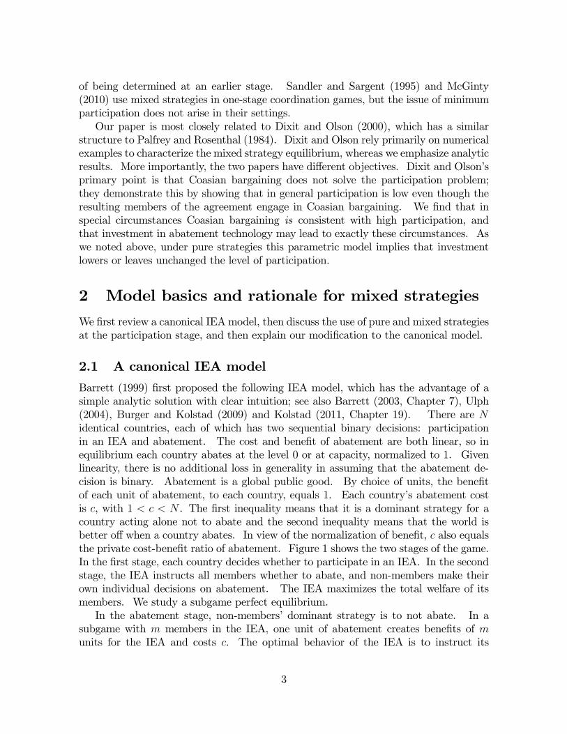
the private cost-benefit ratio of abatement. Figure 1 shows the two stages of the game.

In the first stage, each country decides whether to participate in an IEA. In the second

stage, the IEA instructs all members whether to abate, and non-members make their

own individual decisions on abatement. The IEA maximizes the total welfare of its

members. We study a subgame perfect equilibrium.

In the abatement stage, non-members’ dominant strategy is to not abate. In a

subgame with members in the IEA, one unit of abatement creates benefits of

units for the IEA and costs . The optimal behavior of the IEA is to instruct its

3

Figure 1: A canonical IEA model

members to abate if and only if − ≥ 0. An IEA with () members, where the

function () returns the smallest integer not less than , is the “minimally successful

IEA” under the assumption that the IEA optimizes conditional on membership.

Under the tie-breaking assumption that an agent who is indifferent between joining

and not joining will join, the unique pure strategy Nash equilibrium at the participation

stage consists of () members. For example, with = 32, there are four members

in the pure strategy equilibrium. An outcome with more than () members is not

internally stable because the “extra” members would want to leave: each member’s

defection leaves unchanged other members’ equilibrium action, resulting in a net benefit

− 1 0 to the defector. An outcome with () members is internally and externally

stable; defection by a single member causes the IEA to instruct remaining members to

not abate, causing a net loss to the defector ()− ≥ 0; a non-member loses − 1 byjoining. An outcome with ()−1 members is not externally stable because by joining,a nonmember induces other members to abate and obtains a net benefit ()− ≥ 0.By the tie-breaking assumption, outcomes with fewer than ()− 1 members are alsonot externally stable.

Equilibrium global welfare here is ( − ) (). A small reduction in can lead

to a discrete reduction in equilibrium membership, consequently reducing global welfare.

The potential benefits of cooperation are ( − ) . The fraction of benefits that are

realized,()

, is weakly increasing in the abatement cost, , and thus weakly decreasing

in the potential benefits of cooperation. This conclusion reflects a pessimistic con-

sensus of the literature: the IEA mechanism is especially ineffective when benefits of

cooperation are large. Mixed strategies can reverse this conclusion.

2.2 Mixed strategies

Our contributions rely on the assumption that countries use mixed strategies, whereas

most previous papers assume that countries use pure strategies. Here we discuss the

rationale for using mixed strategies. With pure strategies, the Nash equilibrium selects

the number but not the identity of the participants; ex ante identical agents behave

differently. With (symmetric) mixed strategies, ex ante identical agents use the same

4

strategy, and the number of participants is the realization of a random variable. A

coordination problem arises with pure but not with mixed strategies: How does the

group choose which agent participates and which stays outside the agreement under

pure strategies? The coordination difficulty motivates the use of mixed strategies

in the literature of corporate takeovers (Bagnoli and Lipman, 1988; Holmstrom and

Nalebuff, 1992) and wars of attrition (Maskin, 2003).

A pure strategy equilibrium does not capture the uncertainty about the ability of

nations to agree on a meaningful treaty; a mixed strategy equilibrium captures exactly

this uncertainty. Benedick (2009, page xv), in discussing his experience as a US

negotiator in many IEAs, objects to what he considers academics’ tendency to view the

negotiating process as mechanistic, yielding a deterministic outcome. He emphasizes

the contingency of the process, and the possibility of surprises. The empirical literature

that attempts to explain participation in IEAs (Murdoch, Sandler and Vijverberg, 2003)

of course uses a probabilistic model.

Harsanyi (1973) points out that a mixed strategy equilibrium of a game with com-

plete information can be interpreted as a pure strategy Bayesian Nash Equilibrium of

a closely related game with a small amount of incomplete information. Makris (2009)

suggests that restricting attention to the symmetric mixed-strategy equilibrium of the

game with no uncertainty provides a shortcut for a model where there is very small un-

certainty about the players’ preferences and the expected group-size is large. Crawford

and Haller (1990) consider games in which identical players have identical preferences

among multiple equilibria, but must learn to coordinate over which equilibrium to play

by repeatedly playing the game. They show that in finite time the equilibrium con-

verges to a strategy profile in which all players obtain equal expected payoffs. In the

IEA game only the symmetric mixed-strategy equilibrium has this property.

Finally, given that much of the IEA theory focuses on pure strategies, it is at least

worthwhile looking at how insights might change due to the use of another equilibrium

concept.

2.3 Our modification

We alter the model in Subsection 2.1 in two respects. First, we consider the symmetric

mixed strategy equilibrium at the participation stage. Countries choose a participation

probability, understanding that the IEA will instruct its members to abate if and only

if the number of members is at least (). Second, we include a stage prior to partic-

ipation in which countries individually decide whether to invest in a public good that

reduces abatement costs. In this model, agents have three sequential binary decisions:

investment, participation, and abatement; there are two public goods: investment and

abatement.

At the participation stage is given, but previous investment determines its level.

If countries invested, = (), a decreasing function. The cost of investment is

, which might be either large or small. Countries have rational expectations, and

understand that their investment decision affects and thereby affects equilibrium

5

expected participation. We are especially interested in situations where () is only

slightly larger than 1. In this case, if countries invest, equilibrium membership in

the pure strategy equilibrium is 2, and few of the potential benefits of cooperation are

realized.

We have in mind investment in developing a technology that can be easily replicated.

Patent law enables investors to capture some of the benefit of their investment, but

in many cases there are significant spillovers. Our emphasis on the situation where

investment is a public good captures an important element of the problem. Modeling

investment as a public good means that agents that did invest in the first stage and

those that did not invest have the same abatement costs at the participation stage.

Consequently, we can consider symmetric strategies at the participation stage, a fact

that greatly simplifies the analysis. The public good nature of investment also means

that for the world as a whole, investment has a high return.

3 The participation stage

We characterize the equilibrium mixed strategy, = (), the probability that any

country joins the IEA at the participation stage. We emphasize the risk neutral case.

Here, for most but not all of parameter space, the model with mixed strategies is

more pessimistic than the model with pure strategies. This result is interesting as a

robustness check to one of the major insights of this literature: optimal behavior on

the part of the IEA does little to resolve the problem of providing a global public good.

We then note that risk aversion increases equilibrium participation probabilities.

In the trivial case where = () there exists no strictly mixed strategy equi-

librium. In the rest of this paper, we focus on the nontrivial case (). The

IEA instructs its members to abate if and only if there are at least = () members.

Therefore, a country is pivotal if and only if exactly () − 1 other countries join. If

fewer than () − 1 other countries join, then there would still be too few membersto elicit abatement even if an additional country joins. If more than () − 1 othercountries join, then membership by an additional country is (from its own standpoint)

superfluous: by joining it has no effect on other countries’ abatement but it incurs the

net cost − 1 0.With the probability of each country joining equal to , the probability that a

country is pivotal is

() =( − 1)!

( − 1)! ( − )!−1 (1− )

−

The probability that at least other countries join is

() =

−1X=

( − 1)!! ( − 1− )!

(1− )−1−

6

The net expected benefit of joining is the benefit of joining when the country is

pivotal, − , times the probability that it is pivotal, , minus the loss when the IEA

would have abated even had this country not joined, −1, times the probability of thatevent, . In a mixed strategy equilibrium, must be such that a country is indifferent

between joining and not joining. The equilibrium condition for is therefore

( − ) () = (− 1) () (1)

Remark 1 The right side of equation (1) is continuous in . The left side is discon-

tinuous in at integers; as approaches an integer (greater than 1) from below, the left

side approaches 0; moreover, the left side equals 0 when is an integer. For 1

the right side equals 0 if and only if = 0. Thus, as approaches an integer greater

than 1 from below, the equilibrium approaches 0, and = 0 is the only mixed strategy

equilibrium when is an integer.

For non-integer values of 1, there are two solutions to equation (1), = 0 and

0 1. We are interested in the latter. To study non-integer values of we

rearrange equation (1) to obtain

−

− 1 = ()

() (2)

When 6= 1 and 6= 0, the right hand side of equation (2) is well defined because

() 6= 0. We simplify the right side of equation (2) using

()

()+ 1 = ( − 1)

Z 1

0

(1− )−2

µ1 +

1−

¶− ≡ (; ) (3)

The appendix contain the derivation of this equation and proofs of some propositions.

Equation (3) leads to a simple demonstration of the following:1

Proposition 1 (i) When is a non-integer, there is a unique nontrivial symmetric

mixed strategy equilibrium () 0. (ii) Over any interval of for which is

constant, the equilibrium mixed strategy is a decreasing function of .

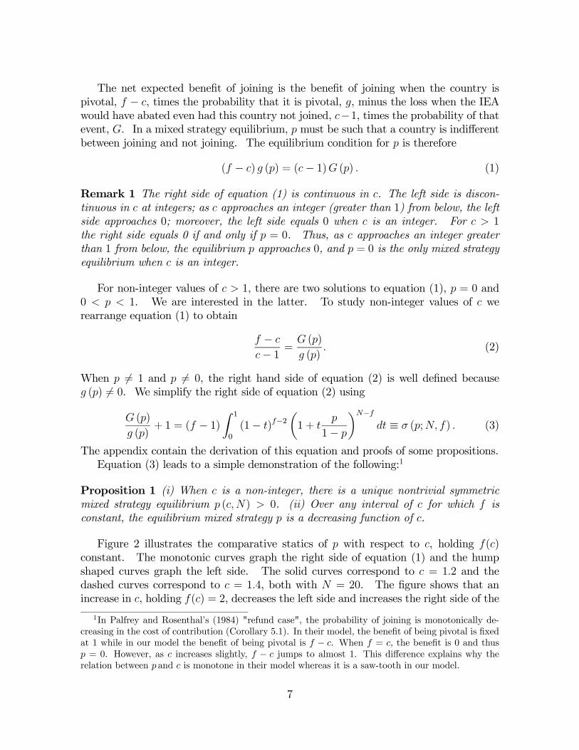
Figure 2 illustrates the comparative statics of with respect to , holding ()

constant. The monotonic curves graph the right side of equation (1) and the hump

shaped curves graph the left side. The solid curves correspond to = 12 and the

dashed curves correspond to = 14, both with = 20. The figure shows that an

increase in , holding () = 2, decreases the left side and increases the right side of the

1In Palfrey and Rosenthal’s (1984) "refund case", the probability of joining is monotonically de-

creasing in the cost of contribution (Corollary 5.1). In their model, the benefit of being pivotal is fixed

at 1 while in our model the benefit of being pivotal is − . When = , the benefit is 0 and thus

= 0. However, as increases slightly, − jumps to almost 1. This difference explains why the

relation between and is monotone in their model whereas it is a saw-tooth in our model.

7

Figure 2: Monotonic curves show ( − 1) and hump-shaped curves show ( − ).

Solid curves correspond to = 12 and dashed curves correspond to = 14. = 20

for both pairs of curves.

equilibrium condition, thereby reducing the equilibrium value of . Intuitively, with

() being fixed, an increase in decreases the benefit of joining when the country is

pivotal, − , increases the loss of joining when the IEA would have abated even had

this country not joined, − 1, and consequently makes joining the IEA less attractive;as a result, is lowered in equilibrium.

Remark 1 and Proposition 1 imply that the graph of as a function of is a saw-

tooth, with upward jumps occurring at integers. Figure 3 illustrates this relation for

= 20 and ∈ (101 6). In the pure strategy equilibrium denotes the deterministic

number of participants; here we use to denote the expected number of participants:

≡ . Because is proportional to , expected membership is also a saw-toothed

function of .

The next result compares the equilibrium expected membership under mixed strate-

gies with membership in the pure strategy equilibrium:

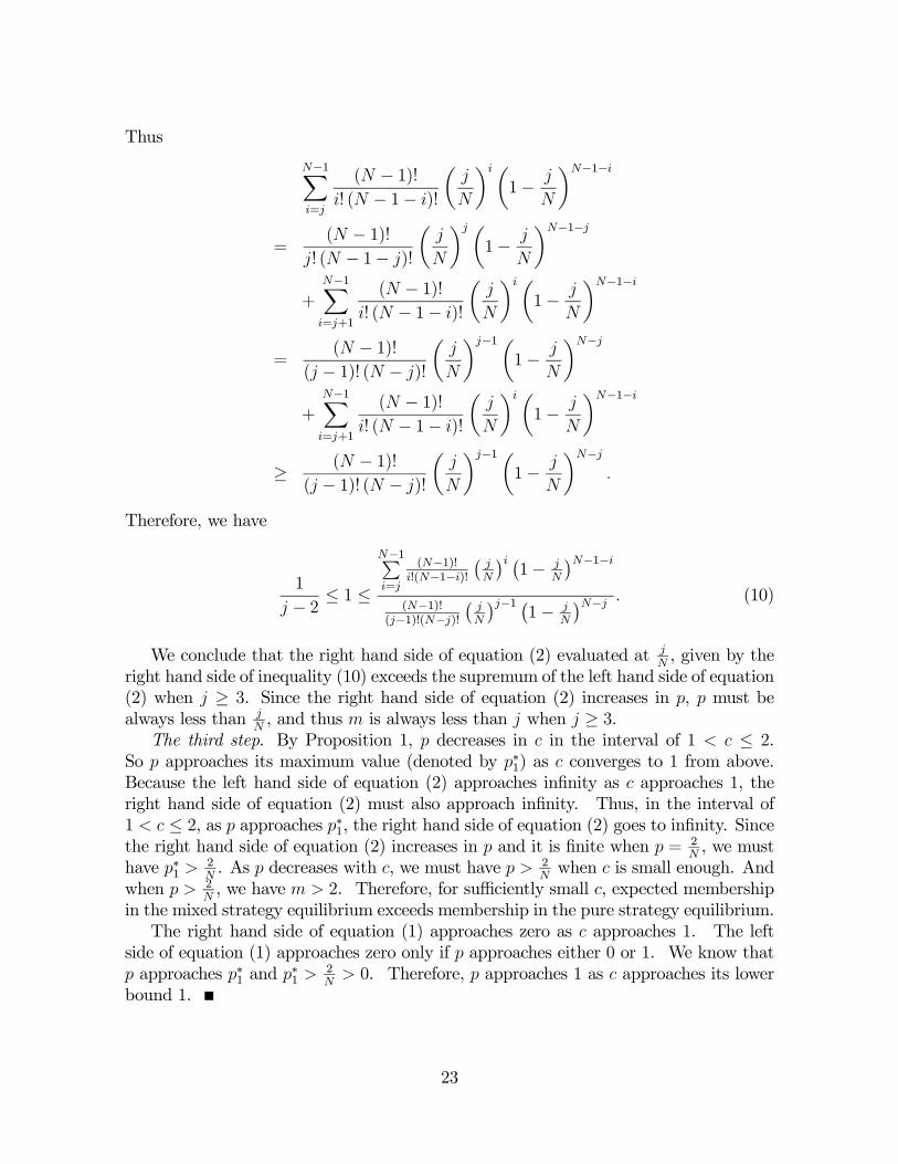
Proposition 2 (i) In the interval ∈ ( − 1 ] for any integer ≥ 3, the expected

membership in the mixed-strategy equilibrium, , is less than (the membership of

the corresponding pure-strategy equilibrium). (ii) In the interval ∈ (1 2], is greater

than 2 (the membership of the corresponding pure-strategy equilibrium) for sufficiently

small. Moreover, as approaches its lower bound 1, converges to 1, and converges

to .

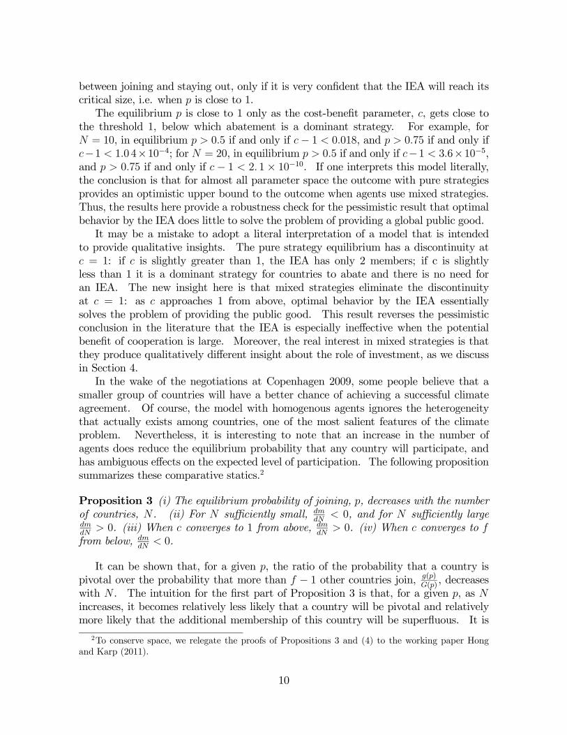
Table 1 summarizes the results in Proposition 2.

8

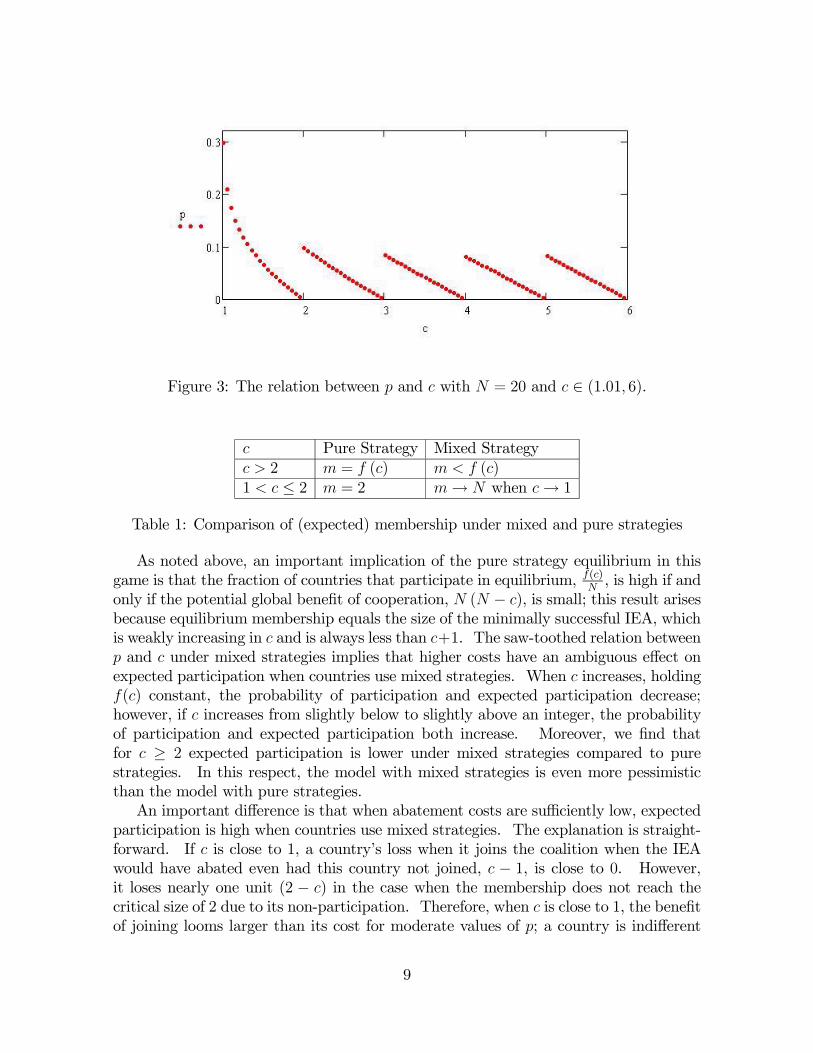
Figure 3: The relation between and with = 20 and ∈ (101 6).

Pure Strategy Mixed Strategy

2 = () ()

1 ≤ 2 = 2 → when → 1

Table 1: Comparison of (expected) membership under mixed and pure strategies

As noted above, an important implication of the pure strategy equilibrium in this

game is that the fraction of countries that participate in equilibrium,()

, is high if and

only if the potential global benefit of cooperation, ( − ), is small; this result arises

because equilibrium membership equals the size of the minimally successful IEA, which

is weakly increasing in and is always less than +1. The saw-toothed relation between

and under mixed strategies implies that higher costs have an ambiguous effect on

expected participation when countries use mixed strategies. When increases, holding

() constant, the probability of participation and expected participation decrease;

however, if increases from slightly below to slightly above an integer, the probability

of participation and expected participation both increase. Moreover, we find that

for ≥ 2 expected participation is lower under mixed strategies compared to pure

strategies. In this respect, the model with mixed strategies is even more pessimistic

than the model with pure strategies.

An important difference is that when abatement costs are sufficiently low, expected

participation is high when countries use mixed strategies. The explanation is straight-

forward. If is close to 1, a country’s loss when it joins the coalition when the IEA

would have abated even had this country not joined, − 1, is close to 0. However,

it loses nearly one unit (2 − ) in the case when the membership does not reach the

critical size of 2 due to its non-participation. Therefore, when is close to 1, the benefit

of joining looms larger than its cost for moderate values of ; a country is indifferent

9

between joining and staying out, only if it is very confident that the IEA will reach its

critical size, i.e. when is close to 1.

The equilibrium is close to 1 only as the cost-benefit parameter, , gets close to

the threshold 1, below which abatement is a dominant strategy. For example, for

= 10, in equilibrium 05 if and only if − 1 0018, and 075 if and only if

−1 10 4×10−4; for = 20, in equilibrium 05 if and only if −1 36×10−5,and 075 if and only if − 1 2 1× 10−10. If one interprets this model literally,the conclusion is that for almost all parameter space the outcome with pure strategies

provides an optimistic upper bound to the outcome when agents use mixed strategies.

Thus, the results here provide a robustness check for the pessimistic result that optimal

behavior by the IEA does little to solve the problem of providing a global public good.

It may be a mistake to adopt a literal interpretation of a model that is intended

to provide qualitative insights. The pure strategy equilibrium has a discontinuity at

= 1: if is slightly greater than 1, the IEA has only 2 members; if c is slightly

less than 1 it is a dominant strategy for countries to abate and there is no need for

an IEA. The new insight here is that mixed strategies eliminate the discontinuity

at = 1: as approaches 1 from above, optimal behavior by the IEA essentially

solves the problem of providing the public good. This result reverses the pessimistic

conclusion in the literature that the IEA is especially ineffective when the potential

benefit of cooperation is large. Moreover, the real interest in mixed strategies is that

they produce qualitatively different insight about the role of investment, as we discuss

in Section 4.

In the wake of the negotiations at Copenhagen 2009, some people believe that a

smaller group of countries will have a better chance of achieving a successful climate

agreement. Of course, the model with homogenous agents ignores the heterogeneity

that actually exists among countries, one of the most salient features of the climate

problem. Nevertheless, it is interesting to note that an increase in the number of

agents does reduce the equilibrium probability that any country will participate, and

has ambiguous effects on the expected level of participation. The following proposition

summarizes these comparative statics.2

Proposition 3 (i) The equilibrium probability of joining, , decreases with the number

of countries, . (ii) For sufficiently small,

0, and for sufficiently large

0. (iii) When converges to 1 from above,

0. (iv) When converges to

from below,

0.

It can be shown that, for a given , the ratio of the probability that a country is

pivotal over the probability that more than − 1 other countries join, ()

(), decreases

with . The intuition for the first part of Proposition 3 is that, for a given , as

increases, it becomes relatively less likely that a country will be pivotal and relatively

more likely that the additional membership of this country will be superfluous. It is

2To conserve space, we relegate the proofs of Propositions 3 and (4) to the working paper Hong

and Karp (2011).

10

thus less attractive for a country to join. In order to maintain indifference, the value of

must decrease. It is not surprising that expected membership, , is non-monotonic

in : a larger increases one factor in this expectation and decreases the other factor.

The next proposition gives the formula for the equilibrium expected participation

as →∞.3

Proposition 4 As →∞, (i) → 0 and (ii) → , where is determined by

1

− 1 =Z 1

0

(1− )−2

; (4)

and (iii) membership follows a Poisson distribution with parameter .

The right side of equation (4) increases in while the left side decreases in .

Therefore, over a region where remains constant, the equilibrium decreases in .

Where passes through an integer value from below, the right side jumps down for

given so the equilibrium must jump up. Thus, in the limit as →∞ we have the

same kind of saw tooth pattern as in the case with finite .

In moving from pure to mixed strategies with no exogenous uncertainty, we create

endogenous risk about participation. The model above assumes that the payoff equals

the expected value of abatement minus abatement costs, i.e. it assumes risk neutrality.

Our working paper (Hong and Karp, 2011) shows that the equilibrium participation

probability increases with the level of risk aversion: concave transformations of the

risk neutral payoff increase expected participation. Examples show that for moderate

levels of constant relative risk aversion, countries are likely to join the IEA when en-

vironmental damage is large relative to the baseline level of income (when no country

abates).

4 The investment stage

Here we investigate how, under risk neutrality, the use of pure or mixed strategies in

the participation game affects the equilibrium in the investment game, and overall equi-

librium welfare. By incurring the investment cost , a country reduces the abatement

cost in the next stage. We emphasize the situation where countries use pure strategies

at the investment stage.

The two participation games (with pure strategies and with mixed strategies) induce

two investment games. In both games, there may be multiple equilibria, but the

nature of the multiplicity is quite different. When countries use pure strategies at

the participation game, the multiplicity at the investment stage arises from the non-

monotonicity of payoffs in costs. In this game, simulations show that the equilibrium

with higher investment leads to lower welfare, exclusive of investment costs. Because

3Myerson (1998a, 1998b, 2005) uses the Poisson limit theorem to study the limiting behavior in

binary action games when the number of players approaches infinity.

11

the countries that invest incur the investment cost, all countries have lower welfare in

the high-investment equilibrium, so the low-investment equilibrium is Pareto dominant.

The investment game when countries use mixed strategies at the participation stage

is more interesting. The fact that , and therefore = , is a saw-toothed function

of means that the reduction in caused by higher investment might lower equilibrium

participation and hence lower welfare, just as with pure strategies. However, Proposition

2.ii implies that if the investment lowers abatement costs sufficiently, the benefit of

investment may be high. In this case, the investment decisions may be strategic

complements. Consider matters from the standpoint of a country that has not yet

decided whether to invest. If that country believes that few other countries will invest,

it may rationally calculate that its own investment would lower expected participation

in the next stage and could be unprofitable even if investment costs are negligible.

However, if it believes that many other countries will invest, the additional decrease

in abatement costs caused by its investment might then increase expected membership

and be profitable. In this case, the mixed strategy at the participation game induces

a coordination game at the investment stage, with high and low investment equilibria.

Here, the high investment equilibrium is likely to be Pareto-dominant.

The non-monotonicity of payoffs, and the fact that they are defined only over integer

values of , complicates the analysis. However, the basic conclusions are intuitive, and

we illustrate these using a numerical example. Additional simulations confirm that the

reported results are robust.

4.1 Pure strategies at the participation stage

Investment is a pure public good, so a country’s investment decision does not distinguish

that country at the participation stage. As in Barrett (2006) and Rubio and Ulph

(2007), we therefore assume that all countries expect to face the same probability

that they will be one of the participants in the next stage, regardless of whether they

invested. Therefore, the probability that any country joins the IEA in the pure strategy

equilibrium is simply the number of members, (), divided by the total number of

countries, . Let () be the next-stage expected payoff given investment level :

() = ( ())− ( ())

()

The benefit of investment for a country given that − 1 other countries invest isthe change in its next-stage expected payoff:

( − 1) = ()− ( − 1)

Given the belief that − 1 other countries invest, a country will invest if and only if ( − 1) ≥ .

If (0) , then there is a corner equilibrium in which no country invests; if

( − 1) ≥ , there is a corner equilibrium in which every country invests. If there

12

exists a , with 0 and ( − 1) (), then there is an interior

equilibrium in which countries invest and − countries do not invest.

Global welfare as a function of is

Φ () = ( − ()) ( ())−

A larger value of lowers abatement costs but it increases total investment costs and

might decrease participation; therefore, global welfare may be non-monotonic in . The

difference in global welfare under zero investment and under a positive value of is

∆ () ≡ Φ (0)−Φ () = ( − (0)) [ ( (0))− ( ())]− ( ()) [ (0)− ()] +

Remark 2 When investment changes the level of participation (i.e. ( (0))− ( ()) 0), ∆ () 0 for sufficiently large . In this situation, global welfare is lower under

0 compared to = 0.

The following example illustrates some of the possibilities:

() =599

0248 + 1 = 20 = 011 (5)

With this example, unit abatement costs fall from 599 to 1005 and participation in

the pure strategy equilibrium falls from 6 members to 2 members as the amount of

investment, ranges from 0 to 20.

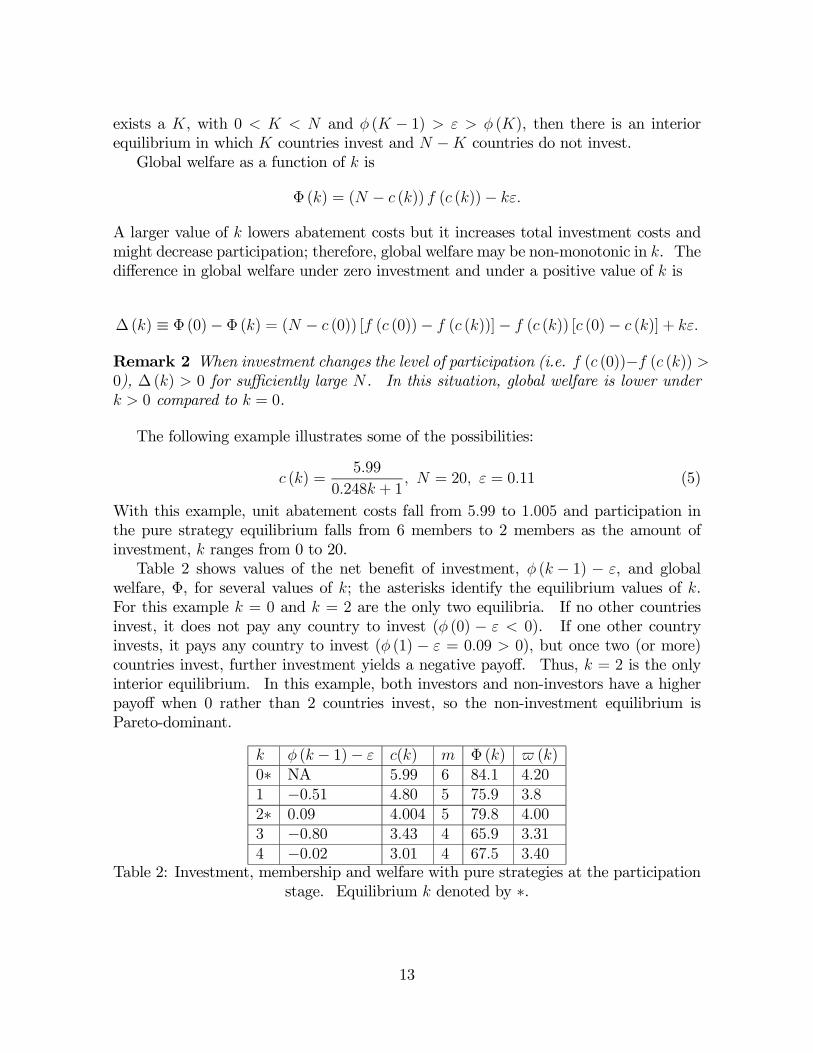
Table 2 shows values of the net benefit of investment, ( − 1) − , and global

welfare, Φ, for several values of ; the asterisks identify the equilibrium values of .

For this example = 0 and = 2 are the only two equilibria. If no other countries

invest, it does not pay any country to invest ( (0) − 0). If one other country

invests, it pays any country to invest ( (1) − = 009 0), but once two (or more)

countries invest, further investment yields a negative payoff. Thus, = 2 is the only

interior equilibrium. In this example, both investors and non-investors have a higher

payoff when 0 rather than 2 countries invest, so the non-investment equilibrium is

Pareto-dominant.

( − 1)− () Φ () ()

0∗ NA 599 6 841 420

1 −051 480 5 759 38

2∗ 009 4004 5 798 400

3 −080 343 4 659 331

4 −002 301 4 675 340

Table 2: Investment, membership and welfare with pure strategies at the participation

stage. Equilibrium denoted by ∗.

13

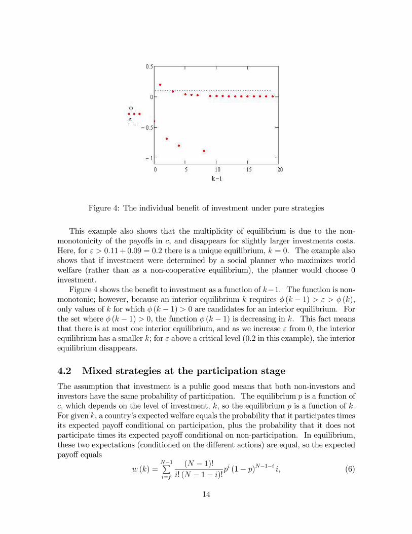
Figure 4: The individual benefit of investment under pure strategies

This example also shows that the multiplicity of equilibrium is due to the non-

monotonicity of the payoffs in , and disappears for slightly larger investments costs.

Here, for 011+ 009 = 02 there is a unique equilibrium, = 0. The example also

shows that if investment were determined by a social planner who maximizes world

welfare (rather than as a non-cooperative equilibrium), the planner would choose 0

investment.

Figure 4 shows the benefit to investment as a function of −1. The function is non-monotonic; however, because an interior equilibrium requires ( − 1) (),

only values of for which ( − 1) 0 are candidates for an interior equilibrium. Forthe set where ( − 1) 0, the function ( − 1) is decreasing in . This fact means

that there is at most one interior equilibrium, and as we increase from 0, the interior

equilibrium has a smaller ; for above a critical level (0.2 in this example), the interior

equilibrium disappears.

4.2 Mixed strategies at the participation stage

The assumption that investment is a public good means that both non-investors and

investors have the same probability of participation. The equilibrium is a function of

, which depends on the level of investment, , so the equilibrium is a function of .

For given , a country’s expected welfare equals the probability that it participates times

its expected payoff conditional on participation, plus the probability that it does not

participate times its expected payoff conditional on non-participation. In equilibrium,

these two expectations (conditioned on the different actions) are equal, so the expected

payoff equals

() =−1P=

( − 1)!! ( − 1− )!

(1− )−1−

(6)

14

which is the expected abatement when at least one country does not join. When − 1other countries invest, the benefit to a country of also investing is

Ω ( − 1) = ()− ( − 1)

IfΩ (0) , then there is a corner equilibrium in which no country invests; ifΩ ( − 1) ≥, there is a corner equilibrium in which every country invests; again, there may be in-

terior equilibria.

As varies between adjacent integers (so that is fixed), the left side of equation

(2) is continuous in , and the right side is continuous in , by equation (3); moreover,

the derivative of the right side with respect to is bounded away from 0 for ∈ (0 1).Therefore, the equilibrium () is continuous on the domain ∈ (1 2). Remark 1 andPropositions 1 and 2 state that over this domain, decreases in , implying that the

range of is (0 1). Consequently, for any (0) 1 there exists a ∈ (1 2) that solves () =

((0))

, i.e. = −1

³((0))

´, a weakly decreasing step function in (0). The

following proposition considers the case where a high level of investment leads to large

cost reductions, which may then lead to relatively high participation and abatement. In

this situation, a country’s expected payoff (exclusive of investment costs) is monotonic

in investment for sufficiently high levels of investment, and is maximized when all

countries invest.

Proposition 5 Assume that is sufficiently large and decreases sufficiently rapidly

in that there exists a smallest integer ≤ at which () ≤ . In this case, for any

1 ≥ and all 2 1, (1) (2): () is therefore maximized at = .

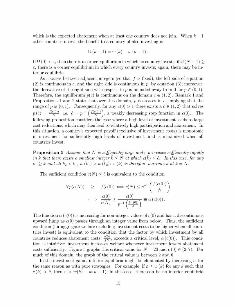
The sufficient condition () ≤ is equivalent to the condition

(()) ≥ ((0))⇐⇒ () ≤ −1µ((0))

¶⇐⇒ (0)

()≥ (0)

−1³((0))

´ ≡ ((0))

The function ((0)) is increasing for non-integer values of (0) and has a discontinuous

upward jump as (0) passes through an integer value from below. Thus, the sufficient

condition (for aggregate welfare excluding investment costs to be higher when all coun-

tries invest) is equivalent to the condition that the factor by which investment by all

countries reduces abatement costs,(0)

(), exceeds a critical level, ((0)). This condi-

tion is intuitive: investment increases welfare whenever investment lowers abatement

costs sufficiently. Figure 5 graphs this critical value for = 20 and (0) ∈ (2 7). Formuch of this domain, the graph of the critical value is between 2 and 6.

In the investment game, interior equilibria might be eliminated by increasing , for

the same reason as with pure strategies. For example, if ≥ () for any such that

() , then () − ( − 1); in this case, there can be no interior equilibria

15

Figure 5: The critical ratio of()

(0)for = 20 and (0) ∈ (2 7).

with investment less than . By eliminating equilibria, a large value of eases the

coordination problem. Of course, an extremely large value of eliminates all equilibria

with positive investment. However, if , and

Ω ( − 1) Ω ( − 1) for all

then there are two equilibria, at which = 0 and = . (There may be other

equilibria with investment ≤ .) If it is individually rational for a country

to invest, then that investment also increases global welfare. We saw that with pure

strategies at the participation stage, it might be individually rational to invest in cases

where this lowers social welfare. The expected global welfare as a function of is

Ψ () = ()−

Using example (5), Figure 6 shows that (under second stage mixed strategies) the

benefit to investment, although non-monotonic, increases rapidly for large . The

figure also shows horizontal lines corresponding to three possible values of . An

interior equilibrium requires Ω ( − 1) Ω (). Increases in eliminate the

smaller equilibria, but not the boundary equilibrium = until becomes large.

Table 3 shows levels of welfare and expected participation for several values of ,

including all of the equilibrium values when = 011, marked by an asterisk. There

are four equilibria, with = 20 giving the highest level of welfare both for investors

and non-investors. Increasing to greater than 011 + 015 = 026 removes the = 4

equilibrium, and increasing to greater than 011 + 028 = 039 removes the = 8

equilibrium. Zero investment is always an equilibrium, and = 20 is an equilibrium

provided that ≤ 011 + 198 = 2 09.44We also examined the equilibria of the investment game under logarathmic utility (contant relative

16

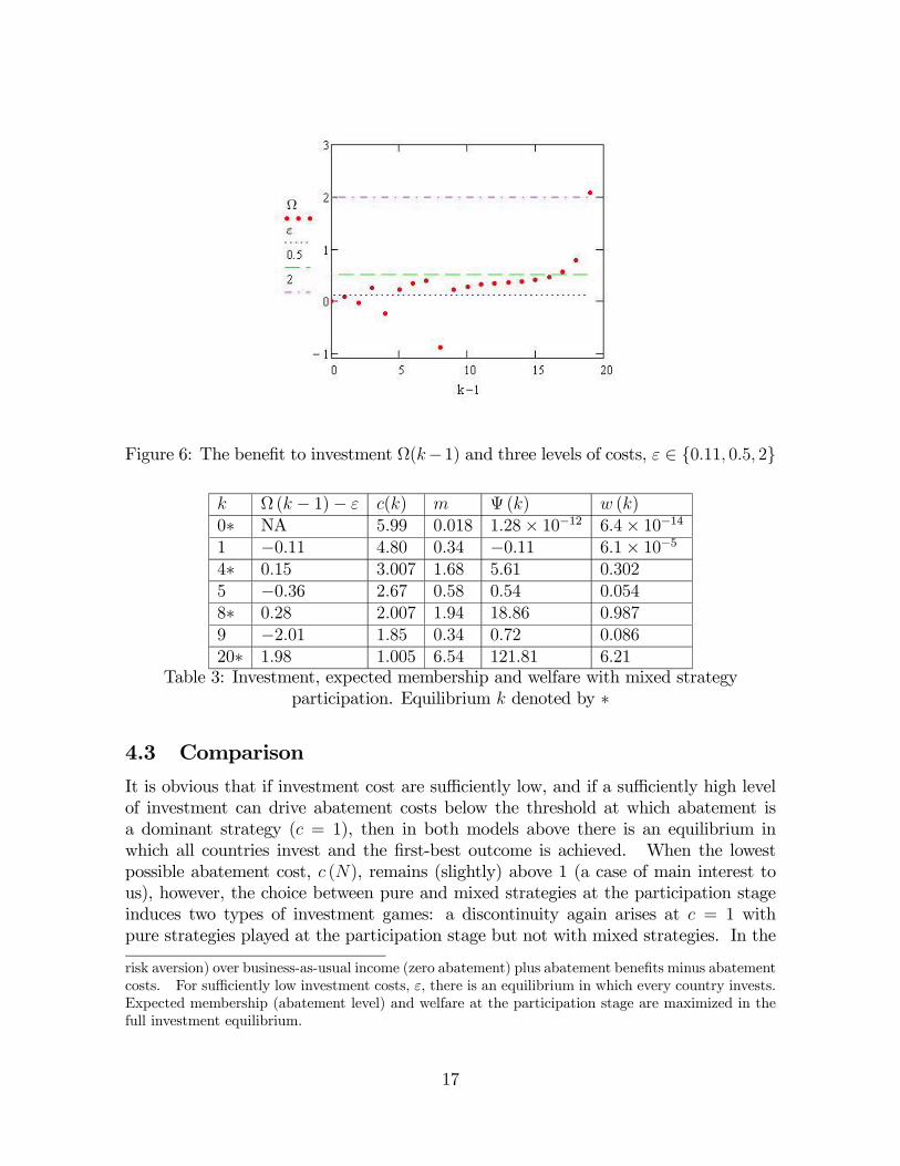
Figure 6: The benefit to investment Ω(−1) and three levels of costs, ∈ 011 05 2

Ω ( − 1)− () Ψ () ()

0∗ NA 599 0018 128× 10−12 64× 10−141 −011 480 034 −011 61× 10−54∗ 015 3007 168 561 0302

5 −036 267 058 054 0054

8∗ 028 2007 194 1886 0987

9 −201 185 034 072 0086

20∗ 198 1005 654 12181 621

Table 3: Investment, expected membership and welfare with mixed strategy

participation. Equilibrium denoted by ∗

4.3 Comparison

It is obvious that if investment cost are sufficiently low, and if a sufficiently high level

of investment can drive abatement costs below the threshold at which abatement is

a dominant strategy ( = 1), then in both models above there is an equilibrium in

which all countries invest and the first-best outcome is achieved. When the lowest

possible abatement cost, (), remains (slightly) above 1 (a case of main interest to

us), however, the choice between pure and mixed strategies at the participation stage

induces two types of investment games: a discontinuity again arises at = 1 with

pure strategies played at the participation stage but not with mixed strategies. In the

risk aversion) over business-as-usual income (zero abatement) plus abatement benefits minus abatement

costs. For sufficiently low investment costs, , there is an equilibrium in which every country invests.

Expected membership (abatement level) and welfare at the participation stage are maximized in the

full investment equilibrium.

17

former case, when there are two investment equilibria (a boundary equilibrium = 0

and an interior equilibrium), the 0-investment equilibrium has higher membership, and

with sufficiently large, higher welfare for both investors and non-investors. In

contrast, when agents use mixed strategies at the participation stage, for sufficiently

low investment costs, there is a boundary equilibrium at which all countries invest, as

well as interior equilibria and the boundary equilibrium at which no country invests.

Expected participation and welfare are higher at the equilibria with high investment

that drives abatement costs close to 1.

The two types of equilibria in the participation game therefore lead to different

policy implications regarding investment. The pure strategy equilibrium, emphasized

by the previous literature, leads to a game in which even if investment might occur

in equilibrium, that investment would likely lower abatement and welfare. This re-

sult occurs because the pure strategy participation equilibrium equals the minimally

successful IEA, which is weakly increasing in abatement costs. The mixed strategy

equilibrium, which we emphasize, leads to a game in which again investment might

occur in equilibrium, but here it increases abatement and welfare.

Unless the abatement cost can be reduced to a level extremely close to the threshold

= 1, the implications of the game with mixed strategies — like those of the game with

pure strategies — are pessimistic. In our example, expected participation in the mixed

strategy when all countries invest (6.54) is only slightly higher than participation in the

pure strategy when no countries invest (6). Expected welfare is much higher in the

former case (122 compared to 84) due to the lower abatement cost resulting from invest-

ment. However, even the larger level is only a fraction of the potential global welfare,

equal to (20− 1005− 011) 20 = 377 7, so both models are pessimistic about being

able to capture the benefits of cooperation. We also found examples where expected

participation under mixed strategies is lower but expected welfare higher, compared

to the levels under pure strategies. Thus, when costs are endogenous, determined at

the investment stage, the model with mixed strategies may be less pessimistic than the

model with pure strategies.

In the interest of completeness, we also examined the use of mixed strategies at

the investment stage. For the example in equation (5), we found that the unique

mixed strategy investment equilibrium, given that countries use pure strategies at the

participation stage, involves a zero probability of investment. When countries use

mixed strategies at both stages, the levels of expected membership and welfare are

between the highest and the lowest equilibrium levels corresponding to the scenario

(reported in Table 3) in which countries use pure strategies at the investment stage and

mixed strategies at the participation stage.

5 Summary

Most previous theory about IEAs (within the strand of literature that we follow) uses

a participation game with a pure strategy equilibrium. These models (typically) imply

18

that the equilibrium participation is low and that investment that reduces abatement

costs also reduces the incentives to join the IEA, resulting in lower equilibrium member-

ship. Under risk neutrality and predetermined abatement costs, the use of mixed rather

than pure strategies tends to reinforce the conclusion that optimal behavior by the IEA

does not solve the problem of providing a global public good. For low abatement costs,

however, the use of mixed strategies overturns this conclusion.

More significantly, the participation games with mixed and with pure strategies

have opposite policy implications with regard to investment. In both of the investment

games induced by the two types of strategies at the participation stage, there may be

multiple Pareto-ranked (pure strategy) investment equilibria. Under pure strategies

at the participation stage, society would like to coordinate on a low-investment equi-

librium, and under mixed strategies at the participation game, society would like to

coordinate on the high-investment equilibrium. The overall policy conclusion is that

when nations use mixed strategies, the promotion of investment that lowers abatement

cost can ameliorate the problem of climate change, even though it is unlikely to provide

a complete solution to that problem.

19

A Appendix

This appendix derives equation (3), and proves Propositions 1, 2, and 5.

Derivation of equation (3) To ease notation, we define = − 1, the number of“other” countries and = − 1, the number of “other members” needed for a countryto be pivotal; because , we have ≥ + 1. Using these definitions we have

()

()=

P=+1

!!(−)!

(1−)−

!!(−)!

(1−)−

=

P=

!

! (− )!(1−)−

− !

! (− )!(1−)−

!

! (− )!(1−)−

=

P=

!

! (− )!(1−)−

!

! (− )!(1−)−

− 1

Define

=

P=

µ!

! (− )! (1− )

−¶

!

()! (− )! (1− )

−= hypergeom

µ[1−+ ] [1 + ]

−1 +

¶(7)

where hypergeom (·) is the hypergeometric function. Using the definition of the hyper-geometric function, and the fact that the gamma function Γ (+ 1) = ! when is an

integer, we write5

=Γ(1+)

Γ(1)Γ(1+−1)R 10

1−1(1−)1+−1−1

(1− −1)

−

=Γ(1+)

Γ()

R 10

(1−)−1

(1− −1)

− = R 10

(1−)−1

(1+ 1−)

−

= R 10(1− )

−1³1 +

1−

´−

(8)

5To check this result we also derived equation (3) without using the hypergeometric function and

instead using the identity

P=

µ!

! (− )! (1− )

−¶=

!

( − 1)! (− )!

Z

0

−1 (1− )−

from Wang (1994, page 116); details are availble on request.

20

Proof. (Proposition 1) Part (i) The fact that is defined over a positive interval

implies

³1 +

1−

´

=

(−1 + )2 0

Using this expression, we have

()

()

=

=

Z 1

0

(1− )−1(− )

µ1 +

1−

¶−−1

(−1 + )2 0 (9)

Define =

1− . By using the last equality of equation (8), we have

(0) =

Z 1

0

(1− )−1

= 1 6

=

Z 1

0

(1− )−1(− ) (1 + )

−−1 0

and2

2=

Z 1

0

(1− )−1(− ) (− − 1) (1 + )

−−22 ≥ 0

for any ≥ + 1. Because is increasing and convex in , the domain of is [0∞)and (0) = 1, we know that the range of is [1∞). Thus − 1 is increasing andconvex in and the range of − 1 is [0∞). When is not an integer, −

−1 is positive.Therefore, − 1 will cross −

−1 once and only once. There is a unique solution to theequation −

−1 = − 1. By the one-to-one correspondence between and , there exists

a unique that satisfies the equilibrium condition.

Part (ii) Equation (9) shows()

()

0. Consider an interval of over which is

constant. Differentiating equation (2) with respect to , treating as a function of we

have

¡−−1¢

= − − 1

(− 1)2

=

()

()

⇒

= −

()

()

(− 1)2 − 1 0

Proof. (Proposition 2) The first step. When ∈ ( − 1 ], () = . The limit of the

left hand side of equation (2) as converges to − 1 from the right is:

lim→(−1)+

−

− 1 =1

− 2

6 (1− )−1

is the density function of (1 ).

21

When = 2, lim→1+

−−1 =

12−2 = ∞; when ≥ 3, lim

→(−1)+−−1 =

1−2 ≤ 1. Since the

left hand side of equation (2) decreases in , the limit 1−2 is the supremum of the left

hand side over the interval ∈ (− 1 ]. For the equality to hold, 1−2 must also be the

supremum of the right hand side of equation (2).

The second step. For any integer ≥ 3, the supremum of the right hand side of

equation (2), 1−2 , is not more than 1. We now show the right hand side of equation (2),

()

(), evaluated at =

exceeds 1. Given that this is true, the inequality

()

()

0

implies that the equilibrium must be strictly less than

and therefore must be less

than the level in the pure-strategy equilibrium. To confirm that the right hand side of

equation (2), evaluated at

exceeds 1, we evaluate the numerator and the denominator

separately.

With () = , the first term in the sum in the numerator on the right hand side

of equation (2) evaluated at =

equals

=( − 1)!

! ( − 1− )!

µ

¶ µ1−

¶−1−

=( − 1)!

( − 1)! ( − 1− )!

µ

¶−1µ1−

¶−1− µ

1

¶=

( − 1)!( − 1)! ( − 1− )!

µ

¶−1µ1−

¶−1−1

The denominator on the right hand side of equation (2), evaluated at

, equals

( − 1)!( − 1)! ( − )!

µ

¶−1µ1−

¶−

=( − 1)!

( − 1)! ( − 1− )!

µ

¶−1µ1−

¶−−11

−

µ1−

¶=

( − 1)!( − 1)! ( − 1− )!

µ

¶−1µ1−

¶−−11

These two intermediate results imply

( − 1)!! ( − 1− )!

µ

¶ µ1−

¶−1−

=( − 1)!

( − 1)! ( − )!

µ

¶−1µ1−

¶−

22

Thus

−1X=

( − 1)!! ( − 1− )!

µ

¶µ1−

¶−1−

=( − 1)!

! ( − 1− )!

µ

¶ µ1−

¶−1−

+

−1X=+1

( − 1)!! ( − 1− )!

µ

¶µ1−

¶−1−

=( − 1)!

( − 1)! ( − )!

µ

¶−1µ1−

¶−

+

−1X=+1

( − 1)!! ( − 1− )!

µ

¶µ1−

¶−1−

≥ ( − 1)!( − 1)! ( − )!

µ

¶−1µ1−

¶−

Therefore, we have

1

− 2 ≤ 1 ≤

−1P=

(−1)!!(−1−)!

¡

¢ ¡1−

¢−1−(−1)!

(−1)!(−)!¡

¢−1 ¡1−

¢− (10)

We conclude that the right hand side of equation (2) evaluated at

, given by the

right hand side of inequality (10) exceeds the supremum of the left hand side of equation

(2) when ≥ 3. Since the right hand side of equation (2) increases in , must be

always less than

, and thus is always less than when ≥ 3.

The third step. By Proposition 1, decreases in in the interval of 1 ≤ 2.

So approaches its maximum value (denoted by ∗1) as converges to 1 from above.

Because the left hand side of equation (2) approaches infinity as approaches 1, the

right hand side of equation (2) must also approach infinity. Thus, in the interval of

1 ≤ 2, as approaches ∗1, the right hand side of equation (2) goes to infinity. Sincethe right hand side of equation (2) increases in and it is finite when = 2

, we must

have ∗1 2. As decreases with , we must have 2

when is small enough. And

when 2, we have 2. Therefore, for sufficiently small , expected membership

in the mixed strategy equilibrium exceeds membership in the pure strategy equilibrium.

The right hand side of equation (1) approaches zero as approaches 1. The left

side of equation (1) approaches zero only if approaches either 0 or 1. We know that

approaches ∗1 and ∗1 2 0. Therefore, approaches 1 as approaches its lower

bound 1.

23

Proof. (Proposition 5) Because 1 2, we have (1) (2). We consider the case

of (1) (2) 2 and the case of (1) 2 (2) separately.

(a) (1) (2) 2. We have ( (1)) = ( (2)) = 2. Given = 2, we can

write equation (6) as

=−1P=2

( − 1)!! ( − 1− )!

(1− )−1−

= ( − 1) − ( − 1) (1− )−2

= ( − 1) h1− (1− )

−2i

which increases with . By Proposition 1, we have (2) (1). Therefore (1)

(2).

(b) (1) 2 (2). Proposition 2 shows that () ()

when 2. Because

(0) ≥ for any , we have ((0))

when 2, which implies that (2)

((0))

. By

Proposition 1, (1) ≥ ((0))

because (1) ≤ . Thus, we have (2)

((0))

≤ (1).

Moreover, 2 = ( (1)) ( (2)) because (1) 2 (2). We have

(2) =−1P

=((2))

( − 1)!! ( − 1− )!

( (2))(1− (2))

−1−

−1P

=((1))

( − 1)!! ( − 1− )!

( (2))(1− (2))

−1−

−1P

=((1))

( − 1)!! ( − 1− )!

( (1))(1− (1))

−1−

= (1)

The last inequality comes from the fact that is increasing in when = 2, as shown

in case (a).

B Referee’s appendix: Proofs of Propositions 3 and

4

Proof. (Proposition 3) To prove part (i) we differentiate the equilibrium condition

−

− 1 = − 1 =

Z 1

0

(1− )−1µ1 +

1−

¶−− 1

with respect to to obtain

= −

R 10(1− )

−1³1 +

1−

´−ln³1 +

1−

´R 1

0(1− )

−1(− )

³1 +

1−

´−−1

(1−)2 0

24

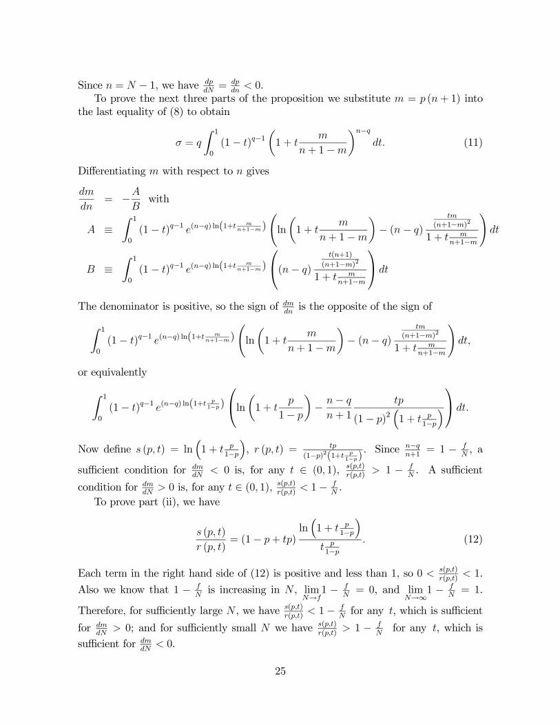
Since = − 1, we have

=

0.

To prove the next three parts of the proposition we substitute = (+ 1) into

the last equality of (8) to obtain

=

Z 1

0

(1− )−1µ1 +

+ 1−

¶− (11)

Differentiating with respect to gives

= −

with

≡Z 1

0

(1− )−1

(−) ln(1+

+1−)

Ãln

µ1 +

+ 1−

¶− (− )

(+1−)2

1 + +1−

!

≡Z 1

0

(1− )−1

(−) ln(1+

+1−)

⎛⎝(− )

(+1)

(+1−)2

1 + +1−

⎞⎠

The denominator is positive, so the sign of is the opposite of the sign ofZ 1

0

(1− )−1

(−) ln(1+

+1−)

Ãln

µ1 +

+ 1−

¶− (− )

(+1−)2

1 + +1−

!

or equivalentlyZ 1

0

(1− )−1

(−) ln(1+

1−)

⎛⎝lnµ1 +

1−

¶− −

+ 1

(1− )2³1 +

1−

´⎞⎠

Now define ( ) = ln³1 +

1−

´, ( ) =

(1−)2(1+ 1−)

. Since −+1

= 1 −

, a

sufficient condition for

0 is, for any ∈ (0 1), ()

() 1 −

. A sufficient

condition for

0 is, for any ∈ (0 1), ()

() 1−

.

To prove part (ii), we have

( )

( )= (1− + )

ln³1 +

1−

´

1− (12)

Each term in the right hand side of (12) is positive and less than 1, so 0 ()

() 1.

Also we know that 1 −

is increasing in , lim

→1 −

= 0, and lim

→∞1 −

= 1.

Therefore, for sufficiently large , we have()

() 1−

for any , which is sufficient

for

0; and for sufficiently small we have()

() 1 −

for any , which is

sufficient for

0.

25

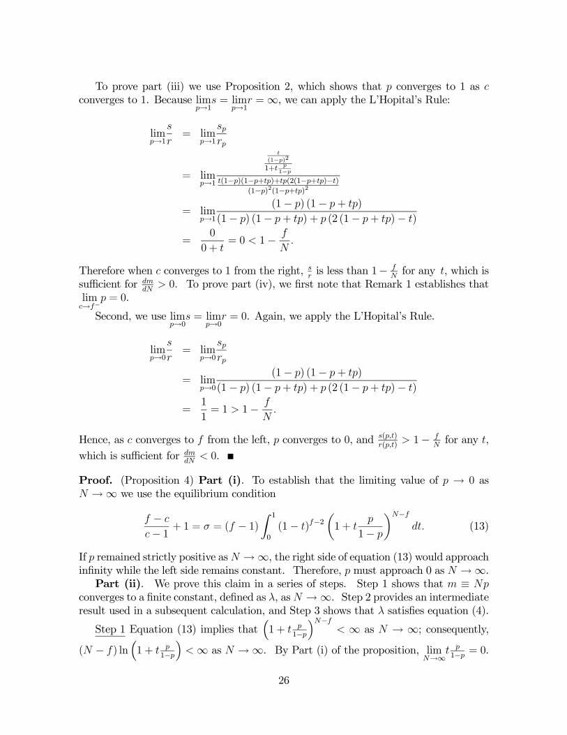
To prove part (iii) we use Proposition 2, which shows that converges to 1 as

converges to 1. Because lim→1

= lim→1

=∞, we can apply the L’Hopital’s Rule:

lim→1

= lim

→1

= lim→1

(1−)21+

1−

(1−)(1−+)+(2(1−+)−)(1−)2(1−+)2

= lim→1

(1− ) (1− + )

(1− ) (1− + ) + (2 (1− + )− )

=0

0 + = 0 1−

Therefore when converges to 1 from the right, is less than 1−

for any , which is

sufficient for

0. To prove part (iv), we first note that Remark 1 establishes that

lim→−

= 0.

Second, we use lim→0

= lim→0

= 0. Again, we apply the L’Hopital’s Rule.

lim→0

= lim

→0

= lim→0

(1− ) (1− + )

(1− ) (1− + ) + (2 (1− + )− )

=1

1= 1 1−

Hence, as converges to from the left, converges to 0, and()

() 1−

for any ,

which is sufficient for

0.

Proof. (Proposition 4) Part (i). To establish that the limiting value of → 0 as

→∞ we use the equilibrium condition

−

− 1 + 1 = = ( − 1)Z 1

0

(1− )−2

µ1 +

1−

¶− (13)

If remained strictly positive as →∞, the right side of equation (13) would approachinfinity while the left side remains constant. Therefore, must approach 0 as →∞.Part (ii). We prove this claim in a series of steps. Step 1 shows that ≡

converges to a finite constant, defined as , as →∞. Step 2 provides an intermediateresult used in a subsequent calculation, and Step 3 shows that satisfies equation (4).

Step 1 Equation (13) implies that³1 +

1−

´− ∞ as → ∞; consequently,

( − ) ln³1 +

1−

´∞ as →∞. By Part (i) of the proposition, lim

→∞

1− = 0.

26

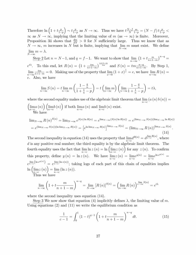
Therefore ln³1 +

1−

´∼

1− as →∞. Thus we have −1− = ( − )

1−

∞ as → ∞, implying that the limiting value of (as → ∞) is finite. Moreover,

Proposition 3ii shows that

0 for sufficiently large. Thus we know that as

→ ∞, increases in but is finite, implying that lim→∞

must exist. We define

lim→∞

= .

Step 2 Let = −1, and = −1. We want to show that lim→∞

¡1 +

+1−¢−

=

. To this end, let () =¡1 +

+1−¢+1−

and () = −+1− . By Step 1,

lim→∞

+1− = 0. Making use of the property that lim→0

(1 + )1 = , we have lim

→∞ () =

. Also, we have

lim→∞

() = lim→∞

µ1−

1 + 1−

¶=

³lim→∞

´µ

lim→∞

1−

1 + 1−

¶=

where the second equality makes use of the algebraic limit theorem that lim→

( () ()) =³lim→

()´³lim→

()´if both lim

→ () and lim

→ () exist.

We have

lim→∞ ()()

= lim→∞ () ln() = lim→∞(() ln()) = (lim→∞ ())(lim→∞ ln())

= (lim→∞ ())(ln lim→∞()) =£ln lim→∞()

¤lim→∞ ()= (lim→∞ ())

lim→∞ ()

(14)

The second inequality in equation (14) uses the property that lim→

() = lim→

(), where

is any positive real number; the third equality is by the algebraic limit theorem. The

fourth equality uses the fact that lim→

ln () = ln³lim→

()´for any (). To confirm

this property, define () = ln (). We have lim→

() = lim→

() = lim→

ln ()

=

lim→(ln ())

= lim→

(ln ()); taking logs of each part of this chain of equalities implies

ln³lim→

()´= lim

→(ln ()).

Thus we have

lim→∞

µ1 +

+ 1−

¶−= lim

→∞[ ()]

()=³lim→∞

()´ lim→∞()

=

where the second inequality uses equation (14).

Step 3 We now show that equation (4) implicitly defines , the limiting value of .

Using equations (2) and (11) we write the equilibrium condition as

1

− 1 =Z 1

0

(1− )−1µ1 +

+ 1−

¶− (15)

27

We have1

−1 = lim→∞

R 10(1− )

−1 ¡1 +

+1−¢−

=R 10

hlim→∞

(1− )−1 ¡

1 + +1−

¢−i

=R 10(1− )

−1

(16)

The first equality comes from taking limits of both sides of equation (15); the third

equality comes from step 2; the second equality, where we pass the limit operator

through the integral, is nontrivial, and requires that we use the “dominated convergence

theorem”. This theorem states that the second equality in equation (16) is valid if we

can find a function () that is independent of and integrable (that is,R 10 () ∞)

and “dominates” () (that is, | ()| ≤ ()), where

() = (1− )−1µ1 +

+ 1−

¶−

is the integrand in the second line of equation (16). We construct the function ()

in a separate lemma, available on request, thus establishing the validity of the second

equality in equation (16).

Part (iii). When is finite, membership of the mixed strategy equilibrium follows

a binomial distribution. Parts (i) and (ii) of the proposition show that → 0 and

→ when →∞. Then by Poisson Limit Theorem, the membership of the mixedstrategy equilibrium follows a Poisson distribution with parameter , when →∞.We include the final lemma, used in the proof of Proposition 4 for the sake of

completeness.

Lemma 1 It is valid to pass the limit operator through the integral, i.e.

lim→∞

Z 1

0

(1− )−1µ1 +

+ 1−

¶− =

Z 1

0

"lim→∞

(1− )−1µ1 +

+ 1−

¶−#

Proof. (Lemma 1) We rewrite the integrand () as

(1− )−1"µ1 +

+ 1−

¶+1−

# +1− (−)

(17)

We now construct the function () that satisfies the conditions of the dominated con-

vergence theorem (integrability and dominance), using Steps (a) and (b) as follows.

Step (a): We first show that for any 0,¡1 + 1

¢increases in , i.e. we show

that the derivative of¡1 + 1

¢is positive:

¡1 + 1

¢

= ln(1+

1)

= ln(1+

1)

"ln

µ1 +

1

¶+

¡− 1

2

¢1 + 1

#

= ln(1+1)∙ln

µ1 +

1

¶− 1

+ 1

¸ 0

28

Note that lim→0

£ln¡1 + 1

¢− 1+1

¤=∞, lim

→∞

£ln¡1 + 1

¢− 1+1

¤= 0, and

£ln¡1 + 1

¢− 1+1

¤

=− 1

2

1 + 1

+1

(+ 1)2=

1

+ 1

µ1

+ 1− 1

¶ 0

Thus ln¡1 + 1

¢− 1+1

is always positive. As a result,(1+ 1

)

is always positive.

Step (b): In this step, we construct the function (). Using the definition =

+1−

= 1

³−1 + 1

´, we have

¡1 +

+1−¢+1−

=¡1 + 1

¢. As increases,

decreases (by Proposition 3(i), thus increases, and¡1 + 1

¢increases by Step (a).

Also we know that lim→∞

¡1 + 1

¢= . Hence,

¡1 + 1

¢ , and we have

() (1− )−1

[(−)+1− ] (18)

By the algebraic limit theorem lim→∞

(−)+1− =

³lim→∞

´³

lim→∞

1−

1+ 1−

´= . Given

any positive 2, we can find ∗ such that

¯(−)+1− −

¯ 2 for any ≥ ∗. Note that

depends on . Thus ∗ depends on 2 only, independent of . Let () = (1− )−1

where = maxmax∗

(−)+1− +2, which is independent of . Thus () is independent

of . We have

0 () (1− )−1

[(−)+1− ] ≤ () (19)

Thus | ()| (), i.e., () is dominated by (). Also, since is finite,(−)+1− is

finite, is finite, and thus () is finite, so () is integrable. As a result, by dominated

convergence theorem, the second equality of (16) holds.

29

References

Bagnoli, M., and B. L. Lipman (1988): “Successful Takeovers without Exclusion,”Review of Financial Studies, pp. 89—110.

Barrett, S. (1994): “Self-enforcing International Environmental Agreements,” Ox-ford Economic Papers, 46, 878—894.

(1997): “Heterogenous International Agreements,” in International Environ-

mental Negotiations: Strategic Policy Issues, ed. by C. Carraro. Edward Elgar, Chel-

tenham, 9-25.

(1999): “A theory of full international cooperation,” Journal of Theoretical

Politics, 11(4), 519—41.

(2002): “Consensus Treaties,” Journal of Institutional and Theoretical Politics,

158, 519—41.

(2003): Environment and Statecraft. Oxford University Press.

(2006): “Climate Treaties and Breakthrough Technologies,” American Eco-

nomic Review, 96, 22—25.

Bayramoglu, B. (2010): “How does the design of international environmental agree-ments affect investment in environmentally-friendly technology,” Journal of Regula-

tory Economics, 37, 180—195.

Benedick, R. (2009): Foreword to "Negotiating Environment and Science" by RichardSmith. Resource for the Future, Washington DC.

Burger, N., and C. Kolstad (2009): “Voluntary public goods provision: coaltionformation and uncertainty,” NBER Working Papers 15543.

Carraro, C., C. Marchiori, and S. Oreffice (2009): “Endogenous minimumparticipation in international environmental treaties,” Environmental and Resource

Economics, 42, 411—425.

Carraro, C., and D. Siniscalco (1993): “Strategies for the International Protectionof the Environment,” Journal of Public Economics, 52, 309—28.

Chander, P., and H. Tulkens (1995): “A core-theoretic solution for the design

of cooperative agreements on transfrontier pollution,” International Tax and Public

Finance, 2(2), 279—293.

(1997): “The core of an economy with multilateral environmental externali-

ties,” International Journal of Game Theory, 26, 379—401.

30

Chwe, M. S. (1994): “Farsighted Coalitional Stability,” Journal of Economic Theory,63, 299—325.

Crawford, V. P., and J. Haller (1990): “Leaning How to Cooperate: OptimalPlay in Repeated Coordination Games,” Econometrica, 58, 571—95.

Dannenberg, A., A. Lange, and B. Sturm (2009): “On the formation of coalitionsto provide public goods — experimental evidence from the lab,” Working paper.

D’Aspremont, C., A. Jacquemin, J. Gabszewicz, and J. Weymark (1983):“On the Stability of Collusive Price Leadership,” Canadian Journal of Economics,

16(1), 17—25.

Dixit, A., and M. Olson (2000): “Does Voluntary Participation undermine the CoaseTheorem,” Journal of Public Economics, 76, 309 — 335.

Ecchia, G., and M. Mariotti (1998): “Coalition Formation in International En-vironmental Agreements and the Role of Institutions,” European Economic Review,

42(3-5), 573 — 582.

Finus, M. (2001): Game Theory and International Environmental Cooperation. Chel-tenham:Edward Elgar.

Finus, M., and S. Maus (2008): “Modesty may pay!,” Journal of Public EconomicTheory, 10, 801—826.

Golombek, R., and M. Hoel (2005): “Climate Policy under Technology Spillovers,”Environmental and Resource Economics, 31, 201—227.

(2006): “Second-best Climate Agreements and Technology Policy,” Advances

in Economic Analysis and Policy, 6.

(2008): “Endogenous Technology and Tradable Emission Quotas,” Resource

and Energy Economics, 30, 197—208.

Harsanyi, J. (1973): “Games with Randomly Disturbed Payoffs: A New Rationalefor Mixed Strategy Equilibrium Points,” International Journal of Game Theory, 2,

1—23.

Hoel, M. (1992): “International Environmental Conventions: the case of uniformreductions of emissions,” Environmental and Resource Economics, 2, 141—59.

Hoel, M., and A. de Zeeuw (2009): “Can a Focus on Breakthrough Technolo-

gies Improve the Performance of International Environmental Agreements,” NBER

Working Paper.

31

Holmstrom, B., and B. Nalebuff (1992): “To the Raider Goes the Surplus? AReexamination of the Free-rider Problem,” Journal of Economics and Management

Strategy, 1, 37—62.

Hong, F., and L. Karp (2011): “International environmental agreements with mixedstrategies and investment,” Working Paper.

Ioannidis, A., A. Papandreou, and E. Sartzetakis (2000): “International envi-ronmental agreements: A literature review,” University of Laval.

Karp, L., and L. Simon (2011): “Participation games and international environmen-tal agreements: a non-parametric model,” Giannini Foundation working paper.

Kohnz, S. (2006): “Ratification Quotas in International Agreements: An Example ofEmission Reduction,” Munich Economics Discussion Paper 2006-10.

Kolstad, C. D. (2011): Environmental Economics. Oxford University Press, NewYork, second edn.

Kosfeld, M., A. Okada, and A. Riedl (2009): “Institution formation in publicgoods games,” American Economic Review, 99, 1335—1355.

Makris, M. (2009): “Private Provision of Discrete Public Goods,” Games and Eco-nomic Behavior, 67, 292—99.

Maskin, E. (2003): “Bargaining, Coalitions and Externalities,” Presidential Addressto the Econometric Society.

McGinty, M. (2010): “International Environmental Agreements as EvolutionaryGames,” Environmental and Resource Economics, 45, 251—269.

Murdoch, J., T. Sandler, and W. Vijverberg (2003): “The Paraticipation De-cision versus the Level of Partication in an Environmental Treaty,” Journal of Public

Economics, 87, 337—62.

Muuls, M. (2004): “The dynamic effect of investment on bargaining positions. Is therea hold-up problem in international agreements on climate change?,” London School

of Economics.

Myerson, R. (1998a): “Extended Poisson Games and the Condorcet Jury Theorem,”Games and Economic Behavior, 25, 111—131.

(1998b): “Population Uncertainty and Poisson Games,” International Journal

of Game Theory, 27, 375—292.

(2005): “A Short Course on Political Economics,” Lecture notes, Peking Uni-

versity.

32

Palfrey, T., and H. Rosenthal (1984): “Participation and the Provision of DiscretePublic Goods: A strategic Analysis,” Journal of Public Economics, 24, 171—93.

Ray, D., and R. Vohra (2001): “Coalitional Power and Public Goods,” Journal ofPolitical Economy, 109(6), 1355 — 1382.

Rubio, S., and A. Ulph (2007): “An Infinite-horizon Model of Dynamic Membershipof International Environmental Agreements,” Journal of Environmental Economics

and Management, 54(3), 296—310.

Sandler, T., and K. Sargent (1995): “Management of Transnational Commons:Coordination, Publicness, and Treaty Formation,” Land Economics, 71(2), 145—62.

Ulph, A. (2004): “Stable international environmental agreements with a stock pollu-tant, uncertainty and learning,” Journal of Risk and Uncertainty, 29, 53—73.

Wagner, U. (2001): “The Design of Stable International Environmental Agreements:Economic Theory and Political Economy,” Journal of Economic Surveys, 15(3), 377—

411.

Wang, R. (1994): Introduction to Probability. Peking University Press, Beijing.

Xue, L. (1998): “Coalitional Stability under Perfect Foresight,” Economic Theory, 11,603—627.

33