Internal Migration, Urbanization, and Poverty in Asia:Dynamics andInterrelationships

Kankesu JayanthakumaranReetu VermaGuanghua WanEdgar Wilson Editors

Internal Migration, Urbanization, and Poverty in Asia: Dynamics and Interrelationships

Kankesu Jayanthakumaran • Reetu Verma Guanghua Wan • Edgar WilsonEditors

Internal Migration, Urbanization, and Poverty in Asia: Dynamics and Interrelationships

ISBN 978-981-13-1536-7 ISBN 978-981-13-1537-4 (eBook)https://doi.org/10.1007/978-981-13-1537-4

Library of Congress Control Number: 2018957470

© Asian Development Bank 2019,

The views expressed in this publication are those of the authors and do not necessarily reflect the views and policies of the Asian Development Bank (ADB) or its Board of Governors or the governments they represent.ADB does not guarantee the accuracy of the data included in this publication and accepts no responsibility for any consequence of their use. The mention of specific companies or products of manufacturers does not imply that they are endorsed or recommended by ADB in preference to others of a similar nature that are not mentioned.By making any designation of or reference to a particular territory or geographic area, or by using the term “country” in this document, ADB does not intend to make any judgments as to the legal or other status of any territory or area. Open Access This work is available under the Creative Commons Attribution-NonCommercial 3.0 IGO license (CC BY-NC 3.0 IGO) http://creativecommons.org/licenses/by-nc/3.0/igo/. By using the content of this publication, you agree to be bound by the terms of this license. For attribution and permissions, please read the provisions and terms of use at https://www.adb.org/terms-use#openaccess. This CC license does not apply to non-ADB copyright materials in this publication. If the material is attributed to another source, please contact the copyright owner or publisher of that source for permission to reproduce it. ADB cannot be held liable for any claims that arise as a result of your use of the material. Please contact pubsmarketing@adb.org if you have questions or comments with respect to content, or if you wish to obtain copyright permission for your intended use that does not fall within these terms, or for permission to use the ADB logo.Note: ADB recognizes “China” as the People’s Republic of China; “Hong Kong” as Hong Kong, China; and “Vietnam” as Viet Nam.Some rights reserved. Published in 2019.

This Springer imprint is published by the registered company Springer Nature Singapore Pte Ltd.The registered company address is: 152 Beach Road, #21-01/04 Gateway East, Singapore 189721, Singapore

EditorsKankesu JayanthakumaranSchool of Accounting, Economics & Finance, Faculty of BusinessUniversity of WollongongWollongong, NSW, Australia

Guanghua WanInstitute of World EconomyFudan UniversityShanghai, People’s Republic of China

Reetu VermaSchool of Accounting, Economics and FinanceUniversity of WollongongWollongong, NSW, Australia

Edgar WilsonSchool of Accounting, Economics and FinanceUniversity of WollongongWollongong, NSW, Australia

corrected publication 2020.This book is an open access publication.

v

Acknowledgments

This book developed from the papers presented and reviewed at the Asian Development Bank (ADB) Workshop on Internal Migration, Urban Development, Poverty, and Inequality in Asia: Sustainable Strategies and Coordinated Policies to Improve Well-being held in Siem Reap, Cambodia, on November 5–7, 2014. Dr. Guanghua Wan initiated the project with ADB, which provided funding for the travel arrangements of the participants of the Siem Reap workshop. The University of Wollongong academics, Drs. Kankesu Jayanthakumaran, Reetu Verma, and Ed Wilson, organized the workshop and enabled the book chapters to materialize. This book is the result of the research conducted under ADB’s technical assistance proj-ects on poverty and urbanization.

As the editors of this book, our sincere thanks go to all of the chapter contribu-tors, who, throughout the last 3 years, have ceaselessly worked hand in hand to bring out the book.

We also thank the International Organization for Migration (IOM) for accepting to reproduce the paper published in the 2015 World Migration Report titled ‘Urban Migration Trends, Challenges, Responses and Policy in the Asia- Pacific’, by Graeme Hugo; and Elsevier for accepting to reprint the paper published in Economic Modelling titled ‘The Labor Market Effects of Skill-Biased Technological Change in Malaysia’, by Mohamed A. Marouani and Björn Nilsson.

vii

Contents

1 Introduction . . . . . . . . . . . . . . . . . . . . . . . . . . . . . . . . . . . . . . . . . . . . . . . 1Kankesu Jayanthakumaran, Reetu Verma, Guanghua Wan, and Edgar Wilson

Part I The Dynamic Interplay of Internal Migration, Urbanization, and Poverty

2 Patterns and Trends of Urbanization and Urban Growth in Asia . . . . . . . . . . . . . . . . . . . . . . . . . . . . . . . . . . . . . . . . . . . . . 13Graeme Hugo

3 Examining the Interdependencies Between Urbanization, Internal Migration, Urban Poverty, and Inequality: Evidence from Indonesia . . . . . . . . . . . . . . . . . . . . . . . . . . . . . . . . . . . . 47Riyana Miranti

4 Rural–Urban Migration, Urban Poverty and Inequality, and Urbanization in the People’s Republic of China . . . . . . . . . . . . . . 77Xin Meng

5 Interdependencies of Internal Migration, Urbanization, Poverty, and Inequality: The Case of Urban India . . . . . . . . . . . . . . . 109Edgar Wilson, Kankesu Jayanthakumaran, and Reetu Verma

Part II Migration, Urbanization, and Poverty Alleviation

6 Internal Migration and Poverty: A Lesson Based on Panel Data Analysis from Indonesia . . . . . . . . . . . . . . . . . . . . . . . . 135Endang Sugiyarto, Priya Deshingkar, and Andy McKay

7 Poverty and Inequality in Urban India with Special Reference to West Bengal: An Empirical Study . . . . . . . . . . . . . . . . . . 163Nandini Mukherjee and Biswajit Chatterjee

viii

8 Rural-Urban Migration, Urbanization, and Wage Differentials in Urban India . . . . . . . . . . . . . . . . . . . . . . . . . . . . . . . . . . 189Jajati Keshari Parida

9 The Labor Market Effects of Skill-Biased Technological Change in Malaysia. . . . . . . . . . . . . . . . . . . . . . . . . . . . . . . . . . . . . . . . . 219Mohamed A. Marouani and Björn Nilsson

Part III Polarization and Poverty Gaps

10 The Pattern of Urban–Rural Disparities in Multidimensional Poverty in the People’s Republic of China: 2000–2011 . . . . . . . . . . . . 267Jing Yang and Pundarik Mukhopadhaya

11 Distribution of Urban Economic Growth in Post-reform India: An Empirical Assessment . . . . . . . . . . . . . . . . . . . . . . . . . . . . . . 309Sabyasachi Tripathi

12 Internal Migration and Employment in Bangladesh: An Economic Evaluation of Rickshaw Pulling in Dhaka City . . . . . . 339Abu Hena Reza Hasan

Correction to: Internal Migration, Urbanization, and Poverty in Asia: Dynamics and Interrelationships . . . . . . . . . . . . . . . . . . . . . . . . . . . . . . . . . . . C1

Index . . . . . . . . . . . . . . . . . . . . . . . . . . . . . . . . . . . . . . . . . . . . . . . . . . . . . . . . . 361

Contents

ix

Editors and Contributors

About the Editors

Kankesu Jayanthakumaran is Senior Lecturer at the University of Wollongong, Australia. His research has concentrated on trade facilitation and performance. The outcome is reflected in his 30 peer-reviewed journal articles, 5 book chapters, 2 edited books, 1 book and 15 students’ Doctoral theses. He has been the sole author of the book titled Industrialization and Challenges in Asia with Palgrave Macmillan (United Kingdom). His current research focus is on integrative trade and logistics in land-locked countries.

Reetu Verma is Senior Lecturer and one of the Head of Students in the Faculty of Business at the University of Wollongong, Australia. Reetu’s principal areas of expertise are in (i) economic growth and development, (ii) student engagement and support, (iii) statistics/quantitative techniques and (iv) applied econometrics. Her current research interests are in the areas of economic growth and development in Asia with emphasis on food security, poverty and inequality, migration and urban-ization and inclusive education and student well-being.

Guanghua Wan is the Director of the Institute of World Economy, Fudan University, People’s Republic of China (PRC). Previously, he worked for the Asian Development Bank, the United Nations and the University of Sydney. Trained in development economics and econometrics, Dr. Wan is a leading scholar on the Chinese economy and an expert on Asia, with a publication record of more than 100 professional articles and a dozen books, including two published by Oxford University Press. Some of his publications can be downloaded from http://ideas.repec.org/f/pwa395.html.

x

Edgar Wilson is Associate Professor at the University of Wollongong, Australia. He was president of the Economic Society of Australia, New South Wales. He has research interests in macroeconomics modelling and empirically estimating the determinants of economic growth and productivity and the consequences of policies to reduce poverty and child labour in Asia.

Contributors

Biswajit Chatterjee teaches Economics in the Department of Economics, Jadavpur University, India. He was Professor-in-Charge and Chair of the Planning and Development Unit at Jadavpur University. He has served for The Indian Econometric Society, the Indian Society of Labour Economics and Bengal Economic Association. Professor Chatterjee authored books titled Globalisation and Health Sector in India and Growth, Distribution and Public Policy in West Bengal. His research interest is in poverty, labour economics and regional economics.

Priya Deshingkar is Research Director of the 6-year DFID-funded ‘Migrating out of Poverty Research Consortium’, Principal Investigator for the Capitalising Human Mobility for Poverty Alleviation and Inclusive Development in Myanmar (CHIME) project and Senior Research Fellow at the School of Global Studies. Her research focuses on migration and poverty with a focus on precarious occupations, debt- migration, trafficking, slavery, labour rights and agency.

Abu Hena Reza Hasan is Professor of International Business at the University of Dhaka, Bangladesh. He has research interests in migration, global value chain, con-nectivity and corridors and WTO issues. At present, he is doing research on the trade and connectivity policies of the People’s Republic of China and India.

Graeme Hugo was Professor of Geography and Director of the Australian Population and Migration Research Centre at the University of Adelaide, Australia. In 1987, he was elected a fellow of the Academy of the Social Sciences in Australia. In 2012, he was honoured as an Officer of the Order of Australia for his work in population research.

Mohamed A. Marouani is Associate Professor in Economics at Paris 1 Pantheon- Sorbonne University and Deputy Director of the Research Unit ‘Development and Societies’. He is also Research Fellow and Member of the Advisory Committee of the Economic Research Forum and Research Associate of DIAL. His research focuses on structural change and skills dynamics and on migration and employment interactions.

Editors and Contributors

xi

Andy McKay is Professor at the University of Sussex, Brighton, United Kingdom. He researches on development economics, especially in relation to poverty/inequal-ity and how these are impacted by policy (trade, fiscal, etc.), on labour issues includ-ing female employment and informality, on inclusive growth, on agriculture and on international trade. In terms of geographic focus, he works predominantly on Africa, especially East and West Africa, and Viet Nam.

Xin Meng is Professor at the Research School of Economics, College of Business and Economics, Australian National University. Xin Meng has published papers in journals such as Science, The Review of Economic Studies, The Economic Journal, Journal of Economic Perspectives, Journal of Labour Economics, Journal of Development Economics, Labour Economics, Journal of Public Economics, Oxford Economic Papers, Economic Development and Cultural Change, Review of Income and Wealth, Journal of Comparative Economics and Journal of Population Economics.

Riyana Miranti is Associate Professor at the National Centre for Social and Economic Modelling (NATSEM), Institute for Governance and Policy Analysis, University of Canberra, Australia. She has a strong research interest in the areas of social well-being and equity, particularly focusing on the issues of disadvantage, poverty, social exclusion and inequality. Her current research focuses on the devel-opment of a well-being measurement across the life cycle.

Nandini Mukherjee teaches Economics in the Department of Economics, Asutosh College, University of Calcutta, West Bengal, and is Visiting Professor at the University of Gour Banga and Diamond Harbour Women’s University, India. Previously, she has worked at the School of Women’s Studies, Jadavpur University, as Assistant Professor and at EPWRF, Mumbai, as Research Associate. She has written on issues related to poverty and inequality, urbanization and women employ-ment. Her works have been published in Indian Journal of Human Development, Journal of Economic and Social Development and also in edited volumes. She is currently engaged as a Co-PI of an ICSSR-funded collaborative project, along with the Institute of Human Development, Delhi, on ‘Female Employment and Urban Care Economy’.

Pundarik Mukhopadhaya is Associate Professor at Macquarie University, Australia. His research interest includes income distribution, poverty, welfare and economics of trade. He has written 3 books (Routledge publication), 15 book chap-ters and 30 academic papers in international refereed journals on theoretical and empirical economics, including Researches on Economic Inequality, Applied Economics, Social Indicators Research, Economic Record, European Journal of Development Economics and Journal on Income Distribution. He is a co-editor of The Singapore Economic Review. He has worked for UNESCO, the World Bank, WHO and ADB.

Editors and Contributors

xii

Björn Nilsson holds a PhD from Université Paris-Dauphine, France. His research interests revolve around labour markets, migration and the school-to-work transi-tion. He is currently employed as a Postdoctoral Fellow at the French Institute for Development Research (IRD).

Jajati Keshari Parida is currently an Assistant Professor in the Department of Economic Studies, Central University Punjab, India. Until recently, he was Deputy Director of the National Institute of Labour Economics Research and Development, NITI Aayog, Government of India. He has several contributions in the World Development, Social Indicators Research, Economic and Political Weekly, Indian Economic Review and Indian Journal of Labour Economics. His areas of research include migration, employment, regional development, poverty and human development.

Endang Sugiyarto is Associate Tutor in Geography and Research Student in Migration Studies at the University of Sussex, Brighton, United Kingdom.

Sabyasachi Tripathi is Assistant Professor at Adamas University, India. Broadly, his research interests focus on linking urban agglomeration with urban economic growth as well as urban economic growth with income distribution through mea-surement of poverty, inequality and inclusiveness in the Indian context.

Jing Yang is Associate Professor at Jiangxi Agricultural University, People’s Republic of China. Her research focuses on the multidimensional poverty and anti-poverty strategy in the People’s Republic of China. She has published the book China’s War Against the Many Faces of Poverty: Towards a New Long March with Pundarik Mukhopadhaya, and several papers about multidimensional poverty.

This volume has been corrected on 2 March 2020 since its original publication on 19 July 2019. The correction to this book can be found at https://doi.org/10.1007/978-981-13-1537-4_13

Editors and Contributors

1© Asian Development Bank 2019 K. Jayanthakumaran et al. (eds.), Internal Migration, Urbanization, and Poverty in Asia: Dynamics and Interrelationships, https://doi.org/10.1007/978-981-13-1537-4_1

Chapter 1Introduction

Kankesu Jayanthakumaran, Reetu Verma, Guanghua Wan, and Edgar Wilson

The purpose of this book is to provide a dynamic portrayal of internal migration, urbanization, and poverty in Asia. It comprises papers presented and critically reviewed at an Asian Development Bank workshop held in Siem Reap, Cambodia, on November 5–7, 2014. The issues addressed in this volume are important as unprecedented demographic transitions and structural transformations are taking place in Asia. While these changes have the potential to improve the well-being of many households, the complexities involved represent significant challenges to pol-icymakers and other stakeholders. Also, there is an apparent lack of attention to the interrelated and dynamic nature of these issues.

Asia deserves special attention since it is home to over 50% of the world’s urban population.1 The People’s Republic of China (PRC) has the largest urban population of 758 million, followed in second place by India with 410 million, while Indonesia has the world’s fifth largest urban population of 134 million. These three countries account for around one-third of the world’s urban population.2 Further, Asia is fast urbanizing, and by 2050, the urban population of the region may increase by one billion or more. The largest increases are projected to be in India (over 400 million), the PRC (300 million), and Indonesia (100 million). More than one-third of the

1 This compares with Europe comprising only 14% and Latin America and the Caribbean 13% of the world’s urban population (UN DESA World Urbanization Prospects: The 2014 Revision).2 The other countries with large urban populations are the United States with 263 million, Brazil 173 million, Japan 118 million, and the Russian Federation 105 million.

K. Jayanthakumaran (*) · R. Verma · E. Wilson Faculty of Business, School of Accounting, Economics and Finance, University of Wollongong, Wollongong, NSW, Australiae-mail: kankesu@uow.edu.au; reetu@uow.edu.au; ewilson@uow.edu.au

G. Wan Institute of World Economy, Fudan University, Shanghai, People’s Republic of Chinae-mail: guanghuawan@fudan.edu.cn

2

increase in the world’s urban population by 2050 will occur in India and the PRC alone.

Rural to urban migration is estimated to contribute about one-third of this urban expansion in Asia. In the PRC, around 150 million people have moved from rural to urban regions since the start of the 1990s (Freeman 2006), while in India there are almost 100 million transient migrants (Deshingkar and Akter 2009). It is expected that these contributions to the predicted 2.4% annual growth in Asian urbanites will certainly help promote regional growth. However, these factors may also contribute to the problem of aging.3 In general, migrants to urban areas are younger, but the fertility of migrants tends to decline relative to rural counterparts, mainly because of the higher costs of raising children, better education, higher age at marriage, and greater access to contraception.

Turning to poverty, although urban poverty has been falling and is typically less prevalent than rural poverty, urban inequality has been rising. Urban gaps between the formal and informal sectors are widening, and there is also evidence of increas-ing polarizations. A large proportion of urban migrants have to survive in slums. For example, in 2009, the percentage of slum dwellers in the urban population was 62% in Bangladesh, 47% in Pakistan, 41% in the Philippines, 36% in Viet Nam, and 29% in both the PRC and India (UN Habitat 2012).

There are other important issues related to internal migration, urbanization, and poverty. Rapid urbanization will continue to place pressure on the provision of infrastructure, utilities, health care, and education services.4 It will also stimulate the demand for energy, thus increasing air, water, and land pollution.5

Given this background, it is important to examine the complex and evolving dynamic interrelationships between internal migration, urbanization, and poverty. The studies presented in Part I form the thematic epistemological contribution of these interdependencies, and the new evidence presented covers a wide range of possibilities. Part II focuses on the better-known positive effects of migration and urbanization in reducing urban poverty. This is then balanced in Part III with studies showing worsening multidimensional poverty and widening relative poverty gaps.

3 This very positive outcome contrasts with the predicted decline in the Asian rural sector popula-tion of 0.2% per annum over the same period and dominates the slower forecast urban population growth of 0.7% per annum in the more developed regions of the world.4 While global spending on infrastructure and capital projects is expected to increase from US$ 4 tn in 2012 to US$ 9 tn by 2025, Asia’s emerging economies’ proportional share of global spending on infrastructure is expected to increase from 30% of global spending in 2012 to 48% by 2025 (Beyondbrics, 2014).5 Rapid urbanization places tremendous pressure on the environment, especially due to increase in particulate matter (PM) and carbon monoxide levels because of rapidly increasing industrial prod-ucts and road transport. Of the world’s most polluted 57 cities, around 60% are located in Asia. If European air quality standards are used as the benchmark, 67% of Asian cities fail to meet those standards compared to less than 11% of non-Asian cities (Wan and Wang, 2014).

K. Jayanthakumaran et al.

3

1 Part I: The Dynamic Interplay of Internal Migration, Urbanization, and Poverty

Chapter 2 by Graeme Hugo comprehensively reviews the recent demographic pat-terns of urbanization in the Asia region. He distinguishes between two dimen-sions—urbanization, which refers to the increasing proportion of the population living in urban areas as opposed to urban growth, which is measured as the increase in the absolute numbers living in urban areas. Urbanization is highest for the coun-tries of East Asia (the PRC’s proportion of urbanized population was 54% in 2014), followed by Southeast Asia, with South Asian countries having lower ratios (India’s urbanization is 32%). These proportions have been increasing over time, with the number of people in urban areas steadily increasing to nearly 1.7 billion in 2010. While the more recent focus has been on issues relating to megacities, Hugo acknowledges that small- to medium-sized cities are also contributing to urban growth, particularly in the PRC, India, and Indonesia. The growth is due to natural population increases, internal and international migration, and the reclassification of rural areas due to expanding urban zones. Hugo argues there is a clear link between urbanization, economic growth, and poverty reduction, although wide vari-ations are experienced across the Asia region. He claims that while poverty rates are falling, the sizeable growth in urban populations means that urban poverty is becom-ing an important issue in Asia.

Riyana Miranti examines possible interdependencies between internal migra-tion, urbanization, urban poverty, and inequality in Indonesia in Chap. 3. Indonesia has a high urbanization rate (over 50%), large intra-provincial migration, and a rela-tively low urban poverty rate, but it has relatively high urban inequality. Regressions are run on the 2008 wave of longitudinal microeconomic rural to urban migration in Indonesia (RUMiI) data. Migration status is used to proxy migration, and demo-graphic characteristics of households (including labor market details of the house-hold head) are used as controls. The estimates provide strong support for recent rural to urban migrants being more likely to be in the top quintile of the household per capita expenditure distribution and less likely to be below the poverty line expenditure level. Education, age, housing infrastructure, and job status are found to reduce poverty, while household size has a negative effect.

Four waves of Indonesian interprovincial migration data for the 5 yearly periods during 1995 to 2010 are then examined. The random effects estimates show that urbanization reduces urban poverty. Dual causality is also found with a positive relationship between urban poverty and urban inequality (this is further considered for India in Chap. 5). The study concludes that rural to urban migration reduces poverty in Indonesia with the implication that the authorities should formulate coor-dinated policies to reduce poverty and inequality by promoting access to urban infrastructure and education and reducing labor market barriers.

In Chap. 4, Xin Meng reports migration dynamics for the PRC where over 130 million people have moved to cities in the last 15 years. This migration is much larger and faster than that experienced in Europe and the United States during their

1 Introduction

4

industrial revolutions. Ten to 20 million migrants with rural hukou migrated each year from 1998 to 2004. These increases, coupled with sustained strong economic growth, seem to indicate that the PRC was running out of surplus unskilled labor. However, Xin Meng disagrees with this deduction because unskilled migration rep-resents 25% of the hukou labor force, which is less than 20% of the total labor force in the PRC. She argues that the significant official migration restrictions are the cause, making it more costly and risky for individuals to migrate, restricting family members to follow them, and increasing the likelihood of the migrants returning to their rural homes. These institutional restrictions to rural–urban migration, by reducing migration numbers and shortening the migration duration, have reduced the unskilled labor supply in urban areas. The resulting upward pressure on wages creates a bias away from labor toward capital-intensive industries. Ming argues that it is therefore necessary to increase employment opportunities in smaller cities and local towns and improve education in rural areas in order to encourage rural workers to migrate.

A linear probit model is estimated using the rural–urban migration in the PRC (RUMiC) survey data for the 3 years 2008 to 2010 (similar to the longitudinal sur-vey data used by Riyana Miranti for Indonesia in Chap. 3). Using poverty mea-sured in per capita income terms for migrant households, the regressions show they are less likely to be poor. However, using per capita expenditure as the poverty measure, the estimates show the reverse effect—poverty is approximately 1.5% higher for migrant households. This difference may be due to migrants working very hard to save for the short duration they are in the city. Since migrants are gen-erally without their families (the average urban migrant household size is only around 1.5 people), savings may be remitted back home. Their expenditure is therefore expected to be lower than income. These positive findings between migration and poverty using expenditure measures contrast with Riyana Miranti’s findings of reducing poverty for Indonesia using per capita expenditure data. The dynamic evidence relating poverty and migration is therefore ambiguous and influ-enced by the official policies restricting migration numbers and the duration of migration.

Wilson, Jayanthakumaran, and Verma’s analysis in Chap. 5 focuses on urban migration, urban poverty (measured by the expenditure-based urban headcount ratio), and inequality in India. The time series analysis for four decades from 1982 to 2012 shows that migration to urban areas increases urban poverty nationally. The spatial estimates for 16 Indian states for the shorter period 2006–2011 reinforce the time series results. Migrant urbanization is found to increase urban poverty with a significant elasticity of around 0.7 or more.

The results also show that additional feedback effects are occurring between urban poverty and inequality, indicating an upward/downward spiral and, as was found for Indonesia in Chap. 2, the necessity to provide coordinated policies to reduce both urban poverty and inequality. These results are consistent with the expenditure findings for the PRC in Chap. 3.

To summarize, the conclusion from Part I is that there are strong dynamic links between internal migration, urbanization, urban poverty, and inequality, but these

K. Jayanthakumaran et al.

5

links differ across the three countries. The mostly shorter-range internal migration and smaller rural to urban movements in Indonesia have helped reduce urban pov-erty. However, the official restrictions to internal migration in the PRC have had ambiguous effects on urban poverty. For India, internal migration to cities and towns that are relatively less urbanized compared to those of Indonesia and the PRC is associated with increasing urban poverty and inequality. The lessons here are that the dynamic interplays are important in Asia and that rural to urban migration is a necessary but not sufficient condition for reducing urban poverty.

2 Part II: Migration, Urbanization, and Poverty Alleviation

Given the complicated dynamics involved, the chapters in this section focus on the better-known positive effects of migration and urbanization in reducing urban pov-erty. The World Bank and the IMF (2013) argue that internal migration and urban-ization are important to support efforts in reducing poverty and achieving the Millennium Development Goals (MDGs). With internal migration, many workers move from low-skilled jobs to working in higher value-added industries. These movements create new opportunities for skilled migrants, increasing wages and reducing poverty. Part II supports these traditional theories, showing that internal migration and urbanization have been mostly poverty reducing (Chaps. 6, and 7) and skilled migrants receive higher wages (Chaps. 8, and 9).

In Chap. 6, Endang Sugiyarto, Priya Deshingkar, and Andy McKay examine internal migration and poverty in Indonesia using the Indonesian Family Life Survey (IFLS) panel data for 2000 and 2008. They show that 28% of the population has migrated over a 7-year period, with the majority moving by themselves and locally within provinces. The most common causes of migration are for family rea-sons, followed by work and then school. Migration is more likely for older house-hold members with higher education, while gender is not found to be a determining factor. Costs, distance, and locations are important determinants of internal migration.

Contrary to the common view, the authors find that only 8% of all migrants move from rural to urban areas, 40% rural to rural, 37% urban to urban, and 15% urban to rural. No matter what the movement type, poverty reduction among return migrants is always higher compared to current migrants. The authors find that 35% of “cur-rently away” migrants are in the top per capita expenditure quintile compared to 19% of nonmigrants. This agrees with the findings for Indonesia in Chap. 3 of Part I. However, the poorer migrants move from rural to urban areas and are found to experience the least, if any, improvement in poverty. Chapter 7 by Nandini Mukherjee and Biswajit Chatterjee also shows a decline in poverty for India. The National Sample Survey (NSS) data for six rounds shows that urban poverty has fallen both at the national and state level in India since the 1990s. However, the authors find there are substantial differences across states and time, and the results do vary depending on the type of methodology used in estimating the urban poverty

1 Introduction

6

line. Orissa (Odisha) was the only state that experienced no fall in poverty during these years. In comparison, the large and increasingly urbanized state of West Bengal experienced large falls in poverty, although there was an increase in inequal-ity during this time, consistent with the findings on India in Chap. 5 of Part I. The fixed and random effects panel regressions reveal that the decline in urban poverty is significantly associated with increased urbanization, per capita public expendi-ture on education and health, and per capita industrial income.

Of the other determinants of urban income and poverty, the effects of urban–rural wages and their differentials are major. Collective bargaining, minimum wage laws, and efficiency wages in the urban formal sector widen income disparities between the urban formal–informal and rural–urban sectors and skilled–unskilled workers. In Chap. 8, Jajati Keshari Parida analyzes the migration-specific National Sample Survey (NSS) data for India for the years 2000 and 2008. The share of migrants in urban population increased from 33.3% in 1999–2000 to 35.5% in 2007–2008. This share is more than 40% in Maharashtra, Delhi, Haryana, Andhra Pradesh, Orissa, Chhattisgarh, and Uttarakhand. Small and medium cities are grow-ing faster than the big cities. Chapter 11 identifies top 10 urban areas (cities) which received the highest rural to urban migration in order in 2001: Surat, Dhanbad, Nashik, Greater Mumbai, Kochi, Asansol, Jamshedpur, Delhi, Rajkot, and Patna. Bivariate probit regressions are used to simultaneously estimate the dual migration and workforce participation decisions. Labor force participation in India is affected by the level of technical education and is found to be the main determinant of rural to urban migration. The average wage of migrants is higher than that of nonmigrants across industries and occupations for regular salaried employment. This difference also applies to migrants in the higher wage distribution quintiles who are engaged in casual or informal employment, but the difference is not consistently higher across industries and occupations. All industries have average wages higher than in agriculture, which confirms the pull of workers from agriculture to other sectors. Decomposing the wage gap between migrants and nonmigrants shows that differ-ences in productivity endowments like age, sex, and education levels are significant, explaining over 90% of the wage differentials between the two groups. These results are consistent with the analysis in Chap. 4 finding that migrants in the PRC work harder and obtain higher wage incomes.

The high incidence of poverty; increasing mean years of schooling; growing enrollments at higher, technical, and vocational education; and increasing number of migrant’s labor force participation have implications on urban infrastructural facilities especially on urban housing/slums. Chapter 8 has some limitations by not explicitly analyzing the impact of rural–urban migration, with the implications on urban infrastructural facilities especially on urban housing/slums. Chapter 11 addresses this issue, indicating that about 18.78 million urban households are facing housing shortage and around 17.4% of urban households are living in slums in 2011.

In Chap. 9, Mohamed Marouani and Björn Nilsson examine the role of skills in increasing productivity. They show that the evolution of educational attainment among Malaysians, as a measure of human capital skills, has increased substantially in the last two decades. They highlight the large drop in numbers with only a pri-

K. Jayanthakumaran et al.

7

mary education or less, coupled with an increase in the number of secondary and tertiary educated. This has coincided with a sixfold increase in the number of uni-versities from 7 in 1990 to 42 in 2009 and the increase in vocational education poly-technics and community colleges.

The authors then examine the impact of education by developing a dynamic gen-eral equilibrium model. Detailed labor market characteristics include jobs across sectors and workers with different ages and skills defined according to education and fields of study. A microdata social accounting matrix with social security con-tributions and transfers is developed using an available 2005 input–output matrix and the 2007 Labor Force Survey (LFS). The model is simulated to consider, first, the possible effects of skill-biased technological change on wages and unemploy-ment and, second, the consequences of affecting the supply of education in Malaysia. The counterfactual simulations show that skill-biased technological change increases skilled wages and reduces skilled unemployment, with the unskilled fac-ing lower wages and higher unemployment. However, substantial expansion of higher education significantly reduces wage inequalities by limiting the increases in skilled wages. The simulations show that skill-biased technological change benefits the skilled labor sectors, provided it is coupled with open-door higher educational policies. Again, the findings here are in line with those of Chap. 4 for the PRC and Chap. 8 for India that migrants are better off because they tend to obtain higher wages.

The chapters in Part II, therefore, collectively indicate that internal migration and urbanization have led to declines in urban poverty mostly due to the traditional arguments that skilled migrants receive higher wages and income in formal and, to a lesser extent, informal employment. However, there is evidence for Indonesia that poorer, less skilled rural workers do not receive the same benefits from migrating to urban areas. This will be further considered, along with the case for the PRC, in the next section.

3 Part III: Polarization and Poverty Gaps

The chapters in Part III focus on the complications arising from internal migration and urbanization, particularly in terms of increasing multidimensional poverty and widening poverty gaps.

The Harris–Todaro model predicts that higher wages in urban areas induce rural–urban migration, which helps close the urban–rural wage gap. But such migration may lead to rising urban inequality when labor heterogeneity is taken into account and skilled migrants move to cities. The impact of migration on the wage of the unskilled migrants depends almost entirely on the magnitude to which skilled and unskilled workers are complements or substitutes. Such wage divergences are only a part of the story because urban migrants may invest in physical and riskier invest-ments, and this will eventually influence on real average income and income

1 Introduction

8

inequality of urban sector (Lucas, 1997). In reality, the effect of urban migration on income inequality is ambiguous.

Jing Yang and Pundarik Mukhopadhaya examine the dimensions of poverty in the PRC in Chap. 10. They use the China Health and Nutrition Survey (CHNS) longitudinal data for the years 2000 to 2011 to incorporate capability and social inclusion as additional poverty indicators. The four dimensions they take into account are income, health, education, and living standards, and the income poverty line is adjusted to include economic vulnerability and food insecurity. Until now, measures of poverty have been based on income in Chaps. 4, 8, and 9 or on con-sumption expenditure in Chaps. 3, 5, 6, and 7. This method helps identify not only different categories of the poor but also target resources and policies of poverty alleviation more accurately. The authors find that multidimensional poverty declined over the decade, but the decline has slowed since 2009. Including economic vulner-ability and food insecurity reduces these falls, and using the $1.51 cutoff even increases the index. The rural–urban disparity for moderate poverty decreased prior to 2009 but has increased since then. The disparity for severe poverty is high for all the sample years.

Per capita income, health insurance, and the highest level of education are the major contributors to decreasing multidimensional poverty for urban dwellers. It is more difficult to determine the main contributors to reducing rural poverty, although improved toilet facilities and cooking fuels as well as per capita income and educa-tion appear important. For the rural poor, vulnerability to risk, particularly with income fluctuations, is very important. The analysis concludes that the rural–urban gap has narrowed in terms of the severity of multidimensional poverty but less so in terms of its intensity.

In Chap. 11, Sabyasachi Tripathi tests whether urban economic growth has been absolutely or relatively pro-poor in India. “Absolute pro-poor” is defined as the income of the poor increasing in absolute terms, while “relative pro-poor” is defined as the increase in income being at least the increase in mean expenditure. The data used to calculate the indices comes from the urban household monthly per capita consumer expenditure (MPCE) figures of the NSS for 2004, 2009, and 2011. The statistical evidence supports that India’s urban economic growth has been abso-lutely pro-poor but relatively anti-poor in this period.

This conclusion can be linked to Chap. 5, which shows evidence of increasing urban inequality in India. Given that most of the poverty reduction policies in India and the PRC are designed to target rural rather than urban poverty, these findings indicate a need to reorient policies to reduce poverty.

The final chapter is a study of the unskilled rural poor migrating to urban areas only to become part of the urban poor. Abu Hena Reza Hasan studies migrants who become rickshaw pullers in urban Dhaka, Bangladesh, and this can be considered as a case study for Chaps. 10, and 11 of Part III. Dhaka is one of the largest cities in the world. Since it lacks motorized public transport, human-pulled pedicabs are the primary mode of transport. These human rickshaws provide over half of the

K. Jayanthakumaran et al.

9

estimated daily trips in the city for its 15 million inhabitants. The lack of any required skills reduces barriers to entry for workers from the rural sector, and there has been a large increase in these urban workers.

The researcher completed 127 survey questionnaires with the rickshaw pullers in Dhaka during 2014. Nearly all of those interviewed migrated to Dhaka to become rickshaw pullers—with two-thirds previously agricultural workers—and came without their families. Regression analysis shows their expected income is two- thirds higher than for employment at home outside Dhaka and marginally higher than that for other employment in Dhaka. The calculated present value benefit–cost ratio is 1.37 for a rickshaw puller who migrated with his family and only 1.19 for migration without family. The survey found that one-third of the rickshaw pullers were not able to increase wealth, and a quarter had only cash savings. The lack of ability to accumulate assets over the short physically arduous working period dimin-ishes their ability to get out of poverty.

The central thread of the chapters in Part III is the complexities involved in examining urban poverty in the PRC, India, and Bangladesh. Multidimensional poverty has increased since the global financial crisis (GFC). The rural–urban gap for severe poverty also remained high for this period, and the rural poor remain vulnerable to risk. India’s urban economic growth is found to be pro-poor in abso-lute income changes but anti-poor in relative income terms for the same period. For the case study of Bangladesh, the induced migration to the big city of Dhaka trans-forms the rural poor into urban poor, caught in a poverty trap with worsening urban working and living conditions.

4 Concluding Remarks

The recent demographic transitions in Asia in the form of spectacularly increasing internal migration and urbanization are unprecedented in history, and as Hugo says in Chap. 2, poverty is fast becoming an urban issue. Skilled workers in urban areas and migrants returning home are quickly moving out of poverty. So while poverty is falling and winners are now being identified, there are those in urban areas who are being left behind. The new challenge is for research to identify the newly emerg-ing urban disadvantaged and provide policies to assist them out of poverty. Data remains a problem, but more importantly there is a need for new methodologies relating to the complex and evolving dynamic interrelationships in urban areas. The examination of one or two issues in isolation must give way to a system-wide approach based on innovative concepts and measures of poverty. The chapters pre-sented here are an attempt to start this process of enquiry.

1 Introduction

10

References

Beyondbrics. (2014). Emerging Asia to drive global infrastructure spend to 2025. http://blogs.ft.com/beyond-brics/2014/06/23/emerging-asia-to-drive-global-infrastructure-spend-to-2025-says-pwc/

Deshingkar, P., & Akter, S. (2009). Migration and human development in India. In Human Development Research Paper No. 13. New York: United Nations Development Programme, Human Development Report Office.

Freeman, R. (2006). People flows in globalization. Journal of Economic Perspectives, 20, 245–270.Lucas, R. E. B. (1997). Internal migration in developing countries. In M. R. Rosenzweig & O. Stark

(Eds.), Handbook of population and family economics. Amsterdam: Elsevier Science B. V.Ministry of Urban Development. (2011). Report on Indian urban infrastructure and services,

Government of India, New Delhi. http://icrier.org/pdf/FinalReport-hpec.pdfUnited Nations. (2012). Millennium Development Goals Indicators. http://mdgs.un.org/unsd/mdg/

SeriesDetail.aspx?srid=710.United Nations Habitat. (2012). State of the world’s cities report 2012/2013: Prosperities of cities.

Nairobi, UN Habitat.Wan, G., & Wang, C. (2014). Unprecedented urbanisation in Asia and its impacts on the environ-

ment. Australian Economic Review, 47, 378–385.World Bank and International Monetary Fund. (2013). Global Monitoring Report 2013: Monitoring

the MDGs.

The views expressed in this publication are those of the authors and do not necessarily reflect the views and policies of the Asian Development Bank (ADB) or its Board of Governors or the governments they represent.

ADB does not guarantee the accuracy of the data included in this publication and accepts no responsibility for any consequence of their use. The mention of specific companies or products of manufacturers does not imply that they are endorsed or recommended by ADB in preference to others of a similar nature that are not mentioned.

By making any designation of or reference to a particular territory or geographic area, or by using the term “country” in this document, ADB does not intend to make any judgments as to the legal or other status of any territory or area. Open Access This work is available under the Creative Commons Attribution-NonCommercial 3.0 IGO license (CC BY-NC 3.0 IGO) http://creativecommons.org/licenses/by-nc/3.0/igo/. By using the content of this publication, you agree to be bound by the terms of this license. For attribution and permissions, please read the provisions and terms of use at https://www.adb.org/terms-use#openaccess.

This CC license does not apply to non-ADB copyright materials in this publication. If the mate-rial is attributed to another source, please contact the copyright owner or publisher of that source for permission to reproduce it. ADB cannot be held liable for any claims that arise as a result of your use of the material.

Please contact pubsmarketing@adb.org if you have questions or comments with respect to content, or if you wish to obtain copyright permission for your intended use that does not fall within these terms, or for permission to use the ADB logo.

Note: ADB recognizes “China” as the People’s Republic of China; “Hong Kong” as Hong Kong, China; and “Vietnam” as Viet Nam.

K. Jayanthakumaran et al.

Part IThe Dynamic Interplay of Internal

Migration, Urbanization, and Poverty

13© Asian Development Bank 2019 K. Jayanthakumaran et al. (eds.), Internal Migration, Urbanization, and Poverty in Asia: Dynamics and Interrelationships, https://doi.org/10.1007/978-981-13-1537-4_2

Chapter 2Patterns and Trends of Urbanization and Urban Growth in Asia

Graeme Hugo

1 Introduction

One of the most significant causes and consequences of the rapid social and eco-nomic transformation that has swept Asia1 in recent decades is the transition from predominantly rural to urban societies. In 1970, 519 million or 24.1% of Asians were living in urban areas, but the estimates (United Nations 2014a) indicate that more than two billion Asians (46.3%) live in urban areas in 2014. This represents not only a profound change in the population distribution but also in terms of the way Asians live their lives, work and interact. Since Asia is such a diverse and vast region, the extent and rate of urbanization has varied between countries and regions, but urbanization has been inextricably linked with those areas with the most rapidly growing economies. This chapter seeks to examine recent patterns of urbanization in Asia. In doing this, it relies upon demographic data from national censuses and data compiled by the United Nations (2014a). Accordingly, at the outset, we sound some important warnings about differentiating between urban and rural areas since the criteria vary widely between countries. An analysis is then made of changing levels of urbanization across the region, and a simple attempt is made to relate it to the level of development. A common misconception regarding urbanization in Asia is that it involves a simple redistribution of people from living in rural areas to urban

1 In this chapter, ‘Asia’ refers to Asia and the Pacific which is defined using the United Nations classification, including Eastern, Central, Western, Southeastern, and Southern Asia and Oceania.

The paper ‘Urban Migration Trends, Challenges, Responses and Policy in the Asia-Pacific’ by author Graeme Hugo was previously published in December 2014 as one of the background papers for the 2015 World Migration Report published by the International Organization for Migration (IOM). See https://www.iom.int/sites/default/files/WMR-2015-Background-Paper-GHugo.pdf

G. Hugo (*) (deceased)Australian Population and Migration Research Centre, The University of Adelaide, Adelaide, SA, Australia

14

areas. It is demonstrated here that the process is a much more complex one involv-ing a mix of migration and mobility strategies. A closer examination is made then of the dynamics of population growth in urban Asia. Finally, some comments are made regarding future patterns of urbanization in the region.

2 Defining Urban Areas in Asia and the Pacific

There is little argument that the rural–urban divide is the most significant economic and social distinction. However, the reality is that over recent decades, there has been a blurring of the distinction between the rural and the urban and nowhere has this been more marked than in the Asian region. A number of processes have con-tributed to the difficulty in distinguishing between:

(a) Rural and urban areas (b) Rural and urban populations

This is related to two major considerations that have led to considerable debate as to the extent to which official urban population figures accurately depict the actual urban populations (Jones and Douglass 2008; Zhu 1999):

(a) The failure of boundaries of urban areas (especially the megacities) to reflect accurately either the extent of built-up areas or the functional urban or metro-politan areas that constitute their effective labour market (Champion and Hugo 2004). These boundaries tend to lower urban centres and lead to significant underestimates of urban, especially metropolitan, populations, which rapidly expand laterally and swallow up adjacent urban areas.

(b) The fact that there are millions of residents of the People’s Republic of China (PRC) and ASEAN (Association of Southeast Asian Nations) countries whose official residence is in rural areas or small towns and their families reside full- time there but who earn much of their living and spend much of their lives in large cities through circular migration or commuting strategies, this means that official figures on urban populations understate the functional urban popula-tions (Hugo 1978, 1982; Jun 2010; Tie 2010).

The latter point is especially important. In most nations, especially the larger ones, one can distinguish between a permanently settled resident population and a tempo-rarily present group of ‘circular migrants’ from the outside. However, there are two things that distinguish the situation in the PRC from that in other ASEAN megacities:

(a) First, the massive size of the circular migrant worker population. In 2008, such migrants in the PRC numbered 225 million, of whom 140 million worked in urban areas outside of their home communities (Jun 2010). This means that migrant workers make for around one in four urban residents, although the proportion is higher in some large cities. Moreover, these migrants contribute to

G. Hugo

15

a large part of the rapid population increase in the PRC’s cities. Tie (2010) has indicated that 38.1% of the 420 million population increase in the PRC’s urban population between 1978 and 2007 was accounted for by the influx of rural migrant workers. In 2006, a survey of 2799 villagers by the Development Research Centre of the State Council found that 18.1% of all rural workers had migrated to do long-term off-farm jobs.

(b) Second, the differentiation between the resident population and migrant work-ers is institutionalized through the hukou system. People are registered in their home area, and it is difficult to transfer hukou, especially from rural to large urban areas. Accordingly, there are important differences in access to services in cities between residents with home hukou and migrant workers who still have a rural farmer hukou.

Jones (2004), in examining these issues, concludes that the recorded statistical increase in urbanization fails to capture what has really been going on. The key point here is that UN and other data in most countries in Asia considerably underes-timate the scale and impact of urbanization because they define urban in traditional terms which fail to take account of the ‘new mobility in Asia’.

A second definitional issue to bear in mind relates to the massive differences between Asian nations in the ways in which they define urban areas. Many countries simply use an administrative boundary, which may or may not coincide with intrin-sically urban population occupied areas. Others use more functional definitions based on population density, income, type of economic activity, availability of facil-ities and so on. Jones (2004) demonstrates the impact of this factor by comparing the Philippines and Thailand. An updated version of his table is provided in Table 2.1. Jones shows that due to the quite different urban definitions used in the

Table 2.1 Comparison of the Philippines and Thailand: development indicators and level of urbanization

1960 1970 1980 1990 2000 2014

Per capita income Philippines 295 410 690 730 1040 2765 Thailand 200 380 670 1570 2010 5779% male employment in agriculture Philippines 59 57 62 53 47 39 Thailand 78 75 72 64 56a 41% urban Philippines 30.3 33.0 37.5 48.8 58.6 44.5 Thailand 12.5 13.3 17.0 18.7 31.1 49.2Difference in % urban 17.8 19.7 20.5 30.1 27.3 4.7

Sources: Jones 2004; United Nations 2014a; World Bank, World Development Indicators, online dataNotes: Per capita income for 1970 is actually for 1976, for 1990 actually 1991 and for 2014 actu-ally 2013aBoth males and females

2 Patterns and Trends of Urbanization and Urban Growth in Asia

16

censuses of the two countries, there has been a massive underestimation of Thai urban populations and an exaggeration of that of the Philippines.

Table 2.1 shows that urban percentage between the Philippines and Thailand has been widening prior to 2000. Thailand’s urban percentage was much lower than the Philippines. Even though Thailand’s economic development was faster than that of the Philippines, this does not reflect in the urbanization statistics. Therefore, some care needs to be exercised in interpreting the trends in urban growth and urbaniza-tion in Asia, which are described subsequently.

3 The Pace of Urbanization

In examining the rural to urban transition in Asia, there are two key dimensions that need to be considered. Urbanization is defined as the percentage of the national population living in urban areas. In the Asian context, however, it is also important to examine the second dimension—urban growth. This refers to the numbers of national citizens living in urban areas, and in Asia, there has been a massive growth in the numbers living in urban areas, while in several countries rural populations have begun to decline.

The tempo of urbanization in Asia since 1950 and projected through to 2050 is presented in Fig. 2.1, which also shows patterns for some key Asian countries as well as global patterns. Notwithstanding the data issues, this shows that there has been a large increase in the proportion of Asians living in urban areas, with the 50% threshold to be passed in 2020. While the graph for the more developed countries (MDCs) increased in the 1950s–1970s, it has subsequently increased more slowly. Most striking in Fig. 2.1, however, is the PRC. In 1950, the PRC had the lowest level of urbanization of all the jurisdictions shown in the diagram. However, it increased rapidly during the 1990s and 2000s and is projected to continue to increase rapidly so that by 2050 it would approach the level of urbanization in the MDCs. India, on the other hand, had higher levels of urbanization than the PRC up to 1985 but sub-sequently experienced more modest growth in urbanization, although the UN pro-jections suggest there will be an increase in tempo over the next three decades. The patterns for ASEAN countries are also shown in Fig. 2.1 and indicate a strong con-sistent pattern of increase over the 100 years shown, which will see their level of urbanization increase from 15% to over 60% by 2050.

Figure 2.2 shows the levels of urbanization for selected economies for the selected years 1950, 2014 and 2050. While some variations from the rapid urbaniza-tion shown for regions in Fig. 2.1 are apparent, in some areas, there are clearly some definitional issues. At one end, Hong Kong, China; Macau, China; and Singapore represent one extreme, but there are a number of economies with less than a third of their population in urban areas in 2014. Sri Lanka, with 18.3% urban, is clearly a case with an urban definition that fails to include its functional urban population. However, most of these economies have low incomes and are lagging in develop-ment compared to many Asian economies. Several of these economies have suffered

G. Hugo

17

0

10

20

30

40

50

60

70

80

90

1950 1955 1960 1965 1970 1975 1980 1985 1990 1995 2000 2005 2010 2015 2020 2025 2030 2035 2040 2045 2050

World

Asia

People’s Republic of China

India

ASEAN

More developed regions

Fig. 2.1 Selected regions: percentage of the population in urban areas, 1950 to projected 2010–2050. (Source: United Nations 2014a)

-

10

20

30

40

50

60

70

80

90

100

Nep

al

Sri L

anka

Cam

bodi

a

Afg

hani

stan

Tim

or-L

este

Indi

a

Vie

t Nam

Ban

glad

esh

Mya

nmar

Lao

Peo

ple’

s D

emoc

ratic

Rep

ublic

Bhu

tan

Paki

stan

Phili

ppin

es

Mal

dive

s

Tha

iland

Indo

nesi

a

Peop

le’s

Rep

ublic

of

Chi

na

Dem

ocra

tic P

eopl

e’s

Rep

ublic

of

Kor

ea

Mon

golia

Iran

Mal

aysi

a

Bru

nei D

arus

sala

m

Rep

ublic

of

Kor

ea

Japa

n

Hon

g K

ong,

Chi

na

Mac

au, C

hina

Sing

apor

e

1950 2014 2050

Fig. 2.2 Selected Asian economies: percentage urban by economy, 1950, 2014 and 2050. (Source: United Nations 2014a)

2 Patterns and Trends of Urbanization and Urban Growth in Asia

18

prolonged conflicts, which clearly have delayed development and urbanization such as Cambodia (20.5%), Afghanistan (26.3%), Timor-Leste (32.1%) and Viet Nam (33%). However, some of the poorest economies in Asia are included here—Nepal (18.2%), Bangladesh (33.5%) and Myanmar (33.6%).

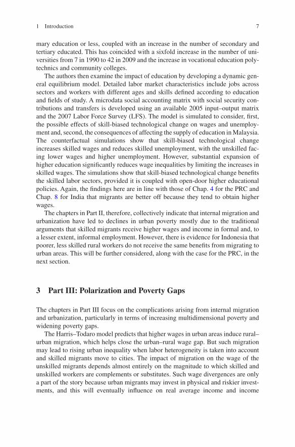
It is notable in Fig. 2.2, however, that many Asian economies had passed the 50% threshold in 2014, whereby the majority of their populations lived in urban areas. This of course includes the ‘tiger’ economies of the 1980s and 1990s but also some of the largest economies in the region (PRC [54.4%] and Indonesia [53%]). The

Fig. 2.3 Asia: urban and rural population by region, 1950–2050. (Source: United Nations 2014a)

0

200000

400000

600000

800000

1000000

1200000

1950 1975 2010 2030 2050

People’s Republic of China

Popu

latio

n at

mid

year

(th

ousa

nd)

Popu

latio

n at

mid

year

(th

ousa

nd)

Urban Rural

0

100000

200000

300000

400000

500000

600000

1950 1975 2010 2030 2050

ASEAN

Urban Rural

G. Hugo

19

Thailand/Philippines anomaly noted by Jones (2004) is still in evidence. A strong pattern of lower urbanization in South Asia than East Asia, with Southeast Asia lying in between, is apparent. Low levels of urbanization in 2014 were evident in each South Asian economy—India (32.4%), Pakistan (38.3%) and Bangladesh (33.5%).

Much of the discussion on the urban transition in Asia examines only the per-centage of national populations living in urban areas, but it is important also to focus on the numbers of people involved since this gives a more striking perspective on the challenges being faced in urban Asia, especially the largest cities. Accordingly, we have shown in Fig. 2.3 the changes in the rural and urban population sizes in key

0

200000

400000

600000

800000

1000000

1200000

1400000

1950 1975 2010 2030 2050

South AsiaPo

pula

tion

at m

idye

ar (

thou

sand

)Po

pula

tion

at m

idye

ar (

thou

sand

)

Urban Rural

0

500000

1000000

1500000

2000000

2500000

3000000

3500000

4000000

1950 1975 2010 2030 2050

Total Asia

Urban Rural

Fig. 2.3 (continued)

2 Patterns and Trends of Urbanization and Urban Growth in Asia

20

Asian regions over the 1950–2050 period. The patterns depicted here are very strik-ing. It is apparent that not only in 1950 but also in 1975, Asia was overwhelmingly a rural society and economy, with rural populations being clearly dominant. Thereafter, there have been dramatic changes with exponential growth of urban populations and a concomitant decline in rural population, although timing has dif-fered between different regions.

Figure 2.4 shows the massive urban growth that occurred in the Asian urban sec-tor between 1950 and 2010 (from 252 million to almost 1.9 billion people), while the rural population increased from 1.2 to 2.3 billion. On the other hand, the Asian rural population is expected to decline over the next two decades, while the urban population will increase. While reclassification of areas from rural to urban status has been of major significance, the main reason for faster population growth in urban areas has been rural–urban migration.

However, the overall Asia data has enormous variations between economies. Table 2.2 shows that South Asia is the least urbanized part of the region with less than a third (32.7%) of its population living in urban areas, while East Asia is the most urbanized (54.3%). By 2030, more than two in three residents in East Asia will live in urban areas, while the urban proportion will be 42% in South Asia and 55.8% in Southeast Asia. The variation is even greater between individual economies with the level of urbanization varying from economies of Hong Kong, China and Singapore to the rural economies of Timor-Leste (29.5% living in urban areas) and Bhutan (34.8%) in 2010. It is especially important to consider trends in the largest economies. Of the 10 economies with more than 100 million residents in 2000, 6 were in Asia. Table 2.3 shows trends in growth of the urban populations in these economies.

0

500000

1000000

1500000

2000000

2500000

3000000

Urban Rural

Pop

ulat

ion

(tho

usan

ds)

1950 2010 2030*

Fig. 2.4 Urban and rural population in Asia, 1950, 2010 and 2030. (Source: United Nations 2014a). Note: * = projections

G. Hugo

21

Clearly, there has been massive urban growth over the 1950–2000 period, and this will at least double again except in Japan and the PRC. Only Japan had more than half of its population in urban areas in 2000, but by 2030 this will also be the case in the PRC and Indonesia. It is also important to consider the tempo of change in urbanization and urban growth.

In net growth terms, urban areas of Asia and Africa will absorb almost all of the world’s net population growth over the period up to 2050. Around 90% of the 2.5 million urban dwellers added to the global population will live in Asia and Africa. One of the clear differences between Asia and Africa, however, is depicted in Fig. 2.5—while half of the Asian countries are experiencing a decline in their rural populations, both urban and rural populations are increasing in Africa. UN projections indicate that two-thirds of countries will experience decreases in their rural populations between 2014 and 2050, including most countries in Asia (United Nations 2014b, 3).

Table 2.2 Urban population in Asia, number and percentage estimates, 1950 to 2010, and 2030*

Region1950 2000 2010 2030*No. (‘000) % No. (‘000) % No. (‘000) % No. (‘000) %

Eastern Asia 119,111 17.9 632,396 42.0 865,826 54.3 1,207,794 71.5Central Asia 5715 32.7 22,870 41.5 24,951 40.4 34,020 44.1Southern Asia 78,950 16.0 420,685 29.1 550,607 32.7 875,188 42.0Southeastern Asia 26,066 15.5 199,681 38.1 265,801 44.5 403,284 55.8Western Asia 14,732 28.8 117,108 63.8 157,652 68.1 232,170 74.1Oceania 7906 62.4 22,013 70.5 25,924 70.7 33,747 71.3Asia 252,480 17.9 1,414,753 37.7 1,890,760 45.0 2,786,204 56.5

Source: United Nations (2014a)Note: * = projections

Table 2.3 Asia’s largest countries: urban population, number and percentage estimates, 1950 and 2000 and 2030*

1950 2000 2030*

No. (‘000) %% Growth 1950–2000 No. (‘000) %

% Growth 1950–2030 No. (‘000) %

PRC 64,180 11.8 615.8 459,383 35.9 117.4 998,925 68.7India 64,134 17.0 349.6 288,365 27.7 102.2 583,038 39.5Indonesia 9001 12.4 874.9 87,759 42.0 110.7 184,912 63.0Pakistan 6578 17.5 625.0 47,687 33.2 126.2 107,880 46.6Bangladesh 1623 4.3 1824.6 31,230 23.6 166.3 83,160 44.9Japan 43,896 53.4 125.2 98,873 78.6 18.3 116,918 96.9

Source: United Nations (2014a)Note: PRC People’s Republic of China; * = projections

2 Patterns and Trends of Urbanization and Urban Growth in Asia

22

4 Patterns of Urbanization

The processes of urbanization and urban growth have been fundamental elements in Asia’s economic ‘miracle’. Asia’s percentage of urban share remains at 47.5 in 2014 (UN 2014a). However, this has, by no means, been a uniform process across Asia. Table 2.4 shows how the level of urbanization varied widely across Asia in 2014. The broad pattern of high levels of urbanization in East Asia, low in South Asia and with Southeast Asia falling between them is in evidence.

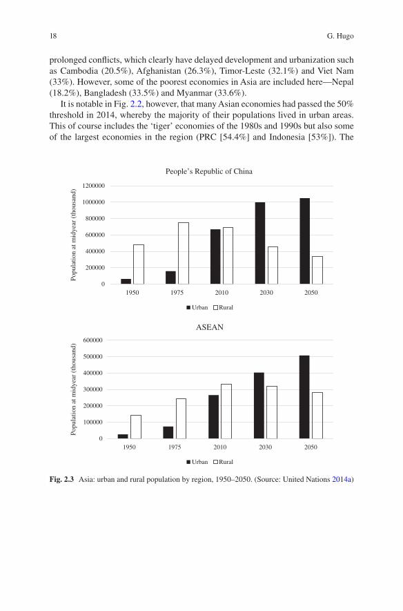
There are important linkages between urbanization, on the one hand, and eco-nomic development and poverty reduction, on the other. While the data (especially that on the level of urbanization) is compromised in a number of economies, Fig. 2.6 shows that there is a clear correlation in Asia between level of urbanization and GDP per capita. ‘Location’ is important at all stages of development, but it is espe-cially significant in poorer and developing economies (World Bank and IMF 2013, 85). It is apparent, however, that not only are there wide disparities between rural and urban areas in development and living standards, but also processes associated with urbanization have an impact upon national development.

Turning to the linkages between urbanization and poverty, there are a number of global generalizations which are emerging:

86

42

0

-4 -2

Urban decline/rural decline

Region Total population> 1 billion500 million to 1 billion100 million to 500 million50 million to 100 million10 million to 50 million5 million to 10 million1 million to 5 million500,000 to 1 million< 500,000

AsiaAfrica

OceaniaLatin America and the CaribbeanEurope and Northern America

Urban decline/rural growth

Papua New Guinea

Niger

India

United StatesBrazil

PRC

Urban growth/rural decline Urban growth/rural growth

HaitiNigeria

Rwanda

Japan

Bulgaria

Belarus

Netherlands

0

Average annual rate of rural populationgrowth (%)

Ave

rage

ann

ual r

ate

of u

rban

pop

ulat

ion

grow

th (

%)

2 4

Fig. 2.5 Average annual rates of urban and rural population growth, 1990–2014. (Source: United Nations 2014b, 4)Note: 201 countries or areas with at least 90,000 inhabitants in 2014; PRC People’s Republic of China

G. Hugo

Table 2.4 Percentage urban by economy, 2014

Percentage urban Percentage urban

Eastern Asia 58.9 Western Asia 69.6 China, People’s

Republic of54.4 Armenia 62.8

Hong Kong, China 100.0 Azerbaijan 54.4 Macau, China 100.0 Bahrain 88.7 Korea, Democratic

People’s Republic of60.7 Cyprus 67.0

Korea, Republic of 82.4 Georgia 53.5 Japan 93.0 Iraq 69.4 Mongolia 71.2 Israel 92.1 Other non-specified areas 76.5 Jordan 83.4

Kuwait 98.3Central Asia 40.4 Lebanon 87.7 Kazakhstan 53.3 State of Palestine 75.0 Kyrgyz Republic 35.6 Oman 77.2 Tajikistan 26.7 Qatar 99.2 Turkmenistan 49.7 Saudi Arabia 82.9 Uzbekistan 36.3 Syrian Arab Republic 57.3

Turkey 72.9Southern Asia 34.4 United Arab Emirates 85.3 Afghanistan 26.3 Yemen 34.0 Bangladesh 33.5 Bhutan 37.9 Oceania 70.8 India 32.4 Australia 89.3 Iran (Islamic Republic of) 72.9 New Zealand 86.3 Maldives 44.5 Fiji 53.4 Nepal 18.2 New Caledonia 69.7 Pakistan 38.3 Papua New Guinea 13.0 Sri Lanka 18.3 Solomon Islands 21.9

Vanuatu 25.8Southeastern Asia 47.0 Guam 94.4 Brunei Darussalam 76.9 Kiribati 44.2 Cambodia 20.5 Marshall Islands 72.4 Indonesia 53.0 Micronesia, Fed. States of 22.4 Lao People’s Democratic

Republic37.6 Nauru 100.0

Malaysia 74.0 Northern Mariana Islands 89.3 Myanmar 33.6 Palau 86.5 Philippines 44.5 American Samoa 87.3 Singapore 100.0 Cook Islands 74.3 Thailand 49.2 French Polynesia 56.0 Timor-Leste 32.1 Niue 41.8 Viet Nam 33.0 Samoa 19.3

Tokelau 0 Tonga 23.6 Tuvalu 58.8 Wallis and Futuna Islands 0

Source: United Nations (2014a)

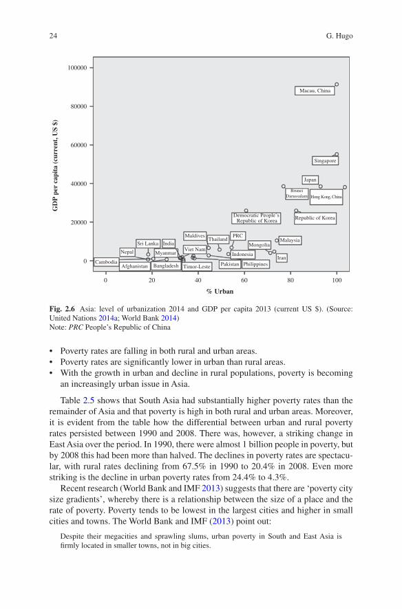
24

• Poverty rates are falling in both rural and urban areas.• Poverty rates are significantly lower in urban than rural areas.• With the growth in urban and decline in rural populations, poverty is becoming

an increasingly urban issue in Asia.

Table 2.5 shows that South Asia had substantially higher poverty rates than the remainder of Asia and that poverty is high in both rural and urban areas. Moreover, it is evident from the table how the differential between urban and rural poverty rates persisted between 1990 and 2008. There was, however, a striking change in East Asia over the period. In 1990, there were almost 1 billion people in poverty, but by 2008 this had been more than halved. The declines in poverty rates are spectacu-lar, with rural rates declining from 67.5% in 1990 to 20.4% in 2008. Even more striking is the decline in urban poverty rates from 24.4% to 4.3%.

Recent research (World Bank and IMF 2013) suggests that there are ‘poverty city size gradients’, whereby there is a relationship between the size of a place and the rate of poverty. Poverty tends to be lowest in the largest cities and higher in small cities and towns. The World Bank and IMF (2013) point out:

Despite their megacities and sprawling slums, urban poverty in South and East Asia is firmly located in smaller towns, not in big cities.

100000

80000

60000

40000

20000

0

0

Cambodia

Nepal

Sri Lanka

Afghanistan Bangladesh

India

Myanmar

Timor-Leste

Viet Nam

MaldivesThailand

PRC

Mongolia

Indonesia

Pakistan PhilippinesIran

Malaysia

Republic of KoreaDemocratic People’s Republic of Korea

BruneiDarussalam Hong Kong, China

Japan

Singapore

Macau, China

20 40 60

% Urban

GD

P p

er c

apit

a (c

urre

nt, U

S $)

80 100

Fig. 2.6 Asia: level of urbanization 2014 and GDP per capita 2013 (current US $). (Source: United Nations 2014a; World Bank 2014)Note: PRC People’s Republic of China

G. Hugo

25

Tabl

e 2.

5 Sh

are

of th

e po

pula

tion

belo

w $

1.25

a d

ay

1990

1996

2002

2008

Rur

alU

rban

Rur

alU

rban

Rur

alU

rban

Rur

alU

rban

Eas

t Asi

a an

d Pa

cific

67.5

24.4

45.9

13.0

39.2

6.9

20.4

4.3

Eur

ope

and

Cen

tral

Asi

a2.

20.

96.

32.

84.

41.

11.

20.

2L

atin

Am

eric

a an

d th

e C

arib

bean

21.0

7.4

20.3

6.3

20.3

8.3

13.2

3.1

Mid

dle

Eas

t and

Nor

th A

fric

a9.

11.

95.

60.

97.

51.

24.

10.

8So

uth

Asi

a50

.540

.146

.135

.245

.135

.238

.029

.7Su

b-Sa

hara

n A

fric

a55

.041

.556

.840

.652

.341

.447

.133

.6To

tal

52.5

20.5

43.0

17.0

39.5

15.1

29.4

11.6

Sour

ce: W

orld

Ban

k an

d In

tern

atio

nal M

onet

ary

Fund

201

3, 8

7

2 Patterns and Trends of Urbanization and Urban Growth in Asia

26

They present two examples to demonstrate this relationship. Figure 2.7 shows pat-terns for India and Viet Nam, which show that poverty is greater in smaller towns than cities. In India, for example, research in 2004–2005 found that the poverty rate was 28% in rural areas and 26% in urban areas. However, in Indian urban areas, poverty rates in towns (population less than 50,000) double those in cities with one million or more residents (Lanjouw and Marra 2012; World Bank 2011). In Pakistan and Bangladesh, the incidence of poverty is highest in rural areas (43%), followed by smaller towns and cities (38%) and then metropolitan areas (26%) (Deichmann et al. 2009).

The Viet Nam example in Fig. 2.7 shows an interesting U-shaped pattern. The two largest cities in the country (Ha Noi and Ho Chi Minh City) have nearly a third of Viet Nam’s urban population but only a tenth of the national population in pov-erty. However, 55% of the urban poor live in the 634 smallest towns (World Bank and IMF 2013, 90).

Much attention has been focused on the emergence of megacities in Asia—urban agglomerations with populations of ten million or more residents. They are complex cities of a scale and complexity not previously seen, often multinuclear in that they have enveloped smaller cities in their lateral spread. A key feature of Asian megaci-ties is the fact that they include extensive peri-urban regions of mixed urban and rural land use but which are heavily tied to the urban area by commuting and other linkages (Jones 2004). However, UN data on megacities usually applies to areas defined by city boundaries. In megacities, the built-up area usually overspills these boundaries, and the definition also excludes the large peri-urban development. A decade ago, Hugo (2004) showed that while the United Nations estimated the Jakarta megacity population at 11.4 million, the real functioning population of the megacity at that time was 20.2 million. Jones and Douglass (2008) have demon-strated this systematic underestimation of the size of Asian megacities in censuses

Ruralareas

0

10

20

30

40

Pov

erty

rat

e(%

)a.India:Poverty rate in small towns

is higer than in rural areasb.Viet Nam:Urban poor are concentrated

in the extra-small towns

Shar

e of

urb

an p

opul

atio

nth

at is

poo

r (%

)50

60

Urbanareas

Source: World Bank 2011.Note: Poverty rates based on Uniform Recall Period (URP) and official poverty line.

Source: Lanjouw and Marra 2012.Note: XS = > 4k–50k; S = 50k – 300k; M = 300k –500k; L = 1m–5m for centrally governed and 0.5m–1m for locally governed;XL = > 5m

Smalltowns

Mediumtowns

Largetowns

XS

0

10

20

30

40

50

60

Share of urban population1983 1993-94 2004-05

Share of urban poor

S M L XL

Fig. 2.7 In India and Viet Nam, poverty in small towns is worse than in large cities. (Source: World Bank and International Monetary Fund 2013, 91)

G. Hugo

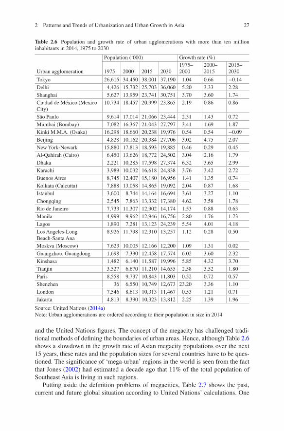
27

and the United Nations figures. The concept of the megacity has challenged tradi-tional methods of defining the boundaries of urban areas. Hence, although Table 2.6 shows a slowdown in the growth rate of Asian megacity populations over the next 15 years, these rates and the population sizes for several countries have to be ques-tioned. The significance of ‘mega-urban’ regions in the world is seen from the fact that Jones (2002) had estimated a decade ago that 11% of the total population of Southeast Asia is living in such regions.

Putting aside the definition problems of megacities, Table 2.7 shows the past, current and future global situation according to United Nations’ calculations. One

Table 2.6 Population and growth rate of urban agglomerations with more than ten million inhabitants in 2014, 1975 to 2030

Urban agglomeration

Population (‘000) Growth rate (%)

1975 2000 2015 20301975–2000

2000–2015

2015–2030

Tokyo 26,615 34,450 38,001 37,190 1.04 0.66 −0.14Delhi 4,426 15,732 25,703 36,060 5.20 3.33 2.28Shanghai 5,627 13,959 23,741 30,751 3.70 3.60 1.74Ciudad de México (Mexico City)

10,734 18,457 20,999 23,865 2.19 0.86 0.86

São Paulo 9,614 17,014 21,066 23,444 2.31 1.43 0.72Mumbai (Bombay) 7,082 16,367 21,043 27,797 3.41 1.69 1.87Kinki M.M.A. (Osaka) 16,298 18,660 20,238 19,976 0.54 0.54 −0.09Beijing 4,828 10,162 20,384 27,706 3.02 4.75 2.07New York-Newark 15,880 17,813 18,593 19,885 0.46 0.29 0.45Al-Qahirah (Cairo) 6,450 13,626 18,772 24,502 3.04 2.16 1.79Dhaka 2,221 10,285 17,598 27,374 6.32 3.65 2.99Karachi 3,989 10,032 16,618 24,838 3.76 3.42 2.72Buenos Aires 8,745 12,407 15,180 16,956 1.41 1.35 0.74Kolkata (Calcutta) 7,888 13,058 14,865 19,092 2.04 0.87 1.68Istanbul 3,600 8,744 14,164 16,694 3.61 3.27 1.10Chongqing 2,545 7,863 13,332 17,380 4.62 3.58 1.78Rio de Janeiro 7,733 11,307 12,902 14,174 1.53 0.88 0.63Manila 4,999 9,962 12,946 16,756 2.80 1.76 1.73Lagos 1,890 7,281 13,123 24,239 5.54 4.01 4.18Los Angeles-Long Beach-Santa Ana

8,926 11,798 12,310 13,257 1.12 0.28 0.50

Moskva (Moscow) 7,623 10,005 12,166 12,200 1.09 1.31 0.02Guangzhou, Guangdong 1,698 7,330 12,458 17,574 6.02 3.60 2.32Kinshasa 1,482 6,140 11,587 19,996 5.85 4.32 3.70Tianjin 3,527 6,670 11,210 14,655 2.58 3.52 1.80Paris 8,558 9,737 10,843 11,803 0.52 0.72 0.57Shenzhen 36 6,550 10,749 12,673 23.20 3.36 1.10London 7,546 8,613 10,313 11,467 0.53 1.21 0.71Jakarta 4,813 8,390 10,323 13,812 2.25 1.39 1.96

Source: United Nations (2014a)Note: Urban agglomerations are ordered according to their population in size in 2014

2 Patterns and Trends of Urbanization and Urban Growth in Asia

28

Tabl

e 2.

7 Po

pula

tion

of c

ities

with

ten

mill

ion

inha

bita

nts

or m

ore,

195

0, 2

001,

201

4 an

d 20

30

1950

2001

2014

2030

City

Popu

latio

n (‘

000)

City

Popu

latio

n (‘

000)

City

Popu

latio

n (‘

000)

City

Popu

latio

n (‘

000)

New

Y

ork-

N

ewar

k

12,3

38To

kyo

34,6

69To

kyo

37,8

33To

kyo

37,1

90

Toky

o11

,275

Kin

ki M

.M.A

. (O

saka

)18

,662

Del

hi24

,953

Del

hi36

,060

Ciu

dad

de M

éxic

o (M

exic

o C

ity)

18,6

18Sh

angh

ai22

,991

Shan

ghai

30,7

51

New

Yor

k-N

ewar

k17

,868

Ciu

dad

de M

éxic

o (M

exic

o C

ity)

20,8

43M

umba

i (B

omba

y)27

,797

São

Paul

o17

,260

São

Paul

o20

,831

Bei

jing

27,7

06M

umba

i (B

omba

y)16

,753

Mum

bai (

Bom

bay)

20,7

41D

haka

27,3

74D

elhi

16,4

12K

inki

M.M

.A. (

Osa

ka)

20,1

23K

arac

hi24

,838

Shan

ghai

14,5

67B

eijin

g19

,520

Al-

Qah

irah

(C

airo

)24

,502

Al-

Qah

irah

(C

airo

)13

,922

New

Yor

k-N

ewar

k18

,591

Lag

os24

,239

Kol

kata

(C

alcu

tta)

13,2

53A

l-Q

ahir

ah (

Cai

ro)

18,4

19C

iuda

d de

Méx

ico

(Mex

ico

City

)23

,865

Bue

nos

Air

es12

,621

Dha

ka16

,982

São

Paul

o23

,444

Los

Ang

eles

-Lon

g B

each

-San

ta A

na11

,834

Kar

achi

16,1

26K

insh

asa

19,9

96

Rio

de

Jane

iro

11,4

15B

ueno

s A

ires

15,0

24K

inki

M.M

.A. (

Osa

ka)

19,9

76D

haka

10,6

96K

olka

ta (

Cal

cutta

)14

,766

New

Yor

k-N

ewar

k19

,885

Bei

jing

10,6

26Is

tanb

ul13

,954

Kol

kata

(C

alcu

tta)

19,0

92K

arac

hi10

,378

Cho

ngqi

ng12

,916

Gua

ngzh

ou, G

uang

dong

17,5

74M

oskv

a (M

osco

w)

10,1

69R

io d

e Ja

neir

o12

,825

Cho

ngqi

ng17

,380

Man

ila10

,140

Man

ila12

,764

Bue

nos

Air

es16

,956

Lag

os12

,614

Man

ila16

,756

G. Hugo

29

1950

2001

2014

2030

City

Popu

latio

n (‘

000)

City

Popu

latio

n (‘

000)

City

Popu

latio

n (‘

000)

City

Popu

latio

n (‘

000)

Los

Ang

eles

-Lon

g B

each

-San

ta A

na12

,308

Ista

nbul

16,6

94

Mos

kva

(Mos

cow

)12

,063

Ban

galo

re (

Ben

galu

ru)

14,7

62G

uang

zhou

, G

uang

dong

11,8

43T

ianj

in14

,655

Kin

shas

a11

,116

Rio

de

Jane

iro

14,1

74T

ianj

in10

,860

Che

nnai

(M

adra

s)13

,921

Pari

s10

,764

Jaka

rta

13,8

12Sh

enzh

en10

,680

Los

Ang

eles

-Lon

g B

each

-San

ta A

na13

,257

Lon

don

10,1

89L

ahor

e13

,033

Jaka

rta

10,1

76H

yder

abad

12,7

74Sh

enzh

en12

,673

Lim

a12

,221

Mos

kva

(Mos

cow

)12

,200

Bog

otá

11,9

66Pa

ris

11,8

03Jo

hann

esbu

rg11

,573

Kru

ng T

hep

(Ban

gkok

)11

,528

Lon

don

11,4

67D

ar e

s Sa

laam

10,7

60A

hmed

abad

10,5

27L

uand

a10

,429

Thà

nh P

ho H

o C

hí M

inh

(Ho

Chi

Min

h C

ity)

10,2

00

Che

ngdu

10,1

04

Sour

ce: U

nite

d N

atio

ns (

2014

a)

2 Patterns and Trends of Urbanization and Urban Growth in Asia

30

such agglomeration was located in Asia in 1950, but by 2001, 10 of the 18 global megacities were in Asia. In 2014, there were 28 world megacities, of which 16 were in Asia. In 2014, some 12% of the world’s urban dwellers lived in megacities (United Nations 2014c).

Projections of world megacities in 2030 predict that the seven largest megacities will be in Asia, from Tokyo (37.2 million) to Karachi (24.8 million). Of the 42 coun-tries with more than 10 million inhabitants, 23 will be Asian.

Figure 2.8 shows the past and anticipated future growth of the world’s largest six cities, of which four are Asian. Although Tokyo’s population is expected to decline, it is expected to remain the largest city with 37 million inhabitants in 2030. However, by then, the same population level will be almost reached by Delhi, for which the projected population is 36 million.

However, the poor measurement of Asian city size means that these figures sub-stantially underestimate both the total number of Asian megacities and their size. Jones and Douglass (2008) have demonstrated this by considering the several ASEAN coastal capitals that have indeed passed the ten-million resident threshold (Jakarta, Bangkok, Ho Chi Minh City). This undoubtedly is the case also for Chinese cities like Shenzhen, Chongqing and Guangzhou. These megacities are playing a major role in the development of the PRC and ASEAN countries, and it is crucial that we develop better ways of delineating their boundaries so they represent the functional mega-urban areas. The remarkable growth of Chinese cities especially has not been well captured in these data. One striking example is the city of Shenzhen, one of the first special economic zones in the PRC. From a population of 20,000 in 1980, Shenzhen had reached 12 million and megacity status within just 40 years (Shen 2008).

The spatial distribution of cities with more than two million inhabitants in Asia indicates the strong coastal orientation in the location of large cities, especially megacities. This is partly a function of the strong colonial heritage of these large coastal port cities (McGee 1967). The lack of large cities in the inland is strongly in evidence. The East–West divide in the PRC also strikingly reflects the strong spatial divide in development between the two parts of the nation. It contrasts with India where the distribution of large cities is more evenly spread geographically. The lack

1970 19750

5

10

15

Pop

ulat

ion

(mill

ions

)

20

25

30

35

40

1980 1985 1990 1995 2000 2005 2010 2015 2020 2025 2030

Tokyo

Delhi

Shanghai

Mexico City

Mumbai

São Paulo

2014

Fig. 2.8 Population of the largest cities in 2014, from 1970 to 2030. (Source: United Nations 2014c, 1)

G. Hugo

31

of urban development in the poorest and least developed parts of the region such as Eastern Indonesia, Lao People’s Democratic Republic and Cambodia is clear.

The strong coastal orientation of Asia’s megacities and indeed of the total urban population has some implications from the perspective of climate and environmen-tal change, particularly in terms of a substantial exposure to the risk of impact from sea level rise. Accordingly, in a global assessment (Wheeler 2011) of the projected population at risk from sea level rise in 2050, the 20 countries with the largest num-bers included 11 Asian countries of which 6 were Southeast Asian—Indonesia (20.9 million people), the Philippines (13.6 million), Viet Nam (9.5 million), Myanmar (4.6 million), Malaysia (3.5 million) and Thailand (2.6 million). McGranahan et al. (2007) identified the global population living in urban areas in the low elevation coastal zone (LECZ, coastal areas 10 m or less below sea level). Of the ten nations with the largest numbers of people living in the LECZ, eight are Asian and four are in Southeast Asia—Viet Nam, Indonesia, Thailand and the Philippines.

Internal migration in Asia is increasingly characterized by:

• Increasing settlement in coastal areas.• Increasing urbanization.

In fact, current patterns of internal migration in many countries are increasingly concentrating national population in areas with high risk of being influenced by climate change. The Asian megacities vary in their exposure to the risk of sea level rise, as Table 2.8 shows (Hugo and Bardsley 2014).

In recent discussions of urbanization, there has been a focus on megacities, yet it is apparent that small- and medium-sized cities are also making a major contribu-tion to urban growth, especially in large nations like the PRC, India and Indonesia. Smaller- and medium-sized cities also are experiencing ‘extended urbanization’ in that they are expanding beyond their boundaries and creating what Zhu (2004) describes in the PRC as ‘in situ urbanization’, whereby hitherto rural populations are ‘swallowed up’ by expanding urban areas. A study by Fahmi et al. (2014) exam-ines Cirebon in Indonesia where the city has 300,000 inhabitants and an additional 400,000 live in the outer areas surrounding the city proper. There are real problems in providing services and infrastructure to such areas.

Table 2.8 Southeast Asia: megacities’ projected population 2005–2025

Average height above sea levelPopulation (‘000)2005 2020 2025

Bangkok 2 m 6,582 7,807 8,322Jakarta 8 m 8,643 11,682 12,363Manila 16 m 10,761 13,892 14,808Ho Chi Minh City 19 m 5,072 7,293 8,149

Source: United Nations (2008)

2 Patterns and Trends of Urbanization and Urban Growth in Asia

32

5 Drivers of Urbanization and Urban Growth

The dynamics of rapid urbanization and urban growth in Asia are complex. However, much of the discourses see urbanization purely as a permanent shift of people involving migration from living in a rural location to living in an urban one. However, there are a number of processes involved:

• Natural increase (i.e. excess of births over deaths)• Net internal migration (i.e. excess of immigrants from elsewhere in the country

compared with out-migrants moving to such areas)• Net international migration (an excess of immigrants from other countries over

emigrants moving to such countries)• Reclassification of areas from being classified as rural to urban, often by the

lateral extension of large urban areas to swallow up surrounding rural areas and smaller cities and towns

Unfortunately, the relative contribution of these four factors of urban growth in Asia over the last 15 years has not been calculated. In fact, this estimation has only been made for the 1960s, 1970s and 1980s (United Nations 2001). One more recent estimate suggests that 40% of the increase in the urban population in developing countries comes from migration or reclassification of the rural to the urban. In the large countries of the PRC and Indonesia, however, these two factors accounted for more than 70% of urban growth (World Bank and IMF 2013, 85).

While the emphasis is on internal rural–urban migration as the major driver of rapid growth in urban areas, in most countries, it accounts for less than half of net urban growth. Nevertheless, rural to urban migration is not only important in influ-encing a nation’s demography but also often associated with substantial social and economic transformations.

As the urban populations of Asian countries increase rapidly, it is the children born to the urban residents that are becoming a major factor in the growth of these centres. However, an important characteristic of all Asian countries is that, as Table 2.9 shows, fertility levels are generally significantly lower in urban areas than in rural. This consistent feature of Asian demography has been seen in the past as being largely a function of the educational, income and occupational differentials between urban and rural areas. However, work in Africa (Brockerhoff 1998) has shown that, even when holding such differences constant, urban fertility is lower, thus indicating that there may be something about urban living and conditions that works independently to lower fertility. This may be such things as greater housing pressures, the type of work of women which makes it more difficult to keep working while having young children than in the village, difficult patterns of marriage and partnering, different peer group pressures and influences, etc.

Nowhere in Asia have urban–rural differentials in fertility decline been greater than in the PRC (Lavely and Freedman 1990; Yao 1995; Zhao 2001). Figure 2.9 shows that in the PRC’s dramatic fertility decline, the fall has been more dramatic in urban than rural areas. The urban total fertility rate (TFR) had fallen to 1.13 in the

G. Hugo

33

late 1990s, while that in Shanghai was 0.87 (Yuan 2003)—one of the lowest rates of any place in the world.

The lower fertility in urban than rural areas means that despite most urban areas having lower mortality than rural areas, natural increase rates are lower in urban than rural areas. However, the build-up of massive urban populations means that in many countries the numerical size of the natural increase is very large.

Another aspect of the decreased fertility in Asian urban areas, especially where it has fallen well below replacement levels, as in the PRC, is the impact on age

Table 2.9 Selected Asian countries: differences in total fertility rate between urban and rural areas

Country YearUrban fertility rate

Rural fertility rate

Percent lower in urban areas

Bangladesh 2011 2.0 2.5 20.0Cambodia 2010 2.2 3.3 33.3India 2005–2006 2.1 3.0 30.0Indonesia 2012 2.4 2.8 14.3Maldives 2009 2.1 2.8 25.0Nepal 2011 1.6 2.8 42.9Pakistan 2012–2013 3.2 4.2 23.8Philippines 2013 2.6 3.5 25.7Sri Lanka 1987 2.1 2.8 25.0Thailand 1987 1.7 2.4 29.2Timor-Leste 2009–2010 4.9 6.0 18.3Viet Nam 2002 1.5 2.0 25.0

Source: Demographic and Health Surveys, STATcompiler

1970 1975

Years

Tot

al F

erti

lity

Rat

e

1960 19651950 1955

0

1

2

3

4

5

6

7

8

1980 1985 1990

Rural

Total

Urban

City

Town

1995 2000 2005 2010

Fig. 2.9 People’s Republic of China: total fertility rate, 1950–2010. (Source: Zhao 2001; Peng 2004, 136; 2010 Census of PRC)

2 Patterns and Trends of Urbanization and Urban Growth in Asia

34

structure and thus on the size and characteristics of its working population, the demand for health services, social security for the elderly and so on. We will exam-ine here the Chinese city of Shanghai, the changing age structure of which is shown in Table 2.10. This demonstrates the massive changes over the recent decades. First, the impact of the plummeting fertility that saw the proportion made up of the depen-dent child age groups (0–14 years), which made up 42.3% of the total city popula-tion in 1964. This declined rapidly in the 1980s, and by 2010, only 8.6% of Shanghai’s population was in this age group. On the other hand, the percentage aged 65+ increased from 3.6% in 1964 and increased to 11.5% in 2000. Particularly strik-ing, however, was the proportion of the working population in the total population increasing from 54.1% to 81.3% between 1964 and 2010. In fact, this change in age structure in Shanghai (and in the PRC) has delivered a marked demographic divi-dend. An important issue here is that the pattern of age structure in Shanghai is duplicated across other Asian cities, albeit often in a less spectacular way. It is important to note that one of the elements which contribute to Asia’s urban areas being an ‘engine of growth’ in the region is the demographic dividend factor.

The demographic dividend can be defined as follows:

A rapid decline in fertility such as China has experienced can create a ‘youth bulge’ of large numbers of young people born in the final years of high fertility. As they move through the age pyramid they can deliver a demographic dividend of economic growth when the bulge passes through the working age groups so that the workforce grows faster than the total population. If countries take advantage there is a virtuous cycle of wealth creation. (Bloom et al. 2003, 39).

This virtuous cycle is created through:

• Increased labour supply, with women more ready to enter the workforce.• Increased savings.• Increased human capital investments.

However, there is a need for a favourable policy environment to be put in place if this dividend is to be realized.

Although Asia’s cities will continue to grow, the effects of continued low fertility will be very much felt in the cities. It already has been shown that these nations will record significant ageing of their populations and resultant imbalances between working age and aged dependent populations. These effects will be greater in cities than elsewhere in these nations since, in many cases, the percentage of the aged

Table 2.10 Change of age structure in Shanghai (percent)

Year 0–14 15–64 65+

1964 42.31 54.08 3.611982 18.15 74.25 7.601990 18.23 72.39 9.382000 12.26 76.28 11.462010 8.61 81.26 10.13

Source: Child Population Censuses in 1964, 1982, 1990, 2000 and 2010

G. Hugo

35

population living in urban areas will be greater than the percentage of the total population living in cities. This is due to the fact that there tends to be net migration gains of the ‘old–old’ population due to the greater availability of high-order health facilities and specialized housing and other care services for the aged in larger cit-ies. In addition, aged people often migrate to join their children who have moved to cities. Hence an important point here is that while overall urban populations in Asia will continue to increase, the balance between their working age and older popula-tions will deteriorate, and the workforce itself will age as the effects of fertility decline exacerbate.

The low-fertility and ageing populations of urban areas of Asia would indicate that other things being equal, they will grow more slowly than national populations. Net migration gain is essential to the demographic, economic and social sustain-ability of Asian cities. There will be a need for ‘replacement migration’ to occur. This concept was developed in relation to the needs of low-fertility European coun-tries that currently or in the near future will experience population declines due to continued low fertility and the potential of countries of the south to make up the shortfalls through international migration. It came to particular prominence in early 2000 when the United Nations Population Division (2000: 01) published a report entitled ‘Replacement Migration: Is It a Solution to Declining Aging Populations? The report defined ‘replacement migration’ as ‘the international migration that would be needed to offset declines in the size of population, the declines in the population of working age, as well as to offset the overall ageing of the population’. While the report attracted a great deal of comment and criticism when it was pub-lished, the ‘replacement migration’ concept was a useful one because it pointed to the fact that migration was going to play a more significant role in the European countries than it had in the past.

In the current context of cities in Asia, it needs to be stressed that internal migra-tion of young people to the cities is replacing the local young workers that would have been moving into the workforce age had it not been for the extremely low fertility.

5.1 Internal Migration and Urban Development in Asia

Population movement has played a key role not only in the growth of urban centres in Asia but also strongly influenced the social, economic and demographic structure and development of these centres. From the perspective of the growth of urban cen-tres, it is apparent that net internal migration from the rural areas has been substan-tial. While intercensal reclassification of rural areas as urban due to the lateral expansion of urban areas has been important, rural–urban immigration has been a major engine of growth. Table 2.11 shows estimates of the components of growth in several major Asian cities in the 1990–2000 period. It indicates that net migration has been substantial. In 2005, Shanghai had a population of 17.78 million of which 4.38 million were migrants who had lived in the city for more than 6 months.

2 Patterns and Trends of Urbanization and Urban Growth in Asia

36

Moreover, one-third of all babies delivered were born to migrants (Xinhua News Agency, 7 April 2006). This shows the major role that migration is already playing in Shanghai’s demography. The table shows that were it not for the net migration factor, Shanghai’s population would have declined over the 1990–2000 period.

Table 2.11 shows that the contribution of net migration to the growth of four ASEAN megacities varied between 16.2% in Jakarta and 52% in Bangkok.

The increasing complexity of rural–urban migration and urbanization in Asia is depicted in Fig. 2.10, which is a model of the main forms of rural–urban migration. It indicates that permanent displacement from rural to urban areas is only one of the elements involved. There is a great deal of circular migration in Asian countries like the PRC (Zhu 2007) and Indonesia (Hugo 1982). This often involves a migrant leav-ing his/her family in the village and then returning to the village periodically while working in the city.

One of the distinguishing features of the PRC’s urban population is the duality between the resident population and the migrant worker population that largely comprises circular migrants. Such a distinction applies in all other Asian urban areas between a permanently settled resident population and a temporarily present group of ‘circular migrants’ from the outside.

Table 2.11 Contribution of net migration to population change in Asian megacities, 1990–2000 (percent)

Subregion of megacity Jakarta Bangkok Manila

Ho Chi Minh City Shanghai Taipei,China

Core Negative 3 19 na 11.4 NegativeInner zone 60.9 71 54 na 94.7 31.9Outer zone Negative 62 42 na 62.4 40.7Mega urban region 16.2 52 38 46.3 104.4 na

Source: Jones and Douglass 2008Note: na not available

RURAL URBAN

OVERSEASMIGRATION

OVERSEASMIGRATION

Permanent settlement

Circular migrationand

circulation

Return Migration

Reciprocal Migration

Fig. 2.10 A model of rural–urban population mobility in Asia

G. Hugo

37

Many commentators in the PRC have emphasized the need for the migrant worker population to become permanent urban residents and for this duality in Chinese cities to be ended, with migrant workers becoming integrated as settled city residents. While these recommendations have considerable merit, research findings on circular migration not only in the PRC (Zhu 1999; Hugo et al. 2009) but also elsewhere (Hugo 1982, 2009) have indicated that a more nuanced policy towards circular migration would have greater dividends for economic development and poverty reduction in Asian urban areas.

One of the ‘truisms’ of migration research is that ‘there is nothing so permanent as a temporary migrant’ (Martin 2001: 01). This is based on the belief that all tempo-rary migrants see their current non-permanent status as a preliminary stage before they are able to settle permanently at the destination. If given the opportunity, they will make the transition from temporary to permanent residence. However, research in both internal (Hugo 1978, 1982) and international migration (Hugo 2009) has shown that while some temporary migrants certainly fit this description, for others, circular, temporary migration is seen as a persistent, continuing and preferred mobil-ity strategy. For some temporary migrant workers in Chinese cities, there are signifi-cant advantages to circular migration between rural and urban areas over permanently settling in the city. Box 2.1 summarizes some of the main advantages that accrue from circular migration as a rural–urban mobility strategy. These advantages apply at individual, family, community and sectoral levels. Of course, there are disadvantages that are associated with circular migration as well, which are summarized in Box 2.2.

Box 2.1 Advantages of Circular Migration to Asian CitiesSource: IOM (2015)

• Circular migration allows poorer families to maximize income and spread risk of income failure by facilitating working in both rural and urban areas and in both agricultural and non-agricultural sectors.

• It maximizes the benefit of this income by earning in the city, where both wages and costs are higher, and spending in the village, where both are lower.

• It facilitates the redistribution of wealth from the fast-developing urban areas, which are the centre of investment and economic growth, to periph-eral and poorer rural areas, which lack such investment.

• It provides a scarce source of funds in rural areas to facilitate job creation and development in those areas.

• It reduces the pressure on urban areas to provide housing, schooling, infra-structure, health facilities, etc., for their inhabitants.

• In the PRC, if a circular migrant keeps his rural hukou, he can have two or three children rather than one, which is enforced in the city.

• In the PRC, if a migrant surrenders his rural hukou, he will have to give up his land. Land is an important consideration for support in old age.

• In the PRC, some migrant workers are also reluctant to pay the high costs of being an urban resident through taxes, contributions to health and pen-sion schemes, etc.

2 Patterns and Trends of Urbanization and Urban Growth in Asia

38

The important point to make here is that not all migrant workers in Asian cities want to shift permanently to live in large cities. Moreover, it needs to be recognized that both permanent rural to urban relocation and circular migration between rural and urban areas can have positive outcomes on development and poverty reduction:

• For those who permanently relocate, their personal situation improves because they gain access to all the services available in the city; they get the chance to increase their incomes and gain access to education, health and other services for their families.

• However, circular migration has also been shown to have the potential to deliver development dividends (Hugo 2009) and reduce poverty in rural communities. Migrant workers remit much of their earnings back to rural communities, which can be used not only to improve the situation of their village-based families but also the local community through their investment in it. Moreover, returning workers bring back new ideas and ways of doing things and can potentially invest in productive activity in their home communities. Circular migration provides the potential for the benefits of rapid economic growth in cities to be spread to the countryside.

Hence, there is great complexity in the substantial contribution that internal migration is making to the growth of urban areas in Asia. Yet there is another type of migration which is also increasingly shaping the size, composition and function of urban population in Asia—international migration.

Box 2.2 Disadvantages of Circular MigrationSource: IOM (2015)

• The social costs of separation from family can be substantial and very painful to the people involved, especially where there is a great distance separating the origin and the destination. In the PRC, only 20% of migrant workers bring their families with them (Jun 2010, 4).

• It is difficult to adjust to the time demands of modern-sector jobs, which require 5–6 day weeks and 8 h days of their workers.

• The origin community can lose substantial numbers of its youngest, entre-preneurial and most economically and socially active members for long periods as a result of which economic and social capital is diminished in those areas.

• Migrant workers in the destination can experience considerable hardship because of their marginal position and their lack of access to urban services.

G. Hugo

39

6 International Migration and Urban Development in Asia

A final dimension of population mobility that needs to be mentioned when consid-ering urbanization in Asia is international migration. Of course, international migra-tion has not been as substantial an element in Asian urbanization as it has in contemporary population growth in the major cities of Euro-American societies. Nevertheless, international migration is assuming greater significance, especially in cities in the most developed economies in the region. In Singapore, for example, it is now estimated that 36% of the population comprises foreign citizens and 27.7% of the workforce comprises foreigners (Hugo 2004). In Hong Kong, China, 6.7% of the population are citizens of other economies (Chiu 2003). The number of foreign nationals in 2010 in Japan was over 2.2 million, and there were some 224,067 over-staying illegal migrants, most of them in the nation’s urban areas (Hayashi 2013). In Seoul, the number of foreign residents increased from 114,685 in 2004 to 129,660 in 2005 (Asian Migration News, 15–31 June 2006). In cities like Kuala Lumpur and Bangkok, there are also significant numbers of foreigners, although in the PRC and India’s cities, the number of foreigners in cities is still quite small, but it is certainly growing as these cities are becoming more globally linked. As the megacities of the Asian region become ‘world cities’, their economic and social linkages to other countries grow (Sassen 1991; Friedmann 1986). Along with this, multinational cor-porations are increasingly locating activities in these cities and transferring their multinational workers in and out. Moreover, with increasing economic and political cooperation between nations in the region such as ASEAN and Asia-Pacific Economic Cooperation (APEC), the barriers to some movements have been reduced a little. This is especially true of student and skilled migrations. Moreover, there are forces in the cities of the better-off nations of the region that are creating a demand for unskilled workers, especially in niches that have low status, insecurity and low wages. Accordingly, unskilled immigrants are becoming increasingly evident in many Asian cities. It is important to stress that most of the increasing international migration to Asian countries is destined for urban locations so its impact is highly concentrated in cities, especially the largest cities.

There are a number of elements in the increasing international migration being directed into Asia’s largest cities. Most of the migrants are from other, usually nearby, Asian countries, and much of the movement is from less developed, labour surplus continents to more developed, better-off labour deficit economies. However, there is also a movement of more skilled persons (Hugo 2014), often employed by multinational companies, from OECD and more developed Asian countries to less developed nations. This is partly a function of the human resource policies of mul-tinational companies but also reflects the fact that the education/training systems in some economies are a mismatch with the skills needed in rapidly developing econo-mies, which is why they need to bring in management, engineering and other skills.

In summary, the main international migrations into Asian cities are as follows:

• There is an inflow of a professional and managerial group of expatriates. This group is increasing in size throughout the region, and while it involves some

2 Patterns and Trends of Urbanization and Urban Growth in Asia

40

foreigners of Asian origin, especially from India and the Philippines, skilled people from Europe, North America, Japan, the Republic of Korea and Australia–New Zealand predominate. It is partly associated with increased foreign direct investment in these cities and the associated transfer of staff from parent compa-nies located in MDCs. It also includes other skilled people who are in demand because local mismatches between rapidly growing and restructuring economies demand jobs which cannot be met by the local training/education system.

• International students are increasingly mobile within the Asia region. Asia has been for some time the major origin of students to OECD countries (Abella 2005; Kritz 2006), but there is an increasing movement to other Asian countries. For example, 20% of Singapore’s university students are foreign. There have also been large student migrations to Malaysia, the PRC, Japan and the Republic of Korea.

• There is a substantial influx of women to work as domestic maids, especially in the cities in the newly developing economies (NDEs)—Taipei,China; Hong Kong, China; Singapore; Brunei Darussalam; and Malaysia. They are predomi-nantly drawn from Indonesia, the Philippines and Sri Lanka and number more than two million (Huang et al. 2005).

• The construction industry in many cities in NDEs is dominated by foreign work-ers. In several economies, low-skilled foreign workers have been brought in to work in factories and in other low-pay, low-skill areas.

• The so-called entertainment or sex industry is an important element in the major cities (Lim 1998), and in several places, foreigners, especially women, are involved. Undocumented workers often trafficked into the country are substantial.

• In several cities, foreign workers, many of them undocumented, have become an important part of the informal sector.

• The gender differentials discussed earlier are contributing to increased marriage migration of women in the Asian region. Hugo (2006) shows that a third of mar-riages in the Republic of Korea and a quarter in Taipei,China, are now to foreign-ers, mostly from elsewhere in Asia. Asian international marriage is also being driven by increased global movement of young Asians, the role of a burgeoning marriage migration industry and the changing role of women in many receiving economies.

All of these increasing flows of intra-Asian international migration are dispro-portionately concentrating foreign populations in the cities of Asia. They are lead-ing to increased diversity in these cities—even in places like Japan, the Republic of Korea and Taipei,China, which have traditionally stressed their ethnic homogeneity. Other cities like Singapore, Kuala Lumpur, Jakarta, Bangkok and Ho Chi Minh have long had ethnic diversity because of the diversity of the nations in which they are located and earlier waves of international migration from the PRC and India. As the demographic and development differences between Asian economies become more stark, it is likely that the pressures for international migration to fast-growing cities in better-off economies will continue.

G. Hugo

41

7 Conclusion

Urban areas house more than a half of Asia’s population, while two generations previously, only one in ten Asians lived in urban areas. This represents a profound change in the way in which Asians live their lives. However, there are many chal-lenges that Asian urbanization presents to policymakers, planners and researchers. One crucial area lies in the arena of data collection and research. Planning for effi-ciency and equity in Asian cities requires timely and relevant research. However, in Asia, as elsewhere, conceptualization and definition of urban areas has remained mired in the thinking of the 1970s and does not capture the nature of contemporary dynamic urban systems. Moreover, data collection systems are based on large areas, while modern technology allows small building block units for censuses and other data collection, which in turn allows flexible and appropriate definition of urban boundaries. Sound planning and governance of urban centres in Asia require better delineation of boundaries and of appropriate specifically disaggregated data within those boundaries. Moreover, research in urban areas needs to be integrated so that an understanding of the dynamics of population change in urban areas may be achieved.

While there is variation between Asian cities in the extent of fertility decline and ageing, there can be no doubt that in several major cities in the region, especially those in the PRC, considerable challenges will be experienced especially in terms of:

• A reduction in the number of local young people entering the workforce.• A rapid growth in the elderly population and in their ratio to the replacement

working age population.

Migration from internal, and to a lesser extent international, sources will be essential to the sustainability of those cities that are most strongly affected. There is no doubt that the proportion of immigrants of major cities in several Asian nations is likely to continue to increase. This, however, is not simply a function of ‘replacement migration’. There are a number of processes operating to increase migration, both internal and international, in Asia. Moreover, that migration is disproportionately directed towards major cities, and this will continue because the labour markets into which they predominantly move are found in those cen-tres. The forces of globalization and economic restructuring which are reshaping the economic and social, as well as physical, form of Asia’s major cities of north nations have included an important population movement component. Indeed, an increased volume of international migration has been identified as one of the key defining characteristics of world cities (Friedmann 1986) and global cities (Sassen 1991).

Asian cities have undergone substantial demographic change in the last decade, and these trends seem likely to continue over the next two decades. These changes are both interrelated with social, economic and political transformations occurring

2 Patterns and Trends of Urbanization and Urban Growth in Asia

42

in those cities and have implications for those transformations. The shifts can be summarized as follows:

• The overall growth of urban populations will be slower than in the past half cen-tury but will continue at a significantly higher rate than in national populations.

• The working age population will stabilize because of low fertility, meaning the numbers of local people moving into the working age will decrease.

• The aged population will increase substantially, creating increased pressure on pension schemes, health services and so on.

• The distinctive residential pattern of aged populations will be increasingly evi-dent in north cities, and the services they require will account for an increased part of the workforce.

• Ageing of the population will result in different demands for transport, housing, retail services, human services and so forth.

• There will be increased levels of female participation in the urban workforce and an increase in the average age of retirement.

The future of these cities will depend to a large degree on the extent to which immigration can compensate for the slow local growth (or decline) of the workforce and ageing. Much will therefore depend on the policies at the city, regional and national levels towards migration, both internal and international. Currently, throughout much of Asia, there are policies in place that are effectively anti- migration and anti-migrant. Migration is too often seen as a temporary necessity rather than a crucial long-term structural feature of these cities. Emphasis is on stop-ping migration altogether or restricting it in a variety of ways. Yet migration is cru-cial to both the short-term and especially the longer-term sustainability of those cities. There is a need for policies that accept this reality and hence facilitate the flow of migrants and protect their rights as being important contributors to the pros-perity of cities. Hence, policies towards not only who may enter a country or city but also newcomers settling in cities on a permanent or temporary basis need to be reconsidered. Too often, migrants are unfairly negatively stereotyped or made scapegoats for cities’ problems like crime, health, pressure on services and environ-mental degradation. They need to be seen as being significant, indeed in being increasingly significant, to the long-term sustainability of cities. However, develop-ment of appropriate policies with respect to migrants and migration needs to be based upon an understanding of the relevant migration processes. This understand-ing can be an important separate tool that urban policymakers and planners can use to not only accommodate rapid demographic change but also meet it head on and initiate interventions to maximize its potential benefits and minimize its negative impacts.

G. Hugo

43

References

Abella, M. I. (2005 January 13–14). Global competition for skilled workers and their consequences. Paper presented at Conference on Competing for Global Talent, Singapore Management University, Singapore.

Bloom, D. E., Canning, D., & Sevilla, J. (2003). The demographic dividend: A new perspective on the economic consequences of population change, Population matters. Santa Monica: RAND.

Brockerhoff, M. (1998). Migration and the fertility transition in African cities. In R. E. Bilsborrow (Ed.), Migration, urbanization, and development: New directions and issues (pp. 357–390). New York: UNFPA.

Champion, A., & Hugo, G. (Eds.). (2004). New forms of urbanisation: Beyond the urban-rural dichotomy. Aldershot: Ashgate.

Chiu, S. W. K. (2003, February 6–7). Recent trends in migration movements and policies in Asia: Hong Kong region report. Paper prepared for Workshop on International Migration and Labour Markets in Asia, Japan Institute of Labour, Tokyo.

Deichmann, U., Shilpi, F., & Vakis, R. (2009). Urban proximity, agricultural potential and rural non-farm employment: Evidence from Bangladesh. World Development, 37(3), 645–660.

Fahmi, F. Z., Hudalah, D., Rahayu, P., & Woltjer, J. (2014). Extended urbanization in small and medium-sized cities: The case of Cirebon, Indonesia. Habitat International, 42, 1–10.

Friedmann, J. (1986). The World City Hypothesis. Development and Change, 17, 69–83.Hayashi, R. (2013, October 31). Introduction. Presentation to the 18th Institute of Population and

Social Security (IPSS) Annual Seminar, ‘New Trends in International Migration—Towards a Japanese Model’, National Institute of Population and Social Security Research, Tokyo, Japan.

Huang, S., Yeoh, B. S. A., & Rahman, N. A. (Eds.). (2005). Asian women as transnational domes-tic workers. Singapore: Marshall Cavendish.

Hugo, G. J. (1978). Population mobility in West Java. Yogyakarta: Gadjah Mada University Press.Hugo, G. J. (1982). Circular migration in Indonesia. Population and Development Review, 8(1),

59–84.Hugo, G. J. (2004, April 28–30). Labour mobility and urbanisation in Asia: Lessons learned and

good practices. Paper prepared for China Employment Forum organised by the Ministry of Labour and Social Security of China and the International Labour Office, Beijing.

Hugo, G. J. (2006, August 10–11). Cross national marriage in Asia: Trends and issues. Presentation to workshop on cross national marriage in globalized background, University of Social Sciences and Humanities National University of Ho Chi Minh City, Ho Chi Minh City, Vietnam.

Hugo, G. J. (2009). Circular migration and development: An Asia-Pacific perspective. In O. Hofirek, R. Klvanova, & M. Nekorjak (Eds.), Boundaries in motion: Rethinking contem-porary migration events (pp. 165–190). Brno: Centre for the Study of Democracy and Culture.

Hugo, G.J. (2014, September 22–23). High skilled migration to Asian Nations. Paper prepared for US National Academies’ Board on Science, Technology and Economic Policy Conference on Global High Skilled Immigration Policy, Keck Center, Washington, DC.

Hugo, G. J., & Bardsley, D. (2014). Migration and environmental change in Asia, chapter 2. In E. Piguet & F. Laczko (Eds.), People on the move in a changing climate: Comparing the impact of environmental change on migration in different regions of the world (pp. 21–48). Dordrecht: Springer.

Hugo, G.J., Bardsley, D.K., Tan, Y., Sharma, V., Williams, M. & Bedford, R. (2009, August). Climate change and migration in the Asia-Pacific region (Final Report to Asian Development Bank).

International Organization for Migration. (2015). Urban migration trends, challenges, responses and policy in the Asia–Pacific. IOM world migration report 2015.

Jones, G. W. (2002). Southeast Asian urbanization and the growth of mega-urban regions. Journal of Population Research, 19(2), 119–136.

Jones, G. W. (2004). Urbanization trends in Asia: The conceptual and definitional challenges. In A. Champion & G. Hugo (Eds.), New forms of urbanization (pp. 113–132). Aldershot: Ashgate.

2 Patterns and Trends of Urbanization and Urban Growth in Asia

44

Jones, G. W., & Douglass, M. (Eds.). (2008). Mega-urban regions in Pacific Asia: Urban dynamics in a global era. Singapore: National University of Singapore Press.

Jun, H. (2010). Study on social service delivery in rapid urbanization of the People’s Republic of China. Study for Asian Development Bank.

Kritz, M. M. (2006, June 28–30). Globalisation and Internationalization of Tertiary Education. Paper prepared for the symposium on international migration and development, Turin, Italy.

Lanjouw, P., & Marra, M. (2012). Urban poverty and city size in Viet Nam. Washington, DC: World Bank.

Lavely, W., & Freedman, R. (1990). The origin of the Chinese fertility decline. Demography, 27, 357–367.

Lim, L. L. (Ed.). (1998). The sex sector: The economic and social bases of prostitution in Southeast Asia. Geneva: International Labour Office.

Martin, P. (2001, April). There is nothing more permanent than temporary foreign workers, Backgrounder, Center for Immigration Studies.

McGee, T. L. (1967). The Southeast Asian city: A social geography of the primate cities. London: G. Bell.

McGranahan, G., Balk, D., & Anderson, B. (2007). The rising tide: Assessing the risks of climate change and human settlements in low elevation coastal zones. Environment and Urbanization, 19, 17–39.

Peng, Z. (2004, March). Is it time to change China’s population policy? China: An International Journal, 2(1), 135–149.

Sassen, S. (1991). The global city: New York, London, Tokyo. Princeton: Princeton University Press.

Shen, J. (2008). Urban growth and sustainable development in Shenzhen City 1980–2006. The Open Environmental Journal, 2, 71–79.

Tie, L. (2010). Urban development strategy in the People’s Republic of China. Study for Asian Development Bank.

United Nations. (2000). Replacement migration: Is it a solution to declining and ageing popula-tions? New York: United Nations.

United Nations. (2001). The components of urban growth in developing countries. September, ESA/P/WP.169, Population Division, Department of Economic and Social Affairs, United Nations, New York.

United Nations. (2008). World urbanization prospects: The 2007 revision. New York: United Nations.

United Nations. (2014a). World urbanization prospects: The 2014 revision, data in Excel files. http://esa.un.org/unpd/wup/CD-ROM/Default.aspx. Accessed 1 Dec 2014.

United Nations. (2014b). Population facts—Our urbanizing world. August, No. 2014/3, Department of Economic and Social Affairs, Population Division, United Nations, New York.

United Nations. (2014c). Population facts—A world of cities. August, No. 2014/2, Department of Economic and Social Affairs, Population Division, United Nations, New York.

Wheeler, D. (2011, January). Quantifying vulnerability to climate change: Implications for adap-tation assistance (Working Paper 240). Washington, DC: Center for Global Development.

World Bank. (2011). Vietnam urbanization review (Technical assistance report). Washington, DC: World Bank.

World Bank. (2014). World development indicators online. http://data.worldbank.org/indicator/NY.GDP.PCAP.CD. Accessed 9 Dec 2014.

World Bank and International Monetary Fund. (2013). Global monitoring report 2013: Rural- urban dynamics and the millennium development goals. Washington, DC: World Bank.

Yao, X. (1995). Fertility data of China [in Chinese], Beijing: China Population Publishing House.Yuan, X. (2003, December 10–12). Impacts of rapid fertility decline and rural-urban temporary

migration on age structure of large cities in China, presented at the Workshop on Population Changes in China in the Beginning of the 21st Century, Canberra, Australia.

G. Hugo

45

Zhao, Z. (2001, April). Low fertility in urban China, presented at IUSSP Low Fertility Working Group Seminar on International Perspective on Low Fertility: Trends, Theories and Policies, Tokyo.

Zhu, Y. (1999). Seeking more balanced patterns of urbanisation: Case studies in Fujian Province of China. Unpublished PhD thesis. Demography Program, Research School of Social Sciences, Australian National University, Canberra.

Zhu, Y. (2004). Changing urbanization processes and in situ rural-urban transformation: Reflections on China’s settlement definitions. In A. Champion & G. Hugo (Eds.), New forms of urbanization (pp. 207–230). Aldershot: Ashgate.

Zhu, Y. (2007). China’s floating population and their settlement intention in the cities: Beyond the

Hukou reform. Habitat International, 31(1), 65–76.

The views expressed in this publication are those of the authors and do not necessarily reflect the views and policies of the Asian Development Bank (ADB) or its Board of Governors or the governments they represent.

ADB does not guarantee the accuracy of the data included in this publication and accepts no responsibility for any consequence of their use. The mention of specific companies or products of manufacturers does not imply that they are endorsed or recommended by ADB in preference to others of a similar nature that are not mentioned.

By making any designation of or reference to a particular territory or geographic area, or by using the term “country” in this document, ADB does not intend to make any judgments as to the legal or other status of any territory or area. Open Access This work is available under the Creative Commons Attribution-NonCommercial 3.0 IGO license (CC BY-NC 3.0 IGO) http://creativecommons.org/licenses/by-nc/3.0/igo/. By using the content of this publication, you agree to be bound by the terms of this license. For attribution and permissions, please read the provisions and terms of use at https://www.adb.org/terms-use#openaccess.

This CC license does not apply to non-ADB copyright materials in this publication. If the mate-rial is attributed to another source, please contact the copyright owner or publisher of that source for permission to reproduce it. ADB cannot be held liable for any claims that arise as a result of your use of the material.

Please contact pubsmarketing@adb.org if you have questions or comments with respect to content, or if you wish to obtain copyright permission for your intended use that does not fall within these terms, or for permission to use the ADB logo.

Note: ADB recognizes “China” as the People’s Republic of China; “Hong Kong” as Hong Kong, China; and “Vietnam” as Viet Nam.

2 Patterns and Trends of Urbanization and Urban Growth in Asia

47© Asian Development Bank 2019 K. Jayanthakumaran et al. (eds.), Internal Migration, Urbanization, and Poverty in Asia: Dynamics and Interrelationships, https://doi.org/10.1007/978-981-13-1537-4_3

Chapter 3Examining the Interdependencies Between Urbanization, Internal Migration, Urban Poverty, and Inequality: Evidence from Indonesia

Riyana Miranti

Keywords Poverty · Inequality · Urbanization · Internal migration

JEL Classification R11 · R23 · O15

1 Introduction

The Global Monitoring Report 2013 published by the World Bank and the International Monetary Fund (IMF) has put a special focus on internal migration research, particularly on the issues of rural–urban dynamics, urbanization, and its relationship with progress of the Millennium Development Goals (MDGs). The report indicates that urbanization in the developing countries has been very fast, with around half of the developing world population currently living in urban areas. This report argues that urbanization has been a significant determinant of poverty reduction and progress in other MDGs (World Bank and IMF 2013). Countries that experience a higher rate of urbanization (e.g., the People’s Republic of China [PRC] and countries in East Asia and Latin America) have lowered their poverty rates, calculated by the international standard of less than US$ 1.25 per day measured at

The author would like to thank Professor Abu Hena Reza Hasan and other participants of the work-shop on Internal Migration, Urban Development, Poverty and Inequality in Asia: Sustainable Strategies and Coordinated Policies to Improve Well-being, 5–7 November 2014. The author would like to thank Research School of Economics, ANU College of Business & Economics, for providing access to use Rural–Urban Migration in Indonesia (RUMiI) data. The author also thanks Adjunct Associate Professor Chris Manning for his kind advice with regard to using RUMiI data.

R. Miranti (*) National Centre for Social and Economic Modelling (NATSEM), Institute for Governance and Policy Analysis (IGPA), University of Canberra, Canberra, ACT, Australiae-mail: riyana.miranti@canberra.edu.au

48

2005 PPP. This is better compared to countries which have experienced lower rates of urbanization, such as those in South Asia and Africa (World Bank and IMF 2013).

The country of focus here, Indonesia, has also experienced rapid urbanization, with the growth of urban population being more than 4% per year during 1970–2010. This is faster than other Asian countries such as India, the Philippines, Thailand, and Viet Nam, which experienced increases of around 3% in the urbaniza-tion rate per year, during the same period. According to the latest 2010 Census, almost half of the Indonesian population lives in urban areas. The growth of urban population has been faster than the growth of total population of around 1.7% per year between the two Indonesian Population Censuses, 2000 and 2010. Urbanization and the development of urban areas in Indonesia have been concentrated in the larger cities, particularly in the Greater Jakarta area, which covers Jakarta and its neighborhoods of Bogor, Tangerang, and Bekasi (Firman et al. 2007).

There have been two interesting phenomena that have accompanied the rapid urbanization process in Indonesia since the early 2000s—Indonesia’s poverty reduction record has been impressive, while at the same time inequality has been increasing. Although the economy grew more slowly at 5–6% per year after 2001 (compared to the period prior to the crisis with the annual growth of 7% per year), the poverty rate has still been declining at around 3.7% per year during the same period (although this rate was also slower compared to the period 1990–1996 when the poverty rate declined by 4.9% annually, as discussed in Miranti et al. 2013). However, inequality in Indonesia has been increasing from a relatively low and stable Gini coefficient of 0.33 in early 2000 to a high of 0.41 since 2011, a level that has never been experienced in Indonesia before.

As argued by the World Bank and IMF (2013), the role of urbanization is impor-tant to support efforts in reducing poverty. With urbanization, a significant propor-tion of the population shifts out from work in the agricultural sector to work in sectors with higher value added, such as in the labor-intensive manufacturing sector. This sectoral transformation has created new opportunities and may increase the aggregate demand, fostering economic growth and reducing poverty (Christiaensen et al. 2013). By the same token, the relationship between urbanization and inequal-ity has been firmly acknowledged in the literature with Kuznets’ (1955) seminal chapter. Kuznets argued the existence of an inverted U-shaped inequality curve pointing out that as a country develops, inequality will increase before it falls after a certain income level. Further, the discussion on urbanization cannot be separated from the discussion of internal migration, particularly the rural–urban migration (Firman et al. 2007).

The overall objective of this chapter is to analyze the potential interdependencies between urbanization, urban poverty, urban inequality, and internal migration in Indonesia. So far, the literature has discussed factors associated with poverty, inequality, urbanization, or migration separately, despite the potential for these four variables to interact with each other. The discussion about how these four variables interact is still missing, which may be due to data limitations or the complexity of the issue. For example, despite the proliferation of migration studies, very few of these have examined the relationships between migration, poverty, and inequality

R. Miranti

49

comprehensively. International migration has featured in the discussions on poverty usually only in terms of remittances, and this has been discussed as a determinant of poverty reduction in the cross-country literature (see Adams and Page 2003, 2005) but not within a country.1 Nevertheless, Miranti (2007) has investigated the relation-ship between interprovincial migration and regional poverty in Indonesia. The study finds that interprovincial migration has positive and significant effects on economic growth that will transfer indirectly to reduce poverty. Thus, the contribution of this chapter is to fill the gap in the literature to explore whether those interdependencies exist between the four key variables of interest.

The analysis will be based on two sets of data, the macro-provincial-level data mainly collected by the Central Board of Statistics of Indonesia (Badan Pusat Statistik [BPS]) and the Rural–Urban Migration in Indonesia (RUMiI) data for the microlevel or household analysis. This micro-data is, to our knowledge, the most comprehensive data that contains information on rural–urban migration, activities of the migrants, and their social and economic characteristics.

The rest of the chapter is organized as follows. The next section discusses the patterns and trends of the four key variables: poverty, inequality, urbanization, and internal migration. This will include some regional analysis, such as urban–rural disaggregation and analysis at the provincial level. Section 3 presents a literature review of these variables and their possible linkages. Section 4 presents the data, approach used, and methodology, while Sect. 5 outlines the empirical results. Finally, Sect. 6 summarizes the findings and presents the conclusions and policy implications.

2 Current Trends and Patterns of Poverty, Inequality, Urbanization, and Internal Migration

This section discusses the trends and patterns of these four variables of interest. Each is considered in turn.

2.1 Poverty

Figure 3.1 shows the trend in poverty headcount rates, starting just before the Asian financial crisis in 1996 to the latest data we have in 2014. The trend shows that the poverty rate has been continuing to decline, for both urban and rural areas, except for an increase in the 2006 when the reduction in the fuel subsidy increased fuel prices, which further led to price rises in rice and other commodities. Figure 3.1 also shows

1 There are three types of migration or population mobility that are usually a focus of the literature, rural–rural, rural–urban, and international migration, although urban–urban and urban–rural migrations are also worthy topics for discussion.

3 Examining the Interdependencies Between Urbanization, Internal Migration, Urban…

50

that the gap between the urban and rural areas continues, with urban areas recording lower poverty rates than rural areas. The poor are also concentrated in rural areas, with 63% of the poor population (17.8 million) living in rural areas, based on the 2014 data. Despite this, there are still more than 10.5 million poor people living in urban areas, which is only around 1 million less than it was 10 years ago.

Economic growth has been considered as the driver behind this rapid poverty decline. However, it is also worth noting that after the period of the economic crisis, Indonesia has also embarked on a direct poverty alleviation strategy, which covers three clusters of poverty programs and includes programs such as the Unconditional and Conditional Cash Transfers (Bantuan Langsung Tunai, BLT, and Program Keluarga Harapan, PKH) and the National Program for Community Empowerment (Program Nasional Pemberdayaan Mandiri, PNPM) (see Manning and Sumarto 2011; Manning and Miranti 2015; Miranti et al. 2013 for discussions about the pro-gram, issues and challenges).

One should also note that although economic growth has been pro-poor and pov-erty rates have been declining at the national level, there are still significant dispari-ties in the provincial poverty rates. The province of Papua has a high incidence of poverty despite having the highest income per capita (30.5%) in 2014. This high-lights the fact that provincial poverty figures may not be consistent with economic indicators and that high regional gross domestic products may not necessarily trans-late into improving the welfare of the respective provincial populations. Nevertheless, it is interesting that the poverty rate in urban Papua was low at 4.5%; meaning for this province, poverty is more of a rural phenomenon. Table 3.1 presents the top 10 provinces in Indonesia in 2014 (the latest data) where both total and urban poverty rates are high.

11.3

14.2

8.3

0

5

10

15

20

25

30

1996

1998

1999

2000

2001

2002

2003

2004

2005

2006

2007

2008

2009

2010

2011

2012

2013

2014

Hea

dcou

nt R

atio

(%)

Total

Rural

Urban

Fig. 3.1 Trend in poverty, 1996–2014. (Source: BPS, SUSENAS, various years)

R. Miranti

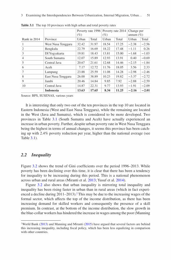
51

It is interesting that only two out of the ten provinces in the top 10 are located in Eastern Indonesia (West and East Nusa Tenggara), while the remaining are located in the West (Java and Sumatra), which is considered to be more developed. Two provinces in Table 3.1 (South Sumatra and Aceh) have actually experienced an increase in urban poverty. Further, despite urban poverty rate in West Nusa Tenggara being the highest in terms of annual changes, it seems this province has been catch-ing up with 2.4% poverty reduction per year, higher than the national average (see Table 3.1).

2.2 Inequality

Figure 3.2 shows the trend of Gini coefficients over the period 1996–2013. While poverty has been declining over this time, it is clear that there has been a tendency for inequality to be increasing during this period. This is a national phenomenon across urban and rural areas (Miranti et al. 2013; Yusuf et al. 2014).

Figure 3.2 also shows that urban inequality is mirroring total inequality and inequality has been rising faster in urban than in rural areas (which in fact experi-enced a decline during 2011–2013).2 This may be due to the increasing wages of the formal sector, which affects the top of the income distribution, as there has been increasing demand for skilled workers and consequently the presence of a skill premium. In contrast, at the bottom of the income distribution, the slow growth in the blue-collar workers has hindered the increase in wages among the poor (Manning

2 World Bank (2013) and Manning and Miranti (2015) have argued that several factors are behind this increasing inequality, including fiscal policy, which has been less equalizing in comparison with other countries.

Table 3.1 The top 10 provinces with high urban and total poverty rates

Rank in 2014

Poverty rate 1996 (%)

Poverty rate 2014 (%)

Change per annum (%)

Province Urban Total Urban Total Urban Total

1 West Nusa Tenggara 32.42 31.97 18.54 17.25 −2.38 −2.562 Bengkulu 22.79 16.69 18.22 17.48 −1.11 0.263 DI Yogyakarta 19.81 18.43 13.81 15.00 −1.68 −1.034 South Sumatra 12.07 15.89 12.93 13.91 0.40 −0.695 Central Java 20.67 21.61 12.68 14.46 −2.15 −1.846 Aceh 7.17 12.72 11.76 18.05 3.56 2.337 Lampung 23.88 25.59 11.08 14.28 −2.98 −2.468 East Nusa Tenggara 26.00 38.89 10.23 19.82 −3.37 −2.729 Jambi 20.46 14.84 9.85 7.92 −2.88 −2.5910 Central Java 14.87 22.31 9.77 13.93 −1.91 −2.09

Indonesia 13.63 17.65 8.34 11.25 −2.16 −2.01

Source: BPS, SUSENAS, various years

3 Examining the Interdependencies Between Urbanization, Internal Migration, Urban…

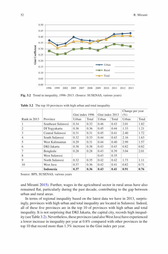
52

and Miranti 2015). Further, wages in the agricultural sector in rural areas have also remained flat, particularly during the past decade, contributing to the gap between urban and rural areas.

In terms of regional inequality based on the latest data we have in 2013, surpris-ingly, provinces with high urban and total inequality are located in Sulawesi. Indeed, all of these five provinces are in the top 10 of provinces with high urban and total inequality. It is not surprising that DKI Jakarta, the capital city, records high inequal-ity (see Table 3.2). Nevertheless, these provinces (and also West Java) have experienced a lower increase in inequality per year at 0.8% compared with other provinces in the top 10 that record more than 1.3% increase in the Gini index per year.

0.00

0.05

0.10

0.15

0.20

0.25

0.30

0.35

0.40

0.45

0.50

1996 1999 2002 2005 2007 2008 2009 2010 2011 2012 2013

Gin

i Coe

ffic

ient

Urban

Rural

Total

Fig. 3.2 Trend in inequality, 1996–2013. (Source: SUSENAS, various years)

Table 3.2 The top 10 provinces with high urban and total inequality

Rank in 2013 ProvinceGini index 1996 Gini index 2013

Change per year (%)

Urban Total Urban Total Urban Total

1 Southeast Sulawesi 0.34 0.32 0.46 0.43 2.01 1.822 DI Yogyakarta 0.36 0.36 0.45 0.44 1.33 1.213 Central Sulawesi 0.31 0.31 0.45 0.41 2.40 1.724 South Sulawesi 0.32 0.33 0.44 0.43 2.16 1.635 West Kalimantan 0.29 0.31 0.44 0.40 2.99 1.576 DKI Jakarta 0.38 0.38 0.43 0.43 0.82 0.827 Bengkulu 0.28 0.28 0.43 0.39 3.04 2.018 West Sulawesi 0.43 0.359 North Sulawesi 0.32 0.35 0.42 0.42 1.73 1.1110 West Java 0.37 0.36 0.42 0.41 0.82 0.71

Indonesia 0.37 0.36 0.43 0.41 0.91 0.76

Source: BPS, SUSENAS, various years

R. Miranti

53

2.3 Urbanization

The speed of urbanization in Indonesia has been fast. By 2010, almost half of the population in Indonesia lived in urban areas, and it is predicted to increase to two- thirds of the population by 2035. Figure 3.3 shows that North Sumatra and Banten (which are included in the RUMiI data) have recorded high urbanization rates, which are higher than the national average and are expected to reach an urbanization rate of around 60% or more by 2035.3

Skeldon (1990, 1997) has proposed six stages of mobility transition when ana-lyzing the migration pattern in developing countries. A pre-transitional society is followed by early transitional and then intermediate transitional, late transitional, early advanced, advanced, and, finally, late advanced society. Chotib (2002) has argued that if the urbanization rate has achieved 50%, this means the area has been close to the early advanced society. Looking at the data in 2010, Indonesia may have been close to the stage of early advanced society. Further, Table 3.3 displays the top 10 provinces with high urbanization rates. There are three main observations: (i) the high urbanization areas are concentrated in Western Indonesia, particularly in Java

3 The BPS (1980, 1990, and 2000) defines an Indonesian locality as urban if it fulfills the following characteristics: “(i) having a population density of 5000 people or more per square kilometer; (ii) having 25% or less of households working in the agricultural sector; (iii) having eight or more kinds of urban facilities”(Firman 2004, p. 425).

84.9

77.7

59.6

66.668.1

0

10

20

30

40

50

60

70

80

90

1995 2000 2005 2010 2015 2020 2025 2030 2035

Urb

aniz

atio

n R

ate

(%)

North Sumatra

Banten

East Kalimantan

South Sulawesi

INDONESIA

Fig. 3.3 Trend in urbanization, 1995–2035. (Source: BPS)Note: Figures for 2015–2035 are predicted figures

3 Examining the Interdependencies Between Urbanization, Internal Migration, Urban…

54

and Sumatra provinces, with the exception of East Kalimantan; (ii) the urbanization rate is very high—with the top 7 recording more than 60% urbanization rates; and (iii) three of the top 10 provinces are new provinces that were formed after the decentralization period.

Nevertheless, one should keep in mind that there are three factors that influence urbanization. They are natural population increase, rural–urban migration, and reclassification (Firman et al. 2007; Gardiner 1997). In the case of Indonesia, it is important to take into account the reclassification of rural to urban areas as Gardiner (1997) explained that reclassification contributed to the high urban growth rate of 35% in 1980–1990.

2.4 Internal Migration

The most common type of internal migration discussed in the literature is rural–urban migration and interprovincial migration. Due to the nonavailability of long series rural–urban migration data, this subsection only discusses interprovincial migration.

The literature has discussed several types of migration based on reasons for migrating in Indonesia. The types of migration basically cover (i) economic-induced migration, (ii) education-induced migration, and (iii) migration for social and cultural reasons (see, e.g., Miranti 2007, 2013 for more details on interprovincial migration).

Figure 3.4 shows a comparison of the net interprovincial migration rates for 1995 and 2010. Positive net migration happens when in-migration to a province is higher than out-migration from that particular province, while negative out-migration is recorded when out-migration is higher than in-migration. Ordering the provinces based on the rank of net migration rates in 2010, the Outer Islands or Eastern Indonesia provinces mostly recorded a positive net migration rate, with an increase in the rate

Table 3.3 The top 10 provinces with high urbanization rate

Rank in 2010 Province 1995 2010 Change p.a. (%)

1 DKI Jakarta 100 100 0.002 Riau Islands 82.83 Banten 674 DI Yogyakarta 58.05 66.4 0.965 West Java 42.69 65.7 3.596 East Kalimantan 50.22 63.2 1.727 Bali 34.31 60.2 5.038 North Sumatra 41.09 49.2 1.329 Bangka Belitung 49.210 East Java 27.43 47.6 4.90

Indonesia 35.91 49.8 2.58

Source: BPS

R. Miranti

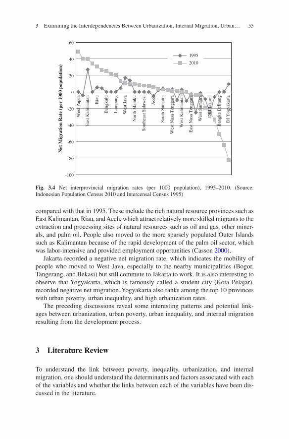
55

compared with that in 1995. These include the rich natural resource provinces such as East Kalimantan, Riau, and Aceh, which attract relatively more skilled migrants to the extraction and processing sites of natural resources such as oil and gas, other miner-als, and palm oil. People also moved to the more sparsely populated Outer Islands such as Kalimantan because of the rapid development of the palm oil sector, which was labor-intensive and provided employment opportunities (Casson 2000).

Jakarta recorded a negative net migration rate, which indicates the mobility of people who moved to West Java, especially to the nearby municipalities (Bogor, Tangerang, and Bekasi) but still commute to Jakarta to work. It is also interesting to observe that Yogyakarta, which is famously called a student city (Kota Pelajar), recorded negative net migration. Yogyakarta also ranks among the top 10 provinces with urban poverty, urban inequality, and high urbanization rates.

The preceding discussions reveal some interesting patterns and potential link-ages between urbanization, urban poverty, urban inequality, and internal migration resulting from the development process.

3 Literature Review

To understand the link between poverty, inequality, urbanization, and internal migration, one should understand the determinants and factors associated with each of the variables and whether the links between each of the variables have been dis-cussed in the literature.

-100

-80

-60

-40

-20

0

20

40

60

Wes

t Pap

ua

Eas

t Kal

iman

tan

Ria

u

Ben

gkul

u

Lam

pung

Wes

t Jav

a

Nor

th M

aluk

u

Sout

heas

t Sul

awes

i

Ace

h

Sout

h Su

mat

ra

Wes

t Nus

a T

engg

ara

Wes

t Kal

iman

tan

Eas

t Nus

a T

engg

ara

Wes

t Sum

atra

DK

I Ja

kart

a

Ban

gka

Bel

itung

DI

Yog

yaka

rta

Net

Mig

rati

on R

ate

(per

100

0 po

pula

tion

)1995

2010

Fig. 3.4 Net interprovincial migration rates (per 1000 population), 1995–2010. (Source: Indonesian Population Census 2010 and Intercensal Census 1995)

3 Examining the Interdependencies Between Urbanization, Internal Migration, Urban…

56

The literature on the determinants of poverty, including empirical studies, has been abundant (see the literature review in Miranti 2007). It includes discussions on the impact of economic growth on poverty and the links between poverty and inequality.

Ravallion et al. (2007) have also studied the links between urbanization and claimed that urbanization is important for poverty reduction. Christiaensen et al. (2013) further proposed the mechanisms by which urbanization affects the speed of poverty reduction, which is not necessarily limited to urban poverty. These mecha-nisms are as follows. First, it is through the process of agglomeration economies that urban concentration can create economic growth and employment. Second, through the role of externalities, the production network is located close to not only its suppliers but also service providers and consumers. Third, rural off-farm employ-ment facilitates the flow of inputs, goods, and services with urban areas, potentially contributing to declining poverty in rural areas. Fourth, remittances through urban-ization (via rural–urban migration) play a potentially effective role in poverty reduction.

On reverse causality, the theory on the relationship between urbanization and economic development has been well developed. This includes the seminal chapter of Kuznets’ (1955) theory. Sagala et al. (2014) examine the link between urbaniza-tion and expenditure inequality in Indonesia using SUSENAS data to test the Kuznets hypothesis. They find that the inverted U-shaped hypothesis exists in both of their inequality estimates measured by the Theil index and the Gini coefficient. They also argue that inequality will reach its peak at an urbanization rate of around 46–50%. As urbanization rate in Indonesia has achieved 50%, this means that Indonesia has achieved the peak urbanization rate.

On the other hand, to the best of our knowledge, the discussion on the determi-nants of urbanization has been limited. For example, Hofmann and Wan (2013) focused on the potential impact of the growth of per capita GDP, structural transfor-mation (industrialization), and knowledge spillovers (education) in determining urbanization. Applying OLS estimation using cross-country data and acknowledg-ing the potential dual causality between urbanization and GDP growth, they find that the direction of effect is more likely from economic growth to urbanization rather than the opposite, as has been proposed by the World Bank and IMF (2013). They also find a positive impact of education on the urbanization rate and a signifi-cant positive impact of industrialization (measured by the proportion of nonagricul-ture to the total GDP) on urbanization. Firman et al. (2007) also argue that the services sector, which tends to be concentrated in large cities, is the driving factor behind urbanization and economic development as the growth of this service sector is supported by the availability of urban utilities such as water supply and electricity.

Having discussed urbanization, what does the literature say about migration or population mobility? The push–pull migration model in the neoclassical theory of migration argues that labor mobility aims to improve income and wealth and that it is a selective process (Sjaastad 1962; Greenwood 1975). The two most significant

R. Miranti

57

reasons for the decision to migrate are the income differential between the area of origin and area of destination and also the interaction of these with individual demo-graphic and socioeconomic characteristics such as age, gender, and education (Harris and Todaro 1970; Fields 1982). However, the decision to migrate has since shifted to the family (Mincer 1978), and migration is also considered as human capital migration (Schultz 1961; Becker 1962). Recent literature has extended migration studies within the context of social capital (de Haas 2010).

Miranti (2007, 2010) has argued that the link between migration and poverty is ambiguous and depends on the role of the labor market. Using the example of inter-provincial migration in Indonesia, she differentiates the roles of in-migration and out-migration in relation to poverty, directly or indirectly through economic growth, as follows:

In-migration (potential impact on the destination provinces)

• Direct effect. In-migration is expected to have a negative association with poverty if migrants have a higher educational level than the population in the destination region and, therefore, they have a higher opportunity of working in activities that give higher returns.

• Indirect effect. The assumption is that in-migration augments labor supply with increasing capital or/and human capital in destination areas and, there-fore, migration contributes to economic growth in these regions, which is, in turn, negatively associated with poverty.

Out-migration (potential impact on the origin provinces)

• Direct effect. Out-migration is expected to have a positive relationship with poverty if out-migrants usually have higher educational levels than the popu-lation in the areas of origin and, therefore, a higher income status than those who remain behind.

• Indirect effect. The assumption is that migration contracts the labor supply because of a brain drain, but the possible offsetting impact of remittances contributes to an ambiguous impact from out-migration on growth in the regions of origin.

Further, Van Lottum and Marks (2012) have estimated the determinants of inter-nal migration in Indonesia using a longer time series data spanning 1930–2000. By applying a gravity model, they find the capital city of Jakarta has a strong impact on the direction and the size of migration flows, while, in contrast, the wage differen-tials between the original and destination provinces are not significant.

At the level of micro-data analysis, in line with the literature that discusses migration as a family or household decision, the literature has highlighted the inter-play between migration status, individual characteristics, household characteristics, and residential characteristics with poverty and other socioeconomic and well-being measures (see, e.g., Meng et al. 2010 for the Rural–Urban Migration project in the PRC and Indonesia).

3 Examining the Interdependencies Between Urbanization, Internal Migration, Urban…

58

4 Data, Approach, and Methodology

Two approaches are adopted in the analysis in this chapter. First, the quantitative analysis of the relationship between the poverty, inequality, urbanization, and inter-nal migration in Indonesia uses RUMiI data, which is part of the output of the Rural–Urban Migration in China and Indonesia (RUMiCI) project hosted by the Australian National University (ANU). The data is longitudinal, conducted through four waves (2008, 2009, 2010, and 2011), and surveyed in four provinces in Indonesia that recorded major enclaves of rural–urban migrants. These provinces are North Sumatra, Banten, East Kalimantan, and South Sulawesi.4 Rural–urban migrants or the migration status is differentiated into (i) recent migrant (less than 5 years), (ii) long-term migrant (at least 5 years), and (iii) local nonmigrants.

The advantage of using this micro-data is that it allows the analysis of diversity of internal migrants and the changes in their well-being. Nevertheless, at this stage, for the purpose of this chapter, utilizing the longitudinal characteristic of the data may not be necessary, and instead the focus was on the early wave in 2008 where the economic situation was considered normal with no major economic shocks. The level of inequality proxied by the Gini coefficient in this particular year was also stable, while it started increasing in 2009 and reached 0.41 in 2011. Two regressions using the logit econometric technique are carried out to estimate (i) the likelihood to be in the bottom 20% of expenditure per capita and (ii) the top 20% of expendi-ture per capita (from relative poverty–inequality point of view) at the household level. This is in line with the literature which argues that migration is a household decision. Resosudarmo et al. (2010) have estimated the likelihood of being poor defined using absolute poverty line and probit model on the same dataset. A slightly different technique—the logit model—which may be easier to interpret is used. More detailed explanatory variables in the estimation, such as labor market industry and status, and include housing conditions to represent access to basic facilities/infrastructure, are incorporated.

Urbanization/internal migration are proxied by the migration status in the RUMiI data. Other explanatory variables include the demographic characteristics of the household heads, labor market characteristics of the household heads (industry and employment status), and housing condition (sanitation). The marginal effects of the variables of interest from these regressions are estimated and presented in the next section.

The second quantitative analysis of the relationship between urban poverty, urban inequality, urbanization, and internal migration in Indonesia uses panel data at the provincial level from 1995 to 2010. The dependent variable of the main equa-tion is urban poverty. At this macro-level analysis, interprovincial migration data as proxy of internal migration is used since the rural–urban migration data is not avail-able. The urbanization and interprovincial migration data are sourced from SUPAS 1995 and 2005 and the Indonesian Population Census 2000 and 2010, while urban

4 These locations should be kept in mind when interpreting the findings.

R. Miranti

59

poverty and urban inequality data are more frequently calculated based on the three yearly consumption modules of the household SUSENAS survey.

5 Therefore, we can only include the 2010 data as the latest data for the analysis. The discussion on migration will only be limited to recent migration, which covers those whose cur-rent residence is different from their place of residence 5 years ago.

Other data collection is sourced from the Indonesia BPS (Badan Pusat Statistik), including data taken from SAKERNAS (labor force survey) and Statistics Indonesia. In addition, some assembled data from the CEIC Indonesia Premium Database is also included.

Taking into account the high degree of heterogeneity across provinces in Indonesia, it is therefore important that an econometric technique for panel data is applied. The data is constructed as an unbalanced panel due to, first, some missing values—a result of the creation of new provinces, particularly after the application of the decentralization policy in 2001. In 1995, there were 26 provinces, which expanded to 33 provinces by 2010. Second, the data is unbalanced because, SUSENAS being the main source of data for urban mean expenditure per capita, data was not collected in several provinces due to social conflicts or natural disasters (such as the tsunami in Aceh).

Urbanization is measured by the proportion of population living in urban areas, and the regressions also include other explanatory variables discussed in the litera-ture to be associated with poverty. The best, suitable, and available proxy for each variable is chosen. These variables particularly include the role of the labor market such as provincial minimum wages; provision of physical infrastructure, which is proxied by percentage of households with state electricity (which could also repre-sent the energy access) and education status of the population (educational attain-ment or net enrollment ratios at junior high school level); the size of the agricultural sector; and economic growth. Since this data is not published with urban–rural dis-aggregation, this limitation needs to be kept in mind when interpreting the results. Other variables were also considered important, but they could not be included in the analysis due to data unavailability. These include climate impact and data on wage disparities/convergence. There are also other limitations to the data including the fact that urbanization may increase as a result of changing classification from rural to urban areas as discussed earlier. The short panel data may also not be able to fully capture the interdependencies properly.

4.1 Empirical Models of Interdependencies

Since the focus of the chapter is the interdependencies between urban poverty, urban inequality, urbanization, and internal provincial migration, the estimations are carried out by acknowledging the dual causality between urban poverty as the dependent variable and urban inequality, urbanization, and internal provincial

5 Some are calculated by special data request from the Indonesia BPS.

3 Examining the Interdependencies Between Urbanization, Internal Migration, Urban…

60

migration (and economic growth) as the endogenous variables, with other variables assumed as exogenous. Our hypothesis is that dual causality between these four key variables is present as indicated in Fig. 3.5.

We aim to carefully examine the interdependencies with simultaneous equations, in which each estimation will give the relative responsiveness of each variable to the other variables. However, we start with the simple panel data first without acknowl-edging the interdependency issue.6

Without interdependencies: These regressions are estimated separately using either the fixed effects or the random effects estimation of panel data.

1. Urban poverty equation

ln ln _, , ,urbanpoverty urbangini prop urban nei t i t i t= + + +γ 0 1 2 3γ γ γ ttmig rate

economic growth urban cap pi t

i t i t

_

ln exp_,

, ,+ + +−γ γ γ4 5 6 rrop electricity

wage ner junhighi t

i t i t i

_

lnmin_ ln _,

, ,+ + + +γ γ δ7 8 εε i t,

2. Urban inequality equation

ln ln _, , ,urbangini urbanpoverty prop urban nei t i t i t= + + +β β β β0 1 2 3 nig rate

economic growth urban cap pi t

i t i t

_

_ ln exp_,

, ,

++ +β β β4 5 6 rrop electricity

wage ner junhigh ni t

i t i t

_

lnmin_ ln _,

, ,+ + +β β β7 8 9 oon agri i i t_ ,+ +δ ε

3. Urbanization equation

prop urban urbanpoveny urbangini neti t i t i t_ ln ln, , ,= + + +λ λ λ λ0 1 2 3 mmig rate

economic gowth urban cap proi t

i t i t

_

_ ln exp_,

, ,+ + +λ λ λ4 5 6 pp electricity

wage ner junhigh noni t

i t i t

_

lnmin_ ln _,

, ,+ + +λ λ λ7 8 9 −− + +agri i i tδ ε ,

6 We also try the Arellano–Bond estimation using the xtabond2, which is suitable for analysis of dynamic panel data with small T but larger N. However, our data is too short for this type of estima-tion for three reasons. First, we will lose much information due to the inclusion of lags. Second, there is also a requirement to limit the number of endogenous variables to be less than the total observations in each group. Third, the Arellano–Bond estimation does not provide the results of the first stage of the equation, so it does not reveal the interdependencies.

Urban poverty Urban inequality

Urbanization Internal migration

Fig. 3.5 Potential interdependencies between urban poverty, urbanization, urban inequality, and internal migration. (Source: Author’s summary)

R. Miranti

61

4. Interprovincial migration equation

netmig rate urbanpoverty urbangini pi t i t i t_ ln ln, , ,= + + +ρ0 1 2 3ρ ρ ρ rrop urban

economic gowth urban cap propi t

i t

_

_ ln exp_ _,

,+ + +ρ ρ ρ4 5 6 eelectricity

wage ner junhigh non ai t

i t i t

,

, ,lnmin ln _ _+ + +−ρ ρ ρ7 8 9 ggri i i t+ +δ ε ,

With interdependencies: We carefully examined various strategies to achieve the best estimation, investigating whether the interdependencies between urban poverty and particularly urban inequality, urbanization, and internal migration exist. The main argument in this chapter can be summarized as follows: whether each of the variables of interest affects each other simultaneously. To incorporate dual causality into the model, we use the instrumental variable estimation technique, in which the 5-year lag of the endogenous variables and the 5-year lag of the incidence of urban poverty are used as the instruments for the first-step estimations. As the literature also indicates that economic growth affects poverty reduction and vice versa, we also include this as the endogenous variable. Size of the nonagricultural sector is included as an additional instrument, particularly to represent the degree of struc-tural transformation in each province, which the literature points out is associated with urbanization. We assume that the instruments are not correlated with the error terms in the main equation as the instruments used also include 5-year lags of the endogenous variables. Due to the nature of the data, which covers only a short period, time dummy variables are not included in the analysis as they are highly correlated with the explanatory variables.

We use panel data estimation, fixed effects, or generalized least squares random effects—two-stage least squares—and use the Hausman test to decide the preference.

5. Urban inequality equation

ln ln _, ,urbangini lag urbanpoveny lagprop urbani t i t i= + +−η η η0 1 5 2 ,,

_ _ _t

r tlagnetmig rate lageconomic growth non ag−

− −+ + +5

3 5 4 5 5η η η rri

urban cap prop electricity wt

i t i t

−

+ + +5

6 7 8η η ηln exp_ _ lnmin_, , aagener junhigh lag urbangini

i t

i t i t i i t

,

, , ,ln _ ln+ + + +η η δ ε9 10

6. Urbanization equation

prop urban lag urbanpoveny lagprop urbani t i t i− −= + +, , ,ln _σ σ σ0 1 5 2 tt

r tlagnetmig rate lageconomic growth non agr−

− − −+ + +5

3 5 4 5 5σ σ σ_ _ ii

urban cap prop electricity wat

i t i t

−

+ + +5

6 7 8σ σ σln exp_ _ lnmin_, , ggener junhigh lag urbangini

i t

i t i t i i t

,

, , ,ln _ ln+ + + +σ σ δ ε9 10

3 Examining the Interdependencies Between Urbanization, Internal Migration, Urban…

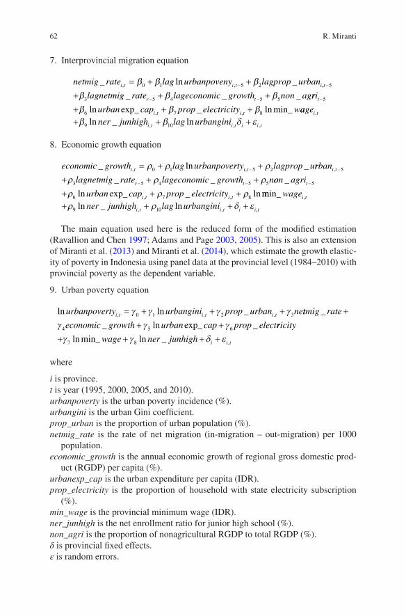
62

7. Interprovincial migration equation

netmig rate lag urbanpoveny lagprop urbani t i t i_ ln _, ,= + +−β β β0 1 5 2 ,,

_ _ _t

r tlagnetmig rate lageconomic growth non ag−

− −+ + +5

3 5 4 5 5β β β rri

urban cap prop electricity wt

i t i t

−

+ + +5

6 7 8β β βln exp_ _ lnmin_, , aagener junhigh lag urbangini

i t

i t i t i i t

,

, , ,ln _ ln+ + +β β δ ε9 10

8. Economic growth equation

economic growth lag urbanpoverty lagprop ui t i t_ ln _, ,= + +−ρ ρ ρ0 1 5 2 rrban

lagnetmig rate lageconomic growth ni t

r t

,

_ _−

− −+ + +5

3 5 4 5 5ρ ρ ρ oon agri

urban cap prop electricityt

i t i t

_

ln exp_ _ ln, ,

−

+ + +5

6 7 8ρ ρ ρ mmin_ln _ ln

,

, ,

wagener junhigh lag urbangini

i t

i t i t i i+ + + +ρ ρ δ ε9 10 ,,t

The main equation used here is the reduced form of the modified estimation (Ravallion and Chen 1997; Adams and Page 2003, 2005). This is also an extension of Miranti et al. (2013) and Miranti et al. (2014), which estimate the growth elastic-ity of poverty in Indonesia using panel data at the provincial level (1984–2010) with provincial poverty as the dependent variable.

9. Urban poverty equation

ln ln _, , ,urbanpoverty urbangini prop urban nei t i t i t= + + +γ γ γ γ0 1 2 3 ttmig rate

economic growth urban cap prop elect

_

_ ln exp_ _

++ +γ γ γ4 5 6 rricity

wage ner junhigh i i t+ + + +γ γ δ ε7 8lnmin_ ln _ ,

where

i is province.t is year (1995, 2000, 2005, and 2010).urbanpoverty is the urban poverty incidence (%).urbangini is the urban Gini coefficient.prop_urban is the proportion of urban population (%).netmig_rate is the rate of net migration (in-migration – out-migration) per 1000

population.economic_growth is the annual economic growth of regional gross domestic prod-

uct (RGDP) per capita (%).urbanexp_cap is the urban expenditure per capita (IDR).prop_electricity is the proportion of household with state electricity subscription

(%).min_wage is the provincial minimum wage (IDR).ner_junhigh is the net enrollment ratio for junior high school (%).non_agri is the proportion of nonagricultural RGDP to total RGDP (%).δ is provincial fixed effects.ε is random errors.

R. Miranti

63

5 Estimation Results

5.1 Findings from Household Data Analysis

The estimated marginal effects of the explanatory variables of probability of being in the bottom 20% or top 20% of household per capita expenditure are shown in Table 3.4. The bottom 20% and top 20% are calculated on the basis of the distribu-tion of yearly household per capita expenditure. Some important findings are as follows.

5.1.1 Migration Status

Table 3.4 shows that after controlling for individual and household characteristics and compared to the local population or nonmigrants, the migration status (par-ticularly for the recent migrants) has a significant effect in determining the likeli-hood of being in the bottom quintile and top quintile. Being a recent migrant has a higher marginal effect in reducing the probability of being in the bottom 20% than the long-term migrant. The likelihood of being in the bottom 20% of house-hold expenditure is reduced by 11.4 percentage points for a recent migrant and around 4.2 percentage points for a long-term migrant compared to the nonmi-grants. The finding for recent migrants indicates those migrants have better socio-economic status than the nonmigrants, which may refer to the fact that migration is indeed selective. Effendi et al. (2010a, b) find that recent migrants consist of younger individuals with better education. Compared to the nonmigrants and holding other variables constant, the impact of being a recent migrant is significant and increases the likelihood of being in the top of the expenditure distribution by five percentage points.

5.1.2 Head of Household/Demographic Characteristics

It seems the number of children—that is, the number of dependents in a house-hold—is a significant determinant and increases the likelihood of being in the bot-tom quintile of household expenditure. Age has a significant and negative association with the likelihood of being in the bottom 20% and increases the likelihood of being in the top 20%. This may indicate that the older the age, the more capable/experi-enced the person is to explore various opportunities to increase the likelihood of their household living in a better socioeconomic condition. The impact of gender of the head of household is surprisingly not significant, while the impact of marital status is limited, with a divorcee/widow decreasing the likelihood of being in the top

3 Examining the Interdependencies Between Urbanization, Internal Migration, Urban…

64

20% by 11.5 percentage points, compared to a single person. Marriage is also nega-tively correlated with being in the top of the expenditure distribution, as compared to a single person; being married decreases the likelihood of being in the top 20% by almost 30 percentage points. The main message from the marriage variable is

Table 3.4 Findings of RUMiI data

Probability of being in the bottom 20%

Probability of being in the top 20%

Marginal effectStd. error Sig

Marginal effect

Std. error Sig

(1) (2) (3) (4) (5) (6)

Head of household demographic characteristics

Female headed 0.015 0.029 −0.003 0.022Age −0.002 0.001 * 0.004 0.001 ***Number of children 0.025 0.004 *** −0.027 0.006 ***Education (Base: no schooling)

Did not complete the primary

−0.016 0.031 −0.112 0.022 ***

Primary school −0.048 0.026 * −0.083 0.024 ***Junior high school −0.069 0.024 *** −0.030 0.028Senior high school −0.118 0.025 *** 0.024 0.029Diploma −0.138 0.016 *** 0.121 0.064 *Bachelor’s degree and above

−0.132 0.016 *** 0.154 0.055 ***

Marital status

(Base: single)

Married 0.145 0.027 −0.295 0.041 ***Divorce/widow 0.281 0.081 * −0.115 0.018 ***

Head of household labor market characteristics

Industry (Base: manufacturing)Construction 0.074 0.038 * −0.056 0.030 *Finance 0.153 0.118 0.079 0.087Real estate 0.143 0.158 0.008 0.114Education and health 0.003 0.047 0.034 0.042Trade, service, and others

0.025 0.021 −0.027 0.021

Employment status (Base: not working)

Employee 0.030 0.029 0.031 0.028Civil service or military

−0.094 0.029 *** 0.121 0.062 **

Self-employee/unpaid

−0.028 0.029 0.111 0.040 ***

Source: Author’s calculation from RUMiI dataNote: Significance at the 1%, 5%, and 10% levels is denoted by ***, **, and *, respectively

R. Miranti

65

that a person who is single, or without any dependents, is more correlated with higher income/wealth.

Human capital is also an important determinant in comparison to those who do not have education. For example, having an educational attainment of a bachelor’s degree or above decreases the likelihood of being in the bottom quintile of house-hold per capita expenditure by 13.2 percentage points compared to those who do not have education. The higher the level of educational attainment, the stronger these effects tend to be. The regression to estimate the likelihood of being in the top 20% indicates that the role of having tertiary education at the diploma level or bachelor’s degree and above is crucial.

5.1.3 Head of Household Labor Market Characteristics

The labor market effect is somewhat limited, with only working in the construction industry (compared to manufacturing) having a significant increase in the likelihood of being in the bottom quintile and reducing the likelihood of being in the top quin-tile. This indicates that having a blue-collar occupation is related to a higher likeli-hood of being at the bottom of the income distribution.

Based on the labor market status, the findings show that being a member of the civil services or military services is advantageous (compared to not working), which reduces

Probability of being in the bottom 20%

Probability of being in the top 20%

Marginal effectStd. error Sig

Marginal effect

Std. error Sig

(1) (2) (3) (4) (5) (6)

Migration status (Base: local, not migrant)

Recent migrant −0.114 0.020 *** 0.049 0.028 *Long-term migrant

−0.042 0.015 *** 0.010 0.018

Housing condition—sanitation (Base: no sanitation)

Have toilet and bathroom

−0.141 0.065 ** 0.067 0.060

Have either toilet or bathroom

−0.022 0.048 −0.026 0.076

Public toilet −0.049 0.042 0.011 0.082Number of observation 2426 2426Log likelihood −1052.724 −1024.280Pseudo R2 0.135 0.155Marginal effects after logit 0.154 0.152

Source: Author’s calculation from RUMiI dataNote: Significance at the 1%, 5%, and 10% levels is denoted by ***, **, and *, respectively

Table 3.4 (continued)

3 Examining the Interdependencies Between Urbanization, Internal Migration, Urban…

66

the likelihood of being in the bottom quintile or increases the likelihood of being in the top quintile, other things held constant. Having an own business or family work signifi-cantly increases the likelihood of being in the top quintile (Appendix Table 3.8).

5.1.4 Housing Condition (Infrastructure)

We have chosen sanitation to represent the housing condition of the household as the other categories within this variable are mutually exclusive. As expected, com-pared to households that do not have sanitation facilities, living in households that have proper sanitation (e.g., toilet and bathroom) reduces the likelihood of being in the bottom quintile.

5.2 Findings from Macro-panel Data Analysis

Appendix Table 3.9 discusses the regression results for model (i), which has not acknowledged the interdependencies between the four variables.7 It is shown that there are some significant associations between the four variables. For example, interprovincial migration has a negative impact on urban inequality; urban inequality reduces interprovincial migration; urbanization significantly reduces urban poverty.

Tables 3.5 and 3.6 present the regression results for model (ii), which acknowl-edges the interdependencies. The result from the Hausman test indicates the prefer-ence to use random effects estimation rather than fixed effects. Table 3.5 displays the results from the first stage of the regressions, where the causality runs from the lag of the urban poverty incidence 5 years ago and other exogenous variables to the endogenous variables (urban inequality, urbanization, net interprovincial migration, and economic growth). Table 3.6 provides the second stage of the main equation, where the opposite causality runs from urban inequality, urbanization, net interpro-vincial migration, and economic growth to urban poverty.

The results of the first-stage regressions show that, as expected, the lags of the explanatory variables have significant impacts on their respective contemporaneous dependent variables (see Table 3.5). Urban inequality is positively affected by urban mean expenditure per capita and the 5-year lag of the urban poverty rate, which is expected. Although there is a positive impact of urbanization on urban inequality, the impact is not significant. The higher the expenditure per capita of urban popula-tion on average, the higher is the inequality. The results of the coefficient of lag of urban poverty rate 5 years ago mean that higher poverty rates in the past should be translated to higher effort required to improve the welfare of people living in the bottom quintile of income distribution, and if the other part of the distribution does not change, this may increase inequality.

7 Table A1 presents the correlation coefficient between the variables.

R. Miranti

67

Tabl

e 3.

5 Fi

rst-

stag

e re

gres

sion

s—en

doge

nous

var

iabl

es (

rand

om e

ffec

t, 2S

LS)

Urb

an in

equa

lity

Urb

aniz

atio

nN

et p

rovi

ncia

l mig

ratio

nE

cono

mic

gro

wth

Coe

f.St

d.Si

g.C

oef.

Std.

Sig.

Coe

f.St

d.Si

g.C

oef.

Std.

Sig.

lnur

bane

xp_c

ap0.

185

0.06

7**

*8.

937

2.81

3**

*−

3.19

813

.046

2.26

92.

319

prop

_ele

ctri

city

0.00

20.

002

0.20

00.

066

***

−0.

200

0.30

80.

105

0.05

5*

lnm

in_w

age

−0.

038

0.06

3−

8.52

12.

645

***

4.42

812

.268

−1.

188

2.18

1ln

ner_

junh

igh

0.15

80.

142

2.10

75.

959

−6.

517

27.6

405.

509

4.91

4la

g ln

urba

ngin

i−

0.27

00.

092

***

-13.

438

3.88

8**

*10

.257

18.0

31−

0.61

43.

206

lag

prop

_urb

an0.

002

0.00

20.

510

0.07

4**

*−

0.39

20.

341

−0.

132

0.06

1**

lag

netm

ig_r

ate

2.27

8E-0

40.

001

−7.

824E

-03

0.02

2−

4.11

9E-0

10.

103

***

5.66

7E-0

30.

018

lag

econ

omic

gro

wth

−2.

626E

-04

0.00

10.

028

0.03

1−

0.12

50.

144

−0.

194

0.02

6**

**pr

op n

on_a

gri t

o G

DP

−0.

003

0.00

30.

412

0.12

3**

*0.

104

0.57

1−

0.02

40.

101

lag

lnur

banp

ov_r

ate

0.05

70.

031

*−

0.27

91.

320

−0.

509

6.12

1−

1.26

81.

088

cons

tant

−4.

366

0.66

1**

*−

109.

372

27.7

75**

*74

.792

128.

819

−39

.512

22.9

02*

Sour

ce: A

utho

r’s

calc

ulat

ion

Not

e: S

igni

fican

ce a

t the

1%

, 5%

, and

10%

leve

ls is

den

oted

by

***,

**,

and

*, r

espe

ctiv

ely

3 Examining the Interdependencies Between Urbanization, Internal Migration, Urban…

68

We also examine variables that explain urbanization and find that there are signifi-cant and positive impacts of urban mean expenditure per capita, access to electricity, and the proportion of nonagricultural sector to the GDP. These associations are expected as urbanization would increase when a province is more developed with higher income and better access to infrastructure and when the development of the nonagricultural sector (which supports the finding from Hofmann and Wan 2013) or formal employment also happens. Minimum wage is surprisingly found to reduce urbanization. Increasing the minimum wage to protect employees and increase their well-being may hinder formal employment in the urban areas when it is set above the market wage and creates unemployment, as indicated in the Harris–Todaro model. This is particularly true for Indonesia, where the application of a minimum wage potentially has an adverse impact on employment in the urban labor-intensive manu-facturing sector. Further, despite minimum wages having increased by around 6.5% per year between 2000 and 2010, the effect has been limited, and it is not beneficial for those who are in the bottom of the wage distribution. Not to mention that an increase in the minimum wage is usually also followed by increases in commodity prices, which does not improve workers’ consumption (Bird and Manning 2008). If this is happening, it is not surprising that it has impeded the urbanization process.

Table 3.6 Main equation

Urban povertyCoef. Std. err. Sig.

lnurbangini 1.488 0.817 *prop_urban −0.016 0.008 **netmig_rate 1.796E-04 0.004economic growth −0.014 0.012lnurbanexp_cap −0.654 0.303 **prop_electricity 0.000 0.006 ***lnmin_wage −0.050 0.229lnner_junhigh 0.697 0.529constant 10.470 4.354 **sigma_u 0.407sigma_e 0.204rho 0.799R2: within 0.687

between 0.587overall 0.586

N 69

Source: Author’s calculationNote: Significance at the 1%, 5%, and 10% levels are denoted by ***, **, and *, respectively

R. Miranti

69

The net migration equation surprisingly shows that only the lag of the net migra-tion variable is significant. The finding from the economic growth equation that urbanization has a negative association with economic growth is also somewhat surprising. An increase in the urbanization rate by 1 percentage point reduces eco-nomic growth by 0.13 percentage point. This may be the result of the short panel data we have used in estimating the model or the fact that the urbanization rate has reached 50%, meaning it may have reached its peak so that economic growth may experience diminishing returns despite urbanization. Further investigation is required on this aspect. It is surprising that the education variable is not significant in all specifications that may indicate the limitation of the data we use—that is, the net enrollment ratio for junior high school. This variable may not capture the varia-tion within provinces as Indonesia adopts the policy of 9 years of schooling. It is expected that the results would be better if we use the net enrollment ratio for the senior high school level. However, the longer time series of enrollment ratio data for secondary high school is not available. We have also used the educational attain-ment data, which does not improve the regression results.

Table 3.6 shows further findings from the main equation, which examines the reverse causality from the endogenous explanatory variables on urban poverty and the impacts on poverty of the other exogenous variables, which are the urban expen-diture per capita, access to electricity, minimum wage, and net enrollment ratio at the junior high school and equivalent level. As expected, the results show that 1% increase in urban inequality measured by the Gini index will contribute to around 1.5% increase in urban poverty rate, while a 1% increase in the mean expenditure of the urban population will contribute to 0.7% decline in the urban poverty rate. Inequality has hampered the impact of the increase of average expenditure to the poverty rate. The rate of urbanization is poverty reducing in urban areas. It is inter-

Table 3.7 Summary of interdependencies

Dual causality

Urban poverty Urban inequalitySingle causality

Urbanization Urban povertyUrban inequality UrbanizationUrban mean expenditure per capita Urban povertyUrban mean expenditure per capita Urban inequalityUrban mean expenditure per capita UrbanizationMinimum wage UrbanizationProportion of electricity Urban povertyProportion of electricity Economic growthProportion of nonagricultural sector to GDP Urbanization

Source: Author’s summary

3 Examining the Interdependencies Between Urbanization, Internal Migration, Urban…

70

esting that the coefficient of better facilities and infrastructure, as indicated by elec-tricity, while significant at 1%, is really marginal, being close to zero.

Table 3.7 provides the summary of the results from the aggregate/macroanalysis, which shows that interdependencies do indeed exist but mostly in the form of single direction causality. Dual causality has been only found in the relationship between urban poverty and inequality.

6 Conclusion and Policy Recommendations

This chapter investigates the issues and interdependencies of urbanization, internal migration, urban poverty, and urban inequality in Indonesia. There are two key objectives of the chapter. First, in the microanalysis, the focus is on examining the determinants of the likelihood of being in relative poverty (the bottom versus the top expenditure quintile). Second, the macroanalysis examines the determinants of urban poverty by taking into account the potential interdependencies between urban poverty, urbanization, internal migration, and urban inequality.

The results from microanalysis using rural–urban migration data in Indonesia (RUMiI), which test the determinants of the likelihood of being in the bottom 20% and top 20% of expenditure distribution, show the importance of migration status and various demographic and socioeconomic characteristics as the explanatory variables. These include age, number of children, education, marital status, and labor market characteristics. The results from macro−/aggregate analysis using panel data of provinces in Indonesia from 1995 to 2005 show that the presence of causality is mostly in the form of a single causality, except the dual causality that exists between urban poverty and urban inequality.

The findings from both the macro- and microanalyses, if not supporting each other, are complementary. The link between micro- and macroanalysis is present from the analysis, particularly on two main points. First, the finding that urbaniza-tion is poverty reducing (from the macroanalysis) has been supported by the finding that rural–urban migration (measured by migration status), which is one of the determinants of urbanization, has an impact on reducing the likelihood of being in the bottom 20%. Second, both the macro- and microanalyses support the impor-tance of the provision and access to basic facilities or infrastructure as a strategy to reduce poverty. The results from the housing (sanitation) condition from the microanalysis and the proportion of households with electricity from the macro-analysis support this conclusion. However, it looks like the channel at the aggregate

R. Miranti

71

level is indirect, which is from electricity, which significantly increases urbaniza-tion, which in turn reduces the rate of urban poverty.

With microanalysis, the results provide more evidence from the labor market perspective that the two measures used in the analysis—that is, industry of work and employment status—have some effect on the likelihood of being in the bottom or top 20% of the distribution. In contrast, the impact of minimum wage is not signifi-cant in the macroanalysis, whereas that of education is also captured by the micro-analysis but not the macroanalysis.

We conclude that interdependencies do exist between the four variables, but they are complex. Given these results, our question is: what are the strategies and policy recommendations to jointly manage the interdependencies among the elements of the internal migration–urbanization–poverty–inequality nexus in Indonesia? First, the dual causality between urban poverty and urban inequality suggests that policies should aim to reduce not only poverty but also inequality. Policies to reduce inequal-ity are back on the table for discussion, after many concerns have been raised on the increasing inequality experienced by this country. Efforts are required to not only improve the welfare of the bottom 20% of the population, which includes those who are poor, but also have more equalizing fiscal policy and tax reforms to ensure the redistribution from the top 20% of population. Second, urbanization through rural–urban migration is poverty reducing since migrants who move to urban areas are usually the young and the more educated. The implication of this is the need for better formal job opportunities being made available in the urban areas for absorb-ing these workers. This will be a challenge because previous data suggest that job seekers are never fully absorbed into the labor market, given the number of vacan-cies available to those seeking employment. Thus, incentives should be offered to various business/investment opportunities to create more jobs in urban areas and to reduce barriers to labor market entry. Third, the importance of education and avail-ability of good infrastructure, in terms of access to electricity and good sanitation, are also very important. These will improve the quality of life of the rural–urban migrants and link them with employment, trade activities, further education, and other activities. More expenditure directed toward this should be recommended.

3 Examining the Interdependencies Between Urbanization, Internal Migration, Urban…

72

App

endi

x

Tabl

e 3.

8 C

orre

latio

n co

effic

ient

Var

iabl

esur

banp

ov_

rate

urba

ngin

iur

ban

netm

ig_

rate

Eco

nom

ic

grow

thur

bane

xp_

cap

prop

_el

ectr

icit

ym

in_

wag

ene

r_ju

nhig

hpr

op n

on_a

gri t

o G

DP

urba

npov

_rat

e1

urba

ngin

i−

0.03

1.00

urba

n−

0.35

0.33

1.00

netm

ig_r

ate

−0.

13−

0.21

−0.

191.

00ec

onom

ic g

row

th0.

090.

11−

0.05

0.00

1.00

urba

nexp

_cap

−0.

460.

440.

320.

03−

0.10

1.00

prop

_ele

ctri

city

−0.

160.

400.

71−

0.19

−0.

050.

361.

00m

in_w

age

−0.

420.

360.

190.

05−

0.10

0.94

0.29

1.00

ner_

junh

igh

−0.

140.

330.

57−

0.13

−0.

170.

450.

720.

411.

00pr

op n

on_a

gri t

o G

DP

−0.

390.

100.

79−

0.02

−0.

130.

190.

540.

120.

361

Sour

ce: A

utho

r’s

sum

mar

y

R. Miranti

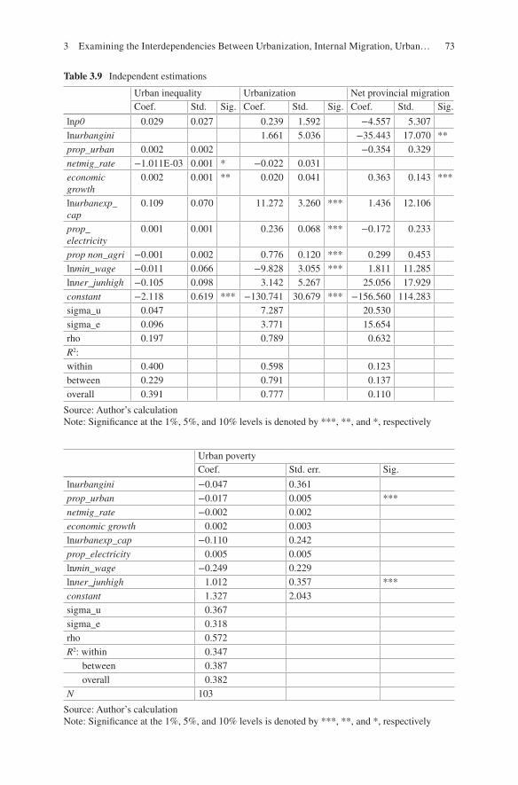
73

Table 3.9 Independent estimations

Urban inequality Urbanization Net provincial migrationCoef. Std. Sig. Coef. Std. Sig. Coef. Std. Sig.

lnp0 0.029 0.027 0.239 1.592 −4.557 5.307lnurbangini 1.661 5.036 −35.443 17.070 **prop_urban 0.002 0.002 −0.354 0.329netmig_rate −1.011E- 03 0.001 * −0.022 0.031economic growth

0.002 0.001 ** 0.020 0.041 0.363 0.143 ***

lnurbanexp_cap

0.109 0.070 11.272 3.260 *** 1.436 12.106

prop_electricity

0.001 0.001 0.236 0.068 *** −0.172 0.233

prop non_agri −0.001 0.002 0.776 0.120 *** 0.299 0.453lnmin_wage −0.011 0.066 −9.828 3.055 *** 1.811 11.285lnner_junhigh −0.105 0.098 3.142 5.267 25.056 17.929constant −2.118 0.619 *** −130.741 30.679 *** −156.560 114.283sigma_u 0.047 7.287 20.530sigma_e 0.096 3.771 15.654rho 0.197 0.789 0.632R2:within 0.400 0.598 0.123between 0.229 0.791 0.137overall 0.391 0.777 0.110

Source: Author’s calculationNote: Significance at the 1%, 5%, and 10% levels is denoted by ***, **, and *, respectively

Urban povertyCoef. Std. err. Sig.

lnurbangini −0.047 0.361prop_urban −0.017 0.005 ***netmig_rate −0.002 0.002economic growth 0.002 0.003lnurbanexp_cap −0.110 0.242prop_electricity 0.005 0.005lnmin_wage −0.249 0.229lnner_junhigh 1.012 0.357 ***constant 1.327 2.043sigma_u 0.367sigma_e 0.318rho 0.572R2: within 0.347

between 0.387overall 0.382

N 103

Source: Author’s calculationNote: Significance at the 1%, 5%, and 10% levels is denoted by ***, **, and *, respectively

3 Examining the Interdependencies Between Urbanization, Internal Migration, Urban…

74

References

Adams Jr., R. H., & Page, J. (2005). Do international migration and remittances reduce poverty in developing countries. World Development, 33(10), 1645–1669.

Adams Jr., R. H., & Page, J. (2003). International migration, remittances, and poverty in develop-ing countries (The World Bank Policy Research Working Paper 3179).

Becker, G. S. (1962). Investment in human capital. Journal of Political Economy, 70(5), 9–49.Bird, K., & Manning, C. (2008). Minimum wages and poverty in a developing country: Simulations

from Indonesia’s household survey. World Development, 36(5), 916–933.Casson, A. (2000). The hesitant boom: Indonesia’s oil palm sub-sector in an era of economic crisis

and political change (No. 29). Bogor: Center for International Forestry Research.Chotib. (2002). Urbanisasi Tidak Selalu Berkonotasi Negatif. Warta Demografi, 4(32), 55–63.Christiaensen, L., Weerdt, J., & Todo, Y. (2013). Urbanization and poverty reduction: The role of

rural diversification and secondary towns. Agricultural Economics, 44(4–5), 435–447.de Haas, H. (2010). Migration and development: A theoretical perspective. International Migration

Review, 44(1), 227–264.Effendi, T. N., Mujiyani, F. I., Darmawan, D. A., & Widhyarto, D. S. (2010a). Assessing the wel-

fare of migrant and non-migrant households in four Indonesia cities: Some demographic, social and employment characteristics. In X. Meng, C. Manning, L. Shi, & T. N. Effendi (Eds.), The great migration: Rural-urban migration in China and Indonesia (pp. 153–197). Northampton: Edward Elgar Publishing.

Effendi, T. N., Mujiyani, F. I., Darmawan, D. A., & Widhyharto, D. S. (2010b). Assessing the welfare of migrant and non-migrant households in four Indonesian cities: Some demographic, social and employment characteristics. In X. Meng, C. Manning, L. Shi, & T. N. Effendi (Eds.), The great migration: Rural-urban migration in China and Indonesia (pp. 153–177). Northampton: Edward Elgar Publishing.

Fields, G. S. (1982). Place-to-place migration in Colombia. Economic Development and Cultural Change, 30(3), 539–558.

Firman, T. (2004). Demographic and spatial patterns of Indonesia’s recent urbanization. Population, Space and Place, 10(6), 421–434.

Firman, T., Kombaitan, B., & Pradono, P. (2007). The dynamics of Indonesia’s urbanization, 1980–2006. Urban Policy and Research, 25(4), 433–454.

Gardiner, P. (1997). Migration and urbanization: A discussion. In Indonesia assessment: Population and human resources (pp. 118–133). Canberra: Australian National University.

Greenwood, M. J. (1975). Research on internal migration in the United States: A survey. Journal of Economic Literature, 13(2), 397–433.

Harris, J. R., & Todaro, M. P. (1970). Migration, unemployment and development: A two-sector analysis. The American Economic Review, 60(1), 126–142.

Hofmann, A., & Wan, G. H. (2013). Determinants of urbanization (ADB Working Chapter Series, No. 355). Manila: Asian Development Bank.

Kuznets, S. (1955). Economic growth and income inequality. American Economic Review, 45, 1–28.Manning, C., & Miranti, R. (2015). The SBY legacy on jobs, poverty and income distribution:

A mixed record. In E. Aspinall, M. Mietzner, & D. Tomsa (Eds.), The Yudhoyono years: An assessment. Singapore: Institute of Southeast Asian Studies.

Manning, C., & Sumarto, S. (2011). Employment, living standards and poverty: Trends, policies and interactions. In C. Manning & S. Sumarto (Eds.), Employment, living standards and pov-erty in contemporary Indonesia. Singapore: Institute of Southeast Asian Studies.

Meng, X., Manning, C., Shi, L., & Effendi, T. N. (2010). The great migration: Rural-urban migra-tion in China and Indonesia. Northampton: Edward Elgar Publishing.

Mincer, J. (1978). Family migration decisions. Journal of Political Economy, 86(5), 749–773.Miranti, R. (2007). The determinants of regional poverty in Indonesia:1984–2002. PhD thesis,

Australian National University.

R. Miranti

75

Miranti, R. (2010). Poverty in Indonesia 1984–2002: The impact of growth and changes in inequal-ity. Bulletin of Indonesian Economics Studies, 46(1), 79–97.

Miranti, R. (2013). Provincial poverty rates in Indonesia, 2006–2011. Report prepared for the TNP2K, Support for Economic Analysis Development in Indonesia (SEADI), USAID.

Miranti, R., Vidyattama, Y., Hansnata, E., Cassells, R., & Duncan, A. (2013). Trends in poverty and inequality in decentralising Indonesia (OECD Social, Employment and Migration Working Chapters, No. 148). OECD Publishing.

Miranti, R., Duncan, A., & Cassells, R. (2014). Revisiting the impact of consumption growth and inequality on poverty in Indonesia during the decentralisation period. Bulletin of Indonesia Economic Studies, 50(3), 461–482.

Ravallion, M., & Chen, S. (1997). What can new survey data tell us about recent changes in distri-bution and poverty ? World Bank Economic Review, 11(2), 357–382.

Ravallion, M., Chen, S., & Sangraula, P. (2007). New evidence on the urbanization of global pov-erty. Population and Development Review, 33(4), 667–701.

Resosudarmo, B. P., Suryahadi, A., Purnagunawan, R. M., Yumna, A., & Yusrina, A. (2010). The socio-economic and health status of rural-urban migrants in Indonesia. In X. Meng, C. Manning, L. Shi, & T. N. Effendi (Eds.), The great migration: Rural-urban migration in China and Indonesia (pp. 178–193). Northampton: Edward Elgar Publishing.

Sagala, P., Akita, T., & Yusuf, A. A. (2014). Urbanization and expenditure inequality in Indonesia: Testing the Kuznets hypothesis with provincial panel data. Letters in Spatial and Resource Sciences, 7(3), 1–15.

Schultz, T. W. (1961). Investment in human capital. The American Economic Review, 51(1), 1–17.Sjaastad, L. A. (1962). The costs and returns of human migration. Journal of Political Economy,

70(5), 80–93.Skeldon, R. (1990). Population mobility in developing countries. London/New York: Belhaven Press.Skeldon, R. (1997). Of migration, great cities, and markets: Global systems of development. In

W. Gungwu (Ed.), Global history and migrations (pp. 183–215). Boulder: Westview Press.The World Bank and International Monetary Fund. (2013). Global monitoring report 2013:

Monitoring the MDGs.Van Lottum, J., & Marks, D. (2012). The determinants of internal migration in a developing coun-

try: Quantitative evidence for Indonesia, 1930–2000. Applied Economics, 44(34), 4485–4494.Yusuf, A. A., Sumner, A., & Rum, I. A. (2014). Twenty years of expenditure inequality in Indonesia

1993–2013. Bulletin of Indonesia Economic Studies, 50(2), 243–254.

3 Examining the Interdependencies Between Urbanization, Internal Migration, Urban…

76

The views expressed in this publication are those of the authors and do not necessarily reflect the views and policies of the Asian Development Bank (ADB) or its Board of Governors or the governments they represent.

ADB does not guarantee the accuracy of the data included in this publication and accepts no responsibility for any consequence of their use. The mention of specific companies or products of manufacturers does not imply that they are endorsed or recommended by ADB in preference to others of a similar nature that are not mentioned.

By making any designation of or reference to a particular territory or geographic area, or by using the term “country” in this document, ADB does not intend to make any judgments as to the legal or other status of any territory or area. Open Access This work is available under the Creative Commons Attribution-NonCommercial 3.0 IGO license (CC BY-NC 3.0 IGO) http://creativecommons.org/licenses/by-nc/3.0/igo/. By using the content of this publication, you agree to be bound by the terms of this license. For attribution and permissions, please read the provisions and terms of use at https://www.adb.org/terms-use#openaccess.

This CC license does not apply to non-ADB copyright materials in this publication. If the mate-rial is attributed to another source, please contact the copyright owner or publisher of that source for permission to reproduce it. ADB cannot be held liable for any claims that arise as a result of your use of the material.

Please contact pubsmarketing@adb.org if you have questions or comments with respect to content, or if you wish to obtain copyright permission for your intended use that does not fall within these terms, or for permission to use the ADB logo.

Note: ADB recognizes “China” as the People’s Republic of China.

R. Miranti

77© Asian Development Bank 2019 K. Jayanthakumaran et al. (eds.), Internal Migration, Urbanization, and Poverty in Asia: Dynamics and Interrelationships, https://doi.org/10.1007/978-981-13-1537-4_4

Chapter 4Rural–Urban Migration, Urban Poverty and Inequality, and Urbanization in the People’s Republic of China

Xin Meng

1 Introduction

Over the past three decades, the Chinese economy has expanded at an exceptional 10% per annum, and the per capita income has increased sixfold, accompanied by extraordinary rural–urban migration and urbanization. There are now 166 million rural–urban migrants working in cities (National Bureau of Statistics 2014), among them are 130 million who moved to cities in the past 15 years. Over the course of the next two decades, the People’s Republic of China (PRC) is expected to trans-form to a largely urban- based society. It is estimated that approximately two-thirds of the rural labor force will migrate to urban areas.

The PRC has witnessed this population movement on a much larger scale and within a much shorter period of time compared to most developed countries, where similar population movements occurred at the height of the Industrial Revolution. This phenomenon is driven by the PRC’s current economic growth rates, which are twice as high compared to growth in the United States and Europe during the Industrial Revolution. Thus, the government is confronted by extremely challenging policy questions brought about by the unprecedented scale and pace of the migra-tions in the PRC.1

To gauge the dynamics of rural–urban migration, urbanization, and the policy challenges brought about as a result of the large-scale migration, the Rural–Urban Migration in China (RUMiC) project at the Australian National University was initiated in 2007. The survey is conducted in 15 cities located in 9 provinces, and these cities include (i) major exporting regions—Guangzhou, Shenzhen, Dongguan,

1 See also (RUMiC.anu.edu.au)

X. Meng (*) Research School of Economics, ANU College of Business and Economics, The Australian National University, Canberra, ACT, Australiae-mail: xin.meng@anu.edu.au

78

Shanghai, Wuxi, Nanjiang, Hangzhao, and Ningbo, and (ii) major cities in the inte-rior regions—Chengdu, Chongqing, Wuhan, Hefei, Bangbu, Zhengzhou, and Luoyang. Two companion surveys of rural and urban households were also con-ducted between 2008 and 2010. The rural survey was conducted in the rural areas of the provinces where the 15 cities are located while the migrant survey was con-ducted in the same 15 cities and the urban household survey was conducted in 4 additional cities. Both the rural and urban surveys utilized the National Bureau of Statistics Annual Household Survey sample. A comparison of the migrant survey and these two samples permits us to identify the distinctive features of migrants.2 Due to lack of funding, the rural and urban household surveys were discontinued after 2010, but the survey of city migrants was continued till 2016.

RUMiC is intended to be a longitudinal survey. In 2008, 5000 migrant house-holds from 15 cities were randomly selected. The attrition rate in the 2009 wave, however, was extremely high (63%) due partly to the nature of the sample (frequent mobility) and partly to the global financial crisis (GFC). GFC reduced the PRC’s exports by 20% and, as a result, many migrants returned home. After 2009, the attri-tion rate has reduced gradually, and in 2012 it stands at 35%, which is quite normal for a mobile population. To maintain the original sample size, each year RUMiC resamples a certain number of new households, resulting in two subsamples: one traces part of the previous year’s sample (labeled old sample) and one draws a new random sample (labeled new sample). The new sample provides a representative picture of migrants in general, while the old sample offers the dynamic picture of migrant life and work.3

In this report, I assess the dynamics of rural–urban migration in the PRC in the past decades or so, examine some of the remaining challenges the government is facing, and provide some policy suggestions. The data used is mainly from the RUMiC survey.

This chapter is structured as follows: The next section provides an institutional background on rural–urban migration and urbanization in the PRC. The third sec-tion presents an aggregate picture of rural–urban migration. The fourth section examines the changes in labor market outcomes for migrant workers. The fifth sec-tion discusses migrant access to urban social welfare and social services and the sixth section examines the impact of rural–urban migration on urban poverty and income inequality. In the seventh section, I investigate the urbanization trends and current policy impediments with regard to the urbanization strategy. The last section discusses policy recommendations and concludes the chapter.

2 For detailed information on the RUMiCI survey, see http://rse.anu.edu.au/rumici/ or Gong et al. (2008).3 See also RUMiC.anu.edu.au

X. Meng

79

2 Background: Rural–Urban Migration and Urbanization

The PRC’s rural–urban migration and urbanization process differs considerably from the normal development process observed in other countries, largely due to its special institutional settings. Ever since the Communist Party came to power in 1949, the Chinese economy has been segregated into two parts, the rural and urban economies. For the next 30 years, rural–urban migration was forbidden. Individuals who were born in rural areas were given “rural household registration,” commonly known as “rural hukou,” and were deemed to live and work in rural areas (Meng, 2000).

Economic reforms began in the rural areas in 1978. As a result of rural reforms, agricultural productivity increased sharply, which, in turn, created large-scale sur-plus labor for agriculture. During that period, rural–urban migration was forbidden. The only way out for surplus labor was to develop rural nonagricultural industries. Thus, during the 1980s and early 1990s, government policy encouraged rural non-agricultural sector development, and rural Township and Village Enterprises (TVEs) thrived (Meng, 2000). Between 1980 and 1995, the share of the rural hukou labor force employed in the TVEs increased from 9.4% to 26.3%.

From the early 1990s, the government gradually relaxed the previously rigid rural–urban migration restrictions to allow rural people to work in cities in response to the PRC’s “Open Door” policy, which encouraged large inflows of foreign direct invest-ment and generated substantial demand for unskilled labor in cities. However, these migrants were treated as “guest workers,” and after two decades of allowing farmers to work in cities and with gradually changing restrictions, migrant workers, as a gen-eral rule, are still not allowed access to urban social services and social welfare. There are two reasons for the persistence of the restriction: one is the potential financial burden and the complications in changing the current public finance system to accom-modate rural workers as city residents. The other is the deep-rooted idea that “farmers can leave the agricultural sector but not their hometown.” In 2014, the State Council of China announced the National New Urbanization Plan 2014–2020, which still reflects this idea and emphasizes the orderly building of small cities and towns to accommo-date the future excess supply of agricultural workers (State Council of China 2014).

The new urbanization strategy of building small cities and towns works hand in hand with emerging big cities that incorporate the “industry upgrading” policy. It is widely discussed that if the PRC wants to become an economic superpower, its industrial structure should be dominated by capital-intensive high-end technology and future economic growth should be based on innovation and sophisticated tech-nology and not on cheap labor. The “industrial upgrading” policy assumes that the PRC has diminishing low-skilled labor supply and the time has come for it to move from the “world factory” of cheap labor to the “world laboratory” that hires highly skilled workers. Since the GFC, many coastal cities have experimented “industry upgrading” policies to actively push low value-added firms and low-skilled labor out of the city (Meng 2014).

These policies have an increasingly significant impact on wages, labor supply, and the PRC’s future urbanization and economic development outcomes.

4 Rural–Urban Migration, Urban Poverty and Inequality, and Urbanization…

80

3 Rural–Urban Migration Dynamics

In this section, I present the general trends of rural–urban migration since the begin-ning of the 1990s.

Figures 4.1 and 4.2 show the evolution of the total number of migrant workers with rural hukou between 1990 and 2013. Figure 4.1 presents the total number of migrant workers and the annual increase in the number of migrants, while Fig. 4.2 depicts the total number along with the 3-year moving average of the annual growth. In 1990, the stock of migrant workers was just below 25 million. It then increased to 39 million in 1997 with an average annual increase of 1.8 million or around 6% per annum. After 1997, the migration momentum picked up, lasting till the begin-ning of the GFC. The total number of migrants increased from 39 million to 140 mil-lion in 2007, an annual average net inflow of 10 million or an 11% increase per annum. In particular, from 1998 to 2004, just before the United States abolished the PRC’s textile quota, the annual net inflow was between 10 and 20 million. After 2004, the inflow dropped below that level to around 6 to 8 million a year. The GFC saw Chinese exports reducing by more than 20% per annum, which considerably reduced the migrant labor net inflow. Soon after, as a result of the government res-cue package, the inflow rebounded to the pre-crisis levels but faded away again as the PRC’s economic growth momentum slowed.

As a result of the slowdown in the migrant net inflow and the strong per capita GDP growth (between 2004 and 2007, the annual growth rate was around 13%), coastal regions began to witness unskilled labor shortages from around 2004 and soon after, many economists began to announce that the PRC had run out of surplus labor. At that point, the Chinese migrants who move to county above cities numbered

0

500

1000

1500

2000

2500

0

2000

4000

6000

8000

10000

12000

14000

16000

18000

1990

1991

1992

1993

1994

1995

1996

1997

1998

1999

2000

2001

2002

2003

2004

2005

2006

2007

2008

2009

2010

2011

2012

2013

Anu

ual i

ncre

ase

in m

igra

nts (

10,0

00 p

erso

ns)

Tot

al m

igra

nt n

umbe

rs (1

0,00

0 pe

rson

s) Annual increase (actual)

Number of Rural-Urban Migrant Workers

Annual increase (3-year moving average)

Fig. 4.1 Dynamics of rural–urban migration. (Source: Author’s calculation)

X. Meng

81

about 130–140 million, around 25% of the total rural hukou labor force or 18% of the total labor force. These proportions seem a little low to be representative of a situa-tion where it can be said that the PRC has “run out” of surplus agriculture workers.

Why is it that at such an early stage, with only less than one-third of the rural labor force migrating to cities, the economy is already confronted with an unskilled labor shortage problem? The reason is largely due to institutional migration restric-tions. Because migrants’ access to city social insurance and social services is restricted, many people are unable to move to cities where they work permanently. These restrictions include limited access to health, unemployment, pension insur-ances, and limited or no access to childcare or children’s schooling. As a result, individuals who are temporarily unemployed, sick, or need to give birth, rear chil-dren, or look after elderly household members have to return to their rural home-town. This, in turn, reduces the duration of migration and, hence, the stock of migrants in cities.

Figure 4.3 shows the gender breakup of the share of the rural hukou labor force that migrated to cities to work in 2012. Women tend to go to cities in their late teens, and the proportion peaks at 45% of the cohort when they are aged 20. Afterward, the share declines. At age 25, the ratio drops to less than 30%, and by the age of 30, it further drops to around 20%. Between 20 and 30 years of age, women tend to get married, give birth, and rear children.

0

2

4

6

8

10

12

14

16

18

20

0

2000

4000

6000

8000

10000

12000

14000

16000

18000

1990

1991

1992

1993

1994

1995

1996

1997

1998

1999

2000

2001

2002

2003

2004

2005

2006

2007

2008

2009

2010

2011

2012

2013

Ann

ual g

row

th r

ate

(%)

Tota

l num

ber

of m

igra

nt w

orke

rs (1

0,00

0 pe

rson

)

Year

Number of Rural-Urban Migrant WorkersAnnual changes (3 year moving average)

Fig. 4.2 Dynamics of rural–urban migration: total number and 3-year moving average. (Source: Author’s calculation)

4 Rural–Urban Migration, Urban Poverty and Inequality, and Urbanization…

82

For men, the decline in the migration proportion comes much later. They begin to return home when they turn 30, and by the age of 35, only 25% of the labor force remains in cities. Women tend to take all the responsibilities for children before they go to school, whereas after they go to school, fathers are more responsible for chil-dren’s schoolwork. These age patterns can be shown in another way by the propor-tion of rural hukou workers who are return migrants at any particular point in time. For example, in 2010, 34% of the total rural workers who have ever migrated had returned home at the time of the survey. The age and gender distributions of the rural hukou labor force for migrants, return migrants, and nonmigrants are pre-sented in Fig. 4.4 separately. The figure clearly indicates that a significant propor-tion of the rural labor force of all ages returns home.

Because migrants have to leave family members behind when they go to work in cities, normal life events, such as marriage, birth, children going to school, and sick-ness, often become obstacles for migrants to continue their working life in cities. Based on the RUMiC survey, the average number of years migrants stay in cities is between 8 and 9 years. The short duration of migration significantly reduces the stock of migrant workers. If the current duration doubled, the stock of migrant supply in cities would have doubled to 320 million rather than to 166 million. If so, it would be inconceivable if any unskilled “labor shortage” would have arisen at this point (Meng 2012 and Golley and Meng 2012).

Another possible reason that may have exacerbated the current “labor shortage” is a strange phenomenon in the Chinese manufacturing sector. Firms seem to prefer young workers to older and more experienced workers (Kuhn and Shen 2014). Even

0.1

.2.3

.4.5

Mig

rant

s as p

ropo

rtio

n of

rur

al h

ukou

labo

r fo

rce

20 30 40 50 60 70Age

Males Females

Fig. 4.3 Proportion of rural hukou workers that migrated to cities (by age and gender). (Source: Author’s calculations)

X. Meng

83

though the returns for on-the-job training seem to peak at 22 years of city work experience, suggesting that labor productivity increases with more city work experi-ence (Meng 2012), factories are not bothered about the high level of job turnovers. For example, administrative data obtained from seven Adidas factories in Guangdong province in 2004 shows that the job turnover rate is above 30% (Meng 2006).

The situation may have changed slightly in the past 5 years due to unskilled labor shortage in cities. Table 4.1 (using RUMiC survey data) shows that the average age for the full sample increased by 3 years and for the new sample by 1.6 years. In addition, the proportion of male workers reduced by 3–4 percentage points over this period.

Whereas the average statistics of age and gender composition of migrants may not indicate significant changes, the distribution pictures can reveal detailed changes (see Fig. 4.5). The two panels of Fig. 4.5 present age–gender distributions for the total and the new samples. Focusing on the new sample, we observe that the propor-tion of old migrant workers over the age of 40 has increased a lot over the past 6 years while the proportion of those under 20 has declined. This is particularly true for the female labor force. Figure 4.6 presents the age distribution of the inflow at each year. It also shows some changes toward older workers, but the shift is quite small. These results could either suggest a change in demand for different age groups or a change in migration intention by different age groups. However, labor force pyramids alone will not provide the answer to these questions.

1626

3646

5666

Age

1626

3646

5666

Age

1626

3646

5666

Age

100 50 0 50 100Population Share

Male Female

Male Female

Male Female

Never Migrated Currently migrated

100 50 0 50 100Population Share

100 50 0 50 100Population Share

Return Migrants

Fig. 4.4 Age and gender distribution of the rural hukou labor force, 2010. (Source: Author’s calculation)

4 Rural–Urban Migration, Urban Poverty and Inequality, and Urbanization…

84

4 Migrants’ Employment and Wages

Migrants have no or very limited access to the minimum living allowance and/or unemployment benefit in cities. Thus, if they lose jobs, they normally go back to their rural homes. Because of this, the measured migrant unemployment rate in

Table 4.1 Age distribution of migrant labor force: summary statistic of different samples

Age MalesYear since first migration Schooling No. of obs.

Panel A: migrant full sample

2008 31.18 0.60 7.81 8.99 67492009 32.19 0.58 8.59 9.05 73992010 32.50 0.58 8.54 9.15 71552011 33.12 0.56 9.60 9.01 77932012 34.32 0.56 10.55 8.96 8068Panel B: migrant new sample

2008 31.18 0.60 7.81 8.99 67492009 31.57 0.59 7.96 9.12 45942010 31.20 0.58 6.67 9.30 33082011 31.78 0.56 8.09 8.97 30832012 32.88 0.57 8.95 9.02 2647

Source: Author’s calculations

1626

3646

5666

Age

0.03 0.02 0.01 0 0.01 0.02 0.03

Age and gender share of the labor force within each year

Males 2008 Males 2013

Females 2008 Females 2013

Full-sample

1626

3646

5666

Age

0.03 0.02 0.01 0 0.01 0.02 0.03

Age and gender share of the labor force within each year

Males 2008 Males 2013Females 2008 Females 2013

New-sample

Fig. 4.5 Age–gender distribution of migrant labor force. (Source: Author’s calculations)

X. Meng

85

cities is very low. Between 2008 and 2013, the migrant unemployment rate sur-veyed in RUMiC surveys has never exceeded 2.2%. This, however, does not imply that migrants do not lose jobs. It is simply an artifact that most unemployed prob-ably have left the survey location at the time of the survey. Had we been able to track down all the migrants from the first wave survey (2008), we would have observed a larger proportion that returned home or changed cities due to unemployment.

In this section, I examine labor market outcomes for migrant workers and focus mainly on the employment sector, self-employment, work hours, and earnings.

4.1 Type of Employment4

The majority of migrants work in the private sector. The ratio of migrants working in the private sector has increased slightly over the past 6 years (both self-employed and wage–salary workers) (see column 1 in each panel of Table 4.2). The ratio of wage and salary earners has also increased over time.

4 This part of the report draws some material from Meng (2013, 2014, 2015).

0.05

.1.15

0.05

.1.15

15 25 35 45 55 65 15 25 35 45 55 65 15 25 35 45 55 65

2007 2008 2009

2010 2011 2012

Den

sity

Age at first year of migration

Fig. 4.6 Distribution of age at first year of migration. (Source: Author’s calculations)

4 Rural–Urban Migration, Urban Poverty and Inequality, and Urbanization…

86

The government introduced the New Labor Law in January 2008. The law requires all employees to have formal contracts. We observe an interesting pattern with regard to the proportion of migrant workers whose employment is under a formal contract. In 2008, the ratio for all migrant workers and for wage and salary earners is 49% and 64%, respectively. By 2013, the ratio dropped to 40% and 56%, respectively, for the representative sample (new sample).

Is the reduction due to a change in the observable individual, industrial, owner-ship, and regional characteristics? Table 4.3 reports the regression results. Controlling for all observable characteristics, the proportion of wage-earning migrants with a formal contract is reducing significantly and monotonically over the past 6 years.

The literature often views employment under a formal contract as an indicator of the formality of employment. This reduction in the share of migrant workers with a formal contract is unexpected. This is because over the past few years, the unskilled labor market in cities has been tight, which should encourage more formal employment. In addition, the trend of a decline in the share of workers with formal contracts seems to be in an opposite direction to that observed for wages and other benefits, as will be discussed later in this chapter.

The rate of self-employment is relatively high among migrant workers. For the total sample (old plus new samples), the ratio of self-employment increased from 24% in 2008 to 36%, and for the representative sample, it increased from 24% to 27%. The reason why the total sample has a much higher rate of self-employment is due to the lower mobility rate and, hence, a higher probability of being tracked over time for the self-employed.

The RUMiC urban surveys show that the rate of self-employment for urban hukou workers in 2009 was 8.7% and the ratio did not increase much in 2010

Table 4.2 Type of employment: 2008–2013

Panel A: total sample Panel B: new sampleEmployed in the state sector

With a contract

Self- employed

Employed in the state sector

With a contract

Self- employed

All workers2008 48.77 23.75 48.77 23.752009 8.75 48.44 28.74 9.06 52.19 22.802010 8.93 48.92 28.83 10.04 55.33 23.082011 8.75 44.23 31.84 7.56 47.93 24.522012 6.33 40.47 33.56 6.34 46.88 23.662013 5.71 37.64 36.45 6.16 40.30 28.68Wage and salary earners2008 64.00 64.002009 11.98 68.26 11.48 68.062010 12.03 69.06 12.37 72.362011 12.83 65.90 9.99 65.332012 9.61 61.42 8.36 62.012013 8.86 59.01 8.55 56.20

Source: Author’s calculations

X. Meng

87

(Frijters et al. 2011). In the same year, self-employment in the United States was 10.8% (Hipple 2010). Migrant workers are highly self-employed mainly due to their difficulties of getting salary jobs. To investigate this issue, the RUMiC survey directly inquires why individuals became self-employed and whether they are still looking for paid work. Table 4.4 summarizes the results for the new sample. The data shows that a very small proportion of individuals become self-employed because they could not find a wage–salary job, and this ratio has been reducing over time. In addition, an even smaller proportion of the self-employed is still looking for a wage–salary job.

Another employment-related issue is the size of firms where migrant workers are employed. Figure 4.7 presents the firm size distribution for the new sample of wage–salary earners. It shows that around 37% of migrant workers were working in firms with above 100 workers in 2008, and this percentage reduced to around 30% in 2013. The proportion of workers employed in firms with 8 to 49 workers increased from 30% in 2008 to 37% in 2013.

Table 4.3 Probability of having a contract (linear probability model)

Baseline Including industry controlAll samples New sample All samples New sample

2010.year −0.006 0.020*[0.009] [0.012]

2011.year −0.021** −0.026** −0.035*** −0.035***[0.009] [0.012] [0.009] [0.013]

2012.year −0.068*** −0.072*** −0.081*** −0.070***[0.009] [0.013] [0.009] [0.013]

2013.year −0.091*** −0.126*** −0.102*** −0.118***[0.009] [0.014] [0.010] [0.014]

Age 0.018*** 0.017*** 0.018*** 0.018***[0.002] [0.002] [0.002] [0.003]

Age squared −0.000*** −0.000*** −0.000*** −0.000***[0.000] [0.000] [0.000] [0.000]

Years of schooling 0.025*** 0.027*** 0.025*** 0.025***[0.001] [0.002] [0.001] [0.002]

New sample −0.022*** −0.024***[0.006] [0.007]

Firm size control Yes Yes Yes YesOwnership dummies Yes Yes Yes YesCity fixed effects Yes Yes Yes YesIndustry fixed effects No No Yes YesObservations 23,430 11,032 18,648 8,628R-squared 0.208 0.181 0.231 0.22Standard errors in brackets.

Source: Author’s calculationNote: ***p < 0.01, **p < 0.05, *p < 0.1

4 Rural–Urban Migration, Urban Poverty and Inequality, and Urbanization…

88

4.2 Working Hours and Wages5

Because of the institutional restrictions on migration, as discussed previously, migrants do not see a future in settling down in cities. Thus, they come to cities and work as hard as they can to make money and then return home. While in cities, they work long hours. For example, in 2008, there was a 17-h difference between the

5 This part of the report draws some material from Meng (2013, 2014, 2015).

Table 4.4 Proportion of self employed and wage-salary job status

Could not find a wage job

Still want to find a wage job

2008 12.61 11.982009 9.95 9.612010 6.63 7.872011 9.74 7.212012 11.49 6.212013 10.75 5.292014 10.51 7.66

Source: Author’s calculations

0

5

10

15

20

25

30

2-5people

6-7people

8-20people

21-49people

50-99people

100-900people

above1000

Prop

ortio

n of

wor

kers

in e

ach

type

of

firm

(%)

2008

2009

2010

2011

2012

2013

Fig. 4.7 Migrant employment distribution across different sized firms. (Source: Author’s calculations)

X. Meng

89

average number of hours worked by migrant wage–salary workers (59 hours per week) and urban hukou workers (43 hours). The majority of urban workers worked 40 hours a week compared to more than half of the migrants who worked above 50 hours weekly, as shown in Fig. 4.8.

Table 4.5 presents the new migrant sample’s average working hours for the years 2008 to 2013.6 Over the past 6 years, weekly hours worked for the self-employed increased slightly, whereas for wage–salary earners, it reduced by 2 hours from 59 to 57.

Although working hours have change marginally, the wages of migrant workers have increased significantly between 2008 and 2013. This partly reflects the tighten-ing of the unskilled labor market and partly is a result of government policy.

Between 2008 and 2013, the annual increase in monthly and hourly earnings for wage–salary earners were 10% and 12%, respectively (see Table 4.6). More specifi-cally, between 2010 and 2011, real hourly earnings increased by 21% for the new sample and 30% for the total sample. During the same period, the average minimum wage in the 15 cities of our sample increased by around 19%. For Shenzhen, Dongguan, and Guangzhou, the cities located in the Pearl River Delta and Yangtze River Delta in our sample, the average increase was around 20%.7 This may suggest that minimum wages are being used by many local governments to influence the industrial structure. In recent years, cities in the more developed regions have been talking about the importance of moving up the value-added chain and are trying to trim down labor-intensive industries. Perhaps, the governments are trying to use the minimum wage as a policy device to achieve the objective of pushing the low-profit

6 I observe very few differences between the total and the new samples.7 Data for minimum wages in the 15 cities is from various city government webpages.

0.0

5.1

.15

.2.2

5

Den

sity

0 20 40 60 80 100

hours

Migrants

Urban hukou workers

Fig. 4.8 Weekly hours worked for urban and migrant wage–salary workers, 2008. (Source: Author’s calculation)

4 Rural–Urban Migration, Urban Poverty and Inequality, and Urbanization…

90

industries out of the cities, instead of directly picking industry winners. This, how-ever, requires more in-depth research to be confirmed (Meng 2014, 2015).

The wage growth data presented here does not take into account that every addi-tional year working in the city generates more work experience and, hence, increases migrant work skill, which, in turn should increase their earnings. This growth of earnings can be estimated from an earnings regression that controls for individual human capital and other wage-related characteristics (age, education, gender, year since migration, and city fixed effects). In Table 4.7, I present these regression results, which also include year dummy variables to examine the changing pay mainly due to the change in market prices for the same quality of workers. I use earnings data in two different ways. In addition to the monthly earnings of their cur-rent jobs, the RUMiC survey also asks migrants to report the year when they first migrated and the earnings they received in the first month of the first job. The earn-ings for the first month of the first job after migrants moved to cities give us a longer time period. It also teases out the wage increase due to the skills accumulated from additional city work experience. The data used in the regression restricts the earliest migration year to 2000.

Using the current monthly earnings data as the dependent variable, I found that the average annual increase over the 6 years (2008–2013) is 9.4%. Using the first month of first pay data, the annual average increase over the 14-year period is 5.7% per annum. If we only examine the 2008–2012 period, the annual change is 7.3%.

Table 4.5 Weekly hours worked

All workers Self-employed Wage–salary

2008 63.3 76.7 58.52009 62.1 77.6 57.32010 61.7 77.1 57.02011 62.7 76.0 58.32012 62.1 77.6 57.32013 62.6 77.8 56.5

Source: Author’s calculation

Table 4.6 Summary statistics of monthly and hourly earnings

Whole sample New sample

Wage–salary earners

Real monthly earnings

Real hourly earnings

Annual change of hourly earnings

Real monthly earnings

Real hourly earnings

Annual change of hourly earnings

2008 1,207.16 5.26 1,207.16 5.262009 1,418.27 6.38 0.21 1,411.62 6.32 0.202010 1,565.45 7.14 0.12 1,545.26 7.12 0.132011 1,935.90 9.30 0.30 1,929.72 8.62 0.212012 1,953.22 9.12 −0.02 1,958.96 8.73 0.012013 2,158.49 10.11 0.11 2,195.34 10.41 0.19

Source: Author’s calculation

X. Meng

91

Table 4.7 Earnings regression results (whole sample)

Log real monthly earnings

Log real hourly earnings

Log real first month earnings

Age 0.032*** 0.045*** 0.036***[0.002] [0.002] [0.003]

Age squared −0.001*** −0.001*** −0.000***[0.000] [0.000] [0.000]

Years of schooling 0.028*** 0.047*** 0.032***[0.001] [0.001] [0.002]

Dummy for males 0.184*** 0.143*** 0.059***[0.005] [0.006] [0.009]

Years since first migration

0.023*** 0.020***[0.001] [0.002]

Years since first migration2

−0.001*** −0.000***[0.000] [0.000]

2001 0.018[0.021]

2002 0.067***[0.019]

2003 0.118***[0.018]

2004 0.128***[0.019]

2005 0.196***[0.018]

2006 0.290***[0.019]

2007 0.297***[0.019]

2008 0.355***[0.020]

2009 0.149*** 0.161*** 0.503***[0.008] [0.010] [0.022]

2010 0.221*** 0.234*** 0.540***[0.008] [0.010] [0.023]

2011 0.461*** 0.488*** 0.647***[0.008] [0.010] [0.029]

2012 0.454*** 0.478*** 0.742***[0.008] [0.010] [0.034]

2013 0.561*** 0.592*** 0.793***[0.009] [0.011] [0.046]

(continued)

4 Rural–Urban Migration, Urban Poverty and Inequality, and Urbanization…

92

However, it is important to note that even in 2010 (the last year for which we have the urban household survey data), migrant wage–salary workers were only making 52% of the hourly earnings of the urban wage–salary workers.

5 Social Insurance and Social Services Access

One of the most important remaining hurdles for migrants to stay in cities perma-nently is lack of access to city social insurance and social services. As discussed previously, migrants face problems in obtaining adequate health facilities, work injury, unemployment insurances and pensions. This, to a large extent, reduces the migrants’ duration of migration, which, in turn, puts a significant strain on migrant labor supply. Therefore, the increase in migrant social insurance access not only benefits the migrants themselves but is also going to increase migrant labor supply. Interestingly, this is the opposite of what economists would predict—that is, increas-ing social welfare availability decreases labor supply.

The past 6 years have seen some improvements on this front, as seen in Table 4.8. For example, for the total sample, the proportion of migrant workers with unem-ployment insurance increased from 11% to 24% between 2008 and 2013. The pro-portion of migrant workers with health and work injury insurances and pension increased from 9%, 17%, and 18% in 2008 to 30%, 25%, and 32% in 2013, respec-tively. Nevertheless, the majority of migrant workers still work in cities without any protections. For the representative new sample, the increases are much smaller, especially for health and pension insurances (see bottom panel of Table 4.8).

Another important deterrent for migrants that leads them to shorten their dura-tion of migration is whether their children are able to go to schools in cities where migrants work. Although RUMiC surveys did not directly ask this question, there are a few indicative questions related to this issue. The first useful question is whether the child is currently living in this city or in a rural area. The summary statistics for the answers to this question show that among all children in the repre-sentative new sample, around 39% stayed in the same city as their parents in 2008 (see Table 4.9). If I restrict the sample to school-age children, this ratio dropped by

Table 4.7 (continued)

Log real monthly earnings

Log real hourly earnings

Log real first month earnings

Dummy for new sample

−0.007 −0.029***[0.005] [0.007]

City first effects Yes Yes YesObservations 28,054 27,798 18,224R-squared 0.421 0.368 0.181

Source: Author’s calculationsNote: *** indicates significant at the 1% level

X. Meng

93

2 percentage points to 36%. In both samples of children, around 56% were left behind in their rural hometowns. The ratio of children who came to cities with their parents has been increasing slightly over the past 6 years. By 2013, 42% of the chil-dren (total children and school-age children) were living in the same city as their parents. For the total children, 49% were left behind in rural areas, whereas for school-age children, this ratio in 2013 is 46%.

Another relevant question in the survey is “If your child goes to school in this city without local hukou, how much extra you will need to pay this year?” We have

Table 4.8 Migrant access to social welfare (in percentage)

Unemployment insurance Health insurance Pension insurance Work injury insurance

Whole sample2008 0.113 0.090 0.182 0.1672009 0.119 0.107 0.201 0.1632010 0.143 0.230 0.219 0.1872011 0.179 0.208 0.253 0.1952012 0.206 0.273 0.305 0.2332013 0.240 0.305 0.317 0.252New sample2008 0.113 0.090 0.182 0.1672009 0.122 0.108 0.202 0.1652010 0.131 0.212 0.189 0.1672011 0.176 0.182 0.245 0.1922012 0.230 0.306 0.325 0.2602013 0.225 0.266 0.277 0.242

Source: Author’s calculation

Table 4.9 Migrant children’s current living place

% living in:Total new sample This city Another city Rural area Total number2008 38.86 5.37 55.77 2,1592009 39.43 5.23 55.34 1,3012010 37.78 4.70 57.52 9372011 40.59 4.31 55.10 8132012 40.60 4.48 54.92 1,0272013 42.42 8.66 48.92 693New sample for school-age children only:2008 35.96 7.34 56.70 1,3212009 38.43 7.29 54.29 8512010 36.23 7.05 56.72 6102011 40.49 6.27 53.23 5262012 39.38 6.48 54.13 6172013 42.49 11.37 46.14 466

Source: Author’s calculation

4 Rural–Urban Migration, Urban Poverty and Inequality, and Urbanization…

94

data for the answers to this question from 2008 to 2012. I summarize the average amount of additional fees for school-age children who are currently living in the same city as their parents in Table 4.10. In 2008, almost 60% of the parents paid additional fees while this ratio dropped significantly over time to 24% in 2012. However, for those who paid additional fees, the amount paid increased signifi-cantly from around 2000 yuan to 4800 yuan between 2008 and 2012. As a result of the combination of a reduced proportion of individuals who paid positive fees and an increased amount paid, the average additional fee paid for school-age children who lived in cities has not increased much.

The data suggests that over the past 5–6 years, migrant children’s access to city schools has increased and, at the same time, the proportion of children who have to pay additional fees to attend urban schools has reduced. However, for the 24% who have to pay additional fees, the average amount paid has increased significantly.

6 Impact of Rural–Urban Migration on Urban Poverty and Income Inequality

To understand urban poverty and inequality in the PRC, we have to understand the PRC’s rural–urban divide policy. For most of the first 40 years since the Communist Party took over power at the end of the 1940s, rural–urban migration was forbidden. Thus, urban poverty and inequality were only about poverty and inequality among the urban hukou population. At the end of the 1980s, income levels in both rural and urban areas were quite low and income distribution within each area was quite equal. For example, the average real per capita annual household income for urban and rural areas in 1988 were 686 yuan and 392 yuan (or US$ 106 and US$ 60 according to the exchange rate of US$ 1:6.5 yuan), respectively, while the Gini coefficients among urban and rural households were 21.1 and 29.7, respectively. Nonetheless, the income gap between the two parts of the economy is very large. The urban household per capita income in 1988 was twice as high on average as that of rural households. On combining rural and urban households, the Gini coefficient increases to 0.33 (Ravallion and Chen 2007).

Table 4.10 The proportion paid in additional school fees and the amount paid

Zero Non-zero Total number and average amount% % Amount (yuan) Number of obs. Amount (yuan)

2008 40.10 59.90 1984.3 384 1188.52009 50.00 50.00 3179.3 268 1589.62010 54.97 45.03 2791.7 171 1257.12011 62.92 37.08 4420.6 178 1639.12012 76.19 23.81 4812.7 168 1145.9

Source: Author’s calculation

X. Meng

95

Since then, the rural–urban income gap has increased, and by the early 2000s, the average urban per capita income was more than three times that of the average rural per capita income (see Fig. 4.9), and the national Gini coefficient increased to a level above 45% in 2001 (Ravallion and Chen 2007).

Large-scale rural–urban migration occurred at the end of the 1990s (see Fig. 4.1). However, due to the lack of a coherent data collection, the PRC’s household income level and distribution have continued to be analyzed for “rural” and “urban” sepa-rately. The National Bureau of Statistics was collecting household survey data sepa-rately for rural and urban households until 2010, and migrant workers were supposedly being covered by the “Rural Household Surveys” (RHS) conducted in rural areas. In the RHS, the income of migrant workers is included only if migrants remit the income home. Thus, it does not truly cover migrant income. In “Urban Household Surveys” (UHS) until 2009, only less than 4% of the sample had rural hukou, and among them, only 1% were not local residents—that is, rural–urban migrants.8 As a result, none of the official household surveys take into account this large population group.

The RUMiC survey fills in the gap by surveying three separate population groups: the rural households in rural areas, the urban hukou households in urban areas, and the rural–urban migrants in urban areas. The migrants and urban hukou households were surveyed in the same 15 cities. However, due to funding con-straints, urban and rural household surveys were terminated in 2010. Thus, the latest

8 This is due mainly to the fact that NBS sample listing is residential based and mainly covers urban districts. Due to a lack of access to social welfare, migrants are less likely to bring their family to cities, and to save money, many migrants are living in factory dormitories, construction sites, and other workplaces. Those who are renting are largely renting from periphery rural residential places around cities.

0

50

100

150

200

250

300

350

1978

1980

1982

1984

1986

1988

1990

1992

1994

1996

1998

2000

2002

2004

2006

2008

2010

2012

Fig. 4.9 Urban/rural per capita household income ratio (%), 1978–2013. (Source: National Bureau of Statistics, various years)

4 Rural–Urban Migration, Urban Poverty and Inequality, and Urbanization…

96

data we can use to understand the impact of migration on urban poverty and inequal-ity is 2010. In addition, as the survey for the two population groups was sampled separately, combining the two samples requires population weights, which we do not have. Thus, the analysis that follows should be interpreted with caution.

To understand how migration may change urban poverty and inequality, there are two important issues to note. First, migrant workers are the lowest paid group among all urban workers. For example, using the RUMiC survey of both urban workers and migrant workers in the same 15 survey cities, we find that in 2008, migrant workers, on average, earned 6 yuan an hour while urban local workers in the same cities earned 14 yuan an hour. This situation improved somewhat, but the gap was still quite large by 2010 with migrants’ and urban workers’ hourly earnings being 8.6 yuan and 17.3 yuan, respectively. This fact seems to suggest that migra-tion should have increased urban poverty and worsened urban income distribution. However, the second point may offset this effect. As discussed earlier, the restric-tions on migrant workers’ access to social welfare and social services in cities have prevented many migrant families from moving to cities. Thus, a large proportion of migrants are living in the cities alone and without family members. For example, in 2010, the proportion of total households with one household member in the urban sample is 1.3%, whereas in the migrant sample, it is 31%, even though the propor-tion of married individuals in the migrant sample is as high as 55%, which is only 12 percentage points lower than the married proportion of the urban local popula-tion. As a result, in the years we have data for, the household size in the same 15 cities for migrants is around 1.5 to 1.6 while for urban households, it is around three people. In addition, the majority of migrants who are in the city are employed because very few have access to city unemployment insurance or minimum living insurance (Dibao). If they lose their jobs, they normally go back to their rural hometowns. For example, in 2010, the proportion of people who were currently working was 81% for the migrant sample while it was 50% for the urban sample.

When analyzing poverty and inequality, we were concerned mainly with per capita income. Even though migrants earn less, with more people working and fewer household members sharing income, migrant per capita household income may not be lower than that of urban households.

6.1 Poverty and Inequality Within the Migrant Sample

Table 4.11 presents the mean per capita income and expenditure, the Gini coeffi-cients calculated from per capita income and expenditure, as well as the poverty rate based on two different poverty lines, the urban Dibao line and the US$ 2/day line using both per capita income and per capita expenditure. “Dibao” is the term for the minimum living allowance in Chinese. These data are only available for our 15 survey cities for the years 2008 and 2010.9 I use the simple average of the 2008 and

9 I downloaded these data for 11 of our 15 cities from the Ministry of Civil Affairs website. But the data is only available for 2008 and 2010.

X. Meng

97

2010 as a proxy Dibao line for 2009 for the 15 cities. I believe that Dibao is a good measure for a poverty line. It takes into account regional living cost differences. Another possible measure of the poverty line is US$ 2 per day. I calculated this poverty line using the purchasing power parity (PPP) exchange rate. For example, for 2010, the PPP exchange rate for the PRC is 3.32,10 thus, the poverty line mea-sured this way should be 201 yuan monthly, which is significantly below the Dibao poverty line (the mean Dibao line is 353 yuan, with the minimum being 260 yuan and the maximum being 450 yuan across the 15 cities in our sample).

Table 4.11 shows that both Gini coefficients have increased slightly among migrant workers as the per capita income and expenditure increases. The level of the Gini among migrants, however, is low relative to that for the country as a whole.

10 Data obtained from OECD StatExtracts: http://stats.oecd.org/Index.aspx?DataSetCode= SNA_Table4

Table 4.11 Per capita income and expenditure, the Gini coefficient, and poverty

Migrant households

Per capita income (pcinc)

Per capita expenditure (pcexp)

Ratio of pcexp to pcinc

Gini pcinc Gini pcexp

2008 1,499.00 898.60 0.60 0.29 0.322009 1,645.62 1,065.90 0.65 0.27 0.302010 1,921.13 1,220.73 0.64 0.29 0.312011 2,464.44 1,560.43 0.63 0.32 0.412012 2,696.96 1,539.28 0.57 0.33 0.332013 2,848.65 1,623.93 0.57 0.33 0.35

Poverty rate pcinc (Dibao)

Poverty rate pcexp (Dibao)

Poverty rate pcinc (US$ 2/day)

Poverty rate pcexp (US$ 2/day)

Household size

2008 0.004 0.053 0.002 0.021 1.52009 0.003 0.041 0.001 0.009 1.62010 0.005 0.033 0.003 0.009 1.62011 . . 0.009 0.007 1.62012 . . 0.008 0.005 1.72013 . . 0.025 0.031 1.9Urban households

Per capita income (pcinc)

Per capita expenditure (pcexp)

Ratio of pcexp to pcinc

Gini pcinc Gini pcexp

2008 1,733.43 1,031.39 0.59 0.36 0.342009 1,963.85 1,271.79 0.65 0.32 0.342010 2,067.71 1,228.32 0.59 0.38 0.37

Poverty rate pcinc (dibao)

Poverty rate pcexp (dibao)

Poverty rate pcinc (US$ 2/day)

Poverty rate pcexp (US$ 2/day)

Household size

2008 0.009 0.030 0.004 0.009 3.002009 0.001 0.021 0.001 0.002 2.902010 0.025 0.050 0.019 0.013 2.93

Source: Author’s own calculation based on RUMiC survey data

4 Rural–Urban Migration, Urban Poverty and Inequality, and Urbanization…

98

The Gini coefficients for migrant workers during this period ranged between 0.27 and 0.33. During the same period, the official report on the Gini coefficient for the country as a whole ranges between 0.47 and 0.49. Academic studies have reported much higher inequality, with Gini coefficients reaching 0.6 in 2010 (Gan et al. 2013). The distribution of the per capita income in 2008, 2010, and 2012 is pre-sented in Fig. 4.8. It seems that the increase in the extreme value of income in both a positive and a negative direction in 2012 contributed to the Gini increase.

The poverty rates based on the Dibao line using per capita income and expendi-ture are both trivial—0.3% and 0.5% for the 2 years, respectively. The poverty rate (Dibao line) using per capita expenditure is higher at 5.7% and 3.4% for the 2 years, respectively. The large difference between the poverty rate measured by per capita income and by expenditure is understandable. Migrant workers do not see their future life in cities. They come to cities to make money. They normally save a sizable amount of income to take back to their rural hometowns. This can be seen clearly when we compare their per capita income with per capita expenditure. Although income increases for migrant workers are significant over the period, the increases in expenditure are limited (see columns 1 and 2 of Table 4.11). The expenditure share of per capita income actually reduced in the final 2 years (see also Fig. 4.10).

The poverty rate measured by the US$ 2/day poverty line is very low for both per capita income and per capita expenditure terms, except for the year 2013. In all the other years, the poverty rate is below 1%. The reason the data in 2013 has 2.5% to 2.9% poverty is related to the fact that there is a sizable number of self-employed households reporting zero or negative income. Table 4.2 shows that the self- employed proportion increased in 2013. For the total sample, around 38% of migrant

0.00

500.00

1000.00

1500.00

2000.00

2500.00

3000.00

3500.00

2008 2009 2010 2011 2012 2013

per capita income

per capita expenditure

Fig. 4.10 Trend of per capita income and expenditure (in US $), 2008–2013. (Source: Author’s calculation)

X. Meng

99

workers were self-employed in that year, and the ratio is 28% for the new sample. In addition, a significantly larger proportion of the self-employed reported zero or negative income in 2013 (2.3% in 2013 compared with less than 0.5% in any other years). The reason for this is hard to identify.

Panels A and B of Fig. 4.11 present the standardized per capita income and expenditure adjusted by the Dibao poverty line ((pcinc-dibao)/SD(pcinc)) and the US$ 2/day poverty line, respectively. Households with a standardized per capita income or expenditure below zero are those who are living under the poverty line. As can be seen from Panel A, the distributions of per capita income around the pov-erty line in both years are not very dense (Fig. 4.11). Thus, if the poverty line shifts, the change in the poverty rate may be mild. However, the distributions of per capita expenditure around the poverty line are very thick (Panel B of the figure), suggest-ing that the poverty rate can be sensitive to where the poverty line lies.

The clear left shift of the standardized per capita income distribution for the year 2013 in Panel A of Fig. 4.11b indicates both the increase in the PPP exchange rate-adjusted poverty line and the significant increase in the left tail of the per capita income distribution.

0.2

.4.6

.8

-2 0 2 4 6

Standardized PC Income

2008 2009 2010

Panel A: Standardized PC Income (Dibao)

0.2

.4.6

.8

kden

sity

sdp

cexp

2

-2 0 2 4 6

Standardized PC Expenditure

2008 2009 2010

Panel B: Standardized PC Expenditure (Dibao)kd

ensi

ty s

dpci

nc2

Fig. 4.11 Distribution of per capita income and expenditure standardized by the Dibao poverty line (2008 and 2010). (Source: Author’s calculation)

4 Rural–Urban Migration, Urban Poverty and Inequality, and Urbanization…

100

6.2 Poverty and Inequality Comparison Between Migrants and Urban Hukou Workers

In this subsection, I compare the distribution of per capita income and expenditure as well as the poverty rate between migrants and urban hukou workers. The data used is from the 2008–2010 surveys only. As discussed earlier, due to the lack of information on migrant population share in each city, I am reluctant to pool the two samples to examine the combined poverty and inequality. Later in this subsection, however, I will estimate whether being a migrant increases an individual’s probability of being poor.

The lower panel of Table 4.11 reports the income and expenditure per capita, the Gini coefficients, and the poverty rate using two different poverty lines for the urban households in the same 15 cities. I find that despite urban households having twice as many members as the average migrant household, their per capita income is higher in each of the 3 years. This reflects the fact that migrant workers on average earn much less than urban workers in the labor market.

Comparison between the top and lower panels of Table 4.11 also indicates that inequality among migrants is less serious than that among urban households. Gini coefficients for per capita income for the 3 years are between 6 and 9 percentage points lower for the migrant households than those for the urban households. The difference is smaller if we measure per capita expenditure differences.

Because per capita income (and expenditure) dispersion is narrower for migrant households than for urban households, including the former in the city sample should not increase the poverty rate even though migrant average per capita income and expenditure are slightly lower than that of urban households. Figure 4.12 pres-ents the standardized per capita income distributions. In each of the 3 years, the left tail of the distribution for urban households is thicker than that for the migrant sample.

If we examine the poverty measured in terms of per capita expenditure, the situ-ation changes slightly (Fig. 4.13). Here, for both 2008 and 2009, the left tails of the distribution are thicker for migrants than for urban households. As a result, poverty rates among migrant households for these 2 years are higher for migrants than for urban households.

I estimate a linear probit model to examine whether migrant households are more or less likely to fall under the poverty line (Table 4.12). There are two specifications: one regression without any control variables (dummy for migrant households and year dummies only) and one with household head age, gender and schooling, and household size controls. Using poverty measured by per capita income, the dummy for migrant households is negative and statistically significant. The magnitude of the coefficient suggests that with or without other controls, migrant households are 0.7 percentage point less likely to be poor. Given that the total poverty rates for both samples are very small, the difference is statistically significant.

When poverty is measured using per capita expenditure, the coefficient on the migrant dummy variable switches signs and becomes positive and statistically sig-nificant. As such, migrant households are 0.9–1.5 percentage point more likely to be poor than urban households.

X. Meng

101

In both regressions, the family size variable is positive and statistically signifi-cant. As the dependent variable in both cases is measured in per capita terms, the family size effect indicates that large families have additional disadvantages. This is not consistent with the idea of economies of scale within the household, which sug-gests that using per capita measures, a larger family size should have a lower prob-ability of being poor. Here, the positive effect is perhaps related to behavioral issues, such as fertility.

7 Policy Implications and Recommendations

The PRC’s historical rural–urban divide policies, its anti-big city urbanization strat-egies, and its planned economy have generated many past and future development challenges. At the same time, it also avoided many development diseases, such as slum in large cities and a worsening of city poverty and inequality. The question naturally arises as to whether the orderly growth of the large cities is a worthwhile trade-off for the past and future potential challenges. In this section, I discuss some of the most imminent challenges due to this trade-off and conclude the report by providing some recommendations.

0.2

.4.6

.8

kd

ensi

ty s

dp

cin

c2

-2 0 2 4 6

Standardized PC Income

Urban Migrants Urban Migrants

Urban Migrants

2008

0.2

.4.6

.8

kd

ensi

ty s

dp

cin

c2

-2 0 2 4 6

Standardized PC Income

2009

0.2

.4.6

.8

kd

ensi

ty s

dp

cin

c2

-2 0 2 4 6

Standardized PC Income

2010

Fig. 4.12 Distribution of per capita income standardized by Dibao poverty line (2008–2010). (Source: Author’s calculation)

4 Rural–Urban Migration, Urban Poverty and Inequality, and Urbanization…

102

7.1 Migration Restrictions and Labor Shortage

The discussion in this report seems to suggest that unskilled labor in Chinese coastal and other more developed cities is partly due to the institutional restrictions on rural–urban migration. In a normal market economy, within the country, rural–urban migration is free. Individuals are treated equally in terms of access to social welfare and social services whether they were born in cities or in rural areas. Thus, people who wish to live in cities (large or small) will move there and settle there and sever their ties with the agricultural sector and rural life. The inability to do this means that the majority of migrants have no choice but to shorten their working life dura-tion in the cities to attend to their families. The RUMiC survey asks migrant workers that if the policy allowed them to stay, how long would they like to stay in the city. Over the past 6 years, the proportion that would like to stay in cities forever has always been around 60%, suggesting a strong desire.

As discussed earlier, the shortened migration duration significantly reduces unskilled labor supply in cities, leading to a pressure on wage increases, which in turn generated the new implicit policy of shifting labor-intensive industries to other low-cost countries.

Urban Migrants

Urban Migrants

Urban Migrants

0.2

.4.6

.8kd

ensi

ty sd

pcex

p2

-2 0 2 4 6

Standardized PC Exp

2008

0.2

.4.6

.8kd

ensit

y sd

pcex

p2

-2 0 2 4 6

Standardized PC Exp

2009

0.2

.4.6

.8

kden

sity

sdpc

exp2

-2 0 2 4 6Standardized PC Exp

2010

Fig. 4.13 Distribution of per capita expenditure standardized by the Dibao poverty line (2008–2010). (Source: Author’s calculation)

X. Meng

103

7.2 Misreading of the Labor Shortage and the Consequence of Industrial Upgrading11

Partly due to the pressure of labor shortage in cities, perhaps exaggerating its extent and misreading the cause (Lewisian turning point), and partly due to the belief that an economic power should have a more advanced industrial structure, many Chinese cities have begun industrial upgrading to systematically push the unskilled labor- intensive industry out. One such policy tool is to increase the minimum wage sig-nificantly to make low-skilled labor-intensive activities, which are only marginally profitable, to become unviable in these cities. Between 2008 and 2013, among our 15 survey cities, the average minimum wage increased by 10% per annum. During the same period, the total number of migrant workers in these cities reduced by 18% while the proportion of them working in the manufacturing and construction sectors reduced from 27% to 15%—a 12 percentage points reduction.

11 See Meng (2013, 2014) for a detailed discussion.

Table 4.12 Linear probit model on poverty (Dibao line)

Poor measured in pcinc Poor measured in pcexp

Dummy for migrant household

−0.007*** −0.007*** 0.009*** 0.015***

[0.001] [0.002] [0.002] [0.004]Age of household head −0.001*** 0.000

[0.000] [0.000]Age squared 0.000*** 0.000

[0.000] [0.000]Household gender −0.001 0.000

[0.001] [0.002]Household years of schooling

−0.001*** −0.003***

[0.000] [0.000]Family size 0.004*** 0.007***

[0.001] [0.001]2009.year −0.003*** −0.003** −0.010*** −0.010***

[0.001] [0.001] [0.003] [0.003]2010.year 0.008*** 0.008*** −0.003 −0.003

[0.001] [0.001] [0.003] [0.003]Constant 0.010*** 0.027*** 0.038*** 0.044***

[0.001] [0.005] [0.002] [0.011]Observations 28,206 28,057 28,200 28,051R-squared 0.005 0.007 0.001 0.009

Source: Author’s calculationNote: *** indicates significant at the 1% level

4 Rural–Urban Migration, Urban Poverty and Inequality, and Urbanization…

104

As industrial upgrading reduces the demand for low-skilled workers in medium and large cities, the main question becomes whether this will bring the PRC to a new and sensible equilibrium point with regard to migrant labor supply and demand. The short answer is no. The discussion in Sect. 7.3 demonstrated that the majority of the rural labor force (aged 16–65 years and not currently at school) has not migrated. Note that migration in that section was defined as moving to county- or above-level cities (of the 553 million rural hukou workers, only 166 million migrated to county or above level cities to work in 2013 according to NBS [2014]). The rest of the workforce is employed either in the rural agriculture or nonagriculture sec-tors. On average, those who are currently living in rural areas and working primarily in the agriculture sector work 154 days a year based on the China Family Panel Survey conducted by Peking University in 2012, which is comparable to the 150-day figure using the RUMiC 2010 data. In other words, these workers are grossly underemployed.

Can these workers be employed in cities where the upgraded industries have significantly changed the skill level demanded? Probably not. The farm workers who are currently remaining in rural areas have a much lower level of education than those who have migrated. Around 60% of the workers currently remaining in rural areas only have primary school education. In summary, the industrial upgrading policy currently being implemented will not provide a favorable labor market condi-tion for those who are currently engaged in agricultural work and will soon become redundant from the agricultural sector.

7.3 New Urbanization Strategy and Future Growth12

The future excess supply of agricultural workers can be accommodated by the orderly building of small cities and towns, as emphasized by the PRC’s newly pub-lished “National New Urbanization Plan 2014–2020” (State Council of China 2014). Can this strategy be a solution to the labor market fiction? Not really.

The “National New Urbanization Plan 2014–2020” states that hukou permit access for megacities (5 million and above) is “strictly restricted”; for large cities (3–5 million), it should be “reasonably contained”; for cities with 1–3 million popu-lation, hukou restriction can be relaxed “slightly”; for cities with 0.5 to 1 million population, it can be “relaxed orderly,” while for local towns, there will be “no restriction.” The document makes it clear that low-skilled migrants are to be rechan-neled to medium-sized cities and many current farm workers are to be channeled to small local towns. However, no concrete measures or indicative directions are given in the document. For example, will individuals and their families who are currently working in megacities or large cities be able to obtain hukou status there, will they be rechanneled to medium or small cities, or will they be kept the current “floating” status, that is, working in large or megacities without access to local services?

12 See Meng (2014) for a detailed discussion.

X. Meng

105

Although the New National Urbanization Plan documents at great length the hukou permit restrictions at different city levels, very little is said about where the jobs would come from. Urbanization process in most developed countries occurred as a result of individuals choosing to go to cities where they could thrive or survive or, in other words, where they could obtain jobs. The current New National Urbanization Plan, however, uses permits for citizenship (hukou) to direct people where they can take their families to live with access to city privileges regardless of whether jobs are available. It is unlikely that the central planners are capable of designing such a large-scale social movement given the current less planned nature of the Chinese economy.

There may be ways, rather than direct administrative intervention, to “rechan-nel” population movement toward medium-sized cities. For instance, building sat-ellite cities near mega- and large cities to reduce housing prices or reducing taxes to redirect industries to median and small cities. But all of these will involve some adjustment costs. Alternatively, using administrative tools may create more labor market tensions. The most important thing for policymakers is to understand the potential costs of each option.

Moving current farm workers to local towns could also be challenging if it is not more so. The main issue once again is related to where jobs should come from. Anecdotal evidences suggest that such administratively directed reallocation may lead to a deterioration of local communities and the idleness of the workforce. Of course, if farmers continue to work on their land while living in local towns, it will not create a big problem. However, as agriculture productivity continues to increase, a large group of the farming workforce will lose their jobs, and idleness in small towns will become a social problem. Thus, reallocation needs to be considered together with job opportunities.

In addition to the fact that small towns are too far away from the input and output markets and are not economically optimal for development, the strategy of reallo-cating farmers to small towns may also have a negative impact on human capital accumulation in the long run. A study by Bleakley and Lin (2012) found that there are not enough firms offering jobs in the same occupation or industry within small cities, and, as a result, individuals in less population dense markets cannot be too specialized, or they risk not being able to find another job once displaced. Consequently, encouraging development of small towns in the long run may depress human capital investment.

7.4 Recommendations

Based on the foregoing analysis, it seems that the cost of following an “orderly growth” route is quite high. Many unforeseeable challenges may completely change the PRC’s economic growth potential.

4 Rural–Urban Migration, Urban Poverty and Inequality, and Urbanization…

106

First, at this stage, it is important to understand the skill level of current and future rural labor supply, which is and will be the majority of the new entrants into the urban labor market, and rethink whether the PRC can afford to only develop high- tech industries.

Second, the development of cities should follow what economic development requires rather than what central planners wish. The latter strategy may create more problems than it can solve. In particular, if rural workers will only be allowed to live in small cities where jobs are not available, it may create both economic and politi-cal problems.

Third, more importantly, given that the industrial structure in the PRC is already changing toward more capital and technology intensiveness, the PRC should try to improve education for rural and migrant children so that, in the near future, when they enter the urban labor market, they will not become unemployable.

Fourth, the most difficult reform may be to allow migrants to settle in cities where they can find jobs. This requires changes in the social welfare system, which, in turn, requires change in the public finance system so that the system can accom-modate the basic idea of equal treatment to all citizens.

References

Bleakley, H., & Lin, J. (2012). Thick-market effects and churning in the labor market: Evidence from US cities. Journal of Urban Economics, 72, 87–103.

Frijters, P., Kong, T., & Meng, X. (2011). Migrant entrepreneurs and credit constraints under labour market discrimination (IZA Discussion Papers 5967).

Gan, L., Yin, Z., Jia, N., Xu, S., Ma, S., & Lu, Z. (2013). Data you need to know about China: Research report of China household finance survey. Springer. http://www.springer.com/economics/financial+economics/book/978-3-642-38150-8

Gong, X., Kong, S. T., Li, S., & Meng, X. (2008). Rural–urban migrants: A driving force for growth’. In Ligang Song and Wing Thye Woo (Eds.), China’s Dilemma. Canberra: ANU E Press and Asia Pacific Press.

Golley, J., & Meng, X. (2012). Has China run out of surplus labor? China Economic Review, 22, 555–572.

Hipple, S. (2010, September). Self-employment in the United States. Monthly Labor Review.Kuhn, P., & Shen, K. (2014). Do employers prefer undocumented workers? Evidence from China’s

Hukou system (IZA Discussion Paper 8289).Meng, X. (2000). Labor market reform in China. Cambridge: Cambridge University Press.Meng, X. (2006). Key findings on wage growth and turnover of workers from seven Adidas con-

tracting factories. Unpublished Report to Adidas.Meng, X. (2012). Labor market outcomes and reforms in China. Journal of Economic Perspectives,

26(4), 75–102.Meng, X. (2013). Rural-urban migration. In R. Garnaut, C. Fang, & L. Song (Eds.), China: A

new model for growth and development (pp. 179–198). Canberra: The Australian National University E-Press.

Meng, X. (2014). China’s labor market tensions and future urbanisation challenges. In R. Garnaut, C. Fang, & L. Song (Eds.), Deepening reform for China’s long-term growth and development (pp. 379–406). Canberra: The Australian National University E-Press.

X. Meng

107

Meng, X. (2015). Harnessing China’s untapped labor supply. Paulson Policy Memorandum, February 2015, Paulson Institute, University of Chicago.

National Bureau of Statistics. (various years). China statistical yearbook. China Statistics Press.Ravallion, M., & Chen, S. (2007). China’s (uneven) progress against poverty. Journal of

Development Economics, 82, 1–42.State Council of China. (2014). National new urbanisation plan (2014–2020). Published by

Xinhua News Agency: http://politics.people.com.cn/n/2014/0317/c1001-24649809.html

The views expressed in this publication are those of the authors and do not necessarily reflect the views and policies of the Asian Development Bank (ADB) or its Board of Governors or the governments they represent.

ADB does not guarantee the accuracy of the data included in this publication and accepts no responsibility for any consequence of their use. The mention of specific companies or products of manufacturers does not imply that they are endorsed or recommended by ADB in preference to others of a similar nature that are not mentioned.

By making any designation of or reference to a particular territory or geographic area, or by using the term “country” in this document, ADB does not intend to make any judgments as to the legal or other status of any territory or area. Open Access This work is available under the Creative Commons Attribution-NonCommercial 3.0 IGO license (CC BY-NC 3.0 IGO) http://creativecommons.org/licenses/by-nc/3.0/igo/. By using the content of this publication, you agree to be bound by the terms of this license. For attribution and permissions, please read the provisions and terms of use at https://www.adb.org/terms-use#openaccess.

This CC license does not apply to non-ADB copyright materials in this publication. If the mate-rial is attributed to another source, please contact the copyright owner or publisher of that source for permission to reproduce it. ADB cannot be held liable for any claims that arise as a result of your use of the material.

Please contact pubsmarketing@adb.org if you have questions or comments with respect to content, or if you wish to obtain copyright permission for your intended use that does not fall within these terms, or for permission to use the ADB logo.

Note: ADB recognizes “China” as the People’s Republic of China.

4 Rural–Urban Migration, Urban Poverty and Inequality, and Urbanization…

109© Asian Development Bank 2019 K. Jayanthakumaran et al. (eds.), Internal Migration, Urbanization, and Poverty in Asia: Dynamics and Interrelationships, https://doi.org/10.1007/978-981-13-1537-4_5

Chapter 5Interdependencies of Internal Migration, Urbanization, Poverty, and Inequality: The Case of Urban India

Edgar Wilson, Kankesu Jayanthakumaran, and Reetu Verma

Keywords Internal migration · Urbanization · Poverty · Inequality · Interdependencies · India

1 Introduction1

In India, the number of metropolitan cities with a population of around 1 million people and above has increased from 35 in 2001 to 53 in 2011. Around 43% of the urban population resides in metropolitan cities.2 By 2030, the urban population of India is predicted to increase by a total of 163 million, relative to an increase in the rural population by 30.9 million (UN DESA 2014). Unplanned growth in the urban population tends to put pressure on regional/urban disparities and the rapidly increasing slum-dwelling population. In 2011–2012, the headcount ratio (HCR) based on $ 1.90 (2011 PPP) per person per day for India is around 21.3%, and the total number of people under this poverty line is 260 million. The urban Gini index increased by nearly 5 points from 34.3 to 39.1, and the urban mean log deviation (MLD) index increased by over 6 points from 19.3 to 25.5 during 1993–1994 to 2011–2012 (World Bank 2015a, b). The figures show a rapid increase in urban pov-erty and inequality.

Studies in India show some mixed results. Urbanization is a product of poverty- induced rural-urban migration, and it is due to urban pull and rural push (Datta 2006). Migration for employment from rural to urban areas emerges as a major tool for poverty alleviation (Kundu and Mohanan 2009). Urbanization has a systematic

1 The views expressed in the study do not necessarily reflect those of the Government of India.2 Shrinivasan, R. and Chhapia, H. (2011), Delhi topples Mumbai as maximum city. The Times of India, India: Bennett, Coleman & Co. Ltd. Retrieved 28 February 2017.

E. Wilson · K. Jayanthakumaran (*) · R. Verma School of Accounting, Economics and Finance, University of Wollongong, Wollongong, NSW, Australiae-mail: Kankesu@uow.edu.au

110

and strong association with poverty reduction in neighbouring rural areas (Cali and Menon 2009). Urban to rural remittances appear to be particularly important in the well-being of the poorest states in India (Castaldo et al. 2012). The positive impacts of migration improved the status of migrants of both urban and rural households. However, these positive impacts come at a cost. The cost involves the risks of injury, exposure to disease, and long periods of separation from family (Deshingkar 2010). In general, despite the importance of the rate of urbanization and its link to urban poverty and urban inequality (Jack 2006; Satterthwaite 1997), it is surprising that existing research only pays attention to each dimension in isolation.3 Accommodating appropriate models to explain the link is challenging.

Thus, the objective of this paper is to systematically address the research gap between the dynamic links of internal migration, urbanization, and the poverty nexus in India. The remaining sections are organized as follows: Section 5.2 explores the trends and patterns of internal migration, urbanization, poverty, and inequality. Section 5.3 describes the methodology of stationarity testing and explains the data, followed by a cointegration time series analysis for a long period and a special state panel generalized method of moments (GMM) estimation at the state level. Section 5.4 discusses the results. Section 5.5 provides some conclusions related to the iden-tified interdependencies.

2 Trends and Patterns

India shifted to a higher growth path trajectory in the 1990s based on the strength of its economic reforms in 1991 and the acceleration of further economic reforms in 2000s. Since the reforms, yearly growth was on average above 5%. Economic reforms caused structural changes in the Indian economy: a slowing agricultural sector, a rising services sector, and increasing regional disparities. Growth in the agricultural sector has fallen from 24% in 2000 to 14% in 2012, while growth in the service sector has improved from 49% to 58%. There was a slight increase in the manufacturing sector. Regional differences have also increased, for example, the per capita gross domestic product (GDP) ratio of the wealthy Indian state (Punjab) to the poor, populous state (Bihar) rose from nearly 3:1 in 1980 to over 4:1 in 2010.

Urbanization is also a consequence of the structural change from agriculture to the industrial and service sectors, which may be noted as the increased share of the national population residing in urban areas. Indian censuses indicate that urban population has increased by 91 million whereas urban population share has grown from 28% (286 million) in 2001 to 31% (377 million) in 2011. Rural population has increased by 90 million whereas rural population share has fallen from 72% (743 million) in 2001 to 69% (833 million) in 2011. This can be considered rapid

3 For example, Carlsen (2000) shows some important empirical implications of the amenity and matching models and studies the regional pattern of migration, unemployment, and wages in Norway. The results confirm the matching model.

E. Wilson et al.

111

urbanization, and the increase in urban population is due to the increase in natural growth rate, increase in in-migration, extension of city limits, and reclassification of areas from rural to urban. Urban migration from rural areas is an important compo-nent in determining urbanization. According to National Sample Survey (NSS) data (55th and 64th rounds), the number of rural-urban out-migrants increased by around 42 million (24%) from 175 million in 1999–2000 to 217 million in 2007–2008. The presence of circular migration flows (the returning periodic urban to rural migra-tion) makes it difficult to determine the actual statistics of migration.

Regardless of the aforementioned complications of migration, Fig. 5.1 shows the reality of actual net migration to urban areas. Positive net urban migration highly influences the overall urban population, although net migration has experienced considerable variation during the study period. Urban population growth in the 1970s stagnated in the 1980s and 1990s and then accelerated in the later part of the 1990s and early 2000s. Since the late 1990s, the urban population has experienced steady increases overall.

Rapid urbanization has consequences for urban poverty and income inequality. Hugo (2014) finds three possible linkages between urbanization and poverty: falling poverty rates in both rural and urban areas, significantly lower poverty rates in urban than in rural areas, and increasingly urban issues. For India, the pattern of change in the HCR and the increase in the slum-dwelling population indicate that poverty is becoming an increasingly urban issue. Applying the $1.90 (2011 PPP) poverty line in India, poverty dropped from 410 million people in 1987 (HCR 50%) to 260 mil-lion in 2011(HCR 21%) (World Bank 2015a, b). Even though the HCR has fallen, the rate of decrease has been much slower in urban areas as compared to rural areas. In addition, the urban Gini index increased by around 5 points from 34 to 39 during 1990–2014, and the urban MLD index increased by around 7 points from 19 to 26

0

5

10

15

20

25

30

35

0

1000000

2000000

3000000

4000000

5000000

6000000

1971

1973

1975

1977

1979

1981

1983

1985

1987

1989

1991

1993

1995

1997

1999

2001

2003

2005

2007

2009

2011

Urb

an p

opul

atio

n (%

of

tota

l)

Net

mig

rati

on t

o ur

ban

(per

sons

)

Net Migration to Urban (person)

Urban Population (% of total population)

Fig. 5.1 Urban migration and population, 1971–2012. (Source: Urban population share of the total population [1971–2012] comes from World Development Indicators [World Bank 2014]. Net migration to urban areas is derived using authors’ estimations)

5 Interdependencies of Internal Migration, Urbanization, Poverty, and Inequality…

112

(World Bank 2015a, b). These increases are much larger than the 2–3 percentage point increases in the two rural indices (Fig. 5.2).

The increasing number of slum-dwelling people is also an indication of urban poverty. The Indian census shows that the number of the urban population living in slums was around 65 million people in 2011 with a decadal growth of 25% from the 2001 census.4 Living in slums places social, economic, and financial burdens on households, and causes intergenerational poverty.

There are wide disparities across Indian states with regard to demographic and economic features. For example, Rajasthan, Madhya Pradesh, and Maharashtra are the biggest in land size; Uttar Pradesh, Maharashtra, Bihar, and West Bengal have the largest populations; Bihar, Uttar Pradesh, Madhya Pradesh, and Rajasthan have poor literacy rates; and Bihar, Orissa (Odisha), and Uttar Pradesh are relatively poor. Tamil Nadu, Maharashtra, and Gujarat are focusing on industries. Punjab and Haryana are still dependent on agriculture (for more details, see Cashin and Sahay 1996). Figure 5.3 shows the large variation across selected Indian states with regard to net migration to urban areas. The richest states (Tamil Nadu, Maharashtra, and Gujarat) have lower HCR and attract more migration to urban areas. In contrast, poorer states (such as Uttar Pradesh, Bihar, and Orissa) have higher HCR and net out-migration occurs as a result.

4 In the census, the definition of slum-dwelling population is based on at least one of these charac-teristics: lack of access to water supply and sanitation, overcrowding, and using non-durable mate-rials for dwellings.

16.6

15.515.913.9

31.130.0

30.528.6

39.1

39.337.6

34.3

25.525.723.3

19.3

0

5

10

15

20

25

30

35

40

45

1990 1995 2000 2005 2010 2015

MLD Rural Gini Rural Gini Urban MLD Urban

Fig. 5.2 India MLD and Gini index. (Source: World Bank (2015a, b) computed using PovcalNet)

E. Wilson et al.

113

The reduction in HCR of urban poverty in the last decade corresponds with an increase in numbers migrating to urban areas from 2000 onwards. However, during the same period, the Gini coefficient has increased drastically. Both affordability (demand side) and public spending on infrastructure (supply side) should go hand in hand to tackle disparity. In the absence of this, rapid urbanization has conse-quences on health conditions via the lack of hospital and healthcare facilities. Studies indicate that income polarization is highly associated with the unequal shar-ing of infrastructure (Bandyopadhyay 2011). In addition, rapid infrastructure devel-opment demands considerable energy use, and this may also be associated with environmental harm and can be linked to increasing poverty.

The dynamic and changing interdependencies between the available variables that represent health (infant mortality rate), education (gross enrollment ratio in primary school), and the environment (carbon emissions) can be seen in Fig. 5.4. The urban infant mortality rate has been decreasing at a fast pace, while the gross enrollment ratio in primary schools has increased over the 1971–2012 period. However, as expected, with rapid urbanization, carbon emissions have been increas-ing rapidly in India over the same period.

3 Methodology

To test for dynamic temporal interdependencies between the key variables, it is important to first determine the temporal properties of the data. The dynamic long-run cointegrating analysis will be followed up to show complex interdependencies

-10000

0

10000

20000

30000

40000

50000

60000

70000

80000

90000

-5Kera

la

Mah

arash

tra

Punjab

Delhi

Gujarat

Haryan

a

Rajasth

an

Wes

t Ben

gal

Karnata

ka

Orissa

Mad

hya P

rades

h

Chhatt

isgarh

Jhark

hand

Uttar P

rades

hBiha

r

Tamil

Nadu

Andhr

a Prad

esh

0

5

10

15

20

25

30

35

40

45

Mig

rati

on t

o ur

ban

(100

00 p

erso

ns)

Gin

i coe

ffic

ient

and

pov

erty

(%

)Urban gini coefficientHeadcount index of urban povertyNet migration to urban (10000 person)

Fig. 5.3 State urban migration, Gini coefficient, and HCR of urban poverty: 2011. (Source: Ministry of Statistics NSS Report No. 533, Migration in India 2007–2008, National Sample Survey Office and Programme Implementation 2010). Note: The HCR of urban poverty is the estimate of the Tendulkar Committee for 2009–2010. This is based on the national poverty line (Planning Commission 2012)

5 Interdependencies of Internal Migration, Urbanization, Poverty, and Inequality…

114

and feedback at the national level over a long period. The spatial panel analysis calculates the respective elasticities at state level. A conclusion will be drawn using both analyses.

3.1 Stationarity Tests

The augmented Dickey-Fuller stationarity test is used to examine the unit roots of the time series. The results reported in Table 5.1 show that all variables in Naperian logs are nonstationary in their levels except the Gini coefficient measure of inequality. Differencing and testing show that all variables become stationary in the first differences with the exception of the urban population (which is possibly nonlinear or second difference stationary—this will be considered in subsequent estimations).

Based on these results, a cointegration estimation is required in order to avoid finding spurious relationships between the stochastic variables. We start with the autoregressive distributed lag (ARDL) cointegration approach and then consider the Johansen cointegration method. These procedures are limited to using national data, which are available for the years from 1971 to 2012. The procedures allow us to identify the long-run relationships between the variables (in addition to the observed trends) and determine long-run elasticities. The short-run (error correcting) devia-tions from these long-run relationships can be derived, providing the elasticities of the short-run dynamics.

0

1000

2000

3000

4000

5000

6000

7000

0

20

40

60

80

100

120

140

160

1971

1973

1975

1977

1979

1981

1983

1985

1987

1989

1991

1993

1995

1997

1999

2001

2003

2005

2007

2009

2011

Net

Mig

rati

on, C

O2

Em

issi

ons

Infa

nt M

orta

lity

Rat

e, G

ross

Enr

ollm

ent

Rat

ioat

Pri

mar

y Sc

hool

, Pov

erty

, Gin

i, P

opul

atio

n

Gini Coefficient Headcount indexUrban Population (% of total population) Infant Mortality RateGross Enrollment Ratio at Primary School Net Migration to Urban (1000 persons)CO2 (100,000 metric tons of carbon)

Fig. 5.4 Urban interdependencies, 1971–2012. (Source: World Bank 2015a, b)

E. Wilson et al.

115

This dynamic overview of the intertemporal interdependencies will then be com-plemented with the spatial panel estimation of GMM. The procedure will apply fixed effects to the state-level data and includes fixed effects for the more recent period 2006–2011. Each method will be subsequently considered.

3.2 The ARDL Cointegration Approach

To test for the long-run association between the chosen variables, this study adopts the ARDL approach proposed by Pesaran and Shin (1998) and Pesaran and Pesaran (1997, 2009). This method has four advantages. First, the ARDL can be used regard-less of the order of integration while other cointegration techniques involve

Table 5.1 Augmented Dickey-Fuller test

Intercept only Intercept and trend

Levelsm −0.529 −1.524p −0.595 −2.874ie −1.826 −4.584***

ud 0.224 −3.050co −0.797 −1.634en 1.550 −1.375im 1.105 −1.993ed −0.824 −2.313First differencesm −3.987*** −3.995**

p −6.953*** −6.852***

ie −6.606*** −6.579***

ud −1.757 −1.164co −4.409*** −4.497***

en −3.524** −3.689***

im −5.537*** −5.829***

ed −5.453*** −5.441***

Source: Authors’ computationsNote: All variables are in Naperian logs; Definitions of the variables are in Sect. 3.5*** significant at the 1% level; ** significant at the 5% level; * significant at the 10% level

5 Interdependencies of Internal Migration, Urbanization, Poverty, and Inequality…

116

variables to be of equal degree of integration, thus avoiding the pretesting issues associated with the standard cointegration tests (Pesaran et al. 2001). Second, the ARDL is a statistically significant and robust approach for establishing cointegrat-ing associations in small samples. The current study, though having a relatively small number of 42 annual observations, has a large sample size spanning over four decades, 1971–2012. Third, the ARDL applies the F-test, and this distinguishes which series is the dependent variable when cointegration occurs (Narayan and Narayan 2003). Fourth, the ARDL allows a simple linear transformation from which a dynamic error correction model can be generated. The error correction method incorporates the short-run dynamics with the long-run equilibrium, preserving long-run information.

The ARDL bounds testing approach includes two stages for assessing the long- run relationship. The first stage is to confirm a long-run association among the vari-ables. If a cointegrating relationship exists, the second stage estimates elasticities in both long and short runs. The estimated error correction term also provides valuable information regarding the short-term adjustment to its long-run equilibrium.

Without any a priori knowledge about the long-run association between our cho-sen variables, the subsequent unrestricted error correction regressions have been estimated, considering each of the variables in order as a dependent variable, Dy m p ie udt t t t t= ( ), , , :

D = + + + + +

+ + +

- - - -

- - -

y t m m m m

m m m

t t t t t

t t t

a a p p p

p p p

0 1 1 1 2 1 3 1 4 1

5 1 6 1 7

p

11 8 1 11

20

30

4

+ + D

+ D D

- -=

-=

-=

å

å å

p g

g g g

m m

p ie

t i t ii

n

i t ii

n

i t ii

n

i

,

, , , DD +

+ +

-= =

-

=-

=

å å

å å

ud co

en im

t ii

n

ii

n

t i

ii

n

t i ii

n

t

05

0

60

70

g

g g

,

, ,

D

D D --=

-+ +åi ii

n

t i itedg e80

, D

(5.1)

where mt stands for net migration to urban areas, pt is the headcount index of urban poverty, iet is the urban Gini coefficient, udt is the urban population as a share of the total population, cot is the national CO2 emissions, ent is the national energy consumption, imt is the infant mortality rate, and edt is the gross enrollment rate at primary school. The operator Δ denotes the first difference and all variables are in Naperian logarithms. The parameters πj (j = 1, …, 8) are the corresponding long-run multipliers in the cointegrating vector of the ARDL model, while the parameters γji (j = 1, …, 8) are the short-run dynamic coefficients in the error correction mechanism.

To capture the autonomous time-related changes, the time trend, α1t, is included in the equations. This is confirmed by the figures indicating the variables have trends. A dummy variable for 1991, d91, coinciding with the start of deregulation in India, is added to the constant term α0 to capture any structural breaks. The ARDL model is therefore to be estimated with an unrestricted intercept and an unrestricted trend.

E. Wilson et al.

117

We test the null hypothesis of no cointegrating relation in Eq. (5.1), H0 : πi = πj = 0 ∀i,j = 1,2,…,8; i ≠ j, against the alternative hypothesis H0 : πi ≠ πj ≠ 0. The F-test is applied to establish whether cointegration occurs among the lagged level of the variables. The null hypothesis is that there is no cointegration between the examined variables, irrespective of whether the variables are purely I(0) or I(1). There are two sets of asymptotic critical values: one all variables are I(0) and the other all variables are I(1) (Pesaran et al. 2001). If the estimated F-statistic is greater than the upper- bound critical value, then the null hypothesis of no cointegration will be rejected. If the estimated F-statistic is less than the lower-bound critical value, then we will not reject the hypothesis of no cointegration.

3.3 Johansen Vector Error Correction Model (VECM)

The Johansen (1995) error correction specification for simultaneous equations is

D G D Yy t y y wt y y y t

i

p

iy t i t t= + - + + +Õ å-=

-

-a a e0 1 11

1

(5.2)

where yt = (mt, pt, udt) is the vector of endogenous I(1) variables; wt = (iet, cot, ent, imt, edt) is a vector of I(0) deterministic, iet; and cot, ent, imt, and edt are exogenous variables. As for the ARDL approach, the time trend t is included as well as the structural change variable d91.

The benefit of this cointegration method is that it is a multiple equation specifica-tion and therefore allows a distinction between endogenous and exogenous vari-ables, which is important in our explorations of directions of causation. The maximum eigenvalue, trace, and model selection criteria determine the number of cointegrating associations required to span the data, which describes the uniqueness or otherwise of the long-run cointegrating relationships. Because of the simultane-ity specification, the estimation of the parameters has efficiency gains and consis-tency properties. However, the method requires distinguishing between the I(1) and I(0) variables, as determined in the stationarity testing earlier.

3.4 State–Level Analysis: Generalized Method of Moments (GMM)

The problem of estimating this dynamic panel model for state-level data by using ordinary least squares (OLS) leads to a “dynamic panel bias,” as the endogeneity problem is unaddressed. The lagged dependent variable mi,t − 1 is endogenous to the fixed effects μi, which leads to a “dynamic panel bias” or so-called Nickel bias. In addition, one or more other regressors in the model may be correlated with μi and νt.

5 Interdependencies of Internal Migration, Urbanization, Poverty, and Inequality…

118

In our analysis, migration and labour market settings are jointly performed (Alecke et al. 2010). The same is true for migration and urban development, migra-tion and poverty/inequality. In these circumstances, the OLS estimates of this base-line model will be unpredictable irrespective of fixed or random effects. First differencing may be one of the options to overcome the problem. However, when an explanatory lagged dependent variable is first differenced, it leads to a correlation among these variables and the differenced error term.

Arellano and Bond (1991) developed the GMM estimator for linear dynamic panel data models that use appropriate instruments to perform with endogeneity of the independent variables. This approach resolves the issue of instrumenting the differenced predetermined endogenous variables with lags in levels. This is also known as differenced GMM (DGMM). Arellano and Bover (1995) show increased efficiency by introducing a system GMM (SGMM) estimator by introducing addi-tional moment conditions. The SGMM procedure shows that in cases where the first differences of the right-hand side. Variables are not correlated with the individual impacts, one can apply the lagged values of the first differences as instruments in levels. This allows the advantage of the better modeling of nonstationary data and good small sample properties, which is relevant to this study.

The expectation of our following baseline models reflects the dynamics and interdependencies among the key variables:

m m p ie ud imom

i t i t i t i t i t i t

i t t

, , , , , ,

,

= + + + + ++ +

-a b g g g gg n1 1 1 1 2 3 4

5 ++ +m ei i t, (5.3)

p p m ie ud imom

i t i t i t i t i t i t

i t t

, , , , , ,

,

= + + + + ++ +

-a b g g g gg n1 1 1 1 2 3 4

5 ++ +m ei i t, (5.4)

ie ie m p ud imom

i t i t i t i t i t i t

i t

, , , , , ,

,

= + + + + ++ +

-a b g g g gg n1 1 1 1 2 3 4

5 tt i i t+ +m e , (5.5)

ud ud m p ie imom

i t i t i t i t i t i t

i t

, , , , , ,

,

= + + + + ++ +

-a g g g gg n1 1 1 1 2 3 4

5

b

tt i i t+ +m e , (5.6)

where mi,t, pi,t, iei,t and udi,t are, respectively, defined previously for net migration to urban areas, poverty index, Gini coefficient, and urban population share. The con-trol variables available for the states are restricted to the infant mortality rate, imi,t, and another health measure, the all-others mortality rate, omi,t. The period-specific effects are represented by νt and state-specific effects by μi while εi,t is the error term. In addition to these fixed affects, the lagged variables mi,t − 1, pi,t − 1, iei, t − 1, and, udi,t − 1 form the dynamic GMM specification. The parameters to be estimated, γ1, γ2, γ3, γ4, and γ5, are the elasticities of the interdependencies while the estimates of β1 measure the degree of inertia in the transmission of shocks.

Migrants will gain by migrating to urban areas. This is mainly due to the urban sector providing higher initial wages relative to the rural sector. One would expect

E. Wilson et al.

119

that both rural inhabitants and urban migrants gain due to rural to urban migration, but already occupied urban workers may likely experience job losses and wage reductions. If we assume skilled migrants move from rural to urban areas, then the increase or decline of the wages of unskilled migrants depends on the nature of work (e.g. complements or substitutes). If there is a huge wage divergence in the urban sector, this may trigger an income inequality. However, if urban migrants invest in physical capital, this will have implications on urban income and urban income inequality (Lucas 1997).

The association of poverty and inequality with migration is ambiguous. Positive associations between poverty, the Gini coefficient, and net migration indicates that migration will contribute to increased poverty and inequality. This may be due to skilled-biased urban development or high-return investments in new technology by urban migrants.

The greater the in-migration, the greater the urbanization. On the other hand, urbanization motivates more in-migration. The expected positive association will have implications for urban infrastructure, energy use, and the environment. The variables infant mortality rate im and percentage of urban deaths om (where medical attention is received before death) are used as control variables indicating the health problems associated with urbanization. Their associations with migration are ambiguous.

3.5 Data

Migration (m) Data for net urban migration are not available and are estimated using the following equation:

m ud ud

ud udb dt t t

t tt t= -( ) -

+( )´ -( )-

-1

1

2

where mt is the net urban migration and udt denotes urban population as a share of total population while bt and dt represent the urban birth and death rates, respec-tively. All data are obtained from the Planning Commission, Government of India (2014a,b). The national data is estimated for the period 1971–2012, whereas the state-level data is estimated using the same method for the period 2006–2011.

Poverty (p) The proportion of the population with a per capita consumption less than the poverty line is the headcount index (Datt and Ravallion 2009). In India, the urban poverty line is a nutritional norm of 2100 calories per person per day, which is endorsed by the Planning Commission (1993). The poverty line indicates the level of average per capita total expenditure at which this caloric norm was fulfilled. The urban per capita monthly expenditure was considered as Rs 57 at 1973/74 prices (Datt and Ravallion 2009).

5 Interdependencies of Internal Migration, Urbanization, Poverty, and Inequality…

120

The national headcount index of urban poverty data for 1971–2006 is collected from Datt and Ravallion (2010). The state-level headcount index of urban poverty data for the years 2006, 2009, and 2011 is obtained from the Planning Commission (2014a, b).

Inequality (ie) The Gini coefficient is used as a measure of inequality. National urban Gini coefficients for the period 1971–2012 are taken from the World Income Inequality Database of UNU-WIDER and the World Bank (2014). The state-level Gini coefficient data for 2006–2011 are obtained from the Planning Commission, Government of India (2014a, b). Both are based on the NSS distribution of house-hold consumption data.

Urbanization (ud) The urban population share of the total population is an indica-tor of urbanization. The national-level data from 1971 to 2012 come from the World Development Indicator (WDI), World Bank (2014) and the state-level data from the Planning Commission (2014a, b).

Control Variables National CO2 emissions, (co) (thousand metric tons of carbon, 1971–2012) and energy consumption, (en) (kg of oil equivalent, 1971–2011) are obtained from the WDI, World Bank (2014). National- and state-level data for the urban infant mortality rate (im), national data for the gross enrollment ratio in primary school (ed), and state-level data for the all-others mortality rate (om) (per cent of deaths in urban areas where medical attention was received before death) are from the Planning Commission, Government of India (2014a,b). All data are in Naperian logs.

4 Empirical Results

The dynamic, long-run cointegrating analysis will use national-level data from 1971 to 2012 and focus on urban migration, urban poverty (measured by the expenditure- based urban headcount ratio), and inequality. The spatial estimates for 16 Indian states using SGMM for the shorter period from 2006 to 2011 reinforce the time series results. The results will also show additional feedback effects that are occurring between urban poverty and inequality, demonstrating an upward/downward spiral.

4.1 Cointegration

For the ARDL estimation, the F-statistic indicating the null hypothesis of no coin-tegration among the variables is rejected when net urban migration, inequality, pov-erty, and urban population are the respective dependent variables. The computed F-statistic for these four variables are 22.04, 12.53, 8.02, and 25.00, respectively, greater than the upper-bound critical value at the 5% significance level. This result suggests that there exists a long-run association between net urban migration, m, and the variables p, ie, ud, co, en, im, and ed. This is also true for inequality ie,

E. Wilson et al.

121

poverty p and urban population share ud being the dependent variables. Given that the test results suggest that a long-run cointegrating association exists between the variables, the next step is to estimate the long-run and short-run coefficients. The maximum lag set for error correction is three.

With net urban migration m as the dependent variable, Table 5.2 indicates a signifi-cant, positive relationship between net urban migration m and Gini coefficient ie as well as poverty p but a negative relationship with urban population share ud. A 1% increase in the Gini coefficient increases migration by 0.71% in the long run, which is significant at the 5% level, indicating an increase in urban inequality and thus increased migration to urban areas. As explained earlier, this may reflect a skill and technology bias in urban migration. Increasing inequality in the form of an emerging middle class could also act as a signal to migrants. The coefficient of headcount urban poverty index p is also positive in the long run, showing that 1% rise in the proportion of the popula-tion with a standard of living below the poverty line will increase migration to urban areas by 0.5%, which is significant at the a 1% level. This result may reflect increasing rural poverty relative to urban poverty acting as a push effect from agriculture.

The negative coefficient of urban population share ud indicates that a 1% increase in urban population will lead to a 3.42% decrease in in-migration to urban areas in the long run at the 1% level of significance. Carbon dioxide emissions co affect urban migration negatively in the long run—a 1% increase in co leads to a 1% decrease in in- migration m to urban areas, possibly indicating that cities with low air pollution are the preferred destination of migrants.

Lastly, both the national infant mortality rate im and primary school enrollment ed have positive relationships with urban migration in the long run. Specifically, a 1% increase in im and ed leads to an increase in the long-run urban migration m of around 2.80% and 0.64%, respectively, both significant at the 1% level.

The error correction is significant at the 1% level with the expected negative sign. The estimate of −1.36 represents a rapid within year adjustment of migration to its stable long-run relationship following a shock, with some overcorrection in the next year.

Table 5.2 indicates that poverty p is positively affected by net urban migration m. This is an important finding: a 1% increase in-migration m increases poverty p by 0.83% in the long run, significant at the 1% level. Poverty also increases with CO2 emissions. There is a two-way causation; the previous section found that poverty p causes net urban migration m. A 1% increase in co increases poverty p by a large 2.55%, at the 1% significance level. But a 1% increase in im decreases poverty p by a large 3.31% at the 1% significance level.

Again, as with the previous two models, the significant error correction of −1.35 indicates a rapid within-period overshooting adjustment to the long-run steady state.

For inequality ie as the dependent variable, Table 5.2 indicates only one signifi-cant, long-run, positive relationship with the urban population share of total popula-tion ud. A 1% increase in ud increases ie by 3.13% in the long run, significant at the 1% level. This indicates that an increase in urban population leads to inequality in urban areas. The structural break dummy of 1991 coinciding with India’s deregula-tion was significant at the 5% level. The short-term error correction also shows significant overshooting.

5 Interdependencies of Internal Migration, Urbanization, Poverty, and Inequality…

122

Tabl

e 5.

2 L

ong

run

AR

DL

coe

ffici

ent e

stim

ates

Dep

ende

nt v

aria

bles

End

ogen

ous

vari

able

sE

xoge

nous

var

iabl

esD

eter

min

istic

var

iabl

esm

pie

udco

enim

edc

td 9

1

m–

0.50

04**

*0.

7065

**−

3.42

15**

*−

0.99

71**

0.49

512.

795**

*0.

6426

***

3.52

310.

0762

***

−0.

0013

p0.

8260

***

–0.

3610

−2.

1973

2.54

83**

−0.

9603

−3.

3143

**−

0.27

78−

0.46

75−

0.09

23**

*0.

0572

ie−

0.01

73−

0.04

52–

3.12

78**

*−

0.11

83−

0.16

24−

0.20

58−

0.17

19−

0.67

88*

−0.

0105

0.02

60**

*

ud−

0.18

16*

0.02

570.

0311

–0.

4369

**−

0.53

34**

−0.

0465

−0.

0335

3.09

48**

*0.

0042

−0.

0040

Sour

ce: A

utho

rs’

com

puta

tions

Not

e: A

ll en

doge

nous

and

exo

geno

us v

aria

bles

are

in N

aper

ian

logs

; Defi

nitio

ns o

f th

e va

riab

les

are

in S

ect.

3.5

*** D

enot

es s

igni

fican

t at t

he 1

% le

vel;

**si

gnifi

cant

at t

he 5

% le

vel;

* sig

nific

ant a

t the

10%

leve

l; ‘’

–’’

exc

lude

d

E. Wilson et al.

123

Table 5.2 shows that CO2 emissions and energy consumption significantly affect urbanization (urban population as a percentage of total population) positively and negatively, respectively. A 1% increase in co increases urbanization ud by 0.44% at the 1% significance level, while a 1% increase in en decreases ud by 0.53% at the 1% significance level.

The diagnostic tests show that the model passes majority of the tests in relation to serial correlation, functional form, normality, and heteroscedasticity. The R2 is high for all the ARDL models. This shows that the overall goodness of fit for the model as a whole. Lastly, the Durbin-Watson statistic for all the models is close to or more than two.

The important conclusion here is that there are positive feedback effects between urban migration and urban poverty and between urban poverty and urban migration. These positive feedback effects are unexpected, given the increasing migration and decreasing poverty measures shown in Figs. 5.1, 5.2, and 5.3. A closer analysis of the ARDL results shows that the time trend term for both equations is significant at the 1% level. The trend for the migration equation is positive at 7.6%, and the trend for the poverty equation is falling at −9.2%. The important, estimated, long-run positive relationships between urban migration and poverty are over and above these trends. However, this relationship may be due to the endogeneity effects pro-viding inconsistent estimates. This will now be explored.

The Johansen estimation accounts for endogeneity that requires the distinction between I(1) and I(0) variables. Accordingly, as shown in Table 5.3, the stationary inequality variable ie (which accords with its constancy in Figs. 5.2 and 5.3) is clas-sified as a deterministic, non-endogenous variable. There is therefore no column for it in the endogenous section, which is consistent with the ARDL findings of the variable having no significant effects on the I(1) endogenous variables. Since it can-not be included in the long-run cointegrating vector, there is also no equation or row with it as the long-run-dependent variable.

The VAR model selection criteria set the optimum lag as one. The cointegration estimation with unrestricted intercept and trend derived the eigenvalues of 0.947, 0.504, and 0.369. The maximum eigenvalue criterion selected a rank of one, reflect-ing the very high first eigenvalue, while the trace and model selection criteria indi-cated a possible rank of two (the maximum of three was not considered because of the degrees of freedom constraint). The rank of one was selected, and the cointegrat-ing vector was estimated as

m p ud co en im= = - = - = - = =1 773 0 800 5 073 1 291 2 766 0 52. . . . . ., , , , , 33 0 614, ed = . .

Imposing the required normalizing identifying restriction for each of the three equations gives the elasticity estimates shown in Table 5.3. The results are similar to the ARDL findings with some changes to coefficient sizes.

The positive relationships between urban migration and urban poverty remain, with the elasticity for poverty affecting migration, which falls only slightly from 0.50 to 0.45, still significant at the 1% level. However, the inelastic effect of migra-tion on poverty increases from 0.83 to an elastic 2.22, again significant at the 1% level. Remember that the Johansen procedure takes into account the endogeneity of

5 Interdependencies of Internal Migration, Urbanization, Poverty, and Inequality…

124

Tabl

e 5.

3 L

ong-

run

Joha

nsen

coe

ffici

ent e

stim

ates

Dep

ende

nt v

aria

bles

End

ogen

ous

vari

able

sE

xoge

nous

var

iabl

esD

eter

min

istic

var

iabl

esm

pud

coen

imed

iec

td 9

1

m–

0.45

12**

*2.

8600

***

0.72

78**

*−

1.55

91**

*−

0.29

50−

0.34

61*

0.09

260.

0256

−0.

0003

0.01

00p

2.21

64**

*–

−6.

3388

−1.

6130

*3.

4557

***

0.65

390.

7671

0.56

83−

1.31

19−

0.00

100.

0015

ud0.

3497

***

−0.

1578

–−

0.25

450.

5452

0.10

320.

1210

*0.

0012

−0.

7200

***

−0.

0001

***

0.00

01

Sour

ce: A

utho

rs’

com

puta

tions

Not

e: A

ll no

n-bi

nary

var

iabl

es a

re in

Nap

eria

n lo

gs; D

efini

tions

of

the

vari

able

s ar

e in

Sec

t. 3.

5**

* Den

otes

sig

nific

ant a

t the

1%

leve

l; **

sign

ifica

nt a

t the

5%

leve

l; * s

igni

fican

t at t

he 1

0% le

vel;

‘’–’

’ =

exc

lude

d

E. Wilson et al.

125

these variables and provides robust evidence with the ARDL findings of this posi-tive relationship. While the error corrections are not significant, the diagnostic tests are satisfactory but with the possibility of a serial correlation in the poverty variable. Whether this is sufficient to question the positive, identified long-run relationship can be further explored with the spatial estimation using data for the Indian states. The panel SGMM estimation will add another dimension to this temporal analysis and will give an indication of robustness or otherwise.

4.2 SGMM Panel

We start with estimating coefficients using a fixed effect model (FE), and the results are reported in Table 5.4. The results span 16 states and 6 years, 2006–2011. Using urban migration as a dependent variable, a 1% rise in urban poverty in the states increases urban migration by 0.59% at the 5% significance level. The reverse effect is also positive but small, with a 1% rise in urban migration increasing urban pov-erty by 0.08% at the 5% significance level.

There is an interesting positive feedback effect occurring between urban poverty and urban inequality. The elasticities are significant at the 1% level, with values 0.12 for poverty affecting inequality and 1.99 for inequality affecting poverty. The urban inequality increases net migration by 2.78%.

This method ignores the likely endogeneity problems with our main variables and excludes the use of a lagged dependent variable. Theory suggests that the vari-ables are endogenous, and this brings suspicion to the results of fixed effects. To overcome this problem, second lagged variables are used as instruments, as they are exogenous in both the dynamic and system GMM procedures (DGMM and SGMM). The SGMM approach also incorporates state effects separately as instruments, whereas DGMM automatically differences out the state effect, as it is a fixed effect.

The SGMM method considers migration, poverty, inequality, and urban popula-tion to be endogenous variables. All other variables are treated as exogenous. The Sargan test fails to reject the null, indicating the instruments used in the regressions are appropriate.

The AR(1) test looks at the correlation between the differenced residual between time t and time t − 1. This is expected to be correlated because, by definition, it is the differenced term (both terms share the same lagged residual term). However, we would not expect any correlation between time t and time t − k for k greater than unity because the residuals should not be correlated. The AR test makes more intui-tive sense when using DGMM, which differences the equation, whereas SGMM uses alternative methods, and therefore the AR(1) test is not as applicable.

The Sargan test fails to reject the null in general when applying only the second lag of endogenous variables as instruments (except poverty as a dependent vari-able). The reason why the second lag is used is because of the limited observations, and it leads to overidentifying restrictions being valid. The AR(2) test performs poorly if either migration or inequality is the dependent variable.

We therefore prefer the SGMM procedure and used a one-step SGMM that included the state effects. The results are presented in Table 5.5. A 1% rise in poverty

5 Interdependencies of Internal Migration, Urbanization, Poverty, and Inequality…

126

Tabl

e 5.

4 Fi

xed

effe

cts

stat

e es

timat

es

Dep

ende

nt

vari

able

sE

xpla

nato

ry v

aria

bles

Lag

ged

depe

nden

t var

iabl

esE

xoge

nous

var

iabl

esm

pie

udm

−1

p −1

ie−

1ud

−1

cim

om

m–

0.59

7**2.

783**

*1.

266**

*–

––

–20

.330

−0.

818*

−0.

443

p0.

085**

–1.

994**

*−

0.04

9–

––

–1.

375

0.79

2***

−0.

205

ie0.

024**

*0.

123**

*–

−0.

016

––

––

−1.

429**

*−

0.09

1**−

0.01

2ud

0.25

9***

−0.

070

−0.

372

––

––

–−

0.57

8−

0.56

7***

−0.

172

Sour

ce: A

utho

rs’

com

puta

tions

Not

e: A

ll va

riab

les

are

in N

aper

ian

logs

; Defi

nitio

ns o

f th

e va

riab

les

are

in S

ect.

3.5

*** D

enot

es s

igni

fican

t at t

he 1

% le

vel;

**si

gnifi

cant

at t

he 5

% le

vel;

* sig

nific

ant a

t the

10%

leve

l; ‘’

–’’

= e

xclu

ded

E. Wilson et al.

127

Tabl

e 5.

5 SG

MM

Sta

te E

stim

ates

Dep

ende

nt v

aria

bles

Exp

lana

tory

var

iabl

esL

agge

d de

pend

ent v

aria

bles

Exo

geno

us v

aria

bles

mp

ieud

m−

1p −

1ie

−1

ud−

1c

imom

m–

0.68

5***

−1.

639

−0.

385

0.22

6–

––

6.60

1−

0.95

22.

190

p0.

697**

*–

3.25

2***

0.24

0–

−0.

120

––

0.05

92.

110**

*−

2.68

5*

ie−

0.11

8**0.

130**

–−

0.05

9–

–0.

530**

*–

2.01

6−

0.25

2**0.

044

ud−

0.32

30.

166

0.37

7–

––

–−

0.63

67.

700

0.00

70.

867

Sour

ce: A

utho

rs’

com

puta

tions

Not

e: A

ll va

riab

les

are

in N

aper

ian

logs

; Defi

nitio

ns o

f th

e va

riab

les

are

in S

ect.

3.5

*** D

enot

es s

igni

fican

t at t

he 1

% le

vel;

** s

igni

fican

t at t

he 5

% le

vel;

* sig

nific

ant a

t the

10%

leve

l; ‘’

–’’

= e

xclu

ded

5 Interdependencies of Internal Migration, Urbanization, Poverty, and Inequality…

128

will increase migration by 0.68%, whereas a 1% rise in migration will increase pov-erty by 0.69%. Both of these elasticities are at the 1% significance level. Allowing for endogeneity in estimation has increased the estimated elasticity from the fixed effects value of 0.08 for migration affecting poverty to the SGMM value of 0.70.

Using poverty as a dependent variable, a 1% rise in inequality will increase pov-erty by 3.25%. Using inequality as a dependent variable, a 1% increase in poverty will increase inequality by 0.13%. The same increase in net migration will decrease inequality by 0.12%. Infant mortality increases poverty with an elasticity of 2.11. Lagged inequality has a positive and significant impact in this model by affecting the current inequality with an elasticity of 0.53.

We do estimate state and time impacts in all four dependent variables. The major-ity of the coefficients are not significant, and therefore they are not reported here. Agricultural-based Haryana (−15.8) and the poor state of Orissa (−10.4) show neg-ative state coefficients when we use poverty as a dependent variable. Chhattisgarh attracts positive net migration and shows positive and significant impacts on inequal-ity (+1.15) as the dependent variable. The time variable shows lower inequality in the earlier years, 2007 and 2008, and increased urban growth in 2010.

5 Conclusions

In order to show the interdependencies, the dynamic long-run cointegrating analysis and the spatial Indian state-level panel analysis using SGMM have been used. There are significant long-run bidirectional linkages between urban poverty and urbanization.

The two-way effects are positive with urbanization, m (increasing urban popula-tion due to migration and urban sprawl) increasing urban headcount poverty, p. The elasticities range from 2.2 to 0.3, with the larger elastic response identified and estimated concurrently with all the other possible relationships while the inelastic estimate comes from estimating the individual urbanization-poverty pairing in iso-lation. These relationships are determined net of the longer term drifts for these variables and so demonstrate the linkages based on variations in the annual data over and above the trend effects. Both estimation procedures show a feedback where urban poverty is linked to urbanization with a mid-range inelastic value of around 0.5. This may reflect the long-run process whereby rural areas develop into urban areas and the previously defined rural poor are reclassified as new urban poor. These statistically significant estimates clearly show that increasing urban populations contribute to urban poverty in India.

There is also an interesting bidirectional feedback between relative urban size and urbanization. The major direction of influence, with an elasticity of nearly 3, runs from relative urban size to urbanization. This is consistent with agglomeration,

E. Wilson et al.

129

in terms of urban growth being concentrated in larger cities, which, in turn, feeds through to increasing urban poverty. This is consistent with the outcomes of Ravallion et al. (2007) who provide evidence that urbanization facilitated a fall in absolute poverty, in general, but did little for urban poverty. They found that over the 1993–2002 period, the estimate of the “$1 a day” poor reduced by 150 million in rural areas but increased by 50 million in urban areas. In contrast, one can find there is no indication of any significant long-run linkages between urban inequality ie, and urban poverty p nor with any of the other variables.

The linkages differ for the spatial estimations for India over the later and shorter time period. Urban inequality ie is very much part of the story, having bidirectional links with urban poverty p across the 16 Indian states. Urban inequality adversely affects urban poverty with an elastic estimate of over 3, dominating the reverse inelastic measure for poverty to inequality. The estimated bidirectional elasticities between poverty and urbanization for the Indian states remain and are comparable with the intertemporal long-run estimates. Urban poverty is therefore central to the development of the Indian states, having links with both urbanization and inequal-ity. They are significant at the 1% or 5% levels, whereas the longer-run demographic influences via urban size are not significant for the 16 states over this shorter and later time period.

Based on this evidence, urban poverty and urban inequality should therefore not be considered independent and separable problems, particularly with the identified further linkages with migrant expenditure and the process of urbanization. This interdependence requires formulating appropriately encompassing and consistent urban development strategies. Policies therefore need to take into account possible policy-induced linkages when attempting to reduce urban inequality and urban poverty.

References

Alecke, B., Mitze, T., & Untiedt, G. (2010). Internal migration, regional labour market dynam-ics and implications for German east-west disparities: Results from a panel VAR. Review of Regional Research, 30(2), 159–189.

Arellano, M., & Bond, S. (1991). Some tests of specification for panel data: Monte Carlo evidence and an application to employment equations. Review of Economic Studies, 58(2), 277–297.

Arellano, M., & Bover, O. (1995). Another look at the instrumental variable estimation of error- components models. Journal of Econometrics, 68(1), 29–51.

Bandyopadhyay, S. (2011). Rich states, poor states: Convergence and polarization in India. Scottish Journal of Political Economy, 58(3), 414–430.

Cali, M., & Menon, C. (2009). Does urbanization affect rural poverty? Evidence from Indian Districts. Discussion Paper 14, Special Economics Research Centre, London School of Economics.

Carlsen, F. (2000). Testing equilibrium models of regional development. Scottish Journal of Political Economy, 47(1), 1–24.

5 Interdependencies of Internal Migration, Urbanization, Poverty, and Inequality…

130

Cashin, P., & Sahay, R. (1996). Internal migration, center-state grants, and economic growth in the states of India. IMF Staff Papers, 43(1), 123–171.

Castaldo, A., Deshingkar, P., & McKay, A. (2012). Internal migration, remittances and poverty: Evidence from Ghana and India. Working Paper 12, University of Sussex.

Datt, G., & Ravallion, M. (2009). Has India’s economic growth become more pro-poor in the wake of economic reforms?. Policy Research Working Paper 5103, World Bank.

Datt, G., & Ravallion, M. (2010). Shining for the poor too? Economic & Political Weekly, 13(7), 55–60.

Datta, P. (2006). Urbanization in India, population studies unit Indian. Kolkata: Statistical Institute.Deshingkar, P. (2010). Migration, remote rural areas and chronic poverty in India. ODI Working

Paper 323, London: Chronic Poverty Research Centre.Hugo, G. (2014). ‘Migration, Urbanization and poverty in Asia: A Demographic Response’,

invited paper presented to the ADB workshop on Internal Migration, Urban Development, Poverty and Inequality in Asia: Sustainable Strategies and Coordinated Policies to Improve Well-being, 5–7 November, City Angkor Hotel, Siem Reap, Cambodia.

Jack, M. (2006). Urbanization, sustainable growth and poverty reduction in Asia. IDS Bulletin, 37(3), 101–113.

Johansen, S. (1995). Likelihood based inference on cointegration in the vector autoregressive model. Oxford: Oxford University Press.

Kundu, A., & P. C. Mohanan (2009). “Employment and inequality outcomes in India”, unpub-lished working paper, New Delhi: Jawaharlal Nehru University/Indian Statistical Service.

Lucas, R. E. B. (1997). Internal migration in developing countries. In M. R. Rosenzweig & O. Stark (Eds.), Handbook of population and family economics. Amsterdam: Elsevier Science B. V.

Ministry of Statistics. (2010). Migration in India 2007–08, NSS Report No. 533, National Sample Survey Office and Programme Implementation. Government of India.

Ministry of Urban Development. (2011). “Report on Indian Urban Infrastructure and Services. Government of India, New Delhi. http://icrier.org/pdf/FinalReport-hpec.pdf

Narayan, P., & Narayan, S. (2003). Savings behaviour in Fiji: An empirical assessment using the ARDL approach to cointegration. Discussion Papers, 02/03, Melbourne: Monash University.

Pesaran, M., & Pesaran, B. (1997). Working with microfit 4: Interactive econometric analysis. Oxford: Oxford University Press.

Pesaran, M., & Pesaran, B. (2009). Working with microfit 5: Interactive econometric analysis. Oxford: Oxford University Press.

Pesaran, M. H., & Shin, Y. (1998). An autoregressive distributed lag modelling approach to coin-tegration analysis. In S. Storm, A. Holly, & P. Diamond (Eds.), Econometrics and economic theory in the 20th century: The ranger Frisch centennial symposium. Cambridge: Cambridge University Press.

Pesaran, M. H., Shin, Y., & Smith, R. P. (2001). Bounds testing approaches to the analysis of level relationships. Journal of Applied Econometrics, 16(3), 289–326.

Planning Commissions. (1993). Report of the expert group on estimation of proportion and num-ber of poor. New Delhi: Government of India.

Planning Commission. (2012). Poverty Estimates for 2009–10, Government of India, New Delhi, http://pib.nic.in/newsite/PrintRelease.aspx?relid=81151, Accessed at 14 Dec 2017.

Planning Commission. (2014a). Data book for using Deputy Chairman, Planning Commission. New Delhi: Government of India.

Planning Commission. (2014b). “Data and Statistics, Government of India”, New Delhi, http://planningcommission.nic.in/data/datatable/index.php?data=datatab,accessed, Accessed at 9 Oct 2014.

Ravallion, M., Chen, S., & P. Sangraula (2007). New evidence on the urbanization of global pov-erty. World Bank Policy Research Working Paper 4199, World Bank, Washington, DC, April.

Satterthwaite, D. (1997). Urban poverty: Reconsidering its scale and nature. IDS Bulletin, 28(2), 9–23.

E. Wilson et al.

131

UN DESA. (2014). Population division, world urbanization prospects: The 2014 Revision, CD-ROM Edition, United Nations, Geneva.

World Bank. (2015a). Development research group, Washington, http://iresearch.worldbank.org/PovcalNet/index.htm?0. Last Accessed 5 June 2015.

World Bank. (2015b). World Development Indicator (WDI). Geneva: World Bank.World Income Inequality Database of UNU-WIDER (WIID). (2014). World Bank, Geneva.

The views expressed in this publication are those of the authors and do not necessarily reflect the views and policies of the Asian Development Bank (ADB) or its Board of Governors or the governments they represent.

ADB does not guarantee the accuracy of the data included in this publication and accepts no responsibility for any consequence of their use. The mention of specific companies or products of manufacturers does not imply that they are endorsed or recommended by ADB in preference to others of a similar nature that are not mentioned.

By making any designation of or reference to a particular territory or geographic area, or by using the term “country” in this document, ADB does not intend to make any judgments as to the legal or other status of any territory or area. Open Access This work is available under the Creative Commons Attribution-NonCommercial 3.0 IGO license (CC BY-NC 3.0 IGO) http://creativecommons.org/licenses/by-nc/3.0/igo/. By using the content of this publication, you agree to be bound by the terms of this license. For attribution and permissions, please read the provisions and terms of use at https://www.adb.org/terms-use#openaccess.

This CC license does not apply to non-ADB copyright materials in this publication. If the mate-rial is attributed to another source, please contact the copyright owner or publisher of that source for permission to reproduce it. ADB cannot be held liable for any claims that arise as a result of your use of the material.

Please contact pubsmarketing@adb.org if you have questions or comments with respect to content, or if you wish to obtain copyright permission for your intended use that does not fall within these terms, or for permission to use the ADB logo.

5 Interdependencies of Internal Migration, Urbanization, Poverty, and Inequality…

Part IIMigration, Urbanization, and Poverty

Alleviation

135© Asian Development Bank 2019 K. Jayanthakumaran et al. (eds.), Internal Migration, Urbanization, and Poverty in Asia: Dynamics and Interrelationships, https://doi.org/10.1007/978-981-13-1537-4_6

Chapter 6Internal Migration and Poverty: A Lesson Based on Panel Data Analysis from Indonesia

Endang Sugiyarto, Priya Deshingkar, and Andy McKay

Keywords Internal migration · Current and return migrant · Individual and family migrant · Distance and urban-rural · Poverty · Panel data · Indonesia

1 Introduction

Internal migration in Indonesia has officially been recognized since 1930, when the country was still a Dutch colony (World Population Year 1974)1. It was historically a kind of forced migration initiated to redistribute the population over the country—that is, a form of transmigration (Hugo 2004). The government then had a programme to shift the population from the most densely inhabited areas of Java to other, less populated islands to improve the overall welfare of the ‘transmigrants’ as most of them were poor farmers. During the later decades, more and more people have been migrating voluntarily across areas in the country. This is a result of the massive restructuring and transformation of the economy as well as for other reasons.

As far as studies on internal migration are concerned, there have been very few due to the lack of data that can be used to study the issue comprehensively, among other reasons (McNicoll 1968; World Population Year 1974; Hugo 1982). This is partly because of the complexity involved in defining internal migration and the lack of migration data in the existing statistical system. The former is reflected from

1 In the colonial period, the 1930 Indonesian census was the last census that had information on the place of birth and place of residence, and it was more reliable compared to the previous one in 1920. Post-independence, the Indonesian government conducted the first comprehensive census in 1961, followed by similar censuses every 10 years—1970, 1980, 1990, 2000 and 2010. In between the population census years, there have also been inter-census population surveys.

E. Sugiyarto (*) · P. Deshingkar Migrating out of Poverty Research Programme Consortium, University of Sussex, Brighton, UK

A. McKay Development Economics, University of Sussex, Brighton, UK

136

the fact that many authors have used different administrative boundaries to define migration such as district or province while the latter is evident from the fact that there is no systematic and consistent migration data collection effort at different administration levels. The problem is made worse by the dynamics of internal administration boundaries that keep changing following the changes in the admin-istration boundaries of provinces, districts, subdistricts and villages as a result of their increasing numbers and changes in the extent of area development and decen-tralization. Many areas of villages, districts and provinces were merged, split or expanded during the period concerned (BPS http://www.bps.go.id).

This chapter tries to address a key issue related to the link between internal migration and poverty reduction. The two are complex issues, and therefore their links would be complex too. In general, internal migration can reduce or increase poverty for the origins and destinations. From the household perspective, internal migration can be a way for the poor to escape poverty through direct participation in the migration as well as from the effects of remittances to migrant and non-migrant households.

Given the nature of the panel data set used in the study, migration can be further classified into current and return migration to reflect the migration cycle issue. The current migrant is further grouped into ‘away’ and ‘staying’ within the Indonesian Family Life Survey (IFLS) sampled households. On the basis of how migrants move, the migration can be classified into individual and whole family migrations, while in terms of distance covered, it is grouped into within district, within province and across province. Furthermore, the areas of origin and destination can be classi-fied as rural or urban. The main reasons for migration are examined as well as the characteristics of the migrants themselves. All these aspects are directly related to the literature on (internal) migration, highlighting the important roles of the migra-tion cycle, distance, areas and other characteristics, and are essential for understand-ing the link between internal migration and the poverty situation.

Therefore, this research contributes to the internal migration literature by analys-ing the issue and putting it in the context of whether the migration is done individu-ally or with the whole family, the distance covered, the origin and destination areas of urban and rural and in relation to the main reasons for migration. All these factors are linked to the migrants’ poverty conditions before and after the migration. Moreover, the chapter considers other characteristics of migrants and their house-holds to further shed light on how internal migration contributes to poverty reduc-tion. The results from analysing the key dynamic factors driving different forms and patterns of internal migration in helping reduce poverty is not only an interesting topic but also have relevant and timely policy implications.

This paper is organized as follows: Section 2 provides the context of internal migration and poverty in Indonesia. Section 3 describes the data and concept of internal migration used in this research. Section 4 provides the methodology. Section 5 presents the results and analysis while the last section summarizes the findings and provides their policy implications.

E. Sugiyarto et al.

137

2 The Context of Internal Migration and Poverty

Theoretically, migration is a spatial issue involving change in the residential place from the origin to the destination area. In terms of administrative boundaries, this could be within a district, within a province and across provinces. In terms of time, migration could occur over a given period of time such as a lifetime, 5 years or any other specific time interval.2 In this context, a migration analysis attempts to explain the causes and/or consequences of migration in the context of answering key ques-tions, such as who migrates, why, where, when and what are the consequences of migration, including in terms of poverty reduction. This is an important issue given that Indonesia, with more than 17,000 islands and a 245 million population, still has a relatively high percentage of poor people, and the geographical condition of the country has created a remarkable difference in poverty levels. The eastern part of the archipelago is relatively less developed than the western part, and this contrib-utes to the main factors that influence people to move. Indonesia is also one of the countries that has shown an increasingly high population movement, which needs immediate policy actions, such as improving data and information related to migra-tion, developing social security and financial services for migrants and building (urban and other) infrastructure and human capacities (Deshingkar 2006).

The internal migration examined in this chapter includes the movement of peo-ple individually, or as part of the whole family, from rural to urban, rural to rural, urban to rural and urban to urban areas by covering a distance within a district, within a province and across provinces for various different reasons. It has been observed that migrants seek better economic opportunities, particularly in cities and towns (Harris and Speare 1986). Internal migration is a result of a combination of ‘push factors’ from the original place and ‘pull factors’ from the destination areas. In between, there are always barriers to movement. The push factors include eco-nomic, demographic, political, social, cultural and environment issues. The pull factors are mostly better economic opportunities in the destination places, such as better employment and standard of living. Empirical studies show that economic factors are more important in driving internal migration in Indonesia (Hugo 2004; Lottum and Marks 2010). Other factors may also contribute to migration such as economic and demographic imbalances resulting from excess demand for some types of labour and ageing in some places, worsening opportunities in traditional/low-yield agriculture and increasing opportunities in urban areas, increasing global-ization and the effects of the climate change (The House of Commons 2004).

2 Many have argued that the spatial aspect is not limited to the place of residence since migration can also be viewed as a result of spatial differences in many aspects that make people move from their original place to a new destination (Greenwood 2005).

6 Internal Migration and Poverty: A Lesson Based on Panel Data Analysis⋯

138

2.1 Internal Migration in Indonesia

In terms of numbers, internal migration in Indonesia is at a much larger scale than international migration. As the fourth-most populous country in the world, internal migration of all types in Indonesia accounts for about 9% of the population (Lu 2008). The figure is still lower than internal migration in other developing countries, especially in terms of internal migration density relative to population movement (Bell and Muhidin 2009). On the other hand, the share of international migration in Indonesia is estimated as less than 3% of the population.

The transmigration programme initiated during the Dutch colonization is still implemented by the new Indonesian government. The policy basically offers free land, housing, transportation, food and fertilizers as incentives for the inhabitants of the island of Java to migrate to less densely populated areas in Sumatra and the eastern part of Indonesia, such as Papua, Kalimantan and Sulawesi. The transmigra-tion programme was expanded, and in 1980–1990, there were more people reset-tling in transmigration provinces than before. However, the programme was stopped for a while due to lack of funds following the 1997–1998 Asian financial crisis that hit Indonesia hard (Lottum and Mark 2010). Currently, internal migration in Indonesia is more voluntary in nature, including for those joining the transmigration programme.

People migrate to different places in search of a better life, such as a higher income and living standard compared to the original place. In this context, distance is still an important factor in influencing migration. Recent research by Deb and Seck (2009) shows that most movement in Indonesia between 1993 and 2000 occurred within the same province, which could be seen as the most favourable distance for work-related opportunities, given that moving to the city brings with it many challenges. They also found that Indonesian households with internal migrants earn less than half of the top two quintiles of households in 1993, but the figure rose to nearly two-thirds of the top two quintiles in 2000. This means that internal migrants are not among the richest and the poorest and their income levels have relatively increased over the period. The study also found that households with more adult members and those in industrial areas are more likely to migrate than those that live in agricultural communities. Internal migrants (both urban and rural) are more likely to live longer and achieve higher education levels than non-migrants. An empirical study shows that internal migrants overall achieve a higher level of human development than non-migrants (Harttgen and Klasen 2009).

On the other hand, internal migration can also contribute to poverty conditions in the destination area in many different ways (Perlman 1976; Rondinelli 1985; Tacoli 2012), such as from a combination of poor and non-poor people moving from the original to the destination place and becoming the new poor in the destination area. With regard to the place of origin, the moving out of the poor and the non-poor can worsen or improve the poverty situation depending on the dynamic links between migrants and non-migrants. Therefore, the interlink between internal migration and poverty is a matter of empirical context, which cannot be predetermined by theory.

E. Sugiyarto et al.

139

2.2 Poverty in Indonesia

Indonesia has experienced significant poverty reduction in urban and rural areas during the three decades before the Asian financial crisis in 1997/1998. This was due to mainly robust economic growth. The crisis, however, caused the poverty rate to increase from 18% in 1996 to 24% in late 1998. About two-thirds of the poor in Indonesia reside in rural areas, so poverty is more of a rural than an urban issue (BPS-Statistics Indonesia). It is important to note that a person is considered to be poor if her average per capita expenditure per month is below the poverty line, which is defined at the provincial level with the poverty line for urban and rural areas cal-culated separately.3 Therefore, poverty incidence at the provincial level in total is an aggregation of the poverty incidences in the rural and urban areas of the province.

The poverty incidence or headcount ratio from 1996 to 2013 has been declining, ranging between 11% and 24%. As mentioned earlier, the percentage of the poor has decreased every year, except in 1998 and 2006 when the numbers increased due to economic crises. Figure 6.1 shows the declining trend of poverty in Indonesia with the spikes in 1998 due to the Asian financial crisis and in 2006 due to the global financial crisis, both of which hit Indonesia hard. Despite the declining poverty incidence, poverty remains an important issue in Indonesia. For instance, a World Bank study in 2006 showed that 40% of the Indonesian population earned below US$ 2/day, 16.7% earned below US$ 1.5/day (close to the national poverty line) and 7.4% earned below US$ 1/day. These figures highlight that poverty and low income are still a significant issue in the country.

It is also important to note that the country has experienced a rapid and continued increase in urbanization, which has helped reduce poverty. Poverty reduction in rural areas is higher than in urban areas. More than half of Indonesia’s total popula-tion now resides in urban areas while the share of the urban population 20 years ago was only about one-third. Despite the progress, the rural population is still relatively poor. Table 6.1 shows poverty incidences in rural and urban areas over time based on consumption outlays based on the national poverty line4, showing not only a higher poverty incidence but also a faster poverty reduction in rural areas. During the period of 1996–2012, the poverty incidence in rural areas declined from 20% to 15%, a reduction by 5 percentage points, while in urban areas, it declined from 12% to 9%, a reduction of 3 percentage points. This makes sense since the poverty inci-dence in urban areas is already low, and reducing it further would be difficult.

3 BPS-Statistics Indonesia has used the concept of the basic needs approach to estimate poverty incidence. The concept measures poverty based on consumption expenditure on basic goods and services as the poverty line.4 Consumption outlays based on the national poverty line Rp 302,735 (US$25) per month per per-son (Aji 2015).

6 Internal Migration and Poverty: A Lesson Based on Panel Data Analysis⋯

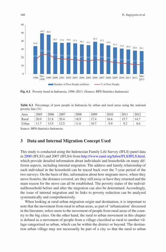
140

3 Data and Internal Migration Concept Used

This study is conducted using the Indonesian Family Life Survey (IFLS) panel data in 2000 (IFLS3) and 2007 (IFLS4) from http://www.rand.org/labor/FLS/IFLS.html, which provide detailed information about individuals and households on many dif-ferent aspects, including internal migration. The address and family relationship of each individual in the household can be traced back over the 7-year period of the two surveys. On the basis of this, information about how migrants move, where they move from/to, the distance covered, are they still away or have they returned and the main reason for the move can all be established. The poverty status of the individ-ual/household before and after the migration can also be determined. Accordingly, the issue of internal migration and its links to poverty reduction can be analysed systematically and comprehensively.

When looking at rural-urban migration origin and destination, it is important to note that the movement from rural to urban areas, as part of ‘urbanization’ discussed in the literature, refers more to the movement of people from rural areas of the coun-try to the big cities. On the other hand, the rural to urban movement in this chapter is defined as a movement of people from a village classified as rural to another vil-lage categorized as urban, which can be within the district or beyond. The destina-tion urban village may not necessarily be part of a city so that the rural to urban

Table 6.1 Percentage of poor people in Indonesia by urban and rural areas using the national poverty line (%)

Area 2005 2006 2007 2008 2009 2010 2011 2012

Rural 20.0 21.8 20.4 18.9 17.4 16.6 15.7 14.7Urban 11.7 13.5 12.5 11.6 10.7 9.9 9.2 8.6

Source: BPS-Statistics Indonesia

0

1996 1999 2000 2001 2002 2003 2004 2005 2006 2007 2008 2009 2010 2011 2012Mar2013

Dec1998

10

20

30

4034.0

48.049.5

38.7 37.9 38.4 37.3 36.1 35.1

39.337.2

35.032.5

31.0 30.0 28.6 28.1

17.5

24.2 23.4

19.1 18.4 18.2 17.4 16.7 16.017.8 16.6 15.4 14.2 13.3 12.5 11.7 11.4

50

60

Number of Poor People (million) % of Poor People

Fig. 6.1 Poverty trend in Indonesia, 1996–2013. (Source: BPS-Statistics Indonesia)

E. Sugiyarto et al.

141

movement is not a rural to city movement. This notion is important to keep in mind, as the definition of rural and urban used in the survey is determined at the village level, based on a combination of factors such as population density, share of nonag-riculture in the economy and availability of urban facilities in the village (BPS http://www.bps.go.id). Accordingly, one needs to establish a city as a new category of destination (from the place identifiers used in the survey) to be able to address the urbanization issue.

The IFLS is arguably among the most comprehensive and complicated surveys due to its panel data approach and detailed coverage and content. The IFLS repre-sents about 83% of the Indonesian population, covering 13 major provinces out of the total 27 provinces that Indonesia had at that time (Strauss et al. 2009). Provinces excluded from the IFLS are those in the eastern part of Indonesia, where the popula-tion density is still very low so that the cost of conducting a survey per household is very high. After cleaning the data such as dropping some household samples due to missing/incomplete data and nonresponse, this research uses about 35,679 panel household members from IFLS3 and IFLS4.

In relation to the internal migration issue, a lower-level administrative boundary of subdistrict is adopted to define internal migration. Accordingly, the shortest dis-tance of migration is within a district so that any movement covering distances shorter than this such as within a village is not included as internal migration. This approach is different with those using the district or province to define internal migration, and this can better capture the dynamics of internal mobility. Therefore, internal migration in this research covers mobility within districts, within provinces and across provinces during the period of 2000 and 2007. Internal migration is then further classified by urban and rural origin and destination, whether it is done indi-vidually or with the whole family and different distances covered. In terms of how migrants move, internal migration can be seen as moving individually (split house-hold) or moving with the whole family (whole household).

Figure 6.2 shows a complete classification of internal migration in Indonesia. As can be seen from the picture, the individual is first grouped into migrant and non-migrant based on the fact of whether they have moved or not, which is identified from their address between the two periods of 2000 and 2007. The migrant group is then further classified into current and return migrants, with the current migrant categorized into two types—‘away’ current migrant and ‘staying’ current migrant. The away cur-rent migrant is the current migrant originating from the previous IFLS household that was currently away from the household while staying current migrant is the current migrant coming from the same IFLS household that was currently staying in the household. To capture the dynamics of current migrants, both away and staying current migrant must be considered. Therefore, there would be three types of migrants: away current migrant, staying current migrants and return migrants. Given the complex nature of internal migration and the importance of considering the migration cycle in analysing the effect of migration, the analysis would be conducted for the current and return migrants. This is important, as their characteristics could be very different and the effects of migration on poverty reduction may take time to realize.

6 Internal Migration and Poverty: A Lesson Based on Panel Data Analysis⋯

142

4 Methodology

A combination of methods is used in this study. First, a cross tabulation and descrip-tive statistics are used to analyse the mobility of people within districts, within prov-inces and across provinces, including examining whether they migrate individually or with the whole family. The same methods are also used for analysing their move-ments from rural or urban areas to destinations in rural or urban areas. The reasons for migration of away current migrants could be work, family related, schooling and others. Understanding these patterns and dynamics of internal migration is an important aspect of understanding the internal migration issue. These patterns and dynamics are then linked to poverty conditions before and after migration by com-paring with the condition of the non-migrant group as a benchmark. To examine the distribution of expenditures of migrants and non-migrants and where the migrants coming from, a quintile analysis of per capita expenditure is performed.

Second, an econometrics probit model based on the panel data is employed to further determine factors that drive migration. This is also to observe the different characteristics of migrants based on their urban and rural origin. As the intention is to see the effect of migrants’ characteristics, the analysis focuses on the main factors associated with the poverty condition, such as per capita expenditure, agriculture as the main income source and lack of housing ownership. The model also takes into account urban and rural areas as well as demographic factors, such as the number of

Individual/hhmin 2000

Migrant

Staying in thisHH in 2007?

AwayCurrent Migrant

StayingCurrent Migrant

Past member whoreturned in 2007?

Yes

Yes

Yes Yes

No

No No

Non-migrant

Return Migrant

Moved within7 years?

Fig. 6.2 Classification of internal migrants in Indonesia. (Source: Authors’ classification based on the coverage of the research and data used from IFLS3 in 2000 and IFLS4 in 2007. [From http://www.rand.org/labor/FLS/IFLS.html])

E. Sugiyarto et al.

143

family members in the household, the number of primary school children (aged 6 to 11 years), the number of middle school children (aged 12 to 14 years) and the num-ber of persons in productive age (between 15 and 64 years), household head age, male household head and marital status of the household head. The inclusion of the variables is to improve the ability of the model to predict, as there can be some other variables that cannot be captured by the main variables but can be captured in the model with the additional variables. The study also looks at the role of education in influencing migration, which is why the variable of average length of study of the household members is also included.

To anticipate the selection effect that migrants might be poorer than non-migrants, an additional variable of squared per capita expenditures is included in the model to account for a possible non-linear relationship.

5 Key Findings and Analysis

The key findings and analysis of cross tabulations and descriptive statistics are pre-sented as patterns and dynamics of internal migration, which cover an analysis of the population that migrated by distance and among urban-rural, the type of migra-tion and whether it was individual/split or with the whole family. The analysis also examines the reasons for ‘away’ current migration, poverty status and gender. The econometrics method is presented in the analysis of what sort of people migrated.

5.1 Patterns and Dynamics of Internal Migration

Results in Table 6.2 show that 28% of the population has migrated over the 7-year period. Among the migrants, 17% are away current migrants and 56% are staying current migrants while the remaining 28% are return migrants. This implies that internal migration has been going on for a long time, and it is not a new phenome-non. Given that the IFLS has covered about 83% of the Indonesian population cov-ering 13 major provinces out of the total of 27 provinces, then the higher share of staying current migrants compared to the away current migrants shows that more people stay in the same household rather than move to a new household outside the IFLS sample. This reflects the strong family connection among internal migrants, which can still be directly maintained in internal migration. This fact provides an additional explanation for why internal migration is theoretically more significant than international migration in terms of the number of people involved.5

A majority of the migrants—60%—move as individual migrants, so the share of migrants who move with the whole family is about 40%. This is expected since

5 This is obviously different from international migration in which the migrants must stay away from their families.

6 Internal Migration and Poverty: A Lesson Based on Panel Data Analysis⋯

144

Tabl

e 6.

2 N

umbe

r an

d pe

rcen

tage

of

mig

rant

s in

200

7 by

dis

tanc

e an

d ty

pe o

f m

igra

tion

Mig

ratio

n di

stan

ceD

idn’

t mov

eA

way

cur

rent

mig

rant

sSt

ayin

g cu

rren

t mig

rant

sR

etur

n m

igra

nts

Tota

l ind

ivid

uals

Freq

%Fr

eq%

Freq

%Fr

eq%

Freq

%

Non

-mig

rant

s:25

684

72.0

2568

472

.0W

ithin

dis

tric

t27

90.

879

72.

255

61.

616

324.

6W

ithin

pro

vinc

e98

52.

835

513.

713

053.

758

4116

.4A

cros

s pr

ovin

ces

410

1.1

1208

3.4

904

2.5

2522

7.1

Tota

l mig

rant

s16

744.

755

5615

.627

657.

799

9528

.0To

tal

2568

472

.016

744.

755

5615

.627

657.

735

679

100.

0

Sour

ce: A

utho

rs’

tabu

latio

n of

dat

a fr

om I

FLS3

and

IFL

S4

E. Sugiyarto et al.

145

individual migration is much more common, as it is relatively more flexible and relatively less ‘costly’ than whole family migration. The large share of migrants with the whole family migration (40%) undermines the dynamics of the Indonesian population as part of the significant structural transformation in the economy. This must also be related to flexibility and lack of restrictions for internal mobility in the country. Moreover, this finding also shows an encouraging phenomenon of a higher level of integration or unity within the country given that the country is home to a significant number of ethnic groups with different cultures and languages.

On the distance covered (Table 6.3), a majority of migrants move within prov-inces (58%), followed by moving across provinces (25%) and within districts (16%). In the context of existing migration literature that the longer the distance, the less the number of migrants (for instance, the gravity model), this finding seems to suggest that a district provides relatively more homogeneous characteristics that can be associated with similar opportunities. Therefore, migrants see moving within districts as the least desirable option, even though at the same time, it might be the most convenient way. In other words, moving within a district can be seen as pro-viding the least favourable opportunity that the migrant is commonly looking for. Beyond the district, the migration distance is still an important factor in internal migration and consistent with the theory’s prediction of the longer the distance, the less the number of migrations.

Comparing current migrants and return migrants, there seems not much chang-ing in the migrant destinations. Migration within provinces remains the most popu-lar destination, but migration across or to other provinces has become less. This is interesting since one may expect that migration to other provinces should tend to increase given the increasing number of provinces. On the other hand, this finding suggests that the average distance of internal migration in Indonesia tends to decrease, which is in line with the increasing number of centres of agglomera-tions—that is, areas producing more job opportunities.

Among current migrants and return migrants, the share of migrants who move with the whole family has been increasing. Their share has increased by only less than 4% among return migrants, while it is about 18% among away current migrants and almost 80% among hosted current migrants. In other words, migration with the whole family has been increasing over time.

About 52% of migrants are from urban areas and the remaining 48% are from rural areas (Fig. 6.3a). Most migration movements are from the same type of areas, such as from urban to urban and rural to rural. Movements from rural to rural con-tribute to 40% of the total migration, while urban to urban migration is about 37%. Migration from urban to rural is about 15%, while rural to urban is only about 8%. Therefore, there are more numbers of migration from urban than from rural areas based on the classification used in this research.

6 Internal Migration and Poverty: A Lesson Based on Panel Data Analysis⋯

146

Tabl

e 6.

3 N

umbe

r an

d pe

rcen

tage

of

mig

rant

s in

200

7 by

dis

tanc

e an

d ty

pe o

f m

igra

tion

and

the

way

they

mov

e

Mig

ratio

n di

stan

ceA

way

cur

rent

mig

rant

sSt

ayin

g cu

rren

t mig

rant

sR

etur

n m

igra

nts

Tota

l ind

ivid

ual m

igra

nts

Split

Who

leA

llSp

litW

hole

All

Split

Who

leA

llSp

litW

hole

All

With

in d

istr

ict

136

143

279

270

527

797

519

3755

692

570

716

32%

2.3

3.6

2.8

4.5

13.2

8.0

8.7

0.9

5.6

15.4

17.7

16.3

With

in p

rovi

nce

602

383

985

1565

1986

3551

1234

7113

0534

0124

4058

41%

10.0

9.6

9.9

26.1

49.7

35.5

20.6

1.8

13.1

56.7

61.0

58.4

Acr

oss

prov

ince

s20

820

241

060

660

212

0885

549

904

1669

853

2522

%3.

55.

14.

110

.115

.112

.114

.31.

29.

027

.821

.325

.2To

tal

946

728

1674

2441

3115

5556

2608

157

2765

5995

4000

9995

%15

.818

.216

.740

.777

.955

.643

.53.

927

.710

0.0

100.

010

0.0

Sour

ce: A

utho

rs’

tabu

latio

n of

dat

a fr

om I

FLS3

and

IFL

S4

E. Sugiyarto et al.

147

5.2 Reasons for ‘Away’ Current Migration

Looking at the main reasons for ‘away’ current migration, the most dominant one is related to family, which contributes to about 39% of the total migration (Fig. 6.3b). This is followed by work (26%) and schooling (only 7%). This pattern is common for both individual migrants and migrants who move with the whole family, though it is more prominent in the case of the former.

In relation to distance, migration due to family reasons is highest among migrants who move within districts, followed by those who move across and within prov-inces (see Appendix Table 6.10) while the previous result indicates that most migrants move within provinces, followed by across provinces and then within dis-tricts. Therefore, there seems to be no clear and systematic pattern between family reasons and migration distance, though one may expect that family connections in the original place will make the number of migrations to farther destinations less—that is, strengthening the gravity model of the distance being negatively correlated to the number of migrations.

In terms of schooling, there is a catchment area system in primary and secondary schools that influences the decision of people or households to move to or stay in the catchment area depending on the location of their favourite (high-quality) school. For the tertiary education level, however, universities are not widely accessible and are commonly located in cities and/or provincial capitals. The number of specific faculties or courses in universities is even more limited. These factors may force people to move to get access to a university. Most migrants moving for schooling reasons move within districts, comprising 11 of the total migrants, followed by within provinces and across provinces, with 7% and 6% shares, respectively.

Looking at the linkages between the reason for migration and the destination areas, one finds that the work reason is more dominant among those moving from rural to urban areas, followed by within rural, urban to urban and urban to rural (see Appendix Table 6.11). For nonagricultural work, it is expected that urban areas will provide more job opportunities than rural areas, so migration to urban areas tends to be more dominant.

A. Percentage of Migrant by Urban-Rural Origin andDestination from 2000 to 2007

Urban-

Rural-Rural

50

40

30

20

10

0Work

2724 26

42

3439

8 7 7

23

36

28

Family

Split HH Whole HH All

School Others

40%

Rural-

RuralUrban Urban-

8%15%

Urban37%

B. Percentage of Away Current-Migrant by Reasonsfor Migration (%)

Fig. 6.3 Percentage of migrant households by urban-rural origin and destination from 2000 to 2007. (Source: Authors’ calculations from IFLS3 and IFLS4)

6 Internal Migration and Poverty: A Lesson Based on Panel Data Analysis⋯

148

On the other hand, among migrants moving for family reasons, the highest share is movement within urban areas, followed by movement within rural, urban to rural and rural to urban. For schooling reasons, the highest share is of migration from rural to urban areas, followed by within rural, within urban and from urban to rural. The results indicate that the reasons for migration do influence the destination of migration (see Appendix Table 6.12, Table 6.13, Table 6.14, and Table 6.15).

5.3 Poverty Status Before and After Migration

On the poverty status, it is important to note that both migrant and non-migrant groups experience poverty reductions. Among the non-migrants, the poverty rates declined from 18% in 2000 to 4.7% in 2007, showing a reduction of 13.3 percentage points (Table 6.4). For the total migrants, the poverty rate in 2000 was 16%, declin-ing to 3.3% in 2007—a reduction of 12.6 percentage points.

Table 6.4 Poverty incidence among non-migrants and migrants before and after migration (%)

Type of mobilityIFLS3 (before migrating) IFLS4 (after migrating)Non-poor Poor Total Non-poor Poor Total

Non-migrants 82.0 18.0 100.0 95.3 4.7 100.0All migrantsWithin the same district 81.9 18.1 100.0 96.0 4.0 100.0Within the same province 83.9 16.1 100.0 96.3 3.7 100.0Other provinces 86.2 13.8 100.0 98.2 1.8 100.0Total all migrants 84.1 15.9 100.0 96.7 3.3 100.0Away current migrantsWithin the same district 84.9 15.1 100.0 87.8 12.2 100.0Within the same province 89.4 10.6 100.0 92.7 7.3 100.0Other provinces 85.1 14.9 100.0 95.6 4.4 100.0Total away current migrants 87.6 12.4 100.0 92.6 7.4 100.0Staying current migrantsWithin the same district 83.9 16.1 100.0 96.5 3.5 100.0Within the same province 82.9 17.1 100.0 96.0 4.0 100.0Other provinces 86.3 13.7 100.0 97.8 2.2 100.0Total hosted current migrants 83.8 16.2 100.0 96.5 3.5 100.0Return migrantsWithin the same district 77.5 22.5 100.0 99.5 0.5 100.0Within the same province 82.1 17.9 100.0 99.7 0.3 100.0Other provinces 86.5 13.5 100.0 99.8 0.2 100.0Total return migrants 82.6 17.4 100.0 99.7 0.3 100.0Total households 82.6 17.4 100.0 95.7 4.3 100.0

Source: Authors’ calculations from IFLS 3 and IFLS 4

E. Sugiyarto et al.

149

If the migrant households are classified further into current migrants and return migrants, the poverty reduction in the two groups is very different. The poverty rate among return migrants in 2000 was 17.4%, and it declined to 0.3% in 2007, show-ing a remarkable poverty reduction of more than 17 percentage points. For the away current migrants, the poverty rate in 2000 was 12.4%, and it declined to 7.4% in 2007—a reduction of only 5 percentage points. The poverty rate of staying current migrants was 16.2% in 2000 and it declined to 3.5% in 2007, showing a reduction of 12.7 percentage points. Therefore, the poverty reduction of staying current migrants is almost 8 percentage points higher than that of away current migrants. The findings show that the poverty reduction effect of internal migration takes time to realize, and there is also a worsening period when the migration is still in process. The success of returning migrants in reducing poverty is really remarkable to the extent that the poverty incidence among them is nearly eradicated. Moreover, the higher rate of poverty reduction among the staying current migrants compared to the away current migrants suggests that being with the family is helpful, as other family members may contribute to reducing the poverty incidence.

Looking further into a specific household group that was poor in 2000 and then became non-poor in 2007, one finds that the share of non-migrants is 16.1% while the share of away current migrants, staying current migrants and return migrants is 11.5%, 14.6% and 17.3%, respectively (see Appendices 3, 4, 5 and 6). Therefore, a complete cycle of internal migration helps further reduce poverty by about at least 3 percentage points.

On the other hand, there is also a household group that was not poor in 2000 but became poor in 2007. The share of non-migrants in this group is about 2.8% while the share of the away current migrants, staying current migrants and return migrants is 6.6%, 1.9% and less than 0.5%, respectively. This highlights that migrants strug-gle and some of them become poor in the process, even though by the end of the migration process, most of them manage to succeed.

Linking poverty reduction effects with the patterns and dynamics of migration, some interesting findings emerged. First, in terms of how people migrate, the high-est share is movement within districts, followed by within provinces and across provinces (Table 6.5). This pattern is more common among individual migrants than those who move with the whole family. Individual migrants are much more successful in helping themselves escape poverty than migrants with the whole fam-ily. The poverty reduction among individual migrants reaches 14 percentage points, while that among whole family migrants is only 10 percentage points. Among the whole family migrants, poverty reduction among those moving within districts and across provinces is the same at about 11.3 percentage points migrant. The smallest poverty reduction is among those moving within provinces.

Among current migrants, the overall poverty reduction of individual migrants and those migrating with the whole family is about the same at 11.2 and 10.6 per-centage points, respectively. Individual migration within districts experiences the least poverty reduction—only 6.9 percentage points.

Among return migrants, poverty reduction of individual migrants is almost 18 percentage points while the rate for whole family migration is less than 5 percentage

6 Internal Migration and Poverty: A Lesson Based on Panel Data Analysis⋯

150

Tabl

e 6.

5 Pe

rcen

tage

of

pove

rty

redu

ctio

n am

ong

non-

mig

rant

s an

d m

igra

nts

by m

igra

tion

dist

ance

, typ

e of

mig

ratio

n an

d th

e w

ay th

ey m

ove

from

200

0 to

20

07

Mig

ratio

nN

on-m

igra

nts

All

curr

ent m

igra

nts

Ret

urn

mig

rant

sA

ll m

igra

nts

Split

Who

leA

llSp

litW

hole

All

Dis

tanc

eSp

litW

hole

All

Non

-mig

rant

s−

13.3

With

in

dist

rict

−6.

9−

11.9

−10

.0−

23.5

0−

21.9

−16

.2−

11.3

−14

.1W

ithin

pro

vinc

e−

12.2

−9.

8−

10.9

−18

.1−

8.5

−17

.5−

14.3

−9.

8−

12.4

Acr

oss

prov

ince

s−

10.7

−11

.8−

11.2

−13

.9−

2.0

−13

.3−

12.3

−11

.3−

12.0

Mig

rant

s−

11.2

−10

.6−

10.9

−17

.8−

4.5

−17

.0−

14.1

−10

.4−

12.6

Sour

ce: A

utho

rs’

calc

ulat

ions

fro

m I

FLS

3 an

d IF

LS

4

E. Sugiyarto et al.

151

points. There is no impact among return migrants moving with the whole family within districts, as there is no movement of poor migrants within the group. Overall, migrants moving within districts show the highest poverty reduction, while migrants moving across provinces experience a reduction of only 2 percentage points.

Second, Table 6.6 presents poverty reduction in relation to areas of movement. Overall, the highest poverty reduction is among migrants moving within urban areas, which is 14.9 percentage points, followed by those moving from urban to rural at 12.2, within rural at 11.7 and the least from rural to urban at 6.4 percentage points. These reductions are also observed among return migrants, but they are much higher—23.1 percentage points among those moving within urban areas, 15.7 from urban to rural, 15.4 within rural and 12.5 from rural to urban.

The poverty reduction situation among current migrants is very different. The highest is still among those moving within urban areas (13.2 percentage points), followed by movement within rural (10.4) and from urban to rural (8.5) and the low-est one is from rural to urban (2.9). The poverty reduction among return migrants is always higher compared to current migrants for all types of movements and the highest difference is among those moving within urban areas, which is almost 10 percentage points. The lowest difference is among those moving within rural (5 percentage points only) while the difference for those moving from rural to urban and from urban to rural is 9.6 and 7.2 percentage points, respectively.

Looking at the link between the way migrants move and the area of movement, one finds that individual migrants contribute significantly to poverty reduction for all types of migrants (i.e. current and return migrants), but the results are very dif-ferent in the case of whole family migration. The poverty reduction of individual return migrants moving within urban areas is very high at 23.4 percentage points, followed by those moving within rural and from urban to rural, which is the same at 16.4 percentage points, and those moving from rural to urban at 13.9 percentage points. However, there are no effects on migrants who move with the whole family from rural to urban areas and within rural areas, as there are no poor migrants who move within these groups. The results for migrants moving with the whole family in this return migration should be interpreted more cautiously due to the small size of the sample. On the other hand, individual migrants and those who move with the whole family have a similar effect on poverty reduction at about 11 percentage points. The movement from rural to urban contributes the least, followed by migra-tion from urban to rural, within rural and from rural to urban.

Finally, with regard to the migration reasons of the away current migrants and their relation to poverty reduction, those who move for schooling reasons show the highest poverty reduction, which is 8.9 percentage points, followed by those who move for family reasons at 4.6. The least poverty reduction is among those who move for work-related reasons, which is 1.7 percentage points only, while it is 7.4 points among those who move for ‘other’ reasons (Appendix Table 6.16).

6 Internal Migration and Poverty: A Lesson Based on Panel Data Analysis⋯

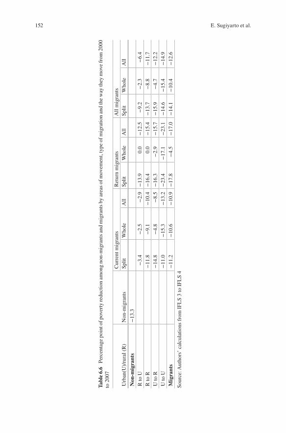
152

Tabl

e 6.

6 Pe

rcen

tage

poi

nt o

f pov

erty

redu

ctio

n am

ong

non-

mig

rant

s an

d m

igra

nts

by a

reas

of m

ovem

ent,

type

of m

igra

tion

and

the

way

they

mov

e fr

om 2

000

to 2

007

Urb

an(U

)/ru

ral (

R)

Non

-mig

rant

sC

urre

nt m

igra

nts

Ret

urn

mig

rant

sA

ll m

igra

nts

Split

Who

leA

llSp

litW

hole

All

Split

Who

leA

ll

Non

-mig

rant

s−

13.3

R to

U−

3.4

−2.

5−

2.9

−13

.90.

0−

12.5

−9.

2−

2.3

−6.

4R

to R

−11

.8−

9.1

−10

.4−

16.4

0.0

−15

.4−

13.7

−8.

8−

11.7

U to

R−

14.8

−4.

8−

8.5

−16

.3−

2.9

−15

.7−

15.9

−4.

7−

12.2

U to

U−

11.0

−15

.3−

13.2

−23

.4−

17.1

−23

.1−

14.6

−15

.4−

14.9

Mig

rant

s−

11.2

−10

.6−

10.9

−17

.8−

4.5

−17

.0−

14.1

−10

.4−

12.6

Sour

ce: A

utho

rs’

calc

ulat

ions

fro

m I

FLS

3 to

IFL

S 4

E. Sugiyarto et al.

153

5.4 Considering Gender

To consider the gender dimension in the analysis, cross tabulations of migrants by type with gender are made as well as with regard to the poverty impact. The results show that there are more male migrants than female migrants, but the difference is very small. This applies for different types of migrants and the differences are less than 1% (Table 6.7). This shows that women have been part of the internal migra-tion in all cases.6

On the poverty impact, it seems that gender is not a determining factor in influ-encing the internal migration results, and the effects across different types of migrants show no systematic pattern. The poverty reduction impact among female non-migrants is only slightly higher than the male—13.4 compared to 13.2 percent-age points, but the impact among migrants is different, with males performing bet-ter, though the difference is again very small—12.7 for male migrants and 12.4 for female migrants (Table 6.8). The only noticeable difference is among the away cur-rent migrants, in which case the poverty reduction declined by 6.5 percentage points for males but was only 3.1 percentage points for females.

Looking at the initial condition in 2000, poor female migrants, both away and staying current migrants, are fewer than male migrants, while the number is higher among return migrants (see Appendix Table 6.17).

Who Migrate?The quintile analysis of the per capita expenditures of migrants and non-migrants shows a very different result. Figure 6.4 presents the frequency distributions of migrants, which are concentrated in the upper levels of the quintiles, while it is the opposite in the case of non-migrants. More than 35% of away current migrants, about 25% of staying current migrants and 23% of return migrants come from the top quintile group, while it is only 19% in the case of non-migrants. This indicates that migrants are coming from richer groups.

Table 6.9 shows regression results on the factors influencing people to migrate. As can be seen from the results, the monthly per capita expenditure and housing ownership status have positive signs showing that people with stable incomes and the rich tend to migrate. The negative sign of the squared per capita expenditure coefficient strengthens the finding. This shows that migrants are less poor than non-migrants. Households with agriculture as the main income source show a negative sign, indicating that agriculture household do not tend to migrate. This may also indicate that the agriculture households need their members to do farm work, mak-ing them less likely to migrate. This finding is also in line with the result that migrant households are more likely to be from urban areas than from rural because agricul-ture jobs in urban areas are less than in rural.

Analysing the demographic factors, people in households with more family members, more members of productive age and a male household head tend to

6 This finding is very different compared with international migration in which women interna-tional migrants are dominant.

6 Internal Migration and Poverty: A Lesson Based on Panel Data Analysis⋯

154

Table 6.7 Number and percentage of individuals in IFLS4 by gender and type of migration

GenderNon-migrants All current Return All migrantsFreq % Freq % Freq % Freq %

Male 12,686 49.4 3,689 51.0 1,388 50.2 5,077 50.8Female 12,998 50.6 3,541 49.0 1,377 49.8 4,918 49.2Total 25,684 100.0 7,230 100.0 2,765 100.0 9,995 100.0

Source: Authors’ calculations from IFLS 3 to IFLS 4

Table 6.8 Percentage points of poverty reduction by gender and type of migration from 2000 to 2007

Gender Non-migrantsAway current migrants

Staying current migrants Return migrants Total migrants

Male −13.2 −6.5 −12.8 −16.5 −12.7Female −13.4 −3.1 −12.5 −17.6 −12.4Total −13.4 −5.0 −12.7 −17.1 −12.6

Source: Authors’ calculations from IFLS 3 to IFLS 4

0.0Q1 Q2 Q3 Q4 Q5

Non-Migrant

Away Current-Migrant

Staying Current-Migrant

Return Migrant

5.0

10.0

15.0

20.0

25.0

30.0

35.0

40.0

Fig. 6.4 Distribution of migrant by household per capita expenditure quintile and type of migrant household. (Source: Authors’ calculations from IFLS 3 to IFLS 4)

E. Sugiyarto et al.

155

migrate. On the other hand, households with more older members and married household heads have a negative sign, showing that they are less likely to migrate. Looking at the role of education, households with a larger number of middle school children and higher education members show positive signs, reflecting that they are more likely to migrate. Households with more primary school children show a nega-tive effect and are less likely to migrate. This may be related to the widespread availability of facilities for compulsory primary and secondary education in the catchment areas where they live.

The economic factors of the model results for urban and rural areas show similar results. All signs on household per capita expenditures and housing ownership sta-tus are the same. The squared per capita expenditure among those moving have the

Table 6.9 Probit results to identify the main characteristics of migrants by origin and destination (y=1 if migrant, and 0 for otherwise)

VariablesOrigin and destination of migrationNational Rural to urban Rural to rural Urban to rural Urban to urban

Per cap. expenditure

4.63E-07*** 2.6E-07 5.89E-07*** 4.34E-07 8.88E-08

Squared per cap expd

−1.48E-13***

5.12E-13 −2.1E-13*** −2.78E-14 −5.22E14

Agric. main inc. source

−0.31*** −1.26*** −0.17** 0.11 −0.46***

Housing status 0.35*** 0.23 0.20*** 0.17 0.49***Urban area 0.22*** x x x xHousehold size 0.004 −0.22*** −0.02 −0.04 0.06**No kids (6–11) yrs

−0.002 -0.04 0.06 0.04 −0.06

No age (12–14) yrs

0.05* 0.10 0.002 0.06 0.04

No age (15–64) yrs

0.009 0.20*** −0.02 0.03 0.02

Avg. lstudy hhm (yrs)

0.003 0.06** 0.03*** −0.008 −0.05***

hh head age −0.006*** −0.0005 −0.006*** −0.01*** −0.004*hh head male 0.16** 0.19 0.13 0.03 0.16hh head married

−0.24*** −0.25 −0.27*** −0.18 −0.06

Constant −0.51*** 0.46 −0.50*** 0.43* −0.48***No. of observations

35679 1288 15407 3427 15557

Pseudo R2 0.032 0.3011 0.0317 0.0224 0.0422

Source: Authors’ calculations from IFLS 3 and IFLS 4Notes: Please see Appendix Table 6.18 for definitions of the variables; ***Denotes significant at the 1% level, **significant at the 5% level, *significant at the 10% level

6 Internal Migration and Poverty: A Lesson Based on Panel Data Analysis⋯

156

same signs except for those moving from rural to urban, which shows that migrants from rural to urban areas tend to be poorer than non- migrants. Other types of migrants who moved from urban to rural areas tend to be richer. An agriculture income source has the same negative results except among those moving from urban to rural, which is positive. This means that households with agriculture as the main income source are more likely to migrate from urban to rural to get back to farming in rural areas.

The demographic factors of all migrants based on areas of movement show a common pattern as in the overall model. Households with higher numbers of elderly members and married household heads are less likely to migrate, and households with higher numbers of male household heads are more likely to migrate. People from households with a larger household size are less likely to migrate except in the case of movement within urban areas. Therefore, the relationship between family size and migration is also affected by the origin and destination of migration. Household members of a more productive age are more likely to migrate except in the case of movement within rural areas. On the other hand, people from households with a larger number of middle school children are more likely to migrate in all the areas of movement, while those from households with larger numbers of primary school children are more likely to migrate in the case of movement within rural and from urban to rural areas. Finally, higher education household members are more likely to migrate in the movement from rural to urban and within rural areas, but it is opposite in the movement from urban to rural and within urban.

6 Conclusions and Policy Implications

The extent and effects of internal migration have increased and are becoming more significant. On the other hand, the dynamics and patterns of internal migration have become complex, especially with regard to how the migration is conducted, the main reasons, the distance covered and the origin, destination and characteristics of the migrants. There is a need for a rigorous analysis to address these issues.

More internal migration takes place at the individual level, with a majority of the individual migrants moving within provinces. More migrants are from urban areas, and most migrants move within the same area, such as urban to urban and rural to rural, while rural to urban migration is actually the least common. This is very dif-ferent from the perception of internal migration from the literature, which is domi-nated by rural to urban migration (i.e. urbanization). This rural to urban migration primarily refers to movement from rural areas to cities.

The poverty effects of internal migration seem to be influenced by the migration type:

(i) First, the poverty condition of both migrants and non-migrants has improved during the period studied.

E. Sugiyarto et al.

157

(ii) Second, poverty reduction among return migrants is higher than among current migrants. This highlights that the poverty reduction effect of internal migration takes time to materialize or that the poverty reduction effect on current migrants is not fully realized. In other words, migrants must struggle to escape poverty at the beginning, as the full impact on poverty reduction can only be seen when the cycle of migration is completed.

(iii) Third, the strongest poverty reduction effect is among those moving within districts, showing that the shorter the distance, the stronger the poverty reduc-tion effect. This seems consistent with the theoretical prediction that the longer the distance, the more costly and stronger the barriers to migration. The results also show that the shortest distance of migration is more pro-poor, as the pov-erty incidence of people moving within districts is the highest compared to those moving within provinces and across provinces.

(iv) Fourth, poverty reduction in the case of individual migration performs better than in the case of whole family migration, which is a matter of concern and requires more attention. Whole family migration seems to be facing more bar-riers when it comes to poverty reduction.

(v) Finally, those moving from urban to urban areas experience the most pro-poor effects than other types of movement, and those moving from rural to urban areas face more challenges.

The gender effect is less obvious and shows no clear pattern. Moreover, migrants tend to come from a rich background, with more productive age and higher educa-tion members. They are less likely to be from households that are dependent on agriculture and households with more primary school children, which are linked to migration reasons and household circumstances, such as the availability of jobs, higher-level schooling and the catchment area system implemented at the primary school level.

The overall findings indicate the complexity of the internal migration issue, espe-cially in relation to its poverty reduction effects. This calls for further examination so as to distil more detailed policy implications. The more obvious conclusion from this research is that the migration cycle, individual or family migration, distance, origin and destination, migration reasons and characteristics of migrants are all sig-nificant in influencing the migration results. Therefore, these factors should be taken into account in addressing the various internal migration issues, including transmi-gration and introduction of barriers to migration to big cities.7

It is clear from the different impacts for the different migrant groups that there will be no one strategy that can address all the issues, as each case requires a specific intervention. Whole family migration requires greater attention, and there is a need for better facilitation to complete the migration cycle, which will contribute posi-tively to poverty reduction. Moreover, considering the migration dynamics, reduc-

7 The capital city of Jakarta once introduced ‘a close city policy’ to prevent migrants with no jobs and other guarantees to enter the city. Many other big cities try to copy the policy but end up with no clear implementation or results.

6 Internal Migration and Poverty: A Lesson Based on Panel Data Analysis⋯

158

ing the overall migration costs and improving the human capacity of the migrants will further augment the positive impact of internal migration.

Appendices

Table 6.11 Number and percentage of away current migrants by reason for migration and area of origin and destination

Reason for migration

Rural to Urban Rural to Rural Urban to Rural Urban to Urban AllFreq % Freq % Freq % Freq % Freq %

Work 81 37.33 194 27.52 41 19.07 114 21.23 430 25.69Family 50 23.04 269 38.16 80 37.21 250 46.55 649 38.77School 20 9.22 59 8.37 11 5.12 33 6.15 123 7.35Others 66 30.41 183 25.96 83 38.60 140 26.07 472 28.20Total 217 100.00 705 100.00 215 100.00 537 100.00 1674 100.00

Source: Authors’ calculation from IFLS 3 and IFLS 4

Table 6.10 Number and percentage of away current migrants by reason for migration and migration distance

Reason for migrationWithin district Within province Across province AllFreq % Freq % Freq % Freq %

Work 49 17.56 273 27.72 108 26.34 430 25.69Family 113 40.50 375 38.07 161 39.27 649 38.77School 30 10.75 70 7.11 23 5.61 123 7.35Others 87 31.18 267 27.11 118 28.78 472 28.20Total 279 100.00 985 100.00 410 100.00 1674 100.00

Source: Authors’ calculation from IFLS 3 and IFLS 4

Table 6.12 Number and percentage of non-migrants by poverty status in IFLS3 and IFLS4

IFLS3

IFLS4

%Poor

%Total

%Non-poorFreq Freq Freq

Non-poor 20338 79.19 717 2.79 21055 81.98Poor 4134 16.10 495 1.93 4629 18.02Total 24472 95.28 1212 4.72 25684 100.00

Source: Authors’ calculation from IFLS 3 and IFLS 4

E. Sugiyarto et al.

159

Table 6.16 The share of away current migrants by reason for migration and poverty status before and after migration

Type of mobilityIFLS3 (before migrating) IFLS4 (after migrating)Non-poor Poor Total Non-poor Poor Total

Work 90.2 9.8 100.0 91.9 8.1 100.0Family 86.9 13.1 100.0 91.5 8.5 100.0School 87.8 12.2 100.0 96.7 3.3 100.0Others 86.2 13.8 100.0 93.6 6.4 100.0Total migrants 87.6 12.4 100.0 92.6 7.4 100.0

Source: Authors’ calculation from IFLS 3 and IFLS 4

Table 6.15 The share of return migrants by poverty status before migration (in 2000) and after migration (in 2007)

IFLS3

IFLS4 TotalNon-poor Poor

Freq %Freq % Freq %

Non-poor 2279 82.42 6 0.22 2285 82.64Poor 477 17.25 3 0.11 480 17.36Total 2756 99.67 9 0.33 2765 100.00

Source: Authors’ calculation from IFLS 3 and IFLS 4

Table 6.14 The share of staying current migrants by poverty status before migration (in 2000) and after migration (in 2007)

IFLS3

IFLS4 TotalNon-poor Poor

Freq %Freq % Freq %

Non-poor 4550 81.89 107 1.93 4657 83.82Poor 810 14.58 89 1.60 899 16.18Total 5360 96.47 196 3.53 5556 100.00

Source: Authors’ calculation from IFLS 3 and IFLS 4

Table 6.13 The share of away current migrants by poverty status before migration (in 2000) and after migration (in 2007)

IFLS3

IFLS4 TotalNon-poor Poor

Freq %Freq % Freq %

Non-poor 1357 81.06 110 6.57 1467 87.63Poor 193 11.53 14 0.84 207 12.37Total 1550 92.59 124 7.41 1674 100.00

Source: Authors’ calculation from IFLS 3 and IFLS 4

6 Internal Migration and Poverty: A Lesson Based on Panel Data Analysis⋯

Table 6.17 Poverty incidence among non-migrants and migrants by gender and type of migration in 2000 and 2007 (%)

Type of mobilityIFLS3 (before migrating) IFLS4 (after migrating)Non-poor Poor Total Non-poor Poor Total

Non-migrant 82.0 18.0 100.0 95.3 4.7 100.0Male 82.1 17.9 100.0 95.2 4.8 100.0Female 81.9 18.1 100.0 95.3 4.7 100.0All migrantsMale 84.1 15.9 100.0 96.8 3.2 100.0Female 84.2 15.8 100.0 96.6 3.4 100.0Total all migrants 84.1 15.9 100.0 96.7 3.3 100.0‘Away’ current migrantMale 86.7 13.3 100.0 93.2 6.8 100.0Female 88.7 11.3 100.0 91.8 8.2 100.0Total current migrants 87.6 12.4 100.0 92.6 7.4 100.0‘Staying’ current migrantMale 83.7 16.3 100.0 96.5 3.5 100.0Female 84.0 16.0 100.0 96.5 3.5 100.0Total current migrants 83.8 16.2 100.0 96.5 3.5 100.0‘Return’ migrantMale 83.3 16.7 100.0 99.8 0.2 100.0Female 82.0 18.0 100.0 99.6 0.4 100.0Total ‘return’ migrants 82.6 17.4 100.0 99.7 0.3 100.0Total households 82.6 17.4 100.0 95.7 4.3 100.0

Source: Authors’ calculation from IFLS 3 and IFLS 4

Table 6.18 Definition of each independent variable

List of variables Definitions

Per cap. expenditure Monthly per capita expenditureSquared per cap expd Squared monthly per capita expenditureAgric. main inc. source Agriculture main income source (the value is 1 if household main

income source is agriculture and 0 for otherwise)Housing status Housing ownership (the value is 1 if household owns the house and

0 for otherwise)Urban area Location of the household (the value is 1 if the household is in rural

area and 0 for otherwise)Household size Number of household membersNo kids (6–11) yrs Number of children aged 6 to 11 years in the householdNo age (12–14) yrs Number of children aged 12 to 14 years in the householdNo age (15–64) yrs Number of productive aged people in the householdAvg. lstudy hhm (yrs) Average length of study (in years) of household members aged 15

years and overhh head age Household head age (years)hh head male Male household head (the value is 1 if male household head and 0

for otherwise)hh head married Married household head (the value is 1 if married household head

and 0 for otherwise)

161

References

Aji, P. (2015). Summary of Indonesia’s poverty analysis, ADB Papers on Indonesia, No. 4 https://www.adb.org/sites/default/files/publication/177017/ino-paper-04-2015.pdf. Accessed on 12 Dec 2017.

Badan Pusat Statistik (BPS). http://www.bps.go.id, Indonesia.Bell, M., & Muhidin, S. (2009). Cross-national comparisons of internal migration, Human

Development Research Paper 2009/30, UNDP.Deb, P., & Seck, P. (2009). Internal migration, selection bias and human development: Evidence

from Indonesia and Mexico. Online at http://mpra.ub.uni-muenchen.de/19214/. MPRA Paper No. 19214, posted 13. December 2009 06:54 UTC.

Deshingkar, P. (2006). Internal migration, poverty and development in Asia. Promoting growth, ending poverty ASIA2015. Institute Development Studies and Overseas Development Institute.

Greenwood, M. J. (2005). Modelling migration. Encyclopedia of social measurement, Volume 2, Elsevier Inc. All Rights Reserved.

Harris, J., & Speare, A. (1986, January). Education, earnings, and migration in Indonesia. Economic Development and Cultural Change, 34(2), 223–244 Published by: The University of Chicago Press.

Harttgen, K., & Klasen, S. A human development index by internal migration status. Human Development Research Paper 2009 / 54, UNDP.

IFLS 3. (2000). Available: https://www.rand.org/labor/FLS/IFLS.htmlIFLS 4. (2008). Available: https://www.rand.org/labor/FLS/IFLS.htmlThe House of Commons International Development Committee. (2004). Migration and develop-

ment: How to make migration work for poverty reduction, Sixth Report of Session 2003–04 Volume I.

Hugo, G. J. (1982, March). Circular Migration in Indonesia. Population development review, 8(1), 59–83 Published by: Population Council.

Hugo, G. J. (2004). Forced migration in Indonesia: Historical perspectives. In Revised paper presented to international conference on toward new perspectives on forced migration In Southeast Asia, organised by Research Centre for Society and Culture (PMB) at the Indonesian Institute of Sciences (LIPI) and Refugee Studies Centre (RSC) at the University of Oxford, Jakarta, 25–26 November 2004.

Lu, Y. (2008). Test of the “healthy migrant hypothesis”: A longitudinal analysis of health selectiv-ity of internal migration in Indonesia. Social Science and Medicine, 67, 1331–1339.

Lottum, J. V., & Marks, D. (2010). The determinants of internal migration in a developing coun-try: Quantitative evidence for Indonesia, 1930–2000. JEL codes: J61; J68; N15; O15.

McNicoll, G. (1968). Internal migration in Indonesia: Descriptive notes. Published by: Southeast Asia Program Publications at Cornell University.

6 Internal Migration and Poverty: A Lesson Based on Panel Data Analysis⋯

162

Perlman, J. E. (1976). The myth of marginality: Urban poverty and politics in Rio de Janeiro (pp. xxi–341). Berkeley/Los Angeles/London: University of California Press.

Rondinelli, D. A. (1985, June). Population distribution and economic development in Africa: The need for urbanization policies. Population Research and Policy Review, 4(2), 173–196.

Strauss, J., Witoelar, F., Sikoki, B., & Wattie, A. M. (2009). User’s Guide for the Indonesia Family Life Survey, Wave 4. Working Paper Volume 2, 2009. RAND Labour and Population.

Tacoli, C. (2012). Urbanization, gender and urban poverty: Paid work and unpaid carework in the city. Urbanization and emerging population issues, Working Paper 7. United Nations Population Fund.

World Population Year. (1974). The population of indonesia. Lembaga Demography Universitas Indonesia. CICRED Series.

The views expressed in this publication are those of the authors and do not necessarily reflect the views and policies of the Asian Development Bank (ADB) or its Board of Governors or the governments they represent.

ADB does not guarantee the accuracy of the data included in this publication and accepts no responsibility for any consequence of their use. The mention of specific companies or products of manufacturers does not imply that they are endorsed or recommended by ADB in preference to others of a similar nature that are not mentioned.

By making any designation of or reference to a particular territory or geographic area, or by using the term “country” in this document, ADB does not intend to make any judgments as to the legal or other status of any territory or area. Open Access This work is available under the Creative Commons Attribution-NonCommercial 3.0 IGO license (CC BY-NC 3.0 IGO) http://creativecommons.org/licenses/by-nc/3.0/igo/. By using the content of this publication, you agree to be bound by the terms of this license. For attribution and permissions, please read the provisions and terms of use at https://www.adb.org/terms-use#openaccess.

This CC license does not apply to non-ADB copyright materials in this publication. If the mate-rial is attributed to another source, please contact the copyright owner or publisher of that source for permission to reproduce it. ADB cannot be held liable for any claims that arise as a result of your use of the material.

Please contact pubsmarketing@adb.org if you have questions or comments with respect to content, or if you wish to obtain copyright permission for your intended use that does not fall within these terms, or for permission to use the ADB logo.

E. Sugiyarto et al.

163© Asian Development Bank 2019 K. Jayanthakumaran et al. (eds.), Internal Migration, Urbanization, and Poverty in Asia: Dynamics and Interrelationships, https://doi.org/10.1007/978-981-13-1537-4_7

Chapter 7Poverty and Inequality in Urban India with Special Reference to West Bengal: An Empirical Study

Nandini Mukherjee and Biswajit Chatterjee

1 Introduction1

The rapid growth in the urban population of developing nations witnessed in the twentieth century has been accompanied by a corresponding rise in the urban pov-erty incidence in these nations. According to the World Development Report (2000–2001), nearly half of the poor people of the world reside in South Asia, though it is home to just about 30% of the population of the world. In India, the discussion on poverty has been dominated by rural poverty due to its sheer volume (Planning Commission estimates). With the rapid increase in urban population, the trends and linkages of urban poverty have crucial implications regarding the basic services and infrastructure required for maintaining a dignified life. Though India managed to achieve the Millennium Development Goal target of a 50% reduction in its poverty rate, according to 2011–2012 estimates, nearly 22% of India’s population is still below the poverty line. This calls for an exploration of the issues related to urban poverty.

1 The views expressed in the study do not necessarily reflect those of the Government of India.

We would like to offer our special thanks to Prof. Rajarshi Majumdar of University of Burdwan, West Bengal, India, for his immense help in dealing with the unit-level data of the National Sample Survey along with his valuable comments.

N. Mukherjee (*) School of Women’s Studies, Jadavpur University, Kolkata, West Bengal, Indiae-mail: nandini55@rediffmail.com

B. Chatterjee Department of Economics, Jadavpur University, Kolkata, West Bengal, Indiae-mail: chatterjeeb@vsnl.net

164

1.1 Urbanization and Poverty

Urban poverty is a complex, multidimensional problem that exists in both develop-ing and developed nations. The living conditions and environment of the urban poor are mainly characterized by a high density of population, unhygienic shelter, poor- quality drinking water, inadequate sanitation facilities, and poor drainage and solid waste disposal. Estimates show that the towns and cities in the developing world account for 1.9 billion people in the present decade and the same may reach up to 3.5 billion by 2020 (Sandhu 2000). Urbanization is perceived to be associated with urban poverty manifested through various ways like the explosion of slums, the rapid growth of the informal sector, the casualization and underdevelopment of labor, high pressure on civil services, high rate of education and health deprivation, and rising crime rates and group violence (Satpal Singh 2006).

The quality of life deteriorates if the rise in urban population is not accompanied by a corresponding improvement in living conditions. While tracing the magnitude and trends of urban poverty in South Asia, Gunewardena (1999) observed that the percentage of population in urban areas of South Asia has been rising and in many countries, urban poverty has been decreasing at rates much slower than that of rural poverty.

Among the world’s 100 fastest-growing large cities, 11 are found in India (Satterthwaite 2007). Such a fast pace of urbanization may occur due to several fac-tors like the natural growth of population in urban areas, rural-urban migration, and the re-stratification of (rural) areas (to urban). While natural growth and reclassifica-tion are important factors, rural-urban migration is a crucial factor due to its link with poverty and slums. According to Pradhan (2013), incidences of migration hap-pen to be the cause of the nearly 22.2% growth in the urban population during 2001–2011 in India. The magnitude of migration has increased in 2007–2008 as compared to 1999–2000 at the all-India level.

The world’s top-10 most populous urban areas include metro cities like Mumbai, Delhi, and Kolkata which also attract the majority of internal migrants. Such high migration into cities and towns seems to have caught city planners unaware and resulted in a rise in urban slums. Around 17.4% of urban Indian households lived in slums in 2011 (Chandramouli 2011). However, the proportion was more than 30% in 10 million+ cities and more than 40% in 5 million+ cities, the highest being in Visakhapatnam (44%). In 2011, the number of Indians residing in slums constituted 65 million.

That the issues of migration and the spread of slums are linked has been acknowl-edged by urban planners in recent times. For example, the city development plan for the area Asansol, in West Bengal, vividly states, “most peri-urban slums areas are not legally part of the cities they encircle and thus not commonly viewed as the responsibilities of municipal officials. Many of these areas are totally lacking in infrastructure for water supply, sanitation and solid waste disposal” (Chandrasekhar and Sharma 2014; Asansol Durgapur Development Authority 2006, p. 159).

N. Mukherjee and B. Chatterjee

165

This has clearly caused a rethink in recent times, and issues related to urban poverty are among the primary concerns of the planners now. Against this backdrop, this study looks at urban poverty in West Bengal, a federal state in the eastern part of India which has consistently been among the top five states in terms of urbaniza-tion, migration, and urban slums.

1.2 Objectives of Study

The main focus of the current study is to estimate poverty in urban areas of India and then explore possible determinants of urban poverty. Specifically, the major objectives are to (i) examine the pattern of urban poverty in major states of India and in the regions and districts of West Bengal for different years by finding out the estimates of urban poverty and (ii) find out the determinants of urban poverty by examining the effect of various socioeconomic factors like degree of urbanization, urban household size, level of urban inequality, per capita income from the indus-trial sector, and per capita public expenditure on education and health on the level of poverty.

The organization of the current chapter is as follows. The second and third sec-tions give the analytics of the estimation and decomposition exercise on the basis of the parameterized Lorenz curve method. Next, an attempt has been made to estimate urban head count ratio (HCR) by directly calculating the number of people living below the poverty line using unit-level data of the National Sample Survey Organization (NSSO), and the two estimates of HCR—one obtained by using the parameterized Lorenz curve method and the other obtained by directly calculating the number of people living below the poverty line for the same time period—have been compared. The fourth section examines the effect of various socioeconomic factors on urban poverty in West Bengal. The last section summarizes the major find-ings and prescribes some relevant policies for urban poverty reduction in the state.

2 Database

The present study is based on the consumption expenditure data (unit level) of six quinquennial rounds of the National Sample Survey (NSS)—38th, 43rd, 50th, 55th, 61st, and 66th rounds. As a measure, HCR has been used to find the urban poverty incidence and its pattern in the major states of India and in the regions and districts of West Bengal for years where data is available.

For different years, the average monthly per capita expenditures (μ in our study) in urban areas have been obtained from the NSS reports in case of India and other states. The mean expenditure for the regions and districts of West Bengal is calcu-

7 Poverty and Inequality in Urban India with Special Reference to West Bengal…

166

lated from the unit-level data of the NSS. The poverty line used here is from the official estimates of the Planning Commission’s urban poverty line (here z) for dif-ferent years. The estimates of HCR for urban areas of the Indian states for all years are calculated on the basis of the uniform reference period (URP) of the consump-tion expenditure unit-level data of the NSS. For the years 1983, 1987, 1993, 1999, and 2004, for estimating urban HCR, we have used the urban poverty line in case of all the states of India calculated on the basis of the Modified Expert Group method-ology (using URP data).2 Also, for the years 1993, 2004, and 2009, the urban HCR is calculated using the poverty line based on the Tendulkar methodology (based on MRP data).3

3 Technical Framework

Studies by Firdausy (1994), Fan et al. (2002), and Jong Gie Kim (1994) in Indonesia, urban People’s Republic of China (PRC), and the Republic of Korea, respectively, showed that urban poverty reduction during the 1990s has been mainly caused by rapid economic growth. Bhanumurthy and Mitra (2004a, b) assessed the effect of reforms on poverty for the rural and urban areas of India and its states using the decomposition exercise as in Kakwani and Pernia (2000) and Mazumdar and Son (2002) with NSS data for 1983 to 1993–1994 and 1993–1994 to 1999–2000 and showed that the growth effect rules over inequality, causing the incidence of poverty in India to fall both in the 1980s and 1990s. Datt and Ravallion (1992) showed the decomposition of changes in the poverty measures into other components like growth, redistribution, and residual by the use of parameterized poverty measures together with Lorenz curves taking India and Brazil into consideration during the 1980s.

3.1 Estimation of Urban Poverty

In this chapter, we have used the parameterized Lorenz curve method following Datt’s (1998) methodology for constructing poverty measures. This methodology has been applied here as the measure is relatively accurate, and the Lorenz curve method of estimating poverty acts as an efficient device for poverty simulation.

2 While considering Uniform Recall Period (URP), all information on consumption expenditure has been gathered on a month-long recall period basis.3 While considering the Mixed Recall Period (MRP), information on the five broad categories of household consumer expenditure having low frequency of purchase—like clothing, footwear, edu-cation, institutional medical care, and durables—is taken on a yearly or 365-day recall basis, and information on consumption expenditure on all other substances is obtained on a monthly or 30-day recall period (Planning Commission, GOI 2009).

N. Mukherjee and B. Chatterjee

167

From this, many different simulations can be done, one of which is the decomposi-tion analysis used in the study. The present study shows how changes in urban poverty have been decomposed over the periods of 1983–1984 to 1987–1988, 1987–1988 to 1993–1994, 1993–1994 to 1999–2000, 1999–2000 to 2004–2005, and 2004–2005 to 2009–2010 for the urban areas of India into growth/mean effect (holding inequality constant), inequality effect (holding mean unchanged), and residual effect (Mukherjee 2013).

An attempt has also been made to estimate the HCR by using the Planning Commission’s official estimates of the urban poverty line and then directly calculat-ing the total number of people living below that poverty line, which would yield the HCR.

3.1.1 Construction of the Poverty Measure

Let the Lorenz curve and poverty measure functions be L = (p;π) and P = (μ/z, π), respectively, where L is denoted as the proportion of the bottom p percent of the population in aggregate consumption, π is a measure of vector of (estimable) param-eters of the Lorenz curve, and P is denoted as a poverty measure and is defined as a function of the ratio of the mean consumption μ to the poverty line z and the param-eters of the Lorenz curve π.

The relationship between the Lorenz curve and the distribution function has been used to derive the headcount index H as follows:

The following gives the equation for the parameterized Lorenz curve:

L L a p L bL p c p L

L p bp e mp np e

1 1

1 2

2

2 2 1

−( ) = −( ) + −( ) + −( )

( ) = − + + + +( ).

/ (/22( ),

where

e = −(a + b + c + 1)m = b2 − 4an = 2be − 4c

Here the poverty line/mean consumption has been estimated for all the districts or regions of West Bengal for different years. This has been initiated by constructing the cumulative proportion of population (p) and the cumulative proportion of con-sumption expenditure (L). Then by using the values of p and L from the survey data, we regress L(1 − L) on (p2 − L), L(p − 1), and (p − L) to find the parameterized Lorenz curve parameters a, b, and c. Then with the help of a formula, the H estimate of the poverty measure has been constructed using the values of z/μ and the coeffi-cients a, b, and c as obtained above:

7 Poverty and Inequality in Urban India with Special Reference to West Bengal…

168

Headcount index H m n r b z b z m( ) = − + +( ) +( ) −( )

−

1 2 2 22 1 2

/ / / ,/

µ µ

where

e = −(a + b + c + 1)m = b2−4an = 2be−4cr = (n2−4me2)1/2

3.2 Decomposition of Urban Poverty Changes

In this study, an attempt has been made to find the decomposition of the change in poverty ratio into growth effect and redistribution effect and effect of a residual component which is neither due to growth nor distribution.

Considering any two dates 0 and 1, the growth component of a change in the poverty measure is the change in poverty due to a change in the mean from μ0 to μ1 while holding the Lorenz curve fixed at L0 = L(p, π0). The component for redistribu-tion is the change in poverty due to a change in the Lorenz curve from L0 to L1 = L(p; π1) holding the mean constant at μ0.

Hence, we get the decomposition as follows (as in Datt 1998):

P z P z P z P z

P z P

µ π µ π µ π µ π

µ π1 1 0 0 1 0 0 0

0 1

/ / / /

/

, , , ,

,

( ) − ( ) = ( ) − ( )( )+ ( ) − µµ π0 0/ z, Residual( )( ) +

or,

Poverty Change Growth Component Redistribution Component Resi= + + ddual

The poverty line is kept constant over the two periods. The means have been adjusted taking into account the changes in the cost of living over the two dates. Then, with the help of the estimated value of H, we try to find how changes in poverty have been decomposed into growth effect, redistribution effect, and effect due to a resid-ual term (Mukherjee 2013). This has been done for the states of urban India, and then the study has been extended for the regions of urban West Bengal.

From the NSSO, robust district-level estimates of well-being and poverty are available for the 61st and 66th rounds only. Thus, we first compare region-level estimates of urban poverty in the state of West Bengal and analyze different issues at the region level for all these years. Then, we analyze the districts for the years where data is available.

N. Mukherjee and B. Chatterjee

169

In the next section, we have tried to examine the effect of various socioeconomic factors on urban poverty in the state of West Bengal.

3.3 Determinants of Urban Poverty

That the urbanization process plays a quantitatively significant role in overall pov-erty reduction has been revealed by various national and international studies such as Ravallion et al. (2007), Deolalikar and Dubey (2003), and ADB (1999). A study by Serumaga-Zake and Naude (2002) in the context of a southwest province of South Africa has shown that larger households are comparatively much poorer. A study on the incidence of urban poverty and its response to income and inequality by Yao et al. (2004) in rural as well as urban sectors of the PRC has shown that a significant level of urban poverty in a region is associated with a high level of inequality. Nayyar (2005) showed how economic growth leads to poverty reduction in India with the use of panel data regression. Mitra (1992) showed how the spread of industrialization leads to income growth in the industrial sector, resulting in urban poverty reduction. Nayyar (2005) and Jha et al. (2001) used health expendi-ture and education expenditure as explanatory variables and showed that these help to reduce poverty in the case of India.

To understand the interconnection and interdependence between urban poverty and different socioeconomic variables like the degree of urbanization, urban house-hold size, level of urban inequality, per capita income from the industrial sector, and per capita public expenditure on education and health, panel data regressions have been done taking 16 districts3 of West Bengal for the years 1983, 1987,1993, 1999, 2004, and 2009. We have used two regression models. Model 1 includes three vari-ables—degree of urbanization, per capita income from the industrial sector, and per capita public expenditure on education and health. Model 2, in addition to these three variables, includes two more variables, urban household size and urban inequality. We have conducted both the fixed effects model (FEM) and the random effects model (REM) under models 1 and 2 and tried to show which one is appropriate.

To explore this relationship, the following equations have been used.

3.3.1 Fixed Effects Model (FEM)

We estimate the following FEM:

Model 1

H URB PCIND PCEMit it it it i ita u i= + + + + + …( )β β β β0 1 2 3

7 Poverty and Inequality in Urban India with Special Reference to West Bengal…

170

Model 2

H a u iit it i i it= + + + + + + + …β β β β β β0 1 2 3 4 5URB HSIZE PCIND GINI PCEMit it (( )

where

i = 1, 2, … 16 are the districts; t = 1,2, … 6 are the time periods.Hit is the urban headcount ratio.HSIZE is the urban household size.PCIND is the per capita income from the industrial sector.Gini is the urban Gini coefficients.PCEM is the per capita public expenses on education and health.ai is generally termed as the unobserved effect. ai includes all unobserved time con-stant factors that influence UHCRit.. (The fact that ai has no subscript tells us that it does not change over time.) ui is the idiosyncratic error or time-varying error since it captures unobserved factors which vary over time and has an impact on UHCRit.

3.3.2 Random Effects Model (REM)

We also estimate the following REM:

Model 1

H u iit i it it it it= + + + + ( )β β β β0 1 2 3URB PCIND PCEM

Model 2

H u iit i it it it it it it= + + + + + +β β β β β β0 1 2 3 4 5URB HSIZE PCIND GINI PCEM (( )

where

β0i = β0 + ai

Thus, instead of treating the district effects, β0i, as fixed, the REM assumes that each is a random variable having a mean value of β0 and a random error term, ai, having a zero mean and constant variance. So REM can be rewritten as:

Model 1

H wit it it it it= + + + +β β β β0 1 2 3URB PCIND PCEM

N. Mukherjee and B. Chatterjee

171

Model 2

H wit it it it it it it= + + + + + +β β β β β β0 1 2 3 4 5URB HSIZE PCIND GINI PCEM

where

wit = ai + uit is the composite error term.

4 Empirical Evidence

4.1 Indian Scenario

4.1.1 Pattern of Urban Poverty

If we study the pattern of urban poverty in India between 1983 and 2010, we will find that at both the national and state levels, there occurred a significant reduction in poverty level (Table 7.1)4. However there are considerable differences at the state level. Some believe that this decline in poverty in urban India is the consequence of the high growth rate experienced by the states. If we divide our period of analysis between the pre-reforms period and the post-reforms period, then we will find that urban India has done well under economic reforms. In the first case, we analyze the incidence of urban poverty in India and its states for 1983, 1987, 1993, 1999, and 2004 following the Modified Expert Group estimation of the urban poverty line (URP). This is shown by Estimate 1 in our table. Then based on the Tendulkar meth-odology (MRP) of estimation of urban poverty line, we calculate the incidence of urban poverty for the years 1993, 2004, and 2009, which we term as Estimate 2 in our analysis.

Analyzing Estimate 1 from Table 7.1, we find that between 1983 and 1987, urban poverty has fallen in almost all the states except a few states like Andhra Pradesh, Bihar, Karnataka, Rajasthan, and West Bengal. Between 1987 and 1993, a consider-able fall in HCR could be noticed in almost all the states, particularly Kerala, West Bengal, Bihar, Rajasthan, Punjab, and Gujarat. During the 1990s, the reduction in urban poverty accelerated. Between 1993 and 2004, a significant fall in urban poverty was experienced in Gujarat, Andhra Pradesh, Tamil Nadu, Punjab, and West Bengal. Orissa (Odisha) was the only state where there was no change in the poverty ratio during these years. Now if we consider Estimate 2, then we find that between 1993 and 2004, urban poverty declined significantly in states like Andhra Pradesh, Tamil Nadu, Gujarat, and Punjab. However, the percentage fall in urban poverty has been

4 We report statistics for states where the sample size of NSS data is sufficiently large.

7 Poverty and Inequality in Urban India with Special Reference to West Bengal…

172

more in the case of URP as compared to MRP during these years for these states. Thus, we find that based on the type of methodology used in estimating the urban poverty line, the results vary. Between 2004 and 2009, a significant fall in urban poverty could be noticed in most states like Kerala, Tamil Nadu, Maharashtra, Karnataka, Andhra Pradesh, Madhya Pradesh, Rajasthan, Gujarat, Orissa, and West Bengal.

It can be seen that in our estimates, the value of HCR is more or less the same as the HCR obtained by using the Planning Commission’s official estimates of the urban poverty line (Table 7.2) and then directly calculating the number of people living below that poverty line, which yields the HCR for the Modified Expert Group methodology of estimating the poverty line during different years. On the other hand, the value of HCR in our estimates is a little higher than the directly calculated estimates in the case of the Tendulkar methodology of estimating the poverty line during 1993–1994, 2004–2005, and 2009–2010. We thus find that the latter esti-mates provide an underestimation of urban poverty for India and all its states.

It is interesting to note that whatever method we choose in estimating urban poverty, the relative place of the states in respect of their rank (Tables 7.3 and 7.4) in the prevalence of urban HCR remains almost the same for all the states for differ-ent years of the study.

Table 7.1 Estimates of urban headcount ratio in selected states of India

StateEstimate 1 Estimate 21983 1987 1993 1999 2004 1993 2004 2009

Andhra Pradesh 36.4 40.0 45.8 27.5 27.8 46.9 30.2 23.5Bihar 47.6 49.1 35.6 33.2 33.5 44.4 47.2 43.1Gujarat 38.7 36.6 28.8 16.4 14.8 34.7 25.7 20.0Haryana 22.5 20.6 17.3 11.4 16.3 29.2 27.5 27.5Karnataka 42.5 46.8 39.5 25.4 33.3 37.7 32.1 24.1Kerala 45.5 41.5 26.2 20.5 21.3 28.1 23.5 16.8Madhya Pradesh 52.0 44.4 48.0 37.5 41.7 36.6 37.3 26.9Maharashtra 39.5 32.7 34.8 27.4 32.9 34.9 29.9 22.2Orissa 49.0 42.7 41.2 42.6 42.2 36.6 38.5 30.2Punjab 23.6 16.3 12.2 5.6 7.6 30.4 24.1 23.7Rajasthan 37.2 42.4 31.0 21.3 32.6 35.9 33.6 24.4Tamil Nadu 45.7 38.6 39.4 23.8 24.0 37.3 25.3 18.4Uttar Pradesh 50.2 41.5 35.6 30.9 30.6 41.6 36.9 34.2Delhi 27.0 14.6 17.1 10.2 16.2 18.3 18.7 25.4West Bengal 32.3 34.1 23.4 16.8 15.8 34.1 28.0 22.0Chhattisgarh NA NA NA NA 39.0 NA 34.1 28.2Jharkhand NA NA NA NA 19.0 NA 26.5 35.4Uttarakhand NA NA NA NA 34.3 NA 30.4 29.1All-India 40.6 37.8 32.7 24.2 26.0 35.1 30.0 24.8

Source: Authors’ calculation from different NSS roundsNote: NA Not available

N. Mukherjee and B. Chatterjee

173

The following figures show the position of West Bengal with respect to India’s national average of poverty estimates in urban areas (Figs. 7.1 and 7.2).

4.1.2 Incidence of Urban Inequality

This is measured by the Gini index. Let the Lorenz curve be given by the following function:

Y L X= ( ),

then

Table 7.2 Estimates of urban headcount ratio in selected Indian states (directly calculated from unit-level data)

Modified Expert Group methodology (URP)Tendulkar methodology (MRP)

State/UTs1983–1984

1987–1988

1993–1994

1999–2000

2004–2005

1993–1994

2004–2005

2009–2010

Andhra Pradesh

36.3 40.1 38.3 26.6 28.0 35.2 23.4 17.7

Bihar 47.3 48.7 34.5 32.9 34.6 44.7 43.7 39.4Gujarat 39.1 37.3 27.9 15.6 13.0 28.0 20.1 17.9Haryana 24.2 18.0 16.4 10.0 15.1 24.2 22.4 23.0Karnataka 42.8 48.4 40.1 25.3 32.6 34.2 25.9 19.6Kerala 45.7 40.3 24.6 20.3 20.2 23.9 18.4 12.1Madhya Pradesh

53.1 47.1 48.4 38.4 42.1 31.8 35.1 22.9

Maharashtra 40.3 39.8 35.2 26.8 32.2 30.3 25.6 18.3Orissa 49.2 41.6 41.6 42.8 44.3 34.5 37.6 25.9Punjab 23.8 14.7 11.4 5.8 7.1 27.2 18.7 18.1Rajasthan 37.9 41.9 30.5 19.9 32.9 29.9 29.7 19.9Tamil Nadu 47.0 38.6 39.8 22.1 22.2 33.7 19.7 12.8Uttar Pradesh 49.8 43.0 35.4 30.9 30.6 38.3 34.1 31.7West Bengal 32.3 35.1 22.4 14.9 14.8 31.2 24.4 22.0Delhi 27.9 13.6 16.0 9.4 15.2 15.7 12.9 14.4Chhattisgarh NA NA NA NA 41.2 28.1 28.4 23.8Jharkhand NA NA NA NA 20.2 41.8 23.8 31.1Uttarakhand NA NA NA NA 36.5 18.7 26.2 25.2All-India 40.8 38.2 32.4 23.6 25.7 31.8 25.7 20.9

Source: Authors’ calculation from different NSS roundsNote: The all-India poverty line (implicit) level is calculated from the expenditure class-wise dis-tribution of persons and the poverty ratio at the all-India level (in percentage). The all-India pov-erty ratio comes from the weighted average of the state-wise poverty ratio

7 Poverty and Inequality in Urban India with Special Reference to West Bengal…

174

G L X dX= − ∫ ( )1 2 .

In many cases, the whole of the Lorenz curve remains unknown, and values are given at some intervals only (Rongxing Guo 2013) (Appendix Tables 7.1, 7.2a, 7.2b, 7.2c, 7.2d, and 7.2e).

Let (Xk, Yk) be the given points on the Lorenz curve and also:

Xk (where k = 0,… n, with X0 = 0, Xn = 1) is the cumulated proportion of the popula-tion variable, having Xk with increasing order (Xk−1 < Xk).

Yk (where k = 0,… n, with Y0 = 0, Yn = 1) is the cumulated proportion of the income variable, having Yk with non-decreasing order(Yk > Yk−1).

Then the resulting approximation for G is:

G X X Y Y

k

n

k k k k11

1 11= − −( ) +( )=

− −∑

By using this method for Gini calculation, we get the values of Gini coefficients for all the states of India for the years 1983, 1987, 1993, 1999, 2004, and 2009 in Appendix Table 7.8a, which shows that there has been little difference in the inci-dence of urban inequality in the Indian states for different years of study in almost

Table 7.3 Rank in urban poverty corresponding to Table 7.1

Estimate 1 (URP) Estimate 2 (MRP)States/year 1983 1987 1993 1999 2004 1993 2004 2009

Andhra Pradesh 5 8 14 11 9 15 10 6Bihar 12 15 9 13 14 14 18 18Gujarat 7 6 6 4 2 6 5 3Haryana 1 3 3 3 5 3 7 12Karnataka 9 14 12 9 13 12 12 8Kerala 10 10 5 6 7 2 2 1Madhya Pradesh 15 13 15 14 17 10 16 11Maharashtra 8 4 8 10 12 7 9 5Orissa 13 12 13 15 18 9 17 15Punjab 2 2 1 1 1 4 3 7Rajasthan 6 11 7 7 11 8 13 9Tamil Nadu 11 7 11 8 8 11 4 2Uttar Pradesh 14 9 10 12 10 13 15 16West Bengal 3 1 2 2 4 1 1 10Delhi 4 5 4 5 3 5 8 4Chhattisgarh – – – – 16 – 14 13Jharkhand – – _ – 6 – 6 17Uttarakhand – – – – 15 – 11 14

Source: Authors’ calculations from various NSS roundsNote: In headcount ratio, Rank 1 means the occurrence of the lowest poverty incidence; “–” = not available to compute

N. Mukherjee and B. Chatterjee

175

all the years. Gujarat experienced a low incidence of urban inequality among other states. States that improved their position among all the states with respect to urban inequality between 1983 and 2009 are West Bengal, Karnataka, and Tamil Nadu. When we consider the percentage change in urban inequality in India between 1993 and 2004, we find that except Andhra Pradesh, all other states experienced an increase in urban inequality (Table 7.4). Between 2004 and 2009, Karnataka, Punjab, Madhya Pradesh, Uttar Pradesh, Tamil Nadu, West Bengal, and Chhattisgarh experienced a declining value of the Gini coefficient, whereas the rest of the states showed a rise in the value of the Gini coefficient. From Appendix Table 7.8b, we find that between 1993 and 2004, the percentage reduction in urban inequality was the highest in Andhra Pradesh, followed by Tamil Nadu, Maharashtra, Gujarat, Delhi, Bihar, and West Bengal. Between 2004 and 2009, the highest urban inequal-ity occurred in Chhattisgarh, followed by West Bengal, Karnataka, Punjab, Madhya Pradesh, and Tamil Nadu.

Table 7.4 Rank in urban poverty (calculated from direct estimates corresponding to Table 7.2)

Modified Expert Group methodology (URP)Tendulkar methodology (MRP)

State/UTs1983–1984 1987

1993–1994

1999–2000

2004–2005

1993–1994

2004–2005

2009–2010

Andhra Pradesh

5 8 11 10 9 15 7 4

Bihar 12 15 8 13 14 18 18 18Gujarat 7 5 6 5 2 6 5 5Haryana 2 3 3 3 4 4 6 12Karnataka 9 14 13 9 12 13 11 8Kerala 10 9 5 7 6 3 2 1Madhya Pradesh

15 13 15 14 17 11 16 11

Maharashtra 8 7 9 11 11 9 10 7Orissa 13 10 14 15 18 14 17 15Punjab 1 2 1 1 1 5 3 6Rajasthan 6 11 7 6 13 8 14 9Tamil Nadu 11 6 12 8 8 12 4 2Uttar Pradesh 14 12 10 12 10 16 15 17West Bengal 4 4 4 4 3 10 9 10Delhi 3 1 2 2 5 1 1 3Chhattisgarh – – – – 16 7 13 13Jharkhand – – – – 6 17 8 16Uttarakhand – – – – 15 2 12 14

Source: Authors’ calculations from HCR obtained from direct calculation of the number of people living below that poverty line using unit-level data of the NSSONote: “–” = not available

7 Poverty and Inequality in Urban India with Special Reference to West Bengal…

176

4.2 West Bengal Scenario: Determinants of Urban Poverty

In a large-scale agrarian economy like India, there has been a steady rise in the pro-cess of urbanization, and the impact of urbanization has, in turn, been immense. In West Bengal, towns were initially developed mainly as trading centers in the

0

Harya

naPun

jab

Delhi

Wes

t Ben

gal

Andhr

a Pra

desh

Rajasth

anGuj

arat

Mah

aras

htra

All In

dia

Karna

taka

Kerala

Tamil

Nadu

Bihar

Orissa

Uttar P

rade

shM

adhy

a Pra

desh

10

20

30

40

50

60

Fig. 7.1 State-level urban headcount ratio—1983. (Source: All the above figures are plotted from authors’ calculations)

0

5

10

15

20

25

30

35

40

45

50

Kerala

Tamil

Nadu

Gujarat

Wes

t Ben

gal

Mah

arash

tra

Andhr

a Prad

esh

Punjab

Karnata

ka

Rajasth

an

All-In

diaDelh

i

Mad

hya P

rades

h

Haryan

a

Chhatt

isgarh

Uttarak

hand

Orissa

Uttar P

rades

h

Jhark

hand

Bihar

Hea

dcou

nt R

atio

(%

)

Fig. 7.2 State-level urban headcount ratio—2009. Note: State-level estimates are Tendulkar esti-mates (GOI, 2009). (Source: All the above figures are plotted from authors’ calculations)

N. Mukherjee and B. Chatterjee

177

precolonial era. A majority of such towns traded mainly in textile products. During the colonial era, with the forceful decay of such production activities, urbanization in West Bengal centered around Calcutta (Kolkata), which served as the capital city of the British empire in India. Later, with the setting up of jute mills, initiation of railways, growth of the tea sector in northern Bengal, and increased mining activi-ties in the western part, certain new towns came up. The pattern of urbanization during the colonial era in West Bengal was thus characterized by the fall of old towns, higher mining activities, agricultural stagnation, decay of handicrafts, and famines. These patterns continued in the post-independence period along with the burden of large- scale immigration due to the partition as well as with the birth of Bangladesh in the 1970s (West Bengal Development Report 2010). Presently, the urbanization pattern in West Bengal remains uneven. It is observed that the propor-tion of the population of the state from class I towns has increased from 77% to 83%

Table 7.5 Regression results: urban HCR taken as dependent variable

Explanatory variables Model 1 Model 2 Model 1 Model 2Variables (1) (2) (3) (4) (5)

Degree of urbanization −0.2397913 −0.1732241 −0.4011721*** −0.4157852***(−0.41) (−0.26) (−3.24) (−3.76)

Household size 1.915036 2.556649*(1.17) (1.80)

Income inequality (Gini) 34.94222 59.63368**(1.18) (2.32)

Per capita income from the industrial sector

−6698.427 −6520.174*** −5761.618*** −5584.198***(−3.11) (−2.85) (−3.23) (−3.03)

Per capita public expenditure on education and health

−0.1335463 −0.1229321 −0.1415973** −0.1286999**(−1.48) (−1.34) (−1.98) (−1.91)

Constant 43.45603 21.09893 45.92639*** 14.37175(3.90) (1.10) (11.62) (1.17)

Observations 96 96 96 96R-squared 0.3123 0.3432 0.3027 0.5306Model Fixed effect Fixed effect Random

effect—GLSRandom effect—GLS

Breusch-Pagan LM test, chi2(p)

0.83 0.24(0.1463) (0.3119)

Hausman test,chi2 (p-value)

0.62 4.51(0.7351) (0.3415)

Mean VIF 1.15 1.25Wald chi2 (p-value) 31.51 41.53

(0.000) (0.000)Wald test, F (p-value) 1.88 1.35

(0.0485) (0.2073)

Source: Authors’ calculationsNote: ***significant at 1% level, **significant at 5% level, and *significant at 10% level

7 Poverty and Inequality in Urban India with Special Reference to West Bengal…

178

in 1991–2001, whereas the proportion of people living in small towns has declined. The uneven growth of the urban population is not only in terms of space but with respect to time also. During 1950–1970, the urban population figure of the state was around 24%, which increased sharply to more than 30% in 2009. Obviously the urbanization process has a major role in the living conditions of its citizens.

We find that the pattern of urban poverty has shown a decreasing trend over the years of the study, whether the estimates of urban headcount ratio are obtained using MRP or URP for calculating the urban poverty line. If we look at the values of the Gini coefficient for West Bengal, we find that it increased from 0.33 in 1983 to 0.38 in 2009, implying a rise in the level of inequality between these years.

Next, we explore whether the degree of urbanization, urban household size, urban inequality, per capita income from the industrial sector, and per capita public expenditure on education and health affect urban poverty significantly. For this, panel data regressions have been done taking 16 districts5 of West Bengal for the years 1983, 1987, 1993, 1999, 2004, and 2009.

The summary of basic statistics has been given in Appendix Table 7.9. Appendix Table 7.10 shows that there exists some amount of correlation among some of these variables. But since the correlation is not very high, these variables could be used together in the panel regression. The results of regression analysis are presented in Appendix Table 7.10.

5 Discussions

The insignificant p-value in columns 2 and 3 in the F test in FEM suggests that the constant terms are not all equal. Here, the null hypothesis is rejected and we do panel regression instead of OLS. From the Breusch and Pagan LM (Lagrange mul-tiplier) test, the insignificant p-value in columns 4 and 5 suggests the selection of random effects over classical regression. So the models do not suffer from a

5 West Bengal districts include Darjeeling, Jalpaiguri, Coochbehar, Uttar Dinajpur, Dakshin Dinajpur, Malda, Murshidabad, Birbhum, Nadia, Burdwan, Howrah, Hooghly, 24 Parganas North and South, Kolkata, Bankura, Purulia, Paschim, and Purba Medinipur.

• The estimates of urban population for the required years, 1983, 1987, 1993, 1999, 2004, and 2009, are arrived at by the interpolation and extrapolation of the census data on urban popula-tion (1981, 1991, 2001, and 2011 population census) obtained from the census reports.

• The average household size has been calculated from the unit-level data of the National Sample Survey Organization.

• The estimates of industrial income per capita have been calculated after dividing the domestic product of the industrial sector by the urban population for the required years from the interpo-lation and extrapolation of the census data on urban population (1981, 1991, 2001, and 2011 population census).

• We take per capita public expenses on education and health by the municipalities from the report of municipal statistics.

• The values of urban HCR for the regions have been taken for the corresponding districts of that region wherever estimates of urban HCR for the respective district are unavailable for any year.

N. Mukherjee and B. Chatterjee

179

selection bias. In the random effect model, it is found that the value of Wald chi2 is 31.51 in column 4 for Model 1 and the value of Wald chi2 is 41.53 in column 5 for Model 2 with probability = 0.0000. This suggests that the test statistic is significant. So a null hypothesis cannot be rejected, and hence it can be concluded that the unobserved effect and the explanatory variables are uncorrelated. This supports the use of the random effects model. In the Hausman test, the computed value of chi2 is 0.62 with probability >chi2 = 0.7351 for Model 1 in column 4. Again, the computed value of the chi2 is 4.51 with probability >chi2 = 0.3415 for Model 2 in column 5. The value of the test statistic is low and p-value is insignificant in both models. Hence, the null hypothesis cannot be rejected. A failure to reject the Hausman test means that there do not exist significant differences between the two FE and RE estimates. So this suggests that the random effects regression is found to be more suitable than the fixed effects. Low values of mean VIF (lower than a tolerance level of 10) in both the models (1.15 in Model 1 and 1.25 in Model 2 in columns 2 and 3) suggest that our models do not suffer from multicollinearity (Appendix Table 7.11).

We find that when we use random effects in Model 1, there are negative coeffi-cients on URB, PCIND, and PCEM, which implies that they are indeed poverty reducing in urban West Bengal. The estimated coefficients of URB and PCIND are significant at the 1% level and that of PCEM is significant at the 5% level. Now including HSIZE and the Gini coefficient, we find that in Model 2, the overall explan-atory power of the REM has improved with a value of R2 at 0.5306. Here also, we have negative coefficients on URB, PCIND, and PCEM as before, which imply they are poverty reducing in urban West Bengal. We have positive coefficients on Gini and HSIZE, which means that urban poverty is directly related with Gini and HSIZE.

The study reveals that the reduction in urban poverty is coupled with a quicker pace of urbanization in West Bengal (estimated coefficient is −0.4157852 in Model 2 and significant at 1% level). During the period 1999 to 2009, the urban population increased from 32.03% to 37.80% in West Bengal. The regression result suggests that during these 10 years, the process of urbanization, with an increase of 5.77 percentage points, contributed to a fall in urban HCR of nearly 2.39 percentage points. The study reveals that per capita public expenses on education and health significantly contribute to a decline in urban poverty reduction (estimated coeffi-cient is −0.1286999, significant at the 5% level). In measuring the above variable, we have used the expenditure by the municipalities on education and health together because the data source does not permit further segregation. It is also to be noted that municipalities mainly run primary schools. During the period 1999 to 2009, the per capita expenditure of West Bengal on health and education increased from Rs 22.43 to Rs 32.38. This 10 percentage point rise in the expenditure led to a drop in urban HCR by 1.2 percentage points. This indicates the impact of primary education as well as the health services provided by municipal authorities.

The negative relationship of urban HCR with per capita income from the indus-trial sectors suggests that as per capita income from the industrial sector rises, urban poverty falls. It is evident in all developing nations that economic growth remains central to poverty reduction. It is seen that urban HCR has a positive relationship with urban household size. The positive relationship of urban HCR with urban

7 Poverty and Inequality in Urban India with Special Reference to West Bengal…

180

household size suggests that poverty has been more intense for urban households with a larger family size (estimated coefficient is significant at 10% level). In other words, the greater the household size, the greater the probability of the household being poor. The positive relationship of urban HCR with urban inequality suggests (estimated coefficient is significant at 5% level) that urban inequality raises the probability of incidence of urban poverty. Here, from the estimated results of the panel regression, it can be suggested that the estimated coefficients of all the explan-atory variables are significant at 1–10% level. Hence, the above variables act as significant determinants of urban poverty in West Bengal.

6 Conclusions

Urban poverty is perhaps one of the most serious development challenges that India is facing in present times. Though the incidence of urban poverty has declined over the years of the study, the performance of the country in reducing the rate of urban poverty incidence has not been very satisfactory.

Taking into account the emerging pattern of urbanization in India, the formula-tion and implementation of a long-term national urbanization policy, including an integrated urban slum policy for the states, are required in the country in order to channelize the future urban growth in an equitable and sustainable manner. Keeping in mind the importance of education in urban poverty reduction as the study suggests, sufficient investments are required for community-based primary educa-tion programs aimed at making elementary education accessible to girls, children in deprived communities, children from minority groups, and children with special needs. This would also raise the enrollment ratio in the future and further promote greater participation in the secondary levels and higher levels of education. Adequate investment support from the private sector and NGOs would also entail improved health services to the poor.

Moreover, there is a requirement for proper coordination and integration between different poverty alleviation programs, and elected bodies and city administration departments such as health and family welfare, education and women, and child development. Since migration fuels a large portion of urbanization and the associ-ated push to poverty, policy making must factor in the reality of regional disparity and movements of people toward economic magnets. The present form of urbaniza-tion should therefore be inclusive in nature such that the marginalized sections that form a substantial section of the rural immigrants are absorbed as partners or eco-nomic agents in the development process of big cities to a considerable extent. The country demands a conducive environment to live for the urban poor that would guarantee entitlements, provide work opportunities, and ensure essential living con-ditions for sustainable development (Appendix Table 7.11).

N. Mukherjee and B. Chatterjee

Appendix

Table 7.6 Estimates of percentage change in urban headcount ratio in the states of India

Estimate 1 (URP) Estimate 2 (MRP)States/year 1983–1987 1987–1993 1993–2004 1993–2004 2004–2009

Andhra Pradesh 9.72 14.58 −39.18 −35.55 −22.34Bihar 3.10 −27.46 −5.99 6.36 −8.56Gujarat −5.45 −21.24 −48.78 −25.99 −22.22Haryana −8.16 −16.00 −6.16 −5.70 0.01Karnataka 10.15 −15.47 −15.78 −14.71 −24.95Kerala −8.80 −37.01 −18.67 −16.60 −28.50Madhya Pradesh −14.48 7.95 −13.15 1.89 −27.94Maharashtra −17.28 6.40 −5.44 −14.30 −25.66Orissa −12.88 −3.46 2.43 5.17 −21.50Punjab −31.13 −24.97 −38.10 −20.74 −1.77Rajasthan 13.95 −26.97 5.23 −6.39 −27.57Tamil Nadu −15.39 1.90 −39.07 −32.16 −27.34Uttar Pradesh −17.36 −14.13 −14.06 −11.41 −7.15Delhi −45.94 16.80 −4.98 2.12 35.97West Bengal 5.76 −31.55 −32.32 −18.12 −21.40Chhattisgarh NA NA NA NA −17.25Jharkhand NA NA NA NA 33.55Uttarakhand NA NA NA NA −4.19All-India −6.79 −13.50 −20.60 −14.44 −17.62

Source: Authors’ calculations from different NSS roundsNote: NA Not available

Table 7.7a Average monthly per capita expenditure (μ) in urban areas in Rupees (1983–1984 to 2009–2010)

States/UTs 1983–1984 1987–1988 1993–1994 1999–2000 2004–2005 2009–2010

Andhra Pradesh 153.48 230.28 408.6 773.52 1018.55 1982.23Bihar 138.53 186.48 353 601.9 696.27 1092.33Chhattisgarh NA NA NA NA 989.97 1352.45Gujarat 163.61 240.65 454.2 891.68 1115.2 1859.01Haryana 186.86 287.76 473.9 912.08 1142.35 1898.18Jharkhand NA NA NA NA 985.43 1390.87Karnataka 166.32 222.78 423.1 910.99 1033.21 1716.38Kerala 176.36 266.22 493.8 932.62 1290.81 2663.45Madhya Pradesh 144.87 235.98 408.1 693.56 903.68 1469.35Maharashtra 184.35 279.53 529.8 973.33 1148.27 2231.98Orissa 151.42 225.2 402.5 618.49 757.31 1425.41Punjab 185.2 269.95 510.7 898.82 1326.09 1992.68Rajasthan 159.92 237.87 424.7 795.81 964.02 1669.5Tamil Nadu 163.74 248.79 438.3 971.63 1079.65 1678.69Uttar Pradesh 135.48 216.73 389 690.33 857.05 1364.99Uttarakhand NA NA NA NA 978.26 1572.71Delhi 228.81 485.51 794.95 1383.6 1319.31 2181.98West Bengal 169.95 249.45 474.2 866.59 1124 1735.66All-India 164.03 249.93 458 854.92 1052 1785.81

Source: Reports of different rounds of NSSNote: NA Not available

182

Table 7.7b State-specific poverty lines (z) in urban areas in Rupees (1983–1984 to 2009–2010)

Modified Expert Group estimates Tendulkar estimates

States/UTs1983–1984

1987–1988

1993–1994

1999–2000

2004–2005

1993–1994

2004–2005

2009–2010

Andhra Pradesh

106.43 151.88 278.14 457.40 542.89 282.0 563.16 926.4

Bihar 111.80 150.25 238.49 379.78 435.00 266.9 526.18 775.3Chhattisgarh NA NA NA NA 560.00 283.5 513.70 806.7Gujarat 123.22 173.18 297.22 474.41 541.16 320.7 659.18 951.4Haryana 103.48 143.22 258.23 420.20 504.49 312.1 626.41 975.4Jharkhand NA NA NA NA 451.24 304.1 531.35 831.2Karnataka 120.19 171.18 302.89 511.44 599.66 294.8 588.06 908.0Kerala 122.64 163.29 280.54 477.06 559.39 289.2 584.70 830.7Madhya Pradesh

122.82 178.35 317.16 481.65 570.15 274.5 532.26 771.7

Maharashtra 126.47 189.17 328.56 539.71 665.90 329.0 631.85 961.1Orissa 124.81 165.40 298.22 473.12 528.49 279.3 497.31 736.0Punjab 101.03 144.98 253.61 388.15 466.16 342.3 642.51 960.8Rajasthan 113.55 165.38 280.85 465.92 559.63 300.5 568.15 846.0Tamil Nadu 120.30 165.82 296.63 475.60 547.42 288.2 559.77 800.8Uttar Pradesh 110.23 154.15 258.65 416.29 483.26 281.3 532.12 799.9Uttarakhand NA NA NA NA 637.67 306.7 602.39 898.6Delhi 123.29 176.91 309.48 505.45 612.91 320.3 642.47 1040.3West Bengal 105.91 149.96 247.53 409.22 449.32 295.2 572.51 830.6All-India 115.65 162.16 281.35 454.11 538.60 NA 578.80 859.6

Source: Government of India (2009) and (2014)Note: NA Not available

Table 7.7c Average monthly per capita expenditure (μ) in urban West Bengal in Rupees (1983–1984 to 2009–2010)

Regions/year 1983–1984 1987–1988 1993–1994 1999–2000 2004–2005 2009–2010

West Bengal 169.95 249.45 474.20 866.59 1124.00 1735.66Himalayan plain 179.02 242.76 335.39 713.09 884.98 1765.13Eastern plain 176.65 176.49 387.86 673.23 831.33 1431.44Central plain 236.61 262.48 511.42 910.55 1216.45 2025.37Western plain 184.69 188.60 339.53 823.23 875.02 2097.22

Source: Unit-level data of different rounds of NSS

N. Mukherjee and B. Chatterjee

183

Table 7.7e State-specific poverty lines (z) in urban areas (1983–1984 to 2009–2010) (Rs monthly per capita)

Modified Expert Group estimates Tendulkar estimatesStates/UTs

1983–1984

1987–1988

1993–1994

1999–2000

2004–2005

1993–1994

2004–2005

2009–2010

West Bengal

105.91 149.96 247.53 409.22 449.32 295.2 572.51 830.6

Note: State-specific poverty lines of West Bengal for any year are taken as the poverty line of all its regions and districts for that respective year

Table 7.7d Average monthly per capita expenditure (μ) in districts of West Bengal in Rupees (urban) (1983–1984 to 2009–2010)

Districts/year 1987–1988 1999–2000 2004–2005 2009–2010

Darjeeling 289.50 756.99 913.48 2005.03Jalpaiguri 232.07 463.17 873.29 1484.69Cooch Behar 213.56 794.04 846.63 1285.80Uttar Dinajpur 182.66 843.93 762.70 1450.12Dakshin Dinajpur NA NA NA 2644.05Malda 172.94 655.18 1286.92 1913.49Murshidabad 164.95 423.43 891.19 1375.02Birbhum 188.42 853.64 590.93 1296.97Nadia 180.12 764.52 793.62 1264.97Burdwan 287.09 877.95 824.44 1563.1924 Parganas (N) 242.24 833.73 1261.13 1861.58Hooghly 270.45 703.61 1056.57 1837.82Howrah 209.55 1214.01 1022.58 1835.06Kolkata 299.86 1051.33 1519.82 2666.0224 Parganas (S) 161.25 486.50 1120.93 1680.06Bankura 170.16 701.13 629.61 1898.75Purulia 175.77 689.70 846.12 1755.98Paschim Medinipur district 203.18 603.00 991.34 2251.17Purba Medinipur district NA NA NA 2140.07

Source: Unit-level data of different rounds of NSSNote: NA Not available

7 Poverty and Inequality in Urban India with Special Reference to West Bengal…

184

Table 7.8a Urban inequality in major states in India (1983–2009)

Gini coefficientStates/UTs 1983 1987 1993 1999 2004 2009

Andhra Pradesh 0.37 0.36 0.39 0.31 0.37 0.38Bihar 0.30 0.30 0.31 0.33 0.34 0.34Gujarat 0.26 0.29 0.29 0.29 0.31 0.33Haryana 0.31 0.38 0.28 0.29 0.36 0.36Karnataka 0.34 0.34 0.32 0.32 0.36 0.34Kerala 0.38 0.39 0.35 0.32 0.40 0.42Madhya Pradesh 0.28 0.32 0.33 0.32 0.40 0.37Maharashtra 0.33 0.34 0.35 0.35 0.37 0.41Orissa 0.28 0.33 0.31 0.30 0.36 0.39Punjab 0.31 0.28 0.28 0.29 0.39 0.37Rajasthan 0.31 0.35 0.29 0.28 0.37 0.38Tamil Nadu 0.35 0.27 0.34 0.38 0.36 0.34Uttar Pradesh 0.31 0.33 0.32 0.33 0.37 0.36Delhi 0.37 0.34 0.30 0.34 0.33 0.39West Bengal 0.33 0.35 0.33 0.34 0.38 0.35Chhattisgarh NA NA NA NA 0.44 0.33Jharkhand NA NA NA NA 0.35 0.36Uttarakhand NA NA NA NA 0.32 0.33All-India 0.32 0.33 0.33 0.34 0.37 0.38

Source: Authors’ calculationsNote: NA Not available

Table 7.8b Percentage change in urban inequality in major states in India (1983–2009)

States/UTs 1983–1987 1987–1993 1993–1999 1999–2004 2004–2009 1993–2004

Andhra Pradesh −1.60 8.46 −20.46 18.04 3.76 −6.11Bihar 0.07 2.95 5.73 3.43 0.07 9.36Gujarat 9.83 0.66 −0.34 6.50 8.60 6.14Haryana 21.14 −25.50 2.75 25.30 0.84 28.74Karnataka −0.92 −6.05 2.05 13.01 −7.70 15.33Kerala 2.14 −9.82 −8.16 24.38 5.05 14.23Madhya Pradesh 15.75 1.30 −3.42 24.87 −7.37 20.60Maharashtra 3.72 2.96 −1.22 6.74 11.07 5.44Orissa 16.43 −6.32 −2.61 20.04 9.85 16.90Punjab −10.32 −0.60 4.78 35.77 −4.64 42.26Rajasthan 11.75 −16.08 −3.50 30.85 3.85 26.27Tamil Nadu −24.10 29.54 10.73 −6.15 −6.11 3.92Uttar Pradesh 6.77 −1.88 2.41 10.90 −1.37 13.58Delhi −8.11 −11.76 14.00 −4.17 17.99 9.25West Bengal 7.57 −5.96 2.52 10.37 −7.88 13.15Chhattisgarh NA NA NA NA −24.58 NAJharkhand NA NA NA NA 0.78 NAUttarakhand NA NA NA NA 3.56 NAAll-India 3.13 1.03 1.98 9.53 3.26 11.70

Source: Authors’ calculationsNote: NA Not available

N. Mukherjee and B. Chatterjee

185

Table 7.9 Summary of basic statistics

Variable Mean Std. dev. Min Max

HCR 96 26.27719 12.14862 2.485515 62.91685Degree_urbanization 96 25.70021 23.4412 5.344606 100Household_size 96 4.995394 0.845439 2.808787 7.677066Gini_coefficient 96 0.315339 0.046778 0.127987 0.4015671PCI_industry 96 0.001021 0.000801 8.33E-05 0.0034429PC_expen_edu_health 75 24.53669 19.28231 0.315398 92.32468

Source: Authors’ calculations

Table 7.10 Correlation matrix

Degree urbanization Hhd size Gini

PCI industry

Per capita expen_edu_health

Degree_urbanization

1

Household_size −0.2267* 0.0263

1

Gini_coefficient 0.2883* 0.0044

−0.2543* 0.0124

1

PCI_industry −0.3189* 0.0015

−0.1535 0.1355

0.021 0.8388

1

PC_Expen edu health

0.0348 0.7668

−0.2194 0.0586

0.0831 0.4784

0.2811* 0.0146

1

Source: Authors’ calculationsNote: *Significant at 5% level

Table 7.11 VIF scores Variable VIFa 1/VIF

Corresponding to column 3URB 1.34 0.747105HSIZE 1.22 0.818221Gini 1.17 0.857224PCI IND 1.42 0.706659PCEM 1.12 0.889901Mean VIF 1.25Corresponding to column 2URB 1.13 0.887766PCI IND 1.22 0.818615PCEM 1.11 0.904538Mean VIF 1.15

Source: Authors’ calculationsaTolerance value 10

7 Poverty and Inequality in Urban India with Special Reference to West Bengal…

186

References

Asian Development Bank. (1999). Fighting poverty in Asia and the Pacific: The poverty reduction strategy. Manila, Philippines.

Bhanumurthy, N. R., & Mitra, A. (2004a). Economic growth, poverty, and inequality in Indian states in the pre-reform and reform periods. Asian Development Review, 21(2), 79–99 Asian Development Bank.

Bhanumurthy, N. R., & Mitra, A. (2004b). Declining Poverty in India: A decomposition analysis. Institute of Economic Growth, Delhi University Enclave, Delhi – 110 007, India.

Chandramouli, C. (2011). Housing stock, amenities and assets in slums – census 2011. Registrar General & Census Commissioner of India. http://censusindia.gov.in/2011-Documents/On_Slums-2011Final.ppt

Chandrasekhar, S., & Sharma, A. (2014, May). Urbanization and Spatial Patterns of Internal Migration in India. Indira Gandhi Institute of Development Research, Mumbai. http://www.igidr.ac.in/pdf/publication/WP-2014-016.pdf

Datt, G. (1998). Computational tools for poverty measurement and analysis (FCND Discussion Paper No. 50). Food Consumption and Nutrition Division, International Food Policy Research Institute.

Datt, G., & Ravallion, M. (1992). Growth and redistribution components of changes in poverty measures: a decomposition with applications to Brazil and India in the 1980s. Journal of Development Economics, 38, 275–295.

Deolalikar, A. B., & Dubey, A. (2003). Levels and determinants of hunger poverty in urban India during the 1990s. Paper prepared for Urban Research Symposium, The World Bank.

Fan, S., Zhang, L., & Zhang, X. (2002). Growth, inequality, and poverty in rural China: The role of public investments (Research reports 125, International Food Policy Research Institute (IFPRI)).

Firdausy, C. M. (1994). Urban poverty in Indonesia: Trends, issues, and policies. Asian Development Review, 12(1), 68–89.

Government of India, 2009. Report of the Expert Group to Review the Methodology for Estimation of Poverty. Planning Commission, New Delhi.

Government of India, 2014. Report of the Expert Group to Review the Methodology for Measurement of Poverty. Planning Commission, New Delhi.

Govt. of West Bengal. (2004). West Bengal Human Development Report (2004). Development and Planning Department. ISBN:81-7955-030-3.

Govt. of West Bengal. (various years). Kolkata Municipal Corporation Budget of different Years.Govt. of West Bengal. (various years). Statistical Abstract (1978–1989, combined), Statistical

Abstract (1994–95). Bureau of Applied Economics and Statistics.Gunewardena, D. (1999). Urban poverty in South Asia: What do we know? What do we need to

know? Paper prepared for Poverty Reduction and Social Progress: New Trends and Emerging Lessons, Regional dialogue and consultation on WDR2001 for South Asia.

Guo, R. (2013). Understanding the Chinese economies. New York: Elsevier.Jha, R., Bagala, B., & Biswal, U. D. (2001). An empirical analysis of the impact of public expen-

ditures on education and health on poverty in Indian states (Queen’s Economics Department Working Paper No. 998).

Kakwani, N., & Pernia, E. M. (2000). What is pro-poor growth? Asian Development Review, 18(1), 1.

Kim, J. G. (1994). Urban poverty in the Republic of Korea: Critical issues and policy measures. Asian Development Review, 12(1), 1.

Mazumdar, D., & Son, H. H. (2002). Vulnerable groups and the labor market in Thailand: Impact of the Asian financial crisis in the light of Thailand growth process. Paper presented at a Workshop on Impact of Globalization on the Labor Markets. Delhi: National Council of Applied Economic Research.

Mitra, A. (1992, March). Growth and poverty: The urban legend. Economic and Political Weekly, 27(13), 659–665.

N. Mukherjee and B. Chatterjee

187

Mukherjee, N. (2013, December). Pattern of urban poverty in India: An inter-state analysis. Journal of Economic & Social Development, IX(2), 1. http://www.iesd.org.in/jesd/Journal%20pdf/2013-IX-2%20Nandini%20Mukherjee.pdf

National Sample Survey Organisation (NSSO). (2009, March). Seminar on Issues in Measurement of level of living based on NSS Surveys. Kolkata.

National Sample Survey Organisation (NSSO), Unit level data on Consumer expenditure, round 43(1987–88), schedule 1.0; round 50 (1993–94), schedule 1.0; round 55 (1999–00), schedule 1.0; round 61 (2004–05), schedule 1.0 and round 66 (2009–10), schedule 1.0; Ministry of Statistics and Programme Implementation, GOI.

National Sample Survey Organisation(NSSO), NSS Reports “Level and Pattern of consumption expenditure” (Report no 538, 508, 457, 402, 374, 372 and 319). Ministry of Statistics and Programme Implementation, GOI.

Nayyar, G. (2005, April 16). Growth and poverty in rural India: An analysis of inter-state differ-ences. The Economic and Political Weekly

Pradhan, K. C. (2013, September 7). Unacknowledged urbanization: New census towns of India. Economic & Political Weekly, XLVIII(36).

Ravallion, M., Chen, S., & Sangraula, P. (2007). New Evidence on the Urbanization of Global Poverty (Policy Research Working Paper 4199). World Bank.

Sandhu, R. S. (2000, March–June). Housing poverty in urban India. Social Change, 30(1&2), 1.Satterthwaite, D. (2007). The transition to a predominantly urban world and its underpinnings

(Human Settlements Discussion Paper Series). IIED. http://pubs.iied.org/pdfs/10550IIED.pdfSerumaga-Zake, P., & Naude, W. (2002). The determinants of rural and urban household poverty in

the North West province of South Africa. Development Southern Africa, 19, 561.Singh, S. (2006). Extent of urban poverty in India. Published in Dimensions of Urban Poverty,

edited by Sabir Ali (Rawat Publication).Yao, S., Zhang, Z., & Hanmer, L. (2004). Growing inequality and poverty in China. China

Economic Review, 15(2, 145–163.

The views expressed in this publication are those of the authors and do not necessarily reflect the views and policies of the Asian Development Bank (ADB) or its Board of Governors or the governments they represent.

ADB does not guarantee the accuracy of the data included in this publication and accepts no responsibility for any consequence of their use. The mention of specific companies or products of manufacturers does not imply that they are endorsed or recommended by ADB in preference to others of a similar nature that are not mentioned.

By making any designation of or reference to a particular territory or geographic area, or by using the term “country” in this document, ADB does not intend to make any judgments as to the legal or other status of any territory or area. Open Access This work is available under the Creative Commons Attribution-NonCommercial 3.0 IGO license (CC BY-NC 3.0 IGO) http://creativecommons.org/licenses/by-nc/3.0/igo/. By using the content of this publication, you agree to be bound by the terms of this license. For attribution and permissions, please read the provisions and terms of use at https://www.adb.org/terms-use#openaccess.

This CC license does not apply to non-ADB copyright materials in this publication. If the mate-rial is attributed to another source, please contact the copyright owner or publisher of that source for permission to reproduce it. ADB cannot be held liable for any claims that arise as a result of your use of the material.

Please contact pubsmarketing@adb.org if you have questions or comments with respect to content, or if you wish to obtain copyright permission for your intended use that does not fall within these terms, or for permission to use the ADB logo.

Note: ADB recognizes “China” as the People’s Republic of China.

7 Poverty and Inequality in Urban India with Special Reference to West Bengal…

189© Asian Development Bank 2019 K. Jayanthakumaran et al. (eds.), Internal Migration, Urbanization, and Poverty in Asia: Dynamics and Interrelationships, https://doi.org/10.1007/978-981-13-1537-4_8

Chapter 8Rural-Urban Migration, Urbanization, and Wage Differentials in Urban India

Jajati Keshari Parida

1 Introduction

The Indian economy has been through a rapid economic growth phase since early 2000s, which was accompanied by structural changes in both output and employ-ment. The share of the Gross Domestic Product (GDP) in the agriculture, industry, and service sectors has changed from 24% to 14%, 27% to 28%, and 49% to 58%, respectively, from 2000–2001 to 2011–2012. The share of employment in agricul-ture decreased from 61% to 49%; in industry, it increased from 15.5% to 24.3%; and in services, it increased from 22.5% to 26.7% during the same period (see Parida 2015). For the first time in the history of India, an absolute decline (23.7 million) in agricultural employment was noticed during 2004–2005 and 2009–2010, of which 22.5 million were unpaid family workers (see Appendix Table 8.8). These are the workers whose marginal productivity is very low. The substantial increase (about 25 million) in nonfarm employment (16 million in industry and 9 million in services) during this period, on the other hand, clearly indicates a Lewisian (Lewis 1954) transition in India. On the demand side, agricultural distress1 (see Abraham 2008), mechanization in agriculture (see Himanshu 2011 and Mehrotra et al. 2014), and rising agricultural/rural wages (Gulati et al. 2013 and Mehrotra et al. 2014) were the major factors leading to the decline in the agriculture workforce. On the supply side, the withdrawal of female workers from agriculture (Mehrotra et al. 2014) and increasing participation in education in recent years (see Kannan and Raveendran,

1 This distress is partly reflected by the growing farmer suicides in India (see Gill and Singh 2006; Mitra and Shroff 2007; and Jeromi 2007 for details).

I am highly thankful to S. Mehrotra, S. Madheswaran, E. Wilson, G. Wan, K. Jayanthakumaran, G. Sugiyarto, and R. Verma, for their valuable comments and suggestions. The views expressed in the study do not necessarily reflect those of the Government of India.

J. K. Parida (*) Centre for Economic Studies, Central University of Punjab, Bathinda, Punjab, India

190

2012; Rangarajan et al. 2011; Thomas 2012; and Mehrotra and Parida 2017) would sustain this rural to urban migration process for the next few years in India.

In the Lewisian transition process, it is expected that labor productivity will increase as the surplus laborers (mainly underemployed workers) in agriculture move to the modern sector. Recent studies on employment trends in India (see Mehrotra et al. 2014; and Parida 2015) state that workers leaving agriculture are mainly employed in construction; labor-intensive manufacturing units like textile, wearing apparel, leather and wood products, and manufacture of furniture; services like trade, hotels, and restaurant, transport and communications, and financial ser-vices; etc. Earlier studies of migrant workers like Joshi and Joshi (1976), Dupont (1992), Kundu and Gupta (1996), Srivastava (1998), Singh (2002), Bhattacharya (2002), Mitra (2003), Vijay (2005), and Deshingkar and Akter (2009) have found that migrant unskilled or semiskilled workers in small towns and suburban areas are normally employed in either construction (including brickmaking, stone quarries, and mines), textiles (mostly in small-scale and marginal enterprises), hospitality services, etc. Given the significance of rural-urban migration in the process of eco-nomic growth in India, it is important to know: (1) What is the volume and pattern of rural to urban migration and what factors are driving these in India? (2) What is the share of migrants and their employment patterns in urban India? (3) What role does rural to urban migration play in the processes of urbanization, informalization, and slum development in India? (4) What are the factors that determine the work-force participation decision of migrants and non-migrants in urban India? (5) Is there any productivity/wage difference between migrants and non-migrant workers, and if so, what accounts for it in urban India? This paper tries to answer these ques-tions using the national-level migration survey data collected by the National Sample Survey Organization (NSSO).

This chapter is organized as follows: Section two explains the data and econo-metric methodology used in the empirical estimation of migration, workforce par-ticipation decisions, and factors determining the earnings/wages of migrants and non-migrants and wage gaps between them. Section three explores the recent trends of rural-urban migration, the trends and composition of urban population growth, the patterns and structure of migrants’ employment in urban India, and the factors determining migration decision and workforce participation in India. Section four estimates the wage/earning differential between migrant and non-migrant (native) workers and decomposes this wage differential to assess its composition in urban India. Finally, section five focuses on the conclusion and policy recommendations.

2 Data and Econometric Methods

This paper is based on secondary data. The unit-level data collected by the National Sample Survey Organization (NSSO) of India in its 55th (1999–2000) and 64th (2007–2008) rounds of migration-specific surveys are used for the analysis. These surveys provide a comprehensive national coverage: a sample size of 819,013

J. K. Parida

191

persons (509,779 rural and 309,234 urban) during 1999–2000 and 572,254 persons (374,294 rural and 197,960 urban) during 2007–2008 at the national level. Both these surveys provide both family- and individual-level information on various socioeco-nomic indicators. The absolute volume of migration is estimated and adjusted to the Census population to get the exact approximation. The data on poverty head count ratio is taken from the estimates of the Planning Commission (2004–2005) whereas the average expenses (during 2003–2004 to 2006–2007) on subsidizing agricultural equipment (a proxy for mechanization in agriculture) and state-wise minimum wages of unskilled agriculture workers are taken from the Ministry of Agriculture. Rural and urban population data are taken from the Census of India.

Migration and workforce participation decision functions are estimated using the bivariate probit model. This is in line with the Mincerian (Mincer 1974) wage model. The Mincerian wage equations of both migrants and non-migrants are esti-mated after controlling for the selection bias (see Heckman 1979). And finally, the wage/earning differential between them (migrants and natives of the town/city) is decomposed using the Oaxaca-Blinder method (see Oaxaca 1973; and Blinder 1973). The formal derivation of the bivariate probit regression, the Mincerian wage equation, and the Oaxaca-Blinder decomposition methods are given below:

A bivariate probit model involves two equations (each equation is a binary choice model). The model is as follows:

y X y yi1 1 1 1 1 11 0 0= + = > =∗i i i iif and otherwiseβ ε ; , (8.1)

y X y yi i i i iif and otherwise2 2 21 2 2 21 0 0= + = > =∗β ε ; , (8.2)

E Eε ε

ε εi i

i i

and are equal to zero

and are equal t1 2

1 2

( ) ( )( ) ( )

;

var var oo one and

, i ni i

;

cov ; , , . ,ε ε1 2 1 2 3( ) = = …ρ

Using Eq. 8.1, a standard probit model can be set as:

Pr Pr . Pr

Pr Pr

y y X

X

i i i i

i i

1 1 1 1 1

1 1 1

1 0 0=[ ] = > = + >[ ]= > −[ ] =

∗ β ε

ε β ε ii i i1 1 1 1 1<[ ] = ( )X Xβ ϕ β

where ϕ(.) implies the cumulative distribution function of the standard normal. We have used symmetry of the normal distribution to get the penultimate equality above. To set up the bivariate probit model, based on both Eqs. (8.1) and (8.2), we need to consider the following four possible cases:

P y y z z z z

X X

11 1 2 2 1 2 1 21 11 1 2 21

= = =[ ] = ( )−∞ −∞∫ ∫Pr i i, ,, ,, d di iβ β

ϕ ρ

8 Rural-Urban Migration, Urbanization, and Wage Differentials in Urban India

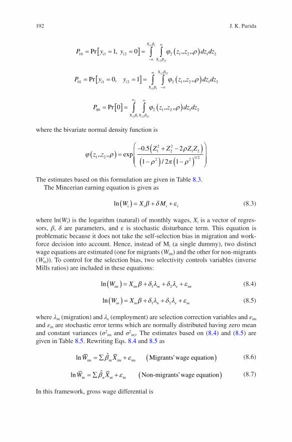
192

P y y z z dz dzi i

X

X

i

i

10 1 2 2 1 2 1 21 01 1

2 21

= = =[ ] = ( )−∞

∞

∫ ∫Pr , ,, ,,β

β

ϕ ρ

P y y z z dz dzi i

X

X

i

i

01 1 2 2 1 2 1 20 11 1

2 21

= = =[ ] = ( )∞

−∞∫ ∫Pr ,β

β

ϕ ρ,, ,,

P z z dz dzX X

00 2 1 2 1 201 1

1

2 21

= [ ] = ( )∞ ∞

∫ ∫Pri i

,, ,,β β

ϕ ρ

where the bivariate normal density function is

ϕ ρρ

ρ π ρz z

Z Z Z Z1 2

12

22

1 2

2 2 1 2

0 5 2

1 2 1,, ,,( ) =

− + −( )−( ) −( )

exp

.

//

The estimates based on this formulation are given in Table 8.3.The Mincerian earning equation is given as

ln W X Mi i i i( ) = + +β δ ε

(8.3)

where ln(Wi) is the logarithm (natural) of monthly wages, Xi is a vector of regres-sors, β, δ are parameters, and ε is stochastic disturbance term. This equation is problematic because it does not take the self-selection bias in migration and work-force decision into account. Hence, instead of Mi (a single dummy), two distinct wage equations are estimated (one for migrants (Wim) and the other for non-migrants (Win)). To control for the selection bias, two selectivity controls variables (inverse Mills ratios) are included in these equations:

ln W Xim im m e im( ) = + + +β δ λ δ λ ε1 2

(8.4)

ln W Xin in n e in( ) = + + +β δ λ δ λ ε1 2

(8.5)

where λm (migration) and λe (employment) are selection correction variables and εim and εin are stochastic error terms which are normally distributed having zero mean and constant variances (σ2

im and σ2in). The estimates based on (8.4) and (8.5) are

given in Table 8.5. Rewriting Eqs. 8.4 and 8.5 as

( )im m im imln Migrants’wage equat onˆ iW Xβ ε= ∑ +

(8.6)

( )in n ni inln Non-migrants’wage eqˆ uationW Xβ ε= ∑ +

(8.7)

In this framework, gross wage differential is

J. K. Parida

193

im in m im n inˆln ln ˆW W X Xβ β− = ∑ −∑ (8.8)

In Oaxaca decomposition method, Eq. 8.8 is expanded. For a specific endow-ment, if migrants were paid as per non-migrants wage structure (no discrimination case), then migrant’s earning function would be

im n imln ˆW Xβ= ∑ (8.9)

Subtracting Eq. (8.9) from Eq. (8.8), we get

( ) ( )

im in im m im n in n im

im in n im m im n in n im

im in m im in im m n

ˆ ˆ ˆ

ˆ ˆ ˆln ln ln

ln ln

l

ˆ

ˆn l ˆn ˆ

W W W X X X

W W X X X X

W W X X X

β β β

β β β β

β β β

− − = ∑ −∑ −∑

⇒ − −∑ = ∑ −∑ −∑

⇒ − = ∑ − +∑ −

(8.10)

Alternatively, the decomposition can also be done as

( ) ( )im in n im in in m n

ˆ ˆln n ˆlW W X X Xβ β β− = ∑ − +∑ −

(8.11)

In Eqs. (8.10) and (8.11), the terms on the right-hand side are termed as endow-ment differences and are unexplained (or discrimination) components. The determi-nation of the components of the twofold decomposition is more complicated because an estimate for the unknown nondiscriminatory coefficients vector β* is needed. Several suggestions have been made in the literature. For example, there may be reasons to assume that discrimination is directed toward one of the groups only, so that β∗ = βm or β∗ = βn (see Oaxaca 1973, who speaks of an “index number prob-lem”). If wage discrimination is only directed against one group, there will be no problem, but, there is no definite reason to assume this (Madheswaran and Attewell 2007). However, Cotton (1988) argued that the undervaluation of one group comes along with an overvaluation of the other. Reimers (1983) proposed to use the aver-age coefficients of both these groups as an estimate of the nondiscriminatory param-eters, i.e., ˆ ˆ ˆ. .β β β∗ = +0 5 0 5m n . The weight suggested by Cotton (1988) is based on the coefficient of group sizes of migrants (Nm) and non-migrants (Nn), that is,

ˆ ˆ ˆβ β β∗ =+

+

+

N

N N

N

N Nm

m nm

n

m nn

On the other hand, Neumark (1988) suggested to use coefficients of the pooled regression (β*). The empirical estimates based on the above formulations are given in Tables 8.6 and 8.7.

8 Rural-Urban Migration, Urbanization, and Wage Differentials in Urban India

194

3 Rural-Urban Migration, Urbanization, and Employment in Urban India

3.1 Rural-Urban Migration Trends in India

During the period of structural transformation in India, a large number of people out-migrated from rural areas. The number of out-migrants increased by 42 million (about 24% increase) during 1999–2000 and 2007–2008. The total number of out- migrants (within the Indian geographical territory) was about 175.3 million during 1999–2000. This increased to about 216.8 million during 2007–2008 (see Table 8.1). Both the number and percentage of out-migrants are high in relatively poor and backward states, most of which are agrarian. These states2 include Orissa (Odisha), Bihar, Chhattisgarh, Jharkhand, Madhya Pradesh, Uttar Pradesh, and Andhra Pradesh. In terms of the number of rural out-migration, Uttar Pradesh stands at the top position during 1999–2000 (35.6 million) and 2007–2008 (about 37 million) with an absolute increase in the same of 1.3 million. Maharashtra registered the second highest number of rural out-migrants followed by Andhra Pradesh during 2007–2008. In terms of the increase in out-migration, Chhattisgarh is followed by Andhra Pradesh and Bihar. It is important to note that the states with relatively high poverty headcount ratio (HCR) are showing a large number of rural out-migrations in India.

The continuous growth of rural population and lack of nonfarm employment opportunities in rural areas could have caused a huge increase in agricultural employment during 2004–2005 (see Appendix Table 8.8) with most of it being unpaid family members. However, during post 2004–2005 periods, growing mecha-nization3 (as evident from the increase in average government expenses on subsidiz-ing agricultural equipment to farmers across the states in India) in agriculture on one hand and increasing rural unemployment4 rate (current daily status (CDS)) in some states, on the other, led huge segments of the rural population to migrate. The increase in rural literacy rates (particularly due to Sarva Shiksha Abhiyan and Right to Education) during these periods would also have enabled a large segment of the rural educated youth to migrate. The rural out-migrants working in urban industry and service sectors would increase labor productivity (Lewis, 1954), and that would boost economic growth. Hence, it is important to know where these migrants go.

2 The correlation efficient between poverty headcount ratio (HCR) and rural out-migration is posi-tive (0.43)3 The correlation between mechanization in agriculture and rural out-migration is positive (0.52).4 As the correlation between rural unemployment and out-migration is positive (0.06).

J. K. Parida

195Ta

ble

8.1

Stat

e-w

ise

rura

l out

-mig

ratio

n an

d th

e fa

ctor

s af

fect

ing

it in

sel

ecte

d In

dian

sta

tes,

199

9–20

00 a

nd 2

007–

2008

Nam

e of

the

stat

e

Pove

rty

HC

R

in 2

004–

2005

(%)

Agr

icul

tura

l

wag

ea

rate

s (R

s.)

Avg

. exp

ense

s

on m

echa

niza

tionb

(Rs.

in la

kh)

Rur

al li

tera

cy r

ates

(%

)

Rur

al u

nem

ploy

men

t

(CD

S) r

ates

(%

)

Num

ber

of p

eopl

e ou

t- m

igra

ted

from

rur

al a

reas

(mill

ion)

Rur

al o

ut- m

igra

tion

rate

(%)

1999

–200

020

07–2

008

1999

–200

020

07–2

008

1999

–200

020

07–2

008

Cha

nge

1999

–200

020

07–2

008

And

hra

Prad

esh

29.9

112

1335

42.2

49.6

1.8

5.3

12.5

18.7

6.2

22.7

29.7

Bih

ar54

.411

461

335

.146

.41.

03.

612

.814

.41.

615

.120

.3

Guj

arat

31.8

100

299

54.3

60.5

0.8

2.1

9.3

11.0

1.7

28.9

32.1

Har

yana

24.1

167.

2328

856

.061

.20.

82.

43.

75.

11.

425

.231

.1

Kar

nata

ka33

.413

3.8

988

48.2

58.2

0.8

3.7

9.9

10.6

0.7

26.4

29.3

Ker

ala

19.7

200

3181

.685

.24.

36.

76.

57.

71.

230

.130

.1

Mad

hya

Prad

esh

48.6

114

368

43.9

57.7

0.8

2.9

14.7

14.0

−0.

723

.429

.1

Mah

aras

htra

38.1

120

295

58.4

67.6

1.4

4.4

18.7

20.9

2.2

32.3

34.0

Ori

ssa

57.2

9054

046

.857

.21.

33.

47.

09.

72.

722

.729

.0

Punj

ab20

.914

811

057

.863

.30.

93.

74.

55.

61.

129

.032

.5

Raj

asth

an34

.413

551

240

.147

.40.

71.

910

.614

.74.

128

.231

.8

Tam

il N

adu

28.9

100

259

59.2

64.8

1.8

10.8

10.1

9.7

−0.

425

.723

.4

Utta

r Pr

ades

h40

.910

030

043

.351

.10.

61.

835

.636

.91.

326

.126

.3

Wes

t Ben

gal

34.3

120.

526

954

.264

.62.

65.

413

.316

.73.

421

.625

.3

Del

hi13

.123

46

7376

.31.

41.

30.

60.

6−

0.1

22.2

61.1

Chh

attis

garh

49.4

100

194

NA

58.5

NA

2.1

NA

6.4

6.4

NA

30.0

Jhar

khan

d45

.311

125

NA

54.3

NA

3.9

NA

3.9

3.9

NA

17.9

Utta

rakh

and

32.7

113.

6819

3N

A63

.2N

A3.

0N

A2.

32.

3N

A33

.4

Oth

er U

Ts

NA

NA

864

.271

.42.

17.

70.

30.

30.

044

.226

.2

All

Indi

a37

.2N

A26

3.1

48.9

58.1

1.3

3.8

175.

321

6.8

41.5

24.0

27.1

Sour

ce: T

hese

dat

a ar

e ta

ken

from

mul

tiple

sou

rces

lik

e Pl

anni

ng C

omm

issi

on (

pove

rty)

and

Min

istr

y of

Agr

icul

ture

(w

ages

and

exp

ense

s) a

nd t

he r

est

are

estim

ated

usi

ng N

SS u

nit

data

. The

tabl

e re

port

s st

atis

tics

for

stat

es w

here

the

sam

ple

size

of

NSS

dat

a is

suf

ficie

ntly

larg

e.

Not

e: N

A N

ot a

vaila

ble

a Thi

s da

ta is

take

n fr

om s

tate

-wis

e m

inim

um w

ages

(da

ily)

for

unsk

illed

agr

icul

tura

l wor

kers

’ M

inim

um W

ages

Act

, 194

8 in

Ind

ia (

31 M

arch

201

1). I

n th

e st

ates

whe

re m

ore

than

one

wag

e ra

tes

prev

ail t

he h

ighe

st v

alue

of

the

wag

e ra

te is

take

n in

to c

onsi

dera

tion

b Thi

s da

ta is

use

d as

a p

roxy

. The

sta

te-w

ise

finan

cial

out

lay

for A

gric

ultu

ral E

quip

men

t to

Farm

ers

at S

ubsi

dize

d R

ates

is u

sed

for

mec

hani

zatio

n (t

his

data

incl

udes

all

the

expe

nses

mad

e un

der

Cen

tral

ly S

pons

ored

Sch

emes

of

Mac

ro M

anag

emen

t in

Indi

a du

ring

200

3–20

04 to

200

6–20

07)

8 Rural-Urban Migration, Urbanization, and Wage Differentials in Urban India

196

3.2 Rural to Urban Migration and Urbanization in India

A huge share of the rural out-migrants is residing in urban areas, as the absolute number of in-migrants in urban India increased by about 23.2 million (from 93.6 million in 1999–2000 to 116.8 million in 2007–2008) or about 3 million per annum (see Table 8.2). The census data also reflect the same (Fig. 8.1). According to census population data, while the about 40 million growth in urban population is due to natural growth, about 22 million is due to rural to urban migration during 2001 and 2011. The share of natural growth in the urban population in India decreased from 59% to 44%, while the share of migrant population increased from 21% to 24% (Fig. 8.1).

Migrants contributed massively to the increase in urban population (Fig. 8.1) in recent years, which is clearly reflected with the increasing share of migrants in the urban population across the states of India. The share of migrants increased from 33.3% in 1990–2000 to 35.5% in 2007–2008. In Maharashtra, Delhi, Haryana, Andhra Pradesh, Orissa, Chhattisgarh, and Uttarakhand, this share is more than 40% (Table 8.2), while in a few other states, this share is above the national average in 2007–2008. In India, out of the total migrants in urban areas, about 60% have come from rural areas. A similar observation is made across the states of India. This shows the “Lewisian transition” occurring during the post 2004–2005 periods in India.

The states receiving the highest numbers of urban in-migrants are Maharashtra (20.3 million), Uttar Pradesh (13.3 million), Andhra Pradesh (about 10.5 million), Gujarat (8.3 million), Tamil Nadu (8.3 million), West Bengal (about 8.2 million), Karnataka (about 6.4 million), Delhi (about 6.2 million), and Rajasthan (6.1 million). But the states that registered the highest increase in the absolute number of migrants include Delhi (about 6 million), Maharashtra (3.25 million), Gujarat (2.2 million), Rajasthan (1.66 million), Andhra Pradesh (1.5 million), West Bengal (1.23 million), and Karnataka (1.22 million). Most of the large metro and medium-sized cities of India belong to these states. This clearly indicates the fact that most rural migrants are attracted to both large and medium-sized cities. However, the natural growth of population in small and medium cities is probably higher than that of the big cities like Mumbai, Delhi, Kolkata, and Chennai. This is clearly reflected in Fig. 8.2.

3.3 Rural to Urban Migration and Urban Employment in India

The share of migrants in the urban workforce is greater than that of their share in the total urban population. During 1999–2000 and 2007–2008, 37% of the total urban workers were migrants. The share of migrants in the workforce was highest (about 59%) in Delhi and Maharashtra (about 50%). It is important to note that two of the major metro cities, viz., New Delhi and Mumbai, are in these states. The share of migrants in the workforce is also more than the national average in most of the

J. K. Parida

197Ta

ble

8.2

Stat

e-w

ise

in-m

igra

nts

and

thei

r em

ploy

men

t pat

tern

s in

sel

ecte

d ur

ban

stat

es in

Ind

ia, 1

999–

2000

and

200

7–20

08

Nam

e of

the

stat

e

Tota

l num

ber

of u

rban

in

-mig

rant

s (i

n m

illio

n)%

of

mig

rant

s in

ur

ban

popu

latio

n

% o

f ru

ral-

urba

n m

igra

nts

in to

tal

mig

ratio

n

% o

f m

igra

nts

in

the

urba

n w

orkf

orce

(U

P+SS

)

Dis

trib

utio

n of

tota

l mig

rant

wor

kers

in u

rban

are

as

by th

eir

type

s of

em

ploy

men

t (%

)

Self

-em

ploy

edR

egul

ar w

orke

rsC

asua

l wor

kers

1999

–20

0020

07–

2008

Cha

nge

1999

–20

0020

07–

2008

1999

–20

0020

07–

2008

1999

–20

0020

07–

2008

1999

–20

0020

07–

2008

1999

–20

0020

07–

2008

1999

–20

0020

07–

2008

And

hra

Prad

esh

8.9

10.5

1.53

3540

6572

4147

3537

4137

2427

Bih

ar3.

23.

0−

0.13

2235

6572

1929

4253

5036

812

Guj

arat

6.1

8.3

2.20

3637

5868

3840

3440

3940

2720

Har

yana

3.0

3.0

0.05

4643

5664

5247

3638

5255

128

Kar

nata

ka5.

26.

41.

2233

3250

5737

3433

2650

5617

19K

eral

a3.

03.

30.

2736

3462

6139

3542

3638

3521

29M

adhy

a Pr

ades

h5.

95.

9−

0.01

2934

5655

3030

3744

4234

2123

Mah

aras

htra

17.0

20.3

3.25

4143

6158

5250

3033

5650

1416

Ori

ssa

2.4

2.7

0.24

3644

7562

4242

3640

5150

1310

Punj

ab3.

13.

60.

4538

3856

5042

3536

3052

5912

11R

ajas

than

4.4

6.1

1.66

3737

5966

4340

4449

4336

1316

Tam

il N

adu

8.2

8.3

0.08

3324

5058

3725

3336

4937

1727

Utta

r Pr

ades

h13

.513

.3−

0.21

3431

6257

3725

4748

4541

911

Wes

t Ben

gal

7.0

8.2

1.23

3736

4849

4033

3944

4740

1416

Del

hi0.

36.

25.

913

4380

595

5921

3369

5910

8C

hhat

tisga

rhN

A2.

12.

05N

A45

NA

63N

A49

NA

27N

A49

NA

24Jh

arkh

and

NA

1.2

1.24

NA

25N

A51

NA

27N

A37

NA

38N

A25

Utta

rakh

and

NA

1.3

1.26

NA

49N

A46

NA

53N

A41

NA

47N

A13

Oth

er U

Ts

0.6

0.8

0.22

4146

5058

5353

3024

6253

823

All

Indi

a93

.611

6.8

23.2

3336

5960

3837

3637

4845

1618

Sour

ce: C

alcu

latio

n us

ing

NSS

uni

t-le

vel d

ata,

55t

h (1

999–

2000

) an

d 64

th (

2007

–200

8) m

igra

tion-

spec

ific

roun

ds. T

he ta

ble

repo

rts

stat

istic

s fo

r st

ates

whe

re th

e sa

mpl

e si

ze o

f N

SS d

ata

is s

uffic

ient

ly la

rge.

Not

e: N

A N

ot a

vaila

ble

8 Rural-Urban Migration, Urbanization, and Wage Differentials in Urban India

198

states that registered relatively higher rural out-migration. Out of the total migrant workers, the percentage share of self-employed was about 36%, regular-salaried workers was about 48%, and casual workers was 16%, respectively, in 1999–2000.

The percentage share of the self-employed increased to 37%, regular-salaried workers declined to 45%, and casual workers increased to 18%, respectively, in 2007–2008. The share of regular-salaried workers declined across the states of India. During 1999–2000 and 2007–2008, the share of regular workers declined from 69% to 59% in Delhi, from 56% to 50% in Maharashtra, from 49% to 37% in Tamil Nadu, from 47% to 40% in West Bengal, from 45% to 41% in Uttar Pradesh, from 41% to

100

90

80

70

70%

60%

50%

40%

30%

20%

10%

0%

60

50

40

30

20

10

01961-71

1961-71

% S

hare

of

Urb

an P

opul

atio

n G

row

th

Net Rural to Urban migration New towns less declassified towns

Natural Growth Expansion in urban area / agglomeration

Urb

an P

opul

atio

n G

row

th (

in m

illio

n)

1971-81

1971-81

1981-91

1981-91

1991-2001

1991-2001

2001-2011

2001-2011

Fig. 8.1 Share of urban population growth in India, 1961–2011. Note: The colors in the top panel (bar graph) correspond to the color in the bottom panel (line graph). (Source: IIHS analysis based on Census of India, 2011 (Indian Institute of Human Settlement 2011, page 43))

J. K. Parida

199

37% in Andhra Pradesh, and from 40% to 39% in Gujarat, respectively. An increas-ing share of self-employed and casual employment along with a corresponding declining share of regular workers indicate that there was a high inflow of low- skilled and unskilled workers into the urban areas, of which most are from rural areas. The unskilled and semiskilled workers from rural areas are most likely to work as either casual laborers or be self-employed by opening small shops or engaging themselves in petty trade, street vending, rickshaw pulling or auto rickshaw driving, etc.

The share of regular migrant workers, however, increased in a few states like Punjab, Haryana, and Karnataka. It might be due to the fact that the emerging techno-cities like Bangalore (Bengaluru) in Karnataka, Gurgaon in Haryana, and Chandigarh in Punjab attracted lots of modern service sector workers in recent years. Most of them are expected to be highly qualified and skilled in their respec-tive domains. However, earlier studies on migrant labor like Connell et al. (1976) and Joshi and Joshi (1976) have found that relatively poorer households are mainly participating in the rural-urban migration process. These migrants move either per-manently or semi-permanently, and most of them are engaged in the informal/unor-ganized sector. The findings of Srivastava and Bhattacharya (2002) and Deshingkar and Akter (2009) also show increased rural-urban employment in India. Given the intricacy of this phenomenon, it is important to find out the individual- and house-hold-level factors that drive the rural to urban migration decision of individuals and their workforce participation in urban India.

01901 1911 1921 1931 1941 1951 1961 1971 1981 1991 2001 2011

Greater Mumbai UA

Delhi UA

Kolkata UA

Chennai UA

Bangalore UA

Hyderabad UA

Ahmedabad UA

Pune UA

Surat UA

Jaipur (M Corp.)

Kanpur UA

Lucknow UA

Nagpur UA

Ghaziabad UA

Indore UA

Coimbatore UA

Kochi UA

Patna UA

Kozhikode UA

Bhopal UA2

4

6

Popu

latio

n in

mill

ions

8

10

12

14

16

18

20

Fig. 8.2 Total population in the major cities of India. Note: UA stands for urban area. (Source: IIHS analysis based on Census of India, 2011 (Indian Institute of Human Settlement 2011, page 13))

8 Rural-Urban Migration, Urbanization, and Wage Differentials in Urban India

200

The estimated results of migration and labor force participation decisions are given in Table 8.3. A positive and significant ρ suggests that both these decisions are influenced by the same set of random forces. A positive sign indicates that unob-servables, those that determine labor force participation decision, are likely to posi-tively influence migration decision too. Age, sex, marital status, education, landholdings, standard of living, castes, and religion influence both decisions.

A positive sign for the age coefficient and negative sign for age squared terms reflect the true labor market phenomenon. With increasing age, individuals’ chance of migrating to urban areas increases and hence their participation in the urban workforce. However, after a certain age, they tend to withdraw from the workforce and are less likely to migrate. Sex dummy is negative in the migration equation and it is positive in the labor force participation equation. This is obvious as Indian females (reference category) migrate for marriage in increasing numbers to accom-pany their husbands or go to their in-law’s place. Nevertheless, the coefficient of migration and sex interaction dummy reflects that the probability of labor force participation of male migrants is relatively higher than their female counterparts. The coefficient of marital status dummy indicates that other things being constant, individuals currently married, on average, migrate more and are likely to participate in the workforce as compared to their unmarried (reference category) counterparts. This precisely reflects the Indian society, in which the household responsibility of individuals normally increases after marriage. The coefficients of widowed and divorced/separated are showing positive signs, reflecting greater participation as compared to unmarried individuals.

The unexpected negative signs of general education dummies (illiterates are the reference category) indicate the fact that during these transition phases, more chil-dren are participating in general education and hence are less likely to participate in migration and the workforce. This result supports the findings of Rangarajan et al. (2011), Kannan and Raveendran (2012), Thomas (2012), and Mehrotra et al. (2014) which suggest that the recent increase in enrollments at various levels restricts the growth of the labor force size and hence the workforce. However, individuals with better skills (those having either a below graduate- or a graduate-level technical degree) are more likely to participate in both the decisions as compared to individu-als with no technical education (reference category). This result is as expected in the period of a high growth regime.

The coefficients of landholding dummies (reference category landless) indicate that the probability of migration among the landless is higher as compared to others. This is again a clear indication of the “Lewisian transition” in India, as the coeffi-cients of landholding dummies are negative and are increasing with the increase in the size of holdings. The coefficients of monthly per capita expenditure (MPCE) dummies, on the other hand, explain the aspiration aspect of rural to urban migra-tion, as these coefficients are showing positive signs with a relatively higher value of the coefficients in higher MPCE categories. Despite a high probability to migrate, few other caste (mostly general castes) people have a high chance of entering the labor market as compared to scheduled caste (SC), scheduled tribes (ST), and other backward classes (OBC). While comparing across religion categories, it is found

J. K. Parida

201

Tabl

e 8.

3 Se

emin

gly

unre

late

d bi

vari

ate

prob

it es

timat

es f

or m

igra

tion

deci

sion

and

wor

kfor

ce p

artic

ipat

ion

in u

rban

Ind

ia

Var

iabl

es

1999

–200

020

07–2

008

Mig

ratio

nW

orkf

orce

par

ticip

atio

nM

igra

tion

Wor

kfor

ce p

artic

ipat

ion

Coe

ffici

ent

Z-v

alue

sC

oeffi

cien

tZ

-val

ues

Coe

ffici

ent

Z-v

alue

sC

oeffi

cien

tZ

-val

ues

Inte

rcep

t1.

821

−88

.5−

4.42

1−

125

−1.

315

−66

.6−

4.34

7−

109.

1A

ge0.

042

50.4

90.

223

132

0.04

147

.30.

232

126.

3A

ge s

quar

e−

0.00

05−

46.8

−0.

003

−12

3−

0.00

05−

47.8

−0.

003

−12

0.0

Prim

ary

−0.

118

−13

.8−

0.22

7−

20−

0.11

7−

12.8

−0.

161

−13

.3Se

cond

ary

−0.

180

−19

.3−

0.32

−28

−0.

226

−23

.4−

0.32

9−

28.1

Hig

her

seco

ndar

y−

0.23

4−

17.3

−0.

508

−33

−0.

283

−21

.3−

0.51

5−

34.2

Gra

duat

e an

d ab

ove

−0.

320

−24

.5−

0.19

3−

13−

0.37

6−

28.4

−0.

262

−17

.7Te

ched

u. b

elow

gra

duat

e0.

237

13.0

90.

421

190.

272

10.0

0.58

517

.8Te

ched

u. g

radu

ate

and

abov

e0.

194

5.24

0.28

86.

50.

211

7.6

0.43

012

.7M

ale

−0.

453

−72

.91.

393

85−

0.54

2−

84.8

1.27

974

.1C

urre

ntly

mar

ried

0.65

661

.04

0.43

833

0.74

266

.70.

359

26.2

Wid

owed

0.58

630

.88

0.64

527

0.73

737

.90.

606

25.4

Div

orce

d/se

para

ted

0.10

62.

150.

756

130.

368

7.5

0.80

414

.2L

andh

oldi

ng <

1 h

ecta

re−

0.12

2−

18.3

−0.

246

−35

.4L

andh

oldi

ng 1

to 2

hec

tare

s−

0.18

8−

8.97

−0.

245

−13

.1L

andh

oldi

ng 2

to 4

hec

tare

s−

0.09

7−

3.8

−0.

146

−5.

5L

andh

oldi

ng 4

to 8

hec

tare

s−

0.02

4−

0.71

−0.

218

−5.

3L

andh

oldi

ng >

8 h

ecta

res

−0.

285

−6.

7−

0.26

1−

5.6

MPC

E c

lass

20.

110

9.18

0.11

411

.9M

PCE

cla

ss 3

0.21

917

.94

0.25

125

.3M

PCE

cla

ss 4

0.39

031

.40.

430

42.4

MPC

E c

lass

50.

582

45.3

10.

611

56.3

SC0.

288

17.9

10.

061

3.5

0.22

013

.10.

096

5.2

(con

tinue

d)

8 Rural-Urban Migration, Urbanization, and Wage Differentials in Urban India

202

Tabl

e 8.

3 (c

ontin

ued)

Var

iabl

es

1999

–200

020

07–2

008

Mig

ratio

nW

orkf

orce

par

ticip

atio

nM

igra

tion

Wor

kfor

ce p

artic

ipat

ion

Coe

ffici

ent

Z-v

alue

sC

oeffi

cien

tZ

-val

ues

Coe

ffici

ent

Z-v

alue

sC

oeffi

cien

tZ

-val

ues

OB

C0.

322

21.7

90.

065

4.1

0.23

315

.20.

045

2.7

Oth

er c

aste

s0.

345

24.2

7−

0.11

8−

7.7

0.26

717

.5−

0.08

2−

4.8

Hin

du0.

172

15.3

70.

034

2.7

−0.

302

−34

.0−

0.06

6−

6.4

Mus

lims

−0.

163

−12

.3−

0.07

−4.

7−

0.23

7−

14.3

0.08

64.

7M

igra

nt−

1.18

1−

52−

1.20

0−

49.9

Mal

e m

igra

nt0.

413

270.

417

27.7

Ath

rho

(z-v

alue

)0.

575(

30.9

1)0.

626

(29.

7) R

ho0.

519

0.55

6W

ald

chi2

(45)

1063

80.7

110

4242

.62

Wal

d te

st (

rho=

0)ch

i2(1

) =

955

.423

chi2

(1)

= 8

82.0

5N

o. o

f ob

s.22

8235

2086

08

Sour

ce: A

utho

r’s

estim

atio

n ba

sed

on N

SS u

nit d

ata

(55t

h an

d 64

th)

mig

ratio

n ro

unds

J. K. Parida

203

that the probability of migration and workforce participation among Hindus is high in comparison to Muslims and other religions (reference category).

Since a huge number of persons migrated from rural areas to urban India during the periods of high economic growth, it is important to know whether this transition brings about any change in their productivity in the urban areas. The productivity of the migrant and non-migrant workers can be measured through the estimation of their daily wages/earnings (a proxy measure).

4 Migration, Wage Determinants, and Differentials in Urban India

When the log of monthly wage is plotted (see Fig. 8.3), it is observed that migrants’ wage distribution is positioned rightward to the non-migrants’ wage distribution. This suggests that migrants, on average, tend to earn higher than non-migrants. To have a clear picture of this differential, we plot the earnings distributions by their employment status. It is clear (Fig. 8.3, Part B) that, on average, migrant regular employees are better paid as compared to their non-migrant counterparts, as their wage distribution is placed to the right of non-migrants’ wage distribution. However, the wage distribution of casual workers shows an interesting pattern particularly in 2007–2008. The earnings distribution of migrants is slightly placed toward the left of non-migrants’ distribution in the lower quintiles (well before median wage), but it is located toward the right to the non-migrants’ wage distribution throughout the upper quintiles (including the median wage). This indicates the fact that even within casual (informal) employment, migrant workers are better paid than their non- migrant counterparts.

The average daily wages of migrant and non-migrant, regular-salaried and casual workers are given in Table 8.4 by industry and occupation. From the figures of the average daily wages of migrants and non-migrants in various industries, it is clear that except in the agriculture and allied sector in 2007–2008 and casual employment in the real estate (only in 2007–2008) and other service sectors, in all other indus-tries, irrespective of the types of employment, migrant workers, on average, earn more than that of their non-migrant counterparts. The mean wage difference between migrants and non-migrants within regular-salaried employment was about Rs. 23, while in the case of casual employment, it was about Rs. 2.50 during 1999–2000. This difference was also noticed during 2007–2008 for regular-salaried workers, but the reverse was seen for casual workers. The mean wage difference between migrants and non-migrants within regular-salaried employment was about Rs. 55, while in the case of casual employment, it was negative Rs. 2.70 in 2007–2008.

During 1999–2000, migrant casual workers in the agriculture and allied sector (Rs. 6) and other service (Rs. 5) sectors, on average, earn less than non-migrants. However, in all other sectors, regardless of the types of employment, the absolute

8 Rural-Urban Migration, Urbanization, and Wage Differentials in Urban India

204

difference in average daily wages favors the migrants. The mean wage difference was highest among regular-salaried workers in real estate and finance (Rs. 83); min-ing and quarrying (Rs. 52); hotel, trade, and restaurant (Rs. 22); transport and com-munication (Rs. 21); manufacturing (Rs. 19); and electricity, gas, and water (Rs. 18), respectively. Further, within casual employment in the mining and quarrying and real estate and finance sectors, it is also observed that migrant workers earn Rs. 26 and Rs. 17, respectively, more than non-migrants.

During 2007–2008, the mean wage difference within regular-salaried employ-ment favors the migrants in all sectors but agricultural and allied. And within casual employment, the mean wage difference favors the migrants in all sectors except agricultural and allied, real estate and finance, and other service sectors. The aver-age wage difference between migrants and non-migrants within regular-salaried workers was highest in sectors like real estate and finance (Rs. 160); electricity, gas, and water (Rs. 98); transport and communication (Rs. 69); construction (Rs. 56);

Part AAll workers, 1999-00 All workers, 2007-08

Part BRegular salaried workers, 1999-00 Regular salaried workers, 2007-08

Part CCasual workers, 1999-00 Casual workers, 2007-08

0.1

.2.3

.4.5

4 6 8 10 12x

Migrant Non-migrant

0.1

.2.3

.4.5

kden

sity

logm

wag

e

5 10 15x

Migrants Non-migrant

0.1

.2.3

.4.5

4 6 8 10 12x

Migrant Non-migrant

0.1

.2.3

.4

kden

sity

logm

wag

e

5 10 15x

Migrant Non-migrant

0.2

.4.6

.8

kden

sity

logm

wag

ekd

ensi

ty lo

gmw

age

kden

sity

logm

wag

e

4 6 8 10 12x

Migrant Non-migrant

0.2

.4.6

.81

kden

sity

logm

wag

e

5 6 7 8 9 10x

Migrant Non-migrant

Fig 8.3 Distribution of log monthly wage/earning of migrants and non-migrants’ in urban India, 1999–2000 and 2007–2008. (Source: Author’s estimation based on NSS unit data (55th and 64th) migration rounds)

J. K. Parida

205

Table 8.4 Average daily nominal wages (Rs.) of migrants and non-migrants by industry of employment and occupation in urban India, 1999–2000 and 2007–2008

Categories

1999–2000 2007–2008

MigrantNon- migrant Diff. Migrant

Non- migrant Diff.

Industry of employment

Regular- salaried workers

Agriculture and allied

107.12 94.24 12.88 109.99 118.53 −8.54

Mining and quarrying

238.09 186.49 51.60 411.78 407.84 3.94

Manufacturing 145.43 126.58 18.85 223.77 186.25 37.52Electricity, gas, and water

256.94 238.89 18.05 480.84 382.98 97.86

Construction industry

136.53 128.34 8.18 267.53 211.33 56.20

Hotel, trade, and restaurant

111.74 89.37 22.36 170.95 135.15 35.80

Transport and communication

173.73 152.28 21.46 292.91 223.65 69.27

Real estate and finance

312.20 229.06 83.14 588.95 428.79 160.16

Other service 196.74 186.73 10.01 301.14 271.57 29.57Total 174.81 151.61 23.20 292.60 237.18 55.43

Casual workers

Agriculture and allied

37.35 43.48 −6.12 55.00 78.60 −23.60

Mining and quarrying

92.02 66.24 25.78 115.40 111.93 3.47

Manufacturing 68.21 59.26 8.95 94.06 87.25 6.80Electricity, gas, and water

85.06 76.28 8.79 103.88 90.00 13.88

Construction industry

69.11 66.64 2.47 108.30 106.49 1.80

Hotel, trade, and restaurant

59.84 53.16 6.69 103.30 97.03 6.28

Transport and communication

68.35 63.05 5.31 114.15 113.78 0.37

Real estate and finance

77.32 60.42 16.90 82.51 104.35 −21.84

Other service 40.43 45.50 −5.07 68.18 81.92 −13.74Total 59.73 57.24 2.49 93.50 96.18 −2.69

(continued)

8 Rural-Urban Migration, Urbanization, and Wage Differentials in Urban India

206

manufacturing (Rs. 37.50); and hotel, trade, and restaurant (Rs. 36), respectively. Within casual employment, this difference was highest in electricity, gas, and water (Rs. 14); manufacturing (Rs. 7); hotel, trade, and restaurant (Rs. 6); and construc-tion (Rs. 2). The negative values in the agricultural and allied (Rs. 24), real estate and finance (Rs. 22), and other service (Rs. 14) sectors lead to a Rs. 2.70 (negligi-ble) wage difference in favor of non-migrant workers. These negligible differences within casual employment, however, do not affect the overall wage difference.

A similar conclusion can be drawn from the occupation-wise average daily wages of migrant and non-migrant workers. Within regular-salaried employment, migrant workers earn more than non-migrants in all occupations, with the only exception being agriculture and fishery in 2007–2008, while migrant workers within

Table 8.4 (continued)

Categories

1999–2000 2007–2008

MigrantNon- migrant Diff. Migrant

Non- migrant Diff.

Occupations Regular- salaried workers

Professional and admin

303.81 257.79 46.02 549.91 438.18 111.72

Clerical jobs 197.10 186.38 10.71 308.41 281.18 27.22Sales and services

102.12 94.72 7.40 178.53 146.42 32.11

Craft and trade workers

107.15 93.31 13.84 183.39 150.79 32.60

Plant and machine operators

143.51 112.51 30.99 200.03 178.76 21.27

Elementary occupation

127.66 116.76 10.90 120.82 118.16 2.66

Agriculture and fishery

110.42 104.09 6.32 122.32 167.49 −45.17

Total 174.93 151.72 23.21 292.78 237.23 55.55 Casual workers

Professional and admin

91.89 75.17 16.72 151.62 133.42 18.20

Clerical jobs 78.49 53.92 24.57 240.71 109.56 131.15Sales and services

47.19 47.86 −0.68 85.17 101.11 −15.94

Craft and trade workers

62.37 59.31 3.05 110.65 107.58 3.07

Plant and machine operators

76.77 60.49 16.28 107.45 103.74 3.71

Elementary occupation

67.11 62.13 4.98 84.26 87.13 −2.87

Agriculture and fishery

37.79 45.06 −7.27 100.85 116.54 −15.69

Total 59.85 57.30 2.54 93.30 96.22 −2.69

Source: Author’s estimation based on NSS unit data (55th and 64th) migration rounds

J. K. Parida

207

casual employment earn more than non-migrants in all other occupations except agriculture and fishery, sales and services, and elementary occupations. It can be noted that the average daily wage/earning difference is highest among highly skilled workers and vice versa. Within regular-salaried employment, the absolute wage dif-ference was highest among professionals and administrative workers (Rs. 46 in 1999–2000 and Rs. 112 in 2007–2008), and this is followed by craft and trade work-ers (Rs. 14 in 1999–2000 and Rs. 32.60 in 2007–2008), plant and machine operators (Rs. 31 in 1999–2000 and Rs. 21 in 2007–2008), sales and services (Rs 7 in 1999–2000 and Rs. 32 in 2007–2008), and clerical (Rs 11 in 1999–2000 and Rs. 27 in 2007–2008) occupations, respectively. A similar observation is made in the case of casual employment with a few exceptions.

In a transition phase that the Indian economy is presently going through, this wage difference is anticipated as it leads to more economic growth. Rural to urban migration would enhance economic growth if and only if the productivity of the migrants increased because of migration. Before drawing any conclusion, it is important to know the factors determining these wage/earning differences in urban India.

Migrants’ and non-migrants’ wage equations are specified to include a set indi-vidual and establishment variables explaining the earning/wage ratio. The estimated results (see Table 8.5) show that the overall model is significant. The statistically sig-nificant coefficients of the selectivity variables (hence the absence of these selection variables in the model would have produced bias estimates) imply that there exist correlations between some unobservable factors that are likely to influence migration, workforce participation as well as wage/earning functions simultaneously.

Individual characteristics like age, sex, level of education, marital status, etc. influenced wage/earning. Age (a proxy for experience) positively affects wages, and it reflects the true labor market phenomenon, as its squared term has produced a negative sign in both the equations, implying negative returns to experience in the most advanced ages of the life cycle. The coefficients of the male dummy in both the equations imply that male workers (both migrants and non-migrants) are earn-ing more as compared to female workers. This is as expected as earlier studies (Duraisamy 2002; Mukherjee 2007; Barua 2010; and Das 2012) have found that men are likely to earn more than women in India. Furthermore, a relative stronger coefficient in the migrants’ equation implies that the male-female wage gap is high in the case of migrants as compared to non-migrants.

The level of education turned out to be the most important determinant of migrant and non-migrant wages in urban India. The statistically significant and expected signs of the six (four general education and two technical education) education dummies confirmed a positive relation between wage and education. The greater the levels of education, the greater will be the wage income. A relatively stronger coef-ficient of the general education dummy in the case of migrants implies that with the same level of general education, migrants tend to earn more. A similar result is found when the coefficients of different occupations are compared. The workers in agriculture and fishery and in elementary occupations earn less than that of those who are engaged in semiskilled and highly skilled occupations. This result is as expected.

8 Rural-Urban Migration, Urbanization, and Wage Differentials in Urban India

208

Tabl

e 8.

5 M

igra

nt a

nd n

on-m

igra

nt e

arni

ng e

quat

ions

in u

rban

Ind

ia

Var

iabl

es

1999

–200

020

07–2

008

Mig

rant

Non

-mig

rant

Mig

rant

Non

-mig

rant

Coe

ffici

ents

t-va

lues

Coe

ffici

ents

t-va

lues

Coe

ffici

ents

t-va

lues

Coe

ffici

ents

t-va

lues

Inte

rcep

t7.

299

.57.

112

4.8

7.2

120.

87.

114

7.2

Age

0.03

412

.30.

040

18.8

0.02

89.

80.

034

15.3

Age

squ

are

−0.

0003

−7.

7−

0.00

03−

13.2

−0.

0001

−4.

2−

0.00

02−

8.8

Mal

e0.

552

41.6

0.51

641

.00.

728

54.6

0.65

348

.7C

urre

ntly

mar

ried

−0.

106

−6.

3−

0.11

0−

8.5

−0.

173

−10

.8−

0.14

7−

11.2

Wid

owed

−0.

248

−8.

9−

0.27

1−

10.7

−0.

245

−8.

8−

0.23

9−

8.9

Div

orce

d/se

para

ted

−0.

305

−5.

0−

0.29

2−

6.8

−0.

382

−6.

9−

0.23

3−

4.8

Prim

ary

0.24

915

.70.

265

21.3

0.26

115

.70.

271

19.5

Seco

ndar

y0.

490

30.9

0.47

037

.60.

496

29.8

0.44

832

.5H

ighe

r se

cond

ary

0.67

932

.60.

651

37.3

0.68

232

.20.

649

35.7

Gra

duat

e an

d ab

ove

0.92

246

.70.

933

55.7

0.97

945

.70.

948

51.5

Tech

edu.

bel

ow g

radu

ate

0.02

41.

5−

0.01

8−

1.1

−0.

012

−0.

50.

018

0.8

Tech

edu.

gra

duat

e an

d ab

ove

0.29

39.

10.

327

9.8

0.28

312

.80.

285

12.4

SC−

0.08

0−

3.7

−0.

168

−10

.4−

0.17

9−

8.2

−0.

184

−10

.6O

BC

−0.

228

−11

.3−

0.27

6−

18.0

−0.

247

−12

.2−

0.25

8−

15.8

Oth

ers

−0.

211

−10

.6−

0.27

7−

18.1

−0.

268

−13

.3−

0.23

5−

14.1

Hin

du−

0.23

8−

14.6

−0.

291

−21

.70.

277

16.1

0.24

919

.9M

uslim

s−

0.00

6−

0.3

−0.

049

−3.

10.

254

12.3

0.31

218

.5M

anuf

actu

ring

0.40

97.

20.

417

9.4

0.46

510

.80.

578

14.7

Min

ing

and

quar

ryin

g−

0.03

3−

0.8

−0.

015

−0.

5−

0.05

47−

2.0

−0.

058

−2.

8E

lect

rici

ty, g

as, a

nd w

ater

0.35

06.

60.

364

7.9

0.39

08.

60.

316

7.2

Con

stru

ctio

n in

dust

ry0.

216

4.9

0.21

46.

40.

227

8.3

0.13

67.

0H

otel

, tra

de, a

nd r

esta

uran

t0.

020

0.5

−0.

0002

0.0

−0.

059

−2.

0−

0.11

4−

5.0

Tra

nspo

rt a

nd c

omm

.0.

209

4.8

0.20

66.

10.

201

6.7

0.12

95.

6

J. K. Parida

209

Rea

l est

ate

and

finan

ce0.

294

6.4

0.19

85.

40.

222

7.1

0.18

57.

3O

ther

ser

vice

0.18

84.

50.

198

6.2

0.06

62.

50.

077

3.7

Prof

essi

onal

and

adm

in0.

230

11.5

0.18

110

.70.

587

30.8

0.52

231

.0C

leri

cal j

obs

0.15

98.

60.

168

11.3

0.51

123

.60.

485

27.0

Sale

s an

d se

rvic

es−

0.27

2−

15.7

−0.

223

−15

.60.

105

5.8

0.07

04.

3A

gric

ultu

re a

nd fi

sher

y−

0.06

5−

1.7

−0.

001

0.0

0.34

27.

00.

269

8.2

Cra

ft a

nd tr

ade

wor

kers

−0.

078

−3.

8−

0.11

7−

6.8

0.13

68.

50.

111

8.6

Plan

t and

mac

hine

ope

rato

rs0.

037

1.9

−0.

019

−1.

30.

184

9.5

0.18

210

.8L

ambd

a m

igra

tion

−0.

610

−39

.6−

0.56

7−

46.9

−0.

703

−48

.8−

0.56

4−

49.5

Lam

bda

empl

oym

ent

−11

59.8

−30

.7−

577.

7−

31.2

−14

.5−

13.2

−12

.8−

17.5

Adj

uste

d R

20.

633

0.59

30.

644

0.60

1F-

stat

istic

s81

0.76

1026

.71

831.

5794

2.95

No.

of

obse

rvat

ion

1597

023

947

1558

220

514

Sour

ce: A

utho

r’s

estim

atio

n ba

sed

on N

SS u

nit d

ata

(55t

h an

d 64

th)

mig

ratio

n ro

unds

Not

e: D

epen

dent

var

iabl

e is

log

of m

onth

ly w

ages

8 Rural-Urban Migration, Urbanization, and Wage Differentials in Urban India

210

The coefficients of the industries of employment reflect that, on average, the wages of workers working in all industries are greater than that of workers in the agriculture and allied sectors except mining and quarrying in 1999–2000 and except mining and quarrying and hotel, trade, and restaurant services in 2007–2008. This is an interesting result that indicates how people from agriculture are attracted to non-agricultural employment. The relatively higher wages in these sectors might have pulled a significant volume of agricultural workers to these sectors in recent years, as the workers in these sectors, on average, earn better than the workers in agriculture.

The relatively stronger coefficients of migrants’ industry dummies raise the question whether these wage differentials are due to the difference in productivity or favorable treatment toward migrant workers. To answer this question, we use Oaxaca-Blinder (OB) decomposition results because these results show how much the wage gap is due to a difference in endowments and due to discrimination (or favor). The decomposition result based on Blinder’s (1973) original formulation is presented in Table 8.6.

Comparing the output of the migrants’ and non-migrants’ wage equations, it is clear that migrants have higher constants values. This implies about 13.2% advan-tage during 2007–2008. The variables that play a major role include age, sex, level of education, etc. The group difference is found as 6.5%. Around 92.9% of the wage/earning difference is due to a difference in endowments or productivity, and only 7.1% of this difference is unexplained. The decomposition based on Oaxaca and Ransom (1994) on the other hand suggests that about 98.4% is due to endow-ments or productivity differences (see Table 8.7), and only 2% is due to unexplained factors (see Appendix Table 8.9 for the detailed result).

Table 8.6 Summary of Oaxaca-Blinder decomposition

Summary of decomposition 1999–2000 2007–2008

Amount attributable −25.7 −4.6Amount attributable due to endowments (E)

−21.1 −16.5

Amount attributable due to coefficients (C)

−4.6 12.0

Amount attributable shift coefficient (U)

3.7 −13.2

Raw differential (R) E+C+U −22.0 −17.8Adjusted differential (D) C+U −0.8 −1.3Endowments as% total (E/R) 96.2 92.9Discrimination as% total (D/R) 3.8 7.1

Source: Author’s estimation based on NSS unit data (55th and 64th) migration roundsNote: A negative number indicates an advantage for migrants and a disadvantage for non-migrants

J. K. Parida

211

The present finding is similar to the findings of Nakosteen and Zimmer (1980) in the United States, Robinson and Tomes (1982) in Canada, Ahmed (1998) in Pakistan, Margirier (2006) in France, and Nanfosso and Akono (2009) in Cameroon. They also have found that migrant workers are more productive than natives and they tend to earn higher wages compared to natives. However, this result is contra-dictory to the findings of Chiswick (1978), Borjas (1985), and Portes and Bach (1985) in the United States, Knight and Sabot (1982) in Tanzania, and Banerjee and Knight (1985) and Duraisamy and Narasimhan (1997) in India, who found that migrants tend to earn less than non-migrants.

Banerjee and Knight (1985) conducted their study in Delhi, focusing on the caste discrimination among rural migrants in the urban labor markets, doing a compara-tive analysis of formal and informal sectors’ cadre-wise workers, whereas Duraisamy and Narasimhan (1997) estimated the wage differential between migrants and native workers in the informal sector using the survey data from Chennai. Both studies found significant wage/earning differentials. This is due to the discriminatory treat-ment of migrant workers in the informal sector. This result is just in contrast to what they have found in Delhi and Chennai. The recent growth of the informal sector and implementation of the informal workers’ laws, particularly the social security mea-sures to protect these workers, might have improved their bargaining power, which is partly reflected by improved earnings/wages in the case of casual employment.

5 Conclusion

During the period of high economic growth, a “Lewisian transition” is taking place in India. About 5 million persons per year are out-migrating from rural India, of which about 3 million per year are coming to urban areas. The rural out-migration rate is high in most of the poor and backward states, which are mostly agrarian. Mechanization in agriculture is driving rural-urban migration in India. An increasing number of people are migrating to the relatively advanced states, particularly toward relatively modernized medium-sized cities and to large metro cities. Though a proportion of rural to urban migrants are working as regular workers in urban India, due to the rapid

Table 8.7 Oaxaca-Blinder twofold (pooled) decomposition

Overall1999–2000 2007–2008Coefficients SE Coefficients SE

Migrant 8.096 0.007 8.519 0.007Non-migrant 7.876 0.006 8.341 0.006Difference 0.220 0.009 0.178 0.010Explained 0.218 (99.3%) 0.007 0.175 (98.4%) 0.008Unexplained 0.001 (0.7%) 0.006 0.003 (1.6%) 0.006

Source: Author’s estimation based on NSS unit data (55th and 64th) migration round

8 Rural-Urban Migration, Urbanization, and Wage Differentials in Urban India

212

growth of rural to urban migration, both the size of the urban population and the share of casual and informal employment among migrants increased in urban India.

The working of push and pull factors simultaneously determines rural-urban migration in India. The high incidence of poverty, growing mechanization in agri-culture, and lack of suitable job opportunities in the rural areas push a large number of people out of rural areas in search of employment and living. Furthermore, with increasing mean years of schooling and growing enrollments in higher education and technical and vocational education, a large number of young job aspirants are moving toward the urban areas for employment. This is also reflected by the migrants’ labor force participation in urban India. The rural to urban migration not only causes the growth of the urban population and informal sector activities but also creates a competitive environment for all urban job seekers. This is partly evi-dent from the relatively higher average wages/earnings of migrants than their non-migrant counterparts in most of the sectors (including manufacturing, construction, electricity, gas and water, hotel trade business, transport and communications, etc.) in which migrants are engaged. Furthermore, the overall wage differentials favor migrants with a 98.4% difference owing to the difference in productivity in 2007–2008.

Since rural to urban migration is an outcome of the higher economic growth and structural changes that are occurring in both output (GDP) and employment in India, an increase in labor productivity after migration would help speed up this process. The volume of rural-urban migration is expected to increase further given that huge numbers of children are currently participating in higher education. Hence, the proposal of increasing investment in infrastructure and creating a num-ber of medium-sized (tier-III) cities in India would absorb a large number of rural to urban unskilled (those who are leaving agriculture) and semiskilled migrant work-ers. This would partly solve the problems of urban housing and growth of slums in large metro cities. Hence, a long-term (might be 15 to 20 years) planned investment in infrastructure, including the construction of roads, dams (for the management of river water for irrigation and production of electricity), electricity projects, housing and telecommunications, etc. would not only sustain the growth of output and employment but also help sustain the urbanization process in India. Furthermore, the government should focus on (i) initiating a new set of reform measures for strengthening labor-intensive manufacturing units in micro-, small-, and medium-size enterprises for assisting these enterprises to grow further and enabling them to create more jobs and (ii) expanding service sectors like education, health, and pub-lic administration and security (to counter the increasing insecurity among women) by increasing the share of government expenditure on these sectors which would also create a number of jobs in urban areas. These policies would help accommo-date the increasing number of both skilled and unskilled migrant workers and would sustain the growth process in India.

J. K. Parida

213

Appendix

Table 8.8 Distribution of workers (PS+SS) by sectors and types of employment in India, 1993–2012

Sectors

No. of workers (million)Change in employment (million)

1993–1994

1999–2000

2004–2005

2009–2010

2011–2012

1994–2000

2000–2005

2005–2010

2010–2012

Types of employment in agriculture and allied sectorsAgriculture and allied

Own account worker

67.8 70.4 78.5 76.3 80.8 2.5 8.2 −2.2 4.5

Employer 5.0 2.6 3.2 2.8 3.4 −2.4 0.7 −0.5 0.6Unpaid family worker

72.3 69.5 90.6 68.0 66.9 −2.8 21.1 −22.5 −1.1

Regular workers

3.3 3.5 2.9 2.1 1.9 0.2 −0.7 −0.7 −0.2

Casual workers

93.1 100.6 93.3 95.6 78.9 7.5 −7.3 2.3 −16.7

Total 241.5 246.6 268.5 244.9 231.9 5.0 22.0 −23.7 −13.0Industry total 54.7 63.1 83.3 99.0 115.0 8.4 20.2 15.8 16.0Services total 77.7 89.8 107.3 116.3 127.3 12.1 17.5 9.1 11.0All Sectors 374.0 399.5 459.0 460.2 474.3 25.5 59.5 1.2 14.1

Source: Calculation using NSS unit-level data from various employment roundsNote: PS, principal status (worked at least 180 days in a particular job), and SS, subsidiary status (worked at least 30 days but less than 180 days in a particular job)

8 Rural-Urban Migration, Urbanization, and Wage Differentials in Urban India

214

Tabl

e 8.

9 D

etai

led

Oax

aca-

Blin

der

deco

mpo

sitio

n re

sult

Var

iabl

es19

99–2

000

2007

–200

8E

xpla

ined

t-va

lue

Une

xpla

ined

t-va

lue

Exp

lain

edt-

valu

eU

nexp

lain

edt-

valu

e

Inte

rcep

t–

–−

0.02

22−

0.21

––

0.13

231.

72A

ge0.

1046

13.2

−0.

1994

−1.

30.

0464

9.6

−0.

2327

−1.

7A

ge s

quar

e−

0.05

76−

9.5

0.11

871.

5−

0.01

71−

6.2

0.13

612.

0M

ale

−0.

0436

−17

.60.

0327

1.8

−0.

0726

−23

.20.

0613

3.7

Cur

rent

ly m

arri

ed−

0.01

42−

10.7

0.00

240.

1−

0.01

33−

11.5

−0.

0182

−1.

2W

idow

ed−

0.00

41−

6.2

0.00

120.

7−

0.00

44−

7.0

−0.

0002

−0.

1D

ivor

ced/

sepa

rate

d0.

0008

2.9

−0.

0001

−0.

2−

0.00

01−

0.4

−0.

0010

−1.

8Pr

imar

y0.

0032

5.1

0.01

253.

20.

0044

5.4

0.00

070.

2Se

cond

ary

0.00

725.

50.

0120

1.8

0.00

534.

10.

0030

0.4

Hig

her

seco

ndar

y−

0.02

11−

12.7

0.03

212.

7−

0.01

97−

12.0

−0.

0143

−1.

3G

radu

ate

and

abov

e−

0.02

77−

17.6

0.04

172.

5−

0.01

84−

16.3

0.00

381.

6Te

ched

u. b

elow

gra

duat

e0.

0026

2.7

0.00

401.

4−

0.00

62−

7.5

−0.

0041

−2.

2Te

ched

u. g

radu

ate

and

abov

e−

0.01

12−

9.3

−0.

0023

−0.

6−

0.00

82−

7.2

−0.

0015

−0.

4SC

−0.

0104

−4.

20.

0074

1.2

−0.

0163

−7.

10.

0148

2.4

OB

C0.

0065

3.0

0.00

271.

00.

0102

4.3

0.00

461.

2O

ther

s0.

0459

11.2

−0.

0026

−0.

50.

0336

7.6

0.00

821.

1H

indu

0.00

000.

10.

0030

1.6

0.00

010.

4−

0.00

14−

0.9

Mus

lims

0.00

235.

2−

0.00

06−

0.8

0.00

598.

0−

0.00

01−

0.1

Man

ufac

turi

ng0.

0134

11.0

0.00

821.

60.

0279

10.7

0.01

612.

4M

inin

g an

d qu

arry

ing

−0.

0006

−0.

8−

0.00

24−

0.6

−0.

0094

−5.

90.

0030

1.1

Ele

ctri

city

, gas

, and

wat

er−

0.00

69−

7.0

−0.

0098

−2.

20.

0011

3.1

0.00

551.

5C

onst

ruct

ion

indu

stry

0.00

071.

6−

0.00

31−

1.1

−0.

0017

−4.

60.

0008

1.2

Hot

el, t

rade

, and

res

taur

ant

−0.

0005

−1.

90.

0031

1.5

-0.0

019

−3.

90.

0040

1.4

Tra

nspo

rt a

nd c

omm

.−

0.00

01−

1.2

0.00

562.

50.

0005

0.9

0.00

030.

1R

eal e

stat

e an

d fin

ance

−0.

0007

−1.

30.

0001

0.1

0.00

213.

2−

0.00

15−

2.1

J. K. Parida

215

Var

iabl

es19

99–2

000

2007

–200

8E

xpla

ined

t-va

lue

Une

xpla

ined

t-va

lue

Exp

lain

edt-

valu

eU

nexp

lain

edt-

valu

e

Oth

er s

ervi

ce−

0.00

04−

0.6

0.00

010.

0−

0.00

26−

4.5

0.00

100.

2Pr

ofes

sion

al a

nd a

dmin

0.00

193.

90.

0000

0.1

0.00

163.

90.

0009

1.4

Cle

rica

l job

s−

0.00

50−

5.5

0.00

050.

1−

0.00

81-9

.70.

0096

3.4

Sale

s an

d se

rvic

es−

0.00

06−

0.7

0.00

490.

60.

0031

5.3

0.00

661.

6A

gric

ultu

re a

nd fi

sher

y−

0.00

26−

3.6

0.00

120.

2−

0.00

21−

4.5

0.00

582.

2C

raft

and

trad

e w

orke

rs0.

0009

1.7

0.00

491.

80.

0010

2.0

0.00

261.

0Pl

ant a

nd m

achi

ne o

pera

tors

0.01

316.

90.

0014

0.1

0.00

273.

0−

0.00

27−

0.3

Lam

bda

mig

ratio

n0.

2152

44.0

−0.

0457

−2.

00.

2265

50.3

−0.

1397

−7.

8L

ambd

a em

ploy

men

t0.

0069

4.04

−0.

0110

−2.

70.

0050

6.0

−0.

0008

−0.

5N

o. o

f ob

serv

atio

n39

917

3609

6

Sour

ce: C

alcu

latio

n us

ing

NSS

uni

t-le

vel d

ata,

55t

h (1

999–

2000

) an

d 64

th (

2007

–200

8) m

igra

tion-

spec

ific

roun

ds

8 Rural-Urban Migration, Urbanization, and Wage Differentials in Urban India

216

References

Abraham. (2008). Employment growth in rural India: Distress driven? (Working Paper 404). Available at http://vinojabraham.ucoz.com/geo_export/0/wp404.pdf, Accessed on 4 Aug 2014.

Ahmed, A. M. (1998). Sources of earnings differentials among migrants and natives. Pakistan Development Review, 37(4), 939–953.

Banerjee, B., & Knight, J. B. (1985). Caste discrimination in the Indian labor market. Journal of Development Economics, 17(3), 277–307.

Barua, K. (2010). Variation in wage earnings among agricultural laborers in rural bengal: A fieldwork- based analysis. Indian Journal of Labour Economics, 53(4), 677–686.

Bhattacharya, P. C. (2002). Urbanization in developing countries. Economic and Political Weekly, 37(41), 4219–4228.

Blinder, A. S. (1973). Wage discrimination: Reduced form and structural estimates. Journal of Human Resources, 8(4), 436–455.

Borjas, B. J. (1985). Assimilation, changes in cohort quality, and earnings of immigrants. Journal of Labour Economics, 3(4), 463–489.

Chiswick, B. (1978). The effect of americanization on the earnings of foreign-born men. Journal of Political Economy, 86(5), 897–921.

Connell, J. B., Das Gupta, L., & Lipton, M. (1976). Migration from rural areas: The evidence from village studies. New Delhi: Oxford University Press.

Cotton, C. J. (1988). On the decomposition of wage differentials. Review of Economics and Statistics, 70(2), 236–243.

Das, P. (2012). Wage inequality in India decomposition by sector, gender and activity status. Economic Political Weekly, XLVII(50), 58–64.

Deshingkar, P., & Akter, S. (2009). Migration and human development in India (Human Development Research Paper, No. 13). UNDP.

Dupont, V. (1992). Impact of In-Migration on industrial development: Case study of Jetpur in Gujarat. Economic and Political Weekly, 27(45), 2423–2436.

Duraisamy, P. (2002). Changes in returns to education in India, 1983–94: By gender, age-cohort and location. Economics of Education Review, 21(6), 609–622.

Duraisamy, P., & Narasimhan, S. (1997). Wage differentials between migrants and non-migrants and discrimination in urban informal sector in India. Indian Journal of Labour Economics, 40(2), 223–235.

Gill, A., & Singh, L. (2006). Farmers’ suicides and response of public policy: Evidence, diagnosis and alternatives from Punjab. Economic and Political Weekly, 41(26), 2762–2768.

Gulati, A.,Jain, S., & Satija, N. (2013). Rising farm wages in India: The ‘Pull’ and ‘Push’ factors (Discussion Paper No. 5). New Delhi: Commission for Agricultural Costs and Prices, Dept. of Agriculture & Cooperation, Ministry of Agriculture, Government of India.

Heckman, J. (1979). Sample selection bias as a specification error. Econometrica, 47(1), 153–161.Himanshu. (2011). Employment trends in India: A Re-examination. Economic and Political

Weekly, 46(37), 43–59.

J. K. Parida

217

Indian Institute for Human Settlements, Urban India. (2011). Evidence. http://iihs.co.in/knowl-edge-gateway/wp-content/uploads/2015/08/IUC-Book_02-03-12-LOW-RES.pdf viewed on 14/12/2018.

Jeromi, P. D. (2007). Farmers’ indebtedness and suicides: Impact of agricultural trade liberalisa-tion in Kerala. Economic and Political Weekly, 42(31), 3241–3247.

Joshi, H., & Joshi, V. (1976). Surplus labor and the City: A study of Bombay. Bombay: Oxford University Press.

Kannan, K. P., & Raveendran, G. (2012). Counting and profiling the missing labor force. Economic and Political Weekly, XLVII(6), 77–80.

Knight, J. B., & Sabot, R. H. (1982). Labor market discrimination in a poor urban economy. Journal of Development Studies, 19(1), 67–87.

Kundu, A., & Gupta, S. (1996). Migration, urbanization and regional inequality. Economic and Political weekly, 31(52), 3391–3398.

Lewis, A. (1954). Economic development with unlimited supplies of labor. Manchester School of Economic and Social Studies, 22, 139–191.

Madheswaran, S., & Attewell, P. (2007). Caste discrimination in the Indian urban labour market: Evidence from the National Sample Survey. Economic and Political Weekly, 42(41), 4146–4153.

Margirier, G. (2006). Mobilitégéographiqueet salaries à l’entréesur le marché du travail. Revue d’EconomiePolitique, 116(5), 657–679.

Mehrotra, S., & Parida, J. K. (2017). Why is the labour force participation of women declining in India? World Development, 98, 360–380.

Mehrotra, S., Parida, J., Sinha, S., & Gandhi, A. (2014). Explaining employment trends in the Indian economy: 1993–4 to 2011–12. Economic and Political Weekly, XLIX(32), 49–57.

Mincer, J. (1974). Schooling experience and earnings. New York: Columbia University Press.Mitra, A. (2003). Occupational choices, networks and transfers: An exegesis based on micro data

from Delhi Slums. New Delhi: Manohar.Mitra, S., & Shroff, S. (2007). Farmers’ suicides in Maharashtra. Economic and Political Weekly,

42(49), 73–77.Mukherjee, D. (2007). Post-reform trends in wage-differentials: A decomposition analysis for

India (MPRA Paper No. 12754). Available at http://mpra.ub.uni-muenchen.de/12754/Nakosteen, R. A., & Zimmer, M. (1980). Migration and income: The question of self-selection.

Southern Economic Review, 46(3), 840–851.Nanfosso, R. T., & Akono, C. Z. (2009). Migration and wages differentials in urban Cameroon.

Research in Applied Economics, 1(1), 1–14.Neumark, D. (1988). Employers discriminatory behaviour and estimation of wage discrimination.

Journal of Human Resources, 23(3), 279–295.Oaxaca, R. L. (1973). Male-Female wage differentials in urban labor market. International

Economic Review, 14(3), 693–709.Oaxaca, R. L., & Ransom, M. R. (1994). On discrimination and the decomposition of wage dif-

ferentials. Journal of Econometrics, 61(1), 5–21.Parida, J. K. (2015). Growth and prospects of Non-farm employment in India: Reflections from

NSS data. The Journal of Industrial Statistics, 4(2), 154–168.

8 Rural-Urban Migration, Urbanization, and Wage Differentials in Urban India

218

Portes, A., & Bach, R. L. (1985). Latin journey: Cuban and Mexican immigrants in the United States. Univ of California Press.

Rangarajan, C., Padma, I. K., & Seema. (2011). Where is the missing labor force? Economic and Political Weekly, 46(39), 68–72.

Reimer, C. W. (1983). Labour market discrimination against hispanic and black men. Review of Economics and Statistics, 65(4), 570–579.

Robinson, C., & Tomes, N. (1982). Self-selection and interprovincial migration in Canada. Canadian Journal of Economics, 15(3), 474–502.

Singh, C. S. K. (2002). Daily labor market in Delhi: structure and behaviour. Economic and Political Weekly, 37(9), 884–889.

Srivastava, R. (1998). Migration and the labor market in India. Indian Journal of Labour Economics, 41(4), 583–616.

Srivastava, R. S., & Bhattacharyya, S. (2002). Globalization, reforms and internal labor mobil-ity: Analysis of recent Indian trends. Paper presented at a seminar ‘Labour Mobility and Globalising World: Conceptual and Empirical Issues’ during Sept, 2002, V.V. Giri National Labour Institute. New Delhi.

Thomas, J. (2012). India’s labor market during the 2000s: Surveying the changes. Economic and Political Weekly, XLVII(51), 39–51.

Vijay, G. (2005). Migration, vulnerability and insecurity in new industrial labor markets. Economic

Political Weekly, 40(22/23), 2304–2312.

The views expressed in this publication are those of the authors and do not necessarily reflect the views and policies of the Asian Development Bank (ADB) or its Board of Governors or the governments they represent.

ADB does not guarantee the accuracy of the data included in this publication and accepts no responsibility for any consequence of their use. The mention of specific companies or products of manufacturers does not imply that they are endorsed or recommended by ADB in preference to others of a similar nature that are not mentioned.

By making any designation of or reference to a particular territory or geographic area, or by using the term “country” in this document, ADB does not intend to make any judgments as to the legal or other status of any territory or area. Open Access This work is available under the Creative Commons Attribution-NonCommercial 3.0 IGO license (CC BY-NC 3.0 IGO) http://creativecommons.org/licenses/by-nc/3.0/igo/. By using the content of this publication, you agree to be bound by the terms of this license. For attribution and permissions, please read the provisions and terms of use at https://www.adb.org/terms-use#openaccess.

This CC license does not apply to non-ADB copyright materials in this publication. If the mate-rial is attributed to another source, please contact the copyright owner or publisher of that source for permission to reproduce it. ADB cannot be held liable for any claims that arise as a result of your use of the material.

Please contact pubsmarketing@adb.org if you have questions or comments with respect to content, or if you wish to obtain copyright permission for your intended use that does not fall within these terms, or for permission to use the ADB logo.

J. K. Parida

219© Asian Development Bank 2019 K. Jayanthakumaran et al. (eds.), Internal Migration, Urbanization, and Poverty in Asia: Dynamics and Interrelationships, https://doi.org/10.1007/978-981-13-1537-4_9

Chapter 9The Labor Market Effects of Skill-Biased Technological Change in Malaysia

Mohamed A. Marouani and Björn Nilsson

Abstract During the last half-century, the evolution of educational attainment in Malaysia has been spectacular, and current enrollment rates suggest this progres-sion will continue. Such a transformation of the labor skill composition should bring about macroeconomic effects such as wage compression, sectoral shifts, and high skill unemployment, unless compensatory mechanisms exist. Relying on decomposition techniques, we argue that skill-biased technological change (SBTC) occurred in Malaysia in recent years and permitted unemployment figures to remain low and skill premia not to sink. We also develop a dynamic general equilibrium model, simulating the absence of SBTC and limiting the number of admissions to higher education. The results are fed to a microsimulation module. They show that the reduction in wage inequalities could have been substantially more important had SBTC not been present. Furthermore, they suggest that the open-door higher educa-tion policy has contributed heavily to a reduction in wage inequalities.

Reprinted from Economic Modelling, Vol 57, Mohamed A. Marouani, Björn Nilsson. The labor market effects of skill-biased technological change in Malaysia, pages 55–75, Copyright (2016), with permission from Elsevier. This paper is one of the background papers for the report titled “Developing Skills for Innovation and High Income Economy in Malaysia.” The authors thank Mr. Amir Omar, Director of Institute of Labor Market Information and Analysis (ILMIA), and his excellent team in the Ministry of Human Resources of Malaysia for their hard work throughout this engagement. Thank you also to the Department of Statistics of Malaysia for assistance with all data-related matters, other government agencies represented in the steering committee for their guidance throughout consultations, and all stakeholders (employers, union representatives, and business associations) for their valuable contributions throughout the drafting of this paper. The findings, conclusions, and views expressed in this paper are entirely those of the authors and should not be attributed to the World Bank, its executive directors, and the countries they represent.

M. A. Marouani (*) Université Paris 1 Panthéon-Sorbonne, DIAL and ERF, Nogent sur Marne, Francee-mail: marouani@univ-paris1.fr

B. Nilsson DIAL, Université Paris-Dauphine, Paris, Francee-mail: nilsson@dial.prd.fr

220

Keywords Skills acquisition · CGE · Education and the labor market · Input- output · Technological change

JEL Classification E17 · I28 · E24 · H52 · O30 · O53

1 Introduction

Many countries have experienced sharp increases of enrollment in tertiary educa-tion1 in the last decades, with varying economic and social outcomes. The massifi-cation of higher education is sometimes a deliberate policy tool and sometimes the result of a laissez-faire attitude from policy-makers facing increased demand for higher education. Should increased educational attainment, especially at the tertiary level, always be encouraged? Will an exogenous increase in the numbers of tertiary educated be followed by increased demand from firms, in some sort of skills-driven structural change? What is the likely impact of increased enrollment on returns to education and on graduate unemployment?

In the presence of an increasing supply of educated labor, labor market outcomes of educated workers are conditional on the evolution of their demand. An underly-ing issue here is that of the substitutability between labor categories with different educational attainment. Several authors argue (Goldin and Katz 1998; Caselli and Coleman 2006) that this substitutability is imperfect, some countries being better at taking advantage of their skilled workers than others. Caselli and Coleman (2006) argue that countries more abundant in skilled labor will choose technologies best suited to skilled labor, while countries abundant in unskilled labor will choose tech-nologies best suited to unskilled labor, barriers to technology adoption explaining why some countries are unable to make efficient use of their skilled labor. While it would be a stretch to argue that there is consensus on the issue, skill-biased techno-logical change (SBTC) has often been suggested as one of the drivers behind simul-taneously rising wage premia and share of skilled workers in the United States (Autor et al. 1998). Empirical evidence has also suggested this is the case in other developed countries. There is some scarce evidence of skill-biased technological change in developing countries (Berman and Machin 2000), but not many country-specific studies have been carried out. To our knowledge, no one has attempted to study skill-biased technical change in Malaysia. We choose to study Malaysia since its spectacular increase in educational attainment has not been accompanied by fall-ing wage premia of tertiary graduates.

1 Gross enrollment rates in tertiary education for upper- to middle-income countries have increased from 8% to 30% in the period 1990–2010. In Malaysia, they have increased from 7% to 37% dur-ing the same period.

M. A. Marouani and B. Nilsson

221

The other major labor market adjustment to rising relative quantities of skilled labor is increased unemployment of skilled workers. High public investment in edu-cation has been shown to increase unemployment in some contexts, high-skilled unemployment sometimes even being higher than that of low and medium skilled.2 The Middle East and North Africa (MENA) region, which has heavily invested in education over four decades,3 serves as a good example of an unsuccessful absorp-tion of young graduates into the labor market (Marouani 2010; Marouani and Robalino 2012). However, not only do employment figures matter in their own, it is also important to consider the type of employment facing young graduates. The sug-gested theoretical links between educational accumulation and growth have some-times been hard to demonstrate empirically. The arguments put forward range from quality of education to a misallocation problem. Pritchett (1996) argues that one of the reasons education has not been positive for growth is due to inefficient use of graduates, who end up in low-productivity sectors such as state-owned enterprises. This could particularly be the case in those contexts where the state acts as a de facto employer of last resort.

An increase in educational attainment implies two things: first of all, a steadily increasing demand for education. Second is that this increased demand has been met by an increased supply, either from the government or from private actors. The question is whether this expansion of supply is a deliberate policy choice or just an expansion to cover what is called the social demand for education. Blaug (1967) reflects on this in an early paper, arguing that the spontaneous increase of educa-tional supply faced with increasing demand could find its origin in a belief that something akin to Say’s Law operates in the market for professional manpower, i.e., that supply of skilled labor will create its own demand. Thus, planners need not fear increasing educational supply in the sense that labor market constraints are unlikely to operate. The topic is however difficult to apprehend: first of all, without a precise picture of the demand for education, it is impossible to know whether supply has been a constraint or not in the evolution of educational attainment. That is, have all those who wished to go into tertiary education been able to do so? If this is the case, have there not been shadow costs associated with the increase, such as increasing rates of exam failure?

Methodological differences and accuracy problems render educational projec-tion exercises notoriously difficult. Blaug (1967) describes the three major methods of forecasting skill requirements, all relying on a number of assumptions and restric-tions. Firstly, manpower forecasts attempt to project sectoral quantities of skilled labor needed to attain certain GDP targets. They rely on labor-output coefficients and education-occupation matrices that are difficult to estimate. Secondly, social demand methods attempt to project the private demand for education, given fixed

2 This is the case for Morocco (Kabbani and Kothari 2005).3 MENA countries spent around 5% of GDP on education over the period. At similar levels of educational attainment, the MENA region boasts significantly higher unemployment rates of grad-uates (World Bank 2008) than other emerging regions. The equivalent spending figure for two groups of Asian and Latin American countries, respectively, is around 3%.

9 The Labor Market Effects of Skill-Biased Technological Change in Malaysia

222

direct and indirect costs. Finally, rate of return methods, which are perhaps the most well-known methods used by educational planners. Ceteris paribus, the evolution of the rate of return to a certain skill gives an indication of the value the market places on the skill. If this rate is increasing, it means that employers’ demand for this par-ticular skill is rising faster than its supply. Rates of return could thus be used by planners as an indicator of skill gaps to be filled. All three methods have their own weaknesses. In particular, manpower planning has been largely abandoned in aca-demia since its less than desirable track record (Blaug and Ahamad 1974).

Glytsos (1990) argues that severe imbalances between supply and demand for certain skills have been a feature of developed and developing countries alike during the 1970s and 1980s, which tends to confirm the mediocre track record of educa-tional planning before and during this period.4 Interestingly, he argues that these imbalances have not only been a feature of countries with open enrollment policies, i.e., where quantitative restrictions on the number of students do not exist (perhaps due to social concerns such as equality of access), but also in those countries where admission controls are a fact. We contend that a general equilibrium approach to educational planning permits to overcome some of the most obvious drawbacks of the main methods used to project or forecast educational needs. Notably, manpower forecasts and social demand estimates both consider educational dynamics from one side – that of demand in the case of manpower forecasts and that of supply in the case of the “social” demand for education. The evolution, however, is deter-mined jointly by supply and demand factors. Furthermore, the demand and supplies are derived using a constant price hypothesis. A general equilibrium approach per-mits prices to vary according to relative supply and demand but also according to productivity and international demand trend differentials. Also, while manpower forecasting and social demand gives target figures, our model permits a simulation of the labor market impacts of educational policy designed to achieve such target figures. Our focus in doing this is on wage premia and unemployment figures.

The higher education policy of the Malaysian government stems from a willing-ness to increase quickly and significantly the share of skilled labor in the economy (40% enrollment in higher education is a policy target [Guan 2012]). This article aims to study the impact of this policy on labor market and income distribution outcomes. As explained above, similar policies have proven inefficient in other con-texts. Relying on decomposition techniques, we argue that it is thanks to skill-biased technological change that expected wage premia have been relatively stable in Malaysia, maintaining a strong social demand for higher education, thereby per-petuating the educational dynamics. We also develop a dynamic general equilibrium model in which we run a retrospective simulation, looking at how unemployment and wages would have reacted had skill-biased technological change not been prev-alent. Furthermore, we simulate the effects of a restriction in the supply of educa-

4 An alternative to educational planning could have been to let the market regulate supply and demand of educational services, requiring that the total cost of educational services be covered by students. Such a system would however have obvious drawbacks in terms of equality of opportunities.

M. A. Marouani and B. Nilsson

223

tion to understand the impact of recent educational policy in Malaysia. The results are fed to a microsimulation module, addressing distributional concerns.

The rest of the article is organized as follows. Section 2 describes the Malaysian educational expansion of the last two decades and the accompanying labor market adjustments. Section 3 lays out the various blocks of the model, with a particular emphasis on the accumulation of skilled labor. Section 4 presents the data and the calibration of the model. Section 5 lays out the microsimulation module used to analyze wage inequalities. Section 6 presents the simulations and their results. Section 7 concludes.

2 The Evolution of Malaysians’ Educational Attainment

Educational attainment in Malaysia has increased remarkably in the last two decades. The two main features of this increase are a big drop in the number of Malaysians with a primary education or less, coupled with a strong increase in the number of secondary and tertiary educated. The second feature has been a clear policy target for the Malaysian government, desirous to see enrollment rates in higher education of 40% by 2010 (Guan 2012). The increase in supply of higher education has taken two forms. Firstly, private universities were established in the 1990s (the number of private universities in Malaysia increased from 0 in 1990 to 21 in 2009). Secondly, the number of public universities increased from 7 in 1990 to 20 in 2009. The expansion of tertiary education has not only been a general higher education phenomenon. The creation of community colleges and the expan-sion of polytechnic establishments have increased enrollment over the last two decades and show how the share of highly educated Malaysians has risen sharply and continuously since the early 1990s (Fig. 9.1).

Standard economic theory holds that this important shift in relative quantities should be accompanied – ceteris paribus – by a decrease in the wage premium for educated employees. Figure 9.2 shows that average wages in Malaysia have remained relatively constant between 2007 and 2010.5 An indicator of wage premia can be obtained from studies on returns to education in Malaysia. Chung (2003) looks at the returns to education in Malaysia using a dataset from 1997 and finds that the returns to secondary education are 12% and 15.7% for male and female, respectively, while the returns to higher education are 18.1% and 16.4%. Kenayathulla (2013) recently revisited those figures, using Household Income Survey figures from 2007. She finds evidence of a return to secondary education of 16.5% and 27.2% for males and females, the corresponding figures for higher edu-cation being 15.5% and 16.1%. This anecdotal evidence thus suggests the presence of some mechanism favorable to skilled labor during the last two decades in Malaysia.

5 Unfortunately we do not have wage data from before 2007.

9 The Labor Market Effects of Skill-Biased Technological Change in Malaysia

224

Fully noting that the concept of skill is a multidimensional and complex one, we choose to define skilled labor categories in terms of various levels of education and fields of study. We hereby ignore any skills acquired in the workplace or any skill endowments independent of schooling.

From Fig. 9.1, it can be seen that the share of educated Malaysians in the work-force has risen steadily since the early 1990s. The situation is analogous to the US one in the 1980s–1990s and merits a closer look. At the aggregate level, a standard CES production function yields the following relative wage when profits are maxi-mized (Sanders and ter Weel 2000):

ωθθ

ρ ρ

= =

−w

w

L

LS

U

S

U

U

S

1

(9.1)

where wS, wU and LS, LU are wages and employment of skilled and unskilled workers, respectively, θS and θU are the productivity parameters associated with

0%

10%

20%

30%

40%

50%

60%

70%

80%

90%

100%

Degree

Certificate/Diploma

Postsecondary (STPM, equiv)

Upper secondary (SPM)

Lower secondary (PMR)

No certificate/primary

N/A

201020082007200620052004200320022001200019991998199719961995199319921990

Fig. 9.1 Educational distribution of the Malaysian labor force, 15–64 years old. (Source: Labor Force Surveys from 1990 to 2010). Note: N/A corresponds to individuals who never went to school

M. A. Marouani and B. Nilsson

225

skilled and unskilled labor, and 1

1− ρ is the elasticity of substitution between

productivity- corrected labor bundles. It thus becomes apparent that in presence of increasing relative quantities of skilled workers, a decrease in the wage premium of skilled labor can only be avoided if there is an increase in the relative technological efficiency of this labor category. Figures 9.1 and 9.2 would thus suffice to argue for the presence of skill-biased technological change in Malaysia. However, when one considers a sectorally disaggregated production structure, it becomes apparent that sector-biased technological change – if favoring skill-intensive sectors – might in the same fashion increase the demand for skills, counteracting the supply shift and ensuring stable wage premia. Several authors have used translog cost functions to investigate the presence of skill-biased technological change (Machin and Reenen 1998; Autor et al. 1998; Sanders and ter Weel 2000). Since we were unable to find R&D data at the industry level in Malaysia, we do not follow this approach. Table 9.3 however shows the evolution of industry labor shares and industry-skilled labor concentrations between 2007 and 2010. Decomposing the aggregate change in the proportion of skilled labor into changes between and within sectors (Machin and

0No

certificate SRP/PMR SPMV/SPM STPMDiplomacertificate Degree

500

1000

1500

2000

2500

3000

3500

4000

4500

5000

2007

2008

2009

2010

Fig. 9.2 Average wage by educational attainment, Malaysian employees (RM). (Source: Labor Force Surveys from 2007 to 2010. Wages represent average nominal wages for 15–64-year-old Malaysian out-of-school wage earners)

9 The Labor Market Effects of Skill-Biased Technological Change in Malaysia

226

Reenen 1998; Berman et al. 1998)6 for Malaysia shows that the lion’s share of the upskilling has occurred within industries (74%) rather than between industries (26%), which leads us to believe that the simultaneous stability of wage premia and high increase of the skill share are associated with skill-biased technical change, rather than a structural change due to a Stolper-Samuelson effect, or any other industry-biased demand alteration. The same analysis was carried out for a period of 20 years (1990–2010) at the three-digit industry level, with the within component of upskilling being equal to 73%. An analysis of labor at the firm level, using the 2005 and 2010 rounds of the Economic Census, is carried out in the World Bank (forthcoming) and shows that significant upskilling has occurred at the firm level.

Instead of affecting wages, which might be prevented from falling by union activities, it could be that the labor market adjusts to the increase of skilled workers

6 Following these authors, we decompose the change in the aggregate skill proportion into two components: ∆S S E S E

ii i

ii i= +∑ ∑ , where Si is the share of skilled labor at the industry level

and Ei the employment share of each industry in total employment.

Table 9.1 Labor force in 1990, by highest certificate obtained

Degree Employed (%) Unemployed (%) Total labor force (%)

SRP/PMR 92.7 7.3 100.0SPMV 89.6 10.4 100.0SPM 93.4 6.6 100.0STPM 93.2 6.8 100.0Diploma 97.5 2.5 100.0Degree 97.9 2.1 100.0Not applicable 97.9 2.1 100.0No certificate 96.2 3.8 100.0Missing 100.0 0.0 100.0Total 95.5 4.5 100.0

Source: 1990 Labor Force Survey

Table 9.2 Labor force in 2011, by highest certificate obtained

Degree Employed (%) Unemployed (%) Total labor force (%)

UPSR or similar 97.5 2.5 100.0PMR/SPR or similar 97.3 2.7 100.0SPM or similar 96.7 3.3 100.0STPM or similar 96.2 3.8 100.0Certificate 94.9 5.1 100.0Diploma 96.5 3.5 100.0Tertiary degree 96.4 3.6 100.0No degree 98.4 1.6 100.0Not applicable 95.8 4.2 100.0Total 96.9 3.1 100.0

Source: 2011 Labor Force Survey

M. A. Marouani and B. Nilsson

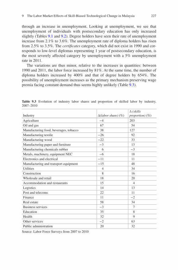
227

through an increase in unemployment. Looking at unemployment, we see that unemployment of individuals with postsecondary education has only increased slightly (Tables 9.1 and 9.2). Degree holders have seen their rate of unemployment increase from 2.1% to 3.6%. The unemployment rate of diploma holders has risen from 2.5% to 3.5%. The certificates category, which did not exist in 1990 and cor-responds to low-level diplomas representing 1 year of postsecondary education, is the most severely affected category by unemployment with a 5% unemployment rate in 2011.

The variations are thus minor, relative to the increases in quantities: between 1990 and 2011, the labor force increased by 81%. At the same time, the number of diploma holders increased by 400% and that of degree holders by 654%. The possibility of unemployment increases as the primary mechanism preserving wage premia facing constant demand thus seems highly unlikely (Table 9.3).

Table 9.3 Evolution of industry labor shares and proportion of skilled labor by industry, 2007–2010

Industry ∆(labor share) (%)∆ (skills proportion) (%)

Agriculture −4 203Oil and gas 67 54Manufacturing food, beverages, tobacco 38 127Manufacturing textile −26 92Manufacturing wood −22 33Manufacturing paper and furniture −3 13Manufacturing chemicals rubber 6 −3Metals, machinery, equipment NEC −6 18Electronics and electrical −11 11Manufacturing and transport equipment −15 48Utilities 4 34Construction 8 16Wholesale and retail 18 20Accommodation and restaurants 15 4Logistics 14 13Post and telecoms 22 11Finance 11 −2Real estate 58 34Business services −3 7Education 35 8Health 32 9Other services −2 63Public administration 20 32

Source: Labor Force Surveys from 2007 to 2010

9 The Labor Market Effects of Skill-Biased Technological Change in Malaysia

228

3 The Model

We develop a dynamic general equilibrium model with a detailed description of the labor market, taking into account jobs across sectors and workers with different ages (youth and non-youth) and levels of education (Marouani and Robalino 2012). The model also formalizes educational choices and immigration flows. The follow-ing section will lay out the main equations of the model. The economy is disaggre-gated into 23 sectors, with 21 different factors of production, corresponding to labor of 20 different skill types, and physical capital. At the sectoral level, value added is a nested constant elasticity of substitution (CES) function of capital and labor. The labor aggregate is disaggregated into three bundles: a high-skilled labor bundle (HS), a medium-skilled labor bundle (MS), and a low-skilled labor bundle (LS). The nested production structure allows for differentiated elasticities of substitution between various factors of production.

3.1 The Production Structure

Value added is a constant elasticity of substitution function of capital and a labor aggregate L7:

X K Lt K t L t= +

− − −α ασ σ σ

11

11

1

11

1 1 1

(9.2)

The first-order conditions imply the following factor demands:

K XPVA

Rt tK t

t

=

ασ1

(9.3)

L XPVA

PLt tL t

t

=

ασ1

(9.4)

At the following nest, L is decomposed into three bundles containing workers with academic degrees, vocationally trained, and secondary school graduates or lower:

7 Sectoral indices have been omitted in this section for readability.

M. A. Marouani and B. Nilsson

229

L A HS MS LSt t HS t MS t LS t= + +

− − − −α α ασ σ σ σ

11

11

11

1

11

2 2 2 2

(9.5)

Each labor bundle is a CES aggregate of workers of different skill types. The HS bundle contains degree holders of eight different types, corresponding to eight broad fields of study. The MS bundle contains vocationally trained workers, in the same eight broad fields of study. Finally, the LS bundle contains workers of four educational categories: primary and less, lower secondary, upper secondary, and pre-university. The choice of a three-bundle structure comes from an appreciation of the skill specificity at the different educational levels, ranging from relatively gen-eral skills at the lower end of the educational spectrum to relatively profession- specific skills at the higher end. The skill specificity is likely to be inversely related to the substitutability of workers at the given educational level:

HS A LDt HS tf

f HS f t=

∑− −

, , ,β σ σ1

11

11

3 3

(9.6)

MS A LDt MS tg

g MS g t=

∑− −

, , ,β σ σ1

11

11

4 4

(9.7)

LS A LDt LS tl

l LS l t=

∑− −

, , ,β σ σ1

11

11

5 5

(9.8)

Each of the 20 skill types is composed of local and migrant labor:

LD LDL MIGlf t loc lf t mig lf t, , ,= +

− − −α ασ σ σ

11

11

1

11

6 6 6

(9.9)

And local labor of skill type s is made up of young and old workers:

LDL LDLA LDLAlf t y y lf t ny ny lf t, , , , ,= +

− − −α ασ σ σ

11

11

1

11

7 7 77

(9.10)

9 The Labor Market Effects of Skill-Biased Technological Change in Malaysia

230

3.2 Labor Supply

Each year, workers leave the labor force through death and retirement.8 New work-ers enter from the educational system, upon finishing an educational cycle and on deciding not to pursue further education. A skill-specific percentage of graduates (estimated from Labor Force Survey (LFS) data) do not enter the labor force.

3.2.1 Educational Dynamics

Facing the above demands for workers of various skill types, origin, and age, the evolution of supply of workers is determined in an educational module calibrated from data from past years. Students move between educational cycles depending on dropout rates, and the willingness to join the labor market at the end of each cycle. For low-skill content cycles, these rates are calculated as averages from the period 2009 to 2010. The dropout rates are calculated using the following formula:

dropout

enrolled entrants grad enrolledc

c c c=+ − −, , ,2009 2010 2009 cc

enrolled,2010

2009 (9.11)

For each cycle, the dropout rate is calculated as a residual. It corresponds to dis-appearances from the stock of enrolled between 2009 and 2010, which are not accounted for, relative to the stock of enrolled in 2009. We make the assumption that repetition rates (for which we have no information) are negligible. Graduates decid-ing not to pursue further education are captured by the parameter exdip:

exdip

grad entrants transmapgrad

c

c c c c cc

=

− ×( )×∑, , ,,

2009 2 2010 220009

2 2 2009

2009

c c c c

c

equiv grad

grad∑ ×( , , )

,

(9.12)

where transmap is a mapping parameter between different educational cycles and equiv parameter mapping cycles that are equivalent, in the sense that they can both precede c2. Thus, graduates who choose not to pursue into the next cycles are the residual of the graduates from cycle c, less entrants into the next cycle weighted by the importance of cycle c as a cycle of origin. As such, exdip refers to the per-centage of graduates who leave a given cycle in 2009, less those who choose to continue into any of the next possible cycles:

NEWENR popent GRAD transmap exdipc t c t c c t c c c t, , , , ,= + × × −∑ − −2 1 2 11(( )

(9.13)

Newly enrolled are equal to children arriving at school age (popent) for the pri-mary cycle, plus last year graduates from preceding cycles, less those who choose

8 The mortality and retirement rates were obtained from UNESCO data.

M. A. Marouani and B. Nilsson

231

not to pursue further studies. Thus, the number of enrolled is simply equal to the number of enrolled of the previous year, less graduates and dropouts, plus newly enrolled in the current year:

ENR ENR dropout GRAD NEWENRc t c t c c t c t, , , ,= × −( ) − +− −1 11

(9.14)

Furthermore, we assume a stable share of graduates:

GRADc t gradrate ENRc c t, ,= ×

(9.15)

Students hence move through the educational system cycle by cycle, depending on dropout rates and the willingness to pursue further education, a willingness that is determined by preferences and the expected rate of return to education. At the end of Form 5, students who choose to pursue higher education make a choice of enter-ing pre-university education or seeking vocational training.

3.2.2 Educational Choices

The hypothesis that expected wages orient the demand for a certain level of educa-tion has been confirmed in numerous studies (e.g., McIntosh (2001) and Canton and de Jong (2005)). Average wages by skill type and field of study have been found to be positively correlated with relative demand for education of a particular skill type and in a particular field of study (Montmarquette et al. 2002; Freeman and Hirsch 2008; Beffy et al. 2012). In Belgium, Duchesne and Nonneman (1998) find some support for relative wages, driving enrollment choices both in university and non-university higher education. The choice between pre-university education and voca-tional training is thus modeled through a constant elasticity of transformation (CET) function where the first-order conditions render the following demands for voca-tional training and academic degrees, respectively9:

NEWENR TOTNEWENR

LD Ur avfw

Lvoc t voc t

g g t g t g t

g,

, , ,

= × ×

× −( )×( )∑∑

α

1

DD

LD Ur avfw

LD

g t

f f t f t f t

f f t

,

, , ,

,

( )× −( )×( )

( )

∑

∑1

σ10

(9.16)

9 See the Annex for the initial CET functions. The logic behind the use of a CET function to model educational demands is analogous to that of an income-maximizing firm choosing between exports and the domestic market as an outlet for its production. The representative agent maximizes expected income, subject to the constraint that total endowment in higher education is defined using a constant elasticity of transformation function. This maximization thus gives the optimal allocation of the educational endowment between vocational and general higher education.

9 The Labor Market Effects of Skill-Biased Technological Change in Malaysia

232

NEWENR TOTNEWENR

LD Ur avfw

L

t t

f f t f t f t

g

deg, deg

, , ,

= ×

×

× −( )×( )∑∑

α

1

DD

LD Ur avfw

LD

f t

g g t g t g t

g g t

,

, , ,

,

( )× −( )×( )

( )

∑

∑1

σ10

(9.17)

The demand for vocational training thus increases according to the expected relative mean wage of vocationally trained and degree holders, respectively, and with an elasticity of σ10. The total number of students having decided to pursue education after finishing secondary school is thus broken down into two categories: students who continue to vocational training and students who go on to university. For medium and high skilled, newly enrolled choose different fields of study based on preferences and expected wages in each field. This choice is again modeled through a constant elasticity of transformation (CET) function, which gives an opti-mal allocation of demand for skills given expected wages. We here assume that workers have myopic expectations and believe the wage distribution by skill to remain constant and equal to that of the previous year. The first-order conditions imply the following demand for educational services of type f, for vocational and university students, respectively:

NEWENRFIELD NEWENRavfw Ur

avfwtotg t g voc t

g t g t

v, ,

, ,= × ×−( )− −γ 1 11

ooc t, −

1

11σ

(9.18)

NEWENRFIELD NEWENRavfw Ur

avfwtotf t f t

f t f t

, deg,

, ,

d

= × ×−( )− −γ 1 11

eeg,t−

1

12σ

(9.19)

where avfwtotedu,t − 1 is the average expected wage of diploma- and degree- holding non-youth on the labor market, with voc,deg ⊂ edu. Each year, NEWENRedu,t is fixed and equal to the demand for vocational and university studies, respectively. These blocks of equations thereby give us educational demand by skill. These demands are confronted with supply in a sequential fashion: first, fields of study are ranked according to the wage premium associated with each one. Then, desired entrants into that field are confronted with the number of available places in the field. Students not accepted are regrouped with those desiring to enter the second rank field. A second cutoff is carried out, with leftovers going into the third ranked field of study. The mechanism is repeated throughout the list of fields of study, for vocationally trained and degree holders, respectively. Any students cut off from the eighth field of study are considered to be secondary school graduates of which a fraction will enter the labor force.

M. A. Marouani and B. Nilsson

233

3.2.3 Labor Force Evolution

Graduates from lower cycles are added to the youth labor force in the following fashion:

LSTA LSTA transage

GRAD exdip

lf y t lf y t lf

cc t c

, , , ,

,

= × −( )+ × ×

−

−∑1

1

1

eedumap inact

ENR dropout inact

c lf lf

cc t c lf

,

, )

× −( )( )

+ × × −( ) ×∑

1

12 cc

c c c lftransmap edumap∑ ×( )

, ,2

(9.20)

That is, the local labor force of skill lf equals the previous year’s local labor force of skill lf, less those workers who flow from the young to the not young category. Graduates from cycle c who choose not to continue their studies are mapped to a labor skill, and a percentage of them are added to the labor force according to their labor force participation rate. Finally, dropouts from cycles above c are added to the relevant labor force category using mapping parameter transmap, denoting pas-sages between cycles. For vocational and university students, the logic is the following:

LSTA LSTA transage

CANDID pla

lf y t lf y t lf

lf t n

, , , ,

,min

= × −( )+

−

−

1 1

, cces inactlf t n lf, −( )× (9.21)

The labor force holding diplomas and degrees is thus equal to diploma and degree graduates in the labor force the previous year, less those who transit to the not young category. Students who were accepted into their desired field of study are added, a percentage being removed depending on the labor participation rate of the category in question. The index n reflects the time it takes to complete a given cycle. We have set n to equal 4 years for all degree students, and 2 years for all vocational degrees, reflecting the average duration of these cycles in Malaysia. The inclusion of a delay between entrance in a given field and labor market participation has important implications. During the time of studies, workers are effectively immobi-lized, such that any increase in the number of students is likely to carry an initial negative impact on growth. In short, instead of being potential low-skilled workers, these individuals do not contribute directly to production. We thus include a tempo-ral dimension of the efficiency of education policy in the model.

Finally, the evolution of older workers depends on the transit rate between age groups and the mortality and retirement rates of old workers:

LSTA LSTA x mort retir

transagelf ny t lf ny t lf t lf t

l

, , , , , ,= − −( )+

−1 1

ff lf y tx LSTA , , −1 (9.22)

9 The Labor Market Effects of Skill-Biased Technological Change in Malaysia

234

3.3 The Migrant Block

Immigration in Malaysia has increased substantially over the last decades, poten-tially influencing labor market dynamics. These migrants tend to be low educated, arriving in Malaysia from primarily Indonesia and the Philippines. Various push and pull factors explain the supply of migrants in Malaysia. We model the total supply of migrants using a CET function, where the evolution of the migrant stock at a given skill level depends on the relative wage premium of migration in a given year compared to the relative wage premium in the base year:

SMIG IMMIG

avfwm

wdom

avfwm

w

lf tAC

AC lf

lf t

lf t

lf, , ,

,

,

,

= ×∑ 20052005

ddomlf ,2005

8

σ

(9.23)

Furthermore, migrants move between sectors according to relative wages and initial preferences:

SMIG IMMIGlf tAC

AC lf AC lf t, , , ,= ×

∑+ +

γ σ σ1

11

11

9 9

(9.24)

Migrants thus make their decision sequentially. First, the decision to migrate is taken based on expected wages and the elasticity of substitution. Once immigrated, they will reallocate between sectors depending on the wage rate and the elasticity of the migrant sectoral supply.

3.4 Labor Market Adjustments

Migrants and local workers’ wages are assumed to be different due to an imperfect substitution by employers (Ozden and Wagner 2014). It is assumed that the local wage does not clear the labor market, such that there is unemployment among locals. The wage is modeled using a wage curve, reflecting the often observed empirical relationship between wage and unemployment. The local average wage by skill is thus given by

logafw x Urlf t lf lf lf t, , , ,log= +β β1 2

(9.25)

Sectoral wages are then equal to the average wage, plus an exogenous wage differential:

M. A. Marouani and B. Nilsson

235

wf afw fwdistAC lf t lf t AC lf, , , ,= ×

(9.26)

Initially, the migrant wage clears the migrant labor market. We thus make the assumption that there is no migrant unemployment. Furthermore, reasonably in line with the regulatory framework, we assume that migrants do not pay social security. Following the minimum wage law passed in Malaysia in 2012, restrictions are imposed on the market wage from 2013. It follows that wages no longer clear the migrant labor market. Since there is no migrant unemployment, the introduction of a minimum wage – supposing it is binding – implies rationing of migrants in Malaysia. The level of the minimum wage is set according to the actual minimum wage introduced, deflated to reflect 2005 prices (since the model is exempt from inflation). The minimum wage is introduced sequentially. First, market wages below the minimum wage level are fixed at the minimum wage rate. The model is then resolved to allow for sectoral adjustments to take place. Any market wage having fallen below the minimum wage rate is fixed at the minimum wage, and the proce-dure is repeated. The sequence stops when all wages are equal to or above the mini-mum wage rate.

3.5 Closure and Dynamics

The model has five closures: a macro closure, a government closure, an external balance closure, a labor market closure, and a closure of the social security accounts. Concerning the macro closure, it is savings driven (households’ marginal propen-sity to save is exogenous), which means that the level of investment is determined by the level of total available savings in the economy (including foreign savings). Hence as savings increase, the stock of capital and output increase. The government closure chosen consists in fixing government expenditures as a constant share of GDP and tax rates and leaving the government budget balance endogenous. The social security account is modeled separate from the government budget. It earns its income from employers’ payroll taxes and pays benefits that are distributed to households. The social security balance is endogenous. The foreign balance closure consists of fixing the exchange rate and leaving the current account balance endog-enous. The formal labor market closure consists of a joint determination of unem-ployment and average local wages through the wage curve described above and no unemployment for foreign workers (wages clear the market).

Model dynamics are of the sequential type. Capital accumulation is sectoral. Each year the stock of capital in each sector corresponds to last year’s stock plus new investment, minus the depreciation of capital. Sectoral investment has been modeled as a function of the sectoral stocks of capital, sectoral rates of return to capital, and capital acquisition costs. As already mentioned, the evolution of the active population by skill is modeled within the education block, which relies on the actual performance rates of the educational system and endogenous educational

9 The Labor Market Effects of Skill-Biased Technological Change in Malaysia

236

choices in Malaysia. Government and foreign debts increase (decrease) with the yearly level of the net deficit (surplus) of government and foreign savings.

4 Data and Calibration

4.1 The Database

We build a social accounting matrix using an input-output table of 2005, the base year for the simulations. A social security contribution account has been added, with a fixed percentage of employer and worker contributions being drawn from labor income. Total employment is taken from the 2007 LFS, the first survey for which wages are available. It represents wage earners in each sector, with the exception of the agricultural sector where employment refers to all employed due to the particu-lar nature of this sector (hosting many informally employed workers)10 and health (where employment corresponds to the estimated amount of wage earners for 2005).

Total value added (including social security benefits) in each sector is taken from the 2005 input-output (IO) table. Wage-related data come from the LFS. In the agri-culture, health, and education sectors, aggregate wage bills are those of the 2005 IO tables. In the remaining sectors, wage bills are taken from the LFS 2007 by multi-plying mean wages by skill and industry with the number of workers of that skill and industry (the difference between these and the original wage bill is imputed from capital remuneration). Thus, mean wages and wage earners are kept in accor-dance with the LFS in all except the three sectors mentioned. For those three sec-tors, the standard methodology could not be used since the imputed wage bill would necessitate a negative capital remuneration. The original wage bill is thus kept, and wages are imputed and not equal to those of the LFS.

Investment by origin is taken from the 2005 IO table and is portioned out to des-tination sectors. Information from a report titled “National Accounts Capital Stock Statistics” by the Department of Statistics proved very useful for this exercise. Since the data reflect a higher aggregation than the one used for the estimation, we assume that investment is equally distributed among our subsectors. Ideally, an investment origin-destination matrix would have been used, but such a matrix was not avail-able. Current results will thus fail to accurately capture some subsector dynamics that are due to relatively high or low investment with respect to sector size. World and local growth rates are taken from the World Bank Databank. Data on enroll-ment, intake, and graduates for each cycle were available for 2009 and 2010. These data are used to calculate (for each cycle) the dropout rates and the share of gradu-ates who move to the next cycle. Enrollment data for the base year are estimated from a dynamic calibration exercise, retracing the evolution of educational out-comes between 2005 and 2010.

10 The LFS does not include workers in communal housing, which is common among migrant agricultural workers, who are thus likely to be underrepresented.

M. A. Marouani and B. Nilsson

237

Using production and LFS data from 2005 through 2011, we dynamically cali-brate the main parameters of the model through an iterative process. The result from this exercise is that the reference scenario is reasonably in line with the survey fig-ures and the evolution of the main variables at the macro and sectoral levels.

4.2 Calibration

Model parameters include initial values of endogenous variables, as well as exoge-nous parameters. The social accounting matrix provides such values for production and consumption, exports, imports, etc. Labor Force Surveys provide us with infor-mation on wages and employment status of migrants and locals. Some unobservable parameters can be calculated using initial values obtained from these sources. Others, such as elasticities of substitution, have to be estimated. When possible, we have attempted to estimate these elasticities. When impossible, reasonable values from the literature have been used.

As for the demand elasticity of substitution between high-skilled labor and capi-tal, we follow Card and Lemieux (2001) and derive elasticities of substitution between workers of different age groups, education levels, fields of study as well as elasticities of different labor aggregates of these worker categories. The limited number of years for which we have data on wages sharply limits the regression results, and significant coefficients were not obtained for the full production struc-ture. There are, however, indications of elasticities decreasing as we move up the production structure. The price elasticities of demand for migrants with respect to locals have been estimated from LFS data.11

We consider current macroeconomic trends to prevail. As such, the savings rate and the rate of increase of foreign direct investment have been set to values produc-ing reasonable figures, in line with IMF data for the period 2005–2011. Furthermore, we are assuming the government deficit to continue its downward trend, declining to 3% of GDP in 2015 and completely absorbed in 2020.12

5 A Microsimulation Module

A microsimulation module is added to the CGE framework in order to study distri-butional impacts of SBTC and educational rationing. Since we are focusing on wage inequalities, a microaccounting approach is used, linking model outcomes to microlevel data. The LFS survey contains information on wage earners only, which is why we exclude interest rate variations from our analysis.

11 We thank Caglar Ozden and Mathis Wagner for providing us with these elasticities.12 As by PEMANDU objectives.

9 The Labor Market Effects of Skill-Biased Technological Change in Malaysia

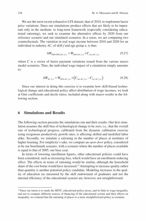
238

We use the most recent exhaustive LFS dataset, that of 2010, to implement factor price variations. Since our simulations produce effects that are likely to be impor-tant only in the medium- to long-term framework (especially considering educa-tional rationing), we seek to examine the alternative effects by 2020 from our reference scenario and our simulated scenarios. In a sense, we are comparing two counterfactuals. The variation in real wage income between 2010 and 2020 for an individual in industry AC, of skill f and age group a, is thus

∆W W CAC f a AC f a scen AC f a2020 2010 2010/ , , , , , , , , ,= ×

(9.27)

where C is a vector of factor payment variations issued from the various macro model scenarios. Thus, the individual wage impact of a simulation simply amounts to:

∆W W C CAC f a AC f a sim AC f a ref AC f a, , , , , , , , , , ,= × −( )2010

(9.28)

Since our interest in doing this exercise is to examine how skill-biased techno-logical change and educational policy affect distribution of wage incomes, we look at Gini coefficients and decile ratios, included along with macro results in the fol-lowing section.

6 Simulations and Results

The following section presents the simulations run and their results. Our first simu-lation assumes the skill bias of technological change to be zero, i.e., that the overall rate of technological progress, calibrated from the dynamic calibration exercise using exogenous productivity growth rates, is affecting skilled and unskilled labor alike. Secondly, we simulate a rationing in the number of places at institutes of higher learning. For simplicity’s sake, we compare an open-door policy, considered to be our benchmark scenario, with a scenario where the number of places available is equal to that of 2005, our base year.

In terms of lowering enrollment figures, other educational policies could have been considered, such as increasing fees, which would have an enrollment-reducing effect. The effects in terms of rationing would be similar, although the household share of the cost borne would have increased.13 Attempting to increase quality rather than quantity is another potential policy candidate. Modeling increases in the qual-ity of education (as measured by the skill endowment of graduates and not the internal efficiency of the educational system) are, however, not straightforward.

13 Since our intent is to study the SBTC, educational policy nexus, and its links to wage inequality, and not to compare different sources of financing of the educational system and their effects on inequality, we contend that the rationing of places is a more straightforward policy to examine.

M. A. Marouani and B. Nilsson

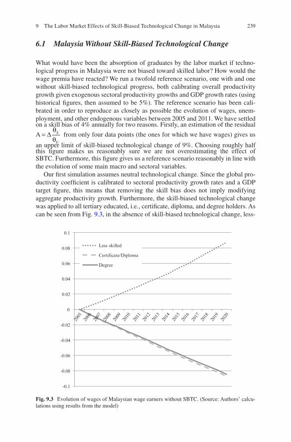
239

6.1 Malaysia Without Skill-Biased Technological Change

What would have been the absorption of graduates by the labor market if techno-logical progress in Malaysia were not biased toward skilled labor? How would the wage premia have reacted? We run a twofold reference scenario, one with and one without skill-biased technological progress, both calibrating overall productivity growth given exogenous sectoral productivity growths and GDP growth rates (using historical figures, then assumed to be 5%). The reference scenario has been cali-brated in order to reproduce as closely as possible the evolution of wages, unem-ployment, and other endogenous variables between 2005 and 2011. We have settled on a skill bias of 4% annually for two reasons. Firstly, an estimation of the residual

A = ∆θθ

S

U

from only four data points (the ones for which we have wages) gives us

an upper limit of skill-biased technological change of 9%. Choosing roughly half this figure makes us reasonably sure we are not overestimating the effect of SBTC. Furthermore, this figure gives us a reference scenario reasonably in line with the evolution of some main macro and sectoral variables.

Our first simulation assumes neutral technological change. Since the global pro-ductivity coefficient is calibrated to sectoral productivity growth rates and a GDP target figure, this means that removing the skill bias does not imply modifying aggregate productivity growth. Furthermore, the skill-biased technological change was applied to all tertiary educated, i.e., certificate, diploma, and degree holders. As can be seen from Fig. 9.3, in the absence of skill-biased technological change, less-

-0.1

-0.08

-0.06

-0.04

-0.02

0

0.02

0.04

0.06

0.08

0.1

Less skilled

Certificate/Diploma

Degree

2005

2020

2019

2018

2017

2016

2015

2014

2013

2012

2011

2010

2009

2008

2007

2006

Fig. 9.3 Evolution of wages of Malaysian wage earners without SBTC. (Source: Authors’ calcu-lations using results from the model)

9 The Labor Market Effects of Skill-Biased Technological Change in Malaysia

240

skilled workers would have had a higher wage growth than in the reference sce-nario. On the other hand, tertiary educated – vocationally and academic alike – would have seen their wages decrease, thus eroding returns to education. Detailed break-downs by field of study for diploma holders and degree holders and by level of education for less skilled can be found in the Annex. They show that for diploma holders, the biggest winners from SBTC are engineers. For degree holders, those with degrees in agriculture have benefited the most. Figure 9.3 shows that the agri-cultural sector has known the highest upskilling in the period 2007–2010. This large sector has the highest ratio (more than 95%) of unskilled to skilled labor, implying that an important substitution of skilled for unskilled labor needs to take place, sig-nificantly affecting wages of the high skilled.

Looking at unemployment (Fig. 9.4), we see that the tendency is the same as for wages. Had skill-biased technological change not been present, the unemployment rates of tertiary educated would have been around 15–20% higher, while those of less-skilled workers would have been 15% lower. Thus, SBTC has clearly had a positive impact on the labor market outcomes of graduates in Malaysia.

The macroeconomic impacts over the period are minor (mainly since the model is calibrated to the same GDP target figures). Unemployment would however have been slightly lower during the period but returning to a very close figure (3.1%) by 2020. Results also show that immigration would have been higher had SBTC not prevailed, since this would have stimulated growth of migrant-intensive sectors

-0.2

-0.15

-0.1

-0.05

0

0.05

0.1

0.15

0.2

0.25

Less skilled

Certificate/Diploma

Degree20

05

2020

2019

2018

2017

2016

2015

2014

2013

2012

2011

2010

2009

2008

2007

2006

Fig. 9.4 Evolution of unemployment of Malaysian wage earners without SBTC. (Source: Authors’ calculations using results from the model)

M. A. Marouani and B. Nilsson

241

more than in a scenario with SBTC. Malaysia’s immigration in recent years has been important, important enough to spark a concern among the government about its economic and social impact. Unbiased technological progress, relatively more favorable to low-skill-intensive sectors, can thus be seen as increasing the pull fac-tor in the Malaysian context, where the main migration pool is made up of low- skilled Indonesians and Filipinos.14 Had productivity increases been unbiased, the migrant stock would have been 14% higher by 2020.

Table 9.4 shows the production growth differentials from 2010 to 2020 in the absence of skill-biased technological change. It suggests that SBTC has led to struc-tural change, benefiting sectors such as business services, finance, and certain types of manufacturing, the common denominator of which is a large share of skilled labor. Symmetrically, it has played a role in the relative decline of sectors such as wood or wholesale and retail. Thus, the recent evolution of Malaysia toward a more skill-intensive economy, a policy target, has been facilitated by technical progress biased toward skilled labor.

14 According to the 2010 Labor Force Survey, the proportion of employed migrants with at least a diploma or certificate in 2010 stood at less than 4.5%. The equivalent figure for Malaysians is 22%. The bulk of Malaysia’s immigrants being low-skilled immigrants, migration responds strongly to variations in low-skilled wages, which are related to the skill bias of technological progress.

Table 9.4 Sectoral production growth differentials 2010–2020 without SBTC (private sectors)

Agriculture 11%Oil and gas 3%Manufacturing food, beverages, tobacco

10%

Manufacturing textile 2%Manufacturing wood 12%Manufacturing paper and furniture 3%Manufacturing chemicals rubber −1%Metals, machinery, equipment NEC 0%Electronics and electrical −2%Manufacturing and transport equipment

−1%

Utilities 1%Construction 1%Wholesale and retail 8%Accommodation and restaurants 5%Logistics 4%Post and telecom 0%Finance −1%Real estate 0%Business services −10%

Source: Authors’ calculations using results from the model.

9 The Labor Market Effects of Skill-Biased Technological Change in Malaysia

242

6.2 Constraining the Supply of Higher Education

Our reference scenario supposes no rationing of supply of educational services in Malaysia. Demand factors alone thus determine the evolution of skilled labor. In this simulation, we restrain the supply of educational services to that of the base year, 2005. Every year, the number of places in each field of study is thus equal to the number of places available in 2005.15 We here assume the cycle of diploma studies to be 2 years and that of degree studies to be 4 years. An increased enrollment in degree studies would therefore only create an increase in high-skilled labor 4 years later.

Figure 9.5 shows the evolution of unemployment of various high-skilled catego-ries when places are kept constant. Unsurprisingly, by 2009, as the effects translate into a lower amount of degree holders than in the reference scenario, the unemploy-ment of degree holders starts to decrease. At the end of the period, unemployment rates are 35% to 50% lower than in the reference scenario. The effect is also felt on wages, which would have been up to 20% higher by the end of the period (see Annex). By constraining access to higher education, a rent is created and awarded to those in possession of a tertiary education. For diploma holders, there is more variation in unemployment decreases and wage increases (See Annex). Some fields of study experience large increases while others get relatively minor ones. In par-ticular, diploma holders in health do not benefit much from the rationing. This is partially due to the fact that the demand for health diplomas was falling in the refer-ence scenario. Rationing actually creates a slight increase in the long-term supply of health diploma graduates, since some of those diploma students that are cut out from more desirable fields due to rationing end up joining health programs as a fallback option (Table 9.5).

Looking at sectoral production growth differentials over the decade 2010–2020, we find disparate results across sectors. Several mechanisms are at play. Firstly and most intuitively, rationing increases the relative cost of skilled labor. Sectors that are relatively intensive in unskilled labor will thus benefit. The most unskilled labor- intensive sectors (agriculture, wood, wholesale and retail trade) are therefore those where production increases the most. Symmetrically, the most skill-intensive sec-tors (business services, finance, and manufacturing of transport equipment) see their production decrease. Secondly, a variation of wage costs affects most those sectors that are relatively labor intensive. This explains why manufacturing of wood bene-fits more than agriculture from the rationing, agriculture being more capital inten-sive. Among the relatively skill-intensive sectors, the most capital-intensive sectors such as finance are less hurt by the rationing than relatively labor-intensive ones such as business services.

Looking at Figs. 9.15–9.17 in Annex 1 provides insight into the determinants of wage shifts and their sensitivity to variations in these determinants. Skill-biased

15 An important caveat here is that we do not actually know the number of places in 2005, only the number of enrolled in each field of study. It is possible that more places were available in some fields.

M. A. Marouani and B. Nilsson

243

-0.6

-0.5

-0.4

-0.3

-0.2

-0.1

0

0.1

Arts & Humanities

Social science, business,law

Science, math, IT

Engineering

Agriculture

Health

Services

Education

2005

2020

2019

2018

2017

2016

2015

2014

2013

2012

2011

2010

2009

2008

2007

2006

Fig. 9.5 Evolution of unemployment of degree-holding wage earners with a restriction in places. (Source: Authors’ calculations using results from the model)

technological change is indeed a strong one, as has been shown in the previous results. However, the magnitude of the bias sharply correlates to the subsequent wage loss (gain) of more (less) skilled workers. Furthermore, the elasticity of sub-stitution between the three main labor bundles is also a strong determinant of the distributional effects of skill-biased technological change and educational rationing. We feel that our main hypotheses are reasonable. Our main variable, the skill shifter, is at 4%, although the residual estimated stood at 9%. The elasticity of substitution between skilled labor bundles is also conservatively set at 1.5. As a matter of com-parison, Katz and Murphy (1992) find an elasticity of supply between high school and college labor of 1.4 for the United States. They do not, however, implicitly account for substitutability within these two labor aggregates. When doing so, Card and Lemieux (2001) find estimates ranging between 2 and 2.5 in the UK and United States.

9 The Labor Market Effects of Skill-Biased Technological Change in Malaysia

244

6.3 Distributional Results

The microaccounting exercise shows that the scenarios considered have substan-tially different impacts on Gini coefficients and interdecile ratios. In all cases, how-ever, the massification of higher education together with SBTC brings about a decrease in overall wage inequality, as confirmed by the systematically lower Gini coefficients of our counterfactual scenarios. The same holds true for the interdecile measures, which are systematically lower than in the 2010 LFS (the exception being the p90/p50 indicator in Simulation 2) and the Atkinson index. The Atkinson index emphasizes inequality at the lower end of the distribution to affect the index more than inequality at the upper end and the more so the higher the inequality aversion parameter e.16

As stated above, the reference scenario corresponds to skill-biased technological change and an open-door educational policy. This is what we consider to be the path Malaysia is currently on. The increased educational attainment of Malaysians will

16 As long as e greaterthan 0, the sensitivity to inequality in the lower end of the distribution is increasing in e. We have chosen to set e = 1 in the simulation.

Table 9.5 Sectoral production growth differentials 2010–2020 with rationing (private sectors)

Agriculture 3.6%Oil and gas 1.4%Manufacturing food, beverages, tobacco

3.0%

Manufacturing textile 1.1%Manufacturing wood 4.5%Manufacturing paper and furniture 1.4%Manufacturing chemicals rubber −0.1%Metals, machinery, equipment NEC 0.1%Electronics and electrical 0.1%Manufacturing and transport equipment

−0.5%

Utilities 0.5%Construction 0.4%Wholesale and retail 4.8%Accommodation and restaurants 2.2%Logistics 1.9%Post and telecom 0.2%Finance −0.4%Real estate 0.1%Business services −5.1%

Source: Authors’ calculations using results from the model.

M. A. Marouani and B. Nilsson

245

lead to a wage compression, substantially reducing wage inequality (almost a 3-point drop in the Gini coefficient). When comparing this with a situation without SBTC, maintaining the educational policy, the corresponding drop in the Gini is about 4.1. Skill-biased technological change thus prevented a reduction in wage inequality over the period. Similarly, both interdecile ratios would have been lower, had SBTC not been present (Table 9.6).

Turning to educational policy, the second simulation shows the counterfactual Gini coefficient and interdecile ratios in a situation with SBTC and with educational rationing. Thus, the Gini coefficient would have been 1.6 points higher had the number of educational places been maintained at their 2005 level. The open-door policy of the Malaysian government has thus contributed to a decrease in wage inequality. It should be noted that even in this scenario, the counterfactual Gini coef-ficient for 2020 is lower than the one computed from the 2010 LFS data. This is because demographic factors, namely, the fact that the low-skilled working popula-tion is older than the high-skilled one, contribute to an increase in the share of skilled labor even when higher education is rationed. Also, the introduction of the minimum wage in 2013 contributes to an inequality-reducing compression of the wage distribution. The different simulations are thus to be understood as deviations from this general downward-sloping trend. Turning to Simulation 3 (no SBTC, rationing), it shows that the impact of rationing is lower, but not far from that of SBTC. It thus seems that the open-door educational policy has counteracted the inequality maintaining effect of skill-biased technological change in Malaysia.

The full story of educational impacts on inequality should mention social returns to education. While private returns have largely been the focus of the literature (although a sizeable literature on social returns to education exists), externalities of educational accumulation might impact the distribution of income in indirect ways. Primarily, there is an evident link between education and the innovation process, likely to impact technical progress directly. The impact of this nexus on the relative productivity bias is however uncertain, and we therefore assume the absence of such an effect. Secondly, spillover effects in worker productivity might be expected. It is plausible that an indi-vidual in training will increase not only his or her productivity but also that of his or her coworkers, for example, by introducing new ideas or forms of organization of the

Table 9.6 Summary of distributional indices from microaccounting exercise

2010 LFS

Ref. Sim. 1 Sim. 2 Sim. 3

SBTC, no rationing

No SBTC, no rationing

SBTC, rationing

No SBTC, rationing

Gini coefficient 0.40743 0.3782 0.36686 0.39393 0.38078Atkinson index (1)

0.24532 0.2143 0.20306 0.23019 0.21683

p90/p10 6.415 5.66 5.458 6.133 5.695p90/p50 2.52 2.399 2.301 2.559 2.425

Source: Authors’ calculations using results from the model.

9 The Labor Market Effects of Skill-Biased Technological Change in Malaysia

246

workplace. This is perhaps the most relevant type of externality for our purposes. Acemoglu and Angrist (1999) try to estimate social returns using variations in com-pulsory schooling laws in US states. They find little evidence of a higher social than a private return. Furthermore, to our knowledge, there are no studies trying to estimate the social returns to education in Malaysia. Again, we are unable to ascertain any impact on the skill bias of technological change from these mechanisms.

6.4 The Hypothesis of Exogenous SBTC

A major drawback of the canonical model of skill-biased technological change (Acemoglu and Autor 2011) is that it says nothing about the origin of SBTC. Could it not be that the increase of skilled labor has provoked the direction taken by techni-cal bias? Acemoglu (1998, 2002) creates a model in which a marketplace for inno-vation exists, and firms can choose to develop technologies suited to one factor of production rather than the other. He shows that whatever the elasticity of substitu-tion between factors, an increase in the relative abundance of one creates some amount of technical change biased toward that factor. This however relies on profit incentives as the main source of the direction of technological bias. While arguing that innovation might indeed not be driven by profits, the direction of innovation somehow is. No clear explanation is given as to why this would be the case.

If SBTC results from firm responses to modifications of factor proportions, then this type of mechanism should be the most prevalent in countries that carry out a lot of innovation domestically, such as high-income economies. To our knowledge, only one paper has tested for endogeneity of SBTC, in the German context (Bogliacino and Lucchese 2015). Using the influx of East Germans as a source of exogenous variation in the proportion of skilled labor, they conclude on the absence of a demand-pull effect on skill-biased technological change. The experience of MENA countries and their record-high unemployment rates for tertiary graduates can also be raised as an argument for the absence of a demand-pull effect. The con-siderable increases in quantities witnessed by these countries have not been fol-lowed by job creation suited to their qualifications.

In an era of openness and globalization, innovation travels fast. Berman et al. (1998), using data from 12 countries, show that skill-biased technological change such as the one observed in the United States has been pervasive, occurring simulta-neously in all countries. Berman and Machin (2000) further show that this pervasive-ness extends to middle-income countries (of which Malaysia is one) in the 1980s, whose skill upgrading is correlated with that of the United States. Since the world has

M. A. Marouani and B. Nilsson

247

not ceased to be a globalized place, it is likely that the same kind of pervasiveness of SBTC is at least as evident today as three decades ago. The hypothesis of SBTC through imports of goods which embody skill bias has been tested by Conte and Vivarelli (2011), who find evidence of such a mechanism on a set of 23 low- and middle- income countries in the period 1980–1991. Eaton and Kortum (2001) show that the production of capital goods is highly concentrated among seven OECD countries which provide the main source of imports of capital goods for the rest of the world.

Cross-country regressions and the little evidence testing directly the demand- pull hypothesis thus suggest that SBTC is at least partly unrelated to the proportion of skilled labor in the economy. In the Malaysian case in particular, being a middle- income country relying on imports of capital goods to a larger extent than high- income countries (and in particular, high-technology countries such as Germany), there is reason to believe that much of the technological bias experi-enced is embodied in imported technology.

If SBTC is to a large extent exogenous with respect to skill proportions, the results of our simulations are valid. Should a significant share of SBTC be due to the increase in skilled labor, this would nuance some of the results obtained but would not change their rank order. Simulation 1 would slightly overestimate the drop in the skill premia and subsequently the reduction in the inequality measures. Simulation 2 would slightly underestimate the increase in skill premia and subsequently the reduction in the inequality measures.

7 Conclusion

This article has looked at the labor market impacts of two alternative scenarios: a neutral technological change and a rationing of places available in tertiary educa-tion. We develop a dynamic general equilibrium framework in which we extensively model educational choices both on the demand and the supply side, while taking into account immigration decisions. We are thus able to fully endogenize labor sup-ply dynamics in the Malaysian context.

Our results show that in the absence of skill-biased technological change, rela-tively skilled wage earners should have expected lower wages and higher unem-ployment, while unskilled labor would have been able to expect higher wages and lower unemployment. The absence of SBTC would also have meant increased migration. We also show that skill-biased technological change has led to structural change, benefiting sectors with a large share of skilled labor, such as business ser-

9 The Labor Market Effects of Skill-Biased Technological Change in Malaysia

248

vices. Furthermore, our model does not take into account geography. A limitation of the study is thus that territorial inequalities or geographical shifts of production linked to internal migration of relatively more−/less-demanded skills across admin-istrative divisions are ignored.

With rationing of the supply of higher education, we find that rents are created for high-skilled workers, who would have seen their wages increase and unemploy-ment decrease. At the sectoral level, we identify two mechanisms affecting sectoral production growth: relatively less-expensive unskilled labor, benefiting low skill- intensive sectors, and substitution effects among high skill-intensive sectors favor-ing the more capital-intensive sectors. These macro effects translate into distributional effects in the microaccounting module. We show that skill-biased technological change and rationing of educational services both have adverse effects on wage inequalities in the medium term (their presence generates a Gini index of 0.394 in 2020 compared to 0.367 in their absence), although even with both mecha-nisms in play we would expect wage inequalities to drop. It seems therefore that the expansive educational policy adopted in Malaysia has counteracted some of the increase in inequalities expected from skill-biased technological change. The presence of skill-biased technological change in Malaysia thus constitutes a case for continued open enrollment policies to reduce wage inequalities.

In this paper we assume that total factor productivity and skill bias are unrelated, to be able to isolate the effect of skill bias on the evolution of skill-specific unem-ployment and wage rates. Further research should be aimed at understanding in depth the linkages between skill-biased technological change and total factor productivity.

M. A. Marouani and B. Nilsson

249

Annex 1

Table 9.7 Variables used in the CGE model

XAC,t Composite production by sector AC in year t

KAC,t Capital stock by sectorLAC,t Aggregate labor bundlePVAAC,t Value-added priceRAC,t Interest ratePLAC,t Price of aggregate labor bundleHSAC,t High-skilled labor bundleMSAC,t Medium-skilled labor bundleLSAC,t Low-skilled labor bundleLDAC,f,t High-skilled labor bundle of type fLDAC,g,t Medium-skilled labor bundle of type gLDAC,l,t Low-skilled labor bundle of type lLDLAC,lf,t Local labor bundle of skill type lfMIGAC,lf,t Migrant labor of skill type lfLDLAa,lf,t Local labor of age a and skill type lfENRc,t Enrolled by educational cycleGRADc,t Graduates by educational cycleNEWENRedu,t Newly enrolled in cycles voc or deg

TOTNEWENRt Newly enrolled in tertiary educationNEWENRFIELDlf,t Newly enrolled in tertiary educationavfwlf,t Average wage of labor of skill type lfUrlf,t Unemployment rate of labor of skill

type lfCANDIDlf,t − n Successfully accepted candidates by

labor skill typeavfwmlf,t Average wage of migrant labor of skill

type lfSMIGlf,t Total migrant supply by skill typeIMMIGAC,lf,t Sectoral demand for migrant labor of

skill type lfwfAC,lf,t Sectoral wage of local labor of skill

type lfafwlf,t Average wage of local labor of skill

type lf

9 The Labor Market Effects of Skill-Biased Technological Change in Malaysia

250

Table 9.8 Parameters used in the CGE model

AAC,t Labor-augmenting productivity parameterαAC,K Share parameter of capitalαAC,L Share parameter of laborαAC,HS Share parameter of high-skilled laborαAC,MS Share parameter of medium-skilled laborαAC,LS Share parameter of low-skilled laborAHS,AC,t High-skilled labor productivity parameterAMS,AC,t Medium-skilled labor productivity parameterALS,AC,t Low-skilled labor productivity parameterβf Share parameter of high-skilled labor type fβg Share parameter of medium-skilled labor type gβl Share parameter of low-skilled labor type lαAC,loc,lf Share parameter of local laborαAC,mig,lf Share parameter of migrant laborαy,lf Share parameter of young local laborαny,lf Share parameter of older local labordropoutc Dropout rate by educational cycleenrolledc,t Enrolled by educational cycle (historical figure used in calculations)entrantst New entrants by educational cycle (historical figure used in calculations)gradc,t Graduates by educational cycle (historical figure used in calculations)exdipc Share of graduates pursuing further studies, by cycletransmapc,c2 Mapping parameter relating different educational cyclesequivc,c2 Equivalency parameter denoting cycles which are similar in the educational

hierarchygradratec Graduation rate, by cycleαvoc Share parameter of vocational studentsαdeg Share parameter of academic studentsγf Share parameter of field of study f in academic degreesγg Share parameter of field of study g in vocational degreestransagelf Transition rate between age categories, by skill typeedumapc,lf Mapping parameter between educational cycles and labor skill typesinactlf Inactivity rate by skill typeplaceslf,t Number of places by field of study (tertiary cycles only)mortlf Mortality rate by labor skill typeretirlf Retirement rate by labor skill typewdomlf,t Domestic country wage rate by skill typeβ1,lf Wage curve intercept parameterβ2,lf Wage curve elasticity parameterfwdistAC,lf Exogenous sectoral wage differentials by skill type

M. A. Marouani and B. Nilsson

251

Table 9.9 Elasticity parameters used in the CGE model

σ1,AC Elasticity of substitution between aggregate labor and aggregate capital

σ2,AC Elasticity of substitution between high-skilled, medium-skilled, and low-skilled labor

σ3,AC Elasticity of substitution between high-skilled labor bundlesσ4,AC Elasticity of substitution between medium-skilled labor

bundlesσ5,AC Elasticity of substitution between low-skilled labor bundlesσ6,AC,lf Elasticity of substitution between migrant and local laborσ7,AC Elasticity of substitution between younger and older laborσ8,AC,lf Elasticity of transformation of migrant supplyσ9,lf Elasticity of transformation of migrants between sectorsσ10,lf Elasticity of transformation between vocational and academic

studiesσ11,lf Elasticity of transformation between vocational degreesσ12,lf Elasticity of transformation between academic degrees

Table 9.10 CET equations used to derive educational demands

The maximization problem at hand is

Max (edu

edu t eduavfw NEWENR∑ × , )

subject to TOTNEWENR NEWENR NEWENRt voc voc t t= × + × α αρ ρ ρ, deg deg,

10 10 10

1

For the choice of field of study, the following CET functions were used:For general higher education:

Max (f

f t f tavfw NEWENRFIELD∑ × , , )

subject to NEWENR NEWENRFIELDt ff

f tdeg, ,= ×

∑γ ρρ

1212

1

For vocational higher education:

Max (g

g t g tavfw NEWENRFIELD∑ × , , )

subject to NEWENR NEWENRFIELDvoc t gg

g t, ,= ×

∑γ ρρ

1212

1

9 The Labor Market Effects of Skill-Biased Technological Change in Malaysia

252

Table 9.11 Evolution of industry labor shares and proportion of skilled labor by industry, 1990–2011

Industry∆(labor share) (%) ∆(skills share) (%)

Agriculture −13.6 2.1Oil and gas 0.0 27.0Manufacturing food, beverages, tobacco −0.2 8.9Manufacturing textile −2.3 7.0Manufacturing wood −0.4 2.7Manufacturing paper and furniture 0.4 10.7Manufacturing chemicals rubber 0.4 16.2Metals, machinery, equipment NEC −0.1 12.3Electronics and electrical 4.1 16.5Manufacturing and transport equipment 0.4 16.0Utilities −1.5 23.2Construction 2.9 11.2Wholesale and retail 2.1 10.3Accommodation and restaurants 2.1 6.3Logistics 1.4 11.7Post and telecom 0.9 59.6Finance 0.7 33.7Real estate 0.2 30.6Business services 3.8 15.8Education 0.7 20.9Health 0.9 44.0Other services −2.3 6.8Public administration −0.6 23.0

Source: Authors’ calculations from the 1990 and 2011 LFS.

M. A. Marouani and B. Nilsson

253

0

0.02

0.04

0.06

0.08

0.1

0.12

UPSR/UPSA or less

PMR or equivalent

SPM or equivalent

STPM or equivalent

2005

2020

2019

2018

2017

2016

2015

2014

2013

2012

2011

2010

2009

2008

2007

2006

Fig. 9.6 Evolution of wages of low-skilled Malaysians without SBTC. (Source: Authors’ calcula-tions using results from the model)

9 The Labor Market Effects of Skill-Biased Technological Change in Malaysia

254

-0.12

-0.1

-0.08

-0.06

-0.04

-0.02

0

Arts &

Humanities

Social science,

business, law

Science, math, IT

Engineering

Agriculture

Health

Services

Education

2005

2020

2019

2018

2017

2016

2015

2014

2013

2012

2011

2010

2009

2008

2007

2006

Fig. 9.7 Evolution of wages of diploma holders without SBTC. (Source: Authors’ calculations using results from the model)

M. A. Marouani and B. Nilsson

255

-0.12

-0.1

-0.08

-0.06

-0.04

-0.02

0

Arts & Humanities

Social science,

business, law

Science, math, IT

Engineering

Agriculture

Health

Services

Education

2005

2020

2019

2018

2017

2016

2015

2014

2013

2012

2011

2010

2009

2008

2007

2006

Fig. 9.8 Evolution of wages of degree holders without SBTC. (Source: Authors’ calculations using results from the model)

9 The Labor Market Effects of Skill-Biased Technological Change in Malaysia

256

-0.18

-0.16

-0.14

-0.12

-0.1

-0.08

-0.06

-0.04

-0.02

0

Degree eng/PMR

Dip Science/SPM

Deg Edu/STPM

2005

2020

2019

2018

2017

2016

2015

2014

2013

2012

2011

2010

2009

2008

2007

2006

Fig. 9.9 Evolution of selected wage differentials without SBTC. (Source: Authors’ calculations using results from the model)

M. A. Marouani and B. Nilsson

257

-0.35

-0.3

-0.25

-0.2

-0.15

-0.1

-0.05

0

0.05

Arts & Humanities

Social science, business,

law

Science, math, IT

Engineering

Agriculture

Health

Services

Education

2005

2020

2019

2018

2017

2016

2015

2014

2013

2012

2011

2010

2009

2008

2007

2006

Fig. 9.10 Evolution of unemployment of diploma-holding wage earners with rationing. (Source: Authors’ calculations using results from the model)

9 The Labor Market Effects of Skill-Biased Technological Change in Malaysia

258

-0.02

0

0.02

0.04

0.06

0.08

0.1

Arts & Humanities

Social science, business,

law

Science, math, IT

Engineering

Agriculture

Health

Services

Education

2005

2006

2007

2008

2009

2010

2011

2012

2013

2014

2015

2016

2017

2018

2019

2020

Fig. 9.11 Evolution of wages of diploma holders with rationing. (Source: Authors’ calculations using results from the model)

M. A. Marouani and B. Nilsson

259

-0.05

0

0.05

0.1

0.15

0.2

0.25

Arts & Humanities

Social science, business,

law

Science, math, IT

Engineering

Agriculture

Health

Services

Education

2005

2006

2007

2008

2009

2010

2011

2012

2013

2014

2015

2016

2017

2018

2019

2020

Fig. 9.12 Evolution of wages of degree holders with rationing. (Source: Authors’ calculations using results from the model)

9 The Labor Market Effects of Skill-Biased Technological Change in Malaysia

260

0

0.05

0.1

0.15

0.2

0.25

Degreeeng/PMR

DipScience/SPM

DegEdu/STPM

2005

2006

2007

2008

2009

2010

2011

2012

2013

2014

2015

2016

2017

2018

2019

2020

Fig. 9.13 Evolution of selected wage differentials with rationing. (Source: Authors’ calculations using results from the model)

-20%

-18%

-16%

-14%

-12%

-10%

-8%

-6%

-4%

-2%

0%

Sigma: 1.1

Sigma: 1.5

Sigma: 2

Sigma: 3

2005

2006

2007

2008

2009

2010

2011

2012

2013

2014

2015

2016

2017

2018

2019

2020

Fig. 9.14 Evolution of degree holders’ wages without SBTC (4%) for various elasticities of sub-stitution. (Source: Authors’ calculations using results from the model)

M. A. Marouani and B. Nilsson

261

-18%

-16%

-14%

-12%

-10%

-8%

-6%

-4%

-2%

0%

2005

2006

2007

2008

2009

2010

2011

2012

2013

2014

2015

2016

2017

2018

2019

2020

SBTC: 1%

SBTC: 4%

SBTC: 8%

Fig. 9.16 Evolution of degree holders’ wages for various levels of SBTC (Sigma: 1.5). (Source: Authors’ calculations using results from the model)

0%

5%

10%

15%

20%

25%

Sigma: 1.1

Sigma: 1.5

Sigma: 2

Sigma: 3

2005

2006

2007

2008

2009

2010

2011

2012

2013

2014

2015

2016

2017

2018

2019

2020

Fig. 9.15 Evolution of wages of less-skilled workers without SBTC (4%) for various elasticities of substitution. (Source: Authors’ calculations using results from the model)

9 The Labor Market Effects of Skill-Biased Technological Change in Malaysia

262

References

Acemoglu, D. (1998). Why do new technologies complement skills? Directed technical change and wage inequality. Quarterly Journal of Economics, 113, 1055–1089.

Acemoglu, D. (2002). Directed technical change. Review of Economic Studies, 69(4), 781–809.Acemoglu, D., & Angrist, J. (1999). How large are the social returns to education? Evidence from

compulsory schooling laws. Technical report, National bureau of economic research.Acemoglu, D., & Autor, D. (2011). Skills, tasks and technologies: Implications for employment

and earnings. Handbook of labor economics, 4, 1043–1171.Autor, D. H., Katz, L. F., & Krueger, A. B. (1998). Computing inequality: Have computers changed

the labor market? The Quarterly Journal of Economics, 113(4), 1169–1213.Beffy, M., Fougere, D., & Maurel, A. (2012). Choosing the field of study in postsecondary educa-

tion: Do expected earnings matter? Review of Economics and Statistics, 94(1), 334–347.Berman, E., Bound, J., & Machin, S. (1998). Implications of skill-biased technological change:

International evidence. The Quarterly Journal of Economics, 113(4), 1245–1279.Berman, E., & Machin, S. (2000). Skill-based technology transfer around the world. Oxford

Review of Economic Policy, 16(3), 12–22.Blaug, M. (1967). Approaches to educational planning. The Economic Journal, 77, 262–287.Blaug, M., & Ahamad, B. (1974). The practice of manpower forecasting. Amsterdam: Elsevier.

0%

2005

2006

2007

2008

2009

2010

2011

2012

2013

2014

2015

2016

2017

2018

2019

2020

2%

4%

6%

8%

10%

12%

14%

16%

18%

20%

SBTC: 1%

SBTC: 4%

SBTC: 8%

Fig. 9.17 Evolution of wages of less-skilled workers for various levels of SBTC (Sigma: 1.5). (Source: Authors’ calculations using results from the model)

M. A. Marouani and B. Nilsson

263

Bogliacino, F., & Lucchese, M. (2015). Endogenous skill biased technical change: testing for demand pull effect. Industrial and corporate change, dtv010.

Canton, E., & de Jong, F. (2005). The demand for higher education in The Netherlands, 1950–1999. Economics of Education Review, 24(6), 651–663.

Card, D., & Lemieux, T. (2001). Can falling supply explain the rising return to college for younger men? A cohort-based analysis. The Quarterly Journal of Economics, 116(2), 705–746.

Caselli, F., & Coleman, W. J. (2006). The world technology frontier. American Economic Review, 96(3), 499–522.

Chung, T. P. (2003). Returns to education: Updates for Malaysia. Applied Economics Letters, 10(13), 837–841.

Conte, A., & Vivarelli, M. (2011). Imported skill-biased technological change in developing coun-tries. The Developing Economies, 49(1), 36–65.

Duchesne, I., & Nonneman, W. (1998). The demand for higher education in Belgium. Economics of Education Review, 17(2), 211–218.

Eaton, J., & Kortum, S. (2001). Trade in capital goods. European Economic Review, 45(7), 1195–1235.

Freeman, J. A., & Hirsch, B. T. (2008). College majors and the knowledge content of jobs. Economics of Education Review, 27(5), 517–535.

Glytsos, N. P. (1990). Modelling future higher education-labor market imbalances: A multi- scenario approach. Economics of Education Review, 9(1), 1–23.

Goldin, C., & Katz, L. F. (1998). The origins of technology-skill complementarity. The Quarterly Journal of Economics, 113(3), 693–732.

Guan, L. H. (2012). Racial citizenship and higher education in Malaysia. In E. T. Gomez & J. Saravanamuttu (Eds.), The new economic policy in Malaysia. Singapore: NUS Press.

Kabbani, N., & Kothari, E. (2005). Youth employment in the MENA region: A situational assess-ment (SP Discussion Paper 534). Washington, DC: World Bank.

Katz, L. F., & Murphy, K. J. (1992). Changes in relative wages, 1963-1987: Supply and demand factors. Quarterly Journal of Economics, 107(1), 35–78.

Kenayathulla, H. B. (2013). Higher levels of education for higher private returns: New evidence from Malaysia. International Journal of Educational Development, 33, 380–393.

Machin, S., & Reenen, J. V. (1998). Technology and changes in skill structure: Evidence from seven OECD countries. The Quarterly Journal of Economics, 113(4), 1215–1244.

Marouani, M. A. (2010). More jobs for university graduates: Some policy options for Tunisia. Applied Economics Letters, 17(10), 933–937.

Marouani, M. A., & Robalino, D. A. (2012). Assessing interactions among education, social insur-ance and labor market policies in Morocco. Applied Economics, 44(24), 3149–3167.

McIntosh, S. (2001). The demand for post-compulsory education in four European countries. Education Economics, 9(1), 69–90.

Montmarquette, C., Cannings, K., & Mahseredjian, S. (2002). How do young people choose col-lege majors? Economics of Education Review, 21(6), 543–556.

Ozden, C., & Wagner, M. C. (2014). Immigrant versus natives? Displacement and job creation. Displacement and Job Creation (June 1, 2014). World Bank Policy Research Working Paper (6900).

Pritchett, L. (1996). Where has all the education gone?(1581). Technical report, The World Bank.

9 The Labor Market Effects of Skill-Biased Technological Change in Malaysia

264

Sanders, M., & ter Weel, B. (2000). Skill-biased technical change theoretical concepts, empiri-cal problems and a survey of the evidence (00–8) (Technical report). DRUID, Copenhagen Business School, Department of Industrial Economics and Strategy/Aalborg University, Department of Business Studies.

World Bank (Forthcoming). Developing skills for innovation and high income economy in Malaysia.

World Bank. (2008). The road not traveled: Education reform in the Middle East and Africa. Washington, DC: World Bank.

The views expressed in this publication are those of the authors and do not necessarily reflect the views and policies of the Asian Development Bank (ADB) or its Board of Governors or the governments they represent.

ADB does not guarantee the accuracy of the data included in this publication and accepts no responsibility for any consequence of their use. The mention of specific companies or products of manufacturers does not imply that they are endorsed or recommended by ADB in preference to others of a similar nature that are not mentioned.

By making any designation of or reference to a particular territory or geographic area, or by using the term “country” in this document, ADB does not intend to make any judgments as to the legal or other status of any territory or area. Open Access This work is available under the Creative Commons Attribution-NonCommercial 3.0 IGO license (CC BY-NC 3.0 IGO) http://creativecommons.org/licenses/by-nc/3.0/igo/. By using the content of this publication, you agree to be bound by the terms of this license. For attribution and permissions, please read the provisions and terms of use at https://www.adb.org/terms-use#openaccess.

This CC license does not apply to non-ADB copyright materials in this publication. If the mate-rial is attributed to another source, please contact the copyright owner or publisher of that source for permission to reproduce it. ADB cannot be held liable for any claims that arise as a result of your use of the material.

Please contact pubsmarketing@adb.org if you have questions or comments with respect to content, or if you wish to obtain copyright permission for your intended use that does not fall within these terms, or for permission to use the ADB logo.

M. A. Marouani and B. Nilsson

Part IIIPolarization and Poverty Gaps

267© Asian Development Bank 2019 K. Jayanthakumaran et al. (eds.), Internal Migration, Urbanization, and Poverty in Asia: Dynamics and Interrelationships, https://doi.org/10.1007/978-981-13-1537-4_10

Chapter 10The Pattern of Urban–Rural Disparities in Multidimensional Poverty in the People’s Republic of China: 2000–2011

Jing Yang and Pundarik Mukhopadhaya

Keywords Multidimensional poverty · PRC · Rural · Urban · China Health and Nutrition Survey

JEL Classification I32 · I15 · I25 · I 38

1 Introduction

According to the World Bank’s estimate of poverty using the international poverty line of $1.25 a day (in 2005 PPP), the People’s Republic of China (PRC) has shown a remarkable achievement in reducing income/consumption poverty over the past two decades or so. In 2014, the Asian Development Bank (ADB) released a report which attempted to adjust this poverty line using the poverty lines of selected Asian countries. The ADB report proposed an absolute cut-off of $1.51 for Asia. Furthermore, the report suggested that the poverty line be adjusted for vulnerability of income and insecurity with respect to food. With all these adjustments, the report’s poverty estimate for PRC is almost three times more than the World Banks’ estimate. However, ADB (2014) did not make any comparison of the difference between the rural and urban scenarios of poverty. This chapter aims to utilize the poverty lines used in the ADB 2014 report in estimating the rural–urban disparities

The paper is a part of the research results of the Chinese National Social Science Funds No. 13CJL070. We would like to thank Jacques Silber for his valuable comments on an earlier draft of this paper. The usual caveats applied.

J. Yang Economics and Management Department, Jiangxi Agricultural University, Nanchang, People’s Republic of China

P. Mukhopadhaya (*) Economics Department, Macquarie University, Sydney, Australiae-mail: pundarik.mukhopadhaya@mq.edu.au

268

in poverty. We also compare the results with the $1.25 poverty line to specify the differences.

As proposed in the Outline for Development-oriented Poverty Reduction for China’s Rural Areas (2011–2020) [hereafter Outline (2011–2020)], the current objective of the government of the PRC is not only promoting the income growth of the poor but also providing adequate compulsory education, basic medical care and housing services to the poor population. To appreciate this goal, our chapter has further added value by incorporating other dimensions of poverty beyond income to evaluate and contrast rural and urban poverty.

The idea of multidimensional poverty is derived from the capability approach propounded by Sen (1985). Since Sen’s proposition, researchers have tried to develop a framework to measure multidimensional poverty, and three categories of measurement strategies have been put forward into practice—item-by-item analysis strategy, the non-aggregative strategy and the aggregative strategy (Brandolini 2009). The last one is currently more appreciated by researchers because it builds up a composite index of multidimensional poverty so that the breadth, intensity and severity of multidimensional poverty can be compared. For example, Chakravarty et al. (1998), Tsui (2002) and Bourguignon and Chakravarty (2003) employed the axiomatic approach in multidimensional poverty measurement to set up composite indices, which are similar to the Foster–Greer–Thorbecke (FGT) index applied in unidimensional poverty. Moreover, the Multidimensional Poverty Index (MPI), which is based on the counting approach called the Dual Cut-offs Approach (here-after AF approach) developed by Alkire and Foster (2008), is now adopted by the United Nations Development Programme (UNDP) to measure and compare multi-dimensional poverty across countries.

Many Chinese researchers have also estimated multidimensional poverty. For example, Shang and Yao (2005) and Chen (2008) developed composite indices of multidimensional poverty using the axiomatic approach. However, the most popular approach in the PRC is the AF approach. Wang and Alkire (2009) first introduced this method in the PRC to calculate the urban and rural multidimensional poverty of 2006 using the China Health and Nutrition Survey (CHNS). Following them, other researchers attempted to improve the measurement by this approach. For instance, Zou and Fang (2011) extended this method into a dynamic analysis and examined the trend of multidimensional poverty from 1997 to 2006. Gao (2012) compared the differences between urban and rural multidimensional poverty. Jiang et al. (2011) changed the weighting structure from equal weights to weights determined by prin-cipal component analysis method. Besides the measurement of multidimensional poverty at the national level, it was also explored in different regions by household investigations (Sun et al. 2012; Guo 2012; Chen 2012; Chen and Zhang 2013).

J. Yang and P. Mukhopadhaya

269

Despite several studies that have measured multidimensional poverty in the PRC, there is still a gap in the analysis of urban–rural disparities from the multidimen-sional perspective. Moreover, due to the feature of a dual economy in the PRC, studies on the PRC’s income inequality report that the urban–rural income gap has increased over time and become the most significant factor contributing to the overall inequality (Sicular et al. 2007; Li and Luo 2010).1 In light of this finding, whether there is a significant diversity in multidimensional poverty between urban and rural PRC and, if so, which indicators contribute most to the diversity is worthy of consideration. The purpose of this chapter is to fill this gap by comparing the diversity between urban and rural multidimensional poverties and exploring the contribution of the indicators to the urban–rural disparity. The rest of the chapter is organized as follows. The second section introduces the methodologies and related literature. The third section presents the dataset used in this chapter and explains the dimensions, indicators, cut-offs and weights that are used to identify a multidimen-sional poor household. The fourth section provides the trends and contributions of urban and rural multidimensional poverty and discusses urban–rural disparity. The fifth section explores the deprivation and contribution of each dimension and indi-cator in explaining urban–rural disparities, while the sixth section presents and dis-cusses the implications of the variations in the weighting scheme. Section 7 deliberates some policy issues while the last section concludes.

2 Methodologies

The AF method is the most popular in studies of multidimensional poverty in the PRC. Labar and Bresson (2011) and Yu (2013) adopted this method to measure multidimensional poverty. Similarly, Ray and Mishra (2012) adopted a hybrid approach that is based on the spirit of HDI and the AF approach to construct a mul-tidimensional poverty index. Besides the AF approach, Lu (2010) used the partici-patory poverty assessment to construct a multidimensional poverty index. Cohen and Sullivan (2010) argued that the eight dimensions in their multidimensional, water- focused thematic indicator should not be aggregated into a composite index. However, in the studies of multidimensional poverty in other countries, the fuzzy set approach is also popular. Deutsch and Silber (2005) and D’ambrosio et al. (2011) compared the fuzzy set approach, information theory approach, efficiency analysis approach and axiomatic approach and found that the assessment by different approaches is not of high difference. For the purpose of our analysis, we have adopted the AF approach. See Yang and Mukhopadhaya (2016a, b) for detailed dis-cussion of the method.

1 See also Mukhopadhaya et al. (2011) and Li et al. (2014).

10 The Pattern of Urban–Rural Disparities in Multidimensional Poverty…

270

3 Data and Definition

3.1 Description of Dataset

The dataset used in this chapter is from the CHNS, which is an international col-laborative project between the Carolina Population Centre at the University of North Carolina at the Chapel Hill and the National Institute of Nutrition and Food Safety at the Chinese Centre for Disease Control and Prevention. The CHNS dataset is a longitudinal survey for the years 1989, 1991, 1993, 1997, 2000, 2004, 2006, 2009 and 2011. The focus of this chapter is to determine the trend of multidimen-sional poverty since 2000; thus the data in the last five waves were used. There are nine provinces included for all the five waves: Liaoning, Jiangsu, Shandong, Heilongjiang, Henan, Hubei, Hunan, Guangxi and Guizhou. Three more prov-inces—Beijing, Shanghai and Chongqing—were covered in the 2011 wave, but in order to make a comparison between waves, these three provinces are dropped in the 2011 wave in our calculation (Table 10.1).

There are at least two reasons for us to adopt the CHNS dataset. First and fore-most, one purpose of this chapter is to reveal the trend of urban and rural multidi-mensional poverty, which requires a dataset that not only contains enough information on different dimensions of poverty but also covers different years. Second, the CHNS dataset has been quite popular in previous research on multidi-mensional poverty in the PRC because it collects adequate information on socioeco-nomic factors (income, employment, education and modernization) as well as others related to health, nutritional and demographic measures.

The CHNS includes community-level, household-level and individual-level sur-veys (adult and child). Since community-level data are not publicly available,2 we have only used the latter two. Table 10.1 shows the size of the valid household sample after treating with the missing values. It should be noted that although the CHNS is considered as longitudinal data, nearly 12–17% household samples are dropped in each wave of survey (Table 10.2); the dropped households are replaced by new households. The total sizes of samples are quite stable, and over 80% house-hold samples are kept from the previous wave. This advantage makes the CHNS appropriate for comparisons over time. However, there are two disadvantages of the CHNS. One is the small size of samples (Qi and Wu 2014), and the other is that there are no sampling weights to make the data representative of the whole of PRC.3 These two weaknesses may lead to unreliable estimates.4

2 The CHNS dataset is available at the CHNS official website: http://www.cpc.unc.edu/projects/china3 The document on the explanation of the sampling weights is listed at the official website: http://www.cpc.unc.edu/projects/china4 The limited panel aspect of the survey was not used for the analysis because the sample size is quite small in each survey and around 20% of the sample was replaced by new observations in every wave.

J. Yang and P. Mukhopadhaya

271

Tabl

e 10

.1

Size

of

the

valid

sam

ple

hous

ehol

ds o

f th

e C

HN

S—va

riou

s w

aves

Reg

ions

Eas

tC

entr

alW

est

Tota

lPr

ovin

ces

Lia

onin

gJi

angs

uSh

ando

ngH

eilo

ngjia

ngH

enan

Hub

eiH

unan

Gua

ngxi

Gui

zhou

2000

U12

514

813

314

913

414

312

514

114

512

43R

324

317

275

298

293

298

237

307

311

2660

T44

946

540

844

742

744

136

244

845

639

0320

04U

133

159

136

160

160

159

154

148

158

1367

R33

732

631

131

532

831

430

232

334

228

98T

470

485

447

475

488

473

456

471

500

4265

2006

U13

715

715

615

914

415

217

214

616

213

85R

342

317

320

316

328

305

317

336

352

2933

T47

947

447

647

547

245

748

948

251

443

1820

09U

140

159

155

163

159

153

173

160

157

1419

R34

533

131

732

333

031

231

036

134

629

75T

485

490

472

486

489

465

483

521

503

4394

2011

U14

015

915

416

315

615

917

214

015

313

96R

337

324

321

313

327

318

314

343

335

2932

T47

748

347

547

648

347

748

648

348

843

28

Sour

ce: A

utho

rs’

com

puta

tion

Not

e: U

urb

an, R

rur

al, T

tota

l

10 The Pattern of Urban–Rural Disparities in Multidimensional Poverty…

272

At this juncture, we must mention that the CHNS is an increasingly important database for poverty and inequality research.5 Labar and Bresson (2011) used the multidimensional stochastic dominance procedures on the joint distribution of income, education and health based on the CHNS (1991–2006). They found that multidimensional poverty had decreased during the period. However, the decrease is statistically significant only in 1994–2004. Ray and Mishra (2012) used the CHNS (1993, 2000 and 2006) to compare the multidimensional poverty in India and the PRC and found that rural poverty was much worse in India, but the urban poverty level in the two countries was similar.

3.2 Definition of Multidimensional Poverty

To define the multidimensional poor household, one should first select the dimen-sions and indicators as well the poverty line in each indicator. Based on the five methods to choose the dimensions of multidimensional poverty (Alkire 2007), we selected four dimensions for our analysis. For choosing the indicators, we have paid attention to the key tasks of the Outline (2011–2020) and the indicators used in the MPI of the United Nations (Table 10.3).

First, income has been used to measure poverty for a long time, though it is not included in the famous MPI. However, net income per capita is used as the indicator of income dimension in this study because there is no more appropriate proxy than income to present the poor’s ability to not worry about food and clothing. Furthermore, the Outline (2011–2020) proposes that the growth of net income per capita of the residents in the poor rural regions will be higher than the national aver-age. We use ADB’s “$1.51 per day” poverty line in this chapter because the national poverty line has changed considerably during the period. Moreover, we also incor-porate the effects of food insecurity and vulnerability in the poverty line. In the view of food insecurity, the per capita household income is adjusted according to the food consumer price index (CPI) rather than the general CPI in different waves and prov-inces because, in line with ADB (2014), we consider that food prices have a higher

5 Liu (2008) introduced the methodology of the CHNS and the information that is collected.

Table 10.2 The change of samples in various waves of CHNS

Year Dropped sample Added sample Kept sample Total sample

2000 – – – 39032004 639 1001 3264 42652006 529 582 3736 43182009 771 847 3547 43942011 554 488 3840 4328

Source: Authors’ computation

J. Yang and P. Mukhopadhaya

273

effect on the livelihoods of poor people.6 To adjust vulnerability, we use the vulnerability- adjusted poverty line in the case of multiplicative risk similar to the ADB (2014) report.7 The vulnerability-adjusted poverty line of each wave is listed in Table 10.4.

6 Table 10.18 in the Appendix compares the general CPI and the food CPI for different provinces. We found that for all regions and all waves, inflation rate of food CPI is higher than the general CPI.7 In the estimation of the vulnerability-adjusted poverty line, the coefficient of constant relative risk aversion is 3, which is suggested by ADB (2014). We have used a multiplicative model of vulnera-bility. Note that our vulnerability factor is somewhat in the higher range than the ADB estimates.

Table 10.3 The dimensions, respective indicators, their weights and cut-offs used

Dimension Indicator Weight Deprived if

Income Net income per capita

1/4 The net income per capita is less than the “$1.51 per day”a poverty lineMoreover, the vulnerability and food insecurity are incorporated in the poverty line

Education School attendance

1/8 Any child aged from 6 to 15 is not attending school

Highest level of education

1/8 No adult member has completed primary school

Health care Health insurance

1/4 No member has the health insurance

Standard of living

Electricity 1/20 The household has no electricityDrinking water 1/20 The household does not have access to in-house or

in-yard water or clean drinking water that is from water plants or wells with over 5 m depth

Toilet 1/20 There is no flush toiletCooking fuel 1/20 The household does not use clean cooking fuelConsumer durables

1/20 Household does not have even one electrical appliance

aNote: The National Poverty Line (NPL) is not used for our calculation because the NPL changed over the time period considered here. Considering that $1.25 of the World Bank may not be appro-priate for Asian economies (as discussed in ADB 2014), this chapter adopts the $1.51 poverty line with adjustments discussed in the text

Table 10.4 The vulnerability-adjusted poverty lines—various years

Year z0 Vulnerability z2 (Dollar) z2 (Yuan)

2000 $1.51 1.13 $1.70 2684.9482004 $1.51 1.40 $2.12 3341.4572006 $1.51 2.01 $3.03 4782.5672009 $1.51 2.57 $3.88 6116.6622011 $1.51 2.83 $4.27 6739.24

Source: Authors’ computationNote: The poverty line z0 is the $1.51 poverty line, while z2 is the vulnerability-adjusted poverty line

10 The Pattern of Urban–Rural Disparities in Multidimensional Poverty…

274

Second, there are two indicators in the education dimension: school attendance and highest level of education. The reason to select these two indicators emanates from the proposal for consolidation and improvement of a 9-year compulsory edu-cation in the Outline (2011–2020). Furthermore, no young adult illiteracy by 2015 was in the lists of the key tasks. In the existing studies, school attendance is widely used as an indicator to specify the educational functioning of the household, and the household with no school-aged dropout children is considered not deprived. Although completing primary school as the highest level of education is not the best indicator to reflect the quality of education, we have to adopt it as proxy due to the lack of information on adult illiteracy in the CHNS dataset. In view of previous studies in which a person whose “highest level of education is less than primary school” is considered to be illiterate or semi-illiterate and is always deemed deprived, we adopt this cut-off for the highest level of education.

Third, unlike MPI that includes mortality and nutrition in the health dimension, in the health-care dimension, there is only one indicator in this chapter: health insur-ance. Health status indicators are excluded in this chapter due to data restrictions. Moreover, this indicator is chosen because it is listed in the key tasks of the Outline (2011–2020), which proposes that in the New Cooperative Medical Care System, the participation rate of villagers will be above 90% by the end of this decade. Accordingly, a household is deprived if any member of the household does not have health insurance.

Fourth, there are five indicators in the living standard dimension: electricity, drinking water, toilet, cooking fuel and consumer durables.8 A household is deprived if it has no electricity according to MPI and Outline (2011–2020). Like MPI, the cut-off of drinking water is whether the household has access to clean drinking water that is tap water or water that comes from a depth of more than 5 m under-ground. The cut-offs of toilet and cooking fuel are no flush toilet and no clean cook-ing fuel, respectively. The consumer durable indicator is also included in MPI and in most previous studies. Considering that the CHNS dataset lists 18 electrical appliances, we define the household that has none of the listed electrical appliances as deprived by this indicator.9

8 We have used income and standard of living as two different dimensions. One may be critical of this because there is high likelihood that these two are correlated. In the normative approach of Participation Optimum and Critical Optimum of Need Satisfaction (Doyal and Gough 1991), the concepts of income and standard of living are considered in the same dimension. However, income and standard of living are considered as two different dimensions in Nussbaum’s (2000) central human capabilities and the participatory approach of Mukherjee (1999). Wagle (2008) has also supported this approach. Ranis et al. (2006) and McGillivray and White (1993) argued that highly correlated indicators could be dropped, while Saisana et al. (2005), Foster et al. (2013) and OECD (2008) argued that including the indicator with high association could generate a robust measure.9 Actually, the list of electrical appliances changed a little over different waves. In 2000, there is no cell phone or satellite dish. In 2004, there is no satellite dish. In 2009 and 2011, radio, tape recorder and black/white television do not feature in the list.

J. Yang and P. Mukhopadhaya

275

3.3 The Choice of Weights

As the counting deprivation score is the weighted mean of the deprivation status values, it is also needed to weight each dimension and indicator. Decancq and Lugo (2013) suggest three approaches to set the weights: data-driven weights, normative weights and hybrid weights. Since the equal weights method is most popular in the multidimensional measurement of well-being indices, in this chapter we use equal weights as used in the normative weight approach to give equal weight to each dimension and equal weight to each indicator in the same dimension.10

3.4 The Determination of the Poverty Cut-Off (k)

The last issue in defining the multidimensional poor household is the poverty cut- off (k). In accordance with the weighting structure, the poverty cut-off varies from 1/20 to 1. k = 1/20 means the household which is deprived in either indicator is multidimensional poor11; k = 1 means the household which is deprived in all indica-tors is multidimensional poor.12 Alternatively, when k is say 0.25 (or generally between 1/20 and 1), the household which is deprived in 25% of all indicators is deemed to be multidimensional poor.13 More specifically, for example, the house-hold is considered poor if he/she is deprived in least: (1) any one dimension or (2) one indicator in education plus three indicators in living standard, etc.

In the fourth section, we will provide the multidimensional poverty measurement for k = 0.25, k = 0.5, k = 0.75 and k = 1 in order to investigate whether there is a difference between urban and rural regions with varying poverty cut-offs. However, we will take k = 0.25 as the poverty cut-off when the multidimensional poverty is decomposed in Sects. 4.3, 5 and 6.

10 In this weighting scheme, some dimension (like standard of living) includes five indicators, while others (e.g. health) have only one indicator. This means that the health insurance indicator has a much larger weight than electricity or drinking water. This discrepancy may lead to a result that shows a high contribution of the health indicator. To avoid any such problem, we will also present the results with equal weight for all indicators as a comparison.11 The union method.12 The intersection method.13 The median method.

10 The Pattern of Urban–Rural Disparities in Multidimensional Poverty…

276

4 Comparison of Urban and Rural Multidimensional Poverty

Table 10.5 presents the urban, rural and national multidimensional poverty mea-surements (including H, A and M0) in each wave,14 while Table 10.6 presents the trends of these multidimensional poverty measurements.

The trend in national poverty for the period 2000–2011 has been summarized in Fig. 10.1. It may be observed that the multidimensional poverty (irrespective of the income poverty line) used is decreasing over the period. However, the income pov-erty trend does not follow the same pattern if the adjusted ADB poverty line is used. The increase in poverty at the national level with vulnerability and food insecurity adjusted to the $1.51 poverty line is not surprising. According to ADB (2014), the measure of headcount in East Asia (that comprises mostly the PRC) with combined poverty line moves from 40.7% in 2005 to 45.8% in 2008 to 45.6% in 2010, while that with the $1.25 poverty line is 16.3%, 13.1% and 11.6%, respectively (see Table 5.2 in ADB 2014). However, our estimate of poverty in the PRC with the adjusted $1.51 poverty line is not as high as the ADB estimate. This observation clearly indicates that income poverty is still no less important in the PRC and spe-cial provision of income growth in targeted sectors must be considered. We will come back to the differences of this trend in income poverty in further detail later.15

One must also note that the multidimensional poverty index H decreased a lot over time, but in 2009, it has become quite similar to the income poverty rate derived by ADB (2014) for 2008. Given the growing relative importance over time of the income poverty indicator, the coincidence is not fortuitous.16

14 Note that M0 = H × A where H is the headcount ratio and A is the average poverty gap (calculated by adding up the proportion of total deprivation score that each poor household suffers from and dividing it by the number of poor households).15 In the Appendix, we have presented the results of the $1.25 income poverty line and the differ-ences in results with the ADB poverty line. It is to be noted that the difference, in many cases, is statistically significant.16 The following table shows the relation between income poverty and multidimensional poverty (k = 0.25) in 2009. It can be seen that only 12.43% multidimensional poor households were not in income poverty, but no income poor household were not in multidimensional poverty. The Cramer’s V value is 0.7673, which also indicates the high correlation between income poverty and multidimensional poverty.

The correlation between income poverty and multidimensional poverty in 2009:

Multidimensional povertyNonpoor (%) Poor (%)

Income poverty Nonpoor 55.55 12.43Poor 0 32.02

Source: Authors’ computation

J. Yang and P. Mukhopadhaya

277

Tabl

e 10

.5

The

mul

tidim

ensi

onal

pov

erty

inde

x—va

riou

s ye

ars

with

var

ious

val

ues

of k

Yea

rk

HA

M0

Urb

anR

ural

Nat

iona

lU

rban

Rur

alN

atio

nal

Urb

anR

ural

Nat

iona

l

2000

0.25

0.80

050.

9256

0.88

570.

3238

0.41

090.

3859

0.25

920.

3804

0.34

180.

50.

1054

0.25

410.

2068

0.57

390.

6230

0.61

510.

0605

0.15

830.

1272

0.75

0.00

160.

0218

0.01

540.

7750

0.79

400.

7933

0.00

120.

0173

0.01

221

00

00

00

2004

0.25

0.74

250.

8796

0.83

560.

3428

0.41

360.

3934

0.25

460.

3638

0.32

880.

50.

1595

0.28

230.

2429

0.56

730.

6078

0.59

930.

0905

0.17

160.

1456

0.75

0.00

590.

0162

0.01

290.

7750

0.78

620.

7845

0.00

450.

0128

0.01

011

00

00

00

2006

0.25

0.67

510.

7368

0.71

700.

3518

0.42

120.

4002

0.23

750.

3103

0.28

700.

50.

1827

0.26

180.

2365

0.55

840.

6039

0.59

260.

1020

0.15

810.

1401

0.75

0.00

140.

0188

0.01

320.

7750

0.78

640.

7860

0.00

110.

0147

0.01

041

00

00

00

2009

0.25

0.39

390.

4686

0.44

450.

3349

0.35

030.

3459

0.13

190.

1642

0.15

380.

50.

0839

0.05

880.

0669

0.54

830.

5590

0.55

470.

0460

0.03

290.

0371

0.75

00.

0003

0.00

020.

7750

0.77

500

0.00

030.

0002

10

00

00

020

110.

250.

3274

0.43

860.

4027

0.32

110.

3462

0.33

960.

1051

0.15

190.

1368

0.5

0.05

230.

0423

0.04

550.

5342

0.55

710.

5486

0.02

790.

0236

0.02

500.

750

0.00

030.

0002

0.77

500.

7750

00.

0003

0.00

021

00

00

00

Sour

ce: A

utho

rs’

com

puta

tion

10 The Pattern of Urban–Rural Disparities in Multidimensional Poverty…

278

Tabl

e 10

.6

The

cha

nge

in m

ultid

imen

sion

al p

over

ty (

%)

in v

ario

us s

ubpe

riod

s

Peri

odk

HA

M0

Urb

anR

ural

Nat

iona

lU

rban

Rur

alN

atio

nal

Urb

anR

ural

Nat

iona

l

2000−

2004

0.25

−7.

24−

4.97

−5.

665.

860.

651.

96−

1.80

−4.

35−

3.80

0.5

51.3

211

.07

17.4

8−

1.14

−2.

44−

2.56

49.5

98.

3614

.47

0.75

263.

72−

25.6

2−

16.1

10.

00−

0.98

−1.

1126

3.71

−26

.35

−17

.04

2004−

2006

0.25

−9.

08−

16.2

3−

14.2

02.

611.

841.

73−

6.71

−14

.69

−12

.72

0.5

14.5

5−

7.23

−2.

66−

1.57

−0.

65−

1.12

12.7

5−

7.84

−3.

740.

75−

75.3

315

.62

2.36

0.00

0.02

0.18

−75

.33

15.6

52.

5520

06−

2009

0.25

−41

.65

−36

.40

−38

.01

−4.

79−

16.8

3−

13.5

7−

44.4

4−

47.1

0−

46.4

20.

5−

54.0

9−

77.5

4−

71.7

0−

1.81

−7.

43−

6.40

−54

.92

−79

.20

−73

.51

0.75

–−

98.2

1−

98.2

8–

−1.

45−

1.40

–−

98.2

3−

98.3

020

09−

2011

0.25

−16

.90

−6.

39−

9.39

−4.

14−

1.18

−1.

83−

20.3

4−

7.50

−11

.05

0.5

−37

.64

−28

.10

−31

.97

−2.

57−

0.35

−1.

09−

39.2

5−

28.3

5−

32.7

220

00−

2011

0.25

−59

.10

−52

.61

−54

.53

−0.

86−

15.7

5−

11.9

9−

59.4

6−

60.0

8−

59.9

80.

5−

50.3

8−

83.3

6−

77.9

9−

6.90

−10

.59

−10

.80

−53

.81

−85

.12

−80

.36

Sour

ce: A

utho

rs’

com

puta

tion

Not

e: U

rban

pov

erty

doe

s no

t exi

st f

or k

= 0

.75

or m

ore

J. Yang and P. Mukhopadhaya

279

4.1 Trends in Urban and Rural Multidimensional Poverty

It is observed from Tables 10.5 and 10.6 that multidimensional poverty has been mostly decreasing during the whole period, no matter which poverty cut-off (k) is chosen, with two exceptions.

(a) In the subperiod 2000–2004 when k = 0.5, the M0 for all groups increased due to the increase of the incidence (H), and the urban M0 increased when k = 0.75.

(b) In the subperiod 2004–2006, for k = 0.5, the urban M0 increased, and the rural and national M0 increased when k = 0.75.

Generally speaking, multidimensional poverty reduced significantly in the last decade, and the decrease is larger with higher poverty cut-off (k). Moreover, it is worth noting that the largest decrease in multidimensional poverty occurred in the subperiod 2006–2009 for all values of k. The reason may lie in the sharp decrease of the deprivation in health insurance in that subperiod.

The decrease in rural multidimensional poverty is larger than that for urban group for the whole period except in the subperiod 2009–2011 when the multidi-mensional poverty of the urban group decreased more than the rural group. Figure 10.2 presents the observation for k = 0.25 only. Furthermore, the urban group experienced a bigger drop in poverty than the rural group when k = 0.75 in the

0

5

10

15

20

25

30

35

40

2000 2002 2004 2006 2008 2010

Pov

erty

(%

)

Year

Mo (k=0.25)[Z=$1.51 withadjustments)

Mo (k=0.25) [z=$1.25]

Income poverty (z=$1.25)

Income Poverty (z=$1.51and adjustments)

Fig. 10.1 Trends in national poverty (various methods)Source: Authors’ computation

10 The Pattern of Urban–Rural Disparities in Multidimensional Poverty…

280

subperiods 2004–2006 and 2006–2009. There has been no poor urban household since 2009, but there were poor rural households in 2009–2011 when k = 0.75.

4.2 The Diversity Between Urban and Rural Poverty

In order to make comparisons, we demonstrate the urban–rural disparities in multi-dimensional poverty by the rural-to-urban ratio of the aforementioned poverty indi-ces (Table 10.7). If the ratio is more (or less) than 1, rural multidimensional poverty is worse (or better) than urban poverty, while the value of the ratio 1 implies no disparity in terms of multidimensional poverty. It can be seen in Table 10.7 that multidimensional poverty is worse in rural areas than in the urban areas.

Moreover, we can make four observations by comparing the rural-to-urban ratio between different poverty indices and different waves.

First, comparing the rural-to-urban ratio of H and A with varying k, it can be observed that the urban–rural disparity in H became larger before 2009, but the disparity in A became smaller with higher values of k, indicating that more house-holds in the rural areas compared with urban areas are deemed poor when the pov-erty cut-off increases, but the intensity of deprivation of poor households in urban and rural households became similar. However, the disparity in H has become smaller with higher k in 2009 and 2011. As a result, the rural–urban gap in M0, which widened before 2009, narrowed down after 2009 when k increased. As k increases, the deprivation of the poor households becomes more severe. We term the status of the deprivation with higher k (i.e. k = 0.75) as severe poverty and that with lower k (i.e. k = 0.25) as mild poverty, while moderate poverty means the value of k is in the middle (i.e. k = 0.5). In light of this, the disparity of moderate poverty was higher than mild poverty before 2009 but lower after 2009.

0

–5

–10

–20

–30

–40

–50

–45

–35

–15

–25

Urban

Per

cen

t ch

ange

Rural

2000–2004 2004–2006 2006–2009 2009–2011

–1.8–4.35

–6.71

–14.69

–20.34

–44.44–47.1

–7.5

Fig. 10.2 Change in multidimensional poverty (k = 0.25)Source: Authors’ computation

J. Yang and P. Mukhopadhaya

281

Second, all ratios were more than 1 except the case when the ratio of H became lower than 1 after 2009 for k = 0.5. This indicates that only the incidence of moder-ate poverty became lower in rural areas; otherwise rural poverty is always higher than urban poverty.

Third, the urban–rural disparity in terms of mild and moderate poverty shows a decreasing trend before 2009 but increases since then, while disparity in terms of severe poverty remains quite high in this period (with an exceptional drop in 2004).17 There is no doubt that the trend in the urban–rural disparity is in accordance with the trend of multidimensional poverty (listed in Table 10.6), which indicates that rural poverty has decreased faster than urban poverty before 2009 and slower since then.

Fourth, comparing the rural-to-urban ratio of the multidimensional poverty index for two different cut-offs, we observe that in terms of mild poverty, rural people are always more vulnerable than urban people, and the vulnerability has increased more recently.

4.3 The Disparity in the Contributions to Overall Multidimensional Poverty (k = 0.25)

We decompose the adjusted headcount ratio (M0) by urban and rural subgroups to check the contribution of the subgroups to national multidimensional poverty (Table 10.8). We must emphasize that the contribution of the subgroup is positively

17 Because there have been no poor households in urban areas since 2009, Table 10.6 does not report the rural-to-urban ratio when k = 0.75 since then.

Table 10.7 The rural-to-urban ratio of the multidimensional poverty index—various years with different values of k

Year k$1.25 poverty line

$1.51 vulnerability-adjusted poverty line

H A M0 H A M0

2000 0.25 1.16 1.26 1.46 1.16 1.27 1.470.5 2.28 1.09 2.49 2.41 1.09 2.620.75 14.02 1.02 14.37 13.55 1.02 13.88

2004 0.25 1.18 1.20 1.41 1.18 1.21 1.430.5 1.80 1.06 1.91 1.77 1.07 1.900.75 2.90 1.01 2.94 2.77 1.01 2.81

2006 0.25 1.01 1.20 1.22 1.09 1.20 1.310.5 1.56 1.06 1.65 1.43 1.08 1.550.75 8.97 1.02 9.16 12.99 1.01 13.18

2009 0.25 0.78 1.09 0.85 1.19 1.05 1.240.5 0.69 1.00 0.69 0.70 1.02 0.72

2011 0.25 0.90 1.11 1.01 1.34 1.08 1.440.5 0.89 1.02 0.91 0.81 1.04 0.84

Source: Authors’ computation

10 The Pattern of Urban–Rural Disparities in Multidimensional Poverty…

282

related with its sample proportion, so it should be compared with the sample pro-portion to investigate the actual contribution to national poverty. The subgroup of which the contribution is higher (lower) than the sample proportion actually con-tributes more (less) to the total multidimensional poverty.

In all waves, the contributions of the rural subgroup are higher than their popula-tion proportion, indicating that the rural subgroup contributes more to overall mul-tidimensional poverty. However, the gap between the contribution and the sample proportion of the rural subgroup had become narrower before 2009 but widened in 2011. This fact also confirms the descending trend of urban–rural disparity in mul-tidimensional poverty in 2000–2009 and the ascending trend in 2011 as we compare the rural-to-urban ratio.

5 Explanation for the Disparity in Terms of Poverty Indicators

In the preceding section, we have compared urban and rural multidimensional pov-erty and confirm that indeed there is urban–rural disparity in multidimensional pov-erty. Now we will try to examine the causes of this disparity. The observation may lead to specific policy prescriptions. In this section, we will check the deprivation in each indicator and its contribution to overall multidimensional poverty.

5.1 Deprivation in Each Indicator

As shown in Table 10.9, the deprivations in most indicators are worse in rural areas except for health insurance and electricity. More rural households suffered from a lack of health insurance before 2006, but the rural headcount ratio in this dimension dropped rapidly in 2006 and became less than that for the urban population because of the establishment of the New Cooperative Medical Care System in 2003. Despite the fact that the new urban medical care system was extended to the unemployed, students and children in 2007, the deprivation in health insurance is still higher in urban areas since 2006.

Table 10.8 The decomposition by rural and urban areas—various years

2000 2004 2006 2009 2011

Rural Contributions (%) 75.84 75.19 73.45 72.29 75.21Sample proportion (%) 68.15 67.95 67.92 67.71 67.74

Urban Contributions (%) 24.16 24.81 26.55 27.71 24.79Sample proportion (%) 31.85 32.05 32.08 32.29 32.26

Source: Authors’ computation

J. Yang and P. Mukhopadhaya

283

Tabl

e 10

.9

Raw

hea

dcou

nt r

atio

of

each

indi

cato

r [w

ith $

1.51

as

the

pove

rty

line

adju

sted

for

foo

d in

secu

rity

and

vul

nera

bilit

y]—

vari

ous

year

s (k

= 0

.25)

Dim

ensi

onIn

dica

tor

2000

2004

2006

2009

2011

Urb

anR

ural

Urb

anR

ural

Urb

anR

ural

Urb

anR

ural

Urb

anR

ural

Inco

me

Net

inco

me

per

capi

ta11

.50

24.4

416

.68

28.7

421

.44

39.5

520

.93

37.3

123

.28

38.5

4E

duca

tion

Chi

ld s

choo

l atte

ndan

ce1.

372.

560.

070.

620.

140.

510.

140.

340.

070.

61H

ighe

st le

vel o

f ed

ucat

ion

7.72

8.98

10.6

811

.94

10.6

117

.05

9.65

15.2

98.

7416

.47

Hea

lth c

are

Hea

lth in

sura

nce

78.9

291

.69

73.4

585

.99

64.0

458

.64

26.7

114

.22

14.4

08.

80St

anda

rd o

f liv

ing

Ele

ctri

city

0.32

1.09

0.29

0.31

0.22

0.38

0.28

0.37

1.29

0.89

Dri

nkin

g w

ater

3.46

21.3

25.

9317

.94

4.91

15.6

52.

7513

.41

1.93

11.2

9To

ilet

28.2

480

.19

21.8

073

.43

17.3

370

.75

12.2

662

.02

10.0

358

.49

Coo

king

fue

l19

.31

51.5

414

.34

41.8

210

.40

29.1

25.

0715

.29

4.23

11.3

9C

onsu

mer

dur

able

s0.

484.

550.

152.

970.

142.

450.

351.

080.

210.

89

Sour

ce: A

utho

rs’

com

puta

tion

10 The Pattern of Urban–Rural Disparities in Multidimensional Poverty…

284

Furthermore, the highest three deprived indicators for both urban and rural groups were the same in 2000—health insurance, toilet and cooking fuel. Since 2004, income took the place of cooking fuel for the urban group. For the rural group, income replaced cooking fuel in 2006. But health insurance has not been in the highest three deprived indicators since 2009, while cooking fuel came back to the list in 2009, and the highest level of education crept into the list in 2011. It is worth noting that deprivation in income increased from 2000 to 2006, decreasing slightly in 2009 but increasing again in 2011 for both groups. The reason is the consideration of income vulnerability. Table 10.10 shows deprivation in income using different poverty lines and the inflation index. It can be found that the trend of deprivation in income is decreasing if the considered poverty line is general CPI adjusted $1.51 (i.e. not adjusted for vulnerability). Moreover, the trends of depriva-tion do not change much if food CPI is used as the deflator. The incidence of poverty (irrespective of rural or urban) is higher (except for 2000) when adjustment of vulnerability is made on the poverty line.18 Thus we can safely conclude that the increasing deprivation in income is because of the higher vulnerability (for both groups).

From Table 10.10, it can be further observed that the gap in income deprivation between rural and urban areas widened because of the higher-income poverty line. Moreover, the differences are larger for the rural group than the urban group, indi-cating that rural group is more vulnerable.

18 Note that this result is quite different from the ADB (2014) estimate.

Table 10.10 The raw headcount ratio of income (%)

Years 2000 2004 2006 2009 2011

$1.25 poverty line adjusted for general CPI Urban 12.55 13.02 11.05 7.68 8.95Rural 25.53 22.12 20.66 11.33 11.77National 21.39 19.20 17.58 10.15 10.86

$1.51 poverty line adjusted for general CPI Urban 15.85 15.58 13.79 9.37 9.53Rural 31.20 27.02 26.42 14.35 14.02National 26.31 23.35 22.37 12.74 12.57

$1.51 poverty line adjusted for food CPI Urban 10.70 11.49 10.18 8.39 9.53Rural 21.20 20.32 18.51 12.61 14.02National 17.86 17.49 15.84 11.24 12.57

Vulnerability-adjusted $1.51 poverty line using general CPI

Urban 18.34 21.36 29.24 24.10 23.28Rural 34.81 37.89 49.27 41.24 38.54National 29.57 32.59 42.84 35.71 33.62

Vulnerability-adjusted $1.51 poverty line using food CPI

Urban 11.50 16.68 21.44 20.93 23.28Rural 24.44 28.74 39.55 37.31 38.54National 20.32 24.88 33.74 32.02 33.62

Source: Authors’ computation

J. Yang and P. Mukhopadhaya

285

From Table 10.21 in the Appendix, it can be seen that the gap of the censored headcount ratio in terms of income19 is similar to the raw headcount ratio. For other dimensions, the gaps in education and living standards are quite narrow, indicating that the deprivations in these two dimensions do not change much when the income poverty line varies.

5.2 Contribution of Each Indicator20

The contribution of indicators needs to be compared with their weights to explore their real contribution (see Alkire and Foster 2008). For the urban group, health insurance had been the only indicator whose contribution was higher than its weight before 2009 when the contribution of income exceeded its weight (Table 10.11). In other words, the most contributable indicator for urban multidimensional poverty was health insurance. The situation for the rural group is more complex. Moreover, the contribution of toilet was higher than their weights in all waves; the contribu-tions of cooking fuel in 2000 and 2004, health insurance from 2000 to 2006 as well as income from 2006 to 2011 were higher than the weights.

Combining the contribution and deprivation of each indicator for both urban and rural groups, the reason for the disparity trend can be discovered. Before 2009, the health insurance was not only the highest deprived but also most contributable indi-cator for the urban group. Although it has been decreasing since 2000, the descent rate was less than that for the rural group. Conversely, due to the New Cooperative Medical Care System, health insurance was not the highest deprived indicator for the rural group in 2006. Considering its high contribution, rural multidimensional poverty decreased faster than urban poverty. However, in the subperiod 2009–2011, the contribution of health insurance was not the highest for the rural group any lon-ger and deprivation decreased less than that of urban group because the new urban medical care system was introduced in 2007. Moreover, income had become the most contributable dimension for rural groups since 2009, and the deprivation of income was much higher than for the urban group. Consequently, disparity increased in this period.

In the Appendix, Table 10.22 represents the contribution of each indicator using a $1.25 poverty line. It can be observed that when a low poverty line is used, the importance of health insurance as an important contributing factor to poverty both in rural and urban areas increases tremendously.

19 This is the headcount ratio after the application of the second cut-off, while raw headcount ratio is computed before the application of the second cut-off.20 See Table 10.21 in the Appendix for censored headcounts that are ingredients for the calculation in this section.

10 The Pattern of Urban–Rural Disparities in Multidimensional Poverty…

286

Tabl

e 10

.11

The

con

trib

utio

n of

eac

h in

dica

tor

(%):

Urb

an a

nd r

ural

—va

riou

s ye

ars

Dim

ensi

onIn

dica

tor

2000

2004

2006

2009

2011

Urb

anR

ural

Urb

anR

ural

Urb

anR

ural

Urb

anR

ural

Urb

anR

ural

Inco

me

Net

inco

me

per

capi

ta11

.09

16.1

616

.38

19.7

522

.58

31.8

639

.66

56.8

255

.38

63.4

5E

duca

tion

Chi

ld s

choo

l atte

ndan

ce0.

620.

850.

040.

210.

080.

190.

070.

100.

090.

36H

ighe

st le

vel o

f ed

ucat

ion

3.22

2.86

4.17

3.59

4.10

5.77

4.94

6.99

6.30

8.25

Hea

lth c

are

Hea

lth in

sura

nce

76.1

160

.63

72.1

359

.09

67.4

247

.24

50.6

121

.65

34.2

514

.49

Stan

dard

of

livin

gE

lect

rici

ty0.

050.

140.

010.

040.

050.

050.

030.

070.

200.

13D

rink

ing

wat

er0.

622.

730.

922.

410.

712.

120.

292.

170.

371.

86To

ilet

4.87

10.0

43.

759.

063.

098.

503.

029.

212.

229.

13C

ooki

ng f

uel

3.34

6.60

2.59

5.44

1.95

3.91

1.28

2.67

1.09

2.09

Con

sum

er d

urab

les

0.08

0.60

0.01

0.40

0.03

0.36

0.11

0.31

0.10

0.22

Sour

ce: A

utho

rs’

com

puta

tion

J. Yang and P. Mukhopadhaya

287

6 The Results Using Equal Weights for Indicators

In the preceding sections, we have observed a high contribution of income and health in urban and rural poverty in the PRC. While the contribution of income in urban areas decreased from 76.1% in 2000 to 34.3% in 2011, that in rural areas rose from 16.2% to 63.4%; the contribution of health insurance in urban areas increased in the same period from 11.1% to 34.3%, while that in rural areas decreased from 60.7% to 14.5%. In this section, we will present multidimensional poverty and the contribution of various indicators with equal weights for each indicator. This exer-cise is carried out to check whether high weights to income and health insurance influence our previous results.

6.1 The Multidimensional Poverty Measurements

In order to compare the result with equal weight (we will call this weight II) for each indicator with our previous results (let us call it results with weight I), the choice of poverty cut-off (k) must be the same. However, considering that the weights are equal in this case, the poverty cut-off (k) will be between 1/9 and 1. The case of k = 0.25 for weight I is similar to the case of k = 3/9 for weight II, which means the household is considered poor if he/she is deprived in at least three indicators.

Table 10.12 presents the overall multidimensional poverty with weight II, and it is observed that the result is similar to that observed for weight I, except that there were no urban poor households when k = 0.75 in all waves [compare with Table 10.5].

Moreover, the trend was also similar (Table 10.13) to that observed previously with weight I [see Table 10.6]. Mostly, multidimensional poverty has been decreas-ing during the period, no matter which poverty cut-off (k) is chosen, with two exceptions.

(a) In the subperiod 2000–2004 when k = 0.5, the urban M0 increased. (b) In the subperiod 2004–2006, for k = 0.5, the rural and national A increased,

while when k = 0.75, both A and M0 increased at the rural and national levels.

6.2 The Diversity Between Urban and Rural Poverty

The result of diversity is quite different (see Table 10.14) from the result that we previously observed using weight I. First, the rural-to-urban ratios of H and M0 were higher, but the ratio of A was lower. Second, the disparity of moderate poverty (k = 0.5) was higher than mild poverty (k = 0.25) in all waves except 2009. Third, all ratios were more than 1 except the case when the ratio of A became lower than 1 in 2004 and in 2009 for k = 0.5. Fourth, the urban–rural disparity in terms of mild poverty showed a decreasing trend before 2006 and increased since then, while

10 The Pattern of Urban–Rural Disparities in Multidimensional Poverty…

288

Tabl

e 10

.12

The

mul

tidim

ensi

onal

pov

erty

inde

x [w

eigh

t II]

—va

riou

s ye

ars

Yea

rk

HA

M0

Urb

anR

ural

Nat

iona

lU

rban

Rur

alN

atio

nal

Urb

anR

ural

Nat

iona

l

2000

0.25

0.17

620.

5887

0.45

730.

3770

0.42

070.

4154

0.06

640.

2477

0.19

000.

50.

0080

0.11

280.

0794

0.57

780.

5978

0.59

710.

0046

0.06

740.

0474

0.75

–0.

0083

0.00

56–

0.79

290.

7929

–0.

0066

0.00

451

––

––

––

––

–20

040.

250.

1712

0.51

350.

4038

0.38

750.

4173

0.41

330.

0663

0.21

430.

1669

0.5

0.01

680.

0935

0.06

890.

5942

0.58

840.

5888

0.01

000.

0550

0.04

060.

75–

0.00

310.

0021

–0.

7778

0.77

78–

0.00

240.

0016

1–

––

––

––

–0

2006

0.25

0.14

440.

4068

0.32

260.

3761

0.41

920.

4130

0.05

430.

1705

0.13

320.

50.

0108

0.07

770.

0563

0.57

040.

5950

0.59

350.

0062

0.04

630.

0334

0.75

–0.

0041

0.00

28–

0.77

780.

7778

–0.

0032

0.00

221

––

––

––

––

–20

090.

250.

0648

0.20

240.

1579

0.36

590.

3728

0.37

190.

0237

0.07

540.

0587

0.5

0.00

350.

0108

0.00

840.

5778

0.56

600.

5676

0.00

200.

0061

0.00

480.

75–

––

––

––

––

1–

––

––

––

––

2011

0.25

0.03

940.

1736

0.13

030.

3596

0.36

830.

3674

0.01

420.

0639

0.04

790.

50.

0021

0.00

950.

0072

0.55

560.

5952

0.59

140.

0012

0.00

570.

0042

0.75

–0.

0007

0.00

05–

0.77

780.

7778

–0.

0005

0.00

041

––

––

––

––

–

Sour

ce: A

utho

rs’

com

puta

tion

Not

e: U

rban

pov

erty

doe

s no

t exi

st f

or k

= 0

.75

or m

ore

and

ther

e is

no

rura

l pov

erty

for

k =

1; “

–” =

not

est

imat

ed

J. Yang and P. Mukhopadhaya

289

Tabl

e 10

.13

The

tren

d of

the

mul

tidim

ensi

onal

pov

erty

inde

x [w

eigh

t II]

Peri

odk

HA

M0

Urb

anR

ural

Nat

iona

lU

rban

Rur

alN

atio

nal

Urb

anR

ural

Nat

iona

l

2000−

2004

0.25

−2.

84−

12.7

8−

11.7

22.

78−

0.81

−0.

50−

0.14

−13

.49

−12

.16

0.5

109.

14−

17.0

9−

13.2

12.

84−

1.58

−1.

3911

5.08

−18

.39

−14

.42

0.75

–−

62.4

5−

62.5

6–

−1.

91−

1.91

–−

63.1

7−

63.2

820

04−

2006

0.25

−15

.64

−20

.78

−20

.10

−2.

930.

45−

0.06

−18

.11

−20

.43

−20

.15

0.5

−35

.63

−16

.87

−18

.36

−4.

011.

130.

80−

38.2

1−

15.9

3−

17.7

10.

75–

31.7

431

.70

–0.

000.

00–

31.7

431

.69

2006−

2009

0.25

−55

.10

−50

.25

−51

.04

−2.

70−

11.0

6−

9.95

−56

.32

−55

.75

−55

.91

0.5

−67

.47

−86

.16

−85

.04

1.30

−4.

88−

4.37

−67

.04

−86

.84

−85

.69

2009−

2011

0.25

−39

.23

−14

.21

−17

.49

−1.

73−

1.23

−1.

21−

40.2

9−

15.2

6−

18.4

90.

5−

39.0

1−

11.2

2−

14.9

4−

3.85

5.17

4.20

−41

.36

−6.

63−

11.3

720

00−

2011

0.25

−77

.64

−70

.51

−71

.51

−4.

61−

12.4

7−

11.5

5−

78.6

7−

74.1

9−

74.8

00.

5−

73.2

9−

91.5

3−

90.9

8−

3.85

−0.

42−

0.96

−74

.32

−91

.57

−91

.07

Sour

ce: A

utho

rs’

com

puta

tion

Not

e: U

rban

pov

erty

doe

s no

t exi

st f

or k

= 0

.75

or m

ore

10 The Pattern of Urban–Rural Disparities in Multidimensional Poverty…

290

disparity in terms of moderate poverty fluctuated in this period, which decreased in 2004 and 2009 but increased in 2006 and 2011.

6.3 The Disparity in the Contributions to Overall Multidimensional Poverty

The disparity in the contributions of regions is also similar with the result using weight I [Table 10.15]. There are two differences. First, with weight II, the contribu-tion of rural regions becomes larger. Second, the gap between the contribution and the sample proportion of the rural subgroup became narrower before 2006 but has widened since then.

6.4 Contribution of Each Indicator

Table 10.16 presents the contribution of each indicator with weight II. Since the weights are equal for each indicator, the contribution can be compared directly. For the urban group, health insurance was the most contributable indicator before 2009,

Table 10.14 The rural-to-urban ratio of the multidimensional poverty index [weight II]

Year k H A M0

2000 0.25 3.34 1.12 3.730.5 14.02 1.03 14.50

2004 0.25 3.00 1.08 3.230.5 5.56 0.99 5.50

2006 0.25 2.82 1.11 3.140.5 7.18 1.04 7.49

2009 0.25 3.12 1.02 3.180.5 3.05 0.98 2.99

2011 0.25 4.41 1.02 4.510.5 4.44 1.07 4.76

Source: Authors’ computation

Table 10.15 The decomposition by rural and urban areas [weight II]

2000 2004 2006 2009 2011

Rural Contributions (%) 88.86 87.26 86.92 86.96 90.45Sample proportion (%) 68.15 67.95 67.92 67.71 67.74

Urban Contributions (%) 11.14 12.74 13.08 13.04 9.55Sample proportion (%) 31.85 32.05 32.08 32.29 32.26

Source: Authors’ computation

J. Yang and P. Mukhopadhaya

291

Tabl

e 10

.16

The

con

trib

utio

n of

eac

h in

dica

tor

(%)

[wei

ght I

I]

Dim

ensi

onIn

dica

tor

2000

2004

2006

2009

2011

Urb

anR

ural

Urb

anR

ural

Urb

anR

ural

Urb

anR

ural

Urb

anR

ural

Inco

me

Net

inco

me

per

capi

ta13

.06

10.3

016

.79

13.3

123

.19

18.8

426

.73

23.6

628

.09

25.4

3E

duca

tion

Chi

ld s

choo

l atte

ndan

ce1.

211.

110.

120.

320.

150.

310.

330.

250.

000.

65H

ighe

st le

vel o

f ed

ucat

ion

7.40

3.66

10.9

15.

2412

.41

9.13

15.1

813

.91

17.4

216

.78

Hea

lth c

are

Hea

lth in

sura

nce

28.6

726

.02

27.9

425

.71

27.1

820

.22

21.4

57.

1316

.85

4.98

Stan

dard

of

livin

gE

lect

rici

ty0.

130.

460.

000.

140.

150.

220.

330.

352.

250.

77D

rink

ing

wat

er2.

968.

975.

028.

664.

878.

642.

3110

.99

3.37

9.54

Toile

t24

.23

25.6

520

.96

25.2

816

.99

25.0

820

.13

28.2

217

.98

28.1

0C

ooki

ng f

uel

21.8

021

.80

18.0

119

.79

14.7

716

.02

12.2

113

.96

12.3

612

.27

Con

sum

er d

urab

les

0.54

2.02

0.25

1.54

0.30

1.53

1.32

1.53

1.69

1.48

Sour

ce: A

utho

rs’

com

puta

tion

10 The Pattern of Urban–Rural Disparities in Multidimensional Poverty…

292

becoming second in 2009 and fourth in 2011. Besides health insurance, toilet and cooking fuel were in the highest contributable list in 2000 and 2004. In 2006 and 2009, income replaced cooking fuel, and in 2011, the highest level of education replaced health insurance.

For the rural group, the three highest contributable indicators were health insur-ance, toilet and cooking fuel in 2000 and 2004. In 2006, income replaced cooking fuel. But in 2009, the three major contributable indicators were toilet, income and cooking fuel, while in 2011, the highest level of education replaced cooking fuel.

The findings related to the extent of the contribution of indicators using weight II are different from those using weight I, especially for the urban group. For the rural group, the result is quite similar. These results indicate that the choice of weight is an important factor in determining the contributions of indicators of mul-tidimensional poverty.

Rather than computing static contributions for a given year of each indicator, we have also “Shapley decomposed” the change in the multidimensional index M0 into the sum of the change in the contributions of various indicators and that of the change in the poverty line. The results are presented in the Appendix (see Tables 10.23 and 10.24). We will discuss the results and their implication in terms of poli-cies in the next section.

7 Discussion on Policies

Irrespective of the weight of indicators and the method of decomposition, we observe that since 2009, per capita income, health insurance and the highest level of education are the major contributors to urban poverty (Table 10.17). On the other hand, for the rural regions, the choice of weight plays an important role in determin-ing the highest contributors of poverty. Toilet and cooking fuel have prominently contributed to rural poverty, besides income and the highest level of education. Thus, our results suggest that policymakers need to pay more attention to health insurance in urban regions and cooking fuel in rural areas along with overall (both rural and urban) increase in income and the highest level of education. We have also noticed that rural people are more vulnerable to income fluctuations, and thus mea-sures are needed for stabilizing these fluctuations. For this, it is necessary to identify the target groups and the actual causes of the fluctuation. Micro-level surveys in the most vulnerable areas are therefore necessary.

Although this is still an issue that is debated, most official reports and academic research propose that rapid and steady economic growth, especially in rural areas, is the primary factor that can reduce income poverty in the PRC. Policies such as abolishing the agricultural tax, giving subsidies directly to grain growers, giving subsidies for purchasing fine seeds and giving general subsidies for purchasing agri-cultural supplies are supposed to promote agricultural production and raise rural income. Besides, rural–urban migration and urbanization also improve rural income. All these policies that benefit the rural group help narrow the urban–rural gap of

J. Yang and P. Mukhopadhaya

293

Table 10.17 The top 3 highest deprived indicators for weights I and II—various years: rural and urban [figures in parentheses are the contributions]

Ordinary AF decomposition Shapley decompositionYear Area Weight I Weight II Weight I Weight II

2000 Urban Health insurance (76.11%)

Health insurance (28.67%)

Health insurance (84.9%)

Health insurance (28.7%)

Income (11.09%) Toilet (24.23%) Income (12.4%) Toilet (24.2%)Toilet (4.87%) Cooking fuel

(21.80%)Highest level of education (1.9%)

Cooking fuel (21.8%)

Rural Health insurance (60.63%)

Health insurance (26.02%)

Health insurance (76%)

Health insurance (26.00%)

Income (16.16%) Toilet (25.65%) Income (20.1%) Toilet (25.60%)Toilet (10.04%) Cooking fuel

(21.80%)Highest level of education (2%)

Cooking fuel (21.80%)

2004 Urban Health insurance (72.13%)

Health insurance (27.94%)

Health insurance (79.1%)

Health insurance (27.90%)

Income (16.38%) Toilet (25.65%) Income (17.9%) Toilet (25.60%)Toilet (3.75%) Cooking fuel

(18.01%)Highest level of education (2.5%)

Cooking fuel (18.00%)

Rural Health insurance (59.09%)

Health insurance (25.71%)

Health insurance (72.2%)

Health insurance (25.70%)

Income (19.75%) Toilet (25.28%) Income (24%) Toilet (25.30%)Toilet (9.06%) Cooking fuel

(19.79%)Highest level of education (2.4%)

Cooking fuel (19.80%)

2006 Urban Health insurance (67.42%)

Health insurance (27.18%)

Health insurance (72.7%)

Health insurance (27.20%)

Income (31.86%) Income (23.19%) Income (24.5%) Income (23.20%)Highest level of education (4.10%)

Toilet (16.99%) Highest level of education (2.5%)

Toilet (17.00%)

Rural Health insurance (47.24%)

Toilet (25.08%) Health insurance (56.6%)

Toilet (25.10%)

Income (31.86%) Health insurance (20.22%)

Income (38.5%) Health insurance (20.20%)

Toilet (8.50%) Income (18.84%) Highest level of education (3.8%)

Income (18.80%)

2009 Urban Health insurance (50.61%)

Income (26.73%) Health insurance (53.8%)

Income (26.70%)

Income (39.66%) Health insurance (21.45%)

Income (43%) Health insurance (21.50%)

Highest level of education (4.94%)

Toilet (20.13%) Highest level of education (2.9%)

Toilet (20.10%)

Rural Income (56.82%) Toilet (28.22%) Income (69.8%) Toilet (28.20%)Health insurance (21.65%)

Income (23.66%) Health insurance (25.4%)

Income (23.70%)

Toilet (9.21%) Cooking fuel (14.96%)

Highest level of education (3.9%)

Cooking fuel (14.10%)

Education (13.91%)

Education (13.90%)

(continued)

10 The Pattern of Urban–Rural Disparities in Multidimensional Poverty…

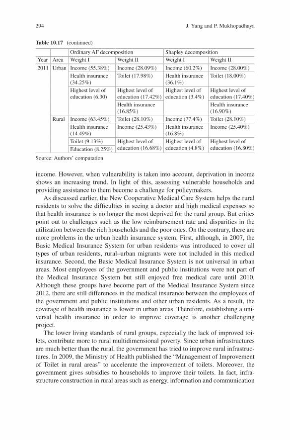
294

income. However, when vulnerability is taken into account, deprivation in income shows an increasing trend. In light of this, assessing vulnerable households and providing assistance to them become a challenge for policymakers.

As discussed earlier, the New Cooperative Medical Care System helps the rural residents to solve the difficulties in seeing a doctor and high medical expenses so that health insurance is no longer the most deprived for the rural group. But critics point out to challenges such as the low reimbursement rate and disparities in the utilization between the rich households and the poor ones. On the contrary, there are more problems in the urban health insurance system. First, although, in 2007, the Basic Medical Insurance System for urban residents was introduced to cover all types of urban residents, rural–urban migrants were not included in this medical insurance. Second, the Basic Medical Insurance System is not universal in urban areas. Most employees of the government and public institutions were not part of the Medical Insurance System but still enjoyed free medical care until 2010. Although these groups have become part of the Medical Insurance System since 2012, there are still differences in the medical insurance between the employees of the government and public institutions and other urban residents. As a result, the coverage of health insurance is lower in urban areas. Therefore, establishing a uni-versal health insurance in order to improve coverage is another challenging project.

The lower living standards of rural groups, especially the lack of improved toi-lets, contribute more to rural multidimensional poverty. Since urban infrastructures are much better than the rural, the government has tried to improve rural infrastruc-tures. In 2009, the Ministry of Health published the “Management of Improvement of Toilet in rural areas” to accelerate the improvement of toilets. Moreover, the government gives subsidies to households to improve their toilets. In fact, infra-structure construction in rural areas such as energy, information and communication

Table 10.17 (continued)

Ordinary AF decomposition Shapley decompositionYear Area Weight I Weight II Weight I Weight II

2011 Urban Income (55.38%) Income (28.09%) Income (60.2%) Income (28.00%)Health insurance (34.25%)

Toilet (17.98%) Health insurance (36.1%)

Toilet (18.00%)

Highest level of education (6.30)

Highest level of education (17.42%)

Highest level of education (3.4%)

Highest level of education (17.40%)

Health insurance (16.85%)

Health insurance (16.90%)

Rural Income (63.45%) Toilet (28.10%) Income (77.4%) Toilet (28.10%)Health insurance (14.49%)

Income (25.43%) Health insurance (16.8%)

Income (25.40%)

Toilet (9.13%) Highest level of education (16.68%)

Highest level of education (4.8%)

Highest level of education (16.80%)Education (8.25%)

Source: Authors’ computation

J. Yang and P. Mukhopadhaya

295

technologies, transport as well as water and sanitation is of drastic importance to growth and poverty alleviation and to narrow the urban–rural gap.

Our findings indicate that the contribution of education in both rural and urban poverty in the PRC is quite substantial. Although the 9-year compulsory education policy was established in 1986 when the first law on compulsory education was promulgated, it is still weak, particularly in rural areas. In order to continuously support the development of compulsory education in rural areas, the government implemented the “two exemptions and one subsidy” policy in 2001. This attempt is meant to exempt rural students from poor families from paying tuition and miscel-laneous fees in compulsory education and to provide living subsidies for boarders. Later in 2005, the State Council announced exemption of all the tuition and miscel-laneous fees for all rural students. Meanwhile, the funds for primary and secondary schools that provided compulsory education in rural areas would be arranged by the central government, which was later confirmed in the New Law on Compulsory Education in 2006. In 2007, the policy of exempting all tuition and miscellaneous fees was implemented nationwide in rural PRC. No doubt, rural people lag behind the urban in terms of education; in urban areas development of a trained workforce is also necessary. Thus, besides compulsory education, vocational education can also enhance both rural and urban human capital in two ways—training the labour force and educating new entrants to a different kind of labour market (e.g. the migrants in the cities)—thus providing cultural quality, higher-quality skills and strong business capabilities. In the rural areas, the latter was issued in 2005 in order to develop farmers’ practical technologies. The “No. 1 documents” in 2006 and 2007 announced an increase in the amount of public financial funds and the size of rural vocational education. In 2009, secondary vocational education became free for the students whose major was related to agriculture. By 2012, this policy has been implemented nationwide. Despite the efforts made, there are disparities in the quan-tity and quality of education between the urban and rural regions. One possible reason for the gap in education between the urban and rural regions is the decentral-ized fiscal system; thus instead of a county-based funding and management, which are unable to provide adequate educational funds, a much wider centralised system for disbursing educational funds to both rural and urban regions could be an option to reduce educational poverty.

8 Conclusion

Using the CHNS dataset, this chapter investigates urban–rural disparities in multi-dimensional poverty in the PRC. The $1.51 poverty line (adjusted for vulnerability and food insecurity) proposed in the ADB (2014) report is used as the income pov-erty cut-off (unlike previous studies where the World Bank’s $1.25 was used as the cut-off). The following important observations are made:

10 The Pattern of Urban–Rural Disparities in Multidimensional Poverty…

296

1. Total as well as rural and urban multidimensional poverty has decreased during the period 2000–2011.

2. Comparison of urban and rural multidimensional poverty shows that there is a disparity between urban and rural areas (income inequality research made a sim-ilar observation). The disparity exists because of the diversity of deprivation in the individual dimension and indicator. Rural households are deprived more in income, education and living standards (toilet).

3. Urban–rural gaps show different results as the poverty cut-off (in terms of num-ber of indicators) rises. Since 2009, the disparities of mild (k = 0.25) and moder-ate (k = 0.50) multidimensional poverty have become smaller because of narrower gaps of incidence. This implies that the special antipoverty policies in rural PRC have made some positive impacts in eliminating the poverty, which may not be in terms of income (with high poverty line) but at least in terms of the multidimensional perspective.

4. Urban–rural disparity in multidimensional poverty decreased in the period 2000–2009 but increased in 2011. Our examination reveals that the trend of dis-parity is influenced mostly by health insurance. The health issue has made the poor vulnerable to risk, and consequently in a wider perspective, they become vulnerable with respect to their earning capabilities. If not addressed properly, this will create more damage to the poor in the longer term.

Appendix: The Comparison of Food CPI and General CPI

Since the CHNS takes 2011 as the base year to inflate income, the food CPI is cal-culated on the assumption that the base year is 2011. So, the food CPI is the same as general CPI in 2011. Table 10.18 shows the general CPI given by the CHNS and the calculated food CPI. It can be found that the food CPI is less than the general CPI for all regions and all waves, indicating that the inflation rate of food CPI is higher. However, the difference between food CPI and general CPI is not as high as observed by ADB (2014).

The multidimensional poverty measurement—difference in results when differ-ent income cut-offs are used.

Table 10.19 corresponds to Table 10.21 with $1.25 used as the poverty line.Table 10.20 shows the differences in the multidimensional poverty measure-

ments between the results using the vulnerability-adjusted poverty line based on $1.51 and the conventional $1.25 poverty line. Moreover, the former result is based

J. Yang and P. Mukhopadhaya

297

on the food CPI-inflated income, while the latter is based on the general CPI. Three findings from Table 10.20 are worth noting. First, the differences in 2000 were dif-ferent from other waves. Poverty was lower using the ADB poverty line in 2000 but higher in other waves. The reason may lie in the quite close result in income depri-vation in 2000. Correspondingly, the differences were not significant in 2000. Second, the differences in M0 were highest when k = 0.5 from 2000 to 2006, but from 2009 to 2011, they were higher when k = 0.25. The reason may be that the gap of the raw headcount ratio of income had been widened. After 2009, more house-holds that were not poor using the conventional poverty line became poor using the adjusted regional poverty line in ADB (2014) just because they were deprived in income. As a result, the headcount ratio increased more when k = 0.25. Third, the differences of rural groups were higher than urban groups in all waves. The reason may be the more widened gap between the income deprivations using different income poverty lines for rural groups.

Table 10.18 Food CPI and general CPI (2011 as base year)

Province

2000 2004 2006 2009 2011Food CPI CPI

Food CPI CPI

Food CPI CPI

Food CPI CPI

Food CPI CPI

Liaoning U 50.56 80.94 59.23 83.20 61.44 84.78 81.92 92.56 100.00 100.00R 43.81 60.99 51.32 66.49 53.24 70.26 70.98 79.60 87.38 87.38

Heilongjiang U 57.95 80.45 65.81 84.01 67.52 86.21 86.09 95.17 104.12 104.12R 50.38 70.02 57.95 74.46 60.76 78.01 80.79 89.23 99.60 99.60

Jiangsu U 59.39 84.71 66.65 87.30 70.90 90.48 90.00 98.66 107.47 107.47R 45.99 62.87 51.85 67.69 55.59 70.49 70.54 77.66 85.79 85.79

Shandong U 56.25 83.91 64.16 86.68 67.08 88.51 86.37 96.18 103.27 103.27R 44.43 64.21 51.98 69.74 54.83 72.12 72.06 80.68 88.43 88.43

Henan U 44.31 67.93 53.14 73.18 56.31 75.61 76.15 83.88 91.42 91.42R 39.74 57.16 46.86 61.88 48.62 64.13 65.87 73.28 80.66 80.66

Hubei U 58.18 80.35 67.65 85.80 70.42 89.35 90.75 97.97 106.22 106.22R 46.41 66.11 54.88 71.28 58.51 75.03 77.42 84.70 92.87 92.87

Hunan U 56.78 81.51 64.72 84.75 68.52 87.92 89.67 97.46 105.96 105.96R 52.64 70.59 63.46 76.66 64.48 79.75 86.39 91.12 99.32 99.32

Guangxi U 53.46 77.49 60.00 81.55 63.34 85.34 84.73 95.00 103.28 103.28R 42.73 63.72 49.37 66.96 51.06 68.65 69.17 77.62 85.38 85.38

Guizhou U 52.03 77.43 58.88 81.90 61.90 83.70 83.16 93.52 101.55 101.55R 45.49 65.67 52.90 70.81 54.98 73.74 74.91 85.36 91.76 91.76

10 The Pattern of Urban–Rural Disparities in Multidimensional Poverty…

298

Tabl

e 10

.19

The

mul

tidim

ensi

onal

pov

erty

inde

x (w

ith $

1.25

as

the

inco

me

cut-

off)

Yea

rk

HA

M0

Urb

anR

ural

Nat

iona

lU

rban

Rur

alN

atio

nal

Urb

anR

ural

Nat

iona

l

2000

0.25

0.80

050.

9259

0.88

600.

3271

0.41

380.

3888

0.26

180.

3831

0.34

450.

50.

1158

0.26

390.

2168

0.56

960.

6229

0.61

390.

0660

0.16

440.

1331

0.75

0.00

160.

0226

0.01

590.

7750

0.79

420.

7935

0.00

120.

0179

0.01

261

00

00

00

00

020

040.

250.

7425

0.87

470.

8324

0.33

050.

3963

0.37

750.

2454

0.34

660.

3142

0.5

0.12

360.

2222

0.19

060.

5737

0.60

910.

6017

0.07

090.

1354

0.11

470.

750.

0051

0.01

480.

0117

0.77

500.

7860

0.78

450.

0040

0.01

170.

0092

10

00

00

00

00

2006

0.25

0.65

780.

6662

0.66

350.

3206

0.38

540.

3648

0.21

080.

2567

0.24

200.

50.

0960

0.14

930.

1322

0.56

880.

6045

0.59

610.

0546

0.09

030.

0788

0.75

0.00

140.

0130

0.00

930.

7750

0.79

140.

7906

0.00

110.

0103

0.00

731

00

00

00

00

020

090.

250.

3150

0.24

670.

2688

0.30

310.

3296

0.31

960.

0955

0.08

130.

0859

0.5

0.03

030.

0208

0.02

390.

5669

0.56

530.

5660

0.01

720.

0118

0.01

350.

750.

0000

0.00

030.

0002

0.00

00.

7750

0.77

500.

0000

0.00

030.

0002

10

00

00

020

110.

250.

2156

0.19

510.

2017

0.30

490.

3389

0.32

720.

0657

0.06

610.

0660

0.5

0.02

080.

0184

0.01

920.

5466

0.55

830.

5542

0.01

140.

0103

0.01

060.

750

00

00

00

00

10

00

00

00

00

J. Yang and P. Mukhopadhaya

299

Tabl

e 10

.20

The

dif

fere

nces

in m

ultid

imen

sion

al p

over

ty in

dex

Yea

rk

HA

M0

Urb

anR

ural

Nat

iona

lU

rban

Rur

alN

atio

nal

Urb

anR

ural

Nat

iona

l

2000

0.25

0−

0.00

03−

0.00

03−

0.00

33−

0.00

29−

0.00

29−

0.00

26−

0.00

27−

0.00

270.

5−

0.01

04−

0.00

98−

0.01

0.00

430.

0001

0.00

12−

0.00

55−

0.00

61−

0.00

590.

750

−0.

0008

−0.

0005

0−

0.00

02−

0.00

020

−0.

0006

−0.

0004

10

00

00

00

00

2004

0.25

00.

0049

0.00

320.

0123

**0.

0173

***

0.01

59**

*0.

0092

0.01

72**

*0.

0146

***

0.5

0.03

59**

*0.

0601

***

0.05

23**

*−

0.00

64−

0.00

13−

0.00

240.

0196

**0.

0362

***

0.03

09**

*

0.75

0.00

080.

0014

0.00

120

0.00

020

0.00

050.

0011

0.00

091

00

00

00

00

020

060.

250.

0173

0.07

06**

*0.

0535

***

0.03

12**

*0.

0358

***

0.03

54**

*0.

0267

***

0.05

36**

*0.

045**

*

0.5

0.08

670.

1125

***

0.10

43**

*−

0.01

04**

*−

0.00

06−

0.00

350.

0474

***

0.06

78**

*0.

0613

***

0.75

00.

0058

*0.

0039

*0

−0.

005

−0.

0046

00.

0044

*0.

0031

*

10

00

00

00

00

2009

0.25

0.07

89**

*0.

2219

***

0.17

57**

*0.

0318

***

0.02

07**

*0.

0263

***

0.03

64**

*0.

0829

***

0.06

79**

*

0.5

0.05

36**

*0.

038**

*0.

043**

*−

0.01

86−

0.00

63−

0.01

130.

0288

***

0.02

11**

*0.

0236

***

0.75

00

00

00

00

01

00

00

00

00

020

110.

250.

1118

***

0.24

35**

*0.

201**

*0.

0162

**0.

0073

0.01

24**

*0.

0394

***

0.08

58**

*0.

0708

***

0.5

0.03

15**

*0.

0239

***

0.02

63**

*−

0.01

24−

0.00

12−

0.00

560.

0165

***

0.01

33**

*0.

0144

***

0.75

00.

0003

0.00

020

0.77

50.

775

00.

0003

0.00

021

00

00

00

00

0

Not

e: **

* , **

, * mea

n th

e di

ffer

ence

is s

igni

fican

t at t

he 1

%, 5

% a

nd 1

0%, r

espe

ctiv

ely

10 The Pattern of Urban–Rural Disparities in Multidimensional Poverty…

300

Tabl

e 10

.21

Cen

sore

d he

adco

unt r

atio

of

each

indi

cato

r

Dim

ensi

onIn

dica

tor

2000

2004

2006

2009

2011

Urb

anR

ural

Nat

iona

lU

rban

Rur

alN

atio

nal

Urb

anR

ural

Nat

iona

lU

rban

Rur

alN

atio

nal

Urb

anR

ural

Nat

iona

l

(a)

$1.2

5 po

vert

y lin

eIn

com

eN

et in

com

e pe

r ca

pita

12.5

525

.53

21.4

013

.02

22.1

219

.20

11.0

420

.66

17.5

87.

6811

.33

10.1

58.

9511

.77

10.8

6

Edu

catio

nC

hild

sch

ool

atte

ndan

ce1.

292.

562.

150.

070.

620.

450.

140.

410.

330.

070.

070.

070.

070.

200.

16

Hig

hest

leve

l of

edu

catio

n6.

688.

658.

028.

4910

.22

9.66

7.58

12.9

911

.25

3.74

4.44

4.21

3.29

4.43

4.07

Hea

lth c

are

Hea

lth

insu

ranc

e78

.92

91.6

987

.63

73.4

585

.98

81.9

764

.05

58.6

460

.37

26.7

114

.22

18.2

514

.40

8.80

10.6

1

Stan

dard

of

livin

gE

lect

rici

ty0.

241.

060.

800.

070.

310.

230.

220.

340.

300.

070.

200.

160.

140.

310.

25D

rink

ing

wat

er3.

2220

.68

15.1

24.

6917

.56

13.4

33.

3912

.38

9.49

0.56

4.10

2.96

0.64

2.39

1.83

Toile

t25

.26

75.9

759

.82

19.0

965

.45

50.6

014

.29

46.8

536

.41

6.06

14.0

811

.49

3.37

11.3

68.

78C

ooki

ng f

uel

17.3

049

.92

39.5

313

.16

39.4

131

.00

8.88

21.7

817

.65

2.68

4.37

3.83

1.93

3.21

2.80

Con

sum

er

dura

bles

0.40

4.51

3.20

0.07

2.90

1.99

0.14

2.11

1.48

0.14

0.91

0.66

0.22

0.55

0.44

(b)

$1.5

1 vu

lner

abili

ty-a

djus

ted

pove

rty

line

Inco

me

Net

inco

me

per

capi

ta11

.50

24.4

420

.32

16.6

828

.75

24.8

821

.44

39.5

533

.74

20.9

337

.31

32.0

223

.28

38.5

433

.62

Edu

catio

nC

hild

sch

ool

atte

ndan

ce1.

292.

552.

150.

070.

620.

440.

140.

480.

370.

070.

140.

120.

070.

440.

32

Hig

hest

leve

l of

edu

catio

n6.

688.

658.

028.

4910

.46

9.83

7.80

14.3

212

.22

5.22

9.18

7.90

5.30

10.0

38.

50

Hea

lth c

are

Hea

lth

insu

ranc

e78

.92

91.7

087

.62

73.4

585

.99

81.9

664

.05

58.6

460

.38

26.7

114

.22

18.2

614

.40

8.80

10.6

0

J. Yang and P. Mukhopadhaya

301D

imen

sion

Indi

cato

r20

0020

0420

0620

0920

11U

rban

Rur

alN

atio

nal

Urb

anR

ural

Nat

iona

lU

rban

Rur

alN

atio

nal

Urb

anR

ural

Nat

iona

lU

rban

Rur

alN

atio

nal

Stan

dard

of

livin

gE

lect

rici

ty0.

241.

060.

800.

070.

310.

230.

220.

340.

300.

070.

230.

180.

430.

410.

41D

rink

ing

wat

er3.

2220

.68

15.1

24.

6917

.57

13.4

43.

4013

.16

10.0

30.

787.

135.

080.

795.

664.

09

Toile

t25

.26

75.9

559

.80

19.0

965

.91

50.9

014

.66

52.7

540

.52

7.96

30.2

523

.06

4.66

27.7

320

.28

Coo

king

fue

l17

.30

49.8

939

.51

13.1

639

.55

31.0

99.

2424

.28

19.4

53.

388.

777.

032.

296.

345.

04C

onsu

mer

du

rabl

es0.

404.

513.

210.

072.

901.

990.

142.

221.

550.

281.

010.

770.

220.

680.

53

(c)

Gap

(vu

lner

abili

ty a

djus

ted)

Inco

me

Net

inco

me

per

capi

ta−

1.05

−1.

09−

1.08

3.65

6.62

5.67

10.4

018

.89

16.1

713

.25

25.9

921

.87

14.3

326

.77

22.7

6

Edu

catio

nC

hild

sch

ool

atte

ndan

ce0.

000.

000.

000.

000.

00−

0.01

0.00

0.07

0.05

0.00

0.07

0.05

0.00

0.24

0.16

Hig

hest

leve

l of

edu

catio

n0.

000.

000.

000.

000.

240.

160.

211.

330.

971.

484.

743.

692.

015.

594.

43

Hea

lth c

are

Hea

lth

insu

ranc

e0.

000.

010.

000.

000.

01−

0.01

0.00

0.00

0.01

0.00

0.00

0.00

0.00

0.00

0.00

Stan

dard

of

livin

gE

lect

rici

ty0.

000.

000.

000.

00−

0.01

0.00

0.00

0.00

0.00

0.00

0.03

0.02

0.29

0.10

0.16

Dri

nkin

g w

ater

0.00

0.00

0.00

0.00

0.00

0.00

0.00

0.78

0.54

0.21

3.03

2.12

0.14

3.27

2.26

Toile

t0.

00−

0.02

−0.

020.

000.

450.

290.

365.

904.

121.

9016

.17

11.5

61.

2916

.37

11.5

0C

ooki

ng f

uel

0.00

−0.

03−

0.02

0.00

0.14

0.09

0.36

2.49

1.80

0.71

4.40

3.21

0.36

3.14

2.24

Con

sum

er

dura

bles

0.00

0.00

0.01

0.00

0.01

0.00

0.00

0.11

0.07

0.14

0.10

0.11

0.00

0.14

0.09

10 The Pattern of Urban–Rural Disparities in Multidimensional Poverty…

302

Tabl

e 10

.22

The

con

trib

utio

n of

eac

h in

dica

tor

(%)—

$1.2

5 po

vert

y lin

e

Dim

ensi

onIn

dica

tor

2000

2004

2006

2009

2011

Urb

anR

ural

Urb

anR

ural

Urb

anR

ural

Urb

anR

ural

Urb

anR

ural

Inco

me

Net

inco

me

per

capi

ta11

.98

16.6

613

.26

15.9

513

.10

20.1

220

.11

34.8

234

.05

44.4

9E

duca

tion

Chi

ld s

choo

l atte

ndan

ce0.

610.

830.

040.

220.

090.

200.

090.

100.

140.

39H

ighe

st le

vel o

f ed

ucat

ion

3.19

2.82

4.32

3.68

4.49

6.32

4.89

6.82

6.27

8.38

Hea

lth c

are

Hea

lth in

sura

nce

75.3

559

.83

74.8

262

.02

75.9

457

.10

69.9

343

.71

54.7

533

.27

Stan

dard

of

livin

gE

lect

rici

ty0.

050.

140.

010.

040.

050.

070.

040.

120.

110.

23D

rink

ing

wat

er0.

612.

700.

952.

530.

802.

410.

302.

520.

491.

81To

ilet

4.82

9.92

3.89

9.44

3.39

9.12

3.17

8.66

2.56

8.59

Coo

king

fue

l3.

306.

522.

685.

682.

114.

241.

402.

691.

472.

42C

onsu

mer

dur

able

s0.

080.

590.

010.

420.

030.

410.

070.

560.

160.

41

J. Yang and P. Mukhopadhaya

303

Tabl

e 10

.23

The

con

trib

utio

n of

eac

h in

dica

tor

by th

e Sh

aple

y va

lue

deco

mpo

sitio

n (%

) [w

eigh

t (I)

]

Dim

ensi

onIn

dica

tor

2000

2004

2006

2009

2011

Urb

anR

ural

Nat

iona

lU

rban

Rur

alN

atio

nal

Urb

anR

ural

Nat

iona

lU

rban

Rur

alN

atio

nal

Urb

anR

ural

Nat

iona

l

Inco

me

Net

inco

me

per

capi

ta12

.420

.118

.117

.924

22.4

24.5

38.5

34.6

4369

.861

.860

.277

.472

.9

Edu

catio

nC

hild

sch

ool

atte

ndan

ce0.

30.

60.

50

0.2

0.1

00.

10.

10

0.1

0.1

0.1

0.3

0.2

Hig

hest

leve

l of

edu

catio

n1.

92

22.

52.

42.

52.

53.

83.

42.

93.

93.

63.

44.

84.

4

Hea

lth c

are

Hea

lth

insu

ranc

e84

.976

78.3

79.1

72.2

74.1

72.7

56.6

61.2

53.8

25.4

33.9

36.1

16.8

21.9

Stan

dard

of

livin

gE

lect

rici

ty0

00

00

00

00

00

00

00

Dri

nkin

g w

ater

00.

20.

10.

10.

20.

10

0.1

0.1

00.

10.

10

0.1

0.1

Toile

t0.

30.

70.

60.

20.

60.

50.

20.

60.

40.

20.

50.

40.

10.

50.

4C

ooki

ng f

uel

0.2

0.4

0.4

0.2

0.4

0.3

0.1

0.3

0.2

0.1

0.2

0.1

0.1

0.1

0.1

Con

sum

er

dura

bles

00

00

00

00

00

00

00

0

10 The Pattern of Urban–Rural Disparities in Multidimensional Poverty…

304

Tabl

e 10

.24

The

con

trib

utio

n of

eac

h in

dica

tor

by th

e Sh

aple

y va

lue

deco

mpo

sitio

n (%

) [w

eigh

t (II

)]

Dim

ensi

onIn

dica

tor

2000

2004

2006

2009

2011

Urb

anR

ural

Nat

iona

lU

rban

Rur

alN

atio

nal

Urb

anR

ural

Nat

iona

lU

rban

Rur

alN

atio

nal

Urb

anR

ural

Nat

iona

l

Inco

me

Net

inco

me

per

capi

ta13

.110

.310

.616

.813

.413

.823

.218

.819

.426

.723

.724

.128

25.4

25.7

Edu

catio

nC

hild

sch

ool

atte

ndan

ce1.

21.

11.

10.

10.

30.

30.

10.

30.

30.

30.

20.

30

0.7

0.6

Hig

hest

leve

l of

edu

catio

n7.

43.

74.

110

.95.

26

12.4

9.3

9.6

15.2

13.9

14.1

17.4

16.8

16.8

Hea

lth c

are

Hea

lth

insu

ranc

e28

.726

26.3

27.9

25.7

2627

.220

.221

.121

.57.

19

16.9

56.

1

Stan

dard

of

livin

gE

lect

rici

ty0.

10.

50.

40

0.1

0.1

0.1

0.2

0.2

0.3

0.3

0.3

2.2

0.8

0.9

Dri

nkin

g w

ater

39

8.3

58.

78.

24.

98.

68.

12.

311

9.9

3.4

9.4

9

Toile

t24

.225

.625

.521

.125

.324

.717

25.1

2420

.128

.227

.218

28.1

27.1

Coo

king

fue

l21

.821

.821

.818

19.8

19.6

14.8

1615

.912

.314

.113

.612

.412

.312

.3C

onsu

mer

du

rabl

es0.

52

1.9

0.2

1.5

1.4

0.3

1.5

1.4

1.3

1.5

1.5

1.7

1.5

1.5

J. Yang and P. Mukhopadhaya

305

References

ADB. (2014). Poverty in Asia: A deeper look. Mandaluyong City: Asian Development Bank.Alkire, S. (2007). Choosing dimensions: The capability approach and multidimensional poverty

(pp. 89–119). New York: Palgrave Macmillan.Alkire, S., & Foster, J. (2008). Counting and multidimensional poverty. In The poorest and hun-

gry: Assessment, analysis and actions (pp. 77–90). Washington, DC: International Food Policy Research Institute.

Bourguignon, F., & Chakravarty, S. R. (2003). The measurement of multidimensional poverty. Journal of Economic Inequality, 1, 25–49.

Brandolini, A. (2009). On applying synthetic indices of multidimensional well-being: Health and income inequalities in France, Germany, Italy, and the United Kingdom. In Against injustice: The new economics of Amartya Sen (pp. 221–251). Cambridge: Cambridge University Press.

Chakravarty, S. R., Mukherjee, D., & Ranade, R. (1998). On the family of subgroup and factor decomposable measures of multidimensional poverty. Research on Economic Inequality, 8, 175–194.

Chen, L. (2008). The measurement and decomposition of multidimensional poverty in transition period of China. Economic Review, 5, 5–10 (In Chinese).

Chen, Q. (2012). The multidimensional measurement and the policy implication of the rural poverty in the poverty-stricken covered area. Journal of Sichuan Normal University (Social Sciences Edition), 39(3), 58–63 (In Chinese).

Chen, H., & Zhang, Q. (2013). Urban multidimensional poverty measurement based on the Alkire- Foster model: A case study of Zhongshan City. Journal of Wuyi University (Natural Sciences Edition), 27(2), 32–36 (In Chinese).

Cohen, A., & Sullivan, C. A. (2010). Water and poverty in rural China: Developing an instrument to assess the multiple dimensions of water and poverty. Ecological Economics, 69, 999–1099.

D’ambrosio, C., Deutsch, J., & Silber, J. (2011). Multidimensional approaches to poverty mea-surement: An empirical analysis of poverty in Belgium, France, Germany, Italy and Spain, based on the European panel. Applied Economics, 43(8), 951–961.

Decancq, K., & Lugo, M. A. (2013). Weights in multidimensional indices of wellbeing: An over-view. Econometric Reviews, 32(1), 7–34.

Deutsch, J., & Silber, J. (2005). Measuring multidimensional poverty: An empirical comparison of various approaches. Review of Income and Wealth, 51(1), 145–174.

Doyal, L., & Gough, I. (1991). A theory of human need. Hampshire: MacMillan Education Ltd.Foster, J. E., McGillivray, M., & Seth, S. (2013). Composite Indices: Rank robustness, statistical

association, and redundancy. Econometric Reviews, 32(1), 35–56.Gao, Y. (2012). The multidimensional poverty in urban and rural China: Measurement and com-

parison. Statistical Research, 29(11), 61–66 (In Chinese).Guo, J. (2012). The multidimensional poverty measurement and its characteristics of rural house-

holds: Based on the data of rural Shanxi Province. Rural Economy, 3, 19–22 (In Chinese).Jiang, C., Xu, Q., & Li, Y. (2011). The measurement of household multidimensional poverty in

China. Statistics & Decisions, 22, 92–95 (In Chinese).Labar, K., & Bresson, F. (2011). A multidimensional analysis of poverty in China from 1991 to

2006. China Economic Review, 22, 646–668.

10 The Pattern of Urban–Rural Disparities in Multidimensional Poverty…

306

Li, S., & Luo, C. (2010). Re-estimating the income gap between urban and rural households in China. Procedia-Social and Behavioral Sciences, 2010(2), 7151–7163.

Li, S., Wan, G., & Zhuang, J. (2014). Income inequality and redistributive policy in People’s Republic of China. In R. Kanbur, C. Rhee, & J. Zhuang (Eds.), Inequality in Asian and the Pacific. London/New York: ADB and Routledge.

Liu, H. (2008). The China health and nutrition survey: An important database for poverty and inequality research. The Journal of Economic Inequality, 6(4), 373–376.

Lu, C. (2010). Who is poor in China? A comparison of alternative approaches to poverty assess-ment in Rural Yunnan. The Journal of Peasant Studies, 37(2), 407–428.

McGillivray, M., & White, H. (1993). Measuring development? The UNDP’s human development index. Journal of International Development, 5(2), 183–192.

Mukherjee, N. (1999). Consultations with the poor in Indonesia: Country synthesis report. Poverty reduction and economic management network, The World Bank.

Mukhopadhaya, P., Shantakumar, G., & Rao, V. V. B. (2011). Economic growth and income inequality in China. In India and Singapore: Trends and policy implications. London/New York: Routledge.

Nussbaum, M. C. (2000). Women and human development. Cambridge: Cambridge University Press.

OECD. (2008). Handbook on constructing composite indicators: Methodology and user guide. Paris: Joint Research Centre-European Commission/OECD Publishing.

Qi, D., & Wu, Y. (2014). Child poverty in China—A multidimensional deprivation approach. Child Indicators Research, 7, 89–118.

Ranis, G., Stewart, F., & Samman, E. (2006). Human development: Beyond the human develop-ment index. Journal of Human Development, 7(3), 323–358.

Ray, R., & Mishra, A. (2012). Multi-dimensional deprivation in the awakening giants: A compari-son of China and India on micro data. Journal of Asian Economics, 23, 454–465.

Saisana, M., Saltelli, A., & Tarantola, S. (2005). Uncertainty and sensitivity analysis techniques as tools for the quality assessment of composite indicators. Journal of the Royal Statistical Society: Series A (Statistics in Society), 168(2), 307–323.

Sen, A. K. (1985). Well-being, agency and freedom: The Dewey lectures 1984. The Journal of Philosophy, 82(4), 169–221.

Shang, W., & Yao, Z. (2005). The research of method in multidimensional poverty measure. Journal of Finance and Economics, 31(12), 88–94 (In Chinese).

Sicular, T., Ximing, Y., Gustafsson, B., et al. (2007). The urban–rural income gap and inequality in China. Review of Income and Wealth, 53(1), 93–126.

Sun, X., Tian, G., Pan, Y., et al. (2012). Research on rural poverty measurement in China: Based the data of Shanxi Province. On Economic Problems, 4, 79–84 (In Chinese).

Tsui, K. Y. (2002). Multidimensional poverty indices. Social Choice and Welfare, 19, 69–93.Wagle, U. (2008). Multidimensional poverty measurement: Concepts and applications. New York:

Springer Science+Business Media, LLC.Wang, X., & Alkire, S. (2009). The measurement of multidimensional poverty in China: Estimation

and policy implication. Chinese Rural Economy, 2009(12), 4–10 (In Chinese).

J. Yang and P. Mukhopadhaya

307

Yang, J., & Mukhopadhaya, P. (2016a). Disparities in the level of poverty in China: Evidence from China family panel studies 2010. Social Indicators Research, 132(1), 411–450.

Yang, J., & Mukhopadhaya, P. (2016b). China’s war against many faces of poverty—Towards a new long March. New York/London: Routledge.

Yu, J. (2013). Multidimensional poverty in China: Findings based on the CHNS. Social Indicators Research, 112(2), 315–336.

Zou, W., & Fang, Y. (2011). A study: On the dynamic multidimensional measurement of China’s poverty. Chinese Journal of Population Science, 6, 49–59 (In Chinese).

The views expressed in this publication are those of the authors and do not necessarily reflect the views and policies of the Asian Development Bank (ADB) or its Board of Governors or the governments they represent.

ADB does not guarantee the accuracy of the data included in this publication and accepts no responsibility for any consequence of their use. The mention of specific companies or products of manufacturers does not imply that they are endorsed or recommended by ADB in preference to others of a similar nature that are not mentioned.

By making any designation of or reference to a particular territory or geographic area, or by using the term “country” in this document, ADB does not intend to make any judgments as to the legal or other status of any territory or area. Open Access This work is available under the Creative Commons Attribution-NonCommercial 3.0 IGO license (CC BY-NC 3.0 IGO) http://creativecommons.org/licenses/by-nc/3.0/igo/. By using the content of this publication, you agree to be bound by the terms of this license. For attribution and permissions, please read the provisions and terms of use at https://www.adb.org/terms-use#openaccess.

This CC license does not apply to non-ADB copyright materials in this publication. If the mate-rial is attributed to another source, please contact the copyright owner or publisher of that source for permission to reproduce it. ADB cannot be held liable for any claims that arise as a result of your use of the material.

Please contact pubsmarketing@adb.org if you have questions or comments with respect to content, or if you wish to obtain copyright permission for your intended use that does not fall within these terms, or for permission to use the ADB logo.

Notes: ADB recognizes “China” as the People’s Republic of China.

10 The Pattern of Urban–Rural Disparities in Multidimensional Poverty…

309© Asian Development Bank 2019 K. Jayanthakumaran et al. (eds.), Internal Migration, Urbanization, and Poverty in Asia: Dynamics and Interrelationships, https://doi.org/10.1007/978-981-13-1537-4_11

Chapter 11Distribution of Urban Economic Growth in Post-reform India: An Empirical Assessment

Sabyasachi Tripathi

Keywords Pro-poor economic growth · Poverty · Inequality · Urban India

JEL Classification D63 · D64 · R11

1 Introduction

The impact of economic reforms of 1991 was quite significant on India’s economic growth. For example, the average growth rate of gross domestic product was signifi-cantly higher at about 6.96% for the years 1992–1993 to 2011–2012, at 2004–2005 prices. However, the main problem encountered by the Indian economy is the unequal distribution of the benefits of higher economic growth, as evidenced by the lower increases in the standard of living of low-income groups, particularly for the lower castes. In recognition of this fact, the Twelfth Five-Year Plan (2012–2017) has fixed its main objective as ‘faster, sustainable and more inclusive growth’ so that benefits of higher economic growth are distributed more evenly to those sections of people who were left out.

Currently, India like most other developing countries is going through a transfor-mation from rural- to urban-based economy. This is evident in the high increase in the absolute number of urban population compared to rural population as of 2011; the percentage of urban population increased from 17.97% in 1961 to 31.16% in 2011. In fact, Indian cities are growing very fast. For instance, Delhi (25 million populations) became the second most populous city after Tokyo (38 million popula-tion) in 2014 (United Nations 2014). According to the projections by McKinsey Global Institute (2010), Indian cities will accommodate about 590 million popula-tion by 2030. The number of million plus cities has increased sharply in India, from 35 in 2001 to 53 in 2011. The number and share of urban population of Class I cities

The views expressed in the study do not necessarily reflect those of the Government of India.

S. Tripathi (*) Department of Economics, Adamas University, Kolkata, West Bengal, India

310

(population with 1 lakh and more) also has increased from 107 (or 51.88% of total urban population) in 1961 to 468 (or 70.24% of total urban population) in 2011. This suggests that in the coming decades, more Indians will be living in Class I cities.

However, India is still relatively less urbanized compared to other countries, with an urbanization rate of 32% in 2014, which is much lower than the global level of 54%. This could be because of the lower rural-urban migration in India. The existing caste system; the diversity of language and culture, traditional values and joint family system; the lack of education; and the predominance of agriculture, semi-feudal land relation and traditional values are found to be the main reasons behind this lower rural-urban migration (Davis 1951). Census data in 2001 (as 2011 Census is yet to be published) shows that India’s interstate migration was about 4% (41 million) com-pared to 26% (268 million) intra-state migration (Bhagat 2010). Table 11.1 shows that about 35% of India’s urban population consist of migrants, according to the latest National Sample Survey (NSS) in 2007–2008. Table 11.1 also shows that the rate of migration declined from 1981–1983 to 1991–1993 of the Census and NSS years. Most importantly, after the Census and NSS year of 1991–1993, the rate of migration to urban areas has increased. The latest NSS data, i.e. 2007–2008, also confirms the increase in the rate of migration. Most importantly, NSS data of 2007–2008 shows that female migration rate to urban areas is much higher than male migration rate.

As India is going through a transformation from agriculture to industry- and service-based economy, it has increased the hope of the rural people of getting higher job opportunities, which in turn has resulted in higher rural-to-urban migra-tion. On the other hand, slow agricultural growth and inadequate development of the rural non-farm sector have forced the rural poor and unemployed people to migrate to urban areas as urban areas provide higher wage rate through realization of higher productivity. Rural-to-urban migration in million plus cities was estimated at 20 million (56%) migrants in 2001. The proportion of male and female was almost equal at more than 55%.

It is also important to note that rural-to-urban migration for male (or female) was 34.2% (or 13.5%) as per the Census 2001. On the other hand, as per NSS data, in 2007–2008, rural-to-urban migration rate for male (or female) was 39% (or 14.8%). Table 11.2 lists the top 10 urban agglomerations which received the highest rural- to- urban migration in 2001. Table 11.2 confirms that the bigger (as per the population

Table 11.1 Migration rates in urban areas, 1981–2008 (migrants per 100 persons)

Census/NSS yearCensus NSSMale Female Total Male Female Total

1981/1983 33.2 40.8 36.8 27.0 36.6 31.61991/1993 26.3 36.2 31.0 23.9 38.2 30.72001/2000 32.0 39.4 35.5 25.7 41.8 33.4NA/2008 NA NA NA 25.9 45.6 35.4

Source: Bhagat (2014)Note: NA Not available

S. Tripathi

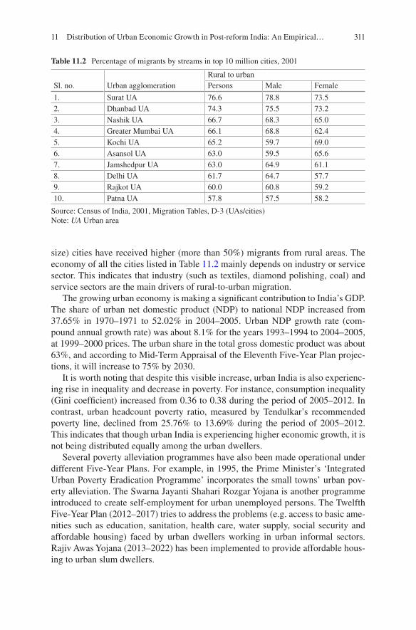
311

size) cities have received higher (more than 50%) migrants from rural areas. The economy of all the cities listed in Table 11.2 mainly depends on industry or service sector. This indicates that industry (such as textiles, diamond polishing, coal) and service sectors are the main drivers of rural-to-urban migration.

The growing urban economy is making a significant contribution to India’s GDP. The share of urban net domestic product (NDP) to national NDP increased from 37.65% in 1970–1971 to 52.02% in 2004–2005. Urban NDP growth rate (com-pound annual growth rate) was about 8.1% for the years 1993–1994 to 2004–2005, at 1999–2000 prices. The urban share in the total gross domestic product was about 63%, and according to Mid-Term Appraisal of the Eleventh Five-Year Plan projec-tions, it will increase to 75% by 2030.

It is worth noting that despite this visible increase, urban India is also experienc-ing rise in inequality and decrease in poverty. For instance, consumption inequality (Gini coefficient) increased from 0.36 to 0.38 during the period of 2005–2012. In contrast, urban headcount poverty ratio, measured by Tendulkar’s recommended poverty line, declined from 25.76% to 13.69% during the period of 2005–2012. This indicates that though urban India is experiencing higher economic growth, it is not being distributed equally among the urban dwellers.

Several poverty alleviation programmes have also been made operational under different Five-Year Plans. For example, in 1995, the Prime Minister’s ‘Integrated Urban Poverty Eradication Programme’ incorporates the small towns’ urban pov-erty alleviation. The Swarna Jayanti Shahari Rozgar Yojana is another programme introduced to create self-employment for urban unemployed persons. The Twelfth Five-Year Plan (2012–2017) tries to address the problems (e.g. access to basic ame-nities such as education, sanitation, health care, water supply, social security and affordable housing) faced by urban dwellers working in urban informal sectors. Rajiv Awas Yojana (2013–2022) has been implemented to provide affordable hous-ing to urban slum dwellers.

Table 11.2 Percentage of migrants by streams in top 10 million cities, 2001

Sl. no. Urban agglomerationRural to urbanPersons Male Female

1. Surat UA 76.6 78.8 73.52. Dhanbad UA 74.3 75.5 73.23. Nashik UA 66.7 68.3 65.04. Greater Mumbai UA 66.1 68.8 62.45. Kochi UA 65.2 59.7 69.06. Asansol UA 63.0 59.5 65.67. Jamshedpur UA 63.0 64.9 61.18. Delhi UA 61.7 64.7 57.79. Rajkot UA 60.0 60.8 59.210. Patna UA 57.8 57.5 58.2

Source: Census of India, 2001, Migration Tables, D-3 (UAs/cities)Note: UA Urban area

11 Distribution of Urban Economic Growth in Post-reform India: An Empirical…

312

Several policies have been introduced by the Government of India in recent years to promote urbanization in India. For example, 100 Smart Cities Mission deals with promotion of mixed land use in area-based developments, expansion housing oppor-tunities for all, creation of walkable localities, preservation and development of open spaces and promotion of variety of transport options. Atal Mission for Rejuvenation and Urban Transformation (AMRUT) focuses on providing basic ser-vices, such as water supply, sewerage and urban transport. It seeks to ensure that every household has access to piped water with assured supply and also sewerage connection. The Swachh Bharat Abhiyan is a massive movement that seeks to create a cleaner India. The programme includes building individual household toilets, community and public toilets and municipal solid waste management in the towns. The Digital India has a vision to transform India into a digitally empowered society and knowledge economy. It is hoped that all these major programmes and policies will reshape urban India for making higher contribution to economic growth along with reduction of poverty and inequality.

Government intervention has to be assessed so that right policies are taken up with scope for time-to-time revision. To plan, supervise and implement poverty reduction policies, it is very important to know the poverty figures not only for a particular time but also for different time periods. Therefore, evaluating of pro- poorness of growth is essential to ensure higher and sustainable development. Ultimately, we have to ensure proper distribution of the accruals from higher eco-nomic growth by formulating appropriate policies; otherwise it will lead to further increase in inequality and several socio-economic problems among the urban dwellers.

With this backdrop, the main objectives of this chapter are as follows: first to measure the poverty and inequality situation in urban India and second to empiri-cally estimate the pro-poorness of distributive changes of urban economic growth; and finally, the chapter seeks to identify appropriate policies for efficient distribu-tion of urban economic growth. The study covers the periods from 2004–2005 to 2011–2012, and the available unit-level data for three rounds—61st round for 2004–2005, 66th round for 2009–2010 and 68th round for 2011–2012—of urban monthly per capita expenditure (MPCE) have been used for analysis in conjunction with data from the National Sample Survey (NSS) conducted by the Department of Statistics of the Indian government (NSSO 2006, 2011, 2013) for analysis.

The framework proposed by Duclos (2009) based on the methodology of Araar et al. (2007, 2009) and Araar (2012) has been used to measure the pro-poorness of urban economic growth. Duclos (2009) formulated two approaches, i.e. relative and absolute, to measure poverty. Relative approach measures the pro-poor growth rate by considering some standard (usually the average growth rate of the median or the mean). Absolute approach measures the pro-poorness by considering absolute income of the poor. These frameworks are based on proper theoretical structure and analyse pro-poor growth in a dynamic manner by employing statistical rationale. The results are very important to formulate appropriate policies for proper distribu-tion of higher urban economic growth.

S. Tripathi

313

The rest of the chapter is structured as follows: The following section provides a brief review of literature, the third section describes the poverty and inequality situ-ation in urban India, the fourth section measures pro-poor growth by explaining the theoretical model and empirical results of pro-poor growth assessment and, finally, the last section presents the summary of findings, conclusions and discussions.

2 Review of the Literature

There are very limited numbers of studies that measure the pro-poorness of eco-nomic growth in India. Datt and Ravallion (2009) measured and compared the pro- poor growth in terms of reduction in poverty and elasticity of poverty with respect to economic growth by considering pre- and post-reform periods in India separately.1 Using consumption expenditure data for the periods of 1958 to 2006, the authors found evidence for long-run decline of poverty as measured by poverty headcount ratio, poverty gap ratio and squared poverty gap ratio. But a higher proportionate rate of action against poverty after 1991 is also evidenced by them. This shows that post-reform India became less pro-poor. They also found evidence of the trickle- down effect of higher economic growth on reduction of rural poverty in the pre- 1991 data.

Using 2009–2010 NSS data, Liu and Barrett (2013) investigated the patterns of job seeking, rationing and participation under Mahatma Gandhi National Rural Employment Guarantee Scheme (MGNREGS) and found that the scheme is not pro-poor as it exhibits a middle-class bias. Dev (2002) examined the degree of pro- poor growth by measuring several quantitative and qualitative aspects of employment, such as employment elasticities of growth, labour productivity, wage rates and job security for the period of 1980 to 2000. The study found a declining trend in the quality of employment in different sectors (e.g. agriculture sector). The growth rate of employment was positive, but it declined for the period of 1994–2000.

In the context of pro-poorness of the institutional interventions, a cross-sectional study of women beneficiaries under the Muthulakshmi Reddy Maternity Benefit Scheme in five districts of Tamil Nadu by Balasubramanian and Ravindran (2012) showed that scheduled caste landless women have received smaller benefits. Most importantly, Ravallion (2000) suggested a number of conditions which determine the poor’s share in economic growth in India. He recommended that higher and stable agricultural growth is essential for poverty reduction in the long run. Therefore, human and physical resource development in rural areas is essential. Ravallion and Datt’s (1999) study found that initial conditions and sectoral compo-sition of economic growth determine the degree of economic growth and reduction in poverty in India. The above review of literature clearly shows that thrust of pro- poor growth in India is very limited. Therefore, this paper tries to fill this gap by using appropriate statistical techniques to measure pro-poor growth in India.

1 For an overview of the various approaches to defining “pro-poor growth”, see Ravallion (2004).

11 Distribution of Urban Economic Growth in Post-reform India: An Empirical…

314

3 The Poverty and Inequality Situation in Urban India

This section seeks to present the poverty and inequality situation by considering different aspects of urban India by using latest unit-/individual-level data on con-sumption expenditure provided by NSS. The extent of inequality is measured by Gini coefficient. The poverty headcount ratio (PHR), the poverty gap ratio (PGR) and the squared poverty gap ratio (SPGR) are used to measure poverty. MPCE used in this study is based on Mixed Reference Period (MRP) and the Modified Mixed Reference Period (MMRP), and Gini coefficient is used to measure the extent of inequality in urban India. Inequality and poverty estimations are based on the Mixed Reference Period (MRP), and the Modified Mixed Reference Period (MMRP) is considered over the Uniform Recall Period (URP).2

Following the suggestion of the Expert Group (Tendulkar Committee, GOI 2009), MRP-based poverty and inequality estimation is considered while using con-sumption expenditure data for the 61st, 66th and 68th NSS rounds. The consump-tion expenditure of a poor household on low-frequency items is better captured by MRP-based estimates compared to URP-based estimates. Following the recommen-dation of the Expert Group (Rangarajan Committee, (GOI 2014)), MMRP-based poverty and inequality estimation is considered while using consumption expendi-ture data for the 66th and 68th rounds, as MMRP-based estimates are expected to yield estimates that are closer to their ‘true value’ (Deaton and Kozel 2005).

Table 11.3 presents the poverty and inequality situation by considering different attributes of urban India in different periods of time, using the MRP-based con-sumption expenditure data based on the Tendulkar Committee’s recommended pov-erty line.3 Urban PHR has declined from 25.8% in 2004–2005 to 13.7% in 2011–2012. This is because of the higher economic growth rate in urban India in recent decades, which led to a reduction in the poverty level. In this context, Tripathi (2013a) estimated that India’s large agglomerations have a robust and positive effect on the city output growth rate as large agglomerations provide higher productivity, wages and capital per worker due to higher economies of agglomeration, which ultimately increases economic growth and reduces the city poverty rate significantly.

The analysis involving the calculated values of the three poverty indices and for three different periods shows that poverty ratios are lower for groups of urban dwell-ers such as those who have an education level ‘postgraduate and above’, ‘graduate’, ‘diploma’, ‘higher secondary’, ‘secondary’ and ‘regular wage earner’. In contrast, the poverty ratios are higher for the urban dwellers in categories like ‘casual worker’,

2 The details about URP, MRP and MMRP can be found in Tripathi (2013c) and NSS report on consumption expenditure. Though URP- or MRP-based consumption data is available for all the periods (61st, 66th and 68th NSS round surveys on consumer expenditure), MMRP-based con-sumption data is available only for the 66th and 68th NSS rounds.3 Latest Expert Committee headed by Dr. Rangarajan has considered MMRP-based MPCE to esti-mate poverty in India. However, MMRP-based consumption expenditure is available 2009–2010 onwards only.

S. Tripathi

315

Tabl

e 11

.3

Mea

sure

men

ts o

f po

vert

y an

d in

equa

lity

for

urba

n In

dia,

200

4–20

05 to

201

1–20

12

Cat

egor

y20

04–2

005

2009

–201

020

11–2

012

PHR

PGR

SPG

RG

ini

PHR

PGR

SPG

RG

ini

PHR

PGR

SPG

RG

ini

Tota

lU

rban

25.8

6.1

2.0

36.4

20.9

4.7

1.5

38.0

13.7

2.7

0.8

37.7

Hou

seho

ld ty

peSe

lf-e

mpl

oyed

27.9

6.5

2.1

35.4

22.5

5.0

1.6

36.7

15.3

3.0

0.9

35.6

Reg

ular

wag

e/sa

lary

ear

ning

14.9

2.9

0.9

33.9

10.4

1.9

0.5

34.9

6.5

1.1

0.3

35.8

Cas

ual l

abou

r58

.416

.05.

924

.647

.411

.74.

025

.332

.27.

12.

226

.2O

ther

s16

.74.

31.

741

.513

.32.

80.

944

.78.

81.

70.

542

.2R

elig

ion

Hin

du23

.15.

41.

835

.918

.94.

21.

337

.812

.22.

40.

737

.5O

ther

s35

.18.

62.

937

.628

.26.

42.

138

.018

.83.

61.

037

.4So

cial

gro

upSc

hedu

led

trib

es35

.110

.44.

235

.229

.07.

02.

541

.323

.35.

01.

635

.3Sc

hedu

led

cast

es40

.110

.13.

630

.233

.07.

82.

632

.621

.64.

31.

331

.8O

ther

bac

kwar

d cl

asse

s31

.57.

42.

532

.625

.45.

71.

934

.916

.23.

31.

034

.3O

ther

s15

.83.

41.

036

.612

.02.

50.

837

.97.

41.

30.

438

.5Se

xM

ale

24.6

5.8

1.9

36.3

20.1

4.5

1.5

38.2

13.3

2.6

0.8

37.7

Fem

ale

27.0

6.4

2.2

36.6

21.8

4.9

1.6

37.8

14.1

2.8

0.8

37.7

Age

aC

hild

34.0

8.6

3.0

34.0

27.7

6.5

2.2

35.2

18.5

3.8

1.1

35.5

Adu

lt21

.44.

81.

536

.717

.73.

81.

238

.511

.52.

20.

637

.9

(con

tinue

d)

11 Distribution of Urban Economic Growth in Post-reform India: An Empirical…

316

Tabl

e 11

.3

(con

tinue

d)

Cat

egor

y20

04–2

005

2009

–201

020

11–2

012

PHR

PGR

SPG

RG

ini

PHR

PGR

SPG

RG

ini

PHR

PGR

SPG

RG

ini

Edu

catio

nN

ot li

tera

te45

.111

.64.

130

.738

.09.

13.

231

.625

.65.

41.

632

.1L

itera

te w

ithou

t for

mal

sch

oolin

g33

.07.

82.

534

.326

.76.

22.

233

.020

.44.

41.

235

.2B

elow

pri

mar

y34

.38.

32.

832

.428

.46.

62.

233

.320

.24.

11.

234

.3Pr

imar

y29

.26.

62.

131

.125

.25.

51.

732

.015

.63.

10.

931

.8M

iddl

e21

.24.

51.

430

.519

.64.

01.

231

.512

.52.

30.

632

.2Se

cond

ary

11.8

2.2

0.6

31.4

12.2

2.3

0.7

33.0

7.7

1.4

0.4

32.5

Hig

her

seco

ndar

y7.

81.

40.

433

.17.

21.

30.

437

.85.

30.

90.

234

.2D

iplo

ma/

cert

ifica

te c

ours

e3.

60.

60.

130

.82.

90.

50.

134

.93.

40.

50.

133

.2G

radu

ate

3.2

0.5

0.1

34.0

3.2

0.5

0.1

36.0

2.0

0.3

0.1

36.1

Post

grad

uate

and

abo

ve2.

20.

40.

134

.81.

40.

20.

135

.51.

20.

20.

138

.2

Sour

ce: C

alcu

latio

ns b

ased

on

the

unit-

leve

l dat

a of

the

cons

umer

exp

endi

ture

rou

nds

of 2

004–

2005

, 200

9–20

10 a

nd 2

011–

2012

, NSS

O, G

OI

Not

e: a T

he U

nite

d N

atio

ns C

onve

ntio

n (U

NC

) id

entifi

es c

hild

as

‘a h

uman

bei

ng b

elow

the

age

of 1

8 ye

ars

unle

ss u

nder

the

law

app

licab

le to

the

child

, maj

or-

ity is

atta

ined

ear

lier’

(T

ripa

thi,

2013

c). H

owev

er, t

he d

efini

tion

of c

hild

is v

ery

ambi

guou

s ac

cord

ing

to I

ndia

n la

ws.

Thu

s, w

e co

nsid

er d

efini

tion

prop

osed

by

UN

C

S. Tripathi

317

‘not literate’, ‘scheduled castes’, ‘scheduled tribes’, ‘other religion group’ and ‘lit-erate without formal schooling’. The extent of inequality has risen from 36.4 in 2004–2005 to 37.7 in 2011–2012. Most importantly, the inequality level is higher for groups like ‘other household type’, ‘other religion group’, ‘adult’, those with education level ‘postgraduate and above’ and ‘male’. The extent of inequality is lower for ‘not literate’, ‘middle-class’ educated people, ‘scheduled caste’, ‘casual labour’ and those who have passed ‘primary’ level education.

Table 11.4 presents the calculated figures of percentage decline of poverty ratios and percentage increase in inequality at different time points during the years 2004–2005 to 2009–2010. As can be seen from the table, PHR declined by about 47% in the periods 2004–2005 to 2011–2012. In contrast, the extent of inequality increased by about 4% during the same period. Categories which experienced a higher decline in the poverty ratio are ‘postgraduate and above’, ‘regular wage/salary earning’, ‘other social group’, ‘other household type’ and ‘scheduled tribe’ during this period. On the other hand, groups like those who have passed ‘middle/higher secondary/graduate/diploma’ experienced a lower percentage decline of poverty ratio in the same time span. Most importantly, those who have passed only secondary-level edu-cation experienced an increase in the poverty ratio during the years 2004–2005 to 2009–2010. Coming to the years 2009–2010 to 2011–2012, it was groups like ‘scheduled castes’ and ‘child’ that experienced a higher percentage reduction in poverty ratio. In contrast, categories which experienced a lower-level decline of pov-erty ratio are ‘postgraduate and above’, ‘higher secondary’, ‘scheduled tribes’ and ‘literate without formal education’. Most noticeably, ‘diploma’ holders experienced an increase in poverty ratio in the years from 2009–2010 to 2011–2012. However, in regard to the percentage of poverty decline for the years from 2004–2005 to 2011–2012, it is groups like ‘other religion’ and ‘female’ that have experienced a high level of poverty decline compared to other categories. Increase in the lower level of inequality is found for groups like ‘other religion’, those who have studied ‘post-graduate and above’ and ‘casual labour’ for the years 2004–2005 to 2009–2010. In contrast, groups like ‘scheduled tribes’, those who have passed ‘higher secondary’, ‘diploma’ holder and ‘scheduled castes’ are found to have experienced a higher rise in the level of inequality during the same period of time. Most importantly, there was a perceptible decline in inequality for the group ‘literate without formal schooling’ in the years 2004–2005 to 2009–2010. The categories that have experienced a decline in inequality in the years 2009–2010 to 2011–2012 are ‘scheduled tribes’, those who have passed ‘higher secondary’, ‘other household types’ and ‘diploma’ holders. On the other hand, there is evidence to show those who have passed ‘post-graduate and above’, ‘below-primary-school’ educated people, ‘literate without for-mal schooling ‘and ‘casual worker’ experienced a rise in inequality. However, during the time periods from 2004–2005 to 2011–2012, groups like ‘scheduled tribes’, ‘self-employed’ and ‘other household type’ did experience a lower increase of inequality. In contrast, those who have passed ‘graduate’-level education experi-enced a higher level of increase in inequality during the same period.

Table 11.5 presents the poverty and inequality situation in terms of the different attributes of urban India for the years 2009–2010 and 2011–2012; these figures are

11 Distribution of Urban Economic Growth in Post-reform India: An Empirical…

318

Tabl

e 11

.4

Dec

line

of p

over

ty r

ate

and

incr

ease

in th

e ex

tent

of

ineq

ualit

y in

urb

an I

ndia

fro

m 2

004–

2005

to 2

011–

2012

Cat

egor

y

Pove

rty

decl

ine

(in

%)

Incr

ease

of

ineq

ualit

y (i

n %

)20

04–2

005

to

2009

–201

020

09–2

010

to

2011

–201

220

04–2

005

to

2011

–201

220

04–2

005

to

2009

–201

020

09–2

010

to

2011

–201

220

04–2

005

to

2011

–201

2PH

RPG

RSP

GR

PHR

PGR

SPG

RPH

RPG

RSP

GR

Gin

i coe

ffici

ent

Tot

alU

rban

Ind

ia18

.823

.525

.634

.541

.947

.846

.955

.661

.24.

4−

1.0

3.6

Hou

seho

ld

type

Self

-em

ploy

ed19

.522

.823

.032

.240

.647

.745

.454

.159

.73.

7−

3.0

0.6

Reg

ular

wag

e/sa

lary

ea

rnin

g30

.034

.236

.037

.443

.546

.756

.262

.865

.92.

82.

75.

6

Cas

ual l

abou

r18

.827

.031

.132

.139

.145

.244

.955

.562

.32.

73.

56.

3O

ther

s20

.134

.147

.233

.941

.745

.947

.261

.671

.57.

7−

5.7

1.5

Rel

igio

nH

indu

18.3

22.4

24.8

35.4

41.5

46.0

47.2

54.6

59.4

5.2

−0.

94.

3O

ther

s19

.725

.727

.033

.343

.452

.246

.457

.965

.11.

2−

1.7

−0.

6So

cial

gro

upSc

hedu

led

trib

es17

.332

.841

.319

.728

.235

.733

.651

.862

.217

.4−

14.5

0.4

Sche

dule

d ca

stes

17.5

23.4

27.7

34.7

44.7

49.9

46.1

57.6

63.8

8.1

−2.

55.

4O

ther

bac

kwar

d cl

asse

s19

.323

.625

.036

.142

.247

.648

.455

.960

.77.

0−

1.7

5.2

Oth

ers

24.3

26.9

26.4

38.4

45.8

53.5

53.4

60.4

65.8

3.7

1.4

5.1

Sex

Mal

e18

.422

.524

.334

.041

.147

.146

.154

.459

.95.

2−

1.5

3.7

Fem

ale

19.3

24.5

26.9

35.1

42.7

48.4

47.6

56.7

62.3

3.5

−0.

43.

1A

geC

hild

18.4

23.9

26.6

33.2

42.4

48.8

45.5

56.1

62.4

3.3

1.0

4.4

Adu

lt17

.521

.222

.334

.940

.846

.246

.353

.358

.25.

0−

1.5

3.3

S. Tripathi

319

Cat

egor

y

Pove

rty

decl

ine

(in

%)

Incr

ease

of

ineq

ualit

y (i

n %

)20

04–2

005

to

2009

–201

020

09–2

010

to

2011

–201

220

04–2

005

to

2011

–201

220

04–2

005

to

2009

–201

020

09–2

010

to

2011

–201

220

04–2

005

to

2011

–201

2PH

RPG

RSP

GR

PHR

PGR

SPG

RPH

RPG

RSP

GR

Gin

i coe

ffici

ent

Edu

catio

nN

ot li

tera

te15

.721

.523

.432

.741

.148

.243

.253

.860

.33.

11.

54.

6L

itera

te w

ithou

t fo

rmal

sch

oolin

g19

.220

.513

.823

.729

.444

.638

.443

.852

.3−

3.9

6.6

2.4

Bel

ow p

rim

ary

17.0

19.6

20.6

28.9

39.0

46.1

41.0

50.9

57.2

3.0

2.8

5.8

Prim

ary

13.7

16.7

19.6

38.1

43.8

46.9

46.6

53.2

57.3

2.8

−0.

62.

2M

iddl

e7.

411

.513

.836

.542

.646

.941

.249

.254

.33.

12.

35.

5Se

cond

ary

−3.

8−

3.9

−6.

036

.839

.742

.134

.437

.438

.65.

0−

1.5

3.4

Hig

her

seco

ndar

y7.

47.

84.

726

.931

.035

.132

.336

.438

.214

.0−

9.5

3.2

Dip

lom

a/ce

rtifi

cate

co

urse

18.4

11.0

1.5

−16

.3−

0.6

8.3

5.2

10.4

9.7

13.4

−4.

87.

9

Gra

duat

e1.

10.

0−

1.4

36.0

41.1

47.9

36.7

41.1

47.1

5.6

0.5

6.2

Post

grad

uate

and

ab

ove

37.7

41.1

50.4

15.3

0.5

1.8

47.2

41.4

51.3

2.0

7.7

9.9

Sour

ce: T

he s

ame

as T

able

11.

3

11 Distribution of Urban Economic Growth in Post-reform India: An Empirical…

320

Tabl

e 11

.5

Mea

sure

men

ts o

f po

vert

y an

d in

equa

lity

for

urba

n In

dia,

200

9–20

10 to

201

1–20

12

Cat

egor

y20

09–2

010

2011

–201

2

2009

–201

0 to

201

1–20

12Po

vert

y de

clin

e (i

n %

)In

crea

se o

f in

equa

lity

(in

%)

PHR

PGR

SPG

RG

ini

PHR

PGR

SPG

RG

ini

PHR

PGR

SPG

RG

ini

Urb

an35

.29.

83.

837

.226

.86.

72.

436

.723

.931

.336

.9−

1.2

Hou

seho

ld

type

Self

-em

ploy

ed38

.710

.54.

034

.829

.97.

52.

735

.122

.728

.532

.90.

9R

egul

ar w

age/

sala

ry e

arni

ng20

.54.

81.

633

.914

.43.

11.

034

.529

.834

.737

.82.

0C

asua

l lab

our

69.4

22.8

9.7

26.1

56.9

15.8

5.9

26.4

18.0

30.6

38.8

1.4

Oth

ers

22.2

6.1

2.4

44.6

18.1

4.7

1.7

42.2

18.8

23.4

29.0

−5.

3R

elig

ion

Hin

du32

.69.

03.

537

.124

.76.

22.

236

.524

.430

.936

.0−

1.6

Oth

ers

44.3

12.8

5.0

36.3

34.0

8.6

3.0

36.8

23.3

33.1

39.6

1.3

Soci

al g

roup

Sche

dule

d tr

ibes

42.1

13.8

6.1

38.7

37.4

10.5

4.1

35.7

11.1

23.9

33.0

−7.

6Sc

hedu

led

cast

es50

.915

.66.

331

.539

.510

.73.

932

.822

.531

.537

.44.

2O

ther

bac

kwar

d cl

asse

s42

.712

.14.

734

.231

.48.

02.

933

.526

.634

.039

.3−

2.3

Oth

ers

22.2

5.4

1.9

37.1

16.6

3.7

1.2

37.6

25.3

31.0

35.8

1.4

Sex

Mal

e34

.39.

53.

636

.926

.06.

52.

336

.624

.231

.637

.0−

0.8

Fem

ale

36.1

10.2

4.0

37.5

27.6

7.0

2.5

36.9

23.5

31.1

36.7

−1.

6A

geC

hild

44.5

13.2

5.3

34.3

34.4

9.1

3.3

34.0

22.6

30.9

36.5

−0.

9A

dult

30.8

8.2

3.1

37.6

23.2

5.6

2.0

37.2

24.5

31.4

36.8

−1.

1

S. Tripathi

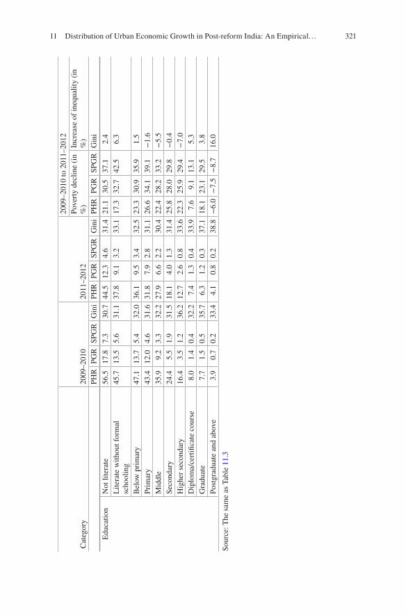
321

Cat

egor

y20

09–2

010

2011

–201

2

2009

–201

0 to

201

1–20

12Po

vert

y de

clin

e (i

n %

)In

crea

se o

f in

equa

lity

(in

%)

PHR

PGR

SPG

RG

ini

PHR

PGR

SPG

RG

ini

PHR

PGR

SPG

RG

ini

Edu

catio

nN

ot li

tera

te56

.517

.87.

330

.744

.512

.34.

631

.421

.130

.537

.12.

4L

itera

te w

ithou

t for

mal

sc

hool

ing

45.7

13.5

5.6

31.1

37.8

9.1

3.2

33.1

17.3

32.7

42.5

6.3

Bel

ow p

rim

ary

47.1

13.7

5.4

32.0

36.1

9.5

3.4

32.5

23.3

30.9

35.9

1.5

Prim

ary

43.4

12.0

4.6

31.6

31.8

7.9

2.8

31.1

26.6

34.1

39.1

−1.

6M

iddl

e35

.99.

23.

332

.227

.96.

62.

230

.422

.428

.233

.2−

5.5

Seco

ndar

y24

.45.

51.

931

.518

.14.

01.

331

.425

.828

.029

.8−

0.4

Hig

her

seco

ndar

y16

.43.

51.

236

.212

.72.

60.

833

.622

.325

.929

.4−

7.0

Dip

lom

a/ce

rtifi

cate

cou

rse

8.0

1.4

0.4

32.2

7.4

1.3

0.4

33.9

7.6

9.1

13.1

5.3

Gra

duat

e7.

71.

50.

535

.76.

31.

20.

337

.118

.123

.129

.53.

8Po

stgr

adua

te a

nd a

bove

3.9

0.7

0.2

33.4

4.1

0.8

0.2

38.8

−6.

0−

7.5

−8.

716

.0

Sour

ce: T

he s

ame

as T

able

11.

3

11 Distribution of Urban Economic Growth in Post-reform India: An Empirical…

322

calculated by using the MMRP-based consumption expenditure data and by apply-ing the Rangarajan Committee’s recommended poverty line. The poverty estimates show that groups like ‘casual labour’, ‘not literate’, ‘scheduled castes’, ‘scheduled tribes’ and ‘below primary educated people’ experienced a higher level of poverty in 2009–2010. On the other hand, those who have education levels ‘postgraduate and above’, ‘graduate’, ‘diploma’ and ‘higher secondary’ experienced a lower level of poverty in the same time period, while the group ‘literate without formal school-ing’ suffered a higher level of poverty in 2011–2012. The extent of inequality was high for ‘other household type’, ‘scheduled tribes’, ‘adult’ and ‘female’ in 2009–2010. On the other hand, the extent of inequality was lower for the groups ‘sched-uled castes’, ‘literate without formal schooling’, ‘not literate’ and ‘casual labour’ in the same period of time. In addition, groups ‘postgraduate and above’ and ‘other social group’ registered a higher level of inequality in 2011–2012. In contrast, those who have passed ‘primary’, ‘middle’ and ‘secondary’ experienced a lower level of inequality in 2011–2012.

Table 11.5 also shows that groups like ‘regular wage/salary’ earner, ‘other back-ward classes’ and those who have ‘primary’ and ‘secondary’ level education also experienced a higher level of poverty decline in the periods of 2009–2010 to 2011–2012. Most importantly, as per the squared poverty gap ratio (SPGR) estimation, ‘literate without formal schooling’ and ‘other religion group’ are also found to have experienced a higher-level poverty decline during the same time period. In contrast, groups like ‘literate without formal schooling’, ‘scheduled tribes’, ‘diploma holder’ and ‘other household type’ also showed a lower decrease in the percentage of the poverty ratio during the period. Surprisingly, groups that have an education level ‘postgraduate and above’ also showed an increase in the poverty ratio in the periods 2009–2010 to 2011–2012. Similarly, the level of inequality increased for groups such as those who have passed ‘postgraduate and above’, ‘literate without formal schooling’ and ‘diploma holders’ in the periods 2009–2010 to 2011–2012. In con-trast, the groups ‘scheduled tribes’, ‘higher secondary level education’ and ‘middle- class level of education’ experienced a fall in inequality. It is important to note that results arrived based on MRP and MMRP do not differ much from each other.

4 Measurement of Pro-Poor Growth

4.1 Theoretical Framework

The theoretical framework developed by Duclos (2009) and Araar et al. (2007, 2009) is used to calculate pro-poor growth in this study.4 In the case of India, a simi-lar approach was used in Motiram and Naraparaju (2015). However, this chapter focuses mainly on different specific aspects of urban India only.

4 The theoretical structures are taken from Araar (2012), Duclos (2009) and Araar et al. (2007, 2009) as presented in Tripathi (2013c).

S. Tripathi

323

The framework such as developed by Duclos (2009) is explained as follows:

The vector of non-negative incomes is presented as y = +n

11y y yn1

121

11, ,………( )∈R

at time 1 of size n1, and let y =2 y y yn12

22

12, ,………( ) be an analogue vector of

income set time 2 of size n2.W(y1, y2,g,z) is the pro-poor evaluation function, where z > 0 represents the pov-

erty line. It is characterized as the difference between evaluation functions π(y1, z) and evaluation function π∗ (y2, g, z), each for time 1 and time 2, respectively, which are analogous to poverty indices for each of the two time periods:

W g z g z zy y y y1 2 2 1, , , , , ,( ) ≡ ( ) − ( )∗π π

(11.1)

The change from y1 to y2 will be considered as pro-poor if W(y1, y2,g,z) ≤ 0.The social welfare function of W satisfies the different axioms (i.e. focus, popu-

lation invariance, anonymity, normalization, monotonicity, distribution sensitivity axioms).

4.1.1 Relative Pro-Poor Measurements

FGT indices in (11.2) are obtained using the assumption that Fj(y) is the distribution function of distribution j and Qj(p) is the quantile function for the distribution Fj. Qj(p) is defined as Qj(p) = inf s ≥ 0| Fj(s) ≥ p for p ∈ [0, 1]. If we assume that this is continuous distribution with a positive income density, then Q(p) is the inverse of the distribution function:

P zQ p

zdpj

F z jj

;αα

( ) = −( )

( )∫ 0 1 .

(11.2)

where Pj(z; α = 0) is the headcount index (and the distribution function) at z and Pj(z; α = 1) is the average poverty gap.

A measure of movement from y1 to y2 will be reflected as pro-poor by all such functions if

P g z P z z z2 11 0 0 0( ;+( ) = ≤ =( ) ∈

+α α; for all ,

(11.3)

Equation (11.3) shows a distributional change. All pro-poor evaluation functions within Ω1(g, z+) find that it is pro-poor and this for any selection of poverty line within [0, z+] and any W complies with the already indicated axioms. Validating (11.3) accommodate examining the range of poverty lines[0, z+]. The headcount ratio in the initial distribution is higher than the headcount ratio in the subsequent distribution when that distribution is normalized by 1 + g. In other words, one can measure first-order relative by using the ratio of quantiles and(1 + g).

11 Distribution of Urban Economic Growth in Post-reform India: An Empirical…

324

Therefore, we need to check whether for all p ∈ [0, F1(z+)]

GIC pQ p Q p

Q pg( ) = ( ) − ( )

( )≥2 1

1

.

(11.4)

The use of (11.4) is identical to ‘growth incidence curves’ as suggested by Ravallion and Chen (2003).

The class Ω2(g, z+) is the subset of Ω1(g, z+) where the evaluation function main-tains the distribution sensitivity axiom. A movement from y1 to y2 will be considered pro-poor by all pro-poor evaluation function Ω2(g, z+) if

P g z P z z z2 11 1 1 0+( ) =( ) ≤ =( ) ∈

+; ; for all ,α α

(11.5)

Equation (11.5) involves checking whether the average poverty gap of the initial distribution is greater than that in the later distribution when a distribution is nor-malized by (1 + g) over the range of poverty lines [0, z+]. The generalized Lorenz curve can be used to check alternatively. Second-order relatively pro-poor condition is if and only if p ∈ [0, F2(1 + g) z+)].

λ pC p

C pg( ) ≡ ( )

( )≥ +2

1

1 .

(11.6)

Through Eq. (11.6), one can compute the growth rates of the cumulative incomes of proportions p of the poorest and compare these growth rates withg. The ratio of mean income is 1 + g. Condition (11.6) helps us to check whether the Lorenz curve for y2 is above that of y1 for the range of p ∈ [0, F2(1 + g) z+)].

4.1.2 Absolute Pro-Poor Measurements

Absolute pro-poorness is calculated by comparing the absolute change in the income (or consumption) of the poor to some standard, denoted by a and usually set to zero. A change in income of the poor is good if it raises living standard of the poor people (Ravallion and Chen 2003). Therefore, the absolute axiom requires that if y + a = y′, then W(y, y′,a,z) = 0.

The formal definition of first-order absolute pro-poor evaluation functions Ω1 a z, +( ) comprises all functions W(., . , a, z) and needs to satisfy the population,

anonymity, focus, monotonicity, normalization and absolute axioms, for which z ≤ z+.

Then a movement from y1 to y2 will be considered as first-order absolutely pro- poor, i.e. pro-poor by all evaluation functions W(., . , a, z) which are members of Ω1 a z, +( ) if and only if

S. Tripathi

325

P z P z z z2 10 0 0+ =( ) ≤ =( ) ∈

+α α α; ; for all ,

(11.7)

Alternatively, the first-order absolute pro-poor can be measured by using the quantiles values for all p ∈ [0,F1(z+):

Q p Q p a2 1( ) − ( ) ≥ .

(11.8)

A similar condition holds good for the evaluation of absolute second-order pro- poorness. These assessments mainly depend on the Ω2 a z, +( ) class of indices, i.e. similarly to Ω1 a z, +( ) . The second-order absolutely pro-poor is defined by

z a P z a zP z z z+( ) + =( ) ≤ =( ) ∈

+2 11 1 0( .; ; for all ,α α

(11.9)

A sufficient condition for (11.9) is

C p C p

pa2 1( ) − ( )

≥ .

(11.10)

4.1.3 Data Used

Urban MPCE from 61st round in 2004–2005, 66th round in 2009–2010 and 68th round in 2011–2012 are used for the analysis. Table 11.6 shows that real urban MPCE increased from Rs 326.8 to Rs 413.53 in the periods of 2005–2012, which accounts for about 27% growth rate.

4.1.4 Empirical Results

The Distributive Analysis Stata Package (DASP) developed by Araar and Duclos (2007) has been used for the empirical analysis. Figure 11.1 shows that the distribu-tion of MPCE improved in the periods 2004–2005 to 2011–2012 as density curves shift to the right. Figure 11.2 and Table 11.3 show marginal increase in inequality in the periods 2004–2005 to 2011–2012. Figures 11.3 and 11.4 and the results in Table 11.3 recommend that absolute poverty, as measured by the headcount and poverty gap indices, had decreased in the years 2004–2005 to 2011–2012.

The first-order absolute and relative urban pro-poorness are calculated and pre-sented in Figs. 11.5, 11.6, 11.7, 11.8, 11.9 and 11.10.5 The absolute and relative pro-poor growth using the first-order and second-order approaches are presented in Table 11.5.

5 The graphs that were generated from testing the second-order approach for absolute and relative pro-poor growth are presented here in the interests of space but available from the author.

11 Distribution of Urban Economic Growth in Post-reform India: An Empirical…

326

The top line of Fig. 11.5 presents the sample estimates of

∆ ( ) = =( ) − =( )− −

12009 10 2004 050 0z P z P z; ;α α

(11.11)

For the difference between 2004–2005 and 2009–2010, the dotted bottom curve is the upper bound of the one-sided confidence interval:

0.001

.002

.003

.004

f(y)

0 200 400 600 800 1000y

2004-05 2009-10

2011-12

Fig. 11.1 Density functions. (Source: Drawn by author by using DASP software and NSS unit- level data in different time periods)

Table 11.6 Growth in MPCEURP at current and constant prices, all India urban

YearAverage MPCEMRP (Rs)

Urban price deflatora

Average urban MPCEMRP(in Rs): base 1987–1988 prices

Number of persons

2004–2005

1104.6 338 326.8 206,529

2009–2010

1856.01 503 368.99 181,412

2011–2012

2477.02 599 413.53 179,164

Source: Calculations based on the unit-level data of the consumer-expenditure rounds of 2004–2005, 2009–2010 and 2011–2012, NSSO, GoINote: aPrice deflators for the years 2004–2005 and 2009–2010 are collected from NSS Report No. 538: Level and Pattern of Consumer Expenditure; they represent price indices for urban India with base 1987–1988=100. For 2011–2012, indices have been calculated as a continuation of this series, with the help of CPI-IW for the urban sector

S. Tripathi

327

0.2

.4.6

.81

FG

T(z

, al

pha

= 0

)

0 200 400 600 800 1000

Poverty line (z)

2004-05 2009-10

2011-12

Fig. 11.3 Poverty headcount curves: P(z; α = 0)for a range of z. (Source: Drawn by author by using DASP software and NSS unit-level data in different time periods)

0.2

.4.6

.81

L(p

)

0 .2 .4 .6 .8 1

Percentiles (p)

45° line 2004-05

2009-10 2011-12

Fig. 11.2 Lorenz curves. (Source: Drawn by author by using DASP software and NSS unit-level data in different time periods)

11 Distribution of Urban Economic Growth in Post-reform India: An Empirical…

328

∆ ( ) − ∆ ( ) ( )1 z zsσ ζ θˆ

(11.12)

As ∆ ( ) − ∆ ( ) <( )1 0z zsσ ζ θˆ in Fig. 11.5 is found accurate mostly for all reason-

able poverty lines, it can be concluded that the growth was absolutely pro-poor in the years 2004–2005 to 2009–2010. The urban poverty line was Rs 860 in 2009–2010 (GOI 2014). It is clear from Fig. 11.5 that in Rs 860, the upper bound of the confidence interval for ∆1(z) is negative, and this indicates that growth was abso-lutely pro-poor for the periods 2004–2005 to 2009–2010. Similar results are obtained for the periods of 2009–2010 to 2011–2012. Figure 11.6 shows that the change in distribution was first-order absolutely pro-poor. The upper bound of the confidence interval for Δ1(z) is negative (the official urban poverty line was Rs 1000 in 2011–2012).

Figure 11.7 shows the test of pro-poorness for the years 2004–2005 to 2011–2012. The results show that the distributive change was first-order absolutely pro- poor. The lower bound of the confidence interval for P2011 − 12(z; α = 0) − P2004 − 05(z; α = 0) is negative for any reasonable poverty line. The official poverty lines esti-mated were Rs 579 in 2004–2005, Rs 860 in 209–2010 and Rs 1000 in 2011–2012.

The test of relative pro-poorness is calculated and presented in Figs. 11.8, 11.9 and 11.10. The sample estimates of P2009 − 10((1 + g)z; α = 0) − P2004 − 05 (z; α = 0) of distributive movement during the periods 2004–2005 to 2009–2010 were not first-

0.2

.4.6

.8

FG

T(z

, al

pha

= 1

)

0 200 400 600 800 1000

Poverty line (z)

2004-05 2009-10

2011-12

Fig. 11.4 Poverty headcount curves: P(z; α = 1) for a range of z. (Source: Drawn by author by using DASP software and NSS unit-level data in different time periods)

S. Tripathi

329

-.08-.06-.04-.020

040

080

012

0016

0020

00

Pov

erty

lin

e (z

)

Diffe

renc

eU

pper

bou

nd o

f 95

% c

onf

iden

ce int

erva

l

Nul

l ho

rizo

nta

l lin

e

Tot

al U

rban

-.08-.06-.04-.020

040

080

012

0016

0020

00

Pov

erty

lin

e (z

)

Diffe

renc

eU

pper

boun

d of

95%

con

fide

nce

inte

rval

Nul

l ho

rizo

nta

l lin

eSelf E

mpl

oyed

-.1-.050

040

080

012

0016

0020

00

Pov

erty

lin

e (z

)

Diffe

renc

eU

pper

bou

nd o

f 95

% c

onfide

nce

inte

rval

Nul

l ho

rizo

ntal

lin

e

Reg

ular

wag

e

-.06-.04-.020.02

040

080

012

0016

0020

00

Pove

rty

line

(z)

Diffe

rence

Upp

er b

ound

of 95

% c

onf

iden

ce int

erva

l

Nul

l ho

rizo

nta

l lin

eCas

ual Lab

our

-.08-.06-.04-.020

040

080

012

0016

0020

00

Pove

rty

line

(z)

Diffe

renc

eU

pper

bou

nd o

f 95

% c

onfide

nce

inte

rval

Nul

l ho

rizo

ntal

lin

e

Hou

seho

ld T

ype_

Oth

ers

-.08-.06-.04-.020

040

080

012

0016

0020

00

Pov

erty

lin

e (z

)

Diffe

renc

eU

pper

bou

nd o

f 95

% c

onfide

nce

inte

rval

Nul

l ho

rizo

ntal

lin

e

Hin

du

-.06-.04-.020

040

080

012

0016

0020

00

Pov

erty

lin

e (z

)

Diffe

renc

eU

pper

bou

nd o

f 95

% c

onf

iden

ce int

erva

l

Nul

l ho

rizo

nta

l lin

eOth

er R

elig

ion

-.04-.020.02.04

040

080

012

0016

0020

00Pove

rty

line

(z)

Diffe

rence

Upp

er b

oun

d of

95%

conf

iden

ce int

erva

lN

ull ho

rizo

ntal

lin

e

ST

-.08-.06-.04-.020

040

080

012

0016

0020

00Pov

erty

lin

e (z

)

Diffe

renc

eU

pper

bou

nd o

f 95

% c

onfide

nce

inte

rval

Nul

l ho

rizo

ntal

lin

e

SC

-.1-.08-.06-.04-.020

040

080

012

0016

0020

00

Pov

erty

lin

e (z

)

Diffe

renc

eU

pper

boun

d of

95%

con

fide

nce

inte

rval

Nul

l ho

rizo

ntal

lin

e

OB

C

-.08-.06-.04-.020

040

080

012

0016

0020

00

Pove

rty

line

(z)

Diffe

renc

eU

pper

bou

nd o

f 95

% c

onfide

nce

inte

rval

Nul

l ho

rizo

ntal

lin

e

Oth

er S

ocia

l G

roup

-.08-.06-.04-.020

040

080

012

0016

0020

00

Pov

erty

lin

e (z

)

Diffe

rence

Upp

er b

ound

of

95%

con

fide

nce

inte

rval

Nul

l ho

rizo

ntal

lin

e

Mal

e

-.08-.06-.04-.020

040

080

012

0016

0020

00

Pov

erty

lin

e (z

)

Diffe

renc

eU

pper

bou

nd o

f 95

% c

onf

iden

ce int

erva

l

Nul

l ho

rizo

nta

l lin

e

Fem

ale

-.08-.06-.04-.020

040

080

012

0016

0020

00

Pov

erty

lin

e (z

)

Diffe

renc

eU

pper

bou

nd o

f 95

% c

onfide

nce

inte

rval

Nul

l ho

rizo

ntal

lin

e

Chi

ld

-.08-.06-.04-.020

040

080

012

0016

0020

00

Pov

erty

lin

e (z

)

Diffe

renc

eU

pper

bou

nd

of 9

5% c

onf

iden

ce int

erva

l

Nul

l ho

rizo

ntal

lin

e

Adu

lt

-.08-.06-.04-.020

040

080

012

0016

0020

00

Pove

rty

line

(z)

Diffe

rence

Upp

er b

ound

of 95

% c

onf

iden

ce int

erva

l

Nul

l ho

rizo

nta

l lin

e

Not

Liter

ate

-.1-.050.05.1

040

080

012

0016

0020

00

Pov

erty

lin

e (z

)

Diffe

renc

eU

pper

boun

d of

95%

con

fide

nce

inte

rval

Nul

l ho

rizo

ntal

lin

e

Liter

ate

withou

t F

orm

al s

choo

ling

-.06-.04-.020.02

040

080

012

0016

0020

00

Pov

erty

lin

e (z

)

Diffe

renc

eU

pper

bou

nd o

f 95

% c

onfide

nce

inte

rval

Nul

l ho

rizo

ntal

lin

eBel

ow P

rim

ary

-.06-.04-.020.02

040

080

012

0016

0020

00

Pove

rty

line

(z)

Diffe

renc

eU

pper

boun

d of

95%

conf

iden

ce int

erva

l

Nul

l ho

rizo

ntal

lin

e

Prim

ary

-.06-.04-.020.02

040

080

012

0016

0020

00

Pov

erty

lin

e (z

)

Diffe

renc

eU

pper

bou

nd o

f 95

% c

onfide

nce

inte

rval

Nul

l ho

rizo

ntal

lin

e

Mid

dle

-.03-.02-.010.01.02

040

080

012

0016

0020

00

Pove

rty

line

(z)

Diffe

renc

eU

pper

bou

nd o

f 95

% c

onfide

nce

inte

rval

Nul

l ho

rizo

ntal

lin

e

Seco

ndar

y

-.02-.010.01

040

080

012

0016

0020

00

Pove

rty

line

(z)

Diffe

renc

eU

pper

boun

d of

95%

conf

iden

ce int

erva

l

Nul

l ho

rizo

ntal

lin

eHig

her

Seco

ndar

y

-.04-.03-.02-.010.01

040

080

012

0016

0020

00

Pove

rty

line

(z)

Diffe

rence

Upp

er b

ound

of 9

5% c

onfide

nce

inte

rval

Nul

l ho

rizo

nta

l lin

e

Dip

lom

a

-.02-.010.01.02

040

080

012

0016

0020

00

Pov

erty

lin

e (z

)

Diffe

renc

eU

pper

bou

nd o

f 95

% c

onf

iden

ce int

erva

l

Nul

l ho

rizo

ntal

lin

e

Gra

duat

e

-.04-.03-.02-.010

040

080

012

0016

0020

00

Pov

erty

lin

e (z

)

Diffe

renc

eU

pper

bou

nd o

f 95

% c

onfide

nce

inte

rval

Nul

l ho

rizo

ntal

lin

e

Pos

t gr

adua

te a

nd a

bove

Fig

. 11.

5 A

bsol

ute

pro-

poor

judg

emen

ts u

sing

the

first

-ord

er a

ppro

ach

from

200

4–20

05 to

200

9–20

10

11 Distribution of Urban Economic Growth in Post-reform India: An Empirical…

330

-.08-.06-.04-.020

040

080

012

0016

0020

00

Pove

rty

line

(z)

Diffe

renc

eU

pper

boun

d of

95%

conf

iden

ce int

erva

l

Nul

l ho

rizo

ntal

lin

e

Tot

al U

rban

-.08-.06-.04-.020

040

080

012

0016

0020

00

Pov

erty

lin

e (z

)

Diffe

rence

Upp

er b

ound

of

95%

conf

iden

ce int

erva

l

Nul

l ho

rizo

ntal

lin

eSelf E

mpl

oyed

-.06-.04-.020

040

080

012

0016

0020

00

Pove

rty

line

(z)

Diffe

renc

eU

pper

boun

d of

95%

con

fide

nce

inte

rval

Nul

l ho

rizo

ntal

lin

eReg

ular

Wag

e

-.2-.15-.1-.050 040

080

012

0016

0020

00Pove

rty

line

(z)

Diffe

renc

eU

pper

bou

nd o

f 95

% c

onfide

nce

inte

rval

Nul

l ho

rizo

ntal

lin

eCas

ual w

orke

r

-.1-.08-.06-.04-.020

040

080

012

0016

0020

00

Pov

erty

lin

e (z

)

Diffe

renc

eU

pper

bou

nd o

f 95

% c

onfide

nce

inte

rval

Nul

l ho

rizo

ntal

lin

e

Hous

ehold

Typ

e: O

ther

s

-.08-.06-.04-.020

040

080

012

0016

0020

00

Pov

erty

lin

e (z

)

Diffe

renc

eU

pper

bou

nd

of 9

5% c

onfide

nce

inte

rval

Nul

l ho

rizo

ntal

lin

e

Hin

du

-.1-.08-.06-.04-.020

040

080

012

0016

0020

00

Pove

rty

line

(z)

Diffe

renc

eU

pper

boun

d of

95%

conf

iden

ce int

erva

l

Nul

l ho

rizo

ntal

lin

e

Oth

er R

elig

ion

Gro

up

-.08-.06-.04-.020

040

080

012

0016

0020

00

Pov

erty

lin

e (z

)

Diffe

rence

Upp

er b

ound

of

95%

conf

iden

ce int

erva

l

Nul

l ho

rizo

ntal

lin

e

ST

-.15-.1-.050

040

080

012

0016

0020

00

Pov

erty

lin

e (z

)

Diffe

renc

eU

pper

bou

nd o

f 95

% c

onf

iden

ce int

erva

l

Nul

l ho

rizo

nta

l lin

e

SC

-.1-.08-.06-.04-.020

040

080

012

0016

0020

00

Pov

erty

lin

e (z

)

Diffe

renc

eU

pper

bou

nd

of 9

5% c

onfide

nce

inte

rval

Nul

l ho

rizo

nta

l lin

e

OB

C

-.08-.06-.04-.020

040

080

012

0016

0020

00

Pov

erty

lin

e (z

)

Diffe

renc

eU

pper

bou

nd o

f 95

% c

onfide

nce

inte

rval

Nul

l ho

rizo

ntal

lin

e

Soci

al g

roup

: O

ther

s

-.08-.06-.04-.020

040

080

012

0016

0020

00

Pov

erty

lin

e (z

)

Diffe

renc

eU

pper

bou

nd o

f 95

% c

onfide

nce

inte

rval

Nul

l ho

rizo

ntal

lin

e

Mal

e

-.08-.06-.04-.020

040

080

012

0016

0020

00

Pove

rty

line

(z)

Diffe

renc

eU

pper

boun

d of

95%

conf

iden

ce int

erva

l

Nul

l ho

rizo

ntal

lin

e

Fem

ale

-.1-.08-.06-.04-.020

040

080

012

0016

0020

00

Pov

erty

lin

e (z

)

Diffe

rence

Upp

er b

ound

of

95%

conf

iden

ce int

erva

l

Nul

l ho

rizo

ntal

lin

e

Chi

ld

-.08-.06-.04-.020

040

080

012

0016

0020

00

Pov

erty

lin

e (z

)

Diffe

renc

eU

pper

bou

nd

of 9

5% c

onfide

nce

inte

rval

Nul

l ho

rizo

ntal

lin

e

Adu

lt

-.15-.1-.050

040

080

012

0016

0020

00

Pov

erty

lin

e (z

)

Diffe

renc

eU

pper

bou

nd

of 9

5% c

onfide

nce

inte

rval

Nul

l ho

rizo

nta

l lin

e

Not

Liter

ate

-.1-.050.05

040

080

012

0016

0020

00

Pov

erty

lin

e (z

)

Diffe

renc

eU

pper

bou

nd o

f 95

% c

onfide

nce

inte

rval

Nul

l ho

rizo

ntal

lin

e

Liter

ate

witho

ut fo

rmal

sch

oolin

g

-.1-.08-.06-.04-.020

040

080

012

0016

0020

00

Pove

rty

line

(z)

Diffe

renc

eU

pper

boun

d of

95%

con

fide

nce

inte

rval

Nul

l ho

rizo

nta

l lin

eBel

ow P

rim

ary

-.1-.08-.06-.04-.020

040

080

012

0016

0020

00

Pov

erty

lin

e (z

)

Diffe

renc

eU

pper

bou

nd o

f 95

% c

onfide

nce

inte

rval

Nul

l ho

rizo

ntal

lin

e

Pri

mar

y

-.08-.06-.04-.020

040

080

012

0016

0020

00

Pov

erty

lin

e (z

)

Diffe

renc

eU

pper

bou

nd o

f 95

% c

onfide

nce

inte

rval

Nul

l ho

rizo

ntal

lin

e

Mid

dle

-.06-.04-.020

040

080

012

0016

0020

00

Pov

erty

lin

e (z

)

Diffe

rence

Upp

er b

ound

of

95%

con

fide

nce

inte

rval

Nul

l ho

rizo

ntal

lin

e

Seco

ndar

y

-.06-.04-.020

040

080

012

0016

0020

00

Pov

erty

lin

e (z

)

Diffe

renc

eU

pper

bou

nd o

f 95

% c

onfide

nce

inte

rval

Nul

l ho

rizo

ntal

lin

eHig

her

Seco

ndar

y

-.08-.06-.04-.020.02

040

080

012

0016

0020

00

Pove

rty

line

(z)

Diffe

renc

eU

pper

bou

nd o

f 95

% c

onfide

nce

inte

rval

Nul

l ho

rizo

ntal

lin

e

Dip

lom

a

-.06-.04-.020

040

080

012

0016

0020

00

Pove

rty

line

(z)

Diffe

renc

eU

pper

boun

d of

95%

conf

iden

ce int

erva

l

Nul

l ho

rizo

ntal

lin

e

Gra

duat

e

-.08-.06-.04-.020

040

080

012

0016

0020

00

Pov

erty

lin

e (z

)

Diffe

renc

eU

pper

bou

nd o

f 95

% c

onfide

nce

inte

rval

Nul

l ho

rizo

ntal

lin

ePos

t G

radu

ate

Fig

. 11.

6 A

bsol

ute

pro-

poor

judg

emen

ts u

sing

the

first

-ord

er a

ppro

ach

from

200

9–20

10 to

201

1–20

12. (

Sour

ce: D

raw

n by

the

auth

or b

y us

ing

DA

SP s

oftw

are

and

NSS

uni

t-le

vel d

ata

in d

iffe

rent

tim

e pe

riod

s)

S. Tripathi

331

-.15-.1-.050

040

080

012

0016

0020

00

Pov

erty

lin

e (z

)

Diffe

rence

Upp

er b

ound

of

95%

con

fide

nce

inte

rval

Nul

l ho

rizo

nta

l lin

e

Tot

al U

rban

-.15-.1-.050

040

080

012

0016

0020

00

Pov

erty

lin

e (z

)

Diffe

rence

Upp

er b

ound

of

95%

con

fide

nce

inte

rval

Nul

l ho

rizo

nta

l lin

e

Self E

mpl

oyed

-.2-.15-.1-.050

040

080

012

0016

0020

00Pov

erty

lin

e (z

)

Diffe

renc

eU

pper

bou

nd o

f 95

% c

onfide

nce

inte

rval

Nul

l ho

rizo

ntal

lin

e

Reg

ula

r W

age

-.25-.2-.15-.1-.050

040

080

012

0016

0020

00Pove

rty

line

(z)

Diffe

rence

Upp

er b

ound

of 9

5% c

onf

iden

ce int

erva

l

Nul

l ho

rizo

ntal

lin

e

Cas

ual

-.25-.2-.15-.1-.050

040

080

012

0016

0020

00

Pov

erty

lin

e (z

)

Diffe

rence

Upp

er b

ound

of

95%

con

fide

nce

inte

rval

Nul

l ho

rizo

ntal

lin

e

Hou

seho

ld T

ype:

Oth

ers

-.15-.1-.050

040

080

012

0016

0020

00

Pove

rty

line

(z)

Diffe

renc

eU

pper

boun

d of

95%

con

fide

nce

inte

rval

Nul

l ho

rizo

nta

l lin

e

Hin

du

-.15-.1-.050

040

080

012

0016

0020

00

Pove

rty

line

(z)

Diffe

rence

Upp

er b

oun

d of

95%

conf

iden

ce int

erva

l

Nul

l ho

rizo

ntal

lin

e

Oth

er R

elig

ion

-.2-.15-.1-.050

040

080

012

0016

0020

00

Pove

rty

line

(z)

Diffe

renc

eU

pper

boun

d of

95%

con

fide

nce

inte

rval

Nul

l ho

rizo

nta

l lin

e

SC

-.1-.08-.06-.04-.020

040

080

012

0016

0020

00

Pov

erty

lin

e (z

)

Diffe

renc

eU

pper

bou

nd o

f 95

% c

onfide

nce

inte

rval

Nul

l ho

rizo

ntal

lin

e

ST

-.2-.15-.1-.050

040

080

012

0016

0020

00

Pov

erty

lin

e (z

)

Diffe

renc

eU

pper

bou

nd o

f 95

% c

onfide

nce

inte

rval

Nul

l ho

rizo

ntal

lin

e

OB

C

-.15-.1-.050

040

080

012

0016

0020

00

Pov

erty

lin

e (z

)

Diffe

rence

Upp

er b

ound

of

95%

con

fide

nce

inte

rval

Nul

l ho

rizo

ntal

lin

e

Soci

al G

roup

: O

ther

s

-.15-.1-.050

040

080

012

0016

0020

00

Pov

erty

lin

e (z

)

Diffe

rence

Upp

er b

ound

of

95%

con

fide

nce

inte

rval

Nul

l ho

rizo

nta

l lin

e

Mal

e

-.15-.1-.050

040

080

012

0016

0020

00

Pove

rty

line

(z)

Diffe

rence

Upp

er b

oun

d of

95%

conf

iden

ce int

erva

lN

ull ho

rizo

ntal

lin

e

Fem

ale

-.15-.1-.050

040

080

012

0016

0020

00

Pov

erty

lin

e (z

)

Diffe

renc

eU

pper

boun

d of

95%

conf

iden

ce int

erva

l

Nul

l ho

rizo

ntal

lin

e

Chi

ld

-.15-.1-.050

040

080

012

0016

0020

00

Pov

erty

lin

e (z

)

Diffe

renc

eU

pper

bou

nd o

f 95

% c

onfide

nce

inte

rval

Nul

l ho

rizo

ntal

lin

e

Adu

lt

-.2-.15-.1-.050

040

080

012

0016

0020

00

Pov

erty

lin

e (z

)

Diffe

renc

eU

pper

boun

d of

95%

conf

iden

ce int

erva

l

Nul

l ho

rizo

ntal

lin

e

Not

Liter

ate

-.15-.1-.050

040

080

012

0016

0020

00

Pov

erty

lin

e (z

)

Diffe

renc

eU

pper

bou

nd o

f 95

% c

onfide

nce

inte

rval

Nul

l ho

rizo

ntal

lin

e

Liter

ate

witho

ut f

orm

al s

chlo

oing

-.15-.1-.050

040

080

012

0016

0020

00

Pove

rty

line

(z)

Diffe

renc

eU

pper

bou

nd o

f 95

% c

onfide

nce

inte

rval

Nul

l ho

rizo

ntal

lin

e

Bel

ow P

rim

ary

-.15-.1-.050

040

080

012

0016

0020

00

Pov

erty

lin

e (z

)

Diffe

renc

eU

pper

bou

nd o

f 95

% c

onfide

nce

inte

rval

Nul

l ho

rizo

ntal

lin

e

Prim

ary

-.15-.1-.050

040

080

012

0016

0020

00

Pov

erty

lin

e (z

)

Diffe

renc

eU

pper

boun

d of

95%

con

fide

nce

inte

rval

Nul

l ho

rizo

ntal

lin

e

Mid

dle

-.08-.06-.04-.020

040

080

012

0016

0020

00

Pov

erty

lin

e (z

)

Diffe

renc

eU

pper

bou

nd o

f 95

% c

onfide

nce

inte

rval

Nul

l ho

rizo

ntal

lin

e

Seco

ndar

y

-.08-.06-.04-.020

040

080

012

0016

0020

00

Pov

erty

lin

e (z

)

Diffe

renc

eU

pper

boun

d of

95%

con

fide

nce

inte

rval

Nul

l ho

rizo

ntal

lin

eHig

her

Seco

ndar

y

-.1-.08-.06-.04-.020

040

080

012

0016

0020

00

Pov

erty

lin

e (z

)

Diffe

renc

eU

pper

boun

d of

95%

con

fide

nce

inte

rval

Nul

l ho

rizo

ntal

lin

e

Dip

lom

a

-.06-.04-.020

040

080

012

0016

0020

00

Pov

erty

lin

e (z

)

Diffe

renc

eU

pper

boun

d of

95%

con

fide

nce

inte

rval

Nul

l ho

rizo

ntal

lin

e

Gra

dua

te

-.15-.1-.050

040

080

012

0016

0020

00

Pov

erty

lin

e (z

)

Diffe

renc

eU

pper

boun

d of

95%

con

fide

nce

inte

rval

Nul

l ho

rizo

ntal

lin

e

Pos

t G

radu

ate

Fig

. 11.

7 A

bsol

ute

pro-

poor

judg

emen

ts u

sing

the

first

-ord

er a

ppro

ach

from

200

4–20

05 to

201

1–20

12. (

Sour

ce: D

raw

n by

the

auth

or b

y us

ing

DA

SP s

oftw

are

and

NSS

uni

t-le

vel d

ata

in d

iffe

rent

tim

e pe

riod

s)

11 Distribution of Urban Economic Growth in Post-reform India: An Empirical…

332

order relatively pro-poor (Fig. 11.8). Also the confidence interval around the sample estimates makes it clear (Fig. 11.8) that the observed differences P2009 − 10((1 + g)z; α = 0) − P2004 − 05 (z; α = 0) are not statistically significant over a wide range of bot-tom poverty lines, i.e. the upper bounds of the one-sided confidence intervals extended above the zero line for z between Rs 400 and Rs 1200 rupees when tested for all urban India. The first-order relative pro-poor condition is not satisfied at 95% statistical confidence.

Figure 11.9 measures the relative pro-poorness for the years 2009–2010 to 2011–2012. The confidence interval of the sample estimates P2011 − 12((1 + g)z; α = 0) − P2

009 − 10 (z; α = 0) is below zero for z after around Rs 700 and indicates no robust first- order relative pro-poorness. The test of second-order relative pro-poorness indicates a very strong anti-relative pro-poorness as the sample estimate of P2011 − 12((1 + g)z; α = 0) − P2009 − 10 (z; α = 0) is positive for z after around Rs 200. This supports the anti-relative pro-poor urban economic growth between 2009–2010 and 2011–2012.

Finally, Fig. 11.10 tests the first-order relative pro-poorness for the years 2004–2005 to 2011–2012. The confidence interval of the sample estimates of P2011 − 12((1 + g)z; α = 0) − P2004 − 05 (z; α = 0) is not always below zero, and it is positive between the ranges of Rs 300 and Rs 700. The robust result of anti-relative pro-poorness is calculated by testing the second-order relative pro-poorness, as the confidence inter-val is not below zero for any reasonable poverty line selected. Results are consid-ered robust as no difference was found while testing first-order and second-order approaches for absolute and relative pro-poor judgements for the entire categories of urban India. Therefore, we conclude that India’s urban economic growth has been absolutely pro-poor but relatively anti-poor between the periods 2004–2005 to 2009–2010, 2009–2010 to 2011–2012 and 2004–2005 to 2011–2012. Table 11.7 summarizes the calculated results.

S. Tripathi

333

-.04-.020.02 040

080

012

0016

0020

00Pov

erty

lin

e (z

)

Diffe

renc

eL

ower

boun

d of

95%

con

fide

nce

inte

rval

Nul

l ho

rizo

ntal

lin

eTot

al U

rban

-.03-.02-.010.01.02

040

080

012

0016

0020

00Pov

erty

lin

e (z

)

Diffe

renc

eL

ower

boun

d of

95%

con

fide

nce

inte

rval

Nul

l ho

rizo

ntal

lin

e

Self E

mpl

oyed

-.04-.03-.02-.010.01 040

080

012

0016

0020

00Pov

erty

lin

e (z

)

Diffe

renc

eL

ower

boun

d of

95%

con

fide

nce

inte

rval

Nul

l ho

rizo

ntal

lin

e

Reg

ular

Wag

e

-.020.02.04.06 040

080

012

0016

0020

00Pov

erty

lin

e (z

)

Diffe

renc

eL

ower

boun

d of

95%

con

fide

nce

inte

rval

Nul

l ho

rizo

ntal

lin

eCas

ual L

abou

r

-.04-.020.02

040

080

012

0016

0020

00Pov

erty

lin

e (z

)

Diffe

renc

eL

ower

boun

d of

95%

con

fide

nce

inte

rval

Nul

l ho

rizo

ntal

lin

e

Hou

seho

ld T

ype:

Oth

ers

-.04-.020.02.04 040

080

012

0016

0020

00

Pov

erty

lin

e (z

)

Diffe

renc

eL

ower

bou

nd o

f 95

% c

onfide

nce

inte

rval

Nul

l ho

rizo

ntal

lin

e

Hin

du

-.03-.02-.010.01

040

080

012

0016

0020

00Pov

erty

lin

e (z

)

Diffe

renc

eL

ower

boun

d of

95%

con

fide

nce

inte

rval

Nul

l ho

rizo

ntal

lin

e

Oth

er R

elig

ion

-.03-.02-.010.01.020

400

800

1200

1600

2000

Pov

erty

lin

e (z

)

Diffe

renc

eL

ower

boun

d of

95%

con

fide

nce

inte

rval

Nul

l ho

rizo

ntal

lin

e

ST

-.020.02.04.06

040

080

012

0016

0020

00Pov

erty

lin

e (z

)

Diffe

renc

eL

ower

bou

nd o

f 95

% c

onfide

nce

inte

rval

Nul

l ho

rizo

ntal

lin

e

SC

-.020.02.04.06

040

080

012

0016

0020

00Pov

erty

lin

e (z

)

Diffe

renc

eL

ower

boun

d of

95%

con

fide

nce

inte

rval

Nul

l ho

rizo

ntal

lin

e

OB

C

-.03-.02-.010.01

040

080

012

0016

0020

00Pov

erty

lin

e (z

)

Diffe

renc

eL

ower

boun

d of

95%

con

fide

nce

inte

rval

Nul

l ho

rizo

ntal

lin

e

Soci

al G

roup

: O

ther

s

-.03-.02-.010.01.02

040

080

012

0016

0020

00

Pov

erty

lin

e (z

)

Diffe

renc

eL

ower

boun

d of

95%

con

fide

nce

inte

rval

Nul

l ho

rizo

ntal

lin

e

Mal

e

-.04-.020.02.04 040

080

012

0016

0020

00Pov

erty

lin

e (z

)

Diffe

renc

eL

ower

boun

d of

95%

con

fide

nce

inte

rval

Nul

l ho

rizo

ntal

lin

e

Fem

ale

-.020.02.04

040

080

012

0016

0020

00Pov

erty

lin

e (z

)

Diffe

renc

eL

ower

boun

d of

95%

con

fide

nce

inte

rval

Nul

l ho

rizo

ntal

lin

e

Chi

ld

-.03-.02-.010.01.02 040

080

012

0016

0020

00Pov

erty

lin

e (z

)

Diffe

renc

eL

ower

boun

d of

95%

con

fide

nce

inte

rval

Nul

l ho

rizo

ntal

lin

e

Adu

lt

-.020.02.04.06 040

080

012

0016

0020

00Pov

erty

lin

e (z

)

Diffe

renc

eL

ower

boun

d of

95%

con

fide

nce

inte

rval

Nul

l ho

rizo

ntal

lin

eNot

Liter

ate

-.1-.050.05 040

080

012

0016

0020

00Pov

erty

lin

e (z

)

Diffe

renc

eL

ower

boun

d of

95%

con

fide

nce

inte

rval

Nul

l ho

rizo

ntal

lin

e

Liter

ate

witho

ut for

mal

sch

oolin

g

-.04-.020.02.04

040

080

012

0016

0020

00Pov

erty

lin

e (z

)

Diffe

renc

eL

ower

boun

d of

95%

con

fide

nce

inte

rval

Nul

l ho

rizo

ntal

lin

eBel

ow P

rim

ary

-.04-.020.02.04 040

080

012

0016

0020

00Pov

erty

lin

e (z

)

Diffe

renc

eL

ower

boun

d of

95%

co

nfid

ence

int

erva

lN

ull ho

rizo

ntal

lin

e

Prim

ary

-.02-.010.01.02.03

040

080

012

0016

0020

00Pov

erty

lin

e (z

)

Diffe

renc

eL

ower

boun

d of

95%

co

nfid

ence

int

erva

lN

ull ho

rizo

ntal

lin

eMid

dle

-.02-.010.01 040

080

012

0016

0020

00

Pov

erty

lin

e (z

)

Diffe

renc

eL

ower

bou

nd o

f 95

%

conf

iden

ce int

erva

lN

ull ho

rizo

ntal

lin

eSeco

ndar

y

-.02-.010.01

040

080

012

0016

0020

00Pov

erty

lin

e (z

)

Diffe

renc

eL

ower

boun

d of

95%

co

nfid

ence

int

erva

lN

ull ho

rizo

ntal

lin

e

Hig

her

Seco

ndar

y

-.04-.020.02 040

080

012

0016

0020

00Pov

erty

lin

e (z

)

Diffe

renc

eL

ower

boun

d of

95%

co

nfid

ence

int

erva

lN

ull ho

rizo

ntal

lin

e

Dip

lom

a

-.02-.010.01 040

080

012

0016

0020

00Pov

erty

lin

e (z

)

Diffe

renc

eL

ower

boun

d of

95%

co

nfid

ence

int

erva

lN

ull ho

rizo

ntal

lin

e

Gra

dua

te

-.03-.02-.010.01 040

080

012

0016

0020

00Pov

erty

lin

e (z

)

Diffe

renc

eL

ower

boun

d of

95%

co

nfid

ence

int

erva

lN

ull ho

rizo

ntal

lin

e

Pos

t G

radu

ate

Fig

. 11.

8 R

elat

ive

pro-

poor

judg

emen

ts u

sing

the

first

-ord

er a

ppro

ach

from

200

4–20

05 to

200

9–20

10. (

Sour

ce: D

raw

n by

the

auth

or b

y us

ing

DA

SP s

oftw

are

and

NSS

uni

t-le

vel d

ata

in d

iffe

rent

tim

e pe

riod

s)

11 Distribution of Urban Economic Growth in Post-reform India: An Empirical…

334

-.01-.0050.005.01

040

080

012

0016

0020

00Pov

erty

lin

e (z

)

Diffe

renc

eL

ower

bou

nd o

f 95

% c

onfide

nce

inte

rval

Nul

l ho

rizo

ntal

lin

e

Tot

al U

rban

-.03-.02-.010.01.02

040

080

012

0016

0020

00Pov

erty

lin

e (z

)

Diffe

renc

eL

ower

bou

nd o

f 95

% c

onfide

nce

inte

rval

Nul

l ho

rizo

ntal

lin

eSelf E

mpl

oyed

-.010.01.02.03 040

080

012

0016

0020

00

Pov

erty

lin

e (z

)

Diffe

renc

eL

ower

bou

nd o

f 95

% c

onfide

nce

inte

rval

Nul

l ho

rizo

ntal

lin

eReg

ular

Wag

e

-.010.01.02.03

040

080

012

0016

0020

00

Pov

erty

lin

e (z

)

Diffe

renc

eL

ower

bou

nd o

f 95

% c

onfide

nce

inte

rval

Nul

l ho

rizo

ntal

lin

eCas

ual L

abou

r

-.010.01.02

040

080

012

0016

0020

00

Pov

erty

lin

e (z

)

Diffe

renc

eL

ower

bou

nd o

f 95

% c

onfide

nce

inte

rval

Nul

l ho

rizo

ntal

lin

e

Hou

seho

ld T

ype:

Oth

ers

-.01-.0050.005.01.015

040

080

012

0016

0020

00

Pov

erty

lin

e (z

)

Diffe

renc

eL

ower

bou

nd o

f 95

% c

onfide

nce

inte

rval

Nul

l ho

rizo

ntal

lin

e

Hin

du

-.015-.01-.0050.005.01

040

080

012

0016

0020

00Pov

erty

lin

e (z

)

Diffe

renc

eL

ower

bou

nd o

f 95

% c

onfide

nce

inte

rval

Nul

l ho

rizo

ntal

lin

eOth

er R

elig

ion

-.02-.010.01.02 040

080

012

0016

0020

00

Pov

erty

lin

e (z

)

Diffe

renc

eL

ower

bou

nd o

f 95

% c

onfide

nce

inte

rval

Nul

l ho

rizo

ntal

lin

e

ST

-.02-.010.01.02 040

080

012

0016

0020

00Pov

erty

lin

e (z

)

Diffe

renc

eL

ower

bou

nd o

f 95

% c

onfide

nce

inte

rval

Nul

l ho

rizo

ntal

lin

e

SC

-.01-.0050.005.01

040

080

012

0016

0020

00Pov

erty

lin

e (z

)

Diffe

renc

eL

ower

bou

nd o

f 95

% c

onfide

nce

inte

rval

Nul

l ho

rizo

ntal

lin

e

OB

C

-.010.01.02.03 040

080

012

0016

0020

00Pov

erty

lin

e (z

)

Diffe

renc

eL

ower

bou

nd o

f 95

% c

onfide

nce

inte

rval

Nul

l ho

rizo

ntal

lin

e

Soci

al G

roup

: O

ther

s

-.01-.0050.005.01

040

080

012

0016

0020

00Pov

erty

lin

e (z

)

Diffe

renc

eL

ower

bou

nd o

f 95

% c

onfide

nce

inte

rval

Nul

l ho

rizo

ntal

lin

e

Mal

e

-.01-.0050.005.01.015 040

080

012

0016

0020

00Pov

erty

lin

e (z

)

Diffe

renc

eL

ower

bou

nd o

f 95

%

conf

iden

ce int

erva

lN

ull ho

rizo

ntal

lin

eFem

ale

-.015-.01-.0050.005.01

040

080

012

0016

0020

00Pov

erty

lin

e (z

)

Diffe

renc

eL

ower

bou

nd o

f 95

% c

onfide

nce

inte

rval

Nul

l ho

rizo

ntal

lin

e

Chi

ld

-.0050.005.01.015 040

080

012

0016

0020

00

Pov

erty

lin

e (z

)

Diffe

renc

eL

ower

bou

nd o

f 95

%

conf

iden

ce int

erva

lN

ull ho

rizo

ntal

lin

eAdu

lt

-.02-.010.01.02 040

080

012

0016

0020

00Pov

erty

lin

e (z

)

Diffe

renc

eL

ower

bou

nd o

f 95

% c

onfide

nce

inte

rval

Nul

l ho

rizo

ntal

lin

eNot

Liter

ate

-.06-.04-.020.02.04

040

080

012

0016

0020

00Pov

erty

lin

e (z

)

Diffe

renc

eL

ower

bou

nd o

f 95

% c

onfide

nce

inte

rval

Nul

l ho

rizo

ntal

lin

e

Liter

ate

witho

ut F

orm

al S

choo

ling

-.02-.010.01 040

080

012

0016

0020

00Pov

erty

lin

e (z

)

Diffe

renc

eL

ower

bou

nd o

f 95

% c

onfide

nce

inte

rval

Nul

l ho

rizo

ntal

lin

eBel

ow P

rim

ary

-.01-.0050.005.01.015 040

080

012

0016

0020

00Pov

erty

lin

e (z

)

Diffe

renc

eL

ower

bou

nd o

f 95

% c

onfide

nce

inte

rval

Nul

l ho

rizo

ntal

lin

e

Prim

ary

-.01-.0050.005.01.015 040

080

012

0016

0020

00Pov

erty

lin

e (z

)

Diffe

renc

eL

ower

bou

nd o

f 95

% c

onfide

nce

inte

rval

Nul

l ho

rizo

ntal

lin

e

Mid

dle

-.010.01.02.03 040

080

012

0016

0020

00Pov

erty

lin

e (z

)

Diffe

renc

eL

ower

bou

nd o

f 95

% c

onfide

nce

inte

rval

Nul

l ho

rizo

ntal

lin

eSeco

ndar

y

-.02-.010.01 040

080

012

0016

0020

00Pov

erty

lin

e (z

)

Diffe

renc

eL

ower

bou

nd o

f 95

% c

onfide

nce

inte

rval

Nul

l ho

rizo

ntal

lin

e

Hig

her

Seco

ndar

y

-.04-.020.02.04.06 040

080

012

0016

0020

00Pov

erty

lin

e (z

)

Diffe

renc

eL

ower

bou

nd o

f 95

% c

onfide

nce

inte

rval

Nul

l ho

rizo

ntal

lin

eDip

lom

a

-.010.01.02.03 040

080

012

0016

0020

00Pov

erty

lin

e (z

)

Diffe

renc

eL

ower

bou

nd o

f 95

% c

onfide

nce

inte

rval

Nul

l ho

rizo

ntal

lin

eGra

duat

e

-.020.02.04.06 040

080

012

0016

0020

00Pov

erty

lin

e (z

)

Diffe

renc

eL

ower

bou

nd o

f 95

%

conf

iden

ce int

erva

lN

ull ho

rizo

ntal

lin

e

Pos

t G

radu

ate

and

abov

e

Fig

. 11.

9 R

elat

ive

pro-

poor

judg

emen

ts u

sing

the

first

-ord

er a

ppro

ach

from

200

9–20

10 to

201

1–20

12. (

Sour

ce: D

raw

n by

the

auth

or b

y us

ing

DA

SP s

oftw

are

and

NSS

uni

t-le

vel d

ata

in d

iffe

rent

tim

e pe

riod

s)

S. Tripathi

335

-.02-.010.01.02 040

080

012

0016

0020

00Pov

erty

lin

e (z

)

Diffe

renc

eL

ower

boun

d of

95%

con

fide

nce

inte

rval

Nul

l ho

rizo

ntal

lin

eTot

al U

rban

-.02-.010.01.02 040

080

012

0016

0020

00Pov

erty

lin

e (z

)

Diffe

renc

eL

ower

boun

d of

95%

con

fide

nce

inte

rval

Nul

l ho

rizo

ntal

lin

eSelf E

mpl

oyed

-.02-.010.01.02 040

080

012

0016

0020

00Pov

erty

lin

e (z

)

Diffe

renc

eL

ower

boun

d of

95%

con

fide

nce

inte

rval

Nul

l ho

rizo

ntal

lin

eReg

ular

Wag

e

-.020.02.04.06 040

080

012

0016

0020

00Pov

erty

lin

e (z

)

Diffe

renc

eL

ower

boun

d of

95%

con

fide

nce

inte

rval

Nul

l ho

rizo

ntal

lin

e

Cas

ual

-.02-.010.01.02.03 040

080

012

0016

0020

00Pov

erty

lin

e (z

)

Diffe

renc

eL

ower

boun

d of

95%

con

fide

nce

inte

rval

Nul

l ho

rizo

ntal

lin

e

Hou

seho

ld T

ype

: O

ther

s

-.020.02.04 040

080

012

0016

0020

00Pov

erty

lin

e (z

)

Diffe

renc

eL

ower

boun

d of

95%

con

fide

nce

inte

rval

Nul

l ho

rizo

ntal

lin

e

Hin

du

-.03-.02-.010.01 040

080

012

0016

0020

00Pov

erty

lin

e (z

)

Diffe

renc

eL

ower

boun

d of

95%

con

fide

nce

inte

rval

Nul

l ho

rizo

ntal

lin

eOth

er R

elig

ion

-.04-.020.02 040

080

012

0016

0020

00Pov

erty

lin

e (z

)

Diffe

renc

eL

ower

boun

d of

95%

con

fide

nce

inte

rval

Nul

l ho

rizo

ntal

lin

e

ST

-.020.02.04.06 040

080

012

0016

0020

00Pov

erty

lin

e (z

)

Diffe

renc

eL

ower

bou

nd o

f 95

% c

onfide

nce

inte

rval

Nul

l ho

rizo

ntal

lin

e

SC

-.020.02.04.06 040

080

012

0016

0020

00Pov

erty

lin

e (z

)

Diffe

renc

eL

ower

boun

d of

95%

con

fide

nce

inte

rval

Nul

l ho

rizo

ntal

lin

e

OB

C

-.010.01.02 040

080

012

0016

0020

00Pov

erty

lin

e (z

)

Diffe

renc

eL

ower

boun

d of

95%

con

fide

nce

inte

rval

Nul

l ho

rizo

ntal

lin

e

Soci

al G

roup

: O

ther

s

-.02-.010.01.02 040

080

012

0016

0020

00Pov

erty

lin

e (z

)

Diffe

renc

eL

ower

boun

d of

95%

con

fide

nce

inte

rval

Nul

l ho

rizo

ntal

lin

e

Mal

e

-.02-.010.01.02.03 040

080

012

0016

0020

00Pov

erty

lin

e (z

)

Diffe

renc

eL

ower

boun

d of

95%

con

fide

nce

inte

rval

Nul

l ho

rizo

ntal

lin

e

Fem

ale

-.02-.010.01.02.03 040

080

012

0016

0020

00Pov

erty

lin

e (z

)

Diffe

renc

eL

ower

boun

d of

95%

con

fide

nce

inte

rval

Nul

l ho

rizo

ntal

lin

e

Chi

ld

-.02-.010.01.02 040

080

012

0016

0020

00Pov

erty

lin

e (z

)

Diffe

renc

eL

ower

boun

d of

95%

con

fide

nce

inte

rval

Nul

l ho

rizo

ntal

lin

e

Adu

lt

-.020.02.04.06 040

080

012

0016

0020

00Pov

erty

lin

e (z

)

Diffe

renc

eL

ower

boun

d of

95%

con

fide

nce

inte

rval

Nul

l ho

rizo

ntal

lin

eNot

Liter

ate

-.1-.050.05.1 040

080

012

0016

0020

00Pov

erty

lin

e (z

)

Diffe

renc

eL

ower

boun

d of

95%

co

nfid

ence

int

erva

lN

ull ho

rizo

ntal

lin

e

Liter

ate

witho

ut for

mal

sch

oolin

g

-.02-.010.01.02.03 040

080

012

0016

0020

00Pov

erty

lin

e (z

)

Diffe

renc

eL

ower

boun

d of

95%

con

fide

nce

inte

rval

Nul

l ho

rizo

ntal

lin

e

Bel

ow P

rim

ary

-.020.02.04 040

080

012

0016

0020

00Pov

erty

lin

e (z

)

Diffe

renc

eL

ower

bou

nd o

f 95

% c

onfide

nce

inte

rval

Nul

l ho

rizo

ntal

lin

e

Prim

ary

-.02-.010.01.02.03 040

080

012

0016

0020

00Pov

erty

lin

e (z

)

Diffe

renc

eL

ower

boun

d of

95%

co

nfid

ence

int

erva

lN

ull ho

rizo

ntal

lin

eMid

dle

-.0050.005.01.015 040

080

012

0016

0020

00Pov

erty

lin

e (z

)

Diffe

renc

eL

ower

boun

d of

95%

con

fide

nce

inte

rval

Nul

l ho

rizo

ntal

lin

eSeco

ndar

y

-.015-.01-.0050.005.01

040

080

012

0016

0020

00Pov

erty

lin

e (z

)

Diffe

renc

eL

ower

boun

d of

95%

con

fide

nce

inte

rval

Nul

l ho

rizo

ntal

lin

e

Hig

her

Seco

ndar

y

-.04-.020.02.04.06 040

080

012

0016

0020

00Pov

erty

lin

e (z

)

Diffe

renc

eL

ower

bou

nd o

f 95

% c

onfide

nce

inte

rval

Nul

l ho

rizo

ntal

lin

e

Dip

lom

a

-.010.01.02.03 040

080

012

0016

0020

00Pov

erty

lin

e (z

)

Diffe

renc

eL

ower

boun

d of

95%

con

fide

nce

inte

rval

Nul

l ho

rizo

ntal

lin

e

Gra

dua

te

-.020.02.04 040

080

012

0016

0020

00Pov

erty

lin

e (z

)

Diffe

renc

eL

ower

boun

d of

95%

co

nfid

ence

int

erva

lN

ull ho

rizo

ntal

lin

e

Pos

t G

radu

ate

and

abov

e

Fig

. 11.

10

Rel

ativ

e pr

o-po

or ju

dgem

ents

usi

ng th

e fir

st-o

rder

app

roac

h fr

om 2

004–

2005

to 2

011–

2012

. (So

urce

: Dra

wn

by th

e au

thor

by

usin

g D

ASP

sof

t-w

are

and

NSS

uni

t-le

vel d

ata

in d

iffe

rent

tim

e pe

riod

s)

11 Distribution of Urban Economic Growth in Post-reform India: An Empirical…

336

Table 11.7 Results of the pro-poor judgements using absolute and relative approaches

Category

2004–05 to2009–10

2009–10 to 2011–12

2004–05 to 2011–12

2004–05 t0 2009–10

2009–10 to 2011–12

2004–05 to 2011–12

Absolute pro-poor growth (first-order and second-order approach)

Relative pro-poor growth (first-order andsecond-order approach)

Total urban Yes Yes Yes No No NoHousehold type

Self-employed Yes Yes Yes No No NoRegular wage/salary earning

Yes Yes Yes No No No

Casual labour Yes Yes Yes No No NoOthers Yes Yes Yes No No No

Religion Hindu Yes Yes Yes No No NoOthers Yes Yes Yes No No No

Social group

Scheduled tribes

Yes Yes Yes No No No

Scheduled castes

Yes Yes Yes No No No

Other backward classes

Yes Yes Yes No No No

Others Yes Yes Yes No No NoSex Male Yes Yes Yes No No No

Female Yes Yes Yes No No NoAge Child Yes Yes Yes No No No

Adult Yes Yes Yes No No NoEducation Not literate Yes Yes Yes No No No

Literate without formal schooling

Yes Yes Yes No No No

Below primary Yes Yes Yes No No NoPrimary Yes Yes Yes No No NoMiddle Yes Yes Yes No No NoSecondary Yes Yes Yes No No NoHigher secondary

Yes Yes Yes No No No

Diploma/certificate course

Yes Yes Yes No No No

Graduate Yes Yes Yes No No NoPostgraduate and above

Yes Yes Yes No No No

Source: Author’s compilation based on empirical results

S. Tripathi

337

5 Conclusions

This chapter seeks to assess the pro-poorness of urban economic growth based on theoretical development by Duclos (2009) and Araar et al. (2007, 2009). As income data is not readily available for India, MPCE data provided by NSS for the years 2004–2005, 2009–2010 and 2011–2012 is used for analysis in this study.

The calculated poverty and inequality indices show that groups like ‘casual worker’, ‘not literate’, ‘scheduled tribes’, ‘scheduled castes’ and ‘other religion’ suffer higher levels of poverty than other groups. In contrast, groups like ‘post-graduate and above’, ‘graduate’, ‘diploma’ and ‘regular wage/salary earners’ have a lower level of poverty rate. Most importantly, the inequality level is high for groups like ‘other household type’, ‘other religion group’, ‘adult’, ‘those who have post-graduate and above level education’ and ‘male’. The extent of inequality is low for groups ‘not literate’, ‘middle-class’ educated people, ‘scheduled castes’, ‘casual labour’ and ‘those who passed primary-level’ education. The calculated results indi-cate that India’s urban economic growth has been absolutely pro-poor in general but relatively anti-poor in the years between 2004–2005 and 2009–2010, 2009–2010 and 2011–2012 and 2004–2005 and 2011–2012.

References

Araar, A. (2012). Pro-Poor Growth in Andean Countries (Working Paper No. 12-25). CIRP EE.Araar, A., & Duclos, J.-Y. (2007). DASP: Distributive Analysis Stata Package. PEP, World Bank,

UNDP and Université Laval.Araar, A., Duclos, J.-Y., Audet, M., & Makdissi, P. (2007). Has Mexican growth been pro-poor?

Social Perspectives, 9, 17–47.Araar, A., Duclos, J.-Y., Audet, M., & Makdissi, P. (2009). Testing for pro-poorness of growth,

with an application to Mexico. Review of Income and Wealth, 55, 853–881.Balasubramanian, P., & Ravindran, T. K. S. (2012). Pro-poor maternity benefit schemes and rural

women: Findings from Tamil Nadu. Economic and Political Weekly, 47, 19–22.Bhagat, R. B. (2010). Internal migration in India: Are the underprivileged migrating more? Asia

Pacific Population Journal, 25, 31–49.Bhagat, R. B. (2014). Urban migration trends, challenges and opportunities In India. Back ground

paper of World Migration Report 2015, International Organization for Migration (IOM).Datt, G., & Ravallion, M. (2009). Has India’s economic growth become more pro-poor in the wake

of economic reforms? (Policy Research Working Paper No. 5103). World Bank, Washington, DC.Davis, K. (1951). The population of India and Pakistan. Princeton: Princeton University Press.Deaton, A., & Kozel, V. (2005). Data and Dogma: The great Indian poverty debate. The World

Bank Research Observer, 20, 177–200.Dev, S. M. (2002). Pro-poor growth in India: What do we know about the employment effects of

growth 1980–2000? (Working Paper No. 161). Overseas Development Institute.Duclos, J.-Y. (2009). What is pro-poor? Social Choice and Welfare, 32(1), 37–58.Government of India. (2009). Report of the expert group to review the methodology for estimation

of poverty. New Delhi: Planning Commission.Government of India. (2014). Report of the expert group to review the methodology for measure-

ment of poverty. New Delhi: Planning Commission.Liu, Y., & Barrett, C. B. (2013). Heterogeneous pro-poor targeting in the national rural employ-

ment guarantee scheme. Economic and Political Weekly, 48, 46–53.McKinsey Global Institute. (2010). India’s urban awakening: Building inclusive cities, sustaining

economic growth. San Francisco: McKinsey Global Institute.

11 Distribution of Urban Economic Growth in Post-reform India: An Empirical…

338

Motiram, S., & Naraparaju, K. (2015). Growth and deprivation in India: What does recent evidence suggest on “Inclusiveness”? Oxford Development Studies, 43, 145–164.

National Sample Survey Organisation (NSSO). (2006). 61st Round of household schedule 1.0 on Consumer Expenditure Survey data. Department of Statistics, Government of India.

National Sample Survey Organisation (NSSO). (2011). 66th Round of household schedule 1.0 on Consumer Expenditure Survey data. Department of Statistics, Government of India.

National Sample Survey Organisation (NSSO). (2013). 68th Round of household schedule 1.0 on Consumer Expenditure Survey data. Department of Statistics, Government of India.

Ravallion, M. (2000). What is needed for a more pro-poor growth process in India? Economic and Political Weekly, 35, 1089–1093.

Ravallion, M. (2004). Pro-poor growth: A primer (Policy Research Working Paper No. 3242). Washington, DC: World Bank.

Ravallion, M., & Chen, S. (2003). Measuring pro-poor growth. Economics Letters, 78, 93–99.Ravallion, M., & Datt, G. (1999). When is growth pro-poor? Evidence from the diverse experience

of India’s states (Policy Research Working Paper No. 2263). Washington, DC: World Bank.Stiglitz, J. E. (2012). The price of inequality. London: Penguin Group.Tripathi, S. (2013a). Do large agglomerations lead to economic growth? Evidence from urban

India. Review of Urban and Regional Development Studies, 25, 176–200.Tripathi, S. (2013b). Does higher economic growth reduce poverty and increase inequality?

Evidence from urban India. Indian Journal for Human Development, 7, 109–137.Tripathi, S. (2013c). Has urban economic growth in Post-Reform India been pro-poor between

1993–94 and 2009–10? (MPRA Paper 52336). Germany: University Library of Munich.Tripathi, S. (2015). Determinants of large city slum incidence in India: A cross-sectional study.

Poverty and Public Policy, 7, 22–43.United Nations. (2014). World urbanization prospects: The 2014 revision, highlights. New York:

United Nations, Population Database, Population Division, Department of Economic and Social Affairs.

World Bank. (2011). Perspectives on poverty in India: Stylized facts from survey data. Washington, DC: Oxford University Press.

The views expressed in this publication are those of the authors and do not necessarily reflect the views and policies of the Asian Development Bank (ADB) or its Board of Governors or the governments they represent.

ADB does not guarantee the accuracy of the data included in this publication and accepts no responsibility for any consequence of their use. The mention of specific companies or products of manufacturers does not imply that they are endorsed or recommended by ADB in preference to others of a similar nature that are not mentioned.

By making any designation of or reference to a particular territory or geographic area, or by using the term “country” in this document, ADB does not intend to make any judgments as to the legal or other status of any territory or area. Open Access This work is available under the Creative Commons Attribution-NonCommercial 3.0 IGO license (CC BY-NC 3.0 IGO) http://creativecommons.org/licenses/by-nc/3.0/igo/. By using the content of this publication, you agree to be bound by the terms of this license. For attribution and permissions, please read the provisions and terms of use at https://www.adb.org/terms-use#openaccess.

This CC license does not apply to non-ADB copyright materials in this publication. If the mate-rial is attributed to another source, please contact the copyright owner or publisher of that source for permission to reproduce it. ADB cannot be held liable for any claims that arise as a result of your use of the material.

Please contact pubsmarketing@adb.org if you have questions or comments with respect to content, or if you wish to obtain copyright permission for your intended use that does not fall within these terms, or for permission to use the ADB logo.

S. Tripathi

339© Asian Development Bank 2019 K. Jayanthakumaran et al. (eds.), Internal Migration, Urbanization, and Poverty in Asia: Dynamics and Interrelationships, https://doi.org/10.1007/978-981-13-1537-4_12

Chapter 12Internal Migration and Employment in Bangladesh: An Economic Evaluation of Rickshaw Pulling in Dhaka City

Abu Hena Reza Hasan

Keywords Internal migration · Urbanization · Poverty · Livelihood opportunity · Rickshaw pulling

1 Introduction

Internal migration of people from one locality to another for livelihood is a regular event in Bangladesh, though adequate secondary data on internal migration in this country is scarce and often not comprehensive. A study by Afsar (2003) on internal migration in Bangladesh analyzed datasets generated by the United Nations, the International Labour Organization (ILO), and the Bangladesh Bureau of Statistics and observed that rural–urban and urban–urban migration were around 90% of the total internal migration in the country. The Bangladesh Population and Housing Census 2011 (BBS 2012) reported that 9.71% of the population of Bangladesh internally migrated in their lifetime and 53.1% of the total internal migration was urban–urban or rural–urban. Available literature has identified income differentials among localities, higher value of work in urban areas, lack of year-round employ-ment in rural areas, and natural disasters as primary determinants of internal migra-tion in the country. Dhaka is the primary destination of urban–urban and rural–urban migration because of the availability of employment in the city. Islam (2013) states that economic forces are the strongest determinants in driving migration to the core urban centers of Dhaka and Chittagong. One of the most popular employment choices for internal migrants in Dhaka is to work as rickshaw pullers.

Dhaka, a megacity of more than 15 million people, has one of the worst public transport systems among the largest cities of the world. According to the Dhaka Metropolitan Police, more than one million cycle rickshaws are plying in the city. Rickshaws are the primary mode of transport of this megacity, where human mus-cles provide the fuel for the public transport system. Rickshaw pulling, the extremely

A. H. R. Hasan (*) Department of International Business, University of Dhaka, Dhaka, Bangladeshe-mail: abuhasan@du.ac.bd

340

labor-intensive transport mode, creates employment opportunities for millions of poor internal migrants. Employment opportunities to work as rickshaw pullers in Dhaka city pull people to migrate to this city. The migration of people for higher income contributes to faster urbanization and increasing urban poverty.

The objective of this chapter is to analyze the income, urbanization, and poverty issues related to internal migration induced by opportunities for rickshaw pulling. The population considered by this chapter comprises internal migrants who came to Dhaka and finally selected the livelihood of rickshaw pulling. The chapter uses data collected through an investigator-administered field survey. This study evaluated the characteristics of economic decisions involved in selecting rickshaw pulling as a profession in Dhaka. It estimated the economic value of rickshaw pulling and com-pared it with two other options of earning for internal migrants—working in their origin localities without migration and working in professions other than rickshaw pulling in Dhaka. The study performed a cost–benefit analysis of three livelihood and living strategies of rickshaw pullers: first, rickshaw pullers living in Dhaka alone, with family members living in their origin localities; second, rickshaw pull-ers living in Dhaka with family; and, third, nonmigrant rickshaw pullers living in their own localities with family. The last option is the base strategy of the compara-tive cost–benefit analysis. The cost–benefit analysis helps to evaluate the probable impact of internal migration on the urbanization process.

2 Background of Internal Migration in Bangladesh

People are primarily dependent on agriculture for livelihood in rural areas of Bangladesh, which has the eighth largest population but the 94th largest land area in the world. The high density of population per kilometer does not allow people to earn a sufficient livelihood from agricultural land. Failure to earn enough for satis-factory living motivates people to undertake intracountry migration as a livelihood strategy (Nabi 1992). Dhaka is the most common destination for people who migrate internally because of work opportunities in the readymade garments industry, trans-port sector, especially as rickshaw pullers, and the households of people who have higher levels of income. Expectations of higher gains from migration encourage people to go to Dhaka in search of livelihoods. Internal migration into the capital city Dhaka had a 6.3% annual rate of increase (Deshingkar 2005). An empirical study by Haider (2010) on poor migrants in Rajshahi city based on primary data observed that loss of income due to natural disasters (49%), unemployment (9%), and poverty (15%) are the main reasons for internal migration. This finding should be applicable to migrants in Dhaka. Using a primary survey on migrants to Dhaka, Al Amin (2010) found that economic reasons play a key role in the migration- related decisions of poor people. He reports that 69% of the respondents migrated due to occupational reasons, and among them, over 53% moved for employment, 31.4% for better income compared to their previous employment, and 10.5% due to

A. H. R. Hasan

341

switching jobs. The evidence suggests that people from other areas of Bangladesh migrate to Dhaka primarily for economic gain and employment opportunities.

Migration, more specifically internal migration, is a livelihood strategy to avoid poverty and to raise income with immediate effect. However, the literature presents evidence on the limitation of internal migration as an economic strategy for liveli-hood. Temporary migration as a routine livelihood strategy for the poor in southeast Bangladesh has a limited ability in lifting households out of poverty, and it is more of a coping strategy to avoid economic misfortunes like losing fixed assets for repaying debts (Finan 2004). Poor migrants often push themselves into the risk of becoming vulnerable at the place of destination in the absence of resources and assistance, and hence their scope to reduce poverty is limited (Afsar 2005). Internal migration without an asset-building strategy may not reduce poverty other than rais-ing the level of consumption in the migrated families (Rogaly and Rafique 2003). The Coalition for the Urban Poor (CUP) in Bangladesh estimated that migrants in Dhaka send up to 60% of their income back to relatives, which constitutes up to 80% of the household budget. Deshingkar (2006) states that remittances are used to finance a range of expenses including food, health, weddings, funerals, and school-ing; even if not spent directly for “productive uses,” such spending can have an overall positive impact at the household level by freeing resources for other produc-tive uses. Afsar (2003) observes that income and subsequent remittances from inter-nal migration provided for about 80% of the consumption of families, helped in savings and investment, facilitated the education of children, and transformed land-less families to landowners in the rural areas of Bangladesh. These evidences point to the economic benefits of internal migration in Bangladesh, though they may not directly contribute to resource accumulation.

Though Dhaka is the economic hub of the country, it lacks a planned mechanized public transport system. Non-motorized transport (NMT) provides for around 58% of the total trips in Dhaka city. As a transport mode, rickshaws deliver 38% of approximately 20.8 million trips generated everyday by the residents of the Dhaka Metropolitan Area (DHUTS 2010). The share of rickshaws is 7.9 million trips. A newspaper report estimates the average value of one rickshaw trip as Bangladeshi Taka (BDT) 30 (Mansoor 2007). Accordingly, the total income of the rickshaw sec-tor should be around BDT 237.12 million per day or USD 1120.8 million per year. About half million rickshaws provide employment up to 1.5 million people daily. The Japan International Cooperation Agency (JICA) reports that the average income of a rickshaw puller is higher than that of a police constable or a second-tier govern-ment officer and eight times the basic minimum salary of a garment worker (Sultana 2009). The average income of a rickshaw puller ranges between BDT 10,000 and BDT 11000. The opportunity of employment as rickshaw puller and higher income thereby is a pull factor for internal migration in Bangladesh. A study reports that about 45% of migrant rickshaw pullers migrated only for better income and 31% followed earlier migrants to have better employment (Morshed and Asami 2011). The Bangladesh Labor Force Survey 2010 reports a positive impact of rickshaw pulling as employment for internal migrant workers on alleviation of chronic pov-erty (BBS 2011).

12 Internal Migration and Employment in Bangladesh: An Economic Evaluation…

342

3 Methodology of Study

The purpose of this study is to explore the economic reasons behind the selection of rickshaw pulling as a livelihood strategy by internal migrants and its impact on urbanization and poverty reduction in Dhaka through the application of economic and financial analytical tools. The sample of this study is the set of people who migrated from outside of Dhaka into the city and selected rickshaw pulling as a profession. It excludes people who were born in Dhaka and have been working as rickshaw pullers. Due to the absence of adequate secondary data on internal migra-tion, this study has generated data from field investigation. The three objectives of this chapter are:

1. To understand the process of selecting rickshaw pulling as a profession in Dhaka city as a livelihood strategy by people who have migrated internally

2. To explore the economic rationality of selecting the profession of rickshaw pull-ing by estimating the economic value of this employment and comparing its economic value with the economic value of employment in other professions in Dhaka and the economic value of professions the migrants had in their own localities

3. To assess the impact of rickshaw-pulling-induced internal migration on the pro-cess of urbanization in the city of Dhaka by estimating the cost–benefit ratios of three migration strategies—individual migration to work in Dhaka as rickshaw pullers leaving family members behind at the original localities, migration to Dhaka with family members, and no migration

The process and background of internal migration for rickshaw pulling in Dhaka city have been analyzed by examining the sociodemographic background of rick-shaw pullers. The study investigates the reasons behind migration and the expecta-tions about employment options in Dhaka city. The association between the length of migration and the length of employment has been analyzed to understand the process of becoming a rickshaw puller. The acquisition of wealth by rickshaw pull-ers is analyzed to understand the impact of migration on resource creation.

3.1 Economic Value of Professions

The study has used a probabilistic quantitative framework to estimate the economic values of professions as stated in the second objective. First, time series data of the three employment options are generated from the data collected through an investigator- administered survey. Only per day income of each option of employ-ment is used in this study. Appendix 1 presents the daily income of all three options of employments. The income function used in this study is

Y f tp = ( )

(12.1)

A. H. R. Hasan

343

where Y is income, p is a profession, and t is time.The probability density function of a profession is

P Yf t

f t dtp

a

b( ) = ( )( )∫

(12.2)

where P indicates the probability density function, a is the lower limit, b is the upper limit of definite integration, and t is time.

The expected value of a profession is

E Y tP Y dtp a

b

p( ) = ( )∫ (12.3)

where E indicates the expected value and the definition of other variables remains the same as earlier.

This chapter assumes E(Yp) as annuity because it is the daily income expected for life-long employment. The first assumption is that a rickshaw puller works 300 days a year and his working life is 25 years. Although these people live from hand to mouth, 300 working days per year is a reasonable estimate because allowances are required for some rest days, sickness, and family engagements. The second assump-tion is that rickshaw pulling is a regular profession. Hence, the economic value of an employment option is

V E Yk

kn kp p

n

= × ( ) +( ) −

= = 3001 1

25 0 06, .

(12.4)

where V is the value, p is profession, k is the discount rate, and n is length of the discount period in years. This chapter uses a 6% rate of discount because it is the common rate for the economic evaluation of social projects.

3.2 Benefit–Cost Analysis (BCA) of Migration Options

This chapter uses a benefit–cost analysis for the third objective of the research. The BCA is a systematic process of calculating and comparing benefits and costs of economic options either for evaluating if an option is economically viable or provid-ing a basis for comparing alternative options. The BCA is the ratio of the money value of benefits of an option to the money value of costs of that option. The bene-fit–cost ratios of alternative options are compared using incremental benefit–cost ratios (IBCR).

The base option is that an individual lives in his/her own locality with family members and earns a livelihood there. The alternative to this is that the individual

12 Internal Migration and Employment in Bangladesh: An Economic Evaluation…

344

migrates to Dhaka for livelihood and becomes a rickshaw puller. This migration may be of two types: individual or with family. The two alternatives of internal migration are compared to the base option of no migration. The benefit of this BCA analysis is the average monetary value earning per day of the specific livelihood option in 2014. The estimated cost is the daily cost of an average family for a spe-cific living arrangement measured in the monetary value of 2014. Hence, the BCR ratio for this chapter is

BCR

MVI

MVCMM

M

=

(12.5)

where BCR is the benefit–cost ratio, MVI is the money value of income, MVC is the money value of cost, and M is migration status.

The following equation is used to estimate the IBCR between the options of migration:

IBCR

MVI MVI

MVC MVC212 1

2 1

=−−

(12.6)

4 Data

This research conducted a field survey through questionnaires administered by field investigators. Most of the questions were close-ended. Six locations in Dhaka city were selected through a random process of lottery, and one investigator was assigned to each location for 3 days during the first week of August 2014. The investigators interviewed rickshaw pullers at these locations. The selection of rickshaw pullers followed a judgemental process according to the definition of the sample of survey. Each investigator interviewed between 20 and 25 rickshaw pullers over the period. The field investigators interviewed 148 rickshaw pullers within the stipulated period, but some questionnaires could not fulfill the required standard. A quality control and editing process by the principal investigator canceled 21 questionnaires and used the remaining 127 questionnaires for the study. In absence of secondary data, this paper utilized only primary data for modeling and statistical analysis. The study used various statistical tools for data analysis and model building.

A set of quantitative and statistical techniques was used to explore the three objectives of this study. A simple frequency distribution and multivariate cross- tabulation in addition to means and standard deviations were the primary statistical techniques for the analysis of the first objective. Regression is the technique to esti-mate income functions. This chapter used linear regression for developing income functions where time is an independent variable. All financial data is in BDT. However, in some cases, the financial figures are presented in USD as well. The time unit of measurement of all income and cost data is a day.

A. H. R. Hasan

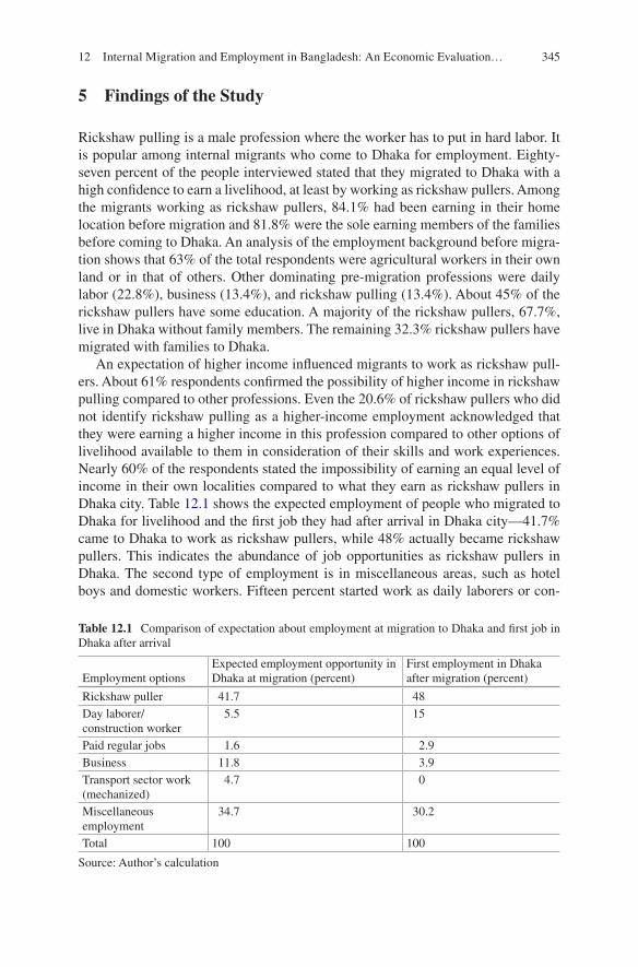
345

5 Findings of the Study

Rickshaw pulling is a male profession where the worker has to put in hard labor. It is popular among internal migrants who come to Dhaka for employment. Eighty- seven percent of the people interviewed stated that they migrated to Dhaka with a high confidence to earn a livelihood, at least by working as rickshaw pullers. Among the migrants working as rickshaw pullers, 84.1% had been earning in their home location before migration and 81.8% were the sole earning members of the families before coming to Dhaka. An analysis of the employment background before migra-tion shows that 63% of the total respondents were agricultural workers in their own land or in that of others. Other dominating pre-migration professions were daily labor (22.8%), business (13.4%), and rickshaw pulling (13.4%). About 45% of the rickshaw pullers have some education. A majority of the rickshaw pullers, 67.7%, live in Dhaka without family members. The remaining 32.3% rickshaw pullers have migrated with families to Dhaka.

An expectation of higher income influenced migrants to work as rickshaw pull-ers. About 61% respondents confirmed the possibility of higher income in rickshaw pulling compared to other professions. Even the 20.6% of rickshaw pullers who did not identify rickshaw pulling as a higher-income employment acknowledged that they were earning a higher income in this profession compared to other options of livelihood available to them in consideration of their skills and work experiences. Nearly 60% of the respondents stated the impossibility of earning an equal level of income in their own localities compared to what they earn as rickshaw pullers in Dhaka city. Table 12.1 shows the expected employment of people who migrated to Dhaka for livelihood and the first job they had after arrival in Dhaka city—41.7% came to Dhaka to work as rickshaw pullers, while 48% actually became rickshaw pullers. This indicates the abundance of job opportunities as rickshaw pullers in Dhaka. The second type of employment is in miscellaneous areas, such as hotel boys and domestic workers. Fifteen percent started work as daily laborers or con-

Table 12.1 Comparison of expectation about employment at migration to Dhaka and first job in Dhaka after arrival

Employment optionsExpected employment opportunity in Dhaka at migration (percent)

First employment in Dhaka after migration (percent)

Rickshaw puller 41.7 48Day laborer/construction worker

5.5 15

Paid regular jobs 1.6 2.9Business 11.8 3.9Transport sector work (mechanized)

4.7 0

Miscellaneous employment

34.7 30.2

Total 100 100

Source: Author’s calculation

12 Internal Migration and Employment in Bangladesh: An Economic Evaluation…

346

struction workers, though only 5.5% had an initial interest in such work. However, the 52% who had a first job other than rickshaw pulling subsequently switched to the profession of rickshaw pulling.

5.1 Migration and Entry into Rickshaw Pulling

Table 12.2 is the cross-tabulation showing the relation between length of migration to Dhaka and length of employment as rickshaw puller. People who migrated in the last 2 years of the survey started employment as rickshaw pullers immediately (11%); 3.1% or 4 persons who migrated to Dhaka more than 15 years ago had an employment length of less than 2 years as rickshaw pullers. This indicates later entry into this employment, after leaving other professions. Information from the table shows gradual late entries of people into rickshaw pulling from other kinds of employment. Further analysis of this issue revealed that 48% started rickshaw pull-ing immediately after their migration to Dhaka and another 14.2% did it within 2 years of their migration; 16.5% entered the profession after 10 years or more of their migration. Rickshaw pulling attracts people employed in other professions and they gradually accept it as their profession. It is important to note that 85% of the respondents informed their reluctance in continuing as rickshaw pullers for a long time. The higher income from rickshaw pulling may have attracted them initially to this profession, but they plan to leave this profession after accumulating wealth from it.

5.2 Wealth Creation

Wealth creation is the scaling up of existing tangible or capital assets that may help generate earnings in the future or may improve the quality of life. Sustainability of economic gains from migration depends on the magnitude of tangible and capital wealth accumulated by the migrant. When earnings from migration increase con-sumption only, they cannot pull out the migrants from poverty. Table 12.3 analyzes the wealth accumulation by the rickshaw pullers. About one-third of the respon-dents could not create any wealth out of their income as rickshaw pullers, 12.6% bought agricultural land, 11.8% bought rickshaws, and 2.4% invested in business. Information from the table does not show any significant wealth creation by rick-shaw pullers.

A. H. R. Hasan

347

Tabl

e 12

.2

Cro

ss-t

abul

atio

n of

leng

th o

f m

igra

tion

and

leng

th o

f em

ploy

men

t as

rick

shaw

pul

ler

in D

haka

city

Len

gth

of e

mpl

oym

ent a

s ri

cksh

aw p

ulle

r (y

ear)

Tota

lL

ess

than

2

year

s2–

5 ye

ars

5–7

year

s7–

10 y

ears

10–

15 y

ears

15 y

ears

and

m

ore

Len

gth

of m

igra

tion

to

Dha

ka (

Yea

r)L

ess

than

2

year

sC

ount

1414

% w

ithin

mig

ratio

n10

0.0%

100.

0%%

with

in e

mpl

oym

ent

51.9

%11

.0%

% o

f to

tal

11.0

%11

.0%

2–5

year

sC

ount

211

13%

with

in m

igra

tion

15.4

%84

.6%

100.

0%%

with

in e

mpl

oym

ent

7.4%

52.4

%10

.2%

% o

f to

tal

1.6%

8.7%

10.2

%5–

7 ye

ars

Cou

nt5

5%

with

in m

igra

tion

100.

0%10

0.0%

% w

ithin

em

ploy

men

t83

.3%

3.9%

% o

f to

tal

3.9%

3.9%

7–10

yea

rsC

ount

46

919

% w

ithin

mig

ratio

n21

.1%

31.6

%47

.4%

100.

0%%

with

in e

mpl

oym

ent

14.8

%28

.6%

37.5

%15

.0%

% o

f to

tal

3.1%

4.7%

7.1%

15.0

%10

–15

year

sC

ount

31

814

26%

with

in m

igra

tion

11.5

%3.

8%30

.8%

53.8

%10

0.0%

% w

ithin

em

ploy

men

t11

.1%

4.8%

33.3

%73

.7%

20.5

%%

of

tota

l2.

4%0.

8%6.

3%11

.0%

20.5

%15

yea

rs a

nd

mor

eC

ount

43

17

530

50%

with

in m

igra

tion

8.0%

6.0%

2.0%

14.0

%10

.0%

60.0

%10

0.0%

% w

ithin

em

ploy

men

t14

.8%

14.3

%16

.7%

29.2

%26

.3%

100.

0%39

.4%

% o

f to

tal

3.1%

2.4%

0.8%

5.5%

3.9%

23.6

%39

.4%

(con

tinue

d)

12 Internal Migration and Employment in Bangladesh: An Economic Evaluation…

348

Len

gth

of e

mpl

oym

ent a

s ri

cksh

aw p

ulle

r (y

ear)

Tota

lL

ess

than

2

year

s2–

5 ye

ars

5–7

year

s7–

10 y

ears

10–

15 y

ears

15 y

ears

and

m

ore

Tota

lC

ount

2721

624

1930

127

% w

ithin

mig

ratio

n21

.3%

16.5

%4.

7%18

.9%

15.0

%23

.6%

100.

0%%

with

in e

mpl

oym

ent

100.

0%10

0.0%

100.

0%10

0.0%

100.

0%10

0.0%

100.

0%%

of

tota

l21

.3%

16.5

%4.

7%18

.9%

15.0

%23

.6%

100.

0%

Sour

ce: A

utho

r’s

calc

ulat

ion

Tabl

e 12

.2 (

cont

inue

d)

A. H. R. Hasan

349

5.3 Economic Value Rickshaw Pulling in Dhaka City

As discussed earlier, this paper considered three alternative employment scenarios for the respondents. Table 12.4 shows the economic value of these three employ-ment options. Income equations, probability density functions of income equations, expected earnings of all employments, and the present values of the employment options are estimated according to the procedure explained in the methodology. Appendix 2 includes regressions analysis tables and equations of income and prob-ability density functions. The linear regression models for rickshaw pulling in Dhaka city and employment in origin localities were statistically significant, while the other option was not. However, this chapter uses all the regression equations for income estimation.

The calculated expected value is highest for rickshaw pulling in Dhaka, followed by other employments in Dhaka. The economic value of employment as rickshaw puller is BDT 5.89 million. The economic values of other employments in Dhaka

Table 12.3 Creation of wealth by rickshaw pullers with their earnings from employment

Type of wealthNo. of people Percentage

No wealth or financial gain 43 33.9Cash savings 29 22.8Purchase of agricultural land 16 12.6Purchase/repair/build home 32 25.2Investment in business 3 2.4Purchase of rickshaw 15 11.8Educational expenses of children 28 22.0Purchase of electronics/electrical durables goods

30 23.6

Purchase of gold 2 1.6

Source: Author’s calculation

Table 12.4 Expected and economic value of three different employment options for rickshaw pullers in Dhaka city

Employment options

Earning per day in BDTEmployment period (years)

Present value of earnings for full employment period, Vp (BDT)

Max (b)

Min (a)

Expected E(Yp) In BDT

In US dollars

Rickshaw puller in Dhaka city

510.63 135.00 357.98 25 5892193.10 76116.69

Other employment in Dhaka city

500.00 84.75 336.17 25 5533128.23 71478.21

Employment in origin locality

325.00 25.00 216.16 25 3557890.40 45961.64

Source: Author’s calculation

12 Internal Migration and Employment in Bangladesh: An Economic Evaluation…

350

and employments in origin localities are BDT 5.54 million and 4.59 million, respec-tively. Both employment options related to internal migration have a higher eco-nomic value than working in the origin locality. People from outside Dhaka probably gain financially from internal migration to this city.

5.4 Benefit–Cost Analysis of the Migration Pattern

This chapter considers two alternative modes of migration and compares these with the no migration situation. The benefit–cost ratio is a ratio of the daily earnings or benefits of a rickshaw puller to daily costs or expenses of the family of a rickshaw puller. Table 12.5 shows the BCA ratio of each type of migration. A favorable BCA ratio is greater than 1. The table shows that the BCA of no migration is 0.86, which means it is not an economically viable option. Thus, working in the original locality and living with family may not help earn a sufficient livelihood. The highest BCA ratio is for migration with family at 1.37. The BCA ratio for migration to Dhaka without family is 1.19. The IBCR between no migration and individual migration is 1.94. The same IBCR ratio between no migration and family migration is 3.40. Rickshaw pullers have higher financial gains when they migrate with their families, but about 68% rickshaw pullers lived alone in Dhaka.

Figure 12.1 shows that economic gains increase at a higher rate when rickshaw pullers migrate to Dhaka with their families compared to individual migration to Dhaka. Migrant rickshaw pullers have lower costs of living when they live with their families in Dhaka. Poor migrant rickshaw pullers gained economically when they lived with their families in Dhaka compared to the other alternatives.

5.5 Analysis

Internal migration to Dhaka from other parts of Bangladesh is a regular phenome-non. The ineffective mechanized mass transport system in the city of Dhaka has widened the scope for rickshaws as a mode of mass transport, and this has turned

Table 12.5 Benefit–cost ratio of migration options available to rickshaw pullers of Dhaka city in comparison to living and working in the origin location

Migration status of rickshaw pullersIncome per day (BDT)

Family expenditure per day (BDT

Cost–benefit ratio

No migration 254.72 297.24 0.86Single migration and family remains in original locality

510.63 428.89 1.19

Migration along with family members

510.63 372.5 1.37

Source: Author’s calculation

A. H. R. Hasan

351

out to be a blessing to the uneducated and less skilled internal migrants. The prob-ability of a higher income without any skill and training and by using only the power of body muscle is a key pull factor for internal migration to Dhaka. Bangladesh has a young population—32.3% of the population is below 14 years, 18.8% is between 15 and 24 years, and 38.0% is between 25 and 54 years. The dependency ratio is 52.2% and households traditionally depend on male members to earn a liv-ing. There is a significant hidden momentum in the population growth. Hence, the city of Dhaka has been experiencing regular inflows of a large number of young males from other parts of the country with an objective to become rickshaw pullers because there is a comparative advantage in this profession. Only 15.9% of the respondents were unemployed in their original localities before they came to Dhaka to work as rickshaw pullers. A significant movement in the workforce may have been undergoing in areas outside Dhaka because of rickshaw-pulling-induced inter-nal migration. Rural and semi-urban areas are losing skilled agricultural and other traditional workers necessary for the economy of these places. Even in Dhaka, workers from other forms of employment are switching to rickshaw pulling. Many switched to rickshaw pulling from other professions even after 15 years of being in Dhaka. A rickshaw puller may earn as high as BDT 1000 per day, and this level of daily income is very difficult to earn in many other employments.

The higher income from rickshaw pulling could not help rickshaw pullers to accumulate resources for future prosperity or for coming out of poverty. The earn-ing from rickshaw pulling may have been fuelling consumption rather than wealth

600

500

400

300

200

100

00 100 200 300 400 500

Cost (Daily Expenditure in BDT)

No Migration

FamilyMigration

IndividualMigration

Ben

efit (D

aily

Inc

ome

in B

DT

)

Fig. 12.1 Benefit to cost of internal migration to Dhaka from other areas of Bangladesh and work-ing as rickshaw pullersSource: Author’s calculation

12 Internal Migration and Employment in Bangladesh: An Economic Evaluation…

352

creation. A majority of the rickshaw pullers could not acquire productive resources with their hard-earned money. Other than building or repairing houses, the income flow of this sector has a limited use in improvements of infrastructure and the econ-omy of the original localities of the migrants.

The economic analysis of rickshaw pulling explored the financial gains from working in this profession compared to alternative professions. The economic value of employment as rickshaw pullers is 1.66 times higher than employment in the origin localities of the migrant workers and 1.07 times higher than working in other employments in the city of Dhaka. Rickshaw pulling has thus become the preferred employment for higher income and may continue as a cause of internal migration till its economic value declines. Further, the benefit–cost ratio uncovered the fact that family migration has more economic benefits than single migration as a liveli-hood strategy. This reality may accelerate the migration of family members of rick-shaw pullers in Dhaka from both rural and urban areas. The highly populated and congested Dhaka may become uninhabitable if 67.7% single migrant rickshaw pull-ers bring their family members to Dhaka because of the inadequate civic infrastruc-ture of the city.

Studies on the socioeconomic aspects of rickshaw pulling have failed to find welfare gains from rickshaw-pulling-induced internal migration to migrants and their family members. A study by Begum and Sen (2005) observes that rickshaw pulling provided easy access for poor people without education and skill in the urban labor markets and helped them to overcome chronic rural poverty initially. In the long run, rickshaw pulling is an unsustainable profession and initial welfare gains decline with the length of employment. Intergenerational mobility of rick-shaw pullers’ households is limited due to poor schooling and few occupational choices. Rickshaw pullers suffer from ill health and are susceptible to systematic health risks. Such findings indicate that rickshaw pulling does not ensure a perma-nent route to escaping poverty. Another study by Al Baki (2013) tried to evaluate whether rickshaw pulling in Dhaka had changed the economic condition of the migrants. He concluded that the long-run expected income from rickshaw pulling was insufficient to improve the economic conditions of most rickshaw pullers and their family members. The living standard of rickshaw pullers and their family members in Dhaka city is not adequate or comfortable. Rickshaw pullers cannot earn an adequate livelihood for themselves and their families in the long run. Family members of rickshaw pullers have to work to earn, and many of the child workers all over the city are the sons and daughters of rickshaw pullers (Roy 2013). Rickshaw pullers and their families live in the slums of Dhaka where living and health condi-tions are far below the requisite standards. The Bangladesh Urban Health Survey (BUHS) 2013 reports acute malnutrition, underweight, prevalence of stunting among young children, suffering from water - and vector-borne diseases, and road accidents as the major health problems of people living in the slums of Dhaka. The survey findings report that 50% of the slum children below 5 years are stunted and 43% of the urban children are underweight. As slum dwellers, rickshaw pullers and their family members suffer from the health problems reported by BUHS 2013. Rickshaw pulling is an easy way of earning more money, but it fails to provide

A. H. R. Hasan

353

social status and an economically sustainable livelihood in the long run (Sadekin et al. 2014). The apparently higher income from rickshaw pulling is thus a delusion. Rickshaw-pulling-induced migration is effectively transferring poverty from other areas of Bangladesh to the city of Dhaka.

The availability of rickshaw-related employments in the city of Dhaka is moti-vating people to migrate from other areas of Bangladesh to the city. The migration of people from rural to urban areas is the main reason for the growing slum popula-tion in Dhaka. The population of Dhaka has been increasing at a faster rate, and it is already beyond the sustainable capacity of the city. About 60% of the current popu-lation of 17 million of Dhaka live in slums. Basic facilities like housing, healthcare, electricity, and clean water are not available to these slum dwellers. The population growth in the city of Dhaka will deprive people further from the availability of basic facilities. The positive and causal association between more population and more demand for transport will create opportunities for more people to work as rickshaw pullers in Dhaka given that the city has an ineffective and unorganized mechanized public transport system. This chapter has calculated the highest economic benefit for rickshaw pullers when they migrate with their family members to Dhaka. This economic incentive may pull more people to Dhaka and accelerate the population growth rate in the city. Moreover, rickshaw pullers have larger families, which may further contribute to rapid population expansion in the city (Roy 2013).

It seems that rickshaws in Dhaka have a negative impact on national productivity and income. Rickshaws as a mode of public transport make the unorganized and inadequate public transportation system of the city more ineffective. About one mil-lion rickshaws clog the roads and make the movement of mechanized vehicles dif-ficult. The economic value of traffic jams in Dhaka is about USD 2253 million per year from a loss of 8.15 million work hours and 3.2 million business hours a year (Hossain 2014). As mentioned earlier, the annual revenue of the rickshaw sector is about USD 1120.8 million per year, which is lower than the cost of traffic jams in the city. This suggests an economic loss from using rickshaws as a mode of public transportation in the city.

6 Strategic Issues

Rickshaw-pulling-induced internal migration to Dhaka is a function of poverty, access to the urban job market without any professional skill and training, initial higher income, and an ineffective public transport system. There is disguised unem-ployment in the agrarian rural economy of Bangladesh because of a very low land-to-human ratio. Poverty due to inadequate livelihood from employment in the agrarian and other sectors in their own localities encourages unskilled people to migrate to other areas for a higher income and to come out of poverty. Those who migrate to Dhaka find rickshaw pulling as an employment that enjoys a higher income compared to other kinds of employment available for their skill level and work experience. Dhaka is the largest city and the main economic hub of Bangladesh,

12 Internal Migration and Employment in Bangladesh: An Economic Evaluation…

354

but it has an ineffective and unorganized mechanized public transport system. This weakness has forced the inhabitants of the megacity to use the alternative mode of transport that rickshaws provide.

The employment of rickshaw pulling cannot reduce the poverty of internal migrants. Many studies have observed that rickshaw pulling is an unsustainable employment to reduce the poverty of migrants. This chapter has estimated the eco-nomic value of rickshaw pulling from the earning side, which attracts people to work as rickshaw pullers. It has assumed that people have the ability to work for 25 years as rickshaw pullers. The profession of rickshaw pulling has a higher eco-nomic value and more income opportunities for unskilled internal migrants to Dhaka if it is a regular profession for a long time. Other studies show that a person cannot work for a long time as a rickshaw puller because of its negative impact on health caused by intensive physical labor (Begum and Sen 2005; Al Baki 2013; Roy 2013). Rickshaw pullers cannot create adequate resources from their profession that may help them to create resources for future solvency. As a result, poor migrants remain poor in the long run and increase the number of poor people in Dhaka. Rickshaws create road congestion and slow down the speed of mechanized trans-portation on the city roads. The cost of doing business should increase with reduced transport. It is believed that the rickshaw-dominated urban transport system of Dhaka has a negative impact on the national productivity of Bangladesh.

The opportunity to work as rickshaw pullers has been increasing the population of Dhaka city because each rickshaw provides employment to at least two persons on an average. About one million rickshaws are keeping around two million people in Dhaka city, excluding their family members. The family members of migrant rickshaw pullers come to Dhaka, following the earning member of the household. These people are poor and live in an unhealthy environment in urban slums. In most the cases, the living conditions of these people are inferior to their living conditions in their own localities. Dhaka is overcrowded and often ranked as one of the least livable cities in the world. The increasing inflow of people to Dhaka to work as rickshaw pullers and in other unskilled works is making the living conditions worse.

In spite of a higher perceived economic value of rickshaw pulling, this profession has the inability to effectively reduce poverty among the migrants. It has been con-tributing to unplanned growth in the urban population and has a negative impact on national productivity through the creation of traffic congestion and reduction of speed of mechanized vehicles on roads. Figure 12.2 shows the relationship between internal migration, urbanization, and poverty in the city of Dhaka because of the opportunity to work as rickshaw pullers.

7 Policy Recommendations

Rickshaw pulling is an economically unsustainable profession and is inefficient in reducing poverty. Internal migration based on the expectation of earning a higher income by rickshaw pulling is often a false reality and ends up transferring poverty

A. H. R. Hasan

355

from rural to urban areas. A set of policies may help control internal migration to Dhaka induced by the profession of rickshaw pulling. First, compulsory licenses for rickshaws and driving licenses for rickshaw pullers within the city of Dhaka may reduce the number of rickshaws on the roads of the city. It will reduce the scope for unskilled new migrants to work as rickshaw pullers and will weaken the motive behind the rickshaw-pulling-induced migration. It may help reduce the population size within Dhaka city as well. Second, investments in manufacturing and other economic sectors in areas outside of Dhaka must be scaled up to create alternative employment for people facing disguised unemployment in their own localities. Third, vocational and other training programs for the skill development of rickshaw pullers may motivate them to leave the profession of rickshaw pulling, which is unable to increase their income as well as the national income in the long run. Finally, an effective and adequate mechanized public transport system is essential for the city of Dhaka to limit the scope of rickshaws to be the alternative mode of transport. Implementation of these policies may help reduce the demand for employ-ment as rickshaw pullers and can effectively slow down the population growth in the city of Dhaka. It should scale down the transfer of rural poverty to urban areas.

There is not much research on the socioeconomic impacts of rickshaw-pulling- induced internal migration. Impacts of this migration on rural agriculture and other sectors need more investigation. The economic and social impact of the settlement process of these migrants and their family members on the urbanization process of

Inadequate MechanisedPublic Transport System inthe CityEconomic andAdministrative Hub of theCountryLarge Size of Population

•

•

•

•••

•

•

•••

••

•

Large Scale EmploymentInitial Higher IncomeShorter Working Life ofRickshaw Pullers

Rural poverty

Hidden Momentum inPopulation Growth

Large Pool of YoungerPopulation

Lower IncomeScarcity of NaturalEndowments forLivelihood

Higher Income

Physical Work

Employment withourTraining, Education, Skill

RapidUrbanization

UrbanPoverty

PopulationBurden in

City

Cost ofSlower

Movement

Demand forTransport

Mode of TransportRickshaw

Demand forEmployment Internal Migration

Fig. 12.2 The relationship between internal migration, urbanization, and poverty in Dhaka among the rickshaw pullersSource: Author’s illustration

12 Internal Migration and Employment in Bangladesh: An Economic Evaluation…

356

Dhaka and other large cities has not received adequate attention. It is also essential to identify alternative employment opportunities for erstwhile rickshaw pullers who are no longer engaged in the profession due to ill health or other reasons.

8 Conclusion

Unskilled migrants from outside Dhaka come to the city and prefer to work as rick-shaw pullers because this profession has the highest economic value of BDT 5.6 million for a 25-year working life compared to other professions. In reality, it is not a regular long-run profession, and 85% of rickshaw pullers stated their desire to not continue with the profession for a long time. The inability to work as rickshaw pullers for a long period cannot deliver the total economic gains that poor migrants expect at the beginning of taking on this profession. Most migrants fail to come out of poverty, and in most cases, they become part of the urban poor. The quality of life of the urban poor is inferior to that of the rural poor because of poor living condi-tions and adverse health conditions. However, the demand for rickshaws as mode of transport continues to pull new people to the city to replace many who leave the profession. This accelerates population growth inside Dhaka. The increasing num-ber of rickshaws on roads acts as a bottleneck for the free flow of mechanized vehi-cles. Evaluating all these negative impacts against the initial hope for higher income from employment as rickshaw pullers, this chapter recommends that the employ-ment of rickshaw pulling should be properly managed. Identification of alternative employment opportunities, improvement in public transport, and providing skills training to unskilled migrants may discourage them from entering this profession. This needs further investigation for evidence-based policy formulation.

Appendices

Appendix 1: Time Series of Income from Different Employment Options (Calculated from Survey Data)

YearDaily income fromRickshaw pulling in Dhaka Other employment in Dhaka Earning in original locality

1990 145.00 285.33 108.281991 150.00 200.00 60.001992 150.00 – 30.001993 150.00 – 25.001994 135.00 84.75 61.801995 150.00 146.00 160.00

A. H. R. Hasan

357

YearDaily income fromRickshaw pulling in Dhaka Other employment in Dhaka Earning in original locality

1996 200.00 255.00 70.001997 241.47 255.00 230.001998 200.00 500.00 136.671999 352.86 197.00 198.752000 192.86 227.50 167.502001 – – –2002 206.25 226.67 141.672003 200.00 210.00 80.002004 283.75 220.00 158.892005 300.00 400.00 175.002006 292.22 206.00 146.672007 370.00 – 177.502008 200.00 – 200.002009 250.00 416.67 260.002010 337.50 – 200.002011 392.86 400.00 325.002012 283.33 207.00 178.002013 327.78 – 237.002014 510.63 – 254.72

Note: ‘–’ = not available

Appendix 2: Income Function and Probability Density Function of Income of Different Employment Options (Estimated from Survey Data)

Regression Parameters of Income Functions

ParametersRickshaw pulling in Dhaka

Other employment in Dhaka

Earning in original locality

Constant 117.00 195.12 55.99Time (t) 10.16 5.64 7.77R square 0.63 0.11 0.58F-statistics 38.26 2.01 31.47Significance (p)

0.00 0.18 0.00

12 Internal Migration and Employment in Bangladesh: An Economic Evaluation…

358

Rickshaw pulling in Dhaka:

• Y tRickshaw = +117 00 10 162. .

• P Y tRickshaw( ) = +( )0 00000078 0 117 00 10 162. . . .

Other employment in Dhaka:

• Y tOther = +195 12 5 46. .

• P Y tOther( ) = +( )0 00000134 195 12 5 46. . .

Income at original location of the person:

• Y tHome = +55 99 7 77. .

• P Y tHome( ) = +( )0 00000235 55 99 7 77. . .

References

Afsar, R. (2003). Internal migration and the development nexus: The case of Bangladesh. Dhaka: Institute of Development Studies.

Afsar, R. (2005, March 14–16). Bangladesh: Internal migration and pro-poor policy. Regional conference on migration and development in Asia, Lanzhou.

Al Amin, M. M. (2010). Factors behind internal migration and migrant’s livelihood aspects: Dhaka City, Bangladesh aspects. Unpublished master’s thesis. Department of Economic History. School of Economics and management. Lund University, Sweden.

Al Baki, A. (2013). Rickshaw pulling and change in life: A case of Uttara in Dhaka city. An unpub-lished dissertation for Masters in Governance and Development at Institute of Governance Studies BRAC University, Dhaka, Bangladesh. Available at: www.hdl.handle.net/10361/3504. Accessed 3 Sept 2014.

BBS. (2011). Report on labor force surve 2011. Bangladesh Bureau of Statistics, Statistics Division, Ministry of Planning Government of the People’s Republic of Bangladesh.

BBS. (2012). Bangladesh population and housing census 2011 (National report, Volume—4). Bangladesh Bureau of Statistics, Statistics and Informatics Division (SID), Ministry of Planning, Government of the Peoples Republic of Bangladesh.

Begum, S., & Sen, B. (2005). Pulling rickshaw in the city of Dhaka: A way out of poverty? Environment and Urbanization, 17(2), 11–25.

Deshingkar, P. (2005, March 14–16). Maximizing the benefits of internal migration for develop-ment. Regional conference on migration and development in Asia, Lanzhou, China.

Deshingkar, P. (2006, May). Internal migration, poverty and development in Asia: Including the excluded. IDS Bulletin, 37(3). Institute of Development Studies.

DHUTS. (2010, March). Dhaka urban transport network development study, 2010. Japan International Cooperation Agency (JICA): Dhaka.

Finan, T. (2004). The dynamics of debt in southeast Bangladesh. CARE Bangladesh, Dhaka, mimeo.

Haider, S. K. U. (2010). Factors of migration on urban Bangladesh: An empirical study of poor migrants in Rajshahi City. Pakistan Journal of Social Sciences (PJSS), 30(2), 307–323.

Hossain, M. (2014, August 17). Rickshaws clog Dhaka city. The Daily Sun, Dhaka, Sunday. Available at: www.daily-sun.com/index.php?view=details&archiev= yes&arch_date=17-08-2014&type=Rickshaws-clog-Dhaka-. Accessed 3 Sept 2014.

A. H. R. Hasan

359

Islam, M. A. A. (2013). Migrant work force. In R. A. M. Titumir (Ed.), Accumulation and alien-ation: State of labor in Bangladesh (Vol. 97, p. 126). Dhaka: Unnayan Onneshan, Shrabon Prokashani.

Mansoor, S. A. (2007, November 7). Rickshaw fare. The Daily Star, Wednesday. Available at: http://archive.thedailystar.net/newDesign/print_news.php?nid=10555. Accesed 3 Sept 2014.

Morshed, M. M., & Asami, Y. (2011). Urban migration, informal economy and rural development: Rickshaw pullers in Dhaka City, Bangladesh. Regional geographic conference (UGI) held on November 14–18, Santiago, Chile.

Nabi, A. K. M. N. (1992). Dynamics of internal migration in Bangladesh. Canadian Studies in Population, 19(1), 81–98.

Rogaly, B., & Rafique, A. (2003). Struggling to save cash: Seasonal migration and vulnerability in West Bengal, India. Development and Change, 34(4), 659–681.

Roy, R. K. (2013, September 6). Rickshaw puller’s life in Dhaka City. Daily Sun. Available At: http://www.daily-sun.com/details_yes_06-09-2013_Rickshaw-Puller%E2%80%99s-Life-in-Dhaka-City_607_4_14_1_6.html#sthash.NX0J0jAi.dpuf. Accessed 6 Sept 2014.

Sadekin, M. N., Aktar, M. A., & Pulok, M. H. (2014). Socioeconomic analysis of the migrated rickshaw pullers in Comilla City of Bangladesh. International Journal of Innovation and Applied Studies, 8(3), 1142–1147.

Sultana, M. (2009, September 3). Rickshaw puller in Dhaka earns Tk 6,300 per month: JICA study. The Financial Express. p. 4b.

The views expressed in this publication are those of the authors and do not necessarily reflect the views and policies of the Asian Development Bank (ADB) or its Board of Governors or the governments they represent.

ADB does not guarantee the accuracy of the data included in this publication and accepts no responsibility for any consequence of their use. The mention of specific companies or products of manufacturers does not imply that they are endorsed or recommended by ADB in preference to others of a similar nature that are not mentioned.

By making any designation of or reference to a particular territory or geographic area, or by using the term “country” in this document, ADB does not intend to make any judgments as to the legal or other status of any territory or area. Open Access This work is available under the Creative Commons Attribution-NonCommercial 3.0 IGO license (CC BY-NC 3.0 IGO) http://creativecommons.org/licenses/by-nc/3.0/igo/. By using the content of this publication, you agree to be bound by the terms of this license. For attribution and permissions, please read the provisions and terms of use at https://www.adb.org/terms-use#openaccess.

This CC license does not apply to non-ADB copyright materials in this publication. If the mate-rial is attributed to another source, please contact the copyright owner or publisher of that source for permission to reproduce it. ADB cannot be held liable for any claims that arise as a result of your use of the material.

Please contact pubsmarketing@adb.org if you have questions or comments with respect to content, or if you wish to obtain copyright permission for your intended use that does not fall within these terms, or for permission to use the ADB logo.

Note: ADB recognizes “China” as the People’s Republic of China.

12 Internal Migration and Employment in Bangladesh: An Economic Evaluation…

C1

Correction to: Internal Migration, Urbanization, and Poverty in Asia: Dynamics and Interrelationships

Kankesu Jayanthakumaran, Reetu Verma, Guanghua Wan, and Edgar Wilson

Correction to: K. Jayanthakumaran et al. (eds.), Internal Migration, Urbanization, and Poverty in Asia: Dynamics and Interrelationships, https://doi.org/10.1007/978-981-13-1537-4

The original version of the book unfortunately contained mistakes. The version has been corrected.

The updated version of the book can be found at https://doi.org/10.1007/978-981-13-1537-4

© Asian Development Bank 2020K. Jayanthakumaran et al. (eds.), Internal Migration, Urbanization, and Poverty in Asia: Dynamics and Interrelationships, https://doi.org/10.1007/978-981-13-1537-4_13

361

AAbsolute poverty/approach, 9, 58, 129, 268,

269, 312, 325Absolute pro-poor, 8, 9, 312, 324, 325,

329–332, 336, 337ADB poverty line, 276, 297Administration boundaries, 136, 137Adult illiteracy, 274Afghanistan, 18, 23Aging/aged population, 2, 35, 42, 137Agriculture/agricultural sector/agricultural

production, 6, 48, 52, 59, 79, 81, 102, 104, 105, 110, 121, 137, 142, 153, 156, 157, 160, 189–191, 194, 203, 205–207, 210–212, 236, 240, 242, 292, 295, 310, 313, 340, 355

Andhra Pradesh, 6, 171–175, 181, 182, 184, 194–197, 199

Asia, 1, 13, 47, 267Asian demography, 32Asian Development Bank (ADB), 1, 169, 267,

272, 273, 276, 284, 295–297Asian financial crisis, 49, 138, 139Asian rural population, 20Asian urbanites, 2Asia Pacific Economic Cooperation

(APEC), 39Association of Southeast Asian Nations

(ASEAN), 14, 16, 30, 36, 39Atal Mission for Rejuvenation and Urban

Transformation (AMRUT), 312Atkinson index, 244

BBadan Pusat Statistik (BPS), 49–54, 59,

139, 140Bangladesh, 2, 8, 9, 18, 19, 26, 177, 339–356Bangladesh Bureau of Statistics, 339Bangladesh Labor Force Survey, 341Below Poverty Line (BPL), 165Benchmark, 2, 142, 238Bhutan, 20, 23Bi-directional links/bi-directional

elasticities, 129Brunei Darussalam, 17, 23-24, 40

CCambodia, 1, 18, 23, 31, 33Capital-intensive, 4, 79, 242, 248Carbon emissions, 113Carolina Population, 270Census data, 178, 196, 310Central Asia, 21, 23Chhattisgarh, 6, 128, 172–175, 181, 182,

194–197China Health and Nutrition Survey (CHNS), 8,

268, 270, 272, 274, 295, 296Chinese Centre for Disease Control and

Prevention, 270Chronic poverty, 341Circular migration/migrants, 14, 36–38, 111Coastal, 30, 31, 79, 80, 102Cointegration, 110, 114, 116, 117, 120, 123Communication technology, 295

Index

© Asian Development Bank 2019 K. Jayanthakumaran et al. (eds.), Internal Migration, Urbanization, and Poverty in Asia: Dynamics and Interrelationships, https://doi.org/10.1007/978-981-13-1537-4

362

Compulsory education, 268, 274, 295Computable general equilibrium (CGE), 237,

249–251Conditional cash transfers, 50Consumption outlays, 139Cooking fuel, 8, 273, 274, 283–285, 292Cooperative Medical Care System, 282,

285, 294Cost–benefit ratios, 342, 350Current migrants, 5, 136, 141–146, 148–154,

157–160

DDaily wages, 203, 204, 206Decentralization, 54, 59, 136Decentralized fiscal system, 295Decomposition analysis/method of

decomposition, 167, 292Deemed deprived, 274Degree of urbanization, 165, 169, 177, 178Delhi, 6, 30, 109, 164, 172–175, 181, 182,

184, 195–198, 211, 309, 311Demand elasticity of substitution, 237Demand for education, 221, 222, 231, 232Democratic People’s Republic of Korea, 23Demographic, 1, 3, 9, 13, 33–35, 40–42, 57,

58, 63, 70, 112, 129, 137, 142, 153, 156, 245, 270

Demographic dividend, 34Deprivation/deprivation score, 164, 269, 275,

276, 279, 280, 282, 284, 285, 294, 296, 297

Deprivation status values, 275Deprived, 180, 273–275, 284, 285, 287,

293–294, 296, 297, 353Destinations, 37, 38, 57, 121, 136–138,

140–142, 145, 147, 148, 155–158, 236, 339–341

Development/development strategies, 13, 16, 22, 26, 30, 35–40, 42, 48, 55, 56, 68, 79, 101, 105, 106, 113, 119, 129, 136, 138, 164, 180, 190, 295, 312, 313, 332, 355

Dhaka, 8, 9, 27, 339–356, 358Dibao poverty line/dibao, 97, 99, 101, 102Disaggregated production structure, 225Disguised unemployment, 353, 355Disparity trend, 285Distributions age-gender/age, 83Distributive Analysis Stata Package (DASP),

325–328, 330, 331, 333–335Diversity of deprivation, 296

Dongguan, 77, 89Drinking water, 164, 273–275, 283, 300–304Dual Cut-offs Approach (AF), 268, 269Dual economy, 269Dynamic general equilibrium, 7, 222, 228, 247

EEarnings distribution, 203East Asia, 3, 19, 20, 22, 24, 47, 276Economic reforms, 79, 110, 171, 309Economic value/economic rationality, 340,

342, 343, 349, 352–354, 356Educational attainment/educational

accumulation, 6, 59, 65, 69, 220, 221, 225, 226, 244, 245

Education (level of education), 2, 38, 56, 90, 113, 138, 164, 189, 220, 268, 341

Elderly population, 41Electricity, 56, 59, 62, 68, 69, 71, 204, 205,

208, 212, 214, 273–275, 282, 283, 286, 291, 300–304, 353

Employment elasticity/elasticity estimates/elasticity for poverty, 123, 313

Employments, 4, 6, 7, 9, 55, 56, 58, 68, 71, 84, 86–88, 109, 137, 189, 190, 192, 194–206, 209–213, 221, 224, 226, 236, 237, 270, 311, 313, 349–353

Endogeneity problems, 117, 125Energy, 2, 59, 113, 116, 119, 120, 123, 294Environment/environmental degradation, 2, 34,

42, 113, 119, 137, 164, 180, 212, 354Expenditure, 3–5, 8, 56, 58, 59, 62, 63, 65, 66,

68–71, 96–100, 102, 119, 120, 129, 139, 142, 153, 155, 165–167, 169, 173, 177, 179, 182, 183, 200, 212, 235, 313, 314, 322, 326, 350

Expenditure per capita, 58, 59, 62, 66, 68, 69, 100

Expert Group, 166, 171–173, 175, 182, 183, 314

Extended urbanization, 31Externalities, 56, 245

FFamily migrations, 136, 145, 149, 151, 157,

350, 352Female migrants, 153Fertility rate/fertility levels, 32, 33Five-Year Plan, 309, 311Foster–Greer–Thorbecke (FGT) index,

268, 323

Index

363

GGDP per capita, 22, 24, 56, 80, 110Gender, 5, 40, 57, 63, 81–84, 90, 100, 103,

143, 153, 154, 157, 160Gender effect, 90, 157Generalised method of moments (GMM/

SGMM/DGMM), 110, 118, 120, 125, 128

Gini coefficients, 48, 51, 56, 58, 62, 94–97, 100, 113, 114, 116, 118–121, 174, 178, 179, 184, 238, 244, 245, 311, 314

Global financial crisis (GFC), 9, 78–80, 139Global poverty line, 163Government of India, 109, 119, 120, 163, 312Gross domestic product (GDP), 22, 56, 68, 80,

110, 189, 212, 221, 235, 237, 239, 240, 311

Guangzhou, 27, 28, 30, 77, 89Guest workers, 79

HHarris–Todaro model, 7, 68Haryana, 6, 128, 172–175, 181, 182, 184,

195–197, 199Hausman test, 61, 66, 177, 179Head count ratio/head count index, 116, 119,

120, 167, 191, 276, 323Health insurance, 8, 93, 273–275, 279,

282–287, 290–292, 294, 296, 300–304Health status indicators, 274Higher education, 5, 7, 57, 138, 155–157, 212,

220, 222, 223, 231, 242, 244, 245, 248, 251

High-skilled unemployment, 221, 242, 248Hong Kong, China, 16, 20, 23, 30, 39, 40Household decision, 57, 58Household income survey/household survey/

household expenditure survey, 78, 92, 95, 223

Households, 1, 49, 78, 110, 136, 164, 169, 179, 199, 235, 268, 312, 340

Housing/housing services, 3, 6, 35, 42, 58, 155, 212, 236, 268, 311, 312, 339, 353

Hukou, 4, 15, 37, 79–83, 86, 89, 93–95, 100, 101, 104, 105

Human capital, 6, 34, 57, 65, 90, 105, 295

IImmigration, 35, 42, 177, 228, 234, 241, 247Imputed wage bill, 236Incidence of poverty, 6, 26, 50, 166, 212, 284

Income distribution, 51, 65, 66, 94, 96, 99, 100, 222

Income poverty/income poverty rate, 8, 276, 284, 292, 295, 297

Income status, 57Income vulnerability, 284India/Indian states, 4, 110, 112, 120, 125, 128,

129, 166, 173, 174, 195Indonesia, 1, 3–5, 7, 18, 21, 23, 31–33, 36, 40,

50, 135–141, 145, 166, 234Indonesian Family Life Survey (IFLS), 5, 136,

140, 141, 143Industry-biased, 226Industry upgrading, 79Inelastic, 123, 128, 129Inequality, 2–8, 69, 87, 115, 177, 178,

184, 223, 237, 244, 245, 247, 248, 272, 296, 311, 312, 314, 317–322, 325, 332

Infant mortality, 113, 116, 118–121, 128Informal employment, 6, 7, 203, 212Informal sectors, 2, 40, 164, 211, 212, 311Infrastructures, 2, 3, 31, 37, 58, 59, 66, 68, 70,

71, 113, 119, 137, 163, 164, 212, 294, 352

In-migration, 54, 57, 83, 111, 119, 121, 128, 192, 200

Input–output matrix/input-output, 7, 236Institutional restrictions, 4, 88, 102Interdependencies, 2, 48, 49, 51, 59–62, 66,

69–71, 113–115, 118, 128, 129, 169Integrated Urban Poverty Eradication

Programme, 311Internal migration, 1–5, 7, 9, 31, 32, 35, 38,

58, 60, 61, 67, 70, 71, 122, 137, 138, 140–143, 145, 149, 153, 156, 157, 248, 349

International migration, 3, 5, 32, 35, 37–41, 49, 143, 153

International Monetary Fund (IMF), 22, 24–26, 32, 47, 48, 56, 237

Interprovincial migration, 3, 49, 54, 55, 57, 58, 61, 62, 66

Interstate migration, 310Interventions, 42, 105, 157, 312, 313Iran (Islamic Republic of), 23

JJakarta, 26, 27, 29–31, 36, 40, 48, 52, 54, 55,

57, 157Japan, 1, 21, 23, 39, 40, 341Job turnovers, 83Johansen cointegration, 114

Index

364

KKnowledge economy, 312Kuznets/Kuznets hypothesis, 48, 56

LLabor-intensive, 48, 55, 68, 89, 102, 103, 190,

212, 242, 340Labor surplus/labor deficit/labor shortages, 39,

79, 80, 82, 103, 104Labour force participation/labour force survey,

6, 7, 59, 200, 212, 224–227, 230, 233, 237, 241, 341

Labour markets, 3, 14, 41, 104, 118, 295Labour productivity, 83, 190, 194, 212,

250, 313Labour supply, 4, 34, 57, 92, 102, 104, 106,

230–233, 247Lao People’s Democratic Republic, 23Lewisian turning point, 103Linkages, 22, 26, 39, 49, 55, 111, 128, 129,

147, 163, 248Livelihood strategy, 340–342, 352Logit model, 58Longitudinal survey, 4, 78, 270Lorenz curves, 165–168, 173, 324, 327Low-income groups, 309Low-productivity sectors, 221

MMacau, China, 16Maharashtra, 6, 112, 172–175, 181, 182, 184,

194–198Malaysia, 7, 23, 31, 40, 239, 248Maldives, 23, 33Male migrants, 153, 200, 202Manpower forecasts, 221, 222Manufacturing, 48, 65, 68, 82, 103, 110, 190,

204, 205, 208, 212, 214, 227, 241, 242, 244, 252, 355

Marginalization, 180Marital status, 63, 64, 70, 143, 200, 207Market wages, 68, 235Marriage migration, 40Mean log deviation (MLD), 109, 112Medical insurance system/medical care, 166,

268, 274, 282, 285, 294Megacities, 3, 14, 24, 26, 27, 30, 31, 36, 39Metropolitan, 14, 26, 109, 339, 341Metropolitan cities/metro cities, 109, 164, 196,

211, 212Microsimulation, 223, 237, 238

Middle-income, 220, 246Migrant unemployment, 85, 235Migrant workers, 14, 15, 36–38, 78–80, 82,

83, 86, 87, 89, 92, 95–100, 102, 103, 190, 197, 198, 203, 204, 210, 212, 341, 352

Migration, 14, 47, 77, 109, 135, 164, 190, 234, 292, 310, 339

Migration costs, 158Migration cycle, 136, 141, 157Migration status, 3, 57, 58, 63, 344, 350Millennium Development Goals, 5, 47, 163Mincerian wage equations, 191Minimum wages, 6, 59, 68, 69, 71, 89, 103,

191, 195, 235, 245Modified Expert Group methodology, 166,

172, 173, 175Mongolia, 23Multidimensional poor, 269, 272, 275, 276Multidimensional poverty measurements/

multidimensional poverty index (MPI), 268, 269, 272, 274–276, 281, 287–290, 296, 298, 299

Myanmar, 18, 23, 31

NNational Institute of Nutrition, 270National New Urbanization Plan, 79, 104, 105National poverty line (NPL), 113, 139, 140,

267, 273National Sample Survey Organization

(NSSO), 190Natural growth, 111, 164, 196Natural increase, 32, 33Nepal, 18, 23, 33Net migration, 35, 36, 54, 55, 62, 69, 111,

112, 116, 118, 119, 125, 128Non-migrants, 5, 6, 58, 63, 136, 138, 141–144,

148–150, 152–154, 156, 158, 160, 190, 191, 193, 203, 204, 206–212, 340

Non-motorized transport (NMT), 341

OOLS estimates, 56, 118, 178On-the-job training one-child policy, 83Open-door policy/open door, 7, 79, 238,

244, 245Origin-destination matrix, 236Orissa, 6, 112, 128, 171–175, 181, 182, 184,

194–197Out-migration, 54, 57, 112, 194, 195, 198, 211

Index

365

PPakistan, 2, 5, 19, 21, 23, 26, 33, 58–62, 69,

70, 118, 136, 140–142, 169, 178, 211Panel regressions, 6, 178, 180Payroll taxes, 235People’s Republic of China (PRC), 1, 3–9, 14,

16, 21, 30–33, 36–38, 40, 47, 57, 97, 101, 104, 166, 169, 267, 276, 292, 295, 296

Per capita, 4, 6, 8, 15, 22, 24, 50, 56, 58, 59, 62, 66, 68, 69, 80, 94, 96–100, 110, 119, 165, 169, 170, 178, 179, 181–183, 272, 273, 283, 286, 291, 300–304

Per capita income/per capita expenditure, 3–5, 8, 15, 63, 65, 77, 95–102, 139, 142, 143, 153–155, 160, 165, 169, 170, 177–179, 181–183, 292

Per capita public expenditure, 6, 165, 169, 177, 178

Philippines, 2, 15, 16, 19, 23, 31, 33, 40, 48, 234

Polarizations, 2, 113Population, 14, 47, 78, 135, 163, 164, 167,

174, 177, 178, 190, 235, 268, 309, 339censuses, 34, 48, 55, 58, 135, 178mobility, 36, 39, 49, 56movement, 35, 41, 77, 105, 137, 138

Post-reforms, 171, 310Poverty, 22, 48, 78, 109, 136, 163, 191, 267,

311, 340city size gradients, 24cut-off, 275, 279, 280, 287, 295, 296impact, 153lines, 3, 6, 8, 58, 96, 98, 99, 102, 119, 121,

139, 140, 163, 165–168, 171–173, 175, 178, 182, 183, 267, 272, 273, 276, 283–285, 296, 300–301, 311, 323, 324, 328, 332

measures, 4, 100, 123, 166–168, 276rates, 3, 24, 26, 47, 49–51, 66, 69, 98, 100,

111, 139, 148, 149, 163, 276, 314, 318–319, 332

reduction/alleviation, 3, 5, 7, 8, 22, 37, 38, 47–51, 56, 61, 109, 110, 136, 137, 139–141, 148–151, 153, 154, 157, 165, 166, 169, 179, 180, 268, 295, 311–313, 342

Poverty gaps/poverty gap ratio (PGR), 2, 7–9, 276, 313, 314, 323–325

Primary school children, 143, 155–157Principle components analysis, 268Probit model, 4, 58, 100, 103, 142, 191Productive uses, 341

Productivity, 6, 79, 105, 189, 190, 203, 207, 210, 212, 222, 224, 238, 239, 241, 245, 248, 250, 310, 314, 353, 354

Pro-poor growth, 312, 313, 324–326, 336Provincial poverty, 50, 62Pull factors, 137, 212, 234, 241, 341, 351Purchasing power parity (PPP), 48, 97, 99, 111Push factors, 137

QQuality of workers, 90Quantitative techniques, 344

RRapid urbanization, 2, 16, 32, 48,

110–111, 113Rate of return, 222, 231Regional growth, 2Regional inequality, 52Relative poverty/approach, 2, 58, 70, 312, 336Relative pro-poor, 8, 323–325, 328, 333–336Religion, 200, 317, 318, 320, 322, 332, 336Remittances, 49, 56, 57, 110, 136, 341Replacement migration, 35, 41Republic of Korea, 40, 166Returned migrants, 78, 82Rickshaw/rickshaw pulling, 8, 9, 199,

339–356Rural, 13, 49, 78, 109, 136, 163, 189, 267,

309, 339Rural household registration (rural hukou), 4,

37, 79–83, 95, 104Rural literacy rates, 194, 195Rural multidimensional poverty, 268–270,

276, 279, 280, 282, 285, 294, 296Rural population share, 110Rural to urban migration, 3Rural–urban disparity, 8Rural–urban migration, 4, 6, 7, 20, 32, 36, 48,

54, 56–58, 70, 71, 98, 140, 164, 189–212, 310, 339

Rural–Urban Migration in China (RUMiC), 77, 78, 82, 85, 86, 90, 92, 95–97, 102, 104

SSAKERNAS, 59Say’s Law, 221Scheduled castes (SC), 200, 201, 208, 214,

313, 315, 318, 320, 322, 332, 336

Index

366

Scheduled tribes (ST), 200, 315, 317, 318, 320, 322, 332, 336

School-age children, 93, 94Sectoral transformation, 48Self-employed, 86, 89, 98, 197, 198, 315, 317,

318, 320, 336Semi-social accounting matrix, 7, 236, 237Service sectors, 56, 110, 189, 199, 212, 311Sex/sex industry, 6, 40, 200, 207, 210, 315,

318, 320, 336Shenzhen, 27, 29, 30, 77, 89Simulations, 7, 166, 222, 236, 238, 239, 242,

244, 245, 247Singapore, 16, 20, 23, 39, 40Skill-biased technology, 7, 119, 227Skilled migrants, 5, 7, 55, 104, 119Skilled workers, 9, 51, 79, 104, 207, 220, 225,

226, 233, 240, 243, 261, 262Skill endowments, 224, 238Skill-intensive economy, 241Skills acquisition, 235Slum dwelling population spatial, 109,

111, 112Slums, 2, 6, 24, 112, 164, 180, 190, 212, 311,

352–354Social demand methods, 221Social insurance, 81, 92–94Social services, 78, 79, 81, 92–94, 96, 102Socioeconomic, 57, 63, 70, 165, 169, 191,

312, 352, 355South Asia, 3, 19, 20, 22, 24, 48, 163, 164Southeast Asia, 3, 14, 19, 20, 22, 27, 31Spatial distribution, 30Spill over effects, 245Squared poverty gap ratio (SPGR), 313, 314,

318, 322Sri Lanka, 16, 23, 33, 40State-level headcount index, 120State-owned enterprises, 221Staying current migrants, 141, 143, 144, 148,

149, 153, 159, 160Stock of migrants, 80–82Stolper-Samuelson effect, 226Structural changes, 110, 117, 189, 212, 220,

226, 241Substitutability, 220, 229, 243Sustainable development, 180, 312Swarna Jayanti Shahari Rozgar Yojana, 311

TTaipei,China, 36, 40Technical progress, 241, 245

Techno-cities, 199Technological bias, 246, 247Technological change, 7, 225Temporary migrants, 37Tendulkar methodology, 166, 171–173, 175Tertiary education, 65, 147, 220, 221, 223,

242, 247, 249Tertiary graduates, 220, 246Thailand, 15, 16, 19, 23, 31, 33, 48Time series analysis, 4, 110Timor-Leste, 18, 20, 23, 33Toilet, 8, 65, 66, 273, 274, 283–286, 291–294,

296, 300–304, 312Total factor productivity, 248Township and Village Enterprises (TVEs), 79Traffic jams/traffic congestion, 353, 354Trafficking, 40Transformations, 1, 13, 32, 41, 48, 56, 61,

116, 135, 145, 194, 231, 251, 309, 310Transient migrants, 2Translog cost functions, 225Transport, 2, 8, 42, 190, 204, 205, 212, 227,

241, 242, 244, 295, 312, 339–341, 345, 350, 353–356

Trends of urbanization, 22, 49–51, 53–55, 78, 110

Trickle-down effect, 313

UUnemployment insurances, 92, 96Unidimensional poverty, 268United Nations, 13, 15, 17, 18, 20–24, 26, 27,

29–32, 35, 272, 309, 339United Nations Development Programme

(UNDP), 268Unskilled workers/migrants, 7, 39, 119, 199,

212, 224, 356Upskilling, 226, 240Urban, 13, 47, 77, 109, 136, 163, 190, 267,

309, 339agglomeration, 26, 27, 129, 310, 311, 314Asia, 14, 19, 35–40development, 26, 31, 35–40, 118, 119, 129Gini index, 52, 69, 109, 111growth, 3, 31, 54, 128, 129, 180households, 6, 8, 78, 92, 94–96, 100, 165,

169, 170, 178, 179, 280household size, 4, 96, 165, 169, 170, 178household surveys, 78, 92, 95hukou workers, 86, 89, 100, 101India, 124, 168, 171, 189–212, 311, 312,

314, 317–322, 326, 332

Index

367

inequality/income inequality, 2, 3, 7, 8, 48, 51, 55, 58–61, 66, 67, 69, 70, 78, 94, 95, 97–101, 110, 111, 119, 121, 125, 129, 165, 169, 173, 175, 179, 184, 269

infrastructural facilities, 6labour market, 3, 14mean log deviation (MLD), 109, 111medical care system, 282, 285population, 1, 6, 14, 16, 19–21, 26, 31–33,

35, 36, 38, 42, 48, 62, 66, 69, 109–112, 116, 118–121, 123, 125, 128, 139, 163, 164, 177–179, 190, 191, 196–198, 212, 282, 309, 310, 354

poverty/poverty line, 2–5, 7–9, 24, 60, 70, 73, 82, 110–113, 116, 119–121, 123, 125, 128, 129, 163–169, 171, 172, 174, 175, 178–180, 272, 278, 280, 281, 285, 288, 289, 292, 295, 311, 328, 340

size, 128, 129slums, 164, 165, 180, 311, 354total fertility rate (TFR), 32, 33unemployment, 68

Urbanization, 1–5, 7, 9, 17, 52, 81, 109, 110, 119, 120, 123, 128, 129, 139–141, 156, 164, 165, 169, 175, 177–180, 189–212, 310, 312, 340, 342, 354, 355

Urbanization process, 48, 68, 79, 105, 169, 177, 212, 340, 355

Urban-rural disparities, 282, 287, 296Urban–rural disparities, 280, 281, 295Urban–rural income gap, 269

VValue added, 5, 48, 79, 89, 228, 236, 249Viet Nam, 2, 18, 23, 26, 31, 33, 48

Vocational education/vocational training, 6, 7, 212, 231, 232, 295

Vulnerability-adjusted poverty lines, 273, 281, 296, 300

WWage, 39, 51, 79, 118, 189, 220, 310

bills, 236differentials, 6, 57, 189–212, 234, 250,

256, 260disparities, 59earners, 225, 236, 237, 239, 240, 243, 247,

257, 314premium, 223, 225, 232, 234

Wage–salary workers, 89, 92Water and sanitation, 295Wealth creation, 34, 346, 351–352Weighted mean of the deprivation, 275West Bengal, 6, 164, 165, 167–169, 171–184,

195–198Whole family migrations, 136, 145, 149,

151, 157Workforce, 6, 34, 35, 39, 41, 42, 104, 105,

189–192, 196, 197, 199–203, 207, 224, 295, 351

Working hours, 88–90, 92World Bank/World Bank study, 5, 15, 22, 25,

26, 32, 47, 48, 51, 56, 109, 111, 112, 114, 120, 139, 221, 226, 236, 267, 273, 295

World cities, 39, 41World factory, 79

YYoung graduates, 221

Index