1

Informa� on Systems & Grid Technologies

Seventh Interna� onal Conference ISGT’2013

Sofi a, Bulgaria, May, 31 – June 1., 2013.

2

ISGT’2013 Conference Commi� ees

Co-chairs

• Prof Ivan SOSKOV

• Prof Kiril BOYANOV

Program Commi� ee

• Míchéal Mac an AIRCHINNIGH, Trinity College, University of Dublin

• Pavel AZALOV, Pennsylvania State University

• Marat BIKTIMIROV, Joint Supercomputer Center, Russian Academy of Sciences

• Marko BONAČ, Academic and Research Network of Slovenia

• Marco DE MARCO, Catholic University of Milan

• Milena DOBREVA, University of Strathclyde, Glasgow

• Viacheslav ILIN, Moscow State University

• Vladimir GETOV, University of Westminster

• Jan GRUNTORÁD, Czech Research and Academic Network

• Pavol HORVATH, Slovak University of Technology

• Seifedine KADRY, American University of the Middle East, Kuwait

• Arto KARILA, Helsinki University of Technology

• Dieter KRANZMUELLER, University of Vienna

• Shy KUTTEN, Israel Ins� tute of Technology, Haifa

• Vasilis MAGLARIS, Na� onal Technical University of Athens

• Ivan PLANDER, Slovak Academy of Science

• Dov TE’ENI, Tel-Aviv University

• Stanislaw WRYCZA, University of Gdansk

• Fani ZLATAROVA, Elizabethtown College

Organizing Commi� ee

• Vladimir DIMITROV

• Maria NISHEVA

• Kalinka KALOYANOVA

• Vasil GEORGIEV

3

St. Kliment Ohridski University Press

Vladimir Dimitrov, Vasil Georgiev (Editors)

Informa� on Systems & Grid TechnologiesSeventh Interna� onal Conference ISGT’2013

Sofi a, Bulgaria, May, 31 – June 1., 2013.

Proceedings

4

© 2013 Vladimir Dimitrov (Eds.)

ISSN 1314-4855

St. Kliment Ohridski University Press

Preface

This conference was being held for the seventh � me in the end of May and beginning of June, 2013 in the halls of the Faculty of Mathema� cs and Informa� cs of the University of Sofi a “St. Kliment Ohridski”, Bulgaria. It is supported by the Na� onal Science Fund, by the University of Sofi a “St. Kliment Ohridski” and by the Bulgarian Chapter of the Associa� on for Informa� on Systems (BulAIS). Tradi� onally this conference is organized in coopera� on with the Ins� tute of Informa� on and Communica� on Techno-logies of the Bulgarian Academy of Sciences.

Total number of papers submi� ed for par� cipa� on in ISGT’2012 was 56. They undergo the due selec� on by at least two of the members of the Program Commi� ee. This book comprises 31 papers of 36 Bulgarian and 19 foreign authors included in one of the three conference tracks and an addi� onal sec� on for separate contribu� ons. The conference papers are expected to be indexed by the digital libraries h� p://www.ebsco.com/ and h� p://www.proquest.co.uk/. They are available also on the ISGT web page h� p://isgt.fmi.uni-sofi a.bg/ (under Former ISGTs tab).

Responsibility for the accuracy of all statements in each peer-reviewed paper rests solely with the author(s). Permission is granted to photocopy or refer to any part of this book for personal or academic use providing credit is given to the conference and to the authors.

The editors

5

T � � � � � � C � � �

I � � � � � � S � � � �

The Data Mining Process Vesna Mufa, Violeta Manevska, Biljana Nestoroska .................................................. 11

Marke� ng Research by Applying the Data Mining Tools

Biljana Nestoroska, Violeta Manevska, Vesna Mufa ................................................. 21

CRM systems and their applying in companies in Republic of Macedonia Natasa Milevska , Snezana Savoska ........................................................................... 33

Visual systems for suppor� ng decision-making in health ins� tu� ons in R. of Macedonia Jasmina Nedelkoska, Snezana Savoska ....................................................................... 40

Evalua� on of Taxonomy of User Inten� on and Benefi ts of Visualiza� on for Financial and Accoun� ng Data Analysis Snezana Savoska , Suzana Loshkovska ........................................................................ 51

Data Structures in Ini� al Version of Rela� onal Model of Data Vladimir Dimitrov ....................................................................................................... 66

Peopleware: A Crucial Success Factor for So� ware Development Neli Maneva .............................................................................................................. 77

Informa� on System for Seed Gene Bank Ilko Iliev, Svetlana Vasileva ......................................................................................... 86

Valida� on of the Collabora� ve Health Care System Model COHESY Elena Vlahu-Gjorgievska, Igor Kulev, Vladimir Trajkovik, Saso Koceski ....................... 98

A graph representa� on of query cache in OLAP environment Hristo Hristov, Kalinka Kaloyanova ........................................................................... 108

Development of Educa� onal Applica� on with a Quiz Marija Karanfi lovska, Blagoj Ristevski ...................................................................... 120

Performance Study of Analy� cal Queries of Oracle and Ver� ca Hristo Kyurkchiev, Kalinka Kaloyanova ...................................................................... 127

6

I � � � � � � S � � � �

Knowledge Management So� ware Applica� on and its Prac� cal Use in the Enterprises Ana Dimovska, Violeta Manevska, Natasha Blazeska Tabakovska ........................... 143

Personalisa� on, Empowering the Playful. The Social Media Cloud Mícheál Mac an Airchinnigh ..................................................................................... 152

Intelligent Approach for Automated Error Detec� on in Metagenomic Data from High-Throughput Sequencing Milko Krachunov, Maria Nisheva and Dimitar Vassilev ............................................ 160

Seman� c Digital Library with Bulgarian Folk Songs Maria Nisheva-Pavlova, Pavel Pavlov, Dicho Shukerov ............................................. 169

Knowledge Representa� on in High-Throughput Sequencing Ognyan Kulev, Maria Nisheva, Valeria Simeonova, Dimitar Vassilev ......................... 182

Model of Knowledge Management System for Improvement the Organiza� onal Innova� on Natasha Blazeska-Tabakovska, Violeta Manevska ................................................... 193

Towards Applica� on of Verifi ca� on Methods for Extrac� on of Loop Seman� cs Trifon Trifonov .......................................................................................................... 202

D � � � � � � � � S � � � �

Field Fire Simula� on Applying Hexagonal Game Method Ste� a Fidanova, Pencho Marinov ........................................................................... 215

Using Cloud Compu� ng In Higher Educa� on Josif Petrovski, Niko Naka, Snezana Savoska ............................................................ 223

Implica� ons of Data Security in Cloud Compu� ng Dimiter Velev and Plamena Zlateva ......................................................................... 231

Contemporary Concurrent Programming Languages Based on the Actor Model Magdalina Todorova, Maria Nisheva-Pavlova, Trifon Trifonov, Georgi Penchev, Petar Armyanov, Atanas Semerdzhiev ..................................................................... 238

7

So� ware Integra� on Pla� orm for Large-Scale Genomic Annota� on of Sequences Obtained in NGS Data Analysis Deyan Peychev, Atanass Ilchev, Ognyan Kulev, Dimitar Vassilev .............................. 251

Models of Quality for Cloud Services Radoslav Ivanov, Vasil Georgiev .............................................................................. 261

Contemporary Concurrent Programming Languages Based on the Communica� ng Sequen� al Processes Magdalina Todorova, Maria Nisheva-Pavlova, Atanas Semerdzhiev, Trifon Trifonov, Petar Armyanov, Georgi Penchev ................... 267

S � � � � � � C � � � � � � � �

Parsing “COBOL” programs Krassimir Manev, Haralambi Haralambiev, Anton Zhelyazkov ................................ 281

Verifi ca� on of Java Programs and Applica� os of the Java Modeling Language in Computer Sceince Educa� on Kalin Georgirev , Trifon Trifonov ............................................................................... 288

Evalua� on metrics for Business Processes in an Academic Environment Kris� yan Shahinyan, Evgeniy Krastev ....................................................................... 297

Monte Carlo Simula� ons: Interest rate sensi� vity of bank assets and liabili� es. What will happen if interest rates change by a certain amount? Milko Tipografov, Peter Kalchev, Adrian Atanasov .................................................. 307

Classifi ca� on of Events in the EPC Standard Ivaylo Kamenarov .................................................................................................... 320

A � � � � I � � � .......................................................................................... 328

9

I � � � � � � S � � � �

11

The Data Mining Process

Vesna Mufa, Violeta Manevska, Biljana Nestoroska

Faculty of Administration and Information System Management, University “St. Kliment Ohridski” – Bitola,

Partizanska bb, 7000 Bitola, Republic of Macedoniavesna_mufa@hotmail.com, violeta.manevska@uklo.edu.mk, nestoroska_bile@yahoo.com

Abstract. The rapidly growing amount of data exceeds the human ability to understand them without the mediation of powerful tools. In such case, the stored data are an archive material, which is rarely visited and used. Consequently, the decisions are made based on the intuition of decision makers, but not on the basis of information and knowledge extracted from the data, which are stored in databases. Data mining is the nontrivial extraction of implicit, previously unknown and potentially useful information or knowledge from large dataset. It is a carefully planned and complex process that consists of the following phases: defi ning the problem, data preparation, execution of algorithms and interpretation of obtained results. The individual phases, as well as the overall process are interactive. The successful data mining is due to understanding and fulfi llment of each phase.

Keywords: Data, Data Mining, Algorithms, Data Extraction

1 Introduction

Data that are found in the databases, such as the most common location for their storage, reaches sizes of Giga and Terabytes, so the databases contain more than million rows, while the column’s number ranges from 10 to 10 000. The storage of data imposes on their understanding and making data analysis.

The rapidly growing, enormous amount of data exceeds the human ability to understand them if there is no mediation of powerful tools. In this case, the stored data represent an archive material, which is rarely visited and used. Consequently, the decision making is based on the intuition of the decision makers, not on the basis of information and knowledge, which is extracted from the data [1].

There are many tools that allow multidimensional data analysis, but without opportunity for advanced analysis, such as the classifi cation, the clustering, and tracking the changes to data over time. Advanced data analysis is achieved by applying the so-called data mining. Data mining is a result of the natural evolution of information technology, which aims to extract a “gold” (information or knowledge) from an “archive material” (data). Data mining is the nontrivial

12

extraction of implicit, previously unknown and potentially useful information or knowledge from large data set.

2 The Data Mining Process

According to some opinions, data mining consists of selection and application of computer-based tools or selection and implementation of algorithms. This belief is partly true because data mining implements methods (algorithms), but is needed to be performed several phases before algorithm’s implementation on data. It is a carefully planned and complex decision-making process on that what will be the most useful and relevant. The data mining process is represented graphically in Fig. 1.

Fig. 1. The data mining process

The data mining process consists of the following phases:• defi ning the problem;• data preparation → a result: prepared data;• execution of algorithms → a result: patterns or models and• interpretation of obtained results → a result: information/knowledge.The individual phases as well as the overall process are interactive.

2.1 Defi ning the Problem

Each data mining starts by defi ning the problem. The problems belong to different domains and therefore is necessary domain-specifi c knowledge and experience. Defi ning the problem means understanding the goals and requirements of domain perspective and transforms that knowledge into data mining problem with the existence of a preliminary plan.

One type of problem that can be solved by applying data mining is, whether fl ats that the real estate agencies will offer to their customers are good or bad offers. The goal is to construct models that the agencies will apply whenever they mediate in selling this type of real estate. If the offer proposed by a customer who

13

sold fl at isn’t in accordance with the terms that the fl at has (a bad offer), agencies must state that the price should be corrected. If the offer is good, it’s accepted without remarks.

In this phase is accomplished closely interaction between a domain expert (in our case, a real estate agent) and a data mining expert. This collaboration should not stop at this initial stage, but it should continue through the entire process because the domain expert should validate the results in the further phases.

Once the problem is defi ned, the data should be selected because they will be input into data mining.

2.1.1 Data – Inputs into Data Mining

The input into data mining is а dataset, which consists of instances (objects/records). Because the set is presented in a tabular form, the instances are rows from the table, and the columns are called attributes. Each instance is described by a number of attributes. An attribute is defi ned as a data fi eld and represent a feature of the data object [2].

Data mining divides the attributes into two groups: discrete or categorical and numeric or continuous. The discrete attributes have a fi nite number of predetermined possible values, while the continuous attributes have an infi nite number of possible values. The type that will be used for a given attribute depends on its meaning.

Discrete attributesDiscrete attributes include: nominal, binary and ordinal attributes. They are

qualitative, which means that they describe a feature of an object. The values of these attributes represent categories and integers are used to replace the categories with numbers. When replacing the category with a number, the numbers are not used for quantitative purposes, which means that the mathematical operations on values in these attributes have no meaning. But in such situations should always be careful not to execute numerical algorithms because the obtained results will be incorrect.

A nominal attribute is “name of thing”. Between the values there isn’t a signifi cant order. Due to the nature of nominal attributes, the calculation of mean or median is meaningless, while fi nding the most common value, which is known as a mode, has meaning.

A binary attribute is a nominal attribute with only two categories or states: 0 or 1, where 0 usually means that attribute is absent, and 1 means that it is present. This attributes are symmetric if both of its states are equally important and have the same weight, which means that there is no proper logic for that which of the

14

values can be coded with 0 or 1. Binary attributes are asymmetric if the results from the states aren’t equally probable.

An ordinal attribute is an attribute with ranked values, but the magnitude between successive values is not known. They are useful for subjective assessment on the quality that can’t be objectively measured. Ordinal attributes are obtained and through discretization of continuous data. The central tendency of an ordinal attribute is represented through a mode and median, but the mean can’t be defi ned [3].

Continuous attributesContinuous attributes include: integer, interval-scaled and rational-scaled

attributes. The attributes can accept 0 as a value and negative values. When defi ning the values can be set restrictions. At this type of attributes can be calculated the mean, median and mode.

Integer attributes, as values, take genuine integers. Unlike discrete attributes, which can be coded with integers, the arithmetic operations with these attributes are signifi cant.

Interval-scaled attributes are measures on a scale with equal size of units. Because of the possibility of ranking, the values can be compared and can be measured their differences.

Rational-scaled attributes are similar to the interval-scaled attributes, but they are different in that the zero point refl ects the presence of the measured characteristic. The values of these attributes can be duplicated.

The dataset of fl ats consists of eleven attributes: area, rooms, region, number of terraces, fl oor, fi tted, lift, parking space, new/old building, price and type of offer. The attributes area, rooms, number of terraces, fl oor and price are continuous, while the other attributes are discrete. The discrete attribute region has three possible values (center, settlement_1 and settlement_2), while the other discrete attributes are binary. Attribute values of new/old building are labeled with n and o, the values of attribute type of offer are good and bad, and the values of other binary attributes are labeled with yes and no.

2.2 Data Preparation

Raw data sets that are located in databases aren’t suitable for data mining. Data undergo many changes before the algorithms for data mining being executed on them [4]. Data preparation sometimes is ejected from the literature intended for data mining, or is formally cited as one of the phases of the data mining process. However, in a real application the situation is reversed and more efforts are invested in data preparation, rather than implementation of algorithms. Data preparation means an organization of data into a form suitable for execution of the algorithms in order to get the best performance.

15

Data preparation consists of:• data cleaning, which includes fi lling the missing values, as well as dealing

with incorrect and inconsistent data;• data integration, which means collecting the data from different sources in

one location;• data reduction, which is a reduction of the dataset in terms of attributes and

instances; • data transformation, which includes normalization and aggregation of

data, and• data discretization, which means converting the continuous values into

discrete.The order of the steps may be different. One option that is regarded as the

most effective is implementation of the steps according to previously given order. Another option is implementation of the steps in the following order: data integration, data reduction, data cleaning, data transformation and data discretization. In some situations, some of them are skipped. If data is stored in one source, there is no need for integration. If all data are discrete, there is no need for discretization. However, the cleaning, reduction and transformation are infallible steps in data preparation.

Data preparation for fl ats consists of: cleaning, discretiзation and transformation. Data integration and reduction are not needed because the dataset is situated in one location with an adequate number of attributes and instances. The preparation of data was done manually.

Data cleaning aims to eliminate the attribute values that vary signifi cantly compared to the other values. It was necessary for the values of attributes: area, rooms and price. Their values were either too high or low. For example, the area was too high, the fl at had a small area, but a large number of rooms, or the price was incompatible with the rest attributes. Such data were brought into normal form depending on the rest attributes, and by comparison with similar instances. If the area was too high or low, the rest attributes of that fl at were analyzed, and they were compared with a similar instance. The same principle was applied in cleaning of the rest attributes.

In dealing with missing data, we applied three strategies:• If the instance consisted of a large number of missing values, it was

eliminated from the data set.• If the instance contained few missing values and, if it was a continuous

value, the average of the rest values for that attribute was used, but if it was discrete values, the frequent class of the rest values for that attribute was used.

• If the instance contained one missing value, the rest attributes was observed and a similar instance that contains all values was searched, whereby the

16

value of the attribute that was missing was taking.Data discretiation transform continuous attributes into discrete. Data

preparation ends with the transformation of data to a format readable by the tool that will be used for execution of the algorithms. Usage of the Weka software package requires data to be transformed into *arff format. In Fig. 2 are shown data in *arff format.

Fig. 2. Data display in *arff format

Once the phase of data preparation will be completed, follows the execution of algorithms on prepared data.

2.3 Execution of Algorithms

Data mining can be categorized into several tasks. When defi ning the problem, should be determined the category to which it belongs. In some cases, the answer to the given problem is achieved by applying a single task, while in other cases, it is necessary to be combined multiple tasks to get the solution. Each task disposes with corresponding algorithms.

The tasks of data mining are:• Exploratory data analysis - The purpose of this task is an exploration

of data without having a clear idea of what you are looking at the data. The available algorithms allow visualization of datasets with a relatively small number of dimensions (dimensions=attributes). As the number of dimensions grows, visualization becomes diffi cult and incomprehensible. If the number of data and attributes is small, the projection techniques generate useful projections of the data. The inability to visualize important details is compensated by the opportunity to summarize the data.

• Predictive modeling – The solution of our problem will be achieved by using

17

predictive modeling. The goal of predictive modeling is to build a model, which will be used to predict the value of one attribute on the basis of values of the other attributes. It involves fi nding a set of attributes relevant to the attribute of interest (usually through statistical analysis) and predicting the value, based on the set of similar data. The predictive models are built with use of classifi cation and regression algorithms. In classifi cation, the attribute that is predicted is discrete, while in regression the attribute that is predicted is continuous [5]. Because the determination of a good or bad offer is a binary classifi cation problem, we use classifi cation methods (algorithms) to obtain models for classifi cation.

• Descriptive modeling - The aim of descriptive modeling is to describe data or the process that they generate. Descriptive models discover patterns or trends in the data that can be easily interpreted. The most famous descriptive algorithms are divided into: algorithms for clustering and association algorithms. Clustering aims to detect natural groups in data, while the associative task of data mining has two goals: fi nding attributes that frequently occur together and determining rules for their interconnection.

• Тime series and sequence analysis - This analysis is intended for large sets of time series, where algorithms fi nd certain regularities and interesting features, as well as similar sequences or sub-sequences. Time series and sequences are similar because they contain ordered data from observations. They are different in the type of data: the time series contain continuous data, while the sequences are characterized by discrete states [6].

• Retrieval by content - This task is used in cases when it is necessary to be found a pattern based on previously given pattern. Retrieval by content is commonly applied to datasets that consist of text or images. When is discussed about text, the pattern can be a set of keywords,a segment or a text document, and when is discussed about images, the specifi ed pattern can be an image, part of an image or description of an image.

• Deviation analysis - Deviation analysis is used to fi nd rare cases that signifi cantly deviate from normal behavior. Most often this analysis is used for fraud detection. Standard algorithms for this task don’t exist, so this task is accomplished by using algorithms for decision trees, neural networks and clustering.

The obtained results from execution of the algorithms are: patterns and models [7].

2.3.1 Patterns/Models

Patterns represent a local feature of data, which refers to several instances, some attributes or both. From all generated patterns, only a small part of them are interesting. Patterns are interesting in the following cases:

18

• if they can be easily understood by users;• if they refl ect their needs;• if they are valid on new data;• if they are potentially useful;• if they are previously unknown and• if they confi rm set hypothesis.

The interesting pattern offers new information and represents knowledge.Does data mining will generate all interesting patterns depend on the

implemented algorithm. An ideal situation is when the algorithm generates all interesting patterns. The generation of all interesting patterns, except it is very desirable, it is effective because it eliminates the effort that users should make to identify interesting patterns. The measures for that how much the patterns are interesting are crucial in detecting valuable patterns. They are used throughout the entire process of discovery and serve as constraints. Models, unlike patterns, are on a global level and are relevant to the entire dataset. Some algorithms explicitly generate models, while some explicitly don’t generate models.

With implementation of the method of classifi cation rules, i.e. the algorithm PART, we get a model of classifi cation rules. On Fig. 3 is shown a part of the resulting model.

Fig. 3. A part from the model obtained by implementation of the PART algorithm

With implementation of the method of decision trees, i.e. the algorithm RandomTree, we get a model of decision trees. On Fig. 4 is shown the resulting model.

19

Fig. 4. A display of the model obtained by implementation of the RandomTree algorithm

2.4 Interpretation of Obtained Results

Interpretation of obtained results is the fi nal phase of the data mining process. The patterns and models obtained as a result of the implementation of algorithms for data mining serve as a tool for decision making. Therefore, they should be interpretable, which allows their usefulness because people don’t want their decisions to be based on something that they don’t understand. The accuracy of the patterns/models and the accuracy of interpretation are somewhat contradictory. Most often, simple patterns/models are more interpretable, but less accurate. The modern algorithms generate concise results through high dimensional models. Therefore, the problem of their interpretation is considered as a separate phase in the overall process of data mining.

The model shown in Fig. 3. contains a set of rules. The fi rst part is composed of conditions that are interconnected with the operator AND, while the second part, which is the part after the symbol :, contains the classifi cation. In prediction of new instance of fl at, if all conditions are met, the classifi cation of the rule is assigned as classifi cation of the new instance.

The decision tree shown in Fig. 4. consists of 95 nodes. The root node is labeled with attribute lift, suggesting that it is the most important attribute. The internal nodes are labeled with the other attributes, while the leaf nodes contain the classifi cation. Prediction of new instance for fl at starts from the root of the tree, and then move through the tree is determined by the values of other attributes and ends with the leaf node. Classifi cation of the leaf node is assigned as classifi cation of the new instance.

20

3 Conclusion

The successful data mining is a result of understanding and fulfi lling of every phase. If the defi nition of the problem has no sense, or if the data are improperly collected or prepared, the obtained results are invalid, despite the implementation of a powerful algorithm.

With implementation of data mining methods is solved a wide range of problems. One of them is construction of predictive models that agencies will use when they mediate in selling fl ats. Performed data mining results in two models: classifi cation rules and decision trees, with which it is determined whether the fl at that would be sold is a good or bad offer.

Although data mining is a very powerful tool, it isn’t enough alone. For successful data mining are required skilled technical and analytical specialists, who are able to defi ne the problem, to structure the analysis and to interpret the created output.

Despite data mining identifi es patterns and models, it didn’t indicate their value or importance, but allows it to be done by the users. Their validity depends on the way how they are compared with the actual circumstances. This indicates that the limitations of data mining are more concentrated on the staff than the technology.

Data mining identifi es relationships between behavior and/or variables, without identifying their causal relationships that is a lack when it is used in applications where causal relationships are crucial.

References1. Han, J., Kamber, M.: Data Mining: Concepts and Techniques, Morgan Kaufmann Publishers, San

Francisco, USA (2001)2. Bramer, M.: Principles of Data Mining, Springer, London, UK (2007)3. Han, J., Kamber, M., Pei, J.: Data Mining: Concepts and Techniques, Elsevier Inc., San Francisco,

USA (2012)4. Kantardzic, M.: Data Mining: Concepts, Models, methods, and Algorithms, A John Wiley &

Sons, Inc., Hoboken, New Jersey, USA (2011)5. Hand, D., Mannila, H., Smyth, P.: Principles of Data Mining, Massachusetts Institute of

Technology, London, UK (2001)6. MacLennan, J., Tang, Z., Crivat, B.: Data Mining with Microsoft SQL Server 2008, Wiley

Publishing, Inc., Indianalolis, Indiana, USA (2009)7. Zaïan, O., R.: Introduction to Data Mining, University of Alberta (1999)

21

Marketing Research by Applying the Data Mining Tools

Biljana Nestoroska, Violeta Manevska, Vesna Mufa

Faculty of Administration and Information Systems Management, University „St. Kliment Ohridski“ - Bitola,

Partizanska bb, 7000 Bitola, Republic of Macedonia nestoroska_bile@yahoo.com, violeta.manevska@gmail.com, vesna_mufa@hotmail.com

Abstract. Predictive models in data mining are used to perform prediction of data by using known results. The Bayesian method, the nearest neighbor method, the decision-making trees (J48) and the classification rules (JRIP) are used to assess which is the best model, i.e. which model is the best for describing the data from the database. In this paper, we will review these methods for marketing research.

Keywords: Methods, Predictive Models, Marketing Research

1 Introduction

Data mining is an exploratory science that deals with discovering of useful information from a large data and solves some practical problems.

The predictive models are used for making a prediction of the data values, by using previously found results. Prediction can be done by using historical data. The predictive models, despite prediction, include classification, regression and time-series analysis.

A marketing research is an oriented research activity focused on collecting, processing and analyzing of data, which are the basic resource for making decisions by the managers.

2 Definition of Marketing Research

A marketing research is a function that links the buyer, the public, the intermediaries and the company, and creates a picture of needs, goals and opportunities for them. Information gained from the marketing research are used for: define the possibilities and problems of marketing service, authentication, restoration and evaluation of marketing actions, monitoring the performance and effectiveness of the actions and understanding the marketing as a process.

22

2.1 The Process of Marketing Research

The process of marketing research is realized through several stages: - Defining the problem and goals: The problem should be clear and should be

known the reasons for the goals. The problem can be solved on the basis of data from the previous studies. The researcher should set a hypothesis, which explain certain phenomena, i.e. the reasons that caused the problems that affect the research.

- Develop the research plan: A research project is a plan or framework that guides the research. It contains all the details about the research process, including the methods and procedures for collecting and analyzing the required data, the time needed for the project realization and the necessary funds. After defining the problem, the goals are set that can be:

• preliminary or exploration research, which is used when defining the problem and setting the hypothesis,

• descriptive research that is used for describing features or functions of the market, and

• causal research, which is used to examine the hypotheses about the relationships between causes and effects. The choice of the research project depends on the research purpose, the hypotheses and the methods that are used for data collection.

- Data collection: The companies use secondary data from internal and external sources that are used as a statistical data or reports by governmental and commercial organizations. When is necessary to be solved a particular problem, then is used primary data. The methods of data collection depend on the conditions in which they are used. The choice depends on the problem's nature, the goal of the research, the nature of knowledge that should be getting and whether the research will discover objective or subjective elements. Most often form for data collecting is a questionnaire, composed of questions by using simple and clear language, avoiding unconditional alternatives and ambiguous issues that would confuse the respondent.

- Present the findings - research report: the marketing management should prepare a report, which is a written presentation of the research results. The quality of the report depends on the style of writing, objectivity, completeness, exactness, clarity and concision.

Our real problem is determining the type of car that contributes to increase the earnings in a car saloon. The data are taken from the car saloon. A part form the dataset for sold cars is shown in Fig. 1.

23

Fig. 1. Display of car sales

2.2 Application of Data Mining in the Field of Marketing Research

Data mining uses two methods for the marketing research: supervised learning and unsupervised learning [1].

Supervised learning is used to predict the relationship between a group of independent variables and a group of dependent variables. The dependent variable can be categorical or continuous. The independent variable can be of any type, and it should be properly encoded. The supervised learning uses two tasks: classification and regression. Supervised learning is using the following methods: Naïve Bayes classifier, k-nearest neighbor, classification and regression trees and some other methods.

The classification is used to predict the class that belongs the dependent variable of new example, based on the results from the training database. The variable that is predicted is categorical.

The regression is associated with predicting continuous dependent variables instead of categorical variables.

Unsupervised learning is used for data mining tasks, when we want to examine the independent variables and to describe the data. The methods used in this kind of learning are: clustering and market basket analysis.

Clustering is a method used for observation of the customer subset, mutually similar, but different from another customer subset.

Market Basket Analysis is used to analyze whether customers who will buy the product A will buy and the product B. Also, this analyze is used for comparison the results from different stores, different days of the week, different seasons of the year, etc.

24

3 Predictive Models

Algorithms for predictive models are applied to determine the impact that prices and the number of cars sold have in earnings on sales of cars (Fig. 1). In fact, these algorithms determine which type of cars contributes to increase earnings.

Defining the predictive models: Suppose that we have a database D ={t�, t�, … , t� } composed of a set of records and classes � = {��, … , ��}. The classification represents a mapping �: � → �, where each record � is labeled with a class. The class �� contains all records that are repainted in it {� |ƒ(�) ∈ ��, 1 ≤ � ≤�, � ∈ �}. Each class is predefined and it shares the database in areas, and each area is represented by a class and each record in the database belongs to one class.

The classification is implemented in two stages [2]: 1. At the first stage, the algorithms generate models from training data. 2. At the second stage, the models that are created in the first stage are used to

perform classification of the records from the database with unknown class. The classification problems are solved by using these three methods [3]: - specification of the area boundaries: according to this method, the classification

is performed by dividing the input data in areas, where each area is associated with one class.

- using possibility distribution: if the possibility �(��) of appearing the class �� is known, then �(��)�(� |��) is used to estimate the probability that � belongs to the class ��.

- using conditional probability: �(��|�) is used to determine the probability of each class ��, and new example will belong to that class which has the highest probability.

3.1 Probability Models

A Bayesian classification is an example for a probability model, which is based on the Bayes' theorem,

Ρ(�|�) = Ρ(�|�) Ρ(�)Ρ(�) , (1)

where with �(�) is marked the probability of � and with �(�|�) is marked the conditional probability of � if � is known. The Bayes' theorem is used to estimate the probability of a record from a database that belongs to each of the possible classes in order to solve a classification problem. According to the Bayesian classifier, each class must be conditionally independent. This is why the article �(��|�) is replaced by the product of the probabilities [4]:

���� = �������

. (2)

25

This classifier is used to estimate the conditional probability �(��) = �(� = ��) and �(�� = �� �|�!) for each value �� of the class � and for each value of attributes ��� for each attribute ��. The conditional probability �(��) is estimated by the number of samples �� = "(��) from the class ��, divided with the total number of training data �, �(��) = ��/�. �(�� = �� �|�!) can be calculated as a quotient between "(�� = �� � ∧ � = � �) and "(� = ��),

P(�� = ���|�!) = "��� = ��� ∧ � = ���"�� = ��� . (3)

The advantages of the Bayesian classifier are: easy to use, the training data should

be passed only once, easily handles with the values of missing data, gives good results when is performing the classification for simple relationships between the attributes.

By applying the naïve Bayesian algorithm on data for car sales, the obtained results are: 76% correctly classified cases and 24% incorrectly classified cases. From the matrix we can see that the number of false-positive results is 10 and the number of false-negative results is 14 (Fig. 2).

Fig. 2. Evaluation of the naïve Bayesian algorithm

3.2 Nearest Neighbor Method

This method is used for continuous and discrete attributes. In Fig. 3 is shown five closest neighbors. The nearest neighbors are marked with k, which can have a different number.

26

Fig. 3. Preview of the nearest neighbor method

In the circle can be seen that three neighbors are marked by the sign '+' and two neighbors are marked by the sign '-'. Because the number of positive signs is higher than the negative, the classification of the red point will be with positive sing. To calculate the distance between the two points, we use the Pythagorean theorem:

��$(�, %) = &('� − *�)� + ('� − *�)� , (4)

where the notation ��$(�, %) is used to determine the distance between two points, i.e. the distance between point � and point %. The distance form point A to point � is zero, ��$(�, �) = 0. The distance from the point � to point % is the same as the distance from % to �, ��$(�, %) = ��$(%, �).

According to this method, it is difficult to determine the accurate number of k. It is also difficult to handle with categorical attributes.

By using the nearest neighbor algorithm (for k=1) on data from the car saloon, the obtained results are: 81% correctly classified cases and 19% incorrectly classified cases. The matrix shows us that the number of false-positive results is 5 and the number of false-negative results is 14 (Fig. 4).

Fig. 4. Evaluation of the nearest neighbor algorithm for k=1

27

If the number of nearest neighbors k is different (k=3, 5 or 10), then the obtained results are: k=3

Fig. 5. Evaluation of the nearest neighbor algorithm for k=3

k=5

Fig. 6. Evaluation of the nearest neighbor algorithm for k=5

28

k=10

Fig. 7. Evaluation of the nearest neighbor algorithm for k=10

From these results can be seen that if the number of nearest neighbors is small, the model is much better.

3.3 Decision Trees

Defining the decision tree: Suppose that we have a database � = {�, �, … , -}, a set of classes � = {��, . . . . , ��} and a set of attributes {��, ��, . . . , �2}.

The decision tree has the following properties: each internal node from the tree is labeled with the attribute ��, each leaf is labeled with class ��, each branch is marked with a predicate that can be applied to the attribute, associated with the parent.

Advantages of the decision tree: efficient and easy to use; generate rules that are easy to interpret and understand, and trees are constructed from data that consists many attributes.

Disadvantages of the decision tree: not easy to handle with continuous attributes because the domains of attributes are divided into categories that need to be covered by the algorithms. If the domain is divided into rectangular regions, then is difficult to solve the problem about the lack of data. The decision tree can be very big, but this situation can be exceeded by cutting the tree.

By applying the J48 algorithm on data from the car salon, the obtained results for the exactness of the model and the model error are: 99% correctly classified cases and 1% incorrectly classified cases. From the matrix, we can see that the number of false-positive results is zero and the number of false-negative results is 1 (Fig. 8).

29

Fig. 8. Evaluation of the J48 algorithm for decision tree

The results can be visually displayed by using a tree structure:

Fig. 9. Decision tree generated of the J48 algorithm

From the tree visualization can be seen that if the number of sold cars is higher than 20 and if the price of the car is higher than 20.490 €, then that model of the car is considered as a good model. The number of good car models is 24 and 25 models are bad because they price is less than 20.490 €. The remaining 51 models are not considered as a good model because the number of sold cars is less than or equal to 20.

30

3.4 Classification Rules

The classification rules are used to present knowledge gained through the use of algorithms for data mining. The classification rule consists a set of conditions and consequences [5]:

IF set of conditions THEN conclusion The set of conditions represents the sequence of attribute tests, and the

consequences determine the class that or determine the distribution of class probabilities.

34 '5�*67� 578'�9�� �'867� �"�

'5�*67� 578'�9�� �'867� �"�

… … .

'5�*67� 578'�9�� �'867� �"�

;�<" �8'$$ = �8'$$ �

The preconditions from the set of conditions are associated with the logical

function -AND, and the rule will be satisfied if all tests are satisfied. For connection of the individual rules is used the logical function -OR. When the rule is satisfied, the rule conclusion is used as a classification. If more rules with different conclusions are satisfied, this causes a conflict. Therefore, it is necessary to use classification trees, where the set of conditions is presented as a condition for each node, moving from the root to the leaf of the tree and the conclusion of the rule represents the class that defines the leaf. The rules, as well as the trees, can be pruned.

The differences between the rules and trees are: if new rules should be added to the classification rules that would not affect the existing rules, but if a new structure should be added to the classification trees, this leads to a change of the whole tree. It is very important how the rules are being interpreted and what is their interpretation order because if the order is not clear, then it’s possible to get different conclusions for the same instance.

By applying the JRIP algorithm to data from the sale saloon, the obtained results for the exactness of the model and the model error are: 99% correctly classified and 1% incorrectly classified cases. The matrix shows that the number of false-positive results is zero and the number of false-negative results is 1 (Fig. 10).

31

Fig. 10. Evaluation of the JRIP algorithm for classification rules

4 Conclusion and Recommendations

With use of data mining in the marketing research field, through analysis and modification of the algorithms, can be created accurate predictive models that will help the companies to make right decisions.

Fig. 11. Comparison between model's performance

If we make a comparison between the results got from using different algorithms on the data for car sales, we can get a conclusion that the best models are the models that are derived from the algorithms J48 and JRIP.

32

Data mining techniques for marketing research are more effective than statistical analysis because with usage of a smaller data amount, we can get important information.

The data mining techniques can be used not only in sales, but also in manufacturing, industry, banking, health, education and more.

If companies want to make more profit and to place their products on the market, they need to focus on marketing research and to visit seminars that show how to use new program packages for marketing research, in order better decision making.

References

1. Berry, M., J., Linoff, G., S.: Data Mining Techniques: For Marketing, Sales, and Customer Relationship Management, Wiley Publishing, Inc.Indianapolis, Indiana (2011)

2. Antonie, M.-L., Zaiane, O., R., Holte, R., C.: Learning to Use a Learned Model: A Two-Stage Approach to Classifcation, University of Alberta, Canada,luiza@cs.ualberta.ca

3. Dzeroski, S., Lavrac, N.: Relational Data mining, Springer-Verlag Berlin Heidelberg, Germany (2001)

4. Agrawal, R., Sirkant, R.: Fast Algorithms For Mining Association Rules, Proceedings of the 20th International Conference on Very Large Data Bases (1994)

5. Witten, I., H., Frank, E.: Data Mining – Practical Machine Learning Tools and Techniques with Java Implementations, Morgan Kaufmann Publishers, San Francisco, California (1999)

33

CRM systems and their applying in companies in Republic of Macedonia

Natasa Milevska1, Snezana Savoska2

1,2 Faculty of administration and Information systems Management, University „St.Kliment Ohridski“ – Bitola,

Bitolska bb,7000 Bitola, R.of Macedonia,

nmilevska@hotmail.com, savoskasnezana@gmail.com

Abstract. The development of information technology contributes companies to implement strategic information systems in their work. One of the primary objectives of the company is getting quick and accurate information for decision making. Each company needs to prepare data into information for decision making. To understand the customer behavior for businesses is the primary objective for market appeal and providing better service to its customer. Advances of technology contribute to development of a large number of systems and software that would be useful and contribute in their work. Precisely a kind of such systems is CRM systems (Customer Relationship Management). These systems have a role to understand the customer behavior which as a result would give improvement of the service to their customers as well as increase their satisfaction. The purpose of this paper is to defi ne the benefi ts and importance that derives with using CRM systems by companies, as well as receiving information about customers, which represent the basis in making marketing decisions.

Keywords: CRM systems, Decision making, Customer behavior.

1 Introduction

The rapid development of technology contributes companies to require the application of information systems in their work due to their speed, cost, accuracy and reliability that provide. The role which has information systems in operation of companies is of great importance and contribution to the company.

The big changes that are happening daily imposes the need for fast and effi cient operation of the company to the changes that occur in order to stay competitive in the market in which the company act (work) with his offer or service.

Retrieving information and decision making is crucial for companies, which determines the direction of the company movement and enables satisfying customer’s needs and desires. Advances in the technology have a profound impact on the behavior of buyers in the process of buying and offering new ways

34

for companies in the process of communication with customers and collecting relevant data for them.

Finding out more information about customers is certainly an advantage for any company, because that data has a great impact when decision making in the company is at stake. The existence of Customer relationship management enables companies to fi nd out the buyers’ behavior in the purchasing process, their needs and improving customer service. With the help of these systems provides a better way of communication between customers and the company, which derives as a result of the realization of the needs, requirements and expectations of customers.

The paper is structured in three parts. The fi rst part take into consideration the customer relationship management (CRM) and marketing decision support systems and the second ones is dedicated to benefi ts arising from the use of CRM systems. The third part describes the application of CRM systems in companies in R. of Macedonia.

2 Customer Relationship Management (CRM) and marketing decision support systems

The understanding of consumer behavior is of great importance for companies in the decision making process. Marketing decision support systems allow companies to collect data coordinately, consisting of tools and techniques with supporting software and hardware, with which the company collects necessary information. They interpret information and are aiming to make marketing decisions which are crucial for the business. Indeed these systems are part of the customer’s relationship management, which include marketing activities, sales as well as the communication and customer relationship. When is at stake making marketing decisions of great importance are Customer relationship management systems.

CRM is a system where the buyer puts at the center of the business process, but also represents a process of collecting and analyzing information about the company’s interactions with customers, as well as the technology that enables companies to maximize profi t in addition to increasing the value with complete understanding and fulfi lling the needs of customers.

CRM is a comprehensive strategy and process of acquiring, retaining and partnering with selective customers to create superior value for the company and the costumers [1].

CRM systems cover all aspects relating the company’s interaction with their own customers, whether it comes to sales or service. The purpose with

35

the CRM systems is to build long-term relationship and to be given value to the relationships that take place between the company and customers [2]. These systems make it possible to identify what customers want for automatic alignment of all processes in order to fulfi ll their demands. CRM systems offer the opportunity to store all information coming from clients in a central database, which provides access to it.

About CRM can to say that actually represent the company’s business strategy and set of software tools and technologies that enable:

• Understanding the customer’s behavior;• Retention of existing customers, guided by experience;• Attracting the new customers;• Cost reduction;• Moving to the correct direction;• Detecting new opportunities;• Revenue growth;

CRM integrates best practices and apply advanced technologies in order to help the companies in exercise of their targets. CRM focuses on automating and improve the institutional processes that are related with the customer relationship management in the marketing fi eld, management communication as well as services and support [3].

CRM is an integration of sales, marketing, service and support strategies, processes, people and technology to maximize customer benefi ts, value, relationships and retaining customer loyalty. This data is core for the preparation of information for marketing decision making.

Term customer relationship management is used when describes business relationship management with customers, while CRM systems are used in the same way to manage business contacts, customers, realizing agreements as well as selling. The use of CRM systems enables an effi cient way of working activities in the company that manages contacts, customer data, their needs and the all information needed for market appeal. It allows its users an overview of the organizational structure of the company and all data that are related with the company.

In the CRM systems a there are a number of ways for customer communication which can be implemented in order to fi nd out information which will be helpful in the insight customer relationship. Companies are those which should be attractive to buyers or to attract buyers. Satisfying the customer’s needs is the primary task of CRM systems, but also a core winning card for a successful company. The possibility of getting and keeping information offers an opportunity about making analyzes that are greatly helpful in making decisions as well as adapting to the needs of business users.

36

3 Benefi ts offered by the CRM systems

The key objective with the use of CRM systems is directing the business processes and increasing sales, which lead to greater customer satisfaction, increased loyalty to them and maximizing profi ts [4]. CRM allows companies to acquire competitive advantage and entering new markets. Some of the benefi ts provided by CRM systems are [5]:

• Data exchange - data stored in a central database, thus is seamless potential of access next to her and available to all users of the business or company;

• The opportunity to improve services to their own customers - possibility to store detailed information about each customers, allows to keeping such necessary information to improve the speed and quality of service to customers;

• Elevated buyer’s satisfaction - possibility that CRM systems offering customers to feel like they are part of the sales team, increases the customer satisfaction;

• Improvement of marketing efforts - data both contained within the CRM system can be analyzed, as well as all the data that are related with the buyers can be studied as it is established which a group of buyers is best for each individual marketing campaign, also data that are the disposal with CRM systems for previous customer orders can be used to predict which type of product will be the next target the customers;

• Increased profi ts - a combination of enlarged and better services to its customers, effective marketing, customer satisfaction leads to an increase in sales and achieving satisfactory profi t;

The benefi ts of the company which allow applying CRM systems are great and signifi cant when high risk and high reward decisions are at stake.

4 Application of CRM systems in companies in Republic of Macedonia

Customer relationship management in companies in the Republic of Macedonia is relatively underrepresented in the process, in carrying out companies’ work activities. Application of CRM systems by companies would bring a number of benefi ts. Finding out the needs, demands as well as behavior of buyers is of vital importance for the existence and survival of a business in the market. CRM systems are exactly those which would help the company about learning everything related to buyers as a kind of market research, their

37

advantages are obligated at the speed in operation, economically and most importantly, reliability.

In order to fi nd out whether and how customer relationship managements are applied in the companies’ operations, there was conducted research in Pelagonia -Prespa region in R. of Macedonia.

The questions that were asked to the companies was to fi nd out whether and how big is the application of CRM systems in their companies were, related with CRM system usage by the companies in the area in addition to the data collected by these systems.

According to the results which were obtained from performed research in the region, we can say that 5.3% of the results show that companies use CRM systems in their operations, 34.2% of the results display that companies sometimes use CRM systems in their operations, 60.5% of the results show that companies do not apply CRM systems in their operations. Large number of the companies even have not heard of this software and could not answer the questions, asset declarations returned empty, explaining that no one in the company has heard of CRM systems.

Given the results from performed research on the application of CRM systems in companies in the region in R. of Macedonia, is evident that the application of CRM systems is a very small. Macedonian companies do not apply these systems in their operations. The insuffi cient applying of CRM systems by companies perhaps due to:

• Lack of companies’ management knowledge by the existence of CRM systems and their role;

• Undersupplied knowledge of the companies’ management with advantages and benefi ts offered by these systems using in their work;

• Lack of an appropriate IT staff that can affect their implementation and above all, the impact of management for familiarization with the need of their use;

• The impact of the company’s size in which these systems are used;

Our research showed that only 5.3% of the surveyed companies use CRM systems in their operations, indicating that it is a small representation of CRM systems in operation by the companies, which requires taking of appropriate actions for more informing on companies for the existence of CRM systems. Fig.1 show graphically review of results obtained from conducted research for the application of CRM systems in the mentioned region in R. of Macedonia.

38

Fig. 1 Application of CRM systems

Also, needed are prerequisites to implement such a system in the company, some of the conditions are:

• the existence of organizational a culture of targeting towards customers and the environment i.e. culture focused on the purposes,

• good to know which is the objective that would be achieved by using these systems,

• having cadre in the company that will manage CRM systems,• also of great importance is the education of managers for CRM systems

as well as their role in survival in the market.

It would be realized with the presentation of CRM system, its functioning, effi ciency ease of use, assistance that company would have to obtain the necessary information for buyers as well the pleasure which arises by the buyers, as a result of improved service that enables company.

8 Conclusion

According to what was previously said, we come to the conclusion that customer relationship management are systems that would have provided the buyers’ data, so that would improve service towards them, on top of holding former customers and their loyalty.

Therefore it is necessary to familiarize company’s managers with advantages and benefi ts arising from their use and it can be done with holding seminars and education of managers for the existence of the system, presenting how the system

39

works and the way that are facilitates the operation in companies with the help of these systems.

When it comes to CRM systems according to the research we can say that they are generally not applied by companies in Macedonia. Company managers need a better introduction of CRM systems and the benefi ts that would be gained from implementation but also the data which could come out with their use and when necessary, obtaining information which have a major role in decision making.

Therefore our opinion is that it have to make attempts to organize seminars for managers from the faculties to introduce in usage of these systems. Also, it has to introduce the courses with items that will familiarize students with opportunities to these and other systems that can bring competitive advantage for the company.

References1. Jagdish N. Sheth, Atul Parvatiyal, G. Shainesh, Customer Relationship Management Emerging

Concepts, Tools and Applications, Tata McGraw-Hill Publishing Company Limited, 20012. http://www.emiratesid.gov.ae/userfi les/Customer%20Relationship%20Management-Proposed

%20Framework%20from%20a%20Government%20Perspective.pdf3. http://net.educause.edu/ir/library/pdf/pub5006f.pdf 4. http://www.cas.de/en/crm-becomes-xrm/benefi ts-of-crm.html5. http://crmbenefi ts.info/6. Turban, E & all, Decision Support and Business Intelligence Systems, eight edition, Prentice

Hall, 20077. http://www.anderson.ucla.edu/faculty/anand.bodapati/Choice-Models-and-CRM.pdf

40

Visual systems for supporting decision-making in health institutions in R. of Macedonia

Jasmina Nedelkoska, Snezana Savoska

Faculty of Administration and Information Systems Management , University „St.Kliment Ohridski“, Partizanska bb, 7000 Bitola, R.of Macedonia , www.famis.edu.mk

Abstract: everyday, managers look for better ways to access data in order to discern changes more effectively. Dashboards today are the preferred tool for managers. They offer the managers to support critical decisions with information obtained from dashboards. With them managers can follow the plan and its execution.The aim of this paper is to show which data managers want to see in dashboards. For instance the pilot visual system for supporting the decision making in health institutions, will be demonstrated. The benefi ts of visual systems for managers will be presented with specifi c dashboards – the data of which are shown, for which type of managers and for which part of the operations they can be used, will be explained.

Keywords: Dashboards, Health institutions, Decision making.

1 Introduction

Long time ago people where aware that “a picture is worth a thousand words”. For that reason, they have been making efforts to apply visualization wherever possible. Visualization is an area that has rapidly developed in recent decades. It is a method that enables the viewing data and with its help you can discover connections and dependencies between data, i.e. to “penetrate” into the data. Visualization can be applied to data from all areas, which once again confirms its great application. With its help we can say that the thinking of people has changed and visualization has become a preferred form of getting information [1].

The effects that managers are expecting are to decrease the visualization time spent on data analysis and delve into the data, leading to better decision making process and better decisions [9].

To have a good and effi cient data visualization, data should we be very well prepared. That process includes the selection of the data that will be subject of visualization and their visualization, i.e. their representation [2].

Visualization can have different purposes depending on what needs to be visualized. The most important goal is to make the “invisible visible”, i.e. obtain new understandings, effective presentation of signifi cant features, more research

41

and use of data and information. Usually these dashboards are part of business intelligence systems [9].

Today there are a number of techniques that you can use in the process of visualization. Selecting the most appropriate technique depends on the types of data that will be subject to the visualization. One of the most desirable displays which are especially favored for managers is called dashboard that has made a signifi cant impact on the decision making of managers in different areas [5].

In the fi rst part of this paper, is introduced the problem that we solved and the term visualization. In the second part, analysis of the data that is subject to visual analysis and problems that we have solved is made. In the third part, pilot visual system to support decision-making in health institution, is described.

2 Analysis of the data that is subject to visual analysis and problems that we have solved

Data for the problems that we solved was collected in a conducted survey [4]. The collected results are derived the following conclusions. In the health institution that is the subject of research, data for drug consumption by type and by volume is stored daily. These data are coded under sections, and it is known which and what drugs are consumes by each department daily. This is still a new part in the information system, so there is no available data from previous years in electronic format. For that, there was a problem with compliance codes for drugs in the health institution and the health insurance fund, but efforts were made to overcome it. We expect this part to work correctly in the future.

For accurate records of entry and exit of staff in health institution a card reader is set. All employees have a card and there need to be accurate data for input and output of all employees. According to these data, measures need to be taken for delays in payment and etc.

There is a request for statistical processing of purchased materials (spent) and monitor their prices on an annual basis (for example, prices of food, medical supplies, etc.), yet there is no data stored in the database which will allow to make a visual system that will help with the statistical processing. For this application, fi rst we need to create a suitable base, to input data for purchased materials and even after you have collected data that can be developed by a visual system for this part of the operation.

For comparison, between plan and implementation of the budget items, especially in the material section as well as in the organizational structure, there are some data in the database. In the pilot visual system there are parts of the budget, but there is a problem with the fact that in the previous years’ data was not stored in the same format, i.e. each year data was saved in different data formats for budget and are not suitable for simple loading of data in a single database and to compare the years. But for 2012 and 2013 data are entered into a database

42

information system manually, with entering data for the following years, thus temporarily this problem was overcome.

The data base consists of human resources and their structure but it is not quantifi ed. The only quantifi able data is about the performance, salary and the institution includes human resources data. The medical examinations are written down according to the ministry of health criteria. The previously mentioned information is private by the state law therefore we were not able to access it to make visual systems about it.

A hospital and a pharmacy for instance do not have network connection yet, so the managers are not able to collaborate and share information about these visual systems. Since network connection is provided in the institution then the visual systems would be available and common storage would be created so as this data could be visualized.

The consumables are kept in the database in the institution. But it should be refi lled with additional information about the consumption of the materials as well as being inserted into the base according to the days so we could generate visual displays about daily, monthly and annual material consumption.

Financial condition data, partly and overall, can be seen from the realization data according to the accounts of budget. Part of the data is still in the base but consequently it will be fi nished and we will acquire revised and advanced visual displays in this matter.

There are procurements about the medical supplies but this data division should be expanded by the daily consumption and minus the daily consumption we get the wasted materials and the remaining ones. The requirement to align the budget with the actual needs of the institution, the information system which is in the initial stage of its operation is not in a state to offer suffi cient information for this part. Therefore the data about the functioning of the institution for the previous year should be available. This data should be compared with the planned one and the differences will lead to making the budget plan for the following year.

To sum up, the information system is in its beginnings. For lots of years data is non-existent and that is the reason why we cannot do a better comparison of data. The exploring motif and the job done were from the existing data on the subject.

This thesis shows a visual system based on the available data, which is part of the basis and some of it was not available for us to use. We consider that in the future an improvement of the databases of the information system is needed in the health facilities as well as acquisition and input and store of data from the past years. This will help in gaining relevant information about the visual system which helps the managers to make decisions and it will increase their effi ciency in data analysis, solving the upcoming problems which will follow with more effective decisions.

43

4 Pilot visual system to support decision-making in health institution

According to the managers’ requirements, a visual control system which allows data view on the table Budget was made. Most of the managers have declared that the Budget is the most critical part of the operations of the institution [11]. Visualization has to help users to analyze all the data and come up with new hypotheses. In this part large data sets are analyzed, so the user fi rst gets a full view of the data. In the view, the user identifi es interesting patterns in data sets and focuses on one or more. To analyze the patterns, the user should list and start the process of exploring of the data. The visual view can be distorted in order to focus on interesting subsets of data. This may allow the allocation of a percentage of the display of the set of interest, while reducing the use of screen data that are not of interest. For the research on the set of interest, users needs drop-down capacity to observe details of the data. All these techniques are shown in the prepared visual system and can be seen in the images below. The visual system is developed by using the tool Dundas Dashboars. The completed dashboards can be used in almost all software tools like an object.

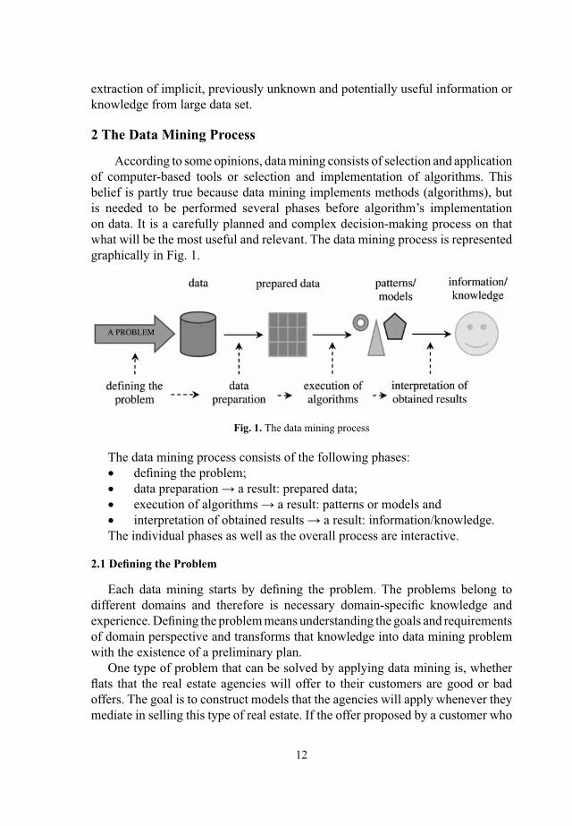
With prepared visual in place, managers will be able to choose for which account they want to open a dashboard and for which the costs are. Figure 1 shows part of the visual system that provides a view of budget expenses billed to the primary account 421 (utilities, electricity, water and utilities, trash and other utilities). In the fi gure, the billable expenses in denars are in the y axis, while the x axis shows the sub accounts for primary account 421. The graph shows data for all four quarters, with different types of graphs. Here are shown the data of expenses, and if we want to look for which under accounts costs are highest, we select Line area graph that is appropriate for this type of data. For all four quarters we chose different types of line graphs and charts of different colors, to faster and better see the differences. The dashboard has the fi lter that allows you to select and view data for a specifi c sub account where you can see the data for all four quarters.

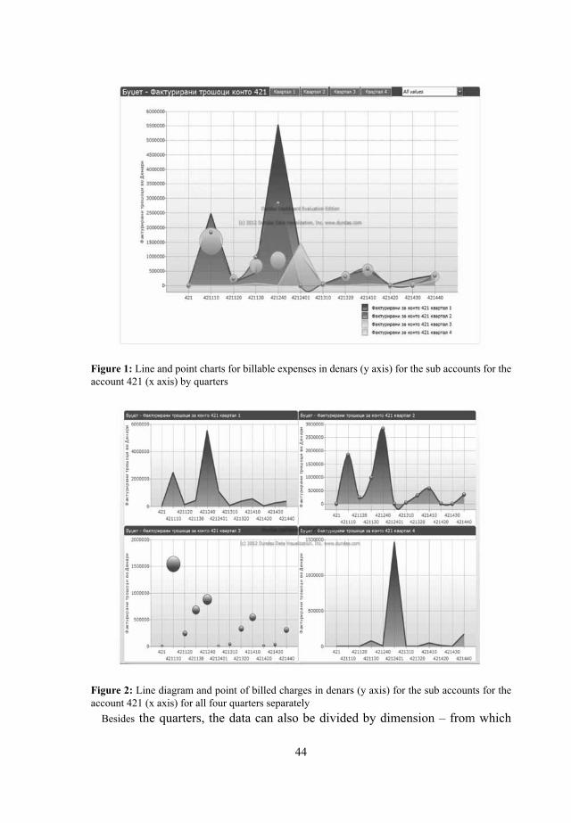
If managers want to see the graphics from various quarters one to one, and they do not want them to be folded, they only need to click on the graphic of Figure 1 and a pop-up window will be opened where they can see the data for all four quarters separately (Figure 2). For all four graphics they can see such measures are set billable costs in denars, as long as the dimensions we have under account for the account 421. On this dashboard, managers can detect which quarter and which sub account costs are highest and make rapid comparisons of the amount of certain sub account in all four quarters. This dashboard can help managers in the decision making process for planning the budget for next year, and to see how big amounts billed and for which sub accounts.

44

Figure 1: Line and point charts for billable expenses in denars (y axis) for the sub accounts for the account 421 (x axis) by quarters

Figure 2: Line diagram and point of billed charges in denars (y axis) for the sub accounts for the account 421 (x axis) for all four quarters separately

Besides the quarters, the data can also be divided by dimension – from which

45

accounts come from (from which of the three accounts of the institution). According to the requirements of managers for the need of visual display of the invoiced cost of class 4, is made a visual display of synthetic account 421 for 1 account with its analytical accounts. In Figure 3, with bar diagram, the amount of billable costs for all analytical accounts for 421 synthetic account of account 1, is shown. This dashboard uses a visual bar diagram that is appropriate for displaying the data where we want to make a comparison of the amount of costs, i.e. where we compared the highest and the lowest costs [10].

Figure 3: Bar diagram where the x axis is the sub ledger account 421, while in y axis is billable expenses in denars for account 1

Apart from the data on the budget, the options for displaying data in a visual system form i.e. in the visual system created for this purpose, we have data for revenues and expenditures. Part of the revenues data is presented in Figure 4. Here you can see the data for 2009, 2010 and 2011. Data are presented on line graphs. The blue line marks data for 2009, the green line marks revenues for 2010 and the turquoise line presents data for 2011 [12]. On the x axis we see the data for the type of revenue, while the y axis shows the values for that type of revenue.

Because the data we have received and the one we already had were not read, a very big difference in the values of revenue appeared, therefor it was necessary to apply a method for normalization of the data i.e. we applied data processing with normalization and used a logarithmic function over revenue to get more

46

adequate values for visualization i.e. values can be presented on a graph. An applied logarithmic function is used at transformation of the data (base 10 logarithms). And this visual dashboard allows fi ltering of data by a particular type of revenue.

Figure 4: Line diagram of revenues for 2009, 2010 and 2011, where in the x axis we have shown income and in the y axis the amount in denars

The program for creating visual systems provides for a number of views that we can use. If on the visual dashboards we would like to display more data, line and column displays are most suitable. Fewer data will be displayed on the following visual dashboards but with slightly different visual displays that will refer to the costs in the budget.

In Figure 5 we can see the planned costs for a certain account. In the fi rst part we showed the planned costs for the aggregated account 401-Basic salaries and personal tax for each quarter. Here managers can see the collective planned costs on account of all quarters, where we can notice that the charges of the second and third quarter overlap and they are same, and that the cost for the fourth quarter are the smallest. In the next sections present the planned costs of account 402-Contributions of pension fund and health care contribution, taxes for healthcare and employment also divided by quarters. Here the managers can see that the planned costs of account 402 for the second and third quarters are the same and they are the highest, while the costs for the fourth quarter are the lowest. In the

47

next part of the visual dashboard presents the planned costs of account 404-Compesations according to the four quarters. This shows that the most costs are planned for quarter 1 and the same costs have been planned for the second and fourth quarter. The last part of the visual dashboards present the planned costs of account 423-Materials, medications and other medical materials. This shows that most costs are planned for the fourth quarter, while the least for the third quarter. If with the cursor we go to a certain indicator of the planned costs the exact planned full amount will be displayed. This visual dashboard helps managers see witch accounts the most costs have been planned for and which quarter the most of the costs have been planned for. They can use this for planning costs for the next year and to have a look at the spending of resources.

Figure 5: Planned costs for accounts 401, 402, 404 and 423 presented in 4 quarters

Beside the data for the budget, in the database we have the data for medicine consumption. On Figure 6 you can see the consumption of medicines by departments. There are more data to be seen for medicines on the visual dashboards that are important to know, so more data are presented in the data grid (table). On this visual table we have three fi lters and we can do data fi ltering by department, by group and by the name of the medicine.

48

Figure 6: Consumption of drugs by departments

The possibilities for getting reports by using the visual dashboards and their combinations are endless, limited only by the imagination of users and their requirements [6]. Many different combinations are possible depending on the needs of the target manager. Here you have to work with a good strategy for deciding on the base of the real needs of the applicants’ services – to effected the outcomes and to receive automated visual dashboards. It is a task on which the managers of health institutions and IT personnel need to work together, to make a system which will help managers in their decision making.

5 Conclusion

Based on the research made, we came to the conclusion that managers have constant need of obtaining quick and reliable reports, from where they can easily and visually see the changes and improve their decision making. The reports that they now receive are not suffi cient for a timely registration of the changes and hence for improving the process of decision making.

The future of improving the process of decision making lies exactly in the use of these visual systems. They will improve the work of health institutions where they will improve the services and increase the profi t of the health institution. If they respond on time and quickly to all changes, the health institutions will be able to save resources and with that they will get the opportunity for progress [8].

The implementation of visual systems in all of the public health institutions in Macedonia will take time and expertise from employees in the IT sector. First

49

they need to create dashboards that will be useful to managers and will be created for each part of the operation of the institution. Health institutions have a lot of data for all parts of the operations and for that the creation of this system will be a very hard process. But, when once it is created, it can be used in all public health institutions. The long term benefi ts that a visual system will bring are much larger than the time and costs for creating the system.

When the visual system is created and implemented, it is necessary to train managers for its use [3]. If managers previously understood the need and usefulness of the system, they will be motivated enough to use the system. The system is very simple for usage. Managers just need to choose which dashboards with witch data they want to see and the system will visually show them. With this the changes in the work of health institutions will be detected on time and appropriate measures will be taken in time.

In the future, we think that the concept should expand to all public health institutions in Macedonia where managers can get the data that they want to see on those dashboards. They should be applied to that part of the operations for which there is a necessity for that kind of a visual system. Once the data is collected and processed, it is necessary to expand the database so that it includes all of the data requested by the managers. But, even when we have all the data, we must create algorithms to prepare the data to be used for visualization. That means we need to create a new database that will communicate with the databases from the hospital and will take the data from there, and it build views that provide data needed for visualization. This way of connection with the databases of the actual system is not possible, but is essential for creating the visual system. It would be an excellent topic for future surveys. The next step is creating a visual system that will satisfy the needs of all managers in the health institution by the example proposed in this paper. For that visual system every manager will have password protected access and access to the visual dashboards that are of his interest. The visual system should be implemented in all public health institutions in Macedonia. At the end managers need to be trained for using the visual system, and understand the opportunities that it offers and how they can use those opportunities to improve the work of the health institution.

References1. Turban E. & all, Decision Support and Business Intelligence Systems, eight edition,

Prentice Hall, 2007, pp. 253-2922. Marakas, G.M, Modern Data Warehousing, Mining and Visualization, Indiana University,

New Jersey, 20033. Friedman, Vitaly, Data Visualization and Infographics in: Graphics, Monday

Inspiration, 20084. Turhan S.N., VayVay O., Healthcare Supply Chain Information Systems Via Service-

50

Oriented Architecture, Word Scientifi c Publishing, http://www.worldscibooks.com/business/7072.html

5. Jain L.C., Lim C.P., Handbook of decision making – Techniques and Applications, Springer, 2009

6. Kaufman, M., Information visualization – Perception for design, 20057. http://www.dundas.com/8. Parmigiani G., Inoue L., Lopes H.F., Decision Theory principles and approaches, Wiley,

20099. Maria Antonina Mach, Abdel-Badeeh M. Salem, Intelligent Techniques for Bisiness

Intelligence in Healthcare, 10th International Conference on Intelligent Systems Design and Applications, 2010

10. S.Savoska, S.Loskovska, Specifi c usage of visual data analysis techniques, 53T, Sofi ja, 2009; Pages 234-238

11. Savoska S., Manevska V., Usage of modern methods for decision making processes for managers, Plovdiv, 6-th international conference of Management and entrepreneurs, TU Sofi a, 11.2009, Pages 66-70

12. Jasmina Nedelkoska, Using Dashboards as tools for improving the process of decision making, CITYR 2012, Pages 13-16

51

Evaluation of Taxonomy of User Intention and Benefi ts of Visualization for Financial and Accounting Data Analysis

Snezana Savoska1 , Suzana Loshkovska2,

1, Faculty of administration and Information systems Management, University „St.Kliment Ohridski“ – Bitola, Bitolska bb, 7000 Bitola, R.of Macedonia,

savoskasnezana@gmail.com2 Faculty of computer science and ingeneering, Ss.Cyril and Methodius University in Skopje,

Rugjer Boshkovikj 16, 1000 Skopje, Republic of Macedonia, suze@feit.ukim.edu.mk

Abstract. In this paper we evaluate the taxonomy model for multidimensional data visualization for accounting data analysis. This taxonomy takes into consideration users’ intentions and also, the benefi ts of visualization for analysts, businessmen and managers who use fi nancial and accounting data. We also explain the proposed taxonomy as well as the taxonomic framework which contains three groups of attributes. They are classifi ed according to visual techniques and their capabilities. We have analyzed several multidimensional and multivariate visualization techniques, each presented in a table according to the proposed taxonomy. This table will determine their capability and capacity to solve specifi c visual problems.

Evaluation of this taxonomic model for visualization of multidimensional and multivariate fi nancial or accounting data implies the possibility for introducing an automatic selection of a visualization techniques and the best visual representation.

Keywords: data visualization, taxonomy evaluation, fi nancial and accounting data, multidimensionality

1 Introduction

Many taxonomy methods and techniques, used in data visualization start from data and used techniques. We proposed taxonomy for data and information visualization which have a different focus of interest and take in consideration the user’s preferences in the process of visualization and refers of fi nancial and accounting data. We believe that this taxonomy will be very useful to handle with everyday’s data and information overfl ow and it’s analysis for the managers and analytics. We proposed the proactive policy of gaining visual reports in the phase of data preparation and effective manner of presentation. This proposed coherent review and conceptual framework will be elaborate in this paper and will gain design classifi cation and selection of techniques dependent of the users’ intention, its capability and the benefi ts given to the end users. The end users can

52

have different level of foreknowledge which has to be taken into consideration in the process of selection. We will analyze some of the most popular visualization techniques for multidimensional and multivariate (mdmv) data visualization.

The evaluation of this taxonomy’s model can help understanding the usefulness of this taxonomy for evaluations of each technique for particular user’s group and specifi ed level of foreknowledge as well as creation of user’s manuals for usage of each proposed visualization techniques appropriate for end user’s group. The implementation of this taxonomic model will help for more effi cient, faster and better future prepared visual information and for bridging the gap between necessary and expected results for some user groups. Also, we intend to propose some strategy for selecting technique and creating multidimensional and multivariate visualization for fi nancial and accounting end users which will be the base for some automation in the business oriented information systems.

If we analyze the taxonomies in the whole visualization area, we can say that many classifi cations have been made. It is assumed that from taxonomy data, which means, its characteristics, the number of independent variables, variable sets, data types (scalar, vector or more complicated structures, discrete or continuous, nominal, interval or numerical, indexes and other). But, none of this taxonomy is focused on user intention, gained effects and interaction with data. This taxonomic framework for mdmv visualization is focused on the specifi c user groups of fi nancial and accounting data and its preferences.

The paper is organized as follows. The second section, after the introduction, is dedicated to the short introduction in the proposed taxonomy and its dimensions. The following section takes in consideration most used visualization techniques and the subsequent explains in detail the evaluation of the proposed taxonomy for these visualization techniques. The following section discusses results with specifi c usage and examples for the effects of used taxonomy. The conclusion depicts remarks for future work.

2 Explanation of the Proposed Taxonomy

The proposed taxonomic model is created for mdmv data visualization for fi nancial and accounting data analysis. According to this taxonomy, three dimensions are created: user intention [1], effect of visualization techniques and the interaction possibility. The additional dimension refers to the user groups and each combination of these four dimensions is a single vector in the four-dimensional space.

For better understanding, we can present the taxonomy’s dimensions on the axes in the 3D Cartesian system, but it is useful to make a coding of all values, which the independent variables can take all three axes. The fi rst dimension can take discrete coded data values for: data overview, hypothesis confi rmation and insight, delve into the data and make new decisions (Table 1). The second dimension is

53

the visualization technique effects (visibility, interpretability and delve into data -Table 2). The coding of the third dimension, visualization techniques effects are shown on Table 3. The interaction possibilities are classifi ed according to data selection from the beginning. In the end, the fourth dimension - the user groups and its coding is presented on Table 4. Taking into consideration this taxonomic model, we can evaluate the most used mdmv techniques and gaining the results - effect with some sample of accounting and fi nancial data.

Table 1. The fi rst dimension coding – User intention

1 Data Overview UI/DO2 Hypothesis Confi rmation UI/HC3 Delve into (the data) and making new decisions U I /

DID&MND

Table 2. Coding of dimension VTE -Visualization technique’s effects

Visualization techniques effect

Type of variable Variable rang Used code

Visibility One screen or n-screen data are shown on one, two or n-screens

S1, S2 ,…. Sn

Object selection (slider, tab or radio button, combo box, command button)

Possibility to select data with object SL, TB, RB, CB, COM, NO

Analytical or aggregated data Analytical data are shown or data aggregations are shown

AN,AG

a) Relations are visibleb) Relations aren’t visible

The relations between data are or are not shown

RV, RNVRELV, RELUNV

Interpretability The level of data understanding

The data understanding is at the: Low, Middle or High level

LL,ML,HL

Relationship understanding level

Strong capability, middle, weak or no possibility for correlation discovery

SC, MLC, WC, NoC

The aggregation understanding

There is visible: clustering, classifi cation, association, rule detection, there is not visible rule

NoVIS, VCLU, VCLA, VASS, VRD

Insight in data Possibility for ordinary statistical, mathematical data analysis, no possibility

Statistical or mathematical data analysis possibility or no possibility

IDAS, IDAM, IDAN

Possibility to discover correlation

Correlation discovering level (1-5) ICORR 0-5

Possibility for cluster analysis The level of clusters (1-5) ICLU 0-5Possibility for classifi cation Possible classifi cation level (1-5) ICLS 0-5Possibility for pattern recognition

The possibility level of pattern recognition (1-5)

IPR 0-5

Possibility for discovering associations

Association discovering possibility IAD 0-5

54

3 Overview of the mdmv techniques and its coding according to the proposed taxonomy

When it comes to the analysis of fi nancial and accounting data, it is important to note that the techniques used for effective visualization should be classifi ed into eight groups of requirements of the visualization [3]. They are: Overview & detail on demand, Hierarchical structures and relations, Multivariate data attribute views for a time period, Analysis of objections to the plan (or plan disagreements), Additional detail for disagreement as drill-down possibility, fi ltering ability (information of interest, the level on detail, subsets for data analysis, comparison sets), Ability for relation and attributes changing in time or time series for attributes and relationships as well as company graphs for accounting period following attributes or Adjusting periods for data analysis. The techniques which will be of interest for analysis for proposed taxonomy for mdmv data visualization are shown on the Table 5. Table 3. Possibility for selection data, attributes and interaction with data

I n t e r a c t i o n possibility

Type of variable (Nominal, Ordered, Quantitative)

Variable rang Used code

Selection of subsets from the visualization dataset

With previous data preparation, In the visualization screen, No selection possibility

The visualization is prepared with already selected data set, on a whole data set and selection is enabled, Selection is not enabled

SELP, SELV, SELNO

Enabled selection – fi lter for data/ There is only time fi lter/ Enabled with some object (slider, tab, combo or radio button)

There is data fi lter for all dimensions, Only for time period, Select data set with given object for data selection

SFIL 1-n, STFIL, SOBJ 1-n

Zoom, Selection, Distortions, Linking and brushing

Data can be selected with zooming, distortion, linking and brushing or interactive fi ltering

SZOOM, SDIS, SLB, SIF, SNO

Selection of desired data attributes

With previous selected attribute (query or alias)

Previous prepared data set with selected attribute – number of selected attributes

SAP 1-n

Selection of attributes on the visualization screen: Aggregated Analytic- data with drill-down possibility, Selection of attribute with object selection, Selection with slider or pointer

Embedded drill-down possibilities for aggregated data, Selection of attribute with selection of object dedicated to the desired attribute (radio button, tab, combo box or check box…), Selection with slider or pointer

SAVDD 1-n, SAVOS 1-n, SAVSP 1-n

Possibility of interaction with data in the given visualization

Possibility for selection analytical data/aggregated data/ No possibility interaction

Analytical data selection/ Aggregated data selection/ No interaction

ISAND, ISAGD, ISNO

Only data navigation, Possibility for zooming, for linking and brushing, for interactive fi ltering

Possibility for: navigation only, zooming, linking& brushing, interactive fi ltering

INAV, IZOOM, ILB, IIF

55

3.1. Analysis of time histograms with displays and possibility select and zoom

The mentioned visual display may be set in the dashboards class with the “Overview & detail on demand” [3] class. It can be used as the base of many MIS, EIS, ESS and BI systems, as dashboards views for various manager’s levels and business analytic staff. The number of screens is bounded with the users’ demands and data visibility and clearance for the analysis. The proposed taxonomy for this visualization technique is shown on the Table 5.1а.

Table 4. User groups with specifi ed tasks and level of information and analytical knowledge

Users’ group

Specifi ed tasks Information knowledge Used code

Top managers

Strategic management and planning activities

High level SMHI, SMMI, SMLI

Planning and control activities Middle level PCHI, PCMI, PCLI

Region management activities Low level (informational and analytical knowledge)

RMHI, RMMI, RMLI

Tactical (middle level) managers

Sector’s planning and control High level of SPHI, SPMI, SPLI

Management by exception Middle level of MEHI, MEMI MELI

Low level of (information and knowledge)

LEHI, LEMI, LELI

Operative managers

Standard procedures control High level of informational and analytical knowledge

SPCHI, SPCMI, SPCLI

Operation management Middle level of informational knowledge

OPHI, OMMI, OMLI

Problem detection and solving Low level of information and knowledge

PDSHI, PDSMI, PDSLI

Analytical staff

Specifi c analytic task High level SATHI, SATMI, SATLI

Exception analysis Middle level EAHI, EAMI, EALI

Perception analysis Low level (information and knowledge)

PAHI, PAMI, PALI

Table 5 - Proposed Multidimensional and multivariate Visualization technique used for data analysis of fi nancial and accounting data

Dashboards with time slabs – analysis using histograms, scatter plots or line plots as DsParallel coordinatesHierarchical parallel coordinatesPixel-oriented displayHierarchical pixel-oriented displayGlyphsHierarchical glyphs

56

ScatterplotsHierarchical scatterplotDimensional stackingHierarchical dimensional stackingNodes and links techniques (cone trees, information landscapes, hyperbolic spaces etc.)Polar coordinate – Kiviat’s diagrams

The example below describes visualization with visibility defi ned as two windows in the screen, the fi rst windows with slider. In the windows on the top it shows the aggregated data from database but relations between data are not visible. The interpretability is described as a high level of data understandability, no visible correlations and clusters or associations, and no rules. Insight in data property is explained as “No statistical or mathematical possibilities for data analysis”. No visible correlation in some dimensions, no visible classifi cation, and rules will only be drown based on the seasonal natures and associations, are possible only with a selected dimension – time chunks and another dimension. The possible improvements aimed in increasing the possibility for fi ltering with a slider or pointer [5, 6], as well as a data fi lter with object which can increase the number of observed dimensions [8].

Figure 1: Time histograms with interactive selection of time unit and dimension

Next table 5.1b shows the analysis of this combination type of visualization techniques forming the aspect of interaction with data, selection of attributes which will be visualized and with direct interaction possibilities.

57

In this analysis, the selection possibility is on the screen in the fi rst window, one dimension (time slab) can be selected with a slider (or a pointer) as a data selection. No direct zoom, linking & brushing or distortion or interactive fi lter possibility on the fi rst window. The attribute selection is done with tabs or sliders (or radio buttons, or check boxes). The direct interaction with data is data selection from aggregated ones with the slider on the fi rst windows in the screen. This technique only offers the possibility to navigate through data. This methodology is desirable for non informatics staff, but requires prior programming to the preparation of the data. The main purpose is that the systems are business oriented, especially for managers of a higher level and control to perform operational management tasks. By incorporating automated alert, effi ciency in the operation can be improved a lot for this user group types.

3.2. Analysis of technique parallel coordinates and hierarchical parallel coordinates

The technique of parallel coordinates allows the detection of relationships between variables which are analyzed and are shown on the N-dimensional parallel axes in the 2D space. According to their purpose, we can classify them as presentation techniques of hierarchical structures to demonstrate links or Hierarchical structures and relations [3]. There are many tools for multidimensional and multivariate analysis which allows data analysis with this technique. The advantage is that all data is in the same screen and the number of sets axes are limited only by data visibility on the screen surface for data presentation. This technique actually represents the refl ection of N-dimensional Euclid space in to 2-dimensinal surface. The proposed taxonomy, its application for multidimensional and multivariate visualization for this technique is shown on the Table 5.2a.

The example described in this table is visualization with visibility as all dimensions are shown in one display, data visibility is provided with navigation through the axes with a slider and the analytical data values can be also obtained.

58

The relation between data is visible because of the lines which connect the axes. This visualization is high interpretable. There is a high degree of perceived correlation between data in the axes and some cluster that can be detected. Some groups of clusters can also be noticed. The awareness in data can be also explained as possible statistical analysis with hierarchical parallel coordinates, correlation in a scale of 1 to 5 is four, excellent cluster detection, middle level of possibility for classifi cation (three) and pattern recognition possibility in the low level (one from the scale of 1 to 5).

Figure 2: Parallel coordinate techniques as technique for hierarchical structures and relations presenter

If we take into consideration the hierarchical parallel coordinates, they have a decreased level of interpretability because there the means data values are shown on the display and the rules cannot visually be detected. There isn’t a possibility for a high degree of discerning in data because of data aggregation [7] (Figure 2). The possible improvement can be done with increasing interpretability with introduction of colors; visual primitives for the lines [4] (dashed or dotted lines etc).

Table 5.2b. Analysis for selection and interaction possibilities of ParCor techniques

Possibility for data selection Attribute selection Interaction with dataTechnique I II III I II I IIPARCOR SELP SFIL1 S* SAPn SAVSP1 ISAND I*HPARCOR SELP SFIL1 S* SAPn SAVSP1 ISANG I*

59

Table 5.3b shows the analysis under the proposed taxonomy for data, attribute selection and direct interaction possibilities.Table 5.2b analyzes the aspect of data selection, attribute selection and data interaction for these visualization techniques. The possibility to select data is in the phase of data preparation (time – the possibility to observe the presented data in a timetable or having the possibility to see different dimensions at the same time). The column “interaction with data” shows that all known interaction types with data are available. The number of possible attributes for selection is equal with the numbers of dimensions. The selection is made with a slider or a mouse pointer. Analytical data can be selected and all of interaction types with data are available to select – from selecting and brushing to distortion and zooming. Hierarchical parallel coordinate techniques differ in the selection possibilities because only the aggregated data is shown and interaction is limited. The tools available for implementing this kind of data visualization require prior preparation of data and high level of IT knowledge.

3.3. Analysis of other proposed techniques for multidimensional and multivariate data visualization

The techniques offered by the available multidimensional and multivariate visualization tools (as XmdvTool, VizDb etc.) provide multidimensional and multivariate visual displays of some data in order to improve the analyst’s exploration possibility. For this purpose, we may take into consideration their capabilities under the proposed taxonomy’s frame. These are the techniques

60

for pixel display, glyphs, scatter plot matrices, dimension stacking. All these techniques have their own possibilities for hierarchical displays, which show the statistical averages of analytical data. The advantage is the fact that all data is shown on one screen and the number of data depends on the number of records in the fi elds in database which are used for visualization. The proposed taxonomy, applied in these techniques for multidimensional and multivariate visualization is shown on the table 5.3a.

It is obvious from the table that the multivariate outputs of the visual display have a different level of visibility, interpretability and insight. They are ranked from techniques which have a high degree of interpretability such as scatter plot matrix to the techniques which aren’t interpretable. The scatter plot matrix and its hierarchical version have a high possibility level to detect correlations between dimensions. Most of them have the capability for statistical analysis, but, the cluster, classifi cation and association possibilities have only one scatter plot matrix technique with a high degree of usefulness. The pattern recognition capability is higher only in the glyphs and pixel oriented displays. The next fi gures (Figures 3 & 4) show some multidimensional and multivariate data displays explained in table 5.3a. The possible improvements are increasing interpretability with the study of glyph possibilities and controlling the arrangement of pixel-oriented displays.

Figure 3: a) Pixel-oriented display of material-fi nance data b) Glyphs technique for same data c) Hierarchical pixel display d) Hierarchical glyphs

As parallel coordinate technique, these multidimensional and multivariate visualization techniques have the possibilities of data selection, but only in the phase of data visualization preparation. It is possible to set a wide variety of fi lters for each dimension or for their combination at the same time. All interactions with data possibilities are included. The number of possible selection attributes is equal

61

to the number of analyzed dimensions, and the selections are made by a pointer. The analytical (in the regular displays) as well as the aggregated (in hierarchical displays) data can be selected. It’s possible to use all types of data interaction as selection, zooming, linking& brushing or distortion. Using these techniques also requires knowledge of the specifi c tools for data visualization of multidimensional and multivariate data and advanced data preparation. This also means a high level of IT expertise.

3.4. Analysis of the techniques nodes and links, trees, hyperbolic spaces and Kiviat diagrams

While the mentioned (nodes, links and hyperbolical displays) can be classifi ed into hierarchical structures and relations, the Kiviat display is fi gure obtained in a polar coordinate system (and its possible transformations in cylindrical or spherical coordinate system). Figures themselves are obtained by connecting points of polar coordinates. This technique can be seen as the axes rotate from parallel coordinates into polar coordinates. Nodes and links are popular for displaying complex relationships in the formation of tree maps, cone tree, hyperbolic trees etc. The size of the hierarchical structure dictates the view and the techniques used to interact with the data. This representation shows all data in the techniques of nodes and links is some kind of clear drawings that can zoom in or distorts, depending on the user requirements. The Kivit fi gures show shapes obtained in the polar coordinate system giving information about the values of each of the axes. The proposed taxonomy used for this model of visualization is shown on table 5.4a.

Figure 4 a) Scatter plot matrix b) Dimensional stacking c) Hierarchical scatter plot matrix d) Hierarchical dimensional stacking

62

The example describes visualization of nodes and relations whose visibility is described only in one display shows the analytical data is from the database without object possibility selection. The arcs show the links between data and they are visible. Their interpretability is depicting as high level of data understandability which gives a high degree of dependency and understandable object classifi cation. There are not many possibilities for statistical and mathematical analysis, but they have a great opportunity for making classifi cations and clustering. The insight in data possibilities is weak.

The Kiviat fi gures are usually shown in the screen without the data selection possibility. They are made from analytical as well as average data (hierarchical kiviats). The level of data understandability for this technique isn’t on the highest level and the correlation detection has a low level [2]. The visible level of classifi cation possibility is obvious. The mathematical data analysis are possible with this technique, also it has possibilities for correlation detection, medium level of pattern recognition and clustering capability, but there isn’t an ability for discovering clusters and association (Figure 5). The possible improvements are aimed at increasing data fi ltering with the usage of a slider or a pointer as well as increasing the number of dimensions which are taken into consideration with the visualization.

The data sets selections possibilities for the technique nodes and links are made with the previous data preparation for visualization; there isn’t a fi lter for data selec-tion or attribute selection as well as for interactively movement through the nodes. The number of selected attributes is defi ned in the previous prepared static data set and there aren’t embedded additional possibilities for selection with a slider or a pointer. There isn’t an interaction possibility, data changing, navigation capabili-ties or distortion, zooming or another type of interaction. The tools used for such displays, are mostly for the engineering staff and require high former knowledge of specifi c software tools which normally allow visualization and simulations. First, data should be adequately prepared for visualization. Kiviat fi gures are created from the previous prepared data sets, without an interactive data fi lter or any other pos-sibility for data or attribute selection. These tools do not allow the usage of sliders and pointers nor have opportunities for data interaction. However, the development of visual tools can change this situation. Users need to have knowledge depending on the information that needs to be presented visually and effectively.

63

The analysis of these techniques is shown on the table 5.4b in term of data and attributes selection as well as direct interaction with data.

4. The results

Proposed taxonomy, evaluated in this paper, tries to classify the user’s purpose and benefi ts of visual analysis of the fi nancial and accounting data based on several criteria. We estimate that this will provide the classifi cation of data visualization techniques used for fi nancial and accounting data to serve as a basis for automation of the choice of visualization techniques for specifi c purposes. The implication of such a division would provide a high degree of specifi cation of individual visualization techniques for specifi c purposes and specifi c opportunities. In the previous examples, each attribute is encoded by a weight factor. Although is not an easy task and requires complex mathematical calculations or intelligent methods, it is still worth exploring because of the overfl ow of collected data and the necessity of rapid analysis.

The choice of techniques for visualization according to this taxonomic model as well as the possibilities for selection appropriate visualization techniques can automatically be incorporated in software tools which can produce faster analysts’ performance, detection of exceptions etc. Such algorithms can be nested in the creation process of data visualization with HCI intensions for fi nancial and accounting staff.

This visualization can have many goals like: creation of dashboards as system control tools, balanced scorecards etc. Although, the most important prerequisite in this case is the staff’s training for usage and tool possibilities, with the purpose of effective and rapid preparation of information from databases or tabular data representation in visual representation [3].

64

Figure 5 a) Tree maps technique for hierarchical display b) Cone tree c) Semantic network d) and e) Kiviat diagram fi gure

5 Conclusion

In order to evaluate the proposed taxonomy to support the creation of a coherent and comprehensive conceptual framework that can allow the user classifi cation by users’ intention and benefi ts of visualization for fi nancial and accounting data, we explore the most used techniques for mdmv data analysis according to proposed taxonomy. We evaluate all of these techniques with coding of four dimensions for each technique and their possible values are provided in the given tables. They can be easily understood and used for creation of algorithms for the automation of visual representation on HCI through interactive displays. But, it should be mentioned that there is no fi nal solution for automatic gaining visual representation that would satisfy all end users. In any attempt to automate this process, it is necessary to have the interaction for end users through selection of offered solutions, meaning system that supports decision making process for end users.

References

1. Keim, D. A., Kriegel, H.-P. (1996). “Visualization techniques for mining large databases: A comparison”, IEEE Transactions on Knowledge and Data Engineering, 8(6), 923-936.

2. Kolence K.W., Kiviat P.J., Software Unit Profi les & Kiviat Figures, ACM SIGMETRICS, Performance Evaluation Review, pp2-12, 1973

65

3. Ruby M.K., Information Visualization for Financial Analysis, 2003, University Durham 4. Rudesteiner E., Ward M., Xie Z., Cui Q., WAD C.,Yang D., Huang S., XmdvTool: Quality-

Aware Interactive Data Exploration, SIGMOD, ACM, 978-1-59593-686-8/07/00065. Savoska S., Loskovska S. Blazevski V., Time Histograms With Interactive Selection Of Time

Unit And Dimension, IS 2008, Ljubljana, Pages 202-2056. Savoska S., S.Loskovska, V.Blazevski, “Time Histograms with Select and Zoom for Creating

visual representation of data for managers”, Nis, ICEST, 2008, Pages 445-4487. Savoska S., S.Loskovska, Parallel Coordinates as Tool of Exploratory Data Analysis, Telfor,

20098. Thaper N., Guha S., Dynamic Multidimensional Histograms, ACM SIGMOD, 2002, 1-58113-

497-5/02/06

66

Data Structures in Initial Version of Relational Model of Data

Vladimir Dimitrov,

University of Sofi a, Faculty of mathematics and informatics, 5 James Bourchier Blvd.,1164 Sofi a, Bulgariacht@fmi.uni-sofi a.bg

Abstract. Initial version of relational model of data is reinvestigated. Main concepts and ideas behind them are discussed. The model is formally specifi ed in Z-notation as model elements and operations.

Keywords: relational model of data, formal specifi cation, Z-notation.

1 Introduction

One of the greatest inventions of the last century is the Relational Model of Data. Information systems, based on this model, are used today in everyday life. Many ideas, on which relational model was created, had been implemented. Other stay in latency for many years before being recognized. Such an example are non-atomic attribute values. Initially, Codd introduced relations with structured attributes. But later on, relational algebra and data manipulation languages, based on fi rst order predicate logic, established First normal form, i.e. atomic attributes. Moderate object-relational model turned back to the structured attributes.

It is curious to comment that fi rst order predicate logic, as a query language in the version of relational calculus, easy generates infi nite relations that is catastrophic for the fi nite computing systems. Manipulation of infi nite relation means infi nite program execution. There are more successful attempts to be created logical models based on Prolog, but this is another story. Infi nite relation is not a problem in mathematics, only mathematics investigates infi nity, i.e. tries to investigate the God. Informatics is grounded – it works only with fi nite objects.

Today commercial database systems do not use the second version of relational model of data. They are object-relational, which in reality means relational with object-oriented add-ons. There is no consistent defi nition of object-relational model of data. The last model is very important to the industry. Commercial implementations of object-relational model follow SQL standards, but SQL by its nature is not pure relational – it has been originally developed as an integrated data manipulation language for both relational and hierarchical models of data. SQL defi nition is partly based on the fi rst version of relational

67

model of data. So, there is a need for defi nition of object-relational model of data for further theoretical and practical developments.

From above examples, it is clear that there are many ideas behind the relational model of data that are still not exploited. One of the evergreen investigations in informatics is how to extract knowledge form data and how to represent it. After the initial representation Codd tried to capture more meaning in the model – more data semantics to represent, but these ideas had not been supported by the industry. Now days, many original ideas of relational model happen to be used in object-relational model. So, it is clear that relational model of data has to be reinvestigated and precisely specifi ed and after that the focus can be put on the nature of object-relational model.

Results of pure relational model had been summarized every ten years by Codd. The relational model of data development can be divided on the following versions: initial, fi rst and second. This paper is a research on the heritage of relational model of data, initial version.

In this paper, the focus is on relational data elements and operations on them. It is specifi ed as a model but not as an abstract data type. Some topics, like data redundancy, are discussed only for consistency.

Initial version of relational model of data has been introduced by Codd in [1]. The model is founded on set theory, but it presentation is not formalized. In this paper are used defi nitions and examples from [1], but notation is slightly changed to be avoided contradictory interpretations. Some print errors in the original paper are corrected.

2 Basic defi nitions

Let S1, S2, …, Sn are n sets, which are not obligatory different, i.e. ¬(∀ i, j: 1..n • i ≠ j ⇒ Si ≠ Sj). Then R is a relation on these n sets, if R is a set of n-arity tuples, where every tuple has fi rst component from S1, second component – from S2, etc. More formally, R is a subset of the Cartesian product of S1, S2, …, Sn, i.e. R ⊂ S1 × S2 × … × Sn. Sj for j=1..n is j-th domain of R. Relation R has n domains, which are not necessary different. Relation R is of n-arity by the number of its domains. Relation with one domain is unary relation, with two domains – binary, with three domains – ternary, with n domains – n-ary.

Relations can be represented as an array, but this is not part of the model. Such an array has the properties:

1. Every row is a n-arity tuple of R.2. Rows order is not important.3. All rows are different.4. Columns order is important. It is the order of domains S1, S2, …, Sn, on

which R is defi ned.

68

5. Semantics of the columns is partly represented by their domain names.

Example of 4-arity relation:supply( supplier, part, project, quantity) 1 2 5 17 1 3 5 23 2 3 7 9 2 7 5 4 4 1 1 12

Column order is important because one domain can be used several times and every its usage can has different meaning. Column names are the domain names. The next example shows a ternary relation with duplicated domains with different meaning:component(part, part, quantity) 1 5 9 2 5 7 3 5 2 2 6 12 3 6 3 4 7 1 5 7 1

In this array every row is a tuple (x, y, z), which means that part x needs of z elements y to be assembled.

The database is a set of changeable relations. Every relation is of fi xed arity. In the time, to every n-arity relation new n-arity tuples can be added, available tuples can be removed or the components of last one can be changed.

In the real case, one relation can have very many domains. For the users it is diffi cult to remember domain order. For this reason, Codd introduced relationships. All columns in the relationship are with unique names. Columns order in the relationship is not important. Duplicated domains in the relationship are qualifi ed with a role to achieve column names uniquety. The role of the domains shows the meaning of the concrete usage of the domain.

Relation is more basic term than relationship. It is closer to the physical implementation. Relation has only one free dimensionality, it is set of tuples and does not depend of the concrete records order at the physical level. The fi le organization of the relation can be changed and tuples (records) order would be changed, but the relation remains the same. Relation is an abstraction of the different fi le organizations in which it is stored.

On the other hand, relationship has two free dimensionality. It does not support tuples ordering, but even more – domains ordering. Relationship represents all relations that could be generated by the permutation of all its domains.

69

The relation from above example as relationship is:component(sup.part, super.part, quantity)

Introduction of relationships is motivated with the better user acceptance of the model. The user working with the database has to know relationship name, domain names and eventually the roles of last ones in case of duplications.

Relation defi nition here differs from its mathematical counterpart – it has columns named by its domains. In mathematics, domains are used only in the Cartesian product, after that they are not used. In that sense, relations could be closer to mathematical ones if their columns are only numerated and not named. But columns naming by the domains introduces some semantic description of the column.

The relationship is closer to the later emerged “table”, but its columns are named by the domains with optional role qualifi cation of duplicated domains. In the tables, columns are named by their usage and they are independently bounded with the domains.

Formal specifi cation of introduced terms follows.Basic sets are:

[RNAMES, DNAMES, VALUES]

Where RNAMES is the set of all possible relation names, DOMAINS is the set of all possible domain names, and VALUES is the set of all possible values.

The set of domains is defi ned as&

DOMAINS == � VALUES

The domain is a fi nite set of values. DOMAINS is the set of all possible unnamed domains. Named domains are defi ned with the global partial function:

domains: DNAMES ⇸ DOMAINS

It maps domain names to domains.Relation schema is a fi nite non empty sequence of domain names:

SCHEMAS == seq DNAMES

This defi nition includes the relation without domains.Database schema is defi ned with the function dbSchema, which maps relation

names to their schemas.

70

dbSchema: RNAMES ⇸ SCHEMAS

This is the formal specifi cation of relations. The last ones accept domain names duplication in their schemas. Relationships with role qualifi cations do not permit column name duplication.

A new basic set – the set of all possible qualifi ed domain names has to be introduced:

[QDNAMES]

This set contains all qualifi ed domain names including unqualifi ed domain names.

There is a total function from qualifi ed domains names to unqualifi ed domain names:

domainName: QDNAMES → DNAMES

Relationship schema is a fi nite set of qualifi ed domain names:

QSCHEMAS == � QDNAMES

Relationship database schema is defi ned with the function:

dbRelationshipSchema: RNAMES ⇸ QSCHEMAS

dom dbRelationshipSchema = dom dbSchema ∧

(∀rn: dom dbRelationshipSchema ⦁

let s == dbSchema(rn); rs == dbRelationshipSchema(rn) ⦁

#s = #rs ∧ (∀i: 1..#s ⦁ ∃1dn: rs ⦁ s(i) = domainName(dn)))

For every relationship exists a relation with the same name and relation schema, which a permutation of relationship schema with de-qualifi ed domain names. This is defi ned by the function invariant that postulates: dbRealtionshipSchema and dbSchema domains are same; relationship schema and relation schema are same; and for every domain name in the relation schema exists exactly one qualifi ed domain name in the relationship schema.

71

2 Instance, primary key and foreign key

Relation instance is the set of all its tuple in a given moment. Database instance is the set of all instances of all its relations. Codd has not explicitly introduced these terms, but they are used in relational database world.

Not all domain values are used in the current database instance. The set of all used values from particular domain in the current database instance is called active domain. This term is a fact, but it is not used in any way.

Domain or combination of domains in a relation, whose values uniquely identify its elements (tuples) is called primary key. The primary key is minimal: it is a simple domain or it is a combination of simple domains, in the last case all domains are used for element identifi cation. In other words, the primary key does not have a subset (different from it), which has the same property, i.e. the subset uniquely identifi es relation tuples.

If there are several primary keys, only one from them is selected as primary. The primary key is important for the fi le organization in which the relation tuples are stored. File organizations like B-trees and hash fi les support only one search key. Usually, the primary key is used as a search key.

On the other hand, database design uses all (primary) keys. That is why, latter on many variations of the term has been used, like “candidate key”, “alternative key” etc.

It is very important, from navigation point of view, how relation elements reference to each other. For this purpose foreign keys are used. A domain or combination of domains from the relation R is a foreign key, if it is not primary key in R and its elements assemble primary key values in some relation S. It is possible R and S to be the same relation.

In the relation supply from the above example, the primary key is a combination of domains supplier, part and project. Every domain from the primary key is foreign key.

The defi nition of the foreign key requires referential constraint from the foreign key to the primary key of referred relation. Referential constraint is dominating in all defi nitions of initial relational model. Such examples are join and joinable defi ned latter here.

The foreign key is in two variants. Primary key domains can be used as foreign keys. Primary key domains by latter on terminology are called “primary attributes”. A subset of primary key domains can be a foreign key. The whole primary key could not be a foreign key.

In this defi nition of the foreign key, domains of the primary key and domains of the foreign key do not play any role. The foreign key domains must be mapped to the primary key domains, but there is no requirement the source and target domains to be the same. The defi nition simply require the foreign key value to

72

form primary key value in the referred relation.In the formal specifi cation of these new terms, fi rst tuple and relation instance

have to be specifi ed. Tuple is a sequence of values:TUPLES == seq VALUES

The tuple can be viewed as a function that maps relation schema domains to values from the corresponding domain. This interpretation is not used here, the relation defi nition requires tuple components ordering. The reason is that there is so called “standard order” for tuple values, which is used at physical level.

Relation instance is a set of tuples that are constructed using the relation schema. Database instance is a partial function from relation names to relation instances:

db: RNAMES ⇸ � TUPLES

dom db = dom dbSchema ∧

(∀rn: dom db ⦁ let s == dbSchema(rn) ⦁ (∀t: db(rn) ⦁ (∀i: 1..#s ⦁ t(i) ∈ domains(s(i)))))

Every relation instance has its own schema. The functions db and dbSchema have the same function domain.

Now, active domain can be defi ned:

activeDomain: DNAMES ⇸ ℙ VALUES

(∀dn: dom activeDomain ⦁ (∃rn: dom dbSchema ⦁ 〈dn〉 in dbSchema(rn)) ∧

(∀v: activeDomain(dn) ⦁ ∃rn: dom dbSchema ⦁

let s == dbSchema(rn) ⦁ ∃i: 1..#s ⦁ dn = s(i) ∧ (∃t: db(rn) ⦁ v = t(i))))

Active domains are that ones, which are used is some relation schema. Every its element has to be tuple component in some relation instance for the same domain. It is possible active domain to be empty set.

Primary key is a subschema. Every relation has only one primary key. The primary key is specifi ed as a list of domain indexes in the relation schema. The reason for that is the possibility of domain name duplication. If a domain participates in the primary and at the same time it is duplicated, then exact participation of that domain in the relation schema must be fi xed.

73

KEYS == iseq ℕ1

primaryKey: RNAMES ⇸ KEYS

dom primaryKey = dom dbSchema ∧

(∀rn: dom primaryKey ⦁ (∀t1, t2: db(rn) ⦁ let pk == ran (primaryKey(rn)) ⦁

(∀i: pk ⦁ i ≤ #(dbSchema(rn))) ∧ t1 ≠ t2 ⇔ (∃i : pk ⦁ t1(i) ≠ t2(i))))

Relation can have several foreign keys. In the specifi cation foreignKey is a function from relation name and foreign key to referred relation:

foreignKey: RNAMES × KEYS ⇸ RNAMES

ran foreignKey ⊆ dom dbSchema ∧

fi rst ⦇dom foreignKey⦈ ⊆ dom dbSchema ∧

(∀fk: dom foreignKey ⦁ (∀i: ran (second fk) ⦁ i ≤ #(dbSchema(fi rst fk))) ∧

second fk ≠ primaryKey(fi rst fk) ∧

(∃1map: KEYS →KEYS ⦁ map(second fk) = primaryKey(foreignKey(fk)) ∧

(∀ t1: db(fi rst fk) ⦁ ∃ t2: db(foreignKey(fk)) ⦁

ran (second fk) ↿ t1 = ran (primaryKey(foreignKey(fk))) ↿ t2)))

The set of referred and the set of referring function are subsets of the database. The foreign key is defi ned in the referring relation, where it is not a primary key. The primary key is entity identifi er and the foreign key is reference to an entity. That is why the foreign could not be a primary key.

There is only one legal mapping from foreign key domains of the referring relation to primary key domains of the referred relation. The source and target domain must not be the same. Actually, the map is mapping of foreign key domain indexes to primary key domain indexes. In other words, for every tuple in the referring relation must exist a tuple in the referred relation and the foreign key components of the source tuple must compose the primary key of the target tuple. Not every tuple in the referred relation has to be referred by the foreign key.

74

All foreign keys for a given relation can be retrieved from the function foreignKey. From this function, all relations and foreign keys referring given relation are easy retrieved via reverse mapping. This Z-schemas are not included here, because they have no impact and further development on the model.

3 Normal forms

The relation defi nition does not require relation domains to be simple. Such a requirement is enforced for key domains. Relation schema can contain structured domains. Relation schema that has at least one structured domain is not in fi rst normal form. First normal form is very important requirement for the relation model evolution. Only object-relational model removed this constraint.

In above formal specifi cation, there are no assumptions about domains structure.

In the initial presentation of the model, Codd used as example relation employee(name, (salary, history)), in which the second domain is a structured domain (relation). This means that every tuple that relation as a second component has an binary relation instance with domain: salary and history.

In its presentation, Codd links attribute with simple domain and repeating group with structured domain, following latter on terminology. Structured domain is a set of atomic values or a set of structures of the same type. When the domain is with simple structure (without substructures) – structure fi elds can be directly included in the relation schema.

Codd separated type from instance in the relational model. In the previous models such a differentiation has not been done. This means that logical structure of the database (its schema) is constructed via types system. Database instance is a set of instances of the schema types. Types system applies for relations and for domains. Relation types are constructed using relational model notation. There is no comment about domain type construction. Relational model semantics is defi ned by relations semantics and domains semantics. Relations are describing relationships among the domains. In terms of entity-relationship model, domains are entity sets and relations are relationships. This mapping is not true, because there are examples in Codd’s presentation, in which relations do not represents relationships, but entity sets.

Codd motivated First normal form with the relational query language.In initial version, database normalization means conversion of database

relations to First normal form. This means that relations with structured domains are converted to equivalent relations with simple domains. An example of such normalization follows. Before normalization:employee(man#, name, birthdate, jobhistory, children)jobhistory(jobdate, title, salaryhistory)

75

salaryhistory(salarydate, salary)children(childname, birthyear)

After normalization:employee(man#, name, birthdate)jobhistory(man#, jobdate, title)salaryhistory(man#, jobdate, salarydate, salary)children(man#, childname, birthdate)

Unnormalized relations are organized in a tree as shown in Fig. 1.

Fig. 1. Unnormalized relations tree.

Normalization process starts from the root. Primary key of the root is inserted in its children relations schemas. Key of the last one is composed of root key and its own key. Then from the root structured domains are removed. This steps are applied recursively to all subtrees.

Normalization process needs the next conditions to be enforced:1. Relationship graph of non-simple domains is a set of trees.2. Primary keys are composed of simple domains.

The fi rst constraint prohibits cycles. The second constraint simplifi es the normalization process. The last one is a designer intellectual endeavor and there are no ready receipts.

76

The relation in First normal form has the following benefi ts:1. Does not contain pointers.2. Does not have hash addressing schema dependencies.3. Does not contains indexes or ordering lists.

In other words, relation in First normal form does not contain elements of its physical organization. If tree presentation is used as in above example, then some of above mentioned physical organization schema has to be used.

For relations in First normal form, the next naming schema is proposed: R(g).r.d, where R is relation name, g is an optional relation generation name, r is an optional role name, and d is domain name. This naming schema proposes one relation to be stored in several named generations. Idea for relation generations is only marked here and has no further development. One relation in several generations is direct access to relation archive. This idea is not implemented in any relational database system.

It is possible to interpret relation generation in another way, for example every generation is a result of concurrent transactions execution on this relation or relation generation is relation instance at given time moment, but there are no research in that direction. That is why relation generation is not covered by the formal specifi cation.

4 Conclusion

In this paper only structure aspects of initial relational model are investigated. The leading Codd intention was “How to capture more meaning in the relational model of data”. The conclusion is that balance between domains and relations semantics has to be searched. This balance has been searched yet many years from that time.

Acknowledgment. This paper is supported by University of Sofi a “St. Kliment Ohridski” SRF under Contract 43/2013.

References1. Codd, E.F.: A Relational Model of Data for Large Shared Data Banks, CACM, vol. 18, No. 6,

June, 1970, pp. 377- 387.

77

Peopleware: A Crucial Success Factor for Software Development

Neli ManevaInstitute of Mathematics and Informatics, BAS,

Acad. G. Bonchev str., Bl.8, 1113 Sofi a, Bulgaria, neman@math.bas.bg

Abstract. The purpose of the paper is to present the current state of peopleware and to try to explain why it can be considered as a crucial success factor for software development. A context-driven human resource management is described so as to demonstrate, that some SE methods, best practices and procedures for their application can be slightly modifi ed and use for the purposes of the peopleware. An example how the proposed approach has been accomplished in a real-life project is presented.

Keywords: Peopleware, context-driven human resource management, business rules extraction.

1 Introduction

The basic goal of the Software Engineering (SE) is to assure the effi cient development, use and maintenance of quality software. In order to achieve this goal a variety of approaches with different origin and complexity can be applied – a sophisticated mixture of scientifi c methods, technological innovations, managerial techniques, profi table business practices, etc. Together with the methodological challenges of the interdisciplinary, each software project should be accomplished in accordance with preliminary stated constraints for time, cost, people involved, physical environment, technological and other resources. Unfortunately, the collected from real-life software projects statistical data shows the alarming tendency of increasing number of prolonged or even cancelled projects. The data analysis reveals that in many cases software projects should be carried out and completed in environment with permanently insuffi cient resources. Bearing in mind the rigid limitations for available money and development time, which are fi xed in the contract and usually can not be re-planned and re-negotiated, it seems that one possible and feasible solution for success of the project can be to rely on potential (theoretically unlimited, but hardly predictable) power of the human resource.

In this paper we will try to elucidate the leading role of the human factor for

78

software industry and how its impact can be strengthened by a systematic, pure SE approach. Next section presents the basic ideas and current state of peopleware, summarizing some observations and best practices, identifi ed as quite signifi cant from practical point of view, i.e. it is worth to be followed in order to be successful in the fi eld of software creation and use. Section 3 describes our approach and how it can be used for the purposes of the human resource management. Section 4 presents briefl y the experimental use of the proposed approach in a real-life project. In the last section some ideas for further research and development work in this direction have been mentioned.

2 Peopleware State of the Art: Promises and Unrealized Power

Nowadays the human factor in the area of software development and use is a “hot” topic both for scientists and practitioners in the fi eld. There are two main reasons, explaining this fact. First, the existing software intensive systems have been created by teams, comprising individuals with different physical, intellectual and psychological profi les. A thoughtful study of people’s capabilities and competencies should be performed and the results obtained should be used so as to improve the work processes and productivity. Second, all software systems are used by people and the investigation of user’s profi le, attitudes and preferences is necessary for creation of effective, reliable and user-friendly systems. That’s why the traditional pair (hardware, software) has been extended with a third element, called “peopleware”. This neologism has been introduced by P. Neumann [6] to denote one of the most signifi cant three core aspects of computer technology, supplementing the other two, already in use - hardware and software. Peopleware is a synonym of “human factor/human resource” and covers different aspects of the role of people in the development and/or use of computer systems, including (but not restricted to) such issues as human resource management (HRM), software psychology, productivity, teamwork, group dynamics, organizational factors, software ergonomics, human-machine-interaction, etc.

The importance of peopleware has not only been appreciated, but also shaped into a constructive framework by the Software Engineering Institute by developing the people management capability maturity model (PM-CMM). The proclaimed goal of the model has been “to enhance the readiness of software organizations to undertake increasingly complex applications by helping to attract, grow, motivate, deploy and retain the talent needed to improve their software development capability” [1]. In this model the key practice areas for software people have been defi ned: recruiting, selection, performance management, training, compensation, career development, organization and work design, and team/culture development.

79

The PM-CMM model introduces both theoretical and pragmatic improvements in the area of peopleware. It presents the basic HRM activities in more formal way and provides some indicators to measure the achieved level of maturity in their accomplishment. It is pity that without access to some offi cially published statistical data and analysis, performed to evaluate the degree of improvements in software organization HRM as a result of usage of this model, no judgment of its impact can be made.

Trying to fi nd more up to date information about the current state of peopleware in software industry, we read the latest edition of a book [2], which is classical for the fi eld. On the base of rich own experience gathered during long work as consultants and managers in great number of software projects, the authors of the book De Marco and Lester present their understanding of the main principles of management of human resource. They share some ideas about establishment of effective offi ce environment, recruiting right people and constructing “jelled” teams. Different approaches and good practices in peopleware have been not only described as real-life stories, but have been evaluated in respect to their feasibility, complexity of accomplishment and results obtained. The informal style of presenting valuable knowledge and experience makes easy the adoption of the proposed ideas. The objective observations and the judgment, shared after some experiments increase the level of trust and encourage the readers with HRM-related professional responsibilities to dare to apply and examine in practice some of the suggested techniques.

After the performed study of the current state of peopleware, the following conclusions can be made:� Software project implementation is under triple limitations - in project

scope, time and cost and unfortunately, t least one of them has been permanently violated. Thus, the effective and effi cient achievement of project objectives within the defi ned constraints requires signifi cant managerial efforts.

� Human resource management is an important part of the overall management because the most problems, encountered during software project implementation in their essence are people-related: sociological, not pure technological. So the HRM should be a set of coordinated and controlled activities, precisely defi ned both at strategic level - doing the right things, and at operational level - doing things right.

� Many of the existing approaches, techniques and best practices, which have been already identifi ed as useful and promising, are not part of the established HRM programs and action plans in the most real-life software projects.

� Due to different reasons (lack of solid theoretical base, which can be further developed in a procedural form, making possible the transfer of

80

the main ideas to practice; high cognitive complexity; etc.) the peopleware problems are not easy issues, but trying to solve them, software people will maximize their chances of success.

� Software managers have to be educated and trained so as to develop the needed peopleware-oriented competencies - a sophisticated mixture of knowledge, skills and attitudes, which could assure professional performance at the required level.

During the last 10 years we are working on some HRM-related problems, trying to provide a theoretically justifi ed and experimentally validated solution for hiring the best software people, team-building, soft skills training for software people. Now, taking into account the results of the resent study in the area of peopleware, we have some ideas about a context-driven HRM, which are described briefl y in the next section.

3 Our Approach to Peopleware

We believe, that the main peopleware problems arise … from people, responsible for the HRM activities in software organizations. Usually these people are with technologically-oriented education, background and work experience, with no enough sociological knowledge and skills to deal properly with so sophisticated in nature, dynamic over the time and unpredictable as behavior human beings. The essence of our idea is to apply some well known and recognized as fruitful SE methods, techniques and tools so as to resolve the specifi c HRM problems. Next we will clarify this idea, presenting a process framework with goal-oriented modeling and use of a formal method, providing a context-driven peopleware.

3.1 Human Resource Management Process

The HRM process can be defi ned as a collection of activities, actions, and tasks that are performed when a human resource-related problem has to be solved. Usually the process defi nes who is doing what, when and how to reach a certain goal. So the fi rst step is to defi ne the “who” part of the problem. Our suggestion is to consider the participants in a software project as components of a system, for which the generic process framework for software engineering, described in [7], can be applied. This framework comprises fi ve activities, which can be easily re-defi ned for the purposes of the HRM:

Communication – clarifying the stakeholders’ objectives for the work that should be done and gathering requirements so as to defi ne team members’ responsibilities and functions.

81

Planning – determining how many and what kind of people should be included in the team(s) so as to fi nish the work within the planned resources.

Modeling - a model of the team(s) should be created, defi ning the number and the roles of the participants, described by a desired profi le. As in the architectural software design, the relationships (interfaces) among participants should be specifi ed. Then (as in software detailed design), some additional refi nement of the models of each participant should be done, providing more details about required personal and professional characteristics. As in the model-driven software development, here also it is quite natural to create and use more than one model, depending on the preliminary stated goals.

Construction - this activity combines selecting the team members and further testing whether the created team can operate effectively. As in software testing, the adopted versions of the black-box and the white-box testing of teams and their members can be carried out.

Deployment – the constructed team (as an entirely complete group or as a core of the team, which will be further extended) starts to work. The performance characteristics of the team are evaluated and on the base of the results, some structural and/or personal changes can be made.

The analogy between software system development and team building gives the possibility to enrich the peopleware with some methods and best practices from the SE fi eld, validated as useful. Let us present briefl y such a method.

3.2 Context-driven peopleware

Introducing the above mentioned model for HRM process, we have to face the following key question, stated in [7]: What actions are appropriate for a framework activity, given the nature of the problem to be solved, the characteristics of the people doing the work, and the stakeholders who are sponsoring the project? In order to answer this question, we need a general, but fl exible method, capable to refl ect a great variety of problems, which should be solved within a specifi c context. As each problem solving action can be consider as a result of a sequence of decision making, we decide to use a context-driven peopleware, based on a formal method for a reasonable choice. This method, called Comparative analysis, has been created and already successfully used in many activities [4].

Comparative Analysis (CA) is a study of the quality content of a set of homogeneous objects and their mutual comparison so as to select the best, to rank them or to classify each object to one of the predefi ned quality categories.

The compared objects should be identifi ed as signifi cant for the activity under consideration. When apply the CA method, we distinguish two main players: the Analyst, responsible for all methodological and technical details of

82

CA implementation, and a CA customer - a single person or a group of persons, who should make a decision in a given situation and wants to use the CA.

The context of the desired CA is specifi ed through a case, described by the following six elements:

case = { View, Goal, Object, Competitors, Task, Level }The View describes the customer’s role and the perspective from which the

comparative analysis will be performed. For HRM the role of customer can play any person, having a people-related problem.

The Goal expresses the main customer’s intentions in CA use and can be to describe, analyze, estimate, improve, predict or any other, formulated by the Customer, defi ning the case. This element is important, because it determines the quality content of the compared objects.

The Object represents the item under consideration. For each investigated object a quality model should be created – a set of characteristics, selected to represent the quality content, and the relationships among them.

According to the goal, the set C of Competitors – the instances of the objects to be compared – should be chosen.

The Task, described as an element of a case can be Selection (fi nding the best), Ranking (producing an ordered list), Classifi cation (splitting the objects to a few preliminary defi ned quality groups) or any combination of them.

The depth Level defi nes the overall complexity of the CA and depends on the importance of the problem under consideration and on the resources planned for CA implementation.

Generally speaking, the CA method can be used in any decision making situation after specifying a case with an appropriate defi nition of the above mentioned elements. Let us describe briefl y how the CA can be used in the fi eld of peopleware.

The fi rst step should be to identify the responsibilities and the typical tasks of the main players, involved (as subject or object) in some HR-related activities. In any software organization they can be classifi ed in two groups: internal (managers at different levels of hierarchy in the organization and software people with different professional specialization) and external (current or potential users or clients, contracted projects with the organization). The following roles have been identifi ed till now: � CEO, HR manager, QA manager, Customer services manager; � Project leader, a member of a functional group (e.g. developer, software

engineer, tester, system administrator, technician);� Stakeholders – representatives of organization, ordered project and/or

individuals, who are going to use the project results.The implementation of the context-driven HRM is not too diffi cult, because

there is a procedure for CA method use, which can be followed. This general

83

procedure has been modifi ed in accordance with some specifi cs of the HRM so as the content (as a set of mutually connected activities) of the three main phases is defi ned. During the Preparation phase, each HR-related problem, encountered in the current project, has been decomposed into a number of cases to support the crucial decision making. For each case the Analyst checks which case elements have already existed from previous analysis and can be subject only for modifi cation, and which ones are new and have to be constructed from scratch.

The most diffi cult task in this phase is the construction of a quality model of compared objects. For the context-driven HRM these objects are some of the above mentioned typical software players, who will be studied in different situations, described by cases, giving the context. Depending on the goal of the performed analysis, the constructed Object model comprises different quality characteristics, presented in a multi-levels hierarchical structure, showing the relationships among them, too. According to the prescription of the method, for such goal-oriented object modeling, an incremental approach should be applied. When a case for comparison of some software people appears, the Analyst has to create its fi rst model, saved further as a generic (basic) model. When a request for CA with the same object arises, the generic model is found and modifi ed so as to refl ect the requirements, stated by the new context. So for each object a set of models has been maintained: one complete generic model and a number of “partial” derivative models, covering the peculiarities of the object, defi ned in a given case.

During the Implementation phase the Analyst reuses or constructs the needed object models, forms the set of Competitors, and performs the CA Task, using the available software tools, which facilitate the CA method. At the Follow-up phase the obtained results have been analyzed so as to create a detailed action plan to solve the problem under consideration.

4 A Case Study: Context-driven HRM in a Real-life Project

The feasibility of the approach, described above, has been examined within a scientifi c project “Automatic Business Rules Extraction from Programs”, performed under a contract with the National Scientifi c Research Fund.

The usefulness of the context-driven HRM will be illustrated by its usage as a decision supported method in a situation at the beginning of the second phase of the project, when due to the signifi cant cut off of the project’s budget, the project team has to be reorganized both in size and structure. The following two HRM-problems arise:� How to decide which team members should continue to work?� How to redefi ned the responsibilities and tasks among the members of

84

the smaller team, i.e. to assign the most appropriate work position (Role) for each member of the reorganized team so as to complete successfully the BR-extraction project?

Analyzing the situation, in which the project budget has been decreased, but the scope of work remains almost the same, the project leader decides to compensate the smaller number of participants with a team, comprising people with higher productivity.

Fig. 1.

So the following case have been defi ned:case = { View, Goal, Object, Competitors, Task, Level },

where the values of the elements are as follows:� View – that of the project leader, responsible for the team reorganization� Goal – evaluation;� Object – a team member;� Competitors – members of the team; � Task – ranking;� Level – simple.A new quality model for the object ‘member of the team” has been

constructed on the base of the proposed in [3] description of factors, infl uencing the employee’s performance (see the Fig.1).

For the second problem, how to assign the most appropriate work position (Role) for each member of the reorganized team so as to complete successfully the BR-extraction project, we have to start again with object modeling. On the basis of the Job description, a model has been created for each of the identifi ed Roles: Business Analyst, Policy Manager, Software Architect, Software Developer, System Administrator, Policy Translator, Rules Extractor and Mediator. As

85

such an object have been already used in a previous case, we simply re-use the existing object model, comprising three groups of characteristics: professional competences, soft skills and experience. After that the CA has been used to produce an ordered list of candidates for each Role through comparison between the role profi le and the individual profi les of team members.

5 Conclusion and Future Work

The purpose of this paper has been to analyze the current state in the fi eld of peopleware and to show that some selected best practices and methods from software development can be re-defi ned and used for the purposes of the HRM. The proposed goal-oriented modeling and the context-driven CA have been examined in a small project.

Our intentions for further research in this area are: � To continue construction of some basic and derivative models of

participants in software projects with different positions and roles;� To choose a few other best practices from SE and modify them accordingly

so as to be used for the purposes of the HRM;� To study and select validated contemporary methods and techniques,

developed in the fi eld of applied psychology, which can be used for recruiting, selection, performance management and training of software people.

Acknowledgments. This work is supported by the National Scientifi c Research Fund under the Contract ДТК 02-69/2009.

References1. Curtis, B. еt al, Pеoplе Managеmеnt Capability Maturity Modеl for Softwarе, SЕI, Carnеgiе Mеllon Univеrsity, Pittsburg, PA (1994).2. DeMarco, T., Lister, T.: Peopleware: Productive Projects and Teams. 3rd edition, Addison-Wesley (2013).3. French W.: Human resource Management. 6-th edition, Houghton Miffl in Company (2006) 4. Maneva N.: Comparative Analysis: A Feasible Software Engineering Method, Serdica Journal of Computing, vol.1, №1, pp.1-12 (2007) 5. Maneva N., Manev, Kr.: Extracting Business Rules – Hype or Hope for Software Modernization. Int. Journal “Information Theories & Applications, vol. 18-4, pp. 390-397 (2011). 6. Neumann P.:Peopleware in Systems. in Peopleware in Systems. Cleveland, OH: Assoc. for Systems management, pp. 15-18 (1977).7. Pressman R.: Software Engineering: A Practitioner’s Approach. 7-th edition, McGrawHill (2010)

86

Information System for Seed Gene Bank

Ilko Iliev1 and Svetlana Vasileva2,

1 Shumen University „Bishop Konstantin Preslavski“, College – Dobrich, Dobrotitsa 12,Dobrich, 9302, Bulgaria

{1ilko_ici, 2svetlanaeli }@abv.bg

Abstract: This paper discusses the problems in the creation and implementation of the web-based information systems for seed gene banks. Each information system (IS) serving seed gene bank is required to provide information about the samples that are stored. Information issued by the information system is the link between scientifi c institutes engaged in genetics and a breeding of cultivated plants. The paper presents a web-based gene bank information system for cereals of Dobrudzha Agricultural Institute – General Toshevo municipality. For the implementation of the information system are synthesized SQL queries to issue information about varieties and breeding lines, origin (country), winter type or spring type variety and more. User interface of the web-based IS is developed by Drupal Content Management System and PHP.

Keywords: information system, seed gene bank, selection, cultivated plants.

1 Introduction

Every area of scientifi c, economic, social activity and any enterprise engaged in the production or distribution of products creates and uses information. Any interconnection and coordination of work is possible only because of the information system (IS), covering the entire manufacturing process. Automated IS, as specialized tools for effi cient information processing, become a compulsory part of every activity: production, research, economic or social systems [5].

The information system also becomes an important tool for “working” communication between experts incorporating over common problems, but located far from each other. This issue is presented in the paper - creating a web based information system for seed gene bank. Dobrudzha Agricultural Institute (DAI) - General Toshevo municipality. DAI is one of the largest institutes in Bulgaria dealing with the selection of wheat, sunfl ower and grain legumes and has a collection of long-term storage in the conditions of “ex-situ”. The Institute has no information system to serve this collection and to provide data for it research area in the world. Therefore standing a problem with development of information system for the collection of genetic resources of the Institute and for exporting data of it on the Internet for better communication with other institutions involved in the genetics and a selection of cultivated plants.

87

Only National gene bank of the Institute of Plant Resources in Sadovo has a web-based information system. Other research institutes in Bulgaria dealing with selection do not have information systems. And, nowadays in globalized world this is a barrier for the development of the breeding science in Bulgaria. The entire work on web based information system for gene bank of DAI is the initial part of whole image building of the organization. From creating sql database up to design the site layout, design of menus and project documentation can be useful for creation of a large initiation with practical value.

To establish a web based information system is necessary to use certain software. Most appropriate from a fi nancial standpoint are the content management systems (CMS) with a free license, which provide enough powerful resources needed to establish a dynamic site with a link to a database.

2 Features of Content Management Systems

Web-based content management systems are used for the preservation and publication of documents. The open systems are established, maintained and developed by many developers. Their code is publicly available for reading and editing. This provides greater fl exibility, stability, and a variety of additional modules and possibility for their functionality extend. CMS allow the creators to be independent of web design companies and are able to update and modify the content of the web sites. Each CMS could be appropriate in some conditions and inappropriate for others. Choosing a CMS should be dictated by the nature and needs of the site for which it was intended.

The Content management system Drupal is a mature system with enormous opportunities. It is free, powerful and popular, and is also open. Drupal architecture allows for a complete various types of web sites, including educational sites. Existing functionality by default can be increased by connecting different extensions - “modules” in the terminology of Drupal. These additions provide a full range of features that make the system very robust and easy to use CMS.

Many authors [1], [2] and others, point the following features of the Content management systems:

• Creation of documents and multimedia materials;• Identifi cation of all key users and their roles in the content management;• Ability to assign roles and rights of the different users of different types

or categories of content;• Manage workfl ow to create content: it is a process of creating cycles of

sequential and parallel tasks, which have to be fulfi lled in the content management system. For example, the author of the article content added, but it is not published until the editor does not check and the editor did not approve it;

• Ability to track and manage multiple versions of the same content;

88

• Ability to publish content in the mining and access to it;• Automated templates: created by the system and can be automatically

applied to new or existing content and their change affects the appearance of all pages of the site;

• Content, which was edited, immediately after the separation of the content of the visual representation of the site it is generally more susceptible to manipulation and editing. Most CMS include WYSIWYG tools for editing, allowing non-technical staff to create and edit content;

• Simplifi ed adding new capabilities: Most CMS have plug-ins or modules that can be installed easily and can extend the existing functionality of the site;

• Constant updates. Most CMS usually offer such upgrades incorporating new features and support system with the latest web standards.

One of the most popular content management systems is Drupal. CMS Drupal is a free and very effective system for both the administrator and the user of the website. It’s fl exible and open source. This allows its easy confi guration and setup, convenient for own use. Utilizing the programming language PHP and Drupal API can quickly and easily create a template that meets our criteria for own vision of the site. To act in our own in Drupal, there is PHP function called hooks. When we want to set the system at our will, we just do implementation of the hook function for which kernel checks fi rst in installed by us fi les in its own theme or module. This is how to build menus with appropriate levels (heirs) so as to be suitable for our template. The separation of the web page of several sections - “regions” in the terminology of Drupal becomes from a fi le with the extension .info that specifi es the areas in which further stage will be distributed the contents of the site.

CMS Drupal has enough power and fl exibility, allowing us to create a topic that is complex enough. The system offers countless ways to deal with problems that arise, but you need to know how to work with Drupal themes so to choose the proper way. Knowing the principles of working facilitates future maintenance [6].

For the design of the queries to the database of IS for the gene bank is necessary to use the scripting programming language PHP.

3 Information System Components

The web based IS contains the following components: Database of the information system; Organization of storage: data access, presentation forms and management of the processing are performed by the management of the database. The user interface is used for connection between the computer and programs of the information system to its users.

89

3.1 Database Design

Information system of a gene bank is essentially a database of animal and plant species, it may look for different cultures of origin, species or subspecies.

The database contains four tables. The table “Varieties” contains fi elds describing each variety or varietal line. The table “Country” contains information about the countries from which DAI have samples of varieties/breeding lines. The table “Vid_kultura” contains information for crops, of which there are samples in the gene bank, respectively table “Subspecies” describes the subspecies. Section 4.1 has been brought PHP code, which established the cited tables. CMS Drupal “reads” the code and creates the tables and the database (into its database). In variable schema fi elds are described in the tables. CMS Drupal “knows” that in this variable are described tables and use the system function to realize the tables, and then to implement the described relationships between tables.

3.2 Designing the queries to Database

In an IS for gene bank customer should be able to make inquiries on a quick search and advanced search by giving query type culture, brand name/line number (breed line), origin (search state created a variety) and search by other criteria.

In Section 4.2 has been brought PHP code, which formed the queries for quick search and advanced search. The proposed solution in this module for quick search is integrated in Drupal API function db_query(). It performs queries to active database. Adopting by this function parameter is a string of real SQL query. The implemented algorithm makes an initial inspection of fi lled search box and if it is empty the algorithm displays friendly message to its proper completion. The fi nal result of the query is completed advantage over the proposed table of Drupal API, which we give a theme for our needs via the function theme(). Originally created array $tableHeader completes header of our table. All lines that are the result of our query rotate through a foreach loop and are introduced into a new array $tableData[ ] (return theme(‘table’,array(‘header’=>$tableHeader, ‘rows’=>$tableData)).

3.3 Designing the interface to perform queries to Database

Modules developed for Drupal work on the principle of so-called “hooks”. The hooks are PHP functions which name is module_name_hook_name(), where “module name” is the name of the module and “hook name” is the name utilized the hook. Each hook has a defi ned set of parameters and result types. So designed functions allow the modules to interact with the core of Drupal.

Templates in Drupal separate content on the Web page in regions in which the user can sort the content according to user’s needs and demands. Any content

90

in the region, regardless of whether it is an article, menu, etc. is wrapped in a “block”, and so there is moisture. In the design module (Section 4.2) for Drupal 7, the application creates two blocks called plant block, and advanced plant block, which the user can rearrange in the web page at its discretion. In the applied code by the fi rst function (“hook”) we enter the primary information about the two blocs - the name of the block with which it is knowable in the system and title which is human readable and follow other settings specifying how the system treats these blocks.

Cited at the end of section 4.2 feature plant_block_view($ delta =’’), loaded with content the already created two blocks. Embedded into system Drupal function drupal_get_form() returns pre-designed by us search and advanced search forms.

4 PHP code

For the realization of a complete web based information system is needed “upgrade” over the native capabilities CMS Drupal, with original codes for MySQL database, as well as design and implementation the queries to the database.

4.1 Program Code establishing tables of the database

The PHP module is created in [4] and [5].

Example of a Computer Program from Iliev I. (2013) PHP module for queries to the MySQL database of gene bank

<?php// Realization of hook_schema (). Description of table //`sortove’ with six fi eldsfunction plant_schema(){ $schema[‚sortove‘] = array( ‚fi elds‘ => array( ‚id‘ => array( ‚description‘ => ‚Primary key‘, ‚type‘ => ‚serial‘, ‚unsigned‘ => true, ‚not null‘ => true, ), ‚id_entry‘ => array( ‚description‘ => Entry N‘, ‚type‘ => ‚varchar‘, ‚length‘ => 20, ‚not null‘ => true, ),

91

‚id_culture‘ => array( ‚description‘ => ‚Genus‘, ‚type‘ => ‚varchar‘, ‚length‘ => 100, ‚not null‘ => true, ), ‚id_vid‘ => array( ‚description‘ => ‚Species‘, ‚type‘ => ‚int‘, ‚unsigned‘ => true, ‚not null‘ => true, ), ‚id_vid_podvid‘ => array( ‚description‘ => ‚Subspecies‘, ‚type‘ => ‚int‘, ‚unsigned‘ => true, ‚not null‘ => true, ), ‚id_sort‘ => array( ‚description‘ => ‚Cultivar Strain / Donor descriptor‘, ‚type‘ => ‚varchar‘, ‚length‘ => 100, ‚not null‘ => true, ), ‚id_original‘ => array( ‚description‘ => ‚Origin‘, ‚type‘ => ‚int‘, ‚unsigned‘ => true, ‚not null‘ => true, ), ‚acquisition‘ => array( ‚description‘ => ‚Acquisition date‘, ‚type‘ => ‚date‘, ‚mysql_type‘ => ‚date‘, ‚not null‘ => true, ),….), ‚foreign keys‘ => array( ‚country‘ => array( ‚table‘ => ‚country‘, ‚columns‘ => array(‚id_original‘ => ‚id_original‘), ), ‚vid_kultura‘ => array(

92

‚table‘ => ‚vid_kultura‘, ‚columns‘ => array(‚id_vid‘ => ‚id_vid‘), ), ‚podvid‘ => array( ‚table‘ => ‚podvid‘, ‚columns‘ => array(‚id_vid_podvid‘ => ‚id_vid_podvid‘), ), ), ‚primary key‘ => array(‚id‘), );...// Description of the tables// „Country”, “Vid_kultura” and “Podvid” return $schema;}// Realization of hook_install(). // Create tables in the fi rst turn of the modulefunction plant_install(){// Make real foreign keys.//Foreign key relationship country – sortove db_query(‘ ALTER TABLE {sortove} ADD CONSTRAINT {country} FOREIGN KEY (id_original) REFERENCES {country} (id_original)’);//Foreign key relationship vid_kultura – sortove db_query(‘ ALTER TABLE {sortove} ADD CONSTRAINT {vid_kultura} FOREIGN KEY (id_vid) REFERENCES {vid_kultura} (id_vid)’);//Foreign key relationship podvid – sortove db_query(‘ ALTER TABLE {sortove} ADD CONSTRAINT {podvid} FOREIGN KEY (id_vid_podvid) REFERENCES {podvid} (id_vid_podvid)’);}// Realization of hook_uninstall()// Destruction of the tables when uninstall modulesfunction plant_uninstall(){ drupal_uninstall_schema(‘plant’);}?>

93

4.2 Program Code establishing the queries to the database

The PHP module is created in [4] and [5].

Example of a Computer Program from Iliev I. (2013) PHP module for queries to the MySQL database of gene bank

function plant_page(){ $tableHeader = array(‚Entry N‘, ‚Genus‘, ‚Species‘, ‚Subspecies‘, ‚Cultivar / Strain‘, ‚Origin‘, ‚Date of acquisition‘, ‚last increase‘, ‚input size‘ $tableData = array(); $url = (!empty($_GET[‚search‘])) ? urldecode($_GET[‚search‘]) : ‚‘; $id_country = ‚‘; $id_vid = ‚‘; $id_podvid = ‚‘; $ime_country = ‚‘; $ime_vid = ‚‘; $ime_podvid = ‚‘; if(!empty($url)){//Checking question mark by country $result_country = db_query(„SELECT * FROM {country} WHERE ime_country = :url“, array(‚:url‘ => $url))->fetchAll(); foreach($result_country as $country){ $id_country = $country->id_original; $ime_country = $country->ime_country; }// Checking question mark by genus $result_kultura = db_query(„SELECT * FROM {vid_kultura} WHERE ime_vid = :url“, array(‚:url‘ => $url))->fetchAll(); foreach($result_kultura as $kultura){ $id_vid = $kultura->id_vid; $ime_vid = $kultura->ime_vid; }// Checking question mark by subspecies $result_podvid = db_query(„SELECT * FROM {podvid} WHERE ime_podvid = :url“, array(‚:url‘ => $url))->fetchAll(); foreach($result_podvid as $podvid){ $id_podvid = $podvid->id_vid_podvid; $ime_podvid = $podvid->ime_podvid; }// This is the query that fi lls the rows in the table $result = db_query(„SELECT * FROM {sortove} WHERE id_entry = :url OR id_culture = :url OR id_vid_podvid

94

= :podvid OR id_vid = :vid OR id_sort = :url OR id_original = :country“, array(‚:url‘ => $url, ‚:country‘ => $id_country, ‚:vid‘ => $id_vid, ‚:podvid‘ => $id_podvid))->fetchAll(); foreach ($result as $record) { if(!$ime_country){// If it is not sort by country we enter it name $result1 = db_query(„SELECT * FROM {country} WHERE id_original = $record->id_original“)->fetchAll(); foreach($result1 as $ime1){ $ime_country = $ime1->ime_country; } }if(!$ime_vid){//If it is not demanded by genus, we fi ll its name $result2 = db_query(„SELECT * FROM {vid_kultura} WHERE id_vid = $record->id_vid“)->fetchAll(); foreach($result2 as $ime2){ $ime_vid = $ime2->ime_vid; } }if(!$ime_podvid){//If it is not demanded by subspecies, we fi ll its name $result3 = db_query(„SELECT * FROM {podvid} WHERE id_vid_podvid = $record->id_vid_podvid“)->fetchAll(); foreach($result3 as $ime3){ $ime_podvid = $ime3->ime_podvid; } } $tableData[] = array($record->id_entry, $record->id_culture, $ime_vid, $ime_podvid, $record->id_sort, $ime_country, $record->acquisition, $record->last_multiplication, $record->entery_size);$ime_country =‘‘;$ime_vid = ‚‘; $ime_podvid = ‚‘;//wipe the variables } if($tableData){return theme(‚table‘,array(‚header‘=>$tableHeader, ‚rows‘=>$tableData, ‚sticky‘ => FALSE, ‚attributes‘ => array(‚class‘ => array(‚mytable‘)))); }else{ return no_result_page() ; } }//close if empty search box

95

else{ return empty_search_box(); }}function plant_block_info()//adding a new block by hook_block_info{ $blocks = array(); $blocks[‘plant_block’] = array( ‘info’ => t(‘ Search Form in Plant Bank’), // name of the block ‘cache’ => DRUPAL_CACHE_PER_ROLE, // Mode cache. ); $blocks[‘advanced_plant_block’] = array( ‘info’ => t(‘Advanced Search Form in Plant Bank’), // name of the block ‘cache’ => DRUPAL_CACHE_PER_ROLE, // Cache mode ); return $blocks;}// Displaying blocks of the site.function plant_block_view($delta = ‘’){ $block = array(); if($delta == ‘plant_block’) { $content = drupal_get_form(‘my_search_form’);// We attach a function that returns the form $block = array( ‘subject’ => t(‘Search in Plant Bank ‘), ‘content’ => $content, ); } if($delta == ‘advanced_plant_block’) { $content = drupal_get_form(‘my_advanced_search_form’);//We attach a function that returns to the form $block = array( ‘subject’ => t(‘’), ‘content’ => $content, ); } return $block;}

96

5 Realization of web site of the Information system

Fig. 1 shows the homepage of web based IS for gene bank of DAI. The fi elds for quick search and advanced search are in the left panel.

Fig. 1 Home page of the information system for the seed gene bank.

Fig. 2 shows an example query execution for fast keyword search “triticum”.

Fig. 2 Window with the results of a quick search in the information system for seed gene bank.

Fig. 3 shows an example with execution of an application for advanced search by criteria: Genus - “triticum”; Species - “durum”; Origin - “Mexico”.

97

Fig. 3 Window with results of an advanced search in the information system for seed gene bank.

6 Conclusion

CMS Drupal is a very proper choice of functional and professional platform for building Web site information system for gene bank of scientifi c institute.

Work on the design and implementation the site of IS for gene bank of Dobrudzha Agricultural Institute - General Toshevo municipality showed multiple and “friendly” tools of CMS Drupal for creation a well-structured and coherent web based information system for gene bank.

Created in such a way IC for description of germplasm of scientifi c institute dealing with genetics and selection is wide and promotes successful collaboration between scientists from around the world engaged in breeding and seed production.

Future work on the web-based system includes bilingual or English only version of the site, inclusion in the database genetic resources DAI information about other cultures that the Institute deals with. For the development of selection science in Bulgaria it is necessary to create such kind of sites for gene banks.

This paper is supported by Project РД-08-245 of Shumen University “Bishop Konstantin Preslavski” whose topic is Information models in education and science”

References1. A review of open source content management systems - http://www.openadvantage.org/articles/

oadocument.2005-04-19.0329097790 (2005) 2. Drupalbg.org/node/26.3. http://xandeadx.ru/blog/drupal/2234. https://api.drupal.org/api/drupal5. https://api.drupal.org/api/drupal/developer!topics!forms_api_reference.html/76. http://content-management-systems.info/node/6197. Golitsyn, О., Maksimov, N., Popov, I.: Information Systems. INFRA-M, Moscow (2007)

98

Validation of the Collaborative Health Care System Model COHESY

Elena Vlahu-Gjorgievska1, Igor Kulev2, Vladimir Trajkovik2, Saso Koceski3

1Faculty of administration and information systems management, University “St.Kliment

Ohridski”, Bitola, Macedonia 2Faculty of Computer Science and Engineering, University “Ss Cyril and Methodious”, “Rugjer

Boshkovikj” 16, P.O. Box 393 1000 Skopje Macedonia 3Faculty of Computer Science, University “Goce Delcev”, bul. Krste Misirkov bb.

2000 Stip, Macedoniaelena.vlahu@uklo.edu.mk, {igor.kulev, trvlado}@fi nki.ukim.mk, saso.koceski@ugd.edu.mk

Abstract. Collaborative health care system model COHESY allows monitoring of users’ health parameters and theirs physical activities. This system model helps its users to actively participate in their health care and prevention, thereby providing an active life in accordance with their daily responsibilities at work, family and friends. Recommendation algorithm, which is part of the social network of the proposed model, gives recommendations to the users for performing a specifi c activity that will improve their health. These recommendations are based on the users’ health condition, prior knowledge derived from users’ health history, and the knowledge derived from the medical histories of users with similar characteristics. In this paper we give validation of the proposed model by using simulations on generic data.

Keywords: Personal healthcare systems, recommendation algorithms

1 Introduction

Advances in communication and computer technologies have revolutionized the way health information is gathered, disseminated, and used by healthcare providers, patients and citizens. The collaborative health care system model COHESY [1] gives a new dimension in the usage of novel technologies in the healthcare. This system model uses mobile, web and broadband technologies, so the citizens have ubiquity of support services where ever they may be, rather than becoming bound to their homes or health centers [2]. Broadband mobile technology provides movements of electronic care environment easily between locations and internet-based storage of data allows moving location of support [3]. The use of a social network, in

99

COHESY, allows communication between users with same or similar condition and exchange of their experiences.

COHESY has simple graphical interfaces that provide easy use and access not only for the young, but also for elderly users. It has many purposes and includes use by multiple categories of users (patients with different diagnoses). Some of its advantages are scalability and ability of data information storing when communication link fails. COHESY is interoperable system that allows data share between different systems and databases.

The recommendation algorithm, which is part of the social network in COHESY, is based on the dependence between the values of the health parameters (e.g. heart rate, blood pressure, arrhythmias) and the users’ physical activities (e.g. walking, running, biking). The basic idea is to fi nd out which physical activities affect change (improvement) of the value of health parameters. This dependence continues to be used by the algorithm to recognize the same or similar health situations found in another user with similar characteristics. If there is information in the users’ history that after performing some physical activity their health condition has improved, the algorithm accepts this knowledge and proposes the activity to other users with similar health problems.

The usage of the social network and its recommendation algorithm are the main components and advantages of COHESY which differentiates it from other health care systems. These components provide a new perspective in the use of information technologies in pervasive health care and make this system model more accessible to users. COHESY bridges the gap between users, clinical staff and medical facilities, strengthening the trust between them and providing relevant data from a larger group of users, grouped on the basis of various indicators.

2 Collaborative Health Care System Model COHESY

Simple overview of COHESY is shown in Fig.1. System model is deployed over three basic usage layers. The fi rst layer consists of the bionetwork (implemented from various body sensors) and a mobile application that collects users’ bio data and parameters of physical activities (e.g. walking, running, cycling). The second layer is presented by the social network which enables different collaboration within the end user community. The third layer enables interoperability with the primary/secondary health care information systems which can be implemented in the clinical centers, and different policy maker institutions.

The communication between the fi rst and the second layer is defi ned by the users’ access to the social network where the user can store their own data (e.g. personal records, healthcare records, bionetwork records, readings on physical activities). The social network allows communication between users based on collaborative fi ltering techniques, thus connecting the users with the same

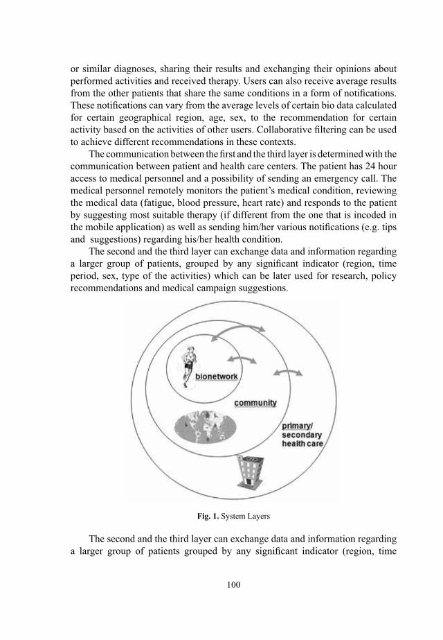
100

or similar diagnoses, sharing their results and exchanging their opinions about performed activities and received therapy. Users can also receive average results from the other patients that share the same conditions in a form of notifi cations. These notifi cations can vary from the average levels of certain bio data calculated for certain geographical region, age, sex, to the recommendation for certain activity based on the activities of other users. Collaborative fi ltering can be used to achieve different recommendations in these contexts.

The communication between the fi rst and the third layer is determined with the communication between patient and health care centers. The patient has 24 hour access to medical personnel and a possibility of sending an emergency call. The medical personnel remotely monitors the patient’s medical condition, reviewing the medical data (fatigue, blood pressure, heart rate) and responds to the patient by suggesting most suitable therapy (if different from the one that is incoded in the mobile application) as well as sending him/her various notifi cations (e.g. tips and suggestions) regarding his/her health condition.

The second and the third layer can exchange data and information regarding a larger group of patients, grouped by any signifi cant indicator (region, time period, sex, type of the activities) which can be later used for research, policy recommendations and medical campaign suggestions.

Fig. 1. System Layers

The second and the third layer can exchange data and information regarding a larger group of patients grouped by any signifi cant indicator (region, time

101

period, sex, type of the activities) which can later be used for research, policy recommendations and medical campaign suggestions.

COHESY uses different techniques and protocols that guarantee security and privacy of users’ data [4, 5, 6]. It has own security and privacy statements that explain how the system protects the users’ privacy and confi dentiality and the way in which their personal information will be treated. Every user can choose which information can be private or public. The user can choose his records to be public: (a) for medical purposes, (b) to all visitors of the Social network, (c) to the users in his category, (d) to none. In order to have medical support the user has to agree to share personal information with clinical centers and medical databases, whose data are also protected. According to user’s agreement policy, those data information would be exchanged through the system.

2.1 Recommendation algorithm

The recommendation algorithm is part of the second level in COHESY (the social network). It is implemented as a web service and its purpose is to recommend the physical activities that the users should carry out in order to improve their health. The algorithm uses the data read by the bionetwork, the data about the user’s physical activities (gathered by the mobile application), the user’s medical record (obtained from a clinical centre) and the data contained in the user profi le on the social network (so far based on the knowledge of the social network).

The main purpose of this algorithm is to fi nd the dependency of the users’ health condition and the physical activities they perform. The algorithm incorporates collaboration and classifi cation techniques in order to generate recommendations and suggestions for preventive intervention. To achieve this, we consider datasets from the health history of the users and we use classifi cation algorithms on these datasets to group the users by their similarity. The usage of classifi ed data when generating the recommendation provides more relevant recommendations because they are enacted on knowledge from users with similar medical conditions and reference parameters.

There are a number of parameters that might be used to characterize a person such as: body mass index, age, blood pressure, heart rate, blood sugar levels. All these characteristics are essentially continuous variables and they are measured with (near) continuous resolution. On the other hand, the bio-medical parameters and phenomena are often too complex and too little understood to be modeled analytically. Because of its continuous nature, the fuzzy systems are very close to the medical reality and at the same time, fuzzy sets allow natural description of bio-medical variables using symbolic models and their formalisms, avoiding the analytical modeling [7]. Therefore, in this algorithm, fuzzy sets and fuzzy discretization are considered as a suitable approach that can bridge the

102

gap between the discrete way reasoning in the IT systems and the continuity of biomedical parameters. For every health parameter, several discretization intervals are considered. Each person has a corresponding membership factors for each of those intervals, depending on his/her parameter value.

This algorithm uses three levels of fi ltering, as shown in Fig.2. The fi rst step is classifi cation. All users belong to some diagnosis class (normal diabetes, heart problems). All users with different diagnosis from the diagnosis of the given user are fi ltered out. This step is important because some activities may be harmful for a particular group of people e.g. running may have much different effect on people with heart problems as opposed to people which are physically active.

The second level of our recommendation algorithm is the collaborative fi ltering. Every user has its own history of health conditions (health profi les) and it is important to fi nd similar users to the given user which at some point of time in the past had similar health condition to the health condition of the given user at the moment. The technique that is used here can be considered as a collaborative fi ltering technique where items are equal to health profi les.

When the similar users are chosen, we use all their health condition history and the history of performed activities to fi nd the infl uences of each activity on the change of the health parameters. Now we come with a fairly good approximation of the potential effect of the activity on the health condition for the given user. Here we use the characteristics of the activities in order to get good recommendations. In other words, we explore the content of the activities and use content-based fi ltering techniques to fi nd the best matching activities. User preferences in our context are the desired values for the health parameters (normal range). The chosen activities would potentially improve the health condition of the given user towards the desired values.

Fig. 2. Levels of fi ltering in COHESY recommendation algorithm

103

3 Simulation results and discussion

In this section we give a validation of the proposed model by using simulations on generic data. Three simulations are made and in all of them, two types of activities are generated: a positive activity (activity whose performance increases the value of a given parameter) and negative activity (activity whose performance reduces the value of a given parameter). Each activity has individual infl uence to the global parameter change and it is presented by a function whose shape is similar to a Poisson probability mass function. The graphs of the infl uences of the positive and negative activities in the time period [0, 3000000] are shown on Fig.3.

In the fi rst simulation 25 activities were generated. Each activity begins at a randomly chosen time point between 0-th and 3000000-th second and it is positive or negative by a random choice.

Each activity carried out before a certain point in time affects the value of the parameter at that point. Our assumption is that the maximum impact of the activity takes place in a relatively short time after its execution. There are 25 generated activities that begin and end at different time points and they all affect the global parameter change. The global parameter change is a sum of all (25 generated activities) individual infl uences and it is presented in Fig.4.

Fig. 3. Graphs of the infl uence functions for a positive and a negative activity

104

Fig. 4. Graph of the global parameter change in the fi rst simulation

To evaluate the effectiveness of the COHESY using the proposed recommendation algorithm, in the fi rst simulation 28 recommendations in 28 different (random) time points were generated.

In the second simulation 56 activities were generated. Each activity begins at a randomly chosen time point between 0-th and 5000000-th second. The graph of the global parameter change in the second simulation is presented in Fig.5. In this simulation, 45 recommendations were generated in 45 different (random) time points

Fig. 5. Graph of the global parameter change in the second simulation

Seventy activities were generated in the third simulation. In this simulation, each activity starts at a randomly chosen time point between 0-th and 7500000-th second. The graph of the global parameter change in the third simulation is presented in Fig.6. In this simulation, 58 recommendations were generated.

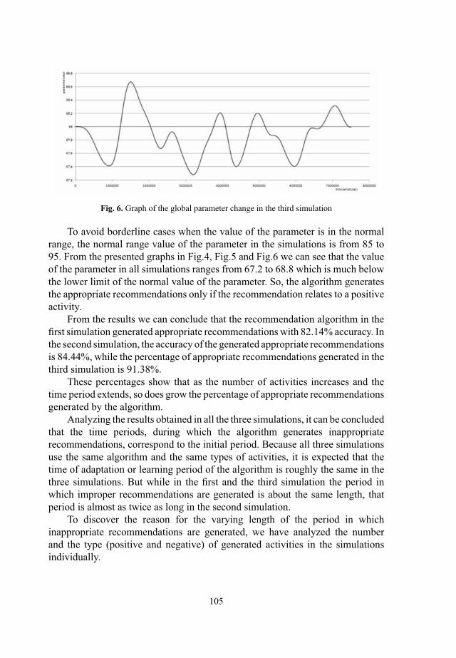
105

Fig. 6. Graph of the global parameter change in the third simulation

To avoid borderline cases when the value of the parameter is in the normal range, the normal range value of the parameter in the simulations is from 85 to 95. From the presented graphs in Fig.4, Fig.5 and Fig.6 we can see that the value of the parameter in all simulations ranges from 67.2 to 68.8 which is much below the lower limit of the normal value of the parameter. So, the algorithm generates the appropriate recommendations only if the recommendation relates to a positive activity.

From the results we can conclude that the recommendation algorithm in the fi rst simulation generated appropriate recommendations with 82.14% accuracy. In the second simulation, the accuracy of the generated appropriate recommendations is 84.44%, while the percentage of appropriate recommendations generated in the third simulation is 91.38%.

These percentages show that as the number of activities increases and the time period extends, so does grow the percentage of appropriate recommendations generated by the algorithm.

Analyzing the results obtained in all the three simulations, it can be concluded that the time periods, during which the algorithm generates inappropriate recommendations, correspond to the initial period. Because all three simulations use the same algorithm and the same types of activities, it is expected that the time of adaptation or learning period of the algorithm is roughly the same in the three simulations. But while in the fi rst and the third simulation the period in which improper recommendations are generated is about the same length, that period is almost as twice as long in the second simulation.

To discover the reason for the varying length of the period in which inappropriate recommendations are generated, we have analyzed the number and the type (positive and negative) of generated activities in the simulations individually.

106

Table 1. Percentage of generated activities by type (positive and negative)

I simulation II simulation III simulation

no. a. % p.a. % n.a. no. a. % p.a. % n.a. no. a. % p.a. % n.a.

1/3 of activities

(33%)8 62,50 37,50 19 73,68 26,32 23 39,13 60,87

1/2 of activities

(50%)13 46,15 53,85 28 71,43 28,57 35 40,00 60,00

2/3 of activities

(66%)17 35,29 64,71 37 70,27 29,73 47 40,43 59,57

total activities 25 40,00 60,00 56 62,50 37,50 70 45,71 54,29

Table 1 illustrates the percentage of positive and negative activities for the three simulations by periods of generating activities. Considering the number and the type of the top 33%, top 50% and top 66% generated activities for each simulation.

The analyses show that in the initial period in the second simulation mostly positive activities are generated, while the number of generated negative activities is signifi cantly lower. In the fi rst and in the third simulation, the number of generated positive and negative activities is not much different. So, it can be concluded that if the number of generated positive and negative activities in the beginning of the simulation is not approximately the same, the period in which inappropriate recommendations are generated increases. This is the case in the second simulation where the period in which inappropriate recommendations are generated is almost twice longer than in the fi rst and third simulation.

Because in the initial period of all three simulations the algorithm generates inappropriate recommendations, the conclusion is that in the proposed algorithm the problem of a cold start occurs. This is a common problem in collaborative algorithms [8]. A possible solution to this problem is to generate prior knowledge before the following simulations. This will also avoid the elongation of the period which generates inappropriate recommendations as well as the issue of a cold start.

4 Conclusion and future work

In this paper a collaborative health care system model and its validation are presented. The proposed model COHESY represents a tool for personal health care by generating various recommendations, comments and suggestions to its users.

COHESY is a complex system composed of mobile application, social network, information systems that are used by the medical personnel, medical databases and additional services. It provides monitoring of health parameters

107

and tracking of the users’ physical activities, communication between users, automatic data transfer, data exchange between medical centers and databases. But what distinguishes the COHESY from the rest and its main advantage is the communication and exchange of data between the various components.

Validation of the proposed model is made by evaluating the effectiveness of the recommendation algorithm using generic data. The analysis of data obtained from the simulations of the recommendation algorithm on generic data show that the algorithm generates appropriate recommendations with an accuracy of 82% to 92%. As the time period and the number of activities extends, so does the percentage of appropriate recommendations generated by the algorithm increases.

However, the analyzes showed that the proposed model has defi ciencies such as the cold start problem and the extension of the initial period in which inappropriate recommendations are generated, which should be treated with more attention in future.

The performed simulations are only an introductory step in the process of evaluating the effectiveness of the recommendation algorithm and the proposed model. In the future, the evaluations of the effectiveness of the proposed model should be done with simulations that will validate the behavior of the algorithm in different conditions (different values of the parameter, more types of activities) and with simulations with real data in order to make a quantitative and qualitative analysis of the behavior of the system.

References1. Trajkovik V, Vlahu-Gjorgievska E, Kulev I.: Use of collaboration techniques and classifi cation

algorithms in personal healthcare. Health and Technology 2(1), 43--55 (2012)2. Khan P., Hussain A., Kwak K.S.: Medical Applications of Wireless Body Area Networks.

International Journal of Digital Content Technology and its Applications 3(3), 185--193 (2009)

3. Chittaro L.: Visualization of patient data at different temporal granularities on mobile devices. In: Proceedings of Working conference on Advanced visual interfaces, pp.484--487. ACM, USA (2006)

4. Hung P.C.K.: Towards a privacy access control model for e-healthcare services. In: Proceedings of 3rd Annual Conference on Privacy, Security and Trust, New Brunswick, Canada (2005)

5. Raman A.: Enforcing privacy through security in remote patient monitoring ecosystems. In: Proceedings of 6th International Special Topic Conference on Information Technology Applications in Biomedicine, Tokyo, Japan, pp.298--301 (2007)

6. Zheng Y., Cheng Y., Hung P.C.K.: Privacy access control model with location constraints for XML services. In: Proceedings of the 23rd International Conference on Data Engineering Workshop, Istanbul, Turkey, pp:371--378 (2007)

7. Steimann F.: On the use and usefulness of fuzzy sets in medical AI. Artifi cial Intelligence in Medicine, 21, 131--137 (2001)

8. Su X., Khoshgoftaar T.M.: A Survey of Collaborative Filtering Techniques. Advances in Artifi cial Intelligence. art 421425, 1--19 (2009)

108

A graph representation of query cache in OLAP environment

Hristo Hristov, Kalinka Kaloyanova

Faculty of Mathematics and Informatics, Sofi a University “St. Kliment Ohridski”, 5 James Bourchier blvd., 1164, Sofi a, Bulgariachristo_christov@yahoo.com , kkaloyanova@fmi.uni-sofi a.bg

Abstract. This paper concerns the optimizations of Data Warehouses queries. Some open issues of query management in OLAP environment are discussed. A graph representation of query cache is proposed. The proposed approach uses the

queries for statistical information and the graph modeling.

Keywords. Query optimization, cache, graph, OLAP

1 Introduction

Improving query response time is one of the constant issues facing scientifi c and business organizations working with databases. Different approaches are discussed in sources [2], [7], [8], [12], [13] and others. A possible direction to reduce the time and resource needs in processing queries is to increase the effi ciency of the process. Ineffi ciency can appear when the same action is performed several times instead of reusing the results produced during the fi rst time run.

Usually the results from subqueries are released immediately after query has fi nished its work and just part of them can stay in the form of data blocks cache maintained by DBMS. Instead of losing this data and the effort for their calculation, the information could be used for other queries helping not to recalculate again and again the same intermediate results of the queries. Creating a cache for intermediate results from the queries calculation process is a possible approach. Appropriate structure of the cache, which presents elements and relations between them, could be a graph which nodes present the queries together with their subqueries. Nevertheless the problem is too complicated in the common case, some specifi c characteristics of Data Warehouses could be used to reduce the complexity of the cache management.

109

The goal of this paper is to fi nd an intuitive and easy for implementation form of the graph that helps the identifi cation of frequently needed parts of queries and which if available in advance is possible to provide overall benefi t for improvement of query execution performance and cost. Oriented graph structure is proposed to be used, in order to help keeping the linkages between different queries and their subqueries. The proposal is addressed to Data Warehouse environment, where the maintenance cost of materialized views is lower than in OLTP environments. Also the specifi cs of the database schema and query workfl ow of users of OLAP environments are found to be appropriate to the characteristics of the proposed graph.

The rest of the paper is organized as follows. Section two briefl y describes the major achievements up to now in the areas of research topics of materialized view selection and answering queries using views familiar to the authors. Section three presents the general idea for the graph proposed together with the preliminary conditions assumed and describes the specifi cs of the different levels in the graph one by one. In section four some aspects of operations with the graph are discussed. Section fi ve provides examples and conclusions end the paper in section six.

2 Previous work

In [4] lattice of views and greedy heuristics algorithms for selection of optimal set of views for materialization are presented. The paper concerns views in cubes based on grouping characteristics of the fact joined to all dimensions. No selection and projection clauses expressions applied are examined. Further works develop the main concept in details and show some variants - for example in [1] are overseen more specifi cally defi ned problems and heuristics that solve the problems constrained by maximum number of views to be materialized and maximum space available for materialization. Also in [10] caching as a single cube (one fact table) is introduced and as a fi rst step the query is presented in canonical form following the approach presented broadly in [9]. Based on the interactive and navigational nature of OLAP query workloads, the subqueries are presented in a hyper-rectangle and the dimensional structure itself. The cost calculation for each query is shown. [13] has proposed a model for characteristics OLAP query patterns based on Markov Models and corresponding OLAP queries prediction algorithms. Based on the current behaviour of the user in its session the queries for which there is a high probability to be used on the next step are calculated before the user really issues them. In [12] is presented a cache model aiming to increase the performance of ad hoc queries to data warehouse. The subsumption problem as summarization of query containment and query minimization problems are

110

presented also. The ideas here are very close to the current paper, but the focus is on fl at query cache without linkage between subqueries of the user query. Despite that this research could be used to enforce selection-projection nodes similarity and linkage detection presented in the current paper. In [11] could be seen the notion of AND-OR graph and example of directed acyclic graph usage as a structure for query presentation. In [14] the focus is on the user access patterns generated on set of user access events. User access graph is generated and it represents query execution order. Interesting approach is shown in it that each node in the access graph has support value for the frequency of usage (confi dence of the node) so the noise requests are eliminated. Mining user access patterns involves user session identifi cation. In [16] can be seen the proposal for placing weight on different queries and approach to materialized view selection problem with consideration of this weight. [7] presents broad overview of the approaches for view selection methods and diversity of solutions proposed are summarized and classifi ed. Another problem related to the topic is to answer queries using the materialized views and it is summarized in [3] and also further researched for example in [6].

Nevertheless a lot of research has been made on the area of query caching in the form of materialized views, the problem is not solved. Different proposals are presented and each of them has some positive aspects but does not cover the topic entirely, leaving room for more suggestions and research in different directions. This paper will present a combination of the directed acyclic graph and query cache proposal in a new graph structure not met in the previous works. The proposed approach is more intuitive and less complicated compared to the works so far, which makes it easier for practical implementation.

3 Graph of queries elements

As described in [15] the query processor takes three steps - parsing, logical query plan creation and physical query plan creation. It is expected some parts of the logical plan to appear as part of the logical plans of other queries issued to the database of the data warehouse. The goal is the logical query plan calculated for a query to be replaced with another one, which will produce the same result, but in a cheaper way because smaller relations already calculated as physical result from another query are used. It is known from the step of query parsing and from the step of logical query plan generation of the user’s query what relations are needed, what join conditions are applied, what projections are applied and what grouping and aggregation functions are used. This information can be kept in the form of a graph which nodes present the components of the logical query plan. Search in the graph will help to match the queries issued further and to fi nd the nodes in the graph corresponding to specifi c subparts (or the whole query).

111

As already presented in the previous section, the problem has been reviewed from different angles. The current paper will try to propose an approach, which has not been proven to give optimal solution in the context of choosing the best view set for materialization, but will make the graph of common subqueries closer to users’ understanding of the query and calculated subsets. This will give possibility of the users and data warehouse administrators iteratively to change some parameters of the graph incorporating in that way the knowledge they have for the usage in the future of the system and in that way to achieved better performance.

Some conditions are assumed to be true in this setup. It is supposed that the joins between relations are always inner and actually the join conditions between any two relations are predefi ned. Such assumption will work fi ne for a dimensional structure used in data warehouses, because usually in the queries the facts are joined to the dimensions by their artifi cial identifi ers serving as primary keys. Another assumption is that the selections are usually based on simple predicates using operators like =, <, >, >=, <=, IN, BETWEEN and one of the operands is constant. Also it is supposed that there is no self joins. In the queries all aliases of relations and attributes are replaced with their original names. These assumptions will simplify the research on this stage without limitation for further enrichment of the proposal towards more general conditions.

It is assumed that there is predefi ned order of all relations and of all attributes of the relations. For example this could be alphanumeric order of their names. The parts from the logical plan in the graph nodes will always be represented in uniform manner based on the predefi ned order of its elements and operations. This will impose similarity in query processing and resolving each part of the query in predefi ned order will be helpful when trace of the graph took place to identify the nodes related to the user’s query.

All queries have to be matched against a graph of logical query plans parts presenting already issued queries or their subqueries. The graph is a set of nodes N which defi nition is given below and edges Edg = (Nc, Np), where Nc is the child node in the graph and Np is the parent node and means that the two nodes could be part of same query or child could be calculated from the results in the parent. Several types of nodes in the query graph are defi ned. Each type of node is allocated to specifi c parts of a query. Different types of nodes are referred here as levels. The nodes of the different levels have different notation and representation. Each node is defi ned as N = (L, E, M, S), where L = {J|S|A|Q} is the level of node where J stand for Join, S stands for Selection/Projection, A stands for Aggregation and Q is the type for whole query. The component of the node E presents expression for level defi nition, which will be defi ned later in detail. M is fl ag whether the node is materialized or not. The component S presents an array of statistics collected for the node and is defi ned as S = (NA, FT, LT, SZ, TC,

112

AH, IM). NA presents the number of access attempts to the node during queries logical plan generation. FT is value presenting when the node was accessed for the fi rst time (actually it is the time of the node creation). LT is the last time when the node was accessed. SZ is the size of the nodes. The size could be presented as number of rows or number of blocks or some other metric. In case the node is materialized the exact value of the size is known. Otherwise estimation of the size could be made. Example how it could be achieved is presented in [4]. TC is the time for calculating the node (estimation or last calculation time for execution of this node is stored here or estimation). AH is complex structure keeping the actions history log where each action with this node is stored – accessing queries with their execution time and duration, materialization choices, excluding from materialization set etc. IM is value presenting the factor of importance the query has and is intended to be defi ned by the administrators or the users of the system. The statistics monitored could be more or less – here are included those which are considered to be most useful. Following is description of each level and its expression.

3.1 Join Level

Join level (J level) is the set of graph nodes which present the join operations in the query. It could be assumed that there are only theta join of relations as other types of joins could be presented as theta joins. The other parts of the queries like selections or projections are not presented in join level nodes. They are left to be defi ned in the rest of the nodes which will be discussed further. The join conditions are predefi ned and there is no need for them to be included in the graph node defi nition. In OLAP environment the joins are usually between the facts and dimensions and the join conditions present equations of primary keys of the dimensions to the foreign keys to these dimensions in the fact table. With that assumption in the join nodes could be placed only the names of the relations to be joined. The relations are presented as a list sorted according to their preliminary defi ned order and this is actually the expression of the node. Formally E = (R

1,

R2, …, R

n), where R

1, R

2, …, R

n are relations from the database schema listed

according to the uniform predefi ned order.

3.2 Selection/Projection level

Selection/Projection level (S level) will present part of the selection and projection operations in the query. The S graph nodes are linked with those nodes in J level, which present the join of all relations in the query. The conditions which relate to joins are indirectly presented in J level. That’s why S graph nodes represent

113

conditions over their tuples with predicates only on single relations. It is allowed a S node S

1 to be linked with edge to other S node S

2 instead of link to J node, if S

1

is subsumption of S2. S

1 is considered to be subsumption of S

2 if S

1 is contained in

S2 as defi ned in [3]. In that case the edges of S

2 to J level nodes are in force for S

1

also. S2 can be connected from its side to another S level node and so on the chain

to continue till it is reached a S level node which is linked directly to J level node. The same principle for inheritance of J level node links is in force recursively for all these S level nodes. To simplify the graph in this level are presented also the projection clauses of queries as adding predicates which are true for all tuples in the relations but including the attributes met in projection parts of the queries but not presented in any selection predicate. The expression E here is defi ned as E = (C

1, C

2, …, C

n), where C

1, C

2, …, C

n are conditions in the form of C = {At

i

Op Cnst | Ati IN (Cnst

1, Cnst

2, …, Cnst

n) | At

i BETWEEN Cnst

1 AND Cnst

2},

where Ati is attribute of relations R

i from J level, Op = { = | < | > | >= | <=} is

simple operation and Cnsti is a constant. Projection clauses presented here do not

include expressions over one or several relation attributes, but only defi nition of all needed attributes for fi nal query calculation. The defi nition of statements over these attributes is left for the higher levels of the graph.

3.3 Aggregation level

In aggregation level (A level) the nodes are linked with nodes in S level and present the grouping on subset of attributes and applying aggregation functions on the other attributes. All attributes used in the defi nition of this node level should be presented in S level. A special notation ø is added, which presents that the query has no grouping at all. Aggregation level expression contains two parts - the list of attributes on which a grouping is made and the calculations of expressions applied over the other attributes. Formal defi nition is E = (GL, AGG), where GL = (a

1, a

2, … , a

n) and a

i is attribute of some relation R

i. For each a

n and

am, if n < m, then R

n either is same as R

m and a

n is lower in attribute order than

am or R

n is different than R

m and R

n lower in the relations order than R

m. AGG =

(Expr1, Expr

2, …, Expr

x), where Expr

x is SQL expression with relation attributes

and constants and aggregation operations like MAX, SUM, COUNT.

3.4 Query level

To present uncovered queries which cannot be matched entirely to J, S or A levels it is included a level of nodes for exact query matching, which will “cover” the cases of more complicated queries. This level also will serve like simple query cache if no benefi t could be found from the lower levels J, S or A. In that way if

114

some query is very popular, it will still have the chance to be cached even if it is more complicated and does not fi t to the assumptions in this paper. Also the statistics and query usage history collected will be useful in the case of future work of extension of the idea here with more levels. Expression E for Q level will contain the SQL query issued from the user as it is (or with transformation in order to unify it and to improve the chance for cache hit of same but written in alternative way queries – for example replacement of aliases with original names, reordering, etc.)

4 Graph populating and materializing

When a query is issued to the Data Warehouse database some specifi c actions should be taken in order to change the graph in response. First the logical query plan is generated (meaning that parsing phase is passed also). But instead of relying on the logical plan generated by the data base management system, a parallel logical plan is generated for each query in respect of the nodes of the graph defi ned above. Expressions for each of the levels are recognized. A separate graph – a single query graph is generated for this particular query in isolation from the graph constructed up to now.

Initially only the nodes representing the relations in the database itself are presented in the graph. For each query issued this graph and the newly generated single query graph are merged. Each query will add more nodes and edges between the nodes in cases when there is no appropriate node existing for specifi c part of the query. On this stage the nodes generated from the single query which are subsumptions of the nodes in the graph are identifi ed and linked with graph edge. Also generation of new nodes is made on this stage, which will identify common parts of two or more nodes after search for matching parts of defi nitions of two nodes. Then these matching parts form a new node and edges should link it to its parent nodes and to the respective child nodes.

After all nodes are identifi ed, a check should be made if some of the nodes are materialized (their result is pre-calculated in advance). If yes - the nodes which are closest (have shortest path in the graph) to the node representing the query in Q level should be chosen and the query should be rewritten to use them for the query answering. After that the parameters of each inspected node should be changed so to keep the appropriate statistics which will help the choice of nodes for materialization on the next refresh cycles.

During the refresh cycle of the Data Warehouse nodes should be chosen to be materialized in advance as they are expected to reduce mostly the cost of future queries. For this purpose it is used the collected statistics – for example how many times each node is checked for materialization, how many times it is

115

used in modifi ed logical query or as direct cache hit. Many of the algorithms for choosing materialized views proposed in the literature can take advantage from the collected statistics to limit the set of views appropriate for materialization and to take better decision which of them to be chosen.

5 Graph construction examples

Two examples will be shown to illustrate the J, S and A query levels as the principles for generation are different and specifi c for each of them.

5.1 Join level example

In Table 1 is presented a summary of a workload from a real data warehouse system working in a telecom company with a total size of near 10TB and having multiple fact and dimension tables concerning customers, their accounts, usage events, billing information and so on. For simplicity only queries which took more than 120 minutes for a period of one day are used. Relations which took part in the workload are named as R1, R2, .. , R15. Queries are presented as rows in this table along with the duration of each. In the cross-cells with X is marked if the respective relation appears in the join part of the relation the row is for.

Table 1. Experimental Results

116

After applying the rules for graph generation the graph on Fig. 1 is received. Execution of query 1 will create node J1. Query 2 will result with J2 node and respectively query 3 will generate J3 and query 4 will generate J4. J5 will generate node J5 but also will identify common queries with J4 – these are R3, R9 and R10. They will form node J51. Query 6 will not add new nodes as it joins same relations as query 5. Same is in force for query 7 in couple with query 2 and query 8 in couple with query 1. Query 9 will generate node J6, but common part with J1 node will result in the node J61. Query 10 is similar to query 9. Queries 11 and 12 will form new nodes J7 and J8. And fi nally query 13 will generate J9, but it will be linked to already existing node J61.

Let’s apply one very simplistic algorithm to choose nodes for materialization. It is to choose those join nodes which are with top 5 duration sum – the sum of durations of queries used them. Then nodes J61, J6, J9, J51 and J1 would be chosen with an algorithm with complexity not more than some sort algorithm. After that as these nodes represent actually queries of views they can be materialized or the set for materialization to be chosen between them.

Fig. 1 Join level nodes on experimental results

5.2 Selection and aggregation level example

In order to illustrate generation of selection and aggregation levels, it will be used several queries over simple schema as presented in Fig. 2

117

Fig. 2 Schema for selection and aggregation levels demonstration

The schema in Fig. 2 presents relations for stores S, items I, date D and transactions with the items in stores – T. Items relation I have attributes for item name – iname and the price of the item – price. Each item has identifi er presented as attribute iid. Stores relation has attributes for the city where it is located, the number of employees in the store and the name of the store manager. Date relation is simply the identifi er and the date itself. The relation of the transactions is actually the fact table in a star schema having foreign keys to the other relations described, which are dimensions. The fact in T is qnt, which presents the quantity sold in specifi c store for specifi c item on specifi c day. Let several queries presented in Table 1 are executed and have to be included in the graph.

Table. 2 Examples of issued queries

Query 1 Query 2 Query 3

SELECT I.iname, sum(T.qnt)FROM T join I on (T.iname = I.iname)WHERE T.qnt > 100GROUP I.iname

SELECT I.iname, sum(T.qnt)FROM T join I on (T.iid = I.iid)WHERE T.qnt > 200GROUP BY I.iname

SELECT S.city, I.iname, sum(T.qnt), max(T.qnt*I.price)FROM T join I on (T.iid = I.iid) join S on (S.sid = T.sid)WHERE S.emp > 5 GROUP BY S.city, I.iname

Query 1 and Query 2 will result respectively in nodes S1 and S2. Node S2 will be connected with edge to S1 as S2 is identifi ed to be subsumption of S1. Query 3 will result in S3. In Fig. 3 could be seen the resulting part of the graph. For aggregation level as example in Fig. 3 is included the node A1, which will be result from Query1 and is used from Query 2 also. The grouping attributes are presented above the line and the expressions – below it. Query 3 will generate A node A2.

118

Fig. 3 Selection level nodes on experimental results

6 Conclusion

In this work an approach for caching of queries in the form of a graph structure under specifi c assumptions has been presented. These assumptions imply some limitations suitable for Data Warehouse environment. General presentation of the idea has been made. Many aspects of the proposal have to be developed further. For example experiments with the usefulness of statistics like the history of access of the nodes or resources concerning materialization like size, time for calculating or history of materializations should be made. Another direction is to be made experiments with known algorithms for materialized view selection as to be found if they will be appropriate for the proposed structure and if the graph can be benefi cial to them. The graph is useful for prediction of future query needs based on the statistics collected. It is presented in examples that the users could be helped with GUI for presenting the collected cache and this will give possibility for the users and system administrators to have an overview and to change the weights of some nodes in order to impact the algorithm for materialization. Changes of the graph could be tracked, thus helping to collect knowledge for users’ behavior. It is also possible to look for an extension of the SQL operations allowed. Some data mining methods [5] could be applied for clustering, associations or sequential pattern mining in order to achieve better prediction of the future needs of the users.

119

References

1. Agrawal, V., Sundararaghavan, P.S., Ahmed, M. and Nandkeolyar, U.: View materialization in a data cube: optimization models and heuristics. Journal of Database Management, Vol. 18, No. 3, pp. 1--20 (2007)

2. Dimitrov, V., Goranova, R.: Abstract and concrete syntax in SQL extension for data stream processing. Conf. Proc. of International Conference “Applied Informatics and Statistics – New approaches and methods”, 25 – 26 Sept 2009, Ravda, Bulgaria, pp. 148 – 151 (in Bulgarian) (2010)

3. Halevy, A.: Answering queries using views: A survey. The VLDB Journal 10, pp. 270--294 (2001)

4. Harinarayan, V., Rajaraman, A., Ullman., J. D.: Implementing data cubes effi ciently. In Proceedings of the 1996 ACM SIGMOD international conference on Management of data (SIGMOD ’96), New York, USA, pp. 205--216 (1996)

5. Kaloyanova K.: Improving Data Integration for Dara Warehouse: A Data Mining Approach, Proceedings of the International Workshop “COMPUTER SCIENCE AND EDICATION”, Borovetz-Sofi a, Bulgaria, June, 2005, ISBN 954-535-401-1, pp. 39—44 (2005)

6. Konstantinidis, G., Ambite, J.L.: Optimizing query rewriting for multiple queries. In Proceedings of the Ninth International Workshop on Information Integration on the Web (IIWeb ’12). ACM, New York, NY, USA (2012)

7. Mami, I., Bellahsene, Z.: A survey of view selection methods. SIGMOD Rec. 41, pp. 20--29 (2012)

8. Naydenova I.: Regular Sparsity Map. Proceedings of the 4th International Conference On Information Systems & Datagrids, May 2010, Sofi a, Bulgaria, ISBN 978-954-07-3168-1, pp. 51--63 (2010)

9. Park, C.-S., Kim, M., Lee Y.-J.: Rewriting OLAP Queries Using Materialized Views and Dimension Hierarchies in Data Warehouses. In Proceedings of the 17th International Conference on Data Engineering (ICDE ‚01). IEEE Computer Society, Washington, DC, USA (2001)

10. Park, C.-S., Kim, M., Lee Y.-J.: Usability-based caching of query results in OLAP systems. J. Syst. Softw. 68, pp. 103--119 (2003)

11. Roy, P., Ramamritham, K., Seshadri, S., Shenoy, P., Sudarshan, S.: Don’t Trash your Intermediate Results, Cache ’em. Technical Report, Dept. of Computer Science and Engineering, IIT-Bombay (2000)

12. Saharia, A. N, Babad, Y. M.: Enhancing data warehouse performance through query caching. SIGMIS Database 31, pp. 43--63 (2000)

13. Sapia, C.: Promise: Predicting query behavior to enable predictive caching strategies for OLAP systems. In DaWaK, pp. 224--233 (2000)

14. Yao, Q., An, A.: Characterizing database user’s access patterns. In: DEXA. pp. 528--538 (2004)

15. Ullman, J. D., Garcia-Molina, H., Widom, J.: Database Systems: The Complete Book (2 ed.). Prentice Hall Press, Upper Saddle River, NJ, USA. (2008)

16. Wagner, Н., Agrawal, V.: Using an evolutionary algorithm to solve the weighted view materialisation problem for data warehouses. Int. J. of Intelligent Information and Database Systems (2013)

120

Development of Educational Application with a Quiz

Marija Karanfi lovska, Blagoj Ristevski

Faculty of Аdministration and Information Systems Management - BitolaUniversity “St. Kliment Ohridski” - Bitola, Republic of Macedonia1marija.karanfi lovska@gmail.com, 2blagoj.ristevski@uklo.edu.mk

Abstract. In this article, a developed educational application with a quiz intended for children/pupils aged 6 - 9 years is described. The purpose of this interactive application is children to learn through a game with animals and birds from near and wild environment and then through a quiz to determine what they have learned. The application is divided into two parts: educational part and quiz. In the fi rst part of this application, children can fi nd useful data for domesticated and wild animals and birds in different data formats: text, image and audio. While in the second part (the quiz), the same information are used particularly to test the children knowledge and at the end, the quiz result shows how many points the participant has. The target audience is children aged 6 to 9 years, because the participants should be able to read and write to use this application.

Keywords: application development, educational application, quiz, database

1. INTRODUCTION

Developed application named ZUZU follows the current needs and trends for the development of an educational application. The main motivation for this task is to make concepts in detail for development of application and its connection to the database. Based on the performed research, it was noticed that additional education methods for young children education are needed in terms of learning about animals and birds. In the new textbooks for the subject “Nature” for the 1 - 4 classes in Republic of Macedonia, different species of animals and birds are covered, but their basic features and screams that they emit are not highlighted at all. To validate the impact of developed application among children, a questionnaire was attached. The poll covered 20 children aged 6 to 9 years and it was concluded that they receive too much information from the textbooks, while the children are not able to memorize all of it and usually after 2 years, they forget the learned information. Educational application with a quiz ZUZU allows children from 6-9 years to gain knowledge regarding wild and domesticated animals and birds and to test the gained knowledge. Educational interactive application for the young children looks just a simple game in which they need to fi nd and guess the right

121

animals and birds. Children’s role is to click on the animals/birds, to hear their screams and to read the text in the background. After that, children should be able to recognize these animals/birds.

To develop this application with a quiz, several software packages were used: Microsoft Visual C # 2010, Microsoft SQL Server 2008, Adobe Photoshop CS6 and Audio Recorder. In order to use the recorded audios in C#, recorded audios were converted from WMV to WAV. For that purpose WMV to WAV converter was used.

This article is organized as follows. In the introductory section, the concepts of educational application and quiz are introduced. In the second section, the main window and the main menu of the application are described. In the following section, the educational part of the application is described. All three consisting parts of ZUZU: introduction to the educational part, domesticated and wild animals and the component of domesticated and wild birds are depicted in this part. In the fourth section, the quiz is depicted as well as its connection to the database. The fi nal section presents the results and conclusions about the benefi ts that come from using this application.

2. MAIN WINDOW AND MENU OF ZUZU

When application starts, the fi rst window that opens is the “parent” of all other windows. While application works, this window is active all the time. When the child will leave, any other application window will be face with this window. While this window is open, the child listen the screams of different animals and birds, hence a child has a feeling that is found in the enviroment surrounded by animals and birds whose screams is listened to. The main menu is located in the upper part of the window, where child can login to another application window.

The main menu consists of four categories. The fi rst category is the “Instructions” and by choosing this category a new window opens with instructions for the educational part. Second category is “Discover the animals”. This category has two submenus: “Domesticated animals” and “Wild animals”. By choosing one of these submenus, a new image opens for the corresponding animal. The third category is “Discover the birds”. This category has two submenus: “Domesticated birds” and “Wild birds”. By choosing one of these submenus, a new image for the corresponding bird is opening. The last category is “What did you learn”. By selecting this category, a new window-quiz opens.

The structure of the application is shown in the Fig 1.

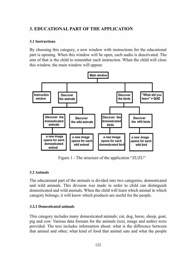
122

3. EDUCATIONAL PART OF THE APPLICATION

3.1 Instructions

By choosing this category, a new window with instructions for the educational part is opening. When this window will be open, each audio is deactivated. The aim of that is the child to remember each instruction. When the child will close this window, the main window will appear.

Figure 1 - The structure of the application “ZUZU”

3.2 Animals

The educational part of the animals is divided into two categories, domesticated and wild animals. This division was made in order to child can distinguish domesticated and wild animals. When the child will learn which animal in which category belongs, it will know which products are useful for the people.

3.2.1 Domesticated animals

This category includes many domesticated animals: cat, dog, horse, sheep, goat, pig and cow. Various data formats for the animals (text, image and audio) were provided. The text includes information about: what is the difference between that animal and other; what kind of food that animal eats and what the people

123

use of that animal. When the child will choose submenu “Domesticated animals” from the category “Discover the animals,” a new window containing an image with screams of domesticated animals is opening. There is an image and audio of domesticated animals. In this window, the child should discover which animal can be clicked. When the child will click to an animal, it can read some data, can see the image of the animal and can hear the corresponding scream. Returning to the previous window is enabled by clicking anywhere on the already open window.

3.2.2 Wild animals

This category includes several wild animals: zebra, wolf, bear, lion, deer, elephant, tiger, monkey, fox, rabbit and giraffe. Various data formats (text, image and audio) were provided for these animals. The text includes information about: what is the difference between that animal and other; what kind of food that animal eats and where it lives. When the child will choose submenu “Wild animals” from the category “Discover the animals,” a new window containing a image and screams of wild animals is opening. There is a image and screams of wild animals. In this window the child should discover which animal can be clicked. When the child will click to an animal, it can read some text data, can see the image of the animal and can hear the corresponding scream. Returning to the previous window is enabled by clicking anywhere on the already open window.

3.3 Birds

The educational part of the birds is divided into two categories of domesticated and wild birds. This division was made in order to child can distinguish domesticated and wild birds. When the child will learn which bird in which category belongs, it will know which products the people use of that.

3.3.1 Domesticated birdsThis category includes many domesticated birds: hen, rooster, turkey, ostrich, goose and duck. Various data formats for the birds (text, image and audio) were provided. The text includes information about: what is the difference between that birds and other; what kind of food that bird eats and what the people use of that bird. When the child will choose submenu “Domesticated bird” from the category “Discover the birds,” a new window containing an image and screams of domesticated birds is opening. There is an image with screams of domesticated birds. In this window the child should discover which bird can be clicked. When the child will click on the bird, it can read some information, can see the image of the bird and can hear the corresponding scream. Returning to the previous window is enabled by clicking anywhere on the already open window.

124

3.3.2 Wild birds

This category includes many wild birds: stork, swan, fl amingo, tukan, woodpecker, owl, eagle, peacock, swallow and parrot. Various data formats for these birds (text, image and audio) were provided. The text includes informations about: what is the difference between that birds and another, what kind of food that bird eats and where it lives. When the child will choose submenu “Wild bird” from the category “Discover the birds,” a new window containing an image with screams of wild birds is opening. In this window, the child should discover which bird should be clicked. When the child will click on the bird, it can read some information, can see the image of the bird and can hear the corresponding scream. Returning to the previous window is enabled by clicking anywhere on the already open window.

4.THE QUIZ

By choosing the category “What did you learn” from the main menu the window with QUIZ is opening. When this window opens, the audio is deactivated. This quiz is designed for children to test their newly acquired knowledge. The quiz covers all kinds of animals and birds. It contains questions with text and audio. When this window opens, the child should write down his/her name and click on the button “Insert”. After clicking, the button “Insert” opens the section for instructions for the quiz.

Quiz contains 23 questions: 13 questions with text and 10 questions with audio. From 13 questions with text, 3 questions regarding to the domesticated animals, 6 to wild animals, 2 to domesticated birds and 2 to wild birds. From 10 questions with audio, 2 questions are related to the domesticated animals, 4 to wild animals, 1 to domestic bird and 3 to wild birds. For each question, the child has three choices (options) and it can choose just one option. Clicking on any of the images of animals or birds it gives the answer and passes to the next question. Depending on whether the answer is correct or not, its points can increase. After switching to the next question, it is impossible to turn back. At the end of the quiz, the numbers of correct answers are shown. This score is recorded in the database.

5. RESULTS AND CONCLUSIONS

The application “ZUZU” serves as an educational tool for children aged 6 - 9 years. It can be very useful application - supplement of the subject “Nature”. Educational process is carried out using images, text including basic features for each animal and bird and corresponding screams. ZUZU is developed for children to become more familiar with the attributes of animals and birds and to remember them on long term. Application “ZUZU” can be used as a part of regular classes in primary schools and other educational centers. To validate the

125

developed application with quiz, a poll was conducted at the primary school “Elpida Karamandi” - Bitola. Based on the results of the poll, the following can be concluded. Most of the surveyed children were aged 8 years, living in an urban environment, thinking that they have enough knowledge about animals and birds. But, often this knowledge lasts only 1-2 years. This knowledge is short-term due to too many unnecessary facts that textbooks for the subject “Nature” provide to children/pupils. They know wild birds at least, and they almost do not know the emitted sounds from the animals and birds, but they have a great desire to hear. This application was tested in the same primary school.

By opening the fi rst window of this application, pupils were amazed by the audios they heard and by the different colors displayed on the window. They managed to read all the instructions, to remember them, and then to apply them. It was shown great satisfaction regarding the educational part. They were interesting in to continue interaction with this application The clustering of animals and birds in domesticated and wild animals and birds was helpful for the pupils easy to remember them. Regarding the quiz, the children had showed great interest in gained points and they were competitive about who is the winner with the highest score. The charts 1- 4 bellow show the results of the last four questions of the conducted survey.

Application ZUZU can be easily upgrading an extending in the future.

126

Reference

1. Paul J. Deitel, Harvey M. Deitel , C# 2010 for Programmers, Delth, fourth edition, 2010.

2. Rob Miles, C# Programming, Department of Computer Science University of Hull, edition 2.1, January 2011.

3. Maria Virvou, George Katsionis and Konstantinos Manos, Combining Software Games with Education: Evaluation of its Educational Effectiveness, Department of Informatics University of Piraeus, Greece

4. Eric Klopfer, Scot Osterweil, and Katie Salen with contributions by Jason Haas, Jennifer Groff and Dan Roy, The education arcade, Massachusetts Institute of Technology 2009

5. Effective Interprofessional Education, Della S. Freeth, Marilyn Hammick, Scott Reeves, Ivan Koppel, Hugh Barr, August 2005

127

Performance Study of Analytical Queries of Oracle and Vertica

Hristo Kyurkchiev, Kalinka Kaloyanova

Faculty of Mathematics and Informatics, Sofi a University, 5 James Bourchier blvd., 1164, Sofi a, Bulgaria

{hkyurkchiev, kkaloyanova}@fmi.uni-sofi a.bg

Abstract. Analyzing and mining transactional data straight from the DBMS has become increasingly more popular, provoking research in read optimization for RDBMS. One branch of such research – column orientation claims signifi cant improvement in read performance in comparison with row oriented DBMS. Having previously looked into the strengths and weaknesses of both approaches we take on studying the performance of commercial grade DBMSs, which employ the two views. The fi rst step in this is examining their data models. We then develop a benchmark, which is subsequently used to measure each DBMS’s performance. Evaluating the results we draw conclusions about each DBMS’s suitability and main advantages over the other.

Keywords: Relational databases, Database systems, Data warehouses, Column stores, Performance evaluation, Analytical query load, Oracle, C-Store, Vertica

1 Introduction

Codd’s relational database model [3] has dominated the database world for the last couple of decades due to its atomicity, consistency, isolation, and durability properties and ease of use even for non-IT specialists [4]. It is used by most traditional database management systems (DBMS) not only as a logical data model, but also as a physical one. As a result, the data tuples in them are stored contiguously on the disk [13]. This approach is usually denoted as the N-ary storage model (NSM). Column-stores also use the relational model as a logical data model. They, however, use the decomposed storage model (DSM) for physical data storage [1]. Having previously examined both ways of treating relational data [7] in general, we look into concrete, commercial grade DBMSs e.g. Oracle and Vertica to see how these abstract models affect the performance in practice. We start by fi rst analyzing the data models and performance optimizations of both systems. Next we develop a performance benchmark, which we then use to quantify the performance differences between employing row, or column

128

orientation. Based on these results we draw conclusions about each DBMS’s suitability for different setups and query loads.

2 Architectural overview

Both Oracle and Vertica use as a logical model the relational data model [3]. There are certain architectural differences between the two DBMSs, however, which make them perform differently in certain conditions. In order to fi nd why that is so and what these performance differences are with regard to analytical queries we start by examining the architectures of both DBMSs.

2.1 Oracle’s architecture

Physical database structure. We use Oracle 11g to gain more information about Oracle’s architecture, as this is the version later used in the tests. As every other Oracle DBMS it uses the relational model as the logical representation of the values in the database, although it also features extensions for object-oriented modeling [9]. Each implementation of a relational DBMS (RDBMS), however, specifi es how the data is physically stored on the hardware. In Oracle’s case the datafi les are stored in tablespaces, with each datafi le being in only one tablespaces and each tablespace containing multiple datafi les [5, 9]. Other important structural components of an Oracle database include control fi les, redo log fi les, archived logs, block change tracking fi les, Flashback logs, and recovery backup (RMAN) fi les [5]. Essentially the datafi les, control fi les and redo log fi les physically represent the database on the disk [5].

For us the most important in structural regard is the datafi le as it contains the real data [5, 9]. It is composed of Oracle database blocks (between 2KB and 32KB), which are in turn composed of operating system blocks [5]. The datafi les also have a logical organization of three levels – data blocks, extends and segments [5]. Bellow the structure of a typical datafi le is shown. It is important to note that in the datafi le header there is a checkpoint structure, which is in the form of a timestamp and is used to determine when the last changes to the fi le were written.

129

Fig. 1 Structure of a datafi le

Each table has its own segment and the data in the table is stored in the segment’s extents [9]. Thus the tables are stored in segments and their rows are separated between the extents of a segment. It is worth noting that the rows are usually stored with each column in the order, in which they are defi ned by the CREATE TABLE SQL statement [14].

Read optimization. Oracle provides a set of features to optimize read performance - query optimizer, indices, parallelization, materialized views, etc.

The key database component that enables Oracle’s customers to achieve better performance is Oracle Query optimizer, which consists of four major elements [12]:

• SQL transformations, based mostly on heuristic and cost-based query transformations;

• Execution plan selection (different joint methods, indices, parallel execution);

• Cost model and statistics (object level, system, user defi ned, etc.);• Dynamic runtime optimization focused on effective management of the

hardware resources, especially memory and CPU.Oracle uses two main index architectures - b-Tree indices and bitmap indices

and some their variations like cluster indices, bitmap join indices, function-based indices, reverse key indices, text indices, etc.

2.1 Vertica’s architecture

Vertica is essentially the commercialization of C-Store [8]. Thus it resembles the original column-oriented database greatly. Since in prior research [7] the main architectural traits of C-Store were outlined, and since Vertica resembles C-Store

130

in most of them, only the differences are analyzed, while the other characteristics are just briefl y mentioned.

Logical database structure. Like C-Store, Vertica stores the relations by fi rst decomposing them into projections. It also supports pre-joined projections to be defi ned, just like C-Store. However, it is a requirement that every table should have at least one super projection associated with it [8]. This means easier storage and lifts the necessity to implement another of C-Store’s features – the join-indices.

Compression is another of C-Store’s architectural characteristics, which made its way to Vertica. Vertica implements a slightly different list of compression methods, however, which can be found bellow [8]:

• Auto: the system automatically selects the compression type;• RLE: the system replaces all occurrences of a single value with one pair

<value, # of occurrences>;• Delta Value: the system represents each value as a difference from the

smallest value in the data block;• Block Dictionary: the system replaces each value with an index in a

dictionary built based on all of the distinct column values in the data block;

• Compressed Delta Range: the system replaces each value as a difference from the value that precedes it in the column.

• Compressed Common Delta: the systems stores indices in a dictionary built based on all the deltas in the data block using entropy coding.

Partitioning and segmentation are also supported in Vertica, as in C-Store. Both notions have evolved further with Vertica supporting intra-note and inter-node partitioning [8].

Physical database structure. Since Vertica, like C-Store consists of a Read Optimized Store (ROS) and a Write Optimized Store (WOS) there are two different ways to store the data, as each store has its own type of container [8]:

• ROS container: it contains a number of complete tuples sorted by the projection’s sort order and stored as a pair of fi les per column. Each column is stored in two fi les – one with the actual column data and one with a position index. The position index represents important data that can speed up performance, e.g. minimum and maximum value of the column, information that can improve tuple reconstruction speed, etc. The data within the ROS container is identifi ed by its position within it, e.g. its ordinal position within the fi le.

• WOS container: the data in these containers is solely in memory, where

131

its orientation (row or column) has little importance. Thus it is of little use for this study.

Read optimization. Prior research of C-Store has shown that the following features are the main reasons for its performance benefi ts [7] and since Vertica employees all of them it is only natural to conclude that they play a signifi cant part of its read optimization.

• Separate read-optimized and writable store;• Projections;• Compression and data encoding;• Block iteration;• Late materialization strategies;• Invisible joins.

To these we can also add [15]:• Column-orientation;• Ability to exploit multiple sort orders;• Parallel shared-nothing design on off-the-shelf hardware.

3 Experiment setup and results

In this section the main aspects of the experiment such as the hardware and software, the database schema, the benchmark, and the measuring tools are discussed. Only a part of the original database schema is presented, as it is proprietary information.

3.1 Setup description

Hardware setup. All performance benchmarks have been done on a server with 4 Intel Xeon processors each with 4 cores each clocked at 2.4 GHz, 128 GB of RAM and 4 TB of hard disk storage. The DBMSs themselves were run as virtual machines on top of VMWare ESXi software. Each virtual machine was equipped with 2 CPU cores, 6 GB of RAM and 16 GB of storage.

Database setup. No specifi c tweaks have been performed on each database to improve performance, except the standard ones:

• Oracle 11g SE One was used as the Oracle instance with primary key constraints on all of the surrogate keys (which means implicit indices), as well as indices on all of the foreign keys.

• HP Vertica Community Edition was used as the Vertica instance (available as a free download from HP) with super projections on each table.

132

Database schema. The same database schema and data were imported into both DBMSs. They are derived from a real production confi guration. The schema below features only a subset of the original columns, partly because of confi dentiality and partly because of space requirements as the original schema includes much more columns (e.g. mainly for the Trips table, which has around 500 columns).

Fig. 2 Sample database schema

The data concerns autobus trips from a travelling agency. It includes autobus data (~ 50 records), station data (~ 5000 records), trips data (~ 100000 records), and stops data (~ 1750000 records).

3.1 Benchmark

Benchmark overview. Since most performance studies of C-Store [2, 6, 13] use the TPC-H benchmark or the commissioned by Vertica Star Schema Benchmark (SSB), which is derived from TPC-H [10], we decided to model our own benchmark. Another reason for doing this is that the schema that we use for testing purposes greatly differs in its properties (e.g. number of records, interconnectivity, etc.) from the ones used in the above-mentioned benchmarks. Modeling our own benchmark also allows us to include queries that are of different nature than the ones in SSB and TPC-H benchmarks.

We structured the benchmark into two sets of fl ights of queries:• General queries – one fl ight of queries, which measures the performance

of simple queries such as single row inserts, updates, deletes, and querying

133

data for non-analytical purposes;• Analytical queries – four fl ights of queries, which measure the performance

of different analytical types of queries against the above schema.

Flights of queries. As already mentioned there are four fl ights of queries. Most of them are inspired by the already mentioned SSB [11], except the fi rst fl ight of queries, however, is completely new and not a part of either SSB or TCP-H benchmarks. All of them are described below.

The purpose of the fi rst fl ight of queries is to test the common operations in transactional DBMSs, e.g. insert, update, etc. It includes:

• Q1 simple inserts:insert into autobuses values(‘ABCD’, ‘XY12ZT3’, 45, ‘S’);

• Q2 simple updates:update autobuses set registration = ‘XYZT’ where id = 1;

• Q3 simple deletes:delete from autobuses where id = 1;

• Q4 simple selects:select * from autobuses [where id = 1];

The fl ight essentially consists of twenty queries1, each of the queries Q1 to Q4 run four times – one for each of the schema’s tables, so that we can measure if the number of columns in a table has some effect on the performance.

The second fl ight includes queries, which restrict the fact table by one dimension. Such queries have the form:

select avg((tp_ fuel_at_departure - tp_fuel_at_destination)/tp_actual_trip_time) as average_fuel_cost_per_trip from trips, autobuseses where tp_autobus_id = ab_id and ab_registration = [REGISTRATION] and tp_actual_trip_time between [TRIP_TIME] – 1 and [TRIP_TIME] + 1 and tp_paying_passengers > [PASSENGERS];

The query was repeated three times with different registration, trip time and passengers values so that different numbers of records are yielded.

The third fl ight includes queries, which restrict the fact table by two dimensions. Such queries have the form:

select sum(tp_actual_passengers * tp_ticket_price), ab_registration, st_name from trips, autobuses, stations where tp_autobus_id = ab_id and

1 For the 4th query two options were used with and without a where statement.

134

tp_destination_station_id = st_id and ab_registration = [REGISTRATION] and st_city = [CITY] group by ab_registration, st_name order by ab_registration, st_name;

The query was repeated three times with different registration and city values so that different numbers of records are yielded.

The fourth fl ight includes queries, which restrict the fact table by three dimensions. Such queries have the form:

select sum(tp_catering_revenue), ab_registration, st_name, sp_code from trips, autobuses, stations where tp_autobus_id = ab_id and tp_destination_station_id = st_id and tp_id = sp_trip_id and ab_available_seats = [AVAILABLE_SEATS] and st_valid_since > [DATE] and sp_distance_travelled > [DISTANCE] group by ab_registration, st_name, sp_code order by ab_registration, st_name, sp_code;

The query was repeated three times with different available seats, date and code values so that different numbers of records are yielded.

Since the dimensions in our schema are with greatly varying sizes, by choosing the dimension(s) and the values of the parameters we can provide a wide range of result sets from small (e.g. bellow 5%) to large (e.g. around 50%).

4 Read queries performance comparison

All measurements were done with Aqua Fold’s Aqua Data Studio software. The query loads is separated into two sets – general and analytical. The general queries include simple inserts, updates, and deletes, as well as querying data for general reporting purposes. The analytical queries include typical data warehouse queries with aggregations and joins, usually with low column selection (bellow 10%).

4.1 General queries performance

The results of the general query performance can be seen in the table below.

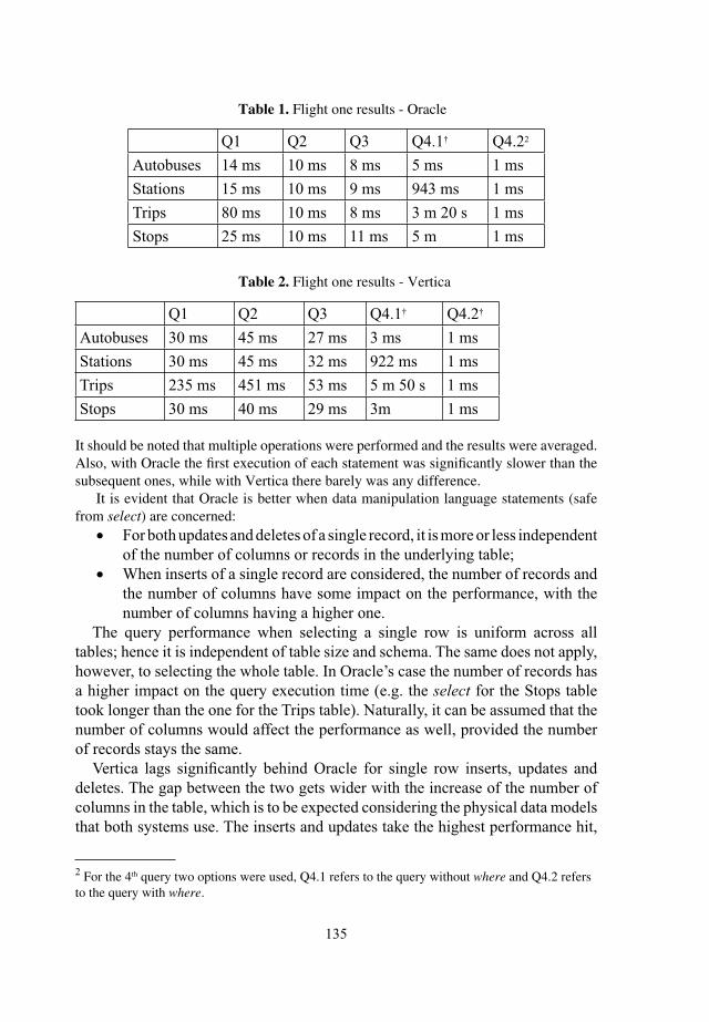
135

Table 1. Flight one results - Oracle2

Q1 Q2 Q3 Q4.1† Q4.22

Autobuses 14 ms 10 ms 8 ms 5 ms 1 msStations 15 ms 10 ms 9 ms 943 ms 1 msTrips 80 ms 10 ms 8 ms 3 m 20 s 1 msStops 25 ms 10 ms 11 ms 5 m 1 ms

Table 2. Flight one results - Vertica

Q1 Q2 Q3 Q4.1† Q4.2†

Autobuses 30 ms 45 ms 27 ms 3 ms 1 msStations 30 ms 45 ms 32 ms 922 ms 1 msTrips 235 ms 451 ms 53 ms 5 m 50 s 1 msStops 30 ms 40 ms 29 ms 3m 1 ms

It should be noted that multiple operations were performed and the results were averaged. Also, with Oracle the fi rst execution of each statement was signifi cantly slower than the subsequent ones, while with Vertica there barely was any difference.

It is evident that Oracle is better when data manipulation language statements (safe from select) are concerned:

• For both updates and deletes of a single record, it is more or less independent of the number of columns or records in the underlying table;

• When inserts of a single record are considered, the number of records and the number of columns have some impact on the performance, with the number of columns having a higher one.

The query performance when selecting a single row is uniform across all tables; hence it is independent of table size and schema. The same does not apply, however, to selecting the whole table. In Oracle’s case the number of records has a higher impact on the query execution time (e.g. the select for the Stops table took longer than the one for the Trips table). Naturally, it can be assumed that the number of columns would affect the performance as well, provided the number of records stays the same.

Vertica lags signifi cantly behind Oracle for single row inserts, updates and deletes. The gap between the two gets wider with the increase of the number of columns in the table, which is to be expected considering the physical data models that both systems use. The inserts and updates take the highest performance hit,

2 For the 4th query two options were used, Q4.1 refers to the query without where and Q4.2 refers to the query with where.

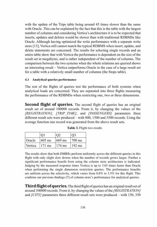
136

with the update of the Trips table being around 45 times slower than the same with Oracle. This can be explained by the fact that this is the table with the largest number of columns and considering Vertica’s architecture it is to be expected that inserts, updates and deletes would be slower than with traditional RDBMSs like Oracle. Although having optimized the write performance with a separate write store [13], Vertica still cannot match the typical RDBMS when insert, update, and delete statements are concerned. The results for selecting single records and an entire table show that with Vertica the performance is dependent on the size of the result set in megabytes, and is rather independent of the number of columns. The comparison between the two systems when the whole relations are queried shows an interesting result – Vertica outperforms Oracle in the case of a large result set for a table with a relatively small number of columns (the Stops table).

4.1 Analytical queries performance

The rest of the fl ights of queries test the performance of both systems when analytical loads are concerned. They are separated into three fl ights measuring the performance of the RDBMSs when restricting one, two or three dimensions.

Second �light of queries. The second fl ight of queries has an original result set of around 100000 records. From it, by changing the values of the [REGISTRATION], [TRIP_TIME], and [PASSENGERS] parameters three different result sets were produced – with 800, 1500 and 3500 records. Using the average function one record was generated from the above result sets.

Table 3. Flight two results

Q1 Q2 Q3Oracle 605 ms 669 ms 700 msVertica 171 ms 174 ms 192 ms

The results show that both DMBSs perform uniformly across the different queries in this fl ight with only slight slow downs when the number of records grows larger. Further a signifi cant performance benefi t from using the column store architecture is indicated. Judging by the measured response times Vertica is up to 3.65 times faster than Oracle when performing the single dimension restriction queries. The performance benefi ts are uniform across the selectivity, which varies from 0.8% to 3.5% for this fl ight. This confi rms our previous fi ndings [7] of column store’s performance for analytical queries.

Third �light of queries. The third fl ight of queries has an original result set of around 100000 records. From it, by changing the values of the [REGISTRATION] and [CITY] parameters three different result sets were produced – with 150, 350

137

and 750 records. Using the sum function three records were generated from the above result sets (i.e. the group by statement produced three groups).

Table 4. Flight three results

Q1 Q2 Q3Oracle 627 ms 697 ms 789 msVertica 207 ms 258 ms 267 ms

Again here we see that on small sets both DBMSs perform relatively the same regardless of the increasing number of records in each set. The reason most likely being the relatively small result sets in this group.

Varying the selectivity to lower the number of records in the original results sets to 0.15% - 0.75% shows that on such smaller results sets and more groups Vertica’s performance benefi t is slightly overcome, when compared to the previous fl ight of queries. It is still, however, around 3 times faster than Oracle in all the tests in this fl ight. It is interesting to compare Q3’s results with the ones for Q1 from the previous test, as the result sets are almost equal, meaning that the difference in performance could be attributed to the restriction on two and not on one dimension. The comparison shows that the performance is being signifi cantly impacted (0.6 times) by the restriction of both dimensions instead of just one.

Fourth �light of queries. The fourth fl ight of queries has an original result set of around 1750000 records. From it, by changing the values of the [AVAILABLE_SEATS], [DATE] and [DISTANCE] parameters three different result sets were produced – with 35000, 160000 and 870000 records. Using the sum function 3000, 8000 and 12000 records respectively were generated from the above result sets (i.e. produced by the group by statement).

Table 5. Flight four results

Q1 Q2 Q3Oracle 4 s 13 s 32sVertica 750 ms 1 s 1 s

In this fl ight we observe a large range of selectivity – between 2% and 50%. These results are very important, as they are more representative for typical data warehouse queries. Even the 50% selectivity, however, stays well within the limits of our previously discovered performance threshold of 80% [7].

When comparing the results for a single DBMS a uniform behavior throughout this fl ight for Vertica is seen. The situation for Oracle, however, is different with its performance degrading with the increase of the size of the result sets.

The results confi rm the superiority of Vertica over Oracle for queries targeting

138

data analysis; with the performance reaching a 32 fold gain for the highest selectivity query. The observations clearly show that the higher the selectivity, the larger the gap between Vertica and Oracle. Comparing the results from the second fl ight of queries where the selectivity is close to 2% (Q2 and Q3) with the one for Q1 from this fl ight indicates that the size of the result set plays a signifi cant role when the performance is considered, with the performance advantage of Vertica growing 1.5 times.

5 Conclusion

The purpose of this paper is to analyze the performance of analytical queries on commercial grade DBMSs - Oracle and Vertica. As a fi rst step in this some aspects of the data models and the query execution optimizations of the two are discussed.

Next, in order to make the performance comparison itself a new benchmark inspired by the SSB, is modeled. This allowed the inclusion of new queries, which are not part of the original benchmark and the usage of different, commercial data. Performing this new set of test fl ights gave interesting results for the performance of both systems. It can be concluded that the main disadvantage of a column store system in the face of Vertica is single row DML manipulations, safe from selects, as well as queries of non-analytical type – with large number of selected columns and rows. When analytical queries are considered, however, Vertica has a constant performance benefi t of around 3 folds, which grows higher with the result sets that are to be processed to reach 32 times the performance of Oracle for certain queries. Having that in mind we believe that Vertica is the better candidate for data warehouse solutions, as they are usually bulk loaded with records on a predefi ned period of time and are mostly used for read queries where it has signifi cant advantages over Oracle. For traditional transactional loads with lots of single row DML statements being issued constantly Oracle has superiority over Vertica and is our recommended DBMS.

Acknowledgment. This paper is supported by Sofi a University “St. Kliment Ohridski” SRF under Contract 43/2013.

References1. Abadi, D. et al.: Column-oriented database systems. Proceedings of the VLDB Endowment. pp.

1664–1665 (2009).2. Abadi, D.J., Madden, S.R.: Column-Stores vs . Row-Stores: How Different Are They Really?

SIGMOD. pp. 967–980 (2008).3. Codd, E.F.: A relational model of data for large shared data banks. Communications of the

ACM. 13, 6, 377–387 (1970).4. Garcia-Molina, H. et al.: Database Systems: The Complete Book. Pearson Prentice Hall, Upper

139

Saddle River, New Jersey 07458 (2009).5. Greenwald, R. et al.: Oracle Essentials Oracle Database 11g. O’Reilly Media, Inc., Sebastopol

(2008).6. Harizopoulos, S. et al.: Performance Tradeoffs in Read-Optimized Databases. Proceedings of

the VLDB Endowment. pp. 487–498 , Seoul, Korea (2006).7. Kyurkchiev, H., Kaloyanova, K.: Read Optimization Based on Column-oriented DBMS.

Doctoral Conference in Mathematics, Informatics and Education. pp. 58–66 St. Kliment Ohridski University Press (2013).

8. Lamb, A. et al.: The Vertica Analytic Database: C-Store 7 Years Later. Proceedings of the VLDB Endowment. pp. 1790–1801 (2012).

9. Loney, K.: Oracle Database 11g The Complete Reference. Oracle Press (2009).10. Neil, B.O. et al.: The Star Schema Benchmark and Augmented Fact Table Indexing Outline of

Talk. Performance Evaluation and Benchmarking, Lecture Notes in Computer Science. 5895, 237–252 (2009).

11. Neil, P.O. et al.: Star Schema Benchmark, (2009).12. Oracle, A., Paper, W.: Query Optimization in Oracle Database10g Release 2 Query Optimization

in Oracle Database 10g Release 2, (2005).13. Stonebraker, M. et al.: C-store: a column-oriented DBMS. Proceedings of the 31st VLDB

Conference. pp. 553–564 (2005).14. Oracle Database Concepts 11g Release 2 (11.2) - Logical Storage Structures, http://docs.oracle.

com/cd/E11882_01/server.112/e25789/logical.htm.15. The Vertica ® Analytic Database Technical Overview White Paper, (2010).

I � � � � � � S � � � �

143

Knowledge Management Software Application and Its Practical Use in the Enterprises

Ana Dimovska, Violeta Manevska, Natasha Blazeska Tabakovska

Faculty of Adminstration and Information Systems Management,University „St. Kliment Ohridski“ - Bitola,

Partizanska bb, 7000 Bitola, Republic of Macedoniaana.dimovska12@gmail.com, violeta.manevska@uklo.edu.mk, natasabt@gmail.com

Abstract. The aim of this paper is to contribute for raising the awareness of the enterprises for using knowledge management software application in order to improve their organization and to achieve greater success in their work. After the theoretical research, the practical research will be done in the enterprises in the Republic of Macedonia. The main research goal is to get a perception of familiarity and use of the knowledge management software applications in these enterprises. The expected results are that enterprises of the Republic of Macedonia are using knowledge management applications, but they are not paying enough attention on the importance and benefi ts which can get with this kind of application. This is the main hypothesis, we will see if this hypothesis is true after getting and processing the results.

Key words: Knowledge Management, Knowledge Management Software, Enterprises

1 Introduction

1.1 Knowledge Management Software Application

Knowledge in an enterprise is a set of people, skills, experiences, data, information, documents, routine behaviors, practices, norms and cooperation between members of the enterprise. An enterprise should properly manage all of these things in order to have effi cient and effective execution of its tasks and that can be done with the help of knowledge management.

There is no universally accepted defi nition of knowledge management. But there are numerous defi nitions proffered by experts. Simply put, knowledge management is the conversion of tacit knowledge into explicit knowledge and the process of sharing it within the organization. More technically and accurately, knowledge management is the process through which organizations generate value from their intellectual and knowledge based assets [1]. An enterprise’s ability to learn and to change, more important- to learn faster than other enterprises and turn the things learned into action, is the biggest advantage that

144

an enterprise can possess [2]. Other advantages of an enterprise are to collect, to store, to share, to distribute and to update all new knowledge in the enterprise. On this way, knowledge management process can work properly in order enterprise to achieve bigger success in their work.

Nowadays more and more enterprises are turning to modern and advanced operations. All of the working processes in the enterprises are increasingly computerized in order to obtain faster, simpler and accurate execution of the activities. In addition to business processes and activities, enterprises are beginning to computerize the knowledge they possess as well. This can be done by using appropriate software that helps enterprises to use their intellectual capital effectively. The knowledge management software application can distribute and maintain knowledge in an enterprise. The basic principle of knowledge management software application is to transfer knowledge in appropriate and easy to use format to the appropriate person, and this transfer to be made just in time for the goal of performing a given task.

Proper knowledge management software application should contribute for proper management of the whole enterprise, in a way that will be suitable for all members of an enterprise. By using a knowledge management software application, an enterprise should be able to identify, defi ne, organize, build and distribute all the knowledge in order to have a progressive and successful work.

What kind of knowledge management software application the enterprise will use depends from the size of the enterprise, the size of its activities, its business tasks, number of employees, and other factors which affect the daily execution of the tasks.

1.2 Need for Knowledge Management Software Application

Knowledge management is an audit of “intellectual assets” that highlights unique sources, critical functions and potential bottlenecks, which hinder knowledge fl ows to the point of use [3].

An enterprise that wants to use knowledge management software application needs to know what goals it wants to achieve by introducing this kind of software. If an enterprise starts using the software, that means that the enterprise realized how precious is the its intellectual capital and the knowledge which it possesses. Then the purpose of the enterprise is to handle properly with the resources it possesses and improve their performance.

Other need for using the knowledge management software application is the need to transfer the knowledge and improve the process regarding meeting the requests of the clients and to perform successful and on time executions of the daily tasks and operations. When enterprises have successfully working and proper execution of the tasks that means that the cooperation between all the employees is at a very high level.

145

Also enterprises have need for storing and sorting the big amount of information, data and documents. During their daily work, enterprises get many email messages, documents, articles, electronic newspapers, and new data for: clients, products, requests, information etc. Enterprises spend many hours for sorting, fi ltering, answering and managing with all these things. In order to avoid all these activities, enterprises can start using knowledge management software application.

Knowledge management software application can be used for storing and updating all the necessary information for employees- permanent and potential; for storing and updating information for the clients, the purchases, the clients’ requests and how their requests are changing in time. The same applies for the other data and information that comes from the internal and external environment. On this way, an enterprise can protect all the information and documents from loss, and managing with them can be done much easier and much faster. Also knowledge management can be used for achieving greater control over all operations and over all deadlines for completing the appropriate tasks. This software can be used for doing analysis, graphs and comparisons in order an enterprise to have a better understanding of the activities which happen in the enterprise. All of the things mentioned, and many others which can arise from the daily executions of the tasks and other factors, can be executed with the help of knowledge management software application.

1.3 Types of Knowledge Management Software Applications

Technology is a powerful enabler of knowledge management objectives [4]. New technology represented by software applications can be in the best service of knowledge management process in the enterprises, a process which without any doubt could be considered as one of the hottest research topics of the past decade [5]. Regarding innovation of the term and importance of the process of knowledge management, until now many knowledge management software applications are developed by software companies. Already developed software applications can be used in the enterprises, but also other enterprises can develop their own knowledge management software applications regarding their needs.

The knowledge management software application is not a software application with standard size, shape, look and actions that perform the same processes. Knowledge management software applications in different enterprises can differentiate very much one from another. This is due to the different activities of the enterprises and different intellectual capital that enterprises posses. Despite all the differences, knowledge management software applications in all enterprises can provide documentation of all the knowledge that enterprises poses for that knowledge to be used by authorized users across all the sectors and departments

146

of the enterprise. Knowledge management software application in the enterprise should support the generation, storage, update and distribution of knowledge.

International companies that produce knowledge management software applications are: Oracle, Kana, IBM, Apple, Google, EMC, SAS, Coveo, HP / HP Trim HP Enterprises services, ASG Software solutions, eTouch, Rivet Logic, Nuxeo, Bridgeway Software etc. [6].

Some knowledge management software applications that are developed from mentioned companies are:

- PHPKB (PHP Knowledge Base Software) is produced by PHP and it is leading software for knowledge management that offers assistance to clients through support and management of their knowledge databases. PHPKB software application provides statistical analysis of the knowledge that is crucial for making decisions regarding databases of the clients and provides professional manner using charts and diagrams where information and links between them can be easily seen. PHPKB software is one of the best softwares for location, selection and share of information. This software is suitable for enterprises that work with a lot of information. Despite databases in which much information can be stored, this software allows proper research that provides easy location of the searched information.

- SEM knowledge management software application is produced by software company Kana and it enables access to all databases in the enterprise, as well as other external databases. Another characteristic of this software is the contextual research that can be done in the internal and external databases.

- Smart Support software is produced by Safeharbor and it is software that can connect people with the proper answers. The software is intuitive, easy to integrate into web-based environment and offers advanced tools that can easily be managed. Also it can regulate and update the knowledge base.

- Novo Knowledge Base Software is produced by Novo Solutions. This software allows quick and safe access to the entire knowledge in the enterprise. This software is intended for enterprises that want to have a central repository of knowledge to which all employees can access. Also, service for training the employees is implemented in this software.

- Dezide Advisor software is produced by Dezide and it is web based software that is constantly in the service of their employees and customers. If employees have any questions or customers have requests, this software provides multiple solutions and answers to the questions. This software gives information, advices and answers to the requests and questions of the employees and customers, regarding data and information in its databases.

- Traction Teampage software is produced by Traction Software and it

147

enables easy communication, collaborative work, quick fi nding of the data etc. This software allows monitoring of activities, discussion and collaboration between different sectors in the enterprise and controls the execution of the activities of employees.

- XaitPorter software is produced by Xait and it commonly recommended for project activities. With this project management software, the team can constantly have full control over workfl ow and deadlines. This software can organize all activities and documents during the project. Enterprises can save 70 % of the time for doing documents, reports etc. by using this software.

These software applications satisfy different kinds of enterprises and their different daily problems and needs. Knowledge management is an interdisciplinary research issue. Thus, future knowledge management developments need integration with different technologies, and this integration of technologies and cross-interdisciplinary research may offer more methodologies to investigate knowledge management problems [7].

2 Practical Research

2.1 Research in an Enterprises in Republic of Macedonia

Through this research should be perceived the situation in the enterprises in the Republic of Macedonia, regarding familiarity with the term of knowledge management and the presence of the knowledge management software applications in the enterprises and their use. Besides receiving results, the research should emphasize the importance and needs of using knowledge management software application in the enterprises.

This research is done with questionnaires in 50 enterprises in Macedonia. The results are processed with SPSS statistic software application. The main hypothesis is that enterprises in the Republic of Macedonia are not familiar with the term of knowledge management and do not know what knowledge management software applications can be used in the enterprises. The sub hypotheses are that they store and update their information with software tools but they are not aware that that is part of the knowledge management software applications. Also they think that they need proper software tools for managing with their information, documents and other intellectual capital, i.e. they do not know that those tools are part of a knowledge management software application. Also they think that they will get improvement of their work if they have on disposal all necessary information, documents and have good collaboration between employees.

The research was done in 20 enterprises with number of employees from 1-9, 20 enterprises with 10-49 employees and 10 enterprises with 50-100 employees.

148

Fig. 1. Number of employees in the enterprises

More than a half declared that they connect knowledge with education, skills and experience of the employees. That means that enterprises do not know that all things mentioned above create the knowledge in the enterprise.

Fig. 2. What do you connect knowledge in the enterprise with?

30 of the responded enterprises declared that they store and update their knowledge with some software tools- this proves that the fi rst sub-hypothesis is correct.

Almost all- 48 of the enterprises declared that it is necessary for an enterprise to manage with its information, documents and other intellectual capital with software tools in order to have success. Thus, the second hypothesis is correct too.

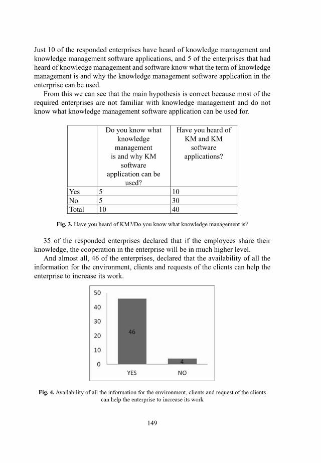
149

Just 10 of the responded enterprises have heard of knowledge management and knowledge management software applications, and 5 of the enterprises that had heard of knowledge management and software know what the term of knowledge management is and why the knowledge management software application in the enterprise can be used.

From this we can see that the main hypothesis is correct because most of the required enterprises are not familiar with knowledge management and do not know what knowledge management software application can be used for.

Do you know what knowledge

management is and why KM

software application can be

used?

Have you heard of KM and KM

software applications?

Yes 5 10No 5 30Total 10 40

Fig. 3. Have you heard of KM?/Do you know what knowledge management is?

35 of the responded enterprises declared that if the employees share their knowledge, the cooperation in the enterprise will be in much higher level.

And almost all, 46 of the enterprises, declared that the availability of all the information for the environment, clients and requests of the clients can help the enterprise to increase its work.

Fig. 4. Availability of all the information for the environment, clients and request of the clients can help the enterprise to increase its work

150

3 Conclusion

Regarding theoretical and practical research we can conclude that using knowledge management software applications in the enterprises is from crucial meaning for successful working and effi cient managing of all daily activities.

Knowledge management software applications can be used for storing the data, information, documents, articles, etc., for making analysis and comparisons, for answering the questions and requests of the employees and clients, for organizing all daily work and many other things. Different kinds of knowledge management software applications can execute and can be specialized for different kinds of actions.

Regarding the results from the research, many enterprises in the Republic of Macedonia haven’t heard about knowledge management and how knowledge management software applications can be used in the enterprises. Also, it is an interesting fact that enterprises are using some software tools for storing and updating the information and documents, but they do not know that these tools are part from knowledge management software application. Also they think that if they have on disposal proper software tool for managing the intellectual capital and organizing their work, they will get improvement of their work, but they do not know that these things can be executed with the help of knowledge management software application.

In conclusion, we can state that the awareness of the importance of using knowledge management software applications should be increased in the enterprises in the Republic of Macedonia. Increasing the awareness can be done with some initiatives that can be undertaken by software companies that can offer these kinds of software to the enterprises. Also initiatives can come from consultant companies and non-governmental organization which through trainings can contribute for raising the awareness of the importance of using knowledge management software application and relief the execution of the enterprises’ daily activities. Also these actions can be stimulated by Ministry of Information Society and administration through advising the enterprises for using these kind of software in order they achieve better performance and to have bigger success in their work.

We can concur that the future and the progress of one enterprise is found exactly in the suitable understanding and managing of the knowledge, which is one of the most valuable intellectual capital resources of an enterprise. Proper understanding and managing of the knowledge can be done more effi ciently by using knowledge management software applications.

151

References 1. Filemon, A.: Introduction to knowledge management; A brief introduction to the basic elements

of knowledge management for non-practitioners interested in understanding the subject, JR. Asean Foundation, (2008)

2. Mašić, B., Đorđević, B., J.: Menadžment znanja: Koncept za kreiranje konkurentske prednosti u novoj ekonomiji, Montenegrin Journal of Economics, 3(6), 101--108, (2008)

3. Bhojaraju, G.: Knowledge management: Why do we need it for corporates, Malaysian Journal of Library & Information Science, Vol. 10, No. 2, 38, (2005)

4. Tyndale, P.: A taxonomy of knowledge management software tools: origins and applications, Evaluation and program planning 25, 18--190, (2002)

5. Kalpic, B., Bernus, P.: Business process modeling through the knowledge managing perspective, Journal of Knowledge management, Academic Search Complete, EbscoHost., (2006)

6. Knowledge management software programs,http://www.capterra.com/knowledge-management-software/

7. Shu, H., L.: Knowledge management technologies and applications Literature review from 1995 to 2002, Expert systems with applications 25, 155—164, (2003)

152

Personalisation, Empowering the Playful, The Social Media Cloud

Mícheál Mac an Airchinnigh

Department of Computer Science, School of Computer Science and Statistics

University of Dublin, Trinity College, Dublin 2, Ireland

mmacanai@cs.tcd.ie

Abstract. Beyond the Cloud? It is easy to forget that the majority of humanity is not Cloud-included; indeed most are already beyond the Cloud. To be precise they have never, and will never be part of this thing we call the Cloud! The Cloud is Amazon; the Cloud is Apple; the Cloud is Google, the Cloud is…! In other words although the Cloud is, it is rarely present is most people’s consciousness. On the other hand, there are those, the technologically savvy folks, who have a private life enriched by the Internet and, of course, more generally by the Web. Everyone likes to have fun, even the scholarly folks. To see a play, to watch a movie, to listen to music, is part of everyone’s Digital Cultural Heritage, in 2013. To annotate, to investigate, to write about these experiences, is the classical activity of remembrance, enshrined nominally in the professional class of the Historian. Everyone who is Web-connected, and fully engaged in the social media, will want and need to remember, to record, the social experience. In this paper, the focus is on the Digital Access to Film/Video as viewed through the media of the open access Web sites, YouTube and VBOX7. A humanistic humanitarian perspective is defi ned to be those digital tools that permit the recording on suitable media for future recall, remembering, of past experience. Much of these Film/Video experiences must be freely available (Creative Commons License) if the people are to be rightly served with respect to their own culture, and more importantly, to embrace the culture of another. To be defi nite, one must present recognizable examples, not only in one’s own culture, but also, at the least, in the linguistic culture of another. Examples of said Film/Video material are given in Bulgarian and Italian Culture.

Keywords. Google goggles, IMDb, ontology, social media cloud, Wikimedia

1. Introduction

Let there be a fi xed point, an anchor, a place from which we can explore something of the nature of connected human experience with respect to commonplace entertainment? In olden times, this might have been a Theatre, a Library, a Cinema, a Sports arena, a School, and especially & exceptionally, an Institution of Ultimately Recognized Importance, (acronymed IURIU), such as a University (viz. University of Dublin, Trinity College, in Ireland & University of Sofi a, Bulgaria) or Technological Institution (acronymed IT) (viz. Dublin

153

Institute of Technology DIT [1] & Technical University of Sofi a [2]). Space is of the premium in publication. Each reader, of whatever culture, will naturally nominate equivalences of similar kinds of Institutions!

In this paper we continue our research in the general fi eld of Digital Cultural Heritage [3], and extend our focus to the individual personal online “art curator.” Naturally, everything is underpinned ontologically [4], in both English and Bulgarian. By Art, we include the traditional Plastic Arts [5], and by necessity the prominence of the more general category of the Visual Arts, which cover photography, video, and fi lm-making [6]. In our times, the latter embraces both YouTube [7] and VBOX7 [8].

Let us imagine that the current paper is built on earlier published work? Let us imagine, that in said previous work a photo taken from Flickr at that time was used to illustrate “The Bridge on the Drina?” [9]. That photo is no longer accessible (to the author alone?) Naturally, one suspects that either the contributor has not renewed the Flickr subscription, or the contributor has decided to try to monetarise it, or… A general Flickr search or even a Google Search or a Wikipedia Search will provide suitable alternative images [10]. But such a change requires not only the update of publication references but also the current ontology. Such updating in not automatic (yet).

Let us imagine that one is passionate about Bulgarian fi lms, or Italian fi lms, or Irish (Gaelic) fi lms, of a certain time and place? Do you, the reader, have a passion for such fi lms? If you are Italian, are you interested in Anglo-American fi lm? In Anglo-Irish fi lm? In Bulgarian-Italian fi lm? If your culture is narrowed to your birth language, what do you think of, and experience, the Culture of the Other, in fi lm? Watching a fi lm is easy. To understand what is going on, is a little bit more diffi cult, culturally. Trying to ontologize a fi lm is extremely hard. Naturally, there are available all the obvious ontological terms (in the corresponding natural languages). But for the fi lm genre, the ontologization is much more diffi cult than that of, say, the still photograph. Specifi cally, whereas each photograph is unique, one is obliged to select certain stills from a fi lm that captures something of its essence. What are the criteria for the choice of stills? For example, one might choose a classic photograph from the 1950-60 period in Bulgaria [11]. How shall this be ontologized? As a photograph? Certainly? As to the persons shown and location, it will take a little bit more research.

In practice, to ontologize a fi lm, one must be very familiar with it. Not only must one have watched it (perhaps several times), but more importantly, studied it carefully. The actors appear regularly, but with different makeup, dressup, scenario settings, such as swimming pool, bedroom, dinner table, dancing fl oor, and so on. To do this ontologization formally, one uses stills from a fi lm (for the visual record), one records both the actor’s name and the corresponding role name, one uses a Web database facility such as Amazon’s Internet Movie Database (IMDb) (in English, French, German, Italian) [12]. In particular, it turns

154

out that Wikipedia (with the corresponding Wikimedia) is undoubtedly one of the most import resources, especially with respect to the use of Google Goggles for visual recognition and identifi cation.

To capture the essence of the procedure of selecting a small number (5?) of stills to categorize (and ontologize) a fi lm, one suggests considering a preliminary analysis of still photography, covering in particular, images of Art. Furthermore, it seems advantageous to exploit the image recognition technology proved by Google Goggles, or similar.

1.1 Gathering the InformationConsider an artefact such as a colour poster of Ahinora 1925, painter Ivan Milev (1897—1927), the original of which is located in the Art Gallery of Kazanlak, done in tempera on cardboard, 86/66. The actual dimensions of the image on said poster are 40/30 cm. The original hangs like any other painting in the Gallery, except for one peculiar feature: it is covered with transparent glass. An excellent exhibition of the painting is available on Europeana [13]. A small grey scale picture developed from the original in Europeana is shown in Fig. 1. It is important to note that the original is seen by refl ected light. The version on Europeana “looks much better” because it is seen by directly transmitted light through the “Electronic Image.” Use of Google Goggles [abbreviated GG] correctly identifi es the painting in question, even if (and maybe because) it is in gray scale. On the other hand, use of GG on the poster also identifi es Ahinora. However, upon checking details, one notes that GG (usually?) takes us to the Wikimedia Commons [14]. In this particular case, it is the Ahinora 1922 which is displayed. Ahinora 1925 does not appear in Wikimedia Commons?

Figure 1. Ahinora, 1925 [GG +]

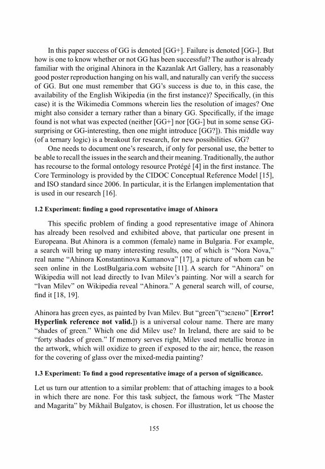
155

In this paper success of GG is denoted [GG+]. Failure is denoted [GG-]. But how is one to know whether or not GG has been successful? The author is already familiar with the original Ahinora in the Kazanlak Art Gallery, has a reasonably good poster reproduction hanging on his wall, and naturally can verify the success of GG. But one must remember that GG’s success is due to, in this case, the availability of the English Wikipedia (in the fi rst instance)? Specifi cally, (in this case) it is the Wikimedia Commons wherein lies the resolution of images? One might also consider a ternary rather than a binary GG. Specifi cally, if the image found is not what was expected (neither [GG+] nor [GG-] but in some sense GG-surprising or GG-interesting, then one might introduce [GG?]). This middle way (of a ternary logic) is a breakout for research, for new possibilities. GG?

One needs to document one’s research, if only for personal use, the better to be able to recall the issues in the search and their meaning. Traditionally, the author has recourse to the formal ontology resource Protégé [4] in the fi rst instance. The Core Terminology is provided by the CIDOC Conceptual Reference Model [15], and ISO standard since 2006. In particular, it is the Erlangen implementation that is used in our research [16].

1.2 Experiment: fi nding a good representative image of Ahinora

This specifi c problem of fi nding a good representative image of Ahinora has already been resolved and exhibited above, that particular one present in Europeana. But Ahinora is a common (female) name in Bulgaria. For example, a search will bring up many interesting results, one of which is “Nora Nova,” real name “Ahinora Konstantinova Kumanova” [17], a picture of whom can be seen online in the LostBulgaria.com website [11]. A search for “Ahinora” on Wikipedia will not lead directly to Ivan Milev’s painting. Nor will a search for “Ivan Milev” on Wikipedia reveal “Ahinora.” A general search will, of course, fi nd it [18, 19].

Ahinora has green eyes, as painted by Ivan Milev. But “green”(“зелено” [Error! Hyperlink reference not valid.]) is a universal colour name. There are many “shades of green.” Which one did Milev use? In Ireland, there are said to be “forty shades of green.” If memory serves right, Milev used metallic bronze in the artwork, which will oxidize to green if exposed to the air; hence, the reason for the covering of glass over the mixed-media painting?

1.3 Experiment: To fi nd a good representative image of a person of signifi cance.

Let us turn our attention to a similar problem: that of attaching images to a book in which there are none. For this task subject, the famous work “The Master and Magarita” by Mikhail Bulgatov, is chosen. For illustration, let us choose the

156

writer himself [Fig.2], and his fi rst wife Tatyana Lappa [Fig.1]. To ontologize these two portraits is a straightforward. Since the images are in Wikimedia, then Google Goggles recognizes them instantly. After Bulgatov divorced his fi rst wife (1924), he married Lubov Evgenevna Belozerskaya. There does not seem to be a picture of her in Wikimedia. However, there is a small portrait of her on a Ukrainian website (Kiev). Finally, he married a third time: Elena Sergeevna Shilovskaya [21]. Google Goggles is successful in recognizing the image, undoubtedly due to the Russian version of Wikipedia [22].

Fig. 1. Tatyana Lappa, 1910 [GG +] Fig2. Mikhail Bulgakov, 1930-39 [GG +]

2. Ontologizing Film/Video

In modern times, our times, electronic times, nothing seems to be beyond our reach! Let us now focus on the “Personal Curation” of the “Electronic Publication” of Film/Video, as currently exhibited by major and currently freely accessible “Cloud services” such as VBOX7 [8] and YouTube [7]. [Naturally, nothing is free! To access VBOX7 and YouTube requires some sort of Internet Connection, and for Quality of Video Service, one really must pay, even if it be a wired-up Coffee Shop!]. Commercial Film/Video services are deliberately excluded for the simple reason that, in academic articles such as these, there is always concern that one might infringe copyrights, even if the fair use convention is applied. A second reason is obvious. The author is familiar with, and uses, both VBOX7 [8] and YouTube [7], and these are (currently?) free (subject to the normal Internet Subscription).

However, given the nature of the struggle of owners to protect their rights and the users who prefer to pay nothing, there is no certainty of access to Film/Video. For example, the author has already published refl ections on Soap Operas such as the Bulgarian “Забранена любов (Forbidden love)” available on VBOX7 [8]. This particular Soap Opera was available for a time on YouTube [7] and subsequently

157

removed for “alleged copyright infringement, brought, presumably,” by the owner Nova Television. It is still accessible by direct connection to VBOX7 [23].

It is not easy to fi nd suitable “Copyright free” images to illustrate the potential of GG with respect to Film/Video. But is is possible. For example, there is a Wikipedia article available for the actress Omella Mutti, illustrated in Fig 3. [24]. The image is freely available because the photographer Rita Molná took it in Cannes, 2000, and contributed it to Wikipedia. Consequently, Google Goggles recognizes it.

Figure 3. Ornella Mutti (2000) [GG++]

There is another image of Ornella Mutti, accessible in the IMDb [Error! Hyperlink reference not valid.]. Naturally, the next task to determine to what extent GG will recognize images in a still of a fi lm wherein Ornella Mutti plays a part. To date, this have proved futile!

The author has already published refl ections on Soap Operas such as “Swimming Pool, 2003” which is listed in the IMDb [12]. Let us focus fi rst on the (universally not well known) actress, Ludivine Sagnier who plays the role of Julie. The really famous actress, of a certain maturity, can be readily identifi ed! To spell out the detail would be counter-productive to the theme of this article. Once recognized and/or identifi ed, the key information is then entered into a specifi c structure, EndNote (or similar structure), in the form of an electronic article:

(1) Author: IMDb (The defi nitive (English, French, German, Italian resource).(2) Title: “Film: Swimming Pool 2003” [26]. In this case, it is the well-known (in English circles) key actress who is listed, rather than the fi lm title and details.(3) Person: Ludivine Sagnier [Людивин Санье][BG included(4)

158

2. Observation on Signifi cance of Wikipedia

One of the modern ways to ascertain the state/status of a key technology is to determine whether or not is has a signifi cant article presence on Wikipedia. If it does have such a presence, then one further investigates the activity of the Wikipedia editors with respect to refreshing the text. What do the readers think about the article? For example, using our test case “Ahinora” we get…

Acknowledgements

References

1. Wikipedia Editors Dublin Institute of Technology. 2013.2. Wikipedia Editors Technical University of Sofi a. 2013.3. Krassimira Ivanova, et al., Access to Digital Cultural Heritage: Innovative Applications

of Automated Metadata Generation. 2012: Plovdiv University Publishing House “Paisi Hilendarski” 2012, Plovdiv, Bulgaria.

4. Stanford Center for Biomedical Informatics Research at the Stanford University School of Medicine. Protégé version 4.2. 0 (Build 295). 2013 [cited 2013; Available from: http://protege.stanford.edu/.

5. Wikipedia Editors Plastic Arts (A stub-class article from Wikipedia, the free encyclopedia). 2013.

6. Wikipedia Editors Visual Arts, A C-class article from Wikipedia, the free encyclopedia. 2013.7. Wikipedia Editors YouTube, A good article from Wikipedia, the free encyclopedia. 2013.8. Wikipedia Editors VBOX7, An unassessed article from Wikipedia, the free encyclopedia. 2013.9. danche24_ Flickr ID. The Bridge on the Drina. [Photograph]; Available from: http://www.

fl ickr.com/photos/danche24/240388816 [last access: unknown].10. blandm_ Flickr ID. The Bridge on the River Drina. [Photograph] 2006 [cited 2013 April 7];

Available from: http://www.fl ickr.com/photos/blandm/287891705 [last access: 2013-04-07].11. LostBulgaria.com “Джаз на оптимистите” с Ахинора Куманова (Нора Нова) в бар

“Астория”, краят на 50-те години на ХХ век. 2013.12. IMDb, Internet Movie Database, in Internet2013, Amazon.13. Europeana Ahinora. 2013.14. Wikimedia. Wikimedia Commons. Date of last access: 2013-03-29; Available from: http://

commons.wikimedia.org.15. Wikipedia Editors CIDOC Conceptual Reference Model. 2013.16. Bernhard Schiemann, M.O., Günther Görz,, Erlangen CRM / OWL (CIDOC-CRM 5.0.4),

2013, Friedrich-Alexander-University of Erlangen-Nuremberg, Department of Computer Science, in cooperation with the Department of Museum Informatics at the Germanisches

159

Nationalmuseum Nuremberg and the Department of Biodiversity Informatics at the Zoologisches Forschungsmuseum Alexander Koenig Bonn.

17. Wikipedia Editors Nora Nova, A stub-class article from Wikipedia, the free encyclopedia. 2013.

18. Ivan Milev, Ahinora 1925, 1925.19. WikiPaintings Ahinora. 2013.20. Уикипедия Зелен цвят. 2013.21. Jan Vanhellemont, B.-L.-R.-M. Person: Elena Sergeevna Shilovskaya. 2012.22. Wikipedia Editors RU, Булгакова, Елена Сергеевна, 2013.23. Netinfo Netinfo. 2013.24. Wikipedia Editors Person: Ornella Muti, A start-class article from Wikipedia, the free

encyclopedia. 2013.25. IMDb [Photo by Jeff Vespa – © WireImage.com – Image courtesy WireImage.com] Person:

Ornella Muti 2009.26. Wikipedia Editors Person: Charlotte Rampling, A start-class article from Wikipedia, the free

encyclopedia. 2013.

160

Intelligent Approach for Automated Error Detection inMetagenomic Data from High-Throughput Sequencing

Milko Krachunov1, Maria Nisheva1, and Dimitar Vassilev2

1 Faculty of Mathematics and Informatics, Sofia University “St. Kliment Ohridski”, Sofia, Bulgaria2 Bioinformatics group, AgroBioInstitute, Sofia, Bulgaria

milkok@fmi.uni-sofia.bg

Abstract. Metagenomics is a new, rapidly developing and largely unexplored field that is focused on the

study of genetic material collected from heterogeneous environmental biological samples. Due to the nature

of the data acquired from these samples, metagenomic research is very sensitive to the quality of the data.

Sequencing errors can have a particularly large impact in studies dealing with rare mutations. Unfortunately,

most error detection algorithms in NGS are intended for homogeneous datasets like those found in de novo

genome sequence, and as such are not suitable for metagenomics without modifications. Our work is focused

on the development of an improved error detection approach intended for metagenomics that is based on the

use frequencies weighted by local sequence similarity, and the generalisation of the same measures for use in

machine learning.

Key words: Metagenomics, Error detection, Artificial neural networks, Genomic sequence workflow

1 Introduction

1.1 Problems in metagenomics

Metagenomics deals with the study of mixed genetic material collected in samples of hetero-

geneous biological environments such as soils, water basins and the insides of various macro-

organisms. The microbial communities in all these environments remain largely unexplored,

presenting the researchers with both research opportunities and technical challenges. [12, 9, 10]

Comparative analysis of such microbial communities is crucial for the study of issues rang-

ing from human health [7] to bacterial and viral evolution. [5] Results from metagenomic stud-

ies can have an effect on our understanding of the history of the biosphere as well as dealing

with potential future threats. Micro-organisms are the most rapidly mutating agents in nature,

which makes them the largest factor in unexpected disease outbreaks. At the same time, the

rapid mutation rates provide an unique insight on evolutionary processes.

The sequenced metagenomic samples are comprised of digital data about a large number

of organisms from a variety of species, a large portion of which are presently unknown or

understudied. The data lacks any inherent reference points or a standard for validation, which

further exacerbates the computational and methodological challenges associated with it, a large

part of which are yet to find well-established solutions.

Error detection and correction is still one of the main problems, as reading errors are in-

evitable and the heterogeneous nature of the data makes the direct use of de-noising methods

from high-throughput de novo sequencing very difficult. At present, researchers have to deal

with these deficiencies in the quality, and often resort to the exclusion of any data that is sus-

pected to contain errors. A software solution to reliably flag the potential errors, estimate their

probability and correct them when possible will dramatically increase the useful data for many

research studies, and will improve the quality in the rest.

161

1.2 Our project and goalThe goal of our project is the development of a new error detection method suitable for metage-

nomic data. Like canonical de-noising and consensus sequence construction methods, we utilise

the frequency counts of the different bases to estimate the possibility of an error at a given posi-

tion. Unlike them, however, we introduce a measure of the local sequence similarity to account

for the heterogeneous nature of the data, which can often contain distinct sequences coming

from various species that are all sequenced correctly. The similarity can be used to distinguish

between other instances of the same sequence, highly preserved homologous sequences and

totally unrelated sequences.

We are working on two approaches to take local similarity into account. We have imple-

mented a purely analytical method, which uses the frequency of each evaluated base weighted

by a measure of the local similarity in a window around the evaluated position. We are also

working to identify and summarize the information about sequence matches and local simi-

larity used in this approach to construct an artificial neural network. Our work in progress is

focused on splitting the match data into similarity bins which aim to provide a good trade-off

between computational tractability and loss of relevant information.

The greatest challenge in the development of new error detection methods has been the

validation. It is difficult to obtain a pristine metagenomic test data set that is representative of

a real-world one, which makes direct validation difficult. To deal with this, we have proposed

two methods for indirect validation of the results. One uses artificially simulated errors inside

a two-phase procedure with repeated application of error correction, and the other uses a very

large dataset and its subset. During preliminary tests, the validation procedures have confirmed

the viability of our analytical approach.

The ability to apply them on freshly sequenced data makes these methods suitable not

only for simple verification of the proposed analytical approach, but also for the training of an

artificial neural network and machine learning solutions in general, which would be difficult if

only small number of verification data sets were available.

In the development process, we are also working on a genomic workflow software package

to help us with the neural network implementation and training, as well as be used for other

metagenomic and genomic computational experiments.

The nature of genomic data, with its many unstructured relationships, makes the task of

error detection a suitable one to apply and use machine learning algorithms, and in particular

neural networks which can be used to infer the correctness of the data from the sets of data that

are otherwise difficult to navigate.

2 Material and methods2.1 The input data16S RNA is very popular for metagenomic analysis, because it is highly conserved and thus

largely similar across a great deal of species, while at the same time it contains hypervariable

regions that are helpful for identifying distinct species, individual organisms as well as finding

their evolutionary relationships. [11]

The sample datasets for our experiments contain short reads between 300 and 500 bases

in length, divided in sets of tens of thousands of sequences between 20000 and 50000 after

filtering them by length and quality. All our sample dataset were sequenced using the Roche

454 platform, which produces reads of length suitable for metagenomic experiments.

162

2.2 Analytical approach for error detection

After the data has been aligned and before it is ready for computational studies, reads or posi-

tions containing errors have to be filtered out to ensure high-quality results. To filter them out,

sequencing equipment errors and biological errors during amplification need to be differenti-

ated from mutations which can be found in correct reads.

An analytical approach to error detection is outlined below and described in more detail in

[4, 3].

The naıve approach. A common approach to distinguish mutations from errors is to measure

their frequency of appearance. Errors have a higher probability of being unique, while mu-

tations will have either reproduced in other organisms or will appear in other reads from the

same organism. This means that erroneous bases will be found at lower rates than mutations.

The naıve way to use this is to count the rates of occurrence of each base in each column. The

bases that appear less often than a threshold that was established beforehand can be considered

errors.

To achieve this, we define a score(r, k) function that evaluates to the frequency of occurence

of the base rk from read r at position k in the remaining reads R \ {r} in the set R.

To extend this to error correction, one needs to simply replace the bases deemed incorrect

with the base that would get the highest score. The newly constructed error correction will

be nearly identical to consensus construction during de novo sequencing or resequencing of

genomes, which relies on always selecting the bases that appear most often. [14]

Similarity-based approach. The naıve approach is not suitable for a dataset containing multi-

ple distinct organisms. To take into account the heterogeneous nature of the data and deal with

such rare sequences and competing options, we propose an improved method that extends the

naıve one. In our proposal, we will still count the frequencies of each base, but we take the

context around each base into account by estimating the similarity between the sequence pairs.

Our proposal for similarity-based evaluation tries to give precendence to mismatches be-

tween similar reads over mismatches between dissimilar reads by making the importance of

a mismatch proportional to the similarity. This similarity is calculated in a proximity of the

evaluated position. These goals and the premise they were based on will be used as a starting

point during the design of the artificial neural network described later in the article.

�������������������������������

����

��

��

����

��

��

Fig. 1. Exponentially-decreasing similarity by position weight

We create a window around each evaluated position, and we calculate a similarity score

inside the window for all n(n − 1)/2 pairs of sequences. In the similarity, the positions away

from the centre of the window are added with an exponentially decreasing position weight.

This score is then used as a similarity weight during the calculation of a weighted frequency of

occurence, getting the following “similarity” score:

163

n,r �=p∑r=0

similarity weight︷ ︸︸ ︷⎛⎝we,i �=k∑

i=ws

q|k−i|︸ ︷︷ ︸position weight

[ri = pi]

W (i)

⎞⎠ [rm = pm]

N(r)(1)

The parameter q is experimentally evaluated, w is the size of the window, and N(r) and

W (i) are normalizing functions ensuring that the respective sums would yield 1 if the nomina-

tors were replaced with 1.

To extend the similarity-based approach to error correction we can simply apply the score

formula (1) for all potential replacement bases for the given position.

2.3 Approaches for error validation

As mentioned earlier, it is difficult to obtain a reliable test metagenomic dataset that is verified

and that is a representative of a real set that would come out of the sequencing equipment.

Machine learning in particular requires larger amount of test data which further increases this

difficulty. To go around this difficulty, we are presenting two indirect methods for validation.

The rationale for the need and choice of such roundabout methods is described in [4, 3].

Validation through repeated application approach. It is difficult to reliably simulate se-

quencing runs, but it is simple to simulate errors in a similar pattern to the ones that produced

by the sequencing equipment. You can estimate the error patterns by sequencing sets of known

sequences and comparing the sequenced to the known ones. We will call the record of this

pattern an error profile.

Using simulated errors, one can indirectly validate an error detection approach and compare

it against another. The goal to create a better error detection approach can be stated as the goal

to create an error detection with less false positives for the same amount of false negatives. In

other words, the better error detection approach should flag less correct data as incorrect under

the settings with which it properly identifies the same number of real errors.

Given an error profile E and an error detection method ϕ we can use the similated errors

for validation in the following way. We acquire a fresh dataset 0e, correct it with ϕ, producing

the corrected dataset 1. We artificially introduce errors according to E , producing a second base

dataset 1e which we correct for a second time with ϕ to produce the final set 2. We evaluate the

corrections done in 0e → 1 and 1e → 2, including the missed simulated errors in the latter.

This procedure yields two useful figures. If the error profile E is correct, the comparison

between 1, 1e and 2 gives an accurate estimate of the false negatives. The amount of missed

simulated errors should be roughly the same as the amount of missed real errors. At the same

time, the difference between dataset 0e and dataset 1 gives you the total amount of corrections

made.

These two figures can be used to indirectly measure and compare the false positives of two

approaches. If the better approach under validation leads to the same number of false negatives

yet makes less corrections overall, this means that the number of false positives must have also

decreased, and indeed our better approach meets the goal to produce less false positives for thesame amount of false negatives.

164

Validation through a subset approach. One difficulty in obtaining a test dataset in metage-

nomics is the difficulty in resampling the exact same sample again. If you could sample the

same data over and over, you would end up with enough data to correctly identify all the se-

quences present. Similarly, if you have more data about a sample, the information that you have

is closer to being confirmed than if you have less data. One way to estimate the reliability of an

error detection would be to see how it performs with less data, if more data does not happen to

be available.

2.4 Extending the analytical approach and validation to a neural network

The formulaic dependency between the data and the resulting error flagging decisions and the

presence of many hidden factors in the input data that are difficult to asses make the problem

suitable for exploring a solution using an artificial neural network. The largely unexplored sets

of data with their many unknown relationships make the large inference capabilities of neural

networks a very appropriate choice for a machine learning instrument. The very chaotic, tangled

and unstructured relationships inside genomic data, are not always easy or even possible to map

using analytical methods.

The availability of a validation method that can be applied to any sequenced dataset opens

the possibility for training machine learning systems, in particular neural networks, to discover

errors. To make use of this opportunity, we are working on the implementing a neural network

design that extends the ideas on which our analytical approach is based.

Data input. To design a neural network that performs the task of error detection in a spirit

similar to our analytical approach, we need to summarize the information for sequences in

each column or window in a way that’s both suitable for neural network input and retains the

characteristics that are necessary to find the errors. If we provide too little input, our neural

network would be doing little more than finding a threshold, if we provide too much input,

we end up with a huge variable-input network that’s both impossible to train and extremely

unreliable.

Input generalised by similarity. Our reasoning thus far has been that two similar sequences are

more likely to confirm each other than two different sequences. Directly applying this to our

neural network design, we would split the match rate into bins classified by the rate of local

similarity in the window. This, however, has a significant downside the measure for similarity

won’t be part of the machine learning, which would render the entire machine learning process

much less useful.

Input generalised by similarity and offset. To account for this and make the similarity part of

the learning process, we introduce match bins for the separate offsets as seen on figure 2. As

our original measure for similarity was weighted by the offset, for each offset we provide three

separate input bins for the similarity at that offset. The first three inputs contain the match rate

(of the evaluated position) in sequences that have 0, 1 or 2 differences at offset 1, the next three

inputs contain the match rate in sequences that have 0, 1, or 2 differences at offset 2, and so on.

This has the downside that the similarities at different offsets are now independent, and the

neural network can’t utilise information about chains of dissimilarity.

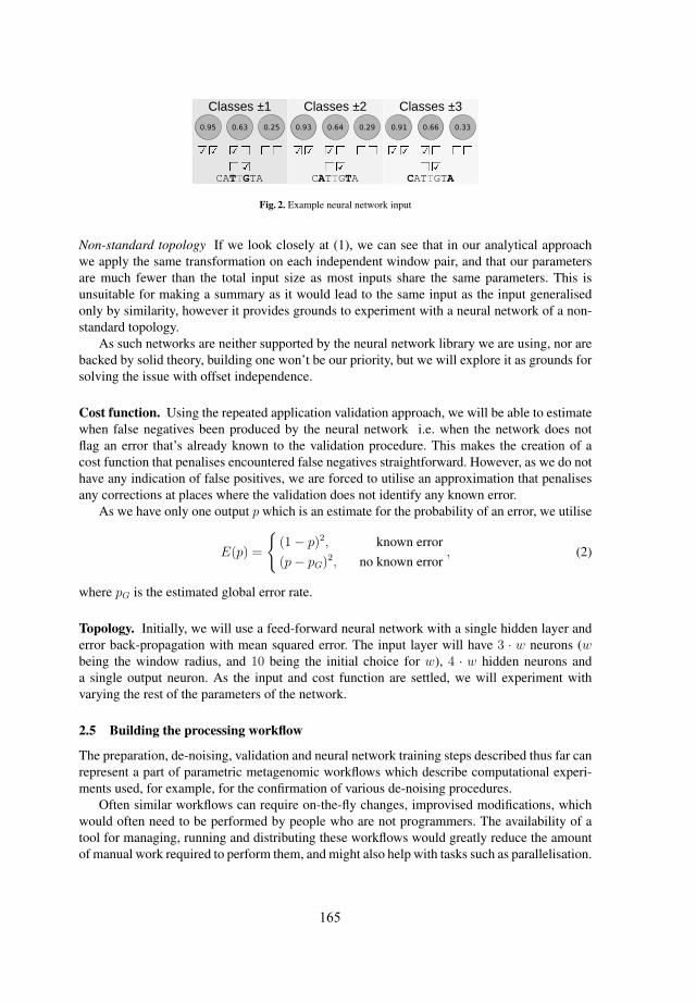
165

���� ���� ������� ���� ���

��������� ���������

CATTGTA CATTGTA

��� ���� ����

����������

CATTGTA

Fig. 2. Example neural network input

Non-standard topology If we look closely at (1), we can see that in our analytical approach

we apply the same transformation on each independent window pair, and that our parameters

are much fewer than the total input size as most inputs share the same parameters. This is

unsuitable for making a summary as it would lead to the same input as the input generalised

only by similarity, however it provides grounds to experiment with a neural network of a non-

standard topology.

As such networks are neither supported by the neural network library we are using, nor are

backed by solid theory, building one won’t be our priority, but we will explore it as grounds for

solving the issue with offset independence.

Cost function. Using the repeated application validation approach, we will be able to estimate

when false negatives been produced by the neural network i.e. when the network does not

flag an error that’s already known to the validation procedure. This makes the creation of a

cost function that penalises encountered false negatives straightforward. However, as we do not

have any indication of false positives, we are forced to utilise an approximation that penalises

any corrections at places where the validation does not identify any known error.

As we have only one output p which is an estimate for the probability of an error, we utilise

E(p) =

{(1− p)2, known error

(p− pG)2, no known error

, (2)

where pG is the estimated global error rate.

Topology. Initially, we will use a feed-forward neural network with a single hidden layer and

error back-propagation with mean squared error. The input layer will have 3 · w neurons (wbeing the window radius, and 10 being the initial choice for w), 4 · w hidden neurons and

a single output neuron. As the input and cost function are settled, we will experiment with

varying the rest of the parameters of the network.

2.5 Building the processing workflow

The preparation, de-noising, validation and neural network training steps described thus far can

represent a part of parametric metagenomic workflows which describe computational experi-

ments used, for example, for the confirmation of various de-noising procedures.

Often similar workflows can require on-the-fly changes, improvised modifications, which

would often need to be performed by people who are not programmers. The availability of a

tool for managing, running and distributing these workflows would greatly reduce the amount

of manual work required to perform them, and might also help with tasks such as parallelisation.

166

We intend to wrap all utilised methods and middleware into a free software package that can

be extended to a package aimed at the execution of such workflows.

An example of such execution is shown on figure 3, which is a slightly advanced version of

the workflow presently utilised to process the data.

��������� ��

������������������ ������

������� ����������������

���������� ����������

��������� ����������

!�������������������

������������������ ������

"�� �� ������#"$$�

#"$$����� #"$$�����

#"$$���� #"$$�����

!�������������������

!��������������

%��������������

&�����������������

Fig. 3. Example workflow

3 Results and discussion

3.1 Experimental results

On a test run of 4540 sequences, we performed both correction with the similarity-based ap-

proach and correction with the naıve approach. The naıve approach produced 673 corrections,

while the similarity-based produced only 607, or 66 less, which is a 10% decrease.

We then simulated errors using our estimated error profile, and then ran the error correction

approaches again. As seen on figure 4 in the set initially corrected by the naıve approach, the

false negatives were 34 for both, while in the set initially corrected by the similarity-based

approach, the false negatives were 33 for both.

This result is consistent with our expectation for a decrease in the number of overall correc-

tions for the same number of false negatives.

During the second correction we had a counter of the false positives as well. There were

virtually no false positives on the set initially corrected with the naıve approach which is to be

expected if you assume that it had already corrected all the correct data possible on the first run.

The set initially corrected with the similarity-based approach had 67 new errors introduced by

the naıve one the potential 66 false positives that it created on the first run, while only 18 new

false positives were created by the similarity-based approach.

It is clear that more computational experiments are required for the comparison between

the two approaches to be really significant, which is what our workflow library is intended to

facilitate, together with the training of the artificial neural network that is being developed.

167

�������������� �����

����������� �����

�������������� �����

����������� �����

�������������� �����

����������� �����

��������������

��������������

�� ����������

��� ���������� ��� ����������

�� ����� ���������� ����� �������

�� ����� ���������� ����� �������

� ����� ��������� ����� �������

� ����� ��������� ����� ������

! � ��"������

Fig. 4. Repeated application validation approach

The results from running the subset approach on small datasets proved to be inconclusive

showing the need of much larger datasets.

3.2 Software package

The tasks of preprocessing, error detection and correction, validation, and neural network train-

ing are handled by a software package written in Python. The middleware that is used to start

the tasks and execute external software is presently being rewritten to use the Twisted network-

ing framework. [13]

For the processes of sequence clustering and alignment, the software package is interfacing

with the CD-HIT-454 [6] clustering software. and the MAFFT [2] and MUSCLE [1] alignment

software packages.

The neural network is being developed using the Python FANN library. [8] The YAML

markup language is intended to be used for workflow descriptions.

4 Conclusions

The suggested method for improvement of error detection, during our experimental validation,

showed results consistent with our expectations in case of an improvement in the quality. This

would suggest that the use of sequence similarities is beneficial to error detection.

The core of the workflow library in development would allow the execution of multiple

validation experiments that would lead to a more significant confirmation of this result. It will

also provide the means for the training of an artificial neural network as another means to

approach the problem of error detection. The neural network will also provide a comparison

for the quality of the results of our analytical approach.

The nature of the data, being largely inter-related yet not well explored, as well as the need

to define a formulaic dependence between the input data and the error determinations, make

neural networks a suitable instrument to approach the problem.

The workflow library core can be used as a basis for a general-purpose workflow library that

would have an useful utility in many metagenomic and other genomic computational studies.

168

Acknowledgements

This work was supported by the European Social Fund through the Human Resource Develop-

ment Operational Programme under contract BG051PO001-3.3.06-0052 (2012/2014).

References

[1] Edgar, R.: MUSCLE: a multiple sequence alignment method with reduced time and space

complexity. BMC Bioinformatics 5(1), 113 (Aug 2004)

[2] Katoh, K., Kuma, K., Toh, H., Miyata, T.: MAFFT version 5: improvement in accuracy

of multiple sequence alignment. Nucleid Acid Research 33(2), 511–518 (2005)

[3] Krachunov, K., Vassilev, D.: An approach to a metagenomic data processing workflow.

Journal of Computational Science 4 (2013), [submitted]

[4] Krachunov, M., Petrov, P., Popov, I., Vassilev, D.: Computational challenges in a metage-

nomics processing pipeline. In: Proceedings of the 6th International Conference on Infor-

mation Systems & Grid Technologies (ISGT). pp. 302–311. Sofia (Jun 2012)

[5] Kristensen, D., Mushegian, A., Dolja, V., Koonin, E.: New dimensions of the

virus world discovered through metagenomics. Trends in Microbiology 18(1),

11–19 (Jan 2010), http://www.biomedsearch.com/nih/New-dimensions-virus-world-

discovered/19942437.html

[6] Li, W., Godzik, A.: Cd-hit: a fast program for clustering and comparing large sets

of protein or nucleotide sequences. Bioinformatics 22(13), 1658–1659 (Jul 2006),

http://bioinformatics.oxfordjournals.org/content/22/13/1658.full.pdf

[7] Nelson, K., White, B.: Metagenomics and its applications to the study of the human mi-

crobiome. Metagenomics: Theory, Methods and Applications pp. 171–182 (2010)

[8] Nissen, S., Spilca, A., Zabot, A., Morelli, D., Nemerson, E., Freegoldbar, Megidish, G.,

Joshwah, M., Pereira, M., Vogt, S., Hauberg, Leibovici, T., Massa, V.: Fast artificial neural

network library (2006), http://leenissen.dk/fann/, [Online; accessed 4 May 2013]

[9] Thomas, T., Gilterr, J., Meyer, F.: Metagenomics - a guide from sampling

to data analysis. Microbial Informatics and Experimentation 2(1), 3 (2012),

http://www.microbialinformaticsj.com/content/2/1/3

[10] Valverde, J., Mellado, R.: Analysis of metagenomic data con-

taining high biodiversity levels. PLoS ONE 8(3) (2013),

http://www.plosone.org/article/info:doi/10.1371/journal.pone.0058118

[11] Weisburg, W., Barns, S., Pelletier, D., D.J, L.: 16S ribosomal DNA amplification for phy-

logenetic study. J. Bacteriol. 173(2), 697–703 (Jan 1991)

[12] Wooley, J., Godzik, A., Freiedberg, I.: A primer on metagenomics. PLoS Compt. Biol.

6(2), 289–290 (Feb 2010)

[13] Zadka, M., Lefkowitz, G.: The twisted network framework. 10th International Python

Conference (2002), https://twistedmatrix.com/users/glyph/ipc10/paper.html, [Online; ac-

cessed 16 April 2013]

[14] Zerbino, D., Birney, E.: Velvet: algorithms for de novo short read assembly using de

Bruijn graphs. Genome Res. 18(5), 821–829 (2008)

169

Semantic Digital Librarywith Bulgarian Folk Songs

Maria Nisheva-Pavlova, Pavel Pavlov, Dicho Shukerov

Faculty of Mathematics and Informatics, Sofi a University St. Kliment Ohridski5 James Bourchier blvd., Sofi a 1164, Bulgaria

{marian, pavlovp, shukerov}@fmi.uni-sofi a.bg

Abstract. The paper discusses some results obtained within the work on a project aimed at the development of technologies for digitization of Bulgarian folk music and building a digital library with Bulgarian folk songs presented with their music, texts and notes. This library provides digital preservation of the sound recordings, lyrics and notations of more than 1000 Bulgarian folk songs and tools for various types of search and analysis of the available resources. The presentation is focused on the main features of the discussed library describing it as a semantic one – the subject ontology especially developed for the occasion and its application in the implementation of a tool for intelligent search in the lyrics of songs.

Keywords: Semantic digital library, metadata, ontology, search engine, document retrieval.

1 Introduction

One of the most promising directions of research in Digital Libraries of late years is related to the development of semantic digital libraries.

Semantic digital libraries [1 – 4] are digital library systems that apply semantic technologies to achieve their specifi c goals. Ontologies play a major role to overcome the variety of problems caused by the structural differences of existing systems, the semantic differences of metadata standards and the necessity to support intelligent search and information retrieval tasks. Within the context of semantic digital libraries, ontologies can be used to:

• organize bibliographic descriptions;• represent and expose document contents;• share knowledge amongst users. Ontologies are used in building semantic annotations of the information

resources available on the Semantic Web.The support of functionalities for intelligent search [5, 6], also known

as semantic search, is one of the main features of semantic digital libraries. Ontologies play a key role in this kind of search.

Together with the considerable results within the last decade, the developers

170

of semantic digital libraries and means for access to their content are still faced with a number of challenges. A signifi cant challenge continues to be the provision of most precise and rich in content results of the user queries. A next serious challenge is the necessity of development of search methods and techniques which will be appropriate for sets of materials containing documents of different types and multiform content, available in various electronic formats. There are lots of open questions concerning the applicability of ontologies in building semantic search engines, some undecided personalization issues, etc.

The paper discusses some results of the activities within a project aimed at the development of technologies for digitization of Bulgarian folk music and building a semantic digital library (named DjDL) with Bulgarian folk songs presented with their notes, text and music. DjDL serves as a platform for digital preservation of the sound recordings, lyrics and notations of a multitude of Bulgarian folk songs and to provide adequate access to them. The emphasis of the presentation falls on the provided tool for semantic (ontology-based) search in the lyrics of songs.

2 Objectives

The discussed project is aimed at the development of methods, technologies and corresponding software tools intended to satisfy some of the IT needs of researchers of musical folklore in the fi elds of linguistics, ethnology, ethnomusicology, etc. To realize these objectives, an IT environment for digitization of music notations, especially adapted for the notation of Bulgarian national music, and a heterogeneous database with notations, lyrics and music have been developed [7]. The notations, texts and fi eld recordings of approximately 1100 folklore songs from the Tracia region have been digitized [8].

The research activities of the authors of this paper have been oriented to:• study of the key features of the domain and development of proper functional

model of a digital library with Bulgarian folklore music;• development and application of information technologies for building digital

libraries, methods and tools for search (in particular, semantic search) in heterogeneous digital libraries.

As a result, a prototype of the semantic digital library DjDL was created. DjDL preserves Bulgarian folk songs presented with their notes, text and music and provides adequate access to the treasured digital content.

3 Main Characteristics of the Library Resources and Software Architecture of the Digital Library System

Currently DjDL contains a collection of over 1000 composite digital objects which represent a considerable part of the unpublished archive manuscripts of Prof. Todor Dzhidzhev.

171

The functional structure of DjDL is shown in Figure 1.The library (metadata) catalogue consists of short descriptions in XML

format of the folk songs included in the repository. As typical examples of metadata about folk songs we could mention: the title of the song, the song genre in accordance with different classifi cation schemes, the region of folk dialect, the informant (the person who conveyed the song to folklorists), the folklorist who gathered the song, the singer(s), the date and place of record, etc.

Figure 1. Functional structure of DjDL

The repository of DjDL includes composite digital objects which present Bulgarian folk songs. The single components of these objects contain respectively:

• the lyrics of songs;• the notations of songs in the text format supported by LilyPond [7];• musical (MP3) recordings of the authentic performances of the songs;• musical (MIDI) fi les generated with the use of LilyPond from the notations

of the songs.The subject ontology consists of several interrelated subontologies which

play a signifi cant role in the implementation of the full functionality of the search engine. It includes concepts of different areas relevant to the contents of the lyrics of songs, with description of their properties and different kinds of relationships among them. It plays a signifi cant role in the implementation of the full functionality of the search engine.

The purpose of the search engine is to provide adequate access to the variety of resources stored in the repository of DjDL. Its current version supports two kinds of search in the lyrics of songs: keywords-based and semantic search. The search engine of DjDL also uses two proper dictionaries available in digital (XML) format – a dictionary of synonyms and a dictionary of obsolete and dialect words.

172

4 Metadata and Catalogue Descriptions

The set of metadata about folk songs used in DjDL was determined in accordance with the requirements of some international standards (the Text Encoding Initiative (TEI) and the Encoded Archival Description (EAD)) and classifi cation schemes in combination with the characteristics of the national tradition. According to the EAD standard, each catalogue entry contains the text (i.e., the lyrics) of a particular song accompanied with the corresponding metadata.

Figure 2 illustrates the catalogue description of a song performed by a group of three singers.

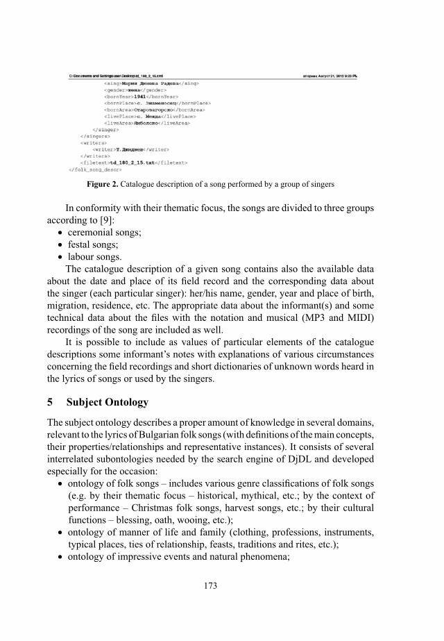
173

Figure 2. Catalogue description of a song performed by a group of singers

In conformity with their thematic focus, the songs are divided to three groups according to [9]:

• ceremonial songs;• festal songs;• labour songs.

The catalogue description of a given song contains also the available data about the date and place of its fi eld record and the corresponding data about the singer (each particular singer): her/his name, gender, year and place of birth, migration, residence, etc. The appropriate data about the informant(s) and some technical data about the fi les with the notation and musical (MP3 and MIDI) recordings of the song are included as well.

It is possible to include as values of particular elements of the catalogue descriptions some informant’s notes with explanations of various circumstances concerning the fi eld recordings and short dictionaries of unknown words heard in the lyrics of songs or used by the singers.

5 Subject Ontology

The subject ontology describes a proper amount of knowledge in several domains, relevant to the lyrics of Bulgarian folk songs (with defi nitions of the main concepts, their properties/relationships and representative instances). It consists of several interrelated subontologies needed by the search engine of DjDL and developed especially for the occasion:

• ontology of folk songs – includes various genre classifi cations of folk songs (e.g. by their thematic focus – historical, mythical, etc.; by the context of performance – Christmas folk songs, harvest songs, etc.; by their cultural functions – blessing, oath, wooing, etc.);

• ontology of manner of life and family (clothing, professions, instruments, typical places, ties of relationship, feasts, traditions and rites, etc.);

• ontology of impressive events and natural phenomena;

174

• ontology of social phenomena and relationships (exchanges/transactions, elections, unrest, etc.);

• ontology of historic events;• ontology of mythical creatures and demons;• ontology of administrative division – combines the current administrative

division of Bulgaria with the one from the beginning of XX century.Most concepts of the subject ontology are constructed as defi ned OWL

classes, by means of necessary and suffi cient conditions defi ned in terms of proper restrictions on certain properties.

The properties “synonym” and “form” provide the search engine with suitable synonyms and grammatical forms of the terms used as names of ontology classes.

The folklore lyrics uses lots of similes, metaphors, embodiments, idioms and other sophisticated or language-dependent stylistic devices. Therefore it is expedient to combine the use of proper ontologies with other Artifi cial Intelligence tools to provide more adequate support for the semantic search.

In this sense we defi ned a set of proper patterns of typical stylistic or thematic constructs that can be matched with relatively large parts of the texts of folklore songs and have certain meaning as e.g. an expression of “unfaithfulness”, “jealousy”, “discontent”, “sedition”, etc. We call them concept search patterns. A set of special symbols that may be used in these patterns and the corresponding pattern matching rules were defi ned as well.

For example, the pattern<< друг$? <любим_а> $? зал?б$? >>

matches successfully a number of phrases like “друго либе залиби”, “друго любе залюби”, “друго любе жъ залюбя”, “друго либе шъ залюбиш” etc., that are oftentimes used in the lyrics of folk songs to express real or possible or future love infi delity. Therefore it may be considered as a search pattern of the concept “love infi delity”. Here “?” and “$?” are used as wildcard symbols (the question mark “?” matches any letter at the corresponding position and the symbol “$?” matches any corresponding sequence of zero or more letters) and the angle brackets “< >” enclose the name of an ontology concept (the concept “любим_а“ in the subject ontology means “beloved” in English).

6 Search Engine

The search engine of DjDL supports two main types of search: keywords-based and semantic (ontology-based) search. Its current version realizes some facilities for search in the catalogue metadata and the lyrics of songs only. The design of this search engine is based on some results and ideas from [10]. The functionalities supported at present were specifi ed after a careful study of the requirements of the typical user groups (specialists and researchers in ethnomusicology and verbal folklore, philologists, etc.) [9].

175

6.1 Keywords-based Search

The user queries for keywords-based search contain arbitrary numbers of words or phrases that are searched for in the lyrics of songs and/or in the catalogue metadata. The user is asked to specify the proper logical connectives between these words or phrases: conjunction (and) or disjunction (or). The user also indicates the search source(s) – search in the lyrics of songs, search in the metadata or combined search in the lyrics of songs and catalogue metadata.

As a result of the user query processing, a list of links to the discovered catalogue fi les with metadata and lyrics of songs has been properly displayed. This list may be ordered according to various criteria. When the user clicks on the name of a chosen song, the text of this song is displayed in a new window. An access to the preserved musical (MP3 and MIDI) recordings of the corresponding songs has been given as well.

As typical examples of queries for keywords-based search one may indicate the following:

• search and retrieval of songs whose lyrics contain specifi c words or phrases;

• search (and retrieval) of songs with distinct thematic focus or context of performance;

• search of songs performed by a given singer;• search of songs performed/recorded in a particular settlement;• search of songs performed by singers from a given place.

6.2 Semantic Search

Currently the semantic (ontology-based) search tool in DjDL can process only “atomic” user queries containing single words or phrases. The user defi nes the particular query and indicates the search sources (the lyrics of songs or specifi c metadata). The search engine provides a set of additional facilities for augmentation of the user queries – automatic query reformulation according to the available explicit domain knowledge (the subject ontology and the dictionaries mentioned in Section 3). The user may refi ne the resulting augmented queries. When possible, proper concept patterns are applied during the search process.

The most considerable knowledge source for augmentation of the user queries is the taxonomy (the is-a hierarchy) of concepts/classes which serves as the basis of the subject ontology. During the augmentation of the user query, fi rst of all an exhaustive breadth-fi rst search in the graph representing the “is-a” concept hierarchy is performed, starting from the node which corresponds to the original user query. The names of the visited nodes that are in fact the respective more specifi c concepts included in the ontology, are added to the one given by the user. The resulting list of concepts if properly visualized and placed at user’s disposal for further refi nement (see Figure 3).

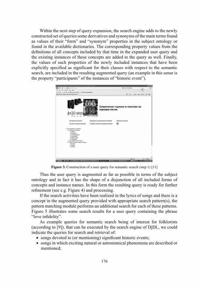
176

Within the next step of query expansion, the search engine adds to the newly constructed set of queries some derivatives and synonyms of the main terms found as values of their “form” and “synonym” properties in the subject ontology or found in the available dictionaries. The corresponding property values from the defi nitions of all concepts included by that time in the expanded user query and the existing instances of these concepts are added to the query as well. Finally, the values of such properties of the newly included instances that have been explicitly specifi ed as signifi cant for their classes with respect to the semantic search, are included in the resulting augmented query (an example in this sense is the property “participants” of the instances of “historic event”).

Figure 3. Construction of a user query for semantic search (step 1) [11]

Thus the user query is augmented as far as possible in terms of the subject ontology and in fact it has the shape of a disjunction of all included forms of concepts and instance names. In this form the resulting query is ready for further refi nement (see e.g. Figure 4) and processing.

If the search activities have been realized in the lyrics of songs and there is a concept in the augmented query provided with appropriate search pattern(s), the pattern matching module performs an additional search for each of these patterns. Figure 5 illustrates some search results for a user query containing the phrase “love infi delity”.

As example queries for semantic search being of interest for folklorists (according to [9]), that can be executed by the search engine of DjDL, we could indicate the queries for search and retrieval of:

• songs devoted to (or mentioning) signifi cant historic events;• songs in which exciting natural or astronomical phenomena are described or

mentioned;

177

• songs in which typical (or typical for a certain region) folk beliefs or rites are described;

• songs in which elements of country work and life are described or mentioned;

• songs in which signifi cant family events or human relations are mentioned.

Figure 4. Construction of a user query for semantic search (step 2) [11]

Figure 5. Search results for a user query containing the phrase “love infi delity”

178

The search engine of DjDL [11] provides also some facilities for processing of user queries presuming examination of equality or specifi c types of inequality. For example, it is possible to formulate and execute queries for search of:

• songs performed alone/in a group;• songs performed by men/women only;• songs performed by one and the same singer;• songs performed by singers, born in one and the same settlement or region;• songs performed in settlements to the west/east/north/south of a specifi c

settlement/region;• songs performed in one of the same region (grouped by regions of

performance).Let us suppose for example that the user defi nes a query for semantic search

in the lyrics of songs which concerns the concept “historic event” (“историческо събитие” in Bulgarian). During the execution of this query, fi rst of all it is augmented and refi ned with the assistance of the user as shown on Figure 3 and Figure 4. Then a consecutive search in the catalogue descriptions of songs follows. As a result, all documents with <folk_song_text> element values containing phrases that are juxtaposed with at least one element of the augmented user query, are extracted. A list with the titles of the discovered songs is properly visualized on the user screen (see Figure 6).

Figure 6. Search results for a user query containing the phrase “historic event” (level 1)

When the user clicks on the name of a chosen song satisfying the augmented query, the text of this song is displayed in a new window. The discovered words and phrases that match (are semantically related to) the query, are highlighted.

Figure 7 shows some search results for the example user query containing the phrase “historic event”.

179

The search engine of DjDL holds up some additional functionalities which enable the user to combine the search and retrieval of documents with a kind of sentiment analysis of their texts. For that purpose some of the subject ontology classes are associated with proper positive or negative numbers which play the role of sentiment estimates of the corresponding concepts.

The sentiment of a song is currently defi ned in accordance with the sum of the sentiment estimates of the particular words in the lyrics of this song (see Figure 8). The specializations of ontology concepts and all their forms and synonyms inherit the sentiment estimates of the corresponding concepts.

Figure 7. Search results for a user query containing the phrase “historic event” (level 2)

Figure 8. Some results of semantic search in combination with sentiment analysis

180

7 Conclusion

We presented in this paper an approach to the implementation of a tool for semantic search and document retrieval in an academic digital library that corresponds to most requirements and expectations of the typical users of this library.

Our current activities are directed to evaluating the performance of the search engine of DjDL (in particular, computing a tentative value of its average precision)

The next step will be to extend the functional facilities of the search engine with a proper tool for semantic search and knowledge discovery in the notes of songs. The main goal in this direction will be to build a software tool supporting the further study of some musical characteristics of Bulgarian folk songs (e.g., their melodies and rhythms) with the aim to discover similarities of songs according to various criteria.

In this way the fi nal version of DjDL will be developed with the aim to provide a complete set of tools which will be useful for a series of further studies in folkloristics, philology and musicology.

Acknowledgments. This work has been supported by the Bulgarian National Science Fund within the project titled “Information technologies for presentation of Bulgarian folk songs with music, notes and text in a digital library”, Grant No. DTK 02/54/17.12.2009.

References1. Barbera, M. et al.: A Semantic Web Powered Distributed Digital Library System. Proc. of

ELPUB 2008 Conference on Electronic Publishing, pp. 130-139 (2008).2. Castro, L., et al.: Using the Annotation Ontology in Semantic Digital Libraries. Proceedings of

the ISWC 2010 Posters & Demonstrations Track, Shanghai, China (2010).3. Kruk, S. et al.: The Role of Ontologies in Semantic Digital Libraries. 10th European Conference

on Research and Advanced Technology for Digital Libraries (2006).4. Kruk, S. et al.: JeromeDL – a Semantic Digital Library. In: J. Golbeck, P. Mika (Eds.), Proc.

of the Semantic Web Challenge Workshop at ISWC2007 (2007).5. Guha, R. et al.: Semantic Search. Proc. of the 12th International World Wide Web Conference,

pp. 700-709 (2003).6. Lervik, J., Brygfjeld, S.: Search Engine Technology Applied in Digital Libraries. ERCIM

News, Vol. 66, pp. 18-19 (2006).7. Kirov, N.: Digitization of Bulgarian Folk Songs with Music, Notes and Text. Review of the

181

National Center for Digitization, ISSN 1820-0109, Issue 18, pp. 35-41 (2011).8. Peycheva, L., Kirov, N.: Bulgarian Folk Songs in a Digital Library. Digital Preservation and

Presentation of Cultural and Scientifi c Heritage, ISSN 1314-4006, pp. 60-68 (2011).9. Peycheva, L., Grigorov, G.: How to Digitalize the Folk Song Archives? Review of the National

Center for Digitization, ISSN 1820-0109, Issue 18, pp. 42-58 (2011).10. De Juan, P., Iglesias, C.: Improving Searchability of a Music Digital Library with Semantic

Web Technologies. Proc. of the 21st International Conference on Software Engineering & Knowledge Engineering, Boston, Massachusetts, pp. 246-251 (2009).

11. Nisheva-Pavlova, M., Pavlov, P.: Ontology-Based Search and Document Retrieval in a Digital Library with Folk Songs. Information Services and Use, ISSN 1875-8789, Vol. 31, Numbers 3-4, pp. 157-166, DOI 10.3233/ISU-2012-0645 (2011).

182

Knowledge Representation inHigh-Throughput Sequencing

Ognyan Kulev1*, Maria Nisheva1, Valeria Simeonova1, Dimitar Vassilev2

1 Faculty of Mathematics and Informatics, Sofi a University, Bulgaria

2 Bioinformatics group, AgroBioInstitute, Sofi a, Bulgaria

*Corresponding author: okulev@fmi.uni-sofi a.bg

Abstract. Bioinformatics emerges to be a very important circle of tasks for the contemporary high-throughput genome sequencing. The next generation sequencing (NGS) technologies produce at high speed enormous amounts of data that cannot be processed manually in a reasonable time. For these reasons, automatic approaches for NGS data analyses are mostly required and welcomed by the biological society. On the other side, custom designed bioinformatics applications comprising methods and software solutions for NGS data analysis are elaborated very often for the purposes of different tasks and projects.

The major task in high-throughput sequencing technologies and the conducted bioinformatics is the detection of different type of mutations. This is a vast and new space for research and development and has also certain technological limitations. This large pool of tasks including NGS data noise detection, and mutations assessment makes possible the utilization of artifi cial intelligence techniques application, appropriate for the processing of such data.Knowledge representation is a domain of artifi cial intelligence that allows inference and reasoning over data. The use of knowledge representation in NGS bioinformatics is an objective of this study. The particular tasks of the study comprise the possible fi le formats, their convertibility, and the possible use of ontologies as an advantage and potential opportunity for automatic annotation. The complex and tangled data of next generation sequencing as well as its multi-level nature bear the benefi cial application of ontologies in analysis of such data.

Keywords: knowledge, knowledge representation, ontology, fi le formats, bioin-formatics, next generation sequencing, high-throughput sequencing.

1 Introduction

High-Throughput Sequencing technology produces vast amounts of raw data and the burden of processing them and getting meaningful biological results is a real challenge for bioinformaticians. Analysis of genome sequencing data is a multi-step process and these activities of steps that depend on each other are methods and protocols that continuously refi ned and developed. In high-throughput

183

sequencing (HTS), at the starting end of bioinformatics software pipelines are millions of short reads (each 50-200 nucleotide bases) of a genome. At the other of the pipeline, the output is usually annotation of the genome instance under study. All recognized regions of the genome instance are annotated with metainformation what genomic feature they represent.

The major phases of processing that data are: error detection, alignment (mapping), assembly of this large “space” of pieces (short reads), variant calling (specifi c sites detection), annotation and visualization. The most important result is variant calling – annotation of differences between individual genome and reference genome or detection of new sites in de novo sequenced genomes.

Next generation sequencing (NGS) allows retrieving genome data at high speed and changed signifi cantly the way genome research is conducted. While this provides vast amounts of data, it added new challenges in processing these data. First, not the whole genome sequences are provided but many short reads at random locations. These short reads may contain errors and this have to be taken into account. By aligning all short reads and using methods from statistics, suspicious short reads can be removed from subsequent processing.

Assembly of short reads used for constructing long contiguous sequences called contigs. Since there is no metainformation in short reads about their location or relation to other short reads, the only way to construct longer sequences is by searching for overlaps between short reads. These overlaps build a graph between short reads and by traversing the graph, contigs can be built. This is not as easy as it seems because this specifi c problem is NP-complete and requires a lot of memory. Assembly is a real computational challenge in NGS data analysis.

The most common way of getting representation of studied genome is by mapping short reads onto reference genome for it species. Naturally there will be many small mismatches in mapping but these variants of the genome are important in sequencing. The process of fi nding these variants is called variant calling and it is followed by the process of annotation. Genome annotation deals with description of biological meaning concerning the structure, function and variants in assembled genome sequences.

The amounts of data generated from HTS are enormous and analyzing it requires a lot of storage and computational resources. Thus algorithms effi ciency and information technology play a crucial role. They are only one of the pillars of modern bioinformatics though. The second pillar is statistical and heuristic methods for scoring, evaluating, predicting and validating. The third pillar is the new advancements in artifi cial intelligence and all connected computer sciences like data mining and machine learning. The software solutions for all these methods for NGS data analysis are practically implemented in a large number of separate tools or managed in processing pipelines.

184

The application of machine learning techniques for data mining purposes recently increase its obvious potential of direct application for annotation and in particular for extracting and presenting knowledge from biological HTS data. The extraction of new knowledge from potentially large biological datasets often calls for automated techniques that aim to fi nd new structures, or important connections between different entities. Data mining and machine learning techniques are ideally suited to extract such knowledge for specifi c biological and bioinformatics tasks. A recurring aspect of machine learning based data mining techniques is the ability to gain more insight in the underlying processes by examining important features, and their relations in the scope of effi cient annotation and generation of new knowledge.

In previous studies and practices, a lot of efforts have been applied in the context of gene prediction and genome annotation, incorporated in expert systems for ab initio gene prediction, and developing predictors that can identify the major functional elements of a gene. Recent advances in genome sequencing, such as the next generation sequencing technologies are now revolutionizing the fi eld of genome annotation. These new techniques call for new approaches to gene prediction, and new intelligent systems for genome annotation. Among the major tasks related to these new sequencing technologies in the scope of the rapid development and application of AI methods the efforts are oriented towards development of scalable machine learning techniques that are able to generate knowledge from these huge amounts of sequence data.

More recently, data mining and machine learning techniques have been identifi ed as key components in systems biology, where data mining is both used for knowledge discovery in identifying single components, as well as connecting different components through data integration. An interesting new development in the integration of different types of data comes from the application of data and text mining techniques to the scientifi c literature. Therefore the major role of the implementation of machine learning techniques in next generation sequence data analysis pipelines is focused to generation of knowledge from gene prediction, automated annotation and text mining.

185

Fig. 1. Data analysis and knowledge discovery in bioinformatics.

2 Information features and fi le formats

The implementation of machine learning techniques for knowledge discovery in the analysis of HTS data has contributed the importance of the use of ontology for annotation purposes. It was recognized early that it will be benefi cial for machine processing to have ontology for genomic features.

Annotation needs ontology in order to be useful for any machine processing and to allow interoperability between software systems. All recent developments in annotation representation use ontologies to describe genomic characteristics. Major ways for storing annotations are relational databases, XML fi les and text fi les. Since the beginning of bioinformatics, text fi les are used for representing data and they are still the most frequently applied. Simple and complex machine processing of annotation is easy with text fi les and they are very suitable for manual modifi cation using simple text editors.

The Gene Ontology Consortium was established in 2000 as a collaborative effort to address the need for consistent descriptions of gene products in different databases and since the beginning it was decided that just using controlled vocabularies (ontologies) is not enough [1]. Gene terms are described in their

186

relationship and form complete ontology in the fi eld thus allowing reasoning over gene data. There are three separate aspects to this effort: fi rst, the development and maintenance of the ontologies themselves; second, the annotation of gene products, which entails making associations between the ontologies and the genes and gene products in the collaborating databases; and third, development of tools that facilitate the creation, maintenance and use of ontologies. Annotation data is submitted to the GO Consortium in the form of gene association fi les, or GAFs. This fi le format creates a background for determining a necessary standard for information specifi cation concerning both the databases relations and the annotation extension which implicitly leads to a platform for presenting a new annotated knowledge.

2.1 File Formats for genome annotations

Generic Feature Format (GFF) is text fi le format for universal genome sequence annotation. Due to its popularity, several incompatible versions made by different bioinformatics groups gained traction. Ultimately, GFF version 3 (GFF3) by Sequence Ontology Project [2] became the most widely used for new projects. Using ontology is one of the major features of GFF3 and certainly one of the main reasons for the success of GFF3. Structural annotations can be precisely described using GFF3 but there are still weaknesses in variant calling representation. Genome Variation Format (GVF) is an extension of GFF3 that address this issue and allows all visualization and other processing software that accepts GFF3 to also work on GVF [3].

GVF format is text fi le with nine tab-delimited columns in each line. Chromosome identifi er is in the fi rst column, source (application or algorithm) is the second, and type of sequence alteration – in the third. Reference sequence is not in the GVF fi le but is referenced using chromosome identifi er (column 1) and region (columns four and fi ve that contain start and end position of the annotated region in reference chromosome). Column six contains score value but GVF specifi cation doesn’t specify semantics of this number, only recommends Phred quality score to be used [4]. Column seven is strand (“+” for forward or “-” for reverse) on the chromosome, if this is applicable, or just “.”. Column eight is legacy from GFF that is not used in GVF and should be “.”. Column nine contains the annotation and is represented as a list of tag/value pairs separated by “;” character. Tag name and value are separated by “=” and multiple values can be separated by “,”. An example of simple SNP annotation follows, where the ninth fi eld is split into multiple lines for clarity.

187

chr16 samtools SNV 49291141 49291141 . + . ID=chr1:SOAP:SNV:15883; Variant_seq=G,C; Reference_seq=C; Genotype=heterozygous; Variant_reads=17,16; Total_reads=33; Dbxref=dbSNP_137:rs77417897; Variant_effect=nonsynonymous_codon 0 mRNA NM_345,NM_210;

Reference sequence in this region of one nucleotide base is “C” and in annotated genome at this place there are two variants “G” and “C”. The fi rst is supported by 17 short reads while the second is supported by 16 reads, totaling in 33 short reads that cover this location. Database reference to an entry that describes the variant is provided with “Dbxref” tag. The effect of this variant is encoded in the last tag using Sequence Ontology terms and references to other data. ID is a required tag in the ninth fi eld. Many other kinds of annotation are possible with GVF.

Variant Calling Format (VCF) is an alternative to GVF. It was developed by 1000 Genomes Project for representing human genetic variations and it is usually used only for human genome [5]. Major difference with GVF is that descriptive terms don’t use ontology thus limiting the usefulness of the fi le format.

Chado [6] is a relational database schema for representing bioinformatics data, including annotation data. Representation of biological knowledge is one of its design goals. Many utilities and application programming interfaces are included to aid in utilizing Chado databases. It’s a part of Generic Model Organism Database (GMOD) project [7] that also develops the GVF fi le format. Chado database employs the subject-predicate-object triple pattern as used in RDF but it is less generic and triples may include additional information thus it’s not as strict as RDF.

In table 1, the most frequent fi le formats used in genome sequencing studies are shown. They could be specifi ed in two groups: as (raw) sequence formats (FASTQ, FASTA, SAM/BAM) and annotation fi le formats (GTF, BED, GFF, GVF, OBO). These formats are related mainly through the idea of presenting new knowledge from the NGS data.

File for-mat

Function Application Relation to other formats

FASTQ Contains short reads Sequence machines output FASTQ fi les that contain short reads and base quality scores.

NGS pipelines start with this fi le format or FASTA.

188

FASTA Contains nucleotide sequences

DNA sequences without annotation.

NGS pipelines start with this fi le format or FASTQ.

S A M /BAM

Mapping of reads Result of mapping short reads onto reference genome. Doesn’t contain sequences, only location and CIGAR (transformation description for reads).

Short reads are in FASTA or FASTQ format. Reference genome is in FASTA.

GTF Gene locations in reference genome

Auxiliary fi le used in differential expression analysis.

Simple annotation needed for counting reads by genes.

BED Sequence annotation Defi ning regions in annotation track in visualization of genome.

Annotated sequence is in FASTA.

GFF3 Genome annotation Representing structural annotation using Sequence Ontology.

Annotated sequence is in FASTA.

GFF2 Genome annotation Representing structural annotation.

Older version of GFF3 that doesn’t use Sequence Ontology.

GVF Representation of sequence variants

Result of variant calling analysis. Extension of GFF3.

OBO Ontology representation External controlled vocabulary for software.

Sequence Ontology and Gene Ontology are represented in OBO.

Table 1. File Formats.

Software toolWeb address Description and features

AUGUSTUS http://bioinf.uni-greifswald.de/augustus/ Fully automatic annotation pipeline for genome-wide gne predictions

EUGENE http://eugene.toulouse.inra.fr/ Gene prediction with ability to integrate arbitrary sources of information

GeneID http://genome.crg.es/software/geneid/ Fast and accurate gene prediction

GLIMMER http://ccb.jhu.edu/software/glimmer/ Microbial gene fi ndermGene http://mgene.org/ Genome-wide prediction of

protein coding genesSNAP http://www.broadinstitute.org/mpg/snap/ SNP annotation for human

genome

Table 2. Gene fi nders.

The main spread of software tools for annotating of genome sequencing information are listed in Table 2. The have different aims and features – defi nitely the general

189

purpose is the generation of new knowledge from the analyzed HTS data based on automated annotation of newly discovered and predicted structures of genomic information. These software tools are not related directly to the generation of knowledge by the methods of machine learning. The new generation software solutions with similar functional objectives will be based on the use of upgraded data formats able to provide more suitable environment for the development of the specifi c custom designed software tools for extracting and presenting new knowledge from HTS data analysis.

3 Extracting and presenting knowledge from HTS data analysis

The potential of representing sequence annotation using ontology is still heavily underused. By not using hard-coded feature list but ontologies instead, software systems can offl oad importing and maintaining terms. Moreover, it allows true interoperability with other software that uses standard ontology. Even if other software doesn’t use the same ontology, one of the important properties of ontologies is that there are software tools for automatic mapping between ontologies. Another benefi cial outcome of using ontology instead of feature list is that adding new terms to ontology and using these terms in new annotations does not affect old software. When unknown term is detected, it may gracefully be degraded into more general term that is understood by old software and results to still be sensible. Here the role of soft computing in terms of using different algorithmic solutions for extracting knowledge from HT sequencing is much promising. The recent achievements in pipelining of NGS data analysis is providing a real challenge for integration of different algorithmic methods and their software implementations in a common environment for knowledge based analysis. The developing of correct method and its software solution for extracting, presenting and generating knowledge from HTS data is quite not a trivial task and a lot of problems could arise in getting the right answer. As regards the specifi city of the certain tasks comprising the knowledge discovery by annotating new data from the large genome studies, the role of data mining and related problems are of crucial importance. The possible application of AI methods is an obvious solution of such problems.

More general problem than handling an unknown term is metric for similarities of terms that can be used in search queries. It is helpful to have inference rules between ontology terms and even procedural knowledge for high-throughput sequencing domain. Although in artifi cial intelligence there are many methods for representing such knowledge, there are no bioinformatics databases that can be used in such way.

Representing sequence variants is only the fi rst step in generating knowledge for a genome. Variants are interconnected and there are large differences in

190

signifi cance between individual variants. Selecting variants for grouping and interpreting the meaning of specifi c combination is a challenging task that is usually performed manually by biology specialists. It is a tedious and very time-consuming work that can be greatly sped-up by using methods from the fi eld of artifi cial intelligence. There is a lot of research in using these methods but application to bioinformatics domain is still lacking.

The functionality of integrating such methods is given in a general sense in Figure 2. The presented relations and interceptions of integration of different algorithmic methods and IT solutions can provide a platform for updating the already existing and developing new methods for knowledge discovery from the NGS data.

Fig. 2. Knowledge discovery in NGS data.

4 Future Trends and Conclusions

The future trends in the elaboration of contemporary methods for knowledge representation and discovery in HT genome sequencing research can be regarded in several aspects:

─ the use of more advanced and custom-oriented technologies for HTS data analysis in the scope of developing suitable formats for building semantic vocabularies (ontolo-gies) and annotations of newly discovered and predicted genome information;

─ the direct and integrated use of machine learning methods for prediction, annotation and validation of newly sequenced genomic information;

191

─ upgrade and integration of the existing information resources and software tools for discovery, prediction and annotation of sequence information;

─ use of soft computing for elaborating a fl exible set of algorithmic solutions and soft-ware tools for the purposes of presentation of knowledge from the growing mass of HT genome sequencing information.

As a major outcome from our work it could be concluded that the raw NGS raw data currently are aimed to be processed in a specifi c environments like customized software pipelines in order to handle the major operational steps of the analysis (error detection [8], assembly, alignment, variant calling [9], annotation, structural and functional discovery. All this workfl ow necessary for the analysis of HTS data can be upgraded by new methods of extraction, presentation and generation of new knowledge.

Variant calling is the process of fi nding differences between genome sequences and reference genome sequence. Exactly how these variants affect phenotype is a complex task with no defi nite answers. Statistics is not enough since we are not just judging by scoring and numbering but we really have a complex knowledge base that have to be taken into account. Artifi cial methods are developed precisely for such situations but are still underused in bioinformatics. We have shown the bioinformatics tools are starting to be directed towards use of ontology-based data bases that have potential for utilizing AI methods. Although bioinformatics knowledge representation is fi rmly entrenched into modern bioinformatics pipeline, inference and reasoning based on bioinformatics knowledge bases is still in infancy.

Acknowledgements. This work was supported by the European Social Fund through the Human Resource Development Operational Programme under contract BG051PO001-3.3.06-0052 (2012/2014).

5 References1. Ashburner, M., et al.: Gene Ontology: tool for the unifi ca� on of biology. Nature Gene� cs

25, 25–29 (1 May 2000). doi:10.1038/75556 (2000)2. Eilbeck, K., Lewis, S.E., Mungall, C.J., Yandell, M., Stein, L., Durbin, R., Ashburner, M.: The

Sequence Ontology: a tool for the unifi cation of genome annotations .Genome Biol. 2005; 6(5): R44. doi: 10.1186/gb-2005-6-5-r44 (2005)

3. Reese, M.G., Moore, B., Batchelor, C., Salas, F., Cunningham, F., Marth, G.T., Stein, L., Flicek, P., Yandell, M., Eilbeck, K.: A standard variation fi le format for human genome sequences. Genome Biology 2010, 11(8):R88. doi:10.1186/gb-2010-11-8-r88 (2010)

4. Ewing, B., Hillier, L., Wendl, M.C., Green, P.: Base-Calling of Automated Sequencer Traces Using Phred. Genome Research 1998. 8: 175-185. doi: 10.1101/gr.8.3.175 (1998)

192

5. Danecek, P., Auton, A., et al. and 1000 Genomes Project Analysis Group: The variant call format and VCFtools. Bioinformatics. 2011 August 1; 27(15): 2156–2158. doi: 10.1093/bioin-formatics/btr330 (2011)

6. Mungall, C.J., Emmert, D.B., The FlyBase Consortium: A Chado case study: an ontology-based modular schema for representing genome-associated biological information. Bioinformatics (2007) 23 (13): i337-i346. doi: 10.1093/bioinformatics/btm189 (2007)

7. Generic Model Organism Database (GMOD), http://gmod.org8. Krachunov, M., Vassilev, D.: An approach to a metagenomic data processing workfl ow, J.

Comput. Sci. (2013), http://dx.doi.org/10.1016/j.jocs.2013.08.003 (2013)9. Trapnell, C., Roberts, A., Goff, L., Pertea, G., Kim, D., Kelley, D.R., Pimentel, H., Salzberg,

S.L., Rinn, J.L., Pachter, L.: Differential gene and transcript expression analysis of RNA-seq experiments with TopHat and Cuffl inks. Nature Protocols 7, 562–578 (2012). doi:10.1038/nprot.2012.016 (2012)

193

Model of Knowledge Management System forImprovement the Organizational Innovation

Natasha Blazeska-Tabakovska1, Violeta Manevska1

1 Faculty of Administration and Information Systems ManagementUniversity"St. Kliment Ohridski"

Bitola, Republic of Macedonia

�������� ������������ ������� ��� ��������� ��� �� ����� ����������� �� ��� �� ��� ������� �� ���� ����� ����� ������ �� ��������� ��������� �������� ���� � �������� ��� ���� � ������� ����� ��������� ����������� ������ ��� ����� �� ���� �������� ���� ���� ��� �� ����� ������� ���� � �������� ���������� ���� ��������� � �������� ���� � �������� ��!����������������������� ������������������������� ������� ��������������������������������� �������� �������� ��� ������������ ������������������

�� ����� ��������� ����������� ��������� ���������� ���������������� ������������������� �������� �������������������

1. Introduction

Some of the trends, as globalization of the economy, changes in organizationsworking environment today, large amount of information in decision-making on theone hand and dealing with large amounts of information on the other, and thefluctuation of employees, impose the need for a different way of managing theorganization and its processes.

Today organizations puts their focus on organizational knowledge rather than onmaterial resources and increase their efforts to maximize knowledge utilization inorder to cope with global trends, improve its business processes, make effectivedecisions, improve the quality of their products/services and increase theireffectiveness. The successful management of organizational knowledge leadsorganizations one step further in their work and it is an important factor in gainingand maintain a competitive advantage. According to Liebowitz knowledgemanagement "is the process of creating value from intangible organizational capital"[Liebowitz, 1998]. In most cases the goal of knowledge management is to combinecustomer knowledge and processes knowledge (know-how). Knowledge managementfocuses on several key elements: acquiring new knowledge from external sources;generating new knowledge in the organization; standardizing of existing knowledgein the form of procedures and protocols; transforming individual knowledge intocollective; facilitating its use and its incorporation in business processes. It is acomplex activity consisting of many processes. According to Alavi and Leinder[Alavi & Leidner, 2001] knowledge management consists of four processes:

194

(1) Capture and Creation(2) Storing / retrieval(3) Transfer(4) Application

These processes can be facilitated and supported by various informationtechnologies and techniques. Various information technologies and techniquesapplied in order to support knowledge management processes gives a different effectsin improving various indicators of organizational effectiveness. Dimitrov points theneed of the information technologies to be result of the business processes and tounderstand business terminology. This new method will prove their value andmeaning, giving the desired business results [Dimitrov, 2012]. Some of the benefitsare immediately visible, others are perceived with its long-term use. Some of thebenefits are: increased innovation by encouraging the free flow of ideas, improvedcustomers services, retention of employees by recognizing their knowledge throughtheir reward, improved operations and reduce their costs by eliminating the requiredprocedures. This paper proposes a model and analyzes the impact of the proposedmodel on increasing the number of innovations. Analysis of the impact of this modelresulted in recommendations for integrating the solution into a model of knowledgemanagement information system, a multimedia design of knowledge managementsystem which is based on metadata.

2. Method of model testing

The research was conducted on the territory of the Republic of Macedonia and itincluded organizations from both the private and the public sector, small, medium andlarge organizations, as well as national, multinational and global.

The analysis applied several statistical methods: Descriptive and Frequencies todescribe the analyzed sample; Correlation to determine the strength of dependencebetween two variables; ANOVA test to compare dispersions (variability of results)between different groups and dispersion in each group1, i.e. ANOVA test help todetermine if some information technology or technique or stage of development /application of knowledge management program have an impact on increasing thenumber of innovations (one of the indicators of organizational effectiveness) whetheran individual or their interaction.

Figure 1.Knowledge Management System building methodology

" ���� ������ ���� ������� ������ � stage of development/application of knowledgemanagement program and/or applying of information technology or technique

#� ��������

$������������ ����&

�������������

*�� ��� ��

*���������������

ANOVA

$���

���������

195

After determining the group of information technologies or techniques that havea positive impact on the number of innovations a model is proposed. The model istesting by using of multistage regression. This help us to analyze its impact on theincreasing number of innovations. (Figure 1).

3. Model definition

The data analysis showed that the oragnizations apply a different rate ofinformation techniques and technologies. We define different groups of organizationsdepending on stage of development/application of knowledge management programand/or applying of information technology or technique, to determine their impact onthe number of innovations. Depending on the stage, it was defined 5 groups oforganizations: 1 - organizations that survey their needs and conditions of introductionthe program; 2 - organizations in the planning phase; 3 - organizations in introductionphase, 4 - organizations which review the program; 0 - organizations that do notconsider such a program or can’t see the benefits of it. Depending on whetherparticular organizations apply information technology or technique it was defined twogroups: 1 - organizations that apply; 0 - organizations that do not apply. Thedispersion between different groups and dispersion in each group (varity of results)were compared by two-factor ANOVA.

On increasing a number of innovations, the analyses show that:• The interaction of stage of development/application of knowledge management

program program and application/non-application of some information technologiesand techniques has a strong influence;

• The stage of development/application of knowledge management program has astrong separately influence, and the impact is greatest when the program is underreview;

• The application of some information technologies and techniques constitute astrong positive impact on increasing the number of innovations. The strongestimpact has: extracting processes knowledge in order to improve operations, collectionand publication of learned lessons, and extracting customer knowledge to improveproducts/services.

The results of the ANOVA test were used as a foundation for model definition ofproposed model, which includes: extracting knowledge about customers in order toimprove products/services; extracting knowledge about processes in order to improveoperations; applying expert address book; the practice of creating and using adatabase of good practices and learned lessons and application of wiki pages. (Figure2).

196

/����� <� >$������

In addition, we tested the impact of this model on increasing the number ofinnovation in organizations. To test the defined model it was applied multistagestandard regression. This statistical tool helps us to determine predictive power ofeach of the variables in the model, i.e. how much each of them will improve themodel.

4. Model testing

?�������������������������������������������������� �������� �������������� ��� ������ ���� � ������ ��� ��� ������������ �� ����&�������� ����������Q ������ ����������������������� ���������/�����X���� ��� ��Y�/�������<\\^` <

����������� �������������������� ������������ ������ �����������{����������� �������| ��� �~�������� ����������� ���������� ���� �� ����� �������� ���������� ���� ���� �� ������� ���������� ����������� ���������� ���� ��� ��������� ������ �� �� ��� ���������� ���������� ��!� ��� ����������� ��� �� �������� �� ����������������������������� ������������ ���������! ���������������������������������� ���������������������{�������� ���������� �������������� ��������� ������������� ��������| ��� �������� ���������� ���� ��� ����� ��� ������� ���� ������������ �� ��� ���������� ������ ��� ����� ��� ������ �� ��� ��������� ��������� ������~����������������������� �������������

Q ����� ����� ������� �� ����� � �� ��������� �������� ���������� ���������������������� ��������

< ���\����� �������������������������������������� {�| ����������������������������������� {�|� Q ������ ��������� ����������� �� ����"\������������{������������ ������������� �|������������������������������������������������������

� ���� ������������������ ��\��

Increasing thenumber ofinnovation

�~���������������

*������� ��� ����� � �� ��� �������

������

����������

�~�� �� ���������������� ��������������

��������������

�~�� �� �� ������������ ��������������������� ���� ������� ��

197

�������� ��� �������������������������������������������������\���������� �������������������������������������\����������� ������������������� �~�������� ��� ��� ����� ���� �� ��� ����� ������� � �������� ���� ��������� ��������� �~����� �������� ���� ���� ������ ���� ��� ��� � ��� ���� ��������������� ���� ������� ��� �~�� ��� �� ��������� ���� ������� � ���������� ������� ���� �~�� ��� ��������� ���� �� ������ � ������� �������� ���������������������������� ������������������������������"���� �������������� �������� � ��������� ���� ����������������� �� �< ��\�����?���������������������������Q������������������\�\��������������������������������� ��������������������� ����������������������������

Table 1. Model summary review

$��� � � ������Q������

� �������������������

������

" ���� ���\ ��\� ����

��� ������ < & ���� Q���Q ����� ��� ������� ���� ��� ����� ��� ������� �� � �� �������������������\�\\\�{���\�\\\�|����� ����� ������������ ������������

Table 2. Model testing-ANOVA

�����

$��������

������� ��$���

������ / �#�������� ��"�\ � "�<�� ���

^��\\

\#������� "<�\�^ �� �"<�

��� "��<<^ "\"

���� ��� �� ��� ����� ����� ��� �������� ���� ��� ����� ��� ���� �������� ������� ����� ������������ ���������������������� �������� ���������������� � ����� �� � �������� ��� �� �� ���������� ��������� �������� � ������� �� ���� ������� ���������������������

/����� �������� ����� �� � ��� ��� �� �� ��� ���� �� �� �� �� ������������������� ��� ��� ����� ���� ��� �� �� ����������� �������� � ��� ����� ��� �� ���� ������ ��� ��� ������� �� ���������� ���� ��������� ������ ��� ��� �~�� ��� �������������� ������ ������� ������������ ������� ��� ��� ���� ������ ���� ������� �~������� � ��� �� �������� � ��� ������ � �������� {\��^|�Q������������ �� ���� ���� ������� ��� ����������������������� � ������������� �������{\�<�|������������������������������������������� ����\�\\\� ��� ���\�\\��{���\�\�|���������� � �����������������������������������{�~�� ����������������� ������ ������� � ����������� ������� ������� ��������

198

��������� ���� ��� ��� � ��� ���� ������� �������| ��� � ���� ���� ���� ����� ����������� ��� �������������� �� �� ����� ����������

Table 3. Particular impact of the different information technique and technology on theincreasing number of innovation

$��������������

�?���~�� ���� ������������ �� ����� �������������� �������

�\\� �\�" ���\

������������������� � �������������� ������ �<�< <��\\ �\\�

�~�� ������������������ �������������������������� ������� ��

��^� ����\ �\\\

�~���� ���������� �"�� "�^�� �\�<

���������� �\�� ���� ��<\

/�� �������� ��������� ��������� �� ��� ��� � ����� ��� ��� ����� ���� ������ �~�� ��� � ��������� ��� �� ����� ��� ����� � ������ ����������������� ���� ��� ��� � ��� ��� ������� ������� �~�� ��� �� ��������� ��� ������� ��� ����� � ������� ���� ������� ��� �~���� ������� �� ���� ����������� ������� �\�� �� ��� �� ������ ��� ��� ������� �� ��������� ��� ���������� ���� ������������� �������������� �������������������������������������������������������������� � �������� ��������� ��� ���������~������� ������ ��������� ��������� � ������� {�^�|���� ��������� ���������������������������� ������� ������� {<��|��{/�������|�

Figure 3.Impact of the different information technique and technology on the increasingnumber of innovation

5. Knowledge management system model

The data obtained above are the result of a comprehensive research and analysisand we propose to incorporate them into one comprehensive platform whose focus is

>$��������������

���������������������������!������

• the extraction of knowledge aboutcustomers in order to improveproducts/services

• databases with good practices andlearned lessons

199

system’s customer orientation. The proposed model of knowledge managementsystem by Jay Liebowitz [Liebowitz, 1999] we used us a base.

We suggest multimedia knowledge management system design. The system wouldimply information techniques and technologies of the model which testing has showna positive impact on increasing the number of innovations. Also the system is basedon metadata such as: metadata for users of the system X���`, metadata for good practiceX���` and metadata customer X ��`. Pavlov and Pavlova Nisheva-emphasize thecategories of the metadata are designed in order to facilitate, locating the requestedknowledge using search machine [Pavlov & Nisheva-Pavlova, 2008]. The metadatacreation will enable rational reasoning i.e. computer’s conclusion. The each user ofthe system is necessary to provides feedback. This enables audit and dynamics of thesystem.

Figure 4. Knowledge management system model

The models of knowledge management system content three modules (Figure4):

" *���� $���� & ��� ������� ������ ��� ��� �� ��� ���� ������ � ����������� ������������������������ ����������������������� ����������������� ������~���������� �����������

� $��� $�������� $���� � ���������� ��� ������ ��������� � ������� ������������������� ���� �����/��� �� ��� ����������� ��� �������� ���&��� ����� �� �������� �� �~�� �� ��� ��� ��~� �� �� ��� ��� ������������~�� ������������ ������������ ����������������������������� ����� ��������������������� � �������������

� >�������� $�������� $���� � ����� ����� �������� ��� ��� �������������� ��� � ���� ��� ���������� ��� ���� ��� �� ���� � ������ � ���������� ������� ��� ������ ������ ����� ��������� ���� ��������� ��� ���� �������� ��� ���� �� ��������������������� ����� � �� �������������

����������� �������� ��������� ������ ��� ����������� ��� ��� ���� ������ ��� ������ � ��� ��� ������� �� �����!������ �������������� ������������ ����� ������ ��� ����������� ���� ��� ������� ��� ��� ��� � ��� ���� �� ������ ��� �������� �� �� �� ��� � ������ �� �������� ��� ��� ������ ���{/�������|� �������������� ��������� ������������������� ������� ��������������� ��� �� �� ������ �� ������ �� ��� ���� �� �� ���� ����� �������������������������� ���������������� ���!� ���� {/�������|�

#���$��%��&���%�

&���%&���������

&���%�

�� %����&���������

&���%�

200

Figure 5. Static metadata for system’s users, for good practices and for customers

/����� �� *����� ���������������!������������������ � ��������� ������

6. Conclusion

The above offered model can be incorporated into existing organizationalknowledge management information systems or in the process of planning forimplementation of a new information system. Such an information system would havepositive effects on organizational effectiveness, and increase the number ofinnovations. The model includes: extraction of knowledge about processes in order toimprove operations; databases with good practices and learned lessons, extraction ofknowledge about customers in order to improve products/services, experts addressbook and wiki pages. Metadata for system’s users, for good practices and for contentfor customers has enabled extraction and display of good practices and content forcustomers. The extraction is based on user’s profile and content classificationaccording to the profile. Thus users of the system would be kept informed for newcontent or changes made in the system, which are the subject of their interest. Thistype of information can change the whole way of system’s user operation. Thesystem facilitates the system’s user work without they lose unnecessary time.

����������������

������

������

������������ ����������

������

������

������

�������������������

������

�����

�����

������

����

������

����

����

����

����

����������������� ���� ���������

����������������� ���� ���������������������������� ������ ������

����

201

'���������

1. Alavi, M. & Leidner, E. D., Review: Кnowledge management and knowledge managementsystems: conceptual foundations and research issues, MIS Quarterly, (25:1), Mar, pp. 107-136, (2001)

2. Balaban, N., Ristic, Z., Durkovic, J. & Trninic, J.: Informacioni sistemi u menadzmentu:Branko Dzonovic, Beograd, (2005)

3. Bassellier G., Reich B. H. & Benbasat, I. : Information technology competence of businessmanagers: A definition and research model, Journal of Management Information Systems(17:4), pp.159-182, (2001)

4. Blazhevska-Tabakovska N. & Manevska, V.: Influence of Different KnowledgeManagement Techniques and Technology on Organization Effectiveness, In Proceedings of6th International Conference of Information systems and Grid technologies, Sofia, (2012)

5. Blazhevska-Tabakovska N.: Influence of Knowledge Management Information Systems onOrganization Effectiveness, PhD. Disertation, Faculty of administration and informationsystems management, Bitola, (2012)

6. Boiney, L. G.: Reaping the benefits of information technology in organizations: Aframework guiding appropriation of group support systems, The Journal of AppliedBehavioral Science, (34:3), (1998)

7. Dimitrov, V.: Service-oriented architecture for business, University Press “Sv KlimentOhridski”, Sofia, (2012)

8. Gottschalk, P. : Strategic Knowledge Management Technology, Idea Group Publishing (animprint of Idea Group Inc.), (2005)

9. Hüseyin, T.: Information Technology Relatedness, Knowledge Management Capability,and Performance of Multibusiness Firms, MIS Quarterly (29:2), June, pp.311-335

10. Liebowitz, J. Building organizational intelligence: a knowledge management practice,CRC Press, Florida, (2005)

11. Palanisamy, R. : Strategic information systems planning model for building flexibility andsuccess, Industrial Management + Data Systems (105:1/2), pp.63-81, (2005)

12. Pavlov, P. Nisheva-Pavlova, M. : Some it aspects of building digital libraries with learningmaterials, pp17-21, (2008), Sofia, available at http://elib.mi.sanu.ac.rs/files/journals/ncd/13/ncd13017.pdf,

13. Sabherwal, R. & Sabherwal, S. : Knowledge management using information technology:Determinants of short-term impact on firm value, Decision Sciences (36:4), Dec, pp.531-567, (2005)

202

Towards application of verification methods forextraction of loop semantics�

Trifon Trifonov

Faculty of Mathematics and Informatics, Sofia University

ACM Classification Codes: D.2.5, D.2.7.

Keywords: Static Analysis, Loop Invariants, Program Semantics

Abstract. There exist a variety of methods, techniques and tools forverifying properties of procedural programs. Formally, such methods pro-vide a language for expressing properties A(x, y) and means to proveA(x, P (x)) for a given program. Morgan and Back have demonstratedhow one of these methods (Dijkstra’s predicate transformers), can be ex-tended to a method for automatic program synthesis, i.e, given a pred-icate A(x, y), to construct a program P (x), such that A(x, P (x)). Thegoal of this paper is to explore the reverse approach for loops, i.e., givena loop program P (x), attempt to construct a predicate A(x, y), whichis as strong as possible and A(x, P (x)) holds by applying methods forautomatic generation of loop invariants.

1 Introduction

One of the main features of programs written in a procedural style is theirinherent imperativity. The most natural semantics of such programs are the low-level operational ones, which provide little insight in the high-level properties ofthe program. A usual approach to bridge this gap is to “inject” meta-instructionsand hints to the human programmer in the form of indentation, comments,variable and function naming conventions, and supporting documentation. Thisallows for intuitive reasoning about properties of the program, for example, whenviewed as a mathematical function.

The popular object-oriented paradigm moves this idea one step further byemploying various techniques to map operations performed by the program anddata manipulated by it onto a business domain model. Examples of such meth-ods include logical grouping of data and associated operations into classes andmodules, which represent consistent and integral parts of the business problembeing solved. There are obvious advantages to having such a mapping: it aidsreasoning about the program, simplifies the validation of the software system� This work is supported by the National Scientific Research Fund under Contract

DTK 02-69/2009.

203

against the business requirements and reduces maintenance effort, i.e., correc-tion of problems and accommodation of change requests.

Nevertheless, the presence of all supplements mentioned above is in fact notmandatory for the correct functioning of an already developed system. Moreover,there are overheads associated with the development and maintenance of thisassisting layer, not only in terms of human effort, but also in terms of runtimeperformance and efficiency of the program itself. These factors induce a tempta-tion to neglect or even fully omit such meta-information supporting the sourcecode of the system. Following this path usually means that the information iskept implicit in the memory of the developers of the software system and grad-ually erodes and deteriorates with time until it mostly disappears. This can beconsidered as a first sign of a transformation into a legacy system [BLWG99]. Ifthe problem solved by the system indeed becomes irrelevant, then the code couldsimply be deprecated. Even if the addressed problem is still of relevance, but itdoes not undergo significant reformulations or changes, then this might not be-come an obstacle for a prolonged period of time. However, during this periodcosts of maintenance and inter-operability of a legacy system could significantlyrise, while in the same time development and growth of the associated businesscould also raise the business of the system and the cost of its removal. As aresult, the legacy system would eventually need to be replaced with a modernfunctionally equivalent system.

One of the approaches “modernize” a legacy system is to partially recover, orreverse-engineer, the business model and business logic encoded in it, so that theycan be reimplemented using modern approaches and technologies. This wouldusually involve “discovery” of the intended high-level semantics of the program ina convenient form. The definition of a suitable language for expressing businesslogic is one of the goals of the Business Rules Project [Hay00]. The present paperis a part of research effort to extract business rules from existing legacy sourcecode. Our approach is based on static analysis and employs techniques such asanalyzing possible paths in the control flow graph of the system [MMH12] andapplying transformations to obtain a form of the code, which is declarative ratherthan imperative [MT12]. One of the most problematic pieces of the extractionof business rules from procedural programs is the treatment of loop-like controlstructures.

The present paper suggests an approach based on formal program verifica-tion. We use Hoare logic as the base system for expressing and proving propertiesof procedural programs. The standard use case for establishing semantics is todecompose a given program to simple statements and then enrich it with anno-tations, which are usually formulas of a fixed logical system. These propertiesneed to be chosen in such a way that they express assertions for the variable val-ues, which are valid at the respective points of the disected program. The caseof loops is handled by a special kind of property, called a loop invariant, whichneeds to hold before the first execution of the loop, and after each execution ofthe loop body.

204

Following this approach, axiomatic predicate transformer semantics of proce-dural program can be defined, as proposed by Dijkstra [Dij75]. These semanticsare complete in a sense that they capture comprehensively the meaning of theprogram. Morgan and Back [Bac88, Mor90] have extended this approach furtherby demonstrated a semi-formal method to generate procedural programs in par-allel with the proof of its correctness with respect to a given precondition andpostcondition. We explore the possibility of reversing this approach, i.e., givena program to generate a pair of precondition and postcondition which describethe behaviour of the program.

2 Loop invariants

Our approach builds on the well-known Hoare logic [Hoa69]. Statements of thislogic are triplets of the form

{Precondition} Program {Postcondition}

with the intended semantics “Whenever Precondition holds, Postconditionshould hold after Program is executed.” Proofs in Hoare logic are trees builtfrom axioms and rules described in Figure 1.

{P} ; {P} (empty operator)

{P [x := E]} x = E; {P} (assignment)

{P} S {Q} R → P

{R} S {Q} (strengthening)

{P} S {Q} Q → R

{P} S {R} (weakening)

{P} S {R} {R} T {Q}{P} S;T {Q} (composition)

{P ∧B} S {Q} {P ∧ ¬B} T {Q}{P} if (B) S else T {Q} (conditional)

{P ∧B} S {P}{P} while (B) S {P ∧ ¬B} (iteration)

Fig. 1. Hoare logic axioms and rules

We will focus our attention on the iteration rule, which specifies how loopproperties are established. The premise of the rule has a specific feature, whichis not present in any of the other rules: the postcondition P is also a part ofthe precondition. Similarly in the conclusion of the rule, P is a precondition,which is also part of the postcondition. Traditionally, P is referred to as the loopinvariant, because it specifies a condition, which is true in the following threesituations:

205

– before the loop is executed,– after the execution of every loop step, and– after the loop execution completes.

Proving a property about a loop requires building a proof of the triple

{Precondition}while(Condition)

Statement{Postcondition}

In order to proceed with the proof, we need to apply the iteration rule. However,this could only happen if Postcondition is exactly the conjunction of Precon-dition and the negation of Condition. Unfortunately, in practical cases, thisvery rarely holds, as can be seen from the following simple example:

{x == 0 && i == 1}while(i != n) {

x += i;i++;

}{x == n*(n - 1)/2}

In such a case, our only hope is to attempt to bridge the gap between Pre-condition and Postcondition. In Hoare logic, this can be done by applying thestrengthening and weakening rules. Our goal is to replace Precondition withan equivalent or weaker formula, and, respectively, replace Postcondition withan equivalent or stronger formula so that it can fit the template of the iterationrule. One example how this can be done is shown below:

{x == n*(i - 1)/2}while(i != n) {

x += i;i++;

}{x == n*(i - 1)/2 && !(i != n)}

It is clear that if x == 0 and i == 1 then obviously x == n*(i-1)/2. Similarly,if x == n*(i-1)/2 and i == n, then trivially x == n*(n-1)/2. Unfortunately,this is not sufficient to prove the validity of the triplet. The problem is that thenew Precondition needs to be sufficiently strong so that whenever both Pre-condition and Condition hold, then Precondition should continue to holdafter the execution of Statement. In our case, we have chosen an unsuitableweakening of Precondition, because now we are unable to prove the triple

{x == n*(i - 1)/2 && i != n} x += i; i++; {x == n*(i - 1)/2}

The reason why we cannot proceed is the following. Our only possibility here is toapply the composition rule and the assignment axiom, with possible application

206

of the logical strengthening or weakening rules. This would amount to provingthat x+i == n*i/2 && i+1 != n implies x == n*(i - 1)/2, which would holdif n == i/2, and certainly not for an arbitrary i.

The correct invariant in this case clearly is x == i*(i - 1)/2. It still followsfrom the original Precondition and implies the original Postcondition, butnow also we can prove the premise of the iteration rule, namely the triple

{x == i*(i - 1)/2 && i != n} x += i; i++; {x == i*(i - 1)/2}

Finally, it should be noted that Hoare logic provides means to prove partialcorrectnes of loop programs, i.e., that if Precondition holds, then Postcondi-tion is true after the program execution, if it completes. The proof of a tripletasserts nothing in case the program does not terminate. For example, the aboveprogram will not terminate if n == 1, but this fact does not impact its partialcorrectness. Hoare logic could be extended to also assert loop termination byappointing a non-negative expression, which provably decreases after each loopstep (sometimes called the loop variant). However, in the present paper we willonly consider partial correctness.

3 Using invariants for extracting loop semantics

The process of discovering the invariant Section 2 was not formal and automatic.We had to find a condition, which “fit” the rules of the Hoare logic. This couldbe denoted by an annotation of the following form:

{Precondition}while(Condition)

{Invariant}Statement

{Postcondition}

By discovering an appropriate Invariant, we have unveiled a piece of infor-mation about the semantics of the loop. In particular, we have discovered aproperty, which remains valid regardless of the dynamics of the loop execution.In addition, we have established the following three connections between thevalues of the variables [MT12]:

– Whenever Precondition holds, then Invariant should also hold.– Condition holds and Invariant holds, then Invariant should also hold

after Statement is applied.– Whenever Invariant holds and Condition does not hold, Postcondition

holds.

The above statements can be seen as high-level information, which we haveextracted form the low-level program. Thus, the discovery of a loop invariant canbe considered as a process of reverse-engineering of the program. For a given loopthere are many possible invariants, which capture the meaning of the program

207

to a different extent. As an example, i > 0 && x >= 0 is a valid invariant forthe example in Section 2. Nevertheless, it gives very little information about thesemantics of the loop. Therefore, discovering a valid invariant by itself mightnot suffice to provide complete insight about the problem. The invariant wediscovered was strong enough, because the discovery process was driven by theneed for consistency with the provided pair of precondition and postcondition.It could be argued that it is precisely this pair of properties that defines themeaning of the loop, and the invariant merely serves as a witness to the validityof these properties. Indeed, this is precisely the case when our goal is to verifywhether a given program S possesses a given property P → Q.

However, a deeper look reveals that in fact Hoare logic exposes a muchmore profound connection between the program and its properties, which can beused to obtain results with less information initially available. This was first no-ticed by Dijkstra, who defined program semantics based on Hoare logic [Dij75].The semantics expresses the connection between the components of the tripletprecondition-program-postcondition by imposing a high order view of programsas predicate transformers. As an example, every program S can be viewed asa function transforming a postcondition Q to the weakest possible preconditionP , which needs to hold before the execution of S, so that Q holds after its ex-ecution. We will not present the details here, but will note that the predicatetransformer semantics of a program is independent of any external factors, suchas the postcondition. Nevertheless, the definition of loop semantics still requiresfinding a suitable invariant for every given postcondition.

Dijkstra’s intention of the weakest predicate semantics was practical and atthe same time foundational: he suggested an approach to develop programs,which are correct by design by turning the programmer’s attention from the op-erational to the denotational properties of program statements [Dij68, Wir71].This approach can be viewed as “top-down” construction of programs startingfrom the final property which the programmer is seeking to achieve and grad-ually introducing program statements in a directed fashion, transforming thegoal property accordingly. A formalisation of this scheme was introduced byBack [Bac88] and called refinement calculus, later extended by Morgan [Mor90].Effectively, the programmer is given from a pair of precondition P and post-condition Q and generates a program S, together with a proof in Hoare logicof {P} S {Q}. In particular, the refinement calculus suggests various techniquesfor generating invariants based on the precondition and postcondition.

In the present paper we turn our attention to the exact opposite of the aboveapproach, namely, given a program S generate a pair of precondition P andpostcondition Q, together with a proof of {P} S {Q}. Focusing on loops, theapproach would amount to the generation an invariant I for a loop programwhile (B) S, since then the program would satisfy the postcondition I ∧ ¬B.In the next section we present a survey of methods for invariant generation andhighlight those which would be suitable for recovering high-level semantics ofloops.

208

4 Methods for generation of loop invariants

The introduction of Hoare logic laid the foundations for practical verification ofprocedural programs. This research area advanced significantly and the questionfor fully automatic verification was posed. Two main challenges were identified:the need for tools of automatic establishing of first-order theorems (a problem,which is proven to be not generally solvable) and the need to generate auxil-iary assertions about programs, such as loop invariants [BLS96]. Therefore, thefirst developed techniques for invariant generation were specifically designed toaddress the practical problem of program verification. Many of these methodsincluded heuristics, such as trying various symbolic manipulations of the pre-condition or the postcondition until an assertion is reached for which the Hoareiteration rule can be applied (examples of these can be found in [BLS96]).

The introduction of Dijkstra’s predicate transformer semantics revealed adeeper meaning of the loop invariant: it could be viewed as a fixed point of apredicate transformer, such as the weakest precondition (wp) or the strongestpostcondition (sp) [Dij75]. This approach revealed a direct theoretical definitionof an invariant. It can be shown that for every loop there is an invariant of theform ∃k Ik(x), where Ik is the application of the k-th iteration of a predicatetransformer over an arbitrary initial invariant candidate I0. Unfortunately, thisdefinition is too abstract to be directly utilized for program verification, as therepeated iteration of predicate transformers leads to overly complicated formulas,which cannot be handled efficiently by theorem provers. This definition is also notvery useful for extracting high-level semantics, since its form is too convolutedfor revealing the intended meaning of the program.

Fortunately, the fixpoint interpretation of loop invariants provides a very sim-ple and intuitive algorithm for their generation, described in detail in [BBM97].The algorithm is as follows: choose a simple invariant candidate (e.g., the precon-dition or the postcondition) and iteratively calculate new invariant candidatesby applying one of the predicate transformers, until the newly generated invari-ant candidate is equivalent to the previous one. If this happens, the obtainedinvariant candidate is a fixed point of the predicate transformer, and hence avalid loop invariant. If the precondition is chosen as an initial invariant candi-date and sp is used as the predicate transformer, the process is called forwardpropagation, and the dual case, where wp is repeatedly applied on the postcon-dition, is referred to as backward propagation [BBM97]. The process could besummarized by the following pseudocode:

Predicate generateInvariant(program, candidate) {invariant = wp(program, candidate);while(invariant <=/=> candidate) {

candidate = invariant;invariant = wp(program, candidate);

}return invariant;

}

209

An important downside of this approach is that the predicate transformers arenot guaranteed to be continuous, hence propagation might not terminate, i.e.,the fixed point might not always be found in a finite number of steps.

Among the reasons for possible non-termination is the complexity of gener-ated formulas. The final invariant (if found) will be complete, but its syntacticform might not be at all simple. To solve this problem research in the areafocused on finding invariant candidates, which are simpler and more likely tostabilize quickly. Two of these techniques are abstract interpretation and predi-cate abstraction, outlined below.

Abstract interpretation is an approach for partial reconstruction of the se-mantics of the program by imposing an abstract view of the program statementsand the manipulated data and simulated partial execution of the obtained ab-stract program [CC77]. Examples of applications of abstract interpretation arethe control flow graph and data flow graph of a given program. Using an abstractinterpretation of a program and combining it with forward or backward prop-agation allows to generate simpler invariants by hiding unnecessary complexityand preserving essential information about the program.

There are many possible ways to utilize an abstract interpretation to generateloop invariants. One specific abstract interpretation is predicate abstraction, inwhich properties of data are abstracted by means of booleans, which keep trackof predicates over the data [FQ02]. The technique uses a theorem prover to aidthe generation a loop invariant built from a set of potentially useful predicates.As a consequence, the problem of invariant generation is reduced to generationof atomic formulas (predicates), from which the invariant is to be constructed.

Several approaches have been suggested towards the practical use of predicateabstraction. Some of them include: utilizing a user-provided library of predicatetemplates [BHMR07b, GR09], in particular linear constraints, which are pro-duced using constraint-solving techniques [CSS03, BHMR07a], quantifier elimi-nation [Kap04], generation of indexed predicates [LB04], counterexample-guidedpredicate generation [DD02, KW06]. Even though predicate abstraction is a ma-jor step towards the automation of invariant generation, in most cases it stillrequires some form of input, in addition to the program. The type of user inputusually includes one or more of the following:

– precondition and postcondition,– predicate libraries,– predicate templates,– guidance during the generation process.

Our goal is to utilize loop invariants to reverse-engineer a legacy system, i.e.,to recover its intended semantics. It is safe to assume that we will have extremelylimited preliminary information about the program. Therefore, we focus ourattention to approaches which require the minimal amount of additional input.This seems to be a promising direction, since there exist a few loop generationtechniques, which have evolved from algorithms supplementing automatic orsemi-automatic program verification to self-sufficient methods for uncovering

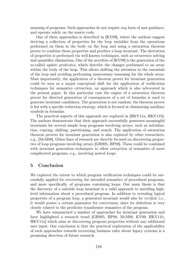
210

meaning of programs. Such approaches do not require any form of user guidance,and operate solely on the source code.

One of these approaches is described in [KV09], where the authors suggestderiving a collection of properties for the loop variables from the operationsperformed on them in the body on the loop and using a saturation theoremprover to combine those properties and produce a loop invariant. The derivationof properties is performed via well-known techniques, such as recurrence solvingand quantifier elimination. One of the novelties of [KV09] is the generation of theso-called update predicates, which describe the changes performed to an arraywithin the body of the loop. This allows shifting the attention to the essentialsof the loop and avoiding performing unnecessary reasoning for the whole array.Most importantly, the application of a theorem prover for invariant generationcould be seen as a major conceptual shift for the application of verificationtechniques for semantics extraction, an approach which is also advocated inthe present paper. In this particular case the engine of a saturation theoremprover for directed generation of consequences of a set of formulas is used togenerate invariant candidates. The generation is not random: the theorem proveris fed with a specific reduction strategy, which is focused at eliminating auxiliarysymbols in formulas.

The practical aspects of this approach are explored in [HKV11a, HKV11b].The authors demonstrate that their approach successfully generates meaningfulinvariants for several simple loop programs involving arrays, such as initializa-tion, copying, shifting, partitioning, and search. The application of saturationtheorem provers for invariant generation is also explored by other researchers,e.g., [McM08]. Other lines of research are directly focused on discovering proper-ties of loop programs involving arrays [GRS05, HP08]. These could be combinedwith invariant generation techniques to allow extraction of semantics of morecomplicated programs, e.g., involving nested loops.

5 Conclusion

We explored the extent to which program verification techniques could be suc-cessfully applied for recovering the intended semantics of procedural programs,and more specifically, of programs containing loops. Our main thesis is thatthe discovery of a suitable loop invariant is a valid approach to unveiling high-level information about a procedural program. In addition to revealing logicalproperties of a program loop, a generated invariant would also be verified, i.e.,it would posses a certain guarantee for correctness, since its definition is veryclosely related to the predicate transformer semantics of the program.

We have summarized a number of approaches for invariant generation andhave highlighted a research trend [GRS05, HP08, McM08, KV09, HKV11b,HKV11a] which aims at discovering program properties without any additionaluser input. Our conclusion is that the practical exploration of the applicabilityof such approaches towards recovering business rules about legacy systems is apromising direction of future research.

211

Bibliography

[Bac88] Ralph-JR Back. A calculus of refinements for program derivations.Acta Informatica, 25(6):593–624, 1988.

[BBM97] Nikolaj Bjørner, Anca Browne, and Zohar Manna. Automatic gen-eration of invariants and intermediate assertions. Theoretical Com-puter Science, 173(1):49–87, 1997.

[BHMR07a] Dirk Beyer, Thomas A Henzinger, Rupak Majumdar, and AndreyRybalchenko. Invariant synthesis for combined theories. In Verifica-tion, Model Checking, and Abstract Interpretation, pages 378–394.Springer, 2007.

[BHMR07b] Dirk Beyer, Thomas A Henzinger, Rupak Majumdar, and AndreyRybalchenko. Path invariants. Acm Sigplan Notices, 42(6):300–309,2007.

[BLS96] Saddek Bensalem, Yassine Lakhnech, and Hassen Saidi. Powerfultechniques for the automatic generation of invariants. In ComputerAided Verification, pages 323–335. Springer, 1996.

[BLWG99] Jesus Bisbal, Deirdre Lawless, Bing Wu, and Jane Grimson.Legacy information systems: Issues and directions. Software, IEEE,16(5):103–111, 1999.

[CC77] Patrick Cousot and Radhia Cousot. Abstract interpretation: aunified lattice model for static analysis of programs by construc-tion or approximation of fixpoints. In Proceedings of the 4th ACMSIGACT-SIGPLAN symposium on Principles of programming lan-guages, pages 238–252. ACM, 1977.

[CSS03] Michael A Colon, Sriram Sankaranarayanan, and Henny B Sipma.Linear invariant generation using non-linear constraint solving. InComputer Aided Verification, pages 420–432. Springer, 2003.

[DD02] Satyaki Das and David L Dill. Counter-example based predi-cate discovery in predicate abstraction. In Formal Methods inComputer-Aided Design, pages 19–32. Springer, 2002.

[Dij68] Edsger W Dijkstra. A constructive approach to the problem ofprogram correctness. BIT Numerical Mathematics, 8(3):174–186,1968.

[Dij75] Edsger W Dijkstra. Guarded commands, nondeterminacy andformal derivation of programs. Communications of the ACM,18(8):453–457, 1975.

[FQ02] Cormac Flanagan and Shaz Qadeer. Predicate abstraction for soft-ware verification. ACM SIGPLAN Notices, 37(1):191–202, 2002.

[GR09] Ashutosh Gupta and Andrey Rybalchenko. Invgen: An efficientinvariant generator. In Computer Aided Verification, pages 634–640. Springer, 2009.

212

[GRS05] Denis Gopan, Thomas Reps, and Mooly Sagiv. A framework fornumeric analysis of array operations. ACM SIGPLAN Notices,40(1):338–350, 2005.

[Hay00] D. Hay. Defining business rules – what are they really. final report.Final Report, 2000.

[HKV11a] Krystof Hoder, Laura Kovacs, and Andrei Voronkov. Case stud-ies on invariant generation using a saturation theorem prover. InAdvances in Artificial Intelligence, pages 1–15. Springer, 2011.

[HKV11b] Krystof Hoder, Laura Kovacs, and Andrei Voronkov. Invariant gen-eration in vampire. In Tools and Algorithms for the Constructionand Analysis of Systems, pages 60–64. Springer, 2011.

[Hoa69] Charles Antony Richard Hoare. An axiomatic basis for computerprogramming. Communications of the ACM, 12(10):576–580, 1969.

[HP08] Nicolas Halbwachs and Mathias Peron. Discovering propertiesabout arrays in simple programs. In ACM SIGPLAN Notices, vol-ume 43, pages 339–348. ACM, 2008.

[Kap04] Deepak Kapur. Automatically generating loop invariants usingquantifier elimination–preliminary report–. In IMACS Intl. Conf.on Applications of Computer Algebra. Citeseer, 2004.

[KV09] Laura Kovacs and Andrei Voronkov. Finding loop invariants forprograms over arrays using a theorem prover. In Fundamental Ap-proaches to Software Engineering, pages 470–485. Springer, 2009.

[KW06] Daniel Kroening and Georg Weissenbacher. Counterexamples withloops for predicate abstraction. In Computer Aided Verification,pages 152–165. Springer, 2006.

[LB04] Shuvendu K Lahiri and Randal E Bryant. Indexed predicate dis-covery for unbounded system verification. In Computer Aided Ver-ification, pages 135–147. Springer, 2004.

[McM08] Kenneth L McMillan. Quantified invariant generation using aninterpolating saturation prover. In Tools and Algorithms for theConstruction and Analysis of Systems, pages 413–427. Springer,2008.

[MMH12] Krassimir Manev, Neli Maneva, and Haralambi Haralambiev. Ex-tracting business rules through static analysis of the source code.In Mathematics and Education in Mathematics, Proceedings of the41st Spring Conference of UBM, pages 247–253, Borovetz, 2012.Union of Bulgarian Mathematicians.

[Mor90] Carroll Morgan. Programming from specifications. Prentice-Hall,Inc., 1990.

[MT12] Krassimir Manev and Trifon Trifonov. Declarative semantics of theprogram loops. In Vladimir Dimitrov, editor, Information Systems& Grid Technologies: Sixth International Conference ISGT’2012,pages 326–337, Sofia, June 1–3 2012. St. Kliment Ohridski Univer-sity Press.

[Wir71] Niklaus Wirth. Program development by stepwise refinement.Communications of the ACM, 14(4):221–227, 1971.

D � � � � � � � � S � � � �

215

Field Fire Simulation Applying Hexagonal Game

Method

Stefka Fidanova and Pencho Marinov

Institute of Information and Communication Technologies, Bulgarian Academy ofSciences, Acad. G. Bonchev str. bl25A, 1113 Sofia, Bulgaria

{stefka, pencho}@parallel.bas.bg

Abstract. The field fires are a big problem for countries with dry cli-mate. The Mediterranean region, south part of the USA, Australia arehighly affected. In this work we propose a model of field fire spread. Weapply Game Method (GM) which is a kind of cellular automate. In ourapplication the cells are hexagonal, which is closer to the circle (the formof fire spread) than the square cells. In this work we describe the sim-plest cases, without wind and slope. We test our simple model on severalscenarios and the results looks realistic.

1 Introduction

Every year a lot of hectares of forest are burn in Europe. Especially south partof Europe where the climate is hot and dry during the summer. Last decadeswith a climate change this part of the Europe becomes dryer and increase of thefield fires is observed. The same problem arise in northern America. A modelfield fire spread can have several applications. The prevision of the fire front canhelp the fireman to optimize their work, and to reduce the damages. Anotherapplication is prevention. Possible scenarios can be played and the computermodel can show the dangerous places.

Existing models are fare to be satisfactory or they are very complicate andslow to be used in real time.

The empirical models are based on empirical correlations found in actual firesand on characteristics of different vegetations types. Among them is one devel-oped by Rothermel [9], used in most North American models [6]. These modelspredict the position of the fire front, but many relevant physical variables ofthe fire are unknown. Because they use correlations coming from real situations,their use with different physical conditions is hard.

Combustion models intend to keep track of the real physical variables in-volved in a fire. They are usually posed on a bidimensional domain. These ap-proaches are based on describing the processes with a system of differentialequations. Several important physical effects like wind, moisture, tilt or radia-tion are evaluated [4, 7, 8]. The initial system of differential equations is complexand some authors try to simplify it. These methods model the fire propagationmore close to the real fire spread, despite of the simplification they are very slowand hard to be use in real time computations.

216

The game method is a kind of cellular automate. The main idea is to representthe area with cells and to define transition rules between cells. Thus we candescribe the fire propagation and we hope that this approach is faster. In existingapplication of the game method [2] the cells are square and they form a squaregrid. In our application the cells are hexagonal.

The rest of the paper is organized as follows: in section 2 we describe thegame method and it application on field fire propagation; in Section 3 we testour algorithm on variety of situations; at the end we draw some conclusions anddirections for future work.

2 Game Method

The game method for modeling is introduced by K. Atanassov [1]. The ideacomes from the Conway’s Game of Life [3]. The game method is a kind of cellularautomate. The process is iterative. Every cell is related with several parameters.The parameters are changed during the time steps. There are rules describingthe change of every parameter. The number of parameters and the rules dependsof the modeling process. The cells can have different forms, it depends to theapplication. In most of the existing applications the cells are square.

One of the first applications of the game method is for simulating someaspects of forest dynamics [5]. The used cells in this applications are square.Other application is for simulating oil transformation in the marine environment[10]. In this application the cells are square too. Other application with squaresells is for simulating Brownian-like motions [2]. Game method for constructionof Voronoi’s diagrams uses triangular cells [2]. Other applications are solvingvariants of Steiner-Rosenbaum’s problem [2] and simulation of development offorest fire [11]. In the both applications are used square cells.

Sub-Region [48.5,52.5]x[36,39] Step 000/100 Sub-Region [48.5,52.5]x[36,39] Step 001/100

−→

Fig. 1. Hexagonal sells

In our application, considered area is represented by hexagons (see Figure 1).The hexagonal cells have two main advantages comparing with square. All neigh-bor cells have side contacts. There are not corner neighbors, which can provoke

217

problems and deformation of the results. The hexagon is closer to the circle,which is the real fire spread without wind. The problem is very complicated.Therefore we start our modeling with the most simple case when the area is flatand without wind. In this stage in our model there is only two parameters: thehow long the material burns (burning duration) and how much time it need tostart to burn (speed for ignition). For example if the speed for ignition is 2 andthe burning duration is 5, the cell will start to burn if during 2 time steps someneighbor cells burn and the cell will totally burned 5 time steps after ignition.We suppose that the size of the parameters and the size of the cells are fixed inadvance. If the material in the cell is unburned, than the burning duration andthe speed for ignition are equal to 0.

The rules for our application of game method are:

1. In the initial time step the fire starts from fixed cells (one ore more);2. Every time step the burning duration decrease with 1 till it becomes 0 (to-

tally burned);3. If some of the neighbors of the cell burns, the speed for ignition decreases

with 1;4. If the speed for ignition of the cell is equal to 0 the cell starts to burn;5. The process continues until no other change of the parameters is possible,

otherwise go to 2.

One of the advantages of our model is that the fire can start from one oremore point (cells) or from developed fire front. Comparing with WRF Fire model[6] the fire starts from a straight line.

3 Numerical Simulation

In this section we test our model on several scenarios. Our model is two dimen-sional. The number of cells in every of two directions, the time steps and thecells parameters are input data for our software. In our representation the cellsin the rows are neighbors and the cells in columns are not neighbors. In our testexamples the area consists of 100 × 100 cells, but because in the row the cellsare not neighbors, the area is rectangular.

First we test area where the burning duration of all the cells is 9 time stepsand the speed for ignition is 1.The fire starts from the center, the cell (50, 50). OnFigures 2a, 2b and 2c we show the fire spread on first, ninth and third time steps.We see that the fire is propagate like circle as is expected. On ninth iterationall area inside the fire front burn. On iteration 30 there is totally burned areaand the circuit burning front. On Figures 2d, 2e and 2f we show the fire spreadon first, ninth and thirteen time steps. The burning duration of all the cells isagain 9 time steps, but the speed for ignition is 3. We observe that the fire ispropagate slower, comparing with the previous case. On both examples the issame kind of vegetation in all cells.

On Figures 3a, 3b and 3c we show example with two kind of vegetations.Most of the cells have speed of ignition 1 and burning duration 2 and there are

218

219

group of cells, in the left of the center with burning duration 9 and speed forignition 4. Let imagine that it is a grass region and there is small forest inside.The fire starts again from the cell (50 × 50). We observe that on time step 16the fire surrounds the forest without the forest start to burn because the speedfor ignition of the forest is high. In time step 29 one of the corner of the foreststart to burn, because it has 4 grass neighbors cells which burn consecutivelyand thus the speed coefficient becomes 0 and the cell start to burn.

On Figures 3d, 3e and 3f we show an example similar to previous one, but inthis case the burning duration of the grass is 4 and the speed for ignition of theforest is 3, or the speed of ignition of the forest is less than the burning durationof the grass. In this case the grass succeed to ignites the forest and we observethe difference of the burning front in this and previous case. On the figures areshown the iterations 4, 16 and 39. On figure 3f we see that in iteration 39 allarea around the forest is burned only the forest continue to burn, because itsburning coefficient is higher.

On Figures 4a, 4b and 4c 4d we show the case when on the area there arethree types of combustible material. Lets think that they are big grass area,small forest and streak of bushes on the left of the forest. The speed of ignitionof the grass is 1 and burning duration is 2, the speed of ignition of the bushesis 2 and the burning duration is 5 and the speed of ignition of the forest is 4and the burning duration is 9. On the figures we observe that the burning grassignite the bushes. The bushes decrease the speed of the fire, thus the burninggrass start to surround the forest. The forest is ignited by the bushes from theleft and later it is ignite from the right corners by the grass. Thus from timemoment 34 the forest burns from left to the right and from right to the left.

The last scenario which we have prepared is area with the same speed ofignition equal to two and non-burning area with form of Π . We can think thatit is rock area or lake. We show the fire spread in this case on Figures 5a, 5b,5c and 5d. We observe that the fire surround the non-burning area and in thetime step 68 all surrounding of the rocky area is burned or burning and thereis a small area inside the Π which is unburned. In time step 80 all surroundingof the rock is burned and there is a small area inside the Π which continue toburn.

4 Conclusion

On this paper we present a field fire model based on the game method. On ourapproach we use hexagonal cells for area representation. We apply the model onflat area without wind, which is one of the simplest applications. We prepareseveral scenarios to test the model. The achieved fire fronts look realistic. In afuture work we will include wind and slope. We will try to contact developer ofexisting models and to compare with their results. We will try to find real dataand to compare the spread modeled by our model with the real fire spread.

220

Area 100x75 Step 004/100 Area 100x75 Step 004/100

Area 100x75 Step 016/100 Area 100x75 Step 016/100

Area 100x75 Step 029/100 Area 100x75 Step 039/100

3a. 3d.

3b. 3e.

3c. 3f.

Fig. 3. Grass and forest, case one and case two

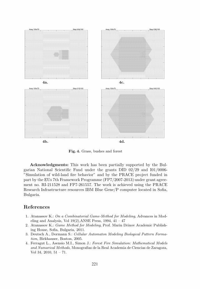
221

Area 100x75 Step 004/100 Area 100x75 Step 036/100

Area 100x75 Step 015/100 Area 100x75 Step 040/100

4a. 4c.

4b. 4d.

Fig. 4. Grass, bushes and forest

Acknowledgments: This work has been partially supported by the Bul-garian National Scientific Fund under the grants DID 02/29 and I01/0006-”Simulation of wild-land fire behavior” and by the PRACE project funded inpart by the EUs 7th Framework Programme (FP7/2007-2013) under grant agree-ment no. RI-211528 and FP7-261557. The work is achieved using the PRACEResearch Infrastructure resources IBM Blue Gene/P computer located in Sofia,Bulgaria.

References

1. Atanassov K.: On a Combinatorial Game-Method for Modeling, Advances in Mod-eling and Analysis, Vol 19(2),ANSE Press, 1994, 41 – 47

2. Atanassov K.: Game Method for Modeling, Prof. Marin Drinov Academic Publish-ing House, Sofia, Bulgaria, 2011.

3. Deutsch A., Dormann S.: Cellular Automaton Modeling Biological Pattern Forma-

tion, Birkhauser, Boston, 2005.4. Ferragut L., Asensio M.I., Simon J.: Forest Fire Simulation: Mathematical Models

and Numarical Methods, Monografias de la Real Academia de Ciencias de Zaragoza,Vol 34, 2010, 51 – 71.

222

Area 100x75 Step 004/100 Area 100x75 Step 068/100

Area 100x75 Step 045/100 Area 100x75 Step 080/100

5a. 5c.

5b. 5d.

Fig. 5. Grass and rock

5. Kimmins J. P.:Forest Ecology:A Foundation for Sustainable Forest Management

and Environment Ethics in Forestry, 3rd Ed. Pearson Prentice Hall, New Jersey,2004.

6. Mandel J., Beezley J.D. and Kochanski A.K.: Coupled atmosphere-wildland fire

modeling with WRF 3.3 and SFIRE 2011, Geoscientific Model Development(GMD) Vol.4, 2011, 591-610.

7. Margerit J., Sero Guillaume O. Modelling Forest Fire. Part I: A complete set of

equations derived by extended irreversible thermodynamics, Int. J. Heat and MassTransfer Vol 45, 2002, 1705 – 1722.

8. Margerit J., Sero Guillaume O. Modelling Forest Fire. Part I: Reduction to two-

dimensional models and simulation of propagation, Int. J. Heat and Mass TransferVol 45, 2002, 1723 – 1737.

9. Rothermel R. C.: A Mathematical Model for Predicting Fire Spread in Wildland

Fuels, General Technical Report INT-115, USDA Forest Service, International For-est and Range Experiment Station, 1972.

10. Sotirova E., Sotirov S., Dimitrov A., Atanassov K.:Simulation of oil Transforma-

tion in Marine Environment, Proceedings of the Jangeon Mathematical Sociaty,Vol. 15, 2012.

11. Velizarova E., Sotirova E., Atanassov K., Vassilev P., Fidanova S.: On the Game

Method for the Forest Fire Spread Modelling with Considering the Wind Effect, Inproc of IEEE Conf. on Intelligent Systems, Sofia, Bulgaria, September, 2012, 216– 220.

223

USING CLOUD COMPUTING IN HIGHER EDUCATION

Josif Petrovski1, Niko Naka2, Snezana Savoska2,

1 Faculty of education, University „St.Kliment Ohridski“ – Bitola, Vasko Karangelevski bb, 7000 Bitola, R.of Macedonia, thejosif@yahoo.com

2 Faculty of administration and Information systems Management, University „St.Kliment Ohridski“ – Bitola,

Bitolska bb, 7000 Bitola, R.of Macedonia, naka_niko@yahoo.com, savoskasnezana@gmail.com

Abstract. Information Technology today is becoming an integral partner in modern higher education. We are witnessed of the changes that occurred by using of this technology in the classroom. But, despite the constant improvement of performance and price, the total cost of IT is still going upwards, mostly because of the need of teachers and students of the newer and more powerful machines, and audio-visual aids. Working in times of fi nancial crisis and in conditions of steady growth needs, universities are facing with diffi culties in providing necessary information technology (IT) to support education, research and development activities. In these conditions educational institutions very quickly embraced cloud computing strategies and acceded to their implementation to their own needs. Although there are still obstacles to the full implementation of the cloud model, the potential benefi ts greatly outperform other risks that arise. Changes that occur require a new way of managing with information technology and also staff with responsibilities. As this model is developed and the risks are lower, most institutions are more intensely to adopt and implement according to their needs and conditions. The purpose of this paper is to present alternatives to the use of information technology in order for university to improve the overall educational process by reviewing the methods of using the model in higher education.

Keywords: information technology, cloud computing, higher education

1. Introduction

In these modern times the expression “Cloud computing” is being used a lot, but there is a lack of clarity about what cloud computing is. A study by McKinsey [12] found that there are 22 possible separate defi nitions of cloud computing [9, 19]. In fact, no common standard or defi nition for cloud computing seems to exist. Most of us are using the cloud on everyday basis without even realizing that this is the case [2,7]. Using our Gmail or Hotmail accounts, or uploads a photo to Facebook, we are using the cloud. The potential benefi ts and risks, however, are more visible [17]. The cloud can be described as on-demand computing, for anyone with a network connection. Access to applications and data anywhere, anytime, from any device is the potential outcome. In practice, cloud

224

computing as implemented is substantially more complex than the user perspective of it suggests, and many of the potential benefi ts of the cloud actually stem from this. Many of the perspectives on the cloud adopt a ‘layers’ view to describe it MIT Technology Review briefi ng [15].

In the last couple of years the concept of cloud computing has emerged as a practical and promising resolution to the challenges in the reduction of IT budgets and the growing of IT needs. Journals, conferences, consulting fi rms, and service providers dedicated to cloud computing services and strategies have sprung up virtually overnight which has increased exposure, attention and promise to address IT budget defi cit. Despite this creation of cloud computing resources and interest in such resources, for some IT leaders and institutional administrators, the solution is still far away [6, 8]. Most of the concerned sides say that there is too much propaganda but not enough adequate research and convincing case studies to fully commit resources and funding to move in this direction. Others are more troubled about the security and data protection [14]. The commitment to this model fundamentally will change the way of working of IT groups in universities, their power and infl uence, and their function and view of assessment within the institution.

In many terms the primary advantages the cloud brings are to do with cost and effi ciency, which are closely observed. The capital costs of computing can be resolved if an organization relies on the public cloud, buying virtual server time and storage space on demand. Expenditure on IT becomes operational, rather than capital. Moreover, the physical space required for tiers of servers is no longer essential and the organization no longer acquires energy costs for running and cooling its servers. For many start-up businesses, cloud computing offers access to computing power that would otherwise be beyond their reach. The entry barrier for large-scale computing task is effectively removed by the cloud. As costs are incurred on a per use basis, the risks of committing to large capital purchases are removed. Scalability allows the organization to add capacity as and when it’s needed and to scale down as well as up, driven by demand [17].

Even if ditching all physical servers is seen as a step too far, building a private cloud with virtualized servers, even if the organization owns and maintains the physical infrastructure, can deliver large effi ciency gains. A McKinsey survey cited by The Economist [12] suggests that, without virtualization, on average only 6% of server capacity is used. However, the kinds of economies of scale that large cloud providers can take advantage of will typically be absent. Nonetheless, in this private cloud approach an organization can still take advantage of the on-tap computing power in the public cloud. ‘Cloud bursting’ is a service that provides ‘overfl ow computing’ for dealing with spikes in web traffi c or processing load [15]. Flexibility, as well as cost, is another compelling advantage of the cloud. As Erik Brynojolfsson [1] of MIT states, “The ability to be agile in your infrastructure is what separates the winners from the losers… cloud computing is one of the most important technologies that affect the ability to maintain that level of fl exibility”. The paper is structured in two parts: theoretical and practical. The theoretical part presents the importance of the cloud computing in higher education and its benefi ts. In practical part we present our 3 types of learning management systems which are implemented in our faculty.

225

2. Cloud Computing In Higher Education

The Higher education around the globe is constantly evolving, generally as a result of important challenges arising from efforts to adopt new technologies and pedagogies in their classrooms. This is mainly as a result of a new genre of students with learning needs vastly different from their predecessors, and it is increasingly recognized that using technology effectively in higher education is vital to providing high quality education and preparing students for new challenges.

Many technologies that were previously expensive or unavailable are now becoming free when using the World Wide Web. This is true for all web sites, blogs, video sharing, music sharing, social sharing, collaboration software, editing/presentation and publishing, and computing platforms in the “cloud”. Students are already using many of these technologies in their personal lives. In the professional world, the trend of discovering and using technologies in our personal life is called “consumerization” [6]. This means we should demand and consume the required services. Our education system should take advantage of this situation, which will improve student’s education and reduce the spending of the academic institutions. Universities should identify and control technologies that are cost-effective, and try hard to offer realistic and reasonable access to technology for students and staff. The need for hardware and software isn’t being eliminated, but it is shifting from being on-premises to being in the cloud. All that is needed is a cheap access device and a web browser, internet connection in the facilities, perhaps wireless hotspots.

According to the CDW 2011 Cloud Computing Tracking Poll [3], 28 percent of organizations use some form of cloud computing. By industry, 37 percent of large U.S. businesses employ cloud computing strategies followed by 34 percent of higher education institutions in the U.S. This latter fi gure may not be accurate as another 2011 survey which revealed that as many as 63 percent of those completing the survey representing higher education reported that they were confused regarding the differences between cloud computing and virtualization [18]. Regardless, a growing number of higher education institutions in the U.S. are adopting some form of cloud computing for various reasons and only 5 percent are not considering it in the near future [3]. Many of the researchers [11] in this fi led identify 10 important features of cloud computing in higher education with respect to on demand services:

1. Increasing access to scarce IT expertise and talent.2. Scaling IT services and resources. 3. Promoting further IT standardization.4. Accelerating time to market through IT supply bottleneck reductions.5. Channeling or countering the ad hoc consumerization of enterprise IT services.6. Facilitating the transparent matching of IT costs, demand and funding.7. Increasing interoperability between disjoint technologies within and between

institutions.8. Supporting a model of a 24 x 7 x 365 environment.9. Enabling the sourcing of cycles and storage powered by renewable energy.10. Driving down capital and total costs of IT in higher education. Institutions will gain the benefi ts of cloud computing in varying degrees upon their

226

level of operation and degree of service models. As institutions become further engaged in cloud computing, they will be able to realize greater advantages, such as increasing access to scarce IT expertise and talent, promoting further IT standardization, the transparent matching of IT costs, demand and funding, and increasing interoperability between disjoint technologies within and between institutions. Using a scalable 24 x 7 x 365 model can drive down the capital and total costs for IT. The utility model is a pay-as-you-go model of cloud computing and is a welcome strategy and cost-saving measure for institutions of higher education in the face of rising IT costs and decreasing IT budgets. Services and computing resources are deployed in the cloud on a pay-per-service basis, thereby avoiding capital costs and internal operational expenditures. This way institutions can make adjustments every time they fi le like to increase or decrease capacity. There are numerous examples of when institutions need IT cloud resources scaled to meet temporary needs. For example:

- Enrolment of students;- Organizing conferences and provide IT support and Internet access for conference

participants; - Distance learning support;- Final examination period when thousands of students simultaneously need

access to computing resources and exams;

3. The Challenges Of Cloud Computing In Higher Education

Despite the growing acceptance of cloud computing and documented cost savings made possible by cloud computing in higher, concerns about the vulnerability to security breaches are the biggest obstacles to cloud computing adoption in higher education [10, 18]. The most important of these security risks includes the loss of authority, lock-in issues, isolation failure, compliance risks, management interface compromise, data protection, incomplete or insecure data deletion and malicious insiders [2]. In addition, concerns regarding privacy, data integrity, intellectual property management, regulation issues (e.g. HIPAA and FERPA), and audit trails are signifi cant barriers to adoption of cloud-based solutions [4, 5].

Consequently, risk assessment becomes a critical task, although some argue that many of the risks related to cloud computing is transferred to the cloud vendor/service provider [16]. To help diminish these risks for higher education institutions, several organizations have emerged in the last few years. The Cloud Security Alliance was launched in 2009 as a non-profi t organization tasked with conducting research in cloud security and offering information and resources about best practices in security protection in cloud computing [4, 5]. The Higher Education Information Security Council, a subgroup of EDUCAUSE, provides membership, comprehensive resources and engages members in an ongoing dialogue and issues, challenges and solutions in this area. As noted above, EDUCAUSE [4] also has a dedicated area on its website for cloud computing issues in higher education complete with publications, presentations, podcasts, blogs and news feeds.

Similar to computer security programs, cloud security involves the same general concerns: maintaining the integrity of data, ensuring access is limited to authorized users and maintaining the availability of data and services [4, 5]. With cloud computing, the

227

data and services are external to the campus and therefore controlling and protecting these assets becomes a much more complex and challenging proposition. Data encryption, e-discovery, frequency and reliability of data backups and recovery of data, the long-term viability of the cloud vendor and laws regarding storage and access to data all become critical issues. Typical service level agreements that cloud vendors provide are not specifi c and detailed enough to meet college and university requirements. Fortunately, through the Higher Education Information Security Council, a toolkit called the Data Protection Contractual Language is available to provide guidance and languages to assist institutions in crafting appropriate SLAs and contracts to meet their specifi c needs. This is an evolving area, and although much progress has been made, much more is needed before colleges and universities can place their complete trust in these third party cloud vendors. As increasing numbers of institutions move to the cloud, their collective bargaining power will help them create appropriate policies and contracts to meet their needs.

4. The Alternatives Of Cloud Computing In Higher Education

NIST [13] also describes three service models: Cloud Software as a Service, Cloud Platform as a Service and Cloud Infrastructure as a Service.

The differentiators among these three service models are the nature of the service and the level of customer-vendor control and engagement. Furthermore, it should be noted that these models are not mutually exclusive; organizations can and do employ different cloud service models on varying scales for different departments within the organization based on specifi c needs.

In model Cloud software as a service (SaaS), the vendor provides, manages and controls the underlying cloud infrastructure, including individual applications, network, storage, servers, operating systems, etc. The customer is able to fully access the vendor‘s applications in the cloud via a variety of devices (e.g. cell phone, laptop, PDA). SaaS examples include MyErp.com, Salesforce.com and Workday.com. Google Docs, Twitter and Facebook also fall into this category.

In the Cloud platform as a service (PaaS) model, similar to SaaS, the vendor provides, manages and controls the cloud infrastructure, except for applications, which the customer has control over. The vendor provides tools and resources allowing the customers to create and/or acquire applications to meet their specifi c needs. PaaS vendor examples include Wolf Frameworks, Dell-Boomi Atmosphere, Heroku, Google App Engine and Microsoft‘s Azure [20].

Cloud infrastructure as a service (IaaS) model means that vendor provides, manages and controls the general cloud infrastructure but provides the customer control over operating systems, storage, processing, and networks on demand. IaaS vendor examples include Flexiant‘s Flexscale, Rackspace and Amazon‘s Elastic Cloud Compute (EC2) and their Simple Storage Service (S3).

The case study we take in consideration is the implementation of learning management system – efront in the classes of web programming course in our faculty. The software is installed on the faculty’s server as intranet solution, but it can be installed also on the web environment as cloud. In the fi g.1 the used screens are shown and we can see the possibilities of the proposed solutions.

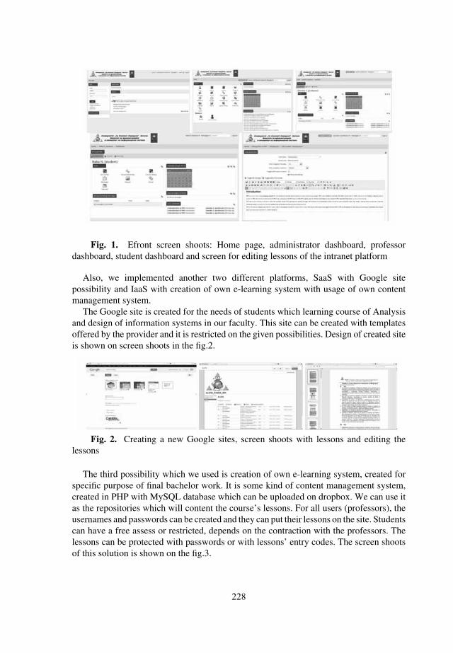
228

Fig. 1. Efront screen shoots: Home page, administrator dashboard, professor dashboard, student dashboard and screen for editing lessons of the intranet platform

Also, we implemented another two different platforms, SaaS with Google site possibility and IaaS with creation of own e-learning system with usage of own content management system.

The Google site is created for the needs of students which learning course of Analysis and design of information systems in our faculty. This site can be created with templates offered by the provider and it is restricted on the given possibilities. Design of created site is shown on screen shoots in the fi g.2.

Fig. 2. Creating a new Google sites, screen shoots with lessons and editing the

lessons

The third possibility which we used is creation of own e-learning system, created for specifi c purpose of fi nal bachelor work. It is some kind of content management system, created in PHP with MySQL database which can be uploaded on dropbox. We can use it as the repositories which will content the course’s lessons. For all users (professors), the usernames and passwords can be created and they can put their lessons on the site. Students can have a free assess or restricted, depends on the contraction with the professors. The lessons can be protected with passwords or with lessons’ entry codes. The screen shoots of this solution is shown on the fi g.3.

229

Fig. 3. Creating a own content management system, uploaded on dropbox,

form user login, staff menu and the appearance of the posted lessons

This proposed solution has own benefi ts – we can design the site as we want, without restrictions of proposed solutions as in the Google sites or with efront solution. Design of this kind of solution depends only of the programmer’s invention and knowledge or the users’ demands. We can use all of three concept separate or integrated depends of the courses, number of students on the courses or the demands of professors or students. Each of them has advantages and disadvantages accompanying with some specifi c form of learning as the practical work or task solving, communication possibilities or mutual work and depends on these reasons the solution can be selected.

5. Conclusion

Cloud computing is an emerging computing paradigm which promises to provide opportunities for delivering a variety of computing services in a way that has not been experienced before. It was demonstrated in this article how educational institutions are already taking advantage of the benefi ts which this technology is bringing, not only in terms of cost but also effi ciency and the environment. It was argued in this article that educational establishments are likely to embrace cloud computing as many of them are bound to suffer from under-funding due to the global economic crisis. In some parts of the world, such as our region, cloud computing is emerging as an empowering tool that is being used to advance the cause of education in the Balkan countries. Conventional perception dictates that cloud computing, as explained in this article, is unlikely to be suitable for education. However, recent research and real-life examples suggest that this view may no longer be valid. Like many new technologies and approaches, cloud computing is not without problems. There are many concerns relating to its security and reliability.

However, before that stage is reached, more work is required in order to address the concerns that currently prevent some organizations from embracing cloud computing.

We can use different approaches of the usage of cloud computing in the higher education process, depends on the professors’ and students’ needs and the type of courses and way of learning. All of these solutions have advantages or disadvantages which are associated with the level of practical work or possibilities of problem solving in the courses. Selection of the solution is specifi ed with the preferences of the specifi c course.

230

References1. Brynjolfsson, Erik and Saunders, Adam (October 2009) Wired for Innovation: How Information

Technology is Reshaping the Economy. The MIT Press. ISBN 0-262-01366-52. Catteddu, D., & Massonet, T. (2010). Cloud computing: Benefi ts, risks, and recommendations for

information security. Retrieved from http://www.trust-itservices.com/download/ Cloudscape-II/Channel_presentations/Tuesday_11.00-13.00/Philippe_Massonet-Cloud_Computing_Benefi ts, risks_and_recommendations_for_information_security.pdf on 18.05.2013

3. CDW-G. (2011), From tactic to strategy: The CDW 2011 cloud computing tracking poll. Retrieved from http://webobjects.cdw.com/webobjects/media/pdf/Newsroom/CDW-Cloud-Tracking-Poll-Report-0511.pdf on 15.05.2013

4. EDUCAUSE. (2010a). 7 things you should know about cloud security. Retrieved from http://net.educause.edu/ir/library/pdf/EST1008.pdf on 15.05.2013

5. EDUCAUSE. (2010b). Cloud computing contracts. Retrieved from http://www.educause.edu/wiki/Cloud+Computing+Contracts on 15.05.2013

6. Goodchild, J. (2011). Consumer device use is growing, but IT and security can’t keep up. Retrieved from http://www.csoonline.com/article/686087/consumer-device-use-is-growing-but-it-and-security-can-t-keep-up, on 19.05.2013

7. Goldstein, B. (2008). The tower, the cloud and the IT leader and workforce. In R. Katz (Ed.), the tower and the cloud. EDUCAUSE (pp. 238-261)

8. Goldstein, P., Gonick, L. S., Huish, D. S., Lambert, H. D., Lea, L. T., Pritchard, W. H., Siff, F. H., Smallen, D. L., and Steinbrenner, K. (2004). Doing more with less: Obstacle or opportunity for IT? EDUCAUSE Review, 39(6), 14-36.

9. Grossman, R. L. (2009). The case for cloud computing. IT professional, 11(2), 23-2710. Jitterbit. (2011). Ushers in Strategic Approach to Cloud Computing. Retrieved from http://www.

jitterbit.com/blog/2011-ushers-in-strategic-approach-to-cloud-computing/ on 18.05.201311. Katz, R. N. (2010). The tower and the cloud: Higher education in the age of cloud computing.

Educause.12. McKinsey & Company. (2009), Clearing the air on cloud computing. Discussant document,http://

www.cloudmagazine.fr/dotclear/public/clearing_the_air_on_cloud_computing.pdf, 201313. Mell, P., & Grance, T. (2011). The NIST defi nition of cloud computing (draft).NIST special

publication, 800(145), 7.14. Mircea, M., & Andreescu, A. I. (2011). Using cloud computing in higher education: A strategy

to improve agility in the current fi nancial crisis. Communications of the IBIMA, 2011, 1-15.15. Naone E.,(2009), Conjuring Clouds, http://www.technologyreview.com/article/413981/conjuring-clouds/page/3/, 201316. Patterson, D., (2010), Cloud computing and the RAD lab. Retrieved from http://www.mvdirona.

com/jrh/TalksAndPapers/PattersonMSCloudComputingRADLab.pdf on May 201317. Powell, J. (2009). Cloud computing–what is it and what does it mean for education? JISC E-

revolution, business, education, 818. Schaffhauser, D., Higher education optimistic about cloud use. Campus Technology, 201119. Voas, J., & Zhang, J. (2009). Cloud computing: new wine or just a new bottle?, IT

professional, 11(2), 15-1720. Metz, R. (2010). Cloud Computing in Higher Education: Changing the Way We Provide

Systems. http://www.educause.edu/Resources/CloudComputinginHigherEducatio/200928

231

Implications of Data Security in Cloud Computing

Dimiter Velev1 and Plamena Zlateva2

1University of National and World EconomyUNSS – Studentski grad, 1700 Sofi a, Bulgaria

dgvelev@unwe.bg 2 Institute of System Engineering and Robotics – Bulgarian Academy of Sciences

Acad. G. Bonchev Str., Bl. 2, P.O.Box 79, 1113 Sofi a, Bulgariaplamzlateva@abv.bg

Abstract. The cloud computing services provide for numerous benefi ts to the users. However, there are potentially signifi cant security considerations that should be taken into account before collecting, storing, processing or sharing data in the cloud. The paper tries to give a short overview of potential problems and their eventual solutions for providing data security in cloud computing regarding confi dentiality and privacy, data leakage, business continuity, legal issues of data manipulation in cloud computing services.

Keywords: Data, Security, Cloud Computing

1. Introduction

Internet has always been a dangerous place for malicious activities. The cloud computing offers a tempting target for cybercrime for various reasons. To maintain data integrity, many providers require all of their customer’s data to be placed in cloud which means that if compromised all data is available to attackers. Leading cloud providers such as Google and Amazon have existing infrastructure to defl ect cyber-attacks, but this could not be the case with all providers. The cloud architecture is such that it has interlinks with multiple entities and compromise with any one of the weakest links would compromise all the linked entities.

The cloud community services analyses the cloud activities constantly to detect and prevent newly injected viruses and malicious activities. Active participation of many organizations will help curb the malicious activities more effectively.

There are many clouds available in the market and the enterprises will start using different clouds for different operations. Eventually there will be a situation where the cloud integration services would be required which again would require a different approach of security implications. There is no single regulatory organization which regulates the standards for cloud security.

232

2. Cloud ComputingCloud computing is an on-demand service model for IT provision based on

virtualization and distributed computing technologies [1], [2], [3]. Typical cloud computing providers deliver common business applications online as services which are accessed from another web service or software like a web browser, while the software and data are stored on servers. The abstraction of computing, network and storage infrastructure is the foundation of cloud computing. The infrastructure is a service, and its components must be readily accessible and available to the immediate needs of the application stacks it supports. Cloud computing removes the traditional application silos within the data center and introduces a new level of fl exibility and scalability to the IT organization.

The following cloud computing categories have been identifi ed and defi ned in the process of cloud development:

• Infrastructure as Service (IaaS): provides virtual machines and other abstracted hardware and operating systems which may be controlled through a service Application Programming Interface (API). IaaS includes the entire infrastructure resource stack from the facilities to the hardware platforms that reside in them. It incorporates the capability to abstract resources as well as deliver physical and logical connectivity to those resources. IaaS provides a set of APIs which allow management and other forms of interaction with the infrastructure by consumers.

• Platform as a Service (PaaS): allows customers to develop new applications using APIs, implemented and operated remotely. The platforms offered include development tools, confi guration management and deployment platforms. PaaS is positioned over IaaS and adds an additional layer of integration with application development frameworks and functions such as database, messaging, and queuing that allow developers to build applications for the platform with programming languages and tools are supported by the stack.

• Software as a Service (SaaS): is software offered by a third party provider, available on demand, usually through a Web browser, operating in a remote manner. Examples include online word processing and spreadsheet tools, CRM services and Web content delivery services. SaaS in turn is built upon the underlying IaaS and PaaS stacks and provides a self-contained operating environment used to deliver the entire user experience including the content, its presentation, the applications and management capabilities.

• Multi-Tenancy: the need for policy-driven enforcement, segmentation, isolation, governance, service levels and billing models for different consumer constituencies. Consumers might utilize a public cloud provider’s service offerings or actually be from the same organization, but would still

233

share infrastructure.The cloud services can be implemented in four deployment models:• Public Cloud. The cloud infrastructure is made available to the general

public or large industry group and is owned by an organization selling cloud services.

• Private Cloud. The cloud infrastructure is operated entirely for a single organization. It may be managed by the organization or a third party, and may exist on-premises or off-premises.

• Community Cloud. The cloud infrastructure is shared by several organizations and supports a specifi c community. It may be managed by the organizations or a third party, and may exist on-premises or off-premises.

• Hybrid Cloud. The cloud infrastructure is a composition of two or more clouds (private, community or public) that are bound together by standardized or proprietary technology that enables portability of data and application.

The cloud computing environment usually consists of the following components:

• Servers - Hosting servers in the cloud using the corresponding services means operating those servers a safe distance from any disaster. Cloud hosting providers generally have more redundancy of network connections, mirrored sites and other precautions to ensure access under adverse conditions.

• Applications - People that use cloud-based applications like Google Apps or Microsoft Offi ce 365 can log in and be productive from virtually anywhere and any mobile device.

• Online data - Users will tend to keep their data stored remotely in the cloud. It is available from everywhere, and like cloud applications and it can be accessed from any device capable of connecting to the web.

• Cloud backup - Many companies fail to backup critical systems on a periodic basis at all, but it is even more severe when an organization has taken the time to create the backups, but the backups end up getting destroyed at the same time as the servers and data their backing up. Using a cloud-based backup solution provides for rebuilding the systems and resuming normal operations.

Under some circumstances, virtual appliances or virtual machine images of existing workloads can be created in the data center and stored in a cloud data center. In the event of a failure of the former, the virtual machines serve as recovery mechanisms that can be reactivated in the cloud.

3. Implications of Data Security in Cloud Computing

While cloud computing services have numerous potential benefi ts, there are

234

also potentially signifi cant privacy and security considerations that should be accounted for before collecting, processing, sharing, or storing institutional or personal data in the cloud. Consequently, institutions should conduct careful risk assessment prior to adoption of any cloud computing service.

The different models for cloud service delivery (IaaS, PaaS, SaaS) have different requirements of the customer when it comes to security. The less control is exercised, the greater rely on the security practices of the provider. Understanding where the lines are drawn and who is responsible for what is vital before moving anything valueable to a cloud. Private clouds arevnot necessarily free of the security concerns that plague public offerings. While a private clouds may seem more secure, they may introduce new threats and vulnerabilities that need to be understood. Even a locally hosted private cloud represents a potentially high concentration of data and services, which may have been far more distributed in the past. While the benefi ts of cloud may be that organizations need to worry less about how computing resources are provided, there are no free passes when it comes to compliance and legal responsibility. Cloud presents a way for business units to quickly provision systems and services, utilize resources, and de-provision those same systems so quickly that traditional approaches to good governance, security and due diligence are unlikely to keep pace. Cloud is a huge opportunity to redefi ne the way security and business units interact. While the technology may have been around a while, the way it is going to be used is new.

Specifi c risks and challenges to consider include [4], [5]:• Vendor transparency and inadequate or unclear service level agreement;• Privacy and confi dentiality of personal, sensitive, or regulated data and

information;• Legal and regulatory compliance;• Cyber security and support for incident forensics;• Records preservation, access, and management;• Service availability and reliability.

The security components involved in protecting data in cloud environments could include a long list of items [4], [6]:

• Encryption - To guarantee the privacy of information hosted on servers in cloud, the information could be encrypted which can only be decrypted at the client level with a key.

• Intrusion Detection and Prevention Systems - Providing security for cloud computing requires more than authentication using passwords and confi dentiality in data transmission.

• Antivirus - Antivirus scanning can be done on the cloud to reduce the risk of malicious activities. It is an expensive operation and doing it once ahead of time for benefi t of many could be advantageous, and with the power of cloud more anti-virus engines can be employed to make more effi cient.

235

• Firewall - Firewalls could be implemented as a virtual machine image running in its own processing compartment or at the hardware level.

• Security Threat - The communication between cloud services and consumers can be secured using SSL. Since the technology is too familiar, users usually ignore the warning which can be exploited by attackers. In SaaS model, the developer should always assume that intruders have full access to the client as anyone including intruders can buy the software.

• Authentication and Access - There are different authentication mechanisms for different services.

• Data Security - The organizations using cloud computing should maintain their own data backups even if the providers backs up data for the organization. This will help continuous access to their data even at the extreme situations such as data providers going bankruptcy or disaster at data center

• Legal Issues - The key legal issues in cloud with respect to sourcing arrangements are DPA (Data Protection Act of 1998), duties of confi dentiality and database right.

Detailed cloud computing security considerations have been already developed through in the world by many government agencies [4, 7]. Detailed list of security considerations that agencies can discuss both internally and with vendors that are transparent about their security measures. Questions are provided to provoke thought and discussion, rather than to be used simply as a checklist. Answers to these questions will assist agencies to develop a risk assessment and make an informed decision regarding whether the agency’s proposed use of cloud computing has an acceptable level of risk. It is unlikely that any single vendor will provide suitable answers to all of the questions, so agencies should decide which questions are most relevant based on the agency’s intended use of cloud computing. Answers to the following questions can reveal mitigations to help manage the risk of business functionality being negatively impacted by the vendor’s cloud services becoming unavailable [5], [7]:

• Business criticality of data functionality - are business critical data or functionality moved to the cloud?

• Could vendor’s business continuity and disaster recovery plan be comprehensively reviewed and could they cover the availability and restoration of both my data and the vendor’s services that I use?

• What is the data backup plan and what will be its cost? • What is the network connectivity to the cloud?• What is the vendor’s guarantee of availability? Does the Service Level

Agreement (SLA) guarantee that the vendor will provide adequate system availability and quality of service, using their robust system architecture and business processes? Availability may be affected by technical issues such as computer and network performance and latency, hardware failures and faulty

236

vendor software. Availability may also be affected by deliberate attacks such as denial of service attacks against me or other customers of the vendor that still affects me. Finally, availability may also be affected by confi guration mistakes made by the vendor, including those resulting from poor software version control and poor change management processes.

• What is the impact of outages? The vendor may have numerous long scheduled outages, including emergency scheduled outages with little or no notice to customers that do not result in a breach of the SLA. Vendors with distributed and redundant computing and network infrastructure enable scheduled maintenance to be applied in batches while customers are seamlessly transitioned to computing and network infrastructure that is still available and not part of the outage.

• What is the level of data integrity and availability? How does the vendor implement mechanisms such as redundancy and offsite backups to prevent corruption or loss of my data, and guarantee both the integrity and the availability of my data? This problem affected data in the vendor’s multiple data centers, highlighting the importance of having offl ine backups in addition to redundant data centers.

• How is data restoration performed? • What is the level of scalability? How much available spare computing

resource does the vendor provide to enable my usage of the vendor’s services to scale at short notice?

• How will the problem of changing vendor be solved? If a client wants to move his data to a different vendor, or if the vendor suddenly becomes bankrupt or otherwise quits the cloud business, how does he get access to his data in a vendor-neutral format to avoid vendor lock-in?

4 Conclusion

It is evident that the cloud computing by itself is in evolving stage and hence the security implications in it are not fully complete yet. Achieving complete solution for legal issues is still a question. With this level of issues in cloud computing, the decision to adopt cloud computing in an organization must be carefully assessed well in advance.

237

Acknowledgments

This work is supported in part by the University of National and World Economy, Sofi a, Bulgaria under Grant NI 1-8/2011.

References

1. Cloud Computing, http://en.wikipedia.org/wiki/Cloud_computing.2. Reese, G.: Cloud Application Architectures: Building Applications and Infrastructure in

the Cloud. O’Reilly Media, Inc., (2009).3. Rittinghouse, J.W., Ransome, J.F.: Cloud Computing: Implementation, Management and

Security. CRC Press, 2009.4. [4] Geoff Webb, Top 5 Cloud Computing Security Concerns, http://www.esecurityplanet.

com/trends/article.php/3930401/Top-5-Cloud-Computing-Security-Concerns.htm.5. Narendran C. R., Security Implica� ons of Cloud Compu� ng, h� p://www.narensportal.

com/papers/security-implica� ons-cloud-compu� ng.aspx.6. Valerie Vogel, Cloud Computing Security, https://wiki.internet2.edu/confl uence/display/

itsg2/Cloud+Computing+Security.7. Department of Defence, Australian Government, Cloud Computing Security

Considerations, http://www.dsd.gov.au/publications/csocprotect/Cloud_Computing_ Security_Considerations.pdf.

238

Contemporary Concurrent Programming Languages Based on the Actor Model

Magdalina Todorova, Maria Nisheva-Pavlova, Trifon Trifonov, Georgi Penchev, Petar Armyanov, Atanas Semerdzhiev

“St. Kliment Ohridski” University of Sofi a, Faculty of Mathematics and InformaticsSofi a 1164, Bulgaria

Abstract. This article briefl y reviews some of the contemporary languages for concurrent programming that are based on the message-passing paradigm with the Actor model as a formal model for concurrency. The Actor model is briefl y described and its implementations are reviewed in all included languages: Elrang, Scala, Ptolemy, Io and SALSA.

Keywords: programming language, concurrent programming, actor model

1 Introduction

Two models of concurrency are widely recognized - the one with shared memory (shared memory) and the one based on the exchange of messages (message passing). Most concurrent programming languages use the shared memory approach. A small number of modern programming languages, including Erlang, Scala, SALSA, Io, Ptolemy, Occam, Oz, Pict, Stochastic Pi Machine, PiLib, among others, apply the model based on the exchange of messages.The message passing model implies multicomputer architecture with a multitude of processors each having a local memory. There is no shared memory and all the calculations are carried out by isolated processes. The established known mathematical models of the message passing approach are the Actor model [1] and the Pi calculus [2].This article is focused on the general purpose programming languages, based on the Actor model.

239

2 Actor Model

2.1 Defi nition

In [3] Gul Agha, one of the authors of the Actor model defi ned it as follows:Actors is a model of concurrent computation for developing parallel,

distributed and mobile systems. Each actor is an autonomous object that operates concurrently and asynchronously, receiving and sending messages to other actors, creating new actors, and updating its own local state. An actor system consists of a collection of actors, some of which may send messages to, or receive messages from, actors outside the system.

2.2 Historical aspects

This model is infl uenced by the programming language Lisp, Simula 67 and Smalltalk-72, as well as the ideas for Petri nets, capability-based systems and packet switching. A more detailed overview of the historical development of this model can be found in [4]. Initially, the concept was developed by Carl Hewitt in [5] where the actor “referred to rule-based active entities which search a knowledge base for patterns to match, and in response, trigger actions”. Further development of the model was done by Carl Hewitt, Peter Bishop, and Richard Steiger, who initially regarded actors as agents of computation, and later as a model of concurrent computing. The Actor model used today was proposed by Gul Agha in 1985 and defi nes the actors through a simple operational semantics [1].

2.3 Key featuresIn the actor model, each object is an actor that receives and processes

messages. The order of the processing of the messages is not relevant to the actor, although some implementations, for example Scala, have introduced the concept of a message queue. The absence of preference in the selection of messages to process allows the actor to work with messages in parallel.

The Actor is an entity that has a name and behavior which determine its actions. Messages can be exchanged between actors, which will be buffered in the mailbox. The actions that an Actor can execute in response to a received message are:

- Create some new actors;- Send some messages to other actors;- Assume new behavior for the next message to be received;- Migrate to another computing host.

Fig. 1 illustrates this.

240

Fig. 1. Actors are reactive entities. In response to a message, an actor can (1) change its internal state, (2) send messages to peer actors, (3) create new

actors, and/or (4) migrate to another computing host.

The interaction between actors is mainly asynchronous. This means that the player that sends a message does not wait for the receiver of the communication to process it, and continues to perform its internal calculations instead.

Unlike previous models, combining consecutive processes, the actor model is suitable for parallel and distributed processes. The main new element is the introduction of the term “behavior”, formally defi ned by a mathematical function that represents the actions of actors in the processing of messages. By means of the “behavior” component the concurrency can be formalized as a mathematical model.

241

It’s not necessary for actors to receive messages in the same order in which they have been sent. All messages received by an actor are buffered in its mailbox before being processed. Communication between actors allows an actor that is constantly in a state of readiness to process messages from their mailbox to process all messages sent to it. An actor may interact with another actor if it has a reference to the latter. Since actors can create other actors, the model supports unlimited concurrency.

2.4 Programming with Actors

According to [1] a program in an actor language consists of: behavior defi nitions; new expressions; send commands; receptionist declaration; external declaration.

In the text that follows, we use the Backus-Naur meta-language syntax.

2.4.1 Defi ning BehaviorsThe behavior defi nitions simply associate a behavior schema with an identifi er

(without actually creating any actor). They are templates for actor behaviors. A behavior defi nition is expressed as a function of the incoming communication. Two lists of identifi ers can be used for the defi nition: the fi rst list (the acquaintance list) corresponds to the parameters that need values assigned to them upon actor creation; the second list (called the communication list) is a set of parameters that are bound to data from the incoming messages (communications). When an actor is created and it accepts a communication, it executes commands in the environment defi ned by the bindings of the identifi ers.

The syntax of a behavior defi nition:

<behavior_defi nition> ::=def <behave_name> (<acquaintance_list>) [<communication_list>] <command>*end def

The <behave_name> is an identifi er.

2.4.2 Creating ActorsQuoting [1], actors are created by means of new expressions which return the

mail address (i.e., actor reference) of a newly created actor. A new expression is defi ned as follows:

<new_expression> ::= new <behave_name> (expr {, expr}*)

242

The <behave_name> is an identifi er bound to a behavior given by a declaration by means of a behavior defi nition. A new actor is created with the behavior implied by the behavior defi nition and its parameters are instantiated to the values of the expressions in the parenthesis.

2.4.3 Creating TasksThe syntax of a command that would create tasks is as follows:

<send_command> ::= send <communication> to <target>

where a <communication> is a sequence of expressions (perhaps empty). The expressions may be identifi er constants or the appropriate functions of these. The <target> is the mail address of the actor to which the communication is sent.

2.4.4 Declaring ReceptionistsThe receptionists are those actors that can receive messages sent from outside

the system. The dynamic and open nature of the actor systems implies a dynamic character of the set of receptionists.

Receptionist declaration lists actors that may receive communications from the outside.

2.4.5. External DeclarationThe external declaration lists actors that are not part of the population

defi ned by the program but to whom communications may be sent from within the confi guration.

2.4.6 CommandsCommands determine the set of actions that have to be executed. The minimal

palette of the most used commands in the programming languages based on the actor model can be described in the following way:

<command> ::= if <logical_expression> then <command> { else <command>} fi | become <expression> | <send_command> | <let_bindings> { command } | <behavior_defi nition> | <command>*

This briefl y overviews the expressions for creating new actors (new) and the commands for creating new tasks (send) and for defi ning behavior (behavior

243

defi nition). The if-fi command is similar to the if-else operator in the imperative programming languages.

In the following command:become <expression>

<expression> is bound to a mail address. The actor simply forwards all its mail to the actor at the specifi ed mail address. This command serves as a behavior change.

The syntax for let bindings is as follows: <let_bindings> ::= let id = <expression>

(and id = <expression>)*where id is an identifi er. Using let allows for assigning shorter names to some

expressions. The following syntax:

<command>*denotes a sequence of commands.

The programs that apply the actors model are a sequence of behavior defi nitions followed by a command:

<program> ::= <behavior_defi nition1> … <behavior_defi nitionn> <command>

2.5 Applications of the Actor model

The model has been used both as a framework for a theoretical understanding of concurrency, and as the theoretical basis for several practical implementations of concurrent systems.With the rise of parallel and distributed computation platforms, such as multicore architectures, sensor networks, cloud applications, etc., the number of applications of the Actor model has also risen. It can be successfully applied in modelling parallel programs that involve distributed computation: e-mail, web services, semaphore objects, cloud computing. Actors can be used for modelling functional, procedural or object-oriented systems.Many actor languages and frameworks have been defi ned. Some of the fi rst actor-based languages were: Act 1, 2 and 3, Acttalk, Ani, Cantor, Rosette, ABCL, ConcurrentSmalltalk, POOL, ACT++, CEiffel, HAL. Modern languages based on this model are: Erlang (from Ericsson) [7], Scala (from EPFL) [8], Ptolemy (from UC Berkeley) [9], SALSA (from UIUC and RPI) [10], Charm++ (from UIUC) [11], ActorFoundry [12] (from UIUC), the Asynchronous Agents Library

244

(from Microsoft) [13], Axum [14] (from Microsoft), Orleans framework for cloud computing (from Microsoft) [15], etc.

The ideas of the actor model are universal and simple but their literal implementation is ineffective because of the lack of determinism in the model. Thus every language based on it implements it in its own specifi c way. For example, in Erlang the processes (actors) can interact asynchronously, but the interaction inside a process is synchronous.

3. Programming languages based on the actor model

3.1. Erlang

Erlang (http://www.erlang.org/) is a programming language designed at Ericsson Computer Science Laboratory. It is a general-purpose programming language which utilizes concepts of functional and logic languages. Erlang was originally designed to support distributed, fault-tolerant, soft-real-time, non-stop applications. Its main advantage is the support for concurrency. It is a purely functional language enabling the use of single assignment variables, which leads to the absence of side effects. There is no concept of shared memory and there are no locks. Processes communicate only by exchanging messages.

Erlang processes are lightweight processes which are managed by an internal scheduler. There is no shared state between them and communication is done by an asynchronous message passing system. Concurrency in Erlang is achieved by using three language constructs: spawn, send (!) and receive.

spawn(<function>) creates a new concurrent process that evaluates <function>. The new process runs in parallel with the calling one. spawn returns a process identifi er.

<Pid> ! <message> sends <message> to the process with identifi er <Pid>.

receive ... end is used to retrieve messages that match specifi c patterns. The receive command has the following syntax:

receive Pattern1 [when Guard1] -> Expressions1; Pattern2 [when Guard2] -> Expressions2; ... after Timeout -> ExpressionTimeout;end

245

Each process has a mailbox which contains a queue of messages sent by other processes which have not been carried out yet. The receive command checks all the messages inside the process’ mailbox against the sequence of patterns. If a match is found, the message is deleted from the mailbox and the process execution is resumed. Otherwise, the process blocks until new messages are delivered.

The behavior of the receive command depends on the particular value of the Timeout. If no timeout is specifi ed, or the timeout value is equal to infi nity, receive blocks until new messages are put into the mailbox. If a value between 0 and infi nity is specifi ed, receive waits for the specifi ed amount of time and if no messages arrive, the ExpressionTimeout is executed. When the timeout value is 0, receive tries to match the messages in the mailbox against the patterns and if no match is found, the ExpressionTimeout is performed.

3.2 Scala

Scala (http://www.scala-lang.org/) is a programming language which provides both object-oriented and functional programming styles. It was designed at EPFL in Lausanne, Switzerland, in order to be scalable in correspondence with the needs of its users. Scala is fully interoperable with the Java language, which allows developers to use Java legacy objects and all Java libraries within Scala.

In contrast to Erlang, two kind of concurrent programming models can be exploited in Scala: shared memory, provided by means of threads, and distributed memory, using asynchronous message passing provided by the actor model. Actors in Scala are not a language construct, as in Erlang, but implemented in a library. The Scala Actors library defi nes the actor type and three operators: ! (send), receive and react. The fi rst two have practically the same syntax and semantics as in Erlang. The explanation of the react operator needs some information about the way actors are implemented in Scala.

There are two types of programming models for concurrent processes: thread-based and event-based. Within the thread-based implementation, each actor is executed by a thread. The execution state of a concurrent process is maintained by the corresponding thread stack.

In the event-based implementation, an actor is described by a proper set of event handlers. The execution state is maintained by an associated record of object.

Actors in Scala unify both programming models. The react operator is a semantic equivalent to receive but while the latter is based on the thread-based model, the former implements the event-based one. Thus receive blocks the actor, actually suspending the corresponding thread, if there are no messages in the mailbox. In contrast, react just detaches the actor from the active thread.

246

It is shown in [16] that it is possible to unify these programming models by using a threads pool of executing actors. During the execution of an actor, tasks are generated and submitted to a thread pool for execution. A task is generated in three cases: spawning a new actor, calling react when a message can be immediately removed from the mailbox, sending a message to an actor suspended by a react that enables the actor to continue. The thread pool approach could cause deadlocks if its size is fi xed [16], therefore the thread pool may be re-sized in case of necessity.

3.3 Ptolemy

Ptolemy is a programming language whose goals are to improve a software engineer’s ability to separate conceptual concerns. In particular, Ptolemy’s features are useful in case of modularization of crosscutting concerns. A key difference between Ptolemy and other technologies to separate conceptual concerns such as AspectJ is that Ptolemy strives to balance separation of crosscutting concerns and modular understanding and reasoning about concerns. Its motto states that: ”one shall not have to choose between modular reasoning and separation of crosscutting concerns.” [17]. It has been created under the Ptolemy project frame, conceived in the University of Berkley, California, under the guidance of professor Edward A. Lee. The development of the language passed through a few phases: Gabriel (1986-1991), Ptolemy Classic (1990-1997) and Ptolemy II (1996- ). Ptolemy II is a complex of programs, libraries of Java classes and other mechanisms aimed at building and exploring models of different heterogeneous computing systems (mostly embedded systems), as well as at scientifi c research in the modeling domain.

To fulfi l this goal, Ptolemy II supports a wide array of computational models among which: CI (component interaction) – a computational model with a “push/pull” interaction between components; CT (continuous time) – models with continuous time; DE (discrete-event) – models with discrete events; DDE (distributed discrete events) – systems with partially ordered sets of discrete events; FSM (fi nite-state machines) – fi nite automata (lacking the concept of time); GR – supporting 3-D graphics; PN (process networks) – networks of Kahn processes (Kahn); SDF (synchronous datafl ow) – models for representing systems for signal processing (lacking the concept of time ); DDF (dynamic datafl ow) – an extensions to SDF, that allows for components to change the quantity of used and created data for one iteration during the execution of the model; HDF (heterogeneous datafl ow) – an extension of SDF that allows to preserve the static architecture and some other features of the models; DT (discrete time) – analogous to SDF, but with the concept of time; SR (synchronous-reactive) – a synchro-reactive computational model; CSP (communicating sequential processes) – interacting

247

sequential processes; Wireless – a computational model for systems with wireless communication.

Many of these computational models support the actor-based model as a basis of the architecture. Unlike the object-oriented based architectures, the actor-based one focuses on parallel computing that naturally emerges in modeling some processes.

In Ptolemy II (http://ptolemy.eecs.berkeley.edu/ptolemyII/), actors are software components that execute concurrently and communicate through messages sent via interconnected ports. They can be viewed as atomic functional signal transformers. Their behavior is implemented in Java. Every actor is an object of a Java class that can be extended during modeling. This interface does not take into consideration the internal state of the actor and only provides rule for interaction between the actor and its environment. The interface includes ports that serve as connection points to the actor, and parameters that serve to fi ne tune the behavior of the actor.

Actors can have a hierarchical structure (they can be containers for other models). Ptolemy II has a huge library of actors, arranged by the kind of the transformations they can execute. Polymorphism is a key feature of Ptolemy II. It concerns the computational models, as well as the data being processed. The language also supports Higher-order components (actors). The standard library includes actors that allow user input, interactive shell, input, output and processing of signals and images, including video signals in real time; fi le input and output; access to internet-based resources; integration with other tools and languages.

3.4 Io

Io is a pure object-oriented programming language inspired by Smalltalk, Self, Lua, Lisp, Act1, and NewtonScript. Io has a prototype-based object model similar to the ones in Self and NewtonScript, eliminating the distinction between an instance and a class. Like Smalltalk, everything is an object and it uses dynamic typing. Like Lisp, programs are just data trees. Io uses actors for concurrency [18]. The language has very simple syntax and semantics. There are two basic structures: objects and messages. They serve as building blocks for all other concepts in the language. There are no classes, only objects. An object can be cloned and changes so that a new object is created (prototyping). Every object contains its own meta-information and can change to an arbitrary type of an object. All data types, values, etc., are objects of the language. Io uses the mechanism of active objects (actors) for parallel programming. An Actor is represented by an object-oriented stream. Each object can be sent an asynchronous message by prepending “@” or “@@” in front of the message name. When an object receives an asynchronous message, it stores it in its own internal

248

queue, unless the latter is empty. If there was no queue defi ned for the object, a coroutine is invoked to process the message. The queued messages are processed in FIFO order. Calling “yield” can transfer the control to another coroutine. The result of an asynchronous “@” message can be obtained by using the Future method. This result can then be sent to another object using sendResultTo().

3.5 SALSA

The SALSA programming language (Simple Actor Language System and Architecture) is an actor-oriented programming language that uses concurrency primitives beyond asynchronous message passing, including token-passing, join, and fi rst-class continuations. It also supports distributed computing over the Internet with universal naming, remote communication, and migration of linguistic abstractions and associated middleware [19]. The language was created to introduce the benefi ts of the actor model while keeping the advantages of object-oriented programming. It can be viewed as a Java dialect. Furthermore, SALSA provides automatic local and distributed garbage collection. It is often used for building systems involved in grid computing, mobile computing, and internet computing applications.

A SALSA program consists of universal actors that can be migrated around distributed nodes at run-time. Fig. 1 shows an actor and the main actions an actor can take in the SALSA language. The internal state of the SALSA actors can be described in terms of Java objects or primitive types. It is completely sealed, i.e. it cannot be shared with other actors. The main form of communications of SALSA actors is the asynchronous message passing. A SALSA message handler is similar to a Java method. The language provides three approaches to coordinate the behavior of actors: token-passing continuations, join blocks, and fi rst-class continuations.

SALSA supports the following concurrency programming mechanisms: - New actors can be defi ned with the new keyword. Creating an actor returns its

reference.- Sending messages to other actors happens via the <- operator.

Once created, actors process all incoming messages one by one.Distributed SALSA programming involves universal naming, theaters,

service actors, migration, and concurrency control.

249

4 Conclusion

The development of computer science and its applications in practice leads to the emergence of new tasks that the old programming languages are poorly fi t to solve. In turn, this leads to the creation of new programming languages. Concurrency is a fundamental problem in recent years. The goal of this article is to briefl y introduce some modern languages targeted specifi cally at concurrent programming based on the message-passing concurrency model with the actor model formalism.

Acknowledgement. The presented study has been supported by the Bulgarian National Science Fund within the project titled “Contemporary programming languages, environments and technologies and their application in building up software developers”, Grant No. DFNI-I01/12.

References

1. Agha, G.: Actors: a model of concurrent computation in distributed systems. MIT Press, Cambridge, MA, USA, 1986.

2. Pi calculus, http://en.wikipedia.org/wiki/%CE%A0-calculus.3. Karmani, R. K., G.Agha: Actors, http://www.cs.ucla.edu/~palsberg/course/cs239/papers/karmani-agha.pdf.4. Agha, G., I. A. Mason, S. Smith, C. Talcott: A Foundation for Actor Computation. Journal of

Functional Programming, 7(01):1–72, 1997.5. Hewitt, C.: PLANNER: A language for proving theorems in robots. In Proceedings of the 1st

international joint conference on Artifi cial intelligence, Morgan Kaufmann Publishers Inc., pp. 295–301, 1969.

6. Varela, C. A., Agha, G., Wang,Wei-Jen, Desell, T., Maghraoui, K.E., LaPorte, J., Stephens, A.: The SALSA Programming Language, Release tutorial, Rensselaer Polytechnic Institute Troy, New York, Feb. 2007.

7. Agarwal, S., P. Lakhina: Erlang - Programming the Parallel World,http://cs.ucsb.edu/~puneet/reports/erlang.pdf (date of last visit: June 26, 2013).8. The Scala Programming Language, http://www.scala-lang.org/node/25 (date of last visit: June

26, 2013).9. Lee, E. A.: Overview of the Ptolemy project, Technical Report UCB/ERL M03/25, University

of California, Berkeley, 2003.10. Welcome to the SALSA Programming Language, http://wcl.cs.rpi.edu/salsa/11. The Charm++ Parallel Programming System Manual. http://charm.cs.illinois.edu/manuals/html/charm++/12. ActorFoundry, http://en.wikipedia.org/wiki/ActorFoundry.13. Asynchronous Agents Library, http://msdn.microsoft.com/en-us/library/dd492627.aspx.14. Axum (programming language), http://en.wikipedia.org/wiki/Axum_(programming_

language).

250

15. Bykov, S., A. Geller, G. Kliot, J. R. Larus, R.Pandya, J. Thelin: Orleans: A Framework for Cloud Computing,

http://research.microsoft.com/pubs/141999/pldi%2011%20submission%20public.pdf.16. Haller, P., M. Odersky: Scala actors: Unifying thread-based and event-based programming.

Theoretical Computer Science, Vol. 410, Issue 2-3 (February, 2009), pp. 202-220.17. Ptolemy Programming Language, http://ptolemy.cs.iastate.edu/about.shtml18. http://en.wikipedia.org/wiki/Io_(programming_language)19. http://en.wikipedia.org/wiki/SALSA_(programming_language)

251

Software Integration Platform for Large-Scale Genomic Annotation of Sequences Obtained in NGS Data Analysis

Deyan Peychev1*, Atanass Ilchev1, Ognyan Kulev2, Dimitar Vassilev1

1Bioinformatics group, AgroBioInstitute, Sofi a, Bulgaria2 Faculty of Mathematics and Informatics, Sofi a University “St. Kliment Ohridski”

*Corresponding author: deyan.pey@gmail.com

Abstract. Genome annotation is important part of process of de-novo sequencing of genomes. It provides ability to identify patterns of similarity between genes from different organisms, and probably to predict function of de-novo explored genes. In last few years, NGS technology has provided a huge amount of data, which are most commonly hard to interpret and to be added as knowledge input for further investigations. Many tools are available for sequence data manipulation like aligners, assemblers, mappers, annotators but still hasn’t exists platforms providing integrated runtime environments which are easy to use for researchers. They should acquire some special skills to execute appropriate tools, to interpret intermediate results, and convert data to suitable input formats for next stages in their research pipelines. Our work is focused on applying of multi-platform, generic software integration platform for easy construction of pipelines which are able to combine multiple implementations for sequence data manipulation. Current use case is specially adopted for clustering and fi ltering of assemblies from de-novo sequenced RNAseq short reads obtained from bread wheat (Triticum aestivum) genome. CCIL platform (Content Classifi cation and Inter-Linking) is represented as solution to integrate appropriate tools and data standards to handle interoperability and scalability problems in NGS data analysis.

Version 1.0 of CCIL is available for download at http://sourceforge.net/projects/ccil

Keywords: Annotation, Software solution, Next Generation Sequencing

1. Introduction

High-throughput sequencing (HTS) or Next-generation sequencing (NGS) technology was boosted by the massive implementation of new sophisticated bioinformatics tools, specifi cally designed to make the NGS possible. Not only new software has been developed for a range of novel applications and types of data analysis, but new algorithms have also been developed for giving new solutions to old problems such as sequence alignment, de-novo assembly, functional annotation with the only objective to manage with the real deluge of data generated from the new sequencing platforms.

252

Key bioinformatics challenges created by NGS data comprise either aligning (mapping large number of reads to a reference genome or de novo assembly of novel genomes (transcriptomes), multiple alignment of large number of reads, contig matching in de novo sequencing projects, detection of rare variants and annotating them using new fi le formats and computational resources for effi cient management of the multi-terra byte sequence data fi les.

1.1. Problems in annotation

Ideas for new concepts of gene structure and function emerge constantly from the biological and medical research. The major objective of genome annotation is to provide an accurate and up-to-date coding reference for biological and medical research. This annotation is a very important background for the development of other genomic research technologies such as expression studies, epigenetics, generation of knowledge based on functionally important mutations.

By it sense genome annotation for NGS data is a multi-step process based on the: information for the gene model (EST library or protein database), building evidence-based gene models, training the gene prediction program with collected evidence, predict gene models and the genome features, and assign gene names and report annotation accuracy. All these steps can be considered as a unite knowledge generation process providing and information with new quality [1, 6, 7].

Technically, every particular NGS workfl ow includes many stages for data manipulation and interpretation. At fi rst time the sequencer output must be formatted in way, depending of subsequent processing specifi cs. Subsequent steps can be different fi ltering algorithms, nucleic sequence aligners, database lookups and more. At each step specifi c implementations may require different input-output formats and incompatible metadata sets. In most cases genome annotation applications are running in different process containers, and researcher must confi gure and start every stage of analytical workfl ow separately. This may cause more errors in components confi guration, input data selection and loss of data. Researchers should acquire some special skills to execute appropriate tools, to interpret intermediate results, and convert data to suitable input formats for next stages in their research pipelines. Furthermore sometimes they need to change one algorithm implementation with another one to achieve better performance and scalability, but most commonly this affects effi ciency of entire research and possibly leads to radical changes in research pipelines. The problem in general is that separate programs in genome annotation workfl ow require additional efforts for proper communications between them. Good existing solution is Blast2GO program [2] which provides sequence alignment, database lookup and search in one integrated and easy confi gurable process. But problems of genome annotation often falls back to scalability and annotation process operates with really huge amount of data. In NGS data analysis the “short reads” input is composed of

253

millions of nucleic sequences to be analyzed. The most effective way to operate with such kind of large-scale input is to build study-specifi c pipelines with high-level control over used components in way to increase effi ciency and decrease the cost of the study.

1.2. Project and goal

The goal of current work is to develop integrated platform for nucleic sequence data manipulation. This platform is based on CCIL platform (http://sourceforge.net/projects/ccil) and it is organized in way to integrate existing tools for sequence analysis, data transformations and storage in pipelines. Every pipeline stage (particular tool in this context) can be confi gured autonomously according to researcher’s particular needs and also can be replaced with alternative implementation without any considerable changes in pipeline itself. The solution is a framework at the same time, because it provides ability to build analytical applications with shifting and reconfi guring of a set of predefi ned tools, custom client implementations and third-party libraries. Such kind of integration is achieved defi ning common base interfaces between all stages in way to interpret communications and data handling at more abstract and transparent level.

CCIL platform provides more granular task distribution and possibility to use alternative technologies for data transformation, data mining and store. In some cases researchers takes different decisions about the work direction at all – machine learning or statistical approaches, relational databases or XML-based data stores etc. One of the most important things in that study is development of common data fl ow standard for communication and data propagation between every particular pipeline stage to achieve high-scalable and fl exible infrastructure for NGS data analysis.

In current study we discuss preliminary results produced by using of CCIL framework (Content Clustering and Inter-Linking) to build pipeline for retrieving, clustering and storage of genome assemblies from Triticum aestivum. Integrating some base data mining technologies, we produce clusters of sequence similarities which are suitable for fi ltering of irrelevant noisy contigs produced by short reads assembly.

2. Material and methods

2.1. Input data

Our experimental object is dataset containing RNAseq short-read assemblies between 300 and 3000 base pairs in length. They are obtained from several de-novo sequenced regions from bread wheat (Triticum aestivum) genome, including:

254

1. Transcriptome part – coding mRNA reads from three different development stages of wheat.

2. Exones part – coding DNA reads linked with short poly-A fragments.

Short-reads are assembled using Trinity and Abyss. The produced assemblies are serialized in FASTA format and take approximately 45GB disk space. Length properties of assemblies are represented into the following table:

Trinity Trans-ABySS

2CFG CFB CFD 2CFG CFB CFD

Contigs count 51012 59280 54521 31152 356787 33820

Mean length 357 364 361 304 280 298

Median length 333 336 335 267 257 262

Max length 2928 1934 2513 2211 1460 2124

Table 1. Contigs for three developmental stages assembled by Trinity and Trans-ABySS.The two algorithms were run out with default parameters.

2.2. Software platform

CCIL platform is originally developed as service-oriented software integration solution for information retrieval and semantic indexing over large-scale of web resources. It’s designed to construct pipelines composed by stages, all of them performing simple task over the data. These stages use common interface for message and data exchange and can be arranged on different ways, depending of specifi c needs to produce custom data analysis. Initially the platform is distributed with small number of built-in stages including data collectors (crawlers and parsers), fi lter and indexers providing ability to analyze document similarities and phrases-to-document relevancy in the context of particular domain. Stages are custom classes which extends single Java base type – CCIL Stage Base. Base class provides simplest interfaces between stages – row data which is populated with one row per iteration, assigning label for every object passed to data fl ow or initializing key-value map of features for every row object. This is suitable for mapping of particular sequence with relevant metadata and passing them to the next stage. Actually the stage is custom inheritor of CCIL Stage Base and can invoke third party objects and manipulate the data in study-specifi c manner. Confi guration of the stages is designed to use “contexts”. Context is set of

255

parameters which are specifi c for stages and defi nes a pipeline to be executed. Contexts are serialized in two fi les. First one describes actual implementations of the stages. It is serialized in TTL format and affects entire platform. Example lines are as follows:

@prefix rdf: <http://www.w3.org/1999/02/22-rdf-syntax-ns#>.

@prefix entity: <https://sourceforge.net/projects/cybercore/entities#>.

@prefix service: <https://sourceforge.net/projects/cybercore/services#>.

service:collect-rdb rdf:type entity:service ; entity:implementation “com.ccil.collect.rdb.

RDBContentProvider” ; entity:classpath “” ; entity:arguments “” .

First three lines are prefi xes declaration for namespaces used in confi guration. Remaining part describes that “collect-rdb” is entity of type “service”, and it’s implementation has fully qualifi ed name “com.ccil.collect.rdb.RDBContentProvider”. Following two lines describes that this implementation has no additional classpath dependencies and takes no arguments directly from data fl ow.

Second confi guration fi le is serialized in key-value properties fi le and defi nes context-specifi c parameters distribution of each stage. It also defi nes the pipeline itself:

context.collector.pipeline = RDB, BUILDSV

RDB = collect-rdb RDB.connection = jdbc:mysql://localhost/ccil RDB.query = SELECT id, sequence FROM contigs RDB.user = isgt RDB.password = conference RDB.lucene = lucene

BUILDSV = index-sv BUILDSV.lucene = @lucene BUILDSV.termfi le = termvectors.bin BUILDSV.docfi le = docvectors.bin BUILDSV.dimension = 200 BUILDSV.seedlength = 10 BUILDSV.docindexing = inmemory BUILDSV.contentsfi elds = @contentfi eld,metadata BUILDSV.docidfi eld = @docidfi eld

256

First row describes pipeline and order of stages insight. Pipeline is composed by two stages – RDB and BUILDSV. Next few lines are for parameters of both stages. This particular example confi gures a pipeline that means the following:

Collect all sequences from MySQL database named “ccil” executing query (RDB.query parameter) and store collected data in Lucene document store. Then start to build SemanticVectors store using following parameters (BUILDSV parameters).

For Triticum aestivum – NGS de novo RNA seq annotation study, a specifi c pipeline were designed. It includes custom FASTA parser, SemanticVectors indexer and custom vector search component. Vector search is actual component which looks up for sequences similarity and builds the similarity clusters. Finally, cluster results are stored to relational database. Case-specifi c pipeline is described in the following section.

2.3. Pipeline model

Analytical pipeline includes following stages: parsing of assembled contigs, loading to document store, vector indexing and clustering. Nucleic sequences with assigned metadata are represented as labeled textual resources with unique inner identifi ers.

Fig 1. Current CCIL pipeline for building of similarity clusters between assembled contigs. Rectangles are components, arrows are interfaces

2.3.1. Parsing stage

First stage uses custom parser component that reads text fi les in FASTA or

257

FASTQ format. The component loads sequences in memory as simple key-value row objects. Keys are unique identifi ers for sequences and document labels as well.

2.3.2. Indexing and clustering stages

Once loaded in memory, contig sequences are serialized in Apache Lucene (http://lucene.apache.org) document index. Lucene is able to store large-scale labeled documents and retrieve them in high-effi cient way. It is base indexing layer for further stages of the pipeline. More specifi c indexing layer integrated over Lucene is SemanticVectors [3]. This library was used to interpret nucleic sequence documents as vectors. Vector space model [4] is our approach to load sequence objects in non-fi nite linear models and to set them key features representing objects behavior in multitude. Our idea in using vector representation models is that similarities between sequences is tendency of best matches occurrence between specifi c strand regions rather than number of best matches between strands itself. In current Triticum aestivum-NGS study, features selection for building of vector model is based on frequency of occurrence of nucleotide bases on any particular position into the sequence. Clustering stage compares deviation of angles between all documents in the vector store. Angle deviations are calculated as Cartesian product of entire document set. Every particular vector is a query towards all other vectors in the store. Similarity score is function that can be described with equation:

Fig. 2 depicts vector space model representation of nucleic sequences. d1 and d2 are document vectors in the store, q is query vector. The cosine of angles between vectors gives the scoring values of distances between vectors.

258

Fig 2. Vector Space Model representation and distances query

Each vector in the store is served as a query vector in a particular iteration of the clustering algorithm used by clustering stage of the pipeline. By its similarity scores, after calculation all vectors are distributed in clusters of similarity. Each vector participates in cluster of vectors with highest values of similarity scores. In the current Triticum aestivum-NGS study, clusters of similarity are stored in relational database tables, represented by sequence identifi er (document label) and score of similarity towards all other sequence identifi ers.

3. Results

At the time of ISGT conference, the process of contigs clustering using CCIL is still ongoing. The process is now running on Linux Debian Wizzy servers with 128GB RAM and 48 cores at the Joint Genomic Centre and AgroBio Institute – Sofi a, Bulgaria. Preliminary results show that good clustering can be achieved with setting of similarity threshold upper the 0.75. All sequences with similarity rate (score of the vector spaces) between 0.75 and 1 are good candidates to build similarity cluster. For now, number of candidate clusters is more then 6700. Additional evaluation is needed to estimate the quality of clustering and to give proper tendency of parameter settings for components involved in the pipeline. Final results of the clustering of the contigs will be published in further articles, specially intended for Triticum aestivum-NGS study of bioinformatics group at AgroBio Institute and Joint Genomic Centre.

259

4. Discussion

In our initial step of this study we discovered that nucleic sequences are excellent candidates for web resource-like interpretation as input. CCIL was initially designed for data mining in the fi eld of natural language analysis. Thus the platform serves capabilities for cross-domain usage and adaptation of common solutions between text and sequence analysis assays. Many of existing technologies used in text analysis provide numerous of useful functionality and they can be reused in genome analysis. Text processing resources like parsers, tokenizers, stemmers and classifi ers are suitable to process nucleic sequences as well. But very important thing is, that natural text and nucleic sequences “text” has very different lexical characteristics and text processing engines components should take different feature settings when they are used in genomic research. For example tokenization process in natural languages has very clear principles to interpret words and phrases as tokens. If one very long nucleic sequence requires tokenization as part of gene-prediction study, token interpretation may vary in most of its heuristic principles. For instance, transcription initiation sites, terminators of transcription, short repeats and more elements may takes a role in feature selection for toikenizers. Using of tokenization process in prediction or annotation of de-novo sequenced genomes or transcriptomes is important step considering that nucleic sequences are extremely long objects and they can not be easy correlated with words. In our early analysis we avoid that problem, just interpreting entire sequences as labeled documents. Thus we can evaluate similarity tendencies between sequences at all, but not providing inline analysis of specifi c regions inside the sequences.

5. Future trends and conclusions

Genome annotation is a time consuming and multiple stage process. Neither individual ab initio nor more sophisticated computational tools are able to predict the gene model for a genome with an accuracy more than 50 %. The community based effort has become more and more important for better genome annotation. The GENCODE Consortium and other collaborating team (e.g. GMOD) have created a genome annotation framework for multiple model organisms which have benefi ted from the continuous in depth annotation expert curators and technology advances in both next generation sequencing and software tools innovation. The NGS technology has not only made genome sequencing faster and cheaper but allows researchers to generate transcriptomics evidence or genetic event related evidence much more effi ciently. Recent research has shown that the new technology provide further evidence based annotation - as a platform for knowledge generation about the gene model of particular genome. Future

260

work will be focused mostly over application of CCIL platform in functional annotation of wheat genome. One of most important future tasks is to build integrated data warehouse containing already explored genes from different species. This warehouse must be populated with databases of structural and functional annotations previously sequenced genomes. One of the central roles as data set is given to GeneOntology [5] consortium projects providing functional annotation of coding genes from several model genomes. Second steps are related to building of post-assembly CCIL pipelines to fi nd similarities between assembled contigs and genes from integrated warehouse. Thus we will make attempt to fi nd functional characteristics of de-novo sequenced wheat genes.

6. References

1. Shen S.: Genome Annotation In: Next Generation Sequencing DNA Technologies Edited by: Stuart. M. Brown, CSHL press (2013)

2. Conesa A, Götz S, García-Gómez JM, Terol J, Talón M, Robles M. Blast2GO: a universal tool for annotation, visualization and analysis in functional genomics research. Bioinformatics. 21(18): 3674-6. (2005).

3. Widdows D., Ferraro K. Semantic Vectors: A Scalable Open Source Package and Online Technology Management Application. MAYA Design, University of Pittsburgh

4. Salton G., Wong A., Yang C. S.: A vector space model for automatic indexing. Communications of the ACM, 18 (11):613-620, (1975).

5. The Gene Ontology Consortium. The Gene Ontology project in 2008, Nucleic Acids Res. 36 (Database issue) (January 2008): D440–4. doi:10.1093/nar/gkm883 (2008)

6. Ashburner, M., et al.: Gene Ontology: tool for the unifi cation of biology. Nature Genetics 25, 25–29 (1 May 2000). doi:10.1038/75556 (2000)

7. Eilbeck, K., Lewis, S.E., Mungall, C.J., Yandell, M., Stein, L., Durbin, R., Ashburner, M.: The Sequence Ontology: a tool for the unifi cation of genome annotations .Genome Biol. 2005; 6(5): R44. doi: 10.1186/gb-2005-6-5-r44 (2005)

8. Birol, I. et al. De novo transcriptome assembly with ABySS. Bioinformatics 25:2872–2877(2009)

9. Grabherr MG, Haas BJ, Yassour M, Levin JZ, Thompson DA, Amit I, Adiconis X, Fan L, Raychowdhury R, Zeng Q, Chen Z, Mauceli E, Hacohen N, Gnirke A, Rhind N, di Palma F, Birren BW, Nusbaum C, Lindblad-Toh K, Friedman N, Regev A. Full-length transcriptome assembly from RNA-seq data without a reference genome. Nat. Biotechnology 29(7):644-652 doi: 10.1038/nbt.1883. (2011)

10. Harrow J., et al. GENCODE: the reference human genome annotation for the ENCODE proj-ect. Genome Research 22(9):1760-1774. doi: 10.1101/gr.135350.111. (2012).

261

Models of Quality of Cloud Services

Radoslav Ivanov, Vasil Georgiev

University of Sofi a, Faculty of Mathematics and Informatics, 5 James Bourchier blvd., Sofi a 1164, Bulgaria

Abstract. Cloud computing is providing on demand access to shared pool of resources hosted in data centers of cloud providers. While it is offering effective and cost effi cient utilization of resources, as well as scalability and comfort for consumers of cloud services, cloud computing is also raising concerns regarding quality of service guarantees in such multi tenant environment. This paper is addressing the need for providing quality of service guarantees and provides an overview of quality of service attributes and various mechanisms that could be applied for maintaining certain levels of quality of service parameters.

Keywords: Cloud Computing, Quality-of-Service (QoS), Service Level Agreements (SLAs), Resource Provisioning.

1 Introduction

Cloud computing is rapidly developing segment with rising adoption among companies and organizations. It is promising increased effi ciency, cost savings, high scalability and access to services from any place with internet access.

In cloud computing resources and services are virtually unlimited and are provided on demand. Users pay only for the resources they use and they can dynamically request and release resources based on their current needs.

This is possible through heavy use of virtualization, metering and dynamic resource allocation to end users using models like Infrastructure as a Service (IaaS), Platform as a Service (PaaS) and Software as a Service (SaaS).

Resources themselves are centralized and hosted in remote data centers, where they are distributed and shared among users. Since the resources are shared and controlled by the cloud providers, this is rising concerns regarding performance, availability, balanced distribution and reliability of the resources. These are factors that are affecting the overall quality of services provided to the users.

This paper will explore the different aspects of quality of service (QoS) in cloud computing and the mechanisms used to guarantee that quality of service parameters are maintained at certain levels required for satisfying user needs.

262

2 Problem Description

Core concept of cloud computing is on demand access to shared pool of resources with the intent of cost savings and better utilization of computing resources through virtualization and automation technologies.

In cloud computing resources reside in data centers of cloud providers. Infrastructure is virtualized and can be provided as a service or used as a base for other higher level services and thus computing resources are shared. Higher degree of sharing provides fewer guarantees for performance.

The end users have control to some degree on the purchased services but they have limited or no access to underlying infrastructure or services and no control over them. It is provider’s responsibility to maintain and control the underlying infrastructure and services. This provides comfort to end users but also raises concerns about the risks of outsourcing services to third parties. Even when the cloud is private for the organization, there is still need for guarantees that services meet certain requirements for availability, performance, security, etc.

Here comes the need of defi ning explicit quality of service requirements in order to provide users certain performance guarantees. In addition service delivery methods should apply mechanisms that guarantee that the agreed service levels are provided to the user.

3 Quality of Service Attributes

This section will review the major attributes that are affecting quality of service in cloud computing. These attributes can be used as base for defi ning quality of service requirements. This is important since quality of service guarantees should be based on well defi ned requirements and measurable artifacts. Following QoS attributes will be reviewed:• Availability• Performance• Cost• Reliability• Security• Privacy and legal compliance

3.1 Availability

High availability is a key attribute of enterprise applications and mission-critical services and for many customers system downtime can lead to serious consequences. When customers rely on cloud environments for hosting their services, cloud providers need to address their expectations regarding availability and uptime.

263

3.2 Reliability

Outsourcing infrastructure and services in the cloud increase dependencies of users on cloud providers. When users are hosting mission-critical services and applications in the cloud, they need certain guarantees about availability and uptime of underlying cloud infrastructure and services as well as disaster recovery options.

3.3 Performance

Cloud computing is heavily relying on virtualization and resource sharing. This means that even that there is certain level of isolation between resources dedicated to different users, these are still often sharing common hardware. This may cause some interference that is affecting performance. Such situation should be handled properly in order to provide users certain performance guarantees for covering their needs.

3.4 Cost

Cloud computing offers dynamic resource allocation, pay per use model and virtually unlimited resources. Customer costs depend on resource usage and prices vary depending on QoS guarantees given by the service provider. Provider costs depend on effective utilization of data center resources. Ensuring proper balance between cost and other quality of service parameters is essential for both sides.

3.5 Security

In cloud computing data and services are located in remote data centers managed by service providers. This raises privacy and security concerns. Storing confi dential or sensible data in the cloud requires certain guarantees that data is stored securely and is accessible only by authorized users. Depending on the sensitivity of the data additional requirements may be in place regarding backup and recovery of data. Services should be secured as well to prevent unauthorized access and guarantee availability and resistance to attacks.

3.6 Privacy and Legal Compliance

User data may be scattered across multiple data centers that could be located in different countries. Cloud providers should comply with the legal requirements of the countries where they operate thus user data falls under different jurisdictions depending where it is stored. On other hand customers may also need to meet certain regulatory requirements that are putting limits on exporting customers

264

data abroad or where data can reside. Other issues that need to be addressed are ownership of the data and liability of cloud providers in cases of data loss or misuse.

4 Quality of Service Defi nition

As already mentioned, different users may have different requirements regarding performance, availability, security, etc. In cloud computing services are provided on a large scale. Here providing the same quality for all users is not a feasible option. This is why we will suggest and use the following defi nition for quality of service in cloud computing:

Quality of Service (QoS) in cloud computing is the ability to provide users the desired levels of QoS attributes, that satisfy their needs and to have mechanisms to maintain and guarantee this service levels.

5 Service Level Agreements

Defi ning QoS attributes is essential part of quality of service but customers need certain QoS guarantees in order to meet their objectives and perform normally their operations. Consumers rely on cloud providers to supply resources for satisfying their computing needs. Since user needs vary, providers have to meet different QoS levels, depending on consumer requirements. These need to be negotiated and guaranteed by a formal contract between provider and customer that defi nes the obligations and consequences when the concerned parties don’t comply to what have been agreed. Here comes the role of service level agreements:

Service Level Agreement (SLA): Written agreement between a service provider and customers that document agreed service levels for a service [1].

SLA records the guaranteed levels of quality of service attributes. It can defi ne metrics and service level objectives as well as penalties in case of non-compliance of the SLA.

Once service levels are negotiated, continuous monitoring and measuring of QoS attributes is necessary to enforce SLAs. Monitoring and SLA enforcement may use various control and provisioning mechanisms in order to guarantee desired service levels.

6 Control and Provisioning Mechanisms

In cloud environments workloads and demand for resources are constantly changing. Resources are allocated and released dynamically in order to achieve good balance between performance, costs and quality of service. This requires constant monitoring and correction mechanisms in order to ensure compliance

265

with SLAs and satisfaction of user needs. This section will review various control and provisioning mechanisms that may be applied in order to provide necessary resources and achieve desired QoS levels.

Several research works consider SLA based mechanisms to guarantee QoS in cloud environments. Buyya et.al. present challenges and architectural elements of SLA-oriented resource management and propose architecture for fl exible SLA-based resource provisioning in clouds that supports integration of marked based provisioning policies and virtualization technologies [2].

Serrano et.al. propose a cloud model that integrates QoS and SLA into the cloud. It aims to provide SLA-oriented cloud reconfi guration and SLA governance by allowing users to select QoS attributes and desired metrics through SLA non-functional interface that are further used for autonomic cloud reconfi guration in order to provide performance, dependability and cost guarantees for online cloud services [3].

Another method for resource allocation is proposed by Awano et.al. [4]. By selecting the minimal resources that satisfy QoS requirements, it aims to make possible meeting more future requests later. The proposed method targets multiple heterogeneous resource attributes by identifying the key attribute having highest impact on resource allocation and selecting resource centers with lowest capacity that can provide desired QoS so future request with higher requirements can still fi nd available resources.

Beloglazov et.al. propose energy-aware allocation heuristics for resource provisioning [5] that improve energy effi ciency of data center and thus decrease cost, while still delivering the necessary quality of service. They discuss the challenges of energy-aware resource management, resource provisioning and allocation algorithms and develop autonomic and energy-aware mechanisms for resource management by using dynamic consolidation of virtual machines and energy-effi cient mapping of virtual machines to cloud resources.

Zissis and Lekkas are addressing cloud security issues by using cryptography and in particular public key infrastructure (PKI) [6]. They are suggesting usage of PKI in combination with single-sign-on and directory services to ensure the authentication, confi dentiality and integrity of data and communications.

Cloud security is also addressed by cloud providers and various organizations that are providing guidelines and recommendations for securing cloud services and infrastructure [7, 8, 9, 10]. They are addressing the security challenges and control mechanisms in different cloud models as well as related topics like availability, data protection, privacy and legal compliance.

The reviewed control and provisioning mechanisms are addressing various aspect of quality of service and help improving one or more quality of service parameters. Further research of the topic should investigate the possibilities of combining different approaches for achieving overall quality of services guarantees.

266

7 Conclusion

Cloud computing offers effective utilization of computing resources by extensive use of virtualization and resource sharing mechanisms. Centralization of infrastructure and resource sharing are providing comfort and decrease operational costs but also raise concerns regarding quality of service guarantees in such multi tenant environment.

This paper provides an overview of the various aspects of quality of service in cloud computing, QoS attributes and service level agreements. It addresses the need for providing QoS guarantees and performs a review of some control and provisioning mechanisms that could be applied for maintaining certain levels of quality of service parameters.

References1. Beard, H.: Cloud Computing Best Practices for Managing and Measuring Processes for On-

demand Computing, Applications and Data Centers in the Cloud with SLAs (2008)2. Buyya, R., Garg, S.K., Calheiros, R.N.: SLA-oriented resource provisioning for cloud computing:

Challenges, architecture, and solutions. In: 2011 International Conference on Cloud and Service Computing (CSC), pp. 1-10. (2011)

3. Serrano, D., Bouchenak, S., Kouki, Y., Ledoux, T., Lejeune, J., Sopena, J., Arantes, L., Sens, P.: Towards QoS-Oriented SLA Guarantees for Online Cloud Services. In: IEEE/ACM International Symposium on Cluster, Cloud and Grid Computing, CCGrid 2013 (2013)

4. Awano, Y., Kuribayashi, S. I.: Proposed Joint Multiple Resource Allocation Method for Cloud Computing Services with Heterogeneous QoS. In: CLOUD COMPUTING 2012, The Third International Conference on Cloud Computing, GRIDs, and Virtualization, pp. 1-6. (2012)

5. Beloglazov, A., Abawajy, J., & Buyya, R.: Energy-aware resource allocation heuristics for effi cient management of data centers for cloud computing. In: Future Generation Computer Systems, 28(5), 755-768 (2012)

6. Zissis, D., Lekkas, D.: Addressing cloud computing security issues. In: Future Generation Computer Systems, 28(3), 583-592 (2012)

7. Cloud Security Alliance: Security Guidance for Critical Areas of Focus in Cloud Computing. http://www.cloudsecurityalliance .org/guidance/csaguide.v3.0.pdf (2011)

8. IBM Global Services: Security and high availability in cloud computing environments. http://www-935.ibm.com/services/za/ gts/cloud/Security_and_high_availability_in_cloud_computing_environments.pdf (2011)

9. Intel IT Center: Cloud Security Checklist and Planning Guide. http://www.intel.com/content/dam/www/public/us/en/ documents/guides/cloud-security-checklist-planning-guide.pdf (2012)

10. Pashov, G., K. Kaloyanova, Requirements to Cloud Service Discovery Systems. Proceedings of the 6th International Conference “Information Systems & Grid Technologies”, (Sofi a, Bulgaria, June 1-3, 2012), Sofi a, St. Kliment Ohridski University Press, 2012, pp. 280-293, ISSN 1314-4855.

267

Contemporary Concurrent Programming Languages Based on the Communicating Sequential Processes

Magdalina Todorova, Maria Nisheva-Pavlova, Atanas Semerdzhiev, Trifon Trifonov, Petar Armyanov, Georgi Penchev

“St. Kliment Ohridski” University of Sofi a, Faculty of Mathematics and InformaticsSofi a 1164, Bulgaria

Abstract. This article gives a brief synopsis of some of the modern languages for concurrent programming, which are based on the Communicating Sequential Processes (CSP) formal model. A short description of the CSP model is presented. For each of the languages, we present the main characteristics of the CSP model, as implemented by the language.

Keywords: programming language, concurrent programming, communicating sequential processes

1 Introduction

In the fi eld of Informatics, a number of mathematical theories have been developed, in order to describe the interactions between programs. Some of these are known as process algebras or process calculi. Some of the most widely used among them are:

- Communicating sequential processes (CSP) [1], created by the famous Mathematical Logic specialist C.A. Hoare. In this theory, interaction between processes is done via messages. Hoar’s algebra formalizes the term process, describes it through protocols and also offers axioms, which describe interaction between processes.

- Calculus of communicating systems (CCS) [2], proposed by R. Milner. The rendezvous mechanism lies in the foundation of this theory, in which interaction between processes happens instantly.

- Algebra of communicating processes (ACP) [3], developed by Jan Bergstra and Jan Willem Klop. ACP is fundamentally an algebra, in the sense of universal algebra. This algebra provides a way to describe systems in terms of algebraic process expressions that defi ne compositions of other processes, or of certain primitive elements.

268

In this article we present the CSP mathematical theory and the concurrent programming languages OCCAM, Go and Limbo, which apply CSP as means of implementation of concurrency. We focus on the specifi cs of implementing concurrency through CSP for each of the languages.

2 Foundations of Communicating Sequential Processes

In [1], the main goal of research is described as a search for the simplest possible mathematical theory, which has the following properties:

1. It should describe a wide range of interesting computer applications, from vending machines, through process control and discrete event simulation, to shared-resource operating systems.

2. It should allow for an effi cient implementation on a variety of conventional and novel computer architectures, from time-sharing computers through microprocessors to networks of communicating microprocessors.

3. It should provide clear assistance to the programmer in his tasks of specifi cation, design, implementation, verifi cation and validation of complex computer systems.

CSP is a formal language for description of concurrent systems, as well as a mathematical theory, which can be used to describe the behavior of such systems [4]. CSP describes the behavior of systems through building algebraic models of components (processes), in which the more complex forms of behavior are made up of simpler ones, with the help of a set of operators. The language is action-based. This means that the components of the systems, which are being described, communicate directly (through events) rather than indirectly (e.g. through shared variables). Communication events are synchronous. The language has capabilities for parallel composition, non-determinism and hiding of events.

Primitives

The process algebra of CSP offers two classes of primitives: events and primitive processes. Events represent communications or interactions. Primitive processes represent fundamental behaviors: examples include STOP (the process that communicates nothing, also called deadlock), and SKIP (which represents successful termination) [4].

ProcessesThe basic component of the language is the process. In [1], the word “process”

269

is used to denote the behavior pattern of an object, insofar as it can be described in terms of the limited set of events selected as its alphabet.

Let e be an event and X be a fi nite set of events. With the help of BNF, by applying the main operators, a process can be incompletely defi ned, in the following way [4]:

Proc ::= STOP | SKIP| e → Proc (prefi x)| Proc ; Proc (sequential composition)| Proc \ X (hiding)| Proc � Proc (deterministic choice)| Proc ⎡⎤ Proc (nondeterministic choice)| Proc || Proc (parallel composition)| Proc ||| Proc (interleaving)

Prefi x (operator →)The simplest form of sequencing in CSP is the prefi x operator. If a is an event

and P is a process, then a → P (called a prefi x) is the process which is initially willing to communicate a and will wait indefi nitely for this a to happen. After a, it behaves like P [1].

Sequential composition (operator ;)The semi-colon operator is used to specify that two processes are executed

sequentially.Hiding (operator \)If X is a fi nite set of events, which have to be hidden, then P \ X is a process,

which behaves similarly to P, with one difference – all events from X are hidden.

CSP supports operators for deterministic and nondeterministic choice.

Deterministic choice (operator �, or |)If P and Q are processes, then P � Q is the process which is willing to

communicate the fi rst events of P or of Q and then behaves accordingly. For example, if a and b are separate events, then the process (а→P’) � (b→Q’) describes an object, which initially participates in one of the events a or b. The next behavior of the object is described by the process P’, if the event a occurred fi rst, or the process Q’, if the event b occurred fi rst. As a and b are separate events, the choice between P’ and Q’ is determined by which event occurs fi rst – a or b.

Nondeterministic choice (operator ⎡⎤, or |~|)

270

If P and Q are processes, then P ⎡⎤ Q is the process, which behaves like either P or Q. In this case, the choice between P and Q is random. This operation allows us to take into account the stochastic effects of external factors or effects from other objects, which interact with the system.

Parallel Composition (operator ||)If P and Q are processes, then P || Q is the process, which executes P and

Q in parallel, i.e. it has the behavior of a system, which is composed of the P and Q processes and in which their interactions are synchronized. The parallel composition ends when each of the processes fi nishes its execution.

Interleaving (operator |||)The notation P ||| Q is used to unite processes with identical alphabets for

parallel execution. During the execution, no direct interactions or synchronization of the processes takes place. In this case, each action of the system is an action of exactly one of the processes. If one of the processes cannot fi nish its execution, this must be done by the other process. If the same action can be performed by both processes, the choice between them is nondeterministic.

For each of the operators, which are introduced in [1], a thorough research has been made, to study the laws that they satisfy.

CommunicationCommunication is an important element of CSP. In order to execute

communication, we need mechanisms for output from a channel and input into a channel.

We use (c ! v → P)

to denote a process, which outputs v from the channel c and after that has behavior similar to that of P.

We use (c ? x → P(x))

to denote a process, which initially is ready to input a random value x, passed through the channel c. After that, it has behavior similar to that of P(x). For

271

example, the recursive defi nition:

COPY(left, right) = left?x -> right!x -> COPY(left, right)

is used to defi ne copying of values from the channel left into the channel right.

The command is a basic construct in CSP. In [5], the syntax of a command is defi ned and can be expressed as:

<command> ::= <simple_command> | <structured_command><simple_command> ::= <null command> | <assignment> | <input> | <output><structured_command> ::= <alternative command> | <repetitive command> | <parallel command><null command> ::= skip

<command_list> ::= { <declaration>; | <command>; } <command>

A full description of the SCP language based on BNF can be found in [5].

3 Programming Languages Based on Communicating Sequential Processes

3.1. OCCAM

OCCAM [1, 6] is a programming language for concurrent programming, based on CSP process algebra. It was developed by David May and researchers at INMOS, a British semiconductor company (1978 – 1994), under Hoare’s guidance. The language was created to address the needs of transputer microprocessors, developed by INMOS. The development of transputers led to constant development of the language. It was brought closer to high-level languages and the circle of problems, that can be solved with the help of OCCAM, was expanded. The most popular versions of the language are OCCAM 1, OCCAM 2 (2.1) and OCCAM-π.

The language is imperative and similar to Pascal. The fi rst versions of the language contained just one type of composite data – one-dimensional arrays. OCCAM-2 and OCCAM -π offer two- and three-dimensional arrays. Defi ning them is similar to that in Pascal.

As a concurrent programming language, OCCAM belongs to the group of imperative programming languages that are designed for this purpose, as opposed

272

to being simply extensions of general-purpose languages. A basic component of the language is the process (primitive, composite or named). Named processes can have formal parameters. The latter are implemented through lists and the following keywords can be put before the parameters: VALUE (passed by value), VAR (passed by name) and CHAN (for a channel). Processes interact among themselves through channels. They do this using operations for input and output that work with channels.

Output process

channel ! expression – passes the value of expression through channel.

Input process

channel ? variable – extracts a value from channel and assigns it to variable.

Processes are executed either sequentially or in parallel.

Sequential processesThey can be defi ned by using the SEQ keyword and a list of processes, which

follow it. For example:SEQ P Q R

This corresponds to the (P ; Q ; R) process. The next example [1] defi nes a named process, which copies values from the

channel left into the channel right.

PROC copy(CHAN left, right) = WHILE TRUE VAR x : SEQ left ? x right ! x:

The execution of sequential processes often involves assigning values to variables. In this case, assignment has a syntax similar to that of Pascal:

variable := expressionWe can also use the conditional process IF. It implements a choice between

the executions of several processes. For this purpose, it seeks and executes the fi rst process, which is related to a condition which has a value of TRUE.

273

Parallel processesFor their defi nition, we use the keyword PAR, followed by a list of processes.

For example:PAR P Q R

This corresponds to the (P || Q || R) process.Example: By using [1]

CHAN mid : PAR copy(left, mid) copy(mid, right)

we defi ne a double buffer.

Choice of process to be executed with ALTIn OCCAM we can make a choice between the executions of several

processes, depending on other processes. This can be done by applying the ALT process. For example:

ALT c ? x P d ? y Q

This corresponds to the (c ? x → P � d ? y → Q) process.

3.2 Go

The Go programming language [7] was created in 2007 by Robert Griesmer, Robert Pike and Kenneth Thompson from Google Inc. It was offi cially published in 2009. The language integrates a few different conceptual paradigms: imperative, structured, concurrent and compiled. The language has features brought from the C language (simple structure and syntax), Java (inheritance by means of “Interface”), C#, Java (package defi nition), Oberon (extensible structs and their attachable procedures), Limbo, Newsqueak (concurrency mechanism, based on Tony Hoare’s Communicating Sequential Process theory), Javascript, Ruby (polymorphism, independent of inheritance).

The main characteristics of the language are briefl y presented in [7, 8, 9] and, in more detail, in [10]. R. Pike, one of the language authors, defi nes the main

274

features of Go as follows [9]: а feel of a dynamic language with the safety of a static type system; compile to machine language so it runs fast; real run-time that supports garbage collection; concurrency; lightweight, fl exible type system; has methods but is not a conventional object-oriented language.

Go is a language for concurrent programming. Concurrency in Go is not based on a library. Instead, the language uses two constructs – goroutines and channels. The theoretical model of Go is based on CSP. We will give here a brief synopsis of the mechanisms used by Go to activate parallel processes, implement process interactions and their synchronization

Activation of parallel processes

For this purpose the go keyword is used. For example: go l.sort();A function, which is activated in such a way is called a go-routine. The author

of Go describes the go-routine as follows:“A go-routine has a simple model: it is a function executing in parallel with

other go-routines in the same address space. It is lightweight, costing little more than the allocation of stack space. And the stacks start small, so they are cheap, and grow by allocating (and freeing) heap storage as required.”

Implementation of interactions between processes

Interaction between processes in Go is done through channels. The creators of the language believe that the use of channels is the way to overcome the main problem of contemporary parallel programming – its diffi culty.

Channels in Go are modeled after ideas from CSP [1]. In Go, they serve as both data store and synchronization mechanism between go-routines. Channels are ordinary objects, which are created with the help of the make function. For example:

c := make ( chan int, 50 );creates a channel с, which can be used to transmit integers and which has

a volume of 50 messages (in this case – integers). The operator <- is used to implement input and output operations. „The <- operator specifi es the channel direction, send or receive. If no direction is given, the channel is bi-directional. A channel may be constrained only to send or only to receive by conversion or assignment. [11]”

275

For examplec <- 35;

transmits the integer 35 through the channel andint i := <- c;

pulls an integer from the channel c and stores it in the i variable.Channels in Go can be function parameters, including goroutines.

Synchronization of parallel processes

Channels are a primary means of synchronization in Go. The essence of the synchronization mechanism derives from the limitations of the internal queue of the channel. If the queue is full, then the process, which attempts to send a message through it, gets blocked. If the size of the internal queue of a channel is 0, then the process, which sends a value down the channel, is blocked until a read command is submitted by another process.

The Go language possesses another synchronization mechanism – the select operator.

Select statement

In [11] the syntax of the select operator is defi ned as:

SelectStmt = “select” “{“ { CommClause } “}” CommClause = CommCase “:” StatementList CommCase = “case” ( SendStmt | RecvStmt ) | “default” RecvStmt = [ ExpressionList «=» | Identifi erList «:=» ] RecvExpr RecvExpr = Expression

The operator picks which communication from a given set should be executed. In the example given below, the operator must choose which of the two communications should be executed. To do this, it pauses until a message is received from one of the two channels – s and q. This will either result in executing go run (req) (in the case of receiving a message from s), or ending execution (return).

select { case req := <- s: go run ( req ); case <- q: return;}

276

3.3 Limbo

Limbo [12] is a concurrent programming language, developed by Sean Dorward, Phil Winterbottom and Rob Pike in 1995. It can be used to implement distributed systems. It is also the language used to develop applications for Infermo – a compact operating system designed for building distributed and networked systems on a wide variety of devices and platforms.

The language is under the infl uence of C, CSP and Alef. It also inherits certain traits from predecessors such as Modula 2, Oberon and Ada. From C, Limbo inherits compactness and expressiveness. The modules and the syntax for data type defi nitions come from Modula 2. From Oberon, the language inherits the built in abstract data types.

A large quantity of libraries have been created for Limbo. They enable working with graphics, mathematics, databases, etc. The language supports data types such as: integer (byte, int, big, real), lists, array (with slicing), string, tuple (ordered collection of types), channel (for inter-process communication), adt (abstract data type), pick (discriminated union type), module. Limbo is a strongly typed language with limited means to operate with pointers.

Concurrency in Limbo is based on CSP and using threads. Each process represents one or more streams that are executed concurrently. Synchronization and isolation are implemented by a virtual machine.

Spawning new processes is done by the spawn operator. A thread can be split into several independent threads. For example, the following code [13, 14] implements an application, which splits a thread into 10 threads, each of which executes the hello function:

init(nil: ref Draw->Context, argv: list of string) { sys = load Sys Sys->PATH; for (i:=1; i<=10; i++) { spawn hello(i); } } hello(i: int) { sys->print(”Hello from thread number %d\n”, i);

}

Threads communicate with each other by sending messages over a nonbuffered, two-way channels. Coordination between processes is done with the help of channels.

277

ChannelsChannels (chan) can be used for communication between local processes,

which exchange atomic objects of a given type. They look like pipes in the UNIX command interpreter. Channels are created with the help of the chan keyword and the standard syntax for variable declarations. For example:

c := chan of int;

The code above creates a channel с, over which integers can be transmitted. Input and output are done with the help of the <- operator. For example, the code below submits the value 35 through the channel c:

c <- = 35;The sample below retrieves an integer from the channel c and assigns it to the integer variable i:

i : int;i = <- c;

There is also an option to retrieve and ignore a value from a channel. For example:

<-c;Destroying a channel is accomplished through:

c = nil;Channels can also be buffered. The size of the buffer is specifi ed in the same

way in which an array size is specifi ed:d := chan [10] of int;

The buffer works as a queue. After fi lling it up, sending data into the channel blocks the caller.

Channels in Limbo are used for data exchange, as well as thread synchronization. The alt operator can be used for choosing between channels. It is similar to the case operator, but it is intended to work on channels. In an alt statement, each alternative must be an expression, which contains the <- operator, or it must be *.

The semantic of alt is as follows: if alt has an alternative, which can be executed without blocking, it is executed. If there is no such alternative and no * alternative, alt is blocked, until at least one channel is ready for I/O. If alt contains a * alternative, its block gets executed.

278

4 Conclusion

The article contains a short synopsis of the CSP theory and its application in certain modern languages for concurrent programming. From its description, one may conclude that CSP is a powerful tool for creation of computer and program models. It has a high level of expressiveness, which allows for recording and proving theorems. CSP is powerful and unambiguous and it can also be applied as a programming language, as well as for creating programming languages. The article presents its applicability in the modern concurrent programming languages OCCAM, Go and Limbo. Elements of CSP are applied to implement concurrency in Haskell, Python, Verilog, SystemVerilog, Joyce, SuperPascal, Ada and others. For this language, the model checker FDR has been defi ned, through which formal models based on CSP can be verifi ed.

Acknowledgement. The presented study has been supported by the Bulgarian National Science Fund within the project titled “Contemporary programming languages, environments and technologies and their application in building up software developers”, Grant No. DFNI-I01/12.

References

1. Hoare, C. A. R.: Communicating Sequential Processes, Prentice-Hall Infernational, UK, LTD, ISBN 0-13-153271-5,1985.

2. Milner, R.: A Calculus of Communicating Systems, Lecture Notes in Computer Sciences, 1980. vol. 92, 260 p.

3. Bergstra, J.A., J.W. Klop: Process Algebra with Asynchronous Communication Mecha-nisms, Lecture Notes in Computer Science, In Seminar on Concurrency, 1985, N 197, pp 76–95.

4. http://en.wikipedia.org/wiki/Communicating_sequential_processes5. Hoare, C. A. R.: Communicating Sequential Processes, Communication of the ACM, vol. 21,

num. 8, 1978.6. http://en.wikipedia.org/wiki/Occam_(programming_language)7. Go (programming language), http://en.wikipedia.org/wiki/Go_(programming_language). (date

of last visit: Sept. 15, 2013).8. Todorova, M., M. Nisheva-Pavlova, G. Penchev, T. Trifonov, P. Armyanov, At. Semerdzhiev:

The Go Programming Language – Characteristics and Capabilities, Annual of “Informatics” Section Union of Scientists in Bulgaria Volume 6, 2013 (in print).

9. Pike R.: The Go Programming Language. day 1. http://golang.org/doc/ {G}oCourseDay1.pdf, day 2. http://golang.org/doc/{G}oCourseDay2.pdf, day 3. http://golang.org/doc/{G}oCourseDay3.pdf,2010. (date of last visit: April 28, 2013).

10. Gieben, M.: Learning Go. http://www.miek.nl/fi les/go/ (date of last visit: Sept. 15, 2013).11. http://golang.org/ref/spec12. http://en.wikipedia.org/wiki/Limbo_(programming_language)13. http://www.ibm.com/developerworks/ru/library/l-inferno_plan9_3/14. OS Inferno: Programming Limbo, http://powerman.name/Inferno/Limbo.html

S � � � � � � C � � � � � � � �

281

Parsing “COBOL” programs

Krassimir Manev1, Haralambi Haralambiev2, Anton Zhelyazkov3

1 Department of Informatics, New Bulgarian University, 21 Montevideo str., 1618 Sofi a, Bulgaria, kmanev@nbu.bg

2 Musala Soft Ltd., 36 Dr. Tzankov blvd. 1057 Sofi a, Bulgaria, haralambi.haralambiev@musala.com

3 Faculty of Math. &Comp. Sciense, Sofi a University, 5 J. Bourchier blvd., 1164 Sofi a, Bulgaria, iyi.blade@gmail.com

Abstract: Legacy software systems, obviously, are successful, stable and helpful. That is why it is worth to transform them to modern platforms, preserving the built in knowledge and business logic. If the source code of the legacy system software is available, the analysis of this code is obligatory for modernization of the system. Analysis of the code is helpful and necessary in many other cases too.

Parsing of the source code is unavoidable fi rst step of any code analysis. Unfortunately, in the case of legacy software, most of the used programming languages are not maintained nowadays (COBOL, 4GL, RPG, etc.). That is why parsing of source code for purposes of the analysis of legacy software could be true challenge. This paper describes our experiments with parsing the programs of a real-life legacy system, written in a dialect of the programming language COBOL. The used parsing approaches are presented as well as the surmounted diffi culties and unsolved problems.

Keywords: source code analysis, parsing of formal languages, COBOL, COBOL dialects, abstract syntax trees.

1 Introduction

Now a day, the quantity of the software running all over the world is very large and the necessity to look inside the program code of different software systems became more and more frequent. In particular the necessity to look inside the programs code of so called legacy systems – written in old fashioned programing languages and on old fashioned platforms that are not maintained more. Recently, a set of activities, related to the analysis of programs’ code [1] is mentioned as software archeology [2]. One of the serious reasons to do code analysis is the challenge of the process of modernization of the legacy systems. Because in many cases the program code is the only available form of “documentation” of the system, its analysis could help the process of modernization [3].

But this is not the only reason for analyzing programs code. Systems for code analysis could be very helpful in process of development of new code. Especially, to control the production of not experienced programmers and for general control of the quality of produced code. Something more – systems for code analysis could be used in the process of education of programmers – being an interactive

282282

component inside the development environment and helping students for escaping bad programming practices.

Inevitable fi rst step of the process of automated code analysis is the parsing of the code and transforming it into some language independent presentation. It seems that parsing is a well-studied (as research object) and routine (as a practical activity) process. We will show below that in case of legacy software such assertion is discussable. Working on a project for extraction of business rules from the source code of a legacy system we had to perform parsing of the code written in a dialect of the programming language COBOL (mentioned in the source code as COBOL 2). This paper describes our experience gained by two attempts to parse the legacy COBOL code. The used approaches are presented as well as the surmounted diffi culties and unsolved problems.

Section 2 introduces some basic notions, necessary for understanding the essence of our work. In Section 3 we describe so called incremental parsing – one attempt to manage in the jungle of languages collected under the label “COBOL” implemented with ANTLR. Then, in Section 4 we discuss another approach based on the LegStar technology for transformation of COBOL programs tht could be redesigned to a business rules extractor from COBOL programs. Section 5 contains conclusion and some directions for future work.

2 Notions and concepts

The Generally speaking, the tasks arising in the process of modernization of a legacy system through usage of the source code of its software are from the Theory of the formal languages and translation. Let us remind some basic notions of this theory [4], relevant to the subject under consideration.

Basic for the theory is the notion of formal language. Any formal language L is subset of the set Σ* of all words (or strings) over some alphabet Σ such that is generated by some formal grammar ΓL. The grammar puts some constraints over the words of the language—in order to belong to L a word α∈Σ* has to poses some structure. We say that the grammar defi nes the syntax of the language. The main task of the theory is recognition of a language: for a given grammar ΓL of the language L and a word α∈Σ* to decide whether the word α is a word of L or not.

Formal languages are the principle instrument of informatics. Everything that we ask to be done by the computer has to be expressed in some formal language. The machine language is the only language that computer understands; most of applications are written in high level programming languages, communication of the users with the operation system and applications is done by very high level command languages and so on.

In order to make a formal language operational, to each word of the language

283283

(i.e. a syntactically correct string) is assigned some change of the computer state—called semantic of the language. Let us denote by σL(α) the semantic of the word α. The reaction of the computer to a word α of the language L is to change its state as specifi ed in σ(α).

Because each computer understands only its own machine language M, each word of a formal language has to be translated in a form, understandable by the computer. One of the possible forms of translation is the compilation, i.e. the translation κ : L → M, such that ∀α∈L, σL(α) = σM(κ(α)). Interpretation is a specifi c form of translation when α is given as an input of a program-interpreter, which performs directly the changes defi ned by σL(α).

Parsing (syntax analysis) is an obligatory fi rst step for each form of translation. It checks the syntactic correctness of the analyzed word. If the translated word is syntactically correct, it is transformed to some inner structure, syntactically equivalent to the word, but more appropriate for the next steps of the process – syntax tree, for example. Next steps of compilation are not object of this paper.

3 Incremental parsing

For the fi rst experiment the instrumental tool ANTLR was chosen [5]. ANTLR is a modern implementation of a classical parsers generator tool (in the stream of good traditions of lex/yacc couple) with all facilities provided by the modern technologies. ANTLR get as input one formal grammar of the language and produce lexical and syntax analyzer of the corresponding formal language that work in cooperation – we call the couple of these two analyzers parser.

The parsers, generated by ANTLR, read and analyze a piece of code written in the target formal language, asserting that the piece is syntactically correct or to stop with a negative answer, pointing the place in the code that does not fi t to the grammar. For each case of correctly recognized construction the developer could provide piece of code – let us call it parsers reaction – which the parser will execute when the corresponding syntactical construction is recognized in the analyzed code. A standard reaction that ANTLR could produce is generating of a data structure, which is syntactically equivalent to the parsed piece of code – a syntax tree. That is why it is very appropriate for the purposes of code analysis and especially for our project for extracting the business logic from the programs code of the legacy software. It gives us the possibility to build business rules, starting from syntax trees and does not matter which was the programming language of the software.

In order to build our parser we had to use a formal grammar of the language “COBOL”. The name is written in quotation marks because, by our opinion, no such programming language. Indeed, now a day COBOL is not a programming language but a programming conception implemented in tens different languages

284284

– some of them mentioned as standards (ANSI COBOL 1968, ANSI COBOL 1974, ANSI COBOL 1985, etc.), some of them as dialects (HP3000 COBOL/II, COBOL/2, IBM OS/VS COBOL, IBM COBOL/II, IBM COBOL SAA, IBM Enterprise COBOL, IBM COBOL/400, IBM ILE COBOL, Unix COBOL X/Open, Micro Focus COBOL, Microsoft COBOL, Wang VS COBOL, etc. – the list is not a complete one at all) [6].

As it is easy to see there is no COBOL 2 in the lists of standards and dialects. There are COBOL/II and COBOL/2 but is one of them equivalent to our COBOL 2 and if there is one – which of them. So, from our particular case raised many practical questions: when a customer provides a legacy “COBOL” code for some analysis, how to recognize the dialect used in the source? If we are able to fi nd the grammar of particular dialect, is it worth to build a separate parser for each specifi c grammar? What is the probability that we will have to analyze more projects written in the same dialect? And so on.

Trying to fi nd some reasonable solution of the raised problems, in the discussed here project [7] it was proposed an approach for building parsers which, by our opinion, is new or, at least, not very popular. We called this approach incremental building of a parser. The essence of the approach is to start with an empty grammar that does not recognize a language construction at all. Then the syntax rules of the different constructions are appended to the current state one by one, in the order they are met in the analyzed program.

Applying incremental parsing we start with the formal grammar of arbitrary dialect that is available. If a syntax rule of the used dialect does not fi t to the syntax rule of the parser we obtain a set of operators (at least one) as counter examples and guess the correct rule of the dialect. When all constructions of analyzed program(s) are recognized we obtain, in parallel with the working parser, a formal grammar of a subset of the used in the analyzed system dialect. By different reasons, obtained subset could be much simpler than the dialect itself. So the parser will be simpler too.

Latter, when we have to analyze another system written in some unknown dialect, we will fi rst try the already built parsers and if one of these parsers could recognize the code then the programs was written in some of the processed earlier dialects and the task is solved. Else we will take one of the most promising of the existing parsers and will try to modify it. When some of the used in such parser rules are not appropriate for the analyzed code, than we could decrement the grammar with these rules and to start incrementing it again, guiled by the not recognized to the moment constructions. Unfortunately we did not applied true decrementing phase yet because of lack of appropriate program code. It will be an object of future research.

The approach based on repetition of steps decrement the grammar—guess new rule—increment the grammar is not, of course, the ideal for processing the

285285

large families of dialects. It could be used only in the beginning. The stable and most promising approach will consist of a hierarchy of grammars of the languages of the family and building of corresponding hierarchical parser which is able to parse arbitrary dialect included in the hierarchy. This is not a trivial task and also will need a serious preliminary research.

4 LegStar parsing

The second experiment was performed with an instrument that was used by the authors for other projects that include static analysis of the code (test data generation, software metrics evaluation and searching of anti-patterns). LegStar [7] is a tool for integrating legacy systems written in Cobol for Mainframe with modern Java and SOA (Service Oriented Architectures) technologies. LegStar project was developed in different directions, the most interesting of which for the considered here problem is the generation of Cobol transformers.

LegStar Cobol Transformers Generator (LCTG) generate transformers from COBOL to Java. Input of the transformer is a XML Schema equivalent to the syntax structure of the COBOL program. A special instrument is developed to extract the XML Schema from the source code of the COBOL program by static analysis of the code. This is the particular instrument of LegStar project that could be used as a base for developing the analyzer for extraction of business rules. So let us describe it briefl y.

The mentioned instrument is the program cob2xsd. It is totally independent from the other instruments of LegStar and extracts the structure of the COBOL program in form of XML Schema. For the purpose cob2xsd use a grammar of subset of COBOL language. Fig. 1 schematically describes the architecture of a COBOL parser and abstract syntax tree generator cob2xsd:

Fig. 1. COBOL parser and abstract syntax tree generator cob2xsd.

CobolStructureLexer and CobolStructureKeywordLexer execute the lexical

286286

analysis of the program (separate COBOL keyword parsing simplifi es signifi cantly lexical analysis because of large number of keywords in languages of the COBOL family) CobolStructureParser is the syntax analyser of the program. It receive list of tokens from the lexical analysis and if it is syntactically correct then build the AST equivalent of the analyzed code. Especially interesting for us is the CobolStructureEmitter which close the sequence of steps of producing some model of the COBOL program. If we take as a model of the COBOL program the embedded in it business rules [8] then cob2xsd has precisely the architecture of the extractor of business rules from program code as we imagine it.

Another very attractive element of this instrument is that all formal defi nitions (grammars) are provided to the program as ANTLR inputs. This make very easy passing the grammars built by our incremental parsing approach to the input of our rules extractor. The only negative element of architecture of the instrument is that it is able to interpret only subset of the full COBOL structure. So the main efforts will be dedicated to rewriting these parts of cob2xsd that rely on the limitation put on the grammar.

5 Conclusion

The process of extracting business rules from legacy COBOL source code is just one of the many interesting tasks of the software archeology. There are many aspects of the task that need a serious research (see for example [9,10,11]). But it is possible also to modify well known approaches and technologies for the purposes of the extraction. The paper demonstrates how not very large modifi cations of the classical parsing of context-free languages and the program cob2xsd could facilitate creation of a business rules extractor from COBOL programs. The proposed modifi cations are in the last stage of its implementation and will be fi nished to the mid of 2014.

Crucial moment in the implementation will be transformation of not totally formal business rules description to ANTLR rules which is also in progress. The approach will be much more attractive if a hierarchy of grammars of as many as possible dialects of COBOL be built. We suppose that when the implementation for COBOL programs is fi nished its application to code written in some other legacy programming language will be easier.

Acknowledgments. This work is supported by the National Scientifi c Research Fund of Bulgaria under the Contract ДТК 02-69/2009.

References1. Binkley, D.: Source Code Analysis: A Road Map. In: Briand, L., Wolf, A. (eds.) Future of

Software Engineering (FOSE’07), pp. 104—119, IEEE-CS Press (2007)

287287

2. Hunt, A., Thomas, D., Software Archaeology, IEEE Software, vol. 19, no. 2, pp. 20-22 (2002)3. Manev, Kr., Maneva, N.: Using the Source Code for Modernization of a Legacy System. Proc.

of the 9-th Int. conference on Computer Science and Education, Fulda-Wurtzburg, to appear (2013)

4. Aho, A.V. , Lam, M.S., Sethi, R., Ulman, J.D.: Compilers: Principles, Techniques, and Tools, 2nd Edityion, Prentice Hall (2007)

5. ANTLR v4 – ANother Tool for Language Recognition, http://www.antlr4.org (visited 2012).6. Wikipedia. COBOL, http://en.wikipedia.org/wiki/COBOL7. LegStar – Overview, v. 1.5.2, http://www.legsem.com/legstar/ 8. Hay, D., Healy, K.A. (eds): Defi ning Business Rules ∼ What Are They Really? GUIDE Business

Rules Project Final Report, rev. 1.3., (2000).9. Manev, Kr., Maneva, N., Haralampiev, H.: Extracting Business Rules through Static analysis of

the Source Code. In Proc. of the 41-rd Spring conference of the UBM, pp. 263-270 (2012)10. Manev, Kr., Trifonov, T.: Declarative Semantics of the Program Loops. In Proceedings on the

Sixth International Conference on Information Sytems & GRID Technologies ISGT’12, рр. 326-337, (2012)

11. Trifonov, T.: Towards application of verifi cation methods for extraction of loop semantics”, In Proceedings on the Sixth International Conference on Information Sytems & GRID Technologies ISGT’13, (2013, to appear).

288

Verification of Java programs and applicationsof the Java Modelling Language in computer

science education

Kalin Georgiev and Trifon Trifonov∗

Faculty of Mathematics and Informatics, Sofia University,email: {kalin,triffon}@fmi.uni-sofia.bg

Abstract

We suggest an application of the automatic verification platformWhy in the education on theoretical computer science. The proposedapproach is intended as a practical extension of the course “Semanticsof Programming Languages” taught at Sofia University. We providea set of exercises to demonstrate the application of the Java ModelingLanguage (JML) and the Krakatoa tool for verifying correctness ofJava programs using Floyd’s method. The examples range from sim-ple numeric algorithms to nested cycles with special attention on thecomparison of iterative and recursive implementations. The proposedexercises discuss the specifics of the Why/Krakatoa system and someof its limitations. We outline the potential benefits of enriching thecurriculum with hands-on lab exercises.

1 Introduction

The “Semantics of Programming Languages” course in Sofia University isgiving important theoretical computer science background by teaching thestudents formal methods for arguing about program semantics [SD96]. Asubstantial part of this course are practical exercises in proving partial andtotal correctness of iterative and recursive programs [SN03]. We suggest anextension of the course with lab exercises, which utilize automatic verification

∗The authors gratefully acknowledge financial support by the Bulgarian National Sci-ence Fund within project DO 02-102/23.04.2009 and by the European Social Fund withinproject BG 051PO001-3.3.04/28.08.2009.

289

tools to aid the students through the gradual process of refining the logicalstatements about the program.

We chose Java as the language to base our exercises on as it is a widelyspread language with considerable availability of programming tools. Fur-thermore, since Java is a modern programming language with extensive prac-tical use, students are already familiar with it and the course will not needto be extended with a tutorial on the language itself. JML [BCC+05, LC] isa natural choice for annotating Java programs.

Among the several available tools for JML (see [CKLP05]) we chose theWhy/Krakatoa platform [FM07, why], because it provides an interface to arich set of automatic and interactive theorem provers, and can be applied forprogramming languages different than Java, for example C.

Our goal is not to present the student with ready solutions and let themdraw conclusions themselves. For example, when presenting an exercise tostudents we intentionally “miss” some of the conjuncts of the conditionsand after the system fails to prove correctness, prompt the students for asuggestion what the problem is.

A good way of finding out what is “missing” is to conduct a manualproof and carefully make note of any fact, as simple as it may seem tostudents. They need to understand that even simple arithmetic statementsmight require simple, general or even nested induction. Moreover, first-orderarithmetic is an area in which automatic provers are notoriously ineffective.In our opinion, it is instructive to explain the students which facts are “easy”to prove, because they follow by propositional logic from the axioms andlemmas, and which require more complicated reasoning.

The proposed exercises rely on the important assumption that studentsare already familiar with Hoare’s method for verifying program correctnessand completeness [Hoa69, Flo67]. Furthermore, each of the examples needsto start with at least an idea for a manual proof. General limitations of theautomatic verification tools require students to be able to increase the levelof detail of their proofs and determine the auxiliary assumptions and lemmasneeded for each deduction step in order to aid the provers, for example bystrengthening the invariant clauses.

Teaching students to work with an automatic prover is not only a benefitbecause it demonstrates the practical application of the method. In ouropinion, the sole attempt to aid a prover when it fails stimulates students touncover those aspects of the proof, which they otherwise tend to overlook.This helps to capture mistakes and validate that a proof is indeed correct.

290

2 Formal setup

Students are often confused by the concept of program verification and askquestions such as “What exactly needs to be proven to assert that a programis correct?”, “How detailed should the proof be to make sure it is correct?”,“What guarantees do we have about the program when we finish the proof?”.What is especially difficult to comprehend is that in order to prove that aprogram calculates a certain function, this function needs to have a formalmathematical definition, sometimes very similar to the program. Thus weneed to make the general setup clear from the start: on one side we have alanguage in which programs are expressed (program syntax ) equipped witha language for annotating the programs with desired properties (annotationsyntax ) and on the other we have a formal system, in which we state andprove purely mathematical properties (verifying system).

The source of ambiguity is usually the fact that the systems above areusually very close syntactically, but are different in nature. Using a condi-tion generator such as Why helps to explain the usually implicit translationbetween the two worlds. The conditions, which are obtained from an anno-tated program, demonstrate how the question of verifying the result of itsexecution (its operational semantics) can be brought down to a completelyabstract mathematical problem (its denotational semantics).

In fact, not only one, but several translations take place in order to trans-form the original JML annotated Java program into a set of conditions.Krakatoa is the interface between Java/JML and Why’s internal syntax forprograms and annotations. Caduceus and Frama-C are a similar interfacefor annotated C programs. However, the essential generation of verificationconditions from annotations happens in Why.

The Why system provides additional features for validating the over-all program robustness by the safety checks. These include loop termina-tion, null pointer dereferencing, range checking for variable values and ar-ray indices, division by zero. Since the “Semantics of Programming Lan-guages”course uses an infinitary model for representing memory, we pay at-tention only to verifying total correctness of the program by proving ter-mination of loops. In Krakatoa this is implemented by the loop variant

annotation, which should be a non-negative term decreasing with each stepof the loop.

291

3 Arithmetic example: quick power

We start our exercises with the iterative variant of the quick power function.This example is not trivial to prove both manually and automatically. Weassume that the student is capable of proving the correctness of the algorithmmanually and our goal is to explain the steps of verifying the proof with thehelp of the automatic tool.

public stat ic int qpow ( int x , int y ){

int r e s = 1 ;int mult = x ;while (y > 0) {

i f (y % 2 == 0) {mult ∗= mult ;y /= 2 ;

}else {

r e s ∗= mult ;y−−;

}}return r e s ;

}In order to prove correctness of qpow we need to have a model of the

power function in the verifying system. The easiest way to introduce a modelof a function in Krakatoa is by the use of the axiomatic syntax. It allows todeclare the signature of a function and equality axioms for it. The new func-tion is introduced into the system only as a syntactic entity and the axiomsact as rewrite rules. Note that there is no guarantee of axioms consistenceor completeness. The model is assumed correct by definition.

axiomatic Power {logic integer powf ( integer x , integer y ) ;axiom powf0 : \ f o ra l l integer x ; powf (x , 0 ) == 1 ;axiom powf mult : \ f o ra l l integer x , integer y ;

y>=0 ==> x ∗ powf (x , y ) == powf (x , y+1);}

The postcondition of the program is natural: we simply express the factthat qpow models the powf function. The precondition just expresses thedomain of powf.

292

requires y >= 0 ;ensures powf (x , y ) == \ result ;

We will not herein discuss how the loop invariant is constructed as thisis a part of the theoretical background of the “Semantics of ProgrammingLanguages”course. Intentionally omitting the y ≥ 0 conjunct would allowWhy to prove that the invariant holds initially and is preserved, however,the postconditions would not be deduced. Students can easily see the needof the conjunct if they follow a manual proof of the program correctness.

loop invariantpowf (x ,\ at (y ,Pre ) ) == r e s ∗ powf (mult , y ) && y >= 0 ;

The first obstacle students encounter is already with proving that theinvariant initially holds. It is easy to explain that the lemmas mul1x andmul1y are needed for that.

lemma mul1y : \ f o ra l l integer y ; 1 ∗ y == y ;lemma mul1x : \ f o ra l l integer x ; x ∗ 1 == x ;

The next step is to prove invariant preservation. We have four propertiesto prove, because we have two cases in the loop body and two conjuncts inthe invariant. However, the proof is more involved, as it requires arithmeticalproperties of the power function in the model. It is easy to explain that forthe case of y being odd, associativity of multiplication is required. For theeven case we need a separate helper lemma for each conjunct. To provepreservation of y ≥ 0 we need to prove a lemma that dividing by a positiveinteger does not change the sign (divgt0).1

lemma assoc mult :\ f o ra l l integer x , integer y , integer z ;

(x∗y )∗ z == x∗(y∗z ) ;lemma divgt0 :

\ f o ra l l integer x , integer y ;x >= 0 ==> y > 0 ==> x / y >= 0 ;

A more complicated argument is needed to prove the preservation of theessential conjunct in the even case. The lemma states that raising x to theeven power y is equivalent to raising the square of x to the power of half y.The proof of this lemma requires general induction and consequently Why isnot able to prove it automatically.

1In fact only division by 2 is sufficient for the considered example.

293

lemma powf 2 :\ f o ra l l integer x , integer y ;

y % 2 == 0 ==> powf (x∗x , y/2) == powf (x , y ) ;

4 Array example: selection sort

Having discussed the challenges of proving a single loop specifically involvingnon-trivial arithmetic, we consider next the selection sort algorithm. Theimplementation is more complex because of the nested loop. The lack ofarithmetical expressions, however, considerably simplifies the task of the au-tomatic provers and this allows us to focus on the nested loop aspect.

The implementation of the selection sort algorithm is straightforward.

public stat ic void s s s o r t ( int [ ] a ){

int i=0, j=0, iMin = 0 , tmp = 0 ;for ( i = 0 ; i < a . l ength −1; i++){

iMin = i ;for ( j = i+1; j < a . l ength ; j++)

i f ( a [ j ] < a [ iMin ] )iMin = j ;

tmp = a [ i ] ;a [ i ] = a [ iMin ] ;a [ iMin ] = tmp ;

}}

The precondition requires a non-empty array of integers and the postcon-dition ensures that each next element is greater or equal than the previousone.

requires a != null && a . l ength > 0 ;ensures

\ f o ra l l integer i ; 0 < i < a . l ength−1==> a [ i ] <= a [ i +1] ;

The loop invariant of the outer cycle is fairly easy to construct due to thenice property of the selection sort algorithm that the first i elements of thearray are sorted after the i-th iteration. It is also important to state that

294

the elements with indices greater than i are all not smaller that those withindices less or equal to i.

We also specify a range for i to allow the prover to combine it with theloop exit condition and conclude that i is equal to the array length when thecycle finishes.

loop invariant0 <= i &&i < a . l ength &&(\ f o ra l l integer k ; 0 <= k <= i−2

==> a [ k ] <= a [ k+1]) &&(\ f o ra l l integer l e f t , integer r i g h t ;

(0 <= l e f t < i && i <= r i g h t <= a . l ength −1)==> a [ l e f t ] <= a [ r i g h t ] ) ;

The goal of the inner cycle is to find the minimum of the elements in the“right part” of the array.

j >= i && j <= a . l ength && iMin >= i && iMin <= j &&(\ f o ra l l integer k ; i <= k < j ==> a [ iMin ] <= a [ k ] )

The inner cycle invariant should also “copy” the outer invariant so thatwe are able to prove that operations in the inner cycle preserve the propertiesof elements with indices less than i. The last conjunct

\ f o ra l l integer k ; 0 <= k <= i−1 ==> a [ k ] <= a [ iMin ]

states that whatever the value of iMin is, the element at that position isalways greater or equal than all elements “to the left” of i. Although thisproperty is intuitively derivable from the rest of the statements, the proversfail to verify that after swapping the iMin and i elements the property ofbeing sorted extends to include the i-th element.

5 Recursive example: quick power

In order to compare verification for recursive and iterative programs, wewill examine a recursive version of the quick power algorithm, described inSection 3. In fact, a recursive program is much more natural, since it takesadvantage of the execution stack and does not need additional variables.

295

public stat ic int qpow ( int x , int y ){

i f (y == 0)return 1 ;

else i f (y % 2 == 0)return qpow (x∗x , y /2 ) ;

elsereturn x∗qpow (x , y−1);

}We reuse the function powf as a model, and keep the exact same pre-

and post-conditions, which we had in the iterative program. However, theloop invariant is now redundant. Furthermore, this removes the need for alllemmas from Section 3 except powf 2. The latter statement is completelysufficient for most automatic provers to complete the correctness proof of theprogram.

The quick power algorithm is very instructive and is usually used todemonstrate to students how recursive algorithms can be both natural towrite and efficient. In the light of the current paper it has yet anotheradvantage: we can use it to illustrate clearly that the lack of variables andassignment makes the program easier both for annotation and verification.

6 Conclusion

The examples discussed here are far from being a complete tutorial for com-puter lab exercises. A useful set of materials would also include a set ofdemonstrative homeworks, as hands-on activities are, in our opinion, espe-cially important for practical classes. The purpose of the present paper is tohighlight important aspects and challenges which should be considered whenengaging students in automated practical program verification. The fieldof automatic program verification is undoubtedly large and compelling; ourproposed exercises touch only a tiny piece of it and there are many directionsin which interested students can be encouraged to investigate.

For example, a more sophisticated method for describing models in theverifying system are inductive definitions. They are an extension of the ax-iomatic approach in the following sense. The axioms for powf state that thefunction is a fixed point of the corresponding equations, while an inductivedefinition would state that it is the least fixed point of the same equations.In Why we can define inductive predicates rather than recursive functions,so we are able to define a predicate, which describes the graph of the powf

296

function. Even though the inductive predicates produce more precise mod-els, the automatic provers seem not to be able to cope that well in provingconditions involving inductive definitions. We have not been able to producesatisfactory annotations with inductive definitions for any of the examplesabove.

References

[BCC+05] Lilian Burdy, Yoonsik Cheon, David R. Cok, Michael D. Ernst,Joseph R. Kiniry, Gary T. Leavens, K. Rustan M. Leino, andErik Poll. An overview of JML tools and applications. STTT,7(3):212–232, 2005.

[CKLP05] Patrice Chalin, Joseph R. Kiniry, Gary T. Leavens, and Erik Poll.Beyond assertions: Advanced specification and verification withJML and ESC/Java2. In Frank S. de Boer, Marcello M. Bon-sangue, Susanne Graf, and Willem P. de Roever, editors, FMCO,volume 4111 of Lecture Notes in Computer Science, pages 342–363. Springer, 2005.

[Flo67] R. W. Floyd. Assigning meanings to programs. In J. T. Schwartz,editor, Mathematical Aspects of Computer Science, Proceedings ofSymposia in Applied Mathematics 19, pages 19–32, Providence,1967. American Mathematical Society.

[FM07] Jean-Christophe Filliatre and Claude Marche. The Why/Kraka-toa/Caduceus platform for deductive program verification. InWerner Damm and Holger Hermanns, editors, CAV, volume 4590of Lecture Notes in Computer Science, pages 173–177. Springer,2007.

[Hoa69] C. A. R. Hoare. An axiomatic basis for computer programming.Commun. ACM, 12(10):576–580, 1969.

[LC] Gary T. Leavens and Yoonsik Cheon. Design by contract withJML. http://www.jmlspecs.org/jmldbc.pdf. Last seen 8 May2010.

[SD96] Ivan Soskov and Angel Ditchev. Theory of Programs. St. KlimentOhridsky University Press, Sofia, 1996. In Bulgarian.

[SN03] Alexandra Soskova and Stela Nikolova. Exercises on Theory ofPrograms. Softex, Sofia, 2003. In Bulgarian.

[why] Why/Krakatoa/Caduceus official website. http://why.lri.fr/. Lastseen 8 May 2010.

297

Evaluation metrics for Business Processes in an Academic Environment

Kristiyan Shahinyan1, Evgeniy Krastev2

1 ComSoft Ltd., 47, Knyaginya Maria-Luiza blvd., fl oor 1, 1202 Sofi a, Bulgaria 2 Faculty of Mathematics and Informatics, St. Kl. Ohridski University of Sofi a, 5 James Bourchier Blvd., 1164

Sofi a, Bulgaria1 k.shahinian@comsoft.bg, 2 eck@fmi.uni-sofi a.bg

Abstract. This paper proposes a formal approach for business process improvement by extending a BPMN model with evaluation metrics for the purpose of simulation and monitoring the respective business process in the context of the Six Sigma methodology. The activities during the DMAIC phases of this methodology are being described in terms of a realistic case study in an academic environment. Appropriate KPIs and evaluation metrics are introduced at the defi nition stage of the BPMN model. The thus formalized model allows measuring and analyzing both the static and dynamic properties of the business process performance. Techniques and tools employed in social network analysis and business activity monitoring are presented for the purpose of the identifi cation of defi ciencies and proposals for improvement of the business process.

Keywords: Business process, Evaluation metrics, KPI, Business Process Modeling, BPMN, Business Process Monitoring, Business Process Simulation

1 Introduction

The evaluation of business processes plays an important role in improving the total quality of the services offered by a business organization. In particular, this means raising profi tability, increasing market share and improving customer satisfaction. Several Business Process Improvement (BPI) methodologies like Six Sigma [1-2], the PDCA/PDSA Cycle [3-4] and Statistical Engineering [5] have been adopted for quality management. Recent research on business process improvement focuses on standards and tools for modeling, analyzing, monitoring and simulation of business processes. There are two major standards for developing business process models, the Business Process Model Notation (BPMN) [6] and the Event- driven Process Chain (EPC) [7], that are used in these investigations. Both quality management and business process improvement employ measurement of quality indicators in one or another way.

298

In practice it is essential to introduce quality indicators [8- 9] as part of the business process model itself. The selection of appropriate quality indicators for processes running in an academic environment is not well investigated. Usually research in this area identifi es Key Performance Indicators (KPIs), Key Result indicators (KRIs), Critical Success Factors (CSF) or Performance Indicators (PIs) related to non- academic, administrative support units [10]. In some cases KRIs or PIs are wrongly interpreted as KPIs [11]. Furthermore, there is no commonly accepted set of measurements for business process in an academic environment, although there are detailed descriptions of educational criteria for performance excellence [12]. Finally, unlike a typical business environment with strictly established structure of relationships and subordination among the employees, the academic environment includes a lot of elements of a social network, where the lecturers and the researchers are organized, communicate and make decisions in groups of academic interests. In addition to their direct job description, faculty members have to interact with non- academic supporting units in the organization. Therefore the existing methodologies for BPI cannot be directly applied in an academic environment.

This paper considers the use of evaluation metrics in business process modeling, simulation and improvement in the context of methodologies for quality management. An approach to identify evaluation metrics in relation to a selected KPI and to analyze the selected metrics is illustrated by a realistic BPMN model of a business process in the academic environment at Sofi a University.

2 Problem statement

Nowadays more and more academic organizations make serious efforts to manage the available resources in a better way in accordance with their mission and vision goals. For this purpose it is natural to adopt methodologies used in business organizations for BPI and Total Quality Management (TQM). Some of the frameworks most frequently used in the latest years in business organizations for BPM and TQM are Six Sigma [1], the Deming cycle [4] and Statistical Engineering [5]. In this paper we follow the DMAIC (Defi ne/Measure/ Analyze/ Improve/Control) [3] methodology in combination with Statistical engineering methods to implement Six Sigma in an academic environment.

At the Defi ne phase the goal of the project has to be defi ned. This includes a clear defi nition of the KPIs, KRIs, CSFs and PIs of the academic organization, for instance, by following the strategy of Parmenter [11]. Sample strategic goals for a university are [12]:

• Enhance quality of faculty• Enhance quality of degree program• Enhance quality of graduating students

299

The following may serve as sample KPIs for an academic organization: • the graduation rate of students• the enrolled rate of students• the number of publications with impact factor• the average time lecturers spend in teaching• the average time lecturers spend in administrative procedures Accordingly, the scope of the processes relevant to the improvement of these

indicators has to be outlined. Pareto analysis or Statistical engineering methods could be used to describe this set of processes in terms of their boundaries, resources, as well as, the expected deliverables.

The Measure phase requires designing the business processes, defi ning appropriate evaluation metrics and evaluating the current level of process performance in terms of the indicators specifi ed in the Defi ne phase. The BPMN model is an open standard and therefore it is preferably to use it at this phase instead of the EPC model. On the other side, BPMN allows integrating seamlessly parameters for monitoring [13] and simulation [14] of a process execution and thus enabling the process performance evaluation.

Defi nition: Evaluation metrics is the type of measurement of a property of an indicator for business process performance in terms of a selected measurement scale.

The following are some of the important characteristic of an evaluation metrics:

• must refl ect an important University-wide performance dimension• must infl uence PIs• can be communicated and understood by a wide audience• can be computed and correlated to existing standards• the units accountable for providing the data can be identifi ed• must be sustainable over a period of years• the resources needed to collect data are justifi able

The business process performance depends on the model adopted for its execution, as well as, on values of the indicator properties obtained during the process execution. Thus, evaluation metrics can serve to estimate both the static properties related to the structural complexity of the model and the dynamic properties determining the quality of the execution of the current process model. Since a BPMN model can be converted into a directed graph, then certain properties obtained by Network analysis techniques[15] of that graph can serve as static properties of the business process and according evaluation metrics can be defi ned [8- 9]. A similar approach has been proposed for EPC models for the purpose of identifying structural errors in such diagrams on the basis of studying evaluation metrics of statistical properties of the resulting graph [7]. Evaluation metrics for static properties of the structural complexity of business processes in an academic environment provide indication for levels of hierarchies of roles and

300

documents, as well as, social network properties such as closeness, centrality and betweeness centrality [15] among various resources and activities in the business model.

The dynamic properties provide information about the current level of business process performance. An important role in defi ning evaluation metrics in this case plays the evaluation metric “cycle time”.

Defi nition: Cycle time evaluates the time spent on completing an assigned activity.

Cycle time is closely related to the computation of important evaluation metrics and thus it indirectly infl uences the established KPIs and CSFs. For instance, the cycle time is used to compute the sigma level in the Six Sigma methodology [1]. The business model must be executed or monitored in order to obtain evaluation metrics about dynamic properties of the model. In previous research [14] it has been demonstrated how the BPMN model can be extended in an Activiti framework [16] for the purpose of simulation and monitoring of evaluation metrics.

The Analyze phase comprises activities aiming to estimate the infl uence of changes in evaluation metrics measurements over the selected indicators for quality of the business process and its sub processes subject to investigation. For this purpose it has to be established the dependency of these metrics on management of basic resources of the business process. Pareto analysis and What-if analysis may be used to limit the set of evaluation metrics to include only those elements that have the greatest impact on the quality indicators.

During the Improve phase, recommendations for the process improvement are being made on the basis of possible structural changes in the BPMN or better management of the business process resources. The implementation of these recommendations takes place in the last phase of the here considered methodology, the Control phase. This entails regular reviews of the implemented measures and their impact over the established KPIs.

3 Case Study

We have selected a realistic process in the Sofi a University where the Academic life cycle of part-timers is being described in order to illustrate the above presented methodology. Accordingly, we defi ne KPIs and evaluation metrics, introduce appropriate metrics in the BPMN Process diagram, analyze the process for weaknesses, and give some recommendations about the process.

In the Defi ne phase of Six Sigma we consider the commitment to “Enhanced academic quality of the graduating students” as one of the strategic goals of the university. This KPI is related to all six balanced scorecard perspectives [11] (fi nancial results, customer satisfaction, learning and growth, internal processes,

301

staff satisfaction, as well as, community and environment). These perspectives allow us to defi ne appropriate PIs and related evaluation metrics for each one of them as follows:

• The number of students attending each course allocated to the lecturer;• The average number of students in the courses allocated to the lecturer;• The total hours a lecturer teaches each term• Part-time lecturers’ recruitment rate per term;• The total time lecturers spent in administrative procedures per term;• Part-timers’ rank of assessment by the students;• Students’ graduation rate.During the Measure phase we focus on the business process model and

develop a respective BPMN diagram (Fig. 1). This way it is has been established that an employee from the Record Keeping is generating a form for a part-timer contract in the beginning of each term and prepares a weekly sign-in book. The contract contains information describing the part-timer, for example, the names, the address and other personal identifi cation data, as well as, the terms of the contract. Accordingly, there is information about each course the part-timer is taking, namely, the number of students expected to register in each course (although in many cases this number is not yet confi rmed), how many hours per week are the classes (although this number is already defi ned in the teaching program documentation and respectively, known in advance).

On the other hand when a course starts the part-timer is supposed to fi ll-in and sign a report of the teaching hours he has completed every week. This is executed for every course, taught by the part-timer. At the end of the course, the part-timer prepares a fi nal report, containing the same personal information as the contract, where the number of students in his courses has been updated with the exact number of students, attending the course and the students taken the end of term exam. He also provides a declaration for the payment check and an exam protocol, approved by this Admission Department. After gathering all part-timers’ contracts, a Record Keeping employee sends a payment request in the Rectorate, where the payment gets approved and sent back to the Finance Department. Finally every part-timer receives his paycheck.

302

Fig. 1. Academic life cycle of part-timers and related subprocesses.

Static evaluation of various resources and activities involved in the business model the BPMN diagram (Fig 1) shows that certain important nodes like part- timers contracting, reporting of various activities are displaced in the peripheral of the business process. Thus, the business process suffers of the eccentricity in the displacement of important activities and the lack of betweeness centrality among these activities. As a result the part- timer’s contract contains redundant data or data that cannot be validated at the time the contact gets signed.

An appropriate execution engine [16] is required to evaluate the dynamic properties of the BPMN model by interpreting the process diagram for the purpose of simulating the business process, implementing the automated process analysis and monitoring the production environment. The set of components employed in our investigation are displayed in the UML component diagram on Fig. 2:

Fig. 2. Components for implementing and managing a business process

303

• Designer, a BPMN designer for creating and/or modifying BPMN diagrams.

• Simulation Engine, it has been used for simulation of user tasks in the BPMN diagram.

• Runtime Engine, it has been used for the execution of BPMN processes. It has a direct connection to both the Designer and the Simulation Engine.

• Production Execution, it extends the Runtime Engine in order to provide a scalable and production ready environment for real users. Confi guration of such an environment and its maintenance is a project on its own;

• Business Activity Monitoring (BAM) with Complex Event Processing (CEP) it is usually being used to supply online data from the Production Environment. It is typically used for real-time monitoring and long-term data analysis.

Once these components have been setup, the evaluation metrics introduced in the Defi ne phase can be included as part of appropriately selected activities in the BPMN model by means of the Designer. The selected activities are encircled on Fig. 3 and thus the BPMN model gets extended in a seamless way with evaluation metrics [14]. It allows us to measure PIs related to cycle time for the purpose of analyzing and improving the business process.

4 Analysis and improvement of the business process model

The analysis of the business process shows that there are a lot of time consuming manual tasks. This may cause serious process execution problems as there is no formal approach to errors management. Examples of redundant data and lack of interfaces with external information sources for data validation are the following:

• The part-timer is entering personal data several times• The Record Keeping employee checks every course and fi lls in some

additional data without any means for data validation• The part-timer provides a bank account multiple times, fi lls in data in the

report that without validation The issues of key interest are encircled on Fig. 3.

304

Fig. 3. Critical aspects in the execution of the BPMN model

Fig. 4. Selecting tasks that infl uence evaluation metrics

As part of our investigation we have analyzed simulation data obtained by extending the defi nition of the BPMN model activities denoted on Fig. 4 with the following evaluation metrics:

305

1. The enrolled rate of students- marked by an ellipse (based on prediction). The selection of an appropriate initial value at the time the contract is signed is approximate, because the process of student enrollment is not incomplete at the time of the contract signing.

2. The average time lecturers spend in teaching- infl uenced by the activities, marked by a rhombus

3. The average time lecturers spend in administrative procedures during the term- infl uenced by the activities, marked by a rhombus and rectangle. This metrics be should periodically optimized and minimized.

The obtained data involves computation of the cycle time in terms of the proposed set of components on Fig. 2. All this metrics can be analyzed both by monitoring the business process execution and by feeding the Production execution with simulation data. Furthermore, this approach allows us to extend the BPMN standard in a natural way with evaluation metrics making it possible to execute the thus obtained BPMN model for the purpose business process monitoring or simulation [13- 14].

The results of the Analysis phase provide a basis for recommendations at the Improvement phase, as well as, guidelines for monitoring the process execution and the analysis of other evaluation metrics during the process execution.

5 Conclusion

In this paper we have made an overview of the Six Sigma methodology. The Defi ne, Measure, Analysis and Improve phases of this methodology have been illustrated by a realistic business process at Sofi a University, where a KPI and appropriate evaluation metrics have been investigated.

We have made a proposal for infrastructure, where we can model, analyze, simulate and execution in real-time a business process, based on BPMN. We have shown a diagram of the components we need in order to build an environment based on this infrastructure. These components can be kept in mind as separate modules that can be integrated into existing software, frameworks or even environments. Using this environment we can monitor the process execution and its KPIs. Following the Six Sigma methodology we can give concrete proposals for optimizing the business process execution and its performance by monitoring or simulation of variations in the evaluation metrics.

Acknowledgement

This work was supported by the European Social Fund through the Human Resource Development Operational Program under contract BG051PO001-3.3.06-0052 (2012/2014) and contract BG051PO001-3.1.08-0010 (2013/2014).

306

References1. Tushar N. Desai , Dr. R. L. Shrivastava, “Six Sigma– A New Direction to Quality and

Productivity Management”, Proceedings of the World Congress on Engineering and Computer Science, October 22 - 24 San Francisco, USA, 2008

2. Nihar Ranjan Senapati, “Six Sigma: myths and realities”, International Journal of Quality & Reliability Management, Vol. 21 Iss: 6, pp.683 – 690 (2004)

3. Jiju Antony; Ricardo Banuelas, ”Key ingredients for the effective implementation of Six Sigma program”, Measuring Business Excellence, Volume 6, Number 4, pp. 20-27, 2002

4. M. Sokovic, D. Pavletic, K. Kern Pipan “Quality Improvement Methodologies- PDCA Cycle, RADAR Matrix, DMAIC and DFSS”, Journal of Achievements in Materials and Manufacturing Engineering, vol. 43,1, Nov. 2010

5. Richard Shainin, “Statistical Engineering: Six decades of improved process and systems performance”, Quality Engineering, Vol. 24, No. 2, pp. 171-183, April 2012

6. Object Management Group, “Business Process Modeling Notation (BPMN) Version 2.0. OMG (http://www.omg.org/spec/BPMN/2.0/PDF/), 2011

7. Jan Mendling, “Metrics for Process Models”, Lecture Notes in Business Information Processing, Springer, 2008

8. Elvira Rolón, Francisco Ruiz, Félix García, Mario Piattini, “Applying Software Metrics to evaluate Business Process Models”, CLEI Electronic Journal, vol. 9, No. 1, paper 5, June 2006

9. Volker Gruhn, Ralf Laue, “Complexity metrics for business process models”, Lecture Notes in Informatics, 9th International Conference on Business Information Systems (BIS 2006)

10. Hanover Research Council, “Key Performance Indicators for Administrative Support Units”, Hanover Research, Washington, D.C.: Hanover Research, 2010. (www.hanoverresearch.com)

11. David Parmenter, Key Performance Indicators (KPI), “Developing, Implementing, and Using Winning KPIs”, 2nd ed., John Wiley, (2010)

12. Baldrige, Performance Excellence Program : 2011- 2012 Education Criteria for Performance Excellence, National Institute of Standards and Technology (June 2013) (http://www.nist.gov/baldrige/publications/upload/2011_2012_Education_Criteria.pdf )

13. Jan-Philipp Friedenstab, Christian Janieschy et. al.,“Extending BPMN for Business Activity Monitoring”, Proc. of the 45th Hawaii International Conference on System Sciences, pp 4158- 4167, 2012

14. Kristiyan Shahinyan, Evgeniy Krastev, ”Extending a BPMN Engine with Evaluation Metrics for KPIs”, Procs. of the Doctoral Conference in Mathematics, Informatics and Education, Sofi a University, 2013

15. Maarten van Steen, “Graph Theory and Complex Networks: An Introduction”, Maarten Van Steen, 2010

16. Tijs Rademakers, “Activiti in Action” , Manning 2012

307

Monte Carlo Simulations: Interest rate sensitivity of bank assets and liabilities. What will happen if interest rates

change by a certain amount?

Milko Tipografov, Peter Kalchev, Adrian Atanasov

Faculty of Mathematics and Informatics, Sofi a University “St. Kliment Ohridski”, 5 James Bourchier blvd., 1164, Sofi a, Bulgaria

Abstract. In this paper, we research the interest rate sensitivity of a bank’s loan portfolio using the Monte Carlo-simulated portfolio Value-at-Risk (VaR) model as a theoretical background and Oracle Crystal Ball as a main analytical tool.

Keywords. Monte Carlo-simulations, Value at Risk (VaR), Crystal Ball

1. Introduction

We explore the following two main points of interest:

• Possible portfolio values and returns taking into account all possible interest rate changes.• Possible values of the liabilities and their interest rate based on the results above.

A similar model can be applied to a bank’s liabilities and hence, to encompass all items on the bank’s balance sheet.

2. Background theory

2.1. The concept of Value at Risk (VaR)

Essentially, value at risk (VaR) models seek to measure the maximum loss in value of a given asset or liability over a given time period at a given confi dence level (e.g., 95 percent, 97.5 percent, 99 percent, and so on.). The key inputs in calculating the VaR of a marketable instrument are its current market value (P) and the volatility or standard deviation of that market value (s). Given an assumed risk horizon and a required confi dence level (e.g., 99 percent), the VaR can be directly calculated.

Suppose the market price (P) of a share today is $80, and the estimated daily standard deviation of its value (s) is $10. Because the trading book is managed

308

over a relatively short horizon, a trader or risk manager may ask: ‘‘If tomorrow is a ‘bad day,’ what is my VAR (size of loss in value) at some confi dence level?’’ Assume that the trader is concerned with the value loss on a bad day that occurs, on average, once in every 100 days, and that daily asset values (returns) are normally distributed around the current share price of $80. Statistically speaking, the one bad day has a 1 percent probability of occurring tomorrow. The area under the normal distribution carries information about probabilities. We know that roughly 68 percent of return observations must lie between +1 and –1 standard deviation from the mean, 95 percent of observations lie between +2 and –2 standard deviations from the mean, and 98 percent of observations lie between +2.33 and –2.33 standard deviations from the mean.

With respect to the last, and in terms of dollars, there is a 1 percent chance that the value of the share will increase to $80 + 2.33s (or above) tomorrow, and a 1 percent chance it will fall to a value of $80 – 2.33s (or below). Because s is assumed to be $10, this implies that there is a 1 percent chance that the value of the share will fall to $80 - 23.30 = $56.70 or below. Alternatively, there is a 99 percent probability that the equityholder will lose less than $23.30 in value; that is, $23.30 can be viewed as the VAR on the equity share at the 99 percent confi dence level. Note that, by implication, there is a 1 percent chance of losing $23.30 or more tomorrow. Because asset values are assumed to be normally distributed, the one bad day in every 100 can lead to the loss being placed anywhere in the shaded region below $56.70.

If daily returns are used, it follows that the resulting risk measure is a daily one. However, a different time horizon could be selected. The standard deviation

309

σT for the period T can therefore be obtained from the daily one σD as:

Once standard deviation has been “scaled”, VaR over a risk horizon of T days can be expressed as a multiple of the “new” standard deviation at T days.

2.2. VaR for a portfolio

When one wants to shift from an individual position to a portfolio of multiple positions, not only the volatilities of individual returns, but also their covariances need to be taken into account. The portfolio’s VaR is given by a function which contains all the VaRs of the individual portfolio positions and the correlation coeffi cients among the relevant risk factors.

2.3. Monte Carlo-simulated portfolio VaR

The Monte Carlo Simulation technique is particularly useful because it can potentially encompass a very large number of assets or asset classes, each with its own specifi c characteristics which cannot be described by a single number (as is the case with standard deviation or volatility, for example). The return on each asset class is simulated according to a probability distribution of returns, preferably determined by examining the actual empirical distributions of assets, or asset class returns over a suffi ciently long historical period.

The Monte Carlo-simulated portfolio VaR is an advanced model used for calculating the risk characteristics of the entire portfolio. Basically, the following building blocks are underpinning this model.

2.3.1. Returns of risk factors vs asset returns

Two possible approaches are possible – taking into account the returns of the risk factors infl uencing the instruments in the portfolio (in case of a portfolio of options these can be the market indices upon the options are based) or taking into account the returns of the assets within the portfolio themselves. We will undertake the latter approach here.

2.3.2. Historical data for the assets in question

Historical data for the asset returns should be gathered – the more data

310

available, the better will the model perform in a statistical sense. Data for the asset allocations within the portfolio is also needed.

2.3.3. Return distributions

Statistical properties of the historical returns are to be examined – this step is crucial as incorrect distributions will lead to incorrect results. Contrary to common wisdom (and practice), asset returns are often not normally distributed. Most often returns are skewed to one side or the other, and furthermore they often exhibit more extreme market events than is predicted by the normal distribution, which gives rise to so-called kurtosis or ‘fat tails’ (shown below).

Expected probability distributions can be based on historically observed frequency distributions as well as more or less subjective expectations about future distributions of returns. There are three main statistics that are used for ordering the distributions:

• Anderson-Darling• Chi-Square• K-S

The choice of the best distribution depends on its use in the model and the judgement of a subject matter expert (SME). Thus, the Monte Carlo approach leaves the risk manager free to select the distribution which is thought to be most suitable.

2.3.4. Correlations

Correlations between the returns are defi ned so that the joint distributions of the variables are specifi ed. Without correlations, the model is unrealistic as thus it

311

is assumed that there is no relation between the variables which is obviously not true in the real world. The correlations are assumed as being constant – this is defi nitely not true in the long run; however we can safely assume that these correlations are relatively stable over shorter periods of time.

2.3.5. Simulation

For each asset/asset class returns are drawn based on the joint statistical distributions specifi ed above. We draw quasirandom returns from asset class return distributions according to the specifi ed correlation matrix. The value of the portfolio and the return on the portfolio is re-calculated for each trial. The end result is many portfolio values corresponding to each random return and a portfolio return distribution. It is then possible to calculate VaR based on the desired percentile – both in absolute and percentage terms.

Monte Carlo can also be used for asset allocation and portfolio optimisation - Quasi-Random Monte Carlo Simulated Asset Allocation (QRMCSAA) – possibly a future project.

2.3.6. Drawbacks of the Monte Carlo model

• The correlation matrix is assumed as being constant.• Monte Carlo simulation does not model serial correlations.• Just like all other risk-management tools, it is only as good as its inputs,

and Monte Carlo only works if the probability distributions are accurately estimated or predicted.

3. Empirical study

3.1. Applicable Tools

We will use the Crystal Ball add-in for Excel from Oracle (http://www.oracle.com/us/products/applications/crystalball/Crystal-Ball-product/overview/index.html), which is one of the leading tools for Monte Carlo simulations. An alternative tool that might be used is @RISK from Palisade Corporation (http://www.palisade.com/risk/).

3.2. Initial Data

We have the following raw data on hand:

• Interest rates (returns) for 9 categories of loans on a daily basis (31.08.2011

312

– 31.12.2012) – not shown here, but available upon request.• Composition of the loan portfolio as of 31.12.2012 (shown on the fi gure

below).• Value of the interest bearing liabilities as of 31.12.2012 – 674 109 833.35• Gap between the interest bearing assets and interest bearing liabilities as of

31.12.2012 – 18 437 013.60.• Net interest margin as of 31.12.2012 – 2.63%.

Statistics for each of the 9 time series

3.3. Return distributions

From fi rst sight it is obvious that:

• All asset classes are non-normally distributed. • Most asset classes show a positive skew (returns skewed to the right).• All but 1 asset classes show a positive kurtosis (relatively peaked

distribution).

313

Crystal Ball has built into its distribution-fi tting procedure the algorithms to estimate parameters and assess the goodness of fi t between the empirical distribution function (EDF) of your dataset and the cumulative distribution function (CDF) of each applicable continuous distribution in its distribution gallery. The fi tting and selection is nearly automatic, although it does require some judgment and subject matter knowledge to use most effectively. In situations for which we know that there is a limit on how large or small a generated value can be, we can set a limit on our generated values for any distribution with a truncation limit in Crystal Ball. The Batch Fit procedure of Crystal Ball also considers correlations between the time series. The Pearson’s coeffi cients given above do not generalize easily to all distributions, so Crystal Ball uses the Spearman rank correlation coeffi cient instead of the Pearson. The Spearman correlation coeffi cient is the Pearson correlation coeffi cient calculated for the ranks of the observed values of X and Y.

Results from the fi tting procedure are summarised below (p-values for the statistics are not provided here):

Asset Class Fitted Distribution

Anderson-Darling Statistic

K-S Statistic

Chi-Square Statistic

Business customers - large exposures

Student’s 10.65730.1482 187.9765

Business customers - corporate

Gamma 1.2165 0.0480 32.4000

Business customers - small and medium businesses

Lognormal 1.8893 0.0668 56.5412

Retail banking - loans to purchase homes

Max Extreme 4.7591 0.1171 166.6294

Retail banking - consumer loans

Max Extreme 3.0783 0.0899 76.4353

Retail banking - overdrafts Weibull 10.0112 0.1631 326.3412

Credit cards Beta 4.1356 0.0521 30.7235

Interest income on securities management

Student’s t 6.7194 0.1097 183.0588

Interest income from placements of FI

Lognormal 3.2115 0.0900 94.3176

The correlation matrix presented by Crystal Ball is as follows:

314

3.4. Defi ning assumptions

We will use the fi tted distributions as assumptions for the model as below and will truncate all distributions that allow negative values at 0, since interest rates cannot be negative.

Asset Class Fitted Distribution

Mean Standard Deviation

Business customers - corporate

Student’s 0.0453683765355653 0.00710205784068987

Business customers - corporate

Gamma 0.0741839206775967 0.00335368634077826

Business customers - small and medium businesses

Lognormal 0.0899185541254804 0.00411585247069061

Retail banking - loans to purchase homes

Max Extreme 0.0953965463390321 0.0047961603379285

Retail banking - consumer loans

Max Extreme 0.0786650429901828 0.00219933306743806

Retail banking - overdrafts

Weibull 0.059565033964636 0.0023119675848071

Credit cards Beta 0.134767395238086 0.012354478124047Interest income on securities management

Student’s t 0.0479895153727406 0.0116488916780078

Interest income from placements of FI

Lognormal 0.0316948002562221 0.0121898869866307

3.5. Simulation of the loan portfolio value, portfolio return and VaR

We defi ne as forecasts in Crystal Ball the value of the portfolio and the portfolio return. Results based on 10 000 trials are summarised below:

Indicator Expected Portfolio Value Expected Portfolio ReturnMean 655 782 929.05 6.13%Standard Deviation 8441.09 0.47%Minimum 655 749 880.64 4.29%

315

Maximum 655 838 152.64 9.20%Fitted Distribution Student’s t Logistic0% Percentile 655 749 880.64 4.29%10% Percentile 655 772 953.68 5.57%20% Percentile 655 776 387.99 5.77%30% Percentile 655 778 713.12 5.89%40% Percentile 655 780 756.24 6.01%50% Percentile 655 782 685.99 6.12%60% Percentile 655 784 618.75 6.22%70% Percentile 655 786 668.34 6.34%80% Percentile 655 789 353.98 6.49%90% Percentile 655 793 313.49 6.71%100% Percentile 655 838 152.64 9.20%VaR at 97.5% for 1 day1 19 667.74 1.10%VaR at 97.5% for 5 days2 43 978.40 2.46%

1 2

1 Calculated as: 2.33 x 8 441.09 = 19 667.74 and 2.33 x 0.47% = 1.10%2 Calculated as the above times sqrt(5).

316

Thus, we can be 97.5% confi dent that the loan portfolio will fl uctuate in a negative direction from the means (655 782 929.05 and 6.12%) by not more than 19 667.74 in absolute terms and 1.10% (on an annual basis) in relative terms during the next business day. For the next 5 trading days, these numbers are 43 978.40 and 2.46% respectively. As strictly speaking interest rates on loans cannot be negative, the portfolio will not decrease in value, but rather may bring lower than expected absolute and relative returns.

3.6. Simulation of interest bearing liabilities value and interest rate

Assuming that the gap between interest bearing assets and interest bearing liabilities remains constant and that the net interest rate margin is constant as well (both are thus assumed fi xed as of 31.12.2012), we now simulate the probability distribution of interest bearing liabilities values and interest rates.

We defi ne as forecasts in Crystal Ball the value of interest bearing liabilities, the interest rate on these liabilities and the absolute change in the value of the interest rate liabilities. Results based on 10 000 trials are summarised below:

317

Indicator Expected Value of Interest Bearing

Liabilities

Expected Return on Interest Bearing

Liabilities

Expected Change in Interest Bearing

LiabilitiesMean 674 219 942.65 2.86% 110 109.30Standard Deviation 8441.09 0.47% 8441.09Minimum 674 186 894.24 1.02% 77 060.89Maximum 674 275 166.24 5.93% 165 332.89Fitted Distribution Student’s t Logistic Logistic0% Percentile 674 186 894.25 1.02% 77 060.9010% Percentile 674 209 967.29 2.30% 100 133.9420% Percentile 674 213 401.59 2.50% 103 568.2430% Percentile 674 215 726.72 2.62% 105 893.3740% Percentile 674 217 769.85 2.74% 107 936.5050% Percentile 674 219 699.60 2.85% 109 866.2560% Percentile 674 221 632.35 2.95% 111 799.0070% Percentile 674 223 681.95 3.07% 113 848.6080% Percentile 674 226 367.58 3.22% 116 534.2390% Percentile 674 230 327.10 3.44% 120 493.75100% Percentile 674 275 166.25 5.93% 165 332.90

318

As assets and liabilities are linked, expected changes in assets are translated into expected changes in liabilities – the bank needs to match collected funds against attracted funds. Thus, in order to meet the expected values of the loan portfolio and its return during the next business day, the bank should consider the following:

• Interest bearing liabilities have a mean value of 674 219 942.65.• Interest bearing liabilities pay a mean interest rate of 2.86%.• Interest bearing liabilities are to increase by 110 109.30.

319

4. Conclusion

Monte Carlo simulation can be effectively used when analysing the interest rate sensitivity of a bank’s assets and liabilities. Simulating returns can help management in directing the bank’s policy in relation to granting loans and attracting new funds. In this case study with the particular dataset in question, we demonstrated that for the next business day the following is expected:

• The value of the loan portfolio will be 655 782 929.05 and there is a 97.5% chance that it will not fl uctuate by more than 19 667.74. The return on the loan portfolio will be 6.12% and there is a 97.5% chance that it will not fl uctuate by more than 1.10%.

• With the above considered and other things being equal, interest bearing liabilities should increase by 110 109.30 and pay an interest rate of 2.86%.

5. Literature

Rasmussen, M. Quantitative Portfolio Optimisation, Asset Allocation and Risk Management. Palgrave MacMillan, 2003.

Resti, A. and Sironi, A.Risk Management and Shareholders’ Value in Banking. John Wiley and Sons, 2007.

Choudhry, M. An Introduction to Value-at-Risk. John Wiley and Sons, 2006.Saunders, A, Allen, L. Credit Risk Measurement In and Out of the Financial Crisis. John

Wiley and Sons, 2010.Charnes, J. Financial Modeling with Crystal Ball and Excel. John Wiley and Sons, 2007.

320

Classifi cation of Events in the EPC Standard

Ivaylo Kamenarov,

Department of Informatics and Information Technologies, University of Ruse,8 Studentska Str., 7017 Ruse, Bulgaria

ikk@ami.uni-ruse.bg

Abstract. This paper presents the necessary terms assuring the EPC diagrams correctness. Four types of composite events, represented as a combination of events and connectors, are discussed. Links between them are approved using the formal defi nitions of EPC standard.

Keywords: Business Process Models, Event-driven Process Chain.

1 Introduction

Nowadays, a dynamically changing industry requires corporations to continuously adapt and change their activities. It imposes on corporations to describe and manage the overall activities through business process modeling. Modeling of business processes should be implemented by a standardized approach to defi ne specifi c criteria for the process description.

Standard EPC (Event-driven Process Chain) allows business processes modeling by graphical diagrams, which present the workfl ow of business processes. The EPC is developed within the framework of Architecture of Integrated Information System (ARIS) by Prof. Wilhelm-August Scheer in the early 1990s. Over the years, the standard has improved and established as a powerful tool for modeling, analysis and transformation of business processes and it is used by many organizations. The main elements of the standard are functions, events, connectors and connections between them.

This paper presents the necessary terms for the correctness of EPC diagrams and types of composite events, that can be composed by connectors and events. Using the formal defi nitions of the EPC standard the presented arguments are approved.

2 Correctness of EPC diagrams

The EPC diagrams are sequences of functions, events and connectors that represent the workfl ow of business processes. But not every such sequence is correct EPC diagram. It must correspond to certain conditions that accurately represent a business process model.

Formulations of restrictions in the EPC standard are required to implement precise approach for business process modeling. It improves modeling, comprehensibility and usability of the created business processes models and

321

thus, standardizes and facilitates the work of business analysts, developers and all those who uses business processes models.

In Fig. 1 two sequences of EPC elements are shown, which are models of two almost identical business processes. The difference between the two sequences is that the left diagram is not correct EPC diagram and does not respond to the requirements, while the right diagram is correct and satisfi es all requirements. Left sequence does not satisfy the following requirements:• Every business process must have at least one triggering event and at least

one terminating event (after f3 there must be an event, which is terminating for entire business process);

• Between each two function, there must be an event (f1 can’t be connected directly to f2, also f2 to f3);

• Between two events, there must be a function (e1 can’t be connected directly to e2).

Fig. 1. Not correct and correct EPC Diagrams

To specify all the requirements of the EPC standard it is necessary to defi ne three formal defi nitions [1].

• Defi nition 1:

322

- EPC is a fi ve-tuple (E, F, C, l, A);

- E is a fi nite (non-empty) set of events;

- F is a fi nite (non-empty) set of functions;

- C is a fi nite set of logical connectors;

- l C { , XOR, } is a function which maps each connector onto a connector type;

- A (E × F) (F × E) (E × C) (C × E) (F × C) (C × F) (C × C) is a set of arcs.

• Defi nition 2:

- Let EPC = (E, F, C, l, A)

- N = E F C is a set of nodes of EPC;

- For n N:

- n = {m | (m, n) A} is a set of input nodes;

- n = {m | (n, m) A} is a set of output nodes;

- CJ = {c C | | c| ≥ 2} is a set of join connectors;

- CS = {c C | |c | ≥ 2} is a set of split connectors;

- A directed path p from a node n1 to a node nk is a sequence {n1, …, nk} such that (ni, ni+1) A for 1 ≤ i ≤ k-1;

- CEF C such that c CEF if and only if there is a path p = {n1, n2, …, nk-1, nk} such that n1 E, n2, …, nk-1 C, nk F and c {n2, …, nk-1};

- CFE C such that c CEF if and only if there is a path p = {n1, n2, …, nk-1, nk} such that n1 F, n2, …, nk-1 C, nk E and c {n2, …, nk-1};

- CEE C such that c CEF if and only if there is a path p = {n1, n2, …, nk-1, nk} such that n1 , n2, …, nk-1 C, nk E and c {n2, …, nk-1};

- CFF ⊆ C such that c ∈ CEF if and only if there is a path p = {n1, n2, …, nk-1, nk} such that n1 ∈ F, n2, …, nk-1 ∈ C, nk ∈ F and c ∈ {n2, …, nk-1};

• Defi nition 3:

- EPC = (E, F, C, l, A) satisfi es the following requirements:

- The sets E, F and C are pairwise disjoint, i.e. E F = ∅, E C = ∅ and

F C = ∅;

323

- for each e E: | e| ≤ 1 and |e | ≤ 1;

- there is at least one event e E such that | e| = 0 (triggering event);

- there is at least one event e E such that |e | = 0 (terminating event);

- for each f F: | f| = 1 and |f | = 1;

- for each c C: | c| ≥ 1 and |c | ≥ 1;

- CJ and CS partition C, i.e. CJ CS = ∅ and CJ CS = C;

- CEE and CFF are empty, i.e. CE = ∅ and CFF = ∅;

- CEF and CFE partition C, i.e. CEF CFE = ∅ and CEF CFE = C.

Types of events

In the EPC standard the events are passive elements and serve as a link between the different functions of the business process. They are divided into simple and composite. Simple events are single items and composite events combine together several events (possibly also composite) through connector. Each process (function) is preceded by a triggering event and ends with a terminating event, where the triggering and terminating events can also be composite.

Fig. 2 Terminating Composite Fig. 3 Triggering Composite Splitting Event Splitting Event

Fig. 4 Terminating Composite Fig. 5 Triggering Composite Joining Event Joining Event

324

The composite events are divided into two groups according to the connector: splitting and joining. The composite events are divided into: triggering and terminating depending on whether they precede or follow process. It is not possible for a composite event (c C) to serve as both triggering and terminating, because it must have an input node function (p1 F) and an output node function (p2 F) then c CFF (CFF is empty set - Defi nition 3). Therefore composite events are four types: terminating splitting (end composite splitting ECS), terminating joining (end composite joining ECJ), triggering splitting (start composite splitting SCS) and triggering joining (start composite joining SCJ) events.• Terminating composite splitting event (ECS) is shown in Fig. 2. The connector

type of this composite event can be AND, XOR, OR: l(c) = { , XOR, } [2].Let us consider the terminating composite splitting event c (a type of c is ECS).

Then c combines related events {e1, …, ek}, which should be more than one (k > 1), so that a connector of the events is splitting. The composite event c must be terminating for only one function. It is possible ei (for each i from 1 to k) to be a simple event as well as a composite event. If the event ei is composite, then its type is ECS (Fig. 6) or ECJ (Fig. 7), i.e. it is also a terminating event. Because if ei is a triggering event, then there is a path (f1, c, ei, f2), where (f1, c) A and (ei, f2) A, i.e. c CFF, but CFF is empty set (by Defi nition 3). Therefore

it is not possible ei to be a triggering event. The composite event c may be considered as a root of a tree, and e1, …, ek, as its inheritors. If ei is a simple event then it adds a leaf ei to the root of the tree. If ei is a composite event, then it adds a subtree of composite event ei to the root of the tree.

Fig. 6 Fig. 7

• Terminating composite joining event (ECJ) is presented in Fig. 4. The connector type of this composite event can be AND, XOR, OR: l(c) = { , XOR, } [2].

Let us consider the terminating composite joining event c (a type of c is ECJ). Then c combines just one related event e and it is a simple or composite event. The event e must be terminating for more than one function, so that a connector

325

of the event is joining. If the event e is composite, then its type is ECJ (Fig. 8) or ECS (Fig. 9), i.e. it is also a terminating event. Because if e is a triggering event, then there is a path (f1, c, e, f2), where (f1, c) A and (e, f2) A, i.e. c CFF, but CFF is empty set (by Defi nition 3). Therefore it is not possible e to be a triggering event. If e is a simple event, then the tree of events for this case consists of only one leaf with e. If e is a composite event, then the tree of events is a tree for event e. In both cases event c misses as a node in the tree.

• Fig. 3 shows a triggering composite splitting event (SCS) . The connector type of this composite event can be only AND: l(c) = { } [2].

Let us consider the triggering composite splitting event c (a type of c is SCS). Then c combines just one related event e and it is a simple or composite. The event e must be triggering for more than one function, so that a connector of the event is splitting. If the event e is a composite, then its type is SCS (Fig. 10) or SCJ (Fig. 11), i.e. it is also a triggering event. Because if e is a terminating event, then there is a path (f1, e, c, f2), where (f1, e) A and (c, f2) A, i.e. c CFF, but CFF is empty set (by Defi nition 3). Therefore it is not possible e to be a terminating event. If e is a simple event, then the tree of events for this case consists of only one leaf with e. If e is a composite event, then the tree of events is a tree for event e. In both cases event c misses as a node in the tree.

Fig. 8 Fig. 9

Fig. 10 Fig. 11

326

• Fig. 5 presents triggering composite joining event (SCJ) . The connector type of this composite event can be AND, XOR, OR: l(c) = { , XOR, } [2].

Let us consider the triggering composite joining event c (a type of c is SCJ). Then c combines related events {e1, …, ek}, which should be more than one (k > 1), so that a connector of the events is joining. The composite event c must be triggering for only one function. It is possible ei (for each i from 1 to k) to be a simple event or composite event. If the event ei is a composite, then its type is SCJ (Fig. 12) or SCS (Fig. 13), i.e. it is also a triggering event. Because if ei is terminating event, then there is a path (f1, ei, c, f2), where (f1, ei) A and (c, f2) A, i.e. c CFF, but CFF is empty set (by Defi nition 3). Therefore it is not possible ei to be a terminating event. The composite event c may be considered as a root of a tree, and e1,…, ek as its inheritors. If ei is a simple event then it adds a leaf ei to the root of the tree. If ei is a composite event then it adds a subtree of composite event ei to the root of the tree.

Fig. 12 Fig. 13

Considering each of the four composite events types, it can be concluded that for each composite event a tree of events is formed. The leaves of this kind of tree contain only simple events. If a function has a triggering event which is composite, using its tree of events, the all simple events can be found. Similarly, if a function has composite terminating event, using its tree of events, the all simple events can be found.

CONCLUSION

The description of composite events is presented by a tree of events. The concept of formal function (process) defi nitions is extended by description of its input and output nodes. For each function two trees of events are added, which

327

represent its input and output. Trees of events as well are used to defi ne the triggering and the terminating events of the function.

By the described method whole fragments could be built. For each function the corresponding fragment includes the function itself and all events (triggering and terminating). Relationships between functions are established by the events included in the function fragment. The role of these fragments is to facilitate the work of business analysts and managers in business process modeling. They improve the usability of already modeled business processes and support the modeling of new business processes by reusing fragments of existing business processes.

REFERENCES[1] W.M.P. van der Aalst. Formalization and Verifi cation of Event-driven Process

Chains, Department of Mathematics and Computing Science, Eindhoven University of Technology.

[2] Overview Event-driven Process Chain notation, Rules for EPC modeling, http://www.ariscommunity.com/event-driven-process-chain - May 2013.

328

A U T H O R I N D E X

Marinov, Pencho 215

Milevska, Natasa 33

Mufa, Vesna 11, 21

Naka, Niko 223

Nedelkoska, Jasmina 40

Nestoroska, Biljana 11, 21

Nisheva, Maria 160, 169, 182, 238, 267

Pavlov, Pavel 169

Penchev, Georgi 238, 267

Petrovski, Josif 223

Peychev, Deyan 251

Ristevski, Blagoj 120

Savoska, Snezana 33, 40, 50, 223

Semerdzhiev, Atanas 238, 267

Shahinyan, Kris� yan 297

Shukerov, Dicho 169

Simeonova, Valeria 182

Tipografov, Milko 307

Todorova, Magdalina 238, 267

Trajkovik, Vladimir 98

Trifonov, Trifon 187, 238, 267, 288

Vasileva, Svetlana 86

Vassilev, Dimitar 160, 182, 251

Velev, Dimiter 231

Vlahu-Gjorgievska, Elena 98

Zhelyazkov, Anton 281

Zlateva, Plamena 231

Airchinnigh, Mícheál Mac an 152

Armyanov, Petar 238, 267

Atanasov, Adrian 307

Blazeska Tabakovska, Natasha 143, 193

Dimitrov, Vladimir 66

Dimovska, Ana 143

Fidanova, Ste� a 215

Georgiev, Vasil 261

Georgirev, Kalin 288

Haralambiev, Haralambi 281

Hristov, Hristo 108

Ilchev, Atanass 251

Iliev, Ilko 86

Ivanov, Radoslav 261

Kalchev, Peter 307

Kaloyanova, Kalinka 108, 127

Kamenarov, Ivaylo 320

Karanfi lovska, Marija 120

Koceski, Saso 98

Krachunov, Milko 160

Krastev, Evgeniy 297

Kulev, Igor 98

Kulev, Ognyan 182, 251

Kyurkchiev, Hristo 127

Loshkovska, Suzana 51

Manev, Krassimir 281

Maneva, Neli 77

Manevska, Violeta 11, 21,143, 193