INDIAN CARTOGRAPHER - INCA INDIA
444
Survey of India Dept. of Science & Technology Indian National Cartographic Association Journal of the Indian National Cartographic Association (INCA) New Age Cartography and Geospatial Technology in Digital India INDIAN CARTOGRAPHER Journal of the Indian National Cartographic Association (INCA) New Age Cartography and Geospatial Technology in Digital India Volume 39, 2019 Volume 39, 2019 Volume 39, 2019 Volume 39, 2019
-
Upload
khangminh22 -
Category
Documents
-
view
0 -
download
0
Transcript of INDIAN CARTOGRAPHER - INCA INDIA

Survey of IndiaDept. of Science & Technology
Indian NationalCartographic Association
Journal of the Indian National Cartographic Association (INCA)
New Age Cartography and
Geospatial Technology in Digital India
INDIAN CARTOGRAPHERJournal of the Indian National Cartographic Association (INCA)
New Age Cartography and
Geospatial Technology in Digital India
Volume 39, 2019Volume 39, 2019Volume 39, 2019Volume 39, 2019


INDIAN CARTOGRAPHER
Volume - 39, 2019
NEW AGE CARTOGRAPHY AND
GEOSPATIAL TECHNOLOGY IN DIGITAL INDIA
Sh. Naveen TomarAddl. S.G., Survey of India
Lt Gen Girish Kumar, VSMSurveyor General of India
Sh. Naveen TomarAddl. Surveyor General
Col Rakesh SinghDirector
Sh. Mohan RamSuperintending Surveyor
Sh. R.K. MeenaDirector
Sh. S.K. SinhaDeputy Surveyor General
Sh. S.V. SinghDirector
Sh. D.N. PathakDirector
Sh. Dheeraj ShahDirector
Col S.K. SarkarDeputy Surveyor General
Sh. Pankaj MishraDeputy Survey or General
Journal of the Indian Cartographic Association(INCA)
Chief Editor
Chief Patron
Chairman
Organising Secretary
Treasurer
Members

The views expressed by the Author(s) are their own and INCA does not necessarily endorse them in part or whole.
Publication Year : 2021
Publication by:
INCA
Regd. Office:Room No. 234, 2nd Floor, APGDC Block,Survey of India, UppalHyderabad - 500039
Printed by:
INCA
Organising Committee39th INCA International Congress,Survey of India, DehradunPin - 248001
Copyright © INCA
INDEX
1- VELOCITY COMPONENT ANALYSIS USING GPS POSITIONING FOR 1
INDIAN TECTONIC PLATE
Dr. S. K. Singh, Deepak Kumar
2- ENTERPRISE PRODUCTION MAPPING IN SURVEY OF INDIA 6
Col Sunil S Fatehpur
3- SPATIAL DATA MODEL STRUCTURE FOR NATIONAL TOPOGRAPHIC DATABASE 10
Kaushik Dey, Officer Surveyor, GIS & RS Dte, SOI, Hyderabad
4- DEVELOPMENT OF GEOID MODEL AND COMPARATIVE EVALUATION 19
Dr Upendra Nath Mishra,
5- APPLICATION OF PRECISE POINT POSITIONING IN CONTROL WORK 31
Upkar Pathak
6- SHIFTING AGRICULTURE & LANDUSE LANDCOVER CHANGE : 37
A CASE STUDY OF KALIANI RIVER BASIN , ASSAM, INDIA
Sucheta Mukherjee
7- COMPARATIVE ANALYSIS OF DIFFERENT SATELLITE BASED WATER 45
INDICES FOR THE ASSESSMENT OF WATER BODIES
Burhan ulWafa, Syed Zubair, Shivangi S. Somvanshi, Rashid Faizy
8- InSAR & Optical DEM Fusion 55
Sweety Ahuja
9- ESTIMATING VACANT LAND PARCELS ON THE GANGA RIVERBED NEAR 64
FATEHPUR DISTRICT, UTTAR PRADESH USING GIS AND REMOTE SENSING
Mannu Yadav, Dhava Mehta, R. C. Vaishya
10- SPATIAL ANALYSIS ON THE SUSTAINABLE DEVELOPMENT OF WATER 75
SOURCES IN ALANDUR TALUK, KANCHEEPURAM DISTRICT
E. Grace Selvarani Dr. P.Sujatha
11- INVESTIGATING RELATIONSHIP BETWEEN DROUGHT AND ENSO IN 88
BUNDELKHAND REGION OF INDIA
Shivani Pathak1, Dr. Neeti
12- POST-FANI CYCLONE VULNERABILITY ASSESSMENT OF PURI TOWN: 98
A REMOTE SENSING AND GIS BASED APPROACH
Debdip Bhattacharjee, Nabendu Sekhar Kar, Raja Ghosh
13- FULL PAPER 111
S.V. Singh

The views expressed by the Author(s) are their own and INCA does not necessarily endorse them in part or whole.
ISSN: 0927-8392
Publication Year : 2021
Publication by:
INCA
Regd. Office:Room No. 234, 2nd Floor, APGDC Block,Survey of India, UppalHyderabad - 500039
Printed by:
INCA
Organising Committee39th INCA International Congress,Survey of India, DehradunPin - 248001
Copyright © INCA
INDEX
1- VELOCITY COMPONENT ANALYSIS USING GPS POSITIONING FOR 1
INDIAN TECTONIC PLATE
Dr. S. K. Singh, Deepak Kumar
2- ENTERPRISE PRODUCTION MAPPING IN SURVEY OF INDIA 6
Col Sunil S Fatehpur
3- SPATIAL DATA MODEL STRUCTURE FOR NATIONAL TOPOGRAPHIC DATABASE 10
Kaushik Dey, Officer Surveyor, GIS & RS Dte, SOI, Hyderabad
4- DEVELOPMENT OF GEOID MODEL AND COMPARATIVE EVALUATION 19
Dr Upendra Nath Mishra,
5- APPLICATION OF PRECISE POINT POSITIONING IN CONTROL WORK 31
Upkar Pathak
6- SHIFTING AGRICULTURE & LANDUSE LANDCOVER CHANGE : 37
A CASE STUDY OF KALIANI RIVER BASIN , ASSAM, INDIA
Sucheta Mukherjee
7- COMPARATIVE ANALYSIS OF DIFFERENT SATELLITE BASED WATER 45
INDICES FOR THE ASSESSMENT OF WATER BODIES
Burhan ulWafa, Syed Zubair, Shivangi S. Somvanshi, Rashid Faizy
8- InSAR & Optical DEM Fusion 55
Sweety Ahuja
9- ESTIMATING VACANT LAND PARCELS ON THE GANGA RIVERBED NEAR 64
FATEHPUR DISTRICT, UTTAR PRADESH USING GIS AND REMOTE SENSING
Mannu Yadav, Dhava Mehta, R. C. Vaishya
10- SPATIAL ANALYSIS ON THE SUSTAINABLE DEVELOPMENT OF WATER 75
SOURCES IN ALANDUR TALUK, KANCHEEPURAM DISTRICT
E. Grace Selvarani Dr. P.Sujatha
11- INVESTIGATING RELATIONSHIP BETWEEN DROUGHT AND ENSO IN 88
BUNDELKHAND REGION OF INDIA
Shivani Pathak1, Dr. Neeti
12- POST-FANI CYCLONE VULNERABILITY ASSESSMENT OF PURI TOWN: 98
A REMOTE SENSING AND GIS BASED APPROACH
Debdip Bhattacharjee, Nabendu Sekhar Kar, Raja Ghosh
13- FULL PAPER 111
S.V. Singh

14- CROWN DENSITY AROUND A WIDENED TRACK: TEMPORAL ASSESSMENT 116
OF FOREST COVER CHANGE AND FRAGMENTATION AROUND
HABAIPUR-DIPHU RAILWAY STRETCH IN ASSAM, INDIA
Rekib Ahmed
15- ESTIMATION OF WATER SPREAD AREA USING OPENLY ACCESSIBLE 126
EARTH OBSERVATION DATA - A CASE STUDY OF KANOTA DAM, JAIPUR
Ashutosh Bhardwaj, Ojasvi Saini, Kshama Gupta, R.S. Chatterjee
16- LAND SUBSIDENCE MONITORING USING GNSS OBSERVATION & 134
HIGH PRECISION LEVELLING: A CASE STUDY
Dr. S. K. Singh, Sh. Veerendra Dutt, Mrs. Swarnima Bajpai
17- IMPLEMENTATION OF AUTO-PATTERNING METHOD IN SOI 142
Bijal N. Tevar
18- “A STUDY ON MORBIDITY STATUS IN KARUR TALUK WITH REFERENCE 145
TO PRIMARY HEALTH CARE SYSTEM USING GIS”
P. Umasankar, Dr. R. Vijaya, Dr. V. Saravanabavan
19- SPECTRAL BASED MULTI COLUMN DESTRIPING IN HYPERSPECTRAL DATA 152
Vikash Tyagi, Sushma Leela T, Suresh Kumar P, Chandrakanth R
20- IMAGE FUSION WITH MULTI-RESOLUTION SUBTRACTION 159
Vikash Tyagi, Sushma Leela T, Suresh Kumar P, Chandrakanth R
21- GENERATION OF RADARGRAMMETRIC DIGITAL ELEVATION MODEL (DEM) 166
AND VERTICAL ACCURACY ASSESSMENT USING ICESAT-2 LASER
ALTIMETRIC DATA AND AVAILABLE OPEN-SOURCE DEMS
Ojasvi Saini, Ashutosh Bhardwaj, R.S. Chatterjee
22- SUSTAINABLE DEVELOPMENT STRATEGY FOR SMART CITY PLANNING: 176
AN INDIAN CASE STUDY
Dr. Swapna Saha, Shreya Bhattacharjee
23- MAPPING OF SUNDARBANS MANGROVE FOREST WITH ALOS PALSAR 183
DUAL POLARIMETRIC SAR DATA USING SVM CLASSIFIER
Ojasvi Saini, Ashutosh Bhardwaj, R.S. Chatterjee
24- “SAHYOG” MOBILE APPLCATION: A STEP TOWARDS CROWD SOURCING 189
Swapan Chowhan
25- FINALISATION OF ARTIFICIAL CANAL ALIGNMENT USING DRONE 197
TECHNOLOGY- MAHE- VALAPATANAM WATERWAY PROJECT IN KERALA,
A CASE STUDY
G.Prasanth Nair
26- CHALLENGES IN LARGE SCALE MAPPING OF KARNATAKA BY 203
UAV IMAGERIES AND ITS ACCURACY ASSESSMENT
Dr. M.Stalin, Rukmangadan D., Debanjana Gupta and Y.K.Rathod.
27- MAPPING LOW LYING AREAS IN CHENNAI, THIRUVALLUR AND 213
KANCHEEPURAM DISTRICTS USING SRTM DATA IN GIS ENVIRONMENT
B. Sukumar, Ahalya Sukumar
28- IMPLEMENTING GEOPORTALS FOR SoI 221
Bhupendra Parmar,
29- LANDSLIDE HAZARD ZONATION MAPPING USING WEIGHTED OVERLAY 225
ANALYSIS IN THE NILGIRIS DISTRICT, TAMIL NADU, INDIA
Aneesah Rahaman1 and MadhaSuresh.V2
30- DIGITAL ELEVATION MODEL (DEM) EXTRACTION FROM GOOGLE EARTH: 232
A STUDY OF ACCEPTIBILITY
Dr. Debdip Bhattacharjee, Anushree Panigrahi, Dr. Ratnadeep Ray, Dr. Sukla Hazra
31- EVALUATION OF OPENLY ACCESSIBLE MERIT DEM FOR VERTICAL 239
ACCURACY IN DIFFERENT TOPOGRAPHIC REGIONS OF INDIA
Ashutosh Bhardwaj
32- LAND USE/LAND COVER MAPPING WITH RESPECT TO POPULATION 246
EXPANSION OF GUWAHATI CITY, ASSAM, USING GOOGLE EARTH
ENGINE AND SAGA
Jyotish Ranjan Dekaa, Kongseng Konwara
33- IDENTIFICATIONOF HELICOPTER LANDING ZONES ANDDROP ZONES IN 254
DISASTER/CONFLICT AFFECTED AREAS USING GEOSPATIAL TECHNOLOGIES
Rohit Malhotra, Dr AS Jasrotia
34- AUTOMATED GENERALISATION OF BUILDINGS USING CartAGen PLATFORM 262
J. Boodala, O. Dikshita, N. Balasubramaniana
35- CHANGING TRENDS OF LAND SURFACE TEMPERATURE IN RELATION TO 271
LAND USE/LAND COVER OF LUCKNOW CITY USING GEO-SPATIAL TECHNIQUES
Akanksha1, Pranjal Pandey, Rajeev Sonkar & Maya Kumari
36- TREND ANALYSIS OF URBAN EXPANSION AND URBAN SPRAWL 280
DEVELOPMENT IN FARIDABAD CITY, HARYANA, INDIA
Sunil Kumar, Swagata Ghosh, Sultan Singh
37- 105_HERITAGE MAPPING USING LIDAR TECHNOLOGY FOR ARCHAEOLOGICAL
INFORMATION SYSTEM OF KOYIKKAL PALACE, THIRUVANANTHAPURAM
DISTRICT, KERALA
CHAPTER - I 288
CHAPTER - II 296

CHAPTER - III 309
CHAPTER - IV 328
38- MAPPING DECADAL GROWTH OF POPULATION IN KERALA 339
STATE FROM 1901-2011
Deepthi P, Dr. I. K. Manonmani, Ahalya Sukumar and B. Sukumar,
39- CHANGE ASSESSMENT OF SPATIO-TEMPORAL DYNAMICS OF LAND 345
USE/LAND COVER USING REMOTE SENSING AND GIS: A CASE STUDY OF
LUCKNOW CITY (1993-2019)
Md. Omar Sarif, R. D. Gupta
40- 1. PAPERS 355
41- FLOOD MAPPING AND MONITORING USING MICROWAVE DATA 356
Shivani Pathak, Jyoti Rathour, Vaibhav Garg
42- FOREST FIRE PROGRESSION IN PARTS OF (UTTARAKHAND) 370
USING REMOTE SENSING DATA
Komal Priya Singh,
43- SPATIAL ANALYSIS ON THE SUSTAINABLE DEVELOPMENT OF WATER 377
SOURCES IN ALANDUR TALUK, KANCHEEPURAM DISTRICT.
E. Grace Selvarani Dr. P.Sujatha
44- IMPACT OF HUMAN ACTIVITIES ON NATURAL RESOURCES IN ARID 394
WESTERN RAJASTHAN
Dr. Balak Ram
45- LAND SUITABILITY MAPPING FOR KANNUR DISTRICT, KERALA USING 403
SOIL PARAMETERS IN GEOGRAPHIC INFORMATION SYSTEM
Prasad K., R. Sunilkumar, B. Sukumar
46- IDENTIFICATION OF SPATIO-TEMPORAL URBAN GROWTH OF COIMBATORE 410
CITY USING SATELLITE IMAGERY AND GIS
Jyothirmayi P Ahalya Sukumar, B.Sukumar
47- IMPACT OF SEWAGE DISPOSAL OF BHUBANESWAR CITY ON THE RIVER DAYA 416
AND THE LAGOON CHILIKA: A GEO-CHEMICAL STUDY
Kumbhakarna Mallik
Post Graduate Department of Geography
48- LARGE SCALE MAPPING USING INTEGRATED GEO SPATIAL TECHNIQUES 429
A CASE STUDY
Dr. P.K. Kar, Officer Surveyor
49- 2. POSTERS 433
1
VELOCITY COMPONENT ANALYSIS USING GPS POSITIONING FOR INDIAN TECTONIC PLATE
Dr. S. K. Singh1, Deepak Kumar2
1,2 Geodetic and Research Branch, Survey of India, Dehradun – 248 001 (sk.singh.soi, deepak.soi) @gov.in
Abstract
GPS is essential in applications that require high (sub centimetre) positioning precision, such as in the velocity field estimation of tectonic plates. GPS network positioning is a very simple and efficient method, which, as shown in this paper, can be applied to determine the velocity field. This paper outlines the use of GPS positioning time series for estimating the station velocity. Station coordinates and velocity vectors are inferred, and an estimation of the Indian Plate velocity components (VX, VY and VZ) is given. The repeatability of station coordinates is better than 10mm, and comparisons of the final solution with other sources, such as NNR- NUVEL-1A generally show good agreement.
In this study, 4-year span GPS data from 6 sites were processed by using Bernese 5.2 and using recomputed precise International GNSS Service orbits to generate daily position time series of each station as well as the related velocity estimates. The velocity vector of various permanent stations has been computed and it has been noticed that the Indian Plate is moving in the North- East direction.
Keywords: GPS, GNSS, local velocity field, NNR-NUVEL-1A.
Introduction
Recently generation of tectonic velocity field with number of GPS sites and longer time series is common (UNAVCO, 2019). The changes in time series are often due to geophysical effects such as offsets due to earthquakes, post seismic transient behaviour after earthquakes (Zhang,
1997), and more noise like phenomena such as the effects of groundwater table. The variations
in time series can also arise from offsets due to GPS antenna and receiver changes and the addition or removal of antenna radomes. In some typical cases GPS receiver generate reasonable carrier phase measurements but corrupt the position estimates. The present paper examines in detail the velocity fields and the time series from which the velocities were generated. The data obtained from the six well spread permanent stations on Indian plate maintained by Survey of India was used and results were derived against the IGS stations spread across the adjacent plates. The GPS data has been processed using Bernese 5.2 software. While processing the GPS data all the important files used by the Bernese 5.2 software has been taken into account. The velocity vector of various PS has been computed.
Several reasons contribute to the tremendous growth in GPS research. GPS provides three dimensional relative positions with the precision of a few millimetres to centimetre over baseline separations of hundreds of meters to thousands of kilometres. The three dimensional nature of GPS measurements allows one to determine vertical as well as horizontal displacement at the same time and place. Previously, horizontal measurements were often made by trilateration/triangulation and vertical measurements by spirit levelling. Furthermore,vertical and horizontal information together often place more robust constraints on physical processes than do either data type alone. GPS receivers and antennas are portable, operate under essentially all atmospheric conditions, and do not require inter-visibility between sites.
GPS Data Acquisition
The data acquired since 2015 to 2018 from the Six Permanent GPS Tracking station at Dehradun (DUN), Bhubaneswar (BHUB), Pune (PUNE), Trivendrum (TRIV), Shillong (SHIL) and Port Blair (PTBL) have been used in the analysis along with the data from the IGS stations situated at Indian plate and Eurasian plate the data was processed in the global network solution using Bernese version 5.2. The strategy used in the data processing and analysis is given in Table 1.
39th INCA International Congress, Dehradun (India)

39th INCA International Congress, Dehradun (India)
2
Table 1: Processing strategy for Bernese 5.2
Parameters
GPS Processing Software
Sessions
Earth orientation parameters
Elevation angle cut-off
Ambiguity Resolution
Tropospheric dry delay Model
Tropospheric Wet Delay
Apriori station positions
Station Position Constraints
Description
Bernese Version 5.2
24hours
IERS Bulletin B
10º
Quasi Ionosphere-Free (QIF)
ZPD model
Wet GMF
ITRF 08
Network Approach
Figure 1: Stations used for evaluating Indian Plate Velocity
GPS Data Processing
The GPS data of permanent stations has been processed using Bernese 5.2 software. All required files like the final satellite clocks, *.CLK, with an interval of 30 s, and satellite orbits,
*.SP3, with an interval of 15 min are used in the processing. Ionospheric maps, *.ION, earth orientations parameters, *.ERP, and code biases, *.DCB, solution are downloaded from a CODE server ( ftp://ftp.unibe.ch/aiub/CODE/ ). In case of IGS satellite clocks and orbit data, the relevant data are downloaded from the IGS ftp server ( ftp://igscb.jpl.nasa.gov/pub/product/ ). Only the final satellite clock with an interval of 30 s is used in this research, igswwww.clk_30 and used in processing to achieve the better accuracy. In order to compute combined coordinates of permanent stations at day wise campaign, the session's normal equations of the complete day are combined in the program ADDNEQ2 (Abdallah, 2006).
39th INCA International Congress, Dehradun (India)
3
If the positioning data is available for reasonable long time interval, e.g., one year or more, it is possible to estimate station velocity with regression studies in MATLAB software (MATLAB, 2019). Hence, velocity of the permanent stations has been estimated using the time series of network adjusted coordinates of permanent station obtained by using Bernese 5.2 software by adjusting all epoch solutions (combination of all normal equations) for a session of 24 hrs in the ADDNEQ2 model.
GPS Positioning Time Series Analysis
The position time series is a graphical depiction of the horizontal and vertical positions with respect to time, and each dot in the position time series represents the daily position of the GPS site. In geodetic and geodynamic studies, time series analysis is very important, particularly when uninterrupted GPS observations are utilized for investigating wide regions with a low percentage of deformation (Dong, 2002). Therefore, having robust and precise tools for processing the raw GPS/GNSS data and analysing the position time series is indispensable.
Figure 2: ECEF X, Y and Z plots of Dehradun PS for 2015-18 obtained from the 24-hr session network positioning
Methodology Adopted
In order to investigate the tectonic motion of the Indian Plate, the methodology adopted is depicted in the figure 3. Initially based on the data availability of permanent stations, the 6 permanent stations namely Dehradun (DUN), Bhubaneswar (BHUB), Pune (PUNE), Trivendrum (TRIV), Shillong (SHIL) and Port Blair (PTBL) were selected and their daily raw GNSS observation data from 2015 to 2018 was archived at 30 second sampling interval in RINEX format. In the second step this data is processed via Bernese 5.2 using the strategy stated in table 1 in network mode using the IGS stations on the adjacent tectonic plate namely ANKR, POL2, LHAZ, KITG, BJFS, WUH2 etc (IGS, 2019). The daily solution report for each processed GPS raw data was generated and accurate GPS point coordinates were obtained. The third step involves the processing of positioning time series obtained from second step for linear regression analysis and determination of correlation factors, based on which the velocity components VX, VY and VZ in 3D space and WGS 84 frame were derived. The ECEF velocity derived from the time series analysis was transformed to ENU (East, North, UP) velocity vector. Finally, the velocity vector for Indian tectonic plate is estimated based on the produced position time series and compared with results of geodetic studies (Demets, 2010). The IERS (International Earth Rotation Service) has adopted the kinematic plate model NNR-NUVEL
1A to derive velocity vectors for stations without estimated velocities (McCarthy, 1996).
Figure 3: Methodology adopted for investigating the tectonic motion of the Indian Plate

39th INCA International Congress, Dehradun (India)
2
Table 1: Processing strategy for Bernese 5.2
Parameters
GPS Processing Software
Sessions
Earth orientation parameters
Elevation angle cut-off
Ambiguity Resolution
Tropospheric dry delay Model
Tropospheric Wet Delay
Apriori station positions
Station Position Constraints
Description
Bernese Version 5.2
24hours
IERS Bulletin B
10º
Quasi Ionosphere-Free (QIF)
ZPD model
Wet GMF
ITRF 08
Network Approach
Figure 1: Stations used for evaluating Indian Plate Velocity
GPS Data Processing
The GPS data of permanent stations has been processed using Bernese 5.2 software. All required files like the final satellite clocks, *.CLK, with an interval of 30 s, and satellite orbits,
*.SP3, with an interval of 15 min are used in the processing. Ionospheric maps, *.ION, earth orientations parameters, *.ERP, and code biases, *.DCB, solution are downloaded from a CODE server ( ftp://ftp.unibe.ch/aiub/CODE/ ). In case of IGS satellite clocks and orbit data, the relevant data are downloaded from the IGS ftp server ( ftp://igscb.jpl.nasa.gov/pub/product/ ). Only the final satellite clock with an interval of 30 s is used in this research, igswwww.clk_30 and used in processing to achieve the better accuracy. In order to compute combined coordinates of permanent stations at day wise campaign, the session's normal equations of the complete day are combined in the program ADDNEQ2 (Abdallah, 2006).
39th INCA International Congress, Dehradun (India)
3
If the positioning data is available for reasonable long time interval, e.g., one year or more, it is possible to estimate station velocity with regression studies in MATLAB software (MATLAB, 2019). Hence, velocity of the permanent stations has been estimated using the time series of network adjusted coordinates of permanent station obtained by using Bernese 5.2 software by adjusting all epoch solutions (combination of all normal equations) for a session of 24 hrs in the ADDNEQ2 model.
GPS Positioning Time Series Analysis
The position time series is a graphical depiction of the horizontal and vertical positions with respect to time, and each dot in the position time series represents the daily position of the GPS site. In geodetic and geodynamic studies, time series analysis is very important, particularly when uninterrupted GPS observations are utilized for investigating wide regions with a low percentage of deformation (Dong, 2002). Therefore, having robust and precise tools for processing the raw GPS/GNSS data and analysing the position time series is indispensable.
Figure 2: ECEF X, Y and Z plots of Dehradun PS for 2015-18 obtained from the 24-hr session network positioning
Methodology Adopted
In order to investigate the tectonic motion of the Indian Plate, the methodology adopted is depicted in the figure 3. Initially based on the data availability of permanent stations, the 6 permanent stations namely Dehradun (DUN), Bhubaneswar (BHUB), Pune (PUNE), Trivendrum (TRIV), Shillong (SHIL) and Port Blair (PTBL) were selected and their daily raw GNSS observation data from 2015 to 2018 was archived at 30 second sampling interval in RINEX format. In the second step this data is processed via Bernese 5.2 using the strategy stated in table 1 in network mode using the IGS stations on the adjacent tectonic plate namely ANKR, POL2, LHAZ, KITG, BJFS, WUH2 etc (IGS, 2019). The daily solution report for each processed GPS raw data was generated and accurate GPS point coordinates were obtained. The third step involves the processing of positioning time series obtained from second step for linear regression analysis and determination of correlation factors, based on which the velocity components VX, VY and VZ in 3D space and WGS 84 frame were derived. The ECEF velocity derived from the time series analysis was transformed to ENU (East, North, UP) velocity vector. Finally, the velocity vector for Indian tectonic plate is estimated based on the produced position time series and compared with results of geodetic studies (Demets, 2010). The IERS (International Earth Rotation Service) has adopted the kinematic plate model NNR-NUVEL
1A to derive velocity vectors for stations without estimated velocities (McCarthy, 1996).
Figure 3: Methodology adopted for investigating the tectonic motion of the Indian Plate

4
Table 2: Velocity in form of ECEF vectors and ENU vectors
Stations
BHUB
DUN
PTBL
PUNE
SHIL
TRIV
Vx
(cm/yr)
-4.97
-3.81
-1.381
-3.656
-4.496
-4.796
Vy
(cm/yr)
-7.158
-1.384
0.554
0.435
-1.811
-0.271
Vz
(cm/yr)
0.614
2.421
1.922
3.382
2.567
2.53
Lat
(Deg)
20.263
30.325
11.643
18.558
25.566
8.423
Lon
(Deg)
85.792
78.055
92.739
73.882
91.885
76.969
uEast
(cm/yr)
4.431
3.441
1.353
3.633
4.553
4.611
vNorth
(cm/yr)
3.175
3.172
1.757
3.396
3.033
2.700
wUp
(cm/yr)
-6.826
-0.627
0.994
0.510
-0.392
-0.960
V
resultant
(cm/yr)
5.451
4.680
2.218
4.973
5.471
5.344
Azimuth
(Deg)
54.382
47.334
37.590
46.930
56.331
59.653
Results and Discussion
The regression analysis on time series of six permanent stations namely Dehradun (DUN), Bhubaneswar (BHUB), Pune (PUNE), Trivendrum (TRIV), Shillong (SHIL) and Port Blair (PTBL) have shown a clear trend. The velocity in the Earth Centered Earth Fixed (ECEF) vector form was obtained from the ECEF timeseries. These velocity vectors were then transformed to East, North and Up (ENU) vectors. The resultant velocity vector for each station was obtained by combining the East and North component which was depicted by its magnitude and azimuth. There is stark difference in the magnitude and azimuth of the velocity vector with the changing geographical locations. The resultant velocity of Bhubaneswar (BHUB) and Shillong (SHIL) is significantly greater and Port Blair (PTBL) bearing the minimum velocity. The Up component of the velocity at Bhubaneswar (BHUB) clearly depicts a significant magnitude.
Conclusion
The new global network with the inclusion of IGS stations on Indian and Eurasian plates and six permanent stations of India for a time span of 4 years of GPS data when analyzed and processed in the global network solution revalidate the earlier studies of Indian plate motion relative to Eurasian plate. However, the permanent stations located at various geographical locations depicts differential velocities varying between 2.218 to 5.471cm/year. The velocity of PTBL (Port Blair) station is significantly different from the mainland velocity due to the ocean loading effect (Luttrell K, 2010).
Figure 4: Transformation of ECEF velocity vector to ENU velocity vector
39th INCA International Congress, Dehradun (India)
5
References
Abdallah, A. (2006). Short Toturial for Bernese GNSS Software V. 5.2.
Demets, C. G. (2010). Geology current plate motions. Geophysical Journal International, 181, pp.1-
80.
Dong, D. F. (2002). Anatomy of apparent seasonal variations from GPS derived site position time series. Journal of Geophysical Research, 107, pp. 1-16.
IGS. (2019, Oct 13). IGS network. Retrieved from http://www.igs.org/network
Luttrell K, S. D. (2010). Ocean loading effects on stress at near shore plate boundary fault systems.
Journal of Geophysical Research, VOL. 115, B08411.
MATLAB. (2019, Sept. 10). Linear Regression. Retrieved from https://in.mathworks.com/help/matlab/ data_analysis/linear-regression.html
McCarthy, D. (1996). IERS Conventions: IERS Technical Note 2. Central Bureau of IERS – Observatoire de Paris.
UNAVCO. (2019, Sept 10). Retrieved from https://www.unavco.org/education/resources/modules- and-activities/exploring-tectonic-motions/exploring-tectonic-motions.html
Zhang, J. B. (1997). Southern California Permanent GPS Geodetic Array: Error analysis of daily position estimates and site velocities. Journal of Geophysical Research-Solid Earth ,
102:18035-18055.
39th INCA International Congress, Dehradun (India)

6
ENTERPRISE PRODUCTION MAPPING IN SURVEY OF INDIA
Col Sunil S Fatehpur
Deputy Surveyor General,Indian Institute of Surveying and Mapping
Abstract : Production Mapping provides work flow tools for managing production from beginning to the end. Workflows are unique to each organization depending upon type of data and the type of product being delivered. The Enterprise Production Mapping extension uses the GIS data and map production, by providing tools that facilitate data creation, maintenance, and validation, as well as tools for producing high-quality cartographic products. This technology provides tools for managing the production from beginning to the end. However, each organization has workflows that are unique to the type of data being collected and the type of product being delivered and it is important that these workflows should be generalized into a basic production workflow that consists of steps to create geodatabase and capture or load an initial set of data, perform edits to the data, ensure the data is valid and accurate, and produce digital or hard-copy output. Production Mapping is thereby designed to streamline each of these steps while remaining flexible to adapt to the rules and workflows. This technology allows us to tie all the components of data capture, editing, validation, and cartography together in high-level workflows. The customised workflow will contain automate data validation which helps to produce high-quality maps and perform accurate data analysis, for which the source database must be of high quality and well maintained. Production Mapping provides a complete system for automating and simplifying data quality control, which can quickly improve the integrity of the data.
Introduction: Survey of India, The National Survey and Mapping Organization of the country bears a special responsibility to ensure that the country's domain is explored and mapped suitably, it also provide base maps for expeditious and integrated development and to ensure that all resources contributed with their full measure to the progress, prosperity and security of our country now and for generations to come. Geospatial advancements have proven that its judicious implementation can generate tremendous value for an organization like SOI. SOI wishes to take maximum benefits by incorporating production mapping technologies to improve the quality and efficiency in output through standardization, repeatability, and configuration of their production processes. This new technologies helps to create and maintain large amounts of geospatial data with desired quality and efficiency. The Production Mapping implementation at Survey of India will be helpful in achieving the objectives like centralizing operations wherein store production- related information such as validation rules, workflows, tasks, data, and map documents in a secure, centralized location which in turn will help in maintaining consistency across operations with quality output and fewer resources.To meet the objective of end to end mapping the workflow is also customised for standardized cartographic production which is designed as per the organisations rules/parameters. This auto patterning helps to create precise maps with dynamically updating text, tables, legends, and symbology, based on the map scale and area of interest. For better management of workflow the tools for allocating resources and tracking the status and progress of jobs is been developed which is configured and distributed to micro- level workflows that guide users through defined processes. Spatial notifications can also be automatically triggered, when certain features are changed this arrangement helps to manage the data in effective and efficient manner thereby increasing the productivity and saving of resources.
Methodology: The methodology for creation of Production Mapping at Survey of India contains the following objectives
a. Creation of centralised database:
The conventional database management are incapable of providing the advanced services. Update and retrieval time,storage capacity, reliability and capabilities to respond intelligently fall short requirement and information models are needed for advanced information management.Therefore the centralised database function in production mapping will increase the integration of the system, automated data collection and will improve the computerised management support tools could reduce the cost management with increase its efficiency. Further, the system also provides optimisation of storage and retrieval efficiency, distribution of data in heterogenous environment, checking of data correctness, representing an information for different users, improving the quality of improved data
39th INCA International Congress, Dehradun (India)
7
Centralised database workflow
b. Workflow manager
Workflow Manager is an enterprise workflow management application that provides an integration framework for ArcGIS multi-user geodatabase environments. It simplifies many aspects of job management and tracking andstreamlines the workflow, resulting in significant time savings for any implementation. Workflow Manager provides tools for allocating resources and tracking the status and progress of jobs. A detailed history of job actions is automatically recorded for each job to give managers a complete report on how the job was completed. This information can be supplemented with comments and notes to provide even richer job documentation. Workflow Manager handles complex geodatabase tasks behind the scenes by assisting the user in the creation and management of versions. An integration of the Workflow Manager and ArcGIS geodatabase tools provides a way of tracking feature edits made through Workflow Manager jobs using the geodatabase archiving tools.
(i) Creation and Assigning of work: Job creation is simplified through the tools available in Workflow Manager. The work can be easily created and assigned to registered Workflow Manager users within the SOI.
(ii) Tracking job activities: Using the tracking tools available, Workflow Manager allows us to identify the who, what, when, and how of activities on all jobs within our organization. The workflow Manager also provides us with step-by-step information on these jobs.
(iii) Distribution of work geographically: Areas of interest (AOIs) allow us to define jobs spatially. There are also tools that allow us to create jobs based on user-defined boundaries. These boundaries could be freehand drawings or might come from existing geographic data like shapefiles or feature classes. The AOIs can be represented on maps using symbols to allow us to quickly identify jobs of interest.
SOI EPM workflow
39th INCA International Congress, Dehradun (India)

8
(iv) Integration with GIS and other applications: The job types usually have a workflow associated with them. These workflows consist of steps that execute applications or perform some automated tasks. The steps that are available in the Workflow Manager library allow us to open a predefined ArcMap document, executables,geoprocessing tools, URL addresses, or custom applications that are business specific.
(v) Reporting: The reports provide a real-time view of the jobs in the Workflow Manager repository. This allows us to communicate information of the users by defining the contents of the reports. These reports can be executed on the desktop and/or through the Workflow Manager Web services.
(vi) Managing distributed workforce: In some organizations, the GIS work is done by the staff from different geographic locations. The network might cause a bottleneck in such situations. By using the repository replication tools available in the Workflow Manager administrator, we can share an identical configuration across multiple servers and synchronize the contents to keep track of the GIS work being done at the various locations within the organization
(vii) Data Reviewer: To produce high-quality information products and perform accurate spatial analysis, our source data must be of high quality and well maintained. In ArcGIS Data Reviewer it enables management of data in support of data production and helps in analysis by providing a complete system for automating and simplifying data quality control that can quickly improve data integrity. It provides a comprehensive set of Quality Control (QC) tools that enable an efficient and consistent data review process. This includes tools that support both automated and semi-automated analysis of data to detect errors in a feature's integrity, attribution, or spatial relationships with other features. The errors detected during analysis are stored to facilitate corrective workflows and data quality reporting. Data Reviewer also includes a library of configurable out-of-the-box automated checks that enable data owners and managers to implement data validation processes based on SOI rules.
(viii) Operations Dashboard: To take a decisions dashboard at giving information of the users and the progress can be viewed at glance. It is represented with charts, gauges, maps, and other visual elements to reflect the status and performance of people, services, assets, and events in real time. From a dynamic dashboard, view the activities and key performance indicators most vital to meeting objectives.
Workflow dashboard
The work flow follows top down approach in SOI, a typical sequence is as below:
39th INCA International Congress, Dehradun (India)
9
Inputs for Map Generation:
(a) GDC Geodatabase on the scale to be digitised
(b) Font Description
(c) Customized Tools
(d) Designed Map Template
(e) Symbology Layers & Style Files
(f) Remarks Update based on the SOI Surveyor's information
Quality Control Requirements:
The quality control and assurance are very critical for any production mapping environment. The production workflow post customisation provides a very robust solution to ensure that the output follows the standards. Some of the highlights of the tools are:-
- QC tools will be helpful in identifying the possible errors in a SOI geodatabase and navigates user to the error location.
- Quality checking tools not only finds the errors, but also provide several solutions to solve those errors, either automatic or semi-automatic mode
Conclusion: Adopting workflow, that standardize and automate the creation of cartographic outputs from a GIS benefits the organisation in a whole to a large extent. Managing spatial data and documents is critical to the success of any geographic information system (GIS) project. During the life cycle of a project, many versions of files, such as databases, map documents, production rules, and outputs, are produced. Managing changes to these files, including knowing which version is the latest and being able to find historical versions if something goes wrong, can be a daunting task. With the use of centralise database and managing the files and the users during the project/task of digitisation not only helps to monitor the task but also helps to optimise the resources and manpower. This inturn increases the efficiency, accountability and currency of data.
39th INCA International Congress, Dehradun (India)

10
SPATIAL DATA MODEL STRUCTURE FOR NATIONAL TOPOGRAPHIC DATABASE
Kaushik Dey, Officer Surveyor, GIS & RS Dte, SOI, [email protected]
INTRODUCTION
Survey of India, the national mapping agency of India, mapped every inch of the nation since 1967 of its existence. The topographical maps produced by survey of India used for engineering and defense purpose because of its accuracy and precession. Initially Survey of India produces map only as hard copy format but as per the mandate of national map policy 2005 Survey of India has started digitization of 1:50K scale topographical maps covering entire nation in CAD (.dgn) format to produce new series of digital maps (OSM/DSM). The purpose of the process is to create a Digital Topographical Database (DTDB) of entire nation and to convert all the conventional map production methods into digital platform. The problem with the existing DTDB is that it is in CAD format and contains no defined relationship between spatial and non spatial entity. It is a requirement of time to maintain these huge map data in Spatial RDBMS to facilitate the data dissemination, standard data service and cross platform interoperability support.
Due to advancement of technology it is the need of the hour that these data are made GIS ready to serve the GIS community via OGC compliant web services in this modern era of distributed GIS. The integration of geo-datasets from distributed GIS data sources is must to address the interoperability issue among the increasing geo-dataset producers and GIS user community.
As per NMP-2005 Survey of India is working on the line to create, and maintain National Topographical Database (NTDB). So Technically NTDB will be working as the mother Database and it will be possible to derive any subset or by-product based on the requirement of map scale and objective.
Designing Spatial Data Model Structure (SDMS) for NTDB requires planning, proper understanding of feature classes, categories and sub categories, and relationships among various feature classes. It also involves thorough analysis of the level of specialization and generalization. This book is all about the spatial data model structure that has been used to define the schema of all feature classes. The honorable president of India inaugurated the first version of Spatial Data Model Structure (SDMS) on may 2018 designed by Survey of India. This is the modified version of the SDMS and will be referred as SDMS V2 for NTDB.
SALIENT FEATURES AND COMPARISON WITH SDMS V1
y for creation of Production Mapping at Survey of India contains the following objectives
A. Various existing Data Model Structures (DMS) like Departmental DMS for topographical maps, DMS for Large scale projects (ICZM, AMRUTH), NTDB-SDMS V1 have been referred. Relevant feature classes of those data models have been incorporated and remapped into this new SDMS. Inclusion of various spatial data model has helped to accommodate a large number of spatial features in a single SDMS.
B. Domain and Sub-domain concept is used to group or accommodate multiple similar features into single feature class where ever feasible and thus reducing total no of feature classes in logical way. This concept has provided a broader scope to accommodate new features in the SDMS without affecting core structure of Data Model.
C. This SDMS is capable to accommodate both small scale as well as large scale features. So either the whole schema or a subset of it may be found suitable to meet the purpose and objective of a particular project of any scale.
D. Approximately 750 features were mapped into 223 feature classes as compared to 255 features classes for 255 features in earlier SDMS v1.
E. Feature classes are categorized in a more logical way as compared to existing schema to provide more flexibility in GIS query and data service.
F. Each feature class is having a UNIQUE_ID field to contain a universally unique identifier (UUID) to identify each feature uniquely irrespective of their origin of creation.
G. Provision has been made to store Metadata information in a separate table. Each record in the metadata table is having a primary key field Metadata ID. All feature classes are related with this Metadata table
39th INCA International Congress, Dehradun (India)
through Metadata ID which makes it possible to store and access metadata info for each feature.
H. New Dataset has been introduced to accommodate cadastral data including cadastral parcel and cadastral boundary.
I. Separate Feature classes have been introduced to store built-up land area, building foot print and building blocks. Additionally a set of building use point features like residential, commercial, religious etc. are there to accommodate multiple units inside a building polygon.
J. Provision has been made to accommodate various thematic boundaries and divisions such as PIN code area, police jurisdiction area etc.
K. New fields added to accommodate census codes for administrative divisions enabling it to establish relation between SOI spatial data with census attribute data.
L. Provisions have been made to collect area name, locality name and area boundary which can be used in GIS based geo-coding analysis.
M. To implement attribute based styling an additional field named S_CODE has been kept in every feature attribute set. Every feature class is having its own unique domain for S_CODE field.
SCHEMA ABSTRACT
SDMS V2 for NTDB contains around 223 feature classes to accommodate approximately 750 features. These 223 feature classes are categorized into following 7 major categories.
But from the perspective of ease of implementation and data organization the above 7 major categories are further categorized in 20 Sub-Categories which are represented by 20 Feature Datasets in physical schema to accommodate all 223 feature classes as shown below.
1
2
3
4
5
6
7
Category
Transportation
Hydrography
LULC And Cadastral
Landform
Utility And Disaster Management
Boundary
Other
Feature Classes Included
54
32
73
24
16
12
12
Category
Transportation
Hydrography
Landuse Landcover
Sub-Category / Feature Dataset
1.TRANSPORT_ ROAD
2.TRANSPORT_ RAIL
3.TRANSPORT_ WATER
4.TRANSPORT_AIR
5.TRANSPORT_ OTHER
6.HYDRO_ WATERBODY
7.HYDRO_ INFRASTRUCTURE
8.HYDRO_COVERAGE
9.LANDUSE
10.LANDCOVER
11.CADASTRAL
Feature Classes
21
20
6
5
2
12
10
10
51
16
6
11
39th INCA International Congress, Dehradun (India)

10
SPATIAL DATA MODEL STRUCTURE FOR NATIONAL TOPOGRAPHIC DATABASE
Kaushik Dey, Officer Surveyor, GIS & RS Dte, SOI, [email protected]
INTRODUCTION
Survey of India, the national mapping agency of India, mapped every inch of the nation since 1967 of its existence. The topographical maps produced by survey of India used for engineering and defense purpose because of its accuracy and precession. Initially Survey of India produces map only as hard copy format but as per the mandate of national map policy 2005 Survey of India has started digitization of 1:50K scale topographical maps covering entire nation in CAD (.dgn) format to produce new series of digital maps (OSM/DSM). The purpose of the process is to create a Digital Topographical Database (DTDB) of entire nation and to convert all the conventional map production methods into digital platform. The problem with the existing DTDB is that it is in CAD format and contains no defined relationship between spatial and non spatial entity. It is a requirement of time to maintain these huge map data in Spatial RDBMS to facilitate the data dissemination, standard data service and cross platform interoperability support.
Due to advancement of technology it is the need of the hour that these data are made GIS ready to serve the GIS community via OGC compliant web services in this modern era of distributed GIS. The integration of geo-datasets from distributed GIS data sources is must to address the interoperability issue among the increasing geo-dataset producers and GIS user community.
As per NMP-2005 Survey of India is working on the line to create, and maintain National Topographical Database (NTDB). So Technically NTDB will be working as the mother Database and it will be possible to derive any subset or by-product based on the requirement of map scale and objective.
Designing Spatial Data Model Structure (SDMS) for NTDB requires planning, proper understanding of feature classes, categories and sub categories, and relationships among various feature classes. It also involves thorough analysis of the level of specialization and generalization. This book is all about the spatial data model structure that has been used to define the schema of all feature classes. The honorable president of India inaugurated the first version of Spatial Data Model Structure (SDMS) on may 2018 designed by Survey of India. This is the modified version of the SDMS and will be referred as SDMS V2 for NTDB.
SALIENT FEATURES AND COMPARISON WITH SDMS V1
y for creation of Production Mapping at Survey of India contains the following objectives
A. Various existing Data Model Structures (DMS) like Departmental DMS for topographical maps, DMS for Large scale projects (ICZM, AMRUTH), NTDB-SDMS V1 have been referred. Relevant feature classes of those data models have been incorporated and remapped into this new SDMS. Inclusion of various spatial data model has helped to accommodate a large number of spatial features in a single SDMS.
B. Domain and Sub-domain concept is used to group or accommodate multiple similar features into single feature class where ever feasible and thus reducing total no of feature classes in logical way. This concept has provided a broader scope to accommodate new features in the SDMS without affecting core structure of Data Model.
C. This SDMS is capable to accommodate both small scale as well as large scale features. So either the whole schema or a subset of it may be found suitable to meet the purpose and objective of a particular project of any scale.
D. Approximately 750 features were mapped into 223 feature classes as compared to 255 features classes for 255 features in earlier SDMS v1.
E. Feature classes are categorized in a more logical way as compared to existing schema to provide more flexibility in GIS query and data service.
F. Each feature class is having a UNIQUE_ID field to contain a universally unique identifier (UUID) to identify each feature uniquely irrespective of their origin of creation.
G. Provision has been made to store Metadata information in a separate table. Each record in the metadata table is having a primary key field Metadata ID. All feature classes are related with this Metadata table
39th INCA International Congress, Dehradun (India)
through Metadata ID which makes it possible to store and access metadata info for each feature.
H. New Dataset has been introduced to accommodate cadastral data including cadastral parcel and cadastral boundary.
I. Separate Feature classes have been introduced to store built-up land area, building foot print and building blocks. Additionally a set of building use point features like residential, commercial, religious etc. are there to accommodate multiple units inside a building polygon.
J. Provision has been made to accommodate various thematic boundaries and divisions such as PIN code area, police jurisdiction area etc.
K. New fields added to accommodate census codes for administrative divisions enabling it to establish relation between SOI spatial data with census attribute data.
L. Provisions have been made to collect area name, locality name and area boundary which can be used in GIS based geo-coding analysis.
M. To implement attribute based styling an additional field named S_CODE has been kept in every feature attribute set. Every feature class is having its own unique domain for S_CODE field.
SCHEMA ABSTRACT
SDMS V2 for NTDB contains around 223 feature classes to accommodate approximately 750 features. These 223 feature classes are categorized into following 7 major categories.
But from the perspective of ease of implementation and data organization the above 7 major categories are further categorized in 20 Sub-Categories which are represented by 20 Feature Datasets in physical schema to accommodate all 223 feature classes as shown below.
1
2
3
4
5
6
7
Category
Transportation
Hydrography
LULC And Cadastral
Landform
Utility And Disaster Management
Boundary
Other
Feature Classes Included
54
32
73
24
16
12
12
Category
Transportation
Hydrography
Landuse Landcover
Sub-Category / Feature Dataset
1.TRANSPORT_ ROAD
2.TRANSPORT_ RAIL
3.TRANSPORT_ WATER
4.TRANSPORT_AIR
5.TRANSPORT_ OTHER
6.HYDRO_ WATERBODY
7.HYDRO_ INFRASTRUCTURE
8.HYDRO_COVERAGE
9.LANDUSE
10.LANDCOVER
11.CADASTRAL
Feature Classes
21
20
6
5
2
12
10
10
51
16
6
11
39th INCA International Congress, Dehradun (India)

12
Landform
Utility And Disaster
Management
Boundary
Other
12. LANDFORM_EMBANKMENT_AND_
CUTTING
13. LANDFORM_HYPSOGRAPHY
14. LANDFORM_OTHER
15. UTILITY
16. DISASTER_MANAGEMENT
17. BOUNDARY_ADMINISTRATIVE
18. BOUNDARY_OTHER
19. ANNOTATION
20. GRID_INEX
8
2
14
13
3
5
7
9
3
CONCEPTUAL DATA MODEL
39th INCA International Congress, Dehradun (India)
13
CLASS DIAGRAM OF NTDBDataset Level Diagram:
Feature Level Class Diagram:
39th INCA International Congress, Dehradun (India)

14
XML schema generation:
Database Created:
DOMAINS AND SUBDOMAINS
In NTDB V2 Domains and sub-domain concept has been introduced to accommodate many features in single feature class.
ROAD_CENTER_LINE
ROAD TRACK OTHER
39th INCA International Congress, Dehradun (India)
15
Class Diagram:
UNIQUE ID FIELD IN NTDB SDMS
A universally unique identifier (UUID) is a 128-bit value used to identify information in computer systems. The term globally unique identifier (GUID) is also often used synonymously. Universally Unique Identifier (UUID) concept has been implemented in NTDB to tag each feature geometry with a unique id. The 128-bit value is represented as 32 hexadecimal digits, separated in 5 groups by hyphens.
General format is in the form 8-4-4-4-12. So it will display total 36 characters which include 32 alphanumeric characters and 4 hyphens. On display, the whole string may be embraced in curly bracket. All popular databases, GIS software are using and supporting UUID concept and have introduced special datatype to handle UUID values.
To address the issue of assigning unique id with each feature, it is found beneficial to use inbuilt Global ID data type instead of generating it through a custom formula.
METADATA IN NTDB V2 (IS 16439:2016).
Metadata is mandatory to keep track lineage and other information related to spatial data. Metadata table has been incorporated in NTDB in conformation with IS 16439:2016. All features are related with a METADATA_ID field of type UUID.
39th INCA International Congress, Dehradun (India)

16
Defining Relationship:
Metadata Linkage:
39th INCA International Congress, Dehradun (India)
17
SCALABILITY
This SDMS has been designed to cater to all small scale as well as large scale projects. Existing 1:50K and 1:25K SOI topographic data has been mapped into 123 feature classes to migrate in NTDB schema. At the same time various features like fuel station, parking, shop, ATM, Lamp post, Garbage Collection point etc. are there which will be useful for large scale mapping project.
Separate category has been kept for cadastral features. Feature classes to collect Cadastral land parcel and asset units can be linked through land parcel id. Building foot print can also be linked with land parcel.
Thus the whole or a subset of NTDB schema can be chosen based on requirement and scale of a project.
USE OF SYMBOL CODE
In new SDMS V2 for NTDB multiples features were merged into a single feature class by introducing domain and sub-domain concept. Styling of features in a feature class may be dependent on one or more attributes. To simplify the styling process a new field S_CODE (i.e. Symbol Code) has been introduced. Each feature class is having a S_CODE field. The S_CODE field is attached with a domain covering possible sub features with different styles in that feature class. So styling can be done based on that S_CODE field only.
39th INCA International Congress, Dehradun (India)

18
FUTURE SCOPE
There is scope to further refine NTDB schema. Additional specialized attribute tables can be generated for various features based on requirement. Separate attribute tables can be related with the original features by using Unique_Id.
Domains used to categorize various features within a feature class can be enriched further to accommodate new features.
*********
39th INCA International Congress, Dehradun (India)
19
DEVELOPMENT OF GEOID MODEL AND COMPARATIVE EVALUATION
Dr Upendra Nath Mishra, Director, Survey of India
Abstract: Geoid related heights (orthometric height) are required for engineering projects where as modern, easy, economic and ubiquitous technology such as Global Navigational Satellite System (GNSS) provide height above ellipsoid (ellipsoidal height). Thus estimation of separation between Geoid and ellipsoid surfaces (geoid undulation or geoid height) which varies from point to point throughout the globe is needed to derive orthometric height from ellipsoidal height. This estimation is done through geoid modeling in geodetic surveying. There are three methods for geoid modeling (i) Gravimetric (ii) Astrogeodetic and (iii) Geometric. In this study an attempt has been made to evaluate the accuracy and economy of the methods of geoid modeling and their comparison among themselves as well as with global models to adopt the most suitable geoid model for a project or a region. It has been found that even about 5 centimeter accurate geoid model is a distinct possibility in Indian context. The study gives an insight into the most economical solution for contouring on large scale topographical maps and Digital Elevation Model (DEM) without resorting to extensive costly leveling work.
Key words: Geoid Height, Bouguer Anomaly, Height Anomaly, Polynomial Regression, Deflection of Vertical
1. INTRODUCTION
Position of a point on the surface of earth is determined with respect to a reference frame and a datum. The planimetric position is determined on a smooth datum known as reference ellipsoid whereas the third dimension i.e., elevation is measured with reference to another datum known as geoid which is an equi-potential surface of the earth approximating with mean sea level. Geoid, being an irregular complex surface caused by irregular mass distribution inside the earth, cannot be used for planimetric positioning.
Before the advent of Global Navigational Satellite System (GNSS), datum for horizontal positioning was chosen as an ellipsoid which was locally best fitting with the geoid of a country or region. Subsequently, as seamless positional data became a reality with satellite geodesy, concept of global geoid and global ellipsoid came. World G e o d e t i c S y s t e m ( W G S - 8 4 ) e l l i p s o i d i s o n e s u c h g l o b a l h o r i z o n t a l d a t u m (http://gis.icao.int/eganp/webpdf/REF08) whose centre coincides with centre of gravity of earth. However, the third dimension provided by GPS i.e. the height measured with reference to the ellipsoid cannot be used for engineering projects as it is not a level surface (equi-potential physical surface). The height above ellipsoid, ellipsoidal height (h) which can be measured by GNSS whereas height above geoid, orthometric height (H) is measured by leveling which is a cumbersome, laborious and costly field procedure burdened with systematic errors. Separation between ellipsoid and geoid corresponding to a point on the surface of the earth is known as geoid undulation (N). The relation among these three (Seeber, 2002) is given by
h ≈ H + N……………………………………………………………………….(1.1)
The ellipsoidal height, orthometric height and geoid undulation of a point on the surface of earth have been shown in fig.1.
Fig 1: Separation among actual surface, geoid and ellipsoid.
39th INCA International Congress, Dehradun (India)

20
Fig 2: Best fit geoid curve by least square collocation
In order to convert ellipsoidal height to orthometric height which is required for engineering projects, geoid height (N) is obtained through a modeling known as 'Geoid Modeling'. The difference between gravity potential and normal gravity potential gives rise to anomalous potential. This anomalous potential is the cause of not only geoid undulation but gravity anomaly, deflection of vertical and height anomaly Geopotential number (Heiskanen and Moritz, 1967) etc also. So, these qualities are functional of anomalous potential (Moritz, 1980). These quantities which are collected from field, are used for computation of spot geoid undulations which are used for geoid modeling. Depending on the data used for computation of geoid undulation, following four can be categorized as methods for geoid modelingi) Gravimetric method, (ii) Astrogeodetic method, (iii) Geometric method and (iv)Hybrid method.
Gravimetric methods of geoid determination with dense surface gravity data, topography and a global geo potential model are widely applicable to model geoid regionally and locally. The most reliable model of the geoid in terms of spatial resolution and accuracy may be obtained by combining gravimetric geoid model with GPS/Levelling geoid undulations (Smith and Milbert, 1999). Based on the above concept, latest gravimetric geoid model of Japan, JGEOID 2000 has been combined with the nationwide network of GPS at Bench Marks (B.Ms) to yield a new hybrid geoid model of Japan, fitting JGEOID2000 to GPS/Levelling geoid undulations. This model named as GSIGEOID2000 has been evaluated and its precision (standard error) has been found to be 4 cm throughout the whole Japan (Kuroishi Y., 2000). The astrogeodetic geoid model CHGeo2003 combined with GPS/Levelling solution provided millimeter accuracy in flat areas and few centimeter accuracy in mountainous areas in Switzerland (Marti Urs, 2007). A geometric geoid model for an area of 50x60 sq km was made in Turkey using GPS and leveling data with benchmark density approximately 3 points/sq km. The model was accomplished using 302 bench marks in total without any inconsistent points. 181 of these BMs were taken as modelling points and rest 121 points were chosen for testing the model. On testing, the maximum error and root mean square error were found 10.41 cm and ±3.9 cm respectively (Erol Bihter and Celik Rehmi Nurhan, 2004). In India,Astrogeodetic geoid model was attempted in seventies and eighties (Khosla et. al., 1982) using geodetic coordinates of non-geocentric reference ellipsoid which is not valid in present GNSS era.
2. BACKGROUND THEORY
Essential parameter required for geoid modelling is the geoid undulation. It is a derived quantity which is obtained from field observed data. Gravity is the primary data for gravimetric method, deflection of vertical is the primary field observed data for astro-geodetic method where as heights from GPS observation as well as from field levelling are primary data for geometric method.
Having geoid undulation calculated above ellipsoid using primary data at salient points, derivation of geoid is an evolution of best fitting surface (Fig 2) which is obtained by mathematical/analytical procedures.
2.1 Gravimetric Method
Gravimetric Geoid model has been developed using GRAVSOFT software (Tscherning et al., 1992) adopting Remove- Compute-Restore (RCR) concept. Development of the covariance model to predict gravity anomaly, height anomaly or geoid undulation at desired location is the central idea behind gravimetric method of geoid modelling and free air gravity anomaly is the most important data used for development of the model.
39th INCA International Congress, Dehradun (India)
21
Geoid undulation (N) is a function of gravity anomaly. But even in the densest gravity network on land, gravity is measured at a relatively few points. So it has to be estimated at other points using local covariance functions. Gravity anomaly is caused by anomalous potential (T) of the earth which is the difference between its gravity potential (W) and normal potential (U) at a point such that Geo- potential on geoid,W0 and geo-potential on reference ellipsoid U0 are same and T which is quite small can be considered varying linearly between two points. Disturbing or anomalous field (T) is the reason for spatial separation between geoid and ellipsoid giving rise to geoid undulation (N). Gravity anomaly, at a point on geoid is computed from field observed gravity data, g and mathematically computed normal gravity, by the relation
Thus gravity anomalies are the observational data from which other quantities of geodetic interest such as geoid undulation, N, height anomaly, ζ etc., which are also a functional of anomalous potential (T) can be computed. Fundamental equations of Physical Geodesy connecting gravity anomaly with disturbing potential is:
………………………………………………………………(2.1)
On solving this equation for T, geoid height N gets computed by Brun's Formula (Heiskanen and Moritz, 1967). As and N are related to T, they can also be written in terms of harmonic coefficients of different degree and order as following (Heiskanen and Moritz, 1967) which represent geoid
× …………(2.2)
and
× …………(2.3)
where GM is the geocentric gravitational constant referring to the total mass (earth's body plus atmosphere), (r, θ, λ) are the spherical polar coordinates of the computation point (i.e. geocentric radius, colatitudes and longitude respectively), is the mean normal gravity, a is semi major axis of reference ellipsoid and and are the fully normalised harmonic coefficients of the disturbing potential (T). are the fully normalised associated Legendre functions of given degree n and order m. Molodensky (1945) proposed the concept of quasi geoid and height anomaly which get determined without concerning the density of the earth mass above geoid. Relation among normal height, ellipsoidal height and height anomaly is given by
…………………………………………………………………………(2.4)
where height anomaly, ζ is the distance from ground surface to telluroid. Telluroid is a surface such that normal potential U at this surface at point Q is equal to the actual potential, W at the corresponding point P on ground so that UQ = WP and P and Q are situated on the same ellipsoidal normal. H* is the normal height (the height of telluroid from ellipsoid) which can be computed by an analytical expression (Heiskanen and Moritz,1967). Q, P0 and Q0 are the points on telluroid, quasigeoid and ellipsoid respectively corresponding to the point
P on the surface of the earth along the ellipsoidal normal (Fig.3).
Fig 3: The telluroid and quasigeoid
39th INCA International Congress, Dehradun (India)

22
As both geoid undulation, N and height anomaly, ζ depend on anomalous gravity potential, these are also related to anomalous gravity, . If T is the disturbing potential at ground level, such that and Δg is the p
gravity anomaly at the ground surface such that then T at at point P can be obtained from eq. (2.1) and height anomaly (ζ) from Brun's formula (at Heiskanen and Moritz, 1967).
But telluroid is not a level surface as to every point on the earth surface, in general, there is a different geopotential surface. So, unlike in case of geoid, eq. (2.1) is not valid for entire telluroid and relation between and ζ is considerably more complicated.The issue gets resolved by using the relations between orthometric height of a point, H and its normal height, H* as
……………………………………………………………………………..(2.5)
and
…………………………………………………………………………….(2.6)
where C is the geo-potential number, is the mean gravity along plumb line between geoid and ground and is the mean normal gravity along the ellipsoidal normal between reference ellipsoid and telluroid. Thus, from eq. 2.4, 2.5and2.6, geoid undulation, N can be reduced to the relation
…………………………………………………………………….(2.7)
( - ) may be approximated with Bouguer anomaly.The gravity anomaly ( ) may also be considered to be consisted of three components and is expressed as
………………………………………………….(2.8)
Where, part of gravity anomaly represented by earth geoid model; represents the component due to residual topographical mass and denotes the residual component of gravity anomaly which varies randomly. The earth geoid models have been developed assuming an average height of topography of earth which generally deviate from the actual topography. This deviation gives rise to residual topographical mass and gravity anomaly due to this residual mass is represented by Δg . Thus residual gravity anomaly, Δg can be rtm rtm
computed by relation:
………………………………………………….(2.9)
Further, each component of gravity anomaly has been considered to provide a corresponding component both for height anomaly, ζ and geoid undulation, N. For height anomaly, components are considered as ζegm, ζrtm and ζres and that of geoid undulation Negm, Nrtm and Nres respectively.The value of height anomaly(ζ) and correction (N- ζ), for stations whose geoid height (N) and orthometric height (H) are known, can be extended to other stations using local covariance function which help in prediction of geoid undulation of a point.
2.1.1 Covariance Function and Least Square Collocation
The empirical and local covariance functions of gravity anomalies are required to estimate the residual gravity anomalies which help build a local covariance model required for interpolation and extrapolation of gravity. The residual gravity being a random quantity can be treated statistically. Collocation is the draping of the geoid on local/regional levelling terms. Here, the geoid is fitted to known geoid undulation by least square adjustment procedure.
The covariance characterizes the statistical correlation of residual gravity anomalies Dgres and i.e. gravity
39th INCA International Congress, Dehradun (India)
23
anomalies at two points on earth separated by a distance 's' which is their tendency to have about same size and sign.
For small distances s (say 1 km), Δg׳ is almost equal to Δg, so the covarianceis almost equal to the variance. The covariance C(s) decreases with increasing s, because the anomalies become more and more independent. For very large distances, the covariance will be very small but not exactly zero because gravity anomalies are affected by regional factors also instead of local mass disturbances only.
The covariance function of gravity anomaly derived from gravity potential model such as EGM2008 does not provide true value due to error (Tscherning C.C., 2004) in harmonic coefficients which define it. It causes error of the order of the flattening (Heiskanen and Moritz, 1967). Therefore, it is desirable to estimate the covariance function locally and subsequently model it analytically using local gravity anomalies which are based on actual gravity observation. The gravity field which is compatible with discreet field observations can be defined analytically.
An analytic covariance function model depends on four parameters: (i) The radius of Bjerhammar sphere (RB), (ii) free air gravity anomaly variance (A) (iii) scale factor (λ) of the error degree variance and (iv) n, the maximal summation index of the error degree-variance.
The fitting of the empirical covariance functions to local covariance function (analytical models) may be performed using the formula (Arabelos D. and Tscherning C. C., 2003)
C( X,Y)= (CsoyXY) + (CosyXY)… (2.10)
where n is the degree of expansion of the geo-potential model for reduction of gravity anomalies, r,r¢ are the distances of the point X, Y from the earth's centre, error anomaly degree variances associated with geo- potential model coefficients, RB the radius of Bjerhammar sphere, the Legendre polynomial of degree i, yXY the spherical distance between X and Y while A is the gravity anomaly variance.
This covariance function is used for predicting gravity anomaly at desired locations using observed gravity
Δg1, Δg2, Δg3,……..Δgn such that the gravity anomaly at unknown point x is Δgx= F(Δg1, Δg2, Δg3,……Δgn).
For optimal prediction, the statistical behaviour of the residual gravity anomalies must be known through covariance function so that Dgx = Dgi (Heiskanen and Moritz, 1967).
2.1.2 Fitting of a Geoid to Local Vertical Datum
As a result of different computation based on gravity such as Fast Fourier Transform (FFT), Least Square
Collocation (LSC) or Stokes' ring integration (Forsberg Rene and Tscherning C.C., 2008), a gravimetric geoidis obtained which refers to a global reference system. This geoid may be offset by 1-2 m from the apparent geoid height computed using local levelling height (orthometric height). This difference results mainly due to assumption of zero level. Zero level for a region or a country is different from the global zero due to sea surface topography, tide gauge measurements etc. So, the bias (e) between geoid undulation obtained from levelling (NLev) and same from gravimetric geoid (NGrav) may be expressed as
e=N - N .......................................................................................................... (2.11)Lev Grav
Where N =h – H. By adding the modelled e correction to the gravimetric geoid, a new geoid is obtained which is Lev
in tune to the local/regional levelling datum.This geoid model will be able to provide orthometric height more closer to the levelling height.Thee may be written as
39th INCA International Congress, Dehradun (India)

24
e = e + e .........................................................................................................(2.12)trend res
Here, e is the long wave length trend correction and e is the short wavelength residual. This is due to both trend res
datum differences and errors. The simplest model is a bias, e = c where c is a constant. e is modelled by least trend res
square collocation using Gauss-Markov covariance model (Forsberg Rene and Tscherning C.C., 2008).
2.1.3 Variance-Covariance Propagation
Let Ɛxx and Ɛyy be the covariance matrices of the random vectors x and y respectively such that linear function y
t t=Ax + b and Ɛ xx= and Ɛyy= Then Ɛyy= A Ɛ A where A = and A is xx
the transpose matrix of A.This relation is found holds not only for vector x with n=2 components and vector y with
m=2 components but this relation holds good for all values of m and n and it represents the general law of propagation of variances and co-variances (Mikhail and Gracie ,1981). Observed gravity anomaly, Δg, geoid undulation, N or height anomaly, ζ being a linear functional of anomalous potential, T, their covariance functions can be propagated one to each other by applying the proper linear operators to the analytical model of covariance (2.10) of either anomalous potential or any of the above (Moritz, 1980).
2.2 Astro-geodetic Method
Astrogeodetic method discusses the theory behind finding geoid undulation from deflection of vertical (DOV) (Venicek, 1980) at discreet points on the surface of the earth. Components of deflection of vertical (Venicek,
1980) at a point is found from natural latitude and natural longitude (Mueller Ivan I. and Eichhorn Heinrich,
1969) which are computed from observation of different stars and geodetic latitude and geodetic longitude which are derived from geodetic measurements such as measurements from GNSS. Components of deflection of vertical provide slope of the geoid which is used to calculate geoid undulation at close by points provided it is known for at least one point. Thus, geoid undulation is computed at sufficient number of points and a best fitting curve passing through these undulations above ellipsoid provides the geoid.
Fig 4 : Slope of geoid and geoid height difference
39th INCA International Congress, Dehradun (India)
25
The geoid height of point B (fig 4) is then evaluated from the approximate formulae
..……………………………(2.13)
…………………………(2.14)
or
where N = geoid undulation at point A is known and distance between A and B is denoted by s.A
2.3 Geometric Method
Geoid undulation varies from point to point on earth. However, the geoid surface model of an area can be generated by using geographic coordinates, plan coordinates of the control points and known value of geoid undulation at those control points (Akcin 1998; IGNA 1999; Ollikainen1997; Soycan 2002) and if geoid undulations of fairly close points are accurately known, same at intermediate points can be interpolated using various interpolation techniques. Polynomial Regression Method though more cumbersome in computation, but generally more accurate has been used in this study and is discussed here.In geometric method ellipsoidal height and orthometric height of sufficient number of common points is used to find geoid undulation straight away and subsequently the best fitting curve as geoid (Fig 2).
2.3.1 Polynomial Regression Method
Geoid is a complex surface whereas an ellipsoid is a smooth mathematical surface. Separation between geoid and ellipsoid i.e. geoid undulation of points varies from point to point on the earth. So, geoid undulation which is not a linear phenomenon can be described by a model developed based on polynomial regression technique.
In Polynomial Regression method, the geoid undulation (N) can be given by a function of latitude and longitude after Soycan Matin, 2003 as:
where a are the polynomial coefficients.ij
In practice, for geoid undulation surface modelling, selection of polynomial degree is very important which depends on number of reference points and degree of freedom. As far as possible, it should start with highest degree of polynomial and suitable coefficients must be determined by using statistical tests (Schut, 1976).
3. STUDY AREA AND RESULTS
In this study one area of study Dehradun region (Fig.2) has been taken up.
3.1 Dehradun Region
The study area is popularly known as Doon Valley which is bordered by Himalayas in the North, Shivalik Hill in the South, River Ganges in the East and Yamuna River to the West.
The study area (about 600 square kilometers) contains Dehradun [30°30¢N 77°36¢E], having significantly undulating hilly terrain the height varying from 410 m to 1600 m The area lies in seismically active zone IV.
Where i+j£ x andxis degree of polynomial. Thus, the 4th degree polynomial for N (say) can be expressed as
39th INCA International Congress, Dehradun (India)

26
Fig 5: Topographical Map of Dehra Dun Study Area with control stations marked
3.2 Geoid Models for Dehradun Region
In gravimetric geoid modeling, 45 nos. of gravity values and 10 nos. of known geoid undulations have been used. The statistics of 'remove' step (Dg, Dg-Dgegmo8 and Dgres) has also been computed and shown in Table 3.1. It indicates that global model though represent the major portion of gravity anomaly, it is unable to represent gravity anomaly closely in this area. Sufficiently big residual terrain gravity anomaly is in conformity to undulating topography of the area. Geoid undulations of 8 nos. of stations spread throughout the region were computed from the developed model and same were compared with their actual geoid undulation which were calculated from the level height and GPS ellipsoidal height.
Table 3.1 Statistics of remove step (Dehradun area)
The astrogeodetic model of Dehradun region was developed with astronomical data of 10 nos. of astro stations and only one leveling B.M. data and its actual geoid undulation. The astro-levelling was adjusted using level net program. Polynomial of 2nd degree has been used to define geoid. The performance of the model was evaluated with the geoid undulation obtained at 8 test points from this model.
Geometric geoid model of Dehradun has been developed using 10 model points and tested on 8 test points. Geoid undulation of all these 18 points is accurately known from leveling and GPS data. Polynomial curve of
Criteria
Max
Min
Mean
S.D
∆g (mgal)
–58.950
–117.280
–84.493
13.649
∆g – ∆gegm08
(mgal)
10.466
–36.731
–10.455
11.839
∆gres (mgal)
10.522
–27.850
–7.206
11.280
39th INCA International Congress, Dehradun (India)
27
2nd degree has been used due to less number of model points.In order to examine the behaviour of the best global geoid models in Dehradun region and for comparison of above described three developed geoid models for Dehradun region with them, three global models namely Eigen6C3stat, Eigen6C4 and EGM2008 were taken up. The geoid undulation of each of the 8 test points were obtained from them and kept under heading 'NEIGEN6C3', 'NEIGEN6C4' and 'NEGM2008'. Their deviation from NActual
was also computed and kept under appropriate heading.The entire test data of Dehradun region has been tabulated. MEAN and SD of absolute values of Errors (Deviations) have been computed in Table 3.2. Statistics of the error have been shown in Table 3.3.
Table 3.2 Comparative study of geoid models of Dehradun Region
St. No.
(1)
10
11
12
13
14
15
16
MAX
MIN
MEAN
S.D.
Station
(2)
HAR
KKH
FRB
SUD
EEN
RAA
RAG
NEIGEN6C3
(3)
-43.4798
-40.2265
-42.3873
-42.7931
-43.6430
-40.9259
-40.9311
-40.2265
-43.6430
-42.0552
1.258596
NEIGEN6C4
(4)
-43.4548
-40.1604
-42.4510
-42.8107
-43.6284
-40.8790
-40.8846
-40.1604
-43.6284
-42.0384
1.281925
NEGM2008
(5)
-43.4248
-40.1592
-42.4400
-42.7995
-43.6044
-40.8716
-40.8772
-40.1592
-43.6044
-42.0252
1.273634
NACTUAL
(6)
-43.6355
-40.1033
-42.6504
-43.0860
-43.8542
-41.0641
-41.0529
-40.1033
-43.8542
-42.2066
1.351552
NGEOMET
(7)
-43.6740
-40.2650
-42.6080
-43.0160
-43.9160
-41.0450
-41.0500
-40.2650
-43.916
-42.2249
1.328053
NASTROGEO
(8)
-43.5000
-40.3100
-42.5100
-43.0400
-43.7500
-40.9400
-40.9400
-40.31
-43.75
-42.1414
1.28827
NGRAVIMET
(9)
-43.4500
-40.0800
-42.4200
-42.8200
-43.6400
-40.9000
-40.9100
-40.08
-43.64
-42.0314
1.293858
(9)-(6)
(12)
0.1855
0.0233
0.2304
0.2660
0.2142
0.1641
0.1429
0.2660
0.0233
0.1750
0.0787
(8)-(6)
(13)
0.1355
-0.2067
0.1404
0.0460
0.1042
0.1241
0.1129
0.1404
-0.2067
0.1240
0.0480
(7)-(6)
(14)
-0.0385
-0.1617
0.0424
0.0700
-0.0618
0.0191
0.0029
0.0700
-0.1617
0.0570
0.05176
(5)-(6)
(15)
0.2107
-0.0559
0.2104
0.2865
0.2498
0.1925
0.1757
0.2865
-0.0559
0.1970
0.0725
(4)-(6)
(16)
0.1807
-0.0571
0.1994
0.2753
0.2258
0.1851
0.1683
0.2753
-0.0571
0.1840
0.0667
(3)-(6)
(17)
0.1557
-0.1232
0.2631
0.2929
0.2112
0.1382
0.1218
0.2929
-0.1232
0.187
0.0699
Test Points Global Models Developed Models Errors
Table 3.3 Statistics of Difference of geoid undulations obtained from Developed Models and Global Geoid
Models from True Geoid Undulations at Test Points
4. DISCUSSION
A plot of (NGravimet - NActual) vs test station number has been drawn and plot for all 8 test points are drawn. It is observed that point to point variation in deviation (NGravimet - NActual) is high in case of Gravimetric developed geoid model, whereas it is lowest in case of Geometric developed geoid model. This displays that RMSE of deviation is highest in Gravimetric developed model and lowest in Geometric developed geoid model which has been evident from computed values also. The plot has been shown in Fig. 6. The bar chart of accuracy and the bar chart of cost of development of geoid model has been shown in fig 7 and 8 respectively.
Area of Study Developed Models Global Models
Sl. No.
1
Region
Dehradun
Statistics
Max
Min
RMSE
Mean
Geometric
Geoid Model
(m)
0.162
0.003
0.074
0.057
Gravimetric
Geoid Model
(m)
0.266
0.023
0.190
0.175
Astro-Geodetic
Geoid Model
(m)
0.207
0.046
0.132
0.124
Eigen6C4
Global Geoid
Model (m)
0.275
0.056
0.195
0.175
Eigen6C3stat
Global Geoid
Model (m)
0.293
0.122
0.197
0.187
EGM2008
Global Geoid
Model (m)
0.287
0.056
0.208
0.197
39th INCA International Congress, Dehradun (India)

28
Fig 6: Plot of deviations at test points
A- Gravimetric Geoid
Model
B- Geometric Geoid
Model
C- Astrogeodetic
Geoid Model
D- EGM – 2008
E- EIGEN6C4
F- EIGEN6C3 stat
LEGEND
Fig 7. Accuracy (Mean) bar chart of Dehradun Region
Fig 8. Bar chart of fractional cost of different methods of geoid modeling
39th INCA International Congress, Dehradun (India)
29
5. CONCLUSION
Engineering projects require orthometric height having accuracy better than 10 cm. Geoid model is being used to obtain orthometric height from GPS height. In order to find a suitable method for development of a cost effective accurate geoid model for Indian terrain, this study has been taken up.The models developed are comprehensive and simple.The accuracy of geometric geoid model has been found to be superior to the accuracy of astrogeodetic and gravimetric model. Cost of developing a geometric geoid model is highest whereas the cost involved in development of an astrogeodetic geoid model is the lowest. Cost of developing a gravimetric geoid model is in between the cost of developing a geometric and an astrogeodetic model and its accuracy also generally lies between them.Geoid undulation at any point within the area of the model can be found out by putting the value of planimetric coordinate of the point. These models can be used to replace the densification of leveling lines and thus reducing significant amount of cost for engineering projects. The models have given option to opt for a particular model depending on resource available, accuracy requirement as well as cost involved. However, some leveling data inside the model area is invariably required irrespective of the model type. Therefore, the costly and laborious leveling procedure cannot be dispensed with altogether for development of any geoid model.For gravimetric geoid model, the system must be equipped with gravimetric modelsoftware as the model works with this software in background. Global geoid models are also sufficiently accurate which can be used for very large scale topographical maps for contouring and DEM as such.
REFERENCES
1. Akçin H. (1998). A study on the obtaining practice heights from GPS measurement. Ph.D. Thesis, Istanbul.
2. Arabelos, D. and Tscherning C. C. (2003). Globally covering a-priori regional gravity covariance models. Advanced Geoscience, 1,143-147, doi: 10:5194.
3. Carrion D., Kumar N, Barzaghi R., Singh A. P. and Singh B. (2009). Gravity and geoid estimate in south India and their comparison with EGM2008. Newton's Bulletin No.4; pp.275-283.
4. Erol B. and Celik R. N. (2004). Precise Local Geoid Determination to Make GPS Techniques More effective in Practical Applications of Geodesy, FIG Working Week, Athens, Greece 2004, pp. 22-27.
5. Forsberg Rene; Tscherning C.C. (2008). An overview manual for the GRAVSOFT Geodetic Gravity Field Modelling Programs. National Space Institute (DTU-Space), Denmark. 2nd Edition, August 2008.
6. Heiskanen Weikko A. and Helmert Moritz, (1967). Physical Geodesy, W. H. Freeman & Co., Sanfrancisco.
7. IGNA (Istanbul GPS benchmark Network) Technical Report November 1999 (Supervisor)
8. Khosla K.L., Lt. Col., Arur M.G.Col(Dr), Bains P.S (1982).: Gravimetric And Astrogeodetic Geoid and Mean Free Air Anomalies in India, Bulletin Geodesique.
9. Kuroishi Y., Ando H., Fukuda Y.(2002). A new hybrid geoid model for Japan, GSIGEO2000, Journal of Geodesy, vol. 76, issue 8, pp. 428-436.
10. Lin Lao-Sheng (2007). Application of a Back-Propagation Artificial Neural Network to Regional Grid- Based Geoid Model Generation Using GPS and Leveling Data, Journal of Surveying Engineering 133: 81-89
11. Marti Urs (2007). Comparison of High precision Geoid Models in Switzerland. Dynamic Planet. IAG Symposia, vol.130, pp. 377-382.
12. Moritz , Helmut (1980). Advanced Physical Geodesy. Herbert Wichmann Verlag Karlsruhe, Abacus Press Tunbridge Wells Kent, pp. 169.
13. Mueller Ivan I., Eichhorn Heinrich (1969). Spherical and Practical Astronomy as applied to Geodesy; Frederick UNGAR Publishing Co., New York.
14. Ollikainen Matti (1997). Determination of orthometric heights using GPS levelling. Finish Geodetic Institute.
39th INCA International Congress, Dehradun (India)

30
15. Smith A. Dru and Milbert G. Dennis (1999). The Geoid 96 high resolution geoid height model for United States, Journal of Geodesy vol. 73, No.5 pp. 219-236.
16. Soycan, MetinandSoycan MSC Arzu (2003). Surface modeling for GPS-levelling geoid determination. Newton's Bulletin 1, France, pp. 41-52.
17. Schut G.H. (1976). Review of Interpolation Methods for Digital Terrain Models. The Canadian Surveyor, Vol.30. No.5.
18. Tscherning C. C. and R. Forsberg (1992). Harmonic continuation and gridding effects on geoid height prediction. Bulletin Geodesique, vol.66, issue 1, pp. 41-53.
19. Tscherning C.C. (2004). A discussion of the use of spherical approximation or no approximation in gravity field modelling with emphasis on unsolved problems in Least-Squares Collocation. V Hotine- Marussi Symposium on mathematical Geodesy of the series International Association of Geodesy Symposia ,vol.127 , Sringer, pp. 184-188.
20. Vanicek Petr, Edward Krakiwsky, (1980). Geodesy the Concepts, North Holland Publishing Company, Amsterdam, New York, Oxford.
21. Seeber Gunter, (2003). Satellite Geodesy, Walter de Gruyter GmbH & Co. KG, 10785 Berlin.
39th INCA International Congress, Dehradun (India)
31
APPLICATION OF PRECISE POINT POSITIONING IN CONTROL WORK
AUTHOR:Upkar Pathak
Odisha Geo-Spatial Data CenterSurvey of India, Nayapalli Bhubaneswar-13
Tele: 0674-2303155, Fax: 0674-2301418, Mobile: 9131276210Email: [email protected]
ABSTRACT :
PPP i.e. Precise Point Positioning can be defined as a technique which provides high level of positional accuracy from an independent receiver, by means of removal of GNSS system errors. GNSS orbit and satellite clock corrections, generated from a network of reference stations around the world are used for deriving the solution in PPP method. The calculated corrections are delivered to the end user via satellite or over the Internet. By using these corrections, the user can get up to decimeter-level or better positioning without using any base station. Typically, a PPP solution requires some time to converge up to decimeter accuracy. The convergence time is required to resolve the local biases such as the errors due to atmospheric conditions, multipath error and high GDOP. The final accuracy achieved and the required convergence time depends upon the quality of the corrections and how they are applied in the receiver.
This paper examines the achievable accuracy & convergence time in respect of positioning by PPP method, and whether it can be used to cater the need of big projects by efficiently using the available resources.
INTRODUCTION:
In this age of information, very high-resolution imageries are available at affordable cost. These imageries are used to generate high resolution topographical Database. With increasing resolution of imagery area covered with each image is getting reduced, resulting in high density of required control points for geo-referencing. Everything is moving at fast pace, so information if not provided within time is of no use. So, to cater the need of big projects low cost and time saving solution is required.
There are several methods for provision of horizontal control by GNSS observation. Most commonly used is by network of braced quadrilaterals, and triangles. It is also the most accurate method, since every station is observed multiple times, increasing the redundancy of observations thus resulting in better error distribution. But redundancy can be achieved by multiple re-observations, increasing the duration of the project, hence total cost also increases. This trivializes the benefit of very high accuracy. The surveyor may also go for methods which do not require re-observations, viz. individual triangles, radial etc. But these methods still require at least one receiver to be placed on an already established Ground Control Point as base station, and for better accuracy more than one base station are required to be observed. The observed data at the base station(s) is used to calculate and distribute the errors along the baseline(s). The more are the number of base stations; more will be the accuracy. If it is required to maximize the efficiency, all receivers should be place on new control points as rovers. To obtain correct position the errors are to be resolved in this case as well, and the total observed error are to be calculated in respect of some reference station(s). The observation data of station(s) continuously observing an already established Ground Control point(s) may be used for the aforesaid error calculation, and this data may be transmitted to the rover stations via internet or GSM networks, which will then be used by the receivers at rover station to remove the errors and get correct coordinates. This method of GNSS observation is termed as Precise Point Positioning (PPP). PPP is a method of independent GNSS observation, in which a receiver gets the co-ordinates by removing the error using the data of network of Permanent stations around the globe. Independent GNSS observation saves a huge amount of time as every receiver placed will give co-ordinates in mere minutes, to reach the solution some time is required which is termed is convergence time. The convergence time is required by the receiver to remove the local influences like atmospheric disturbance, geometry of the satellites, and error due to multipath etc. This method is gaining popularity these days and various service providers are offering the PPP services, like BKG NTRIP Client, Magic GNSS, NRCan PPP, GAPS by UNB etc. NTRIP i.e. Networked Transport of RTCM via Internet Protocol is a system that is used for the transmission of differential GNSS corrections and other GNSS data via the internet and GSM networks. It provides a quick and low cost means of GNSS positioning, using both code and carrier phase. The NTRIP project was initiated by the German Federal
39th INCA International Congress, Dehradun (India)

32
Agency for Cartography and Geodesy. It is meant to be an open non-proprietary protocol. It works on the popular HTTP standard, which makes it comparatively easy to implement in case availability of client and server platform resources is limited. It can support mass usage as it is able to disseminate hundreds of streams simultaneously for up to a thousand users with use of modified Internet Radio broadcasting software. There is no issue of security at receiver's end, as stream providers and users are not necessarily in direct contact, and streams are usually not blocked by firewalls or proxy servers protecting the Local Area Networks.
BNC can be used for different purposes for different kinds of data flows [2]. For PPP, the real-time communication follows the NTRIP protocol over TCP/IP (probably via SSL), RTSP/RTP or UDP, plain TCP/IP protocol, or serial communication links. Stream content could be observations, ephemeris, satellite orbit/clock products or NMEA sentences. However, during the field exercise availability of internet and mobile network is limited, so it is better to post process the data. Canadian Geodetic Survey (CGS) of Natural Resources Canada (NRCan) provides several geodetic tools and their corresponding desktop applications, enabling accurate positioning, heights and coordinates transformations. This paper inspects the aspects of the Canadian Spatial Reference System (CSRS) Precise Point Positioning (PPP) tool that allows the computation of higher accuracy positions of raw Global Navigation Satellite System (GNSS) data.
METHODOLOGY:
There were two observations made for the duration of 9 Hr. 34 min.at 15Sec. interval and 1Hr. 22 min. at 1 sec interval. The observations were processed in respect of a Base station in both, DGNSS mode and PPP post processing mode and following results were obtained. The details of observation are as follows:
For Precise point positioning Online Service of Canadian Spatial Reference System (CSRS) was used, through Trimble Business Center. The data was submitted and observation details were filled in the requisite form. Results were supplies through mail. The data is available with the NRCan's CSRS-PPP for 48 Hours only, so that the safety of data is not an issue. The Convergence time was interpreted from the PPP plot and the accuracy was taken as supplied with the result. The total error in horizontal positioning was computed as RMSE of error in Latitude and Longitude.
Differential GNSS processing was done by using baseline processing tool of Trimble Business Center. For the base station, permanent GNSS Station of Survey of India at 'Khandagiri', Bhubaneswar was used. The error in positioning was computed for horizontal and vertical positions by the software and mentioned in the results.
RESULT:
The results of processing were sent by NRCan through email is displayed below:
A) Results in respect of Observation 1:
TABLE 1: DETAIL OF THE OBSERVATIONS MADE
TABLE 1: DETAIL OF THE OBSERVATIONS MADE
Obs. No.
Observation 1
Observation 2
Duration
9 Hours 34 Minutes
1 Hour 22 Minutes
Recording Interval
15 Seconds
1 Second
CSRS-PPP Positions
Error (σ = 95%)
Latitude
20° 18' 21.692”
0.003 m
Longitude
85° 49' 21.083”
0.007 m
Elipsoidal Ht.
-5.503 m
0.013 m
39th INCA International Congress, Dehradun (India)
33
FIG 1: LATITUDE DIFFERENCES FOR OBSERVATION 1
FIG 2: LONGITUDE DIFFERENCES FOR OBSERVATION 1
FIG 3: HEIGHT DIFFERENCES FOR OBSERVATION 1
39th INCA International Congress, Dehradun (India)

34
TABLE 3: DIFFERENTIAL GNSS RESULTS FOR OBSERVATION 1
ΔV (σ = 95%)
0.024m
Latitude
20° 18' 21.68980”
Longitude
85° 49' 21.10773”
Ellipsoidal Ht.
0.473m
ΔH (σ = 95%)
0.004m
B) Results in respect of Observation 2:
TABLE 4: PPP (POST PROCESSED) RESULTS FOR OBSERVATION 2
FIG 4: LATITUDE DIFFERENCES FOR OBSERVATION 2
CSRS-PPP Positions
Error (σ = 95%)
Latitude
20° 18' 14.733”
0.037 m
Longitude
85° 49' 28.176”
0.084 m
Elipsoidal Ht.
0.613 m
0.085 m
FIG 5: LONGITUDE DIFFERENCES FOR OBSERVATION 2
39th INCA International Congress, Dehradun (India)
35
FIG 6: HEIGHT DIFFERENCES FOR OBSERVATION 2
TABLE 5: DIFFERENTIAL GNSS RESULTS FOR OBSERVATION 2
ΔV (σ = 95%)
0.1m
Latitude
20° 18' 14.75725”
Longitude
85° 49' 28.22894”
Ellipsoidal Ht.
2.618m
ΔH (σ = 95%)
0.046m
CONCLUSION:
From the experiments following conclusions were made:
1. The convergence time for 9.5 Hr. observation at 15 Sec. Interval was 35 minutes and for the 1.5 Hr. observation at 1 Sec. interval was 12 Minutes. So it can be concluded that convergence time reduces with increased interval of measurement.
2. Accuracy with 95% confidence interval is compared below:
TABLE 6: COMPARISION OF ACCURACY OF POSITIONING
Observation
Observation 1
Observation 2
Horizontal Positioning Vertical Positioning
PPP
0.005m
0.064m
PPP
0.013m
0.085m
DGNSS
0.004m
0.046m
DGNSS
0.024m
0.100m
39th INCA International Congress, Dehradun (India)

36
From the table 6 and Fig. 7, it may be concluded that accuracies of PPP and Differntial GNSS are comparable. The PPP can be successfully used for provision of horizontal control, without significant compromise of accuracy. Since the latest available satellite imageries are up to 0.4m resolution, they can be efficiently georeferenced by the control points obtained using Precise Point Positioning.
FUTURE SCOPE:
This paper has used third party open source PPP services but using the CORS network indeginious PPP service maybe developed for catering the need of a big organisation.
ACKNOWLEDGMENTS:
Natural Resource Canada (NRCan) provides an open source Platform CSRS-PPP, which was used for post-processing of data in Precise Point Positioning Mode in this paper.
REFERENCES:
[1] https://www.novatel.com/an-introduction-to-gnss/chapter-5-resolving-errors/precise-point-positioning-ppp/
[2] BUNDESAMT FÜR KARTOGRAPHIE UND GEODÄSIE (BKG). Ntrip – Networked Transport of RTCM via Internet Protocol. Available in <https://igs.bkg.bund.de/ntrip/about>.
[3] Sunil Bisnath, John Aggrey, Garrett Seepersad and Maninder Gill, Examining precise point positioning now and in the future, GPS World, March 2018.
[4] Prof. Charles Merry, University of Cape Town, NTRIP – the future of differential GPS?, PositionIT, Jan/Feb 2017
[5] Mireault, Yves & Tétreault, P. & Lahaye, François & Héroux, Pierre & Kouba, Jan. (2008). Online precise point positioning: A new, timely service from natural resources Canada. GPS World.
[6] https://www.novatel.com/tech-talk/velocity/velocity-2014/advanced-gnss-positioning-solutions-with-precise-point-positioning-ppp/
FIG 7: COMPARISION OF ACCURACY OF POSITIONING
39th INCA International Congress, Dehradun (India)
37
Shifting Agriculture & Landuse Landcover change : A case study of Kaliani river basin , Assam, India
By Sucheta Mukherjee*
Shifting agriculture is the most primitive form of subsistence agricultural practice.It is still carried out in parts of the world by some population groups. It is a part of their traditional practices for growing foodcrops . In the Kaliani river basin , Assam,India populated by the Karbi tribe, this agricultural type is an integral part of their lifestyle.Practiced by them in this part of North Eastern India .This region , regarded as one of the richest biodiversity zone isalso most sensitive in terms of regional climate change impact.
This type of agricultural practice endangers flora and fauna of the region and is a silent threat to landcover landuse change ,stripping the region of vegetal cover and accelerating soil loss.Soil loss is the most crucial factor responsible for land degradation and desertification which are both silentdisasters that operate over a long period of time ,are introduced by anthropogenic causes and yet finally controlled and taken forward by natural agents like wind and water in tropical regions.Land degradation not only reduces the total virgin forested area but brings in a host of natural disasters like reduction in soil fertility due to removal of top soil, landslides on the sloping hilly regions,increasing drainage channel load due to deposition of washed down top soil ,floods,disruption of the natural foodweb due to breakdown of ecosystems ,loss of natural species of both flora and fauna leading to climate change on a regional level.
This paper is an attempt to study the change in LandUse LandCover (LULC) due to traditional shifting agriculture using geospatial techniques and assess the future impact foreffective disaster management of the hill slopes.
Key words : subsistence,desertification,degradation,anthropogenic,disaster
Introduction
Application of geographical knowledge is essential to combat climate change,landscape transformation,development of landuse patterns and to understand spatial patterns of human settlement in co existence with their immediate ecosystems.
Mankind has gradually evolved observing,learning and using nature and its resources to satisfy their requirements .Basic needs like air,water and food are fulfilled by nature . It has been observed that nature always replenishes herself but there is limit to this capacity of regeneration and replenishment. Forest areas that have been unventured into and lying on the fringe of human settlements are always under duress as there has risen demand for gratification of supplemental needs to improve the standards of life . The regions which are the common fringes of both settlement and forest support human life that are totally dependent upon forest resources or land.They clear small patches of virgin forested land for cultivation of crops for sustenance on a subsistence basis. This pattern of landuse brings out irreversible landcover change.Ancient virgin tall evergreen forests are replaced by growth of coarse ,stunted scrubs which grow and adapt themselves to less moisture and reduced soil fertility.
Shifting Agricultureis one of the most primitive form of subsistence agriculture .It is practiced in around the world by tribal communities to utilize soil on a “as is where is basis”.All work is done manually and crop fields are abandoned after When a shift to a new clearing is made for cultivation the abandoned patch of land is left to regenerate itself naturally.This is the most important stage in deteoration of soil quality as the natural landcover has been damaged and removed due to a detrimental landuse practice.This type of landuse practice is generally prevalent amongst human communities that cultivate on a subsistence basis since primitive times along hill slopes or have less soil mositure.
Study area :
The Kaliani River Basin is located between geo - coordinates 26º 13' 47" N - 26º 40' 38" N and 93º 12' 28" E - 93º 12' 48" E.It forms part of the Kaliani Reserve Forest situated on the eastern edge of the Mikir Hills in Assam ( NE India) . It occupies a part of the Karbi Anglong district ( Diphu
39th INCA International Congress, Dehradun (India)

38
subdivision ) of Assam , India . The total catchment area of the Kaliani River Basin is 1,202 km² while the general elevation ranges from 100 m ( Kamargaon ) mouth, to 1281 m ( Inglang Ikpi)source .
Geomorphologically the Meghalaya Plateau including the Karbi Anglong region of Assam is detached part of the peninsular India. The Kaliani River Basin is a biodiversity reserve zone and provides resources for the sustenance of the locals who reside along its banks .Shifting cultivation is a chief source of livelihood for them.Clearing of forests which have pure stands of bamboo for sale in the local markets is a lucrative earning source . The forests on the banks of the Kaliani River are cleared of bamboo growth for cultivation and building homesteads.The cut bamboo fetches them money
The study is based on the following objectives:
i) To identify and demarcate the areas under shifting agriculture and forest cover using satellite data,
ii) To assess the change in landcover as a result of landuse due to shifting agriculture and
iii) To assess the flooding potential of the river basin using geomorphological parameters.
Methodology :
Satellite data,topographical sheets,climatic data,agricultural data,landuse and landcover data,demography,general ecosystem data have been used.The Land use/Land cover map is prepared from satellite imageries of IRS P6 LISS–III data at 1:50,000 scale . The satellite imageries are interpreted on the basisofimage elements like tone, size, shape, pattern and their association in ArcGIS 10.2.Mapping was done at1:50,000 scale and area deforested for shifting agriculture in a year from the False ColourComposite (FCC) of the imagery were identified ,marked and interpreted. Those forest areas plots that have a higher reflectance in the both red and NIR band are the areas before any slash and burn has taken place, while the burnt shifting agricultural plots have low reflectance inthe red as well NIR band covering forest land and thus the land use/land cover of the river basin can easily be delineated. The Land Use/ Land Coveranalysis is done by comparing data from 1986/87 with that of2017 to understand the patternand change in Land Use/ Land Cover and also to identify the shifting agriculture area and forestcover area specifically.
Results and Discussions :
Landuse can be described as the modification and use of land for anthropogenetic purpose such as agriculture,infrastructure building for human use, pastures,bio-reserves and border zones. The type of landuse is always a result of terrain characteristics.Landcover in natural regions is defined as the natural vegetation that covers land .It is a product of climatic factors ,soil quality and latitudinal factors which interact in a complex way to encourage vegetation growth. Land cover gives rise to ecosystems which sustain a plethora of flora and fauna . The region is rich in medicinal plants and many other rare and endangered species. It is regarded as a biodiversity hotspot.The general crops that are sown are mustard during winter,rice after monsoon rains,vegetables like tubers,gourds and a few variety of spinach & betel leaves along with bananas .The landcover is of dense bamboo
Photo Plate 1.1 Photo Plate 1.2
39th INCA International Congress, Dehradun (India)
39
groves in some places which are extracted for sale in the nearby markets and has high economic value .
The chief reasons for depleting fertility of land due to shifting agricultural use are :
1. Removal of trees and vegetation cover thus the soil is exposed to natural agents of erosion ,
2. Loss of mulch material produced from the shed leaves as trees are removed. Thus the moisture that is trapped in a forest environment is rapidly depleted and results in inadequate scope for decomposition and generating of humus and humic acid.
3. The soil is no longer replenished by decomposition of mulch material . The exposed soil now becomes drier and gradually looses its capacity to hold moisture.
4. The land when immediately cultivated upon produces good yield yet after subsequent rounds , fertility and soil moisture with adequate presence of organic elements is greatly reduced.
5. If the area cleared for shifting cultivation is near a drainage channel , there is a risk of flooding.The soil cover when depleted or removed is prone to rapid sheet erosion of regolith . The eroded soil flows down to the channel aided by rain water movement downslope and to some extent by wind action.This increases channel bed load and excess water deposited in the channel by rain leads to overflow or spillage.This leads to quick flooding on both banks during the rainy season .
6. The rate of water infiltration is reduced due to sheet erosion.
7. The patches of land that are cleared for cultivation after being abandoned now support species which require less moisture like coarse grasses and deciduous vegetation and are relatively lesser in number.The landcover character is greatly altered with more exposed bare land . This results in increased heat absorption by the terrain , leading to hotter summers and less cooler winters .
The terrain and its influence on the biodiversity of the region :
Terrain characteristics play a vital role in regulating climatic factors and the amount of heating and the depth of the soil cover determines the rapidness with which the heat shall be radiated back. It also is crucial in directing man to the type of cultivation that he shall engage in to maintain his life.. The type of landuse is solely guided by the quality of terrain.
The North East Indian region has a predominantly humid sub-tropical climate with hot, humid summers, severe monsoons, and mild winters . This region has some of the Indian subcontinent's last remaining rainforests, which support diverse flora and fauna and several crop species. Reserves of petroleum and natural gas in the region are estimated to constitute a fifth of India's total potential.” ²
Shifting Agriculture in the NorthEastern part of India is practiced since primitive times . This region being located at the foothills of the Himalayas has a geomorphological history of upliftment and sinking during the last 100 million years. Landuse methods have thus been greatly influenced by physiography.³ “The Karbis, besides cultivating maize, vegetables, potatoes, cotton, ginger, chilies, etc., also grow castor, tapioca, and mulberry (Mows laevigata) which helps to rear silkworms. Shortage of flat land prevented has prevented sedentary forms of
agriculture.”⁴
Landuse and Landcover change as a result of Shifting Agriculture :
Shifting Cultivation ( locally called Jhum ) along the river banks has led to siltation of the river bed and local floods during the monsoons is a common event . The Kaliani River flows over a hard gneissic terrain and is a fifth order stream that is rain fed.Due to insufficient channel depth the spilling of excess water during monsoon rains causing floods is a common event.The washing down of regolith from bank slope increases the risk of flooding .(Mukherjee 2012).Shifting agriculture methods in past times involved the land to be left fallow for 10 to 15years, and hence the land could replenish its lost fertility naturally during this period. At present due to increasing population on land and the demand for more, the intervening cycles have been brought down to 4 to 8 years which is insufficient a time for the soil to replenish itself naturally.This results in lower yields and thus the farmer is more keen to farm upon forest land.This has led to destruction of original tree species and forest cover.The problems are as mentioned below :
39th INCA International Congress, Dehradun (India)

40
i. Deforestation has led to destruction of ecosystems
ii. Consequently the period of shifting agriculture cycle has shortened.The fallow period was 25 to 30 years before but has now come down to 4 to 5 years. Asa result there is decrease in land productivity and poor replenishment of forest cover.
iii. Thisform of agriculture was developed under the conditions of physiographic conditions of hill slopes, lackof flat land and where density of population is low and farmlands can be managed manually.
iv. The system is on a subsistence basis and involves no capital and inputs.Labour is manual.
“There has also been a marked decrease in the area under forest, from 26.5% in1978 to 21.8% in 2006, as a result of shifting agriculture in the district. The shiftingagricultural area hasalso alarmingly increased from 21,853 hectares in 1978 to 64,000 hectares in 2006.Moreover the number of families involved in Jhum has rapidly increased from 20,000 to54,000 from 1978 to 2006 respectively.”
Co- relation with Geomorphic characteristics and LULC
The Kaliani River Basin shape analysis is an attempt to co relate geomorphic characteristics with LULC. The topographic character is strongly related to the lithology and this can be analysed with the following parameters given in the table 1.1 below .It can be also concluded with the result of shape indices quantitave analysis i.ecirculatory ratio and elongation ratio which clearly indicates the efficiency of drainage basin in terms of discharge of sediment and water . These discrepancies are due to diversity of slope and relief , together with different structural controls present within the basins . Since the river is in its late youth stage with rugged banks ,the washing down of loose regolith will decrease the depth of the channel to fail to accommodate excess runoff or rainwater during monsoons and increase the flooding potential .
“ There are two divergent views about shifting cultivation one condemning it and another, a liberal one, upholding it as a humane practice. The first one, often termed an "outsider's view", states that it dries up the springs of the hills, causes soil erosion, destroys valuable forests and adversely affects rainfall and deprives people of benefits of forest produce. The second one, often called an "insider's view", considers it as "an organic response of the people engaged in it to certain specific ecological conditions, rather than to a particular ecotechno system . . . It is crude but it is interlaced with the way of life of people who possess a crude technology and very little capital" (Bhowmik 1976). The opinion of M. D. Chaturvedi, former Inspector General of Forests (Chaturvedi and Uppal 1953), may be taken as a representative statement:
“The notion widely held that shifting cultivation is responsible in the main for large-scale soil erosion needs to be effectively dispelled. The correct approach . . . lies in accepting it not as a necessary evil, but recognizing it as a way of life; not condemning as an evil practice, but regarding it as an agricultural practice evolved as a reflex to the physiographical character of land.”(Thangam,1980)
The major soil types of the Kaliani river basin are :
Sandy Loam
Old Alluvium
Laterite
Recent Alluvium
Clayey Loam
Deposits of Hill Areas
covering 372sq.km. i.e. 31% of the basin
covering 120 sq.km. i.e.10% of the basin
covering 36 sq.km. i.e 3% of the basin
covering 276 sq.km. i.e 23% of the basin
covering 156 sq.km i.e 13% of the basin
covering 240 sq.km. i.e 20% of the basin
Total Basin Area 1200 sq.km.
Source : Mukherjee, 2012
39th INCA International Congress, Dehradun (India)
41
The river Kaliani passes through Tertiary formations of recent alluvial deposits in narrow stretches along its course . The hill area sediments are mostly composed of sandstone, calcareous and carbonaceous shales with clays, silt and clay underlined by pre- cambrian quartz felspathic materials. Most of the deposits of this catchment are composed of transported sediments of the above mentioned rock types.The soils of the region are chiefly characterised by a light brownish grey to dark grey colour and the texture is sandy clay loam to loam and silty clay to clay . younger alluvial are Entisols and older alluvial are Inceptisols. The soils of the region are deep along the flat patches and well drained and moderately permeable on the slopes which favours cultivation of tea on a commercial basis.
The analysis of the Kaliani River Basin on areal as well as linear parameters using techniques as stated in table 1.1the following results can be concluded :
Dissection Index : It expresses the relationship between the vertical distance of relief from the erosion level and relative relief , i.e. the dynamic potential state of the area . The maximum portion i.e about 49.17%( 590 km²) of the river basin with an area of 1200km² is categorized under 0.1 to 0.2 (Mukherjee,2012) which signifies a moderately sharp,rugged terrain.
Average slope : The average slope data points to more rugged terrain on the southern western part of the basin area.
Relief Ratio: It denotes the overall steepness of a drainage basin and is an indicator of the intensity of degradational processes operating on the slopes of that basin . Correlation between relief ratio and the hydrologic characteristics of a basin can be also analysed . Areas of steep slopes and strong relief are characterized by high relief ratios.The basin in late youth or maturity display a lower relief ratio of 0.01.
Elongation ratio : “ This ratio runs between 0.6 and 1.0 over a wide variety of climatic and geologic types . Values near 1.0 are typical of regions of very low relief , whereas values in the range of 0.6 to 0.8 are generally associated with strong relief and steep ground slopes''( Strahler ,1964, p.4 – 51 ). The ratio is meaningful index for classifying drainage basins into varying shapes such as i) circular ( above 0.9 ) ii) oval ( 0.8 – 0.9 ). iii) less elongated (0.7 – 0.8 ), and iv ) elongated ( below 0.7 ) . A circular basin has maximum efficiency in the movement of run – off, whereas an elongated basin has the least efficiency in draining run – off . This is significant for predicting the drainage discharge capability of a river basin especially for flood forecasting . It displays a value of 0.43 i.e. below 7 signifying elongated basin shapes and thereby least efficient in draining run – off . Circulatory Ratio The Kaliani River Basin has a circularity ratio of 0.52 which indicates a moderate circular shape for the basin . Siltation of the channel due to washing downslope of loose soil increases the flooding potential of the channel.
Sinuosity Index : Sinuosity is an index , which measures the deviations of drainage lines from their geometric paths. The SSI is supposed to be 1.6 at full maturity , which indicates strong hydraulic sinuosity . It is a meaningful index for classifying drainage basins into varying stages on the basis of SSI such as : i ) youthful ( > 1.15 ) , ii ) early mature ( 1.15 – 1.30 ) , and iii ) mature ( < 1.30 ) .The SSI for the Kaliani River Basin is 1.14 signifying youth due to multiple episodes of upliftment and progressing towards mature stage.
Summary : The present configuration of the Kaliani River Basin is the result of geomorphic processes which can be due to endogentic or exogenetic causes :
1. The northern part of the basin receives maximum rainfall and has a higher erosion potential . The southward facing slopes also receive moderate to heavy rainfall and are more rugged .
2. Decomposition and loosening of rock masses because of rainfall leads to landslides and soil creep upon parts which are not covered by dense vegetation.
3. Congestion of drainage lines due to deposition of soil through surface runoff of Jhum ( shifting agriculture ) lands , growth of weeds within the channel upon these deposits , impedes the free flow of water in the channel . This is also due to the shallow nature of the channel .
4. The rugged terrain is unsuitable for setting up of expansive irrigation network . These leads to no cultivation during the dry months . Thus the farmer shifts to a new,virgin patch which has moist soil .
5. Stream erosion plays a dominant role because channel volume increases during the monsoons , the granitic terrain is washed clean of any debris , and the elongated shape of the basin leads to slow discharge of this excess load to the Dhansiri River .This causes lot of eroded silt in suspension in the channel and flooding . Recurring floods due to the incapability of the Kaliani River to carry excess load of water during the monsoon months is prevalent.
39th INCA International Congress, Dehradun (India)

42
6 . Sheet erosion , rill erosion and river bank failure is dominant due to removal of vegetation cover and trees and mismanaged agricultural practices ( shifting agriculture ) .
7. Due to high velocity run off at the sites of steep river banks , removal of top soil cover leads to rapid land degradation by inhibiting vegetation growth . (Mukherjee,2012)
8. River overflow is significant factor in the lower course , which submerges a sizeable portion of agricultural land along the bank slope . The farmer shifts to favorable ground abandoning his former agricultural patch the next time farming is carried out.Since shifting agriculture is a community practice the farmers do not own land and can choose to farm any patch that is selected by his tribe headman.
Conclusion : Thus, it is concluded that the river basin is prone to rapid erosion given its both geomorphic and geologic character. Shifting Agriculture practiced by the Karbi people accelerates the rate of soil erosion . Landuse Landcover change is governed by the human appreciation and utilization of the natural resources of land,slope thereby leading to initiation and acceleration of erosional processes.If landuse practices are not guided towards more sustainable outcomes the landcover will gradually loose its original character and will be replaced by much inferior varieties of flora .This will bring about a negative impact on the ecosystem of the basin.Landcover changes can be monitored by use of aerial and satellite images and help in planning and management of the resources of the region.
The landuse can be oriented more towards settled or sedentary forms of agriculture :
i) Orchard farming
ii) Livestock & fishery, silk worm rearing
iii) Cultivation on the water sheds and semi circular terracing
iv) Preventing runoff during fallow by contour bunding & contour trenching
v) Small check dams and grassed waterways
Government alongwith ICAR Research Complex for NEH Region is working on various alternative farming systems to prevent land degradation and depletion of forest cover.
Soil Erosion Areas within the Kaliani River Basin ( Table 1.2)
Serial no.
1
2
3
4.
5
Erosion Class
Slight
Moderate
Moderate to Severe
Severe
Total
Area (km²)
337
419
296
148
1200
% Area
12.33
34.92
24.67
28.08
100
Source : Deithor Soil Conservation Range, Karbi Anglong , Assam
39th INCA International Congress, Dehradun (India)
43
Dissection Index
Average slope
Relief Ratio
Elongation ratio
Circulatory Ratio
Sinuosity index
to reveal the sharpness of a given landscape.
It denotes the overall steepness of a drainage
basin and is an indicator of the
intensity of degradational processes operating on the slopes
of that basin
distribution of average slopes in the basin &
correlating with morphometric geologic
& tectonic condition
This is significant for predicting the drainage discharge capability of a river basin especially for flood forecasting.
is a dimensionless parameter which
provides a quantitative index of the shape of
the basin .
which measures the deviations of drainage
lines from their geometric paths.Their
formation depends upon the underlying
rock structure , climate, vegetation and the time taken in the development of the
drainage system
Visual interpretation and field survey
Dissection Index ( D.I. ) = Relative Relief ( R.R)Absolute Relief
(A.R.)
Tan Ø = Number of contour cutting/mile ×
Contour interval / 3,361 ( constant )
RH=H/Lb Where:
RH = Relief RatioH = Total Relief
Lb = Basin Length
Re = d/Lb, Re = Elongation Ratio ,d-
diameter of the circle of the same area as basin, Lb-maximum basin length
Rc = 4∏A/P²Where Rc – Circularity
ratioA – Area of basin
P – Perimeter of basin
Channel Sinuosity Index CSI = CL/VL
SSI = CI/V whereCL = Channel lengthVL = Valley length
CSI- Channel Sinousity Index
SSI = Standard Sinousity Index
visual interpretation of Precision geocoded P6 and
LISS III on 1:50000 Satellite imageries and field
survey on the basis of observation points as
obtained from satellite
Dovnir(1957))
Wentworth (1930
Schumm, (1956 )
Schumm(1956)
Miller (1953 )
Mueller ( 1968 )
0.3 to 0.4 ( 59% of basin area ) signifying
signifying high dynamic potential
Southern side is more steeper.
0.01 (the basin in its late youth or maturity
displays a lower relief ratio
0.43 (values below 7 signifying elongated
basin shapes and thereby least efficient in draining
run – off .)
0.52 ( moderate circular shape for the basin )
CSI =1.13 ( late Youth )SSI = 1.14 (is in its
youthful stage due to its multiple episodes of
upliftment .)
PurposeTechniques used Derivations PostulatorResults for Kaliani River
Basin,Assam (India )
39th INCA International Congress, Dehradun (India)

44
Agro-forestry has been defined as a "sustainable and management system which increases the overall yield of the land, combines the production of crops (including tree crops) and forest plants and/or animals simultaneously or sequentially, on the same unit of land, and applies management practices that are compatible with the cultural practices of the local population" (King and Chandler 1978,Thangam 1980). Though agro-forestry is not new, during recent years its importance has increased dramatically especially as regards its potential for optimizing land use in the tropics.Its primary aims are the production of food and wood, and conservation and rehabilitation of soil resources needed for future production, at the same time maintaining and improving the quality of the producing environment.(Thangam 1980). A shift towards agro forestry will not only help to maintain the ethos of this agricultural community but also create awareness and train them for a sustainable livelihood.
References:
1. (http://www.yourarticlelibrary.com/cultivation/shifting-cultivation-cropping-patterns-jhum-cycle-and-problems/44650
2. ( https://en.wikipedia.org/wiki/Northeast_India )
3. ( http://ggrjbsmug.blogspot.com/2017/02/physiography-of-north-east-india.html )
4. Bhowmik, P.K. 1976 "Shifting cultivation: A Plea for New Strategies." Shifting Cultivation in North-East India. Shillong, India.
5. Borthakur, D.N. 1976. Indian Council of Agricultural Research Journal. Shillong, India.
6. Chaturvedi, M.D. and B.N Uppal. 1953. "A Study in Shifting Cultivation in Assam." ICAR, India. Landuse/landcover analysis with special reference to shifting cultivation in Karbi Anglong and N.C Hills districts of Assam on 1: 50,000 scale (1995) sponsored by IFAD
7. Mukherjee.S(2012) : Kalyani River Basin,Assam – A study in Engineering Geomorphology, Published Ph.D Thesis Visva Bharati Santiniketan (2012).
8. Roy.PS., Das. KK ., Naidu KSM., Forest cover and landuse mapping in Karbi Anglong and North Cachar Hills districts of assam using landsat MSS data : June 1991, Volume 19, Issue 2, pp 113–123;https://link.springer.com/journal/12524
9. Thangam E.S,.Agro-forestry in shifting cultivation control programmes in India,
http://archive.unu.edu/unupress/unupbooks/80502e/80502E0a.htm
*. Sucheta Mukherjee(Ph.D) : Assistant Professor, Deptt . of Geography Sripat Singh College, University of Kalyani, Jiaganj, District: Murshidabad 742113 West Bengal, India : Email : [email protected]
39th INCA International Congress, Dehradun (India)
45
COMPARATIVE ANALYSIS OF DIFFERENT SATELLITE BASED WATER INDICES FOR THE ASSESSMENT OF WATER BODIES
1Burhan ulWafa, 2Syed Zubair, 3Shivangi S. Somvanshi, 4Rashid Faizy
1, 2, 4 Amity School of Engineering and Technology, Amity University, Noida3 Amity Institute of Environmental Sciences, Amity University, Noida
Email: [email protected], [email protected], [email protected]@gmail.com
Abstract
The principle objective of analysis of satellite based water indices is to process theindices images so that the best suitable water index is chosen for water body assessment. This paper will provide a comparative analysis of different existing water enhancement indices with respect to the visual interpretation and analysis of some major water bodies in Kashmir. Different water indices used in present study are Automated Water Extraction Index (AWEI), Modified Normalised Difference Water Index-1 (MNDWI-1), Modified Normalised Difference Water Index-2 (MNDWI-2), Normalised Difference Moisture Index (NDMI), Normalised Difference Water Index (NDWI), Water Index (WI) and Water Ratio Index (WRI). These enhanced images were evaluated using different objective image quality measures like Mean Square Error (MSE), Root Mean Square Error (RMSE), Entropy, Mean Absolute Deviation (MAD), Correlation Coefficient (CC), Relative Dimensionless Global Error (ERGAS), Normalized Least Square Error (NLSE), Peak Signal-to-Noise Ratio (PSNR), Relative Average Spectral Error (RASE) and Standard Deviation (SD). These image quality measures helped in determining the preservation of spectral and spatial integrity in the satellite images. Based on the statistical results of the image quality measures, MNDWI-1 is proposed as most efficient index followed by WRI, for enhancing the image with respect to water bodies.
Keywords: Water, Water Indices, Image enhancement, Landsat-8, NDWI, NDMI, MNDWI-1, WRI.
1. Introduction
The enhancement of assessment and transliteration of satellite based images for the end users is called digital enhancement and it has an essential role in DIP (Digital-Image-Processing) [19]. In day to day life, the error-free recognition and verification of objects are more often required, accompanied with good accuracy [2]; the enhancement of image has a crucial role in it. The enhancement of image attempts to change an image's attributes to make it more suitable for a particular task and for different observers [14]. The techniques used for enhancement can be divided systematically into two following categories: the techniques of frequency domain & spatial domain. In the spatial domain, the values of the image pixels are precisely manipulated to achieve the needed enhancement and the orthogonal transformation of an image is changed in-spite of the image itself in case of frequency domain process [9].
The spatial variation of a satellite based image is one of the principle parameters used for image interpretation. By changing the spatial distribution of the radiance value of an image, it is feasible to put focus on few image characteristics, for enhanced interpretability. Enhancement is necessarily needed for blurred and noise containing satellite images. Hence, spatial filtering techniques are extensively accustomed for enhancing the images by reducing the noise [13]. Spatial filtering transforms the pixel value on the basis of the values assigned to the adjacent pixels and hence decreasing noise of the image.
Quality measures are further needed for evaluating quality of the enhanced images. The employed techniques could be either quantitative or qualitative. Qualitative operations are usually put in use for enhancing the visual interpretation of the image, because of the limitation of human eyes. Although, quantitative operations are much preferred in mathematical modeling. Based on the necessity for quality assessment of the enhanced images, a lot of image quality measures have come into being. It was investigated that 27 quality measures exist and are classified into five groups based on the alikeness of the measures using hierarchical clustering [11]. Image quality measures can either be objective or subjective. Subjective quality measures assess the quality of image by making use of histogram based on human observance, while objective evaluation quality measures are based on statistical parameters. Although, subjective quality measure is tedious, consumes more time, not convenient, costly and differs from individual to individual; hence, objective image quality measure is more expedient [3].
The assessment of image quality is a vital parameter in the image fusion process in order to compare the quality of the fused images as well as the performance of the technique put in use. Efforts to establish a protocol for quality
39th INCA International Congress, Dehradun (India)

46
evaluation have been published [21, 20, 22]. Quality evaluation indicators which are mostly put in use to assess the fusion outcomes are the mean value and standard deviation [6], the mean gradient, i.e., the disparity amongst the detailed variation of pattern on the image and clarity of the image [6], the spectral and simple two-dimensional correlation [4, 16] , the root mean square error (RMSE) [4,5], the universal quality index [1], and the peak signal-to-noise ratio (PSNR) [10].
2. Materials And Methods
2.1. Study Area:
Figure 1 : Study Area
The major water bodies of Kashmir constitute various lakes and rivers among which WularLake and Dal Lake are of immense importance. Wularlake is the second largest fresh water lake in Asia and placed at the foothills of PirPanjal Mountains towards north, northeastern and northwestern side which empty out their runoff via different water streams, of which themost distinctiveones are, Erin and Madhumati apart from the Jhelum river (which originates from Verinaag and flowsacross thevalley of Kashmir) and is situated thirty four kilometers, towards northwestern side of Srinagar city. The lake is located in Sangrama between the towns of Sopur and Bandipore, nearby Baramullah road at an altitude of 1,530 mwith coordinates 34° 20′ 0″ N, 74° 36′ 0″ Eand expands to an area of 189 km2.
Dal Lake is located towards the North Eastern side of Srinagar city and is a tectonic lake at an altitude of around 1,584 meters AMSL. It is stretched over 6.4km length and 4km width covering an area of about 11.50 km2 and is divided into four expanses – Lokut Dal, Bod Dal, Gagribal, and Nigeen. The lake is situated between 34o 6' N and 34o10' N latitude and 74o 50' E and 74o 54' E longitude.
2.2. Satellite Data Used
The dataset used for the study was procured from Land sat 8 (OLI & TIRS)acquired from the United Sates Geology Survey (USGS) on 22nd April 2015. The projection used to project the downloaded images in Arc GIS was WGS84 UTM Zone 44N. Bands used were B2 (Blue), B3 (Green), B4 (Red), B5 (NIR), B6 (SWIR1), B7 (SWIR2) and the details are tabulated below.
Table : Satellite Data
Satellite
Landsat 8
Sensor
OLI & TIRS
Date
22 April 2015
Resolution
30 m
Bands Used
Blue, Green,
Red, NIR,
SWIR1,
SWIR2.
39th INCA International Congress, Dehradun (India)
47
2.3. Spectral Enhancement through various Water Indices
In order to enhance and highlight the details related to water in the image and study the different water quality parameters better and thus make the image more appealing, different water indices are used. For computing relatively best results in accordance with the image quality measure, 7 indices wereput in usefor this study, which are given in following table:
Table :List of Indices
S. No.
1
2
3
4
5
6
7
Index
Normalised Differential water Index (NDWI)
Modified Normalised Differential Water Index
(MNDWI 1)
Modified Normalised Differential Water Index
(MNDWI 2)
Automated Water Extraction index (AWEI)
Water Ratio Index (WRI)
Water Index (WI)
Normalised Differential Moisture Index (NDMI)
Formula
(Green - NIR)/(Green + NIR)
(Green – SWIR1)/(Green + SWIR1)
(Green – SWIR2)/(Green + SWIR2)
Blue + 2.5 * Green – 1.5 * (NIR +
SWIR1) – 0.25 * SWIR2
(Green + Red) / (NIR + SWIR2)
1.7204 + 171 * Green + 3 * Red -70
* NIR - 45 * SWIR1 – 71 * SWIR2
(Red - NIR)/(Red + NIR)
The value of NDWI spans from −1 to +1. Water reflectance in the green band is higher and lower in the NIR band. It is found that water characteristics cannot be reliably evaluatedby using NDWI only because of the spectral ambiguity between urban land and water bodies, as built-up region may also have positive values in the image derived from NDWI[25]. Thus, more indices have been developed as enumerated in the table for better assessment. MNDWI is proposed to accurately predict and assess the water characteristics. The values of MNDWI spans from -1 to +1 as well. In the MNDWI generated image, higher reflectance of built-up area and lower water reflectance in the SWIR band results in negative values of built-up and positive water characteristics.NDWI and MNDWI have been extensively used for evaluation of waterlogging problems by fusing digital elevation model and ground-water level.AWEI was introduced to improve classification accuracy in areas that often failed to properly classify shadow and dark surfaces,where water bodies have positive values.Because of the dominant spectral reflection of water in green and red bands, relative to NIR and MIR, WRI shows water values greater than 1 [17, 7]. NDMI is sensitive to the moisture levels in vegetation, where water bodies have positive values.
2.4. Statistical Quality Measures
For the assessment of quality of enhanced images, three approaches that can be used areno reference (NR), full reference (FR) and reduced reference (RR) [23]. None of references is put in usein NR quality assessment while as a reference image is used as a standard for comparingthe FR and RR quality assessment and the resolution of the images must be same in order to compare. In this study, NR and FR approaches wereemployed for determining the quality of enhanced images. The original multispectral image was then used as a reference image using Bands 3, 4 and 5 [18].
Fordetermining thequality of an image with respect to an ideal image, image quality measure is an essential tool. Various statistical quality parameters that are usedto assess and compare the different water indices in the present study include Mean Square Error (MSE), Root Mean Square Error (RMSE), ENTROPY, Mean Absolute Deviation(MAD), Correction Coefficient (CC), ERGAS, Normalised Least Square Error(NLSE), Peak Signal to Noise Ratio (PSNR)and Standard deviation (SD).
39th INCA International Congress, Dehradun (India)

48
Table : List of Quality Parameters
S. No.
1
2
3
Quality Parameters
Equation Remarks
MSE estimates the
squares of errors on
average. MSE is
specifically positive (and
not zero) almost always.
RMSEis also termed as
those root mean square
deviation (RMSD).
RMSE typically
compares a predicted
quality and as well as
observed value. RMSE is
the simplest and
moreextensively used
total reference value
metric.The most
important aspect in
RMSE is that Lower
RMSE values provide
higher quality of image.
Entropy is used in
enhanced images to
calculate the quality of
data [8].
Ideal value: Min entropy
value is zero and it occurs
when the pixel value of
the object at any position
is unchanged.Entropy's
maximum value
pertaining to an object is
dependent on the number
of gray (N) scales given
by Log 2 (N).Max value
exists when all histogram
bins possessalike constant
value or when the object
frequency is distributed
uniformly.
ENTROPY
Root Mean Square
(RMSE)
Mean Square Error (MSE)
39th INCA International Congress, Dehradun (India)
49
S. No.
4
5
7
6
Quality Parameters
Correction Coefficient
(CC)
Mean Absolute Deviation (MAD)
Equation Remarks
MAD provides the
summation of absolute
differences in between
the initial pixel values
and the improved image
divided by the number of
observations.It is used to
calculate the enhanced
image's standard error.
Optimum Value: the
better quality is the lesser
the value of MAD.
For calculating the level
of correlation amongst
the enhanced and the
original images, the
correlation coefficient is
used [24]. Optimum
value: if the two objects
are absolutely identical,
the correlation coefficient
has the value r = 1; r = 0
if they are completely
uncorrelated; and r = −1
in case they are
completely uncorrelated.
Relative dimensionless
global synthesis error
(ERGAS) gives an
overview of the enhanced
image quality[15, 22].
Used to demonstrate the
uniform discrepancy
between the improved
and the initial MS images
[12]. Ideal Value: Low
the value of NLSE,more
preferrable is the
standard.
Normalised Least Square Error (NLSE)
ERGAS
39th INCA International Congress, Dehradun (India)

50
S. No.
8
9
Quality Parameters
Equation Remarks
PSNR is used to describe
the quantitative
relationship between the
peak signal strength and
the intensity of
interrupting noise which
affects the accuracy of its
representation [26].
Values between 30 and 50
are the optimum values
for PSNR where higher is
better.
Standard deviation is
used to reflect the
enhanced image contrast.
Optimum Value: a high
standard deviation refers
that data points are
distributed across a
broader span of values
whereas low SD means
that data points appear to
be similar to the fixed
average.
Standard deviation
(SD)
Peak Signal to Noise
Ratio (PSNR)
3. Results and Discussions
3.1. Spectral Enhancement
The enhanced images obtained for various indices used in this study are given in figure 2. As per the visual interpretation, the contrast quality is best for AWEI and WI. However, the variations due to different water quality aredepicted best in MNDWI1 and WRI.
39th INCA International Congress, Dehradun (India)
51
(a)
(d)
(b)
(e)
(c)
(f)
(g)
Figure 2: (a) AWEI (b) MNDWI1 (c) MNDWI2 (d) NDMI (e) NDWI (f) WI (g) WRI
39th INCA International Congress, Dehradun (India)

52
3.2. Image Quality
The comparative analysis of water indices with the statistical parametersis summarized in Table 4 as follows:
Table : Comparison of different water indices based on Quality Measures
Water Indices
AWEI
MNDWI1
MNDWI2
NDMI
NDWI
WI
WRI
MSE
12213.8
6910.302
14563.03
17906.72
17681.65
16670.39
7121.221
RMSE
110.5161
83.12822
120.6774
133.816
132.9724
129.1138
84.38733
ENTROPY
-2.61143
-4.37354
-4.41017
-4.37989
-4.37636
-4.02002
-4.34848
MAD
78.4342
78.8222
119.5261
128.2137
126.8641
103.5711
77.59437
CC
0.834
0.292
0.318
0.287
0.181
0.084
0.355
ERGAS
30.68
23.14
23.12
24.03
24.11
28.68
23.82
NLSE
0.819494
0.785195
0.840113
0.856708
0.857303
0.874429
0.790487
PSNR
55.46109
57.93463
54.69708
53.79944
53.85437
54.11014
57.80406
RASE
406.835
378.1578
548.9724
608.741
604.9033
584.9975
383.8856
SD
84.44868
27.26273
17.42091
39.27244
40.50215
80.49799
34.28423
From the above mentioned table it is evident that, MNDWI 1 is the most adequate index for the assessment of water quality with the value of MSE as 6910.302, RMSE value as 83.12822, MAD value as 78.8222, NLSE value as 0.785195, PSNR value as 57.93463; followed by WRI with MSE value as 7121.221, RMSE value as 84.38733, NLSE value as 0.790487, PSNR value as 57.80406.
PSNR value is used for the mathematical relationship between a signal's maximum power and the cancelling noise power that affects its depiction's reliability [26]. The optimum PSNR values in an image range from 30 to 50 dB, where higher is better. In this study the value of PSNR is highest for MNDWI1 amongst all other indices as 57.93463.The higher values of MSE implies that the data values are widely dispersed around its central moment (mean), and a lower MSE means otherwise, and it is certainly the preferred and/or desired option as it indicates that the data values are scattered near to its central moment (mean). Hence in this study, MSE is lowest for MNDWI1 as 6910.302.RMSE is only MSE's square root. The square root is applied in order to make the error rate the same as the target scale. Smaller value is therefore more desirableand in this study MNDWI1 ranks as the best with a least value of 83.12822.
4. Conclusion
The study containsenhanced images ofseven water indices, NDWI, MNDWI1, MNDWI2, AWEI, WI, WRI, NDMIthat were developed using six bands, Bands 2, 3, 4 and 5, i.e., Blue, Green, Red, NIR, SWIR1 and SWIR2 respectively of Landsat 8 – OLI & TIRS. The enhanced images had higher resolution and better quality as compared to original images as perthe visual interpretation.Significant differences in tonality and sharpness were found in AWEI and WI at a good margin.While as the variations pertaining to the difference in quality measureswas found evident in MNDWI- 1 and WRI indices. The results obtained from visual interpretation were supported by the statistical measures used. The ten statistical measures which were put in use to check the rationality and authenticity of the best suited water index revealed that, MNDWI-1 and WRI are the best two indices for assessment and analysis of water bodies amongst all other water indices.
39th INCA International Congress, Dehradun (India)
53
References:
1. Aiazzi, B., et al., 2004. Spectral information extraction by means of ms + pan fusion. Proceedings ofESAEUSC 2004, Spain, ESA SP-553.
2. Anita, G., Khandizod, R., and Deshmukh, R., 2014. Analysis and feature extraction using wavelet based image fusions for multispectral palmprint recognition, International Journal of Enhanced Research in Management & Computer Applications, 3 (3), 57–64.
3. Anita, G., Khandizod, R., and Deshmukh, R., 2015.Comparitive analysis of image enhancementtechnique for hyperspectral palmprint images. International Journal of Computer ApplicationVolume, 121 (23), 30–35.
4. Bretschneider, T. and Kao, O.D., 2000. Image fusion in remote sensing. First Online Symposium ofElectronics Engineers, OSEE 2000, United States of America.
5. Beaulieu, M., Foucher, S., and Gagnon, L., 2003. Multi-spectral image resolution refinement usingstationary wavelet transform. Proceedings of the IEEE International Geoscience and RemoteSensing Symposium, IGARSS '03, 4032–4034.
6. Choi, M., et al., 2003. Biorthogonal wavelets-based Landsat 7 image fusion. Proceedings of the24th Asian Conference on Remote Sensing (ACRS 9ʹ 03) and the International Symposium onRemote Sensing (ISRS), Korea, 24,494–496.
7. Fang-fang Z., Bing Z., Jun-sheng L., Qian, S., Yuan-feng W., Yang S.,2011.Comparative analysis of automatic wateridentification method based on multispectral RemoteSensing,Procedia Environmental Sciences,Vol. XI, pp.1482-1487.
8. Han, S.S., Li, H.T., and Gu, H.Y., 2008. The study on image fusion for high spatial resolution remotesensing images. International Archives of the Photogrammetry, Remote Sensing and SpatialInformation Sciences, 37, 1159–1163.
9. Khandizod, A.G., Deshnukh, R., and Manza, R., 2013. Wavelet-based image fusion and qualityassessment of multispectral palmprint recognition, 2nd National Conference on Computer Communication and Information Technology, Sinhgad Institute of Computer Science,Pandharpur, NC2IT–2013.
10. Li, Q. and Hu, Q., 2004, 3D wavelet compression to multiple band remote sensing images based on edge reservation. Proceedings of the ISPRS, Commission VII, Istanbul, paper no. 11.
11. Li, S., Li., Z., and Gong, J., 2010. Multivariate statistical analysis of measures for assessing the qualityof image fusion. International Journal of Image and Data Fusion, 1 (1), 47–66.
12. Liu, Z. and Laganiere, R., 2006. Phase congruence measurement for image similarity assessment.Pattern Recognition Letters, 28, 166–172.
13. Makandar, A. and Halalli, B., 2015. Image enhancement techniques using highpass and lowpass filters.International Journal of Computer Applications, 109 (14), 0975–8887.
14. Maini, R. and Agrawal, H., 2010. A comprehensive review of image enhancement techniques, Journal of Computing, 2 (3), 8–13.
15. Otazu, X., et al., 2005. Introduction of sensor spectral response into image fusion methods.Application to wavelet-based methods. IEEE Transactions on Geoscience and Remote Sensing,43 (10), 2376–2385.
16. Sanjeevi, S., Vani, K., and Lakshmi, K., 2001. Comparison of conventional and wavelet transformtechniques for fusion of IRS-1C LISS-III and PAN images. Proceedings of the 22nd AsianConference on Remote Sensing, ACRS'01, 140–145.
17. Shen, L., Li C,2010.Water Body Extraction from Landsat ETM+Imagery using Adaboost algorithm. Proceedings of 18thInternational Conference on Geoinformatics, Beijing, China,pp.1-4.
18. Somvanshi, S, S. P, Kunwar. Tomar, S. Singh, Madhulika., 2017. Comparative Statistical Analysis of the Quality of Image Enhancement Techniques. International Journal of Image and Data Fusion. 9 (2), 131-151.
19. Terai, Y. and Goto, T., 2009. Color image enhancement. Proceedings of IEEE, Iligan City, 392–393.
20. Vrabel, J., 2000. Multispectral imagery advanced band sharpening study. PhotogrammetricEngineering and Remote Sensing, 66 (1), 73–79.
39th INCA International Congress, Dehradun (India)

54
21. Wald, L., Ranchin, T., and Mangolini, M., 1997. Fusion of satellite images of different spatialresolutions: assessing the quality of resulting images. Photogrammetric Engineering andRemote Sensing, 63 (6), 691–699.
22. Wald, L. and Ranchin, T., 2002. Comment: liu smoothing filter-based intensity modulation: aspectral preserve image fusion technique for improving spatial details. International Journal of Remote Sensing, 23 (3), 593–597.
23. Wang, Z., &Bovik, A. C. (2006). Modern Image Quality Assessment. Synthesis Lectures on Image, Video, and Multimedia Processing, 2(1), 1–156.
24. Yang, X.H., 2007. Fusion of multi-spectral and panchromatic images using fuzzy rule. Communications in Nonlinear Science and Numerical Simulation, 12 (7), 1334–1350.
25. Xu, H., 2006. Modification of normalised difference water index (NDWI) to enhance open water features in remotely sensed imagery. International Journal of Remote Sensing,27(14), 3025-3033
26. Zhang, Z.L., Sun, S.H., and Zheng, F.C., 2001. Image fusion based on median filters and SOFMneural networks: a three-step scheme.Signal Processing, 81, 1325–1330.
39th INCA International Congress, Dehradun (India)
55
InSAR & Optical DEM Fusion
Author: Sweety Ahuja
* Photogrammetry department, Indian Institute of Remote Sensing'
Abstract-
Digital elevation models are generated using different remote sensing techniques like SAR Interferometry (InSAR), radargrametry (SAR stereo) and optical stereo. Each technique suffers from their respective limitations that has to be abridged and reduced by DEM fusion. DEM fusion approach is adopted to improve the overall accuracy of global DEMs. In this paper, the study is done on two types of terrain i.e. Uttarakhand and Rajasthan regions. Weighted averaging method is used for DEM fusion where, open source DEMs, ALOS PALSAR and CartoDEM v3 R1 are taken as Input DEMs with TanDEM-X 90 m as a reference DEM.
Two Input DEMs are fused using weight maps which are obtained from the height error maps with calculation using raster calculator in ArcGIS software. The fused DEM then obtained is compared and quality-checked with the input DEMs. Furthermore, the overall comparison and assessment of fused DEM is made with Ice-Sat 1-point elevation data /GLAS (Geoscience Laser Altimeter System).
1. INTRODUCTION
Digital elevation models and Digital Terrain models are the digital (numerical) representation of the bare terrain void of any natural/man- made objects on surface. As Global elevation datasets (GDEMs) are inevitably subjected to errors, mainly due to the methodology followed to extract elevation information and the various processing steps the models have undergone[1]. Therefore, DEM Fusion is of the utmost importance. The goal is to use existing DEMs to create automatically a new improvised DEM surface which is geometrically accurate by depicting the correct height information of the area, by eliminating blunders and errors which are present in the initial data and by modelling all area on the highest possible resolution.[2]
Fusion Strategy:
The assumption is that we fuse two DEMs, called DEM1 and DEM2, with grid spacing s1 and s2, where s1>s2, and we produce a new DEM, called DEM3, with grid spacing s3. The only a priori information that we have for the DEMs, i.e. DEM1 and DEM2 is their technology (i.e. laser, photogrammetry, SAR) and one global measure of accuracy.
Individual input DEM is precisely evaluated through DEM assessment for different Terrain types using ICESat-1 Land elevation data. The strategy used for DEM fusion is followed as given in the form of flow chart:
DEM 1 DEM 2
Converting DEMs to same extent & re-
projected to common reference system
Resampling DEMs with reference DEM to the
same pixel size, i.e. 90m
Pixel Based fusion
Create HeightError Maps
Merging with weighted average
FusedDEM S3
Accuracyassessment
39th INCA International Congress, Dehradun (India)

56
2. DATA SETS USED
Data Type
Microwave
Optical
Space Born Lidar
Digital Elevation Model
TanDEM-X
ALOS PALSAR
CartoDEM V3 R1
IceSat / GLAS (Ice, Cloud and Land
Elevation/ Geoscience Laser
Altimeter System )
Spatial Resolution
12.5 m
90 m
30 m
70 m
3. DEM FUSION PROCESS
Pre- processing
Under pre-processing Geometric Correction is done where, the input DEMs are aligned to a common reference system i.e. WGS-84
Datum. DEMs are converted from Geographic coordinate system to Projected coordinate system, i.e. UTM zone 43N for the value o f pixels to be in meters.
Resampling
Then the next step is resampling which is done in ArcGIS under Data Management tool in which the cell size is altered, but the extent of the raster dataset will remain the same. In the study Nearest Neighbor resampling is used which is the is the fastest of the interpolation methods, which is used primarily for discrete data, such as a land-use classification, since it will not change the values of the cells. As Tandem- X is considered as the reference DEM, therefore it is chosen as the existing raster layer under o utput cell size option, where pixel size of ALOS PALSAR and CartoDEM is resampled to TanDEM-X pixel size i.e. 90 m for further processing.
Height Error Map Calculation
Using Raster Calculator in ArcGIS tool, the deviation in the elevation from reference DEM is calculated for each grid point of input
DEM.
The Difference/error map is generated by taking the difference of reference DEM, i.e. TanDEM-X and input optical and InSAR DEMs i.e. CartoDEM and ALOS PALSAR for Uttarakhand and Rajasthan study areas respectively.
Rajasthan HEM (Height Error Map) CartoDEM Elevation Error_Rajasthaan
FR
EQ
UE
NC
Y
300000
250000
200000
150000
100000
50000
0
-23
-20
-17
-14
-11
-8 -5 -2 1 4 7 10 13 16 19 22 25 28 31 39
DEM_ERROR_RANGE
MAP 1: HEM of Rajasthan Graph 1: CartoDEM Elevation Error w.r.t. TanDEM-X (reference) for Rajasthan
39th INCA International Congress, Dehradun (India)
57
ALOS PALSAR Elevation Error_Rajasthan
-23
-18
-13
-8 -3 2 7 12 17 22 28 65 70 75 80 85 90 95 100
105
110
115
120
1310
FR
EQ
UE
NC
Y
50000
200000
150000
100000
50000
0
DEM_ERROR_RANGE
Graph2: ALOS PALSAR Elevation Error w.r.t. TanDEM-X (reference) for Rajasthan
Uttarakhand HEM (Height Error Map)
MAP 2: HEM of Uttarakhand
Similar, below Graph plots (histograms) are generated out of Height error maps of the study area, Uttarakhand. Where the DEM error range of ALOS PALSAR is less than CartoDEM elevation error
39th INCA International Congress, Dehradun (India)

58
0
2000
4000
6000
8000
10000
12000
14000
16000
18000
20000
-13
4-1
25
-11
6-1
07
-98
-89
-80
-71
-62
-53
-44
-35
-26
-17 -8 1 10
19
28
37
46
55
64
73
82
91
100
109
118
127
136
145
154
163
172
181
19
01
992
082
17
FR
EQ
UE
NC
Y
DEM_ERROR_RANGE(m)
ALOS PALSAR Elevation Error
Graph 3: CartoDEM Elevation Error w.r.t. TanDEM-X (reference) for Uttarakhand
0
1000
2000
3000
4000
5000
6000
7000
8000
9000
-13
0-1
22
-11
4-1
06
-98
-90
-82
-74
-66
-58
-50
-42
-34
-26
-18
-10 -2 6 14
22 30
38
46
54
62
70
78
86
94
102
110
118
126
134
142
150
158
166
174
FR
EQ
UE
NC
Y
DEM_ERROR_RANGE(m)
CartoDEM Elevation Error
Graph 4: CartoDEM Elevation Error w.r.t. TanDEM-X (reference) for Uttarakhand
From the given graphs and map results the inference made is that error distribution of Input DE Ms with respect to TanDEM-X has increased in the Uttarakhand hilly terrain than Rajasthan plain terrain. This is specifically due to the nature of terrain. Also “TanDEM- X & ALOS PALSAR” deviation is more than “TanDEM-X & CartoDEM” in Hilly Terrain. “TanDEM-X & ALOS PALSAR” deviation is more than “TanDEM-X & CartoDEM” in Plain Terrain.[3][4]
Weight Estimation
For DEM fusion, pixel-wise weight maps should be created from the Height Error maps (HEM). And the Strategy used for weight calculation is to calculate weights as the inverse proportional of the squared height errors ��: �
Wi =1
2ei
39th INCA International Congress, Dehradun (India)
59
Therefore, the weights for both the DEMs i.e. ALOS PALSAR and CartoDEM is calculated by using the above equation, using Raster Calculator Spatial Analyst tool.
DEMs are fused using weight maps delivered from the provided height error maps using simple weighted averaging:
Where W and W are the normalized weights of the ALOS PALSAR and CartoDEM respectively.1 2
D and D are the height values taken from the AlosPalsar and CartoDEM raster layers, denotes the element-1 2
wise product and D refers to final fused DEM. [5]F
Merging with Weighted average
After the weight calculation the fused DEM height is calculated, the mathematical formulation of the fusion is based on the weighted average. The height H3 of fused DEM S3 is calculated as:
Where H and H are the height values in DEM1 and DEM2 and W and W are the weights based on error maps 1 2 1 2
E1 and E2 respectively.
The advantage of this method is that the low weights prevent from the consideration of erroneous values. With this formulae and fusion strategy, input DEM which is the most accurate is given more weightage.[3]
As an output of above calculations of error and weights, the Output fused DEM is generated, whose minimum and maximum raster value is less than Input DEMs.
D = W D + W DF 1 1 2 2
W H + W H1 1 2 2
W + W1 2
H = 3
4. RESULTS & FINDINGS
The fused DEM H3 (input DEM1 + input DEM2) generated is as shown below in figure 1
Figure 1: Fused DEM
Below are the graph plots of elevation error in respective study areas, i.e. Uttarakhand and Rajasthan. Where the height error in case of Uttarakhand Hilly terrain is more than Rajasthan plain terrain.
39th INCA International Congress, Dehradun (India)
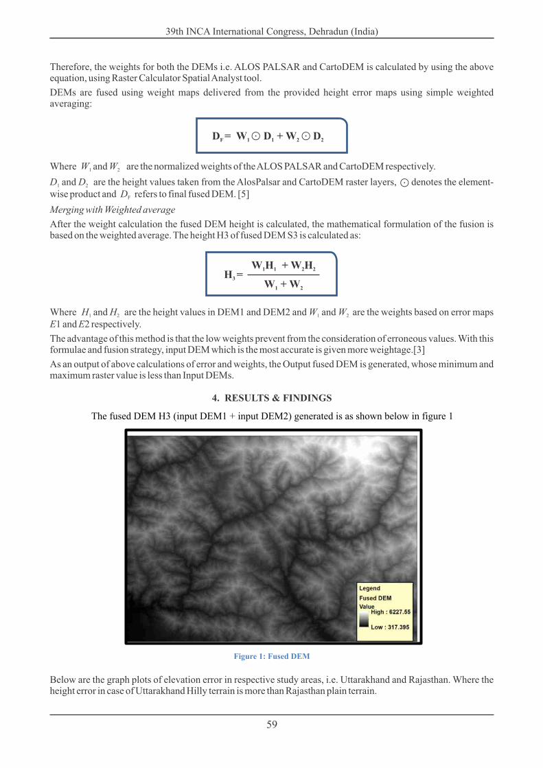

60
InSAR and Optical DEM fusion
0
100000
200000
300000
400000
500000
600000
-21 -19 -17 -15 -13 -11 -9 -7 -5 -3 -1 1 3 5 7 9 11 13 15 17 19 21 23 25 27 29 35
FR
EQ
UE
NC
Y
DEM_ERROR_RANGE (m)
Fused DEM Elevation Error_Rajasthan area
Graph 5: Elevation Error plot of Fused DEM w.r.t. TanDEM-X (reference) for Rajasthan
0
10000
20000
30000
40000
50000
60000
70000
-13
9-1
32
-12
5-1
18
-111
-10
4-9
7-9
0-8
3-7
6-6
9-6
2-5
5-4
8-4
1-3
4-2
7-2
0-1
3 -6 1 81
52
22
93
64
35
057 6
47
17
88
59
29
91
06
FR
EQ
UE
NC
Y
DEM_ERROR_RANGE (m)
Fused DEM Elevation error_Uttarakhand area
Graph 6: Elevation Error plot of Fused DEM w.r.t. TanDEM-X (reference) for Uttarakhand
5. ACCURACY ASSESSMENT
From the above plots and graphs, the accuracy of fused DEM could be accessed using 3 statistical parameters,i.e. MAE, MBE and RMSE in meters. For which study areas need to be divided in terms of Land use land cover, i.e.
For Rajasthan area, the Land Use Land Cover is highlighted in Green color with respect to the ICESat points falling over respective
DEMs for the further analysis and assessment. By dividing the study areas in terms of Land use land cover, i.e.[6]
➢ Barren/Scrub Land,
➢ Barren/Sandy Land and
➢ Agriculture
39th INCA International Congress, Dehradun (India)
61
MAP 3 :ICESat points with respect to LULC
For Uttarakhand area, LULC is Overlayed on the Fused DEM and input DEMs S1 and S2 simultaneously for DEM elevation extraction Land covers defined for Uttarakhand region, hilly region:
Map 4: ICESat Points with respect to LULC
➢ Agriculture
➢ Forest/Evergreen and
➢ Snow/Glacier
39th INCA International Congress, Dehradun (India)

62
Statistical Study of Rajasthan
Statistical Study of Uttarakhand
LULC: Barren/Sandy Land
Statistical Parameters FUSED DEM ALOS PALSAR CartoDEM V3 R1
RMSE 2.4 3.94 2.81
MAE 0.54 1.26 0.78
MBE -0.39 -1.04 -0.52
Digital Elevation Model
LULC: Agriculture
RMSE 0.63 1.55 0.93
MAE 0.54 1.26 0.78
MBE -0.27 -0.95 -0.22
Digital Elevation Model
Statistical Parameters FUSED DEM ALOS PALSAR CartoDEM V3 R1
LULC: Barren/Scrub Land
RMSE 1.76 2.12 3.9
MAE 1.3 1.65 1.38
MBE -0.39 -1.04 -0.52
Digital Elevation Model
Statistical Parameters FUSED DEM ALOS PALSAR CartoDEM V3 R1
RMSE 11.43 15.88 19.25
MAE 11.29 12.87 15
MBE 7.48 8.78 -11.8
Digital Elevation Model
Statistical Parameters FUSED DEM ALOS PALSAR CartoDEM V3 R1
LULC: Agriculture
RMSE 18.34 23.01 30.54
MAE 12.34 16.04 17.22
MBE -3.54 0.32 -7.03
Digital Elevation Model
Statistical Parameters FUSED DEM ALOS PALSAR CartoDEM V3 R1
LULC: Snow/Glacier LULC: Forest/Evergreen
RMSE 12.07 12.08 14.56
MAE 9.61 10.32 11.03
MBE 0.43 -1.81 -0.21
Digital Elevation Model
Statistical Parameters FUSED DEM ALOS PALSAR CartoDEM V3 R1
The conditions for Fused DEM H to be accurate , RMSE < RMSE , RMSE < RMSE and 3 H3_fused DEM1 H3_fused DEM2
MAE≤ RMSE is validated for both the study areas ,i.e. plain and hilly terrain with TanDEM-X as the reference ,where, statistical analysis of the accuracy of fused DEM reveals a substantial improvement up to 66.5% in the mean error deviation for plain terrain and 58% improvement in the mean absolute error of Hilly terrain
6. CONCLUSION AND OBSERVATION:
On comparison and assessment with ICESat altimetry data, the conclusion made is that in plain areas, the height variation of fused and CartoDEM is showing reliable behavior with less range of height error. In undulating hilly terrain, accuracy of TanDEM-X degrades due to the type of terrain, as Tandem X-band with 3.75 to 2.5cm wavelength is having less penetrating effect. As in hilly and dense forest terrain wavelength of at least 15 cm is required for reliable DEM generation. Whereas Fused DEM generated out of input DEMs, ALOS PALSAR and CartoDEM shows reliable and satisfactory behavior.
For further analysis and assessment, when compared with IceSat/ GLAS elevation data which is the most accurate height data, the results came up as input DEM, ALOS PALSAR (L-band) is reliable in hilly areas and fused DEM closest to input DEM, CartoDEM is the most accurate in plain areas.
Overall conclusion is made that the Error of Fused DEM is reduced than the Error of Optical and InSAR DEMs taking TanDEM-X as a reference DEM. Also the advantage of the weighted averaging method is that the low weights prevent from the consideration of erroneous values.
39th INCA International Congress, Dehradun (India)
63
7. FUTURE WORKS AND RECOMMENDATIONS
The coarse resolution of external digital elevation models (DEM) i.e. SRTM 1 sec HGT available for topographic corrections of high resolution SAR images results into degradation of spatial resolution or improper estimation of backscatter values in SAR imag es. Also, many a times the external DEMs do not spatially co-register well with the SAR data. Therefore, Ground Control Point's and other manual intervention should be incorporated so as to improve the height accuracy of InSAR DEM. Also other improvements and corrections in InSAR data processing should be adopted, such as phase unwrapping, atmospheric artifacts, linear trends, and DEM filtering, etc. Despite, Sentinel-1 is a two-SAR satellite constellation designed to guarantee global coverage with a revisit time of 12 days. Due to the 12 days repetitively there is de-correlation due to the vegetation and forest, decorrelation due to surface as well as temporal decorrelation is also there, which directly affects the quality of coherence and InSAR DEM generation that in turn gives scope to further scientific studies and research questions. Further, the DEM fusion of already available optical and Inferometry DEM products was considered in this research taking TanDEM-X as a reference DEM, whereas further study could be done with different fusion method taking CartoDEM as a reference in plain areas whereas ALOS PALSAR as a reference in hilly and mountainous areas looking at the behavior specifically while comparing with the ICESat/GLAS elevation data.
8. REFERENCES
[1] A. Bhardwaj, “Assessment of vertical accuracy for TanDEM-X 90m DEMs in plain , moderate and rugged terrain,” 2019.
[2] D. L. Bickel, “SAR image effects on coherence and coherence estimation.,” no. January, 2014.
[3] C. Processor, “THE GLOBAL TANDEM-X DEM : PRODUCTION STATUS AND FIRST VALIDATION RESULTS,” vol.
XXXIX, no. September, pp. 45–50, 2012.
[4] A. Rosenqvist, M. Shimada, and M. Watanabe, “ALOS PALSAR: Technical outline and mission concepts,” Proc. Int. Symp.
Retr. Bio- Geophys. Parameters from SAR Data L. Appl., vol. 1, no. 7, pp. 1–7, 2004.
[5] H. Lu, Z. Suo, Z. Li, J. Xie, J. Zhao, and Q. Zhang, “DEM Generation,” 2018.
[6] P. Communication, “Chapter-2 LITERATURE SURVEY 2.1 Introduction,” pp. 33–68, 1900.
39th INCA International Congress, Dehradun (India)

64
Estimating vacant land parcels on the Ganga riverbed near Fatehpur district, Uttar Pradesh using GIS and Remote Sensing
Mannu Yadav1, Dhaval Mehta2, R. C. Vaishya3
1Research Scholar, Geographic Information System (GIS) Cell, M.N.N.I.T. Allahabad, Prayagraj-21004, Email ID: [email protected], 7052560675
2Research Scholar, Geographic Information System (GIS) Cell M.N.N.I.T. Allahabad, Prayagraj-21004, Email ID: [email protected], 9537468632
3Professor, Civil Engineering Department, and Member of GIS Cell M.N.N.I.T. Allahabad, Prayagraj-21004; Email ID: [email protected]
Abstract-
Dynamics fluvial system of rivers affects the daily livelihood of people living in surrounding habitat. The river Ganga is one of the most important sources of water in northern India as it passes through five main states. It is observed that in non-rainy season the bed of river Ganga often contains many vacant land parcels due to receding of water during the months of November to June, which can be used for agricultural purpose due its fertile nature. The main aim of this study is to estimate this type of vacant land parcels using modern techniques i.e. Geographic Information Systems (GIS) and Remote Sensing (RS) in Ganga river bed at Fatehpur district in Uttar Pradesh (India). To identify different types of features i.e. water body, vegetation, sandy area and soil at different time intervals (2004, 2009, 2014 and 2019) in study area Land Use Land Cover (LULC) classified maps have been generated using Maximum likelihood supervised classification of multi band of Landsat satellite imageries. Overall accuracy of this classification for year 2004, 2009, 2014 and 2019 is 90.5, 91.0, 90.0 and 89.0 respectively. After classification, percentage wise area of all the four features for different time intervals have been calculated, based on this data total vacant area was calculated and according to availability of vacant land parcels in different zone overall agricultural and economic development plan of the study area has been proposed.
Keywords: Land Use Land Cover; riverbed agriculture; GIS & RS.
1. Introduction
The Ganga basin outspreads in India and it covers states of Uttar Pradesh 28.68% of its total area (CWC report, 2019). In the agriculture fields satellite based remote sensing has become an important technological means in terms of suitability of land resources, availability of water resource, planning of transportation facility and disaster prevention and reduction (Haibo et al., 2011). Due to limited land resource it's become important step to evaluate this resource in the process of land use planning (Bandyopadhyay et al., 2009). Due to natural disasters like land sliding, floods, drought, desertification etc. the food scarcity is increasing day by day and people are shifting towards the urban as well plain area (McMillan et al., 1990; Reija et al., 2005). Human cause like construction of new pavements, highways, roads and other structures the plain agricultural land is acquired by them and these developments are responsible for shrinkage or loss of fertile land (Ashraf et al., 2007; Keller et al.,1998). Satellite imagery data set made it possible to document and map changes in vegetation, soil, water and other features spread on land use area (Reij et al., 2005). In developing nations alone, it is estimated that 10 to 20 thousand square kilometers of cropland are converted annually to cope with urban pressures. By changing the direction of the river in the upward and downward direction the riverbed create a new water channel in order to achieve a new hydrodynamic balance in the undulated surface of the fluvial system (Lapuszek et al., 2015). Due to changing the path of the river in the fluvial system create vacant land area in the form of soil, bare sand and vegetation type on the surface of the riverbed. These tremendous vacant areas can be used for the agriculture to compensate the agricultural land utilized by development program. Diara land farming or riverbed cultivation is nothing but growing of vegetables, cucurbits as well as main crops when flood level receded (Singh, 2012). Diara land farming or riverbed cultivation is dynamic agriculture (Lapuszek et al., 2015).High economic returns of Rs 16,500 kg/ ha can get out of cucurbit vegetables cultivation (Kumar et al., 2018). Early yield, ease in irrigation, low cost, high net return per unit area and high yield, less mineral requirement due to high fertility, limited weed growth, easy in control of pest and disease by cultural, means, low cost labour facilities and additional crop are the advantages of river bed cultivation (Singh, 2012). It means the vacant riverbed area can be used by local people
39th INCA International Congress, Dehradun (India)
65
near the river bank for the agricultural purpose in order to fulfill the basic necessities of life (Bailly, 2007). The main objective of the study was to evaluate the nature, significance and estimate the free vacant land, due to meandering of the river, on the surface the riverbed from 2004 to 2019. It also intended to find out the areas of different types of features present in riverbed, magnitude of change and assess the past and present condition of Land Cover to understand the dynamics and trend of change. For a better planning of future riverbed agriculture (daira farming) planning, administrative authorities need to know vacant riverbed phenomenon of Fatehpur district, its distribution and in what way it is likely to move in the years to come.
2. Study Area
Fatehpur district, located in southeastern part of Uttar Pradesh, north India is selected as the study area. The land of this area is very fertile because of its location in Indo – Gangetic plain. The length covered by it is 88.97 km having center latitude 26°13'43'' N to 25°48'12'' N and longitude 80°33'5''E to 81°20'16'' N has been taken. Arid and semiarid areas are described by patterns of fluctuating annual rainfall. Thus, such areas are subjected to drought cycles during the precipitation deficit period that result in deterioration of the vegetation cover, which may recover following a season with good precipitation.
Fig.1: Study area map (the inset is the map of Fatehpur district).
39th INCA International Congress, Dehradun (India)

66
3. Approaches and Methods
The workflow of the study has been depicted in Figure 2 which has been clearly stating each steps of the execution of the whole task. The each methods has been explained below which has been taken into consideration, i.e., supervised classification (maximum likelihood classifier (MLC)), accuracy assessment, extent of change, vacate land estimation.
Fig. 2: Workflow of the study
3.1. Data acquisition
Different year of multi-temporal Landsat data were used for channel dynamic analysis of the river Ganga for different study interval. The whole study area has expanded in Fatehpur district of Uttar Pradesh in India and covered by different land features. A total of 8 Landsat scenes were required to provide the two-slice epoch coverage of 2004, 2009, 2014, and 2019 for this study. All the satellite imagery was acquired from open source site of USGS i.e. earthexplorer (http://earthexplorer.usgs.gov/). All the satellite scenes have been selected in the months of January to March. Such months were selected because during these days flood free atmosphere and cloud free satellite scene is there.
Table 1: Data used descriptions
Data
Topographical Map
Landsat 7
Landsat 5
Landsat 8
Sensor
ID
-
ETM
TM
TM
OLI/TIRS
Path / Row
-
144/42,
143/42
Resolution/
Scale
1:50000
30m
Year
1974-1975
2004
2009
2014
2019
Source
Survey of India
aUSGS
aUSGS: United states Geological Survey.
39th INCA International Congress, Dehradun (India)
67
3.2 Data preparation
For the extraction of the channel boundaries of the river and further the polygons of River channel for years 2004, 2009, 2014 and 2019 were delineated using GIS on-screen manual digitization tools (Langat et al., 2019). At a scale of 1:4000 zooming level was used to ensure the consistency in on-screen digitising of the river boundary from each georeferenced satellite image. Using the Geographic Information System (GIS) and Remote Sensing (RS) techniques, geocoded geomorphic polygons representing active river channels of each digitally classified image was prepared. For visualization of geomorphological change of river channel the satellite images of the years 2004, 2009, 2014 and 2019 were used.
3.3 Data processing
Image extraction, rectification, restoration and classification were the various standard image processing techniques used for the analysis of the satellite images in five year of intervals (2004,
2009, 2014 and 2019) (Jat et al., 2008). ArcGIS 10.5 software (ESRI) was used for image analysis. Different possible features available on the surface of the vacant riverbed were estimated by using different band combination assigned for the Landsat image on the basis of their respective reflectance values (DN values) using ArcGIS 10.5 (Jat et. al., 2008). Four separable land use classes have been identified, such as water area, sandy area, soil area and vegetation area in the years 2004, 2009, 2014 and 2019. Riverbed is bounded mostly by water, sand, soil and vegetation. Wetland was not taken as in the separate class during the development of the classification scheme. Initially, supervised classification using maximum likelihood algorithm has been performed for the land use/land cover (LU/LC) classification of various Landsat satellite images where, four classes has been considered viz. Water body (WB), Vegetation land (VL), Bare land (BL), and Sand Area (SA). Supervised classification method is used because it gives more accuracy and for this, it requires analyst specified training data which needs to create with the help of Spectral signature tool which widely available in image processing and statistical software packages, like ERDAS IMAGINE (Richards, 1995). The procedure of supervised classification is based on the means and variances of the training data to estimate the probability that a pixel is a member of a particular class. The classified maps of study area were prepared by ArcGIS 10 at interval of 5 years (2004–2019) and results were compared with Google Earth images and Landsat (TM, ETM+ and OLI/TIRS) FCC.
3.4 Area calculation for particular feature
The area of a particular feature (AoPF) has been included the estimated for each feature distinctly like, WB, VL, BL, and SA. The following Equation 1 has been used to extract the AoPF:
Where x is particular feature, SRL is spatial resolution length, and SRB is spatial resolution breadth.
3.5 Vacate Land Calculation
The vacate land (VLD) has been included the feature vegetation, bare and, sand. So, in the study area has been excluded water body. The following Equation 2 has been used to extract the VLD:
Equation 1
Equation 2
39th INCA International Congress, Dehradun (India)

68
4. Results
4.1 Interval-wise spatial and temporal river channel changes and dynamics Classification
In this study maximum likelihood supervised classification method was used for image classification purpose. Year-wise classified maps of the study area are shown below:
Fig. 3: Classified Map of river Ganga (2004)
Fig. 4: Classified Map of river Ganga (2009).
39th INCA International Congress, Dehradun (India)
69
Fig. 5: Classified Map of river Ganga (2014).
Fig. 6: Classified Map of river Ganga (2019).
The calculated assessment result of each classified satellite image from 2000 to 2015 was shown from Table 2. Discharge flow, sediment and debris transport, floodplain erosion and deposition are natural autogenic process for morphological dynamics of an alluvial river (Camporeale et al., 2005; Kleinhans et al., 2011).
Table 2: Calculated area (sqkm) of the AoPF in study area
Water Body
Vegetation Area
Soil Area
Sandy Area
2004
31.82
44.92
38.73
47.15
2009
30.05
53.92
42.24
36.39
2014
27.21
46.09
48.21
30.08
2019
26.92
42.00
48.51
26.95
39th INCA International Congress, Dehradun (India)

70
Due to geomorphological dynamics of river course the size (channel width) of river also changes. Development, population growth, urban sprawl etc. were responsible factor to grasping the fertile agricultural basin area of the river. From the above table it was observed that total area of riverbed changes during study intervals.
Water Body
After the classification it was analyzed that number of pixel which contained water body was decreasing in every intervals that means the covering area of water class was decreasing continuously form 2004 to 20019 and from the below bar graph it was clear that water body in 2004 was 31.82 sqkm reduced to 26.92 sqkm in 2019.
Fig. 7: Change in water area of the river Ganga (2004-2019).
One of the major reasons behind this water deceasing in the Ganga basin in low rainfall in basin of its average rainfall in water years (1955-1984), (1965-1984) and (1985-2015) was 1069mm, 1035mm, 1007mm respectively (CWC report, 2019). Classification results supported the above mentioned facts that the area covered by water class has also witnessed a decrease from 2004 to 2019.
Vegetation Area
During the 2004–2019 periods the area covered by agriculture class on the surface of the riverbed was lightly decreased. Classification results supported vegetation land in year 2004 was 44.92 sqkm and in the year of 2019 it was 42 sqkm of the riverbed area respectively years. It has also been observed in riverbed that the vegetation area is mostly surrounded by bare soil and sandy areas, especially in the catchment area and by the main streams. Variation in rainfall, sediment transportation, meandering and others are the main cause for the disparity of agricultural land on the riverbed (Haque et al.; 2107). From the classified image it was analyzed that vegetation area were also affected by geomorphological dynamics of the River (Langat et al.; 2019).
39th INCA International Congress, Dehradun (India)
71
Fig. 8: Change in vegetation area on the surface of the riverbed Ganga (2004-2019).
One of the major reasons behind this water deceasing in the Ganga basin in low rainfall in basin of its average rainfall in water years (1955-1984), (1965-1984) and (1985-2015) was 1069mm, 1035mm, 1007mm respectively (CWC report, 2019). Classification results supported the above mentioned facts that the area covered by water class has also witnessed a decrease from 2004 to 2019.
Vegetation Area
During the 2004–2019 periods the area covered by agriculture class on the surface of the riverbed was lightly decreased. Classification results supported vegetation land in year 2004 was 44.92 sqkm and in the year of 2019 it was 42 sqkm of the riverbed area respectively years. It has also been observed in riverbed that the vegetation area is mostly surrounded by bare soil and sandy areas, especially in the catchment area and by the main streams. Variation in rainfall, sediment transportation, meandering and others are the main cause for the disparity of agricultural land on the riverbed (Haque et al.; 2107). From the classified image it was analyzed that vegetation area were also affected by geomorphological dynamics of the River (Langat et al.; 2019).
Fig. 9: Change in bare land area on the surface of the riverbed Ganga (2004-2019).
39th INCA International Congress, Dehradun (India)

72
Sand Area
In classification it was analyzed that the sand covered pixels in satellite imagery is decreasing continuously in the study period 2004-2019.
Fig. 10: Change in sand area on the surface of the riverbed Ganga (2004-2019).
It happened because of conversion of sand covered to bare soil and vegetation areas. From the classified image it has been observed that the sandy areas are mostly surrounded by river stream and soil areas, especially in the catchment area and by the main streams. It has also been observed in riverbed that the sandy areas mostly surrounded by Agricultural area, especially in the catchment area and by the main streams.
Total Vacate Area
Total vacate land area is nothing but the sum of bare land, vegetation Land and sand area. So it will be calculated from equation 2 and the result of the different class is in table 2. So the VLD was 130.8 sqkm in 2004, 143.31 sqkm in 2009, 124.38 sqkm in 2014, 117.46 sqkm in 2019.
4.2 Accuracy Assessment Report of LU/LC Classification
Riverbed area of Fatehpur district in Uttar Pradesh (India) has been classified into four distinct LULC classes, i.e., VL, WB, SA, and BL (Table 2). In this analysis, four different time-points (2004, 2009, 2014, and 2019) have taken into consideration to depict the spatial pattern of LULC dynamics, where user accuracy and producer accuracy have indicated more than 84% in all LULC classes. The overall accuracy achieved for all classifications was more than 89%. The Kappa coefficient was 0.873 in 2004, 0.88 in 2009, 0.867 in 2014, and 0.853 in 2019 (Table 3).
Table 3: Descriptions of extracted classes of LU/LC classification of the riverbed of Fatehpur district
SN. No.
1
2
3
4
Classes of LULC
VL
WB
SA
BL
Description LULC Class
Trees, Grass, and Agriculture Land
River
Sand and Wet land
Open land and Barren land
39th INCA International Congress, Dehradun (India)
73
Table 4: Report of accuracy assessment on LU/LC classification (2000–2018) of the riverbed ofFatehpur district
YearLULC Classes
VL
WB
SA
BL
VL
WB
SA
BL
Overall Accuracy
Kappa Coefficient
2004
86.0
96.0
92.0
88.0
91.4
96.0
90.1
84.6
90.5
0.873
2009
84.0
100.0
90.0
90.0
91.3
94.3
90.0
88.2
91.0
0.880
2014
90.0
98.0
84.0
88.0
88.2
96.0
91.3
84.6
90.0
0.867
2019
88.0
100.0
86.0
82.0
86.2
94.3
89.5
85.4
89.0
0.853
User
Accuracy
Producer
Accuracy
5. Conclusions
In this study, spatial and temporal details of the river Ganga in Fatehpur district was studied in term of change in features area available in the study area over a 15- year (2004-2019) period using RS and GIS tools and techniques. These techniques were helpful in image processing,
analysis and LULC maps generation. Segment of the study area that has separate class in the particular study interval was identified like water, sand, soil vegetation. Narrowing and relocating position of water class was observed in LULC map during the study period. The result analysis shows around 4.90 sqkm of area deep water body has degraded within study intervals
2004–2019, which will be major concern for upcoming future to all who directly or indirectly depends upon the Ganga. Vegetation cover area showed random increment and decrement because of changing pattern of river. From the image analysis it found that vegetation area change into soil area due to erosion and urban. Soil area is increased by 9.78 sqkm within 15 years, because of transportation of sediments by river fluvial system increases the amount soil in riverbed. Due to natural cause like floods, ran fall, erosion, accretion influenced the morphological dynamics of river Ganga and these dynamic changes were the major cause behind the increment of soil area. Finally vegetation, soil and sand area of riverbed was found as vacant land and further using some site select those areas will have selected for riverbed farming. It was difficult to manual assessment of this work because of requirement of much time and man power but this technique provides a useful remote sensing framework for evaluation and monitoring of vacant area. Due to increasing pressure on agricultural land management and planning authority of river needs such information to better planning and management in context of food security, living standard, and other significance for biotic living.
References
- Langat, P.K., Kumar, L., Koech, R. 2019. Monitoring river channel dynamics using remote sensing and GIS Techniques. Geomorphology, 325, 92-102.
- Reij, C., Tappan, G., Belemvire, A. 2005. Changing land management practices and vegetation on the Central Plateau of Burkina Faso (1968–2002).
- Haibo, Y., Zongmin, W., Hongling, Guo. Yu, G. 2011. Water body Extraction Methods Study Based on RS and GIS. Procedia Environmental Sciences, 10, 2619 – 2624.
- Bandyopadhyay, S., Jaiswal, R.K., Hegde, V.S., Jayaraman, V., 2009. Assessment of land suitability potentials for agriculture using a remote sensing and GIS based approach. International Journal of Remote Sensing, 30, 879–895.
Journal of Arid Environments, 63, 642-659.
39th INCA International Congress, Dehradun (India)

74
- Lapuszek, M. & Matyas, A.L. 2015. Methods of analysis the riverbed evolution: A case study of two tributaries of the upper Vistula River. Infrastruktura i Ekologia Terenów Wiejskich, 1313–1327.
- Kumar, R., Sharma, A., Bhagta, S., Kumar.R. 2018. River Bed Cultivation: A Kind of Vegetable Forcing for Remunerative Returns. International Journal of Current Microbiology and Applied Sciences, 7, 359-365.
- Ahmed, S. A., Kheiry, M.A., Hassan, I.A.M. 2018. Impact of Vegetation Cover Changes on Gum Arabic Production Using Remote Sensing Applications in Gedarif State, Sudan. Gum Arabic, 29-43.
- Jat, M.K., Garg, P.K., Khare, D. 2007. Monitoring and modelling of urban sprawl using remote sensing and GIS techniques. International Journal of Applied Earth Observation and Geoinformation, 10, 26–43.
- Thapa, R.B. & Murayama, Y. 2009. Urban mapping, accuracy, & image classification: A comparison of multiple approaches in Tsukuba City, Japan. Applied Geography, 29,135-144.
- Singh, P.K. 2012. Cucurbits Cultivation under Diara-Land. Asian Journal of Agriculture and Rural Development, 2, 243-247.
- Haque, M.I. & Basak R. 2017. Land cover change detection using GIS and remote sensing techniques: A spatio-temoral study on Tanguar Haor, Sunamganj, Bangladesh. The Egyptian Journal of Remote Sensing and Space Sciences, 20, 251–263.
- Ashraf, S., Brabyn, L.; Hicks, B.J. Image data fusion for the remote sensing of freshwater environments. Appl. Geogr, 32, 619–628.
- Keller, A.A. & Goldstein, R.A., 1998. Impact of carbon storage through restoration of drylands on the global carbon cycle. Environ. Manage, 22, 757.
- Bailly, H. 2007. Environmental baseline study of Margala and Margala north blocks. MOL Pakistan Oil and Gas Company BV, Islamabad.
- Langley, S.K., Cheshire, H.M., Humes, K.S. 2001. A comparison of single date and multitemporal satellite image classifications in a semi-arid grassland. Journal of Arid Environments, 49, 401-411.
- Richards, J.A., 1995. Remote Sensing Digital Image Analysis: An Introduction. Springer-Verlag, 265–290.
- Camporeale C., Perona P., Porporato A., Ridolfi L. 2005. On the long-term behavior of meandering rivers. Water resources research, 41.
- Kleinhans, M.G., Cohen, K.M., Hoekstra, J., IJmker, J.M. 2011. Evolution of a bifurcation in a meandering river with adjustable channel widths, rhine delta apex, the netherlands, Earth Surf. Processes Landforms, 36, 2011-2017.
- Pal, R., Pani,P. 2019. Remote sensing and GIS-based analysis of evolving planform morphology of the middle-lower part of the Ganga River, India. The Egyptian Journal of Remote Sensing and Space Science , 22, 1-10.
- Ustun, B. 2008. Soil erosion modelling by using gis & remote sensing : a case study, Ganos mountain. The International Archives of the Photogrammetry, Remote Sensing and Spatial Information Sciences. 37, 7.
- Basin planning & management organisation central water commission. 2019. Reassessment of water availability in basins using space inputs. 1-120.
- McMillan, D., Nana, J.B., Sawadogo, K. 1990. Settlement and Development in River Basin
- Control Zones: Case study Burkina Faso. World Bank Technical, Paper No.200.
39th INCA International Congress, Dehradun (India)
75
Spatial Analysis on the Sustainable Development of water sources inAlandur Taluk, Kancheepuram District
E.Grace Selvarani* Dr. P.Sujatha**
*Research Scholar**Assistant Professor
Department of Geography, Bharathi Women's [email protected]
Abstract-
Water is considered as a basic commodity to sustain life. Water is considered as the base of our survival like, oxygen. Though the earth is mostly covered with water, just few percentages of surface and ground water is edible. According to United Nation Organisation, Water scarcity, poor water quality and inadequate sanitation negatively impact food security, livelihood choices and educational opportunities for poor families across the world. At the current time, more than 2 billion people are living with the risk of reduced access to freshwater resources and by 2050, at least one in four people is likely to live in a country affected by chronic or recurring shortages of fresh water. The best definition ever coined on sustainable development is the one given by World Commission on Environment and Development (Brundtland Commission) which runs as the "development that meets the needs of the present without compromising the ability of future generations to meet their own needs.”
For the present study to show the distribution of water sources, consuming level of population and, to show the uneven distribution of water supply for the consuming population, 'Alandur Taluk' has been chosen to make Sustainable Devlopment in the Study area. Based on the Primary and Secondary data, the datas have been transferred into spatial and non-spatial data with the help of GIS and Statistical tools. The results have been arrived in both the sites of potential and non-potential regions. According to the results, suggestions has been framed with the government policy and planning strategies.
Key words: Water sources, Population, Alandur, Water Consumers, Sustainable Development.
1.1 Introduction
Throughout the human history, water has always been considered as an essential commodity for human welfare and economic development. Next to oxygen, water is an
essential requirement for survival of life on this earth. It is a prime natural resource and has been declared as a precious national asset. Water is one of the abundantly available substances in the nature which men have exploiting more than any otherresources for the sustenance of life. Water of good quality is required for living organisms.
International changes and demands for multiple use of increasing population make water management a difficult task. In India with exploding population, weak economy and several social issues such as disputes over Trans-boundary Rivers, resettlement and rehabilitation issues during project implementation, corruption and vested political and regional interests Water management is more difficult to manage. With the increase in population, reliable water is becoming a scarce resource. The principal source of water for India is the southwest monsoon. Availability of safe drinking water is inadequate. Specifically, growing demand across competitive sectors, increasing droughts, declining water quality, particularly of groundwater, and unabated flooding, inter-state river disputes, growing financial crunch, inadequate institutional reforms and enforcement are some of the crucial problems faced by the country's water sector. According to John Flavin, Professional Geologist and Engineer Advisor (2011-present), United States., there are five sources of water supply. They are Oceans and Seas, Glaciers or Ice melt, Rain Water, Surface water and Ground water.
1.2 Source of water supply –Tamil Nadu
Tamil Nadu is predominantly a shield area with 73% of the area covered under hard crystalline formations while the remaining 27% comprises of unconsolidated sedimentary formations. As far as groundwater resource is concerned scarcity is the major problem in hard rock environment while salinity is the problem in sedimentary areas.
39th INCA International Congress, Dehradun (India)

76
1.3 Rainfall:
Tamil Nadu is a state with limited water resources and the rainfall in the state is seasonal. The annual average rainfall in the state is 960 mm. Approximately 33 % of this is from the southwest monsoon and 48 % from the northeast monsoon.
The average annual rainfall and the 5 years rainfall collected from IMD, Chennai is as follows:
1.4 Surface Water Potential:
The total surface water potential of the 17 river basins of Tamil Nadu is assessed as 24160 MCM (853 TMC).The average Runoff (surplus flow) to the sea from the 17 Basins of Tamil Nadu State is computed as 177.12 TMC.
1.5 Ground Water Level:
The Ground Water levels from the 47 number of observation wells of TWAD have been analyzed for Post-Monsoon and Pre- Monsoon. Since 1991, the average Groundwater level in m Below Ground Level for pre and post-monsoon is as follows:
According to, Agarwal and Narain 1997, Centre for Science and Environment. New Delhi., states that, Wells and bore wells have been a private enterprise, and therefore the exact extent and significance of groundwater use have stayed hidden to all except the most diligent administrations throughout the history of the subcontinent. Asia Pacific Journal of Marketing & Management Review Vol.1 No. 3, November 2012 states, Modern India is no exception – the widespread development of private wells that accounts for groundwater becoming the primary source of water today has also been furtive in nature, in that it has happened mostly outside the knowledge and control of governments. Groundwater has therefore been invisible not only physically, but also institutionally, as a critical resource literally underpinning millions of lives and livelihoods in the country.
39th INCA International Congress, Dehradun (India)
77
2 Study Area
2.1 Location
Alandur Taluk with the latitude of 13.0025 and the llongitude of 80.20611, is the highest populated area (680852) in the Kancheepuram District with no rural area identified in it. According to Census, this region comprises of, 4 Munnicipalities (Alandur, Pallavaram, Anakaputhur and Pammal), 3 Town Panchayats (Nandambakkam, Thruneermalai and Meenambakkam), 1 Cantonment Board (St. Thomas Mount – Pallavaram), 3 Census Towns (Polichalur, Tirusulam and Moovarasampettai) and 1 Out Grown Area (Cowl Bazaar) (Ref Map No: 2.1 &2.2).
Map No: 2.1 Map No: 2.2
Pallavaram Municipality has a population of 233984, Alandur Municipality has 164430, while Pammal Municipality and Anakaputhur Municipality has 75870 and 48050 respective populations in them (Ref Map No: 2.3).
Map No: 2.3
39th INCA International Congress, Dehradun (India)

78
Households by Source of Drinking Water at Alandur Taluk
Map No: 2.4 Map No: 2.5
According to the census of 2011, Alandur Taluk which has 172733 household (ref. Map No:2.4), depend on tap water from treated source in 61.01 %, then 10.67% use tap water from untreated source whereas,4.03% use uncovered well and 2.24% use covered well for drinking purpose.
Fig No: 2.1 (Source: Census 2011)
Fig No: 2.1 (Source: Census 2011)
According to the census of 2011, in Alandur Taluk nearly 22% of household, depend on direct ground water for drinking. 2.98% use handpump, 15.63% use tubewell, 9.19 use spring, 0.46% use river/canal, 0.15% use tank/pond and 2.64% depend on other sources for drinking.
3 AIM & OBJECTIVES:
3.1 Aim
3.2 Objectives
1. To show the distribution of water source.
2. To show the present demand and need of water to the consuming population.
3. To show the level of service being provided to the population.
39th INCA International Congress, Dehradun (India)
79
4 Methodology:
Both Secondary and Primary data has been adopted to fulfill the aim and objectives of the present study framed. Out of 13 administrative boundary divisions, all 4 Municipality divisions has been randomly selected as a case study on the basis of total population. Totally, 1000 survey (scheduled questioner) samples was been collected from all the 4 Municipalities Alandur, Anakaputhur, Pammal and Pallavaram Municipalities (250 each) for this present study to show the demand and source of water in these areas to grow towards sustainability. And Secondary Datas from Ground Water department from Taramani, TWAB and CWDB were been used. The Data has been converted in to Spatial and non Spatial Datas using Statistical and GIS tools.
5 The findings of Spatial Analysis:
5.1 Distribution of Total Population
(Ref Map No: 2.3)
Interpretation:
Alandur Taluk, is the highest populated area with a population of 680852. In which, Pallavaram Municipality has a population of 233984, Alandur Municipality has 164430, while Pammal Municipality andAnakaputhur Municipality has 75870 and 48050 respective populations in them.
5.2 Distribution of Household
(Ref Map No: 2.4)
Interpretation:
Alandur Taluk has 172733 household. In which, Pallavaram Municipality and Alandur Municipality has 60954 and 43411 households respectively. While Pammal Municipality and Anakaputhur Municipality has 18812 and 12146 respective households in them.
5.3 Distribution of water sources on ground and underground
(Ref Map No: 2.5) Interpretation:
Interpretation:
Alandur Taluk shows sparsely distributed with potential water sources on ground and underground.
5.4 Distribution of water needed for drinking
Interpretation:
According to World Health Organization, in general a human being needs 3.7 liters/day for drinking. Accordingly, Alandur Taluk, needs, 2509881.7 liters/day for drinking when we calculate with the total population in the Alandur Taluk Division.
5.5 Distribution of water needed for household
Interpretation:
According to World Health Organization, in general a household needs 25 liters/day. Accordingly, Alandur Taluk, needs,
17021300 liters/day when we calculate with the total population in the Alandur Taluk Division.
Map No: 5.5
Map No: 5.4
39th INCA International Congress, Dehradun (India)

80
5.6 Distribution of water storage capacity
Interpretation:
Alandur Taluk in total has 12065 liters of storage capacity in it according to the census of 2011. The St.Thomas Mount –
Pallavaram Cantonment areas has 21.5% of
storing capacity and is the highest among the all divisions in the storage capacity.
5.7 The Gap between the Demand and the Service
Interpretation:
While calculating the ranks of the required amount of water with the water capacity, all the four municipalities show High demand with High service provided on the whole.
5.8 Theisson Polygon for underground water source
Interpretation:
The 2016 data from the Groundwater and surface water development Board shows 6 groundwater wells and from it, when we derive theisson polygon, for analysing proximity and neighborhood. From which areas from Pammal, St.Thomas Mount – Pallavaram Cantonment, Cowl Bazaar and Polichalur areas have a good accessibility.
6 The findings of the Sample Survey:
The sample survey gave out a comparative study on both the municipality regions on the below aspects.
1. Socio Economic Aspect,
2. Environmental Aspect,
Map No: 5.6
Map No: 5.7
Map No: 5.8
39th INCA International Congress, Dehradun (India)
81
3. Water usage, and
4. Water Perception.
Then, while compiling the results, we come to know on the distribution of water source, Water consuming level and the uneven distribution of water supply to the consuming people.
The Findings are,
6.1 Socio-economic aspect
6.1.1 Type of stay
6.1.2 Number of family members
Interpretation:
The people who stay in the rental accommodations is higher than the people with own house among the collected samples in all four municipalities.
Interpretation:
At Pallavaram, 45% people live in small sized family upto 3 family members. Whereas, at Alandur, 57%, at Anakaputhur 39% and at Pammal, 50% people live in Medium Size family with 4 to 6 members.
6.1.3 Income
Interpretation:
Mainly, Income range of Rs.15,001 to Rs.25,000 is seen widely in all four municipalities.
39th INCA International Congress, Dehradun (India)

82
6.2 Environmental aspect6.2.1 Water Source
Interpretation:
Bore well is the main source of water in all four municipalities
6.2.2 Depth
Interpretation:
At the most, the Groundwater level has gone upto 151 to 200 feet in all four municipalities. And among the four municipalities, Anakaputhur still has 101 to 150 feet depth.
6.2.3 Groundwater Usage
Interpretation:
Alandur: 30% drinking; 41% cooking, 100% washing and 48% for other purposes. Pallavaram: 42% drinking; 37% cooking, 100% washing and 39% for other purposes. Pammal: 39% drinking; 52% cooking, 100% washing and 84% for other purposes.
Anakaputhur: 68% drinking; 63% cooking, 100% washing and 80% for other purposes.
6.2.3 Usage of Purifiers for Groundwater
Interpretation:
At the most, people are not using purifiers for ground water and most people are not aware of such purifiers too.
39th INCA International Congress, Dehradun (India)
83
6.2.4 Groundwater Availability
6.2.5 Rainwater harvest plant
Interpretation:
Some way or the other people try to convey that the ground water availability depends on rainfall.
Interpretation:
Though most of the houses have rain water harvest plant at their houses, most of the houses have not maintained the rainwater harvest plant properly in the recent years and has it just because of the law enforcement. While the remaining has responded that either that they are not aware of it or its importance or they have bribed the officials who come for checking.
6.3 Water usage6.3.1 Alternative Water usage
Interpretation:
Alandur: 79% use corporation water; 84% use can water and 57% use lorry water. Pallavaram: 62% use corporation water; 96% use can water and 37% use lorry water. Pammal: 84% use corporation water; 86% use can water and 66% use lorry water Pamma: Pamaal
Anakaputhur: 78% use corporation water;
86% use can water and 96% use lorry water.
Interpretation:
Alandur: Monsoon - 55% once in 2 days; 45% once in a week. Summer - 7% once in 2 days; 40% once in a week; 41% once in 2 weeks and 12% once in a month.
Pallavaram: Monsoon - 14% once in 2 days; 78% once in a week and 8% once in 2 weeks. Summer - 1% once in 2 days; 24% once in a week; 39% once in 2 weeks and 36% once in a month.
Pammal: Monsoon - 20% once in 2 days; 34% once in a week and 46% once in 2 weeks. Summer - 3% once in 2 days; 13% once in a week; 38% once in 2 weeks an 46% once in a month.
Anakaputhur: Monsoon - 19% once in 2 days; 32% once in a week and 49% once in 2 weeks. Summer - 4% once in 2 days; 33% once in a week; 54% once in 2 weeks and 10% once in a month.
6.3.2 Water Disbursement
39th INCA International Congress, Dehradun (India)

84
6.3.2 Alternative Water usage (drinking water) Interpretation:
Alandur: 82% use corporation water; 82% can water, 25% use lorry water and 41% use ground water for drinking.
Pallavaram: 46% use corporation water;
96% can water, 88% use lorry water and
16% use ground water for drinking. Pammal: 90% use corporation water; 86% can water, 66% use lorry water and 79% use ground water for drinking.
Anakaputhur: 95% use corporation water;
98% can water, 74% use lorry water and
78% use ground water for drinking.
6.4 Water perception6.4.1 Water perception at alandur
Interpretation:
Ground Water: At Pallavaram and Pammal, most have said Poor and while at Alandur and Anakaputhur, most have said better.
Corporation Water: At Pallavaram, Pammal and anakaputhur, people have mostly voted for Average and at Alandur as Better.
Water Pollution: At Pallavaram, People have mostly voted as worstly affected, while at Pammal, people has voted as better and atAlandur and Anakaputhur, people has said
Good.
39th INCA International Congress, Dehradun (India)
85
This Study, finds out that,
1. Distribution of water sources is, uneven in the study areas.
2. According to WHO, on an average a human should drink 3.7 liters of water per day and 25 liters for household use. Thus, on an Average, Pallavaram Municipality needs 865740.8 liters, while Alandur Municipality needs 608391 liters, 28719 Liters for Pammal Municipality and 177785 Liters for Anakaputhur Municipality Per Day just for drinking Purpose. And for House hold Purpose, on an Average, Pallavaram Municipality needs 5849600 liters, while Alandur Municipality needs 4110750 liters, 189675 Liters for Pammal Municipality and 1201250 Liters for Anakaputhur Municipality Per Day.
3. Alandur Taluk in total has 12065 liters of storage capacity in it according to the census of 2011. And, this study clearly shows uneven distribution to the consuming people in all the regions. And in it, except Alandur Municipality region in the other entire three regions the level of service being provided is uneven for its consumers.
7 Results and Conclusion:
This study concludes with the following suggestions, the study finds that, the groundwater in Pallavaram Municipality Region is more polluted as well as scarce.
And so, the ground water is supposed to be managed efficiently and swiftly through new scientific planning and through using new technology and scientists. Whereas, Alandur Municipality region is quite above the danger line, does not make it safe. At Pammal, though the water scarcity is there Government has taken steps to provide water for them from unused quarries and ponds temporarily to ease the pain. While at Anakaputhur, though the ground water level has still managed to be quite good compared with the other three areas, inefficient usage and lethargic behavior towards the ground water has started to reap its fruits by making the ground water level go down in the last few years. Making 100% of houses and industries to have rainwater harvest plant and it is supposed to be ensured that the existing plants are been well maintained.
Encouraging the locals to use water purifiers for groundwater could be quite useful for people who depend on groundwater for drinking purpose.
Regularising the interval of corporation water could be beneficial in this area. And, make sure everyone equally get water from the corporation equally in regular intervals and not just few areas getting water regularly while most suffer. The Government's Metro Water Department are Working on it with meter's attached.
Preserving the lakes and ponds in the study area through cleaning the siltation and the grown plants to meet the water scarcity (Ref. Map No: 2.5). Without stopping from there, saving the lakes and ponds from encroachment is also to be mainlyconcentrated to safeguard and manage the groundwater resource in the study area. Stopping the over exploitation of groundwater through bore wells by the industries. Controlling the Real estate mafia as well as the real estate builders who are the most crucial players in encroaching the water bodies and in corrupting the government officials, could do a better job in saving our water resource.
Alandur, Pallavaram and Pammal Municipality areas are already over settled and populated. While, Anakaputhur Municipality region is a big Hot spot for real estate as the residential plots and buildings are raising fast. Yet few planning and regulations in settlement too could be put forth. An extensive planning is to be made by the government to preserve, manage and improve ground water resource without corruption.
Creating awareness to be responsible towards our natural resources especially towards the groundwater resource is to be focused among the locals, Institutional areas and the industrial management at the Industrial regions. And for future sustainability, school children could be encouraged for preserving the water resource. And the non workers could be educated through canvassing at Banks and markets.
The government, from time to time has stated that ground water needs to be managed as a community resource. However, Section 7(g) of the Easement Act, 1882 states that every owner of land has the right to collect and dispose within his own limits all water under the land and on its surface which does not pass in a defined channel. The legal consequence of this law is that the owner of the land can dig wells in his land and extract water based on availability and his discretion. Additionally, landowners are not legally liable for any damage caused to the water resources as a result of over extraction. The lack of regulation for over-extraction of this resource further worsens the situation and has made private ownership of ground water common in most urban and rural areas. The CGWB identifies over-exploited and critical areas within states. However, the Board does not have the power to stop ground water extraction in such areas and can only notify the owners. Additionally, because of a very large number of small users, it becomes increasingly difficult for the Board to
39th INCA International Congress, Dehradun (India)

86
identify and penalize the offenders.
Like the suggestion in, Qian-qi YIN et al. Water Science and Engineering, Jan. 2014, Vol. 7, No. 1, 49-59, the concept of harmoniousness of the total amount control of water use could be suggested along with, Principle of systematization (Cao 2007): considering a river basin the basic unit for rational allocation, the issues causing the constraints of water resources shortage on socioeconomic sustainable development should be resolved; Principle of equity: water resources are owned by the state, and the water users at all levels of society have rights to share and allocate the water resources so as to achieve coordinated development; Principle of harmoniousness (Wang et al. 2003): according to the flexible characteristics of the total amount control of water use, domestic water use, industrialwater use, and ecological water use are coordinated to optimize systemic comprehensive benefits and long-term benefits using quantitative and qualitative analysis; Principle of economy: development efficiency of water resources, water use benefits, and water-saving level are improved by means of the optimized allocation.
At the same time, like in the report of World Bank's Study and Technical Assistance Initiative on Groundwater management in India, Deep Wells and Prudence: Towards Pragmatic Action for Addressing Groundwater Overexploitation in India, Community-based groundwater management should not require sacrifice; Participatory engagement should be the core focus of community-based groundwater management investments; Community- based groundwater management needs state engagement. Groundwater overexploitation is a widespread problem in India; Pragmatic policies can strengthen community-based groundwater management; Limitations of community-based approaches need to be recognized;
Like in the Report of the World Commission on Environment and Development: Our Common Future, Human progress has always depended on our technical ingenuity and a capacity for cooperative action. These qualities have often been used constructively to achieve development and environmental progress: in air and water pollution control, for example, and in increasing the efficiency of material and energy use. Many countries have increased food production and reduced population growth rates. Some technological
advances, particularly in medicine, have been widely shared. But this is not enough. Failures to manage the environment and to sustain development threaten to overwhelm all countries. Environment and development are not separate challenges; they are inexorably linked.
Development cannot subsist upon a deteriorating environmental resource base; the environment cannot be protected when growth leaves out of account the costs of environmental destruction. These problems cannot be treated separately by fragmented institutions and policies. They are linked in a complex system of cause and effect.
The concept of sustainable development provides a framework for the integration of environment policies and development strategies - the term 'development' being used here in its broadest sense. The word is often taken to refer to the processes of economic and social change in the Third World. But the integration of environment and development is required in all countries, rich and poor. The pursuit of sustainable development requires changes in the domestic and international policies of every nation. Sustainable development seeks to meet the needs and aspirations of the present without compromising the ability to meet those of the future. Far from requiring the cessation of economic growth, it recognizes that the problems of poverty and underdevelopment cannot be solved unless we have a new era of growth in which developing countries play a large role and reap large benefits. In some areas excessive use of ground-water is rapidly lowering the water table - usually a case where privatebenefits are being realized at society's expense. Where ground-water use exceeds the recharge capacity of local aquifers, regulatory or fiscal controls become essential. The combined use of ground and surface water can improve the timing of water availability and stretch limited supplies.
Portions of forests may be designated as prevention areas. These are predominantly national parks, which could be set aside from agricultural exploitation to conserve soil, water, and wildlife. They may also include marginal lands whose exploitation accelerates land degradation through erosion or desertification. In this connection, the reforestation of degraded forest areas is of utmost importance. Conservation areas or national parks can also conserve genetic resources in their natural habitats. The challenge today is to revive the old methods, improve them, adapt them to the new conditions and develop new ones. Like Tree plantations for every Household.
Water being the main source to live is to be managed well with advanced technology, responsibility, truthfulness towards Mother Nature without over exploitation and proper methodology to use it. That too ground water is more precious as in the recent days the groundwater level is going down. Through creating awareness among the locals to preserve the water resource and through making the consumers to understand the importance of water resource could create a good positive impact in the water resource management.
39th INCA International Congress, Dehradun (India)
87
Bibliography
1. Deep Wells and Prudence: Towards Pragmatic Action for Addressing Ground water Overexploitation in India, The World Bank, March 2010, http://siteresources.worldbank.org/IN DIAEXTN/ Resources/295583-1268190137195/Deep Wells Ground Water March2010.pdf.
2. USSR Committee for the International Hydrological Decade, World Water Balance and Water Resources of the Earth (Paris: UNESCO, 1978).
3. International Task Force, Tropical Forests: A Call for Action (Washington, DC: World Resources Institute, 1965)
4. Dr M.K. Tolba, 'Desertification and the Economics of Survival', UNEP Information 86/2. 25 March 1986
5. Agarwal et al., Water, Sanitation and Health for All? (London: IIED/Earthscan, 1981); World Bank, World Development Report, 1984 (New York: Oxford University Press, 1984)
6. M. Falkenmark, 'New Ecological Approach to the Water Cycle: Ticket to the Future', Ambio, Vol. 13, No.3, 1964; S. Postel, Water: Rethinking Management in an Age of Scarcity, Worldwatch Paper 62 (Washington, DC: WorldWatch Institute, 1984).
7. Jyotigram Yojana, Department of Petrochemicals Department, Government of Gujarat; http://guj- epd.gov.in/epd_jyotiyojna.htm
8. Report of the Working Group on Sustainable Ground WaterManagement, Planning Commission, October 2011, http://planningcommission.gov.in/ab outus/committee/wrkgrp12/wr/wg_s usgm.pdf.
9. Performance Audit of Water Pollution in India, Comptroller and Auditor General of India, Report No. 21 of 2011-12, http://www.saiindia.gov.in/english/h ome/Our_Products/Noddy/Union/Re port_21_12.pdf.
10. Water and Related Statistics, April 2015, Central Water Commission, http://www.cwc.gov.in/main/ downlo ads/Water%20&%20Related%20Stat istics%202015.pdf. 3 Central Ground Water Board website, FAQs, http://www.cgwb.gov.in/faq.html.
11. The Policy (T)angle, Thirsty Nation- Priorities for India's Water Sector, Joseph P. Quinlan, Sumantra Sen and Kiran Nanda, Random House India 2014.
12. 12th Five Year Plan, Planning Commission, 2013 http://planningcommission.gov.in/plans/planrel/ fiveyr/12th/pdf/12fyp_vol1.pdf.
13. Chang, J. X., Huang, Q., and Wang, Y. M. 2004. Water distribution control model in the Yellow River Basin. Water International, 29(4), 483-491. [doi:10.1080/02508060408691811]
14. Overview of Ground Water in India, Roopal Suhag February 2016
15. https://www.businesstoday.in/magazi ne/case-study/case-study-chennai- metropolitan-water- supply/story/203655.html
16. https://www.esciencecentral.org/ebo oks/ebookchapter/a-review-on- status-of-groundwater-in-india-a- case-study-in-chennai-metropolitan- area-cma--5/1
17. https://sandrp.in/2017/10/18/river- wise-rainfall-in-monsoon-2017/
18. https://wle.cgiar.org/solutions/groun dwater
19. http://envfor.nic.in/
20. https://www.sciencedirect.com/scien ce/article/pii/S092180090700434X
21. https://www.nature.com/articles/ncli mate2765
22. http://science.sciencemag.org/conten t/319/5863/573.full
23. http://www.academia.edu/902661/W ater_in_Crisis_Chapter_2_Oxford_U niversity_Press_1993
24. https://www.thehindu.com/news/cities/mumbai/the-alarming-levels-of- indias- groundwater/ article19253949.ece
25. http://www.prsindia.org/administrato r/uploads/general/1455682937~~Overview%20of% 20Ground% 20Water% 20in%20India.pdf
26. https://groundwaterscience.com/
27. https://www.mae.gov.nl.ca/waterres/quality/drinkingwater/dwqi.html
28. http://scientific.cloud- journals.com/index.php/IJAESE/artic le/viewFile/Sci-133/pdf
39th INCA International Congress, Dehradun (India)

88
INVESTIGATING RELATIONSHIP BETWEEN DROUGHT AND ENSO IN BUNDELKHAND REGION OF INDIA
Shivani Pathak1, Dr. Neeti1
1 Department of Natural Resources, TERI SAS, Plot No. 10, Vasant Kunj Institutional Area, Vasant Kunj, Institutional Area, New Delhi, Delhi 110070, Contact No. 8178733014, [email protected]
Abstract-
Drought is a natural disaster which has a slow onset and can cause land degradation, water scarcity, loss of crop production, etc. For drought monitoring remote sensing based indices plays vital role and gives accurate result and it is able to cover large spatial extent. Several studies in past have been done in different countries which shows that ENSO and meteorological drought are closely related. So, this study aims to estimate the meteorological and agricultural drought,drought frequency, time lag between meteorological drought and agricultural drought. Meteorological drought was estimated by SPI, agricultural drought was estimated by calculating VCI, TCI and VHI. Generally, SPI-3 has highest correlation with SPI but in this study it was found that for Bundelkhand region SPI-6 shows high correlation between SPI and VHI which explains the relationship between the meteorological and agricultural drought in the study area. Multivariate ENSO Index was used for ENSO variables for finding the relationship between El Nino and meteorological drought in the study area. It was found that partial correlation between MEI values and SPI showspositive correlation where the values are high and low values shows negative correlation. In Nov-Dec MEI and SPI, the areas with low values shows negative correlation which means if the MEI value increases (El Nino) the SPI value will decrease (drought) and the results show that all drought prone districts i.e. Banda, Jhansi, Hamirpur, Datia, etc have negative correlation.
Keywords : Drought, Agricultural drought, Meteorological drought, Bundelkhand drought, VCI, TCI, VHI, SPI
1.INTRODUCTION
Due to the varying characteristics of drought it is very difficult to provide one precise definition as every drought is unique and different from other droughts. Drought has slow onset, develops over months or years, covers large area and it causes less structural damage.
On world scale North Africa, Mid-East, West Asian countries, India, China, North Central America and South America have widespread drought conditions. The intensity and frequency of extreme disasters have been increased in last two decades which can be triggered due to global warming. According to the NOAA report “every month 3% of global land area is affected by extreme drought conditions.”
Drought is no longer related to the absence or scarcity of rainfall but it is related to the inefficient water resources management. In India due to regional variation in rainfall, the probability of occurrence of drought varies from once in 2 years in Western Rajasthan to once in 15 years in north-eastern states. About 28% of the total agricultural land is prone to drought which faces severe water shortages. Drylands are highly prone to drought which are found from north to south in western part of India. Drought prone states of India are Maharashtra, Madhya Pradesh, Uttar Pradesh, Andhra Pradesh, Telangana, Karnataka, Chhattisgarh and Odisha.
El Nino / La Nina-Southern Oscillation is known as global scale climate phenomena which controls rainfall anomalies in many parts of the world including India. Generally, El Nino causes dryness which can trigger drought events. In several studies it was found that extreme drought occurred in El Nino years. One such study is done on Indonesia and it was found that “some extreme droughts were occurred simultaneously with El Nino years such as 1997/1998, 2002/2006, 2006/2007 and 2009/2010.”
Drought has significant impact on the agriculture, economy, social consequences and environment of the area. Monitoring of drought is important to minimize the drought impacts. Understanding the relationship between drought and ENSO is also important for forecasting the future droughts by studying the past relationships between both events. Remote sensing and GIS can play an important role in drought monitoring. They allows long term time series studies, covers large area, overlay and analyse different variables at same time for better understanding. Remote sensing and GIS improves the accuracy and accessibility of the study.
39th INCA International Congress, Dehradun (India)
89
2. Literature Review
Droughts can be classified into four types
i. Meteorological Drought: - It occurs when the area receives seasonal rainfall less than 25% of its long term average value. It can also further divided into two type
a. Moderate Drought – When the area receives rainfall deficit between 26-50%.
b. Severe Drought – When the rainfall deficiency exceeds 50% of long term normal rainfall value.
ii. Hydrological Drought: - Deficiency of surface or subsurface water supply which leads to water scarcity. Such conditions can arise even when the precipitation is average or above average.
iii. Agricultural Drought: - It can be triggered by both meteorological and hydrological drought. It occurs when soil moisture decreases due to lack of water which causes crop stress during its growing period. In India it is defined as a period of 4 consecutive weeks or 1 month with rainfall scarcity of more than 50% of long term average.
iv. Socio-economic Drought: - It is related to the human activity. It can occur due to meteorological, hydrological and agricultural drought or it can occur due to mismanagement of water resource or increase in water demand.
2.1 ENSO
Walker discovered that there is a strong relationship between low pressure conditions over Indonesia and high pressure over the eastern Pacific Ocean (Peru coast). The variations in this relationship is known as El Nino/ La Nina- Southern Oscillation (ENSO). Variations eastern Pacific ocean and Indian Ocean surface temperature and air temperature is characterised as ENSO. The warm phase is known as El Nino and cold phase is La Nina. The two ends exhibit see saw like condition for pressure condition. This phenomena causes drought and flood condition is several parts of the world.
“The surface temperature variations over the west and central Pacific ocean are important in influencing the atmospheric circulation which also influence the Indian Summer Monsoon Rainfall (ISMR).” . According to the association between El Nino and Indian drought has strengthened since 1980s. In 34 years all the six drought years were El Nino years but the remaining six El Nino years didn't resulted in drought years for India. From 2000 to 2013 the relationship strengthened further. 3 out of 4 drought years were El Nino years. Since 1980, there severe droughts occurred in India, the years were 1987, 2002 and 2009 all the three years were El Nino years. So, from literature it is clear that there is a relationship between the El Nino and Indian Droughts.
2.2 Meteorological Drought
Widely used meteorological drought indices are Palmer Drought Severity Index (PDSI) (Palmer, 1965) and the Standardized Precipitation Index (SPI) (Mckee et al., 1993). Mckee et. al developed an index for the purpose of defining and understanding meteorological drought. In this index the precipitation is normalised using gamma distribution because gamma distribution fits the climatological precipitation time series data well. In gamma distribution a continuous random variable (precipitation) taking non negative value follows the gamma
distribution with two parameters α (shape) and β (scale). X ≥ 0 and α and β > 0. If the value of x is less than 0 than the PDF value will be 0. Then the gamma distribution is converted into normal distribution which allows estimating dry and wet periods. The SPI values seen as SD from the median, the values are used to study the drought magnitude and severity. The negative values shows the drought conditions and the positive values shows wet conditions. SPI is normalized with time it can be computed for any number of time scales. Minimum 30 year time series data is required for the calculation of SPI. It is based on long term precipitation data of any area. used SPI to monitor the drought conditions in Brazil's upper Sao Francisco River basin they used TRMM precipitation data. They calculated 7 SPI which are SPI-1, SPI-3, SPI-6, SPI-9, SPI-12, SPI-24 and SPI-48 for understanding the long term impacts of drought.
2.3 Agricultural Drought
Widely used indices for agricultural drought estimations are Vegetation Condition Index, Temperature Condition Index and Vegetation Health Index.
estimated drought conditions in East java of Indonesia, they calculated VCI, TCI and VHI. MODIS LST/ Emissivity and Vegetation indices product of 0.05 degree spatial resolution were used. VCI shows vegetation
39th INCA International Congress, Dehradun (India)

90
stress with respect to soil moisture whereas TCI shows vegetation stress due to increase in temperature which causes decrease in soil moisture. From VCI and TCI they have calculated VHI which provides comprehension about occurrence of drought than using single index (TCI and VCI).
did a study on Indonesia in which they estimated meteorological drought by SPI and agricultural drought by VCI, TCI and VHI. CHIRPS and MODIS EVI and LST products were used for calculation. They found that the meteorological drought occurs during June to November whereas the agricultural drought occurs during August to November. They also calculated the lag between the occurrence of both droughts for that they did correlation between SPI and VHI. SPI -3 and VHI has highest correlation which means the lag time between the droughts in 3 months.
in their study found that during El Nino years the intensity of both droughts is higher than in the normal years. In El Nino years (2015) the drought intensity and extent was higher than the non El Nino drought year (2002). did their study in Central Plain of Thailand. Multivariate ENSO Index (MEI) was calculated using NOAA data for ENSO estimation. Multiple regression analysis for MEI and SPI shows that ENSO affects the seasonal rainfall during November to April. Acc. to the study MEI provides useful information about water resource availability.
Several studies have been done for understanding the relationship between ENSO and meteorological drought in the world mostly on Indonesia and Thailand and they have found strong relationships between the two phenomena. Literature suggests that several extreme drought were occurred during the El Nino years but no study has been done on India, so this study is an attempt to understand whether there is any relationship between the ENSO and meteorological drought in Bundelkhand region. The objectives of the study are: 1. To identify the spatial distribution, severity and frequency of meteorological drought; 2. To estimate agricultural drought spatial distribution and relationship between meteorological and agricultural drought; 3. To investigate the relationship between meteorological drought with ENSO events.
3. STUDY AREA
Bundelkhand region extends from 23° 10′ and 26° 27′ N latitude to 78° 4′ and 81° 34′E longitude. The total area is 70,000 sq. km. According to the state governments of Uttar Pradesh and Madhya Pradesh, 'Bundelkhand' region consists 7 districts of southern U.P. (Jhansi, Lalitpur, Jalaun, Hamirpur, Mahoba, Banda, Chitrakoot) and 6 districts of northern M.P. (Datia, Tikamgarh, Chhatarpur, Panna, Sagar and Damoh).The region has hot and semi-humid climate Bundelkhand is one of the 'hotspot' of drought which means its cropped areas receives less than 750 mm rainfall. The region has history of witnessing droughts and famines. Since 60% of the main workers are engaged in livestock rearing, crop production and seasonal out migration the effect of drought is highly devastating. The region has faced droughts in the years 1985, 1990, 1993, 1997, 1999, 2000, 2001, 2004, 2006 and 2010.
The northern most part is narrow ravine strip along the Yamuna river, towards the south vast Bundelkhand plain is located covering Jalaun, Jhansi, Hamirpur, Banda districts and parts of Chhatarpur and Mahoba districts. The whole Bundelkhand region has low altitude and slopes from south to north and the rivers also flows in the same direction from south towards the north. Major LULC class is cropland, more than 50% of the total main workers are engaged in agricultural activity.
4. MATERIALS AND METHODOLOGY
4.1 Data Used
1. CHIRPS: Climate Hazards Group InfraRed Precipitation with Station data (CHIRPS) monthly product from 1981 to 2017 was downloaded. The data has 5.5 km spatial resolution. CHIRPS data was used for estimating Standardized Precipitation Index (SPI).
2. Multivariate ENSO Index (MEI): MEI is a value having weighted average of six major variables controlling the ENSO phenomena. The negative MEI values shows cold period or La-Nino condition whereas the positive values shows warm period or El-Nino condition
3. MODIS NDVI/ LST: MODIS products were downloaded for 2001 – 2017 time period from Earth data. Both NDVI and LST product has spatial resolution of 1km. NDVI product has 1 month composite and LST product was of 8 day composite.
4. LULC: LULC of 100 m spatial resolution for Bundelkhnad region was downloaded from ORNL for the year of 2005-06.
39th INCA International Congress, Dehradun (India)
91
4.2 Methodology
4.3 Estimation of Meteorological Drought
The CHIRPS imageries were first subset at Bundelkhand extent. The SPI was calculated for meteorological drought estimation. SPI for 1 month (SPI-1) 3 month (SPI-3), 6 month (SPI-6), 9 month (SPI-9) and 12 month (SPI-12) were calculated using R. The output was in the form of raster imagery showing SPI values for each pixel. SPI values represent a z-score or the number of SD above or below an event from the mean. The negative values shows the drought conditions and the positive values represents the wet conditions. SPI values also shows the intensity of drought.
4.4 Meteorological Drought Duration and Frequency
used run theory acc. to them if SPI value is negative for at least 2 continuous months it is considered as drought. The drought indicators i.e. Drought intensity(DI), Drought severity (DS) and Drought area (DA) can be calculated after drought identification. Drought duration is the number of months where the SPI value is negative as shown in the figure. In the current study the drought duration was calculated. Drought frequency was calculated for June, July and August. The SPI rasters were reclassified where the drought condition pixel were assigned as 1 and others as 0. The rasters of the three months were added separately and this gave per pixel drought frequency.
Figure I: Run Theorysource: (Guo, et al., 2017)
39th INCA International Congress, Dehradun (India)

92
4.5 Estimation of Agricultural drought
NDVI and LST was first extracted from HDF to TIFF format using TERRSET. The rasters were reproject to UTM 43N. The rasters were clipped to Bundelkhand extent. Both NDVI/LST rasters were multiplied with the scalar value, scalar value for NDVI was 0.0001 and for LST the value was 0.02. LST data was converted from Kelvin to Celsius. The gaps in the LST data were filled using temporal interpolation and climatology interpolation in TERRSET. Three indices VCI, TCI and VHI were calculated for agricultural drought estimation. Figure is showing the methodology for agricultural drought estimation.
Figure 2 : Vegetation Health Index methodology
Correlation analysis between meteorological and agricultural drought
To determine the lag time between meteorological and agricultural drought. SPI and VHI minimum, maximum and average values were calculated for the crop land taking reference from ornl LULC map using “Zonal Statistics as Table” tool of ArcGIS. Then the correlation was calculated between SPI-1, SPI-3, SPI-6, SPI-9 and SPI-12 and VHI for the months of June, July and August.
Relationship between meteorological drought with ENSO events
Multivariate ENSO Index (MEI) by NOAA gives one value for each month i.e. Dec-Jan, Jan-Feb, etc. The MEI value were taken for three pair of months – Oct-Nov, Nov-Dec and Dec-Jan from 1982-2017. Two text files were created for each pair of months MEI-0 and MEI-1. Value of previous year was considered because it modulates the rainfall pattern of the current year. SPI-1 of august for each year was taken and linear modelling of Earth Trend Modeller of TERRSET was used. Partial R was calculated for all three pair of months.
5. RESULTS AND DISCUSSION5.1 Meteorological Drought
Table 1. SPI Categories
Fig.3 Shows SPI for the month of June, July and August month for 1994, 2006, 2008 and 2012
39th INCA International Congress, Dehradun (India)
93
Fig.3 shows the SPI values of June, July and August months for 1994, 2006, 2008 and 2012 and Table. Is showing the categories of SPI. Year 2006 is a drought year and in the figure it can be seen that in June all parts except the northern part have negative values, july shows western and south-western part have negative values and in august almost whole region has negative or drought condition. The literature also supports that 2006 was a drought year. 2008 was a dry year, in July and August south-western part has negative values. 2012 was a wet year, June has all negative values whereas July and August have positive values throughout the study area.
5.2 Drought Duration
Fig 4. is showing drought duration for different years – 1982, 1985, 1990, 1995, 2000, 2005, 2010, 2015 and 2017. In 1982 the western, north western and south western parts have negative SPI value for two simultaneous months for more than two times. 2000 and 2017 faced meteorological conditions for more than two times. In 2010 only northern portion faced drought.
5.3 Meteorological Drought Frequency
Fig. 5. Drought frequency for June, July and August month considering whole time period
Fig. 4. Drought Duration for different years
39th INCA International Congress, Dehradun (India)

94
In Fig.5.it can be seen that every part of the region has faced atleast 2 drought in the time period of 1982 – 2017. For the month of June maximum drought frequency is 7(20%) which is in central and north-east portion of the study area. For July minimum and maximum frequencies are 3(6%) and 8 (23%) respectively. Maximum frequency is in Chitrakoot, Banda, Panna, Hamirpur, Mahoba and Jalaun district. For August mminimum is 3 times and maximum us 8 times(23%) covering Datia, Jhansi, Tikamgarh, parts of Lalitpur and Sagar, Panna, Chitrakoot and Banda districts. Districts with extreme meteorological
drought more than 2 times are Datia, Jhansi, Tikamgarh and Lalitpur.
5.4 Agricultural Drought
TCI, VCI and VHI were used for agricultural drought estimation.
Fig 6. is showing TCI, VCI and VHI in August. For 2006 which was a drought year. All three indices are showing values less than 30. 2008 also has similar results to 2006 and it was also a drought year. 2012 was a normal year and it has all values more than 50. 2017 was a dry year and it has some extreme drought values.
Table 2. Drought Categories for TCI, VCI & VHI
Value
0 - 10
10 - 20
20-30
30 - 40
>40
Category
Extreme Drought
Severe Drought
Moderate Drought
Mild Drought
No Drought
Fig. 7.6 = Showing the TCI, VCI and VHI for the month of august for different years
5.5 Correlation between meteorological and agricultural drought
Correlation between SPI and VHI was calculated for the crop land to estimate lag time between the meteorological and agricultural drought.
Table 3. Correlation between SPI and VHI
39th INCA International Congress, Dehradun (India)
95
Correlation between VHI and SPI-1, 3, 6 and 12 was calculated. Generally, SPI-3 has highest correlation with VHI minimum, but in the current study SPI-6 has highest correlation with all minimum, maximum and average value of VHI.
5.6 Relationship between ENSO and SPI
Partial R was calculated for August month to understand the relationship between meteorological drought and ENSO phenomena. MEI value for Oct-Nov, Nov-Dec and Dec-Jan were taken.
Figure 3: Partial R between SPI-1 and ENSO events
In Fig. , yellow colour is associated with negative correlation and purple/blue colour shows positive correlation between SPI and ENSO. In Oct-Nov map, shows negative correlation between Oct-Nov MEI and August SPI-1 in western portion. MEI high value shows El-Nino conditions and low SPI values shows drought so negative correlation will show drought conditions. Second image is showing the developed ENSO phase where north eastern portion have negative values and Dec-Jan map is showing the retreating phase here north, central and south eastern portion is showing negative correlation and eastern and south western portions are having positive correlation.
1. CONCLUSION
The current study provides the spatio-temporal distribution of drought in Bundelkhand region over last few decades. The meteorological drought analysis using SPI suggests that whole bundelkhand has faced atleast two drought events and maximum 8 drought events in 35 years considering SPI-1. When linked with agricultural drought the result suggested that SPI-6 has highest correlation with VHI in all the SPIs which suggests that for the study area the lag between meteorological and agricultural drought is 6 month. Althought El Nino is known for making the condition dry in India, the correlation analysis suggest that relationship suggest that relationship has spatial variations. In the analysis all the areas with negative correlation are drought prone areas such as Banda, Chitrakoot, Hamirpur districts. In this study the partial correlation was calculated only between SPI- 1 and ENSO due to lack of time but further studies can be done for understanding the relation between different SPI and ENSO which will be useful to understand the relationship between drought and ENSO and the characteristics.
39th INCA International Congress, Dehradun (India)

96
REFERENCES:
- Amalo, L. F., Hidayat, R. & H., 2017. Comparison between remote sensing based drought indices in East Java. s.l., IOP Conference Series: Earth and Environmental Science.
- Chakrabarti, P., Kumar, S., Sehgal, V. K. & Mall, R. K., 2009. Manual for Drought Management, New Delhi: Department of Agriculture and Cooperation, Ministry of Agriculture, Government of India.
- Guo, H. et al., 2017. Meteorological Drought Analysis in the Lower Mekong Basin Using Satellite-Based Lonh-Term CHIRPS Product. MDPI.
- Gupta, A. K. et al., 2014. Bundelkhand Drought: Retrospective Analysis and Way Ahead, New Delhi: National Institute of Disaster Management.
- Keshavamurthy, R. N., 1982. Response of the Atmosphere to the Sea Surface temperature Anomalies over the Equatorial Pacific and the Teleconnections of the Southern Oscillations, Journal of Atmospheric Sciences. Journal of Atmospheric Sciences, 39(6), pp. 1241-1259.
- Krishna, K. K. et al., 2006. Unravelling the Mystery of Indian Monsoon Failure During El Nino. Science, 315(5796), pp. 115-118.
- Ma'rufah, U., Hidayat, R. & Prasasti, I., 2017. Analysis of relationship between meteorological and agricultural drought using standardized precipitation precipitaion index and vegetation health index. s.l., IOP Conference Series: Earth and Environmental Science.
- Saini, S. & Gulati, A., 2014. El Nino and Indian Droughts - A Scoping Exercise, New Delhi: Indian Council For Research On International Economic Relations.
- Santos, C. A. G., Neto, R. M. B., Passos, J. S. d. A. & Silva, R. M. d., 2017. Drought Assessment using a TRMM derived standardized precipitation index for upper Sao Francisco River basin, Brazil. Environ Monit Assess, pp. 189-250.
- Scott, M. & Lindsey, R., 2018. Climate.gov. [Online]
Available at: https://www.climate.gov/print/832228
[Accessed 31 August 2018].
- Wikarmpapraharn, C. & Kositsakulchai, E., 2010. Relationship between ENSO and Rainfall in the Central Plain of Thailand. Natural Science, Volume 44, pp. 744-755.
- Dodamani, B. M., R., A. & Mahajan, D. R., 2015. Agricultural Drought Modeling Using Remote Sensing. International Journal of Environmental Science and Development, Volume 6.
- Du, L. et al., 2013. A comphrehensive drought monitoring method integrating MODIS and TRMM data. International Journal of Applied Earth Observation and Geoinformation, Volume 23, pp. 245-253.
39th INCA International Congress, Dehradun (India)
97
- Karnieli, A. et al., 2006. Comments on the use of the VHI over Mongolia. International Journal of Remote Sensing, 27(10), pp. 2017-2024.
- Meroni, M., Rembold, F., Fasbender, D. & Vrieling, A., 2017. Evaluation of the SPI as an early predictor of seasonal vegetation production anomalies in the Sahel. Remote Sensing Letters.
- Mishra, A. K. & Desai, V. R., 2005. Spatial and Temporal Drought Analysis in the Kansabati River Basin, India. International Journal River Basin Management, 3(1), pp. 31-41.
- Moye, A. L., Kapadia, A. S., Cech, I. M. & Hardy, R. J., 1988. The Theory of Runs with Application to Drought Prediction. Journal of Hydrology, Volume 103, pp. 127-137.
- Masih, I., Maskey, S., Mussa, F. E. A. & Trambauer, P., 2014. A review of drought on the African continent: a geospatial and long term perspective. Hydrology and Earth System Sciences, Volume 18, pp. 3635-3649.
39th INCA International Congress, Dehradun (India)

98
Post-Fani Cyclone Vulnerability Assessment of Puri town: A Remote Sensing and GIS Based Approach
Debdip Bhattacharjee1Assistant Professor of Geography, Sukanta Mahavidyalaya, Dhupguri, Jalpaiguri
Residential Address: 81/1, Old Calcutta Road, PO-Talpukur, Barrackpore, Kolkata- 700123Mobile- 9804171250, Email- [email protected]
&Nabendu Sekhar Kar2
Assistant Professor of Geography, Shahid Matangini Hazra Government College for Women, Purba Medinipur
Residential Address: Andul, Howrah, 711302, West BengalMobile – 8420744947, [email protected]
&Raja Ghosh3
Assistant Professor of Geography, Khudiram Bose Central College, KolkataResidential Address: 21/1 A, Nather Bagan Street, Kolkata-700005
Mobile- 9051366517, Email- [email protected]
Abstract-
Cyclones do tremendous harm to the coastal areas of Odisha, an eastern state of India, located along the Bay of Bengal (BoB). Some of the major cyclones that hit Odisha in the recent past are Phailin in 2013, Hudhud in 2014, Titli in 2018 and most recently Fani in 2019. The extremely severe cyclonic storm Fani made its landfall close to the famous coastal resort Puri, Odisha on May 3rd of 2019 at 8 a.m. with highest sustained wind speed of 175-185 kmph (100 knots) gusting to 205 kmph. A low pressure was developed over east Equatorial Indian Ocean (EIO), southeast of BoB on April 25th and turned into a severe cyclonic storm over the next few days. In this article Cyclone Vulnerability Assessment is done for Puri Municipality with three parameters: exposure, sensitivity, and adaptive capacity, each having quantifiable sub-parameters, accessed through remote sensing sources, census data and reports and field investigation, spatially represented with the help of GIS. The results are then correlated with the aftereffects of cyclone Fani. The results show vulnerability trends and future susceptibilities of the Puri town.
Keywords: Cyclone, Fani, Odisha, Puri, Coastal Vulnerability Index
1. Introduction
Odisha, located on the eastern coast along the Bay of Bengal (BoB), is one of the major tropical-cyclone affected states of India. Odisha is historically prone to cyclones and they do tremendous harm to the coastal areas of the state. In the last ~120 years (1891-2018) 98 cyclones made their landfall on the Odisha coast, highest among all east-coast states of India. Although Odisha occupies only 17% of the coastal tract of India it is affected by nearly 35% of the cyclones that originated in the North Indian Ocean (The Pioneer, 2018). In the year 1999, Odisha faced the most intense recorded tropical cyclone in the North Indian Ocean that took life of ~10,000 people and did damages worth $4.4 million (UNDMT, 1999). Some of the major cyclones that hit Odisha in the present decade are Phailin in 2013, Hudhud in 2014, Titli in 2018 and most recently cyclone Fani in 2019.
The Extremely Severe Cyclonic Storm (ESCS) Fani made its landfall close to the famous coastal resort Puri, rdOdisha on May 3 of 2019 at 8 a.m. with highest sustained wind speed of 175-185 kmph (100 knots) gusting to
205 kmph. A Low Pressure Area (LPA) was formed over east Equatorial Indian Ocean (EIO) and adjoining thsoutheast BoB on April 25th of 2019. On 27 it became a Cyclonic Storm (CS) and got its name 'Fani' meaning
th'hood of snake', given by Bangladesh. Moving north-northwest it turned into a Severe Cyclonic Storm on 29 over th
central BoB. On 30 morning moving nearly northward it intensified in a Very Severe Cyclonic Storm (VSCS) and positioned over southwest BoB. At the same day it further intensified into an ESCS. On 1st of May it started
nd rdrecurving north-northeastwards and reached its peak intensity (115 knots) on the 2 to early hours of 3 May. It continued to move north-northeastwards and made its landfall between Gopalpura and Chandbali area, close to Puri, Odisha at 8 a.m. on the same day (IMD, 2019; Figure 1).
39th INCA International Congress, Dehradun (India)
99
Figure 1: Observed track of ESCS Fani over east Equatorial Indian Ocean (EIO) and adjoining southeast Bay of Bengal (BoB) during 26 April-04 May, 2019 (IMD, 2019).
Cyclone Fani made its landfall close to the famous coastal resort Puri, located at the Odisha coast at 8 a.m. on 3rd May, 2019. See section 1 for details.
After its landfall it moved in the same direction over land and battered everything that fell in its path, accompanied by heavy to very heavy rainfall. At Puri coast estimated storm surge height was ~1.5 m above the astronomical tides. On 3rd noon, as a VSCS, it was positioned east of Bhubaneswar, the state capital. Further weakened into an SCS over north coastal Odisha, on the night of the 3rd it moved northeast close to Balasore, another coastal town of Odisha. On 4th it entered in Gangetic West Bengal as a CS. Further it influenced West Bengal and Bangladesh in its path and became insignificant on May 5th, 2019 (IMD, 2019; Figure 1).
Severe damages were reported in Odisha's 14 coastal districts namely Puri, Jagatsinghpur, Kendrapara, Bhadrak, Balasore, Mayurbhanj, Gajapati, Ganjam, Khordha, Cuttack, Rayagada, Gajapati, Nayagarh and Jajpur covering 159 Community Development Blocks, 52 Municipal Areas, 52 Towns and 18,168 Villages. Out of the above extensive and extreme damages were reported in Puri, Cuttack, Kendrapara and Jagatsinpur. 43 causalities were recorded (Puri 21, Khordha 4, Cuttack 5, Jajpur 4, Mayurbanj 4, Kendrapada 3) in Odisha. More than 5,08,467 houses and 1,52,985 ha of agricultural land were severely damaged affecting approximately 16.53 million persons (35% of the total population of Odisha). Fani resulted in complete devastation of almost all civic facilities in the affected areas. Over 10 million trees and numerous electric and communication towers were grounded. The situation was worse in Puri and surrounding areas with complete disruption in telecommunication, transport, power supply, food and drinking water supply, medical aid, internet and banking services. Besides, the
39th INCA International Congress, Dehradun (India)

100
storm surge resulted in breaching and damages of coastal embankments, salinization of areas nearby the shore and severely damaged the fisheries infrastructure (Indian Red Cross Society, 2019).
Puri is one of the oldest and largest coastal resorts of eastern India, attracts 36% of the total tourists visiting Odisha (Mohapatra et al., 2019), famous for the Sri Jagannath Temple, an important Hindu pilgrimage site and its sea beach. Every year millions of tourists and pilgrims visit Puri. In 2018 total tourist footfall were recorded as 18,444,253 (DoT, GoO, 2019). Developed around the Temple the Puri town is one of the populous towns of Odisha, both in terms of total population (2,000,564 persons) and population density (11,910 km-2) (Census of India, 2011). Administered by Puri Municipality (16.84 km2) since 1881, Puri town comprises 32 municipal wards and 11,910 households (Census of India, 2011; Puri Municipality, 2019). Apart from the residences there are 552 registered hotels (DoT, GoO, 2019) and a number of temporary structures mostly built along the beach, providing services to the tourists.
As cyclone Fani made its landfall very close to the Puri town, it faced large scale devastations. In this article Cyclone Vulnerability Assessment is done for Puri Municipality with three parameters: exposure, sensitivity, and adaptive capacity. The results are then correlated with the aftereffects of cyclone Fani.
2. Defining 'Vulnerability'
Widely used in the writings related to the hazards and environmental change, 'vulnerability', a complex term, implies a future state of high risks or exposure from hazards combined with an inability to cope (Smith, 2004). Not only the possible threats posed by an event like flood, cyclone or drought etc. vulnerability is also viewed as the resistance offered by a social system to the impact of a hazardous event (Timmerman, 1981 in Smith, 2004). Vulnerability signifies potential degree of harm that any hazard can do to a particular area by taking into consideration the socio-economic capacity of the people living there. Different scholars interpret the term in various ways. Chamber (1983) stated vulnerability has two aspects: an external aspect, called risk, that includes the threats or shocks posed by an event that an individual, family or society and an internal aspect i.e. the degree of defencelessness, called resistance, means the ability to cope with the situation. Adger (1999) viewed vulnerability as a threshold state defined by risk and resistance. Watson et al., (1996) observed vulnerability as the degree to which environmental change may harm by considering not only the existing anti-hazard framework, called reliability, but also the capacity or flexibility, called resilience, to adjust with the resulting changes. Blaikie et al., (1994) scaled the degree of vulnerability from adaptability to helplessness depending on the ability of a society to envision, adapt to, oppose and recoup from the perils of a hazard.
3. Data and Methods
To assess cyclone vulnerability of the Puri town three major parameters were taken into consideration: exposure, sensitivity, and adaptive capacity, each having quantifiable sub-parameters, accessed through remote sensing sources, census data and reports (municipal ward-wise) and field investigation, spatially represented with the help of GIS. The mappings were done on TNT mips 2014 and Q GIS 2.14 platforms and for data processing MS Excel was used.
Exposure may be interpreted as the measure of the direct threat posed by any hazard. In case of cyclones it includes climatic, marine, tidal and geomorphic variables of coastal areas e.g., extreme weather events like cyclone, winds, sea level change, sea wave character, tidal behaviour, geomorphology of the coast, rate of coastal erosion and nature of coastal slope etc. In this study, to define exposure, a Coastal Vulnerability Index (CVI; Equation 1, see below) (Thieler and Hammar-Klose, 1999) was calculated for the Puri town (Table 1), which includes six quantitative variables: GEO (Geomorphology), CS (Coastal Slope), RSLR (Relative Sea-Level Rise), ERO (Shoreline Erosion/accretion Rate), T (Mean Tide Range) and Hs (Mean wave height).
39th INCA International Congress, Dehradun (India)
101
Data on coastal processes like wave (Hs), tides (T) were collected from related literatures (Panda, 1989; Chauhan, 1992; Ramesh et al., 2011; Nayak & Faruque, 2010; Rao et al., 2010; Mukhopadhyay et al., 2017). SRTM 1 arc second digital elevation model (SRTM1N19E085V3; Date of Acquisition: 2000-02-11) was used to prepare relief and slope maps of the Puri town (Figure 2 & 3). Shoreline change (HWL) data were collected with the help of GNSS (Garmin Etrex 10) survey during 2006 to 2019. The 2019 shoreline survey was done just after 15 days of the landfall of cyclone Fani. Orthogonals were drawn on the DEM along the beach and to validate beach cross-sections were surveyed in selected sites by autolevel (Leica NA300) survey (Figure 4) relative to the HWL (0 m). Relative sea level rise data was not incorporated because of unavailability of data.
Sensitivity incorporates the socio–environmental conditions or parameters that help in aggravating or moderating the impacts of a hazard. In this study ward-wise household density, population density, presence of slum area, and presence of heritage area were taken as sensitivity variables (McLaughlin et al., 2002). Exposure and sensitivity together represent the potential impact of cyclonic hazards on Puri.
Adaptive capacity from any type of hazards depends on the awareness of the residents. Therefore, literacy rate was chosen as the prime indicator. Relative location of wards (distance from shoreline measured from geocentre of the ward) is another important factor that was incorporated under this parameter.
For the three parameters of vulnerability, the collected data are then arranged in the form of a rectangular matrix with rows representing wards/locations and columns representing the variables/indicators, which were in different units and scales. The methodology used in UNDP's Human Development Index (HDI) (UNDP, 2006) was followed to normalize them. Here, in order to obtain unit-free values they are normalized in a manner so that in case of all variables the values lie between 0 and 1. By averaging the exposure and sensitivity parameters cyclone vulnerability index (in percent; Figure 7a) and adaptation capacity parameters adaptation scope (in percent; Figure 7b) for Puri town were computed and mapped. Oral interviews of individuals and groups of local residents were conducted to gaze the impact of Fani on Puri town.
1. Results and Discussion
1.1. Exposure
The results derived from the CVI analysis of the sub-parameters defining the physical exposure of the Puri town are summarised in Table 1.
“A beach is a dynamic deposition and acts as a buffer to the destructive effects of sea” (Chauhan, 1992). The Puri town sea beach is a part of the Puri-Konark littoral sector of Odisha coast. This is primarily wave-dominated and nourished by the longshore currents operative west to east during the greater part of the year (Panda, 1989; Ramesh et al., 2011; Nayak & Faruque, 2010; Mukhopadhyay et al., 2017). As per the CVI vulnerability of such beaches are very high (Table 1; Figure 2a).
The rate at which shoreline gets eroded or accreted, due to natural processes like wave action, winds, littoral currents, tide, sediment input and relative sea level-rise, is one of the fundamental component of the CVI. Although it is primarily a natural process, it can be influenced by added urbanization, infrastructure development and increased population in steady time. Data from GNSS survey for the years 2006, 2013, 2015 and 2019 shows that the mean shoreline shift rate during the period was –1.18% which represents high vulnerability (Table1; Figure 3).
Beach slope is another defining factor of CVI; a steep beach of a wave dominated coast is highly vulnerable to the storm surges associated with the tropical cyclones. Based on the DEM derived slope data the Puri town is divided into six zones (Figure 2b). From the orthogonals drawn on the DEM (Figure 4) nature of beach slopes was estimated and validated by beach profiling (Figure 4). Such slopes also indicate high to very high vulnerability (Table 1).
39th INCA International Congress, Dehradun (India)

102
Figure 2: Relief and slope character of Puri town derived from SRTM 1 arc second digital elevation model (SRTM1N19E085V3; Date of Acquisition: 2000-02-11).
See section 4.1 for details.
39th INCA International Congress, Dehradun (India)
103
Figure 3: Shoreline change during 2006-2019. The mean shoreline shift rate during the period was –1.18% (GNSS survey by the authors). See section 4.1 for details.
Table : CVI (Coastal Vulnerability Index) sub-parameters defining physical exposure of Puri town to coastal hazards. For details see section 4.1 and Figures 2– 4.
The annual average tidal range in Puri coastal area was estimated as 1.7 m by Mukhopadhyay et al. (2017) which also suggests high exposure to the hazards (Table 1). As computed based on the sub-parameters, CVI (4.8 out of 5 or ~96%) suggests that in terms of physical exposure vulnerability level for Puri town is very high
5
Very high
Beaches
deltas
<-2
<3
>1.25
<1
4
High
Lagoon,
cobble
beaches
from -2 to -1
6 to 3
1.05 to 1.25
1 to 2
3
Moderate
Low cliff,
alluvial
plains
from -1 to 1
9 to 6
0.85 to 1.05
2 to 4
2
Low
Medium
cliffs
coast
from 1 to 2
from 12 to 9
0.55 to 0.8
4 to 6
Geomorphology
Shoreline erosion (%)
Coastal slope (%)
Mean wave height (m)
Mean tide range (m)
1
Very low
Rocky,
Cliff
coasts
> 2.0
12
<0.55
>6.0
GEO
ERO
CS
Hs
T
VARIABLES
39th INCA International Congress, Dehradun (India)

104
Figure 4: Orthogonals drawn on SRTM DEM along the Puri town beach and to validate, beach profiles were drawn in selected sites by autolevel (Leica NA300)
survey relative to the HWL (0 m). See section 4.1 for details.
39th INCA International Congress, Dehradun (India)
105
4.2. Sensitivity
Household and population density are considered the most important parameters of hazard sensitivity, as they directly related to the hazard impact. More the densities, higher the chances of a hazard turning into a disaster and hence higher is the vulnerability. Along with the two, slum distribution was taken as a parameter as the poor are more vulnerable to any hazard. As Puri is one of the oldest heritage towns with historical temples and neighbourhoods, the heritage areas were also considered as sensitive (Figure 5c).
Figure 5: Parameters used in this study to assess cyclonic hazard sensitivity of the Puri town: ward-wise (a) household density (b) population density, (c) heritage area and (d) distribution of slums (Census of India, 2011 and Puri Municipality). See section 4.2 for details.
As the maps (Figure 5a-b) reveal, highest densities are found in the central part (ward 4,9,16,18,20) around Sri Jagannath temple but along the beach resident population is low due the presence of hotels and lodges. The major slums are located farthest from the beach (Figure 5d).
4.3. Adaptive Capacity
Literacy level and distance of the shoreline from the geo-centres of the municipal wards (Figure 6b) were used as the parameters for assessment of adaptation capacity. Higher is the awareness or literacy the higher the capacity to cope with the adverse effects of the hazard. The literacy rate of the residential population of Puri is quite high (~80%).
39th INCA International Congress, Dehradun (India)

106
4.4. Cyclone Vulnerability Index and Adaptation Scope
The results show that although not located near the shores (i.e. low exposure), ward number 16 of Puri is the most vulnerable among all, primarily due to high household and population density and with presence of slums (high sensitivity). On the other hand cyclone vulnerability is lowest for municipal ward number 31, primarily due to lower number of residential population (less sensitivity) but located nearest to the shoreline (high exposure). Similarly the presence of slums and heritages also influences the vulnerability pattern (Figure 7a).
Scope of adaptation is high for ward numbers 1, 16, 21, 22, 29, 28 and 30. It is observed that the wards categorised as the most vulnerable ones also score higher in adaptation scope e.g. wards 1 and 16. Interplay of these two may reduce the effects of cyclonic hazards. Adaptation scope is lowest for ward number 7, 11, 26 and 32 (Figure 7b).
Figure 6: Parameters used in this study to assess adaptation capacity of the Puri town from cyclonic hazards: (a) literacy and (b) distance from the shoreline (Census of India, 2011 and the distances computed by the authors).See section 4.3 for details.
39th INCA International Congress, Dehradun (India)
107
Figure 7: (a) Cyclone vulnerability index (in percent) and
(b) adaptation scope (in Percent) for Puri town. See section 3 and 4 for details (computed by the authors).
1. Impact of Cyclone Fani on Puri town and its Future Susceptibility
Cyclone Fani literally battered the Puri town. Large numbers of electric shafts (~40,000) and 28 electric stations were harmed (Indian Red Cross Society, 2019). Without electric, the pipe-water supply collapsed throughout the town. However mobile water carrying vans were employed by the administrative authorities but they were unable to meet the demands. The food supply was also badly affected as the roads were blocked by the grounded trees, posts and other debris. The railroad transport was also heavily disrupted; Puri railway station was plundered by the gusts. Sharp increase of prices of food items were reported by the respondents.
39th INCA International Congress, Dehradun (India)

108
Figure 8: Glimpses of the devastations caused by Cyclone Fani at Puri town: (a) main bus stand of Puri, the shade was blown away, so in case of a (b) petrol pump,(c) shattered glass structures of one of the hotel at Marine drive, Puri(d) twisted coconut trees, (e) destroyed concrete walls and sand encroachment at one of the beach side hotel, (f) devastated beach-side-open hotel rooms, (g) uprooted and twisted shades and (h) road side debris (photos taken by the authors).
39th INCA International Congress, Dehradun (India)
109
The health infrastructure was also badly affected; absence of electricity made the situation worse. Primarily power generators were employed but after one or two days fuel ran out as there was lack of fuel supply. The injured and affected persons were taken to emergency clinics of Bhubaneswar and Cuttack for proper treatment, though ambulance services and drug supplies were erratic.
Apart from that, the communication system was almost collapsed, though temporarily restored after sometime, absence of electric supply made charging of mobile phones difficult. Internet, banking and other commercial facilities were badly affected resulted in shortage of cash in hand. The kaccha houses and slums were mostly damaged by the direct impact of the cyclone but several pacca constructions were also gravely harmed (Figure 8) accompanied with sand encroachment and salinization especially along the shores. The fishing communities of Puri were also severely affected by the cyclone, with major losses of properties and apparatus (Panda & Mishra, 2020).
But all said and done it is to be admitted that the toll rate was really low considering the magnitude of the cyclone. The credit goes to the prompt actions taken by the administration and to the IMD for near accurate cyclone forecast.
There are growing scientific evidences that the numbers or frequency of tropical cyclones like Fani is increasing due to climate change. Notably, the Fifth Assessment Report of the Intergovernmental Panel on Climate Change (IPCC, 2014) stated that in the North Indian Ocean region frequency of tropical storms will remain unaltered or set to increase in the coming decades. So more and more recurrent cyclones will occur in closer time gaps in the BoB and surely will bring more hardship to the states of the eastern coast of India like Odisha. In this study it is revealed that the Puri town is highly susceptible to the cyclone exposures and at the same time chances are very high that in future cyclones may again rattle the town. On the other hand it was also observed that there is ample adaptation scope that can moderate the damages. Keeping that in mind it can be said that in case of Puri town, a fast recovery from the effects of Fani is expected.
Hazards are natural phenomenon and the CVI shows that in terms of operating physical processes the Puri town is highly vulnerable or exposed to the natural forces like cyclones. So the only alternative for curbing the susceptibility is to lessen the cyclone sensitivity in scientific and innovative ways.
References:
- (2002) Socio-economic data in coastal
- Adger, W.N., 1999. Social Vulnerability to Climate Change and Extremes in Coastal Vietnam,World Development, 2,249-269.
- Blaikie, P., Cannon, T., David I., Wisner, B., 1994. At Risk: Natural Hazards, People's Vulnerability, and Disasters. Routledge. London.
- Census of India, 2011. Primary Census Abstract Data Tables – Odisha. Available at: https://censusindia.gov.in/pca/pcadata/Houselisting-housing-OR.html
- Chamber, R., 1983. Rural Development: Putting the Last First. Essex, Longman.
- Chauhan, O.S., 1992. Sediment dynamics at Puri and Konarak beaches, along northeast coast of India. Indian Journal of Marine Sciences, 21, 201-206.
- DoT, GoO, 2019. Statistical Bulletin, 2018. Department of Tourism, Government of Odisha. Available at: https://dot.odishatourism.gov.in/sites/default/files/Statistical%20Bulletin%202018_0.pdf
- IMD, 2019. Extremely Severe Cyclonic Storm “FANI” over east-central equatorial Indian Ocean and adjoining southeast Bay of Bengal (26 April – 04 May, 2019): Summary, India Meteorological Department. Available at: http://www.rsmcnewdelhi.imd.gov.in/images/pdf/publications/preliminary-report/fani.pdf
- Indian Red Cross Society, 2019. Odisha FANI cyclone Assessment Report. Available at: https://reliefweb.int/sites/reliefweb.int/files/resources/OdishaFaniAsessmentReport.pdf
- IPCC., 2014. Climate Change 2014: Synthesis Report. Contribution of Working Groups I, II and III to the Fifth Assessment Report of the Intergovernmental Panel on Climate Change [Core Writing Team, R.K. Pachauri and L.A. Meyer (eds.)]. IPCC, Geneva, Switzerland: 151.
- McLaughlin, S., McKenna, J., Cooper J.A., 2002. Socio-economic data in coastal vulnerability indices: constraints and opportunities, Journal of Coastal Research, SI 36, 487-497.
39th INCA International Congress, Dehradun (India)

110
- Mohapatra, M., Behera, R.R., Daspattanayak, P., 2019. Trends and Patterns of Tourism in Odisha. International Journal of Research in Social Sciences, 9(7), 570-589.
- Mukhopadhyay, A., Mukherjee, S., Mukherjee, S., Ghosh, S., Hazra, S., Mitra, D., 2017. Automatic shoreline detection and future prediction: A case study on Puri Coast, Bay of Bengal, India. European Journal of Remote Sensing, 45(1), 201-213. DOI: 10.5721/EuJRS20124519
- Nayak, S.S., Faruque, B.M., 2010. Fluvial and Marine Processes Along Puri Shoreline. e-planet 8 (1), 43 - 47.
- Panda, G.K., 1989. The drainage and floods in Orissa coastal plain a study in applied geomorphology. Unpublished Ph.D. Thesis. Utkal University, 200p. Available at: https://shodhganga.inflibnet.ac.in /handle/10603/118561
- Panda, S., Mishra S.P., 2020. Confronting and Coping with Resilient Environment by Fishermen Community of Penthakata, Puri during Fani. Adalya Journal, 9(1), 230-242.
- Puri Municipality, 2019. About us: Puri Municipality at a Glance. Available at: http://purimunicipality.nic.in/QLPdf/AboutUs.pdf
- Ramesh., R., Purvaja., R., Senthil Vel., A. 2011. National Assessment of Shoreline Change: Odisha Coast. NCSCM/MoEF Report 2011-01, 57 p. Available at: http://www.ncscm.res.in/cms/more/pdf/ ncscm-publications/orissa_final.pdf
- Rao, A.; Babu, S.; Prasad, K.; Murty, T.R.; Sadhuram, Y.; Mahapatra, D., 2010. Investigation of the generation and propagation of low frequency internal waves: A case study for the east coast of India. Estuarine, Coastal and Shelf Science, 88, 143–152.
- Smith, K., 2004. Environmental Hazrads. Routledge, London and New York.
- The Pioneer, 2018. 98 cyclones hit Odisha from 1891 to '18. Available at : https://www.dailypioneer.com/2018/state-editions/98-cyclones-hit-odisha-from-1891-to----18.html
- Thieler, E.R.; Hammar-Klose, E.S., 2000. National Assessment of Coastal Vulnerability to Sea-level Rise; Preliminary Results for the US Gulf of Mexico Coast. Geological Survey Open-File Report, USA.
- Timmerman, P., 1981. Vulnerability, Resilience and the Collapse of Society. Environment Monograph 1, Toronto: Institute for Environmental studies, University of Toronto.
- UNDMT, 1999. Orissa Super Cyclone Situation Report 9, United Nations Disaster Management Team. Available at: https://reliefweb.int/report/india/orissa-super-cyclone-situation-report-9
- UNDP, 2006. Human development report, United Nations Development Program. Available at: http://hdr.undp.org/sites/default/files/reports/267/hdr06-complete.pdf
- Watson, R.T., Zinyowera, M.C., Moss, R.H., 1996. Climate Change 1995: Impacts, Adaptations and Mitigation of Climate Change: Scientific-Technical Analyses. Cambridge University Press, Cambridge.
39th INCA International Congress, Dehradun (India)

111
FULL PAPER
S.V.SinghDirector, National Geo-Spatial Data Centre (NGDC)&
Project Director,NHP-III ProjectSurvey of India, Hathibarkala Estate, Dehradun
E-mail :[email protected]
1) INTRODUCTION
National Hydrology Project (NHP-III) is an initiative of Government of India with financial assistance from World Bank. NHP is envisaged to improve the planning, development and management of water resources as-well-as flood forecasting and reservoir observations in real time. It aims at to improve the extent and accessibility of water resources information and strengthen institutional capacity to enable improved water resources planning and management across India. Survey of India role under National Hydrology Projectis to provide the required geo-spatial data and services for implementing agencies.
The key components, which Survey of India will address through NHP are as under:-
Ø Providing updated digital topographical database on 1:25K scale survey of around 8,35,000 sq.km. area.
Ø Generation of DEM of 3-5m accuracy of around 8,35,000 sq.km. area.
Ø Generation of DEM of 0.5m accuracy of approximately 58,472 sq.km. area.
Ø Apart from the above following are also executed under NHP
o Establishment of CORS Network in UP and Uttrakhand
o Establishment of Geoidal Model
o Orthometric Heights to Hydromet stations
o Cross section Bathymetry of Rivers
Ø Training to other Implementing Agencies on Geospatial Technologies.
Ø Capacity building of personnel in each spatial domain and strengthening IT infrastructure of Survey of India for data processing and dissemination
Details of the all key components, Survey of India is providing under NHP, are as follows:-
2) DEM of 3-5m accuracy and Geo-Database
Survey of India is creating the geo-database and digital elevation model of 3-5m accuracy of around 8,35,000 sq.km. area. The extent of the area is as shown in figure-1 below. To create the geo-database, the ortho rectified satellite imagery of 0.8 meter spatial resolution is being used and contours of Survey of India 1:25K scale maps has been taken. The spatial data model structure has been standardized and a sample geo-database map is shown in figure-2.For feature extraction the whole area is divided into 8 zones. In brief, the steps follows are as below:-
STEPS:
§ Tendering of the Bid for feature extraction.
§ Procurement of Mono Imagery.
§ Procurement of Stereo imagery.
§ Quality control of existing contours.
§ Field work for providing control for mono satellite imagery.
§ Field work for providing control Stereo satellite imagery.
§ Geo referencing of Imagery.
39th INCA International Congress, Dehradun (India)

113112
§ Generation of Geo-database and DEM.
§ Field Verification.
§ Preparation for Data Delivery.
(Figure - 2)(Figure - 1)
3) DEM of 0.5 m accuracy
SOI is providing Digital Elevation Model (DEM) of 0.5m accuracy covering area of 5 km. on either side of the river bank (including river area between the river bank) of the selected rivers. The area covered for DEM of 0.5m accuracy, is shown as Figure-3. The details of the area covered are shown in Figure-4.
(Figure - 4)(Figure - 3)
The aircraft based LiDAR is being used to capture the terrain data.
LIDAR:
LiDAR (Light Detection and Ranging) provides accurate altimetry data at high speed. This technology offers several advantages over the conventional methods of topographic data collection viz. higher density, higher accuracy, less time for data collection and processing, mostly automatic system, weather & light independence, and minimum ground control required. LiDAR data is extremely useful in flood hazard zoning, improved flood modeling, coastal erosion modeling and monitoring, bathymetry, geomorphology, glacier and avalanche studies, forest biomass mapping and forest DEM (Digital Elevation Model) generation, route/corridor mapping and monitoring, cellular network planning etc.
STEPS:
a. Floating of Tender for flying for 0.5 m DEM
b. Preparation of Geoidal Model of the area covered. It mainly includes following three type of observations, followed by computations for creation of Geoidal Model.
i. Gravity Observation
ii. HP Levelling
iii. GPS Observation
c. Creation of Final DEM and Quality control
d. Procurement of the following
i. Absolute n Relative Gravimeter
ii. GNSS
4) Establishment of Continuously Operated Reference Stations
A network of Continuously Operated Reference Station (CORS) for UP & UK area is being established in NHP-III Project. CORS is network, which will replace the traditional Base station used in observation using DGPS. The instant position accuracy using Rover Receiver with CORS network will be approximately 20 mm. Apart from Hydrology, it will be extremely useful for precisioning position for agriculture, construction, mining, transportation, urban map, revenue etc. and many other functional areas.The locations of CORS stations and one station site are shown in Figure-5 and 6 respectively.
(Figure - 6)(Figure - 5)
The establishment of CORS network is extremely important for the country, which is evident from the fact that Prime Minister of India in his speech at 106 India Science Congress at Jalandhar in February, 2019
39th INCA International Congress, Dehradun (India) 39th INCA International Congress, Dehradun (India)

115114
CORS Advantages:
i. Robust, Accurate, Reliable and Economical positioning
ii. The distance dependent errors are greatly reduced
iii. Multi-purpose infrastructure
iv. Absolute accuracy and no-single point error
v. Covering larger area with few reference stations
vi. User needs only one RTK enabled GNSS receiver
vii. Improved efficiency and transparency
viii. Reduce GPS observation time considerably.
ix. Horizontal - No DGPS required. Only Rover needed.
x. Vertical – GPS leveling enough for all applications. Laborious and time consuming Leveling will almost diminish.
xi. Give big boost to Urban Mapping, Cadastral Mapping etc. in country
xii. It is next big thing in mapping and so development of country
5) Creation of Geoidal Model
To convert the ellipsoidal heights to orthometric heights a high precision geoidal model of better than 10 cm. accuracy is being prepared under NHP by Survey of India. The model will considerably reduce the laborious levelling work and will enable deducing faster orthometric DEM for the project. The planning of the Geoidal Model for UP area is as shown in figure-7
(Figure - 7)
6) Ortho-metric Height to Hydromet stations
In the country, there are more than 60,000 Hydromet Stations; mainly two type i.e. Surface Water & Ground Water. Under NHP-III, levelling height is being provided to all SW Hydromet points. Height to Ground Water Hydromet Points will be provided using Geoidal Model.To facilitate this, Geoidal Model of the entire country is being prepared using high precision levelling and gravity observations.
The tentative locations of all the hydromet station and there statewise distribution is as shown in figure 8 & 9. The actual number of ground water stations is expected to be more than 50,000.
(Figure - 8) (Figure - 9)
7) Cross Section Bathymetry of Rivers
This is one of the additional activities of Survey of India under NHP-III Project. So far, there is no observed data regarding depth of the water in rivers. So, under NHP Bathymetry i.e. Topography under water for cross-section of designated rivers is being provided under NHP. This will help to estimate the volume of flood water as-well-as many other hydrological applications.
8) Capacity Building
Under NHP, training is being provided to various Implementing Agencies regarding Digital Elevation Model, use of GPS, Total Station, levelling and use of GIS & Remote Sensing etc. So far, more 100 personnel of various Implementing Agencies have been trained.
39th INCA International Congress, Dehradun (India) 39th INCA International Congress, Dehradun (India)

1716
Crown density around a widened track: temporal assessment of forest cover change and fragmentation around Habaipur-Diphu railway stretch in Assam,
India
Rekib AhmedResearch Scholar, Gauhati University, Assam
E-mail: [email protected]
Abstract
Roads and railways are perhaps the most widespread and pervasive form of linear infrastructures that have greatly impacted on forested habitats through habitat fragmentation and habitat loss. In the light of the distress around the transportation infrastructures, monitoring forest cover dynamics is an indispensable tool for sustainable management of natural resources. This research assessed forest cover change and fragmentation within 10km buffer of Habaipur-Diphu railway stretch in Assam, India using the forest canopy density (FCD) model. Statistics derived through FCD model revealed that most of the changes in forest canopy density occurred in 41-70% and >71% FCD categories during 1988–2018. A sharp decline in area of >70% (dense forest) FCD category was observed during the post gauge conversion period of the railway track with an average rate of deforestation of -1071 ha/year-1. These myriad changes have also caused a widespread fragmentation of dense forest around the track. Restoring the integrity of dwindling dense forests is being an urgent priority for current conservation efforts to halt the ongoing biodiversity crisis and achieve sustainability goals.
Key words: forest canopy density, fragmentation of dense forest, gauge conversion
Introduction
Transportation infrastructures are expanding across the globe at an unprecedented rate, both in total length and spatial extent. Nine-tenths of all new infrastructures is being built in developing nations, mainly in tropical and subtropical regions that contain Earth's most diverse ecosystems (Sperling & Gordon, 2009). Further China, India, and Russia have an extensive railway networks, and where associated environmental impacts are likely to be important. Railways building in forested habitats can affect biodiversity both directly, as an immediate consequence of construction of railway lines; or indirectly, as a result of human activities that are facilitated by enhanced such infrastructures. Examples of direct effects include wildlife-/train collisions, reduced reproductive capacity of sensitive species as a result of chronic train noise and behavioural avoidance of railways (Borda-de-Aǵua, Barrientos, Beja & Pereira, 2017). Moreover, tropical forests have a uniquely complex structure and humid, dark microclimate that sustain a huge number of endemic species. Many of these avoid altered habitats near railway lines and cannot traverse even narrow clearings. Others run the risk of being hit by vehicles or killed by people hunting near railway lines. This can result in diminished or fragmented wildlife populations, and can lead to local extinctions. Moreover habitat loss and fragmentation caused by road and railways have long been considered the primary cause for biodiversity loss and ecosystem degradation worldwide. As the pressures mount, it is vital to know whether existing reserves can sustain their biodiversity. To appraise both the ecological integrity and threats for intact forest areas around railway lines, I conducted a systematic and uniquely comprehensive assessment of long-term forest cover change within 10 km buffer of the Habaipur-Diphu railway line. The objectives of this study were (1) to assess temporal patterns of forest cover change around the railway line during the period from 1988 to 2018 and (2) to understand the level of fragmentation of dense forest category since it harbours the richest biodiversity.
Study area
The study was conducted along 58km long railway line between the Habaipur railway station (latitude 26˚9ˊ37ˮN, longitude 92˚39ˊ28ˮE) and Diphu railway station (latitude 25˚57ˊ9ˮN, longitude 93˚45ˊ16ˮE) in Karbi Anglong, a hilly district of Assam. Given the increasing demand to enhance connectivity with north-eastern region of India, this railway section was converted from meter gauge to broad gauge (the distance between two rails is 1676 mm) in 1997 (North East Frontier Railway, 2019). The railway line dissects Dhansiri-Lungding elephant reserve, one of the prime habitats of Asian elephant (Elephas maximus) in India, and passes through
other elephant ranges and corridors in the districts of Karbi Anglong in Assam. Three reserved forest (Lumding, Langting Mupa and Dhansiri) and a wildlife sanctuary (Morat Longri) are encompassed around the study railway section. These forested areas provide the living space and resources to the numerous wildlife species for their survival around the track.
Figure 1. Location of the study area.
The wildlife habitats around the track are characterized by tropical semi-evergreen and tropical moist deciduous forest (Choudhury, 1999). The climate of the study area is tropical monsoon with a hot and wet summer and a cool and dry winter. The minimum and maximum temperature ranges from 5°C (December to February) to 37°C (June to August). The annual rainfall of the area ranges from 800 to 2,800 mm. The area is traversed by the rivers of Kapili, Lumding, Langcholiet, Borlangpher, Diphu and Dhansiri. Among these rivers, the Kapili and Dhansiri created floods annually, which largely confined to the southern part of the railway track.
Data and methods
Landsat 5 TM (thematic mapper) and Landsat 8 OLI (operational land imager) satellite imagery for the year 1988, 1997, 2007 and 2018 were selected for forest canopy density (FCD) classification of the study area. Selection of the dates for this imagery was based on minimal cloud cover, time of year, and the time frame in which forest change could be monitored. FCD Mapper V2 (ITTO/JOFCA, 2003) was used to examine the temporal change in FCD around the railway section. The FCD model comprises bio-physical phenomenon modelling and analysis utilizing data derived from four (4) indices: Advanced Vegetation Index (AVI), Bare Soil Index (BI), Shadow Index or Scaled Shadow Index (SI, SSI) and Thermal Index (TI) (Rikimaru, Roy & Miyatake, 2002). It determines FCD by modeling operation and obtaining from these indices. To assess the vegetation status of forests, the characteristics of chlorophyll were first examined using the Advanced Vegetation Index (AVI) that is calculated with the following formula (Eq.1).
(1/2)AVI= [(B4 + 1) x (256-B3) x B43] (1)
39th INCA International Congress, Dehradun (India) 39th INCA International Congress, Dehradun (India)

119118
where B3 and B4 are correspond to red and near infrared bands of Landsat TM/OLI imagery. For more reliable estimation of the vegetation status, a bare soil index (BI) which is formulated with the following formula (Eq.2).
where B1, B2 and B5 are correspond to blue, green and short-wave infrared bands. By combining both vegetation and bare soil indices in the analysis, one may assess the status of forest lands on a continuum ranging from high vegetation conditions to exposed soil conditions. One unique characteristic of a forest is its three dimensional structure To extract information on the forest structure from remote sensing data, the Shadow Index (SI) examine the characteristics of shadow by utilizing (a) spectral information on the forest shadow itself and (b) thermal information on the forest influenced by shadow. The shadow index is formulated through extraction of the low radiance of visible bands (Eq.3).
Two factors account for the relatively cool temperature inside a forest. One is the shielding effect of the forest canopy which blocks and absorbs energy from the sun. The other is evaporation from the leaf surface which mitigates warming. The source of thermal information is the thermal infrared band of TM/OLI data. Further, Vegetation Density (VD) is the procedure to synthesize AVI and BI by using principal component analysis. Since, AVI and BI have high negative correlation. Then it is scaled between zero to hundred percent (Rikimaru, 1996). On the other hand, the shadow index (SI) is a relative value. Its normalized value can be utilized for calculation with other parameters. The Scaled Shadow Index (SSI) was developed in order to integrate AVI values and SI values. In areas where the SSI value is zero, this corresponds with forests that have the lowest shadow value (0%). In areas were the SSI value is 100, this corresponds with forests that have the highest possible shadow value (100%). SSI is obtained by linear transformation of SI. Integration of VD and SSI means transformation for forest canopy density (FCD) value. Both parameter has no dimension and has percentage scale unit of density. It is possible to synthesize both indices safely by means of corresponding scale and units of each. The FCD is finally obtained for each pixel of forested land by integrating the values of VD and the SSI using following equation (Eq.4).
To validate the FCD estimation by FCD Mapper for 2018 data, the canopy cover was measured on the ground using a convex spherical densiometer (Forestry Suppliers Inc., Jackson, MS, USA) during November and December 2018 to coincide with the time of year that the image was acquired to minimize possible errors. The sample plots (n = 114) were selected using stratified random sampling. The size of the sample plot applied was (7 × 7 m) with a minimum 500 m interval to sample each canopy density class in the study area. In each plot, canopy density was measured at five survey points (four corners and the centre of each plot) and average reading was calculated to get percentage of forest canopy density.
(B5 + B3) - (B4 + B1)
(B5 + B3) - (B5 + B1)BI = x 100 + 100
(1/3)SI= [(256 - B1) x (256 - B2) x (256 - B3)]
(1/3) FCD= (VD X SSI) + 1) - 1
(2)
(3)
(4)
Table 1. Description of parameters.
Sl.No
1
2
3
4
5
6
7
Parameters
FCD 0%
FCD 1-10%
FCD 11-40%
FCD 41-70%
FCD >70%
PRGC period
POGC period
Descriptions
Non-forest lands
Scrub or degraded forest lands
All lands with open forest cover
All lands with moderately dense forest cover
All lands with dense forest cover
Pre-gauge conversion period (1987-1997) of the railway track
Post gauge conversion period (1997-2018) of the railway track
While landscape metrics offer a wide variety of indices with which a landscape can be analysed, I have limited my choice of indices based on a perusal of forest fragmentation studies (Saikia, Hazarika & Sahariah, 2013; Sharma, et.al., 2016). The particular metrics I chose to use to measure the landscape structure were number of patches (NP) and patch area. These landscape metrics were derived using the programme Fragstats V4.2 (McGarigal et al., 2012).
LANDSAT TM/OLI data
Noise Reduction Process (Atmospheric
noise, Cloud area & Cloud shadow area)
Range Normalization of TM/OLI data for each band
Advanced Vegetation Index Bare Soil Index
Shadow Index Thermal Index
Black Soil Detection
Advanced Shadow Index
Scaled Shadow Index
Vegetation/Bare soil
synthesis model
Vegetation density %
Integration Model
Forest Canopy Density (FCD) Map
Accuracy Assessment
FCD change analysis
Figure 2. Flow chart showing the steps followed in determining forest canopy density
Result & discussion
Accuracy assessment
Accuracy is estimated from the error matrix over the training class, in terms of percentage of number of correctly classified category against the total number of classes, viz., class 1 (0 %), class 2 (1-10%), class 3 (11-40%), class 4 (41-70%) and class 5 (>70%). The error matrix of measured and estimated classes of forest cover (Table 2) shows the accuracy of the FCD Mapper in classifying forest cover, that is 102 of 114 observations were correctly classified with an overall accuracy of 89.47% and a kappa coefficient of 0.87.
Extent of forest canopy density change
Forest canopy densities (FCD) are expressed in percentages from 0% to 100% for each pixel. Five categories of canopy density were assessed based on the FSI (forest survey of India) classification for forest cover mapping (FSI, 2017). The five FCD classes were 0% which included pixel values of 0 (non-forest), 1–10% where pixels
39th INCA International Congress, Dehradun (India) 39th INCA International Congress, Dehradun (India)

121120
value ranged between 0–10% (scrub), 11–40% (open forest), 41–70% class (moderately dense forest) and FCD class above 70% (dense forest). Overall analysis of FCD indicates that most of the forest in the study area has canopy density of 41-70% in all the study years. Temporal variations of forest cover are apparent from the FCD maps of 1988, 1997, 2007 and 2018 where forest covers with canopy density ranged between 41-70% and above 71% decreased substantially over year. On the other hand, the 11–40% and 0% canopy cover classes accrued significantly during the period 1988-2018. These categories were mostly the result of degradation of dense and moderately dense forest coupled with the regeneration of secondary forest in abandoned “jhum” lands. Moreover, shifting cultivation cycles have been reduced due to population pressure in the hilly districts of Assam. Although the causes of tropical deforestation vary between countries (Geist and Lambin 2002), most forest loss is associated with agricultural expansion (Benhin 2006).
Although shifting cultivation is identified as the single largest factor behind forest cover change in the Karbi Anglong district, factors such as encroachment of forest areas, bamboo harvesting, illegal timber trade and consumption of fuelwood are also drivers of forest cover dynamics in that region. Encroachment occurs in the forest areas that are perceived as being common resources. Poverty, landlessness and increasing population inflows from neighbouring areas, people displaced by floods or by river bank erosion are all contributing factors (Saikia, 2014). Encroachment and poaching by vested interests is occurring in National Parks such as Kaziranga (Das 2006). Within Assam, the Karbi Anglong district is the largest producer of bamboo and almost 40 % of bamboos at the Hindustan Paper Corporation Limited mill in Jagiroad are supplied by this district (Gogoi, 2015). However, suppliers mostly engage in indiscriminate felling of different bamboo species leading to a disruption in the natural regeneration process and the ecological balance of the forests in the district. Of late illegal felling in Karbi-Anglong has risen to alarming levels. Illegal saw mills have also mushroomed to process the logs and these are running openly without being apprehended by the administration. The proliferation of militancy in this district has boosted the illegal trade in timber because some of the militant groups are known to raise funds by engaging in illegal timber trade. Further the region's growing population has not helped as rising rural human population densities with low income levels have no option than to use timber resources as fuel wood.
Table 2. Simplified error matrix of the accuracy estimates using field data for FCD map 2018.
FCD
0%
1-10%
11-40%
41-70%
>70%
Column Total
User's accuracy
Producer's accuracy
Kappa coefficient
0%
18
1
1
0
0
20
90.00
81.82
0.87
1-10%
1
18
1
0
0
20
90.00
90.00
0.88
11-40%
0
0
22
2
0
24
91.67
95.65
0.89
41-70%
1
0
0
20
3
24
86.96
86.96
0.84
>70%
0
1
0
1
24
26
88.89
92.31
0.86
Row total
20
20
24
23
27
114
Figure 3. FCD around Habaipur-Diphu railway line for 1989, 2002, 2009 and 2016.
Figure 4. Forest cover areas under different crown cover categories.
Rate of forest canopy density change
The detected changes represent either a loss or gain in the FCD classes in the two study periods, which categorised as PRGC (pre-gauge conversion) and POGC (post gauge conversion) periods. It is apparent that the annual rates of loss/gain in FCD classes were significantly high during the POGC period (1997-2018), when compared against the PRGC period (1988-1997). More importantly, 0% (non-forest) FCD category registered an eleven-fold increase while above 71% (dense forest) FCD category characterized by nine-fold decrease in the extent (ha/year-1) during the POGC period. Improvement of transportation infrastructures in forested areas is particularly damaging because they tend to spawn networks of secondary and tertiary roads that can increase the spatial scale of their impact on forest covers. For example, the 2000-km-long Belem-Brasilia Highway, completed during the early 1970s, has now evolved into a 400-km-wide swath of forest destruction and secondary roads across the
39th INCA International Congress, Dehradun (India) 39th INCA International Congress, Dehradun (India)

123122
eastern Brazilian Amazon (Laurance, 1998). In the tropics, enhanced transportation infrastructures often greatly facilitate invasions of illegal migrants, hunters, miners and land speculators, a phenomenon dubbed the Pandora's Box effect. In Brazilian Amazonia, for example, 95% of all deforestation and fires occur within 50 km of highways or railways (Laurance, 2001). Moreover the growing populations and aspirations of developing nations are justifiably creating a powerful impetus for improvement in road and railway infrastructures, yet the tropics also harbour much of the planet's biodiversity.
Fragmentation of dense forest at patch level
Patchiness in forested area is of great importance since it serves as an important indicator of natural habitat fragmentation (Kammerbauer & Ardon, 1999). Generally, an increase in the number of smaller patches is considered one of the basic indicators of forest fragmentation (Sivrikaya et al., 2007). Changes in patchiness of dense forest are of primary concern, as they are a key indicator of forest fragmentation and prime habitat. For dense forest patches, the NP (number of patches) in the <1 ha size category increased more than three times during the period 1988-2018. Additionally, the area of these smallest patches increased sharply from 2314 ha in 1988 to 4696 ha in 2018. Conversely, the NP of the 20–99 ha size category declined from 50 to 31 during same period. A similar trend was evident in the behaviour of patches in the 100-999 and >1000 ha size categories. More importantly, increase in the NP was ostensibly at the cost of the largest (>1000) patch and nullified any aggregation tendencies overall. From the early twentieth century, ecologists have suspected that habitat fragmentation can alter succession trajectories, with smaller patches affected more greatly than larger ones (Clements 1936). Empirical studies have shown that, as predicted by island biogeography theory (MacArthur & Wilson, 1967), small fragments often caused faster extinction of different species including birds (Pimm and Askins 1995), ants (Schoereder et al. 2004) and plants (Joshi et al. 2006).
Table 3. Temporal pattern of orest cover change under different canopy cover categories.
FCD
Class
0%
1-10%
11-40%
41-70%
71-100%
aPRGC: Pre-gauge conversion period of the railway track (1988-1997)
aPOGC: Post gauge conversion period of the railway track (1997-2018)
% FCD change
1988-1997
9.40
6.91
14.89
-3.07
-3.61
1997-2007
128.11
72.73
8.12
-16.38
-31.13
2007-2018
41.42
28.43
32.01
-16.19
-47.05
FCD gain/loss in
aPRGC period
(ha/year-1)
143.1
13.36
220.2
-228.25
-147.39
FCD gain/loss in
bPOGC period
(ha/year-1)
1577.92
107.85
311.27
-925.08
-1071.95
Figure 5. Annual rate of FCD loss/gain around Habaipur-Diphu railway track.
Figure 6. Patch metrics of dense forest category.
There is emerging evidence that the remaining dense forest cover supports an exceptional confluence of globally significant environmental values relative to degraded forests, including rich biodiversity, carbon sequestration and storage, water provision, indigenous culture and the maintenance of human health (Watson et al., 2018). Beyond outright forest clearance, forest degradation from different anthropogenic activities is the most pervasive threat facing species inhabiting dense forests. It has been pointed out that fragmentation of dense forest patches and associated edge effects are severe threat to forest-dependent species, especially those requiring large areas to maintain viable populations, including wide-ranging predators and tree species that occur naturally at very low densities. It is evident that dense forests around Habaipur-Diphu railway line are under severe and rising pressure, and there is an urgent need for greater conservation efforts.
Conclusion
If nations build fewer new railway lines overall, but concentrate them in strategic locations, then they can provide better socioeconomic advantages and considerably less environmental damage. Factoring in the high maintenance costs for railway networks in hilly and forested environments in infrastructure decisions will also promote a more pragmatic attitude to railway building: one that recognizes that it is better to build fewer railway lines overall and to ensure that those that are built provide strong returns on investments with fewer social, financial, and environmental risks. Nature's vulnerable elements and modern humanity do not mix easily. In the
39th INCA International Congress, Dehradun (India) 39th INCA International Congress, Dehradun (India)

125124
longer term, they will only persist if we can keep them at least partially separate. The most effective way to achieve this is by proactive land use zoning that development is concentrated in agriculturally suitable areas, especially where most native vegetation has already been cleared. Such areas are prime locales for new or improved railway lines, which increase transport efficiency and access to growing urban markets for farmers, while attracting investments that enhance rural livelihoods.
Forest Canopy density is one of the most useful parameters to consider in the planning and implementation of afforestation, reforestation and rehabilitation of logged over areas. Forest cover is of great interest to a variety of scientific and land management applications, many of which require not only information on forest categories, but also tree canopy density.
References
Benhin, J. K. A. (2006). Agriculture and Deforestation in the Tropics: A Critical Theoretical and Empirical Review. AMBIO: A Journal of the Human Environment, 35(1), 9.
Borda-de-Aǵ ua L., Barrientos, R., Beja, P., & Pereira, H. M. (2017). Railway Ecology. Cham: Springer Open.
Choudhury, A. (1999). Status and conservation of the Asian Elephant Elephas maximus in north-eastern India. Mammal Review, 29(3), 141-174. doi:10.1046/j.1365-2907.1999.00045.x
Clements, F. E. (1936). Nature and Structure of the Climax. The Journal of Ecology, 24(1), 252. doi:10.2307/2256278
Das MM (2006) Illegal encroachment on 18,640 hectares. The Assam Tribune, Guwahati, 16 September 2006.
ITTO/JOFCA. (2003). FCD-Mapper Ver. 2 User Guide. International Tropical Timber Organisation and Japan Overseas Forestry Consultants Association. Yokohama, Japan.
FSI. (2017). State of Forest Report 1995. Forest Survey of India, Ministry of Environment & Forests, Government of India, Dehradun. Retrieved from http://www.fsi.nic.in/forest-report-2017
Gogoi, M. (2015). Kaziranga Under Threat Biodiversity Loss and Encroachment of Forest Land. Economic and Political Weekly, 50(28).
Geist, H. J., & Lambin, E. F. (2002). Proximate Causes and Underlying Driving Forces of Tropical Deforestation. BioScience, 52(2), 143.
Joshi, J., Stoll, P., Rusterholz, H.-P., Schmid, B., Dolt, C., & Baur, B. (2006). Small-scale experimental habitat fragmentation reduces colonization rates in species-rich grasslands. Oecologia, 148(1), 144–152. doi:10.1007/s00442-005-0341-8
Kammerbauer, J., & Ardon, C. (1999). Land use dynamics and landscape change pattern in a typical watershed in the hillside region of central Honduras. Agriculture, Ecosystems and Environment, 75, 93–100.
Laurance, W. (1998). A crisis in the making: responses of Amazonian forests to land use and climate change. Trends in Ecology & Evolution, 13(10), 411–415. doi:10.1016/s0169-5347(98)01433-5
Laurance, W. F. (2001). ENVIRONMENT: The Future of the Brazilian Amazon. Science, 291(5503), 438–439. doi:10.1126/science.291.5503.438
MacArthur, R.H., & Wilson, E.O. (1967). The theory of island biogeography. Princeton, N.J: Princeton University Press.
McGarigal, K., Cushman, S. A., & Ene, E. (2012). FRAGSTATS v4: Spatial pattern analysis program for categorical and continuous maps. Amherst: Computer Software Program Produced by the Authors at the University of Massachusetts. Retrieved from https://www.umass.edu/landeco/research/fragstats/fragstats.html
North East Frontier Railway. (2019). Lumding division-an overview. Retrieved 5 November 2019, from https://nfr.indianrailways.gov.in/view_section.jsp?lang=0&id=0,6,655,659,848
Pimm, S. L., & Askins, R.A. (1995). Forest losses predict bird extinctions in eastern North America. Proceedings of the National Academy of Sciences, USA.
Rikimaru, A., Roy, P. S., & Miyatake, S. (2002). Tropical forest cover density mapping. Tropical Ecology, 43(1), 39–47.
Rikimaru, A. (1996). LANDSAT TM Data Processing Guide for Forest Canopy Density Mapping and Monitoring Model, ITTO workshop on utilization of remote sensing in site assessment and planning for rehabilitation of logged-over forests. (pp.1-8) Bangkok, Thailand.
Saikia, A., Hazarika, R., & Sahariah, D. (2013). Land-use/land-cover change and fragmentation in the Nameri Tiger Reserve, India. Geografisk Tidsskrift – Danish Journal of Geography, 113, 1–10. doi:10.1080/00167223.2013.782991
Saikia, A. (2014). Over-Exploitation of Forests: A Case Study from North East India. Cham: Springer International Publishing.
Schoereder, J. H., Sobrinho, T. G., Ribas, C. R., & Campos, R. B. F. (2004). Colonization and extinction of ant communities in a fragmented landscape. Austral Ecology, 29(4), 391–398. doi:10.1111/j.1442-9993.2004.01378.x
Sharma, K., Robeson, S. M., Thapa, P., & Saikia, A. (2016). Land-use/land-cover change and forest fragmentation in the Jigme Dorji National Park, Bhutan. Physical Geography, 38(1), 18–35. doi:10.1080/02723646.2016.1248212
Sivrikaya, F. C., Kadiogullari, A. I., Keles, S., Baskent, E. Z., & Terzioglu, S. (2007). Evaluating land use/land cover changes and fragmentation in the Camili forest planning unit of north eastern Turkey from 1972 to 2005. Land Degradation & Development, 18, 383–396.
Sperling, D., & Gordon, D. (2009). Two billion cars: Driving toward sustainability. Oxford: Oxford University Press.
Watson, J., Evans, T., Venter, O., Williams, B., Tulloch, A., & Stewart, C. et al. (2018). The exceptional value of intact forest ecosystems. Nature Ecology & Evolution, 2(4), 599-610. doi:10.1038/s41559-018-0490-x
39th INCA International Congress, Dehradun (India) 39th INCA International Congress, Dehradun (India)

127126
Estimation of Water Spread Area using Openly Accessible Earth Observation Data - A Case Study of Kanota Dam, Jaipur
Ashutosh Bhardwaj*, Ojasvi Saini, Kshama Gupta, R.S. ChatterjeeIndian Institute of Remote Sensing (IIRS), Dehradun
([email protected], [email protected], [email protected] [email protected])
* Corresponding Author
Abstract
Water bodies are an intrinsic part of the landscape and ecosystem, which are perpetually under increased stress due to developmental activities in their catchment areas. In this study, 42 openly accessible temporal optical remote sensing-based datasets of Google Earth (GE) platform covering a time span of over two decades (1999-2019) were analysed through visual interpretation and Heads-up digitization, to map the maximum water spread area (WSA) of Kanota dam, Jaipur. The openly accessible microwave datasets of Sentinel-1A were analyzed by applying thresholding method to the generated sigma nought image for assessing the maximum inundation area of Kanota dam during monsoon in the year 2019, wherein heavy rainfall was observed during 14th August to 16th August 2019. The study shows that SAR datasets during monsoon and peak rainfall period can be effectively utilized for identification of inundation area. The delineated boundary using GE platform was assessed using orthoimage generated from Cartosat-1 stereo data. The maximum WSA estimated in this study using the temporal optical datasets is nearly 2.78 km2. The insight obtained can be utilized to define safe and unsafe zones in the development plan to protect natural drainage, upcoming settlements in upstream as well as downstream and water resources in the area.
Keywords: Water-spread area estimation, Thresholding, Heads-up digitization, Sentinel-1A, Cartosat-1
Introduction
The settlements near the urban cities and water bodies are on the rise with the increase in the population. Open Source or openly accessible Earth observation (EO) datasets have immense potential for temporal monitoring of land-water boundaries and their mutual interactions. Hence, in this study 42 temporal scenes of GE platform covering a time span of nearly two decades (1999-2019) have been analyzed in and around; as well as in the downstream of Kanota dam, Jaipur India to visualize the scenario arising due to the development pressure. Kanota dam is situated on the downstream side of the famous man-made Ramgarh Lake, which is also known as Jamwa Ramgarh. The WSA of Ramgarh lake has reduced over time due to extensive construction of anicuts and developments in its vicinity, which acted as a water reservoir for water supply to Jaipur city and irrigation purposes for a long time. However, with the increase in the population, high demand for water and reduced WSA, the water requirements have been met with the extraction of underground water and water from Bisalpur dam.Unplanned development and improper solid waste disposal are affecting the quality of life and water resources in the region. Settlements are common near the streamlines and flood plains leading to catastrophe every year in various parts of India. Anicuts have been constructed at a large number of places affecting the recharge of lakes and reservoirs. WSA of Singoor was calculated for the estimation of the capacity of the reservoir [1]. The pH of the Ramgarh lake water ranged from 6.8 to 8.5, which may be due to the high buffering capacity of the system. A higher alkalinity is observed during the summer season followed by a decrease in alkalinity during monsoon and indicate a threat to its ecology due to high alkalinity [2]. Water quality of Kanota Dam, Galta Kund, Jal Mahal and Amanishah Nallah by researchers [3]. An orthoimage is required for assessing the mapping of the area, which in the presented study is generated from cartosat-1 stereo data. Among the openly accessible DEMs, currently, TanDEM-X was found to be performing better than the other openly accessible DEMs from missions such as SRTM, ALOS PRISM and ASTER [4] and can be a possible input source for orthoimage generation. It is reported in various reports that the water bodies near Jaipur which includes Kanota dam also are losing their WSA. Here in this study, Kanota dam is studied for estimation of its WSA.
Figure1: Location of study area
Study Area
Kanota dam is situated in north-east of Jaipur city (Figure 1). The construction of Kanota dam begins in 1999 with a planned storage capacity of 52 million cubic meters (MCM) as estimated in the feasibility reports prepared by Water Resource Department, Government of Rajasthan (http://environmentclearance.nic.in /writereaddata/Online/TOR/28_Sep_2018_1148535205OJ2VHPCFinalvolume.pdf.pdf) on Eastern Rajasthan canal project. The construction of Kanota dam completed in 2001 for planned usage of irrigation and water storage.
Material and Methods
Openly accessible Sentinel-1A remote sensing-based SAR datasets were obtained to assess the maximum area inundated by Kanota dam (Table 1). Heavy rainfall was reported on 14-16 August 2019. The openly available SAR datasets acquired from Sentinel-1A were downloaded for assessment of WSA during pre- and post- conditions of heavy rainfall, i.e. 13th August and 26th August respectively. 42 temporal scenes of GE platform available during 1999-2019 period were used for analysis in and around the Kanota dam. 1:50000 scale Survey of India toposheet number 54A/4, 45M/16 & 45N/13 were used for analysis.
Table 1: Characteristics of Sentinel-1A datasets used in the study
Dataset Acquisition Date
Platform
Polarization
Satellite Pass
Data Acquisition Mode
Band
Data Type
14 August 2019
S1A
Dual-Pol (VH, VV)
Descending
Interferometric Wide (IW)
C-Band
Ground Range
26 August 2019
S1A
Dual-Pol (VH, VV)
Descending
Interferometric Wide (IW)
C- Band
Ground Range
Cartosat-1 was the eleventh satellite, built in the Indian Remote Sensing (IRS) series and was launched on May 5, 2005. Cartosat-1, was the first Indian satellite capable of providing in-orbit along-track stereoscopic images and designed for applications, such as cartography, and terrain modelling. Table 2, gives the specification and scene descriptions of Cartosat-1 stereo pairs used in the study.
39th INCA International Congress, Dehradun (India) 39th INCA International Congress, Dehradun (India)

129128
Table 2: Characteristics of Cartosat-1 data
Sentinel-2 data was also downloaded for observations, however, as evident the scene mostly covered with clouds during the monsoon season and thus not discussed hereafter. Figure 2, describes the overall methodology adopted in this study for estimation of WSA using openly accessible optical and microwave datasets along with assessment and visualization using the orthoimage generated from Cartosat-1 stereopair.
Delineation/Extraction of water-spread area
The maximum WSA or the area inundated by Kanota dam (water body) was estimated to about
2.78 km2 using the temporal optical datasets of GE in this study. However, in case of the external boundary, the area covered under WSA using was estimated to about 2.78 km2 with the presence of some elevated region in between the WSA.
Heads-up-digitization
The available scenes for the study area from GE platform were visually interpreted for selection and delineation by of maximum water spread area. The WSA is visually interpreted from the optical dataset and is mapped through Heads-up-digitization on the GE platform. The maximum area inundated is an essential input for the development plan in its surroundings by defining the safe and unsafe zones.
Figure2: Overall Methodology
Study Area
Imaging mode
Product ID
Product Type
Image Format
Date of acquisition
Time
Orbit Number
Stereo position
Path-Row
SceneCenterLat
SceneCenterLon
Stereo
055063100301
Orthokit
GeoTIFF
18 May 2005
05:32:28:0630
194
FORE
520-273
26.90277882
75.87239612
Stereo
055063100301
Orthokit
GeoTIFF
18 May 2005
05:33:21:0151
194
AFT
520-273
26.90308889
75.88258729
Jaipur site
Pre-processing and Threshold for Sentinel-1A data
Pre-processing included radiometric calibration and subset image generation for the study area. In the case of Sentinel-1A data with VV polarizations, the backscattering coefficient of watervaries from −6 to −15 dB, and it varies from −15 to −24 dB for VH polarization [5]. The water extent was extracted using the upper and lower threshold values (−15 dB and −24 dB). It is observed from the result of area extracted using Sentinel-1A SAR image that the WSA during August 2019 was within the limits of WSA boundary as extracted from temporal series data from GE platform implying no breach of WSA (Figure 3 and Figure 4).
Results and Analysis2The maximum WSA is estimated as nearly 2.78 km using the open-source temporal datasets available on GE
platform covering a time span of nearly last two decades (1999-2019) and openly accessible microwave datasets of Sentinel-1A for monsoon period of the year 2019. Figure 3 shows the WSA boundary of Kanota dam extracted from Sentinel-1A SAR data. Figure 3 depicts some areas within the WSA as background due to shallow water depth and the presence of elevated ground in between the inundated area. This is verified through the optical dataset and found true. Figure 4, depicts the WSA boundary of the Kanota Dam on calibrated Sigma nought (db) image generated from Sentinel-1A.
Figure 3: The extent of water spread extracted using Sentinel-1A SAR Image
Figure 5, shows the WSA boundary of Kanota dam overlaid on orthoimage generated from Cartosat-1, which nearly matches with the openly accessible datasets on Google Earth platform. Orthoimage prepared from Cartosat-1 stereo pair was utilized for visualization of theextent and adjacent area. The orthoimage was generated using the digital elevation model (DEM) generated from Cartosat-1 stereo pair using ground control points (GCPs) acquired through differential GPS (DGPS) survey.
39th INCA International Congress, Dehradun (India) 39th INCA International Congress, Dehradun (India)

131130
Figure 4: Kanota Dam WSA on calibrated Sigma nought (db) image (Sentinel-1A)
Figure 5: WSA Boundary overlaid on orthoimage generated from Cartosat-1
6: Water Spread area (WSA) depicted for Kanota Dam on 3rd April 2019
Figure 6, depicts the WSA during April 2019 showing the water availability in the entire WSA. However, as observed during the fieldwork the quality of water is degrading due to landfill on the upstream side and siltation. Figure 7, depicts the pre-construction image of the Kanota sam site. Figures 8, 9 and 10 respectively show the variation in the WSA during the year 2008 as less water availability, 2010 as very less water availability and 2018 as good water availability covering almost the entire WSA. From the completion year of Kanota dam in 2001, the WSA has been seen varying over the various years and season. However, all the 42 datasets are not shown here due to limitation of space.
Figure 7: Pre-construction of the site in 1984
Figure 9: Kanota Dam (2010)
Figure 8: Kanota Dam (2008)
Figure 8: Kanota Dam (2018)
39th INCA International Congress, Dehradun (India) 39th INCA International Congress, Dehradun (India)

133132
The unplanned developments in the downstream side, which includes flood plain area may lead to flood situation in the low lying regions in future. These developments on the upstream side are predominantly taking place towards the National Highway connecting Jaipur and Delhi. It is essential to map the area inundated due to the Kanota dam during and after the monsoon season. It was also observed that a dumping ground (landfill site) is also situated in the vicinity of the Kanota dam, which can be a major source of environmental pollution in its neighbourhood including groundwater table. During the fieldwork in monsoon in the year
2019, it is observed that the WSA of Kanota dam has not decreased, however, its condition is deteriorating with time in terms of water quality and factors like siltation which is reported by other researchers also [6]. Besides this, the Kanota dam is also facing the threat of an increase in water pollution from the landfill site on its upstream site, which is barely at a distance of 1km from the WSA boundary. The pollution will endanger the ecology in the region of the dam.
Discussion
The open-source microwave Sentinel-1A datasets have been optimally analyzed by applying image processing algorithms using thresholding to assess the maximum WSA of Kanota dam. The study shows that SAR datasets during the period of peak rainfall period can be effectively utilized for identification of maximum inundation area. The result of the analysis of GE images has shown that there is an increase in development activities around the dam as well as in its downstream area. In the study the orthoimage was generated using a DEM created from Cartosat-1 stereo pair, potentially depicting the generation of orthoimage using GCPs to provide high positional accuracy within a pixel [7], [8]. It is required to put an effort to do desiltation for the dam and protect it from the pollution to keep its ecology safe. The developments on the upstream as well as downstream side should be planned to avoid any disaster in the wake of heavy rainfall or dying of the dam and its ecology itself due to blockage in the upstream making it devoid of water.
Acknowledgement
Authors would like to thank the space agencies: NASA, ESA, JAXA and ISRO for their insights and support provided to the researchers through openly accessible data from data sharing platforms as well as software, which are highly valuable and critical in the presented study. Authors are highly grateful to Director, IIRS for guidance and encouragement for the research activities.
References
[1] S. Shanmuga Priyaa, V. S. Jeyakanthan, C. Heltin Genitha, and S. Sanjeevi, “Estimation of Water-Spread Area of Singoor Reservoir, Southern India by Super Resolution Mapping of Multispectral Satellite Images,” J. Indian Soc. Remote Sens., vol. 46, no. 1, pp. 121–130, Jan. 2018.
[2] C. Moundiotiya, R. Sisodia, M. Kulshreshtha, and A. L. Bhatia, “A Case Study of the Jamwa Ramgarh Wetland with Special Reference to Physico-Chemical Properties ofWater and its Environs,” J. Environ. Hydrol., vol. 12, no. December, pp. 1–7, 2004.
[3] C. Pradhan, P. E. Andrew, and S. S. Chauhan, “Comparative Study on the Analysis of Water Quality of different Water Bodies of Jaipur,” Int. J. Geol. Earth Environ. Sci., vol. 4, no. 2, pp. 1–5, 2014.
[4] T. Kramm and D. Hoffmeister, “EVALUATION OF DIGITAL ELEVATION MODELS FOR GEOMORPHOMETRIC ANALYSES ON DIFFERENT SCALES FOR NORTHERN CHILE,” in The International Archives of the Photogrammetry, Remote Sensing and Spatial Information Sciences, 2019, pp. 1229–1235.
[5] P. Manjusree, L. Prasanna Kumar, C. M. Bhatt, G. S. Rao, and V. Bhanumurthy, “Optimization of threshold ranges for rapid flood inundation mapping by evaluating backscatter profiles of high incidence angle SAR images,” Int. J. Disaster Risk Sci., vol. 3, no. 2, pp. 113–122, Jan. 2012.
[6] P. K. Singh, A. Kumar, and K. Banerjee, “Methane Emission and Its Variability in Different Land-uses of Semi-arid Region, Rajasthan,” J. Clim. Chang., vol. 4, no. 2, pp. 67–75, Aug. 2018.
[7] A. Bhardwaj, K. Jain, and R. S. Chatterjee, “Generation of high-quality digital elevation models by assimilation of remote sensing-based DEMs,” J. Appl. Remote Sens., vol. 13, no. 04, p. 1, Oct. 2019.
[8] A. Bhardwaj, R. S. Chatterjee, and K. Jain, “Evaluation of Cartosat-1 satellite triangulation & DSMs in varied terrain conditions,” Sci. Res., vol. 1, no. 2, pp. 19–24, 2013.
1.
2.
3.
4.
Name:
Affiliation:
Email:
Phone no.:
Name:
Affiliation:
Email:
Phone no.:
Name:
Affiliation:
Email:
Phone no.:
Name:
Affiliation:
Ashutosh Bhardwaj
Photogrammetry and Remote Sensing Department, Indian Institute of
Remote Sensing, 4, Kalidas Road, Dehradun- 248001
+919410319433
Ojasvi Saini
Photogrammetry and Remote Sensing Department, Indian Institute of
Remote Sensing, 4, Kalidas Road, Dehradun-248001
+919416556074
Kshama Gupta
Urban and Regional Studies Department, Indian Institute of Remote
Sensing, 4, Kalidas Road, Dehradun- 248001
+919219021565
R. S. Chatterjee
Geoscience Department, Indian Institute of Remote Sensing,
4-Kalidas Road, Dehradun- 248001
Author(s) Information:
39th INCA International Congress, Dehradun (India) 39th INCA International Congress, Dehradun (India)

135134
LAND SUBSIDENCE MONITORING USING GNSS OBSERVATION & HIGH PRECISION LEVELLING: A CASE STUDY
Dr. S. K. Singh1, Sh. Veerendra Dutt2, Mrs. Swarnima Bajpai3I1,2,3Geodetic & Research Branch, Survey of India, Dehradun, Uttarakhand, India
ABSTRACT
Land subsidence is the sinking of the Earth's surface due to movement of subsurface materials. Land Subsidence may be sudden process if associated with the natural causes, such as tectonic motion or gradual sinking of earth's surface if associated with man-induced causes, such as the heavy withdrawal of ground water. Rate of subsidence may vary from few millimetres as observed in Turkey upto few metres as in case of Mexico, California and Arizona (Sahu & Sikdar, 2011). Subsidence occurs in many parts of the India, particularly in densely populated regions
In 2016 , when Geodetic & Research Branch of Survey of India carried out High Precision Levelling (HPL) in Mohali and Chandigarh area. During field observations in the above area, check levelling was perfo rmed to check the stability of permanent bench mark type B, Survey of India (SOI), Chandigarh. Results of check leveling when compared to the results obtained during 2007-08, was not found within the permissible limit (permissible limit =
3.0√K mm where K = Average distance between considered BMs in Kms). In view of the above, during 2016-17,
GNSS observations were carried out on twelve old existing GCPs (observed in
2007-08), eight close to Chandigarh-Mohali area and four away (about 100km) from the area considered as stable. The GNSS data was processed using broadcast as well as precise ephemeris and adjusted geodetic coordinates were derived. After analysing the results obtained, a considerable Ellipsoidal height difference of about 1.38 m at Ambala station and 0.23 m at Chandigarh station were noticed, which indicates the magnitude of land subsidence in the study area.
In order to, further, monitor subsidence in the above area where considerable subsidence was noticed during GPS observation, it was decided to re-observe this area by different field geodetic technique like High Precision Levelling (HPL) to validate the results of GPS observations. Since, High precision levelling is a slow and labour-intensive technique and it covers comparatively smaller area in large amount of time, Therefore, HP Levelling was done for small stretch of about 120 km along a levelling line. During 2017-18, approximately 120 km of HP Levelling (HPL) has been carried out from Kharar to Nahan. From the analysis of results, it was found out that whole stretch from Kharar to Naraingarh lies in the unstable zone. Hence, check levelling continued to extend along the leveling line (Chandigarh to Naraingarh) upto Type B, Nahan until results of check levelling were found within the permissible limits. Hence, Type B, Nahan was considered a stable point with respect to which heights of other points were calculated.
After getting the stable point from the results of check levelling, Fore and back levelling from Type B, Nahan to Type B, Kharar was carried out which connects 6 permanent BMs. After computation of surface Gravity observations on BMs, orthometric Heights of these BMs were computed then compared these heights with those of 2007-08. From the results, Subsidence of 0.281 m and 0.50 m were found at BMs in Chandigarh & Kharar respectively.
Since in this study, only one point was common i.e. Chandigarh but both surface plots prepared from the data of GNSS and HP Levelling are showing almost same pattern of subsidence in the Chandigarh and its surrounding area. Periodic geodetic observations like HP levelling, GNSS observations and also Gravity observations need to be carried out to monitor the exact trends of land subsidence in the area in future.Key words:-Subsidence, HPL, BM, Check Levelling, Permissible Limits, GNSS, Ellipsoidal Height, Orthometric Height, GCP
1. Introduction
A significant level of ground subsidence in Chandigarh area and its surroundings was found in the images of northern India extracted from DInSAR (Differential Interferometric Synthetic Aperture Radar) technique, observed by Indian Institute of Remote Sensing (IIRS), Dehradun. In order to validate the results interpreted from
DInSAR techniques, the IIRS approached Geodetic& Research Branch of Survey of India which is the only organization in the country having the capabilities to provide high precision Geodetic Controls (Horizontal as well as Vertical) to revalidate the results by other geodetic techniques such as High Precision Levelling (HPL). During field observation of High Precision Leveling on HP line passing through Chandigarh, results of check levelling were not found within the permissible limit. In view of the above, it was decided to re-observe Chandigarh area and its surroundings by different field geodetic techniques like High Precision Levelling & GPS observation. As a result, different teams of surveyors were deputed for the field work of HP levelling & GPS observations in the above area.
GPS observations were conducted on few GCPs surrounding Chandigarh area in order to determine their accurate Ellipsoidal heights in second epoch (during 2016-17), which were subsequently compared with their old values evaluated in first epoch (2007-08). In the same way, HP Levelling were carried out along the line passing through Chandigarh connecting few Permanent BMs and several ordinary BMs in second epoch (during 2017-18) and orthometric heights were calculated & compared with the older ones computed in first epoch (during 2007-08).
All these geodetic techniques have their own advantages like the levelling measurements are used for the monitoring of ground subsidence and provides highest accuracy. GPS observation is an accurate in 3D positioning and is capable of extending its working range from local, regional to even global level.
2. Study Area
Chandigarh is located at the foothills of the shiwaliks. In this paper, Chandigarh and its surrounding are considered lying between latitudes 30020'00” to 31000'00” N and longitudes 76000'00” to 77020'00” E. (Fig.
Fig 1 Study Area for Land Subsidence Monitoring
3. GNSS Observation
In GNSS survey, carrier phase based dual frequency GPS receivers were used and classical static survey was adopted for achieving millimetre level positioning accuracy. From GPS observations, the changes in horizontal coordinates of the monuments (GCPs) were calculated to obtain lateral movement of land surface (horizontal
39th INCA International Congress, Dehradun (India) 39th INCA International Congress, Dehradun (India)

137136
displacement). We conducted GPS survey in Mohali and Chandigarh area to check the difference in ellipsoidal height.Two independent GPS surveys were conducted in first epoch (during 2007-08) and in second epoch (during 2016-17). The duration for data reception in each session was set at 10-12 hrs, with an epoch interval of 30 sec and an elevation mask of 150. GPS data was collected during good GPS satellite constellation when the geometric dilution of precision (GDOP) was less than 4. GPS data processing was done by TBC software in triangulation mode with respect to a reference station which is located in a relatively unaffected place in the neighbourhood and in BERNESE software as well.
3. 1 Methodology
3.1.1 Selection of GCPs
Eight GCPs were selected close to Mohali and Chandigarh area for GNSS observation. Four GCPs were also selected far from the area of interest (AOI) expected as stable area.The following GCPs were selected close to Chandigarh station.
CHANDIGARH, RUPNAGAR, KASAULI, SARAHAN, SADHAURA, AMBALA, RAJPURA and KHANNA
The following four GCPs were selected far from Chandigarh, expected as stable area.MOGA, SANGRUR, SONIPAT and FARIDABAD
3.1.2 Field Observations
GNSS Observation was carried out on 12 numbers of GCPs including two GCPs, namely MOGA and SANGRUR, situated sufficiently away from the AOI. 6 to 10 hours GNSS observations were carried on each GCP. Dual frequency geodetic receivers were used for GNSS observations. (Fig. 2)
Fig 2 : GPS Network
3.1.3 GNSS Data Processing
Fig 2 GPS Network
GNSS data collected in the field was processed using TBC software. The precise ephemerides used while processing the GNSS data. The fixed solution was obtained for all baselines i.e. ambiguities of all the baselines resolved.
3.1.4 Network Adjustment
The network adjustment was carried out using TBC software. The GCP Phase-I stations included in the network was taken as reference station. The coordinates were derived on ITRF-2008 and Epoch-2005. Initially only one station MOGA was kept fixed and the adjusted coordinates of SANGRUR were checked against the old coordinates. In the second iteration, SANGRUR was kept fixed and adjusted coordinates of MOGA were derived and checked. After comparing the results with old values both stations were found stable. Finally, both GCP MOGA and SANGRUR were kept fixed and adjusted coordinates of remaining GCPs were derived.
Table 1 : Reference Stations Stability Check Results
Point Id Latitude
30049'10.40”
30015'01.10”
30015'01.10”
Longitude
75011'49.81”
75050'30.25”
75050'30.25”
Ellipsoidalht. (in m)
175.861
187.810
187.806
Remarks
Station held fixed
New adjusted
Old
MOGA
SANG
SANG
Adjusted Coordinates – MOGA FIXSANGRUR CHECKED
Point Id Latitude
30015'01.10”
30049'10.36”
30049'10.36”
Longitude
75050'30.25”
75011'49.81”
75011'49.81”
Ellipsoidalht. (in m)
187.806
175.856
175.861
Remarks
Station held fixed
New adjusted
Old
SANG
MOGA
MOGA
Adjusted Coordinates – SANGRUR FIXMOGA CHECKED
3.2 Results and Analysis
Fig. 3 : Surface Plot of Ht. Difference from GNSS Results
39th INCA International Congress, Dehradun (India) 39th INCA International Congress, Dehradun (India)

139138
The GNSS data was processed using Precise Ephemerides. The results obtained after network adjustment were compared against the old coordinates. The differences obtained are given in table 2 and surface plot of ht. difference has been shown in fig.3, which gives the approximate trend of subsidence in the AOI.
Table 2 : Comparison Between Old And New Coordinates (Using Precise)
Si. No.
1
2
3
4
5
6
7
8
9
10
11
12
Point Id
Ambala
Chandigarh
Faridabad
Kasauli
Khanna
Moga
Rajpura
Rupnagar
Sadhaura
Sangrur
Sarahan
Sonipat
Lat
(in secs)
0.0003
-0.0003
0.0003
0.0006
-0.0017
0.0000
-0.0001
0.0008
0.0000
0.0000
-0.0005
-0.0006
Differences (old-new)
Long
(in secs)
-0.0024
-0.0014
-0.0013
0.0003
-0.0004
0.0000
0.0004
-0.0002
-0.0004
0.0000
-0.0002
-0.0010
Ellipsoidal Height
(in m)
1.38
0.30
-0.11
-0.02
0.08
0.00
0.03
-0.04
0.09
0.00
-0.10
0.01
4. High Precision Levelling
In 2017-18, HP levelling was carried out along the existing levelling line, passing through Chandigarh bench mark, on which HP levelling was previously conducted during 2007-08. Trimble/ Leica digital level which carries out measurements electronically and provides height resolution up to 0.01 mm and distance resolution up to 1 mm was used. Order of observation for 2 sets was taken as Back-Fore-Fore- Back (BFFB). It was carried out along National/State-highways. Standard bench-marks such as type P, type B, established at a spacing of every 25-30 km were connected and levelling was carried out by making intermediate bench-marks also at every 1 to 2 km apart. The distance between Instrument and staff positions was restricted to 60m and instrument was kept in the middle of the two staff positions so as to ensure the elimination of collimation error. No readings were taken on the bottom 30cm of a staff to eliminate the effect of atmospheric refraction and all other precautions of HP leveling were followed. In these two independent epochs i.e. 2007-08 and 2017-18, orthometric heights of all BMs were calculated and checked the difference. orthometric heights were computed with respect to permanent bench mark, which was located in stable zone in nearby region.
4.1 Methodology
4.1.1 Field Observation
1. Check Levelling
Before commencement of main levelling on the line from Chandigarh to Nahan, check levelling was performed from type 'P' Bench Mark, SOI, Chandigarh upto type 'B' Bench Mark, Kharar (Fig. 4) to check the stability of type P, BM in Chandigarh but the check levelling results were not found within permissible limit
(permissible limit = 3.0√K mm where K = Average distance between considered BMs in Kms). Again, check levelling was carried out in the other direction from Type 'P' SOI Chandigarh to Type 'B' BM Shakti Bhawan, Panchkula then to Ramgarh (Fig.4). This time also the check levelling results were not found within permissible limit. It indicates that the entire stretch from Kharar to Ramgarh lies in the stable zone. Since, it is essential to
locate Bench Mark in the stable zone to calculate the exact value of height difference of any area. Hence, check levelling continued to extend along the leveling line (Chandigarh to Naraingarh) upto Type B, Nahan where check levelling was found within the permissible limits. Hence it was considered that type B, BM, Nahan lies in the stable region.
2. HP Levelling
During 2017-18, High precision levelling was carried out from type B BM, Nahan to Type P BM, Kharar which connects 6 permanent BMs i.e. Type B, Naraingarh, Type B, Raipur Rani, Type B, Ramgarh, Type B, Panchkula, Type B, Chandigarh & Type P Chandigarh and ordinary BMs have also been connected after being constructed at 1-2 kms in fore as well as in back direction (Fig. 4) and Helmert's orthometric heightsof BMs were calculated with respect to type B, BM, Nahan. The height differences of the bench marks were calculated to obtain the vertical displacement of the terrain.
Fig.4 : Levelling Line Showing Permanent Bench Marks
4.1.2 Line Adjustment
The levelling line was checked section wise (between consecutive Bench marks) and was also checked in a rundown manner i.e after every 5 km, 10km, 20km, 50 km. The line as a whole was also checked and it should
come within the permissible limit (4. 0√Kmm, Where K is the mean of Fore and Back distance in Km), then only, the line was said to be passed.
39th INCA International Congress, Dehradun (India) 39th INCA International Congress, Dehradun (India)

141140
4.2 Calculation of Helmert's Orthometric Height
For gravity observation, relative gravimeter CG05 was used. Gravity observations on BMs were taken in close circuit/loop means at the end of the day the station that was observed at the starting of day is again observed. In case, if any drift in observation at the closing station was found then the circuit was adjusted by distributing the closing error with respect to time to each stations. This drift per unit time correction was applied to all intermediate stations in proportion to the time interval starting from the observation time of first station.
After calculating the observed gravity of permanent BMs, it was combined with HP levelling height using Helmert's formula. Hence, The Helmert's orthometric height was calculated as per following formula using iteration method and the converged value of h was considered the final Orthometric Height.
C
g + 0.0424h0
Hi =
Where C= Geo-potential number (GPN) at station i, {ℎ 0 is assumed to be = 'C' for 1st iteration}
GPN of consecutive BMs were calculated by adding ∆GPN{ = ∆ h X gavg} between 2 BMs with respect to known GPM of Bench Mark.The difference between new GPN value and old GPN value for the last BM was the error. This error was distributed linearly among all the BMs to obtain corrected GPN of all the BMs.
Figure 2: ECEF X, Y and Z plots of Dehradun PS for 2015-18 obtained from the 24-hr session network positioning
Where C= Geo-potential number (GPN) at station i, {ℎ 0 is assumed to be = 'C' for 1st iteration}
GPN of consecutive BMs were calculated by adding ∆GPN{ = ∆ h X gavg} between 2 BMs with respect to known GPM of Bench Mark.The difference between new GPN value and old GPN value for the last BM was the error. This error was distributed linearly among all the BMs to obtain corrected GPN of all the BMs.
4.3 Results and Analysis
Table3 : Showing the Difference in Orthometric Height
Si. No.
1
2
3
4
5
6
7
8
Station Name
Type B, BM, Nahan
Type B, BM, Naraingarh
Type B, BM, Raipur rani
Type B, BM, Ramgarh
Type B, BM, Panchkula
Type B, U.T. Guest
House, Chandigarh
Type P, SOI, Chandigarh
Type P, Kharar
Distance
(in Km)
0.00
25.00
43.00
75.00
79.00
88.00
95.00
113.000
Difference in
Orthometric Height
(Subsidence) (m)
0.00
0.1700
0.1688
0.1681
0.1150
0.2813
0.3372
0.5020
5. Conclusion
In this study, we attempted to determine land subsidence in Chandigarh and surroundings using two different geodetic techniques such High Precision levelling & GPS observation.§ From the results of high precision levelling, it has been found that maximum subsidence of 0.50 m and 0.281 m occurred at BMs of Kharar and Chandigarh respectively.
§ The analysis of the results of GPS observation indicates that there is minor variation in the horizontal coordinates of the stations observed, however considerable height difference of 1.38 m and 0.30 m has been noticed at Ambala and Chandigarh respectively which indicates land subsidence in the area.
§ Since in this analysis, only one point was common i.e. Chandigarh but both surface plots derived from GNSS observations and HP Levelling observations are showing approximately same trend of subsidence in the Chandigarh and its surrounding area.
§ This methodology can also be used successfully for detection, mapping and monitoring of subsiding areas where the causes of subsidence are complex, spatially varied and temporally irregular. This will facilitate efficient planning and designing of surface infrastructures and other developmental structures in such areas.
6. References
· R S Chatterji et al, August, 2015, “Detecting, mapping and monitoring of land subsidence in Jharia Coalfield, Jharkhand, India by space-borne differential interferometric SAR, GPS and precision levelling techniques”, Indian Academy of Sciences pp. 1359–1376
· Report on “Development of High Resolution Geoid Model For India” by Dr. S. K. Singh, Director, Geodetic & Research Branch (G&RB) of Survey of India
· Project Report on “Redefinition of Indian Vertical Datum”(IVD 2009) BY by Dr. S. K. Singh, Director, Geodetic & Research Branch (G&RB) of Survey of India
· Geodetic Handbook Part VI (Levelling) Fourth Edition Published by order of Dr. Hari Narain , Surveyor General of India.
· Chia-Chyang Chang, “Estimation of Local Subsidence Using GPS and Leveling Combined Data”
· Cheinway Hwang et al, 2010 , “Land Subsidence Using Absolute And Relative Gravimetry: A Case Study in Central Taiwan”, Survey Review Ltd.
· Thesis on “Land Subsidence Modelling Using Space-Borne Geodetic Techniques And Field Based Measurements” by Sumi Kala, Aug. 2015
39th INCA International Congress, Dehradun (India) 39th INCA International Congress, Dehradun (India)

143142
IMPLEMENTATION OF AUTO-PATTERNING METHOD IN SOI
Bijal N. Tevar, Officer SurveyorGIS & RS Directorate, Survey of India,Uppal, Hyderabad.
ABSTRACT
In the modern map making, the importance of cartography is crucial. Over the years SOI has used the manual method of map making and symbolization. The symbolic representation of various features captured by the SOI was a tedious job. It takes considerable amount of time and manpower to complete the task in the CAD environment in the present scenario. In this method Digital Topographical Data Base (DTDB) data is patterned (symbolized) using CAD S/W like Microstation which consumes more time over editing the patterned data. The purpose of this study is to demonstrate the efficiency of Auto-patterning method in Arc GIS environment for map making which is recently under progress in SOI. The method can be efficiently implemented in symbolizing map data on various scales. This automated method will minimize the human errors which arise due to repeated manual editing and inconsistency in symbolizing features. This will provide a Ready-to-Publish map data as and when feature database is created in GIS and hence requirement of creating separate Digital Cartographic Database is also eliminated, which was the case with previous patterning method in CAD environment.
INTRODUCTION
Maps weather it is printed or published have ever been an important element for any Survey related task or planning and analysis of any project work. Representation of appropriate “Symbols” is crucial for map making process. Survey of India having years of extensive experience in cartography have been implementing various methods for preparing maps with incorporating new technologies in the map making process.
With the launch of computer based cartography CAD has been the environment for creating the map features/data and making patterned maps. But it requires considerable amount of time and manpower over editing work. The study aims at usage of GIS softwarefor map making which provides various options for symbolization and auto-mated provisions for better representation which minimize the manual editing work.
STUDY AREA
The vector data of SOI on 1:50 k and 1:250k scale are taken into consideration and auto patterning process is implemented in two different AOI. These sheets contains variety of topographical features need to be patterned. The features which exist in the respective sheets should be displayed with suitable symbology corresponding to the respective scale, so that it connects the nature of the feature on ground and well correspond with other features to make the map look appreciable.
METHODOLOGY
In the SOI topographical maps more than 500 types of features are represented using predefined symbology which is the outcome of extensive cartographic experience. In CAD environment first typographic feature database is created and then it is patterned using symbol file. This symbol file is available with SoI. After patterning extensive editing work is required and this data is created as a separate database called as DCDB.
The method previously used in SOI using CAD software like Microstation needs to keep these two databases separately. First DTDB is generated for any AOI and then it is symbolized with appropriate symbols. This process required considerable amount of manual editing to prepare final print of the map and which was tedious and time taking task.
With the use of GIS Software this process can be automated as GIS software allows the display of the features present in the database in the way user wants, with so many symbology options. With preparation of layout of any desired map template it is easy to print/publish all the data in similar way with minimal corrections respective of the particular AOI information.
SOI mainly aims at topographic maps and features. Varieties of topographic features which are present on the ground are represented on maps with complex symbols to make the map user friendly and well readable. Once these symbols are created and assigned to the features and map layout created as per SOI specific retirement, it is easy to crate map from existing data at particular scale.
The main task of symbolizing using GIS S/W is to get the desired symbols of different features i.e. Point, Line and Polygon geometry. The next is assigning the same symbols with proper size of corresponding scale and colour to the features present in the database.
Here the following software and inputs were used to implement the Auto-patterning process.
SOFTWARE USED: ARC GIS 10.6
INPUT:
i) Feature datasets converted from .dgn or created in Arc GIS with particular schema.
ii) Style file
iii) Template .gdb containing all the border details.
This template.gdb and .mxd is created by ESRI team under the guidelines of SoI officials.
While creating template.gdb and .mxd different data frames are placed for border items and data layers during this process. Respective symbology is assigned to all the features and graphic elements are added and modified in the layout window as per requirement.
Sample auto-patterned sheet on 1:50k scale
39th INCA International Congress, Dehradun (India) 39th INCA International Congress, Dehradun (India)

145144
RESULTS AND DISCUSSIONS
This auto-patterning process has expedited the work, as the work efficiency of the operators enhanced.
Repetitive tedious editing work is minimized considerably.
Data is stored as a single database, hence eliminated the requirement of keeping DTDB and DCDB separately.
Feature database created is GIS Ready, can be further used for various mapping and analysis purposes.
This method will be implemented at the national level within SoI for various scale mapping.
Challenges:
1) When an area feature boundary is overlapped with other important feature, while auto patterning process, the area boundary is masked (buffering) which reflects the partial missing of the feature in the map.
For example Cultivation boundary overlapped with stream or track feature.
2) Organization of layers while preparing the final patterned map requires manual definition.
3) Handling of heavy topographical data in particular sheets is bit difficult while working, like zoom in or zoom out operations.
RECOMMENDATIONS
Complex symbology options for area features can be developed for the comprehensive auto patterning of topographical features.
Similar methods can be developed for auto vectorization to reduce the manual efforts and bring consistency during the process.
Further, enhancement of the auto-patterning method is required to make it more robust.
“A STUDY ON MORBIDITY STATUS IN KARUR TALUK WITH REFERENCE TO PRIMARY HEALTH CARE SYSTEM USING GIS”
ABSTRACT
The health is multidimensional in nature and every dimension is influenced by numerous factors, some known and many unknown. Understanding the factors which explain the geographical pattern of association may lead to hints of disease causation, in case where the cases of the disease are unknown. Understanding the disease occurrence in the case of associative occurrence of diseases gives a clue about the spatial distribution to search for common behavioural or behavioural- geographical factors. Generally epidemiological investigations are equally impressive in the use of a particular disease. In most area of research, the major concepts and methods of ecological association of diseases and health care delivery system and their association with disease pattern have experienced significant changes. Hence, the present study has made an attempt to analyze the morbidity conditions of the villages with reference to primary health centre to identify the type of diseases mostly reported to primary health centres in Karur Taluk. The secondary disease prevalence data and the month wise morbidity statistics for two years (2017-2018) available in the primary health centres of Karur Taluk were used as the data base for the study. The investigator aims to bring out the disease pattern of the reported diseases recorded by the Primary Health Centres (PHCs) in Karur Taluk.
Keywords: Primary Health Centres, Morbidity Statistics, Disease Pattern, Factor Analysis
Introduction
Health has evolved over centuries as a concept from an Individual concern to a world-wide social goal and encompasses the whole quality of life. The ancient Indians and Greeks shared this concept of health as an attributed disease formed due to disturbances in bodily equilibrium. The medical profession viewed the human body as a machine. Disease as a consequence of breakdown of the machine and the doctor's task is to repair the machine. Ecologists viewed health as a dynamic equilibrium between man and his environment. Health implies the relative options of pain and discomfort and a continuous adaptation and adjustment to the environment to ensure optimal function. Psychologists viewed health as a biological and social phenomenon. The holistic approach of health is a sound mind in a sound body, in a sound family and in a sound environment.
Health is influenced by number of factors such as adequate food, housing, basic sanitation-health lifestyles, protection against environmental hazards and communicable diseases. The frontiers of health extend beyond the narrow limits of medical care. It is thus clear that 'health care Implies more than 'medical care. Health care covers a broad spectrum of personal health services ranging from health education and information through prevention of disease, early diagnosis, treatment and rehabilitation. Thus, health largely depends on nutrition, housing, environmental hygiene, personal hygiene, socio-economic status, social security, health education and organised public health medical care services.
Study area
Karur taluk has been selected for this comprehensive study. It has an area of 314.9 sq km and is located in of the centre of the Karur district. It is located at 10040 and 10058 north latitude, and 78003 and 78011 east
P. UMASANKAR,Research Scholar UGC- Human Resource Development Centre, Madurai Kamaraj University,Madurai – 21,Tamil Nadu,
Email:[email protected]
Dr. R. VIJAYA, Assistant Professor, UGC- Human Resource Development Centre,Madurai Kamaraj University, Madurai – 21,Tamil Nadu,
Emai:[email protected]
Dr.V. SARAVANABAVAN,Assistant ProfessorDepartment of Geography,Madurai Kamaraj UniversityMadurai – 21Tamil Nadu,
39th INCA International Congress, Dehradun (India) 39th INCA International Congress, Dehradun (India)

147146
longitude at an elevation of 78m above mean sea level. Amaravathy is the major River in Karur taluk. The average annual maximum and minimum temperature are 31.30C and 23.30C respectively. The area has an average rainfall of 630 mm. Karur taluk got better educational and medical service facilities. Textile industries and bus body building industries are more in Karur.
The transport and communication network is well developed in Karur. There are 32 Primary Health Centres (PHCs) and 168 health sub centres and one Government medical college Hospital in Karur district. Karur taluk has four primary health centres in Uppidamangalm, Velliyanai, Kodangipatti, and Vadakkupalayam. Each PHC covers about 6-8 villages and each one has six sub centres.
Aims and objectives of the study
The main objectives of the study are:
Ø To analyze the morbidity conditions of the villages with reference to primary health centre to identify the type of diseases mostly reported to primary health centres in Karur Taluk.
Ø To identify the prevalence of major diseases and the occurrence in the PHCs through factor analysis
Methodology and Techniques Used
The present study heavily depends upon secondary data. We have collected primary health centre morbidity statistics two years (2017-2018) in month wise on each primary health centre. Then we have collected to population characteristics are collected from various census volumes and the information related to geographical phenomena is collected from district statistical office in Karur. 2011 census data details have been downloaded from the official website of census of India. For the purpose of this paper two important techniques used are statistical techniques and Cartographic Interpretation. It includes mapping of the study area, Overlay analysis and Buffering using the GIS software of Arc GIS.
Discussion and Analysis
The Primary Health Centre is a multipurpose unit established at the peripheral level to render preventive and curative medical service to the rural community. Primary Health Centre has been established in the two Blocks of Karur taluk namely Karur and Thanthoni. There are 3 PHC in Thanthoni Block. Totally Karur taluk has 3 PHC. The PHC are rendering health care services to various diseases but due to geographical and socio-economic variation the diseases registered in each PHC also varies.
Types of diseases
Vitamin deficiency diseases
Vitamins are a class of organic compounds categorized as essential nutrients. They are required by the body in very small amounts. They fell in the category of micro nutrients. Vitamins do not yield energy of micro nutrients. Vitamins do not yield energy but enable the body to use other nutrients. Since the body is generally unable to synthesize them they must be provided by food. A well balanced diet supplies in most instances the vitamin needs of healthy person.
Each vitamin has specific function to perform and deficiency of any particular vitamin may lead to specific deficiency diseases. For some vitamins no deficiency diseases is yet known the minimum intake for the maintains of health in respect of many of the vitamins has been determined but the optimum intake remains somewhat speculative.
Eye
These are Conjunctivitis, Cataract, Foreign body, Refractive error, other infections.
Ear/Throat/Nose
These are Foreign body i) Nose ii) Ear, Hearing defects, Middle Ear infection, Tonsillitis Sinusitis.
Dental
Caries, Gingivitis, Tooth Extraction
Skin
Scabies, Eczema, Fungal infection, other infection
Heart Diseases
Congenital, Rheumatic, Congestive Failure, Ischemic
Respiratory infections
An acute infections disease caused by variola virus, and clinically characterized by a sudden onset of Fever, Headache, Backache, Vomiting, and sometimes convulsions especially in children. On the third day of fever, a typical rash appears which is centrifugal in distribution and passes through successive stages of maculae, papule, vesicle, pustule and scab with subsequent scarring. Respiratory infections include the Smallpox, Chickenpox, Measles, Diphtheria, Whooping cough, Tuberculosis.
Viral Preventable Diseases
Chicken pox, Measles, Whooping Cough, Diphtheria.
Intestinal Digestion Infection
Acute Diarrhoeal Diseases, Peptic Ulcer, Amoebiasis , Worm Infection, Typhoid Fever, Viral Fever, Other Fever, Food Poisoning, Ulcers, Jaundice, Arthritis, Abdominal colic
39th INCA International Congress, Dehradun (India) 39th INCA International Congress, Dehradun (India)

149148
Zoon sis
Zoon sis diseases have been known since antiquity. Bubonic plague and rabies were known since biblical times. The discovery of causative agents during the “golden ere” of microbiology called attention principally to diseases exclusively pathogenic to man only as human infections came under better control was attention drawn to zoonotic diseases. Zoonotic diseases include the Rabies, Dog bites, Snake bites, Scorpion sting, other insect bites.
Tuberculosis (a) Children (b) Others
Vaccine Preventable Diseases
Neo-natal Tetanus, Tetanus (Others), Poliomyelitis, Asphyxia of New Born
Surface infections
Surface infection includes the Leprosy, STD, Reproductive tract infection, Urinary tract infection, Pregnancy related disorders, menstrual disorder.
Non-communicable diseases
Non-communicable diseases include Cardiovascular, renal and mental diseases, musculo-skeletal conditions such as Arthritis and Allied diseases, chronic non-specific respiratory diseases. Permanent results of Accidents, Senility, Blindness, Cancer, Diabetes, Obesity and others.
Neurological Diseases
Nephrotic System, Epilepsy, Other Neurological Complaints
All other cause
Factor analysis
Factor analysis is a general name denoting a class of procedures primarily used for data reduction and summarization. Here a large number of inter correlated variables are reduced to a basic independent dimension which are sufficient themselves to account for practically, all the observed variations in the phenomena concerned. It is a technique designed primarily to synthesize a large number of variables into a smaller number of general components, which may explain the maximum amount of description of variation. Principal components are statistically independent of each other. It is also to be noted that only those components having higher variance and which explain major portion of the total variance of the variables are explained in detail.
For this analysis a total of 41 type diseases are chosen as variables. Broadly they are grouped into 16 major categories, namely
1. Vitamin Deficiency Diseases
2. Eye
3. Ear
4. Dental
5. Skin
6. Heart Diseases
7. Respiratory infection
8. Viral preventable diseases
9. Intestinal Digestion infection
10. Zoon sis diseases
11. Tuberculosis
12. Vaccine preventable diseases
13. Surface infection
14. Non-communicable diseases
15. Neurological diseases
16. All other cause
The factor analysis output extract is given in the form of tables. The statistics of morbidity from 4 PHC are included in the statistical analysis; the extracted rotated components are taken on the basis of their significant loadings.
Table 1. Factor analysis - Karur taluk - Disease pattern
phc name
V
itamin deficiency
diseases
Eye
Ear
Den
tal
Skin
hea
rt d
isea
ses
Res
pira
tory
in
fect
ion
Vir
al p
reve
nta
ble
dise
ases
In
test
inal
dig
esti
on
infe
ctio
n
Zoo
n s
is d
isea
ses
Tu
berc
ulo
sis’
V
acci
ne
prev
enta
ble
dise
ases
su
rfac
e in
fect
ion
N
on –
com
mu
nic
able
di
seas
es
N
euro
logi
cal
dise
ases
All
oth
er c
ause
Tot
al
Uppidamangalm .697 .659 .657 .428 .513 .961 .842 .548 8
Velliyanai .472 .581 .579 .955 .954 .412 6
Kodangipatti
.451
.451
.506
.607
.946 .680
.580
7
vadukkupalayam
.569
.410
.783
.992
4
Total 3
4
2
1
3
1
3
0
4
1
0
0
2
1
0
0
Uppidamangalm
In Uppidamangalm PHC from the registered 3 components accounts for 98% of the total variance. Even though in the present factor analysis principal component and rotated components extract 3 factors, the first two factors are comparatively more important than the last one in terms of the rotated variables loading. Hence, first two factors are selected.
The first components have the highest share of 53% of the total variance loaded with 12 variables most of them are infection diseases. The second component explains 37% of the total variance with high loading of 7 variables. These are mostly related to deficiency and personal hygiene.
Velliyanai
Among the registered diseases in Velliyanai the factor analysis extract 3 components. First, two factors are comparatively more important than the last one in terms of the related variance. Hence, first two factors are considered.
The first components have the highest share of 78% of the total variance loaded with 9 variables. In this first factor highly explains the infection &personal deficiency diseases. The second component explains the 8% of the total variance it is also related with 9 variables. The second component in related to Epidemic diseases.
Kodangipatti
Factor analysis computed for the registered diseases in Kodangipatti, extracts 4 components which accounts for 98% of the total variance. The first three factors are comparatively more important than the last one in terms of the related loading variables.
39th INCA International Congress, Dehradun (India) 39th INCA International Congress, Dehradun (India)

151150
The first components have the highest share of 66% of the total variance loaded with 10 variables. This factor highly explains the Intestinal Digestion diseases and Zoon logical diseases. The second component explains the 11% of the total variance in also related to 7 variables highly related skin diseases, the third component explains the 9% of the total variance loaded with 6 variables. The third component in related to Intestinal Digestion diseases.
Spatial distribution of diseases
Intestinal digestion infection related diseases includes 3 groups are almost present in the entire villages in the taluk as all the PHCs have high occurrence and the factor loading also high. Among the 16 group of diseases next to Intestinal & digestion infection and skin related infections diseases are widespread in nature. Since it has been separated in all PHC's it shows water borne diseases are highly concentrated in Karur taluk. It may be the season of polluted Water by the industries and poor personal hygiene in several areas. The improvement in environment conditions related to good quality of water supply and sanitation may help to reduce this type of diseases. Hence, the Government has to concentrate more on creating awareness among the people and eradicators.
Eye and Ear related problem third as it has been highly loaded with 2 PHC's. They are Uppidamangalm and Velliyanai. Next to this Respiratory disorder related diseases are
reported as high in 2 PHC's. They are Velliyanai and Kodangipatti. Others are Heart diseases, Dental, Vitamin deficiency, and surface infections. These are mostly related to dietary habits and personal hygiene. Tuberculosis, Vaccine preventable diseases are poorly registered in the analysis. Apart from this it is evident the PHCs located on the National Highways provide less service coverage of diseases group than the PHCs located in the interior and also distance from Karur city. Hence more dependency for health care services to rural people. It should be noted that while it might be common to say that AIDS is Endemic in Africa, this is a use of the word in its colloquial form (meaning found in an area). AIDS cases in Africa are still increasing. So the diseases are not in an Endemic steady state. It is more correct to call the spread of AIDS in Africa an Epidemic.
Conclusion
Medical geography is mostly concerned with the differences in environments and ways of life in various geographical areas and among various social groups in terms of prevalence and spatial distribution of diseases. Health is one of the important components in the socio-economic development. In a country like India, where the rural people constitute 72% of the total population, it is necessary to give maximum attention to identify the major problems like poverty, under development, malnutrition etc., of the rural environment and to draw out suitable measures for solving the problems.
Hence, the present study has made an attempt to analyze the morbidity conditions to identify the type of diseases mostly reported to the Primary Health Centres. This study tries to analyze spatial distribution of disease pattern and to identify the prevalence of major diseases recorded in the PHCs through factor analysis and also tries to identify the PHC service areas in Karur taluk. The aim and objectives of PHCs and norms and policies of health care services are analyzed with reference to the study area of Karur taluk.
The morbidity statistics of month wise registered documents collected from each PHC. In this statistics become the based for analysis. There are 74 types of diseases. These 74 diseases are grouped into 16 types. In order to compile the data a statistical multivariate analysis has been applied. Using factor analysis in each PHC factor score and the percentage variation are tabulated and highly explained factors are taken for the study. In Uppidamangalm PHC highly loaded with diseases like intestinal digestion, deficiency and personal hygiene. In Velliyanai PHC mostly explain the infections, personal deficiency and epidemic diseases. In Kodangipatti is highly related to skin diseases and intestinal digestion diseases. In Vadakkupalayam PHC personal and deficiency diseases are highly loading The present analysis helps to identify the types of diseases with more concentration among the primary health centres. People living in Karur taluk suffer due to polluted air, water and land which have affected the health of the people. In these areas labourers are mostly engaged in agricultural activities. This is mainly because of the low socio-economic status of the people. Further the environmental conditions of the study area is also polluted and degraded. Hence the awareness of the people towards protecting the quality of the environment is very much essential. This could be achieved only through environmental education. People should be offered better opportunities to improve their economic conditions. This could be achieved by the co-operative effort of the people and government.
Reference:
- World Health Organization (1978) Primary Health Care: Report of the International Conference on Primary Health Care. WHO, Alma Ata, Geneva.
- Park,K (2009) Text book of preventive and Social Medicine. M/S Banarasidas Bhanot, Jabalapur, India, 2009.
- Shanmuganandan. S (1987) Ecological Structure and Spatial Pattern of Primary Health Care System in Madurai District.
- Mustard Cmerm and Fruhlich Norman (1995) “Socio economic status and the health of the population” journal of medical care vol.22, No.12, pp 43-54.
- Devadasan et.al (2011) “Community health insurance schemes & patient satisfaction evidence from India” Indian J Med Res 133, pp 40-49.
- www.gov.in
- www.tn.gov.in
39th INCA International Congress, Dehradun (India) 39th INCA International Congress, Dehradun (India)

153152
Spectral Based Multi Column Destriping In Hyperspectral Data
*Vikash Tyagi, Sushma Leela T, Suresh Kumar P, Chandrakanth RAdvanced Data Processing Research Institute (ADRIN) Department of Space, Govt. of India
203, Akbar Road, Manovikas Nagar, [email protected], [email protected]
Abstract
Most of the remote sensing images suffer from bad pixel lines or residual stripes even after Non Uniformity Correction. Residual stripes may be due to response of bad/degraded detector, non- linear or random behavior of CCDs or temporal variations. These stripes may prevent image analyst from using the data for various application like End-member extraction, SR (Spectral Reflectance) generation, Spectral Signature extraction, classification etc. Even sometimes the visual interpretation also becomes difficult, if the width of bad pixel lines is continuous and wider. Hence the correction of stripes and bad columns is an essential preprocessing step to achieve accurate results for classification and spectral signature based applications. There are many algorithms available in spatial domain like interpolation, in-painting, filtering etc. But the spatial domain methods can correct up to limited pixel lines effectively, beyond that there may be visual and spectral disturbances. For Hyperspectral Data there is an advantage of having Spectral dimension. With spectral domain method like spectral distance approach, results can be noisy due to multiple pixels may have same spectral distance. In this paper we proposed a method based on spectral moment matching. The proposed method will use advantages of both spatial domain and spectral domain. Due to CCD effects location of bad pixel lines or stripes can be different in different bands. In this method, statistics were calculated for every column of each band, then spectrally correlated bands are found and there after expected mean and standard deviation estimated for the current column. The pixel values for the bad pixel lines and stripes are interpolated from other bands based on expected mean and standard deviation. Also the neighboring good pixels with respect to other bands are considered for obtaining better seamlessness for visual interpretation where continuous columns were bad. In order to avoid disturbance to the normal detector columns, initial estimation of striping is done automatically and correction will be applied only on columns that are affected by striping. The proposed method was applied on Hyperion data and results are presented in the paper.
I. Introduction
Images obtained by satellite contain stripes because of differential sensitivities of the detector elements to incoming radiation. The stripes affect the visual effect and quantitative interpretability. The stripes will also affect the results of automatic digital mapping, since many automatic mapping algorithms based on segmentation and classification approaches. These stripes will affect the thresholding and spectral signatures thus leading to incorrect classification and segmentationresults. So the correction of stripes without disturbing the spectral and spatial correlation is very important for digital mapping applications. The stripes have different characteristics based on the scanning instrument. Push broom type imaging instruments are designed to acquire complete rows of images using a linear CCD array placed across-track. Whiskbroom instrument obtain the image by scanning forward and backward across-track using all the detectors at a time. Striping is clearly visible in hyperion data. If one detector of an array (in either the VNIR or SWIR arrays) has a slightly modified or unbalanced responsivity from that of its neighbors or from its normal conditions resulting in a vertical column stripe. The Striping artifacts in imagery is divided into two classes, namely missing lines and stripes. The missing lines are the along-track columns that were recorded by dead detector elements, so there is no valid information in this lines but stripes contain valid image information, the main problem with that is that they have different overall brightness relative to that of their neighborhood pixels. There are two types of stripes in remotely sensed images. Periodic stripes are caused by poor radiometric calibration of the relative gain and offset of the individuals detectors of the acquisition system. The deviation between the input/output transfer function of neighboring elements of detector matrix remain constant with time. Periodic stripes originate in fine variation in the width of the slit. Random stripes, are caused by thermal noise or random fluctuations in the sensor response. This type of disturbance results in bright and dark stripes with random length across the track. Stripes may affect the results of subsequent hyper spectral data analysis, such as spectral unmixing, anomaly detection, vegetation spices identification and canopy liquid water estimation. There are different techniques to automatically identify whether the image contain the vertical
stripes or not which are as. First method is to locate the dark pixel, dark pixel are those pixel whose radiance value is less than local neighborhood pixels. If a certain threshold percentage of dark pixel exist in a column then the entire column is term as stripe. Second method is by computing mean and variance of the entire row and then if a
column has more 95% pixels whose value is less than m - s then that column is a stripe. Third method is grey scale
slope threshold method. In this method pixels with grey-scale slopes higher than a certain threshold (2.0-2.2) are marked as abnormal pixels and a threshold percentage of abnormal pixels in a column formed a stripe.
Where s is the slope. The correction of image stripes is commonly known as image destriping. At highest level destriping techniques can be divided into frequency domain or spatial domain algorithm. Frequency domain algorithm is to process the image data with a low pass filter using discrete Fourier Transform (DFT). The advantage of this method is that it is usable on geo-rectified images, but it does not remove all stripes and lead to significant blurring within the image. Wavelet Analysis remove stripes by taking advantage of the scaling and directional properties to detect and eliminate striping patterns. In spatial domain destriping algorithms examine the distribution of digital numbers for each sensor and adjusts this distribution to some reference distribution. In thispaper, section II presents various destriping methods. Section III presents the proposed framework for elimination of column destriping in hyperion data. Section IV presents the Experiment and results. Section V presents the conclusion and future challenges.
II .Destriping Algorithms
Existing algorithms as described in the reference1 are presented below
1. Polynomial Fitting- The main basis of this method is to find out the statistics curve of the mean of along track columns by way of polynomial fitting. The mean of each stripped column in the image will be calculated and then stripped columns are showed in the corresponding curve. Then optimum curve fitting is obtained by polynomial fitting. Now find the column deviation between the original curve and fitted curve. Then for each pixel value subtract the deviation value corresponding to that column and the result will be the destriped image.
2. Digital Filtering- It reduces the stripes by filtering the image in either spatial domain or frequency domain. The assumption in this method is that stripes must be spatially periodic with a frequency distinct from those contributed by the scene variations. Hyperion imagery does not form any pattern of the stripes hence this method is not suitable for removing the column stripping.
3. Histogram matching-The assumption in this method is that sub scene detected by different detector for one band have same histogram. First a reference histogram is chosen and then all other histogram of other sub scene is matched to reference histogram. The matching procedure is implemented by means of cumulative distribution functions. There had been three methods for creating the reference histogram for an individual band. Firstly creating the reference histogram by using the entire image for a band. Second way is to create the reference histogram by using those sub scenes which have similar histogram. This is further extended to choose one histogram of scene which is more stable and has less noise. Histogram matching deals with possible nonlinearity of a detector's transfer functions. The accuracy of histogram matching depends upon the accurate reference histogram which in turn provides better de-striping results.
4. Moment Matching- In this method first and second order moment statistics such as means and standard deviation of the sub scenes in given band are adjusted to match one or multiple references. This method assume that each detector element responds linearly to level of incoming radiation. The advantage of this method is that multiple references can be employed for a given band. The spatial domain moment matching method are as follows 4.1. The global approach- This algorithm is based on calculating the gain and offset for each detector such
[ DN + DN - DN ]i - 1,j,k i + 1,j,k i,j,k
DN - DNi + 1,j,k i - 1,j,k
S =i,j,k(1)
39th INCA International Congress, Dehradun (India) 39th INCA International Congress, Dehradun (India)

155154
that the value of image at band i location (j,k) is modified as
Image = gain *Image + offseti,j,k i,j,k i,j,k i,k
Where gain and offset are computed as
gain =i,j,k
si,k
si,k
offset = m - gain * mi,k i,k i,k i,k
(2)
(3)
(4)
Where l_med indicates a local median of selectable neighborhood. Pixels with similar standard deviation are also identified by a similar formula. The Outlier de-striping is applied as an initial step to identified bands using mean values as reference values. Local de-striping proceeds when the outliers have been treated. The reference values are and as mean and standard deviation of the local neighborhood of the bad column pixels.
Moment matching method causes edge effect that the brightness presents discontinuity for the entire image because the means of columns with different values are adjusted to same reference. The above described method estimate the expected statistics either by spatially smoothing the measured statistics of neighborhood sub scenes in the same band or by simply employing the measured statistics of a reference which is based on spatial autocorrelation between spatially adjacent sub scenes. But in case of hyperion data, a poor spatial autocorrelation between adjacent does not guarantee that one is a stripe. In the data all along track column may or may not have same statistics, because along track column is limited by flight length and there are thousands of pixels in columns. Hence subscene to subscene statistical variations in the means and standard deviations introduced by natural variability of scene can mask the statistical variation caused by striping artefacts. So applying moment matching and histogram matching directly to the data may not produce efficient results in all cases due to which presenting the modified moment matching to take advantage of spectral properties which is explained in section III.
III. Proposed Framework
The radiometric response function will be linear for most of the sensors and the stripes will not be at the same spatial location in different bands. Current method consists of estimating expected statistics for each along track column. This is done by averaging the measured first and second order statistics of corresponding along track columns in a group of highly correlated bands. Thegain and offset statistics are then derived from the first, second and expected statistics. Lastly each pixel value in image is adjusted by applying the derived gain and offset of the along track column where the pixel is located. The flow chart of method is explained in Figure 1.
where �denote the mean of the whole image, denote the standard deviation of whole image, denote
the mean of the �column of the band, denote the standard deviation of the column of the band.
4.2. The local approach- In this method column destriping is corrected by using the mean and standard deviation values of the neighborhood column around the bad column. It involve either outlier detection and replacement or use of local smoothing filters. Outlier detection is computed as in equation (5) assuming that bad pixels have been previously fixed. Outlier pixels are those where “test” is above a specified threshold.
mi,k Si,k mi,kthk thi thiSi,k
thk
| m - I_med (m ) |i,k i,k
I_med (S )i,k
test =
mi,k Si,k
Figure 1 explaining the spectral moment matching procedure for destripping hyperspectral data.
Mathematical Explanation- Hyperspectral image can be described as 3D matrix. Let
where I,J and K are its spectral, across- track and along-track
spatial dimensions and is the measured value of pixel located in band I at image column j and line k. The
following steps are followed to destripe the hyperspectral image.
1. The average matrix and RMSD(Root Mean Square Difference) matrix is calculated as
Image = {DN : 1 < i < I, 1 < j <J, 1 < k < K} i,j,k i,j,k
DNi,j,k
(6)
(7)
Each row in either of these two matrices stands for the average or RMSD profile of all across-track detectors for a
single band. This matrix provide the basis of the proposed Spectral Moment Matching algorithm.
2. Since we wanted to solve multicolumn striping and to minimize the effects of either low or very high average
and RMSD caused by stripes on the smoothed results, the moving average filtering method is used to smooth all
rows along across-track spatial dimension in average matrix and RMSD matrix and create two different matrix as
movavg_average matrix and movavg_RMSD matrix. Each (i,j) location of matrix contain the Moving average
filter applied across row where window of the moving average filter is 2N+1 and N should be greater than or equal
to maximum number of stripes in continuous columns.
(8)
(9)
3. Let and represent across track row segments centered on and in rows i of
movavg_average and movang _RMSD . They can be written as follows:i,j i,j
RSi,j
AverageRSi,j
RMSD A_mi,j
~RMSDi,j
~
Where 2M+1 is the user specified length of row segment. If rows i and l are used to stand for a target row and a test
row in both movavg_average and movavg_RMSD, two rescaling factors, and can be then calculated
using equations (12) and (13) to transform the averag ntensity levels of and to those of
and respectively.
Si,j
AverageSi,j
RMSD
RSi,j
AverageRSi,j
AverageRSi,j
RMSD
RSi,j
RMSD
39th INCA International Congress, Dehradun (India) 39th INCA International Congress, Dehradun (India)

157156
Step 4- Based on rescaling factors calculated in step 3 find the highly correlated segment based on Euclidean distance. A P number of similar row segments are selected for each target row of movavg_average and movavg_RMSD.
Step 5- On the basis of two sets of row numbers selected in step 4 for the pair and subsets of average and RMSD spectral columns and , and are created. Note that and
must be generated by elements of average and RMSD matrix, instead of movavg_average and movavg_RMSD. This avoids introducing to the destriping image undesired changes caused by the spatial smoothing. Once
and created, the elements in the subsets are rescaled by multiplying the corresponding rescaling factors in step 3. These transform them to same intensity level as that of target elements or The rescaled
and are symbolized as and .
Step 6- the expected average and root mean square difference for an along track column are estimated by averaging the elements in the subsets as and . To reduce the impacts of extreme outliers on the estimations of and , two averaging steps are employed. First ,the initial average and initial root mean square difference of and are calculated, and a and are then filtered by replacing some elements with the corresponding initial average if the original values of elements are more than two RMSD away from the corresponding initial mean. Second averages of filtered and are used as the estimations of and .
Step 7- The gain and offset for destriping an entire along-track column are derived from ,
of , of and as follows.
A_mi,j
~RMSDi,j
~
Cj
A_m
Cj
A_m
Cj
RMSD
Cj
RMSD
Cj
^ A_m
Cj
^ A_m
Cj
^ RMSD
Cj
^ RMSDÌ Ì
Cj
^ A_m
Cj
^ RMSD
A_mi,j
~RMSDi,j
~Cj
^ A_m
Cj
^ RMSD
Cj
^ RMSD
Cj
^ A_m
A_mi,j
A_mi,j
RMSDi,j
RMSDi,j
Cj
^ , RMSD
Cj
^ , A_m
A_mi,j RMSDi,j
Cj
^ , A_m
Cj
^ , A_m
Cj
^ , RMSD
Cj
^ , RMSD
Cj
^ , A_m
Cj
^ , RMSD
A_mi,j RMSDi,jgi,j oi,j
A_mi,j RMSDi,j A_mi,j RMSDi,j
g =i,j o =i,jRMSDi,j A_mi,j/ RMSDi,j / RMSD - g A_mi,j i,j i,jand (14)
Step 8- Lastly, the destriped value for any pixel in a Hyperspectral image cube can be calculated by applying the linear function
Imagei,j,k Imagei,j,k
Imagei,j,k= g Image + oi,j i,j,k j,k
IV. Experiment and Result
In this experiment hyperion data of 168 bands, 3900 scans and 254 columns has been taken. Figure 2(a), 2(c) shows the column stripes in the data, Figure 2(b), 2(d) shows the destriped image after spectral moment matching algorithm has been applied. The smoothing window has been set to 15, row segment size has been taken as 20 and number of highly correlated taken to estimate expected average and rmsd is 8. In spatial moment matching method one can also apply different window size of smoothing filter as per the wavelength range of radiation to correct the column destriping.
While in spectral moment matching method choose only one parameters of window and it is applicable to all bands of hyperspectral data. The advantage of spectral Moment matching is that it is self-adapting, as it automatically identified column stripes and destripe the defective columns, making no significant change to the originally non-stripped columns. In this hyperion data, in almost 150 bands of 168 bands had column stripes but at different locations, here presented two results related to two bands in which column stripe are removed by proposed method.
Fig 2(a): Hyperion band1 Fig 2(b): Output imageafter stripe removal
Figure 2(c): Hyperion band49 Figure 2(d): Output image after stripe removal
39th INCA International Congress, Dehradun (India) 39th INCA International Congress, Dehradun (India)

159158
V. Conclusion
Destriping is the process of removing stripes or streaks from images. A new destriping technique called spectral statistics based is described in this paper for the removal of the striping artifacts in hyperion data. This method does not assume that frequencies of statistical variations caused by striping effects should be separable from the frequencies contributed solely by the scene content of viewed ground targets, which means that spectral moment matching can inherently handle the stripes appearing at various frequencies in a specific band, whether or not these frequencies overlap the spatial frequencies of the imaged scene. This method can automatically destripe an entire hyperion image cube without requiring the user to manually specify the defective bands, image columns, wavelength ranges and corresponding applicable window sizes for the image areas and band without apparent stripes, it leaves the image content effectively unchanged. The results produced by spectral moment matching are very effective and good.
VI. Future Challenges
In this method, it removes the stripes which are basically not correlated, means stripes are present at different location at different bands. This method does not produce good results when the stripes are present in the same location in all bands. For correcting the problem of stripes present in same location in all bands some further research is needed.
References:
1. Z.Hamadache, Y.Smara “Destriping methods of EO-1 Hyperion hyperspectral sensor”.
2. Prashant Kawishwar “Atmospheric Correction Models for Retrievals of calibrated Spectral profiles from Hyperion EO-1 data”.
3. M.K.Pal and Alok Porwal, “A local Brightness Normalization algorithm for destriping hyperion images”.
4. Y.S. Xie, J.N. Wang, K.Shang, “An improved approach based on Moment matching to destriping for hyperion data”.
5. D. Scheffler, P. Karrasch,”Preprocessing of hyperspectral Images a comparative study of destriping algorithms for EO-1 hyperion”.
6. D. Scheffler, P.Karrasch “Destriping of hyperspectral image data: an evaluation of different algorithms using EO-1 hyperion data.”
Image Fusion with Multi-resolution subtraction
*Vikash Tyagi, Sushma Leela T, Suresh Kumar P, Chandrakanth R Advanced Data Processing Research Institute (ADRIN) Department Of Space, Govt. of India
203,Akbar Road, Manovikas Nagar, [email protected] , [email protected]
ABSTRACT
Abstract--Image Fusion is the process of merging spatial details of high resolution panchromatic image and spectral details of low resolution multispectral image. There are many methods available for image fusion like IHS, wavelets based, Brovey, Multi- Resolution Pyramid etc. But there are some limitations with these methods. IHS cannot be applied if multispectral image has more than 3 bands. Enhanced Brovery gives good spatial details, but less spectral information. With Multi-Resolution Pyramid Method, the co- registration accuracy should be up to sub pixel level, or else improvement in the sharpness will not be seen much. To overcome these limitations, in this paper a new methodology was proposed i.e., Multi-Resolution subtraction fusion which provides us spatial details as well as preserving spectral similarity with respect to input image. In this method, we used LPF (Low Pass Filter) and HPF (High Pass Filter) to get details at different resolution levels and subtracting the low frequency contents from high frequency contents, scaling it with normalization factors and adding to the low resolution image background. Noise and other information from the images can be tuned with normalization factors. This approach is scalable, doesn't limit on the number of bands in multispectral image. In order to merge any panchromatic or SAR image with any other multispectral image, normalization factors were introduced at different levels. Depending upon the end user application, contribution of panchromatic or multispectral can be tuned with single weight parameter. The proposed image fusion was successfully applied for optical (PAN-MX) fusion and SAR(SAR-MX) fusion. The results were analyzed with standard metrics like Root Mean Square Error, Mean Bias, ERGAS. The quality parameters and visual inspection confirms that the proposed method is better than other pan sharpening methods. The outputs with estimated quality metrics were presented in the paper.I.
INTRODUCTION
There are many remote sensing satellites such as cartosat_2S, QuickBird, GeoEye-1, WorldView-2 etc. which provide two types of sensor data. One is panchromatic Imagery and other is multispectral imagery. Generally panchromatic image has high spatial resolution and also has broader bandwidth. Spatial resolution means the distance between two pixels on the ground. Spatial resolution is the most significant factor that influences the accuracy of freshwater vegetation classification due to limited width and their heterogeneous nature. Multispectral Imaginary have narrower bandwidth hence it has high spectral resolution. Cartosat-2S sensor has 4 multispectral bands and the resolution is 1.6 meters. Similarly the Panchromatic image has 1 band with spatial resolution of 0.6 meters. Now to obtain an image of high spatial resolution as well as high spectral resolution, Image fusion needs to be performed. Image Fusion is a post processing operation applied on remote sensing images to enhance the spatial and spectral quality. Image Fusion may be considered as extraction of high frequency details from the high resolution spatial image and injection of these components into low resolution spectral image in order to obtain high spatial resolution and high spectral resolution image. Image Fusion helps in extracting as much as of the information from the available data as possible. However for image fusion, the spectral and spatial qualities of the fused image should be complementary in nature. Image Fusion is a novel means of combining the spectral information of a coarse resolution image with spatial resolution of a finer image. Generally we apply the image fusion method after registering the panchromatic and multispectral images. There are different image fusion methods applied at different levels as at data levels, feature levels and decision levels. In data level fusion, fusion is performed at each pixel. The information is associated with each pixel. Feature level extracts remarkable attributes such as intensities of pixels, edges in an image and a particular region of interest. The homogenous features are fused together. Decision level combines the result from multiple algorithms to produce a final based decision. Decision rules are applied to the obtained information to strengthen common interpretation. But in this paper we are basically focusing on data level image fusion. There are many data level image fusion algorithms are available such as Enhance Brovey, Multi-resolution Pyramid, IHS
39th INCA International Congress, Dehradun (India) 39th INCA International Congress, Dehradun (India)

161160
(Intensity, Hue and Saturation) etc. Each method has its own limitations in some scenarios. According to different objectives there are different categories of Image fusion in remote sensing such as multi view spatial fusion, spatio-spectral fusion and spatio-temporal fusion. Multi view spatial fusion refersto the process of combining a sequence of multi view low-spatial-resolution remote sensing images, generally acquired by one imaging system to produce a higher spatial resolution image. Spatio-spectral Fusion is used to fuse the high spatial resolution image and several bands of low spatial resolution multispectral image simultaneously acquired over the same area. Spatio- Temporal methods can make use of spatial and temporal information of multisource. Image fusion is very helpful for a large number of applications such as land use, precision agriculture, pollution monitoring, mapping vegetation or urban areas etc. After Image Fusion the interpretability of human observer increases. The reason for development of Image fusion methods as it has been motivated by advances in remote sensing means focuses on variation of number of spectral bands and difference of spectral range between multispectral image and pan image, it has been motivated by application of relevant new emerging theories or other hot spot mathematical researches. There are many applications where image fusion is widely needed as thematic mapping, visual interpretation, change detection etc. Thematic map focuses on specific theme or subject area such as physical phenomenon like temperature variation, rainfall distribution and population density in an area. In this paper we are presenting a new image fusion method i.e., Multi resolution Subtraction which creates a highly spectral resolution and highly spatial resolution image. The advantage of the Multi resolution Subtraction method is it retains the proper color of the multispectral image while spatial resolution of Panchromatic image is kept intact. The current Paper has been divided into five sections. Section II presents some Image Fusion Methods. Section III describes the proposed image fusion algorithm. Section IV presents the experiment results and analysis with different quality metrics. Section V presents the conclusion.
II.Image Fusion Methods
There are basically many image fusion methods that have been divided into three main categories as:
(i) Component Substitution based Methods or Projection Substitution Method- With the help of spectral transformation, spectral data are transformed into new spectral space and then there is a replacement of component that represent spatial information by high resolution pan image and inverse projection is applied to obtain fused image. This category includes IHSmethods, Gram-Schmidt (GS) methods, Principal Component Analysis. The advantage of this method is that it leads to faster implementation of the traditional methods. However it should be noted that component to be substituted is linearly generated from the available spectral bands. These methods are based on assumption that greater the correlation between the component and the PAN image, the better the fused result.
(ii) Multi-resolution analysis (MRA)-based methods- In this method first we decompose the HR PAN image into low and high frequency. Similarly, LR MX image into low and high frequency. Then low frequency component of PAN image are fused with low frequency component of MX image and high frequency component of PAN image with high frequency component of MX image. Then after reconstruction we get fused image. The main difference between CS-based Methods and MRA-based methods is that in MRA-based methods, the high spatial structure information is obtained by difference between the PAN image and its low-pass version.
MS-FUSED = MS + NF ( PAN - PAN_LOWER)
where NF is the normalization Function. There are different ways for calculating the PAN_LOWER image. With the help of high pass filter we can calculate the PAN_LOWER. Another way to calculate PAN_LOWER is through multi-resolution DWT due to better spectral preservation ability. While in wavelet decomposition, artifacts generally appears in the spatial structures. The calculation of the PAN_LOWER with the above kind of filters is divided into two ways, i.e. the calculation based on decimated filters and undecimated filters. In case of decimated filters, the low pass version has the same spatial dimension with the PAN. With Decimated filter such as DWT filter, the low pass version has to go through down sampling and interpolation operation, due to which there is introduction of spatial aliasing artifacts. The performance of MRA-based method will be better if the filters used are closely tuned to match the modulation transfer function of the sensor. For the calculation of Normalization Function there are different methods such as High-pass modulation, Context-based methods,
Spectral distortion minimizing model etc.
(iii) Variational optimization(VO)-based Methods- VO based methods are based on construction of energy function followed by optimization of energy function. Energy Function can be defined in terms of spectral fidelity model, spatial enhancement model and prior model.
EF(X) = FSPECTRAL(X,LR MS) + FSPATIAL(X,HR PAN) + FPRIOR(X)
Where X represent the ideal fused image. Ideal Fused image is related to LR MS image by spectral fidelity. Spectral fidelity is based on the assumption that the observed LR MS image can be obtained by blurring, down sampling and noise operators performed on the HR MS image. Spatial enhancement correlates the ideal fused image to the high resolution PAN image. There are many prior models proposed which poses the constraint on the ideal fused image such as Laplacian Prior, a Huber-Markov prior, a total variation Prior, a nonlocal prior and a low-rank prior etc. Iterative Optimization Functions are applied on the energy function such as gradient descent algorithm, conjugate gradient descent, split Bregman iteration algorithm etc.
III. Proposed Image Fusion Method
Image Fusion with Multi-resolution subtractive is described in flow diagram in figure 1 and the computation are presented in the eq(1). A property of Image Fusion using Multi-resolution Subtractive which differentiates it from other methods is that it modifies data before subtracting aHRPIcomposite from the actual HRPI, which intensifies the edge details to integrate in LRMS.
The equation of Image Fusion using Multi-resolution Subtractive is
HRMSn = (MF * LRMS'n) +(HRPI – MF*HRPIcomposite) · SDCF · NFn (1)
Where LRMS' represent the bilinear convolution up-sampled LRMS, n represent number of bands in multispectral image, MF is a mean filter which can be kernel size of 5 x 5, HRPIcomposite is a bilinear convolution up-sampled LRPIcomposite, SDCF is the Spatial Detail Contribution Factor which indicate how much details of the panchromatic image is to fused in the multispectral image. SDCF value may range from 0.1 to 1.3 with 0.1 increments. NFn is the normalization function explained in eq (2)
NFn = RMSD( LRMSn ) / RMSD( HRPI ) (2)
Figure 1 describing the Multi-Resolution Subtractive Algorithm.
39th INCA International Congress, Dehradun (India) 39th INCA International Congress, Dehradun (India)

163162
where RMSD is root mean square difference. The compulsion of Image Fusion with Multi- resolution Subtractive is to estimate HRPIcomposite as close as possible to HRPI to calculate spatial edge details. LRPIcomposite is estimated from ABS(Average Band Sum) of the LRMS bands. ABS is stretched to same mean and variance of the HRPI to generate the LRPIcomposite and is defined in eq(3)
Where m is the mean and is the standard deviation.ABS is calculated as shown in eq(4)s
Where j represents the scan location, k represents the pixel location and n is total number of bands.
IV. Experiment and Result
First experiment presents an example of fused optical image from the panchromatic and multispectral image to show the color distortion problem. The test images used here are PAN of 0.6m resolution and MX image of 1.6m resolution. The size of test PAN image is 700 pixels x 1500 pixels. Figure 2(b) represents the resized multispectral image. Figure 2(c)-2(e) shows the image fused with enhanced Brovery, Multi-resolution Pyramid, and Multi-resolution Subtractive. Spatial Analysis can be done by looking at the clear edges of the image obtained by different fusion methods.
Figure 2 represents (a) PAN Image (b) MX Image (c) Fused Image with HIS (d) Fused Image with Enhaced Brovey
(e ) Fused Image with Multi-resolution Pyramid (f) Fused Image with Multireslution Subractive Merge
With Multi-resolution Pyramid we observed edge aliasing effects, which is not there with the multi-resolution subtractive method. With enhanced Brovery there is color distortion problem is there while in Multi-resolution Subtractive colour distortion problem is not observed. Second experiment presents an example of fused image from the SAR image and optical mulitspectral image.The SAR image has the size of 4487 pixels x 4316 pixels with 0.993m resolution. In this experiment colour distortion problem can be observed clearly in Enhanced Brovery while edge aliasing effect in Multi-resolution Pyramid. But these effects are not observed with the Multi-
resolution subtraction method. Buth multiresolution pyramid is very sensitive to coregistration.
The misregistration will lead to double edge effect. Compared with multi resolution pyramids the multiresolution subtractive merge is tolerant to some extent of misregistration. The spectral signatures are very near to input multispectral at the same time maintaining the sharpness in the image.
Quantitative Analysis
To evaluate the ability of enhancing spatial details and preserving spectral information, some quality indices like RMSE, SAM, Mean Bias, Ergas were used and results are shown in Table 1. RMSE computes the variation in pixel value between reference and fused iamge. If RMSE value is close to zero it indicates the fused image high spectral quality and formula is given in eq(5)
(3)
(4)
(5)
39th INCA International Congress, Dehradun (India) 39th INCA International Congress, Dehradun (India)

165164
Spectral Angle Mapper (SAM) determines the spectral similarity between reference image and fused image by calculating the angle between the spectra. It is performed pixel by pixel. If no spectral distortion SAM value will be equal to zero. ERGAS computes the quality of fused image in terms of normalized average error of each band. Lower value of ERGAS indicates the fused image is similar to reference image. Mean Bias(MB) is the difference between the mean of the reference and fused image. Mean value of an image refers to the gray level of pixels in an image. If the value is zero, it indicates that the reference and the fused images are similar. SAM, ERGAS, MB formulas are given in equation 6, 7, 8.
where h is spatial resolution of panchromatic image, l is the spectral resolution of multispectral image. After computing different quality indices mentioned above it has been found that Multi- resolution Subtractive performs better than enhanced Brovey and Multi-resolution Pyramid.
Agro-forestry has been defined as a "sustainable and management system which increases the overall yield of the land, combines the production of crops (including tree crops) and forest plants and/or animals simultaneously or sequentially, on the same unit of land, and applies management practices that are compatible with the cultural practices of the local population" (King and Chandler 1978,Thangam 1980). Though agro-forestry is not new, during recent years its importance has increased dramatically especially as regards its potential for optimizing land use in the tropics.Its primary aims are the production of food and wood, and conservation and rehabilitation of soil resources needed for future production, at the same time maintaining and improving the quality of the producing environment.(Thangam 1980). A shift towards agro forestry will not only help to maintain the ethos of this agricultural community but also create awareness and train them for a sustainable livelihood.
References:
1. (http://www.yourarticlelibrary.com/cultivation/shifting-cultivation-cropping-patterns-jhum-cycle-and-problems/44650
2. ( https://en.wikipedia.org/wiki/Northeast_India )
3. ( http://ggrjbsmug.blogspot.com/2017/02/physiography-of-north-east-india.html )
4. Bhowmik, P.K. 1976 "Shifting cultivation: A Plea for New Strategies." Shifting Cultivation in North-East India. Shillong, India.
5. Borthakur, D.N. 1976. Indian Council of Agricultural Research Journal. Shillong, India.
6. Chaturvedi, M.D. and B.N Uppal. 1953. "A Study in Shifting Cultivation in Assam." ICAR, India. Landuse/landcover analysis with special reference to shifting cultivation in Karbi Anglong and N.C Hills districts of Assam on 1: 50,000 scale (1995) sponsored by IFAD
7. Mukherjee.S(2012) : Kalyani River Basin,Assam – A study in Engineering Geomorphology, Published Ph.D Thesis Visva Bharati Santiniketan (2012).
8. Roy.PS., Das. KK ., Naidu KSM., Forest cover and landuse mapping in Karbi Anglong and North Cachar Hills districts of assam using landsat MSS data : June 1991, Volume 19, Issue 2, pp 113–123;https://link.springer.com/journal/12524
9. Thangam E.S,.Agro-forestry in shifting cultivation control programmes in India,
http://archive.unu.edu/unupress/unupbooks/80502e/80502E0a.htm
*. Sucheta Mukherjee(Ph.D) : Assistant Professor, Deptt . of Geography Sripat Singh College, University of Kalyani, Jiaganj, District: Murshidabad 742113 West Bengal, India : Email : [email protected]
39th INCA International Congress, Dehradun (India) 39th INCA International Congress, Dehradun (India)

167166
Generation of Radargrammetric Digital Elevation Model (DEM) and Vertical Accuracy Assessment using ICESat-2 Laser Altimetric
Data and Available Open-Source DEMs
Ojasvi Saini*, Ashutosh Bhardwaj, R.S. Chatterjee Indian Institute of Remote Sensing (IIRS), Dehradun ([email protected], [email protected],
* Corresponding Author
Abstract
DEMs can be generated using various techniques such as stereoscopy, clinometric, interferometry and polarimetry. Stereoscopy and interferometry are the most popular techniques for DEM generation. SAR Interferometry and Radargrammetry play a complementary role to each other. For highly vegetated areas such as dense forests, the interferometric DEMs generated using short- wavelength temporal SAR data sets, fail to give good elevation accuracy due to the lack of coherence. On the other hand, the radargrammetric approach may be used to generate DEMs with acceptable elevation accuracy in such areas. In this study, a radargrammetric DEM is generated using RISAT-1 (C-band) SAR stereo pair for the highly vegetated Himalayan mountainous terrain of Uttrakhand state, India. ICESat-2 laser altimetric points were used to assess the elevation accuracies of openly accessible DEMs, such as TanDEM-X, SRTM, ASTER, ALOS PALSAR, and CartoDEM. The comparison between the elevation profiles of generated radargrammetric DEM and openly accessible DEM (found with highest elevation accuracy), was performed. The elevation accuracy of generated radargrammetric DEM over different geolocations has been assessed in terms of RMSE by using ICESat-2 laser altimetric points and GCPs. Comparing the elevation values of generated radargrammetric DEM and GCPs, an RMSE value of 8.14 m was achieved.
Keywords: Radargrammetry, Stereo SAR, DEM, RISAT-1, ICESat-2, TanDEM-X
Introduction
A Digital Elevation Model (DEM) is digital representation of 3D geometric information of any terrain [1]. Conventionally, DEMs are generated using topographic ground surveys. Though, these surveys are extremely time consuming and DEMs generated using this method are less efficient for an area where, it is difficult to reach and which possess complex topography [2]. Availability of remotely sensed, high resolution optical and synthetic aperture radar (SAR) data of the entire globe opened a new era of 3D geometry analysis of terrain with minimum requirement of ground survey. DEMs have been used with a great demand since beginning of the advancement of photogrammetry technique. Initially, remotely sensed high resolution stereo photos have been used for the extraction of DEMs with high spatial resolution. But photogrammetric technique is limited in its exploitation in many emergency situations. Uncertainty in getting a useful information from photogrammetric data due to many unfavorable conditions such as night time, cloud cover, rain, haze and fog became a great reason to adopt a new technique which was free from all thoselimitations, with which photogrammetric technique was bound. Radargrammetry has been introduced with all those possibilities which make it suitable to be used as an improved substitute of photogrammetry [3]. Radargrammetry was first used in 1950s [4]. But it could not attract much attention because of the availability of low-resolution SAR data at that time. Nowadays, due to the advancement of technology, high resolution SAR DATAs are available. These high-resolution RADAR images can be used efficiently for the extraction of topographic information irrespective of the weather conditions and day-night circumstances. Radargrammetry is defined as “the technology of extracting geometric information from SAR images”. DEMs can be generated using various radargrammetric techniques such as stereoscopy, clinometric, interferometry and polarimetry. Among these stereoscopy and interferometry are most popular techniques for DEM generation [3].
SAR interferometry is relatively much effective and having large coverage. However, quality of DEMs generated from interferometric technique is strongly affected by decorrelation, atmospheric disturbance and conditions on incidence angle [5]. The terrain elevation information can be computed with the knowledge of phase difference
between SAR signals scattered from the tparget. Interferometric SAR extracts information of the terrain from the phase difference “interferogram” of two SAR data images. This phase difference between two SAR waves scattered from a target is directly proportional to the difference of path travelled between the two RADAR waves reaching RADAR receiver antennas [6].
On the other hand, SAR stereoscopy is similar to the photogrammetry. Stereoscopy is based on the disparity between the corresponding targets visible in two stereo intensity images. A parallax is computed between two stereo SAR intensity images and then elevation is computed using a suitable math model. This technique is less affected by temporal and atmospheric decorrelation and requires stereoscopic SAR pairs acquired from same side but with different incidence angles. The quality of radargrammetry DEM mainly depends upon stereo viewing and observed parallax of pair images [3]. To observe good parallax for height calculation, intersection angle between two images must be large enough. But good stereo viewing or nearly identical images (small intersection angle) are necessary for better match processing of SAR pair images. Thus, a compromise has to be reached between a better stereo viewing and more accurate elevation determination [7]. A stereo SAR pair of images with intersection angle of 10-20 degree between them and shallow look angle greater than 20̊ is considered to be optimal for DEM generation of medium to high relief areas [5].
In this Study, potential of a fully automatic radargrammetric DEM generation method is analyzed. This method does not require ground control points. For elevation reference, external open source available DEM is supplied. Accuracy of generated DEM has been checked with the help of various available open source DEMs and LASER altimeter points of ICESat-2 mission.
Study Area
The study area is shown in figure 6, with the overlap of two RISAT-1 MRS (21-23 m (Azimuth) x 8 m (Range) resolution, 115 km swath) Operating mode. Study area is extending between 29 49'04.54N and 30 56'18.11N latitude and 77 55'52.53E and 78 36'46.61E longitude. Theoverlapping area of two imagery is approximately 90Km x 90Km located in Himalayan mountain range near Dehradun, India. Most of the part of study area is situated in Uttrakhand state. Study region mostly contains mountainous terrain with high relief topography along with urban residential, river, forest and agriculture lands. The north side of the study area is covered with Himalayan mountain range containing Uttar Kashi, New Tehri etc.
Datasets Used
RISAT-1 georeferenced SAR data sets provided by National Remote Sensing Centre (NRSC) India, acquired on 21 August, 2012 and 10 August, 2012 in MRS (Medium Resolution ScanSAR) mode with 25m slant range resolution have been used for the study. Only ground range sigma naught images with HH polarization have been used for the generation of radargrammetric DEM. Incidence angles of images are 35.060 and 51.352 respectively, forming an intersection angle of 16.292 between two images. As mentioned in Table 1, both the images have been chosen with left looking, descending satellite pass configuration possessing enough overlapping to create good stereo viewing for better processing.
Figure 1: The study area - RISAT-1 (FRS-1 mode) image
39th INCA International Congress, Dehradun (India) 39th INCA International Congress, Dehradun (India)

169168
Figure 2. Boundary of study area over optical image of the study area
Table 1. Properties of RISAT-1 stereo SAR datasets
Properties
Product Id.
Imaging Mode
Product Type
Sensor Orientation
Date of Pass
Incidence Angle
Reference Image
133300621
MRS
L1 Ground Range
LEFT
21-AUG-2012
35.060
Match Image
133491811
MRS
L1 Ground Range
LEFT
10-AUG-2012
51.352
ICESat-2 laser altimetric point data and different available openly accessible DEMs, such asTanDEM-X, SRTM, ASTER, ALOS PALSAR, and CartoDEM have also been used for the validation purpose of the extracted DEM using RISAT-1 stereo pair images. The properties of the laser altimetric point data and different openly accessible DEM datasets are given in Table 2.
Table 2. Specifications of datasets used for the validation
Type
Optical
Microwave
SAR
Space borne
Lidar
Name
CartoDEM V3R1
ASTER GDEM
SRTM
TanDEM-X
ALOS PALSAR
ISESat-2
Satellite
Carto-1
NASA’s Terra
STS-99
TerraSAR-X
ALOS
ICESat-2
Resolution (m)
30
30
30
90
12.5
Discrete points
Datum
WGS84
EGM96
EGM96
WGS84
WGS84
WGS84
Methodology
Radargrammetric DEM Generation
Flow Chart of Steps Followed
Figure 3. Flow chart of steps followed
Stereo Radar Geometry
Stereo radargrammetry requires two radar images of same area with different incidence angles[8]. Difference in incidence angle (intersection angle) provides better parallax for height calculation. But good stereo viewing or approximately identical (small intersection angle) images are needed for better image matching process. Therefore, a compromise has to be reached between good stereo viewing and more accurate elevation extraction. Images with intersection angle of 16.292 ° has been used for this study. This selection of intersection angle best lies in the optimal range of intersection angle suitable for the DEM generation of mountainous region. Figure 2 represents the flow of steps taken for DEM generation.
Concept of radargrammetry is based on stereo vision, similar to stereogrammetric approach used in optical remote sensing for elevation extraction [4]. Radar stereo geometry is shown in figure 3 where, S1 and S2 are positions of imaging sensors placed on satellite platform.
39th INCA International Congress, Dehradun (India) 39th INCA International Congress, Dehradun (India)

170 171
Figure 4 : The different observation positions and geometry for stereo radargrammetry
R1 and R2 are the distances between the ground target P and sensor positions (S1 and S2). BX and BZ are the horizontal and vertical baselines respectively. P1 and P2 are the positions of ground target P in both the SAR images as seen by sensor S1 and S2. dp (disparity) is the difference in the positions of point target P in image coordinate system of two images. From geometry and mathematics, dp can is represented as:
From equation (1) it is verified that for a target point P with no ground elevation (h=0), disparity is also zero and it increases as ground elevation increases. From equation (1) height of the target point P is given by:
(1)
(2)
(3)
(4)
As the images are acquired from satellite sensors, satellite’s elevation (H1 ) >> target point elevation (h). Equation (2) is further simplified as:
Elevation can be calculated simply by using disparity (dp) and look angles of both the sensors for corresponding target points.
Comparison of Elevation Values
After calculating the heights of all the datasets in WGS84 datum, the ultimate task is to compare the vertical accuracy of the DEMs with respect to ICESat-2 data with the help of statistical models.
The comparative analysis has been done between different datasets. The comparison of open source DEM data with ICESat GLAH14 and ICESat-2 ATL06 data is based on the elevation differences of TanDEM-X and ICESat (Tan-ICE), the elevation differences of CartoDEM and ICESat (Carto-ICE), the elevation differences of ALOS PALSAR and ICESat (ALOS-ICE), the elevation differences of ASTER GDEM and ICESat (ASTER-ICE) and the elevation differences of SRTM and ICESat (SRTM-ICE).
The deviation in the elevation of the above pairs of datasets has been statistically analyzed with the help of RMSE (Root Mean Square Error), MAE (Mean Absolute Error), R-square, the standard deviation of errors, maximum error and minimum error.
Among the above parameters, the major and most recognized statistical parameter is RMSE, which makes it easier to understand the differences between two different types of data. RMSE gives the size of error deviation from the regression line. The mathematical formula for RMSE is:
(5)
(6)
(7)
Yi = (AD-AR)Where,
AD = Elevation value of respective DEM
The next statistical parameter used is the Coefficient of determination, which is commonly known as R-square 2 2or R . It predicts the outcome in the linear regression setting. The formula for R is:
ResultsATL08 data product of ICESat-2 mission is known for Land Water Vegetation Elevation. Height of ground including canopy surface is given in the data for discrete locations. Where data permits, it includes canopy height, canopy cover percentage, surface slope and roughness, and apparent reflectance. Due to the unavailability of ATL06 data (telemetry data for Land Ice Elevation), which gives Surface height for each beam with along and across-track slopes calculated for each beam pair, for the selected study area, ATL08 data product has been used for the analysis.
AR = Elevation value of ICESat GLAH14 or ICESat-2 ATL06
N = No. of samples
2R =
MSSTSS
= TSS - RSS
TSS
Where, MSS = model sum of squares, TSS = total sum of squares, and RSS = residual sum of squares.
Table 3: Comparisons of elevation values of DEMs with ICESat-2
Parameter
Elevation points
RMSE (m)
MAE (m)
R-square
STD.DEV. (m)
Carto- ICE
376
32.02
23.75
0.9966
28.20
Tan-ICE
376
28.42
22.37
0.9966
27.66
ALOS-ICE
376
20.91
16.69
0.9983
20.12
SRTM-ICE
376
40.45
32.31
0.9927
40.42
ASTER- ICE
376
56.46
45.86
0.9858
56.27
39th INCA International Congress, Dehradun (India) 39th INCA International Congress, Dehradun (India)

173172
Figure 5 : RMSE Variation of DEMs
Figure 6 : R-square of CARTO DEM-ICESat-2 Figure 7: R-square of SRTM-ICESat-2
Figure 8 : R-square of TanDEM-X-ICESat-2 Figure 9 : R-square of ASTER-ICESat-2
Figure 10 : R-square of ALOS DEM-ICESat-2
From the elevation analysis of ICESat-2 ATL08 data products, it is clear that among all the open source DEM analyzed, ALOS PALSAR DEM elevation is exhibiting best results in the mountainous terrain of study area. It showed RMSE value of 20.91 when compared with ICESat2 ATL08 data product.
Elevation Analysis of RISAT-1 Radargrammetry DEM
It is self-evident from the previous analysis that ALOS PALSAR possess most accurate elevation values for mountainous terrain present in the study area. Therefore, vertical accuracy assessment of radargrammetry DEM generated using RISAT-1 Stereo SAR pairs has been done by comparison of elevation values between RISAT-1 radargrammetry DEM and ALOS PALSAR DEM on the geolocations of ICESat-2 altimetry points.
R-square value of the analysis between ALOS PALSAR and RISAT-1 stereo radargrammetry DEM is found to be 0.991. RMSE value for the elevation difference between ALOS PALSAR and RISAT-1 DEM, over 372 geolocations is found to be 43.78.
Figure 11. R-square of ALOS-RISAT-1 Figure 12. R-square of ICESat-2 & RISAT-1
Radargrammetry DEM generated using RISAT-1 stereo SAR pairs has also been compared with the ICESat-2 altimetry points on 372 geolocations. RMSE for the elevation difference between ICESat-2 altimetry points and RISAT-1 radargrammetry DEM is found to be 46.28 with R-square value of 0.9907.
When the generated RISAT-1 DEM was validated with the GCPs, the RMSE value calculated using the elevation difference of GCP and corresponding DEM elevation value was found to be 18.22 m with an error range -35.98 to 35.80. The RMSE value after blunder removal was found to be 8.14 m.
39th INCA International Congress, Dehradun (India) 39th INCA International Congress, Dehradun (India)

175174
Elevation profile of ALOS PALSAR and radargrammetry DEM generated from RISAT-1 stereo pair is shown for three different zones on the study area. Elevation profile of RISAT-1 radargrammetry DEM is in good agreement with the elevation profile of ALOS PALSAR DEM. Blunders can be observed at some places because of ineffective image matching due to the presence of low back-scattered response from the targets or due to bad stereo-viewing.
ALOS RISAT - 1
ALOS RISAT - 1
ALOS RISAT - 1
Figure 7. Elevation profile of ALOS PALSAR and RISAT-1 DEM on three different sites of study area
Conclusion
Statistical analysis of the elevations of open source DEMs with ICESat- 2 shows that, in mountainous terrain, ALOS PALSAR DEM (12.5 m spatial resolution) exhibiting minimum RMSE and MAE values and can be used for the validation purpose of elevation value derived from various other techniques such as PolSAR Tomography, Radargrammetry, and Interferometry. Due to the unavailability of ATL06 data product (which is known for land and ice elevation) of ICESat- 2 mission on the study area, more refined elevation accuracy analysis of open source DEMs could not be done. But comparing elevation values of DEMs with ATL08 data product of ICESat-2, itcan be certified with confidence that ALOS PALSAR DEM is best among all other DEMs used in this study for elevation accuracy analysis purpose in mountainous terrain.
Vertical accuracy assessment of radargrammetry DEM generated using RISAT-1 (MRS mode) stereo images shows that, vertical accuracy of derived DEM is satisfactory and can be improved further. Due to the low spatial resolution (25 m slant range) of the SAR images used and difficulty in recognition of the GCPs in the imagery,
GCP refinement could not be done and DEM has been extracted using tie points only. Collection of tie points has been done automatically and due to the presence of low radiometric response at some places in the imageries as well as presence of layover, fore-shortening and shadow make it difficult to collect confident target candidates to be tie points in the images.
Acknowledgement
This study was made possible with the openly accessible resources of NASA, DLR, JAXA and
JAROS. Authors are thankful to the ISRO for providing RISAT-1 stereo pair images.
References
[1] M. A. Demir, E. Sertel, N. Musaoglu, and C. Ormeci, “Accuracy Assessment of Radargrammetric Dems Derived From Radarsat-2 Ultrafine Mode,” ISPRS Istl. Work. Model. Opt. airborne spaceborne Sensors, vol. XXXVIII, pp. 1–6, 2010.
[2] B. Pradhan, T. Bolch, and M. F. Buchroithner, “Elevation Modeling using Radargrammetry : Case study from Malaysia,” Proc. 12th Int. Conf. Geogr. Inf. Sci., no. January, pp. 1–11, 2009.
[3] T. Toutin and L. Gray, “State-of-the-art of elevation extraction from satellite SAR data,” ISPRS J. Photogramm. Remote Sens., vol. 55, no. 1, pp. 13–33, 2000.
[4] S. Adiloğlu, “We are IntechOpen , the world ' s leading publisher of Open Access books Built by scientists, for scientists TOP 1 %,” Heavy Met. Remov. with Phytoremediation, vol. i, no. tourism, p. 13, 2016.
[5] J. H. Yu, X. Li, L. Ge, and H. Chang, “Radargrammetry and Interferometry Sar for Dem,” 15th Australas. Remote Sens. Photogramm. Conf., pp. 1212–1223, 2010.
[6] M. Gelautz, P. Paillou, C. W. Chen, and H. A. Zebker, “Radar stereo- and interferometry- derived digital elevation models: Comparison and combination using Radarsat and ERS-2 imagery,” Int. J. Remote Sens., vol. 24, no. 24, pp. 5243–5264, 2003.
[7] M. F. Buchroithner, Remote Sensing for Environmental Data in Albania: A Strategy for Integrated Management. Springer Netherlands, 2012.
[8] F. W. Leberal, 217_-
_Radargrammetry_in_Manual_of_Radar_Remote_Sensing,_1998.pdf. .
[9] F. Fayard et al., “Matching stereoscopic SAR images for radargrammetric applications To cite this version : HAL Id : hal-00200859 Matching stereoscopic SAR images for radargrammetric applications,” 2007.
39th INCA International Congress, Dehradun (India) 39th INCA International Congress, Dehradun (India)

177176
Sustainable Development Strategy for Smart City Planning: An Indian case study
Dr. Swapna Saha, Scientific Officer, NATMO Mail id. [email protected]
& Shreya Bhattacharjee, Research Assistant. NATMO
Mail id. [email protected]
Abstract:
Urban mapping is a technique which generates a proper plan to bring about proper urban infrastructural development. Present era is the era of urbanization where rapid growth of population and rapid expansion of cities go hand in hand. Present study is based on Amritsar city where a high congestion of built up area with a total population of 11.3 lakhs (Census 2011) can be seen. The total area of the city is 210 Sq Km with a population of 932 persons per Sq Km. This paper seeks to find ways of building efficient urban infrastructure based on the principles of sustainable development. Amritsar is one of the oldest heritage cities of India and also a major site of tourism due to presence of famous spots like Golden Temple, Jallianwala Bagh etc. The rapid urbanization in Amritsar city puts pressure on the natural resources leading to improper utilization of natural resources and environmental pollution. At the same time rapid development of tourism causes high rate of tourist influx which causes threat to environmental quality. This paper approaches to suggest ways to convert Amritsar city into an Eco city where the use of land, energy and other resources will be minimized. The main objective of this study is to promote urban mapping to build a city which will provide core infrastructure, a clean and sustainable environment and also 'Smart' solutions to provide a decent quality of life to the citizens. Various graphical and statistical analyses are applied in the study with the help of both primary and secondary data collected from the chosen site. Here several measures like assessment and planning of green spaces, water resource management, solid waste management and sustainable tourism are discussed which shows how Amritsar city can be developed as an Eco city as well as a smart city. It is essential to integrate technological advancement with sustainable approaches along with public awareness for planning and management of an urban city due to the present worldwide crisis of resources.
Keywords: Eco tourism, Public awareness, Environmental Quality, Resource management
1.Introduction:
Urban planning is a systematic approach to plan a determined area according to various chosen parameters. Several factors influence urban planning which are total population, land use pattern, transportation network, environmental capacity etc. Smart city planning is a recent dimension in urban planning where digital technologies and services are implemented for multiple purposes, electronic services are utilized in decision making and rendering public services. Keeping in mind the recent environmental crisis throughout the world principles of sustainable development should be included in smart city planning by including environmental parameters. This paper has clarify few suggestive measures which can be applies for smart city planning. The Amritsar city area has been selected for the following study. The reasons behind this selection are the excessive amount of population and increasing environmental pollution. This paper tries to merge sustainable technologies with smart technologies to prepare a systematic urban planning.
1. General characteristics of the study area: Amritsar city is situated in Punjab located in north western India and lies about 25 km. east of the border of Pakistan. Amritsar is a major commercial, cultural and transportation centre. It is also the centre of Sikhism and the site of principal place of worship for the Sikhs. Amritsar means “The tank of nectar or the tank of immortality” and the district derives its name from the sacred tank in the Amritsar city. The present Golden temple is surrounded by this tank which was originally a small natural pool and is said to have been visited by Guru Nanak Dev. The site was permanently occupied by the Fourth Guru, Ram Das who in 1577 obtained more of land in its
neighbourhood. The pool soon acquired a reputation for sanctity and the followers of the guru migrated to the sacred spot and there a small town grew up and was known as Ramdaspur or Guru-ka-chak and later as the pool was converted into tank it came to be known as Amritsar. Amritsar has been the important educational hub from the beginning. Khalsa College, Amritsar was established in 1892. In 1969 Guru Nanak Dev University was established. In addition to this Government Medical College, Dental College and many other Art Colleges were established.
2. Location: The Amritsar town is situated in between 31º N and 37º N latitude and between 74º E and 52.3º E longitude. The Amritsar district falls in the Jullandur Division of Punjab. In shape it is a Trapezium with its base resting on the river Beas. The total area of the district is 267000 Hectares, comprising Tahsil Amritsar, Tehsil Ajnala , Tahsil Patti.
Places of tourist attractions: Amritsar is famous for tourism and also it is one of the best pilgrimages of Sikh community. It is very near to Pakistan only 24km (Lahore).In general twenty one tourist places are more attractive viz. Golden Temple, Wagh Boarder, Gobindgarh Fort, The Partition Musium, Jalliwanwala Bagh, War Memorial and Museum, Sri Ram Tirtha Temple, Gurudwara Bir Baba Budhha Sahib, Mahraja Ranjit Singh Statue, Durgiyana Temple, Mandir Mata Lal Devi, Khalsa College, Maharaja Ranjit Singh Museum, Company Bagh, Hanuman Temple, Rambagh Garden, Gurudwara Chheharata Sahib, ISCON Amritsar, Baba Deep Singh Ji Memorial etc.
Another attraction:
Explore other tourist places from Amritsar : There are 14 tourist places are easily explore from Amritsar as followes:
Serial No.
1.
2.
3.
4.
5.
6.
7.
8.
9.
10.
11.
12
13.
14.
Place Name
Lidhiyana
Dalhousie
Dharam Sala
Macleod Ganj
Jammu
Khajjiyar
Chandigarh
Palampur
Chamba
Manali
Vaishno Devi
Kangra
Pathankot
Kasol
Distance in K.m.
140
198
204
209
212
212
225
228
234
389
273.5
202.6
115
378.9
It is very important and crowded tourist destination. People are coming from all over the world and it is old, unplanned and densely populated city. So sustainable urban planning is essential for proper development of the city and smart city planning is one of them.
3. Negative consequences of Urbanisation and Blooming Tourism: Golden Temple located in Amritsar is the holiest site for Sikhs which attracts around 7 million tourists in a month. Due to the increasing number of tourists, hotels are spreading around the temple which is creating urban congestion.
Due to the crowd of tourists poor waste management has become a serious concern. Residents report about the foul smell and risks of diseases coming from the dumping sites.
39th INCA International Congress, Dehradun (India) 39th INCA International Congress, Dehradun (India)

179178
According to the report of World Health Organisation Amritsar has been ranked among 30 most polluted cities in the world in terms of particulate matter. The chronic air pollution is also affecting the gold plating of the Golden Temple and it is a serious concern to restore and protect the heritage shrine.
4. Basic dimensions required for sustainable urban planning: Following dimensions are inseparable parts of sustainable urban planning –
i) Environmental protection: It deals with maintenance of environmental quality, quality of life, mental and physical well being and conservation of biodiversity.
ii) Sustainable development of residential area: This helps in delimiting urbanization zones according to the need of present generation without compromising the need of future generation.
iii) Optimum utilization of resources: It deals with capitalization of both natural and human resources to reduce irrational use and wastage.
iv) Conservation of culture: It embraces urban historical landscape based on planning and implementation of government programmes. It respects traditional settlements, archaeological areas, forests, parks etc.
5. Types of smart city : A smart city can be built in many ways. The following are some of the types of smart city which can be built individually or combining each other.
i) Digital cities: These cities are metropolitan regions where virtual and physical spaces are assimilated to deal local challenges.
ii) Intelligent cities: These are smart cities with various ICT solutions to offer services based on broadband network around the urban area.
iii) Eco cities: These cities utilize ICT applications for sustainable growth and environmental protection. ICT contributions like energy capacity restoration and expansion, renewable energy production etc.
Main components of Eco city:
· Sustainable use of water resources and waste water management
· Proper Sanitation, including Solid Waste Management.
· Efficient Urban Mobility and Public Transport.
· Green housing Complex, especially for the poor.
Maximum consumption of Solar energy
Purity and Cleanliness in Amritsar, India
Air pollution Data From WHO
Air Pollution
Drinking Water Pollution and Inaccessibility
Dissatisfaction with Garbage Disposal
Dirty and Untidy
Noise and Light Pollution
Water Pollution
Dissatisfaction to Spend Time in the City
Dissatisfaction with Green and Parks in the City
Air quality
Drinking Water Quality and Accessibility
Garbage Disposal Satisfaction
Clean and Tidy
Quiet and No Problem with Night Lights
Water Quality
Comfortable to Spend Time in the City
Quality of Green and Parks
20.65
43.24
15.54
22.44
37.16
23.03
27.44
37.16
Low
Moderate
Very low
Low
Low
Low
Low
Low
Pollution Index Very High
79.35 High
56.76 Moderate
84.46 very High
77.56 High
62.84 High
76.97 High
72.56 High
62.84 High
85.58
Contributors: 47
Last update: August 2019
These data are based on perceptions of visitors of this website in the past 3 years.
If the value is 0, it means it is perceived as very low, and if the value is 100, it means it is perceived as very high.
Layers Which Are Required For Smart City Planning:
· User layer accounts significantly in all approaches except in Broadband and Mobile cities, where users mostly consume telecommunication services, while the networks extend to most populated areas.
· The Infrastructure layer does not contribute in Virtual and in Knowledge Based cities, while Smart, Digital and Eco-Cities can mostly focus on e-services that can be deployed either via alternative infrastructure providers.
· The service layer has significant contribution to the approaches beyond the smart city approach, while only a few services are offered in the other approaches. in Virtual City approach the existence of various ICT infrastructure is not necessary, while data and user layers are crucial for city virtualization
39th INCA International Congress, Dehradun (India) 39th INCA International Congress, Dehradun (India)

181180
Planning of urban green spaces:
Urban Green Space play vital role in urban planning. They have a greater contribution to urban heat reduction and many other social, physical and environmental benefits. Smart allocation of green spaces in a city makes the purpose successful. Smart allocation depends on strong techniques that are scientifically convincing. Thus, any city's green cover can be assessed using these techniques of Per capita green space and proportional green space.
Waste Water management:
By promoting the coordinated development and management of urban water, SWM allows cities to strengthen institutional capacities, while striving to improve the sustainability of its natural resource base, particularly with respect to water and the environment. However, careful design and proper coordination among all relevant sectors – from the initial stages of project design, to implementation and assessment – is crucial to realize these opportunities
Smart water management (SWM) in cities seeks to alleviate challenges in the urban water management and water sector through the integration of ICT products, solutions and systems in areas of water management and sanitation, as well as storm water management. Such technologies are adapted to continuously monitor water resources and diagnose problems in the urban water sector, allowing to prioritize and to manage maintenance issues more effectively, as well as to gather data needed to optimize all aspects of a city's water management system and feed information back to citizens, water operators, and technical services of cities.
Solid waste management :
The Integrated Solid Waste Management (ISWM) is mainly related to 3R (Reduce, Reuse and Recycle) Approach which mainly focus on the minimization of the solid waste generated from different sources and implementation of waste processing plants by involving the stakeholders. The strategies for waste minimization are: Minimizing the usage of packing materials, promoting the refill containers, introduce incentives for customers to return the package material, encouraging the environmental friendly design of products, promoting the development of eco industrial plants.
Eco Tourism :
The Action Plan spells out the steps needed to implement the strategy and addressing a number of practical questions.
As the actions have to be tailored to regional circumstances, there is no standard Action Plan for all. However, Action Plans usually include measures in the following fields:
· Administration: e.g. promotion of co-operation between sectors and of integrated development models across sectors; involving local people in shaping tourism policy and decisions
· Socio-economical sector: e.g. promoting local purchasing of food and building material; setting up networks of local producers for better marketing; development of new products to meet the needs of tourists, etc.
· Environment: e.g. improving control and enforcement of environmental standards (noise, drinking water, bathing water, waste-water treatment, etc.); identification and protection of endangered habitats; creation of buffer zones around sensitive natural areas; prohibition of environmentally harmful sports in jeopardised regions; strict application of Environmental Impact Assessments and Strategic Environmental Assessment procedures on all tourism related projects and programs
· Knowledge: training people involved in coastal tourism about the value of historical heritage; environmental management; training protected area management staff in nature interpretation; raising environmental awareness among the local population; introducing a visitors information programme.
Location map of Amritsar
39th INCA International Congress, Dehradun (India) 39th INCA International Congress, Dehradun (India)

183182
References:
Amritsar : Punjab Tourism
Data collect from field (GPS Survey and land use survey), GeoEye-1.
Web site:Pollution in Amritsar, India, www.numbo.com.
Mapping of Sundarbans Mangrove Forest with ALOS PALSAR Dual Polarimetric SAR Data using SVM Classifier
Ojasvi Saini*, Ashutosh Bhardwaj, R.S. ChatterjeeIndian Institute of Remote Sensing (IIRS), Dehradun
([email protected], [email protected], [email protected])
* Corresponding Author
ABSTRACT
The Sundarbans mangrove forest is situated on the delta formed by three rivers namely Meghna, Ganges, and the Brahmaputra in the proximity of Bay of Bengal. It is one of the largest mangrove forests of such kind in the world with a rich ecosystem providing habitat for a wide range of threatened species such as Indian python, Bengal tiger, and estuarine crocodile. Since the mangrove forests play a key role in the process of carbon sequestration and shoreline protection, the conservation and preservation of these forests may help in regulating climate change. Mapping of mangrove forests is the very first and important step required for building better forest conservation and promotion planning. This study includes the mangrove land cover extraction for Sundarbans mangrove forests using openly accessible ALOS PALSAR (CEOS Format) dual polarimetric (HH and HV) SAR data acquired on November 23 April 2014. Land cover features show different backscattering responses for different polarimetric bands (HH or HV) according to their interaction with incoming SAR waves. An RGB stack was created by assigning the red color to HH, green color to HV, and blue color to HH/HV bands respectively. Jeffries-Matusita (J-M) and Transformed Divergence (TD) separability analysis methods were used for the generation of separability analysis statistics for different land use land cover (LULC) classes. Based on the results of the separability analysis, the Support Vector Machine (SVM) classification method was performed to classify different classes of the study area.
Keywords: Sundarbans Mangrove, ALOS PALSAR, SAR, Dual-Pol, SVM.
1. Introduction
Tropical forests are very important in the context of preserving and managing the eco- system by regulating water flow, storing carbon content in the form of biomass, and controlling climate change [1][2][3]. Mangroves forests help in ecosystem stabilization since they play a significant role in offering habitats for many aquatic and terrestrial species [4] along with a vast ability to absorb greenhouse gases and carbon sequestration [5][6]. mangrove forests convert carbon dioxide into biomass very rapidly. Mangroves aids in arresting shoreline erosion by reducing wave height up to a great extent which helps in shielding the human settlement as they form a natural obstruction against storm surges and high sea tides [2]. In most cases, the eco- system of the forest has been badly affected and went under huge environmental pressure due to the vicinity of human settlement in the vicinity of mangrove forests [7]. Acknowledging the need of temporal mapping, observation and conservation of the coastal mangrove forests, repeated ground surveys along with numerous mapping, and bio-mass assessment remote sensing methodssuch as polarimetric synthetic aperture radar interferometry (Pol-InSAR), tomographic SAR (TomoSAR), Lidar full waveforms, and small-footprint Lidar (SFL) have been invented and exploited [8][9]. The ecology of the forest can more precisely understood by realizing the need of knowing the extent of the mangrove land cover, distinction in mangrove type, and the rate and origin of mangrove land cover change. These are some milestones to execute the better plan for the safeguarding and promotion of the mangroves.
Space-borne or air-borne side-looking synthetic aperture radar (SAR) provides high- resolution remotely-sensed data of different radio wavelengths enabling us to study numerous aspects about the physical nature of the ground targets[10][11]. SAR has been utilized as a robust tool in several ground applications such as agriculture, glaciology, seismology, forestry, climate change, geology, and oceanography. The SAR data acquired over the area of interest may be utilized for the retrieval of three-dimensional information of the illuminated ground
39th INCA International Congress, Dehradun (India) 39th INCA International Congress, Dehradun (India)

185184
target[12][13]. SAR is one of the promising and advanced imaging systems serving the society in the field of space-borne and air-borne remote sensing[14]. Multi-polarimetric SAR data is proven for delivering better information about the back-scattering behavior of the ground targets than the single polarimetric SAR data. More polarimetric bands in the SAR data (such as quad-polarimetric or dual-polarimetric) signifies better information about the ground target since the combination of the different polarimetric bands can be utilized for retrieving different physical aspects of the back- scattering behavior of the target [15]. The coherent and incoherent decomposition methods utilize multi-polarimetric SAR data and provide more detailed scattering information of the ground target[16].
Researchers are more motivated on utilizing and developing remote sensing methods for the observation, mapping, and monitoring of mangrove forests since it is very difficult to execute repeated field surveys of the mangrove forests due to several difficulties such as the dense and complex structure of the forest, the presence of protected wildlife. More often every area of the forest is not accessible to the researchers for physical ground surveys due to regional or connectivity issues. The mangrove forest regions away from directly connected waterways are difficult to reach. In the presented study the mapping of a part of Sundarbans mangrove forest is performed by using openly accessible dual polarimetric L-band SAR data (ALOS PALSAR) of the study area.
2. Study Area and Datasets
The Sundarbans mangrove forest is situated on the delta formed by three rivers namely Meghna, Ganges, and the Brahmaputra in the proximity of Bay of Bengal. It is spread between the Hooghly River in of West Bengal state of India to the Baleswar River in Bangladesh. It consists of mudflats, agricultural land, barren land, open and closed mangrove forest, and several tidal river channels intersecting it. Sundarbans West, Sundarbans East, Sundarbans South, and Sundarbans National Park Wildlife Sanctuaries are the four protected areas in the Sundarbans which are registered as UNESCO World Heritage Sites[17]. It is one of the largest mangrove forests of such kind in the world covering an area of 10,000 km2 [18] with a rich ecosystem providing habitat for a wide range of threatened species such as Indian python, Bengal tiger, and estuarine crocodile. 453 faunal wildlife, including 120 fish, 290 birds, 35 reptiles, 8 amphibians,and 42 mammal species get habitation in this forest[19]. Sundri (Heritiera fomes) and Gewa (Excoecaria agallocha) are the most profuse tree species in the Sundarbans forest. The study area covers the latitude and longitude range from 21º57'58” to 22 º35'51” and 88 º51'10” to 89 º37'16” respectively which is shown in figure 1. Sunflower, paddy and pulses and are the major crops grown in the study area. The property of SAR dataset used in the study is given in table 1.
Table 1: Properties of the dataset used for the mapping of mangrove land cover of the study area.
Dataset Acquisition Date
Product
Polarization
Product type
Antenna pointing
Band
Pass
Sample type
Azimuth spacing
Range spacing
ALOS-H1_1
23 April, 2014
A-ORBIT ALPSRP149170430
Quad Pol (HH, HV)
H1.1
Right
L
Ascending
Complex
15.854
9.368
Figure 1: Location of study area shown with RGB stack created by assigning red color to HH, green color to HV and blue color to HH/HV bands respectively.
3. Methodology
The methodology adopted for the study is shown in figure 2. The ALOS PALSAR dual polarimetric (HH & HV intensity bands) SAR image of the study area was first radiometrically calibrated for the generation of sigma naught images for both the HH and HV bands.
Figure 2: Flow chart of methodology adopted in the study.
39th INCA International Congress, Dehradun (India) 39th INCA International Congress, Dehradun (India)

187186
3.1 Median Filtering
The pixels with comparatively large pixel values (amplitudes) can be considered as Speckles in SAR Images. Speckle noise is inherently associated with the SAR images because of the coherent mechanism of the SAR system and responsible for the degradation of the SAR image. In SAR images, Speckle noise has the characteristic of Rayleigh distribution and multiplicative and additive in nature[20]. The image smoothing methods can remove high valued pixels from the image but the major problem of these filters is that they blur the sharp edges present in the images. Due to which the huge loss in image information is associated with these kinds of smoothing filters. Another technique is to use median filters, which are well-known for preserving sharp details and edges in the images[21]. The median filter works on a very simple mechanism. It replaces the central pixel value of the moving kernel with the median of the neighboring pixel values of the central pixel. This filter is very useful in removing the salt-and-pepper pattern present in SAR images[22].
In the presented study a median filter of 11X11 window size has been used for the reduction of speckle noise. Large window size has been chosen to ignore the smaller variation present in themangrove forest. The speckle filtered combination (HH: red, HV: Green, and HH/HV: Blue) of these two bands were used for the generation of RGB composite for better visual information of different LULC classes of the study area.
3.2 Separability Analysis
Transformed divergence (TD) and Jeffries-Matusita (J-M) methods (provided in ENVI 5.5. geospatial software) have been used for the separability analysis of the different land cover classes of the study area. The transformed divergence (TDivercd) between two class a & b can be expressed as:
Where Tr [·] is the trace of a matrix, Va and V are the covariance matrices for the two classes a and b under b
investigation, and Ma and Mb are the mean vectors for the classes a and b.
This statistic gives an exponentially decreasing weight to the increasing distance between the classes. It also scales the divergence value to lie between 0 and 2000. A transformed divergence value of 2000 suggests an excellent separation between classes. Above 1900 provides good separation, while below 1700 is poor. In the presented study the Transformed divergence TD values for a pair of LULC classes are shown by dividing with 1000. Therefore, the range of the TD values here is from 0 to 2 instead of 0 to 2000. Jeffries-Matusita Distance calculates the separability of a pair of probability distributions.
4. Results and Discussions
The selected Region of Interests (ROIs) for mangrove land cover, water body, and cropland were used for separability analysis of different LULC classes. Jeffries-Matusita (J-M) and Transformed Divergence (TD) separability analysis methods were implemented using ENVI 5.5 software which showed good separability among all the classes of the study area. The Jeffries- Matusita (J-M) separability values for Mangrove-Water, Mangrove-Crop Land, and Water-Crop Land class pairs were found to be 1.998, 1.997, and 1.999 respectively. whereas Transformed Divergence (TD) separability value for Mangrove-Water, Mangrove-Crop Land, and Water-Crop Land class pairs was found to be 2.000. Based on the results of the separability analysis, the SVM classification method was performed to classify all three classes of the study area. The classified image of the study area is shown in figure 3. Mangrove, water, and cropland classes are shown with green, blue, and yellow colors respectively. A total of 2203.53 Km2 area of mangrove land cover was extracted using the SVM classification method. The classified image of the study area is shown in figure 3 which depicts the clear delineation of the mangrove forest class. Some pixelsare misclassified as mangrove class due to the volume scattering taking place due to other tree- covered areas outside the mangrove forest region.
Regions having other than river water channels and drainage system a considerable area has been classified in the
Where, Diverab is the degree of divergence of separability between class a & b and may be expressed as:
TDiver ab = 2000 1 − exp − Driverab
8 (1)
(2)Diver ab = +Tr [(V - V )(V - V )]a b b a Tr [(V - V )(M - M )(M - M ) ]a b a b a b
1
2
1
2
-1 -1-1 -1 T
Figure 3: Classified SAR image (using SVM classifier) overlaid on Google Earth Image depicting detection of different LULC classes
water class due to the presence of water in ground fields due to commercial activities utilizing water or agriculture (paddy crop). The cropland area which is not filled with water has been classified with yellow color. Since the presented study is more focused on the extraction of mangrove land cover, only the extracted area of mangrove land cover (2203.53 Km2) is calculated.
Accuracy analysis of the classification was performed using the confusion matrix method. The ground truth ROIs were used for the accuracy analysis of the classification approach. Theoverall classification accuracy of 94.7482% is achieved with the Kappa Coefficient value 0.88. Particularly for mangrove land cover class, an accuracy of 92.97% is achieved. Out of 466700 mangrove class pixels, 433881 number of pixels were correctly classified as mangrove class.
5. Conclusions
The methodology used in the study is found effective for the extraction of mangrove land cover class. The dual polarimetric L-band SAR data (co-pol & cross-pol) is observed reasonably effective for the detection of dense forest (mangrove) area. The RGB band stacking technique of the dual-pol SAR data (HH: red, HV: Green, and HH/HV: Blue) gives a clear visual as well as digital interpretation of the major LULC classes of the study area based on their scattering behavior. The study may be more profound with the availability of quad polarimetric SAR data of the area. The exploitation of fully polarimetric SAR data with coherent and incoherent decomposition methods may improve the results of the study.
39th INCA International Congress, Dehradun (India) 39th INCA International Congress, Dehradun (India)

188
References
[1] C. B. Field et al., “Mangrove biodiversity and ecosystem function,” Glob. Ecol. Biogeogr. Lett., vol. 7, no. 1, pp. 3–14, 1998, doi: 10.2307/2997693.
[2] M. Spalding, A. McIvor, F. Tonneijck, S. Tol, and P. van Eijk, “Mangroves for coastal defence,” Wetl. Int. Nat. Conserv., p. 42, 2014.
[3] O. Saini, A. Bhardwaj, and R. S. Chatterjee, “The Potential of L-Band UAVSAR Data for the Extraction of Mangrove Land Cover Using Entropy and Anisotropy Based Classification,” Proceedings, vol. 46, no. 1, p. 21, 2019, doi: 10.3390/ecea-5-06673.
[4] I. Nagelkerken et al., “The habitat function of mangroves for terrestrial and marine fauna: A r e v i e w , ” Aquatic Botany, vol. 89, no. 2. pp. 155–185, Aug. 2008, doi: 10.1016/ j.aquabot. 2007.12.007.
[5] R. W. Gorte, “Carbon sequestration in forests,” Role For. Carbon Capture Clim. Chang., no. May 2015, pp. 11–42, 2010.
[6] V. Patil, a Singh, N. Naik, U. Seema, and B. Sawant, “Review Paper SS-I CARBON SEQUESTRATION IN MANGROVES ECOSYSTEMS,” J. Environ. Res. Dev., vol. 7, no. 1, pp. 1–8, 2012.
[7] J. F. Blanco, E. A. Estrada, L. F. Ortiz, and L. E. Urrego, “Ecosystem-Wide Impacts of Deforestation in Mangroves: The Urabá Gulf (Colombian Caribbean) Case Study,” ISRN Ecol., vol. 2012, pp. 1–14, 2012, doi: 10.5402/2012/958709.
[8] I. El Moussawi et al., “L-Band UAVSAR tomographic imaging in dense forests: Gabon forests,” Remote Sens., vol. 11, no. 5, pp. 1–17, 2019, doi: 10.3390/rs11050475.
[9] J. M. Kovacs, C. V. Vandenberg, J. Wang, and F. Flores-Verdugo, “The Use of Multipolarized Spaceborne SAR Backscatter for Monitoring the Health of a Degraded Mangrove Forest,” J. Coast. Res., vol. 241, no. 1, pp. 248–254, Jan. 2008, doi: 10.2112/06-0660.1.
[10] A. Moreira, P. Prats-iraola, M. Younis, G. Krieger, I. Hajnsek, and K. P. Papathanassiou,“SAR-Tutorial-March-2013,” ieee Geosci. Remote Sens. Mag., no. march, 2013.
[11] Y. K. Chan and V. C. Koo, “An introduction to Synthetic Aperture Radar (SAR),” Prog. Electromagn. Res. B, vol. 2, pp. 27–60, 2008, doi: 10.2528/pierb07110101.
[12] Y. Yu, M. M. d'Alessandro, S. Tebaldini, and M. Liao, “Signal processing options for high resolution SAR tomography of natural scenarios,” Remote Sens., vol. 12, no. 10, pp. 1–23, 2020, doi: 10.3390/ rs12101638.
[13] J. F. Penner and D. G. Long, “Ground-based 3D radar imaging of trees using a 2D synthetic aperture,” Electron., vol. 6, no. 1, pp. 1–13, 2017, doi: 10.3390/electronics6010011.
[14] C. Elachi, T. Bicknell, R. L. Jordan, and C. Wu, “Spaceborne Synthetic-Aperture Imaging Radars: Applications, Techniques, and Technology,” Proc. IEEE, vol. 70, no. 10, pp. 1174–1209, 1982, doi: 10.1109/PROC.1982.12448.
[15] G. Singh, G. Venkataraman, Y. Yamaguchi, and S. E. Park, “Capability assessment of fully polarimetric alos-palsar data for discriminating wet snow from other scattering types in mountainous regions,” IEEE Trans. Geosci. Remote Sens., vol. 52, no. 2, pp. 1177–1196, 2014, doi: 10.1109/TGRS.2013.2248369.
[16] K. Ji and Y. Wu, “Scattering mechanism extraction by a modified Cloude-Pottier decomposition for dual polarization SAR,” Remote Sens., vol. 7, no. 6, pp. 7447–7470, 2015, doi: 10.3390/rs70607447.
[17] C. Giri, B. Pengra, Z. Zhu, A. Singh, and L. L. Tieszen, “Monitoring mangrove forest dynamics of the Sundarbans in Bangladesh and India using multi-temporal satellite data from 1973 to 2000,” Estuar. Coast. Shelf Sci., vol. 73, no. 1–2, pp. 91–100, Jun. 2007, doi: 10.1016/j.ecss.2006.12.019.
[18] S. K. Sarangi, R. C. Misra, and D. Bhandari, “Exploration, Evaluation and Conservation of Salt Tolerant Rice Genetic Resources from Sundarbans Region of West Bengal,” 2012. Accessed: Aug. 25, 2020. [Online]. Available: https://www.researchgate.net/publication/284730299.
[19] M.S. Iftekhar and M. R. Islam, “Managing mangroves in Bangladesh: A strategy analysis,” J. Coast. Conserv., vol. 10, no. 1–2, pp. 139–146, 2004, doi: 10.1652/1400- 0350(2004)010 [0139:MMIBAS] 2.0.CO;2.
[20] A. Achim, E. E. Kuruoǧlu, and J. Zerubia, “SAR image filtering based on the heavy-tailed rayleigh model,” IEEE Trans. Image Process., vol. 15, no. 9, pp. 2686–2693, 2006, doi: 10.1109/ TIP.2006.877362.
[21] A. Ben Hamza, P. L. Luque-Escamilla, J. Martínez-Aroza, and R. Román-Roldán, “Removing noise and preserving details with relaxed median filters,” J. Math. Imaging Vis., vol. 11, no. 2, pp. 161–177, 1999, doi: 10.1023/A:1008395514426.
[22] F. Qiu, J. Berglund, J. R. Jensen, P. Thakkar, and D. Ren, “Speckle noise reduction in SAR imagery using a local adaptive median filter,” GIScience Remote Sens., vol. 41, no. 3, pp. 244–266, 2004, doi: 10.2747/1548-1603.41.3.244.
189
“SAHYOG” MOBILE APPLCATION: A STEP TOWARDS CROWD SOURCING
Swapan ChowhanSurveyor, GIS&RS Directorate, Survey of India
ABSTRACT:
In this modern era of internet and smart phones, GIS can play a vital role in easing day-to-day life issues of an individual by means of various Location Based Services (LBS) over smart phones. Today an individual can search his nearby facilities such as hotels, hospitals, markets, and stores or even he can book a cab using LBS available on mobile.
Survey of India (SOI) has taken initiative to provide such LBS indigenously for Indian citizens. To accomplish this goal SOI needs a huge high-resolution Point of Interest (POI) dataset with PAN India distribution. The Creation of such a huge dataset is a long time taking process which requires lots of manpower and resources. So to enhance this process SOI has developed an android mobile application name “SAHYOG” for the GIS user community where they can voluntarily support and contribute in preparing, updating and enriching the POI database based on “By the users and for the users” concept.
Using these application users like Government (centre\state) departments, Organizations, Institutions, students and any citizens of India can upload POI to the SOI server which after security clearance can be used for various LBS to serve the users.
1. Introduction
Survey of India, The National Survey and Mapping Agency of India, is the oldest scientific department of the Govt. of India. SOI plays a major role in providing user community an accurate, cost-effective, reliable and quality geospatial datasets, information for meeting the needs of new information markets. As per the NMP-2005 Survey of India maintain and allow access and make available the National Topographic Database (NTDB) of the SOI conforming to national standards.
1.1 Goals:
Now SOI also adopting a new survey method to build a large scale data base and serve the nation by providing quality data service. To achieve this goal SOI has launched a mobile application 'Sahyog'. Sahyog mobile application is a step towards Location-based mapping which gives a platform for common people to contribute toward updating NTDB. Points of interest (POI) data collected using “SAHYOG” application will be used for creating various applications for common usage and would facilitate the building of our own Indian database with the “SAHYOG” of people of India.
Sahyog will replace the old conventional method of data collection from the field. Data can be instantly stored into a remote database reducing data processing time. A common man without any basic GIS knowledge can collect POI data and contribute towards building a nation's own database.
Its mission is to avoid increasing data colonization by global corporations and give an indigenous alternative to Indian citizens by ensuring that India's data remains inside India and utilized for the benefit of the people of India. The Survey of India needs active support from the people of India in this Endeavour to serve the nation.
1.2 Process:
The process of mobile application is very simple. POI collected by users stored in a remote database from which it sent to the QA/QC team. After QA/QC process valid accepted POI are now exported into shapefile and forwarded to MOD for security clearance. On receipt of security cleared data, it is then published into the indiamaps.gov.in/SOI G2G portal as a WMS service. The same data also updated into NTDB to enhance its capability.
39th INCA International Congress, Dehradun (India) 39th INCA International Congress, Dehradun (India)

190
Sahyog application process flow diagram
Data collection using mobile application
Data stored in
Database QA/QC of
collected data Security clearance
from MOD
Uploaded in Indiamaps.gov.in/
SOI G2G portal
Data updated into
NTDB
Other Location
Based services
1. Sahyog application architecture
The whole architect of sahyog application can be categorized into two major parts. One is the android mobile application “SHYOG” and another is the web application to manage the collected data and user roles from the back end. The mobile application runs on the client's mobile or tablet, whereas the web application is a browser-based application accessible only for admin. Admin can organize things that are available in the mobile application as well as the backend database.
“SAHYOG” application is available on Google play store for free download where any Indian citizen can download it. Using this application user can send his nearby point of interest information along with its geographic location and images to our remote server which is situated in SOI campus Hyderabad. The application uses mobile inbuilt GPS to collect the user's location whereas the user can enter other information's in a prescribed format. After the verification of entered details, the user can click on the submit button to finally submit the POI into the server.
SAHYOG MOBILE APPLICATION ARCHITECTURE
Node.js
Express
A P IPOSTGIS
Driver
Back-End Server Client
Machine
Browse
React
Application
DASHBOARD ARCHITECTURE
Postgresql
DB
Client Mobile
Device
Java Platform
Sahyog Application
Laravel Architecture
Model
Controller
View
Routing
191
Once the data received from the user can be viewed and manage by admin using the dashboard web application. The dashboard can be used to do a lot of operation on collected data such as QA/QC of data, the export of data, user management, feature table manage, etc. this dashboard is a very important part of the whole system.
Both applications access data from a common Postgis database where data stored in various relational tables. Data collected by the user using sahyog mobile application get stored in the database instantly once the user clicks on the submit button, the same data then can be validated using the backend dashboard.
3. Key features of mobile application
The mobile application is made with a very simple user interface to provide a platform to upload POI to the server in the simplest manner.
3.1 User registration process:
The registration process in sahyog mobile app is very simple. Each user has to register him in a mobile application using a valid mobile number before start using this application. While registration his mobile number will be validated using OTP based service. It's a onetime process and once the registration is done he can log in using his mobile no/user id and password. So the data collected using this mobile app can be organized by user id and the correctness of uploaded data can be ensured depending upon the user profile.
Besides individual registration, any got/private organization employee can also register using their organization name. Even there is an option for group registration using API key facility where an organization employee can register himself using this unique API key. This API key can be generated by the SOI admin using the dashboard in the backend and the same can be shared with the concern organization, which they can use while registration their employees using their organization name. This will help to restrict anonymous users from registering themselves using false organization name.
39th INCA International Congress, Dehradun (India) 39th INCA International Congress, Dehradun (India)

192
3.2 Data collection process:
As the common user may not be aware of using any GIS software so the data collection method in this mobile app is made very simple and user-friendly. Any mobile user with basic android application knowledge can map his nearby place using this app. Once a user logged in using his credentials the app will open a map window with a base map in the background and shows the user's current location cursor on the map. The current location of the user is detected using an inbuilt mobile GPS and the cursor will move on the map as the user moves around. Now to collect a nearby point feature, the first user has to identify the feature on the ground and select the same feature listed in the mobile app from the drop-down menu. The features are categorized into three categories, for which three dropdown menus listed in the app to select the exact features or he can search the feature by name. Once the user selected the required feature in the application he needs to stand near the feature and start entering its attributes in a prescribed format. Most common attributes like name, address and photographs can be collected. Once the user enters all the details he can finally submit the data. After submission, the data along with its current location will be stored into our remote server situated at Hyderabad SOI campus instantly.
In this way, a common man can create a new point feature using his current location and contribute towards building the nation's own point of interest database. Sometime it may require capturing the centre location of a feature like big building, pond, etc. but due to the inaccessibility of that location, it's not possible to reach there. In such a situation user can tap on the cursor point and shift the cursor location to the desired place with the help of the background base map. This way the accurate position of the point feature can be established, even if mobile's inbuilt GPS deflect beyond the limit then also this function can be used to correct it. E.g if a user is standing near a shop on the left side of a road and wants to collect it, but due to the deflection of mobile GPS it may happen that his location is appears right side of the road on the map. In such situation, the user can correct his current location by tapping and dragging the location cursor to the left side of the road.
193
3.4 Data Visualization:
All data collected by an individual can be seen under “Data collected” Tab in the application. Here he can view his data date wise.
3.5 My Account:
Under my account user can view his profile.
3.6 POI Status:
There is an option to upload point features in offline mode also. If the data is collected in offline mode then it's stored in the local device first and soon the devices connected online the same data will be synchronized with the database. The status of offline collected data can be seen under “POI status” tab.
3.7 Settings:
Here user can change the language of the app currently, the app is available in Engish, Hindi and Telague language.
4. Key features of Dashboard for data management
The Dashboard is a backend web application to monitor, manage and export the data from database. Here admin can do a lot of things like user management, features QA/QC, duplicate feature detection, category management, data export and backup, API key generation, etc. Here are some key points of the Dashboard
4.1 Dashboard:
It is the home screen of the dashboard application where the admin can see all the points collected by all the registered users of sahyog mobile application.
3.3 Bulk uploading Module:
In current version of the application, there is one module called “Bulk upload” where users can upload already existing POI data in bulk. There is one csv format available for download under the bulk upload module, user need to create one csv file in that same format and upload the file. In this way, user can upload thousand of POI at once.
39th INCA International Congress, Dehradun (India) 39th INCA International Congress, Dehradun (India)

194
Overall reports regarding the sahyog application can be seen here, like total point features collected so far, total registered users, list of validated points, etc. All points' overlays on a base map can be filtered by its geographic location like state and district.
4.2 Executive management:
This is to view and manage registered users profile. Here admin can edit or export user's data if required. If admin wants he can restrict an individual's from point collection if he feels a particular user posting too much false data. This will helps admin to prepare a report for number point collection by users.
4.3 Record management:
This is a very important part of the dashboard where admin can see actual data that were collected using sahyog app.
Here admin can see the list of the features along with their attributes and collected images on the map and do the basic QA/QC. Admin can edit the feature name, attributes, and location as a part of the QA/QC process using this module. After the QA/QC process admin can accept the features or he can reject it. All the accepted features will be considered for export and other operations.
4.4 Duplicate Record:
This is a duplicate detection module where admin can find the duplicate features collected by various users. Here admin can solve the duplicate issue by deleting repeating features.
195
4.5 Category Management:
This is to manage the list of categories and features visible on the mobile application. Here admin can add new features and their schema or edit existing one and the same will be reflected on the sahyog mobile application
Sub-theme: Mapping for Location Based Services4.6 Export Data:
This is a very import module where admin can export the collected and verified data into shape file format along with their associated images. There is an option to filter by GDC area, features class or by an individual user while exporting.
4.7 Register Pvt. Company:
Here users can generate API key to uniquely identify registered users associated with a particular organization.
Besides these functionalities, there is an option to keep back up of the full data back end database in the Dashboard.
5. Data validation
When a crowd sourcing method is used to collect GIS points feature the correctness of the data is always a matter of concern. As the data submitted by the user may not be from the geospatial background, we have to go through a number of quality checks before accepting the point feature to ensure the quality of the data. There are some automatic modules in the backend dashboard web application where admin can detect faulty POI and reject them. Few of QA/QC list are:
Ø Checking of collected features overlaying on the base map and satellite imagery to see whether the position showing on the map is relevant to its corresponding attribute or not.
Ø Check location weather it's falling in the centre of a road or middle of a lake.
Ø Checking of spelling entered by the users to maintain uniformity.
Ø Comparison with uploaded images and attributes.
Ø Detecting of duplicate entries and deletion.
6. Data standards
After clearing all the process this data will be used to enhance the existing NTDB database, so it is very important to follow the same data model standard as used for NTDB database. For sahyog database also we have used common data model structure so that the data can be consumed everywhere and there should not have any compatibility issue.
7. Challenges
Creating Location-based map using crowd sourcing method itself is a challenging task and in the process, we have overcome all of them indigenously.
39th INCA International Congress, Dehradun (India) 39th INCA International Congress, Dehradun (India)

196
Ø The most challenging part of this project is to create a mobile application with a simple user interface so that it can be easily used by common people without compromising its GIS capabilities.
Ø Since it's a crowd sourcing process so the correctness of the collected data is always questionable and it's a bit challenging job for QA/QC team to ensure error-free correct reliable data. There are tools created to carry out QA/QC work in the dashboard web application.
Ø Multiple users may push the same information into a database so detecting duplicate records and removing them is also a bit challenging task. In the back end dashboard, we have created an automated module to handle duplicate records.
Ø It is quite challenging to check the authenticity of a user when he uses an organization name while registration. To establish the authenticity of the user we have introduced an API key system by which we can identify the real employees of that organization.
4. Future scope of work
Still, there is a lot of work that can be done in the coming days
Ø To provide satellite image services in sahyog mobile applications to help the user for better identifying features.
Ø Providing location-based service to the user in the same application so that the user can consume the SOI services through mobile.
Ø Launch ios and windows version of the application.
Ø The publicity of this mobile application needs to be done in print/electronic media as well as on social media platforms to spread awareness to increase the number of registered volunteers.
5. Conclusion
The union government has been considering data security law, were-in data centres of all companies to be physically located in India and SOI as a geospatial fraternity are perhaps need to align our self towards this principle goal and this SAHYOG MOBILE app is the initiative by SURVEY OF INDIA towards DIGITAL INDIA MISSION.
197
Finalisation of Artificial Canal alignment using Drone technology- Mahe- Valapatanam Waterway project in Kerala, a case study
By G.Prasanth NairConsultant (Water Transport), Kerala Waterways & Infrastructures Ltd.
(Email: [email protected], Mob # 9497307948)
1. Introduction
Inland Water Transport (IWT) is a fuel efficient and environment friendly mode of transportation. IWT for passenger and freight movement involves lower operating costs and environmental pollution than that for road, rail or air options. It could relieve pressure on the other modes of transport which face their own constraints. The global experience offers interesting comparisons. In several countries, IWT accounts for a substantial share of inland transportation as a percentage of the total: 32 % in Bangladesh, 20 % in Germany, 14 % in the U.S. and 9 % in China. By contrast, in India less than 1% of domestic surface transport is accounted for by the IWT compared with 68 % by road and 30 % by rail, even though India is richly endowed with navigable waterways.
The cost of development of waterways is comparatively lesser than that required for the development of road or rail infrastructure. Similarly, the cost associated with maintenance for waterways is only about 20% of that required for roadways. In terms of efficiency of transportation, it has been found that IWT is far more fuel-efficient than transportation by roads or railways. One litre of fuel can move 24 tonne-km of cargo by road, 85 tonne-km by rail and 105 tonne-km by waterways. Similarly, 1 HP can move 150 kg by road, 500 kg by rail and 4000 kg by water. This assumes the importance of IWT in the wake of economic and environmental concerns that govern the global discourse on transportation currently.
Government of Kerala has set up a Special Purpose Vehicle (SPV) called Kerala Waterways & Infrastructures Ltd. (KWIL), a joint initiative of Government of Kerala and Cochin International Airport Ltd (CIAL) with a view to give impetus for the development of theambitious Kovalam- Kasaragod waterway project (630 km) in the State. The waterway will provide alternative connectivity between the south and north of the State which will enhance the tourism potential in the “Gods Own Country”. It also facilitates diversion of cargo movement from the otherwise congested road mode to the green waterway mode.As per the study conducted by the consultant NATPAC in 2014 about 3.4 million tonnes of cargo/ annum can be diverted from the road to the waterway mode, once the project is commissioned.
2. Kovalam- Kasaragod waterway project
The Kovalam- Kasaragod waterway consists of the following stretches:
Kovalam- Akkulam stretch of Parvathy Puthenar - 16 km
Akkulam- Kollam stretch (backwaters & canals) - 62 km
Kollam- Kozhikode stretch of West Coast Canal - 328 km
Kozhikode – Mahe stretch of canals - 72 km
Mahe- Valapatnam stretch (river & link canals) - 51 km
Valapatnam – Bakel stretch (river & link canal) - 81 km
Total - 610 km
Of this, the Kollam- Kozhikode stretch of West Coast Canal (WCC) is already declared as National Waterway-3 by the Central government and therefore the responsibility of its regulation, development and maintenance rests with the Central Government/ Inland Waterways Authority of India (IWAI). The southern stretch between Kovalam and Kollam and the northern stretch between Kozhikode and Bakel comes under the purview of State Waterways and the State Government/ KWIL is responsible for its development and maintenance. The KWIL has decided to develop this waterway in a phased manner.
At present continuous water body exists between Kovalam and Mahe, however, except for the national waterway stretch, the waterway is in a dilapidated condition which requires rejuvenation for making it navigable. The KWIL
39th INCA International Congress, Dehradun (India) 39th INCA International Congress, Dehradun (India)

198
along with State Inland Navigation Department (IND) have taken up this rejuvenation work since June 2018 with a view to commission the operation of 1st phase by May, 2020. Apart from this, artificial canals need to be constructed at three reaches connecting the existing rivers so as to ensure through navigation upto Azheekkal port at the mouth of the Valapatanam river. In the 1st phase, the KWIL has taken up development these reaches between Mahe and Valapatanam (51 km), the details of these artificial canals are given below:
No.
1
2
3
Total length
Description
First Artificial cut between Mahe river &Eranjoli river
Second Artificial cut between Eranjoly River and
Dharmadom River
Third Artificial cut between Anjarakkandy River and
Valapatanam River
Approx. length (in km)
10.00
0.80
15.00
25.80
Map showing Kerala Waterway
199
1. Fixing of alignment for making Artificial canal using drone technology
As Kerala is a thickly populated State, especially the coastal region and the Kannur district where the project is envisaged has a population density of 852 people per sq.km (as per 2011 Census), it will be difficult to conduct conventional methods of survey (like total station survey) to identify and finalise the best alignment. Besides, there are two more reasons viz. i)obstructions in getting clear line of sight due to the existence oflarge-scale built-up area and ii) opposition from the local public. To overcome these hurdles, after a preliminary study of the project area based on google earth, Survey of India toposheets and recce survey, the KWIL has adopted drone technology for finalizing the alignment for all the three cuts.
3.1 Surveying using Drone
Surveying drone offers enormous potential for surveyors and GIS professionals. With a drone, it is possible to carry out topographic survey of the same quality as that of highly accurate measurements collected by traditional topographic surveys, but within shortest possible time. This will facilitate reduction in cost of the survey and the workload of specialists in the field.
Survey drones generate high resolution orthomosaics and detailed 3D models of areas where low quality, outdated or even no data, are available. They thus enable cadastral maps to be produced quickly and easily, even in difficult terrain and otherwise inaccessible areas. Surveyors can also extract features from the images such as signs, curbs, road markers, fire hydrants and drains.
After post processing with any photogrammetry software, the images can produce very detailed elevation models, contour lines and break lines, as well as 3D reconstruction of land sites or buildings. These images also provide the foundation for detailed models of site topography for pre-construction engineering studies and planning. The generated data can also be transferred to any CAD or BIM software so that engineers can immediately start working from a 3D model.
Drone equipment used for survey
39th INCA International Congress, Dehradun (India) 39th INCA International Congress, Dehradun (India)

200
The methodology adopted for the drone survey is briefed below:
Step-1Fixing up of a preliminary alignment based on google map, SoI toposheet and recce survey
Selected alternative routes (typical drawing for 2nd cut)
Step-2 (Drone survey)
A 300 m wide corridorwas fixed for the survey. Thereafter, the centre line of the corridor was identified. Ground Control Points (GCPs) were established with DGSP position accuracy (RTKS method)using Trimble DGPS for a grid of 250 m x 250 m and the same was marked on the ground using white paint. The drone used was a customized equipment of the company called M/s Meridian Survey, Kochi. The camera fitted on the drone was Sony 7R having 36 mega pixel output. Thereafter, flying of the drone was carried out at a uniform height of approx. 120 m above the ground level so that maximum clear images are obtained. Four flying was carried out with 70% overlap for side and 80% overlap for the centre.
Step-3
Chart was prepared from the drone images. A typical chart is shown below
Image of drone survey (typical chart 2nd cut)
201
Step-4
DTM was generated using Pix 4D software and Trimble Inpho software for spot levels/ contours. Spot levels were marked on a grid of 25 m x 25 m. (4 cm x 4 cm on chart depending on scale)
Step-5
By adopting check leveling from SoIBenchmark to the selected identified spot level locations, the levels werecorrected, and final chart was prepared.
Step-6
Alignment for the artificial link canal wasdrawn for a 60 m wide right of way (RoW) following lowest terrain, avoiding maximum number of houses/ buildings, other obstructions like HT lines etc. 60 m ROW has been adopted for making 40 m wide waterway with 10 m wide approach road on both banks.
Chart with spot levels (typical chart 2nd cut)
Chart marked with waterway alignment (typical chart 2nd cut)
39th INCA International Congress, Dehradun (India) 39th INCA International Congress, Dehradun (India)

202
Step-7
Block-wise Field measurement Book (FMB) details collected from the concerned Revenue offices and superimposed over the alignment to get the details of survey number for submitting land acquisition requisition to the District Collector. Now the land acquisition is in progress.
1. Advantages of Drone survey
The following advantages are there by adopting a drone survey:
a) Considerable manpower and time saving
b) Reduce survey cost
c) High resolution data
d) Mapping of otherwise inaccessible areas
e) Extract features from the images such as signs, curbs, road markers, fire hydrants and drains.
f) Data can be transported to any CAD or GIS platform for working
g) Facilitate detailed 3D modelling and data analysis
h) Planning of pre-engineering/ construction work in a better and effective manner.
2. Conclusion
By using the drone surveying technology, the KWIL could complete the entire field work within 6 days period. Preparation of charts after post processing took another 7 more days and marking the alignment of the canal took another 7 days. So, the entire process for finalizing the new alignment for the three artificial canals for a length of 26 km could be completed within 20 days' time. Whereas if we go for a conventional topographic survey method, nothing less than 3 months would have been taken to complete this work. In short, by adopting the drone surveying technology we could produce highly accurate maps with considerable cost and time savings.
203
CHALLENGES IN LARGE SCALE MAPPING OF KARNATAKA BY UAV IMAGERIES AND ITS ACCURACY ASSESSMENT
Dr. M.Stalin, Rukmangadan D., Debanjana Gupta and Y.K.Rathod.Karnataka Geo-Spatial Data Centre, Survey of India, Department of Science and Technology.
Contact Address: Karnataka Geo-Spatial Data Centre, Survey of India, Post Box No. 3403, Sarjapur Road, Koramangala 2nd Block, Bengaluru – 560034.
Telephone – 080-25533595/ 25534364Fax – 080-25533595, *Email: [email protected]
ABSTRACT
Large Scale maps have innumerable applications in today's world because of the great number of details visible in these maps. One such use is the distinction of administrative boundaries till village levels, which make them an obvious choice for many administrative units. But, to survey for such maps using traditional methods, is a mammoth task. Also, the requirement of resources is humongous. However, with the use of Unmanned Aerial Vehicle (UAV) as a low-altitude platform, these constraints can be mitigated. UAVs combined with remote sensing technology have been intending to make use of available technologies in order to acquire the spatial data about land cover, resources, and the environment for processing and analysing remote sensing data.
In this paper, an attempt has been made to assess the accuracy of the UAV (Trinity Plus) imagery for the production of large scale maps.The pilot study has been conducted in the districts of Bengaluru and Ramanagara of Karnataka state. The accuracy is assessed by comparing the ortho-rectified image of UAV with respect to ground features measured on field after processing of raw images using Agisoft Metashape software, by statistical methods. The study reveals that the accuracy of ortho photo generated from UAV images is less than 5 cm at 95% confidence interval. Various issues, that were encountered during the flying of the drones, are also discussed in the paper.
1. Introduction
Unmanned Aerial Vehicle (UAV) is emerging as one of the most preferred photogrammetric tools for large scale maps in recent times. Its ability to serve as a low-altitude platform, is helpful in avoiding the cloud cover thereby providing a clearer image of the area. A UAV equipped with a high-resolution camera sensor along with GPS and IMU, can be used substantially for mapping purposes.
However, a project involving the use of UAV as a platform for the sensors for the purpose of surveying and mapping,comes with speculations regarding its feasibility. Especially, when such project is one of its kind in the country.
In this study, an attempt has been made to estimate the accuracy of the maps on scale 1:500, obtained from the ortho rectified UAV imagery. This has been achieved by comparing the dimensions of features acquired from the ground with that obtained from the map. These comparisons are then quantified in terms of statistical parameters in order to assess the accuracy.Also, discussions regarding the key features of the ongoing project of large scale mapping in Karnataka (LSMK) have been done in this paper. This also includes the constraints and challenges encountered in field while operating the UAV.
2. Study Area
The study area comprises of the districts of Bengaluru (Urban) and Ramanagara
(i) (ii) (iii)
Fig 2.1: (i) The location of the study area in the map of Karnataka (A) Bengaluru (B) Ramanagara
39th INCA International Congress, Dehradun (India) 39th INCA International Congress, Dehradun (India)

204
Both the areas predominantly consist of residential buildings along
with a few commercialand public places (parks, bus depot etc).
3. Methodology
3.1 Workflow
A brief account of the sequence of tasks undertaken,
has been presented in the following flow chart.
Fig 2.1: (i) The location of the study area in the map of Karnataka (A) Bengaluru (B) Ramanagara
3.2 Data Acquisition
The data used in this study was obtained from the UAV: Trinity Plus model of the Quantum Systems.It is a fixed-wing UAV and as reference, Quantum Systems' iBase ground station was used. The entire system is PPK enabled.
The co-ordinates and the mean sea level (MSL) heights of the ground control points (GCP) were obtained using GNSS observations and HP levelling respectively. These ground control points were then used as the iBase stations.
For flight planning, Quantum Systems' QBase3D software was used, which again was responsible for the monitoring of the UAV during the flight. The raw images obtained from the field were then processed and ortho-rectified images were generated using the software: Agisoft Metashape.The software, ArcGIS, was used for the purpose of feature extraction.
Fig 2.2: Trinity Plus UAV
*1. The Main body (UAV Drone Trinity) & Payload (PMB),
2. The Battery Pack,
3. The Rear fusage, 4.Trinity Outside Wings, 5.Trinity Elevator.
Max. Take-off Weight
Max. Flight Time
Max. Range (Area)
Command and Control Range
Payload
Cruise Speed
Wind Resistance
(ground wind)
Wind Resistance
(in cruise flight)
Classification as per DGCA
Focal Length of the lens in PMB
4.5 kg
60 min
70 km = 500 ha
up to 2 km
Max. 550 g
17 m/s
up to 7 m/s
up to 12 m/s
Small
16 mm
Table 2: Technical Specifications of Trinity Plus UAV
205
The length of the linear featuresfrom the ground are determined using distance measuring tool such as a tape. These values were then compared with that obtained from the ortho-rectified UAV imagery.
3.3 Analysis
3.3.1 Error Analysis
The error of the sampled data describes the difference between the true value and the observed value. In this paper, the true value represents the length of the linear feature whereas the observed value represents the measurements of the corresponding features from the orthorectified image.
Error = True Value – Observed Value.
The mean and standard deviation of the error of the sampled data are determined, which will be useful in further analysis.
3.3.2 Root Mean Square Error (RMSE)
RMSE is one of the most widely used statistical parameter for the comparison of two data sets. Since the residuals (deviation of the observed value from the true value) can either be positive or negative, the average of the error, can under estimate the actual value because the residuals of opposite signs may compensate one another. Hence, the use of RMSE provides a more accurate estimate of the error of the sampled data. Mathematically, RMSE is defined as
2S (L - L )1 2
NRMSE =
Where,L = True value1
L = Observed value2
N = Number of data points in the sample
3.3.3 Confidence Interval
A confidence interval is an interval which will contain the population parameter of interest. It helps to identify how well a sample statistic represents the underlying population value. Generally, confidence interval is defined at 95% confidence level. It describes that if the same population is sampled in numerous occasions, then the true population parameter will lie in the given interval in 95% of the cases.
3.3.4 Student's t-test
A student's t-test is a statistical method of testing the null hypothesis, regarding the mean of the sample of a normally distributed population. For a one-sample t-test, the null hypothesis states that there is no significant difference between population mean and the hypothesized mean value. The parameter used to test the hypothesis is known as the t-value and which can be defined as:
Where,x = is the mean of the sample.
m = is the hypothesized mean of the population.s = standard deviation of the sample.n = number of data points.
t-value = (x - m) / s 2/n
If the t-value is less than the critical value, then the null hypothesis is accepted. The critical value is determined from the t-table based on the degrees of freedom (DOF), the required probability (α) and the number of tails. Based on the direction of the variance, the t-test can either be one-tailed (only in one direction) or two-tailed (both directions).
39th INCA International Congress, Dehradun (India) 39th INCA International Congress, Dehradun (India)

206
4. Results and Discussions
Table 4.1 shows the data points of the sample collected from the districts of Bengaluru and Ramanagara. The data obtained from the ground, ranges from 9.040 m to 71.550 m.
A two-tailed t-test is conducted at 95% confidence level. m is taken as zero in this case. Table 4.2 enumerates the
statistical parameters used in this study
Table 4.1: Accuracy Assessment of LSM by UAV
Sample No.
1
2
3
4
5
6
7
8
9
10
11
12
13
14
15
16
17
18
19
20
21
22
23
24
25
26
27
28
29
30
31
32
33
34
35
36
37
38
39
40
Ground (L1)
11.350
18.700
11.760
15.000
55.660
18.100
18.570
11.900
31.950
16.500
9.180
17.720
17.680
30.850
23.380
14.000
15.200
9.200
26.800
13.300
9.040
9.170
16.750
19.350
9.140
9.100
9.140
9.400
28.200
12.550
12.180
12.120
12.080
12.250
12.130
12.070
19.900
11.300
71.550
17.920
Map (L2)
11.395
18.754
11.810
14.993
55.591
18.030
18.660
11.903
31.980
16.468
9.107
17.704
17.642
30.870
23.353
13.978
15.162
9.158
26.772
13.365
9.054
9.133
16.790
19.387
9.210
9.130
9.206
9.439
28.320
12.582
12.190
12.200
12.040
12.190
12.160
12.140
19.861
11.310
71.510
17.910
Difference (L1- L2)
-0.045
-0.054
-0.050
0.007
0.069
0.070
-0.090
-0.003
-0.030
0.032
0.073
0.016
0.038
-0.020
0.027
0.022
0.038
0.042
0.028
-0.065
-0.014
0.037
-0.040
-0.037
-0.070
-0.030
-0.066
-0.039
-0.120
-0.032
-0.010
-0.080
0.040
0.060
-0.030
-0.070
0.039
-0.010
0.040
0.010
207
Table 4.2: Statistical Parameters used in the study
Parameter
RMSE (m)
Mean (m)
Standard Deviation (m)
Number of samples
DOF
Probability (α)
t-value
t-critical
Value
0.049
-0.008
0.049
40
38
0.05
-1.021
2.038
Since the t-value obtained is less than the t-critical, hence we can accept the null hypothesis.
5. Large Scale Mapping, Karnataka
5.1. Background
Department of Survey Settlement and Land Records, Government of Karnataka approached Survey of India to undertake the large scale mapping of the urban and rural areas. The entire project will be carried out in two phases. In first phase, a total area of 51,000 sq. km area covering five districts of Karnataka was proposed including 1000 sq. km area in Bengaluru and adjoining areas. The other towns and cities will come in the second phase.
* 1 Belagavi, 2 Uttar Kannada, 3Hassan, 4 Tumkuru, 5 Bengaluru (Urban), 6 Ramanagaram
The deliverables of this project mainly include maps on 1:500 scale in UTM/WGS-84 for rural and urban areas, along with seamless digital database with all layers as per data model specified. The Horizontal and Vertical accuracies to be obtained are 12.5 cm and 50 cm respectively.
Fig 5.1: Districts to be surveyed as a part of LSMK Phase 1
39th INCA International Congress, Dehradun (India) 39th INCA International Congress, Dehradun (India)

208
5.2. Provision of control points
The first and most essential step in any form of survey is the provision of control points as it is in line with the principle of working from whole to part. Similarly, in LSMK Phase-1, the planning and establishment of control points were required before the flying of the drones can take place. Considering the condition that the maximum distance betweenany point in the flying area and the control point and is 5 km, the entire area under Phase-1 are divided into 7 km X 7 km grid.
5.3. Planning of grids for Flying and Feature Extraction.
In order to execute and monitor a huge task like the large scale mapping of Karnataka in an organised manner, it is required to divide the entire area into zones or grids. The reason being that it is easier to control and monitor the progress of the project, if the concerned area is divided into smaller sections.
Since the International Sheet Numbering System is the standard and one of the most stable numbering systems in the geospatial world, hence the nomenclature of the grids used in LSMK is in the line with it. Also, since the deliverables (maps on 1:500 scales) are to be numbered as per International Sheet Numbering, it will be easy for reference, if the flown and processed grids also follow the same trend.
The grid system for the LSMK project comprises of grids of size 1.5' X 1.5', whose total area is approximately 7.71 sq. km. This area is one-fourth of the total area covered by a map on 1:10,000 scale. Hence, the nomenclature of these grids are as follows:
Fig 5.2: Grid for planning control work
Fig 5.3: Nomenclature of the Grids
209
The reasons for selecting grids of the aforesaid dimensions are as follows:
i. Considering that in one day, three flights can be conducted by a drone and a single flight covers 2.5-2.7 sq. km of area under ideal conditions (little to no undulating terrain), 7.7 sq. km is the maximum area that can be covered in a single day.
ii. One such grid can generate 100 maps of 1:500 scale. This makes the monitoring simpler.
The grids are accompanied by a set of metadata which are provided in the following table
Fig 5.4: Map on 1:500 scale
Fig 5.4: Map on 1:500 scale
5.4 Layout of the office set-up for LSMK
The sections involved in the LSMK project can be broadly classified into three categories: i. The field section, ii. The Image Processing section, iii. The Feature Extraction section.
The Image Processing Section and the Feature extraction Sections are connected to the Server for uploading and accessing any file or data. The Server is then connected to the Data Centre, where all the data are finally archived.
39th INCA International Congress, Dehradun (India) 39th INCA International Congress, Dehradun (India)

210
Fig 5.6: Office layout for LSMK
6. Challenges faced in the field
Every new technology or method of surveying comes with its baggage of advantages as well as certain drawbacks. In this section, discussions have been made regarding the challenges encountered in the field while implementing the LSMK project.
6.1 Nature of the Terrain
6.1.1 Moderate to highly undulating: In the LSMK project, the altitude at which the drone has been flying is 120 m with respect to the highest point along a flight line. Hence, for an undulating terrain, the resolution of the image covering the nearby low-lying points is comparatively low. In fact, it may not be enough to extract features for maps scaled as large as 1:500 scale. To avoid such situations, the drones are thus flown in smaller flying areas (almost 1-1.5 sq. km) such that the difference between the highest and lowest points in an area is not significant. But as a consequence, the number of flights increases.
6.1.2 Urban areas: High rise buildings pose a similar situation as discussed above. Also, during feature extraction, it was difficult to demarcate the property boundaries at some locations. The reason being that the neighbouring properties may or may not share a common compound wall. At certain situations, the adjacent walls are a metre apart but are not recognizable in the image.
211
Fig 6.1: A significant gap between the two buildings, but the compound walls are untraceable.
The extraction of features become almost impossible when the ground is covered with tree canopy. This problem is more evident in case of Bengaluru, as it being the garden city of India, roads are lined with trees and hedges.
In order to deal with such problems, the data are required to be supplemented with the ground verifications.
6.1.3 Coastal areas: The coastline of Karnataka is approximately 320 km long with a few island groups off the coast. The major concern anticipated for the flying of the UAVin the coastal areas is the high wind speed. The wind resistance limit of the UAV in use is 7 m/s, beyond which the dynamic equilibrium is likely to be lost. Hence, flying the UAV within the safety limits in the coastal areas (Usually witnessing high speed gush of winds) will be a big hurdle to overcome.
6.1.4 Forest areas: Karnataka is blessed with a total of 38720 sq. km of forest cover which constitutes almost 20.19% of the total area of the state. As discussed in the section 6.1.2, the tree canopies cover the ground underneath thereby making the process of feature extraction very difficult.
Fig 6.2: Tree canopies on the sides of the roads, covering the compound walls of the adjacent buildings.
39th INCA International Congress, Dehradun (India) 39th INCA International Congress, Dehradun (India)

212
6.2 Technical issues:
Apart from the aforementioned challenges, there were some other problems encountered on field, pertaining to the instruments in use. They are as follows:
a.Loss of connectivity between the UAV and the base was witnessed at several occasions. As a result of which, the UAV continued to move off the assigned trajectory and at one occasion, even leading to its crash.
b. Another error, which was observed quite a number of times during the fly is the PMB error (the time lag between the exposure and trigger of the camera) which consequently hindered the continuous capturing of images in a single flight.
c. At certain days, it was observed that the files of the first flight of the day were only saved in the instrument and the subsequent flights left unrecorded. Almost the entire day's work had to be repeated.
7. Conclusions
In this study, the accuracy of the map, obtained from the UAV imagery and scaled at 1:500, was found to be less than 5 cm at 95% confidence level. With such accuracy, the UAV technology is preferred over the traditional photogrammetric methods for the generation of large scale maps. However, there are certain challenges that one may encounter in the field during the flying of the UAV. Some of these problems can be mitigated with technical aids. While for some unavoidable natural factors such as the terrain, wind, forest cover etc, certain measures can be taken to ensure that the accuracy of the final product remains intact.
Acknowledgement
References
- Ahmad, M.J., Ahmad, A. and Kanniah, K.D., 2018, June. Large scale topographic mapping based on unmanned aerial vehicle and aerial photogrammetric technique. In IOP Conference Series: Earth and Environmental Science (Vol. 169, No. 1, p. 012077). IOP Publishing.
- Arif, F., Ab Rahman, A.A. and Maulud, K.N.A., 2018, January. Low-cost unmanned aerial vehicle photogrammetric survey and its application for high-resolution shoreline changes survey. In 39th Asian Conference on Remote Sensing: Remote Sensing Enabling Prosperity, ACRS 2018.
- Karnataka Forest Department<https://aranya.gov.in/new/homesh.aspx>
- Liu, Y., Zheng, X., Ai, G., Zhang, Y. and Zuo, Y., 2018. Generating a high-precision true digital orthophoto map based on UAV images. ISPRS International Journal of Geo-Information, 7(9), p.333.
- Parisaramahiti: (ENVIS Centre Karnataka) <https://www.karnataka.gov.in /Parisaramahiti/ Pages/Coastal-Zone.aspx>
- Udin, W.S. and Ahmad, A., 2012. Large scale mapping using digital aerial imagery of unmanned aerial vehicle. Int. J. Sci. Eng. Res, 3, pp.1-6.
213
Mapping low lying areas in Chennai, Thiruvallur and Kancheepuram districts using SRTM data in GIS environment
B.Sukumar and Ahalya SukumarScientists, Retd (CESS)
Thiruvananthapuram [email protected]
Introduction
Disaster is a sudden event of hazard. It could happen naturally and manmade. It varies from place to place on the surface of the earth's surface. Management needs coordinated efforts of all. Disaster Management Act 2005 defines a disaster as a catastrophe, mishap, calamity or grace occurrence in any area, arising from natural or manmade causes, or by accident or negligence which results in substantial loss of life or human sufferings or damage to, and destruction of, property, or damage to, or beyond the coping capacity of the community of the affected area. Disaster management as a continuous and integrated processes of planning, organising, coordinating and implementing measures which are necessary or expedient for prevention of danger or threat of any disaster, mitigation or reduction of risk of any disaster, prompt response to any threatening disaster situation or disaster, assessing the severity or magnitude of effects of any disaster, evacuation, rescue and relief, rehabilitation and reconstruction.
Disaster management envisages a paradigm shift from the erstwhile relief centric response to a proactive prevention, mitigation and preparedness driven approach, so as to conserve the developmental gains and also minimize losses to lives, livelihood and property. Disaster management can be classified into Pre-Disaster and Post Disaster. Pre-disaster includes preparedness and prevention. Post disaster includes response, rehabilitation and recovery.
Earth Scientists or Geographers can play an important role in pre-disaster and post disaster management by identifying areas prone for disaster by mapping areas vulnerable for disaster. Same way they can also coordinate with others in response, rehabilitation and recovery by adding some more inputs in the maps. Study of topography is an important for natural hazards.
In this paper, an attempt is made to identify the low lying areas vulnerable for floods by preparing relief map in Chennai, Thiruvallur, and Kancheepuram districts showing areas below 5 meters, 5-10 meters, 10-15 meters, 15-20 meters above mean sea level using SRTM data. Administrative boundaries like district, taluk and village were superimposed and areas were calculated and tabulated. This study would act as a base for disaster management for flood mitigation and drain water in Chennai Metropolitan Region according to the relief and other parameters. Topography or relief is an important factor to be considered for demarcating flood prone areas.
Study area
Study area covers three districts of Tamil Nadu viz., Thiruvallur, Chennai and Kancheepuram (Map.1). Total area covered is 7,993.57 sq.km (Thiruvallur district, 3422 sq.km, Chennai, 178.20 sq.km and Kancheepuram district, 4393.37 sq.km). Though entire districts covered, area below 20 meters covers eastern part of these districts. It is the low lying area, experience flood during heavy rainy days. All these districts have coast, experience storm surge during North East Monsoon period with cyclonic storm and sea level rise threat.
Methodology
Topographic maps of 1:50,000 scale of this area has starting contour with 20 meters only. It is very difficult to demarcate relief below 20m contour. So the study used SRTM data for generating contours of 5, 10, 15 and 20 meters using SAGA GIS software. From the contours, areas below 5m, 5 to 10m, 10 to 15m and 15 to 20m were obtained using GIS (Map.2). Administrative boundaries like district, taluk, , Chennai Corporation and village of these districts were digitised using QGIS software and overlaid over the relief map prepared. Areas of relief falling under different relief categories were calculated village wise. Thus the low lying areas were calculated and demarcated.
Analysis
All the relief category of the study area covers 33.45 per cent of the total area of all the districts. Area covered under different relief category in the three districts are given in Table.1
39th INCA International Congress, Dehradun (India) 39th INCA International Congress, Dehradun (India)

214
Among the districts, below 5 meters area found more in Thiruvallur district followed by Kancheepuram and Chennai districts. Same trend is found in 5 to 10 meters area. In 10 to 15 meters and 15 to 20 meters categories Kancheepuram district stands first flowed by Thiruvallur and Chennai districts.
Chennai district only cover all the four categories of relief. Thiruvallur district covers 35.77 per cent of the total area of the district. Kancheepuram district covers 28.93 per cent of the total area of the district. Percentage of relief categories district wise given in the following tables.
Table.1Relief categories and area in the districts (area in sq.km)
Relief category
Below 5 meters
5 to 10 meters
10 to15 meters
15 to 20 meters
Area in
Thiruvallur
District
349.07
343.12
271.27
260.48
1223.94
Area in
Chennai
District
16.55
68.36
83.45
9.78
178.24
Percentage to
the total study
area
8.1
8.96
8.57
7.82
Area in
Kancheepuram
District
281.5
304.75
330.13
354.52
1273.9
Table.2Chennai district- Percentage of relief to the total area of the district
Relief category
Below 5 meters
5 to 10m
10 to 15m
15 to 20m
Area in sq.km
16.65
68.36
97.77
9.78
Percentage to total area
9.4
38.35
46.82
5.49
Table.3Thiruvallur district - Percentage of of relief to the total area of the district
Relief category
Below 5 meters
5 to 10m
10 to 15m
15 to 20m
Area in sq.km
349.07
343.12
271.27
260.48
Percentage to total area
10.20
10.03
7.93
7.61
Table.4Kancheepuram district - Percentage of relief to the total area of the district
Relief category
Below 5 meters
5 to 10m
10 to 15m
15 to 20m
Area in sq.km
281.50
304.75
330.13
354.56
Percentage to total area
6.41
6.94
7.51
8.07
215
39th INCA International Congress, Dehradun (India) 39th INCA International Congress, Dehradun (India)

216 217
In order to prevent floods and take mitigation measures, priority villages identified in two districts viz., Thiruvallur and Kancheepuram districts. In Chennai district taluks are considered for priority. Areas calculated using GIS software and are tabulated (above 5 sq.km are tabulated) for each relief category in the descending order. The tables show village, taluks, districts and area in sq.km.
Table.4Villages, taluks, districts and area below 5 meters
Sl.No.
1
2
3
4
5
6
7
8
9
10
11
12
13
14
15
16
17
18
19
20
21
22
23
24
25
26
27
28
29
30
31
32
33
34
35
36
37
38
Village
Cheyyur
Voyalur
Karimanallur
Annamalaicheri
Thaiyoor-a & B
Karimanallur
Pallikaranai
Vallur
Sholinganallur - 1
Kolur
Kattur
Kadaloor
Thiruvottiyur
Paiyanur
Pazhaverkadu
Puzhuthivakkam
Chinnareddykandigai
Nemmeli
Athipattu
Edur
Thirupalaivanam 1
Thangalaperumpulam
Neidavoyal
Edayanchavadi
Thiruvedanthi
Pattipullam
Sadayankuppam
Sunambedu
Piralayambakkam
Mamallapuram
Chemmancheri
Annamalaicheri
Kattupalli
Puthupattinam
Paramankeni
Vayaloor
Perumbedu
Perpakam
Taluk
Cheyyur
Ponneri
Ponneri
Ponneri
Thiruporur
Ponneri
Thambaram
Ponneri
Sholinganallur
Ponneri
Ponneri
Cheyyur
Ambathur
Chengalpattu
Ponneri
Ponneri
Gummidipoondi
Chengalpattu
Fort-Todiarpet
Taluk
Ponneri
Gummidipoondi
Ponneri
Ponneri
Ponneri
Ponneri
Thiruporur
Thiruporur
Ambathur
Cheyyur
Ponneri
Tirukalukundram
Thambaram
Ponneri
Ponneri
Tirukalukundram
Cheyyur
Tirukalukundram
Ponneri
Thambaram
District
Kancheepuram
Tiruvallur
Tiruvallur
Tiruvallur
Kancheepuram
Tiruvallur
Kancheepuram
Tiruvallur
Kancheepuram
Tiruvallur
Tiruvallur
Kancheepuram
Tiruvallur
Kancheepuram
Tiruvallur
Tiruvallur
Tiruvallur
Kancheepuram
Chennai
Tiruvallur
Tiruvallur
Tiruvallur
Tiruvallur
Tiruvallur
Tiruvallur
Kancheepuram
Kancheepuram
Tiruvallur
Kancheepuram
Tiruvallur
Kancheepuram
Kancheepuram
Tiruvallur
Tiruvallur
Kancheepuram
Kancheepuram
Kancheepuram
Tiruvallur
Kancheepuram
Area in sq.km.
21.45
21.45
20.34
19.06
16.63
16.10
15.17
11.89
11.56
11.17
10.66
9.86
8.97
8.33
8.32
8.28
7.93
7.80
7.69
7.64
7.58
7.56
7.16
6.96
6.94
6.79
6.49
6.46
6.38
6.10
5.98
5.96
5.95
5.90
5.81
5.65
5.43
5.36
5.31
39th INCA International Congress, Dehradun (India) 39th INCA International Congress, Dehradun (India)

218
Table.5Villages, taluks, districts and area between 5 and 10 meters
Sl.No.
1
2
3
4
5
6
7
8
9
10
11
12
13
14
15
16
17
18
19
20
21
22
23
24
25
26
27
28
29
30
31
32
33
34
35
36
Village
Madhavaram
Redhills
Thiruvottiyur
Medur
Ayanallur
Thaiyoor-a & B
Vallur
Parameswara Mangalam
Vittalapuram
Aaladu 1
Chinnakavanam
Sunambedu
Nallur
Cheyyur
Minjur
Karimanallur
Mugaiyur
Lathur
Naikuppi A
Vichoor
Vedal
Chinnareddykandigai
Sanaputhur
Paiyanur
Vilangadupakkam
Kadukalur
Puthupattinam
Avoor
Voyalur
Koovathur
Paramankeni
Taluk
Fort-Todiarpet Taluk
Mambalam-Guindy Taluk
Mylapore-Triplicane Taluk
Ambathur
Ambathur
Ambathur
Purasawalkam-Perambur Taluk
Ponneri
Gummidipoondi
Mambalam-Guindy Taluk
Thiruporur
Ponneri
Cheyyur
Tirukalukundram
Ponneri
Ponneri
Cheyyur
Ponneri
Cheyyur
Ponneri
Ponneri
Cheyyur
Tirukalukundram
Tirukalukundram
Ponneri
Cheyyur
Gummidipoondi
Gummidipoondi
Thiruporur
Ambathur
Cheyyur
Tirukalukundram
Ponneri
Ponneri
Cheyyur
Cheyyur
District
Chennai
Chennai
Chennai
Tiruvallur
Tiruvallur
Tiruvallur
Chennai
Tiruvallur
Tiruvallur
Chennai
Kancheepuram
Tiruvallur
Kancheepuram
Kancheepuram
Tiruvallur
Tiruvallur
Kancheepuram
Tiruvallur
Kancheepuram
Tiruvallur
Tiruvallur
Kancheepuram
Kancheepuram
Kancheepuram
Tiruvallur
Kancheepuram
Tiruvallur
Tiruvallur
Kancheepuram
Tiruvallur
Kancheepuram
Kancheepuram
Tiruvallur
Tiruvallur
Kancheepuram
Kancheepuram
Area in sq.km
27.41
17.19
17.19
15.97
12.71
11.90
11.52
10.57
10.07
9.62
9.12
8.91
8.73
8.65
8.62
8.60
8.07
7.50
7.48
7.11
6.74
6.47
6.45
5.90
5.77
5.76
5.60
5.52
5.51
5.45
5.41
5.38
5.37
5.18
5.16
5.13
219
Table.6Villages, taluks, districts and area between 10 and 15 meters
Sl.No.
1
2
3
4
5
6
7
8
9
10
11
12
13
14
15
16
17
18
19
20
21
22
23
24
25
26
27
28
29
30
31
Village
Thokkamoor
Ambattur
Egumadurai
Puduvoyal
Amoor
Thadaperumbakkam 1
Nayar
Nerumpur
Pandour
Eliambedu
Panayur
Panayur
Panayur
Panayur
Redhills
Kottaikkadu
Kottaikkadu
Kottaikkadu
Kottaikkadu
Ponneri 1
Naduvakkarai
Thatchur
Kangadevankuppam
Kangadevankuppam
Kangadevankuppam
Kangadevankuppam
Pappankuppam
Taluk
Egmore-Nungambakkam Taluk
Mambalam-Guindy Taluk
Puraswalkam-Perambur Taluk
Gummidipoondi
Ambattur
Gummidipoondi
Mylapore-Triplicane Taluk
Gummidipoondi
Ponneri
Ponneri
Ponneri
Tirukalukundram
Tirukalukundram
Ponneri
Cheyyur
Cheyyur
Cheyyur
Cheyyur
Ambathur
Cheyyur
Cheyyur
Cheyyur
Cheyyur
Ponneri
Tirukalukundram
Ponneri
Cheyyur
Cheyyur
Cheyyur
Cheyyur
Gummidipoondi
District
Chennai
Chennai
Chennai
Tiruvallur
Tiruvallur
Tiruvallur
Tiruvallur
Tiruvallur
Tiruvallur
Tiruvallur
Kancheepuram
Kancheepuram
Tiruvallur
Kancheepuram
Kancheepuram
Kancheepuram
Kancheepuram
Tiruvallur
Kancheepuram
Kancheepuram
Kancheepuram
Kancheepuram
Tiruvallur
Kancheepuram
Tiruvallur
Kancheepuram
Kancheepuram
Kancheepuram
Kancheepuram
Tiruvallur
Area in sq.km
29.48
26.35
21.79
12.14
12.00
10.04
9.39
8.39
8.25
7.79
7.16
6.68
6.59
6.47
6.42
6.42
6.42
6.42
5.57
5.54
5.54
5.54
5.54
5.44
5.31
5.26
5.25
5.25
5.25
5.25
5.09
39th INCA International Congress, Dehradun (India) 39th INCA International Congress, Dehradun (India)

220
Table.7Villages, taluks, districts and area between 15 and 20 meters
Sl.No.
1
2
3
4
5
6
7
8
9
10
11
12
13
14
Village
Ambattur
Chinnambedu
Kannigaiper
Egumadurai
Thokkamoor
Varatharajapuram
Jagannathapuram
Eesur
Kayaar
Villipuram
Veeranak Kunnam
Kinnar
Manimangalam A & B
Panpakkam
Taluk
Ambathur
Ponneri
Uthukkotai
Gummidipoondi
Gummidipoondi
Sriperumbudur
Ponneri
Madhuranthangam
Chengalpattu
Tirukalukundram
Madhuranthangam
Madhuranthangam
Sriperumbudur
Gummidipoondi
District
Tiruvallur
Tiruvallur
Tiruvallur
Tiruvallur
Tiruvallur
Kancheepuram
Tiruvallur
Kancheepuram
Kancheepuram
Kancheepuram
Kancheepuram
Kancheepuram
Kancheepuram
Tiruvallur
Area in sq.km
20.79
9.89
9.46
7.84
7.49
7.27
7.12
5.79
5.47
5.31
5.23
5.17
5.11
5.00
Conclusion
Thiruvallur and Kancheepuram districts have more low lying areas vulnerable for flood and storm surge. In Chennai district, taluks Fort-Todiarpet, Mambalam-Guindy, and Mylapore-Triplicane have low lying areas vulnerable for flood and storm surge. Strand line along the coast between 5 and 10 meters height has to be protected, not breaking its continuity. It acts as a barrier to sea water entering into the interior areas during high tide. Proper drainage facilities are to be extended with gradient along the coastal low lands. Low lying area maps should be made available to the public so that people living in those areas can take precautionary measures during rainy season. By overlaying road network map, precautionary measures can be taken to regulate or prevent traffic during rainy season. The Survey of India, Topographic maps of 1:50,000 scale starts with 20 meter contour. It is very difficult to demarcate areas below 20m. Present study enabled to demarcate areas below 5 meters, between 5 and 10 meters, 10 and 15 meters and 15 and 20 meters. The results of the present study would act as a base for disaster management.
39th INCA International Congress, Dehradun (India)

221
IMPLEMENTING GEOPORTALS FOR SoI
Bhupendra ParmarSurveyor, GIS & RS Directorate,
Survey Of India, Uppal, Hyderabad, Telangana.
ABSTRACT :
The purpose of this study was to assess the existing spatial data type holdings within Survey of India and other departments and determine their current spatial data sharing patterns. The main objective was to implement a geoportal to enhance spatial data sharing and effective management in SoI. The methodology entailed configuration of the database followed by server and web setup. The data sharing practices in the country is poor. The final results comprise of a working geoportal application, with data querry, analysis and other repository tabs together with the interactive web map embedded to the map viewer. The main conclusion is that SoI own various features in spatial data format based on their surveyed maps on various scales. The main recommendation is that the model used at the SoI can be scaled and used to agglomerate the data from different departments at the national level.
INTRODUCTION:
Appropriate management and sharing of geospatial data is important in the development of a nation as it reduces duplication of spatial data collection efforts and increases the rate of decision making. This needs collaboration across geospatial organizations both private and public that produce different datasets in order to solve the spatial data sharing problem. Accessing these data in local organizational files is a great challenge as there is no established platform that would enhance sharing of data. Collaboration between organizations that use geospatial data is impossible without an operating Spatial Data Infrastructure where agencies are allowed to share and access data. With the recent developments in web GIS and portal technologies an effective solution can be achieved.
The major objective of this research was to develop an online geoportal for SoI in order to enhance geospatial data sharing across departments for effective management. The development of the geoportal would ensure that the metadata uploaded is certified, facilitate adoption of metadata standards, enhance publishing and downloading of datasets. This would enhance the SDI operations from the SoI level which can be replicated at the national level. Such a framework would also promote collaborations within key ministries in the country and provide a platform for sharing spatial data sets in the efficient governance.
STUDY AREA:
Required Geoportal capabilities and implementing it for publishing the datasets own by SoI and other participating organizations. The challenges and infrastructure required for placing the data and application functionality into service.
METHODOLOGY:
The methodology took the approach in figure 1 below in the development of the geoportal. The vector dataset of 1:50k scale of SoI is used as WMS services. It is further strengthened by the non spatial data for the features collected by Sahyog Mobile Application. This will be used for the future WFS capabilities. The portal is designed by ESRI Inc. under the guidelines of SoI.
39th INCA International Congress, Dehradun (India)

223222
SOI's Public Portal Application is a web-based GIS solution designed primarily to visualize on map through functionalities like layer list, search nearby, base maps, import shape files etc. and to draw, download layers etc.
RESULTS AND DISCUSSIONS:
The results for spatial data type holdings show that organizations own data on various topographical features. These include but not limited to data on buildings, land parcels, utilities e.g. sewer, transportation e.g. road networks and natural resources. The spatial data is in various formats but the most common format observed is the shape file. Challenges:
1) The survey shows that majority of organizations have their own data which is generally mismatch with the other datasets of the same features.
2) Security of the data from invalid users.
3) Maintenance of server and internet connectivity.
4) Providing services to the different users with different requirements from single platform.
SOI's Public Portal Application is a web-based GIS solution designed primarily to visualize on map through functionalities like layer list, search nearby, base maps, import shape files etc. and to draw, download layers etc.
The developing g2g portal required is an endeavor to provide one single platform for the map users. This will benefit the users as follows:
1) Improve e-governance.
2) Ability to reuse the data by many stakeholders.
3) Flexibility to reconfigure, improve functionality.
4) Provides transparency across multiple application and data source at lower end.
5) User driven.
6) Ensures existing data ownership and privacy.
S.No.
1
2
3
4
5
6
7
8
9
10
11
12
13
14
15
16
17
18
19
20
21
22
23
Service Name of G2G Server
G2G_IndiaBoundary
G2G_Portal
POI_Cluster
VillageBoundaryData
Bihar_VillageBoundaryData
Datar_Nagar_Haveli_VillageBoundaryData
Daman_VillageBoundaryData
Delhi_VillageBoundaryData
Div_VillageBoundaryData
Goa_VillageBoundaryData
Haryana_VillageBoundaryData
Himachal Pardesh_VillageBoundaryData
Kerala_VillageBoundaryData
Uttrakhand_VillageBoundaryData
Uttar Pardesh_VillageBoundaryData
Punjab_VillageBoundaryData
Coastal_Data
Coastal_Data_Maharashtra
NUIS_Data
DSSDI_Data
Railway_Network
G2G_Route_Network
DEM_KARNATAKA
Remarks
Sate, District & Sub-District Boundary data are available
50K DSM Data, NUIS Data & DSSDI data are available
POI point data available in 1:10K scale
Village Boundary data published for 12 States
State wise Village Boundary Data published
Gujarat Coastal data
Maharashtra Coastal data
NUIS Data available in 1:10K scale
DSSDI Data available in 1:10K scale
G2G Railway network data
G2G Road network data
Published DEM data for Karnataka
39th INCA International Congress, Dehradun (India) 39th INCA International Congress, Dehradun (India)

224 225
According to the results data owned is in separate repositories and is difficult to share. A geoportal with web mapping and geocoding capabilities was successfully developed to enable easy search, discovery of data hence solve the data sharing problem. The testing results show that these capabilities are working fine. The online geoportal offers a viable solution to the interoperability and data sharing problem among various departments and organizations within SoI. The implementation of the geoportal can lead to enhanced and effective decision making since geospatial organizations would be able to access data from the portal.
At present the IMD, Census, MoSPI and DDA data is available. Present users of https://g2g.indiamaps.gov.in/soig2g/
Total Users: 667
· Intelligence Bureau
· Department of Land Resources (DLR)
· Railways
· Delhi Development Authority
· Department of Telecommunication
· Central Armed Police Force
RECOMMENDATIONS:
More research is required to improve the geoportal analysis and geoprocessing capabilities especially the web mapping analytical capabilities e.g. shortest route analysis.
This study focused on development of a geoportal to address the problem of data sharing at the county level. However, the same model can be scaled and replicated at the national level for WFS capabilities.
Provision of important features for Map users like
1) Administrative boundaries upto Village level
2) National Express Highways, National Highway and State Highways
3) Forest boundaries
4) Other topographical features pertaining to users requirement.
The future scope of this study should further entail the development of a geoportal with a WFS
capabilities on the web map interface for users to see and interact with.
REFERENCES:
Public portal URL: https://indiamaps.gov.in G2G portal URL:
https://g2g.indiamaps.gov.in
https://geomapspublic.aucklandcouncil.govt.nz/viewer/index.html
Landslide Hazard Zonation Mapping Using Weighted Overlay Analysis in The Nilgiris District, Tamil Nadu, India
Aneesah Rahaman1* and MadhaSuresh.V21Research Scholar CNHDS, University of Madras, Chennai 600025
2 Professor and Head, CNHDS, University of Madras, Chennai 600025*Corresponding Author: [email protected]
ABSTRACT:
Landslide are the common disastrous events in the the Nilgiris District, it shows a historical record in the study area. The objective of this present study is to prepare a landslide hazard zonation map. The present study has been carried out by using secondary sources of data. Total 33 landslides have been recognized through Landsat-8 satellite imagery. In this study the most four causative parameters have been taken such as land-use/ land cover, rainfall, slope and geology. The hazard zonation map has been done with the technique of Weighted Overlay Analysis by using GIS software ARC GIS 10.4. The results of this study reveal that the most of the landslide has been occurred in the east and center part of Nilgiris district which are highly prone to landslides. These regions are in very high and high zones. The northern most part of the Nilgiris is in the low zone due to dense forest covered. There are only 0.21 percentage of area is in under very high zone, 1.82 percentage is under high zone, 41.72 percentage is under moderate zone,50.38 percentage is under low zone and 5.91 percentage is under very low zone out of the total study area. Therefore, the results of this study also reveals that the final map of hazard zonation can be useful for mitigate the hazard and is very helpful to planners and engineers for determining the safe and suitable locations to continue the developmental works.
Keywords: Landslide, Hazard Zonation, Weighted Overlay Analysis, GIS, Nilgiris.
1. INTRODUCTION
Landslide hazard causes in loss of lives and extensive property damages, and these became a major problem of maximum countries. Penang Island in Malaysia experiences frequent rainfall and this region is susceptible to landslides. Tropical rainfall along with uncontrolled urbanization and deforestation play an effective role to aggravate slope destabilization in this island (S. Lee and Pradhan, 2006). In order to forecast and specify the region where future land failure is likely to happen, it is necessary to mapping the landslide prone areas (Althuwaynee, Pradhan, and Lee, 2012). Reliable and accurate landslide susceptibility map can be helpful for land planners, decision makers, and for riskassessment. Over the last few decades, Geographic Information System (GIS) has become a compulsory tool in landslide hazard and risk assessment, thus many landslide susceptibility maps have been produced using different GISbased methods including the analytical hierarchy process (AHP), frequency ratio, bivariate, multivariate, Logistics Regression, Fuzzy logic, and Artificial Neural Network (Matori, Basith, and Harahap, 2011). Although, all techniques have advantages, incomplete knowledge applied through qualitative methods makes the expert decisions inaccurate or wrong, and imprecise or inaccurate data have the similar impact in the case of using quantitative approaches (Vahidnia, Alesheikh, Alimohammadi, and Hosseinali, 2010). Therefore, the results from the different mixture of qualitative and quantitative techniques, known as semi-quantitative approaches, which merge ranking and weighting, may be more credible (Ayalew and Yamagishi, 2005). The Analytic Hierarchy Process (AHP) (Saaty, 1980), and analytic network process (ANP) (Saaty, 1999), Weighted Linear Combination (WLC) (Ayalew, Yamagishi, and Ugawa, 2004), and Fuzzy Logic theory (Zadeh, 1965), are the examples of semi-quantitative techniques.
In this study the Weighted Overlay Analysis has been applied for preparing the landslide hazards zonation mapping. This is one of the common as well as popular methods for hazards zonation mapping through ArcGIS software.
Landslides are the common disastrous events in the Nilgiris District, it shows a historical record in the study area. The main cause of landslide events in the study area is heavy intense rainfall which is occurred during October and December. The study area Nilgiris District has a steep and rugged hilly topography with poor geological
39th INCA International Congress, Dehradun (India) 39th INCA International Congress, Dehradun (India)

226 227
formations and is situated at an altitude of 1,370m aboveMean Sea Level (MSL). Lithologically major part of the area is covered with charnockite rock which covers more than 60 percent of the study area, and this vulnerable rock has increased the landslide which is affecting the life and property of the residents. Being a very attractive tourist spot, the district has been growing very fast, especially since last decade. Many multi-storied buildings have been constructed on the weak, fragile and seismically active hill slopes to accommodate the influx of tourists. The heavy loadings of slopes by such buildings have made the slopes vulnerable to landslides resulting in great loss of human lives and properties. Communication network is also disrupted due to it. Landslides pose a great threat during rainy season in most of the localities and cause hardship and related hazard problems.
1.iOBJECTIVE
The objective of this present study is to prepare a landslide hazard zonation map for Niligiri district, Tamil Nadu, India.
2. STUDY AREA
The hilly district Nilgiris is situated in the northwestern part of the Tamil Nadu state which is covered an area of 2,500 sq. km. The area lies between 11°12 N to 11°37 N latitude and 76° 30 E to 76° 55 E longitudes. The northern part of the district is bordered by the state of Karnataka, western and southern parts by the state of Kerala and in the east by the districts Erode and Coimbatorerespectively. According to 2011 Census the total population of the study area is 735394.Lithologically the area is covered by Charncokite and pyroxene granulite. The deeply weathered rocks are occurred in the entire region and soil thickness is found to be upto 40m. Geomorphologically thisarea is situated at an altitude of 1,370m above Mean Sea Level. Topographically this area is a hilly region. The dendritic and radial pattern drainages are found at places with prominent rapids and waterfalls. The maximum and minimum summer temperature is 25°C and 10 °Crespectively. In winter season this region has a maximum temperature of 20°C and a minimum temperature of 0°C. This region receives heavy rainfall from both South-west and North-east monsoon winds. The headquarters of the district is Ooty, which is one of the prominent tourist stations in South India
3. DATABASE AND METHODOLOGY
The present study has been carried out by using secondary sources of data.Total 33 landslides have been recognized through Landsat-8 satellite imagery. Landsat-8 image of January, 2016 has been downloaded from the USGS Earth-explorer. Land-use map has been prepared from Landsat image. Monthly rainfall data of two decades from 1996 to 2016 has been taken from the India Meteorological Department (IMD). Geology map of 1:50,000 has been taken from the Geological Survey of India (GSI). Slope and Aspect map has been prepared from the SRTM DEM data, which has been downloaded from the USGS Earth-explorer.
The Weighted Overlay Analysisin one type of semi-quantitative technique which can measure the theory and also this technique has plays an important role in decision management in analysis of site suitability, landslide management, planning of region etc. This technique is related to GIS environment. Overlay analysis is related to AHP technique and it is the function of GIS software.In this present study the hazard zonation map has been done with the technique of Weighted Overlay Analysis(WOA)and rank value of each factor have been done to prepared this hazard zonation map of the study area. Before applying the WOA method, all the thematic maps have been integrated by using GIS software ArcGIS 10.4.The base map has been prepared on the basis of Google earth map and satellite images of the study area. For this study, seven factors, such as geology, slope, aspect, soil, rainfall, land-use, roads and landslide location of the study area have been used to prepare the Landslide Hazard Zonation Map. With the help of this technique the zonation such as very high to very low has been done.
4. RESULTS AND DISCUSSION
The Nilgiris district in the Western Ghats has a long history of disastrouslandslide events. In the recent times casualties and damage due to landslideshave increased in the Nilgiri Hills. The district receives heavy rainfall during North East Monsoon, so generally October to December is the season forlandslide in this region. The notable landslides have been recorded from the year 1865 to 2009. The present study gives an over view of the various causal factors involved in triggering of landslides in Nilgiris. Figure 2 explains the location of landslides in Nilgiri district.
4.1 Geology
There are various types of rock in Nilgiri District. Charnockite is one of the major types of rock which cover more than 60 percentage of the area. In this study, lithological map has been classified into five classes such as alkali rock in the east side, charnockite group which is found in the east and southern part of the region, migmatite complex in the west side, peninsular gneiss in the northern part of the district and satyamangalam group in the most western side of the study area (figure 3).
The figure 3 shows that all of the landslides occurred in the charnockite rock which is very prone to landslides. This rock is basically metamorphic rock and also a weathered rock due to high temperature.
Figure 1: Study Area Map
Table 1: Data used in the present study area
Data type
SRTM DEM
Landsat-8
Meteorological data
Geology
Source
USGS Earth-explorer
USGS Earth-explorer
India Meteorological Department
(IMD)
Geological Survey of India (GSI)
Data derive
Slope and Aspect map
Landslide inventory map,
LU/LC map
Rainfall Map
Rock type map
39th INCA International Congress, Dehradun (India) 39th INCA International Congress, Dehradun (India)

228 229
4. 2 Geomorphology
The study area is situating at an altitude of 1370 m above mean sea level. This area is surrounded by the plains and plateau region such as Coimbatore plain situated in the south-east, Bhavani plain in the north-east, in the northern side MoyarValley and in the north-east Gudalur Plateau. According to Geological Survey of India Dodabeta is the highest peak in Tamil Nadu state. Moyar is the major river in this region which flows in the northern portion of this district.
4. 3 Rainfall
The study area Nilgiri District faces heavy intense rainfall two times in a year during South-West and North-East monsoon. Gudalur, Pandalaur and Kundah taluks, some parts of Udhagamandalam taluk of this district receive rainfall by the South-west monsoon and the whole Coonoor and Kotagiri taluks faces rainfall through North-east monsoon. In this district 16 rainfall stations are there and the average rainfall of this area is between 1500mm-3000mm.
In this present study, two decades of 1996 to 2016 rainfall has been taken to show the rainfall distribution map of the study area. Rainfall map has been classified into six classes such as 1000-1200 mm, 1200-1400mm, 1400-1600mm, 1600-2000mm, 2000-2400mm and 2400-2800mm. The figure 4 shows that maximum landslides occurred in between 1600-2000mm class and few are in between 2400-2800mm class in the study area.
4. 4 Slope
Slope is an important factor in the analysis of landslide. As the slope increases the probability of the occurrence of landslide increases because the shear stress of the soil increases.In this study slope map has been prepared from the SRTM DEM data with the help of spatial analyst tool in GIS platform. The slope map has been classified into five classes in degrees such as 00-80, 90-200, 210-400, 410-600 and >600. The figure 5 shows that maximum number of landslides occurred under 210-400, few are in 410-600 class. Hence it can be said that the slope has a major role behind landslide events.
4.5 Land use pattern
Changes in vegetation cover and cropping pattern often contribute to landslides (Glade, 2003). From various studies, it is learnt that land use pattern of thick afforestation area and deep root helps to stabilize the slopes. The areas with thick vegetation were less prone to sliding with reference to the area with mild or no vegetation. (Gokceoglu and Aksoy, 1996).In this study the land use/ land cover map has been classified into five classes such as arable land, settlement, forest, waterbody and scrub and grass with the help of GIS software 10.4 version. The figure 6 shows that, most of the landslides occurred in the agricultural land as well as near to settlements. Remaining landslides occurred in the scrub and grass lands and also near the waterbodies.
4.6 Landslide Hazard Zonation Map
Landslide hazard zonation mapping useful tool which works as a risk reducer in decreasing the risk of landslides. The Landslide hazard zonation mappingcan be done by using many techniques. In this study, WOAmethod has been applied to prepare hazard zonation mapping in Nilgiris District, Tamil Nadu. Due to geology, geomorphology, climate and the heavy load of population make this region landslide prone zone. Total 33 landslides have been detected in this study area through satellite images. Most of the landslide has been occurred due to land use/ land cover changes, steep slope, slope direction, rock types and heavy rainfall.
Figure 7 shows the landslide hazard zonation map of the Nilgiris district. Thefive layers including geology, slope, slope direction, land use/ land cover changes and rainfall have been considered as the most important causative factors of landslide in the present study area. The results of this study reveal that the most of the landslide has been occurred in the east and center part of Nilgiri district which are highly prone to landslides. These regions are in Very high to high zones. Thenorthern most part and the west side of the study area are in the very low zone due to
densely forest covered.
From the figure it is clearly identified that the 2.03 percent area is under very high and high zone which are covered by the Charnockite rock formation, very prone to landside events. 56.29 percent areas are under low and very low landslide hazard zone which are fissile hornblende biotite gneiss rock type. Remaining 41.72 percent areas are under medium hazard prone zone which is also under the charnockite rock type. Most of the arable land has been noticed in this zone. Table 2 shows the percentage of area under landslide in the study area.
Figure 2: Landslide Location MapFigure 3: Lithology Map
Figure 4: Rainfall Map Figure 5: Slope Map
Figure 6: Land use/ Land cover Map
39th INCA International Congress, Dehradun (India) 39th INCA International Congress, Dehradun (India)

230 231
Table 2: Shows the Hazard Zone with Percentage of Area and Landslides
Figure 7: Landslide Hazard Zonation Map
5. CONCLUSION
From the above study it has been concluded that the results of this study can be more developed either with the help of other methods which is include direct or indirect impact on the landslide and which are not taken in this study or to improve those factors which were taken like lithology, slope, land use/ land cover and high resolution satellite data for accurately detecting the landslide area in this study to prepare the landslide hazard zonation map using WOA methods with the help of ArcGIS software. Therefore, the results of this study also reveals that the final map of hazard zonation can be useful for mitigating the hazard and is very helpful to planners and engineers for determining the safe and suitable locations to continue the developmental works. Another main issue is no clear early warning system is readily available for landslides, possibility of the occurrence of an event, the size and in a location that would cause casualties, damage or disruption to an on hand standard of safety.In the hazard prone areas, no clear warning isnowhere designated in the vulnerable slopes. In this regard the local people can take initiation in help of Government officials to create awareness among the vulnerable community.This study can be suggested that if we want to reduce or prevent the risks and damages of landslide in the study area, it is recommended to the local people to do land use changes according to planning and also prevent the deforestation in the district.
REFERENCE
1. Boroumandi, Mehdi., & Khamehchiyan, M. (2014). Using of Analytic Hierarchy Process for Landslide Hazard Zonation in Zanjan Province, Iran,Engineering Geology for Society and Territory, 2.
2. Dong, Wei., Jing, Wang., Li, Guo., Fang, Gang., & Sheng Chang, Xin. (2012). A subjective and objective integrated weighting method for landslides susceptibility mapping based on GIS, Environmental Earth Sciences, 65(6), 1705–1714.
3. Ganapathy, G.P., Mahendran, K., & Sekar, SK. (2010).Need and Urgency of Landslide Risk Planning for Nilgiri District, Tamil Nadu State, India, International Journal of Geomatics and Geosciences, 1.
4. Ganapathy, GP., & Hada, CL. (2012).Landslide Hazard Mitigation in the Nilgiris District, India – Environmental and Societal Issues, International Journal of Environmental Science and Development, 3.
5. Kumar, Rohan., (2016). Landslide Susceptibility Mapping Using Analytical Hierarchy Process (AHP) in Tehri Reservoir Rim Region, Uttarakhand, Journal of the Geological Society of India, 87.
6. Kumar, R, T., Negassa, Lensa., & Kala, P, M. (2015). GIS based Grid overlay method versus modeling approach – A comparative study for landslide hazard zonation (LHZ) in Meta Robi District of West Showa Zone in Ethiopia, The Egyptian Journal of Remote Sensing and Space Science, 18(2), 235-250.
7. Mondal, Sujit., & Maiti, Ramkrishna. (2011). Landslide Susceptibility Analysis of Shiv-Khola Watershed, Darjiling: A Remote Sensing & GIS Based Analytical Hierarchy Process (AHP), J Indian Soc Remote Sens, 40(3), 483–496.
8. Moradi, Mehdi., Bazyar, H, M., & Mohammadi, Z. (2012). GIS-Based Landslide Susceptibility Mapping by AHP Method, A Case Study, Dena City, Iran, Journal of Basic and Applied Scientific Research, 2, 6715-6723.
9. Nichol, E, J. ,Shaker, Ahmed., &Sing, Wong, Man. (2006). Application of high-resolution stereo satellite images to detailed landslide hazard assessment, Geomorphology, 76, 68-75.
10. Noorollahi, Younes., &Sadeghi, Saeideh. (2018), Landslide modelling and susceptibility mapping using AHP and fuzzy approaches, International Journal of Hydrology, 2.
11. Pardeshi, Sudhakar, D., Autade, Sumant, E.,& Pardeshi, Suchitra,S.(2013). Landslide hazard assessment: recent trends and techniques Landslide hazard assessment: recent trends and techniques, Pardeshi et al. Springer Plus, 2, 523.
12. Quan, He-Chun., & Gul Lee, Byung. (2012). GIS-Based Landslide Susceptibility Mapping Using Analytic Hierarchy Process and Artificial Neural Network in Jeju (Korea), Journal of Civil Engineering, 16, 1258-1266. SANJEEVI,
13. Roslee, Rodeano., Clancey,Alvyn., Simon, Norbert., & Norhisham, Norazman, Mohd (2017). Landslide Susceptibility Analysis (Lsa) Using Weighted Overlay Method (Wom) Along The Genting Sempah to Bentong Highway, Pahang, Malaysian Journal Geosciences (MJG), 1(2), 13-19.
14. Semlali, I., Ouadif, L, & Bahi., L. (2019). Landslide Susceptibility Mapping Using the Analytical Hierarchy Process (AHP) and GIS: A study from Morocco, Current Science, 116, 5.
39th INCA International Congress, Dehradun (India) 39th INCA International Congress, Dehradun (India)

232 233
DIGITAL ELEVATION MODEL (DEM) EXTRACTION FROM GOOGLE EARTH: A STUDY OF ACCEPTIBILITY
Dr. Debdip Bhattacharjee1Assistant Professor, Department of Geography, Sukanta Mahavidyalaya, Dhupguri, JalpaiguriResidential Address: 81/1, Old Calcutta Road, PO-Talpukur, Barrackpore, Kolkata- 700123
Mobile- 9804171250, Email- [email protected] &
Anushree Panigrahi2JRF, Department of Science & Technology & Bio-Technology, Government of West BengalResidential Address: Kamarhati housing estate, HIG 2R 4/6, 1, B.T. Road, Kolkata- 200058
Mobile- 9432648151 Email- [email protected]&
Dr. Ratnadeep Ray3Visiting Faculty, Department of Geography, East Calcutta Girls' College, Lake Town, Kolkata-89, Residential
Address: 9/2 A, Halitaki Bagan Lane, Kolkata 700006Mobile- 8777763694 Email- [email protected]
&Dr. Sukla Hazra4
Principal, East Calcutta Girls' College, P-237, Block B, Lake Town Link Road, Lake Town,Kolkata-700089, West Bengal, Contacts. : +91-9433531594, 033-25210154 (Office),
033-2534 8039 (Fax), E-mail: [email protected]
Abstract
Digital Elevation Model (DEM) is a bare earth grid referenced to a vertical datum. A bare-earth elevation model is particularly useful in hydrology, soils and land use planning. There are a few types of DEM data among which Space Shuttle Radar Topography Mission (SRTM), Advanced Spaceborne Thermal Emission and Reflection Radiometer (ASTER) and Light Detection and Ranging (LiDAR) are widely acceptable and accessible as well. This paper aims to introduce Google Earth as another source to retrieve the elevation information in terms of DEM by deploying an open source altitude converter utility named as TCX Converter. This utility can update altitude data through truncating tracks from Google Earth. Neora river basin of India has been chosen as study where for preparing DEM the altitudinal informations have been extracted. First, tracks has been generated over the respective spatial location on Google Earth which later on have been converted to *.csv format followed by waypoint conversion through the truncation of the tracks by TCX Converter utility. Finally the *.csv file having altitude informations have been converted to point layer in GIS shape file (*.shp) environment using the spatial coordinates and interpolated using surfacing principal to prepare DEM in Geo Tiff format. The study area has been classified into hilly and comparatively flat sections and compared with the conventional DEMs generated from space borne digital data like ASTER, SRTM, Cartosat etc. A strong correlation between them has been seen. So this can be concluded that Google Earth derived DEM is so justified that this is relatively as acceptable as DEMs from other space borne sources.
INTRODUCTION
A primary element of bodily and infrastructural improvement is elevation information, additionally referred to as heights of factors. They are extensively utilized in creation of roads, rails, bridges, Dams, and other scientific applications requiring peak information. Currently, several strategies are to be had for acquiring the terrain elevation records of a given topography. Some of the most common practices being the conventional or present day land survey strategies, aerial photogrammetry, satellite tv for pc photogrammetry, radar interferometry, Lidar scanning, global positioning gadget (GPS) and many others. Some of the global elevation information obtained the use of any of these techniques are publically available. The public availability of elevation information has revolutionized the complete process of topographic information collection for engineering research and alertness.
The introduction of alternative belongings to elevation facts aside from the conventional method of obtaining
such facts is simply a game changer. Amidst the ones opportunity assets of elevation is Google Earth (G.E.). One awesome feature of this elevation data supply is ease of accessibility and prepared availability.
The center of the GE generation is that the rendering of a 3-d globe made out of a mixture of tract records overlain through satellite representational approach and aerial pix. The lowest tract facts are a virtual elevation model (DEM) amassed with the aid of the journey measuring device geography mapping undertaking (SRTM) supplemented via opportunity datasets for top latitudes and mountainous areas that requiring better-selection statistics. Though SRTM statistics underlie the Google Earth elevation information, it's far surpassed via non-save you refinement through serial addition of immoderate resolution information from various assets as they grow to be reachable. Seeable of the on top of facts it's important to keep out an accuracy evaluation elevation facts available with Google Earth.
Although the vertical accuracy of elevation statistics from the G.E. Isn't always within the public domain or to be had to researchers, literatures are ordinary of their opinion of Shuttle Radar Topographic Mission records due to the fact the baseline records used for the technology of Google Earth (G.E.) elevation dataset (ibid). Also properly worth mention is the fact G.E. Elevation database is constantly being subtle as more correct information from special belongings are made to be had.
A distinctly few wide type of research has been performed, which objectives to assess the accuracy of G.E. Elevation statistics in competition to diagnosed benchmark facts (Wang et al., 2017; El-Ashmawy et al., 2016; ). Literatures available to the researcher exceptional show that G.E. Information has most effective been evaluated in one vicinity in Nigeria (Richard & Ogba, 2017).
Hossain (2018) evaluated G.E. Information to verify if it became a probable opportunity to SRTM & ASTER. It was assessed alongside the strains of its similarity – in describing the topography – with SRTM & ASTER. Strong Pearson's correlation values of 0.905 & 0.88 for G.E. As against SRTM 30m & SRTM 90m were respectively stated.
In this present study a comparative assessment has again been done between SRTM DEM and GE generated DEM so that an alternative elevation data can be introduce rather than conventional available DEM for micro geomorphological study as well as micro level infrastructural planning for a smaller area.
METHODOLOGY
As per the objective of the present study, Google Earth has been introduced as alternative source to retrieve the elevation information in terms of DEM by deploying an open source altitude converter utility named as TCX Converter. This utility can update altitude data through truncating tracks from Google Earth. Neora river basin of India has been chosen as study where for preparing DEM the altitudinal information have been extracted. Firstly, tracks have been generated over the respective spatial location on Google Earth which later on have been converted to *.csv format followed by waypoint conversion through the truncation of the tracks by TCX Converter utility. Finally the *.csv file having altitude information have been converted to point layer in GIS shape file (*.shp) environment using the spatial coordinates and interpolated using surfacing principal of IDW (Inverse Distance Weightage) to prepare DEM in Geo Tiff format. The study area has been classified into hilly and comparatively flat sections and compared with the conventional DEMs generated from space borne digital data like SRTM.
It is mention worthy that the point cloud has been extracted from GE following the spherical co-ordinate i.e. Geodetic latitude (φ) and longitude (λ) on WGS 84 spatial reference system. So for the sake of planimetric measurement the co-ordinate values are converted to Geocentric latitude (x) and longitude (y) following the UTM principle on WGS 84 spatial reference system using the following manner:
X = (R + h) cos φ cos λn
Y = (R + h) cos φ sin λn
2 2Z = [(b / a )*R + h] sin φn
2 2 2 2 2Where, R = a / √ (a cos φ + b sin φ)n
In these equations Rn is the prime vertical radius of curvature at latitude (φ) and a, b are the semi major and semi
39th INCA International Congress, Dehradun (India) 39th INCA International Congress, Dehradun (India)

235234
minor axis of ellipsoid respectively.
Finally for the comparison SRTM DEM of the corresponding study area has also been re-projected to UTM co-ordinate on WGS 84 spatial reference system.
For assessing the accuracy of the GE generated DEM, the SRTM data has been used as reference and for both of the data set zonal statistics have been extracted for each classified zones (Appendix 1). The accuracy has been assessed in terms of Maximum Absolute Error (MAE), Mean Error (ME) and Root Mean Square Error (RMSE) and can be computed as following:
Absolute Error = | known elevation - predicated elevation |
Mean Error = [Ʃi=0
n 2 = (known elevation - predicated elevation)] / n
RMSE = [Ʃi=0
n = (known elevation - predicated elevation)] / n
(Where, n is the number of data point)
Figure 1 : Data extraction from Google Earth and creation of Google Earth image Figure 2 : Relation between Google Earth DEM and SRTM DEM
The hilly area of Neora basin region was chosen as study area to get un-inhabited surface expression. The whole basin region was considered as a single study unit to examine the validated DEM. To compare with other available data like SRTM DEM there are 360 points has been extracted to get elevation information. Same points were used to extract elevation data of SRTM image.
Here in this analysis it has been observed that Mean and Maximum elevation data is not matched between GE DEM and SRTM DEM. Coefficient of Variation value is also showing the same disparity. Only the minimum value is found to be quite similar to SRTM data (Table 1). Thus, it indicates high amount of error between this two data.
The Scatter plots between SRTM data and GE DEM is given below where we can experience the disparity in ample number of points occurred (Figure 2).
Table 1 Comparison between GE DEM and SRTM DEM considering the study area as a single unit
Parameters
Mean Elevation in meter
Maximum elevation in meter
Minimum elevation in meter
Standard Deviation value
Co-efficient of Variation in percentage
Sum of absolute error
3047.68343
Square sum of error
1020135.14236
Mean error
2833
RMSE
53.23259
Google Earth Dem
597.40088032778
2965.59862487000
95.96570
791.54650825822
132.49838330066
SRTM Dem
656.02918169573
3070.14130729000
95.63626901730
795.54445325895
121.26662585384
Table 2 Calculation of RMSE
39th INCA International Congress, Dehradun (India) 39th INCA International Congress, Dehradun (India)

236 237
It is calculated that the RMSE of two DEM was found to be almost 53.23259, which could not be acceptable. The figure of these two images is given below (Figure 3).
Figure 3 Google Earth DEM and SRTM DEM images of Neora river basin
Figure 4 Classified Google Earth DEM and SRTM DEM images showing distrution of elevation zones of Neora river basin
Table 3 Comparison between GE DEM and SRTM DEM considering the study area as three separate zones
There after GE DEM was classified into zones and same extraction of elevation data was done but this time it was channelized zonally. This time in total 399 points data have been extracted from both GE and SRTM images from every single zones i.e. high relief, moderate relief and low relief zones. The figure of these two images is given in figure 4.
Parameters
Mean Elevation
in meter
Maximum elevation
in meter
Minimum elevation
in meter
Standard Deviation
value
Co-efficient of
Variation in
percentage
Zone 1
2279.24423
1945.01580
1711.78558
352.040380
15.4454880
Zone 2
1061.365
1678.899
649.0564
354.4100
33.39188
Zone 3
245.47715
649.11992
95.965699
153.38968
62.48633
Zone 1
2196.4020
3070.1413
1701.10778
343.33729
15.631805
Zone 2
1062.85235
1698.15374
644.642089
357.627155
33.64786
Zone 3
244.84555
648.281607
95.652598
152.654878
62.34741
Google Earth DEM SRTM DEM
39th INCA International Congress, Dehradun (India) 39th INCA International Congress, Dehradun (India)

238 239
Here in this analysis now we can see that CV data area now almost matched within its categories. So zone wise study reveals a better interpretation of GE DEM (Table 3). Thus, it indicates higher amount of accuracy between this two data.
After analyzed the zonal elevation data it is seen that RMSE has dramatically reduced and wonderfully acceptable as pure DEM image i.e. Google Earth DEM (Table 4). There are 63, 65 and 271 points data in total 399 points were taken into consideration this time. What we can see is the most minimum RMSE is found in zone no. 3 where maximum numbers of point's data were taken. It means in other two regions with having more points data into consideration we can get more accurate results too.
FINDINGS AND CONCLUSION
This study has revealed the importance point of computing validation statistics for DEM before and after bias correction. Another significant validation made in this paper is the acceptance of Google Earth DEM for research. Further study can be prepared to evaluate the bias transformation based on the reasons for their land cover occurrence.
References
El-Ashmawy, K. L. A. (2016)., Investigation of the accuracy of google earth elevation data, Artificial satellites, 51(3). https://doi.org/10.1515/arsa-2016-0008
Hossain, F. (2018), Digital Elevation Modeling of Saint Martin Island, Bangladesh: a Method Based on Open Source Google Earth Data. International Journal of Advanced Research, 6(2), 379–389. https://doi.org/10.21474/IJAR01/6449
Richard, J., & Ogba, C. (2017), Analysis of Accuracy of Differential Global Positioning System (DGPS) and Google Earth Digital Terrain Model (DTM) Data using Geographic Information System Techniques Analysis of Accuracy of Differential Global Positioning System (DGPS) and Google Earth D. In FIG Working Week 2017; Surveying the world of tomorrow - From digitalisation to augmented reality (pp. 1–13).
Wang, Y., Zou, Y., Henrickson, K., Wang, Y., Tang, J., & Park, B.-J. (2017). Google Earth elevation data extraction and accuracy assessment for transportation applications. PLoS ONE, 12(4), 1–17
Table 4 Calculation of RMSE
RMSE (Zone 1)
8.78054667
RMSE (Zone 2)
9.961197
RMSE (Zone 3)
3.515422
Evaluation of Openly Accessible MERIT DEM for Vertical Accuracy in DifferentTopographic Regions of India
Ashutosh BhardwajIndian Institute of Remote Sensing (IIRS), Dehradun
Abstract
Open source geo-spatial technologies provide users with many resources including datasets at various spatial resolutions and software. It also provides an opportunity for experimentation and usage of these immense datasets available from local to global levels. Data assimilation techniques are now widely used for the generation of topography; however, they need strict quality assessment to avoid misrepresentation of terrain. Openly accessible Multi-Error-Removed Improved-Terrain (MERIT) DEM is the product generated by using SRTM3 v2.1 and AW3D-30m v1 along with supplementary datasets available in different parts of the globe. In this study, MERIT DEM is evaluated using ground control points (GCPs) acquired using differential global positioning system (DGPS). MERIT DEM was compared to TanDEM-X 90m DEM, which is recently released, by DLR and CartoDEM V3R1 dataset from NRSC. Data assimilation for the generation of improved DEM aids in correction for erroneous features such as spikes and holes, due to mass points in floating or digging. Mean error (ME), root mean square error (RMSE) and standard deviations (SD) were calculated for the six experimental sites at Dehradun, Kendrapara, Jaipur, Delhi, Chandigarh, and Shivalik hills near Kalka. The minimum and maximum RMSE in elevation for MERIT datasets were found at Jaipur site as 3.27m and Shivalik hills near Kalka as 16.61m respectively.
Keywords: Data assimilation, MERIT DEM, CartoDEM, TanDEM-X, GCPs, SRTM, AW3D30
Introduction
The easy availability of open-source global DEMs has given impetus to various applications such as hydrology, environmental and other scientific as well as engineering disciplines. Recently researchers have adopted for various data as well as DEM fusion strategies for such datasets to improve the DEM products at local, regional and global scales. The vertical accuracy is now widely evaluated for globally available DEMs from Global 30-arc second DEM (GTOPO30), Shuttle Radar Topography Mission (SRTM), Advanced Spaceborne Thermal Emission and Reflection Radiometer (ASTER), Advanced Land Observing Satellite (ALOS) World 3D and TanDEM-X DEMs. However, the selection of DEM for specific utilization requires a criticalevaluation of the DEMs especially using ground validation techniques like using GCPs [1]–[4] or reference DEMs [5], [6].
Besides these, the global datasets generated using combinations of multiple DEMs as inputs such as MERIT and GTED2010 (Global Multi-resolution Terrain Elevation Data) are also being evaluated and utilized for various applications. The analysis of the accuracy of all these global DEMs is still not available for different parts of the world due to lack of suitable validation datasets. Combining different sources such as TLS and point cloud from UAV photogrammetric datasets are also successfully experimented in forest areas [7]. Openly accessible or open-source DEM datasets are assessed for different parts of various countries: India [4], [8]–[10], Chile [11] , China [12], United States [13] and many other regions [14], [15].
Algorithm for error removal and gap-filling while creating ASTER GDEM Version 3 considers SRTM as generally reliable and PRISM as less error-prone than the input GDEM, especially where two or fewer ASTER scenes were used to create GDEM. The average vertical accuracy of the ASTER GDEM V3 was estimated with a standard deviation of 12.1 m, which is 0.5 m superior to the prior version [16]. Extensive study over large areas over different continents using KGPS carried out by precise point positioning (PPP) method and GPS benchmark data revealed that land cover based RMSE values: for low vegetation the RMSE is ±1.1m, whereas it is slightly
39th INCA International Congress, Dehradun (India) 39th INCA International Congress, Dehradun (India)

240 241
higher for developed areas (±1.4m) and for forests (±1.8m) [3]. The analysis showed that in extremely rugged terrain the 90 m TanDEM-X (RMSE: 22.2 m, NMAD 21.0 m) and 90 m SRTM (RMSE:
20.6 m, NMAD 19.6 m) perform with similar error values. However, 12 m TanDEM-X was able to achieve similar accuracies in comparison to the local DEMs derived from Pléiades and SPOT imagery [11]. The results of the ASTER GDEM show that the accuracy of this DEM is already lower in flat landscapes than the accuracy of high-resolution DEMs in rough terrain [11], [17]. GCPs are usually collected in open-flat areas due to which the steep slopes and high altitude points are less represented [1]. DEM assimilation is successfully done with improved elevation accuracies for different terrain condition in parts of India [18].
Material and Method
MERIT DEM datasets were downloaded from the website: http://hydro.iis.u- tokyo.ac.jp/~yamadai/ MERIT_DEM/ for the experimental sites at Dehradun, Kendrapara, Jaipur, Delhi, Chandigarh, and Shivalik hills near Kalka. GCPs collected through DGPS method were utilized for evaluation of the MERIT DEMs at the six experimental sites. Major LULC was interpreted through visual interpretation and ground truth. Statistical parameters like root mean square error (RMSE), mean error (ME), mean absolute error (MAE), and standard deviation were computed using the input MERIT DEMs and GCPs. For normally distributed observations, the linear error at 90% confidence level is LE90=STD*1.65 [19], [20]. MERIT DEM is assessed useful for hydrological studies [21]. The range of elevation values were calculated using maximum, and minimum elevation values in the terrain. The standard deviations for the topography was computed as a measure of topographic ruggedness.
Results and Discussion
The range of elevation values were calculated using maximum, and minimum elevation values for the six experimental sites. Standard deviations were calculated for the terrain providing an estimate of the terrain ruggedness (Table 1). Table 2 describes the statistical evaluation of MERIT DEM at the experimental sites. Large mean error (ME) at Delhi site indicates the underestimation by MERIT DEM. As can be observed from ME and MAE values at Kalka site, that MAE is a better measure for errors than ME.
It is clearly seen that the MERIT DEM performance is best at the Kendrapara site with lowest MAE value of 3.33m followed by MERIT DEM at Jaipur site with MAE value of 4.03m. Similar performance is seen from the RMSE as well as LE90 values at Kendrapara site and Jaipur site. The standard deviation values ins Table 2 describes the Kalka site as more rugged as compared to the Dehradun site. The MERIT DEMs with GCP locations on the six experimental sites are shown respectively in Figure 1 (Parts of South Delhi), Figure 2 (Dehradun & its surroundings), Figure 3 (Chandigarh), Figure 4 (Jaipur site), Figure 5 (Kalka site between Chandigarh and Shimla), and Figure 6 (Kendrapara site).
Table 1: Land Use Land Cover (LULC) and Characteristic statistics for the experimental sites
Experimetnal
Sites
Jaipur Site
Kendrapara site
Dehradun Site
Chandigarh Site
Kalka Site
Delhi Site
Characteristics Major
LULC
Dense Urban, less vegetation
cover, Aravalli hills
Agriculture, plain, river
Urban, forest, hilly, rugged
terrain
Urban, high vegetation cover
Settlements, forest, hilly,
rugged terrain
Dense Urban, sparse
agriculture
Minimum
Elevation
(m)
324.93
-0.36
347.67
269.44
266.40
205.53
Maximum
Elevation
(m)
652.40
121.40
2033.46
385.10
1904.50
290.11
Range
(m)
327.47
121.76
1685.79
115.66
1638.1
84.58
St. Dev.
(m)
32.60
2.24
134.79
22.13
261.08
10.06
Table 2: Vertical accuracy measures computed for the experimental sites
Experimetnal Sites
Jaipur Site
Kendrapara site
Dehradun Site
Chandigarh Site
Kalka Site
Delhi Site
ME (m)
1.37
-3.33
3.17
0.27
-0.19
-11.19
MAE (m)
4.03
3.33
4.79
4.79
12.82
10.07
RMSE (m)
3.27
4.00
7.82
5.59
16.61
13.14
St. Dev. (m)
2.97
2.21
7.15
5.58
16.58
6.90
LE90 (m)
4.91
3.65
11.79
9.20
27.36
11.38
Figure 1: MERIT DEM (Site: Part of South Delhi)
39th INCA International Congress, Dehradun (India) 39th INCA International Congress, Dehradun (India)

242 243
Figure 2: MERIT DEM (Site: Dehradun & its surroundings)
Figure 3: MERIT DEM (Site: Chandigarh)
Figure 4: MERIT DEM (Jaipur Site)
Figure 5: MERIT DEM (Kalka Site: Hilly region between Chandigarh & Shimla)
39th INCA International Congress, Dehradun (India) 39th INCA International Congress, Dehradun (India)

244 245
Figure 6: MERIT DEM (Kendrapara Site)
Study has shown that the for MERIT DEM in plain areas (Kendrapara site) have high accuracies as compared to medium (Jaipur and chandigarh sites) and highly rugged terrain (Dehradun and Kalka sites) as seen in other studies also with different datasets like TanDEM-X DEM, CartoDEM and others [4], [22]. The higher ME at Delhi site can be attributed to the dense unplanned multi- storeyed residential and commercial buildings in the southern part of Delhi. The GPS benchmark data set usually have the GPS points located in exposed and better accessible sites where the points are mainly representing the ground [1]. Reference DEMs such as DEMs generated from LiDAR data can give an even better assessment, however, such DEMs are seldom available except at very few sites. Thus the most appropriate method used is through the GCPs.
Acknowledgement
Authors would like to thank the space agencies: NASA, ESA, JAXA and ISRO for their insights and support through data sharing platforms and software, which are highly valuable and critical in the presented study. Authors are thankful to Dr. Dai Yamazaki for generating and making the MERIT data available to the researcher community. Authors are highly indebted to Director, IIRS for encouraging the studies across various experimental sites.
References
[1] D. Gesch, M. Oimoen, Z. Zhang, D. Meyer, and J. Danielson, “VALIDATION OF THE ASTER GLOBAL DIGITAL ELEVATION MODEL VERSION 2 OVER THE CONTERMINOUS UNITED STATES,” ISPRS - Int. Arch. Photogramm. Remote Sens. Spat. Inf. Sci., vol. XXXIX-B4, pp. 281–286, Jul. 2012.
[2] K. Jacobsen and R. Passini, “Analsysis of ASTER GDEM Elevation Models,” Proc. ISPRS Comm. I Mid-Term Symp. “Image Data Acquis. Platforms, pp. 1–6, 2010.
[3] B. Wessel, M. Huber, C. Wohlfart, U. Marschalk, D. Kosmann, and A. Roth, “Accuracy assessment of the global TanDEM-X Digital Elevation Model with GPS data,” ISPRS J. Photogramm. Remote Sens., vol. 139, pp. 171–182, May 2018.
[4] A. Bhardwaj, “Assessment of Vertical Accuracy for TanDEM-X 90 m DEMs in Plain, Moderate, and Rugged Terrain,” Proceedings, Jun. 2019.
[5] H. Papasaika, D. Poli, and E. Baltsavias, “A framework for the fusion of digital elevation models,” Int. Arch. Photogramm. Remote Sens. Spat. Inf. Sci., vol. XXXVII, no. Part B2, pp. 811–818, 2008.
[6] C. E. Fuss, A. A. Berg, and J. B. Lindsay, “DEM Fusion using a modified k -means clustering algorithm,” Int. J. Digit. Earth, vol. 9, no. 12, pp. 1242–1255, Dec. 2016.
[7] J. Šašak, M. Gallay, J. Kaňuk, J. Hofierka, and J. Minár, “Combined Use of Terrestrial Laser Scanning and UAV Photogrammetry in Mapping Alpine Terrain,” Remote Sens., vol. 11, no. 18, p. 2154, Sep. 2019.
[8] B. Sadasiva Rao, G. Anil Kumar, P. V. S. S. N. Gopala krishna, P. Srinivasulu, and V. Raghu Venkataraman, “Evaluation of EGM 2008 with EGM96 and its Utilization in Topographical Mapping Projects,” J. Indian Soc. Remote Sens., vol. 40, no. 2, pp. 335– 340, Jun. 2012.
[9] A. Bhardwaj, “Evaluation of DEM, orthoimage generated from Cartosat-1 with its potential for feature extraction and visualization,” Am. J. Remote Sens., vol. 1, no. 1, pp. 1–6, 2013.
[10] S. Mukherjee, P. K. Joshi, S. Mukherjee, A. Ghosh, R. D. Garg, and A. Mukhopadhyay, “Evaluation of vertical accuracy of open source Digital Elevation Model (DEM),” Int. J. Appl. Earth Obs. Geoinf., vol. 21, no. 1, pp. 205–217, 2012.
[11] T. Kramm and D. Hoffmeister, “A Relief Dependent Evaluation of Digital Elevation Models on Different Scales for Northern Chile,” ISPRS Int. J. Geo-Information, vol. 8, no. 10, p. 430, Sep. 2019.
[12] C.-F. Chen, Z.-M. Fan, T.-X. Yue, and H.-L. Dai, “A robust estimator for the accuracy assessment of remote-sensing-derived DEMs,” Int. J. Remote Sens., vol. 33, no. 8, pp. 2482–2497, 2012.
[13] X. Duan, L. Li, H. Zhu, and S. Ying, “A high-fidelity multiresolution digital elevationmodel for Earth systems,” Geosci. Model Dev, vol. 10, pp. 239–253, 2017.
[14] L. Hawker, J. Neal, and P. Bates, “Accuracy assessment of the TanDEM-X 90 Digital Elevation Model for selected floodplain sites,” Remote Sens. Environ., vol. 232, p. 111319, Oct. 2019.
[15] D. Yamazaki et al., “A high-accuracy map of global terrain elevations,” Geophys. Res. Lett., vol. 44, no. 11, pp. 5844–5853, 2017.
[16] M. Abrams and R. Crippen, “ASTER GDEM V3 (ASTER Global DEM) - User Guide,” California Institute of Technology: Pasadena, CA, USA, 2019.
[17] A. Bhardwaj, “Assimilation of Digital Elevation Models Generated from Microwave and Optical Remote Sensing Data,” Indian Institute of Technology Roorkee, India, 2018.
[18] A. Bhardwaj, K. Jain, and R. S. Chatterjee, “Generation of high-quality digital elevation models by assimilation of remote sensing-based DEMs,” J. Appl. Remote Sens., vol. 13, no. 04, p. 1, Oct. 2019.
[19] L. Yue, H. Shen, L. Zhang, X. Zheng, F. Zhang, and Q. Yuan, “High-quality seamless DEM generation blending SRTM-1, ASTER GDEM v2 and ICESat/GLAS observations,” ISPRS J. Photogramm. Remote Sens., vol. 123, pp. 20–34, 2017.
[20] H. Yousif, J. Li, M. Chapman, and Y. Shu, “Accuracy Enhancement of Terrestrial Mobile Lidar Data using Theory of Assimilation,” Int. Arch. Photogramm. Remote Sens. Spat. Inf. Sci., vol. 38, pp. 639–645, 2010.
[21] D. Yamazaki, D. Ikeshima, J. Sosa, P. D. Bates, G. H. Allen, and T. M. Pavelsky, “MERIT Hydro: A High-Resolution Global Hydrography Map Based on Latest Topography Dataset,” Water Resour. Res., vol. 55, no. 6, pp. 5053–5073, 2019.
[22] F. Pasquetti, M. Bini, and A. Ciampalini, “Accuracy of the TanDEM-X Digital Elevation Model for Coastal Geomorphological Studies in Patagonia (South Argentina),” Remote Sens., vol. 11, no. 15, p. 1767, 2019.
Author(s) Information:
1. Name : Ashutosh Bhardwaj
Affiliation : Photogrammetry and Remote Sensing Department, Indian Institute of
Remote Sensing, 4, Kalidas Road, Dehradun- 248001
Email : [email protected]
Phone no. : +919410319433
39th INCA International Congress, Dehradun (India) 39th INCA International Congress, Dehradun (India)

246
Land use/Land cover mapping with respect to population expansion of Guwahati City, Assam, using Google Earth Engine and SAGA
“Jyotish Ranjan Dekaa* and Kongseng Konwara”a. Aaranyak, 12, Kanaklata Path, Survey, Beltola, Assam, Guwahati – 781 028
* Corresponding author: [email protected]
Abstract:
The migration of people from rural and peri-urban areas to urban areas has been a trend since the past. The rampant developmental activities and increase in infrastructures have resulted in a major expansion in geographical areas of the urban landscape characterized by the settlement, population density, and proliferation of built-up areas and infrastructure development. The study area 317.742 km2 includes the Guwahati Metropolitan Development Authority (GMDA). The Google Earth Engine (GEE) has proven to be a powerful tool by providing access to different imagery in one consolidated system. The land cover maps were produced using supervised classification in (GEE) at three time periods for a total of 7 common land cover classes with overall accuracy assessments of 88.12% (2009), 84.35% (2014), and 91% (2019). The change detection was performed in the System for Automated Geo-scientific Analyses (SAGA) software. The 159.18 km2 of the area has been covered by a built-up area in 2019 prior to 89.51 km2 in 2009. It shows that degraded forest has been extensively transformed to the built-up area from the past few years. The study not only elucidates the LULC but also demonstrated the use of open source GEE and SAGA software and monitor the change over time.
Keywords: Google Earth Engine, SAGA,, FOSS, LULC, Urbanization.
Introduction:
Geographic Information Systems (GIS) are increasingly being used as the principal „tool‟ for such digital exploration of variation in landscapes, as they provide the necessary functions for spatial data collection, management, analysis and representation (Turner et al., 2001; Longley et al., 2005; Steiniger & Weibel 2009; Steiniger, S., & Hay., J. G. 2009). While Free and Open-source Software (FOSS) is a new approach and advancement in terms of GIS technology. Learning GIS using FOSS tools offers several advantages, linked to the licenses used to distribute the programs, that allow the freedom to learn, improve and process GIS information (Zatelli., P. et al., 2017).
The FOSS tools that we used in this study, the Google Earth Engine (GEE) is a cloud computing platform designed to store and process huge data sets (at petabyte-scale) for analysis and ultimate decision making (Mutanga., O. & Kumar., L. 2019). It is a warehouse of necessary tools to analyze vast data, with more than 40 years of historical and current global datasets available. Another tool, System Automated Geoscientific Analyses (SAGA) that we have utilized for our study that has been designed for a user-friendly experience and effective implementation of spatial algorithms and cross-platform GIS software (Conrad, 2007; O. Conrad et al., 2015 ).
Land use/land cover change includes biophysical ones operating at various scales. It is an effective way to determine the current human footprint on the planet (Parker, 2002; Parker et al.,
2003, Sindhu et al., 2018). We emphasize the use of free and open-source software in our study as it gives us the freedom to integrate with other open-source software. The LULC is a dynamic process that changes over time, and it helps us to understand the countries land cover status in a different time with the help of geo-informatic technology.
The purpose of this study was to monitor the population or LULC of the city in due time, that take advantage of the Google Engine cloud computing geospatial tools to process large data sets for the applications. Special priority was given in this study on how the city has been expanding with respect to the population. The excessive increase of population is taking place in the city. Currently, the population is a prerequisite for development but excessive population leads to many unwanted problems in the city such as environmental issues, civic issues, scarcity of potable water.
247
The Government is conducting government-sponsored capacity building workshops and training to facilitate the students and professionals from various backgrounds to actively participate and utilize the Geospatial Technology in their studies because GIS knowledge is required both in research and at the professional level. Therefore, the present study is to understand the use of FOSS with special reference to land cover status in Guwahati city and population expansion. Frequent transmutation and alteration of land resources to meet the growing demand for population expansion lead to the emergence of several environmental problems. Hence, through this study we want general people can get access to the GEE and SAGA software and monitor the change over time.
Study area:
The Guwahati city is one of the preeminent places of North East India, as it is considered the Gateway of North East India. Guwahati has seen a rapid influx of population from different parts of the country, chiefly for education and occupation purpose resulting in undesirable expansion of population in the city, which further brings many collateral problems in the city. Increase in population is one of the primary factors leading to forest depletion in and around the city of Guwahati. Guwahati has seen a rapid influx of population from different parts of the country, chiefly for education and occupation purposes resulting in undesirable expansion of population in the city, which further brings many collateral problems in the city. An increase in population and infrastructure development is one of the primary factors leading to forest depletion in and around the city of Guwahati. The city has been endured with recent development and expansion of the human population over the last 10 years. Hence, It is a significant river port city of Assam and one of the quickest developing urban areas of India. The study area 317.742 km2 includes the Guwahati Metropolitan Development Authority (GMDA). The aerial extension of Guwahati is between 26°5‟ to 26°13‟ North Latitude and 91°35' to 91°52' East Longitude. It has a population of 9,57,352 according to the census of India, 2011. The city is bounded on the north by foothills of Bhutan and Nalbari district, south by the state of Meghalaya, east by Nagaon and Darrang districts and in the west by Goalpara and Nalbari districts.
Figure: 1: Location of the study area
39th INCA International Congress, Dehradun (India) 39th INCA International Congress, Dehradun (India)

248
The physiography of the city varies from plain to undulating slope. The swampy tracts of land rise up to a height of 3000 feet above mean sea level. All hills are covered with evergreen grass,bamboo, and forests. There are no high mountains in the city but small hills can be found almost everywhere, the most beautiful of which is Kamakhya Hill.
Database and Methodology:
In this paper, we try to use the open-source software to analyze the land use land cover of Guwahati city with respect to population expansion. Since the Google Earth Engine (GEE) is the recent development in the field of GIS and Remote sensing. We are concentrating more on the tools that can be accessible by the general people and proffer effective results. From the processing of satellite imagery to the accuracy assessment of Land use/Land cover has been done with GEE and other statistical analyzed has been done with another open- source software named SAGA.
In this study, we used the LANDSAT series of satellite imagery for the year of 2009, 2014 and 2019. The satellite imageries were open with GEE API script var image = ee.Image (ee.ImageCollection ('LANDSAT/LC8_L1T_TOA') And var image = ee.Image (ee.Image Collection ('LANDSAT/LC7_L1T_TOA'). In this study supervised classification (maximum likelihood algorithm) technique has been used to analyze the land use land cover mapping of Guwahati city. The following code has been used for supervised classification:
//Train the supervised classifier (algorithm)
var classifier = ee.Classifier.cart().train({ features: training,
classProperty: 'landcover', inputProperties: bands });
print(classifier.explain());
//Run the classifer
var classified = image.select(bands).classify(classifier); print(classified);
//Display the supervised classification
Map.addLayer(classified, {min: 0, max: 5, palette: ['blue', 'white', 'green', 'lightgreen',
'lightblue', 'red', 'yellow']});
Before exporting the classified image accuracy assessment has been done in code editor with using following code:
//Validation of landcover of against the classification result
var testAccuracy = validation.errorMatrix('landcover', 'classification');
//Print the error matrix to the console print('Validation error matrix: ', testAccuracy);
//Print the overall accuracy to the consoleprint('Validation overall accuracy: ', testAccuracy.accuracy());
The classified image has been exported to google drive for the further analysis in SAGA. The area of interest (AOI) has been uploaded in code editor to export the required area. The AOI has been drawn from the Toposheet of Survey of India. To export the classified maps the following code has been used:
//Export the classified image to my drive
Export.image.toDrive({ image: classified, description: 'RGB_Image', scale: 30,
crs: 'EPSG: 4326', //wgs84 maxPixels: 1e12 });
The land use and land cover types derived from digital image classification validated with data obtained from limited post-classification ground verification and using high-resolution Google Earth images. Further random reference point has been generated from the field-based knowledge and the GPS points for the accuracy assessment. Finally, change detection has been performed with the SAGA open-source software.
249
Figure: 2: Flowchart of the methodology.
Result and Discussion: The quantitative results and maps of land use and land cover assessment based on GEE for three different time periods,namely 2009, 2014 and 2019 are shown in Table 1 and Figure 3 (a, b and c respectively) Each LULC map (2009, 2014 and 2019) contains 7 LULC classes, i.e., built up, forest, river, wetland, sand, degraded and agriculture with overall accuracy assessments of 88.12% (2009), 84.35% (2014), and 91% (2019).It has been found that the 159.18 km2 of the area has been covered by a built-up area in 2019 prior to 89.51 km2 in 2009 which represents 69.67 km2 of built up area that has increased in 10 years. As per the 2011 census report kamrup metro had the decadal growth rate of 18.34
% during the period of 2001-2011.
Figure.3 : LULC Map of (a) 2009, (b) 2014 and (c) 2019
(a) (b)
(c)
39th INCA International Congress, Dehradun (India) 39th INCA International Congress, Dehradun (India)

250
It has been found that massive decline of forest area of 49.99 km2 occurred between the periods of 2009 to 2019. Similarly, as the forest area has been decline the degraded forest has been increased and converted to built-up land.
In the table.1 it shows that the built-up area of Guwahati city in 2019 covers 50.10 % of the total area of the land. From this study it reveals that the Guwahati city has been incessant in growing the human foot print. It has been observed that only 14.40% of forest has been left in the city, and the16% of land area has been covered by degraded forest. The agricultural land has been decreased by 17.79 km2 from 2009 to 2019.
The net change area of forest during 2009-2014 has declined by 20.60 km2 compared to net change area during 2014 – 2019 by 29.39 km2. Due to increase of urban population the forest has been declining very rapidly from 2009 onwards.
The analysis of LULC indicated substantial changes in built-up and forest areas. Out of the total geographic area, larger proportion was under forest area (30.13%) during the study period 2009-2014, whereas during 2019 larger portion of the total geographic area accounts for built-up area (50.10%) (Figure 4).
Table.1: Trend of LULC and net change
(2019-2014)(2014-2009)
Class
River
Forest
Agriculture
Wetland
Sand
Built-Up
Degraded
LULC 2009 LULC 2014 LULC 2019
Area 2
in km
17.41
95.74
34.26
13.68
7.13
89.51
59.99
317.73
Area 2
in km
19.61
75.14
16.09
19.64
3.99
138.80
44.46
317.73
Area 2
in km
14.61
45.75
16.47
17.17
7.35
159.19
57.19
317.73
Area
in %
5.48
30.13
10.78
4.31
2.25
28.17
18.88
100.00
Area
in %
6.17
23.65
5.06
6.18
1.26
43.69
13.99
100
Area
in %
4.60
14.40
5.18
5.41
2.31
50.10
18.00
100
Net
Change
2.19
-20.60
-18.17
5.96
-3.14
49.29
-15.52
Net
Change
-5.00
-29.39
0.39
-2.47
3.36
20.39
12.73
Figure.4: Trend of LULC changes (2009-2019)
251
Change of LULC between 2009 and 2019 (figure 5 a, b, and c) and transitional change of LULC (figure.6) with graphical representation shows the trend of transition from one land cover to another land cover. The larger portion of the forest has been transition to built-up area and forest has been converted to degraded area.
Figure.5: Change map (a) 2009-2014, (b) 2014-2019 and (c) 2009-2019
(a) (b)
(c)
The transition of Forest area to River, Sand and Built-up area has occurred gradually between the time period of 2009 and 2019. Similarly, Degraded Forest area has switched to Built-up area, Sand, Wetland and also has regenerated to Forest area. The transition of wetland area to builtup is notable as most of the smaller wetlands from the past has diminished and as per the statistical handbook of Assam there are about 430 registered beels and 767 un-registered beels in Assam with a water spread area of 60215 Hectare between 2015-2016. The city once had large areas covered by the wetlands, but unplanned infrastructure and land encroachments have caused degradation of those wetlands.
The forest area was decreased maximum during 2014-2019 with 29.39 km2. Overall decrease of forest was recorded at the rate of 5.24% annually during 2009-2019 due to illegal encroachment and developmental activities. The increasing rate of population has tremendously changed in the land cover status of the city. Table.2. shows the error matrix table of land use and land cover.
39th INCA International Congress, Dehradun (India) 39th INCA International Congress, Dehradun (India)

252
Figure.6: Trend of transition 2009-2019
Table 2.: Error matrix table of land use land cover change (2009-2019)
Class
River
Forest
Agriculture
Wetland
Sand
Built-Up
Degraded
River
10.08
0.54
0.37
0.40
2.16
0.77
0.29
Forest
0.42
31.90
0.97
1.49
0.07
2.99
7.91
Agriculture
0.13
3.12
5.79
0.31
0.14
3.93
3.06
Wetland
1.28
4.36
1.43
4.21
0.58
3.21
2.10
Sand
2.35
0.29
0.95
0.23
2.02
1.21
0.31
Built-Up
2.64
33.55
21.33
4.94
2.12
62.25
32.36
Degraded
0.51
27.93
3.42
2.11
0.05
9.21
1.40
LULC 2019
LU
LC
200
9
Conclusion:
The present study deals with the use of free open source software (FOSS), GEE and SAGA to understand the land cover status of Guwahati city with respect to population expansion. The study reveals that significant loss of forest areas has occurred in the study site. It shows that 49.99 km2 of forest area has been lost and 21.93% of built-up area has been increased during the period of 2009-2019. The transition of large portion of forest to built-up
area has been increased in last 10 years. The main cause of these transition occurred largely due to the anthropogenic activity. As the population has been expanded the development activities in the city attained every corner of the GMDA area. To minimize the increasing expansion of population, the land cover status should be timely monitored. Therefore the use of FOSS i.e, Google Earth Engine is very essential tools to produce landuse landcover maps in a short period of time and SAGA also proves to be a powerful tool to monitor the land cover change for different time periods with large amounts of tools available for processing.
Acknowledgment:
The authors are grateful to the Geo-spatial Technology and Application Division, Aaranyak for extending its help and facilities during the study. Authors are also thankful to the developers of Google Earth Engine (GEE) and the developers of System Automated Geoscientific Analyses (SAGA).
253
References:
Acharjee, S., Goswami, U., and Saikia, R., (2013) “Visual change detection study of some of the urban areas of Assam, India using Remote Sensing.” International Journal of Geomatics And Geosciences, Vol 3, No 3: pp. 501-510.
Ciolli., M. Federici., B. Ferrando., I. Marzocchi., R. Sguerso., D. Tattoni., C. Vitti., A. and Zatelli., P. (2017). FOSS Tools and Applications for Education in Geospatial Sciences. International Journal of Geo-Information. , 6, 225; doi:10.3390/ijgi6070225
Longley, P.A., Goodchild, M.F., Maguire, D.J., Rhind, D.W., (2005). Geographic information systems and science, 2nd ed. Wiley, Chichester.
Mutanga., O. & Kumar., L. (2019). Google Earth Engine Application. Remote Sens. 11(5), 591;
doi.org/10.3390/rs11050591
O. Conrad, B. Bechtel, M. Bock, H. Dietrich, E. Fischer, L. Gerlitz, J. Wehberg, V. Wichmann, and J. Böhner. (2015). System for Automated Geoscientific Analyses (SAGA) v. 2.1.4. Geosci. Model Dev. Discuss., 8, 2271–2312
Open Source Initiative (OSI). Available online: https://opensource.org/ (accessed on 22st
October 2019).
Parker, D.C. (2002). Agent-based models of land-use and land-cover change. LUCC, Indiana
University, USA.
Parker, D.C., Manson, S.M., Janssen, M.A., Hoffmann, M.J., & Deadman, P. (2003). Multi- agent systems for the simulation of land-use and land-cover change: A review. Annals of the Association of American Geographers, 93, 314–337.
Sindhu, N., Pebesma, E., & Camara., G. (2018). Using Google Earth Engine to detect land cover change: Singapore as a use case. European Journal of Remote Sensing, Vol-51, Issue-1
School of Agricultural, Earth and Environmental Sciences, University of KwaZulu Natal, P. Bag
X01 Scottsville, Pietermaritzburg 3209, South Africa
Steiniger, S., & Hay., J. G. (2009). Free and open source geographic information tools for landscape ecology . Ecological Informatics 4, 183–195
Steiniger, S., Weibel, R., (2009). GIS software a description in 1000 words. Available from:
http://www.geo.unizh.ch/publications/sstein/gissoftware_steiniger2008.pdf
The GNU Operating System and the Free Software Movement. Available online:
https://www.gnu.org/ (accessed on 21st October 2019).
Turner, M.G., Gardner, R.H., O‟Neill, R.V., (2001). Landscape ecology in theory and practice:
pattern and processes. Springer, New-York
39th INCA International Congress, Dehradun (India) 39th INCA International Congress, Dehradun (India)

255254
IDENTIFICATIONOF HELICOPTER LANDING ZONES ANDDROP ZONES IN DISASTER/CONFLICT AFFECTED AREAS USING GEOSPATIAL
TECHNOLOGIES
Rohit Malhotra1, Dr AS Jasrotia11University of Jammu,
Authors1Rohit Malhotra
1Dr AS Jasrotia
Affiliation of authors1 University of Jammu, Baba Saheb Ambedkar Road, Jammu Tawi (J&K)-180006 (INDIA).
Email of corresponding authorRohit Malhotra [email protected]
Abstract
Recent natural calamities and armed conflict have astonished the world with the magnitude of destruction they can cause. The relief and rescue operations, often in unknown and hostile areas will entail quick concentration of scarce resources at the place of occurrence. With traditional means of transportation denied due to damage of infrastructure, congestion and/or occupation by the adversary, the use of aircraft for the task is inevitable. While in air aerial platforms are flexible in their employment, they are extremely sensitive and vulnerable to climate and nature of the terrain, especially on or near the ground. Detailed knowledge of the terrain on a real-time basis, before the conduct of such operations, is therefore imperative for the establishment of Drop zones and Helicopter Landing Zones. This paper proposes the use of geospatial technologies for the identification of suitable areas for establishing Drop Zones and Helicopter Landing Zones in Disaster/Conflict-affected areas. Terrain parameters that affect selection are nature, declivity and resistance. Suitable layers were generated using satellite imagery and available secondary data. Spatial analysis was then carried out to present the result as a thematic map showing likely areas where Drop Zones and Helicopter Landing Zones could be established. The obtained result has enabled quick selection of Drop zones and Helicopter Landing Zones in Disaster /Conflict-affected areas, significantly reducing the OODA cycle while conducting relief and rescue operations.
Key words
Landing Zones, Helicopter Landing Zones HLZ, LZ, Helicopter,DisasterManagement, Remotesensing, GIS, Digital Image Processing, MCDA.
Introduction
Recent catastrophes, may they be natural or manmade have astonished the world with the magnitude of destruction that they can cause leaving thousands of dead, wounded or homeless. Examples of such tragedies are ample such as the Bhuj Earthquake (2003 Geological Survey of India), landslides at Kedarnath (2013 National Institute of Disaster Management), Kerala Floods (2018 Kerala Rescue) being a few. During rescue operations speed is of the essence in the evacuation of victims, to contain damage and supply of life-critical resources. Often conventional means of surface transportation will be denied due to either damage, congestion in lines of communications in and around the affected areas or due to in interference of the adversary, forcing us to use aircraft for the conduct of such operations. While in air, aerial platforms are flexible in their employment they are extremely sensitive and vulnerable to climate and the nature and condition of the terrain while on or near the ground (1990 US Army Department of Defence). Intimate knowledge of the terrain before the conduct of such operations is therefore imperative. Planning for such operations must be ideally done in advance, but this is hardly the case as the location of disaster/conflict is seldom known before occurrence. Moreover, developing such compiled information by conventional means is a tedious, long-drawn and manpower-intensive task and the
solution will seldom be available in the required time frame for conduct of rescue operations. This necessitates the development of a simple quick and efficient method for the selection of drop zones and helicopter landing zones using available inputs and lucidly presenting the result.
Drop zones are used on terrains where landing is not possible and if there are no helicopters available. They are used to drop by parachute rescue personnel or supplies. Helicopter Landing Zones, on the other hand, are terrain appropriate for landing and take-off of helicopters for provisioning of relief material, transportation of rescue personnel and evacuation of victims from Disaster/Conflict affect areas (1990 US Army Department of Defence).
Terrain parameters that affect the selection of Drop zones and Helicopter landing zones may be broadly classified as nature, declivity and resistance (2018 Lacerda, M.G. et al).
AS355
Bell 206 B3
Bell 206 L3 & L4
Bell 212
Bell 230
Bell 407
Bell 412 EP
Bell 430
Cheetah SA315
Allouette III SA316B
Daupin AS 365N3
EC135 T1
Ecureuil AS350
Eurocopter EC130
Sikrosky S76C
Length A (m)
12.99
11.91
12.95
17.45
15.30
12.7
17.37
15.30
12.94
10.17
13.73
12.19
12.93
12.64
16
Overall Under Carriage B
Height (m)
3.15
3.16
3.13
3.84
3.65
3.32
4.57
4.02
3.35
2.96
4.06
3.50
3.34
3.6
4.41
Type (m)
Skid
Skid
Skid
Skid
Wheel/Skid
Skid
Skid
Wheel/Skid
Skid
Wheel
Wheel
Skid
Skid
Skid
Wheel
Length (m)
2.91
2.52
3.01
3.68
3.71
3.01
2.40
3.81
3.29
3.50
3.64
3.2
1.43
3.2
5
Width (m)
2.10
2.07
2.34
2.68
2.37
2.28
2.53
2.53
2.37
2.59
1.89
2.01
2.28
2.4
2.44
Type
Table 1: Dimensions of Some Common Indian Registered Helicopters(2005 DGCA)
The specific requirement and procedures for establishment of a Helicopter Landing zone and that of a drop zone have been listed out in documents such NATO Standard agreements STAGNAG 2999 “Use of Helicopters in Land Operation Doctrine, ICAO (International Civil Aviation organisation) and DGCA “Minimum Safety requirements for temporary Helicopter Landing Areas”, US Army FM 5-33 “Terrain Analysis”.
The documents were studied in detail and from the plethora of factors listed the following factors which affect our study were selected for consideration.
· Ground Slope. Ground Slope is an important factor while locating a Drop Zone or a Helicopter Landing Zone. The ground slope is defined as the rise or fall of the land surface. It is a ratio between the vertical distances to the horizontal distance and is expressed in degrees or a percentage. The acceptable slope of a
39th INCA International Congress, Dehradun (India) 39th INCA International Congress, Dehradun (India)

257256
Drop zone is up to 10% where personnel are being dropped and up to 30% where only cargo is to be dropped. The acceptable slope for an HLZ is up to 15%.
· Obstacles There are two types of obstacles associated with the establishment of a drop zone or a HLZ.
o Vertical obstacles are obstacles which affect aircraft/helicopter approach to and departure from a landing/drop site such as power lines, transmission towers and chimneys. The maximum obstruction angle to obstacle should not exceed 6° to a distance of 500 m by day and 4° to a distance of 3000m by night for an HLZ. For a Drop Zone, the area should be free of obstacles such as trees and pylons.
52m
3000m500m
212m
46
Landing Point
Day
Night
Figure 1: Landing point obstruction angle by day and night
o Ground obstacles are obstacles within the landing sites such as rocks, water, stumps and holes. For an emergency Drop zone, the requirement is that of a 1000m X1000m obstacle-free area. And that for an HLZ 200mX200m. This size varies with the number and type of ac being used and the type of cargo being handled. However, for this study, we will take these figures as standard.
· Vegetation Landing area should be free of trees, shrubs and cultivation. Vegetation may also act as an obstacle to ac to carry out operations in the surrounding areas, due to the restrictions imposed by height.
· Soil condition affects the conduct of operations and may seriously affect the safety of the equipment. Powdery soil in arid climates causes excessive downwash reducing visibility, clogging of the aircraft intakes and aircraft damage endangering the crew and aircraft. On the other hand, boggy soil may hinder the collection of stores and even cause helicopter wheels to settle into the soil immobilising it. Soil types are such as Rocky Outcrops, Permanent Wet Soils are not acceptable.
Study Area
The study area is located between latitudes 29° 49´ 6´´ N, 30° 10´ 41´´ N and longitudes 75° 56´ 525´´ E, 76° 21´ 41´´ E. The general elevation of the area varies from 230 to 280 MSL. The study lies in the administrative boundaries of the Patiala and Sangrur districts of Punjab and Ambala and Kurukshetra districts of Haryana. The area lies in the floodplains of PatialawaliNadi and Ghaghar River and is generally flat. Major Towns/villages in the area are Samana, Dirba, Khanauri, Ghagha, Cheeka and Patran. Major roads being NH 71, NH 10 and SH 11 apart from other metalled and unmetalled roads in the area of interest. A Broad-gauge line Patiala-Samana lies in the North South direction in the area of interest. Major water bodies in the area are Para River and Choe Nala which flow from N to S. Apart from the natural waterlines, numerous canals also line the area.
Figure 2: Study Area
Methodology and Data
The methodology adopted for this study has been shown in Fig 1 through a schematic diagram. To delineate the areas where likely helicopter landing zones and Drop zone may be established several satellite images and traditional; data sets have been garnered from different web sources and government establishments as listed in Table 2.
39th INCA International Congress, Dehradun (India) 39th INCA International Congress, Dehradun (India)

259
OA = åWi * Rin
i=1
258
No
1
2
3
4
6
7
Datasets
Survey of India
Topographical sheets
LANDSAT-8 OLI
ASTER DEM
Soil data (Texture and
Coarseness)
Helicopter/Aircraft
Parameters
Drop zone and
Helicopter Landing
Zone Parameters
Format
Raster
Raster
Raster
Raster
Numeric
data
Numeric
Data
Scale/Resolution
1:50000
30m
1 Arc Second (30m)
1:50000
Projection
Polyconic
GCS
GCS
GCS
Datum
India Nepal
1956
WGS-84
WGS-84
WGS-84
Source
Survey of
India
USGS
USGS
Digitized
from WRIS
WMS
Various net
sources and
field survey
US Army
FM 100-5
DGCA
Table 2: Data Sources
Selection of a Helicopter Landing Zones and Drop Zones
The problem of selecting locations suitable for drop zones and HLZ can be divided into two parts:
· Identification of potential terrain suited for the establishment of Drop zones and HLZ.
· Selecting optimal Drop zones and HLZ for an aircraft.
Identification of Suitable Terrain
Terrain suited for the establishment of a Drop zone of an HLZ must be free of obstacles, meet the slope parameters and have the required soil condition. The geospatial problem is dealt with by the creation of individual thematic layers and then carrying out multi-criteria decision analysis to find an optimal solution meeting the composite requirement.
LANDSAT
Imagery
SOI MapsSoil DataASTER DEM
Vegetation
Roads and Tracks
Canals
SlopeWater Bodies
Utilities
Habitat
On Screen Digitisation
Other Obstacles
Obstacle Layer
Multi Criteria Decision Analysis
Selection and ClassificationThematic Map
Figure 3: Schematic Diagram
Preparation of the Thematic layers:
Obstacle Layer Both natural and manmade features may represent as obstacles to the aircraft carrying of the drop task or helicopter landing in an area. Features may act as obstacles due to their height, for example, forests, power lines, or communication towers. While other features may impede landing/dropping of cargo by their nature, such as lakes, swamps. The features were using satellite imagery and topographical maps. LANDSAT imagery for the area of interest was obtained from United States Geological Survey (USGS) official website and processed using ERDAS IMAGINE 2014 to calculate NDVI and NDWI and further prepare the Land use Land classification map. Digital copies of Survey of India maps in Raster format in scale 1:50000 were obtained from Survey of India. The extracted features were then grouped into the following layers:
· Vegetation: Forests, wood strip, nursery, orchard, cultivation, and reed grass.
· Water: Lakes, rivers, streams, ditches, swamps.
· Transportation: Road, rail, aerial cableway.
· Utilities: Pipeline, power lines,canal.
· Population areas: Built up areas, settlements.
· Other Obstacles: Chimneys, Water tanks, antenna, any other obstacles of significance.
Buffer analysis was then carried out for each of the above layers based on the height of the obstacles. This analysis was carried out for both day and night. The size of the buffer was calculated as per the formulae below:
Buffer =Height of object/Tan 6°Day
Buffer =Height of object/Tan 4°night
While determining the buffer an allowance for the size of the obstacle was also made, as the buffer is calculated from the centre of the feature. For objects whose height was unknown suitable heights were assumed. Roads canals and rail were assumed to have a height of 10 m each due to existence of trees and/or power lines alongside these features. Population areas and water bodies only the outline was used for analysis they are examples of individual obstacles. These buffer layers were combined to give the composite obstacle layer.
SlopeLayer Advanced Space-borne Thermal Emission and Reflection Digital Elevation Model (ASTER DEM) (30m) was obtained from the United States Geological Survey (USGS) official website. The DEM was processed using ArcGIS for preparation of the slope map. Information classes of terrain not suitable for utilisation due to the slope of the ground were derived individually for both day and night.
Soil Layer Soil data was obtained from the BhuwanWMS. The data was confirmed by collection of physical soil samples .The soil data was suitably classified.
After preparation of the thematic layers, the rasters were standardised to a resolution of 30 m and then reclassified based on AHP ranks.
Multicriteria Analysis
After preparation of all the thematic layers,multicriteria analysis has been carried out to give different weights to the parameters considered in the study. The factors that control the selection of terrain for establishing the Drop zone and Helipad landing zones are Slope, Obstacles, and Soil.
AHP model has been applied to determine the weights and ranks of different terrain parameters for the selection optimal drop zone or a Helicopter Landing Zone. The Optimal Area Model can be stated as
39th INCA International Congress, Dehradun (India) 39th INCA International Congress, Dehradun (India)

261260
Where, OA is the optimal area index, Wi is the weight of each parameter, Ri is the rank of rating of the classified values under a parameter. The suitability of the terrain has beenassessed using the OA index where the final map has been classified intofive classes, namely very low, low moderate, high and very high. The OA was for the reclassified into acceptable and non-acceptable area and the acceptable areas were converted into polygons.
Selection of Suitable Area for DZ and HLZ
For the selection of an area for a HLZ or a DZ in support of a disaster A hypothetical disaster scenario may be considered of a chemical leak at a factory atLatitude 19 8' 9.18''N andLongitude76 18 2.4'' E.The disaster as affected everything within a radius of 5 Km to include population centres at villages Budana, Narnaund, BhainiAmirpur, Rajthal, Sulchani ,SulchaniKhera. Areas within the disaster zone are not available for utilization. A suitable area for establishment of a helipadlanding zone/Drop zonesmust be selected, in support of relief operations, within 2 km from the outer periphery of the designated disaster zone.
From the OA polygons at the outset the disaster zone was excluded. A buffer of 2 km from the outer periphery of the designated disaster zone was created and all suitable polygons selected for further consideration.
The suitable polygons will then be assessed on ground for final selection during confirmatory reconnaissance on ground.
Figure 4: Optimal Area Map
Result and Discussion
The OA thematic map so created confirms 52% of the area is suitable for landing /dropping subject to availability of suitable size depending on the size of the aircraft and number of aircraft being deployed for the operation. This area meets the aircraft restriction for ground slope and does not have vertical obstacles. On examining the hypothetical situation an area of 38 Sq.Km is available for establishment of a suitable drop zone / helicopter landing zone. The exercise significantly reduces decision time required during reconnaissance and quickens the pace at which evacuation of casualties, establishment of critical command control and relief infrastructure and concentration of relief stores.
Conclusion
The problem of quick pre-selection of Drop zones and Helicopter Landing zones prior to commencement of relief and rescue missions in times of natural calamities/conflict was studied in detail. The factors that affected their selection were listed andspatial analysis was then carriedand the outcome was presented as a thematic map showing probable areas where Drop Zones and Helicopter Landing Zones could be established. The obtained result enabled quick selection of Drop zones and Helicopter Landing Zones in Disaster /Conflict affected areas and significantly reduced the OODA cycle while conducting relief and rescue operations.
However, it must be understood that irrespective of the precision and reliability of the result presented. The solution can only be used as adecision-makingtool. The result will be as good as the datasets used for its generation which cannot mimic the true ground situation.Hence the results will always have to be verified prior to commencement of actual operations and the final decision to land will always rest with that of the pilot. However, the use of this decision-making tool will hasten up selection of probable HLZ and drop zones by elimination of unsuited areas and identification of probable areas.
References
- Bennett, J. L., 1983. Building decision support systems.
- Burrough, P.A., 1986. Principles of geographical information systems for land resources assessment. Eastman, J.R., 1999. Multi-criteria evaluations and GIS, pp 493-502.
- Director General of Civil Aviation, Government of India, 2005.Civil aviation requirements: Minimum safety requirements for temporary Helicopter Landing Areas pp1-5.
- ESRI, 2014. Advance GIS Spatial analysis using raster and vector data.
- ESRI, 2014. User documentation. ArcGIS Desktop 10.2.2.
- Koravik,V ,2014. Use of Spatial Modeling to Select the Helicopter Landing Sites, pp 69-78.
- Lacerda, M.G. et al, 2018. Identification and classification of Drop Zones and Helicopter Landing Zones in images obtained by small sized remotely piloted aircraft systems pp 7906-7911.
- U.S. Army, 1994. Field manual 5-430-00-1. Planning and design of roads, airfields, and heliports in the theatre of operations.
- US Army Department of Defence, 1990. Terrain Analysis, pp 7.1-7.12.
- Geological Survey of India 2013. Kutch (Bhuj) Earthquake 2001 Special Publication No 76 GSI.
- National Institute of Disaster Management, Ministry of Home Affairs, Government of India,2013. Uttarakhand Disaster 2013, pp44.
- www.KeralaRescue.com accessed 18 Feb 2018.
- Saaty, TL, (1980). TheAnalytic Hierarchy Process: Planning, Priority Setting, Resource Allocation. McGraw, New York.
39th INCA International Congress, Dehradun (India) 39th INCA International Congress, Dehradun (India)

263262
AUTOMATED GENERALISATION OF BUILDINGS USING CartAGen PLATFORM
a aJ. Boodala , O. Dikshit , N. Balasubramaniana
aGeoinformatics, Department of Civil EngineeringIndian Institute of Technology Kanpur, Kanpur - 208016, Uttar Pradesh, India
[email protected], (onkar, nagaraj)@iitk.ac.in
ABSTRACT
In this paper,we present a methodology to automatically derivethe generalised representations of buildings at scales 1:25K, 1:50K, and to delineate the urban area for 1:250Kscale representation. These generalised representations are derived from 1:10K scale.The automatic generalisation processes arerealised using the specific algorithms and the generalisation models available in the CartAGen (CARTographic Agent GENeralisation) platform. The CartAGen is an open source map generalisation platform developed by IGN France.The proposed methodology in this paper isevaluated usingthe data products available from the Ordnance Survey, UK, and the Survey of India, India.This studyinvestigatesthe applicability of the CartAGen platform for generalising thedata products which have been excluded from the investigations by IGN France. This paper discusses the modifications required for such data products.
KEYWORDS: Generalisation, Building, CartAGen, Merging, AGENT, Urban area.
1. INTRODUCTION
The generalisation is a process of derivingless detailed information from the more detailed ones. The research in generalisation is mainly carried out by the National Mapping Agencies (NMAs) . The automation of generalisation process is of prime importance to NMAs. The automation helps to produce data products of different scales in less time and hence reduces the cost. The NMAs which are actively involved in the automation of generalisation process are Ordnance Survey (UK), IGN France, USGS (USA), ICC (Catalonia), Kadaster (Netherlands), Adv (Germany) and Swisstopo (Switzerland) . The current scope of research in generalisation also finds its application in deriving application dependent generalised products, in developing spatial data infrastructures, etc. These benefits of generalisation make this an important research problem to be solved.
The remaining part of this paper is organised as follows. Section 2 defines the objectives of this research work and the data products used. The methodology followed to achieve the objectives is explained in section 3. The results are delineated and discussed in section 4. Finally, the conclusionsare drawn and the scope for future work arediscussed in section 5.
2. OBJECTIVES AND DATA PRODUCTS USED
The objectives of this study are to derive generalised representations of buildings at scales 1:25K, 1:50K and to delineate the urbanarea for 1:250K scale representation. Figure 1 shows the structure of the derivation processevaluated in this paper. The target scales, i.e., 1:25K, 1:50K and 1:250K are derived using automatic generalisation from thesource data which is of 1:10K scale.Table 1 lists the data products which are used in this study. The OS OpenData products from Ordnance Survey, UK, are used to derive1:25K, 1:250K representations and also to validate the results.However, the data productsfrom Survey of India are used to derive 1:50K, 1:250K representations. The same data productsarealso used for validating the results.
Source(1:10K)
Target(1:25K)
Target(1:250K)
Target(1:50K)
Automatic generalisation
Figure 1: The target scales for automatic generalisation.
Table 1: Data products used
Organisation
Ordnance
Survey (OS),
UK
Survey of India
(SoI), India
Name
OS Open Map -
Local (OML)
OS VectorMap
District (VMD)
Strategi
SoI 10K
SoI 50K
Feature type
Building
Building
Urban
Building
Block
Product
Scale
1:10K
1:25K
1:250K
1:10K
1:50K
Region
Oxford district
Oxford district
Oxford district
Kanpur city
Kanpur city
Purpose
Source
Validation
Validation
Source
Validation
1. METHODOLOGY
To achieve the aforementioned objectives, as shown in Figure 1, the CartAGen (CARTographic Agent GENeralisation) platformis used.The CartAGen is an open source map generalisation platform developed by IGN France.This platform includes various generalisation algorithms, multi-agent models and also offers the possibility of building on the existing platform .Figure 2 illustrates the application of the CartAGen platform that is used in this research.
1.1 MergingOperation
The merging is defined as a process by which the related features are replaced by a single feature of the same dimensionality, i.e., polygons are merged to form a single polygon .An algorithm to mergea set of close buildings in the source data (1:10K)is used to derive 1:25K and 1:50K scale representations. This algorithm is based on morphological operators. The closure followed by opening (i.e., dilation, erosion, erosion and dilation)is applied to derive the generalised representations of buildings.These morphological operations are followed by an edge simplification step to remove the short edges . The merging algorithm takes two parameters; (1) buffer size (m) for dilation or erosion operations, (2) edge length (m) for edge simplification.
39th INCA International Congress, Dehradun (India) 39th INCA International Congress, Dehradun (India)

265
Source(1:10K)
Merging
CartAGen
Enrichment AGENT model
Target(1:50K)
Target(1:25K)
Target(1:25K)
Target(1:250K)
Target(1:50K)
264
Figure 2 : The generalisation process using the CartAGen platform.
1.1 Enrichment Operation
The input data (i.e., buildings) is used for theenrichment process to delineate the urban area. This urban area feature can be used for 1:250K scale representation to depict the town/city boundaries.The data enrichment process supports characterisation of the input data, which is necessary for automatic generalisation , e.g., AGENT model. The urban area delimitingalgorithm available in CartAGen platform is proposed by . It considers the minimum size of the town as a generalisation constraint.
1.2 AGENT Model
The CartAGen offers several multi-agents models like AGENT , CartACom (Cartographic generalisation with Communicating Agents) , GAEL (Generalisation based on Agents and Elasticity) , etc. However, the AGENT model is suitable for urban areas .Hence,this model is considered for the investigations of the generalisation process with the data products listed in Table 1.
In the AGENT model, each geographic entity (for e.g. building, block) is modelled as an agent. The constraints are defined for each agent. If any of these constraints are not satisfied, then appropriate generalisation action is taken to improve the satisfaction . The agents which take care of their own generalisation are called micro agents (e.g. building) and the agents that control the generalisation of a set of agents are called meso agents (e.g. block agent composed of building agents). Figure 3 shows the hierarchical structure of agents in the AGENT model.
The constraints defined for micro agents are size, granularity, squareness, convexity and elongation. Similarly, those defined for meso agents are block density, big building preservation and proximity. If an agent fails to satisfy the constraint, then the appropriate generalisation algorithm is selected in the AGENT model to improve satisfaction. The input data is enriched to create the block feature, which acts as a meso agent. After the generalisation of buildings, if there are any overlapping buildings that exist then the block (meso agent), which contains these overlapping buildings, will handle the conflict. In the AGENT model, the agents communicate in a hierarchical way, and there is no communication between agents of the same level .
meso
micromicro micro
building_1 building_2 building_n...
block_1
Figure 3 : Agents in the AGENT model.
Figure 4 : (a) Input OML data, (b) Output of the merging operation, (c) Output of the merging overlaid on OML, (d) VMD overlaid on OML. Contains OS data © Crown copyright and database right (2017).
(a)
(c)
(b)
(d)
1. RESULTS AND DISCUSSIONS
1.1 Results of Merging Operation
Figure 4 shows the results of the merging algorithm using 7m as the buffer size and 1m for edge simplification. These parameter values were chosen empirically. The algorithm has removed small isolated buildings (highlightedinthe black ring in Figure 4 (c)). It has created a merged building from a set of nearby buildings (highlighted inthe brown ring in Figure 4 (c)). The algorithm has failed to retain some of the big individual buildings and also to mergenearby buildings (highlighted in the red ring in Figure 4 (c)). Figure 4 (d) shows the VMD data product which is used for validation. By comparing Figures 4(c) and (d), it is evident that the algorithm has to be improved for OS data products. Alternatively, a different algorithm has to be tested or developed for this data.
39th INCA International Congress, Dehradun (India) 39th INCA International Congress, Dehradun (India)

267266
Figure 2: ECEF X, Y and Z plots of Dehradun PS for 2015-18 obtained from the 24-hr session network positioning
(a)
(c)
(b)
(d)
1.1 Results of Enrichment Operation
Figures 6 and 7 show the results of enrichment of OML and SoI 10K data products, respectively. This enrichment results in the delineation of urban areas (Figures 6 (c) and 7 (b)) using correspondingbuilding features. The algorithm used to delineate the urban areas has successfully dropped the isolated small buildings (highlighted in the black ring in Figures 6 (c) and 7 (b)). The urban areas delimited in Strategi product are more than that of the results ofthe delimiting algorithm (highlighted in the red ring in Figures 6 (c) and (d)). This is due to the minimum size of the town constraint used by the delimiting algorithm. In this case, it was set to 750000 m2. It is to be noticed that the boundary of the derived urban area (Figures 6 (c) and 7 (b)) has to be further simplified and smoothed in order to get better visual clarity at 1:250K.
The same merging algorithm is tested on SoI data product. Figure 5 illustrates the results obtained using 6m as the buffer sizeand 1m for edge simplification. These parameter values were chosen empirically. The algorithm is able to detect and drop the small buildings (highlighted in the black ring in Figure 5 (c)). Comparing the results with the SoI 50K data, the merging algorithm is able to retain the shapes of merged buildings corresponding to the source data (highlighted in the green ring in Figures 5 (c) and (d)). Further, the results can be improved by smoothing the boundaries of buildings.
Figure . (a) Input OML data, (b) Output of the enrichment operation, (c) OML overlaid on the output of enrichment, (d) OML overlaid on Strategi. Contains OS data © Crown copyright and database right (2017 & 2015).
(c) (d)
(a) (b)
Figure 7 : (a) Input SoI 10K data, (b) SoI 10K overlaid on the output of enrichment.
(a) (b)
39th INCA International Congress, Dehradun (India) 39th INCA International Congress, Dehradun (India)

269268
Figure 8: (a) Input OML data, (b) Block created using enrichment, (c) Output of the AGENT model using building micro agents, (d) Output of the AGENT model using block meso agent, (e) Output of the AGENT model overlaid on OML,
(f) VMD overlaid on OML. Contains OS data © Crown copyright and database right (2017).
(a)
(c)
(e)
(b)
(d)
(f)
1.1 Results of AGENT model
Figures 8 and 9 illustrate the results obtained after generalisation using the AGENT model to derive 1:25K and 1:50K representations respectively. In both cases, the block feature (Figures 8 (b) and 9 (b)) is created by an enrichment process and it acts as a meso agent. After the enrichment process, the generalisation is initially carried out on buildings(micro agents). The results obtained after this step are shown in Figures 8 (c) and 9 (c). In this step, each building (micro agent) tries to satisfy its constraints and does not communicate with its neighbouring buildings (micro agents). This may result in the overlapping of the buildings due to generalisation (highlighted in the red ring in Figures 8 (c) and 9 (c)). To solve this overlapping conflict, the block (meso agent) is then generalised. The overlapping buildings within the block are handled by this meso agent. The results after generalising the block are shown in Figures 8 (d) and 9 (d), and resolved conflicts are highlighted in the red ring in both figures. Figures 8 (e) and 9 (e) show the results of generalisation using the AGENT model where newly
created and displaced features are seen after resolving the overlapping conflicts (highlighted in the red ring in Figures 8 (e) and 9 (e)). The squared and granularity reduced buildings are highlighted in brown and orange rings in Figures 8 (e) and 9 (e), which can be compared with the input data highlighted using the respective colour rings in Figures 8 (a) and 9 (a).The results of the AGENT model (Figures 8 (e) and 9 (e)) compared to that of OS and SoI data products (Figures 8(f) and 9 (f)) need to be improved.
Figure 9: (a) Input SoI 10K data, (b) Block created using enrichment, (c) Output of the AGENT model using building micro agents, (d) Output of the AGENT model using block meso agent,
(e) Output of the AGENT model overlaid on SoI 10K, (f) SoI 50K overlaid on SoI 10K.
1. CONCLUSIONS AND FUTURE WORK
In this paper, the study has been carried out to test the suitability of CartAGen platform for generalising OS and SoI data products.The merging algorithm is not providing the desired results for OS data products. However, for SoI data product, it is giving improved results compared to that of SoI 50K data. It is identified that the boundaries of buildings, after the merging operation,needs further smoothing.The results of the urban area delimiting algorithmshow that the boundaries of the urban areasrequire simplification and smoothing for better visual clarity at 1:250K representation. From the experiments on the AGENT model, it is realized that the results
39th INCA International Congress, Dehradun (India) 39th INCA International Congress, Dehradun (India)

271270
can be improved by tuning the constraints with appropriate values separately for OS and SoI data products. Furthermore, efforts are being proposed to solve the issues identified in this research as our contribution to the CartAGen platform.
ACKNOWLEDGMENTS
The authors would like to thank the Ordnance Survey, UK, for their OS OpenData products. We also thank the Survey of India, India for providing the 1:10K scale data. We would like to present our sincerest gratitude to Dr. Guillaume Touya for providing his generous support in the usage of the CartAGen platform.
REFERENCES
- Boffet, A. (2001). Méthode de création d'informations multi-niveaux pour la généralisation de l'urbain (PhD Thesis). University of Marne-la-Vallée, France.
- Damen, J., van Kreveld, M., & Spaan, B. (2008). High Quality Building Generalization by Extending the Morphological Operators. 12th ICA Workshop on Generalisation and Multiple Representation, Montpellier, France, 20th to 21st June 2008.
- Duchêne, C., Baella, B., Brewer, C. A., Burghardt, D., Buttenfield, B. P., Gaffuri, J., . . . Wiedemann, A. (2014). Generalisation in Practice Within National Mapping Agencies. In D. Burghardt, C. Duchêne, & W. Mackaness (Eds.), Abstracting Geographic Information in a Data Rich World (Lecture Notes in Geoinformation and Cartography, pp. 329–391). Springer, Cham. https://doi.org/10.1007/978-3-319-00203-3_11
- Duchêne, C., Ruas, A., & Cambier, C. (2012). The CartACom model: Transforming cartographic features into communicating agents for cartographic generalisation. International Journal of Geographical Information Science, 26(9), 1533–1562.
https://doi.org/10.1080/13658816.2011.639302
- Gaffuri, J. (2007). Field Deformation in an Agent-Based Generalisation Model: the GAEL Model. In K. Carsten (Ed.), GI Days 2007 - Young Researchers Forum (Vol. 30, pp. 1–24). Münster: IfGI prints.
- Renard, J., Gaffuri, J., & Duchêne, C. (2010). Capitalisation Problem in Research - Example of a New Platform for Generalisation: CartAGen. 13th ICA Workshop on Generalisation and Multiple Representation, Zurich, Switzerland, 12th to 13th September 2010.
- Roth, R. E., Brewer, C. A., & Stryker, M. S. (2011). A typology of operators for maintaining legible map designs at multiple scales. Cartographic Perspectives. (68), 29–64.
https://doi.org/10.14714/CP68.7
- Ruas, A. (1999). Modèle de généralisation de données géographiques à base de constraints et d'autonomie (PhD Thesis). University of Marne-la-Vallée, France.
- Ruas, A., & Duchêne, C. (2007). A Prototype Generalisation System Based on the Multi-Agent System Paradigm. In W. A. Mackaness, A. Ruas, & L. T. Sarjakoski (Eds.), Generalisation of Geographic Information: Cartographic Modelling and Applications (pp. 269–284). Elsevier. https://doi.org/10.1016/B978-008045374-3/50016-8
- Touya, G., Lokhat, I., & Duchêne, C. (2019). CartAGen: An Open Source Research Platform for Map Generalization. Proceedings of the ICA, 2, 1–9. https://doi.org/10.5194/ica-proc-2-134-2019
CHANGING TRENDS OF LAND SURFACE TEMPERATURE IN RELATION TO LAND USE/LAND COVER OF LUCKNOW CITY USING GEO-SPATIAL
TECHNIQUES
1 2Akanksha *, Pranjal Pandey , Rajeev Sonkar3 & Maya Kumari4
1 PG Student, Amity School of Engineering and Technology, Amity UniversityMob: 8527781656
2 PG Student, Amity School of Engineering and Technology, Amity UniversityMob: 8447833057
3 Project Scientist, CIP and DM Division, RSAC UP, LucknowMob: 9450238619
4 Assistant Professor, Amity School of Natural Resource and Sustainable DevelopmentMob: 9873658891
E-mail address: [email protected], [email protected],[email protected],[email protected]
Abstract
The alarming increase in the rate of unplanned urban sprawl in recent years has lead to the inevitable growth in urbanization especially in developing countries, thus making it the primary concern for urban planners and other environmental professionals. The present study deals with multi-temporal satellite data to map and monitor the Land Use/Land Cover (LULC) change patterns of the capital city of Uttar Pradesh .With the help of our study, we also tried to portray the impact of urban sprawl on the Land Surface Temperature (LST). The long-term LULC and urban spatial change modeling was carried out using Landsat satellite data from 2000 to 2019. The assessment of the outcome showed that increase in urban built-up areas favored a substantial decline in the agricultural land and vegetation covers, during the entire tenure of the study. The classification shows increase of 96.51 sq.km of built-up area over a period of nineteen years. An overall rise of 3.26℃ and 2.01℃ were noticed in lowest and highest temperature respectively from 2000 to 2019. The overall proliferation of the population and an unsustainable growth rate of urbanization of the study region depict the elevation in Land Surface Temperature.
Keywords: LULC Change, Landsat Images, Land Surface Temperature
1.0 INTRODUCTION
Urbanization signifies a population transposition from rural areas to urban areas and due to this shift a dynamic and socio-economic transformation of a rural landscape into a more developed and modernized area is observed leading to a natural urban demographic growth in those areas. Due to the rapid, unpredicted and disruptive trends of urban sprawl in recent years, the evolving cities are starting to be cornerstones for many new environmental challenges and thus become a major concern for urban planners and other environmental practitioners.
Urbanization can be represented as a trend, phase, and its results. Slow but steady population growth with displacement of rural to urban population leads to urbanization (Liu, 2007). The pernicious socio-economic and environmental consequences are the main priorities with the growing urban sprawl and shifts in land activity and land covering use. (LULC) ( Buiton 1994; EEA 2006; Hasse and Lathrop 2003). Therefore, as natural resources such as land, water, and air and so on are abundant, it becomes important to keep in mind that probable & suitable process to use it (Adger and Brown 1994).Thus, to promote more balanced urban growth, impactful and coherent land-utilization planning is essential for urban architects and authoritative bodies(Somvanshi et al.,2018).
Due to energy conversion in LU / LC and human induced practices of urbanization, the climatic situations in or around city areas and other built-up areas are changed. Several of the most obvious and negative impacts of population growth and urbanization is the rising thermal storage generating capability of impermeable surfaces. Urbanized areas are also described as so-called urban heat islands due to the increase in surface temperature when collated to agrestic areas. (Singh et al., 2017; Jeganathan et al., 2016).Land surface temperature (LST) is an
39th INCA International Congress, Dehradun (India) 39th INCA International Congress, Dehradun (India)

273272
integral source of specific surface characteristics (physical) and climatologically data that helps in governing various environmental phenomenon (Dousset & Gourmelon 2003; Weng, Lu & Schubring 2004).
By using geo-spatial data, remote sensing performs a vital role in evaluating, plotting and observing the transition and metamorphosis of land (Niyogi et al., 2018).The benefits of utilizing remotely detected information are the accessibility of high goals, predictable and tedious inclusion and capacity for estimating the condition of earth's surface (Owen, Carlson & Gillies 1998). Land cover is amongst the most essential sources of data governing the repercussions of land-use transitions, particularly cause of human induced activities. A variety of techniques on satellite imagery can be used to generate land-use maps. Multiple analyses were planned and executed to accumulate land-use / land-cover mapping by using the Landsat satellite imaging systems and models (Yang et al. 2012; Tian et al. 2011; Castella and Verburg 2007). The chief motive of this study is to monitor the urban spatial extinction trends and its impacts using the possible ways of remote sensing in Lucknow, India and utilize the information of satellite images.
2.0 STUDY AREA
Lucknow is amongst the most substantial metropolises and capital of 5th largest Indian state- Uttar Pradesh. It is located at 26.8467° N, 80.9462° E of northern India. The entire region of the Lucknow city has a overall expanse of 2528 sq.km (976 sq mi) with an average annual rainfall of 1001mm approx. In this work, the study area is of 404 sq. km which consists of major urban regions of the city. Lucknow became a huge urbanized city in 2016 from a small population center in 1972.Population of Lucknow district has been increased from 36.48 lakhs to 45.90 lakhs from 2001 to 2011 according to government of India census record. With 2,817,105 number of inhabitants consisting 1,460,970 & 1,356,135 males and females respectively, when combined with the growing number of residents, the population size of the city reaches to 8,100 residents per square kilometer. The map of Lucknow city (fig.1) is shown below
3.0 METHODOLOGY
The entire process of methodology adopt for this study is as per the flow chart given below:
Fig - 1
Fig - 2
3.1 Data Used
This study has been performed by utilizing the multi-temporal and remotely sensed Landsat data TM/ETM in geo-tiff format. Data has been obtained from USGS earth explorer site (http://earthexplorer.usgs.gov/). The time duration for which data has been extracted is been of around two decades i.e data used is of years 2000, 2009 and 2019. Landsat satellite have thermal band which has been used for analysis of land surface temperature.
Satellite Data Specification
Satellite
Landsat 7
Landsat 5
Landsat 8
Date
29-Feb-2000
03-March-2009
25-Feb-2019
Sensor
ETM
TM
OLI/TIRS
Table .1
3.2 Image Processing
The satellite data images are enhanced as false color composite after that these images were exposed to image classification. A supervised classification (maximum likelihood classifier) and unsupervised classification (iso-cluster classifier) were performed to classify the images on ArcGIS 10.6.Using Erdas imagin15, with the help of error matrix and Kappa Khat methods w mapping veracity was evaluated. Overall accuracy is 89.2% and kappa coefficient is 0.84 as per confusion matrix. Four classes were distinguished in our concerned region i.e the study area, Water body, Built-up, Vegetation and Barren land.
39th INCA International Congress, Dehradun (India) 39th INCA International Congress, Dehradun (India)

275274
3.3 LULC Change Detection
The change detection has been performed on ArcGIS 10.5 using “re-classify” tool & raster calculator in order obtain LULC change pattern of 19 years i.e from 2000 to 2019
3.4 Land surface temperature
3.4.1 Atmospheric Radiance
The LST derivation techniqueis as per the LANDSAT Science Data Users Handbook. In the thermal band of the image, digital numbers (DN) are transmuted to Spectral Radiance (Lλ)
II. Land Surface Emissivity (LSE):
Land surface emissivity (LSE) can be calculated with the help of NDVI values as the average emissivity of an element on the surface of the Earth. It consists of following equations (Anandababu, et al., 2018).
® Formula for Proportion of vegetation (Pv):
® Formula for Emissivity ( ε) Calculation:
III . Calculate the Land Surface Temperature
Formula for the calculation of LST is given below (Anandababu, et al., 2018)Here:
Lλ =Spectral Radiance (Watts/ (m2 * sr * μm),
ML = Radiance multiplicative Band No.,
AL = Radiance Add Band No. ,
Qcal = Digital Number
3.4.2. Conversion of TOA to Brightness Temperature
Formula for conversion of TOA to Brightness temperature is (Anandababu, et al., 2018) :
T = Temperature (°C),
Lλ = Spectral Radiance (Watts/( m2 * sr * μm)),
K1 = Constant Band No,
K2 =Constant Band No,
The values of K1 and K2 with respect to sensors are mentioned in the table below: -
Table. 2
3.4.3 For Landsat 8 OLI/TIRS
I. NDVI Calculation
TheNDVI proportion is standardized difference between Near-infra red (NIR) and Red band which can be determined utilizing the equation beneath: (Kumari M,et al., 2017, Anandababu, et al., 2018)
Where:
λ = Wavelength of the emitted radiance (for which the peak response and the average of the limiting wavelengths λ=11.5 will be used)
BT = Top of atmosphere brightness temperature (°C) ,ε= Land Surface Emissivity
4. 0 Results and Discussion
4.1 Land Use Land Cover Change detection
The LULC change has been performed in two time interval i.e. 2000-2009 and 2009-2019. A pixel-based comparison method has been utilized to generate the LULC change using ArcGIS 10.5. The major change has been identified in buildup areas. Most of the agricultural lands have been converted to Barren land up to 2009 and further this land has been converted into buildup areas till now.
Ø LULC Statics for Lucknow City
Table-3
39th INCA International Congress, Dehradun (India) 39th INCA International Congress, Dehradun (India)

277276
Ø Change conversion stats of Lucknow City (2000-2019)
Table- 4
LULC Change detection maps(Fig.3, Fig.4, Fig.5, Fig.6, ) are given below
Fig.= 3
4.2 Land Surface Temperature
The pattern of changes in Land surface Temperature (LST) of year 2000, 2009 & 2019 can be observed in the maps (Fig.7, Fig.8 & Fig.9 ) given below :
Fig. = 5
Fig. = 4
Fig. = 6
Fig. = 7
39th INCA International Congress, Dehradun (India) 39th INCA International Congress, Dehradun (India)

279278
Fig. = 9 Fig. = 8
5.0 Conclusion
The study depicts a strong relationship for Lucknow city between LU/LC transition and LST. Vegetated areas in this region are gradually transitioning into built up zones, so this analysis aims to evaluate the alarming trend in land surface temperature with the evolving land use / land cover trends in the years 2000, 2009 and 2019 respectively. This study also explored the areal change (%) of land use/land cover from 2000 to 2019. The temperature variance was tracked and a significant increase in the max temp. was observed i.e from 30.16°C to 32.3°C and a certain decreases in the least temp. was observed too i.e from 17.93°C to 21.1°C. This study also explored the areal change (%) of land use/land cover from 2000 to 2019 from 75.4 to 171.9 sq.km respectively. Population growth and urbanization is major factor for change in LU/LC and LST raise. Conserving unoccupied spaces with less concrete coatings to reduce LST is very important in city.
REFERENCES
1. Adger, W. N., & Brown, K. (1994). Land use and the causes of global warming. John Wiley & Sons.
2. Anandababu, D., Purushothaman, B. M., & Suresh, B. S. (2018). Estimation of land surface temperature using Landsat 8 data. International Journal of Advance Research, Ideas and Innovations in Technology, 4(2), 177-186.
3. Balha, A., & Singh, C. K. (2018). 7 Urban Growth and Management in Lucknow City, the Capital of Uttar Pradesh. In Geospatial Applications for Natural Resources Management (pp. 109-122). CRC Press.
4. Buiton, P. J. (1994). A vision for equitable land use allocation. Land Use Policy, 12(1), 63–68.
5. Burgess, R., & Jenks, M. (Eds.). (2002). Compact cities: Sustainable urban forms for developing countries. Routledge.
6. Castella, J. C., & Verburg, P. H. (2007). Combination of process-oriented and pattern-oriented models of land-use change in a mountain area of Vietnam. Ecological modelling, 202(3-4), 410-420. Census of India, 1991
7. Census of India Provisional population totalsRegistrar General & Census Commissioner, Ministry of Home Affairs, Government of India, India, New Delhi (1991).
8. Census of India, 2001 Census of India Provisional population totalsRegistrar General & Census Commissioner, Ministry of Home Affairs, Government of India, India, New Delhi (2001).
9. Census of India, 2011 Census of India Provisional population totalsRegistrar General & Census Commissioner, Ministry of Home Affairs, Government of India, India, New Delhi (2011).
10. Dousset, B., & Gourmelon, F. (2003). Satellite multi-sensor data analysis of urban surface temperatures and landcover. ISPRS journal of photogrammetry and remote sensing, 58(1-2), 43-54.
11. Kumari, M., Sarma, K., Sharma, R., & Karmakar, S. (2017). Quantitative Estimation of Land Surface Temperature and Its Relationship with Land Use/Cover Around Mahan Essar Thermal Power Plant in Singrauli District, Madhya Pradesh, India. Cover Around Mahan Essar Thermal Power Plant in Singrauli District, Madhya Pradesh, India (OCTOBER 30, 2017).
12. Niyogi, D., Subramanian, S., Mohanty, U. C., Kishtawal, C. M., Ghosh, S., Nair, U. S., ... & Rajeevan, M. (2018). The impact of land cover and land use change on the Indian monsoon region hydroclimate. In Land-atmospheric research applications in South and Southeast Asia (pp. 553-575). Springer, Cham.
13. Owen, T. W., Carlson, T. N., & Gillies, R. R. (1998). Assessments of satellite remotely-sensed land cover parameters in quantitatively describing the climatic effect of urbanization. International journal of remote sensing, 19(9), 1663-1681.
14. Shukla, A., & Jain, K. (2019). Critical analysis of rural-urban transitions and transformations in Lucknow city, India. Remote Sensing Applications: Society and Environment, 13, 445-456.
15. Singh, P., Kikon, N., & Verma, P. (2017). Impact of land use change and urbanization on urban heat island in Lucknow city, Central India. A remote sensing based estimate. Sustainable Cities and Society, 32, 100-114.
16. Somvanshi, S. S., Bhalla, O., Kunwar, P., Singh, M., & Singh, P. (2018). Monitoring spatial LULC changes and its growth prediction based on statistical models and earth observation datasets of Gautam Budh Nagar, Uttar Pradesh, India. Environment, Development and Sustainability, 1-19.
17. Tian, G., Ouyang, Y., Quan, Q., & Wu, J. (2011). Simulating spatiotemporal dynamics of urbanization with multi-agent systems—A case study of the Phoenix metropolitan region, USA. Ecological Modelling, 222(5), 1129-1138.
18. Yang, X., Zheng, X. Q., & Lv, L. N. (2012). A spatiotemporal model of land use change based on ant colony optimization, Markov chain and cellular automata. Ecological Modelling, 233, 11-19.
19. Yansui, L. (2007). Rural transformation development and new countryside construction in eastern coastal area of China. Acta Geographica Sinica, 62(6), 563-570.
39th INCA International Congress, Dehradun (India) 39th INCA International Congress, Dehradun (India)

281280
TREND ANALYSIS OF URBAN EXPANSION AND URBAN SPRAWL DEVELOPMENT IN FARIDABAD CITY, HARYANA, INDIA
1 2Sunil Kumar , Swagata Ghosh1*, Sultan Singh
1Amity Institute of Geoinformatics and Remote Sensing (AIGIRS), Amity University, Sector 125, Noida– 201313, Uttar Pradesh, India
2Haryana Space Applications Centre Node, Gurgaon New labour court building, Mini Secretariat, Sector 11, Gurugram, Haryana 122001
*Corresponding author. Email address: [email protected]; [email protected]
Abstract
Development of urban sprawl due to process of land use change has been considered as a prominent characteristic of urban expansion. Present research aims to investigate urban growth pattern and process in Faridabad city focusing on urban sprawl with respect toland use change from two distinguished year of observation years2012 and 2017. Urban expansions can be measured by identifying two classes: built-up and non-built up and measure the temporal expansion in the extent of built-up over the study area. Urban densityand annual urban growth rate have been calculated using multi-ring buffer and sixteen directions (containing four cardinal, four diagonal as well as eight mid compass direction) to investigate the impact of distance from the central point of the city and effect of growth directions over urban sprawl occurrence and development.Major increase in built up area (1.68% of the total study area) has been observed between 2012 and 2017. Due to natural and structural limitations, the barren lands, stone cliffs, and agricultural lands are occupied by built-up areas . Such irregular expansion of Faridabad city must be controlled to achieve sustainable development.
Key words: Urban expansion,Urban sprawl pattern, Urban density, Faridabad, Remote Sensing
1. INTRODUCTION
The rapid urbanization throughout the world is the result of the rapid global increase in human population.Urbanpopulation which has been triggered by rural to urban migration resulted from less opportunities for employment in the rural area. This rapid urbanization is comparably higher into developing countries like India, China, Vietnam, Indonesia etc. than developed countries due to changes in urban policies, industrial infrastructure, economic reforms, various socio-economic policy. So, the irregular urbanization resulted due to the burden of all those activities on megacities and their hinterland first and subsequently on other cities and towns. Faridabad belongs to one such hinterland (of Delhi) in India. Delhi stands on second rank globally in human inhabitant and followed by Shanghai, Mexico City and Sao Paulo (UN DATA). Therefore, trend analysis of such city is effective for better management and development of industrial, civil as well as socio-economic aspects.
Internationally, GIS and Remote Sensing allied by its techniques showed better potential for urban growth and analysis. The land use and land cover classes are important indicators to study the inter-relation between environment and human activities, which can be easily obtained from satellite imageries through image classification and trend analysis. Those trends are immensely useful for developing country like India, where ground monitoring data are scarce and inaccessible due to diverse geographical extent. The fast-growing cities of India require considerable attention from urban geographers and regional planners for detection and management of problems associated due to urban sprawl through LULC and trend analysis using remotely sensed data.
The regional economic growth is the result of urban growth and to some extenturban sprawl. Although,deforestation and modification of agricultural and forest landscape to the constant building, water supplies, transport networks, sewage system and mining activities exertnumerous negative impacts on land and
soil, vegetation, biodiversity, air-water-soil qualities which resulted into overall environmental degradation both inside and outer vicinity of urban areas. In addition, major infrastructure projects and road network transform cities into the impervious surface in which formation of lowest water table, quick flooding, development of heat islands contributes to local and regional climate changes and increase on the occurrence of infectious diseases.
The policymakers of every developing country go through various challenges concerning urban planning, infrastructure development, transport management and land use & land cover (LULC) management. The changes in LULC and rapid urban growth are subject to great concern throughout the world. Rural-urban migration, natural urbangrowth and administrative reclassification of rural areas to urban areas are the major components of global patterns urbanization.Assessment of urban density and its change over space and timeis useful to studytheamount of built up area and its dispersion pattern over the area
The objective of the present research is to investigate the spatial patterns of urban growth during 2012-2017 and analyze the occurrence of urban sprawl over the study area.
2. STUDY AREA
Faridabad city(Latitudinal Extent28° 17' 46''N to 28° 30' 27''N and Longitudinal Extent 77° 13' 8'' to 77° 21' 49'' E) (Figure 1) under Faridabad MunicipalCorporation, is surrounded by National Capital Territory (NCT) Delhi on the northern boundary, Gurgaon district on the western boundary, Yamuna river on eastern boundary and Ballabgarh suburban on the southern boundary. It belongs to “Cwg” (sub-humid, warm temperate rainy climate followed by dry winter season) according to Koppen's Climatic Classification. Therefore, forest cover of Faridabad is mostly open forest followed by moderately dense forest and completely absence of very dense forest. The total Urbanpopulation of Faridabad city is 14,38,855 according to the census of India 2011 with Urban growth rate 36.26% . The road, railway and metro are well connected to the city from major cities and conglomerates. Delhi-Agra National Highway No. 44 passes through the heart of the city. It has a major Railway station under code name of Faridabad (FDB) and two minor Railway station belongs to the Northern Railway Zone of Indian Railwayswhile Metro Rail lies along Delhi-Mathura Highway up to Ballabgarh suburb. The Agra Water Canal passing through city from north to south extension which separates Faridabad from Greater Faridabad.
Fig. 1 Overview of the study area (as viewed on False Colour Composite with band combination R=Near-Infrared, G= Red, B= Green)
39th INCA International Congress, Dehradun (India) 39th INCA International Congress, Dehradun (India)

283282
1. DATA USED AND METHODOLOGY
Total four scenes of LISS-IV sensor for the year 2012 (5th April and 29th April) and 2017 (3rd April and 27th April) with the spatial resolution of 5.8 meter have procured from National Remote Sensing Centre (NRSC). Further pre-processing of satellite imagery with Atmospheric correction which involved calculation of ground reflectance and georeferencing of the imageusing.Atmospheric / Topographic Correction-2 (ATCOR)Study area has been extracted using municipal corporation boundary which is provided by municipal corporation FaridabadinERDAS IMAGINE 2015 platform. As shown in figure 2 this pre-processed imagery further classified with reference to various training sets according to number of classes in land use land cover (LULC). The LULC classification has been performed using object-based image classification technique using eCognition 9.0 software. The accuracy assessment taken for validation of LULC data which give accuracy for preparing LULC mapping by omitting comparatively less accurate data.
Radial Analysis Linear Analysis
Atmospheric
correction
Geo-
referencing Classification for year 2012
& 2017
Urban Areaextraction
Urban Expansion
Satellite Images
Pre-processing
Radiometric
correction
Fig. 2 : Flowchart of Methodology
1.1 Urban Density and Growth Rate
The Urban per unit area considered as Urban density. This research evaluates the urban density and growth rate using following formulae [5] :
Where, urban density conducted for every arc of ring viz., radial zones on each ring to compare and assess the differentiation of urban settlement and urban sprawl in cases of comparatively higher differences.
Urban Area / Zone
Total Zonal AreaUrban Density = ................... eq. (1)
TFUA - TIUA
TIUAGrowth Rate = x 100 ....................... eq. (2)
where,
TFUA = total final urban area (km2)
TIUA = total initial urban area (km2)
1.1 Urban Density
The series of urban density of any area gives us brief account on geographical extension of city in particular period in addition to urban sprawl, topography, civilization, human settlement, magnitude of development and directional increase of city in specific way due to distribution of market area, industrial infrastructure, educational facility, transportation network, water availability, medical services and so on. Here the urban density has been analyzed on two basis viz. directional analysis and multiple ring buffer analysis.
1.1.1 Directional Analysis
The urban density studied on sixteen directions and its relationship with road network, industrial infrastructure, urban decentralization, freight corridor. These sixteen directions are cardinal directions (north, east, south, west), diagonal directions (northeast, northwest, southeast, southwest) and mid-compass direction (north-northeast, east-northeast, east-southeast, south-southeast, south-southwest, west-southwest, west-northwest, and north-northwest)with radian distance of 22°30' shown in fig.2. The study shows significance of urban density via directional uplift and manner of development during year 2012 to 2017.
1.1.2 Multiple Ring Buffer Analysis
The multiple ring buffer analysis used in this study give justice to every single element (or land class) of the urban area. This model is the combination of parameters such as LULC data and its temporal change in addition to growth rate of five years based on reference year. The multiple rings are generated equidistantly from centre of city. The ring buffer provides multiple land classes which lies equidistantly from the centre of city give brief account on distribution of urban density. TheseDensity data fulfil the primary causes of urban sprawl and their distributional attributes.
This model involved the LULC data classification, their temporal change in land utilization with respect to growth. These multiple rings are generated using the centre- point of the city (point of intersection of North-South and East-West profiles) with the interval of 500 meter from source for identification of radial urban expansion. There are total 26 bufferring zones generated using ArcGIS software for the year 2012 and 2017.
4. RESULTS AND DISCUSSION4.1 Urban area transformation analysis between the year 2012 and 2017
Fig. 3 : Spatial allocation of Built up and Non-Built up land use in 2012 and 2017
39th INCA International Congress, Dehradun (India) 39th INCA International Congress, Dehradun (India)

285284
Table 2 represents the overall increase in urban growth of 5.62 km2 of Faridabad city. This growth has positive as well as negative consequences over multiple parameters of socio-economic development. Industrialization, agriculture, mining operation, biodiversity conservation, infrastructure development are the most competitive factors to each other; increase in one factor automatically impact on another factor. The protection from illegal mining plays important role in conservation of scrub land and maintaining biodiversity of the region.
In the directional analysis, the change in urban density has been observed for16radial directions throughout 360° as represented in figure3. The significantgrowth rate in urban density observed in industrialzone lies northwest to Ballabgarh and its adjoining area followed by western part of Greater Faridabad due to industrialization and democratic decentralization respectively.Sector No. 49, 51, 53, 55, 57,58, 59 and 150 of Faridabad block as well as Sector No. 25, 56A, 57,58, 59, and Jharsentli of Ballabgarh blockgive significant rise in industrial area. Minor growth has been observedaround the foothills of Aravallirangesdue to altitudinal isolation from surrounding urban areawhich could be attributed to the topographic distinction. All the other areas showgeneral variations ingrowth, which are also result of compound of industrialization, closeness of Delhi conglomeration, north-south extension of National Highway 2 and mining activities in the past.
Table-2 : Calculation of urban change for period 2012-2017
Class Name
Urban Area
Direction
N
NNE
NE
ENE
E
ESE
SE
SSE
S
SSW
SW
WSW
W
WNW
NW
NNW
Urban density
in 2012 (%)
38.69
58.13
38.64
49.26
55.9
64.31
60.53
67.61
54.42
64.92
33.7
29.88
10.76
9.26
6.54
6.32
Urban density
in 2017 (%)
40.52
60.44
40.86
54.63
60.73
67.96
62.95
71.48
59.75
70.74
39.59
33.73
11.17
9.39
0.63
6.92
Change in Urban density
during 2012-2017
1.83
2.3
2.21
5.37
4.84
3.66
2.42
3.87
5.33
5.82
5.89
3.85
0.41
0.13
0.09
0.59
Growth rate
during 2012-2017
4.74
3.96
5.73
10.9
8.65
5.69
4.01
5.73
9.8
8.97
17.49
12.88
3.85
1.39
1.4
9.4
(km2)
Year 2012
84.45
Year2017
90.07
Difference
5.62
Growth Rate
6.66
4.1 Spatiotemporal trends of UD based on directional analysis of 2012 and 2017
Table-1 : Calculation of Urban density and growth rate in different direction of the study area
Generally, the numerical changes observed unilateral to significant urban growth in many directions throughout the city in every directionjust exception of one or few.Remarkable changes have been observed in southwest direction followed by south-southwest and east-northeast as 5.89, 5.82and 5.33; while least changes found over northwest followed by west-northwest and west as 0.09, 0.13 and 0.41 respectively.
Figure 4 shows that there was major extension of urban growth in 1st,3rd, and 4th quarter and very nominal changes in 2nd quarter. The reason behind the exception of 2nd quarter from other quarters is due to geographic boundary between high elevated Aravalli ranges and low elevated Great Indian Northern plain.The highest industrial growth is possible due to vast extensive plain, water availability through canals from Yamuna river, decentralization from Delhi city. The inner scale indicates urban density of year 2012 while outer scale indicates urban density of year 2017.The southward and northward growth shows dominancy of road network andindustrialization while northeastern growth shows dominancy of urban decentralization due to more lavish lifestyle with low cost of living.
4.3 Spatiotemporal trends of UD based on radial analysis of 2012 and 2017
Figure 5 shows percentage of urban density on Y-axis and distance from centre (intersection point) on X-axis. It represents that urban density is inversely proportional to the distance from centre as increase in distance from results into subsequent decrease in urban density and vice versa. The trend shows that continuous reduction in urban density as the distance increases from centre which signify the commonness in urban expansion in developing countries; especially lower middle-income countries. The inset graph shows the percentage change in urban growth which is significantly increases from 10.5 km to 11.0 km (from centre) due to decrease in forest cover and increase in industrial area. The highest decline in growth of urban area observed from 8.0 km to 8.5 km due to industrial stability over period.
Fig.4 : Directional distribution of Urban Density
39th INCA International Congress, Dehradun (India) 39th INCA International Congress, Dehradun (India)

287286
Fig.5 : Radial distribution of Urban Density
Urban sprawl is sparsely founded in Ballabgarh region as compared to Faridabad region and New Industrial Town. The number of patches of built-upfound more in New Industrial Town though total area covered by sprawl is highest in Faridabad region. Urban sprawl has started to occur surrounding Ram Nagar, Nehru Colony, Santosh Nagar, Rajeev Nagar, Krishna Nagar, AC Nagar, New Rahul Colony, Millhard colony and along right bank of Gurgaon canal. Major development of urban sprawl has been observed in southeast direction followed by south-southwest, south-southeast, north-northeast, east-northeast, northeast. Moreover, development ofurban sprawl has also been foundat outer extensions of various industries and in between boundary zones between Faridabad, New Industrial Town and Ballabgarh.
4. Conclusion
The steady urban growth of Faridabad shows character of maturity of infrastructural development, limit of expansion area, decentralization of core city towards its suburban regions, transformation of illegal mining into legal one, high urbanization in past decades and development of capital territory. The definite urban aerial boundarypushes the problem of increased urban sprawl along canals, freight corridor, near industrial area. In urban sprawl area, there is huge pressure in management of urban settlement and proportionate distribution of urban resources throughout the city territory to transform it into smart city under state legislature and Government of India. The radial urban density near centre and far away from indicates developed central business district and democratic decentralization for lavish life in marginal cost.
Acknowledgements
The corresponding author acknowledges Science & Engineering Research Board (SERB), Department of Science & Technology (DST), Government of India for funding this work through project File no. ECR/2017/000331
Reference
[1] S. S. Mohsen Dadras, Helmi Zulhaidi Mohd Shafri, Noordin Ahmad, Biswajeet Pradhan, “Land Use/Cover Change Detection and Urban Sprawl Analysis in Bandar Abbas City, Iran Information | Open Access Article | openaccessarticles.com,” Sci. World J., vol. 2014, p. 12, 2014.
[2] M. T. Rahman, “Detection of Land Use / Land Cover Changes and Urban Sprawl in Al-Khobar , Saudi Arabia : An Analysis of Multi-Temporal Remote Sensing Data,” 2016.
[3] P. S. Roads et al., “HARYANA GOVERNMENT TOWN AND COUNTRY PLANNING DEPARTMENT NOTIFICATION The 25,” no. Ii, pp. 1–20, 2008.
[4] Haryana Rail Infrastructure Development Corporation Limited, “Haryana orbital rail corridor connecting palwal to sonipat by linking asaoti-patli-asaudah-rathdhana stations feasibility study report.”
[5] M. S. Boori, M. Netzband, K. Choudhary, and V. Voženílek, “Monitoring and modeling of urban sprawl through remote sensing and GIS in Kuala Lumpur, Malaysia,” Ecol. Process., vol. 4, no. 1, pp. 1–10, 2015.
39th INCA International Congress, Dehradun (India) 39th INCA International Congress, Dehradun (India)

289288
105_HERITAGE MAPPING USING LIDAR TECHNOLOGY FOR ARCHAEOLOGICAL INFORMATION SYSTEM OF KOYIKKAL PALACE,
THIRUVANANTHAPURAM DISTRICT, KERALA
CHAPTER - I
Chapter Contents:
Introduction……………………………………………………………………………………………………
Data Sources of Heritage Mapping……………….…………………………………….…….…...............…
Aerial Imagery……………………………………………………………………………………………………
Terrestrial Imagery……………………………………………………………………………….…….…………
Satellite Imagery……………………………………………………………………….………….………….
LiDAR……………………………………………………………………………………………………………
Types of LiDAR System……………………………………………………………….…………….…………
Advantage of Heritage Mapping……………………………………………………………………………….
Scope of study……………………………………………………………………………….………………..
Need of the study…………………………………………………………………..………………….…….
Aim of the study……………………………………………………………………………………….……..
Objective of the study……………………………………………………………………………….………
Theoretical frame work…………………………...................................................………….……………..
Organization of the dissertation …………………………………………………………………………………..….……….……………….
1.1 INTRODUCTION
Heritage Mapping/Survey is a well-established technique for systematically investigating heritage resources within a defined geographic area. These resources are likely to include places, such as sacred sites, that are of cultural heritage significance solely through their association with Aboriginal tradition or Island custom as well as places that are connected to the history of the State after the arrival and settlement of Europeans. The major aim was the generation of a realistic digital walkthrough of cultural heritage site using the LiDAR technology in order to examine the geometric features of the site. The advent of digital technology has resulted in a great surge in interest to digitally restore heritage sites. A large number of cultural heritage sites are deteriorating or being destroyed over a period of time due to natural weathering, natural disasters and wars. Digital preservation of the heritage sites can be done using modern techniques which include computer vision and graphics. Through the computer vision application, the Digital restoration of cultural heritage sites were possible. The notable works reported in the literature are Modelling from Reality Though heritage resources may be surveyed concurrently, different skills, methods and knowledge are required for each. It may be possible to combine both heritage surveys into a consolidated final report. While this guideline focuses on post-settlement heritage resources, care should be taken to include heritage places such as mission settlements, which are associated with the experiences of Aboriginal and Torres Strait Islander people in contact with the European settlers. Under the Heritage Act, members of the public can nominate individual sites for inclusion in the Queensland Heritage Register and, depending on the policies of the local government, to local heritage registers. While it might reflect individual community views, the public nomination is not the most efficient or comprehensive method of investigating an area's heritage resources. A heritage survey provides a more proactive and orderly way to engage the community in identifying its heritage and collecting the necessary evidence to inform heritage registers and planning schemes. The results of a heritage survey are used by local government to make decisions about heritage protection, such as which places to enter into a local heritage register and which heritage areas to protect under the
local government planning scheme. On 1 July 2015, Government of India launched Digital India as a campaign to promote technology development in India. The efforts are taken to making the country digitally empowered in the field of technology. 3D modeling develops a capacity for designing and make a better understanding and appreciate the relations between features. Heritage mapping is the process of developing a mathematical and geometrical representation of any three-dimensional surfaces of an object via specialized GIS tools and visualization software. The expected output will be a 3D walkthrough model which enables the layman to handle the complicated data easily and productively. Architectural Information System (AIS), which depict all minuscule information about the mapped feature. As per the growing technology, the software companies are adopting new methods and techniques. The LiDAR remote sensing technology has been adopted by the archeologist and the technologists around the globe to digitally capture the rich cultural heritage of the country. Recently the technology has been adopted by the CyARK in collaboration with Google Arts & Culture to document the world's cultural heritage (CyARK's open Heritage Program, 2018) (http://cyark.org/projects/). In India, the famous Rani Ki Vav & Aam Khas Bagh have been mapped by the same organization. Apart from this various research institutes of the country have adopted the technology for creating the 3D models of Taj Mahal and structures in Hampi.
Kerala Heritage
The Kerala State, a land of cultural diversity, is a complete whole made up of a blending of various religions, communities, regional cultures and language variations. Kerala's cultural heritage is centuries old. The culture of Kerala is an amalgam of native art forms, language, literature, architectural style, music, festivals, cuisine, archaeological monuments, and heritage centers and so on. There are many cultural institutions dedicated to protect these as well. The artistic field of Kerala comprises ancient classical art, folk art as well as modern artistic forms like the cinema. Kerala has a distinctive architectural tradition. Places of worship and ancient houses are examples of that architectural style that gave importance to simplicity. They were built according to “Thachushastra”. You can also see a distinct temple architectural style. Thantra Samuchayam, Shilpachandrika and Manushyalaya Chandrika are some of the famous books on the science of architecture. There is a great need of preserving the Eternal Stories or Historic integrity and Historic context due to Historic significance because these are the Gift of Heritage to us. One of the important aspects of Archaeological monuments is that it has got the global attention were the foreign research scholars continuously concentrating due to the varied eternal stories and diverse architecture style. Archaeological sites like Temples, mosques, tombs, churches, cemeteries, forts, palaces, stepwells, rock-cut caves and secular architecture, ancient mounds and sites of ancient habitation were based on standalone design, material, interior, paint colours or landscapes. There is a great need to conserve these sites due to retaining its historical, architectural, aesthetic and cultural significance by means of maintenance, preservation, restoration, reconstruction and adoption or combination of these as cultural, economical and environmental.
In Kerala, palaces under the state archaeology department is vulnerable by a series of natural factors (Flood, Biological Factors, Moisture, Ground salts and water, Air Pollutant, Solar Radiation, Temperature, Vibration) and social factors (Fire, Urban Development, Vandalism) which resulting in discoloration, abrasion, crack, stains and fungal growth on structural elements. The problem faced by most of the archaeological monuments today is the absolute and relative displacement/cracks of structures. The planners still struggle to implement a systematic monitoring program for anomalies in the morphology of each material especially the hidden strata's and caves. The Ancient Monuments and Archaeological Sites and Remains Act – 2010; strictly quoted the permission for repair and renovation but no construction or reconstruction. In such situation replacing the actual geometric properties with its spectral signature integrity which possess the originality is a herculean task so far. There are still un-identified materials and mixtures in mineralogy and petrography from the historic sites, which need to be identified and determine for monitoring the level sustainability in a future course.
As a remedy for the above-mentioned problem, little intervention as possible without altering or modifying the original character along with identifying the target factors responsible for deterioration. The study also focuses on
39th INCA International Congress, Dehradun (India) 39th INCA International Congress, Dehradun (India)

291290
the Heritage Site for monitoring the limits of the prohibition on the other building construction etc. within a metre of 100 – 200m respectively. Currently, evaluations are done by a direct destructive technique that even can lead to the vandalism. The policy which prompted the study is that there is a big gap in the modus operandi that the existing theory, knowledge and concept lacking systematic approaches. Great example for such event is that the 'Kuthiramalika' palace in Eastfort- Thiruvananthapuram, Palace in Alappuzha and Palace in Pathanamthitta (recently affected by flood) restricted the visitors in most of the sides due to damage. Till now they don't have to find any constructive sustainable remedy for it to renovate. Current practices like Manual intervention leading to minor to major errors, Deformation measurement is less accurate due to extrapolation because of the use of limited utility tools. Time wasted in post- fieldwork and trivial paperwork/documentation, lack of consolidated data for timely management and monitoring, due to the lack of portable database prolonged decision making, Inefficiency/ inconsistency while sharing data across departments, Less attractive means for digital invention and sharing for education & research, there is lack of consolidated database for tourism, walkthrough and entertainment. As the evaluation of the conservation state of historical buildings using destructive techniques should be avoided to preserve the integrity of the cultural heritage, the development of non-destructive and non-contact techniques becomes of crucial importance. Currently, although several non-destructive techniques are available, there is an increasing demand for instruments with greater reliability, sensibility, user-friendliness and high operational speed.
Nowadays aerial LiDAR is used widely for the production of digital terrain models and the derivation of urban models for dynamic planning. Although the conventional GIS data and tools were being replaced by the LiDAR technology due to its precision. LiDAR studies found robust in my objectives, Heritage mapping using the TLS technology. It's believed that the heritage sites have the eternal stories to say. It's been the main focus of the planners. By Heritage mapping, we capture the site scene on a map as-is Structural, Characteristics which includes the color, engravings, texture, material and details.
1.2 DATA SOURCES FOR HERITAGE MAPPING
The recently emerged technique of LiDAR (Light Detection and Ranging) provides accurate topographic data at high speed. A terrestrial LiDAR system has high productivity and accuracy for topographic mapping. LiDAR is similar to radar technology, which uses radio waves, a form of electromagnetic radiation that is not in the visible spectrum. The range to an object is determined by measuring the time delay between transmission of a pulse and detection of the reflected signal. LiDAR technology has applications in Archaeology, Geography, Geology, Geomorphology, Seismology, remote sensing and many more areas. A LiDAR system operating from different platforms i.e., different techniques are accessible for collecting information for Heritage mapping are as follows,
· Photogrammetric Method
o Aerial Imagery
o Terrestrial Imagery
o Satellite Imagery
· Laser Scanning Method
The photogrammetric method is demonstrated and provides exact and definite interpretation results and the laser scanning technique gives an expensive amount of unstructured components, it can be utilized ideally to achieve the interpretation the interpretation processing. A ground survey of photogrammetry method is used to capture the 'Z' coordinates but the problem with this method was that the time is being consumed more and is of less accuracy. But considering the LiDAR is capable of measure the elevation data accurately easier and quicker.
1.3 AERIAL IMAGERY
Aerial photographs of the ground are taken from an elevated/direct-down position. Platforms from the aerial photography include fixed-wing aircraft, Helicopters, unmanned aerial vehicles (UAV or drones), balloons, blimps and dirigibles, Rockets, Pigeons, Kites, parachutes, Stand-alone telescoping and Vehicle mounted poles. Traditional photogrammetric estimation is point based, which is not able to exploit the inherent structure of the building and thus cannot be optimal economical. On a certain point, the aerial images are most commonly used raw data for capturing the 3D point cloud, the stereo pair of the images are needed. In aerial imageries with an overlap of 30 to 60 percent is needed for the 3D demonstration.
1.4 TERRESTRIAL IMAGERY
Photographs were taken with the handheld camera located on the surface of the earth which is mounted on the tripods or suspended from towers or other specially designed mounts. The term close-range photogrammetry is generally used for terrestrial photographs having object distance up to 300m. Almost all framework apply airborne information from the gathering of 3D features. Obviously information collected is also based on terrestrial images because commercially available software tools allow for 3D measurement at high accuracies, nevertheless, close rage technique for architectural photogrammetry currently are too time-consuming for data collection
1.5 SATELLITE IMAGERY
Satellite images are the images of the topography of the earth or other planet collected by imaging satellite operated by government and business around the world. The data capturing process is the same as with aerial images, a large area can be covered with satellite image but the accuracy may be less, measurement error can be up to 1m in height. Present days, new high- resolution satellite images such as World View and Quick Bird provides full information for the individual identification of surface objects (like trees, Building, Water Bodies, Mountains, Roads etc.) when compared with previous satellite images captured by SPOT, Landsat etc. Because of the strong shadows, clouds, the radiometric characteristics and the large search space, the object detection in the satellite is very difficult to achieve directly.
1.6 LASER SCANNER DATA
Laser scanning is an advanced technology in remote sensing for capturing digital information about the shape of an object with equipment that uses a laser or light to measure the distance between the scanner and the object. Laser scanning is also known as 3D imaging, 3D scanning, laser digitizing and digital shape sampling & processing (DSSP). Laser scanning is a propelled innovation that permits checking of substantial data in a brief time frame to run the relief geometric objects with a high level of details and completeness, based on the signal emitted by the laser and the corresponding signal return. The laser scanner is furnished with an advanced camera, the consequence of the estimation procedure is an arrangement of focuses in XYZ facilitates demonstrating a high thickness and precision with radiometric and RGB tone. Laser scanner creates “Point Clouds” of data from the surface of an object. In other words, 3D laser scanning is a way to capture physical objects exact size and shape into the computer world as a digital 3dimensional representation. Nowadays laser scanned data are mainly used for the 3D reconstruction and city modelling. Taking consideration of heritage mapping, it is less used in the total Indian scenario and foremost work in Kerala.
1.7 LiDAR
LiDAR (Light Detection and Ranging) is an active kind of remote sensing. It does not require electromagnetic radiation rather it record the laser pulses that strike on the object and back to the sensor as received signals. LiDAR measures the distance from the sensor to the object by determining the time between the releases of the light pulse to receiving the reflected pulses. Multiplying this time by the speed of light and dividing it by to will give the distance by the sensor and the target.
39th INCA International Congress, Dehradun (India) 39th INCA International Congress, Dehradun (India)

293292
1.8 TYPES OF LIDAR SYSTEM
LiDAR is mainly used to quickly deliver precise 3dimensional computerized maps of the landscape and structures. This is an active remote sensing system, so the data can be gathered during the day or night time. A typical LiDAR system is operated from aircraft, a helicopter or a satellite. Some of the major LiDAR systems are as follows:
Ø Spaceborne LiDAR
Ø Airborne LiDAR
à Topographic LiDAR
à Bathymetric LiDAR -
Ø Ground-based LiDAR
à Mobile LiDAR
à Static LiDAR
The spaceborne platform, where the sensor was mounted on a satellite. Aerial Platform, Scanner positioned on Helicopter, Airplane (ALS-airborne laser scanning, is an emerging remote sensing technology with the promising potential to assisting mapping, monitoring, and assessment of forest resources), Unmanned Aerial Vehicle (UAV). Mobile platform Scanner mounted on a moving vehicle such as Car, Truck, wagon/trailer etc. The terrestrial platform, Stationary scanners to capture surrounding areas or an object of a specific target. Compared to traditional analog or digital passive optical remote sensing, LiDAR offers tangible advantages, including nearly perfect registration of spatially distributed data and the ability to penetrate the vertical profile of a forest canopy and quantify its structure. This technology offers several advantages over the conventional methods of topographic data collection viz. higher density, higher accuracy, less time for data collection and processing, mostly automatic system, weather and light independence, minimum ground control required, and data being available in digital format right at the beginning. Due to these characteristics, LiDAR is complementing conventional techniques in some applications while completely replacing them in several others. Various applications where LiDAR data are being used are flood hazard zoning, improved flood modeling, coastal erosion modeling and monitoring, bathymetry, geomorphology, glacier and avalanche studies, forest biomass mapping and forest DEM (Digital Elevation Model) generation, route/corridor mapping and monitoring, cellular network planning etc. The typical characteristics of LiDAR have also resulted in several applications which were not deemed feasible hitherto with the conventional techniques viz. mapping of transmission lines and adjoining corridor, change detection to assess damages (e.g. in buildings) after a disaster. This Work aims at describing the various aspects of TLS technology in Heritage Mapping and creating Architectural Information System which is capable of visualizing in the web-based platforms.
1.9 ADVANTAGES OF LIDAR TECHNOLOGY
The other methods of topographic data collection are land surveying, GPS, interferometry, and photogrammetry. LiDAR technology has some advantages in comparison to these methods like higher accuracy, fast acquisition and processing, minimum human dependence, as most of the processes are automatic unlike photogrammetry, GPS or land surveying, Weather/Light independence, Data collection independent of sun inclination and at night and slightly bad weather. Canopy penetration is possible LiDAR pulses can reach beneath the canopy thus generating measurements of points there, unlike photogrammetry. Higher data density, Multiple returns to collect data in 3D. GCP independence only a few GCPs are needed to keep reference receiver for the purpose of DGPS. There is no need for GCPs otherwise. This makes LiDAR ideal for mapping inaccessible and featureless areas. The cost has been found by comparative studies that LiDAR data is cheaper in many applications. This is particularly considering the speed, accuracy and density of data.
The thesis concentrates in applying the TLS technology for heritage mapping. So far, there were no work has been carried out for the Kerala region. The same technology has been used in the mapping of Taj Mahal & Hampi heritage mapping. It found unique among the conventional GIS tools in terms of time, Manpower and cost-effectiveness. Such kind of data will help the planners in their future development systematically. We will be able to identify the minute detailing of the site structure and enabling the user a 3d photorealistic walkthrough on what we scanning and that will be considered as the one of the prime superiority of my study. Ancient works have been done using the conventional tools which the users have to compromise for a long extent and thus the generalization of many facts leads to the fading of the aesthetic and uniqueness of the sites. In the case of accuracy, Lidar will be able to detect minute deformations and the concerned department can renovate the site with immediate effect which keeps the complete soul of the structure.
1.10 LIDAR; ADVANTAGE ON HERITAGE MAPPING
Terrestrial LiDAR Scanning (TLS), nowadays frequently used in the areas of earth science studies to achieve greater precision and completeness in surveying natural environments and manmade structures that what was feasible a few years ago. Some of the major advantages of heritage mapping in 3D modelling are as follows:
1. On Ground Positioning: - As compared to the geospatial studies, location plays an important role in the future developments of any experiment. The data which is generated from the TLS is ortho-georeferenced and if needed further rectification also possible. So gathering these many grounds positioned cloud data can generate highly precise and exact outputs dynamically.
2. Speed: - Engineers and architects are able to virtually construct 3D models of structures using LiDAR point cloud data which is very faster when compared to the conventional scanning methods and 2D drawings. The 3dimensional information i.e. X, Y, Z provides detailed elevation details for the reconstruction of building with accurate dimension and geometry with reference to the exact ground.
3. Time:- The 3D model rendered using point cloud data is very accurate and flexible, can be linked with different software packages because architects and engineers are able to spend less time on the design stage of their projects and can save more time on the actual completion of each task. Temporal monitoring is another important feature of the LiDAR data which helps in identifying the displacements and irregularities with respect to time data.
4. 3Dimension:- LiDAR scanners provide resultant 3D point cloud information, and the data involves feature extraction in terms of roads, buildings and trees followed by 3D visualization.3deimensional immersive visualization for LiDAR data would be helpful in checking the quality of the data and also for the applications such as atmospheric science, bathymetric data collection, law enforcement, telecommunications, disaster management strategies, city modelling and heritage mapping/ documentation.
5. Precise and Completeness: - The city, buildings, roads, or other objects reconstructed using the point cloud data are very precise in their dimension and also preserve the geometry. The point cloud data shows the accurate dimension even elevation of trees, buildings, poles, or other structures, the slope of the terrain are exactly the same as that of the original dimension of the object.
6. Cost Effective: - The data is being collected with the help of an instrument can be reused many times because of the digital nature. Data can be shared among the various departments without any disturbances in data. By this, we will be able to reduce the labor & time. Also helps in eliminating the frequent time-consuming site revisit in case of any hazard. Data coupling method like inspecting the spectral library of the historical materials was successful to great extent. Also helps in creating the augmented reality for the advertising purpose, which the Archaeology department currently lacks to get the global viewers.
7. Adaptability: - It can operate day and night also works at extreme hot, cold, windy conditions. There will not be any health issues to the people in contact with the instrument.
39th INCA International Congress, Dehradun (India) 39th INCA International Congress, Dehradun (India)

295294
1.11 SCOPE OF THE STUDY
Conserving the architectural heritage usually requires a multidisciplinary approach in which it takes into consideration many factors involving a variety of specialist expertise, techniques and tools. For such studies, destructive techniques may be avoided for maintaining the signature of each heritage sites to its maximum in order to preserve the integrity of the historical building. Therefore the development of non-destructive and non-contact techniques is extremely important in the studies of these type. LiDAR is complementing all conventional techniques in applications and in few cases, completely replacing them in several many others. Various applications where LiDAR data are being used are flood hazard zoning, improved flood modeling, coastal erosion modeling and monitoring, bathymetry, geomorphology, glacier and avalanche studies, forest biomass mapping and forest DEM (Digital Elevation Model) generation, route/corridor mapping and monitoring, cellular network planning etc. The typical characteristics of LiDAR have also resulted in several applications which were not deemed feasible hitherto with the conventional techniques viz. mapping of transmission lines and adjoining corridor, change detection to assess damages ( e.g. in buildings) after a disaster. This Work aims at describing the various aspects of TLS technology, viz. Heritage Mapping & Mineral Exploration. The motivation was obtained, such that the conventional studies have to undergo more generalization and the new technology were able to produce facts very productively. The similar studies show that the heritage mapping using LiDAR technology gives the full-fledged detailing on the surveying sites.
1.12 NEED OF THE STUDY
Satellite image and aerial photographs produce resultant 2D maps but in LiDAR application, the resulting product is the densely spaced network of highly accurate georeferenced elevation points/point cloud in a photo-realistic finished image of the heritage site. Generally viewed as an image taken by a digital media but if we zoom in we will be able to see the random cloud points. For the past few years the heritage mapping done with the help of conventional method which we have a compromise to many known factors like deformation measurements, the situation where the site is in difficult terrains, in identifying the target factor for deterioration etc. All the conventional methods will generalize those factors to a long extent. Here the LiDAR is able to cover a large area in the single observation with high precision and point density and exhibit much higher productivity. Kerala is a region having enormous heritage sites from which attracts the attention of the entire globe. So there is a need conserve these sites precisely to maintain the dignity of the past culture. In this Dissertation, the LiDAR technology found to be the best suited upcoming technology for developing smart cities within a short period of time. Digitally acquired data can be distributed among the department with greater standards and also uses for boosting the publicity by creating a photo-realistic walk-through model in the web-based platform allowing the layman to explore the site via web.
1.13 AIM OF THE STUDY
The aim of the study is to exploring the potentiality of 3D mapping & develop a photo-realistic walk through 3D model for the Koyikkal palace which allows assisting the Archaeological Information System (AIS) by creating a web-based data visualization.
1.14 OBJECTIVES OF THE STUDY
The preservation of architectural and cultural heritage sites against social and the physical factors mainly aims at the implementation of the continuous monitoring of the heritage sites from the displacement/ cracks, finding out the anomalies. Also attempts to renovate the deteriorated objects with its integrity using the LiDAR data and tools. The main objective of this research is to systematically create an Archaeological Information System of Koyikkal Palace in Thiruvananthapuram district of Kerala. The objectives of this research have been:
1. To the study the potentiality of 3D Mapping using the LiDAR Technology and inspecting the measurement comparison to the reality.
2. To the study the features and working principles of FARO FOCUS 350 terrestrial LiDAR scanner over the Heritage Site Mapping of Koyikkal Palace.
3. To study the possibilities of applying algorithms for Building Reconstructions process were the Hole Filling is required in the site.
4. To Classify and separate each and every point cloud as ground, building, low vegetation, medium vegetation, high vegetation for topographic interpretation.
5. To create a photo-realistic model of the heritage site using to independent GUI (Graphical User Interface) which enables 3D walkthrough/Augmented reality and interpret the Archaeological Information System (AIS).
1.15 THEORETICAL FRAME WORK
Developing a photo-realistic 3D walkthrough model along with the Architectural Information System (AIS) was an upcoming idea by the researchers. In the early periods, heritage mapping has been done using aging old techniques of surveying in 2D data. Creating a 3D model was something which is a herculean task. But in the case of LiDAR TLS study, it found to be robust in dealing the topographical mapping, city mapping even in heritage mapping. Researchers focus on creating a 3D point cloud realistic model which enables the planners to renovate and conserve the signature and dignity of such sites. The theoretical framework includes the TLS Mapping, georeferencing the scanned strips, applying various kinds of filters for the building reconstruction and uploading the generated layers to the web platform along with the Architectural Information System(AIS).
1.16 ORGANIZATION OF THE DISSERTATION
This thesis organized as follows, Chapter 2 deals with a detailed account of literature review which motivates to carry out this study. Also, mention about all the instrumentation to carry out the fieldwork and all the processing software including the program based tools for web-based visualization of generated data. Chapter 3 comprises of methodology, data pre- processing like Registration & Georeferencing of the acquired data along with the methods generation of terrain models, building reconstruction and web-based visualization. In Chapter 4, research findings followed by results and discussion with detailed mentioning of the entire process, finally concludes the chapter with a few recommendations for the future development of techniques and methodologies in the field of study.
Figure 1: Theoretical Framework for the dissertation
39th INCA International Congress, Dehradun (India) 39th INCA International Congress, Dehradun (India)

297296
CHAPTER - II
Chapter Contents:
Introduction…………………………………………………………………………………………………
Literature Review…………………………………………………………………………………………..
Study Area Description….…………………………………….…………………………………….....…...
Tools and Software used…………………………………………….………………..……………….……
Chapter Conclusion………………………………………………………………………………..…..……
Organization of the dissertation ……………….……………………………………………………..…….
2.1 INTRODUCTION
The 3D modeling of the natural environment is a challenging task, mainly because of the complexity and the variability of the landscape and the difficulty in the surveys. Point cloud is the commonly used and basic data type in the surface reconstruction, 3D city modeling and Heritage mapping. The 3D demonstration is a way of deciding the shape and appearance of features present on the earth surface. Various strategies have been proposed in the remote sensing field for the procurement of the information. The accompanying segment surveys techniques used in the protest identification and 3D demonstrate recreation using the point clouds.
2.2 LITERATURE REVIEW
Heritages Survey/Mapping/Documentation was one of the well-established techniques for systematical heritage resources investigation within a defined geographic area. These resources are likely to include places, such as sacred sites, that are of cultural heritage significance places that are connected to the history of the State after the arrival of Europeans. From the time being the heritage resources were surveyed by different skills and knowledge. Recently all the studies especially the conventional type of surveys' portraits, result from such kind of outdated methods has generalized many elements which were having prime importance. Terrestrial LiDAR is found to be an innovative application in such area of my research. Till now, works have been carried out only for few of the heritage sites like Taj Mahal and Hampi. Every day the technology is developing. Even though, man has to compromise many situations which we called as the limitation of our ability to explore rest. Developing such kind of a Terrestrial LiDAR technology will help the planners to use such data for a long period of time with the great amount of accuracy to retain the signature of such monuments. TLS found to be quick, adaptive, safe, precise and cost-effective while considering all the conventional tools, which include the Remote Sensing tools has got many limitations on such studies. Manual intervention lead to an error such as the deformation measurement, time wasted in the post fieldwork, trivial pare work or the documentation, lack of consolidated data, prolonged decision making, inefficiency while transferring the data over different departments. The new platform of LiDAR has the capability to minimize the error factor dynamically and that will help the concerned departments to conserve the resources.
A team headed by Uma Mudenagudi followed by Syed Altaf Ganihar, Shreyas Joshi, Shankar Setty, Rahul G., Somashekhar Dhotrad, Meera Natampally, Prem Kalra B. V. Bhoomaraddi College of Engineering and Technology, Hubli, NIAS Bangalore and IIT-Delhi provide details of the study using the TLS mapping of Hampi heritage site to create a Photorealistic
3D walkthrough model. The has been motivated by the notable works reported in the literature are Modelling from Reality, The Great Buddha Project, Stanford University's Michelangelo Project, IBM's Pieta Project and Columbia University's French cathedral project to mention a few. Modelling from Reality discusses the modelling process of cultural heritage sites in a precise manner using the laser range scanners. The Great Buddha Project describes the pipeline for the digital preservation and restoration of Great Buddhas using a pipeline, consisting of acquiring data, aligning data, aligning multiple ranges 2 Authors Suppressed Due to Excessive
Length images and merging of range images. The Stanford University's Michelangelo Project describes a hardware and software system for digitizing the shapes and colours of large fragile objects under the non- laboratory conditions. Columbia University's French cathedral project describes the building of a system which can automatically acquire 3D range scans and 2D images to build 3D models of urban environmental planning.
Another notable work by Bharat Lohani, Professor, Department of Civil Engineering IIT Kanpur India, using an example of Bhitar Gaaon Temple near Kanpur, Taj Mahal reconnaissance work, Archaeological excavation site- Jajmau, Shiv temple, Bibi ka Maqbara and Cave 17 Ajanta Caves case studies states the need of such studies and benefits of archiving such information for the future development of the site with respect to the signature of the site. According to his findings, Heritage sites affected by natural and anthropogenic causes which may cause the degradation of the site. There were no accurate records (like CAD drawings) available for the further renovation of such heritage sites. For that the planners need records for Regular maintenance of sites, Retrofitting, Structural analysis, Analysis of human and nature induced effects in case of any post-disaster phase, Archiving data for future renovation, such archived data can be used for Virtual Tourism, scope of such studies will boost the Academics and Research efforts in the field, Scientific question on how the sites were built and capable of creating an Architectural Information System (AIS) for further reference.
A similar case study is represented by St. Augustine Monumental Compound, which was located in the historical centre of the town of Cosenza (Calabria, South Italy). Adopting the proposed similar methodologies, the paper illustrates the main results obtained for the building test overlaying and comparing the collected data with both techniques of LiDAR and IR Thermography, in order to outline the capabilities both to detect the anomalies and to improve the knowledge on the health state of the masonry building. Basically, the reflectance emitted by different material is different. Using the technique categorization is possible by the amount or the extent of the expected time period of life. The 3D model will also allow providing a reference model for laying the groundwork for implementation of a monitoring multisensor system based on the use of the non- destructive technique.
Bostorm G, et.al (2006), The paper depict a system for 3D reconstruction of substantial outdoor regions utilizing laser scanning and 3D reconstruction of the city centre of Verona. An aggregate sum of 63 scans has been procured bringing about around 700 million point estimations. The aggregate checking time was 9 hours and the filtering as performed utilizing a Z+F Imager 5003 laser scanner. The position and heading were enrolled by GPS (Global Positioning System) and IMU (Inertial Measurement Unit) Subsystems. A computerized camera mounted on the scanner machines was utilized to get the shading pictures utilized for finishing the models. This study introduces the worldview for automated 3D registration and necessities of the situating and introduction subsystem to deal with completely programmed 3D registrations. It breaks down the distinctive issues and difficulties related to such kind of situations, including the examination of checking nonstatic objects (eg: trees and people) and different difficulties like checking in limit road condition. At last, the paper shows the outcomes for a final triangulated model that having commitments from both terrestrial scanning data/images as well as aerial DSM data/image.
Antonio Costanzo et al. a case study of a monastery was built in 1507 by friars of the Augustinian mendicant order, in the ancient village of Pignatari. The church had suffered strong damage, first as a result of strong earthquakes Calabria earthquakes of 1638, but also from subsequent major seismic events in 1854, 1870 and 1905) and then by a fire in the XVII century (1640). History of monastery demonstrates the great importance of the building in the cultural and architectonical heritage of the town and, more broadly, for the Calabria Region, which has led it to become an important civic museum. Today the facade of the church still preserves some features from its foundation, in particular, the lancet arch above the entrance, two decorative columns in the central part and the bricks left exposed corresponding to the lateral edges. The historical and architectural analysis has highlighted the likely presence of a rosette, instead of the window, surrounded by the abovementioned columns and arch. The conceived methodology, involving the coupled use of TLS and IRT, was applied to the ancient monumental compound, in order to highlight the anomalies and to detect its vulnerability. In the survey phase, the TLS was used such to define an accurate geometry of the building, setting “high resolution” of instrument and obtaining scans characterized by resolution at least one centimetre, as to carry out the detailed survey for evaluating the anomalies on the surfaces, with “super high” or “extremely high” resolution of the sensor, obtaining millimetre or sub-millimetre resolution of the scan depending on the distance.
39th INCA International Congress, Dehradun (India) 39th INCA International Congress, Dehradun (India)

299298
The data processing phase was divided into two different stages: the pre-processing, consisting of data filtering, and the post-processing, aimed to align more scans. In fact, for the reconstruction of a whole historical building, characterized by a complex shape and lots of elements, the alignment of more point clouds is often required, introducing an intrinsic error due to the distortion of data. Therefore, with reference to the purpose of acquisition, also in the processing phase of data two assessment procedures were identified. In fact, in order to reconstruct the 3D model, both stages of data processing were carried out; conversely, the detailed analyses were performed on the basis of single scans, to avoid invalidation of the extremely high resolution used during the surveys. These analyses were aimed to highlight cracks, degradation and kind of materials, rotation and misalignment of the selected elements, therefore more detail. TLS data and acoustic techniques. In some research works available in the literature, this application has been tested to monitor the displacements over time, comparing more geo-referenced scans respect to the same mathematical surface.
Ong Chee Wei et al. Digital photogrammetry and laser scanning are the most two common techniques used for the data acquisition of heritage digital models. Digital photogrammetry techniques for object capturing are already well established. The image-based technique has a simple data acquisition procedure but it has the limitation on capturing complex surface. Laser scanning technique does not bother with the surface shape. It also accomplishes the needs of the high density of data, the speed of capturing and accuracy in the different field. Unfortunately, the laser ray cannot identify the colour of the measured surface. As the result, the obtained 3D point clouds from the laser scanner are colourless. Thus, in most cases, a proper combination of both laser scanning and photogrammetry technique able to produce better 3D textured model when the characteristics of the study area are complex and with large dimensions. According to (EL-Hakim et al, 2002), the generation of detailed 3D models of heritage buildings and artifacts have to accomplish some specifications and requirements in term of geometric accuracy and level of details. In order to get an accurate 3D point cloud data of the whole object surface, there are two factors that need to be concerned such as distance accuracy and space resolution of the laser scanner. There is also research discussing the quality of the intensity value and a feasible influence on distance measurement using a laser scanner. In recent years, many researchers have combined both photogrammetry and TLS in different ways. Laser scanning technology also improves the efficiency and quality of construction projects.
In the above literature reviews, 3d models are generated from different data, such as satellite images, infrared orthophotos, airborne LiDAR point clouds, MLS Data, photogrammetric data and TLS data which are necessary for the preservation of the heritage sites by timely temporal monitoring. Heritage mapping using terrestrial LiDAR scanner, different software and algorithms and its related information are gathered and observed to my knowledge, this helps me to prepare the detailed methodology of this dissertation. In recent technology, a large number of software are available in the market such as Mesh Lab, FugroViewer Cloud Compare, Potree Viewer (GUI), XAMPP (Local Web server), found to be excellent in 3D heritage mapping software which is capable of creating the Archaeological Information System of Koyikkal Palace.
2.3 STUDY AREA DISCRIPTION
Koyikkal Palace in Nedumangad situated 18 km from Thiruvananthapuram/Trivandrum, the capital city of Kerala. Nedumangad is a municipality which is a metropolitan area of Thiruvananthapuram district in the Indian state of Kerala. Also, it's a Suburb and a satellite city of Thiruvananthapuram). It's also the headquarters of Nedumangad (tehsil) and Nedumangad Revenue Divisional office (RDO). It is a suburb of the extended metropolitan region of Thiruvananthapuram city. It is located around 18 km to the north-east of Thiruvananthapuram city on the Thiruvananthapuram — Shencottah (State Highway 2). It is a growing commercial, educational hub and important Government institutions situated in the Town. It is an important center for the commercial trade in pepper and rubber. A wholesale market set up by the Department of Agriculture (with the assistance of the European Union) is also situated there. The palace is well acclaimed for its architectural magnificence. The palace houses museums of folklore and numismatics. Situated near Thiruvananthapuram on the route to the pristine hill station of Ponmudi.
Map 1: Study Area Map - Koyikkal Palace, Nedumangad Municipality
Koyikkal Palace, the 17th (1677-1684) century monument, was the official residence of the Venad Royal family. The Folklore museum at Koyikkal Palace is unique in Kerala. It displays the rich cultural heritage of Kerala. The Numismatic Museum of Koyikkal Palace displays an elaborate collection of rare ancient coins. The museum also showcases a coin believed to be presented to Jesus Christ. Koyikkal Palace is a magnificent monument standing as a living testimony of rich historical legacy of Kerala. The palace also provides ample opportunities for studying and appreciating the rich traditional architecture of Kerala
Attractions:- Koyikkal Palace is located amidst picturesque beauty. Built in traditional Kerala architectural style, Koyikkal Palace arouses a historical feeling in the mind of visitors. Folklore Museum, located on the first floor of Koyikkal Palace, exemplifies the rich cultural heritage of Kerala. The floor preserves musical instruments used in the old times. Occupational implements, household utensils and models of folk arts can also be found here. The exhibits of wooden kitchenware, brass and copperware, Thaliyola - old manuscripts, Chilambu - a kind of anklet, Maravuri - dress material, depicts the lifestyle of the Keralites during different periods. Other preserved materials include Oorakkudukku - a device for intellectual exercise, Gajalekshmi - a lamp depicting Lakshmi, and different models such as the Muthappan Theyyam, Patayani/Padayani Kolam, endow an understanding of the performing arts and the rituals of Kerala. The Numismatics Museum, located on the ground floor of Koyikkal Palace, is one of its kinds in Kerala. The museum houses an elaborate exhibition of ancient and rare coins of Kerala as well as of other states and countries such as Dutch, Portuguese, British and Arabs, to name a few. They are the evidence of the international trade relation of Kerala in the olden times. The few valuable coins are Amaida - a coin believed to be presented to Jesus Christ, Karsha - 2500-year-old Indian coin, Rasi - the world's smallest coin, Anantharayan Panam - the first modern gold coin of Travancore, and about 374 Roman gold coins.
Figure 2: Front view Koyikkal Palace
39th INCA International Congress, Dehradun (India) 39th INCA International Congress, Dehradun (India)

301300
2.4 TOOLS & SOFTWARE USED
In recent years the engineering and construction industry has observed an exclusive technological and managerial shift towards heritage mapping. It is of keen value to understand the developments in the building modelling occurring over time using point cloud data. Terrestrial LiDAR mainly used for collecting the detailed information of the heritage site, the resultant data product is a 3D High-density photo realistic point cloud data. There are some inbuilt features offered in many software which now allow working with point cloud data for heritage mapping, but development in the technology has developed several software for processing, Designing, and modelling it in a 3D object using the point cloud data. Following areas provide detailed information about the terrestrial LiDAR scanner and some of the software used for processing cloud data, hole filling filters, classification, uploading it into the web platforms and modelling of point cloud data collected from the study area.
2.4.1. TOOLS:-
· Terrestrial LiDAR Scanner:-
In my study FARO FOCUZ 350 terrestrial LiDAR is used for scanning the study area i.e., the heritage site. FARO is a terrestrial laser scanner for fast and exact indoor and outdoor measurements in three dimensions. FARO focus laser scanner enables to capture fast, straightforward and accurate measurement of complex objects and buildings. A familiar trait such as lightweight, small size and 4.5-hour battery run time per charge make the FARO instrument truly mobile for fast, secure and reliable scanning. An extended temperature range allows scanning in extreme hot humid environment like deserts. All the terrestrial LiDAR models are certified via the industry standard Ingress protection (IP) Rating and classified in class 54 for environment protection. Integrated GPS & GLONASS receiver enables easy positioning. The device is built to safeguard against intrusions such as dirt, dust, fog & rain. The FARO laser scanner is a high-speed three-dimensional laser scanner for detailed measurement and documentation. The resulting image is an assembly of million points. Faro works by sending a laser beam on a vertical rotation around the environment being scanned. Scattered light from surrounding objects is then reflected back into the scanner. The laser deflection of FARO terrestrial LiDAR is shown below;
The X, Y& Z coordinates of each point are then calculated by using angle encoder to measure the mirror rotation and the horizontal rotation of the focus. The angle is encoded simultaneously with the distance measurement. Distance, Vertical angle and horizontal angle make up a popular coordinate (δ, α & β), which is then transformed to a Cartesian coordinate (X, Y & X). The scanner covers a 360˚ x 300˚ field of view. The vertical and horizontal rotation of FARO FOCUZ is shown below:
The following components were complimentary along with the FARO instrument, Integrated GPS & GLONASS for plotting the Latitude and Longitude of our study area. The electromagnetic compass will give the orientation in scans. With help of height sensor or Altimeter height relative to a fixed point can be detected and added to scan. Dual Axis Compensator enables the leveling of each scan with an accuracy of 19 arcsec valid within ±2˚. A built-in 165 megapixel, HDR camera captures detailed imagery easily while providing a natural color overlay to scan data in extreme lighting conditions. 65 color photos are captured per second. The user is able to operate using the touch screen or else access the instrument using a client network WLAN connection by the mobile device with HTML5. Finally, it provides an accessory bay on the top of the instrument enables to connect versatile accessories to the scanner.
Figure 3: FARO FOCUZ Laser Scanner & Laser DeflectionSource: Scene 7.1 User Manual, October 2017
Figure 4: Vertical & Horizontal Rotation of FARO FOCUZ InstrumentSource: Scene 7.1 User Manual, October 2017
Figure 5: Components of FARO FOCUZSource: Scene 7.1 User Manual, October 2017
39th INCA International Congress, Dehradun (India) 39th INCA International Congress, Dehradun (India)

303302
Along with, some other important parts of FARO Terrestrial scanners are: carbon fiber tripod, which is used to support instrument, keep the scanner leveled and enable a suitable standing capacity over a period of time. Rechargeable batteries provide a continuous runtime of 4.5 hours and make the FARO scanner truly mobile for fast, secure and reliable scanning. A large amount of data (32GB) can be stored in SD card and it has a speed of Class 6 also the temperature range is from -20˚C (-4˚F) to 85˚C (185˚F). SD memory card also enables the easy and secure transfer to FARO's proprietary point cloud manipulation data called SCENE software. By providing AC power cable, charging the battery with the low power of 80W make the instrument more reliable by consuming a few minutes for recharging.
· Differential Global Positioning System (DGPS):-
GPS stands for Global Positioning System and it allows users to determine their location on the land, sea, and in the air around the Earth. It does this using satellites and receivers. There are currently 24 satellites in orbit operated by the US Department of Defence that provide worldwide coverage 24 hours a day, 7 days a week, in all weather. How the system works is by the satellites sending information to receivers. This information includes time, position, and satellite strength among other things. The receivers pick up this information and use it to determine the user's location. Using the signals from at least 4 satellites, a receiver can determine latitude, longitude, and elevation. Some receivers can then convert the latitude and longitude into other coordinate system values. The accuracy of GPS depends on several factors such as which receiver is being used, the surroundings it's being used in, and Selective Availability. Selective Availability is the Department of Defence deliberately interfering with the satellite signals to reduce positional accuracy to around 30m - 100m. With Selective Availability receivers are divided into two types:
Precise positioning systems (PPS) and
Standard positioning systems (SPS).
PPS receivers are used by the military and are not affected by Selective Availability. Currently, there are efforts underway to end the use of Selective Availability. Differential GPS (DGPS) uses position corrections to attain greater accuracy. It does this by the use of a reference station. The reference station (or base station) may be a ground-based facility or a geosynchronous satellite, in either case, it is a station whose position is a known point. When a station knows what its precise location is it can compare that position with the signals from the GPS satellites and thus find the SA error. These corrections can then be immediately transmitted to mobile GPS receivers (real-time DGPS), or the receiver positions can be corrected at a later time (post-processing). The use of DGPS can greatly increase positional accuracy (in general, the better it is the more expensive it is). Some surveying systems can give sub-centimeter readings. There are a lot of different differential providers that supply real-time and post-processing corrections, many are private companies. The availability of these services varies greatly depending on what part of the country you are in, but the US Coast Guard covers the US coastline and the number of private and governmental providers is increasing, so I imagine that someday the entire US will be covered.
Application of DGPS:
Differential GPS is currently being used for many things, and it is a growing technology. One of its more popular applications is in air navigation. By using it a pilot can receive constant information about where the plane is in 3 dimensions. It is also becoming a hot topic in precision farming. (MORE) (MORE) Farmers can use DGPS to map out their crops, map crop yields, and control chemical applications and seeding. It is also proving to be useful in the ground and hydrographic surveying. Another application is in weather forecasting, where atmospheric information can be gained from its effects on the satellite signals. There has also been at least one
experiment where it was used for beach morphology and monitoring. DGPS can also be used for train control for such things as avoiding collisions and routing. There is even been research into using it to help the visually impaired in getting around in cities. There is also at least one project that is working on using DGPS for car navigation. In the sports world, it is finding a place in balloon and boat racing. I think that the future of DGPS applications will only be limited by imagination and money, and I predict that it will eventually become an integral part of much of our technology.
2.4.2. SOFTWARES:-
· FARO SCENE:-
SCENE is a comprehensive 3D point cloud data processing and rendering software tools for professional users. It is proprietary software, which will be given along with the FARO FOCUZ instrument. It is specially designed for viewing, administration, and working with the extensive 3D scan data that were obtained from the high-resolution FARO laser scanner. It process and manage the scanned data efficiently and easily by using real-time, on-site registration, automatic object recognition, scan registration and positioning. It also generates high-quality data true color, which is called the 'Photo Realistic' Cloud data quickly and conveniently by incorporating images from automated cloud top cloud and target-based scan positioning. It will create a project, which supports the formats like FLS, E57, PTZ, and unstructured point data in ASCII XYZ file when we process the scans in SCENE software. The software has an inbuilt workspace file format called .Isproj, .fws etc.
Figure 6: DGPS Surveying MethodSource: James R. Clynch, Naval Postgraduate School, December 2001, http://www.oc.nps.edu
39th INCA International Congress, Dehradun (India) 39th INCA International Congress, Dehradun (India)

305304
Figure 7: Scene; comprising of Scanned data of Koyikkal Palace Point cloud data, processing and rendering software
· LasTools
LAS – Abbreviation for Laser File Format, the LAS file format is a public file format for the interchange of 3dimensional point cloud data between data users. LAS is a binary file format that maintains information specific to the LiDAR data while not being overly complex. LasTools provide the tools required to generate DSMs (Digital Surface Models) and DTMs (Digital Terrain Models) from raw or basically preprocessed LiDAR data. This tools also can be used along with ArcGIS software platform as an extension toolbox to carry out all the LiDAR/point cloud data operations. It features intelligent management of project data, import and geocoding of raw LiDAR data and image data, System calibration, filtering and classification of LiDAR data, generation of elevation models, and also the export of results in various common formats (LAS, LAZ, XYZ, TIFF, HDR and IMG). Special emphasis is laid on an intuitive graphical user interface and streamlined workflow to enable efficient and rapid production. Additionally, LasTools provides a feature for handling and processing of advanced LiDAR data like return signal waveform and true surface color, as well as rapid integration of LiDAR and digital image data into digital orthoimages.
Figure 8: LasTools Extension for ArcGIS
· FugroViewer
FugroViewer is an open source, robust, easy to use software designed to help the user to make the most of their geospatial data. FugroViewer is designed for use with various types of t=raster and vector-based geospatial datasets including data from photogrammetric, LiDAR and IFSAR sources. This software support .LAS, .LAZ, .XYZ, .TIFF, .HDR and .IMG file formats. So the overall utility of this software is that the user is fully able to communicate with the data is being generated. This software is mainly used for listing the elevation of the point cloud data, measure the distance between two points, to create points or polygons. It also provides tools like Color Points by Elevation for point cloud data based on its elevation us blue to red from the bottom top and based on the earth tone. Another tool named Color Points by Classification enables the user to view the point cloud data based on its classified values. Color Points by Intensity tool enables the user to view clouds data based on the reflectivity values. Viewing the data based on the flight path is possible through the tool called Color Point by Source. If the user wishes to work with multiple data at the same time then the tool named Color Point by File enables this operation. Next one is the Color points by Return Number enables the user to view the point cloud data based on it return number. This also works better with colorized RGB points cloud value by the tool called Color Points by Encoded RGB image values. The limitation of this software is that the editing option for the point cloud data was few because the preliminary aim of this software to communicate with the data.
Figure 9: Fugro Viewer containing Koyikkal Palace Point Cloud data at one window and its 3D representation in another window
· CloudCompare
CloudCompare is an open source freely available platform enables the user to visualize 3D point cloud data. It is a triangular mesh editing and processing software which is designed to perform a direct comparison between the dense 3D point clouds. It is laid on a specific octree structure that enables to achieve great performances when performing this kind of task in dealing the bulk point cloud data. Generally, all the point cloud data are collected by the Terrestrial LiDAR scanner, here the CloudCompare is meant to deal with huge point clouds on a standard workstation (PC's). Many upgradations is taken place after the development of the platform like the comparison between a point cloud and a triangular mesh has been supported. Afterward, many other point cloud processing algorithms were also implemented like registration, resampling, colour/normal vectors/scalar field's management, statistics computation, sensor management, interactive or automatic segmentation, etc. Apart from this display enhancement tools like custom colour ramps, colour & normal vectors handling, calibrated pictures handling, OpenGL shaders, plugins, etc. were also improved the reliability of the software. Nowadays CloudCompare will let the user apply some tools directly on a mesh structure modelling. In a CloudCompare platform change detection or the subsidence monitoring as a triangular mesh is a very common way to represent a reference shape like building structures because it is especially able to compare two point clouds directly, without the need to generate an intermediary mesh.
39th INCA International Congress, Dehradun (India) 39th INCA International Congress, Dehradun (India)

307306
· MeshLab
MeshLab is a 3D mesh processing software system that is specially designed to the manage and processing of unstructured large meshes and thus by provides a set of tools for editing, cleaning, healing, inspecting, rendering, and converting different kinds of mesh objects. MeshLab is freely available and open-source software and is only subjected to GNU (General Public License. There will be an inbuilt library for the processing point cloud data. It found notable in the areas of technical fields of 3D development and data handling. It's a software developed by ISTI – CNR research centre, but initially, it is created as course assignment at the University of Pisa in last of 2005. The automated mesh cleaning filters are the main features of MeshLab in case of the building reconstruction which includes the removal of duplicated, unreferenced vertices, non-manifold edges, vertices, and null faces on the field. Two surface reconstruction algorithms from point clouds based on the ball-pivoting technique and other one called the Poisson surface reconstruction were the important feature in MeshLab which help in the building Reconstruction. For the removal of noise in the field usually, present in scan scene, MeshLab enables various kinds of smoothing, plotting and filters & tools for the curvature analysis and visualization. MeshLab is suited for almost platforms like Linux, Mac OS X, Windows and with limited functionality on Android and iOS. The system has the supported file formats like PLY, STL, OFF, OBJ, 3DS, VRML 2.0, U3D, X3D and COLLADA. Nowadays MeshLab is used in various academic and research areas, like microbiology, cultural heritage, surface reconstruction, palaeontology, for rapid prototyping in orthopaedic, in orthodontics, and desktop manufacturing.
Figure 10: Processing of LiDAR Cloud Points of Koyikkal Palace in CloudCompare
Figure 11: Building reconstruction process of Koyikkal Palace using MeshLab
· Potree Viewer
Potree software is a JavaScript-based open source software that is free for anyone to acquire and to deploy. WebGL based point cloud viewer for very large datasets. The Potree software allows publishing large LiDAR point clouds on the Web such that anyone can explore the data with nothing more but a modern browser. The interactive 3D viewer not only visualizes the LiDAR in many useful and intuitive ways but also comes with tools to perform various measurements and the java experts can modify the GUI as per the user requirement. This open source LiDAR data visualizer is good in optimization for massive airborne LiDAR data, profile selection, tools for distance and area measurements, options to color by classification, return type, and point source ID, and a clipping tool. The combine robust algorithms with efficient I/O and clever memory management to achieve high throughput for datasets containing billions of points. Currently, the Potree is being heavily used in industry, government agencies, research labs, and educational institutions. This visualizer also enables the user to select different point density and detailing depending upon the priority.
· XAMPP
XAMPP is a free and open source cross-platform web server solution stack package developed by Apache Friends, consisting mainly of the Apache HTTP Server, MariaDB database, and interpreters for scripts written in the PHP and Perl programming languages. XAMPP stands for Cross-Platform (X), Apache (A), MariaDB (M), PHP (P) and Perl (P). It is a simple, lightweight Apache distribution that makes it extremely easy for developers to create a local web server for testing and deployment purposes. Everything needed to set up a web server – server application (Apache), database (MariaDB), and scripting language (PHP) – is included in an extractable file. XAMPP is also cross-platform, which means it works equally well on Linux, Mac and Windows. Since most actual web server deployments use the same components as XAMPP, it makes transitioning from a local test server to a live server extremely easy as well. It has got the features like, regular updates to the latest releases of Apache, MariaDB, PHP and Perl. It also comes with a number of other modules including OpenSSL, phpMyAdmin, MediaWiki, Joomla, WordPress and more. Self-contained, multiple instances of XAMPP can exist on a single computer, and any given instance can be copied from one computer to another. XAMPP is offered in both a full and a standard version.
Usage:- Officially, XAMPP's designers intended it for use only as a development tool, to allow website designers and programmers to test their work on their own computers without any access to the Internet. To make this as easy as possible, many important security features are disabled by default. XAMPP has the ability to serve web pages on the World Wide Web. A special tool is provided to password-protect the most important parts of the package. XAMPP also provides support for creating and manipulating databases in MariaDB and SQLite among others. Once XAMPP is installed, it is possible to treat localhost like a remote host by connecting using an FTP client. Using a program like FileZilla has many advantages when installing a content management system (CMS) like Joomla or WordPress. It is also possible to connect to localhost via FTP with an HTML editor.
Figure 12: Potree Viewer Point Cloud Data visualizer
39th INCA International Congress, Dehradun (India) 39th INCA International Congress, Dehradun (India)

209308
Figure 13: XAMPP server showing the Local Web servers
· Coupling & Generation of EXE file
The procedure mainly aims at the integration of data which was generated by means of multiple platforms. Inno Setup compiler has been used for the integration of multiplatform into a single EXE (Executable file). After the completion, the mapping, the Archaeology Department of Kerala demanded the 3D data for the implementation of large-scale mapping using the LiDAR technology. In order to reduce the complexity of the data size and software used, coupling technique was used to compile the generated data to a single .exe file with minimum compatibility settings for the better functionality in the systems have basic specifications. The integrated data will be of small in size and doesn't require many specifications for the visualization and interpretations.
2.5 CHAPTER CONCLUSION
The chapter covered all details about the available literature reviews which motivate to participate Terrestrial Laser scanner in Heritage Mapping. The detailed functioning procedure of the tools like FARO FOCUS and Trimble DGPS are mentioned in the chapter. In order to deal with the Point Cloud data pre-processing, registration, Georeferencing, building reconstruction and visualization of finished data into the web platform was mentioned in the chapter. A series of software packages have been used in my study, also the basic description of those software packages have been mentioned above. Overall, the chapter covered the details on all the instrumentation and software packages which helps in enabling my objective in the research.
CHAPTER - III
Chapter Contents:
Introduction…………………………………………………………………………………………………
Methodology………………………………………………………………………………………………..
TLS Mapping……………………………………..………………………………………………………...
Data Pre-Processing….……………………………………..…….…………………….………….………
DGPS Point Process…………………………………………………………………………………...……
Surface Re-Construction………………………………..…………………………………………………..
Web Based Visualization……………………………………………………………………………………
Compilation and EXE Generation………………………………………………………………………….
Developing GUI for Archaeological Information System………………………………………...………..
Classification of Points……………………………………………………………………………………..
Generation of Terrain Models……………………………………………………………………………...
Chapter Conclusion………………………………………………………………………………………....
3.1 INTRODUCTION
The chapter covers the core part of the dissertation which comprises of the detailed workflow of study utilizing Terrestrial LiDAR information to make photo-realistic 3D walk-through of the palace. Detailed methodology, that has been used for the research work has been depicted in this chapter. Information on the field work using Terrestrial Laser Scanner, DGPS and other instruments are also added in the following chapter. Data pre-processing, surface re- construction, web-based visualization of processed data and the generation of terrain models etc.
3.2 METHODOLOGY
Figure 14: Methodology Chart
3.3 FIELD SURVEY
For the field data collection instruments like Terrestrial LiDAR Scanner, Differential Global Positioning System (DGPS) has been used simultaneously for precise ground registrations. There will be a series of terrain models like DEM, Contour and bare earth model etc. for the study area. Points have been also classified based on ground and non-ground points.
39th INCA International Congress, Dehradun (India) 39th INCA International Congress, Dehradun (India)

311310
3.3.1 Terrestrial Laser Scanning (TLS)
The TLS data was used in the study which was acquired with FARO FOCUS 350 system. It is an advanced instrument for scanning the 3D point cloud data in high density. FARO FOCZ 350 terrestrial LiDAR scanner was operated to take 15 scans covering around 80 cents of the Koyikkal palace compound including the inner courtyard. Each scan was directed for a 12 minutes scanning for acquiring the point cloud data. The total scan was taken in the time span of approximately five hours. The scanner mirror in the instrument rotates horizontally 360o and vertically 300o for covering the entire region in the form of 3D. This instrument can record 976000 points per second with a maximum vertical scan speed of 97Hz. The instrument was set with resolution of 1x4 and with the HDR image quality of 4x. A built-in 165 megapixel, HDR-camera captures detailed imagery easily while providing a natural color appearance to the scan data in extreme lighting conditions. A number of 65 color photos are captured per scan. It operates in the wavelength of 1550nm. The scanned point cloud data will be stored in the SD card which is mounted in the instrument. The instrument also allows the user to operate it wireless for avoiding the noises in the scanning strips.
Figure 15: TLS mapping at Koyikkal Palace
Figure 16: Parameter setting for the TLS scanning Figure 17: Faro instrument during Scanning
3.3.2 Differential Global Positioning System (DGPS)
DGPS has been used simultaneously with TLS mapping for the Georeferencing the point cloud data. DGPS is able to spot the accurate or zero error positioning of the study area. Trimble DGPS instrument consists of a Base and Rover. The Base will be placed in the IIST campus were already a zero error station has been identified or known station and Rover will be placed in the study area at different points. Each control point will be named and the same will be marked for further Georeferencing with the laser scanned point cloud data while processing. A minimum of three points is required to Geo-reference the entire LiDAR cloud data. Around six stations have been surveyed around the palace with DGPS with a surveying time of five minutes each. If the time of each point survey increased, the amount of precision and correctness will be very high. Once the survey is done with DGPS, processing those surveyed locations with the Trimble Business Centre (Proprietary Software of Trimble). During the processing user will note the before processing value and after processing value. Here the error will be in the decimal area only that even minor. Final exported DGPS point will be converted into decimal degree and plotted in the Excel.csv format will append or exported to LiDAR data for Georeferencing.
39th INCA International Congress, Dehradun (India) 39th INCA International Congress, Dehradun (India)

313312
Figure 18 : DGPS point consists of Base station at IIST and Rover Points on the Study area
3.4 DATA PRE-PROCESSING
After field mapping with TLS, the point cloud data stored in SD card were transferred to the workstation for further pre-processing of the data. The far most step after collecting the data will be pre-processing and is done by the SCENE 7.1.1.81 is shown in the figure, a proprietary software along with the FARO instrument. The pre-processing will validate the data collected for its readability for further processing of the point cloud data
· Registration & Geo-referencing
Registration and Geo-referencing are also done by FARO SCENE software. The steps followed for the tasks are as; Registration is the process of aligning all the 15 containing 488,212,112 points (including noises) an order based on their geographical coordinate system. There are two methods of registration i.e., manual & automatic registration. In some cases, if the scan doesn't identify the nearest objects and its geometry the option of manual registration will choose for further operation. Manual registration offers the possibility to identify corresponding similar scan points of two scan by picking such scan points or scan area. Automatic registration can be applied if the scanned data doesn't have any distortion. While doing the processing the strips which having issues will be kept in a different cluster along with three different color, i.e. Red for a major correction, Yellow for optimization and Green for corrected strips. In between the registration, sometimes registration will not take place due to the missing of connection or without the cloud to cloud relation with the adjacent scans. To that area, the user has to go for target based registration. Those targets can be plane, checkerboards that we kept in the scan area to identify the number of the scan, sphere objects or a well-known point. An example has been shown in the following figure. Once all above-said task is done, optimization will run the registration of strips based on selected targets. Then a different cluster of registered scans converted into a single cluster using the cloud to cloud registration. Manual registration requires nearly five hours to registering all the 15 scans. The following figure shows the registration process of two sans, the similar scan point or scan areas appear as the same color plane in the two scans.
Figure 19: Scanned strips dropped for pre-processing using SCENE software
Figure 20: Pre-processing the strips of scanned point cloud data
Figure 21: Manual Registration using Scene software
39th INCA International Congress, Dehradun (India) 39th INCA International Congress, Dehradun (India)

315314
Figure 22: Plane identification during Manual Registration
3.5 PROCESSING DGPS POINTS
DGPS points where processed for the correction of RMS error with respect to the base station. Trimble Business Center software has been used to carry out the process. Six GCP (Ground Control Points) were surveyed around the palace. Once the process is finished, generation of detailed survey reports will give you the errors from Rovers station. With respect to the Zero Error Station, all the GCPs where corrected. A detailed report of each station has been mentioned below:
Baseline Observation: Koyikkal --- cp1 (B1)
Processed:
Solution Type: Float
Frequency used: L1 only
Horizontal Precision: 0.435 m
Vertical Precision: 0.324 m
RMS: 0.001 m
Maximum PDOP: 2.894
Project File Data Coordinate System
Name: F:\DGPS Koyikkal Palace\Koyikkal Name: UTM
Palace\Koyikkal Datum: WGS 1984
Size: 209 KB Zone: 43 North (75E)
Modified: 26-12-2018 18:00:11 (UTC:5) Geoid: EGM96 (Global)
Time zone: India Standard Time Vertical datum:
Reference
Number:
Description:
Ephemeris used: Broadcast
Antenna Model: NGS Absolute
Processing Start Time: 23-09-1882 06:16:14 (Local: UTC+5hr)
Processing Stop Time: 23-09-1882 06:21:29 (Local: UTC+5hr)
Processing Duration: 00:05:15
Processing interval: 15 seconds
Baseline Observation: Koyikkal --- cp2 (B2)
Processed:
Solution Type: Float
Frequency used: L1 only
Horizontal Precision: 0.120 m
Vertical Precision: 0.073 m
RMS: 0.001 m
Maximum PDOP: 5.673
Ephemeris used: Broadcast
Antenna Model: NGS Absolute
Processing Start Time: 23-09-1882 06:23:59 (Local: UTC+5hr)
Processing Stop Time: 23-09-1882 06:29:29 (Local: UTC+5hr)
Processing Duration: 00:05:30
Processing interval: 15 seconds
Baseline Observation: Koyikkal --- cp3 (B3)
Processed: ?
Solution Type: Float
Frequency used: L1 only
Horizontal Precision: 0.651 m
Vertical Precision: 0.898 m
RMS: 0.001 m
Maximum PDOP: 4.019
Ephemeris used: Broadcast
Antenna Model: NGS Absolute
Processing Start Time: 23-09-1882 06:32:44 (Local: UTC+5hr)
Processing Stop Time: 23-09-1882 06:38:44 (Local: UTC+5hr)
Processing Duration: 00:06:00
Processing interval: 15 seconds
Baseline Observation: Koyikkal --- cp4 (B4)
Processed: ?
Solution Type: Float
39th INCA International Congress, Dehradun (India) 39th INCA International Congress, Dehradun (India)

317316
Frequency used: L1 only
Horizontal Precision: 0.192 m
Vertical Precision: 0.134 m
RMS: 0.001 m
Maximum PDOP: 4.152
Ephemeris used: Broadcast
Antenna Model: NGS Absolute
Processing Start Time: 23-09-1882 07:54:44 (Local: UTC+5hr)
Processing Stop Time: 23-09-1882 08:04:14 (Local: UTC+5hr)
Processing Duration: 00:09:30
Processing interval: 15 seconds
Baseline Observation: Koyikkal --- cp5 (B5)
Processed: ?
Solution Type: Float
Frequency used: L1 only
Horizontal Precision: 0.586 m
Vertical Precision: 0.583 m
RMS: 0.001 m
Maximum PDOP: 3.804
Ephemeris used: Broadcast
Antenna Model: NGS Absolute
Processing Start Time: 23-09-1882 08:06:59 (Local: UTC+5hr)
Processing Stop Time: 23-09-1882 08:11:59 (Local: UTC+5hr)
Processing Duration: 00:05:00
Processing interval: 15 seconds
Baseline Observation: Koyikkal --- cp6 (B6)
Processed: ?
Solution Type: Float
Frequency used: L1 only
Horizontal Precision: 0.558 m
Vertical Precision: 0.398 m
RMS: 0.001 m
Maximum PDOP: 4.127
Ephemeris used: Broadcast
Antenna Model: NGS Absolute
Processing Start Time: 23-09-1882 08:14:14 (Local: UTC+5hr)
Processing Stop Time: 23-09-1882 08:19:59 (Local: UTC+5hr)
Processing Duration: 00:05:45
Processing interval: 15 seconds
Figure 23: Surveyed DGPS points (cp1-cp6) along with Base (koyikkil)
Figure 24: Coordinates of Zero Error Station (36th station) at IIST campus used for the correction of GCPs from the Koyikkal Palace
Once all the registration is done we will convert the latitude & longitude to a decimal degree and plot it in Excel. CSV file and import it to the SCENE dashboard were the registered scans have been kept. A point file will be created on the respective scan numbers having the same name on the excel sheet. The following figure shows the control points and that has been added to the dashboard and again cloud to cloud optimization will carry out.
Figure 25: Processed DGPS points consists of base & rover draped over the google earth and zoomed view of GCPs of Koyikkal Palace
39th INCA International Congress, Dehradun (India) 39th INCA International Congress, Dehradun (India)

319318
Figure 26: DGPS excel.csv file after imported to SCENE software
Table 1: Control points obtained from DGPS
Once it is finished we will have planner view of the processed data, the following figure shows the planner view;
Figure 27: Registered scans respective scan number along with individual color
Once it is finished we will have planner view of the processed data, the following figure shows the planner view;
Figure 28: Registered scans in photorealistic color in SCENE
After registration, the resultant scans are exported to .pts format using Export project point cloud tool in SCENE software. The software takes approximately five hours for complete Registration and Georeferencing and takes nearly 2 hours for exporting all the 488,212,112 points. The resultant report shows that all scans are successfully processed within 10.1 mm point error. The final report for processed point clouds is shown in the following figure. In that report, the resultant values are represented as green color which shows all the scans are processed successfully. The exported pts file format was converted to .las file format for further works using point zip/LasTools.
Figure 29: Final report for processed point clouds
39th INCA International Congress, Dehradun (India) 39th INCA International Congress, Dehradun (India)

321320
Table 2: Final Status of Scan Error & Registration Error in the Point Cloud Data
3.6 SURFACE RE-CONSTRUCTION
Surface reconstruction was applied to the pre-processed data. Basically, its aim is to fill gaps were the noise data was cleared from the field. Posson algorithm was applied for the reconstruction and smoothing the object. In the case of hole filling, Posson algorithm is widely used because of its functionality to deal with the Point Cloud Data. There is a need to merge all the individual points from the cloud data as it is a collection of random points. MeshLab package was selected for the building reconstruction of the processed data because it can handle the cloud data fast and which allows the export and import operation of all LiDAR extensions. Once the filter applied on the processed cloud data it will be visualized such a manner where it seems to be a photorealistic image which enables the user to have a third dimension. The following figure shows the reconstructed data with the help of Hole filling algorithm. After all the data will be again exported as LAZ format for visualization using web-based GUI.
Figure 30: Point Cloud Data A, before –and- B, after Re-Construction
39th INCA International Congress, Dehradun (India) 39th INCA International Congress, Dehradun (India)

323322
3.7 WEB BASED VISUALIZATION OF LIDAR DATA
In order to create the 3D visualization on the web-based platform, Potree viewer has been used here. It's an open source javascript platform were the LiDAR data can be visualized and it enables the measurement, volume, elevation interpretation etc. For that, the first step is to install the Potree.exe in the system along with the local server named XAMPP. The data is being called by the below-mentioned command,
It will flush all the point cloud data to the binary module within several minutes, depending on the size of data the compiling time will be more. Once this complete the LiDAR data will be saved in the XAMPP local server folder named 'tomcat'. The end product will comprise of an HTML file, LiDAR data binary folder and the several JavaScript modules for the visualization of the point cloud data. Opening the HTML file directly deploy the user to the web-based HTML portal of Potree viewer along with the data specified.
3.8 COMPILING & EXE GENERATION
A series of applications are compiled in order to reduce the complexity of the data. The end product will be delivered to the State Archaeology department. It is designed such a manner were a layman should use the data without any uncertainty. Compiling method exclude the installation of the local web server and Potree LiDAR visualizer which works with a coding platform.
3.9 DEVELOPING GUI FOR ARCHAEOLOGICAL INFORMATION SYSTEM
To exploring the Archaeological Information system of the given site, an independent GUI which enable the user to have a look around both inside and outside with the capabilities of Angle, Height, distance, point, Area & Volume measurement, rotation, colorized elevation view etc. Selection of tools is based on the nature of the data and the utility of the data. The independent java based GUI is capable of many types of navigation like the fly control, Helicopter control, Earth control, Orbit control, Full extent etc. The density of the point cloud can be controlled from low point density to high point density. Investigation of the height in different aspect like Intensity gradient, RGB & Elevation also simple using the height profile tool. The GUI was altered using the Style.css file for including the necessary layers and tools like a map, a brief description of the palace, title of the object, and necessary logos etc.
Figure 31: Inno Compiler chart showing the different platforms for integration
Figure 32: Graphical User Interface enabling Archaeological Information of Koyikkal Palace
Style.css file for modifying the GUI:
.logo
.logo img
.logo1{
.logo1 img{
.description-btn{
.iframe-map-container{
{
}
{
}
}
}
}
position:
top:
right:
z-index:
padding:
width:
height:
position:
bottom:
left:
z-index:
padding:
width:
height:
position:
bottom:
right:
height:
width:
z-index:
position:
fixed;
absolute;
fixed;
absolute;
0;
0;
999;
1em;
310px;
45px;
0;
300px;
999;
1em;
300px;
40px;
10px;
10px;
30px;
100px;
999;
39th INCA International Congress, Dehradun (India) 39th INCA International Congress, Dehradun (India)
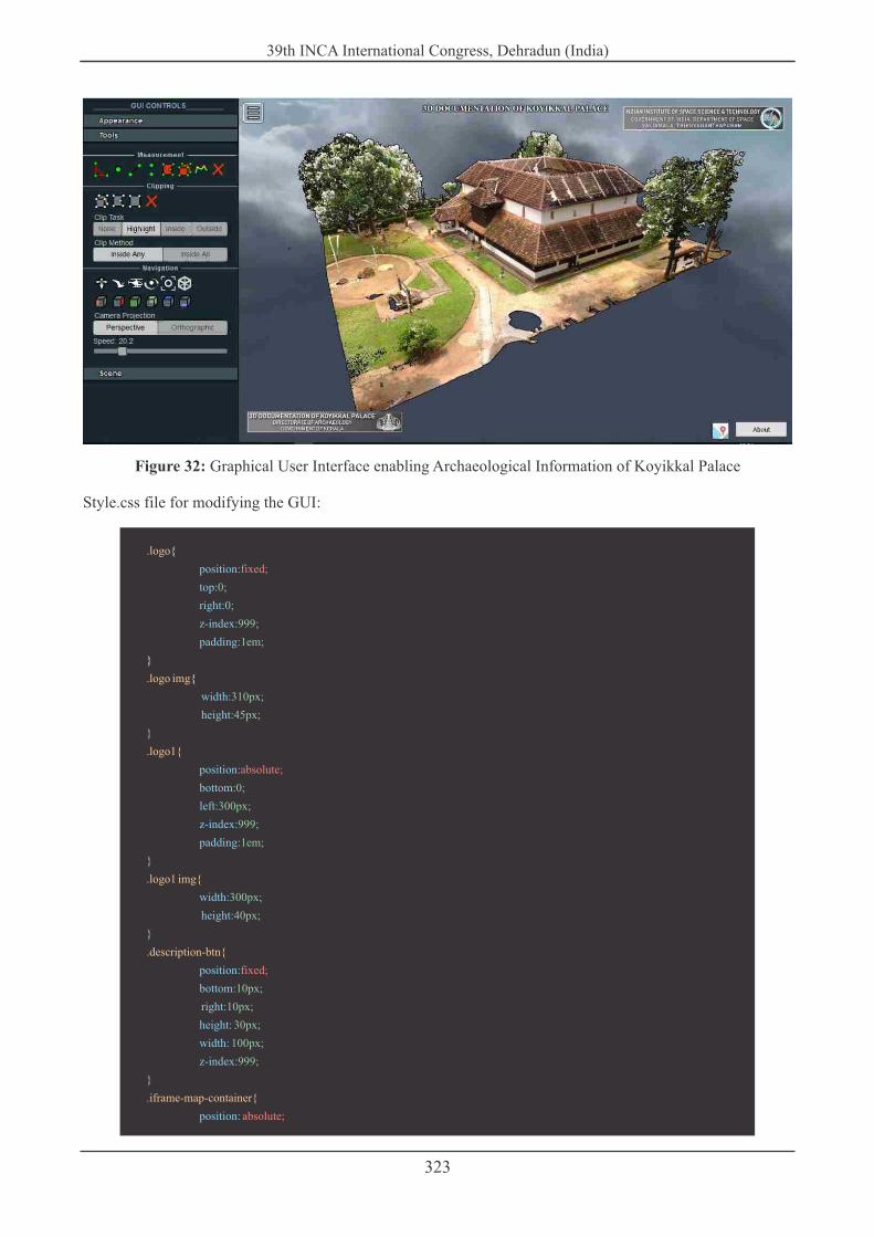
323322
3.7 WEB BASED VISUALIZATION OF LIDAR DATA
In order to create the 3D visualization on the web-based platform, Potree viewer has been used here. It's an open source javascript platform were the LiDAR data can be visualized and it enables the measurement, volume, elevation interpretation etc. For that, the first step is to install the Potree.exe in the system along with the local server named XAMPP. The data is being called by the below-mentioned command,
It will flush all the point cloud data to the binary module within several minutes, depending on the size of data the compiling time will be more. Once this complete the LiDAR data will be saved in the XAMPP local server folder named 'tomcat'. The end product will comprise of an HTML file, LiDAR data binary folder and the several JavaScript modules for the visualization of the point cloud data. Opening the HTML file directly deploy the user to the web-based HTML portal of Potree viewer along with the data specified.
3.8 COMPILING & EXE GENERATION
A series of applications are compiled in order to reduce the complexity of the data. The end product will be delivered to the State Archaeology department. It is designed such a manner were a layman should use the data without any uncertainty. Compiling method exclude the installation of the local web server and Potree LiDAR visualizer which works with a coding platform.
3.9 DEVELOPING GUI FOR ARCHAEOLOGICAL INFORMATION SYSTEM
To exploring the Archaeological Information system of the given site, an independent GUI which enable the user to have a look around both inside and outside with the capabilities of Angle, Height, distance, point, Area & Volume measurement, rotation, colorized elevation view etc. Selection of tools is based on the nature of the data and the utility of the data. The independent java based GUI is capable of many types of navigation like the fly control, Helicopter control, Earth control, Orbit control, Full extent etc. The density of the point cloud can be controlled from low point density to high point density. Investigation of the height in different aspect like Intensity gradient, RGB & Elevation also simple using the height profile tool. The GUI was altered using the Style.css file for including the necessary layers and tools like a map, a brief description of the palace, title of the object, and necessary logos etc.
Figure 31: Inno Compiler chart showing the different platforms for integration
Figure 32: Graphical User Interface enabling Archaeological Information of Koyikkal Palace
Style.css file for modifying the GUI:
.logo
.logo img
.logo1{
.logo1 img{
.description-btn{
.iframe-map-container{
{
}
{
}
}
}
}
position:
top:
right:
z-index:
padding:
width:
height:
position:
bottom:
left:
z-index:
padding:
width:
height:
position:
bottom:
right:
height:
width:
z-index:
position:
fixed;
absolute;
fixed;
absolute;
0;
0;
999;
1em;
310px;
45px;
0;
300px;
999;
1em;
300px;
40px;
10px;
10px;
30px;
100px;
999;
39th INCA International Congress, Dehradun (India) 39th INCA International Congress, Dehradun (India)

325324
}
bottom:
right:
z-index:
margin:
position:
bottom:
right:
z-index:
padding:
width:
height:
position:
right:
bottom:
z-index:
padding:
width:
height:
display:
22px;
0;
999;
1em;
22px;
0;
999;
1em;
250px;
450px;
120px;
0;
999;
0.2em;
30px;
30px;
}
}
}
}
}
.description-sidebar{
.description-sidebar img{
.custom-map-icon{
.custom-map-icon img{
.hide{
fixed;
absolute;
none;
· The Java Library Modules used for the GUI functionalities.
Each module has individual functions as the measurement, rendering the point cloud data, navigation controls etc. Altering this java code modifies the tools as per the user requirement. The GUI has been edited using modules for the attachment of tools and for the deletion of a few tools due to less functionality. Once the changes are saved, the HTML file will automatically read the attached modules along with the data.
Figure 33: GUI Java Library Module
3.10 CLASSIFICATION OF POINTS
With the help of Microstation software, obtained LiDAR point data has been classified into different classes as Ground, Building and Vegetation. In order to generate the DTM and DSM from the classified points will reduce the computation time without rendering the entire data.
Figure 34: Classified Building & Vegetation Points
Figure 35: Classified Ground Points and classification of ground & non-ground
3.11 GENERATION OF TERRAIN MODELS
To identify the topographic conditions by generation of terrain model DTM and DSM etc. help to interpret the location. Mostly this interpretation will help in the region having the vulnerable conditions like hazards. It helps in interpret the different elements with different functionality. DTM is actually the same as that of a DEM. This means that the DTM is simply a elevation surface representing the bare earth referenced to a common vertical datum.
3.11.1 Digital Terrain Model (DTM)
The resultant Terrain model having minimum elevation value that resampled to 0m up to 57.20m above the Mean Sea Level.
39th INCA International Congress, Dehradun (India) 39th INCA International Congress, Dehradun (India)

327326
Map 2: Digital Terrain Map of Koyikkal Palace
2.3 Geometric Method
Geoid undulation varies from point to point on earth. However, the geoid surface model of an area can be generated by using geographic coordinates, plan coordinates of the control points and known value of geoid undulation at those control points (Akcin 1998; IGNA 1999; Ollikainen1997; Soycan 2002) and if geoid undulations of fairly close points are accurately known, same at intermediate points can be interpolated using various interpolation techniques. Polynomial Regression Method though more cumbersome in computation, but generally more accurate has been used in this study and is discussed here.In geometric method ellipsoidal height and orthometric height of sufficient number of common points is used to find geoid undulation straight away and subsequently the best fitting curve as geoid (Fig 2).
2.3.1 Polynomial Regression Method
Geoid is a complex surface whereas an ellipsoid is a smooth mathematical surface. Separation between geoid and ellipsoid i.e. geoid undulation of points varies from point to point on the earth. So, geoid undulation which is not a linear phenomenon can be described by a model developed based on polynomial regression technique.
In Polynomial Regression method, the geoid undulation (N) can be given by a function of latitude and longitude after Soycan Matin, 2003 as:
3.12 CHAPTER CONCLUSION
The followed chapter is about the methodology and techniques which used to generate the objectives. Sufficient details of the tools with adequate screenshots have been provided in this chapter. The section comprises of information about the data pre-processing to the visualization of data, which have been done with the help of different software packages.
Map 3: Digital Surface Model of Koyikkal Palace
39th INCA International Congress, Dehradun (India) 39th INCA International Congress, Dehradun (India)

329328
CHAPTER - IV
Chapter Contents:
Research findings ……………………………………………………………………………………………
Results & Discussions ..……………………………………………………………………………………..
Conclusion .....……………………………………..………………………………………………………...
Recommendations ....….……………………………………..…….…………………….………….………
4.1 RESEARCH FINDINGS_
During the development of the dissertation, many important outcomes have been obtained which can be a worthy lead for the future endeavor. Basically, it's a first-ever approach of participating the emerging technology of LiDAR on the heritage mapping/survey which has been done using conventional tools for past years. There is great need to conserve this archaeological information digitally for the management of such cultural sites due to the yearly waning event which may be on behalf of human intervention or by natural events like disaster etc. The following are some of the research findings which has been emerged out of my study;
˜ Creation of Archaeological Information System, Augmented reality, CAD file, terrain model, shapefiles etc. can be done fast using the LasTools. Archiving such cultural heritage data digitally is of prime importance in the developed countries. A country like India is known for its wide variety of culture and that culture have to be preserved for the future with the techniques of LiDAR mapping.
˜ 3D data enables the basic measurement of the objects, sculptors and many more found exactly similar to the actual geometry. Incase if any renovation is needed in the palace, the palace officials can use of it for the reconstruction with the actual geometry.
˜ With the help of processed LiDAR data separation or the classification of points into ground, non-ground and vegetation enables the user to interpret the layers differently very fastly than the conventional GIS tools.
˜ While sharing data among different department, keeping the standard is the prime important of the planners. In case of LiDAR data keeps the exactness when it is shared among different departments.
˜ The instrument which was used for the mapping found dynamic due to the mobile nature. Also found there is great potentiality in participating the LiDAR technology in Heritage Mapping that to without much human effort, the measurement comparison of the geometry to the reality found exact to actual object and can be obtained very fast. As Geography is concerned with the geospatial information, the instrument enables the user to take the discipline to a next level where the third dimension can be derived within seconds which was done by conventional tools with a deliberate agreement in much important information.
˜ Georeferencing with the DGPS points will exactly locate the area without Zero percent error. Correction of error values will be done with the help of Zero error base station which is already error free.
˜ Another important feature of this instrument is that the interlinkage of the data with different platforms. The combining of DGPS points in the generated LiDAR data produces a great extent of accuracy and precision for the data. Generation of all GIS models found easy with the point cloud data. Developing a 3D model was once found capable only by a computer vision expert. As a person with average knowledge in the computer vision, I was able to handle all the data and analysis more confidently due to the simplified instrumentation and user-friendly data.
4.2 RESULT & DISCUSSION
4.2.1 RESULTS:-
3D modelling is extensively being used in various industry vertical for numerous purposes such as getting the detailed schematic of the products, as well as modelling a particular area or monument. A detailed methodology for processing, classification, DEM and Contour generation and 3D modelling of the Heritage site using point clouds have developed.
Based on the methodology;
a) The terrestrial point clouds are Processed, Registered and Georeferenced using FARO SCENE software.
b) Building reconstruction and applying hole filling algorithms for smoothing the object for 3D visualization.
Figure 36: Point Cloud Data showing X, Y & Z Coordinates
Figure 37: Point Cloud Data after applying Hole filling Algorithm
b) Building reconstruction and applying hole filling algorithms for smoothing the object for 3D visualization.
c) Processed Points are classified into different categories. Visualization of the finished data into the web platform with the help of GUI for Photorealistic 3D Walk-through of the palace with Archaeological Information System.
39th INCA International Congress, Dehradun (India) 39th INCA International Congress, Dehradun (India)

331330
d) The end product can also be took part as an Archaeological advertising element which the State Archaeological Department currently lacks.
4.2.2 DISCUSSION:-
Terrestrial LiDAR scanning is a popular technique for the acquisition of a huge amount of high-density point cloud data, which provides detailed. Reliable, precise and accurate elevation data for both topographic surface and above ground objects on the earth surface. The Terrestrial FARO SCENE FOCUS 350 can able to collect the point up to the range of 350 m but in the study, scans are recorded at 20 m interval for the detailed identification of all object. The focus of the study is to reconstruct the acquired data of Koyikkal palace and creation of Photo Realistic 3D walkthrough of the heritage site along with Archeological information system. Some of the important results that emerge from the part of the study are summarized below.
1. The FARO instrument was operated to take 15 scans covering around 80 cents of the Koyikkal Palace including the inner courtyard. Each scans requires 12 minutes for acquiring the point cloud data. Total Scans have been taken in the time span of five hours.
2. Processing, Registration and Georeferencing of all 15 scans using the SCENE software produce the resultant 488,212,112 point clouds with 10.1 mm mean point error. The time required for the Processing, Registration, Georeferencing and Exporting of all point clouds covers approximately two to three hours.
4.3 CONCLUSION
The main aim of this study is to create a Photo Realistic Walk-through of Koyikkal palace along with the Archaeological information system using the terrestrial LiDAR data. The TLS is the advanced technology in remote sensing. There is a situation that the conventional GIS tools fail in complete conservation of such heritage sites. In such situations, the Terrestrial LiDAR are capable of completely delivering the most accurate real-time high resolution three Dimensional data that have multi-functionality usage in monitoring such sites. In this research, FARO FOCUS 350 terrestrial laser scanner with an integrated GPS is used to scan the Koyikkal Place with an area of 80 Cents. The built-in 165 megapixel, HDR camera captures detailed imagery easily while providing a natural color overlay to the scanned data in the extreme lighting conditions. A total number of 15 scans with 488,212,112 points are recorded. The recorded points are pre-processed, registered and georeferenced with resultant 10.1 mm mean point error. The classification of point helps to identify various features based on the elevation. There is a need to reconstruct the scanned data for smoothing the surface for improved documentation. Using the MeshLab software, applied various algorithms for reconstructing the object. Once the object (Palace) is ready, the finished layer will visualize using the web-based platform with the help of independent GUI. Creating a basic GUI enables the layman to use the result productively. The GUI enables to measure the height, area, height based demarcating of the palace, etc. Along with the GUI Archaeological Information Archive system also provide the digital information for the future palace renovation. Bare earth model, Contour and DEM are some of the layers which was generated with the help of acquired point cloud data.
4.4 RECCOMMENDATIONS
After the completion of the dissertation, few recommendations have been derived so as to overcome those limitations in the future works. Selection of the scanning parameter in the Terrestrial LIDAR Scanner has got very much important because depending on the parameter only it will give the reflectance. The user should be a well-versed with such elements before starting the scan. Once the scans start, always maintain a regular distance between the point of the scan in order to reduce the distance error while registration. In case of scanning the building the field of view should be there with the adjacent scan for the cloud to cloud registration. If not, it will not be registered with the near strip and it will affect the entire scanned point cloud while pre-processing. Once the mapping over, one of the herculean tasks is to register the images along with the ground control points. For this, a dedicated system or workstation is needed with sufficient GPU. For dealing the millions of point cloud data system configuration is a must element for timely processing of the data. Archiving the digital data of Koyikkal Palace found effective such a way, it could be used for creating an augmented reality where the layman can explore the site through the web. The archaeological information system should help in identifying all the minute details of the palace digitally, also which enables the temporal monitoring of such sites. There is a need to give pressure on the heritage site mapping with this technology as Kerala's foundation was built on a wide verity of culture. Still, the palaces in Kerala lacks the systematic method of preserving the sites. Recent technologies like Spectroradiometer, IR thermography, Ground Penetrating Radar (GRP) would be coupled along with the LiDAR is capable for advanced study on the displacement and anomalies were the heritage site recently going through.
Figure 2: ECEF X, Y and Z plots of Dehradun PS for 2015-18 obtained from the 24-hr session network positioning
Figure 39: Area measurement using the GUI
Figure 2: ECEF X, Y and Z plots of Dehradun PS for 2015-18 obtained from the 24-hr session network positioning
39th INCA International Congress, Dehradun (India) 39th INCA International Congress, Dehradun (India)

332
REFERENCE
· Anguelov, Dragomir, Dulong, Carole, Filip, Daniel, Frueh, Christian, Lafon, Ste´phane, Lyon, Richard, Ogale, Abhijit, Vincent, Luc, Weaver, Josh, 2010. Google street view: capturing the world at street level. Computer 43 (6), 32–38.
· Axellson, P., 2000. DEM generation from laser scanner data using adaptive TIN models. In: International Archives of the Photogrammetry, Remote Sensing and Spatial Information Sciences, XXXIII, pp. 110–117.
· Baltsavias, E.P., 1999. Airborne laser scanning: basic relations and formulas. ISPRS J. Photogramm. Remote Sens. 54 (2–3), 199–214. Biljecki, Filip, Stoter, Jantien, Ledoux, Hugo, Zlatanova, Sisi, C¸ o¨ ltekin, Arzu, 2015. Applications of 3D city models: state of the art review. ISPRS Int. J. Geo-Inf. 4 (4), 2842–2889. Burtch, Robert, 2002. Lidar principles and applications. In: IMAGIN
Conference, pp. 1–13.
· Dadras, Mohsen, Shafri, Helmi Z.M., Ahmad, Noordin, Pradhan, Biswajeet, Safarpour, Sahabeh, 2015. Spatio-temporal analysis of urban growth from remote sensing data in Bandar Abbas City, Iran. Egypt. J. Remote Sens. Space Sci. 18 (1), 35–52.
· Bharat Lohani, PhD Associate Professor, Department of Civil Engineering IIT Kanpur, 2016, Airborne Altimetric LiDAR: Principle, Data collection, processing and Applications.
· Ong Chee Wei, Cheong Siew Chin, Zulkepli Majid, Halim Setan, Faculty of Geoinformation and Real Estate, Universiti Teknologi Malaysia, Malaysia, 2015 3d Documentation And Preservation Of Historical Monument Using Terrestrial LaserScanning - Geoinformation Science Journal, Vol. 10, No. 1, 2010, pp: 73-90.
· Uma Mudenagudi, Syed Altaf Ganihar, Shreyas Joshi, Shankar Setty, Rahul G., Somashekhar Dhotrad, Meera Natampally, Prem Kalra B. V. Bhoomaraddi College of Engineering and Technology-Hubli, NIAS Bangalore, 2014 IIT-Delhi - Realistic Walkthrough of Cultural Heritage Sites-Hampi.
· Jan Bohm, Terrestrial LiDAR in Urban Data Acquisition, Stuttgart Photogrammetric Week '09 Dieter Fritsch (Ed.) Wichmann Verlag, Heidelberg, 2009
· Antonio Costanzo 1,*, Mario Minasi 1, Giuseppe Casula 2, Massimo Musacchio 3 and Maria Fabrizia Buongiorno 3- Combined Use of Terrestrial Laser Scanning and IR Thermography Applied to a Historical Building - Sensors 2015, 15, 194-213; doi:10.3390/s150100194
· T. Temizer a, G. Nemli a, E. Ekizce b, A. Ekizce b , S. Demir c, B.Bayram d, Askin F.H e, A. V. Cobanoglu f, H. F. Yilmaz g - 3d Documentation Of A Historical Monument Using Terrestrial Laser Scanning Case Study: Byzantine Water Cistern, Istanbul - International Archives of the Photogrammetry, Remote Sensing and Spatial Information Sciences, Volume XL-5/W2, 2013 XXIV International CIPA Symposium, 2 – 6 September 2013, Strasbourg, France.
· Suddhasheel Ghosh and Bharat Lohani Department of Civil Engineering, Indian Institute of Technology Kanpur, Kanpur, 208 016, 2016, India - Development of a system for 3D visualization of LiDAR Data.
· Pablo Rodríguez-Gonzálvez 1,*, Belén Jiménez Fernández-Palacios 1, Ángel Luis Muñoz-Nieto 1, Pedro Arias-Sanchez 2 and Diego Gonzalez-Aguilera, 2012, - Mobile LiDAR System: New Possibilities for the Documentation and Dissemination of Large Cultural Heritage Sites.
· Hyoungsig Cho, Seunghwan Hong, Sangmin Kim, Hyokeun Park, Ilsuk Park, and Hong-Gyoo Sohn - Application of a Terrestrial LIDAR System for Elevation Mapping in Terra Nova Bay, Antarctica - Sensors (Basel). 2015 Sep; 15(9): 23514–23535.
· UllaWandinger Leibniz Institute for Tropospheric Research, Permoserstraße 15, D-04318 Leipzig, Germany - Introduction to Lidar, 2015.
· Fabio Remondino 3D Optical Metrology (3DOM) Research Unit, Bruno Kessler Foundation (FBK), 38122 Trento, Italy - Heritage Recording and 3D Modeling with Photogrammetry and 3D Scanning- Remote Sens. 2011, 3, 1104-1138; doi:10.3390/rs3061104.
333
ANNEXURE
Figure: Aerial LiDAR Surveying Figure: Terrestrial LiDAR Scanner andMeasured points in different returns
Figure: TLS Scanning MethodFigure: Principle of range measurement using LiDAR
Figure: Satellite based LiDAR Mapping
Source: Airborne Altimetric LiDAR: Principle, Data collection, processing and Applications, Department of Civil Engineering IIT Kanpur INDIA
39th INCA International Congress, Dehradun (India) 39th INCA International Congress, Dehradun (India)

334
Figure: Major LIDAR SystemsSource: Airborne Altimetric LiDAR: Principle, Data collection, processing and Applications, Department of Civil Engineering IIT Kanpur INDIA
Figure: Bathymetry LIDAR Systems for Oceanic studiesSource: Airborne Altimetric LiDAR: Principle, Data collection, processing and Applications, Department of Civil Engineering IIT Kanpur INDIA
335
Figure: TLS mapping progressing in Koyikkal Palace
Figure: TLS mapping progressing in Koyikkal Palace
39th INCA International Congress, Dehradun (India) 39th INCA International Congress, Dehradun (India)

337336
Figure: (clockwise) DGPS Rover displaying survey duration, Rover placed at the corner of palace for Surveying, Mapping progressing in palace with different scan stations.
Figure: Interior of palace being scanned by TLS mapper
Figure: TLS mapping for acquiring wooden architectural works inside the palace
39th INCA International Congress, Dehradun (India) 39th INCA International Congress, Dehradun (India)

338
Fig
ure
: T
eam
inc
ludi
ng K
oyik
kal
Pal
ace
offi
cial
s, I
IST
Fac
ulty
, M.T
ech
stud
ents
fro
m I
IST
who
hel
ped
and
cont
ribu
ted
to m
ake
this
map
ping
a s
ucce
ss
39th INCA International Congress, Dehradun (India)

339
MAPPING DECADAL GROWTH OF POPULATION IN KERALA STATE FROM 1901-2011
Deepthi.PResearch Scholar, Madurai Kamaraj University ,Madurai
Dr.I.K.ManonmaniAssistant Professor, Department of Geography, Madurai KamarajUniversity, Madurai
AndAhalya Sukumar and B.Sukumar,
m Scientists (Retd) Centre for Earth Science StudiesThiruvananthapura 695031
Email: [email protected]
Abstract
Study of growth of population at regional level is an important aspect of Population Geography. Growth of population was varies from one state to another state in India. In this paper an attempt is made to map the growth of population in Kerala state from 1901 to 2011. It shows the spatio-temporal and intra-regional variation of growth of population for eleven decades. District is chosen as unit of study. There are 14 districts in Kerala. Percentage of growth of population for each decade is collected from the Census of India. Statistical techniques like mean and standard deviation were used to calculate standard score to normalize the data for each decade at district level. Using GIS, thematic maps were prepared to show the spatial distribution of growth of population from 1901-11 to 2001-11.
From the study it is found that Idukki district shows high growth rate above state average in 1901-11. In 1951-61, decadal growth was found high in Kannur, Wayanad, Idukki, Kollam and Thiruvananthapuram districts which were above the state average. In the decade 1991-2001, Kasaragod,Wayanad, Kozhikode, Malappuram, Palakkad,Thrissur, Ernakulam and Thiruvananthapuram districts show high growth rate. In 2001-11, all the districts in the northern part fromKasaragod to Ernakulam show high growth of population. Idukki and Pathanamthitta districts show minus growth and rest of the southern districts show low growth of population.
Introduction
Population growth is one of the major concerns of the present world as human population is not a static factor. Rather, it is growing at a very alarming rate. In spite of the increasing world population, the resources of the earth remain constant. Thus, the ability to maintain sustainable development is becoming a major challenge to mankind today. Population growth is the change in a population over time and can be quantified as the change in the number of individuals of any species in a population using per unit time for measurement. The world's population is currently growing by over 80 million people each year, and is projected to exceed 12 billion people by around the year 2050.
The Growth rate of population is an important demographic characteristics which not only helps understanding the population change that a society has undergone , but also helps in predicting the future demographic characteristics of an area. It is useful to study the pattern of population growth, and analyse this pattern to identify the major factors that determine growth rate of population in the particular area. The concept regarding growth of population is often used to denote the change in the number if inhabitants of a territory during a specific period of time, irrespective of the fact whether the change is positive or negative and when the change is in positive direction, ie, if the population increases , the growth is positive and vice versa.
Study Area
Kerala is one of the states in India situated in the south western part of PeninsularIndia (fig.1). It has an area of 38,
39th INCA International Congress, Dehradun (India)

341340
Analysis
In 1901-11, southern districts except Kottayam district all others show very high to high population growth rate. Northern districts exceptWayanad and Malappuram shows very low population growth. Wayanad&Malappuram district shows moderate growth rate(Figure1).In 1911-21 Kollam, Pathanamthitta, Alapuzha&Kottayam districts shows very high population growth rate. Northern districts shows very low to low growth rate. Central part of Kerala is having moderate to low growth in population (Fig.2).In 1921-31,Idukki district shows very high growth rate followed by Kottayam with high and all other southern districts show moderate growth rate (Fig.3). In 1931-41 same trend of growth of is found(Fig.4). In 1941-51, Wayanad and Idukki districts have shown very high and high growth rate respectively (Fig.5). Almost similar trend was found in 1951-61 (Fig.6). In 1961-71, Northern district have shown high growth rate than southern districts except Idukki district which showed very high growth rate (Fig.7). In 1971-81, northern districts and Pathanamthitta district have shown high to moderate growth rate (Fig.8).In 1981-91, 1991-2001,and 2001- 2011, northern districts continues to show high growth rate than southern districts (Fig.9, Fig.10 and Fig.11).
Conclusion
Kasaragod district showed high growth rate only after 1961-71. Kannur district showed high growth rate after 1951. Growth rate of population of Wayanad increased from 1941. Kozhikode district also show similar trend. Malappuram district shows high growth rate of population only after 1961. Palakkad district showed low growth rate from 1901 to 1971. High growth rate is found after 1971.Thrissur and Ernakulam districts showed mixed trend of growth with moderate to high. Idukki showed high growth rate from 1901 to 1971. From 1981 onwards it showed low growth rate.Kottayam district showed very low to low growth rate from 1941-51. Alappuzha and Kollam showed the similar trend. Pathanamthitta showed low growth rate from the last three decades. Earlier it was showing mixed growth trend from moderate to very high. Thiruvananthapuram district showed moderate to high growth trend in all the decades except 1971-81 and 2001 to 2011. High growth rate in Idukki and Wayanad districts attributed to the migration people from low land to high land in search of new agricultural land at the cost of forest land and expansion of plantation crops in the high land. In the last three decades northern districts of Kerala shows high growth rate. It is mainly due to migration of people from southern districts in search of land for plantation crops and increase in tertiary occupation.
863 sq.km (1.2% of India's total area) with a populationof 3,34,06,061 (Census 2011). Kerala is home to 2.76% of India's people, and itsland is three times as densely settled as the rest of India. However,Kerala's population growth rate is far lower than the national average, Kerala's population more than doubled between 1951 and 1991, adding 15.6 millionpeople to reach a total of 29.1 millionin 1991, 31.8 million by 2001 and 33.3million in 2011. Populationis most densely settled in the coastal region, leavingthe eastern hills and mountains comparatively sparsely populated.Kerala state has 14 districts and 63 taluks.Socio-economic and demographicaspects are controlled by the physiography, land use/ land cover, religion of thestate. Keralahas achieved remarkable progress in human development, as reflected in the highlevels of education and health of its population. The level of literacy amongKeralites is far higher than the national average. Crude death rate, infantmortality rate, and life expectancy at birth in Kerala are comparable even to those in the developed countries.
Figure .1
Methodology
The data source related to the study area is secondary, collected from Census of India. Percentage of growth rate is converted into “Z score” or “standard score. It is astatistical technique used for the calculation decadal population growth deviating from average and standard deviation. GIS isused for creating thematic maps and analysis.
Figure . 2 Figure . 3
39th INCA International Congress, Dehradun (India) 39th INCA International Congress, Dehradun (India)

343342
Figure . 4 Figure . 5
Figure . 6 Figure . 7
Figure . 8 Figure . 9
Figure . 10 Figure . 11
39th INCA International Congress, Dehradun (India) 39th INCA International Congress, Dehradun (India)

343342
Figure . 4 Figure . 5
Figure . 6 Figure . 7
Figure . 8 Figure . 9
Figure . 10 Figure . 11
39th INCA International Congress, Dehradun (India) 39th INCA International Congress, Dehradun (India)

345344
Figure . 12
Change assessment of spatio-temporal dynamics of land use/land cover using remote sensing and GIS: A case study of Lucknow city (1993-2019)
Md. Omar Sarif 1*, R. D. Gupta 2
1 PhD Research Scholar, Geographic Information System (GIS) Cell,Motilal Nehru National Institute of Technology Allahabad, Prayagraj-211004 (India), Email ID:
[email protected] / [email protected]
2 Professor, Civil Engineering Department and Member of GIS Cell,Motilal Nehru National Institute of Technology Allahabad, Prayagraj-211004 (India), Email ID:
Corresponding Author*: Md. Omar Sarif ([email protected])
Abstract:
Lucknow City, the capital of Uttar Pradesh State, is experiencing high land use/ land cover changes due to high population growth and its related effects. In present study, multi- temporal multi-spectral Landsat images of TM and OLI/TIRS of 9th June, 1993 and 1st June, 2019 respectively are first pre-processed and then classified using ERDAS IMAGINE 2014. The supervised classification is carried out using Maximum Likelihood Classifier (MLC). The overall classification accuracy achieved for both classified images is more than 85%. The results indicate that maximum increase is observed in built-up land while agriculture land observed the maximum decrease. During 1993-2019, city experienced increase in built-up land by 138.25 km2 (43.80%), barren land by 4.54 km2 (1.44%) and water body by 0.12 km2 (0.04%). At the same time, agriculture land decreased by 140.74 km2 (44.59%) and forest land by 2.16 km2 (0.69%). The change analysis (1993-2019) results reveal that the most of the transformation was because of built-up land, mainly at the cost of agriculture land by 109.31 km2 (34.63%) and forest land by 18.69 km2 (5.92%). This trend explains the remarkable alterations of LU/LC dynamic in city landscape. This study can help policy makers and urban planner for creation of efficient plans to restore the urban environment for sustainable development.
Keywords: LU/LC, Landsat (TM, OLI/TIRS), maximum likelihood classifier, change analysis, Lucknow city.
1. Introduction
Globally people have settled down in urban settings due to its pulling attraction because of better standard of living with economic viabilities. In 2016, 54.5% of total population of the world lived in urban area, and if the trends go same then it will be 60% of total population in 2030 (UN, 2016). IPCC asserted in 2019 that due to dramatic changes in land uses, an alarming alteration has been going on the natural land and for this a quick monitoring and planning needs to be incorporated on small to large landscape by measuring its risk and mitigation for sustaining the land capacity (IPCC, 2019). In the process of land transformation, an explosive changes has been seen on the face of the Earth due to urbanization and impervious development, industrialization, forest logging, agriculture expansion, and mining which continuously makes land as a scarce resources day by day (Dubovyk, 2017). Further, land changes have severe effects on substantial ecosystem of the world (Polasky et al., 2011). Hence, land use/land cover (LU/LC) information and its possible optimal use has become an essential requirement of a scheme for selection, planning, and implementation to fulfil the massive demands for human's basic needs as well as welfare (Deka et al., 2019).
Various studies has been carried out worldwide about LU/LC where major purpose was to comprehend the land dynamics and changes occurred in terms of spatial and temporal context of agriculture, settlements, forest, water body and over all environment (Lambin et al., 2003; Mallupattu et al., 2013; Oliveira et al., 2014; Rousta et al., 2018). In recent times, the extensive use of remote sensing and GIS has been explored to quantify the spatial and temporal changes on the natural landscape due to its efficient capabilities to address small to large scale analysis on the face of the Earth (Kogo et al., 2019; Sarif et al., 2017; Wang et al., 2018). These studies have been possible because of the availability of satellite imageries that deliver the information of actual ground situations which has been used for depicting LU/LC dynamics to extract the actual status of the landscape. Time to time detailed
39th INCA International Congress, Dehradun (India) 39th INCA International Congress, Dehradun (India)

347346
information of LU/LC provides spatial pattern understanding and its influencing factors about past to recent times about the landscape (Mengistu and Salami, 2007; Srivastava and Gupta, 2003). The foremost aspect of LU/LC is to determine the occurrence of change, types, trend and magnitude of change (Lu et al., 2004; Srivastava and Gupta, 2002).
India, one of the most transforming countries in the world, is witnessing high transformation in its land features especially in last five decades. In recent past, numerous studies has been carried out for the different Indian cities like Mumbai (Samant and Subramanyan, 1998), Bengaluru (Govind and Ramesh, 2019; Ramachandra et al., 2014), Chennai (Aithal and Ramachandra, 2016), Kolkata (Sharma et al., 2015), Delhi (Chakraraborty et al., 2015; Tripathy and Kumar, 2019) for depicting the spatial changes of land dynamics.
Lucknow city, the capital of Uttar Pradesh state, is selected as the study area. This is one of the largest economic and industrial cities of North India. In recent past, various studies has been carried out for Lucknow city, like Singh et al. (2017) extracted the spatial distribution of LU/LC but alteration in LU/LC is missing. Shukla and Jain (2018) evaluated LU/LC for detecting sprawl and its types but transition of LU/LC classes is missing. Siddiqui et al. (2018) used land cover to portray the distribution of urban growth and its prediction of 2023 but transition of LU/LC classes is not recognised.
This work is carried out using Landsat datasets of two different time points, 1993 and 2019 where we were selected summer time (June) for both the images. The reason behind these time points is best spectral information of land features as well as cloud free data which enables to understand the differentiations among distinct classes of LU/LC (Fonji and Taff, 2014). The major objectives of the present study are: (a) extraction of LU/LC maps for 1993 and 2019; (b) transition of LU/LC classes during 1993-2019.
2. Materials and Methods
2.1 Study Area
Lucknow city, the capital of the State of Uttar Pradesh, covers an area of 315.63 km2 and its latitudes ranging between 26°44'08"N and 26°57'57"N and longitude ranging between 80°49'50"E and 81°03'14"E, is chosen as study area (Figure 1). The city is drained by Gomti river on its central part in which this river flowing North-West to South-East (Figure 1c). The location of the city above mean sea level is near 123.000m. The climate of the city is sub- humid where average annual rainfall is 904 mm and temperature ranges 40-45 ºC (maximum) and 5-15 ºC (minimum) (Singh et al., 2017).
Figure 1: Study Area, Lucknow City; (a) Location of Uttar Pradesh in India; (b) Location of Lucknow District and Lucknow City in Uttar Pradesh;
(C) Landsat 8 Standard False Colour Composite (FCC) of Lucknow City of 01/06/2019
2.2 Data Used
In this study, Landsat images of Thematic Mapper (TM) of 09/06/1993 and Operational Land Imager (OLI)/Thermal Infrared Scanner (TIRS) of 01/06/2019 are used with spatial resolution of 30m (Table 1). This datasets of Landsat is obtained from the portal of United States of Geological Survey (USGS) (https://earthexplorer.usgs.gov/).
2.3 Methods
2.3.1 Image Classification
LU/LC map is generated using supervised classification where maximum likelihood classifier (MLC) is employed to perform the task (Langat et al., 2019). This classification is performed after selection of ground features as spectral signatures (Kogo et al., 2019). We selected band 3 (Red), band 4 (Near Infrared (IR)) and band 5 (Short-wave IR (SWIR)) in Landsat 5 (TM) datasets to execute the classification as it is standard form of selection of bands; whereas band 1 (Coastal blue), band 5 (Near IR), band 6 (SWIR 1), band 7 (SWIR 2), band 9 (Cirrus), band 10 (Thermal IR (TIR) 1), and band 11 (TIR 2) in Landsat 8 (OLI/TIRS) are chosen as it has best band combination to perform LU/LC classification (Liu and Zhang, 2019). Anderson's classification system of is adopted to extract the LU/LC class into five different classes at level-I, which are built-up land, agriculture land, forest land, water body and barren land (Anderson et al., 1976). The whole process is carried out in ERDAS IMAGINE 2014.
2.3.2 Accuracy Assessment
Accuracy assessment has been carried out for classified LU/LC images of 1993 and 2019. Total 500 points has been selected for both classified image based on spectral signatures through random sampling method. Then, the validation has been carried out based on authors' interpretation knowledge of FCC for 1993 and Google Earth images for 2019; it is also cross-checked and validated by published work for Lucknow city (Shukla and Jain, 2018) where they carried out the LU/LC map of 1990 and 2016. This accuracy assessment approach has been carried out by construction of error matrix for the time points of 1993 and 2019, where statistics measures like user accuracy (Equation 1), producer accuracy (Equation 2), overall accuracy (Equation 3), and kappa coefficients (Equation 4) has been computed (Rousta et al., 2018).
Table 1: Briefing of data used
Satellite (Sensor)
Landsat 5 (TM)
Landsat 8 (OLI/TIRS)
Path/Row
144/41
144/41
Acquisition Date & Time
(GMT)
09/06/1993 04:29:25
01/06/2019 05:06:37
Spatial
Resolution (m)
30
30
Where, Ʊ defines corrected classified pixels (CCP) (category); Ω (ω ) defines classified pixels (CP) in that category (row total (RT)); Ω (φ ) defines CP in that category (column total (CT)); $ defines CCP (diagonal); " defines classified reference pixels in that category; N defines total samples; r defines number of rows error matrix
th(EM); X total corrected samples in i row and column; X defines RT; X defines CT.δi ξ ξ
39th INCA International Congress, Dehradun (India) 39th INCA International Congress, Dehradun (India)

349348
2.3.3 Change Detection and Change Matrix
The change detection of LU/LC between 1993 and 2019 has been carried out due to its advantages and suitability in portraying the nature of change (Langat et al., 2019). The classified maps are used through subtracting themselves between the time period of 1993-2019 for depicting the land cover changes and this approach offers information of 'from-to' called transition change detection approach (Kogo et al., 2019) or change matrix approach (Rawat and Kumar, 2015) which enables to detect transformation of distinct class to other classes and vice versa. Transition change detection examples are like Vegetation land to built-up land, agriculture land to built-up land, barren land to built-up land, water body to barren land and among others (Langat et al., 2019).
3 Results and Discussion
3.1 Accuracy Assessment Report
The description of error matrix for LU/LC of 1993 has been shown in Table 2 and the description of error matrix for LU/LC of 2019 has been shown in Table 3. Based on results of accuracy assessment report, it has been found that the overall accuracy were 88.4% in 1993 and 91.4% in 2019, whereas kappa coefficients were 0.85 in 1993 and 0.89 in 2019 (Table 2- 3). The LU/LC classes, built-up land, agriculture land to built-up land, barren land to built-up land, water body to barren land has been found user accuracy as well as producer accuracy more than 85% in both the time points, 1993 and 2019 (Table 2-3).
3.2 LU/LC coverage, magnitudes and trends
The results of supervised (MLC) classification has been portrayed agriculture land as the most dominating class in 1993 (60.98% of total land) in Lucknow city but this dominant place has been replaced by built-up land (63.20% of total land) in 2019 (Table 4). Therefore it is pretty clear that a huge alteration has happened in Lucknow city during 1993-2019.
2In 1993, the coverage of LU/LC classes revealed that agriculture land was 192.47 km (60.98%) which was the 2 2
highest of area coverage, built-up land was 33.22 km (19.40%), forest Land was 61.24 km (10.52%), barren 2 2
land was 24.60 km (7.79%) and water body was 4.12 km (1.31%) which was the lowest area coverage (Table 4 2and Figure 3a-b). Whereas in 2019, the coverage of LU/LC classes revealed built-up land was 199.49 km
2(63.20%) which was the highest of area coverage, agriculture land was 51.73 km (16.39%), forest land was 2 2 2
31.05 km (9.84%), barren land was 29.14 km (9.23%) and water body was 4.24 km (1.34%) which was again the lowest of area coverage (Table 4 and Figure 3a-b).
2Between 1993 and 2019, the most increased LU/LC class was built-up land by 138.25 km (43.80%), the other
2 2increased classes were barren land by 4.54 km (1.44%) and water body by 0.12 km (0.04%) (Table 4 and Figure 23c); whereas the most decreased class was agriculture land by 140.74 km (44.59%) and another decreased class
2was forest land by 2.16 km (0.69%) (Table 4 and Figure 3c). The LU/LC map generated for 1993 and 2019 are shown in Figure 2(a) and Figure 2(b) respectively. The Built-up land was major alteration class in LU/LC which dramatically change the city landscape of Lucknow city.
Table 2: Error matrix LU/LC of Lucknow City of 1993
Table 3: Error matrix LU/LC of Lucknow City of 2019
Error Matrix
Built-up Land
Agriculture Land
Forest Land
Water Body
Barren Land
Total
Producer Accuracy
Built-up
Land
120
5
2
3
7
137
87.59
Agriculture
Land
7
110
3
1
4
125
88.00
Forest
Land
2
3
70
4
1
80
87.50
Water
Body
0
2
1
60
1
64
93.75
Barren
Land
6
5
2
2
82
97
84.54
Total
135
125
75
70
95
User
Accuracy
88.89
88.00
93.33
85.71
86.32
Error Matrix
Built-up Land
Agriculture Land
Forest Land
Water Body
Barren Land
Total
Producer Accuracy
Built-up
Land
172
3
1
1
6
183
93.99
Agriculture
Land
4
58
1
0
5
68
85.29
Forest
Land
3
1
71
2
0
77
92.21
Water
Body
0
1
2
69
0
72
95.83
Barren
Land
7
2
3
1
87
100
87.00
Total
186
65
78
73
98
User
Accuracy
92.47
89.23
91.03
94.52
88.78
1993
Total Samples = 500
Overall Accuracy = 91.4 Kappa coefficients = 0.89
Figure 2: LU/LC dynamics of Lucknow city; (a) LU/LC map of 1993; (b) LU/LC map of 2019
39th INCA International Congress, Dehradun (India) 39th INCA International Congress, Dehradun (India)

351350
Table 4: LU/LC Change Statistics of Lucknow City
LU/LC Classes
Built-up Land
Agriculture Land
Forest Land
Water Body
Barren Land
Total
1993
Area (km2)
61.24
192.47
33.22
4.12
24.60
315.65
2019
Area (km2)
199.49
51.73
31.05
4.24
29.14
315.65
1993
Area (%)
19.40
60.98
10.52
1.31
7.79
100
2019
Area (%)
63.20
16.39
9.84
1.34
9.23
100
Area (km2)
138.25
-140.74
-2.16
0.12
4.54
-
Area (%)
43.80
-44.59
-0.69
0.04
1.44
-
Change (1993-2019)
Figure 3: LU/LC Change Statistics of Lucknow City; (a) Area (km2); (b) Area (%); (c) from 1993 to 2019
3.3 Transition Matrix
The transition matrix or transition change detection for 1993-2019 has been spatially presented in Figure 5, its transformation in Figure 5 and its statistics in Table 5 (area in km2) and Table 6 (area in %). This has been represented by two ways; one was from one class of LU/LC to another class(s) of LU/LC and vice versa, and another was unchanged classes of LU/LC which remains constant during the time periods in the city landscape of Lucknow.
2 2Between 1993 and 2019: from built-up land, 1.22 km (0.39%) of area converted into agriculture land, 1.07 km 2(0.34%) of area converted into barren land and 1 km (0.32%) of area converted into forest land. From other
2 classes of LU/LC to Built-up land was very noticeable as it was converted from agriculture land by 109.31 km
2 2(34.63%), forest land by 18.69 km (5.92%), and barren land by 12.19 km (3.86%). The unchanged agriculture
2land was 57.65 km (18.26%) of total area of city landscape.
2Between 1993 and 2019: from agriculture land, 119.31 km (34.63%) of area converted into built-up land which
2was the major findings in this result, whereas 20.77 km (6.58%) of area converted into barren land and 17.18 km2 (5.44%) of area converted into forest land. From other classes of LU/LC to agriculture land was very negligible as it was converted from barren land by 5.36 km2 (1.70%), forest land by 1.38 km2 (0.44%), and water body by 1.65 km2 (0.52%). The unchanged built-up land was 43.51 km2 (13.78%) of total area of city landscape.
2Between 1993 and 2019: from forest land, 18.69 km2 (5.92%) of area converted into built-up land, 1.07 km (0.34%) of area converted into barren land and rest was negligible. From other classes of LU/LC to forest land
2was very noticeable as it was converted from agriculture land by 17.18 km (5.44%), barren land by 1.56 km2 (0.49%) and rest were negligible. The unchanged forest land was 10.97 km2 (3.48%) of total area of city landscape.
Between 1993 and 2019: from water body, 1.65 km2 (0.52%) of area converted into built-up land and rest were negligible. From other classes of LU/LC to water body was very noticeable only in agriculture land by
21.69 km2 (0.54%) and rest were negligible. The unchanged water body was 1.83 km (0.58%) of total area of city landscape.
2 2Between 1993 and 2019: from barren land, 12.19 km (3.86%) of area converted into built-up land, 5.36 km 2
(1.70%) of area converted into agriculture land, 1.56 km (0.49%) of area converted into forest land and rest was negligible. From other classes of LU/LC to barren land was very noticeable only from agriculture land by 20.77
2 2km (6.58%) and rest were negligible. The unchanged barren land was 5.40 km (1.71%) of total area of city landscape.
Figure 4: The transformation of LU/LC in Lucknow city (1993-2019)
Table 5: Transition matrix (area in km2) of LU/LC classes of Lucknow city (1993-2019)
1993
Change Matrix 2(area in km )
2019
Built-up Land
Agriculture Land
Forest Land
Water Body
Barren Land
Total
Built-up
Land
57.65
109.31
18.69
1.65
12.19
199.49
Agriculture
Land
1.22
43.51
1.38
0.25
5.36
51.73
Forest
Land
1.00
17.18
10.97
0.34
1.56
31.05
Water
Body
0.28
1.69
0.34
1.83
0.09
4.24
Barren
Land
1.07
20.77
1.84
0.06
5.40
29.14
Total
61.24
192.47
33.22
4.12
24.60
-
39th INCA International Congress, Dehradun (India) 39th INCA International Congress, Dehradun (India)

353352
1993
Change Matrix 2(area in km )
2019
Built-up Land
Agriculture Land
Forest Land
Water Body
Barren Land
Total
Built-up
Land
18.26
34.63
5.92
0.52
3.86
63.20
Agriculture
Land
0.39
13.78
0.44
0.08
1.70
16.39
Forest
Land
0.32
5.44
3.48
0.11
0.49
9.84
Water
Body
0.09
0.54
0.11
0.58
0.03
1.34
Barren
Land
0.34
6.58
0.58
0.02
1.71
9.23
Total
61.24
192.47
33.22
4.12
24.60
-
Table 6: Transition matrix (area in %) of LU/LC classes of Lucknow city (1993-2019)
2Figure 5: Conversion of LU/LC classes in Lucknow city during 1993-2019: (a-e) conversion (Area (Km )) of Built-up land, Agriculture land, Forest land, Water body, and Barren land respectively; (f-j) conversion
(Area (%)) of Built-up land, Agriculture land, Forest land, Water body, and Barren land respectively.
3.4 Evaluation of LU/LC in Urban Sustainability and Planning
During 1993-2019, in the gap of 26 years, Lucknow city has gone through a dramatic change in its city landscape. In the process of urbanisation, the most reduced class was agriculture land by the growth of built-up land by 109.31 km2 (34.63%). The other reduced class was forest land 18.69 km2 (5.92%) and it was also because of built-up land. Barren land space has increased at the cost of agriculture land. Water body has negligible growth change but city has new man-made water body called, Kathota Jheel (~0.431 km2) on North-East part of the city.
The change in agriculture and forest land has severe consequences on rural economy (farming, markets, etc.) and functioning of the land because of impervious developments on city landscape. The major adverse effects can be seen on agriculture production, stabilities of food supply and access of food which directly impacts the food security and natural resource sustainability (Langat et al., 2019). Due to urban spatial growth, the major warming effect was Land Surface Temperature (LST) intensification which has severe effects on humans including animals (Rousta et al., 2018).
At present scenario, LU/LC alteration has played one of the major roles to drastic change in the city landscape which has been a matter of great attention for urban planner, policy makers, urban investors, environmentalist and other scientific communities to control the drastic effects of landscape change on climate change. IPCC has said for small to large scale landscape monitoring and planning to minimize the severe effects of landscape change to sustain land capacity as well as sustainability of the environment (IPCC, 2019).
4. Conclusion
This study, incorporated with the help of geospatial methods, explored the LU/LC dynamics over the landscape of the Lucknow city. The overall accuracy of the classified images is more than 85% which confirms the classification effectiveness. Based on the results of change detection approach for the gap of 26 years (1993-2019), it is observed that due to dramatic development of built-up land (19.40% to 63.20%), a drastic alteration has been seen where the major effected class are agriculture land (60.98% to 16.39%) and forest land (10.52% to 9.84%). The results of transition matrix reveals the loss of agriculture land by 109.31 km2 (34.63%) and forest
land by 18.69 km2 (5.92%) only for the gain of built-up land. On the other hand, barren land also expanded at the cost of agriculture land by 20.77 (6.58%). This all together helped in filling the LU/LC data gap for the city.
The major emphasis of the present study is to bring out the real status of city landscape and to control the depletion of forest and agriculture land for minimising the severe effects of landscape alteration on local climate change. The adopted approach demonstrates the usability of spatiotemporal images of Landsat in LU/LC mapping and in extracting the LU/LC change detection. This study will be helpful in critical planning and regulating policy making to address the present adverse situation of the landscape for enhancing the land capacity as well as sustainability of the environment.
Acknowledgements
Authors are very thankful to USGS for their datasets, i.e. Landsat TM and Landsat OLI/TIRS freely available on their own portal. Author, Md. Omar Sarif, is very grateful for financial support from University Grants Commission (UGC) through Maulana Azad National Fellowship (MANF) scheme (2017-18).
Reference
- Aithal, B.H., Ramachandra, T. V., 2016. Visualization of Urban Growth Pattern in Chennai Using Geoinformatics and Spatial Metrics. J. Indian Soc. Remote Sens. 44, 617–633. https://doi.org/ 10.1007/s12524-015-0482-0
- Anderson, J.R., Hardy, E.E., Roach, J.T., Witmer, R.E., 1976. A Land Use And Land Cover Classification System For Use With Remote Sensor Data, in: A Revision of the Land Use Classification System as Presented in U.S. Geological Survey Circular 671. Washington.
- Chakraraborty, S.D., Kant, Y., Mitra, D., 2015. Assessment of land surface temperature and heat fluxes over Delhi using remote sensing data. J. Environ. Manage. 148, 143–152. https://doi.org/10.1016/ j.jenvman.2013.11.034
- Deka, J., Tripathi, O.P., Khan, M.L., Srivastava, V.K., 2019. Study on land-use and land-cover change dynamics in Eastern Arunanchal Pradesh, N.E. India using Remote sensing and GIS. Trop. Ecol. https://doi.org/10.1007/s42965-019-00022-3
- Dubovyk, O., 2017. The role of Remote Sensing in land degradation assessments: opportunities and challenges. Eur. J. Remote Sens. 50, 601–613. https://doi.org/10.1080/22797254.2017.1378926
- Fonji, S.F., Taff, G.N., 2014. Using satellite data to monitor land-use land-cover change in North-eastern Latvia 1–15.
- Govind, N.R., Ramesh, H., 2019. The impact of spatiotemporal patterns of land use land cover and land surface temperature on an urban cool island: a case study of Bengaluru. Environ. Monit. Assess. 191, 1–20. https://doi.org/10.1007/s10661-019-7440-1
- IPCC, 2019. Climate Change and Land Grabbing, An IPCC Special Report on climate change, desertification, land degradation, sustainable land management, food security, and greenhouse gas fluxes in terrestrial ecosystems. https://doi.org/10.4337/9781784710644
- Kogo, B.K., Kumar, L., Koech, R., 2019. Analysis of spatio-temporal dynamics of land use and cover changes in Western Kenya. Geocarto Int. 1–16. https://doi.org/10.1080/10106049.2019.1608594
- Lambin, E.F., Geist, H.J., Lepers, E., 2003. Dynamics of Land-Use and Land-Cover Change In Tropical Regions . Annu. Rev. Environ. Resour. 28 , 205–241. h t tps : / /doi .org/10.1146 /annurev.energy.28.050302.105459
- Langat, P.K., Kumar, L., Koech, R., Ghosh, M.K., 2019. Monitoring of Land Use/Land - Cover dynamics using remote sensing: A case of Tana River Basin, Kenya. Geocarto Int. 1–20. https://doi.org/10.1080/10106049.2019.1655798
- Liu, H., Zhang, Y., 2019. Selection of Landsat8 Image Classification Bands Based on MLC– R F E . J . Indian Soc. Remote Sens. 47, 439–446. https://doi.org/10.1007/s12524-018-0932-6
- Lu, D., Mausel, P., Brondízio, E., Moran, E., 2004. Change detection techniques. Int. J.Remote Sens. 25, 2365–2407. https://doi.org/10.1080/0143116031000139863
- Mallupattu, P.K., Reddy, J., Reddy, S., 2013. Analysis of Land Use / Land Cover Changes
- Using Remote Sensing Data and GIS at an Urban Area , Tirupati , India 2013, 1–7. Mengistu, D.A., Salami, A.T., 2007. Application of remote sensing and GIS inland use/land cover mapping and change
39th INCA International Congress, Dehradun (India) 39th INCA International Congress, Dehradun (India)

355354
detection in a part of south western Nigeria. African J.Environ. Sci. Technol. 1, 99–109.
- Oliveira, J.C. De, Carlos, J., Epiphanio, N., Rennó, C.D., 2014. Window Regression: A Spatial-Temporal Analysis to Estimate Pixels Classified as Low-Quality in MODIS NDVI Time Series 3123–3142. https://doi.org/10.3390/rs6043123
- Polasky, S., Nelson, E., Pennington, D., Johnson, K.A., 2011. The impact of land-use change on ecosystem services, biodiversity and returns to landowners: A case study in the state of Minnesota. Environ. Resour. Econ. 48, 219–242. https://doi.org/10.1007/s10640-010-9407-0
- Ramachandra, T. V., Aithal, B.H., Sowmyashree, M. V., 2014. Monitoring Spatial Patterns of Urban Dynamics in Ahmedabad City, Textile Hub of India. Spatium 85–91.
- Rawat, J.S., Kumar, M., 2015. Monitoring land use/cover change using remote sensing and GIS techniques: A case study of Hawalbagh block, district Almora, Uttarakhand, India. Egypt. J. Remote Sens. Sp. Sci. 18, 77–84. https://doi.org/10.1016/j.ejrs.2015.02.002
- Rousta, I., Sarif, M.O., Gupta, R., Olafsson, H., Ranagalage, M., Murayama, Y., Zhang, H., Mushore, T., 2018. Spatiotemporal Analysis of Land Use/Land Cover and Its Effects on Surface Urban Heat Island Using Landsat Data: A Case Study of Metropolitan City Tehran (1988–2018). Sustainability 10, 4433. https://doi.org/10.3390/su10124433
- Samant, H.P., Subramanyan, V., 1998. Landuse/Land Cover change in Mumbai-Navi Mumbai cities and its effects on the drainage basins and channels- a study using GIS. J. Indian Soc. Remote Sens. 26, 1–6. https://doi.org/10.1007/BF03007333
- Sarif, M.O., Jeganathan, C., Mondal, S., 2017. MODIS-VCF Based Forest Change Analysis in the State of Jharkhand. Proc. Natl. Acad. Sci. India Sect. A - Phys. Sci. 87, 751–767. https://doi.org/10.1007/s40010-017-0446-6
- Sharma, R., Chakraborty, A., Joshi, P.K., 2015. Geospatial quantification and analysis of environmental changes in urbanizing city of Kolkata (India). Environ. Monit. Assess. 187. https://doi.org /10.1007/s10661-014-4206-7
- Shukla, A., Jain, K., 2018. Modeling Urban Growth Trajectories and Spatiotemporal Pattern: A Case Study of Lucknow City , India. J. Indian Soc. Remote Sens. 1–14. https://doi.org/10.1007/s12524-018-0880-1
- Siddiqui, A., Siddiqui, A., Maithani, S., Jha, A.K., Kumar, P., Srivastav, S.K., 2018. Urban growth dynamics of an Indian metropolitan using CA Markov and Logistic Regression. Egypt. J. Remote Sens. Sp. Sci. 21, 229–236. https://doi.org/10.1016/j.ejrs.2017.11.006
- Singh, P., Kikon, N., Verma, P., 2017. Impact of land use change and urbanization on urban heat island in Lucknow city, Central India: A remote sensing based estimate. Sustain. Cities Soc. 32, 100–114. https://doi.org/10.1016/j.scs.2017.02.018
- Srivastava, S.K., Gupta, R.D., 2003. Monitoring of changes in land use/land cover using multi-sensor satellite data, in: 6th International Conference on GIS/GPS/RS: Map India 2003. New Delhi.
- Srivastava, S.K., Gupta, R.D., 2002. Urban Sprawl Mapping using Digital Image Processing Techniques: A Case Study of Allahabad City, in: ISPRS TC VII International Symposium on Resource and Environmental Monitoring. Hyderabad.
- Tripathy, P., Kumar, A., 2019. Monitoring and modelling spatio-temporal urban growth of Delhi using Cellular Automata and geoinformatics. Cities 90, 52–63. https://doi.org/10.1016/j.cities.2019.01.021
- UN, 2016. The World ' s Cities in 2016. Departmentof Economic and Social Aff airs, Population Division (2016). The World's Cities in 2016 – Data Booklet (ST/ESA/ SER.A/392). https://doi.org/http://www.un.org/en/development/desa/population/publications/pdf/urba nization/the_worlds_cities_in_2016_data_booklet.pdf
- Wang, R., Derdouri, A., Murayama, Y., 2018. Spatiotemporal simulation of future land use/cover change scenarios in the Tokyo metropolitan area. Sustainability 10, 2056. https://doi.org/ 10.3390/su10062056
1.PAPERS
Table 1A : STATUS OF RECEIPT OF PAPERS
Table 1B : SUBTHEME WISE FULL PAPERS RECEIVED
Total papers Invited for Presentation
Total papers actually Presented at INCA
Full papers received from actually presented papers
Full papers received from Invited Authors who could
not turn up for presentation
TOTAL FULL PAPERS RECEIVED
86
45
32
07
39
SUB THEME
LAND, WATER & FOREST RESOURCE MAPPING
URBAN MAPPING & SMART CITIES
ADVANCES IN GEOSPATIAL DATA GENERATION TECHNOLOGIES
MAPPING WITH UAV OR DRONES
MAPPING FOR LOCATION BASED SERVICES
OPEN SOURCE GEOSPATIAL TECHNOLOGIES
NEW AGE CARTOGRAPHY IN WEB SERVICES & APPLICATIONS
TOTAL
Sl. No.
01.
02.
03.
04.
05.
06.
07.
NO. OF FULL
PAPERS
17
06
06
03
01
05
01
39
39th INCA International Congress, Dehradun (India) 39th INCA International Congress, Dehradun (India)

357356
FLOOD MAPPING AND MONITORING USING MICROWAVE DATA
Shivani Pathak1, Jyoti Rathour1, Vaibhav Garg2
1 Department of Natural Resources, TERI SAS, Plot No. 10, Vasant Kunj Institutional Area, Vasant Kunj, Institutional Area, New Delhi, Delhi 110070, Contact No. 8178733014, 8859293435
2 Water Resources Department, Indian Institute of Remote Sensing Dehradun, 4-Kalidas Road, Dehradun 248001
ABSTRACT
This paper talks about the penetration ability of Synthetic Aperture Radar (SAR) data through hazy and cloudy atmospheric conditions like smog, fog, mist, light rain etc., enables to observe the flood events continuously for getting rapid, cost effective and accurate flood mapping. Sentinel-1A data for monsoon period of year 2017 has been used for flood inundation mapping for Darbhanga and Samastipur districts of Bihar, India. The raw SAR imagery was calibrated, filtered and geometrically corrected. Water and non-water classes were separated using density slicing method using threshold method. For delineation of flooded area the permanent water bodies (like rivers, ponds, lakes etc.) were erased from LULC map. The flood map was superimposed and analysed to find out the duration, spatial nature of flood and changes in extent with time. Damage was assessed with respect to LULC class, focussing on the agricultural land and infrastructure (roads and railways). This study explains how SAR data combined with GIS can be used effectively for mapping & monitoring of flood and damage assessment (agricultural & infrastructural damage). The satellite altimetry is a new technique to estimate the water levels, so using SARAL data the changes in the water level of Ganga were estimated. The results of this study will help to plan relief measures and hence in flood management process.
Keywords: Flood Inundation Mapping, Radar altimetry, SARAL, SAR imagery, Density slicing, Flood depth
1. INTRODUCTION
Flood comes under one of the most costly and frequent natural disasters. National Institute of Disaster Management (NIDM) defines flood as “an excess of water (or mud) on land that's normally dry and is a situation where in the inundation is caused by high flow, or overflow of water in an established watercourse, such as a river, stream, or drainage ditch; or ponding of water at or near the point where the rain fell. This is a duration type event. A flood can strike anywhere without warning, occurs where a large volume of rain falls within a short time.”(Kanda & Aggarwal, 2008)
In the past studies flood mapping methods were based on aerial observations and ground surveys, but when the flood is widespread, then these methods are time taking and costly. Furthermost timely aerial observations can be very difficult due to bad (cloudy) weather conditions. An alternative option is use of satellite remote sensing data where optical sensors were used to acquire data which were on board spacecraft used to map inundated areas (P.A. Brivio, 2002). Flood monitoring constitutes identification of inundated areas and estimation of flood water depth.Flood inundated areas can be identified using flood mapping techniques which will give flood extent of the study area. Time series analysis can be done for showing the changes in the inundated areas and changes in flood water depth over the time.
There are two methods for estimating Flood water level:
(a) Estimating flood water level using DEM -The calculation of the flood water depth is done by using flood extent map and DEM. The boundary of flood polygon will have high elevation and inner portion will have low elevation. The difference of the two elevations will give the flood depth.
(b) Altimetry data for estimating river water level - Radar Altimetry is a technique for profiling in which the two way travelling time is measured for a pulse emitted by onboard satellite antenna and its reflection from the earth's surface. The time series of water stage over water bodies are calculated by repeated
along-track nadir measurements (Lueng&Cazenave, 2001). For studying changes in water level altimeter data is very useful. It can also be used to estimate changes in the flood water levels over the period of time.
2. STUDY AREA
Bihar, experiencing several disasters like Floods, Droughts, Earthquakes, Heat/Cold waves, etc. almost every year, is one of the vulnerable state of India. Flood is the most prevalent phenomenon in Bihar.
Fig.1 Location Map of the Study Area
The two districts Darbhanga and Samastipur of the state, facing flood almost every year due to Kosi and Ganga River, have been chosen for our study (Fig.1).
Darbhanga and Samastipur districts comes under thirty-seven districts of Bihar with Darbhanga and Samastipur town as their town administrative headquarters. The total geographical area of the Darbhanga and Samastipur districts is 2,279 km2 and 2642.82 km2 respectively.(Sahu, 2013) (Shukla, 2013)
Darbhanga district is a part of Bagmati Sub-Basin of Ganga Basin and contains four main river systems, viz. the Bagmati, little Bagmati, Kamla and Tiljuga.(Sahu, 2013) whereas Samastipur district is a part of Ganga basin. Rivers like BurhiGandak, Bagmati, Baya, Kamla, Kareh, Nun and Jhamwari and Balan traverse Samastipur district. However, the BurhiGandak and the Ganga constitute the principal drainage in the area.(Shukla, 2013) The Darbhanga district has dry climate whereas Samastipur district lies in tropical zone characterized by Semi-arid to Sub-tropical climate.
Agriculture is the major land use class here. Around 81% of the area is covered by the agricultural land. It is also one major class which is affected by the flood during monsoon season. Followed by wasteland as second major class, Built-up and Forest class covers approx. 2% of the study area each. Water body constitutes 1% of the study area. Both the districts have National Highways and Railway lines passing through them.
39th INCA International Congress, Dehradun (India) 39th INCA International Congress, Dehradun (India)

359358
3. Literature Review
3.1 Definition of Flood?
Flood comes under one of the most costly and frequent natural disasters.
According to United Nations Office for Outer Space Affairs:-
“Flood is a general and temporary condition of partial or complete inundation of normally dry land areas from overflow of inland or tidal waters from the unusual and rapid accumulation or runoff of surface waters from any source.”
3.2 Types of Flood
Floods are majorly of five types: Flash flood, Riverine/ Fluvial floods, Coastal flood, Urban flood, Ice Jam, Glacial Lake Outbursts Flood (GLOF) . Areas with poor drainage facilities get flooded by accumulation of water from heavy rainfall. Excess irrigation water applied to command areas and an increase in ground water levels due to seepage from canals and irrigated fields also are factors that accentuate the problem of water-logging.
The problem is intensified by factors such as: Silting of the riverbeds, Reduction in the carrying capacity of river channels, Erosion of beds and banks leading to changes in river courses, Synchronization of floods in the main and tributary rivers and retardation due to tidal effects, Excessive rainfall in river catchments or concentration of runoff from the tributaries and river carrying flows in excess of their capacities, Cyclone and very intense rainfall when the EL-Nino effect is on a decline, Poor natural drainage system.
3.3 Remote Sensing as a Technology for Flood Mapping and Monitoring
For formulating any flood management strategy the first step is to identify the area most vulnerable to flooding, with the equipment currently installed at river gauging stations it is sometimes difficult to record an extreme flood event having a very high return period. Remote sensing is a reliable way of providing synoptic coverage over a wide area in a very cost effective manner. It also overcomes the limitation of the ground stations to register data in an extreme hydrological event. In addition multi-date imageries equip the investigators with an additional tool of monitoring the change or reconstruct progress of a past flood.
3.4 Advantages of Microwave over Optical Remote Sensing for Flood Mapping
The existence of cloud cover appears as the single most important impediment to capture the progress of floods in bad weather condition. The development of microwave remote sensing, particularly radar imageries, solve the problem because the radar pulse can penetrate cloud cover. Currently the most common approach to flood management is to use synthetic aperture radar (SAR) imagery and optical remote sensing imagery simultaneously in one project. Apart from its all-weather capability the most important advantage of using SAR imagery lies in its ability to sharply distinguish between land and water. Thresholding is one of the most frequently used techniques in active Remote Sensing to segregate flooded areas from non-flooded areas in a radar image. Commonly, a threshold value of radar back scatter is set in decibel (dB) and a binary algorithm is followed to determine whether a given raster cell is 'flooded' or not. Radar back scatter is computed as a function of the incidence angle of the sensor and digital number (DN). The threshold values are determined by a number of processes depending on the study area and overall spectral signature of the imagery. Change detection can be used as a powerful tool to detect flooded area in SAR imagery .
3.5 Polarization of SAR signal
The polarization of a SAR instrument refers to the orientation of the transmitted SAR beam's electric field vector. In case of the vector oscillating in the horizontal direction, the beam is said to be “H” polarized and perpendicular to the horizontal direction, the beam is known as “V” polarized. 4 possible polarization combinations are HH, VV, HV & VH (Centre for Remote Imaging, Sensing & Processing, 2001). SAR polarization is a key factor in flood detection. HH-polarized images are considered more adequate for flood detection than VV- or cross-polarized images. This is mostly due to the fact that HH- polarization gives the highest distinction in backscatter values between dry and wet forested areas (Promiadis, 2017)
3.6 Flood Mapping and Damage Assessment
Flood Hazard Mapping is an exercise to define those areas which are at risk of flooding under extreme conditions. As such, its primary objective is to reduce the impact of flooding. “Flood Hazard Mapping is a vital
component for appropriate land use planning in flood-prone areas. It creates easily-read, rapidly-accessible charts and maps which facilitate the identification of areas at risk of flooding and also helps prioritize mitigation and response efforts” .
3.7 Satellite Altimetry
The Satellite radar altimetry datasets are extensively used for continental water monitoring although it was primarily designed for oceanic surface and ice cap studies. Radar altimetry, a profiling technique, measures the two-way travelling time of a pulse emitted by the antenna onboard a satellite and its reflection from the earth's surface. The repeated along-track nadir measurements are used for calculation of water stage time series over water bodies (Fu and Cazenave 2001).Water level estimated from satellite altimetry can help to assess many hydrological parameters like river discharge and reservoir volume. These parameters can be employed for calibration and validation purposes of hydrological and hydrodynamic models, near real-time flood forecasting and many more. SARAL/AltiKa (Satellite with ARgos and AltiKa) have been successfully used for retrieving water level in reservoir and river, estimating river discharge and calculating reservoir sedimentation.
4. MATERIALS AND METHODOLOGY
This part deals with the various datasets and methodology used for mapping and monitoring of flood of Darbhanga and Samastipur districts of Bihar occurred during August-September, 2017.Datasets used for the study are Remote Sensing data and Ancillary data.
Remote Sensing data:
(a) Sentinel 1 A SAR datasets for the dates 23rd Aug, 4th Sep, 16th Sep and 28th Sep have been used for the study.
(b) Landsat 8 OLI satellite imagery for 21st March 2017 have been used for preparing LULC Map. The data has been downloaded from the USGS website.
(c) The DEM of ALOS PALSAR with spatial resolution 12.5m has been downloaded from Alaska Satellite Facility website for the flood depth estimation of the study area (Fig.2).
Fig.2 : Study Area DEM
39th INCA International Congress, Dehradun (India) 39th INCA International Congress, Dehradun (India)

361360
(d) The Altimetry data of SARAL / AltiKa with repeating period of 35 days has been used for the estimation of water level. Table 1 shows the different data for the sensor SARAL / AltiKa used for the study.
Table 1: SARAL / AltiKa data for 2 cycles
Cycle
111
112
Track
170
441
628
84
355
542
813
1000
Date
30-07-2017
09-08-2017
15-08-2017
31-08-2017
09-09-2017
16-09-2017
25-09-2017
02-10-2017
SARAL / AltiKa
Ancillary Data
Census map from district census handbook, 2011 has been used as base map for administrative boundary (district and block), roads, railway lines and rivers.
4.1 Methodology
Fig.3: Flow chart of methodology
The methodology involves processing of SAR data & altimeter data, creation of LULC map & flood inundation map and overlay analysis for damage assessment. The Fig.3 shows the overall methodology for this study.
Pre-processing of the satellite data have been done in order to perform LULC classification (Fig.4).
The permanent waterbodies were extracted from the LULC map. After this damage assessment of the agricultural land has been done so as to take proper steps for mitigation. Using Sentinel 1A satellite images for 23rd August 2017 water extraction have been done. To get only flood water from this permanent water bodies have been removed from it. The following expression was involved in the calculation of water level:
[alt_40hz - ice1_range_40hz - (rad_wet_tropo_corr + model_dry_tropo_corr
+ pole_tide + iono_corr_gim + solid_earth_tide) – geoid]
For the current study flood water depth estimation have been done for four flood polygons. Two point classes were taken one on the boundary and other inside of the polygon, average of both point classes was calculated using “Zonal Statistics as table tool” of ArcGIS for 23rdAugust 2017. The difference of the average of two point classes will give the flood depth of that Polygon.
4. RESULTS
5.1 Land Use Land Cover Classification
The LULC map was prepared using supervised classification with Landsat 8 OLI satellite imagery of 21st March 2017 in ERDAS Imagine software as shown in Fig.5. The study area is classified in five classes on the basis of NRSC Level 1 classification scheme. The LULC classes are agricultural land, forest, water bodies, built-up, wasteland.
Fig.6.1: LULC Map of the Study Area
39th INCA International Congress, Dehradun (India) 39th INCA International Congress, Dehradun (India)

363362
Table 2. : Land Use Land Cover Classes
S. No.
1.
2.
3.
4.
5.
Color LULC class
Built-up
Wasteland
Forest
Agricultural land
Water Bodies
Area(sq. km)
78.535
613.296
110.246
4298.11
99.944
Fig.6: Area of the LULC Classes of the Study Area
5.2 Accuracy Assessment:-For estimating accuracy of the map 200 random points were generated. The overall classification accuracy is 93.5%.
Table 3.: Accuracy Totals
Class Name
Class 1
Class 2
Class 3
Class 4
Class 5
Totals
Reference
Totals
35
10
54
85
16
200
Classified
Totals
36
12
50
85
17
200
Number
Correct
34
10
49
79
15
187
Producers
Accuracy (%)
97.14
100
90.74
92.94
93.75
Users
Accuracy (%)
94.44
83.33
98
92.94
88.24
Table 4: Conditional Kappa for each Category
Class Name
Class 1
Class 2
Class 3
Class 4
Class 5
Kappa
0.9327
0.8246
0.9726
0.8772
0.8721
Kappa statistics value is 0.9085
5.3 Flood Extent
The inundated area was extracted from the SAR imagery using threshold method.The flood extent was estimated for four days for the year 2017 on 23rd august, 4th September, 16th September and 28th September shown in Fig.7. to Fig. 10. According to our analysis 23rd August 2017 has the highest flood extent among all the 4 dates.
5.4 Damage Assessment
The damage assessment has been done by overlaying flood extent layer over district, block and infrastructure (road and railway line). This result in estimation of district wise, block wise and infrastructural inundated area.
5.5 Estimation of Inundated Area
Fig.7. 23rd August
imagery has highest
flood inundated area
Fig.10. The flood
inundated area on 28th
Fig.9. On 4th September
total flood inundated
Fig.8. 490 sq. km. (10%)
area was inundated in
flood water on 16th
39th INCA International Congress, Dehradun (India) 39th INCA International Congress, Dehradun (India)

365364
5.6 Inundated area District wise
Flood extent map of different dates has been used for estimating inundated area district wise. The district wise flood inundated area for different dates has been shown in Table 5.
As 23rd August has highest flood extent according to the analysis so all the further damage assessment were done for the same day. Flood map of 23rd August 2017 shown in Fig 6.8 validate the result analysed.
5.7 Inundated area Block wise
Block with highest amount of inundated area is Darbhanga Block with 106 sq. km inundated area on 23rdAugust. Fig.12 shows block wise flood inundated area.
The highest flood extent was on 23rd August which was approx. 40% of the total area of Darbhanga and 8% of Samastipur District. For the comparison between districts receding flood pattern has also been shown in Fig.10. The flood water extent decreases which time and 28th September has lowest flood extent.
Table 5: District wise Flood Inundated Area
Date
23/08/2017
04/09/2017
16/09/2017
28/09/2017
Samastipur
222
192
100
62
Darbhanga
977
703
391
181
Flood Area (sq. km.)
Fig.10 : Receding flood for different dates
Fig.11: Flood map of 23rd August 2017Source: Bhuvan | ISRO's Geoportal
Fig.12 : Blockwise Flood Inundated Area for 23rd August
Table 6: Blockwise Flood Inundated Area
Inundated Area (sq.km)
0 – 21
21 – 42
42 – 64
64 – 85
85 – 106
Block Name
Manigachhi, Tardih, Kiratpur, Warisnagar, Shivaji Nagar,
Khanpur, Singhia, Rosea, Nasanpur, Bithan, Bibhutpur,
Dalsinghsarai, Ujarpur, Sarairanjan, TajpurMorba, Tajpur,
Patori, Mohanpur, Mohiuddinagar
Alinagar, Baheri, Mayaghat, Kalyanpur, Pusa, Samastipur
Gora Bauram, Benpur, Bahadurpur, Keotiranway
Biraul, Jale, KusheswarAsthan, KusheswarAsthanPurbi, Vidhyapatinagar
Darbhanga, Hanumangarh, Singhwajia
Blocks with inundated area more or equal to 85 sq. km are Darbhanga, Hanumangarh and Singhwajia as shown in Table 6. All the three blocks lies in Darbhanga District.
5.8 Infrastructural Damage
Infrastructural Damage includes the roads and railway line inundated in the flood water. Roads were further divided into three parts National Highway, State Highway and Major Roads shown in Fig.13.
39th INCA International Congress, Dehradun (India) 39th INCA International Congress, Dehradun (India)

367366
Fig.13: Infrastructural Flood Inundation Map for the Study Area
The estimated flood inundated stretch for different infrastructural commodities are shown in Table 6.3.
Table 7: Infrastructural Flood Inundated Stretch
NH
SH
Major Road
Railway line
Total Stretch
105
30
588
208
Inundated Stretch
21
15
105
23
(%)
20
50
17.85
11.05
5.9 LULC Damage AssessmentAgricultural Land class has been extracted from the LULC map for overlay analysis and then calculating class wise flood inundated area.
Table 8: LULC class wise Flood Inundated Area
S.No.
1
2
3
4
5
LULC Class
Built-up
Wasteland
Forest
Agricultural Land
Waterbodies
Total
Area
(sq. km)
78.53
613.29
110.24
4298.11
99.94
5200.13
Flood Area
(sq. km)
3.25
162.25
13.55
1016.16
3.91
1199.15
Inundated
Area (%)
0.06
3.12
0.26
19.54
0.08
With 1016 sq. km flood area Agricultural land is the topmost flood affected class. The effects of flood water inundation can be short term such as water logging, crop damage, etc. and can be long term such as loss of nutrients, erosion of top layer of soil, soil salinity and loss of soil productivity. Water logging of agricultural land due to flood also cause economic loss due to crop failure.
26% (162 sq. km) area of Wasteland class is inundated. The estimation of inundated area of Built-up and Forest can differ due to specular and diffused scattering of radiations respectively.
5.10 Water Level Estimation
From the Fig.14 it is clear that there were 6 tracks of SARAL/ AltiKa available for the study area. The part encircled in figure 14 shows water level of the stretch of the Ganga river. Similarly, the water levels for different dates are shown in Table 9. This shows with time how the water level is changing in the stretch. If there would have been more altimeter tracks for different sensors passing from the study area, the comparative study could be done and hence could be used for further analysis and management.
Fig.14: SARAL/ AltiKa Tracks
Table 9: Water Level for different dates
S.No.
1
2
3
4
5
6
7
Date
30-07-2017
08-08-2017
15-08-2017
09-09-2017
16-09-2017
25-09-2017
02-10-2017
Water Level (in m)
41.70
42.17
44.69
46.76
47.08
47.40
49.21
39th INCA International Congress, Dehradun (India) 39th INCA International Congress, Dehradun (India)

369368
5.11 Flood Water Depth Estimation using DEM
The point classes on the boundary and center of the 4 different flood polygons and the location of selected flood polygons in the study area are shown in Fig.15.
The flood water depth of all four polygons are given in Table 10. This method can be used to estimate flood water depth if flood extent map and DEM is available.
Fig.15: Flood Depth Estimation
Table 10: Flood Water Depth
Polygon
1
2
3
4
Inner Points
(Average)
51.67
47.71
47
43.17
Outer Points
(Average)
53.35
48.5
51.71
44.56
Depth (in m)
1.68
0.79
4.71
1.39
4. Conclusion
From results and discussion it is clear that using remote sensing and GIS techniques it is possible to identify the flood inundated area and hence flood depth. In this study an overview of the use of SAR for flood mapping is given and experiences using the SAR data along with key processing elements and important analysis techniques that are used for the extraction of flooded area, spread of flood water and duration of flood dynamics. The Sentinel data is very useful for accurately delineating flood inundated area because it allows acquisition of images independent of the cloud cover and its sensor is very much sensitive to response the land or water surface, rough for land and smooth for water. For thedates 23 Aug, 4 Sep, 16 Sep and 28 Sep the flood extent map has been
prepared using single sensor satellite imagery i.e. Sentinel 1A but if we would have adopted the multi sensor approach then flood boundary delineation, duration of flood and hence flood extent could have been analyzed more precisely. Similarly, if we consider long term flood occurred in past, mapping flood inundation and on adding all of them flood hazard map could be generated for the study area. Altimetry data from single sensor provides a few details as discussed in previous chapter but using multiple sensors data results in getting the complete profile of any water body of the study area which could be helpful for further analysis and management. The depth of the river or any other water reservoir could be calculated if the estimated water level data are there.
References
- B, S. S. S. S., 2013. Ground Water Information Booklet, s.l.: Central Ground water Board.
- Gasmelseid, T. M., 2011. Handbook of Research on Hydroinformatics: Technologies, Theories and Applications. New York: Information Science Reference.
- India, C. o., 2011. District Census Handbook, s.l.: Census of India.
- Lee-Lueng Fu, A. C., 2001. Satellite Altimetery and Earth Sciences : A Handbook of Techniques and Applications. 1 ed. New York: Academic Press.
- Lu, J. S. a. X., 2004. Application of Remote Sensing in Flood Management with Special Reference to Monsoon Asia: A Review. Natural Hazards, Volume 33, pp. 283-301.
- NIDM, n.d. Hydro-Meteorological Disasters, New Delhi: NIDM.
- P.A. Brivio, R. M. a. R. T., 2002. Integration of remote sensing data and GIS for accurate mapping of flooded areas. International Journal of Remote Sensing, 23(3), pp. 429-441.
- Psomiadis, E., 2017. FLASH FLOOD AREA MAPPING UTILISING SENTINEL-1 RADAR DATA. s.l., s.n.
- Sinha, G. B. a. R., 2005. GIS in Flood Hazard Mapping: A Case Study of Kosi River Basin , s.l.: GIS Development.
- Sri R.R.Shukla, S.-C., 2013. Ground Water Information Booklet, s.l.: Central Ground Water Board.
- Surajit Ghosh, P. K. T. R. S. S. N. V. G. G. A. S. B., 2017. The Potential Applications of Satellite Altimetry with SARAL/AltiKa for Indian Inland Waters. The National Academy of Sciences, 87(4), pp. 661-677.
39th INCA International Congress, Dehradun (India) 39th INCA International Congress, Dehradun (India)

371370
FOREST FIRE PROGRESSION IN PARTS OF (UTTARAKHAND)USING REMOTE SENSING DATA
Komal Priya Singh,
Jamia Millia Islamia Central University, New DelhiUnder the Supervision of Dr. Arijit Roy, Sc 'G', IIRS- ISRO
Introduction
Forest fire is the most common and the serious hazard in forests leading to huge loss of flora and fauna, including soil nutrient, biological diversity soil inhabitants etc. For millenniums, Forest and wildland fires have been taking place and shaping landscape structures, patterns and even the species composition of ecosystems. It is one of the major causes of destruction in western Himalayas. Himalayan forests in Uttarakhand are prone to high incidence of forest fire and is an annual phenomenon in more than 50% of forests in the state. Years of Drought and a rise in the average temperature, low relative humidity and strong winds have all contributed to the forest fires. Anthropogenic activities are also the one of the main reason of forest fire. Garhwal Himalayas have been burning regularly during the last few summers, with colossal loss of vegetation cover of that region. It mostly occurs in the month of April and May. The burned area mapping thus becomes important for the forest officials to plan for mitigation measures and restoration after the fire season. The use of the remote sensing has become important to estimate the burnt areas since then spatial and temporal variations in the distributions of the burnt areas is high so accurate assessment from the field data is not possible. Himalaya are more frequently vulnerable to forest fires as compared to those in Eastern Himalayas. This is because forests of Eastern Himalayas grow in high rain density. With large scale expansion of chir (Pine) forests in many areas of the Himalayas the frequency and intensity of forest fires has increased.
Study Area
Tehri Garhwal is one of the largest districts in the hill state of Uttarakhand, India. Lying on the southern slopes of mid Himalayas, Tehri Garhwal is one of the sacred hilly districts of Uttarakhand State. Its hilly terrain and lack of easy communications have helped it to preserve its culture almost intact. Tehri and Garhwal are the two words combined for naming the district as Tehri Garhwal. Its administrative headquarters is at New Tehri Town. The topography by and large is rugged and except for the narrow strip of Bhabhar, the entire region is mountainous.
Geographic area consists of 3642 square km area. 298sq.km area comes under very dense forest, whereas 1232sq.km area comes under moderate dense forest. 617sq.km area consists of open forest. Every year, Tehri Garhwal districts of Uttarakhand loses a large part of its forest cover to fires, mostly during the months of April- June.
TEHRI ±
!(!(!( !(
!( !(!( !(
!(!(!( !(!(!(!(
!((!!( !((
!( !( !(!(
!(!!(!(!(!( !((!( !( !(!(!(!(
(
!( !(
!!(!((( !
(!(!(
!( !(!( (
(!( !(
!( !( !( !(!(!( !( !( (!
!(
!( !(!( !(
0 1.25 2.5 5 7.5 10
Figure 1:- Location of Study Area Figure 2:- Methodology Chart
There are various types of forests including Khair/Sisso Forests, Chir Pine Forests, Oak Forests, and Deodar Forests. Tehri experiences the sub temperate climate which remains pleasant throughout the year except during winters, when it gets extremely cold. The highest point of the area is 3116m at Dudhatoli and the lowest point is 295m near Chilla. The cross profiles of the fluvial valleys show convex form with sleep valley sides, interlocking spurs descending towards the main channel, hanging valleys, water falls, rapids and terraced agricultural fields on the gentle slopes on the valley sides. The diverse topographical & climatic factors give remarkable biodiversity to the district. The district lies in the region of tectonic or folded and over thrust mountain chains has strata structurally marked by complex folds, reverse faults, over thrusts and nappes of great dimension all of the above factors make the region unstable.
Material and Methodology
Satellite Data (2019)
Pre, Post Fire Event
Assessment and Validation
using FIRMS Data
Sentinel 2A/2B
Pre-Processing
Surface Reflectance
Burn Area Severity Map
Burn Severity Trend
Thresholding
dNBR
NBR
Temporal Burn Area Map2A/2B
ANALYSIS
INFERENCE
39th INCA International Congress, Dehradun (India) 39th INCA International Congress, Dehradun (India)

373372
The study is based on the use of multi datasets from different sensors for burnt area extraction for this purpose different images were downloaded for the year 2019. Pre and Post images of the fire event were downloaded for Sentinel-2 from United States Geological Survey (USGS). The table below gives the timeline of the data used in the study.
Software Used: Following Softwares are used in this study- QGIS 2.18.25, ARC MAP 10.1, ERDAS IMAGINE 2016, MS WORD 2007, MS EXCEL 2007.
Methodology: Methodology involves various processes at different stages-
Pre-processing of Data
The pre-processing of data includes, atmospheric correction, radiometric enhancement, and geometric correction of satellite data. During the burning period, the atmosphere is normally affected by haze and smoke, so it is necessary to apply the atmospheric correction. Pre- Processing is done using Semi Automatic Classification Plugin (SCP) in QGIS for the Atmospheric Correction using ( Dark Object Subtraction) DOS. The Semi- Automatic Classification Plugin allows for the semi-automatic classification (also supervised and unsupervised classification) of remote sensing images. The DOS1 is an empirical correction method which assumes that the darkest pixel in every band reflects no light back to the sensor, thus, this is then subtracted from every other pixel in the band. This method requires no user input and makes assumptions about the reflectance values being recorded. The images did not require cloud masking as there was no cloud coverage within the area of interest. The image bands were homogenized to 10m resolution by using the nearest neighbor sampling techniques in QGIS. All other ancillary data sets were also resample to 10 m resolution.
The resultant corrected data obtained is reflectance.
Use of Normalized Burn Ratio (NBR) as an Index to detect the burnt area
NBR uses the mid infra region of spectrum. Mid infrared region is usually effective for assessing burnt area scars as it minimizes the contamination problems of vegetation signal by critical factor such as soil background and atmosphere. NBR has been used to highlight the burnt areas, and is calculated from the NIR and SWIR bands, in case of sentinel, bands 8 and 12 were used (Key and Benson, 1999). Generally, NBR values are ranging from -1 to +1. Healthy vegetation has very high reflectance in NIR region, where as the burnt areas show low reflectance. In contrast, burnt areas show higher reflectance and healthy vegetation show lower in SWIR region. Therefore, the higher NBR value indicates healthy vegetation and lower value for burned areas.
Pre and Post images were generated after the processing of NBR/ dNBR. The difference between the pre-fire and post-fire NBR obtained from the images is used to calculate the delta NBR (dNBR or ∆NBR), which then can be used to estimate the burn severity. A higher value of dNBR indicates more severe damage, while areas with negative dNBR values may indicate regrowth following a fire.Typically, NBR and ΔNBR images are generated shortly after a fire burns to get an initial assessment of burn severity and to support field work.
After the NBR was computed for all the sensors fixed value thresholding approach was applied using the previous literatures, visual interpretation to extract the burnt areas. The NBR were computed using the formula
SENSOR
SENTINEL 2
MODIS FIRMS DATA
PRE- EVENT
1st March, 2019
-
POST- EVENT
5th May, 10th May, 15th May,
25th May, 30th May, 4th May,
9th June,2019
1st May to 30th June, 2019
Table 1:- Material Used
for pre and post image. The value of dNBR, was between ranges of -1 to 1 as such thresholding value depends upon the region also as it may vary little. The thresholding to give best result was obtained for NBR. The spectral signature of burnt areas shows similarity with water pixels when the False Colour Composite consists of the SWIR band. The burnt areas gets enhanced when use of SWIR band is done.
Active fire data base for validation
Thresholding was used to map burnt areas and accuracy was determined using the MODIS active fire points obtained from FIRMS website in the form of point shape file. The active fire points is used for validation of burnt areas. The points are divided into 3 categories of confidence level i.e. Low, Normal and High.
Results and Discussion
5th MAY, 2019
±
Burn Severity
1Unburn
2
Low
3
Medium
0 1.5 3 6 9 12
10th MAY, 2019 ±
Burn Severity
1Unburn
2
Low
3
Medium
0 1.5 3 6 9 12
15th MAY, 2019 ±
Burn Severity
1Unburn
2
Low
3
Medium
0 1.5 3 6 9 12
25th MAY, 2019 ±
Burn Severity
1Unburn
2 Low
3
Medium
0 1.75 3.5 7 10.5 14
30th MAY, 2019 ±
Burn Severity
1Unburn
2
Low
3
Medium
0 1.75 3.5 7 10.5 14
4th JUNE, 2019
±
Burn
Severity
1Unburn
2
Low
3
Medium
0 1.75 3.5 7 10.5 14
Figure 3:- Burn Severity Maps
9th JUNE, 2019 ±
Burn Severity
1Unburn
2 Low
3 Medium
0 1.75 3.5 7 10.5 14
39th INCA International Congress, Dehradun (India) 39th INCA International Congress, Dehradun (India)

373372
The study is based on the use of multi datasets from different sensors for burnt area extraction for this purpose different images were downloaded for the year 2019. Pre and Post images of the fire event were downloaded for Sentinel-2 from United States Geological Survey (USGS). The table below gives the timeline of the data used in the study.
Software Used: Following Softwares are used in this study- QGIS 2.18.25, ARC MAP 10.1, ERDAS IMAGINE 2016, MS WORD 2007, MS EXCEL 2007.
Methodology: Methodology involves various processes at different stages-
Pre-processing of Data
The pre-processing of data includes, atmospheric correction, radiometric enhancement, and geometric correction of satellite data. During the burning period, the atmosphere is normally affected by haze and smoke, so it is necessary to apply the atmospheric correction. Pre- Processing is done using Semi Automatic Classification Plugin (SCP) in QGIS for the Atmospheric Correction using ( Dark Object Subtraction) DOS. The Semi- Automatic Classification Plugin allows for the semi-automatic classification (also supervised and unsupervised classification) of remote sensing images. The DOS1 is an empirical correction method which assumes that the darkest pixel in every band reflects no light back to the sensor, thus, this is then subtracted from every other pixel in the band. This method requires no user input and makes assumptions about the reflectance values being recorded. The images did not require cloud masking as there was no cloud coverage within the area of interest. The image bands were homogenized to 10m resolution by using the nearest neighbor sampling techniques in QGIS. All other ancillary data sets were also resample to 10 m resolution.
The resultant corrected data obtained is reflectance.
Use of Normalized Burn Ratio (NBR) as an Index to detect the burnt area
NBR uses the mid infra region of spectrum. Mid infrared region is usually effective for assessing burnt area scars as it minimizes the contamination problems of vegetation signal by critical factor such as soil background and atmosphere. NBR has been used to highlight the burnt areas, and is calculated from the NIR and SWIR bands, in case of sentinel, bands 8 and 12 were used (Key and Benson, 1999). Generally, NBR values are ranging from -1 to +1. Healthy vegetation has very high reflectance in NIR region, where as the burnt areas show low reflectance. In contrast, burnt areas show higher reflectance and healthy vegetation show lower in SWIR region. Therefore, the higher NBR value indicates healthy vegetation and lower value for burned areas.
Pre and Post images were generated after the processing of NBR/ dNBR. The difference between the pre-fire and post-fire NBR obtained from the images is used to calculate the delta NBR (dNBR or ∆NBR), which then can be used to estimate the burn severity. A higher value of dNBR indicates more severe damage, while areas with negative dNBR values may indicate regrowth following a fire.Typically, NBR and ΔNBR images are generated shortly after a fire burns to get an initial assessment of burn severity and to support field work.
After the NBR was computed for all the sensors fixed value thresholding approach was applied using the previous literatures, visual interpretation to extract the burnt areas. The NBR were computed using the formula
SENSOR
SENTINEL 2
MODIS FIRMS DATA
PRE- EVENT
1st March, 2019
-
POST- EVENT
5th May, 10th May, 15th May,
25th May, 30th May, 4th May,
9th June,2019
1st May to 30th June, 2019
Table 1:- Material Used
for pre and post image. The value of dNBR, was between ranges of -1 to 1 as such thresholding value depends upon the region also as it may vary little. The thresholding to give best result was obtained for NBR. The spectral signature of burnt areas shows similarity with water pixels when the False Colour Composite consists of the SWIR band. The burnt areas gets enhanced when use of SWIR band is done.
Active fire data base for validation
Thresholding was used to map burnt areas and accuracy was determined using the MODIS active fire points obtained from FIRMS website in the form of point shape file. The active fire points is used for validation of burnt areas. The points are divided into 3 categories of confidence level i.e. Low, Normal and High.
Results and Discussion
5th MAY, 2019
±
Burn Severity
1Unburn
2
Low
3
Medium
0 1.5 3 6 9 12
10th MAY, 2019 ±
Burn Severity
1Unburn
2
Low
3
Medium
0 1.5 3 6 9 12
15th MAY, 2019 ±
Burn Severity
1Unburn
2
Low
3
Medium
0 1.5 3 6 9 12
25th MAY, 2019 ±
Burn Severity
1Unburn
2 Low
3
Medium
0 1.75 3.5 7 10.5 14
30th MAY, 2019 ±
Burn Severity
1Unburn
2
Low
3
Medium
0 1.75 3.5 7 10.5 14
4th JUNE, 2019
±
Burn Severity
1Unburn
2 Low
3
Medium
0 1.75 3.5 7 10.5 14
Figure 3:- Burn Severity Maps
9th JUNE, 2019 ±
Burn Severity
1Unburn
2 Low
3 Medium
0 1.75 3.5 7 10.5 14
39th INCA International Congress, Dehradun (India) 39th INCA International Congress, Dehradun (India)

375374
Result and Discussion.
Total area of this Tehri region is 12,0542 ha. On 5th may, 2019 there were very less incidents of forest fire. Most of the area falls under the unburnt category i.e 91152.7 ha, whereas only
312.28 ha of land is highly effected by the fire. 12335.4 ha of land falls under low category and 3567.38 ha falls under the category of medium burn severity.
10th May observed an increase in fire incidents in the low and medium burn severity category. Area affected increased from 12335.4 ha to 16990.7 ha. Whereas area falling under the category of high burnt severity decreased from 312.28 to 300.61 ha on 10th May, 2019.
15th May, 2019 observed the continuous growth in the area of affected region. Numbers increased from 16990.7 to 20233.1 ha and 5989.75 ha from 4543.85 ha. Percentage of area falling under the burn severity has increased with time. Area falling under the category of high severity has decreased from 300 to 40 hectares.
There is a drastic change in the numbers – low medium and highly burned areas. The fire incidents has increased and the area affected is simultaneously increasing. Area under Highly burned severity category shows the growth in large scale from 40 hectares to 629 hectares.
Fire incidents and the area affected has increased. There is a tremendous growth in the area affected under medium burn severity from 12162.2 to 12934.9 hectares. Fire incidents has increased in all the three categories. There is an increasing trend.
Area falling under medium and high burn severity has increased from 12934.9 hectares to 18253.5 in the medium category. Whereas 902.36 from 641.1 hectares in the highly burn category. There is an increasing trend in the number of fire incidents.
9th June observes the largest area affected in the category of high, medium and low burn severity. We can clearly see the fire incidents has increased and has led to the growth in the area affected due to fire. The Forest fire was severe in the category of medium and high severity which occurred between 25th May to 4th June, 2019.
Remote sensing over the last two decades has made great strides in terms of providing data to address operational and applied research questions beyond the scope and feasibility that ground-based studies can provide (Lentile et al.2006).
An account of increasing role of geo-informatics in reporting real time fire events of Uttarakhand forest fire has been given by Jha et al. (2016) which involved rapid assessment of active fire locations derived from Moderate Resolution Imaging Spectroradiometer (MODIS).Using MODIS, Forest fire was severe in the category of medium and high severity which occurred between 25th May to 4th June, 2019.
Conclusion and Recommendation
The study was carried out for mapping of the burnt areas over Tehri region. As we know that Forest Fires are usually seasonal. They usually start in the dry season and can be prevented by adequate precautions. With the use of remote sensing and GIS the monitoring and assessment of the forest fire has become easier and convenient. Remote sensing has been a key tool to see the impact of forest fire burning by detecting the burnt areas which help in measuring the losses and in forest management.
Satellite remote sensing is a very useful technology for monitoring the forest fire burning at global and regional level. It provides means to measure the burnt area extent and potentially the proportions of burned surface in fire affected areas. The burned area mapping, aims at detecting and delineating the scars left by fires using their spectral signature. The burned area mapping provides the assessment of area affected by fire.
In forest management it is essential to analyse the impact of a fire on the ecosystem. From abroad outlook, fire severity can be defined as the degree of change in the soil and vegetation caused by fire. Determining the perimeter of the fire, as well as the distribution of severity levels inside it, facilitates the process of making decisions aimed at restoring the affected areas. It also permits an analysis of fire effects on the post-fire vegetation succession various works has been done to determine the burnt area assessment due to forest fire using various techniques. Using Indices gives the assessment fast and remote sensing can be effectively used.
The most preferred indices to map burnt area is Normalized Burn Ratio. The potential of NBR estimating the threshold to extract the burnt areas using the sentinel 2 was evaluated. Thresholding values for dNBR after reading various literature was greater than 0.1 and in the cases of present study the range of the threshold was coming on average 0.22. Some literature that was carried out in Indian region context reveals that the dNBR is the most preferred indices for the mapping and extraction of the burnt area.
Finer the resolution better the results obtained. Atmospheric correction needs to be done correctly to obtain better results and as many factors hinders the accuracy especially in the hilly regions. The factors like shadow, water pixels etc. effects the interpretation results.
The incidence of forest fires in the country is on the increase and more area is burned each year. The major cause of this failure is the piecemeal approach to the problem. Both the national focus and the technical resources required for sustaining a systematic forest fire management programme are lacking in the country. Important forest fire management elements like strategic fire centres, coordination among Ministries, funding, human resource development, fire research, fire management, and extension programmes are missing. Taking into consideration the serious nature of the problem, it is necessary to make some major improvements in the forest fire management strategy for the country. The Ministry of Environment and Forests, Government of India, has prepared a National Master Plan for Forest Fire Control.
This plan proposes to introduce a well-coordinated and integrated fire- management programme that includes the following components:
Prevention of human-caused fires through education and environmental modification. It will include silvicultural activities, engineering works, people participation, and education and enforcement. It is proposed that more emphasis be given to people participation through Joint Forest Fire Management for fire prevention. Prompt detection of fires through a well-coordinated network of observation points, efficient ground patrolling, and communication networks.
Remote sensing technology is to be given due importance in fire detection. For successful fire management and administration, a National Fire Danger Rating System (NFDRS) and Fire Forecasting System are to be developed in the country.
DATE OF PASS
30th 4th June 9th June
May
25th
May
5th May 10th 15th
May May
50000
40000
30000
20000
HIGH+MEDIUM+LOW
Figure 4:- Burn Severity Trend
Figure 5:- Burn Severity Statistics
DATES/AREA (ha)
UNBURN
LOW
MEDIUM
HIGH
5th May
91152.7
12335.4
3567.38
312.28
10th May
85532.6
16990.7
4543.85
300.61
15th May
81104.2
20233.1
5989.75
40.64
25th May
75329.1
19247.2
12162.4
629.02
30th May
67929.7
25862
12934.9
641.1
4th June
64235
23976.8
18253.5
902.36
9th June
61318.8
26058.7
19103.6
886.63
39th INCA International Congress, Dehradun (India) 39th INCA International Congress, Dehradun (India)

377376
Reference
- Escuin, S., Navarro, R., & Fernandez, P. (2008). Fire severity assessment by using NBR (Normalized Burn Ratio) and NDVI (Normalized Difference Vegetation Index) derived from LANDSAT TM/ETM images. International Journal of Remote Sensing, 29(4), 1053-1073.
- Babu KV, S., Roy, A., & Prasad, P. R. (2016). Forest fire risk modeling in Uttarakhand Himalaya using TERRA satellite datasets. European Journal of Remote Sensing, 49(1), 381- 395.
- Gupta, S., Roy, A., Bhavsar, D., Kala, R., Singh, S., &; Kumar, A. S. (2018). Forest fire burnt area assessment in the biodiversity rich regions using geospatial technology: Uttarakhand Forest Fire event 2016. Journal of the Indian Society of Remote Sensing, 46(6), 945-955.
- Chen, X., J. E. Vogelmann, M. Rollins, D. Ohlen, C. H. Key, L. Yang, C. Huang, and H. Shi. 2011. Detecting post-fire burn severity and vegetation recovery using multitemporal remote sensing spectral indices and field-collected composite burn index data in a ponderosa pine forest. International Journal of Remote Sensing 32 (23):7905–7927.
- Lentile, L. B., Holden, Z. A., Smith, A. M., Falkowski, M. J., Hudak,A. T., Morgan, P., et al. (2006). Remote sensing techniques to assess active fire characteristics and post-fire effects. Interna-tional Journal of Wildland Fire, 15(3), 319–345.
Spatial Analysis on the Sustainable Development of water sources inAlandur Taluk, Kancheepuram District.
E.Grace Selvarani* Dr. P.Sujatha***
Research Scholar**Assistant Professor
Department of Geography, Bharathi Women's [email protected]
Abstract
Water is considered as a basic commodity to sustain life. Water is considered as the base of our survival like, oxygen. Though the earth is mostly covered with water, just few percentages of surface and ground water is edible. According to United Nation Organisation, Water scarcity, poor water quality and inadequate sanitation negatively impact food security, livelihood choices and educational opportunities for poor families across the world. At the current time, more than 2 billion people are living with the risk of reduced access to freshwater resources and by 2050, at least one in four people is likely to live in a country affected by chronic or recurring shortages of fresh water. The best definition ever coined on sustainable development is the one given by World Commission on Environment and Development (Brundtland Commission) which runs as the "development that meets the needs of the present without compromising the ability of future generations to meet their own needs.”
For the present study to show the distribution of water sources, consuming level of population and, to show the uneven distribution of water supply for the consuming population, 'Alandur Taluk' has been chosen to make Sustainable Devlopment in the Study area. Based on the Primary and Secondary data, the datas have been transferred into spatial and non-spatial data with the help of GIS and Statistical tools. The results have been arrived in both the sites of potential and non-potential regions. According to the results, suggestions has been framed with the government policy and planning strategies.
Key words: Water sources, Population, Alandur, Water Consumers, Sustainable Development.
1.1 Introduction
Throughout the human history, water has always been considered as an essential commodity for human welfare and economic development. Next to oxygen, water is an
essential requirement for survival of life on this earth. It is a prime natural resource and has been declared as a precious national asset. Water is one of the abundantly available substances in the nature which men have exploiting more than any otherresources for the sustenance of life. Water of good quality is required for living organisms.
International changes and demands for multiple use of increasing population make water management a difficult task. In India with exploding population, weak economy and several social issues such as disputes over Trans-boundary Rivers, resettlement and rehabilitation issues during project implementation, corruption and vested political and regional interests Water management is more difficult to manage. With the increase in population, reliable water is becoming a scarce resource. The principal source of water for India is the southwest monsoon. Availability of safe drinking water is inadequate. Specifically, growing demand across competitive sectors, increasing droughts, declining water quality, particularly of groundwater, and unabated flooding, inter-state river disputes, growing financial crunch, inadequate institutional reforms and enforcement are some of the crucial problems faced by the country's water sector. According to John Flavin, Professional Geologist and Engineer Advisor (2011-present), United States., there are five sources of water supply. They are Oceans and Seas, Glaciers or Ice melt, Rain Water, Surface water and Ground water.
39th INCA International Congress, Dehradun (India) 39th INCA International Congress, Dehradun (India)

379378
1.2 Source of water supply – Tamil Nadu
Tamil Nadu is predominantly a shield area with 73% of the area covered under hard crystalline formations while the remaining 27% comprises of unconsolidated sedimentary formations. As far as groundwater resource is concerned scarcity is the major problem in hard rock environment while salinity is the problem in sedimentary areas.
1.3 Rainfall:
Tamil Nadu is a state with limited water resources and the rainfall in the state is seasonal. The annual average rainfall in the state is 960 mm. Approximately 33 % of this is from the southwest monsoon and 48 % from the northeast monsoon.
The average annual rainfall and the 5 years rainfall collected from IMD, Chennai is as follows:
According to, Agarwal and Narain 1997, Centre for Science and Environment. New Delhi., states that, Wells and bore wells have been a private enterprise, and therefore the exact extent and significance of groundwater use have stayed hidden to all except the most diligent administrations throughout the history of the subcontinent. Asia Pacific Journal of Marketing & Management Review Vol.1 No. 3, November 2012 states, Modern India is no exception – the widespread development of private wells that accounts for groundwater becoming the primary source of water today has also been furtive in nature, in that it has happened mostly outside the knowledge and control of governments. Groundwater has therefore been invisible not only physically, but also institutionally, as a critical resource literally underpinning millions of lives and livelihoods in the country.
2 Study Area
2.1 Location
Alandur Taluk with the latitude of 13.0025 and the llongitude of 80.20611, is the highest populated area (680852) in the Kancheepuram District with no rural area identified in it. According to Census, this region comprises of, 4 Munnicipalities (Alandur, Pallavaram, Anakaputhur and Pammal), 3 Town Panchayats (Nandambakkam, Thruneermalai and Meenambakkam), 1 Cantonment Board (St. Thomas Mount – Pallavaram), 3 Census Towns (Polichalur, Tirusulam and Moovarasampettai) and 1 Out Grown Area (Cowl Bazaar) (Ref Map No: 2.1 &2.2).
Pallavaram Municipality has a population of 233984, Alandur Municipality has 164430, while Pammal Municipality and Anakaputhur Municipality has 75870 and 48050 respective populations in them (Ref Map No: 2.3).
1.4 Surface Water Potential:
The total surface water potential of the 17 river basins of Tamil Nadu is assessed as 24160 MCM (853 TMC). The average Runoff (surplus flow) to the sea from the 17 Basins of Tamil Nadu State is computed as 177.12 TMC.
1.5 Ground Water Level:
The Ground Water levels from the 47 number of observation wells of TWAD have been analyzed for Post-Monsoon and Pre- Monsoon. Since 1991, the average Groundwater level in m Below Ground Level for pre and post-monsoon is as follows:
Source: TWDB
Map No: 2.1Map No: 2.2
Map No: 2.3
39th INCA International Congress, Dehradun (India) 39th INCA International Congress, Dehradun (India)

381380
Households by Source of Drinking Water at Alandur Taluk
Map No: 2.4 Map No: 2.5
According to the census of 2011, Alandur Taluk which has 172733 household (ref. Map No:2.4), depend on tap water from treated source in 61.01 %, then 10.67% use tap water from untreated source whereas,4.03% use uncovered well and 2.24 % use covered well for drinking purpose.
Fig No: 2.1 (Source: Census 2011)
Fig No: 2.2 (Source: Census 2011)
According to the census of 2011, in Alandur Taluk nearly 22% of household, depend on direct ground water for drinking. 2.98% use handpump, 15.63% use tubewell, 9.19 use spring, 0.46% use river/canal, 0.15% use tank/pond and 2.64% depend on other sources for drinking.
3 Aim & Objectives:
3.1 Aim
3.2 Objectives
1. To show the distribution of water source.
2. To show the present demand and need of water to the consuming population.
3. To show the level of service being provided to the population.
4 Methodology:
Both Secondary and Primary data has been adopted to fulfill the aim and objectives of the present study framed. Out of 13 administrative boundary divisions, all 4 Municipality divisions has been randomly selected as a case study on the basis of total population. Totally, 1000 survey (scheduled questioner) samples was been collected from all the 4 Municipalities Alandur, Anakaputhur, Pammal and Pallavaram Municipalities (250 each) for this present study to show the demand and source of water in these areas to grow towards sustainability. And Secondary Datas from Ground Water department from Taramani, TWAB and CWDB were been used. The Data has been converted in to Spatial and non Spatial Datas using Statistical and GIS tools.
5 The findings of Spatial Analysis:
5.1 Distribution of Total Population
(Ref Map No: 2.3)
Interpretation:
Alandur Taluk, is the highest populated area with a population of 680852. In which, Pallavaram Municipality has a population of 233984, Alandur Municipality has 164430, while Pammal Municipality and Anakaputhur Municipality has 75870 and 48050 respective populations in them.
5.2 Distribution of Household
(Ref Map No: 2.4)
Interpretation:
Alandur Taluk has 172733 household. In which, Pallavaram Municipality and Alandur Municipality has 60954 and 43411 households respectively. While Pammal Municipality and Anakaputhur Municipality has 18812 and 12146 respective households in them.
5.3 Distribution of water sources on ground and underground
(Ref Map No: 2.5)
Interpretation:
Alandur Taluk shows sparsely distributed with potential water sources on ground and underground.
5.4 Distribution of water needed for drinking
Map No: 5.4
39th INCA International Congress, Dehradun (India) 39th INCA International Congress, Dehradun (India)

383382
Interpretation:
According to World Health Organization, in general a human being needs 3.7 liters/day for drinking. Accordingly, Alandur Taluk, needs, 2509881.7 liters/day for drinking when we calculate with the total population in the Alandur Taluk Division.
5.5 Distribution of water needed for household
Interpretation:
According to World Health Organization, in general a household needs 25 liters/day. Accordingly, Alandur Taluk, needs, 17021300 liters/day when we calculate with the total population in the Alandur Taluk Division.
5.6 Distribution of water storage capacity
Map No: 5.5
Map No: 5.6
Interpretation:
Alandur Taluk in total has 12065 liters of storage capacity in it according to the census of 2011. The St.Thomas Mount –
Pallavaram Cantonment areas has 21.5% of storing capacity and is the highest among the all divisions in the storage capacity.
5.7 The Gap between the Demand and the Service
Map No: 5.7
Interpretation:
While calculating the ranks of the required amount of water with the water capacity, all the four municipalities show High demand with High service provided on the whole.
5.8 Theisson Polygon for underground water source
Interpretation:
The 2016 data from the Groundwater and surface water development Board shows 6 groundwater wells and from it, when we derive theisson polygon, for analysing proximity and neighborhood. From which areas from Pammal, St.Thomas Mount – Pallavaram Cantonment, Cowl Bazaar and Polichalur areas have a good accessibility
6 The findings of the Sample Survey:
The sample survey gave out a comparative study on both the municipality regions on the below aspects.
1. Socio Economic Aspect,
2. Environmental Aspect,
3. Water usage, and
4. Water Perception.
Map No: 5.8 Map No: 5.9
39th INCA International Congress, Dehradun (India) 39th INCA International Congress, Dehradun (India)

100%88%
90%Alandur
80%
60%
72%66%
Pallavaram
Pammal
Anakaputhur
40%
20% 13%
26%14%
10%10% 8%1%
0%0%
Well Borewell Handpump
40%
0%
60%
50%50%
41%41%
43%
Alandur
Pallavaram
Pammal
Anakaputhur
40%
30%
20%
36%
26% 30%
20% 16%11%
10%
0% 0%0% 3%
Below
4%
Rs.5001 to Rs.15001 Rs. 25001
4%1%
1%0%
AboveRs.5000 Rs.15000 to 25000 to 35000 35000
37%
70%
60%
50% 45%
57%50%
Alandur
Pallavaram
40%
30%
38% 39%33%
25%
Pammal
Anakaputhur
15%18%
20%
10%
0%
Upto 3 4 to 6
10% 12%
7 to 9
8% 7% 6%
0%
Abovemembers members members than 9
members
385384
Then, while compiling the results, we come to know on the distribution of water source, Water consuming level and the uneven distribution of water supply to the consuming people.
The Findings are,
6.1 Socio-economic aspect
Interpretation:
The people who stay in the rental accommodations is higher than the people with own house among the collected samples in all four municipalities.
Interpretation:
At Pallavaram, 45% people live in small sized family upto 3 family members. Whereas, at Alandur, 57%, at Anakaputhur 39% and at Pammal, 50% people live in Medium Size family with 4 to 6 members.
AlandurPallavaram
80%
70%
60%
50%
40%
72%64%61%
52% 48%
PammalAnakaputhur
36%39%
30%
20%
28%
10%
0%
Rented Own House
6.1.1 Type of stay
6.1.2 Number of family members
6.1.3 Income
Interpretation:
Mainly, Income range of Rs.15,001 to Rs.25,000 is seen widely in all four municipalities.
Interpretation:
Bore well is the main source of water in all four municipalities.
6.2 Environmental aspect
6.2.1 Water Source
6.2.2 Depth
42% 41% 39%
50%
40%
Alandur
Pallavaram
Pammal38% 42%
46% 45%
37%
30%
20%
Anakaputhur
11%
17%
8% 12%8%
10%
0%
2%0%
0%1%
2%3% 4%
Below 50 51 to 100 101 to 150 151 to 200 Above 200Feet Feet Feet Feet Feet
39th INCA International Congress, Dehradun (India) 39th INCA International Congress, Dehradun (India)

387
Alandur Pallavaram
Pammal Anakaputhur120%
100%96%
86%
96%
80%
60%
40%
20%
0%
84%78%
62%
84%86%
66%57%
37%
79%
Coporation Water Can Water Lorry Water
100%
80%Alandur 85%
65%
88%
60%
Pallavaram63%
40% 35% 37%
20% 15% 12%
0%Yes No
386
Interpretation:
At the most, the Groundwater level has gone upto 151 to 200 feet in all four municipalities. And among the four municipalities, Anakaputhur still has 101 to 150 feet depth.
Interpretation:
Alandur: 30% drinking; 41% cooking, 100% washing and 48% for other purposes. Pallavaram: 42% drinking; 37% cooking,100% washing and 39% for other purposes. Pammal: 39% drinking; 52% cooking, 100% washing and 84% for other purposes. Anakaputhur: 68% drinking; 63% cooking, 100% washing and 80% for other purposes.
Interpretation:
At the most, people are not using purifiers for ground water and most people are not aware of such purifiers too.
6.2.3 Groundwater Usage
6.2.3 Usage of Purifiers for Groundwater
120%Alandur
100% Pallavaram
80%
60%
40%
Pammal
20%
0%Drinking Cooking Washing Others
6.2.4 Groundwater Availability
100%
90% Alandur Pallavaram
87%
80% 70%
60%
50%
40%
30%
21%
74%
19%
Pammal Anakaputhur
75% 74%
22%
20% 12% 8%
10% 0%
4%2% 3%
Yes No Depends onRainfall
Interpretation:
Some way or the other people try to convey that the ground water availability depends on rainfall.
Interpretation:
Though most of the houses have rain water harvest plant at their houses, most of the houses have not maintained the rainwater harvest plant properly in the recent years and has it just because of the law enforcement.
While the remaining has responded that either that they are not aware of it or its importance or they have bribed the officials who come for checking.
6.2.5 Rainwater harvest plant
6.3 Water usage6.3.1 Alternative Water usage
120%
92% 97% 100%
Yes No
100%
80%
60%
40%
70%
30%
20%8%
3% 0%0%
Alandur Pallavaram Pammal Anakaputhur
39th INCA International Congress, Dehradun (India) 39th INCA International Congress, Dehradun (India)

38%
90%Alandur Monsoon Alandur Summer Pallavaram Monsoon
Pallavaram Summ
78%
er Pammal Monsoon Pammal Summer
80%
70%
60%55%
Anakaputhur Monsoon Anakaputhur summer
54%
50% 45% 44% 49% 46%40% 41%
39%
36%36%40%
30%
20%20%
19%14%
7%
32%33%
24%
13%8% 12% 10%10%
0%1%
3%4%0% 0% 0%
0%0%
Once in 2 Days Once in a week Once in 2 weeksOnce in a month
389388
Interpretation:
Alandur: 79% use corporation water; 84% use can water and 57% use lorry water.
Pallavaram: 62% use corporation water; 96% use can water and 37% use lorry water.
Pammal: 84% use corporation water; 86% use can water and 66% use lorry water.
Anakaputhur: 78% use corporation water; 86% use can water and 96% use lorry water
Interpretation:
Alandur: Monsoon - 55% once in 2 days; 45% once in a week. Summer - 7% once in 2 days; 40% once in a week; 41% once in 2 weeks and 12% once in a month.
Pallavaram: Monsoon - 14% once in 2 days; 78% once in a week and 8% once in 2 weeks. Summer - 1% once in 2 days; 24% once in a week; 39% once in 2 weeks and 36% once in a month.
Pammal: Monsoon - 20% once in 2 days; 34% once in a week and 46% once in 2 weeks. Summer - 3% once in 2 days; 13% once in a week; 38% once in 2 weeks and 46% once in a month.
Anakaputhur: Monsoon - 19% once in 2 days; 32% once in a week and 49% once in 2 weeks. Summer - 4% once in 2 days; 33% once in a week; 54% once in 2 weeks and 10% once in a month.
6.3.2 Water Disbursement
6.3.2 Alternative Water usage (drinking water)
120% Alandur PallavaramPammal Anakaputhur
100% 95%90%
96%88%
80%82% 82 % 86% 86%
74%
79%78%
60%
40%
20%
46%
25%
66%
41%
16%
0%Corporation Can Water Lorry Water Ground water
Water
Interpretation:
Alandur: 82% use corporation water; 82% can water, 25% use lorry water and 41% use ground water for drinking.
Pallavaram: 46% use corporation water; 96% can water, 88% use lorry water and 16% use ground water for drinking.
Pammal: 90% use corporation water; 86% can water, 66% use lorry water and 79% use ground water for drinking.
Anakaputhur: 95% use corporation water; 98% can water, 74% use lorry water and 78% use ground water for drinking.
Interpretation:
Ground Water: At Pallavaram and Pammal, most have said Poor and while at Alandur and Anakaputhur, most have said better.
Corporation Water: At Pallavaram, Pammal and anakaputhur, people have mostly voted for Average and at Alandur as Better.
Water Pollution: At Pallavaram, People have mostly voted as worstly affected, while at Pammal, people has voted as better and at Alandur and Anakaputhur, people has said Good.
6.4 Water perception
6.4.1 Water perception at alandur
80%
70%
60%
50%
40%
30%
20%
10%
0%
Ground water
42%
33%
74%
66% Alandur
Pallavaram
Pammal
Anakaputhur
37%
2%
13%
18%
30%
21%
9%14%
0%0%
Poor Average Better Good
4%
37%
70%
60%
50%
40%
30%
20%
Alandur
Pallavaram
Pammal
Anakaputhur
42%
37%
24% 24%
Water Pollution
57%54%
46%42%
39%
14%
10%
0%
4% 4%0% 0%
10%6%
0%0%
0%0%
ExtremelyPolluted
WorstAffected
Better Good Cleanest
3.2%
60.0% Corporation water
50.0% 48.4%48.8%
46.4%
50.8%
Alandur
Pallavaram
Pammal
42.8% Anakaputhur
40.0% 39.2% 38.4%
30.0%
20.0%
10.0% 10.0%
0.8%
29.6%
8.8%
9.6%8.8%
10.4%
0.0%
1.6%0.4%
Poor Average Better Good Best
1.6%0.4%
0%
39th INCA International Congress, Dehradun (India) 39th INCA International Congress, Dehradun (India)

391390
This Study, finds out that,
1. Distribution of water sources is, uneven in the study areas.
2. According to WHO, on an average a human should drink 3.7 liters of water per day and 25 liters for household use. Thus, on an Average, Pallavaram Municipality needs 865740.8 liters, while Alandur Municipality needs 608391 liters, 28719 Liters for Pammal Municipality and 177785 Liters for Anakaputhur Municipality Per Day just for drinking Purpose. And for House hold Purpose, on an Average, Pallavaram Municipality needs 5849600 liters, while Alandur Municipality needs 4110750 liters, 189675 Liters for Pammal Municipality and 1201250 Liters for Anakaputhur Municipality Per Day.
3. Alandur Taluk in total has 12065 liters of storage capacity in it according to the census of 2011. And, this study clearly shows uneven distribution to the consuming people in all the regions. And in it, except Alandur Municipality region in the other entire three regions the level of service being provided is uneven for its consumers.
7 Results and Conclusion:
This study concludes with the following suggestions, the study finds that, the groundwater in Pallavaram Municipality Region is more polluted as well as scarce.
And so, the ground water is supposed to be managed efficiently and swiftly through new scientific planning and through using new technology and scientists. Whereas, Alandur Municipality region is quite above the danger line, does not make it safe. At Pammal, though the water scarcity is there Government has taken steps to provide water for them from unused quarries and ponds temporarily to ease the pain. While at Anakaputhur, though the ground water level has still managed to be quite good compared with the other three areas, inefficient usage and lethargic behavior towards the ground water has started to reap its fruits by making the ground water level go down in the last few years. Making 100% of houses and industries to have rainwater harvest plant and it is supposed to be ensured that the existing plants are been well maintained.
Encouraging the locals to use water purifiers for groundwater could be quite useful for people who depend on groundwater for drinking purpose.
Regularising the interval of corporation water could be beneficial in this area. And, make sure everyone equally get water from the corporation equally in regular intervals and not just few areas getting water regularly while most suffer. The Government's Metro Water Department are Working on it with meter's attached.
Preserving the lakes and ponds in the study area through cleaning the siltation and the grown plants to meet the water scarcity (Ref. Map No: 2.5). Without stopping from there, saving the lakes and ponds from encroachment is also to be mainlyconcentrated to safeguard and manage the groundwater resource in the study area. Stopping the over exploitation of groundwater through bore wells by the industries. Controlling the Real estate mafia as well as the real estate builders who are the most crucial players in encroaching the water bodies and in corrupting the government officials, could do a better job in saving our water resource.
Alandur, Pallavaram and Pammal Municipality areas are already over settled and populated. While, Anakaputhur Municipality region is a big Hot spot for real estate as the residential plots and buildings are raising fast. Yet few planning and regulations in settlement too could be put forth. An extensive planning is to be made by the government to preserve, manage and improve ground water resource without corruption.
Creating awareness to be responsible towards our natural resources especially towards the groundwater resource is to be focused among the locals, Institutional areas and the industrial management at the Industrial regions. And for future sustainability, school children could be encouraged for preserving the water resource. And the non workers could be educated through canvassing at Banks and markets.
The government, from time to time has stated that ground water needs to be managed as a community resource. However, Section 7(g) of the Easement Act, 1882 states that every owner of land has the right to collect and dispose within his own limits all water under the land and on its surface which does not pass in a defined channel. The legal consequence of this law is that the owner of the land can dig wells in his land and extract water based on availability and his discretion. Additionally, landowners are not legally liable for any
damage caused to the water resources as a result of over extraction. The lack of regulation for over-extraction of this resource further worsens the situation and has made private ownership of ground water common in most urban and rural areas. The CGWB identifies over-exploited and critical areas within states. However, the Board does not have the power to stop ground water extraction in such areas and can only notify the owners. Additionally, because of a very large number of small users, it becomes increasingly difficult for the Board to identify and penalize the offenders.
Like the suggestion in, Qian-qi YIN et al. Water Science and Engineering, Jan. 2014, Vol. 7, No. 1, 49-59, the concept of harmoniousness of the total amount control of water use could be suggested along with, Principle of systematization (Cao 2007): considering a river basin the basic unit for rational allocation, the issues causing the constraints of water resources shortage on socioeconomic sustainable development should be resolved; Principle of equity: water resources are owned by the state, and the water users at all levels of society have rights to share and allocate the water resources so as to achieve coordinated development; Principle of harmoniousness (Wang et al. 2003): according to the flexible characteristics of the total amount control of water use, domestic water use, industrialwater use, and ecological water use are coordinated to optimize systemic comprehensive benefits and long-term benefits using quantitative and qualitative analysis; Principle of economy: development efficiency of water resources, water use benefits, and water-saving level are improved by means of the optimized allocation.
At the same time, like in the report of World Bank's Study and Technical Assistance Initiative on Groundwater management in India, Deep Wells and Prudence: Towards Pragmatic Action for Addressing Groundwater Overexploitation in India, Community-based groundwater management should not require sacrifice; Participatory engagement should be the core focus of community-based groundwater management investments; Community- based groundwater management needs state engagement. Groundwater overexploitation is a widespread problem in India; Pragmatic policies can strengthen community-based groundwater management; Limitations of community-based approaches need to be recognized; Like in the Report of the World Commission on Environment and Development: Our Common Future, Human progress has always depended on our technical ingenuity and a capacity for cooperative action. These qualities have often been used constructively to achieve development and environmental progress: in air and water pollution control, for example, and in increasing the efficiency of material and energy use. Many countries have increased food production and reduced population growth rates. Some technological advances, particularly in medicine, have been widely shared. But this is not enough. Failures to manage the environment and to sustain development threaten to overwhelm all countries. Environment and development are not separate challenges; they are inexorably linked.
Development cannot subsist upon a deteriorating environmental resource base; the environment cannot be protected when growth leaves out of account the costs of environmental destruction. These problems cannot be treated separately by fragmented institutions and policies. They are linked in a complex system of cause and effect.
The concept of sustainable development provides a framework for the integration of environment policies and development strategies - the term 'development' being used here in its broadest sense. The word is often taken to refer to the processes of economic and social change in the Third World. But the integration of environment and development is required in all countries, rich and poor. The pursuit of sustainable development requires changes in the domestic and international policies of every nation. Sustainable development seeks to meet the needs and aspirations of the present without compromising the ability to meet those of the future. Far from requiring the cessation of economic growth, it recognizes that the problems of poverty and underdevelopment cannot be solved unless we have a new era of growth in which developing countries play a large role and reap large benefits. In some areas excessive use of ground-water is rapidly lowering the water table - usually a case where privatebenefits are being realized at society's expense. Where ground-water use exceeds the recharge capacity of local aquifers, regulatory or fiscal controls become essential. The combined use of ground and surface water can improve the timing of water availability and stretch limited supplies.
Portions of forests may be designated as prevention areas. These are predominantly national parks, which could be set aside from agricultural exploitation to conserve soil, water, and wildlife. They may also include marginal lands whose exploitation accelerates land degradation through erosion or desertification. In this connection, the reforestation of degraded forest areas is of utmost importance. Conservation areas or national
39th INCA International Congress, Dehradun (India) 39th INCA International Congress, Dehradun (India)

393392
parks can also conserve genetic resources in their natural habitats. The challenge today is to revive the old methods, improve them, adapt them to the new conditions and develop new ones. Like Tree plantations for every Household.
Water being the main source to live is to be managed well with advanced technology, responsibility, truthfulness towards Mother Nature without over exploitation and proper methodology to use it. That too ground water is more precious as in the recent days the groundwater level is going down. Through creating awareness among the locals to preserve the water resource and through making the consumers to understand the importance of water resource could create a good positive impact in the water resource management.
Bibliography
1. Deep Wells and Prudence: Towards Pragmatic Action for Addressing Ground water Overexploitation in India, The World Bank, March 2010, http://siteresources.worldbank.org/IN DIAEXTN/Resources/ 295583-1268190137195/DeepWellsGround WaterMarch2010.pdf.
2. USSR Committee for the International Hydrological Decade, World Water Balance and Water Resources of the Earth (Paris: UNESCO, 1978).
3. International Task Force, Tropical Forests: A Call for Action (Washington, DC: World Resources Institute, 1965)
4. Dr M.K. Tolba, 'Desertification and the Economics of Survival', UNEP Information 86/2. 25 March 1986
5. Agarwal et al., Water, Sanitation and Health for All? (London: IIED/Earthscan, 1981); World Bank, World Development Report, 1984 (New York: Oxford University Press, 1984)
6. M. Falkenmark, 'New Ecological Approach to the Water Cycle: Ticket to the Future', Ambio, Vol. 13, No. 3, 1964; S. Postel, Water: Rethinking Management in an Age of Scarcity, Worldwatch Paper 62 (Washington, DC: WorldWatch Institute, 1984).
7. Jyotigram Yojana, Department of Petrochemicals Department, Government of Gujarat; http://guj- epd.gov.in/epd_jyotiyojna.htm
8. Report of the Working Group on Sustainable Ground WaterManagement, Planning Commission, October 2011, http://planningcommission.gov.in/ab outus/committee/wrkgrp12/wr/wg_s usgm.pdf.
9. Performance Audit of Water Pollution in India, Comptroller and Auditor General of India, Report No. 21 of 2011-12, http://www.saiindia.gov.in/english/h ome/Our_Products/Noddy/Union/Re port_21_12.pdf.
10. Water and Related Statistics, April 2015, Central Water Commission, http://www.cwc.gov.in/main/ downlo ads/Water%20&%20Related%20Stat istics%202015.pdf. 3 Central Ground Water Board website, FAQs, http://www.cgwb.gov.in/faq.html.
11. The Policy (T)angle, Thirsty Nation- Priorities for India's Water Sector, Joseph P. Quinlan, Sumantra Sen and Kiran Nanda, Random House India 2014.
12. 12th Five Year Plan, Planning Commission, 2013 http://planningcommission.gov.in/pla ns/planrel/fiveyr/12th/pdf/12fyp_vol 1.pdf.
13. Chang, J. X., Huang, Q., and Wang, Y. M. 2004. Water distribution control model in the Yellow River Basin. Water International, 29(4), 483-491. [doi:10.1080/02508060408691811]
14. Overview of Ground Water in India, Roopal Suhag February 2016
15. https://www.businesstoday.in/magazi ne/case-study/case-study-chennai- metropolitan-water- supply/story/203655.html
16. https://www.esciencecentral.org/ebo oks/ebookchapter/a-review-on- status-of-groundwater-in-india-a- case-study-in-chennai-metropolitan- area-cma--5/1
17. https://sandrp.in/2017/10/18/river- wise-rainfall-in-monsoon-2017/
18. https://wle.cgiar.org/solutions/groun dwater
19. http://envfor.nic.in/
20. https://www.sciencedirect.com/scien ce/article/pii/S092180090700434X
21. https://www.nature.com/articles/ncli mate2765
22. http://science.sciencemag.org/conten t/319/5863/573.full
23. http://www.academia.edu/902661/W ater_in_Crisis_Chapter_2_Oxford_U niversity_Press_1993
24. h t tps : / /www.thehindu.com/news/c i t ie s /mumbai / the-a larming- levels -of - indias- groundwater/article19253949.ece
25. http://www.prsindia.org/administrato r/uploads/general/1455682937~~Ove rview%20of% 20Ground%20Water%20in%20India.pdf
26. https://groundwaterscience.com/
27. https://www.mae.gov.nl.ca/waterres/quality/drinkingwater/dwqi.html
28. http://scientific.cloud- journals.com/index.php/IJAESE/artic le/viewFile/Sci-133/pdf
39th INCA International Congress, Dehradun (India) 39th INCA International Congress, Dehradun (India)

395394
Impact of Human Activities on Natural Resources in Arid Western Rajasthan
Dr.Balak Ram
Former Principal Scientist, Central Arid Zone Research Institute, Jodhpur, RajasthanE.Mail:[email protected]
Abstract: In fragile hot arid ecosystem, natural resources are very poor, scarce and much prone to degradation. Burgeoning population and increased demand for land based products in recent past, led to overexploitation of natural resources and environmental degradation. Major human activities/interventionsrelated to natural resources and their impact on health and quality of natural resources as well as socio-economic condition of peoples in Arid Western Rajasthan, are examined.. Both positive as well as negative impacts are highlighted. Development of irrigation through canals and extracting more ground water have increased agricultural production to a tune of 14.41 million tons during 2016-17 but rendered 62 Development Blocks overexploited. Irrigation with saline/sodic water rendered hectares of land out of cultivation while excessive irrigation in IGNP led to waterlogging/salinization problem. Mining activities developed at larger scale, have created new wasteland and health hazard. Total production from 31 minerals in 2012-13 reached to 155.19 million tons. Production of 8.7 lakh metric tonnes of crude oil and 3.7 (MMSCMD) gas from Barmer–Sanchor Basin and coming up of Pachpadra Refinery are land mark development. Industrial effluents from textile dyeing and printing industries polluted river bed and badly affected irrigation wells. Shrinkage, encroachment and degradation of pastures and forest is another negative impact.
Keywords:Population, land use, irrigation, ground water, salinity, mining, land degradation
INTRODUCTION
Natural resources are the basis for our life on earth. Everything material in our culture ultimately comes from them. They provide ecosystem services that provide better quality of human life. Natural resources support ecological balance, sustain future generation, preserve the biodiversity, and survival of human race. Poorly managed and overexploited NR and ecosystems increases the long-term risks to our well-being. As such it is a pre-requisite to assess the kind and quantum of losses (present and long term), impact on socio-economic life of people and future scenario on which coming generation will subsist. In fragile hot arid ecosystem, natural resources are very poor, scarce and much prone to degradation. Burgeoning population and increased demand for land based products in recent past, led to overexploitation of natural resources and environmental degradation. The present study is designed to assess the impacts of human activities on natural resources in Arid Western Rajasthan covering an area of 298751 Km2, bring out major issues and challenges, and advocate strategies and technologies are given for rehabilitation and sustainable development and management of neglected and degraded natural resources in long term perspective. Development of irrigation through canals and extracting more ground water have increased agricultural production to a tune of 14.41 million tons during 2016-17 but rendered 62 Development Blocks overexploited. Irrigation with saline/sodic water rendered hectares of land out of cultivation while excessive irrigation in IGNP led to waterlogging/salinization problem. Mining activities developed at larger scale, have created new wasteland and health hazard. Total production from 31 minerals in 2012-13 reached to 155.19 million tons. Production of 8.7 lakh metric tonnes of crude oil and 3.7 (MMSCMD) gas from Barmer–Sanchor Basin and coming up of Pachpadra Refinery are land mark development. Industrial effluents from textile dyeing and printing industries polluted river bed and badly affected irrigation wells. Shrinkage, encroachment and degradation of pastures and forest is another negative impact.
Study area
Hot arid zone in India occupy about 31.7 mha areas of which 61.9% is concentrated in 12 western districts of Rajasthan with a total geographical area of 208,751 km2. The region extends from 24 37 00 to 30 10 48 north latitudes and between 69 29 00 and 76 05 33 east longitudes. This hot arid region is characterized by low and high erratic rainfall, high evaporation loss and extremes of diurnal and seasonal temperatures. The average annual
rainfall varies from 456 mm in north east to less than 100 mm in western most part of Jaisalmer district. The coefficient of variability of annual rainfall varies from 36% to 65%. Temperature during long hot summer days goes as high as 50 C while in cold winter it falls below – 6 C. Mean maximum temperature is 33.35 C and mean minimum 18.53 C. Mean aridity index is 78%. Probability of occurrence of drought varies from 50-60%. Mean moisture index varies from -59.5 in Sikar to -88.9 in Jaisalmer. The length of crop growing period varies from 8-15 weeks. The mean maximum expected wind velocity is about 30-40 km/ph, but can reach as high as 100 km/ph during severe dust storms. Mean relative humidity during July and August ranges between 75-80% and during winter from 46-56%. Frequency of drought comes to once in 2-3 years in Barmer, Jaisalmer, Jodhpur and Pali districts; once in 3-4 years in Jalor, Nagaur, Bikaner, Sikar, Ganganagar and Hanumangarh districts and once in 4-5 years in Churu and Jhunjhunun districts (Narain et al. 2006).
Dominant landforms of the region are sandy plains with varying degree of hummocks and sand dunes. These are encountered with hills and outcrops (of mainly granite, rhyolite, sandstone and limestone), saline depressions and buried channels. Light textured sandy soils cover major part of this region. Desert soils are lower in fertility status, water holding capacity, very low in organic matter and high in pH values. The soils have high infiltration rate (Dhiret al.2018). Deep sandy soils within dunes and interdunes occupy 28.36%, soils of sandy plains 40.05%, shallow soils with hard pan 3.87%, fine sandy loam 7.06%, medium sandy loam to loam 5.99%, clay loam 6.87%, saline soils 1.25% and shallow gravelly soils 3.88% area. Vegetation is quite sparse with limited number of xerophytic plants and thorny bushes. The drainage, except the ephemeral Luni river system, is mostly internal. Ground water is deep, scares and over exploited. Ground water in 45% area is saline to very saline and in 40% moderately brackish. As per 2011 census the region has 27115542 million human populations. The density of population varies from 17 in Jaisalmer to 361 in Jhunjhunun district. Rural poor ratio varies from 3.3% in Jaisalmer and 3.6% in Jhunjhjunun districts to 35.4% in Bikaner district. Similarly the percent of BPL families varies from 4.44% in Jhunjhunun district to 31.14% in Bikaner district. Total livestock population as per 2012 census, was 30,177,959. Of this cattle constitute 20.48%, buffaloes 13.08%, sheep 22.79%, goat 42.38%camel 0.92%, horse & ponies 0.06% and others 0.29 % respectively.
MEHTOD AND MATERIALS
The extent and distribution of natural resources viz. soils, water, vegetation, land use/land cover and their limitations and potentials are adopted from district wise reports from CAZRI on appraisal of natural and human resources. Latest situation in respect of major changes are identifies through interpretation of IRS LISS-III and LISS-IV satellite imagery. Quantitative data on natural resources are taken from respective departments/organizations like CGWB, Ground Water Department, Department of Mining and Geology, Water Resources Department, Economics and Statistics and Agricultural Department, Rajasthan. Besides, the reports of Cairn India LTD, IGNP Control Board, Census of India, 2011 are consulted to extract relevant information. Recently published research papers by various authors on the impact of human activities on different resources are considered to know the views and findings of the experts. Maps are based on the data from various sources.
RESULTS AND DISCUSSION
Human Resources: As per 2011 census the region has 27.12 million human populations. Density of population varies from 17 in Jaisalmer to 361 in Jhunjhunun district. Working force is 45.13%. Out of this 67.1% are cultivators, 11.67% agricultural labourers, 2.25% household industries and 18.98% other workers. BPL households are 23.09%. The region has 14,374 villages and 86 towns. Livestock population is 30.18 million as per livestock census 2012. Of the total livestock cattle constitute 20.98 %, buffalo 13.08%, sheep 22.79%, goat 42.38%, camel 0.92% and rest by mules, donkeys and pig.
Land use, agriculture and irrigation:
Agriculture (rainfed in particular) is the dominant land use system comprising 69.33% of the total geographical area i.e. 208751 Km2 arid Rajasthan. This includes 12.82% fallow land and 56.51% net sown area. The total cropped area comes to 74.86% and double cropped area 18.75 % as per land use statistics of 2016-17 (Anon. 2019). Are under forest constitute 2.35%, land put to non-agricultural uses 5.28%, barren and uncultivable land 4.66%, permanent pasture/grazing land 3.8% and culturable waste 14.55% respectively. Net and gross irrigated area is 18.04% and 28.11%. Out of gross irrigated area 54.33% is served by wells and tube wells, 45.26% by canals, 0.38% by tanks and others 0.03%. Out of total irrigated area by canals IGNP contribute 48.19%, Bhakhra
39th INCA International Congress, Dehradun (India) 39th INCA International Congress, Dehradun (India)

397396
Canal 26.38%, gang canal 19.66 % and rest 5.77% through other canals.
In cropping pattern kharif crops are grown in 73.37% of gross cropped area and rabi crops in 23.79% area. Bajra is most important cereal crop produced in 19.52% of the total cropped area during 2017-18. Among other cereals wheat occupies 7.13%, barley 0.86%, jowar 0.95%. Among pulses mothbean constitute 6.81%, moongbean12.53%gram 6.4% and cowpea 0.55%. In oilseed crops rape and mustard covers 6.17%, groundnut 3.49%, sesame 0.89% and castor 0.69%. Cumin and isabgol are famous spices crops produced in 3.69 and 2.55% area. Other crops are cotton 2.89%, guarseed 27.27%, taramira, fennel, fenugreek, onion and mehandi. Area under fodder, vegetables and fruits is101363 ha, 15167 ha and 65567 ha. Out of total crop production of 15.02 million tons during 2017-18 cereals share 40.45%, pulses 13.81%, oilseeds 17.59% and others 28.15 percent respectively (Anon. 2019).
Land use changes: During the period over 1966-67 to 2016-17 the net sown area and gross cropped area increased by 20.89% and 67.34%. Net irrigated area is increased by 5.37 times (436.94%) and gross irrigated area by 7.06 times (606.52%). Fallow land over the period are declined by 14.88% and culturable waste land by 34.51%.
Water Resources:
Surface Water: CAZRI (1990) worked out 1361.21 MCM as total surface water resources and identified 550 storage tanks (ranging from less than 1.51 to 208 x 106 m3 capacity) in 12 districts in western Rajasthan. Mean surface water resources in the region are estimated to Mm3/year (Beg and Ahmad, 2015). Western Rajasthan has 2 major dams (Jawai and SardarSamand), 33 medium bunds and 62 small bunds with total capacity of 811.963 MCM. (Water Resources Rajasthan Portal, 2019). Imported water (through irrigation canals) accounts 14765.65 Mm3/year.
Ground Water: Estimated total Ground Water Resources in the region are 62171.12 Mm3/year (Fresh 31228.65 and saline 30942.4 Mm3/year) while availability of total ground water resources comes to 23880.64 Mm3/year and total GW requirement 37395.0 Mm3/year (Beg and Ahmad, 2015). As per CGWB (2019) assessment the total annual GW recharge comes to 4.01 BCM, total annual extractable GW resources 3.63 BCM and current annual GW extraction 5.59 BCM respectively. The stage of GW extraction comes to 161.6 %. Ground water is deep, scares and over exploited. Ground water in 45% area is saline to very saline and in 40% moderately brackish. District wise dynamic ground water resources is given in table 1.
Impact of Human Activities
Arid Rajasthan witnessed176.45% increase in human population between1971 to 2011 and livestock population by 85.3% during 1972 to 2012. The extent and rate at which humans have been exploiting land and freshwater resources is unprecedented in history. Together with intensification of land use, the exploitation has already led to loss of biodiversity and ecosystem services, and has hastened land degradation and desertification that impacts the livelihoods of millions of people. Land must remain productive to maintain food security as global population increases. There's an increase in the negative impacts of climate change on vegetation, the SRCCL report said. Types of environmental damages are the depletion of natural resources; pollution and its ecological and human effects; disturbances that cause damage to natural ecosystem; impairment of ecosystem services; endangerment and extinction of species; and social effects of environmental damage (Freedman, 2018). The potential impacts of human activities are depletion of renewable and non-renewable resources;soil and groundwater contamination; erosion/desertification; reduction/removal of wildlife habitat; removal/reduction of wetlands; reduction in biodiversity (soil organisms, plants, wildlife); mining waste (tailings).The reasons for abuse of the natural resources are (1) An ethic has developed in all communities that human have right to take whatever they want from nature; (2) people and society are self-interested; and (3) natural resources are perceived as being boundless.
Degradation of Ground Water: The situation of dynamic ground water resources during 2017 is shown in table 1(CGWB, 2019). Due to over exploitation the water level has declined by more than 0.4 m/year in Jodhpur, Jalor, Pali, Nagaur , Sikar and Jhunjhunun districts; 0.20 to 0.40 m/year in Barmer and Churu districts ; and 0.10 to 0.20 m/year in Bikaner and Jaisalmer district respectively (CGWB, 2013). So far the status of degradation is concerned, out of total 92 Development Blocks in western Rajasthan, 22 categorized as notified as unfit for any
further GW extraction,38 blocks are put under over exploited category, 8 in critical stage, four in semi-critical and remaining 20 in safe position (Rolta, 2012, GWD and Rolta, 2013). Block wise categorization is shown in fig.1. CGWB (2019) re-categorised 5 blocks which shown improvement. These are Chohtan from critical to safe; Sindhari from overexploited to critical; Chitalwana from critical to semi-critical; Nagaur from critical to semi-critical; and Rohat from semi-critical to safe. The status of four blocks was found deteriorated. These are Kolayat from safe to critical; Churu and Ratangarh form safe to critical; and Pali from semi-critical to critical. Water level during pre-monsoon 2017 was recorded lowest in Bikaner district (66.65 mbgl) followed by Jodhpur, 58.63, Jhunjhunun 58.63, Sikar 46.65, Jaisalmer 45.76 mbgl. (GWD, 2018).
Decline in irrigated/double cropped area: Irrigated area has mainly declined due to decline in water level due to over exploitation of ground water mostly in Jalor, Pali, Jodhpur Nagaur, Sikar and Jhunjhunun districts; development of waterlogging/salinization due to excessive irrigation particularly in IGNP Canal command area in Ganganagar, Hanumangarh and Bikaner districts and development of salinity and sodicity through irrigation with saline and high RSC water in Barmer, Jalor, Pali and Nagaur districts specifically in younger alluvial plains and flat older alluvial plains. Gupta et al. (2000) estimated 4500 Km2 irrigated area of western Rajasthan affected by high RSC water. Sharma et al. (2016) worked out 1733 ha saline land and 243 ha sodic land in western Rajasthan. Natural resources assessment reports from CAZRI indicate 10.36% area of Hanumangarh district (CAZRI, 2003)affected by waterlogging and 2.39% area by secondary salinization. This includes 1.42% permanent waterlogged, 1.34% critical, seasonal waterlogged 4.5% and 3.11% under stagnated water. In Ganganagar district (CAZRI, 2003) 4972 ha area is turned into waterlogging and 7525 ha under salinity.Waterlogged area in Bikaner district covers 4459 ha (Balak Ram, 2004) and Pokaran tehsil of Jaisalmer district 851 ha (CAZRI, 1997b) .In Sikar district 34 Km2 area under younger alluvial plain and 193 Km2 under older alluvial plain has been degraded through irrigation with saline/sodic water (CAZRI, 1996). In Nagaur district (CAZRI, 1989a) such area is mainly found in Parvatsar tehsil. About 5.2% area within saline flat older alluvial plain and 2.4% within saline younger alluvial plain in Jalor district (CAZRI, 1995) is degraded. Severity wise 75.6 Km2is slightly and 141.9 Km2 moderately degraded specifically in Ahor, Bhinmal and Sanchore tehsils. In Barmer district (CAZRI, 1989b) this hazard has engulfed about 550 Km2 area particularly inBalotra andSiwana region. Budiwara, Tapra, Jagsa, Meli, Kusheep, Khakharlai are identified as severely affected villages by high RSC water. In Jodhpur district the irrigated area affected with salinity/sodicity occur in flat older alluvial plains in southern Bilara and Pipar region (CAZRI, 1982). About 0.67% area of Pali district is affected by this hazard (New-tech Edu. 2012). Raina et al.(1993) estimated 8% of total 0.36 mha area under alluvial plain, has degraded due to salinity.AICRP (2010) estimate 198000 ha area affected by salinity in western Rajasthan.
During 2016-17 out of total 331694 wells 39.38% were unused as these become dry. Maximum wells were unused in Jodhpur 63.4%, Nagaur 52.1%, Jhunjhunu 47.6% and Pali 46.2 percent respectively.
Exploration of Mineral Resources: Mining is one of the most important sector after agriculture. In Rajasthan about 28.58% or 116009.93 ha area is under mining with 34999 registered leases. The state got 30886 crore revenue in 2013-14. It has given direct employment to 4 lakh people and indirect employment to 20 lakh. There are 5386 mine leases covering 120477 ha area in western Rajasthan.District wise details are given in table 2. 29 minerals are extracted with a total production of 194.8 million tons during 2017-18 (DMGR, 2019). Out of this total production major minerals contribute 8.81% and minor minerals 91.19%. Important major minerals are limestone, iron ore, lignite, siliceous earth, selenite and copper ore. Lignite is chiefly occur in Jaisalmer; Bikaner and Barmer; limestone in Nagaur, iron ore in Jhunjhunun and Sikar; copper ore in Jhunjhunun; limestone in Nagaur, Jaisalmer and Pali; silicious earth in Barmer and gypsum in Bikaner, Nagaur, Barmer, Hanumangarh and Jaisalmer districts. However, out of total production kankar/bajri alone constitute 52.74% and murram 17.27%. The production of limestone comes to 7.22%, lignite 4.49%, gypsum 1.035 and ball clay 1.85% respectively. Besides, salt is also produced from more than 11 salt ranns. Among them Sambhar salt lake and that of Deedwana, Pachpadra and Lunkaransar are important. During 2011-12 salt production was 1787749 tons. Of this Nagaur district produces 79.8 % salt. Increasing trend of salt production from private cultivated land around Sambhar Lake is to finish agriculture for ever.
Creation of Mine Spoil Area: Most of the mining areas are operated by private contractors who in spite of any development; never cares for any rules and restoration of land condition. Consequently, the area become totally useless with high undulation of mine humps, reversal of soil profile, disruption of drainage system, total loss of vegetation and no scope for water and soil conservation. The activities cause disease like silicosis, pneumoconiosis, tuberculosis, asbestosis and asthma etc. among mine workers. An area of 11228 ha has been
39th INCA International Congress, Dehradun (India) 39th INCA International Congress, Dehradun (India)

399398
identified as mine spoiled through interpretation of remote sensing data (CAZRI, 2005).
Impact of effluents discharged from textile dying and printing industries on natural resources: CAZRI (1997) carried out study on impact assessment of industrial effluents discharged from textile dying and printing industries located along Jojri river near Jodhpur, Bandi river near Pali and Luni river near Balotra towns. The region covers an area of 345 Km2 (55 km2 along Jojri, 219 Km2 along Bandi and 71 Km2 along Luni rivers). The impact was assessed on landforms, soils, water, vegetation and present land use. Over all, these natural resources covering an area of 19.39% were very severely affected. Severely affected area constitute 24.48%, moderate 33.73% and slightly affected 22.40% respectively.
Degradation of Forest: As per land records the region has 4891.73 Km2 area under forest and occur dominantly in Bikaner, Barmer, Pali and Sikar districts. During 1966-67 to 2016-17 though the area under forest and has increased from 1490.0 Km2 by 228.24% but they are in highly degrades state due to large scale mining operations, cutting of trees and shrubs and agricultural activities. CAZRI (2005) assessed 113114 ha forest area as degraded.
Degradation and shrinkage of pasture/grazing land: Every village in Rajasthan has such lands locally known as gochar, oran and agor. These common lands constitute 3.94% or 792374 ha area in western Rajasthan. These common lands are freely open for grazing, cutting of wood, regeneration capacity and removing soil. Due to increasing pressure of burgeoning human and livestock population and total neglect, these lands turned highly degraded in terms of grazing material, biomass and biodiversity. Not only, these lands also shrinked due to encroachment and converting into other uses like settlements, roads, school, hospital and other public buildings. During 1966-67 to 2016-17 though the area under such lands has shown increasing trend by 18.97% but in Sikar , Jhunjhunun, Nagaur and Jalor districts it has been declined by 20.1, 14.7, 13.6 and 7.1 percent respectively. CAZRI (2005) estimated 608344 ha (2.9%) such land as degraded.
Positive Landmark Impact
Hydrocarbon Oil and Gas exploration, development and production: Initiated in 1999, the exploration, development and production of hydrocarbon crude oil in Barmer district was commenced from 2004 in Barmer Basin RJ-ON-90/1 Block by CAIRN Oil and Gas Division of Vedanta group. This basin was discovered in 2004 and production started in August 2009 in Mangala, 2012 in Bhagyam and 2013 in Aishwariya oil fields. The block with an area of 3111 Km is spread mainly in Barmer and partly in Jalor districts (Fig.2). Mangala Processing Terminal (MPT) and Raageshwari gas terminal (RGT) are two terminals for processing hydrocarbons. MPT is producing on an average 175000 BOPD. RGT is producing up to 55 MMSCFD of natural gas (CAIRN, 2018). CAIRN has developed 700 km long and 24” crude oil pipeline (from MPT in Barmer to Bhogat in Gujarat) and 600 km long 8” gas pipeline from RGT to Bhogat, Dwarka. 38 oil and gas fields are discovered 783 oil wells are drilled which will able to produce 400000 BOPD and 750 MMSCFD of gas. In addition, multiple satellite fields are developed. The crude oil from these satellite oil fields can be directly spiked to export crude to oil pipeline. A total of 640.09 lac metric tons or 463.00 million barrels crude oil has been produced so far from 29.8.2009 to May 2018 (Kothari et al. 2015).
In Jaisalmer district Oil India has undertaken 220 crore project for drilling 20 wells in Baghewala area. For hydrocarbon 207 were drilled by Focas Energy, Essar oil, HoEC, GSPC, ONGC, OIL, ENI and GAIL. 30 billion cubic meter of natural gas is discovered from gas field of ManheraTibba, dandewala, ChhinnewalaTibba and SGL (Shahgarh) field). Presently 2.9 to 3.2 mmscmd natural gas is being produced and supplied to Ramgarh Power Plant. https:// petroleum. rajasthan.gov. in> landmark- development. html.
HPCL Rajasthan Refinery, Pachpadra: HPCL Rajasthan Refinery Limited is coming up near Pachpadra town with a capacity of 9.0 MMTPA (Million metric ton per annum) with an investment of 37230 crores. Rajasthan Govt. has provided 926 ha of land free of cost. It will be located in villages SajiyaliRoopjiKanthawar and Sambhara of Pachpadra tehsil. It will spread over 1780.75 ha for Refinery cum Petro-chemical complex and marketing terminal and additional 167.42 ha is reserved for township and reservoir which will be 2.5 km from complex (EIL, 2018).
Vision for tomorrow: It is evident from the study that exploitation of natural resources by man caused many negative impacts while positive impacts are few. Complete and permanently destroying a natural resource is a matter of great concern. These negative impacts will create more problems in coming days. The cumulative impacts of all these happenings will have an indirect adverse impact on climate, economy, food security, biodiversity, health and other environmental hazards. Lot of suitable and proven technologies are with us. Therefore, it is duty of all of us to protect, conserve, use appropriately, efficiently manage, maintain and develop our national natural wealth to save earth, ourselves and our future generations.
CONCLUSION
Unabated increase in human population by 435% from 1971 to 2011 and 500% increase of livestock population in the region has naturally exerted high pressure on natural resources to meet their needs/greed. Division of holdings taken place and per head agricultural land sharply reduced. The poor, illiterate and orthodox society with lack of knowledge, lack of foresightedness and lack of inputs evidently misused and overexploited the natural resources far beyond their use and regeneration capability. The situation though led to manifold increase in agricultural and mineral production but adverse impacts in form of degradation of fertile soils, ground and surface water resources, forest and pasture/grazing land, are occurred. Development of secondary salinization/ sodicity, waterlogging, creation of large scale mine spoils areas, suppression/disappearance of native flora and loss of biodiversity taken place. Emergence of industrial and environmental hazards are other problems. Landmark developments are took place in exploration of oil and natural gas; better connectivity of roads and creation of infrastructures. Further lot of proven and tested technologies are developed over the period for better, conservation, sustainable development and management of natural resources provided there is a will within government, development agencies and people. Cooperation between all functionaries of development programme; dedicated moral duty to save natural resources and ultimately earth for self-sustenance and future generations.
REFERENCES
- AICRIP (2010). Quiniquennial Report of 2006-2010 of All India Co-ordinated Research Project (ICAR), RAU, Bikaner.
- Anon. (2019). Rajasthan Agricultural Statistics at a Glance 2017-18. Commissionerate of Agriculture, Rajasthan, Jaipur, p.221.
- Balak Ram (2004). Wasteland Updating Report of Bikaner district, Rajasthan. Central Arid Zone research Institute, Jodhpur, p.28.
- Beg, M. and Ahmad, S. (2015). Water resources management in arid and semi-arid regions of Rajasthan: A Case study. Proc. 8th Int. Conf. on Recent advances in Civil Engineering, Architecture and Environmental Engg. for sustainable development. ISBN 978-81-930585-7-3.
- CAIRN (2018). EIA for proposed expansion of onshore oil and gas production from existing 300,000 barrels of oil per day (BOPD) to 400,000 BOPD and 165 Million standard feet per day (MMSCFD) to 750 MMSCFD from RJ-ON-90/1 Block, Barmer, Rajasthan. Final draft EIA Report, CAIRN India LTD. p.547.
- CAZRI (2005). Wastelands management in Arid Western Rajasthan. CAZRI and RRSSC, Jodhpur and NRSA, Hyderabad, p.6
- CAZRI (1989a). Natural and human resources of Nagaur district. Central Arid Zone Research Institute, Jodhpur, p. 142.
- CAZRI (1989b). Integrated natural and human resources appraisal of Barmer district. Central Arid Zone Research Institute, Jodhpur, p. 179.
- CAZRI (1995). Integrated natural and human resources appraisal for sustainable development of Jalor district. Central Arid Zone Research Institute, Jodhpur, p. 108.
- CAZRI (1996). Integrated natural and human resources appraisal for sustainable development of Sikar district. Central Arid Zone Research Institute, Jodhpur, p. 17
39th INCA International Congress, Dehradun (India) 39th INCA International Congress, Dehradun (India)

401400
- CAZRI (1997a). Impact assessment of industrial effluent on natural resources along the Jojri, the Bandi and the Luni rivers (Eds.Surendra Singh and Balak Ram). Central Arid Zone Research Institute, Jodhpur, p. 134.
- CAZRI (1997b). Integrated study through space application for sustainable development in Pokaran tehsil, Jaisalmer district, Rajasthan. Central Arid Zone Research Institute, Jodhpur, p. 144.
- CAZRI (2003a). Integrated naturalresources and environmental impact assessment for sustainable development of Hanumangarh district, Rajasthan (Eds. M.A.Khan and Balak Ram). Central Arid Zone Research Institute, Jodhpur, p. 172.
- CAZRI (2003b). Integrated natural resources and environmental impact assessment for sustainable development of Ganganagar district, Rajasthan (Eds. M.A.Khan, PC Moharana and SK Singh). Central Arid Zone Research Institute, Jodhpur, p. 111.
- CAZRI (1982). Basic and human resources of Jodhpur district, Rajasthan. Central Arid Zone Research Institute, Jodhpur, p. 141.
- CGWB (2019).Dynamic Ground Water Resources of India, 2017. Central Ground Water Board, Faridabad (Haryana), p.298.
- Dhir, R.P., Joshi, D.C. and Kathju, S. (2018).Thar Desert in Retrospect and Prospect. Scientific Publishers, Jodhpur, p.405.
- DMGR. (2019). Mineral Statistics, 2017-18. Department of Mines and Geology, Rajasthan, Udaipur, p. 132.
- GWD and Rolta (2013). District wise Ground Water Atlas of Rajasthan, 2013. Ground Water Department and Rolta India Limited.
- GWD (2018). Ground Water level scenario in Rajasthan-2017. Ground Water Deptt., Govt. of Rajasthan, Jaipur, p.206.
- Gupta, J.P., Joshi, D.C. and Singh, G.B. (2000).Management of Arid Agro-ecosystem. In:Yadav, JSP, Singh, GB (eds.) Natural Resources Management for Agricultural Production in India. Int. Cong. on Managing Natural Resources for Sustainable Agriculture Production in twenty first century, New Delhi, pp. 557-568.
- Freedman, B. (2018). Resource and sustainable development. www.ecampusontario.
- Press books. Pub > environmental science.
- New-Tech Education (2012).Nature of salt affected soils and poor quality waters in Rajasthan. www.newtech.education.blogpot.com/2012/04.
- Kothari, V., Naidu, B., Sunder, V.R., Dolson, J., Burley, S.D., Whitley, Mohapatra, P. and Ananthakrishnan, B. (2015). Discovery of Petroleum System of Barmer Basin, India. CAIRN India LTD. p. 80.
- Raina, P., Joshi, D.C. and Kolarkar, A.S. (1993). Mapping soil degradation by using remote sensing on alluvial plain, Rajasthan. Arid Soil Research and Rehabilitation, 7:145-161.
- Raju. K.S. (2019). New approaches to agriculture sector. FAI Annual Seminar on new approaches to fertilizer sector, Dec. 2-4, 2019, New Delhi
- Rolta, (2012). Aquifer mapping and development of GIS based data base for assessment of village wise ground water potent ia l and s t ra tegy for development , Final Repor t , p .139. www.phedwater.rajasthan.govt.in
- Sharma, R. (2009). Sustainable development: The way for future, where we are?. Indian J. Community Medicine, 2009 Oct. 34(4), 276-278.
- Sharma, R.P., Singh, R.S., Singh, S.K. and Reddy, G.P.O. (2016). Extent of land degradation and status of wastelands in Rajasthan (NW India) with a focus on Bhilwara district. Journal of Agriculture and Environment for International Development, JAEID (2016), 110 (1): 97-115.
Table 1: Dynamic of Ground Water Resources (ham) in Arid Rajasthan, 2017
District
Barmer
Bikaner
Churu
Ganganagar
Hanumangarh
Jaisalmer
Jalor
Jhunjhunu
Jodhpur
Nagaur
Pali
Sikar
Total
Total annual
GW recharge
30343.62
26603.80
12617.69
45471.02
21019.92
6764.24
53247.59
23033.23
43955.22
57354.61
49796.99
30991.84
401199.77
Annual Extractable
GW Resources
27591.20
24098.53
11568.89
40923.91
19047.46
6087.82
48032.59
20785.24
39710.05
52142.49
45556.86
27892.65
363437.69
Current annual
GW extraction
34284.65
41034.31
12758.51
15750.38
12401.02
17828.21
85277.35
45251.41
86806.36
101152.06
57182.22
49530.44
559256.92
Stage of GW
Extraction (%)
124.26
170.28
110.28
38.49
65.11
292.85
177.54
217.71
218.60
193.99
152.52
177.58
161.60
Source: CGWB, 2019
Table 2. District wise number of leases, area, production and category wise production (%) ofMinerals in western Rajasthan 2017-18
District
Barmer
Bikaner
Churu
Ganganagar
Hanumangarh
Jaisalmer
Jalor
Jhunjhunun
Jodhpur
Nagaur
Pali
Sikar
Total WR
No. of
leases
579
251
229
11
16
628
459
482
542
1038
516
635
5386
Area in
ha
40809
13984
251
930
884
4310
25119
1815
8368
14334
7653
2020
120477
Production
in Million
tons
10.48
16.56
6.45
3.80
3.41
4.63
92.11
9.61
16.16
13.48
6.03
12.08
194.80
Mineral
Category
Copper ore
Iron ore
Lignite
Silicious Earth
Selenite
Ball Clay
China Clay
Bentonite
Dolomite
Felspar
Fuller's Earth
Granite
Gypsum
Kaolin
Limestone (B)
Production
(%)
0.60
0.03
4.78
0.03
0.00
1.89
0.66
0.09
0.00
0.13
0.01
0.62
1.05
0.02
7.15
17.06
Mineral
Category
Limestone(D)
Marble
Ochre
Phylite
Quartz
Quartzite
Sandstone
Rhyolite
Mas. Stone
MurramGitti
Kankar Bajari
Brick Earth
Silica Sand
Mitti
Total
G. Total
Production
(%)
0.07
0.46
0.02
0.16
0.20
0.01
4.87
0.81
17.63
0.08
53.84
3.90
0.02
0.87
82.94
100.0
Source: Deptt. of Mines and Geology, Rajasthan : Mineral Statistics, 2017-18
39th INCA International Congress, Dehradun (India) 39th INCA International Congress, Dehradun (India)

403402
Land suitability mapping for Kannur district, Kerala using Soil parameters in Geographic Information System
1 2 3Prasad K ., R. Sunilkumar , B. Sukumar
*1.Research scholar, P.G.& Research Dept. of Geography Govt. Arts college Coimbatore, 2. Assistant
professor in Geography, P.G.& Research Dept. of Geography, Govt. Arts College, Coimbatore, 3. Scientist (Rtd.),NCESS- Thiruvananthapuram
Abstract
Land suitability is the fitness of a given type of land for a defined use. The land may be considered in its present condition or after improvements. There are several methods used for land suitability analysis. In this paper an attempt is made to map land suitability using soil related maps like soil texture, soil depth, soil drainage, soil irrigability and soil water availability and soil erosion, collected from the Soil Survey Department. Study area chosen is Kannur district in Kerala State. It is situated in the northern part of Kerala.
Maps collected from the Soil Survey Department were digitized and rasterised using ArcGIS software. Weighted overlay method is used by giving appropriate weightage to suit the agricultural practices. Derivative map is classified into four classes viz., Most suitable, moderately suitable, marginally suitable and not suitable for agriculture.
This analysis will be useful for identifying the main limiting factors for the agricultural production and enables decision makers to develop crop managements able to increase the land productivity.
Key words-Land suitability, soil parameters, agricultural production.
Sub theme: Land, Water and Forest Resource mapping.
Introduction
Land is the base for all human activities in the world. Land suitability is the fitness of a given type of land for a defined use. The land may be considered in its present condition or after improvements. Land suitability analysis can be made for various purposes. It started mainly for agriculture and many methods have been followed for agricultural production and sustainable agriculture. FAO (1975, 1976, 1996) has suggested methods based on physical and soil parameters of various countries in the world. Young et al (1977), shah et al (1988), Satya Priya (1997) and Jyothirmayi (2012), Jyothirmayi et al (2019) have also suggested land suitability and land evaluation methods in their studies.
In this paper an attempt is made for land suitability analysis for enhancing agricultural productivity based on the soil parameters in Kannur district of Kerala state. Soil related maps like soil texture, soil depth, soil drainage, soil irrigability and soil water availability and soil erosion, collected from the Soil Survey Department. Physical parameters like relief, landform, slope, aspect and others are very important for land suitability analysis. It is purposefully omitted and to see how far the soil parameters alone can be used for the suitability analysis to suit the agricultural production.
Aim and Objectives
· The aim of the study is to analyse the land suitability for agriculture based on soil parameters.
· To prepare Land Suitability Map for Kannur district based on soil parameters using GIS
Study Area
Kannur district is located between latitudes 110 40' North to 120 48'North latitudes and 740 52'East to 750 56'East longitude (Map.1). The district is bound on the north by Hosdurg Taluk of Kasargode district and the south by Mananthavady Taluk of Wayanad district and Vatakara Taluk of Kozhikode district and Mahe of Pondichery. The eastern boundary of the district shares with Koorg district of Karnataka State.The Lakshadweep sea lies in the
39th INCA International Congress, Dehradun (India) 39th INCA International Congress, Dehradun (India)

405404
Western side of the district. The landform of Kannur district undulates from east to west with series of hillocks and valleys dissected by the streams and rivers. The general gradient of the slope is steeper in the eastern part and gentler towards the western side of the district. Based on physiography the district is divided in to three broad physical units., namely, the high land ,the mid land and the coastal plains and low lands. The district experience humid climate with a severe hot season from March to the end of May followed by South West Monsoon season which continuous till the end of September. Retreating Monsoon is from October to November. December to April, the district has dry season. The average annual rainfall recorded in the district during the year 2014-15 was 3438 mm., of which 70% of rainfall received during the period from June to September. With seven major rivers and about twenty minor streams , Kannur district is endowed with a well developed drainage system. Most of the rivers in the district originate from the Western ghat in the east and drains in to Lakshadweep Sea in the west.
Methodology
To achieve the objectives, the soil texture, soil depth, soil drainage, soil irrigability, water availability and soil erosion maps collected from the Soil Survey Department were scanned and digitised using ArcGIS software (Maps.2, 3, 4, 5, 6,7). Digitsed maps were converted into raster format again and reclassified according to the weightages. For this spatial analyst, conversion and analysis tools were used. Higher weightages were given to more suitable classification for cultivation. Low weightages were given to non-suitable classes for cultivation. These maps were overlaid and the cumulative weightages were classified into four classes viz., Most suitable, moderately suitable, marginally suitable and not suitable for cultivation. Then areas and percentage to the total areas were calculated for each suitability class for the entire district.
Soil parameters
Soil suitability evaluation
Soil is one of the important resources which support all the life forms on the earth surface. In Kannur district, the soils in the low lands are very deep and are sandy to loamy sandy in texture. The soils in the midland are alluvial and drained laterite. The soils in the high land are forest soils with clay loam to clayey in texture. In this paper an attempt is made to map land suitability using soil related maps like soil texture, soil depth, soil drainage, soil irrigability and soil water availability and soil erosion
Soil texture: The texture of surface soil is an important factor to evaluate the soil suitability for cultivation .Clay to loamy texture are widely distributed over the study area, followed by loam texture which are distributed over Kannur corporation and its neighbouring Ramanthali Panchayath in the coastal area and Aralam , Payam, Muzhakkunnu, Peravoor, Kelakam and Chittariparamba Panchayaths in the easat south part of the district. The lateritic duricrust are widely spreaded in the mid land area and it extend up to the north western part of the district. Sandy texture are found mainly concentrated in the coastal regions of the district. Loamy texture is found in the eastern part of the district.
Soil depth: Soil depth determines the plants effective rooting and water holding capacity of the soil column. Majority of the portion of the study area comes under very deep to deep with 100-150 cm. depth of soil. The soil depth comes under deep class is distributed over Kannur Corporation and its neighbouring Panchayaths. Soils with deep to rocky outcrop class are widely distributed in the midland area of the study area.
Soil drainage: In the drainage classes given, most preferred class for cultivation are well drained and moderately to excessively drained. A major portion of the study area spreads in the well drained class.
Soil irrigibility: It deals with evaluating soil for suitability to irrigation based on its different characteristics. In the study area, maximum weightage is given to soil irrigability class with marginal limitations under soil and drainage characteristics, and the area comes under this class is widely distributed in the mid land and low land area of the district. Soil irrigability class with not suitability is covered the major portions of the eastern high land and the lateritic mid land areas.
Soil erosion: The level of soil erosion is classified into none to slight, moderate to slight, moderate, moderate to severe and moderate rocky. Among these classes, moderate to slight class is most widely distributed in the study area. The south eastern part of the district comes under moderate erosion classes, where as the midland lateritic zones and north eastern part comes under moderate erosion class.
Soil water availability: Based on the assessment of the water holding capacity of the soil, suitability classes were derived for the study area, as high, Medium to high, low to high, low, low, very low to low, low(rocky), and very low. A major area of the district comes in the class 'low' of soil available water capacity, and it is followed by the class low(rocky),in the midland and north eastern part of district. The eastern and south eastern part of the district, the soil available water capacity is comparatively high, and these areas come under 'low to high' class.
Land suitability analysis
Land suitability is the fitness of a given type of land for a defined use. The land may be considered in its present condition or after improvements. There are several methods used for land suitability analysis. In this paper an attempt is made to map land suitability using soil related maps like soil texture, soil depth, soil drainage, soil irrigability and soil water availability and soil erosion. Based on the above parameters, the land suitability for cultivation is classified in to four classes, viz., Most suitable, moderately suitable, marginally suitable and not suitable for cultivation (Map.8). Then areas and percentage to the total areas were calculated for each suitability class for the entire district.
Most suitable- Among 71 Panchayaths of the district, 34 Panchayaths fully and 19 Panchayaths partially comes under the area of most suitable zone for cultivation. Most of the Panchayaths , which locates in the coastal area and in the southern part of the district comes under this group.
Moderately suitable- Kottiyoor, Padiyoor Kalliad, Pattiom, half the area of Payyavoor Naduvil, Cherupuzha and Madayi panchayaths comes under moderately suitable area for cultivation.This class mainly found in the eastern part of the district.
Marginally suitable- Marginally suitable area for cultivation in the study area are locates in the panchayaths of eastern highlands and in the mid lands. Areas of Naduvil, Cherupuzha, Payyavoor, Kelakam, Kottiyoor, Padiyoor, Koodali, Kankol Alapadamba Panchayaths are comes in this class.
Not suitable: The Panchayaths locates in the lateritic mid lands and in the north eastern part of the district comes in this class. A major area of Cherupuzha,Udayagiri,Alakkode Kankol Alapadamba and Eruvessi Panchayaths ,which are locates in the north eastern part of the district are in this not suitable class.
39th INCA International Congress, Dehradun (India) 39th INCA International Congress, Dehradun (India)

407406
Table 1- Land suitability classes and weightages
Soil depth
Soil texture
Soil irrigability
Soil drainage
Soil erosion
Soil water
availability
Map number
1
2
8
5
9
10
1
2
3
4
5
6
1
5
6
11
14
7
8
10
12
13
14
15
1
3
4
5
6
1
2
7
9
10
11
13
Depth Class
Very Deep
Very Deep to Deep
Deep to Moderately Deep
Deep to Rocky Outcrops
Moderately Deep to Shallow
Moderately Shallow to Very Deep
Sandy
Loamy
Loamy to Clayey
Loamy to Rocky Outcrops
Clayey to Loamy
Clayey
Moderate limitation (soil and drainage)
Severe limitation (soil and drainage)
Severe limitation (topographic)
Marginal limitation (soil and drainage)
Not suitable
Imperfectly to well drained
Moderately drained
Well drained
Fast surface runoff
Moderate to excessively drained
well to excessively drained
Excessively drained
None to slight
Moderate to Slight
Moderate
Moderate to severe
Moderate rocky
High
Medium to High
Low to high
Low
Very low to low
Low (Rocky)
Very low
Weightage
5
4
2
4
3
1
2
6
3
1
5
4
4
3
2
5
1
1
5
4
1
5
3
2
5
4
1
1
1
6
4
2
5
3
1
1
Conclusion
The application of GIS technique in land suitability classification has the greatest potential and capabilities in analysing and preparing maps for the Kannur district. This study is done based on soil parameters, and we are getting a generalised picture about the land suitability of the area. It is mainly due to the generalised map prepared by the Soil Survey Department. This suitability map is not suitable for micro level studies. If parameters like relief, slope and landforms included, suitability classes will be much closer to field reality.
REFERENCES
- Shah, P.B. Schreier, H. (1985). Agricultural Land Evaluation for National Land Use Planning in Nepal: A Case Study in the Kalai District, Mountain Research and Development. 5(2): 137-146.
- FAO (1972). Background Document. Expert Consultation on Land Evaluation for Rural Purposes. AGL. LERP 72/1, OCT.1972. FAO. Rome.
- FAO (1975). Report on the Ad hoc, Expert Consultation on Land Evaluation Rome, Italy, 6-8. Jan.1975. world Soil Resources Report. 45.
- FAO (1976). A Framework for Land Evaluation, FAO soils Bulletin, and 32, Rome
- FAO (1996) Agro-Ecological Zoning; Guidelines. FAO Soils Bulletin 73. Rome
- Satya Priya (1997). GIS Aided Land Evaluation for Crop Suitability, A Case Study of Panchana Watershed. Geographic Information System (GIS) and Economic Development. Pp 66-77.
- Young, A. and Goldsmith, P.F. (1977). Soil Survey and Land Evaluation in Developing Countries: A Case Study in Malwai, Geographical Journal, J. 153: 407- 438.
- Jyothirmayi (2012) Land evaluation for sustainable agriculture in Valapattatanam River Basin, Kannur district, Kerala. Ph.D Thesis submitted to the Kannur University, Kannur
- Jyothirmayi P and B.Sukumar (2019) Role of Relief and Slope in Agricultural Land Use: A Case Study in Valapattanam River Basin in Kannur District, Kerala Using GIS and Remote Sensing, Journal of Geography, Environment and Earth Science International, 21(2), pp 1-11.
Map: 2 Map: 3
39th INCA International Congress, Dehradun (India) 39th INCA International Congress, Dehradun (India)

409408
Map: 4
Map: 6
Map: 5
Map: 7
Sub theme: Land, Water and Forest Resource mapping.
Corresponding Author- Prasad K,1
Research scholar,
P.G. & Research Dept. of Geography
Govt. Arts college Coimbatore. 641018
Mobile- 09446265848
Email- [email protected]
Map: 8
39th INCA International Congress, Dehradun (India) 39th INCA International Congress, Dehradun (India)

411410
IDENTIFICATION OF SPATIO-TEMPORAL URBAN GROWTH OF COIMBATORE CITY USING SATELLITE IMAGERY AND GIS
Jyothirmayi .P* Ahalya Sukumar**, B.Sukumar **
Department of Geography, Nirmala college for women,Email:[email protected]
*Head &Assistant Professor, Nirmala College for Women (Autonomous), Coimbatore-641018
** Ahalya Sukumar &B.Sukumar, Scientists (Retd), Centre for Earth Science Studies, Thiruvananthapuram 695031
ABSTRACT
Urbanisation is a dynamic process of growth of a city. Urbanisation occurs mainly because people move from rural areas to urban areas and it results in the growth, of size of urban population and the extent of urban areas. These changes in population lead to other changes in land use, economic activity and culture. Historically, Urbanisation has been associated with significant economic and social transformations. Urban living is linked with higher levels of literacy and education, better health, lower fertility and a longer life expectancy, greater access to social services and enhanced opportunities for cultural and political participation. However, urbanisation also has disadvantages caused by rapid and unplanned urban growth resulting in poor infrastructures such as inadequate housing, water and sanitation, transport and health care services. In this paper an attempt is made to study the spatial growth of Coimbatore City situated in the western part of Tamil Nadu. It is the second largest town in Tamil Nadu in terms of population and area. It is an industrial town called 'Manchester of South India' with cotton textile industry and cotton growing area around.
To study the spatial growth, Landsat MSS data of 1973 and the Sentinel data of 2019 were used. QGIS and SAGA GIS were used for the analysis. Hundred Corporation wards were digitised and using image processing method, built up areas was delineated and areas were calculated. Present Corporation boundary was used for 1973 built up area extent, to compare with the growth in 2019. From the analysis, it was found that built up area has increased from 67 sq.km in 1973 to 129 sq.km in 2019. The Built up area includes residential area, industrial area, commercial area and institutional area. In 1973 built up area was in the southern part of Coimbatore Corporation and north and south of Noyyal River. In 2019 built up area has spread in the northern and eastern part of Coimbatore Corporation.
INTRODUCTION
Urbanisation is a dynamic process of growth of a city. Urbanisation is an increase in the number of people living in towns and cities. Urbanization refers to a process in which an increasing proportion of an entire population lives in cities and the suburbs of cities. Urbanization is considered as the most influential drivers of land use and land cover change in human history associated with growth of populations and economy (Weng, 2001). Urbanisation occurs mainly because people move from rural areas to urban areas and it results in growth in the size of the urban population and the extent of urban areas. These changes in population lead to other changes in land use, economic activity and culture. Historically, urbanisation has been associated with significant economic and social transformations. Urban living is linked with higher levels of literacy and education, better health, lower fertility and a longer life expectancy, greater access to social services and enhanced opportunities for cultural and political participation. However, urbanisation also has disadvantages caused by rapid and unplanned urban growth resulting in poor infrastructures such as inadequate housing, water and sanitation, transport and health care services.
In this paper an attempt is made to study the spatial growth of Coimbatore City, situated in the western part of Tamil Nadu (Fig.1). It is the second largest town in Tamil Nadu in terms of population and area. It is an industrial town called 'Manchester of South India' with cotton textile industry and cotton growing area around. Satellite-based remote sensing data have been successfully utilized for mapping, monitoring, planning and development of urban sprawl, urban land use and urban environment. Growth of Coimbatore city and environmental problems were studied by Mitra in 1986. Pathan et al (1993) used satellite imagery and GIS for the study of growth trend
analysis of Bombay Metropolitan Region. Sukumar et al (2000) attempted spatio-temporal growth of Coimbatore City using satellite imagery of 1991 and topographic maps of Survey of India surveyed in 1965. Ahalya Sukumar et al (1997, 2000, 2001, 2003,and 2008), Raghavswamy et al (2005) mentioned application of satellite imagery for urban planning and development. Devavrathan et al (2006) used Satellite imagery and GIS for the study of urban growth in cities in Kerala. Apart from the above mentioned studies, many geographers used satellite imagery and GIS for the urban studies in India.
MATERIALS AND METHODOLOGY
To study the spatial growth, Landsat MSS data of 1973 and the Sentinel data of 2019 were used. QGIS and SAGA GIS were used for the analysis. Semi Automatic Classification plug-in was used in QGIS for image processing. Hundred Corporation wards were digitised and used for the study. Using image processing method, built up areas was delineated, digitised and areas were calculated. Present Corporation boundary is used for 1973 built up area extent to compare with the growth in 2019.
39th INCA International Congress, Dehradun (India) 39th INCA International Congress, Dehradun (India)

413412
ANALYSIS AND DISCUSSION
Coimbatore was a small place west of present railway station in the historical past. Growth of the city was set in progress when it was made district headquarters in 1805. A race course was constructed in 1810 on the eastern side of the core area of the city. When the Christian Missionaries (Roman Catholic) French and London Missionaries extended their activities in the city, a number of churches and schools were established in the Fort area. During middle British period, city was extended towards east, due to the influence of the new European settlers. A hospital was constructed in 1850. The central jail was established to the north of the race course in 1862 encouraged the urban spread towards north. The first cotton mill was constructed in 1881 (Stanes Mill) in the heart of the city, near railway station. This was the stepping stone for the industrial growth of the city. City's growth was accelerated with the construction of Municipality building in 1865 and the introduction of railway line in 1872. In the beginning of the later British period from 1900 to 1910, the city suffered a setback in its growth, due to the outbreak of plague. It affected the congested parts like Pettai and Fort area. This area was evacuated in 1903 and reconstructed with sanitary conditions. This has resulted demolition of old structures constructed during Tippu Sultan and other earlier rulers. Growth of population of Coimbatore City from 1901 is given in the following Table.1
In 1911 and 1991 Coimbatore city had negative growth rate. Highest growth rate is found in 1981. The negative and high growth rates of Coimbatore city in 1981 and 1991are due to reorganisation of the city areas.
There are three bus terminals in the city, one in the north at Gandhipuram, second in the south at Ukkadam and the third at Singanallur in the east. The city has radial pattern road network connecting Mettupalayam and Sathyamangalam in the north, Avinashi, Tiruppur, Bengaluru and Chennai in the east, Pollachi, Palakkad , Kochi and Trichi in the south, Attapady and Thadagam in the west. All along the main roads, commercial, educational and industrial areas have come up. Railway Divisional Office was in Podanur till 1961. Because of this, southern side of Coimbatore got developed well. Southern and northern part of Coimbatore city was divided by Noyyil River. On either side of the river, the land is occupied by cultivable lands, coconut groves and marshy area. Coimbatore airport was constructed in 1940. It was a civil airport. It was reopened in 1987 for air traffic. In 2008, it was expanded to accommodate larger flight operations. In 1992 new terminal was built to accommodate more passengers and this was further expanded with more floor space for departure terminal. International Airport status was given in 2012. This development in the east accelerated growth of built up area in the east. In the north, Cognizant Technology Solutions Pvt. Ltd, Robert Bosch SEZ, G.N Mills and other educational and industrial units contributed to the growth of the city. In the east, International Airport, Codissia, FCI gowdown, PSG College of Technology, Lakshmi Mills and leading hospitals has facilitated the growth. Madukarai cement factory and Podhanur Railway station and godowns helped the growth. In the west, Agricultural College, and
Table : 1Coimbatore City – Population from 1901 and the growth rate
Year
1901
1911
1921
1931
1941
1951
1961
1971
1981
1991
2001
2011
Population
53,080
47,007
65,788
95,198
1,30,348
1,97,755
2,86,306
3,53,469
9,17,155
8,16,321
9,30,882
16,01,438
Growth rate in percentage
+14.4
-11.44
+39.95
+44.70
+36.92
+51.71
+44.78
+23.46
+159.47
-10.99
+1434
+72.03
Bharathiyar University promoted the growth of the city.
From the analysis, it was found that built up area has increased from 67 sq.km in 1973 to 129 sq.km in 2019. The Built up area includes residential area, industrial area, commercial area and institutional area. In 1973 built up area was in the southern part of Coimbatore Corporation and north and south of Noyyal River. In 2019 built up area has spread in the northern and eastern part of Coimbatore Corporation. Among the wards maximum built-up area is found in ward number 32 with 6.05 sq.km followed by wards 36, 33, 28, 89, 100, 35, 27, 41, 37, 97, 16, 74 (where the built-up area is more than 3 sq.km) and others.
CONCLUSION
Geographical visualisation of the urban growth would aim in decision making towards a sustainable developed city with all the basic infrastructure and amenities. Remote sensing and GIS plays a major role in mapping and understanding of urban dynamics. Identification of regional factors that are more likely to influence the urbanisation rate like, physical, cultural, economical and even political factors can surely improve the accuracy of prediction.These visualizations must be considered as an important need to build up policy decisions that would influence further growth of these regions. This paper reveals the fact that as all cities grew post 1990, from the city centre towards the outskirts Coimbatore city also has grown to its outskirts reclaiming agricultural lands and even marshy land. From the study it is evident that the spatial pattern of urbanization in Coimbatore City is towards Northern and eastern part of corporation.
FCC Of COIMBATORE
39th INCA International Congress, Dehradun (India) 39th INCA International Congress, Dehradun (India)

415414
REFERENCES
1. Ahalya Sukumar and Sukumar B (2001) Application of Satellite remote sensing and GIS in Urban studies- A study of Kochi city, Kerala, Indian Cartographer Vol.21 pp.490-498.
2. Ahalya Sukumar and Sukumar B (2003) Spatio-temporal growth of Kozhikode City: A study using Satellite Remote Sensing and Population data in GIS environment, Proc. ISRS Annual Conference held in Thiruvananathapuram. (in CD)
3. Ahalya Sukumar, N.Savitha and B.Sukumar (2008) Spatio-temporal growth of Thrissur Corporation, Kerala: A study using satellite imagery and GIS, INCA Journal Vol.28 pp.535-44
4. Ahalya Sukumar, Sukumar B and Raju K (2000) Urban density Mapping in a GIS environment: A case study of Thiruvananthapuram, Kerala Remote Sensing Applications, Ed.by Srinivas MS, Narosa Publishing House, New Delhi pp.403-408
5. Ahalya Sukumar, Sukumar B, Raju K and Arunachalam B (1997) Urban density mapping in a GIS environment: A case study of Thiruvananthapuram, Kerala Indian Cartographer Vol.17 pp.49-53
6. Brahmabhatt V.S., Dalwadi G.B., Chhabra S.B., Ray S.S. and Dadhwal V.K. (2000) Journal of the Indian Society of Remote Sensing, 28(4), 221-232.
7. Chakraborty S., Chatterjee S., Das K. and Roy U. (2015) Asian J. Res. Social Sci. Humanities, 5 (5), 169-181.
8. Devavrathan S, B.Sukumar and Ahalya Sukumar (2006) Urban sprawl and its impact on the environment in Thiruvananthapuram City, Kerala, The Indian Geographical Journal, Vol.79(1) pp.51-56
9. Holdgate M.W. (1993) Ambio, 22(7),481-482. [5] Weng Q. (2002) Journal of Environmental Management, 64, 273-284.
10. Kannan, Balaji & Ramalingam, Kumaraperumal & Kaliaperumal, Ragunath & Ramasamy, Jagadeeswaran. (2020). Evaluating urbanization by land use/ land cover change detection in Coimbatore using Remote Sensing and GIS. International Journal of Agricultural Sciences. International Journal of Current Microbiology and Applied Sciences. 9. 2935-2939.
11. Mithra M (1986) Urban Growth and Emerging Environmental Problems: A case study of Coimbatore City (Tamil Nadu State), Unpublished Ph.D Thesis submitted to the University of Madras.
12. Mohan M. (2005), 'Urban land cover / Land use change detection in national capital region (NCR) Delhi: A Study of Faridabad District', Pharaohs to Geoinformatics, FIG Working Week, Cairo, pp.1-14
13. Prabu, P. & Dar, Mithas. (2018). Land-use/cover change in Coimbatore urban area (Tamil Nadu, India)—a remote sensing and GIS-based study. Environmental Monitoring and Assessment. 190. 445. 10.1007/s10661-018-6807-z.
14. Stow D.A. and Chen D.M. (2002) Remote Sensing of Environment, 80(2), 297-307.
15. Sukumar B and Ahalya Sukumar (2000) Spatio-temporal growth of Coimbatore City: A study using Satellite Remote sensing data in GIS environment, Proc. of National Conference on Geoinformatics 2000, Dept. of Civil Engineering, PSG College of Technology, Coimbatore pp.276-281
16. Swaminathan E (1976) Market centres and consumer preference within Coimbatore Metropolitan area, Unpublished Ph.D Thesis submitted to the University of Madras
17. Weng, Q. and Lo, C.P.; (2001); Spatial Analysis of Urban Growth Impacts on Vegetative Greenness with Landsat TM Data; Geocarto International, Vol. 16, No. 4; pp. 19-28.
18. Bhatta, 2009: Analysis of urban growth pattern using remote sensing and GIS: a case study of Kolkata, IndiaInt. J. Remote Sens., 30 (18) (2009), pp. 4733-4746
19. J.B. Campbell 2002 Introduction to Remote Sensing (third ed.), Taylor Francis, London, UK (2002), p. 605
20. M. Fujita, M. Kashiwadani (1989), Testing the efficiency of urban spatial growth: a case study of Tokyo J. Urban Econ., 25 (2) pp. 156-192
39th INCA International Congress, Dehradun (India) 39th INCA International Congress, Dehradun (India)

417416
IMPACT OF SEWAGE DISPOSAL OF BHUBANESWAR CITY ON THE RIVER DAYA AND THE LAGOON CHILIKA:
A GEO-CHEMICAL STUDY
Kumbhakarna MallikPost Graduate Department of Geography
Utkal University, [email protected]
Key words: Physicochemical, Contaminated, Pollution, Chemical toxicity, Lagoon Chilika
ABSTRACT
In the development as well as subsistence of all living beings, water plays a crucial role. Water quality affects social, political and economic development of society. When water becomes contaminated or polluted by the effect of unwanted or unexpected substances, we consider it as harmful for the environment. There are many problems of liquid waste disposal in Bhubaneswar city. All the liquid disposals are being allowed to a natural drain called Gangua Nallah.Then flow to the river Daya and subsequently flow to Chilika. This paper aims to evaluate the physicochemical standards and the heavy metals polluting the river upstream, the main drain Gangua and the water quality downstream in 2018-2019. The digital equipments are used to find the physical, biological parametric values and for heavy metals by the XRF spectrometer. The different parameters measured are pH, DO, BOD, COD, TDS, Ca, P, K, Ni and Ca. The present study indicates that the water quality during non-monsoon is deteriorating matching with the anthropogenic impacts. Weekly water samples were taken for the non-monsoon and monsoon to study the chemical toxicity. The results are compared with the previous studies made by CPCB and other researchers. The findings of this paper would provide baseline data that can facilitate long term monitoring of Chilika and its stability.
INTRODUCTION
Bhubaneswar is endowed with a number of natural water sources like rivers, small streams, canals and tanks/ponds in and around the city. The new city which was planned by the German architect, Otto Koenigsberger in 1948 for 40,000 people has now significantly grown above 10 lakh people living in the city and it's out growth area. In addition rapid growth of population, owing to unscrupulous land use schemes many of the existing water bodies like ponds, lakes, canals and rivers are being encroached upon illegally either by the vested interest groups or by influential persons or even by the Government organisations in the name of development / urbanisation. Loss of wetlands and water bodies have become a common phenomena in Bhubaneswar owing to rapid2expansion of construction of houses, road network, growth of slums in and around water bodies and above all failure of our water policies. Most of the natural streams (estimated to be 10-12) existing in and around Bhubaneswar and more particularly, the historic and heritage river like the Gangawati / Gangua are either blocked for various construction activities or the existing ones are highly polluted due to discharge of urban liquid and solid wastes into those streams. The rapid growth of the city during last two decades in terms population growth and consequent growth of housing, public institutions including academic institutions have added to the problems. It is in this context that the present paper attempts to trace the Impact of Sewage disposal of Bhubaneswar city on the river Daya and the Lagoon Chilika This paper aims to evaluate the physicochemical standards and the heavy metals polluting the river upstream, the main drain Gangua and the water quality downstream in 2018. The different parameters measured are pH, DO, BOD, COD, TDS, Ca, P, K, Ni and Ca. The present study indicates that the water quality during non-monsoon is deteriorating matching with the anthropogenic impacts. Weekly water samples were taken for the non-monsoon and monsoon to study the chemical toxicity. The results are compared with the previous studies made by CPCB and other researchers. The findings of this paper would provide baseline data that can facilitate long term monitoring of Chilika and its stability.
GANGUA DRAINAGE SYSTEM:-
Among the natural streams, estimated to be 10-12 existing in and around Bhubaneswar, prominent among them is an independent tributary river of the Mahanadi system, viz. the Gangawati / Gangua that circumferences the city. Once upon a time it was the main river around which the Utkal-Kalinga civilization flourished under the leadership of Emperor, Mahameghabahan Aier Kharbel in the 2nd B.C. The map shows only a portion of the river within Bhubaneswar. But the river Gangua originating from the Damapara-Chandka forests flows north-east direction via Nandankanan, Patia, Kalarahanga, Mancheswar, Chakeisiani, Rasualgarh and crosses NH 5 near Palasuni. Instead of joining river Kuakhai, which flows in its vicinity, then it moves in South-east direction and flows via Pandra, Jharpada, Laxmisagar, Badagarh, Sisupalgarh, and Old Town area and finally joins the Daya River near Kapileswarprasad. The river course is either blocked due to various construction activities or the existing ones are highly polluted due to discharge of urban liquid and solid wastes into it. At many places it is converted into a sewage stream and many people do not recognise it as a river. But in recent years, all these streams instead of carrying fresh water to Gangua are carrying untreated sewage water to pollute its course and making it unfit for human use either drinking or bathing. Because of high level of BOD and other chemicals the wateris also unsuitable for agriculture and fishing. The pollution load has already crossed its threshold levels at different locations. The levels of pollution pose a threat to the socio-economic system of the villages located downstream and ultimately to the biodiversity and eco system of the famous lake Chilika. This trend may pose problems for sustenance of the Ramsar status of Chilika lake
Table 1:- The major drains flowing in Bhubaneswar City and draining to Daya, Dash A. K. 2010 [2]
SLNo
1
2
3
4
5
6
7
8
9
10
11
Drain Name
Gangua nallah
Patia &Damana
Mancheswar
OAP area
Barana
Jharpada
Baragarh drain
Gosagareswar
Airport area
Ghatikia
Nicco park drain
Starting from
Chandaka Forest
Patia forest
Sainik School
Vani Vihar
Vani Vihar
Old Rly station
Baragarh area
Old
Bhubaneswar
Baramunda
Aiginia
CRP Area
Outfall Point
Daya R.
Daya west canal
Ganguanallah
Ganguanallah
Ganguanallah
Ganguanallah
Ganguanallah
Ganguanallah
Ganguanallah
Ganguanallah
Ganguanallah
River
Daya
Kuakhai
Daya
Daya
Daya
Daya
Daya
Daya
Daya
Daya
Daya
Length
Km
37.18
4.32
1.13
2.42
5.63
3.13
2.16
4.34
4.33
4.24
5.48
Catchment
Ha.
10343
1693
144
331
1367
366
289
946
1299
1255
1028
Discharge
MLD
107.25
17
1.55
3.55
16.4
4.45
3.45
5.45
14.3
28.8
12.3
39th INCA International Congress, Dehradun (India) 39th INCA International Congress, Dehradun (India)

419418
STUDY AREA
Bhubaneswar, the capital city of Odisha, has a population of about 8, 40,834 with a population density of 6,228 per sq km (Census, 2011) and is located tween 20°08′00′′ N to 20° 25′ 00′′ N latitude and 85°38'00” E to 85° 55′ 00′′ E longitude on the western fringe of the coastal plain across the main axis of the Eastern Ghats. The city has an average altitude of 45 mt and morphologically it lies in the Deccan upland of Gondwana origin. It lies southwest of the Mahanadi River that forms the northern boundary of Bhubaneswar metropolitan area, within its delta. The city is bounded by the Daya River to the south and the Kuakhai River to the east; the Chandaka Wildlife Sanctuary and Nandankanan zoo lie in the western and northern parts of Bhubaneswar, respectively. Bhubaneswar is topographically divided into western uplands and eastern lowlands, with hillocks in the western and northern parts. Kanjia lake on the northern outskirts affords rich biodiversity and is a wetland of national importance. The municipal areas of Bhubaneswar is 135 Sq Km. and theperipheral developmental area is 233 Sq. Km. The area used under residential, commercial, industrial, administrative, institutional and other utilities are 49.61 Sq Km , 3.64 Sq Km , 6.23 Sq Km , 4.08 Sq Km and 10.93 Sq Km respectively. Still vast areas in the suburbs are under construction as residential complexes and satellite cities. Daily water supply of 182 MLD (except personal drawls) to Bhubaneswar and corresponding liquid waste is 145.6 MLD (80%).The total BOD load as organic matter as suspended is 100.64 t/day and dissolved solids is 127 t/day. In undulated valley topography and without any integrated liquid waste treatment the entire liquid waste and storm water is disposed to the Kuakhai or Daya River flowing in the outskirts of the city. For sludge disposal most of the families are using septic tank in small or large. Open yard defecation is still in practice even within Bhubaneswar Municipal Corporation (BMC) area.
OBJECTIVES
Ø To critically examine the various issues associated with the water bodies of Bhubaneswar and the need for their rejuvenation and renovation.
Ø To study the levels of pollution pose a threat to the socio-economic system of the villages located downstream and ultimately to the biodiversity and ecosystem of the famous lake Chilika.
Ø To examine the water quality of the river Daya and to find out the impact of Gangua Nallah, a major sewage discharge system of Bhubaneswar city.
Figure 1: Satellite view of Gangua Nallah joining the river Daya at Kantikotha bada along the Pipili-Khurdha-Jatni Highway
Fig. 1: Location map of Bhubaneswar
DATA USED AND METHODOLOGY
The entire area of Bhubaneswar is thoroughly studied and location of Daya River was earmarked. Water samples were collected at strategic locations. The digital equipments are used to find thephysical, biological parametric values and for heavy metals by XRF spectromerter.The heavy metals and the REE's were also determined during the flow. Weekly water samples were taken for the Non-monsoon and monsoon to study the chemical toxicity and their impact on day today behaviour to decide the human activity and manage the brain chemistry as guided by neurotransmitters. The results are compared with the previous studies made by CPCB and other researchers. Monitoring of chemical parameters, heavy metals and rare earth metals were done on each day in a week from Sunday to Saturday and samples for two weeks (one in monsoon and other in non-monsoon) were collected and studied. For collection of the representative samples of water is drawn as per the IS 1622 -1981 and IS 3025-1994 (Part 1).The Indian standard methodology procedures are adopted to find the values of water quality parameters and are Compared with the water quality standards prescribed by IS specification like IS: 3025 (Part 1): 1986, IS: 3025 (Part 38): 1989, IS: 7022 (Part 2): 1979 and IS: 2296-1992
Sampling and Experimental Design:
The collected water samples were encoded as given below.
· The water samples were analyzed in Water Quality Level-2 Laboratory, Central Water Commission,
BBSR, using standard methods
· The parameters analyzed are temperature, ph, electrical conductivity, dissolved oxygen, biochemical
oxygen demand, bicarbonate, sodium, potassium, calcium, magnesium, fluoride, chloride, nitrate, phosphate, sulphate, Total Dissolved Solid & Total Coliform.
· The overall physicochemical analysis was done & the harmful inorganic anions were taken into
consideration.
The details of the sampling stations are given below:
Sample I: Before the joining of Gangua Nallah & river Daya
The water sample of river daya before the joining of gangua nallah was collected from the river flowing through the village 'matha sahi chakka' in barimula village along the 'pipili- khurdha-jatni highway'.
The water at this site was clear at vision & village people used this water for activities like bathing, washing clothes & vehicles, irrigation, drinking purposes & household use, etc.
Sample II: At the point of joining of Gangua Nallah & river Daya.
The water sample was collected just at the point of joining of gangua nallah with river daya which is situated at the end point of village 'Kani-Kothabada' along the 'Pipilli-Khurdha-jJatni Highway'. The water at this joining point was marked with complete distinction of the blackish foul smelling water of Gangua & the water of river Daya. The water at this point is used by a nearby brick making industry which also drains all its effluents into the Gangua
SAMPLE III: After the joining of gangua nallah & river daya
The water samples after the joining of Gangua Nallah & river Daya was collected at the beginning of the village 'kanti-kothabada' along the 'Pipilli-Khurdha-Jatni Highway' where the river flows under the Daya Bridge. The water over here was not clear, foul smelling, algal deposits, oil & many other pollutant were seen floating in it .The villagers normally didn't use this water, except some who take bath here. The use of this water cause many skin diseases among villagers along with itching
39th INCA International Congress, Dehradun (India) 39th INCA International Congress, Dehradun (India)

421420
The classification for liminic/ riverine ecosystem, designated best use of river water or primary water quality benchmark and their physic chemical parameters as reported By CPCB and Global sustainable surface water UNECE-1994 (www.oecd.org/env/eap) are in Table 2
Table 2:- The designated best use of river water, class, and their criteria (Source: CPCB)
Class Primary Use Minimum Standards CPCBE Minimum Standard UNECE
A(i)
B(II)
C(III)
D(IV)
E(V)
DrinkingWater Source without conventional treatment bafter disinfection
Outdoorbathing(Organised)
Drinking watersource after conventional treatment and disinfection
Propagation ofWild life andFisheries
Irrigation,IndustrialCooling, Controlled Waste disposal
1. Total Coliforms: MPN/100ml : 50 or less2. pH between 6.5 to 8.53. Dissolved Oxygen 6mg/lit or more4. Biochemical Oxygen Demand (BOD) 5 days
20,0C 2mg/l or less
1. Total Coliforms : MPN/100 ml shall be 500 or less
2. pH between 6.5 to 8.53. Dissolved Oxygen 5mg/l or more4. Biochemical Oxygen Demand 5 days 20 0C,
3mg/l or less
1. Total Coliforms: MPN/100ml shall be 5000 or less
2. pH between 6 and 93. Dissolved Oxygen 4mg/lit or more4. Biochemical Oxygen Demand 5 days 20 0C,
3mg/lit or less
1. pH between 6.5 and 8.52. Dissolved Oxygen 4mg/lit or more3. Free Ammonia (as N)4. Biochemical Oxygen Demand 5 days 20
1. pH between 6.0 and 8.52. Electrical Conductivity at 25 0C micro mhos/cm,
maximum 22503. Sodium absorption Ratio Max. 264. Boron Max. 2mg/l
1. TC: MPN/100ml: 50 or less2. pH between 6.5 to 9.03. Dissolved Oxygen 7mg/lit or
more4. Chemical Oxygen Demand
(COD) 200C, <3mg/l
1. Total Coliforms : MPN/100 ml shall be 500 or less
2. pH between 6.05 to 6.33. Dissolved Oxygen 6-7mg/l4. Chemical Oxygen Demand
(COD) 20
1. Total Coliforms: MPN/100ml shall be 5000 or less
2. pH between 6.0 to 6.33. Dissolved Oxygen 4-6mg/lit4. Chemical Oxygen Demand
(COD) 200C, 10-20mg/lit
1. pH between 5.3 to 6.02. Dissolved Oxygen 3-4mg/lit3. Free NH3 (as N):1500 to 25004. Chemical Oxygen Demand
(COD) 200C, 20-30mg/l
1. pH < 5.32. DO < 3,3. Alkalinity <104. COD >305. Free NH3 (as N):> 25006. Boron Max. 2mg/l
RESULTS AND DISCUSSION
Water quality parameters
Water quality parameters are Physical, chemical, toxic metals, organic bacteriological, biological and Radioactive metals (REE). The physical parameters are colour, odour, taste, turbidity, pH, conductivity and TDS whereas chemical parameters are hardness, ions of Ca+2, Mg+2, K+1, Cl-1, F-1, SO4-2 , NO3 -1, PO4-3 and alkalinity. The toxic and heavy metals are Cu, Cr, Cd, Pb, Hg, Fe, Mn, As and the organic nutrient or demands are biological oxygen demand (BOD),Chemical Oxygen demand (COD), pesticides, phenols, nitrates, oils and greases. The bacteriological parameters are total coliform (TC) and Faecal coliform (FC) and biological parameters are phytoplankton and Zoo planktons etc. The rare earth elements are the α-emitters and γ – emitters. Sample collection on different days and their preservation of the water collected and effect of the highly concentrated physico-chemically, heavy metals and rare earth element found in the sample with limits for usable standards for the riparian stake holders downstream are listed in table 3.
Table 3(a):- Physical Parameters, Limits, health concerns and the apparatus (samples drawn as per IS 1622 -1981 And IS 3025-1994 (Part 1)
Temperature
Colour
Odour
Taste
pH
Turbidity
TSS mg/l
IS 10500:2012And UNECE-1994
10500:2012 IS
IS10500:2012
10500:2012 IS
10500:2012 IS
10500:2012 IS
10500:2012 IS
Natural
5-10 hazen
Agreeable
01-05
01-05
500-2000
Increases plant growth/ algal blooms, harmful tothe local ecosystem and aquakingdom. Fish growth optimum at 150C
Red-Fe –Lungs Infection. Brown—Mn-Parkinson, lung embolism/ bronchitis. Yellow- soil- No effect. Blue/ Green- Cuvomiting,dia- rrhea, gastrointestinal distress. Foamy/cloudy – Turbid-no effect
Metallic taste –Fe or MnRotten Egg- H2SMusty/ unnatural smell: Pesticides Turpentine taste or odor: methyl tert-butyl ether (MTBE)- cancer
Metallic taste –Fe or Mn Rotten Egg- H2S Musty/ unnatural smell: Pesticides Turpentine taste or odor: methyl tert-butylether (MTBE)- cancer
Medium for microbial growth and can cause nausea, cramps, diarrhea and associated headaches.
laxative effects, heart disease, Increases hardness
http://www.fondriest.com/envi ronmental-measurements /parameters/waterquality/water-temperatur
(http://extoxnet.orst. Edu faqs/safedrink/colors.htm
http://extoxnet.orst. Edufaqs/safedrink/colors.htm
http://extoxnet.orst. Edu/faqs/safedrink/colors.htm
Electronic pH meter: (www. healthline.com/health/foodnutrition/alkaline-waterbenefits- risks#risk-factors)
https/www.epa.gov/sites/production/files/documents/PN_Turbidity_BoilAdvisory.pdf
www.who.int/water_sanitationhealth/dwq/chemicals/tds
Parameter Referencecode(IS code)
UsableStd. Limits
Health concerns of users on excesses
Apparatus used / source
During non-monsoon the water quality parameters (WQP) of the river Daya was observed when the flow is lean and not even knee dip. For the month December to Feb from 2000, the discharge of the river Daya is closed by a temporary cross bundh (dam) to supplement irrigation to the 30000 Ha in and around the lake Chilika. The water of the river Daya carries the effluent of the Bhubaneswar city only in pre-monsoon period. The norms fixed by federal agencies for biological parameters are in Table-3 and the monsoon flow and effluent combined dilute to concentration of effluent which is also observed and reported in Table 4
39th INCA International Congress, Dehradun (India) 39th INCA International Congress, Dehradun (India)

423422
Table 3(b):- Limits, health concerns and the apparatus used to Find Biological Parameters
DO(mg/lit)
BOD(mg/lit)
COD(Mg/lit0
TDS(mg/lit)
IS 3025 (38) 2003CPHEEO-2012, Environmentalpollutants Part –A, Schedule IV Env. Prot. rule1986, National river conservationDirectoriate guide
Lines for faecalcolliformsIS 10500:2012
IS 10500:1991
4 (UNECE-1994(min) tolerable up to 5
30-350 (min -30CPCB norms)
250
500-2000
Too high or too lowcan harm aquatic life and affect waterquality. – Fish Kills –Gas Bubble Disease- Dead Zones
Reduce Do level.Accelerate bacterial growth, consume the oxygen levels in theriver. Loss of bio- diversity, Anoxia,
Reduce Do level.Threats to human health,Growth of toxic algal blooms from organicwastes and sea food contamination,
Gastro intestinalirritations; corrosion or incrustation Hardness,scaly deposits,sediment, cloudy colored water, staining, salty or bitter taste, corrosion of pipes and fittings
http://www.fondriest.com/environmental-measurements/parameters/water-quality/dissolved-oxygen
Eldo_PPT-Indian Standa rds_WWT.pdf. https://epd. georgia.gov/sites/epd.georgi a.gov/files/related_files/site_page/devwtrplan_b.pdf
Eldo_PPT-Indian Standards_WWT.pdf. http://www.fao.org/docrep/009/t1623e/ T1623E03.htm
http://www.indiawaterportal.org/sites/indiawaterportal.org/files/indian_standard_for_drinking_water
Apparatus used in Lab ofCUTM,and source
Health concerns ofusers on excesses
Usable Std. LimitsRefered (IS code)Parameter
N.B.: Recommended value of parameter on discharge to surface water: used as source for drinking water During monsoon the distributaries Daya receives 4-5% of the flood of the Mahanadi system, the water quality of monsoon months (JJASO) from non-monsoon period (NDJFMAM) months. The water quality samples of the Daya River have been monitored for the months July and September
2018 for one week each at vulnerable points in Gangua Nallah (Benabili), before/after confluence point (Anantapur and Kantikothabeda). The monsoon flow and effluent are diluted to lower the concentration of effluent and addition of new elements which was observed. The adulterate of the river Daya during non-monsoon and monsoon are reported in Fig -2 and Table 4.
Table 4:- The WQP (Bio-chemical) of the Polluted River Daya at Manitri Village during Non-monsoon
Mon
Tues
Wed
Thu
Fri
Sat
Sun
Avg
Non
Mon
soon
34
31
33
30
33
30
35
32.29
Mon
soon
30
26
27
28
30
31
34
29.4
Non
Mon
soon
8.46
8.53
8.48
8.34
7.94
8.20
8.50
6.92
Mon
soon
7.75
6.68
6.10
7.23
7.22
7.10
7.91
7.14
Non
Mon
soon
1.3
1.4
1.0
1.6
1.7
2.0
1.4
1.49
Mon
soon
4.0
3.4
4.8
5.1
3.7
28
46
41
Non
Mon
soon
164
160
154
124
96
82
200
140
Mon
soon
60
65
62
60
74
62
54
624
Non
Mon
soon
64
65
62
41
36
35
23
466
Mon
soon
25
28
42
35
44
31
23
33
Non
Mon
soon
280
120
160
240
280
360
440
2686
Mon
soon
680
800
480
1080
280
560
600
640.0
Non
Mon
soon
0007
0026
0038
0035
0005
0025
0040
003
Mon
soon
0.040
0.008
0.050
0.024
0.015
0.012
0.049
0.03
Day Temperature(In °c)
PH (hydrogenconc.)
Turbidity(In mg/l)
DO ppm/lit BOD (mg/l)(1- 5days)
COD mg/l TDS gm/lit.
From the above data it is found that temperature is high in non-monsoon period, the pH value is within prescribed limit 6.5-85 but during non- monsoon the water of the river Daya is more alkaline than monsoon Fig 7-(a). The turbidity is within the prescribed range except on a Thursday during monsoon. The dissolved oxygen is not within the prescribed limit so the effluent needs natural/artificial aeration before entry to the river water. The BOD value is well below the MOEF standard of 30 and recommended by CPCB for use. But the BOD value is higher during summer than rainy season. The COD value well within the prescribed standards in non-monsoon period but not during monsoon. It depicts the flood water of Mahanadi system increases the COD value during monsoon i.e. the sediment transported by the river. Interestingly it is observed the DO level is high on Sunday as it is an off day for industries, less regular activities in the city and even in biomedical sector. It is observed that the BOD is decreasing whereas the COD is increasing gradually from Monday to Sunday. During monsoon the physicochemical parameters when studied it is found that pH value is less than that of non-monsoon period. The turbidity widely varies between 2.8 to 5.1. The dissolved oxygen level is found least on Sunday (5.8 ppm/lit) and highest on Friday (7.4ppm/l). BOD values are less than standard and COD values are much higher than the prescribed limit, it may be due to the sediments carried from other reaches (Fig -5 and Fig -6).
Fig 5:- Weekly Physico-chemical parameters of summer flow of Daya River after joining Gangua drain
Rare earth metals and Heavy metals:-
Fig 6:- Weekly Day wise physico-chemical parameters of monsoon flow of Daya R. after join of Gangua drain Different digital instruments were also used for finding the parametric values Like pH, DO, BOD,
COD, TDS, in the laboratory of Centurion University of technology and management Fig 7(a).
During non-monsoon, contaminated water of the Daya River has abnormal concentration of Phosphorous, Iron, chlorine, tin and Manganese in comparison to the standards fixed by Indian standards and other global standards. Concentrations of heavy metals and nonmetals are compared for the days in a week and also during both monsoon and non-monsoon period. The comparative study indicates. Phosphorous, sulpher (3days) and chlorine can be harmful to the local person using the river water as their drinking purposes (Table 5). The conc. of iron is much above the required standard , action is pertinent for removal of iron from the water. Fe may enter the ground water and also can affect the yield of the area (Fig 6 and Tab- 6)
39th INCA International Congress, Dehradun (India) 39th INCA International Congress, Dehradun (India)

425424
Table 5:- Limits, health concerns and the different standards for non-metallic parameters
Silica(Si)
Aluminium (mg/l)
Phosphorous)
SulpherSO4
Chlorine
Potassium (K)
Calciummg/l
Stannum(Sn/ tin)
Iron Fe+2or +3 (ous or ic)
Manganese (Mn)
IS 10500/2012
IS 10500 :2012/ IS260:2001
IS 10500 :2012/IS4581:1978/IS 11744:1986
IS 10500 :2012/EPA
IS 10500:2012/WH O drinkingwater 2017
BIS: IS:10500,1991
IS 10500 :2012, RecommeNded DietAllowanc es RDAs
IS 10500 :2012, IS3025 (Part53)
IS 10500 :2012/ SMCL
20–50mg/day
0.2mg/L
Adult700 mg/day
250mg/lit (EPA Std.)
250/1000 mgl/l
Recommend3510 mg/day
1000 to1300mg /day
0.001mg/l
0.03to 0.2 mg/L
1.15mmol/lit
200-400m g/l
250/1000 mgl/l
Noguide lines
75-200 mg/lit
0.3mg/l
Natural silica Nontoxic. But Eye irritant, and may also cause breathing problems silicosis and skin irritation:
Alzheimer's Disease, affect Kidney and lever, nerve damage, allergies, and is believed to be carcinogenic
Affect kidney damage, osteoporosis, Hyper-kalemia, Hyper-phosphatemia, problem of hypophosphatemia, weakening bones and teeth, liver, cardiovascular system, central nervous s y s t e m ( C N S ) , A l g a l g r o w t h , (//www.ncbi.nlm.nih.gov/books/NBK109813
TOXIC, pulmonary edema, severe irritation,Neurological effects and behavioral changes, Disturb blood circulation, Heart damage, Effects on eyes, Reproductive failure, Damage to immune systems, Stomach/ gastro intestinal disorder, - Damage to liver/ kidney functions, Hearing defects, Disturb hormonal metabolism, Dermatological effects, Suffocation/ lung embolism
Cancer risk of intestinal cancer, low birth-weight and premature birth, birth defects. WHO ban chlorinated drinking water 2017, Required for normal cell functions in plant and animal life.
Adults – blood pressure, cardiovascular disease, stroke,coronary heart disease, renal function, blood lipids, catecholamine levels.Children – blood pressure, blood lipids, catecholamine levels etc.(WHO
Causes laxative effects, hyper-calcemia, Kidney stones, heart disease, Increases hardness hyperparathyroidism but act against Blood pressure and hypertension, Cardiovascular, colon andrectumlar disease, Cancer of the prostateisease, Bone health and osteoporosis, Preeclampsia, Wt. manage..
Tin poisoning (Vomiting, diarrhea, fatigue and headache), Carcinogenicity, damage to DNA , reproductive hazards
For growth & metabolism, hemoglobin, myoglobin, carrier oxygen, cause anemia, maintain body temp, Make Energetic, Improves Appetite, Aids Muscle Function, Aid to Brain Dev. Ensures A Healthy Pregnancy, Enhances Immunity, Eases Restless Leg Syndrome.Relief From Premenstrual Symptoms but Fe- based enzymes. but high dose is fatal (infants) gastro intestinal system, But warning : Total concentration of manganese (as Mn) and iron (as Fe) shall not exceed 0.3 mg/l
Cause gray or black stains on porcelain, enamel, and fabrics. Can promote growth of bacterias that clog pipes and wells.
http://www.lenntech.com/periodic/water/si licon/silicon-and- water
https://www.dhs.wisconsin.gov/publication s/P0/poo261.pd
http:www.nytimes.com/health/guides/nutrit i o n / p h o s p h o r u s - i n - diet/overview.html
https://www.lenntech.com/periodic/lelemen ts/s.htm#ixzz4vVO87P33
http://apps.who.imt/ iris/bitstream/ 10665/25467/1/978924549950 -eng.pdf
http://cgwbc.nic.in/qulstd,www.who.int/nut rition/publications
www.who.int/water_sanitation_health/dwa/chemicals/tds.https:o ds.od.nih.gov/factshe e t s / c a l c i u m - H e a l t h Professional
http://www.who.int/water_sanitation_health/dwq/chemicals/tin.pf
http:www.styeeraze.com/articles/benefits- of-iron-for-skin-hair- and-health(In IS10500/2012)
Htto:pubs.usgs.gov/wri/wri024094/pdf
Para meters
Refered(IS code)
Standard.LimitsWHO
/ SEPA
StandardLimits
ISHealth Concerns of Users on Excesses Apparatus/Source
Table 6:- The observation results of quality of heavy metals and rare earth metals of the Daya River (Monsoon and Nonmonsoon 2018)
Si(mg/l)
P (mg/l)
S (mg/l)
Cl(mg/l)
K (mg/l)
Ca(mg/l)
Ti(mg/l)
Mn
(mg/l)
Fe
(mg/l)
Sn (mg/l)
Eu (mg/l)
Al (%)
H2O ( %)
769
607
30.6
828
101
231
11.4
3.6
85.3
54.3
515.6
600.6
450.8
306.2
412.6
110.4
18.9
527
52.4
7.8
98.04
963.8
617.9
506.6
247.6
10
7.1
98.9
55.1
99.76
650
556
377
172
240
45
9
198
57.7
99.1
937
659
39.3
616
57
268
10.2
15.1
124
57.6
99.7
943
551.2
34.4
420.1
357.8
314.6
107.7
23.2
468.3
58.3
0.156
98.67
687
536
362
233
261
76.8
17.1
332
444.2
99.13
876
593
447
198
38
58
1064
547
30.5
373
193
514
55.5
122.2
390
45.8
0.12
99.60
989.6
585
504
204
44.8
56.4
594
551
29
369
238
46
5.1
197
39
99.2
961
624
542
216
38.5
44.5
276
550
425
206
18.9
102
50.3
99.58
858
616
479
206
38.1
59.2
Elements Sunday Monday
NM
Tuesday
NM
Thursday
NM
Satusday
NM
Friday
NMM M M M M MNon
Monsoon
Metal Monsoon
Wednesday
NM
Non-metals ans Heavy metals concentration in Nonmonsoon period Daya RiverJune 2018
Figure 6:- Observed quantity of nonmetals and heavy metals in Daya water (Nonmonsoon) in June /2018.
The concentration of Silicon dioxide in the water sample is alarming during monsoon it is due to the presence of suspended solid in water. Chlorine, Potassium, phosphorous, Iron and tin is harmfulto the users downstream (Table 5). Since 99% of the effluent flows away to sea via Chilika lake with a faster speed in the river get less time to enter the ground water Table -6 and Fig – 6.
Weekly Non-metals and Heavy Metals conc. In monsoon period Daya River Sept.2018
39th INCA International Congress, Dehradun (India) 39th INCA International Congress, Dehradun (India)

427426
Table7: The comparative study of Physico-chemical Parameters/Non metals before and after confluence of Ganguadrain with the River Daya
N.B :-( source datA: 2006: Draft plan BMC, 2011.2013 & 2015: SPCB,Part 2013, Mahapatra et al. 2014, Abhshek etc.2017,2018 Present study, Note-NMS: non monsoon, MS: monsoon otherwise stated units are in mg/1.
Temp ( C)
PH
Turbidity
Do
(mg/1)
BOD
(mg/1)
COD
TDS
(mg/1)
Calcium
(mg/1)
Chlorine
Phosphorous
Sulphur
NMS
MS
NMS
MS
Av.
NMS
MS
NMS
MS
NMS
MS
NMS
MS
NMS
MS
NMS
NMS
MS
NMS
MS
2006Partameter Season 2011 2013
Days R.before Gangua Nallah Days R.before Gangua Nallah Gangua Nallah
2015 2017 2018 2006 2011 2013 2015 2017 2018 2006 2017 2018
25
8.57
6.2
3
10.8
28.01
25.5
7.2
7.7
4.4
5.0
3.4
4.3
8.5
15.4
152
79
25.7
13.09
30
7.8
7.4
6.7
4.6
3.8
4.0
187
91
36.7
31
7.9
7.5
6.6
4.5
3.9
4.1
188
90
37.8
23
8.54
9.5
7
14.5
56
32.3
30
8.35
14
4.66
2.69
251
224
312
56
6.15
5.66
31.4
30
32.4
30
8.35
14
4.67
2.68
251
224
312
56
6.16
5.57
31.4
30
20
8.33
5.8
3
8.6
32.3
29.4
8.05
5.8
5.2
5.5
6.4
118
282
235
47
6.89
5.51
35
30
32
29
8.1
5.8
5.5
5.2
6.5
119
284
235
47
6.9
5.5
35
30
7.8
7.4
6.4
5.9
2.7
3.4
151
71
25.7
4.5
7.9
7.4
3.63
5.3
5.6
2.9
3.4
152
77
26.3
9.81
8.2
7.7
6.5
5.3
3.3
2.7
165
83
31
12.9
7.7
7.6
6.1
6.2
2.6
3.8
147
74
26.4
7.9
Table B: The comparative study of Physicochemical Parameters before and after confluence of Gangua drain with the River Daya.
Titannum mg/1
Maganese mg/1
Iron(Fe) mg/1
Stannum(Tin) mg/1
Silicon mg/1
Aluminum
Nickel mg/1
Copper mg/1
Zinc mg/1
Lead (Ph)
Chromium
Chdmium
Boron
TC 00'
MPN/100mL
NMS
MS
NMS
MS
NMS
MS
NMS
MS
NMS
MS
NMS
NMS
MS
NMS
MS
NMS
MS
NMS
MS
NMS
MS
NMS
NMS
NMS
MS
3.92
6.0
0.004
0.004
0.008
0.005
0.039
0.003
0.062
269
527
3.92
5.3
0.004
0.002
0.005
0.004
0.023
trace
0.061
493
707
1.66
5.1
0.003
0.003
0.006
0.005
0.041
0.002
0.048
70
220
2.93
5.54
0.005
0.002
0.004
0.005
0.022
0.001
0.065
295
497
1.60
5.4
0.012
0.006
0.006
0.009
0.035
0.0033
0.045
1260
633
0.36
0.36
1100
10.5
14.3
8.6
6.69
3.16
0.055
0.05
0.008
0.092
62
10.7
12.9
4.31
2.87
0.044
50
446
515.6
0.138
0.091
60
10.5
12.8
4.32
2.89
0.43
50
447
515.7
0.136
10.5
14.2
8.5
6.68
3.15
0.057
0.052
0.079
14.3
2.53
0.48
0.056
0.052
919
14.5
2.54
0.49
0.057
0.053
919
2.17
5.4
0.014
0.004
0.007
0.013
0.046
0.0037
0.05
749
730
Season 2011 2013 2015 2017 2018 2011 2013 2015 2017 2018 2006 2017 2018Partameter
Days R.before Gangua Nallah Days R.before Gangua Nallah Gangua Nallah
N.B.: (Source data: 2006: Draft plan BMC, 2011, 2013 &2015: SPCB, Part 2013, Mahapatra et al, 2014, 2017:present study,NM: non monsoon, MS: monsoon otherwise stated units are in mg/l.
POSSIBLE REMEDIAL MEASURES SUGGESTED:
v Conservation of the Gangua:
It suggests that attempts should be made to conserve the Gangua, its corridors and associated infrastructure by the Depart of Water Resources with participation of all stakeholders.
v Revival and Rejuvenation of the original natural streams
Proper steps be undertaken to renovate and rejuvenate them for which the BMC, BDA and district administration should take the lead in terms of not allowing any sewage water to enter the water bodies.
v Restoration and Removal Encroachment
It is urged upon the Government and BMC that the restoration work should properly planned on a long term basis and all encroachments of the river and its embankment be removed by the administration.
v Prevention of Pollution of the river:
Since the national water policy has envisaged that sources of water and water bodies should not be allowed to get polluted, we urge upon the BMC/BDA, SPCB, as well as district administration to take some preventive measures:
v Revitalisation and Rejuvenation of Daya West Canal
The rejuvenation of the canal and its vicinity area development would provide an opportunity for recreation for the nearby residents. Moreover, both the environment and aesthetic of the area would improve.
v Heritage river status to accord for Gangua:
It is further suggested that in view of primacy Gangua / Gongwati in Utkal- Kalinga history, heritage and culture, this river should be declared as a heritage river by the Government of Odisa, so that it can be given priority for restoration of its original status.
v Scope of community participation
In all these above mentioned remedial exercises, a greater role has to be played by all stakeholders including Government, District administration, BDA, BMC, SPCB, the NGOs and specially all those who encroach and pollute the water bodies as well as the community living downstream of the Gangue river who bear the burden of pollution and loss of productivity of land.
CONCLUSION:-
The monitoring of the water pollutants and ameliorative measures is highly essential for future study in the present Anthropogenic epoch. To reduce the impact of the water pollution it will be better to develop large water bodies in the drainage system, manage liquid waste in a planned manner and allow the water to cure naturally.
REFERENCE:-
1. Rath, B.(1992), "Grass Roots Approach to Community Development Programmes". Productivity, Vol.33, No.2, July- Sept., 1992, pp.325-328.
2. Rath, B. (1992), "Community Action for Social Justice: Grass Root Organisation in India, (Review), Productivity, Vol.33, No.2, July-September, 1992, pp. 383-384.
3. Rath B. (2003), “People's Participation for Efficient and Accountable Management of Irrigation Systems”, India
Infrastructure Report – 2003, Oxford University Press, New Delhi, pp 243-246.
4. Rath, B. (2012), “Technology Devoid of Human Approach Brings Misery to the Masses: A Case Study”, presented in the 6th International Conference on “Environmental Science & Technology” organized by American Academy of Sciences, Houston, Texas, USA, June 25-29.
5. Dr. Akshaya Kumar Sabat (2012), “Analysis of the Underlying Causes of Environmental Degradation in Bhubaneswar City”, International Journal of Engineering Research and Applications (IJERA), Vol. 2, Issue 2,Mar-Apr 2012, pp.210-214
6. Bibhuti Barik and Lelin Kumar Mallik, “Facelift Eludes Water bodies”, The Telegraph, September 4, 2012
39th INCA International Congress, Dehradun (India) 39th INCA International Congress, Dehradun (India)

429428
7. Bibhuti Barik, “Revamp prod for Daya West Canal”, the Telegraph, October 7,2010
8. Government of Odisha, 2016, Water quality of major rivers of Odisha, (during 2011-2015), State Pollution Control Board, Odisha, A/118, Nilakantha Nagar, UNIT-viii,Bhubaneswar-751012
9. Dash, A. K. 2010. Biological treatment of municipal waste water: A case study at Vani Vihar lake and Nicco park of Bhubaneswar. M.Tech. thesis Sambalpur University.
10. Sing S., Lal S., Harjit J., Amlathe S. and Kataria H.C.,2011, Potential of Metal Extractants in Determination of Trace Metals in Water Sample Vol.3,2011(5),239-246 33-40.
11. Mohod C. V., Dhote J. 2013, Review of heavy metals in drinking water and their effect on human health, International Journal of Innovative Research in Science, Engineering and Technology, Vol. 2, Issue 7, pp 2992- 2996. www.ijirset.com
12. Maiti S. Ku., De S., Hazra T., Debsarkar A.and Dutta A., 2015, Assessment of Impact of Landfill Leachate Generation on Ground and Surface Water Quality- A Municipal Solid Waste Landfill Site, Dhapa, Kolkata Case Study, International Journal of Engineering pp-212 to 224, www.ijetmas.com
13. Das A. K., 2013, Characterization of domestic waste water at Bhubaneswar, Odisha India” The Ecoscan, : Special issue, An international quarterly journal of Environment. Vol. III: pp- 297-305 www.theecoscan.in
14. Mohapatra K., Biswal S. K., Nayak G., 2014, Drinking water quality analysis of surrounding rivers in Bhubaneswar, Odisha, International Journal of Advance Research In Science And Engineering IJARSE, Vol. No.3, Issue No.5, May 2014, http://www.ijarse.com
15. Hegazi Hala Ahmed, 2013, Removal of heavy metals from wastewater using agricultural and industrial wastes as adsorbents, Housing and Building National Research Center, ELSIVIER, HBRC Journal, Vol. 9, pp-276– 282, doi.org/10.1016/j.hbrcj.2013.08.004
16. Karnib M., Kabbani A., Olamaa H. H. Z., 2014, Heavy Metals Removal Using Activated Carbon, Silica and Silica Activated Carbon Composite, ELSIVIER, Energy Procedia Volume 50, 2014, Pages 113-120, doi.org/10.1016/j.egypro.2014.06.014
LARGE SCALE MAPPING USING INTEGRATED GEO SPATIAL TECHNIQUES A CASE STUDY
Dr.P.K.Kar, Officer SurveyorSurvey of India, Hyderabad
ABSTRACT:
The Legitimate, logical and relevant information is key to success of effective planning of any infrastructure development project. Geo Spatial Information Technology/Techniques have emerged as a powerful, effective and a decision making solution to assist decision makers to implement the project very efficiently. In particular, large scale mapping using High Resolution Satellite (HRS) Images has certain advantages over small scale as it contains fullest information of the land cover. The integration of various sources of data inputs viz., Remote Sensing data(RS),Global Positioning Data(GPS),Geographical Information System data(GIS) and Total Station Data(TS) has changed the Global scenario in map making process and paved and effective and efficient method helping us to drive towards modern technology into a reliable and cost effective process.
This case study illustrates / gives an insight into integrated approach of RS, GPS and Total Station i.e Geospatial techniques for assessment of desired accuracy for the project work in generation of 1:5K scale map along with 2mt contour intervals. In this aspect two approaches has been applied independently to ascertain the Planimetry as well as Altimetry. The first being Digital Photogrammetric (DP) techniques, followed by mapping using Total station. World View-2 stereo Imagery of 0.5 mt resolution was used with an aim to generate 2mt contour interval along with details using Photogrammetric technique. The final output was checked by ground verification method. In both the cases contour was checked using cross levelling method.
Results suggest that planimetric accuracy for both Photogrammetric method and Total Station is accurate in 1:5000 scale mapping , where as 2mt vertical contour is not accurate in Photogrammetric method. From present study it can be concluded that by integrating the contours obtained from Total Station and planimetry data obtained from Photogrammetric is ideal way to get the desired result.
Introduction
Now significant developments in the field of Remote sensing ,especially in terms of spatial resolution has changed the global scenario in the field of modern map making process. In addition to it advancements in the digital photogrammetric and cartographic techniques facilitate the use a variety of tools for data integration and manipulation in to flexible and efficient manner. large scale mapping using High Resolution Satellite(HRS) Images has certain advantages over small scale as it contains fullest information of the land cover. Now question comes what possible large scale mapping is possible using particular type of high resolution Imagery. Therefore, map maker has to decide the input type and methodology to be adopted for the particular work.
Aim of the Project
The aim of the project is to generate
· 1:5K map
· 2mt contour generation of Area of Interest.
· Generation of Digital Elevation Model
· Finding out of sub-mergence area from particular contour.
Study Area
The study area falls under Telangana State and covers in small portion of 1:50k sheet i.e 65C15.and part of covering two topo sheet of 1:25K as shown in figure-1.The area has been selected as per project authority for construction of Dam. The minimum and maximum height of the project area is 45mt and 56 mt respectively. The area is more or less plain wth elevated portion on the center of region.
39th INCA International Congress, Dehradun (India) 39th INCA International Congress, Dehradun (India)

431430
MAP SHOWING STUDY AREA
Input, Hardware and software used
I. World view stereo Imagery(0.5 mt))-One pair of vintage 2016
II. Ground control points(16)
III. Two OSM maps - 65C15NE and 65C15NW
IV. Digital Photogrammetric Work station
V. Erdas Imagine 2018 (LPS)Software
VI. Total station(Topcon) with foresight Software
Methodology
For this project one stereo pair of World view-2 of 0.5 mt resolution along with RPC file and 16 GCP points were used for carrying out Block triangulation .Block triangulation is the process of establishing a mathematical relationship between the Images, Sensor model and real ground. The accuracy of stereo model using only RPC have systematic offsets in the raw scenes location determination. The accuracy can be improved using GPS supplied GCPs at particular predefined location. Total 16 GCPs points were used as full control points and out of which 6 points are used as check points to ascertain the accuracy of the Block triangulation. Block triangulation was run by generating auto tie points generation and finally removing erroneous tie points to achieve best result in Block triangulation. Finally RMSE in pixels for block file is achieved .Further using final block file DEM was generated so as to generate ortho photo for subsequent feature extraction. Using Block triangulated file manual contour at 2 mt intervals were drawn in Microstation V8i environment.
All 16 GCP points were provided with GPS instruments and all are connected with MSL height by leveling method. All 16 points were further used for total station points for providing offset points in the area of interest. Some prominent points like road junction, cart rack junction and building corner where co ordinates were collected to check the planimetry accuracy.
Using Total station offset heights contour were generated by foresight software. Using AutoCAD/GIS Software contour also can be generated. The image below shows distribution of control , check points and Total station off set points in Fig-2.
Control Points and Check Points by GPS Total Station Offset Points
Fig-2
WORK FLOW
39th INCA International Congress, Dehradun (India) 39th INCA International Congress, Dehradun (India)

433432
Result
Contour by Photogrammetric method was generated by manual tracing method as the ground elevation difference is very less i.e. within 10mt .Only center of the Sheet which covers village area is undulated and rest of the area is nearly plain area .Contour also generated by total station method using offset points and was super imposed on manual Photogrammetric contour. Maximum places both the contours are not in agreement and even they are crossing each other at several places. The super imposed both contours are shown as in Fig.3.
Fig-3
Fig-4 Shows the heights of offset points measured by Total Station.
Few details are also surveyed by Total station method so as to check the accuracy in both the metod.The figure 4 shows the places where co ordinates are checked by both the methods.
From the survey it was found that planimetric details are agreeing well within 0.44 to 0.76 mt and are within permissible accuracy of 1; 5K scale. Table-1 shows few details comparison and error at each point and RMSE.
Fig-5
Tabale-1
1
2
3
4
5
6
Unmetalled Road jn (from Photo)
By Total stn
Stream and road jn(from Photo)
By Total stn
Road tri jn(by Photo)
By Total stn
Road and track jn(by photo)
By Total stn
Isolated building corner
By Total stn
Survey tree(by photo)
By total stn
484381.46
484381.89
484824.07
484824.82
485869.04
4858769.81
487116.25
487115.97
485220.50
485220.01
485249.12
485249.88
1950178.66
1950178.01
1950283.36
1950283.80
1950916.30
1950916.93
1950236.49
1950235.98
1951252.70
1951253.01
1951255.30
1951254.77
0.43
0.75
0.77
0.50
0.49
0.76
0.65
0.44
0.63
0.49
0.69
0.47
RMSESl. No. Description of Points Easting in Metre Northing ΔX ΔY
0.791951
Scatter Diagram Showing Error of Above Points
39th INCA International Congress, Dehradun (India) 39th INCA International Congress, Dehradun (India)

435434
Conclusion
Results suggest that plannimetric accuracy for both Photogrammetric and Total Station method is accurate for 1:5000 scale mapping , where as 2mt vertical contour is not accurate in Photogrammetric method as it is either crossing total station contour or deviating. From present study it can be concluded that by integrating the contours obtained from Total Station and planimetry data obtained from Photogrammetric is ideal way to get the desired result. Submergence area from the particular contour to the required extent can be calculated very easily by using AutoCAD or Arc GIS software. Further it is suggested that Drone data can be used for planimetric map making process as it gives sufficient accuracy for large scale mapping.
2. POSTERS
Table 2A : STATUS OF POSTERS
Table 2B: SUBTHEME WISE POSTERS RECEIVED
Total posters Invited for Presentation
Total posters actually Presented at INCA
Posters received from actually presented posters
Posters received from Invited Authors who could not
turn up for presentation
TOTAL POSTERS RECEIVED
38
4
03
05
08
SUB THEME
LAND, WATER & FOREST RESOURCE MAPPING
URBAN MAPPING & SMART CITIES
ROLE OF HYDROLOGY IN MARINE MAPPING
OPEN SOURCE GEOSPATIAL TECHNOLOGIES
TOTAL
Sl. No.
01.
02.
03.
04.
NO. OF
POSTERS
05
01
01
01
08
39th INCA International Congress, Dehradun (India) 39th INCA International Congress, Dehradun (India)

SURVEY OF INDIADepartment of Science & Technology
H.Q.: Surveyor General's Office, Hathibarkala, Dehradun - 248001
SURVEY OF INDIADepartment of Science & Technology
H.Q.: Surveyor General's Office, Hathibarkala, Dehradun - 248001