Report No. 41101-IN

India Accelerating Growth and Development in the Lagging Regions of India

February 21, 2008

Poverty Reduction and Economic Management South Asia

Document of the World Bank

Pub

lic D

iscl

osur

e A

utho

rized

Pub

lic D

iscl

osur

e A

utho

rized

Pub

lic D

iscl

osur

e A

utho

rized

Pub

lic D

iscl

osur

e A

utho

rized

ii

CURRENCY EQUIVALENTS (Exchange Rate Effective)

Currency unit = Rupees (Rs.)

Rs. 1 = US$ 0.023218

US $ 1 = Rs.41….

FISCAL YEAR April 1 – March 31

ABBREVIATIONS AND ACRONYMS (To be revised)

ASI Annual Survey of Industries NESCS North-Eastern Special Category States BIA Bihar Industries Association NGO Non-Government Organization BPL Below Poverty Line NIC National Industry Classification CBO Community Based Organization NSS National Sample Survey CDS Current Daily Status JNNURM Jawaharlal Nehru National Urban Renewal Mission CMIE Centre for the Monitoring of the Indian Economy PAC Public Accounts Committee CII Confederation of Indian Industries PESA Panchayati Extension to Scheduled Areas CSS Centrally Sponsored Scheme PFMA Public Financial Management and Accountability CWS Current Weekly Status PRI Panchayati Raj Institution DRDA District Revenue/ District Administration PSU Public State Undertaking FDI Foreign Direct Investment REG National Rural Guarantee Act FICCI Federation of Indian Chambers of Commerce &

Industry Rs. Indian National Rupee

FRBM Fiscal Responsibility and Budget Management Act GDP Gross Domestic Product (National) SC / ST Scheduled Cast / Scheduled Tribe GSDP Gross State Domestic Product SEWA Self-Employed Women’s Association GOI Government of India SEZ Special Economic Zones GVA Gross Value Added SHG Self Help Group HIS High Income States SME Small & Medium Enterprises IDA Industrial Disputes Act, 1947 UHIS Universal Health Insurance Scheme LIS Low Income States UPS Usual Principal Status LTU Large Taxpayer’s Unit VAT Value Added Tax MIS Middle Income States WUA Water User’s Association MPCE Mean per-capita Expenditures

Vice President: Praful C. Patel, SARVP Country Director: Isabel Guerrero, SACIN Sector Director: Ernesto May, SASPF Sector Manager: Ijaz Nabi, SASPF Task Managers: Ahmad Ahsan and Ashish Narain, SASPF

iii

TT eeaamm aanndd AA cckk nnoowwlleeddggeemmeennttss

Report Team and Acknowledgements

This Report was prepared by a team led by Ahmad Ahsan and Ashish Narain (SASPF), under the guidance of Ijaz Nabi, Sector Manager. Sadiq Ahmed (SASPF), Ernesto May (SASPF) Michael Carter (SACIN), Isabel Guerrero, Fayez Omar (SACIA) provided overall guidance. Other Bank team members were: Dina Umali-Deinenger (SASSD), Vinod Ahuja (Consultant), principal authors of Chapter 3; Somik V. Lall (DECRG/FEU), David Savage (Consultant) Chapter 4; Binayak Sen (SASPF), Chapter 5; Paul Wade, Farah Zahir (SASPF), Mohan Gopalakrishnan (SASFM); Chapter 6; Saumik Paul and David Savage (author of background papers and notes); Zhaoyang Hou (RA, Database and analysis, Maps), A. Nayar (RA, Data analysis and Maps), Shiny Jaison, and Rita Soni (SASPR, Program Assistants).

The team thanks Dipak Dasgupta, (SASPF), Maitreyi Das (SASDS), Richard Damania (SASDS), Shanta Devarajan (SASVP), Ravi Kanbur (Cornell University), Santosh Mehrotra (Planning Commission Government of India) for very helpful comments and discussions on earlier drafts of this study. The team thanks peer reviewers Francois Bourgouignon (World Bank), Ravi Kanbur (Cornell University), Pronab Sen (Government of India), Govinda Rao (NIPFP, New Delhi India), Fayez Omar (SACIA and Chair of the Review Meeting) and other participants of the Review in October 2007for their very helpful comments on the concept note for the study. In addition the team thanks Mr. Yugandhar, Member, Planning Commission, and members of the Planning Commission’s Expert Committee on Inequality for their comments during a presentation of the preliminary findings of the study in March 2007. This report has drawn on parallel World Bank studies on Orissa and UP, and previous reports on Bihar, Jharkhand, and Rajasthan, the World Bank Development Policy Review of 2006, and several other Bank reports.

iv

Table of Contents

Summar y ……… .................................................................................................................... i T he L agging R egions in M aps ............................................................................................ xvii C hapter 1. Over view and Stylized facts ............................................................................ 1

A. Introduction ................................................................................................................. 1B. Stylized Facts on Growth Across Indian States .......................................................... 9C. Migration in India ..................................................................................................... 13D. International Experience of Lagging Regions .......................................................... 17E. Conclusions ............................................................................................................... 26

C hapter 2. Sour ces of R egional Diver gence in I ndia – A nalysis of R egions, and Distr icts ……………………………………………………………………. ……. .. 28

A. Introduction – The Issue ........................................................................................... 28B. Proximate Sources of Divergence: Growth Accounting ........................................... 30C. Sources of Divergence - The Growth Diagnostics Approach ................................... 31D. Sources of Divergence: Growth Empirics ............................................................... 36E. Taking Stock: Policy Implications ........................................................................... 56

C hapter 3. F oster ing A gr icultur e Development in L agging R egions ........................... 57

A. Introduction ............................................................................................................... 57B. Agriculture in Lagging States: Recent Performance ................................................ 59C. Factors Affecting Crop Agriculture Performance ..................................................... 61D. Differentiated Agriculture and Rural Development Strategy for Lagging Regions . 74E. Exiting Out of Agriculture: Developing the Non-Farm Rural Economy ................ 79

C hapter 4. Developing C ities and A ttr acting I ndustr ies in the L agging R egions ....... 82

A. Introduction and Main Message ................................................................................ 82B. The Spatial Divide in Industry Performance – Stylized Facts .................................. 84C. Identifying factors that matter for industry location and performance ..................... 95D. How can policies improve industrial development in lagging regions? ................. 102E. Improving Local Service Delivery .......................................................................... 105

C hapter 5. H uman and Social Development in L agging R egions ............................... 110

A. Perspectives on Regional Disparity in Human and Social Development ............... 110B. Regional Profile and Trends in Human Development ............................................ 112C. Role of Growth ....................................................................................................... 116D. Role of Service Delivery ......................................................................................... 118E. Social Development as Driver of Human Development ......................................... 122F. Explaining the Persistent Pockets of Distress -- Poor Districts in Rich States ....... 134

v

C hapter 6. F iscal A djustment and Quality of Public Spending in L agging States ... 136

A. Introduction ............................................................................................................. 136B. Creating Fiscal Space in Lagging States ................................................................. 138C. Raising More Own Revenues ................................................................................. 141D. Improving Effectiveness of Public Spending In the State ..................................... 144E. Making Centrally Sponsored and Central Sector Schemes Work Better ............... 158F. Public Financial Management and Accountability (PFM) ..................................... 165

Bibliography …………………………………………………………………………….…173 Appendix……………………………………………………………………………………178 Technical Annex……………………………………………………………………………181

vi

List of Figures Figure 1. 1: States of India by Income Levels and Growth ...................................................... 2Figure 1. 2: Typology of Lagging States .................................................................................. 6 Figure 1. 3: Region-wise Growth in Per Capita Incomes ....................................................... 10 Figure 1. 4: Sources of GDP and Employment Growth: 1981/82-2001/02 ............................ 11 Figure 1. 5: Growth has had Lesser Impact on Poverty in the Low Growth Areas ................ 12 Figure 1. 6: Human Development and Economic Growth ..................................................... 12 Figure 1. 7: Inequality across states of India remains low ..................................................... 13 Figure 1. 8: Economic Migrations across States & Regions, 1997-2000 ............................... 14 Figure 1. 9: Daily Wages for Casual Industrial Workers, 2004 .............................................. 14 Figure 1. 10: Where is Divergence Most Pronounced? ........................................................... 20 Figure 1. 11: Relationship between distance from Port to State Capital and Growth ............ 21 Figure 1. 12: Poor states are well endowed with Mineral and Forest Resources .................... 22 Figure 1. 13: Endowments of arable land and irrigation ......................................................... 23 Figure 1. 14: Infrastructural Availability and Its Impact on Growth ....................................... 24 Figure 1. 15: Education and Health Indicators Across State Categories ................................. 25 Figure 1.16: Violent Crimes Are Strongly Correlated with Incomes s.................................... 25 Figure 1.17: Ranking of Investment Climate in Indian States ................................................. 26 Figure 2.1: Decomposing Differences of Growth in Per Capita Incomes ........................................... 30 Figure 2.2: Identifying Binding Constraints to Growth – A Diagrammatic Approach ........................ 32 Figure 2.3: Share of Schedule Tribe Populations by Districts ............................................................. 35 Figure 2.4: Economic Growth and Human Development Outcomes at the ......................................... 38 Figure 2.5: Scatterplot Showing Correlation Income, Growth and Infrastructure ............................... 39 Figure 2.6: Clustering of Facilities at the District Level (slide 20)..................................................... 40 Figure 2.7: Linkages Between Roads, Power and Credit to Per Capita Income .................................. 44 Figure 2.8: Lack of Village Paved Road Access in LIS and NESCS but High Highway Access ....... 47 Figure 2.9: Most districts in the LIS and the NESCS have little power supply ................................... 48 Figure 2.10: Some Key Institutions and Per Capita Incomes ............................................................... 49 Figure 2.11: Linkages Between Development Expenditures and Growth ............................................ 53 Figure 2.12: Per capita expenditures have higher impact on per capita incomes and growth .............. 54 Figure 2.13: Impact of Expenditures on Infrastructure Development .................................................. 55

Figure 3. 1: Most of the rural poor are concentrated in the low income states (2004/05 Survey) ....... 57 Figure 3. 2: A highly agriculture dependent rural labor force with low labor productivity. ................ 58 Figure 3. 3: Average farmer yields for major crops (2002/03 to 2005/06) .......................................... 61 Figure 3. 4: Share of states in all India gross cropped area .................................................................. 62 Figure 3. 5: Institutional credit per gross cropped area, year?? ........................................................... 64 Figure 3. 6: Percent irrigated area and irrigated area utilized over ...................................................... 64 Figure 3. 7: Ground Water Utilized as a Percentage of Ground Water Potential, 2002 ...................... 65 Figure 3. 8: Statewise targets of irrigation development under the irrigation component .................. 65 Figure 3. 9: Farmer source of production and marketing information, 2003. ...................................... 66 Figure 3. 10: Limited market Infrastructure in wholesale markets, 2005. ............................................ 70 Figure 3. 11: Constraints in the investment climate in agricultural trading. 2005. ............................... 73 Figure 3. 12: Agricultural production systems: a national perspective ................................................. 74 Figure 3. 13: Net Returns in the production of cereals and vegetables, 2003. ...................................... 78

Figure 4. 1: Urbanization and rural poverty (2001 and 1991) ............................................................. 87 Figure 4. 2: Access to business services .............................................................................................. 88 Figure 4. 3: Industrial diversity increases with proximity to international and domestic markets ...... 89

vii

Figure 4. 4: Firm Size Distribution ...................................................................................................... 90 Figure 4. 5: How important is advanced manufacturing? .................................................................... 93 Figure 4. 6: Manufacturing value added per worker ............................................................................ 94 Figure 4.7: Share of Households with access to tap water ................................................................. 99 Figure 4. 8: Private capital formation in leading and lagging regions ............................................... 105 Figure 4. 9: Funding can distort incentives and reduce accountability .............................................. 107 Figure 4. 10: A virtuous cycle of service delivery .............................................................................. 109

Figure 5. 1: Two Way Linkages between Human Capital and Growth: ............................................. 111 Figure 5. 2: Household Consumption Growth per capita .................................................................. 117

Figure 6. 1: Composition of Revenue Receipts ................................................................................. 137 Figure 6. 2 : Relatively Much Lower Investments in Economic and Social Services in the LIS ....... 140 Figure 6. 3: Relatively Much Lower Development Spending in the LIS .......................................... 140 Figure 6. 4: Outline of Intergovernmental Transfers in India ............................................................ 160 Figure 6. 5: Flow of Plan Funding Can be Regressive ...................................................................... 161 Figure 6. 6: State GDP Per Capita & Grant Allocations Per Capita .................................................. 161 Figure 6. 7: PFM System ................................................................................................................... 166 Figure 6. 8: Plan Revenue Expenditure by Quarter for selected states (2004-05) ............................. 167 Figure 6. 9: Backlog in audit of State owned Enterprises .................................................................. 169

LLiisstt ooff TTaabblleess

Table 1.1: Main State Groups Ranked by Per Capita Income Groups and ............................................. 4

Table 2.1: Per-capita Incomes and Productivity Levels by States ....................................................... 29Table 2.2: Poorer Infrastructure in the LIS .......................................................................................... 33Table 2.3: Differences in Some Crime, Court System and Violence Indicators .................................. 34Table 2.4: Dispersal of Facilities Across Districts. .............................................................................. 40Table 2.5: Significance Neighborhood Effects, Infrastructure and Other Factors – ............................ 42

Table 3.1: Agricultural Growth in the Lagging Regions ..................................................................... 60 Table 3.2: Farmer ownership of livestock, 2003.. ............................................................................... 61 Table 3.3: Selected socio-economic indicators, 2003. ......................................................................... 62 Table 3.4: Average distance from the farmer’s residence to the fertilizer ........................................... 63 Table 3.5: Access to wholesale markets, roads and electricity ............................................................ 69 Table 3.6: Wholesale market improvements requested by farmers, 2005. .......................................... 70 Table 3.7: State Level Progress in Adopting Model APM Act, ........................................................... 71 Table 3.8: Tailoring development pathways to agricultural production systems ................................ 76 Table 3.9: Policy and investment implications of a differentiated agricultural strategy ...................... 76 Table 3.10: Aspects of formal borrowing in Andhra Pradesh and Uttar Pradesh ................................. 80

Table 4.1: Industrial Investment Flows as measured by Letters of Intent .......................................... 85Table 4.2: Top 25 industrial districts and their investment shares ....................................................... 86Table 4.3: Industry and city type ......................................................................................................... 92Table 4.4: Determinants of Private and Government Manufacturing Firm Investment ...................... 96Table 4.5: The effects of regional infrastructure vary between LIS and other states ........................... 97Table 4.6: Zakaria Committee Norms .................................................................................................. 99Table 4.7: Expenditure relative to Zakaria committee norms for lagging and other states ............... 100Table 4.8: Municipal Resource Gap .................................................................................................. 101Table 4.9: Factors that Influence supply and demand of Local Infrastructure Services .................... 102

viii

Table 5.1: Health Indicators Are Much Worse in the Lagging Regions, 1999-2001 ........................ 113Table 5.2: Descriptive Statistics on Education Indicators by Regions, 1999-2001 ........................... 114Table 5.3: Gender Inequality in Education Indicators ....................................................................... 114Table 5.4: Inter-District Variation in Human Development in the Lagging and Leading Regions ... 116Table 5.5: Variation in Women’s Empowerment .............................................................................. 123Table 5.6: Distribution of SC, ST and Muslim Population by State/ Region .................................... 125

Table 6.1: Key Fiscal Indicators (% GDP) ........................................................................................ 138Table 6.2: Initial conditions: Lagging, Middle and High Income States ........................................... 139Table 6.3: Trends in Tax Effort and Sales Tax (1985-2005) ............................................................. 142Table 6.4: Lagging states: Quality of Spending ................................................................................. 145Table 6.5: Composition of Expenditure (% of Revenue Expenditure) .............................................. 145Table 6.6: Relative Performance of States in Public Services: Ranking 1/ 2/ ................................ 146Table 6.7: Public Health services and associated costs, 2004-05 ...................................................... 147Table 6.8: Overview of models for estimating efficiency in public education spending .................. 148Table 6.9: Ranking of efficiency in government education spending using ...................................... 149Table 6.10: Models B and C: Where do the states stand in terms of efficiency and outcomes? ........ 150Table 6.11: Examples of district-wise SSA allocations and expenditures (2004-05) ......................... 151Table 6.12: Analysis of on-budget grant allocations (average 1985-2005) ........................................ 159Table 6.13: Contributions of selected CSSs to state sector spending in LIS ...................................... 159Table 6.14: Average annual utilization rates of selected CSSs ........................................................... 160

LLiisstt ooff BBooxxeess Box 1.1: Why the North-Eastern States are Different ............................................................................ 5Box 1.2: Rich Districts in Poor States and Rich Districts in Poor States ............................................... 7Box 1.3: Seasonal Migration in India .................................................................................................. 16Box 1.4: Natural Resources in India’s Poorer States ........................................................................... 22

Box 2.1: Accounting for Specification, Endogeneity, And Spatial Correlation Issues. ...................... 41Box 2.2: Strategic Options for Increasing Rural Access to Electricity ................................................ 45Box 2.3: Key Institutional Development Challenges ........................................................................... 50Box 2.4: Electoral Politics and Development Outcomes in India ........................................................ 52

Box 3.1: Floods in Bihar ...................................................................................................................... 66Box 3.2: Agriculture Trading and Milling Licensing Laws in Uttar Pradesh ...................................... 72 Box 4.1: Infrastructure and Lagging region development in Indonesia ............................................. 103

Box 5.1: Conflict and Development in the Indian States ................................................................... 112Box 5.2: CSS Schemes and the Poorest Regions: The Illustrative Case of SSA ............................... 120Box 5.3: How Does Local Democracy Matter for the Well-Being of the Poor? ............................... 128Box 5.4: Role of Social Mobilization in Human and Social Development: ..................................... 131

Box 6.1: Risks and challenges to States’ Fiscal Consolidation ............................................ 141Box 6.2: Fiscal Consolidation in Some Lagging States ........................................................ 143Box 6.3: Bangalore: Making City Agencies Work ............................................................... 154Box 6.4: Moving from Implementation Monitoring to Results Monitoring ......................... 155Box 6.5: Orissa: a successful case of restructuring public investment programming ......... 157Box 6.6: Key debates in the reform of CSS .......................................................................... 163Box 6.7: What Can the Federal Government do to help the LIS? ........................................ 170

ix

LL iisstt ooff MM aappss

Map 1: GSDP per capita 2001 ......................................................................................................... xviiMap 2: Consumption Per Capita 2004/05 ........................................................................................ xviiMap 3: % of Population below poverty ............................................................................................ xixMap 4: Population Density 2001 ....................................................................................................... xxMap 5: % of 0-6 Year Olds in the Population ................................................................................... xxiMap 6: Urbanization Share 2001 ..................................................................................................... xxiiMap 7: Non Agriculture Share 2001 ............................................................................................... xxiiiMap 8: Share of SC population 2001 .............................................................................................. xxivMap 9: Share of ST population 2001 ............................................................................................... xxvMap 10: Local Connectivity ............................................................................................................ xxviMap 11: Approach – Paved Road in Share 2001 ............................................................................ xxviiMap 12: Power Supply in Share 2001 ........................................................................................... xxviiiMap 13: % of Villages with at least one Primary School 2001 ....................................................... xxixMap 14: Complete Immunization ..................................................................................................... xxxMap 15: Absence rates for Health Workers by State ....................................................................... xxxi

SUM M A R Y

A. The Issue and Main Findings 1. Although the Indian economy has been growing at a stellar rate of about 6 percent per annum since the mid-1980s, this achievement has been clouded by growing inequality and divergence in development outcomes among India’s different regions. Growth and human development over the past three decades have been markedly slower in the populous states in the north and central regions, home to more than 400 million people, and in the less densely populated states in the northeastern part of the country home to more 40 million person. These states, classified as ’lagging states’ in the report, fall into two groups (with this study focusing on the first group): (i) Bihar, Chhattisgarh, Jharkhand, Madhya Pradesh (MP), Orissa, Uttar Pradesh (UP), and Rajasthan, henceforth referred to as the low income large states (or LIS), which have an average per capita income of Rs. 11,000 (US$ 250 in 2003); and (ii) the North-Eastern Special Category States1 (henceforth NESCS): Arunachal Pradesh, Assam, Manipur, Mizoram, Nagaland, and Tripura. 2

Divergence in development across states increased further in the 1990s when India’s economy was liberalized. Reforms in regulations in the 1990s (such as the Freight Equalization Act), the dismantling of investment licensing and the growth of regional political parties accentuated policy differences and progress among states. As a result, while per capita incomes in rich and middle income states shot up by about 150 percent between 1980/81 and 2002/03, incomes in the LIS and NESCS increased by only 63 percent.

2. This issue is central to India’s inclusive growth agenda because the low-income, low-growth regions of India are home to about 44 percent of India’s population, 60 percent of India’s poor, and account for about a quarter of India’s GDP. Demographic projections suggest that about 60 percent of India’s future population growth will also take place in these states. These regions include 86 of the 131 ‘backward’ districts of India, as defined by the Government of India (GoI). Concerns have been raised widely, including by senior policy-makers, that the existing regional inequalities, compounded by the slower growth in these large and populous states (while the rest of the country enjoys robust growth), could prove to be socially and politically explosive. Moreover, these inequalities could create obstacles to India’s future growth and ability to attain its millennium development goals (MDGs). Most of the differences in socioeconomic indicators across the states (from about one-half to two-thirds) are correlated to differences in incomes and average household expenditures, and low-income states already rank well below the other states on a range of social indicators. If large differences in growth rates between rich and poor states persist over long stretches of time, they could eventually translate into vast differences in material well-being. Addressing spatial and regional disparities is thus an important theme in the Government of India’s (GoI) Approach Paper to the next 11th

Five Year Plan (2007-2012), titled, ‘Towards Faster and More Inclusive Growth.’

3. Recognizing the importance of addressing these issues, the GoI is using fiscal transfer arrangements and Special Area Development Programs to stimulate development in the lagging regions. As per the 12th Finance Commission’s awards, 50 percent of the share of Central tax collection for each state is determined by the gap between that state’s per capita income and the per capita income of the richest state in the country, an arrangement that favors the poorer states. Special agencies such as the North Eastern Council, set up in 1972, or the recently established Department of North Eastern Affairs, have also been tasked with the responsibility of coordinating regional development. In addition, the GoI’s Five Year Development Plan expenditures have focused on the development of lagging regions through programs such as the Hill States Area Program, the

1 The Government of India (GoI) uses the term ‘special category states’ to refer to these northeastern states. Two other state groups used in this report are the Middle Income States (Arunachal Pradesh, Himachal Pradesh, Karnataka, Kerala, Sikkim, and West Bengal with an average per capita income of Rs. 20,271 or US$ 440 or PPP$ 2250) and the Higher Income States (Goa, Gujarat, Punjab, Haryana, and Tamil Nadu with an average per capita income of Rs. 26,165). The states have been classified on the basis of per capita income. 2 There are also clusters of poverty in the better-off states – this topic is addressed in chapter 5 of the report.

ii

Backward District Program and the Tribal Development Program. The impact of these, however, has been limited in practice owing to factors such as low utilization by the lagging states and the relatively small amount of Central Government funds invested, so far, in regional development programs (for example, current planned expenditures are less than 0.2 percent of GDP while in the past they were about 0.05 percent of GDP). 4. This study, ‘Accelerating Growth and Development in the Lagging Regions of India’, prepared in close consultation with the Central and several state governments, addresses two main questions:

• What are the characteristics of and the main constraints to growth and development in the lagging regions? For reasons noted below, the focus is on the populous low income states, that is, the LIS group.

• What are the strategic options for the GoI and state governments to address these constraints as part of their 11th Development Plan? 5. The findings of this study are based on the analysis of key aspects of the lagging regions, as highlighted below, which use various data sources from state, region, district, firm and farm levels, as well as some secondary sources. The report also draws on a rich range of reports prepared by World Bank teams on the low income states and regions. The analytical framework is comparative and empirical, contrasting the experience of the lagging regions with that of other middle income and higher income states for over two decades and trying to understand the factors driving the different development paths. The methodologies used vary from examining trends, decomposing differences in growth, trying to determine linkages among the different factors affecting growth, and sometimes drawing on case studies. 6. While the study sometimes refers to the northeastern states (the NESCS group of lagging states), its focus is the poorest LIS group of states. The lack of comparable data on the NESCS group (except for the state of Assam), the social and cultural heterogeneity within this group, and some of its unique features such as remoteness and terrain, make it difficult to generalize the findings of the study for this group. Thus, the findings and recommendations mainly apply to the LIS group; a follow-up study on the northeastern states will focus exclusively on the NESCS. 7. This study’s main findings are, briefly:

• There is a need to develop a coordinated regional development strategy for the lagging regions for at least four reasons:

-- evidence that there are strong “neighborhood effects”, as explained below, in the LIS states that drag down the growth of the states in this group and of the region. As a result, these low growth states tend to get clustered and ’divided’ from the rest of the Indian economy. -- their strong growth potential. This is a densely populated region, with a large potential market, a rich natural geography, mineral resources, abundant water, rainfall, good soil, and forests. Developing these resources is important not only for the region but for India’s overall growth. The region’s location, between fast growing centers such as Delhi and Mumbai and a potential center such as Kolkata, also holds promise for growth. -- limited labor mobility, as indicated by India’s very low economic migration rates. This implies that most of the 400 million people in the region do not have recourse to out-migration as the main strategy for improving their welfare. -- growth in the lagging regions also matters for the rest of India. The spillover effects of lower growth in this region will also affect growth in the rest of India. Further, as the analysis of returns to investment in transport and communications infrastructures in (Lall, 2006) and in this study suggests, growth in the lagging regions and national growth are complementary in the medium- to long-term.

• The first priority in a regional development strategy will be to address the marked dependence of the LIS on low productivity volatile agriculture, a constraint to the growth of the region. The medium- to long-term challenge for these primarily agricultural economies will be to

iii

transition to more diversified and higher productivity manufacturing and services sectors. But, such a transition will need to be spurred by growth in agricultural productivity first, so as to build the base for economic diversification and urban development.

• The ‘agriculture-first’ strategy will need to be complemented with rural-urban linkages and urban development focusing on small market towns close to the rural economy. Investment in urban infrastructure and services, of which there is a huge lack in the LIS, and improvement of urban management will be two important elements of the agenda here. Over the medium term the priority will be to support the growth of the larger towns in the LIS -- urban centers where most economic growth is likely to take place but most of which are not included in the Jawaharlal Nehru National Urban Renewal Movement (JNNURM).

• Agricultural growth, urban development and rural-urban linkages in the LIS are constrained particularly, by poor ’local infrastructure’. It is most important to address this issue by expanding paved roads that link villages with state and national highways and market towns, and improving connectivity between market towns and other towns. Other elements that need to be addressed in this respect are increasing access to credit and power.

• While the LIS and NESCS lag behind in most human development indicators which affect long-term growth prospects, the underlying constraint that needs to be addressed is social development. Greater investments in human capital and improvements in service delivery, where the LIS sometimes lag behind by a factor of 2 or 3 times compared to the other states, will be necessary. But most important will be social development, by prioritizing: female literacy, work participation and empowerment; targeted programs to improve infrastructure and opportunities for tribal, minority and some pockets of scheduled caste communities, and; promoting ‘local democracy’ and community mobilization.

• Finally, growth and development in the LIS are markedly constrained by the complementary factors of significantly lower development expenditures and weak institutions. Public investments in infrastructure and social development in the LIS, on a per capita basis, have been one-third to one-half of those in the richer states, for well over a decade. Increasing fiscal space in a sustainable manner to bridge these investment gaps will be important. But equally important will be increasing the efficiency and effectiveness of public spending by strengthening institutions and incentives to deliver development outcomes. On its part, the GoI can introduce targeted programs to increase Central transfers to the LIS, and make them conditional on improvements in results (outputs and outcomes), better financial management and accountability, and monitoring and evaluation of development outcomes. 8. This study, thus, identifies a regional development strategy built around policies that are good for both the development of the LIS and for India’s overall development. That is, these policies are more in the nature of win-win rather than trade-offs between regional and national development. They focus on and address key issues: adverse neighborhood effects; the comparative advantages of the LIS in agriculture and small town, agro-based, labor intensive industries; support for relatively inexpensive ’local/rural’ infrastructure; critical human and social development that addresses exclusion, and; targeted investments of public expenditures alongside a build-up of capacity. These choices focus on core necessities rather than trade-offs between national and regional development. Further, they aim to achieve greater equity in welfare for the population of different regions rather than equality of economic activity in all regions. 9. A regional development body, such as a Low Income States Development Council analogous to the North Eastern Development Council, may be set up to design and coordinate the implementation of the regional development strategy. Such a Council, comprising the state governments and the Central Government at the political level could help to: (i) strengthen national focus on regional development and coordinate regional infrastructure investments to avoid duplication and congestion in some areas and underdevelopment in other areas; (ii) coordinate fiscal, industrial and regulatory policies to avoid ‘race to the bottom’ through providing competing and excessive fiscal, credit, regulatory and land concessions to investors; and (iii) design targeted area and conditional transfer programs using both Central and state resources aimed at improving human development indicators for females, tribal groups and other excluded minorities.

iv

10. The rest of this summary discusses these findings in more detail. The next section, Section B, presents the stylized facts about the lagging states; Section C summarizes the findings on the constraints they face in raising growth and development.

B. Stylized Facts – Diversity, Geography and Low Migration 11. There is considerable diversity within the lagging regions. Five different types of lagging regions can be identified, the last of which actually lies in the richer states: (i) the densely populated districts of Bihar and UP that lie in the Indo-Gangetic plain, with access to abundant water and good soil; (ii) the richer districts of western UP, Rajasthan and MP, where average state incomes are high; (iii) the poorer, less densely populated districts with a significant tribal population that are clustered around the Vindhya mountain range starting from southeastern Rajasthan, southern MP, Jharkhand, Chhattisgarh, and Orissa; (iv) the hilly NESC states where arable land is in short supply, except in the Assam plains; and (v) the 47 poor districts in the rich states, extending southwards into Karnataka, eastern Maharashtra and northern Andhra Pradesh. Significantly, this last group borders the poor lagging states. 12. Most of the LIS and the NESCS have a rich natural geography. The LIS face one disadvantage in that, except for Orissa, they are all landlocked. At the same time, it is important to keep in perspective that other landlocked Indian states like Punjab, Haryana and Delhi have grown rapidly over many years. Even a poor landlocked state like Rajasthan has been able to raise its pace of growth over the last two decades. The situation of the NESCS is, however, different. With only 2 percent of their boundary touching the rest of India, and the rest bordering adjoining countries such as Bangladesh, Myanmar and China, their position is akin to that of landlocked countries. However, most parts of the LIS and the NESCS, except for the arid regions in Rajasthan, are well endowed with natural resources, especially water, fertile soil, forests, and minerals. Jharkhand is the most mineral-rich state in India. Orissa alone has 26 percent of India’s iron ore, 23 percent of its coal, 70 percent of its bauxite reserves, and 90 percent of its chrome. Generally, 25 percent of all mineral resources are concentrated in Bihar and MP. Virtually all of India’s petroleum reserves are in the states of Assam and Rajasthan. These ‘lagging regions’ are thus well endowed with what economic geographers call ‘first nature geography.’ 13. At the same time, the lagging states are clearly poorer in ‘second nature geography,’ that is, infrastructure and human development. While overall highway development and road density have improved considerably in the LIS since the 1980s, they have consistently lagged behind the richer states in terms of villages having access to paved roads (67 percent in the LIS vs. 95 percent in the HIS), power (70 percent vs. 98 percent), and credit (per capita credit is about one-fifth that of richer states). The difference in availability of infrastructure has made a perceptible difference: states with better infrastructure in the 1980s experienced relatively faster growth during the 1990s. Village access to paved roads and rural-urban connectivity were particularly important for generating growth in agricultural productivity and non-farm employment, and in supporting urban development. The evidence also suggests that infrastructure availability, particularly of power, is one of the most important factors determining industry location. A survey in 2004 revealed that firms in the LIS consistently identified corruption, power and lack of credit in their states to be among the worst in India, listing them as key constraints to growth. 14. Intra-state differences in infrastructure and human development are also strikingly higher in the case of low income states. The poorer, lagging states also have their own lagging districts and regions. This is seen in the significantly higher clustering – three times according to spatial correlation measures – of infrastructure and development indicators at the district levels rather than at the state levels. The coefficient of variation in education, health and infrastructural development, across districts in the LIS, can be as much as 5 to 10 times higher than in the HIS. Further, while inter-district inequality has fallen dramatically for some indicators (such as access to power) over the past three decades, it has widened for other indicators (such as access to roads or educational facilities).

v

15. At present inter-state migration rates are unusually low in India, indicating constraints to labor mobility. While there is some long-term migration out of the LIS, in the 2001 census, only 0.2 percent of the total Indian population reported migrating across state borders in the preceding year -- less than one-tenth of the cross-state migration rate of 2.7 percent of the highly mobile US population. Net outward migration was highest from UP, Bihar and Punjab. Male migrants came mostly from rural areas and 60 percent reported that they had moved for work and perennial employment-related reasons. Overall, however, factors such as the large and fast growing populations of the LIS, cultural impediments to migration, the lack of sufficient good jobs in urban areas as indicated by low and even declining real urban casual wages, and the relatively low casual wage differentials across regions (20 percent to 30 percent) suggest that long term economic migration cannot be the main instrument for solving the problems of the lagging regions. 16. Migration, especially seasonal migration, however, could help people in lagging regions move out of poverty. Such seasonal, and often repetitive, migration of labor for employment is an important component of the livelihood strategies of people living in rural areas, especially those living in the lagging regions of India. While there are no reliable estimates of the extent of seasonal out-migration for employment, a growing number of micro-studies suggest that this is both large and growing. Such migration is often a vital source of cash for households. At the same time, the really poor face many problems in taking advantage of migration opportunities. A minimum level of assets is required to make the investment for migration – money for travel, purchasing supplies to take to the destination and leaving enough behind for running the household. In addition, with few safety nets to fall back on, migrants are a very vulnerable group. Interventions that address these issues will be needed to help the poorest take advantage of migration opportunities. This is especially important given that migration can be important for livelihoods in the sparsely populated areas around the Vindhya mountain range; western Rajasthan; the interior regions of MP, Chhattisgarh and AP, and; parts of the NESCS. Facilitating migration may also be important for districts in Bihar and Orissa.

C. International Experience, Constraints to Development and Policy Implications 17. The LIS’ potential for development and their large population all suggest that the regional development strategy should emphasize ’bringing jobs to the people’. It is important to keep in mind two key lessons of international experience in designing such a strategy. First, investments and incentives for regional development should target the binding constraints. International evidence suggests that broad fiscal incentives, such as tax breaks or subsidies, have modest effects on influencing regional growth or on the location of firms in lagging areas. While they may affect investors’ location decisions when the incentives are large enough, they do not guarantee that the resulting investments will have broader multiplier effects on the regional economy or that such effects will be sustained. Even a specific intervention, such as providing infrastructure, needs to be well targeted; in the case of roads, for instance, evidence suggests, major inter-regional road connectivity investments have significant productivity impacts on existing industries but their effect on inducing industrialization in lagging areas is limited. In some cases, inter-regional infrastructure improvements, without complementary investments in local infrastructure and public services, may in fact worsen the performance of lagging regions by exposing small local producers to larger outside firms and reducing manufacturing in the lagging regions. Offsetting such problems will require investments in improving local infrastructure and investment climate. Similarly, investments in power and telecommunications will have an impact only if they address more basic binding constraints such as property rights and law and order. 18. Second, interventions need to be based on the region’s strengths and comparative advantages. Both economic geography and the experience of regional development suggest that economic activity locates where it does for very good reasons: large and growing markets, the presences of suppliers and services, and lower costs. It follows then that efforts by central and state Governments to alter the location of economic activity against these factors may be costly, both in terms of budgets and efficiency of the economy. The evidence also suggests that any single solution, of either promoting capital flows to lagging regions or stimulating mobility of people out of poor areas, is unlikely to deliver. What will be required is a package of interventions that combines

vi

improvements in service delivery, local amenities, and a supply of factors and management that take advantage of the characteristics of the region and address key constraints. 19. In the case of the LIS, five main constraints will need to be addressed: (i) clustering and strong neighborhood effects, through which the low growth of the LIS lowers the growth of its ‘neighbors’ and the region as a whole; (ii) the dependence of LIS economies on low-productivity agriculture which is associated with low growth of non-farm jobs and urban development; (iii) infrastructure, financial development and regulatory weaknesses; (iv) low levels of human and social development; and (v) the complementary challenges of low investment rates and weak institutions. These are discussed below. Addressing Clustering and Neighborhood Effects… 20. Regional clustering of outcomes – as measured by spatial correlation data -- is evident in a variety of dimensions: in income levels, in the diversification of the economy, in the development of facilities, and in human development and service delivery indicators. The following pattern emerges: (i) poverty is clustered in the LIS and NESCS districts, often in contiguous locations; close to 80 percent of the poorest districts, measured by consumption of households, are located in the low income states group and the NESCS; (ii) except for western UP and eastern Rajasthan, the LIS and all of the NESCS are not industrialized; (iii) facilities development, such as paved road connectivity, power connections, postal communications, etc., is similarly clustered, with the LIS and NESCS lagging behind markedly; (iv) key human development indicators, such as high infant mortality rates, low female literacy and female participation rates, which represent the effects of both personal incomes and policies, are also significantly clustered in the LIS; (v) the clustering is even stronger at the sub-state level. Districts in southern Orissa, MP and eastern Rajasthan are grouped together in one cluster that extends to some districts in eastern Maharashtra, northern AP and Karnataka. This cluster also corresponds well with the districts that have significant tribal populations; and (vi) there is a wide disparity of outcomes within the lagging states. Western UP, which borders Delhi, shows much more progress than eastern UP. Similarly, coastal Orissa, the Assam plains, Manipur and Nagaland, central Rajasthan, and northern MP show significantly more development than other areas. 21. Clustering leads to neighborhood effects which, in turn, again reinforce clustering, leading to a vicious cycle of development. This means that the slower development of districts and states, particularly in the LIS, acts as a drag on the growth of neighboring regions through spillover effects. The evidence for this comes from formally testing the relationship between the income of a state and its neighboring states’ incomes: if the per-capita incomes of a state’s neighboring states are lower (or higher) by 10 percent than their current levels, the per-capita income in the state decreases (or increases) by 6 percent, even after taking other factors into account. 3

This would imply that if, in a five-year period, growth rates in neighboring states were lower by 2 percent per annum, this would lower the growth in one’s own state by 1.2 percent per annum. The evidence of the neighborhood effect also comes from other sources: (i) the positive effect of infrastructure in neighboring districts leading to higher agricultural productivity, more non-farm jobs and urban development in a particular district; and (ii) the significant and higher impact of infrastructure variables in the LIS. This means that the high inequality within the LIS group is itself an important factor in constraining the region’s development. It also means that the slower growth in the LIS states has spillovers, adversely affecting the growth of the neighboring richer states and India’s overall growth.

22. The significance of clustering and neighborhood effects on growth and development highlight the importance of developing a coordinated strategy for regional development. A regional development body, such as a Low Income States Development Council, set up at the political level could be one option. Such a council could address the following: (i) strengthening the focus on LIS problems by developing a regional strategy that recognizes the inter-dependence of development 3 These estimates and others mentioned here are based on empirical techniques that try to control for errors introduced by the endogeneity of variables ( that is, when causality between variables may run both ways or when the related variables may only be linked through the effect of another unobserved third variable) or those introduced by “spatial correlation”. Box 2.1 in chapter 2 and Annex 1 and 2 provide more details.

vii

among these states, and the need to address the lagging districts through state programs and not just Central government programs; (ii) coordinating infrastructure investment requirements to avoid duplication and congestion in some areas and underdevelopment in other areas; this would specifically ensure that the district development plans being prepared are coordinated and consistent; (iii) coordinating fiscal and regulatory policies to avoid ‘race to the bottom’ by excessively competitive fiscal and tax concessions; (iv) coordinating and harmonizing regulatory policies so that industry faces a level playing field in all the states; and (v) designing and implementing capacity building and institutional development in financial management, public investment programs, urban management, and knowledge and technology dissemination. Here, it will be important to have a division of responsibility among the states in establishing centers of excellence and training in these areas to take advantage of economies of scale. Another alternative could be to have a specialized window to address the development of the lagging regions in the central Planning Commission, but without the political leadership, which would be important for a regional development strategy. …Following by Stimulating Agricultural Productivity Growth As the Starting Point…. 23. The lagging regions’ economies are characterized by large shares of low-productivity and volatile agriculture, and low shares of urbanization and manufacturing. However, raising agricultural productivity is likely to be the cornerstone of the lagging regions’ growth strategy for several reasons: (i) the decomposition of productivity growth and empirical work suggest that it was differences in agricultural productivity growth in the 1980s that led to divergence in per-capita incomes in the first instance; (ii) the relative abundance of water, rainfall and good soil in most of the LIS and in parts of the NESCS is conducive to raising agricultural productivity and horticulture; (iii) the lower crop productivity in the LIS areas compared to other states (40 percent in the case of food grains), despite their natural advantages, suggests that with the right technology, LIS productivity can be increased significantly; and (iv) productivity growth in agriculture, which constitutes a large share of the economies and employment in the LIS, would result in sustained increase in income for the majority of the population and promote economic diversification. 24. The support for an agriculture-first strategy also comes from analyzing the sources of per capita income growth across Indian states. Differences in the growth of labor productivity in agriculture in the 1980s and in services, later, between the LIS and other Indian states, account for most of the differences in per capita growth between the LIS and the other states. In decomposing per capita income growth between the early 1980s and 2005 into three components -- labor productivity growth, growth of employment rates, and growth of the working age population -- labor productivity growth explains more than 70 percent of the difference in per capita income growth between the LIS and the other states. Growth in employment opportunities accounts for about 10 percent of the difference in growth, while the rise in the working age population has been higher in the LIS than in the other groups. Labor productivity growth in the agriculture and services sectors have been equally important: together they account for about 80 percent of the difference in productivity growth between LIS and the other states. However, while productivity differentials in agriculture played a leading role in the 1980s, differences in services sector productivity growth became increasingly important in the 1990s. 25. The agriculture-first strategy for the LIS could provide India with a win-win strategy. India is likely to remain dependent on domestic production to meet most of its demand for cereals because turning to international markets for food supply could raise prices significantly. Sustaining the growth of food grain production, based on growth in yields in the traditional granaries of Punjab, Haryana and the southern states which are dependent on the incentives provided by power and water subsidies and high priced procurement, may be unsustainable for fiscal reasons. Water logging in Punjab and a drop in ground water levels in southern states like AP, Karnataka and Tamil Nadu may also lead to long term soil degradation, reducing the returns to cereal production and causing long term harm to the environment. Increasing yields in the LIS to meet India’s cereal needs thus makes good economic sense. This could be done by shifting large parts of the Minimum Support Price-based procurement of crops to the low income states but without providing farmers with high unsustainable subsidies for power, fertilizer, water, and procurement which currently amount to more than 2 percent

viii

of the GDP. This would require resisting political pressures to give farmers the full subsidy packages that are currently provided. Thus, the savings from smaller subsidies can be used to build and rehabilitate much-needed infrastructure. This can become a win-win strategy: India can produce food more efficiently and with less fiscal subsidies in the LIS states, and simultaneously spark growth in the poorer and lagging regions. 26. Reducing the large gaps in the yields of major crops (about 40 percent for cereals) between the LIS and the NESCS on the one hand and the southern states, Haryana and Punjab on the other, will require action on many fronts. The important factor here will be helping the lagging regions with access to modern inputs, more efficient land markets, technology, and a more equitable government subsidy policy. For example, the NSS 59th

farmer survey revealed that the use of improved seeds is considerably lower in the low income and northeastern states (only 7 percent) compared to the all-India average of 20 percent. Fertilizer use, per hectare of gross cropped area, is about one-third in Orissa and MP and about one-fifth in Rajasthan of the fertilizer use in Tamil Nadu and Haryana.

The other areas where action is needed are: • Realizing the untapped irrigation potential of the LIS. Less than 30 percent of agricultural

land is irrigated in most low-income and northeastern states, despite considerable untapped irrigation potential. Only 19 percent of the area that has a potential for irrigation is utilized in MP. The corresponding figures are 36 percent in Orissa and 50 percent in Bihar. Less than 30 percent of groundwater potential is currently utilized in the northeastern states. In Orissa, the utilization level dips further to 8 percent. A combination of approaches to rehabilitating and investing in surface irrigation will be needed, with minor and medium irrigation to be maintained by water users’ associations (WUA) and incentives for cost recovery and credit facilities to farmers for using more ground water.

• Improving access to production and marketing information in the LIS. Despite significant Government expenditure on agricultural extension, only 7 percent to 9 percent of LIS farmers have access to Government extension services. Institutional innovations will be needed, such as spreading the new decentralized farmer-driven private partnership based approach using the Agricultural Technology Management Agency (ATMA) framework, which is showing promise in some LIS states.

• Making land markets more efficient: This could enable consolidation through leasing and developing contract markets for land use. Land surveys need to be improved. Maps of agricultural lands at the village or FMB level are virtually non-existent in states like UP, Bihar and Orissa, compared to full or near-full mapped coverage of land in Gujarat, Maharashtra, Tamil Nadu, and AP.

• Enabling the development of facilities for marketing, storing and cold-chains. These will helps bring about investment in food processing and other labor-intensive manufacturing activities.

• Improving connectivity with markets. On average, a wholesale market in a low income state services 30,500 hectares of cropped area, compared to a wholesale market in the middle and high income states which services 17,000 to 22,000 hectares. In Rajasthan, wholesale markets service, on average, areas of about 52,000 hectares each, while in MP and UP they service over 40,000 hectares each. Linking to the markets is made more difficult by the lack of roads. The LIS have 40 percent of the area and about 45 percent of the population of the country, but paradoxically own only about 38 percent of the total road length.

• Making the GoI’s agricultural subsidy policies more equitable. In 2005-2006, only about 20 percent of the total fertilizer subsidy of Rs 184.5 billion ($4.1 billion) flowed to the LIS (excluding UP). Food procurements during this period were concentrated almost wholly in Punjab, with the Central Government pumping in more than Rs. 30 billion in subsidies into the state, compared to the Rs. 10 billion it spent on regional programs in the past decade.

….Complemented by Urban Development and…

27. Increasing agricultural productivity in the lagging regions will need to be complemented with policies that support urban development along three lines: (i) development of small market towns for agricultural marketing which can also host small-scale manufacturing clusters; (ii) development of medium-size towns which can provide agglomeration and scale advantages to draw in

ix

services; and (iii) development of urban management capacity to support urban development. Evidence from Census data and farm surveys shows that agricultural productivity and non-farm rural employment increase when villages have easy access to neighboring towns. Well-functioning towns and cities offer market access to farmers where they can get higher prices (sometimes 30 percent higher) and other facilities to market their produce. These towns also benefit local manufacturing firms. 28. Three specific interventions will be needed for developing markets and small towns. First, local roads need expansion and improvement to make it easier to link neighboring towns to rural areas. Second, empirical evidence suggests that the provision of primary schools, electricity and paved roads is positively related with market development. Finally, the development of small market towns will be facilitated by the growth of small industry clusters, an area where the LIS are currently lagging. Of the 1,223 clusters covering 321 products that have been identified in the registered small-scale industries (SSI) sector, only 355 clusters (29 percent) are located in the LIS states of Bihar, Jharkhand, MP, Chhattisgarh, and Orissa. They produce only 12 percent of the national cluster output and account for 16 percent of the country’s employment. State governments, will, however, have to avoid picking particular sectors for cluster development and focus instead on improving the overall investment climate through better infrastructure and services. A good strategy would be to nurture those clusters in the LIS that have already revealed their competitiveness: such as sugar, textiles and food processing. 29. In the medium-term, a broader strategy for urban development, aimed at the larger towns (more than 100,000 persons each), will also be important, considering that India’s growth since the 1990s has been mostly urban-based and larger towns provide more agglomeration benefits of a diversified economy. Overall, lagging states are at a disadvantage here. The urbanization rate in the LIS, on average, has been low (20 percent of the population) compared to the richer states (40 percent). Lower urban development in the LIS, in turn, is linked to significantly lower public and private investment rates compared to the HIS and MIS. Although it is difficult to obtain reliable estimates of aggregate state level investment, available data on investment growth in manufacturing surveys shows that growth of fixed assets in the richer and higher growth states can be three times higher than that in poorer, low growth states. The destination of more than 75 percent of foreign direct investment (FDI) is the four fast-growing states in peninsular India – AP, Karnataka, Tamil Nadu, and Maharashtra. In recent years, however, private investment in manufacturing and minerals has significantly increased in Orissa, in part due to the availability of mineral resources and ports, but perhaps more importantly, owing to a sustained reform and public investment effort. 30. Improving city level infrastructure and service delivery are crucial for attracting private investment; this will require a significant ramping up of local infrastructure. Overall, local infrastructure expenditures in lagging states are a meager 14.6 percent relative to estimated requirements (per the Zakaria Commission norms). Other states spend significantly more (78 percent of requirements). Private expenditure may help in certain areas but overall public expenditure will need to be boosted by scaling up Central and state transfers dedicated to improving service delivery and infrastructure complemented by better expenditure management. Increasing transfers in the short run is likely to stimulate economic benefits, both in terms of improvement in household welfare and in willingness of consumers to pay for services via direct user charges (as households see visible improvements in service performance). This would, in turn, stimulate new economic activity – thereby increasing the tax base. 31. In the medium-term, it will be necessary for states to decentralize functions to urban local bodies (ULBs) and increase their own revenues, in order to improve services and increase accountability. In practice, service delivery arrangements in the LIS are mostly very centralized. Decentralization will bring decision-making over the type, quality and cost of services to be provided physically closer to smaller groups of consumers and citizens. This is particularly necessary in the case of the LIS where distances between state capitals and individual towns are large, and where citizens’ needs vary considerably between areas, based on geography, ethnicity or other factors. Raising the LIS’ own revenues will also be important for increasing accountability. This will require

x

using a combination of new valuation methods and enhanced administrative capacity. If an area-based system is adopted, as is used now in some of the larger urban local bodies in the country, then a method of updating the guidance values on a regular basis is necessary. This will not only require reliable values from the ‘Stamp Offices’ but also a set of procedures for updating these values. It will also require trained staff that is capable of valuing real property. Perhaps the creation of a central valuation unit in each state should be considered. Much will need to be done to implement such a system. As things stand today, most local governments do not have cadres of trained assessors to assess property values and update them regularly. A capital value system would be even more difficult because valuation of individual units would be required. In either case, a method to update information on new constructions or major renovations or urban sub-divisions will need to be put in place. But, implementing such revenue measures in small- and medium-sized towns will require political skills and significant investments in enhancing administrative capacities ….Improving the Investment Climate for Manufacturing and Mining Alongside… 32. Accelerating the growth of manufacturing in the LIS will require a two-fold approach: (i) improving the investment climate in these states, currently ranked as the worst in India; and (ii) implementing policies to support the growth of small and medium enterprises (SMEs), which dominate manufacturing in the LIS. A recent 2004 survey of more than 2,000 firms in India clearly showed that while the best performing states, in terms of attracting investment and raising productivity, did not necessarily have the best investment climate in all respects, the lagging states fared the worst in all key indicators, including corruption (which is linked to tax administration and inspector visits), and access to credit and power. Not only were these problems most severe in the lagging regions, the cost of the poor investment climate – in terms of lowering productivity and profitability – was also higher. Not surprisingly, the lagging regions had the lowest rates of entry by new firms in the formal sector, and accounted for less than 20 percent of all industrial investment over the past decade and a half. Recent investment growth in these states is only a third of that in the HIS group. The LIS states also need to consider introducing policies to stimulate (and subsidize) local innovations, particularly in small-scale industries. This would be a low-cost option for local entrepreneurs to try out various lines of businesses, and help to promote diversification and exploit learning externalities. In addition, technical skills development would be a useful complementary policy to increase productivity in the long term. 33. Another important source of growth for the LIS lies in the development of mineral-based resources. The policy failures in the LIS in this sector are evident from the underdevelopment of this sector compared to the southern states, where the contribution of this sector is much higher despite their smaller endowments. While a host of leasing, royalty and other regulatory issues impede growth of this sector, some progress has been made in establishing a comprehensive mining policy framework at the national level in India and also in some states like Orissa. The minerals previously reserved for exploitation by the public sector (iron ore, manganese ore, sulphur, chromite, gold, diamond, copper, lead, zinc, molybdenum, tungsten, nickel, and the platinum group of minerals) have been opened to private and foreign investment. The preferential rights of the private sector are now recognized when granting mining leases, provided the parties have carried out the actual prospecting. The next stage will be to define the role of the state as a regulator and non-operator and, to put in place: (i) comprehensive social and environmental protection, risk management and benefit sharing mechanisms, to ensure that the mining sector growth stimulates broader development instead of becoming an enclave industry; (ii) a level-playing field to attract private investors; (iii) a competitive, predictable, stable, transparent, and well-administered fiscal regime; and (iv) a stable and predictable investment environment in which companies are able to operate on a commercial basis. A larger issue that needs addressing is increasing the share of mineral-based revenues for state governments. 34. A key priority in the LIS group, given the large presence of tribal populations, will be to develop mechanisms to extend the benefits of mining to the local communities living around the mining belts. This could be in terms of (i) accelerating shared growth and job creation; (ii) developing appropriate benefit sharing mechanisms; (iii) improving public service delivery; and (iv) strengthening social protection. The issues here are: (a) making the local people realize the potential

xi

of their common property resources lying beneath their land that attract global attention; and (b) enabling the private sector to gain public acceptance for extracting such mineral resources and accepting the affected communities as partners by allowing them to share the benefits. Dedicated Mineral Revenue Development Funds may be set up at state or local government levels in states such as Bihar, Jharkhand and Orissa to ensure that these resources are used wisely and with probity. Local governments in these areas should be called upon to play a more active role in service delivery as envisaged under the Panchayati Extension to Scheduled Areas Acts (PESA) of 1996, but whose implementation has been largely stalled. Attention is also needed to match the capacity of these bodies with additional commitments. ….Developing Infrastructure and Increasing Access to Credit… 35. Three factors stand out significantly in helping explain the differences in growth between the richer and poorer states and districts. These are: village access to paved roads that connect villages to towns and highways, and access to credit and power. Perhaps the most important factor is village access to paved roads. Analysis suggests that the highway density of some key states such as Bihar, UP, Orissa, and even Assam is now among the highest across all the Indian states. The key difference between the LIS and the other states is the low village access to paved roads of the former, which is found to significantly affect agricultural productivity, non-farm employment and urbanization at the district levels. After trying to account for other factors that have a role, evidence suggests that a 10 percentage point increase in the share of villages with access to paved roads and electricity in the districts could raise the share of non-farm employment in these districts by close to 2 percent points. If similar improvements take place in the surrounding districts, then too non-farm employment share increases by 2 percentage points. This finding is also consistent with the spatial geography literature which suggests that increases in inter-regional highway connectivity by themselves may not have the desired impact unless they are complemented with local connectivity and city development. 36. The second important factor behind lower growth in the LIS is credit constraints. Per capita credit flow in the LIS is only 1/5th

that in the HIS and 40 percent that in the MIS. Lower credit in the LIS partly reflects the low demand for credit in these states. But, even after accounting for this, credit to industry is seen to be closely linked to income: a 10 percent increase in per capita credit for industry is associated with a 4 percent increase in per capita GDP, after controlling for other factors. While most banks in the LIS use the same lending methods for small business financing as they do for large corporations, they do not have the necessary credit information on SMEs to assess credit risks. Also, small firms often lack collaterals to secure loans. Problems in using land as collateral (due to lack of updated land records and titles), non-recognition by lenders of other types of collaterals, difficulty in collateral enforcement and loan recovery, and a bankruptcy framework that does not allow for the easy exit of troubled firms, further drive up the risks of defaults. In this context, it becomes important for governments to help the financial sector invest in gathering credit rating information to lower credit risks for lending to SMEs.

37. The unavailability of reliable power supply is the third important constraint to growth. Per capita electricity consumption in the LIS and the NESCS ranges from one third to one-half that of high and middle income states respectively. Increasing access to power at the village level is roughly as important to raising productivity, non-farm employment and urbanization at the district levels as increasing access to paved roads. At the state level, increasing access to power will be the key to attracting manufacturing investment. Further, while power is a relatively less important constraint in the LIS than in the HIS because of lower demand in the LIS, this will change in the future as the LIS economies diversify and ground water use increases. There are two important ways to meet this potential demand. First, the exceptionally high power distribution losses of around 30 to 40 percent in some of the LIS states such as Bihar and UP can be reduced to meet most of the demand. Second, there is significant potential to generate (hydro) power from the water resources in these regions. The potential hydro-based capacity of the NESCS alone is estimated at 75,000 MW. Generating only a small part of this potential will help to meet the demand to a considerable extent.

xii

…..Supported by Investment in Human and Social Development… 38. As a group, the LIS is behind in virtually all the indicators pertaining to health, nutrition, education, and gender-equality. The worse indicators in the LIS are closely related to lower growth of household consumption in these regions: between one-half to two-thirds of the variation in human development (HD) indicators across the regions can be accounted by the variation in household consumption. The differences in human development are particularly marked in the areas of health outcomes and gender differences, key indicators of social development. For example, infant mortality ranges from a low of 15 deaths per thousand live births in Kerala, to 73 deaths per thousand live births in UP; child immunization rates vary from 81 percent in Tamil Nadu to 21 percent in Nagaland to 23 percent in UP; total fertility rates vary from 1.8 percent in AP to 4 percent in Bihar, and; the number of malnourished women is less than 15 percent of the population in Kerala and Punjab but rises to 43 percent in Bihar and 37 percent in Assam. Even more disturbing is the fact that recent results for the National Family Health Survey (NFHS) III round results show deterioration or extremely slow progress in a key indicator like the child vaccination rate in a number of LIS states. 39. Apart from household consumption growth, three other proximate factors affect human development outcomes: These are (i) lower public expenditures; (ii) limited access to infrastructure and facilities; and (iii) poor governance and public service delivery. First, one of the key and foremost reasons for poor social service delivery in the lagging states is under-funding and, consequently, the understaffing of facilities. In UP, for example, 3,000 public health centers (PHCs) do not have any doctors; out of 52,000 ANM posts only 18,000 auxiliary nurse midwife (

ANMs) workers are presently available. Understaffing is also a huge problem in Bihar, Orissa and Assam. Overall, cross-state comparisons show that average per capita real social expenditure (averaged over 1990-2001) have been much lower in the LIS than in the richer states. Conversely, some of the better human development outcomes in the NESC states are likely related to the three to four times higher, per capita, social sector spending in these states. Second, access to basic infrastructure and facilities is important for improving human development: for example, the availability of primary health centers makes a statistically significant and favorable impact on health outcomes such as infant mortality rate, awareness about oral rehydration solution (ORS), sex ratio, total fertility rate (TFR), antenatal check-up, consumption of IFA tablets for reducing anemia, institutional delivery, etc. Third, funding and facilities are not sufficient: the evidence suggests that poor service delivery adversely affects human development outcomes in the LIS. Low immunization coverage and teacher absenteeism are much more significant problems in the LIS and the NESCS than in other states. Service delivery in health, education, road transport, and water supply in the LIS is rated as the worst in India.

40. The underlying factor behind lower human development and poor service delivery in the LIS and the NESCS is the lack of progress in social development. Measured in terms of female empowerment, social inclusion and ‘local democracy’, the LIS lag markedly behind in all these aspects of social development. Lower female empowerment in the LIS -- as indicated by several factors such as gender inequality in adult literacy, female participation, and female disadvantage in child mortality -- adversely affects health indicators such as fertility, birth, infant mortality, and child vaccinations rates. It also impacts educational indicators such as adult female literacy, gross primary enrollment and gender inequality in basic education, even after accounting for other indicators. Thus, empowering women or strengthening ‘female agency’ is not only an important development goal in itself, but will also be instrumental in achieving other MDG targets for the lagging region. 41. Some of the LIS, the NESCS as well as the poor districts in the richer states are characterized by the presence of significant tribal populations or religious minorities. About 80 percent of India’s tribal population lives in the LIS and NESC groups, while the scheduled caste (SC) population is more evenly spread. The evidence suggests that not only do scheduled tribe (ST) groups have lower access to assets such as education and land, but they also get lower returns to the assets they have, even after accounting for the quality of these assets and the lower skill levels of the STs. The lower returns for ST groups are due either to discrimination or the lack of access to other complementary factors that would increase their returns. The relatively low returns for the same levels of resource endowments reduce the demand for schooling in SC/ST households. Since some of the

xiii

MIS and HIS states (with relatively low ST shares) also show significant presence of tribal disadvantage in human development, this may indicate that the tribal population pockets are relatively by-passed by the otherwise improved policy environments in these states. The social development prism also provides insights into the case of poor regions and districts in the rich states. Evidence suggests that the poorest pockets (districts) in the rich states have a much higher proportion of ST population (10 percent vs. 3 percent on average). This is matched by persistent differences in the development of health and education facilities as well as infrastructure. In 1971, only 20 percent of the poorest districts had middle schools as opposed to 35 percent in other districts; by 2001, the comparable figure for the poorest districts had risen slowly to 31 percent compared with 48 percent in other districts. Similarly, the difference in all-weather road access between the two groups of districts has remained significant over the past three decades. Finally, the poorest districts also suffer from lower female literacy rates: 57 percent in the poorest pockets vis-à-vis 64 percent in the other districts. 42. Social development can address these issues by empowering the excluded groups and by targeting services to the excluded population. The NESCS – where by virtue of their numbers the tribal population is politically more powerful – perform better in maternal and child nutrition, child survival possibility, and general literacy than the other lagging states. In other cases also, states which have pursued active policies of reserving seats in local and state legislatures for SC and ST groups have done much better in most indicators of human development compared to similar states that have not: examples are West Bengal vs. Himachal Pradesh, Tamil Nadu vs. UP, Karnataka vs. Rajasthan, and AP vs. Orissa. Specific policies can also be designed to provide conditional transfers to SC, tribal and minority households based on their participation in female education, maternal health care and fertility control programs. These community targeting programs could also be strengthened by making benefits provided to communities in other social protection programs partly conditional on improving these core human development indicators. 43. Strengthening ‘local democracy’ will be another key element in social development. When local democracy (the social mobilization of population in organizations such as self-help groups, and political competition), as measured by PRI activity, is well-functioning -- as in the southern states, or MP and Rajasthan and more recently in Assam in the LIS group -- it has helped to generate improved service delivery, enhancing the chances of the local population moving out of poverty and reducing discrimination in schools and heath care access. The problem is that, currently, local democracy is not functioning well, particularly in the LIS, where society is more fractured along caste and religious lines than in the richer states. In such a scenario, local government performance can be strengthened by the policy of mandated reservations along caste/tribal lines, leading to greater allocation of benefits to the SC/ST population, both in terms of improved targeting of safety net spending and placement of physical and social infrastructure. A second element of this program will be to support the development of social and community mobilization through community-led infrastructure and livelihoods projects. But, all this can best be achieved by promoting more public awareness and ensuring that the government is held accountable. Ideally, NGOs and other civil society organizations should be equipped to provide information on government programs, as well as to carry out independent third-party monitoring of the quality of services being provided. …Through Public Investments, Stronger Fiscal and Financial Management and Institutions 44. As with most other states in India, the LIS have undergone a difficult adjustment in reining in high fiscal deficits and lowering debt. The year 2004-2005 was marked by a significant overall improvement in state finances, helped by higher Central transfers (grants, loans and tax share); slower growth in expenditure and buoyancy in sales tax revenues in particular and own tax revenues in general. The fiscal correction in the lagging states, however, was largely revenue-led. A number of taxation-related reforms, such as rate rationalization, simplification of the tax structure, and broadening of the tax base contributed to the revival of buoyancy in sales tax revenues. Central transfers in 2004-2005 were also high because gross Central revenues registered a growth of about 20 percent compared to an average rate of 11 percent in the previous three years (2001-2004). Since poor and populous states have a higher share of the divisible tax pool, states such as UP, Orissa and MP

xiv

gained significantly. But states like Orissa, UP and Rajasthan also contributed to fiscal adjustment by keeping expenditure growth low. 45. The LIS now face the challenge of addressing a large backlog of development expenditure requirements, by increasing their fiscal space. For over a decade, the LIS have consistently spent half or even one-third of per capita expenditures than that spent correspondingly by higher income states, on development and economic and social services. Such low investments have, in fact, had a strong adverse impact on growth, infrastructure and human development. Lower growth also leads to lower revenues and lower resources for investment, leading to yet another type of development trap. In this context, the main challenge for the LIS governments is two fold: one, to create more fiscal space in a sustainable manner, and; two, to use it effectively. 46. There are four options for increasing fiscal space for development in a sustainable manner. First, raising more internal revenues. A variety of measures to strengthen tax administration and tax policies are presented in this report. It is worth stressing that raising their own revenues, at both the state and city levels, will have the additional and important benefit of raising the accountability of the LIS states which, in turn, will raise the quality of their expenditure. Second, the GoI can direct more ‘central government’s plan transfers to the LIS to increase their resource base, without violating their deficit and borrowing caps set under the Fiscal Responsibility and Budget Management Act (FRBM). As discussed below, this will need to be complemented with better design of Central transfers through the Centrally Sponsored Scheme (CSS) that stresses outcomes and results, and with better monitoring and evaluation. Third, after the current targets of the FRBM are attained in 2008/09 and fiscal discipline restored, FRBM targets for the LIS may need to be revisited in terms of dividing the burden of fiscal adjustment across the states in a more equitable manner. Thus, richer states can have lower deficit caps while poorer states may be allowed more than the 3 percent deficit cap now set. Fourth, fiscal space can also be increased through increasing expenditure effectiveness and efficiency, by starting a gradual process of shifting from the current implementation and input focus in the public sector to a results focus, as elaborated below. 47. The design of transfers under the Centrally Sponsored Schemes, which currently provide a significant part of the LIS development spending, will need to be strengthened and their incidence made progressive. At present, CSS expenditures per capita are significantly lower in the LIS, by about 1/3rd

compared to the HIS. However, increasing CSS transfers will address only one part of the problem. Another problem is the poor management and low funds utilization by the LIS. This may require a re-appraisal of the program design in some cases, and some consolidation and simplification of programs from their current number of about 200 programs. Improving transparency would strengthen sub-national planning, budgeting systems and predictability in CSS fund flows.

48. The Union Government can direct more plan transfers to the LIS to increase their resources and also induce a results focus and improved efficiency of spending in these states. It can achieve this by providing performance-based transfers to eligible lagging states, based on their meeting agreed target improvements in high priority areas such as health and education outcomes for their states’ populations. Such an arrangement would have the following key elements: agreed targets would be on objectively measurable improvement in a small set of results indicators for service delivery outputs. The threshold for determining which states are eligible could be per capita GSDP, and flexibility should be given to the states in the design of programs and achievement of these objectives. 49. Overall, however, strengthening Public Financial Management and Accountability (PFMA) systems in the LIS will be the key to increasing public expenditure effectiveness. Increased public spending in the lagging states is often constrained by the absorptive capacity of the states’ PFMA systems. In fact, the infusion of more financial resources into a weak governance and PFMA environment can lead to lower efficiency in public spending and high leakages, especially in an environment where other income-earning opportunities are low. Thus, increased spending will have to go hand in hand with better resource management. These efforts should include work on improving expenditure planning, execution, accounting and transparency, and involve the private

xv

sector, civil societies and communities as important partners in this endeavor. Concurrently, there is a need to introduce technical improvements in budgeting, execution, procurement, accounting, control and transparency, and monitoring and oversight arrangements. While these will vary by state, they should draw upon innovations that have already been introduced in states such as Karnataka, AP, and Tamil Nadu. Ultimately, improving the functioning of public financial management will require lagging states to address the fragmentation in their systems for planning, spending, and accounting in the use of public money. The states will require leadership and additional support from the GoI in this endeavor. 50. A reorientation of the public sector, towards greater focus on results, is needed. While this is a gradual process, key elements of such a system would be: enhanced accountability, including of agency managers, for delivery of results (outputs) produced by the agency compared to agreed targets; increased managerial flexibility, notably in the use of staff and other inputs, to produce the agreed results; strengthened monitoring and evaluation systems, reoriented towards measuring results as opposed to currently measuring compliance and activity implementation. Strengthening financial management will also be a key element here. 51. To this end, the GoI can consider introducing a financial management reform cum a technical assistance window, similar to the FRBM and Electricity Acts. Under this proposal, states can commit to a phased action plan to implement financial management reforms to computerize accounts, strengthen district accounts, improve monthly accounts reporting, update accounting and auditing of public enterprises, increase fiscal transparency through monthly or quarterly reporting of expenditures, improve the timeliness of preparing appropriation and financing accounts at the end of the fiscal year, and eventually strengthen procurement, including introducing e-procurement. Most importantly, performance and outcome targets in budgeting could be set. States can be rewarded with technical assistance and increased CSS flows based on their progress against performance benchmarks. 52. The findings of this study consistently highlight the importance of strengthening institutions, public and legislative oversight, and demand for good governance at all levels. For the majority of lagging states, the combined effect of dependency on a highly top-down system of Central transfers has led to a fracturing of accountability systems, as well as a hollowing out of the formal processes at the state level. For instance, the process of producing well-deliberated public budgets is one key aspect of such formal processes. In this case, two major LIS states, UP and Bihar, present examples of egregious institutional failures, presenting full budgets in only seven out of the last 20 years – from 1986-1987 to 2005-2006. Only twice were budgets presented in succession. In effect, this means that Bihar's and UP’s institutions failed to properly utilize perhaps the most important economic policy instrument for development. In addition, a wide range of institutional weaknesses -- such as long delays in the court system, ineffective tax administration, poor urban management, lack of information on Government performance -- all serve to weaken property rights, lower accountability, fail public services, and create a poor investment climate in the LIS. 53. The inability to maintain law and order, avoid conflict and provide timely justice are other examples of fundamental institutional failures in the lagging states in particular. Violent crime rates are 70 percent higher in Assam and the NESCS group and 40 percent higher in Bihar, compared to all-India rates. Overall, violence, slow court processes, and caste, ethnicity and land-related conflicts discourage economic activity, especially in Assam, Bihar, Jharkhand, and UP. These conflicts, combined with the economic underdevelopment of clearly marked ethnic groups such as certain tribal people, are also sustaining leftist Naxalite-led or ethnic conflicts. All these suggest that pursuing development and economic growth, resolving conflict, and improving governance will have to go hand in hand. 54. The key underlying question is: how can good governance and institutions be fostered in the lagging regions? The relationship between political institutions and growth in the LIS is complex. Bihar and UP present two contrasting models of how political stability, or lack thereof, have affected governance. In Bihar, 15 years of uninterrupted rule by the Rashtriya Janata Dal party empowered the

xvi

SCs but neglected the development agenda. In UP, more than 10 governments have held office since the early 1990s, providing little scope for focus on development. These frequent changes were sparked by political competition between the two main parties that also, in a way, empowered the erstwhile marginalized non-Brahmin castes. Now, with empowerment, there is a growing demand for leadership that delivers public services and opportunities for livelihoods. More generally, a growing body of research suggests that India’s electorate tries to be aware of the Government’s performance when it votes, beyond caste or other identities. This demand for good governance and awareness about the Government’s performance at the state and local government levels will need to be supported by promoting the social monitoring and transparent dissemination of information on the performance of governments, to influence election outcomes. This will create incentives for the political process to improve development outcomes.

xvii

T H E L A G G I NG R E G I ONS I N M A PS The LIS Group and the NESC group remain the poorest states in India in the beginning of the 21st

century and even at a Sub-state level, most of the poorest NSS regions in terms of household per capita consumption are in the LIS. However, Rajasthan, parts of western and southern MP and NESCS are relatively better off. Conversely, households in eastern Maharashtra, Northern Karnataka and AP regions are poor.

For details see Tables in Appendix.

Map 1: GSDP per capita 2001

Map 2: Consumption Per Capita 2004/05

xviii

The share of population below poverty levels at the district level also shows the concentration of the poor in the LIS and in some lagging regions of the richer states of northern AP and Karnataka, and Southern Maharashtra

xix

Map 3: % of Population below poverty

xx

The lagging regions are densely populated…

Map 4: Population Density 2001

and will remain heavily populated in the future as most of India’s young population live there. This makes it unlikely that migration can be the main strategy to address development of the region.

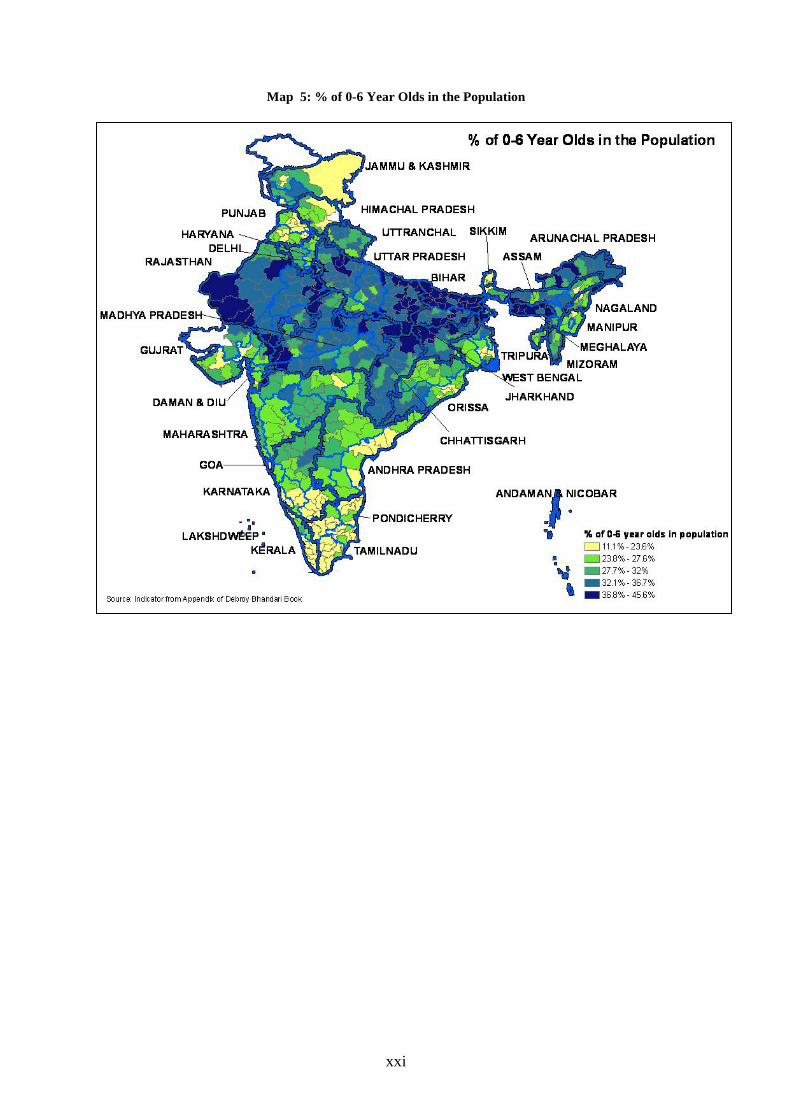
xxi

Map 5: % of 0-6 Year Olds in the Population

xxii

The lagging regions are much less urbanized than the other regions of India, indicating that these regions economies are undiversified.

Map 6: Urbanization Share 2001

….And there are relatively far fewer non-agricultural jobs even in the rural areas compared to the more advanced regions.

xxiii

Map 7: Non Agriculture Share 2001

xxiv

While the schedule caste population is distributed relatively evenly across India.

Map 8:Share of SC population 2001

xxv

Most of the scheduled tribe population lives in the lagging regions or in the poorer districts of the richer states. This raises the importance of inclusion.

Map 9: Share of ST population 2001

xxvi

Connectivity Will Be Key – However, the priority now is building local connectivity. While highways and main roads are quite dense in the lagging regions and key states such as UP, Bihar and Assam….

Map 10: Local Connectivity

xxvii

……the LIS and the NESCS lag starkly behind in village access to paved roads, i.e. in connecting rural areas to towns and the national economy.

Map 11: Approach – Paved Road in Share 2001

xxviii

The LIS also lag behind in power supply. While this is relatively a lesser constraint now, it will become more binding in the future…

Map 12: Power Supply in Share 2001

xxix

Social Service Facilities are also much poorer in the lagging regions.

Map 13: % of Villages with at least one Primary School 2001

xxx

Service delivery is also much poorer….with far less immunization coverage for example

Map 14: Complete Immunization

xxxi

And governance is weaker with much higher absenteeism in health…

Map 15: Absence rates for Health Workers by State

xxxii

…and in education….

1

CHAPTER 1. OVERVIEW AND STYLIZED FACTS Summary

This chapter lays out the stylized facts about the lagging regions of India. It defines which are the lagging regions and states, and the differences within these regions, the patterns of growth and initial condition and endowments. It shows how income disparities among Indian states are large, sustained and growing, with divergence accelerating in the 1990s and how the absence of structural change is the main feature of the lagging regions. It shows how the low income states or the North, which include 80% of India’s poorest districts, are rich in resources like minerals, forests, water and fertile agricultural land. It argues that while efforts to facilitate migration may be important, given the high population density in large parts of the low income states and the low rates of economic migration in India, the main thrust of the strategy has to focus on bringing jobs to the people, or regional development. It then draws on the international literature on lagging regions to show that how in India also second generation geography issues such as poorer infrastructure, human capital, inferior investment climate and weaker institutions characterize the lagging regions.

A. I ntr oduction

1. Balanced regional development has long been one of the declared objectives of national policy. India is a large and heterogeneous country with wide divergences in economic and human development. The management of these divergences has been a major concern for policy makers for the past four decades. The third Five Year plan (1961-66), for example, noted that the “balanced development of different parts of the country, extension of the benefits of economic progress to the less developed regions and widespread diffusion of industry are among the major aims of planned development.” Initial attempts to broad base growth relied on promoting agricultural growth and the spread of irrigation in lagging areas. At the same time, there was a push to spread industrial development more widely. This was achieved through instruments such as using licenses to redirect investment towards backward areas, setting up industrial parks in areas with potential, banning heavy industry from locating in metropolitan centers, and locating large public sector projects in the less industrialized states. The period of the 1970s and 1980s consequently saw industry spreading to many more cities and states beyond the original leaders. 2. A variety of fiscal and regional development programs have also tried to promote regionally balanced development. As per the 12th Finance Commission’s awards, 50% of the share of central tax collection for each state is determined by the gap between that state’s per-capita income and the richest state in the country, an arrangement, which favors the poorer states. Special agencies such as the North Eastern Council, set up in 1972, or the recently established Department of North Eastern Affairs have also been tasked with the responsibility of coordinating regional development. In addition, the GoI’s Five Year Development Plan expenditures have focused on the development of lagging regions through programs such as the Hill States Area Program, the Backward District Program and the Tribal Development Program. The impact of these, however, has been limited in practice owing to factors such as low utilization by the lagging states, and the relatively small amount of central government funds invested, so far, on regional development programs (current planned expenditures are less than 0.2% of GDP; in the past it has been about 0.05% of GDP). 3. Many of the industrial policy instruments used to achieve these objectives however became less relevant after the economic reforms which started in the mid 1980s. Around this time, a rethinking about the role of the private sector and a market economy lead to the initiation of the first set of reforms. This process picked up further pace after 1991. Licensing requirements were gradually abolished for most sectors, except for security or environmental reasons. The freight equalization policy was also abandoned. In addition, the state ceded the primacy of the role assigned to the public sector in leading industrial development to the private sector. Restrictions on industrial location were also significantly

2

diluted. All these changes meant that the state essentially gave up the major tools it had used so far for promoting balanced regional development. 4. Concerns are now being expressed about the uneven distribution of growth since the 1990s. Although the Indian economy has been growing at a stellar rate of about 6% p.a. since the mid-1980s, this achievement has been clouded by growing inequality and divergence in development outcomes among India’s 32 states and union territories (See Figure 1.1 below). A number of studies have established that inter-state disparities, as measured by differences in the growth of states’ GSDP, have increased in the post reform 1990s compared to the 1980s. Some of the most populous but poor states like Bihar, Orissa and UP are being left behind, as are some areas even within the relatively better performing states. In general states which were poor to start off with did worse than those which were relatively better to start off with.4 Concerns have been raised that the existing regional inequalities, compounded by slow growth in these states − while the rest of the country enjoys robust growth − can be socially and politically explosive.5

It has also prompted thinking about what can be done to spread growth more evenly, and the instruments available to policymakers under the new policy environment to achieve this goal.

Figure 1. 1: States of India by Income Levels and Growth

5. Growing spatial inequalities by themselves could lead to several problems. For one, the geographical clustering of lagging states together in the north and northeastern region creates a danger that this region may be turning into a “spatial poverty trap”: i.e. an area where the slower growth and 4 Alhuwalia (2000) however cautions against easy generalizations. Not all poor states did badly in the 1990s: Rajasthan (6.5%) and MP (6.2%) for example, performed relatively well. At the same time, not all rich states did well: growth decelerated in the 1990s in Punjab and Haryana. 5 Ahluwalia (2000), op. cit

Low Income States

North Eastern States

3

development of these lagging states, regions and districts can adversely affect neighboring areas, leading to even slower growth for the whole area. As result capital and skilled labor either exit or bypass that region in favor of faster growing and richer regions perpetuating a vicious cycle of underdevelopment, and further deepening the problem. Secondly, the slow growth of some of India’s largest and most populous states, such as Bihar and UP, creates a drag on overall growth and threatens the achievement of human development goals in India. 6. This issue is also important because the low-income, low growth regions of India comprise of some of the most politically and economically important states. The lagging states of India (as defined below) account for more than a quarter of India’s GDP. They together make up about 44% of India’s population – which constitutes the politically important Hindi heartland - and account for close to 60% of India’s poor. In addition, demographic projections suggest that most of India’s population and labor force growth will take place in these states. Alhuwalia (2000) warns that the existing regional inequality, compounded by slow growth in states accounting for a third of India’s population while the rest of the country enjoys robust growth, can be socially and politically explosive, and create obstacles to future growth. 7. In this context this study, prepared in consultations with the Government of India and various state governments, aims to address the following two questions:

• What are the main constraints to growth and development of the lagging regions of North and North Central India? The report focuses on the states of Bihar, Chhattisgarh, Jharkhand, MP, Orissa, UP, and Rajasthan (henceforth referred to as the low income large states or LIS); The experience of these states are contrasted with that of India’s middle income and higher income states (see Table 1) to address the questions posed.6

• What are the strategic options for the GoI and State Governments to address these constraints as part of the 11th Development Plan of the Government and of the States? The discussion here centers on fiscal and regional development policies at both the central level and at the state levels, infrastructure investments, and improving regulations, governance and institutions.

The preliminary findings of this study were presented to the Expert Committee on Inequality, Planning Commission, Government of India, in March 2007. The study team thanks the Panel for the rich comments received, which the team has tried to incorporate in the current draft. 8. State administrative boundaries are the most politically relevant unit of analysis to facilitate an understanding of regional development issues. Previous work on regional issues has used state divisions extensively. In this report, however, we follow the traditional state level approach for three reasons. First, states are a good unit for analysis because state level policies are often the most important policy variable in understanding specific constraints to growth. Second, this is necessitated by the availability of data. Production and income data, for example, is available only at the state level. 7

District level information is much more limited. Third, there is a close correlation between state boundaries and backward districts: 80% of the poorest districts in India, as defined by the Planning Commission, lie in the lagging states.

9. The study defines “lagging” states, as those states of India which were in the bottom quarter in terms of per-capita income in 2000/01 (See Table 1.1 and Figure 1.1). Most of these states were also in the same group in the 1970s, and were the relatively slower growers over the period (as discussed in more detail below). The chosen definition of “lagging” thus holds both in a dynamic as well as a static sense. We can further split this group into two distinct groups. The first group of low income states (LIS) is located in the Northern and North-Central regions. They are large and populous, and constitute the

6 There are also clusters of poverty in the better off states – this topic is addressed in chapter 5 of the report. 7 Many states do compile district level GDP data. However these are not readily available, and are also believed to be much less reliable than state level data.

4

heartland of India. A second group of states consists of the North East Special Category States termed as NESCS. These states have low population densities, and are geographically remote from the rest of the country. The average per capita income of both these groups is less than half that of the richest group (See Table 1.1 and Figure 1.1 below). It is worth stressing that although there are important differences within these groups, as discussed below, in per-capita terms these groups are remarkably homogenous on the one hand and distinct from each other on the other hand. The variations between the groups in per capita incomes (co-efficient of variation of 0.32) accounts for almost all the variations in per-capita incomes between individual states (co-efficient of variation of 0.33). On the other hand the variation in per capita incomes between states within each group is only 0.11. This report focuses only on the LIS, as these are distinct in many ways from the NESCs (see Box 1.1).

Table 1.1: Main State Groups Ranked by Per Capita Income Groups and Development Indicators

LIS: Low Income States NES: North Eastern Special Category States

MIS: Middle Income States

HIS: Higher Income States

Bihar Chhattisgarh Jharkhand Madhya Pradesh Orissa Rajasthan Uttar Pradesh Uttaranchal (will be excluded from this group).

Arunachal Pradesh Assam Manipur Mizoram Meghalaya Nagaland Tripura (Jammu &Kashmir and Sikkim not included due to data problems).

Andhra Pradesh Himachal Pradesh Karnataka Kerala Sikkim West Bengal

Goa Gujarat Haryana Maharashtra Punjab Tamil Nadu

State Groups

Nominal Income per Capita (Rs, current price), average of 2000/01-02/03

Relative per capita Income compared to HIS (=100, current price)

Income per Capita (Rs, 93~94 price), average of 2000/01-02/03

Population 2001 (million)

Share of Population in India (%)

LIS 11057.3 42.3 7398.9 464.1 44.8 NESCS 14046.0 53.7 7986.6 37.7 3.6 MIS 20271.1 77.5 12157.4 249.9 24.1 HIS 26165.8 100.0 17256.0 258.4 24.9 India 17770.1 67.9 11376.2 1036.6 100.0

5

Box 1.1: Why the North-Eastern States are Different

The states in India’s North Eastern Region, while classified as “lagging” for the purposes of this study, are often quite distinct from the other lagging states. The most marked difference is in terms of the density of population. In all the NESCS, other than Assam and Tripura- the population density is very low compared to the northern states like Bihar, UP or Orissa. These low densities are attributable to the hilly terrain of the region and the high forest cover. The second major difference is in terms of access to the rest of India. This large region is linked to the rest of the country only through a narrow belt of Bengal. Only 2% of the border of this region is with the rest of India, making it somewhat similar to a land locked country. Before independence in 1947, the region was well integrated to the Bengal economy through waterways and to Burma through the Stillwell road. Now, however, it has limited links with markets in the surrounding countries: Bangladesh, Myanmar and China. Another important characteristic of the region is the high proportion of scheduled tribes in the area. Thus there is a great deal of heterogeneity of population within the area. Some tribal groups have a history of contact with the market economy, but many other groups live a more isolated existence. The ability of different tribal communities to cope with a market economy is thus different. Besides the pattern of land tenure and communal land ownership of resources also pose several problems when it comes to the exploitation of the rich mineral and hydro resources of the region. Low and ethnically diverse population densities locally, in combination with poor infrastructure availability and limited access to markets outside, all translate into low market access. This put the problems of these states in a very different category compared to the more populous, but poorer states of north and central India. For this reason and the relatively limited data available on the states in this group, this study’s treatment of the NESCS group has been comparatively light. A more detailed study of the region is planned for later. 10. Using the state as the only unit of analysis for regional development, however, has its limitations because development does not follow political and administrative borders. There are some deprived regions even within the richer Indian states, which have lower income and worse human development indicators. The poorest districts in Maharashtra, for example, have worse infant mortality rate than the average in the poorer states. There are several districts in northern Karnataka, and AP which are also poor. However, not withstanding these the importance of sub-state and district is also because most of the policy instruments for development lie with the central and State governments, and key data such as on income and production are not available at the state level, states are the most relevant unit for deriving policy implications from regional analysis. 11. This study accordingly also analyzes regional development issues at the sub-state NSS region and district levels in Chapter 2. In fact at a sub-state level 5 different typologies of lagging regions can be identified: (i) the densely populated districts of Bihar and UP that lie in the Indo-Gangetic plain with access to abundant water; (ii) the richer districts of Rajasthan and MP, where average state incomes are also high; (iii) the poorer districts with significant tribal populations and less densely populated clustered around the range starting from South Eastern Rajasthan, Southern MP, Chhattisgarh, and Orissa; (iv) the hilly districts in the NESC where arable land is in short supply except in the Assam plains and (v) the poorer districts in the rich states extending southwards into Karnataka, Eastern Maharashtra and Northern AP. (Figure 1.2).

6

Figure 1. 2: Typology of Lagging States

Source: Staff Estimates

12. A four way comparison of the richer and poorer districts in the richer and poorer states brings out some important features associated with the lagging regions in both the richer (HIS and the MIS group) and poorer states (LIS and the NESCS groups). As discussed in some detail in Box 1.2 four key aspects stand out: (i) most, four out of five, of the poorest districts lie in the poorer states; (ii) the poorer districts in the richer states share some common characteristics with the districts in the poorer states: their agricultural sector productivity is much lower on the one hand, and their economies are much less diversified on the other hand; (iii) however, infrastructure and facility development in the poorer districts of the richer states are currently significantly better than even the richer districts in the poorer states. This may partly reflect the recent development shows that and shows the importance of state boundaries in determining development outcomes. This is done in Box 1.2

13. This chapter looks at the stylized facts regarding states’ growth experience from the 1970s to present. It highlights the point that differences between Indian states are large and persistent. However starting from the 1980s, a group of middle income states managed to significantly close their gap with the traditionally high income states. These states were not significantly different from the poorer states when this growth spurt started, and this suggests that their experience may also be replicable in the lagging states. A few areas of significant difference however stand out: infrastructure, urban management and governance. At the same time, smaller economies and lower growth also translate into lower resources for state governments. This places them at a disadvantage vis-à-vis faster growing states. Central transfers alone cannot bridge the resource gap.

Bihar and UP Plains

NESC states

Vindhya Range and Tribal Belts

Poor Districts in Rich States

Richer districts in poor

7

Box 1.2: Rich Districts in Poor States and Rich Districts in Poor States

As noted, there is considerable intra-state variation in development across districts within states and this variation is particularly higher in the lagging regions. Second, there is also the issue of lagging regions or districts with the middle or higher incomes states. As in the case of states the differences in development outcomes between the poorer and better of areas within these states have also persisted across decades. In this exercise poor districts are defined as those where poverty rates are higher than the national average: that is when 28 percent or more of the population in the district live below the poverty level (as measured by Debroy and Bhandari (2006)). On average, 14% of the population lives below the poverty level in the richer districts, while 41% does so in the poorer districts. In another simplification, the states are divided in two groups: the LIS and the NESCS group classified as the poorer states and the MIS and the HIS group classified as the richer states. Now putting these groups of districts and states together, 183 districts out of the 230 poor districts or about 80% of the poorer districts in 2001 fell in the LIS/NESC group. This share is very similar to that of the Planning Commission, where also 80% of the poorest districts fall in the LIS group. However, some of the richer states have a large number of poor districts. These include Maharashtra, Karnataka and Tamil Nadu and West Bengal. In addition to higher number of poor living in the poor districts, poor districts in richer states also have three important characteristics which are different from richer districts in richer states and similar to districts in the poorer states. First, agricultural yields were significantly lower in poorer districts and districts in poorer states compared to the richer districts. Second the share of non-farm employment and urban population were also lower in the poorer districts implying that the economies were less diversified and more dependent on agriculture. But while these poor districts in richer states may be relatively poor and less developed, some of their physical infrastructure or educational facilities are significantly more developed than even the richer districts in poorer states as evident from the diagram below. The poorer districts in the richer states also have significantly more village access to paved roads and power or secondary schools than the richer districts in poorer states.

Moreover, the poorer districts even do not lag even behind significantly compared to the richer districts in respect of important facilities such as power, roads, or primary schools, though may have done so in the past. While they lag behind in medical facilities, coverage is uniformly poor and that is unlikely to make a difference. They do, however, lag behind the richer districts in secondary school, which may have some significance.

Number of Districts and Percentage Share

Rich districts

Poor districts

HIS and MIS states

168 (59%)

48 (20%)

LIS and NESCS

115 (41%)

183 (80%)

Total 283 (100%)

230 (100%)

Poorer Districts in Richer and Poorer States Have Lower Yields and Economies are Agriculture Dependent.

Richer districts Poorer districts

yield 1950 1610 Rich States Non-farm

employment 16 11

Urban share 29 22 yield 1622 1529

Poor States Non-farm employment

10 8

Urban share 20 16

8

Two important implications seem to be emerging here. First, poorer districts in the richer states are not that constrained by key infrastructure facilities when we compare them to the districts in the LIS states. As discussed in more detail in chapter 2, these infrastructure facilities such as village access to electricity and paved roads are closely linked to growth and development at both the state and district level. Second, the differences in infrastructure development between richer and poorer states seem to be more important than differences between richer and poorer districts. That is state policies and state differences seem to be the relevant factor here.

Thus it seems that other explanations have to be sought for the differences in rich and poor districts in the richer states than in infrastructure or facility development. One underlying factor that may help to explain this is the differences in human and social development among these districts. This theme, discussed in some length in Chapter 5 of this study, is the following: richer and poorer districts and states are characterized by systematic differences in human development indicators, which in turn are linked to key social development indicators.

Analogous to the exercise of classifying districts by below poverty line households, another exercise can be to classify districts by four human development indicators:: infant mortality, total fertility, crude birth, and female adult literacy rates. Districts performing better than the national average are classified as developed and those below as less developed. Three aspects stand out. - First, by far, the worst performing districts (in terms of a specific HD indicator) lie in the poorer states. Thus, only nine districts in the HIS and MIS have below-national level TFR, compared to 207 districts in the LIS. In case of IMR, 30 out of 116 districts in the HIS and 22 out of 75 districts in the MIS have IMR that is higher than the national average. In contrast, 158 LIS districts display worse than the average national performance. - Second, poorer districts in richer states have improved human development compared to the poor districts in poorer states. Thus, high TFR districts in the HIS and MIS have on an average a TFR of 3.6-3.8 compared to 4.4 in case of LIS and 3.9 in NESC. The contrast between the two categories of poorest districts is also high in case of IMR. The same difference is noticeable in case of female adult literacy. These observations suggest that poor districts in richer states are in the nature of specific pockets, while in the case of poorer states, their presence defines the norm. -- Third, while the poorest districts in richer states have seen improvements, the gap between the poorest pockets and the rest of the districts in richer states remained persistent over the past three decades As Chapter 5 of this study discusses in more detail, the underlying differences between human development across states and districts in both richer and poor states appear to lie in inadequate social development and exclusion of important segments of the population. This is indicated by significantly lower female participation literacy rates and the relatively higher state of the scheduled tribe populations. Accompanying these features are low population density and significantly lower access to higher education, represented here by secondary schools. Poorer and less

Infrastructure and Public Facilities in Poorer Districts in Richer States vs. Richer Districts in Poorer States

0.0%10.0%

20.0%30.0%

40.0%50.0%60.0%

70.0%80.0%

90.0%100.0%

primary

scho

ol

high sc

hool

electr

icity

roads

post

office

tank

healt

h cente

r

dispe

nsary tap

Urban s

hare

nonfa

rm empl

Poor state - Rich district Rich State - Poor district

Source: Estimated from 2001 Census Data

Infrastructure and Facilities: Richer and Poorer Districts (Share of Villages in the District with Access to Richer

Districts Poorer Districts

primary school 88 82 high school 28 16 electricity 98 94 roads 89 86 post office 50 32 tank 63 79 health center 13 6 dispensary 9 4

9

educated women also seem to compound the effects of inadequate health facilities because they are less aware of illness and more prone to give up medical treatment. In sum this analysis would suggest that first the development of the poorer districts in richer states would need to focus on social development centering on female empowerment: lowering of fertility and increase in literacy and higher education for women. A second aspect would be to design policies to foster tribal development through protecting their traditional livelihood and introducing new opportunities, and providing higher education. Finally, there is also evidence that while poorer districts in richer states do not lag behind in infrastructural facilities, districts with significant tribal population does lag behind in infrastructure and facility development.

B . Stylized F acts on G r owth Acr oss I ndian States

14. Income disparities among Indian states are large, sustained and growing. These disparities have existed for over five decades, and predate the reforms of the 1990s. One remarkable fact is how little change there has been since the 1970s in the relative ranking of states: there is over 90% correlation in relative state rankings over two decades. Poorer states like Bihar, Orissa and UP have continued to remain among the country’s poorest states. Others like Punjab, Haryana, Gujarat and Maharashtra have maintained their position as India’s richest states. Poorer states have also tended to grow slower: While per capita incomes in rich and middle income states rose about 150% between 1980/81 and 2002/03, those in the poor and North-east states increased by only 63% (Figure 1.3). Consequently inter-state disparities have risen. While the income of the higher income states (HIS) was about 78% higher than that of the lower income states (LIS) in 1980/81, it was 91% higher in 1990/91 and by 2004/05 it was almost 160% higher. 15. Divergence accelerated in the 1990s. An extensive literature has developed looking into the issue of divergence in India. The broad conclusion it comes to is that there is divergence in economic performance among states in India, howsoever measured using various indicators. Divergence fell in the 1980s, and then rose again in the 1990s.8 If one looks at the per capita state GSDP, the standard deviation of states’ decadal growth almost doubled from 1% in the 1980s to 1.9% in the 1990s.9 There was also an important qualitative change. In the 1980s, 15 out of 20 states recorded growth in per capita incomes within a 1% band around the median rate. Four out of the remaining five fell outside because they all grew faster. Two of these were low income states: Rajasthan and Arunachal Pradesh. In the 1990s, however, incomes in 13 of 20 states grew at rates more than 1% different from the median rate. Six of these states grew slower, and seven grew faster. Importantly, of the states which grew slower, 5 were either LIS or NES. Among the seven faster growing states, six were Middle (MIS) or high income (HIS) states. Thus the 1990s saw states breaking out from each other, with the higher income states growing significantly faster, and the lower income states growing significantly slower than the median.

8 Prominent papers are those by Casin and Sahay (1996), Das and Barua (1996), Nagaraj, Varoudakis, and Veganzones (1998), Rao, Shand and Kalirajan (1999), Ahluwalia (2000), Sachs, Bajpai and Ramiah (2002), Singh (2003), Basu (2004), Bhattaracharya and Satkhivel (2005?), Kar and Sakthivel (2004), Besley and Burgess (2005), Purfield (2006). 9 The coefficient of variation also increased from 0.33 to 0.58.

10

Figure 1. 3: Region-wise Growth in Per Capita Incomes

0.0% 1.0% 2.0% 3.0% 4.0% 5.0% 6.0%

LIS

NES

MIS

HIS

1980s 1990s

Source: Staff Estimates 16. Much of the increased divergence derives from the growth spurt in the middle income states. Compared to the 1980s, growth significantly accelerated in every MIS in the 1990s (right panel, Figure 1.3). There was not much change in growth in the HIS as a whole. Indeed the modest pickup in the 1990s owes everything to Gujarat, while growth slowed down in Maharashtra, Punjab and Haryana. Growth slowed down marginally in all the LIS, the only exception being the coastal state of Orissa. In the North-east, except for Tripura and Meghalaya, all states also saw a slight slowdown. On average, however, divergence increased not because growth in the poorer states slowed down significantly, but because middle income states were able to substantially accelerate their growth. 17. Manufacturing was a more important driver of growth in the richer states than in the lagging states. While economic growth was overall slower in the lagging states, across all categories of states, the tertiary sector was the main engine of growth. This accounted for almost half of overall growth over the period 1981-2001.10

Again, apart from the NES, roughly a quarter of growth in the other states came from agriculture (Figure 1.4, left panel). In strictly accounting terms, manufacturing sector was the more important factor in driving growth in the richer states: it accounted for a bigger part of overall growth in the in the MIS (18%) and the HIS (25%) than in LIS (14%) and NES (7%). Most of the divergence in growth, however, came from the inability of the LIS and the NESCS in lower productivity growth in agriculture and in services (Chapter 2 elaborates on this).

10 There may however be significant differences in the compositional mix of services among states. There is evidence of differences in labor productivity in this sector among states. This is explored in chapter 2.

Low Income

11

Figure 1. 4: Sources of GDP and Employment Growth: 1981/82-2001/02

Sources of GSDP Growth: 1981/82-2001/02

0%

10%20%

30%40%

50%

60%70%

80%90%

100%

LIS MIS HIS NE

contribution of services contribution of agriculturecontribution of manufacturing contribution of other industry

Sources of Employment Growth - 1983/2000

0%

10%

20%

30%

40%

50%

60%

70%

80%

90%

100%

LIS MIS HIS NE

Services Agriculture Manufacturing Other industry

Source; Staff Estimates Based on CSO and NSS data 18. Poor states remain heavily dependent on agriculture for employment. The agricultural nature of the LIS and NES economies is reflected in the sectoral deployment of their workforce. The LIS had larger parts of their workforce dependent on agriculture (72%) than the MIS (59%), HIS (63%), and even the NE states (65%) in the early 1980s. Lagging states were also more dependent on the sector for generating new jobs. More than 50% of employment growth in both LIS and NE between 1983 and 2000 was in agriculture. On the other hand the MIS and HIS had significantly higher share of employment in manufacturing (14% and 12%) than the LIS (9%). Importantly, services and manufacturing were more important in driving employment growth than agriculture. The manufacturing sector alone accounted for 12% of the overall growth in employment in the higher income states, compared to 9% in the LIS and just 1% in the NES (Figure 1.4, right panel). The fact that agriculture in the LIS accounted for only a fourth of economic growth but more than half of employment growth is worrisome because it points towards declining labor productivity in the sector, and suggests that these states have been less successful in moving workers to more productive jobs in manufacturing and services than the MIS and HIS. 19. Growth in poorer states had a smaller impact on reducing poverty in the poorer states. Given that a large part of the workforce in the lagging states remains stuck in the slow-growing, low productivity agricultural sector, it is not surprising that their pattern of growth has also been less effective in reducing poverty (figure 1.5, left panel). Purfield (2006) estimates that on average, for each percentage point of growth, richer states have been about 50% more effective in reducing poverty than poorer states. This, combined with the fact that economic growth has also been lower in the LIS while their population has been growing rapidly has placed a huge drag on efforts to reduce poverty nationally. Consequently between 1983 and 2000, while the absolute number of people below the poverty line fell by 39% in MIS and 30% in HIS from already low levels, this declined by only 6% in the LIS. Poverty is thus increasingly becoming concentrated in these states (Figure 1.5, right panel). In 1983, a group of four states -- Bihar (undivided), MP (undivided), UP (undivided), and Orissa, had a 50% share of the rural poor in 1983. This share increased to 61% in 2004.

12

Figure 1. 5: Growth has had Lesser Impact on Poverty in the Low Growth Areas

0.2

0.4

0.6

0.8

1

1.2

1.4

1.6

1.8

2500 4500 6500 8500 10500

pc income in 1981/82

po

vert

y-g

row

th e

last

icit

y

Source: Purfield (2006), Debroy and Bhandari (2006) 20. Poorer states are also lagging in terms of human development. Convergence in social indicators between regions is much easier to attain through directed state policies than economic convergence, as the experience of Mexico, the US and EU suggests. In the absence of such interventions, however, the strong relationship between per capita incomes and the composite Human Development Index (HDI) is likely to dominate (Figure 1.6, left panel). The fear is that if large differences in growth rates between states are sustained over time, these could also translate into differences in human well-being. In India, the economically lagging states in the early 1980s were also lagging in terms of the composite HDI. Over the next decade all states saw improvements in this. However states which were richer to start off with saw faster improvements over the decade, from already higher levels (Figure 1.6, right panel). Thus poorer states are being left behind in terms of human development as well.

Figure 1. 6: Human Development and Economic Growth

Source: National Human Development Report (2001), Staff Estimates

21. While inter-state inequality remains smaller in India than in other large countries and regions, it has been increasing over the past two decades (Figure 1.7). Wide divergences in growth and development are not peculiar to India, but also exist in other large economies like the US, Brazil and China. There are large and sustained sub-national regional disparities in economic performance and living standards in all these countries, where a few regions account for much of national employment and investment (see section D below for a more details). Comparison with these shows that the current gap

13

between Indian states is lower than in other developing countries, but higher than in integrated developed regions like the US and the EU. At the same time, international experience also shows that few countries have managed to successfully promote economic convergence. A century and a half ago, the poorest county in the US was in the Appalachian region. It still is today. In Europe, after two decades of active regional policy, there has been convergence among countries, but divergence among sub-national regions.

Figure 1. 7: Inequality across states of India remains low But Increasing Compared with Other countries

0

0.1

0.2

0.3

0.4

0.5

0.6

0.7

0.8

Indonesia China Brazil India EU US

1980s 1990s

Source: World Bank (2006)

22. Long term migration has done little towards reducing disparities in India. Differences in economic activity would be less problematic if people could easily migrate to better-off regions where the jobs are. Though there is evidence of labor migrating to the richer states, inter-state migration rates are low in India. In the 2001 census, only 0.2% of the population reported migrating across state borders in the preceding year. Migration out of LIS states was higher at 0.3%. Net outward migration was highest from UP, Bihar and Punjab. Male migrants came mostly from rural areas, and 60% reported moving for work/employment related reasons. The prime destinations were Gujarat and Maharashtra, which attracted about half of total migrants during 1999/2000 (Purfield, 2006). However the very small scale of long term migration suggests that this cannot be relied on as the mechanism for bridging the large differences in level of economic activity (also see section C below), and equalizing incomes across regions. It also means that poorer growth in certain regions will also imply leaving the populations in those areas behind.

C . M igr ation in I ndia

23. Given the significant differences in economic conditions across India, its unusually low economic migration rates present a puzzle. Overall while about 1.8% of India’s population migrated on average each year between 1997 and 2000, only 0.2%, migrated outside their states. 11 In comparison some 2.7% of the US population migrated across the county between 2000 and 2001.12

11 The lack of data however makes it difficult to quantify the substantial seasonal migration that happens across states, especially out of states like Bihar and UP and into richer states like Punjab, Haryana, Gujarat and even Tamil Nadu.

Between 1998 and 2000, most regions showed less than 1 percent net in- or out- migration (Figure 1.8). Chandigarh, Haryana, Punjab, Delhi, Mumbai and the Kolkata areas showed the maximum inflow, while Maharashtra and Gujarat showed high in-migration rates of around 0.5% and 0.2% respectively. The main out-migration regions are Bihar, western Rajasthan and J&K, Kerala, Karnataka and Southern Tamil Nadu. In general, migration out of LIS states was higher at 0.3%, and was overwhelmingly out of rural areas. Almost 82% of male migrants from the lagging states were from rural areas, and 60% of these reported

12 U.S. Bureau of the Census, Geographic Mobility: March 2000 to March 2001

14

moving for work/employment related reasons.13

Most migrants moved to states “where the jobs are.” For instance, 47% of people moving out of UP, moved to Maharashtra and Delhi.

Figure 1. 8: Economic Migrations across States & Regions, 1997-2000

Source: Estimated from NSS data, 55th Round 24. The convergent trend of wages across regions on the one hand, and growing unemployment rates in the major urban areas may explain why migration rates have not picked up. Wage inequality is falling across regions for all categories of casual wages, though substantial differences remain (Figure 1.9). Differences between casual wages in rural and urban areas also largely disappeared in the 1990s. The difference in casual wages in industry between rural areas in the LIS and urban areas in the MIS was only 12%. This is hardly enough to induce migration, especially when there is no guarantee that employment will be available in the urban areas. Interestingly, the impact of wage differentials on migration is low (World Bank, 2007; Cashin and Sahay, 1996). On the other hand, unemployment rates are significantly inversely related to net economic migration rates.

Figure 1. 9: Daily Wages for Casual Industrial Workers, 2004

13 Staff estimates based on Census 2001.

Andhra Pradesh

Tamil Nadu

Arunachal Pradesh

Jammu & Kashmir

Uttar Pradesh

Orissa

A & N Islands

Mizoram

Nagaland

West Bengal

Rajasthan

Gujarat

Maharashtra

Karnataka

Punjab

Kerala

Madhya Pradesh

Bihar

Not Available

In migration, %0 - 0.10.1 - 0.250.25 - 0.50.5 - 11 - 2.52.5 - 8

Out migration, %-8.3-8.3 - -1-1 - -0.5-0.5 - -0.25-0.25 - -0.1-0.1 - 0

N

EW

S

15

25. India’s urbanization rates are also surprisingly low, and within it urbanization in low income population is half that of that the richer states. Demographic projections in 1981 estimated that India’s urban population would be about 31 percent in 2001. In reality, it turned out to be only 27 percent of the population, i.e. lower by about 40 million persons.14 China provides a dramatic contrast: the urban population there grew by some 190 million between 1990 and 2003. In India the corresponding number was 80 million or less than half. Even in the larger metropolitan areas of Mumbai, Delhi, Kolkata and Chennai that attract the highest rates of migrants, the in-migration rates, about 1.5 percent of the population per annum, are low. Further the share of economic migration to urban areas has been stagnant at around 65% from the mid 1990s. Part of the reason behind this would appear to lie in the converging trend in rural-urban wages. As the gap between rural and urban wages narrow, and urban unemployment rates are growing, the expected earnings from migration are falling. It follows that the incentives to migrate to the cities are declining accordingly (World Bank, 2007).15

This convergence is surprising, and probably reflects that urban infrastructure and service development are not proceeding fast enough to create jobs that are better paying than jobs in rural areas. This may be a particular constraint for the LIS and the NESC group where the urban population’s share is only 20 percent, half of the share in the richer states.

26. Migration, especially seasonal migration, has potential to mpact poverty in the lagging states. Migration may have a major role to play in the sparsely populated areas around the Vindhya mountain range, in western Rajasthan, the interior regions of MP, Chhattisgarh, and AP, and parts of the NESCS. Facilitating migration can also be important for districts in Bihar and Orissa. Similarly, seasonal, and often repetitive, migration of labor for employment is an important component of the livelihood strategies of people living in rural areas, especially in the lagging regions of India While there are no reliable estimates of its extent, a growing number of micro-studies suggest that this is both large and growing. Such migration is often a vital source of cash for households and plays an important role for the poor in the LIS in raising their incomes and as a coping strategy (Box 1.2). 27. However the really poor may not be able to take advantage of this opportunity. Liquidity constraints inhibit migration. If migration costs are non-trivial, they may be beyond the means of potential poor migrants. In this case only the relatively better off would be able to move. Kundu and Sarangi (2007) use the national labor survey data on migrants to show that the people migrating to cities are often not the poorest in their area of origin. In contrast to perceptions, migrants on the average are also no worse off than the city inhabitants: almost half of migrants fall in the top two quintiles of consumption expenditure in the cities. Similarly micro-studies how that it is small and marginal farmers, with some minimum income, who are most likely to migrate, and not the landless. Liquidity constraints particularly affect rural areas, where uncertain land title prevents potential migrants from converting their assets into a form (i.e. cash) they can use on arrival (World Bank, 2007) 28. The Government has a role to play in removing impediments to migration. Labor market liberalization can increase employment opportunities in potential destination regions. Improvements in rural land titling could also provide potential migrants with a stake to finance the costs of relocation. In addition, investments in human capital—on education and skills training—could also increase the likelihood that people in poor regions have access to better paying jobs once they migrate. This is unlikely to eliminate poverty traps entirely, but it may improve outcomes for some.

14 Mohan and Dasgupta (2004). 15 It is true though that part of the answer may lie in the lack of updating of rural areas due to which many actually urban areas may be classified as a rural area – such as environs of Delhi. Thus higher “rural” wages may be partly reflecting this misclassification and the migration may be being under-reported. Still, it would be hard to ascribe all the changes to this fact.

16

Box 1.3: Seasonal Migration in India

In India much of the research focus has centered on permanent economic migration, supposedly induced by differences in economic development which “push” people away from poor areas and “pull” them to faster growing areas where the jobs are. Recent work has however stressed the importance of short-term, often repetitive, seasonal migration of labor for employment as a component of the normal livelihood strategies of people living in rural areas, especially in the lagging regions of India ((Mc Dowell and De Haan, 1997). Awareness of the magnitude of seasonal migration or the importance of it in the lives of the poor though remains low. Official information on the extent of seasonal out-migration does not exist at either the national or even at the local level, making the planning of development interventions difficult. Most information comes only from a growing number of micro-studies. These suggest that seasonal migration for employment is both large and growing. Rogaly (1998) draws on many of these studies to conclude that the number of temporary migrants increased during the 1980s and 1990s in both western and eastern India, and did `not ebb’ in northern India. The National Commission on Rural Labor estimated that the number of circular migrants in rural areas alone could be as high as around 10 million. Who do people migrate? Undeniably some migration is induced by economic or social hardship and is used by the very poor for survival and coping during times of distress. Most of these migrants are landless or land-poor, unskilled and illiterate poor laborers. However, recent studies show that seasonal migration is also used as an accumulative option by the poor and non-poor alike to improve the economic position of the household. (Deshingkar and Start, 2003). This sort of migration is undertaken even by landed families. For example, a study of households in Jalpara, West Bengal, found that while 59% of landless households surveyed had at least one member who migrated during the year, even among the landed households, some 17% included a migrant. In practice, coping migration often becomes accumulative over time, as information improves, skills are acquired and relationships with employers stabilize. An interesting thing to note is that often the poorest in a region do not migrate. In MP, small and marginal farmers have a slightly higher chance of migrating compared to sub- and semi-marginal farmers (Deshingkar and Start, 2003). Support for this proposition also comes from Kundu and Sarangi (2007) who use national labor survey data on migrants to show that the people migrating to cities are often not the poorest in their area of origin. In part this can be explained by the fact that a minimum level of assets are required to make the investment for migration; for travel, purchasing supplies to take to the destination and leaving some money behind for running the household. The poorest often lack even this. In Andhra Pradesh (AP) and Madhya Pradesh (MP), other important factors determining migration patterns have been information links between regions formed over time, the availability of surplus labor within the household, cultural norms regarding the sexual division of labor, as well as decisions related to children’s education. Caste is also important: This is because of the strong correlation between belonging to a Scheduled Caste and being poor, illiterate and asset-less (Deshingkar and Start, 2003). Similarly Rogaly (2003) points out that in some villages of West Bengal, seasonal migrants are usually people with some cultivable land, or at least a homestead plot, in the village they come from. They are also likely to have small livestock. In addition, they may have young children or elderly dependants. Seasonal migration is often a vital source of cash for households. While the landless households used remittances entirely for food or repaying loans, households with some cultivable land also reported using these for purchasing agricultural inputs also (Rogaly and Rafique, 2003). Temporary migration can also have long term positive effects for the poor. Case studies in Andhra Pradesh and Madhya Pradesh show that migrant sugarcane cutters, earthworkers and agricultural laborers from remote and poor villages of AP and MP could significantly improve their standard of living, and invest in agriculture and educating their children (Deshingkar and Start, 2003). It must also be recognized however that the returns from migration are often uncertain: Making money depends on the migrant getting a job, remaining physically fit to work and actually getting paid. With few safety nets to fall back on, migrants remain a very vulnerable group.

17

D. I nter national E xper ience of L agging R egions16

29. There are large and sustained sub-national regional disparities in economic performance and living standards in several large developing countries. To put the Indian situation in context, it is useful to also take a look at the experience of other countries. Differences exist, and are often quite large, in countries like China, Brazil, Mexico, and Indonesia among others. These disparities in development outcomes across sub national regions raise serious concerns about the potential of lagging regions, as well as the critical factors that influence the spatial distribution of economic activity within countries. While there has been much academic and ‘policy’ interest in examining convergence or divergence of inter-regional economic performance over the past 15 years, the findings from this body of work do not provide satisfactory answers on why we observe persistent disparities in economic performance. They also provide insufficient guidance on what role policy can play in promoting growth in lagging areas. 30. There are several schools of thoughts concerning regional and spatial differences in development. Classical growth theory predicts income convergence among regions, because diminishing returns in the faster growing regions provide incentives for factors and technology to move to the lagging regions where input prices were lower, markets still untapped and the returns higher. An alternate view provided by the new economic geography and the endogenous growth literature, however, suggest that divergence could persist and even grow under certain conditions. For example, agglomeration advantages and externalities arising from scale and economic diversification in the faster growing region could lead to increasing returns to scale that offset the effect of diminishing returns, and enable these regions to draw investment and human capital away from the lagging regions. This could result in self-perpetuating and rising spatial inequalities with its attendant costs. Regions which historically lack these agglomerations, or are unable to attract dynamic, increasing return industries and create such agglomerations, tend to get left behind. A third view holds that even without increasing returns, regions could attain different income levels because of differences in either their natural endowments or the policies they follow. 31. There is also considerable heterogeneity in what constitutes a lagging region. One way to classify regions and aid understanding is the taxonomy suggested by Lall, Luo, and Sundberg (2005). They classify lagging regions along two axis, poverty density and market access, as follows:

-Regions with low poverty density, low market access. These regions are sparsely populated, remote, and face particular geographic challenges. Distance, combined with poor resource endowment, often with weak social indicators, generally poor infrastructure and weak regional voice, place them at the periphery of national economic activity and opportunity. China’s western provinces or Russia’s frozen Northern settlements are some examples.

-Regions with low poverty density, high market access. These are regions that have usually been

booming at one point in history, and well integrated with the national economy. Changing demand patterns or resource exhaustion has placed these regions in decline, although they may continue to enjoy political influence. Examples includes coal towns in the US, UK and France.

-Regions with high poverty and a range of high and low market access. These are the regions

where poverty is concentrated, population density is relatively high, and there is some lack of market integration, generally not due to geographical factors. Examples include Thailand’s Northeast, Italy’s south, Mexico’s southern states, or Brazil’s Northeast. There are often specific externalities that are behind this which argue for government intervention –weak governance, poor institutional capacity and

16 This section is derived from two Bank reports, namely “Issues in Regional Development in Eastern Europe and Central Asia” (2007), Brazil: Regional Economic Development- Lessons From Experience” (2005), and Kanbur, R., and T. Venables (2005), “Spatial Inequality and Development” in R. Kanbur and T. Venables, (ed) Spatial Inequality and Development, Oxford University Press, Helsinki, Finland

18

human capital, a history of social-cultural conflict and domination, poor investment climate and security problems. 32. An analysis of the experience of different countries suggests that market access and agglomeration economies are dominant sources of increasing returns leading to economic concentration. Empirical evidence from various developing countries support predictions from analytic models, that firms get considerable benefits from co-locating near firms in the same or inter-related industries (intermediate suppliers), as well as from locating in areas with existing transport hubs and high inter regional accessibility. In the case of China, for example, Head and Reis (1996) show that foreign firms still preferred to locate in cities with large industrial bases and established foreign investment presence, even after controlling for factors such as fiscal incentives, and availability of infrastructure, which made some regions inherently more attractive than others. 33. National policies such as liberalization tend to encourage further concentration, as it allows firms to make more efficient location choices. This can lead to disproportionately high levels of investment in existing agglomerations and regions with good market access. Another important observation is that reforms in many countries which lead towards greater decentralization, and require regions to become more self- reliant for resources, further aggravate regional disparities in the absence of redistributive fiscal transfers. The positive effects of decentralization may be lost in regions that have weaker fiscal capacity. 34. Fiscal incentives have generally not been successful in successfully industrializing disadvantaged areas. In response to regional inequalities, many governments have opted for interventions to offset some of these market pressures and promote relatively balanced regional development. Most fiscal policy instruments either take the form of incentives such as regulations and tax breaks or subsidies, or the form of expenditures in physical and social infrastructure. The evidence suggests that fiscal incentives, in general, have modest effects on influencing relocation of firms from large agglomerations to lagging areas or small cities. The Mexican Government, for example, has historically used fiscal incentives to promote industrial development outside the three largest urban agglomerations: the Mexico City Metropolitan Area, Guadalajara and Monterrey. Between 1970 and 1980, industries locating outside these three large cities were eligible for 50 to 100 percent reduction in import duties, income, sales, and capital gains taxes, as well as accelerated depreciation and lower interest rates. Reviews of the program (World Bank 1977, Scott 1982) showed that the overall impact of fiscal incentives on industry location had been either insignificant or undesirable. On the whole, fiscal incentives can affect investors’ location decisions, if the incentives are large enough. But they do not guarantee that the resulting investments will have broader multiplier effects on the regional economy, or that the investors will remain once the incentives expire. Firms brought in through incentives are expected to have broader impacts on the economy through purchases of inputs from local suppliers, sales of outputs to local producers, and through the impact of their employees’ spending on local demand. The literature--particularly the reviews prepared for the Bank--argues that these expectations are often disappointed. Firms operate in isolation, importing equipment and materials from other regions and exporting their products outside the region. The OECD, similarly, reports that “numerous studies have found that…branch plants are weakly embedded in local production systems, generating very low levels of local supplier linkages.” At the same time, fiscal incentives often lead to inter-jurisdictional fiscal competition which if uncoordinated or unconstrained, is likely to have adverse consequences for local tax bases and public services in competing jurisdictions. Firm-specific investment incentives also have a mixed track record.

19

35. Infrastructure investments and providing public services have been found to be more effective in a range of countries, but these have to be undertaken with attention to local conditions. An explicit motivation behind these large investments derives from the view that increasing the stock of infrastructure in lagging regions will improve productivity of existing firms and attract new firms, thereby helping these regions grow closer to more developed ones. While evidence confirms that such inter-regional connectivity investments do indeed have significant productivity impacts, their effect on inducing industrialization in lagging areas has generally been limited. For instance, Deichmann et al (2005) found that improving road densities in lagging east Indonesia induced some relocation of firms in transport sensitive sectors, but the relocation was limited from major agglomerations to other large cities with comparable amenities (such as Surabaya), and not to the peripheral parts of the country. In some cases, inter regional infrastructure improvements without complementary investments in local infrastructure and public services many in fact worsen the performance of lagging regions. This is because by improving the connectivity of lagging regions and reducing its remoteness, they also allow access to firms serving larger markets and benefiting from economies of scale to expand into these regional markets, often crowding out smaller local producers. In such a context, increasing local connectivity may be more important as highlighted in this report. Similarly investments in power and telecommunications have an impact only if they address binding constraints. 36. Comprehensive, tailor-made approaches to regional development may be one answer. This approach relies on a clear diagnosis of a particular region’s comparative advantages and the constraints on its development. This makes sense given the wide range of factors that contribute to regional economic growth and the variety of factors which make a region disadvantaged. In principle, one can distinguish between three types of regions, with corresponding development strategies: (a) production site regions, which can derive competitiveness from cheap inputs (low cost sites, absence of congestion, affordable housing and cheap labor); (b) dynamic growth sector regions with industry-specific agglomeration economies, where the key advantages are labor skills and the availability of specialized services and suppliers); and (c) knowledge regions (large urban areas which can take advantage not only of industry-specific agglomeration economies, but cross-sectoral agglomeration economies as well. The result is a strategy identifying key growth sectors and the actions required to be taken by various stakeholders, including national and local governments, private firms, and NGOs. 37. However efforts at intervention have to be carefully assessed in terms of their effectiveness. Scholars argue over the nature of initial comparative advantages and the relative importance of plant-level, industry-level, and city-level agglomeration economies. On the whole however the literature on economic geography argues fairly persuasively that, in market economies, economic activity locates where it does for very good reasons. It follows that government efforts to alter the location of economic activity are likely to be costly, both in terms of the government’s budget and in terms of the efficiency of the economy as a whole. The evidence also suggests that any one intervention by itself in unlikely to be enough. Any single solution of either promoting capital flows to lagging regions, or stimulating mobility of people out of poor areas is unlikely to deliver. What is required is often a package of interventions that combine improvements in service delivery, local amenities, and management, along with specific interventions designed keeping in mind the special characteristics of the region 38. Existing literature suggests four proximate reasons which could explain the development path of lagging regions. Looking across countries and across India, the experience with lagging regions suggests that there could be many possible factors explaining their relatively disadvantaged position. One factor could be geography and endowments. Economic activity is higher in regions with better resources and better access to markets. Sachs et al identify urbanization – which in turn depends on access to ports and a good “steppe” climate -- as the key factor driving differences in economic growth among states. Another view holds that what matters is the Investment Climate: it is the availability of Infrastructure and good regulations that facilitates growth. Purfield (2006) estimates the impact of several policy variables

20

on per capita incomes over a 30 year period. She finds that investment climate variables, measured by days lost in industrial disputes, the relative size of Government expenditures, and the predominance of the share of agriculture in the economy and lower investment all adversely affect growth rates. A third factor could be that what matters most is the quality of human capital, this in turn depending on the level of education and health of the population. Kar and Sakhtivel (2004) suggest that differences in the performance of the industrial and services sector were largely responsible for divergence in the post liberalization period (see figure 1.10). Bhuamik et al. (2006) show that the availability of skilled labor and “governance” were important in explaining net entry rates into industry in the 1990s. Finally, it could also be that institutions matter, and that regions with better law & order and governance benefit in the form of higher and sustained growth. Kochar et al. (2006) for example, fund that states with weaker institutions and poorer infrastructure did worse in terms of industrial and GDP growth. Besley and Burgess (2005) identify the following variables to be significant for pro-poor growth: (i) property rights defined primarily as land rights; (ii) access to credit as represented by the presence of bank branches; (iii) literacy and human capital; (iv) female literary and labor force participation; (v) gender equality; (vi) labor market flexibility and (vii) the presence of media that holds governments accountable.

Figure 1. 10: Where is Divergence Most Pronounced?

39. It is important, however, to recognize that states classified as “lagging” in the study are different from each other in important respects. While all these states are characterized by high incidence of poverty, they are different in some important ways. Some of the states (Orissa, Bihar and UP) are large and populous. Market access for them is limited both by widespread poverty, but also infrastructural deficiencies. Bihar, for example, has among the poorest road connectivity among Indian states. In other states like Rajasthan and Madhya Pradesh, geography is more important in explaining relatively low market access. In Rajasthan, for example, the Thar desert covers 60% of the state’s land area. It also has several hilly areas. Many parts of Madhya Pradesh are hilly, forested or not very suitable for agriculture. Finally for the North-eastern states, market access is low because population density in the region is low, and because they are distant from the larger markets in Northern and western India. Even

Divergence in Manufacturing

0.0%

1.0%

2.0%

3.0%

4.0%

5.0%

6.0%

7.0%

8.0%

9.0%

0 50 100 150 200 250

p.c. manufacturing output in 1980/81

CAG

R 19

81/8

2 to

200

2/03

Divergence in the Services Sector

5.0%

5.5%

6.0%

6.5%

7.0%

7.5%

8.0%

8.5%

9.0%

0 100 200 300 400 500

p.c. services output in 1980/81

CA

GR

198

1/82

to 2

002/

03

Convergence in Agriculture

0.0%

1.0%

2.0%

3.0%

4.0%

5.0%

6.0%

7.0%

8.0%

9.0%

100 200 300 400 500

p.c. agricultural product in 1980/81

CA

GR

198

1/82

-200

2/03

Source: CSO, Staff Estimates

21

this general characterization does not hold for all regions within the states. Parts of (undivided) UP, for example, are mountainous and remote. Similarly, some parts of Rajasthan have very good connectivity with the major markets of Delhi and Mumbai. Thus any single factor is unlikely to explain the situation for all lagging states as a whole, or even for all regions in a single state. 40. Did Geography matter? Accessibility to markets and sources of raw materials is critical for growth. Krugman (1991), for example, shows that increasing returns activities are pulled disproportionately towards locations with good market access, since this minimizes transport costs. Market access in turn often depends on geography and infrastructure. In India, the data shows on average, states that were located closer to major ports tended to grow faster in the 1990s (figure 1.11). Coastal states on average grew much faster than land-locked states (4.5% Vs 2.5%). Interestingly, Orissa was the only LIS which is not land-locked. It was also the only LIS where growth was higher in the 1990s than the 1980s. Why should a coastal location be advantageous? Partly this might reflect the importance of access to foreign markets. This is the pure geographic advantage. Partly, however, this could also be reflecting the advantage coastal states have in terms of infrastructure. For instance, in 1981, coastal states on average had 27.4 km of road per million people, compared to only 18.3 for the land-locked states, not including the North-east. At the same time, geography can be overcome. Lall and Mengistae (2005) analyze productivity in manufacturing plants across Indian cities, and find that while geography is important in determining a city’s industrial competitiveness, the local Investment Climate is an even more powerful influence. Systematically, inferior geography can be compensated for by a better business environment. The implication however also is, the more geographically disadvantaged a state is, the more it will be hurt by a poor business environment. 41. Resource endowments are not a constraint, as most poor states are richly endowed with mineral and forest resources. LIS, on average, had more of their land area under forests (top 5 states were all either LIS or NE states). They also generated more income per capita from these (Figure 1.11, right panel). In 2003/04, 46% of all mines in India were located in the LIS and produced about 36% of India’s mineral and ores. The states of MP, Bihar and Orissa (Undivided) have substantial coal and iron ore deposits, while Rajasthan had substantial Zinc, Phosphorite and Copper deposits. In the North-East, Assam has petroleum and natural gas. Jharkhand (earlier part of Bihar) alone has 33 percent of the country’s mineral reserves. On average mining and quarrying generated three times more income per capita in both LIS and NE states than in the MIS and HIS (Figure 1.12, left panel). In fact, the lagging states are so richly endowed with mineral resources, that their low per capita incomes have lead some to speculate whether they are suffering from a resource curse (Box 1.4).

Figure 1. 11: Relationship between distance from Port to State Capital and Growth in the 1990s

-3.0%

-2.0%

-1.0%

0.0%

1.0%

2.0%

3.0%

4.0%

5.0%

6.0%

7.0%

8.0%

0 500 1000 1500 2000

distance from nearest major port

growt

h 199

0s

Source: Staff Estimates

22

Figure 1. 12: Poor states are well endowed with Mineral and Forest Resources

0.00

0.02

0.04

0.06

0.08

0.10

0.12

0.14

0.16

0 2500 5000 7500 10000 12500 15000 17500 20000

Income per Capita

Min

era

l share

in 2

002-0

3 G

SD

P

Bihar

Jharkhand

Oriss

Assa MP

UP

Rajasthan

Chhattisgarh

RajasthanRajasthan

Gujarat

Per capita forestry output

0 200 400 600 800 1000 1200

LIS

HIS

MIS

Source: World Bank

Box 1.4: Natural Resources in India’s Poorer States

India’s lagging states generally have a higher dependence on mineral resources, but lower per capita incomes. Other measures of development produce a similar pattern: the mineral dependent states have consistently poorer human development scores, lower growth rates and higher levels of infant mortality. Global evidence indicates that in many countries, a high level of mineral dependence is associated with weaker economic performance, lower growth rates and inferior development outcomes. In particular countries that are dependent on point resources – i.e. resources extracted from a narrow geographic base (such as minerals) – perform poorly across a range of development indicators. This result is termed the “resource curse.” There are numerous explanations as to why the resource curse might occur, but there is a broad consensus that weak governance, coupled with the technology of mining, are a key explanation. Extractive industries tend to be highly capital intensive, rely on a small number of skilled workers and are geographically concentrated. To establish linkages with the mining sector and catalyze growth across the economy requires good institutions and an investment climate that enhances the opportunities for firms to invest and create jobs. But the evidence shows that mineral dependent economies tend to have weak institutions that impede investment and development. Many of the reforms that are necessary to create a growth friendly investment climate place few demands on the budget. Hence the problem is not merely due to a shortage of finance. Instead, the prospect of rapid gain from mining reorients institutional and administrative priorities from concerns about the size of the pie (growth) to concerns about the share of the pie (distribution). Minerals and other point resources are an enticing target for rent seeking. However, this outcome is not inevitable. Many countries have judiciously harnessed their resource wealth to create prosperous economies. Reviewing the diversity of outcomes indicates that there is no single recipe for success. Norway and Australia’s strong accountable institutions ensure that minerals are exploited judiciously, environmental impacts are minimized and the windfalls are used to deliver public goods that sustain broad based development. In the developing world, Botswana’s unique governance structure and fiscal rectitude promotes benefit sharing through the provision of infrastructure and public goods that promote investment, while Chile’s deep reform agenda has generated cross-sectoral growth. In so far as there are common threads, they include the following three elements of success: (i) a strategy that generates broad based growth, (ii) strong institutions and (iii) sequencing of reform. • Broad Based Growth Strategy: Mining in isolation is unlikely to generate broad based growth and

development. The success stories are in economies where mineral extraction has spurred or complemented development in other sectors of the economy. But this can only occur if there is an investment friendly climate that promotes linkages with upstream or downstream industries, or creates investment opportunities in other sectors. These generate the jobs and growth that spread the benefits of mining. Broad based development is therefore a necessary adjunct to a mineral dependent growth strategy.

• Strong Institutions: Strong institutions are needed to prevent the capture of benefits and promote investment.

Institutions are also necessary to address the many and varied environmental and social costs of mineral extraction that impede growth.

23

• Sequencing of Development: Mineral developments in countries with strong and accountable institutions have

produced virtuous outcomes (e.g. Norway and Australia). Where institutions are weak, similar developments have had negative outcomes (e.g. Nigeria and Venezuela). Hence the timing of reform and development matters. Institutional strengthening and reform should be the center piece of a mineral intensive growth strategy.

Source: World Bank (2006)

42. Poorer states were also generally well endowed with agricultural land. While the HIS on average come out on top, primarily on account of Haryana and Punjab, on average both the LIS and MIS were also very well endowed. Per capita availability was higher in the LIS than in the MIS. Interestingly, the poorer states also seem to be endowed with better land: the per capita availability of fertile land, capable of being cultivated more than once a year, was higher in LIS than in the MIS (Figure 1.14). The LIS also had an advantage over the middle income states in terms of irrigation: they had a higher proportion of their net sown area covered by irrigation. 17

Not surprisingly agriculture generated more per capita GSDP in LIS than in MIS. At the same time, not all the poorer states were equally well endowed. While large parts of UP and Bihar fall in the fertile and well irrigated Gangetic plains, a large part of Rajasthan is desert. That state as a whole is also acutely water deficient, and agriculture is mostly dependent on rainfall.

Figure 1. 13: Endowments of arable land and irrigation 43. Low income states however suffered in terms of “second nature geography” such as infrastructure. Infrastructure availability, especially availability of power, is one of the most important factors determining industry location (World Bank, 2005). It is also one of the most critical elements determining the Investment Climate in a state. However since the 1980s, LIS states have consistently lagged behind the India average in terms of infrastructure. Infrastructure deficiencies were also persistent: by 1990 only one LIS state (UP) had managed to rise above the CMIE Relative Infrastructure Index average for India (Figure 1.14, left panel). Many different bits of evidence suggest that this deficiency was a serious constraint, especially for manufacturing. For one, there was a strong relationship between relative infrastructure availability in 1980 and the decadal growth rate over the 1990s (Figure 1.14, right panel). A survey in 2004 also revealed that firms in the LIS were much unhappier with infrastructure quality, compared to firms in other states. Other studies also suggest that infrastructural constraints,

17 Many areas, especially in UP and Bihar, are covered with surface irrigation. The reliability and actual coverage of many of these schemes may be suspect.

0% 20% 40% 60% 80% 100% 120%

gross croppedarea (%)

net irrigated area(% of net sow n

area)

area sow n morethan once (%)

LIS HIS MIS

Source: CMIE

24

especially the reliability of power supply, are an important indicator of growth (Kochar et al., 2006; Purfield, 2006). 44. The effects of infrastructure deficiencies are likely to be long lasting. Chakravorty and Lall (2007) argue that there are strong agglomeration externalities in Indian manufacturing. They show that post 1990s, industry has tended to locate around existing industrial clusters with easy access to the coast. This implies that existing clusters offer advantages to firms, and simply providing the infrastructure which was lacking may not be enough to induce industries to locate outside existing clusters. In 2005, for example, 10 districts alone accounted for 49% of national investment in manufacturing (CMIE).

Figure 1. 14: Infrastructural Availability and Its Impact on Growth

Relative Infrastructure Index in 1980 and 1990 (India average =0)

-40

-20

0

20

40

60

80

100

-50 0 50 100 150

Relative position in 1980

Rel

ativ

e p

osi

tio

n in

199

0

Relative Infrastructure Index and Growth

1.0%

1.5%

2.0%

2.5%

3.0%

3.5%

4.0%

4.5%

50 100 150 200 250

Relative Infrastructure Index 1980

Gro

wth

in 1

980s

Source: CMIE, Staff Estimates

45. Poorer states also suffered in terms of education and health. Poorer states were educationally lagging in early 1980s. They were behind in terms of the literacy rate, enrollments and access to schools, especially in rural areas (Figure 1.15, left panel). Drop-out rates were also much higher, translating into lower enrollment at ages 11-14, and lower completion at the secondary level. Initial differences have continued to persist over two decades. In 2003-04, all the bottom 100 districts in terms of an Education Development Index (EDI) were in the lagging states. Similarly health indicators in the poorer states also lagged behind middle and high income states. In the early 1980s, LIS lagged behind in terms of indicators such as life expectancy and IMR. More than a quarter of the population in these states was not expected to survive beyond the age of 40 (Figure 1.15, right panel). Both of these are indicators of the general state of health of the population, and suggest that the LIS did significantly worse in this respect. At least a part of this was due to poor provision of health services. Health coverage, especially in rural areas was low: in 1991, the number of beds in rural areas per 10,000 people in the LIS (3.57) was half that in MIS (8.82).

25

Figure 1. 15: Education and Health Indicators Across State Categories Educational Status in the early 1980

0 20 40 60 80 100 120

Rural access to primaryschools (upto 0.5 km) (%)

Drop-out Rate class 1-8(%)

Enrolment ages 11-14 (%)

Literacy Rate (%)

HIS MIS NESC LIS

Persons not expected to survive beyond 40 (%) (1981)

5 10 15 20 25 30

HIS

MIS

LIS

Source: National Human Development Report 2001, Planning Commission of India

46. Low income states had higher rates of violent crimes. Data from the National Crime Records Bureau reveals that while the HIS have the highest overall per capita crime rate, most crime here tends to be less violent and more likely to be petty in nature.18

On the other hand, the LIS have persistently had higher rates of violent crimes than either the MIS or HIS (Figure 1.16, left panel). Not surprisingly, firms in LIS were significantly less likely to be satisfied with the law and order situation in their locality (19.4% Vs 14.5%). Interestingly, NESCS have the lowest per capita overall crime rate, but the highest violent crime, reflecting the instability, ethnic violence and secessionist movements in these states. The data also reveals a strong relationship between violent crimes and per capita incomes (Figure 1.16, right panel). In the 1990s as per capita incomes rose, the rate of violent crime fell sharply. At the same time, the judicial system in India is overburdened: the number of completed cases as a proportion of pending cases has been declining. While this is an all India phenomenon, the LIS have witnessed the lowest growth in number of trials completed.

Figure 1.16: Violent Crimes Are Strongly Correlated with Incomes And Were Higher in Lagging States

Violent Crime per Million Population

0

50

100

150

200

250

300

350

400

NESCS LIS HIS MIS

Average 1996-1998 Average 2003-2005

Per Capita Violent Crime and Per Capita Income 1995-2005

y = -0.0059x + 345.94R2 = 0.2583

0

100

200

300

400

500

600

700

5000 15000 25000 35000 45000

PCI

pe

r c

ap

ita

cri

me

Source: National Crime Records Bureau, Staff Calculations

47. The overall investment climate is much worse in lagging states in general. As argued earlier, lagging states can less afford a bad investment climate relative to states which are doing well and where industry is already well established. However the results of the recent (2006) Investment Climate Survey suggest that states classified as “lagging’ in the study consistently also do worse in this respect (Figure

18 High per capita crime in the HIS could be due to the higher urbanization. It is possible that there is higher reporting of crime in the HIS due to higher literacy and awareness, higher per capita police force availability, and better accessibility to police stations while crimes may go unreported in other areas.

26

1.17). In fact the bottom six states in terms of the investment climate are all the lagging states. Businesses are most productive on average in what we have classified as high-income high-growth states, but least productive in low-income low-growth states. Two factors, infrastructure and institutions explain most of this difference. Lagging states do worse in terms of corruption, excessive labor regulation, power shortages and access to business finance. Econometric analysis of survey results in fact suggests that an improvement in business environment in these four critical areas could potentially eliminate observed gaps in investment rates and productivity growth between states (Honorati and Mengistae, 2007). With few exceptions, states with below median income in 1981/82, were also states with worse public service delivery in the 1990s (Paul et al, 2004). Most indicators of Governance also place them below the fast growing MIS (Basu, 2006; Debroy and Bhandari, 2006)

Figure 1.17: Ranking of Investment Climate in Indian States Figure 6. Ranking of Business Climate in Indian

states

1 2 3 4

Rajasthan

Uttar Pradesh

Bihar

Madhya Pradesh

Orissa

Jharkhand

Punjab

Tamil Nadu

Dehli

Maharashtra

West Bengal

Haryana

Andhra Pradesh

Gujarat

Kerala

Karnataka

ICI

Source: Iarossi (2007

E . C onclusions

48. The issue of lagging regions is an important one in India. Though the country is not unique in having regions which have persistently lagged behind in terms of economic development, from a social, economic and political angle the issue is of great importance. While the disparities are not as large in India as in many other countries, these differences are growing, unlike the case of other countries. What is unique is the number of people trapped in these low growing regions: almost 44% of India’s total population in some of its largest, politically important states. Not only has growth been slower in these regions, they are also being left behind in terms of Human Development indicators. At the same time, migration out of these areas has been limited. Given the large number of people living here, the convergent trend in wages and other economic and cultural impediments, migration is also unlikely to ever be a major phenomenon. This raises the fear that unbalanced regional development will also translate into significant proportions of the population being left behind.

27

49. States which are currently lagging however have several things working in their favor. In general they are well endowed with natural resources: minerals, forests, agricultural land and water. Some of them like UP, Bihar and Orissa also have high population densities and thus are potentially large markets. Poverty and poor infrastructure may be the critical factors preventing them from achieving their full potential. In other cases like parts of Rajasthan and MP, population density may be low, but their mineral resources could be a major driver of growth. Similarly in the NE, while market access remains a problem, their mineral reserves and potential for generating hydro-electricity could push up current low growth rates. With the exception of Orissa, all lagging states face the disadvantage of being land-locked. However states’ own experience shows that this is a constraint which can be overcome. 50. In most cases their lagging status owes much to a mix of poor infrastructure and poor institutions. Consistently poorer states do worse in terms of investment climate, especially in terms of infrastructure and institutions. They had among the worst infrastructure in the 1980s, and showed little improvement in this in the 1990s. They also seem to do worse in terms of public service delivery, maintaining law and order, corruption and governance. It must be recognized, however, that the ability of poorer states to spend more on improving infrastructure and economic services is constrained by the smaller size of the economies that constitute their tax base. Decentralization efforts by the center, which force states to rely more on their resources, are also likely to have exacerbated the problem. Some amount of assistance from the Federal Government may thus be warranted. Another important factor to appreciate is that if there are strong agglomeration externalities, improvements in access may not directly translate into greater competitiveness, and there may be lag before this leads to faster growth. 51. Evidence suggests that some of the traditional instruments used to stimulate regional economic growth are effective only if they address the binding constraints to growth. Firm-specific investment incentives, in particular, have a mixed track record. The evidence suggests that while such incentives can affect investors’ location decisions when the incentives are large enough, they do not guarantee that these investments will have broader multiplier effects on the regional economy or that they will last longer than the incentives. Comprehensive, custom tailored approaches, based on detailed diagnoses of the specific impediments to growth in a particular region, appear to be more promising. These are however also difficult to implement. What may often be required is a package of interventions that combine improvements in service delivery, local amenities, and management, along with specific interventions designed keeping in mind the special characteristics of the region.

28

CHAPTER 2. SOURCES OF REGIONAL DIVERGENCE IN INDIA – ANALYSIS OF REGIONS, STATES,

AND DISTRICTS

Summary Why have growth and development been slower in the low income states of India? Analyzing data at the state, regional and district levels and using a variety of approaches, this chapter argues that strong neighborhood and clustering effects, stagnant agriculture, and the lack of diversification have slowed development in these regions. The underlying causes for this have been significant infrastructure deficits, especially in rural paved road connectivity caused by inadequate and spatially uneven public investments and development expenditures, both in the tribal districts of Bihar, Chhattisgarh, Jharkhand, Orissa and MP but also in non-tribal remote districts in Eastern UP and Bihar. This in turn leads to a vicious cycle as lower growth and income leads to lower revenues and development expenditures, further causing lower growth. Compounding this are weaker institutions manifested in conflict, violence and judicial delays (Bihar, UP, Assam and Jharkhand), underdeveloped local governments, poor financial management and dependence on transfers and mineral rents. The policy implications are discussed at the end of the chapter.

A. I ntr oduction – T he I ssue

1. Why are some densely populated regions in India with over 450 million inhabitants lagging behind in development? This chapter attempts to answer this question; however the answer is neither obvious nor simple. As the previous chapter has elaborated in detail, the large, populous states in the North, such as UP, Orissa, Bihar and Assam, are geographically well endowed with good soil and climate as well as abundant water, forest and mineral resources. Even states such as Rajasthan and MP, parts of which are arid or hilly or suffer from low rainfall, have significant mineral resources or other advantages such as proximity to rich states i.e. Gujarat, Maharashtra and Delhi. While the North Eastern special category states have acute problems of being disconnected from the rest of India and have a lower share of arable land, this area is rich in natural resources and water. Finally, most of the low income and lagging states belong to the ‘Hindi heartland’ and are politically influential which presents another puzzle about why they lag behind. 2. The key findings of this chapter in response to the question posed above, are consistent at three levels of analysis- regions, states, (See Table 2.1 below) and districts. A number of factors are at play: • First, there is an adverse neighborhood effect, which leads to a clustering of poor development outcomes in these lagging regions. • Second, slower productivity growth in agriculture and volatility in agricultural production due to floods and droughts have left these states with a weak and unstable basis for sustained growth and economic diversification. The share of non-farm jobs and urbanization is half in the lagging states. • Third, related to these factors is a large infrastructure gap, especially in the form of paved road connectivity between rural and urban areas and, less importantly, in power. Further, not only is infrastructure less developed in the Low Income States (LIS) and the North-Eastern Special Category

29

States (NESCS), but it is more unevenly distributed. Some districts and regions, for instance those with a significant tribal population, lag behind in infrastructure development. • Fourth, significantly lower public investments and development expenditures lead to inadequate infrastructure, which in turn causes lower growth, lower revenues and lower infrastructure. • Fifth, weaker institutions manifested in endemic violent crimes, caste conflict, political instability, and fiscal and financial mismanagement compound these factors.

3. In sum, two types of vicious cycles are at work in the low income states thereby constraining their development. First, there is a cycle of slower growth and lower incomes leading to lower revenues and public investments in infrastructure and institutions, leading in turn to lower growth. Second, there is a strong neighborhood effect: slower growth of incomes, infrastructure, human development in each of these lagging states and districts adversely affects growth, diversification and development in neighboring states and regions. Hence, a regional push is called for. 4. This chapter analyzes the sources of divergence between the lagging and richer states by linking growth and development to factors at the state, regional and district levels. The approach focuses on factors affecting state level per capita income, productivity and economic development at the district level, represented by agricultural productivity, share of non-farm jobs and rural-urban linkages. Subsequent chapters on agriculture, industry and urban development, human and social development and fiscal and financial management elaborate on these stories, including analysis at the firm and farm level. 5. This chapter is structured as follows. Section B sketches out the proximate sources of divergence in growth. This exercise in growth accounting decomposes the sources of growth by labor productivity, employment and demographic factors. The absence of good data on investment and capital stock disallows using the more standard approach of labor and capital and total factor productivity. Section C uses the recently developed growth diagnostics framework to identify what is termed the “binding constraints” to growth and development in the lagging regions. The discussion is mainly conceptual at this point, but applies some data to this framework to reveal interesting insights. Section D draws on empirical analysis at the state and district level to present the main drivers of growth across Indian states, especially in the low income states, and the sources of divergence between low and high income states. Section E concludes by drawing some key policy implications.

Table 2.1: Per-capita Incomes and Productivity Levels by States Regions Population 2001

(million) Share of Population in India (%)

Income per Capita (Rs. 93~94 price), average of 2000/01-02/03

Productivity Levels, 1983-2003 Normalized by Average India

Productivity Growth 1983-2003 Normalized by Average India

LIS 464.1 44.8 7398.9 55.1 64.3 NESCS 37.7 3.6 7986.6 128.5 57.6 MIS 249.9 24.1 12157.4 78.2 122.6 HIS 258.4 24.9 17256.0 130.7 149.6 India 1036.6 100.0 11376.2 100 100 (3.1 % p.a.)

Source: World Bank States Data Base and NSS Surveys

30

B . Pr oximate Sour ces of Diver gence: G r owth Accounting

6. At a proximate level, differential labor productivity growth explains most of the difference in per capita income growth between the low income and other states (Table 2.1 and Figure 2.1). If we decompose per-capita income growth into three components: growth of labor productivity, growth of employment rates and growth of the working age population,19

we see that the growth of labor productivity explains 70% of the difference in per capita income growth between the early 1980s and 2000 between the LIS and the MIS group, and more than 100% of the difference between the LIS and the HIS. Both the employment rate and the share of working age population in total population fell over this period across both state groups. Given that public and private investment rates are higher in the richer states, productivity growth rates will accelerate in the leading southern states. In contrast, labor force growth will be higher in the poorer states. Thus, unless the increase in the labor force in the LIS and the NESCS is absorbed in higher productivity jobs, per capita income growth will diverge further. The key challenge will thus be to attract high quality private investment to the LIS.

Figure 2. 1 Decomposing Differences of Growth in Per Capita Incomes

Labor Productivity Differences in Agriculture and Services Account for Most of the Differences in Per Capita Income Growth 7. A further decomposition of labor productivity growth across different sectors in the 1980s and the 1990s (Figure 2.1) presents an unexpected picture. Across the span of two decades, about 80% of the difference in productivity growth is explained by agriculture and services in equal proportions. However, agriculture plays the most important role in the 1980s, while differences in productivity growth become increasingly important in the 1990s. The increasingly important role of the service sector in explaining differences in productivity growth however reflects two factors: on the one hand agricultural productivity growth in the HIS/MIS groups slowed down relative to the LIS. On the other hand, as the

19 The equation is the following: Δ GDP per capita = Δ GDP/Employment + Δ Employment/Working age pop. + Δ Working age pop./Total population.

Decomposing Growth of Per Capita Incomes Differences in Labor Productivity Growth By Sector

0.010.020.030.040.050.060.070.0

Agriculture Sector(weighted)

Industry Sector (Weighted) Service Sector (Weighted)

HIS vs LIS MIS vs LIS

Source: Authors’ estimates.

-0.50

0.51

1.52

2.5

Grow th in Per CapitaIncomes

Grow th LaborProductivity

Grow th EmploymentRate

Grow th in Proportionof w ork-age people

in population

Difference Between HIS and LIS Difference between MIS and LIS

-1

0

1

2

3

Grow th in Per CapitaIncomes

Grow th LaborProductivity

Grow th EmploymentRate

Grow th in Proportionof w ork-age people

in population

Difference Between HIS and NESC Difference Between MIS and NESC

31

service sector emerged as the main motor of growth in India, the growth in this sector was largely confined to peninsular India and the neighborhoods of Delhi. 8. A second factor behind the difference in productivity growth, as may be expected, lies in the higher public and private investment rates in the HIS and MIS. Although it is difficult to obtain reliable estimates of aggregate state level investment, available data on investment growth in manufacturing surveys shows that the growth of fixed assets in richer states with higher growth, which corresponds to our definition of the HIS, can be 3 times higher than in poorer, low growth states [Taye, 2007]. The destination of more than 75% of FDI was the 4 fast growing states in Peninsular India, namely Andhra Pradesh, Karnataka, Tamil Nadu and Maharashtra, illustrating the deepening divergence in productivity growth that is likely to take place in the future. In the case of Rajasthan, one of India’s fastest growing states, private investment rates have been 70% of all India averages. However investment in manufacturing and minerals has significantly increased in recent years in a state such as Orissa where the availability of mineral resources and ports, but perhaps most important, a sustained reform and public investment effort, have been increasing private investment.

C . Sour ces of Diver gence - T he G r owth Diagnostics Appr oach

9. Before turning to empirical analysis, this section draws on a recently developed growth diagnostics framework20 applied to the sub-national level in India. This framework helps to identify the “binding constraints” – i.e. the constraints that most significantly apply to the lagging regions. The intuition behind this framework, represented in Figure 2.221

(next page), is based on the determinants of a long run “steady-state” growth. Under this scenario, long run growth depends on the rate of growth of investment, which in turn depends on four sets of factors:

-- low rates of returns to investment due to poor infrastructure and human capital and geography; -- the inability to “appropriate” those returns due to weak property rights, economic stability; -- market failures arising out of spillovers and externalities and coordination failures; -- the high cost of finance due to low savings and poor financial intermediation.

20 Hausman, Rodrik, et. al, 2005? 21 This diagram is based on the following equation which determines the “steady-state” or long term rate equilibrium rate of growth:

))1(( irkk

cc

−−==

••

τσ …………………………………(1)

where

c, •c = per capita consumption and per capita consumption growth respectively; this approximates the equilibrium rate of growth.

k, •k = capital stock per labor and its growth respectively

σ = inter-temporal elasticity of substitution r = rate of return to investment τ = rate of taxation, or a rate of expropriation i = rate of interest all variables are expressed in real terms. In sum, long term growth rates are higher if the rate of return to investment is higher, and if the expropriation of this return and the costs of finance are lower.. Assuming that the σ , inter-temporal elasticity of substitution is the same the main challenge will be to see, which among these factors is most different across the different states and how these differences are related to growth performance.

32

10. The growth diagnostics approach helps to focus on the priorities by ruling out less important factors. In the context of analyzing differences in sub-national growth in India, it is safe include in this group macroeconomic or financial instability and low savings. It would be more contentious to propose that geography and human capital have not been the binding constraints to growth. The argument regarding the first set of factors is straightforward: macroeconomic and financial instability are over arching issues that affect national economies and are more likely to affect relatively advanced and economically diversified regions as compared to relatively undiversified areas such as LIS. A second factor ruled out is the unavailability of savings for financing development. Credit as a share of savings is significantly lower (……) in the LIS and NESCS than in the richer states. So the implication is more likely to be that the financial system is unable to intermediate efficiently and provide funding for profitable investments due to higher perceived risks and lack of information about small and informal firms, than the unavailability of funds. Third, as discussed at length in Chapter 1, it is difficult to argue that geography has been the decisive factor as the LIS states have abundant resources and good weather. While all the LIS states, except Orissa, are land-locked, there is no clear evidence that this argument applies to sub-national entities such as provinces or states, where there are no trade barriers that raise the costs of trade. A counter-example is provided by Orissa, which among the poorest states even among the LIS despite being a coastal state. The land-locked state argument may however, be more relevant for the NESC states which acutely suffer from remoteness and lack of connectivity to the rest of India. To conclude, we rule out poor geography as the binding constraint except for the implication of the importance of improving connectivity. 11. Lower human capital as represented by education may also fall among the less important factors in the near term.22

22 There is one important way that human capital is extremely important in the long run: i.e. through female literacy, participation in the workforce and empowerment in general. This is explored in more detail later and in Chapter 5.

If human capital was the binding constraint, then we would expect to see high returns to human capital in the forms of higher wages and earnings of educated workers in the LIS. But there is little evidence of this. This is also consistent with the fairly high labor mobility among the educated and skilled group of workers. Thus, if skill shortages in the LIS were binding, wages would increase and attract skilled workers from other parts of India. The data in fact provides some contrary evidence: relative wages between skilled and unskilled workers are lower in the LIS and NESC group than in the richer states suggesting that the short term returns to education are lower in the LIS.

Figure 2. 2 Identifying Binding Constraints to Growth – A Diagrammatic Approach

A. Growth diagnosticsProblem: Low levels of private investment and entrepreneurship

High cost of financeLow return to economic activity

Low social returns Low appropriability

government failures

market failures

poor geography

low human capital

bad infra-structure

micro risks: property rights,

corruption, taxes

macro risks: financial,

monetary, fiscal instability

information externalities:

“self-discovery”

coordination externalities

bad international finance

bad local finance

low domestic

saving

poor inter-

mediation

33

12. What then are the binding constraints? First, there is a fair amount of evidence that rates of returns to private investment and land are low in the LIS. This is evident from direct estimates, as well as the significantly lower rates of private investment, credit flows, FDI interest or the relative lack of commercial farming and diversification in agriculture. Micro-level evidence of total factor productivity, labor productivity, and direct estimates of profitability shows that returns are lower in the LIS.23

Evidence on lower investment flows and lower FDI flows also suggest that returns to investments are lower. The lower rate of return is in turn likely to be linked to three related factors: (i) significantly poorer and unevenly built infrastructure in the LIS (Table 2.2); (ii) lower “appropriability” of returns due to weaker institutions; and (iii) market failures arising from spillovers, externalities, and coordination failures.

Table 2.2: Poorer Infrastructure in the LIS Low Income States (LIS)

1971 1981 1991 2001 Electricity (in % Villages) 11.85 30.30 63.50 69.11 Post office (in % Villages) 10.84 12.63 20.16 16.52 Paved road (in % Villages) 22.44 22.32 31.43 66.64 High school (in % Villages) 2.11 2.56 4.75 6.41

North Eastern Special Category States (NESCS) 1971 1981 1991 2001 Electricity (in % Villages) 4.68 24.65 33.79 79.18 Post office (in % Villages) 9.22 5.95 8.33 20.71 Paved road (in % Villages) 22.58 16.87 15.68 54.47 High school (in % Villages) 3.11 2.96 7.31 15.54

Middle Income States (MIS) 1971 1981 1991 2001 Electricity (in % Villages) 35.16 68.51 87.56 94.43 Post office (in % Villages) 33.23 28.58 46.04 45.58 Paved road (in % Villages) 42.50 52.54 57.92 78.43 High school (in % Villages) 14.17 18.93 22.78 26.62

High Income States (HIS) 1971 1981 1991 2001 Electricity (in % Villages) 49.29 83.07 98.47 98.90 Post office (in % Villages) 31.35 33.01 37.78 46.08 Paved road (in % Villages) 40.41 61.77 71.45 95.15 High school (in % Villages) 9.43 14.74 19.16 24.39

13. While India’s overall infrastructure deficit is a well known constraint to growth, the lack of infrastructure is strikingly evident in the LIS and the NESCS (Table 2.2). Despite progress in the development of these facilities in the LIS, a variety of evidence suggests that it is a significant constraint to growth at the regional, state and even at the district level. The higher costs of infrastructure are particularly evident in the lack of rural infrastructure, paved road connections between villages and towns, lower access to power and significantly lower levels of urbanization. All these factors inhibit investment, economies of scale and diversification. In agriculture, while irrigation is widely available in the LIS, the

23 Virmani et al (2004), Lall and Mengistu (2005), Mengistu (2007), Lall (2007).

34

condition of surface irrigation facilities on which the LIS are mostly dependent may be in a poor condition leading to water leakages and lower use of potential irrigation. 14. The second factor that stands out is weaker property rights, arising from two reasons. First, Government failures to adequately protect property rights through poor law and order increases risks and lowers “appropriability” of profits. In this scenario, even if investors finds good opportunities to invest in a region, they are deterred from doing so by the uncertainty about whether they can retain their profits and protect their properties or more broadly that their contracts will be honored. This is clearly a critical issue in Assam, Bihar and UP (Table 2.3) where violent crime is endemic, there is conflict (Assam) and where the court system is clogged up leading to delays in dispute resolution and where the court system is clogged up leading to delays in dispute resolution.

Table 2.3: Differences in Some Crime, Court System and Violence Indicators Category Better Performing States Poorer Performing States Share of Violent Crimes in total crimes

Gujarat Andhra Pradesh Tamil Nadu Haryana Madhya Pradesh

Jammu and Kashmir Uttar Pradesh Jharkhand Bihar Assam

Share of the cases with complete investigation by police

Gujarat Haryana Chhattisgarh Rajasthan Madhya Pradesh

West Bengal Punjab Jharkhand Bihar Assam

Proportion of Stolen Property recovered

Andhra Pradesh Haryana Jammu and Kashmir Punjab Rajasthan

Low Share Kerala Maharashtra Jharkhand Bihar Assam

Completion rate of trials by courts Share of Judiciary Posts Filled

Andhra Pradesh Tamil Nadu Karnataka Punjab Orissa Kerala Chhattisgarh Himachal Pradesh Punjab

Gujarat Maharashtra West Bengal Himachal Pradesh Jharkhand Bihar Madhya Pradesh Uttar Pradesh Jharkhand Uttaranchal Assam

Low income an NESC states are in bold. Source: Bhandari and Debroy, (Economic Freedom of the States..)

The politicization and erosion of institutions such as the civil service, police and judiciary in states such as Bihar and UP have been documented extensively elsewhere. 24

24 Kapur and Mehta, 2005.

This is likely to weaken property rights and lower expected returns to investments. It is significant to note that this factor is less of an issue in relatively richer states like Rajasthan and Madhya Pradesh, where private sector investment rates have

35

been higher, or in poor states such as Orissa where sustained governance reforms have been able to attract significant private investment in recent years. 15. The second reason behind weaker property rights may be the significant tribal presence in many of the poorest districts clustered around the Vindhya range (Figure 2.3). Starting from eastern Rajasthan this group of districts goes east to southern MP, Chhattisgarh, Jharkhand and northern Orissa. The tribal belt extends further to southern and south-Eastern Orissa, eastern

Figure 2. 3 Share of Schedule Tribe Populations by Districts

Maharashtra, northern Andhra Pradesh and southward into Karnataka’s poorer districts. Private property laws are weaker in these areas as under the Indian constitution tribal land is protected [as collective property under a constitutional clause - check]. This impedes the use of this land for commercial purposes in agriculture and other sectors. Private property development suffers in states, where more than half the districts have significant tribal population, because these districts have been deprived of infrastructure and facility development in past years. 16. The third and final set of factors constraining growth is market failures arising from “externalities”. Externalities arise when actions of one firm, farm or region affects the performance of other firms, farms and regions. Thus if infrastructure develops and growth takes place in neighboring

Tribal Districts in LIS and the NESCS

Tribal Districts in Rich states

36

regions, and these positively affect growth in the “home state”, then an externality is said to exist. This can work in the opposite direction: when growth and development do not take place in neighboring regions, it adversely affects the “home state”. If such effects are present it could lead to a development trap. As we discuss in more detail in the next section, there is strong evidence of the presence of such externalities at the state, regional and district levels in India. Even a casual glance at a map of poverty levels (Fig 2.4) or infrastructure and human development indicators, suggests the presence of externalities and strong neighborhood effects at both state and sub-state levels, particularly in the lagging regions. Moreover, the relative prosperity of Rajasthan, MP and Western UP in the lagging regions can be explained by their proximity to fast growing states such as Gujarat, Maharashtra and Delhi. 17. A second type of market failure arising from externalities is coordination failures. These can be of three kinds. First, due to insufficient agglomeration of industrial and economic activity, there is low demand for further investment and business services in these regions, the lack of which leads to a vicious cycle of lower productivity and economies of scale of existing economic activity. A second failure is that lower economic activity generates less knowledge and innovation as a result of which lagging regions cannot engage in a process of “self-discovery” to determine their comparative advantage. The third coordination failure arises directly from the spillovers of development outcomes and infrastructure development. If poor development outcomes of neighboring regions affect a state, then an effort to coordinate infrastructure development and economic policies so that all states can grow together becomes necessary. 18. To summarize, the binding constraints framework can help to identify the priorities for developing the lagging regions of India. We have seen how poorer infrastructure, weaker institutions that inadequately protect property rights and contracts, and market failures arising from externalities stand out as key constraints to growth and development in the lagging regions. But while this framework is rich in insights, we need to have a more precise sense of their significance in affecting growth and development. Thus, we now turn to empirics.

D. Sour ces of Diver gence: G r owth E mpir ics

19. It may be helpful to highlight at the beginning of this section the consistent findings that emerge from analyzing the sources of divergence between the LIS and the NESC group and the HIS and the MIS group at the state, sub-state regional and district levels 25

:

• A marked clustering of development outcomes. Clustering means that development outcomes, growth, non-farm activity and urbanization are geographically grouped together. The clustering effect is intertwined with neighborhood or spillover effects. Higher income levels and growth, and more non-farm employment opportunities in rural areas, neighboring states and districts have a significantly positive impact on the “home-region’s” development. Similarly infrastructure development in neighboring states and districts affects growth and income levels in the “home state”. This in turn leads to clustering of outcomes. • Agricultural productivity growth is linked to non-farm employment growth and urbanization in a complementary way. Given the comparative advantage and resource base of most of the LIS, this suggests that boosting agricultural productivity will be the natural starting point for a lagging regions strategy. An increase in productivity and farm incomes will generate demand for manufactured products and release labor for non-farm employment and urbanization. However, separate emphasis on urban development, 25 The empirical results noted below are based on estimation methods that have tried to account for endogeneity – i.e. tried to avoid spurious correlations caused by a third factor or a reverse causality. These estimates have also accounted and corrected for the fact that these variables are affected by regional correlation.

37

especially on small and medium towns will be important for marketing agricultural produce and locating agro-processing industries. • Infrastructure and access to finance generates growth and development, especially in the lagging regions. Specifically, investment in paved roads access to villages, power, and providing credit matters significantly in generating long term income growth, non-farm employment opportunities, urban development and agricultural productivity growth. A related issue is that the development of facilities is much more spatially uneven in the LIS and Assam, accentuating intra-state inequalities of development outcomes. • Government development expenditures are closely linked to infrastructure development and growth at both the state level and at the sub-state level. Systematic under-spending in the LIS appears to have adversely affected growth and development at the state level. There is evidence suggesting that intra-state allocation of expenditures is also inequitable. • However, increasing transfers to raise Government expenditures, per se, may have perverse disincentive effects if it lowers the motivation of Governments to provide infrastructure and services. Thus, institutions matter in the form of ability of states to generate own resources. This raises government accountability before the population and indicates greater capacity in the Government. The channels of Government spending also matter: state level data suggests that higher spending by local Governments is linked to higher levels of growth. Investment in female literacy and female participation in particular are related to higher income growth. These themes are elaborated below. (i) Clustering and Neighboring Effects 20. Although statistical analysis throws up robust evidence on clustering and neighborhood effects, the evidence is even more striking in maps (Fig. 2.4) as presented below.

38

Figure 2. 4: Economic Growth and Human Development Outcomes at the

Regional and District levels Non-agricultural Employment in Rural Areas Infant Mortality Rates By Districts

21. Clustering of outcomes is evident in a variety of dimensions: in income levels, in the diversification of the economy, in the development of facilities, in human development and service delivery indicators. The following pattern emerges: Poverty is clustered in LIS and NESC districts often in contiguous locations; close to 80% of the poorest districts measured by consumption of households are located in the low income states groups and the NESCS. Excepting for Eastern UP and Eastern Rajasthan, the LIS and all of the NESCS are unindustrialized. Industrialization is clustered from Delhi to the South to Gujarat, Coastal Maharashtra and another cluster around AP, Karnataka and Tamil Nadu. Facility development, such as paved road connectivity, power connections, postal communications, etc, is clustered with the LIS and NESCS lagging significantly behind.

39

Key human development indicators, such as infant mortality rates, female literacy and female participation rates, which represent the effects of both personal incomes and policies, are significantly clustered. The clustering is even stronger at the sub-state level. Districts in Southern Orissa, MP and Eastern Rajasthan are grouped together in one chain which extends to some districts in Eastern Maharashtra, Northern AP and Karnataka. This cluster maps well to the tribal districts. There is also wide disparity of outcomes within the sub-state level. Western UP, bordering on the environs of Delhi shows much more progress than Eastern UP. Similarly coastal Orissa, Assam plains (elaborate) districts, Manipur and Nagaland, central Rajasthan and Northern MP show significantly more development than other areas. 22. The clustering effects of income, growth, and facilities are clearly evident at the state level (Figure 2.5 and Figure 2.6). We observe this via the close correlation in development indicators among neighboring states. GDP growth, village access to paved roads, village access to power and education levels are of one state is highly correlated to those of neighboring states. Also growth rates and per-capita income levels in each state is closely related to infrastructure development in neighboring states. There is less of a correlation between income levels and irrigation and education levels of neighboring states. The clustering of per-capita income growth is brought out more formally by looking at “Moran coefficient bands, a statistical measure of the correlation between economic indicators across geographical distances (Figure 2.6).

Figure 2. 5: Scatterplot Showing Correlation Income, Growth and Infrastructure

High Correlation of Incomes, Income and infrastructure, and infrastructure development among neighboring states

40

23. The correlation of development outcomes is, in fact, much more significant at district levels all across India. This point confirms the impression from looking at maps. The “Moran coefficient bands”, presented in Figure 2.6 shows that paved roads access, access to electricity, the presence of high schools and post-offices in villages, and the share of non agricultural rural employment are strongly clustered close to 60 miles of the capital and also between 60 to 120 miles of the capital. Further except in the case of roads, where regional concentration has slightly declined, in other cases clustering or spatial inequality stayed the same or slightly increased across the 1990s. In the case of the share of non-employment opportunities, clustering increased dramatically in the 1990s. 24. Intra-state and inter-district inequality is more significant in the case of low income states. Poorer, lagging regions suffer from their internal problems of lagging regions. This is seen in the high inter-district inequality implied by clustering of development indicators at the district level. But, as Table 2.4, which presents the co-efficient of variation of district wise development indicators, shows inter-district variation is higher or much higher for all the variables, except in the one case of secondary schools, where the variation is higher in the MIS than the LIS. In other cases the dispersion of electricity (with a c.v. of 14.6) and paved roads (18.3) was significantly higher than in HIS (0.1, 0.7 respectively) and MIS (2 and 10.6 respectively). Moreover in the case of variables such as access to power, the spatial inequality has dramatically fallen though still higher than those in the HIS and MIS districts by several times. In the case of the access to roads, inter-district inequality has increased.

Table 2.4: Dispersal of Facilities Across Districts.

Figure 2. 6: Clustering of Facilities at the District Level (slide 20)

41

25. The greater inequality and clustering across states and districts in India and in the LIS in particular have adverse implications for growth through neighborhood effects, which reinforces clustering (see following Box 2.1 on methodological issues and Table 2.5 for a summary of the results). Firstly, this indicates that slower development in some of the districts as well as at the state level in the LIS states acts as a drag on growth in neighboring regions through spillover effects.

Box 2.1: Accounting for Specification, Endogeneity, And Spatial Correlation Issues.

A key challenge in estimating the impact of different factors and other variables is addressing endogeneity and specification issues. Endogeneity issues arise when causality between variables may run both ways or when the related variables may only be linked through the effect of another unobserved third variable A particular issue in estimation in regional analysis, including neighborhood effects, is the presence of “spatial auto-correlation”, when variables are linked together by geographical contiguity. In this study the econometric method for estimating relationships between variables of interest have sought to reduce or eliminate endogeneity of causal variables, avoid specification error, and bias or inefficiencies issued by spatial auto-correlation through the following methods. For Estimates at the State and Regional levels: The explanatory variables have been taken with 5 to 6 year lags to avoid endogeneity with contemporaneous variables. Income per capita and state income variables for particular years have been based on three year averages to remove the impact of any year specific shocks. Fixed effects have been used either at the regional level (low income, Special category, middle income and high income groups) or at the state level to absorb missing variables. In addition Hausman Tests for Endogeneity have been run with “valid” instruments to confirm exogeneity of the lagged explanatory variables. Where endogeneity has still persisted, e.g. between per capita development expenditures and income, valid instruments have been used (e.g. distribution of owned land and age structure of population) to remove endogeneity. Also, C-statistic is calculated as a test of the exogeneity of the instruments in some cases where valid instruments are difficult to find. Then Ramsey tests have been run to check and avoid specification errors. After confirming the presence of spatial auto correlations, spatially auto-corrected Maximum Likelihood Estimation (See Annex 1 for details) methods have been used to avoid biased and inefficient estimates. For Estimates at the District Level The explanatory variables have been taken with 10 year lags to avoid endogeneity with contemporaneous variables. Fixed effects have been used at the state level. Hausmen Tests of Endogeneity have been run with “valid” instruments to confirm exogeneity of the lagged variables. In one specification they have passed exogeneity. Ramsey tests have been run to check for and avoid specification errors. Addressing Spatial Correlation in Estimation: In the standard linear regression model, spatial dependence can be incorporated in two distinct ways: as an additional regressor in the form of a spatially lagged dependent variable (Wy) which is known as spatial lag model, or in the error structure (E[εiεj]≠ 0) known as spatial error model. Formally, a spatial lag model is expressed as y = ρWy + Xβ + ε where ρ is a spatial autoregressive coefficient, ε is a vector of error terms, y is the dependent variable and X is the vector of independent variables. Unlike what holds for the time series counterpart of this model, the spatial lag term Wy is correlated with the disturbances, even when the latter are i.i.d. In the following reduced form model each inverse can be expanded into an infinite series as, including both the explanatory variables and the error terms at all locations (the spatial multiplier)….. y = (I– ρW)−1Xβ + (I – ρW)−1

ε

Consequently, the spatial lag term must be treated as an endogenous variable and proper estimation methods must account for this endogeneity (OLS will be biased and inconsistent due to the simultaneity bias). Annex 1 presents a technical note presenting how this issue is addressed by SAC corrected MLE methods. evidence for this comes from formally testing the relationships between neighboring states’ incomes and the income of the state: at the state level if per-capita incomes in neighboring states were less (or more)

42

by 10% from their current level, the per-capita incomes in own state would decrease (or increase) by 5%, even after other factors are taken into account. This would imply that if in a 5 year period if growth in the neighboring states were lower than 2% pa., it would lead to growth in the own state being less than 1% p.a. The neighborhood effect as we will see in the next section is more significant and larger than a number of the home-state characteristics. The evidence of neighborhood effect also comes from identifying the differential impact of infrastructure and other variables across the different state groups and finding the impact of these factors to be more significant in the LIS. Second, this means that higher inequality within the LIS group is itself important in constraining the region’s development. We turn now to seeing how infrastructure facilities and neighborhood effect interact to constrain development in the lagging regions.

Table 2.5: Significance Neighborhood Effects, Infrastructure and Other Factors – All India and LIS states State Level Neighborhood Effects: Increase of neighboring states’ income by 10%, five years ago leads to state per capita income rising by 4% (on average) and by 6% (LIS states). (Annex 2.2) Agricultural Productivity and Urbanization: An increase in yields by 10% leads to a 3% increase in the urban population over the next 5 years. (Annex 2.8) Urbanization has significant impact on growth: Increase in share of urban population the in state by 2 % points p.a. raises LIS state per capita income by 5% to 6% in subsequent years. (Annex 2.8) Infrastructure: Increase in share of villages with paved roads in a state by 10% point raises State per capita incomes by 4%. (Annex 2.1 and 2.4) Increase in industrial credit per capita by 10% points raises state per capita incomes by 3 to 4% Power consumption is significant but of less impact for LIS. It is much more significant for MIS and LIS. Increase of Development expenditures per capita by 1% five years ago leads to increase in per capita income by 1 to 1.2%. (Annex 2.9) Expenditures: Increase of development expenditures increases power consumption, road density, and far less importantly paved road. Hence, development expenditures are not as well targeted in LIS states on key variables.

District Level Neighborhood Effects: Neighborhood districts’ infrastructure has significant effect on a district’s ability to generate non-farm jobs. A 10% point increase in the number of villages with paved road access in neighboring districts leads to 1% point increase in non farm employment share in the home district. (Annex 2.5) A 10% point increase in the number of villages with electricity access in neighboring districts leads to less 1% point increase in non farm employment share (this is not statistically reliable significant 20% level of significance; Annex 2.5). Urbanization and Rural Infrastructure are Linked: Increase in the share of village access to paved roads or power by 10% points lead to a rise in share of urban population by 1.5% and 1% point respectively. (Annex 2.9) Own Infrastructure – Paved Road: A 10% point increase in share of villages with paved road access to villages over 5 years leads to an 1% increase in non-agricultural employment share. (Annex 2.6) Own Infrastructure – Power Access: A 10% point increase in electricity access to villages over 5 years leads to a 2% increase in non-agricultural employment share in that district. (Annex 2.6)

.Source: Estimates from State level and District level data.

43

(ii) Characterizing the Neighborhood Effects and Pattern of Growth: The Role of Agriculture, Urbanization and Self-discovery 26. The principal characteristic of the lagging regions is that economic activity is largely dominated by low-productivity, subsistence agriculture, while the scale of urbanization and manufacturing is small. Thus agricultural productivity growth is likely to be the foundation of a lagging regions growth strategy. This is suggested by several factors: (i) by the decomposition of productivity growth in Section C that suggests that it was the difference in agricultural productivity growth in the 1980s that led to divergence in the first instance; (ii) by the relative abundance of water, rainfall and good soil in most of the LIS and even in parts of the NESC such as Assam; (iii) by the gap that exists in productivity between LIS and the richer states that suggests the possibility of catch-up specially in a sector where the spread of technology is relatively easier; (iv) by the sheer size of the agricultural sector in the economies of the LIS; and (v) that agro-processing is likely to be an area where the sector has comparative advantage. Given that the southern states have a head start in skill intensive manufacturing and services which are likely to enjoy the advantage of agglomeration economies and economic diversity, the LIS are unlikely to be able to catch up in the other sectors. Rather, it is likely that the LIS will have comparative advantage in agro-processing and some mineral processing. 27. Empirically, the argument for an agriculture-first development strategy for the LIS is based on the linkages found between agricultural productivity and non-farm employment and urbanization. This is evident both at the district level and in the case of urbanization, at the state level. At the state level, as Table 2.5 showed, an increase in agricultural productivity by 10 % increases urbanization in the state by 3 % points, a significant point given than cereal yields are 60% lower in the LIS on average, while urbanization in the LIS is half that in the richer states. At the district level where data is more limited, higher agricultural yield is correlated both with non-farm employment in rural areas and also with urbanization in the districts. This finding, well in line with traditional development economics thought, suggests that as agricultural productivity growth takes place, it stimulates non-farm growth both through the demand side as higher incomes lead to demand for other non-agricultural products and services. And it also enables the diversification from the supply side as higher productivity frees labor for other activities. 28. Increase in agricultural productivity in the LIS will need to be complemented by policies to support urbanization, especially the development of towns that are linked to these markets. If farmers have access to a nearby market, they are likely to get higher prices and incentives to market their produce. Hence, facilities for marketing, storing and some cold-chain development will be crucial for raising productivity and also for enabling investment in food processing and other labor intensive manufacturing activities. Overall, as noted earlier, the lack of urbanization appears to be a particularly acute constraint to growth for the LIS. 29. The agriculture-first strategy for the LIS may also provide India with a win-win strategy. India is likely to remain dependent on domestic production to meet its demand for food. A significant increase in imports by India will lead to a global increase in food prices that will lead to large losses. However, sustaining the growth of food grain production based on yield growth in the traditional granaries of Punjab, Haryana and the Southern states will be unsustainable for both fiscal and environmental reasons. Farmers in these states are dependent on the incentives provided by power and water subsidies and high priced procurement. A significant expansion of agriculture will raise the fiscal costs of these subsidies to an unaffordable point. Environmentally, water logging in Punjab and the drop in ground water in the Southern states such as AP, Karnataka and Tamil Nadu means that diminishing returns are likely to set in quickly. In sum, this means India will need to turn to the LIS and Assam for its food and agricultural needs and it can do so without having to provide farmers with unsustainable

44

subsidized prices. Instead it may use these resources to build and rehabilitate much needed infrastructure. This becomes a win-win strategy: India can produce food more efficiently and with less fiscal subsidies in the LIS states and this also provides the LIS states with a spurt for growth. What are the factors that can help generate overall economic growth and specifically the growth of agricultural productivity, off-farm employment and urbanization? We turn next to answering this question. (iii) Investments in Infrastructure and Finance 30. In addition to the neighborhood effect, three key factors stand out at all levels of analysis in helping explaining the divergence between richer and poorer states and districts. These factors will be crucial to generate the process of agricultural productivity and diversification strategy described above. Figure 2.7 below illustrates how income levels and these factors are related. The most robust factor is village access to paved roads, constructed with tar and bitumen. As table 2.5 shows, at the state level, the share of the number of villages with access to paved roads increasing by 10% points over say a six year period, could lead to an increase in non-farm employment share rising by 2% points or 25% in the LIS states. Thus village access to paved roads is important – where overall road density is either not important or less important is significant. It also helps to explain why despite the significant improvements in inter-regional connectivity, and despite Bihar and UP being relatively well connected with other states in terms of national highways, their per-capita incomes are lower. This finding is also consistent with the spatial geography literature where increase in inter-regional highway connectivity may not have the desired impact unless it is complemented by other factors.

Figure 2. 7 Linkages Between Roads, Power and Credit to Per Capita Income

LIS

HIS

HIS

LIS

MIS

NESC

MISMISHISMIS

LIS

HIS

LIS

LIS

HISHIS

NESC

LIS

MIS

MIS

LIS

MIS

HIS

MIS

LIS

LIS

HIS

HIS

HIS

LIS

HIS

MIS

LIS

HIS

LIS

HIS

MIS

MIS

LISNESC

LIS

HIS

LIS

MIS

HIS

-.4

-.2

0.2

.4e(

log

of G

SD

P p

er c

apita

|X)

-.5 0 .5e(Lag of Industrial credit per capita, Rs.|X)

coef = .3947866, (robust) se = .10105787, t = 3.91

HIS

LIS

MIS

LIS HISMIS

LIS

LISHIS

HIS

MIS

MIS

NESC

LIS

MIS

HIS

HIS

LIS

LISMISHIS

NESC

HIS

MISLIS

HISLISLIS

MIS

LIS

HIS

HIS

HIS

NESC

LIS

MIS

MIS

MIS

HIS

LIS

LIS

MISHIS

HIS

LIS

-.4

-.2

0.2

.4e

(log

of G

SD

P p

er

capi

ta|X

)

-.4 -.2 0 .2 .4e(Lag of log power per capita consumption, kwh|X)

coef = .26074417, (robust) se = .10029442, t = 2.6

HISHIS

LIS

HISHIS

LIS NESC

HIS

MIS

HIS

MIS

MIS

LIS

LIS

MIS

LIS

MIS

LIS

LIS

MIS

MIS

LIS

MIS

HIS

MISMIS

NESC

HIS

MIS

LIS

LIS

LIS

LIS

LIS

HIS

LIS

MIS

HIS

NESC

HIS

LIS

HIS

HIS

HIS

HIS

-.2

-.1

0.1

.2.3

e(lo

g of

GS

DP

pe

r ca

pita

|X)

-.2 -.1 0 .1 .2e(Lag of Share of village approach to paved road|X)

coef = .38744514, (robust) se = .15236607, t = 2.54

45

31. The next most important factor is the availability of credit, followed by the use of power. At the state level, where the data is available, but the number of observations are small, credit to industry is seen to be highly correlated with income: a 10 percent increase in per capita credit for industry is associated with a 4% in GDP levels. Interestingly state level data suggests that it is non-agricultural credit that is more important than agricultural credit, i.e. the binding constraint appears to be financing for economic activities outside of agriculture. 32. As in the case of paved roads, access to power by villages helps to generate both productivity and non-farm employment and urbanization at the district levels, roughly with the same degree of impact as paved roads. At the state level however, the impact is mixed: village access to power is not as important in helping to explain differences in per capita income levels, while power utilization is important, but more so in explaining the growth of manufacturing and the growth of the richer states than the poorer states. The inference is that although at present, power is a less binding constraint for the LIS, but potentially will become one as the economy diversifies into industry and ground water use increases.26

A key challenge then will be to see how this growth of power supply can be supported. One important source will be cutting down transmission and distribution losses and theft in the state run electricity boards, which are markedly higher in the poorer states. Cutting these losses down can alone help to increase current access to power by 15% to 20% of the current supply. However, another challenge will be to quick increase access to electricity in rural areas, discussed in Box 2.2 below.

Box 2.2: Strategic Options for Increasing Rural Access to Electricity The potential for rural electrification to contribute to India's economic development and poverty reduction has not been fully realized. While some states have achieved village electrification rates of 90% or higher, most lagging states are far behind. Even where service is available, supply is unreliable and of poor quality, imposing additional costs on households. At the same time, subsidized prices pose serious financial burden for both state and national governments, creating a disincentive to invest in electrification. They also discourage efficient use of electricity. These factors, combined with political interference and weak incentives for increasing efficiency of utilities, have resulted in a system that is financially unviable, especially in rural areas.

India requires a new approach to achieve rapid and sustainable rural electrification. Recognizing this, the Electricity Act of 2003 mandated the GOI, in consultation with State Governments, to create a National Policy for Rural Electrification. In 2002, the Rural Electricity Supply Technology (REST) mission was established to identify and develop technologies, including distributed generation technologies, assess financing requirements, and coordinate rural-electrification funding from various budgetary sources. International experience supports this approach, that progress can be achieved by drawing on a range of technologies and engaging a wide variety of service providers (including user associations, cooperatives, and the private sector). This will require shifting from Central planning approaches to initiatives that support markets in which a variety of providers and technologies can flourish, allowing consumers to choose among levels of service and modes of delivery. The specific arrangements for delivery of distribution services will depend on many factors (e.g., grid rehabilitation, intensification, and extension and off-grid contexts will likely require different approaches). However for this strategy to succeed, both national and State Governments must commit to rural-specific reforms that create an appropriate institutional, regulatory, and market environment. Recommended reforms are:

• Institutional. At both national and state levels, institutional responsibility for the oversight and co-ordination of rural electrification programs should be clarified and institutional capacity to implement this task should be enhanced. While institutional reforms will vary according to state-specific needs, they should build on existing initiatives to separate tariff-setting mechanisms from political processes, improve the performance of State Electricity Boards (SEBs), tackle sector corruption, and increase the consumer's role in program design and implementation

Regulatory. Reforms are needed to encourage private-sector investment and community involvement.

26 This finding is confirmed by recent investment climate survey based paper, which shows …

46

Box 2.2 Strategic Options for Increasing Rural Access to Electricity (cont.)

• Actions should reduce the cost of regulatory compliance, while ensuring adequate protection for consumers. While measures will vary according to context, states will generally need to provide greater flexibility in licensing and licensing-exemption procedures, simplify and improve access to information on application processes, and reduce the risk of private-sector investment.

• Market development. Reforms should complement others that permit entry of new service providers. India should consider introducing initiatives to encourage new market entrants, including targeted subsidies, supportive regulation, technical assistance, and measures to lower transaction costs. A fundamental objective of these reforms should be to ensure the financial viability of rural electricity suppliers. To this end, tariff and subsidy reforms are prerequisite. They should be designed as follows:

• Tariff reform. This is the first and most important step toward restoring the financial viability of India's rural power sector, without which further investment in the sector would be ill advised. International experience suggests that programs are most successful when tariffs cover the full cost of operations and the financing of capital investment. To promote efficient use of electricity, supply charges should also be a function of the quantity consumed. The most critical obstacle to the financial viability of India's power sector is the highly subsidized agricultural tariff. an issue that requires renewed attention, including that of agricultural and rural development counterparts. There is little doubt that implementation of any tariff changes will be difficult, requiring strong political leadership. It can succeed only if complemented by carefully crafted and consultative transition strategies that deliver early benefits to offset tariff increases.

• Subsidy reform. This will need to accompany tariff adjustments and should focus on improving delivery incentives and subsidy targeting while reducing overall financial burden to sustainable levels. In general, operating subsidies are less efficient and should be eliminated in favor of subsidies that reduce the capital cost of rural electrification. To improve transparency, subsidies should be allocated through normal budgetary processes according to objective project-selection criteria. They should also be accessible to alternative service-providers and technologies. Well-designed subsidy schemes consistently incorporate measures that reward good performance and attract additional financing from government, private-sector, and consumer sources. Where possible, output-based approaches should be considered to sharpen incentives for service delivery.

While State Governments are ultimately responsible for taking the lead to implement these reforms and improving management of rural electrification programs, the GOI can play an important facilitative role. The first step will be to revisit current program goals to ensure they are realistic and generate appropriate performance incentives. This can be complemented by Central Government actions to improve program coordination, including facilitating collaboration between Central ministries and existing poverty programs to ensure that electricity investment is coordinated with other energy and non-energy activities. Finally, the GOI can guide and strengthen incentives for difficult tariff and subsidy reforms by exercising leadership and political commitment, tightly linking subsidies to performance, and actively monitoring progress toward reform milestones and revised program goals. Source: Rural Access to Electricity: Strategy Options for India, World Bank Discussion Paper 2004 33. The final factor of importance is urbanization. State level data for the last 20 years suggest weak linkages between urbanization and income levels on average for all states. However, once we account for separate impact of urbanization for LIS and the other states, the impact for the LIS is significant and huge. This has significant implications as urbanization rates in the LIS are only half of that in the richer states. This also helps to explain why urban based growth is leaving behind the rural economy based LIS. 34. The role of irrigation presents a puzzle. Bihar and UP, for instance have high level of irrigation coverage but low land and labor productivity in agriculture. As a result it is difficult to relate irrigation coverage with overall incomes at the state level and even land productivity at the district level. The main explanation implied is the LIS rely heavily on surface irrigation infrastructure, tank and canal network and less on ground water. Going one level deeper and if we divide the districts by the extent of

47

their poverty, we see that the poorest third of the districts in the LIS have proportionately a much larger dependence on tank water than the richer districts in the LIS group or in the MIS and the LIS. The condition of the surface irrigation infrastructure, inequities and inefficiencies related to the distribution of water, and the well known leakages are preventing Bihar and UP and the poorest districts from taking advantage of water. Conversely, the presence of much more rivers and abundant water points to the potential from using groundwater based irrigation to develop agriculture. 35. In sum, although LIS have made significant advances in developing infrastructure, they still lag considerably behind as made dramatically evident from Figures 2.8 and 2.9 below. It is evident that while Bihar, UP and Orissa are well connected in terms of national highways, they lag behind in village access to paved roads – averaging around 68% compared to 95% in the HIS and MIS remains in short supply. Similarly, large sections of the villages LIS remain in the dark, without power, compared to other richer states groups. And last, the LIS lag dramatically behind the other states in urbanization.

Figure 2. 8: Lack of Village Paved Road Access in LIS and NESCS but High Highway Access

48

Figure 2. 9: Most districts in the LIS and the NESCS have little power supply

(iv) Institutions and Public Finance 36. A win-win strategy of investments in rural and market towns infrastructure to help agriculture productivity growth and urban development will, however, require a complementary strategy of investing resources in the LIS and strengthening institutions of governance. The findings on this are strong and robust: on one side, as discussed below, public expenditures on development are strongly related to per-capita income levels and growth through the development of infrastructure. On the other side, strengthening key institutions – that strengthen property rights, improve common property management, female empowerment, public awareness and local government role have almost as important an impact on income levels and growth at the state level. The issues surrounding these institutions are presented in Box 4.2. It is worth stressing that the correlation of these factors presented in the figure above have tried to account for the fact that these variables are endogenously correlated: i.e. higher income levels and growth can also lead to better institutions or some other factor may be causing growth of both incomes and institutions. However, as noted in Box 2.1 above, these estimates have tried to account for such endogenous effects. 37. Higher development expenditures and investment need to be complemented by stronger institutions so that public investments can be more effective. Only providing good infrastructure in a region where poor law and order and slow court systems, violence and conflict weaken property rights and make contract implementation uncertain, will be unable to attract private sector activity. Not only

49

that, more resources in a context of poor governance, can result in perverse incentives as it can lower the need for a “rentier Government” of the state to improve development outcomes. 38. Although it is difficult at this point to prove empirically, maintaining law and order, avoiding conflict and providing justice are probably the most important institutions that matter for the development of lagging states. And here as noted in Figure….earlier, for Bihar and UP, violence, slow court processes and caste, ethnicity and land related conflicts are clearly binding issues that hamper economic activity. These conflicts combined with economic underdevelopment of clearly marked ethnic groups such as certain tribal people are also sustaining Maoist insurgency type conflict. The role of conflict and violence that arise from a combination of migration pressures and economic nationalism as in the case of Assam, however, has been less clear. However, in such a situation if conflict is allowed to grow uncontained it is bound to affect investment climate and growth prospects. In closing this point, however, it would appear that violence and conflict are closely intertwined with economic undevelopment. More work needs to be done to understand the root cause: is it economic underdevelopment that is primarily causing conflict or is it the other way around. In either case however, it is clear that a parallel approach is called for: pursue development and economic growth on one hand and political and other approaches to resolve conflict and improve government on the other hand. 39. In general, also, the picture is clearer with some other indicators of institutions and their linkages to income levels and growth are presented in Figure 2.10 below. This highlights the four key institutional variables: (i) female empowerment as represented through female literacy; (ii) public awareness; (iii) local government involvement; and (iv) own tax revenue collection rates. Female literacy turns out be the most important factor affecting growth of state level incomes. This is a result echoed again in Chapter 5, where human and social development issues are discussed in more detail. This result also reflects a growing international recognition of the importance of “female agency” in improving growth and human development outcomes. Also significant, but considerably less important in impact is public awareness reflected through newspaper circulation. Finally, the presence of local government as measured by its share of expenditures is also significant but far weaker in its impact. A more complete list of institutional development issues facing the LIS are presented in Box 2.2. The underlying institutional issue is the question of political incentives: i.e. how can incentives for implementing good policies and developing good institutions be strengthened? This issue is taken up in Box 2.3

Figure 2. 10: Some Key Institutions and Per Capita Incomes

Source: Estimated by Staff

State Own Revenue and Growth Female Literacy

Newspaper Circulation Share of Local Government Expenditures

-.4-.2

0.2

.4.6

e(GS

DP pe

r cap

ita|X

)

-1 -.5 0 .5 1e(growth of newspaper circulation per capita|X)

coef = .25507149, (robust) se = .07220608, t = 3.53

-.4-.2

0.2

.4e(

GSDP

per

capit

a|X)

-2 -1 0 1 2e(growth of share of state expenditure spent by rural local government|X)

coef = .09489426, (robust) se = .04008507, t = 2.37

-.4-.2

0.2

.4e(

GSDP

per c

apita

|X)

-.2 -.1 0 .1 .2 .3e(growth of female literacy rate|X)

coef = .67621612, (robust) se = .23141664, t = 2.92

-.4-.2

0.2

.4e(

GSDP

per c

apita

|X)

-.2 -.1 0 .1 .2e(growth of state own tax revenue to own total revenue|X)

coef = .47886792, (robust) se = .54120835, t = .88

50

Box 2.3: Key Institutional Development Challenges

The key challenge will to introduce institutional reforms that change the rules of the game, strengthen organizations and increase incentives to implement good policies. Some of the key challenges will be to strengthen: • Security and Property Rights: Security of life and property are fundamental requirements for

development in a market economy. Investors, large and small, need to feel physically safe, confident about the future, that court systems will honor contracts, that egregious corruption and inspector visits will not eat into their earnings, that disputes will be settled fairly and without long delay. As Table 2.3 key states in the lagging regions, Bihar, UP, Jharkhand and Assam do not meet many of these requirements with extremely high violent crime rates and a relatively dysfunctional court system. The politicization of police and administration, lack of coordination between police and the judiciary, significant vacancies in the court system all need to be addressed to enhance security and property rights.

• Tax administration and Inspections: Tax administration is a key instrument affecting investment climate

in several ways: (i) arbitrariness and expropriatory behavior by tax collectors is often cited by investors as a key factor adversely affecting the investment climate; (ii) on the other hand LIS are revenue strapped, increasing own revenues is important for raising resources for development and strengthening tax administration measures are crucial to achieve this; and (iii) a good own revenue effort at both the state and local Government levels increases the accountability of state and local governments to the citizens respectively. Hence, improving tax administration capacity through separating assessment and collection roles, creating large tax payers’ units, simplifying tax rates, promoting self assessment with ex-poste auditing, updating property records and modernizing unit area valuation methods will be needed.

• Land Markets: One important reason for poorer productivity in the LIS is inefficient land markets

burdened with poor land records and restrictions on leasing in states such as Bihar, UP and Orissa (see Chapter 3 for more details). This prevents the consolidation of land and enabling more efficient farmers from owning or leasing more land, and discourages investments in land. Further, weak land markets prevent the development of financial markets if land cannot be used as collateral, lowering credit and intermediation. Improving and computerizing land records and easing leasing and land sales is a priority.

• Managing Common Property Rights: A key issue for the lagging regions is to ensure that mineral, oil

and gas, and forestry reserves -- i.e. the “common property” -- are properly managed. Three issues need to be addressed: (i) ensuring that the Union government provides a fair share of the revenues earned from mineral and oil deposits; (ii) using the revenues from these extractive industries wisely and encouraging prey to rent seeking; ring-fencing these revenues in Mineral Revenue Development Funds that are transparently managed can be one option; and (iii) empowering local governments in tribal districts, often the site of these reserves, with greater authority over the management of these reserves. The implementation of the Panchayati Extension to the Schedule Areas Act of 1996 will be crucial here.

• Regulatory reforms and Urban Management: Empirical results show that industries are attracted to

urban locations that provide good services and where good investment climate lower transactions costs. This also has a cumulative effect in that industries are also attracted to location where other industries are present and where a diverse range of services are available. The LIS are particularly weak in this area with low levels of urbanization and poor management. Development urban management capacity and investment to provide urban services will be one key requirement. The other will be to improve the investment climate by ensuring adequate infrastructure and lowering transactions costs by sharply reducing arbitrary visits and discretionary behavior by inspectors of industries.

• Delivering local infrastructure: Delivering local infrastructure such as rural roads, minor irrigation, and

rural power requires careful institutional design that combines adequate technical capacity with community participation. Thus, while on the one hand PRIs and other local Governments are well placed to identify sites for rural roads and oversee implementation, this role needs to be backed by technical capacity to build

51

Box 2.3 (Continued) Key Institutional Development Challenges

good quality all weather roads and maintain it. Thus, technical support for local bodies needs to be ensured. Another issue is the practice of awarding small contracts for rural road construction fail to attract technically capable contractors leading to poor quality roads. Consequently, the size of contracts needs to be increased and contractors also made responsible for maintenance work for a few years with oversight by State PWD departments.

• Strengthening local Governments at the District and PRI levels: Although the backbone of the current

backward districts development program are the District Zila Parishads who are responsible for drawing up district development plans, these bodies are constrained by their much weaker authority vis. a vis. the district administrators appointed from the civil service and the state line departments that manage most programs. Further, both the Zila Parishads and the PRIs lack technical support. Thus, a key task is to transfer more authority and provide technical support for these bodies, and making the district administration and the DRDAs work as a secretariat for these Parishads.

• Increasing Accountability at the State Level: State legislatures and its key committees such as the

Public Account Committees and the PSU committees are constitutionally meant to play the central role in ensuring accountability and good governance in the state. However, a crucial issue has been the ineffectiveness of the legislatures in holding Governments accountable. The most egregious example of this has been the failure to present budgets in a normal schedule in Bihar and UP in all but seven years in the previous 21 years since the mid-1980s.

Finally, of course, institutional reforms are difficult and can be politically costly because they challenge vested interests. Thus, the key institutional question how can incentives for policy makers to undertake these institutional reforms be increased. This is taken up in Box 2.4

40. Good institutions and good policies in the LIS can come about only if the politics favor them, and if politicians identify development as a “winning strategy” in elections. This can be difficult, however, as illustrated by the two contrasting experience in Bihar and UP. In UP, where there were more than 10 governments since the early 1990s, political instability, and political competition and frequent changes in Government also led to deterioration in economic management, public expenditure and institutional quality. In Bihar, on the other hand, 15 years of uninterrupted rule by the RJD party, while empowering the lower castes, achieved virtually no progress in developing either physical infrastructure or improving public services, except in recent years. Not only that, there was a marked decline in law and order. These experiences have led the traditional literature to highlight the role of caste and ethnicity based voter behavior unconcerned with broader development outcomes (See Box 2.4). Recently, however, there is growing evidence of a variety of ways that electoral politics and competition can increase incentives for politicians and Governments to focus on development outcomes. The role of information and media is crucial in this scenario.

52

Box 2.4: Electoral Politics and Development Outcomes in India

The traditional political literature has been, at best, ambivalent about the role elections play in development, service delivery and government performance in a poor country like India. As a highly heterogeneous country where the population speaks 16 major languages, belong to numerous caste groups, and a large religious minority, with high rates of illiteracy, India faces deep cleavages in society and politics. These cleavages are particularly deep in the Northern low incomes states of India where the elite Brahmin presence is much larger (12% to 15% in states such as UP and Bihar compared to only about 3% in the South) and in the NESCS where ethnic fragmentation is much more marked. The traditional literature suggests that under these conditions electoral politics will not improve development outcomes because:

-- voting is identity based, taking place along caste, ethnic and religious identities leading to a sectarian political agenda;

-- voters are uninformed about broader development issues and Government performance, and do not regard commitments by the politicians to be credible; and thus,

-- they are more interested in obtaining private goods and services – such as subsidies, employment, BPL rations – rather than broader public goods which would serve overall community interests. This is one reason why public investment in services is substituted by expenditures on subsidies and employment;

-- political parties find it in their interest to serve the narrow caste and ethnicity based constituencies on the one hand and indulge in expropriatory and rent seeking behavior on the other hand. Thus political competition takes place over direct transfers and benefits to individual households (subsidies, welfare payments, jobs), at the expense of broad public services that simultaneously benefit many (Chhibber; Varshney; Chandra; Mehta). Keefer and Khemani (2004)

Recent studies have however have suggested a number of channels through which electoral politics

can lead to positive impact. This line of research suggests that while Indian voters are “pocketbook minded”, i.e. more conscious of the impact of the economy on their personal finances, they are also “ergotropically inclined”, i.e. interested in overall economic outcomes. According to a national survey of voting behavior conducted in 1996, 75 percent of the sample respondents were not guided by anyone in their voting decision, and only 7 percent of the 25 percent seeking advice obtained it from caste and community leaders. State and national elections are characterized by volatility and vote swings between elections. In this scenario, elections and electoral politics have a positive impact when:

-- political competition is higher. As caste and regional mobilization have proceeded in the North, since the mid-1990s, following the decades old pattern in the south, political turnout has increased leading to more intense competition. Political competition has more impact at both state level and local government levels in improving services; e.g. land reforms were more effectively carried out in the electoral constituencies of West Bengal where the party in power faced credible political competition.

-- more information on government performance is available to voters on the performance of elected officials through the presence of media and the vernacular media in particular. The media presence is seen to improve government responsive at the time of floods or food shortfall and other disasters. This suggests the need for benchmarking and providing performance data at the politically relevant levels: at the constituency of local Government and state levels.

-- when non-elite castes are politically empowered through social mobilization and reservations of seats. Quota reservations in seats have led to public goods and services being directed towards areas where SCs have captured power in legislative seats or as heads of local bodies leading to improvements in public goods and services over a period of three decades. However, similar reservations in the case of the tribal population have not worked, perhaps due to the lack of social mobilization.

More broadly even when there is policy manipulation in an election-year, there is little evidence of overall

fiscal profligacy or an increase in populist expenditures. The evidence instead is that parties to favor narrow interest groups by reallocating expenditures to them in return for campaign support—e.g. tax breaks are provided to small groups of producers rather than on popular consumption; spending shifts towards public investment projects, and away from what are generally regarded as more populist categories, such that there is no net effect on overall expenditures. Furthermore, some preliminary evidence shows there are substantial increases in road construction during elections, which suggests strategic placement of investment goods at election times that may be critical for victory.

Sources: Keefer and Khemani (2004), Khemani (2007), Ravishankar (2007).

53

Public Finance Management 41. The LIS have also suffered from poorer management of perhaps the most important economic policy institution: public finances and the budget. Tax effort is also important for more effective public expenditures and good governance while well targeted public expenditures can provide public goods and services at both the state level and within state. Own revenue collection provides incentives for the Government to be accountable for the people to provide better services and invest in the future. A higher rate of own revenue collection also leads to more awareness among the people of the need to provide. Hence, a process of producing well considered and publicly discussed budgets is a key aspect of good economic management. Unfortunately, in this case UP and Bihar present the most blatant example of egregious institutional failures. These states presented full budgets in only seven out of the last 20 years from 1986-87 to 2005-06. Only twice were budgets presented in succession. On 11 occasions, votes-on-accounts were used to ratify the budget. In effect this meant that Bihar's and UP’s institutions failed to utilize the most important policy instrument that affects growth. 42. The adverse impact of poorer fiscal management is seen in two ways. First, LIS and especially the states have a much poorer own tax revenue effort. As a share of revenues, LIS perform significantly below the HIS states. Only a part of the lower revenues can be explained through the smaller size of the non-agricultural GSDP; a significant part of the lower revenue arises from weaker tax administration and in some cases of poorer tax policies. As a result the LIS and the NESC are far more dependent on central Government transfers for public expenditures. Second, only is the share of their own revenues lower, but the share of their own tax revenues are particularly lower, as these states are more dependent on minerals and extractive industry revenue flows. While the own tax revenues have shown an impressive increase in recent years, they still lag behind those of the HIS and the MIS. 43. Second, lower tax revenues and tax effort translates into lower resources available for development expenditures, which appears to have a direct effect on income levels and growth of the state. Even after we account for the fact that expenditures also depend on the levels of income of the state (see Figure 2.11), we see that in fact higher development expenditures per capita have an even higher and more significant effect on incomes.

Figure 2. 11: Linkages Between Development Expenditures and Growth A. Per Capita Incomes Depend on Per Capita Expenditures

B. Per Capita Expenditures Depend on Per Capita Incomes

-.50

.5e(

log

GS

DP

per

cap

ita|X

)

-.5 0 .5e(log development expenditure per capita|X)

coef = .85358231, se = .05927288, t = 14.4

-.50

.5e(

log

deve

lopm

ent e

xpen

ditu

re p

er c

apita

|X)

-.4 -.2 0 .2 .4e(log GSDP per capita|X)

coef = .96647 988, se = .0671125, t = 14.4

54

A one percent increase in real per capita development expenditures result in an equal or an even higher increase in per capita incomes (Figure 2.12). This means that if per capita development expenditures increase by 15% over a 5 year period this leads to an 18% growth in per capita incomes. As chapter 6 discusses in more detail the LIS states have suffered from significantly lower development expenditures for over a decade. In principle if such an increase can be eliminated through greater central transfers, this could lead to the LIS catching up. 44. Development expenditures appear to have affected growth through helping the development of infrastructure and, indirectly, human capital. The data suggest that there has been a systematic link between development expenditures and the growth of power consumption, rural paved roads and overall road density. While development expenditures have also affected the paved roads and village access to power, the impact has been weaker (Figure 2.13). Although not shown here there is also evidence that development the LIS have suffered from much lower social expenditures per capita. As Chapter 5 discusses there is also evidence to suggest that infrastructure development has an important impact in helping human development.

Figure 2. 12: Per capita expenditures have higher impact on per capita incomes and growth after a lag and after controlling for

endogeneity. Without controlling for endogeneity With controlling for endogeneity

00.20.40.60.8

11.21.4

Endogenous Exogenous

log of Development Expenditure per capita

lag of log Development Expenditure per capita

55

Figure 2. 13: Impact of Expenditures on Infrastructure Development

Source: Partial regression diagrams showing impact of variable after controlling other variables.

45. There are two further implications that emerge from this analysis. First, fiscal space for development expenditures for the growth of the LIS is an urgent necessity. This increase in fiscal space can come from increases in revenue growth and efficiency improvements in expenditures, which will take time. The other two sources for revenues will be: (i) increase the share of central flows to the LIS. At present, although, the overall revenue sharing formula provides for x% of the shared revenues to go to states whose incomes are below the national average, the more discretionary development funds by the center favor the higher or middle income states by 20 to 30% more on average (See Chapter 6). This primarily reflects the greater capacity on the part of the MIS and the HIS to absorb central funds. However, the response to this will need to be to earmark more funds for the LIS, build up capacity in the LIS, and build in incentives to use the grants conditional on good performance. This issue is discussed in greater detail in Chapter 6. 46. A second implication is that the intra-state allocations of public expenditures also need to be better targeted and planned for developing lagging regions within states. These need to be targeted toward building rural connectivity and small towns where the population density warrants such expenditures. At present the weak state management in this regard is evident from the fact that district level expenditure data is very difficult to obtain. But where such data is present, as in the case of Rajasthan, there is systematic evidence that public expenditure incidence is biased against the poorer regions and against regions where tribal regions dominate. The higher disparity is clearly evident in all of the economic variables including per capita district domestic product, planned expenditure for development purposes, etc. There is also find negative correlation between distance form capital of a district and both state planned expenditure and planned development expenditure for the same district. Interestingly, the population share below the poverty line of a district increases farther the distinct is located from the state capital.

56

E . T aking Stock: Policy I mplications

47. Some important policy implications emerge from the analysis for both the Union and State Governments. First, the significant clustering and neighborhood effects on growth and development outcomes, especially in the lagging regions highlight the importance of regional coordination. This is theme echoed in Chapter 4 in discussing industry and urban development, a regional development body, such a Low Income States Development Council may be set up at the political level with the following terms of reference: (i) Strengthening focus on LIS problems (ii) coordinate regional development and infrastructure investment requirement to avoid duplication and congestion in some areas and underdevelopment in other areas; this is particularly important given the uneven development in lagging regions; (iii) build up scarce capacity and institutions that can improve financial management and public investment programs by taking advantage of economies of scale; (iv) coordinate fiscal policies to avoid “race to the bottom” by tax give aways; and (v) coordinate and harmonize regulatory policies so that industry faces a level playing field. Intra-state disparity in development will also be needed to be addressed. 48. Second, LIS will have to focus on their comparative advantage – abundant water, good soil, and lower wages -- in agriculture and agro-processing growth. This suggests a strategy for “agriculture-first” based on cereals and vegetables. As the next chapter (Chapter 3) shows returns are particularly high in these sectors. Higher productivity in agriculture helps both non-farm job creation in rural areas and urbanization. Third, a complementary strategy will be to foster urban development that can work as market towns for agriculture and host small industry clusters. Over the longer term, urban development in the LIS will need to attract a diverse range of industry by promoting agglomeration and innovation. Urbanization can have significantly high impact on long term growth rates. Chapter 4 discusses the themes of urban development and industrial growth and policies needed to support growth in these sectors. 49. Fourth, the results of these chapters show that public infrastructure development especially in rural areas, (paved roads access to villages, power, and irrigation) and access to credit will be crucial for supporting a complementary agriculture and small town strategy. Rural paved road connectivity (and not overall or national highways road density), power utilization, (not merely village access), credit for non-farm activity and investments in urban infrastructure will be crucial. 50. Increasing public investments and development expenditures in LIS infrastructure alongside improving public expenditure management will be the basis for this. Performance linked transfers (based on improvement in indicators) for local Governments and municipalities. States to improve financial management, results orientation, will be crucial for raising public expenditure effectiveness. Increase in expenditures, especially if they arise from unconditional transfers or rents, can have perverse incentives and reduce quality and accountability. This will require improvements in investments in improving governance and law and order in UP, Bihar and Assam. Investing in female literacy, community based organizations (including local Governments) and targeting facilities to socially excluded tribal areas will be also be instrument for improving the effectiveness of expenditures and income growth.

57

CHAPTER 3. FOSTERING AGRICULTURE DEVELOPMENT IN LAGGING REGIONS

Summary

Two thirds of India’s rural poor live in the low income states where dependence on agriculture is extremely high. As the previous chapter has noted, the lagging regions strategy has to be based on stimulating agricultural productivity growth in the first instance. Not only will this help to alleviate poverty, but it will also aid economic activities to diversify in the LIS. This chapter argues how agricultural growth in the LIS is constrained by lack of access to modern inputs and technology, the underutilization of its abundant water resources, credit, the absence of marketing facilities, poor infrastructure. These constraints are compounded by GoI’s inequitable subsidy policies that are overwhelming directed to the richer states, and regulatory restrictions on marketing and land transactions. It also shows how recent Government initiatives to build public infrastructure under Bharat Nirman and regulatory reforms in marketing and extension services have the potential to stimulate agricultural growth. It also suggests how a differentiated agricultural development strategy needs to be used stimulate agricultural growth in the lagging regions. Finally, this chapter emphasizes regulatory reforms and financial deepening to stimulate the non-farm sector.

A. I ntr oduction

1. Poverty in India remains largely a rural phenomenon, and mostly concentrated in the low income states of India. Overall 72% of the population and 73% of India’s poor live in rural areas. Despite India’s success in reducing rural poverty from about 53% in 1977/78 to 28% in 2004, facilitated by the “green revolution” which increased rural wages and improved food security, the rising rural-urban income gap and the increasing concentration of the rural poor – currently, two thirds of all rural poor -- in a few low income or lagging states in recent years are raising economic, social and political concerns. Further, the majority of the rural poor live in the six low income states: Bihar, Chhattisgarh, Jharkhand, Madhya Pradesh, Orissa, and Uttar Pradesh (Figure 3.1). They number of rural poor in these six states total 140 million people. In the low income states, with the exception of Rajasthan, the rural poverty rate in 2004/05 exceeded 40% in Bihar, Orissa and Jharkhand and 30% in Uttar Pradesh and Madhya Pradesh. The middle income and high income states have made considerable in-roads in reducing rural poverty, but they still account for about one- third of the rural poor in India. Thus raising incomes and employment in rural areas are major government development priorities.

2. While agriculture remains the main source of employment and livelihoods for the majority of the population in all states in India, it is particularly so in the low income states. In these states, over two-thirds of the labor force work as farmers or agricultural laborers (Figure 3.2). They account for over half of the workers in the middle income, high income and North Eastern states. Labor productivity of farmers and agricultural workers in the lagging states is much lower than in other states. For example, agricultural labor productivity in Punjab, as measured by the agricultural GDP per worker, is four times that of UP and over nine times that of Bihar. Moreover, agricultural labor productivity in all states is far below that of non-agricultural labor.

Figure 3. 1: Most of the rural poor are concentrated in the low income states

(2004/05 Survey)

Distribution of Rural Poor

Low Income States63%

High Income States15%

Middle Income State19%

NE States3%

Source: Planning Commission 2007.

58

Figure 3. 2: A highly agriculture dependent rural labor force (2001), but with low labor productivity (2004/05).

0 50 100 150

PunHarGuj

MahTN

KerWBAPHP

KarUPRaj

OrisMPBihJhaChhTripAssNagAr PManMiz

High

Inco

me

Stat

esM

iddle

Inco

me

Stat

esLo

w In

com

e St

ates

NE S

tate

s

Labor Productivity, Rs 000/worker

Non Ag

Ag

0% 20% 40% 60% 80% 100%

PunHarGuj

MahTN

KerWBAPHP

KarUPRaj

OrisMPBihJhaChhTripAssNagAr PManMiz

High

Inco

me

Stat

esM

iddle

Inco

me

Stat

esLo

w In

com

e St

ates

NE S

tate

s

% of labor force Source: Census 2001 and World Bank state database. 3. It is expected that agriculture’s contribution to the Indian economy will decline with economic development, and an increasing share of labor will move out of agriculture over time, but this process is likely to take considerably longer in the LIS. In general, structural transformation at the national level and more acutely in the lagging states has been far from smooth, which impedes the more rapid reduction in rural poverty in the lagging states. The contribution of agriculture to state GDP has declined to 20% to 30% in almost all states, but as noted above two-thirds of the labor force in the low income states and half of the labor force in the other states remains tied to agriculture in low productivity activities. The deceleration in agricultural growth in the last decade is a major factor contributing to this unbalanced transformation, its impact more distinct in the lagging states. But limited growth in alternative employment opportunities in the non-farm sectors, services and industry, both in rural areas and cities, and segmented labor markets have also stymied the increased diversification of employment and income opportunities for many rural people, especially the rural poor (see previous Chapter 2).

4. In view of the large importance of agriculture for the economy in most of the LIS and the NESCS, the proportion of poor rural households dependent on agriculture for their livelihood, measures to raise agricultural productivity will be the starting point of any development strategy for this region. In the lagging states, this will involve a differentiated strategy tailored to their special needs. This will require increased emphasis on enhancing access to irrigation and modern technologies to raise yields and facilitate agricultural diversification to higher value products, better infrastructural connectivity to enable easier access to markets, improving the policy environment to facilitate the efficient functioning of agricultural input and output markets and improve the investment climate to encourage more rapid inflow of private sector investments and ensuring access to safety nets for those left behind. At the same time, offering rural households greater alternative opportunities to better themselves through access to higher paying jobs in the urban and non-farm sector would also be important. These

59

non-farm employment opportunities may be in services or industry in the rural areas or require migrating out to higher paying jobs in cities and urban centers in other towns, states or countries. 5. The agriculture-first strategy for the LIS could provide India with a win-win strategy. India is likely to remain dependent on domestic production to meet its demand for cereals. Sustaining the growth of food grain production based on growth in yields in the traditional granaries of Punjab, Haryana and the southern states, which are dependent on the incentives provided by power and water subsidies and high priced procurement, may be unsustainable for fiscal reasons. Water logging in Punjab and the drop in ground water levels in the southern states such as AP, Karnataka and Tamil Nadu may also lead to long term soil degradation, reducing the returns to cereal production, and cause long term harm to the environment. Increasing yields in the LIS to meet India’s cereal needs thus makes good economic sense. This could even be done through shifting large parts of the MSP-based procurement to the low income states, but without having to provide farmers with the high unsustainable subsidies in power, water and procurement [which currently amount to more than xx% of the GDP]. Instead, these resources can be used to build and rehabilitate the much-needed infrastructure. This can clearly become a win-win strategy: India can produce food more efficiently and with less fiscal subsidies in the LIS states, and which could also spark growth in the LIS states.

B . Agr icultur e in L agging States: R ecent Per for mance

6. In the last decade the growth rate of agricultural GDP decelerated to less than 2 percent per year nationally, in comparison to the growth performance of manufacturing and services of 6.3% and 8.1% per year respectively. Recognizing agriculture’s importance to the country’s overall economic performance and poverty reduction goals, the Government of India has set the target of raising the agricultural GDP growth rate to 4 percent. To achieve this growth target and make headway in reducing poverty in India will require a sharper focus on the performance of the lagging states. This will be a major challenge. The agricultural growth rate in low income states such as Madhya Pradesh, Chhattisgarh, Orissa and Rajasthan was below 1% during the last decade (Table 3.1). The growth rate in Uttar Pradesh stagnated around 2.5% over the last two decades. Only Bihar and Jharkhand exhibited improvements. Despite the remarkable performance of the north eastern states, agricultural growth decelerated in most states. The major causes of the lackluster performance of the agricultural sector are elaborated below. 7. Structure of Production in Lagging States. Foodgrains dominate agricultural production in the low income and north eastern states. According to the NSS survey of farmers in 2003, foodgrains account for 80% to 90% of the area cultivated by farmers, compared to 50% to 60% of the area in middle and high income states. In some respects, this is encouraged by the relative agro-ecological comparative advantage for foodgrain production of these areas, suitable weather, abundant water and good soils. The area devoted to higher value crops, such as fruits and vegetables, sugarcane, oilseeds and other crops, is more limited in the low income and north eastern states. Although foodgrains account for a large share of the area, they contribute a small share of the value of total crop output. In the low income states, while they account for 90% of the cropped area, they contribute only about 40% of the total value of output. Agricultural diversification to higher value crops thus could offer a potential source of growth.

60

8. The yields of major crops in the low income and north eastern states are substantially lower than the rest of India. Of particular concern is the low foodgrain yield in the lagging states, given the significant area devoted to their production. Cereal yields in the low income and north eastern states are 40% lower than those in the high and middle income states (Figure 3.3). The same is true for oilseeds and sugarcane. Reducing these yield gaps between the lagging areas and middle and high income states can therefore be an important source of untapped growth.

Table 3.1: Agricultural Growth in the Lagging Regions

State

Agricultural Growth Rate Share of Ag GDP 2004/05 85/86- 94/95 95/96-04/05

Low Income States Bihar 0.69% 3.08% 40% Jharkhand 4.93% 21% Madhya Pradesh 2.79% 0.41% 29% Chhattisgarh -0.35% 22% Orissa 0.15% 0.79% 26% Rajasthan 5.20% 0.74% 26% Uttar Pradesh 2.55% 2.50% 32% NE States Arunachal Pradesh 8.19% -0.44% na Assam 15.17% 6.14% 31% Manipur 11.51% 7.69% 28% Meghalaya 14.24% 9.98% 22% Mizoram 13.75% 10.02% 23% Nagaland 17.44% 20.76% 32% Tripura 9.00% 10.61% 24% Middle Income State Andhra Pradesh 4.69% 3.28% 24% Karnataka 4.70% 0.22% 19% Kerala 5.31% -2.44% 14% West Bengal 5.56% 2.90% 22% High Income States Gujarat 6.19% 0.64% 17% Haryana 4.59% 2.26% 28% Maharashtra 6.37% 0.15% 11% Punjab 3.94% 2.33% 37% Tamil Nadu 6.58% -0.88% 13%

Source: World Bank database.

61

Figure 3. 3: Average farmer yields for major crops (2002/03 to 2005/06)

606 651

393

745 711524

685 687832

2355

626

1114

794

1434

19302014

0

500

1000

1500

2000

2500

Cereals (kg/ha) Pulses (kg/ha) Oilseeds (kg/ha) Sugarcane(100kg/ha)

LISNESMISHIS

Source: www.indiastat.com

9. This dependence on foodgrain production presents opportunities and challenges for the low income and northeastern states. Given the comparative advantage of these states in producing foodgrains, improving foodgrain productivity can create greater employment and income opportunities, in addition to strengthening food security for households, the states and the country. However, low productivity and weak access to markets in the low income and north eastern states lower the returns to their production. 10. Livestock production is also an important source of livelihood for farm households in the low income states. About 57% of farmers in the low income states own large ruminants (cows, buffaloes) and about one fifth raise small ruminants (sheep, goats) and poultry. But access to veterinary services, essential for enhancing productivity and animal husbandry, remains limited. In Bihar, Madhya Pradesh and Uttar Pradesh, where about 70% of farmers own a large ruminant, only about 20% of farmers reported using veterinary services (Table 3.2).

Table 3.2: Farmer ownership of livestock, 2003..

States Farmer Ownership of Livestock Farmer User of

Veterinary Services Large ruminants Small Ruminants Poultry Others LIS 57.3 21.4 17.0 4.4 21.2 NES 11.2 10.9 75.2 2.6 23.3 MIS 37.4 21.8 37.6 3.1 37.1 HIS 54.5 19.1 22.2 4.2 49.5

Source: NSS 59th

round.

C . F actor s Affecting C r op Agr icultur e Per for mance

11. Several socio-economic, technical, infrastructural and institutional constraints affect farmers more in the low income and north eastern states, contributing to their lower productivity and weaker farm performance. Farmer education is a factor than can influence the uptake of improved farm practices and technologies. Analysis of the NSS (59th

) survey finds that the literacy of male farmer in the lagging states is 15 to 20 percentage points lower than the middle and higher income states (Table 3.3). While female farmer literacy rates are generally lower than those of male farmers nationally, notably three out every five women farmers in the low income states are not literate compared to less than half to 30 percent in the other states.

62

Table 3.3: Selected socio-economic indicators, 2003.

Literacy Male

Farmer,%

Literacy Female

Farmers %

Average land

owned, ha Use of

Fertilizer %

Use of Improved Seeds %

Households with Loans

%

Household Access to Formal

Credit %

Membership Producer Orgn, %

Household with Crop Insured %

LIS 60.9 39.8 1.2 74.1 31.7 48.4 39.6 0.8 2.9 NES 81.5 70.0 0.9 52.5 33.0 25.3 18.2 3.7 3.8 MIS 74.0 56.3 0.9 80.9 54.8 65.3 47.0 4.5 4.8 HIS 77.7 50.2 1.2 73.8 59.5 57.1 54.1 2.4 7.0

Source: NSS 59th

round and authors’ calculations

12. Access to Modern Inputs. With the availability of land and water being fixed, the goal of 4% growth in agriculture will have to be achieved through increased intensification of production and raising productivity using existing resources. The use of modern inputs (improved seeds and cropping practices, fertilizer, irrigation) will be essential to pushing outward the production frontier. 13. To what extent have the lagging regions been capitalizing on this opportunity? Analysis of the NSS 59th

farmer survey reveals that the use of improved seeds is considerably lower in the low income and northeastern states (Table 3.3). The percentage of farmers using fertilizers does not differ significantly across the different category of states. About 74% of farmers in low income states use fertilizers, similar to those of the high income states. But the volume of fertilizer use per hectare in the lagging states is substantially lower than those of the middle and high income states. Fertilizer use per hectare of gross cropped area in Orissa and Madhya Pradesh is about one-third and in Rajasthan about one-fifth of fertilizer use in Tamil Nadu and Haryana (Figure 3.4).

14. GOI’s agricultural subsidy policies do not favor the low income states. The Government of India subsidizes the cost of fertilizers to farmers and the volume of subsidies has been rising over time. In 2005/06, the total fertilizer subsidy amounted to Rs 184.5 billion ($4.1 billion). Based on the distribution of consumption of fertilizers in India, about 61% of these subsidies flow to the middle and high income states. Excluding Uttar Pradesh, the other low income states received only about 19% of this subsidy.

Figure 3. 4: Share of states in all India gross cropped area and fertilizer consumption, 2004/05.

0

50

100

150

200

250

Bih

Jhar

Oris UP MP

Chat

t

Raj

Ass

WB HP AP Kar

Ker

Har

Pun TN Guj

Mah

Low income state NEstates

Middle incomestates

High incomestates

Ferti

lizer

Con

sum

ptio

n, k

g/ha

02468101214161820

% s

hare

in fe

rtilis

er c

onsu

mpt

ion

Fertilizer Use per Gross Cropped Area Share in All India Fertilizer Consumption

Source: Ministry of Chemical and Fertilizers as cited in www.indiastat.com. 15. Another factor influencing farmer use of modern inputs such as improved seeds and fertilizer is access to input markets. Taking the distance to the nearest fertilizer and improved seed dealer as an indicator of accessibility, analysis of the NSS 59th round reveals that about one third of farmers in Rajasthan and Madhya Pradesh and one fifth of farmers in Jharkhand and Orissa have to travel

63

10 km or more the nearest improved seed dealer (Table 3.4). In Meghalaya, Mizoram, Nagaland, and Arunachal Pradesh over 70% of farmers have to travel over 10 kms to the nearest improved seed dealer., With respect to fertilizers, over 20% of farmers in the low incomes states have to travel over 10 km to the nearest fertilizer dealer. In light of the poor road infrastructure and transport services in many of the low income and north eastern states (chapter 1, 2 and 4), such distances impose significant costs to the farmer in terms of travel time and transport costs. 16. Farmer use of credit does not differ much across state categories, but access to formal credit (government and commercial banks, credit cooperatives), is significantly lower in low income and north eastern states compared to the middle and higher income states. Only about 18% of farmers in the north eastern states and 40% in the low income states report obtaining loans from a formal credit institution (Table 3.3). As illustrated in Figure 3.5, the level of institutional credit per gross cropped area in the low income states and Assam is one fifth that in high income states. This has important implications for farmer capacity to access lower cost credit from formal credit institutions to purchase inputs or undertake long term investments on and off the farm.

Table 3.4: Average distance from the farmer’s residence to the fertilizer

and improved seed dealer, 2003

Distance to Fertilizer Dealer Distance to Improved Seed Dealer

State

Within village up to 5 km 5-10 km >10 km

Within village up to 5 km 5-10 km > 10 km

Low Income States Bihar 72.8 21.7 5.5 68.3 22.9 8.8 Jharkhand 52.5 25.7 21.8 49.7 31.7 18.6 Orissa 71.8 20.4 7.8 61.1 20.7 18.2 UP 77.2 19.6 3.2 65.0 24.7 10.3 Chhattisgarh 68.4 20.6 11.0 61.4 27.8 10.8 MP 50.9 23.8 25.3 39.5 27.8 32.8 Rajasthan 53.1 26.3 20.6 39.8 25.8 34.5 NE States Tripura 93.5 4.6 2.0 96.6 1.4 2.0 Manipur 80.1 8.8 11.1 87.7 6.6 5.7 Assam 76.4 17.1 6.5 69.2 22.0 8.8 Nagaland 46.5 11.1 42.4 24.4 0.8 74.9 Meghalaya 29.8 16.8 53.4 7.1 10.3 82.6 Mizoram 18.2 0.1 81.7 28.9 28.8 69.8 Arunachal Pradesh 47.8 4.3 47.9 11.1 3.3 85.6 Middle Income States Kerala 94.2 3.3 2.5 88.2 7.0 4.8 WB 90.8 6.9 2.3 85.6 8.9 5.5 HP 83.9 10.4 5.8 67.1 16.0 16.9 Sikkim 86.8 7.3 5.9 50.9 5.7 43.4 AP 44.9 25.1 30.0 38.6 25.6 35.8 Karnataka 51.1 27.5 21.3 44.9 28.2 27.0 High Income States Tamil Nadu 70.8 19.6 9.6 86.4 18.0 16.6 Haryana 60.1 19.5 20.4 42.9 34.2 23.0 Punjab 75.5 18.6 5.9 62.9 25.4 11.7 Gujarat 50.3 18.6 31.1 42.6 19.3 38.1 Maharashtra 52.2 22.8 25.1 46.6 25.4 28.1 Goa 87.8 1.7 10.5 100.0 0.0 0.0

Source: NSS 59th

(2003) round and author’s calculations

64

Figure 3. 5: Institutional credit per gross cropped area, year??

0 2000 4000 6000 8000 10000

OriRajMP

Bih & JharUP

AssWBHP

KarAP

MahGujHarPunKerTN

Low

inco

me

stat

eN

Est

ate

Mid

dle

inco

me

stat

eH

igh

inco

me

stat

e

Rs per ha of GCA

Source: www.indiastat.com 17. Access to Irrigation. Irrigation development is an important instrument for promoting agricultural growth and rural development and to enhancing food security. Increased access to irrigation benefits farmers by enabling them to achieve higher productivity through the adoption of higher yielding varieties of crops, increased cropping intensity, and reduced vulnerability to weather risks; and in opening opportunities to cultivate higher value crops. These in turn can contribute to increased employment and incomes and the reduction of poverty in rural areas. 18. . Irrigation is less than 30% in most low income and north eastern states despite considerable untapped irrigation potential. With the exception of a few states (Punjab, Haryana, Uttar Pradesh, Bihar and West Bengal), less than 50% of the total cropped area is irrigatedOnly 19% of the potential irrigated area is utilized in Madhya Pradesh, 36% in Orissa and 50% in Bihar (Figure 3.6). In many low income and North eastern states, investments to exploit this untapped irrigation potential will be essential to maximizing the agricultural potential in these states.

Figure 3. 6: Percent irrigated area and irrigated area utilized over potential irrigable area in different states in India, 2001/02.

0.0%

20.0%

40.0%

60.0%

80.0%

100.0%

MP

Raj

Oris

sa

Bih

ar UP

Man

Ass

Meg Sik

Nag Trip

Aru

nP HP

Kar

Ker AP

WB

Goa

Mah TN Guj

Har

Pun

Low IncomeStates

NE States Middle IncomeState

High Income State

Percent Irrigated Area Utilized/Potential Percent GIA/GSA

Source: Ministry of Water Resources and www.indiastat.com

65

19. The north eastern states, Madhya Pradesh and Orissa have considerable untapped groundwater potential. Less than 30 percent of groundwater potential is currently utilized in the north eastern states and 8 percent in Orissa (Figure 3.7). Groundwater development primarily involves farmer investments in pumpsets and tubewells. Difficulties in accessing long term credit and limited access to electricity contribute to the limited investments in groundwater development in these states (Table 3.4).

20. Recognizing the significant irrigation gap, GOI currently has a number of programs targeted at expanding access to irrigation nationwide. The on-going program of rural electrification under Bharat Nirman will help to increase the incentives of farmers to invest in groundwater development in the lagging states. In addition, the irrigation component of the Bharat Nirman program, is providing resources to assist states to exploit their untapped irrigation potential. The program aims to expand irrigated area by a total of 10 million hectare during the 4 years 2005-06 to 2008-09. This includes the expeditious completion of identified ongoing major and medium irrigation projects covering about 4.2 million hectares. To rectify the gap between the irrigation potential created and the potential utilized, Bharat Nirman will also support the extension, renovation and modernization of schemes along with command area development and water management practices in projects covering 1 million ha. In addition, the irrigation component of Bharat Nirman will directly support the expansion of irrigated area through ground water development covering 2.8 million hectares, minor irrigation schemes using surface flow covering another 1 million hectare, and through the repair, renovation and restoration of water bodies and extension, renovation and modernization of minor irrigation schemes in another 1 million hectare. An examination of the distribution of irrigation investments across states shows that Bharat Nirman is putting significant emphasis on the low income states. About 48% of additional irrigated area is expected to be developed in the low income states and 3% in the north eastern states (Figure 3.8). Figure 3. 7: Ground Water Utilized as a Percentage

of Ground Water Potential, 2002

0% 20% 40% 60% 80% 100%

BihMP

OrisRajUP

ArunPAssManMegMizNagTripAPHP

KarKerWBGoaGujHarMahPunTN

Low

inco

me

stat

eN

E s

tate

s

Mid

dle

Inco

me

Sta

tes

Hig

hIn

com

eS

tate

s

Percent Utilized/Groundwater Potential

Source: Ministry of Water Resources.

Figure 3. 8: Statewise targets of irrigation development under the irrigation component of

Bharat Nirman, 2005.

0

200

400

600

800

1000

1200

1400

1600

1800

Bih

Chh

atJh

ar MP

Oris Raj UP

Aru

nP Ass

Man

Meg Miz

Nag Sik

Trip AP

HP

Kar

Ker

WB

Goa Guj

Har

Mah

Pun TN

Low income states NE states MiddleIncomeStates

High incomestates

Irri

gate

d ar

ea, 0

00 h

a

Major & Medium Irrigation Minor Irrigation

Source: http://mowr.gov.in/bharatnirman/target_states_total.htm

21. The relatively abundant water resources in some parts of the LIS and the NESCS regions, however, comes also with the large costs being vulnerable to floods and significant losses in crops, property and lives. As much as a third of Bihar, the northern part, and significant parts of eastern UP and Assam are affected by flooding with a high frequency. The loss of crops, property and savings by farmers in this region and the costs to the Governments of dealing with floods creates another significant constraint that needs to be overcome with a focused strategy (Box 3.1)

66

Box 3.1: Floods in Bihar

22. Access to Agricultural Extension. The agricultural extension system, both public and private, can help farmers learn about improved farm practices and options for strengthening linkages to the market, thereby contributing to raising their productivity and incomes. The extension system can assist farmers to work more effectively with other farmers, agribusinesses and agricultural research. 23. While the NSS survey of farmers in 2003 indicates that access to production and marketing information from any source is very weak throughout the country, it is lowest in the low income states. Farmers predominantly depend on the mass media—radio, television, and newspapers—as their main source of information. Notably, despite the significant government expenditures on agricultural extension, less than 20 percent of farmers report obtaining any information from the government extension system. In the low income and north eastern states, only 7% to 9% farmers had access to government extension (Figure 3.9).

Figure 3. 9: Farmer source of production and marketing information, 2003.

05

1015202530354045

Govt E

xtens

ion

Radio.

TV & New

spap

ers

Other fa

rmers

Input

Dealer

Output

buye

r

Coope

rative

Private

agen

cy/ N

GOs

Others

Per

cent

of F

arm

ers

Low Income States NE States Middle Income States High Income States

Source: NSS 59th round and authors’ calculations

Floods and drainage are one of the prime problems of Bihar. It is the most flood affected state in India: 73% of the state’s area is flood prone. Bihar alone accounts for 17% of the flood-prone area of the entire country, and more than half of the population affected by floods. The northern parts of Bihar specifically are very flood prone: Almost the area is affected by floods every year. There are two reasons behind this phenomenon. First is that almost 80% of the annual rainfall is usually concentrated in just 4 months of the year, between June and September. This means that during this monsoon period, rivers have markedly higher flows than in the rest of the year. The second factor relates to the geography of the region. Many of the rivers draining North Bihar originate in Nepal. The slope of the river bed in Nepal is very steep, but as soon as they enter Bihar, the terrain is almost flat. Consequently the silt carried settles in the river bed, diminishing the river’s carrying capacity. The situation has been made worse by deforestation in the catchment areas in upper reaches of these rivers. This has not only increased the water discharges during the monsoon, and also the volume of silt the rivers carry. This recurrent problem causes loss of lives, damage to crops, disruption of communication systems, demolition of dwellings, and devastation to all economic development activities in these areas almost every year. In 2007, for example, floods affected 19 districts, and about 14 million people. 7 million hectares of crop were destroyed. The poor were especially badly hit since the damage to their assets such as thatched and mud houses, was enormous. Basic infrastructure such as roads, embankments and irrigation systems were also hit. The issue of water-logging is also of prime importance. About 10% of agricultural land is water-logged in North Bihar. While a number of schemes have been taken up for execution, the acute financial crunch faced by the state in the 1990s resulted in work being held up on these schemes.

67

24. In line with the new Policy Framework for Agricultural Extension (2002), GOI is supporting the nationwide adoption of a new decentralized farmer-driven approach using the Agricultural Technology Management Agency (ATMA) framework and the Farmer Advisory Committees established at the block level.. The ATMA is a registered society of key stakeholders involved in agricultural activities in a district and serves as the focal point for integrating research and extension activities and decentralizing day-to-day management of the public extension systems. This approach involves the creation of new management mechanisms, including an ATMA society and ATMA governing board at the district level, farmer advisory committees and block technology teams at the block level, and producer/self help groups at the village level. ATMAs are quasi-governmental registered societies. They have more flexibility than government line departments, because they can receive funds from both government and nongovernmental sources; enter into contracts; maintain revolving accounts; charge for services; and recover costs from farmers or other service recipients. Bottom-up planning and prioritization of extension needs are institutionalized under this new approach through the preparation of strategic research and extension plans (SREPs) approved by the governing board. Block action plans are prepared by block technology teams within the framework of the SREP and approved by Farmer Advisory Committees. 25. The results of the ATMA pilots in a low income state like Orissa is showing promise. 27

The increased operational flexibility has allowed extension services to respond to local needs and improved program relevance and effectiveness (Sulaiman and van de Ban 2002, Sulaiman 2003a, Swanson and Mathur 2003). In Orissa, over 400 farmer innovation groups (FIGs) were organized in each ATMA district. Supported by the ATMA, these FIGS focused on specific economic activities, such as producing vegetables, spices, flowers, goats, chickens, dairy and fish, mushrooms, eggs, cheese, or ground spices. As these village-level FIGs became economically viable, they united with other FIGs within the block to form different types of farmer organizations, including commodity associations and/or farmer federations. It was also observed that village-level FIGs soon diversified into several commodities or enterprises, depending on the interests and resources of their members. Most ATMAs already require farmers to pay for part of the cost of exposure visits, study tours, and training courses. Some initial lessons from the ATMA experience are (1) integrated implementation of field activities is workable but depends considerably on the state government’s commitment to internalize and implement the new concepts; (2) the block technology teams and farmer advisory committees need to play a more active role in the preparation of block plans, (3) the integrated package of exposure visits and training and demonstration has resulted in better technology adoption; and (4) the flexibility to respond quickly to training and information needs of farmers, the availability of a reasonably untied operational budget, and the participation of the farming community by way of the farmer advisory committee at the block level were major factors in the successful ATMAs. Areas for improvement include increased focus on strengthening marketing extension, strengthening linkages with state universities, ICAR farmer science centers, and the private sector and improving monitoring and evaluation.

26. Access to Markets. Well functioning markets can reduce transaction costs. In reducing marketing margins, the share farmers receive out of consumer prices can increase. It helps reduce the uncertainty of supply and improve food security. By linking farmers more closely to markets and consumers, the marketing system transmits signals to farmers on new market opportunities and guides their production to meet changing consumer preference for quantity, quality, variety and food safety. Adequate availability and quality of rural infrastructure (markets, roads, and electricity) are essential

27 The MoA piloted the ATMA approach in 28 districts in 7 states: Punjab, Bihar, Jharkhand, Himachal Pradesh, Orissa, Andhra Pradesh, and Maharashtra

68

elements for strengthening the links between the farmers and the market. In 2006, there were 7,566 wholesale markets and 20,931 rural primary markets in the country.

27. The lagging states suffer particularly due to lower connectivity with markets. Access to wholesale markets and roads are significantly lower in the low income and northeastern states compared to the other states. On average, a wholesale market in the low income state services 30,500 hectares of cropped area compare to about 17,000 to 22,000 hectares in the middle and high income states (Table 3.5). In Rajasthan, wholesale markets service an area of about 52,000 hectares, while in Madhya Pradesh and Uttar Pradesh, they service over 40,000 hectares. Such large area coverage implies that farmers have to travel longer distances to be able to sell their produce to the wholesale market.

28. Linkage to the market is made more difficult by the lack of roads in the LIS. The LIS have 40% of the area and about 45% of the population in the nation but only about 38 % of the total road length (See table 3.5). By contrast, the HIS have only 21% of the area and 23% of the population and have about 30% of the total road length. Many villages in the LIS remain unconnected to any road. With the exception of Bihar, only about 40% of villages are connected to a road. In Madhya Pradesh and Chhattisgarh, only 15% to 16% of villages are connected by a road in contrast to 80 to 100% of villages in the middle and high income states. To redress road connectivity problems in the country, GOI launched the Pradhan Mantri Gram Sadak Yojana (PMGSY) in 2000, which aims to provide good all-weather road connectivity to unconnected habitations by 2007. Due to delays in achieving these targets, PMGSY was integrated into the Bharat Nirman (BN) program launched in 2005 to complete the plan at a budgeted cost of Rs 480 billion. Implementation of these programs in the lagging states in strengthening farmer linkages to the market will be critical to enable them to take greater advantage of their agro-economic potential.

69

Table 3.5: Access to wholesale markets, roads and electricity

Market Density (000ha/WS mkt)

2004/05

% Villages Connected by Road

2001

%Village Electrified 2006

Bihar 15.5 60% 49% Chhattisgarh 31.9 16% 94% Jharkhand 7.4 44% 0% Madhya Pradesh 40.5 15% 97% Orissa 21.7 41% 79% Rajasthan 52.1 42% 94% Uttar Pradesh 44.2 44% 58% Low Income states 30.5 37.4% 67.40% Arunachal Pradesh 43.8 60% Assam 17.7 Na 76% Manipur 10.9 Na 88% Meghalaya 13.6 Na 52% Mizoram 3.0 Na Nagpur 46.3 Na 95% Tripura 4.0 Na 95% Sikkim 17.3 84% 90% NE states 19.6 79.60% Andhra Pradesh 13.9 90% 100% Himachal Pradesh 25.0 35% 97% Karnataka 23.3 80% 97% Kerala 8.4 64% 100% West Bengal 14.2 49% 84% Middle Income States 17.0 63.6% 95.50% Goa 21.1 100% 100% Gujarat 27.9 85% 99% Haryana 22.5 99% 100% Maharashtra 25.4 95% 98% Punjab 18.1 92% 100% Tamil Nadu 17.7 93% 100% High income states 22.1 94.0% 100%

Source: Staff Estimates from Survey data Note: check MP road data

29. Reducing transaction costs in marketing will require attention to improving the facilities and services in wholesale and other rural markets. A survey of 78 wholesale markets handling agricultural produce in Orissa, Uttar Pradesh, Maharashtra and Tamil Nadu found that wholesale markets are often congested and their marketing infrastructure and services are very limited (Figure 3.10). Limited access to and poor quality of road and telecommunications in many low income and north eastern states further increase the transactions cost in marketing (Chapter 2 and 4).

70

Figure 3. 10: Limited market Infrastructure in wholesale markets, 2005.

0 20 40 60 80 100

Market area enclosed

Market has covered shops

Kutcha road in mkt yard

Paved/pucca road in mkt yard

Parking (all vehicles)

Parking (Trucks)

Drainage

Cold Storage

Warehouse

Drying area

Percent of Wholesale Markets

UP

MH

OR

TN

Source: World Bank 2007. 30. The problems with marketing vary by states even within the low income states. A recent survey of 1500 farmers producing high value crops (maize, tomato, potato, mango and turmeric) in Orissa, Uttar Pradesh, Maharashtra, and Tamil Nadu asked them about the desired improvements in wholesale markets. Their responses varied by state, but in Uttar Pradesh, where functioning regulated markets are more widespread, a reduction in market fees is cited by about half of the farmers. Improved market facilities and more honest traders are also frequently cited. By contrast, in Orissa, there is greater demand for improved market infrastructure, as farmers more frequently mention the need for closer markets, improved transportation, and cold storage facilities (Table 3.6). Investments in market facilities would be pro-poor because sales by poorer farmers would increase proportionately more than those by wealthy farmers. Accessibility to markets is further limited by access to roads. Access to roads by villages in the low income states is about half of those in the high income states (Chapter 2).

Table 3.6: Wholesale market improvements requested by farmers, 2005.

Farmers requesting (%)

State and type of wholesale market Maharashtra Uttar Pradesh Orissa Tamil Nadu All Grain F&V Grain F&V Grain F&V Grain F&V Grain F&V

Closer market 17 19 27 35 60 55 70 70 30 34 Reduced fees 41 41 50 47 13 13 13 15 39 37 Improved transportation 20 48 49 16 48 47 46 30 35 33 Improved facilities 64 66 32 36 8 7 27 27 45 47 Cold storage 17 15 20 17 64 61 7 7 20 18 More honest traders 37 35 58 55 11 13 27 25 41 39 Less theft 11 10 37 31 0 0 3 5 18 16 Permission to sell and/or sell more often 9 10 10 23 3 8 6 19 17 15

Source: Fafchamps, Vargas-Hill, and Minten 2006 Note: Satisfaction with wholesale market includes farmers who were indifferent, satisfied, and very satisfied. F&V = fruits and vegetables 31. Wholesale market regulations in many states had been a serious impediment to improved farmer access to different types of buyers by restricting farmer’s choice. This derives from the state Agricultural Produce Market Act, which gives state governments the sole authority to establish and manage wholesale markets. The Act, adopted by most states in the 1960s and 1970s, prescribes the establishment of a network of state controlled “regulated markets” or mandis and Marketing Committees to operate these. The Marketing Committee is responsible for enforcing the provisions of the Act and is empowered to establish markets; control and regulate admissions to the market; charge fees (market, license and rental fees); issue and renew licenses; and suspend or cancel them. Market committees usually retain a certain percentage of revenues collected with the balance transmitted to the Agricultural Produce

71

Marketing Board. By being required to sell their produce at the regulated markets, it prevents farmers from taking advantage of other channels which can offer better returns. In some cases, by banning direct sale (e.g. to processors and other bulk buyers), it leads to higher transaction costs. Although it is the buyer who pays the market and commission agent fee charged at the regulated markets, these costs eventually get passed on to the farmers in terms of lower purchase prices. The Act constrains the development and modernization of markets, by restricting these functions to the public sector. In some states, traditional retail markets have even evolved into wholesale markets, many of which have very poor facilities—no water, covered areas, drainage, and appropriate waste disposal. The existing Act, however, prevents greater private sector involvement in the construction and operation of wholesale markets. 32. In 2003, the Ministry of Agriculture formulated a model Act, which proposes to remove the restriction on farmer direct marketing, opens market infrastructure development to other agencies, and establishes a framework for contract farming. In 2007, most states including those in the low income and north eastern states have adopted the proposed amendments (Table 3.7). Among the low income states, only Uttar Pradesh has not adopted the model act while in the north east, Arunachal Pradesh, Meghalaya, Mizoram and Tripura, the amendments are still under consideration. For the states that have amended the Act, the next step is to formulate rules that capture the spirit of the amendments and encourage private investments and participation in the markets. 33. Another source of constraints to agricultural growth is barriers to trade in various agricultural and agro-processing activities, where the LIS should have comparative advantage. To consider the example of UP the largest state in this group, and an important agricultural state in India, sale and purchase of agricultural commodities are regulated by types and quantities (See Box 3.2).

Table 3.7: State Level Progress in Adopting Model APM Act, as of January 2007

State Status of APMC Act Amendment

Low Income State Bihar APM Act repealed. Chhattisgarh Model Act adopted Jharkhand No action to date Madhya Pradesh Model act adopted Orissa Model Act adopted, only covers PM and CF Rajasthan Model act adopted. Uttar Pradesh Amendment Bill submitted to Parliament, DM and PM only. North Eastern States

Arunachal Pradesh (UT)

Amendments under consideration by government

Assam DM, CF, and PM allowed under existing Act. Manipur No APM Act Meghalaya Committee set up to study amendments Mizoram Amendments under consideration by state government. Nagaland Model act adopted. Sikkim Model act adopted. Tripura Amendments under consideration by state government. Middle Income States

Andhra Pradesh Model Act adopted Himachal Pradesh Model Act adopted.

Karnataka

Proposal under consideration by Director of Agriculture Marketing. Special waiver for PM for NDDB. Direct marketing allowed under existing Act.

Kerala No APMC Act West Bengal Draft amendment prepared. High Income States Goa Review of proposed amendments initiated.

Gujarat Legal draft amendment under preparation. CF allowed under State resolution.

Haryana Draft Amendment Bill submitted to government. DM allowed under existing Act.

Maharashtra Model Act adopted Punjab Model act adopted. Tamil Nadu DM, CF, PM allowed under existing Act.

Note: DM – direct marketing, CF-contract farming, PM –private sector market development Source: Ministry of Agriculture.

72

Forward trading of good grains, potentially an important risk mitigation measure is also prohibited under some regulations. Flour and padding milling require licensing by district officials, and where Food Officers have the right to enter, search and seize as they see appropriate.

Box 3. 2: Agriculture Trading and Milling Licensing Laws in Uttar Pradesh

34. The improved functioning of agricultural markets in the LIS is further hampered by several rural investment climate constraints. A survey of about 800 wholesale traders in Uttar Pradesh and Orissa illustrates the major problems they face in operating their business. In both states, traders identify the availability and quality of infrastructure (shops, storage, roads, and electricity) and access to credit as the most critical constraints to their trading business (Figure 3.11).

The UP Scheduled Commodity Dealers (Licensing and Restriction) Order, 1989, requires a dealer to obtain a license if s/he carries on the business of sale/purchase of certain scheduled commodities in specified quantities (for example 10 quintals or more of foodgrains of any kind). It also restricts forward trading in such commodities . The UP. Flour Mills Licensing Order, 1966, requires the owners or persons-in-charge of a flour mill, if operated by electricity or mineral oil, to obtain a license from the District Magistrate. The power of entry, search, and seizure has been given to Food Officers. UP Rice and Paddy (Levy and Regulation or Trade) Order, 1985. As per this order, every licensed miller shall sell and deliver to the government, at the notified price, sixty percent of each variety of rice (relaxed to 40 percent in the Varanasi and Gorakhpur zones). The movement of rice or sale of rice can be done only after obtaining a release certificate from the government. U.P. Regulation of Rice Hullers Order, 1975. Under the order, a permit or license has to be obtained under the Rice-Milling Industry (Regulation) Act, 1958, for running a rice milling operation. Additionally, the miller has to comply with the provisions of the UP Rice and Paddy (Levy) Order, 1985. Source: World Bank (1999)d.

73

Figure 3. 11: Constraints in the investment climate in agricultural trading. 2005.

Uttar Pradesh63 61 5747 47 45 45 41

31 27 26 24 23 21 19 19 18

010203040506070

Road c

ondit

ions

Road b

locks

Electric

ity

Corruptio

n

Access

to fina

ncing

Cost o

f finan

cing

Crime/T

heft

Teleco

mmunicatio

ns

Unfair p

ractice

s

Taxatio

n

Licen

se & perm

its

Econ p

olicy u

ncertai

nty

Worker s

kills/e

duc.

Macro

instab

ility

Access

to sho

p/stor

age

Trade re

gulat

ions

Labo

r regu

lations

Perc

ent o

f Tra

ders

Orissa53 52

24 23 24 22

52

25 26 2011 10 12 12 14 14 13

010203040506070

Acces

s to f

inanc

ing

Cost o

f finan

cing

Road c

ondit

ions

Road b

locks

Teleco

mmunicati

ons

Electric

ity

Acces

s to s

hop/s

torag

e

Corrupti

on

Crime/T

heft

Taxati

on

Licen

se & perm

its

Trade re

gulat

ions

Labo

r regu

lations

Worker s

kills/e

duc.

Econ p

olicy

unce

rtaint

y

Macro

instab

ility

Unfair p

ractic

es

Perc

ent o

f Tra

ders

Source: World Bank 2007.

35. The small and fragmented farms in the LIS, restrictions on leasing and poor state of land records create inefficient land markets and constrain agricultural growth in these regions. Operational land holding size in Bihar, Jharkhand, Orissa, and UP is less than one hectare on average. MP and Rajasthan have land holding size of more than two hectares but land quality is a big issue in these states. At the same time, many of the poor states continue to have restrictive land legislation stifling the emergence of efficient land rental markets, consolidation of land and their use by more productive farmers. Bihar and Orissa prohibit any kind of leasing of land, while MP and UP also have other stringent restrictions on leasing. These legislations intended to protect the access of small and marginal farmers to their land frequently have the opposite effect. Land rental activity has also declined precipitously in Bihar, UP and Orissa. Restrictive land leasing also cause farmers to prevent tenants from cultivating land on a continuous basis. Instead tenants are regularly rotated leading to what is termed as “tenants in the wheel”. Neither the tenant nor the farmers have incentives to invest in increasing land productivity under such conditions. Recent evidence made available by Deininger, Jin and Nagarjan (2006) and Mearns (19xx) confirms that suppression of land markets have hurt both efficiency and equity of agricultural production in India. Indeed land rental markets have been suggested to have significant potential to improve productivity as well as equity by allowing landless and land-poor households to access land and improve their livelihoods. 36. In addition to leasing, land survey needs to be improved and modernized to develop more efficient land markets. Maps of agricultural lands at the village or FMB level are virtually non existent in states such as UP, Bihar and Orissa compared to full or near full coverage in Gujarat, Maharashtra, Tamil Nadu and AP. In Bihar, for instance, land records lie with the original land owners, the Zamindars, leading to frequent disputes and conflicts over land ownership.

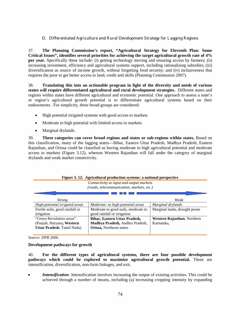
74

D. Differ entiated Agr icultur e and R ur al Development Str ategy for L agging R egions

37. The Planning Commission’s report, “Agricultural Strategy for Eleventh Plan: Some Critical Issues”, identifies several priorities for achieving the target agricultural growth rate of 4% per year. Specifically these include: (i) getting technology moving and ensuring access by farmers; (ii) increasing investment, efficiency and agricultural systems support, including rationalizing subsidies; (iii) diversification as source of income growth, without forgetting food security; and (iv) inclusiveness that requires the poor to get better access to land, credit and skills (Planning Commission 2007). 38. Translating this into an actionable program in light of the diversity and needs of various states will require differentiated agricultural and rural development strategies. Different states and regions within states have different agricultural and economic potential. One approach to assess a state’s or region’s agricultural growth potential is to differentiate agricultural systems based on their endowments. For simplicity, three broad groups are considered:

• High potential irrigated systems with good access to markets

• Moderate to high potential with limited access to markets

• Marginal drylands.

39. These categories can cover broad regions and states or sub-regions within states. Based on this classification, many of the lagging states—Bihar, Eastern Uttar Pradesh, Madhya Pradesh, Eastern Rajasthan, and Orissa could be classified as having moderate to high agricultural potential and moderate access to markets (Figure 3.12), whereas Western Rajasthan will fall under the category of marginal drylands and weak market connectivity.

Figure 3. 12: Agricultural production systems: a national perspective Connectivity to input and output markets (roads, telecommunication, markets, etc.)

Strong Weak High-potential irrigated areas Moderate- to high-potential areas Marginal drylands Fertile soils, good rainfall or irrigation

Moderate to good soils, moderate to good rainfall or irrigation

Marginal lands, drought prone

“Green Revolution areas” (Punjab, Haryana, Western Uttar Pradesh, Tamil Nadu)

Bihar, Eastern Uttar Pradesh, Madhya Pradesh, Andhra Pradesh, Orissa, Northeast states

Western Rajasthan, Northern Karnataka,

Source: DPR 2006.

Development pathways for growth

40. For the different types of agricultural systems, there are four possible development pathways which could be explored to maximize agricultural growth potential. These are intensification, diversification, non-farm linkages, and exit.

• Intensification: Intensification involves increasing the output of existing activities. This could be

achieved through a number of means, including (a) increasing cropping intensity by expanding

75

access to irrigation, (b) increasing yields and/or reducing losses through the adoption of improved farm practices, seed varieties, and livestock breeds and through the use of other inputs, and (c) relaxing some binding constraints, such as labor shortages through the use of mechanization, water shortages through the use of drip irrigation, or access to credit through the use of warehouse receipts. The development of irrigation systems improves agricultural potential in a number of ways, especially in highly fertile areas. It improves agricultural productivity and performance directly by increasing yields and by enabling multiple cropping, but also indirectly by increasing the returns to other factors of production, such as improved seeds, fertilizer and other agrochemicals, and labor. It reduces rainfall-related output volatility and risks, which also makes agricultural diversification to higher-value crops more economically viable. Irrigation expansion, however, is becoming difficult and costly in many states, including some lagging states (Rajasthan and Uttar Pradesh) because the best areas have been developed and expansion is being pushed to more difficult areas. Moreover, increasing water scarcity and competition for water from other sectors (industry and drinking water) further heightens the need for better allocation and management of water resources in many states.

• Diversification: Diversification involves the shift in production to higher-value crops or products

(fruits, vegetables, higher-value cereals, medicinal plants, and livestock) to take advantage of new, more profitable market opportunities. The potential gains from diversification come from improving crop rotations, spreading labor demand, raising incomes, and reducing risks. Agricultural diversification is often viewed as a possible panacea for raising agricultural performance everywhere in India. Agricultural diversification for sustained increases in household income is, however, most successful if it is market driven.

• Non-farm linkages: Connections between farms and related economic linkages can be

strengthened through activities that foster greater value addition, such as trading and agro-processing, as well as activities that provide inputs to the farm sector.

• Exit: Exit is the shift away from farming to non-agriculture occupations. This can imply

migration of farm workers to a new location to take advantage of higher-paying employment opportunities in the industrial or service sectors, usually in a town or city. Or it can simply mean the reallocation of labor to the rural non-farm economy within the same local area.

Matching agricultural strategies with production potential 41. High Potential Areas—Western Uttar Pradesh: Just as the development pathways for achieving more rapid agricultural growth will vary across the different productions systems, so too must the agricultural strategies vary from region to region (Table 3.8). In high-potential irrigated areas such as Western Uttar Pradesh, increasing land and water scarcity heightens the importance of diversification to higher-value products and value addition as a means to maximize the returns from existing resource endowments. Increasing and changing consumer demand, due to growing incomes, for example in the Delhi metropolitan area, and increasingly liberalized export markets , will provide huge opportunities for producers in Western Uttar Pradesh to diversify into higher-value products, including fruits, vegetables, livestock, aquaculture, and associated livestock feeds and forages. Demand for processed products also increases with rising incomes, which presents new opportunities for moving up the value chain into agro-processing and related services. Given the pressures on the natural resource base in high-potential irrigated areas, another development path is the shift in employment from agriculture to industry and services through measures to strengthen rural non-farm entrepreneurship and develop human capital.

76

Table 3.8: Tailoring development pathways to agricultural production systems High-potential irrigated areas Moderate- to high-potential areas Marginal drylands

Diversification of production to higher value products to cope with increasing land and water scarcity. Value addition through agro processing to cater to increased perishability of most high value products. Exit to services/industry sectors.

Increased intensification through increased adoption of high-yield varieties, irrigation, and modern inputs. Diversification by further improving linkages to markets.

Short- and medium-term: Sustaining production. Long term: Exit through off-farm employment (agro processing, services, industry).

42. Fostering agricultural diversification and value addition in high-potential areas require reorienting policies to ensure that incentives favor diversification and sustainable agricultural practices and fostering new institutions to meet the modern marketing needs of higher-value products (Table 3.9). Key public sector institutional changes, reforms, and investments required to provide such an environment are: • Continuing liberalization of agricultural marketing and trade policy (e.g., removal of movement and

storage restrictions, except during emergencies; drafting appropriate rules under the amended Agricultural Produce Market Act).

• Expanding agricultural risk management mechanisms, such as negotiable warehouse receipts, forward and futures contracts, and crop insurance, and developing financial systems for savings, capital redistribution, and risk management.

• Encouraging investment in infrastructure for irrigation (development and rehabilitation), markets (e.g., market yards, cold chains, port infrastructure), and agricultural services (e.g., agricultural research, extension, market intelligence and information systems).

• Supporting capacity building for businesses to conform to market grades and standards and for public agencies to regulate and certify food quality and safety.

Strengthening agricultural research and technology transfer systems. With land and water becoming scarce in many high potential states, diversification and productivity growth will become highly knowledge-intensive processes.

Table 3.9: Policy and investment implications of a differentiated agricultural strategy High Potential Irrigated Areas Moderate to High Potential Areas Marginal Drylands

Policy Market (input/output)

deregulation Land policy (tenancy) and

administration Water resource allocation and

management Price risk management Public Investments Research and extension to

support diversification, SPS requirements

Rehabilitation and maintenance of irrigation systems

Policy • Market (input/output)

deregulation • Land policy (tenancy) and

administration • Price risk management Public Investments • Irrigation development and

management • Research and extension to

support intensification/ diversification

• Rural infrastructure (roads, electricity, markets)

Policy 1. Natural resource management 2. Drought risk management Public Investments • Watershed management • Minor irrigation • R&D on drought tolerant crops,

small ruminants, NRM • Disaster management-safety

nets during droughts • Rural infrastructure to attract

non-agricultural investments

Improved human capital and governance Source: India DPR 2006.

77

43. Moderate to High Potential Areas— Bihar, Eastern Uttar Pradesh, Madhya Pradesh, Orissa, Northeast states. In the moderate- to high-potential regions, most of which comprise the low income and north eastern states, their good biophysical endowments offer the opportunity to maximize their untapped potential through further intensification of production of foodgrains for which they have comparative advantage and agricultural diversification to higher value crops. Indeed these states are seen as potential the future breadbasket of India. But this necessarily involves improving linkages to markets. 44. Creating the enabling environment for growth in moderate- to high-potential areas will require many of the same elements outlined in the strategy for high-potential areas. The main difference is that in contrast to high-potential areas, moderate-potential regions still have scope for improving productivity through agricultural intensification. As noted earlier, there is a significant yield gap for most crops between the lagging regions and the middle and high income states. Enhancing access to improved seeds, other inputs (e.g. fertilizer, irrigation) and agricultural extension services will be necessary to raise agricultural productivity. For both intensification and diversification in these areas, substantial public and private investments to increase labor and land productivity are needed. A key priority is the expansion of irrigation for which the low income and north eastern states still have considerable untapped potential (Table 3.9). The successful implementation of GOI’s Bharat Nirman program, as discussed earlier, will have a big impact in this development agenda.

45. Another critical priority will be to raise farm profitability by improving access to markets for agricultural inputs and outputs in the lagging states. Market development will require improving rural connectivity through investments to improve rural infrastructure (rural roads, electricity, telecommunications), physical markets and support for key market institutions. Effective implementation of Bharat Nirman will be critical to achieving this goal in the low income and north eastern states. Support will also be needed for institutional innovations that facilitate coordination along the supply chain, including contract farming, out-grower schemes (in which an agribusiness complements its supplies through arrangements with surrounding smallholders), and farmers’ and traders’ association. Capacity building is required for regulation and monitoring, which are crucial institutional elements for agricultural markets to function well. It may be necessary to develop official systems of grades and standards and well-functioning market information systems.

46. Access to markets must be improved, but so must access to new technologies and advisory services to improve profitability and expand smallholders’ awareness of market opportunities. To meet these needs, agricultural research and extension priorities for the lagging regions will increasingly have to focus on issues relating to marketing policy, post-harvest technologies and practices, livestock and high-value commodities with strong market demand, and cost-saving technologies.

47. As the productivity and profitability of food crop production increases, priority should be given to diversification. By strengthening links to market outlets (for example, through investments in roads, markets, electricity, and information systems), farmers can produce more crop and livestock products for the market. Diversification to products that require more inputs, processing, and handling will also offer additional non-farm employment opportunities. To help farmers cope with changing markets and production systems, investments in financial systems in these states for managing risk (e.g., futures markets, crop insurance schemes, warehouse receipt systems, commodity exchanges, and social safety nets) will be needed.

48. Diversification of production to higher value crops, such as vegetables, can offer farm households higher income possibilities for farmers in the lagging states (Figure 3.13). Vegetable production generates nearly three times higher net returns compared to foodgrains in Madhya Pradesh; it generates 64% higher

78

net returns in Uttar Pradesh. But the greater perishability of these higher value crops will require attention to improving accessibility to the market.

Figure 3. 13: Net Returns in the production of cereals and vegetables, 2003.

0.0

5.0

10.0

15.0

20.0

25.0

30.0

Bih

arJh

arkh

and

UP

Oris

sa MP

Cha

ttisg

arh

Raj

asth

anA

ssam

Man

ipur

Miz

oram

Nag

alan

dTr

ipur

aH

P AP

Kar

nata

ka WB

Ker

ala

Mah

aras

htra

Guj

arat

Tam

il N

adu

Har

yana

Pun

jab

Low Income States NE states Middle IncomeStates

High IncomeStates

Net R

etur

ns p

er h

a, R

s 00

0

Cereals Vegetables

Source: NSS 59th

round and authors’ calculation.

49. Marginal Drylands—Western Rajasthan, and the poorer districts of Northern Karnataka: In contrast, the strategy for improving livelihoods in marginal drylands, such as Western Rajasthan, Northern Karnataka, and the Vidharba Region in Maharashtra, because of the limited production potential and significant associated production risks in those areas, needs to be differentiated between the short to medium term and the long term. In the short to medium term, the focus will need to be on maximizing or at a minimum sustaining agricultural (crop and livestock) and non-farm incomes from existing natural endowments (Table 3.9). Over the longer term, an important pathway to reducing poverty is to exit agriculture by encouraging the shift to other higher-paying employment locally or in other areas, as well as more profitable non-farm uses for land, such as manufacturing and services to conserve resources and promote off-farm employment.

50. Because exit is a longer-term objective, especially in poorer areas, where opportunities to participate in nonagricultural labor markets are fairly limited, an intermediate step is to reduce poverty by developing those agricultural systems that can be viable. Improvements at the farm level should help rural households enhance food security, conserve natural resources, and if possible enter markets for selected products in which they have a comparative advantage (e.g., arid zone fruits and nuts, spices, honey, herbs, agroforestry, and small livestock). The development process in marginal areas needs to be managed carefully to ensure a smooth transition for rural households over time. They will need a combination of risk management at the farm level, safety nets at the household level, and other forms of transitional support. These differentiated strategies in turn have important implications on the policies and investments for promoting agricultural and rural growth. These are elaborated in the following sections.

51. While the long-term strategy in marginal areas with limited agricultural potential is exit to off-farm opportunities, through promotion of non-farm entrepreneurship and development of human capital, as a transitional strategy, policy should focus on those aspects of agriculture that are viable in the harsher agro-ecological conditions of marginal dryland areas. This necessitates increased priority to the research, development, and diffusion of drought-tolerant crop and livestock varieties, suitable livestock feed and fodder, appropriate soil and water conservation measures, and technical advice on alternative cropping systems that can mitigate agriculture production risks associated with low rainfall. Because the returns to research and extension associated with dryland crops and

79

environmental resource conservation are limited, the government will have to play a major role in delivering these services.

E . E xiting Out of Agr icultur e: Developing the Non-F ar m R ur al E conomy (T o B e R evised – with Data fr om new E mployment Sur vey alr eady pr ocessed)

52. Transforming the rural economy of lagging states will require not only improving agricultural productivity but also facilitating rural non-farm entrepreneurship. According to the 2001 census, lagging regions markedly lag behind in non-farm economic activities, which account for only 8% of rural employment in districts compared to 15% in the case of districts in the richer states. Recent evidence from the 2004/05 survey suggests that as with other states in India the share of non-farm employment has increased in rural areas in states such as Bihar and UP. Mostly the job growth has been for the self-employed workers. However, as a group, employment remains far less diversified in the poorer states than in the richer states. As noted earlier agricultural productivity growth will be needed to stimulate the non-farm economy. In addition, three key requirements will need to be addressed: infrastructure, rural-urban linkages, and urban development; The role of infrastructure has been discussed in the previous chapter and the following chapter (Chapter 4) will discuss strategies for urban development. Here the issue of regulatory reforms and rural finance is highlighted. 53. Non-farm rural development in the LIS is constrained by a variety of regulations, which have received less attention than urban regulatory issues. In the case of forestry, some 100 million forest dwellers, who depend on forestry products, are prevented from harvesting non-timber forest products such as fruits, nuts, flowers and twigs, activities that can be sustainably pursued. The harvesting of prosopis, its conversion into charcoal, and its transportation for sale, activities that can potentially provide significant employment in off-farm activities face numerous restrictions, which particularly affect the lagging regions where the forest resources are rich and significant parts of the population, especially in tribal areas depend on these activities. Other regulations such as the Essential Commodities Act, reservations on the agro-based and food-processing industries, controls on sugar trade and their distribution through the PDS, and restriction on exports of agro-products, are particularly onerous in the case of the lagging regions which have comparative advantage in most of these products. A good example of the success of regulatory reforms come from the easing of licensing requirements for milk processing in UP, which has led to the doubling of milk processing capacity in four years. 54. In addition to regulatory reforms, Governments in the LIS can also help to promote cooperative based non-farm initiatives. A good example comes from the dairy industry in importance in Rajasthan. With large parts of the state classified as desert and the rest prone to droughts, livestock provides the poor with a source of security, income, food, and is an asset in times of need. The Rajasthan Cooperative Dairy Federation (RCDF), established in 1977, has been a prime mover behind dairy development. It is a three tier system working with registered dairy cooperative societies (DCS), who receive technical support, improved feed and veterinary services, in exchange for competitively-priced milk procurement through dairy Unions. The RCDF provides marketing outlets for milk products, and overall planning and programming. It has been actively promoting the Saras brand of milk products, and has 12,000 outlets selling 26 diversified milk products ranging from milk to butter and ice-cream. The growth of DCS from 5200 in 1998-99 to 8500 in 2005 has resulted in sales of 50 billion rupees for the cooperative to date. The cooperative now is investing in new milk routes and chilling plants to increase it s milk procurement and keep up with the rapidly increasing demand both within and outside the state. The RCDF has set a target of increasing household income by 70 percent through access to these new milk routes. 55. Increasing access to finance will be the critical ingredient of rural transformation and here the LIS lags markedly behind in both rural and urban areas. Finance helps the poor catch up with the

80

rest of the economy as it grows. Finance also helps extend the range of individuals, households, and firms that can get a foothold in the modern economy, and it reduces damaging concentrations of economic power. Largely thanks to microfinance, there is now a growing appreciation of the “empowerment” dimension of finance, of the extent to which it can give ordinary people and the poor access to opportunity and the ability to escape ossified social structures. 56. The financial sector strategies of successive post-Independence governments in India have emphasized strategies to direct credit to underserved sector28

To this end, the 1950s and 1960s saw the growth of a large number of rural credit cooperatives across India. The late 1960s witnessed the nationalization of commercial banks, which were charged with loosening the grip of traditional informal sector moneylenders through the use of targeted, low-priced loans. Over the past decade, interest rates have been largely deregulated, although lending rates on small loans (under Rs 200,000) are capped at the prime lending rate, which banks are free to set; there is also a floor on short-term deposit rates. Priority sector credit requirements have been eased, but remain high at 40 percent. Debt or interest waiver schemes are used frequently. However, financial sector competition is particularly weak in rural areas and services particularly limited in the LIS where bank branches offering services are far lower.

57. Consequently, as recent data from a World Bank-NCAER Rural Finance Access Survey (RFAS 2003) indicates that access to formal finance is a particularly severe problem in some of the lagging states. In Uttar Pradesh, 80 percent of all rural households have no access to formal credit, and 87 percent of poor rural households have no access to credit from a formal source.29

According to the Rural Finance Access Survey 2003, for those rural households that do have access to formal finance, commercial banks are by far the most dominant source. They account for 51 percent of household deposits and are also the most important source of credit. Regional rural banks account for 34 percent of household deposits and 31 percent of credit. Other formal sources, such as credit cooperatives and post office branches, appear to play a modest role in providing savings and credit services to rural households (Table 3.10).

Table 3.10: Aspects of formal borrowing in Andhra Pradesh and Uttar Pradesh State Banks of India Regional rural banks Coops Others Andhra

Pradesh Uttar Pradesh

Andhra Pradesh

Uttar Pradesh

Andhra Pradesh

Uttar Pradesh

Andhra Pradesh

Uttar Pradesh

Interest rate (median) as percent per year

15 12 12 14 12 14 21 14

Loan amount received as percent of amount applied

87 93 81 95 88 79 72 95

Households reporting bribes as percent of all households

1.9 38.8 4.4 47.4 2.6 19.2 0 19

Bribes as percent of amount approved

6.5 10.2 9.8 23.8 4.5 16.7 0 13.9

Time taken to process a loan application (weeks)

25.7 36.5 25.9 32.3 25.4 22.0 7.5 22.0

Source: RFAS 2003. 58. For the minority with access to finance from a formal source, transaction costs are high. The 2003 survey indicates that all types of formal institutions demand bribes before approving loans. The bribe amounts are hefty, and higher in Uttar Pradesh than in Andhra Pradesh (Table 3.13). Procedures for opening an account or seeking a loan are cumbersome and costly, with loan processing times tending to 28 Reserve Bank of India: Functions and Working, Mumbai, 1983. 29 See Priya Basu and Pradeep Srivastava, “Scaling-up Microfinance for India’s Rural Poor,” World Bank Policy Research Working Paper 3646, June 2005.

81

be much longer in Uttar Pradesh than in Andhra Pradesh. Longer processing times for loans, together with bribes, result in high effective costs for small borrowers. 59. Ultimately, however, the rural non-farm economy’s development merges into the issue of urban and industrial development in neighboring areas. Such developments will be needed to provide necessary goods and services, including finance and technology, and also for generating demand for goods, services and labor from rural areas. The next chapter turns to the discussion of these issues.

82

CHAPTER 4. DEVELOPING CITIES AND ATTRACTING INDUSTRIES IN THE LAGGING REGIONS

Summary

This chapter examines the spatial distribution of industry in India and examines the implications of inter regional and intra regional infrastructure improvements on industrial prospects of lagging and geographically isolated regions in the country. The key questions are how can industries be attracted to the Low Income States and urban development supported. The analysis is centered around unbundling the characteristics of a location that make it a good place for a firm – and given that much of industrial activity takes places in cities (albeit of different sizes), a complementary lens of urban performance is used to look at how locations can improve their relative attraction for new investment. There are four sets of issues discussed in this chapter. (a) spatial concentration of industry; (b) role of domestic and international market access in enhancing productivity; (c) how cities can improve service delivery to lower the cost of doing business and improve welfare of residents; and (b) what policy can do to improve industrial prospects in lagging regions, particularly facing challenges of agglomeration economies in advanced regions and spatial externalities associated with public expenditures.

A. I ntr oduction and M ain M essage

1. Although stimulating agricultural productivity will be the trigger to stimulate growth in the lagging regions, most of the future growth in this region will show up in the development of cities and towns that attract industries and services and supporting a diversified economy. This will enable this region to meet a wide range of demands, and increase productivity taking advantage of economies of scale and agglomeration. At present, however, urbanization rates in the LIS, at 20% of overall population, are half that in the richer regions of India and relatively underserved by industry. 2. In this context this chapter examines the spatial distribution of industry in India and examines the implications of inter regional and intra regional infrastructure improvements on industrial prospects of lagging and geographically isolated regions in the country. The analysis aims to unbundle the characteristics of a location that make it a good place for a firm – and given that much of industrial activity takes places in cities (albeit of different sizes), a complementary lens of urban performance is used to look at how locations can improve their relative attraction for new investment. 3. There are four sets of issues discussed in this chapter. The first is the spatial distribution of industry. Industrial investment in India is highly concentrated with 20 cities accounting for 60% of private manufacturing investment. Post liberalization trends have favored re-concentration of private investment, favoring existing agglomerations, particularly those offering good access to international and domestic markets, and a broad range of producer services. Access to business services is a good example of general producer services where cities in lagging states have considerably lower business service representation relative to comparable cities in middle and high income states. In addition to low levels of investment, cities in lagging regions specialize in low end manufacturing activities that are less intensive in local binding constraints (particularly inter regional transport and electricity). This has adverse implications for accelerated growth in the future. 4. Second is access to reliable inter-regional infrastructure – including transport, telecommunication and electricity are significant in influencing location decisions of firms. Firms value the benefits of broad based industry services considerably more than industry specific amenities. Cities and regions that provide a broad range of services that reduce production costs and enable easy access to suppliers and markets are more competitive in terms of attracting new investment and raising the productivity of existing firms.

83

5. The third is the development of local and intra regional infrastructure. Recent empirical evidence highlights that the supply of local infrastructure services (municipal roads, street lighting, water supply and drainage) also has a positive and significant effect on city level investment attractiveness. Further, local infrastructure supply is most sensitive to a city’s ability to generate own source revenues via local taxes and user fees. However, cities in lagging states have considerably lower spending on local infrastructure development relative to national norms or cities in other states, and access to basic infrastructure services is also worse in these states. 6. The fourth is what are the policy implications? What role is there for public policy to influence industrial prospects in lagging regions? Can the government of India’s (GOI) inter regional infrastructure investments that increase connectivity of the spatially isolated northeast region to domestic markets and other lagging regions to international ports improve local competitiveness in terms of attracting new industry and increasing performance of incumbent producers? The answer to this question is not obvious. As states in lagging and geographically isolated regions produce standardized / low end manufactured goods, consumers will purchase products based on price and possibly quality differentials. Further, existing firms located in agglomerations accrue scale economies from transport savings and the diversity of input supply. Inter-regional transport improvements that improve the lagging regions’ linkages with the rest of the country will implicitly reduce a natural tariff barrier, and firms serving larger markets (such as non-basic goods producers in the high income states) and benefiting from economies of scale and lower unit costs of production can more easily expand into new markets in competition with local producers when the unit cost of distribution between two points is lowered. In the case where manufactured goods are standardized and product substitution is relatively costless, instead of manufacturing activity moving to or being created in the lagging and NE states, it is likely that producers in the leading regions (such as the Greater Mumbai region) will expand production and crowd out local producers in the lagging region.30

7. The first requirement for policy to offset such trends in the LIS and the NESCS will be city level improvements in local roads, water supply and drainage systems, which will have clear benefits for firms by reducing cost of production and providing local amenities that are valued by workers. Helping cities improve overall management and administration – which includes allocating land use efficiently, relaxing excessive development restrictions, and increasing the capacity of local governments to raise own source revenues that can be linked to local expenditures are likely to enhance local business development. Only part of improvements that are needed fall in the jurisdiction of a typical urban local body. Much of what a city needs is dictated by its relationship with the State and to a lesser extent – the Central government. 8. For cities in lagging regions to take advantage of inter regional and other network based infrastructure improvements there is imminent need to facilitate product diversification, which will improve regional competitiveness and prospects for long term growth. A complementary package of interventions that focuses on innovation and entrepreneurship development will be useful in this context. In theory, if one of the policy objectives of the government is to stimulate long term competitiveness in lagging regions, then there is a strong role for policy to “pick winners” – i.e. new product development, explicitly recognizing the region’s spatial constraints in terms of labor skills and infrastructure, and its opportunities arising from potential backward linkages. However, in practice, implement such strategies have mostly met with failure. Thus, rather than betting on specific sectors, industrial policy should create an environment that stimulates innovation, and then subsidize new activities with credible sunset clauses. 30 There are ‘tipping points’ for industry location in agglomerations when congestion costs and wages are high enough to offset net economies from agglomeration. However, these diseconomies are likely to decongest or de-concentrate in the form of spillover developments in areas that are well connected to buyers and suppliers.

84

9. India’s urban structure is distorted with excessive reliance on large cities to perform functions that can be efficiently performed by small and medium sized cities in efficient urban systems. The nationwide problem is exacerbated in LIS. Small and medium size cities do not offer a mix of producer and consumer services that can enhance performance of local businesses, or improve links with the rural economy. The overdependence on large cities for basic business services (and the limited number of LIS in India’s East-Central belt) provides serious impediments to local growth. For the national government, it is important to extend resources such as in JN-NURM program to address development issues in small and medium sized cities. This will reduce distortions in the functioning of the national urban system as well as extent the benefits of urban development to the rural economy. 10. Improving regional policy coordination in the LIS and the NESCS will be particularly crucial. To improve the attractiveness of a region for specific industries, a package of interventions that address a firm’s location criteria needs to be developed—uncoordinated interventions that only partly compensate for a region’s “unattractiveness” are unlikely to be successful. Regional development policies in India have historically included regulations, infrastructure development, and fiscal subsidies. However, they have been implemented in a piece meal manner, and have little coordination among various institutions and levels of government implementing reform programs. While there is an inherent danger in setting up new institutions that would coordinate expenditures across sectors and states, there is considerable need to have a strong oversight on development programs by officials who have a clear stake in the outcomes and who have political authority at the highest level. The main point here is to have high ranking political representatives who have a vested interest and shoulder the main responsibility for local development. This will guard against self-interested behavior on the part of agencies.

B . T he Spatial Divide in I ndustr y Per for mance – Stylized F acts

11. Indian industry is spatially concentrated outside the lagging regions. More than 50% of the investment flows in the organized sector, measured by letters of intent and actual industrial licenses issued between 1991 and 2007 have been directed to the richer states, while another 25% of it has gone to the middle income states. The states in the LIS group accounting for 40% of the population have received about 18% of these flows, while the 40 million people in the NESCS have received only 2% (Table 4.1). Further, even in the few cases such as Orissa which have received significant share of these manufacturing investment flows (4%), investment has been highly capital intensive – 3 times as much as the all India average. Similarly, investment in Jharkhand has also been relatively capital intensive.

85

Table 4.1: Industrial Investment Flows as measured by Letters of Intent and Direct Industrial License, 1991-2007

Share of Investment

(%)

Investment per Unit (Million Rupees per unit)

Employment Per Unit (no)

Capital Labor Ratio (million or ten lakh Rupees per employee)

Investment per unit (relative to all India average 100)

Employment Per Unit (Relative to all India Average)

Capital Labor Ratio (relative to all India average (100))

Chhattisgarh 0.46 190.72 128.67 1.48 65.7 60.0 109.5

Orissa 4.42 1425.33 312.14 4.57 491.1 145.6 337.4

Uttar Pradesh 7.95 271.45 280.54 0.97 93.5 130.8 71.5

Jharkhand 0.29 210.41 123.31 1.71 72.5 57.5 126.1

Madhya Pradesh

2.58 220.23 210.03 1.05 75.9 97.9 77.5

Rajasthan 1.33 167.83 158.50 1.06 57.8 73.9 78.2

Bihar 1.19 431.71 402.08 1.07 148.8 187.5 79.3

Low Income States (LIS)

17.47 311.05 247.37 1.26 107.2 115.4 92.9

Himachal Pradesh

0.40 145.11 184.96 0.78 50.0 86.3 58.0

Assam 1.98 1915.49 364.56 5.25 660.0 170.0 388.2

Meghalaya 0.01 29.02 42.89 0.68 10.0 20.0 50.0

NESCS 1.99 533.57 211.15 2.53 183.8 98.5 186.7

Andhra Pradesh

11.24 283.66 178.08 1.59 97.7 83.0 117.7

Karnataka 8.41 393.68 286.73 1.37 135.6 133.7 101.4

West Bengal 3.38 408.74 203.72 2.01 140.8 95.0 148.2

Kerala 2.33 397.78 204.35 1.95 137.1 95.3 143.8

MIS 25.36 337.62 213.85 1.58 116.3 99.7 116.7

Gujarat 17.36 466.51 162.22 2.88 160.7 75.6 212.5

Maharashtra 15.18 319.25 226.72 1.41 110.0 105.7 104.0

Tamil Nadu 10.43 156.84 176.56 0.89 54.0 82.3 65.6

Punjab 5.35 267.71 312.42 0.86 92.2 145.7 63.3

Haryana 3.55 180.76 265.61 0.68 62.3 123.9 50.3

Goa 0.14 45.15 92.93 0.49 15.6 43.3 35.9

HIS 52.01 268.11 207.78 1.29 92.4 96.9 95.3

Union Territories

1.55 146.56 152.26 0.96 50.5 71.0 71.1

All India 100.00 290.23 214.44 1.35 100.0 100.0 100.0 Source: BIA, EPW, July 28, 2007 12. The spatial concentration is even more dramatically evident in the case of cities outside the lagging regions. Twenty cities account for 60% of national private manufacturing investment between 2000 and 2005. At the top of the list is the Jamnagar urban agglomeration in the state of Gujarat, which accounted for 6.3% of national private manufacturing investment. Jamnagar is located on the Gulf of

86

Kutch. It has a well functioning seaport and is near one of the World’s largest refineries, run by the Reliance group of industries. Other cities in the top twenty list include Raigarh (Maharashtra) which is adjacent to the Mumbai metro region, Pune (Maharashtra) which is 250 km from Mumbai, Chennai (formerly Madras) and Bangalore. Among the top twenty manufacturing investment cities three each are in Karnataka and Orissa, while the states of Gujarat, Maharashtra and Uttar Pradesh each have two. 13. Post liberalization, industry became even more concentrated, favoring coastal cities, metro areas, and existing agglomerations. Two interesting issues emerge from the data presented in Table 4.2, which shows the top 25 industrial districts in the country. First, even after stringent industrial regulation, very few of the districts in backward regions such as Bihar, Orissa, and Uttar Pradesh show up as major industrial centers. Second, following economic reforms and end of the licensing regulations, there has been a decline of the inland region: every district in the all industry post-reform top ten lies to the south of

Table 4.2: Top 25 industrial districts and their investment shares ALL INDUSTRY PRE-REFORM POST-REFORM

1 Greater Bombay MAH 8.23 Bharuch GUJ 4.29 2 Vadodara GUJ 3.9 Surat GUJ 4.28 3 Lucknow UP 3.71 Jamnagar GUJ 3.55 4 Vishakhapatnam AP 2.93 Chengaianna TN 3.45 5 Barddhaman WB 2.74 Raigarh MAH 2.82 6 Madras TN 2.48 Greater Bombay MAH 2.75 7 Pune MAH 2.34 Dakshin Kannad KAR 2.57 8 Hyderabad AP 2.31 Vishakhapatnam AP 2.06 9 Purbi Singhbhum BIH 2.26 South Arcot TN 2

10 Patiala PUN 1.81 Ratnagiri MAH 1.8 Top 10 Total 32.71 Top 10 Total 29.58

11 Raigarh MAH 1.8 Ghaziabad UP 1.75 12 Bangalore KAR 1.79 Bhatinda PUN 1.68 13 Jabalpur MP 1.67 Pune MAH 1.61 14 Surat GUJ 1.66 Thane MAH 1.61 15 Chengaianna TN 1.52 Barddhaman WB 1.52 16 Sundargarh ORI 1.5 Bellary KAR 1.39 17 N. 24 Parganas WB 1.5 Ganjam ORI 1.36 18 Dhanbad BIH 1.44 Medinipur WB 1.35 19 Sonbhadra UP 1.38 Vadodara GUJ 1.34 20 Dhenkanal ORI 1.36 Sagar MP 1.15 21 Thane MAH 1.33 Cuttack ORI 1.11 22 Bharuch GUJ 1.2 Dibrugarh ASS 1.04 23 Jaipur RAJ 1.17 Purbi Singhbhum BIH 1.04 24 Durg MP 1.02 Raipur MP 1.03 25 Ahmadabad GUJ 0.9 Koraput ORI 0.98

Top 25 Total 53.95 Top 25 Total 49.53 Source: Chakravorty (2003)

the Vindhyas, the somewhat imaginary line dividing north and south India. Uttar Pradesh and Bihar, the two largest and also landlocked states in the country, together account for a quarter of India’s population, yet have only one district each in the post-reform all industry top 25: Ghaziabad (at rank 11) in Uttar

87

-20

020

4060

80Sh

are

belo

w p

over

ty li

ne

0 .2 .4 .6 .8Share of urban population

95% CI Fitted valuespop_bpl

020

4060

80Sh

are

belo

w p

over

ty li

ne

0 .2 .4 .6 .8Share of urban population

95% CI Fitted valuespop_bpl

Pradesh, which is part of the Delhi metropolis, and Purbi Singhbhum (at rank 23), the manufacturing base of the large Tata group. Related empirical evidence on allocation of post reform private sector investment also shows that private sector investments tend to favor existing industrial clusters and metropolitan centers, with access to the coast, and avoid regions with inhospitable local governments. However there is a higher incidence of Central government investments in inland districts. For the private sector, the most significant investment determinants are the size of investment from the pre-reform period in the same district (i.e. agglomeration effects), and the size of new post-reform investment in the neighboring districts. The first factor suggests continuity, or evidence of a historical process of investment location. The second factor suggests that new investments are clustered (Lall and Chakravorty 2005). 14. Concentration is being driven by scale economies from urbanization, which emanate from the overall size (not only in terms of the number of firms but also in terms of population, income, output or wealth) and diversity of the urban agglomeration. For a firm, benefits from urbanization include access to specialized financial and professional services, inter-industry information transfers, and availability of general infrastructure such as telecommunications and transportation hubs. Size is usually correlated with diversity as larger urban areas can support a wider range of activities. Small cities are specialized in a few manufacturing activities, or are either administrative centers (such as regional capitals or university towns in some countries), or agricultural market centers providing services for farmers. In comparison, larger cities are more diverse, supporting a variety of manufacturing activities that require buyers and suppliers to be in close spatial proximity (I-O linkages). Further, larger cities are centers of innovative technologies and usually tend to offer business or productive services.

15. In addition to the benefits that well functioning cities offer to local firms, evidence from census data suggest that at the district level, rural poverty is lower where the share of urban districts is higher. For both years (2001 and 1991) shown in Figure 4.1, there is a strong (negative) relationship between rural poverty incidence and district urbanization levels. Preliminary empirical evidence on district level market development (small towns) suggests that the provision for primary schools, electricity and paved roads are positively related with the market development (Paul 2007). The analysis utilizes fixed effects OLS and uses facility provision in 1981 to explain market development outcomes in 1991. At the same time agriculture productivity and non farm rural employment improves with better access to neighboring towns, as improving local roads in a district makes it easier to access neighboring towns within that district.

Figure 4. 1: Urbanization and rural poverty (2001 and 1991)

88

16. In well functioning urban systems, a diverse array of industries and service activities are often supported in cities of moderate size. In developing countries, ingredients required by advanced industries and services tend to be found mainly in the major and largest cities, and well-integrated local regions that feature multiple exchange of labor flows and supplier linkages (as discussed earlier in this chapter). At the same time, the development of small and dispersed urban areas close to agriculture, in towns that could grow by providing goods and services to the neighboring agricultural population, is limited by constraints in the agricultural economy and often by lack of infrastructure, especially transport linkages to larger markets. Both the farm and nonfarm activities in rural areas need the agglomerative features of urban economies to expand and diversify rural production.

17. Availability of business services such as finance, insurance, trade and logistics matters not only for increasing productivity of individual cities but is important for improving rural outcomes. Figure 4.2 shows the distribution of business services across the urban hierarchy. The business services variable is the number of business service sector jobs that are within a 90 minute travel time. There are two interesting points that emerge. The first one is obvious, that access to business services increases with city size. Second, for all city size categories, lagging states have considerably lower business service representation relative to middle and high income states. This poses a considerable challenge for cities in lagging states to attract investment and to stimulate the rural economy, particularly considering that LIS are more dependent on agriculture for generating employment: the sector accounted for more than 50% of employment growth in both LIS and NE between 1983 and 2000.

Figure 4. 2: Access to business services

18. Recent empirical evidence for Indian industry shows that industrial diversity (i.e., the local presence of a mix of industries) makes local manufacturing competitive. Such diversity provides the most significant and consistent cost savings for firms of all sizes and in all sectors of manufacturing industry (Lall and Chakravorty 2005) In comparison, other spatial factors that, in theory, have some productivity enhancing effects (such as own industry clustering) are found to have little or no influence. Figure 4.3 shows that cities that offer industrial diversity are those that have access to a large domestic and international market.

19. Size of an urban area in turn is usually correlated with industrial diversity as larger urban areas can support a wider range of activities. Small cities are specialized in a few

89

0.0

001

.000

2.0

003

.000

4H

erfin

dahl

Idex

of M

anuf

actu

ring

Div

ersi

ty

1 2 3 4 5

Industrial diversity higher in cities closer to ports

0.0

001

.000

2.0

003

Her

finda

hl Id

ex o

f Man

ufac

turin

g D

iver

sity

1 2 3 4 5

Industrial diversity increases with domestic market access

manufacturing activities, or are either administrative centers (such as regional capitals or university towns in some countries), or agricultural market centers providing services for farmers. In comparison, larger cities are more diverse, supporting a variety of manufacturing activities that require buyers and suppliers to be in close spatial proximity (I-O linkages). Further, larger cities are centers of innovative technologies and usually tend to offer business or productive services.

Figure 4. 3: Industrial diversity increases with proximity to international

and domestic markets

Data Source: ASI 2001 20. One of the main urbanization constraints facing LIS is the limited number of large cities in their neighborhood that provide agglomeration economies from industrial diversity and supporting business services (as discussed above), and provide demand linkages for products developed in smaller and medium sized cities. If one were to take UP out of the mix, there are only 2 cities in Orissa with more than a million people, 1 in Bihar and 4 in Madhya Pradesh. The lack of large cities is not a problem in itself – but becomes a problem when medium and small cities do not perform their functions in terms of providing a mix of producer and consumer services that would be provided in a

Quintiles of travel time to nearest port

90

well functioning urban system (see Figure 4.2). In this context, improving the functional roles of small and medium sized cities becomes particularly important for LIS.

21. Horizontal linkages in the same or related industries are more important for small firms as in the LIS as they cannot integrate various production processes internally. The preceding discussion focused primarily on the links between industrial diversity, market access and performance of medium and large scale manufacturing. Now, we turn to examine how (and if) cluster development is important for growth of small scale industry (SSI). Understanding how SSIs can be promoted is important given that over 50% of manufacturing and over 60% of non agricultural activity in LIS takes places in establishments with less than 6 employees (See Figure 4.4). The Ministry of Small Scale Industry estimates that there are 400 modern small scale enterprise clusters and 2000 rural and artisan based clusters in India. These clusters contribute almost 60 percent of India’s manufactured exports, and the SSE clusters are estimated to have a significantly high share in employment generation.

Figure 4. 4: Firm Size Distribution

22. There are typically three reasons why firms would want to cluster. First, to maximize forward and backward linkages between firms. Firms that produce intermediate goods will want to locate close to their consumers, i.e., the downstream firms that buy their products (a demand or backward linkage). Downstream firms, similarly, will gain from locating close to their suppliers (a cost or forward linkage). There will therefore be a tendency for such activities to co-locate. A second clustering mechanism arises from the advantages of industry specific skills; if specialist skills are required, then workers’ incentives to acquire these skills are greatest in a location where there are many firms. Conversely, firms’ ability to hire these specialist workers is greatest in a location with many such workers. Finally, clustering can have direct productivity effects. Knowledge spillovers, as firms in a location learn best practice techniques by observing other firms, raise overall productivity. More simply, firms observe the success of other firms performing a specific activity in a particular location and might start copying it. 23. Performance of small scale industry clusters in LIS is lower relative to nationwide trends. The third SSI census done in 2001-2002 identifies district level clusters if the district has 100 or more registered SSI units engaged in manufacturing the same product. Using this criterion, 1223 clusters covering 321 products have been identified in the registered SSI sector. Of these, 355 (29%) clusters are located in the LIS that include Bihar, Jharkhand, Madhya Pradesh, Chhattisgarh, Orissa and West Bengal. However, they produce only 12% of national cluster output and account for 16% of employment. In the unregistered sector, each district having 500 or more unregistered SSI units engaged in manufacturing of a product as per ASICC 2000 (at 5 digit) was considered to form a cluster of that product in that district. Using this criterion, 819 clusters covering 250 products were identified in the unregistered SSI sector.

0.010.020.030.040.050.060.070.080.0

LIS NESC MIS HIS

Less than 6 6-9 More than than 10

0.010.020.030.040.050.060.070.0

LIS NESC MIS HIS

Less than 6 6-9 More than than 10

Manufacturing Sectors (NIC 2 and 3) Non-agricultural sectors Source: NSS 55th Round, 1999-00 Survey

91

The LIS mentioned above cover 57% of unregistered SSI clusters, and account for 61% of national output and 69% overall cluster employment. 24. Informal business location is one of the main constraints facing cluster development in small scale industry in the LIS. Most of the tiny and smaller units operate from entrepreneur’s homes. Only the bigger end of small scale units and medium scale units are set up in industrial estates with a formal infrastructure. There are very few private industrial estates, and these are limited to the industrially developed states of Maharashtra and Gujarat. There are several disadvantages associated with operations based in home and unauthorized locations. Not only do such units have problems in expansion and modernization due to space constraints, but they may also be denied registration as SSI units and thus denied access to credit and other support facilities. 25. Has government policy supported SSI cluster formation? This is an important question for assessing whether new clusters can be developed in lagging regions. Empirical evidence provided in UNIDO’s review of industry clusters in India suggest that in most cases, private initiatives of entrepreneurs appear to be the only reason behind cluster formation, even though the government may have played a role in furthering the development of these clusters once these were established (91% of clusters that exist in the country have come up on their own).31

In contrast, only a handful of clusters have been the result of careful government decision making to concentrate similar units in particular locations.

26. The government is not actively involved in the promotion of SME clusters. At this time, there is no special policy either of the central government or state governments for the promotion of the SME clusters in general. The industrial policy related to small scale sector is a small component of the industrial policy in general which relates to the entire small scale sector rather than being based on national or regional priorities by focusing on certain industrial group or cluster of industries. However, there have been attempts to strengthen clusters by providing support through schemes related to technology upgradation, infrastructure provision and training through various institutions at the national and state levels, whose success has been mixed.32

27. Another spatial divide between the LIS and the richer states comes from differences in product specialization across size classes of cities. Manufacturing industries tend to locate in urban areas to achieve economies of scale, save on transport costs, and benefit from ancillary services. Theoretical and empirical work on urban economics and economic geography (see review by Henderson et al., 2001) suggests that the net benefits of industry concentration and location in large and dense urban areas are disproportionately accrued by technology intensive and innovative sectors. This is because the need for knowledge sharing and access to producer services is considerably higher in these sectors than in low-end manufacturing that employs standardized production processes. In this framework, low-end industry producing standardized products are expected to locate production in smaller urban centers with lower costs. 28. As clearly indicated in Table 4.3, manufacturing is relatively concentrated in the larger metropolitan areas. There were 386 Indian districts in the 1990s that we group into five types, ranging from the seven metropolitan areas, their identifiable ‘peri-metropolitan’ fringes, secondary cities (other districts with population greater than 1 million), tertiary cities, and the remainder. Table 4.3 shows that skill intensive industries are significantly over-represented in metropolitan and peri-metro districts and under-represented in tertiary cities and towns and rural areas. High productivity sectors are over-

31 The main reason for their co-existence is raw material availability and industry specific skilled labor 32 http://www.unido.org/userfiles/RussoF/Small.pdf

92

represented in metropolitan areas, while capital intensive sectors and sectors with large average plant size are over-represented in secondary cities and peri-metro areas respectively.33

Table 4.3: Industry and city type

District type Metro Centres

Peri-metro Secondary cities

Tertiary cities

Towns and rural

Industry growth -0.004 0.009 0.017 -0.01 -0.012

Skill intensity 0.160* 0.058* 0.000 -0.068* -0.151*

Capital intensity -0.041* 0.001 0.019* 0.006 0.015

Productivity 0.024* -0.005 -0.012 -0.005 -0.001

Plant size 0.008 0.013* -0.007 -0.009* -0.005

R 0.11 2 0.07 0.01 0.10 0.03

No obs. 346; * = significant at 5% level

Notes: data source is the Indian annual survey of industries. Factory data are aggregated to the industry level for each district type. Regressions are run separately for each district type. Data are pooled industry cross-sections for 1989-90 and 1996-7. Industry growth is the employment growth rate; skill intensity is the ratio of non-production to production worker employment; capital intensity is the ratio of fixed capital to employment; productivity is output per employee; plant size is employment per factory.

29. Low levels of industrial investment in lagging states are accompanied by specialization in low end manufacturing, thereby having adverse consequences for long term competitiveness. The relative scarcity of manufacturing activity and private manufacturing in lagging states such as Bihar indicate that spatial divides in modern sector economic activity are high and increasing. In addition to asking the question on the volume of economic activity, an equally if not more relevant question whether the relative specialization of manufacturing varies among these groups of states? Figure 4.5 compares Haryana and Bihar on machinery output, employment, and value added as shares of overall state level industry performance. These comparisons are based on firm level data reported in the 2001 ASI. Machinery represents over 60% of industry output and value added in Haryana – less than 5% in Bihar; almost 50% of industry employment in Haryana – and 7% in Bihar. In contrast, consider the food and tobacco industry in India, a sector with large variations in quality, which for the most part employs low skilled labor and uses low end technology for production. In Bihar, this sector accounts for 36% of industry gross value added and 43% of industrial employment.

33 For each district type the share of employment in each industry relative to the share of employment in that industry for India as a whole was regressed on a number of industry characteristics.

93

Figure 4. 5: How important is advanced manufacturing?

Data Source: 2001 ASI

30. There is a significant productivity gap in manufacturing between the low income, low growth states (the LIS group) and the faster growing states. Annual manufacturing survey data shows that the average Indian manufacturing worker produces Rs. 164,000 worth of goods net of the consumption of materials, energy and other intermediate input costs. This is 5 percent lower than the average for high-income states and 7 percentage points higher than that in low-income states (Figure 4.6). This implied an 11 percentage point gap in value added per worker between low income states and high income states, which is comparable with the 13 percentage point gap between high growth states and low growth states, but far smaller than the 18-19 percentage point gap between high FDI states or better climate states and the rest of India. The fact that estimated price cost margin varies very little between categories suggest that the gaps in value added per worker may have little to do with quality differences or differences in product market structures, and in that sense, seem to be reliable indicators of gaps in labor productivity.

0%

10%

20%

30% 40%

50%

60%

70%

Chhatishgarh Bihar Andhra Pradesh

Karnataka Maharashtra Haryana

Industry Output Gross value added Industry Employment

94

105

93

104

90

107

87

86

105

High income states

Lower income states

High growth states

Lower growth states

High FDI inflow states

Lower FDI inflow states

Others

Better IC rated states

Source: ASI 1999-2001

105

93

104

90

107

87

86

105

High income states

Lower income states

High growth states

Lower growth states

High FDI inflow states

Lower FDI inflow states

Others

Better IC rated states

Source: ASI 1999-2001

Figure 4. 6: Manufacturing value added per worker

ASI 1999-2001 31. Investment climate data suggest that labor productivity gaps between high FDI states or high growth states and the rest of the country reflect large inter state differences in the equipment of manpower with tools, machinery and space, reflecting the higher investment rates that the high FDI and high growth states have benefited from over the years. For example, establishments in high growth states have 18 percent more equipment and machinery per employee than those in low growth states. Similarly plants in high FDI states employ 14 percent more capital per worker than their counterparts in low growth states. 32. The poorer investment climate and low productivity in the lagging states are also evident in a key source of growth for the LIS, the development of mineral-based resources. The policy failures in the LIS in this sector are evident in the underdevelopment of this sector compared to the Southern states, where the contribution of this sector is much higher despite their smaller endowments. While a host of leasing, royalty and other regulatory issues impede growth, some progress has been made in establishing a comprehensive mining policy framework at the national level in India and also in some states like Orissa. The minerals previously reserved for exploitation by the public sector (iron ore, manganese ore, sulphur, chromite, gold, diamond, copper, lead, zinc, molybdenum, tungsten, nickel and the platinum group of minerals) have been opened for private and foreign investment. Preferential rights of the private sector are now recognized for the grant of a mining lease, provided the party has carried out the actual prospecting. The next stage of these reforms will be to define the role of the state as a regulator and non-operator and to put in place: (i) comprehensive social and environmental protection, risk management and benefit sharing mechanisms, to ensure that the mining sector growth stimulates broader development instead of being an enclave industry; (ii) a level-playing field to attract private investors; (iii) a competitive, predictable, stable, transparent and well-administered fiscal regime; and (iv) a stable and predictable investment environment and the ability of companies to operate on a commercial basis. 33. A key priority in the LIS group, given the large presence of tribal populations, will be to develop mechanisms to extend the benefits of mining to the local communities living around the

95

mining belts. This could be in terms of (i) accelerating shared growth and job creation; (ii) developing appropriate benefit sharing mechanisms; (iii) improving public service delivery; and (iv) strengthening social protection. The issues here are: (a) what should be done so that local people realize the potential of the resources (lying beneath their land and common properties) that attract global attention; and (b) how does private sector gain public acceptance for extracting such mineral resources and accept the affected communities as partners by allowing them to share some of the benefits? Local governments should be called upon to play a more active role in service delivery. Hence, attention would need to be given to matching their capacity with these additional commitments. There are also important environment concerns addressed elsewhere.

C . I dentifying factor s that matter for industr y location and per for mance

34. There are two broad approaches to identifying the factors that influence industry or firm location decisions. One is to ask firms directly as is typically done in investment climate surveys. Such surveys gather responses from firm representatives on aspects of the business environment, including the quality of utilities, infrastructure and the regulatory environment that affects a firm’s operations. For example, there are often large geographic variations in the frequency of power cuts or in the time it takes to acquire a telephone line. Road quality and access to transport hubs can be measured in alternative ways, for example by measures of road density or distance from a container port. Measures of the regulatory environment include the time taken to start a new business, the procedures for hiring and laying off employees, and the existence of corruption among officials. Such measures are of direct importance in enabling areas to benchmark their performance, as well as being inputs to a broader analysis. 35. A second source of evidence on the determinants of firm location decisions is econometric analysis of empirical patterns. A typical study of plant location might estimate the probability of a firm (in a specific sector) establishing production in a particular location, based on a number of explanatory variables that describe factor prices, as well as barriers and opportunities across potential locations. The variables may include: factor prices; quality and cost of complementary utility services, including electricity, water and telecommunication; market access as a function of the size of the region that can be reached given existing transport infrastructure; agglomeration economies as measured by the presence of firms in own industry and of firms in related—e.g., buying or supplying—industries; labor and other regulations. The findings reported in this section are primarily based on econometric analysis of firm and industry survey data. 36. The evidence from the investment climate survey about firm performance is clear. The LIS, Bihar and UP primarily, currently have the worst investment climate in India. Addressing some of these factors would go a long way to removing their competitive disadvantage with the richer states (Taye, 20078). The recent 2004 survey of [2000] firms in India clearly shows that the lagging regions fare the worst in four key indicators of investment climate: corruption, which is closely linked to tax administration, access to credit and power in order of importance. Further not only are these problems most severe in the lagging regions, these states bear the highest costs relating to these poor investment climate indicators. Consequently, the lagging regions suffer from both the lowest rates of entry of new firms in the formal sector and also in the growth of investment, which is only 1/3rd

of that in the HIS.

37. Good connectivity (via inter regional infrastructure) of cities to local, regional, and international markets is a key component of market access. In principle, this will (a) increase the demand for its firm’s products and lower production costs by reducing transport costs of inputs and outputs, (b) generate consumer surplus by reducing cost of consumption thereby improving the general quality of life, and (c) attract private investment. Firms located in cities with good access to market

96

centers are thus likely to be more productive than firms in relatively remote areas. Further, better infrastructure in high accessibility areas encourages interaction and knowledge spillovers between firms, as well as between firms and research centers, government and regulatory institutions, etc. and when transport costs are low, factor market competition takes over. 38. A recent analysis of city competitiveness in India shows that regional and national road transport improvements raise city attractiveness for new investments (see Lall, Wang, and Deichmann 2007). The estimates reported in Table 4.4 show that private manufacturing investment is more sensitive to proximity (travel time) to ports and domestic market access compared to government manufacturing investments.34 The parameter estimate for distance to ports suggests that a 10% reduction in travel time to international ports increases a city’s share of national private manufacturing investment by 5.2%. Similarly a 10% increase in the measure of road transport links that enhance domestic market access increases a city’s share of national private manufacturing investment by 5.6%.35

In contrast to location decisions of private investment, government investment in industry is not sensitive to variations in inter regional infrastructure endowments.

Table 4.4: Determinants of Private and Government Manufacturing Firm Investment36

(1) (2)

National share of private

manufacturing investment

National share of government

manufacturing investment

The impact of a 10% increase in the variable of interest GMM GMM

Local infrastructure 1.132* 2.182*

Travel time to international port -5.187*** 0.754

Domestic market access 5.684*** -0.451 Wages (per worker) -5.578*** 0.265

Access to business services -0.753** -0.583 *** significant at 1% level; ** significant at 5% level; * significant at 10% level.

39. However, the national estimates shown in Table 4.4 mask the differential impact of infrastructure between LIS and other states in the country. Estimates show that investment flows to cities in LIS are not sensitive to variations in inter regional infrastructure, while these factors are very important for city growth prospects in other states (Table 4.5). Why is this the case? Part of the

34 These estimates are the two-step efficient GMM in the presence of arbitrary heteroskedasticity and arbitrary intra-group (within-state) correlation. Instruments are strong with high average partial R2 values (average F values). 35 Market access is defined here as a proximity-weighted average of purchasing power or economic activity in potential trading partners of a location. 36 These are GMM estimates, where the instruments are (i) the average (real) cost of local infrastructure service provision, ln(avg. cost), which is assumed to be exogenously determined by technological and topographical/geographical factors, (ii) a dummy for port cities (distances to ports by roads or rails are less than 5 hours), (iii) a dummy for state capitals, (iv) a year dummy and state dummies, and (v) various state characteristics in year 1970. The 1970 state characteristics include population size; population density; per capita total state government revenue; the share of manufacturing sector in the total Net State Domestic Product (NSDP); per capita NSDP; the share of the number of seats won by Congress Party, hard left parties, and soft left parties; a dummy for President’s (state) rule.

97

reason is that the relative specialization of LIS cities is not in products that are exported regionally or internationally. This is consistent with the specialization index shown in Figure 4.2.

Table 4.5: The effects of regional infrastructure vary between LIS and other states

(1) (2) LIS Other states

The impact of a 10% increase in the variable of interest GMM GMM

Local infrastructure 1.427** 0.697

Travel time to international port -0.529 -4.697***

Domestic market access 1.500 5.300*** Wages (per worker) -1.089 -4.876***

*** significant at 1% level; ** significant at 5% level; * significant at 10% level. 40. The benefits of market access and urbanization economies vary by type of industry; the benefits of international market access increasing with product sophistication. Analysis of the differential impact of investment climate data shows that port distance significantly influences location decisions of firms across industry categories. For example, in medium technology manufacturing, the estimates tell us that a 10 % reduction in distance to the nearest international port will be associated with a 2% increase in the city’s attractiveness for private investment. The corresponding impacts are 1.3% for low technology firms and 4.6% for high technology firms (Lall and Mengistae, 2005). In the analysis, low technology sectors include garments, textiles, leather products, and metals; medium technology includes electronics, electrical white goods, machine tools, and auto components; and high technology includes drugs, pharmaceuticals, and chemicals. From these results we find that the importance of port access in location decisions is highest for firms in technology intensive sectors and reduces for lower technology sectors. This implies that regions that don’t have good port proximity will tend to specialize in low technology manufacturing (thus, the binding constraint has long term consequences). 41. Similarly, the effects of infrastructure shortfalls also vary by sector. The frequency of power outages has a significant negative effect on a city’s investment attractiveness. This finding is consistent for all industry types, and stronger for high technology manufacturing. For these firms, the estimates suggest that a 10 percent increase in the frequency of power outages reduces a city’s investment attractiveness by 2.9 percent (Lall and Mengistae 2005). The negative impact of utility failures is consistent with Mani et al (1997), who also find negative effects of state level power shortages and of energy prices on industry location decisions in India. 42. In addition to influencing location decisions, market access differentials have strong impacts on firm level productivity. For instance, New Delhi has a total factor productivity premium of 26 % in garments production over Bhopal in the state of Madhya Pradesh on account of its economic geography. However, only 4 percentage points of this premium comes from a larger concentration of garment producers in Delhi. The balance of the (geographic) productivity premium reflects better access to markets. 43. Although the effects of local infrastructure delivery, finance and urban management are less important than the effects of inter regional infrastructure provision it is more important for growth in LIS cities.: While national and regional infrastructure placement decisions have considerable impacts on private industry location decisions, city level efforts in terms of local service delivery, land

98

use planning, and municipal management also matter significantly for city competitiveness. As Table 4.3 indicates that the supply of local infrastructure services has a positive and significant effect on city level investment attractiveness. The parameter estimate for local infrastructure provision suggests that a 10% increase in infrastructure supply will increase a city’s share of national private manufacturing investment by 1.1% and government investment by 2.1%.. In the case of the LIS however, the effects of local infrastructure are considerably more important compared to other states in the country (Table 4.4). The parameter estimate for local infrastructure provision in LIS suggests that a 10% increase in infrastructure supply will increase a city’s share of national private manufacturing investment by 1.4%. In contrast, the estimate is insignificant for other states. 44. While inadequate urban service delivery is a nationwide concern, these problems are particularly acute in India’s lagging states. Local governments in India are responsible for delivering various public services, yet severe infrastructure shortages in water supply and sanitation, roads, transportation, housing and waste management, and poor planning and inefficient management have resulted in poor quality of services with limited coverage. Figure 4.7 shows that Bihar, UP and Orissa have low rates of access to tap water for urban households in cities with more than 100,000 residents, and are systematically under performing relative to other states. The situation is worse in smaller sized cities. Other infrastructure service indicators such as access to electricity, networked sewerage, and sanitation facilities also exhibit similar trends. 45. Similarly, the states of Bihar, West Bengal, UP, Orissa and Chhattisgarh have lower access to electricity relative to the national average. If infrastructure and service delivery is relatively poor in lagging regions, the relevant question to ask is why this is the case and what can be done to improve service delivery. A starting point to answer this question is to look at expenditures made by (urban) local governments on infrastructure and service delivery. There have been various efforts in India to develop physical norms and standards for infrastructure services. One of these attempts is by the Zakaria Committee (1963) report on ‘Augmentation of Financial Resources of Urban Local Bodies.’ This report calculates per capita O&M expenditure norms on four core infrastructure services: (i) water supply, (ii) drainage and sewerage, (iii) roads and works, and (iv) street lights and electricity distribution. These are national norms, only differentiated by city population sizes, thereby ignoring any local and geographical factors. For this analysis, normative expenditure levels are calculated based on the per capita norms re-constructed by Mathur (2001) at 1998-99 prices. Since the Zakaria Committee has suggested per capita O&M expenditure norms for (i) water supply, (ii) drainage and sewerage, (iii) roads and public works, and (iv) street lights and electricity distribution, the measure of municipal infrastructure expenditure used here also includes these categories. The reconstructed Zakaria Committee norms are presented in Table 4.6.37

37 A caveat is that in several states some local infrastructure services, such as water supply and sewerage, are taken over by the state governments, parastatal agencies, or in shared responsibility. Therefore, actual infrastructure expenditure of a local government does not necessarily represent overall public sector expenditure in a city.

The data for the analysis draw on the Local Finance Data System (LFDS) developed by the National Institute of Public Finance and Policy (NIPFP). This database has extensive information on local infrastructure service provision and fiscal conditions of local governments The final sample used in this analysis includes data for 151 Indian cities in 1992/93 and 1997/98. For the comparison, lagging states include Bihar, Chhattisgarh, Jharkhand, Madhya Pradesh, Orissa, Rajasthan, and Uttar Pradesh.

99

Figure 4.7: Share of Households with access to tap water (Pop> 100,000 ;

2001 Census Data)

Table 4.6: Zakaria Committee Norms

water supply Drainage & sewerage

Municipal roads & works

street lights & electricity

distribution overall

Pop more than 500000 189.95 217.98 42.51 53.00 503.44 Pop between 100000 and

500000 177.28 195.37 32.56 45.23 450.44

Pop between 50000 and 100000 156.30 168.24 24.42 41.61 390.56

Pop between 20000 and 50000 135.68 157.38 21.71 38.89 353.66

Pop less than 20000 134.23 148.34 19.90 36.18 338.64 Reconstructed by Mathur (2001), at 1998-99 price, Units: 1000 Rs.

46. Local bodies in LIS spend less on local infrastructure services relative to normative levels in other states. Table 4.7 provides a comparison of (population) weighted means of various indicators in lagging and other states. The ratios of actual infrastructure expenditures of local governments in lagging states over the normative expenditure levels of the Zakaria Committee are disappointing. On average, expenditure on sewerage and drainage was just 12.2% of the required expenditure level, water supply 7.3%, roads 56.7% and street lights 13%. The (weighted) mean of overall local infrastructure expenditures (relative the normative levels) in lagging states is 13.3%, which is considerably low compared to other states (78%). It is important to note here that these figures may overstate to some extent the extent of the gap as many local infrastructure services are provided by the state governments or parastatal agencies. Table 4.6 also presents a troubling trend as expenditures on service delivery are falling in lagging states. Relative to Zakaria committee norms, spending on infrastructure went down from an already low 14.6% to 12.3%. The drop in spending is seen across services for lagging areas.

100

Table 4.7: Expenditure relative to Zakaria committee norms for lagging and other states

weighted mean (weight=city population) 1992 1997

Dummy for lagging states (=1) 0 1 Total 0 1 Total 0

1 Total

All services 0.780 0.133 0.721 0.743 0.146 0.688 0.813 0.123 0.750

Water supply 0.812 0.073 0.744 0.769 0.082 0.706 0.849 0.065 0.777

Sewerage 0.448 0.122 0.418 0.396 0.123 0.371 0.493 0.121 0.459

Roads 2.549 0.567 2.367 2.483 0.628 2.313 2.607 0.514 2.415

Street light 0.709 0.130 0.656 0.751 0.165 0.697 0.673 0.100 0.620

47. Is the current revenue base of local governments adequate to finance local infrastructure needs? This resource gap can be measured by the difference between the normative infrastructure expenditure level and the municipal revenue base. We compute two measures of local infrastructure resource gap in a city: the ratios of combined total expenditure requirement of the Zakaria Committee over (i) total revenue incomes and (ii) own revenue receipts. Considering expenditures for other municipal public services, such as public education, public health, and various administrative and regulatory functions, this ratio needs to be greater than 1. Table 4.8 presents these ratios as a measure of the local infrastructure resource gap. Surprisingly, the average ratio of own revenue receipts relative to the required expenditure level was just 53.9%. Own revenue receipts can finance only half the required expenditure level. The average ratio of total revenue incomes including various transfers from higher levels of governments was 90.8%. Considering other municipal public service expenditures for which local governments are responsible, the revenue base of local governments should be increased significantly.

101

Table 4.8: Municipal Resource Gap

own revenue receipts / required level

Number of observations Average coef of

variation 1992 243 0.504 1.220 1997 243 0.574 1.852 Total 486 0.539 1.585

Municipalities 442 0.490 1.506 municipal corporations 44 1.029 1.143

Total 486 0.539 1.585 (a) (b) (share, b/a, %)

≥ the required level 486 64 13.17 total revenue incomes / required level

Number of observations Average coef of

variation 1992 244 0.839 0.610 1997 244 0.976 0.866 Total 488 0.908 0.766

Municipalities 444 0.854 0.725

municipal corporations 44 1.451 0.651 Total 488 0.908 0.766

(a) (b) (share, b/a, %) ≥ the required level 488 146 29.92

48. Municipal corporations are doing better in terms of closing the resource gap. When we compare the resource gap between municipal corporations and municipalities, municipal corporations are in a more favorable position. The own revenue receipts of municipal corporations were enough to meet the required local core infrastructure expenditure level, but those of municipalities were less than half of the required level (102.9% versus 49.0%). In the case of total revenue incomes, the ratios of municipal corporations and municipalities were 145.1% and 85.4%, respectively. In summary, only 13% of cities in our sample can afford to meet local core infrastructure needs from their own revenue sources, and 30% of cities from their total revenue receipts. 49. How can city level infrastructure and service delivery be improved? To answer this question, a model of service provision is developed to identify determinants of the shortfall in public services across Indian cities and for cities in lagging regions in particular. Following Roller and Waverman (2001), the “effective” demand for services rather than “observed” demand for infrastructure services are used for the analysis. The effective demand takes into account the un-met demand which cannot be observed due to supply constraints. More formally, the un-met demand can be defined by the gap between normative infrastructure usage requirement and the actual infrastructure service provision. 50. Municipal tax receipts (per capita, real) have a positive and statistically significant effect on local infrastructure supply, but the effect of transfers from higher levels of governments is not significant. Table 4.9 provides estimates of local infrastructure supply and demand. Column 2 presents supply-side determinants. The price elasticity of local infrastructure supply has the expected positive sign, but is not statistically significant. This may imply that local governments provide infrastructure services on a non-market pricing basis emphasizing the role of governments as public good providers. Local

102

infrastructure provision costs have a negative effect on supply, as expected. Municipal tax receipts (per capita, real) have a statistically significant and positive effect on local infrastructure supply, but the effect of transfers from higher levels of governments is not significant. In summary, “raising municipal taxes” is a more effective way to finance and increase local infrastructure service supply. In another specification, a variable for a town having a municipal corporation was introduced, which turns out to be statistically significant and positive, suggesting that cities with municipal corporation – i.e. cities with higher degrees of political responsibility and fiscal autonomy do a better job in supplying local infrastructure.38

Table 4.9: Factors that Influence supply and demand of Local Infrastructure Services The estimated reported here

are elasticities -- (1) Local Infrastructure

Demand (2) Local Infrastructure

Supply The impact of a 10%

increase in the variable of interest

Local infra prices -1.3*** 0.16 City incomes 2.267*

Average cost of provision -0.84** (0.357)

Local tax revenue (per capita) 1.31**

Per capita transfers -0.39

*** significant at 1% level; ** significant at 5% level; * significant at 10% level.

D. H ow can policies impr ove industr ial development in lagging r egions?

51. The stylized facts and econometric evidence presented in this chapter show that there are close linkages between economic growth, modern sector activity (industry), and urbanization. While there are considerable costs associated with economic production in large cities, both the revealed preferences of firms and systematic empirical analysis suggest that the attractions of good market access and other agglomeration economies remain considerable – even though the relative importance may vary by firm size and industry sector. For national policy makers who need to balance the objectives of overall economic efficiency, adequate opportunities and quality of life throughout the country, this has several implications. One is that policies with low opportunity costs such as streamlining of regulations and those that also provide large quality of life benefits such as transportation investments, are preferable over direct subsidies and tax breaks that rarely bring a sustainable reorganization of regional economic activities. Secondly, the evidence reviewed in this paper suggests that strategies for lagging regions that are directed toward competing with large cities for manufacturing jobs in high skills industries are unlikely to yield significant payoffs. More promising may be policies that build on local specialization in niche industries or on natural advantages linked to agriculture or service sectors. 52. Draconian policies of regulating industry location have not been successful and counter regional comparative advantage: Efforts at reducing regional disparities in economic performance have played a major role in GoI’s policy objectives and planning practices. The policy of the government has been to ensure balanced development across regions. Some concern over regional disparities was voiced as early as the first five-year plan (1951-56), and emphasized again in the Industrial Policy Resolution of 1956 (which identified the dos and don’ts of Indian industrialization). Over time, a number of instruments to achieve balanced regional industrialization were instituted: the industrial licensing system was used to

38 City level income effects are controlled for in this specification.

103

direct investment into lagging areas, and heavy industry was discouraged (and eventually forbidden) from locating in metropolitan centers; large public sector projects (steel plants, for example) were located in lagging states like Bihar, Madhya Pradesh and Orissa; industrial estates, or growth centers, were identified and received some investment in infrastructure; financial incentives for private industrial investment in designated lagging districts (about 60 per cent of all the districts in India) were provided; the prices for “essential” items such as coal, steel, and cement were equalized nationwide by the Freight Equalization Policy of 1956 (Mills and Becker 1986).39

53. Many regional policies have been poorly though out, and have hurt the prospects of lagging regions. Consider the Freight Equalization Policy of 1956 which equalized prices for “essential” items such as coal, steel, and cement nationwide. This effectively negated the location-based advantages of regions that were rich in these resources and placed them at a disadvantage relative to regions that produced “non-essential” items whose prices were not equalized. The affected areas were southern Bihar, western Orissa and eastern Madhya Pradesh, all among the poorest, least-industrialized parts of the country; also affected was West Bengal, which, not coincidentally, went into a deep decline at about the same time that this policy went into effect. The Freight Equalization policy has been discontinued since the early 1990s, but the damage may already have been done. 54. Can inter regional transport improvements alter industrial prospects of lagging regions? Yes, then can, but with two important caveats. While the available empirical evidence shows that inter-regional transport improvements allow firms to relocate from core metro areas to their peripheries, there is no convincing evidence that shows significant relocation to smaller urban centers in lagging areas. The pull of agglomeration economies and local amenities are higher than the benefits of transport cost savings when industries decide where to locate production, and firms in lagging regions face new competition from firms in other parts of the country – thereby threatening their existence. Box 4.1 reports the findings of a study that examines the potential impacts of road expansion on firm entry decisions in remote regions of Indonesia. With a few exceptions in sectors where agglomeration economies are not significant, there is very little new industry development in peripheral regions following simulated transport improvements. So the lesson here is that infrastructure by itself is not sufficient to bring about changes in the industrial performance of geographically isolated regions.

Box 4.1: Infrastructure and Lagging region development in Indonesia

39 While the Freight Equalization policy had been put in place to improve potential in lagging regions, it arguably had the worst effect on lagging region performance as it “robbed the producing areas of Southern Bihar and Bengal, Western Orissa and Eastern Madhya Pradesh of their comparative advantage in industries using these products” (Mohan 1983).

If market access increases performance at the firm and industry level, then can improving inter regional connectivity infrastructure change the industrial prospects of lagging regions? Deichmann et al (2005) address this question for Indonesia and examine (a) the effect of transport infrastructure on regional attractiveness, and (b) the implications of expanding transport capacity on industrial prospects of eastern Indonesia. They find that port access is highly significant in the apparel, wood and paper products sectors, all of which have strong export orientation. Similarly domestic market access also enhances regional attractiveness, where the impacts of road density are positive and statistically significant for seven industry sectors, with large elasticities in the textiles, wearing apparel and furniture sectors.

To examine the implications of expanding transport capacity in remote areas, they ask the following questions: what would happen to distribution of manufacturing if road densities in peripheral Eastern Indonesia were upgraded to a level similar to the country’s major agglomeration (Jakarta)? Would this stimulate large-scale migration of firms to peripheral areas? Or are agglomeration forces and other amenities strong enough to limit the scale of firm migration? They find that there is some relocation of firms in transport sensitive sectors, but the relocation is limited to major agglomerations to nearby large cities (such as Surabaya) with comparable amenities and agglomeration economies, and not to the peripheral parts of the country.

This suggests that large scale transport improvements, without other forms of public service provision and amenity creation may not be adequate to induce firms to relocate from agglomerations to peripheral areas. These findings are consistent with predictions in Krugman’s (1991) analytic work, where in the presence of large regional differences in local amenities (local infrastructure), improvements in inter-regional infrastructure without any concomitant improvement in lagging region ‘local infrastructure’ will not induce firms to relocate out of major agglomerations.

104

55. The second caveat relates to product diversification. For transport improvements to make a positive difference, lagging regions would have to move away from production of standardized products to producing differentiated products. These products don’t have to be in the most advanced sectors, but build on local sources of inputs. Stimulating (and subsidizing) local innovation, particularly in small scale industries and sectors where there could be learning externalities would be low cost option for local entrepreneurs to try out various lines of business. In addition, technical skill development would be a useful complementary policy – which would increase productivity in the long term. From our discussion with the commissioner of SSI, it appears that local innovations – called Kaizen points, are recorded by SSI entrepreneurs and put up on the internet to share experiences with product and process innovation (many of these being very small innovations). Recently, the confederation of Indian industry organized a Kaizen exhibition where close to 200 Kaizens from over 40 MSMEs were displayed.40

These activities should be promoted in lagging states so that local entrepreneurs can engage better in learning and product innovation.

56. Who will spend on regional infrastructure, and how much? Spatial externalities and coordination failures: The impacts of infrastructure on regional development are influenced by the presence of spatial interaction. As most infrastructure (especially network infrastructure) is inherently spatial, productivity effects in a region are spatially linked to productivity effects in adjoining regions. This fact is further augmented by spatial productivity spillovers (productivity shifters) due to the presence of network infrastructure.41

There are no prior expectations about the sign of the interaction terms as the spillover effects could be either positive or negative. For example, it is likely that the availability of ‘good’ transport and communication infrastructure in neighboring states can facilitate trade and commerce, thereby leading to increases in output and productivity. In this case, one would expect to see positive benefits accruing from the availability of infrastructure in neighboring states. It is also possible that the availability of infrastructure in neighboring states leads to out-migration of capital, as firms would locate in regions where they can reduce external costs (such as transport costs). In this case, the availability of infrastructure in neighboring states could have detrimental effects on a region’s output. It is therefore difficult to predict a priori, the effects of infrastructure availability in neighboring regions on output in any region.

57. Empirical evidence at the state level shows that there are significant positive growth externalities from investments in transport and communications, and water supply and sanitation. This means that individual states benefit from investments made by their neighbors (Lall 2007b). Positive externalities may lead to under-investment by individual states where each region expects to benefit from investments in neighboring regions. By altering investments in infrastructure relative to those of the neighboring regions, each region has the ability to modify the size of its infrastructure stock at the expense or to the benefit of its neighbor. The role of a “super-regional” decision making body for the allocation of infrastructure expenditure appears to worth exploring in this context. Given the existence of inter-jurisdictional spillovers and externalities, Hulten and Schwab's (1997) survey of investment patterns by local, state, and federal governments in the United States reveals that grants-in-aid from higher levels of government are not related to the presence of spillovers. They provide a public goods rationale for higher levels of government providing grants to lower levels of government in the context of infrastructure expenditures. 58. Policy effects are non-linear: The estimated production functions used in estimating externality effects were used as the starting point to develop a system of non-linear regional dynamics. The dynamics

40 See http://www.ciionline.org/news_new/newsMain02-05-2007_1.asp 41 Given that output and investment in additional infrastructure in neighboring/ adjoining regions influence productivity in a region, specification error would arise if terms accounting for this interaction were not included in the model.

105

of capital, labor, and public infrastructure were traced over time by regionally disaggregating macroeconomic identities. Numerical simulations were performed with scenarios involving no technological progress and with the introduction of technological progress. The simulations for the Indian economy show that introduction of sophisticated public capital increases the rate of public capital accumulation in both leading and lagging regions, and there appears to be the possibility of regional convergence in the growth of publicly provided infrastructure. However, the simulations also show divergence in private capital formation between lagging and leading states in the short to medium term (see Figure 4.8).

Figure 4. 8: Private capital formation in leading and lagging regions

Source: Lall, 2007

E . I mpr oving L ocal Ser vice Deliver y

59. Improving local service delivery: In the previous section, we show that there is systematic under-provision of public services in LIS cities. One of the main factors contributing to the lower provision of public services in LIS is inadequate spending on service delivery – both in terms of new investments as well as operation and maintenance expenditures. Urban areas in lagging states (for whom data is available) have considerably lower spending on basic services relative to norms set up by the Zakaria commission and compared to spending by better off states. Of course, this statement is likely to be tautological as states in lagging regions do not have the fiscal capacity (both the base and the administrative capacity) to stimulate local resource generation.

60. Empirical evidence emphasizes the importance of own source revenue generation efforts in improving local service delivery. On the other hand non dedicated or general purpose transfers from higher levels of government do not have any clear effects on stimulating local service delivery. The policy implication for improving local service delivery is then to find mechanisms that would expand the local revenue base in poor regions. However, this is not an easy task as local tax bases in these regions are not buoyant and local governments do not have the autonomy to change local tax rates or the administrative capacity to improve collection efficiency. 61. In the short run, there may be a need to increase the scale of transfers that are dedicated for service delivery (as in ring fenced operations). This is likely to stimulate economic benefits, both in terms of improvements in household welfare and willingness to pay for services via direct user charges (as households see visible improvements in service performance) and stimulate new economic activity – thereby increasing the tax base.

13000

14000

15000

16000

17000

egion

4600 4800 5000 5200 5400 5600 5800Lagging Region

106

62. In the medium to long run, efforts should be placed at improving local revenue capacity using a combination of new valuation methods and enhanced administrative capacity. If an area-based system is adopted, as is used now in some of the larger urban local bodies in the country , then a method of updating the guidance values on a regular basis is necessary (see Lall and Deichmann 2006 for details). This will require not only reliable values from the Stamp Office, and from the state Ministries of Construction, but also a set of procedures for updating these values. It also will require trained staff, capable of valuing real property, and perhaps a central valuation unit in each state should be considered. There is much to be done to implement such a system. Most local governments do not have a cadre of trained assessors to evaluate property values and update them regularly. A capital value system is even more difficult, because valuation of individual units will be required. In either case, a method of requiring updating of any new construction or major renovations, sub divisions, etc. will need to be put in place. A capital value system will be difficult and costly to implement, and it will be expensive. Its introduction will require much careful planning and will take considerable time. 63. Decentralization of functions to urban local bodies (ULBs) can assist to improve accountability for service outcomes through bringing decision-making over the type, quality and cost of services physically closer to smaller groups of consumers and citizens. This is particularly the case in LIS where distances between state capitals and individual towns are large, and where citizen needs may vary considerably between areas based on geography, ethnicity or other factors. Given that the urban population of LIS accounts for almost 20% of India’s total urban population, it is reasonable to expect that ULBs might play a significant role in the provision of urban services. 64. In practice, however, service delivery arrangements in LIS are mostly very centralized. In LIS, the revenue expenditures of urban local bodies (Rs. 286 per capita) amount to only 50% of the national average, and account for an average of only 0.43% of GSDP as opposed to the national average of 0.85% in 2001/02 (Mathur, 2006). Between 1997/98 and 2001/02 the average annual growth in revenue expenditures also lagged behind the national average. Assuming that real expenditure on services has remained constant, this indicates the decreasing role that urban local bodies are playing in the provision of services. 65. Local bodies in LIS remain dependent on grants from the state and central government, and thus have little real authority for service provision. Levels of grant dependence are highest in LIS, at 61.6% of total municipal revenues, as opposed to the national average of 31.7%.However transfers per capita are lower than the national average, at Rs. 211.80. These high levels of grant dependence are mirrored by the limited role of own revenue generation. ULBs in LIS generate only Rs. 135 per capita, considerably less than the national average of Rs482. This has shown negative growth in Rajasthan, Madhya Pradesh and Orissa, whereas the national average for own revenue generation per capita has been rising by 10.2% per annum. LIS contribution to national municipal own revenues has fallen by 2.2% since 1997/98. Within LIS, own revenue collections have also declined as a percentage of GSDP (from 0.28% in 1997/98 to 0.2% in 2001/02), whereas the national average grew from 0.65% to 0.71% over the same period. Understanding the failure of urban local services in LIS 66. While the weak fiscal capacity of ULBs is a core contributing factor to their underperformance, the solution is not simply to increase funding. This is because a lack of autonomy in decision-making, weak own revenue performance of ULBs and a reliance on transfers have weakened the accountability of ULBs to a growing urban citizenry in LIS. The urban water sector provides a good example of the problem: even the wealthier cities in India fail to provide a continuous (24x7) and safe supply of water. This is not due to the restricted availability of raw water (per capita availability is higher

107

than many counties in the world that do provide continuous service), nor a lack of investment in the sector (allocations have increased in real terms at a faster pace than population growth), nor insufficient operating subsidies (Indian states spends over Rs51 billion annually on operating subsidies to the water sector, equivalent to 0.5% of GDP, and 4% of total subsidies provided). Indeed, funding most often subsidizes the inefficiency of water utilities, rather than services to the poor who are less likely, in any event, to be connected to infrastructure networks. Unconnected poor households pay disproportionately large amounts per liter of water consumed, notwithstanding large subventions by Government, as they must buy more expensive water from informal vendors, and purify it themselves. 67. The problem is one of distorted incentives and lack of accountability. Service providers, whether at state or ULB level, do not maintain their infrastructure assets or focus on providing quality services. Low (or no) user fees for services and inefficient operational practices create greater reliance on grants from government. This eventually erodes the operational autonomy of service providers, who become more focused on obtaining grants for investment than on service provision for which they are no longer accountable (Figure 4.8).

Figure 4. 9: Funding can distort incentives and reduce accountability

68. Urban local bodies are further compromised by the hierarchical nature of intergovernmental relations, as they lie at the bottom of the system of government. Bureaucratic delays and low levels of transparency in fund transfers are compounded by overlapping functional assignments, lack of own revenue sources and restrictive conditions placed on the use of transfers. This absorbs existing ULB capacity in responding to the needs of government rather than responding to community needs. Transfers to ULBs are, in any event, much less evolved in LIS, because centralized state level line agencies continue to be used for service delivery, despite their widespread failure to address backlogs or improve service quality. This reflects an ongoing concern about “capacity” of local bodies, but fails to address the absence of assigned functions and resources on which actual capacity can be strengthened.

Utility lives off state subsidies

Motivation and service deteriorate further

Low tariffs, low collections

Investment, maintenance are postponed

Consumers use water

inefficiently

Customers are ever less willing to pay

Utility can’t pay wages, recurrent costs

Subsidies often fail to materialize

Managers lose autonomy and incentives

Services deteriorate

High usage and system losses drive up costs

Efficiency keeps dropping

System assets go “down the drain”

108

Improving Service Delivery 69. The problems of urban service delivery are thus more than a need for more infrastructure, or more money, or greater subsidies, or more training to improve “capacity”. The underlying problem is an institutional one, as service delivery agencies (including ULBs) do not face incentives to provide universal or sustainable services. Any solution to urban service delivery challenges of LIS must create incentives for institutions to deliver services, through addressing the separation of authority for service provision, regulation and policy-making. Decentralization of authority to ULBs can assist in this regard, through clearly transferring service delivery functions to local bodies, along with authority and resources, while reorienting state governments to play policy-making and regulatory roles. This separation, if properly designed and carefully implemented, can help to improve the measurability of outcomes in a manner that assists citizen oversight. Enabling reforms 70. CSSs have an important role to play in advancing decentralization, as they already provide a significant source of funds to local bodies. Although at present CSSs tend to by-pass or undermine the capacity of local bodies, their design and management can strengthen fiscal decentralization, support citizen oversight and strengthen core local government capabilities in public financial management, regardless of their sector. Importantly, ULB level reforms cannot occur in isolation to reforms to public management and service delivery within state governments. This is because they are currently deeply enmeshed, with state government agencies in practice performing many functions that are assigned to ULBs in law. 71. LIS need to review the intergovernmental framework for urban service delivery, to align functional competencies with fiscal resources and financial authority. In particular, the fiscal framework must create incentives for service delivery improvements through supporting institutional change and rewarding good performance. This would involve the following: establishing an appropriate fiscal framework requires greater clarity on the rules governing service delivery and the available resources. Key rules required include:

(i) A hard budget constraint to ensure local accountability for resource use. This includes ensuring that the full cost of service provision (such as infrastructure investment, staffing and input costs like electricity bills) are borne by ULBs so that they are able to align their capital investment and operational spending decisions;

(ii) Improving the transparency, certainty, equity and efficiency of grants through prospective 3 year allocations to all municipalities, and eliminating end-of-year transfers; and

(iii) Clarifying the response of state governments to situations of ULB bankruptcy or service delivery collapse, so that upfront knowledge of the political and financial costs of collapse is factored into the decision making of ULBs.

72. In this context, resources available to ULBs should be commensurate with their responsibilities. This requires that revenue sources are assigned to follow clearly delineated functions of ULBs. Where possible, ULBs need to be assigned local taxes of charges, with transfers augmenting their basic income streams in order to ensure resource adequacy, a common minimum standard of service across ULBs, and to influence local expenditure patterns in line with national or state priorities. 73. Adequate resources create a foundation upon which incentives for institutional reforms can be introduced. Ensuring adequate resource availability at the ULB level is an important element of enforcing a hard budget constraint, as this weakens charges that ULBs lack access to the resources necessary to perform their functions.

109

Strengthening local level accountability 74. Consumer demand can become part of a virtuous cycle of service delivery improvements. Improvements in local infrastructure and service delivery are most responsive to increased local tax efforts. Citizens exercise direct oversight of expenditures funded from local revenues, and are thus more likely to ensure that these meet their needs.

Figure 4. 10: A virtuous cycle of service delivery

75. But state and central governments need to trigger the process of strengthening local level accountability, through creating incentives for institutional reforms in local governments. This requires both policy changes associated with decentralization, as well as targeted interventions to support the transition to new service delivery institutions. In particular, state and central governments must work in partnership with ULBs to trigger service improvements through ensuring universal access to services (through providing connection subsidies to poor households only), providing incentives for improved utility efficiency (through funding the transition costs of institutional changes) and to create an enabling regulatory environment.

Improved investment &

operating efficiency

Pressure to improve quality

of service

Provider directly

accountable to consumers

All consumers use &

pay for services

Good services for all

110

CHAPTER 5. HUMAN AND SOCIAL DEVELOPMENT IN LAGGING REGIONS

Summary

Economic, human and social developments are inter-linked in the lagging regions of the country. While the main focus of policy interventions has been on accelerating aggregate growth and improving service delivery, critical social development issues have been neglected. Thus, while growth, defined in this chapter as growth of household real expenditures in different states and NSS regions, picked up at the national level and service delivery schemes have expanded in the lagging regions since the early 1990s, these have not able to bridge the gap between lagging and leading regions even in some basic health and education indicators. This chapter argues that a focused social development approach that strengthens the voice and participation of disadvantaged groups in India including females, tribal and religious minority groups and local communities will be a key condition for achieving faster human development in the lagging regions. The chapter draws attention to the importance of three integral elements of social development, namely, female agency, social inclusion, and local democracy.

A. Per spectives on R egional Dispar ity in H uman and Social Development

1. Low level of human and social development plays a key role in constraining growth42 and development of the lagging regions in India. This chapter discusses four ways through which these outcomes are linked and their policy implications. First, human development (HD), – i.e. improvements in education and health indicators -- while important in itself, is also an important factor affecting long-term growth of household incomes and consumption across Indian states (Figure 5.1). Conversely, growth of household consumption, (henceforth referred to as growth in this chapter), is a key factor affecting human development outcomes. Thus, the marked differences between the leading (HIS/ MIS) and lagging regions (LIS/ NESC) in HD, and the slower growth of the LIS and the NESCS are closely linked. Second, human development in the LIS cannot be significantly improved and spatial disparity is reduced by relying on growth alone as there is considerable variation in outcomes for a given rate of growth. Third, nor can spatial disparity in human development be reduced by appreciably by improving service delivery alone. Fourth, the key message of this chapter is that broad-based social development43

-- i.e. inclusion and empowerment of females, tribal and scheduled caste groups and strengthening of local democracy -- is needed, and will be pivotal in raising demand for services and human development.

2. Four perspectives highlight the importance of human and social development in the lagging regions. First, whether one pursues regional development (i.e., bringing jobs to people) or encourages migration (bringing people to jobs), human development will be an essential element of both strategies. Regions in India which had high initial human development grew faster, i.e. the long-term per capita consumption expenditure growth witnessed between 1983 and 2000 was faster in the regions with higher initial human capital.44

42 Unless otherwise mentioned, growth in this chapter refers to growth in the average household’s real consumption expenditures.

This means that the removal of regional disparity in the level of economic well-being cannot be left to growth alone as the political price of the long waiting period of “catch-up” may

43 In this chapter we define social development as including the dimensions of gender equity, social empowerment, participation in public affairs, collective social action, and access to functioning local democracy. The idea is to move beyond human development and make it “human development plus.” 44 This model is estimated at the level of NSS regions and allows for standard controls such as state-group level effects, initial level of income (expenditure), initial expenditure inequality, and gender inequality in under-five mortality based on NSS-region level data.

111

prove to be too costly. Policy interventions to accelerate human development in the lagging regions will be needed.

Figure 5. 1: Two Way Linkages between Human Capital and Growth: NSS Region Level Evidence

-.02

-.01

0.0

1.0

2e(

rgrp

c__a

| X

)

-.2 -.1 0 .1 .2e( hcadwrk | X )

coef = .0606961, se = .02099961, t = 2.89

-.02

-.01

0.0

1.0

2e(

rgrp

c__a

| X

)

-.2 -.1 0 .1 .2e( hchhed_3 | X )

coef = .03801981, se = .01565096, t = 2.43

Note: Two alternative constructions of human capital have been tried here. In Fig. 1a, we use “percentage of adult workers who completed primary” in the 38th round, while in Fig. 1b we use “% of household heads who completed primary” in the 38th

round. Growth is average growth rate of per capita NSS region expenditure observed during 38-55 rounds. The estimates represent partial effects of human capital on growth control for state-level effects, initial expenditure, gender inequality in under-five mortality and initial expenditure inequality.

Second, widening regional disparity can hurt national growth and development by creating political instability and conflict, which in turn will lead to lowering of investment and deterioration in institutions and governance (see Box 5.1). Third, regional exclusion can hurt national economic growth and development through neighborhood effects: that is neighbors with low levels of human development can not only pull down each other, but also affect the well-being of the richer neighbors. The spillover is clear with indicators such as infectious disease control, but may also be true of fertility, mortality, and gender-sensitive health practices which follow a regional pattern. Fourth, while social development is a key factor driving human development, it also important in itself, and perhaps the ultimate goal of all development policies. 3. The chapter is organized in six sections. This first section, A, introduces the key themes and stresses ‘social development’ as a key driver of human development in addition to channels such as growth and service delivery.45

Section B discusses regional variation and trends in HD across states located in leading and lagging regions. Section C draws attention not only to the importance of economic growth as predictor of subsequent human development but also to the considerable variation in HD performance around the same level of incomes or growth. Section D focuses on the role of service delivery in achieving HD targets drawing upon district level data such as RCH and other program-level evidence such as the SSA. Section E defines the main components of ‘social development’, which drive human development, i.e. female agency, social inclusion, and local democracy. Section F then sees how these factors help to explain the case of the poor districts in richer states.

45 A variety of methods have been used to try to determine causal linkages in this chapter and in the study. See Box 2.1 and Annex 2 for more details.

112

Box 5.1: Conflict and Development in the Indian States

A key factor that retards the pace of human and social development in the lagging states is the adverse interface of conflict and regional disparity. A particular motivation underlying such separatist agitations has been described by Hirschman and Rothschild (1974) as “tunnel effects” embedded in the cycle of hope-frustration-anger arising out of persistent inequality in the pace of progress between “disfavored” (backward) and “favored” (advanced) regions. Persistent lags in development have been the triggers of political conflict in India in many instances, resulting in popular agitation and militancy, often resulting in the movement for a separate province-state. Notably, these events have historically afflicted both leading and lagging states. Among the HIS states these include south Punjab, central Tamil Nadu, Saurashtra and Kutch in Gujarat and Vidharba in Maharashtra; among the MIS states- the list includes Telengana in AP, north Karnataka, and north Bengal. The conflict affected areas in the lagging states include western Arunachal Pradesh, lower Assam, much of the north-eastern states; south-western Bihar, the eastern and hill districts of UP, northern and eastern Madhya Pradesh, and south and western Orissa. Indeed, the creation of Chhattisgarh out of MP, Jharkhand out of Bihar, and Uttaranchal out of UP followed periods of political agitation, much the same way during the creation of new states such as AP and Gujarat in the 1950s, and the division of Punjab into Punjab, Himachal Pradesh, and Haryana in the subsequent period. However, the prevalence of conflict is currently far greater in the lagging states. For instance, in many of the north-eastern states, low economic growth and endemic political conflict have fed into each other. Political conflict in the early 1980s in places such as Assam was led by United National Front of Asom (ULFA) -nationalism and widely perceived as a consequence of pre-existing “grievance” arising out of persistent lags in development witnessed in that state in the preceding three decades. Relatively slow growth in the state provided the environment for easy recruitment of rebels, added fuel to on-going conflicts, and also discouraged further private investment and growth (Collier 2004; Narayan et al 2007). The same applies to continuation of Naxalite political violence in the districts marked by the vicious cycle of low agricultural growth, limited job opportunities, and poor service delivery. Most of the “red districts” (i.e. districts with significant Maoist presence) have been found to have higher poverty, illiteracy and poor health indicators (WDR 2006). However, progress in human and social development is possible even in the context of conflict, especially in the context when democracy and political competition makes policy makers more sensitive about distribution. Some of the NESC states included in the present study provide a good example of this. This is because democracy can have “healing effects,” being sensitive to re-distributive conflicts both within the region and across regions, compared to authoritarian regimes. One typical response of the democratic political regime would be to address the regional grievances through fiscal measures and other economic incentives to encourage investment. There is some evidence for India, which suggests a negative correlation between per capita state GSDP, and the amount of central government transfers received by the state (coefficient of correlation being -0.78). Central transfers to the poor states as a proportion of total transfers have increased between 1985/86 and 1989/90, dropped between 1991/92 and 1997/98 under fiscal stress, and rose thereafter (see, World Bank, State Fiscal Reforms in India: Progress and Prospects, Macmillan, 2005). For the lagging states, the average annual fiscal transfer per capita has increased over time, with sharp rises recorded since the mid-1990s. These trends, of course, are based only on transfers occurring through the formal system, and do not take into account the so-called “hidden transfers.” It is possible that with the on-set and subsequent aggravation of conflict in the north-east, the per capita transfers have, over time, increased at a higher rate than other lagging states. Besides, the terms of transfers are likely to be most beneficial as well, as 90% of the Finance Commission transfers from the Centre are in the form of grants, NESCS being the “special category state.” However, there is a gap in the knowledge on this score, and the broader issue of inter-governmental fiscal transfer with the conflict-prone north-eastern states represents a serious gap in the literature.

B . R egional Pr ofile and T r ends in H uman Development

4. Considerable inter-group and inter-state differentials exist in terms of level of human development and pace of progress. The leading states have in general higher HD outcomes than lagging states, though there are some notable exceptions. The evidence on the state-groups is– presented in Tables

113

5.1 through 5.3 below through three angles: (i) differences in lagging states and the other states; (ii) variations within these groups; and (iii) variations within states.

Table 5.1: Health Indicators Are Much Worse in the Lagging Regions, 1999-2001

(NSS Region-level Data) Regional Groups

TFR IMR Child Vaccination (Measles) Child Malnutrition

LIS 3.91 90.27 35.34 52.77 NESC 3.30 80.00 34.87 29.33 MIS 2.42 57.07 68.19 35.36 HIS 2.49 62.63 78.68 40.87 All 2.96 72.28 56.08 41.72

Note: Independent T-test for mean difference between LIS (group 1) and HIS (group 3) is significant at 1% level for all 4 indicators; the same is true of the difference between NESC (group 4) and HIS except for IMR where it is significant at 5% level.

Variations in Lagging vs. Leading Groups 5. Based on NSS-region level estimates around 1999-2001, several trends are noteworthy: • Lagging regions, considered as a group, are not only lagging in income and household expenditures, but also with respect to almost all the indicators pertaining to health, nutrition, education, and gender-inequality. However, an interesting fact is that while the gap in NSS consumption expenditure between LIS and HIS is about 50%, the gap between the NESC and HIS is only 21%. Indeed, in 1983, the position of the NESC states was better than the MIS and roughly similar to HIS. The decline since then possibly indicates the impact of endemic conflict in NESC states in the past two decades. • In the area of health and nutrition, the difference between LIS and HIS is sharp: 57% for TFR, 44% for IMR, and 29% for child malnutrition. NESC states also rank poorly in respect of health indicators in much the same way as LIS. The extremely high gap in measles vaccination between the lagging states and the HIS epitomizes the poor state of health service delivery in the lagging regions. • In education, the difference between LIS and HIS is 16% for male literacy, 54% for female literacy, and 47% for primary completion rate (Table 5.2). The only area where there is a sign of catching-up relates to primary enrollment in the age-group of 6-11 years.46

• Not only are the average female HD attainments among the lowest in LIS, the extent of gender inequality in these attainments appear to be highest, both now and historically (see later discussion on how HD outcomes and high gender inequality are related). This is seen in the striking exception of much lower child malnutrition rates in NESC, where the position of women are relatively much more favorable, except for Assam and Tripura. The NESCS outperforms all other Indian states here: according to NFHS-II data, the proportion of children underweight is 30% in NESC compared with 35% in MIS, 40% in HIS, and 52% in LIS.

46 Note that the data on enrollment refers to 1999-2000 i.e. before the advent of SSA. The spread of the latter has further diminished the gap in primary enrollment. The main impact of SSA was to close the inter-district gaps in enrollment within each state. This is not to say that there are no poorest pockets at the district and sub-district level in each state where differences in SSA implementation are still lagging behind. Besides, SSA suffers from quality concerns, as suggested by the Probe (1999) and Pratham (2005; 2006) study.

114

Table 5.2: Descriptive Statistics on Education Indicators by Regions, 1999-2001 (NSS Region-level Data)

Region Female adult literacy 55

Male adult literacy 55

Adult workers

with completed primary

education and above

Household head with completed primary

education and above

Gross enrollment 6-11 age

group

Net primary enrollment

Primary completion

rate

LIS

.3916 .6887 .4566 .5662 72.09 49.31 49.160 MIS

.5808 .7673 .5489 .6485 86.57 58.82 66.248 HIS

.6038 .8053 .6304 .7655 89.71 59.36 72.411 NESC

.6762 .8060 .6231 .6733 83.92 56.12 55.381 All

.5422 .7601 .5561 .6630 82.63 55.56 61.262 Note: Independent T-test for mean difference between LIS (group 1) and HIS (group 3) is significant at 1% level for all seven indicators; the same is not true of the difference between NESC (group 4) and HIS: here only for primary completion rate it is significant at 1% level; for female adult literacy and 6-11 years enrollment rate it is significant at 5% level; for male adult literacy and net primary enrollment rate the difference is not significant.

Table 5.3: Gender Inequality in Education Indicators (NSS Region-level Data)

Region

Gender inequality in adult literacy 2001

Gender inequality in adult literacy 1991

Gender inequality in adult literacy 1981

LIS .7885 1.0433 1.6940 MIS .3630 .4521 .8160 HIS .3566 .4851 .7919 NESC .2080 .3294 .6228 All .4726 .6308 1.0568

Note: Gender inequality is defined as the difference of male over female and expressed as proportion of female. Independent T-test for mean difference between LIS (group 1) and HIS (group 3) is significant at 1% level for all three indicators; the same is not true of the difference between NESC (group 4) and HIS: here only for 2001 the difference in gender inequality in adult literacy is significant at 1% level (for 1991 it is significant at 10% level, while for 1981 it was insignificant). For gender inequality in combined primary and secondary enrollment the difference between NESC and HIS is not significant.

Variation among States 6. Data for the different groups of states mask important variation within each group. Using the last two rounds of NFHS data at the state level reveals the following (see, Annex Table 5.1 through 5.4 for details): • Dramatic gaps between individual LIS/NESC states and HIS/MIS in 2005/06 in several variables: in infant mortality (15 deaths per 1,000 live births in Kerala vs. 73 in UP); in full immunization for children (81% in TN vs. 21% in Nagaland and 23% in UP); in total fertility rate (1.79 in AP vs. 4 in Bihar); in contraceptive prevalence (71% in Himachal Pradesh vs. 19% in Meghalaya); in access to antenatal care (97% in TN vs. 17% in Bihar); in skilled birth assistance (99.7% in Kerala vs. 26% in Nagaland and 29% in Jharkhand); in proportion of malnourished women (13% in Kerala and 14% in

115

Punjab as opposed to 43% in Bihar and 37% in Assam); and in proportion of stunted children (21% in Kerala vs. 45% in Chhattisgarh).

7. All the eight states which reached replacement level or below replacement level of fertility belong to the HIS (Tamil Nadu, Punjab, Maharashtra, Delhi) and MIS (AP, Kerala, Himachal Pradesh, Karnataka). • There are also signs of slippages in some key indicators in the LIS. At one extreme is Jharkhand, the only state in India where both fertility and child mortality went up in recent years. Other states also faltered: fertility rate increased in Bihar in LIS, Arunachal and Assam in NESC; IMR increased in Tripura in LIS and HP in MIS. The proportion of malnourished mothers increased in Assam and Arunachal in NESC, and in Bihar and MP in LIS. Similarly, access to antenatal care deteriorated in Arunachal and Mizoram. Full immunization rate dropped noticeably in the LIS but also in AP, HP and Karnataka in MIS, and in Gujarat, Maharashtra, and Punjab in HIS. • At the same time, some better performers stand out within the LIS. These include Uttaranchal (TFR, contraceptive prevalence; infant mortality, full immunization; maternal and child malnutrition; 6+ literacy rate), Orissa (access to antenatal care; births with skilled attendance; 6+ literacy rate), and Rajasthan (maternal and child malnutrition). Thus, infant mortality in Uttaranchal is as low as 42 deaths per 1,000 live births, in contrast to 73 in UP, 70 in Madhya Pradesh, 65 in Orissa and Rajasthan, and 62 in Bihar. Access to antenatal care (with at least three visits) is as high as 61% in Orissa, compared to 17% in Bihar and 26% in UP. • The performance of some of the NESC states comes close to the best performers in India. Manipur has a very high access to antenatal care and skilled birth assistance; Arunachal, Manipur, Meghalaya, Mizoram and Nagaland have very low proportions of malnourished mothers and children; Tripura and Mizoram have a very high level of general literacy. • This encouraging display in respect of some specific HD indicators within the lagging states shows that it is possible to achieve higher social progress even at low-level income. Interestingly, there are also remarkable “underachievers” among the leading MIS/HIS states. Gujarat, Haryana, and to an extent, Maharashtra belong to this category. This shows that increasing aggregate level of economic affluence does not ensure HD achievements. Inter-District Variation within Lagging and Leading Groups and States: 8. Variation within the lagging and leading regions can be even more striking at the sub-state (district) level. Several aspects are noteworthy: • Lagging regions not only have lower levels of HD attainments, they also have significantly higher inter-district inequality (as measured by the coefficient of variation). This is seen across the range of Reproductive and Child Health (RCH) indicators monitored in 2002-2004 (Table 5.4). Inequality in the LIS is very high (cv of more than 50%) in maternal health indicators such as institutional delivery in the government centers, access to iron tablets for reducing anemia, knowledge of ORS; colostrums/ breast-feeding within two hours. They are high (cv of 40% to 50%) in access to antenatal care with three or more visits; full immunization for children as well as measles coverage; awareness of HIV/ AIDS; medium: contraceptive prevalence; awareness of diarrhea; low: TT vaccination of mothers. High inter-district inequality in health care/ nutrition awareness indicators reflects the poor state of BCC campaign in the LIS region.

116

Table 5.4: Inter-District Variation in Human Development in the Lagging and Leading Regions State-cluster v21_rch v32_rch v12_rch v22_rch v26_rch v27_rch v29_rch v32_rch v33_rch v35a_rch HIS 92.63 59.31 55.78 72.16 80.64 53.45 26.82 59.31 24.03 76.96 CV 0.08 0.35 0.13 0.24 0.13 0.33 0.46 0.35 0.63 0.19 LIS 62.15 25.63 35.77 30.91 65.44 30.84 11.78 25.63 13.37 40.07 CV 0.31 0.41 0.32 0.44 0.19 0.43 0.67 0.41 0.69 0.34 MIS 93.54 61.02 57.90 80.27 80.71 59.64 40.82 61.02 31.53 75.19 CV 0.07 0.37 0.16 0.19 0.16 0.28 0.51 0.37 0.42 0.22 NESC 63.25 33.18 30.26 44.18 49.72 34.52 14.24 33.18 25.51 46.26 CV 0.30 0.59 0.50 0.44 0.38 0.49 0.80 0.59 0.72 0.47 All-India 74.96 40.71 43.64 50.89 69.69 41.62 20.90 40.71 20.54 55.71 CV 0.29 0.58 0.35 0.52 0.24 0.47 0.80 0.58 0.72 0.42

State-cluster v49_rch v50_rch V52_rch v53_rch v62_rch HIS 82.22 73.74 74.10 34.31 69.52 CV 0.17 0.23 0.20 0.36 0.29 LIS 44.96 34.49 62.07 23.18 35.04 CV 0.40 0.49 0.33 0.66 0.41 MIS 79.81 69.75 63.59 39.52 71.34 CV 0.17 0.24 0.32 0.44 0.27 NESC 42.56 22.01 55.30 34.90 64.67 CV 0.45 0.77 0.51 0.72 0.32 All-India 59.55 48.35 64.40 30.11 53.28 CV 0.41 0.55 0.33 0.59 0.46

Notes on Variables: V12: Contraceptive use (modern method); V21: Any antenatal check-up; V22: three or more antenatal check-ups; V26: Two or more TT injection for mothers; V27: Consumed one IFA tablet regularly (for anemia); V29: Received more than 100 tablets during pregnancy; V32: Institutional delivery; V33: Institutional delivery (government); V33: Any skilled assistance at birth (home or otherwise); V49: measles coverage; V50: full immunization for child (12-23 months); V52: Awareness about diarrhea; V53: Knowledge about ORS; V62: Women aware of HIV/AIDS. • Inequality in HD attainments within the NESC region is also very high, and even higher than the LIS in the case of RCH indicators. In fact, strikingly, for the majority of RCH indicators considered above, it is higher than that observed for the LIS region. This suggests a much more unequal state of health service delivery within the NESC region itself.

C . R ole of G r owth

9. Growth is important in affecting HD through several channels. First, as poverty declines and incomes increase with growth, poor people can invest in their own human development and in their household members. Second, higher growth provides more public resources for human development and enables the government to respond to demand. This first channel implies the presence of a responsive government acting through public policy, which may be influenced by governance, as well as fiscal and political constraints. But, even when the government’s response is not forthcoming, higher incomes enable the poor to access private providers of HD services (as dramatically seen in rural Bihar). However, when the government is responsive and able, growth leads to much faster improvements in HD, as evidenced in TN. 10. In the case of Indian states, lower growth of household consumption in the LIS and the NESC is significantly correlated to their poorer HD outcomes (see Fig. 5.2). Even after accounting for other

117

important determinants, growth has a discernible impact in reducing TFR, child malnutrition, and increasing adult female literacy. The explanatory power of a growth model (i.e. partial growth correlation) varies from 46% in case of IMR, 52% for child malnutrition, 62% in respect of TFR, to 69% in case of female adult literacy and 70% in case of child vaccination (see Annex Table 5.5). Clearly, the best performers in HD, (with the historically notable exception of Kerala) were fast growing regions and states of India over the period between 1983 and 2000.

Figure 5. 2: Household Consumption Growth per capita (in horizontal axis) and Human Development (in vertical axis)

with Infant Mortality with Total Fertility Rate

-1.5

-1-.

50

.5e(

lnim

r_99

| X

)

- .02 -.01 0 .01 .02 .0 3e( rgrpc__a | X )

coef = -8 .7606775, se = 3.7230177, t = -2.35

-.4

-.2

0.2

.4e

( lnt

fr01

| X )

-.0 2 -.01 0 .0 1 .02 .0 3e( rgrpc__a | X )

coef = -6.7166016, se = 1.9157436, t = -3.51

With Current Child Malnutrition With Current Female Adult Literacy

-40

-20

020

e( c

mn9

9 | X

)

- .02 -.01 0 .01 .02 .03e( rgrpc__a | X )

coef = -307.54829, se = 92.241799, t = -3 .33

-.2-.1

0.1

.2.3

e( a

dlit5

5 | X

)

-.04 -.02 0 .02 .04e( rgrpc__a | X )

coef = 4.2282106, se = .8473824, t = 4.99

Source: NSS-region level data, estimated from NSS 38th and 55th

rounds combined with Census and NFHS data

11. However, there is also considerable variation of HD outcomes around a given level of expenditure and growth; and the linkages between growth and HD appear to be particularly weak in the case of the LIS. Some NSS regions have achieved better HD outcomes than others even at low levels of growth, suggesting that other drivers or channels are also important in driving actual performance. The impact of growth on human development depends on how these channels are affected

118

by economic growth. This is especially important in the case of the LIS, where the poverty responsiveness to growth has been relatively low compared to the leading states (Besley et al 2007). Consequently, the overall responsiveness (elasticity) of human development to growth has also been lower. Overall, there is little evidence of direct impact of growth on IMR, vaccination rate, primary schooling and gender equality in basic education. However, these areas are largely amenable to social policies and could be undertaken even when there is moderate growth or low level of income. 12. The impact of growth on human development is muted in the LIS because the channels through which growth impacts HD outcomes are not as effective. Broadly these channels are the state service delivery arrangements, female empowerment, social inclusion, and local democracy. These are all areas where the LIS lag behind. While the service delivery channel focuses on the “supply-side” of HD attainments, the social development channels -- female agency, social inclusion and local democracy -- stress the “demand-side” of HD attainments. Strengthening some of these channels would require special attention to more innovative public policy and institutional arrangement in the LIS, where service delivery is weak. For instance, in the case of literacy or vaccination programs, new institutional arrangements for implementing a particular public policy (as in the case of PPP in education and health programs, or making service providers accountable to PRIs). In other cases, it may require measures that can only act indirectly via political empowerment of specially disadvantaged groups (policy of mandated political reservation, or influencing attitudinal changes towards favorable gender norms). These factors are discussed below.

D. R ole of Ser vice Deliver y

13. One key reason why LIS and NESCS lag behind in HD is inadequate service delivery in several respects: presence of facilities, access to infrastructure, lower public spending on services, and poor management and governance. The evidence on this is presented below. Some Proximate Factors • First, supply or access to facilities matter for health outcomes. Thus, spatial disparity in basic economic and social infrastructures between the lagging states and the richer states, especially the “supply” of core health and economic infrastructure, affects health human development outcomes.47 The presence of primary health centres makes a statistically significant and favorable impact on health outcomes such as IMR, awareness about ORS, sex ratio (female over male at 0-6 age-group); TFR; antenatal check-up. The declining strength of the infrastructure for elementary education can be vividly seen in Bihar. Here the number of primary schools (normalized per 10,000 populations) registered a negative growth rate between 1981 and 2001.48 Similarly the presence of “middle-schools” (taken here as a proxy for availability of educational facility) has a strong impact on IMR.49

47 One way of capturing the effect of placement of service delivery is to analyze how spatial disparity in economic and social infrastructures (“inequality of opportunity”) impact HD attainments (“inequality of outcomes”) at the district level. We test this relationship on a range of child health, maternal health and education indicators (altogether 15 indicators have been considered in this exercise—8 indicators discussed in Annex Table 5.6 and 7 indicators discussed in Annex Table 5.7). The outcome variables are mainly taken from RCH-II (2002-4). To explain RCH-II level HD outcomes we consider infrastructural variables from 2001 census (Annex Table 5.6). For the 2001 outcomes (using alternative data set provided by Debroy-Bhandari), relating to IMR, TFR, sex-ratio at 0-6 age-group, general literacy rate, adult female literacy rate, and pupil-teacher ratio, we consider 1991 infrastructural data as explanatory variables (Annex Table 5.7). The state-level fixed effects are included in all the regressions.

At the same time, simply

48 During the recent reform attempts to redress the situation under the present Bihar government led by Chief Minister Nitish Kumar, one of the first steps was to support the recruitment of additional 400,000 teachers, out of which 120,000 have already been recruited. The recruitment process is done through the active participation of PRIs.

119

the availability of facilities is not enough. Even when there are facilities, the provision of core services is weak. In UP for instance, 3000 PHCs do not have any doctors; 1,200 posts for doctors have remained vacant; out of 52,000 ANM posts only 18,000 ANMs are presently available; there is only one Anganwadi worker per village, indicating that the supply-line is very thin in the state. In short, inadequate education and health infrastructure is a key problem over and beyond the problem of service quality.

• Second, the presence of economic infrastructure also has significantly positive outcomes. Thus, access to all-weather roads has a favorable impact on maternal health indicators such as regular (three or more) antenatal check-up, and, to a lesser extent, on maternal immunization (two or more TT injection) and institutional delivery. Access to power similarly has a broad range of positive effects on full immunization of children, TFR, contraceptive prevalence rate (modern method); antenatal check-up and institutional delivery, and on raising the general and female adult literacy and lowering pupil-teacher ratio. • Third, one proximate factor for low levels of human development is that the lagging states do not channel enough resources to human development. Cross-state comparison shows that average per capita real social expenditure (averaged over 1990-2001) was Rs. 78 for TN, Rs. 73 in Maharashtra, Rs. 72 in Punjab, Rs. 69 for Kerala, and Rs. 65 for Karnataka. This is opposed to Rs. 36 in UP, Rs. 43 in Bihar, Rs. 51 in Orissa, and Rs. 57 in Assam. Strikingly, other NESC states have much higher social expenditure allocation per capita: Rs. 119 in Meghalaya, Rs. 132 in Manipur, Rs. 179 in Nagaland, and Rs. 272 in Mizoram (Singh 2005). Clearly, some of the better HD outcomes in these NESC states and worse outcomes in UP and Bihar—for a given level of fiscal and administrative governance—would appear to be related to the spending level. Lower spending is likely to affect the lagging states even more, because reaching out to the poorest pockets and poorest groups will involve more “search” and “intermediation” costs, requiring higher allocations. More importantly, the need for providing “quality” primary and secondary education and health-care will also require more public investments (even under a public-private partnership scenario where the government will still be the major purchaser of services). A substantial proportion of schools in the lagging regions does not have separate toilet facilities for girls, or lack science/computer laboratories or additional classroom facilities.50

• Fourth, centrally sponsored schemes that are aimed at promoting infrastructure and human development investments are not adequate to redress the inequality in public expenditures. Not only can they not overcome differences in states’ fiscal capacities, the incidence of centrally sponsored schemes is often regressive on a per capita basis. A look at some specific programs such as the SSA further reveals their inability to target the LIS in general, and the poorer districts in particular (See Box 5.2). Fifth, beyond improving access to facilities and infrastructure, there are deeper service delivery issues in the lagging regions, especially in the LIS. For 12 out of 15 indicators considered here, the outcomes of LIS districts are poorer even when infrastructure facilities are similar. In the case of the NESC, the same is true for eight of the 15 indicators. For a number of indicators such as full-immunization of children, vaccination against measles, TFR and contraceptive use, the presence of a public health center (PHC) has had no impact. This is striking, since these primary health indicators

49 There is a high correlation between middle-school and high-school facility (coefficient of correlation is 0.77 for 2001 census) and between middle-school and primary-school facility (coefficient of correlation is 0.53). We have used the indicator of middle-school also because it may be sensitive to primary completion rate. 50 One official in the Department of Education in Bihar during the course of interviews carried out for the present study mentioned the need for rethinking the “concept of school” itself: “school is not just an infrastructure with a roofless classroom, but with adequate physical and learning materials facilities, including play-ground and construction of physical boundary for the school premises.” The other related point is whether the state should provide “basic” (meaning up to class-VIII education) or “just primary (up to class-V) education”, which fails to meet the minimum knowledge attainment criterion.

120

should arguably be most affected by PHC and health sub-centre services. This shows that service delivery is very important. A telling statistic here is that absenteeism rates are much higher in the LIS than in the richer states.

Box 5.2: CSS Schemes and the Poorest Regions: The Illustrative Case of SSA There are apprehensions whether outlays under CSS have been targeted in an equitable manner across lagging and leading regions and states, and within states, across lagging and leading districts and blocks (i.e. whether allocations are more for districts and sub-districts with “highest need” as defined by the extent of deprivation). The issue is important since the share of CSS has doubled over the last 20 years, increasing from one-third of the central plan allocations to a little less than two-third in 2001/02 (Saxena 2002). The case of Sarva Shiksha Abhiyan (SSA) is instructive in this regard (for details see, Jhingran and Sankar 2006). SSA is the biggest CSS in education, and is generally perceived to have had a positive impact on the enrollment growth at the primary and upper primary levels in recent years. Several aspects are noteworthy: The lagging states and districts do not get higher SSA allocation per child, although they are in higher need (see, Annex Table 5.8). A comparison between Bihar and Punjab bears this out very well. Bihar ranks low, and Punjab ranks high in terms of education development index (EDI), a composite index of various aspects of educational development relevant to SSA.51

The EDI value for Bihar and Punjab are 0.07 and 0.62 respectively. However, both the states receive, on an average, similar per child allocation (PCA) from SSA (Rs. 560 for Bihar and Rs. 597 for Punjab). Similarly, within the LIS, lagging districts get a much lower amount of SSA allocations. This can be seen from the pair-comparison between Dhubri and Sibsagar districts (Rs. 406 vs.Rs. 755) in Assam, and Nabarangapur and Jagatsinghapur districts (Rs. 502 vs. Rs. 843) in Orissa. The poorest pockets within leading regions also get lower allocations, as typified in the case of Raipur vs. Uttar Kannada (Rs. 354 vs. Rs. 908) in Karnataka and Mehboobnagar vs. Chittoor in AP.

-- CSS does not reduce the social gap across communities as well. Thus, three categories of districts—(a) 48 districts with more than 50,000 out-of-school children, (b) 99 districts where Muslims constitute more than 20% of the total population, and (c) districts where population below the poverty line is more than 25% of the total population—all have, on an average, lower education scores (in terms of the EDI), than the average score for all districts of the country. At the same time, they also receive much lower per child allocations under SSA than the average allocation for all districts taken together. This indicates that the SSA has much room to improve upon the spatial targeting for bridging the persistent gaps between lagging and non-lagging regions and communities. -- Disconnect between “regional needs” and CSS allocation becomes even higher if one takes into account the amount actually spent by the state. Poor implementation capacity of CSS is not just restricted to SSA and seems to be a generic problem in the lagging region. In case of Jharkhand, in 2005/06, the health department of the state was able to spend only 68% of funds allocated. The implementation of food security programs is also unsatisfactory, especially the off-take of rice from the public distribution system (PDS). According to the Concurrent Evaluation of the SGRY conducted on behalf of the Ministry of Rural Development, Jharkhand had lifted only 18% of the authorized allocation in 2002/03; and only two-third of the meager share lifted was actually distributed to the beneficiaries.52

However, resource utilization does not mean improved quality of utilization. Much depends on how the CSS resources are managed and how the programs are governed.

51 EDI index is constructed by taking the following indices into account: input index (accessibility index such as primary school coverage and upper primary school per primary; infrastructure index such as percentage of classroom against requirement, percentage of schools with common toilets, percentage of schools with drinking water facilities; and teacher index such as student-teacher ratio at primary and upper primary school levels); equity index (girls’ age specific enrolment ratio and female literacy rate); outcome index (percentage children enrolled at 6-14 years, crude primary school completion rate, and crude elementary school completion rate). For details of the make-up, see Jhingran and Sankar 2006). 52 Poor implementation of social safety net schemes and high extent of leakages have been discussed in World Bank (2007).

121

Governance of Service Delivery in the Lagging Region 14. Disconnect between the placement of facilities and HD outcomes in the LIS may arise from several sources, among which, probably the most important is poor governance. Even with the placement of schools or clinic, other complementary inputs may be missing: service providers may be absent, road connectivity may be poor, infrastructural facilities may be built without important components of intra-facility services. But, the most important reason why just assignment of social infrastructures is not enough relates to the possible social and institutional barriers to accessing particular infrastructural services. In short, we have to distinguish between “placement of physical facility” and “service delivery,” and within service delivery— distinguish between the quantity and quality of service.53

Examples can be vividly seen from case studies of individual states.

• In UP, there is little correspondence between the district’s rank in literacy rate and the number of schools available per 1 lakh population. The coefficient of correlation between the two variables was 0.40 in the 1991 census data, but only 0.07 in the 2001 census data (Singh 2005). • The quality of service providers, even when they are present at the facilities, can be poor. Thus, quality of teacher recruitment in the lagging region can be very poor due to recruitment of “untrained teachers.” This situation prevails because of political patronage or poor governance. A case in point is Assam, which officially has one of the most favorable teacher-student ratios at the primary level in the country (1:25). However, out of 200,000 teachers recruited for primary schools in the estate since the early 1990, most were “untrained” or “inadequately trained” teachers, with the qualification criterion for recruitment being lowered to high school completion after nine months training. Thus, while DISE statistics show a big jump in enrollment (in terms of SSA program implementation, Assam is ranked third in the country), as the quality of instruction and educational outcome remains extremely poor. Importantly, as one official pointed out, “these teachers will remain a drag on the system for another 40 years.”54

• Finally, in the absence of accountability, qualified service providers may not be present on duty. A striking example is the discrepancy between convergence in primary enrollment rate across the states and the high level of teacher and doctor absenteeism, especially in the lagging states (WDR 2004). The difference between quantity and quality of services can be seen in the context of health indicators as well. While Jharkhand, Chhattisgar, and Uttarakhand have similar levels of quantitative achievements in antenatal services, Chhattisgarh lags markedly behind in the quality of maternal care (Rajan and James 2004). • Social development is important. While initial educational attainment in a region can be an important factor attaining higher female adult literacy, primary completion rate, infant mortality rate at the NSS region level (see, Annex Tables 5.9 through 5.11), its impact on TFR/CBR vanishes when female agency and social exclusion factors are included. Initial educational human capital also does not have any independent effect on reducing child malnutrition and lowering gender inequality in primary and 53 These points are well-documented in the literature. See, World Bank (2006) Development Policy Review on service delivery for a recent discussion. 54 Source: Interviews carried out in the course of the present study. In case of Bihar, a similar pattern is noticeable: about 14,000 untrained teachers” were recruited in the 1990s. The damage in case of Bihar was restricted by one High Court order, which put a freeze on further recruitment of primary teachers without proper training credentials. It is only in the recent past, following the change in the political regime, that the freeze on recruitment was lifted after the new government made a commitment that henceforth only trained teachers will be allowed to teach.

122

secondary education. All these indicate the potentially important role of social development to which we now turn.

E . Social Development as Dr iver of H uman Development

15. Social development is a key factor in sustaining growth and human development in the LIS through its impact on the demand side, by increasing the demand for good governance. As noted before, in this chapter we define social development through the prism of (a) female agency and well-being, (b) social inclusion with particular focus on scheduled caste, scheduled tribe, and religious minority, and (c) collective action and local government performance as two integral elements of local democracy. Each is considered in turn below. Role of Female Empowerment 16. One of the reasons why the lagging regions perform poorly in human development in general and in health indicators, in particular, is low female “agency” or empowerment. Women empowerment affects not only improvements in women’s well-being (an important MDG indicator in itself), but also in attaining other HD goals. Evidence from both international experience and India shows there is a causal loop that runs from improving women’s social status and “agency” to reducing maternal malnutrition, which in turn has strong effects on child nutrition, child’s schooling performance, future occupational choice and productivity.55

Overall, maternal health seeking behavior is strongly influenced by women’s social status and empowerment.

17. How can women’s empowerment be measured and operationalized? Several key indicators have been considered in the literature: (a) participation in household decision making; (b) freedom of physical movement; (c) access to education; (d) access to media; (e) access to employment; (f) not too large a difference in age between spouses; (g) freedom from domestic violence; and (h) control over land and other assets. In each of these indicators, there is a large gap across Indian states and within even richer state across regions and districts (western UP and Haryana are two well-known examples). These differences are generally larger in lagging states, but in respect of specific indicators of female agency, even some leading states do not always compare favorably. The reverse example is also in supply (for instance, Manipur and Mizoram in the NESC). 18. By these measures, the LIS have much lower status for women on an average compared not only to the HIS and MIS, but also with the NESC. A comparison of indicators of women’s empowerment across states and regions reveals three striking results (Table 5.5). First, the disadvantaged position of the LIS can be seen in all five statistical measures of female agency (excluding the “use of own earnings” indicator where the LIS-NESC difference is negligible). Only 18% of women can take decisions on their own about their healthcare compared to 31-40% in the leading region. The freedom of physical mobility is restricted to only 17-19% in the LIS vis-à-vis 37-53% in HIS depending on the type of mobility indicators.

55 There is a large body of literature that emphasizes the link between higher women’s agency and improved human development outcomes for women and their families. King and Mason (2002) provide an excellent review. Using biomedical data Sen and Osmani (2004) show the “foetal connection” that causally links maternal malnutrition and child malnutrition that can have long-term ill health effects. They found that the adverse impact of early deprivation can extend up to the adolescent years. Murthi et al (1995) using 1981 district level data for India show that female disadvantage in mortality and high TFR are linked with low female agency even after controlling for the influence of standard economic variables such as household wealth, poverty, and infrastructural access. Begum and Sen (2006) using 2000 DHS data for Bangladesh show that the woman’s decision-making power within a household has a favorable effect on reducing maternal malnutrition even after controlling for household poverty and asset status.

123

Table 5.5: Variation in Women’s Empowerment

State Own Healthcare

Use of own earnings

Mobility to Market place

Mobility to visit friends

Attitude towards equality in education

6 Plus female literacy

I LIS (Average) 18.94 41.3 19.46 16.96 52.98 42.16 1 Bihar 19.4 51.3 21.7 20.5 49.7 35 2 Madhya Pradesh 21.5 33 21 19.5 51.9 44.5 3 Orissa 11.6 29.1 18.2 15.4 60.7 51.6 4 Rajasthan 16.5 42.8 19 17 46.1 37.1 5 Uttar Pradesh 25.7 50.3 17.4 12.4 56.5 42.6 II NESC (Average) 24.13 38.29 34.84 35.47 75.41 67.53 6 Arunachal 32 46.4 46.8 53.7 78.1 56.9 7 Assam 49.1 40 13.2 13.9 69.6 59 8 Manipur 10 59 28.6 28.3 82.5 58.8 9 Meghalaya 24.3 40.7 46.5 48.5 77.3 66.7 10 Mizoram 18.7 26.4 64.1 59.4 89.1 89.6 11 Nagaland 11.1 17.8 17.3 20.1 66.7 68.5 12 Tripura 23.7 37.7 27.4 24.4 64.6 73.2 III MIS (Average) 31.12 44.94 32.24 26.42 73.86 62.68 13 Andhra Pradesh 25.6 32.1 20.1 14.6 61.1 46.1 14 Himachal Pradesh 33.1 58.2 32.6 31.2 81.8 68.7 15 Karnataka 25.6 40.5 43 34.3 70 55.8 16 Kerala 54.6 42.2 47.7 37.9 86.3 85.3 17 West Bengal 16.7 51.7 17.8 14.1 70.1 57.5 IV HIS (Average) 40.65 50.05 53.43 36.88 68.12 62.27 18 Delhi 50.4 65.4 51.7 33.9 84.3 77.8 19 Gujarat 33.6 43 55.1 50.6 57.3 53.5 20 Haryana 33.4 58.2 36.7 20.8 72.1 56.9 21 Maharashtra 35.4 39.1 48.5 32.1 59.4 61.9 22 Punjab 45.7 54.2 50.1 28 74.4 64.9 23 Tamil Nadu 45.4 40.4 78.5 55.9 61.2 58.6 V All - India 28.1 41.1 31.6 24.4 61 51.5

Source: Rajan and James (2004) 19. Secondly, not only is the female literacy rate low, gender stereotyping, as expressed in the adverse attitude towards gender equality in education, is also more prevalent in the LIS compared to other regions. Only about 53% of the population support gender equality compared to 75% in NESC, 74% in the MIS, and 68% in the HIS. Thus more conservative community and social norms appear to act as a force of social regress in this key HD attainment. Thirdly, within each region there is considerable variation across states in respect of specific indicators, suggesting that the link between the level of economic progress and women’s status is a complex one. For example, within the NESC, Mizoram outperforms Nagaland in all measures of female agency; within the MIS, AP and West Bengal are overshadowed in all measures by HC and Kerala; within the HIS, TN ranks better than Gujarat in nearly all respects. Within the LIS, an adverse attitude towards female education is more noteworthy in the case of Bihar and UP, compared to other lagging states. 20. To sum up, strengthening female agency is not only an important development goal in itself, but also has a strong instrumental relevance in achieving other MDG targets for the lagging regions. The variation of female agency across regions and states is a crucial factor explaining variation in gender-sensitive health and education indicators at the all-India level. This is confirmed by the NSS

124

region level data.56

The lack of female agency—as indicated by gender inequality in adult literacy and relatively higher female child mortality—is a strong predictor of spatial distribution of health indicators such as TFR, CBR, IMR, child vaccination rate, as well as education indicators such as adult female literacy, gross primary enrollment and gender inequality in basic education. If a region initially has a one point higher female to male under-five mortality, this leads to subsequent increases in crude birth rate (CBR) by 13.5%, reduction in child vaccination rate for measles by 67%, decrease in primary completion rate by 57%, and increases TFR by about 147%. Similarly, one-unit increase in initial gender inequality in education results in a 6-8% drop in subsequent female adult literacy rates and about 17% increase in TFR. Our results reinforce earlier findings in the literature derived by Murthi et al (1995) and Dreze and Sen (2005). Given that the lagging regions start off at a disadvantage in terms of low women’s empowerment, they require more inclusive social policy, gender-mainstreaming, policy actions and institutional measures to promote female advancement.

Role of Social Inclusion 21. A growing body of evidence for India and other countries suggest that social inclusion and cohesion is broadly a key ingredient of development, and more specifically, of service delivery. Social inclusion helps minorities and socially disadvantaged groups to gain access to opportunities, public services and a role in community affairs57 The absence of “inclusion”– greater “socio-ethnic fractionalization” (i.e., high ethnic diversity) – can lead to under-provisioning of public goods and economic performance.58

Policies that help to promote social (cross-group) interactions, the free flow of information across ethnic lines, and to generate effective cooperation in ethnically diverse societies thus become key considerations.

22. Social inclusion issues are prominent in the lagging regions in at least three respects. First, the share of scheduled tribe (ST) is much higher in the LIS and NESC states (Table 5.6). Within the LIS, the extent of ST is highest in Chhattisgarh (32%), followed by Jharkhand (26%), Orissa (22%) and MP (20%). The share in NESC, of course, is much higher at 95% in Mizoram, 89% in Nagaland, 86% in Meghalaya, 64% in Arunachal, 34% in Manipur, and 31% in Tripura. States in MIS and HIS do not have an ST population share exceeding 10%, with the sole exception of Gujarat (15%). Clearly, the “tribal presence” has been an important distinguishing social characteristic of the lagging states of India. Second, the same cannot be said of other indicators. The distribution of scheduled caste (SC) population can be high in the leading regions, though it shows greater degree of within-group variability. For HIS, the corresponding indicator ranges from 29% in Punjab and 19% in Tamil Nadu to 10% in Maharashtra and 7% in Gujarat. The same applies to the MIS states, as in the case of Himachal Pradesh (25%), West Bengal (23%), AP and Karnataka (16%), with the lowest observed in Kerala (10%).

56 See Annex Tables 5.9 through 5.11. 57 Banerjee and Somanathan 2006; Easterly 2006; Besley et al 1993; Alesina et al 1999; Alesina and LaFerrara 2005. 58 While the empirical connection between ethnic heterogeneity and the under-provision of public goods is widely accepted, the mechanisms that link heterogeneity to public goods provision are not the same in all contexts. Experimental evidence shows that the failure of public goods provisions in ethnically diverse setting may not be due to the fact that different social groups have preferences for different kinds of public goods or exhibit greater degree of altruism towards co-ethnics (Habyarimana et al 2007). Success in public goods provisions in homogenous communities may be due to the fact that the co-ethnics are more cooperative than the non-co-ethnics based on in-group reciprocity norms, perhaps, through the threat of social sanctions. Whatever is the underlying mechanism, there appears to be an important role for policy.

125

Table 5.6: Distribution of SC, ST and Muslim Population by State/ Region

Population Share (%)

State Code State/ Group

SC population

(2001)

ST population

(2001)

Muslim population

(1991)

Share of Muslim population in

urban areas (1991)

LIS

10 Bihar 15.7 0.9 14.8 15.6 22 Chhattisgarh 11.6 31.8 na na 20 Jharkhand 11.8 26.3 na na

23 Madhya Pradesh 15.2 20.3 5.0 63.9

21 Orissa 16.5 22.1 1.8 39.3 08 Rajasthan 17.2 12.6 8.0 49.2 09 Uttar Pradesh 21.1 0.1 17.3 35.6 05 Uttaranchal 17.9 3.0 na na

NESC 4.5 18.1

12 Arunachal Pradesh 0.6 64.2 na na

18 Assam 6.9 12.4 28.4 5.3 14 Manipur 2.8 @ 34.2 na na 17 Meghalaya 0.5 85.9 na na 15 Mizoram 0.0 94.5 na na 13 Nagaland 0.0 89.1 na na 16 Tripura 17.4 31.1 na na MIS

02 Himachal Pradesh 24.7 4.0 1.7 11.8

28 Andhra Pradesh 16.2 6.6 8.9 58.2

29 Karnataka 16.2 6.6 11.6 55.5 32 Kerala 9.8 1.1 23.3 26.6 19 West Bengal 23.0 5.5 23.6 15.7 HIS

07 Delhi 16.9 0.0 9.4 92.4 24 Gujarat 7.1 14.8 8.7 58.5 06 Haryana 19.3 0.0 4.6 9.9 27 Maharashtra 10.2 8.9 9.7 66.9 03 Punjab 28.9 0.0 1.2 39.5 33 Tamil Nadu 19.0 1.0 5.5 63.0

All-India 16.2 8.2 12.1 35.5 Source/ Note: Primary Census Abstract: Census of India 2001; 1991 population census figures are from Bhat and Xavier (2004). The 1991 figures are combined for UP, Bihar and MP before the creation of new states such as Uttaranchal, Jharkhand and Chhattisgarh. All-India figures are the average of all states, including union territories not shown in the table.

126

Three proxy indicators of social exclusion used in this chapter are: The measure of “proportion of SC population,” “proportion of ST population,” and “proportion of religious minority population.”59 These indicators have shortcomings, though. They are, for instance, insensitive to the caste divide within the SC.60 Even as a non-relational measure, they are too aggregate: they do not consider differentiation within caste group—between upper and lower OBCs, or between primitive tribal groups (PTGs) and other dominant tribal groups.61

23. Third, while the distribution of Muslim population is high in three of the LIS states, (UP with 17% and Bihar with 15%), policies to address the community’s development will need to consider their occupation and location. The implications depend on their occupation and their location. For instance, the presence of the muslim population is also high in two coastal and richer states, where the community has a long history of maritime trade (Kerala and West Bengal with about a quarter of the population in this category; to a lesser extent, also Karnataka). In other states they were either part-traders part-agriculturists (Kerala), or mostly engaged in non-agriculture (as in UP). In states with smaller Muslim population share, the urban concentration tends to be higher: e.g. MP, Rajasthan and Orissa where the muslim population share is in the range of 2-8%, the concentration in urban areas can be as high as 39-64%, compared to 35% urban presence in UP and only 16% in Bihar/West Bengal, and a meager 5% in Assam. 24. The importance of social inclusion is enshrined in the Indian Constitution, which emphasizes addressing the historical neglect and persistent inequality of opportunities that afflict SC, ST and “other backward” groups. The Constitution guarantees equality before the law (Article 14 over turning the customary rules of the caste system), makes provisions to promote the educational and economic interests of the SC/ST population, and to protect them from social injustice and all forms of exploitations (Articles 46); it also provides for special measures through reservation in government services, and seats in democratic political institutions (Articles 330 and 335). The Constitution legally abolished the practice of untouchability and discrimination arising out of untouchability (Article 17)62

59 Although this is consistent with the current practice, the measure itself has three drawbacks. First, these indicators of “social exclusion” are demographic measures and do not consider any relational aspect of deprivation and discrimination. The extent to which a particular social group is excluded would much depend on the historical context of social integration and social interaction, which may differ across states and regions. Social casteism, like social religion, can be quite different in social practices, institutions, and outcomes notwithstanding the monolithic claims of the caste-code of Manu or original religious texts. In Bengal, for instance as per the Census of 1871, a majority of Muslims were farmers in contrast to north India where their concentration is higher in urban and non-agricultural occupations. Bengal also saw the resurgence of the Bhakti movement and syncretistic tradition in the practices of rural Muslim population.

and provided for the establishment of a permanent body to investigate and monitor social and economic progress of the schedule castes on an annual basis, and set up monitoring mechanisms at the Centre and the state level for this purpose.

60 Thus, both Tamil Nadu and UP have similar SC share of the population (19-21%). However, the share of upper caste population varies significantly—much lower in TN (about 5%) and much higher in UP (about 20%). One would expect higher SC-upper caste dichotomy in UP than in TN. 61 Just to give an example, in Jharkhand, about 10% of the tribal population belongs to PTG, while within the rest, the significant social status of the more traditionally powerful Munda/ Oraon community stands out. The great diversity within the ST community is also noticeable in other parts of the country, including those located in the NESC region. On this, the Census 2001 Main Report on SC/ST presence in NESC states presents a detailed picture. 62 Toward these objectives, the government has used a two-fold strategy, namely, (a) remedial measures and safeguards against discrimination in various spheres and (b) developmental and empowering measures, particularly in economic spheres. Remedial measures against discrimination include enactment of anti-untouchability act of 1955 (renamed as protection of Civil Rights Act in 1979) and Schedule Caste/Tribe Prevention of Atrocities Act 1989 under which practice of untouchability and discrimination in public places and community life is treated as an offence. The second Act provides legal protection to SCs/STs against violence and atrocities by higher castes.

127

25. Despite the importance stressed in the Constitution and subsequent laws, social inclusion remains a critical pending agenda especially in the LIS. Some improvements have taken place in some areas and for some groups, most significantly in terms of primary enrollment, and more for “Other Backward Classes” than for other social groups. Still, the rise of OBC is an important social trend in HD in India over the last two decades. The HD level attained by OBC—at the all-India level—is similar or close to the all-India average, though still showing gaps vis-à-vis the non-scheduled castes (Srivastava 2007). Growing self-esteem through political power and mobilization in state-level elections has facilitated this rise. However, a critical agenda remains pending both because of the significant presence of ST groups and some SC groups in the LIS and the NESCS who are clearly “excluded,” the impact of which on human development is significant. 26. Combining state-level and NFHS household level empirical findings clearly indicates both the adverse impact of exclusion and the need for policies to mitigate it. The SC/ST disadvantage matters in human development even after accounting for other factors such as incomes and other factors. Thus, the additional SC/ST disadvantage (controlling for assets and other household and community characteristics) is marked in LIS such as Bihar, Orissa, MP, UP, and Rajasthan depending on the choice of health indicators. The SC disadvantage is less visible in MIS/HIS but the ST disadvantage is still persistent (see, Annex Table 5.12 for detailed results). The relatively high disadvantage of SC/ ST groups in human development should not be interpreted as only stemming from supply side failures. NSS data based findings suggest that not only do STs have lower access to assets such as education and land, but they also earn lower returns on their assets (Kijima 2006). This may reflect the underlying poorer quality of services for the SC/ST groups in education, compared to the backward and forward caste-inhabited settlements. The low return for SC/ST may also be related to hidden discrimination (much the same way gender discrimination in wages transpires even after controlling for the level of education). In turn, the relatively low return and earnings for the same level of education reduces the demand for schooling in SC/ST households. Since some of the MIS and HIS states (with relatively low ST shares) also show up significant presence of tribal disadvantage in HD, this may indicate that tribal population pockets are relatively by-passed by the otherwise improved policy environment even in these states. 27. The effect of inclusive social policy can be seen in two ways—through the HD effects of higher social empowerment of tribal population in some of the NESC states, and in divergent HD outcomes in states with roughly similar shares of socially excluded groups. Perhaps, because of very high concentration of STs in some of the NESC states, state power is not just restricted to narrow caste or ethnicity based political interests. Consequently, overall HD policy responsiveness, including public expenditures on social sectors, has been much more pronounced (as in the case of Mizoram and Manipur). In all of the above-mentioned states, maternal and child nutrition, child survival possibility, and general literacy are much better than in the LIS. The second evidence on the impact of public policy is seen in the very different HD outcomes across leading and lagging states even when they have similar social characteristics. This is seen in the contrasting HD outcomes at the state-level, between West Bengal vs. Himachal Pradesh, TN vs. UP, Karnataka vs. Rajasthan, and AP vs. Orissa.63

28. These findings with respect to the SC population are also broadly true for religious minorities. Kerala and West Bengal have a similar share of Muslim population, but the outcomes on HD are dramatically different. Just to illustrate the point, the TFR for the Muslim population is only 1.64 in Kerala (i.e. much below the replacement level), compared to 2.02 in West Bengal (Bhat and Zavier 2004) with the level for West Bengal being an improvement over the lagging states. Thus, it seems that being

63 Of course, differences in state-level average performance may be driven by other economic factors. A more direct contrast in HD status between SCs residing in the states included in the “pair comparison” would have been more convincing to establish this point. At the moment, such data are yet to be compiled for the NFHS-III data.

128

SC does not mean persistence of extra-economic disadvantage: much would depend on the overall economic and social policy environment within which SC/Muslim population is located. 29. What are some of the policies that can address the issue of exclusion and how can lagging regions introduce these policies? First, specific policies can be designed to provide conditional transfers to SCs, tribal and minority households based on their participation in targeted development programs such as female education, maternal health care and fertility control programs. These community-targeted programs could also be strengthened through cross-conditionality by linking benefits provided to these communities conditional on their participation in other social protection and human development initiatives, campaigns and programs. Second, programs to develop entrepreneurship through credit, market access, contract farming and cooperatives should also target these groups which will address the paucity of entrepreneurship in these communities. Third, another broader approach will be to actively address social exclusion through social mobilization of the socially excluded groups. The aim would be to mobilize these groups in movements to improve their development outcomes, such as increasing literacy or immunization, or getting more access to service delivery and government programs. The important point to note here is that typically social mobilization (even the unsuccessful ones) will lead to improved HD outcomes (See Box 5.4). However, the degree of success in achieving the desired outcomes will depend on the extent of “development orientation” of the political regimes in the LIS and NESCS. And it will also depend on the role that “local democracy” plays in these regions. We turn to this theme in the next section. Role of Local Democracy 30. Local democracy or the involvement and participation of people in development activities, the exercise of power, and allocation of public resources involves many actors and activities. These include local government (PRIs), collective action groups (as in the case of tribal groups, or mobilization around dalit identity), activities of the self-help groups, and informal community interactions that spread local awareness and information about HD programs, inputs being provided and outcomes. Recent evidence suggests that even after accounting for the other factors that affect human development discussed above, such as growth, service delivery, and exclusion, there are significant residual unexplained gaps in human development in the LIS and NESC regionss, which local democracy can help to explain. This new research has also thrown up fresh light on the channels through which local democracy can help the poor (Box 5.3). This chapter highlights the importance of three aspects of local democracy that have an impact on human development: (i) “social movement”; (ii) “self-help group” activities often led by CBOs, NGOs, and CSOs; and (iii) local government.

Box 5.3: How Does Local Democracy Matter for the Well-Being of the Poor?

A recent World Bank study suggests that vibrant local democracy appears to be a strong predictor of whether households can escape from poverty as well as for upward mobility of the poor in general. This study by Narayan et al (2007) attempts to combine qualitative and quantitative methods to explore factors that help the poor move out of poverty in the context of West Bengal, UP and Assam. The study asked several qualitative questions regarding the practice of local democracy in a community and noted the household response as to “whether a particular practice of local democracy has improved or deteriorated or stayed the same over the past 10 years.” Then a statistical index of local democracy was constructed through principal component analysis (PCA) using the following measures: (a) communities’ trust in local government officials; (b) ability to contact local government and influence their actions; (c) the level of responsiveness of local government to community problems, and (d) the overall level of satisfaction with the way democracy works in the local government. The impact of local democratic practice on the probability of moving out of poverty (dependent variable is whether an initially poor household has subsequently crossed the poverty line or not) was then tested within a multivariate framework after accounting for other factors such as community and household assets and associated demographic factors.

129

-- The results show that one unit change in the index of local democracy increases the probability of crossing the poverty line by 6% for West Bengal compared to 11% estimated for household assets. The magnitude of impact of local democracy was lower for UP and Assam where local governments have been weak. -- This positive impact of local government was also echoed in the “voices of the beneficiaries” in the community. Most see the positive changes happening over the recent years. As one woman in Lakhimpur in UP narrated: “If the leader or the Pradhan is good, then prosperity and happiness are bound to come to the village because they will do development work for the village and hence there will be progress. Earlier, the Pradhan would not take the advice of anybody. He would only listen to the people he knew and to the wealthy people. But this Pradhan listens to all. Ever since he has become the Pradhan, there have been a lot of benefits in the village. A culvert has been fixed in the village due to which commuting has become easier. He has installed government taps and as a result the problem of drinking water has been solved. For the extremely poor people he has arranged accommodation.” A more modest evaluation came from a male focus group of Kasomari in Assam. The group said: “A few activities are done by the panchayat and it will be wrong to say that nothing is done. Some of the poor receive government housing, the widows receive benefits, and old people receive pensions to maintain their family. The roads are repaired and temples are built. Gradually development is coming to our society.” -- However those who have not benefited from the poverty reduction process seem to hold pessimistic ratings about local government. In UP, for instance, one male group from the Pilibhit district said: “Under democracy things have become expensive. There are many schemes but because of corruption people have not got the full benefit. Whatever funds are allocated, only 25% is spent. Every employee first asks for money and only then he is prepared to do the work.” One male group in Atharo Banki in West Bengal put it candidly: “After getting power one can move out of poverty. After joining a (political) party one can get government benefits. After joining a party, buying land and starting a business becomes easy and so one can move out of poverty.” There is some evidence that the political or caste linkage to local politicians affects benefits received and these relationships favor people with more initiatives to move out of poverty. There is statistical evidence that suggests that distribution of benefits through the channel of local democracy is benefiting the movers but not the rest of the community. This is consistent with the picture of patronage through local government, which is often being used to their advantage by those fortunate few who are well-connected with local government officials through political and other collusive connections. It is worth keeping in mind that in case of lagging states the local government practice is of a recent origin and rationing of the benefits of local government may reflect its early stage of development. The fact that it emerged as an important factor for the mobility of the poor indicates its future potential, provided its governance is further democratized and empowered fiscally, politically and administratively.

130

(i) Role of Social Movement

31. There are three typologies of the linkages between human development and social movements across Indian states.64 The first type are the states in India which have made big strides in terms of moving ahead in human and social development and which witnessed strong social movements earlier in their history. These include some of the high-performing southern states such as Tamil Nadu and Kerala65

. These social movements, although diverse in their origins, have three common elements: (a) the rise of a local vernacular elite; (b) substantial lower class and caste mobilization, and (c) early commitment to popular social policies including social safety nets for the poor and broad-based education and health programs. Box 5.4 further lays out issues concerning social mobilization.

32. The second type of states witnessed limited social empowerment of lower classes along with more modest success in development. Unlike in TN and Kerala, in these states the process of social movement was initiated “from above” after traditional political power coalitions were replaced by new coalitions through elections. The development outcomes are quite mixed in these cases. West Bengal under the Left Front government carried out significant agrarian and local government reforms resulting in the mobilization of sharecroppers and some considerable land redistribution. As a result, agricultural productivity rose at a faster pace in the 1980s, leading to a sharp fall in rural poverty reduction. However, social mobilization was limited and the gap between SCs/STs and the other groups persisted, which showed up in their lower human development and in less progress on an average. 33. The third type of states witnessed lower caste mobilization through forming explicit caste-based political platforms in Parliamentary and local elections. The rise of middle castes (or upper backward castes) in Bihar, increased prominence of OBCs in UP, and of scheduled tribes in Jharkhand are examples of this approach. Political power and mobilization has led to greater “self-esteem” and assertiveness, reversing a long history of historical neglect and discrimination. However, two major limitations in this approach of caste-based political mobilization prevented progress. First, due to the very nature of caste and tribal configuration in these states, political compromises had to be made with the upper castes/non-tribal population. This undermined the potential benefits of lower caste class mobilization. Thus, in UP, upper castes constituted one-quarter of the population with about one-fifth accounted for by the SC category, while in Jharkhand non-tribal population comprised 70%. As a result, lower caste politics in UP had to take other caste interests into consideration for the sake of electoral alliances; the same goes for Jharkhand where the tribal leaders of JMM had to split on forming an alliance with the non-tribal population groups. In Assam, explicit social mobilization attempts based on identity-politics of Assamese sub-nationalism failed to produce political stability, largely because of ever-growing fissures along ethnic and language lines. The net result of such fragmented polities was to undermine fundamental social and governance reforms. Box 5.4 provides examples of the contrast between these types of social mobilization vs. the more grass-roots based mobilization.

64 Acemoglu and Robinson 2006 65 Harris 2006; Dreze and Sen 2005

131

Box 5.4: Role of Social Mobilization in Human and Social Development: The Contrasting Case of UP, Bihar and Tamil Nadu

The contrast in social mobilization between Bihar, UP and TN indicates that a long tradition of grass-roots based social movement involving lower classes castes can have a powerful impact on improving the conditions of socially excluded groups. In TN the nature of social mobilization through the Dravidian movement in the 1950s and 1960s was more inclusive, i.e. sensitive to the participation of the more backward castes. In contrast, social mobilization to challenge the political domination of the upper caste in the northern states was more fragmented by “accommodating” diverse social segments in successive electoral alliances, as in UP, or remain restricted to more middle castes (along with the so-called “upper backward caste”), as in Bihar.

In fact, one of the key limitations of political regimes in UP has been the attempt to forge electoral (often most unpredictable) alliances between the forward and backward castes, between upper castes and lower castes. This has been the weakness of the previous Bahujan Samaj Party (BSP) led coalition governments which otherwise aspired to uphold the social interests of the dalits. The Samajwadi Party (SP), which ruled the states until recently, had targeted OBCs as their social base forging a coalition with upper castes, largely by-passing the cause of the dalits. Either way, the social mobilization process of SCs in UP became compromised by the compulsions of electoral politics, which in turn, limited the extent to which historical backwardness of the SCs could be overcome in the area of human and social development. The main beneficiaries of this process have been social groups belonging to OBCs. The relative progress in education among SCs, OBCs and other castes bears this point well. As per the NSS data for UP, while the proportion of SC population with “secondary and above” education—a statistically more sensitive measure for capturing growth in human capital—rose from 15% in 1983 to 27% in 1999/00, the gap with OBCs (at 63% in 1999/00) and for the upper caste (at 92% in 1999/00) did not decline (Srivastava 2007).

The rise of the Yadav middle castes in Bihar was similar to the rise of OBCs in UP politics (Ghosh et al 2006). While the proportion of “middle caste” was substantial (40% of all seats) in the local (pachayat) elections of 2001 (which is a good indicator of social dynamics as the 2001 election did not have any mandated caste/ women based representation, as was the case with the 2006 election later), the extent of gains of the SCs was relatively modest. In Bihar, the matter is complicated by the well known fact of “anti-developmentalism” of the middle caste dominated political formations that ruled the state in the 1990s.

Of course, one could argue that the recent assembly elections in UP which brought the BSP to power though and overwhelming majority may signal a new beginning, leading to a more focused attack on the historical disadvantages of SCs in the next few years. Similarly, one may expect that the political regime led by Bihar’s current chief minister Nitish Kumar may lead to unleashing much needed development in the state, which would yield greater benefits to the deprived SCs and the Muslim segments as well. It is, however, too early to comment on the outcomes of both of these otherwise progressive (from the excluded social groups point of view) political changes To sum up, although there has been secular improvement in economic and social indicators across the socially backward and forward groups over the past decade the pace of progress has not been fast enough to reduce the economic and social gaps appreciably. There is strong evidence that factors such as caste/tribe and religious minority are associated with higher disadvantages in human development. Mandated political representation by SC/ST groups in the lagging states without pre-existing social movements have yielded some tangible but limited benefits.

132

(ii) Role of Self-Help Group 34. As may be expected, the effectiveness of local democracy is influenced by the activities of organized civil groups who disseminate knowledge about public services and benefits. Even when community based organizations (CBOs) and non-government organizations (NGOs) are set up primarily for economic activities such as accessing credit, they help to disseminate knowledge within the group as well as to citizens outside the group. A number of recent studies find substantial spillover effects from such groups to those outside the group through the dissemination of knowledge on modern family planning and health practices. 35. Two findings from recent studies, although carried out in the richer states in peninsular India and West Bengal have particular relevance for the LIS.66

First, after accounting for standard demographic predictors, educational levels, exposure to media, household’s ‘standard of living index’, the presence of self-help groups in the community as well as participation in group events relating to family planning had a positive effect on adoption of family planning in AP and Tamil Nadu (Dev et al 2002). Second, the qualitative findings suggest that a strong presence of self-help groups create demand for these services and induces their efficient supply. Thus, the members of the group meet every two weeks and discuss not only various issues relating to income generation activities but also such issues as water supply, health, immunization, pregnancy, the public distribution system, and the education of their children. Besides, the group members motivate their peers to take advantage of several existing schemes that offer incentives for family planning and health utilization: e.g., in AP, a woman who adopts family planning after giving birth to two girls is eligible to receive Rs 5,000; and pregnant women who deliver in government hospitals receive Rs 500. Those who accept permanent methods of contraception also receive Rs 500. In short, community level interaction can play an important role in influencing future progress in adoption of contraceptives by changing community norms regarding the desirable number of children.

36. The challenge is in the case of self-help groups, relatively new in the lagging states, which do not always function well. The case of Bihar is illustrative in this regard.67

First, only a handful of NGOs in Bihar are engaged in service delivery such as education, health and micro finance. Second, even for those who are active, their scale of operation is modest, with limited outreach to rural clients. Third, most of these NGOs/CBOs work in isolation with little information and knowledge sharing even though they may be working in the same sector; most of them do not have any M&E activity, lack program funds, suffer from under-staffing, and have little influence over the activities of the state government. As a result, their impact on the quality of local democracy and creating effective demand “from below” for improved service delivery for group and non-group members is presently rather limited. Hence, the challenge will be to form and support NGO/CSO forums built around sectoral issues such as education, water and sanitation, primary health, reproductive health and family planning, and disaster management. These will help to identify the key barriers to fostering their true developmental potential.

(iii) Role of Local Government 37. When local governments function well, they help in generating improved service delivery, better outreach to the poor, enhance chances of moving out of poverty and reduce discrimination in schools and heath care access. As discussed earlier in Chapter 2, the spending by PRIs as a share of state expenditures appears to be linked to growth of incomes. The problem is that currently local governments are malfunctioning in most of the LIS. To give one example, local government is missing in 66 Bongaarts and Watkins 1996; Munshi and Myauz 2000; Basu and Amin 2000; Dev et al 2004 67 Based on interviews of the NGOs by the study team in Bihar.

133

the state of Jharkhand due to legal disputes over the implementation of PESA (World Bank 2007). Further, in several key states such as Bihar and UP the actual release of grants to local governments may be half of their awards recommended by the 11th Finance Commission. Annual release of these grants is also not regular and not conducive to planning. Not surprisingly, utilization of these grants by local governments even when they are released, can also be particularly low in states such as UP (61%) and several of the NESCS.68

Thus, although education and health are concurrent subjects, state governments play the decisive role, while local governments have had very little control or influence over the social service delivery at the local level (with the exception of Kerala).

38. In the lagging states the problem is not just that local government bodies have limited mandate and inadequate fiscal empowerment. The problem is aggravated by the susceptibility of local government bodies to clientelism and elite-capture. As a result, local democracy appears to have a mixed impact on the upward mobility of the poor. A recent World Bank study shows that even after controlling standard household economic and community infrastructure factors there is a significant positive effect of the ‘composite index of local democracy’ on the upward mobility of the poor in UP, West Bengal and Assam69

. However, the same study shows that in all three cases there is evidence of “rationing” i.e. while some sections of the poor benefited (and hence, positively rated the quality of local democracy), others seem to have been by-passed (and hence, negatively rated the quality of local democracy). It is striking that the above result is obtained not just in UP where caste-politics runs deep, but also in West Bengal where decentralization through gram panchayats has a fairly long history (see, Box 5.3 discussed earlier).

39. Strengthening PRI performance in the LIS will not only depend on ensuring that they are properly financed, but also that local governments have incentives to deliver services. For this, it will be crucial to support inclusion, collecting and disseminating information on their performance and helping to generate local political competition. Some recent research suggests that local government performance is influenced by the policy of mandated reservation along caste/tribal lines. Mandated reservation of seats for SC/ST has led to better allocation of benefits to the SC/ST population both in terms of improved targeting of safety net spending and in terms of placement of physical and social infrastructures70. In an encouraging development, in the 2006 local government election in Bihar, where 50% of the seats were reserved for women, women from mostly poor and disadvantaged households won nearly 58% of the seats. Similarly, half of the seats of “Nyaya Mitras” in all the 8,500 panchayats are reserved for women71. In West Bengal, improved performance of local government (measured in terms of land-reform as ‘output’ of GP activities) is found in areas with strong local political contestations (i.e. in ‘marginal’ constituencies’).72

68 GoI, Ministry of PRI, “State of the Panchayats”, 2006. 69 Narayan et al 2007 70 Pandey 1998; Banerjee et al 2005 71 Nyaya Mitras refer to law graduates who are deployed to assist the Gram Katcheries (village courts) headed by sarpanches (elected village headmen) in settling legal disputes. 72 Bardhan and Mookerjee 1998

134

F . E xplaining the Per sistent Pockets of Distr ess -- Poor Distr icts in R ich States

40. The persistent pockets of distress—poor districts in rich states—can be well identified by their relative lack of progress in human development. By comparing four indicators—IMR, TFR, crude birth rate, and female adult literacy—in districts and comparing with the national average, districts can classified into two categories: those with performance better than the national average and those with performance worse than the national average. 41. Two aspects are noteworthy.73

First, most of the worst performing districts (in terms of a specific HD indicator) lie in the poorer states. Thus, only nine districts in the HIS and MIS have below-national level TFR, compared to 207 districts in the LIS. In case of IMR, 30 out of 116 districts in the HIS and 22 out of 75 districts in the MIS have IMR that is higher than the national average. In contrast, 158 LIS districts display worse than the average national performance. The female education indicator also relays the same message: 12 out of 123 districts in the HIS and 28 out of 82 districts in the MIS have female adult literacy level that is worse than the national average. Second, poor districts in richer states have improved human development compared to the poor districts in poorer states. Thus, high TFR districts in the HIS and MIS have on an average a TFR of 3.6-3.8 compared to 4.4 in case of LIS and 3.9 in NESC. The contrast between the two categories of poorest districts is also high in case of IMR. The same difference is noticeable in case of female adult literacy. These observations suggest that poor districts in richer states are in the nature of specific pockets, while in the case of poorer states, their presence defines the norm. This does not mean that less attention is to be paid to the problems of the poor districts in the HIS or MIS. While spatial targeting would be most obvious route to follow in case of HIS/ MIS, the approach for LIS/NESC calls for a broad-based approach.

42. Another point worth stressing is that while the poorest pockets have also seen improvements, the gap between the poorest pockets and the rest of the districts in richer states remained persistent over the past three decades, as indicated by pair comparisons across successive censuses since 1971. Thus, differences remained persistent in the case of primary and secondary school facilities.74

In 1971, only 20% of the poor districts had middle schools as opposed to 35% in other districts; by 2001, the matched figure for the poor districts rose slowly to 31% compared with 48% in other districts. Similarly, the difference in all-weather road access between the two groups of districts remained statistically significant at 1% level for the 1971, 1981 and 1991 censuses. Thus, in 1971, about 35% of poor districts had pucca (paved) road access compared with 45% for other districts; in 1991, 59% of poor districts had pucca (paved) road access compared with 69% for other districts. The difference is not just prominent with respect to social and physical infrastructure, but also in the case of social exclusion and female agency indicators. The poor pockets are characterized by a much higher proportion of ST population compared to other districts in the HIS/MIS states. In 1971, the ST share was 10% in poor pockets compared with 4% in the control districts; in 1991, the corresponding shares were 12% and 6%, respectively. In short, tribal presence seems to be one of the enduring features of the poor pockets.

43. How can these persistent pockets of distress in the richer states be explained? One proximate approach would be to see first whether the same set of factors can account for differences between better and poorer performing districts in both richer and poorer states.75

73 See Annex Table 5.13

Carrying out this exercise for the IMR,

74 In this exercise, the terms “poor” and “rich” districts are defined with respect to a key HD deprivation—infant mortality. However, the broad results relating to persistent infrastructural deprivation in poor districts across successive censuses remain unchanged even if other indicators of HD deprivation such as TFR and female adult literacy are used for defining poor districts. 75 We cannot test this proposition for the entire range of NSS-region indicators given the lack of matched data at the district level, but can examine the validity of this claim for a few key indicators.

135

the results show the importance of female agency, secondary schooling, health facility access, low population density, and social exclusion as proximate factors driving the differences between the poor and rich districts in both richer and poorer states (Annex Table 5.14). 44. Consistent with this, the poor districts also suffer from lower female literacy rate: It is 57% in the poor pockets vis-à-vis 64% in the control districts (the difference is statistically significant at 1% level). Interplays between adverse gender norms and maternal health outcomes are further revealed in case studies of districts within richer states. Thus, in a study of Koppal district in northern Karnataka it was found that the major reason for not treating short or long-term illness of poor women was lack of acknowledgment of the illness itself (as reflected in the statement that “it was not serious”). Poor women also tended to give up medical treatment more quickly. In short, systematic hierarchies of economic class and gender play an important role in structuring the health seeking behavior of households, leading to poor human development outcomes (Gita Sen et al 2006). 45. Although we have dealt in this exercise with a limited set of indicators there is a strong impression that both the LIS and NESC need priority attention in respect of fertility control, which will have beneficial effects on other related maternal and child health indicators. The other area that merits strong policy attention is women’s empowerment, which can be fostered by higher female literacy and by influencing gender-friendly norms on the role and position of women within and beyond the boundaries of domesticity. A gender friendly policy needs to be supplemented by continued and strong emphasis on social inclusion of historically disadvantaged communities—social, ethnic, religious, or otherwise.

136

CHAPTER 6. FISCAL ADJUSTMENT AND QUALITY OF PUBLIC SPENDING IN LAGGING STATES

Summary

Fiscal policies – taxation, transfers and public expenditures – and their management have a central role in influencing development. While all states faced acute fiscal stress starting 1996-97, the lagging states were more severely affected. This made it imperative for them to launch comprehensive reforms aimed at fiscal consolidation. The result has been an impressive turnaround in the fiscal situation, achieved through a combination of revenue growth and expenditure restraint measures. However capital expenditures, especially in the lagging states have suffered, leading to a further widening of the infrastructure gap compared to the middle and high-income states. Transfers from the Central Government have not nearly bridged this gap. The implication for lagging states is that they have to mobilize more own revenue, as well as ensure that their money is spent well. This requires better expenditure effectiveness and budgeting to make sure that budget allocations and priorities are aligned, and better expenditure efficiency. State governments need to shift from the current focus on input use and implementation of activities (e.g., projects) to a focus on producing results that lead to better outcomes. They also need to enhance the development impact of the Central and Centrally Sponsored Schemes (CSSs) which fund a substantial part of states’ development spending. Reforms are needed in the design and management of these schemes, and their link to local governments. Raising the effectiveness and efficiency of public spending will also require improving the overall quality of public financial management and accountability systems for spending public money, to ensure transparency and accountability.

A. I ntr oduction

1. Fiscal policies have a central role to play in promoting development in the lagging states. The financing of public investment and developmental expenditures, as well as the impact of the states’ taxation policies and fiscal incentives on the private sector, have an important bearing on growth. As elaborated in earlier chapters, the LIS states face an important challenge in addressing the large backlog of development expenditure requirements through increasing their fiscal space. Over a decade LIS have persistently spent half or even a third of per capita expenditures on development and economic and social services compared to the higher income states. 2. While states in India have been assigned a major part of the expenditure responsibilities, taxation assignment lie mostly with the central Government. Under the Indian constitution the major subjects assigned to the states comprise public order, public health, agriculture, irrigation, land rights, fisheries and industries and minor minerals. The states also assume a significant role for subjects in the Concurrent list, such as education and transportation, social security and social insurance. Thus the primary responsibility for developing the social and economic infrastructure lies with the states, and they incur about 85% of total (central and state) expenditure on social services, and about 60% of total expenditure for economic services.76

In contrast, states collect 40 percent of the combined revenues, with the Union Government being assigned most of the broad-based and buoyant taxes, including income and wealth taxes, corporation tax, excise taxes on production (excluding those on alcohol) and customs duty. The center has also been assigned all residual tax powers, which has become important with the growing importance of services. While states are allowed to collect a long list of taxes too, in practice, sales tax accounts for three fourth of own tax revenues accruing to states.

3. States in general, and lagging states in particular, are thus heavily dependent on transfers from the Federal Government... The fiscal imbalances between different levels of government are partially covered through transfers from the center to the state, including tax-sharing, grants and loans

76 (Reserve Bank of India, 2002, Report on Currency and Finance 2000-01, Mumbai.).

137

based on the recommendation of the various Finance Commissions, and plan financing through the Planning Commission. Tax sharing and grants from the center are second only to own taxes as sources of state revenues, though there are large inter-state variations (see Figure 6.1). The Finance Commission devolutions have a strong redistributive element with fifty percent of the share of central tax collection for each state determined by the gap between that state’s per-capita income and the richest state in the country. However the overall formula for sharing the divisible tax revenues is quite complicated, a result of attempts to satisfy many different objectives. The result has been that the impact of FC transfers on horizontal equity (equalizing fiscal capacity across states) has been limited (Singh 2007). In addition, GoI’s Five Year Development Plan expenditures have focused on the development of lagging regions through programs such as the Hill States Area Program, the Backward District Program and the Tribal Development Program. Finally, the Central government also operates a number of Centrally Sponsored Schemes (CSS), which support states in specific areas. In some schemes funds flow through the state budget, while others involve direct transfers to the district authority.

Figure 6. 1: Composition of Revenue Receipts Composition of Revenue Receipts: Average over 2000-05

0%

20%

40%

60%

80%

100%

NESCS LIS MIS HIS

States' own Tax Revenue States' own Non Tax Revenue

Share of Central Taxes Grants from Centre

Source; Staff Estimates

4. The key challenge for the LIS will be to meet their infrastructure and development needs by creating additional, sustainable fiscal space. Lagging state governments are constrained by the small size of the state economies and the revenues they can generate. In this environment, not only is it difficult for them to increase public spending, but also without improvements in the weak governance and PFM environment, the efficiency and effectiveness of public spending is low. The main challenge for LIS governments in the lagging states is thus two fold: one, to create more fiscal space in a sustainable manner; and, two, to use it effectively. Enhanced revenue mobilization may have to be the main component of fiscal adjustment in the near term. Another important component will be generating fiscal savings through improvements in the efficiency of spending (i.e., achieving results for the use of public funds) as well as enhancing the effectiveness of spending, through improving the composition of spending, i.e., better alignment between priorities and budget allocation,. 5. This chapter looks at fiscal policies and fiscal management over the last decade and discusses the needed reforms for the coming years. The key theme of this chapter is: how can lagging states put their fiscal house in order and finance development? It examines the degree and nature of fiscal reforms initiated, and assesses the quality of fiscal adjustment undertaken. It also suggests measures that could be taken for further fiscal adjustment and financing development to close the development gaps (infrastructure and human development) to the leading states. The structure of the chapter is as follows:

138

Section B assesses the progress on fiscal consolidation in the lagging states, section C looks at options for raising own revenues both through tax policy and improvements in revenue administration, section D discusses the effectiveness of public expenditures and proposes reforms to increase their effectiveness, Section E points out weaknesses in the current system of CSSs and proposes reforms to the system to enhance delivery of development outcomes, section F discusses strengthening of public financial management and procurement, and section G concludes.

B . C r eating F iscal Space in L agging States

6. Starting since the mid 1990s, the fiscal situation at both the central and state level has been very tight and public indebtedness remains high. The central government saw its deficits widen after the 1991 crisis. In an effort to prune this deficit, it cut resource transfers77 to the states and passed some of the burden of fiscal adjustment on to them. In the late 1990s, the states also received another shock when the award of the 5th (public servants’) Pay Commission led to a steep increase in their wage bill. The fiscal crisis peaked in 2001/02, when the combined (center and state) fiscal deficit was as high as 10.1% (Figure 6.1). Subsequently governments sought to tighten their fiscal position, and the combined gross fiscal deficit has come down steadily, standing at 6.4 percent in 2006-07. One important concern however remains that the combined debt stock is still 82 percent of GDP, and it may take a while for it to decline. This is very high compared to other emerging market economies. Around 40 percent78

of this debt is at the sub national level. In 2005-06, outstanding state debt stock was 32.4 percent of GDP, higher by 10 percentage points than a decade before. The sub national level debt burden would be even higher if unfunded pension liabilities, government guarantees of the state enterprise debt and other contingent liabilities, as well as the prospects of recapitalization of a number of state financial institutions are also taken into account. The case for continuing fiscal consolidation therefore remains strong.

Table 6.1: Key Fiscal Indicators (% GDP) 99-00 00-01 01-02 02-03 03-04 04-05 05-06 06-07(RE) Gross fiscal deficit Center 5.4 /1 5.7 6.3 6.1 5.1 4.1 4.1 3.7 States 4.7 4.2 4.2 4.2 4.5 3.5 2.7 2.8 Combined 9.5 9.6 10.1 9.8 9.2 7.3 6.8 6.4 Interest payments Center 4.6 4.7 4.7 4.8 4.5 4.1 3.7 3.6 States 2.4 2.5 2.8 2.9 3.1 2.8 2.4 2.3 Combined 5.9 5.9 6.3 6.6 6.5 6.0 5.5 5.6 Outstanding debt stock Center 60.3 /2 62.8 66.9 70.3 68.9 66.6 65.9 - States 14.3 17.0 19.5 22.2 23.8 25.3 25.3 - Combined 72.5 76.2 81.5 86.0 86.1 83.7 82.1 - Note: /1: Excludes divestment revenues as per the World Bank definition /2: External debt is at current exchange rates, excludes market stabilization scheme. Source: RBI State Bulletin, Union Budget, IMF and Staff Estimates

77 Central resources were cut and central budget support to state level public enterprises was withdrawn exacerbating the resource crunch. Bulk of the infrastructure needs of the states was met by the State Level Public Enterprises. 78 State outstanding debt stock figures differ from table 6.1 as the latter excludes central loans and advances and the national small saving funds (NSSF) proceeds in order to avoid double counting. Outstanding debt stock (incl. central loans and NSSF proceeds) is 32 percent of GSDP in 2005-06.

139

7. A positive development has been enactment of Fiscal Responsibility Legislations (FRL) by many states, and the strong fiscal adjustment by most major states, including the lagging states (Table 6.2). A noteworthy institutional reform has been the enactment of the Fiscal Responsibility Legislation (FRL) by the center (2003) and more recently by 27 states79

. While some state governments voluntarily enacted FRLs, others were encouraged to do so to avail benefits under the incentive scheme recommended by the Twelfth Finance Commission (TFC). Most states are on schedule to meet key fiscal adjustment targets: (a) eliminate revenue deficit, and reduce fiscal deficit to 3 percent of GSDP by 2008-09, (b) establish annual targets for revenue and fiscal deficits; (c) spend about 7 percent of GDP on capital expenditure. Interestingly, the lagging states have corrected the most compared to their initial conditions, largely on account of higher revenue mobilization. A number of reforms in the area of taxation such as rate rationalization, simplification of the tax structure, broadening of the tax base and imposition of moderate rates over the last couple of years contributed to the revival of buoyancy in sales tax revenues. Moreover, preparation for VAT led to the upgradation and computerization of tax departments, treasuries and check posts, which further improved the tax collections. Some lagging states like Orissa, Uttar Pradesh and Rajasthan also tried to keep the expenditures controlled either at the same level as the previous year, or showed low growth between 2-5%. However another reason for this improvement was the high central transfers (grants, loans and tax share). Dependence on these continues to be high among the LIS, and any slowdown in them will have a direct impact on the finances of the low income states.

Table 6.2: Initial conditions: Lagging, Middle and High Income States % GSDP 85-90 90-95 95-00 00-04 2004-05 % GSDP 85-90 90-95 95-00 00-04 2004-05

avg avg avg avg avg avg avg avgFiscal deficit Fiscal deficit UP 4.0 4.3 5.4 6.0 5.7 AP 3.2 3.0 3.8 4.4 4.0 OR 5.2 5.2 7.5 7.5 2.1 KN 3.3 3.0 3.3 4.4 2.9 MP 3.2 2.4 3.2 5.4 5.8 KR 3.8 3.8 5.0 5.6 5.1 RJ 4.4 3.5 5.5 6.9 5.6 MH 3.2 2.3 3.5 4.8 4.9 BH 3.2 4.3 4.8 8.5 1.8 GJ 5.7 4.6 4.6 5.1 4.3Revenue deficit Revenue deficit UP 0.5 1.5 3.4 4.9 3.2 AP 0.3 0.4 1.8 1.8 1.2 OR 0.8 1.2 4.5 4.3 0.7 KN 0.3 0.3 1.1 1.9 -0.3 MP -0.03 0.2 1.8 3.1 -1.5 KR 1.4 1.7 3.1 4.3 4.4 RJ 1.0 0.3 2.7 4.1 1.9 MH 0.5 0.2 1.6 2.9 2.7 BH -1.2 2.1 2.7 3.9 -1.5 GJ 1.3 1.2 2.3 3.4 2.0Source: States RBI Bulletin,Deptt. Of Expenditure, MOF Source: States RBI Bulletin,Deptt. Of Expenditure, MOF

8. However lagging states in particular have large pending expenditure needs. Per capita expenditures on development, economic and social services in the LIS have persistently been about half or a third compared to the richer states (Figures 6.2 and 6.3). As discussed later in the chapter, the lower public spending in Health and Education in LIS may be partly responsible for their poorer outcomes (e.g., IMR and literacy rates in these states). LIS are particularly impacted since a much larger share of the population in the lagging states depend on public service provision than in the HMIS. The large infrastructure deficits in the lagging states also reflect considerably less development spending per capita over a prolonged time. The evidence of the strong adverse impact of such lower investments on growth, infrastructure and human development has been noted earlier in Chapter 2. Lower growth also leads to lower own revenues and lower resources for investment. If one takes the position that the LIS states

79 Most states enacted FRLs after the award of twelfth finance commission. Among the major states, Karnataka, Kerala, Punjab and Tamil Nadu passed FRLs in 2003 while Andhra Pradesh, Gujarat, Haryana, Madhya Pradesh, Maharashtra, Orissa and Rajasthan passed in 2005 and Uttar Pradesh in 2004. Jharkhand was the latest state to sign the FRBM act in 2007

140

should reach the current all India average per capita development expenditure levels, then additional resources of Rs. 416 billion, or approximately 1% of the national GDP, will be needed. In this context, the main challenge for LIS governments is two fold: one, to create more fiscal space in a sustainable manner; and, two, to use it effectively.

Figure 6. 2 : Relatively Much Lower Investments in Economic and Social Services in the LIS

Per Capita Expenditure on Economic Services (2000-01 to 2004-05)

AP

Bihar

Gujarat

Haryana

Kerala

MPMaharashtra

Orissa

Punjab

Tamil Nadu

Uttar PradeshRajasthan

West Bengal

Karnataka

0

200

400

600

800

1000

1200

1400

Rs

Average Economic services expenditure of Rs 757 across 14 major states

Per Capita Expenditure on Social Services (2000-01 to 2004-05)

AP

Bihar

GujaratHaryana

Kerala

MP

Maharashtra

Orissa

Punjab Tamil Nadu

Uttar Pradesh

Rajasthan

West Bengal

Karnataka

0200400600800

10001200140016001800

Rs

Average social sector expenditure of Rs 1155 across 14 major states

Figure 6. 3: Relatively Much Lower Development Spending in the LIS

The LIS are all below the line with Rajasthan just averaging the All States amountThe story is similar to the graph of per capita Social expenditure

Per Capita Developmental Exp- Avg 1995-2004

Andhra Pradesh

Bihar

Gujarat

Haryana

Orissa

Punjab

Rajasthan

Tamil Nadu

Uttar Pradesh

Madhya Pradesh

Maharashtra

Kerala All States

West Bengal

Karnataka

0

500

1000

1500

2000

2500

3000Per Capita Non-Developmental Exp- Avg 1995-2004

Andhra Pradesh

Bihar

GujaratHaryana

Orissa

Punjab

Rajasthan

Uttar Pradesh

Tamil Nadu

Karnataka West BengalAll States

KeralaMaharashtra

Madhya Pradesh

0

500

1000

1500

2000

2500

3000

9. There are four main options for increasing fiscal space for development in a sustainable manner. First, there is option to increase own revenue through a variety of avenues. Second, GoI can direct more central Plan transfers to the LIS to increase their resource base, without violating their deficit and borrowing caps set under the FRBM. As discussed below, this will need to be complemented by better design of central transfers for CSS that stresses outcomes and results through better monitoring and evaluation. Third, relatedly, the central Government could also consider revisiting the FRBM after meeting the FY 2008/09 targets have been met to see whether the design could be made more equitable. In this scenario, richer states can have lower deficit caps, while poorer states may be allowed more than the 3% deficit cap now set. Fourth, fiscal space can also be increased through increasing expenditure effectiveness and efficiency, including through strengthening financial management systems and monitoring and evaluation. Each of these options is detailed below.

141

Revisiting the FRBM 10. One option may be to revisit the design of the FRBM after the current targets are attained in 2008/09, and fiscal discipline restored. First, however, it is important to appreciate that there still exist important risks and challenges in the way of achieving fiscal consolidation that will need to be addressed (Box 6.1). After the national targets are achieved, however, the FRBM targets for the LIS may need to be revisited in terms of dividing the burden of fiscal adjustment across the states in a more equitable manner. Poorer states could be allowed more latitude for deficits on account of their larger needs, while richer states would have lower deficit targets. Such an approach would be analogous to a “spatial counter-cyclical” fiscal policy. As discussed in more detail below such higher spending room should be accompanied by improvements in public investment programs and financial management portfolios. A fiscally neutral adjustment of the design could be to limit higher income states’ overall fiscal deficits to say around [2%] of GSDP, while allowing poorer states to increase deficits to [3.5%] of GSDP. [Such a move would maintain national deficit targets of 3% of GSDP; but it would allow the poorer states to increase per-capita expenditures on development…%].

Box 6.1: Risks and challenges to States’ Fiscal Consolidation

C . R aising M or e Own R evenues

11. The most important source of greater fiscal space in the lagging states will be increasing own revenues through both tax and non-tax collections The low income states have been lagging behind the high and middle income states in own tax effort for the last 15 years (Table 6.3) by 2-3 percentage points of GSDP. This suggests that there is some scope for collecting more taxes. It is worth stressing here that increasing own tax revenues will be important not only for the fiscal resources that it will provide, but also for the likely impact on increasing the accountability of the Government to its citizens. An encouraging sign here has been the progress several of the LIS have achieved since 2000. Rajasthan, Uttar Pradesh, Orissa and Madhya Pradesh have tried to break away from past low ratios of own tax to GSDP and ‘catch-up’ with the better off states (see Box 6.2). Better revenue effort in the LIS will come from 3 major sources. These are (i) tax administration reforms; (ii) property tax reforms; and (iii) excise tax reforms.

There is strong commitment among states to adhere to FRL targets. In the short run not every state may be able to do so since initial conditions and development challenges in some states are huge. There are also some risks and challenges they will have to confront. • The Fiscal Correction Path of major states shows a turnaround in the state finances, but Central transfers

remain very important for LIS. • The impact of impending elections, sixth pay commission and removal of the hiring freeze on recruitment

need to be dealt with strategically in the medium term • States will have to take serious steps to raise the effectiveness of public expenditures and improve service

delivery mechanisms. • Efficiency of public spending will need to be improved along any medium term adjustment path. • Increasing the effectiveness of spending through better public expenditure management will also be

essential. This will require improvements in timely preparation of budgets, revising budgetary procedures, accountability and transparency in reporting, tracking expenditures, and treasury computerization.

• Capacity constraints as well as quasi fiscal risks like power sector deficit need also to be addressed

142

Table 6.3: Trends in Tax Effort and Sales Tax (1985-2005)

Own tax /GSDP Sales tax/GSDP 85-90 90-95 95-00 00-05 85-90 90-95 95-00 00-05 High Income States Punjab 7.6 7.1 6.3 7.5 3.5 3.3 3.1 4.1 Haryana 7.5 7.4 6.8 8.4 3.5 3.5 4.0 5.1 Gujarat 10.8 10.0 7.3 7.3 7.4 6.9 4.9 4.7 Maharashtra 8.1 7.3 6.9 7.9 5.1 4.6 4.3 4.8 Tamil Nadu 8.3 8.7 8.7 9.3 5.6 5.8 5.7 6.2 Middle Income States Karnataka 8.7 9.1 8.6 9.4 4.9 5.2 5.1 5.1 Kerala 8.4 8.4 8.6 8.7 5.3 5.6 6.1 6.5 Andhra Pradesh 8.5 6.9 6.4 7.8 4.5 4.0 4.5 5.2 West Bengal 5.6 5.7 4.7 4.4 3.2 3.4 2.9 2.6 Low Income States Rajasthan 5.7 5.6 5.6 7.0 3.3 3.0 3.0 3.9 Uttar Pradesh 4.7 5.0 4.9 6.3 2.5 2.6 2.8 3.6 Orissa 4.4 4.8 4.4 6.2 2.3 2.8 3.0 3.6 Madhya Pradesh 5.4 5.2 5.5 7.0 2.6 2.4 2.6 3.5 Bihar 3.9 4.3 4.3 5.8 2.6 2.9 3.0 3.5 Note: Bihar, Madhya Pradesh and Uttar Pradesh were bifurcated in 2000. Figures 2001 onwards do not reflect the old states Source: RBI State Bulletins various issues, Staff estimates, CSO

12. Reforms in the Commercial Tax Department offer important scope for increasing the tax base and increasing revenue collections. States’ experience suggests that measures like re-engineering the tax administration related business processes, updating enabling technologies, as well as managing change in terms of new roles within its human resources organization, development and training, and overall capacity building yield good results.80 One suggestion would be adopting a functional organization, augmented by a special LTU concentrated at a single location to serve large taxpayers. Such a unit would take responsibilities for all service including auditing and collections for between the largest 1,000 to 1,500 dealers by turnover or book value of assets. To the extent possible, the CTD should try to secure additional technical assistance in support of this initiative. Second, introducing ex-post audits by testing, operating, evaluating, and refining the risk-based package of audit selection, build audit performance skills, adopt modern business procedures, and develop core computer competencies. Rajasthan, for example, has moved in this direction, by drawing up an initial list of 28 risk parameters. 81

80 VAT – A Presentation By Commercial Tax Department Government of Rajasthan, December 1, 2004; and Capacity Building for VAT Implementation Commercial Tax Department December 1, 2004

Third, moving to an information-based and formal procedural-based system of administration in which full self-assessment plays a critical role. Fourth, changing the skill mix of staff and implementing measures to effectively utilize human resource skills

81 Through the Canadian Revenue Agency.

143

Box 6.2: Fiscal Consolidation in Some Lagging States

Within the lagging states, Orissa has shown a dramatic correction in its fiscal position. Orissa’s success is backed by 8.9 percent real growth and an almost 2 percentage point increase in revenues. In Orissa two phases of tax reform have taken place – the first during 2001-03 included rationalization of rates of taxes on passenger and goods transport, and the second during 2004-06 included administrative reforms during 2004-05 followed by the replacement of the State Sales Tax by the Value Added Tax on April 1, 2005. The introduction of VAT was preceded by training and organizational preparation in the Department of Commercial Taxes. As a result of VAT introduction, the number of registered dealers jumped from 68,186 in 2004/05 to 90,873 in 2005/061. Electronic information regarding the compliance of dealers is also more easily available, facilitating the initiation of timely enforcement activities by the Commercial Tax Department. In the area of transport taxation, GoO rationalized the rates for passenger and goods transport in 2001/02, soon after signing the MoU with the Government of India committing to initiate fiscal correction. A cross-state study by an Indian tax expert found that Orissa had the best tax effort among all states in 2002/03 with respect to transportation taxes (motor vehicles tax plus goods and passengers tax). In the area of liquor taxation, in the form of State Excise, GoO established a state monopoly at the wholesale level, issuing licenses to private retail vendors. This has been effective at improving compliance and reducing illicit trade and tax evasion. On the expenditure side, the state reduced capital spending by almost 2.5 percentage points. At the same time, the government introduced ‘Zero-Based Investment Review’ to maximize outcomes through reallocation within departmental budgets and emphasized the completion of projects in sectors like irrigation, roads, water supply, housing etc. in a given fiscal year to increase the efficiency of their spending. The most striking feature of fiscal correction in UP during 2000-06 has been the significant increase in own revenues by 2.3 percentage points. This came about from curbing evasion and monitoring collections with increased scrutiny from top government officials, and rate rationalization in sales tax and stamps and registration duty. A floor level of taxation was also ensured by requiring payment of the state development tax (1 percent only) by traders with turnover greater than Rs. 50 lakh. In many cases, procedures were simplified and compounding schemes were introduced based on objective criteria. Rajasthan also made consistent efforts in raising own revenues as a percentage of GSDP by focusing on strengthening and tightening revenue administration. The results were not immediate as tax evasion and avoidance were rampant due to weak institutions and these efforts bore fruit only after 2002-03. The process of revenue augmentation was further facilitated by the implementation of VAT. Rajasthan’s CTD (Commercial Tax Department) took the lead in administrative reforms with regard to VAT. Detailed plans and procedures were developed to improve monitoring of tax collection, handling litigation and electronic data exchange. Revenue generation from stamp and registration duties also improved in the late 1990s. The factors responsible for this were (a) institution of a zone system of land valuation and adoption of conveyance valuations based on market value rather than the recorded “consideration” identified by the purchaser; (b) reduction in the basic rate from 12 percent to 8 percent (5.5 percent for women) following the recommendations of the Chelliah Committee report of the mid 1990s. The state used this increased fiscal space to increase capital outlay and developmental expenditure.

144

13. Stamp duties also provide a significant untapped revenue source. Stamp-duty revenue generation has improved in the late 1990s as reflected in a buoyancy of 1.42 in states such as Rajasthan, following (i) institution of a zone system of land valuation and adoption of conveyance valuations, based on market value rather than the recorded “consideration” identified by the purchaser; and (ii) a reduction in the basic rate from 12 percent to 7 percent following the recommendations of the Chelliah Committee Report of the mid 1990s. The government’s general policy direction for stamp duties appears to be driven by a sound desire to reduce complexity and distortions in the economy arising from stamp duties. Accordingly, the recent 2005-06 budget announced lowering of stamp duty on registration of certain conveyance deeds of amalgamation of companies under court orders and on certain property transactions. Simplifying property registration and property taxes—which is the main revenue source among stamp duties—is another avenue for reforms. The most pragmatic way forward, taking into account multiple constraints, would be a return to the Chelliah Committee rate ceiling of 8 percent inclusive of all cesses, and to rapidly bring about a modernization of registration process and revitalize the work of fixing presumptive norms for the base which would attempt to encompass both white and black money consideration in the purchase prices. Special concession under the stamp duties which have been a source of abuse—such as those for cooperative societies—should be abolished to broaden the base and to remove discretion in the hand of tax administrator. 14. Options for increasing excise tax revenues, which account for about 12 percent of states own taxes, are more complex. Excise revenue on alcoholic beverages is collected primarily from the action of unique economic zones to franchised contractors who submit the top bid. The amount of revenue generated through this system depends critically on the competitiveness of the auction system and any regulatory guideline for the sale of liquor. Some states in India have partially reduced their reliance on the auction system by collecting some portion of the potential revenue through the imposition of explicit unit rated excises on Indian made foreign liquor (IMFL) as well as by holding separate auctions for individual retail outlets in major cities for IMFL and beer.

D. I mpr oving E ffectiveness of Public Spending I n the State 82

15 A key step towards improving the effectiveness of public spending is to ensure that the composition of spending shifts towards public goods and high return activities; LIS have been making efforts in recent years towards such a goal. Such a shift in the composition of spending will help in strengthening the link between growth and other development outcomes; otherwise the gains from fiscal consolidation can wither away. These shifts are however rendered difficult by the underlying structural rigidities in the expenditure mix and the huge development deficit. States are making an effort though. One effort has been to reduce the ratio of committed expenditures

83 to revenue receipts from three fourth to about half over the medium term (Table 6.4). The 6th Pay Commission may slow down the attainment of this goal, but it is unlikely to undo the reform efforts of the lagging states.84

82 The information in this section is derived from a survey designed by the World Bank and undertaken by Indicus Analytics. Interviews were conducted with senior government functionaries at central and state levels in selected ministries/departments of Finance, Planning and line departments like Health, Education, Power, PWD, Irrigation, Urban Development, etc. State visits included Tamil Nadu, Rajasthan and Uttar Pradesh.

The states are in a stronger position to absorb shocks since they have brought down their deficits to reasonable levels.

83 The term ‘committed expenditures’ includes salaries and wages, pensions, interest payments and subsidies. It is difficult to quantify implicit subsidies in Indian states. The explicit subsidies are relatively small. Thus, strictly speaking, committed expenditures includes only the first three items. 84 The impact of the 6th pay award roughly would be in the range of 0.7-1 percentage point of GDP. This would mean that about one percentage point of fiscal space will get sacrificed in meeting the salary hike after 2010.

145

More importantly, in their consolidation paths, states must ensure that the burden of fiscal adjustment does not fall disproportionately on capital expenditures like in the past.

Table 6.4: Lagging states: Quality of Spending % GSDP 04/05 05/06 06/07 07/08 08/09 09/10 Base year RE or LE Proj. Proj. Proj. Proj. Committed expenditure/Revenue Receipts UP 75.7 65.6 62.0 58.8 55.8 52.7 OR 74.1 72.4 70.2 66.7 62.4 59.7 MP 57.6 58.7 56.5 54.4 51.9 49.5 RJ 70.9 66.8 66.6 64.2 61.9 59.5 BH 68.8 71.9 67.3 64.3 60.6 56.9 Salary/Revenue Expenditure (net of interest and pensions) = 35% TFC target UP 45.3 44.1 43.0 40.3 39.1 37.4 OR 54.6 50.8 49.3 46.9 43.3 40.4 MP 48.2 41.6 40.3 39.0 37.6 36.2 RJ 44.2 45.2 45.6 43.9 42.9 41.9 BH 56.6 57.2 53.8 52.1 51.3 46.5 Capital expenditure (net)/GSDP UP 2.6 3.3 3.4 3.2 3.2 3.4 OR 1.4 1.9 2.5 2.4 2.7 2.7 MP 7.3 3.8 4.2 4.0 3.7 3.5 RJ 3.6 3.7 3.6 3.4 3.0 3.4 BH 3.3 6.3 6.0 5.7 5.4 5.6 Source: Department Of Expenditure, MOF

15. Yet much remains to be done on this front. A ‘standard object wise’ classification of expenditures in some states reveals that even today they spend less than 10 percent of their recurrent expenditures on non wage inputs (Table 6.5). States like Uttar Pradesh and Rajasthan show an almost stagnant picture with little or no improvement in the share of committed expenditure in the past six years. An overemphasis on creation of assets rather than maintenance has also blurred the spending priorities in these states. This stands in contrast to the claims made by the states in their consolidation paths about reducing the burden of committed liabilities.

Table 6.5: Composition of Expenditure (% of Revenue Expenditure)

States/Year 2001-02

2002-03

2003-04

2004-05

2005-06(RE)

2006-07(BE)

Salaries Uttar Pradesh 35 37 26 32 33 34 Rajasthan 34 32 31 31 33 32 Andhra Pradesh 32 31 29 28 29 27 Pension Uttar Pradesh 8 9 6 9 9 9 Rajasthan 11 11 10 9 9 10 Andhra Pradesh 9 9 8 10 9 9 Interest Uttar Pradesh 27 23 21 27 20 20 Rajasthan 24 28 28 29 27 27 Andhra Pradesh 19 24 23 23 20 18 Non Wage O&M Uttar Pradesh 3 4 3 4 5 5 Rajasthan 13 9 12 8 8 8 Andhra Pradesh 6 7 8 7 8 9

146

16. Public service delivery is systematically worse in the LIS than in the better off states. Table 6.6 compares the state of service delivery across 16 states in India. The results are based on a survey in 2003-04 measuring user satisfaction with the adequacy, quality, access and reliability of public services. The overall rating of states’ service delivery shows the HIS in the lead, closely followed by the MIS, then the LIS with a relatively wide gap, closely followed by the NESC. One should treat this as giving a broad indication of the state of affairs and note the importance of expectations/demands by the public in this context: e.g., in the case of Himachal Pradesh the rating of the state’s public primary schooling (as derived from users) is 15 (16 is the worst rating). This contrasts sharply with the high level of education outcomes in public schooling relative to most states in India that is discussed later. It is therefore important to supplement the user based survey approach with analytical techniques using objectively measurable data including the use of public resources in the assessment.

Table 6.6: Relative Performance of States in Public Services: Ranking 1/ 2/

Drinking Health

States water facilities care

LIS 12 3NESC 14 4MIS 7 2HIS 6 1

LIS 11 11 13 12 9 12Bihar 16 14 16 12 12 16Uttar Pradesh 9 7 9 14 7 9Madhya Pradesh 6 10 13 8 6 8Orissa 10 13 15 9 10 12Rajasthan 12 12 12 16 9 15

NESC 15 10 14 7 11 14Assam 15 10 14 7 11 14

MIS 7 10 6 8 9 7Andhra Pradesh 7 16 4 2 4 5Karnataka 2 6 3 3 3 3Kerala 13 7 7 5 8 6Himachal Pradesh 4 5 6 13 15 7West Bengal 7 15 11 15 13 13

HIS 7 4 5 6 7 6Gujarat 3 1 1 6 2 2Haryana 11 9 8 11 13 10Maharashtra 5 2 5 4 4 4Punjab 14 3 10 10 16 11Tamil Nadu 1 4 2 1 1 1

2/ Figures in table show rank. Hence 1 shows the best performing and 16 the worst performing state.

Government buses

Public distribution

system

Primary schools

1/ Source: "State of India's Public Services" by S.Paul, S. Balakrishnan, K. Gopakumar, S. Sekhar and M. Vivekananda, EPW, Feb28, 2004. The study is based on a user survey that covers access, use, reliability and user satisfaction.

Average ranking of states in group

Ranking between groups

17. In terms of technical efficiency, lagging states are in general less efficient than the faster growing states. The effectiveness of public spending in turn depends on whether the government is spending money on the right things as per its stated priorities (allocative efficiency), and on whether it doing things right (technical efficiency). Technical efficiency measures how inputs are translated into outputs. Taking public spending on producing education and health outputs as an indicator, analysis shows that the technical efficiency is low in lagging states. Cost estimates of government “production” of intermediate outputs/outputs shows that in general, unit costs are higher and technical efficiency lower in the lagging states for a range of health services (table 6.7). A systematic picture emerges from a

147

comparison of weighted average unit costs across state groups.85 Only on one unit cost variable – Number of hospital discharges per nurse – are the NESC reported as being more efficient.86

Particularly interesting are the comparisons of unit cost for the National Health Schemes such as treatment of malaria, tuberculosis (by DOTS), and child immunization. Inter-state differences in quality, coverage etc. are minimized since they follow a national standard, and hence cost differences are more likely to mainly reflect differences in efficiency. The unit costs in the NESC states are very high, to a large extent explained by difficult topography and low population density. At the same time, the LIS also show higher unit costs than HIS and MIS.

Table 6.7: Public Health services and associated costs, 2004-05 Health Services All India

figures LIS NESC MIS HIS

Average length of stay (days) (2004-05) 8.39 9.87 8.85 9.75 8.06 Number of allopathic doctors per bed in allopathic government hospitals (2004-05)

0.16 0.25 0.41 0.13 0.13

Number of nurses per bed (2004-05) 1.84 2.42 0.89 1.56 2.24 Number of inpatient days in public facilities per allopathic doctor in govt allopathic hospitals (2004-05)

1492.24 1552.11 1411.92 2036.27 1262.18

Number of inpatient days per nurse (2004-05) 147.01 157.59 . 169.78 73.52

Number of hospital discharges in public hospitals per allopathic doctor (2004-05)

148.90 146.0 71.60 179.61 120.50

Number of hospital discharges in public hospitals per nurse (2004-05) 13.15 14.82 32.7 14.98 7.02

Average government expenditure per DOTS treatment (2004-05) (Rs) 802.21 868.93 1943.01 676.13 651.13

Average government expenditure per malaria case treated (govt data source) (2004-05) (Rs)

2743.69 3239.22 3326.82 1486.80 1372.54

Average government expenditure per bed nets distributed (2004-05) (Rs) 91 91 91 91 91

Average government cost per child immunized (2005-06) (Rs) 39.29 3.50 65.37 30.65 32.00

Source: Government data, compiled by Indicus Analytics.

85 Naturally a full comparison would need to complement these estimates with an assessment of whether there are major quality differences in treatment besides the resource input but data are not available at this point. 86 However, this could reflect unusually low staffing of nurses – possibly below optimum levels which would need to be investigated separately.

148

18. Similar results also emerge from information on education spending using “Data Envelopment Analysis (DEA)” to estimate an expenditure efficiency frontier across Indian states in public spending on education. This estimates the degree of efficiency as the distance between observed input-output combinations and an efficiency frontier (defined as the maximum attainable output such as completion rates or learning achievements for a given level of inputs such as public spending or availability of schools, school facilities and teachers). The estimates presented here are for output-inefficiency (output shortfall for a given level of inputs). A number of model specifications with single or multiple inputs and outputs have been tested to cast light on this issue from several angles. Table 6.8 gives an overview of the DEA models used to estimate individual states’ efficiency in public education spending, and table 6.9 shows the results and group rankings of the various model specifications. However, in spite of the quite different approaches the state groups’ ranking based on the efficiency estimates is robust to the various model specifications. In general the most efficient group of states is the middle income states, followed by the high income states and the NESC states. The least efficient group of states is the low income states.87

Table 6.8: Overview of models for estimating efficiency in public education spending using Data Envelopment Analysis

Model Model Type Input Source of Data on Inputs Output Source of Data onOutputs

A.1

Single Input-Single Output

Index created using three parameters: 1. Access; 2. Availability of physical infrastructure; 3. Availability of human resources

Education Development Index (EDI) Report 2005-06 published by MHRD

Index created using three indicators: 1. Primary completion Rate; 2. Middle completion Rate; 3. Age Specific attendance Rate

NSSO 61st round estimates.

A.2

Single Input-Single Output

Index created using threeparameters: 1. Access; 2.Availability of physicalinfrastructure; 3.Availability ofhuman resource

Education Development Index (EDI) Report 2005-06 published by MHRD

Index created using three indicators: 1. Primary completion Rate; 2. Middle completion Rate; 3. Age Specific attendance Rate; 4. Learning Assessment Achievement Levels

NSSO 61st round estimates. Pratham’s ASER

B.1

Single Input-Double Output

Per Capita Real Revenue Exp + Real Capital Exp + SSA (since 2001) (In Rs) (Average over 1996-97 to 2003-04)

Analysis of Education Expenditure for the relevant time periods, published by MHRD.

Two Outputs: 1. Primary Completion Rate; 2. Middle Completion Rate

NSSO 61st round estimates.

B.2

Single Input-Single Output

Per Capita Real Revenue Exp + Real Capital Exp + SSA (since 2001). (In Rs) (Average over 1996-97 to 2003-04)

Analysis of Education Expenditure for the relevant time periods, published by MHRD.

Index created using three indicators: 1. Primary Completion Rate; 2. Middle Completion Rate; 3. Age Specific Attendance Rate

NSSO 61st round estimates.

C

Single Input (composite index) - Single Output (composite index)

Input index using the variables of (a) Access to primary schools; (b) access to upper primary schools; (c) TPR at primary; and (d) TPR at upper primary.

7th AIES for inputs

Output index using the variables of (a) enrolment at primary; (b) enrolment at Upper Primary; (c) Completion of primary ; and (d) Completion of upper primary; (e) Learning levels of children.

NSS 61st rounds & ASER for outputs

87 While the group figures are broadly indicative one should advise caution in interpreting them narrowly for individual states. In particular in the case of Bihar the individual efficiency estimates vary significantly depending on the model formulation

149

Table 6.9: Ranking of efficiency in government education spending using Data Envelopment Analysis 88

Model A Model B Model C

State VRSTE RANK VRSTE RANK VRSTE RANKHIS 0.76 2 0.81 2 0.72 2

Gujarat 0.84 0.82 0.59Haryana 0.79 0.67 0.58Maharashtra 0.73 0.86 0.83Punjab 0.58 0.73 0.62Tamil Nadu 0.88 1.00 1.00

LIS 0.52 4 0.54 4 0.41 4Bihar 1.00 0.57 0.14Chhattisgarh 0.43 0.52Jharkhand 0.41 0.38Madhya Pradesh 0.32 0.44 0.43Orissa 0.68 0.72 0.56Rajasthan 0.44 0.44 0.31Uttar Pradesh 0.31 0.55 0.35Uttaranchal 0.60 0.64

MIS 0.80 1 0.96 1 0.73 1Andhra Pradesh 0.80 1.00 0.56Himachal Pradesh 0.77 0.85 0.88Karnataka 0.71 1.00 0.70Kerala 1.00 1.00 1.00West Bengal 0.70 0.51

NESCS 0.67 3 0.63 3 0.64 3Assam 0.78 0.63 0.61Meghalaya 0.76 0.46Mizoram 0.86Nagaland 0.37 0.72Tripura 0.76 0.58

19. The analysis shows that the lagging states need to both improve the efficiency of service provision and invest more in these public services. Information about individual states’ efficiency levels needs to be supplemented with information about input and outcome levels in order to draw policy conclusions. This is because outcomes depend not only on the efficiency of production, but also the resources devoted to the sector. In general there are three ways to achieve the social sector goals of public spending: (a) if the outcome and efficiency levels are both poor (i.e., the state is in the low-low quadrant), the state needs to invest more in the sector as well as improve the efficiency of production; (b) if the outcomes are poor, but the state is operating at a high efficiency level (the low outcomes-high efficiency quadrant), then there is a need to invest much larger inputs and see how technological changes could be brought in; and (c) if the outcomes are better and still states are inefficient (the high outcomes - low efficiency quadrant), the states should see how they could raise the outcome levels further, mainly by raising efficiency but also possibly by diverting resources within the sector to achieve other related outcomes (for example, if the state is at the best possible output levels in terms of enrolments and completion rates, quality may be an issue, or the learning levels may be an issue where they could focus their resources better. Or else, if the elementary sector outputs are all achieved and still there is some inefficiency in the use of resources, then the focus of expansion could be the secondary level inputs) Table 6.10 gives a stylized categorization of states according to the estimated efficiency level and

88 DEA using output oriented VRS estimation.

150

outcomes based on the relatively similar models B.1 and C. 89 As can be seen, all low-income states show either low scores on both efficiency and outcomes, or a combination of low and low-to-medium levels in these areas. The implication is that they all need to invest more in education as well as improve the efficiency of production.90

Merely increasing spending will thus not solve the problem. It is central that also the efficiency and effectiveness of public spending is increased.

Table 6.10: Models B and C: Where do the states stand in terms of efficiency and outcomes?

Low Middle Middle (q2) High (q3)

Low (q1) Jharkhand, Madhya Pradesh, Uttar Pradesh

Rajasthan

Low-Middle (q2)

Bihar, Punjab, Chhattisgarh, Orissa, Assam, Meghalaya, Nagaland

Middle High (q3)

Karnataka, West Bengal

Gujarat, Haryana, Maharashtra, Uttaranchal, Andhra Pradesh, Tripura

High (q4) Tamil Nadu Himachal Pradesh, Kerala,

Eff

icie

ncy

scor

es

OutcomesLow (q1) High (q4)

20. Not only is public spending less effective but the degree of inequities in inter-district spending tends to be larger in the lagging states. There are wide differences in social indicators between districts within states. These are not being addressed effectively through equity-oriented public spending on basic social services. In the case of education this is illustrated by a detailed analysis of the Sarva Shiksha Abhiyan (SSA)91

89 The categorization is based on averages for each state since specific results can vary with individual models. The averages smoothen out these variations.

, the largest CSS in education which stands for a major share of the funding for primary education in the lagging states. The study finds that many districts with better education indicators (higher levels of the educational development index (EDI) tend to get higher per child allocations than districts in the same state with lower EDIs (worse education indicators) and also spend a higher share of the allocation than the worse off districts (Table 6.11). This pattern is particularly common in lagging states (UP, Bihar and Jharkhand) and it might actually end up perpetuating, or even accentuating the present levels of educational disparity between the better off states and districts and those that are lagging much farther behind. Similar analysis has (to our knowledge) not yet been done of other major CSSs, presumably reflecting weaker databases. Most other CSSs are yet to begin identifying and addressing issues of disparity. It is likely that they show a similar pattern of disconnect and inter-district disparities.

90 This means raising the level of inputs. The inputs are availability of schools, availability of school-related physical infrastructure, and availability of teachers. 91 ““Orienting Outlays toward Needs: An evidence-based, equity-focused approach for Sarva Shiksha Abhiyan”, Dhir Jhingran and Deepa Sankar, mimeo (2007).

151

Table 6.11: Examples of district-wise SSA allocations and expenditures (2004-05)

EDI Per Child Allocation Per Child Expenditure

Mehboobnagar 0.34 253 182 AP

Chittoor 0.55 542 225 Dhubri 0.28 406 311 Assam *

Sibsagar 0.51 755 429 Raichur 0.44 354 291 Karnataka

Uttar Kannada 0.60 908 750 Nandurbar 0.32 450 190 Maharashtra

Sindhudurg 0.62 730 422 Nabarangapur 0.32 502 157 Orissa *

Jagatsinghapur 0.51 843 456

21. Key recommendations to reduce the disconnect and disparities would: (i) ensure evidence-based targeting of geographical units (like district, blocks and Panchayats) and specific social groups that are lagging (i.e., using social indicators as allocation criteria)in the determination of budget allocations,; (ii) maintain reliable databases for key indicators; and (iii) with regard to CSSs that address basic social services: based on a clear set of criteria or indices backward states / districts should get more than proportional allocation of the total outlays on the CSS in question.

22. The key reasons for low efficiency in the public sector are a lack of results-orientation, weak accountability structures, and weak capacity. There is little focus on efficiency and performance in service delivery in these states (with some exceptions). While some southern HMIS states have taken initial steps for outcomes budgets and there is increasing focus on results, in most lagging states the focus is mainly on input use, not enough on outputs and in particular not on outcomes. Fundamentally and over the long term a shift to a results-oriented culture in the public sector is needed. This will be a long-term process and while it is ongoing, in the near term measures to address the most immediate constraints as described below could be taken. 23. Weak accountability structures are seen at many levels of government. Policy makers are not effectively holding service providers accountable for poor results. Managers of the service providing agencies often have little autonomy and flexibility (and therefore accountability) with regard to managing program activities and inputs. It is recommended to strengthen the managerial autonomy of these service providers. One approach could be through the use of state societies in an interim period with reforms. The state societies would subsequently be phased out. Also, senior management should be empowered with the information needed to hold middle management and front-line staff more accountable. This would include making centralized monitoring of public complaints the norm for agencies. Limited accountability of staff undermines performance and is reflected in pervasive absenteeism of frontline providers such as health and education. States can reduce the current problem of short tenures, especially harmful in the case of senior officers, by adopting a statutory law to set minimum tenures, permit exceptions only by approval of a statutory civil services board, and track average length of tenure by post over time. The issue of teacher accountability could best be addressed in the context of devolution. This could include creation of a District Teacher Cadre (for newly hired teachers, existing teachers would be

152

grandfathered).92

One source of absenteeism could be addressed effectively by eliminating the practice of deputing teachers to non-teaching tasks. (Taking advantage of the ambiguity of where they are, teachers often do not report back to their schools in time.)

24. The effectiveness in the public sector is also severely constrained by the capacity and quality of its staff. This constraint cuts across sectors, government tiers and stages of spending programs. Low capacity affects the quality of planning and budget formulation, implementation, and monitoring and evaluation. States will need to restructure the long-term skill profile of its staff to support better quality in all these areas. To address the capacity constraints it is recommended that each state has a capacity building unit for each sector (health, education etc.) that should facilitate cross-learning from other states and districts. In the case of education this would imply strengthening the designated Regional Resource/Research Centers of education and including them in preparing plans. Monitoring and evaluation is further constrained by the data reporting systems. They are designed to address compliance and should be reoriented to measure results. Given the weak capacity for monitoring and evaluation it is recommended to use third party M&E in selected cases while over time also strengthening the capacity for M&E with support from the GoI. It is recommended that the Central Government sets up a facility for the states for technical assistance in M&E and other areas and for operational support in preparing plans for centrally sponsored schemes. 25. The accountability distance between decision-makers (in the state government) and frontline service providers at the local level is long. Any effort at raising the efficiency of public service delivery in the lagging states would need to involve decentralization of funds, functions and functionaries to local governments to some degree. Most lagging states have done less in this area than some southern states, and should carry through on the process of decentralization. Devolution to local governments should be complemented with Memoranda of Understanding between the state government and local governments and between local government and the frontline service providing agency. This gives local governments incentives to build capacity as well. Within each sector where service delivery is devolved, the activities associated with the service delivery need to be unbundled and assigned to the appropriate level of government. The activities fall in general in these categories: policy and standard setting, planning, asset creation, operation, and monitoring and evaluation. While of course the optimum distribution of activities across tiers of government is dependent on the nature of each specific service, in general policy and standard setting should be done by the state governments, planning and asset creation by district governments, operation of the specific service activity by the lowest possible level of government, and monitoring by a government level that is higher than the one operating the activity. Evaluation would in most cases be done by the state governments (Sethi et al (World Bank, 2007)). 26. Capacity needs to be strengthened at all tiers of government. The capacity of the PRIs to execute the devolved functions or activities needs to be strengthened in the process of devolution. This will also be the case of higher tiers of government that will monitor and evaluate their implementation. However, successful decentralization will also require that the existing district administration is reformed and repositioned. In order for district administrations to take on new roles of planning, regulation and oversight, appropriate frameworks need to be established for that purpose. Districts need to formulate their own district development plans based on specific district needs and priorities. However, at present they lack the ability to plan and manage resources effectively. 27. Resource allocation (input use) is far from optimum for ensuring efficiency in public spending. The expenditure share going to fixed salary payments is in general high. In the case of education, a major reason for this is the (much) higher salaries of public teachers than equivalent private sector staff (as has been documented in many studies, including Pritchett and Murgai (2007)). As a

92 For more information, see Pande and Pritchett (2006).

153

consequence, little budget funds are left for necessary supplies that hence are lacking in schools and health centers. There is also little funding for operations and maintenance for existing public infrastructure assets (buildings, roads etc.) which leads to low returns on investment in public capital. This reflects both the very high share of salaries in non-plan spending and a bias towards initiating new investment projects. In the health sector, lagging states appear to lack processes for the regular maintenance of medical equipment. 28. There has been a growing recognition in India of the need for a results-oriented focus in the public sector and initial steps have been taken in recent years. Results-orientation has the following advantages: it can improve efficiency and effectiveness of public management, enhance communication between budget actors, facilitate informed budgetary decision making, and achieve high transparency of and accountability for government activities. The Union Government and a few states 93

have presented outcome budgets which form an important part of a results-oriented public sector management system. While Karnataka has the most widespread exercise, Tamil Nadu has a performance budget for some departments, but most departments present a policy note or a physical performance report on achieved outputs but do not show future targets. The Union Government has an outcome budget but it is not integrated and synchronized with the annual budget. In most instances except Karnataka the outcome budget is more a reporting tool than a budgeting tool and states do not integrate the financial budget planning and the performance target setting to ensure that they allocate resources consistently. In other words, there is not yet realistic costing of the processes that lead to the targeted outputs and outcomes built on a results-framework/logframe analysis. Nevertheless, it is a good start and through its demonstration effect could act as a catalyst for other states. The process of building and consolidating this system is most likely to be gradual though.

29. There have been a number of successful attempts of raising efficiency in public spending on service delivery in India. Bangalore is an instructive case in making city services work (Box 6.3). It builds on key components of an effective management system in the public sector that are sketched out in the following. (See also Annex 6.1 for additional information on the broad structure of results-oriented system in the public sector.) An approach built on these principles can be applied to a range of government operations in the lagging states. Similarly involving civil society organizations/NGOs can also help. A successful example comes from Rajasthan where Midday meals are being handled by NGOs successfully, and enrollment has increased. 30. It is recommended that states start the gradual process of a fundamental re-orientation of the public sector towards a results focus. Key elements of such a system with increased focus on results would be: Government agencies achieve measurable results in the areas they are responsible for. The manager of a given agency is held accountable for the actual results or outputs (quantity and quality of goods and services) produced by that agency compared to agreed targets (for instance, in education there could be targets on learning achievement scores and graduation rates). Government also links the choice of outputs and associated target values to desired outcomes (i.e., the impact on the citizenry) to ensure that the produced outputs are consistent with reaching outcome objectives (program objectives). (See also annex 6.1, figures A6.1 and A6.2 for a more detailed description.) The most effective accountability incentives have been: (a) there is some consequence of an agency’s delivery of outputs for that agency’s annual budget allocation but not a mechanistic, one-to-one link to the performance indicators. (b) Career prospects – and in some cases bonus payments – are linked to how good the results are.

93 Mainly middle/high income states but also Rajasthan, Madhya Pradesh and Chhattisgarh.

154

Box 6.3: Bangalore: Making City Agencies Work

31. In order to facilitate accountability there is a Memorandum of Understanding (or agreement on performance), e.g., between a sector department (e.g., Health, Education, Public Works) and individual agencies under that department (ministry) based on a limited set of indicators of output produced by the agency. Incentives for the agency managers are aligned with performance as determined against the agreed targets in the agreement.

32. Public sector managers are enabled to produce the agreed results. They are given increased managerial flexibility, notably in the use of inputs, including staff, and a variety of central management rules are relaxed that inhibit managerial flexibility. Results-orientation is most effective when human resources are managed based on meritocracy. Staff selection, compensation and career management needs to be professionally managed and based on merit, eschewing political pressures and influence.

33. In order to assess the effectiveness of public programs the system depends critically on good monitoring and evaluation. There needs to be reliable, accurate measurement and reporting of data in a number of areas: inputs; outputs; efficiency (unit cost to produce outputs); service quality (measures of

Bangalore’s population grew rapidly in the 1990s – from 4.1 million in 1991 to 6 million in 2001- fuelled by economic growth. The city’s capacity to deliver critical services (among others, water, sewerage, electricity, telecommunications and local transport) came under heavy pressure and the need for reform became apparent. The first Citizen Report Card (CRC) on city services was undertaken in 1994 and it highlighted the prevalent highly negative perceptions of service delivery among city residents. Agencies were under some pressure to improve service delivery but the strongest momentum for reforms came with the new government taking office in 1999 headed by a Chief Minister who made improved service delivery in Bangalore a priority. Subsequent Report Card surveys were undertaken in 1999 and 2003 and showed steady and rapid improvement. Aggregate satisfaction levels, for all agencies combined, rose from 9 % in 1994 to 34 % in 1999 and to 49% in 2003. What were the key factors behind this success? The Karnataka government took several key steps to improve service delivery that are based on sound principles with wider applicability. Policy-makers in the state government entered into compacts with service-providing agencies to ensure improved delivery. A Memorandum of Understanding (performance agreement) signed with the city corporation made the state government’s financial support conditional on improvements in the city corporation’s performance. To some extent a meritocracy was put in place: the Chief Minister appointed competent civil servants to key posts in city agencies, gave them stability of tenure and autonomy to reshape the agencies (i.e., agency/managerial autonomy). Managers had direct access to the Chief Minister when they needed to resolve urgent problems. In exchange for these measures that enabled managers (agency heads) to manage effectively, the agency heads were expected to deliver concrete results in a relatively short time frame. Other critical measures included involving the private sector and civil society in the governance of the city as well as inter-agency coordination. The Bangalore Agenda Task Force (BATF), headed by the chief executive of a leading national corporation and composed of professionals and prominent members of Bangalore’s civic community, was created. The BATF held ‘public summits’ in the presence of the media and the Chief Minister every six months. At these summits, the agency heads reported on their progress and committed themselves to further improvements in time for the next summit which intensified the pressure to deliver. The BATF also facilitated inter-agency coordination in monthly meetings, chaired by the Chief Minister, with all agency heads to resolve conflicts between agencies and secure necessary inter-agency coordination. Most importantly, the BATF brought together key stakeholders in the city under one umbrella and a common program for change with the full support of the Chief Minister. At the level of the service-providing agencies, once agency heads had the Chief Minister’s endorsement for reform and strong support from the BATF (including technical advice etc.), they introduced wide-ranging reforms and process re-engineering in service delivery. Source: V. Chand (Ed.) “Reinventing Public Service Delivery in India”, 2006)

155

service such as timeliness, accessibility, courtesy, accuracy, and satisfaction); and also importantly, outcomes. On the evaluation side there needs to be analytical capacity to evaluate all steps from inputs to outcome as well as to provide valuable analysis and advice for decision-making and how to improve processes (of service delivery etc). Box 6.4 shows the advantages of moving from a system of implementation monitoring to results monitoring and key elements of the latter system.

Box 6.4: Moving from Implementation Monitoring to Results Monitoring

A functioning M&E system provides a continuous flow of information that is useful both internally and externally. Internally, information from the M&E system is used as a crucial management tool for the public sector manager in achieving results and meeting specific targets. Likewise, the information from an M&E system is important to those outside the public sector who are expecting results, wanting to see demonstrable impacts from government action (and tax monies). Fundamentally, the M&E system aids in thinking about and clarifying goals and objectives. Governments and stakeholders can also use M&E systems for formulating and justifying budgetary requests.

Results-based monitoring systems build upon and add to traditional implementation-focused systems. In contrast to the earlier approach, results based M&E focuses attention on achieving outcomes important to the organization and its internal and external stakeholders. Such M&E systems can help managers identify program weaknesses and take action to correct them. The systems can also aid in promoting greater transparency and accountability within organizations and governments.

Differences between the two approaches are shown below. In order to make it concrete practical examples of inputs, activities, outputs, outcomes and goals are given in the context of a public spending program designed to reach a specific national development goal: reducing mortality rates for children under 5 years old.

Elements of Implementation Monitoring (traditionally used for projects) • Description of the problem or situation before the intervention • Benchmarks for activities and immediate outputs • Data collection on inputs (trainers, ORT (Oral Rehydration Therapy) supplies, funds, participants), activities (launch media campaign to educate mothers, train health professionals in ORT), and immediate outputs (15 media campaigns completed, 100 health professionals trained) • Systematic reporting on provision of inputs • Systematic reporting on production of outputs (increased maternal knowledge of ORT services, access to ORT) • Directly linked to a discrete intervention (or series of interventions) • Designed to provide information on administrative, implementation, and management issues as opposed to broader development effectiveness issues.

Elements of Results Monitoring (used for a range of interventions and strategies) • Baseline data to describe the problem or situation before the intervention • Indicators for outcomes (improved use of ORT for managing childhood diarrhea) • Data collection on outputs and how and whether they contribute toward achievement of outcomes • More focus on perceptions of change among stakeholders • Systemic reporting with more qualitative and quantitative information on the progress toward outcomes • Done in conjunction with strategic partners • Captures information on success or failure of partnership strategy in achieving desired outcomes and overall development .

156

34. Transparency: Public service agreements, resource use and achieved results are made public knowledge, including results from public expenditure tracking surveys. League tables for relevant indicators comparing districts and with other states are prepared and published as well as citizens’ scorecards. Within government, the agencies that are the best candidates for where to start reforms towards results-orientation are municipalities, public works, transport, and essential service agencies such as health and education. This has been the experience in a number of developing countries. The common characteristic of these agencies is that they deliver critical services to the public, their performance on

Box 6. 4 (cont.): Moving from Implementation Monitoring to Results Monitoring

Step 1. The process should start with an assessment of the state’s readiness (political will and institutional capacity) to shift from input-focus to output-outcome management practices. Step 2 involves choosing outcomes to monitor and evaluate; i.e. the road ahead. Key internal and external stakeholders should be consulted and engaged in this process. Step 3 involves setting key performance indicators to monitor progress with respect to inputs, activities, outputs, outcomes, and impacts. Constructing good indicators will be an iterative process. Step 4 relates to establishing performance baselines— qualitative or quantitative—that can be used at the beginning of the monitoring period. The performance baselines establish a starting point from which to later monitor and evaluate results. Step 5 involves the selection of results targets, that is, interim steps on the way to a longer-term outcome. Targets can be selected by examining baseline indicator levels and desired levels of improvement. Step 6, monitoring for results, includes both implementation and results monitoring. Monitoring for results entails collecting quality performance data, for which guidelines are given. Step 7 deals with the uses, types, and timing of evaluation. Step 8, reporting findings, looks at ways of analyzing and reporting data to help decision-makers make the necessary improvements in projects, policies, and programs. Step 9, using findings, is also important in generating and sharing knowledge and learning within governments and organizations. Finally, Step 10 covers the challenges in sustaining results-based M&E systems including demand, clear roles and responsibilities, trustworthy and credible information, accountability, capacity, and appropriate incentives. The 10-step system can be used for projects, programs, and policies. Though visually it appears as a linear process, in reality it is not. One will inevitably move back and forth along the steps, or work on several simultaneously. The use of such results-based M&E systems can help bring about major cultural changes in the ways that organizations and governments operate. When built and sustained properly, such systems can lead to greater accountability and transparency, improved performance, and generation of knowledge. Source: Kusek and Rist, World Bank (2004)

157

these services is easily translated into monitorable performance indicators, and elections are often won or lost based on the quality of or improvements in their services.

35. The Union Government can also contribute to promoting a results culture in the lagging states by amending the fiscal transfer system. It can induce lagging states with performance-based transfers to improve outcomes in high priority areas, e.g., health and education outcomes for the state’s population. In addition to the regular central transfer system covering all states, the GoI could give eligible, lagging states the prospect of augmented funding or a “prize” if agreed targets are met. The targets would be on objectively measurable improvement in a small set of results indicators for service delivery outputs. Ideally the goals would target the state’s overall population. The Union Government could therefore aim for improvement in outputs not only in segments of the population covered by government-provided education and health services but also those services provided by non-government agencies. State governments would then have incentives to find the most cost-effective way for society to “produce” the desired improvement in outputs, be it by the public or the private sector. This will induce contestability in service provision within the state between public and private providers, and increase efficiency. 36. Threshold for determining which states are eligible could be per capita GSDP. Conditions are placed on the results to be achieved while full flexibility is given to states in the design of programs and associated spending levels to achieve objectives. In order to ensure fair and objective treatment all eligible states are subject to exactly the same performance criteria for getting the funds. Since states start from differing baseline levels with regard to outcome values (such as education and health indicators) the criteria should focus on percentage changes in levels of key indicators. In order to ensure fair and objective treatment the reported indicators from all states must be measured using the same yardstick; hence, in the case of education learning scores would be measured by standardized, national exams. The performance agreements as well as the actual values for all results indicators in individual states (even broken down by districts and agencies) should be published. This will increase transparency and accountability to the public and strengthen enforcement. In the longer run the same approach can be applied to all states as part of the general fiscal transfer system.

Box 6.5: Orissa: a successful case of restructuring public investment programming

37. The efficiency of public investment spending also needs to be increased. Improving the efficiency of public investment spending will require better management at each stage of a project. This

The experience of Orissa in recent years shows how severe resource constraint can lead to emphasis and focus on outcomes from capital spending. Orissa started the new millennium with a severe fiscal crisis. The degree of fiscal stress and the massive correction that was required convinced the Government of Orissa (GoO), by 2002/03, that it was not possible to finance any increase in capital spending, which could at best be maintained constant in nominal rupee terms. Within the given constrained resource envelope, GoO launched an exercise called Zero-Based Investment Review, to maximize outcomes through reallocation within the departmental budget. This was a highly successful effort to turn the focus of departmental attention from outlays to outputs (results). “How many investment projects can your department complete this fiscal year, assuming you get the funds needed?” – this question was posed to every infrastructure related department (irrigation, roads, water supply, housing) by a High-Powered Committee headed by the Chief Secretary. Resources were reallocated from lower priority to higher priority projects, those close to completion – and the budget documents began to carry data on the number of investment projects identified and numbers completed by each of the investing departments. The number of bridges completed rose from 19 in 2004 to 85 in 2005 and over 100 in 2006. Thus, by tackling the problem of spreading limited resources thinly across too many projects, GoO achieved an increase in outcomes on the ground, even when budget allocation remained constant. Faster completion of long pending bridges and connector roads, with high benefits to the local population, became a visible ‘quick win’ that the political leadership began to publicize to gain political support.

158

includes project planning and appraisal, selection, implementation, and monitoring and evaluation as discussed below. It should also be noted that considerable progress has been made in Orissa in recent years in improving its capital budgeting, and this can serve as a useful example for other states (Box 6.5). 38. Project Appraisal. There should be a mechanism in place for independent peer review by NGOs, external agency or department for quality and objectivity of appraisal of project proposals, at least for large scale projects. This will lead to better screening of projects (rejection rate in India is 5-10%, compared to 40% in Chile, whose quality of project evaluation is internationally recognized). Examples include National rural roads projects, the Project Formulation & Appraisal Division in Uttar Pradesh. Formal capacity building in project appraisal skills is required. There is hardly any provision for training / capacity building of staff on project appraisal and evaluation skills. Such training programs can be administered through the Administrative Training Institutes functioning in all states. There should be better alignment of the strategic plan (in many states the five-year) plan with the availability of resources to ensure timely completion. 39. Operation and Maintenance Spending Earmark a fixed (average) percentage of all projects’ cost for O&M but channel the funds to a general pool of O&M funds covering all projects. This would ensure that there would be sufficient O&M funds for all projects; since some projects would require less than average and some more. Allocations for ongoing projects and schemes should be reviewed and adjusted based on actual utilization of funds in the previous year 40. Project Implementation Use periodic progress reports, based on a critical mass of quantitative indicators, as a monitoring tool. Facilitate fair competition between public sector agencies and private companies while awarding contracts for public investment projects. Pay adequate attention to social/public-interest related aspects during implementation, otherwise the entire process may get stalled in some cases. Ensure better coordination between various agencies involved in implementation. 41. Project Monitoring and Evaluation Make ex-post evaluation of public investment projects mandatory, although the depth and methodology can vary depending upon the nature and size of the project. Require that all project proposals clearly define the Monitoring and Evaluation System up-front with clear institutional arrangement, and that this is duly considered during appraisal and selection. Ensure capacity building/ training of selected department staff on project evaluation skills though formal training. Disseminate project evaluation reports among all stakeholders though workshops/publications.

E . M aking C entr ally Sponsor ed and C entr al Sector Schemes W or k B etter

42. Centrally Sponsored Schemes (CSS) are another means of providing valuable fiscal space to LIS to respond to their significant development needs. Central Schemes have a long history and an important, specific role in the intergovernmental system. They are conditional transfers by the centre to sub-national governments that fully or partly fund nationally identified development priorities or activities with a high degree of inter-state spillovers, in functional areas that are assigned to states or local

159

governments.94

They are particularly important for LIS. Between 1985 and 2005, grants accounted for 18.5% of all on-budget revenue in LIS (compared to 8.7% for HMIS), with CSS making up 29.7% of all grants received (compared to 21.4% for HMIS; Table 6.12). CSS also make up a small but important portion of capital and revenue expenditures on development activities, averaging 5.5% (3.5% for HMIS).

Table 6.12: Analysis of on-budget grant allocations (average 1985-2005) CSS as

% all grants

CSS as % total

rev

Grants as % of tot rev

Grants per

capita

CSS per capita

LIS 29.7% 5.5% 18.5% Rs.192 Rs.56 HMIS 21.4% 3.5% 8.7% Rs.773 Rs.148 All States 24.0% 4.2% 17.2% Rs.275 Rs.61

Source Staff Estimates 43. This on-budget data at the state level belies the extent of contributions made by CSSs to total sector spending, This is because it excludes funds that are transferred from the centre directly to societies or local governments (i.e. outside of state budgets). Consolidated information on these transfers is difficult to come by. In three major schemes, the Accelerated Rural Water Supply Program (ARWSP), the Reproductive and Child Health (RCH) and Sarva Shiksha Abhiyan (SSA), contributions to total sector spending were significant, particularly related to capital expenditure, as shown in the table below.

Table 6.13: Contributions of selected CSSs to state sector spending in LIS

On-Budget Sector capital expenditure

of States

On-Budget Total sector expenditure

of States ARWSP as % of water sector spending (avg 1998-2005) 35.8% 9.0% RCH as % of health sector spending (avg 2002-2004) 65.2% 3.1% SSA as % of total spending (avg 2003-2005) 662.9%* 10.6%

* Reflecting the off budget nature of transfers under this scheme Source: Staff estimates

44. Opaque budgeting and accounting practices combined with weak monitoring systems limit comprehensive, systemic analysis of the funding outcomes of CSS. Some CSS transfer money directly to societies at state or district level that is not captured in state budgets (Figure 6.4). Cash transfers and inter-governmental loans are sometimes overshadowed by indirect transfers such as directed lending to local governments, loan guarantees, asset transfers and changes to expenditure responsibilities between tiers. This restricts investigation to outputs associated with specific CSSs, based on their own reports.

94 They are part of a system of intergovernmental transfers that aligns fiscal resources with expenditure responsibilities across tiers of government, and reduces regional inequalities in access to resources. Central schemes exist alongside unconditional revenue sharing arrangements (Finance Commission awards) and grants and loans for implementing development projects (Plan transfers). These arrangements have created a fairly complex and opaque intergovernmental fiscal system, which includes non-cash (asset) transfers and intergovernmental loans. Not all fiscal transfers exist to address regional inequalities; there are other important aspects of national policy (such as supporting growth, or achieving greater vertical fiscal balance) that must be met by the transfer system. This section focuses on Central Scheme Transfers, which are made by central Ministries to state governments for specified projects, either wholly funded by the centre (central sector projects) or requiring the states to share a proportion of the cost (centrally sponsored schemes). It does not specifically consider Finance Commission transfers Plan support.

160

Figure 6. 4: Outline of Intergovernmental Transfers in India

45. LIS do not always receive an equitable share of CSS. On a per capita basis, plan loans and grants for both the MIS and the HIS have been higher than that for the LIS. Compared to the middle income states, the poorer states have received as much as a third less (Figure 6.12). For CSS that pass through state budgets, on average over 20 years to 2005, the LIS have received only 61.8% of the per capita allocations given to all other states, and only 75.2% of the total grants per capita given to all other states. The situation is better for off-budget CSS. Here the LIS received an average of 49% of total CSS transfers between 2003/04 and 2004/05, and per capita allocations that were 48% and 11% higher than high income states’ and the national average, respectively. 46. Simply increasing CSS allocations to LIS is however not the solution, improvements in program design are also necessary. Design and management constraints often make CSS inefficient funding vehicles for LIS, which often lack the capacity to spend funds efficiently and effectively. It is commonly perceived that sub-national authorities have managed CSS expenditures poorly and not utilized funds well. Increasing allocations to LIS may perpetuate these problems without improving either the expenditure quality or development outcomes. At the same time, this has not uniformly been an issue across all CSS. LIS have been able to utilize funds under some schemes more than others (see Table 6.14). This indicates that program design plays an important role in sub-national spending performance.

Table 6.14: Average annual utilization rates of selected CSSs

ARWSP (2002/03 to 2005/06)

SSA (2003/04 to 2005/06)

SGSY (2001/02 to 2004/05

SGRY (2002/03 to 2004/05)

LIS 71% 52% 81% 79% All States 74% 56% 77% 69%

Government of India

Finance Commission Planning Commission Line Ministries

State governments

Local bodies (urban and rural)

State societies

Districtsocieties

CS CSS

State FinanceCommission

State PlanningCommission

State Ministries

Gra

nt

Awar

d

Awar

d

Gra

nt

Loan

Grant Grant

Grant G

rant

Grant

Awar

d

Gra

nt

Loan

Gra

nt

Loan

Asse

t

Gra

nt

Government of India

Finance Commission Planning Commission Line Ministries

State governments

Local bodies (urban and rural)

State societies

Districtsocieties

CS CSS

State FinanceCommission

State PlanningCommission

State Ministries

Gra

nt

Awar

d

Awar

d

Gra

nt

Loan

Grant Grant

Grant G

rant

Grant

Awar

d

Gra

nt

Loan

Gra

nt

Loan

Asse

t

Gra

nt

161

Figure 6. 5: Flow of Plan Funding Can be Regressive

Problems in the design and management of CSS 47. The allocative criteria in some schemes work against the interests of the LIS. From the central perspective, there is an implicit bias towards allocating individual schemes on an equitable basis. In reality, however, the allocative outcomes are largely inequitable, within and across CSS. Within individual schemes (for example SSA) there is a bias towards equalizing allocations across districts, irrespective of the considerable variations in their populations and needs. Similarly, across schemes funding basic water supply and sanitation services, per capita allocations decrease as the population of a state increases. This disadvantages large, often poorer states. There is also little correlation between the size of per capita allocations and state per capita GDP levels, which would be expected if CSS were targeting poorer areas (figure 6.6).

Figure 6. 6: State GDP Per Capita & Grant Allocations Per Capita

48. Problems in planning & budgeting may also restrict their use. From the sub-national perspective, allocations are not transparent, predictable or stable, which undermines the ability of sub-

162

national governments to plan or budget for expenditures and associated recurrent costs. This is reflected in the high levels of variance in annual allocations (+400% in urban night shelter program) and actual releases (~15% in ARWSP). 49. There are also other issues in transfers, expenditure management, oversight and accountability which affect the LIS in particular. CSS undermine the discretion and accountability of sub-national governments, as “earmarked” expenditures dominate their budgets. This, in turn, reduces their ownership of programs, despite the significant fiscal commitment they entail95

. It compounds the problems of weak spending capacity, typically arising from lack of skilled staff and inappropriate systems of delegation of authority, and can lead to considerable expenditure under-runs on CSS. It can also undermine hard budget constraints, as bargaining can result in the release of further funds, such as in the case of loan defaults. The problem is exacerbated by the use of non-cash transfers and the transfer of funds through societies, which can be used to reduce on-budget expenditures. These disbursement mechanisms remove formal state or local oversight, engagement or accountability for these programs, despite these schemes often accounting for the most significant share of sector spending in those jurisdictions. This sectoral approach has the unintended effect of weakening governance as a whole and places a significant burden on scheme based monitoring mechanisms

50. Monitoring & evaluation will be key to improving the effectiveness of these schemes. The large number of CSS results in a duplication of monitoring costs across schemes, but with limited meaningful monitoring or evaluation of programs actually occurring. In larger schemes, the scale of effort required to monitor progress across 600 districts is overwhelming. This demonstrates an inherent design weakness in

95 In cases where matching contributions are required to be made by benefiting authorities there is little evidence that this leverages commitment to associated policy reforms. For instance in SSA there is no evidence of a real reallocation of resources towards the education sector, despite a policy commitment by states to increase spending to 6% of GDP.

163

Box 6.6: Key debates in the reform of CSS

limiting the role of citizens in oversight of outputs and performance. Weak, incomplete, cash-based and incomparable financial management systems compound this problem, 96

reducing information available at the very local level where services are delivered. The lack of a performance orientation in allocations rewards failure or lack of effort, as the results of M&E systems are not taken into account when future allocations are determined. In this sense, CSS have become an entitlement for states and local bodies. Although State Finance Commissions (SFCs) were intended to address issues in respect of transfers to local bodies, they have had little impact due to limited capacity, powers and a temporary mandate.

96 This results in significant mismatches between data sets, and no tracking of non-cash transfers. For example, in AP 66% (Rs43 crore) of the differences between reported receipt and reported transfer of ARWSP funds in 2003. There are already large backlogs (+50%) in audit certification in some schemes.

Restructuring the system of CSS can provide incentives for improved governance and service delivery, through aligning transfers with the constitutional framework for oversight and accountability in service delivery. At the central level this requires a greater focus on development outcomes in creating or extending CSS (e.g. reducing infant mortality, as opposed to the number of clinics), enhancing CSS design, improving transparency and equity in CSS allocations, streamlining disbursement procedures, and strengthening monitoring systems. At the sub-national level, this requires all transfers to be reflected on state and/or local government budgets, alongside greater discretion in selecting and executing investments. Fiscal decentralization should not be restricted to transfers, but must ultimately include the expansion of local taxation powers in order to ensure that transfers do not reduce local revenue effort. Looking forward, four debates will inform the future of CSS:

(a) The design and management of CSS: Central (and state) ministries are not convinced of the need for CSS rationalization, largely as there has been little countervailing pressure on them to improve the design and management of schemes. Requirements for common design parameters, regular reporting and performance reviews can create pressure for a thematic consolidation of schemes while also focusing policy-makers on the quality of outcomes associated with each program.

(b) Direct transfers to local bodies: The 73rd & 74th constitutional amendments strengthen the ability of the centre to transfer directly to local bodies, rather than transiting through state governments1. This emerging approach recognizes that a strict hierarchy in intergovernmental fiscal relationships can undermine the ability of the public sector as a whole to respond effectively to emerging economic and social development needs. Transfers must, however, be reflected on the budgets of the transferring and receiving entities, and mechanisms for complementary citizen oversight established.

(c) The size of CSS’s relative to other revenue sources: CSS should not be the sole source of sub-national revenues, nor undermine sub-national revenue performance. There is a positive correlation between own revenue and infrastructure spending which reflects the impact of greater local ownership of project management. Perceptions of “free” grant money can undermine incentives for own revenue generation, accountability and responsiveness to citizens. CSS transfer must thus be balanced against own revenue and matching contributions.

(d) The use of incentives for institutional change vs. fiscal gap filling: CSS should not simply fill the “fiscal gap” between sub-national revenues and expenditures, but create incentives for effective use of resources for service delivery. There is a positive correlation between the extent of decentralization and service delivery, provided own revenues are significant. The weak spending capacity of state governments and local bodies requires more than just money to address. Firstly, institutional strengthening must clarify functions, financing, control over functionaries (the 3F’s) as well as capabilities and accountability of state and local bodies. Secondly, the basis for allocations to sub-national governments must provide predictable rewards for good progress and performance. In the short term this may be based on basic measurements such as expenditure progress or achievement of outputs targets, but in the longer run this can be related to desired outcomes.

164

Improving the design of CSS 51. A radical restructuring of the system of CSS is unlikely given the scale of funds, number of stakeholders and complexities of the debates involved. However, in the short to medium term practical, pragmatic changes are possible to improve the design and management of the system, and enhance delivery of development outcomes.

• Reconcile and clarify the institutional and fiscal framework for basic service delivery across tiers of government: At present there is considerable overlap in the roles of different tiers (both de jure and de facto), due in part to a disjuncture between formal functional assignments and the authority of sub-national governments over fiscal resources and personnel. There is a need to reconcile the assignment of functions, finance and functionaries to sub-national governments to enable them to exercise discretion while ensuring they can be held accountable for outcomes. A necessary first step to achieve this, would be to re-appraise the program design in some cases, and some consolidation and simplification of programs from their current number of about 200 programs to possibly not more than two per sector. For accountability to translate into improved performance, this framework must both enforce a hard budget constraint (to prevent sub-national governments bargaining for more resources) and emphasize (and reward) the importance of own revenue collection, which increases citizen incentives to hold their services providers to account for performance. This framework can serve as a guide to the better design of CSS, by establishing standard rules and incentives for performance1

.

• Strengthen sub-national planning and budgeting systems. This can be done through improving transparency and predictability in CSS fund flow and increasing local oversight and discretion in CSS-supported investments. Critical short term actions include: (i) Requiring all transferring authorities (central or state) to formally gazette multi-year allocations to individual benefiting authorities (state or local) in advance of the FY, as part of their annual budget; (ii) Phasing-out societies and non-cash transfers as mechanisms for CSS, in order to capture all transfers on the budgets of sub-national governments and allow reconciliation between disbursements and receipts. This process can be linked to development of capacities of receiving authorities, which can be measured by uniformly developed and accepted indicators; (iii) Encouraging thematic consolidation of CSS through stronger central oversight of their design and management. This will enable better oversight by citizens and legislatures, while reducing overall transaction costs; and (iv) Strengthening capabilities of sub-national governments based on their actual functions (rather than a promise of a future role) and focusing capacity support on the core functions of revenue and expenditure management. • Improve expenditure management practices at sub-national level: through introducing standardized public finance management requirements (procurement, accounting and auditing practices) across programs to promote compliance and improve oversight. This should include requirements to: (i) Value and record non-cash transfers (particularly infrastructure assets) on the budgets of benefiting entities, to encourage a linkage with their recurrent spending obligations. While non-cash transfers should be eliminated over time, this will require addressing the role of state line agencies that currently provide local services; (ii) Reward performance improvements in the areas of project planning, selection, execution, monitoring and evaluation, based on the functions actually assigned to them. Rewards can be a component of existing transfers and / or a new standalone program, based on relative year-on-year performance improvement. A measurable and objective indicator in this regard is own revenue generation, as this provides an indicator of citizen satisfaction with government performance; and (iii) Strengthen citizen oversight over expenditure performance at local level, though regular and mandatory participation, transparency and disclosure requirements. Sub-national governments should be required to disclose funds allocated, received and spent on a quarterly and (audited) annual basis, and the use of

165

project-specific billboards can be made mandatory. Simple tools for tracking public expenditure can improve public oversight of program performance. • Strengthen and streamline monitoring and evaluation systems: The importance of timely, comprehensive and unqualified annual audit reports for all sub-national expenditures must be emphasized. Specific measures to strengthen core monitoring systems include: (i) Requiring public disclosure of all reports submitted to higher tiers of government, as per (c) (iii) above; (ii) Linking timely and satisfactory reports and audit outcomes to the further allocation or release of funds; (iii) Strengthening oversight by public accounts committees of CSS performance, through streamlining and enhancing annual and in-year performance reporting requirements to legislatures; and (iv) Strengthening of State Finance Commissions (SFCs) as agencies for the collection, management and publication of data on transfers on a timely and recurring basis. A key step to strengthen the capacity of SFCs would be to establish them as permanent, autonomous commissions.

F . Public F inancial M anagement and Accountability (PF M )

52. Strengthening Public Financial Management and Accountability (PFM) systems in the LIS will be crucial to increasing the effectiveness of development expenditures. Over the medium term, growth is likely to be strongly influenced by the extent to which high public spending volumes can be maintained, and the degree to which they can be made more effective. Increased public spending in the lagging states is often constrained by the absorptive capacity of the states’ PFM systems. In fact the infusion of more financial resources into a weak governance and PFM environment can result in lower efficiency and effectiveness in public spending and leakages. For this reason, the functioning of systems for spending money in lagging states takes on extraordinary significance. While some progress has already been made in increasing the quantity and quality of public spending in several states, many states in lagging regions face a substantial challenge in improving the rules, practices and procedures they use to plan, spend, account and disclose their use of public funds. 53. The quality of public financial management is a general issue across India. Unlike fiscal management where there are generally accepted performance indicators there is no authoritative databank or agreed set of performance indicators established by the GoI or the CAG in India to facilitate monitoring the performance of public financial management and accountability systems (PFM) and processes at the central, state or local government level. The CAG audit reports however do provide information on a range of compliance issues including among others backlogs accumulating at the Public Accounts Committees, improper actions taken in regard to specific procurement transactions, amounts of excess expenditure incurred by governments awaiting regularization as well as the performance of public sector undertakings. State Financial Accountability Assessments (SFAAs) and State Procurement Assessment Reports (SPARS) conducted by the Bank also point to significant fiduciary risk relating to use of resources regardless of economic progress of the state – UP, Karnataka, AP, Rajasthan and Orissa each had severe problems with planning, budgeting, internal control, assets/liabilities management, audit and legislative scrutiny97

97For example irregular transfers to personal ledger accounts, civil deposits have existed in states such as Andhra Pradesh and Karnataka as well in lagging states such as Orissa and UP. A review of the unauthorized excess expenditure across states indicates that there have been large un-regularized excess expenditures in states such as Gujarat, Maharashtra, West Bengal, Kerala and Punjab as well as in lagging States of Assam, UP, Bihar and Orissa.

. Significant issues of budget implementation were highlighted in each state including diversion of funds as in the case of Punjab – a state with relatively high per capita income. The PFM system, especially in the lagging regions has been slow to modernize which could be both on

166

account of lack of incentives for improving public sector productivity and absence of demand from the public and the legislatures to enforce accountability. 98

Figure 6. 7: PFM System

54. However, many of the improvements will have to happen at the state level. The PFM framework is largely structured in a uniform manner and its design and operating principles are centrally driven (see figure 6.7). While there is no legislation for financial management per se, there are general financial rules issued under the authority of the constitution i.e. by GOI, State, Urban Local Bodies and Panchayati Raj Institutions. These along with the legislation governing the Comptroller & Auditor General of India (CAG) provide the overall framework for financial transactions, control and financial accountability. There is a similarity in the framework for general financial rules of the states as these have been largely adopted from the GOI rules; however the level of compliance and modernization of the PFM varies across states. The financial reporting i.e. form and content of annual financial statements and audit reports are determined by the CAG. However there are many aspects within this PFM framework which are entirely within the domain of the States including budgeting- prioritization, formulation, execution and control, procurement, internal control processes, treasury and accounting systems, and improvements in PFM systems in ULB, PRI and SOE, legislative oversight and suo moto disclosures of performance. 55. However the PFM environment in the lagging states is weaker. Development in the NE and LIS has been negatively affected by a weak PFM environment with weaknesses in budgeting, spending, the control environment, accounting, monitoring, auditing procedures and disclosure policies of governments as discussed in the next section. These weaknesses are frequently different in nature and severity from those faced in the better performing states. The HIS have been able to broadly establish coherent systems for budgeting, spending, and accounting for public money, and are ahead of the curve in initiating & sustaining PFM reforms. Even in these states, it is important to recognize that PFM reforms

98 The World Bank’s analytical work, for example, indicates that many of the weaknesses are more pronounced as one moves from the State government to public sector undertakings, autonomous bodies and local government

Planning Budget Preparation Legislative

Approval

Budget Execution

Accounting

Legislative Scrutiny Public Financial

Management System Public Financial

Management System

Financial Reporting

External Audit

Project appraisal

Resource allocation

Accountability

Feedback

Internal Controls & Internal Audit

Monitoring

Cash Management & Proc Process/ /Procedures

Control Systems

Fund Flow External Scrutiny

Public Enterprises Rural Local Bodies Urban Local Bodies

167

are in their nascent stages and therefore it is difficult to assess their impact. The lagging States appear to be comparatively constrained by lack of depth in capacity leading to inability to prepare detailed project reports, track expenditures at and below district levels, monitor leakages, and enforce compliance with general financial rules at a greater degree as compared to the HIS and MIS.

Weaknesses in the PFM System in the LIS

56. Given the relationship between public spending and accelerating growth in the lagging states, the imperative is to take the steps necessary to improve the PFM environment to allow for higher volumes of spending. These measures will need to encompass the introduction of technical improvements, as well as changes in the financial relationship between the states and the Union government. They will need to include a combination of short, medium, and long-term efforts. Some specific aspects in the PFM cycle which need to be improved in the LIS are discussed below:

• Budget Preparation, Execution& Monitoring is often weaker in the lagging states: In the lagging States, budgeting is largely seen as an incremental exercise. High dependence on central resources in states such as Bihar, Jharkhand and the North East, coupled with a high incidence of committed expenditure, makes budget preparation a routine exercise with little emphasis on prioritization of resources and planning. This leads to frequent revisions in the original budget as passed by the legislature to accommodate new proposals. Budgeting is also hampered by the lack of critical information. In Uttar Pradesh and Bihar, the lack of accurate data on the number of employees leads to over provisioning for salaries since the budget is based on sanctioned posts rather than actual staff in position. In contrast, in states such as Karnataka the annual budget is dovetailed within a departmental medium term expenditure framework which provides predictability and facilitates medium term planning at the departmental level. In Tamil Nadu the budget preparation process identifies on-going and new schemes, which are prioritized based on the available fiscal space. With improvement in fiscal position, many states have streamlined the fund release process, improving the predictability of the fund availability to line departments99

. Lagging states suffer from lack of adequate systems & processes to monitor fund releases, utilization of resources and track actual expenditures.

Figure 6. 8: Plan Revenue Expenditure by Quarter for selected states (2004-05)

99 e.g. funds released for nine months in Andhra Pradesh and CSS exempted from quarterly expenditure control in Tamil Nadu and in Bihar recently (a) enhanced administrative delegation to line departments to approve schemes; (b) relaxation of quarterly cash controls to increase expenditure especially plan expenditure have led to increased utilization of plan funds.

0% 20% 40% 60% 80%

100%

Andhra Pradesh

Tamil Nadu

Gujarat Madhya Pradesh

Bihar Assam

Plan Revenue Expenditure QI Plan Revenue Expenditure Q2 Plan Revenue Expenditure Q3 Plan Revenue Expenditure Q4

168

• Accounting & Financial Reporting: Impact of Treasury Computerization: Many HIS/MIS have invested in modernization of their treasury systems. Andhra Pradesh and Karnataka have a fully integrated and networked treasury system, while Madhya Pradesh & Uttar Pradesh are networked till district treasuries. The benefits of on-line information systems are many: improved cash management, timely budget utilization reports & expenditure control; improved financial controls; and timely information for decision making for budget and cash management. In contrast, Bihar and Assam get monthly financial reports with a lag of 2 to 4 months (Figure 6.8). Many of the LIS states have started modernizing their treasury systems, but without a common forum, they lack opportunities to learn from experiences of other states and there has been limited emphasis on business process re-engineering. • Internal Control & Staff Capacity: The various SFAA carried out by the Bank and the CAGs audit reports indicate poor compliance with general financial rules across states such as non submission of utilization certificates, non settlements of advances drawn against advance contingency bills, parking of funds in civil deposits to avoid lapse of budget and non reconciliation of accounts with the AG, and delays in rendering accounts to the AG. The level of non compliance 100 appears to be more pronounced in the LIS, possibly due to a skewed spending101

pattern with a peak of spending incurring towards the end of the financial year (figure 6.18). This also lowers the effectiveness of public spending. In contrast, Andhra Pradesh and Tamil Nadu have taken pro-active measures to incentivize compliance with financial rules by linking fund release to adherence to financial rules and timely settlements of advances, audit paras, reconciliation and rendering of accounts. The LIS states also suffer from depth in finance management capacity to effectively manage programs. For e.g. lack of a dedicated finance cadre (Jharkhand) and or large vacancies of cadre (Bihar, Chhattisgarh); in contrast Tamil Nadu has introduced lateral entry of qualified finance professionals in the treasury service and has over 50 such qualified professionals.

• Modernization of Procurement Processes: The studies undertaken by the Bank indicate that issues in effective procurement appear across India but that these issues are often more severe in lagging states. The lack of unified regulations to guide procurement, excessive rigidity in regulations, the absence of dedicated procurement staff with needed expertise and experience, and the lack of managerial oversight and monitoring of performance are issues that exist within almost all states. States such as AP, Karnataka, and Tamil Nadu have begun to address their procurement issues through the adoption of procurement laws, or the application of e-Government Procurement or efforts to ensure proper integration of procurement planning within the overall budget process. Lagging states have made less progress in putting in place new procedures or practices and face more significant performance issues. Moreover, performance in procurement in lagging states is often depressed by the lack of a competitive market for state contracts. The limited number of private sector firms with the experience needed to fulfill state requirements leads to a large number of failed procurements at the same time that it encourages contract sharing and other forms of collusive practices among the small number of private sector participants.

• Reforms in Local Bodies and State Owned Enterprises (SoEs): The higher and middle income states like Tamil Nadu, Karnataka, Andhra Pradesh and Gujarat have been on the forefront of PFM reforms in local bodies by transition to accrual accounting, the use of IT based system such as GIS to improve property tax collections, adopting integrated accounting systems to strengthen controls and transparency and involving civil society organizations in budget analysis and performance monitoring and quality of

100 In Bihar and Jharkhand significant amount of funds are drawn under Advance Contingency Bills but these are either not settled or settled with long delays. In 2005-06 in the two States the AC bills drawn aggregates to Rs 1818 crores and Rs 1073 crores respectively out of which only Rs 27 crores and Rs NIL has been settled leading to risk of mis-use of funds. 101 Funds are transferred other to deposit accounts or released to entities outside the government to avoid lapse of budget and such transfers are recorded and reported as expenditure in the finance accounts.

169

service delivery.102

In contrast, in the LIS there has been little impetus for reforms in ULBs. Similarly a comparison of the status of arrears in audit reports of State owned Enterprises (SOEs) for 2004-05 across states is also indicative of the relative lack of importance to PFM in the LIS; e.g., Assam has over 40% arrears over ten years and Bihar 50% compared to 20% in UP (Figure 6.9). On the other hand, Orissa, Tamil Nadu & Karnataka appear to be beating this trend of arrears with the vast majority being current.

Figure 6. 9: Backlog in audit of State owned Enterprises

0%

10%

20%

30%

40%

50%

60%

70%

80%

Assam

Bihar

Uttar P

radesh

Orissa

Andhra

Prades

h

Maharas

htra

Tamil N

adu

Karnata

ka

States

% o

f com

pani

es w

ith a

rrear

s in

aud

it

10 yrs & Above 3 to 10 yrs 1 to 3 yrs Current

• Compliance with the suo moto provisions of the Rights to Information Legislation. The lagging states, with some exceptions, also tend also to be lagging on the transparency front. 103

This indicator is noteworthy. It reflects the willingness to become open with the public on issues of programming and performance. The lack of willingness to be transparent and therefore accountable may be a factor that mitigates the speed of modernization of the public financial management and accountability systems.

• Fracturing of the state PFM systems. For most lagging states, the combined effect of dependency on central transfers and the mechanisms for transfers has been a fracturing of their PFM systems, as well as a hollowing out of the formal processes.104

102 Public Record of Operations and Finances (PROOF) forum in Bangalore is a collaborative effort in budget analysis / fiscal performance audit of Bangalore Mahanagar Palike (BMP) with focus on disclosure, debate, dialogue on use of public funds.

State societies may have more experienced and professional staff, but their organizational form often places them outside the jurisdiction of state financial regulations, and means that they operate with limited oversight and vague accountability relations. Lagging states are therefore placed in a high-risk situation of depending on untried and poorly monitored agencies as they try to accelerate growth by ramping up the volume and quality of public spending. Improving the functioning of public financial management will also require lagging states to address the fragmentation of systems for planning, spending, and accounting for the use of public money. This is a medium to long-term effort and will require the GoI to determine mechanisms for provide funding for specific purposes that do not enfeeble official state procedures. Movement away from current practices will require defining a clear transition path which rewards demonstrated improvement in the functioning of state PFM systems with greater responsibility for managing and accounting for centrally-transferred funds.

103 As per the Duty to Disclose Index. 104 The hollowing out of the public sector apparatus is quite literally since many lagging states operate with a large number of staff vacancies in critical financial management and procurement positions. State reservation rules relating to public sector employment have created severe human resource issues in states such as Jharkhand and Bihar, where the pool of qualified personnel was already limited.

170

Strengthening PFM Systems in the LIS 57. GoI can consider introducing technical assistance cum financial management reform window similar to the FRBM act. In this scenario, states can commit to a phased action plan to implement financial management reforms to computerize accounts, strengthen district accounts, improving monthly accounts reporting, updating accounting and auditing of public enterprises, increasing fiscal transparency through monthly or quarterly reporting of expenditures, improving the timeliness of preparing appropriation and financing accounts at the end of the fiscal year, and strengthening procurement, including introducing e-procurement, and setting performance and outcome targets in budgeting. States would be rewarded with TA and increased CSS flows based on their progress against pre-set benchmarks. Other ways that the Central Government can help the LIS are laid out in Box 6.7.

Box 6.7: What Can the Federal Government do to help the LIS?

Some of the specific measures that GOI may consider to improve the PFM environment in the near terms are:

• It has to set the tone for states to follow: The Government of India (GoI) has already has taken the lead in some PFM reforms. It could further consider aligning its financial reporting & disclosures with international best practices, modernize internal audit to move to a risk based systems, and to a performance audit from the current compliance audit. Central Institutions can become catalyst for State level PFM reforms by sharing good practices and provide capacity support especially to the lagging States

• Consider linking fund release to performance under CSS programs: CSS funding could be more policy and reform based, with funds linked to performance rather than funding inputs. This could be coupled with technical and project management support to lagging states. Monitoring could be improved by introducing Public Expenditure Tracking systems in selected areas, and using information technology for delivering and monitoring progress of projects. Innovations in service delivery such as food coupons/ smart cards for Food Subsidy support, direct transfer of cash incentives to families in case of health (vaccination programs) and education programs which can create a demand side push for improvement & alternative options for service delivery could also be piloted.

• Encourage improvements with respect to disclosures in Annual Budget and Annual Financial Statements: Given the relatively higher dependence on CSS for development expenditure in the lagging states, consider appropriate disclosures in the state budget of total resources available to the state, departments and programs including CSS, and also disclosing progress (financial and physical) by the State against total resources available. Performance should be reported to the State legislature.

• Develop a standard set of PFM indicators to assist states in self assessment and monitoring their progress over time. It could make use, as a base, the comprehensive public financial management indicators established by the Public Expenditure and Financial Accountability (PEFA) group and modify the indicators to make them suitable for application to Indian states.

• Consider introducing a technical assistance cum financial management reform window similar to that established under the FRBM act. States would be rewarded with TA and increased CSS flows based on their progress against pre-set benchmarks.

E. Conclusions

58. Lagging states are generally progressing well on the path of fiscal consolidation, but face some challenges. While there is strong commitment to adhere to the fiscal targets, the impact of impending elections, the sixth pay commission and removal of the hiring freeze are some of the risks they will face in the medium term. On the one hand, given their huge expenditure needs, they will also need to create more fiscal space by mobilizing more resources, and spending them more efficiently. Part of this process will be containing the committed expenditure, and using the fiscal space created to increase essential developmental spending.

171

59. Improving the effectiveness of public spending and public service delivery will be essential. Not only are lagging states resource constrained, analysis also shows that they don’t spend very efficiently and get less for each Rupee they spend. The unit costs in most health services surveyed in this report were higher for the lagging states. Efficiency frontier analysis of public education also shows lower efficiency in public spending here. The need in all lagging states is thus not just to invest more, but also to improve the efficiency of production. Lagging states can learn by studying the specific practices of the more efficient states, and this will go a long way in getting more results from limited resources. 60. Both short term and longer term measures will be needed to improve expenditure effectiveness. Shorter term measures would include raising the effectiveness of public investments through better management at each stage. The successful experience of Orissa in introducing “zero-based investment reviews” is instructive in this respect. In the medium term, this would require a shift towards more results-orientation, better accountability structures, and stronger capacity in the public sector. While some southern states have taken initial steps for outcomes budgets, the focus in most lagging states remains mainly on input use. Other countries’ experience suggests that within government, the agencies that are the best candidates from where to start reforms towards results-orientation are municipalities, public works, transport, and essential service agencies such as health and education. The common characteristic of these agencies is that they deliver critical services to the public, their performance on these services is easily translated into monitorable performance indicators, and elections are often won or lost based on the quality of or improvements in their services.

61. The central government can contribute towards promoting a results culture in the lagging states with proper incentives. It could do this by giving performance-based central transfers to lagging states, where the amount of financing would be dependent on the degree of progress with regard to outcomes that are of high priority to the central government, e.g., education results, health outcomes etc. The performance agreements, and the actual results achieved in individual states (even broken down by districts and agencies) should be made public. This will increase transparency and accountability to the public, and also strengthen enforcement. In the longer run the same approach can be applied to all states as part of the general fiscal transfer system. 62. Improving the system of CSS could enhance the delivery of development outcomes. Central Schemes have an important, specific role in the intergovernmental system. However some changes in the design and management of the system of CSS are needed to make them more “lagging state friendly.” The institutional and fiscal framework for basic service delivery across tiers of government should be reconciled and clarified. Improving transparency and predictability in CSS fund flow and increasing local oversight and discretion in CSS-supported investments would strengthen sub-national planning and budgeting systems. Monitoring and evaluation systems should be strengthened and streamlined, and expenditure management practices at sub-national level improved through introducing standardized public finance management requirements across programs to promote compliance and improve oversight. 64. Improving the lagging states’ public finance management systems is also critical. Addressing the development gaps requires increased public spending, which is constrained by the absorptive capacity of the states’ PFM systems. Enlarging the absorptive capacity of state systems in the short run requires lagging states to dedicate resources to improving the efficiency and effectiveness of spending in key areas. These efforts should include improving expenditure planning, execution, accounting, and transparency and involve the private sector as a critical partner. Concurrently improvements should be introduced in the state systems for spending money. The technical improvements in budgeting, execution, procurement, accounting, control and transparency, and monitoring and oversight arrangements will vary by state but are likely to draw heavily upon innovations that have already been introduced in the better performing states. Ultimately, improving the functioning of public financial management will require

172

lagging states to address the fragmentation of systems for planning, spending, and accounting for the use of public money. The states will require leadership and support from the GoI.

Bibliography105

Acharya, S. 2002. ‘Macroeconomic Management in the Nineties’, Economic and Political Weekly. , April. Ahluwalia, M.S (2000) ‘Economic Performance of States in Post-Reforms Period’, Economic and Political Weekly, May 6, pp. 1637-48. Anand, S and Ravallion, M (1993) ‘Human Development in Poor Countries: On the Role of Private Incomes and Public Services’, Journal of Economic Perspectives, Vol. 7, No. 1. Bagchi, A (2001) ‘Perspectives on Correcting Fiscal Imbalance in the Indian Economy: Some Comments’, ICRA Money and Finance Bulletin Volume 2, Numbers 4-5, Jan-June. Basu, S. R., ‘Economic Growth, Well-Being and Governance under Economic Reforms: Evidence from Indian States’, Graduate Institute of International Studies/Geneva, HEI Working Paper No: (May 2004). Basu, Sudip R. (2006). “Economic Growth, Well-Being and Governance under Economic Reforms: Evidence from Indian States,” Journal of World Economics Review Besley, T., Burgees R. and B. Esteve-Volart (2005), ‘Operationalising Pro-Poor Growth: India Case Study’ Department of Economics, London School of Economics, London WC2A 2AE (January 2005). Bhattacharya, B. B. and S. Sakthivel, (2004) ‘Regional Growth and Disparity in India Comparison of Pre and Post-Reform Decades’, Economic and Political Weekly, March 6, pp.1071-1077. Bhaumik S. K.., S. Gangopadhyay and S. Krishnan (2006). “Reforms, Entry and Productivity: some Evidence from the Indian Manufacturing Sector,” IDF Working Paper Callen, T, Reynolds, P and Towe C (2001) ‘India at the Crossroads: Sustaining Growth and Reducing Poverty’, International Monetary Fund. Washington, D.C. Cashin, P. and R. Sahay, (1996), ‘International Migration, Center-State Grants, and Economic Growth in the States of India’, IMF Staff Papers, Vol. 43, No. 1, March. Chakravorty S., and S. V. Lall (2007). “Made in India: The Economic Geography and Political Economy of Industrialization,” Oxford University Press, New Delhi Chakravorty, S. (2003). ‘Industrial Location in Post-Reform India: Patterns of Interregional Divergence and Intraregional Convergence’, Journal of Development Studies 40, pp120-52. Chelliah, R (2001) ‘The Nature Of Fiscal Crises in the Indian Federation and Calibrating Fiscal Policy’, ICRA Money and Finance Bulletin Volume 2, Numbers 4-5, Jan-June. Das, S. K. A. Barua and M. N. Ghosh (1993). “Inter-state Income Inequality in India: Some Implication for Development Strategy,” Discussion Paper, International Trade and Political Weekly, Bombay Das, S.K. and A. Barua, (1996), ‘Regional Inequalities, Economic Growth and Liberalisation: A study of the Indian Economy’, The Journal of Development Studies, Vol.32, February. Davis, Donald R. and David. E. Weinstein, “Market Size, Linkages and Productivity: A Study of Japanese Regions, in R. Kanbur and T. Venables, (ed) Spatial Inequality and Development, Oxford University Press, Helsinki, Finland

105 The bibliography is incomplete as more cited references will be added.

174

Deichmann, U, K., Kaiser, S. Lall and Z. Shalizi (2005) ‘Agglomeration, Transport and Regional Development in Indonesia.’ World Bank Policy Research Working Paper 3477, January 2005. Deichmann, U., Lall, S.V., Redding, S.J. and A.J. Venables, ‘Industrial Location in Developing Countries’. The World Bank and London School of Economics and CEPR. Dreze, J and Sen, A.K (1989) ‘Hunger and Public Action’, Oxford University Press, New York Favaro, E M. and Lahiri, A.K (2004) ‘Fiscal Policies and Sustainable Growth in India’, Oxford University Ghosh, M (2006) ‘Economic Growth and Human Development in Indian States’, Economic and Political Weekly, Vol. 40, No. 30. Government of India (2005) Ministry of Finance ‘Report of the Twelfth Finance Commission (2005-10)’. Government of India (2006) Planning Commission ‘Towards Faster and More Inclusive Growth: An Approach paper to the Eleventh Five year Plan’. Government of India (2006), ‘ Provisional Results of Economic Census 2005’, Ministry of Statistics and Programme Implementation , Central Statistical Organisation, New Delhi. Government of India, Economic Census Report of 1998, and Preliminary Results on Economic Census Report of 2005, Government of India. 2005-06. ‘Economic Survey’. Government of India. 2006-07. ‘Economic Survey’. Hausmann, R. and A. Velasco (2005) Slow Growth in Latin America: Common outcomes, common causes? Kennedy School of Government, Harvard University. Head, K. and J. Reis (1996). “Inter-City Competition for Foreign Investment; Static and Dynamic Effects of China’s Incentive Areas,” Journal of Urban Economic, 40(1), 38-60 Honorati, M. and T. Mengistae (2007). “Business Environment and Business Growth in India,” World Bank (mimeo) Iarossi, G. (2007). “The Investment Climate Index in 16 Indian States,” World Bank (mimeo) India Investment Climate 2004 Jalan, B (2005) ‘The Future of India: Politics, Economics and Governance’, Penguin, India, New Delhi Kanbur, R., and T. Venables (2005), “Spatial Inequality and Development” in R. Kanbur and T. Venables, (ed) Spatial Inequality and Development, Oxford University Press, Helsinki, Finland Kar, S. and S. Sakthivel, ‘Regional Divergence in India During The Era of Liberalisation: A Sectoral Decomposition’. Kochar, K., U. Kumar, R. Rajan, A. Subramanian and I. Tokatlidis (2006). “India’s pattern of Development: What Happened, What Follows,” IMF Working Paper No. 06/22. International Monetary Fund Kopitz, G (2001) ‘Fiscal Policy Rules for India?’, Economic and Political Weekly, March 3.

175

Krugman, P. (1991). “Increasing Returns and Economic Geography,” Journal of Political Economy, 99, 483-499 Kundu, A. and N. Sarangi (2007). “Migration, Employment Status and Poverty,” Economic and Political Weekly, February 2 Lall S. V., and T. Mengistae (2005). “The Impact of Business Environment and Economic Geography on Plant Level Productivity: An Analysis of Indian Industry,” World Bank Working Paper 3664, World Bank. Lall, S. V. and S. Chakravorty. (2005) ‘Industrial Location and Spatial Inequality: Theory and Evidence from India’, Review of Development Economics 9, pp47-68. Lall, S. V. and T. Mengistae. (2005) Business Environment and Location of Industry in India. World Bank Policy Research Working Paper. Lall, S.V. (2007)“Infrastructure and Regional Growth: Growth Dynamics and Policy Relevance for India.” Annals of Regional Science, in press. Lall, S.V. and U. Deichmann (2006) ‘Fiscal and Distributional Implications of Property Tax Reforms in Indian Cities’, Economic and Political Weekly, July 22, 2006, pp 3209-3220. Lall, S.V., H. Wang, and U. Deichmann 2007 (2007) Infrastructure and City Competitiveness in India. Mimeo, present at World Bank Economist Forum, April. Lall, Somik V. and Taye Mengistae (2005): “The Impact of Labor Market Regulations on Firm Level Productivity and Manufacturing Growth”, World Bank, processed. Lall, V. Somik and Taye Mengistae (2005). “ The impact of business environment and economic geography on plant level productivity: an analysis of Indian industry”. Development Research Group, The World Bank. Marjit, S. and S. Mitra (1996), ‘Convergence in Regional Growth Rates: Indian Research Agenda’, Economic and Political Weekly, August 17. Mata, D. da., Deichmann, U., Henderson, J.V., Lall, S.V. and H. G. Wang (2006), ‘ Determinants of City Growth in Brazil. DIRUR’, Instituto de Pesquisa Economica Aplicada (IPEA), Brasilia, Brazil, Development Research Group, The World Bank, Washington DC, USA, Department of Economics, Brown University, Providence, RI, USA (June 21, 2006). Mathur, O. P. (2001), Approach to State-Municipal Fiscal Relations, National Institute of Public Finance and Policy, New Delhi. Mohan, R., and S. Dasgupta (2004). “21st

Century: Asia Becomes Urban,” Economic and Political Weekly, January 15

Muthukumara, M., Sheoli, P. and Mainul Huq (1997), ‘Does environmental regulation matter? Determinants of the location of new manufacturing plants in India in 1994’, The World Bank, Policy Research Working Paper, #1718 Nagaraj, R., Varoudakis A. and M. Veganzones (1998), ‘Long-Run Growth Trends and Convergence Across Indian States’, Technical Paper, No. 131, OECD Development Centre, Paris, France. Nagaraj, R., Varoudakis, A. and Marie-Ange Veganzones, ‘Long-Run Growth Trends and Convergence Across Indian States’, Technical Paper No. 131, OECD Development Center.

176

Paul S., S. Balakrishnan, K. Gopakumar, Sita Sekhar, M. Vivekananda (2004). “State of India’s Public Services: Benchmarks for the Status,’ Economic And Political Weekly, February 28 Pinto, B and Zahir, F (2003) ‘India’s Fiscal Policy (Chapter 2)’ in India: Sustaining Reform, Reducing Poverty, World Bank Development Policy Review, Oxford University Press, New Delhi. Pinto, B, Zahir, F (2004) ‘Why Fiscal Adjustment Now’,Economic and Political Weekly, March 6, pp.1039-1048. Pinto, B, Zahir, F and Pang, G. (2006) “From Rising Debt to Rising Growth in India: A case of Microeconomic Dominance”, India Development Policy Review, Macmillan India Ltd, New Delhi. Press. Purfield, C., ‘Mind the Gap—Is Economic Growth in India Leaving Some Sates Behind?’ IMF Working Paper WP/06103. Rakshit, M (2001) ‘Some Public Economics of Food Subsidy and Buffer Stock Operations in India: Part 1’, ICRA Money and Finance Bulletin Volume 2, Numbers 4-5, Jan-June. Rao, G., R. Shand and K. P. Kalirajan (1999). “Convergence of Incomes Across Indian States: A Divergent View,” Economic and Political Weekly, March 27 Ravishankar ,V.J, Zahir, F and Kaul, N (2007) ‘States Fiscal Review: Partial Success in Fiscal Reforms with Wide Inter-state Disparity’, Forthcoming Policy Note, States Cross Cutting Knowledge, World Bank, Washington D.C. Reserve Bank of India. (2004) ‘State Finances study of Budgets 2004-05’. Mumbai Reserve Bank of India. 2004. ‘Annual Report 2004–05’. Mumbai Reserve Bank of India. 2005.’State Finances study of Budgets 2005-06’. Mumbai Reserve Bank of India.. 2006. ‘State Finances study of Budgets.2006-07’ Mumbai Röller, L-H. and L. Waverman (2001), “Telecommunications Infrastructure and Economic Development: A Simultaneous Approach,” American Economic Review, 91, 909–923. Sachs, J., N. Bajpai and A. Ramiah (2002). “Understanding Regional Economic Growth in India,” CID Working Paper No. 88, Harvard University Sankar, D., Zahir, F and Wade, P. (2007) ‘Public Expenditure Efficiency in Indian States: A Frontier Analysis’, Policy Note, States Cross Cutting Knowledge, World Bank, Washington D.C. Scott, I. (1982). ‘Urban and Spatial Development in Mexico,” (mimeo) Singh N., Bhandar L, Chen A. and A. Khare (2003), ‘Regional Inequality in India: A Fresh Look’, Economic and political weekly, March. Srinivasan, T.N.(2001) ‘India’s Fiscal Situation: Is a Crisis Ahead?’, Working Paper 92. Stanford University, Center for Research on Economic Development and Policy Reform, Palo Alto, Ca. Venables, A.J. (2003), ‘Spatial Disparities Countries: Ctities, Regions and International Trade’, Discussion Paper No. CEPDP 0593, Center For Economic Performance, London School of Economics, UK.

177

Wade, P. and Zahir, F (2007) ‘A Basic Indicators Approach to Assessing Efficiency in Public Spending in Education and Health Across Indian States’. Policy Note, Accelerating Growth and Development in Lagging Regions of India, World Bank, Washington D.C. World Bank (1977). “Spatial Development in Mexico,” World Bank Report 1081-ME World Bank (2005). “Brazil: Regional Economic Development- Lessons From Experience,” World Bank, Washington, D.C. World Bank (2006) ‘India Inclusive growth and Service Delivery: Building on India’s successes’, Macmillian Press. World Bank (2006). “India. Inclusive Growth & Service Delivery: Building on India’s Success,” Macmillan India Limited, New Delhi World Bank (2007). “India’s Employment Challenge: Creating Jobs, Helping Workers,” World Bank World Bank (2007). “Issues in Regional Development in Eastern Europe and Central Asia,” World Bank World Bank ‘Natural Resources, Water and the Environment Nexus for Development and Growth in Northeast India’, Strategy Report (May 30, 2006). World Bank (2003). ‘India Sustaining Reform, Reducing Poverty’, Oxford University Press: New Delhi World Bank. 2005 ‘State Fiscal reforms in India: Progress and Prospects’, Macmillan Press. World Bank. Jharkhand: Addressing the Challenges of Inclusive Development, Report No. 36437-IN, Washington D.C.: June 19, 2006. World Bank. Policies to Reduce Poverty and Accelerate Sustainable Development, Report No. 19471-IN, Washington D.C.: January 21, 2000. World Bank. Poverty in India: The Challenge of Uttar Pradesh, Report No. 22323-IN, Washington D.C.: May 08, 2002. World Bank. Program Document for Orissa Socio-Economic Development Program II, Report No. 33767-IN, Washington D.C.: June 28, 2006. Zahir, F (2005) ‘An Analysis of Fiscal Situation in West Bengal’, South Asia PREM, mimeo. Zahir, F and Wes, M (2004) ‘India: States Fiscal Crisis: Is it receding? , State Fiscal Reforms in India: Progress and Prospects, Macmillan India Ltd, New Delhi. Zahir, Farah (2002) “India – Trends and Pattern of Public Spending in Uttar Pradesh”, Policy Note, Uttar Pradesh Fiscal Restructuring and Governance Loan (UPSAL I), World Bank.

178

Appendix

Table 1: State Group and State wise Development Indicators State Income Per Capita

(1993-94 Prices) Relative Per Capita Income

Population (in millions)

Share of India’s Population

Low Income States (LIS) Bihar 5108.0 19.7 82.9 8.1 Chhatisgarh . 20.8 2.0 Jharkhand . 26.9 2.6 Madhya Pradesh 10803.0 41.8 60.4 5.9 Orissa 8547.0 33.0 36.7 3.6 Rajasthan 11978.0 46.3 56.5 5.5 Uttar Pradesh 9721.0 37.6 166.1 16.2 Uttranchal Prade . 8.5 0.8 Average or Total 9231.4 35.7 458.7 44.7 North-Eastern Special Category States (NESCS)

Arunachal Pradesh 14587.0 56.4 1.1 0.1 Assam 10198.0 39.4 26.6 2.6 Manipur . 2.4 0.2 Meghalaya 13114.0 50.7 2.3 0.2 Nagaland . 2.0 0.2 Tripura 14348.0 55.5 3.2 0.3 Average or Total 13061.8 50.5 37.6 3.7 Middle Income States (MIS) Andhra Pradesh 16373.0 63.3 75.7 7.4 Himachal Pradesh 18920.0 73.1 6.1 0.6 Karnataka 18041.0 69.8 52.7 5.1 Kerala 21046.0 81.4 31.8 3.1 Sikkim 15550.0 60.1 0.5 0.1 West Bengal 16072.0 62.1 80.2 7.8

Average or Total 17667.0 68.3 247.1 24.1 High Income States (HIS) Goa 45105.0 174.4 1.3 0.1 Gujarat 19228.0 74.3 50.6 4.9 Haryana 23742.0 91.8 21.1 2.1 Maharashtra 22179.0 85.7 96.8 9.4 Punjab 25048.0 96.8 24.3 2.4 Tamil Nadu 19889.0 76.9 62.1 6.0

Average or Total 25865.2 100.0 256.2 24.9

Jammu & Kashmir 23.4 0.1 10.1 1.0 Mizoram . 0.9 0.1 India 16072.0 62.1 1027.0 100.0

179

Table 2: Structure of Employment, Urbanization, Infrastructure and Financial Development

Statename

Share of Main Workers

Share of Agricultural Workers

Share of Urban Population

Share Of Gross Irrigated Land

Electricity Consumption Per Capita

Road Density

Credit Per Capita In 2002

Low Income States Bihar 25.4 77.4 10.5 47.3 10.6 51.0 748.0 Chhatisgarh 33.9 76.5 20.1 . . . 2000.0 Jharkhand 24.0 66.9 22.3 . . . 1730.0 Madhya Pradesh 31.7 71.6 27.0 26.2 48.0 46.0 2502.0 Orissa 26.1 64.7 15.0 28.0 60.1 169.0 2085.0 Rajasthan 30.9 66.0 23.4 31.8 52.9 41.0 2632.0 Uttar Pradesh 23.7 66.0 20.8 66.4 52.4 97.0 1707.0 Uttranchal Prade 27.4 58.0 25.6 . . . 3141.0 Average or Total 27.9 68.4 20.6 39.9 44.8 80.8 2068.1 North East Special Category States Arunachal Pradesh 37.7 62.3 20.4 14.4 56.6 22.0 1065.0 Assam 26.6 52.7 12.7 14.5 20.4 109.0 1339.0 Manipur 31.7 57.4 23.9 14.7 38.5 51.0 634.0 Meghalaya 32.2 65.9 19.6 20.8 61.2 41.0 1514.0 Nagaland 35.6 68.0 17.7 25.5 55.4 123.0 626.0 Tripura 28.4 50.9 17.0 13.5 29.0 148.0 1297.0 Average or Total 32.0 59.5 18.6 17.2 43.5 82.3 1079.2 Middle Income States Andhra Pradesh 38.1 62.3 27.1 44.7 82.7 65.0 5138.0 Himachal Pradesh 33.4 68.7 99.8 18.8 94.0 53.0 3235.0 Karnataka 36.7 55.9 34.0 25.3 74.8 79.0 7093.0 Kerala 25.9 23.3 26.0 14.4 145.5 382.0 6961.0 Sikkim 39.3 56.3 11.1 12.6 92.2 26.0 2309.0 West Bengal 28.8 43.9 28.0 26.8 54.9 89.0 4359.0 Average or Total 33.7 51.7 37.7 23.8 90.7 115.7 4849.2 High Income States Goa 31.7 16.6 49.8 20.1 177.8 264.0 13265.0 Gujarat 33.7 52.0 37.4 35.3 89.1 48.0 5536.0 Haryana 29.6 51.6 29.0 79.8 110.1 65.0 4666.0 Maharashtra 36.9 55.4 42.4 15.4 121.7 86.0 21275.0 Punjab 32.2 39.4 34.0 92.2 178.3 128.0 8659.0 Tamil Nadu 38.1 49.6 43.9 54.8 115.3 118.0 10028.0 Total 33.7 44.1 39.4 49.6 132.1 118.2 10571.5 Jammu & Kashmir 25.2 50.1 24.9 41.4 127.4 11.0 4102.0 Mizoram 40.8 59.8 49.5 9.0 101.3 23.0 1412.0 India Average or Total 30.6 58.4 27.8 39.2 75.2 77.0 6523.0

180

Table 3: Human Development and Crime Indicators State Litera

cy Female Literacy

Female Participation Rate

popgr90 Number of Violent Crimes

Number of violent crimes per 100000 persons

Crime Rate Relative to Indian Average

Low Income States Bihar 47.5 33.6 18.8 28.4 8402.0 14.6 1.4 Chhatisgarh 65.8 42.4 40.0 18.1 2158.0 12.6 1.2 Jharkhand 54.1 39.4 26.4 23.2 3333.0 16.8 1.6 Madhya Pradesh 64.1 50.3 33.1 24.3 6386.0 15.6 1.5 Orissa 63.6 51.0 24.6 15.9 2535.0 10.7 1.0 Rajasthan 61.0 44.3 33.5 28.3 4961.0 12.5 1.2 Uttar Pradesh 57.4 43.0 16.3 25.8 12222.0 11.2 1.0 Uttranchal Prade 72.3 60.3 27.1 19.2 611.0 10.2 1.0 Average or Total 60.7 45.5 27.5 22.9 40608.0 13.0 1.2

North East Special Category States

Arunachal Pradesh 54.7 44.2 36.5 26.2 178.0 19.8 1.9 Assam 64.3 56.0 20.8 18.9 4291.0 18.0 1.7 Manipur 68.9 59.7 40.5 30.0 339.0 21.2 2.0 Meghalaya 63.3 60.4 35.0 29.9 321.0 16.5 1.5 Nagaland 67.1 61.9 38.3 64.4 165.0 10.0 0.9 Tripura 73.7 65.4 21.0 15.7 466.0 15.8 1.5 Average or Total 65.3 58.0 32.0 30.9 960.0 16.9 1.6

Middle Income States

Andhra Pradesh 61.1 51.2 34.9 13.9 5026.0 8.8 0.8 Himachal Pradesh 77.1 68.1 43.7 17.5 398.0 8.0 0.7 Karnataka 67.0 57.5 31.9 17.3 2742.0 8.3 0.8 Kerala 90.9 87.9 15.3 9.4 1252.0 5.7 0.5 Sikkim 69.7 61.5 38.6 33.0 28.0 6.1 0.6 West Bengal 69.2 60.2 18.1 17.8 3238.0 5.4 0.5

Average or Total 72.5 64.4 30.4 18.1 12684.0 7.0 0.7

High Income States Goa 82.3 75.5 22.2 14.9 56.0 5.7 0.5 Gujarat 70.0 58.6 28.0 22.5 3618.0 8.7 0.8 Haryana 68.6 56.3 27.3 28.1 1609.0 10.7 1.0 Maharashtra 77.3 67.5 32.6 22.6 5621.0 7.6 0.7 Punjab 70.0 63.6 18.7 19.8 1633.0 10.1 0.9 Tamil Nadu 73.5 64.6 31.3 11.2 3434.0 9.0 0.8 Average or Total 73.6 64.3 26.7 19.8 2661.8 8.6 0.8

Jammu & Kashmir 54.5 41.8 22.0 29.0 1956.0 31.7 3.0 Mizoram 88.5 86.1 47.6 29.2 117.0 16.0 1.5 India Average or Total

65.4 54.2 25.7 21.3 . 0.0 1.0

Technical Annex Annex 2-A Note on Empirical Methods and Econometric Strategy to Avoid Endogeneity and Mis-specification of Estimates. 1. Accounting and Econometric Methods: This report uses a variety of empirical methods to make its points. Some of the methods, such as the decomposition of the rate of growth of per-capita incomes, into growth rates of productivity, employment, and demographic structure of the population, or of the contribution of different sectors to the rates of growth follow widely used accounting identities that help to isolate proximate factors. 2. Sources of Data: Overall the empirical work has drawn on State income accounts and credit variables, NSS thick round surveys (for labor and earnings related variables), and census and demographic survey data for district level data on infrastructure and facilities. The district level data has been aggregate to obtain regional and state level variables. 3. Addressing Endogeneity and Specification Issues In Econometric Work: The econometric method for estimating relationships between variables of interest have sought to reduce or eliminate endogeneity of causal variables, avoid specification error, and bias or inefficiencies issued by spatial auto-correlation. 4. Specifically, the following steps have been used. A. For Estimates at the State Level The explanatory variables have been taken with 5 to 6 year lags to avoid endogeneity with contemporaneous variables. Income per capita and state income variables for particular years have been based on three year averages to remove the impact of any year specific shocks. Fixed effects have been used either at the regional level (low income, Special category, middle income and high income groups) or at the state level Hausman Tests of Endogeneity have been run with “valid” instruments to confirm exogeneity of the lagged variables. Where endogeneity has still persisted, e.g. per capita development expenditures and income, valid instruments have been used (e.g. distribution of owned land and age structure of population) to remove endogeneity. Also, C-statistic is calculated as a test of the exogeneity of the instruments in some cases where valid instruments are difficult to find. Then Ramsey tests have been run to check and avoid specification errors. After confirming the presence of spatial auto correlations, spatially auto-corrected MLE methods have been used to avoid biased and inefficient estimates. B.1 For Estimates at the Regional Level For employment and earnings estimates: State level/group fixed effects have been used to account for state specific fixed effects and possible omitted variables. Endogeneity of GDP related variables, wage and employment variables are controlled by using "valid" instruments.

182

Ramsey tests have been run to check for and avoid specification errors. After confirming the presence of spatial auto correlations, spatially auto-corrected MLE methods have been used to avoid biased and inefficient estimates. C. For Estimates at the District Level The explanatory variables have been taken with 10 year lags to avoid endogeneity with contemporaneous variables. Fixed effects have been used at the state level. Hausmen Tests of Endogeneity have been run with “valid” instruments to confirm exogeneity of the lagged variables. In one specification they have passed exogeneity. Ramsey tests have been run to check for and avoid specification errors. Appendix 2-B: Technical Note on Spatial Regression Models In the standard linear regression model, spatial dependence can be incorporated in two distinct ways: as an additional regressor in the form of a spatially lagged dependent variable (Wy) which is known as spatial lag model, or in the error structure (E[εiεj]≠ 0) known as spatial error model. Formally, a spatial lag model is expressed as y = ρWy + Xβ + ε where ρ is a spatial autoregressive coefficient, ε is a vector of error terms, y is tyeh dependent variable and X is the vector of independent variables. Unlike what holds for the time series counterpart of this model, the spatial lag term Wy is correlated with the disturbances, even when the latter are i.i.d. In the following reduced form model each inverse can be expanded into an infinite series as, including both the explanatory variables and the error terms at all locations (the spatial multiplier). y = (I– ρW)−1Xβ + (I – ρW)−1

ε

Consequently, the spatial lag term must be treated as an endogenous variable and proper estimation methods must account for this endogeneity (OLS will be biased and inconsistent due to the simultaneity bias). A spatial error model is a special case of a regression with a non-spherical error term, in which the off-diagonal elements of the covariance matrix express the structure of spatial dependence. Consequently, OLS remains unbiased, but it is no longer efficient and the classical estimators for standard errors will be biased. The spatial structure of this form can be specified in a number of different ways, and (except for the non-parametric approaches) results in a error variance covariance matrix of the form E[εε∋

] = Ω(θ),

where is θ a vector of parameters. When the error process is Spatial Autoregressive, the resulting model can also be expressed as a spatial lag specification, in the form of y = Xβ + ε and ε = λWε + u. Since ε = (Ι − λW)-1u, and thus y = Xβ + (Ι − λW)-1

u,

we can rewrite the error model as

183

y = λWy + Xβ - λW Xβ + ε which is a spatial lag model with an additional set of spatially lagged exogenous variables (WX) and a set of k nonlinear (common factor) constraints on the coefficients (the product of the spatial autoregressive coefficient with the regression coefficients β should equal the negative of the coefficients of WX). The similarity between the error model and the “pure” spatial lag model will complicate specification testing in practice, since tests designed for a spatial lag alternative will also have power against a spatial error alternative, and vice versa. (Anselin, 1988)

184

Chapter 2

Annex 2.1 Infrastructure Variables and Neighborhood Effects OLS SAC OLS SAC

log of GSDP per capita

log of GSDP

per capita

log of GSDP per capita

log of GSDP

per capita

lag of share of village approach to paved road

0.387 0.376 lag of log power per capita consumption

0.261 0.229 (2.12)* (2.79)** (2.84)** (2.14)*

lag of industrial credit per capita 0.395 0.402 lag of agricultural credit per capita

0.096 0.104 (4.82)** (4.39)** -1.5 (2.23)*

lag of log number of diesel engine pumpset -0.044 -0.041 lag of Irrigated Area % of GCA -0.002 -0.002

(2.94)** (2.70)** -1.66 (2.56)*

lag of % of village electricified -0.007 -0.007 lag of log road

density (length/100 sqkm)

-0.051 -0.051

(3.21)** (3.48)** (1.29) (1.14)

lag of share of workers with secondary & above education

-0.902 -0.853 lag of share of workers with primary and above education

0.307 0.257

(2.10)* (2.91)** (0.98) (0.96)

lag of share of urban population -0.457 -0.549 lag of share of urban population

-0.267 -0.158 (0.91) (1.13) (0.52) (0.42)

log of average of neighbor states' GSDP per capita

0.521 0.476 log of average of neighbor states' GSDP per capita

0.204 0.266

(3.52)** (2.25)* (1.3) (1.37)

Constant 3.092 2.602 Constant 5.346 6.047 (2.81)** (1.97)* (4.67)** (3.85)**

Breusch-Pagan test for heteroskedasticity P value = 0.1651

Breusch-Pagan test for heteroskedasticity P value = 0.1996

Ramsey RESET test P value = 0.5881 Ramsey RESET test 0.3817

rho 0.095 rho -0.125 (0.43) (-0.59)

squared corr. 0.932 squared corr. 0.924 sigma 0.1 sigma 0.1 Observations 45 45 Observations 45 45 R-squared 0.93 R-squared 0.92 Adj R-2 0.91 Adj R-2 0.9

185

Notes: 1. Group fixed effect is controlled, but is not reported in this table; 2. SAC - Spatial Autocorrelation Correction; 3. Robust t statistics in parentheses; Robust z statistics in parentheses in SAC; 4. + significant at 10%; * significant at 5%; ** significant at 1%; 5. No heteroskedasticity in both equations; 6. Lag of infrastructure variables are exogenous to GSDP per capita. - variable "lag of share of village approach to paved road " and "lag of industrial credit per capita" pass C test with - variable "lag of log power per capita consumption" pass C test with P-val = 0.6455

186

Annex 2.2 - Estimation of Neighborhood Effects

(1) RHS - Lagged neighboring GSDP values (2) RHS – Contemporaneous neighbour GSDP values

OLS SAC OLS SAC

log of GSDP per capita log of GSDP per capita

log of GSDP per capita

log of GSDP per capita

log of average of neighbor states' GSDP per capita in previous period for LIS

0.628 0.734 log of average of neighbor states' GSDP per capita for LIS

0.475 0.641

(3.45)*** (3.06)*** (3.42)*** (2.62)***

slope differential for MIS -0.224 -0.222 slope differential for MIS 0.009 0.012 (-1.83)* (-1.93)** (0.76) (1.01)

slop differential for HIS -0.389 -4.124 slop differential for HIS 0.054 0.053 (-2.22)** (-2.66)*** (4.37)*** (4.18)***

time dummy for 1987/88 0.151 0.141 time dummy for 1983 0.046 0.029 (3)*** (2.88)*** (0.96) (0.61)

time dummy for 1993/94 0.282 0.252 time dummy for 1987/88 0.136 0.084 (3.48)*** (2.73)*** (2.09)* (0.92)

time dummy for 2004/05 -5.008 -5.063 time dummy for 1993/94 0.234 0.141 (-45.69)*** (-35.07)*** (2.09)* (0.86)

Constant for LIS 3.061 3.251 time dummy for 2004/05 -2.234 -1.555 (1.91)* (2.20)*** (-3.55)*** (-1.35)

intercept differential for MIS 2.285 2.276 Constant for LIS 4.342 4.370 (2.05)** (2.17)** (3.59)*** (4.26)***

intercept differential for HIS 4.042 4.254 intercept differential for MIS 0.172 0.158 (2.53)** (3.01)*** (1.91)* (1.88)*

rho -0.145 intercept differential for HIS 0.089 0.100 (-0.73) (0.99) (1.06)

Squared corr. 0.997 rho -0.229 Sigma 0.12 (-1.03) Observations 60 60 Squared corr. 0.997 R-squared 0.9967 Sigma 0.120 Observations 75 75 Notes: R-squared 0.9964 1. SAC - Spatial Autocorrelation Correction; 2. t statistics in parentheses, robust t is reported where heteroskedasticity exists;

3. + significant at 10%; * significant at 5%; ** significant at 1%

187

Annex 2.3 – Infrastructure Variables Special Effects in LIS OLS SAC

log of GSDP

per capita

log of GSDP

per capita

lag of industrial credit per capita 0.245 0.258 (6.71)** (7.49)**

lag of share of urban population for LIS 3.198 2.808 (5.97)** (4.37)**

slope differential for MIS -3.71 -3.501 (4.80)** (5.06)**

slop differential for HIS -4.169 -3.807 (5.50)** (4.98)**

lag of log number of diesel engine pumpset for LIS -0.075 -0.072 (6.71)** (7.26)**

slope differential for MIS 0.077 0.084 (4.54)** (5.20)**

slop differential for HIS 0.05 0.041 (1.3) (1.2)

log of average of neighbor states' GSDP per capita in previous period for LIS 0.474 0.373 (2.95)** (2.08)*

slope differential for MIS 0.157 0.173 (0.91) (1.19)

slop differential for HIS 0.339 0.443 (1.29) (1.76)+

Constant for LIS 3.304 2.728 (2.61)* (2.17)*

intercept differential for MIS -1.133 -1.358 (-0.77) (-1.08)

intercept differential for HIS -2.268 -3.231 (-1.02) (-1.48)

rho 0.1616 (0.85)

Squared corr. 0.973 Sigma 0.06

Breusch-Pagan test for heteroskedasticity P-val

188

= 0.4193

Observations 45 45 R-squared 0.97

Adj R-2 0.96

Notes: 1. Group fixed effect is controlled, but not reported in this table; 2. SAC - Spatial Autocorrelation Correction; 3. t statistics in parentheses, robust t is reported where heteroskedasticity exists; 4. + significant at 10%; * significant at 5%; ** significant at 1% 5. Variables without interaction terms indicate that their interaction terms are not significant at p-val > 0.10 and excluded in the regression.

189

Annex 2.4. LIS Region Specific Variables

OLS SAC

log of GSDP

per capita log of GSDP per capita

lag of share of workers with primary and above education 0.307 0.283 (1.11) (1.05)

lag of agricultural credit per capita 0.168 0.168 (2.99)** (3.95)**

lag of share of urban population for LIS 3.765 3.822 (2.91)** (3.29)**

slope differential for MIS -5.007 -5.077 (3.00)** (3.53)**

slop differential for HIS -5.539 -5.588 (4.14)** (4.81)**

lag of Irrigated Area % of GCA for LIS -0.012 -0.012

(4.55)** (5.24)**

slope differential for MIS 0.012 0.012 (2.43)* (3.23)**

slop differential for HIS 0.006 0.006 (2.30)* (2.70)**

lag of log road density (length/100 sqkm) for LIS 0.25 0.253

(2.24)* (2.80)**

slope differential for MIS -0.189 -0.194 (-1.53) (1.79)+

slop differential for HIS -0.119 -0.123 (-0.94) (1.19)

lag of log power per capita consumption for LIS -0.165 -0.167 (1.88)+ (2.51)*

slope differential for MIS 0.914 0.893 (9.14)** (4.07)**

slop differential for HIS 0.596 0.597 (3.43)** (4.56)**

log of average of neighbor states' GSDP per capita in previous period for LIS 0.597 0.61

(3.04)** (3.31)**

slope differential for MIS -1.369 -1.326 (6.60)** (3.13)**

190

slop differential for HIS -0.871 -0.876 (1.82)+ (2.39)*

Constant for LIS 2.205 2.304 (1.24) (1.49)

intercept differential for MIS 8.833 8.596 (4.92)** (3.51)**

intercept differential for HIS 6.303 6.367 (1.76)+ (2.25)*

rho -0.0233501 (-0.12)

Squared corr. 0.982 Sigma 0.05

Breusch-Pagan test for heteroskedasticity P-val

=0.0874 Observations 45 45

R-squared 0.98 Adj R-2 0.97

Notes: 1. Group fixed effect is controlled, but not reported in this table; 2. SAC - Spatial Autocorrelation Correction; 3. t statistics in parentheses, robust t is reported where heteroskedasticity exists; 4. + significant at 10%; * significant at 5%; ** significant at 1% 5. Variables without interaction terms indicate that their interaction terms are not significant at p-val > 0.10 and excluded in the regression

191

Annex 2.5 OLS Estimates of Determinants of Agricultural Yield

and Non-Agricultural Labor Share. Importance of Power, Paved Road

Independent Variables Non-agricultural Non-agricultural Agricultural

labor share labor share Yield Primary school 0.001 -0.031** -683.1*** -317.5 (in % Villages) 0.933 0.018 0 0.3 High school 0.066** 0.028 864.2* 839.9* (in % Villages) 0.047 0.477 0.1 0.1 Electricity 0.035*** 0.032*** 313.6* 155.3 (in % Villages) 0 0.001 0.1 0.5 Post office 0.036*** 0.057*** -278.8 -273.8 (in % Villages) 0.008 0.001 0.2 0.3 Paved road 0.031*** 0.063*** 1211.3 1226.4*** (in % Villages) 0 0 0 0 Tank -0.020*** -0.008 -104.8 -144.7 (in % Villages) 0 0.295 0.6 0.6 NDA Primary school 0.036*** -827.6*** (in % Villages) 0.001 0 NDA High school 0.080** (in % Villages) 0.013 NDA Tank -0.003 122 (in % Villages) 0.763 0.7 NDA Electricity 0 346.8 (in % Villages) 0.986 0.3 NDA Post office -0.038** -45.1 (in % Villages) 0.011 0.9 NDA Paved road -0.017 (in % Villages) 0.259

SC share 0.037* 0.037* 884.5* 893.5* 0.072 0.069 0.1 0.1

ST share 0.009 0.013 192.8 183

192

0.383 0.223 0.4 0.4

Constant 0.068*** 0.061*** 1658.6*** 1906.4***

0 0 0 0 State fixed effect Yes Yes Yes Yes

R 0.32 2 0.33 0.56 0.55 Observations 2034 2034 442 442

193

Annex 2.6: Explaining Growth in the Share of Non-Agricultural Employment – Spatial Regressions: Robust Results on Importance Independent Band ( 0 1] Band ( 0 2] Variables Spat-lag Spat-error Spat-lag Spat-error

∆ Non-agri

∆ Non-agri

∆ Non-agri

∆ Non-agri

labor share labor share labor share

labor share

91-01 91-01 91-01 91-01 ∆ Primary school (in % Villages) -0.117 -0.12 -0.099 -0.089 1991-01 0.253 0.248 0.326 0.407 ∆ High school (in % Villages) -0.101 -0.101 -0.083 -0.071 1991-01 0.001 0.001 0.004 0.023 ∆ Post office (in % Villages) 0.047 0.052 0.045 0.041 1991-01 0.298 0.253 0.304 0.379 ∆ Paved road (in % Villages) 0.082 0.087 0.082 0.129 1991-01 0.013 0.013 0.01 0.003 ∆ Electricity (in % Villages) 0.164 0.161 0.16 0.167 1991-01 0.011 0.013 0.011 0.011 SC share 0.024 0.021 0.029 0.026

1991 0.762 0.794 0.711 0.735 ST share 0.008 0.011 0.005 0.002

1991 0.606 0.521 0.756 0.897

Coastal Dummy 1991 -0.009 -0.009 -0.01 -0.009 0.045 0.073 0.033 0.094

Rainfall 1991 0 0 0 0 0.743 0.682 0.5 0.442

Sandy area 1991 0.016 0.016 0.005 0.003 0.68 0.678 0.905 0.95

Barren Rocky area 1991 0.032 0.036 0.04 0.053 0.699 0.664 0.621 0.526

Steep Sloping area 1991 -0.043 -0.068 -0.083 -0.146

194

0.796 0.689 0.61 0.4

Distance form State Capital 1991 0 0 0 0 0.614 0.776 0.544 0.801

Constant -0.005 -0.01 -0.007 -0.016 0.333 0.078 0.06 0.004

Rho 0.548 0.457 0.011 0

Sigma 0.031 0.031 0.03 0.03 0 0 0 0

Lambda 0.621 0.55 0.012 0

Log Likelihood 1030.72 1029.84 1039.33 1039.83 chi2 5.46 3.69 22.68 23.67 N 499 499 499 499

195

Annex 2.7 LIS MIS HIS

% of Districts above the median line of population share below poverty line 69.73 23.91 26.83 Primary school (in % Villages) 71.74 80.66 90.42 High school (in % Villages) 6.41 26.62 24.39 Tank (in % Villages) 79.95 64.5 67.95 Electricity (in % Villages) 69.11 94.43 98.9 Post office (in % Villages) 16.52 45.58 46.08 Paved road (in % Villages) 66.64 78.43 95.15 Non-agricultural labor share 8.17 15.09 15.31 Main employment share 27.67 34.21 34.66

196

Annex 2.10 OLS Outcomes of Private Investment and Urban Population share

Independent Variables Private investment 01 Urban population share 01

Urban population share 71-01

Primary school 1883.22 @ 2089.51 0.013 -0.008 (in % Villages) 2552.68 2134.34 0.022 0.025 High school 3596.83** @ 3433.37 -0.054 -0.101 (in % Villages) 1207.22 3671.68 0.046 0.056 Tank -665.49 @ -268.68 -0.024* 0.008 (in % Villages) 624.96 1313.02 0.011 0.016 Electricity 43.14 @ 780.11 0.061*** 0.101*** (in % Villages) 1105.38 1312.02 0.015 0.021 Post office -3302.42* @ -4158.11 0.031 0.077* (in % Villages) 1469.17 2095.38 0.028 0.032 Paved road 566.48 @ 2851.66 0.093*** 0.146*** (in % Villages) 1539.29 2192.55 0.019 0.031

Literacy 2001 -31.12 -37.90 28.63 35.54

Main worker share 2001

1034.56 3223.20 4566.27 4715.26

Non-agricultural share 2001

9285.79* 5806.17 4252.41 4711.02

Urban share 2001 -2711.02 -1311.32 1342.44 1973.51

Agricultural yield 2001

0.27 -0.25 0.00005** 0.23 0.26 0.00001

SC share -0.013 0.113* 0.107* 0.132 0.046 0.046

ST share -0.077 -0.046 -0.041 0.060 0.025 0.025

NDA Primary school 0.034 (in % Villages) 0.025 NDA High school 0.126* (in % Villages) 0.064 NDA Tank -0.037 (in % Villages) 0.020

197

NDA Electricity -0.049*** (in % Villages) 0.026 NDA Post office -0.119 (in % Villages) 0.032 NDA Paved road -0.051 (in % Villages) 0.037

Constant 2133.70 1180.01 0.193 0.109*** 0.122*** 2240.10 3252.08 0.048 0.021 0.022

State fixed effect No Yes Yes Yes Yes R 0.03 2 0.06 0.22 0.26 0.27 Observations 396 396 439 1990 1990

Second row show the p value (White heteroscedastic standard errors) *significance at 10%, **significance at 5%, ***significance at 1%

198

State

Annex Table 5.1: Fertility and Mortality by State

Infant Mortality Children 12-23 months fully immunized Total Fertility Rate Any Modern Method

1998/99 2005/06 1998/99 2005/06 1998/99 2005/06 1998/99 2005/06 I. LIS (Average) 73.6 64.6 23.4 39.7 3.20 3.13 33.9 42.0 1 Bihar 78.0 62.0 11.6 32.8 3.70 4.00 21.6 28.8 2 Chhattisgarh 81.0 71.0 21.8 48.7 2.79 2.62 42.3 49.1 3 Jharkhand 54.0 69.0 8.8 34.5 2.76 3.31 24.9 31.1 4 Madhya Pradesh 88.0 70.0 22.6 40.3 3.43 3.12 42.8 52.8 5 Orissa 81.0 65.0 43.7 51.8 2.46 2.37 40.3 44.6 6 Rajasthan 80.0 65.0 17.3 26.5 3.78 3.21 38.1 44.4 7 Uttar Pradesh 89.0 73.0 20.2 22.9 4.06 3.82 20.8 29.3 8 Uttaranchal 38.0 42.0 40.9 60.0 2.61 2.55 40.4 55.5 II. NESC (Average) 54.6 46.6 29.1 36.7 3.00 2.99 32.2 33.3 9 Arunachal 63.0 61.0 20.5 28.4 2.52 3.03 32.8 37.3 10 Assam 70.0 66.0 17.0 31.6 2.31 2.42 26.6 27.0 11 Manipur 37.0 30.0 42.3 46.8 3.04 2.83 25.9 23.5 12 Meghalaya 89.0 45.0 9.7 32.8 4.57 3.80 15.5 18.5 13 Mizoram 37.0 34.0 59.6 46.4 2.89 2.86 57.1 59.6 14 Nagaland 42.0 38.0 14.1 21.0 3.77 3.74 24.2 22.5 15 Tripura 44.0 52.0 40.7 49.7 1.87 2.22 43.5 44.9 III. MIS (Average) 43.4 39.0 65.1 63.0 2.15 2.00 55.9 61.7 16 Andhra Pradesh 66.0 53.0 58.7 46.0 2.25 1.79 58.9 67.0 17 Himachal Pradesh 34.0 36.0 83.4 74.2 2.14 1.94 60.8 71.0 18 Karnataka 52.0 43.0 60.0 55.0 2.13 2.08 56.5 62.5 19 Kerala 16.0 15.0 79.7 75.3 1.96 1.93 56.1 57.9 20 West Bengal 49.0 48.0 43.8 64.3 2.29 2.27 47.3 49.9 IV. HIS (Average) 52.7 40.5 70.8 62.2 2.49 2.19 54.5 58.7 21 Delhi 47.0 40.0 69.8 63.2 2.40 2.13 56.3 56.4 22 Gujarat 63.0 50.0 53.0 45.2 2.72 2.42 53.3 56.5 23 Haryana 57.0 42.0 62.7 65.3 2.88 2.69 53.2 58.2 24 Maharashtra 44.0 38.0 78.4 58.8 2.52 2.11 59.9 64.9 25 Punjab 57.0 42.0 72.1 60.1 2.21 1.99 53.8 56.0 26 Tamil Nadu 48.0 31.0 88.8 80.8 2.19 1.80 50.3 60.0 V. All - India 68.0 57.0 42.0 43.5 2.85 2.68 42.8 48.5 Source: NFHS II and III rounds.

199

State

Annex Table 5.2: Maternal Health Care and Nutrition by State

Mothers with 3+ antenatal

care visits Births assisted by skilled

personnel Women whose

BMI below normal % Children < 3 yrs stunted

1998/99 2005/06 1998/99 2005/06 1998/99 2005/06 1998/99 2005/06 I. LIS (Average) 25.8 40.1 26.6 37.7 39.6 37.6 51.1 39.8 1 Bihar 15.9 16.9 24.8 30.9 39.1 43.0 54.9 42.3 2 Chhattisgarh 33.2 54.7 32.3 44.3 48.1 41.0 57.9 45.4 3 Jharkhand 24.5 36.1 17.5 28.7 41.1 42.6 49.0 41.0 4 Madhya Pradesh 27.1 40.2 28.9 37.1 35.2 40.1 49.0 39.9 5 Orissa 48.0 60.9 33.4 46.4 48.0 40.5 44.0 38.3 6 Rajasthan 23.6 41.2 19.3 43.2 36.1 33.6 52.0 33.7 7 Uttar Pradesh 14.6 26.3 21.8 29.2 36.5 34.1 55.7 46.0 8 Uttaranchal 19.7 44.8 34.6 41.5 32.4 25.7 46.6 31.9 II. NESC (Average) 43.2 49.2 39.4 43.3 22.7 20.8 37.3 32.3 9 Arunachal 40.9 36.4 31.9 33.4 10.7 15.5 26.5 34.2 10 Assam 30.9 36.3 21.4 31.2 27.1 36.5 50.2 34.8 11 Manipur 54.7 70.1 53.9 61.7 18.8 13.9 31.3 24.7 12 Meghalaya 32.0 53.4 20.6 31.7 25.8 13.7 44.9 41.7 13 Mizoram 75.1 57.8 67.5 69.4 22.6 15.3 34.6 30.1 14 Nagaland 21.9 31.6 32.8 25.9 18.4 15.9 33.0 30.3 15 Tripura 47.2 58.7 47.5 50.0 35.2 35.1 40.4 30.0 III. MIS (Average) 74.0 76.8 60.6 68.2 33.7 27.3 36.0 30.5 16 Andhra Pradesh 80.2 86.0 65.2 74.2 37.4 30.8 38.6 33.9 17 Himachal Pradesh 61.6 62.6 40.2 50.2 29.7 24.3 41.3 26.6 18 Karnataka 72.4 79.3 59.1 71.3 38.8 31.4 36.6 38.0 19 Kerala 98.6 93.9 94.1 99.7 18.7 12.5 21.9 21.1 20 West Bengal 57.4 62.4 44.2 45.7 43.7 37.7 41.5 33.0 IV. HIS (Average) 64.0 73.7 59.5 69.4 26.8 23.4 39.8 34.1 21 Delhi 68.9 74.4 65.9 65.1 12.0 10.6 36.8 35.4 22 Gujarat 61.2 64.9 43.4 64.7 37.0 32.3 43.6 42.4 23 Haryana 38.2 58.8 42.1 54.2 25.9 27.8 50.0 35.9 24 Maharashtra 66.2 75.3 59.4 70.7 39.7 32.6 39.9 37.9 25 Punjab 58.4 72.5 62.6 68.6 16.9 13.5 39.2 27.9 26 Tamil Nadu 90.9 96.5 83.7 93.2 29.0 23.5 29.4 25.1 V. All - India 44.2 50.7 42.4 48.3 36.2 33.0 45.5 38.4 Source: NFHS II and III rounds.

200

Source: NFHS II and III rounds.

State

Annex Table 5.3: Education by State Literacy Rate (6+) Std 3-5: Learning Levels

2005/06 % of All-India Average

% Children who can read Level 1 text or more

% of All-India Average

% Children who can do subtraction or more

% of All-India Average

I. LIS (Average) 62.6 92.6 67.2 102.0 66.1 101.6 1 Bihar 54.2 80.2 70.6 107.1 72.4 111.2 2 Chhattisgar 63.6 94.1 60.8 92.3 56.6 86.9 3 Jharkhand 58.6 86.7 68.9 104.6 70.5 108.3 4 Madhya Pradesh 60.9 90.1 79.2 120.2 81.4 125.0 5 Orissa 68.8 101.8 67.9 103.0 63.1 96.9 6 Rajasthan 57.4 84.9 63.0 95.6 63.0 96.8 7 Uttar Pradesh 61.6 91.1 51.4 78.0 47.1 72.4 8 Uttaranchal 75.7 112.0 75.9 115.2 74.9 115.1

II. NESC (Average) 75.9 112.3 71.7 108.9 79.3 121.8 9 Arunachal 62.8 92.9 58.7 89.1 72.8 111.8

10 Assam 76.3 112.9 63.8 96.8 67.6 103.8 11 Manipur 76.5 113.2 65.8 99.8 83.2 127.8 12 Meghalaya 72.1 106.7 84.9 128.8 85.6 131.5 13 Mizoram 91.1 134.8 91.7 139.2 93.1 143.0 14 Nagaland 72.5 107.2 65.5 99.4 73.5 112.9 15 Tripura 80.2 118.6 - - - - III. MIS (Average) 75.2 111.2 71.4 108.4 71.1 109.2 16 Andhra Pradesh 63.7 94.2 59.7 90.6 71.7 110.1 17 Himachal Pradesh 81.3 120.3 74.1 112.4 72.1 110.8 18 Karnataka 69.3 102.5 56.1 85.1 45.9 70.5 19 Kerala 89.9 133.0 85.4 129.6 82.7 127.0 20 West Bengal 71.6 105.9 81.9 124.3 82.9 127.3 IV. HIS (Average) 75.6 111.9 67.7 102.7 65.9 101.2 21 Delhi 84.4 124.9 - - - - 22 Gujarat 72.1 106.7 66.5 100.9 62.7 96.3 23 Haryana 71.4 105.6 79.6 120.8 78.1 120.0 24 Maharashtra 77.6 114.8 79.6 120.8 70.4 108.1 25 Punjab 74.0 109.5 66.3 100.6 65.2 100.2 26 Tamil Nadu 74.2 109.8 46.4 70.4 53.0 81.4 V. All - India 67.6 100.0 65.9 100.0 65.1 100.0

201

State

Annex Table 5.4: Household Access to Services by State

Household Access to Electricity Household Access to Piped Drinking Water Household Access to Toilet Facility 2005/06 % of All-India Average 2005/06 % of All-India Average 2005/06 % of All-India Average

I. LIS (Average) 55.6 81.9 23.7 56.4 29.2 65.6 1 Bihar 27.7 40.8 4.2 10.0 25.2 56.6 2 Chhattisgar 71.4 105.2 16.8 40.0 18.7 42.0 3 Jharkhand 40.2 59.2 11.3 26.9 22.6 50.8 4 Madhya Pradesh 71.4 105.2 25.0 59.5 27.0 60.7 5 Orissa 45.4 66.9 10.2 24.3 19.3 43.4 6 Rajasthan 66.1 97.3 45.4 108.1 30.8 69.2 7 Uttar Pradesh 42.8 63.0 10.3 24.5 33.1 74.4 8 Uttaranchal 80.0 117.8 66.3 157.9 56.7 127.4 II. NESC (Average) 73.8 108.6 41.6 99.1 84.2 189.3 9 Arunachal 76.9 113.3 70.4 167.6 66.4 149.2 10 Assam 38.1 56.1 11.6 27.6 76.4 171.7 11 Manipur 87.0 128.1 32.7 77.9 95.5 214.6 12 Meghalaya 70.4 103.7 42.2 100.5 71.3 160.2 13 Mizoram 92.3 135.9 60.8 144.8 98.0 220.2 14 Nagaland 82.9 122.1 40.1 95.5 85.4 191.9 15 Tripura 68.8 101.3 33.5 79.8 96.6 217.1 III. MIS (Average) 83.9 123.6 48.6 115.6 58.0 130.3 16 Andhra Pradesh 88.4 130.2 67.8 161.4 42.4 95.3 17 Himachal Pradesh 98.4 144.9 65.1 155.0 45.6 102.5 18 Karnataka 89.3 131.5 57.4 136.7 46.5 104.5 19 Kerala 91.0 134.0 24.6 58.6 96.0 215.7 20 West Bengal 52.5 77.3 27.9 66.4 59.5 133.7 IV. HIS (Average) 91.4 134.6 72.5 172.6 61.0 137.1 21 Delhi 99.3 146.2 83.8 199.5 92.4 207.6 22 Gujarat 89.3 131.5 72.7 173.1 54.6 122.7 23 Haryana 91.5 134.8 61.1 145.5 52.3 117.5 24 Maharashtra 83.5 123.0 78.6 187.1 53.0 119.1 25 Punjab 96.3 141.8 54.6 130.0 70.8 159.1 26 Tamil Nadu 88.6 130.5 84.2 200.5 42.9 96.4 V. All - India 67.9 100.0 42.0 100.0 44.5 100.0 Source: NFHS II and III rounds.

202

Census 2001 Indicators:

Annex Table 5.5: Factors Influencing District-Level Health Indicators: RCH Data

-1 -2 -3 -4 -5 -6 -7 -8 v21_rch v22_rch v26_rch v27_rch v32_rch v49_rch v53_rch v12_rch

phc01 9.083 [1.68]+

30.791 [2.78]**

10 [1.56]

56.734 [5.32]**

68.178 [5.67]**

11.459 [1.23]

25.792 [1.89]+

-11.678 [1.49]

tap01 -6.096 [1.84]+

-0.912 [0.28]

-1.212 [0.24]

-0.238 [0.07]

-1.504 [0.44]

11.478 [2.28]*

3.608 [0.56]

-0.806 [0.23]

anypower01 26.207 [3.17]**

5.921 [0.90]

-5.194 [0.79]

8.164 [1.01]

8.206 [2.01]*

14.926 [1.28]

-2.071 [0.20]

18.476 [2.71]**

proad01 19.108 [2.79]**

20.472 [3.55]**

10.963 [1.62]

14.303 [1.58]

6.585 [1.54]

20.053 [1.45]

13.598 [1.15]

5.712 [0.80]

middle01 -5.255 [1.02]

1.539 [0.22]

3.29 [0.57]

-12.282 [1.67]

6.582 [0.83]

-7.303 [0.98]

-4.72 [0.49]

2.192 [0.49]

LIS -18.403 [6.53]**

-31.614 [6.99]**

-13.136 [4.97]**

-17.407 [3.79]**

-24.296 [5.38]**

-27.477 [6.25]**

-6.429 [1.58]

-13.608 [5.41]**

MIS 3.649 [1.41]

9.641 [1.82]+

-0.132 [0.03]

4.36 [0.85]

-2.023 [0.35]

3.398 [0.73]

7.647 [1.16]

4.135 [1.53]

NESC -18.369 [4.46]**

-16.693 [2.61]*

-21.114 [4.51]**

-0.807 [0.15]

-24.175 [4.25]**

-21.025 [4.09]**

-5.789 [1.06]

-23.208 [8.15]**

Constant 55.767 [7.40]**

44.286 [5.51]**

74.874 [13.25]**

34.381 [5.01]**

37.95 [5.81]**

39.91 [5.45]**

19.082 [2.75]**

33.175 [6.75]**

Observations 494 494 494 494 494 494 494 494 Adj R-2 0.67 0.75 0.33 0.54 0.65 0.67 0.25 0.65

Notes on Variables and Data: V12: Contraceptive use (modern method); V21: Any antenatal check-up; V22: 3 or more antenatal check-up; V26: Two or more TT injection for mothers; V27: Consumed one IFA tablet regularly (for anemia); V32: Institutional delivery; V49: measles coverage; V53: Knowledge about ORS; all these indicators relate to RCH-II round district-level estimates. Robust t statistics in brackets + significant at 10%; * significant at 5%; ** significant at 1%

203

Initial Infrastructure

Indicators (Census 1991):

Annex Table 5.6: Factors Influencing District-Level Disparity in Service Delivery: Debroy-Bhandari (DB) Data

-1 -2 -3 -4 -5 -6 -7 IMR01

Child

Immunization (DB)

Sex Ratio (DB)

TFR01

General Literacy

(DB)

Adult Female

Literacy (DB)

Pupil-Teacher

Ratio (DB)

phc91 -48.085 [2.01]*

11.594 [0.49]

149.257 [2.71]**

-1.612 [1.63]

35.623 [2.59]*

50.633 [3.03]**

-0.791 [0.04]

tap91 -2.493 [0.21]

5.324 [0.49]

-62.392 [2.60]*

-0.003 [0.01]

5.365 [1.14]

6.542 [1.25]

-12.518 [3.13]**

anypower91 2.653 [0.44]

27.178 [3.46]**

-41.789 [2.25]*

-0.546 [1.63]

18.219 [3.77]**

19.316 [4.21]**

-20.962 [3.89]**

middle91 -25.702 [2.23]*

9.708 [0.82]

-15.815 [0.68]

-0.194 [0.40]

4.1 [0.57]

1.168 [0.15]

1.734 [0.24]

state2 13.159 [2.65]*

-18.828 [3.29]**

15.332 [0.82]

1.238 [5.64]**

-1.713 [0.63]

-5.775 [1.89]+

-9.47 [3.49]**

state3 1.265 [0.22]

0.133 [0.03]

51.522 [3.48]**

-0.146 [0.81]

-0.927 [0.34]

0.194 [0.06]

-2.152 [0.60]

state4 0 [.]

-16.214 [2.85]**

41.718 [2.37]*

0.393 [1.60]

5.239 [1.32]

7.269 [1.86]+

-23.916 [5.12]**

Constant 61.367 [8.36]**

42.002 [5.29]**

950.229 [45.39]**

3.238 [9.97]**

46.359 [9.64]**

35.393 [7.58]**

75.887 [13.24]**

Observations 428 496 496 499 498 496 496 Adj R-2 0.29 0.47 0.38 0.59 0.35 0.49 0.08

Notes on Variables and Data: ‘DB data’ refers to the data set constructed and compiled by Debroy and Bhandari (2003). Robust t statistics in brackets + significant at 10%; * significant at 5%; ** significant at

204

Annex Table 5.7: Status and position of states in EDI and SSA Allocations

Status Sl. No.

State EDUCATION DEVELOPMENT

INDEX (EDI)

Per child allocation (PCA) Percent of allocation spent State average State average

1 AP 0.56 495 57.53 2 Assam 0.45 570 70.56 3 Bihar 0.07 560 39.56 4 Chhatisgarh 0.30 1035 74.47 5 Gujarat 0.54 434 64.83 6 Haryana 0.47 656 50.46 7 HP 0.82 1106 69.36 8 Jharkhand 0.15 845 65.46 9 Kamataka 0.66 590 77.10

10 Kerala 0.79 448 55.64 11 Maharashtr 0.61 731 39.69 12 MP 0.48 1055 53.54 13 Orissa 0.44 869 41.52 14 Punjab 0.62 597 48.10 15 Rajasthan 0.41 762 64.93 16 TN 0.64 716 85.10 17 UP 0.27 478 76.74 18 Uttaranchal 0.63 903 73.04 19 W. Bengal 0.41 801 49.66

Source: Jhingran and Sankar (2006)

205

State

Annex Table 5.8: Relationship between Caste/ Tribe and Health Indicators

Antenatal care Professional Assistance during delivery Body mass index

Scheduled caste

Scheduled tribe

Other backward caste

Scheduled caste

Scheduled tribe

Other backward caste

Scheduled caste

Scheduled tribe

Other backward caste

Rajasthan 0.898 0.742* 0.849 1.165 1.147 0.836 1.397** 1.136 1.183* Madhya Pradesh

1.080 1.961** 1.277 1.193 1.832** 1.120 1.218* 1.656** 1.167

Uttar Pradesh 0.990 1.848** 1.197* 0.985 1.480 1.238* 1.061 0.813 0.984 Assam 0.549* 1.205 0.585 0.687 0.655 0.488* 0.760 0.472** 0.681* Bihar 1.454** 1.215 1.170 1.395* 4.145** 1.295* 1.371** 1.055 1.072 Orissa 0.581* 1.391 0.598* 1.230 2.425** 1.167 1.304 1.232 1.245* West Bengal 0.456** 0.824 0.303 0.727** 1.342 0.605 1.041 1.464** 1.016 Gujarat 1.419 2.001** 1.646* 0.842 1.503* 0.702* 1.625** 1.831** 1.488** Maharashtra 1.616* 2.631** 1.090 0.819 1.124 0.886 1.063 1.350** 1.188* Andhra Pradesh

1.084 3.233** 1.349 0.885 3.088** 0.975 1.184 0.970 1.236*

Karnataka 0.918 1.460 0.900 1.201 1.454 1.076 0.998 1.240 1.088

Note: The figures represent “odds ratio” and give the results of the multivariate logistic regressions based on the NFHS data. The dependent variables are (a) whether a woman did receive ANC (yes=1, no=0); (b) whether a delivery was unsafe (yes=1, no=0); whether a woman has a low BMI (yes=1, no=0). The model controls for age, rural/ urban residence, standard of living (SLI) index, education, exposure to media and access to health facility. ‘Others’ who are not SC, ST, or OBC is the reference category. Source: Roy et al (2004).

206

Annex Table 5.9: Significance of Aggregate Growth for Human Development

Per capita expenditure

growth(83-99)

log of total fertility rate (01)

prevalence of child

malnutrition(99)

growth to bottom

30%(83-99)

female adult literacy rate(99)

log of infant mortality(99)

rate of child vaccination(99)

OLS OLS 2SLS OLS OLS OLS 2SLS OLS 2SLS OLS Share of adult workers with primary education

0.078 (2.17)*

Per capita expenditure growth (83-99)

-6.717 (3.51)**

-15.925 (4.28)**

-3.07548 (3.40)**

0.255 (7.16)**

4.228 (4.99)**

10.847 (3.76)**

-8.761 (1.75)+

-42.968 (3.74)**

3.98196 (2.81)**

Initial per capita expenditure (83)

-0.041 (5.88)**

-0.193 -1.63

-1.117 (3.00)**

-0.20792 (2.89)**

0.004 -1.6

0.371 (7.08)**

1.045 (3.59)**

-1.124 (2.71)**

-4.953 (4.88)**

0.2053 (2.38)*

Initial expenditure inequality(83)

0.062 -1.56

female disadvantage in under-five mortalities(83)

-0.031 (2.07)*

Constant 0.199 (4.93)**

2.044 (3.22)**

6.973 (3.51)**

1.54679 (4.06)**

-0.012 -1.01

-1.414 (5.00)**

-5.019 (3.24)**

10.035 (4.55)**

30.491 (5.58)**

-0.3592 -0.78

Test for heteroskedasticity (P-val = ) 0.0376 0.5389 0.9373 0.0063 0.0671 0.2495 0.8193 0.1168 0.856 0.0032

Observations 54 46 68 70 70 52 58 52 68 Adj R-2 0.60 0.62 0.73 0.52 0.59 0.69 0.17 0.46 0.59 0.70

Notes: 1. Group fixed effect is controlled, but is not reported in this table; 2. t statistics in parentheses. Robust t is reported where heteroskedasticity exists. + significant at 10%; * significant at 5%; ** significant at 1% 3. Hausmant test [conducted with valid instruments for initial per capita expenditure (83) such as “proportion of households with electricity access” and “proportion of households with large landholding” ] shows that initial per capita expenditure (83) is endogenous to total fertility rate(01), female adult literacy rate (99), and infant mortality (99), but exogenous in the rest of equations. 4. C-statistic as a test of for exogeneity shows that per capita expenditure growth is exogenous in all equations. C-statistic shows that Share of adult workers with primary education (83), initial expenditure inequality (83), and female disadvantage in under-five mortalities(83) are exogenous in the per capita expenditure growth equation (first column).

207

Annex Table 5.10: Factors influencing Spatial Variation in Health Indicators of Human Development

OLS OLS OLS OLS

(a) TFR 2001 (b) CBR 2001 ( c ) Measles 1999 (d) Child Malnutrition 1999 State Cluster Effects:

Dummy for low-income states 0.272 [5.16]**

0.06113 [5.64]**

-0.31231 [5.71]**

0.02778 [0.93]

Dummy for middle-income states -0.044 [0.71]

-0.00547 [0.53]

-0.08367 [1.60]

-0.10246 [2.34]*

Dummy for north-eastern states 0.115 [0.73]

0.00915 [0.23]

-0.2822 [1.41]

-0.14286 [0.99]

Initial Affluence/ Initial Inequality: Log of initial per capita

expenditure, 1983 -0.012 [0.08]

0.01152 [0.38]

-0.11713 [0.77]

-0.35793 [2.99]**

Initial expenditure inequality, 1983

-0.144 [0.38]

-0.0316 [0.44]

0.19452 [0.54]

0.50557 [1.43]

Human Capital: Proportion of households heads with primary education, 1983

0.223 [0.59]

0.07775 [1.27]

0.48221 [1.56]

-0.08598 [0.40]

Poverty: Annual growth of per capita expenditure of 'bottom 30%',

1983-2000 -11.301 [2.65]*

-1.38294 [1.56]

-1.35362 [0.30]

-9.57544 [3.18]**

Female Empowerment: Female disadvantage in adult

literacy, 1981 0.16

[3.26]** 0.03542 [3.49]**

-0.0329 [0.64]

0.00714 [0.23]

Female disadvantage in under-five mortality, 1981

0.904 [3.23]**

0.13533 [2.68]*

-0.67278 [2.64]*

-0.1904 [1.00]

Social Exclusion:

Share of Muslim population, 1983 1.133 [3.01]**

0.24501 [3.44]**

-0.9013 [2.50]*

0.22534 [0.79]

Share of ST population, 1983 0.538 [3.34]**

0.12219 [3.31]**

-0.2725 [1.46]

-0.072 [0.51]

Share of SC population, 1983 0.643 [2.59]*

0.11433 [2.07]*

-0.40961 [1.47]

-0.05707 [0.33]

Dummy for former Zamindari settlement

-0.123 [1.86]+

-0.02846 [2.10]*

0.03173 [0.46]

-0.01798 [0.44]

Constant 0.682 [1.06]

0.07487 [0.55]

1.33921 [1.94]+

2.20751 [4.20]**

Breusch-Pagan test for heteroskedasticity (P-value=) 0.1058 0.6077 0.7355 0.0011

Observations 51 51 51 51 Adj R-2 0.82 0.84 0.76 0.55

Note: 1. t statistics in bracket; robust t is reported where applicable, 2. + significant at 10%; * significant at 5%; ** significant at 1% 3. Hausman test conducted with valid instruments (such as "proportion of households with electricity access" and "proportion of households with large landholding") in all these equations show that initial per capita expenditure is exogenous; C-statistics as a test for exogeneity show that female agency, poverty and human capital variables are exogenous as well; 4. The respective dependent variable is: (a) log of fertility rate in 2001, as estimated from Census 2001 data; (b) crude birth rate in 2001, as estimated from Census 2001 data; (c0 child immunization rate against measles in 1999, as estimated from NFHS-II data; and (d) proportion of child malnourished (underweight) in 1999, as estimated from NFHS-II data.

208

Annex Table 5.11: Factors Influencing Spatial Variation in Infant Mortality

OLS OLS 2SLS NSS-Region Level Variables: IMR RCH 2001 IMR NFHS 1999 State Cluster Effects:

Dummy for low-income states [0.74]

0.058 [0.46]

0.083 [0.70]

Dummy for middle-income states [1.23]

-0.24 [1.47]

-0.237 [2.09]*

Initial Affluence/ Initial Inequality:

Log of initial per capita expenditure, 1983 0.551 [1.64]

0.077 [0.22]

1.196 [1.78]+

Initial expenditure inequality, 1983 -1.63 [2.07]*

-0.879 [1.19]

-2.408 [2.17]*

Human Capital:

Proportion of households heads with primary education, 1983 -2.99 [3.12]**

-3.356 [2.98]**

-4.544 [4.90]**

Poverty: Annual growth of per capita expenditure of 'bottom 30%', 1983-2000

-6.124 [0.54]

-13.038 [1.28]

2.344 [0.18]

Female Empowerment:

Female disadvantage in adult literacy, 1981 -0.154 [1.52]

-0.087 [0.95]

-0.063 [0.57]

Female disadvantage in under-five mortality, 1981 0.888 [1.70]+

0.014 [0.02]

-0.178 [0.32]

Social Exclusion:

Share of Muslim population, 1983 0.336 [0.46]

-0.338 [0.41]

0.122 [0.15]

Share of ST population, 1983 0.73 [2.11]*

-0.094 [0.33]

0.291 [0.64]

Share of SC population, 1983 0.834 [1.32]

0.777 [1.22]

0.779 [1.26]

Dummy for former Zamindari settlement -0.074 [0.53]

-0.08 [0.77]

-0.047 [0.31]

Constant 2.875 [2.01]+

5.477 [3.73]**

0.528 [0.18]

Observations 46 49 49 Test for heteroskedasticity (P-value=) 0.0122 0.00 0.3234 Adj R-2 0.62 0.68 0.60 Test for Validity of Instruments Overidentification Test (P-value=) 0.1315 Shea's Partial R-2 for Instrumental Variables Log of initial per capita expenditure, 1983 0.26

Excluded Instruments Proportion of large landholding (3 hectares+) x Proportion of households with electricity access x

Note: 1. t statistics in bracket; robust t is reported where applicable 2. + significant at 10%; * significant at 5%; ** significant at 1% 3. Hausman test conducted with valid instruments in equation 2 (dependent variable=IMR NFHS 1999) show that initial per capita expenditure is endogenous. C-statistics as a test for exogeneity show that female agency, poverty and human capital variables are exogenous. 4. The respective dependent variable is: (a) log of infant mortality rate in 2001, as estimated from Census 2001 data; and (b) log of infant mortality rate in 1999, as estimated from NFHS-II data.

209

NSS-Region Level Variables

Annex Table 5.12: Factors influencing Spatial Variation in Educational Indicators of Human Development

OLS OLS OLS 2SLS OLS 2SLS

Primary Completion Rate NFHS 1999

Gross Primary Enrollment Rate NFHS 1999

Female Adult Literacy 1999/00 NSS

Female Adult Literacy 2001 Census

State Cluster Effects:

Dummy for low-income states -0.15364 [3.53]**

-0.04637 [1.10]

-0.015 [0.58]

-0.004 [0.17]

-0.02728 [0.70]

-0.04603 [1.10]

Dummy for middle-income states -0.05041 [1.21]

-0.00516 [0.18]

0.016 [0.65]

0.026 [1.09]

-0.00734 [0.20]

-0.0117 [0.30]

Dummy for north-eastern states -0.05981 [0.38]

-0.18766 [2.22]*

-0.092 [0.98]

-0.126 [1.11]

Initial Affluence/ Initial Inequality

Log of initial per capita expenditure, 1983 -0.29251 [2.43]*

-0.01907 [0.23]

-0.035 [0.49]

0.126 [1.02]

-0.13659 [1.20]

-0.62721 [2.57]*

Initial expenditure inequality, 1983 0.67672 [2.34]*

-0.09407 [0.56]

0.071 [0.41]

-0.147 [0.68]

0.17062 [0.67]

0.85623 [2.14]*

Human Capital: Proportion of households heads with primary education, 1983

0.58125 [2.36]*

0.24835 [1.64]

0.916 [6.26]**

0.739 [4.08]**

0.46118 [2.08]*

0.94748 [3.00]**

Poverty: Annual growth of per capita expenditure of 'bottom 30%', 1983-2000

-4.59166 [1.29]

-0.11977 [0.04]

3.874 [1.83]+

9.751 [2.88]**

2.79937 [0.86]

-3.5619 [0.81]

Female Empowerment:

Female disadvantage in adult literacy, 1981 -0.00282 [0.07]

-0.03351 [1.23]

-0.068 [2.79]**

-0.068 [2.88]**

-0.08727 [2.41]*

-0.10755 [2.73]**

Female disadvantage in under-five mortality, 1981

-0.57053 [2.81]**

-0.16963 [0.92]

0.02 [0.17]

0.106 [0.80]

-0.01595 [0.09]

0.08179 [0.43]

Social Exclusion:

Share of Muslim population, 1983 -0.60176 [2.10]*

-0.49446 [2.92]**

-0.027 [0.16]

0.045 [0.26]

-0.03214 [0.12]

-0.2345 [0.82]

Share of ST population, 1983 -0.3934 [2.65]*

-0.21037 [2.32]*

0.078 [0.89]

0.15 [1.63]

-0.02354 [0.18]

-0.18739 [1.22]

Share of SC population, 1983 -0.60534 [2.73]**

-0.20611 [1.71]+

-0.137 [1.04]

-0.161 [1.20]

-0.50883 [2.57]*

-0.5512 [2.62]**

Dummy for former Zamindari settlement -0.02571 [0.47]

-0.106 [1.70]+

0.006 [0.19]

0.014 [0.46]

-0.02152 [0.44]

-0.02333 [0.45]

210

Constant 1.9898 [3.62]**

1.04497 [2.75]**

0.411 [1.26]

-0.349 [0.63]

1.18204 [2.28]*

3.36851 [3.08]**

Observations Test for heteroskedasticity (P-value=) Adj R-2

51 0.8989

0.67

51 0.0458 0.68

51 0.6268

0.86

50 0.994 0.82

46 0.5261 0.63

46 0.9868

0.42 Test for Validity of Instruments Overidentification Test (P-value=) 0.7923 0.3052

Shea's Partial R-2 for Instrumental Variables

Log of initial per capita expenditure, 1983 0.35 0.24 Annual growth of per capita expenditure of 'bottom 30%', 1983-2000 0.39

Excluded Instruments

Proportion of large landholding (3 hectares+) x x Proportion of households with electricity access x x Initial infant mortality rate, 1981 x Initial total fertility rate, 1981 x Proportion of principal+ marginal workers engaged as agricultural wage labor x

Note: 1. Absolute value of t statistics in brackets 2. + significant at 10%; * significant at 5%; ** significant at 1% 3. Hausman test conducted with valid instruments in equations 3 and 5 (dependent variable=female adult literacy) show that initial per capita expenditure is endogenous. In addition, in equation 3 the "poverty" variable is also identified as endogenous. C-statistics as a test for exogeneity show that female agency and human capital variables are exogenous in both equations (4) and (6); in addition, the 'poverty' variable is exogenous for equation (6). 4. The respective dependent variable is : (a) primary completion rate in 1999 as estimated from NFHS data; (b)gross primary enrollment rate 6-11 age group in 1999 as estimated from NFHS data; (c) female adult literacy rate in 1999/00 as estimated from the 55th round of NSS; and (d) female adult literacy rate in 2001 as estimated from 2001 census.

211

Annex Table 5.12b: Summary Statistics and Valid Instruments for NSS-Region Level Regressions

NSS-Region variable/ Source N mean cv p25 p50 p75

Total fertility rate in 2001 (Census) 66 2.95 0.28 2.35 2.78 3.40

Crude birth rate in 2001 (Census) 66 24.23 0.21 20.20 23.28 28.03

Infant mortality rate in 2001 (RCH) 54 60.79 0.30 48.40 62.74 74.67

Infant mortality rate in 1999 (NFHS) 58 72.28 0.30 60.00 72.50 83.00 Child immunization rate against

measles in 1999 (NFHS) 69 56.08 0.43 35.26 57.66 78.43 Proportion of children malnourished

(underweight) in 1999 (NFHS) 69 41.72 0.31 33.10 44.01 52.17 Female adult literacy rate in 2001

(NSS) 78 55.00 0.28 44.00 55.00 66.00

Female adult literacy 2001 (Census) 54 53.70 0.24 45.50 53.25 61.80 Primary completion rate in 1999

(NFHS) 78 62.22 0.25 48.67 62.82 76.35

Per capita expenditure, 1983 (NSS) 77 174.69 0.33 131.72 161.21 199.39

Expenditure inequality, 1983 (NSS) 77 0.39 0.26 0.33 0.36 0.44 Proportion of household workers

with primary education, 1983 (NSS) 77 0.36 0.38 0.26 0.35 0.43 Annual growth of per capita

expenditure of ‘bottom 30%’, 1983-2000 (NSS) 70 0.010818 0.53 0.008013 0.010098 0.013721

Female disadvantage in adult literacy, 1981 (Census) 77 1.05 0.61 0.54 0.86 1.43

Female disadvantage in under-five mortality, 1981 (Census) 51 0.03 3.53 -0.05 0.00 0.11

Share of Muslim population, 1983 (NSS) 77 0.11 1.34 0.05 0.07 0.12

Share of ST population, 1983 (NSS) 77 0.17 1.50 0.02 0.05 0.18

Share of SC population, 1983 (NSS) 77 0.14 0.57 0.08 0.15 0.18 Note: P25, P50, P75 refer to the values at the 25th, 50th, and 75th percentile of NSS regions

212

Summary of Valid Instruments In Use:

Annex Table Instrumented variable List of Valid Instruments Used Annex Table

5.10 Initial per capita expenditure (83) in logs Proportion of households with electricity access Proportion of households with large landholding

Annex Table 5.11 Initial per capita expenditure (83) in logs

Proportion of households with electricity access Proportion of households with large landholding

Annex Table 5.12

Initial per capita expenditure (83) in logs

In Equation 3:

Proportion of large landholding Proportion of household with electricity

Annual growth of per capita expenditure of 'bottom 30%', 1983-2000

Initial infant mortality rate, 1981 Initial total fertility rate, 1981 Proportion of principal+marginal workers engaged as agricultural wage labor

Initial per capita expenditure (83) in logs In Equation 4: Proportion of large landholding Proportion of household with electricity

Human Development Indicator

District Annex Table 5.13: Human Development in Poorest Districts: Pair Comparisons within Lagging and Leading Regions

Number of district in states HIS MIS NESC LIS

Counts Mean value

Counts Mean value

Counts Mean value

Counts Mean value

Total Fertility Rate 2001

Poorest districts (> mean)

9 3.78 9 3.60 40 3.94 207 4.35

Other districts (<=mean)

129 2.41 89 2.26 32 2.79 54 2.94

Total 138 - 98 - 72 - 261 - Crude Birth Rate 2001

Poorest districts (> mean)

11 29.78 9 28.64 42 30.72 218 32.05

Other districts (<=mean)

127 20.60 89 19.90 30 22.62 43 23.40

Total 138 - 98 - 72 - 261 - Infant Mortality Rate 2001

Poorest districts (> mean)

30 75.73 22 75.50 NA NA 158 81.16

Other districts (<=mean)

86 42.33 53 35.66 NA NA 84 50.33

Total 116 - 75 - - - 242 - Female Literacy Rate 2001

Poorest districts (> mean)

12 48.17 28 43.43 NA NA 188 37.93

Other districts (<=mean)

111 64.62 54 68.67 NA NA 73 59.25

Total 123 - 82 - - - 261 -

209

ANNEX TABLE 5.14: FACTORS ASSOCIATED WITH POOREST POCKETS

IN RICHER (HIS AND MIS) STATES Descriptive Statistics Poor Districts

(N=69) Non-Poor Districts

(N=139) CHAPTER 7. MEAN

DIFFERENCE Psc71 0.142 0.168 * Pst71 0.103 0.035 *** Anyed71 0.751 0.839 *** Primary71 0.670 0.762 *** Proad71 0.345 0.454 *** Psc81 0.160 0.179 # Pst81 0.124 0.055 *** Primary81 0.820 0.902 *** Middle81 0.203 0.353 *** Hcen81 0.022 0.059 *** Disp81 0.064 0.139 *** Hospital81 0.017 0.073 *** Mcwcen81 0.028 0.092 *** Fpc81 0.045 0.067 # Rp81 0.091 0.081 # Well81 0.666 0.714 # Tap81 0.197 0.151 # Anypower81 0.705 0.807 *** Anypnt81 0.401 0.469 ** Post81 0.287 0.326 * Proad81 0.4872093 0.633153 *** Psc91 0.1690381 0.1956863 ** Pst91 0.1234738 0.0579289 *** Primary91 0.8538323 0.9169174 *** Middle91 0.2435092 0.3951421 *** Mcwcen91 0.0166631 0.0611185 *** Rp91 0.1390957 0.1341197 # Handpump91 0.4945497 0.5816506 * Tubewell91 0.2307943 0.3205238 ** Tap91 0.4396257 0.3634734 * Anypower91 0.9448974 0.933782 # Powdomes91 0.9311831 0.9181515 # Anypnt91 0.4357119 0.4822043 # Post91 0.3789825 0.4338456 * Bus91 0.670962 0.7141455 # Proad91 0.5953805 0.6936294 *** Primary01 0.8267692 0.8839732 ** Middle01 0.3118435 0.4794813 *** Hcen01 0.0697182 0.1459962 *** Disp01 0.0451075 0.104138 *** Mcwcen01 0.0593899 0.1093066 *** Rp01 0.1762665 0.2280254 ** Handpump01 0.8040663 0.8617713 # Tubewell01 0.6639876 0.7579646 * Tap01 0.7900674 0.8551214 # Anypower01 0.9754798 0.9664726 # Powdomes01 0.8956113 0.8673783 # Anypnt01 0.6888804 0.7422843 * Post01 0.4113156 0.4873087 **

210

Phone01 0.5683653 0.6437278 ** Trf01 2.555435 2.366187 ** Imr01 75.63462 39.78417 *** Clex01 60.76563 67.18841 *** Flr01 57.94118 63.75912 *** Db_f_lit_r 58.68102 63.64268 *** Db_f_work_p 26.10449 26.23333 # Db_preg_at∼n 63.07556 73.84638 *** Db_pop_pvt 16.52637 19.68613 * Db_imun 67.50215 77.61159 ***

Note: **** significant at 1%, ** significant at 5%, * significant at 10%, # insignificant

211

Annex Chapter 6

Results Orientation In The Public Sector 1. This Annex provides additional information on results orientation in the public sector. Section A sketches out key principles and a broad structure for a more efficient system in the lagging states. Since it likely will be a long-term and gradual process to fully develop and sustain results orientation in the lagging states, the purpose here is to show what the system could look like in the long term, once in place. Section B then presents a broad proposal for a sequence of stages (from the near to the long term) in moving toward a results orientation in the public sector based on the key principles sketched out in section I.106

Section C describes how management and budgeting based on a results orientation is done in practice, using the experience of Malaysia as example. Section D provides a country example of a public service agreement and performance review against targets.

A. Key elements of a results-oriented system in the public sector: 2. Government agencies achieve measurable results in the areas they are responsible for. The manager of a given agency is held accountable for the actual outputs (results) produced by that agency compared to agreed targets for those outputs consistent with the agency’s budget allocation.107

Government also links the choice of outputs and associated target values to desired outcomes to ensure that the produced outputs are consistent with reaching outcome objectives. However, managers are only held accountable for the outputs since they are under the control of the agency; the outcomes are not as they are also influenced by external factors. An increased focus on results helps government better achieve the overall objectives of its spending programs. It sharpens government’s understanding of the steps and interaction of factors in the results chain (figure A6.1); i.e., the whole chain of factors and steps involved in realizing program objectives by converting inputs (budget funds, staff time, supplies etc.) into intermediate inputs, outputs (quantity and quality of goods and services produced), and outcomes with an impact on the citizenry. The analysis of the results chain enables more accurate and realistic costing of the programs consistent with reaching specific targets (see figure A6.2 for an example with specific target setting in one policy area.)

3. There is a performance agreement (Memorandum of Understanding), e.g., between a sector department (e.g., Health, Education, Public Works) and individual agencies under that department (ministry) based on a limited set of indicators of output produced by the agency.108

Specific target values to achieve for these outputs are agreed consistent with the budget allocation. Incentives for the agency managers are aligned with performance as determined against the agreed targets in the agreement. In some countries good performance is rewarded with substantial bonuses to the salary; consequences of poor performance has in some countries included removal from the position. Such decisions are based on the outcome of an evaluation report for the particular agency. The evaluation report is produced annually and assesses the performance of the respective agency where the results achieved are measured up against those specified in the performance agreement for that agency, and the manager is rewarded or penalized in accordance with the agreed incentive structure.

106 It should be noted that building results orientation in the public sector in the lagging states is a major area of study although some key requirements can be addressed early on. Further in-depth studies of individual states are needed to tailor practical recommendations to the specific circumstances of those states. 107 For instance, in education output indicators to be used as targets could be learning achievement scores, graduation rates (relative to age cohort) and dropout rates. 108 A practical example of a performance (public service) agreement in the UK is given in Annex [..].

212

Figure A6.1. Results chain with an application to education services

Source: A. Shah, World Bank Policy Paper WPS4039 Figure A6.2 Developing Targets for One Policy Area. Example: Educations

Outcomes Indicators Baselines Targets 1. Nation’s children have better access to preschool programs

1. Percent of eligible urban children enrolled in preschool education 2. Percent of eligible rural children enrolled in preschool education

1. In 1999, 75 percent of children ages 3–5 2. In 2000, 40 percent of children ages 3–5

1. By 2006, 85 percent of children ages 3–5 2. By 2006, 60 percent of children ages 3–5

2. Primary school learning outcomes for children are improved

1. Percent of Grade 6 students scoring 70% or better on standardized math and science tests

1. In 2002, 75 percent scored 70 percent or better in math, and 61 percent scored 70 percent or better in science

1. By 2006, 80 percent scoring 70 percent or better in math and 67 percent scoring 70 percent or better in science

Source: Kusek and Rist, 2004 4. Public sector managers are enabled to produce the agreed results. In order to ensure that the results chain will achieve the targets linked to the budget allocation a public manager in the recipient department/agency would monitor program activities and inputs, including intermediate inputs, outputs and outcomes, impact and reach. The manager is given increased managerial flexibility, notably in the use of inputs, including staff, and a variety of central management rules are relaxed that inhibit managerial flexibility. He/she gets a fixed lump-sum allocation and can use resources at his/her discretion within the budget. In some cases this can include the option to use part of the funding allocation to purchase (e.g., health/education) services also from non-government providers in order to reach the results targets (both quality and quantity). 5. In order to assess the effectiveness of public programs the system depends critically on good monitoring and evaluation systems. There needs to be reliable, accurate measurement and reporting of data in a number of areas: inputs; outputs (quantity and quality of goods and services produced); efficiency (unit cost to produce outputs); service quality (measures of service such as timeliness, accessibility, courtesy, accuracy, and satisfaction); and outcomes (progress in achieving program

213

objectives).109

On the evaluation side there needs to be analytical capacity to evaluate all steps from inputs to outcome as well as provide valuable analysis and advice for decision-making and how to improve processes (of service delivery etc). In order to change actual behavior and improve results, management needs to give feedback to staff based on the monitoring data – they need to link the information to incentives and accountability for the staff.

6. Incentives and accountability. Politicians and staff in the (state or local) administration face different incentives. Political re-election typically remains a fairly strong incentive for politically elected heads of agencies/departments, and tangible improvement in the delivery of essential services is often a good strategy for re-election. However, reelection is not normally a strong incentive for the administration. Thus, it then falls on the elected leader to find ways to motivate the administration to improve services. The most effective incentives have been: (a) there is some consequence of an agency’s delivery of outputs for that agency’s annual budget allocation but not a mechanistic, one-to-one link to the performance indicators. In this case performance information is used in the budget cycle along with financial and other information as a starting point for discussions with agencies. From these discussions, performance data have been used to confirm existing allocations or—when results were poor—various actions have been taken to push agencies to improve performance; (b) career prospects linked to good results (as measured against the performance agreement targets) as well as bonus payments (e.g., in some countries a bonus for up to 25% of the salary is given to agency heads for good performance). Poor performance will also have a consequence: for instance, e.g., in Colombia, Department Secretaries in the City Government of Bogota were removed when service delivery was weak compared to the performance agreement; and (c) make the services to be provided by the public agency contestable; i.e., the government lets public sector agencies and non-government entities compete about public funds that the government uses to purchase (e.g., health/education) services from the most competitive service provider (with regard to both quality and quantity). 7. It follows from the above that results-orientation is most effective when human resources are managed based on meritocracy. Staff selection, compensation and career management would need to be professionally managed and based on merit, eschewing political pressures and influence. Like budgets, human resources are a key resource to the delivery of results. An agency/department head cannot be held accountable for results if she/he is not given discretion on the quality of staff provided to the department. Accountability for results demands that such resources be of the highest possible quality and with a repertoire of competencies responsive to the results expected. It also requires reasonable stability of tenure for officers to be held accountable for performance. Short tenures make it virtually impossible to hold officers accountable for their performance and make implementation difficult. 8. Transparency. Public service agreements, resource use and achieved results are made public knowledge, including results from public expenditure tracking surveys. League tables for relevant indicators comparing districts and with other states are prepared and published as well as citizens scorecards (that have been used successfully in a number of Indian states).

109 Note that outcomes should also be monitored. An exclusive emphasis on quantitative output measures without a focus of at least some form of outcomes can distort attention in delivery agencies. It raises the risk that such agencies will lose sight of the bigger picture: the impact of programs on citizens and society.

214

B. A Proposed Sequence For Moving Toward A Results Orientation In The Lagging States 9. How can the states move towards results-based management in the public sector? Initial steps would be to first assess the state’s readiness to move towards results-based management (possibly in a narrow area initially) and then establish goals and targets.110

a. The process should start with an assessment of the state’s readiness (political will and institutional capacity) to shift from input-focus to output-outcome management practices. (This could possibly be done with World Bank assistance.) Performance management arrangements have to be based on a genuine demand for the use of results information to support better program management and policy making. If the readiness assessment concludes that the state/organization lacks the political will and capacity to implement, it can point out areas to strengthen with institutional capacity building and donor assistance.

b. The next step would be to determine what are the key development challenges for the state. Use

the economic/social development plan for the state to determine top challenges (e.g., poverty reduction, improving education and health outcomes).

c. Choose one or two sector(s)/departments/agencies to start with. For example, start pilots in

education and/or a major health program (e.g., malaria eradication).

d. Establish goals: Define what success looks like in each chosen area/program. Choose (very few) medium-and long-term target values for measurable outcomes in each area. Examples could be the poverty incidence, literacy rate or another education indicator, specific health indicators. (Figure A6.2 provides an example of the results framework for a specific policy area; in this case a national education development policy.) Which specific target values would show success? E.g., would a literacy rate going from 50 % in 2006 to 60% by 2009 constitute success? Decide on ambitious but realistic targets. Consult in a participatory, collaborative process with stakeholders and people closest to the problems.

10. Work out the results chain for each outcome (Figure A6.2 provides an example of the results chain for education services). Show in a logical framework how the targeted outcomes are achieved over a given timeframe (max. 3-5 years) and within a specific budget envelope (i.e., the costing of what it will take to produce the outputs by the public sector agency to reach the outcome goal). The targets should be feasible given all resource considerations – of existing capacity, budgets, personnel, funding resources, facilities etc. – as well as organizational capacity to deliver activities and outputs. Realistic “resource programming” is very important so this endeavor could require comprehensive effort to ensure quality analysis. 11. Determine how the government/agency will know whether it is on track to achieve the desired outcomes. The government/agency will need a reporting system with frequent feedback of reliable information (a “dashboard”) for decision-making and if needed course correction. It should first choose key performance measures (indicators) to track. It should choose as few as possible to ensure that performance incentives are right: this would mean very few indicators at the highest level of government, more on the second tier of government but still just a few for each agency/department, and even more for lower tiers of government– again, few for each agency. (As an example: in Chile on average each agency has 12 indicators – the goal should be considerably less in Indian states.) Both implementation of

110 This section draws heavily on Kusek and Rist (2004) and Shah (2006).

215

activities and progress towards the targeted results (desired outcomes) need to be monitored. More frequent data gathering and reporting enables higher-quality analysis about trends etc. 12. Integrate performance monitoring, management, and resource allocation in the same unit to ensure that the performance information actually will be used in decision-making to enable improvements in efficiency and effectiveness. Lessons drawn from experiences in a number of countries have shown that: • If a strong link is to be forged between performance monitoring and resource allocation, a single unit

must be responsible for both. • If performance is intended to influence management, a single unit must be responsible for carrying

out activities and monitoring performance. • The units responsible for performance monitoring, management, and resource allocation must

coincide for accountability to be possible, and to enable improvements in efficiency and effectiveness (or even to enable monitoring of efficiency or effectiveness).

13. Shifting from input to results-based management practices is a comprehensive undertaking even when focusing on just a few agencies or departments (as discussed above). What would be a good entry point for reform? Since results measurement and reporting do not directly affect budgetary allocations, reorienting an existing monitoring and evaluation system towards results measurement and reporting does not immediately incur financial risks for public managers. This therefore serves as a good entry point for reform. The construction of a results measurement and reporting system provides a channel for public officials to reach agreement on program goals and objectives, to discuss and compromise on the selection of performance measures, and to address their questions and concerns. Box A6.1. Possible menu of action for results-oriented management in the lagging states / states with medium readiness government:

Policy and Institutional Environment • Definitions of indicators and targets for contribution of government projects and

programs to MDG progress • Review of ministries and departments’ liaison and work flows, delineation of

functional M&E responsibilities • Establishment and use of MTEF • SWAP: Sector-wide approach to planning • Ministerial MIS on service delivery • Published departmental client charters, service standards • NGO-administered client/citizen scorecard • Performance contracts, annual performance evaluation • Government-wide harmonization of results management concepts & terms • Formation of national evaluation association • Establishment of academic poverty monitoring and government planning liaison

committee

Individual management and technical skills • Strengthening of academic institutions’ capacities for economic and social science

research methodology • Statistical data processing • ICT systems design and integration • Program evaluation • Survey design and management • Participatory appraisal techniques

Source: J. Z. Kusek and A.Hauge, 2004

216

14. With the aim of shifting to results-based monitoring and evaluation which set of actions should the lagging states take first? One should note that there is no “blue-print” for building a results orientation, and that successful strategies are often the result of a will to improve government management, the presence of a strong leader or leaders, or because of demands from civil society for a more accountable government. It is important to know what the environment for building a results orientation in the public sector looks like; in other words, the state’s readiness for moving forward toward a results orientation. The specific set of actions for such a shift depends on the state’s degree of readiness. Based on previous research by the World Bank (J. Z. Kusek and A.Hauge, 2004) India is considered a strong readiness country with regard to results-oriented management. However, given the wide range of institutional strength and capacity between states in India, the lagging states might reasonably be classified as states of medium readiness (but again, this would be determined in readiness assessments of each state separately). Box A6.1 (above) shows the likely set of actions a medium-readiness state typically would need to take to shift management practices from an input focus to a results focus (possibly with support from donors). 15. Similarly, Box A6.2 shows the likely set of actions a strong-readiness state typically would need to take to shift management practices from an input focus to a results focus. It is expected that strong readiness countries/states will have implemented the steps in the table on medium-readiness governments. Box A6.2. Menu of action for results-oriented management: Strong Readiness

Policy and Institutional Environment • Definitions of indicators and targets for government projects and programs’

effectiveness in contributing to MDG progress • Formulation of overarching M&E framework, inter-departmental coordination

arrangements • Government-wide process of Agenda-setting for major studies, evaluations and

reviews • Multisector, integrated data collection and processing • Consolidation, coordination of inspection • National service delivery surveys • Output budgeting • Public notice of funding allocations, releases • Innovation, productivity, outstanding service awards • Establishment of academic, government and civil society committee for coordination

of government performance assessment

Individual management and technical skills • Establishment of national public management M&E, training of trainer programs • Strategic management • Value for money audit • Impact evaluation • Statistical modeling, randomized experimentation J. Z. Kusek and A.Hauge, 2004

217

C. Malaysia: Results Orientation in the Public Sector This section describes how management and budgeting based on a results orientation is done in practice, using the experience of Malaysia as example. Malaysia is internationally acknowledged for efficiency in its public sector. The country’s solid partnership between efficient public sector management and private sector entrepreneurial spirit is an integral part of the country’s development success. It has been implementing Results Based Management practices in the public sector since 1990. Its budgeting system is regarded as performing on par with international best practice and is being used in some developing countries as a model. Malaysia’s Integrated Results Based Management (IRBM) system is focused on outcomes and uses an Integrated Performance Management Framework (IPMF). The IRBM system integrates critical performance components such as the Results-Based Budgeting (RBB) system and the Personnel Performance System (PPS), both using the IPMF. The IRBM system requires top management within the Ministry and Departments to be actively involved in strategic performance planning, consultation efforts and consensus-building with lower management levels. This system focuses on analysis of client needs and problems and on results at the various stages of program implementation, such as efficient resource utilization (inputs), activities completion, outputs completion, and outcome/impact achievement. The cornerstone of the IRBM system is its strategic use of the Program and Activities approach within a long-term macro-planning framework. It focuses on systematic and structured performance measurement with linkages to policy-making, resource management and program performance improvement. The IRBM system consists of five key components - two primary and three complementary or support components. The primary components are the Results-Based Budgeting System (RBB) and the Results Based Personnel Performance System (PPS). There are three support components: • The Results-Based Monitoring and Evaluation (M&E) System is used for systematic and focused program planning, performance monitoring, performance evaluation, performance reporting and information utilization for program improvements and policy decision-making. This factor helps to ensure systematic and structured performance planning, management, and measurement under the RBM and helps to forge tighter linkages between resource use and policy implementation. • The Management Information System (MIS) is used to provide the basis for an effective decision support system at different levels of an organisation. • An Enabling E-Government (EG) System The primary components under the IRBM provide the necessary framework for planning, implementing, monitoring and reporting on organisational performance, with systematic links to personnel performance. The M&E, MIS and EG support components provide the dynamic dimension to the entire performance framework. The system brings to life static information by establishing relationships between cause and effect, which is important for resource allocation decisions by the Central Budget Office. Results-based Budgeting (RBB) is a strategic management tool designed to improve resource management and public sector accountability. The core of the RBB system is the IPMF, and it focuses primarily on performance measurement and linkages with policy-making and resource management. It targets the results of programs and activities undertaken by government agencies using public monies. The RBB results are classified under various performance components: inputs, processes, outputs, outcomes, and impact. Though traditionally there is overwhelming emphasis on outputs and outcomes measurement, RBB also focuses on input application and activity completion, recognizing the close relationship between input utilization and output performance. The RBB measures results achieved at

218

almost every stage of the project from input application, activity completion, outputs delivery, and impact achievement, using a unique Results Ladder approach. The RBB drives the RBM system. The Performance Agreement for the IPMF is normally prepared using a unique program logic tool as part of the budgetary process. The RBB system’s strong focus on results is evident in the approach and strategic components used in the IPMF planning process. The RBB requires considerable strategic inputs and needs assessments before goals and objectives are set for each program and project. The budgeting system has strong linkages between resource utilization, outputs achievement and ensuing program results and is also closely linked with policy implementation Who drives the system? The Treasury drives the RBM public sector reform and the performance agenda using IPMF as part of the RBB system. This allows the planning framework to be integrated with the budgeting process, so that managers can be held accountable for the resources provided to them. Since the planned programs are driven through the IPMF, human capital plays a pivotal role in organisational and personnel performance. These dynamics are captured in an integrated monitoring system that forms the basis of a comprehensive MIS. Problem Solving: the Integrated Performance Management Framework (IPMF) All ministries and departments are required to prepare their strategic plan for resource allocation using the IPMF as part of the RBB system. The IPMF captures detailed information at various levels and establishes strategic linkages between one level and the next. The information focuses on results at different levels that are important to relevant stakeholders. The comprehensive nature of the IPMF also focuses on long-term goals that are broken down into shorter-term budget-linked objectives. RBM allows not only vertical integration, but also horizontal integration at the program level. Programs are normally defined at the national and sectoral levels, and the 18 components in the standard Malaysian IPMF provide sufficient baseline details that can be used by management for program planning and target setting. The IPMF also establishes the necessary linkages between sectors and creates inter-agency coordination. As a result of the integrated nature of the IPMF, it has become the primary performance monitoring and reporting tool. Outcomes IPMF baseline data allow measurement of comparable progress and results at predetermined intervals. Performance data measure performance progress areas such as key result areas (KRAs), goals, objectives, outcomes, outputs, and activities. Such performance data are monitored against predetermined targets. A well-structured national level strategic plan lays the foundation for focused sector and program level plans and allows ministries and departments to establish linkages to higher-level key result areas. For example, the targets under the Millennium Development Goals (MDG) typically form part of such a macro strategic planning framework. Accountability and Incentives for Strong Performance: Personnel Performance System, MIS and M&E need to be inter-linked. Clear lines of accountability have been established within the IPMF that ensure linkages between organizational performance and personnel performance. An individual’s work program is linked to the IPMF through the group work program resulting in more focused and effective Human Resource Management (HRM) and Human Resource Development (HRD) programs. The Results-based Personnel Performance System provides better grounding for planning and implementation of HRM/HRD. The M&E and MIS components drive the linkages within the IPMF in order to produce timely, accurate, and reliable information for both program improvement and policy decision-making. Program monitoring tracks key performance indicators (KPIs), both operational and results-based, at different program levels, so that timely and appropriate steps can be taken to keep a program on track and to ensure that its objectives or goals are met in the most effective manner. The KPIs generate reports for specific stakeholders and user groups

219

including the Budget Office, Cabinet, Permanent Secretaries, Department Heads, and Donor and Aid Agencies.1

The information can be aggregated into an early warning system or information dashboard for management, providing useful information on shortfalls in resource utilization, over-expenditure, variances in achievement, and the identification of weaknesses so that remedial actions can be taken. This process enables timely decisions to be taken on funding and apportionment of resources, human resource deployment, policy adjustment, and program improvement.

The IRBM system, with its integrated approach to performance improvement, is a practical and proven solution to systematic program planning, implementation, monitoring, evaluation, and improved policy decision-making in the public sector. D. Example of Public Service Agreement and Performance Review against Targets -- UK

D.1. 2002 Public Service Agreement for Department For Education And Skills Aim: Help build a competitive economy and inclusive society by: creating opportunities for everyone to develop their learning; releasing potential in people to make the most of themselves; achieving excellence in standards of education and levels of skills.

F . Objectives And Per for mance T ar gets

Objective I: sustain improvements in primary education.

1. Raise standards in English and maths so that: • by 2004 85% of 11 year olds achieve level 4 or above and 35% achieve level 5 or above with this level of performance sustained to 2006; and • by 2006, the number of schools in which fewer than 65% of pupils achieve level 4 or above is significantly reduced.

Objective II: transform secondary education.

2. Raise standards in English, math, ICT and science in secondary education so that: • by 2004 75% of 14 year olds achieve level 5 or above in English, math and ICT (70% in science) nationally, and by 2007 85% (80% in science); • by 2007, the number of schools where fewer than 60% of 14 year olds achieve level 5 or above is significantly reduced; and • by 2007 90% of pupils reach level 4 in English and math by age 12.

Objective III: pupil inclusion.

3. By 2004 reduce school truancies by 10% compared to 2002, sustain the new lower level, and improve overall attendance levels thereafter. 4. Enhance the take-up of sporting opportunities by 5-16 year olds by increasing the percentage of school children who spend a minimum of two hours each week on high quality PE and school sport within and beyond the curriculum from 25% in 2002 to 75% by 2006. JOINT TARGET WITH DCMS

Objective IV: raise attainment at 14-19.

5. Raise standards in schools and colleges so that: • between 2002 and 2006 the proportion of those aged 16 who get qualifications equivalent to 5 GCSEs at grades A* to C rises by 2 percentage points each year on average and in all schools at least 20% of pupils achieve this standard by 2004 rising to 25% by 2006; and • the proportion of 19 year olds who achieve this standard rises by 3 percentage points between 2002 and 2004, with a further increase of 3 percentage points by 2006.

220

Objective V: improve the skills of young people and adults and raise participation and quality in post-16 learning provision.

6. By 2004, at least 28% of young people to start a Modern Apprenticeship by age 22. A wider vocational target for 2010, that includes learning programmes in further education preparing young people for skilled employment or higher education will be announced in the 2002 Pre-Budget Report. 7. Challenging targets will be set for minimum performance and value for money in FE colleges and other providers by the Government and the LSCs. (This is also the department’s value for money target) 8. By 2010, increase participation in Higher Education towards 50% of those aged 18 to 30. Also, make significant progress year on year towards fair access, and bear down on rates of non-completion.

Objective V: tackle the adult skills deficit.

9. Improve the basic skill levels of 1.5 million adults between the launch of Skills for Life in 2001 and 2007, with a milestone of 750,000 by 2004. 10. Reduce by at least 40% the number of adults in the UK workforce who lack NVQ 2 or equivalent qualifications by 2010.Working towards this, one million adults already in the workforce to achieve level 2 between 2003 and 2006.

Who Is Responsible For Delivery? The Secretary of State for Education and Skills is responsible for delivery of the PSA. The Secretary of State for Culture Media and Sport is jointly responsible for delivering target 4.

D.2 Performance Review of 2002 Public Service Agreement targets for the Department for Education and Skills111

ending Review 2002PSA Targets

2002 Public Service Agreement target 2: Raise standards in English, mathematics, ICT and science in secondary education so that:

• by 2007, 90% of pupils reach level 4 in English and mathematics by age 12. Performance against age 12 target Baseline: English 80%, mathematics 79% (2002/03) Latest outturn against trend: English 84%, mathematics 79% (2004/05) Latest assessment: Slippage Performance: In 2004/05, 84% of pupils aged 12 achieved level 4 or above in English and 79% of pupils aged 12 achieved level 4 or above in mathematics. Since 2002/03, there has been a four percentage point increase in the proportion of pupils reaching level 4 in English, and no change in the proportion of pupils reaching level 4 in mathematics.

2002 Public Service Agreement target 5: Raise standards in schools and colleges so that:

• between 2002 and 2006 the proportion of those aged 16 who get qualifications equivalent to five GCSEs at grades A*-C rises by 2 percentage points each year on average.

111 The review of performance is reported in the Department for Education and Skills Autumn Performance Report 2006.

221

CHAPTER 8. CHAPTER 9. PERFORMANCE AGAINST FIVE GCSES AT GRADES A*-C TARGET: Baseline: 51.6% (2001/02) Latest outturn against trend: 58.1% (provisional) (2005/06) Final assessment: Not met Performance: The 1.8 percentage point rise between 2004/05 and 2005/06 is the second biggest ever, and the trajectory towards the 2008 target (60%) looks encouraging. The provisional results show the average annual rise between 2002 and 2006 is 1.6%, falling just short of the target. Also see Spending Review 2004 PSA target 10. GCSE examinations: percentage of 15-year-olds achieving 5 or more A*-C grade GCSEs or equivalent 2001/02 2002/03 2003/04 2004/05 2005/06 5 or more C or better 51.6 52.9 53.7 56.3 58.1 change from previous year +1.3 +0.8 +2.6 +1.8 change since 2002 +6.5 1. Provisional Figures Contact: Max Galla Tel: 020 7925 6977, Email: max.galla@dfes.gsi.gov.uk Web links: UK Department for Education and Skills, Autumn Performance Report 2006: http://www.dfes.gov.uk/publications/APerfRpt2006/docs/DfES2006AutumnPerformanceReport.pdf UK Department of Health, 2002 Public Service Agreement: http://www.dh.gov.uk/en/Aboutus/HowDHworks/Servicestandardsandcommitments/DHPublicServiceAgreement/DH_074514 UK Department of Health, Autumn Performance Report 2006: http://www.dh.gov.uk/en/Publicationsandstatistics/Publications/PublicationsPolicyAndGuidance/DH_062807