Immune networks: multi-tasking capabilities at medium load

E Agliari1,2, A Annibale3,4, A Barra5, ACC Coolen4,6, and D Tantari71 Dipartimento di Fisica, Università degli Studi di Parma, Viale GP Usberti 7/A, 43124 Parma, Italy2 INFN, Gruppo Collegato di Parma, Viale Parco Area delle Scienze 7/A, 43100 Parma, Italy3 Department of Mathematics, King’s College London, The Strand, London WC2R 2LS, UK4 Institute for Mathematical and Molecular Biomedicine, King’s College London, Hodgkin Building,London SE1 1UL, UK5 Dipartimento di Fisica, Sapienza Università di Roma, P.le Aldo Moro 2, 00185 Roma, Italy6 London Institute for Mathematical Sciences, 35a South St, Mayfair, London W1K 2XF, UK7 Dipartimento di Matematica, Sapienza Università di Roma, P.le Aldo Moro 2, 00185 Roma Italy

Abstract. Associative network models featuring multi-tasking properties have been introduced recentlyand studied in the low load regime, where the number P of simultaneously retrievable patterns scales withthe number N of nodes as P ∼ logN . In addition to their relevance in artificial intelligence, these modelsare increasingly important in immunology, where stored patterns represent strategies to fight pathogens andnodes represent lymphocyte clones. They allow us to understand the crucial ability of the immune systemto respond simultaneously to multiple distinct antigen invasions. Here we develop further the statisticalmechanical analysis of such systems, by studying the medium load regime, P ∼ Nδ with δ ∈ (0, 1]. Wederive three main results. First, we reveal the nontrivial architecture of these networks: they exhibit a highdegree of modularity and clustering, which is linked to their retrieval abilities. Second, by solving the modelwe demonstrate for δ < 1 the existence of large regions in the phase diagram where the network can retrieveall stored patterns simultaneously. Finally, in the high load regime δ = 1 we find that the system behavesas a spin glass, suggesting that finite-connectivity frameworks are required to achieve effective retrieval.

PACS numbers: 75.10.Nr, 87.18.Vf

E-mail: agliari@fis.unipr.it,alessia.annibale@kcl.ac.uk,adriano.barra@roma1.infn.it,ton.coolen@kcl.ac.uk,tantari@mat.uniroma1.it

1. Introduction

After a pioneering paper [1] followed by a long period of dormancy, recent years have witnessed a surge ofinterest in statistical mechanical models of the immune system [2, 3, 4, 5, 6, 7, 8, 9, 10]. This descriptioncomplements the more standard approaches, which tend to be phrased in the language of dynamical systems[11, 12, 13, 14]. To make further progress, however, it has become clear that we need new quantitative tools,able to handle the complexities which surfaced in e.g. [15, 16]. This is the motivation for the present study.

There is an intriguing and fruitful analogy (from a modelling perspective) between neural networks,which have been modelled in statistical mechanics quite extensively, and immune networks. Let us highlightthe similarities and differences. In neural networks the nodes represent neurons, which interact with eachother directly through Hebbian synaptic couplings. In (adaptive) immune systems, effector branches (B-clones) and coordinator branches (helper and suppressor T-clones), interact via signaling proteins calledcytokines. The latter can represent both eliciting and suppressive signals. Neural and immune systems areboth able to learn (e.g. how to fight new antigens), memorize (e.g. previously encountered antigens) and‘think’ (e.g. select the best strategy to cope with pathogens). However, neural networks are designed forserial processing: neurons perform collectively to retrieve a single pattern at a time. This is not acceptablein the immune context. Multiple antigens will normally be present at the same time, which requires thesimultaneous recall of multiple patterns (i.e. of multiple defense strategies). Moreover, the architecturesof neural and immune networks are very different. A model with fully connected topology, mathematicallyconvenient but without a basis in biological reality, is tolerable for neural networks where each neuron isknown to have a huge number of connections with others. In contrast, in immune networks, where interactions

arX

iv:1

302.

7259

v1 [

cond

-mat

.dis

-nn]

28

Feb

2013

among lymphocytes are much more specific, the underlying topology must be carefully modelled and isexpected to play a crucial operational role. From a theoretical physics perspective, a network of interactingB- and T-cells resembles a bipartite spin glass. It was recently shown that such bipartite spin glasses exhibitretrieval features which are deeply related to their structures [15, 16], and this can be summarized as follows:• There exists a structural equivalence between Hopfield neural networks and bipartite spin glasses. In

particular, the two systems share the same partition function, and hence the same thermodynamics[17, 18].• One can either dilute directly a Hopfield network, or its underlying bipartite spin glass. The former

does not affect pattern retrieval qualitatively [19, 20, 21, 22, 23, 24], whereas the latter causes a switchfrom serial to parallel processing [15, 16] (i.e. to simultaneous pattern recall).• Simultaneous pattern recall is essential in the context of immunology, since it implies the ability to

respond to multiple antigens simultaneously. The analysis of such systems requires a combination oftechniques from statistical mechanics and graph theory.

The last point is the focus of the present paper, which is organized as follows. In Section 2 we describe aminimal biological scenario for the immune system, based on the analogy with neural networks. We defineour model and its scaling regimes, and prepare the stage for calculations. Section 3 gives a comprehensiveanalysis of the topological properties of the network in the extremely diluted regime, which is the scalingregime assumed throughout our paper. Section 4 is dedicated to the statistical mechanical analysis of thesystem in the medium load regime, focusing on simultaneous pattern recall of the network. Section 5 dealswith the high load regime. Here the network is found to behave as a spin glass, suggesting that a higherdegree of dilution should be implemented – in remarkable agreement with immunological findings [25, 26] –and this will be the focus of future research. The final section gives a summary of our main conclusions.

2. Statistical mechanical modelling of the adaptive immune system

2.1. The underlying biology

All mammals have an innate (broad range) immunity, managed by macrophages, neutrophils, etc., and anadaptive immune response. The latter is highly specific for particular targets, handled by lymphocytes, andthe focus of this paper. To be concise, the following introduction to the adaptive immune system has alreadybeen filtered by a theoretical physics perspective, and immunological observables are expressed in‘physical’language. We refer to the excellent books [25, 26] for comprehensive reviews of the immune system, and toa selection of papers [2, 3, 4, 15, 16, 27] for explanations of the link between ‘physical’ models and biologicalreality. Our prime interest is in B-cells and in T-cells; in particular, among T-cells, in the subgroups ofso-called ‘helpers’ and ‘suppressors’. B-cells produce antibodies and present them on their external surfacein such a way that they are able to recognize and bind pathogenic peptides. All B-cells that produce thesame antibody belong to the same clone, and the ensemble of all the different clones forms the immunerepertoire. This repertoire is of size O(108 − 109) clones in humans. The size of a clone, i.e. the numberof identical B-cells, may vary strongly. A clone at rest may contain some O(103 − 104) cells, but when itundergoes clonal expansion its size may increase by several orders of magnitude, to up to O(106 − 107).Beyond this size the state of the immune system would be pathological, and is referred to as lymphocytosis.

When an antigen enters the body, several antibodies (i.e. several B-cells belonging to different clones)may be able to bind to it, making it chemically inert and biologically inoffensive. In this case, conditionalon authorization by T-helpers (mediated via cytokines), the binding clones undergo clonal expansion. Thismeans that their cells start duplicating, and releasing high quantities of soluble antibodies to inhibit theenemy. After the antigen has been deleted, B-cells are instructed by T-suppressors, again via cytokines, tostop producing antibodies and undergo apoptosis. In this way the clones reduce their sizes, and order isrestored. Thus, two signals are required for B-cells to start clonal expansion: the first signal is binding toantigen, the second is a ‘consensus’ signal, in the form of an eliciting cytokine secreted by T-helpers. Thislatter mechanism prevents abnormal reactions, such as autoimmune manifestations‡.‡ Through a phenomenon called ‘cross-linking’, a B-cell can also have the ability to bind a self-peptide, and may accidentallystart duplication and antibody release, which is a dangerous unwanted outcome.

2

T-cells B-cells

T-cells only

Figure 1. Left: schematic representation of the bipartite spin-glass which models the interaction betweenB- and T-cells through cytokines. The latter are drawn as colored links, with red representing stimulatorycytokines (positive couplings) and black representing inhibiting ones (negative couplings). Note that thenetwork is diluted. Right: the equivalent associative multitasking network consisting of T-cells only, obtainedby integrating out the B-cells. This network is also diluted, with links given by the Hebbian prescription.

T-helpers and T-suppressors are lymphocytes that work ‘behind the scenes’, regulating the immuneresponse by coordinating the work of effector branches, which in this paper are the B-cells. To accomplishthis, they are able to secrete both stimulatory and suppressive chemical signals, the cytokines [28, 29]. Ifwithin a given (small) time interval a B-clone recognizes an antigen and detects an eliciting cytokine from aT-cell, it will become activated and start duplicating and secreting antibodies. This scenario is the so-called‘two-signal model’ [30, 31, 32, 33]. Conversely, when the antigen is absent and/or the cytokine signalling issuppressive, the B-cells tuned to this antigen start the apoptosis programme, and their immuno-surveillanceis turned down to a rest state. For simplicity, we will from now on with the term ‘helper’ indicate any helperor suppressor T-cell. The focus of this study is to understand, from a statistical mechanics perspective, theability of helpers and suppressors to coordinate and manage simultaneously a huge ensemble of B-clones(possibly all).

2.2. A minimal model

We consider an immune repertoire of NB different clones, labelled by µ ∈ {1, ..., NB}. The size of cloneµ is bµ. In the absence of interactions with helpers, we take the clone sizes to be Gaussian distributed;without loss of generality we may take the mean to be zero and unit width, so bµ ∼ N (0, 1). A value bµ � 0now implies that clone µ has expanded (relative to the typical clonal size), while bµ � 0 implies inhibition.The Gaussian clone size distribution is supported both by experiments and by theoretical arguments [4].Similarly, we imagine having NT helper clones, labelled by i ∈ {1, ..., NT }. The state of helper clone i isdenoted by σi. For simplicity, helpers are assumed to be in only two possible states: secreting cytokines(σi = +1) or quiescent (σi = −1). Clone sizes bµ and the helper states σi are dynamical variables. We willabbreviate σ = (σ1, . . . , σNT ) ∈ {−1, 1}NT , and b = (b1, . . . , bNB ) ∈ RNB .

The interaction between the helpers and B-clones is implemented by cytokines. These are taken to befrozen (quenched) discrete variables. The effect of a cytokine secreted by helper i and detected by cloneµ can be nonexistent (ξµi = 0), excitatory (ξµi = 1), or inhibitory (ξµi = −1). To achieve a Hamiltonianformulation of the system, and thereby enable equilibrium analysis, we have to impose symmetry of thecytokine interactions. So, in addition to the B-clones being influenced by cytokine signals from helpers, thehelpers will similarly feel a signal from the B-clones. This symmetry assumption can be viewed as a necessaryfirst step, to be relaxed in future investigations, similar in spirit to the early formulation of symmetric spin-glass models for neural networks [34, 35]. We are then led to a Hamiltonian H(b,σ|ξ) for the combined

3

system of the following form (modulo trivial multiplicative factors):

H(b,σ|ξ) = − 1√NT

NT∑

i=1

NB∑

µ=1

ξµi σibµ +1

2√β

NB∑

µ=1

b2µ, (1)

In the language of disordered systems, this is a bipartite spin-glass. We can integrate out the variables bµ,and map our system to a model with helper-helper interactions only. The partition function ZNT (β, ξ), atinverse clone size noise level

√β (which is the level consistent with our assumption bµ ∼ N (0, 1)) follows

straightforwardly, and reveals the mathematical equivalence with an associative attractor network:

ZNT (β, ξ) =∑

σ

∫db1 . . . dbNB exp[−

√β H(b,σ|ξ)]

=∑

σexp[−βH(σ|ξ)], (2)

in which, modulo an irrelevant additive constant,

H(σ|ξ) = − 1

2

NT∑

ij=1

σiJijσj , Jij =1

NT

NB∑

µ=1

ξµi ξµj (3)

Thus, the system with Hamiltonian H(b,σ|ξ), where helpers and B-clones interact through cytokines, isthermodynamically equivalent to a Hopfield-type associative network represented byH(σ|ξ), in which helpersmutually interact through an effective Hebbian coupling. See Figure 1. Learning a pattern in this modelthen means adding a new B-clone with an associated string of new cytokine variables.

If there are no zero values for the {ξµi }, the system characterized by (3) is well known in artificialintelligence research. It is able to retrieve each of the NB ‘patterns’ (ξµ1 , . . . , ξ

µN ), provided these patterns are

sufficiently uncorrelated, and both the ratio α = NB/NT and the noise level 1/β are sufficiently small[4, 20, 36, 42]. Retrieval quality can be quantified by introducing NB suitable order parameters, viz.mµ(σ) = N−1

T

∑i ξµi σi, in terms of which the new Hamiltonian (3) can be written as

H(σ|ξ) = −NT2

NT∑

µ=1

m2µ(σ). (4)

If α is sufficiently small, the minimum energy configurations of the system are those where mµ(σ) = 1 forsome µ (‘pure states’), which implies that σ = (ξµ1 , . . . , ξ

µN ) and pattern µ is said to be retrieved perfectly.

But what does retrieval mean in our immunological context? If mµ(σ) = 1, all the helpers are ‘aligned’ withtheir coupled cytokines: those i that inhibit clone µ (i.e. secrete ξµi = −1) will be quiescent (σi = −1), andthose i that excite clone µ (i.e. secrete ξµi = 1) will be active (σi = 1) and release the eliciting cytokine. Asa result the B-clone µ receives the strongest possible positive signal (i.e. the random environment becomesa ‘staggered magnetic field’), hence it is forced to expand. Thus the arrangement of helper cells leading tothe retrieval of pattern µ corresponds to clone-specific excitatory signalling upon the B-clone µ.

However, if all ξµi ∈ {−1, 1} so the bipartite network is fully connected, it can expand only one B-cloneat a time. This would be a disaster for the immune system. We need the dilution in the bipartite B-Hnetwork that is caused by having also ξµi = 0 (i.e. no signalling between helper i and clone µ), to enablemultiple clonal expansions. The associative network (3) now involves patterns with blank entries, and ‘purestates’ no longer work as low energy configurations. Retrieving a pattern no longer employs all spins σi, andthose corresponding to null entries can be used to recall other patterns. This is energetically favorable sincethe energy is quadratic in the magnetizations mµ(σ). Conceptually, this is only a reshaping of the network’srecall tasks: no theoretical bound for information content is violated, and global retrieval is still performedthrough NB bits. However, the perspective is shifted: the system no longer requires a sharp resolution ininformation exchange between a helper clone and a B-clone§. It suffices that a B-clone receives an attacksignal, which could be encoded even by a single bit. In a diluted bipartite B-H system the associative

§ In fact, the high-resolution analysis is performed in the antigenic recognition on the B-cell surface, which is based on a sharpkey-and-lock mechanism [2].

4

capabilities of the helper network are distributed, in order to simultaneously manage the whole ensemble ofB-cells. The analysis of these immunologically most relevant pattern-diluted versions of associative networksis still at an early stage. So far only the low storage case NB ∼ logNT has been solved [15, 16]. In thispaper we analyse the extreme dilution regime for the B-H system, i.e. NB ∼ Nδ

T with 0 < δ ≤ 1.

3. Topological properties of the emergent networks

3.1. Definitions and simple characteristics

We start with the definition of the bi-partite graph, which contains two sets of nodes (or vertices): the setVB representing B-cells (labelled by µ) and the set VT representing T-cells (labelled by i), of cardinalityNB and NT , respectively. Nodes belonging to different sets can be pairwise connected via links, which areidentically and independently drawn with probability p, in such a way that a random bipartite network B isbuilt. We associate with each link a weight, which can be either +1 or −1; these weights are quenched anddrawn randomly from a uniform distribution. As a result, the state of each link connecting the µ-th B-cloneand the i-th T-clone can be denoted by a random variable ξµi , distributed independently according to

P (ξµi ) =p

2(δξµi ,1 + δξµi ,−1) + (1−p)δξµi ,0 (5)

We choose p = c/NγT , with γ ∈ [0,∞) subject to p ≤ 1, and c = O(N0

T ). Upon tuning γ, B displaysdifferent topologies, ranging from fully connected (all NT ×NB possible links are present, for γ → 0) to fullydisconnected (for γ →∞). We have shown in the previous section how a process on this bipartite graph canbe mapped to a thermodynamically equivalent process on a new graph, built only of the NT nodes in VT ,occupied by spins σi that interact pairwise through a coupling matrix with (correlated) entries

Jij =

NB∑

µ=1

ξµi ξµj . (6)

The structure of the marginalized system is represented by a weighted mono-partite graph G, with weights (6),whose topology is controlled by γ. To illustrate this, let us consider the weight distribution P (J |NB , NT , γ, c),which can be interpreted as the probability distribution for the end-to-end distance of a one-dimensionalrandom walk. This walk has a waiting probability pw = 1− p, and probabilities of moving left (pl) or right(pr) equal to pl = pr = p/2, i.e.

pw = 1− (c/NγT )

2, pl = pr =

1

2(c/Nγ

T )2. (7)

Therefore, we can write

P (J |NB , NT , γ, c) =

L−J∑

S=0

′ NB !

S!(NB−S−J

2

)!(NB−S+J

2

)!pSw p

(NB−S+J)/2r p

(NB−S−J)/2l , (8)

where the prime indicates that the sum runs only over values of S with the same parity as NB±J . Theresult (8) can easily be generalized to the case of biased weight distributions [38], which would correspondto non-isotropic random walks. The first two moments of (8) are, as confirmed numerically in Figure 2:

〈J〉 = 0, 〈J2〉 = (c/NγT )

2NB , (9)

We now fix a scaling law for NB , namely NB = αNδT , with α > 0. This includes the high-load regime for

δ = 1, as well as the medium-load regime for δ ∈ (0, 1). The low-storage regime δ = 0 has already beentreated elsewhere [15, 16]. We then find

〈J2〉 = αc2/N2γ−δT , (10)

The probability of having J 6= 0 scales like Nδ−2γT for 2γ > δ, while for 2γ < δ it approaches 1 in the limit

NT →∞. One can recover the same result via a simple approximation, which is valid in the case pr � 1:

P (J = 0|NB , NT , γ, c) ≈ pNBw =[1− (c/Nγ

T )2]NB

, (11)

5

102

104

−0.05

−0.04

−0.03

−0.02

−0.01

0

0.01

0.02

0.03

0.04

0.05

γ = 0.1

γ = 0.2

γ = 0.6

γ = 0.7

γ = 0.8

γ = 0.9

Est imate

102

104

10−2

10−1

100

101

102

104

0.1

0.2

0.3

0.4

0.5

0.6

0.7

0.8

0.9

1

NT NT NT

〈J〉 〈J2〉P (J = 0)

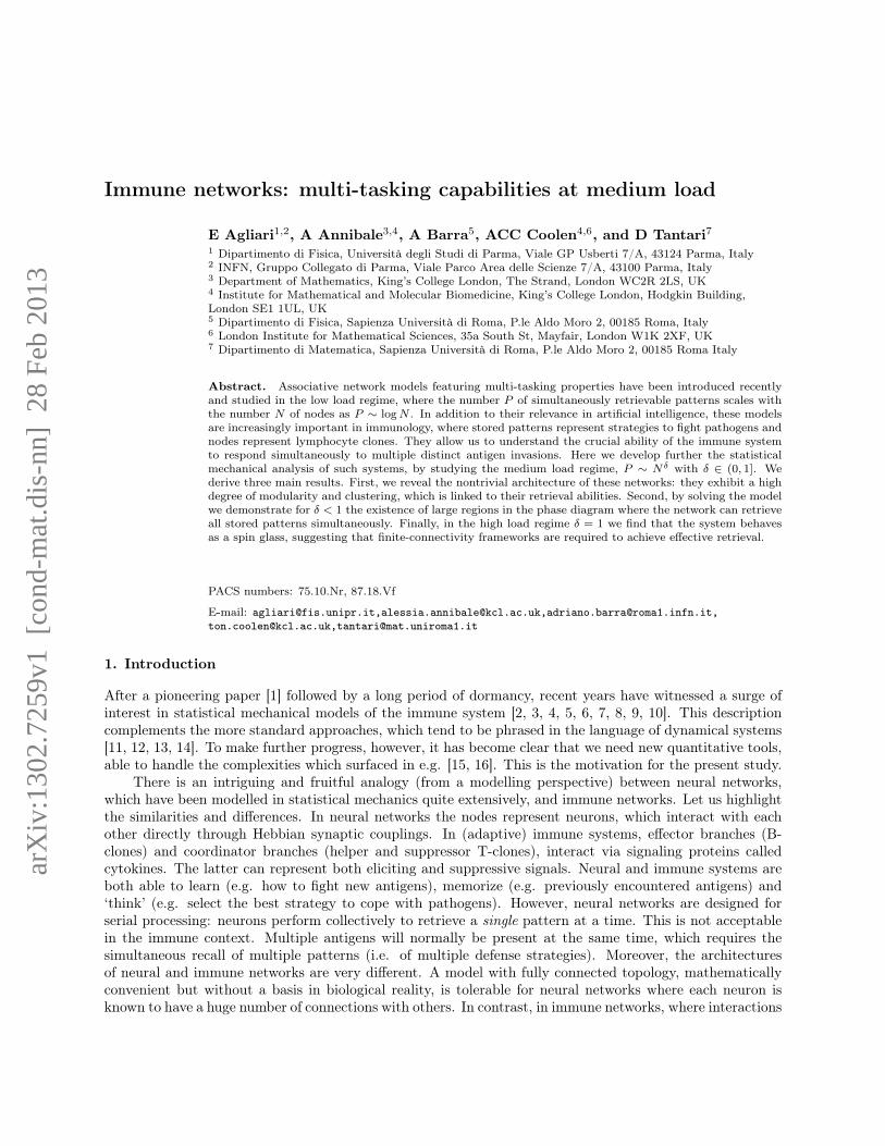
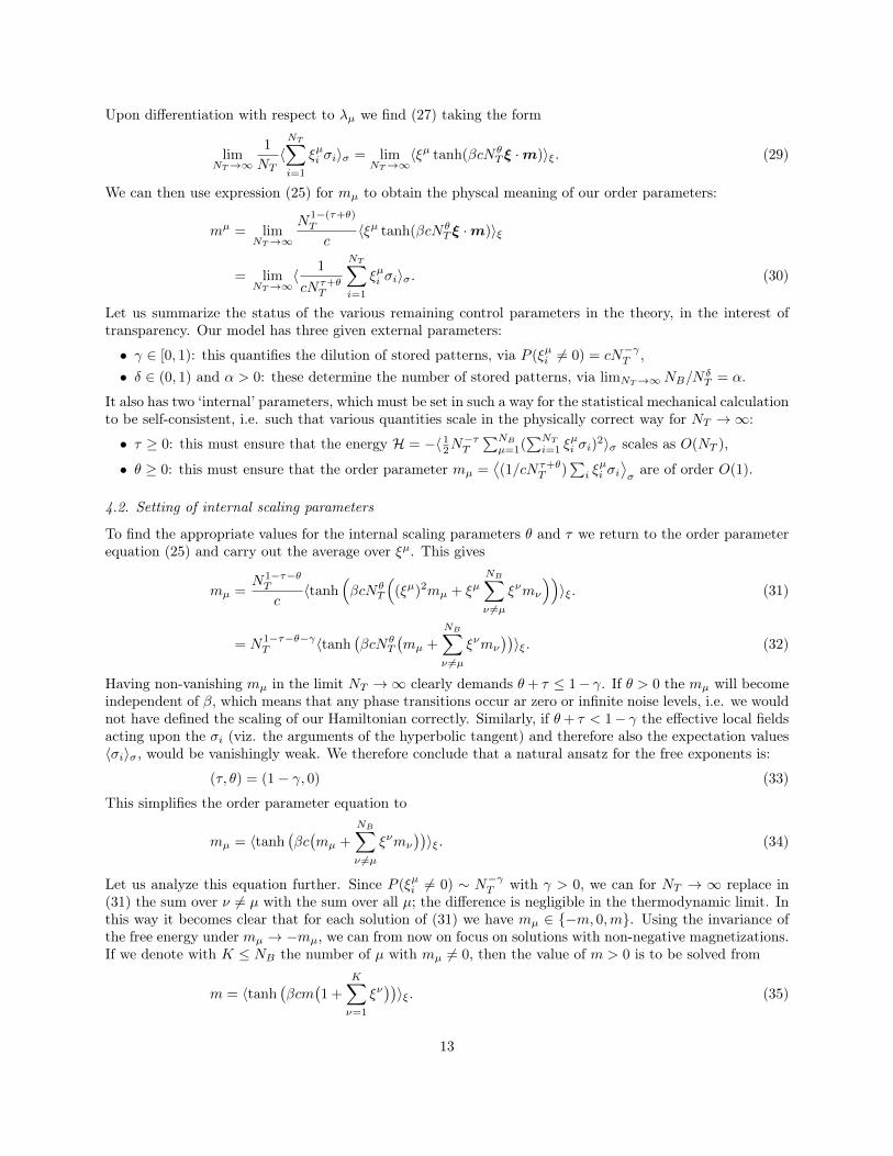
Figure 2. Statistical properties of individual links in randomly generated instances of the graph G atdifferent sizes NT , with NB = αNδ

T . We measured the mean coupling 〈J〉 (left), the mean squared coupling〈J2〉 (middle) and the probability P (J = 0) of a zero link (right), for different values of γ. The parametersδ = 1 and α = 0.5 are kept fixed. Solid lines: predictions given in (9) and (12). Markers: simulation data.

see also Appendix A.1 for a more rigorous derivation of P (J = 0|NB , NT , γ, c). Given the assumed scalingof NB , we get P (J 6= 0|NB(α, δ,NT ), NT , γ, c) ≈ 1− e−αc2NT δ−2γ

, which translates into

P (J 6= 0|NB(α, δ,NT ), NT , γ, c) ≈

αc2NTδ−2γ if 2γ > δ

1− e−αc2 if 2γ = δ1 if 2γ < δ

, (12)

This quantity can be interpreted as the average link probability in G. The average degree z over the wholeset of nodes‖ can then be written as

z = NTP (J 6= 0). (13)

Thus, if we adopt a mean-field approach based only on the estimates (12,13), we find that G can display thefollowing topologies, expressed in terms of the average degree z of G (the average number of links per node):

0 < γ < 1 γ = 1

δ < 2γ − 1 fully disconnected, z → 0 fully disconnected, z → 0

δ = 2γ − 1 finitely connected, z = O(1) finitely connected, z = O(1)

2γ − 1 < δ < 2γ extremely diluted, z →∞ but z/NT → 0 ——

δ = 2γ finitely diluted, z = O(NT ) ——

δ > 2γ fully connected, z = NT ——

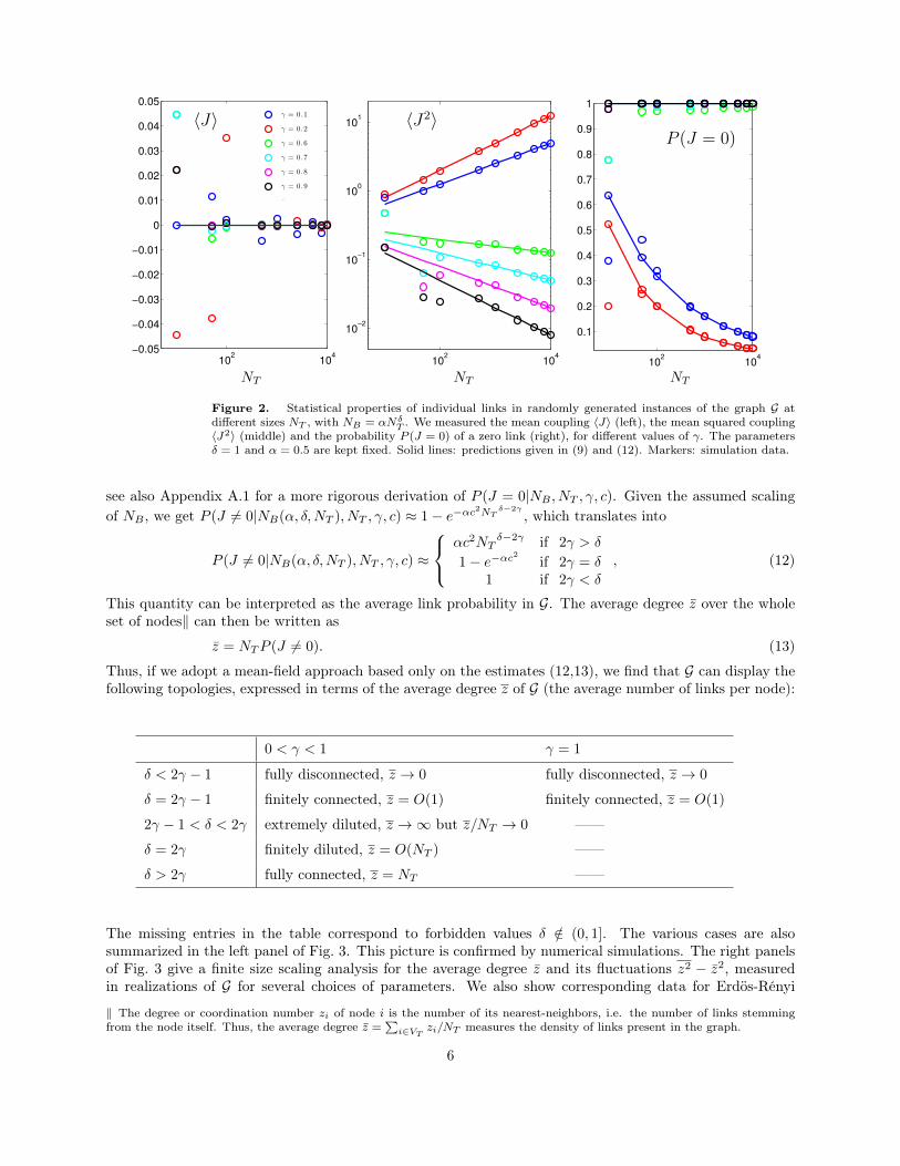
The missing entries in the table correspond to forbidden values δ /∈ (0, 1]. The various cases are alsosummarized in the left panel of Fig. 3. This picture is confirmed by numerical simulations. The right panelsof Fig. 3 give a finite size scaling analysis for the average degree z and its fluctuations z2 − z2, measuredin realizations of G for several choices of parameters. We also show corresponding data for Erdös-Rényi

‖ The degree or coordination number zi of node i is the number of its nearest-neighbors, i.e. the number of links stemmingfrom the node itself. Thus, the average degree z =

∑i∈VT zi/NT measures the density of links present in the graph.

6

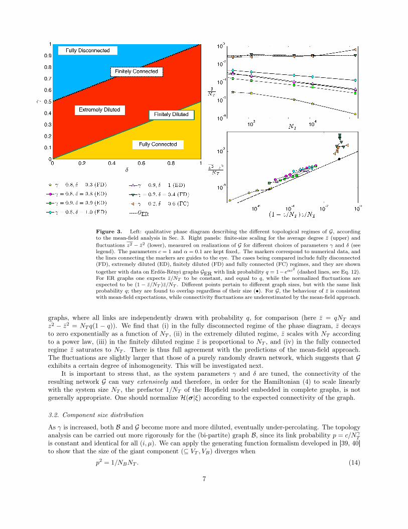
Figure 3. Left: qualitative phase diagram describing the different topological regimes of G, accordingto the mean-field analysis in Sec. 3. Right panels: finite-size scaling for the average degree z (upper) andfluctuations z2 − z2 (lower), measured on realizations of G for different choices of parameters γ and δ (seelegend). The parameters c = 1 and α = 0.1 are kept fixed,. The markers correspond to numerical data, andthe lines connecting the markers are guides to the eye. The cases being compared include fully disconnected(FD), extremely diluted (ED), finitely diluted (FD) and fully connected (FC) regimes, and they are showntogether with data on Erdös-Rènyi graphs GER with link probability q = 1−eαc2 (dashed lines, see Eq. 12).For ER graphs one expects z/NT to be constant, and equal to q, while the normalized fluctuations areexpected to be (1 − z/NT )z/NT . Different points pertain to different graph sizes, but with the same linkprobability q; they are found to overlap regardless of their size (•). For G, the behaviour of z is consistentwith mean-field expectations, while connectivity fluctuations are underestimated by the mean-field approach.

graphs, where all links are independently drawn with probability q, for comparison (here z = qNT andz2 − z2 = NT q(1 − q)). We find that (i) in the fully disconnected regime of the phase diagram, z decaysto zero exponentially as a function of NT , (ii) in the extremely diluted regime, z scales with NT accordingto a power law, (iii) in the finitely diluted regime z is proportional to NT , and (iv) in the fully connectedregime z saturates to NT . There is thus full agreement with the predictions of the mean-field approach.The fluctuations are slightly larger that those of a purely randomly drawn network, which suggests that Gexhibits a certain degree of inhomogeneity. This will be investigated next.

It is important to stress that, as the system parameters γ and δ are tuned, the connectivity of theresulting network G can vary extensively and therefore, in order for the Hamiltonian (4) to scale linearlywith the system size NT , the prefactor 1/NT of the Hopfield model embedded in complete graphs, is notgenerally appropriate. One should normalize H(σ|ξ) according to the expected connectivity of the graph.

3.2. Component size distribution

As γ is increased, both B and G become more and more diluted, eventually under-percolating. The topologyanalysis can be carried out more rigorously for the (bi-partite) graph B, since its link probability p = c/Nγ

T

is constant and identical for all (i, µ). We can apply the generating function formalism developed in [39, 40]to show that the size of the giant component (⊆ VT , VB) diverges when

p2 = 1/NBNT . (14)

7

2 4 6 8 10

10−2

10−1

100

P(s|N

B,N

T,γ,c)

γ = 2, δ = 1

γ = 0.95, δ = 0.95

γ = 0.9, δ = 0.9

γ = 0.97, δ = 0.9

γ = 0.9, δ = 0.8

γ = 0.9, δ = 0.6

0 10 20 30 40 50 6010

−8

10−6

10−4

10−2

100

P(z

|NB,N

T,γ,c)

γ = δ = 0.8

γ = δ = 0.9

γ = 0.8, δ = 1

γ = 0.9, δ = 1

s z

Figure 4. Left: distribution of component sizes of the graph G, for δ = c = 1, α = 0.1 and differentvalues of γ. Symbols represent simulation data; the solid line represents the analytical estimate for theunderpercolated case (�). Right: degree distributions obtained for different values of δ and γ, with α = 0.1and c = 1 kept fixed. The semi-logarithmic scale highlights the exponential decay at large values of z.

Hence, upon setting NB = αNδT , the percolation threshold for the bipartite graph B is defined by

N2γ−1−δT = c2α = O(N0

T ) ⇒ γ = (δ + 1)/2, (15)

which is consistent with the results of Section 3; we refer to Appendix A.2 for full details. Belowthe percolation threshold the generating function formalism also allows us to get the distributionPB(s|NT , NB , c, γ) for the size s of the small components occurring in B. A (connected) component ofan undirected graph is an isolated subgraph in which any two vertices are connected to each other by paths;the size of the component is simply the number of nodes belonging to the component itself. We prove inAppendix A.2 that just below the percolation threshold, PB(s|NB , NT , c, γ) scales exponentially with s. Onefinds that this is true also for the distribution PG(s|NB , NT , c, γ) of graph G (see Figure 4, left panel).

Interestingly, the small components of G that emerge around and below the percolation threshold playa central role in the network’s retrieval performance. To see this, one may consider the extreme case wherethe bi-partite graph B consists of trimers only. Here each node µ ∈ VB is connected to two nodes i1, i2 ∈ VT ,that is |ξµi1 | = |ξµi2 | = 1 and ξνi1 = ξνi2 = 0,∀ν 6= µ. The associated graph G is then made up of dimers(i1, i2) only, and Jij ∈ {−1, 0, 1} for all (i, j). The energetically favorable helper cell configuration σ isnow the one where

∑i ξµi σi = ±2, for any µ. This implies that retrieval of all patterns is accomplished

(under proper normalization). In the opposite extreme case, B is fully connected, and the helper cell systembecomes a Hopfield network where parallel retrieval is not realized. In general, around and below thepercolation threshold, the matrix ξ turns out to be partitioned, which implies that also the coupling matrixJ is partitioned, and each block of J corresponds to a separate component of the overall graph G. Forinstance, looking at the bipartite graph B, a star-like module with node µ ∈ VB at its center and the nodesi1, i2, ..., in ∈ VT as leaves¶ can occur when the leaves share a unique non-null µ-th entry in their patterns,that is |ξµi1 | = |ξ

µi2| = ... = |ξµin | = 1. For the graph G this module corresponds to a complete sub-graph Kn

of n ≤ NT nodes. In this case the retrieval of pattern µ is trivially achieved. In fact, a complete sub-graphKn in G can originate from more general arrangements in B: each leaf i can display several other null entriesbeyond µ, but these are not shared, that is ξνi ξνj = 0 ∀j ∈ VT , ν 6= µ ∈ VB . For instance, all stars withcenters belonging to VB and with leaves of length 1 or 2 fall into this extended class. Again, the retrieval ofpattern µ and possibly of further patterns ν is achieved. However, the mutual signs of magnetizations areno longer arbitrary, as the terms mµξ

µi = mνξ

νi are subject to constraints.

We can further generalize the topology of components in G compatible with parallel retrieval, byconsidering cliques (i.e. subsets of nodes such that every two nodes in the subset are connected by an

¶ The opposite case of a star-like module with the center belonging to VT is unlikely, given that NT > NB .

8

δ = 0.8, γ = 0.8 δ = 0.9, γ = 0.9

δ = 1.0, γ = 0.8 δ = 1.0, γ = 0.9

Figure 5. Plots of numerically generated graphs G for NT = 104 and α = 0.1, and different combinationsof (δ, γ). All isolated nodes have been omitted from the plots. The chosen parameter combinations all givegraphs that are just below the percolation threshold δ = 2γ − 1. However, the two graphs at the top satisfythe further condition δ ≤ γ that marks the ability of simultaneous pattern retrieval (via weakly connectedsmall cliques). In the bottom graphs this latter condition is violated, so these would behave more likeconventional Hopfield networks (here simultaneous retrieval of multiple patterns is not possible).

edge), which are joined together by one link: each clique consists of nodes ∈ VT that share the same non-nullentry, so that the unique link between two cliques is due to a node displaying at least two non-null entries.This kind of structure exhibits a high degree of modularity; each clique is a module and corresponds to adifferent pattern. As for retrieval, this arrangement works fine as there is no interference between the signalon each node in VT . For this arrangement to occur a sufficient condition is that B is devoid of squares, sothat two nodes ∈ VT do not share more than one neighbor. This implies that, among the n nodes connectedto j ∈ VB , the probability that any number k > 2 of these display another common neighbor is vanishing:

limNT→∞

n∑

k>2

(nk

)pk(1−p)n−k = lim

NT→∞

{1−

(1− c

Nγ

)n− cn

Nγ

(1− c

Nγ

)n−1 }= 0. (16)

Since n ∼ Nδ−γT , we obtain the condition γ ≥ δ. Examples of numerically generated graphs G, for different

choices of parameters, are shown in Fig. 5.

9

0 0.2 0.4 0.6 0.8 110

0

101

102

103

104

C

P(C

|NB,N

T,γ,c)

0 0.2 0.4 0.6 0.8 110

0

101

102

103

104

C

P(C

|NB,N

T,γ,c)

0 0.2 0.4 0.6 0.8 110

0

101

102

103

104

C

P(C

|NB,N

T,γ,c)

0 0.2 0.4 0.6 0.8 110

0

101

102

103

104

C

P(C

|NB,N

T,γ,c)

γ = 0.8, δ = 1 γ = 0.9, δ = 1

γ = δ = 0.9γ = δ = 0.8

Figure 6. Histograms for P (C|NB , NT , γ, c), normalized such that P (C|NB , NT , γ, c) = 1 for those valuesof C that have the lowest occurrence frequency. This normalization allows to highlight the intermediateregion, where the frequencies are much lower than those pertaining to C = 0 and C = 1. The results shownhere refer to graphs with NT = 104 nodes, α = 0.1 and c = 1, while δ and γ are varied.

3.3. Clustering properties

We saw that in the operationally most important parameter regime the graph G is built of small cliqueswhich are poorly (if at all) connected to each other. This means that non-isolated nodes are highly clusteredand the graph will have a high degree of modularity, i.e. dense connections between nodes within the same‘module’, but sparse connections between nodes in different ‘modules’. The clustering coefficient Ci of anode i measures how close its zi neighbors are to being a clique. It is defined as

Ci = 2Ei/zi(zi − 1), (17)

where Ei is the number of links directly connecting nodes pairs in Vi, while 12zi(zi − 1) is the total number

of non-ordered node pairs in Vi. Hence Ci ∈ [0, 1]. The average clustering coefficient C = N−1B,T

∑i∈VB,T Ci

measures the extent to which nodes in a graph tend to cluster together. It is easy to see that for a bipartitegraph, by construction, Ci = 0 for any node, while for homogeneous graphs the local clustering coefficients arenarrowly distributed around C. For instance, for the Erdös-Rény random graph, where links are identicallyand independently drawn with probability q, the local coefficients are peaked around q. As for our graphs G,due to their intrinsic inhomogeneity, the global measure C would give only limited information. In contrast,the distribution P (C|NB , NT , γ, c) of local clustering coefficients informs us about the existence and extentof cliques or ‘bulk’ nodes, which would be markers of low and high recall interference, respectively. Indeed,as shown in Figure 6, in the highly-diluted regime most of the nodes in G are either highly clustered, i.e.exhibiting Ci = 1, or isolated, with Ci = 0, whereas the coefficients of the remaining nodes are distributedaround intermediate values with average decreasing with γ, as expected. In particular, when both δ and γare relatively large, P (C|NB , NT , γ, c) approaches a bimodal distribution with peaks at C = 0 and C = 1,whereas when δ is sufficiently larger than γ, there exists a fraction of nodes with intermediate clusteringwhich make up a bulk. Therefore, although the density of links is rather small, the average clusteringcoefficient is very high, and this is due to the fragmentation of the graph into many small cliques.

To measure the extent of modular structures we constructed the topological overlap matrix T, whoseentry Tij =

∑k 6=i,j cikcjk/zi ∈ [0, 1] returns the normalized number of neighbors that i and j share. The

10

1 50 100 150 200

1

50

100

150

20050 100 150 200

1

50

100

150

200

1 50 100 150 200

1

50

100

150

2001 50 100 150 200

1

50

100

150

200

1 100 2001

100

200

γ = δ = 0.8

γ = 0.8, δ = 1 γ = 0.9, δ = 1

γ = δ = 0.9

GER

Figure 7. Overlap matrix T with entries Tij =∑k 6=i,j cikcjk/zi. The nodes are ordered such that nodes

with large overlaps are adjacent, and the most significant part of T is around the diagonal. Note: Tii = 1 forall i, by construction. Darker colours correspond to larger entries, and any extended coloured zone denotesa module, i.e. a set of nodes that are highly clustered and possibly not connected with the remaining nodes.These plots refer to numerically generated graphs with NT = 104 nodes, α = 0.1 and c = 1, while δ and γare varied. To avoid cluttering of the figures, only a fraction 200× 200 of each pattern is shown. A similarfraction of the overlap matrix for an extremely diluted Erdös-Rènyi graph made of 104 nodes is also depictedfor comparison (inset). In this case there is no evidence of modularity; T displays a homogeneous pattern.

related patterns for several choices of parameters are shown in the plots of Fig. 7, and compared to those ofErdös-Rènyi graphs GER. For Erdös-Rènyi graphs T displays a homogeneous pattern, that is very differentfrom the highly clustered cases emerging from G. In particular, for the highly diluted cases considered here,we find that smaller values of γ induce a smaller number of modules, that are individually increasing in size.

4. Medium storage regime in extremely diluted connectivity: retrieval region

We now turn to the statistical mechanics analysis, and consider the immune network model composed of NTT-clones (σi, i = 1, . . . , NT ) and NB B-clones (bµ, µ = 1, . . . , NB), such that the number ratio scales as

limNT→∞

NB/NδT = α, δ ∈ (0, 1), α > 0 (18)

The effective interactions in the reduced network with helper cells only are described by the Hamiltonian

H(σ|ξ) = − 1

2NτT

NT∑

i,j=1

NB∑

µ=1

ξµi ξµj σiσj , (19)

11

where the cytokine components ξµi ∈ {0,±1} are quenched random variables, independently and identicallydistributed according to

P (ξµi = 1) = P (ξµi = −1) = c/2NγT , P (ξµi = 0) = 1− c/Nγ

T (20)

with γ ∈ [0, 1). The parameter τ must be chosen such thatH(σ|ξ) scales linearly withNT , and must thereforedepend on γ and δ. Heuristically, since the number of non-zero entries Nnz in a generic pattern (ξµ1 , . . . , ξ

µNT

)

is O(N1−γT ), we expect that the network can retrieve a number of patterns of order O(NT /Nnz) = O(Nγ

T ).We therefore expect to see changes in τ only when crossing the region in the (γ, δ) plane where patternsparseness prevails over storage load (i.e. δ < γ, where the system can recall all patterns), to the oppositesituation, where the load is too high and frustration by multiple inputs on the same entry drives the networkto saturation (i.e. δ > γ). To validate this scenario, which is consistent with our previous topologicalinvestigation, we carry out a statistical mechanical analysis, based on computing the free energy

f(β) = − limNT→∞

1

βNT〈logZNT (β, ξ)〉ξ. (21)

4.1. Free energy computation and physical meaning of the parameters

If the number of patterns is sufficiently small compared to NT , i.e. δ < 1, we do not need the replica method;we can simply apply the steepest descent technique using the NB � NT / logNT Mattis magnetizations asorder parameters:

f(β) = − 1

βlog 2− lim

NT→∞

1

βNTlog

∫dm e

− 12m

2+NT 〈log cosh(√β/NτTξ·m)〉

ξ . (22)

with m = (m1, . . . ,mNB ), ξ = (ξ1, . . . , ξNB ) and ξ ·m =∑µ ξ

µmµ. Rescaling of the order parameters via

mµ → mµ

√βcN

τ/2+θT then gives

f(β) = − 1

βlog 2− lim

NT→∞

1

βNTlog

∫dm e

NT(− βc

2

2 Nτ+2θ−1T m2+〈log cosh(βcNθTξ·m)〉

ξ

), (23)

Hence, provided the limit exists, we may write via steepest descent integration:

f(β) = − 1

βlog 2− 1

βlim

NT→∞extrm

[⟨log cosh

(βcNθ

T ξ ·m)⟩ξ− βc2

2Nτ+2θ−1T m2

]. (24)

Differentiation with respect to the mµ gives the self consistent equations for the extremum:

mµ =N1−τ−θT

c〈ξµ tanh(βcNθ

T ξ ·m)〉ξ. (25)

With the additional new parameter θ, we now have two parameters with which to control separately twotypes of normalization: the normalization of the Hamiltonian, via τ , and the normalization of the orderparameters, controlled by θ. To carry out this task properly, we need to understand the physical meaning ofthe order parameters. This is done in the usual way, by adding suitable external fields to the Hamiltonian:

H → H−NB∑

µ=1

λµ

NT∑

i=1

ξµi σi (26)

Now, with 〈g(σ)〉σ = Z−1NT

(β, ξ)∑σ e−βH(σ|ξ)g(σ) and the corresponding new free energy f(β,λ),

limNT→∞

1

NT〈NT∑

i=1

ξµi σi〉σ = −∂f(β,λ)

∂λµ

∣∣∣λ=0

, (27)

with the short-hand λ = (λ1 . . . , λNB ). The new free energy is then found to be

f(β,λ) = − 1

βlog 2− 1

βlim

NT→∞extrm

[⟨log cosh

(βξ · [cNθ

Tm+λ])⟩ξ− βc2

2Nτ+2θ−1T m2

](28)

12

Upon differentiation with respect to λµ we find (27) taking the form

limNT→∞

1

NT〈NT∑

i=1

ξµi σi〉σ = limNT→∞

〈ξµ tanh(βcNθT ξ ·m)〉ξ. (29)

We can then use expression (25) for mµ to obtain the physcal meaning of our order parameters:

mµ = limNT→∞

N1−(τ+θ)T

c〈ξµ tanh(βcNθ

T ξ ·m)〉ξ

= limNT→∞

〈 1

cNτ+θT

NT∑

i=1

ξµi σi〉σ. (30)

Let us summarize the status of the various remaining control parameters in the theory, in the interest oftransparency. Our model has three given external parameters:

• γ ∈ [0, 1): this quantifies the dilution of stored patterns, via P (ξµi 6= 0) = cN−γT ,• δ ∈ (0, 1) and α > 0: these determine the number of stored patterns, via limNT→∞NB/N

δT = α.

It also has two ‘internal’ parameters, which must be set in such a way for the statistical mechanical calculationto be self-consistent, i.e. such that various quantities scale in the physically correct way for NT →∞:

• τ ≥ 0: this must ensure that the energy H = −〈 12N−τT∑NBµ=1(

∑NTi=1 ξ

µi σi)

2〉σ scales as O(NT ),

• θ ≥ 0: this must ensure that the order parameter mµ =⟨(1/cNτ+θ

T )∑i ξµi σi⟩σare of order O(1).

4.2. Setting of internal scaling parameters

To find the appropriate values for the internal scaling parameters θ and τ we return to the order parameterequation (25) and carry out the average over ξµ. This gives

mµ =N1−τ−θT

c〈tanh

(βcNθ

T

((ξµ)2mµ + ξµ

NB∑

ν 6=µ

ξνmν

))〉ξ. (31)

= N1−τ−θ−γT 〈tanh

(βcNθ

T

(mµ +

NB∑

ν 6=µ

ξνmν

))〉ξ. (32)

Having non-vanishing mµ in the limit NT →∞ clearly demands θ+ τ ≤ 1− γ. If θ > 0 the mµ will becomeindependent of β, which means that any phase transitions occur ar zero or infinite noise levels, i.e. we wouldnot have defined the scaling of our Hamiltonian correctly. Similarly, if θ+ τ < 1− γ the effective local fieldsacting upon the σi (viz. the arguments of the hyperbolic tangent) and therefore also the expectation values〈σi〉σ, would be vanishingly weak. We therefore conclude that a natural ansatz for the free exponents is:

(τ, θ) = (1− γ, 0) (33)

This simplifies the order parameter equation to

mµ = 〈tanh(βc(mµ +

NB∑

ν 6=µ

ξνmν

))〉ξ. (34)

Let us analyze this equation further. Since P (ξµi 6= 0) ∼ N−γT with γ > 0, we can for NT → ∞ replace in(31) the sum over ν 6= µ with the sum over all µ; the difference is negligible in the thermodynamic limit. Inthis way it becomes clear that for each solution of (31) we have mµ ∈ {−m, 0,m}. Using the invariance ofthe free energy under mµ → −mµ, we can from now on focus on solutions with non-negative magnetizations.If we denote with K ≤ NB the number of µ with mµ 6= 0, then the value of m > 0 is to be solved from

m = 〈tanh(βcm

(1 +

K∑

ν=1

ξν))〉ξ. (35)

13

It is not a priori obvious how the number K of nonzero magnetizations (i.e. the number of simultaneouslytriggered clones) can or will scale with NT . We therefore set K = φNδ′

T , in which the condition K ≤ NBthen places the following conditions on φ and δ′: δ′ ∈ [0, δ], and φ ∈ [0,∞) if δ′ < δ or φ ∈ [0, α] if δ′ = δ.We expect that if K is too large, equation (35) will only have the trivial solution for NT → ∞, so therewill be further conditions on φ and δ′ for the system to operate properly. If δ′ > γ, the noise due to othercondensed patterns (i.e. the sum over ν) becomes too high, and m can only be zero:

E

[( K∑

µ=1

ξµ)2]

=

K∑

µ=1

E[ξµ2] = φcNδ′

T

NγT

→∞. (36)

On the other hand, if δ′ < γ this noise becomes negligible, and (35) reduces to the Curie-Weiss equation,whose solution is just the Mattis magnetization [20, 36, 41]. It follows that the critical case is the one wherewhen δ′ = γ. Here we have for NT →∞ the following equation for m:

m =∑

k∈Zπ(k|φ) tanh(βcm(1 + k)) (37)

with the following discrete noise distribution, which obeys π(−k|φ) = π(k|φ):

π(k|φ) =⟨δk,∑∞µ=1 ξ

µ

⟩ξ

(38)

4.3. Computation of the noise distribution π(k)

Given its symmetry, we only need to calculate π(k|φ) for k ≥ 0:

π(k|φ) = limK→∞

∫ π

−π

dψ

2πe−iψk

⟨eiψξ

⟩Kξ

= limK→∞

∫ π

−π

dψ

2πe−iψk

(1 +

cφ

K(cosψ − 1)

)K

=

∫ π

−π

dψ

2πe−iψk+φc(cosψ−1)

= e−φc∫ π

−π

dψ

2πe−iψk

∑

n≥0

(φc)n

2nn!(eiψ + e−iψ)n

= e−φc∫ π

−π

dψ

2πe−iψk

∑

n≥0

(φc)n

2nn!

∑

l≤n

n!

l!(n− l)!e−iψ(k−n+2l)

= e−φc∑

n≥0

∑

l≤n

(φc

2

)n1

l!(n− l)!δn,k+2l

= e−φc∑

l≥0

(φc

2

)k+2l1

l!(k + l)!= e−φc Ik(φc) (39)

where Ik(x) is the k-th modified Bessel function of the first kind [53]. These modified Bessel functions obey

2k

xIk(x) = Ik−1(x)− Ik+1(x),

2d

dxIk(x) = Ik−1(x) + Ik+1(x). (40)

The first identity leads to a useful recursive equation for π(k|φ), and the second identity simplifies ourcalculation of derivatives of π(k|φ) with respect to φ, respectively:

π(k−1|φ)− π(k+1|φ)− 2π(k|φ)k

φc= 0, (41)

d

dφπ(k|φ) = c

(1

2π(k−1|φ) +

1

2π(k+1|φ)− π(k|φ)

)(42)

14

4.4. Retrieval in the zero noise limit

To emphasize the dependence of the recall overlap on φ, viz. the relative storage load, we will from nowon write m → mφ. With the abbreviation 〈g(k)〉k =

∑k π(k|φ)g(k), and using (41) and the symmetry of

π(k|φ), we can transfer our equation (37) into a more convenient form:

mφ =1

2〈[

tanh(βcmφ(1+k)) + tanh(βcmφ(1−k))]〉k

=1

2

∑

k∈Z

[π(k−1|φ)− π(k+1|φ)

]tanh(βcmφk) =

1

φc〈k tanh(βcmφk)〉k (43)

In the zero noise limit β →∞, where tanh(βy)→ sgn(y), this reduces to mφ = 1φc 〈|k|〉k, or, equivalently,

mφ = limβ→∞

〈tanh(βcm(1+k))〉k = 〈sign(1+k)〉k

=∑

k>−1

π(k)−∑

k<−1

π(k) = π(0|φ) + π(1|φ), (44)

Hence we always have a nonzero rescaled magnetization, for any relative storage load φ. To determine forwhich value of φ this state is most stable, we have to insert this solution into the zero temperature formulafor the free energy and find the minimum with respect to φ. Here, with mµ = mφ for all µ ≤ K = φNγ

T andmµ = 0 for µ > K, the free energy (24) takes asymptotically the form

f(β) =1

2c2φm2

φ −1

β〈log cosh (βcmφk)〉k −

1

βlog 2 (45)

So for β →∞, and using our above identity 〈|k|〉k = φcm, we find that the energy density is

u(φ) = limβ→∞

f(β) =1

2c2φm2

φ − cm〈|k|〉k = −1

2c2φm2

φ (46)

= − 1

2c2φ(π(0|φ)+π(1|φ)

)2 (47)

To see how this depends on φ we may use (42), and find1

c2d

dφu(φ) = − 1

2m2φ − φmφ

d

dφ

(π(0|φ)+π(1|φ)

)

= − 1

2m2φ − φcmφ

(− 1

2π(0|φ) +

1

2π(2|φ)

)= −1

2m2φ +mφπ(1|φ)

= − 1

2mφ

(mφ − 2π(1|φ)

)= −1

2mφ

(π(0|φ)− π(1|φ)

)< 0 (48)

The energy density u(φ) is apparently a decreasing function of φ, which reaches its minimum when thenumber of condensed patterns is maximal, at φ = α. However, the amplitude of each recalled pattern willalso decrease for larger values of φ:

d

dφmφ =

d

dφπ(0|φ) +

d

dφπ(1|φ) = −π(1|φ)/φ < 0 (49)

Hence mφ starts at m0 = 1, due to π(k|0) = δk,0, and then decays monotonically with φ. Moreover, it followsfrom 〈|k|〉2k ≤ 〈k2〉k = 〈∑µ≤K(ξµ)2〉ξ = φc that

mφ = 〈|k|〉k/φc ≤ 1/√φc, u(φ) = −1

2c2φm2

φ ≥ −1

2c (50)

If we increase the number of condensed patterns, the corresponding magnetizations decrease in such a waythat the energy density remains finite.

15

0 2 4 6 8 100

0.1

0.2

0.3

0.4

0.5

0.6

0.7

0.8

0.9

1

φ

0 0.5 1 1.5 20

0.1

0.2

0.3

0.4

0.5

0.6

0.7

T

m

φ = 1

φ = 2

φ = 3

φ = 4

0 5 10

−0.3

−0.2

−0.1

0

φu(φ

)

m(φ)

√φm(φ)

Figure 8. Left: energy density u versus the relative fraction of retrieved patterns, in terms of φ = cφand T = T/c = 1/βc. The minimum energy density is reached when φ is maximal, i.e. when all storedpatterns are simultaneously retrieved, but with decreasing amplitude for each. Right: critical noise levelsfor different values of φ, confirming that T−1

c = βc = 1, independently of φ. In both the panels, solid linesrepresent our theoretical predictions, while symbols represent data from numerical simulations on systemswith NT = 5× 104, γ = δ = 0.45, c = 2 and with with standard sequential Glauber dynamics.

4.5. Retrieval at nonzero noise levels

To find the critical noise level (if any) where pattern recall sets in, we return to equation (25), which for(τ, θ) = (1−γ, 0) and written in vector notation becomes

m =NγT

c〈ξ tanh(βcξ ·m)〉ξ. (51)

We take the inner product on both sides with m and obtain a simple inequality:

m2 =NγT

c〈(ξ ·m) tanh(βcξ ·m)〉ξ

= βNγT 〈(ξ ·m)2

∫ 1

0

dx [1− tanh2(βcxξ ·m)]〉ξ

≤ βNγT 〈(ξ ·m)2〉ξ = βcm2 (52)

Since m2(1− βc) ≤ 0, we are sure that m = 0 for βc ≤ 1. At βc = 1 nontrivial solutions of the previouslystudied symmetric type are found to bifurcate continuously from the trivial solution. This can be seen byexpanding the amplitude equation (43) for small m:

mφ =1

φc〈k tanh(βcmφk)〉k

= βcmφ −1

3β3c2m3

φ〈k4〉k/φ+O(m4φ) (53)

This shows that the symmetric solutions indeed bifurcate via a second-order transition, at the φ-independentcritical temperature Tc = c, with amplitude mφ ∝ (βc − 1)

12 as βc → 1. All the above predictions

are confirmed by the results of numerical simulations, and by solving the order parameter equations andcalculating the free energy numerically, see Figure 8.

16

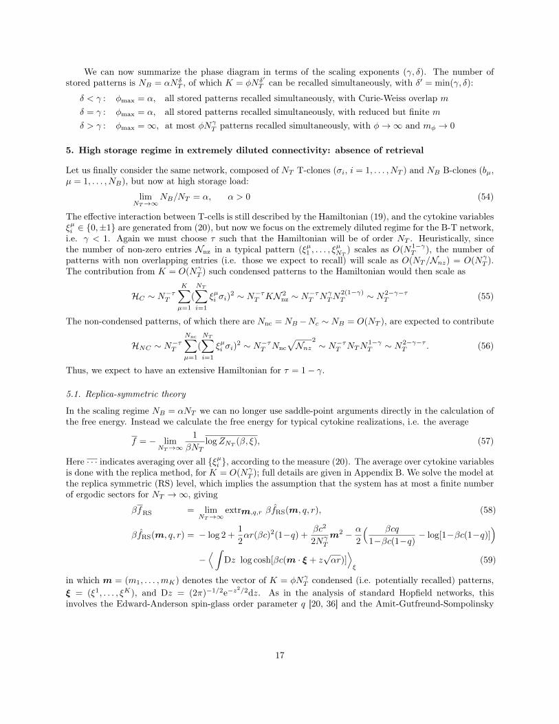
We can now summarize the phase diagram in terms of the scaling exponents (γ, δ). The number ofstored patterns is NB = αNδ

T , of which K = φNδ′

T can be recalled simultaneously, with δ′ = min(γ, δ):

δ < γ : φmax = α, all stored patterns recalled simultaneously, with Curie-Weiss overlap mδ = γ : φmax = α, all stored patterns recalled simultaneously, with reduced but finite mδ > γ : φmax =∞, at most φNγ

T patterns recalled simultaneously, with φ→∞ and mφ → 0

5. High storage regime in extremely diluted connectivity: absence of retrieval

Let us finally consider the same network, composed of NT T-clones (σi, i = 1, . . . , NT ) and NB B-clones (bµ,µ = 1, . . . , NB), but now at high storage load:

limNT→∞

NB/NT = α, α > 0 (54)

The effective interaction between T-cells is still described by the Hamiltonian (19), and the cytokine variablesξµi ∈ {0,±1} are generated from (20), but now we focus on the extremely diluted regime for the B-T network,i.e. γ < 1. Again we must choose τ such that the Hamiltonian will be of order NT . Heuristically, sincethe number of non-zero entries Nnz in a typical pattern (ξµ1 , . . . , ξ

µNT

) scales as O(N1−γT ), the number of

patterns with non overlapping entries (i.e. those we expect to recall) will scale as O(NT /Nnz) = O(NγT ).

The contribution from K = O(NγT ) such condensed patterns to the Hamiltonian would then scale as

HC ∼ N−τTK∑

µ=1

(

NT∑

i=1

ξµi σi)2 ∼ N−τT KN 2

nz ∼ N−τT NγTN

2(1−γ)T ∼ N2−γ−τ

T (55)

The non-condensed patterns, of which there are Nnc = NB −Nc ∼ NB = O(NT ), are expected to contribute

HNC ∼ N−τTNnc∑

µ=1

(

NT∑

i=1

ξµi σi)2 ∼ N−τT Nnc

√Nnz

2 ∼ N−τT NTN1−γT ∼ N2−γ−τ

T . (56)

Thus, we expect to have an extensive Hamiltonian for τ = 1− γ.

5.1. Replica-symmetric theory

In the scaling regime NB = αNT we can no longer use saddle-point arguments directly in the calculation ofthe free energy. Instead we calculate the free energy for typical cytokine realizations, i.e. the average

f = − limNT→∞

1

βNTlogZNT (β, ξ), (57)

Here · · · indicates averaging over all {ξµi }, according to the measure (20). The average over cytokine variablesis done with the replica method, for K = O(Nγ

T ); full details are given in Appendix B. We solve the model atthe replica symmetric (RS) level, which implies the assumption that the system has at most a finite numberof ergodic sectors for NT →∞, giving

βfRS = limNT→∞

extrm,q,r βfRS(m, q, r), (58)

βfRS(m, q, r) = − log 2 +1

2αr(βc)2(1−q) +

βc2

2NγT

m2 − α

2

( βcq

1−βc(1−q) − log[1−βc(1−q)])

−⟨∫

Dz log cosh[βc(m · ξ + z√αr)]

⟩ξ

(59)

in which m = (m1, . . . ,mK) denotes the vector of K = φNγT condensed (i.e. potentially recalled) patterns,

ξ = (ξ1, . . . , ξK), and Dz = (2π)−1/2e−z2/2dz. As in the analysis of standard Hopfield networks, this

involves the Edward-Anderson spin-glass order parameter q [20, 36] and the Amit-Gutfreund-Sompolinsky

17

uncondensed-noise order parameter r [20, 36]. We obtain self-consistent equations for the remaining RSorder parameters (m, q, r) simply by extremizing fRS(m, q, r), which leads to

mµ =NγT

c

⟨ξµ∫

Dz tanh[βc(m · ξ+z√αr)]

⟩ξ,

q =⟨∫

Dz tanh2[βc(m · ξ+z√αr)]

⟩ξ,

r =q

[1−βc(1−q)]2 . (60)

As before we deal with the equation for mµ by using the identity ξµ tanh(A) = tanh(ξµA) (sinceξµ ∈ {−1, 0, 1}) and by separating the term mµξµ from the sum m · ξ:

mµ =NγT

c

⟨∫Dz tanh[βc(mµ(ξµ)2 +

∑

ν 6=µ≤K

mνξνξµ + zξµ√αr)]

⟩ξ

=⟨∫

Dz tanh[βc(mµ +∑

ν 6=µ≤K

mνξν + z√αr)]

⟩ξ

=⟨∫

Dz tanh[βc(mµ +

K∑

ν=1

mνξν + z√αr)]⟩

ξ+O(N−γ)

Again we see that for NT → ∞ we will only retain solutions with mµ ∈ {−m, 0,m} for all µ ≤ K. Giventhe trivial sign and pattern label permutation invariances, we can without loss of generality consider onlynon-negative magnetizations, and look for solutions where mµ = m for µ = 1 ≤ K and zero otherwise. Wethen find

m =

∞∑

k=−∞

π(k)

∫Dz tanh[βc(m+mk + z

√αr)] (61)

with π(k) given in (39). We can now use the manipulations employed in the previous section, to find

m =

⟨k

φ

∫Dz tanh[βc(mk + z

√αr)]

⟩

k

(62)

q =

⟨∫Dz tanh2[βc(mk + z

√αr)]

⟩

k

, (63)

r =q

[1− βc(1− q)]2 .

The corresponding free energy assumes the form

βfRS(m, q, r) = − log 2 +1

2αr(βc)2(1−q) +

1

2βc2φm2− α

2

( βcq

1−βc(1−q)−log[1−βc(1−q)])

−⟨∫

Dz log cosh[βc(mk + z√αr)]

⟩k

(64)

Note that we recover the equations of the medium storage regime simply by putting α = 0.

5.2. The zero noise limit

We now show that in the high storage case the system behaves as a spin glass, even in the zero temperaturelimit β → ∞ where the retrieval capability should be largest. From (63) we deduce that q → 1 in the zeronoise limit, while the quantity C = βc(1− q) remains finite. Let us first send β →∞ in equation (62):

m =⟨kφ

∫Dz sgn

[mk +

z√α

1−C]⟩

k=⟨kφ

Erf(mk(1−C)√

2α

)⟩k, (65)

18

0 0.02 0.04 0.06 0.08 0.1

0.7

0.8

0.9

1

1.1

1.2

1.3

1.4

1.5

α

αr(α

) 10−3

10−2

10−1

101

102

103

α

r(α

)

0 10 20−0.5

−0.4

−0.3

−0.2

−0.1

0

Ξ

G(Ξ

)

Φ = 1

Figure 9. Left panel: Behavior of αr(α) versus α in the spin-glass state (the inset shows only r(α) versus α),as calculated from the RS order parameter equations. This shows that r(α) goes to infinity as α approacheszero, such that αr(α) remains positive; this means that the noise due to non-condensed patterns can neverbe neglected. Right panel: behavior of the function G(Ξ) versus Ξ. Since G(Ξ) < 0 for α > 0, equation (69)cannot have a solution for α > 0, and hence no pattern recall is possible even at zero noise.

with the error integral Erf(x) = (2/√π)∫ x

0dt e−t

2

. A second equation for the pair (m,C) follows from (63):

C = limβ→∞

βc⟨

1−∫

Dz tanh2[βc(mk + z√αr)]

⟩k

= limβ→∞

∂

∂m

⟨1

k

∫Dz tanh

[βc(mk +

z√αq

1−C)]⟩

k,

=∂

∂m

⟨1

kErf(mk(1−C)√

2α

)⟩

k

=

√2

απ(1−C)

⟨exp

(−m

2k2(1−C)2

2α

)⟩k

(66)

We thus have two coupled nonlinear equations (65,66), for the two zero temperature order parameters mand C. They can be further reduced by introducing the variable Ξ = m(1−C)/

√2α, with which we obtain

m =

⟨k

φErf(kΞ)

⟩

k

(67)

and rewriting Ξ = m(1−C)/√

2α gives

C = 1−√

2αΞ

m= 1−

√2αΞ

⟨kφ

Erf(kΞ)⟩−1

k. (68)

Using (66) and excluding the trivial solution Ξ = 0 (which always exists, but represents the spin glass statewithout pattern recall) we obtain after some simple algebra just a single equation, to be solved for Ξ:

√2α = G(Ξ) =

1

Ξ

⟨kφ

Erf(kΞ)⟩k− 2√

π

⟨e−k

2Ξ2⟩k

(69)

One easily shows that

limΞ→0

G(Ξ) = 0, limΞ→∞

G(Ξ) = − 2√ππ(0|φ). (70)

In fact further analytical and numerical investigation reveals that for Ξ > 0 the function G(Ξ) is strictlynegative; see Figure 9. Hence there can be no m 6= 0 solution for α > 0, so the system cannot recall thepatterns in the present scaling regime NB = αNT .

19

6. Conclusions

The immune system is a marvellous complex biological entity, able to execute reliably a number of verydifficult tasks that allow living beings to survive in competitive interaction with a living environment. Toaccomplish this it relies on a huge ensemble of functions and agents. In particular, the adaptive part of theimmune system relies on a broad ensemble of cells, e.g. B and T lymphocytes, and of chemical messengers, e.g.antibodies and cytokines. As for lymphocytes, one can distinguish between an ‘effector branch’, consistingof B-cells and killer T-cells, and an ‘organizational branch’, which coordinates the operation of the effectorbranch and consists mainly of helper and regulator T-cells. The latter control the activity of the effectorbranch through a rich and continuous exchange of cytokines, which are specific chemical messengers whichelicit or suppress effector actions.

From a theoretical point of view, a fascinating ability of the immune system is its simultaneousmanagement, by helpers and suppressors, of several B-clones at once; this is a key ability, as it impliesthe ability to defend the host from simultaneous attacks by several pathogens. Indeed, we investigated thisability in the present study, as an emergent, collective, feature of a spin glass model of the immune network,that describes the adaptive response performed by B-cells under the coordination of helpers and suppressors.In particular, the focus of this paper is on the ability of the T-cells to coordinate an extensive number ofB-soldiers, by fine-tuning the load of clones and the degree of dilution in the network. However, it is worthconsidering this parallel processing capability also from a slightly different perspective. Beyond the interestin multiple clonal expansions (which, in our language, is achieved trough signalling by +1 cytokines), thequiescence signals that are sent to the B-clones that are not expanding (which, in our language, is achievedtrough signalling by −1 cytokines) is fundamental for homeostasis. In fact, B-cells that are not receivinga significant amount of signals undergo a depauperation process called ”anergy" [30][31] and eventuallydie. Hence, in the present multitasking network, the capability of signaling simultaneously to all clones isfundamental, and with implications beyond solely the management of simultaneous clonal expansions; weemphasize that within our approach this is achieved in a rather natural way.

We first assumed that the number NB of B-cells scales with the number NT of T-cells as NB = αNδT ,

with δ < 1, and we modeled the interaction between B cells and T cells by means of an extremely dilutedbipartite spin-glass where the former are addressed only by a subset of T cells whose cardinality scales likeN1−γT , with γ ≤ 1. We proved that this system is thermodynamically equivalent to a diluted monopartite

graph, whose topological properties are shown to depend crucially on the parameters γ and δ. In particular,when γ ≥ δ the graph is fragmented into multiple disconnected components, each forming a clique or acollection of cliques typically connected via a bridge. Each clique corresponds to a pattern and this kindof arrangement easily allows for the simultaneous recall of multiple patterns. On the other hand, whenγ < δ, the effective network can exhibit a giant component, which prevents the system from simultaneouspattern recall. These results on the topology of the immune network are then approached from a statisticalmechanics angle: we analyse the operation of the system as an effective equilibrated stochastic process ofinteracting helper cells. We find that for γ > δ the network is able to retrieve perfectly all the stored patternssimultaneously, in perfect agreement with the topology-based prediction. When the load increases, i.e. whenNB becomes larger (so the exponent δ is increased), overlaps among bit entries of the ‘cytokine patterns’ tobe recalled become more and more frequent, and this gives rise to a new source of non-Gaussian interferencenoise that is non-negligible for γ ≤ δ. If γ = δ the system is still able to retrieve all the patterns, butwith a decreasing recall overlap. In the high storage case, for δ = 1, the network starts to feel also theGaussian noise due to non-condensed patterns, and this is found to destroy the retrieval states. Here thesystem behaves as a spin-glass, from which we deduce that an extremely diluted B-H network (i.e. one withγ < 1) is insufficiently diluted to sustain a high pattern load. Our predictions and results are tested againstnumerical simulations wherever possible, and we consistently find perfect agreement.

Despite the fact that it is experimentally well established that helpers are much more numerous thanB-cells, their relative sizes are still comparable in a statistical mechanical sense. The biological interest liesin the high storage regime, where the maximum number of pathogens can be fought simultaneously. Fromthe present study we now know that to bypass the spin-glass structure of the phase space at this load level,a projection of the model into a finite-connectivity topology (γ = 1) is required. This, remarkably, is also in

20

agreement with the biological picture of highly-selective touch-interactions among B and T cells. It is bothwelcome and encouraging that both biological data and statistical mechanical theory have now convergedto the same suggestion: that the most efficient and biologically most plausible operation regime is likely tobe that of finite connectivity for the effective helper-helper immune network. This must therefore be thedirection of the next stage of our research programme.

Acknowledgements

EA, AB and DT acknowledge the FIRB grant RBFR08EKEV and Sapienza Universitá di Roma for financialsupport. ACCC is grateful for support from the Biotechnology and Biological Sciences Research Council(BBSRC) of the United Kingdom. DT would like to thank King’s College London for hospitality.

References

[1] Parisi G 1990 Proc. Natl. Acad. Sci. USA 87 429-433[2] Barra A and Agliari E 2010 J. Stat. Mech. 07004[3] Agliari E, Asti L, Barra A and Ferrucci L 2012 Phys. Rev. E 85 051909[4] Agliari E, Barra A, Guerra F and Moauro F 2011 J. Theor. Biol. 287 48-63[5] Mora T, Walczak AM, Bialek W and Callan CG 2010 Proc. Natl. Acad. Sci. USA 107 5405-5410[6] Košmrlj A, Chakraborty AK, Kardar M and Shakhnovich EI 2009 Phys. Rev. Lett. 103 068103[7] Košmrlj A, Jha AK, Huseby ES, Kardar M and Chakraborty AK 2008 Proc. Natl. Acad. Sci. USA 105 16671-16676[8] Chakraborty AK and Košmrlj A 2011 Ann. Rev. Phys. Chem. 61 283-303[9] Schmidtchen H, Thüne M and Behn U 2012 Phys. Rev. E 86 011930

[10] Uezu T, Kadano C, Hatchett JPL and Coolen ACC 2006 Prog. Theor. Phys. 161 385-388[11] Perelson AS and Weisbuch G 1997 Rev. Mod. Phys. 69 1219-1267[12] De Boer RJ, Kevrekidis IG and Perelson AS 1993 Bull. Math. Biol. 55, 745-780 and 781-816[13] Nesterenko VG 1988 in Theoretical Immunology (AS Perelson Ed, Addison-Wesley, New York)[14] Farmer JD, Packard NH and Perelson AS 1986 Physica D 22, 187-204[15] Agliari E, Barra A, Galluzzi A, Guerra F and Moauro F 2012 Phys. Rev. Lett. 109 268101[16] Agliari E, Barra A, Bartolucci S, Galluzzi A, Guerra F and Moauro F 2012 submitted to Phys. Rev. E[17] Barra A, Genovese G, Guerra F 2010 J. Stat. Phys. 140, 784-796[18] Barra A, Bernacchia A, Contucci P and Santucci E 2012 Neural Networks 34 1-9[19] Barkai E, Kanter I, and Sompolinsky H 1990 Phys. Rev. A 41 1843-1854[20] Coolen ACC 2001 in Handbook of Biological Physics 4 (F Moss and S Gielen Eds, Elsevier, Amsterdam) 531-59[21] Perez-Castillo I, Wemmenhove B, Hatchett JPL, Coolen ACC, Skantzos NS and Nikoletopoulos T 2004 J. Phys. A: Math.

Gen. 37 8789-8799[22] Skantzos NS and Coolen ACC 2000 J.Phys. A: Math. Gen. 33 5785-5807[23] Sompolinsky H 1986 Phys. Rev. A 34 2571-2574[24] Wemmenhove B and Coolen ACC 2003 J. Phys. A: Math. Gen. 36 9617-9633[25] Janeway C, Travers P, Walport M and Shlomchik M 2005 Immunobiology (Garland Science Publishing, New York)[26] Abbas AK, Lichtman AH and Pillai S 2012 Cellular and Molecular Immunology (Elsevier, Philadelphia)[27] Barra A and Agliari E 2010 Physica A 389 5903-5911[28] 1999 The Cytokine Network and Immune Functions (Theze J Ed, Oxford University Press, Oxford)[29] 2002 Cytokine and Autoimmune Diseases (V Kuchroo, N Sarvetnick, D Hafler, L Nicholson Eds, Humana Press, Totowa)[30] Goodnow CC 1992 Ann. Rev. Immunol. 10 489-518[31] Goodnow CC 2005 Nature 435 590[32] Goodnow CC, Vinuesa CG, Randall KL, Mackay F and Brink R 2010 Nature Immun. 8, 681[33] Schwartz RH 2005 Nature Immun. 4 327[34] Derrida B, Gardner E and Zippelius A 1987 Europhys. Lett. 4 167-173[35] Wemmenhove B, Skantzos NS and Coolen ACC 2004 J. Phys. A: Math. Gen. 37 7653-7670[36] Amit DJ 1992 Modeling Brain Function: The World of Attractor Neural Networks (Cambridge University Press)[37] Coolen ACC, Kuehn R and Sollich P 2005 Theory of Neural Information Processing Systems (Oxford University Press)[38] Amit DJ, Gutfreund H and Sompolinsky H 1987 Phys. Rev. A 35 2293-2303[39] Newman MEJ 2002 Phys. Rev. E 66 016128[40] Allard A, Noël P-A, Dubé LJ and Pourbohloul B 2009 Phys. Rev. E 79 036113[41] Barra A 2008 J. Stat. Phys. 132 787-809[42] Perez-Vicente CJ and Coolen ACC 2008 J. Phys. A: Math. Theor. 41 255003[43] Agliari E and Barra A 2011 Europhys. Lett. 94 10002[44] Barra and Agliari E 2011 J. Stat. Mech. P02027[45] Burroughs NJ, De Boer RJ and Kesmir C 2004 Immunogen. 56 311-320[46] Depino AM 2010 Pro-Inflammatory Cytokines in Learning and Memory (Nova Science Publ, New York)[47] Ellis RS 1985 Entropy, Large Deviations and Statistical Mechanics (Springer, Berlin)

21

[48] Germain RN 2001 Science 293 240-245[49] Golomb D, Rubin N and Sompolinsky H 1990 Phys. Rev. A 41 1843-1854[50] Jaynes ET 1957 Phys. Rev. E 106 620-630 and Phys. Rev. E 108 171-190[51] Kitamura D 2008 How the Immune System Recognizes Self and Non Self (Springer, Berlin)[52] Mézard M, Parisi G and Virasoro MA 1987 Spin Glass Theory and Beyond (World Scientific, Singapore)[53] Abramowitz M and Stegun IA 1972 Handbook of Mathematical Functions (Dover, New York)

Appendix A. Topological properties

Appendix A.1. Rigorous calculation of link probability

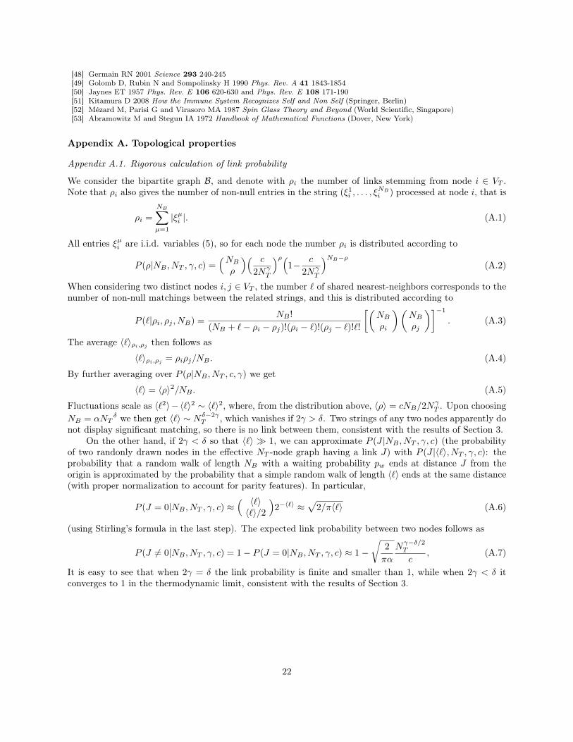
We consider the bipartite graph B, and denote with ρi the number of links stemming from node i ∈ VT .Note that ρi also gives the number of non-null entries in the string (ξ1

i , . . . , ξNBi ) processed at node i, that is

ρi =

NB∑

µ=1

|ξµi |. (A.1)

All entries ξµi are i.i.d. variables (5), so for each node the number ρi is distributed according to

P (ρ|NB , NT , γ, c) =(NBρ

)( c

2NγT

)ρ(1− c

2NγT

)NB−ρ(A.2)

When considering two distinct nodes i, j ∈ VT , the number ` of shared nearest-neighbors corresponds to thenumber of non-null matchings between the related strings, and this is distributed according to

P (`|ρi, ρj , NB) =NB !

(NB + `− ρi − ρj)!(ρi − `)!(ρj − `)!`!

[(NBρi

)(NBρj

)]−1

. (A.3)

The average 〈`〉ρi,ρj then follows as

〈`〉ρi,ρj = ρiρj/NB . (A.4)

By further averaging over P (ρ|NB , NT , c, γ) we get

〈`〉 = 〈ρ〉2/NB . (A.5)

Fluctuations scale as 〈`2〉−〈`〉2 ∼ 〈`〉2, where, from the distribution above, 〈ρ〉 = cNB/2NγT . Upon choosing

NB = αNTδ we then get 〈`〉 ∼ Nδ−2γ

T , which vanishes if 2γ > δ. Two strings of any two nodes apparently donot display significant matching, so there is no link between them, consistent with the results of Section 3.

On the other hand, if 2γ < δ so that 〈`〉 � 1, we can approximate P (J |NB , NT , γ, c) (the probabilityof two randonly drawn nodes in the effective NT -node graph having a link J) with P (J |〈`〉, NT , γ, c): theprobability that a random walk of length NB with a waiting probability pw ends at distance J from theorigin is approximated by the probability that a simple random walk of length 〈`〉 ends at the same distance(with proper normalization to account for parity features). In particular,

P (J = 0|NB , NT , γ, c) ≈( 〈`〉〈`〉/2

)2−〈`〉 ≈

√2/π〈`〉 (A.6)

(using Stirling’s formula in the last step). The expected link probability between two nodes follows as

P (J 6= 0|NB , NT , γ, c) = 1− P (J = 0|NB , NT , γ, c) ≈ 1−√

2

πα

Nγ−δ/2T

c, (A.7)

It is easy to see that when 2γ = δ the link probability is finite and smaller than 1, while when 2γ < δ itconverges to 1 in the thermodynamic limit, consistent with the results of Section 3.

22

Appendix A.2. Generating function approach to percolation in the bipartite graph

Let us consider a bipartite graph B, made of two sets of nodes VT (of size NT ) and VB (of size NB), withboth sizes diverging. The degree distribution for the two parts are pk and qk, respectively, with

∑k pkk = µ

and∑k qkk = ν. Following [39], we introduce the following generating functions

f0(x) =

NT∑

k=0

pkxk, g0(x) =

NB∑

k=0

qkxk, (A.8)

f1(x) =1

µ

d

dxf0(x), g1(x) =

1

ν

d

dxg0(x), (A.9)

We note that f1(x) and g1(x) are the generating functions for the degree distribution of a vertex reachedfollowing a randomly chosen edge (here the degree does not include the link along which we arrived). Onealways has µ/NT = ν/NB , and f0(1) = g0(1) = f1(1) = g1(1) = 1 (by construction).

Next we introduce dilution. We define the matrix t, whose element tk` represents the probability thata directed link going from a node in part k to a node in part ` exists. For bipartite graphs, t is simply a2× 2 matrix with zero diagonal entries. We can now write the generating functions for the distributions ofoccupied edges attached to a vertex chosen randomly as follows [39]:

f0(x|t) = f0(1 + (x− 1)t12), f1(x|t) = f1(1 + (x− 1)t12), (A.10)g0(x|t) = g0(1 + (x− 1)t21), g1(x|t) = g1(1 + (x− 1)t21). (A.11)

Let us now consider a node i ∈ VT , with zi neighbors (where zi is distributed according to pk). Due tothe dilution, only a fraction of the links that could connect to i will be present. The nodes in the secondpart that are reached from i will, in turn, have a number of links hitting some nodes in VT . The generatingfunction F0(x|t) of the distribution of nodes in the first part which are involved in both steps is

F0(x|t) =

∞∑

m=0

∞∑

k=m

pk

(km

)tm12(1− t12)k−m[g1(x; t)]m

= f0(g1(x|t)|t) = f0(1 + (g1(x|t)− 1)t12). (A.12)

In fact, in the expansion of [g1(x; t)]m, the coefficient of xn is simply the probability thatm randomly reachednodes are connected to a set of n other nodes. If we choose an edge rather than a node we have, analogously

F1(x|t) = f1(1 + (g1(x|t)− 1)t12), (A.13)

The corresponding generating functions found upon starting with a note in the part VB have analogousdefinitions, and will be written as G0 and G1.

The generating function H0 for the distribution P (s|t) of the size s of the components (connected sub-graphs) which one can detect is H0(x|t) =

∑s P (s|t)xs. Similarly, H1(x|t) will be the generating function

for the size of the cluster of connected vertices that we reach by following a randomly chosen vertex. Wenote that in the highly-diluted regimes we can exploit the fact that the probability of finding closed loops isO(N−1

T ) (so H0 and H1 do not include the giant component), which allows us to write the explicit expressions

H0(x|t) = xF0(H1(x|t)|t), H1(x|t) = xF1(H1(x|t)|t). (A.14)

This then gives for the average cluster size:

〈s〉 = H ′0(1|t) = 1 + F ′0(1|t)H ′1(1|t) = 1− F ′0(1|t)

1− F ′1(1|t), (A.15)

where we used H ′1(1|t) = 1 + F ′1(1|t)H ′1(1|t). As for F0 and F1, recalling Eqs. (A.12) and (A.13) we getF ′0(1|t) = f0(g1(1|t21)|t12)g′1(1|t21) = f ′0(1|t12)g′0(1)t21, and analogous formulae for F1(1|t). Therefore,

〈s〉 = 1 +t12t21f

′0(1)g′0(1)

1− t12t21f ′1(1)g′1(1). (A.16)

This expression diverges for

t12t21 =1

f ′1(1)g′1(1)=

µν(∑j j(j−1)pj

)(∑k k(k−1)qk

) . (A.17)

23

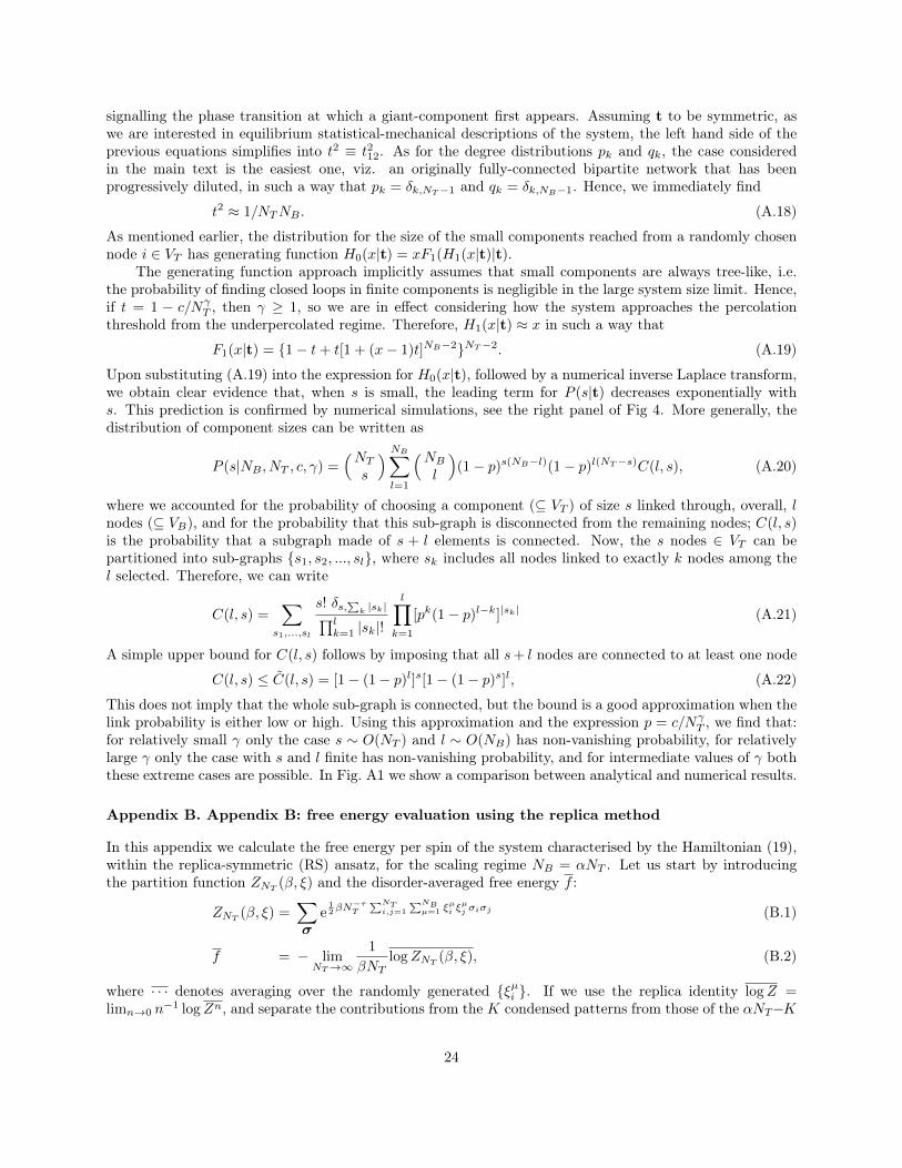
signalling the phase transition at which a giant-component first appears. Assuming t to be symmetric, aswe are interested in equilibrium statistical-mechanical descriptions of the system, the left hand side of theprevious equations simplifies into t2 ≡ t212. As for the degree distributions pk and qk, the case consideredin the main text is the easiest one, viz. an originally fully-connected bipartite network that has beenprogressively diluted, in such a way that pk = δk,NT−1 and qk = δk,NB−1. Hence, we immediately find

t2 ≈ 1/NTNB . (A.18)

As mentioned earlier, the distribution for the size of the small components reached from a randomly chosennode i ∈ VT has generating function H0(x|t) = xF1(H1(x|t)|t).

The generating function approach implicitly assumes that small components are always tree-like, i.e.the probability of finding closed loops in finite components is negligible in the large system size limit. Hence,if t = 1 − c/Nγ

T , then γ ≥ 1, so we are in effect considering how the system approaches the percolationthreshold from the underpercolated regime. Therefore, H1(x|t) ≈ x in such a way that

F1(x|t) = {1− t+ t[1 + (x− 1)t]NB−2}NT−2. (A.19)

Upon substituting (A.19) into the expression for H0(x|t), followed by a numerical inverse Laplace transform,we obtain clear evidence that, when s is small, the leading term for P (s|t) decreases exponentially withs. This prediction is confirmed by numerical simulations, see the right panel of Fig 4. More generally, thedistribution of component sizes can be written as

P (s|NB , NT , c, γ) =(NTs

) NB∑

l=1

(NBl

)(1− p)s(NB−l)(1− p)l(NT−s)C(l, s), (A.20)

where we accounted for the probability of choosing a component (⊆ VT ) of size s linked through, overall, lnodes (⊆ VB), and for the probability that this sub-graph is disconnected from the remaining nodes; C(l, s)is the probability that a subgraph made of s + l elements is connected. Now, the s nodes ∈ VT can bepartitioned into sub-graphs {s1, s2, ..., sl}, where sk includes all nodes linked to exactly k nodes among thel selected. Therefore, we can write

C(l, s) =∑

s1,...,sl

s! δs,∑k |sk|∏l

k=1 |sk|!

l∏

k=1

[pk(1− p)l−k]|sk| (A.21)

A simple upper bound for C(l, s) follows by imposing that all s+ l nodes are connected to at least one node

C(l, s) ≤ C(l, s) = [1− (1− p)l]s[1− (1− p)s]l, (A.22)

This does not imply that the whole sub-graph is connected, but the bound is a good approximation when thelink probability is either low or high. Using this approximation and the expression p = c/Nγ

T , we find that:for relatively small γ only the case s ∼ O(NT ) and l ∼ O(NB) has non-vanishing probability, for relativelylarge γ only the case with s and l finite has non-vanishing probability, and for intermediate values of γ boththese extreme cases are possible. In Fig. A1 we show a comparison between analytical and numerical results.

Appendix B. Appendix B: free energy evaluation using the replica method

In this appendix we calculate the free energy per spin of the system characterised by the Hamiltonian (19),within the replica-symmetric (RS) ansatz, for the scaling regime NB = αNT . Let us start by introducingthe partition function ZNT (β, ξ) and the disorder-averaged free energy f :

ZNT (β, ξ) =∑

σe

12βN

−τT

∑NTi,j=1

∑NBµ=1 ξ

µi ξµj σiσj (B.1)

f = − limNT→∞

1

βNTlogZNT (β, ξ), (B.2)

where · · · denotes averaging over the randomly generated {ξµi }. If we use the replica identity logZ =limn→0 n

−1 logZn, and separate the contributions from the K condensed patterns from those of the αNT−K

24

100

101

102

103

104

0

0.1

0.2

0.3

0.4

0.5

0.6

0.7

0.8

0.9

1

s

P(s|N

B,N

T,c,γ

)

data1

data2

γ = 0.75

γ = 0.90

γ = 0.78

γ = 0.70

Figure A1. Distribution for the cluster size P (s|NB , NT , c, γ) measured numerically over a simulatedgraph G with NT = 104 nodes. The parameters δ = 1, α = 0.5 and c = 1 are kept fixed, while γ is varied(see legend). In the interest of clarity, we plotted the analytical estimate of Eqs. A.20 and A.22 only forγ = 0.78.

non-condensed ones we get

f = − limNT→∞

limn→0

1

βnNTlog

∑

σ1,···,σne

12βN

−τT

∑NTi,j=1

∑NBµ=1

∑nα=1 ξ

µi ξµj σ

αi σ

αj

= − 1

βlog 2− lim

NT→∞limn→0

1

βnNTlog⟨

e12βN

−τT

∑Kµ=1

∑nα=1(

∑NTi=1 ξ

µi σ

αi )2

× e12βN

−τT

∑NBµ>K

∑nα=1(

∑NTi=1 ξ

µi σ

αi )2⟩σ1,...,σn

. (B.3)

We compute the non-condensed contributions first, using the standard tool of Gaussian linearisation, andthe usual short-hands Dz = (2π)−1/2e−z

2/2dz and Dz =∏nα=1 Dzα:

Ξ = e12βN

−τT

∑µ>K

∑nα=1(

∑NTi=1 ξ

µi σ

αi )2 =

[e

12βN

−τT

∑nα=1(

∑NTi=1 ξiσ

αi )2]NB−K

=

[∫Dz e

√βN−τ/2T

∑nα=1 zα

∑NTi=1 ξiσ

αi

]NB−K

=

[∫Dz

NT∏

i=1

(1−cN−γT +cN−γT cosh(

√βN−τ/2T

n∑

α=1

σαi zα))]NB−K

=

[∫Dz

NT∏

i=1

[1+

1

2βcN−γ−τT

( n∑

α=1

σαi zα)2

+O(N−2τ−γT )

]]NB−K

=

[∫Dz e

12βcN

−γ−τT

∑nα,β=1 zαzβ

∑NTi=1 σ

αi σ

βi +O(N1−2τ−γ

T )

]NB−K. (B.4)

Now it is evident, as in our earlier calculations, that the correct scaling for large NT requires choosingτ = 1 − γ. For the correction term in the exponent this gives O(N1−2τ−γ

T ) = O(Nγ−1T ), which is indeed

vanishing since γ < 1. We now arrive at

Ξ = exp{

(NB−K) log

∫Dz e

12βcN

−1T

∑nα,β=1 zαzβ

∑NTi=1 σ

αi σ

βi +O(Nγ−1

T )}

(B.5)

25

We next introduce n2 parameters {qαβ} and their conjugates {qαβ}, by inserting partitions of unity:

1 =∏

αβ

∫dqαβ δ

(qαβ −

1

NT

NT∑

i=1

σαi σβi

)=

∫ [∏

αβ

dqαβdqαβ2π/NT

]eiNT

∑α,β qαβ(qαβ− 1

NT

∑i σ

αi σ

βi ). (B.6)

Substituting (B.6) into (B.5) gives the contribution to the partition function of non-condensed patterns:

Ξ =

∫ [∏

αβ

dqαβdqαβ

]eiNT

∑α,β qαβqαβ+(NB−K) log

∫Dz e

12βc∑nα,β=1 zαqαβzβ+O(NγT )

× e−i∑i

∑α,β σ

αi qαβσ

βi . (B.7)

The contribution from condensed pattern, see (B.3), is

e12βN

γ−1T

∑µ≤K

∑nα=1(

∑NTi=1 ξ

µi σ

αi )2 =

∫Dm e

√βN

(γ−1)/2T

∑µ≤K

∑nα=1

∑NTi=1 ξ

µi σ

αi m

µα , (B.8)

with m = {mµα} ∈ RnK . If we rescale mµ

α → c√βN

(1−γ)/2T mµ

α this becomes(c2βN1−γ

T

)nK/2∫dm e−

12βc

2N1−γT m2+βc

∑µ≤K

∑nα=1

∑NTi=1 ξ

µi σ

αi m

µα . (B.9)

Inserting (B.7,B.9) into (B.3) gives the following expression for the free energy per spin:

f = − 1

βlog 2− lim

NT→∞

{K/2βNT

log(c2βN1−γT )

+ limn→0

1

βnNTlog

∫dm

[∏

αβ

dqαβdqαβ

]

× eNT

[i∑α,β qαβqαβ+

NB−KNT

log∫

Dz e12βc∑nα,β=1 zαqαβzβ− 1

2βc2N−γT m2

]

×NT∏

i=1

⟨eβc

∑µ≤K

∑nα=1 ξ

µi σ

αi m

µα−i

∑α,β σ

αi qαβσ

βi .⟩σ1i ,...,σ

ni

}(B.10)

The number of order parameters being integrated over is of order K, so corrections to the saddle-pointcontribution will be of order O(K logN/N). To proceed via steepest descent we must therefore imposeK � NT / logNT . Since also the energy term N−γT

∑µ≤Km

2 should be of order one, as well as the individualcomponents of m, the only natural choice is K = O(Nγ). Under this scaling condition we then find

f = − 1

βlog 2− lim

K→∞limn→0

1

βnextrm,q,q f(m, {q, q}) (B.11)

with

f(m, {q, q}) = i∑

α,β

qαβqαβ + α log

∫Dz e

12βc

∑nα,β=1 zαqαβzβ − βc2

2NγT

n∑

α=1

∑

µ≤K

(mµα)2 (B.12)

+⟨

log⟨

eβc∑µ≤K

∑nα=1 ξ

µσαmµα−i∑α,β σ

αqαβσβ

.⟩σ1,...,σn

⟩ξ

(B.13)

Now we can use the replica symmetry ansatz, and demand that the relevant saddle-point is of the form

mµα = mµ, qαβ = δαβ + q(1−δαβ), qαβ =

iα(βc)2

2[Rδαβ + r(1−δαβ)], (B.14)

From now on we will denote m = (m1, . . . ,mK) and ξ = (ξ1, . . . , ξK). After some simple algebra we cantake the limit n→ 0, and find that our free energy simplifies to

βfRS = limNT→∞

extrm,q,r fRS(m, q, r) (B.15)

with

fRS(m, q, r) = − log 2 +1

2αr(βc)2(1−q) +

βc2

2NγT

m2 − α

2

( βcq

1−βc(1−q) − log[1−βc(1−q)])

−⟨∫

Dz log cosh[βc(m · ξ + z√αr)]

⟩ξ

(B.16)

26