Human Capital and Economic GrowthRevisited: A Dynamic Panel Data Study

G. AGIOMIRGIANAKIS,∗ D. ASTERIOU,∗∗ AND V. MONASTIRIOTIS∗∗∗∗

Abstract

This paper examines the role of human capital on economic growth by using a largepanel of data including 93 countries. Given the cross-sectional character in most of therelevant studies, there is a possibility that when the long-run dynamics are considered,education might not be a signiÞcant determinant of growth. Following a dynamic paneldata approach, the analysis indicates that education has, indeed, a signiÞcant and posi-tive long-run effect on economic growth. Moreover, the size of this effect is stronger asthe level of education (primary, secondary, and tertiary) increases. This has a straight-forward policy implication that governments taking actions towards an expansion of theirhigher education may well expect larger gains in terms of higher economic growth in theircountries. (JEL E1, F43, C33) Int�l Advances in Econ. Res., 8(3): pp. 177-187, Aug.02. c°All Rights Reserved

Introduction

The early neoclassical theory of economic growth had placed much emphasis on exogenousdemographic factors that affect the growth rate of nations. Factors such as the growth rateof population, the structure of the labor force, and the rate of technological change wereassumed to determine the long-run equilibrium growth rate. Indeed, in neoclassical theory,capital accumulation increases an economy�s growth in the medium term, but the steadystate growth is constrained by the rate of growth of the labor force. Moreover, technicalprogress, which is assumed to be exogenous, is the main driving force of the model. However,a large part of the measured growth in output was left unexplained in the neoclassical model,the so-called Solow�s residual (see Snowdon and Vane [1997] and Romer [1996]).In the mid 1980s, however, the endogenous growth theory, motivated by the work of

Paul Romer and Robert Lucas, has identiÞed a number of factors that determine the growthrate of an economy. Hence, factors such as increasing returns to scale, innovation, opennessto trade, international research and development (R&D), and human capital formation areconsidered key factors in explaining the growth process (see Lucas [1988] and Turnovsky[1999] for a review). In this paper, the analysis on the role of human capital is restrictedto the economic growth of a country and the resulting policy implications that governmentsshould follow are examined. Indeed, since investment in human capital is taking place throughtraining and education, there is a strong rationale in favor of government intervention. More

∗City University, ∗∗The University of Reading, and ∗∗∗London School of Economics�UnitedKingdom. This is a revised version of a paper presented at the Fifty-Þrst International AtlanticEconomic Conference, Athens, Greece, March 13-20, 2001, and also at the conference on Post-Euro Era at the University of Ioannina, Greece, January 27-28, 2000. The authors would like tothank participants in both conferences and, in particular, Nick Apergis for his comments and usefulsuggestions on earlier drafts. The authors remain responsible for any shortcomings of the paper.

177

178 IAER: AUGUST 2002, VOL. 8, NO. 3

speciÞcally, government policies intended to affect publicly-provided education and trainingwill, in effect, determine the process of growth of the whole economy, (see Lucas [1988], Shaw[1992], Romer [1994], Barro and Sala-i-Martin [1995], Aghion and Howitt [1998], Kaganovichand Zilcha [1999] and Capolupo [2000]).The last two decades have witnessed voluminous empirical studies worldwide that try to

quantitatively investigate the relation between education and economic growth. The gen-eral result of these studies indicates that there is a positive correlation between economicgrowth and education. However, many of the existing studies on the relationship betweeneducation and economic growth have been carried out by employing cross-sectional data andtechniques, mostly from the advanced countries that had solved their most crucial problemsof development by the Þrst quarter of the 20th century. In the empirical analysis, panel datais employed using dynamic panel data techniques for a diverse set of 93 countries1 over aperiod of 28 years, with different levels of economic development and different trends in termsof GDP growth. Furthermore, the contemporary panel data estimation techniques take intoaccount country (Þxed) speciÞc effects and allows each country to follow its own short-rundynamics.The Þndings not only suggest the existence of a robust positive relationship between

education and economic growth, but also that higher levels of education have a stronger effecton economic growth. The policy implication of this result is that governments will be inclinedto adopt measures that will expand higher education in their countries in order to increasepotential gains in term of a higher economic growth. This Þnding has a straightforward policyimplication that governments taking actions towards an expansion of their higher educationmay well expect larger gains in terms of higher economic growth in their countries. Moreover,this Þnding may also contribute towards an explanation of the observed expansion of highereducation in several countries.2

The paper is organized as follows. In the second section, the study augments a standardtextbook Solow model by following Mankiw et al. [1992]. This model allows for the deter-mination of the contribution of education to the long-run output per capita. The followingsection presents the empirical methodology appropriate for dynamic panel data as suggestedin a series of papers by Pesaran, Shin, and Smith [1995, 1999]. The fourth section presentsthe estimation results, followed by a conclusion of the paper.

A Growth Model with Human Capital

This section incorporates the case of education into a growth model. Indeed, followingMankiw et al. [1992], the Solow model is augmented by including human capital. Let theproduction function be:

Y (t) = K(t)aH(t)β [A(t)L(t)](1−a−β) , (1)

where Y (t) is output, H(t) is the stock of human capital, K(t) is the stock of physical capital,L(t) is the labor force, and A(t) is the level of technology.Along the lines suggested by Tallman and Wang [1994], it is assumed that human capital

is a function of education, H(t) = E(t)ϕ. Empirical studies (see Maddisson [1991], Pen-cavel [1991], and Tallman and Wang [1994]) suggest that the value of ϕ is very close tounity. Therefore, the analysis does not distinguish between the measure of education and thehypothesized human capital measure.Assuming that L(t) and A(t) grow at constant and exogenous rates n and g, respectively,

gives:

AGIOMIRGIANAKIS ET AL.: HUMAN CAPITAL 179

L(t) = L(0)ent , (2)

A(t) = A(0)egt . (3)

On the other hand:3

úK(t) = sKY (t) , (4)

úH(t) = úE(t) = sHY (t) , (5)

where sK and sH are the fractions of output devoted to physical and human capital accu-mulation, respectively.The evolution of the economy is then described by:

úk = sKk(t)ah(t)β − (n+ g)k(t) , (6)

úh = sHk(t)ah(t)β − (n+ g)h(t) , (7)

where k = K/AL, h = H/AL, and y = Y/AL.Solving for the levels of k and h on the balanced growth path results in:

k∗ =

"s

(1−β)K sβHn+ g

#(1/1−a−β)

, (8)

h∗ =

"saKs

(1−a)H

n+ g

#(1/1−a−β)

. (9)

Substituting into the production function and taking logs results in:

ln y∗ =a

1− a− β ln sK +β

1− a− β ln sH −a+ β

1− a− β ln(n+ g) . (10)

Equation (10) describes how output per capita depends on population growth and theaccumulation of human and physical capital. An increase in the fraction of output devotedto education will increase the level of output on the balanced growth path.

Empirical Methodology

The aim of this study is to examine the long-run effects of education on economic growthin a panel of data. Therefore, the empirical methods need to be geared toward allowing for theestimation of consistent long-run parameters in a regression of GDP growth per employee onits explanatory variables, in this case, the growth rate of investment and educational variables(as human capital proxies) for a panel of 93 (N = 93) countries over a period of 28 years(T = 28) from 1960-87. The data also has complex dynamics and is characterized by strongtrends and non-stationarity. In the type of data set that is being considered, T is sufficientlylarge to allow individual country estimation.Following the standard methodology, this study Þrst tries to establish the order of integra-

tion of the variables. For this reason, individual as well as panel unit root tests are conducted.Using panel data, powerful tests for a unit root in the autoregressive representation of the

180 IAER: AUGUST 2002, VOL. 8, NO. 3

series can be constructed. Following Dickey and Fuller [1979], the unit root hypothesis canbe tested by performing the following regression:

∆yit = µi + βiyi,t−1 +

pXk=1

ϕk∆yi,t−k + γit+ εit ; (11)

i = 1, ..., N ; t = 1, ..., T ,

and testing βi = 0 for all i. Levine and Lin [1992] (LL) propose a panel test based on pooledestimates using least squares, which allows for individual speciÞc intercepts, but retain theassumption of the common AR parameter. Therefore, their model is:

∆yit = µi + βyi,t−1 +

pXk=1

ϕk∆yi,t−k + γt+ µit ; (12)

i = 1, ..., N ; t = 1, ..., T ,

and their proposed test statistic is given then by:

LL =√1.25

"tβ −

√Nµ1T√µ2T

#,

with tβ =�β

�σβ, µ1T = −

1

2− 12T−1, and µ2T =

1

6+5

6T−2 .

On the other hand, Im, Pesaran, and Shin [1997] (IPS) propose a heterogeneous paneldata model for testing for unit roots which is based on the estimate of (11) from which theIPS t-bar statistic can be obtained as:

t̄ =1

N

NXi=1

τ i, τ i =�βi�σi

, (13)

Assuming that the cross-sections are independent, IPS proposed to use the followingstandardized t-bar statistic:

IPSt̄ =

√N − (t̄−E(τ i|βi = 0))p

V ar (τ i|βi = 0). (14)

The means E (τ i|βi = 0) and V ar (τ i|βi = 0) are obtained from Monte Carlo simulations.Both LL and IPS statistics converge weakly to a standard normal distribution as N andT −→ ∞. Hence, the panel data unit root inference can be conducted by comparing theobtained statistics to critical values from the lower tail of the N(0, 1) distribution.After establishing the order of integration of the variables, the estimates will be obtained

using two recently developed methods for the statistical analysis of dynamic panel data: theMean Group (MG) and the Pooled Mean Group (PMG) estimations.4 These methods areparticularly suited to the analysis of panels with large time and cross-section dimensions.5

MG estimation derives the long-run parameters for the panel from an average of the long-runparameters from ARDL models for individual countries (see Pesaran and Smith [1995]). Forexample, if the ARDL is:

ai(L)yit = bi(L)xit + dizit + eit , (15)

AGIOMIRGIANAKIS ET AL.: HUMAN CAPITAL 181

for country i, where i = 1, ..., N , then the long-run parameter for country i is:

θi =bi(1)

di(1), (16)

and the MG estimator for the whole panel will be given by:

θ =1

N

NXi=1

�θi . (17)

It can be shown that the MG estimation with sufficiently high lag orders yields super-consistent estimators of the long-run parameters, even when the regressors are I(1) (seePesaran, Shin, and Smith [1999]).The PMG method of estimation, introduced by Pesaran, Shin, and Smith [1999], occupies

an intermediate position between the MGmethod, in which both the slopes and the interceptsare allowed to differ across country, and the classical Þxed effects method, in which the slopesare Þxed and the intercepts are allowed to vary. In the PMG estimation, only the long-runcoefficients are constrained to be the same across countries, while the short-run coefficientsare allowed to vary.Setting this out more precisely, the unrestricted speciÞcation for the ARDL system of

equations for t = 1, 2, ..., T time periods and i = 1, 2, . . . , N countries for the dependentvariable y is:

yit =mXj=1

λijyi,t−j +nXj=0

δ0ijxi,t−j + µi + εit , (18)

where xij is the (k × 1) vector of explanatory variables for group i, and µi represents the Þxedeffects. In principle, the panel can be unbalanced and m and n may vary across countries.This model can be re-parametrized as a VECM system:

∆yit = θi¡yi,t−1 − β0ixi,t−1

¢+m−1Xj=1

γij∆yi,t−j +n−1Xj=0

γ0ijxi,t−j + µi + εit , (19)

where the βIs are the long-run parameters and the θis are the error correction parameters.The pooled group restriction is that the elements of β are common across countries, so that:

∆yit = θi¡yi,t−1 − β0xi,t−1

¢+m−1Xj=1

γij∆yi,t−j +n−1Xj=0

γ0ijxi,t−j + µi + εit . (20)

All the dynamics and the ECM terms are free to vary. The estimation of this model is bymaximum likelihood. Again, it is proved that under some regularity assumptions, the pa-rameter estimates of this model are consistent and asymptotically normal for both stationaryand non-stationary I(1) regressors. Both the MG and PMG estimations require selecting theappropriate lag length for the individual country equations. This selection was made usingthe Schwarz Bayesian Criterion.

Estimation Results

Table A1 reports summary results from the individual and the panel unit root tests of allthe variables.6 The Þrst column of results presents the ADF statistics for the gross domesticproduct per capita variable. Both the individual tests as well as the panel LL and IPS tests

182 IAER: AUGUST 2002, VOL. 8, NO. 3

cannot reject the null of a presence of unit root. The second column shows the results forthe Þrst differences of the same variable, and in this case, it is obvious from the panel results(both yielding high negative values which well exceed the critical value of �1.645, rejectingthe null of non-stationarity), as well as from most of the individual test statistics7 that thisvariable is stationary. Similar are the results for the capital per capita variable presentedin the third and fourth column, suggesting that capital per capita is as well I(1), while itsÞrst difference is I(0). Continuing the analysis for the educational proxies, it can be seenthat in all cases, there is some inconclusiveness from the individual ADF tests.8 However, inall cases, the panel tests constructed after those individual statistics suggest that the seriesconsidered as a panel are stationary, so they do not need to differenced again in order to usethem in the empirical analysis.Having established the order of integration of the panel data series, the study proceeds

with the estimation of the dynamic model. The results are summarized in Table A2. Inboth the MG and PMG cases, it was found that there is a positive relationship, supportingthe theoretical considerations. The MG estimates provide less information than the PMGones, but they also have the expected signs, and for the case of the capital per capita growthvariable, are signiÞcant (also the capital per capita coefficient in all cases takes values betweenin the range 0.29 to 0.45, which is as expected). However, for both cases, the Hausman testsreported in the last two columns of the table indicate that the data do not reject the restrictionof common long-run coefficients, so pooling the data (by using the PMG estimator) appearsto be a preferable and more informative procedure. The same is suggested by the jointHausman test. Hence, focusing on the PMG estimates, it is observed that the coefficientfor the growth rate of per capita capital is positive and highly statistically signiÞcant for allthree alternative speciÞcations. More importantly, the human capital variables are positiveand highly signiÞcant. Thus, human capital is found to have a direct positive effect on GDPgrowth. Further analyzing the PMG estimation results shows that the obtained coefficientsfor the primary, secondary and tertiary education are 0.05, 0.11, and 0.27 respectively. Thus,not only is there clear evidence that human capital positively affects growth, but it is alsoconcluded that higher levels of educational quality (as represented by the different educationalsectors) are associated with higher economic growth. Indeed, the effect of tertiary educationis higher than that of secondary education, which in turn has a higher effect on growth thanthat of the primary education.

Conclusions

The growth effect of education is a rather intensively studied issue, especially in the lasttwo decades. This paper has provided some further evidence to the results obtained so farin the literature using a large panel of data. Utilizing contemporary panel data estima-tion techniques, the effects of education on economic growth have been analyzed. Giventhe long time-dimension of the data, the investigation not only took into account country-speciÞc (Þxed) effects, but more importantly, allowed each country to follow its own short-rundynamics. Hence, the obtained coefficients for the human capital variables can arguably beconsidered as revealing a long-run structural relationship between human capital and growth.The results support the Þndings of earlier studies of a robust positive relationship between

the two aggregates. Moreover, they suggest that the quality of education (as measuredby the different educational sectors) is itself a signiÞcant determinant of economic growth.SpeciÞcally, the effect of education on growth was found to increase linearly with the level ofeducation considered in the analysis. Thus, the Þndings suggest that government measurestaken towards an expansion of higher (university) education might be a crucial factor for

AGIOMIRGIANAKIS ET AL.: HUMAN CAPITAL 183

economic development and sustained economic growth. Moreover, this Þnding may alsocontribute towards an explanation of the observed expansion of higher education in severalcountries.

APPENDIX

TABLE A1Individual and Panel Unit Root Tests Results

Individual Unit Root TestsVariables yit ∆yit kit ∆kit Hit = prim Hit = sec Hit = tetAGO -0.0350 -7.544∗ -1.230 -2.648 2.549 -0.785 -1.335ARG -0.0544 -4.936∗ -1.231 -2.960 -1.179 -4.021∗ -1.523AUS -0.0339 -2.994∗ -1.212 -2.738 -2.461 -4.434∗ -3.526∗

AUT -0.0320 -2.984∗ -1.214 -3.026∗ -7.166∗ -2.670 -0.669BEL -0.0306 -3.102∗ -1.223 -2.825 -4.206∗ -3.333∗ -2.536BGD -0.0335 -5.461∗ -1.219 -3.483∗ -2.487 -2.336 -2.102BOL -0.0392 -2.436∗ -1.223 -2.961 1.641 -2.411 -1.678BRA -0.0386 -3.467∗ -1.195 -2.997∗ -6.559∗ -3.313∗ -3.141∗

CAN -0.0331 -3.098∗ -1.205 -2.490 -4.255∗ -4.524∗ -3.682∗

CHE -0.0343 -2.837 -1.217 -3.135∗ -4.102∗ -1.924 -1.879CHL -0.0310 -5.826∗ -1.229 -3.114∗ -0.890 -3.077∗ -2.129CHN -0.0317 -6.639∗ -1.170 -1.775 -6.598∗ -0.788 -0.634CIV -0.0307 -5.065∗ -1.204 -3.516∗ -4.569∗ -0.858 -1.259CMR -0.0309 -5.014∗ -1.168 -3.310∗ -5.667∗ -0.657 -1.093COL -0.0299 -2.794 -1.210 -2.685 -0.317 -1.426 -0.889CRI -0.0338 -3.425∗ -1.196 -3.149∗ -0.211 -4.464∗ -3.853∗

CYP -0.0423 -7.633∗ -1.205 -3.579∗ -3.858∗ -0.566 -0.800DEU -0.0317 -3.064∗ -1.223 -3.039∗ -5.773∗ -2.790 -1.847DNK -0.0330 -3.595∗ 1.218 -3.128∗ -3.835∗ -4.181∗ -3.776∗

DOM -0.0376 -6.070∗ -1.174 -3.149∗ 0.519 -0.837 -1.069DZA -0.0338 -10.828∗ -1.207 -2.538 -0.364 -6.990∗ -7.134∗

ECU -0.0315 -4.061∗ -1.207 -2.930 -1.248 -4.084∗ -2.825EGY -0.0364 -3.133∗ -1.177 -3.230∗ -2.603 -2.963 -2.809ESP -0.0285 -2.692 -1.201 -2.798 -2.088 -0.618 -1.187ETH -0.0389 -3.398∗ -1.201 -3.370∗ -2.641 -4.330∗ -3.555∗

FIN -0.0337 -2.940 -1.219 -3.027∗ -4.628∗ -4.137∗ -2.931FRA -0.0305 -2.705 -1.211 -2.964 -3.202∗ -2.475 -2.376GBR -0.0338 -2.875 -1.221 -2.794 -0.526 -0.910 -1.320GHA 0.0332 -5.195∗ -1.241 -3.741∗ -2.837 -2.452 -1.671GRC -0.0302 -3.211∗ -1.208 -3.375∗ -1.439 -2.143 -1.921GTM -0.0379 -2.687 -1.213 -2.820 -0.647 -2.182 -2.451GUY -0.0413 -4.977∗ -1.240 -3.741∗ -1.171 -0.619 -1.014HND -0.0393 -3.102 -1.205 -3.065∗ -2.568 -0.985 -1.222HTI -0.0393 -5.036 -1.204 -2.594 -1.084 -1.447 -1.258IDN -0.0274 -3.403∗ -1.171 -2.216 -9.794∗ -3.057∗ -2.162IND -0.0311 -4.507∗ -1.207 -2.707 -5.689∗ -1.655 -1.583

184 IAER: AUGUST 2002, VOL. 8, NO. 3

TABLE A1 (CONT.)Individual Unit Root Tests

Variables yit ∆yit kit ∆kit Hit = prim Hit = sec Hit = tetIRL -0.379 -3.109∗ -1.207 -2.902 -1.695 -2.414∗ -1.767IRN -0.028 -6.150∗ -1.189 -4.006∗ -2.399 -4.415 -3.554∗

IRQ -0.038 -13.607∗ -1.180 -4.405∗ 1.992 -6.091∗ -4.680∗

ISL -0.034 -3.431∗ -1.202 -2.964∗ -3.687∗ 10.793 17.405ISR -0.035 -3.531∗ -1.210 -3.413∗ -2.988∗ -1.266 -1.266ITA -0.025 -3.251∗ -1.220 -3.314∗ -0.583 -3.563∗ -3.636∗

JAM -0.034 -3.183∗ -1.235 -2.454 -4.673∗ -5.026∗ -3.570∗

JOR -0.041 -8.081∗ -1.174 -4.889∗ 1.423 -0.761 -1.214JPN -0.026 -2.942 -1.183 -3.529∗ -0.979 -2.102∗ -0.553KEN -0.034 -5.224∗ -1.218 -3.144∗ -1.174 -1.120 -1.350KOR -0.027 -3.304∗ -1.127 -2.887 -0.809 -1.098 -1.218KWT -0.040 -7.276∗ -1.177 -4.209∗ -0.305 -1.281 -1.678LBY -0.038 -6.076∗ -1.179 -5.624∗ -0.102 -3.141∗ -2.536∗

LKA -0.034 -3.862∗ -1.190 -2.706 -1.192 -0.683 -1.257LUX -0.034 -3.731∗ -1.226 -2.851 -1.394 -1.261 -1.317MAR -0.034 -4.899∗ -1.189 -3.395∗ 0.757 -0.663 -1.234MDG -0.031 -4.009∗ -1.230 -3.062∗ -1.421 -0.948 -1.379MEX -0.026 -3.174∗ -1.194 -3.116∗ -3.203∗ -0.882 -1.187MLI -0.033 -5.961∗ -1.217 -3.269∗ -0.313 -0.928 -1.181MLT -0.044 -2.844 -1.202 -2.827 0.969 -0.987 -1.415MMR -0.036 -6.193∗ -1.219 -2.805 -4.282∗ -4.019∗ -3.724∗

MOZ -0.033 -4.281∗ -1.228 -2.911 -4.594∗ -3.453∗ -3.072∗

MUS -0.037 -6.657∗ -1.227 -2.843 -1.906 -1.743 -1.260MWI -0.041 -4.349∗ -1.205 -4.609∗ -0.034 -4.400∗ -3.613∗

MYS -0.035 -3.306∗ -1.174 -3.484∗ -0.233 -3.465∗ -2.223NGA -0.035 -6.052∗ -1.198 -3.864∗ -1.814 -5.652∗ -3.028∗

NIC -0.041 -6.651∗ -1.205 -4.118∗ -0.491 -2.493 -1.803NLD -0.033 -2.870 -1.220 -2.897 -3.703∗ -2.113 -2.146NOR -0.033 -2.827 -1.214 -2.890 -1.115 -0.750 -1.361NZL -0.036 -4.521∗ -1.222 -2.971 -0.382 -1.183 -1.461PAK -0.032 -3.198∗ -1.207 -4.377∗ -0.389 -1.185 -1.320PAN -0.039 -3.615∗ -1.194 -3.464∗ -8.257∗ -2.522 -0.294PER -0.067 -4.555∗ -1.219 -3.603∗ -0.141 -0.727 -1.043PHL -0.032 -2.985 -1.202 -3.013∗ 0.763 -1.582 -1.630PRT -0.030 -3.545∗ -1.208 -2.989∗ -4.027∗ -5.070∗ -4.128∗

PRY -0.031 -3.067∗ -1.180 -3.113∗ -1.069 -2.793 -3.382∗

RWA -0.034 -5.319∗ -1.178 -2.930 1.116 -1.614 -1.610SDN -0.037 -5.679∗ -1.221 -6.362∗ -0.506 -2.082 -1.554SEN -0.032 -6.959∗ -1.227 -2.924 2.890 -0.721 -1.319SGP -0.036 -3.432∗ -1.142 -3.518∗ -2.123 -0.893 -1.238SLE -0.038 -12.627∗ -1.220 -3.794∗ -1.073 -2.234 -0.234SLV -0.037 -2.802 -1.211 -3.077∗ -4.356∗ -6.774∗ -4.799∗

SWE -0.032 -2.697 -1.223 -2.787 1.818 -4.348∗ -3.172∗

THA -0.031 -2.887 -1.167 -3.057∗ -4.589∗ -0.970 -1.421TTO -0.038 -3.132∗ -1.206 -3.766∗ 1.964 -0.882 -1.373

AGIOMIRGIANAKIS ET AL.: HUMAN CAPITAL 185

TABLE A1 (CONT.)Individual Root Tests

Variables yit ∆yit kit ∆kit Hit= prim Hit= sec Hit= tetTUN -0.039 -4.412∗ -1.202 -3.024∗ -1.209 -0.525 -0.686TUR -0.028 -3.117∗ -1.193 -2.725 -7.598∗ -2.569 -3.365∗

TWN -0.030 -3.116∗ -1.148 -2.975∗ -5.215∗ -2.025 -2.265TZA -0.034 -3.184∗ -1.213 -2.925∗ -2.154 -5.699∗ -3.123∗

UGA -0.034 -20.174∗ -1.231 -2.851 -4.598∗ -2.154 -3.365∗

URY -0.032 -2.432∗ -1.241 -2.216 -5.269∗ -1.625 -3.002∗

USA -0.030 -3.123∗ -1.220 -2.603 -1.257 -2.365 -3.659∗

VEN -0.032 -3.795∗ -1.215 -2.790 -21.570∗ -1.265 -6.225∗

ZAF -0.034 -3.145∗ -1.208 -2.774 -2.569 -1.897 -4.226∗

ZAR -0.032 -5.369∗ -1.210 -3.899∗ -5.698∗ -2.365 -6.326∗

ZMB -0.038 -6.264∗ -1.244 -3.058∗ -6.257∗ -2.666 -2.265ZWE -0.039 -4.308∗ -1.225 -2.792 -2.356 -5.333∗ -5.556∗

Panel Unit Root TestsPanel t 0.140 -28.695 -1.111 -14.623 -16.302 -13.997 -13.889t-bar -0.035 -4.592 -1.205 -3.198 -2.430 -2.284 -2.060

LL 13.790 -18.449∗ 12.390 -2.715∗ -4.593∗ -2.016∗ -1.895∗

IPS 15.583 -32.337∗ 3.270 -17.678∗ -9.606∗ -8.073∗ -5.717∗

Notes: ∗denotes the rejection of the null hypothesis of the existence of the unit root. For theindividual unit root tests, the 5 percent critical value is -2.97. For the LL and IPS panel unit roottests, the 5 percent critical value is -1.645. Prim, sec, and tet represent enrollments in primaryeducation, secondary education, and tertiary education, respectively.

TABLE A2Pooled Mean Group and Mean Group EstimatesPMG Estimates MG Estimates Hausman Test

Coefficient SE t-ratio Coefficient SE t-ratio h p-value∆kit 0.32 0.04 8.01 0.36 0.08 4.33 1.73 0.19

Hit= prim 0.05 0.02 2.52 0.11 0.24 0.44 0.06 0.82Joint Hausman Test: 2.14 0.17

∆kit 0.45 0.04 11.04 0.34 0.09 3.73 0.20 0.66Hit= sec 0.11 0.04 2.75 0.32 3.02 0.11 0.10 0.75

Joint Hausman Test: 0.32 0.72∆kit 0.29 0.10 2.90 0.45 0.04 10.91 0.12 0.71

Hit= tet 0.27 0.13 2.07 0.34 2.85 0.12 0.44 0.53Joint Hausman Test: 0.28 0.87

Notes: Dependant variable: ∆yit, sample size (N × T ) = 2511. Error correction coefficients, shortrun dynamics, and country estimates are not reported for economy of space. SE represents standarderror; prim, sec, and tet represent enrollments in primary education, secondary education, andtertiary education, respectively.

186 IAER: AUGUST 2002, VOL. 8, NO. 3

TABLE A3List of Countries

Angola AGO Guyana GUY Nicaragua NICArgentina ARG Honduras HND Netherlands NLDAustralia AUS Haiti HTI Norway NORAustria AUT Indonesia IDN New Zealand NZLBelgium BEL India IND Pakistan PAKBangladesh BGD Ireland IRL Panama PANBolivia BOL Iran, Isl. Rep. IRN Peru PERBrazil BRA Iraq IRQ Philippines PHLCanada CAN Iceland ISL Portugal PRTSwitzerland CHE Israel ISR Paraguay PRYChile CHL Italy ITA Rwanda RWAChina CHN Jamaica JAM Sudan SDNCote d�Ivoire CIV Jordan JOR Senegal SENCameroon CMR Japan JPN Singapore SGPColombia COL Kenya KEN Sierra Leone SLECosta Rica CRI Korea, Rep. KOR El Salvador SLVCyprus CYP Kuwait KWT Sweden SWEGermany DEU Libya LBY Thailand THADenmark DNK Sri Lanka LKA Trinidad-Tobago TTODominican Republic DOM Luxembourg LUX Tunisia TUNAlgeria DZA Morocco MAR Turkey TUREcuador ECU Madagascar MDG Taiwan TWNEgypt EGY Mexico MEX Tanzania TZASpain ESP Mali MLI Uganda UGAEthiopia ETH Malta MLT Uruguay URYFinland FIN Myanmar MMR United States USAFrance FRA Mozambique MOZ Venezuela VENUnited Kingdom GBR Mauritius MUS South Africa ZAFGhana GHA Malawi MWI Zaire ZARGreece GRC Malaysia MYS Zambia ZMBGuatmala GTM Nigeria NGA Zimbabwe ZWE

Footnotes

1See Table A3 for a list of the countries used in the empirical analysis.2Quoting from Education at a Glance OECD 2000, �The number of students enrolled in tertiary

programs grew by more than 20 percent between 1990 and 1997 in all but Þve OECD countries, andin eight countries by more than 50 percent.�

3For the sake of simplicity, assume no capital depreciation.4Note that in the traditional pooled estimators, such as the Þxed and random effects, the es-

timation of long-run parameters is prohibited and only the intercepts are allowed to differ acrosscountries, while all other coefficients and error variances are constrained to be the same. Therefore,these methods of estimation are not applicable to this case.

5Quah [1993] has referred to such data sets as data Þelds.6All reported tests include a constant, but no trend, while the lag length of the ADF equation

were chosen to be one. Different versions of the tests (not presented here for economy of space)did not alter the conclusions about the order of integration of the variables. Tables and results areavailable from the authors upon request.

AGIOMIRGIANAKIS ET AL.: HUMAN CAPITAL 187

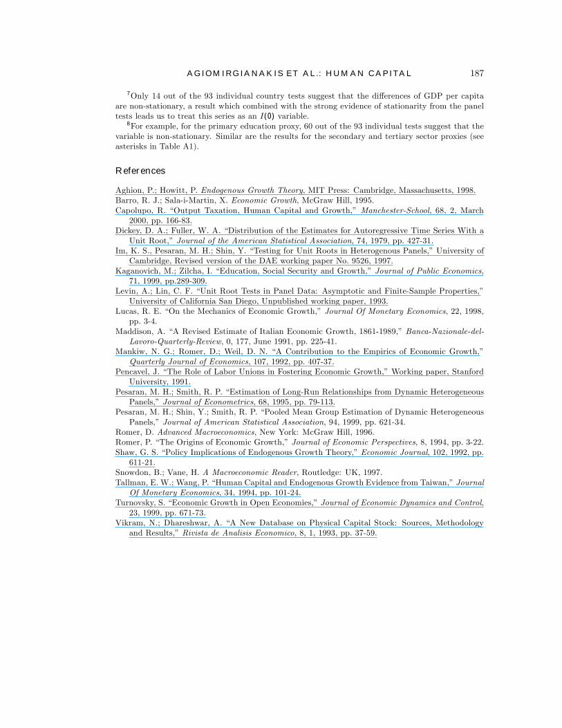
7Only 14 out of the 93 individual country tests suggest that the differences of GDP per capitaare non-stationary, a result which combined with the strong evidence of stationarity from the paneltests leads us to treat this series as an I(0) variable.

8For example, for the primary education proxy, 60 out of the 93 individual tests suggest that thevariable is non-stationary. Similar are the results for the secondary and tertiary sector proxies (seeasterisks in Table A1).

References

Aghion, P.; Howitt, P. Endogenous Growth Theory, MIT Press: Cambridge, Massachusetts, 1998.Barro, R. J.; Sala-i-Martin, X. Economic Growth, McGraw Hill, 1995.Capolupo, R. �Output Taxation, Human Capital and Growth,� Manchester-School, 68, 2, March

2000, pp. 166-83.Dickey, D. A.; Fuller, W. A. �Distribution of the Estimates for Autoregressive Time Series With a

Unit Root,� Journal of the American Statistical Association, 74, 1979, pp. 427-31.Im, K. S., Pesaran, M. H.; Shin, Y. �Testing for Unit Roots in Heterogenous Panels,� University of

Cambridge, Revised version of the DAE working paper No. 9526, 1997.Kaganovich, M.; Zilcha, I. �Education, Social Security and Growth,� Journal of Public Economics,

71, 1999, pp.289-309.Levin, A.; Lin, C. F. �Unit Root Tests in Panel Data: Asymptotic and Finite-Sample Properties,�

University of California San Diego, Unpublished working paper, 1993.Lucas, R. E. �On the Mechanics of Economic Growth,� Journal Of Monetary Economics, 22, 1998,

pp. 3-4.Maddison, A. �A Revised Estimate of Italian Economic Growth, 1861-1989,� Banca-Nazionale-del-

Lavoro-Quarterly-Review, 0, 177, June 1991, pp. 225-41.Mankiw, N. G.; Romer, D.; Weil, D. N. �A Contribution to the Empirics of Economic Growth,�

Quarterly Journal of Economics, 107, 1992, pp. 407-37.Pencavel, J. �The Role of Labor Unions in Fostering Economic Growth,� Working paper, Stanford

University, 1991.Pesaran, M. H.; Smith, R. P. �Estimation of Long-Run Relationships from Dynamic Heterogeneous

Panels,� Journal of Econometrics, 68, 1995, pp. 79-113.Pesaran, M. H.; Shin, Y.; Smith, R. P. �Pooled Mean Group Estimation of Dynamic Heterogeneous

Panels,� Journal of American Statistical Association, 94, 1999, pp. 621-34.Romer, D. Advanced Macroeconomics, New York: McGraw Hill, 1996.Romer, P. �The Origins of Economic Growth,� Journal of Economic Perspectives, 8, 1994, pp. 3-22.Shaw, G. S. �Policy Implications of Endogenous Growth Theory,� Economic Journal, 102, 1992, pp.

611-21.Snowdon, B.; Vane, H. A Macroeconomic Reader, Routledge: UK, 1997.Tallman, E. W.; Wang, P. �Human Capital and Endogenous Growth Evidence from Taiwan,� Journal

Of Monetary Economics, 34, 1994, pp. 101-24.Turnovsky, S. �Economic Growth in Open Economies,� Journal of Economic Dynamics and Control,

23, 1999, pp. 671-73.Vikram, N.; Dhareshwar, A. �A New Database on Physical Capital Stock: Sources, Methodology

and Results,� Rivista de Analisis Economico, 8, 1, 1993, pp. 37-59.