
Hui Jiang, MSc. Thesis submitted to the University of ...
204
Hui Jiang, MSc. Thesis submitted to the University of Nottingham for the degree of Doctor of Philosophy , . March 2012
-
Upload
khangminh22 -
Category
Documents
-
view
3 -
download
0
Transcript of Hui Jiang, MSc. Thesis submitted to the University of ...

Hui Jiang, MSc.
Thesis submitted to the University of Nottingham
for the degree of Doctor of Philosophy
, .
March 2012

To my dear wife, my parents,parents in law
for their full support to my study and life in the UK

Acknowledgements
I would like to express my most sincere gratitude to my supervisor Prof. Mark
Sumner for his persistent support and enlightening guidance throughout this
research.
I am also very thankful to all the friends and colleagues that I have worked with
in the Power Electronics, Machines and Control Group for their support.
discussion, help and kindness.
Finally, I would like to express my appreciation to the external examiner, Prof.
Chris Bingham, from the University of Lincoln, UK, and the internal examiner.
Prof. Greg Asher, for their advice to the corrections to this thesis.

Abstract This thesis has investigated the reduction of audible noise in low speed
sensorless controlled drives for automotive electrical power steering (EPS)
applications. The specific methods considered employ saliency tracking high
frequency (hfJ voltage injection in the machine's estimated d axis. In terms of the
audible noise reduction, a novel random sinusoidal hf injection sensorless
method has been proposed. The perceived audible noise due to the hjinjection
can be reduced by randomly distributing the injection frequencies around a
centre frequency, such that it is perceived as a background hiss rather than the
fixed tone heard with fixed hfinjection methods. By analysing the A-weighting
scales used to classify human perception of audible noise and frequency analysis
of the recorded noise, an injection frequency of (lS00±328) Hz is found to have
the lowest audible noise level compared to other random frequencies and other
fixed frequencies methods. A 10kHz square wave hfinjection sensorless method
has also been implemented. The frequency analysis of the recorded audible noise
indicates that it also may be lower than for the fixed hj sinusoidal injection. In
terms of control performance, sensorless torque control for these methods has
been achieved from zero speed to ±240rpm with up to ±60A load (about 63%
rated load). Similar position estimate quality has been demonstrated. Dynamic
performance for a step change in torque current demand and for a speed reversal
has been performed, and the random injection method with (1S00±328) Hz
frequency has been found to be able to control a step change in torque demand
current of SOA whilst for the 10kHz square wave injection method only a 40A
step change can be achieved. On the other hand, the average position error after
the speed transient has settled is less for the 10kHz square ewave injection than
for the random injection.

List of Contents
Chapter 1 Introduction ......................................................... 1
1.1 ELECTRICALLY POWERED STEERING IN AUTOMOTIVE APPLICATIONS .. 1
1.2 SENSORLESS CONTROL OF EPS ............................................................ 2
1.3 AIMS AND OBJECTIVES OF THE PROJECT .............................................. 3
1.4 OUTLINES OF THE THESIS ..................................................................... 5
Chapter 2 Sensorless Vector Control of Permanent
Magnet Machines ............................................................................. 6
2.1 INTRODUCTION .................................................................................... 6
2.2 MODEL OF THE PM SYNCHRONOUS MACHINES (PMSM) ..................... 6
2.3 MODEL BASED SENSORLESS VECTOR CONTROL .................................... 8
2.3.1 Model based reference adaptive system method (MRAS) ............. 8
2.3.2 State Observer based method ........................................................ 12
2.3.3 Extended Kalman Filter method ................................................... 13
2.3.4 Other model based methods .......................................................... 13
2.4 SPEED/POSITION ESTIMATION BY SALIENCY TRACKING ...................... 14
2.4.1 Saliencies in the PMAC machines ................................................ 14
2.4.2 Overview of High Frequency Injection methods .......................... 15
2.4.3 Saliency tracking by high frequency ap rotating signal injection 16
2.4.3.1 Heterodyne demodulation ............................................. 18
2.4.3.2 Homodyne demodulation method ................................. 20
-2.4.4 Methods for disturbance removal for ap hfsignal injection ......... 22
2.4.4.1 Disturbance elimination by Space Modulation Profiling
(SMP) .................................................................. 22
2.4.4.2
2.4.4.3
Disturbance elimination by Spatial Filtering ................ 23
Disturbance elimination,by the Synchronous Filter and
Memory method .................................................................................... 23

2.4.5 Saliency tracking by d-axis pulsating injection ............................ 25
2.4.5.1 Measurement axis demodulation method ..................... 26
2.4.5.2 Direct demodulation method ........................................ 29
2.4.5.3 Demodulation without use of hf carrier information .... 31
2.4.6 Saliency tracking by dq rotating injection .................................... 34
2.4.7 Saliency tracking by square wave injection .................................. 35
2.4.8 Overview of saliency tracking by measuring Current derivatives
(di/dt) .............................................................................. 36
2.4.9 Saliency tracking by the INFORM method .................................. 36
2.4.10 Saliency tracking by EM method ................................................. 42
2.4.11 Saliency tracking by Fundamental PWM excitation method ....... 46
2.4.12 Saliency tracking by Zero Vector method .................................... 50
2.5 CONCLUSION ...................................................................................... 52
Chapter 3 Random Frequency Sinusoidal Injection and
Square wave Injection methods for audible noise reduction .... 55
3.1 INTRODUCTION .................................................................................. 55
3.2 THE RANDOM HF SINUSOIDAL INJECTION METHOD ........................... 56
3.2.1 Introduction ................................................................................... 56
3.2.2 Random number generation .......................................................... 57
3.2.3 Construction of the injection signaL ............................................ 59
3.2.4 The signal processing procedure .................................................. 63
3.3 SQUARE WAVE INJECTION METHOD .................................................... 67
·'3.3.1 The principle of the method .......................................................... 67
3.3.2 The signal processing procedure .................................................. 70
3.4 SENSORLESS RESULTS FOR THE TWO METHODS .................................. 70
3.4.1 Sensorless results for the random hf sinusoidal injection method 71
3.4.2 Sensorless control results for the fixed hfsquare wave injection
method ............................. , ......... , ...... , ............................ It. 76

3.5 CONCLUSION ..................................................................................... 79
Chapter 4 Experimental Rig ............................................... 80
4.1 INTRODUCTION .................................................................................. 80
4.2 OVERALL STRUCTURE OF THE TEST SYSTEM ...................................... 80
4.3 CONVERTERS ..................................................................................... 82
4.3.1 Gate drivers for the converters ..................................................... 84
4.3.2 Layout of the converters ............................................................... 84
4.4 MEASUREMENT ................................................................................. 84
4.4.1 Current measurements .................................................................. 85
4.4.2 Encoder ......................................................................................... 85
4.4.3 Sound level measurement ............................................................. 88
4.4.3.1
4.4.3.2
Introduction to human hearing and weighting scales ... 88
The sound level measurement ...................................... 90
4.5 FPGAAND DSP ................................................................................. 90
4.5.1 FPGA board .................................................................................. 90
4.5.2 DSP control platform .................................................................... 92
4.5.3 HPI and PC host ........................................................................... 92
4.6 THE DESIGN OF THE CONTROLLER ...................................................... 93
4.6.1 Current controller design .............................................................. 93
4.6.2 Speed controller design ................................................................. 98
4.7 THE DESIGN OF THE MECHANICAL OBSERVER .................................. 101
4.8 SPACE VECTOR MODULATION ........................................................... 102
4.9 DUTY CYCLE MODULATION FOR THE H-BRIDGE .............................. I09
4.9.1 Bipolar type duty cycle modulation ............................................ 109
4.9.2 Unipolar type duty cycle modulation ......................................... 111
4.10 CONCLUSIONS .................................. " ..................... , ........................ 113
Chapter 5 Enhanced position estimation ........................ 114

5.1 INTRODUCTION ................................................................................ 114
5.2 INITIAL POSITION DETECTION ........................................................... 114
5.3 ARMATURE REACTION ..................................................................... 119
5.3.1 Armature reaction compensation by adding predefined angle offset
values ...................................................... , ..................... 120
5.3.2 Armature reaction compensation by decoupling the cross coupling
term ........ , ................... " ........................... , .... " ..... , ........ 122
5.3.3 Compensation results for the two mentioned methods ............... 128
5.4 CONCLUSION ................................................................................... 133
Chapter 6 Sensorless vector torque control results ........ 134
6.1 INTRODUCTION ................................................................................ 134
6.2 CURRENT DISTORTION FOR THE DIFFERENT SENSORLESS METHODS. 134
6.2.1 The current distortion for the sensored system - the benchmark
...................................................... , ..................... 135
6.2.2 The effect of hfinjection on the current distortion ..................... 139
6.2.3 Current distortion for the fixed and random hf sinusoidal injection
methods" ................................................................................................. 141
6.2.4 Current distortion for the fixed hfsquare wave injection method
..........•.•.•...... " ...............................•................... ",143
6.3 AUDIBLE NOISE ................................................................................ 144
6.3.1 Measured audible noise level ..................................................... 144
6.3.2 Frequency analysis of the recorded noise ................................... 146
6~4 DYNAMIC PERFORMANCE ................................................................ 150
6.4.1 Performance during the torque transients ................................... 150
6.4.2 Performance during speed transients .......................................... 159
6.5 CONCLUSION ••......••.........•...•..•.•......••.•...•..•......•....•...•.•..•••••..•..•....•• 164
Chapter 7 Conclusions and Future work ........................ 166

7.1 INTRODUCTION ................................................................................ 166
7.2 AUDIBLE NOISE REDUCTION .. " .......................................................... 167
7.3 CONTROL PERFORMANCE ................................................................. 168
7.4 SUMMARY OF PROJECT ACHIEVEMENTS AND FUTURE WORK ............ 169
Appendix A Phase currents reconstruction through DC link
current measurement .................................................................. 171
Appendix B
Appendix C
References
-
The schematic of the gate drive circuit .......... 175
Pu blications ...................................................... 177
......................................................... 178

List of Figures
Figure 2.1: System Schematic of a MRAS with a PLL type adaptation
mechanism .......................................................................................... 9'
Figure 2.2: Bode plot of a pure integrator (dashed) and a low pass filter
(solid) ................................................................................................ 10
Figure 2.3: Structure of reference model with closed loop flux observer 11
Figure 2.4: Compensation scheme for MOSFET-type switch voltage drop
.......................................................................................................... 12
Figure 2.5: Rotor magnets arrangements for two types ofPMSM machines:
............................................................................. " ......... , ................. 14
Figure 2.6: Scheme of heterodyne demodulation for af3 injection method
............................................. " .............................................. , ............ 19
Figure 2.7: Scheme of homo dyne demodulation for af3 injection method
......................................... , ................................................................ 20
Figure 2.8: Implementation of SMP compensation scheme ..................... 23
Figure 2.9: Structure of a Synchronous Filter .......................................... 24
Figure 2.10: Filling process of memory method ...................................... 25
Figure 2.11: Axis arrangement of measurement axis demodulation method
.............. , ............................... , ... , ....................................................... 27
Figure 2.12: Structure of measurement axis demodulation method ......... 28
Figure 2.13: Direct demodulation scheme for d-axis injection ................ 30
Figure 2.14: Scheme of carrier separation without using injection frequency
information ....................................................................................... 31

Figure 2.15: Diagram to show where boy and y; are found [50] .......... 32
Figure 2.16: Illustration of sign function of the real part of hi current.. ... 33
Figure 2.17: Vector diagram when the demanded voltage resides in sector I
.......................................................................................................... 37
Figure 2.18: INFORM method test vectors injecting arrangement .......... 41
Figure 2.19: Improved test vector sequence of INFORM method ........... 41
Figure 2.20: Definition of sectors for EM method ................................... 42
Figure 2.21: Modified PWM sequence of Extended Modulation method 45
Figure 2.22: Locations of a demanded vector where a shifted PWM
sequence is required .......................................................................... 49
Figure 2.23: Edge shifting of a standard PWM sequence to provide
sufficient time for di/dt measurements ............................................. 50
Figure 3.1: The overall control structure of the PMAC drive system with
random hfsinusoidal injection method ............................................. 57
Figure 3.2: Structure of a 16-bit Feedback Shift Register ........................ 58
Figure 3.3: Plot of injection voltages against different injection frequencies
with the same hi current amplitude ................................................... 60
Figure 3.4: Spectra of the line currents for fixed 1500 Hz and random
.. ' (l500±328) Hz, (1500±656) Hz injection at -60rpm under 30A load
with sensored operation .................................................................... 62
Figure 3.5: The scheme to obtain the amplitude of hi current vector with
different observation coordinates ..................................................... 65
Figure 3.6: The values of i~h with 1.5 kHz and (l500±328) Hz injection

under 30A, -60rpm sensored operation ............................................ 66
Figure 3.7: Square wave hjinjection voltage vector ................................ 68
Figure 3.8: The demodulation scheme of the square wave d-axis injection
method .............................................................................................. 70
Figure 3.9: Sensorless results for control operations with 1.5 kHz fixed,
(1500±328) Hz, and (l500±656) Hz random injections under no load,
-60rpm ............................................................................................... 72
Figure 3.10: Sensorless results for control operations with 1.5 kHz fixed,
(l500±328) Hz, and (1500±656) Hz random injections under 30A
(33%) load, -60rpm ........................................................................... 73
Figure 3.11: Sensorless results for control operations with 1.5 kHz fixed,
(l500±328) Hz, and (1500±656) Hz random injections under 60A
(67%) load, -60rpm ........................................................................... 74
Figure 3.12: Sensorless results for control operations with 10 kHz square
wave injection under no load, -60rpm .............................................. 76
Figure 3.13: Sensorless results for control operations with 10 kHz square
wave injection under 30A (33%) load, -60rpm ................................ 77
Figure 3.14: Sensorless results for control operations with 10 kHz square
wave injection under 60A (67%) load, -60rpm ................................ 78
Figure 4.1 : The overall system of the test rig ........................................... 81 -Figure 4.2: Structure of the converters for the test system ....................... 83
Figure 4.3: Picture of the converters of the test system ............................ 83
Figure 4.4: Encoder outputs signals, clockwise rotation direction (A leading
B) ................. -.......................................... , .......................................... 86

Figure 4.5: Encoder offset obtained by applying a fixed voltage vector to
force the alignment between rotor magnet and stator flux. From left to
right: rotor initially stalled at a random electrical angle, quoted as fPe ;
Cb), rotor aligned with the stator flux ................................................ 87
Figure 4.6: Encoder offset obtained by looking at the phase back-EMF . 88
Figure 4.7: A-weighting scales [72] .......................................................... 89
Figure 4.8: The function block of the FPGA board .................................. 91
Figure 4.9: Equivalent circuit of a PMSM in the d-q rotating frame ....... 94
Figure 4.10: Design schematic of the current loop ................................... 94
Figure 4.11: Feedback current control with feed forward decoupling ..... 95
Figure 4.12: The performance of the current controller for a square wave
type demand of d-axis current while keeping q-axis demand zero.
From top to bottom: Ca), measured id and iqcurrents in 0.4 second; (b),
demanded and measured id ............................................................. 96
Figure 4.13: The performance of the current controller for a square wave
type demand of q-axis current while keeping d-axis demand zero.
From top to bottom: (a), measured id and iqcurrents in 0.4 second; (b),
demanded and measured iq • .............................................................. 97
,,,,, Figure 4.14: Root locus to illustrate the d-axis current loop controller .... 98
Figure 4.15: Controller schematic of the DC machine speed loop ........... 99
Figure 4.16: The performance of the speed controller for speed reversal.
From top to bottom: Ca), demanded and measured speed of the rotor,
with its electrical position from the encoder; Cb), demanded and

measured speed (zoomed in) .......................................................... 100
Figure 4.17: Structure of the Mechanical Observer used to obtain the
position estimate [19] ..................................................................... 101
Figure 4.18: Division of the sectors by active space vectors .................. 103
Figure 4.19: Diagram of a rotating vector falls in Sector 1.. ................... 107
Figure 4.20: A typical seven segment switching sequence when Vs is in
sector I ............................................................................................ 108
Figure 4.21: Switching sequence and the output of a bipolar modulation
........................................................................................................ 110
Figure 4.22: Switching sequence and the output of a unipolar modulation
........................................................................................................ 112
Figure 5.1: D-axis flux distribution of rotor position at 0 and 180 degrees
(aligned with stator phase a) ........................................................... 115
Figure 5.2: Initial polarity detection scheme .......................................... 117
Figure 5.3: Initial polarity detection with correct initial polarity estimation
....................................................................................................... , 118
Figure 5.4: Initial polarity detection with incorrect initial polarity
estimation .................................... , ................................................... 118
Figure 5.5: Total flux shift due to the armature reaction under loaded -conditions ........................................................................................ 120
Figure 5.6: Phase shift of the angle estimate due to the armature reaction
................................................................................. , ... , ....... , ........... 121
Figure 5.7: Scheme of measuring the cro~s c~upling coefficient.. ......... 126

Figure 5.8: Measured cross coupling coefficient values ........................ 127
Figure 5.9: Demodulation scheme with cross coupling effect decoupled
........................................................................................................ 127
Figure 5.10: Phase A current waveform at lOA (11%) with sensorless
operation ......................................................................................... 128
Figure 5.11: Obtained angle without armature compensation at lOA (11 %)
load ................................................................................................. 129
Figure 5.12: Results of armature compensation by predefined offset at lOA
(11 %) load ....................................................................................... 129
Figure 5.13: Results of armature compensation by decoupling the cross
coupling term at lOA (11 %) load .................................................... 130
Figure 5.14: Phase A current waveform at 50A (56%) with sensorless
operation ................................................................ , ....... , ................ 130
Figure 5.15: Obtained angle without armature compensation at 50A (56%)
load ................................. " .............................................................. 131
Figure 5.16: Results of armature compensation by predefined offset at 50A
(56%) load .............. " ...................................................................... 131
Figure 5.17: Results of armature compensation by decoupling the cross
coupling term at 50A (56%) load .................................................... 132
• Figure 6.1: THD of ia for the sensored benchmark at -60rpm and -120rpm
....................................................................................................... , 136
Figure 6.2: Normalized double-sided spectrum of is for a sensored drive
running at -60rpm (-4 Hz electrical) under SA, 20A and 60A loads
........................................................................................................ 138

Figure 6.3: Normalized double-sided spectrum of is for a sensored drive
running at -120rpm (-8 Hz electrical) under SA, 20A and 60A loads
•••• t •••••••••••••••••••••••••••••••••••••••••••••••••••••••••••• " ••••••••••••••••••••••••••••••••••••• 139
Figure 6.4: THDs of ia for fixed frequency sinusoidal injection with
sensored and sensorless operations at -60rpm and -120rpm under
different load conditions ................................................................. 140
Figure 6.5: THDs of ia for fixed and random sinusoidal injection sensorless
operations at -60rpm and -120rpm under different load conditions 142
Figure 6.6: THDs of ia for 10kHz square wave injection sensorless
operations at -60rpm and -120rpm under different load conditions 143
Figure 6.7: Audible noise spectrum of the sensored benchmark running at
-60rpm under 20A load ................................................................... 147
Figure 6.8: Audible noise spectrum for the 1.5 kHz fixed injection
senSOrless operation running at -60rpm under 20A load ................ 147
Figure 6.9: Audible noise spectrum for the (1500±328) Hz random
injection sensorless operation running at -60rpm under 20A load. 147
Figure 6.10: Audible noise spectrum for the (1500±656) Hz random
injection senSOrless operation running at -60rpm under 20A load. 148
Figure 6.11: Audible noise spectrum for the 10kHz square wave injection ....... ,
sensorless operation running at -60rpm under 20A load ................ 148
Figure 6.12: Zoomed spectra of the line currents for sensorless operations
with 1500 Hz fixed injection, (1500±328) Hz random injection, and
(1500±656) Hz random injection at-60rpm, 20A .......................... 149
Figure 6.13: Torque transient, 0-50A (56%), 1.S kHz fixed injection at

-60rpm ............................................................................................. 153
Figure 6.14: Torque transient, 0-50A (56%), (1500 ± 328) Hz random
injection at -60rpm .......................................................................... 154
Figure 6.15: Torque transient, 0-50A (56%), 2 kHz fixed injection at
-60rpm ............................................................................................. 155
Figure 6.16: Torque transient, 0-50A (56%), (2000 ± 328) Hz random
injection at -60rpm .......................................................................... 156
Figure 6.17: Torque transient, 0-40A (44%), (1500 ± 656) Hz random
injection at -60 rpm ......................................................................... 157
Figure 6.18: Torque transient, 0-40A (44%), (2000 ± 656) Hz random
injection at -60 rpm ......................................................................... 158
Figure 6.19: Torque transient, 0-40A (44%), 10kHz square wave injection
at -60rpm ......................................................................................... 159
Figure 6.20: Speed reversal, -240rpm-0-240rpm, sensored benchmark
under 30A (33%) load condition ..................................................... 161
Figure 6.21: Speed reversal, -240rpm-0-240rpm, (1500±328) Hz random
sinusoidal hi injection sensorless operation under 30A (33%) load
condition .................................................................... , ....... , ............ 162
Figure 6.22: Speed reversal, -240rpm-0-240rpm, 10 kHz square wave hi
- injection sensorless operation under 30A (33%) load condition .... 163

List of Tables
Table 2.1: Position signals obtained by di/dt measurements of each
combination of active vector and null vector for a star-connected
machine .... " ...................................................... " .............................. , 48
Table 3.1: The calculated hI current power for fixed and random hf
injection method ............................................................................... 63
Table 4.1: Parameters of the Star-connected PMSM used in the test rig .. 82
Table 4.2: Parameters of the DC load machine used in the test rig .......... 82
Table 4.3: Space vectors and their on-state switches .............................. 103
Table 4.4: Rotating space vectors location and their decomposed stationary
vectors ............................................................................................. 106
Table 6.1: Audible noise measured at -60rpm ........................................ 145
Table 6.2: Audible noise measured at -120rpm ...................................... 145

/\
d dt'P p
re! adp '1'& ,'I's
If! m , 'I' ad and 'I' aq
!dq
!dqh
1\
!8yh
.m !ay ...
Nomenclature
The symbol (hat) denotes an estimated value
Supercript which denotes a reference value
Underscore which denotes a vector
The symbols denote a derivation function
The pole pair number of the machine
The stator flux linkage vector obtained from the reference model and from the adaptive model respectively
The flux vector in the d-q rotor reference frame
The magnet flux, the d and q axis armature current induced flux
The three-phase stator phase currents
Stator current vector in the stationarya-p frame
The high frequency carrier current vector in the stationary a-p frame
Stator current vector in the rotating d-q frame
The high frequency carrier current vector in the rotating d-q frame
The high frequency carrier current vector in the estimated saliency reference frame
The high frequency current vector in the
measurement am -rm frame
The three-phase stator phase voltages
Stator voltage vector in the stationary a-p frame
The high frequency carrier voltage vector in the stationary a -p frame

~dq
~dqh
1\
~orh
ea,eb and ee
rs
Ld ,Lq
Ldq
Ls
ilLs
ilLs
la,lb and le
Br
1\
Br
Bo
1\
Bo
1\
IlBo
-{J)r
1\
{J)r
(J),
r· e
Stator voltage vector in the rotating d-q frame
The high frequency carrier voltage vector in the rotating d-q frame
The high frequency carrier voltage vector in the estimated saliency reference frame
The three-phase stator phase back-EMFs
The stator phase resistor
d and q axis stator self-inductances
d-q axis mutual inductance
Average inductance in the saliency frame
Incremental inductance in the saliency frame
Incremental inductance accounting for the cross-coupling effect in the saliency frame
The stator phase inductances
The electrical rotor position
The estimated electrical rotor position
The saliency position
The estimated saliency position
The angle difference between the real and the estimated saliency position
The electrical rotor speed
The estimated electrical rotor speed
The injection angular velocity
The demanded electrical torque

The error signal to enable the estimation
-

Chapter 1 Introduction
Chapter 1 Introduction
1.1 Electrically Powered Steering in
Automotive applications
Power steering systems are used to provide steering torque assistant to the driver
to steer vehicles. It is particularly helpful when the vehicle is running at very
slow speed or at standstill.
In Hydraulically Powered Steering systems (HPS) [1], the power is provided by
a pump directly connected to the car engine and is delivered to the steering
column through the opening and closing of valves in the hydraulic system to
provide the torque assistance on the steering rack. One of the most important
drawbacks of the HPS system is that since the pump is connected to the engine,
hydraulic pressure is constantly produced whenever the engine is running
regardless of whether the steering assistance is required, causing a waste in fuel
consUmption. In addition, the torque assist is proportional to the speed of the
hydraulic pump which is controlled by the engine, Le. is not a variable or
independently controllable. Another problem of HPS is that it requires a
significant space to mount the hydraulic system, adding extra effort for the
design and assembly of the vehicles.

Chapter 1 Introduction
An improved version of the HPS, namely Electric-Hydraulic Powered Steering
(EHPS) [2], uses an electrical machine supplied from the car battery and a motor
controller rather than the engine to drive the pump, such that the power steering
system can be disengaged when assistance is not needed and therefore the
system efficiency is improved (up to 5% of fuel saving [3]). However, the
hydraulic system is still in place, which means the size of the EHPS remains
quite large.
An Electrically Powered Steering (EPS) [4] replaces the pump and the hydraulic
system with an electrical machine and coupled via gearing to the steering
column to provide the assistance. Therefore, the space for the pump and the
pipes with an HPS system is no longer required and a more compact design and a
higher efficiency can be achieved. Assistance is provided only when it is
required. Also it is controllable and can be varied regardless of the speed of the
vehicle. Another advantage is that with proper gearing, when the EPS fails, no
additional resistance torque (opposing the motion of the steering) is created.
When an HPS is unavailable, e.g. due to failure, a resistance torque is added to
the steering by the hydraulic fluid back pressure, making the steering more
difficult than if an HPS were not employed.
The main drawback of EPS is that in order to give a high torque for assistance
the current needs to be very large due to the small voltage available from the
batteries used in vehicles. This limits the application ofEPS in large vehicles and
shortens the life cycle of the batteries due to frequently high current being drawn -from the batteries. To improve the performance, a higher voltage battery or some
voltage boost procedure [5] can be used.
1.2 Sensorless control of EPS
The present commercial types of EPS mainly use DC motors and synchronous
2

Chapter 1 Introduction
PMAC motors. The former one is beneficial for its ease of control and it does not
need an additional position sensor. The latter is advantageous as it has a higher
power density, longer maintenance cycle (it has no brushes) and higher
efficiency compared to the DC motor. The problem with the PMAC motor is that
the rotor position needs to be known accurately to apply high performance
torque control and adding a position sensor means added cost, reduced reliability
due to the fragile position sensor and extra space is required for mounting it. As a
result, obtaining the rotor position without a position sensor, namely sensorless
control, is attracting interest from the research community [6-20]. Model based
sensorless control methods which estimate speed and position from a
mathematical model of the motor, have been commercialized in some EHPS
systems, where the accuracy of the position signal does not need to be very high,
at low and zero speed [10]. However, with the EPS systems, good control
performance is needed especially at low and zero speed. Model based methods
deteriorate or fail in such situations. Sensorless control methods which aim to
track a geometric or magnetic saliency within the machine are now being
considered for EPS systems. Saliency tracking methods, such as hi injection
methods, current derivative methods, which are suitable in low and zero speeds,
unfortunately induce extra torque ripple and increase the audible noise emitted
by the drive system, making the direct use of these methods undesirable.
1.3 Aims and Objectives of the project
The'aim of this research is to further investigate the application of low speed (0-
240 rpm) sensorless control methods to a PMAC machine used in EPS systems.
The key objectives are:
• To obtain good performance of the sensorless torque control both in
steady state and transient conditions, angle error below 15 electrical
3

Chapter 1 Introduction
degrees in steady states but can be higher in large transients
• To reduce audible noise from the sensorless operation so that a
comparable hearing experience can be achieved for the driver with and
without a position sensor
• To ensure the current distortion due to sensorless operation is kept low
to maintain a high efficiency and low ripple torque
• To achive a system with low cost and ease of implementation; Le., with
minimum sensors, simple control procedures which requires a relatively
low power microprocessor (usually a fixed-point processor) and
minimum pre-commissioning effort
Previous work at the University of Nottingham [13, 21] compared the high
frequency (hf) d-axis injection method and the current derivative method for low
speed control for EPS, including sensorless control performance, torque ripple
due to current distortion and the audible noise produced. It was found that the
current derivative method has a better position estimate since additional
processing for disturbance elimination can be used. However, the d-axis method
is cheaper and easier to implement, since no additional hardware or software
processing effort are needed, and it can be easily used in an existing system. In
terms of audible noise, [13] concluded that the current derivative has a better
sound experience than d-axis method due to its spread of high frequency
components. However, neither of these two methods can be applied directly to
commercial EPS products as yet. A method combining the advantages of these
two methods with minimum side effects needs to be investigated.
This thesis has focused on the reduction of the audible noise, making the
realization of a simple, quiet sensorless torque controlled EPS system with good
control performance possible.
4

Chapter 1 Introduction
The following has not been done before:
• A novel random hf (high frequency) d-axis injection based sensorless
control method has been proposed and implemented for the EPS application
in this research.
• A square wave type hfinjection sensorless control method has been applied
for EPS applications for the first time.
• The behaviour of these two techniques has been compared in terms of
audible noise reduction and sensorless control performance.
1.4 Outlines of the thesis
Chapter 2 gives an overview of the sensorless methods that have been developed
for vector controlled AC motors. Chapter 3 highlights the random high
frequency sinusoidal d-axis injection method and square wave high frequency
d-axis injection method selected for this research in order to improve the sound
experience. Chapter 4 describes the experimental rig with its structure, control
platform and the power electronics. Chapter 5 deals with further issues related to
the sensorless control including the initial magnet polarity detection and
armature reaction effects. Chapter 6 presents the results of the sensorless torque
control of the system, comparing the control performance and the sound
experience for the methods investigated. Chapter 7 provides the conclusion to
the current work and gives suggestions for possible future work. It should be
noted that all the results presented in this thesis have been obtained from
experiment, and if not specified, all position signals in this thesis are referred to
electrical angles.
s

Chapter 2 Sensorless vector control of permanent magnet machines
Chapter 2 Sensorless Vector Control of Permanent Magnet Machines
2.1 Introduction
For industrial application, the vector controlled permanent magnet machine has
been widely used due to its high power density and small size compared to other
machines of comparable power rating. However, the use of a speed/position
sensor mounted onto the shaft of the machine is undesirable for applications
where low cost and high reliability is required, which leads to the increasing
demands for a high performance position sensorless drive system. In this chapter,
various methods of sensorless vector control have been reviewed, and they can
be classified into two main categories, namely model based methods and
saliency tracking based methods. Details of these methods will be given in the
following sections.
2.2 Model of the PM synchronous machine
(PMSM)
Field oriented vector control permits a PMSM m~chine to be controlled as a
sepenltely excited DC machine where the field and torque control are
6

Chapter 2 Sensorless vector control of permanent magnet machines
decoupled so that high dynamic torque response can be obtained.
By making use of the state space theory [22], the individual quantities in a
three-phase system can be combined into a single space vector which will be
discussed in more details in 4.8 from page 102. In this thesis, a peak stator
convention was used for this transformation to preserve the amplitude of the
quantities, e.g. a current vector is defined as:
2 ,211' ,411'
• ( • jO • J 3 • J 3 ) 1 =- l'e +1·e +1·e _s 3 a b c
(2-1)
where is represents the current space vector in a stationary reference frame, ia,
ib , ic are the three phase currents, ia and i f3 are the a and p components of the
current vector in the stationary a-p frame. Other vectors such as voltage and
stator flux linkage vectors can be defined similarly.
To achieve field orientation, the current vector in the stationary frame needs to
be rotated by an angle of Or which is the electrical rotor position with respect
to the positive a axis and the vector in the d-q rotating frame can be written
as:
• • -J'(} 1 =1 'e r -dq -aft (2-2)
where !dq is the current vector in the rotating d-q frame.
Then the dynamic model of the PMSM in a rotating d-q frame can be written
as:
(2-3)

Chapter 2 Sensorless vector control of permanent magnet machines
where Ld and Lq are the d and q parts of the stator inductance, rs is the stator
resistance, p is the diiferentiator, OJr is the electrical speed of the rotor, and
If! m is the rotor permanent magnet flux.
The developed torque can be written in terms of the rotating variables as [23]:
(2-4)
where P is the number of poles of the PMSM.
2.3 Model based sensorless vector control
The method of using a machine's fundamental electrical equations to derive the
rotor position and speed is defined as Model based Sensorless Control. It can be
classified into the following types.
2.3.1 Model based reference adaptive system
method (MRAS)
AMRAS method [8, 19,24] consists of two models: a reference model which is
the voltage model in the stator reference frame and an adaptive model which is
the flux model in the rotor reference frame, to generate two estimates for the
same vector (usually the stator flux linkage for PM machines), which are defined
in (2-5) and (2-6), respectively.
",re! = J (v - r . i )dt '!:...s _s s-s (2-5)
(2-6)
where lflre! is the stator flux linkage obtained from the reference model; ~s and . _s
8

Chapter 2 Sensorless vector control of permanent magnet machines
is are the stator voltage and current vectors respectively; r, is the stator resistor;
lfI odP is the stator flux linkage obtained from the adaptive model; IfI m is the - .\'
magnetic flux linkage; Ld and Lq are the dq axis inductances in the estimated
A
rotating reference frame; id and iq are the dq axis currents; ej()r is a unit vector
which enables the transformation from the estimated rotating reference frame to
the stationary reference frame.
A cross product is performed between the two estimates and the result is
regarded as an error signal which can drive an adaptation mechanism. The
resultant position estimate is then fed back to the adaptive model for tuning the
/\
rotor position Br to achieve zero estimation error. The schematic of a MRAS is
shown in Figure 2.1.
~s + ~oo---__ ~I )/
I Is
Reference Model
~r-------------~
'ls A ,--_-, "
I!~ ;;)-1kp +k,/sr Ys .~ --- ------------. ----.-+ v,.,---.--.-----.-.--- 'l'ad"
I~ L I + - .' Adaptation Mechanism i, I ," L I I (J I L J ," L --<~'~I e-JOr I I -[ eJOr 1-
i~ Lq rt------'
---------------------------_ ... _----------_._---------
Adaptive Model
Figure 2.1: System Schematic of a MRAS with a PLL type adaptation
mechanism
In the schematic of Figure 2.1, a PLL (Phase Locked Loop [6]) type adaptation
law has been chosen to estimate the rotor speed/position and the drive
orientation error to zero. However, a better dynamic performance can be
9

Chapter 2 Sensorless vector control of permanent magnet machines
achieved by replacing the PLL with a Luenberger observer which uses a
feed-forward term of (the torque reference), which will be discussed in detail
later in this chapter.
However, the method suffers from drift problems due to the pure integration
required for obtaining the flux vectors in (2-5). Several alternatives have been
introduced to overcome these problems. In [25], a first order low pass filter with
a carefully chosen cut-off frequency replaces the pure integrator. At frequencies
much higher than the filter's cut-off frequency, the filter behaves as a pure
integrator with its dc offset significantly attenuated compared with that of a pure
integrator, and this is shown by the frequency response plotted in Figure 2.2.
Mag
k /~ :
I I
Low pass '/ilter I I I I I I I
f
O~--~I----------------f : icu,off
Phase : : Low pass filler
: /
- 90 ------------------------- ---------- --- -------- ------- ---
~ Integrator
Figure 2.2: Bode plot of a pure integrator (dashed) and a low pass filter (solid)
However, this approach fails at low frequencies, because the information used
falls within the bandwidth of the low pass filter making it difficult to extract due
to reduced gain. Furthermore, the fact that the 90 degrees lagging property is no
longer valid also affects the use of this method in the low frequency region.
10

Chapter 2 Sensorless vector control of permanent magnet machines
Adding a high pass filter after the pure integration has a similar effect as the low
pass filter approximation method mentioned above, which in other words, also
fails below certain frequencies.
Another solution was proposed in [26-28] to avoid the drift problems, by adding
proper compensation for the dc offset remaining in the voltage or current
measurements, namely a closed loop flux observer, as shown in Figure 2.3.
I. / J Ikp +k, SI
ref
+ + I Ys I '1' ", ...f.
+ I S I --+ adp
l!1 Reference Model with Closed loop flux observer '1'"
i
l +1'1'",
Ld I + J '01
~~. I J -/e, ~ 1\
ejO, I l e I i,~ Lq I
1\
Br
Adaptive Model
Figure 2.3: Structure of reference model with closed loop flux observer
This topology helps the system achieve reasonable estimation under 2Hz
operational frequencies by forcing the reference model to follow the adaptive
model estimation which does not have the integration that the voltage equation
uses in the reference model.
All the above methods are based on measured phase/line voltages. However it is
preferable to avoid this because it relies on accurate measurements and will
contain extra offsets and noise. Alternatively, the voltage reference ~: can be
used for the calculations. However, when speed decreases, the reference voltage 11

Chapter 2 Sensorless vector control of permanent magnet machines
drops accordingly, even to the extent that its amplitude is similar as or smaller
than the voltage drops across the power semiconductors. Thus, a suitable
compensation scheme [29] needs to be considered at low frequency, especially
for the low speed, heavy loaded situation when power MOSFET switches are
used, this is because a power MOSFET switch can be approximated by a small
resistor when conducting. So the voltage drop across the device can be simply
modelled as a function of the conducting current, (is' ron) , and is therefore very
influential under heavy load.
The compensation scheme for the power MOSFET voltage drop is implemented
by feeding forward the device voltage drop to the reference voltage calculated
from the current controller, as shown in Figure 2.4.
• • ,------, ~abc _ n ~COIllP
+ }:device
Figure 2.4: Compensation scheme for MOSFET-type switch voltage drop
2.3.2 State Observer based method
This method [30, 31] basically makes use of a state observer to model the system.
The states are defined as stator currents in the dq synchronous frame and the
rotor position and speed. The latest estimation of the rotor position is used to
perform the frame transformation. The reduced order observer and other types of
observers such as sliding mode observer were also reported in [32, 33], aiming to
reduce the influence of uncertainty of the machine's parameters (e.g. thermal
and flux level changes).
12

I ;
Chapter 2 Sensorless vector control of permanent magnet machines
2.3.3 Extended Kalman Filter method
The Kalman filter method can be generally categorized as a state observer type
of method. It models the system with rotor speed as one state variable, and the
Kalman filter is used to first predict this variable and then correct it in a recursive
manner to achieve the final estimate. The difference between this method and
other observer based methods is that not only is the state variable estimated, but
the error covariance is also calculated so that noise can be removed from the
measurements [25]. The basic implementation of the Kalman filter method is
only applicable for a linear system, while an Extended Kalman filter (EKF) [10,
34] can deal with non-linear systems at the expense of increased computational
effort. This can however be reduced by integrating a predefined look up table [10,
35].
Compared with other model-based methods, the EKF method has a less
tolerance to machine parameter variation such as stator resistance, and has a
poorer dynamic performance, but the advantage is its better noise rejection
ability over the other methods [2, 10,35,36].
2.3.4 Other model based methods
In [37], a different method was proposed which also makes use of the
fundamental machine equations. It relies on injecting a low frequency current
signal on to the stator current, and constructs an error signal by investigating the
back-EMF induced by the injection current. This error is forced to zero to reduce
the oscillation to zero if correct orientation achieved. This method was claimed
to improve the low frequency performance and provide a wider operation range
combined with other model based methods but few implementations were
presented.
13

Chapter 2 Sensorless vector control of permanent magnet machines
There are other methods based on machine fundamental model, such as those
based on neural networks [9] and fuzzy logic observers [7]. The low frequency
performance still remains poor.
2.4 Speed/position estimation by saliency
tracking
2.4.1 Saliencies in the PMAC machines
There are several types of Permanent Magnet Synchronous Machines (PMSM).
With different ways of mounting the permanent magnets, they can be classified
into the following two groups: the Interior Permanent Magnets Machines (IPM)
and the Surface Mounted Permanent Magnets Machines (SMPM). IPM
machines have the magnets buried in the rotor iron, while SMPM machines have
their magnets attached on the surface of the rotor. These two designs can be
illustrated for a four-pole machine as shown in Figure 2.5.
(a) (b)
Figure 2.5: Rotor magnets arrangements for two types of PMSM machines:
(a), Surface Mounted machine (SMPM); (b), Interior machine (IPM)
Since the permeance of the magnet is almost the same as air, the effective air-gap
length along the d-axis for an IPM machine is much longer than that along the
14

Chapter 2 Sensorless vector control of permanent magnet machines
q-axis. As a result, the d-axis inductance is much lower than the q-axis
inductance. This saliency is called the Geometric saliency and is the main
saliency for the IPM machines.
While for the SMPM machines, the effective length of the air-gap along either d
or q axis are the same, indicating that no Geometric saliency is present in SMPM
machines. The saliency in this type of machines is Saturation Induced saliency. It
is due to the flux saturating the iron core causing a reduction of the inductance.
The resulting spatial inductance variation is lmd < lmq when the saturation affects
the main flux path, or 100d > 100q when the saturation affects the leakage flux path.
One of the effects is normally the main source of saturation for SMPM
machines.
The saliency tracking method makes use of these saliencies to identify the rotor
position. These saliencies appear as a rotor position dependent variation of
inductance as described ealier, and therefore if this can be measured electrically,
the saliency and rotor position can be tracked. The methods can be classified into
the following two categories: high/low frequency signal injection method and
current derivative method. A detailed discussion of the two categories will be
given in following sections.
2.4.2 Overview of High Frequency Injection
methods ....
This method involves superimposing a high frequency sinusoidal (h./) signal
(usually several hundred Hz to several kHz) onto the fundamental components
of the machine. The response of this signal is also revealed as an hf component
and its. amplitude is modulated by the machine's saliency, allowing the tracking
of the saliency by a proper demodulation scheme. The injecting signal can be
15

Chapter 2 Sensorless vector control of permanent magnet machines
either a voltage component added to the demanded voltage output from the
current controller, or a current component directly fed into the current controller
as part of the current demand. However, hf current signal injection is often not
desirable since it requires a high bandwidth current controller to allow the
measurement of the induced high frequency voltage signal which increases the
complexity of the controller design. Thus, the hf voltage injection is more
preferable in practice.
Many different types of voltage injection schemes have been proposed. They can
be broadly classified into afJ rotating injection, d/q-axis pUlsating injection and
d-q synchronous frame rotating injection.
2.4.3 Saliency tracking by high frequency ap rotating signal injection
The afJ injection method [38-40] is widely adopted due to its simplicity of
implementation and it does not require frame transformation. This method
superimposes the hf voltage signal onto the stationary reference frame (afJ
frame). The hfinjection voltage vector is given as:
[V a] = ~ . [- sine aJ;I)] vp cos(liJ;I)
(2-7)
where V; is the amplitude and ~ is the frequency of the injected hf voltage
vectgr. For a PM synchronous machine with either geometric saliency or
saturation saliency, the voltage equation in the afJ frame is derived as [19];
(2-8)
16

Chapter 2 Sensorless vector control of permanent magnet machines
where, rs is the stator resistance, and lVrlf/m(-sin(Bo}+ jcos(Bo}} is the
back-EMF term. It is noted that rather than using the actual rotor positionBe
(assuming a one pole pair machine for easily understanding), the saliency angle
is used, quoted as Bo' This is because the saliency position is not always aligned
to the real rotor position and the degree of misalignment increases proportional
to the load current applied to the machine due to the "armature reaction" effect
[19]. The corresponding saliency frame is denoted as the or frame, and the
average inductance Ls and inductance variation Ms can be specified as [19]:
(2-9)
and assumes a sinusoidal variation at twice the electrical frequency. Higher order
effects are ignored at this stage.
When an hi voltage signal such as (2-7) is applied to the machine at a low
rotating speed, the back-emf term of (2-8) can be neglected. The voltage drop
across the stator resistor can be also neglected since the induced hi inductance
term dominates the voltage equation. An approximation of (2-8) can therefore be
written as:
(2-10)
wh~!e the notation h means that the values are the hi components.
By integrating both sides of the equation, the induced hf current is obtained:
(2-11)
Clearly, it shows that the induced hi current signal can be regarded as the
17

Chapter 2 Sensorless vector control of permanent magnet machines
combination of a positive sequence component rotating at a frequency of ~
and a negative sequence component rotating at a frequency of -w;. The saliency
information ( 280 ) is modulated in the negative sequence of the current and can
be extracted to acquire the rotor position. Typical demodulation techniques are
described in the following sections.
2.4.3.1 Heterodyne demodulation
To better understand the heterodyne demodulation method [38] described in this
section, it is worthwhile rewriting (2-11) in complex notation, given by:
(2-12)
The main idea is to extract the saliency component 280 contained in the
negative sequence current. An estimated saliency angle is assumed and a unity
" vector e-}(286-W,t) can be formed. The multiplication of the unity vector and (2-12)
yields:
(2-13)
The resultant current consists of a high frequency term and a low frequency term
and the latter can be extracted by passing the vector through a low pass filter
(LP F). The result is a current component which is only dependent on the real and
estimated saliency angle as:
The imaginary part of the above signal forms an error signal which can be fed to
a tracking mechanism, and can be written as:
18

Chapter 2 Sensorless vector control of permanent magnet machines
(2-15)
Assuming that the error between the estimated saliency angle and the real
1\
saliency angle (()o -()o) is sufficiently small, the ' sine ' term of the error signal
1\
can be approximated by (2()o -2()o). The final form of the error signal is given
as:
(2-16)
The scheme for this demodulation method is presented in Figure 2.6.
1\
OJo
Tracking mechanism
1\
()o
Figure 2.6: Scheme of heterodyne demodulation for afJ injection method
The tracking mechanism can be either a PLL or a Luenberger type position and
speed observer [39]. The latter is preferable due to its better dynamic
performance brought by including the demand torque as a feed forward term.
The limitation of this demodulation scheme is that it relies on the amplitude of
the error signal obtained in (2-16), and it is rather small in a surface mounted PM
machine (the type typically used for EPS). Note that the inductance variation
which causes the error signal is much smaller in a suface mounted PM machine
than in an interior PM machine. The error signal is therefore difficult to identify
after the low pass filter. In addition, noise and other distortions induced by, for
example, dead time and zero crossing effects in the power converter can be
19

Chapter 2 Sensorless vector control of permanent magnet machines
difficult to remove when this scheme is adopted.
2.4.3.2 Homodyne demodulation method
The homo dyne demodulation scheme [41] is outlined in Figure 2.7.
1\
!afJ !afJh lpos () ~ BPF --. ej ( -W,I) HPF ~ ej (2w,1) tan-l -
(j)J
Figure 2.7: Scheme of homo dyne demodulation for afJ injection method
As shown in Figure 2.7, the homodyne method is an open loop demodulation
scheme, which does not need the estimated angle information for demodulating
the useful signal from the induced hi current signals. The advantage of this
approach is that it does not rely on the accuracy of the estimated position signal
(which is critical for a heterodyne demodulation method which uses the
assumption that the estimated position is close to the real position). The signal
processing of the homo dyne demodulation method is discussed below.
The current vector in the stationary afJ frame, lap is first passed through a
band pass filter, centred at the injection high frequency lU;. The induced high
frequency current vector in the afJ frame, laPh is obtained and then
transformed to an arbitrary frame rotating at a frequency of lU; as:
. - jro;l v: (L + A T eJ(20.,-2rojt») LaPl1 • e · = LJ.J.., roLL of S I u Y
(2-17)
A high pass filter (HPF) is then used to remove the DC value from the above
equation and only the saliency associated component is left as:
20

Chapter 2 Sensorless vector control of permanent magnet machines
(2-18)
The signal is then passed through a further frame transformation with a
synchronous frequency of (-2m;) , giving:
(2-19)
This term contains the saliency information.
The next step is to extract the saliency position. Since it is the phase of the !pos
vector containing the saliency information, a simple tan·) function can be used
to derive 2Bo. Noticing that the product of a tan·) function ranges from -7r to
+;r , the saliency angle Ba cannot be directly obtained by dividing 2Bo by 2. A
remainder function is therefore introduced [41] to give the correct position
signal. A PLL or Luenberger observer can be used to replace the tan') function
to improve the quality of the extraction scheme since both benefit from the low
pass property of the PI controller, resulting a saliency angle Ba with reduced
noise.
Unlike the heterodyne demodulation method mentioned in the previous section,
it is possible to remove distortions contained in the saliency angle Ba due to
disturbances such as higher order saliencies and inverter non-linearity. This is , --
because the signal used for extracting Ba is a vector having both amplitude and
phase information, which makes the separation of this signal from disturbances
with other frequencies possible, whereas the signal used in a heterodyne type
method varies only with extracted amplitude information. Different methods to
reduce such distortions will be outlined in the next section.
21

Chapter 2 Sensorless vector control of permanent magnet machines
2.4.4 Methods for disturbance removal for
ap hfsignal injection
Position/speed signals obtained using the demodulation schemes themselves
cannot give optimal performance for orientation and speed control in a vector
controlled system. In fact, the raw position/speed estimations are distorted by
several disturbances. The disturbances originate from higher order saliencies in
the machine [42], the inverter non-linearity effect resulting from the dead time
and zero current crossing situations [43], and also the load current which
introduces further shift of the saliency position due to armature reaction [44].
Several techniques for eliminating these distortions have been proposed in [40,
45,46].
2.4.4.1 Disturbance elimination by Space Modulation Profiling
(SMP)
This technique is proposed in [19, 45, 46]. It involves using a 3-D look-up table
in which the distortion information is stored and accessed using the estimated
current angle and load. A pre-commissioning procedure is needed for the
creation of such a look-up table. The system needs to be operated in sensored
mode at certain speeds and different load conditions. The measured position
signal !pos (refer to Fig. 2.6) passes through a band stop filter [45] centred at
saliency frequency 286 (note this is available as we are in the sensored mode) or
a combination of a band pass filter and a low pass filter to extract the distortion
information. The disturbances and associated load current and estimated current
angle are then stored in the look-up table to compensate the raw signal for
sensorless control. The scheme for the SMP technique is shown in Figure 2.8.
22

Chapter 2 Sensorless vector control of permanent magnet machines
i _ .. tan-I( -!-)
la
• .. Iq
-"" SMP tables
- 1\
~ -1 Demodulation I !JXlS + tan-I
eo p p
Figure 2.8: Implementation of SMP compensation scheme
In [19] a combined SMP technique with extra armature reaction compensation is
proposed to improve the quality of position estimation.
It is noted that the SMP technique assumes that there is little difference in the
disturbance information at different speeds and the SMP table obtained at a
certain speed can be extrapolated to a wide speed range. Another disadvantage is
that it requires intensive commissioning efforts before being applied for
compensation. The space of memory required is also costly especially for a high
current machine as used in this work.
2.4.4.2 Disturbance elimination by Spatial Filtering
The spatial filtering [40] method can be regarded as a simplified SMP. Rather
than storing all disturbance information in the SMP, it extracts higher order
saturation saliencies by passing the position signal ! pos to several band pass
filters centred at these saliency frequencies. The outputs of these filters are the
disturbances and are stored in a look-up table. They are subtracted in a similar
manner as for the SMP technique.
2.4.4.3 Disturbance elimination by the Synchronous Filter and
Memory method
The synchronous filter technique [17, 20, 29, 43 , 47] is an online approach to
23

Chapter 2 Sensorless vector control of permanent magnet machines
remove disturbances at any appointed frequency, shown as Figure 2.9.
Ipos
Synchronous Transformation
(- --- --- ------------- -------- -
- je e LPF
Inverse Synchronous Transformation
[------------- ------------------j + 1---1-11 ~ eJe ~ !syn
, , , 1 ______ --------- _________ __ ____ ,
Figure 2.9: Structure of a Synchronous Filter
The raw position signal [po,\" first transforms to arbitrary frames rotating
synchronously with designated frequencies he at the disturbance frequencies
which need to be removed, denoted as a Synchronous Transformation. The
disturbance components of the specific frequencies become DC values in the
newly defined frames, and narrow bandwidth low pass filters can be applied to
filter out other frequency components leaving only the DC values. The DC
values are d and q values and contain information about both amplitUde and
phase of the disturbance components. The original disturbance signals can be
reconstructed by inverse synchronous transformations. For the final stage the
reconstructed disturbance signals are subtracted from the raw position signal
resulting in a clean position estimate.
The angle used for the synchronous transformation and its inverse Bk can be set
to zero to remove a DC offset, or a higher order saturation saliency, or a
combination of hf carrier angle ±nOJ/ and higher order saturation saliency
" ±m· Bo (known as sideband filter [29]).
However, the synchronous filter approach fails at very low speed due to overlap
of the pass bands of the low pass filters used to extract disturbances. A memory
24

Chapter 2 Sensorless vector control of permanent magnet machines
method is therefore incorporated in the system [43]. The drive should be initially
operated at higher speeds to allow the synchronous filter to fill the memory with
suitable values. After the memory has been populated it can be applied to low
speed sensorless control for disturbance elimination since the current distortion
is considered to be dependent on load only. The memory structure is shown in
Figure 2.1 O.
Synchronous Transformation Inverse Synchronous Transfonnation r-------------------~
-------------------- --:
!pos Memory
o ~
Figure 2.10: Filling process of memory method
A low memory method was proposed in [47] which put the memory cell in the
synchronous frame. In such a way, the contents in the memory are DC values
allowing the reduction of memory space consumption.
2.4.5 Saliency tracking by d-axis pulsating
injection
Unlike the rotating vector used in the hf afJ injection method, the d-axis
pulsating injection method uses a pulsating signal superimposed onto the
1\
estimated saliency axis 8 only, as:
(2-20)
1\ 1\
where 8 -r refers to the estimated saliency reference frame. The advantage of
25

Chapter 2 Sensorless vector control of permanent magnet machines
this pulsating injection over the rotating vector injection is that it only injects an
additional voltage onto the flux axis and not onto the torque producing axis,
which reduces the torque ripple significantly.
The analysis is based on the d-q model of the PM machine with the estimated
A A
saliency frame 0 -y replacing the d-q frame, neglecting the resistor voltage
drop and the back-EMF term, shown as:
(2-21)
A
where Ls and Ms are given in (2-9), IlBo = Bo- Bo is the estimation error
angle. Applying the voltage injection of (2-20) to the equation above, the
resultant current response is given as:
(2-22)
Different demodulation methods have been implemented [15, 16,48,49] and are
discussed below.
2.4.5.1 Measurement axis demodulation method
The "Measurement Axis" method proposed by SuI [16] introduces a new axis
namely the measurement axis om _ym at 45 degrees from the estimated saliency
axis, as snown in Figure 2.11.
26

Chapter 2 Sensorless vector control of permanent magnet machines
..---------- 45·-- --- - -- -- --------------- - --~a
Figure 2.11: Axis arrangement of measurement axis demodulation method
Assuming the estimated saliency axis is superimposed on the real saliency axis,
the measurement axis is therefore 45 degrees from the real saliency axis. The
magnitude of the real <5 axis impedance split along 8 111 axis and yfll axis
should be the same. The resulting hi current amplitude i;' and i;' should also
remain the same. Any difference between these two measurements indicates
misalignment of the estimated and real saliency axis and can be used as an error
signal to adjust the saliency estimation. The overall scheme of measurement axis
method is given in Figure 2.12.
27

Chapter 2 Sensorless vector control of permanent magnet machines
sinC'0I )
cos(m,t)
Tracking
mechanism
Figure 2.12: Structure of measurement axis demodulation method
" Bo
The measured hf current vector is transformed to the measurement frame
gm _ym yielding:
[ i~:] = -J2. v: cos(w;1) [Ls + I:!.L,. cos(2I:!.Bo) -I:!.L, S~n(2I:!.Bo )] iy 2w i LOLy L,. + I:!.L, cos(2I:!.Bo) + I:!.L, sm(2I:!.Bo)
(2-23)
The current vector is then multiplied by the carrier component to create a DC
component and a twice injection frequency component. After low pass filtering
the twice injection frequency component can be removed and only the saliency
related signal is left as:
il = i2 = -J2. v: (L . + I:!.L,. cos(2I:!.B,,) -I:!.L, sin(2L\B,, )) 4w;L8Ly '" u . u
(2-24)
(2-25)
The squaring of the saliency related current magnitude is obtained as:
(2-26)
28
Chapter 2 Sensorless vector control of permanent magnet machines
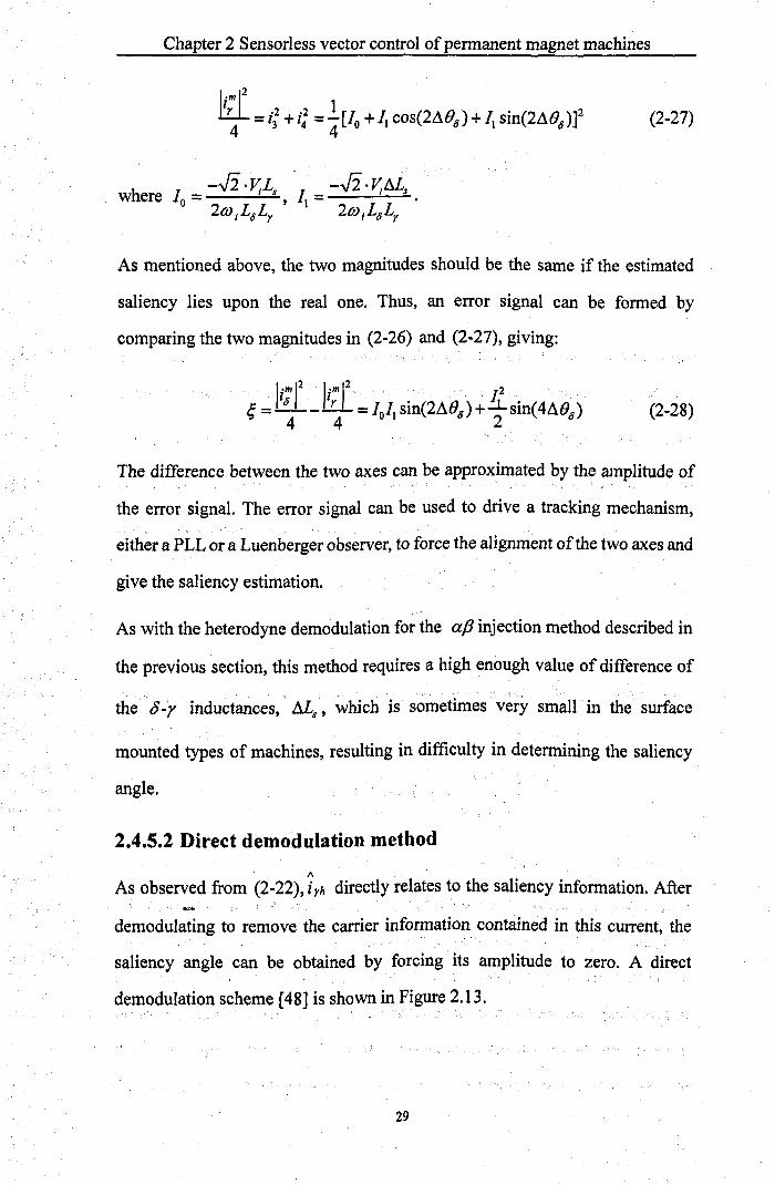
(2-27)
As mentioned above, the two magnitudes should be the same if the estimated
saliency lies upon the real one. Thus, an error signal can be formed by
comparing the two magnitudes in (2-26) and (2-27), giving:
(2-28)
The difference between the two axes can be approximated by the amplitude of
the error signal. The error signal can be used to drive a tracking mechanism,
either a PLL or a Luenberger observer, to force the alignment of the two axes and
give the saliency estimation.
As with the heterodyne demodulation for the afJ injection method described in
the previous section, this method requires a high enough value of difference of
the t5-y inductances, ~s, which is sometimes very small in the surface
mounted types of machines, resulting in difficulty in determining the saliency
angle.
2.4.5.2 Direct demodulation method
A
As observed from (2-22), i rh directly relates to the saliency information. After ... demodulating to remove the carrier information contained in this current, the
saliency angle can be obtained by forcing its amplitude to zero. A direct
demodulation scheme [48] is shown in Figure 2.13.
29

Chapter 2 Sensorless vector control of permanent magnet machines
1\
~r--B-P-F--'~:~PF f~Trnchlng =hanism~ ~': (Jo
cos(a1;l)
Figure 2.13: Direct demodulation scheme for d-axis injection
The measured current vector in the stationary frame first is transformed to the
estimated saliency frame. Then the imaginary part of the new vector is band pass
1\ 1\
filtered to give the hi current at r axis, i.e. i rh . Multiplication by the carrier
component, cos(m/), is made afterwards to give a DC component and a twice
injection frequency component, illustrated as:
(2-29)
By passing this signal through a low pass filter, the twice injection frequency
component can be removed, and assuming the estimation error is sufficiently
small, this yields:
~ = V; . M .f . sin(2L\(Jo) == V; . L\L\ . . L\(Jo
2w;LOLy UJ;LoLy (2-30)
The signal ~ is used to drive the mechanism to track the saliency angle.
Alternatively, the low pass filter can be removed to avoid the phase shift
introduced by this filter. Owing to the low pass property of the PI controller used
in the tracking mechanism, the twice injection frequency component can also be
removed. However, this arrangement requires an adequately low bandwidth of
the controller, which weakens the dynamic performance of the control.
Otherwise a large magnitude of twice injection frequency component still
30

Chapter 2 Sensorless vector control of permanent magnet machines
remains.
The direct demodulation method also faces difficulty when M s is very small as
with the measurement axis method.
2.4.5.3 Demodulation without use of hI carrier information
This method proposed in [15] is similar to the direct demodulation method
mentioned above except for the separation technique of the injection frequency
information and the saliency information. The diagram of this method is shown
in Figure 2.14.
1\
:" " " " " " ": ~ Tracking mo
L!m~e~c~h~an!!!i~sm!!!J-'~" 1\
Bo
Figure 2.14: Scheme of carrier separation without using injection frequency
information
The method used in this scheme for demodulating the saliency information from
the carrier introduces another variable, namely tly, obtained by:
1\ 1\
t:.y = i yh' sign(i oh) (2-31)
1\
This new variable is the angular error between the estimated axis 0 and the
1\
induced current vector i oyh' and can be shown in Figure 2.15.
31

Chapter 2 Sensorless vector control of permanent magnet machines
1
/\
8
t..:::::::.-----------.o ) wr
Figure 2.15: Diagram to show where /).y and 1, are found [50]
1\
In Figure 2.15, angle 1, is the angle of the rotating vector i...§yh' and is given [15]
as:
(2-32)
and the angle relationship of /).y, y, and 11°0 can be obtained by:
(2-33)
It is found that if /).y = 0, then 11°0 = y, = O. Therefore, the signal /).y can be
used to track the saliency. The detail of the demodulation is explained
mathematically below.
For ease of analysis, the injection vector in (2-20) is shifted by 90· , giving:
32
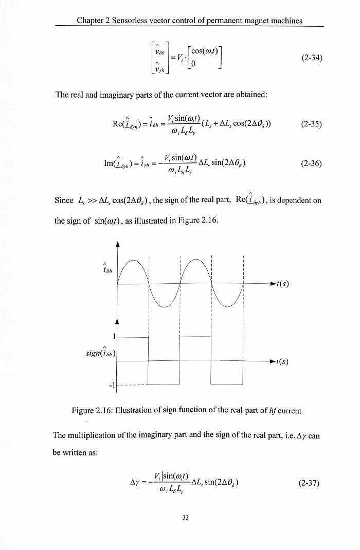
Chapter 2 Sensorless vector control of permanent magnet machines
(2-34)
The real and imaginary parts of the current vector are obtained:
(2-35)
1\ 1\ v: sinew;!) AL.,. sl'n(2 AB,, ) Im(l.Oyh) = i yh = ti ti v
(jJ j LOLy (2-36)
1\
Since L, » Ms cos(2I1Bo) , the sign ofthe real part, Re(lorlz ) , is dependent on
the sign of sin(~t), as illustrated in Figure 2.16.
r:...-----'l---+---+---i---I~t(S )
I I I I I I I I I I I
1 I I I I
I I I I I I
t(s)
1\
sign(ioh)
-1 ----- -
Figure 2.16: Illustration of sign function of the real part of /if current
The multiplication of the imaginary part and the sign of the real part, i.e.l1y can
be written as:
(2-37)
33
Chapter 2 Sensorless vector control of permanent magnet machines
The term of Isin(lV;t)1 can be written in the form of Fourier series as:
Isin( lVt)1 = ~ _.1.. . COS(2lV,t) + ... I 1C 31C
(2-38)
If only the twice injection frequency component and DC component are
considered, then (2-37) can be rewritten as:
With the help of a low pass filter or with a low bandwidth controller, the twice
injection frequency component can be filtered off leaving only saliency
information similar to the other demodulation schemes.
(2-40)
The signal of (2-40) can be driven to zero by a tracking scheme to achieve
correct angle estimation.
2.4.6 Saliency tracking by dq rotating
injection
This method [49] is similar to the ap rotating injection method except that the
injected voltage vector is imposed on the estimated dq frame as:
[~Oh] = v:.[-sin(lV;1)] " 'COS(lV.t) Vyh I
(2-41)
The current response is obtained as [19]:
34

Chapter 2 Sensorless vector control of permanent magnet machines
(2-42)
Again, the negative component contains the position information and the error
between the estimated and real saliency axis can be obtained. This error is then
tuned to zero to give an accurate estimate of the saliency angle. By
compensating for the armature reaction, a final dq frame is obtained for vector
control.
This method can produce better error signal compared to the d-axis injection
method [49]. However, the voltage injection along the q-axis causes additional
torque ripple which is disadvantageous to the d-axis injection method.
2.4.7 Saliency tracking by square wave
injection
The square wave injection method was introduced in [51, 52] where a pulsating
square wave was injected into the estimated d-axis for PM machine sensorless
control. It was claimed to have less time delay due to the eIimintation of the low
pass filter employed in sinusoidal types of injection methods. In [53], the
method was applied to an induction machine and injection axis was switched to
the estimated q-axis to give a better estimate of the flux compared with ad-axis
injection. In [54], the square wave signal was injected to the stationary reference
a-p fram~",as a rotating form for the sensorless control of an IPM machine with
similar performance to that of a pulsating type of square wave injection. This
method was implemented in this thesis for the EPS applications and it will be
discussed further in Chapter 3.
35

Chapter 2 Sensorless vector control of permanent magnet machines
2.4.8 Overview of saliency tracking by
measuring Current derivatives (di/dt)
The current derivative (di/dt) methods are generally linked with PWM transient
excitation. Most of them involve modification of the PWM sequence, and the
transient current response, termed the di/dt signals, is then measured which
contains the saliency position information used to track the rotor position. The
main methods categorized in this group are the INFORM method, the EM
method, the Fundamental PWM excitation method and the Zero vector method,
which will be discussed later. The advantage of these methods is that a higher
signal-to-noise ratio (SNR) than that for the hi injection methods can be
achieved and some of the methods can provide accurate estimation over a wide
range of speed. The other advantage is that similar disturbance removal methods
such as the synchronous filter and memory method as mentioned in 2.4.4 for the
ap hi rotating injection methods can be applied to obtain a clean position
estimate. However, all of these methods involve the modification of the NO
sampling circuitry and increase the sampling rate. The modification of the PWM
sequence will introduce extra torque ripple and more audible noise.
2.4.9 Saliency tracking by the INFORM
method
The INFQRM (Indirect Flux Detection by On-line Reactance Measurement)
method introduced in [55] utilizes active voltage vectors (referred as test vectors)
in addition to the fundamental PWM sequence to excite the machine, and the
position signal can be constructed by examining the transient current (current
derivative) response to the active voltage vectors.
A star connected machine with saturation induced saliency is considered here.
36

Chapter 2 Sensorless vector control of permanent magnet machines
The inductance of each phase can be modelled as [29]:
27r Ib = 10 + M cos(20o --)
3
(2-43)
(2-44)
(2-45)
where 10 is the average stator inductance and M is the inductance variation
due to saturation, 200 is the saturation saliency which needs to be tracked.
Supposing the demanded voltage vector resides in Sector I as shown in Figure
2.17,
V2 '~------------~
V4 VI
V5 V6
Figure 2.17: Vector diagram when the demanded voltage resides in sector I
when active vector VI is applied, the following equations can be derived [29]:
d'(V I) d· (V I ) V = i (V I )r + I _1_0 _ . + e(V I ) - (i ( V I )~ + I _1_6 - + e (V I»)
de 0 a a dl a 6 b b dl b (2-46)
d,(V I) d·(V I ) -V = j (V l)r + I _I_c - + e(V I ) _ (j(V I )r + I _I_a _ + e (V I»)
dc c C c dl C a a a dl a (2-47)
37

Chapter 2 Sensorless vector control of permanent magnet machines
where the superscript (VI) denotes the instantaneous value when the active
vector VI is applied (similar notation for the other 6 vectors including the zero
vectors), ia,ib and ieare the three phase currents, la,lb and le are the three phase
inductances, ra,rb and re are the three phase resistances, and ea,eb and ee are the
three phase back-EMFs,
Similarly, the equations when vector V 4 is applied to the machine are:
(2-48)
(2-49)
If the two test vectors are applied within a short period, then the back-EMF terms
can be assumed equal, and the difference of the voltage drops across the resistor
can be ignored, Then, combining (2-46) to (2-49), yields:
d,(VI) di(V4) di(VI) di(V4) -2V =1 (.-L.--P-)-1 (_a __ --fL-)
de e dt dt a dt dt
Also, for a balanced system,
-dia dib die - 0 -+-+--dt dt dt
Combining (2-50) to (2-52) gives:
dl,(VI) dl,(V4) I +1
b e --1!.- - --1L- = ·2Vd,
dt dt lib +Iie + lie e
38
(2-50)
(2-51)
(2-52)
(2-53)

Chapter 2 Sensorless vector control of permanent magnet machines
di(VI) di(V4) -L-__ b _=
dt dt (2-54)
di(VI) di(V4) I c c b 2V ----=- . d dt dt lib + lie + lie c
(2-55)
Then substituting the inductances from (2-43) to (2-45) into (2-53) yields:
di(Vl) di(V4) 2 t!.1 _0 ___ 0 -=-(2--cos(2Bo»
dt dt Cl 10
t!.[2 1 where Cl = 3/0 (1--2 ) . -, and can be considered constant.
4/0 Vdc
(2-56)
Similar equations can be derived when other opposite vector pairs, V2N5 and
V3N6 are applied to the machine, as:
di(V2) di(VS) 2 t!.[ 2tr _b ---L-=-(2--cos(2Bo--»
dt dt Cl 10 3 (2-57)
di(V3) di(V6) 2 t!.1 4tr -L-_--£...- =-(2--cos(2Bo --»
dt dt Cl 10 3 (2-58)
A position vector can be constructed as:
. 2 P=Pa+apb+ a Pc (2-59)
./2tr Where a = e 3 represents the frame transformation, and Pa/hle are defined as:
-. (2-60)
39

Chapter 2 Sensorless vector control of permanent magnet machines
ill 47l" C dlV3 ) di(V6)
P =-cos(2B __ )=2_--L(_C ___ C_) C I 8 3 2 dt dt o
(2-62)
The resultant orthogonal components of this position vector !!. are obtained:
(2-63)
(2-64)
The saliency angle is the angle of this position vector and can be obtained by:
Pp 2B8 = arctan(-)
Pa (2-65)
It can be noticed that in order to establish the position vector !!.' three pairs of
opposite active vectors need to be applied while keeping the VTA (voltage time
area) unaltered by the test vectors. Consequently, the test vectors are injected in
null vectors (VO and V7) whenever the position estimation is required.
However, due to the high frequency oscillation of the dildt signals induced by
parasitic effects within the machine itself after each switching state, a minimum
duration tmin of each test vector is required for accurate measurement of the di/dt
signals. Therefore, there is not enough time for the three pairs of test vectors to
be within one PWM cycle. The alternative is to put them in three neighbouring
PWM periods [14], and the arrangement is illustrated in Figure 2.18. The -.llrI
disadvantage of this arrangement is that at higher frequencies the positions can
be very different from neighbouring PWM periods and the estimation can be
largely affected. Reference [14] reported a compensation scheme with
estimation error reduced significantly.
40

Chapter 2 Sensorless vector control of permanent magnet machines
VI V 4 V3 V 6 V5 V2
PWMo '--------' Jl~ r-----1
P~ ~u:rL_mJl ~~L p~ nif] I ~ IT121
Figure 2.18: INFORM method test vectors injecting arrangement
An improved vector sequence for the INFORM method is proposed in [56] ,
which introduces an extra pair oftest vectors. For instance, when the pair of test
vectors is V3and V6, another pair ofthese vectors is added with half-length of
each test vector as the sequence shown in Figure 2.19. With these extra vectors,
current distortions due to the injection of test vectors can be reduced while the
VTA remains unchanged.
- 1', .. , V6 , V3 V6
Ch : :
I a , I : ,
PWM
,
PWM. b
i-i , , , , : ; r--
PWM l~f , , , , ,
t t di / dt samples .
Figure 2.19: Improved test vector sequence of INFORM method
The INFORM method is not applicable in the full frequency range, since at
higher frequencies , null vectors are generally very short resulting difficulty in
injecting test vectors in the PWM sequence.
41

Chapter 2 Sensorless vector control of permanent magnet machines
2.4.10 Saliency tracking by EM method
VI
V5 V6
Figure 2.20: Definition of sectors for EM method
The INFORM method makes use of test vectors in addition to the fundamental
PWM sequence, whilst the Extended modulation (EM) method proposed in [57]
integrates the test vectors within a modified PWM sequence. Rather than using
the standard six sector divisions of a SVPWM, four sectors (1, II , III , and N) are
defined by combining neighbouring two 60° sectors as shown in Figure 2.20.
The overlapping regions are only used by I and N. When a reference voltage
y.. is demanded, it can be decomposed in the new extended sectors. The
combination of active vectors is (VI, V3) for I/.:M (Extended Sector I), (V2, V4)
for IT EM ' (V4, V6) for ill1:M and (V5, VI) for N fM • Supposing a voltage
demand falls in I RM , then equations (2-66) to (2-68) can be derived for the
application of active vector VI, neglecting the voltage drop across resistors and
the back-EMF terms as only low frequency operation is considered.
(2-66)
42

Chapter 2 Sensorless vector control of permanent magnet machines
(2-67)
(2-68)
Then, substituting the inductances (2-43) to (2-45) into above equations, yields:
di(VI) 1 M _a_ =-(2--cos(288»
dt Cl 10 (2-69)
di(VI) 1 M 27l' _b _ = --(1 +-cos(288 --»
dt Cl 10 3 (2-70)
di(Vl) 1 M 47l' _0 -=--(1+-cos(28
8 __ »
dt Cl 10 3 (2-71)
where Cl = 3/0 (1- M: ). _1_, and again can be considered constant. 4/0 ~c
Consequently, the scalar position signals can be defined as:
(2-72)
di(VI)
P --I-c _0_ bl - I dt (2-73)
.....
di(Vl)
P =-I-c-1!..-cl I dt (2-74)
A similar approach can be applied to derive the position signals for the
application ofV3, giving:
di(V3)
P =-I-c _c_ a3 I dt (2-75)
43

Chapter 2 Sensorless vector control of permanent magnet machines
di(V3) Pb3 =2-CI _
b -dt
(2-76)
(2-77)
By carefully choosing appropriate position signals to apply to (2-59), a position
vector can be obtained as:
1 . 1 ) Pa = -(Pc3 -'2 Pbl - 2 Pcl
d·(V3) 1 di(VI) di(VI) = -(-l-c ...!.E-)+-[(-l-cl---L-)+(-l-cl - b
-)] I dt 2 dt dt
di(V3) 1 di(VI) 1 di(VI) = c (_0 ___ -L----b -)
I dt 2 dt 2 dt
(2-78)
3 III =--cos(2B8 )
2 10
(2-79)
It can be seen that by constructing this vector and applying to (2-65), the term
~I can be eliminated to derive the final estimation of the saliency angle, which o
means no knowledge of machine inductance required. The selection of the
position signals to form the vector is not unique, as in this case Pa can be also
calculated as (2-80), and results remain the same.
(2-80)
In addition to the modification of the sector division, a minimum time of at least
44
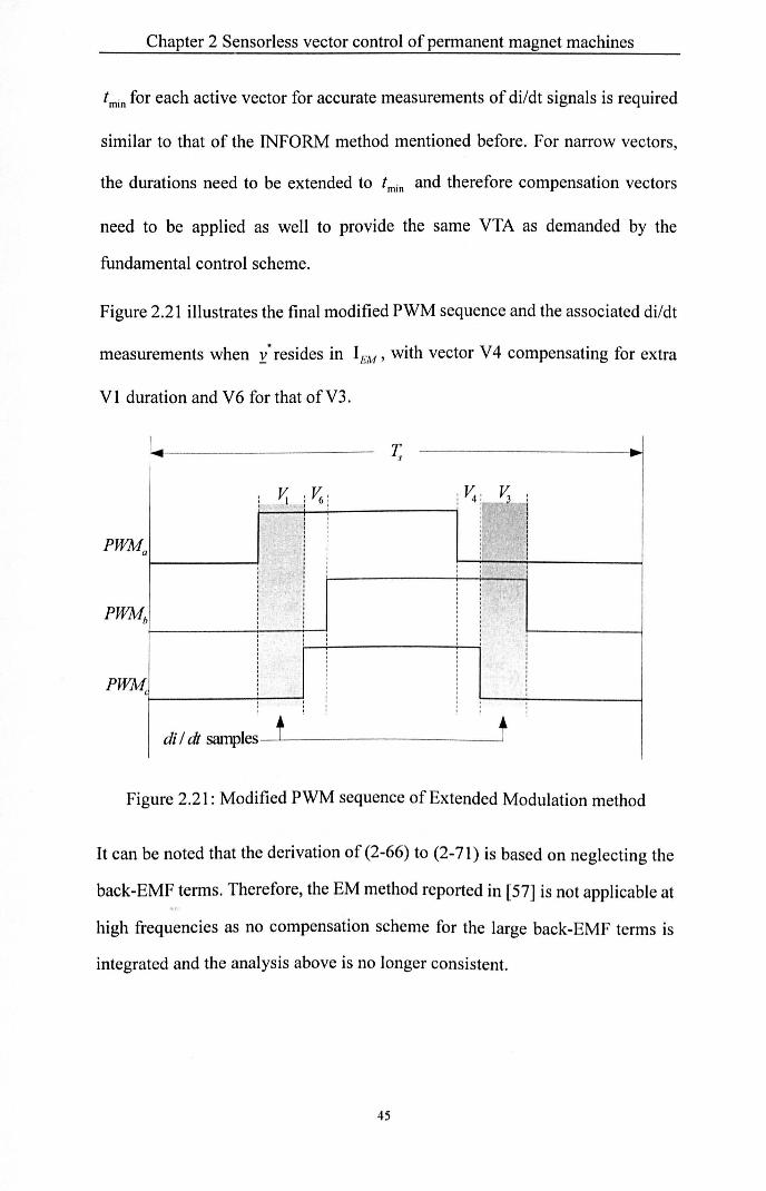
Chapter 2 Sensorless vector control of permanent magnet machines
tmin for each active vector for accurate measurements of di/dt signals is required
similar to that of the INFORM method mentioned before. For narrow vectors,
the durations need to be extended to tmin and therefore compensation vectors
need to be applied as well to provide the same VTA as demanded by the
fundamental control scheme.
Figure 2.21 illustrates the final modified PWM sequence and the associated di/dt
measurements when y.' resides in I EM ' with vector V 4 compensating for extra
V 1 duration and V 6 for that of V3.
1;
~ :~ : iT-:; ~ j , , ,
!
ir I , I
I I
: , , ,
i i "
: i i i
, i , ,
PWM , : ,
di / dt samples t t
Figure 2.21: Modified PWM sequence of Extended Modulation method
It can be noted that the derivation of (2-66) to (2-71) is based on neglecting the
back-EMF terms. Therefore, the EM method reported in [57] is not applicable at
high frequencies as no compensation scheme for the large back-EMF terms is
integrated and the analysis above is no longer consistent.
45

Chapter 2 Sensorless vector control of permanent magnet machines
2.4.11 Saliency tracking by Fundamental
PWM excitation method
Rather than modifying the PWM sequence as in the EM method, the
fundamental PWM method proposed in [17, 20] utilizes, as indicated by its
name, the fundamental PWM voltage vector excitation the machine. For
example, supposing a vector y.' in sector I is demanded, it is decomposed with
VI, V2 and null vectors (VO and V7). When VI and VO are applied to the
star-connected machine, as for the INFORM method, the following equations
can be derived:
di(VI) di(VO) 1 Al _a ___ a -=-(2--cos(2B,,»
dt dt Cl 10 (2-81)
di(VI) di(VO) 1 Al 2:r -E-_-L-=--(1+-cos(2B" --»
dt dt Cl 10 3 (2-82)
di(VI) di(VO) 1 Al 4:r _c -_.-£-=--(1+-cos(2B" --»
dt dt Cl 10 3 (2-83)
Al2 1 where Cl = 3/0 (1-2") . - can be considered as constant.
4/0 Vdc
Three scalar position signals can be defined as:
di{VI) di{VO)
P =2-c (-L-_--L-) 01 I dt dt (2-84)
di(VI) di(VO)
P =-I-c (_C ___ C_) hl I dt dt (2-85)
di(VI) di(VO)
P =-I-c (_h ___ h_) cl I dt dt
(2-86)
46

Chapter 2 Sensorless vector control of permanent magnet machines
By applying the same approach, another set of position signals using V2 and VO
can be defined as:
di(V2) di(VO)
P =-l+c (-L-__ b _) 02 I dt dt
(2-87)
di(V2) di(VO)
P =-I+c (_0 ___ 0_) b2 I dt dt
(2-88)
di(V2) di(VO)
P =2+c (_C ___ C_) c3 I dt dt
(2-89)
To avoid error caused by the uncertainty of the coefficient Cl' it is necessary to
choose position signals with same offset to form a position vector !!.. Therefore
the aft components of this vector are given as (2-90) and (2-91), and the
saliency position angle can be calculated without knowing Cl •
(2-90)
(2-91)
For demand voltage vectors located in the other five sectors, the position signals
for each combination of an active vector and a null vector can also be obtained,
and can be tabulated as Table 2.1. Similar results can be applied to a
delta-connected machine. -
47

Chapter 2 Sensorless vector control of permanent magnet machines
Sampled Pa Ph Pc
Vectors
VI, VD dlV1 ) dlVO ) di(VI) di(VO) di(VI) di(VO) 2 -c (_a ___ a_) -l-c (_C ___ C_) -l-c (_b ___ b_)
1 dt dt 1 dt dt 1 dt dt
V2, VD di(V2) di(VO) di(V2) di(VO) di(V2) di(VO) -l+c (_b __ .J-) -l+c (_a ___ a_) 2+c (_C ___ C_)
I dt dt 1 dt dt I dt dt
V3, VD di(V3) di(VO) di(V3) di(VO) di(V3) di(VO) -l-c (_C __ .-£-) 2-c (_b ___ b_) -l-c (_a ___ a_)
1 dt dt 1 dt dt I dt dt
V4, VD di(V4) di(VO) di(V4) di(VO) di(V4) di(VO) 2+c (-!L- __ a -) -l+c (_C ___ C_) -l+c (_b ___ b_)
1 dt dt I dt dt I dt dt
VS, VD di(VS) di(VO) di(VS) di(VO) di(VS) di(VO) -l-c (.J- __ h _) -l-c (_a ___ a_) 2 -c (_C ___ C_)
1 dt dt 1 dt dt 1 dt dt
V6, VD di(V6) di(VO) di(V6) di(VO) di(V6) di(VO) -l+c (_C ___ C_) 2+c (_b ___ b_) -1+c (_a ___ a_)
1 dt dt 1 dt dt 1 dt dt
Table 2.1: Position signals obtained by di/dt measurements of each combination
of active vector and null vector for a star-connected machine
It is noted that the null vector can be chosen from either VD or V7 depending on
the convenience of di/dt measurements. The rule for choosing appropriate
position signals in constructing position vector is to cancel the offset as
mentioned above.
48

Chapter 2 Sensorless vector control of permanent magnet machines
V2 ir-------.""I.
VS V6
VI
PWM edge shifting
needed in the shaded area
Figure 2.22: Locations of a demanded vector where a shifted PWM sequence is
required
However, modification of the PWM sequence is also required for low
modulation index region and for the cases when demanded voltage vector passes
active vectors, the area where modification of PWM sequence is required is
visualized in Figure 2.22. The difference compared with the EM method is that it
does not change the active vectors applied in a normal PWM, and the only
modification made is to shift corresponding PWM sequence to provide a
duration of tmin for short vectors in the first half of the PWM period and their
compensation is made in the second half of the period as shown in
Figure 2.23, assuming y.. residing in Sector I and extensions for both VI and V2
required. Vector V 1 is applied for the duration of tmin and its compensation V 4 is
applied for (t) -tmin ); V2 and its compensation VS are applied for tmin and
(t2 - tmin ) , respectively. Therefore, the mean voltage vector demanded from the
inverter is conserved. Similar shifting can be utilized for vectors in the other five
sectors and the results follow the above analysis. Theoretically this method can
work in the whole operation range [17]. In the zero and low frequency situation 49

Chapter 2 Sensorless vector control of permanent magnet machines
when modification of the fundamental PWM is required, current distortion is
induced and can be reduced by applying active vectors in consecutive PWM
periods [17]. At higher frequencies where the active vectors are longer due to the
increase in the back-EMF, the requirement for modification of PWM pulses
decreases and even vanishes, and the current distortion is consequently reduced
significantly [17].
PWM
~ ~ :~ V; ~~~~~--~~
t
, ,
.. . .... 1----4-----........ ....,
i~ ishi~ '---'-, , , , , , : :
I 1. _- :, ..... :, , .... J ••••••••. i----~__;.....:___I i ~ftirg
, ,
. " ~ .. --- .. r- .. r- .. ..
t t di / dl samples
Figure 2.23: Edge shifting of a standard PWM sequence to provide sufficient
time for di/dt measurements
2.4.12 Saliency tracking by Zero Vector
method
Reference [58, 59] investigated the possibility of tracking the saliency position
by measurements of zero sequence phase voltage/current caused by the
unbalance nature of stator parameters. However, both of these two methods need
to inject test vectors similar to the INFORM method, which suffers from the
same limitations as the INFORM method as discussed previously.
50

Chapter 2 SensorIess vector control of permanent magnet machines
Another approach which also makes use of the zero sequence information for
position estimation was reported in [60]. It can be regarded as a combined
method of saliency tracking and back-EMF based tracking technique.
Considering that a zero voltage vector is applied to the machine, the voltage
equations in the real dq synchronous frame can be obtained as:
(2-92)
Where superscript (VO) represents the vector being applied, p denotes the
derivate function, 'If mOl, is the back-EMF term, and cross coupling term is
ignored.
Assuming the estimated synchronous frame is misaligned with the real dq
synchronous frame by an angle of dB, then applying transformation (2-93) to
(2-92), the current derivative can be obtained as (2-94).
,.,(VO) did
dt ,.,(VO)
d Iq dt
Id cos(dB) - sm(dB) id
[
.(VO)] . [,.,(VO)]
,;VO) = [Sin( AB) COS( AB) ] ; ~O)
'If mOl, [Sin(dB) ] =T cos(dB)
,JVO)
(2-93)
(2-94)
Using closed loop control, the id term is controlled to zero. Therefore, (2-94)
can be rearranged to:
SI

Chapter 2 Sensorless vector control of permanent magnet machines
,,(VO)
did
dt ,,(VO)
d iq
dt
,,(VO)
(2-95)
c. d id th' l' b d d Then by 10rcing to zero, e mlsa Ignment can e compensate an an dt
estimation of the position can be achieved. In [18], a modified demodulation
scheme was proposed to allow the estimation over the full operation region (Le.
all four quadrants). However, the performance of this method is still limited at
the low speed no load condition, since under this condition, the saliency tracking
taking over is the back-EMF tracking and the error magnitude is zero due to the
lack of torque current.
2.5 Conclusion
In this chapter, a variety of methods for sensorless vector control of permanent
magnet machines has been reviewed. Each of the methods has been described in
terms of the principle, implementation and limitations. For a commercial
application, it is essential to bear in mind the advantages and disadvantages in
association with all possible methods and then choose the most suitable one. A
comparison of the methods mentioned in this chapter has been made regarding
the following aspects and conclusions have been drawn.
In terms 01 hardware usage and implementation complexity, model based
methods have shown superiority over other methods. The measurements
required for these methods can be limited to phase currents measurements,
which is similar to that for high frequency injection methods. However, most of
the model based methods rely on much less signal processing than that of high
frequency injection methods. The current derivative methods on the other hand,
S2

Chapter 2 Sensorless vector control of permanent magnet machines
consume the most hardware resources compared with the other two categories.
Additional current derivative sensors are sometimes required for acquisition of
high resolution current derivative measurements, although multiple phase
current measurements can replace direct current derivative measurements,
adding more requirements to the signal processing and resulting in poorer
performance. More complex modifications to sampling arrangements for the
fundamental PWM sequence have to be incorporated for these methods to work.
Considerating the operating range, model based methods work well at medium
and high speed but deteriorate with a decrease of speed. Zero and low speed
control is still difficult to achieve. The hi injection methods are well suited for
zero and low speed and limited for a higher speed. The INFORM and EM
method can also work well under zero/low speed range while the fundamental
PWM method can work ranging from zero to a high speed range. Zero vector
current derivative method has poorer performance with the decrease of load
level in the low speed region.
Several factors affect the estimation quality, such as inverter non-linearity and
mechanical disturbances of the machine itself. An effective disturbance
elimination procedure is therefore essential for the final implementation of the
control. Model based methods can provide disturbance elimination such as the
use of Kalman filter or other compensation schemes for inverter compensation.
For the hi injection method, rotation signal injection is suited to disturbance
elimination schemes due to its phase dependent tracking nature, and similar ,...
approaches can be applied to most current derivative methods. On the other hand,
pulsating signal injection normally utilizes the amplitude of the stator current,
and there are few measures for disturbance elimination and thus a poorer
estimation quality is expected compared with other methods.
The advantages of the pulsating type hi signal injection method is that firstly a
53

Chapter 2 Sensorless vector control of permanent magnet machines
low torque ripple is generated if injecting onto the flux producing axis, where in
other signal injection methods and most current derivative methods the torque
ripple is generally considered as an issue; secondly, with the pulsating signal
injection, audible noise is kept minimum comparing with other methods except
model based methods. Although audible noise can be reduced using pulsating
signal injection, it is still significant for applications such as electrically powered
steering system of this research. Modifications are required to further reduce the
noise which will be discussed in following chapter.
S4

Chapter 3 Random frequency sinusoidal injection and square wave injection methods for audible noise reduction
Chapter 3 Random Frequency Sinusoidal Injection and Square wave Injection methods for audible noise reduction
3.1 Introduction
When using sensorless motor control wih a high frequency signal injection
method, the frequency of the injection can be clearly heard and can be
uncomfortable. The injection signal manifests itself as noise by creating
mechanical vibration in many of the motor components, e.g. in the winding, in
the motor casing. Other things cause acoustic noise as well, for example, air
displacement due to the rotating of the rotor, but the dominant one is usually the
high frequency signal injection which can range from several hundred Hz to
several kH~. In automotive applications, this high audible noise makes it
unsuitable. In [21], the additional audible noise caused by the d-axis injection
method and fundamental PWM method [56], [17], [20], [43] was compared and
the sound performance with the current derivative method was reported to be
better than the injection method since the high frequency components are spread
over a range of frequencies. To improve the hearing experience for the injection
ss

Chapter 3 Random frequency sinusoidal injection and square wave injection methods for audible noise reduction
based methods, a similar frequency spread can be achieved by using a random
frequency injection instead of a fixed one. Thus, the sound introduced by the
injection will be heard as a spread of components rather than a fixed tone, and
due to the non-linearity of human hearing (see Chapter 4), some of the
components will be highly attenuated, which will reduce the perception of the
noise.
An alternative approach has been proposed to reduce the perception of noise,
where the injection frequency is raised towards the PWM frequency- in this case
using a square wave [52]. If the switching frequency is high enough (20 kHz in
this work), the resultant noise component will be at a frequency that is rather
attenuated by the human hearing. Therefore, a reduction of the audible noise can
also be achieved.
These two methods are discussed in this chapter.
3.2 The Random hfSinusoidal Injection
method
3.2.1 Introduction
A novel approach to reducing the perception of noise for an injection based
sensorless control is to randomly spread the injection frequency over a specified
frequency range. The aim here is to combine the ease of implementation of the ,..,
d-axis injection method, with the spread of frequencies associated with the
fundamental PWM method. The approach is similar to that proposed for
reducing the perception of PWM associated audible noise, by using random
carrier frequencies, as proposed in [61, 62]. The aim of this part of the
investigation is therefore to ensure that if a random hi injection frequency is
56

Chapter 3 Random frequency sinusoidal injection and square wave injection methods for audible noise reduction
employed, it will not affect the behaviour of the sensorless algorithm.
The overall control structure of the implemented random hf sinusoidal injection
method is shown in Figure 3. 1. The random frequency injection method is quite
similar to fixed frequency sinusoidal injection. In this section, its operation will
be covered and the implementation of the method will be presented.
Inverter
/\ [--------------------------- -----! J afJ
Be ! Signal ' ~-+-------processing
/\
idq ! Position demodulation ! , , , , 1 _ _ __ __ -- -- ----- ----- ------ - -- --_.
Figure 3.1: The overall control structure of the PMAC drive system with random
hi sinusoidal injection method
3.2.2 Random number generation
In digital implementations, truly random sequences are difficult to realize since
only predicted values can be generated by the processor. Consequently, a pseudo
random sequence is generally chosen. There are several ways of creating pseudo
random sequences. The feedback shift register [63] has been chosen as the
pseudo random sequence generator due to its ease for implementing digitally. It
is suitable for the DSP-based control platform of the experimental rig. A 16-bit
feedback shift register is used in this work and the structure is shown as in Figure
3.2.
57

Chapter 3 Random frequency sinusoidal injection and square wave injection methods for audible noise reduction
Bit[l] Bit[ 4] Bit[13] Bit[14 Bit[15] Bit[16
XII [1 3] XII [1 5] x,J16]
Shift register
Figure 3.2: Structure ofa 16-bit Feedback Shift Register
The random number generation process can be illustrated mathematically as:
Where XII is the present value of the random number, X n_1 is the last updated
value, EBrefers to the Exclusive-Or operation, and »is the logical right-shift
operation.
The generator is processed at a fixed clock rate of 20 kHz which equals to the
sampling rate of the system. An Exclusive-OR function is performed at each
clock cycle combining the 4th, 13th, 15th and the last bit of the register, and the
product is input to the first bit after a logical right-shift of the previous 16-bit
sequence. In this way, the 16-bit sequence will go through 65535 distinct states
(216 -1) before it repeats itself again. If the number of bit is chosen too small,
the sequence will be soon repeated resulting in a poor randomness. If a higher
number of bits are chosen, a larger number of distinct states will be generated
and hence more randomness is expected with the cost of additional memory
required in a practical fixed-point processor. In fact, with a 16-bit register
updating at a rate of 20 kHz, the generated pattern will repeat itself in 3.3
58

Chapter 3 Random frequency sinusoidal injection and square wave injection methods for audible noise reduction
seconds which is adequate for a motor drive application and is therefore chosen
in this research. It should be noted that a non-zero initial value should be
assigned to the shift register.
3.2.3 Construction of the injection signal
The constructed random frequency signal can be defined as:
[~ oh 1 = kef) [ cos(21r(H+ f ~)ot) 1 Vyh (3-2)
= k(f)[ COs(201r/-t) 1 /'an E [ - /'andom' + /'andom ]
where the superscript denotes that the injection voltage vector is considered in
A A
the estimated saliency 0 -r frame (for convenience, it is referred as the
estimated dq frame in the following contents), kef) is a function depending on
different injection frequencies, J;is the centre frequency of the selected random
range, han is the instantaneous random frequency, I rando;" is the range of the
random frequency, and f = 1; + Iran is the instantaneous injection frequency.
In order to derive the function k(f) , different injection frequencies have been
applied to the PM motor with the fixed injection method. When these injection
frequencies are applied, to ensure the amplitudes of the resultant different
frequency hI currents do not change with the injection frequencies being applied
(about 1.1 A for each of the side bands), different injection voltages are used and
the values are plotted in Figure 3.3. From Figure 3.3, a linearized approximation
of the function kef) can be obtained as:
kef) = 0.0006f + 0.4 (3-3)
59

Chapter 3 Random frequency sinusoidal injection and square wave injection methods for audible noise reduction
and equation (3-4) can be obtained:
v; kef) --=~-=C
27r J; 27r1 (3-4)
where V; is the amplitude of the hf injection voltage in the fixed hi injection
method with the resultant hf current amplitude around 1.1 A, and c is a constant.
2.5
/~
~ V V
~
o o 500 1000 1500 2000 2500 3000 3500
Injection frequency (Hz)
Figure 3.3: Plot of injection voltages against different injection frequencies with
the same hf current amplitude
Applying (3-1), the random injection frequency range is derived as:
J, XII random =- (3-5)
m
where m is a scaling factor to choose appropriate frequency range.
The choice of the injection frequency range should satisfy certain requirements
in order to maintain a good control performance. Thus, the lower range of the
frequency cannot be too low otherwise it will interfere with the current
controller operation, and the upper range of the frequency cannot be too high to
avoid the injection signal being highly stepped due to the limitation of the
60

Chapter 3 Random frequency sinusoidal injection and square wave injection methods for audible noise reduction
switching frequency (20 kHz) as explained in [13]. On the other hand, it needs to
be spread widely and randomly enough to allow the reduction of audible noise
and improve the hearing experience. Some compromises need to be made to
meet both requirements in a practical application. In this research, the centre
injection frequencies have been chosen as 1.5 kHz and 2 kHz respectively to
match the previous work in [13], and the random ranges of ±328 Hz and ±656
Hz have been chosen to allow the reduction of audible noise while maintaining
good sensorless control performance. The generated injection voltage over 20ms
for a frequency range of(1500±328) Hz random injection is shown in Figure 3.4.
~ Cl> Cl ~ (5 >
1 . 5 ~--~--~--~----~--~--~---'----r---~--~
0.5
0
-0.5
-1
-1 . 5 L--__ -1--__ -'-__ --'-____ '---__ -L-__ -L __ --L ____ L-__ -L-~___l
o 0.002 0.004 0.006 0.008 0.01 0.012 0.014 0.016 0.018 0.02 time (sec)
Figure 3.4: The generated random injection voltage with (1500±328) Hz random
range
The results for the measured audible noise and the sensorless control with these
frequencies will be compared and discussed in Chapter 6.
With appropriate selection of the injection voltage as described above, the
61

Chapter 3 Random frequency sinusoidal injection and square wave injection methods for audible noise reduction
resultant hi current can be spread randomly. The wider the frequency range is,
the more spread of the power of the hi current components. This can be
illustrated by the spectrum of the line current obtained through rectangular
windowed FFT operations with zoomed area regarding the hi current
components for a fixed injection at 1.5 kHz and two random injections at
(l500±328) Hz (l500±656) Hz, as shown in Figure 3.5.
Spectrum ofllal with 1500 Hz injection, -60rpm, 30A
1 ---- --- --- --- ------ ---- ~ - ----- ------ -- --- --- ----- ----- ----- ---- -- --- --- -- - ~ ------- ---- -------- -----
<' , , ------._---- -- -- ------- .. ---- ------- ---- --- -- ----- ----- -- --- --- -------- --- -.. ---- -. -.----------------, , '-' 0.5 -'" , , , , , ,
o ~--------~----------~--------~----------~ 500 \000 1500 2000 2500
Spectrum of Ilal with 1500±328 Hz injection, -60rpm, 30A
1 I- - - - - - - - - - - - - - - - - - - - - - - - ~ - - - - - - - - - - - - - - - - - - - - - - - - - ~ - - - - - - - - - - - - - - - - - - - - - - - - - ~ - - - - - - - - - - - - - - - - - - - - - - --, , , , , , , , , , , , , , <' ::. 0.5 I- ---- --- ---- --- ---- --- - - ~-- ---- -- --- ----- ----- ---- ~- -- ---- --- ---- --- -- - ---- - ~ ---- -- ---- --- ----- --. ---
~. O L---------~------~~~~ ______ ~ __________ ~ 500 \000 1500 2000 2500
Spectrum ofllal with 1500±656 Hz injection, -60rpm, 30A
1 1- ----------- -- -- --- -----1---- ------- ------ --------1- -------· ------- -------- -r- --- · ---- ---- ------ --.--<' I : :
::. 0.5 I- - --- ---- - ---- ---- --- ---1------- -- ------ ------ ----1- -- ----- --- --- -----------f ---------- ---------- ----
: ... ~JJl ... c O L---------~----~~~~~----~------~ 500 \000 1500
Frequency (Hz) 2000 2500
Figure 3.5: Spectra of the line currents for fixed 1500 Hz and random (1500±328)
Hz, (1500±656) Hz injection at -60rpm under 30A load with sensored operation
Figure 3.5 also indicates that the reduction of the acoustic noise due to injection
can be achieved by random injection as the hi current components spread as
expected. Details of issues related to acoustic noise will be given in Chapter 6.
62

Chapter 3 Random frequency sinusoidal injection and square wave injection methods for audible noise reduction
The power of the hi current components for the three injection types are
calculated by summing up the related frequency components (for fixed injection,
the power of the amplitude of the two side bands around the injection frequency
is summed, and for random injection, the power of the amplitude of the
components within the frequency range is summed) and is shown in Table 3.1.
1500 Hz (1500±328) Hz (1500±656) Hz
Total Power ( A2 ) 2.5216 2.4682 2.4553
Table 3.1: The calculated hi current power for fixed and random hf injection
method
As noted from Table 3.1, the total power of the resultant hlcurrent components
for the fixed and random injection methods are comparable, which demonstrates
that the total power are preserved.
3.2.4 The signal processing procedure
When the pulsating signal as given in (3-2) is applied to a PMAC motor, the
resultant hi current response in the estimated reference frame can be obtained as:
[7 Oh] = (I)' k(/) sin(2n I· t) [Ls + IlLs cos(2!:::. eo)] (3-6) ~ 17 2nl(L! -1lL~) AT' (2 A O" ) I rh -llLs sm Ll 0
where Ls the average inductance, IlLs the difference in inductance between the
" d and q axes, !:::.Oo the error between the real and the estimated rotor position
[19], and 17(/) is a variable dependent on the integration of the random
frequency variable I .
To see the effect of 17(/) on the resultant hi current components, both the fixed
63

Chapter 3 Random frequency sinusoidal injection and square wave injection methods for audible noise reduction
and random hlinjection were applied into the real d-axis. The resultant h/current
vector in the real dq frame can be obtained by applying equation (3-4) and
1\
ilOo = 0 to (3-6), yielding:
[ ~dh] = 17(/)' c·sin(21rf '/) [1] lqh Ld 0
(3-7)
where idh and iqh represent the hi current components in the real dq frame, Ld is
the d-axis inductance, and for the fixed injection 17(/) equals 1. Then, the
vector was observed on an arbitrary frame, namely dobsqobs frame, shifted from
the real dq frame by an angle Bobs ranging from 0 degree to 360 degrees,
equation (3-7) can be rearranged to the new frame as:
[ 'ObS] [ B . B ] [. ] 'dh cos obs sm obs 'dh i;!S = - sin Bobs cos Bobs • iqh
= 17(/)' c· sin(2tr I· t) [ co.s Bobs ]
Ld -smOobs
(3-8)
h .ohs d .obs h t b d ~ h b' were 'dh an lqh are t e curren components 0 serve Lrom tear Itrary
dobsqobs frame. By multiplying (3-8) by the carrier sin(21r I· t) and passing
through a low pass filter, the DC value can be obtained as:
LPF(sin(2trl ./) .[~~!:]) = LPF(17(f)' c· (I-cos( 4nI ·t» [ co.sBOhS ]) lqh 2Ld -smOobs
(3-9)
[i~]·'" C [cos BObS] => I =17(/)'- . iqh 2Ld - sm Bobs
where LPFO represents the low pass filtering operation, and i~h' i~h are the DC
values. The scheme to obtain these values is shown in Figure 3.6.
64

Chapter 3 Random frequency sinusoidal injection and square wave injection methods for audible noise reduction
+ i; ---'-OO---I~
+ .• 0 'd = -
dq/ labc
PWM
Inverterr-.-++-\
Figure 3.6: The scheme to obtain the amplitude of /if current vector with
different observation coordinates
The values of i;/" for both fixed and random /ifinjection are plotted in Figure 3.7,
where the injection frequencies are 1.5 kHz and (l500±328) Hz, and the motor
was operated under 30A sensored control at -60rpm.
65

Chapter 3 Random frequency sinusoidal injection and square wave injection methods for audible noise reduction
0.8 .----.-----.-----,-----,-----,-----,----,-----,
I
0.6 - - - - - ~ - - - - - -;- - - - - - t ------;- --- -~ ~~~~:,~
0.4 - - -;- - - - - - - - - - - L -----:- / -~ -----~ -- . I I I I
I I I r I I I
0.2 - - - - - 1 - - - - - - 1- - - - - - ~ - - - - - - - - - - - ~ - - - - - ~ - - - - - ~ - - - - -
I I I I ~ I ' I I
I o -- --- .. ------ ,----- - .--- - -1- - - - - - t- - - - - - --t - - - - - - t- - - - - -I I I
-0.2 -
-0.4
-0.6
I I I
I I I
I - - - -1- - - - - - t- - - - - - -1 - - - - - - t- - - - - -
I I I I I I I I I I I
I I I
- - - - - -1 - - - - - - ~ - - - - - ~ - - - - - - I- - - - - -I
-- 1500 Hz fixed injection
150Q±328 Hz random injection -O.8 L--~---L--~-~---------~-~ o 50 100 150 200 250 300 350 400
Sobs (degree)
Figure 3.7: The values of i~" with 1.5 kHz and (1500±328) Hz injection under
30A, -60rpm sensored operation
It is noted from Figure 3.7 that the values of i~" for both 1.5 kHz fixed injection
and (1500±328) Hz random injection are proportional to the sine of Bobs · 1](/)
for the random injection can be regarded as a constant scaling factor. Hence, the
demodulation scheme for the random injection method can use the same
structure as that used for the fi xed frequency injection method shown in Figure
2.13. The current vector in the stationary frame is transformed into the estimated
rotor rotating frame and a band pass filter is used to obtain the hi currents as in
(3-6). Since a spread of frequency components are injected, a band pass filter
with a wider bandwidth than that for a fixed frequency injection is needed to
allow the hi signals in the whole injection range to be extracted from the
measured currents. This however makes it difficult to filter out noise in this
extended frequency range. To filter out the noise, higher order filters can be used,
66

Chapter 3 Random frequency sinusoidal injection and square wave injection methods for audible noise reduction
which will on the other hand cause a longer delay and a poorer dynamic
performance.
The estimated d-axis current is then used to process the q-axis current [64],
yielding:
A = - (I) k(/)lsin(27l'ft)1 III sin(2AOo) r 17 27l' I(L~ _ Ill~) s
1 " 2 2 ';::1,-17(/) 2 2 ALssin(2ABo)·(---·cos(47l'ft))
27r(Ls - IlLs) 7l' 37r
(3-10)
With the help of a Iow pass filter or with a low bandwidth controller, the
component at twice injection frequency can be removed leaving only saliency
information as:
(3-11)
The signal above can then be driven to zero via a tracking scheme to achieve
correct angle estimation. The tracking scheme used here is a mechanical
observer [19] and will be further discussed in Chapter 4.
3.3 Square wave injection method
The square wave injection method [52], [54] uses either a pulsating or a rotating
square wave voltage vector as the injection voltage to inject into either d-axis or
a-fJ axes. In this work, a d-axis pulsating square wave injection was used in -order to keep the torque ripple due to the injection at a minimum.
3.3.1 The principle of the method
The injected pulsating square wave type vector can be illustrated by Figure 3.8.
67

Chapter 3 Random frequency sinusoidal injection and square wave injection methods for audible noise reduction
It is defined as:
(
+v: " I
Vt5h =
-v I , n=1,2,3 ...
(3-12)
" V rh =0
" " where V t5h and Vrh are the injection voltage in the estimated dq frame, V; is the
amplitude of the square wave, and r; is the period of the square wave signal. To
achieve the goal of audible noise reduction, the frequency of the square wave
signal needs to be as high as possible. In this research, 10kHz is chosen as the
injection frequency (i.e. r; = 100 f.1.s), and a sampling frequency of 20 kHz equal
to the switching frequency is used.
j , r: ' r-'-j
" V t5h
~
-11; ~--- 7;~
" V rh
o
Figure 3.8: Square wave Jifinjection voltage vector
When a voltage vector as (3- I 2) is injected into the estimated d-axis, the
resultant hi current derivative signals in the estimated reference frame can be
68

Chapter 3 Random frequency sinusoidal injection and square wave injection methods for audible noise reduction
written as:
A
when V8h >0
(3-13) A
when V8h <0
When the time interval between two current samples is short enough, the
derivative of the currents can be approximated by subtracting the previous
current sample from the present sample, then equation (3-13) becomes:
A
when Voh >0
(3-14) A
when Voh <0
A A
where /j. i 8h and /j. i rh represent the difference between the present value and
the previous value of the hfcurrent, and 1; is the period of the square wave signal.
In this research, since the sampling frequency is 10kHz, the above equation can
be considered valid. The chosen injection voltage for this research is 3V to avoid
control failure at high load. This is because the the output capability of the
inverter is limited by the 12V DC link.
In a similar lllanner to the other demodulation methods, an error signal can be
constructed to drive the estimation mechanism as:
1\ 1\
<: = Sign(VOh)·/j.irh
VT 1\ VT A = ; I • M sin(2/j. B 6 ) ~ -LL . M /j. B 0
2 LoLr s L8Lr s
(3-15)
69

Chapter 3 Random frequency sinusoidal injection and square wave injection methods for audible noise reduction
3.3.2 The signal processing procedure
The demodulation scheme is shown in Figure 3.9.
" ~i oh "
+ Wo ~ Tracking
" mechanism ~ irh "
Bo
Figure 3.9: The demodulation scheme of the square wave d-axis injection
method
In Figure 3.9, Z-I represents a unit delay which gives the previous sample's
value of the sampled hi current signal. It can be seen that the sampled current
vector in the stationary frame first passes through a high pass filter instead of a
band pass filter as used in other d-axis demodulation schemes. This is because
the injection frequency 10kHz is half of the sampling frequency, while for a
valid implementation of the digital band pass filter centred at 10kHz, the
sampling frequency is not high enough. Therefore, a high pass filter with a
cut-off frequency at 1 kHz is used. The tracking mechanism is a mechanical
observer which will be described in Chapter 4 from page 10 1.
3.4 Sensorless results for the two methods
The aforementioned two methods have been tested in the experimental rig which
will be described in detail in Chapter 4. The motor was running at -60rpm under
different load levels. The sensorless results are shown in the following sections.
70

Chapter 3 Random frequency sinusoidal injection and square wave injection methods for audible noise reduction
3.4.1 Sensorless results for the random hi sinusoidal injection method
The centre frequency for the proposed random hi sinusoidal injection is chosen
at 1.5 kHz. The random injection frequency ranges are set at ±328 Hz and ±656
Hz with 4nd order and 6th order butterworth band pass filters with 660 Hz and
1300 Hz bandwidth for each frequency range. A fixed injection method with 1.5
kHz injection frequency was used as a benchmark to evaluate the performance
of the random injection method.
The results for sensorless operation under no load, 30A (33%) load and 60A
(66%) load are shown from Figure 3.10 to Figure 3.12. All results are refered to
electrical angles.
71

Chapter 3 Random frequency sinusoidal injection and square wave injection methods for audible noise reduction
eCSI
and ereal
for 1500 Hz fixed injection method, no load, -60rpm
400 ~--~--~----~--~----~--~--~----~--~----.
'C' .g 200 .:;; o
Q.,
-10
o
0.2 0.4 0.6 0.8 1.2 1.4 1.6 1.8 2 Estimated position error
0.2 0.4 0.6 0.8 1.2 1.4 1.6 1.8 2
e eS I and ereal
for 15QO±328 Hz random injection, noload, -60rp m 400 .---,---=.--~.----.----,----.---,----,----,----,
~
o 'C' .g 200 .:;; o
Q.,
o
0.2 0.4 0.6 0.8 1.2 1.4 1.6 1.8 2 Estimated position error
0.2 0.4 0.6 0.8 1.2 1.4 1.6 1.8 2 e
CSI and e
real for 15QO±656 Hz random injection, no load, -60rpm
400 .---~---'----.----.----'----r---'----.----'----' ~
~ c .g 200 .:;;
~
o
0.2 0.4
0.2 0.4
\
0.6 0.8 1 1.2 1.4 1.6 1.8 2 Estimated position error
0.6 0.8 1.2 1.4 1.6 1.8 2 time(Seconds)
Figure 3.10: Sensorless results for control operations with 1.5 kHz flxed,
(1500±328) Hz, and (1500±656) Hz random injections under no load, -60rpm
72

Chapter 3 Random frequency sinusoidal injection and square wave injection methods for audible noise reduction
SCS! and Srcal for 1500 Hz fixed injection method, 30A load, -60rpm
400 ~
0
'E' 0 200 .'" ' ;ji 0
0.. 0
0 0.2 0.4 0.6 0.8 1.2 1.4 1.6 1.8 2 Estimated position error
o 0.2 0.4 0.6 0.8 1.2 1.4 1.6 1.8 2 SCS ! and Srcal for 150Q±328 Hz random injection, 30A load, -60rpm
400 ,---,----,----,----,----,----,---,----,----,----,
~ 200 -J- t~. _ --: _\~\J~ --\ -: --~~~ ---r:- ---: _\~ -~ f~ '.0 ". I \..... I I I I \.. I ~ I o§ I I I I I I I I I
0.. I I I '-. I "I I O L-~~ __ ~L_ __ _L~ __ L_~_L __ ~L_ __ ~ ____ ~ __ _L~~
o 0.2 0.4 0.6 0.8 1 1.2 1.4 1.6 1.8 2 Estimated p osition error
~
0 'J::" g Q)
0 0.8 SCS! and Srcal for 150Q±656 Hz random injection, 30A load, -60rpm
400 ~ 0
---c: 200 0 .'" ' ;ji
0 0..
0 0 0.2 0.4 0.6 0.8 1 .. 1.2 1.4 1.6 1.8 2
Estimated poslllon error
10 - - - - i- - - - - f- - - - - ~ - - - - -: - - - - -: - - - - - 1- - - - - :- - - - - f- - - - - + - - - -
i 0 V\jV~~ ~\¥~VV ~6 w,\~~,~V~\\~\~W{~Vi~V ~ M -10 - - - - r - - - - T - - - - 1 - - - - -, - - - - - ,- - - - -,- - - - - ,- - - - - r - - - - T - - - -
o 0.2 0.4 0.6 0.8 1.2 1.4 1.6 1.8 2 t ime(Seconds)
Figure 3.11 : Sensorless results for control operations with l.5 kHz fIxed,
(l500±328) Hz, and (l500±656) Hz random injections under 30A (33%) load,
-60rpm
73

Chapter 3 Random frequency sinusoidal injection and square wave injection methods for audible noise reduction
ecst
and erca! for 1500 Hz fixed injection method, 60 load, -60rpm
400 ~
0
'C' 0 200 .'" ':;j 0
0.. 0
0 0.2 0.4 0.6 0.8 1.2 1.4 1.6 1.8 2 Estimated position error
~ 0
't::" g Q)
0 0.2 0.4 0.6 0.8 1.2 1.4 1.6 1.8 2 ecs l and erCa! for 150Q±328 Hz random injection, 60 load, -60rpm
400 ,---,----,----,---,----,----,---,----,----,---,
~ 200 - j~~i --_ ~'S" --_ I:~~~ -Jf~I,. -:- - ~~ --{_~I ---f' ~L - i f-_i~ .'" \ I '-" I 't",,1 I \. I I" I I... .§ I I l.. I I l... I I \.., I '- I
0.. '-. I I \L I , I l.. I ,
o "" o 0.2 0.4 0.6 0.8 1 1.2 1.4 1.6 1.8 2 Estimated position error
o 0.2 0.4 0.6 0.8 1.2 1.4 1.6 1.8 2 e
CS I and erca! for 150Q±656 Hz random injection, 60 load, -60rpm
400 ~ r 0 ._ I
'C' 0 200
::-...- ~- I ':;j 0
0.. 0
"
0 0.2 0.4 0.6 0 .. 8 ed 1 .. 1.2 EsUmat p OSit IOn error
1.4 1.6 1.8 2
~
0
I 0 0.2 0.4 0.6 0.8 1.2 1.4 1.6 1.8 2
time(Seconds)
Figure 3.12: Sensorless results for control operations with 1.5 kHz fixed,
(l500±328) Hz, and (l500±656) Hz random injections under 60A (67%) load,
-60rpm
The angle errors for the the three injection types with the three loading
conditions are summarised in Table 3.2.
74

Chapter 3 Random frequency sinusoidal injection and square wave injection methods for audible noise reduction
Frequency (Hz) No load 30A (33%) load 60A (67%) load
1500 ±10' ±9' ±18'
1500±328 ±10' ±10' ±18'
1500±656 ±1O' ±8' ±I8"
Table 3.2: Ripple of the angle errors (in electrical degree) for the three injection
types with the three loading conditions
As can be seen from Table 3.2, the random injection sensorless method has
similar torque control performance as the fixed injection method under different
loads. It is noted that at higher loads (e.g. 67% load) the ripple of the estimation
error increases significant due to the higher order saliencies when the machine
gets saturated. The error signals between the estimated position and the real
position from the encoder for all injection methods have strong 6 le components.
This is because the current signals will be distorted by the non-linearity of the
inverter together with the dead time [11, 65-68] for protecting the
semi-conductor switches from short circuiting at the zero current crossing points.
Since all of the signal injection sensorless methods require a high frequency
voltage injection which will appear in the current eventually, this will cause
multiple crossings around the zero current point especially at no load when the
line current close around zero. Under loaded conditions, the hi currents which
contain the position signal information also have considerable mUltiple zero
current crossings [11], so the position estimation will be distorted. The order of
the 6 le component relates to the zero current points of the three-phase line
current. That is, two zero current points per phase which gives six points in total
(Le.61e). This distortion in the position estimate will also distort the current
signals in return, and in the line current spectrum, it manifests as 5th and 7th
75

Chapter 3 Random frequency sinusoidal injection and square wave injection methods for audible noise reduction
harmonics [68] as it transforms back to the stationary frame. Methods to
compensate this distortion have been proposed in [11, 65-68] and the research is
ongoing.
3.4.2 Sensorless control results for the fixed
hf square wave injection method
The square wave injection sensorless method was also tested for the position
estimate quality as for the random sinusoidal injection method. The injection
signal is a 10 kHz square wave pulsating voltage vector into the estimated d-axis
with 3V amplitude. The motor was running at -60rpm under sensorless torque
control, and the results of the position estimate are shown in Figure 3.13 to
Figure 3.15 for no load, 30A (33%) load, and 60A (67%) load, respectively.
400
300 0-C g 200 ·00 0 c.. 100
20
0-g- O w
-20
0
8est and 8real for 10KHz square waw injection method, no load, -60rpm
0.2 0.4 0.6 0.8 1.2 1.4 1.6 1.8
Estimated position error
I , I I I I I _ _ _ _ - - - .L ____ .J ____ ..J _____ , _____ 1 _____ L ____ .1.. ____ l. ___ _
I I I I I I I I I
~ : ~!Jt I ~ltI : ~I J ~, : ~A . ffIL~' ~~d~~ ~ -W -\~~~VJVV'-W'- ~ ~tr\f iV W'-\f1~ ~V\V~/vY' -v' -I
I r I I I I I I I I I
----r----T----'-- - -,----------~----r----T----T----I I I I I I
0.2 0.4 0.6 0.8 1.2 1.4 1.6 1.8 time(Seconds)
2
2
Figure 3.13: Sensorless results for control operations with 10 kHz square wave
injection under no load, -60rpm
76

Chapter 3 Random frequency sinusoidal injection and square wave injection methods for audible noise reduction
'0' C
8est
and 8real for 10KHz square wave injection method, 30A load, -60rpm
400 ~--~--~~--~----~--~----~--~----~--~----. I I
\, I ~ I
" ~ 300
.g 200 - ~:---- \----
--: ----~ ! I I .~
a.. 100
0.2 0.4 0.6 0.8 1.2 1.4 1.6 1.8 2
Estimated position error
I
20 ____ L ____ L ____ ..J ___ _ -.J _____ ! _____ 1 _____ L ____ L ____ .L ___ _
I I
£ g 0 w
-20 t I I I I I ----r----r---------,---------------r----- - ---T----
0 0.2 0.4 0.6 0.8 1.2 1.4 1.6 1.8 2 time(Seconds)
Figure 3.14: Sensorless results for control operations with 10 kHz square wave
injection under 30A (33 %) load, -60rpm
77

Chapter 3 Random frequency sinusoidal injection and square wave injection methods for audible noise reduction
e t and e I for 10 KHz square wave injection method, 60A load, -60rpm es rea 400
300 -'0 C 0 200 :e Cl) 0 a.. 100 4---\
0 0 0.2 0.4 0.6 0.8 1.2 1.4 1.6 1.8 2
Estimated position error
I I I I I I I I I 20 - - - - L - - - - ~ - - - _ -' ___ _ .J _____ , _ ____ , __ _ _ _ L ____ ~ _ __ _ ~ _ _ _ _
I I I I I I I I ,
o 0.2 0.4 0.6 0.8 1.2 1.4 1.6 1.8 2 time(Seconds)
Figure 3.15: Sensorless results for control operations with 10 kHz square wave
injection under 60A (67%) load, -60rpm
As can be seen from Figure 3.l3 to Figure 3.15, the sensorless control
performance for the square wave hf injection method has a slightly smaller
position error compared to that for the sinusoidal hfinjection method. This could
be possibly because no low pass filters are needed for the demodulation
procedure for the square wave injection method, and while for the sinusoidal
injection method, the hf sinusoidal carrier signal is present in the error signal
and needs to be filtered out. However, this is not clear enough and future
investigation i needed. The main distortion was again found at 6fe.
It was also found for all three methods mentioned in this chapter the ripple of the
angle error in the steady state are below 15 electrical degrees with no load and
30A (33 %) load, but a bit more than 15 degrees under 60A (67%) load. This
needs to be improved in future investigation.
78

Chapter 3 Random frequency sinusoidal injection and square wave injection methods for audible noise reduction
3.5 Conclusion
In this chapter, issues related to audible noise in the sensorless PMAC control
were discussed. Two injection methods with their implementation were
described aiming to reduce the audible noise associated with the high frequency
injection. The sensorless control results were presented to validate the methods.
79

Chapter 4 Experimental rig
Chapter 4 Experimental Rig
4.1 Introduction
A bespoke high current inverter and loading system has been designed and
constructed to evaluate the control scheames proposed. This test rig is described
in detail in this chapter. The overall structure is first outlined to give a brief idea
of the construction of the test system. Then the components of this system are
discussed individually.
4.2 Overall structure of the test system
The whole test system consists of the AC and DC machines, their driver circuitry,
and the measurement, control, capture and display units, as illustrated in Figure
4.1.
The AC machine is a low power low voltage Interior PM synchronous machine
with the parameters listed in Table 4.1, and the load machine is a permanent
magnet DC machine, the parameters of which can be found in Table 4.2.
The two machines are connected through a 20 N· m coupling. The AC machine
is driven by a bespoke three-phase inverter and the DC machine by a single
H-Bridge. The two converters share the same DC link, which allows power to
80

Chapter 4 Experimental rig
flow bi-directionally between the two machines (i.e. they are able to operate in
four quadrants). The external power supply is a regulated DC power supply set
at 12V providing the losses of the system.
The measurements include current measurements using three current
transducers and position measurement by an encoder mounted at one end of the
machine's shaft. The control platform consists of an FPGA, DSP and a host
computer developed at the University of Nottingham which performs the data
acquisition, control calculation, gating signals output and results display.
galing signals
Inverter Power flow H-Bridge ~
DSP
FPGA
~----- Coupling
Figure 4.1: The overall system of the test rig
81

Chapter 4 Experimental rig
Parameter Value
Rated Power lkW
Rated Speed 2000 rpm
Rated Voltage (In-In) 12 V
Rated Current 90 A
Number of poles 8
Back-EMF constant 0.0083 V /(rad' s)
Inertia 165x 10-6 k.q . m 2
Line-line resistance 43.8mn
Ld 85pH
Lq 115pH
Table 4.1: Parameters of the Star-connected PMSM used in the test rig
Parameter Value
Rated power 250 W
Rated speed 4000 rpm
Peak stall torque 12 N'm
Continuous stall torque 1.77 N'm
Back-EMF constant 0.049 V /(rad 's)
Inertia 282x 10-6 k.q . m 2
Resistance 7.3 mn
Inductance 0.0456 mH
Table 4.2: Parameters of the DC load machine used in the test rig
4.3 Converters
The test rig utilizes a bespoke three-phase inverter to drive the AC machine and
a single-phase H-bridge to drive the DC machine to achieve four-quadrant
operation. The structure of this arrangement is shown in Figure 4.2 and a picture
of the drives is shown in Figure 4.3.
The semiconductor switches used in this rig are ten IXFN230NIO power ..
MOSFETs with a rated maximum voltage of 100V and a maximum current of
230A to suit the low voltage, high current nature of the machines. 82

Chapter 4 Experimental rig
r------------------1 Inverter :
1------------, 1 H-Bridge
p
COCL;nk
N L-__ r-~--_+--~--_+--~--_+~~----r_~----1
Coupling
PMSM DC Machine
Figure 4.2: Structure of the converters for the test system
Figure 4.3: Picture of the converters of the test system 83

Chapter 4 Experimental rig
4.3.1 Gate drivers for the converters
The gate drivers for both the inverter and the H-bridge are the same, and a brief
description of its structure is given in the following section.
A fibre optic cable is used for the transmission of the gate signal. The use of the
opto-coupler provides the isolation between the signal side and the power side. A
push-pull circuitry buffers the signal to provide adequate driving capability for
the power MOSFET to be correctly turned on and off. The proper selection of
the gate resistor TB is required to ensure the fastest possible turn-on/off time of
the MOSFETs without generating a massive voltage. In this research, TB was
selected to be 200 to give around 800 ns turn-on time and 850 ns turn-off time
when the MOSFET is not connected to the load and would increase at loaded
conditions as the parasitic capacitances of the switches vary with the
drain-source voltage. The circuit diagram of the gate drivers is shown in
Appendix B.
4.3.2 Layout of the converters
The layout of the converters is illustrated in Figure 4.3. Due to the high current
(up to 90 A) and high switching frequency (20 kHz) natual of the test rig, it is
essential to minimise the parasitic inductance in connections. Copper bus bars
are therefore used as the power plane. The 3-phase inverter and the H-bridge are
placed close to each other on a same heatsink so that the shared DC link can be
connected ';ith short cables to minimise the parasitic inductance as well.
4.4 Measurement
Measurements are made using three current transducers for motor phase current
measurement, and an incremental encoder for sensing the speed and position of
84

Chapter 4 Experimental rig
the rotor. The details of these instruments together with their principles will be
described in the following sections.
4.4.1 Current measurements
The experimental rig has four current transducers (LEM LA 100-P/SPI3) each
with a range of ± 160 Amps. These are for the three phase currents of the AC
machine and the armature current of the DC load machine. The current
transducers are current source type devices which output current signals
proportional to the current flowing in the primary cables. The benefit of using a
current signal transmission is that less noise is picked up than that for a voltage
signal transmission, as a voltage signal would be distorted by the environmental
noise which normally exists as voltage source. At the receiving side, burden
resistors are used to transform the currents to suitable voltage levels for the
ADCs (analogue to digital converters). The transducers used in this work were
supplied by ±12 V voltage sources with 24 n burden resistors, giving a voltage
level of ±3.84 V corresponding to ±160A.
4.4.2 Encoder
To evaluate the sensorless operation, a sensored operation benchmark needs to
be considered. An incremental encoder (760N/21HV from the British Encoder
Products Co.) with 2500 pulses per revolution (PPR) was used in this rig. The
encoder has three signals operating in differential mode, as shown in Figure 4.4.
8S

Chapter 4 Experimental rig
OUTPUT A ,-I __
OUTPUT A I •
l~90DI~ : OUTPUT B i i
I I I I
OUTPUT B J i j I I I
L ,----------,I
OUTPUTZ --1 180' ~ '-__________________________ __
OUTPUT Z I I
Figure 4.4: Encoder outputs signals, clockwise rotation direction (A leading B)
Two of the signals are shifted 90 degrees electrically apart from each other (the
order of the two signals demonstrates the direction of the rotation) and the third
is used for resetting a reference point and pulse counting. The signals are
received by a differential receiver (Texas SN75175) and the pulses are added or
subtracted (depending on whether A is leading B) by a decoding circuit within
the FPGA. By knowing the number of the counted pulses and the passed time,
the rotated angle can be obtained and thus the absolute position can be calculated
with respect to the reference point. The speed of the rotation can be obtained by
calculating the change in position every 2.5ms (every 50 interrupts to calculate it
since the mechanical time constant is much greater than that of the interrupt
period) shown as:
UJ, = ~%.5ms = ~e·400 (rad / s) (4-1)
where ~eis the change in position (radjs) within 2.5ms.
As the pulse value is an incremental one with respect to the reference point, once
86

Chapter 4 Experimental rig
the encoder is powered off the zero reference point would be lost. Hence, the
motor needs to rotate at least one revolution to reset the zero reference point to
achieve the correct absolute angle at the start of controlled operation.
For a vector controlled PMSM motor, the offset angle between the encoder
reference point and the permanent magnet direction needs to be known and
compensated for correct alignment.
The easiest way to obtain this offset is to inject a constant voltage vector to the
stator winding to force the rotor magnet to align with the stator magnetic field.
The recorded absolute angle is then the required offset. This can be illustrated in
Figure 4.5, where the applied vector has only an a component. It is noted that
all angles referred are in electrical degrees.
b b f3 f3
~ /
/~ ~:. ~ ~ ~ ~ZeroenC()der / ~
/ angleofoet
~ ~ ~ ~ ~ ~ ZeroenCm}Cr
r---~I----c""""':'~--\-':: ngleoff."t Y"'-'-;~--'--I~~--'.-~ a
v, a '----r-----' v, a
c c (a) (b)
Figure 4.5: Encoder offset obtained by applying a fixed voltage vector to force
the alignment between rotor magnet and stator flux. From left to right: rotor
initially stalled at a random electrical angle, quoted as ({Je ; (b), rotor aligned with
the stator flux.
Another method utilizes the back-EMF of the machine. This method will give a
more accurate reading of the encoder offset angle, and the principle is shown in
Figure 4.6.
87

Chapter 4 Experimental rig
I
.... : ... 1------3600
mechanical-------I~ I I I I I I I I
I I I I
-~: :.-angleo"Se,lf :
'JP I I
Figure 4.6: Encoder offset obtained by looking at the phase back-EMF
The AC motor was driven by the DC load machine rotating at a constant speed in
the positive direction. The terminals of the stator windings were open and the
phase voltages were measured, which equals the back-EMF of each phase. Since
the motor used in the experiment has 8 poles, one mechanical revolution
contains 4 electrical revolutions as seen from Figure 4.6. The angle between the
zero crossing point of the encoder position and the zero crossing point of the A
phase back-EMF is the encoder offset angle.
4.4.3 Sound level measurement
4.4.3.1 Introduction to human hearing and weighting scales
The audible range of the human hearing is from 20 Hz up to around 16 kHz and
the upper limit decreases with age [69]. Within this range, however, the human
ear responds in a non-linear way to different frequencies of noise, and is most
sensitive to the frequencies between 2 and 5 kHz, mainly due to the structure of
the human ear [69]. To match the perceived 'loudness' of noise for human
hearing, different weighting scales are used for sound pressure level
measurements, including A, B, C, D, and Z weightings [70, 71], etc. By using
these weighting scales, the measured sound levels in different frequency pitches
are either deemphasized or emphasized. The most commonly used weighting
88
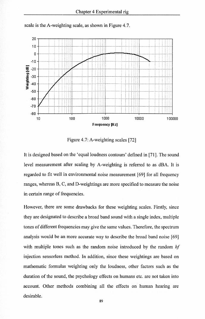
Chapter 4 Experimental rig
scale is the A-weighting scale, as shown in Figure 4.7.
....
20
10
o -10
! -20 Cl
'i -30 "Cl 'a! -40 ~
-50
-60
-70
-80
I
, I I
I I I
lA ,/I
/ /
10
I 11I1 I , I ' I I I i 11 I I I I
I I
1
I 1 11
! I ,
I i I i
,I ./ ~ ~~r I 11 T '" I iVl I II! , i
)rl'i I I I 1 i ! II' i ~ I I ' I' 1 ' !
I'i I I 1
11 I 11 i
I ; I
1 ! ,
I I
I I i 11 ' i I
I I , III 11 1 11
, j i 100 1000 10000
F re(IUellCY [H z)
Figure 4.7: A-weighting scales [72]
I i I: 11 ! I I I! i : ill! I
1
11* , I i i I i 1 1 i U I~ I' Ill' I i I i
I i I! I I' I I I I I
I 11 100000
It is designed based on the 'equal loudness contours' defined in [71]. The sound
level measurement after scaling by A-weighting is referred to as dBA. It is
regarded to fit well in environmental noise measurement [69] for all frequency
ranges, whereas B, C, and D-weightings are more specified to measure the noise
in certain range of frequencies.
However, there are some drawbacks for these weighting scales. Firstly, since
they are designated to describe a broad band sound with a single index, multiple
tones of different frequencies may give the same values. Therefore, the spectrum
analysis would be an more accurate way to describe the broad band noise [69]
with multiple tones such as the random noise introduced by the random hf
injection sensorless method. In addition, since these weightings are based on
mathematic formulas weighting only the loudness, other factors such as the
duration of the sound, the psychology effects on humans etc. are not taken into
account. Other methods combining all the effects on human hearing are
desirable. 89

Chapter 4 Experimental rig
4.4.3.2 The sound level measurement
The audible noise generated for the different injection methods was measured
using a Testo-816 sound level meter [73] with A-weighting [69-71, 74]
processing as mentioned ealier. The PMAC motor and DC load machine were
placed in a wooden box lined with sound proof material. A rubber mat was also
placed under the motor base to absorb the vibrations and noise conducted
through the table.
4.5 FPGA and DSP
The control platform used in this research is a general purpose advanced digital
system, developed in the PEMC group of the University of Nottingham [75].
The core components of this platform are a field programmable gate array
(FPGA) chip and a 32-bit floating point digital signal processor (DSP). They are
used to process all the measurement data, generate gating signals and perform
motor control.
The FPGA is used to manage the I/O interface. Measured values of the motor's
currents and position are stored into the registers of the FPGA and read by the
DSP through the interface. The DSP performs the control calculations and
eventually generates the timing signals for PWM generation, which are then
passed to the FPGA to generate the gating patterns for the converters to perform
the speed and torque control of the motor. For a sensorless control application,
the DSP also performs the calculation of the position estimation. -4.5.1 FPGA board
A ProASIC3-A3P400 type of FPGA chip, a third generation of Actel Flash
FPGA, is chosen in this research due to its good performance/price ratio. It has
400K system gates, 9216 D-flip-flops, 54Kbits RAM and up to 194 user VOs.
90

Chapter 4 Experimental rig
Besides the FPGA chip, the FPGA board also integrates the AID channels, DI A
converter, LED trip display, and user inputs and outputs, etc., which is illustrated
in Figure 4.8.
FPGABoard DSP
l MOSFEfS~ V1L- Vt Gate PWM Generation I
Drivers ~c- ~
I Cwrent b Transducers -v Signal Scaling
~~ Hardware Trips ~ NO
Protection I--v Converters
~~ Trips detection
l/l Software Trips & Watchdo! '\j
~~ LED trip
display
Signal Position [ Encoder l'"
Conditioning v Measurement
Figure 4.8: The function block of the FPGA board
Ten AID channels are available on the board. In this experiment, only four
channels are used for sampling the three phase currents of the AC motor and the
armature current of the DC load machine. The AID circuit measures the voltage
ranging from +5 to -5 V. Then this is converted to 0-2.5V for the AID input
pins. Hardware trips are available by comparing the input voltage with a
pre-defined reference voltage, providing fast protection against over current,
over voltage, etc.
Eight channels of outputs compatible with the fibre optic connectors are
available on the boards for outputting the PWM gating signals. However, ten 91

Chapter 4 Experimental rig
outputs are needed (6 for the 3-phase inverter and 4 for H-bridge). Therefore, an
extension board for more outputs is placed upon the FPGA board, which also
integrates the signal conditioning circuits for the encoder signal. The extension
board is connected to the main board via a 26-pin header connected to a
74LVC16245A buffer and a 74LVC245A buffer chip.
4.5.2 DSP control platform
A C6713 DSP Starter Kit (DSK) is a standalone development platform which
allows users to evaluate and develop applications for the TI C6xx DSP family
[76], and is used in this rig. It is supplied by a single +5V power supply and
consists of a TMS320C6713 DSP chip which operates at 225 MHz, a 32-bit wide
External Memory Interface (EMIF) which connects on-board peripherals
including the SDRAM, Flash and Complex Programmable Logic Device
(CPLD), an on-board analogue audio codec, and an embedded JTAG emulator
which allows debug from Code Composer Studio (a TI's code development tool)
through a PC's USB port.
The DSK also provides three expansion connectors which can be used to accept
plug-in daughter cards. They are for memory, peripherals, and the Host Port
Interface (HPI).
The memory and peripherals connectors are connected with the FPGA board,
providing interfacing the memories on the FPGA board with the DSP's
asynchron~~s EMIF signals, and bringing out the DSP's peripheral signals such
as the external interrupt trigger signal from the FPGA's clock.
4.5.3 HPI and PC host
A TMS320C6713 DSK HPI Daughter card by Educational DSP [77] is
connected to the DSK. In the host service mode, the daughter card allows serial, 92

Chapter 4 Experimental rig
parallel and USB access to the DSK's HPI port. In this research, a USB type of
access is used to interface the PC host and the DSK. A Matlab based user
interface developed by the PEMC group of the University of Nottingham is used
to download a programme built in Code Composer to the DSP, control the
operation of the application and monitor variables on a PC screen.
4.6 The design of the controller
The PMSM is operated under current control and the DC load machine is under
speed control. Both of the controllers are first designed in a continuous time
domain (s-plane) and then digitized into C-code in a DSP.
4.6.1 Current controller design
The vector control theory models AC machine as a DC machine, so the PMSM
can be modelled by the voltage equations including the impedances and the
cross-coupling terms in the rotating d-q frame, as shown in (4-2).
(4-2)
where Vd and v q are the d and q parts of the stator voltage, Ld and Lq are the d
and q parts of the stator inductance, id and iq are the d and q parts of the stator
current, rs is the stator resistance, p is the differentiator, (j), is the electrical
-speed of the rotor, and f// m is the rotor permanent magnet flux.
The equivalent circuit of the PMSM is shown as in Figure 4.9.
93

Chapter 4 Experimental rig
+ +
(a) d - axis model (a) q - axis model
Figure 4.9: Equivalent circuit of a PMSM in the d-q rotating frame
Since the time constant of the mechanical system is far slower than that of the
electrical system, the speed can be regarded as constant in the current transition
time. Therefore, the cross-coupling terms and the back-EMF term can be
neglected for the feedback control design of the current controller. The plant
used for current loop design is assumed as:
1 Gp/an/(s) =--
sL,. + r., (4-3)
where r., is the stator phase resistance and L, represents the average value of the
dq inductances which was used in this design.
In this work, a PI regulator was chosen and the control schematic is given in
Figure 4.10.
.'" Kp(s+a) 1 Idq .~ Idq
sLs + rs -~ S
Figure 4.10: Design schematic of the current loop
No delay terms are considered as the sampling delay (50 J..Ls) is much smaller
than the plant time constant.
94

Chapter 4 Experimental rig
The current controller bandwidth was set to 150 Hz to match the previous work
in [13] and using the classic root locus method the controller was designed as:
Gc(s) = O.l0876(s+539.9) s
(4-4)
The Bi-linear transform, as given in (4-5) was used to digitize the controller for
a DSP.
2 1- Z- I s=-·--
T, l+z-1 (4-5)
where 1'., is the sampling frequency which in this case is 50 f.1S .
An anti-windup procedure was automatically incorporated in the code since the
output of the controller was limited to prevent excessive error being
accumulated when the calculated results exceeded the inverter output capability.
To enhance the dynamic performance of the current controller, feed forward
terms were added after the controller output. Thus the ultimate control block of
the current controller is shown as in Figure 4.11 .
+
+ +
+
Figure 4.11: Feedback current control with feed forward decoupling
The performance of the current controller is tested for d and q current by giving a
pair of opposite step demands to one of the currents and keeping the other zero,
95
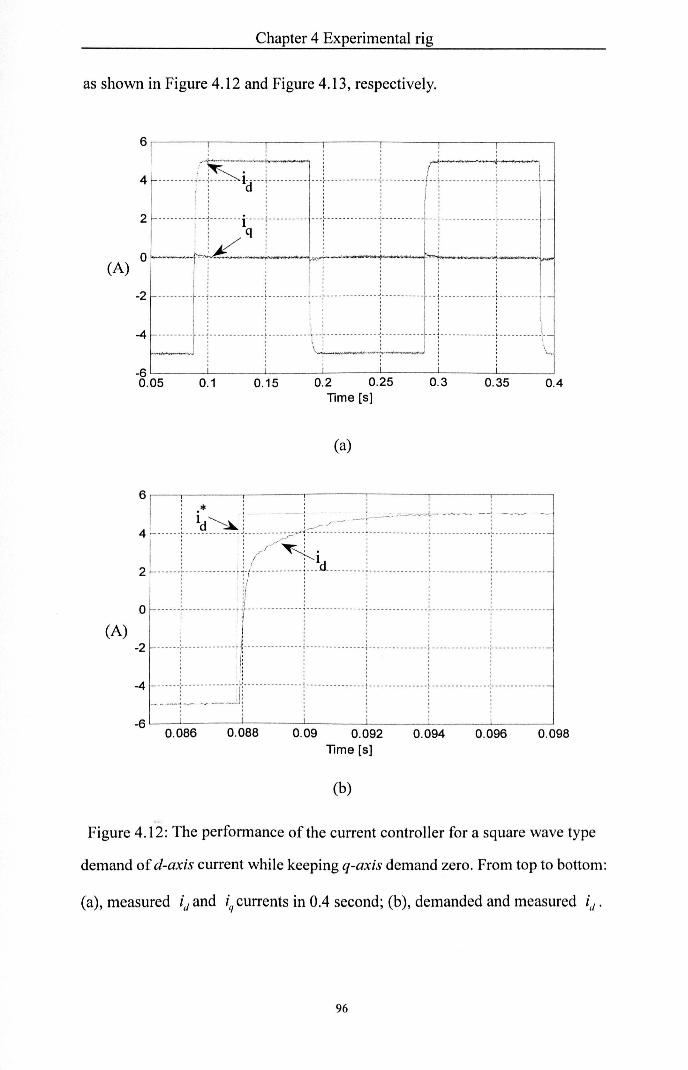
Chapter 4 Experimental rig
as shown in Figure 4.12 and Figure 4.13, respectively.
6 ,-----.-----~----_.----_,------~----~----~ , , . , , ,
~-+--- i i I~·-'----+-l
: IJ :~ IrL lliI_I , . : /: : : : :
o __ J~E-.--,~__ ~-,--~-+-.~~-.. ~-~---J (J\) I 1 i I i 1 i i
, , I I , ,
-2 ........... ~ ... ... ........ : ..... ..... ··r············l··········· ·r··········T······· ·· . -4 -=~~ ··r······ ·· ·· ··· l ········· ·\:~~~~:=+~~:~~~···l··············r············ _6 L-____ ~ ____ _L ____ _L ____ ~ ______ ~ ____ ~ ____ ~
0.05 0.1 0.15 0.2 0.25 0.3 0.35 0.4 lime [5]
(a)
6 ,-~------~----_r------,_----_.------~----~ , . , .* ,_. ~ .- , ~ --.-. --: -.~.' -: Id~ : : _,""-- - :- --' : :
4 r-" -- .. ! ........... --. i· ··· .;>;;~ 'i<··· ···· -- .. i···· -- -- ....... ! ...... --....... : .............. -i : /' ~i : : :
2 r- . . .. .. ~ ...... --. -- . . . ~ -/- ............ ; .. . .d .......... ; .. ..... -- ... --. ~ .... -- -- .... -- .~ ... -- ...... .. -i if i i i i , , ' I , , , , , , I ,
: :/ : : : :
(A) : _; J;.~· •• ;]· •••• • •• • •• • •• I·· ••••• • ••••••• I •••••• ••••••••• I •••••••••••••• I ••••••••••••• -, , I , , ,
i : i : : : _6 L-~-------~-----L--____ L-____ -L ______ L-____ ~
0.086 0.088 0.09 0.092 0.094 0.096 0.098 lime [5]
(b)
Figure 4.12: The performance of the current controller for a square wave type
demand of d-axis current while keeping q-axis demand zero. From top to bottom:
(a), measured id and iq currents in 0.4 second; (b), demanded and measured id'
96

Chapter 4 Experimental rig
5 r--"' ....... --- .------ ---- ---- :--- --------(-..... '.~""' ............. '----!--- ___ __ ______ L __ __ ________ " : : : .f"'. , , , , , , , , , , , ,
CA)
5
(A) 0
-5 ~
, ,
1 q
(a)
, , , ~.~..--....r-:~'-...,.....r---...:---
..._. _ }..-v--...r--,..-................ ;;
~ , : : q , /~ : : : ~, (~ ! '
0.186
/: . : f : 1 :
I j q I , , , '" ----:- ------- -. -----: ---------------: ------- - -------~ --- --- ---------~ ---- ---------
0.188 0.19 0.192 lime [5]
(b)
0.194 0.196 0.198
Figure 4.13 : The performance of the current controller for a square wave type
demand of q-axis current while keeping d-axis demand zero. From top to bottom:
(a), measured id and iq currents in 0.4 second; (b), demanded and measured iq.
As observed from Figure 4.12 and Figure 4.13, the rise time of the current
97

Chapter 4 Experimental rig
controller was about 3 ms , as expected for the designed controller bandwidth.
However, the d-axis current response in Figure 4.12 shows a much faster initial
rising edge at the beginning of the transient followed by a slower transient in the
following period. This is because the closed loop zero of the controller probably
falls on the right hand side of the plant pole for the d-axis current loop (since
average inductance is used instead of actual d-axis inductance for this design).
This can be seen by comparing the two resultant root locus plots in Figure 4.14
for the d and q axis controllers. For the d-axis controller, the pole A corresponds
to the faster rising part of the curve at the beginning and pole B corresponds to
the slower part of the curve.
A ~~------~x~
B
d-axis current loop q-axis current loop
Figure 4.14: Root locus to illustrate the d and q axis current loop controller
The current loop of the DC load machine was designed as a 150 Hz PI controller
in a similar mannor to the PMAC machine. The DC machine has only one
current loop and the armature current was dirrectly measured and used as the
feedback to the controller.
4.6.2 Speed controller design
The DC load machine was controlled under speed control. The plant of the
mechanical model is given as:
98

Chapter 4 Experimental rig
G,p/alii (s) = JS: B (4-6)
where k( is the torque constant, J is the inertia of the motor and B is the
friction of the system which can be ignored since it's very small.
A PI controller was also adopted and the schematic is given as in Figure 4.15,
assuming the current loop as a unity constant with respective to the speed loop.
• OJIII
~ Kp(s+a) k( Will
Js+B - ~ S
Figure 4.15: Controller schematic of the DC machine speed loop
In this work, a controller with a bandwidth of 8.488 Hz was used for the speed
loop, as shown in (4-7).
G,Js') = O.2611(s + 757.95) s
(4-7)
Similar approach was used to transform it into discrete domain as that for current
loop with a sample time of 2.5ms. The performance of the controller was tested
when speed reversal demands were applied, as shown in Figure 4.16.
99

Chapter 4 Experimental rig
20
10 ----- - ----------~ --------------------r ------ ------------.; --------------------r ------ - ---------: "' : : :
(rad/s) 0 : OJ : , : :
--- -- -/lP7n ----------------~ - - - --- 1 -- -------- -~------ ------- --- - -- - f---- -- ----- -- ---, '~ ' , , , , I , I I ,
-10 , I I I ----- ------------.. --------------------.. ------ - ----------.. -------- ------------~ ------ -----------I : _ ~
-20 1 1.5 2 2.5 3 3.5
8
6
(rad) 4
2
I(S)
(a)
, ! ,~~ ' " _o, ! !
10
(raNs) : c. ~:~ •••••• r •• ·SJ; •••••••••• r •••••••••••••• r ••••••• •• ••••• i •••••••••••••
-5 c- { , ~~ -.-.._. , r ' , , , ,
-10 - Ii--;·! .------;--:4" p 0 c:c ;': : : : : I LJU u' : i : i : i
1.15 1.2 1.25 1.3 1.35 1.4
t(s)
(b)
Figure 4.16: The performance of the speed controller for speed reversal. From
top to bottom: (a), demanded and measured speed of the rotor, with its electrical
position from the encoder; (b), demanded and measured speed (zoomed in).
It was found that the rise time of the speed response was around 50 ms, as
100

Chapter 4 Experimental rig
expected.
4.7 The design of the Mechanical observer
A mechanical observer [19] was adopted to process the position estimation for
the sensorless operation. The structure of a typical mechanical position and
speed observer is shown as in Figure 4.17. It is noted that the position estimate
was used as the feedback for the frame transformation for deriving the error
signal and the friction was neglected.
Figure 4.17: Structure of the Mechanical Observer used to obtain the position
estimate [19]
The transfer function of the plant is given in (4-8).
1 GMO plan/(S) = 1. 2
- S (4-8)
where J is the overall inertia of the system, and is defined by summing the two
inertia values in Table 4.1 and Table 4.2.
A PID controller was adopted. Again the root locus method was used to design
the controller. The resulting controller is given as:
G MO cO/llOrli. r (S) = (4-9) S S
The continuous domain controller was decomposed into a PI controller and a
gain equal to kd as shown in Figure 4.17. They were digitized respectively
101

Chapter 4 Experimental rig
using the bilinear transformation.
It is noted that although a higher bandwidth is expected to obtain better dynamic
performance, a trade-off has to be made to maintain good estimation quality. A
bandwidth of 90 Hz was therefore incorporated.
4.8 Space vector modulation
Space vector modulation (SVM) scheme is a widely adopted real-time
modulation technique which is preferred in a digital implementation of a voltage
source inverter (VSI) for generating the PWM timing signals[78], and is used in
this research.
For a 3-phase VSI in Figure 4.2, the operating status of the power devices can be
represented by switching states. State '1' represents the upper switch of the
inverter leg is on and the (VAN' vBN and vCN ) is positive (+Vdc )' while state '0'
represents the lower switch of the inverter is on and the terminal voltage of the
inverter is zero. Eight possible switching states combinations can be found,
including six active states and two zero states, which are defined as active space
vectors and zero space vectors, respectively. The six active vectors divide the
space into six sectors, each covering 60· of the space region. The space vectors
and their corresponding conducting switches as well as the vector values are
listed in Table 4.3 [78], and the division of the sectors is illustrated in Figure
4.18.
102

Chapter 4 Experimental rig
Space Vector Switching State On-state Switches Vector Value
VO 000 52,54,56 0
VI 100 511 54,56 2 '0 -Vd e) 3 c
V2 110 5v 53 ,56 2 .rr
'3Vdcel3'
V3 010 52,53,56 2 .2rr
'3Vdcel3"
V4 011 52,53,55 2 -Vd e jrr 3 c
V5 001 52,54,55 2 .4rr
'3Vdcel3"
V6 101 51,54,55 2 .srr
'3Vdcel3"
V7 111 51,53,55 0
Table 4.3: Space vectors and their on-state switches
Y3(o1O,k---___ --:.\( �IO)
1../ Sector 11 \
/ Sector III Se~tor I \
L "0 Vs ~ Y4(0 11 >\------*Y:..Lo~/7...,.,(O-,-OO-/ I-I -1 )--/ Y 1(1 00)
\ Sector IV Sector VI /
\ // /
Y5(001) "------....3 Y6(101 )
Figure 4.18: Division of the sectors by active space vectors
The values of the active vectors are obtained based on the 3-phase/2-phase
transformation (Park transformation [22]). For the two-level inverter in Figure
4.2, after applying the Park Transformation, phase voltages can be represented
by two orthogonal values in the stationary a-fJplane as: 103

Chapter 4 Experimental rig
1
[::]= ~ 0
1
2 Jj 2
1 [:::] 2 vco
(4-10)
where va , V p are the orthogonal components of the vector, and v AO , V ro and v co
are the instantaneous load phase voltages. The coefficient 2/3 is an arbitrarily
defined constant, and the benefit of using this is that the magnitude of the
three-phase voltages is reserved after the transformation. A space vector ~s can
be constructed as:
(4-11)
Applying (4-10) into (4-11), the space vector can be rewritten in the form of
phase voltages as:
(4-12)
27r 47r . where ejO = cos B + j sin B and B = 0, - and -, respectIvely.
3 3
If the operation of the inverter is balanced (Le. no zero sequence component),
equation (4-13) can be obtained:
(4-13)
When the active vector VI is applied to the two-level inverter, the values of the ,...
phase voltages are obtained:
V -v v -v __ Vdc l AO - dc' BO - co - 72 (4-14)
Applying (4-14) into (4-12), the value of space vector is obtained:
104

Chapter 4 Experimental rig
20 V =-V e) -I 3 de (4-15)
In a similar way, the other five active vectors can be derived and the common
expression of all the active vectors can be written as:
2 j(k-I)!!. V =-Ve 3 -k 3 de
k=I,2, ... ,6 (4-16)
A space vector Ys can be therefore represented by the sum of the nearby two
active vectors and a zero vector, as shown in Figure 4.18. This vector rotates in
the space with a frequency of the fundamental frequency of the inverter output,
defined as f. The angle, () (() := 2:r f) indicates which sector the rotating
space vector falls in. Table 4.4 shows the relationship between the angle value
and the sector, and the stationary vectors (active vectors and zero vectors) used
for representing the rotational vector.
105

Chapter 4 Experimental rig
Sector () Stationary vectors
77: VI V 2 and V O(7) I Q<(}<-- 3
II 77: 277:
V 2 V 3 and V 0(7) -<()<-3- 3
III 277:
V3 V 4 and V O(7) 3'S(}<77:
IV 477:
V 4 Vs and V 0(7) 77:S(}<3'
V 477: 577:
Vs V 6 and V 0(7) -<()<-3 - 3
VI 577:
V 6 VIand V O(7) - < () < 277: 3 -
Table 4.4: Rotating space vectors location arid their decomposed stationary
vectors
The dwell time of the applied stationary vectors detennines the duty-cycle of the
corresponding switches in a sample period r: and is calculated based on the
'Volt-second balancing' theory [78]. For a sufficiently short sample period r:,
the rotating space vector Ys can be regarded as constant value during the time
interval of r:. The product of the rotating space vector Ys and the sampling
period Ta should be equal to the sum of the stationary vectors multiplied by
their dwelLtime. For example, when a space vector is located in Sector I as
shown in Figure 4.19, it can be decomposed into VI' V 2 and V 0(7)' with their
times ~, r; and To.
106

Chapter 4 Experimental rig
p. I I I I rz I I I I I I I I I I
:Tz v : r. - Y------=::w" I I I
Figure 4.19: Diagram of a rotating vector falls in Sector I
From Table 4.3 and the volt-second balancing theory, (4-17) can be written:
~'\' . 7;.. = V I • 1'.. + V 2 12 + V 0 • To ~
jO 2 V T. 2 V .if T v,.e . T,. = - de ' I + - dce . 2 + 0, . ' 3 3
1C (0:::; e <-)
3
Rewritten (4-17) in a stationary a-fJ plane, yielding:
2 1 v, cos (e) . 7;. ="3 Vd" . 1'.. + '3 v" c . I;
v" sin(e)· T, = ~ Vd" . I;
Since ~ = 1'0 + 1'.. + r;, solving (4-18) yields:
(4-17)
(4-18)
(4-19)
For vectors which fall in other sectors, a similar procedure can be applied. The
general expression for the three stationary vector dwell times can be obtained by
replacing the angular displacement e with: 107

Chapter 4 Experimental rig
0' = O-(k -1),,/3 (4-20)
where k = 1,2, ... , 6 indicates that the vector falls In Sector I, 11, ... , VI,
respecti vel y.
The arrangement of the switching sequence of SVM is not unique, and a typical
seven segment arrangement is adopted in this work due to its minimal switching
frequency, as shown in Figure 4.20 for the case when a space vector resides in
sector I.
Sector I 1',.
:.-------------------------------------------~:
___ 00_0 ...... '--1_0_0 --+_11_°--:--1 --,HI Vd,! 110 100 000
r ~ v"i y 3 :
~----------~-----+-----~
Vco
J Hv"'l + + ~ I ~ + - ~ 1'0 T; I; 1'0 T2 I; 1'0 4 2 2 2 2 2 4
Figure 4.20: A typical seven segment switching sequence when V s is in sector J
It can be noted that in one sampling period each switch only turns on and off
once. Thus the switching frequency of the inverter as a whole is equal to the
sampling frequency. Although the switching frequency can be decreased by
using other switching sequences such as a five-segment sequence [78], where
the redundent inactive vector V7(111) is eliminated and the duration of it is
added to VO(OOO) at the start and end of the switching invertal resulting in a
sequence ofVO-V1-V2-VI-VO, it is not desirable to do so in this work 108

Chapter 4 Experimental rig
due to its increased THD.
4.9 Duty Cycle Modulation for the H-hridge
The timing signals for the single phase H-bridge to drive the DC load machine is
also calculated in the DSP and the modulation scheme is described in this section.
The DC load machine is under speed control as mentioned in section 4.6.2. The
controller output is the demanded armature voltage, referred as the reference
voltage Vre/.
The typical duty cycle modulation strategies for controlling a single phase full
bridge (H-bridge) converter as shown in Figure 4.2 are Bipolar and Unipolar
voltage switching methods. In bipolar type of switching, switches (Q}, Q4) and
(Q2'Q3) are set to be two switching pairs. Each pair of switches turns on and off
simultaneously, one of which is always on. Whilst for a unipolar type of
switching, switches (Q}, Q4) and (Q2' Q3) are controlled independently,
allowing Q and Q3 to be on or off at the same time. A unipolar voltage
switching type duty cycle modulation is used in this research to generate the
timing signal for the H-bridge due to its low output ripple characteristic [79].
The details of the two modulation strategies are described in the following
sections.
4.9.1 Bipolar type duty cycle modulation
The switching sequence and the output of the bipolar type modulation strategy is
illustrated in Figure 4.21. For a demanded armature voltage Vre/, a triangular
carrier wave at the sample frequency r: is used to compare with the demanded
value. The amplitude of the carrier wave is chosen to equal to the DC link 109

Chapter 4 Experimental rig
voltage Vde for simplicity. If VreJ is greater than the carrier, the first pair of
switches (Q" Q4) shown in Fig. 4.2 turns on while the other pair is off, vice
versus. The output voltage v 0 ranges between -Vde and V de , as the name
bipolar indicated.
T ' T, :..: .. I-------'-','------.:~-------'------I~
carrier
, ., TJ 4!
, , , , ,
Vde
~' ~ Fd' 00 VDN I; -]
, ' , , , ' , , ' ' , ' , , ' ' , ' , ,
00 0 ~ ~/c
VEN
, : ' , ' : : ' , ' I , f
r---------"'---' Vde
------------ ---------------- --------- ---t------------------------------------------~/c
~~---------L---1-~--------------~~ O
Figure 4.21: Switching sequence and the output of a bipolar modulation
The average output voltage of the converter can be obtained by subtracting the
average value of the two terminal voltage ~)N and ~'N' with respect to the
110

Chapter 4 Experimental rig
negative DC bus in Figure 4.2. In the example of Figure 4.21, the conducting
time of(Q) , Q4) in a sampling period is ~,and the conducting time of (Q2' Q3)
in the same time interval is 1;. Then VDN and V EN can be obtained as:
(4-21 )
Thus the output voltage averaged in a switching period can be derived as:
v = 7; -7; V = J: - 27; V o T dc T dc
s s
(4-22)
Also, from the mathematical point of view, (4-23) can be written:
(4-23)
Comparing (4-22) with (4-23), one can observe that the average voltage output
is equal to the demanded value, as expected.
4.9.2 Unipolar type duty cycle modulation
The switching sequence and the output of the unipolar type modulation strategy
is illustrated in Figure 4.22. The same demanded armature voltage V,., as that for
the bipolar type modulation is applied, and the triangular carrier wave with the
same sampling frequency z: and the same amplitude Vac is used to compare
with the demanded value. If V,., is greater than the carrier, the upper switch of
III
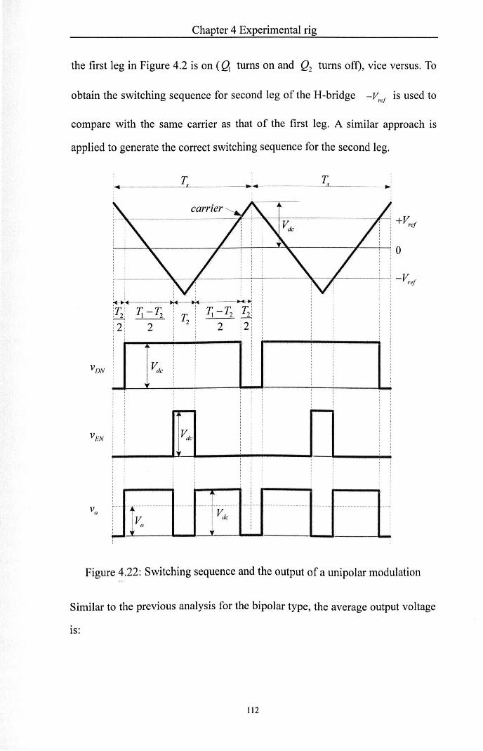
Chapter 4 Experimental rig
the first leg in Figure 4.2 is on (QI turns on and Q2 turns off), vice versus. To
obtain the switching sequence for second leg of the H-bridge - V,ef is used to
compare with the same carrier as that of the first leg. A similar approach is
applied to generate the correct switching sequence for the second leg.
' T T "~ ____ 'S· _____ " :" _____ -' _____ I"~
carrier
,
~--~--------"---7<~~'~--------"---~; 0
r-~; :T2: ~ -~
t~ ~ -~ :12: [2[ 2 2 2[
, :
o v()
i [ ! i i i : i: : :
U ·1;···· ······l····· ~···I·v~ · · · I ··j·· I · ·············· l ······t · ............. ~ Figure 4.22: Switching sequence and the output of a unipolar modulation
Similar to the previous analysis for the bipolar type, the average output voltage
IS:
112

Chapter 4 Experimental rig
~ =VDN-VEN
_ ~ -T2 V - T de
s
= Vre/
(4-24)
Comparing equation (4-24) with (4-22) and (4-23), it can be found that there is
no difference between the average output voltages of the two types of
modulation strategies for a given reference voltage. However, as the 'effective'
switching frequency is doubled for a unipolar type, the voltage ripple presence in
the unipolar PWM type of output is decreased with respect of the output from a
same switching frequency bipolar type strategy [79].
4.10 Conclusions
The experimental rig consists of the AC-DC motor system, their driver system
and the control platform, which were described in this chapter in detail. The
controller design procedure and the modulation scheme used for generating the
gating signals were also mentioned.
113

Chapter 5 Enhanced position estimation
Chapter 5 Enhanced position estimation
5.1 Introduction
In this chapter, other issues associated with the high frequency signal injection
based sensorless control have been addressed, including the initial
discrimination between north and south poles, and the loading influences on
estimation (Le. the armature reaction). Possible measures to solve the
aforementioned problems are discussed and evaluated through experiments.
5.2 Initial position detection
For a saliency tracking based sensorless PMSM control method, since the
desired saliency being tracked is twice the electrical frequency, the polarity of
the estimated position cannot be distinguished (Le. north or south pole), and
therefore the initial rotor position and its polarity must be detected.
The method used in this research for initial position detection is introduced in
[64] and described as follows. Assuming a 2-pole PM motor with the rotor
magnet at 0 and 180 degrees electrically (0 degree aligned with the stator phase a)
as in Figure 5.1, the total flux in the d-axis direction is composed of the magnet
114

Chapter 5 Enhanced position estimation
flux and the stator flux introduced by the d-axis current, yielding:
Be = o· Be = 180·
(5-1)
where '!fd' '!fl/l and '!fad are the total d-axis flux, the magnet flux and the d-axis
armature reaction flux ('!fad = L)d)' respectively.
If the d-axis stator current is rather high (i.e. the induced flux is rather large), the
total flux in the d-axis direction is either saturated (Be = 0· ) or de-saturated
( Be = 180· ). Consequently, the inductance in the d-axis direction is either
decreased or increased. If a fixed amplitude voltage v is applied along the d axis,
the d axis current flowing will be different for the two conditions. By comparing
the values of the two currents, the positive d-axis (+d-axis) and the negative
d-axis (-d-axis) can be distinguished.
d -axis winding d -axis winding
d-axis winding d -axis winding
Figure 5.1: D-axis flux distribution of rotor position at 0 and 180 degrees
(aligned with stator phase a)
/\
To identify the polarity of an estimated rotor angle Bc obtained through the
115

Chapter 5 Enhanced position estimation
saliency tracking sensorless method, two test voltage pulses with the same
amplitude and duration (Le. the same volt-second) are injected onto the
" estimated ±d-axes (± Be). With an injection voltage of high enough amplitude,
the resultant current transients will produce a noticeable difference between the
two peak values due to the impedance variation caused by the change in flux.
The larger peak current value will be obtained when a positive V voltage is
injected along the +d-axis. Thus the correct initial polarity of the rotor magnet
can be identified.
The initial position detection scheme is shown as in Figure 5.2. In this figure,
" Bejuw represents the estimated rotor position without polarity identification,
" Be_co" represents the identified correct rotor initial position, which can be written
as:
if r/ > t;/
if i;/ < i;/ (5-2)
where r:/ is the resultant d-axis current when the voltage pulse is applied to the
estimated positive d axis, and r;/ is the resultant d-axis current when the
voltage pulse is applied in the opposite direction.
It is noted that the motor is kept at standstill throughout whole process of the
initial estimation and polarity identification.
116

1\
Be raw
Chapter 5 Enhanced position estimation
v· - JUlr-----, d - Vpulse
1\
~; =0 dq/
--~ labc 1\ 1\
() eJow & (()eJQw + a)
id
"~Ia--l·~
""'b--~ c
c
Inverter
Figure 5.2: Initial polarity detection scheme
The scheme has been tested by experiment. The injected voltage has been set at
2V with 2ms pulse width, and the results for a correct initial polarity and an
incorrect initial polarity from the estimation are shown as in Figure 5.3 and
Figure 5.4.
117

Chapter 5 Enhanced position estimation
d-axis current responses to +d and -d axis injected '.AJltage pulses 30 ,---,----,----.----,----,----,----,----,----,-,
20 , i;"~ ~i, I'~~· · ··· · · · " ····~ ···l ......... j .................... , ... . : ! ~: : ~l : : : :
$ i i : j : i d : : i i ._u 10 T " II ' \ [T1 ' 1" 0, ,J , -- , , , ---+--- -----+---
:i i i i i i i i -0.06 -0,04 -0,02 0 0,02 0,04 0.06 0.08 0.1 0.12
Position signals from the encoder and from the estimation
6 --- -- - -~ - ---------~------ ---- ;--------- - ~ -------- -- ~ .-- ---- --- ~ ---------L-------~- - --- - -- j -;~ I~ ~ : : : : : ! ! BeN : ~.i_ 4 --- - - -- r- -- - --- · -r --------- r- ---- -- -r-- - ----- r ----------r----------:- - --- ~Si~=Jt -
: : : : : : : : ~ :g 2 --- --- -:--- ----- -- :----- --- --:------ ---- t-- --- ----- t--- ----- --t---- -- --- :----------:----- --T :-- -0.. ~ : : : : : : : I :
o --V __ J ___ muuL ___ m_ ~m- - m_+um.--.l..u _m_Lm ____ ~m ____ u_ ;uuO~ _ .• ~ --0.06 -0.04 -0.02 0 0.02 0.04 0.06 0.08 0.1 0.12
t(s)
Figure 5.3: Initial polarity detection with correct initial polarity estimation
d-axis current responses to +d and -d axis injected '.AJltage pulses 30 ,----,----.----.----.----.----.----,-----,----,-,
, , 20 --······~-------:+i ·--- --- --j --------- t- -------- ~- -- ---- - -- ~ --- - - - ---(------- j - . -------.(-
~ , Id"" .-d , , ,
3, 10 ----- ---i- ---------L ------- ------) -------- ~- - - ~1-- - T- --- ---- ~-------...;-·------ - -j·---
'------!------+------+--, ------ --;- ---- ---- -; ----, , , , , ,
-0.06 -0.04 -0.02 o 0.02 0.04 0.06 0.08 0.1 0.12
Position signals from the encoder and from the estimation
, I , I " , , , I I I , , , ,
6 --------i- ----- --- -j- --------. j--- -- -----t -- --------r -- ---- ----r-' -- -. ---j- ---------j- --- ----- -j ----
! 4 ---------i- u----u- ~--~~~·-----r--·------- ~ ----------l--------~·-------·-L---· ··- i ----g : : : : :F: : : '--£ 2 .--.----i'-- ---00- -l- (jsii;;u-u r-u -- ·---- r-u-.--ur---u----l---- · '-00'1-"- ----00100 --
: :e~: : : : : : o . -- ~ . ----- ----~ - ---- -----~ - ----- --_M ~ - - - - - - - - - - ~ - - - - - - - - - - ~ - -- - - - - - - ~ - - - - - - - - - - ~ - -- - - - - - - - ~ - - --
-0.06 -0.04 -0.02 0 0.02 0.04 0.06 0.08 0.1 0.12 t(s)
Figure 5.4: Initial polarity detection with incorrect initial polarity estimation
118

Chapter 5 Enhanced position estimation
In Figure 5.3, the resultant current for the estimated +d-axis injection (i;d) has a
higher peak value than that of the estimated -cl-axis injection (i~d), which
indicates that the estimated initial rotor position has a correct polarity so no
compensation needed. In Figure 5.4, the initial rotor polarity is incorrect, which
causes i;d to be less than i~d. Therefore, a compensation angle of 180· IS
needed to achieve the correct polarity.
5.3 Armature reaction
For a PMSM machine, the net flux linkage is the combination of the magnet flux
and the stator induced flux. In a vector controlled system with a voltage source
inverter, the flux distribution in a dq rotating frame can be written as:
If/ d = If/ m + If/ ad -;:,:, If/ m + Ldid
If/q =If/aq -;:,:,Liq (5-3)
where If/ad and If/aq are the armature current induced flux in the rotating d and q
axis respectively.
Since the d-axis current is normally controlled to zero to achieve maximum
torque density, only the q-axis current component will affect the net flux. Thus a
phase shift of the total flux is produced under loaded conditions, resulting in a
misalignment between the total flux direction and the rotor d-axis, which can be
illustrated as in Figure 5.5.
119

Chapter 5 Enhanced position estimation
d-axis
Figure 5.5: Total flux shift due to the armature reaction under loaded conditions
As can be seen from Figure 5.5 that with the increase of q-axis current (i.e.
increased loading) the shift angle increases accordingly. The saliency tracking
sensorless techniques track the maximum and minimum spatial impedances
which are sinusoidally distributed according to the net flux spatial rather than the
magnet flux. As a result, the shifted rotor electrical angle will be obtained.
5.3.1 Armature reaction compensation by
adding predefined angle offset values
To achieve correct orientation for vector control, the simplest way to compensate
this angle shift is to find the difference between the estimated angle and the one
obtained from an encoder under sensored operation mode at different loading
conditions. A look-up table or a linear function can be constructed to allow the
correction of the estimated angle with different loading conditions for correct
frame transformation. In this research the angle difference is approximated
through a linear function as:
120

Chapter 5 Enhanced position estimation
1\ 1\
() comp = () e + f (i,: ) (5-4)
1\ 1\
where () comp and () e are the corrected and un-corrected angle estimates, f()
stands for the linear function, and i; -- the demanded torque current is used to
access the function for angle compensation. The measured phase shifts, for the
machine investigated, due to the armature reaction are shown in Figure 5.6 in
radians from -60A to 60A.
Armature Reaction o . 2 ,..- -------.,- -------.,------- -"'1- - - - - - - -., - - - - - - - -., - - - - - - - - - - - - - - - - T - - - - -- - -T -. - - - - - -,. - - - - - - - - r - - -- - - - -r - - - - - - - - ,
: l ! : : : 1 ! : : : : : _ O. 15 ~~~~~~~~7~--- ---T~~~~~~~L~~~~I~~~~~~L~~~~~I~~~~~~~L~~~~I~~~~~~r~~~~~r~~~~~L~~:::J =a 0.1 , " :: i : i i : i :
cos O. 05 ~ - -- -- - -7 -------7 - -- ---- '---- ---------------i--------:--------: -------- : -------- : --------: ----- --~
t 0 ~- ------t-------i---- ---+------l-------T----- ; -----i----- - - - t - :::::::t::~::~:~~~::~~:~:~,: ::::: ::~,: e -0.
0 5 C~::::I:::::::L:::::r::~~::r:::~::l::::~~J ~:: :::::I:::: ----~ ----- ---r----- - -t -0.1 : : : : : i i : : : ........ : ~--o--... , -------~
-0. 1 5 t: :~~ ~~: I: ~ ~~~~I~~ ~~~ ~ ~ I ~ ~ ~~ ~ ~T ~~~~ ~ ~ j :~ ~~~: J :~~: :~:]: ~~~~~:~ i ::~:: ::~ C~~~~ ~ ::t :::~: J:: ::::: J -0.2
-60 -50 -40 -30 -20 -10 0 \0 20 30 40 50 60
iq (A)
Figure 5.6: Phase shift of the angle estimate due to the armature reaction
Then the linear function f(i;) is obtained as:
f«(;) = -0.0023i,; - 0.0015 (5-5)
1\
However, the corrected angle () comp for the motor fundamental model
transformation cannot be used for the high frequency signal injection. This is
because the saliency angle being tracked with this method is aligned with the
direction of the net flux linkage not with the real d-axis. If the compensated
angle is used, instability will be caused for the estimation process.
It should be noted that if the load current is sufficiently high, the q-axis flux will
be saturated making the q-axis inductance reduced significantly. A failure of the 121

Chapter 5 Enhanced position estimation
position estimation with the injection based sensorless method may occur when
the q-axis inductance eventually approaches the d-axis inductance (in some
cases, the sign of the difference may even reverse [80]), since the error signal
used to drive the tracking mechanism will become almost zero independent of
the alignment between the estimated and the real rotor position. It was found that
in order to obtain a correct position estimate in this work, the load torque current
has to be limited between -60A and 60A.
5.3.2 Armature reaction compensation by
decoupling the cross coupling term
The other way of compensating the armature reaction is to take into account the
cross coupling terms [81, 82] for the saliency tracking operation.
With the consideration of the cross coupling terms, the high frequency model
can be written as:
(5-6)
The transformation matrix can be applied to transform the real d-q frame to the
1\ 1\
estimated d-q frame (the d -q frame) with the inverse transformation defined as:
T(ilB =[ cos(ilB,) Sin(ilB,)] ,) - sine il B,) cos( il B,)
T-t (ilB = [COS(ilB,) - Sin(ilB,)] ,) sin(ilB,) cos(ilB,)
(5-7)
...
1\
where ilB, = B, - B, is the estimation error angle.
Equation (5-6) can be rewritten as:
122

Chapter 5 Enhanced position estimation
(5-8)
where Ld and Lq are the high frequency d and q axis inductances respectively.
After some calculation, equation (5-8) becomes [81]:
[ ~dh] = E-" dt Vqh
(5-9)
where Ls and Ms are the average and incremental self-inductances, defined
by:
IlL = _L..:..q _-_L_d
s 2 (5-10)
.". Ms is the incremental inductance accounting for the mutual inductance, and is
given as:
• ~ 2 2 IlLs = IlL s +Ldq (5-11)
123
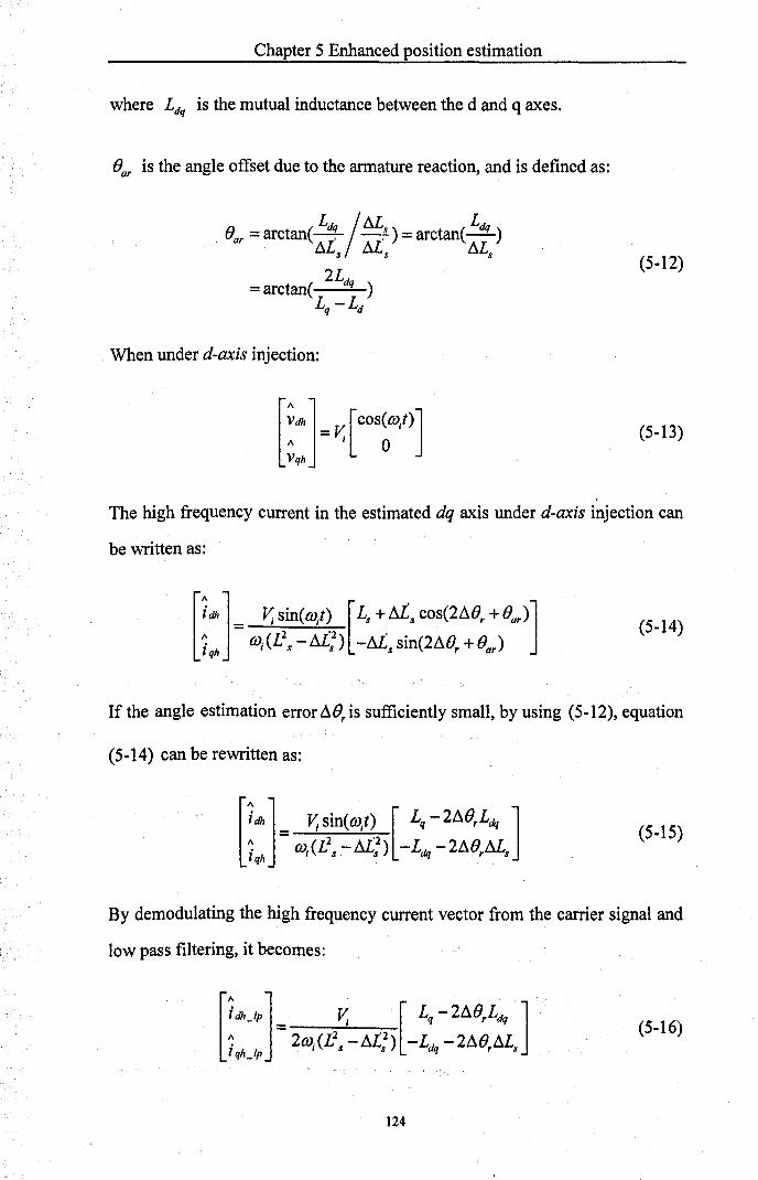
Chapter 5 Enhanced position estimation
where Ldq is the mutual inductance between the d and q axes.
Bar is the angle offset due to the armature reaction, and is defined as:
(5-12)
When under d-axis injection:
(5-13)
The high frequency current in the estimated dq axis under d-axis injection can
be written as:
(5-14)
If the angle estimation error ABr is sufficiently small, by using (5-12), equation
(5-14) can be rewritten as:
(5-15)
By demodulating the high frequency current vector from the carrier signal and
low pass filtering, it becomes:
(5-16)
124

Chapter 5 Enhanced position estimation
By solving equation (5-16), the error A8s can be written as:
AB = r (5-17)
It can be seen that the estimation error is proportional to the term
1\ L 1\
(iqh_lp+ ;q idh_lp). By forcing this term to zero, the estimate will be aligned to q
the real rotor position. This term, rearranged as equation (5-18), is recognized as
the error signal to drive the tracking mechanism.
(5-18)
where the value A. = Ldq is defined as the cross coupling coefficient and can be Lq
calculated either by FE (finite element) analysis or by experiments [81].
The experimental method to derive A. is to inject the hfvoltage vector into the
real d-axis, and the hfvoltage equation is given as:
(5-19)
Then the corresponding hfcurrent can be obtained as:
[idh] 1
."" i = L L _L2 qh d q dq (5-20)
where C is a constant resulting from the integration operation. Similar to
equation (5-15), after multiplying (5-20) by the carrier signal and low pass
filtering, the resultant current vector is obtained as:
125

Chapter 5 Enhanced position estimation
(5-21)
The cross coupling coefficient A can be calculated through:
(5-22)
The overall schematic of measuring the cross coupling coefficient is shown in
Figure 5.7.
.' + Iq --~x}----.! /'-~" d% PWM PMSM )
i~ _-I+~)--j--+p + k,/ Hr-,--:a~b __ C~ ___ In_v_ert_ er--l--+- -+-""_~ ___ ~---,J v; cos(m;l)
abc/ ~~' ___________ I /dq~ ________ ----,
... ... . ............................................. =~ ............ 0···· ....... "'j
A : , , , ,
..................................... _ ......... ~~!.~~!!.~~~?~.?:.?~~~~~.~ .. i
Figure 5.7: Scheme of measuring the cross coupling coefficient
As noted from Figure 5.7, an FFT operation rather than low pass filters is
performed to obtain the current vector in equation (5-21). This is to avoid
additional delay from the filters to give an accurate measurement of A, and is
acceptable as this is a one-off commissioning procedure. The measured
coefficient is plotted as in Figure 5.8.
126

0.06
0.04
0.02
~ 0 ~ -0.02
-0.04
-0.06
-0.08
Chapter 5 Enhanced position estimation
Cross coupling coefficient
: 1 : ! ! ; ; : : : -------~- - -- - -- -~-------- ~ --------~----- - - -! ---- --- - ;- -- --- -- l ----- ---i--- -----i --------i--------
I : i ! l ! : : : 1 -------r------ i----- : ----- '-------+ ------1--------t--------t--------r--------r --------r-------
-------t-------t-------(------t-----r--- : -------: -------+----- -- r ~~~~~~~:t. ~ ~~~~~J:: ~~~~:~~ .---- --t-- ----- -:--------:--------1------ --1----- -- i ---__ __ M! ------ --: --
: : : : : : : : : --- --- -+-------1- - ------ ~----- - --~---- - ---~--- --- - -4---- --- -+ - -------t--------~--------t -- -- -
: : : 1 ! ! ! 1 : : :
-------t-------t-------i--------t------i--------r------t--------t--------(------t--------t-------t , , , I ' I , , I I
-60 -50 -40 -30 -20 -10 o 10 20 30 40 50 60
iq (A)
Figure 5.8: Measured cross coupling coefficient values
The coefficient A can be linearized and derived as:
A = -0.0008· i; -0.00 15 (5-23)
where i(; is the demanded torque current. i; is kept zero at all time.
Then the sensorless demodulation method with the consideration of the cross
coupling effect is given as in Figure 5.9.
/\
DJr
/\
er Tracking mechanism
Figure 5.9: Demodulation scheme with cross coupling effect decoupled
127

Chapter 5 Enhanced position estimation
5.3.3 Compensation results for the two
mentioned methods
The results for the armature reaction compensation using the encoder measured
angle offsets and decoupling the cross coupling terms are compared in this
section. The AC motor is operated under torque control and the DC load
machine holds the speed at -60 rpm. Results for motor under light loads (lOA,
11 %) and heavy loads (50A, 56%) are taken and shown from Figure 5.11 to
Figure 5.17, and the corresponding load currents waveforms are shown in Figure
5.10 and Figure 5.14.
Plot of 10 Amps iq
10.25 ,-----,---------,--,-----,---------,--,-----,---------,--,--_
I I I I 10.2 - - - - L - - - - .L - ___ .J ____ ....J _____ 1 _____ 1 _____ L ____ L ____ l. ___ _
I I I I I I I I I
I I I I I I I
I I I I I I I 10.15 - - - - L - - - - L - - - - ~ - - - - -,1 - - - - _1 __ - - -1 _____ L ____ L ____ L ___ _
I I I I I I I I I
I I (I I I
10.1
10 -.( -
9.95 - --
9.9 - - ~~---+r--------~--------------------~~---~----1 1 1
1 1 1
9.85 __ ~-L----L---------~----------~--------------~----I I I I I I I I I
I I I I I 9.8 - - - - L - - - - 1. _________ ..J _____ 1 _____ 1 _____ L. ____ L ____ J. ___ _
J I I I I I I I I I
1 1
9.75 L--~--L--L--~-~--L--~_~ __ L__~ o 0.1 0.2 0.3 0.4 0.5 0.6 0.7 0.8 0.9
Time [sI
Figure 5.10: Plot of lOA (11 %) iq with sensorless operation
128

Chapter 5 Enhanced position estimation
Estimated position and real position
300 t,~ -~ ----~ --J: ~- ---J -----J -~ --:- ----~ -J ~ ~ ----l- ---~ ~: I \\ : : I : : :
I I I I \ I I I I r I \ I
g 200 - - - - :' \. - - - : - - I -: - - ~\: - - - - -:1 - - - -~ : - - :- - -, -: - - -~ - - - -
.~ : "' I : ~\~_ : : : : I \.
a.. 100 - - - - r - - - "\ T - - - - , - - - - ..., - - - -, - - - - ,- - - - 1;" r - - - r - - - - T - - - -
I I I' I -". 11 I I \.
I : :'\ ' 0 ~ __ ~ ____ -L __ '2·11 __ L-__ ~ ____ ~~ __ -L ____ -L~~~ ____ ~ __ ~
o 0,1 0.2 0.3 0.4 0.5 0.6 0.7 0.8 0.9
Estimated position error 20 ._--_r----,---~----~----._--_,----,_----._--_r--~
~ 10 - - - - r- - - - - 1- - - - - -t - - - - -; - - - - -1- - - - -1- - - - - t- - - - - r - - - - "t" - - - -
J 0 v~l~rNtIJt,~~l~VM~~: 0~~~rJl '1~lt : ~~~ t l
'00 \ I V I t : ~' V: ' v ~ v J : \ I V V' J o -10 ____ 1- ____ ..... ____ ..... ____ --1 ____ I _____ I _____ l- ____ ~ ____ J.. ___ _
a..
-20 ~--~----~--~-----L----~--~----J-----~---L--~
o 0.1 0.2 0.3 0.4 0.5 lime(s)
0.6 0.7 0.8 0.9
Figure 5.11: Obtained angle without armature compensation at lOA (11 %) load
300 - - - 1-- -
\ ' (J
c o 200 -:;:: '00 o a.. I,I ,
100 ~----~--
Estimated position and real position
--- -l-----+-- --1-------- --..----+---. , , I , \
___ 1 _____ 1 _____ 1_ _ _ _ l. __ .... _ 1 ___ _
, ,
- ,~ -~----~-I I
\. ' , I ,
---~----~--- ~----r----T-~--\ , , \
Estimated position error 20 ,---.----,----~--~----~--~--~----._--~--~
_20 L---~---L ____ L-__ ~ __ ~ ____ L_ __ ~ __ ~ ____ L_ __ ~
o 0.1 0.2 0.3 0.4 0.5 lime(s)
0.6 0.7 0.8 0.9
Figure 5.12: Resul ts of armature compensation by predefined offset at lOA (11 % )
load
129

'0' C-~ Cl) 0 a..
~ g <I> c: o :;:
Chapter 5 Enhanced position estimation
Estimated position and real position
I J I I ~ I
300 - - - - +- -~- ~ - - - - ~ - - - ~ ~ t.... - - - -: - - - - -:- - - \0. - ~ - - - - ~ - - - - T ~_ - - -
I : \ ~ I
200 ____ L
I
'-100 - ~ - - r I
---~ ~\- --~ ---r -: ---+ ----:- ----:~\ ---~ ----~ ---\ ---L ---: --- j -----L : ---i- ----~ ----~ ----L ---.
I I I I I I I I
I I I I I I I I
OL-__ ~~ __ L-__ -L __ ~L-__ -L ____ ~~L-__ L-__ -L __ ~~ __ ~ o 0.1 0. 2 0.3 0.4 0.5 0.6 0.7 0.8 0.9
Estimated position error 20 '---'---~----.----'----'----.--~r---'---~----.
·w o -1 0 a..
____ I- ____ J,.. __________ -I _____ 1 __ _
I
I
-1- - __ ~ ____ .L. ____ ... ___ _
_20 L-__ ~ __ ~ ________ ~ ____ l-__ -L __ ~L-__ ~ __ ~ __ ~
o 0.1 0.2 0.3 0.4 0.5 Time(s)
0.6 0.7 0.8 0.9
Figure 5.13 : Results of armature compensation by decoupling the cross coupling
term at lOA (11 %) load
Plot of 50 Amps iq
50.3
0 I I
50 2 - - - l - - - - ~ . I
I I
-1----~----------~----~----~----1----i I I
50.1
50
$ 49.9 - - - - - - - - - J. _
._ 0"
49.8
49.7
49.6
_ L
I
I
_.J __ - I
__ ..L. __
I
I I I ___ 1- __ "", __ _
I
I I
: ----: -----:- ----:- ----: ----: ----~ ----1 I I I I I !
_________ ..L. ____ ..J ____ -I _______________ L..
I I
I J. __
I I l
49.5 L..---'_--'_--'_-.J._-.J._--.-l._---'-_---'-_-'-__ --.J o 0.1 0.2 0.3 0.4 0.5
Time [sI 0.6 0.7 0.8 0.9
Figure 5.14: Plot of 50A (56%) lq with sensorless operation
130

Chapter 5 Enhanced position estimation
Estimated position and real position
300 '0' C 200 ~ en 0 a.. 100
j'" I , ~ I I I I I
- j ~ - ~I,_ - - - ~ - - - - ~1 __ \ _ -1 - - - - _1- ____ ~-1. - - - - ~ - - - - ~ - ~ r _ ~ ___ _ I • r ·,1 I I ~ I I " J
, , ,[ . , I" I ,
- i L -~ --~ -~ ----~! - - - - -:'- - - - -:- - - - -:- - ~'l - :- - - - - ~ - - - - ~~ - - -I 1 I l' I I t I I
I \, I ~ I I \. I ~ I , I I "I I ,. 11 , I I 1 I I r , I
- i - - r - - - - T .... - - - ., - - - - -, - - - .... -,- - - - -,- - - - - r "='" - - - - - - - T - - -"--, ~
0 ' j
0 0.1 0.2 0.3 0.4 0.5 0.6 0. 7 0.8 0.9
Estimated posit ion error
20 - - - - ~ - - - - + - - - - ~ - - - - -: - - - - -'- - - - -,- - - - - :- - - - - + - - - - + - - - -£: I
g Q)
c g ·w o a..
o 0.1 0.2 0.3 0.4 0.5 lime(s)
0.6 0.7 0.8 0.9
Figure 5.15: Obtained angle without armature compensation at 50A (56%) load
Estimated position and real position
'0'
C f g 200 -.~
a.. 100 -~
o t " o 0.1 0.2
l I I
20 ----~----~ f I , \ Q)
c g ·w
,
0.3
o a.. -20 -- - ~ - -.----
o 0.1 0.2 0.3
.. - - - I ----L---~---J , I I j _ _ _ , _ _ -='1;- - - - - - - 1 - - - - - - - -, I
-~--~----~----!----T--~-, '1 1
0.4 0.5 0.6 0.7 0.8 0.9
Estimated position error
, -----r----~----
, I I --------------~----~----r---------
0.4 0.5 lime(s)
0.6 0.7 0.8 0.9
Figure 5.16: Results of armature compensation by predefined offset at 50A (56%)
load
131

Chapter 5 Enhanced position estimation
Estimated position and real posit ion
300 0-C 200 0 :;= '00 0 a.. 100
't. ____ "-
- : : I~: I :: . : - ~ ""; - + - - - - -; - - ] - ~ - - - - -1- - - - - - - - - t- - - - - r - - - - + - - - -~ , • r I ... I I
\ I I I I "~ I .\' " )I I J I I I I I \ ----:\ ---: --1 --: ---\ -: ----------:- \ ---: --,--: ---' \
I '"'- I '! .. ~ I " I I
- - - - ~ - - --..- ~ - - ~ - ~ - - - - -: ~ .. - - - - - - - - -:- - - ~ - ~ - - - - ~ - - - -
\.. : I· I ' , ' j! 0 L-__ J-__ ~ ____ L-~~ __ ~ ____ L-__ ~ __ ~-2 __ L-~
o 0.1 0.2 0.3 0.4 0.5 0.6 0.7 0.8 0.9
Estimated position error
I I I I I I r t - - - - I - - - - - - - - - I - - - - -, - - - - - ,- - - - - - - - - - ,- - - - - I - - - - "I - - - -, ,
o 0.1 0.2 0.3 0.4 0.5 0.6 0.7 0.8 0.9 Time(s)
Figure 5.17: Results of armature compensation by decoupling the cross coupling
term at 50A (56%) load
As observed from the results, it is noted that with both compensation methods
the angle shift can be effectively eliminated. The advantages of compensation by
making use of the cross coupling term over that by directly adding the angle
offset is that the estimation error has a lower harmonic content, and with the
cross coupling term being considered, the estimated angle is almost aligned to
the real d-axis which is then used for the injection of the hfvoltage vector. With
simply adding the angle offset measured from the encoder for compensation, the
injection signal is actually into the estimated d-axis before compensation, which
increases the possibility of instability of the sensorless operation. However, to
calculate the cross coupling coefficient, a more complex procedure needs to be
taken than the other method, requiring increased effort of precomissioning and
complexity of the system setup, and for this reason the linear function
compensation method has been used for the rest of this work. It is also noted that
132

Chapter 5 Enhanced position estimation
when load increases, the phase current will be highly distorted. This will be
discussed in more detail in Chapter 6.
5.4 Conclusion
This chapter has dealt with some enhancements for the quality of the injection
based sensorless control operation, including the initial polarity detection and
the armature reaction compensation. Experimental results have shown the
effectiveness of these methods.
133

Chapter 6 Sensorless vector torque control results
Chapter 6 Sensorless vector torque control results
6.1 Introduction
In this Chapter, the results taken from the test rig will be shown to illustrate the
performance of the motor drive system using the three injection-based sensorless
methods discussed. The results are compared in terms of the current distortion
they produce, audible noise, and dynamic performance. Results from the
sensored vector controlled system are used as a benchmark with which to assess
the sensorless methods.
6.2 Current distortion for the different
sensorless methods
In this section, the current distortion of the line currents for the different hi
injection sensorless methods is evaluated. The test rig setup was described in
Chapter 4. The DC load machine was operated with speed control and the
PMAC machine utilized the position signals obtained either from the encoder for
the sensored operation or from the estimation for the sensorless operation to
perform torque control. The motor was rotating at -60rpm and -120rpm between
134
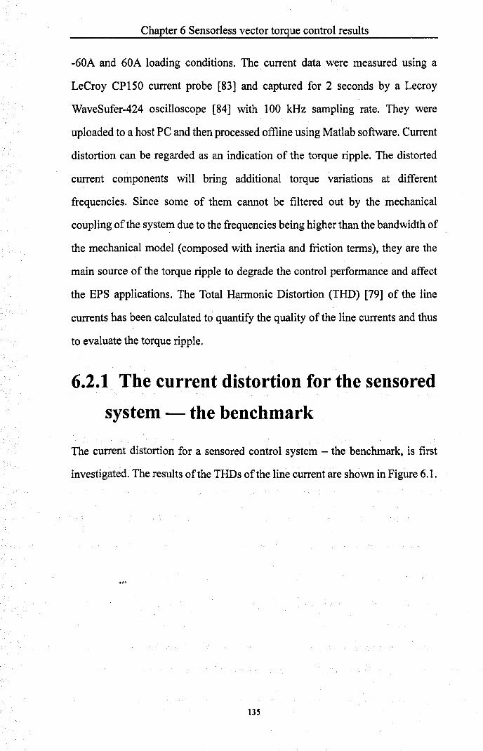
Chapter 6 Sensorless vector torque control results
-60A and 60A loading conditions. The current data were measured using a
LeCroy CP150 current probe [83] and captured for 2 seconds by a Lecroy
WaveSufer-424 oscilloscope [84] with 100 kHz sampling rate. They were
uploaded to a host PC and then processed oflline using Matlab software. Current
distortion can be regarded as an indication of the torque ripple. The distorted
current components will bring additional torque variations at different
frequencies. Since some of them cannot be filtered out by the mechanical
coupling of the system due to the frequencies being higher than the bandwidth of
the mechanical model (composed with inertia and friction terms), they are the
main source of the torque ripple to degrade the control performance and affect
the EPS applications. The Total Harmonic Distortion (THD) [79] of the line
currents has been calculated to quantify the quality of the line currents and thus
to evaluate the torque ripple.
6.2.1 The current distortion for the sensored
system - the benchmark
The current distortion for a sensored control system - the benchmark, is first
investigated. The results of the THDs of the line current are shown in Figure 6.1.
135

---
16
14
12
~ 10 '-' Q 8
== 6 ~
4
2
o
Chapter 6 Sensorless vector torque control results
THD of ia sensored benchmark " ~
I ~ ~~ ..... -.... ~~ ~ -' ~ ~ l/'"
r \ J '- _ ... n
IL. __ - --....... ...... /::{\,
'1-"" .... - 120rpm
-60 -40 -20 o 20 40 60 iq (A)
Figure 6.1: THD of ia for the sensored benchmark at -60rpm and -120rpm
From Figure 6.1, it can be seen that the current distortion reaches its peak THD
value close to no load due to the small amplitude of the load current. With the
increase of load, the THD gets smaller since the harmonics due to the cogging
torque and other mechanical disturbances are relatively fixed in amplitude and
are therefore a smaller percentage of the fundamental component. At above 20A
load the THD increases by a small amount. However, by looking at the spectrum
of the normalized stator current vector (is ), as shown in Figure 6.2, it is found
that under 60A load a large second harmonic of the current is present as well as
a DC component. The 2nd harmonic of current represents a torque disturbance at
the frequency l e with respect to the fundamental electromagnetic torque which
is partly due to the cogging torque of the PMAC machine as it links to the pole
number of the machine (8 poles). The DC component represents a-le torque
disturbance which is partly due to the commutation disturbance of bru hes on
the DC machine. Also there is a 3rd harmonic in the current in both conditions.
This is due to imbalances in the PMAC machine phase impedances. Any
variation in connections or windings will cause a noticeable imbalance.
With the increase of rotating speed, the THDs of the line currents decrease, as 136

Chapter 6 Sensorless vector torque control results
shown in Figure 6.1. The double-sided FFT of the stator current vector has also
been perfonned to analyse the spectrum, as shown in Figure 6.3. The frequency
range of the FFT is zoomed from -40 Hz to 40 Hz as higher order distortions are
below the noise level and are not the main source in the calculation ofTHD. It is
noted that the dominant distortions are still the 2nd harmonic and the DC
components. Since their amplitudes are about 40% of those for the -60rpm
condition, the resultant THDs decrease significantly.
It is also noted that the current THDs for the positive load levels are slightly
bigger than the negative load levels. The reason for this is not clear and needs to
be further investigated.
137

Chapter 6 Sensorless vector torque control results
Double-sided spectrum of normalized is ' -60rpm (-4 Hz electrical). SA
. ... , , (/) 0.5 --------- --,------- --- --
::11> X:-8 ------ -- --;- x:o -----------~ ----------- -,.. - - - --------, , , ,
Y: 0.08139 : Y: 0.1514 :. , O ~--~~--~----~~~~----~--~~----~--~ -40 -30 -20 -10 0 10 20 30
Double-sided spectrum of normalized i • -60rpm (-4 Hz electrical). 20A s
.
: X: 0 : Y: 0,1129
':ii O,S f-- --- ---- ---:- ----- ---- --: ::11> : X: -8
iI
40
Y: 0.08594 :. O ~----~----~--~~~~~~--~----~----~--~ -40 -30 -20 -10 o 10 20 30 40
Double-sided spectrum of normalized is. -60rpm (-4 Hz electrical). 60A
i : , , , , , ,
~ :, ::11> O.S f----- - --- --- -i-- - --- - -----~ X: -8 ----- - ---- ;- X: 0
: i Y: 0.1326 i Y : 0.1421
, , -----------,.------------,..-----------, , , , , ,
O~ ____ ~ ____ ~:~~~: ili~~~'~ __ ~~ ____ ~ ____ ~ __ ~ -40 -30 -20 -10 0 10 20 30 40
Frequency (Hz)
Figure 6.2: Normalized double-sided spectrum of Lv for a sensored drive
running at -60rpm (-4 Hz electrical) under SA, 20A and 60A loads
138

Chapter 6 Sensorless vector torque control results
Double-sided spectrum of normalized is ' -120rpm (-8 Hz electrical), 5A
~ , 0.5 ._'"
. . . ----------1------------ ~- -----------1- ---------i ------------~ ------------~ ------------:------------
: x: -16 : X: 0 : : : Y: 0.03367 i Y : 0.05393 : '
O ~--~·----~-·--~~~·~----~--~----~----~ -40 -30 -20 -10 0 10 20 30 40
Double-sided spectrum of normalized is' -120rpm (-8 Hz electrical), 20A
~
,'" 0.5 t- -- .. - -- .. --!---- .. ------~-----------+ ._'"
. . ---------., ------------} ------------~ ------------r- -----------
I • , ,
1 x: -16 i X: 0 1 :
: Y : 0.03865 : Y : 0.03623 : . . O ~--~·----~·-·--~---·----~----~·----~----~ -40 -30 -20 -10 0 10 20 30 40
Double-sided spectrum of normalized is , -120rpm (-8 Hz electrical), 60A
-,'" 0.5 t- -----------i-------- - ---~----- - -----+ ._'" : X: -16 : : X: 0
, , , , , I ------ --- -. -- ----- ----- ,-- ---- -- ----r- --- --------.------------, " , ,
i Y : 0.05507 i i Y : 0.05086
O ~--~:----~~·~~l~~~.~--~----~----~--~ -40 -30 -20 -10 0 10 20 30 40
Frequency (Hz)
Figure 6.3: Normalized double-sided spectrum of is for a sensored drive
running at -120rpm (-8 Hz electrical) under SA, 20A and 60A loads
6.2.2 The effect of hfinjection on the current
distortion
To illustrate the effect of the hi signal injection only on the current distortion,
/\
position signals obtained from the encoder (fJ) and from sensorless operation (fJ)
are used for the closed loop control with voltage injection applied in both cases.
The THDs of the line currents for both cases are shown in Figure 6.4 at -60rpm
and -120rpm under different load levels. The pulsating signals are 1.5 kHz and 2
kHz sinusoidal voltage vectors with amplitudes of 1.3V and 1.7 V respectively
139

Chapter 6 Sensorless vector torque control results
into the estimated d-axes.
40
35
30
~25
Q 20 ~ 15
10
5
o
40
35
30
~5 Q20
~15 10
5
o
THD of ia, -60rpm
........ -+-se rsored
V ~ -- I. P KHz __ L.
","nz
l J ,
....... -....I "1 '" -60 -40 -20 0 20 40 60
iq (A)
THD of ia, -120rpm
~s ~nsored
C. ~ - I .5 KHz
.Ill --- KHz
J ~ 1/ .... '-......... J ..... -
-60 -40 -20 0 20 40 60 iq (A)
(a) Sensored, using e
40
35
30
~5
§20 Eo-< 15
10
5
o
40
35
30
~5
§20 Eo-< 15
10
5
o
THD of ia, -60rpm
.J """ ~se rsored
~ "'lI r-- 1. p KHz
~2 ~Hz
..... .. ~ .r-. ,...... ~ / '- J,.. ~ I , . ~
~ ..-
-60 -40 -20 0 20 40 60 iq (A)
THD of ia, -120rpm
~s ~nsored
~ )I - , .5 KHz ., --- KHz
Ib • ,",I- ,pI "'\. l/ - ~ , J "
-60 -40 -20 0 20 40 60 iq (A)
1\
(b) Sensorless, using e
Figure 6.4: THDs of ia for fixed frequency sinusoidal injection with sensored
and sensorless operations at -60rpm and -120rpm under different load conditions
It is clear that when load current is below ±20A, there is an agreement between
the current distortions for the sensored operation with lifvoltage injection to the
estimated d-axis and for the sensorless operation. However, when the load
current is increased further, the distortion of the line current in sensored
operation with voltage injection becomes close to that for sensored operation
without voltage injection, and this is less distorted than the full sensorless
operation. Thjs is because at hjgher load levels, the motor has strong higher
order saliencies [80] which will interfere with the tracking procedure in a
140

Chapter 6 Sensorless vector torque control results
sensorless system and degrade the quality of the position estimate, and hence a
higher distortion in current is expected. For the sensored operation with hi
voltage injection, since the amplitude of the resulting hfcurrent is around 1 Amp,
as the load increases the ratio of this disturbance current gets smaller. As a result,
similar THD is obtained compared to the sensored operation with no signal
injection. However, the THD obtained with full sensorless control is larger,
demonstrating that the THD is increased by noise on the position estimate, as
well as due to the hi current induced by the injection.
6.2.3 Current distortion for the fixed and
random hfsinusoidal injection methods
The current distortion for the fixed and random hi sinusoidal injection methods
are compared in this section. The injection signals are chosen with the centre
frequencies at 1.5 kHz and 2 kHz, and with the random ranges of ±328 and ±656
Hz. The results of the line current THDs are shown in Figure 6.5.
141

Chapter 6 Sensorless vector torque control results
40
35
30
~25 ;;- 20
~ 15
10
THD of ia, -60rpm
", ~~ - 1.5 K ~z
r , --~ 1500: 328 Hz
I ..... r- 1500: 656 Hz
.. .. ~ ... /' '- """'~ . .,.... ~
5 ~--+_--+---~--~--~--~
o ~--+_--+---4---~--~--~ -60 -40 -20 0 20 40 60
iq (A)
THD of ia, -120rpm 40 ,-----,.-----,-----,--:..---=-;.!:.:..:.=---.-------.
35
30 ~--+_--+-_+~I__~--~--~
~ 25 f---+----t-+-t-t--t----+---J
§ 20
~ 15 ~ .. ~--~~-r~~~-+~~
10
5
o -60 -40 -20 0 20 40 60
iq (A)
(a) injection centred at 1.5 kHz
40
35
30
~25
§20
~ 15
10
THD of ia, -60rpm
rI .... -+ - 2KH
~ i ,-~ 2000: 328 Hz
1-. r- 2000: 656 Hz
'- .. ~ -... ~ L '-., .~
---5 ~--+_--+---4---~--~--~
o ~--+---+---~---r--~---4 -60 -40 -20 0 20 40 60
iq (A)
THD ofia, -120rpm 40 ,-----.,.----...,..-----,---~----.-------.
35 ~--+_--+-__::; ..... .__+_--~--~
30 ~--+_--+-__ 4lI1__=+_=.:.~~=-l
~25 ~--+_--+-__I_-+-F=lII:F~~JJ.L.I:I.4..j
§20 r-~--_+-+_r~~--+_~ ~15 ~~+---4-~~~~~-+~~
I 0 l~ii:::Ii!iiiii.-----r--T--==O.~--j
5 ~--+_--+---4---_+_---r--~
o -60 -40 -20 0 20 40 60
iq (A)
(b) injection centred at 2 kHz
Figure 6.5: THDs of ia for fixed and random sinusoidal injection sensorless
operations at -60rpm and -120rpm under different load condition
As shown in Figure 6.5, the current distortion for fixed and random lif inusoidal
injection sensorless methods is similar. This is because the sum of power of the
hi current components for the random injection method i comparable to that of
the fixed injection method. It also indicate that for the ame operating point and
SNRs (Signal-to-Noise Ratio) the torque ripple due to the estimation error is not
affected significantly by the injection types (fixed or random) or injection
frequencies since otherwise the difference in estimation error will bring different
ripple components to the current resulting in different THD values. As the speed
increases, the current distortions decrease slightly as well since a lower amount
of disturbances due to the construction of the machine it elf appears as discussed
142

Chapter 6 Sensorless vector torque control results
in 6.2.1.
In addition, by comparing Figure 6.4 and Figure 6.5, it can be seen that for the
fixed injection at 2 kHz with sensorless operations the current THDs are slightly
smaller around no load area than for the fixed injection at 1.5 kHz and the
random injection centred both at 1.5 kHz and 2 kHz.
6.2.4 Current distortion for the fixed hf
square wave injection method
The current distortion for the square wave type injection sensorless method is
evaluated in this section. The injection signal is a 10 kHz square wave with 3V
amplitude injected into the estimated d-axis. Results of the line current THDs are
shown in Figure 6.6 for operations at -60rpm and -120rpm under different
loading conditions. The results of the sensored benchmark are also presented for
comparison.
THD of ia, -60rpm 25 .---,--,--r-"":""::":F =---r---,
20 f--t--t--W:r.-+--+-..---! 20 ~-+--~-~-+==-m-.:~
~ 1 5 ~--r---r.~r1-~~~~ '-'
~ 1 5 ~-+--~~~~+--+-~ '-' Q
~ 10 r-~t--tj~~~t-~~.,.
5 f--t--t--+--+--+-~
o ~-~-r--r--~-~~ o ~-+--~-~-+--+-~ -60 -40 -20 0 20 40 60 -60 -40 -20 0 20 40 60
iq (A) iq (A)
Figure 6.6: THDs of ia for 10 kHz square wave injection sensorless operations at
-60rpm and -120rpm under different load conditions
It is noted that under low loads, the current distortion for sensorless operation is
much higher than those for the sen ored benchmark due to the low values of the
fundamental current. When the load increa es, the distortion tends to decrease
143
Chapter 6 Sensorless vector torque control results
and increase again above ±20A, which is quite similar to the behaviour of the
sinusoidal injection described in 6.2.2. The increase of speed also results in
lower THD as for the other sensorless methods mentioned previously.
By comparing the current distortions with those obtained through sinusoidal
injection, it is found that the THDs are less for the square wave injection method.
This is because the resultant hi currents are nearly 60% of the sinusoidal
injection methods (around 0.6A). A higher injection voltage will result in control
failure especially at high load as it is limited by the inverter output when a 12V
DC·link voltage is· used. However the consequence of this is that the maximum
step change in load torque that can be achieved for the square wave injection
method is lower than for the sinusoidal injection.
6.3 Audible noise
The sensored benchmark and sensorless operation using fixed hi sinusoidal
injection methods and random hi sinusoidal injection methods with different
operational conditions were tested for their meausred noise level in the human
hearing range using a sound level meter described in Chapter 4. The spectra of
the sounds were also analysed for the two aforementioned sensorless
operations as well as for the hi square wave injection method.
6.3.1 Measured audible noise level
The resu1t~ of the audible noise level measurements for the fixed and random
hi sinusoidal injection methods are shown in Table 6.1 and Table 6.2 with
loading from 0 to 60A at ·60rpm and -120rpm respectively.
144

Chapter 6 Sensorless vector torque control results
Fixed HF d-axis Random HF d-axis sensorless (dBA)
Sensored sensorless (dBA) iq(A)
(dBA) 1500 2000 1500± 1500± 2000± 2000± Hz Hz 328Hz 656Hz 328 Hz 656Hz
0 51.2 52.3 59.4 52.5 52.6 59.2 59.6 20 51.8 53.9 60 53.1 54.2 59.8 60.1 40 53.4 55.5 60.9 54.3 55.5 59.7 60.2 60 54.6 56.6 61.2 55.6 56.8 60.7 61.5
Table 6.1: Audible noise measured at -60rpm
Fixed HF d-axis Random HF d-axis sensorless (dBA)
Sensored sensorless (dBA) iq(A)
(dBA) 1500 2000 1500± 1500± 2000± 2000± Hz Hz 328Hz 656Hz 328Hz 656Hz
0 52 53.4 62.1 53.6 53.8 60.7 60.7
20 53.4 54.7 62.5 54.7 55 61.2 61.6 40 54.1 57.1 63.3 56.6 57.2 62.4 62.8
60 55.5 58.1 65.1 57.2 57.7 63.7 64.6
Table 6.2: Audible noise measured at -120rpm
It should be noted that the audible noise measurements did not include those
for the 10kHz square wave injection method since the injection frequency and
its related noise are beyond the measurement bandwidth of the sound meter (up
to 8 kHz [73]). Measurement with higher bandwidth instrument is needed for
future evaluation.
From Table 6.1 and Table 6.2, one can find that with the increase of speed, the
sound level also tends to increase, which is obvious since the air displacement ,
due to rotation increases and the commutation of brushes of the DC load
machine is'1ncreased. In addition, the sound level is increased withthe increase
of load. This can be explained as more vibration will be produced due to the
increased torque ripple with heavier loads. For the sensorless operation, the
increase of the estimation error with load also contributes to the increase of the
torque ripple, which was explained earlier in this chapter. Hence, an increased
145

Chapter 6 Sensorless vector torque control results
audible noise is expected.
For the fixed hfinjection method with the same amplitude of the hf current (set to
around 1 Amp as described in Chapter 3) the measured sound level increases
when the injection frequency is increased from 1500 to 2000 Hz as expected.
For the random hf injection method, the measured audible noise is reduced
slightly. However, with the increase of random frequency range, the measured
audible noise shows a slight increase, which could be possibly due to the
combined effect of the machine structure and the A-weighting scales for
quantifying the noise. For frequency range further away from 1.5 kHz and 2 kHz,
the less the noise components are obtained after the weighting scaling.
6.3.2 Frequency analysis of the recorded • nOise
The sounds of the noise were recorded using the sound level meter microphone
and were input to the PC and captured by the Microsoft Sound Recorder
programme sampled at 48 kHz with 16-bit mono type data for 4 seconds. A
Matlab programme was then used to perform the FFT analysis of the captured
sounds. The results for a sensored benchmark, a 1500 Hz fixed hf sinusoidal
injection sensorless operation, two random hf sinusoidal injection sensorless
operations with frequency ranges of (1500±328) Hz and (1500±656) Hz, and a
10kHz square wave hfinjection sensorless operation are shown from Figure 6.7
to Figure 6.11, with the motor running at -60rpm under 20A load. "'"
146

Chapter 6 Sensorless vector torque control results
Audible noise spectrum, sensored benchmark, -60rpm, 20A load 0.04 .---~---,----~--~----~--~----~--~--~----.
Q) I/) • • • 'g 0.03 --------t ----- ----j --------- -1----- ----- ~ ---------j -- ------- ~------ --- -( -- ---- -- j- -------+ --------'0 ill ~ l i i ! , ~ 0.02 --------r- --- -----1----------r--- ------r---------1----------!-- ---- -- --:----------:-- -- -----1---- -- ---
~ 0.01 ------ --f -------- -j -- --------~ ---- ----+--------j --- --- ---i----------:- --------- j --- ------j ---------:E oljl"J,li. : 1 !!! '
o 2 4 6 8 10 12 14 16 18 20 Frequency (KHz)
Figure 6.7: Audible noise spectrum of the sensored benchmark running at
-60rpm under 20A load
Audible noise spectrum, 1.5 Khz injection sensorless, -60rpm, 20A load 0.04 ,---.----,----.---.----.----.---.----,----.---,
, , I , , , , , I
.~ 0.03 --(~) --------1 ---- --- ---,- ---------, ----- ----, ----------- ------- -_L -- --- --- -j ----- ----i ---------'0 ::::::::: ~ 0.02 ---- - -- r-- -- -- ---1 ---- -- ---r -- -- -- --j -- -- -- -- -1 -- -- -- -- -r ----- --i-- -- -- ----1-- -- -- ---~-- -- -- ----.~ 0.01 -- --- -- f -- -- -----j --- ---- ---!- --------- ~ ----- ----j -------- -j- ---------!- -------- -j ----- ---- j-- ---- ---:E 11 l : .n: : : : : : : : l~,,~ !ll ' ..JIL ' , , , , , • •
O ~~~~~--~--~--~--~~~--~----~~ o 2 4 6 8 10 12 14 16 18 20
Frequency (KHz)
Figure 6.8: Audible noise spectrum for the 1.5 kHz fixed injection sensorless
operation running at -60rpm under 20A load
Audible noise spectrum, 1500±328 Hz injection sensorless , -60rpm, 20A load 0.04 ,---.----,----.---.----.----.---.----,----.---,
Q) , , I/) 003 . , , , . , . , , ~ . --------: ---------1- --- --- ---~ ---- -----r --- ------1-- ------- ~-------- -T --------- 1- --------r --------Cl) 0.02 -- ------~ --------. {--- ------·i· --- ------ ~ -------- -~ -- ---- ---~ - -- -------:- ------ -_. ~ -----_.- -~ -- -------"C ". .,.., ~ . : :::::
:t:: : : : : :
§, 0.01 --------t ---------i ----------!- ---------~ ---------~ ----------i- ---------!- ---------j ---------i ---------CI3 ,K~ ' " ' , . , :E ,j 1 i ::": :
o J,II,.I, J) ,I. : :
0, 2 4 6 8 10 12 14 16 18 20 Frequency (KHz)
Figure 6.9: Audible noise spectrum for the (1500±328) Hz random injection
sensorless operation running at -60rpm under 20A load
147

Chapter 6 Sensorless vector torque control results
Audible noise spectrum, 150Q±656 Hz injection sensortess, -60rpm, 20A load 0.04 ,....--,----,---,----,----,---,----,---,--,-------,
Q) ! 0.03 r -------- !- -------- j----- --- -+---------f---------i---------i-------- --r· --·----- :- --------1---·-- ---
~ 0.02 r--------f--- -- --- -j--- ----- --i----------r---------j-- -------+--------+---------1---------j--------
~ 0.01 ----- ---f---------j ----------i----- ---- +----- ---1----------i----------i---- -- ---- j- --------i--- --- ---~ 0 It.!. (ki .A :::::
o 2 4 6 8 10 12 14 16 18 20 Frequency (KHz)
Figure 6.10: Audible noise spectrum for the (l500±656) Hz random injection
sensorless operation running at -60rpm under 20A load
Audible noise spectrum, 10 KHz square wave injection sensortess, -60rpm, 20A load 0.04 ,....--,----,---,---,---,--,----,----,---,-------,
Q)
.~ 0.03 -------- t- ------- -j -------- --!- --- ------t---------j-------- - ~----------!-- --------j-- - - - - --- j -- - --- ---c ::: '::: '0 " " ", Q) 0.02 --------t---------t ------- ---:- ----- --- -f -------. -t ----------:---- ------:-- ---- -- --t ---- -----t ---- -----"C :: : ::::::
i 0.01 --------f- - ------ -j ----- - ---- !--- - -- - - --[---- -(f-)----- ~-- - - - - ----~ ---- -----l - -- -- -- --j ---- ---- -~ Ilj I: : : : -1---- : : : :
11Ij,~d~.! , I , J_ ' , , , O~~~--~--~--~--~--~--~--~~--~~ o 2 4 6 8 1 0 12 14 16 18 20
Frequency (KHz)
Figure 6.11: Audible noise spectrum for the 10kHz square wave injection
sensorless operation running at -60rpm under 20A load
From the spectra of the recorded noise for the different control operations, it can
be found that there exists an identical low frequency noise band from 0 Hz to
approximately 880 Hz, which originates from the vibrations due to various
reasons including the DC brushes commutation, air displacement while rotating,
etc. By comparing Figure 6.7 to Figure 6.10, it is obviously that the noise
frequency related to the injection tends to spread wider and the magnitude gets
flatter significantly, as marked by the red circles, which will result in a better
hearing experience. However, as can be noted from Figure 6.10, some noise
around 5 kHz is produced, which is an agreement with the previous finding that
with a wider random frequency range (e.g. from 1500±328 Hz to 1500±656 Hz
148
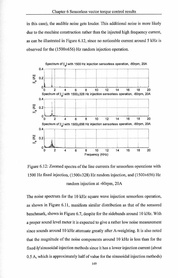
Chapter 6 Sensorless vector torque control results
in this case), the audible noise gets louder. This additional noise is more likely
due to the machine construction rather than the injected high frequency current,
as can be illustrated in Figure 6.12, since no noticeable current around S kHz is
observed for the (lSOO±656) Hz random injection operation.
Spectrum of Ilal with 1500 Hz injection sensorless operation, -60rpm, 20A
~. :} ullupp'upp'uuu,puu 'upu 'uuutpp jupp p,p,puj o 2 4 6 8 10 12 14 16 18 20
Spectrum of Ilal with 1500±328 Hz injection sensorless operation, -60rpm, 20A
~. :: lu,HUP,uuprpuulpUPP,PTPuuru u/puui: o 2 4 6 8 10 12 14 16 18 20
Spectrum of Ilal with 1500±656 Hz injection sensorless operation, -60rpm, 20A
0.4 ,---,----,-----,---,-----,-----.----,---,---,-----,
..- , ,
~. O: 11T:'T1,:-r o 2 4 6 8 10 12 14 16 18 20
Frequency (KHz)
Figure 6.12: Zoomed spectra of the line currents for sensorless operations with
IS00 Hz fixed injection, (IS00±328) Hz random injection, and (IS00±6S6) Hz
random injection at -60rpm, 20A
The noise spectrum for the 10kHz square wave injection sensorless operation,
as shown in Figure 6.11, manifests similar distribution as that of the sensored
benchmar~, shown in Figure 6.7, despite for the sidebands around 10 kHz. With
a proper sound level meter it is expected to give a rather low noise measurement
since sounds around 10kHz attenuate greatly after A-weighting. It is also noted
that the magnitude of the noise components around 10kHz is less than for the
fixed hfsinusoidal injection methods since it has a lower injection current (about
O.S A, which is approximately half of value for the sinusoidal injection methods)
149

Chapter 6 Sensorless vector torque control results
is produced due to the limit of the voltage output from the inverter. Inevitably,
this will give a reduced SNR (signal to noise ratio) and hence poorer estimation
quality.
6.4 Dynamic performance
In order to provide the fast assistant torque response for the EPS system, the
designed dynamics of the sensorless control needs to be fast, which is
determined by the bandwidth of the tracking mechanism. A 90 Hz Luenberger
observer was chosen in this research for all of the sensorless methods being
adopted here and was described in Chapter 4. The dynamic performances of
them were tested and the results are presented in this section in terms of torque
transients and speed transients.
6.4.1 Performance during the torque
transients
In the EPS. applications, a fast torque response is required especially at the
starting stage of the vehicles. The performance during the torque transients was
tested when the motor was controlled at -60rpm (mechanical) steady speed. It is
noted that all of the positions plotted in the figures in this section are electrical
positions and the estimation errors are electrical position errors as well.
A step torque of 50A (56%) was demanded whilst operating with the 1.5 kHz and
2 kHz fixed injection methods, and for (1500 ::I: 328) Hz and (2000 ± 328) Hz
random injection methods, as shown from Figure 6.13 to Figure 6.16. By
comparing the results for the random injection methods to their fixed injection
versions with the same centre frequencies, identical transient performances can
be observed. For all the mentioned sensorless operations, at the instant when a
step torque was demanded, a glitch in the estimated position appeared due to the ISO

Chapter 6 Sensorless vector torque control results
sudden change of torque which can be regarded as a disturbance with its
frequency much larger than the bandwidth of the estimation tracking mechanism.
A large overshoot of speed followed partly due to the low inertia of the drive
system, and a better speed controller is expected to be designed in the future to
overcome it. For a real EPS system, as the inertia is much larger than in the test
rig, this large overshoot will not exist, which means a smoother speed response
is expected. An electrical position error oscillation ranging from approximately
-30 degrees to 5 degrees was then observed during the rest of the transient
interval. It can be seen that the d and q axis currents are controlled accurately and
correctly.
For the fixed frequency injection and for the (1500 ± 328) Hz and (2000 ± 328)
Hz random injection, the transient operation is able to control a step change of
50A (56%) in torque current demand correctly. However for the (1500±656) Hz
and (2000±656) Hz random injection sensorless methods, a step of 50A (56%)
torque would result in failure in estimation, since the band pass filters used for
extraction of the hfcurrent components are of wider bandwidth compared to the
fixed frequency injection methods (2nd order band pass filters with 200 Hz
bandwidth) and ±328 Hz random injection methods (4th order bandpass filters
with 660 Hz bandwidth), higher order of the filter is therefore needed to filter out
the noise and other unwanted disturbances especially when loading, which
inevitably introduces more delays and hence poorer dynamics. The band pass
filters chosen for the (1500±656) Hz and (2000±656) Hz random injection
methods are 6th order butterworth type filters with 1320 Hz bandwidth. A torque
step of 40A (44%) was demanded for both of the methods instead, with the
results shown in Figure 6.17 and Figure 6.18. Similar transient performances can
be found as expected.
For the 10kHz square wave injection sensorless method, the step change of
ISI

Chapter 6 Sensorless vector torque control results
torque demand was set also at 40A (44%). With 50A (56%) step torque demand,
the control would fail as well, probably due to the lower SNR compared to the
other methods, as mentioned ealier. The result for the 40A (44%) transient is
shown in Figure 6.19 with similar performance in transient interval as for other
methods.
In addition, it is found from Figure 6.17 to Figure 6.19 that with the 40A (44%)
step change in torque current demand, the resultant position estimate shows
much less position error once the transient has settled compared to that with 50A
(56%) change in torque current demand as shown from Figure 6.13 to Figure
6.16. This is because the position estimate has been highly distorted by higher
order saliencies when load increases.
For all the aforementioned methods, it is noted that the measured iq contains
much less distortion than id' This is because the most of the hf current is
injected into the d-axis and the torque producing q-axis remains unchanged if a
correct estimation has been achieved.
152

E e-:g
Cl> a. C/)
Chapter 6 Sensorless vector torque control results
Plot of id and iq
, , ~ ..
40 ____ L ___ ! _ i ____ .J ____ .J _____ , _____ , _____ , _____ L _ , , ,
20 , iq ---- ~ ---1-+ - - - -l- - - - -: - - - - -:- - - - -:- - - - -:- - - - - ~ -~----~
: ! : , : : : : : : I o .", ·~.:4~~$r~~:~~~~~~!~~'7~~·:~;~:~:.:~~:r· 1:1't;~~r;.,~~:t.i.,:~r\;.-':':;~ <~fP~.,~.~;\·~:';:.";J,~;l~~,~7,~.'~.~~~~~Ir"~:+J;:,.r;.7': I I 1 I I I I I I I I I I I
-20 L---~--~----~---L----L----L--~----~ __ ~ __ ~ o 0.1 0.2 0.3 0.4 0.5 0.6 0.7 0.8 0.9
Plot of mechanical speed
600 --_~ ____ ~ _____ ~ ____ ~ ____ L ____ ~ ____ J ___ _
400 --~----~-----r----r----r----T----'----I I I I I I I I
20~ ~ ~ ~ ~ 1 ~ ~ J 1 ~ ~ -~ J ~ ~ ~ ~1~ ~ ~ ~ i~ ~ ~ ~ ~ t ~ ~ ~ ~ t : ~ ~ ~ 1 ~ ~ ~ ~ 1 ~ ~ ~ ~ ~ I I I Jf I ~~--~ "------r-- I
-200 - - - - t - - - - ~ - - - - '- ~ - - -: - - - - - :- - - - - :- - - - - ~ - - - - ~ - - - - ~ - - - -
o 0.1 0.2 0.3 0.4 0.5 0.6 0.7 0.8 0.9
Estimated position and real position 400 ,---,_--_.----,---~----,_--_,--_,----,_--_.--__,
',,'
I \ I j I I -,- - ">.r:, - -,- - - - - r - - - - r - - - - T - - I- -
, \ , I , \. 1 ,
I '" I ' I I I I" I
" I I .... ~ I
0.5 0.6 0.7 0.8 0.9
Estimated position error 40 .---_,--_,----,---~----,_--_,----,_--_,--_,-----
I , 'I I I I
~ 20 .- - i~ - t --J ' ----~ ---~ --: -----: ~ -\-~. -:~ ----:- --~ -'1: ~ -: -t, --~ -gO . \,- ':::,'r \ 'v· ~h " 1+, ~ l -,l~.rJ> ~- ~ -, I -, i-\.) ~ , -1,'/;- _IL\ _ A"- - " ' , ~- p'\ 'r" - '1',- ,
Cl> " \ ~ I \ ' ";' \ ( IJ \) r \( ,' J' r ." \ \ , § -20 - - - - ~ - - - - J. - - -~+ ~ -__ ~ __ -_ -:- ----:- ---_ ~ ----~ ---_ ~ ----
:;:::: I
"en -40 - - - - I - - - - I - - - - ~ - - - - ~ - - - - -:- - - - -:- - - - -:- - - - - ~ - - - - + - - - -o I , , I I
Cl. -60 - - - - r - - - - + - - - - ., - - - - -1 - - - - -1- - - - - ,- - - - - I- - - - - + - - - - + - - - -
o 0.1 0.2 0.3 0.4 0.5 0.6 0.7 0.8 0.9 Time(seconds)
Figure 6.13: Torque transient, 0-50A (56%), 1.5 kHz fixed injection at -60rpm
153

Chapter 6 Sensorless vector torque control results
Plot of id and iq
60 ~--~-----r----~--~----~,----~----~--~----~----~ I ( ! \ I I I \ _ ---~ --r'~~~- ~ ____ ~ _____ : _____ : _____ : _____ ~ _ id I I I I I I I I
20 , :' " iq - - - - - - - - - - - - - - 'I - - - - -,- - - - - - - - - -,- - - - - - - - - - I -~ ___ ~
_20 L-__ -L __ ~ ____ ~ __ ~ ____ L_ __ _L ____ L_ __ _L __ ~ __ ~
o 0.1 0.2 0.3 0.4 0.5 0.6 0.7 0.8 0.9
Plot of mechanical speed
E :~~ ~ ~ ~ ~ I ~ ~ ~ -~\-~ ~ : ~ ~ ~ ~ ~! ~ ~ ~ ~ ~!~ ~ ~ ~ ~ [ ~ ~ ~ ~ [ ~ ~ ~ ~ 1 ~ ~ ~ ~ 1 ~ ~ ~ ~ ~ I I I I , I I I !
~ 200 ----~--- ~- --~----~-----~----~----~----~----~----Q) I I I I I I I I I
~ 0 ~-~-- -~- - -~- ---~~-~-~- - -_~::--- -7-~~~--Cl) -200 ____ 1 ____ ~ ___ "\_' _ .! ________ , _____ , _____ L ____ 1 _ _ __ J ___ _
'0 C
I I .L- I I I I I
o 0.1 0.2 0.3 0.4 0.5 0.6 0.7 0.8 0.9
Estimated position and real position 400 ,----,---.----.---------~--~----~--_,--_,--__,
, :2 200 -'00
I I I , ,- - - - - - - - - - T - - - - T - ...J.. __ -
, o a..
0.1 0.2 0.3 0.4 0.5 0.6 0.7 0.8 0.9
Estimated position error 40 , ,
~ 20 g 0 Q)
c -20 ~ -40 Cl) 0 a.. -60
____ L ____ .L ____ J __________________ _ 1 _ ____ l. ____ .. ___ _
I I I I I
. ' \ -I ' "'l J \' (\ ~,. '. 1\ .. ':;--'-Jr"v ~ "'~~--'\\i\t- --<r~-.r\_·.,..""'-'- -; r.~--\-Wl-I_'t~)--~-t ...
-'--~ ~- -'r ~ - -V~~~--lf- _-'-"_~~ _~ ____ ~l: __ .~ ~_~ _. __ ~ ~~_:~~ __ _ I I I I I I I I
- - - - 'I - - - - T - - - - "I - - - - - - - - -,- - - - - - - - - - ,- - - - - T - - - - - - - - -,
- - - - t- - - - - t- - - - - ., ____ -I - - - - -1- - ,- --,.-----+----
0 0.1 0.2 0.3 0.4 0.5 0.6 0.7 0.8 0.9 Time(seconds)
Figure 6.14: Torque transient, 0-50A (56%), (1500 ± 328) Hz random injection
at -60rpm
154

E ~
~ Q) a.
C/)
c;-c 0
:;:; '00 0 a..
~ g Q)
c :2 '00 o
Chapter 6 Sensorless vector torque control results
Plot of id and iq
60 1--:, ---,=-.:~_::::,~=~: :",:,,~,=-=-=:~=-=-=-=-=- r: _~_=--=_-=:~==J,~==:+, =r==r:::::=~~ id - - - - ~ - - - 1 ~ - - - - ~ - - - - ~ - - - - -:- - - - -:- - - - - :- - - - - ~ -40
20 : I I I I I I j iq - - - - f - - - - T - - - - 1-- - - -) - - - - - - - - - -,- - - - -,- - - - - T -L-____ ---'
_20 L-__ -L ____ L-__ -L ____ L-__ -L ____ L-__ -L ____ L-__ -L __ ~
o 0.1 0.2 0.3 0.4 0.5 0.6 0.7 0.8 0.9
Plot of mechanical speed 600 __ J ____ ~ _____ ~ ____ ~ ____ ~ _________ ~ ___ _
I "I I
400 ----~---- -,----~-----~----~----r----T----'----I I I I I I I I 200 ----~---- ~- ___ ~ _____ L ____ L ____ L ____ ~ ____ ~ ___ _
1 1 I I I I , j I o r __ --'----.1 ' - - - - -r- ~ ~--...,·-,- - - - - r - - - - r - - - - T - - - - , - - - -
I I ! /J , " ~ "'-' , ' -r-~~ -200 - - - - 7 - - - - ~ - - - - -, z-- ;rJ_ -'- - - - -:- - - - - :- - - - - ~ - - - - 7 - - - - ~ - - - -
o 0.1 0.2
400
200 1 - - - - f
1 ,I "
0 0 0.1 0.2
I 1 ----1"-- T
1
0.3 0.4 0.5 0.6 0.7 0.8 0.9
Estimated position and real position
0.3
"'- .... __ I 1
" l I
I Il.... I I I I
I I ', I I I I
~ -----:- -'\ -;- ---~ ;- ---~ t ----~ -I I I I I I
I I ' . ~ I I '. I
I I ,'" I '""'" I ' ..
0.4 0.5 0.6 0.7 0.8 0.9
Estimated position error
I - - - - ,- - - - - r - - - - T - - - -
a.. -60 ----t-----t-----~--- .., - - - - -1- - - - I L---~--_L __ ~ ____ L_ __ ~ __ -L __ ~ ____ L-__ ~ __ ~
o 0.1 0.2 0.3 0.4 0.5 0.6 0.7 0.8 0.9 lime(seconds)
Figure 6.15: Torque transient, 0-50A (56%),2 kHz fixed injection at -60rpm
155

Chapter 6 Sensorless vector torque control results
Plot of id and iq
60 , 40
$ 'E 20 ~ ~ 0 0
, .. '~";'II' • .,,;:;.'....,;7 ~.
____ ~ ____ , ~ _~ ___ ~ ____ ~ _____ : ____ _ 1 _ ____ : _____ ~ _ --- id I / 1 I I I I I
I I I I : iq - - - - I - - - - T - - - - I - - - - -I - - - - - - - - - -1- - - - - 1- - - - - I -L-___ ----'
, ,
-20 0 0.1 0.2 0.3 0.4 0.5 0.6 0.7 0.8 0.9
Plot of mechanical speed
~ ~ ~ ~; ~ ~~. ~1~ :~ ~ ~ ~ ~ ~ ~ r ~ ~ ~.~:~ ~ ~ ~ ~:~ ~ ~ ~ ~~ ~ ~ ~ ~ ~ ~ ~~. ~ ~ .. ~ ~ .. ~. ~ ___ - L _ _ _ _ _ ~ \ J ____ .J _____ , _____ , _____ L ____ L ____ 1- ___ _
- - - - ~ - - - - - - - -\: - - - - ~~~ -:- - - - -:- - - - - ~ - - - - ~ - - - - ~ - - - --------j- I I - 1-- "I--I- - ---r~- ---. i ' - ..... ---____ L ____ 1 ____ .J _____ I _____ 1 _____ 1 _____ 1 _____ L _ ___ 1 ___ _
I I '.. I I t I
600
E 400 e- 200 =g-al 0 c..
Cl) -200
0 0.1 0.2 0.3 0.4 0.5 0.6 0.7 0.8 0.9
Estimated position and real position 400
0' C , 0 200 :;::;
, , , - -1-----1-""1'---1---
'00 , , , 0 a..
0 0 0.1 0.2 0.4 0.5 0.6 0. 7 0.8 0.9
Estimated position error 40 1
o 0.1 0.2 0.3 0.4 0.5 0.6 0.7 0.8 0.9 1 Time(seconds)
Figure 6.16: Torque tran ient, 0-50A (56%), (2000 ± 328) Hz random injection
at -60rpm
156

Chapter 6 SensorJess vector torque control results
Plot of id and iq
I I ----L--- 7~----____ ~ ____ ~ ____ ~ ____ ~ ____ ~~ id
I I
20 - - - - ~ - - - - ~ - - - - ~ - - __ ~ __ - - _____ -:- ___ -:- ____ ~ _L-______ i_q-l I
0.1 0.2 0.3 0.4 0.5 0.6 0.7 0.8 0.9
Plot of mechanical speed
600 - ___ ~ _________ ~ ____ _' _____ L ____ ~ ____ L ____ ~ ____ • ___ _
I I I I I
E 400 I ,, , I I i 200 ::: :;::: F '- ,:::::::~:::: ::::: ::~:::: f::::;::::::: {j) -20~ ~ ~ ~ ~ I ~ ~ ~ -~ ~ ~ ~ ~ -~ ~ ~ ~~ ~ ~ I ~ ~ ~~ f ~ ~ ~ ~ ~ ~ ~ ~ ~ ~ ~ ~ ~ ~ ~ ~ ~ ~
o 0.1 0.2 0.3 0.4 0.5 0.6 0.7 0.8 0.9
Estimated position and real position 400 ,---,---_,----~--~----,_--_r--_,~--._--_,-----
()
c ~ 200 .~
a..
0
40
£ 20 g 0 Q)
c -20 0 ~
-40 '(ji 0 a.. -60
0 0.1 0.2 0.3
t- - - +
0 0.1 0.2 0.3
- - ~ - - - -, -: - - - - -:~ - - - - ~- - - - r - - - - + - - -\-I I I I I
0.4 0.5 0.6 0.7 0.8 0.9
Estimated position error
____ L ____ ~ _________ • ___ _
I
I \_... ...- -. ... - i
I -1- - _... t-
0.4 0.5 0.6 0.7 0.8 0.9 lime(seconds)
Figure 6.17: Torque transient, 0-40A (44%), (1500 ± 656) Hz random injection
at -60 rpm
157
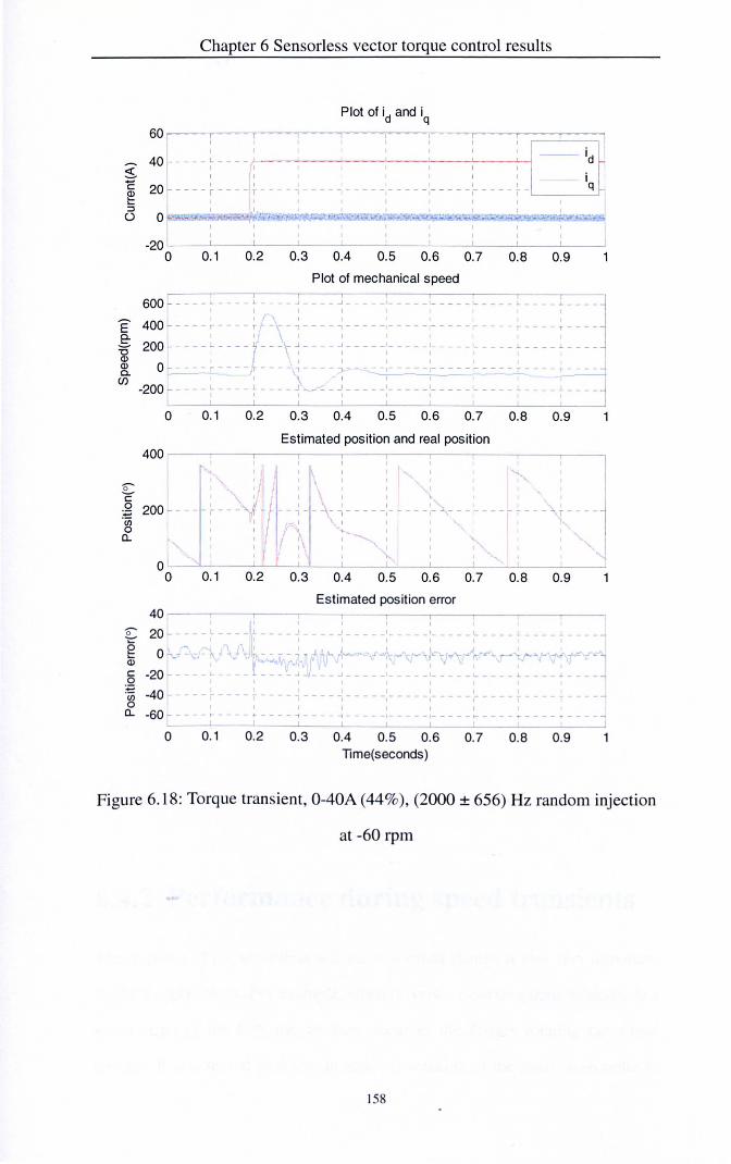
40 ~ C 20 ~ ~
() 0
Chapter 6 SensorIess vector torque control results
Plot of id and iq
____ ~ ____ .~ __ __ -'----'----'----'----L----'"-i id
I : I I I I iq - - - - 'I - - - - T - - - - I - - - - -, - - - - - - - - - - - - - - -,- - - - - r -~ ___ ~
-20 L---~--~----~--~----~--~--~----~--~--~
o 0.1 0.2 0.3 0.4 0.5 0.6 0.7 0.8 0.9
Plot of mechanical speed
600 - - - - - - - - - ~ - - - - ~ - - - - ~ - - - - -:- - - - -:- - - - - L- - - - - ~ - - - - 7 - - - -
E 400 - - - - r - - - - / ~- - ~ - - - - ~ - - - - -:- - - - -:- - - - - ~ - - - - ~ - - - - ~ - - - -
f 2~ ::: t::: J Y: ::. ~ i~~ ~i~ ~ ~ ~ ~:~ ~ ~ ~ ~t ~ . ~ ~ ~ t ~ ~ ~ ~ t ~ ~ ~ ~ 5r r-- I --- , - ~ 1 ~, ----, -- I -I ~ f- "'--200 - - - - L - - - - ~ - - - - J ___ -~ __ , __ - - -:- - ___ : _____ ; _____ L ____ ~ ___ _
o 0.1 0.2 0.3 0.4 0.5 0.6 0.7 0.8 0.9
Estimated position and real position 400 ,----.---.----.----.----,----.----.----.---.----,
0' C 2 200 '00 o 0..
o
0.1 0.2 0.3
0.1 0.2 0.3
0.4 0.5 0.6 0.7 0.8 0.9
Estimated position error
0.4 0.5 0.6 0.7 0.8 0.9 Time(seconds)
Figure 6.18: Torque transient, 0-40A (44%), (2000 ± 656) Hz random injection
at -60 rpm
158

Chapter 6 Sensorless vector torque control results
Plot of id and iq
, _ __ ~L-__ ~ ____ ~ ____ -L ____ ~ ____ ~ ----- id 40 - - - - ; - r- -;-
~ 20 : , iq ~ - - - - - - - - - T - - - - - - - - - -, - - - - - - - - - - - - - - - - - - - - - -'---______ --'
:J ()
E e-:g-Q) Cl.
Cl)
'0 C 0
:;:; ·00 0 a..
:€: g Q)
c: 0
:;:; ·00 0 a..
600
400
200
0
-200
0
400
200
0 0
40
20
0
-20
-40
-60
0
0.1 0.2 0.3 0.4 0.5 0.6 0.7 0.8 0.9
Plot of mechanical speed ____ ~ ____ ~ ____ ~ __________ ~ ____ ~ ____ L ____ " ____ J ___ _
r I I I I I I I I '{' , , , , , , ----T-- - ----,----~-----r----r----r----T----'----
----~----~ ---~----~-----~----~----~----~----~----l I - I I, I I I I
~ ~ ~~ ~ ~ -~ ~ l ~ _ ~~~J~~:~~-~~j~ ~ ~~~f~ ~ ~ ~ ~ ~ ~ ~ F~~~ 0.1 0.2 0.3 0.4 0.5 0.6 0.7 0.8 0.9
Estimated position and real position
I I I I I I I
: \: . \ '=-==< : ,'" : ~ I I" I I I I I I I
-~ --~ --; f --\\ ~ ----j - ~ - ~,-'- --- -1r -- - -~ -, -- - ~ ---- ~ --I fl I I t I , I I' \ ' , , , , , ~~ j (' \J I I~, I
.. j "
0.1 0.2 0.3 0.4 0.5 0.6 0.7 0.8 0.9
Estimated position error
I I I I - - - - - - - - - - - - - -,- - - - - ,- - - - - ,- - - - - f - - - - - - - - -
+- - - - ..., - -- -----~----~----.----.----
0.1 0. 2 0.3 0.4 0.5 0.6 0. 7 0.8 0.9 lime(seconds)
Figure 6.19: Torque transient, 0-40A (44%), 10kHz square wave injection at
-60rpm
6.4.2 Performance during speed transients
The response of the sensorJess scheme to a speed change is also very important
for EPS applications. For example, when drivers are parking their vehicles, fast
speed steps of the EPS motors may occur as the drivers rotating the wheel
quickJy. It is essential to maintain accurate tracking of the position in order to
159

Chapter 6 Sensorless vector torque control results
give the correct assistant torque. The performance during speed transients was
tested when the motor was operated under a 30A (33%) load condition. As it was
concluded in 6.3 that with the random injection frequency of(1500±328) Hz, the
audible noise was reduced the most with respect to the fixed injection, this
frequency range was used for the random hjinjection sensorless method in this
section. The results of a speed reversal from -240rpm to 0 and then to 240rpm for
a sensored benchmark, the random sinusoidal hi injection sensorless method,
and the 10kHz square wave hi injection method are shown in Figure 6.20,
Figure 6.21 and Figure 6.22.
160

Chapter 6 Sensorless vector torque control results
Plot of mechanical speed 400 ,---.----.----,----.----,----,---,----.----.----,
: : : : : ~r,, : : : E 200 e-
---- :--- -: ----:- ---:--n--;- --- :---'- ~~~T~ J I I v-__ I I I I I :g
Q) c..
Cl)
o - - - - r - - - - 1" - - - - "'1 - - - - " - -~ - 1- - - - - t- - - - - t- - - - - 1" - - - -
I I I
-200 1-- _- _- _- ~'- -- -- --_- -'-.~ ~-----_---'.~_-_-_-___' -: - - - - _,_ - - - - - - - - _1- - - - - :. - - - - + - - - -
-400 L---~--~----~---L----L----L--~----~--~--~ o 0.2 0.4 0.6 0.8 1.2 1.4 1.6 1.8 2
Plot of id and iq
40 ,---,----,----,----,----,----r---,----,----,----, I 1 I I I
........ , ............... .,..,.j..-..... -~""-~....._.". .. _ _ I_ . , t.-- - ~ ........-+-.- _ - - -1 ____ _
I I I I I I I I ,--_'~ __ --j
~ 20 - - - - i ----t ----~ ----i -----( ---!- ----!- ----t -1 -- :~ ~ I I I I I I I I 8 0 ~~~~--~~.~~~~~ ~ ~~~ ;~~\&N~
-20 L---~--~----~ __ _L ____ L_ __ _L __ ~ ____ ~ __ ~ __ ~
o 0.2 0.4 0.6 0.8 1.2 1.4 1.6 1.8 2
Electrical position obtained from the encoder
lime(seconds)
Figure 6.20: Speed reversal, -240rpm-0-240rpm, sensored benchmark under
30A (33%) load condition
161

E e:0
<I> <I> Cl.
Cl)
[:: c: o += .~
Cl..
" -.:-e ID c: o += '(ij o
Cl..
Chapter 6 Sensorless vector torque control results
Plot of mechanical speed 500 ~---'----r----r----'----.----'----.----'----.----'
, - , I ,...... ----..J. ___ L
, , , , , y -: : : o - - - - I" - - - - T - - - - "I - - - - -, r - - --, ---,- - - - - ,- - - - - '1 - - - - T - - - -, , , j I I I , I I I I I I I ' I
----I'" ------1'--- ~ I I 1 I i I , ,
-500 L---~--~----~--~----~---L--~L---~--~--~
o 0.2 0.4 0.6 0.8 1.2 1.4 1.6 1.8 2 Plot of id and iq
40 ,----,---.----,----.----,----.---,,---,----.----, i---------'-.-.--....... -~ .... ,----'-----'-
I ____ L ____ 1 ____ J _____ , _____ , _____ , _____ 1 _____ !... _
I I I I id
iq
-20 L---~--~----~--~----~---L----L---~--~ __ ~ o 0.2 0.4 0.6 0.8 1.2 1.4 1.6 1.8 2
Estimated position and real position 400 ,---,----,----,----,----,----,----,---,----,----,
0.4 0.6 0.8 1.2 1.4 1.6 1.8 2
Estimated position error
-20 L---~---L ____ L-__ ~ __ ~ ____ L-__ ~ __ ~ ____ L-~
o 0.2 0.4 0.6 0.8 1.2 1.4 1.6 1.8 2 Time(seconds)
Figure 6.21: Speed reversal, -240rpm-O-240rpm, (l500±328) Hz random
inusoidal hfinjection sen orless operation under 30A (33%) load condition
162

Chapter 6 Sensorless vector torque control results
Plot of mechanical speed 500 ,---,----,----,---,----,----,---,----,----,---,
I ..-L. .. _ ... __ . ..l .. _ .. _ .. -l._~ ... __ ... _ .
I I I I I I I
o - - - - ~ - - - - ~ - - - - ~ - j- :-":'-{, ~. ---j---'- - - - - - - -:- - - - - r - - - - ~ - - - -I I I I
I I I I
1 1 I I
-500 L---~--~----L---~--~----L---~--~----L-~ o 0.2 0.4 0.6 0.8 1.2 1.4 1.6 1.8 2
Plot of id and iq
40 r---,,---,----,----.----,----.----.---,,---.--~
-20 L---~--~----~ __ ~ ____ ~ __ _L ____ L_ __ _L __ ~ __ ~
o 0.2 0.4 0.6 0.8 1.2 1.4 1.6 1.8 2
Estimated position and real position
~
0
c ~ I
-1----- -- -Cl)
0 c..
0 0 0.2 0.4 0.6 0.8 1.2 1.4 1.6 1.8 2
Estimated position error 20
~
0 "l::' g 10 Q)
c: 0
:;::; '00 0 c..
-10 0 0.2 0.4 0.6 0.8 1.2 1.4 1.6 1.8 2
Time{seconds)
Figure 6.22: Speed reversal , -240rpm-0-240rpm, 10kHz square wave hf
injection sensorless operation under 30A (33%) load condition
As observed from Figure 6.20 to Figure 6.22, both the random sinusoidal hf
injection and the square wave hfinjection methods are able to track the position
during the speed reversal and provide comparable assistant torque to the
sensored benchmark. The average position error is however bigger for the
random hfinjection method, presented as uneven position error for positive and
163

Chapter 6 Sensorless vector torque control results
negative speeds: about ±1S· (electrical position) for the negative speed and
about ±S· (electrical position) for the positive rotating speed. Whilst the position
error for the square wave hfinjection method is consistent for these two speeds:
about ±S· (electrical position). The reason of this is not clear and needs to be
investigated in the future.
6.5 Conclusion
In this chapter, the current distortion, audible noise, and the dynamic
performance for fixed and random hf sinusoidal injection methods and square
wave injection method are compared and discussed.
The current distortion for different sensorless methods are very similar with the
same SNR (Le. the hf current amplitudes are the same) for the same operating
points. For this specific test motor, higher loads will cause additional distortions
due to the increase of estimation error, which is different from the work
presented in [13] where with increase of load levels the THDs of current
decrease all the time.
Audible noise due to injection varies with the change of injection frequency. The
lowest audible noise is obtained using the random injection with the frequency
range of (1500±328) Hz. With further widening of the frequency ranges, some
additional noise will occur in the around 5 kHz area, possibly due to motor
construction and a resonant point being reached. For the 10 kHz square wave
injection sensorless method, the audible noise level cannot be obtained properly ... due to the limitation of the instrumentation, and it requires a higher DC link
voltage to give the same hfcurrent levels in order to compare with the sinusoidal
injection methods.
The dynamic performance of all the aforementioned sensorless methods is
compared. The best is shown with fixed injection and with the random injection 164

Chapter 6 Sensorless vector torque control results
of frequency range within ±328 Hz due to the band pass filter delay which
affects the system dynamics. The square wave injection method has similar
performance with ±656 Hz random injection methods due to the low SNR value.
165

Chapter 7 Conclusions and future work
Chapter 7 Conclusions and Future work
7.1 Introduction
This thesis has focused on the reduction of audible noise in sensorless controlled
drives for automotive electrical power steering applications which use saliency
tracking methods and in particular the hlinjection methods. Three methods have
been implemented, the fixed and random hi injection methods and the square
wave hi injection method. The audible noise introduced by the hi injection and
also the control performance of the three methods have been compared and
contrasted.
The novel work presented in this thesis includes:
• Research and development of a novel random hlinjection based sensorless
control
• Research and implementation of a square wave type injection for sensorless
control for power steering applications
• A comparison of the behaviour of the two techniques for power steering
applications
166

Chapter 7 Conclusions and future work
7.2 Audible noise reduction
The audible noise created by hfinjection sensorless control is mainly caused by
the hfvoltage injection itself. In the test rig, the chosen injection frequencies 1.5
kHz and 2 kHz for the fixed hf sinusoidal injection method create significant
audible noise. The frequency of the induced noise is near the injection frequency
and is perceived as a fixed tone. In an EPS system, the motor as well as its
control unit is designed to be close to the driver. The audible noise produced by
the fixed hf sinusoidal injection is not acceptable as it will cause passenger
discomfort. The random hf sinusoidal injection method uses a randomised hf
voltage injection to the machine. The resultant audible noise is a random spread
of frequencies around the centre frequency and is perceived as a background hiss
rather than a fixed tone. Frequency ranges of (1500±328) Hz, (1500±656) Hz,
(2000±328) Hz and (2000±656) Hz have been compared. By analysing the
A-weighting scales used to classify human perception of audible noise, the
injection with a frequency of (1500±656) Hz was expected to have the lowest
sound level. However, it was found that an injection frequency of (1500±328)
Hz exhibits the lowest audible noise level, from direct measurement with a
sound level meter. Frequency analysis of the recorded noise showed that some
noise around 5 kHz is produced with (1500±656) Hz injection due to the
resonance of the mechanical structure of the machine, which caused a higher
sound level measurement compared to the (1500±328) Hz injection. The sound
level measurement for the 10kHz square wave hf injection has not been taken
since the sound level meter used in this test rig has an upper frequency limit of 8
kHz. However, the frequency analysis of the recorded noise for this method was
carried out for comparison. It was found that the noise introduced by the hf
injection is around 10kHz and creates no other noise in the low frequency region.
It should in theory have a lower sound level than the fixed hfsinusoidal injection
167

Chapter 7 Conclusions and future work
at 1.5 kHz and 2 kHz. By using either of these two methods, the audible noise
can be effectively reduced.
7.3 Control performance
Sensorless torque control with the three hfinjection methods has been achieved
from zero speed to ±240rpm with up to ±60A load (about 63% rated load).
Similar position estimate quality for the three hf injection sensorless methods
has been demonstrated. It was found that under no load conditions, the position
estimate has been distorted significantly due to the non-linear behaviour of the
inverter around zero current crossing points and manifests as a 6 le disturbance.
When load increases, the resultant hf current signals that contain the position
information have fewer zero current crossing points compared to that under no
load, and hence a lower distortion was observed. However, with the load
between 30A and 60A, the distortion of the position estimate increased again.
This is because the tracked saliency was affected by the higher order saliencies
when the load increases. When the load increases, sensorless control could not
be achieved since instability of control occurs due to these higher order
saliencies.
The current distortion of the drive system caused by hf voltage injection is
similar for the fixed and random hf sinusoidal injection sensorless control. The
injection frequency also does not affect the current distortion significantly. The
10 kHz hfsquare wave injection sensorless control has smaller current distortion .~
than that for the other two methods, since the resultant hf current for the square
wave injection is much less due to the limitation of the inverter output when a
12V DC-link voltage is used. Under load levels less than 30A, the sensored
control with hi injection and sensorless control result in identical current
distortion. However, above 30A the position estimation is affected by the higher
168

Chapter 7 Conclusions and future work
order saliencies and additional torque ripple is produced resulting in more
distorted current.
Fast torque response is required for automotive power steering applications.
Torque transients for the three sensorless methods have been performed to test
the dynamic performance. It was found with both the fixed and random hf
sinusoidal injection methods, when a 50A torque transient was applied, the
position estimate still tracked the real position with a maximum ±25 degrees
error during the transient intervals. However, with the 10kHz hf square wave
injection method, the largest torque transient that can be applied is 40A. This is
because the method has a lower SNR compared to that for the hf sinusoidal
injection. This is due to the limit of the inverter output voltage and affects the
saliency tracking in a high torque transient. Dynamic response for the speed
transient has also been performed for random sinusoidal hfinjection and square
wave hf injection sensorless methods. Comparable results have been
demonstrated with a sensored control result as the benchmark for analysis.
7.4 Summary of Project Achievements and
and Future Work
Refering to the aims and objectives set in Chapter 1, the following goals have
been achieved:
• Audible noise reduced compared to a traditional fixed injection type
sensOl'less method
• Low speed sensorless torque control from 0-240 rpm
• Angle error below 10 electrical degrees under 40A (44%) load conditions
• Up to 60A (67%) load sensorless operation
169

Chapter 7 Conclusions and future work
• Large torque transient, up to 50A (56% load) step change
Future work on the following aspects needs to be carried out:
• To investigate the relationship between the machine structure and the
minimum audible noise with respect to the applied injection frequency in
order to further optimise the random injection method
• To investigate possibility of rearranging the PWM sequence to apply a
square wave at the switching frequency to further improve the square wave
injection method
• To extend the low speed sensorless operation to full load (90A)
• Combining model based sensorless operation at high speed to achieve full
speed region sensorless torque control
• To investigate the method for reducing the ripple of the angle error at higher
loading conditions (especially above 40 A, 44% load) by compensating for
the loading effects and inverter non-linearities.
170

Appendix A Phase currents reconstruction through DC link current measurement
Appendix A Phase currents reconstruction
through DC link current measurement
For a general 3-phase balanced PMAC drive system as shown in Figure A.I,
when different voltage vectors are applied to the machine, the DC link current
can be split as combinations of different phase currents, as shown in Table A.I .
+ DC
Figure A.I: A general 3-phase PMAC drive system
171

Appendix A Phase currents reconstruction through DC link current measurement
Voltage Vector DC link current
100 (VI) ia
110 (V2) (ia + ib) = -ic
010 (V3) ib
011 (V4) (ib +iJ = -ia
001 (V5) ic
101 (V6) (ia + ic) = -ib
000/111 (VON7) 0
Table A.1: DC link current values during each of the vectors
As a result, it is possible to work out the phase currents by measuring the DC
link current when corresponded vectors are applied. For example, when the
demanded voltage vector is within sector I, as shown in Figure A.2, it can be
decomposed of active vectors VI and V2. With high switching frequency
implemented, the interval between the two DC link current samples for the two
active vectors is sufficiently small and the measured phase currents can be
assumed to be sampled at a same instant, and then the third phase current can be
calculated due to the balance property of the drive system.
172

Appendix A Phase currents reconstruction through DC link current measurement
V3(OlO)
Sector III
V4(Oll)
Sector IV
V5(OOl)
Sector Il
V2(llO)
Sector I
Vl(lOO)
Sector VI
V6(lOl)
Figure A.2: Vector diagram when the demanded voltage resides in Sector I
However, due to the dead time, the diode reverse-recovery and the ADC
acquisition delay, a minimum time of Tmin is required for an accurate current
sample after an active vector is applied. This will cause problems when the
demanded vector passes through the boundaries of the adjacent sectors and when
the demanded vector is below certain threshold, where in both cases, the
durations of one or more of the active vectors in a switching period will be
shorter than Tmin • As a result, pulse extension is applied in these situations. For
example, when the demanded vector is very low in Sector I, both of the active
vectors (VI and V2) need to be extended and the additional active vectors need
to be compensated by applying opposite vectors (V4 and VS) to keep the
volt-second balanced, as illustrated in Figure A.3. For the implementation, the
extension of the active vectors could be done within the first half of the
switching period, and the compensation could be made during the second half of
the period. Other arrangements of allocating the extension and compensation
could also be used to optimize the performance with respect to computation
efforts and the cost reduction. For instance, in order to reduce the sample rate,
the current measurements could be made with several adjacent switching periods,
especially at low speed where the vector almost remains the same during the
adjacent switching periods. By doing so, the extension is also needed only when 173

Appendix A Phase currents reconstruction through DC link current measurement
relevant measurement needs to be made, resulting in reduced torque ripple as
well.
V3(OlO)
V4(Oll)
V5(OOl)
V2(llO)
Sector I
Vl(lOO)
V6(101)
Figure A.3: Vector extension and compensation when Vdemand is small in Sector I
174

Appendix B The schematic of the gate drive circuit
Appendix B The schematic of the gate
drive circuit
The schematic of the gate drive circuit is shown in Figure B.1 .
... ~
175

.. I
"Tj ciQ. s:: (i ttl
-5\. 5!,. ? ~-~~ ~lIi>e _ ...
n
F ... 'JJ (') l E ::r (p
3 a o· 0 -.J ...., ~
16 T~mf
f~f;~-5\· :;:.d p:td.
-5\' .... pod - 5V ::r (p
(IQ ~ .... (p le 0-'"t ..... -< (p - 5V (') ::j . 'iL-r'l'ec
(')
5. .... f~ ...
D
-1'2> -L!~\· -uv O.h::F
Te! T ~
p<! p~
A- iS
."'""
.4.-1
In T i:?(l6'v)
'" .4:>' ...
ActO. 'of Air ~i ~:; T THE(IO\ .'Pd Ap.l
.~- !5
'2 'of £ c;
r h T· All'!
A-15
A-IS . .\-15
l ell Lu T~;;';(i 6V) T ':>F(J 6V)
Afr.d .Apd .A- IS A-j5
LIS T··"""O\~ .4:>'
l e!, T""(! :!\~ .-lp!
)-"'0 "'0 (p
::l 0-x· o:l >-l ::r (p
CIl (')
::r (p
3 a ..... (')
o ...., ..... ::r (p
(IQ
a (p
0-'"t
~t (p
(')
8· 5 . ....

Appendix C Publications
Appendix C Publications
1. Hui J., Sumner M.: Sensorless torque control of PM motor using modified
HF injection methodfor audible noise reduction, 14th European Conference
on Power Electronics and Applications, Birmingham, 2011
177

Bibliography
References
1. Nunney, MJ., Light and Heavy Vehicle Technology. Fourth Edition ed. 2006: Butterworth-Heinemann.
2. TRW, EP HS--Electrically Powered Hydraulic Steering. 2011. 3. TRW, Electrically powered steering - column drive. 2008. 4. T.Sebastian, M.S.I., and S.Mir, Application of permanent magnet
synchronous machines in automotive steering systems. Electrical Machinery and Energy Conversion Systems, KIEE International Transactions on, 2005. 5B(2): p. 111-117.
5. Christopher, E., et al. Power boost unit for automotive Electric Power Steering systems. in Power Electronics, Machines . and Drives (PEMD 2010), 5th lET International Conference on. 2010.
6. Aihara, T., et al., Sensorless torque control of salient-pole synchronous motor at zero-speed operation. Power Electronics, IEEE Transactions on,
1999. 14(1): p. 202-208. 7. Andreescu, G.D., Robust sliding mode based observer for sensorless
control of permanent magnet synchronous motor drives, in PEMe
conference. 1998. p. 172-177. 8. Andreescu, G.D., Position and speed sensorless control ofpmsm drives
based on adaptive observer, in EP E. 1999. 9. Ben-Brahim, L., Motor speed identification via neural networks.
Industry Applications Magazine, IEEE, 1995. 1(1): p. 28-32. 10. C.M. Bingham, B.S.B., Nonlinear state-observer techniques for
sensorless control of automotive pmsm's, including load-torque
estimation and saliency, in EPE Conference. 2003. 11. Chan-Hee, C. and S. Jul-Ki, Pulsating Signal Injection-Based Axis
Switching Sensorless Control of Surface-Mounted Permanent-Magnet Motors for Minimal Zero-Current Clamping Effects. Industry Applications, IEEE Transactions on, 2008. 44(6): p. 1741-1748.
12. Corley, MJ. and R.D. Lorenz, Rotor position and velocity estimation for a salient-pole permanent magnet synchronous machine at standstill and high speeds. Industry Applications, IEEE Transactions on, 1998.34(4): p.
7~4-789. 13. Curs on, A., Low Speed Encoderless Control of Permanent Magnet AC
Machines for Automotive Applications, in Electrical and Electronics Engineering. 2009, University of Nottingham.
14. E. Robeischl, M.S., and K. Salutt. Improved INFORM measurement sequence and evaluation for sensorless permanent magnet synchronous motor drives. in 10th International Power Electronics and Motion
Control Conference. 2002. 15. Holtz, J. Initial Rotor Polarity Detection and Sensorless Control of PM
178

Bibliography
Synchronous Machines. in Industry Applications Conference, 2006. 41st
/AS Annual Meeting. Conference Record of the 2006 IEEE. 2006.
16. Ji-Hoon, l, H. Jung-Ik, and S. Seung-Ki. Vector control of surface mounted permanent magnet motor without any rotational transducer. in Applied Power Electronics Conference and Exposition, 2001. APEC
2001. Sixteenth Annual IEEE. 2001.
17. Gao, Q., et al. Position Estimation of AC Machines at all Frequencies
using only Space Vector PWM based Excitation. in Power Electronics, Machines and Drives, 2006. The 3rd lET International Conference on.
2006. 18. Raute, R, et al. Operation of a sensorless PMSM drive without
additional test signal injection. in Power Electronics, Machines and
Drives, 2008. PEMD 2008. 4th lET Conference on. 2008.
19. Silva, C.A., Sensorless Vector Control of Surface Mounted Permanent Magnet Machines Without Restriction of Zero Frequency, in Electrical
and Electronics Engineering. 2003, University of Nottingham. 20. Yahan, H., et al. Sensorless Control of Surface Mounted Permanent
Magnetic Machine Using the Standard Space Vector PWN. in Industry
Applications Conference, 2007. 42nd IAS Annual Meeting. Conference Record of the 2007 IEEE. 2007.
21. Curson, A. and M. Sumner. A comparison of low speed sensorless
control techniques for low voltage PM machines. in Power Electronics
and Applications, 2009. EPE '09. 13th European Conference on. 2009.
22. Krause, P.C., Analysis of Electric Machinery. 1994: New York: McGraw-Hill.
23. Novotny, D.W. and T.A. Lipo, Vectror Control and Dynamics of AC Drives. 1996, Oxford, UK: Clarendon Press.
24. Blasco..;Gimenez, R, et al., Dynamic performance limitations for MRAS
based sensorless induction motor drives. 1 Stability analysis for the
closed loop drive. Electric Power Applications, lEE Proceedings -, 1996. 143(2): p. 113-122.
25. Holtz, J. Developments in Sensorless AC Drive Technology. in Power
Electronics and Drives Systems, 2005. PEDS 2005. International Conference on. 2005.
26. Hu, J. and B. Wu. New integration algorithms for estimating motor flux over a wide speed range. in Power Electronics Specialists Conference, 1997. PESC '97 Record., 28th Annual IEEE. 1997.
27. Holtz, J. and Q. Juntao, Sensorless vector control of induction motors at
very low speed using a nonlinear inverter model and parameter
identification. Industry Applications, IEEE Transactions on, 2002. 38(4): p. 1087-1095.
28. Jansen, P.L. and R.D. Lorenz. Accuracy limitations of velocity andjlux
179

Bibliography
estimation in direct field oriented induction machines. in Power
Electronics and Applications, 1993., Fifth European Conference on.
1993. 29. Gao, Q., Sensorless Vector control of Induction Machines at zero and low
frequencies, in Electrical and Electronics Engineering. 2006, University of Nottingham.
30. Kubota, H., K. Matsuse, and T. Nakano, DSP-based speed adaptive flux observer of induction motor. Industry Applications, IEEE Transactions on, 1993.29(2): p. 344-348.
31. Jones, L.A. and J.H. Lang, A state observer for the permanent-magnet
synchronous motor. Industrial Electronics, IEEE Transactions on, 1989. 36(3): p. 374-382.
32. Lascu, C., I. Boldea, and F. Blaabjerg, Very-Iow-speed variable-structure control of sensorless induction machine drives without signal injection.
Industry Applications, IEEE Transactions on, 2005. 41(2): p. 591-598. 33. Tursini, M., R Petrella, and F. Parasiliti, Adaptive sliding-mode observer
for speed-sensorless control of induction motors. Industry Applications, IEEE Transactions on, 2000. 36(5): p. 1380-1387.
34. Kim, Y.R, S.K. SuI, and M.H. Park. Speed sensorless vector control of an induction motor using an extended Kalman filter. in Industry
Applications Society Annual Meeting, 1992., Conference Record of the
1992 IEEE. 1992. 35. Hamefors, L. A comparison between directly parametrised observers
and extended Kalman filters for sensorless induction motor drives. in Power Electronics and Variable Speed Drives, 1998. Seventh
International Conference on (Conf Publ. No. 456). 1998. 36. Armstrong, G.J., DJ. Atkinson, and P.P. Acarnley. A comparison of
estimation techniques for sensorless vector controlled induction motor drives. in Power Electronics and Drive Systems, 1997. Proceedings.,
1997 International Conference on. 1997. 37. Kereszty, T., V.M. Leppanen, and J. Luomi. Sensorless control of surface
magnet synchronous motors at low speeds using low-frequency signal
injection. in Industrial Electronics Society, 2003. IECON '03. The 29th Annual Conference of the IEEE. 2003.
38. Cilia, J., et al., Sensorless position detection for vector-controlled induction motor drives using an asymmetric outer-section cage. Industry Applications, IEEE Transactions on, 1997.33(5): p. 1162-1169.
39. Jansen, P.L. and RD. Lorenz, Transducerless position and velocity
estimation in induction and salient AC machines. Industry Applications, IEEE Transactions on, 1995.31(2): p. 240-247.
40. Teske, N., et al., Encoderless position estimation for symmetric cage
induction machines under loaded conditions. Industry Applications,
180

Bibliography
IEEE Transactions on, 2001. 37(6): p. 1793-1800. 41. Teske, N., Asher G.M., Bradley, K. J. and Sumner M., Encoderless
position control of induction machines, in EPE conference. 2001. 42. Holtz, J., Sensorless Control of Induction Machines-With or Without
Signal Injection? Industrial Electronics, IEEE Transactions on, 2006.
53(1): p. 7-30. 43. Gao, Q., G. Asher, and M. Sumner, Sensorless Position and Speed
Control of Induction Motors Using High-Frequency Injection and Without Offline Precommissioning. Industrial Electronics, IEEE Transactions on, 2007. 54(5): p. 2474-2481.
44. A.E. Fitzgerald, C.K., and S. Umans, Electric Machinery. 6th edition ed. 2003: McGraw-Hill Higher Education.
45. Teske, N., Sensorless position control of induction machines using high frequency signal injection, in Electrical and Electronics Engineering. 2001, University of Nottingham.
46. Holtz, J. and P. Hangwen, Elimination of saturation effocts in sensorless
position-controlled induction motors. Industry Applications, IEEE
Transactions on, 2004. 40(2): p. 623-631. 47. Makys, P., et al. Shaft Sensorless Speed Control of Induction Motor
Drive. in Power Electronics and Motion Control Conference, 2006.
EPE-PEMC 2006. 12th International. 2006. 48. Linke, M., R. Kennel, and J. Holtz. Sensorless position control of
permanent magnet synchronous machines without limitation at zero speed. in IECON 02 Industrial Electronics Society, IEEE 2002 28th Annual Conference. 2002.
49. Caruana, C., et al., Flux position estimation in cage induction machines using synchronous HF injection and Kalman filtering. Industry Applications, IEEE Transactions on, 2003. 39(5): p. 1372-1378.
50. Yu-seok, J., et al., Initial rotor position estimation of an interior
permanent-magnet synchronous machine using· carrier-frequency injection methods. Industry Applications, IEEE Transactions on, 2005.
41(1): p. 38-45. 51. Young-doo, Y., et al. High bandwidth sensorless algorithm for AC
machines based on square-wave type voltage injection. in Energy
Conversion Congress and Exposition, 2009. ECCE 2009. IEEE. 2009 .. 52. Young-Doo, Y., et al., High-Bandwidth Sensorless Algorithm for AC
Machines Based on Square-Wave-Type Voltage Injection. Industry
Applications, IEEE Transactions on, 2011. 47(3): p. 1361-1370. 53. Young-doo, Y. and S. Seung-ki. Sensorless control for induction
machines using square-wave voltage injection. in Energy Conversion
Congress and Exposition (ECCE), 2010 IEEE. 2010. .' 54. Kim, S. and S.-K. SuI. High performance position sensorless control
181

Bibliography
using rotating voltage signal injection in IPMSM. in Power Electronics and Applications (EPE 2011), Proceedings of the 20ll-14th European Conference on. 2011.
55. Schroedl, M. Sensorless control of AC machines at low speed and standstill based on the INFORM method. in Industry Applications
Conference, 1996. Thirty-First IAS Annual Meeting, IAS '96., Conference Record of the 1996 IEEE. 1996.
56. Robeischl, E. and M. Schroedl, Optimized INFORM measurement sequence for sensorless PM synchronous motor drives with respect to minimum current distortion. Industry Applications, IEEE Transactions on, 2004. 40(2): p. 591-598.
57. Holtz, J. and J. Juliet, Sensorless acquisition of the rotor position angle of induction motors with arbitrary stator windings. Industry
Applications, IEEE Transactions on, 2005.41(6): p. 1675-1682. 58. Holtz, J. Sensorless position control of induction motors. An emerging
technology. in Advanced Motion Control, 1998. AMC '98-Coimbra., 1998 5th International Workshop on. 1998.
59. Caruana, C., O.M. Asher, and J. Clare. Sensorless flux position estimation at low and zero frequency by measuring zero-sequence current in delta connected cage induction machines. in Industry
Applications Conference, 2003. 38th IAS Annual Meeting. Conference Record of the. 2003.
60. Raute, R, et al. A zero speed operation sensorless P MSM drive without additional test signal injection. in Power Electronics and Applications, 2007 European Conforence on. 2007.
61. Ki-Seon, K., J. Young-Oook, and L. Young-Cheol, A New Hybrid Random PWM Scheme. Power Electronics, IEEE Transactions on, 2009. 24(1): p. 192·200.
62. Habetler, T.O. and n.M. Divan, Acoustic noise reduction in sinusoidal PWM drives using a randomly modulated carrier. Power Electronics,
IEEE Transactions on, 1991. 6(3): p. 356·363. 63. Paul Horowitz, W.H., The Art of Electronics. 1980: Cambridge
University Press. 64. Holtz, J., Acquisition of Position Error and Magnet Polarity for
Sensorless Control of P M Synchronous Machines. Industry Applications, IEEE Transactions on, 2008. 44(4): p. 1172·1180.
65. C.Silva, O.A., and M.Sumner. Influence of dead-time compensation on rotor position estimation in surface mounted pm machines using hf
voltage injection. in IEEE Power Conversion Conference. 2002. 66. J.Holtz, Pulsewidthmodulation for electronic power conversion.
Proceeding of the IEEE, 1994.82: p. 1194·1214. 67. J·L.Lin, A new approach of dead-time compensation for pwm voltage
182

Bibliography
inverters. Circuits and Systems -I: Fundamental Theory and Applications, IEEE Transactions on, 2002. 49(4): p. 476-483.
68. M.Linke, R.K., and J.Holtz. Sensorless speed and position control of synchronous machines using alternating carrier injection. in Electrical Machines and Drives Conference. 2003.
69. V.Szokolay, S., Introduction to ARCHITECTURAL SCIENCE: the basis of sustainable design. 2004: Architectural Press.
70. Standard, I., IEC 61672. 2003. 71. Standard, I., ISO 226.2003. 72. DiracDelta.co.uk. A Weighting. 73. Testo, Testo 816 Sound Level Metre Instruction Manual. 74. Crocker, M.J., ed. Handbook of noise and vibration control. 2007,
Hoboken, NJ. : John WHey & Sons. 75. de Lillo, L., et al., Multiphase Power Converter Drivefor Fault-Tolerant
Machine Development in Aerospace Applications. Industrial Electronics, IEEE Transactions on, 2010.57(2): p. 575-583.
76. Inc, S.D. TMS320C6713 DSK Technical Reference. May 2003. 77. Educational DSP, L. http://www.educationaldsp.com/. 78. Wu, B., High-Power Converters and AC Drives. 2006, WHey & IEEE
Press. 79. Mohan, N., Undeland, T. M. , Robbins, W. P. , ed. Power Electronics:
Converters, Applications, and Design. 3rd ed. 2002, John WHey & Sons. 80. Gerada, C., et al. Loading effects on saliency based sensorless control of
PMSMs. in Electrical Machines and Systems, 2009. ICEMS 2009. International Conference on. 2009.
81. . Yi, L., et al.; Improved Rotor-Position Estimation by Signal Injection in Brushless AC Motors, Accounting for Cross-Coupling Magnetic Saturation. Industry Applications, IEEE Transactions on, 2009. 45(5): p. 1843-1850.
82. Guglielmi, P., M. Pastorelli, and A. Vagati, Cross-Saturation Effects in IP M Motors and Related Impact on Sensorless Control. Industry Applications, IEEE Transactions on, 2006. 42(6): p. 1516-1522.
83. LeCroy, Current probes. 2005. <
84. LeCroy, WaveSufer 400 Series. 2006. -
183