Group Economic Performance, Economic Voting and Electoral Accountability
33
De Boef and Nagler; Economic Voting, April, 2002 1 Group Economic Performance, Economic Voting and Electoral Accountability This research presents a new theoretical perspective on economic voting. There is a long- standing debate on whether voters are: ‘sociotropic’ voters , i.e., basing their vote on the state of the national economy; or ‘pocketbook’ voters, i.e., basing their vote on the state of their own finances (Kiewiet 1983, Kinder & Kiewiet 1979). We believe that this debate can be reduced to asking what information voters use to form expectations about their own pocketbooks in the future. We argue that self-interested and rational voters do not look to the national economy as the best informa- tion of future economic benefit to expect from the incumbent. In essence, growth is not enough information for any given voter’s economic future. Instead, we argue that voters will look for eco- nomic indicators that provide them with information about growth and about how growth will be distributed. People care not just about how big the economic pie is, but as in all politics, they care about what part of it they get. And this should affect vote choice and, more generally, evaluations of the incumbent. We examine presidential approval over time across different demographic groups of voters, and show that those approval ratings are influenced both by national economic perfor- mance and by group economic performance measured by the change in the group’s mean hourly wage. We confirm this finding using pooled individual level data. We also confirm that wages are an important measure of economic performance in determining presidential approval and economic perceptions. And we also offer a specification of approval that avoids the problem of “leakage” of economic events from prior administrations to approval of current presidential administrations. April, 2002 Suzanna De Boef Penn State University Jonathan Nagler New York University Paper prepared for presentation at the Annual Meeting of the Midwest Political Science As- sociation, April 2002, Chicago, Illinois. This research is supported by National Science Foundation grants SES-0078882 to Nagler and SES-0079021 to De Boef. Nagler’s work was supported by the National Science Foundation through SBR-9413939 and SBR-9709214; De Boef’s work was sup- ported by the National Science Foundation through SBR-9753119. We thank R. Michael Alvarez, Bob Erikson, Jasjeet Sekhon and participants in the Seminar in Positive Political Economy at Har- vard University for helpful comments on an earlier version of this research and Chris Baker and Carissa Martorana for research assistance. The authors can be reached at [email protected] and [email protected], respectively. A similar version of this paper was presented at the 2001 APSA meeting in San Francisco.
Transcript of Group Economic Performance, Economic Voting and Electoral Accountability

De Boef and Nagler; Economic Voting, April, 2002 1
Group Economic Performance, Economic Voting and Electoral
Accountability
This research presents a new theoretical perspective on economic voting. There is a long-standing debate on whether voters are: ‘sociotropic’ voters , i.e., basing their vote on the state of thenational economy; or ‘pocketbook’ voters, i.e., basing their vote on the state of their own finances(Kiewiet 1983, Kinder & Kiewiet 1979). We believe that this debate can be reduced to asking whatinformation voters use to form expectations about their own pocketbooks in the future. We arguethat self-interested and rational voters do not look to the national economy as the best informa-tion of future economic benefit to expect from the incumbent. In essence, growth is not enoughinformation for any given voter’s economic future. Instead, we argue that voters will look for eco-nomic indicators that provide them with information about growth and about how growth will bedistributed. People care not just about how big the economic pie is, but as in all politics, they careabout what part of it they get. And this should affect vote choice and, more generally, evaluationsof the incumbent. We examine presidential approval over time across different demographic groupsof voters, and show that those approval ratings are influenced both by national economic perfor-mance and by group economic performance measured by the change in the group’s mean hourlywage. We confirm this finding using pooled individual level data. We also confirm that wages arean important measure of economic performance in determining presidential approval and economicperceptions. And we also offer a specification of approval that avoids the problem of “leakage” ofeconomic events from prior administrations to approval of current presidential administrations.
April, 2002
Suzanna De Boef
Penn State University
Jonathan Nagler
New York University
Paper prepared for presentation at the Annual Meeting of the Midwest Political Science As-sociation, April 2002, Chicago, Illinois. This research is supported by National Science Foundationgrants SES-0078882 to Nagler and SES-0079021 to De Boef. Nagler’s work was supported by theNational Science Foundation through SBR-9413939 and SBR-9709214; De Boef’s work was sup-ported by the National Science Foundation through SBR-9753119. We thank R. Michael Alvarez,Bob Erikson, Jasjeet Sekhon and participants in the Seminar in Positive Political Economy at Har-vard University for helpful comments on an earlier version of this research and Chris Baker andCarissa Martorana for research assistance. The authors can be reached at [email protected] [email protected], respectively. A similar version of this paper was presented at the 2001 APSAmeeting in San Francisco.
De Boef and Nagler; Economic Voting, April, 2002 1
1 Inroduction
That the state of the economy has an impact on elections, both congressional and presidential, has
been accepted folk-wisdom for some time (Kramer 1971, Tufte 1978). However, the debate over
the mechanism by which this happens has not been settled. There is a large literature that has
followed on the work of Kiewiet (1983) and Kinder and Kiewiet (1979) which examines whether
voters react to the state of the national economy or to the state of their own pocketbook. That work
has more or less reached a consensus consistent with Kiewiet’s finding that voters pay attention
to the national economy rather than their own pocketbook. There is also a large literature that
examines whether voters are prospective or retrospective, with MacKuen, et-al (1992) providing
evidence for a prospective point of view.
A much smaller literature exists that posits that voters view the economy through a group
perspective (Kinder, Adams & Gronke 1989, Kinder, Rosenstone & Hansen 1983, Mutz & Mondak
1997). Rather than examining the state of their own pocketbook or the state of the national
economy, these authors posit that voters evaluate the economic performance of different groups –
blacks, women, union-members, etc – in making their political judgements.
In this paper we offer an explicit theory of why voters would look at the economy to form
political judgements, and a theory about what aspects of the economy voters would look at. The
theory we propose has testable empirical implications. The simplest theory of economic voting was
stated by Key (1966) who argued that rational voters would punish incumbents for poor economic
performance. The theory has evolved in different directions since then. There is the aforementioned
sociotropic versus pocketbook debate. And there is the rational partisan versus opportunistic voter
strain (Alesina, Roubini & Cohen 1997). But the core issue of what the objective function of the
voter is has not been addressed very clearly. While some have tried to argue that the sociotropic
versus pocketbook debate is about what voters care about, others have interepreted it as a debate
about what information voters use. A voter could rationally care about his own pocketbook, but
think that the state of the national economy is a better indicator of the incumbent’s competence;
and hence look to the national economy rather than his pocketbook when voting.
We start with the assumption that a voter is interested in maximizing his or her own economic
De Boef and Nagler; Economic Voting, April, 2002 2
well-being. We do not regard this as a controversial assumption. We believe voters will have other
interests. And those other interests could be an altruistic desire for others to be well off, or it could
be a concern for fairness. And we are able to test some of these alternative beliefs. However, as a
basic assumption, we think we are on solid ground believing that people prefer an incumbent who
increases their income or wealth over one who does not, ceteris paribus. Given this assumption,
all questions about what aspect of the economy voters look at in making their political evaluations
reduce to asking what economic measures are the best predictors of the voter’s future income. We
argue below that the best available measures of this will be measures of how the economy performs
for persons in the voter’s economic reference group. Before proceeding to this discussion, we briefly
consider past research on economic voting that has considered the role of groups.
2 Previous Literature Considering Groups
It is of course not new to think about the role of groups in voting or in politics. Early work on
voting in fact considered groups to be of paramount importance. The information an individual
received was expected to be filtered through groups; and the individual was expected to interpret
the information from the perspective of the group. Groups for us, as we will describe below, are
merely a measurement device. They allow the voter to observe a relevant measure of how the
economy is performing. And, they allow us to measure how the economy is performing in a way
that is relevant to the voter.
Two articles by Kinder and various co-authors were the first pieces to explicitly try to incor-
porate the economic performance of groups into a model of economic voting (Kinder, Rosenstone &
Hansen 1983, Kinder, Adams & Gronke 1989). They posit that voters may base their likelihood of
voting for the incumbent on how well different groups in the economy have done, and they also test
the hypothesis that voters may voter based on how well groups that they identify with or belong
to have done economically. Utilizing data from the 1984 ANES and the preceeding pilot study,
they are unable to find that the economic state of groups matter. However, it is important to note
that they have no actual measure of the economic performance of any group. They rely on the
respondent’s perception of how each group has performed economically.
De Boef and Nagler; Economic Voting, April, 2002 3
Diana Mutz and Jeffrey Mondak (1997) utilize the 1984 South Bend survey. While more
explicitly looking for effects of group economic performance, they essentially replicate the results of
Kinder and his colleagues. They do not find that voters weight their perception of group economic
performance in their vote-choice. But again, it is perception of group economic performance they
are measuring. They do not actually measure economic performance.
3 Theory
We have a theory about why people are economic voters. They believe that they are choosing
among presidents with different economic policies. Basically the president produces a level of
growth, and chooses a level of distribution (a ’gini coefficient’ for the growth). A combination of
growth and distribution determines the economic future of any individual based on their place in
the income distribution. The voter infers the president’s type (i.e, the president’s performance, or
the president’s preferences) by observing: a) the change in income of persons sharing the voter’s
position in the income distribution; and b) the overall growth rate of the economy (the net change
in total production). The voter uses (a) and (b) to infer the president’s type, and assumes the
president will behave the same way if elected for another term. The voter’s likelihood of approving
of the president increases if the voter believes that the president is of a type likely to increase the
voter’s income in the next period.
The above distinguishes us from almost all other theories of economic voting because we
don’t think that voters simply prefer economic growth. And for the same reason it distinguishes us
from almost all other past empirical work.1 And our research is very different from previous work
incorporating groups because no previous work attempted to measure the economic performance
of different groups, rather they all relied on the voter’s perception.
So while the group-perspective in the voting literature was replaced by a model of an indi-
vidualistic cost-benefit calculator by Fiorina in Retrospective Voting in U.S. National Elections, the
calculator has generally been assumed to follow a rather naive algorithim. Or, another interpreta-
tion of the literature is that the calculator has been assumed to calculate the wrong quantity. We
think that rational, utility maximizing voters could not be so ignorant as to look at only a single
De Boef and Nagler; Economic Voting, April, 2002 4
measure of economic growth and assume that this is the best available indicator of how well the
incumbent is managing the economy in their interest. As we demonstrate below in the paper with
a series of simple graphs, the voter does not need a complex model of the United States macro-
economy to know that economic growth (the increase in the production of goods and services) could
be quite robust, but that the wages of workers could be quite flat. And if all of one’s income comes
from wages; then productivity increases and rising gross domestic product are worthless if they are
not reflected in those wages.
So we can summarize as follows. One, we think that voters use information about the
economic performance of groups to identify the type of incumbent in office and thus predict the
impact of that incumbent on the voter’s own economic future. Two, we measure group economic
performance (using wages of different groups, income-shares of different groups, and mean income
of different groups) and assume that the voters are informed in some way about group economic
performance. Three, we offer testable implications of the theory that voters are not looking at
the entire economy, but rather the portion of the economy that best measures how the economy is
performing relative to their own interest and thus gives them the best predictor of the incumbent’s
type and whether or not they wish to choose a different incumbent.
4 Equations and Theory
In the usual model of economic voting, the voters observes Yt and Yt−1. The voter uses these 2
observations to infer, or update, the competence of the party in power (call it party 1): c1; the
growth rate they can deliver. Based on previous observations, the voter has a belief about the
competence of party 2: c2. If c1 < c2 then the voter votes for party 2.
But if politics is about who gets what, then this is a view of a very non-political voter. The
distribution of Yt should come into play in the voting choice. Assume that we have two groups of
fixed size in society, the poor and the rich. The income of the jth group, in this case the poor,
would be given by Yt × sj , where sj is the proportion of income going to the jth group. A Rawlsian
voter would be trying to maximize this product (Rawls 1971). And a poor voter trying to maximize
their own income would also be trying to maximize this product.2
De Boef and Nagler; Economic Voting, April, 2002 5
Now assume electoral competition by two parties, one of the left (L) and one of the right
(R). Then each party has a level of competence: cL and cR, respectively. But each party also has
a prefered value of sj : sLj and sR
j . Economic voters in group j would vote based on the values of
cL, sLj , c
R, and sRj . By observing consecutive values of Y , and observing the products Yt × s, the
voter can infer all of these values.
4.1 Implications
We argue that self-interested and rational voters do not look to the national economy as the best
indicator of future economic benefit to expect from the incumbent. In essence, growth is not
enough information for any given voter’s economic future. Instead, we argue that voters will look
for economic indicators that provide them with information about growth and about how growth
will be distributed, about sj . People care not just about how big the economic pie is (Y ), but as
in all politics, they care about what part of it they get (Y ∗ sj). And this should affect vote choice
and, more generally, evaluations of the incumbent.
Then how should the economy predict voters’ vote-choices? And, in the absence of observing
vote-choices (which are rare events), how should the economy predict voters’ assessments of the
performance of the president? To answer this question, we consider whether and how individuals
that are situated at different places in the economy respond to different aspects of the economy. If
voters care about the distribution of economic gains (losses), then different groups of voters should
respond differently and to different aspects of the economy, as indicators of how the president is
handling the economy in the voter’s interest.
4.1.1 Groups (j) and Self Interest (sj)
There are many ways for individuals to see themselves situated in the national economy or equiv-
alently, many ways to define the set that j is indexing. Voters might perceive their self interest by
looking at the condition of citizens at similar places in the income distribution (poor versus the
rich), with similar skills (eligible for similar kinds of and similar paying jobs), in similar occupations
or industries, or in the same state or region. We assume that voters assess their economic future

De Boef and Nagler; Economic Voting, April, 2002 6
by looking at how others in these groups are doing. If they are doing well, then the voter’s best
information is that the president is managing the economy to distribute growth to the voter’s group
and ultimately to benefit the voter; Y ∗sj for the incumbent president is larger than the anticipated
Y ∗sj of the opposition party candidate. Voters may perceive that indicators of their self interest lie
in the economic well being of any or some combination of these groups. In this paper, we consider
income distribution and skill/education levels.
Voters looking for information about how the president is managing the economy in their self
interest need economic information. And if voters assess their economic self interest by looking at
the conditions of people in their income bracket, the most obvious way to assess our theory is by
looking at the effects of increased after-tax income and/or wealth going to a citizen’s income group.
We know that poor people measure their economic performance based more on income than rich
people do: rich people measure their economic performance based not only on income, but also on
the accumulation of wealth. In accounting terms, these can be different. If the value of a stock
appreciates, there may be no increase in income - but the amount of one’s wealth has increased.
Since poor persons in the United States have almost no wealth, we expect them to be much less
sensitive to aggregate economic measures which include wealth than are rich people. Similarly,
since rich people view income as only part of their economic health, they should be less sensitive to
measures of income than they are to measures of wealth, or at least less sensitive relative to poor
people.
If the relevant economic information is the performance of others with similar skills, or work-
ing in similar occupations or the same industry, or who live in the same state or region, then changes
in their group’s income or unemployment level may best indicate the president’s distributional type
and predict a self-interested vote. Citizens in jobs experiencing increases in wages are likely to in-
fer that the president manages the economy in their self interest, for example. The job may be
associated with skills (which allow individuals to move across occupations and industries), with
a specific occupation (which may exist in multiple industries), or with an industry. In each case,
group wages compared to aggregate economic indicators such as gross domestic product provide
them with information on sj , the share of the economic spoils directed to them. Similarly, unem-
ployment rates by industry or region may be relevant for assessing the president’s distributional
De Boef and Nagler; Economic Voting, April, 2002 7
type. When a state experiences low levels of unemployment, for example, voters may infer that
the president is managing the economy in their interest, i.e., that their future prospects for gainful
employment are very rosy.
Whatever the group, however individuals are situated in the economy, economic indicators
that provide information to voters about a president’s distributional type will either affect members
of different groups in different ways, as in the first case above, or they will be group specific, as in
the second case. This means that models of elections and of aggregate approval, which necessarily
limit effects to the national economy, can tell only part of the story. Further, they offer no evidence
for or against our hypotheses. In essence, the heterogeneity of the effects of the economy on voters
preferences is assumed away (or at least ignored) in models of aggregate presidential approval.
This is okay if we are interested in estimating average effects of the economy on approval, but if we
are interested, as we are, in understanding the mechanism relating the economy to voter/citizen
choices, it provides an incomplete and misleading picture.
4.1.2 Design
If aggregate analyses provide no information about the proportion of economic success going to a
group (sj), what can we do? We offer three ways that we might test the hypothesis that citizens
make vote-approval choices based on the distribution of economic spoils and their resulting inference
as to the distributional type of the incumbent president. In this paper our analyses are limited to
presidential approval, but future analyses will also include analyses of vote-choice and vote-share.
First, at the macro level, we can separately model the presidential vote share or approval
ratings of each group (j) as a function of national economic indicators, including measures of income
and wealth. These models look like typical models of aggregate votes or approval, but by separately
estimating them on j subgroups of the electorate, we allow for the self-interested heterogeneity in
responsiveness to the economy that our theory predicts. The form of the approval model is given
by:
Aj,t = βj,0 + βj,1 Aj,t−1 + βj,2 Xt + εj,t

De Boef and Nagler; Economic Voting, April, 2002 8
where:
• Aj,t is the approval rating of the jth group at time t.
• Xt is a set of national economic measures whose effects may be measured in changes or levels.
This design allows us to assess heterogeneity and self-interest by comparing the effects of
the same economic indicators across different groups and by comparing the overall fit of the model
across groups. If the fit is better in some groups, or if the effect of Xt is different across the j
subgroups, there is support for the hypothesis that different voters look at different aspects of
the economy. This further supports the theory that voters are heterogeneous in their economic
demands, and hence cannot all have the same preference to simply increase growth independent of
distributional implications. For instance, if poor voters have strong political reactions to changes
in wages, while rich voters have strong reactions to changes in the stock market, then we will know
that voters are capable of being more sophisticated than to all simply look at the same scalar
measure of the economy.
The data requirements for this design are the least burdensome of the three approaches we
consider. In particular, while survey marginals of approval or vote choice by group are required,
only widely available macro economic measures are needed. But while this design is easiest to apply
to presidential approval, when applied to presidential elections, this strategy generates too few data
points for analyses allowing comparisons across groups and across different economic measures.
The second design strategy is a pooled time series cross sectional design, where the cross
section is the group and group specific economic measures, here group wages, are added to the
model above.
Aj,t = β0 + β1 Aj,t−1 + β2 Xt + β3 Zj,t + εj,t
where:
• Aj,t is the approval rating of the jth education/skill group at time t.
• Xt is a set of national economic measures whose effects may be measured in changes or levels.
De Boef and Nagler; Economic Voting, April, 2002 9
• Zj,t is a set of group specific measures of the economy, such as group wages, whose effects
may be measured in changes or levels.
Note that in contrast to the first design strategy, the βs are not subscripted by group.
However, other than the desire for some level of parsimony, β2 in the model above could be allowed
to vary across groups and as we described above, we have theoretical reasons to think it would.
Here the theoretical linkage between sj and our indicator of the group’s distributional spoils
is more direct. In the first design, we assume the national measures provide different information
to different voters about sj and test whether the relevance of national measures varies by group in
predictable ways. In this design, the measurement is exactly the distributional spoils (zj,t). Each
group’s approval ratings (or vote shares) are a function of economic indicators that vary by group
and over time. We can thus assess the self interest hypothesis by noting the effect of these group
specific measures, here, β3.
The final design strategy is to model individual vote-choice or individual approval as a func-
tion of either: a) group specific economic indicators or; b) interactions involving group identifiers
and national economic conditions. Thus the economic measures, whose effects we expect to vary
across groups, enter the individual level model in much the same way as in the macro level models.
We include measures of the national economy interacted with the group-specific characteristics of
each individual respondent. For instance, we can allow the effect of real disposable income to be
unique for individuals who are wealthy (in a particular group j) by including an interaction term
for real disposable income with wealth. And we include the appropriate group-level wages on the
right hand side for each respondent.
Ai,t = β0 + β1Wi,t + β2 Xt ∗ Ij,t + β3Zj,t + εi,t
where:
• Ai,t is the approval of the ith respondent at time t.
• Wi is a set of variables measuring politically relevant characteristics of the ith individual.
• Xt is a set of national economic measures whose effects may be measured in changes or levels.3
De Boef and Nagler; Economic Voting, April, 2002 10
• Ij,t is an indicator of an individual’s group, j.
• Zj,t is a set of group specific measures of the economy, such as group wages, whose effects
may be measured in changes or levels and is matched to each individual i according to his or
her group, j.
Because wages and other group specific economic measures vary both over time and by group,
we can assess self interest and heterogeneity by assessing the significance of β3. In addition, the
inclusion of interaction effects allows us to test for differential responses to the same measures and
thus β2 also provides information on the validity of our theory.
This strategy requires pooling individual survey data over time, to ensure variation in national
economic indicators. This limits the analyses to groups and economic indicators easily identified in
individual level survey data. But it offers three advantages over the macro level strategy. First, it
allows us to take advantage of the wealth of information available and relevant to individual choice
in both choice-contexts. Second, it allows us to directly model vote choice, even with survey data
on few presidential elections. Third, it allows us to directly assess individual level behavior.
In the analyses below, we follow both individual and aggregate level strategies and model
both approval and vote choice when possible. We describe the data in the next section and present
our findings in section X.
5 The Data
We have identified three modeling strategies; two dependent variables – approval and vote-choices
(more if we also consider economic attitudes); two group breakdowns – income and education/skill
groups; and one measure of sj for each group (sometimes assessing sj indirectly with aggregate
measures, sometimes directly with subgroup measures). This means that the agenda is set for at
least 18 analyses. If we consider economic evaluations, add more groups, or alternative measures of
sj , the number grows geometrically. The data needs are too large for us to present results for each
of these combinations. We focus our current analyses on presidential approval. The availability of
quarterly survey data on approval choice means that we can use approval data for each modeling

De Boef and Nagler; Economic Voting, April, 2002 11
strategy.
5.1 Presidential approval data.
Presidential approval data come from two sources and are used in three ways. First, we use
published Gallup survey marginals of presidential approval broken down by income. Published
survey marginals provide approval data for 3 income groups – low, middle, and high – from the
first quarter of 1965 through the fourth quarter of 1996 (Ragsdale 1998).4 These approval time
series are used to test our theory using the first modeling strategy – using macro level time series
analysis and national economic measures.
Second, we construct education subgroup time series by aggregating CBS/NYT and (a sub-
set of) Gallup survey data. Education serves the dual function of approximating income groups
and also representing skill level.5 The aggregation also controlled for respondents’ age by decade
of birth. The result is 16 quarterly time series of presidential approval, one for each of our 16
cohort/education groups.6 These approval time series are paired with group wages and used to test
our theory using the second modeling strategy.
Third, we pool the individual level approval data from CBS/NYT surveys for the micro
analysis. In addition to the approval data, we extract measures of respondents’: region (south/non-
south), partisanship, gender, race, ideology, and education. The dataset contains almost 200000
respondents surveyed between 1977 and 1999 and is the basis for testing our theory with the third
modeling strategy.
5.2 National economic measures: The Xt.
To distinguish a president’s distributional type we look at changes in income and wealth separately.
People lower in the income distribution will be more dependent on income, people higher in the
income distribution are those more likely to have wealth and be affected by changes in aggregate
wealth. Aggregate measures of these two variables are readily available. Increases in real disposable
income are just that: only measures of income (Hibbs 1987). But changes in gross domestic product
(GDP, per capita) are more likely to pick up changes in wealth. We present real disposable income
De Boef and Nagler; Economic Voting, April, 2002 12
and real GDP per capita in the top left and right columns of Figure 1, along with additional
economic measures used in the analyses.7 The two measures are strongly correlated in levels, but
only weakly correlated in changes (they enter our models in changes), ρ = .492 from 1965 through
1999. In the time period of the individual level data analysis we conduct (1979:2-1999:3) the
correlation is only .192. Clearly changes in disposable income and in GDP are distinct measures of
changes in the national economy.
[Figure 1: Economic Measures ]
So, if we model the approval ratings of poor people as a function of changes in GDP – we
do not expect as good a fit as when we model the approval ratings of poor people as a function of
changes in real disposable per capita income. However, when we do the same for rich people we
expect to get the better fit when modeling their approval ratings as a function of change in GDP
than as a function of change in disposable income.
In addition to these measures of national economic performance, the effects of inflation
and unemployment appear to be robust predictors of the standing of the president in the public
arena: increases in inflation and in unemployment drive down approval ratings, while decreases
similarly boost a president’s popularity (MacKuen, Erikson & Stimson 1989, MacKuen, Erikson
& Stimson 1992, Beck 1991).8 We include these aggregate measures of economic performance.9
Specifically, we include the current rate of inflation and current change in the unemployment rate.
This treatment is fairly standard, although some analysts have looked alternatively at changes in
inflation and levels of unemployment or deviations from expected inflation or the natural rate of
unemployment.
5.3 Group specific economic measures: The Zj,t.
In this analysis we consider only one direct measure of distributional effects zj,t = group wages.
Wages are a basic indicator of economic performance and one we know something about. Of
primary importance, we know that wages vary across groups of voters and that at the individual
level, wages are the most readily available piece of economic information at voters’ disposal. We
De Boef and Nagler; Economic Voting, April, 2002 13
also know that wages of workers in the same level of education move together.10 Further, there is
a consensus that the return to education has increased in the economy; (or, that the wages of the
poorly educated have fallen relative to the wages of the more highly educated (Mishel, Bernstein
& Schmitt 1999)). This suggests the importance of education as a measure of human capital.
Using the Current Population Survey’s Outgoing Rotation Groups, we construct a mean-
wage-path for each of our 16 education cohorts over time. The CPS is a monthly survey of approx-
imately 50,000 households each month. Each household is surveyed for four consecutive months,
then dropped from the survey for eight months, then resurveyed for four consecutive months. In
the outgoing rotation month for each household, the respondent is asked a battery of questions
about wages, hours-worked, and earnings. Thus each month approximately 50,000/4 respondents
are asked about wages. Using the Outgoing Rotation files, we compute the mean of wages for each
group for each quarter from 1979 thru 1993.11 For instance, we look at the mean wages in each
quarter of respondents with a high-school level of education born between 1930 and 1940 for the
period 1979 thru 1999.12 Thus these respondents are between age 49 and 59 at the beginning of our
sample, and between 69 and 79 at the end of our sample.13 We are looking at wages of individuals
to form the average wage of the cohort-education group, not of households.
The bottom two graphs of Figure 1 shows the performance of wages over the time period we
are studying. The lefthand graph shows aggregate real wages from 1980 through 1999. It is readily
apparent that wages were flat over almost this entire period: the only two exceptions being a slight
dip at the beginning of the period, and a slight rise at the end of the period. The righthand graph
shows the wages of two of our education-cohorts: persons with no high school degree born in the
1940s, and persons with a college degree or more born in the 1940s. It is clear that the wages of
the two are diverging over the period.14
We use the wage paths as direct measures of Y ∗ sj . They provide the amount of wages –
the economic spoils – groups of citizens receive under a particular administration. In turn, they
provide information about the president’s distributional type and allow us to test our hypotheses.
The group wages enter the macro models as time series that are matched with the approval ratings
of each education group. They also enter the micro model. Here we assign an individual the wage
De Boef and Nagler; Economic Voting, April, 2002 14
value associated with his or her group. In both cases, the significance of group wages provides a
direct test of our hypothesis that voters assess the president’s management of the economy in terms
of their self interest.
5.4 Events, administrations, and technical issues.
To account for other variation in approval we add an events series to the aggregate model.15 In
addition, we allow for mean levels of approval to differ by administration and include “honeymoon”
controls for the first quarter of each administration.
Anytime approval is modeled, the analyst must consider how to contend with changes in
administrations. We need to avoid the problem that economic conditions during one administration
“leaking” into approval of the subsequent administration. We would not want a new president to
be blamed for economic events of the last quarters of the previous administration. There are two
potential ways to deal with this problem. First, we could simply omit quarters in which righthand
side variables are lagged to previous administrations.
An alternative to dropping the first four quarters is available. We could re-specify the model
such that approval starts with some initial condition in the first quarter of each administration,
and then respondents update based on the economic performance of relevant economic quarters.
Such a model would have the following general form:
Ai,t = α0 + β0 Ai,t−1
+ β11 (q == 1)
+ β21 (∆X̃i,t−1)(q == 2)
+ β31 (∆X̃i,t−1)(q == 3) + β32 (∆X̃i,t−2)(q == 3)
+ β41 (∆X̃i,t−1)(q == 4) + β42 (∆X̃i,t−2)(q == 4) + β43 (∆X̃i,t−3)(q == 4)
+ β51 (∆X̃i,t−1)(q == 5) + β52 (∆X̃i,t−2)(q == 5) + β53 (∆X̃i,t−3)(q == 5)
s + β54 (∆X̃i,t−4)(q == 5)
+ εi,t

De Boef and Nagler; Economic Voting, April, 2002 15
Because our economic measures vary over the groups, this model would be identified. However, we
proceed with the simpler alternative of dropping the first four quarters of each administration.16
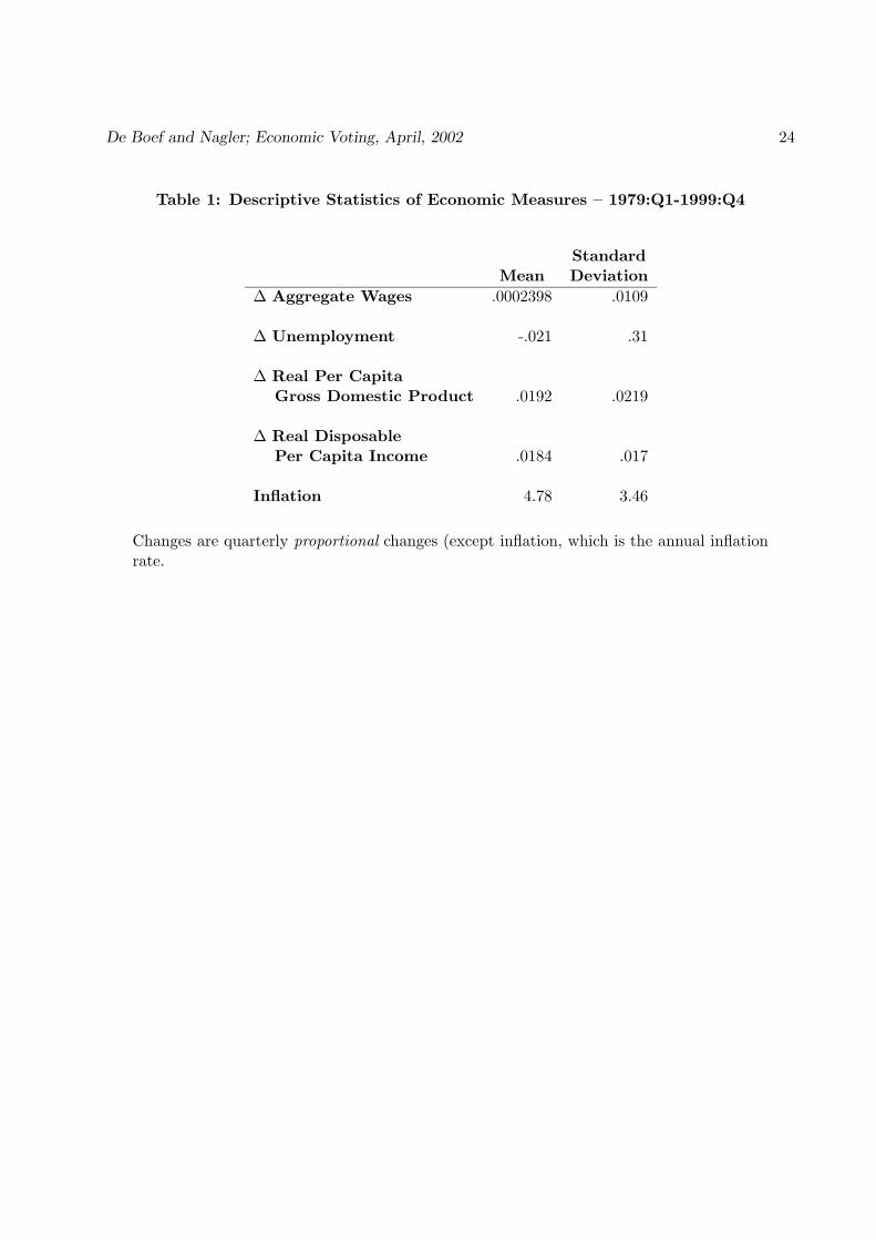
We present some descriptive data before proceeding. Table 1 gives the mean of each of
the aggregate economic indicators. Table 2 gives the correlation between the aggregate economic
indicators. The table confirms the common wisdom that wages were virtually flat over this period:
the mean of the change in aggregate wages is .0001. And wages are obviously measuring something
different than our other economic measures. Changes in aggregate wages are fairly highly correlated
with inflation (ρ = -.42); but are not correlated at all with changes in unemployment, and even
only weakly correlated with changes in real disposable per capita income (ρ = .16).
[Tables 1 and 2 Here]
6 Findings
6.1 Macro Level Results
We begin presenting our findings with the macro level time series analysis of presidential approval
broken down by income level. Table 3 reports estimates from the separately estimated models
of presidential approval by income group (events and administration/honeymoon effects are not
presented).
[Table 3 Here]
The estimates across the 3 income groups are quite similar. Lagged approval has the same
effect in all 3 income groups, suggesting that the autoregressive nature of approval is the same for
each group. Inflation has the predicted negative affect in each income group. The magnitude of
the effect is quite large, almost double that reported by MacKuen, Erikson, and Stimson (1992)
and is highest among the lowest income respondents. Changes in unemployment also behave as
predicted. Consistent with Hibbs (1982), changes in unemployment matter most for low income
adults. For middle and high income adults, the coefficient drops and the p−value increases.
Of particular interest for assessing our theory are the estimates of effects of RDI and GDP

De Boef and Nagler; Economic Voting, April, 2002 16
and the fit of the model across the 3 sets of results. Here the story is much less satisfying. The
model fits equally and relatively poorly for all income groups. The R2 and mean squared error
are unimpressive, but more disturbing for out theory, the effects of RDI and RGDP are are not
significant in any of these models. This finding is robust to changes in the lag specification of all
of the economic measures and to changes in the measures included in the model.
Next we consider the pooled times series models of approval by education cohorts. Table 4
reports results. Here our focus is the effect of group wages and the interactions terms. Neither are
significant in this specification. In fact, virtually none of the economic indicators are significant in
this specification.
[Table 4 Here]
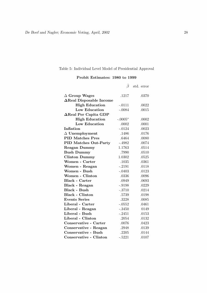
6.2 Individual Level Results
In the individual level model we observe not only the approval rating of respondents, but we
also observe individual attributes that we expect to influence the probability of approving of the
President. We include measures of respondents’: region (south/non-south), partisanship, gender,
race, ideology, and education in the model. Generally we expect Democrats to be more likely than
Republicans or independents to approve of Democratic presidents, women to be more likely than
men to approve of Democratic presidents, blacks to be more likely than non-blacks to approve of
Democratic presidents, and liberals to be more likely than conservatives to approve of Democratic
presidents. The anticipated effect of education is unclear in the model as we do not attempt to
control for income.
We anticipate each of these relationships to vary by regime – i.e., while we expect women to
be more likely than men to approve of Democratic presidents, we also expect that distinction to be
more pronounced for the Reagan presidency than the Bush presidency. Thus each of the individual
attributes enters separately for each regime, by being multiplied by a regime-dummy. The baseline
category is thus college educated, male, white, independent, nonsouthern, and moderate under
President Carter.
The individual level results are presented in Table 5. The effect of changes in mean group
De Boef and Nagler; Economic Voting, April, 2002 17
wages are positive and significant. Consider an individual born in the 1930s with a college degree
and who has a 50% chance of approving of the president. An increase of 2.5% in wages in a quarter
has a net effect of .12 percent. Four quarters of sustained increases in wages has an expected
net effect of almost 5%. This effect is quite substantial. The findings for group wages support our
theory. The wages of an individual’s group provide information about how the president’s economic
management can be expected to benefit that individual. In turn, this information predicts whether
or not a voter approves of the president.
While inflation has the expected effect in this model, the effect of unemployment changes is
positive after controlling for changes in wages. Further the interactions do not behave in a sensible
way and do not support our theory: Increases in real disposable income and growth have negative
effects in all cases.
[Table 5 Here]
The effects of the sociodemographic measures across administrations and the unique admin-
istration effects are, to the extent that we have specific expectations, all in the right direction. The
probabilities of approving of the presidents ranking from the lowest to highest average probability
are: Carter, Bush, Clinton, and Reagan. Members of the president’s party have probabilities of ap-
proving that are are .25 higher than nonpartisans while probabilities for members of the out party
are -.20 lower than nonpartisans and .45 lower than members of the president’s party. Women and
Blacks are more likely to approve of the Democratic presidents while Southerners are more likely to
approve of the Republican presidents. Liberals are more likely to approve of Democratic presidents
and conservatives of Republican presidents. The effects of education exhibit no general pattern.
The model predicts just over 72% of the cases correctly, (59.5% of respondents approve in the
sample), for a .3188 proportional reduction in error. The model without any economic measures
predicts 69% of the cases correctly so that economic measures buy us an additional 5% proportional
reduction in error.
De Boef and Nagler; Economic Voting, April, 2002 18
6.3 Subjective Evaluations of the Economy
While our focus in this paper has been on presidential approval, we offer a taste of how our theory
applies to economic evaluations. Again we ask what aspect of the economy is important for forming
evaluations, this time with respect to voters’ views of current business conditions and consumer
confidence. We have data from the “Survey of Consumer Attitudes and Behavior” (Economic
Behavior Project, Survey Research Center) on a quarterly basis for January 1978 through December
1993.17 This is extremely useful if we are to take seriously the micro-level models we have for
economic voting. If voters base their opinion of current business conditions on sector-specific
factors, rather than the national economy, this would further suggest that sector-specific conditions
are used in determining their vote. Thus we could attempt to predict the consumer confidence
level of different groups of workers based on: 1) the national economy, or 2) the economic-sector
relevant to the workers.
If consumer confidence of the demographic group is predicted by Y ∗sj , the actual performance
of the economic reference group, then we can infer at a minimum that the group members know
the performance of their economic reference group. The methodology employed here is identical
to the methodology used to estimate presidential approval: we are simply substituting economic
perceptions for presidential approval. However, there is now no reason to worry about ‘leakage’
from one presidential administration to the next.
Since so much of the literature showing that the economy has a large impact on elections
really shows that economic perceptions have a large impact on elections, it is extremely important to
determine how people form their economic evaluations. We attempt to model economic evaluations
exactly as we model approval. If wages act as we expect on presidential approval, the mechanism
could be by acting on respondents’ perceptions of the economy.
We utilize two different measures of respondents’ perceptions of the economy: both their
personal retrospective economic evaluations, and their national retrospective evaluations (their
evaluations of business conditions). We see in Table 6 that while the measures of the economy we
use to predict presidential approval predict retrospective business evaluations, they do not predict
personal evaluations.

De Boef and Nagler; Economic Voting, April, 2002 19
[Table 6 Here]
7 Conclusion and Future Research
We have described a new theory of economic voting that assumes that voters behave in a self-
interested manner, and allows them to combine an evaluation of the incumbents’ competence in
managing the economy with an evaluation of the incumbents’ distributional type. This offers an
important advance over theories which seek to treat voters as concerned with economic growth at
the aggregate level, yet indifferent as to whom the growth benefits.
We have not yet presented strong empirical evidence to support our hypotheses. We have
shown that voters pay attention to their peers as evidenced by the role of group wages in the
individual level model and the model of evaluations of the economy. The effects of aggregate
growth in the model are confusing, but are confusing for existing theories of economic voting as
well as our theory.
We expect that our empirical evidence will be stronger when we use data on respondents that
focuses on respondents’ occupation. This is a more directly economically relevant variable than is
education.
De Boef and Nagler; Economic Voting, April, 2002 20
Notes
1. The major exception is Hibbs (1982).
2. We note that it is not true that an altruistic voter would try to maximize the value of Yt. If onemakes the assumption of diminishing marginal return to income, then maximizing Yt is notthe altruistic choice.
3. The national economic measures may also enter in directly, without the interaction.
4. The low income category designates respondents whose income fell at or below the povertyline; medium income category respondents gave incomes around the national mean income;the high income category includes respondents giving the highest income brackets given byGallup.
5. Both CBS/NYT and Gallup survey Americans regularly asking: “In general, do you approve ofthe way (the incumbent) is handling the job of president?” We aggregated answers to thisquestion over quarters using Stimson’s ((1991)) algorithm to aggregate survey data acrosspolling organizations. The algorithm builds dimensional ”factor scores” for each surveyhouse and uses them to estimate a single (latent)time series of presidential approval for eachof our 16 groups. The algorithm thus allows us to use information from both surveys. Thisis particularly important given that Gallup adds large numbers of cases to the quarterlyobservations, but is not available at the necessary level of disaggregation for the full timeperiod. In contrast, CBS/NYT survey data is available over the full period of analysis, butwith much smaller samples. See Stimson, Public Opinion in America: Moods, Cycles, and
Swings, Westview Press: 1991, particularly Appendix 1.
6. Average sample sizes for each quarter and each education-cohort are as follows: adults without ahigh school degree (from oldest to youngest cohort): 541, 600, 276, 222; high school graduates:390, 616, 289, 269; adults with some college, trade, or business school: 336, 758, 491, 512;and adults with a college degree or more: 343, 946, 707, 552.
7. Data on Disposable Personal Income Per Capita, is from The US Department of Commerce,BEA (http://www. bea.doc.gov/bea/dn/nipaweb/AllTables.asp), table 2.1: Personal In-come and its Disposition. Real Gross Domestic Product is also from The U.S. Departmentof Commerce, BEA (http://www.stls.frb.org/fred/data/gdp/gdpc1). Both are presented in1996 chained dollars and are seasonally adjusted.
8. In an effort to clarify this finding, we replicated Beck’s ((1991)) standard model of presidentialapproval, using his data, for a period close to the one we are analyzing: 1979-1999. Inparticular, we estimated presidential approval as a function of lagged inflation rates, changesin unemployment, lagged presidential approval, a series of administration effects (allowingfor mean differences and honeymoons), and an events series. We were able to replicate Beck’sresults for the full time period covered by his analysis, 1953-88, a period over which inflationand unemployment both influenced presidential approval. However, upon re-estimating thismodel from 1979-1988, again using Beck’s data, inflation did not significantly affect approval.
9. Hibbs (1982) argues that these have different distributional effects as well, but we assume thattheir effects are homogenous across voters.
De Boef and Nagler; Economic Voting, April, 2002 21
10. The relationship is not likely to be as strong as for education as it is for workers within the sameoccupation. Workers in the same occupation are more likely to be substitutes for one anotherthen are workers with the same level of education. Education is one measure of human capital.But the level of human capital is going to determine which of many occupations a worker iscapable of having. Contingent on level of education, the choice of occupation will still havea large impact on the wage.
11. Using median wage has some theoretical advantages over mean wage: it removes the impactof outliers, and removes some topcoding problems with the data. In future work we willbe computing median wage rather than mean wage. However, we expect them to be highlycorrelated over time.
12. The Outgoing Rotation files are not available prior to 1979.
13. This may be a problem: we are not necessarily correctly handling life-cycle effects. Over thisperiod the wages of this group will most likely decline just because they are on the wrong sideof the life-cycle curve. But we do not want to suggest that they will punish the incumbentfor this.
14. See also Figure 2 for a look at mean income by income quintiles.
15. We include a minimal series of events in our models to pick up the effects of crisis and “rally”events. These are based on MacKuen, Erikson, and Stimson (1992) include: the Iranianhostage crisis (1979:4=2, 1980:1=1, 1980:2=-1); the assassination attempt on President Rea-gan (1981:1=+1); the invasion of Granada (1983:4=+1); the Iran-Contra scandal (1986:4=-1); and the Gulf War (1990:4=1, 1991:1=2).
16. This should not actually change the estimates we obtain: we are simply choosing not to try andestimate the form of approval for the first four quarters.
17. This data is available for more recent periods, however we have not finished coding it to getmeasures corresponding to our education-cohorts.

De Boef and Nagler; Economic Voting, April, 2002 22
References
Alesina, Alberto, Nouriel Roubini & Gerald D. Cohen. 1997. Political Cycles and the Macroeconomy.Cambridge: Massachussetts Institute of Technology Press.
Beck, Nathaniel. 1991. “Comparing Dynamic Specifications: The Case of Presidential Approval.”Political Analysis 999:51–87.
Hibbs, Douglas A. 1982. “The Dynamics of Political Support for American Presidents AmongOccupational and Partisan Groups.” American Journal of Political Science 26:312–332.
Hibbs, Douglas A. 1987. The American Political Economy: Macroeconomics and Electoral Politics.Cambridge, Mass: Harvard University Press.
Key, V.O. 1966. The Responsible Electorate: Rationality in Presidential Voting 1936-1960. Cam-bridge, Mass: Harvard University Press.
Kiewiet, D. Roderick. 1983. Macroeconomics & Micropolitics : the Electoral Effects of Economic
Issues. Chicago, Illinois: University of Chicago Press.
Kinder, Donald R. & D. Roderick Kiewiet. 1979. “Economic Discontent and Political Behavior: TheRole of Personal Grievances and Collective Economic Judgements in Congressional Voting.”American Journal of Political Science 23:495–527.
Kinder, Donald R., Gordon S. Adams & Paul W. Gronke. 1989. “Economics and Politics in the1984 American Presidential Election.” American Journal of Political Science 33:491–515.
Kinder, Donald R., Steven J. Rosenstone & John Mark Hansen. 1983. “Group Economic WellBeing and Political Choice: Pilot Study Report to the 1984 NES Planning Committee andNES Board.” ANES Pilot Report 1983:1–34.
Kramer, Gerry. 1971. “Short-Term Fluctuations in U.S. Voting Behavior, 1896-1964.” AmericanPolitical Science Review 65:131–143.
MacKuen, Michael B., Robert S. Erikson & James A. Stimson. 1989. “Macropartisanship.” Amer-ican Political Science Review 83:1125–1142.
MacKuen, Michael B., Robert S. Erikson & James A. Stimson. 1992. “Peasants or Bankers? TheAmerican Electorate and the U.S. Economy.” American Political Science Review 86:597–611.
Mishel, Lawrence, Jared Bernstein & John Schmitt. 1999. The State of Working American 1998-
1999. Ithaca, New York: ILS Press.
Mutz, Diana C. & Jeffery J. Mondak. 1997. “Dimensions of Sociotropic Behavior: Group-BasedJudgements of Fairness and Well-Being.” American Journal of Political Science 41:284–308.
Ragsdale, Lyn. 1998. Vital Statistics on the Presidency, Revised Edition. Washington, DC: Con-gresional Quarterly Press.
Rawls, John. 1971. A Theory of Justice. Cambridge: Harvard University Press.
Stimson, James A. 1991. Public Opinion in America: Moods, Cycles, and Swings. Boulder, CO:Westview Press.
De Boef and Nagler; Economic Voting, April, 2002 23
Tufte, Edward R. 1978. Political Control of the Economy. Princeton, N.J.: Princeton UniversityPress.
De Boef and Nagler; Economic Voting, April, 2002 24
Table 1: Descriptive Statistics of Economic Measures – 1979:Q1-1999:Q4
StandardMean Deviation
∆ Aggregate Wages .0002398 .0109
∆ Unemployment -.021 .31
∆ Real Per CapitaGross Domestic Product .0192 .0219
∆ Real DisposablePer Capita Income .0184 .017
Inflation 4.78 3.46
Changes are quarterly proportional changes (except inflation, which is the annual inflationrate.

De Boef and Nagler; Economic Voting, April, 2002 25
Table 2: Corrlations Between Economic Measures – 1979:Q2 - 1999:Q4
∆ Aggregate ∆ Real Disp ∆ Real PerWages ∆ Unemp Per Cap Inc Cap GDP Inflation
∆ Aggregate Wages 1.00
∆ Unemployment -0.0038 1.00
∆ Real DisposablePer Capita Income 0.1554 -0.3748 1.00
∆ Real Per CapitaGross Domestic Product 0.1839 -0.6886 0.5499 1.00
Inflation -0.4177 0.0900 -0.2281 -0.1910 1.00

De Boef and Nagler; Economic Voting, April, 2002 26
Table 3: Models of (Gallup) Presidential Approval Time Series by Income Level
Time Period: 1965 - 1996
Low Income Middle Income High Income
Estimated Std Estimated Std Estimated StdCoefficient Error Coefficient Error Coefficient Error
Constant 14.47 3.93 13.22 3.55 12.82 3.73Approvalt−1 .771 .062 .765 .059 .745 .067∆ Unemploymentt -5.44 2.18 -3.07 2.28 -1.86 2.52Inflationt -.715 .273 -.581 .289 -.542 .316∆ RDI-PCt -.279 .175 -.089 .184 .114 .200∆ RGDP-PCt -.081 .210 -.001 .221 -.089 .243
R2 .7576 .7523 .7753RMSE 5.76 6.06 6.65N 108 108 108
Administration dummies were included in the regressions but are not reported.

De Boef and Nagler; Economic Voting, April, 2002 27
Table 4: Pooled Time Series Model of Presidential Approval
Time Period: 1979 - 1999Estimated StdCoefficient Error
Constant -0.0163 0.0442Approvalt−1 0.8415 0.0063LowEducation -0.0151 0.0064HighEducation 0.0024 0.0048∆Agg Wagest−1 .0027 0.6884
High Education 0.0950 0.3161Low Education 0.3307 0.3588
∆Real Disposable Income -.0035 .0025High Education 0.0001 0.0013Low Education -0.0005 0.0015
∆Real Per Capita GDP .0002 .0002High Education -0.0001 0.0001Low Education 0.0001 0.0001
Inflation 0.0036 0.0034∆Unemployment -0.0177 0.0276Events 0.0523 0.0149Reagan 0.0949 0.0363Bush 0.0750 0.0390Clinton 0.0877 0.0406Reagan Honeymoon 0.0289 0.0556Bush Honeymoon -0.0185 0.0501Clinton Honeymoon 0.0166 0.0491
ρ .016Number of Observations 1264R2 .77
De Boef and Nagler; Economic Voting, April, 2002 28
Table 5: Individual Level Model of Presidential Approval
Probit Estimates: 1980 to 1999
β̂ std. error
∆ Group Wages .1217 .0370∆Real Disposable Income
High Education -.0111 .0022Low Education -.0084 .0015
∆Real Per Capita GDPHigh Education -.0005∗ .0002Low Education .0002 .0001
Inflation -.0124 .0023∆ Unemployment .1486 .0176PID Matches Pres .6464 .0080PID Matches Out-Party -.4982 .0074Reagan Dummy 1.1763 .0514Bush Dummy .7990 .0510Clinton Dummy 1.0302 .0525Women - Carter .1035 .0361Women - Reagan -.2191 .0118Women - Bush -.0403 .0123Women - Clinton .0336 .0096Black - Carter .0949 .0693Black - Reagan -.9198 .0229Black - Bush -.3710 .0214Black - Clinton .5739 .0198Events Series .3228 .0085Liberal - Carter -.0552 .0461Liberal - Reagan -.3450 0149Liberal - Bush -.2451 .0153Liberal - Clinton .2054 .0132Conservative - Carter .0076 .0423Conservative - Reagan .2948 .0139Conservative - Bush .2205 .0144Conservative - Clinton -.5221 .0107
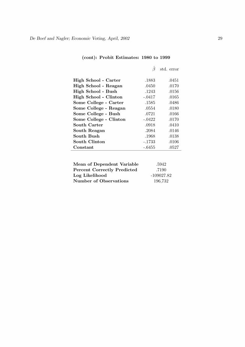
De Boef and Nagler; Economic Voting, April, 2002 29
(cont): Probit Estimates: 1980 to 1999
β̂ std. error
High School - Carter .1883 .0451High School - Reagan .0450 .0170High School - Bush .1243 .0156High School - Clinton -.0417 .0165Some College - Carter .1585 .0486Some College - Reagan .0554 .0180Some College - Bush .0721 .0166Some College - Clinton -.0422 .0170South Carter .0918 .0410South Reagan .2084 .0146South Bush .1968 .0138South Clinton -.1733 .0106Constant -.6455 .0527
Mean of Dependent Variable .5942Percent Correctly Predicted .7190Log Likelihood -109027.82Number of Observations 196,732

De Boef and Nagler; Economic Voting, April, 2002 30
Table 6: Model of Economic Perceptions : 1980 - 1996
Business Retrospective Personal RetrospectiveEconomic Evaluations Economic Evaluations
Estimated Std Estimated StdCoefficient Error Coefficient Error
Constant 20.9∗ 6.33 2.70 2.66Approvalt−1 0.73∗ 0.04 0.94∗ 0.02∆Group Wagest−1 40.85∗∗ 22.72 -2.07 13.58∆Group Wagest−2 59.56∗ 27.24 -12.93 16.19∆Group Wagest−3 13.77 27.37 9.61 16.19∆Group Wagest−4 -5.25 23.97 -13.2 14.66∆Agg Wagest−1 4.95 199.48 64.73 73.78∆Agg Wagest−2 -8.47 199.29 80.63 73.97∆Agg Wagest−3 -71.72 198.8 14.55 73.78∆Agg Wagest−4 -416.35∗ 189.42 -31.24 70.24∆Real Disposable
Personal Incomet−1 0.61 0.49 0.09 0.18∆Real Disposable
Pesonal Incomet−2 0.6 0.52 0.46∗ 0.19∆Real Disposable
Personal Incomet−3 1.12∗ 0.48 0.25 0.17∆Real Disposable
Personal Incomet−4 1.71∗ 0.53 0.32 0.19Inflationt−1 -2.99∗ 0.98 -0.3 0.36Inflationt−2 2.00∗∗ 1.07 0.44 0.39Inflationt−3 -0.53 1.04 0.03 0.38Inflationt−4 -0.25 0.95 -0.19 0.35∆Unemploymentt−1 -23.4∗ 6.35 -4.01∗∗ 2.27∆Unemploymentt−2 -0.16 8.27 1.44 3.01∆Unemploymentt−3 5.17 8.48 0.21 3.11∆Unemploymentt−4 21.01∗∗ 7.37 5.58∗ 2.73Events -2.98 3.93 0.15 1.44
N 880 880R2 .83 .87
Dependent Variables come from the Survey of Consumer Attitudes and Behavior. The unitof analysis is the education-cohort.

De
Boef
and
Nagler;
Eco
nom
icVotin
g,A
pril,
2002
31
1996
Dol
lars
time1980q1 1985q1 1990q1 1995q1 2000q1
4000
4500
5000
5500
6000
Real Percapita Disposable Income
Dol
lars
time1972q3 1985q1 1997q3 2010q1
20
25
30
35
Real per capita GDP
Dol
lars
time1980q1 1985q1 1990q1 1995q1 2000q1
0
5
10
15
20
Aggregate Real Wages 1979-1999
Dol
lars
time1980q1 1985q1 1990q1 1995q1 2000q1
0
5
10
15
20
Real Wages by Education and Decade of Birth 1979-1999
No high school diploma, born in the 1940s
College degree - plus, born in the 1940s
Figure1:Measu
resofEconomicPerform
ance

De Boef and Nagler; Economic Voting, April, 2002 32
Figure 2: Annual Mean Household Income by Income Quintile
Dol
lars
qdate1960q1 1972q3 1985q1 1997q3
0
20000
40000
60000
80000 First
Second
Third
Fourth
Fifth