Ginsbach2020_Redacted.pdf - Edinburgh Research Archive
190
This thesis has been submitted in fulfilment of the requirements for a postgraduate degree (e.g. PhD, MPhil, DClinPsychol) at the University of Edinburgh. Please note the following terms and conditions of use: This work is protected by copyright and other intellectual property rights, which are retained by the thesis author, unless otherwise stated. A copy can be downloaded for personal non-commercial research or study, without prior permission or charge. This thesis cannot be reproduced or quoted extensively from without first obtaining permission in writing from the author. The content must not be changed in any way or sold commercially in any format or medium without the formal permission of the author. When referring to this work, full bibliographic details including the author, title, awarding institution and date of the thesis must be given.
-
Upload
khangminh22 -
Category
Documents
-
view
4 -
download
0
Transcript of Ginsbach2020_Redacted.pdf - Edinburgh Research Archive

This thesis has been submitted in fulfilment of the requirements for a postgraduate degree
(e.g. PhD, MPhil, DClinPsychol) at the University of Edinburgh. Please note the following
terms and conditions of use:
This work is protected by copyright and other intellectual property rights, which are
retained by the thesis author, unless otherwise stated.
A copy can be downloaded for personal non-commercial research or study, without
prior permission or charge.
This thesis cannot be reproduced or quoted extensively from without first obtaining
permission in writing from the author.
The content must not be changed in any way or sold commercially in any format or
medium without the formal permission of the author.
When referring to this work, full bibliographic details including the author, title,
awarding institution and date of the thesis must be given.

From Constraint Programming
to Heterogeneous Parallelism
Philip GinsbachT
HE
U N I V E RS
IT
Y
OF
ED I N B U
RG
H
Doctor of Philosophy
Institute of Computing Systems Architecture
School of Informatics
University of Edinburgh
2020


Abstract
The scaling limitations of multi-core processor development have led to a diversification of
the processor cores used within individual computers. Heterogeneous computing has become
widespread, involving the cooperation of several structurally different processor cores. Central
processor (CPU) cores are most frequently complemented with graphics processors (GPUs),
which despite their name are suitable for many highly parallel computations besides computer
graphics. Furthermore, deep learning accelerators are rapidly gaining relevance.
Many applications could profit from heterogeneous computing but are held back by the
surrounding software ecosystems. Heterogeneous systems are a challenge for compilers in
particular, which usually target only the increasingly marginalised homogeneous CPU cores.
Therefore, heterogeneous acceleration is primarily accessible via libraries and domain-specific
languages (DSLs), requiring application rewrites and resulting in vendor lock-in.
This thesis presents a compiler method for automatically targeting heterogeneous hardware
from existing sequential C/C++ source code. A new constraint programming method enables
the declarative specification and automatic detection of computational idioms within compiler
intermediate representation code. Examples of computational idioms are stencils, reductions,
and linear algebra. Computational idioms denote algorithmic structures that commonly occur
in performance-critical loops. Consequently, well-designed accelerator DSLs and libraries
support computational idioms with their programming models and function interfaces. The
detection of computational idioms in their middle end enables compilers to incorporate DSL
and library backends for code generation. These backends leverage domain knowledge for the
efficient utilisation of heterogeneous hardware.
The constraint programming methodology is first derived on an abstract model and then
implemented as an extension to LLVM. Two constraint programming languages are designed
to target this implementation: the Compiler Analysis Description Language (CAnDL), and
the extended Idiom Detection Language (IDL). These languages are evaluated on a range of
different compiler problems, culminating in a complete heterogeneous acceleration pipeline
integrated with the Clang C/C++ compiler. This pipeline was evaluated on the established
benchmark collections NPB and Parboil. The approach was applicable to 10 of the benchmark
programs, resulting in significant speedups from 1.26× on “histo” to 275× on “sgemm” when
starting from sequential baseline versions.
In summary, this thesis shows that the automatic recognition of computational idioms
during compilation enables the heterogeneous acceleration of sequential C/C++ programs.
Moreover, the declarative specification of computational idioms is derived in novel declarative
programming languages, and it is demonstrated that constraint programming on Single Static
Assignment intermediate code is a suitable method for their automatic detection.
iii

iv

Lay Summary
New computer processors used to improve over the speed of previous versions mostly
because the transistors got smaller and more efficient. In recent years, the engineers have
been unable to continue this process. Because the speed of processors is stagnating, companies
try to improve other metrics. Specialised processors are now widespread, which cooperate with
the central processor and complement its abilities. However, many software programs were not
designed for this and ignore the specific features.
This thesis presents an approach to make existing programs use such specialised hardware
efficiently. This approach was implemented in a software prototype. The prototype detects
particular mathematical methods in other programs. Other researchers have already found the
best ways to compute these methods on new hardware, and stored them in “libraries”. By
detecting that programs rely on the methods, the prototype can make the program use these
efficient “libraries” instead. However, recognising the methods is hard. This thesis introduces
new specification languages to express them. With the resulting precise formulations, it is
possible to identify the mathematical methods automatically with algorithms.
The prototype software was evaluated by using it on standard test programs. Some of these
programs are from NASA and imitate the calculations on their supercomputers. The prototype
understood the essential parts of many programs. This allowed executing them on specialised
processors and made five of them more than ten times faster.
v
Acknowledgements
First of all, I want to thank my adviser, Michael O’Boyle, for his guidance and sound advice
throughout my PhD studies. I would also like to thank my other advisers at the university,
Björn Franke and Adam Lopez, and my mentors at ARM, Chris Ryder and Pablo Barrio, whom
I could rely on for additional insights and suggestions.
My time as a PhD student would not have been half as enjoyable without the PPar cohort.
Amna, Caoimhín, Dan, Daniel, Floyd, Jakub, Paul, Rajkarn, Reese, Vanya, Victor, you made
Edinburgh a great place to be for the last few years! Paul, Vanya, Reese, Dan, I will miss our
lunches in particular. Caoimhín and Braedy, thank you for helping me polish this thesis. Thank
you also to Reese, Lewis, and Vanya for some additional proofreading.
Finally, I am grateful to my parents, who have always supported and encouraged me.
vi

Declaration
Ginsbach et al. [1] Ginsbach and O’Boyle [2] Ginsbach et al. [3]
vii

Table of Contents
List of Symbols and Notation 1
1 Introduction 3
1.1 The Emergence of Heterogeneous Computing . . . . . . . . . . . . . . . . . . 3
1.1.1 Via Multi-Processing to Heterogeneity . . . . . . . . . . . . . . . . . . 3
1.2 The Diminished Role of Traditional Compilers . . . . . . . . . . . . . . . . . 4
1.2.1 Libraries and Domain-Specific Languages . . . . . . . . . . . . . . . . 4
1.2.2 The Consequences of the Decline of Compilers . . . . . . . . . . . . . 5
1.3 Host Compilers and Kernel Compilers . . . . . . . . . . . . . . . . . . . . . . 6
1.3.1 The Spectrum of Specialisation . . . . . . . . . . . . . . . . . . . . . 7
1.4 Moving on the Spectrum of Specialisation . . . . . . . . . . . . . . . . . . . . 8
1.4.1 Contributions of this Thesis . . . . . . . . . . . . . . . . . . . . . . . 8
1.5 Structure of this Thesis . . . . . . . . . . . . . . . . . . . . . . . . . . . . . . 9
1.6 Summary . . . . . . . . . . . . . . . . . . . . . . . . . . . . . . . . . . . . . 10
2 Constraint Programming on Static Single Assignment Code 11
2.1 Background . . . . . . . . . . . . . . . . . . . . . . . . . . . . . . . . . . . . 12
2.1.1 Static Single Assignment Form . . . . . . . . . . . . . . . . . . . . . 13
2.1.2 SSA Emerges During Compilation . . . . . . . . . . . . . . . . . . . . 14
2.2 Deriving the SSA Model . . . . . . . . . . . . . . . . . . . . . . . . . . . . . 16
2.2.1 Data Flow and Control Flow . . . . . . . . . . . . . . . . . . . . . . . 16
2.2.2 Identifying Remaining Structure . . . . . . . . . . . . . . . . . . . . . 18
2.2.3 Putting the SSA Model Together . . . . . . . . . . . . . . . . . . . . . 20
2.2.4 Additional Notation . . . . . . . . . . . . . . . . . . . . . . . . . . . 20
2.2.5 The LLVM Compiler Framework . . . . . . . . . . . . . . . . . . . . 22
2.2.6 LLVM IR Example . . . . . . . . . . . . . . . . . . . . . . . . . . . . 22
2.3 Constraint Programming on the SSA Model . . . . . . . . . . . . . . . . . . . 24
2.3.1 SSA Constraint Problem Example . . . . . . . . . . . . . . . . . . . . 26
2.4 Solving SSA Constraint Problems . . . . . . . . . . . . . . . . . . . . . . . . 28
ix
2.4.1 The Structure of SSA Constraint Problems . . . . . . . . . . . . . . . 28
2.4.2 Backtracking Example . . . . . . . . . . . . . . . . . . . . . . . . . . 32
2.4.3 Implementation, Data Structures and Complexity . . . . . . . . . . . . 34
2.4.4 Additional SSA Constraint Problems . . . . . . . . . . . . . . . . . . 38
2.4.5 Satifiability Modulo Theory . . . . . . . . . . . . . . . . . . . . . . . 40
2.5 Summary . . . . . . . . . . . . . . . . . . . . . . . . . . . . . . . . . . . . . 40
3 Related Work 41
3.1 Constraint Programming and Specification Languages . . . . . . . . . . . . . . 41
3.1.1 Constraint Programming for Program Analysis . . . . . . . . . . . . . 42
3.1.2 Declarative Programming Languages for Program Analysis . . . . . . 44
3.2 Compiler Analysis and Auto-Parallelisation . . . . . . . . . . . . . . . . . . . 45
3.2.1 Compilation with the Polyhedral Model . . . . . . . . . . . . . . . . . 46
3.2.2 Reduction Parallelism . . . . . . . . . . . . . . . . . . . . . . . . . . 48
3.2.3 Dynamic Analysis Approaches . . . . . . . . . . . . . . . . . . . . . . 49
3.3 Heterogeneous Computing . . . . . . . . . . . . . . . . . . . . . . . . . . . . 50
3.3.1 Libraries . . . . . . . . . . . . . . . . . . . . . . . . . . . . . . . . . 50
3.3.2 Domain-Specific Languages . . . . . . . . . . . . . . . . . . . . . . . 51
3.4 Computational Idioms . . . . . . . . . . . . . . . . . . . . . . . . . . . . . . 53
3.4.1 Higher-Order Functions . . . . . . . . . . . . . . . . . . . . . . . . . 53
3.4.2 Berkeley Parallel Dwarfs . . . . . . . . . . . . . . . . . . . . . . . . . 54
3.4.3 Algorithmic Skeletons . . . . . . . . . . . . . . . . . . . . . . . . . . 54
4 The Compiler Analysis Description Language 55
4.1 Introduction . . . . . . . . . . . . . . . . . . . . . . . . . . . . . . . . . . . . 56
4.2 Motivating Example . . . . . . . . . . . . . . . . . . . . . . . . . . . . . . . 57
4.3 Language Specification . . . . . . . . . . . . . . . . . . . . . . . . . . . . . . 60
4.3.1 Top-Level Structure of CAnDL Programs . . . . . . . . . . . . . . . . 60
4.3.2 Atomic Constraints . . . . . . . . . . . . . . . . . . . . . . . . . . . . 61
4.3.3 Range Constraints . . . . . . . . . . . . . . . . . . . . . . . . . . . . 63
4.3.4 Modularity . . . . . . . . . . . . . . . . . . . . . . . . . . . . . . . . 64
4.3.5 Expressing Larger Structures . . . . . . . . . . . . . . . . . . . . . . . 66
4.4 Implementation . . . . . . . . . . . . . . . . . . . . . . . . . . . . . . . . . . 68
4.4.1 Normalisation of LLVM IR . . . . . . . . . . . . . . . . . . . . . . . 68
4.4.2 The CAnDL Compiler . . . . . . . . . . . . . . . . . . . . . . . . . . 71
4.4.3 Developer Tools . . . . . . . . . . . . . . . . . . . . . . . . . . . . . 73
4.5 Case Studies . . . . . . . . . . . . . . . . . . . . . . . . . . . . . . . . . . . . 74
4.5.1 Case Study 1: Simple Optimisations . . . . . . . . . . . . . . . . . . . 74
x

4.5.2 Case Study 2: Graphics Shader Optimisations . . . . . . . . . . . . . . 76
4.5.3 Case Study 3: Detection of Polyhedral SCoPs . . . . . . . . . . . . . . 78
4.6 Conclusions . . . . . . . . . . . . . . . . . . . . . . . . . . . . . . . . . . . . 82
5 Automatic Parallelisation of Reductions and Histograms 83
5.1 Introduction . . . . . . . . . . . . . . . . . . . . . . . . . . . . . . . . . . . . 84
5.2 Motivation . . . . . . . . . . . . . . . . . . . . . . . . . . . . . . . . . . . . . 85
5.3 Recognising CReHCs . . . . . . . . . . . . . . . . . . . . . . . . . . . . . . . 88
5.3.1 Constraint-Based Formulation . . . . . . . . . . . . . . . . . . . . . . 88
5.3.2 The Idiom Detection Language . . . . . . . . . . . . . . . . . . . . . 91
5.3.3 Specification of CReHCs in IDL . . . . . . . . . . . . . . . . . . . . . 96
5.4 Code Generation for CReHCs . . . . . . . . . . . . . . . . . . . . . . . . . . 96
5.5 Experimental Setup . . . . . . . . . . . . . . . . . . . . . . . . . . . . . . . . 98
5.5.1 Benchmarks and Platform . . . . . . . . . . . . . . . . . . . . . . . . 98
5.5.2 Competing Approaches . . . . . . . . . . . . . . . . . . . . . . . . . . 98
5.6 Results . . . . . . . . . . . . . . . . . . . . . . . . . . . . . . . . . . . . . . . 100
5.6.1 Discovery . . . . . . . . . . . . . . . . . . . . . . . . . . . . . . . . . 100
5.6.2 Runtime Coverage . . . . . . . . . . . . . . . . . . . . . . . . . . . . 104
5.6.3 Performance . . . . . . . . . . . . . . . . . . . . . . . . . . . . . . . 104
5.7 Conclusions . . . . . . . . . . . . . . . . . . . . . . . . . . . . . . . . . . . . 106
6 Heterogeneous Acceleration via Computational Idioms 107
6.1 Introduction . . . . . . . . . . . . . . . . . . . . . . . . . . . . . . . . . . . . 108
6.2 Overview . . . . . . . . . . . . . . . . . . . . . . . . . . . . . . . . . . . . . 110
6.2.1 Compiler Flow . . . . . . . . . . . . . . . . . . . . . . . . . . . . . . 110
6.2.2 Accelerating Sparse Linear Algebra . . . . . . . . . . . . . . . . . . . 112
6.3 Specification of Idioms in IDL . . . . . . . . . . . . . . . . . . . . . . . . . . 114
6.3.1 Sparse Linear Algebra . . . . . . . . . . . . . . . . . . . . . . . . . . 114
6.3.2 Dense Linear Algebra . . . . . . . . . . . . . . . . . . . . . . . . . . 116
6.3.3 Stencils . . . . . . . . . . . . . . . . . . . . . . . . . . . . . . . . . . 118
6.4 Comparison to Syntactic Matching . . . . . . . . . . . . . . . . . . . . . . . . 118
6.5 Targeting Heterogeneous Backends . . . . . . . . . . . . . . . . . . . . . . . . 120
6.5.1 Domain-Specific Libraries . . . . . . . . . . . . . . . . . . . . . . . . 120
6.5.2 Domain-Specific Code Generators . . . . . . . . . . . . . . . . . . . . 120
6.6 Translating Computational Idioms . . . . . . . . . . . . . . . . . . . . . . . . 121
6.6.1 Domain-Specific Libraries . . . . . . . . . . . . . . . . . . . . . . . . 121
6.6.2 Domain-Specific Code Generators . . . . . . . . . . . . . . . . . . . . 121
6.6.3 Pointer Aliasing . . . . . . . . . . . . . . . . . . . . . . . . . . . . . 122
xi

6.7 Experimental Setup . . . . . . . . . . . . . . . . . . . . . . . . . . . . . . . . 123
6.8 Results . . . . . . . . . . . . . . . . . . . . . . . . . . . . . . . . . . . . . . . 124
6.8.1 Idiom Detection . . . . . . . . . . . . . . . . . . . . . . . . . . . . . 124
6.8.2 Runtime Coverage . . . . . . . . . . . . . . . . . . . . . . . . . . . . 124
6.8.3 Performance Results . . . . . . . . . . . . . . . . . . . . . . . . . . . 126
6.9 Conclusions . . . . . . . . . . . . . . . . . . . . . . . . . . . . . . . . . . . . 129
7 Conclusions 131
7.1 Contributions . . . . . . . . . . . . . . . . . . . . . . . . . . . . . . . . . . . 132
7.2 Critical Analysis . . . . . . . . . . . . . . . . . . . . . . . . . . . . . . . . . 133
7.3 Future Work . . . . . . . . . . . . . . . . . . . . . . . . . . . . . . . . . . . . 134
7.4 Summary . . . . . . . . . . . . . . . . . . . . . . . . . . . . . . . . . . . . . 136
Bibliography 137
A Full Grammar of CAnDL 159
B Polyhedral Code Sections in CAnDL 163
C Full Grammar of IDL 169
D Complex Reductions and Histograms in IDL 173
xii

List of Symbols and Notation
N The set of all positive integers, N= {1,2,3, . . .}R The set of all real numbers
/0 The empty set, containing no elements
s ∈ S Element-of relationship, s is in the set S
A⊂ B Subset-relationship, every element of A is also in B
|S| Cardinality of S, the number of elements in the finite set S
{x | P(x)} Set-builder notation, the set of all x that satisfy P(x)
A×BCartesian product of sets, A×B = {(a,b) | a ∈ A and b ∈ B},corresponds to pair<A,B> in C++
AnSet of n-tuples in A, short for An = A×·· ·×A,
corresponds to array<A,n> in C++
ABGeneralisation of An, x ∈ AB has a value xb ∈ A for each b ∈ B,
corresponds to map<B,A> in C++
P(S) Power set of S, the set of all subsets of S
f : A→ B Function f that maps elements of A onto elements of B
f : A ↪→ B Injective function x 6= y =⇒ f (x) 6= f (y), generalises A⊂ B
x 7→ y The value x gets mapped onto the value y
P =⇒ Q Logical consequence, “P implies Q”
P ⇐⇒ Q Logical equality, “P if and only if Q”
P ∧ Q Logical conjunction, “P and Q”
P ∨ Q Logical disjunction, “P or Q”
¬P Logical negation, “not P”
1

Chapter 1
Introduction
1.1 The Emergence of Heterogeneous Computing
For several decades, from the 1970s until the early 2000s, advances in processor development
followed Moore’s Law [4] and Dennard Scaling [5]. The density of integrated circuits doubled
every two years, and this allowed increased clock frequencies while maintaining steady power
consumption. These conditions enabled continual processor improvements primarily via rising
clock frequencies and microarchitectural refinements, enabling ever faster computations.
The physics-driven nature [6] of these advances in hardware has had important implications
for software development. Not only did the performance of computers improve exponentially,
but these performance gains were in the form of direct speedups, available to all the already
existing programs. The primary interfaces between software and hardware - the instruction
set architectures of processors - evolved gradually and with few paradigmatic changes [7].
This is best exemplified by the pervasive x86 instruction set architecture, which still retains
backward compatibility with its initial version from 1978, and dominates desktop processors
to this day. Therefore, software developers and users could rely on ever-increasing performance
from hardware progress alone, without any intervention.
1.1.1 Via Multi-Processing to Heterogeneity
This continual progress started breaking down around 2005 with the apparent end of Dennard
Scaling [8]. While the shrinking of transistors continued, this no longer enabled proportionally
increased clock frequencies with the same power budget. Instead, processor designers started
using the increasing transistor budget for additional processor cores. This shift toward multi-
processing has left a deep mark on software development. New programming paradigms and
languages, annotation systems, programming interfaces, libraries and compiler techniques are
still being developed to address the challenges of parallel computing.
3

4 Chapter 1. Introduction
In recent years, transistor scaling has slowed significantly. In response to the breakdown of
both Dennard Scaling and Moore’s Law, the hardware industry has turned toward architectural
innovation [9]. In particular, there is a trend toward specialised processors that work in tandem
as heterogeneous systems. Specialised processor cores outperform general-purpose cores on
specific tasks. Furthermore, as heat dissipation has become a major challenge, simultaneously
powering all transistors is often unviable. This means that different processor cores have to
be masked out dynamically at runtime (“dark silicon”) [8]. This situation favours specialised
cores, which can improve the overall system performance even if they are disabled most of the
time and only used for the specific tasks at which they excel. By contrast, disabling a subset of
a homogeneous multi-core system renders some of its cores redundant.
1.2 The Diminished Role of Traditional Compilers
Heterogeneous computing can help overcome the scaling limitations of homogeneous, general-
purpose processors. However, it also poses a challenge to the associated software ecosystems.
Existing software does not automatically benefit from entirely new accelerator designs in the
way that it profited from the continuous improvements of established architectures. Where
programs previously performed better on each succeeding hardware generation, heterogeneous
accelerators arrive with novel and incompatible interfaces. This puts into question many of
the achievements in portability and longevity of programs that are taken for granted in modern
computing [10].
In particular, this new hardware landscape greatly diminishes the scope of responsibilities
and impact that traditional compilers for languages such as C, C++ and Fortran can have.
Such compilers used to be responsible for orchestrating program execution on the entirety of
available computing resources. They are now generally limited to only targeting the relatively
small homogeneous fraction of processor cores directly.
1.2.1 Libraries and Domain-Specific Languages
In order to reach peak performance on rapidly evolving and highly parallel hardware, new
programming paradigms built around libraries and domain-specific languages have emerged.
They succeed in utilising heterogeneous hardware in situations where traditional compilers fail.
Two examples show the diversity of these approaches. Firstly, Ragan-Kelley et al. [11]
developed the domain-specific language Halide for image processing. The Halide toolchain is
able to generate fast code for heterogeneous platforms by focusing on a well-understood class
of computations, and by using a restrictive program representation. After tuning programs
for particular platforms, it outperforms hand-optimised code, demonstrating the advantage of
domain-specific compiler optimisation under circumstances of constrained semantics.

1.2. The Diminished Role of Traditional Compilers 5
Secondly, Basic Linear Algebra Subprograms (BLAS) [12], a specification of function
interfaces going back to the 1970s [13], remains the standard encapsulation for linear algebra
and has been implemented for most accelerators. These implementations are widely used and
offer unrivalled performance. Some versions are provided directly by hardware vendors to
support accelerators [14, 15, 16, 17, 18], while others originated as academic projects [19].
These competing implementations use a plethora of approaches to achieve as close to peak
performance as possible. These methods include manually written assembly code but also
highly advanced code generation techniques, custom program representations, and many more.
1.2.2 The Consequences of the Decline of Compilers
Domain-specific languages and library interfaces make the full performance of heterogeneous
systems accessible to programs. However, these success stories also leave significant problems
unaddressed. The adoption costs are high, requiring application rewrites for accelerators. This
coincides with often uncertain long-term prospects and minimal cross-platform portability.
Even in the case of the agreed-upon BLAS standard – arguably the best case scenario – adoption
of novel implementations is non-trivial in practice, due to the frequently encountered interface
extensions for managing device handlers and memory synchronisation. For academic-backed
domain-specific languages like Halide, on the other hand, complete rewrites are required in
entirely novel software ecosystems, with an unclear future of support.
On homogeneous systems, programmers could rely on compilers for existing programming
languages to evolve in lockstep with processor development. For example, even decades-old
C++ source code compiles into efficient programs for the newest generation of x86 processors.
Libraries and domain-specific languages are useful on homogeneous systems for achieving
absolute maximum performance, but only in the context of heterogeneous computing do they
become essential. Therefore, the pervasive requirement for domain-specific languages and
libraries only arises because compilers are unable to map programs onto specialised cores.
Instead, compilers are increasingly downgraded to merely coordinating the execution of core
workloads as separate and opaque programs.
It may appear apparent that, for example, a C++ or Java compiler cannot be provided for a
typical graphics processor. After all, most graphics processors have hardware limitations that
prevent them from implementing the entire language standard. Indeed, many accelerators are
further from Turing complete [20]. Nevertheless, this should not prevent a partial compiler.
Such a partial compiler would compile fitting program parts for accelerators and utilise a
fallback system for the remainder of the code. After all, that is precisely the result achieved
with libraries and domain-specific languages, and likely the desirable outcome. Despite the
apparent convenience of such an approach, the next section gives reasons why such a scheme
has not become widespread so far.

6 Chapter 1. Introduction
1.3 Host Compilers and Kernel Compilers
While mainstream compilers for languages such as C, C++, Fortran or Java generally fail to
exploit the full performance of heterogeneous systems, a specific class of compilers already
plays an essential role in targeting heterogeneous hardware. Many of the kernel programs
that remain opaque to the application compilers are themselves products of other, specialised
compilers. This necessitates a distinction between host compilers and kernel compilers, which
is mirrored by the differences between host languages and kernel languages. Host compilers
translate full applications written in host languages – such as C, C++, Fortran and Java – while
kernel compilers handle only succinct computational kernels that are expressed in dedicated
domain-specific programming languages. These two classes of compilers have developed
differently. Kernel compilers successfully apply many advanced techniques that are severely
limited on host compilers [21, 22]. They reason automatically about parallelism [23], are
more successful at accurately modelling data dependencies [11], and incorporate autotuning
techniques [24].
This is made possible by a combination of factors that uniquely apply to kernel compilers.
Smaller programs allow for more expensive compilation techniques; more restrictive languages
and intermediate representations allow for stronger reasoning; abstractions in kernel compilers
can be customised for the exact hardware architecture of accelerators; and domain knowledge
from areas such as image processing can be directly embedded in custom compiler technology,
without requiring their validity on generic programs. Moreover, kernel compilers often run in
more controlled environments, with less need for predictability, reproducibility, and stability.
The range of input programs might even be small enough to ship them in an already compiled
form, making the compiler a behind-the-scenes tool in the library implementation process.
As host compilers operate under less forgiving conditions, it is unsurprising that they have
lagged behind these developments. Because they cannot rely on such a restricted environment,
host compilers are unable to match the optimisation capabilities of kernel compilers, even when
a functional translation is possible. Straightforward approaches to targeting heterogeneous
accelerators from host compilers, therefore, have intrinsic disadvantages when compared to
domain-specific compilers. Host compilers that translate suitable program parts to accelerators
without matching domain-specific performance are undesirable.
Hybrid approaches, such as OpenCL, reinforce this hypothesis. OpenCL is domain-specific
in its expression of parallelism but otherwise designed to be general-purpose. Compilers are
provided for many structurally different computing architectures, but as a consequence of being
a relatively unrestricted language, the compilers often underperform, and OpenCL programs
are notoriously lacking in performance portability [25]. Host compilers that require the same
compromises as the OpenCL toolchain, being unable to leverage the restricted nature of input
programs, would surely suffer the same shortcomings when targeting accelerators.
1.3. Host Compilers and Kernel Compilers 7
constrained semantics enable better optimisations
flexibility to express programs from more domains
C++
pyTorchFortran
OpenCLHalide FFTW
BLASdomain-specific languages
general-purpose languages accelerator libraries
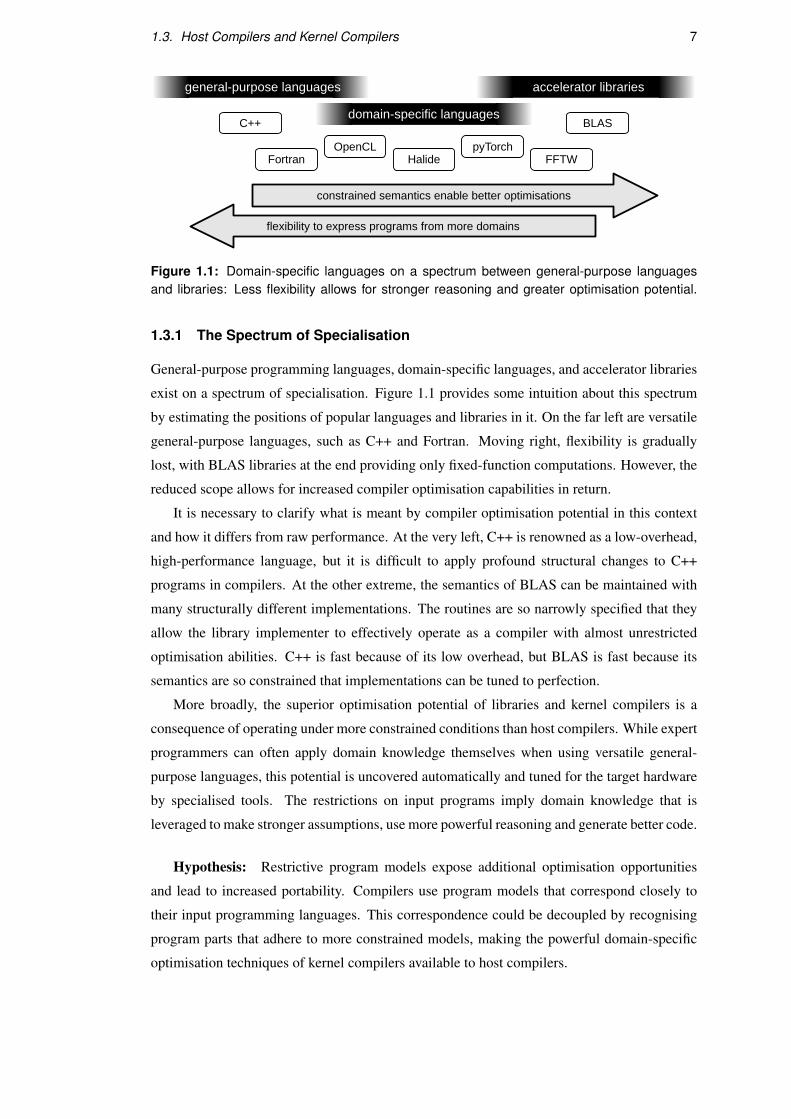
Figure 1.1: Domain-specific languages on a spectrum between general-purpose languagesand libraries: Less flexibility allows for stronger reasoning and greater optimisation potential.
1.3.1 The Spectrum of Specialisation
General-purpose programming languages, domain-specific languages, and accelerator libraries
exist on a spectrum of specialisation. Figure 1.1 provides some intuition about this spectrum
by estimating the positions of popular languages and libraries in it. On the far left are versatile
general-purpose languages, such as C++ and Fortran. Moving right, flexibility is gradually
lost, with BLAS libraries at the end providing only fixed-function computations. However, the
reduced scope allows for increased compiler optimisation capabilities in return.
It is necessary to clarify what is meant by compiler optimisation potential in this context
and how it differs from raw performance. At the very left, C++ is renowned as a low-overhead,
high-performance language, but it is difficult to apply profound structural changes to C++
programs in compilers. At the other extreme, the semantics of BLAS can be maintained with
many structurally different implementations. The routines are so narrowly specified that they
allow the library implementer to effectively operate as a compiler with almost unrestricted
optimisation abilities. C++ is fast because of its low overhead, but BLAS is fast because its
semantics are so constrained that implementations can be tuned to perfection.
More broadly, the superior optimisation potential of libraries and kernel compilers is a
consequence of operating under more constrained conditions than host compilers. While expert
programmers can often apply domain knowledge themselves when using versatile general-
purpose languages, this potential is uncovered automatically and tuned for the target hardware
by specialised tools. The restrictions on input programs imply domain knowledge that is
leveraged to make stronger assumptions, use more powerful reasoning and generate better code.
Hypothesis: Restrictive program models expose additional optimisation opportunities
and lead to increased portability. Compilers use program models that correspond closely to
their input programming languages. This correspondence could be decoupled by recognising
program parts that adhere to more constrained models, making the powerful domain-specific
optimisation techniques of kernel compilers available to host compilers.

8 Chapter 1. Introduction
1.4 Moving on the Spectrum of Specialisation
Host compilers need methods to recognise restrictive program models within general-purpose
code automatically. The term program model in this context means an internal representation
of the program logic with associated assumptions and ways of reasoning about the behaviour.
Reformulating program sections in restrictive models would make the superior domain-specific
capabilities of kernel compilers applicable in host compilers. This would result in a compiler
that can combine the positive aspects of both sides of the spectrum of specialisation.
Such an approach of detecting restricted models in general-purpose code has previously
been used only for specific individual domains and required elaborate manually implemented
compiler analysis functionality. For example, the Polly compiler by Grosser et al. [26] takes
arbitrary C/C++ code as input and recognises whether parts of this code are expressible in the
more restrictive polyhedral model [27, 28]. The compiler reformulates the relevant code in
this model, enabling advanced optimisation techniques that use the domain knowledge of the
polyhedral model for generating faster code [29, 30], substantiating the hypothesis.
1.4.1 Contributions of this Thesis
This thesis derives a systematic and configurable method for recognising constrained program
sections that fit restrictive models during the compilation process. The approach emerges from
the analysis of a standard program model for host compilers: Static Single Assignment (SSA)
form. Intermediate representations based on SSA are accessible to mathematical reasoning,
with their most relevant features built on graph and list structures. With this in mind, structural
restrictions on intermediate representation code – corresponding to restricted domain-specific
models – can be precisely formulated as constraints on a mathematical characterisation of SSA
form programs. Constraint solver techniques then make the automatic recognition of adhering
code sections feasible.
Instead of manually implementing sophisticated compiler analysis functionality, a flexible
constraint programming language is introduced that can express many different such domain-
specific models. An accompanying toolchain is developed that uses these specifications to
automatically recognise code sections that satisfy them. This system captures the spectrum
from Figure 1.1. On one extreme, sections of code are recognised as implementing specific
algorithms, like matrix multiplication, that are parametrised with numeric values. Algorithms
that allow parametrisation with an operator are next. Stencil kernels and reduction operations
fall into this category. More generic again are programs that merely follow certain structural
restrictions, such as code adhering to the polyhedral model. Chapters 4 to 6 cover each of these
domains, culminating in a system for the automatic heterogeneous acceleration of sequential
C/C++ code.

1.5. Structure of this Thesis 9
1.5 Structure of this Thesis
This thesis is divided into seven chapters.
Following the introduction, Chapter 2 derives the underlying methodology of this thesis
in the context of conventional compiler analysis. Based on a mathematical characterisation of
programs in Static Single Assignment form, the chapter presents a new constraint programming
method for expressing algorithmic program structures as constraint formulas. Later sections of
the chapter discuss implementation decisions, the algorithmic complexity of the approach, and
differences to established Satisfiability Modulo Theory (SMT) problems.
Chapter 3 gives an overview of the related work. This literature survey covers the four
main areas of research relevant to this thesis. Firstly, constraint programming underpins the
methodology of this thesis. Secondly, previous compiler analysis and auto-parallelisation
approaches are used used to evaluate the results of this work. Thirdly, heterogeneous computing
and the corresponding challenges motivate many of the compiler approaches that this thesis
implements. Finally, the term “computational idiom” is used in this thesis to denote shared
computational structures of performance bottlenecks. This term is established by comparison
with literature on several overlapping concepts from different research disciplines.
Chapters 4 to 6 are each based on a published research article and elaborate on different
applications of constraint programming in compilers.
Chapter 4 develops the Compiler Analysis Description Language (CAnDL) and presents
its implementation in the LLVM compiler infrastructure. CAnDL is a specification language
that generates compiler analysis passes from declarative descriptions via the CAnDL compiler.
The chapter explores several compiler use cases with CAnDL, including the implementation
of peephole optimisations and the prototyping of graphics shader optimisations. The chapter is
based on published research [1].
Chapter 5 extends CAnDL into the Idiom Detection Langauge (IDL) and develops an
auto-parallelising compiler for Complex Reduction and Histogram Computations (CReHCs)
built on IDL-powered analysis functionality. CReHCs cover loops with indirect data accesses
that are inaccessible to established approaches based on data flow and polyhedral analysis. The
flexibility of constraint programming allows it to capture such irregular computations. The
chapter is based on published research [2].
Chapter 6 applies IDL to the detection of algorithmic structures that go beyond the scope
of traditional compiler analysis, including stencils, histograms, and sparse linear algebra. The
recognition in LLVM enables automatic heterogeneous parallelisation of sequential code with
domain-specific backends, resulting in significant speedups on benchmark programs from the
established NPB and Parboil suites. The chapter is based on published research [3].
Finally, Chapter 7 concludes this thesis with a summary of the core contributions, a critical
analysis of the approaches, and a discussion of future work.

10 Chapter 1. Introduction
1.6 Summary
The end of Moore’s Law and Dennard Scaling has resulted in a shift away from homogeneous
multi-processing, toward architectural innovation and specialised processor cores. The rising
heterogeneity of computing resources poses a challenge to established compiler toolchains,
which often only access the increasingly marginal homogeneous fraction of processing power.
Therefore, application programmers depend on domain-specific languages and libraries that
leverage knowledge from their restricted operating domains to generate efficient code for the
modern hardware landscape.
This domain knowledge can be made available to host compilers with approaches that
automatically specialise general-purpose code and reformulate it in more restrictive program
models. Previous work has established this on individual models, but this thesis develops a
framework to formulate a wide range of restricted program models using a systematic approach
based on constraint solving. To this purpose, a custom constraint programming language is
developed and successively extended. Starting from a discussion of the underlying assumptions
and features of SSA code, the methodology is developed into a complete system, implemented
as part of the mature Clang C/C++ compiler.
In the later chapters, this core system is applied in combination with other techniques on
a range of different compiler challenges. These include the rapid prototyping of compiler
optimisations, the automatic parallelisation of programs with indirect memory accesses, a new
formulation of the polyhedral model, and the detection of computational structures that occur
widely in important bottlenecks of scientific programs.
Eventually, the techniques are combined into a fully integrated, extensible compiler tool for
efficiently mapping sequential programs onto heterogeneous systems. This develops the thesis
all the way from theoretical discussions of constraint programming approaches in compilers,
to the experimental evaluation of real performance improvements on established benchmark
suites and scientific applications.

Chapter 2
Constraint Programming on Static
Single Assignment Code
The research contributions of this thesis are built on a new method for constraint programming
on Static Single Assignment (SSA) compiler intermediate representation. This chapter derives
and motivates the underlying methodology, which is then used as the basis for Chapters 4 to 6.
The constraint programming approach is developed in three steps.
First, an overview of program representations during different compilation stages is given,
and the particular features of SSA representations are highlighted. These features are used to
derive a mathematical characterisation of the static structure of SSA programs, the SSA model.
This is first derived generically and then demonstrated in more detail on LLVM IR, a specific
SSA intermediate representation. Some mathematical notation is used in this section to build
a reliable foundation for later parts of this thesis. The List of Symbols and Notation contains
some of the notational conventions.
After the derivation of the SSA model, the concept of SSA constraint problems is defined.
These are formulas that impose restrictions on parts of SSA code, formulated as constraints on
the SSA model. SSA constraint problems can define code structures such as loops. Detecting
adhering code sections in SSA code is then equivalent to finding solutions to the constraints.
The structure of several classes of constraint formulas is discussed, reflecting conventional
compiler analysis methods like data flow, dominance relationships, and data type restrictions.
Finally, efficient algorithms for solving SSA constraint problems are derived. Backtracking
is used to find solutions quickly by incrementally extending partial solutions. The structure of
specific classes of SSA constraint problems is analysed, and efficient backtracking solutions
are derived individually, yielding composable building blocks for the solver. After deriving the
algorithms, implementation considerations are discussed. Suitable data structures are selected,
and the runtime complexity is analysed. To conclude the chapter, constraint programming on
SSA intermediate representation is compared with Satisfiability Modulo Theory (SMT).
11

12 Chapter 2. Constraint Programming on Static Single Assignment Code
2.1 Background
Modern compilers for procedural languages such as C/C++, Fortran or JavaScript typically use
a succession of different representations for the program during compilation. They reflect the
requirements of the compilation stages in which they are used.
Front end representations are close to the source program and strongly influenced by the
specific grammar of the programming language. Typically, they are built around an abstract
syntax tree with additional annotations, such as type information. These representations are
rich in information about syntactic and stylistic choices of the programmer, and they scale in
complexity with the source language. Some advanced language features, such as overloaded
operators, are not resolved in this class of representations. Therefore, the semantics of program
parts is highly dependent on context.
Back end representations are based on a model of the target hardware. They typically
approach an assembly-style format and expose the instruction set architecture of the hardware,
making them platform-specific. Back end representations also encode decisions for problems
that are removed from the algorithmic content of the user program, such as instruction selection
and register allocation.
Middle end representations are designed to enable the analysis and transformation of
code in order to apply optimisations. Static Single Assignment (SSA) representations have
emerged as a common choice for the middle end in leading compilers. SSA abstracts away
the complexities of the source language and the target architecture, focusing on a relatively
simple description of the user program semantics. This enables reliable analysis and platform-
independent reasoning.
Static Single Assignment was first proposed by Rosen et al. [31], and there are now many
different compiler intermediate representations that implement the concept. Instruction sets,
type systems and syntax (if a textual representation is even specified) of these representations
vary considerably, depending on the requirements of the source languages (static or dynamic)
and the operating constraints (just-in-time or ahead-of-time). Some prominent examples of
compilers using SSA are Clang (LLVM IR), GCC (GIMPLE), v8 Crankshaft (Hydrogen),
and SpiderMonkey (IonMonkey/MIR). Despite many differences, they share the same basic
structure that is discussed in this chapter.
SSA form was developed as an improvement over previously used compiler intermediate
representations. Specifically, the eponymous Static Single Assignment property applies to the
more general Linear Intermediate Representations as an additional restriction, as described in
Torczon and Cooper [32]. The following Section 2.1.1 gives an overview of the characteristic
shared features of SSA representations that are relevant to this work.

2.1. Background 13
2.1.1 Static Single Assignment Form
SSA representations are Linear Intermediate Representations, meaning that they represent each
function as a single linear sequence of instructions. These instructions operate on an unlimited
number of registers, using a well defined – but representation specific – instruction set. Branch
instructions are used to redirect the execution conditionally or unconditionally. Consecutive
instructions with no branching between them are grouped into basic blocks. Within these,
instructions are executed in order of appearance. Basic blocks may have labels or be identified
simply by enumerating them. Instruction arguments can be registers, constants, globals or
function parameters. Additionally, branch instructions take basic block arguments as branch
targets. Instructions may write their result into a single output register.
The SSA property stipulates that within a function, no register can be written at more than
one static location. This means that registers can be identified directly with the instructions that
define them. The registers can, therefore, be made implicit, with only the data flow between
instructions required to recover them. In the presence of dynamic control flow, Φ-instructions
are required to uphold the SSA property. These Φ-instructions are placed at the beginning of a
basic block, and select one of several values dynamically, depending on the origin of incoming
branches, i.e. depending on the previously executed basic block.
Figure 2.1 shows how SSA programs can be represented as a hierarchy of lists. Programs
are lists of functions, which are lists of basic blocks, which are lists of instructions, which take
lists of arguments. The ability to enumerate all these entities in linear sequences enables the
identification of SSA values with integer indices in the later sections of this chapter.
Data Flow Control Flow
program
function
globals
function
function...
function
basic block
parameters
basic block
basic block...
basic block
instruction
label
instruction
instruction...
instruction
argument
opcode
argument
argument...
argument
constantregister global
parameter instruction
label
basic block
Figure 2.1: Structural overview of SSA: Programs are represented as hierarchies of lists. TheSSA property makes registers implicit; values can be statically matched to defining instructions.
14 Chapter 2. Constraint Programming on Static Single Assignment Code
2.1.2 SSA Emerges During Compilation
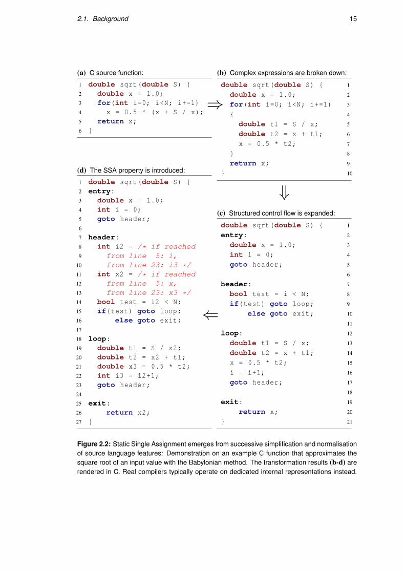
Figure 2.2 shows how critical features of SSA form emerge from simplification steps that are
applied to source code. This is demonstrated on the “sqrt” example function that approximates
the square root of a double-precision floating-point value in C using the Babylonian method in
Equation (2.1). Beginning with an initial guess x0, the approximation is improved iteratively.
x0 ≈√
S, xn+1 =xn +
Sxn
2=⇒ lim
n→∞xn =
√S (2.1)
Starting from the source code (a) at the top left of the figure, the function is first modified
by breaking down complex expressions. The expressions are turned into sequences of basic
operations, shown at the top right (b). Explicit variables appear for the previously implicit
temporary values. This simplifies the program, with many of the operations directly mapping
to individual processor instructions. Moreover, different input programs get mapped to the
same, predictable output by this transformation, making it a normalisation.
In a second step, the structured control flow of the program is replaced with goto statements
that coordinate the control flow between basic blocks. This is shown at the bottom right (c).
Although this does not ease the intuitive understanding of the program, it unifies several distinct
control flow structures provided in the source language into a single mechanism. This simplifies
program analysis. Importantly, no relevant information is lost by discarding the control flow
structures. They can be reconstructed algorithmically.
Finally, the Static Single Assignment property is introduced at the bottom left (d). Each
variable that is assigned at more than one static location in the program is instead duplicated
into multiple variables. Where necessary, these now distinct variables are bound together with
Φ-instructions. This cannot be expressed in the C programming language syntax. Instead, the
behaviour is documented by comments at lines 8–13.
The impact of the SSA property seems minor at first, but convenient implications can
already be identified within the C language. As all local variables are written at exactly one
static location, each variable can be declared and defined in the same place. This means
that it is always known statically, which expression yielded the value of each variable. This
immediately guarantees that the variable “i” in the example always has the value “0”, and that
the variable “x” always has the value “1.0”.
In summary, this section developed an understanding of how SSA originated historically
and how it emerges during the compilation process. The following section uses the observations
from Figure 2.1 – that most parts of SSA code can be enumerated and represented as elements
in lists – to derive a mathematical characterisation of the static structure of SSA programs. This
characterisation then serves as the foundation of later sections, which define compiler analysis
problems on it via constraints.
2.1. Background 15
(a) C source function:
1 double sqrt(double S) {2 double x = 1.0;3 for(int i=0; i<N; i+=1)4 x = 0.5 * (x + S / x);5 return x;6 }
(d) The SSA property is introduced:
1 double sqrt(double S) {2 entry:3 double x = 1.0;4 int i = 0;5 goto header;6
7 header:8 int i2 = /* if reached9 from line 5: i,
10 from line 23: i3 */11 int x2 = /* if reached12 from line 5: x,13 from line 23: x3 */14 bool test = i2 < N;15 if(test) goto loop;16 else goto exit;17
18 loop:19 double t1 = S / x2;20 double t2 = x2 + t1;21 double x3 = 0.5 * t2;22 int i3 = i2+1;23 goto header;24
25 exit:26 return x2;27 }
(b) Complex expressions are broken down:
1double sqrt(double S) {
2double x = 1.0;
3for(int i=0; i<N; i+=1)
4{
5double t1 = S / x;
6double t2 = x + t1;
7x = 0.5 * t2;
8}
9return x;
10}
⇓(c) Structured control flow is expanded:
1double sqrt(double S) {
2entry:3double x = 1.0;
4int i = 0;
5goto header;
6
7header:8bool test = i < N;
9if(test) goto loop;
10else goto exit;
11
12loop:13double t1 = S / x;
14double t2 = x + t1;
15x = 0.5 * t2;
16i = i+1;
17goto header;
18
19exit:20return x;
21}
⇒
⇐
Figure 2.2: Static Single Assignment emerges from successive simplification and normalisationof source language features: Demonstration on an example C function that approximates thesquare root of an input value with the Babylonian method. The transformation results (b-d) arerendered in C. Real compilers typically operate on dedicated internal representations instead.
16 Chapter 2. Constraint Programming on Static Single Assignment Code
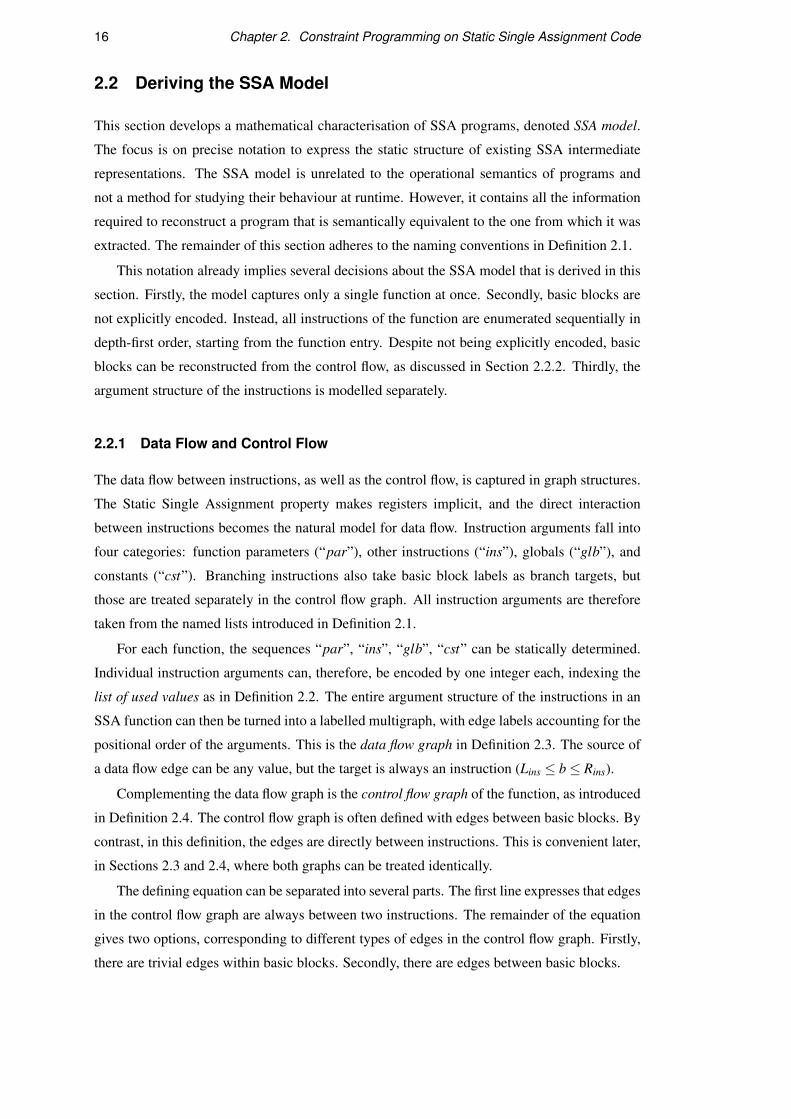
2.2 Deriving the SSA Model
This section develops a mathematical characterisation of SSA programs, denoted SSA model.
The focus is on precise notation to express the static structure of existing SSA intermediate
representations. The SSA model is unrelated to the operational semantics of programs and
not a method for studying their behaviour at runtime. However, it contains all the information
required to reconstruct a program that is semantically equivalent to the one from which it was
extracted. The remainder of this section adheres to the naming conventions in Definition 2.1.
This notation already implies several decisions about the SSA model that is derived in this
section. Firstly, the model captures only a single function at once. Secondly, basic blocks are
not explicitly encoded. Instead, all instructions of the function are enumerated sequentially in
depth-first order, starting from the function entry. Despite not being explicitly encoded, basic
blocks can be reconstructed from the control flow, as discussed in Section 2.2.2. Thirdly, the
argument structure of the instructions is modelled separately.
2.2.1 Data Flow and Control Flow
The data flow between instructions, as well as the control flow, is captured in graph structures.
The Static Single Assignment property makes registers implicit, and the direct interaction
between instructions becomes the natural model for data flow. Instruction arguments fall into
four categories: function parameters (“par”), other instructions (“ins”), globals (“glb”), and
constants (“cst”). Branching instructions also take basic block labels as branch targets, but
those are treated separately in the control flow graph. All instruction arguments are therefore
taken from the named lists introduced in Definition 2.1.
For each function, the sequences “par”, “ins”, “glb”, “cst” can be statically determined.
Individual instruction arguments can, therefore, be encoded by one integer each, indexing the
list of used values as in Definition 2.2. The entire argument structure of the instructions in an
SSA function can then be turned into a labelled multigraph, with edge labels accounting for the
positional order of the arguments. This is the data flow graph in Definition 2.3. The source of
a data flow edge can be any value, but the target is always an instruction (Lins ≤ b≤ Rins).
Complementing the data flow graph is the control flow graph of the function, as introduced
in Definition 2.4. The control flow graph is often defined with edges between basic blocks. By
contrast, in this definition, the edges are directly between instructions. This is convenient later,
in Sections 2.3 and 2.4, where both graphs can be treated identically.
The defining equation can be separated into several parts. The first line expresses that edges
in the control flow graph are always between two instructions. The remainder of the equation
gives two options, corresponding to different types of edges in the control flow graph. Firstly,
there are trivial edges within basic blocks. Secondly, there are edges between basic blocks.
2.2. Deriving the SSA Model 17
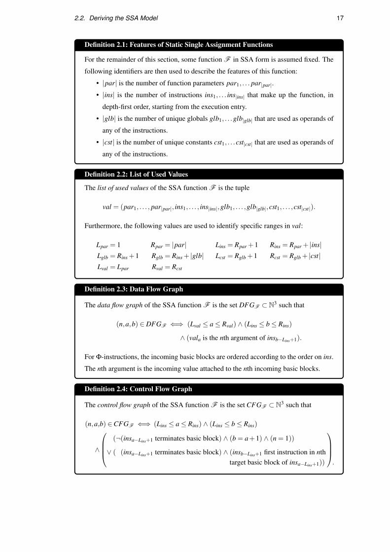
Definition 2.1: Features of Static Single Assignment Functions
For the remainder of this section, some function F in SSA form is assumed fixed. The
following identifiers are then used to describe the features of this function:
• |par| is the number of function parameters par1, . . . par|par|.
• |ins| is the number of instructions ins1, . . . ins|ins| that make up the function, in
depth-first order, starting from the execution entry.
• |glb| is the number of unique globals glb1, . . .glb|glb| that are used as operands of
any of the instructions.
• |cst| is the number of unique constants cst1, . . .cst|cst| that are used as operands of
any of the instructions.
Definition 2.2: List of Used Values
The list of used values of the SSA function F is the tuple
val = (par1, . . . , par|par|, ins1, . . . , ins|ins|,glb1, . . . ,glb|glb|,cst1, . . . ,cst|cst|).
Furthermore, the following values are used to identify specific ranges in val:
Lpar = 1 Rpar = |par| Lins = Rpar +1 Rins = Rpar + |ins|Lglb = Rins +1 Rglb = Rins + |glb| Lcst = Rglb +1 Rcst = Rglb + |cst|Lval = Lpar Rval = Rcst
Definition 2.3: Data Flow Graph
The data flow graph of the SSA function F is the set DFGF ⊂ N3 such that
(n,a,b) ∈ DFGF ⇐⇒ (Lval ≤ a≤ Rval) ∧ (Lins ≤ b≤ Rins)
∧ (vala is the nth argument of insb−Lins+1).
For Φ-instructions, the incoming basic blocks are ordered according to the order on ins.
The nth argument is the incoming value attached to the nth incoming basic blocks.
Definition 2.4: Control Flow Graph
The control flow graph of the SSA function F is the set CFGF ⊂ N3 such that
(n,a,b) ∈CFGF ⇐⇒ (Lins ≤ a≤ Rins) ∧ (Lins ≤ b≤ Rins)
∧
(¬(insa−Lins+1 terminates basic block) ∧ (b = a+1) ∧ (n = 1))
∨ ( (insa−Lins+1 terminates basic block) ∧ (insb−Lins+1 first instruction in nthtarget basic block of insa−Lins+1)) .
18 Chapter 2. Constraint Programming on Static Single Assignment Code
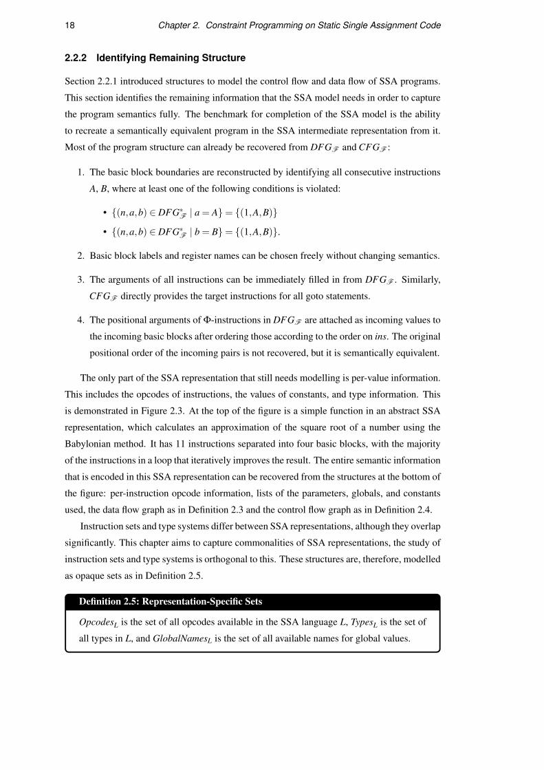
2.2.2 Identifying Remaining Structure
Section 2.2.1 introduced structures to model the control flow and data flow of SSA programs.
This section identifies the remaining information that the SSA model needs in order to capture
the program semantics fully. The benchmark for completion of the SSA model is the ability
to recreate a semantically equivalent program in the SSA intermediate representation from it.
Most of the program structure can already be recovered from DFGF and CFGF :
1. The basic block boundaries are reconstructed by identifying all consecutive instructions
A, B, where at least one of the following conditions is violated:
• {(n,a,b) ∈ DFG∗F | a = A}= {(1,A,B)}
• {(n,a,b) ∈ DFG∗F | b = B}= {(1,A,B)}.
2. Basic block labels and register names can be chosen freely without changing semantics.
3. The arguments of all instructions can be immediately filled in from DFGF . Similarly,
CFGF directly provides the target instructions for all goto statements.
4. The positional arguments of Φ-instructions in DFGF are attached as incoming values to
the incoming basic blocks after ordering those according to the order on ins. The original
positional order of the incoming pairs is not recovered, but it is semantically equivalent.
The only part of the SSA representation that still needs modelling is per-value information.
This includes the opcodes of instructions, the values of constants, and type information. This
is demonstrated in Figure 2.3. At the top of the figure is a simple function in an abstract SSA
representation, which calculates an approximation of the square root of a number using the
Babylonian method. It has 11 instructions separated into four basic blocks, with the majority
of the instructions in a loop that iteratively improves the result. The entire semantic information
that is encoded in this SSA representation can be recovered from the structures at the bottom of
the figure: per-instruction opcode information, lists of the parameters, globals, and constants
used, the data flow graph as in Definition 2.3 and the control flow graph as in Definition 2.4.
Instruction sets and type systems differ between SSA representations, although they overlap
significantly. This chapter aims to capture commonalities of SSA representations, the study of
instruction sets and type systems is orthogonal to this. These structures are, therefore, modelled
as opaque sets as in Definition 2.5.
Definition 2.5: Representation-Specific Sets
OpcodesL is the set of all opcodes available in the SSA language L, TypesL is the set of
all types in L, and GlobalNamesL is the set of all available names for global values.

2.2. Deriving the SSA Model 19
function Sqrt(S)
entry goto header
header
i←Φ(entry : 0, loop : i′)
x←Φ(entry : 1, loop : x′)
c← i < N
if c goto loop else exit
loop
t1← S/x
t2← x+ t1
x′← t2/2
i′← i+1
goto header
exit return x
∼=
1:
parameters:
S
2:
3:
4:
5:
6:
7:
8:
9:
10:
11:
12:
instructions:
goto �
Φ(� : �, � : �)
Φ(� : �, � : �)
�<�
if � goto � else �
�/�
�+�
�/�
�+�
goto �
return �
13:
globals:
N
14:
15:
16:
constants:
1
2
0
+
DFGF = {10 2−→ 3, 16 1−→ 3,
9 2−→ 4, 14 1−→ 4,
3 1−→ 5, 13 2−→ 5,
5 1−→ 6
1 1−→ 7, 4 2−→ 7,
4 1−→ 8, 7 2−→ 8
8 1−→ 9, 15 2−→ 9
3 1−→ 10, 14 2−→ 10,
4 1−→ 12}
CFGF = {2 1−→ 3,
3 1−→ 4,
4 1−→ 5,
5 1−→ 6,
6 1−→ 7, 6 2−→ 12,
7 1−→ 8,
8 1−→ 9,
9 1−→ 10,
10 1−→ 11,
11 1−→ 3}
Figure 2.3: SSA representation is decomposed into individual instructions, data flow and controlflow. This is an equivalent representation of the function; no semantic information is lost. Theexample is a rendering of the Babylonian method in Figure 2.2, abstracting away the C syntax.

20 Chapter 2. Constraint Programming on Static Single Assignment Code
2.2.3 Putting the SSA Model Together
With separate mathematical structures in place to capture all the relevant information contained
in SSA programs, the SSA model can now be assembled. Definition 2.6 shows the completed
SSA model. The data flow graph DFGF and the control flow graph CFGF were discussed in
detail previously, but some clarifications are provided for the remaining five structures.
The type model, instruction model, and constant model assign additional information from
different domains to the values used in the function. Instead of attaching a single type to each
value, the type model allows values to be linked with several elements in the set “Types”.
This is convenient to model subtyping hierarchies where, for example, an integer pointer value
is a pointer in particular. The same is true for the instruction model, which enables it to
express opcode categories, e.g. an arithmetic operation might be a subtraction in particular.
The constant model is defined likewise as a subset of R×N but makes no use of the ability to
assign multiple numeric values to the same constant.
Finally, the parameter model and global model encode which elements in the list of used
values of F are parameters and globals, respectively. Parameter names are not significant,
because their position already identifies parameters uniquely within the function signature.
Therefore, the parameter model identifies all parameters but attaches no additional data. For
global values, on the other hand, the names are attached by the global model as elements from
the set “GlobalNames”.
2.2.4 Additional Notation
The seven basic components of the SSA model are each expressed as a set of tuples. In order
to conveniently manipulate these structures in later sections, Definition 2.7 introduces several
functions and shorthand notation.
For a set of tuples, the function “heads” returns the set of all the first elements of the tuples.
For example, “heads(IF )” yields all the opcodes that are used in the function F . In contrast,
the function “tails” removes the first element of all tuples within a set. For example, “tails(IF )”
identifies the indices of all the instructions within the list of used values of F but removes the
information about their opcodes. Finally, the “select” function is used to filter a set for only
those tuples with a specific first element, and then returns the tails of all these tuples. For
example, “select(add, IF )” gives the indices of all additions within the list of used values of
the function F .
The representation of data flow and control flow as labelled multigraphs contains more
information than is required for many tasks. The simplified versions DFG∗F and CFG∗F are
constructed with the “tails” function, effectively removing the labels and resulting in ordinary
graph structures. Similarly, the sets I∗F and C∗F are used for shorter notation.

2.2. Deriving the SSA Model 21
Definition 2.6: Mathematical Characterisation of SSA Functions
The SSA model of the function F is the tuple
(DFGF ,CFGF ,TF ,PF , IF ,GF ,CF ),
where
• DFGF ⊂ N3 and CFGF ⊂ N3 are the data flow and control flow graph;
• TF ⊂ Types×N is the type model, defined by the property
(t,k) ∈ TF ⇐⇒ (Lval ≤ k ≤ Rval) ∧ (valk has type t);
• PF ⊂ N is the parameter model, defined by the property
k ∈ PF ⇐⇒ Lpar ≤ k ≤ Rpar;
• IF ⊂ Opcodes×N is the instruction model, defined by the property
(c,k) ∈ IF ⇐⇒ (Lins ≤ k ≤ Rins) ∧ (insk−Lins+1 has opcode c);
• GF ⊂ GlobalNames×N is the global model, defined by the property
(n,k) ∈ GF ⇐⇒(Lglb ≤ k ≤ Rglb
)∧ (glbk−Lglb+1 has name n);
• CF ⊂ R×N is the constant model, defined by the property
(x,k) ∈CF ⇐⇒ (Lcst ≤ k ≤ Rcst) ∧ (cstk−Lcst+1 has numeric value x).
Definition 2.7: Notation for Reducing Dimensionality
For a set A, any a ∈ A, and S⊂ A×Nk for some k > 0, the following are defined:
heads(S) = {a ∈ A | (a,b1, . . . ,bk) ∈ S for some b1, . . . ,bk ∈ N}
tails(S) = {b ∈ Nk | (a,b1, . . . ,bk) ∈ S for some a ∈ A}
select(a,S) = {b ∈ Nk | (a,b1, . . . ,bk) ∈ S}.
Note that the case A = N is common.
In addition, rev(S′) = {(a,b) | (b,a)∈ S′} is defined for S′ ⊂Nk and the following used:
DFG∗F = tails(DFGF )
CFG∗F = tails(CFGF )
I∗F = tails(IF )
C∗F = tails(CF )
22 Chapter 2. Constraint Programming on Static Single Assignment Code
2.2.5 The LLVM Compiler Framework
The previously introduced SSA model is generic and applies to all SSA compiler intermediate
representations. However, it needs to be specialised to a specific representation in order to use
it on real compiler problems. LLVM intermediate representation (LLVM IR) is one of the most
common languages in that class, because of its use in the popular LLVM framework started by
Lattner and Adve [33]. It is used throughout this thesis for demonstration and evaluation.
LLVM is a comprehensive compiler infrastructure project, using LLVM IR as its central
abstraction. The LLVM project was formerly named “Low Level Virtual Machine”, alluding
to a hypothetical machine that uses LLVM IR as its native assembly language. The instruction
set of LLVM IR is roughly aligned to the semantics of C-style programming languages, but
the project has matured beyond this background. It is now a widely influential framework with
compiler front ends for a diverse set of languages, including C, C++, Haskell, Julia, Objective-
C, Rust, Scala, and CUDA.
Other mainstream compilers, such as the GCC project, use very similar representations
internally. Despite this, LLVM is unique in understanding the intermediate representation as
an advertised and documented interface within the toolchain, as opposed to an obscure internal
abstraction. This makes it very suitable for research implementations.
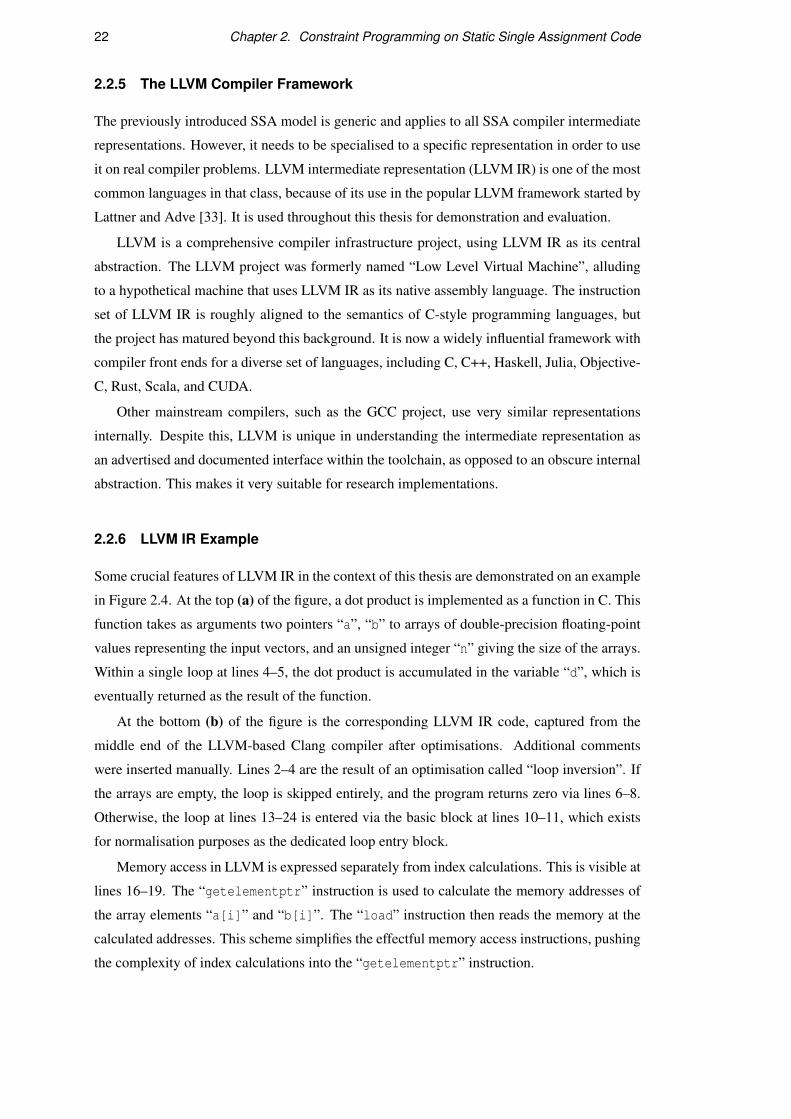
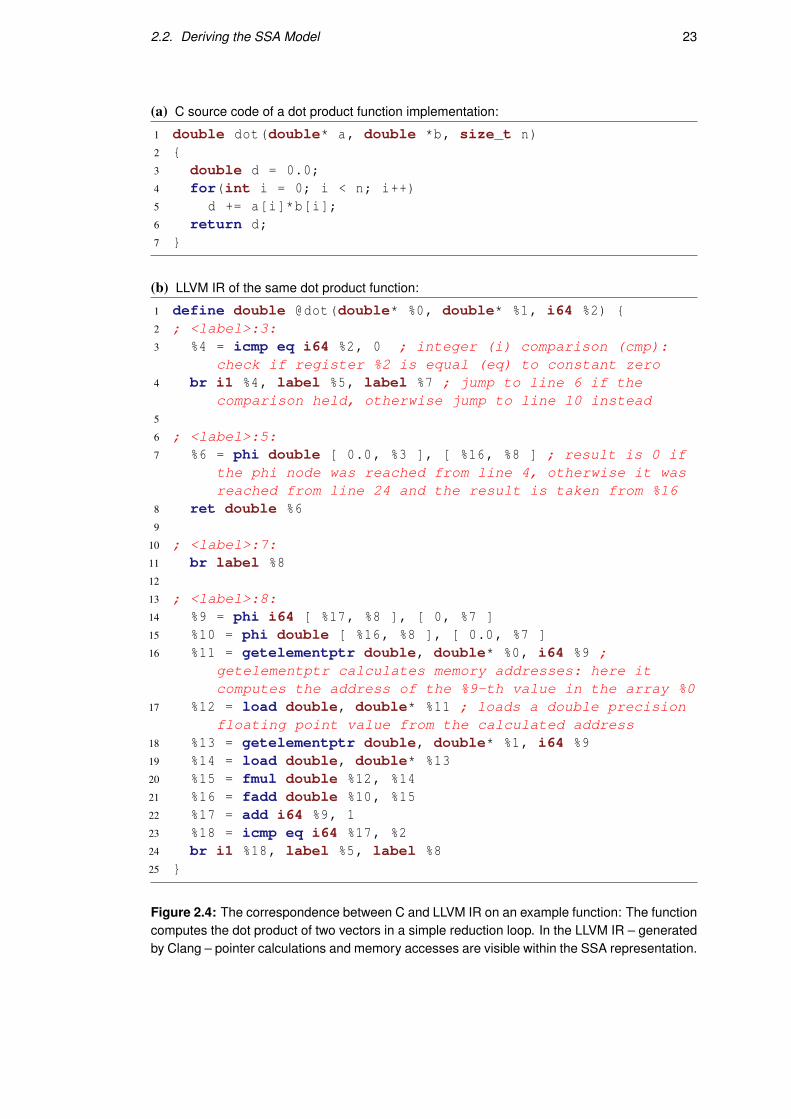
2.2.6 LLVM IR Example
Some crucial features of LLVM IR in the context of this thesis are demonstrated on an example
in Figure 2.4. At the top (a) of the figure, a dot product is implemented as a function in C. This
function takes as arguments two pointers “a”, “b” to arrays of double-precision floating-point
values representing the input vectors, and an unsigned integer “n” giving the size of the arrays.
Within a single loop at lines 4–5, the dot product is accumulated in the variable “d”, which is
eventually returned as the result of the function.
At the bottom (b) of the figure is the corresponding LLVM IR code, captured from the
middle end of the LLVM-based Clang compiler after optimisations. Additional comments
were inserted manually. Lines 2–4 are the result of an optimisation called “loop inversion”. If
the arrays are empty, the loop is skipped entirely, and the program returns zero via lines 6–8.
Otherwise, the loop at lines 13–24 is entered via the basic block at lines 10–11, which exists
for normalisation purposes as the dedicated loop entry block.
Memory access in LLVM is expressed separately from index calculations. This is visible at
lines 16–19. The “getelementptr” instruction is used to calculate the memory addresses of
the array elements “a[i]” and “b[i]”. The “load” instruction then reads the memory at the
calculated addresses. This scheme simplifies the effectful memory access instructions, pushing
the complexity of index calculations into the “getelementptr” instruction.
2.2. Deriving the SSA Model 23
(a) C source code of a dot product function implementation:
1 double dot(double* a, double *b, size_t n)2 {3 double d = 0.0;4 for(int i = 0; i < n; i++)5 d += a[i]*b[i];6 return d;7 }
(b) LLVM IR of the same dot product function:
1 define double @dot(double* %0, double* %1, i64 %2) {2 ; <label>:3:3 %4 = icmp eq i64 %2, 0 ; integer (i) comparison (cmp):
check if register %2 is equal (eq) to constant zero4 br i1 %4, label %5, label %7 ; jump to line 6 if the
comparison held, otherwise jump to line 10 instead5
6 ; <label>:5:7 %6 = phi double [ 0.0, %3 ], [ %16, %8 ] ; result is 0 if
the phi node was reached from line 4, otherwise it wasreached from line 24 and the result is taken from %16
8 ret double %69
10 ; <label>:7:11 br label %812
13 ; <label>:8:14 %9 = phi i64 [ %17, %8 ], [ 0, %7 ]15 %10 = phi double [ %16, %8 ], [ 0.0, %7 ]16 %11 = getelementptr double, double* %0, i64 %9 ;
getelementptr calculates memory addresses: here itcomputes the address of the %9-th value in the array %0
17 %12 = load double, double* %11 ; loads a double precisionfloating point value from the calculated address
18 %13 = getelementptr double, double* %1, i64 %919 %14 = load double, double* %1320 %15 = fmul double %12, %1421 %16 = fadd double %10, %1522 %17 = add i64 %9, 123 %18 = icmp eq i64 %17, %224 br i1 %18, label %5, label %825 }
Figure 2.4: The correspondence between C and LLVM IR on an example function: The functioncomputes the dot product of two vectors in a simple reduction loop. In the LLVM IR – generatedby Clang – pointer calculations and memory accesses are visible within the SSA representation.

24 Chapter 2. Constraint Programming on Static Single Assignment Code
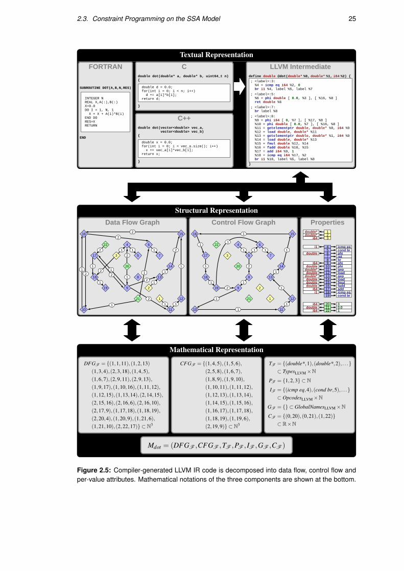
Figure 2.5 shows in detail how the SSA model is constructed from the LLVM intermediate
representation of the program in Figure 2.4. At the top left, implementations of the dot product
are shown in three programming languages that LLVM supports: Fortran, C and C++. At the
top right is the corresponding LLVM IR code. While this is not precisely identical for different
implementations, its basic structure is independent of the source language.
In the middle row, the structure of the LLVM IR code is separated into three components:
labelled multigraphs for the data flow and control flow, as well as the per-instruction properties
represented as a list. Together, they capture all the semantically significant information of the
function, as previously demonstrated in Section 2.2.2. In the bottom row, the SSA model is
shown, adhering to Definition 2.6. The labelled multigraphs for the control flow and data flow
graphs are represented as sets of 3-tuples of integers.
2.3 Constraint Programming on the SSA Model
Properties of SSA programs can now be formulated as constraint problems on the SSA model.
For this purpose, the set of SSA models is introduced in Definition 2.8, which Definition 2.9
then uses to formulate SSA constraint problems.
Definition 2.8: Set of SSA Models
Given a specific SSA representation (LLVM, Hydrogen, MIR, . . . ), denote F the set of
all valid functions that can be expressed in it.
The set of SSA models M is defined as
M = {M |M is the SSA model of some F ∈ F}.
Definition 2.9: SSA constraint problem
An SSA constraint problem (V,C) is a pair of a finite set of variables V and a boolean
predicate C : M ×NV 7→ {1,0}. The set of constraint solutions for an SSA constraint
problem in the context of a specific SSA model M ∈M is given as
SM(V,C) = {s ∈ NV |C(M,s) = 1}.
The following intuition applies: The first argument of C is the SSA model of a function.
The second argument of C is a solution candidate. NV can be understood as abstractly rendering
map<string,unsigned>, with elements assigning an integer to each constraint variable.
These integers represent values in the SSA function by indexing into the list of used values.
The predicate function determines whether these values have a specific relationship to each
other. Finally, the set of constraint solutions lists all those tuples for which the predicate holds.
2.3. Constraint Programming on the SSA Model 25
Textual RepresentationLLVM Intermediate
define double @dot(double* %0, double* %1, i64 %2) {
}
Cdouble dot(double* a, double* b, uint64_t n){
}
; <label>:3: %4 = icmp eq i64 %2, 0 br i1 %4, label %5, label %7
; <label>:5: %6 = phi double [ 0.0, %3 ], [ %16, %8 ] ret double %6
; <label>:7: br label %8
; <label>:8: %9 = phi i64 [ 0, %7 ], [ %17, %8 ] %10 = phi double [ 0.0, %7 ], [ %16, %8 ] %11 = getelementptr double, double* %0, i64 %9 %12 = load double, double* %11 %13 = getelementptr double, double* %1, i64 %9 %14 = load double, double* %13 %15 = fmul double %12, %14 %16 = fadd double %10, %15 %17 = add i64 %9, 1 %18 = icmp eq i64 %17, %2 br i1 %18, label %5, label %8
double d = 0.0; for(int i = 0; i < n; i++) d += a[i]*b[i]; return d;
C++double dot(vector<double> vec_a, vector<double> vec_b){
}
double x = 0.0; for(int i = 0; i < vec_a.size(); i++) x += vec_a[i]*vec_b[i]; return x;
FORTRAN
SUBROUTINE DOT(A,B,N,RES)
END
INTEGER N REAL X,A(:),B(:) X=0.0 DO I = 1, N, 1 X = X + A(i)*B(i) END DO RES=X RETURN
Structural Representation���������������
� �
��
��
��
��
��
��
��
��
�
�
�
��
� �
�
�
�
��
�
� �
�
�
�
�
�
�
��
���
�
�
��
������������
�
�
��
��
��
��
�
�
�
�
�
�
�
� �
�
�
��
�
�
�
�
�
�
�
�
�
�
�
�
�
��
��
�
�
�
��
��
�
��
���
�
��
����������
�������
��������������� ������� �� ���������������������������������
��
������
���������
�������������
�������������������������
�����
�
�
�
�
��
��
��
��
��
��
�
��
�
��
���������
���
�� ��
��
��
��
��������������
���
�
�
�
Mathematical Representation
DFGF = {(1,1,11),(1,2,13)(1,3,4),(2,3,18),(1,4,5),(1,6,7),(2,9,11),(2,9,13),(1,9,17),(1,10,16),(1,11,12),(1,12,15),(1,13,14),(2,14,15),(2,15,16),(2,16,6),(2,16,10),(2,17,9),(1,17,18),(1,18,19),(2,20,4),(1,20,9),(1,21,6),(1,21,10),(2,22,17)} ⊂ N3
CFGF = {(1,4,5),(1,5,6),(2,5,8),(1,6,7),(1,8,9),(1,9,10),(1,10,11),(1,11,12),(1,12,13),(1,13,14),(1,14,15),(1,15,16),(1,16,17),(1,17,18),(1,18,19),(1,19,6),(2,19,9)} ⊂ N3
TF = {(double*,1),(double*,2), . . .}⊂ TypesLLVM×N
PF = {1,2,3} ⊂ N
IF = {(icmp eq,4),(cond br,5), . . .}⊂ OpcodesLLVM×N
GF = {} ⊂ GlobalNamesLLVM×N
CF = {(0,20),(0,21),(1,22)}⊂ R×N
Mdot = (DFGF ,CFGF ,TF ,PF , IF ,GF ,CF )
Figure 2.5: Compiler-generated LLVM IR code is decomposed into data flow, control flow andper-value attributes. Mathematical notations of the three components are shown at the bottom.
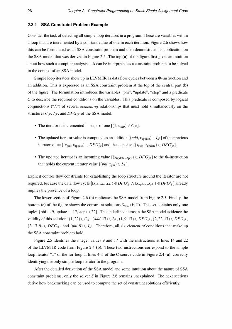
26 Chapter 2. Constraint Programming on Static Single Assignment Code
2.3.1 SSA Constraint Problem Example
Consider the task of detecting all simple loop iterators in a program. These are variables within
a loop that are incremented by a constant value of one in each iteration. Figure 2.6 shows how
this can be formulated as an SSA constraint problem and then demonstrates its application on
the SSA model that was derived in Figure 2.5. The top (a) of the figure first gives an intuition
about how such a compiler analysis task can be interpreted as a constraint problem to be solved
in the context of an SSA model.
Simple loop iterators show up in LLVM IR as data flow cycles between a Φ-instruction and
an addition. This is expressed as an SSA constraint problem at the top of the central part (b)
of the figure. The formulation introduces the variables “phi”, “update”, “step” and a predicate
C to describe the required conditions on the variables. This predicate is composed by logical
conjunctions (“∧”) of several element-of relationships that must hold simultaneously on the
structures CF , IF , and DFGF of the SSA model:
• The iterator is incremented in steps of one [(1,xstep) ∈CF ].
• The updated iterator value is computed as an addition [(add,xupdate)∈ IF ] of the previous
iterator value [(xphi,xupdate) ∈ DFG∗F ] and the step size [(xstep,xupdate) ∈ DFG∗F ].
• The updated iterator is an incoming value [(xupdate,xphi) ∈ DFG∗F ] to the Φ-instruction
that holds the current iterator value [(phi,xphi) ∈ IF ].
Explicit control flow constraints for establishing the loop structure around the iterator are not
required, because the data flow cycle [(xphi,xupdate)∈DFG∗F ∧ (xupdate,xphi)∈DFG∗F ] already
implies the presence of a loop.
The lower section of Figure 2.6 (b) replicates the SSA model from Figure 2.5. Finally, the
bottom (c) of the figure shows the constraint solutions SMdot (V,C). This set contains only one
tuple: {phi 7→ 9,update 7→ 17,step 7→ 22}. The underlined items in the SSA model evidence the
validity of this solution: (1,22)∈CF , (add,17)∈ IF , (1,9,17)∈DFGF , (2,22,17)∈DFGF ,
(2,17,9) ∈ DFGF , and (phi,9) ∈ IF . Therefore, all six element-of conditions that make up
the SSA constraint problem hold.
Figure 2.5 identifies the integer values 9 and 17 with the instructions at lines 14 and 22
of the LLVM IR code from Figure 2.4 (b). These two instructions correspond to the simple
loop iterator “i” of the for-loop at lines 4–5 of the C source code in Figure 2.4 (a), correctly
identifying the only simple loop iterator in the program.
After the detailed derivation of the SSA model and some intuition about the nature of SSA
constraint problems, only the solver S in Figure 2.6 remains unexplained. The next sections
derive how backtracking can be used to compute the set of constraint solutions efficiently.

2.3. Constraint Programming on the SSA Model 27
(a) Initial problem statement:
Detect︸ ︷︷ ︸solver S
simple loop iterators︸ ︷︷ ︸SSA constraint problem (V,C)
in the dot product function︸ ︷︷ ︸SSA model Mdot
.
(b) Formulation as constraint problem:
S
SSA constraint problem
V = {phi,update,step}
C(M,x) = ((1,xstep) ∈CF ∧ (add,xupdate) ∈ IF ∧
(xphi,xupdate) ∈ DFG∗F ∧ (xstep,xupdate) ∈ DFG∗F ∧
(xupdate,xphi) ∈ DFG∗F ∧ (phi,xphi) ∈ IF )
SSA model
DFGF = {(1,1,11),(1,2,13),(1,3,4),(2,3,18),(1,4,5),(1,6,7),(2,9,11),(2,9,13),(1,9,17),(1,10,16),(1,11,12),(1,12,15),(1,13,14),(2,14,15),(2,15,16),(2,16,6),(2,16,10),(2,17,9),(1,17,18),(1,18,19),(2,20,4),(1,20,9),(1,21,6),(1,21,10),(2,22,17)}
CFGF = {(1,4,5),(1,5,6),(2,5,8),(1,6,7),(1,8,9),(1,9,10),(1,10,11),(1,11,12),(1,12,13),(1,13,14),(1,14,15),(1,15,16),(1,16,17),(1,17,18),(1,18,19),(1,19,6),(2,19,9)}
TF = {(double*,1),(double*,2), . . .}PF = {1,2,3}IF = {(icmp eq,4),(cond br,5),(phi,6),(ret,7),(br,8),(phi,9),
(phi,10),(gep,11),(load,12),(gep,13),(load,14),(fmul,15),(fadd,16),(add,17),(icmp eq,18),(cond br,19)}
GF = {}CF = {(0,20),(0,21),(1,22)}
(c) Resulting set of constraint solutions:
SMdot(V,C) = {{phi 7→ 9,update 7→ 17,step 7→ 22}} ⊂ NV
Figure 2.6: Detection of simple loop iterators is formulated as a constraint problem and appliedto the SSA model from Figure 2.5. A single solution corresponding to the C variable “i” is found.

28 Chapter 2. Constraint Programming on Static Single Assignment Code
2.4 Solving SSA Constraint Problems
The solver for SSA constraint problems should efficiently compute SM(V,C) for some concrete
SSA constraint problem (V,C) and SSA model M. This is a search problem: all values in NV
that satisfy C in the context M need to be identified.
The search space NV is infinitely large, but it can immediately be trimmed to only tuples
that have all values ≤ |val|. The case |V |> 50 is common in Chapters 4 to 6, and interesting
functions often have |val|> 100. The remaining search space therefore has > 10050 = 10100
elements. Brute-force search is unfeasible on such a large search space, even when assuming
that the direct evaluation of the predicate for any potential solution can be performed efficiently.
However, backtracking can be used to find partial solutions that are incrementally extended.
Definition 2.10: Backtracking Solution of Constraint Problems
Given an SSA constraint problem (V,C) and an enumeration of V = {v1, . . . ,v|V |}, any
collection (Bk)k=1...|V | of functions Bk : M ×Nk−1→P(N) is denoted a backtracking
solution of (V,C) if and only if the following is satisfied for all M ∈M ,x ∈ NV :
C(M,x) = 1 ⇐⇒ [xvk ∈ Bk(M, pk−1(x)) for all 1≤ k ≤ |V |] , (2.2)
where the projections pk : NV → Nk are defined by x 7→ (xv1 , . . .xvk) for all 0≤ k ≤ |V |.
Definition 2.10 defines the concept of a backtracking solution, but it does not show how
such a backtracking solution could be constructed. That is explained in the next section. The
concept is introduced in order to allow the definition of the backtracking search Algorithm 1,
which works as follows: The variable x iterates over Nn (n = |V |, identified with NV at line 7).
The variable k tracks the number of currently considered dimensions of this partial solution.
After the initialisation assignments at line 2, a single loop spans the remainder of the algorithm.
In each iteration, the algorithm tries to assign a valid value to the latest considered element in
the partial solution x (line 4). By convention, the minimum of the empty set is the symbol “∞”.
If this case occurs, the algorithm backtracks at lines 12–17. Otherwise, the solution is either
complete (lines 6–8), or the dimension k of the partial solution is increased at line 10, and the
algorithm continues by searching for the next element of x in the following iteration.
2.4.1 The Structure of SSA Constraint Problems
Basic construction rules for SSA constraint problems are the element-of constraint problem
in Definition 2.11, and the conjunction and disjunction constraint problems in Definition 2.12.
Definition 2.13 enables the composition of constraint problems that are not defined on the same
set of variables. The example in Figure 2.6 can be constructed with only these rules.

2.4. Solving SSA Constraint Problems 29
Algorithm 1 Backtracking algorithm
1: procedure DETECT(M,(Bk)k=1...n,(vk)k=1...n)2: k← 1, x← (1, . . . ,1) ∈ Nn
3: while true do4: xk← min{y ∈ Bk(M, pk−1(x)) | y≥ xk}5: if xk < ∞ then6: if k = n then7: yield {vk 7→ xk}k=1...n ∈ NV
8: xk← xk +19: else
10: k← k+111: xk← 112: else13: k← k−114: if k ≥ 1 then15: xk← xk +116: else17: exit
Definition 2.11: Element-of Constraint Problem
Given a set of tuples S(M) ⊂ NV that may depend on M ∈M (e.g. S(M) ≈ DFG∗F ),
the element-of constraint problem (V,ES) is defined by
ES(M,x) =
{1 if x ∈ S(M)
0 otherwise.
Definition 2.12: Conjunction and Disjunction Constraint Problems
Given SSA constraint problems (V,C) and (V,C′), the conjunction constraint problem
(V,C∧C′) and the disjunction constraint problem (V,C∨C′) are defined by
C∧C′(M,x) =
{1 if C(M,x) = 1 ∧C′(M,x) = 1
0 otherwise
C∨C′(M,x) =
{1 if C(M,x) = 1 ∨C′(M,x) = 1
0 otherwise.
Definition 2.13: Extension of a Constraint Problem
Given an SSA constraint problem (V,C) and an injection i : V ↪→W , the extension of
the constraint problem (W,CW ) is defined by
CW (M,x) =C(
M,(xi(v)
)v∈V
).
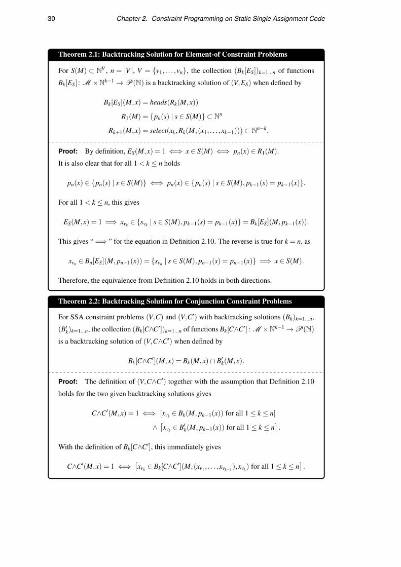
30 Chapter 2. Constraint Programming on Static Single Assignment Code
Theorem 2.1: Backtracking Solution for Element-of Constraint Problems
For S(M) ⊂ NV , n = |V |, V = {v1, . . . ,vn}, the collection (Bk[ES])k=1...n of functions
Bk[ES] : M ×Nk−1→P(N) is a backtracking solution of (V,ES) when defined by
Bk[ES](M,x) = heads(Rk(M,x))
R1(M) = {pn(s) | s ∈ S(M)} ⊂ Nn
Rk+1(M,x) = select(xk,Rk(M,(x1, . . . ,xk−1)))⊂ Nn−k.
Proof: By definition, ES(M,x) = 1 ⇐⇒ x ∈ S(M) ⇐⇒ pn(x) ∈ R1(M).
It is also clear that for all 1 < k ≤ n holds
pn(x) ∈ {pn(s) | s ∈ S(M)} ⇐⇒ pn(x) ∈ {pn(s) | s ∈ S(M), pk−1(s) = pk−1(x)}.
For all 1 < k ≤ n, this gives
ES(M,x) = 1 =⇒ xvk ∈ {svk | s ∈ S(M), pk−1(s) = pk−1(x)}= Bk[ES](M, pk−1(x)).
This gives “ =⇒ ” for the equation in Definition 2.10. The reverse is true for k = n, as
xvn ∈ Bn[ES](M, pn−1(x)) = {svn | s ∈ S(M), pn−1(s) = pn−1(x)} =⇒ x ∈ S(M).
Therefore, the equivalence from Definition 2.10 holds in both directions.
Theorem 2.2: Backtracking Solution for Conjunction Constraint Problems
For SSA constraint problems (V,C) and (V,C′) with backtracking solutions (Bk)k=1...n,
(B′k)k=1...n, the collection (Bk[C∧C′])k=1...n of functions Bk[C∧C′] : M ×Nk−1→P(N)is a backtracking solution of (V,C∧C′) when defined by
Bk[C∧C′](M,x) = Bk(M,x) ∩ B′k(M,x).
Proof: The definition of (V,C∧C′) together with the assumption that Definition 2.10
holds for the two given backtracking solutions gives
C∧C′(M,x) = 1 ⇐⇒ [xvk ∈ Bk(M, pk−1(x)) for all 1≤ k ≤ n]
∧[xvk ∈ B′k(M, pk−1(x)) for all 1≤ k ≤ n
].
With the definition of Bk[C∧C′], this immediately gives
C∧C′(M,x) = 1 ⇐⇒[xvk ∈ Bk[C∧C′](M,(xv1 , . . . ,xvk−1),xvk) for all 1≤ k ≤ n
].

2.4. Solving SSA Constraint Problems 31
Theorem 2.3: Backtracking Solution for Disjunction Constraint Problems
For SSA constraint problems (V,C) and (V,C′) with backtracking solutions (Bk)k=1...n,
(B′k)k=1...n, the collection (Bk[C∨C′])k=1...n of functions Bk[C∨C′] : M ×Nk−1→P(N)is a backtracking solution of (V,C∨C′) when defined by
Bk[C∨C′](M,x) =
({Bk(M,x) if Rk,1(M,x)
/0 otherwise
)∪
({B′k(M,x) if Rk,2(M,x)
/0 otherwise
)
R1(M) =
(1
1
)Rk+1(M,x,xk) =
(Rk,1(M,x) ∧ xk ∈ Bk(M,x)
Rk,2(M,x) ∧ xk ∈ B′k(M,x)
).
Proof: The equivalence from Definition 2.10 holds for the backtracking solutions of
(V,C), (V,C′) by assumption. With C∨C′(M,x) = 1 ⇐⇒ C(M,x) = 1 ∨C′(M,x) = 1,
this gives
C∨C′(M,x) = 1 ⇐⇒ xvk ∈ Bk(M, pk−1(x)) for all 1≤ k ≤ n
∨ xvk ∈ B′k(M, pk−1(x)) for all 1≤ k ≤ n.
After expanding Rk, this directly corresponds to the definition of Bn[C∨C′]. Therefore
C∨C′(M,x) = 1 ⇐⇒ xvn ∈ Bn[C∨C′](M, pn−1(x)).
This is sufficient for the equivalence in Definition 2.10 to hold in both directions, as for
all 1≤ k ≤ n, the definition of Bk[C∨C′] with expanded Rk directly gives
xvn ∈ Bn[C∨C′](M, pn−1(x)) =⇒ xvk ∈ Bk[C∨C′](M, pk−1(x)).
Theorem 2.4: Backtracking Solution for Extensions of Constraint Problems
For an SSA constraint problem (V,C) with a backtracking solution (Bk)k=1...|V | and a
set W with an injection i : V ↪→W and an enumeration of W = {w1, . . . ,w|W |} that is
compatible with the enumeration of V such that i(vk)=wt(k) with some t :N→N strictly
increasing, the collection (Bk[CW ])k=1...|W | of functions Bk[CW ] : M ×Nk−1 →P(N)is a backtracking solution of (V,CW ) when defined by
Bk[CW ](M,x) =
{Bk(M,(xt(1), . . . ,xt(k′−1)
))if k = t(k′) for some 1≤ k′ ≤ |V |
N otherwise.
Proof: This follows immediately from Definition 2.10 and Definition 2.13.
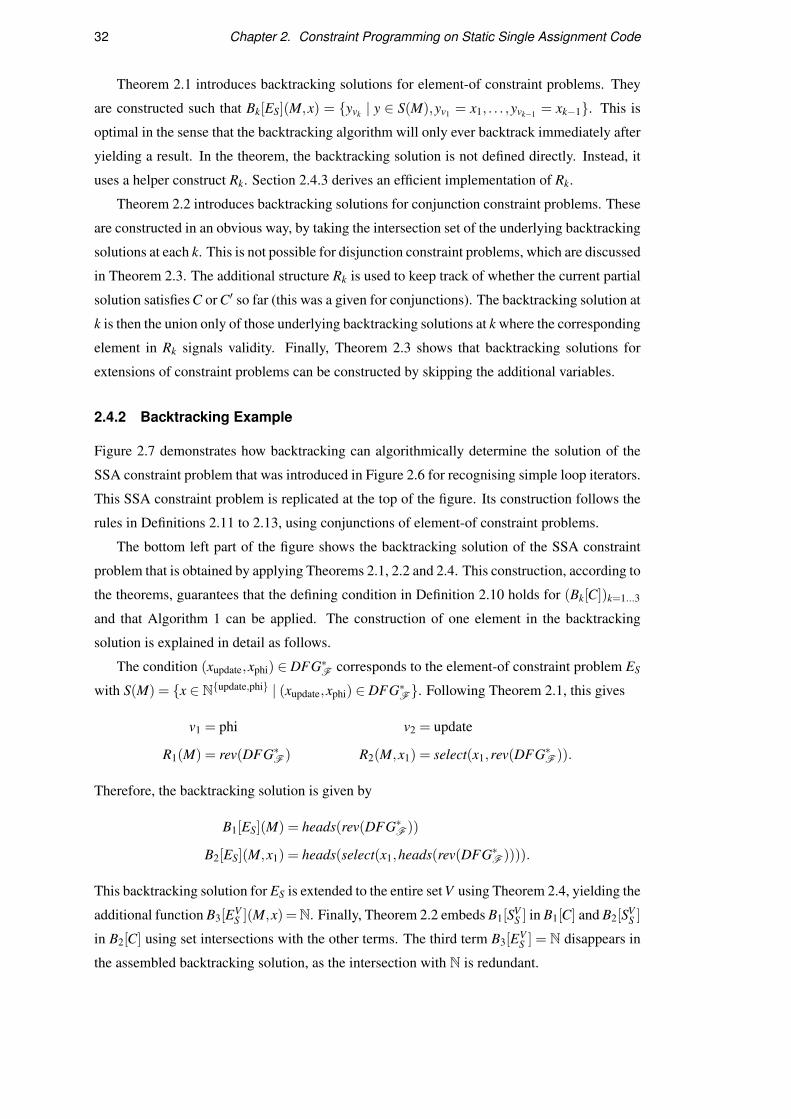
32 Chapter 2. Constraint Programming on Static Single Assignment Code
Theorem 2.1 introduces backtracking solutions for element-of constraint problems. They
are constructed such that Bk[ES](M,x) = {yvk | y ∈ S(M),yv1 = x1, . . . ,yvk−1 = xk−1}. This is
optimal in the sense that the backtracking algorithm will only ever backtrack immediately after
yielding a result. In the theorem, the backtracking solution is not defined directly. Instead, it
uses a helper construct Rk. Section 2.4.3 derives an efficient implementation of Rk.
Theorem 2.2 introduces backtracking solutions for conjunction constraint problems. These
are constructed in an obvious way, by taking the intersection set of the underlying backtracking
solutions at each k. This is not possible for disjunction constraint problems, which are discussed
in Theorem 2.3. The additional structure Rk is used to keep track of whether the current partial
solution satisfies C or C′ so far (this was a given for conjunctions). The backtracking solution at
k is then the union only of those underlying backtracking solutions at k where the corresponding
element in Rk signals validity. Finally, Theorem 2.3 shows that backtracking solutions for
extensions of constraint problems can be constructed by skipping the additional variables.
2.4.2 Backtracking Example
Figure 2.7 demonstrates how backtracking can algorithmically determine the solution of the
SSA constraint problem that was introduced in Figure 2.6 for recognising simple loop iterators.
This SSA constraint problem is replicated at the top of the figure. Its construction follows the
rules in Definitions 2.11 to 2.13, using conjunctions of element-of constraint problems.
The bottom left part of the figure shows the backtracking solution of the SSA constraint
problem that is obtained by applying Theorems 2.1, 2.2 and 2.4. This construction, according to
the theorems, guarantees that the defining condition in Definition 2.10 holds for (Bk[C])k=1...3
and that Algorithm 1 can be applied. The construction of one element in the backtracking
solution is explained in detail as follows.
The condition (xupdate,xphi) ∈ DFG∗F corresponds to the element-of constraint problem ES
with S(M) = {x ∈ N{update,phi} | (xupdate,xphi) ∈ DFG∗F}. Following Theorem 2.1, this gives
v1 = phi v2 = update
R1(M) = rev(DFG∗F ) R2(M,x1) = select(x1,rev(DFG∗F )).
Therefore, the backtracking solution is given by
B1[ES](M) = heads(rev(DFG∗F ))
B2[ES](M,x1) = heads(select(x1,heads(rev(DFG∗F )))).
This backtracking solution for ES is extended to the entire set V using Theorem 2.4, yielding the
additional function B3[EVS ](M,x) =N. Finally, Theorem 2.2 embeds B1[SV
S ] in B1[C] and B2[SVS ]
in B2[C] using set intersections with the other terms. The third term B3[EVS ] = N disappears in
the assembled backtracking solution, as the intersection with N is redundant.

2.4. Solving SSA Constraint Problems 33
Original SSA Constraint Problem
V = {phi,update,step}
C(M,x) = ((1,xstep) ∈CF ∧ (add,xupdate) ∈ IF ∧
(xphi,xupdate) ∈ DFG∗F ∧ (xstep,xupdate) ∈ DFG∗F ∧
(xupdate,xphi) ∈ DFG∗F ∧ (phi,xphi) ∈ IF )
Backtracking Solution:k = 1 v1 = phi
B1[C](M) = heads(DFG∗F )
∩ heads(rev(DFG∗F ))
∩ heads(select(phi, IF ))
k = 2 v2 = update
B2[C](M,x) =
heads(select(add, IF ))
∩ heads(select(x1,DFG∗F ))
∩ heads(rev(DFG∗F ))
∩ heads(select(x1,rev(DFG∗F )))
k = 3 v3 = step
B3[C](M,x) = select(1,CF )
∩ heads(select(x2,rev(DFG∗F )))
Backtracking Algorithm:x = ()
B1[C](M) = {6,9,10}
↓ ↓ ↓x = (6)
B2[C](M,6)
=
{}
backtrack!
x = (9)
B2[C](M,9)
=
{17}
↓
x = (10)
B2[C](M,10)
=
{}
backtrack!x = (9,17)
B3[C](M,9,17) = {22}
↓x = (9,17,22)
Figure 2.7: Backtracking is used to find the single solution of the SSA constraint problem forsimple loop iterators from Figure 2.6. The backtracking solution (Bk[C])k=1...3 is constructed withTheorems 2.1, 2.2 and 2.4. The partial solution x is extended in three steps, from top to bottom.
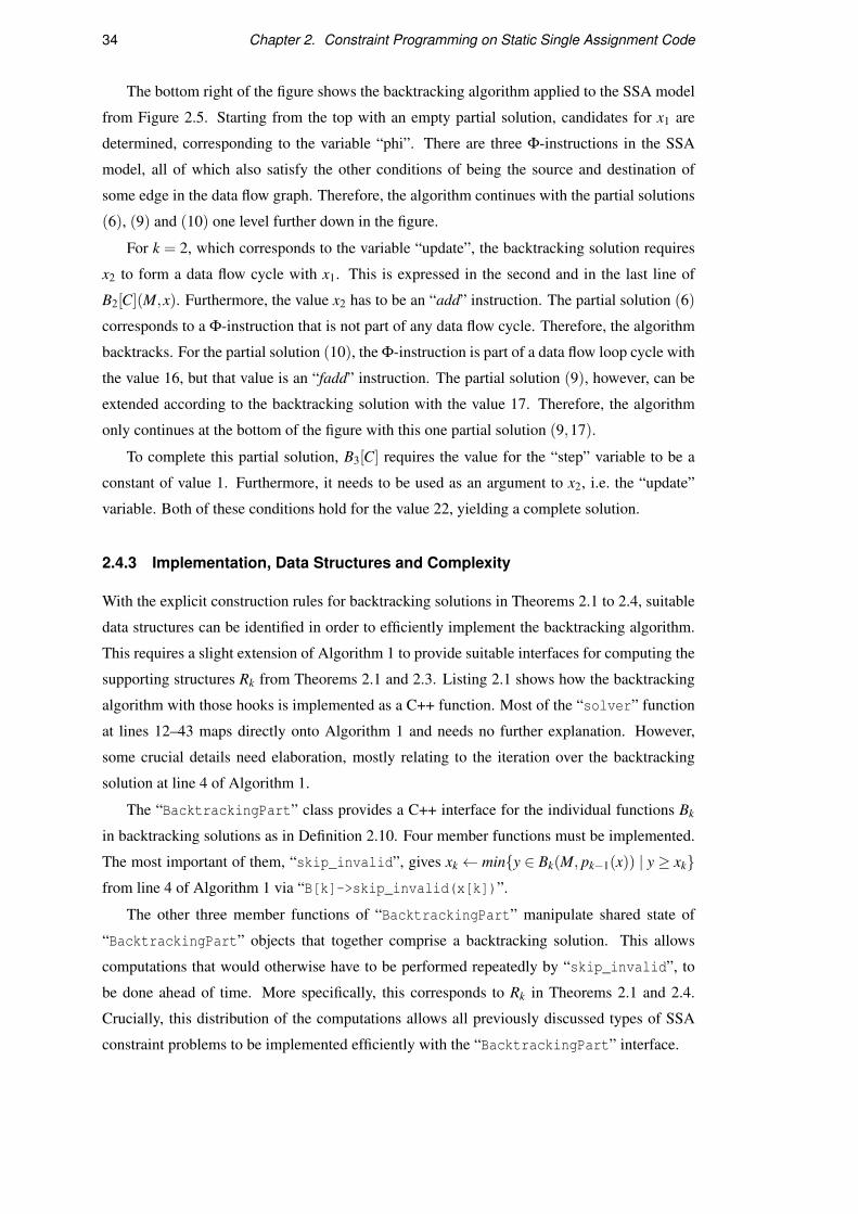
34 Chapter 2. Constraint Programming on Static Single Assignment Code
The bottom right of the figure shows the backtracking algorithm applied to the SSA model
from Figure 2.5. Starting from the top with an empty partial solution, candidates for x1 are
determined, corresponding to the variable “phi”. There are three Φ-instructions in the SSA
model, all of which also satisfy the other conditions of being the source and destination of
some edge in the data flow graph. Therefore, the algorithm continues with the partial solutions
(6), (9) and (10) one level further down in the figure.
For k = 2, which corresponds to the variable “update”, the backtracking solution requires
x2 to form a data flow cycle with x1. This is expressed in the second and in the last line of
B2[C](M,x). Furthermore, the value x2 has to be an “add” instruction. The partial solution (6)
corresponds to a Φ-instruction that is not part of any data flow cycle. Therefore, the algorithm
backtracks. For the partial solution (10), the Φ-instruction is part of a data flow loop cycle with
the value 16, but that value is an “fadd” instruction. The partial solution (9), however, can be
extended according to the backtracking solution with the value 17. Therefore, the algorithm
only continues at the bottom of the figure with this one partial solution (9,17).
To complete this partial solution, B3[C] requires the value for the “step” variable to be a
constant of value 1. Furthermore, it needs to be used as an argument to x2, i.e. the “update”
variable. Both of these conditions hold for the value 22, yielding a complete solution.
2.4.3 Implementation, Data Structures and Complexity
With the explicit construction rules for backtracking solutions in Theorems 2.1 to 2.4, suitable
data structures can be identified in order to efficiently implement the backtracking algorithm.
This requires a slight extension of Algorithm 1 to provide suitable interfaces for computing the
supporting structures Rk from Theorems 2.1 and 2.3. Listing 2.1 shows how the backtracking
algorithm with those hooks is implemented as a C++ function. Most of the “solver” function
at lines 12–43 maps directly onto Algorithm 1 and needs no further explanation. However,
some crucial details need elaboration, mostly relating to the iteration over the backtracking
solution at line 4 of Algorithm 1.
The “BacktrackingPart” class provides a C++ interface for the individual functions Bk
in backtracking solutions as in Definition 2.10. Four member functions must be implemented.
The most important of them, “skip_invalid”, gives xk ← min{y ∈ Bk(M, pk−1(x)) | y ≥ xk}from line 4 of Algorithm 1 via “B[k]->skip_invalid(x[k])”.
The other three member functions of “BacktrackingPart” manipulate shared state of
“BacktrackingPart” objects that together comprise a backtracking solution. This allows
computations that would otherwise have to be performed repeatedly by “skip_invalid”, to
be done ahead of time. More specifically, this corresponds to Rk in Theorems 2.1 and 2.4.
Crucially, this distribution of the computations allows all previously discussed types of SSA
constraint problems to be implemented efficiently with the “BacktrackingPart” interface.

2.4. Solving SSA Constraint Problems 35
1 // This class corresponds to Definition 2.10.2 class BacktrackingPart {3 public:4 virtual SkipResult skip_invalid(unsigned& c) = 0;5 virtual void begin() = 0;6 virtual void fixate(unsigned c) = 0;7 virtual void resume() = 0;8 };9
10 void yield(const vector<unsigned>& solution);11
12 // This function corresponds to Algorithm 1.13 void solver(vector<BacktrackingPart*> B) {14 unsigned k = 0;15 vector<unsigned> x(B.size(), 0);16 while(true) {17 SkipResult result = B[k]->skip_invalid(x[k]);18 if(result == SkipResult::CHANGE) continue;19 if(result != SkipResult::FAIL) {20 if(k + 1 == B.size())21 {22 yield(x);23 B[k]->resume();24 x[k]++;25 }26 else {27 B[k]->fixate(x[k]);28 k++;29 [k]->begin();30 x[k] = 0;31 }32 }33 else {34 if(k > 0) {35 k = k - 1;36 B[k]->resume();37 x[k] = x[k] + 1;38 }39 else40 return;41 }42 }43 }
Listing 2.1: Complete C++ implementation of Algorithm 1: The if-else statements at lines 19–41precisely correspond to those at lines 5–17 of the algorithm. The “BacktrackingPart” objectsiterate over Bk[C](M,x) via the “skip_invalid” method. The remaining member functioncalls at lines 23,27,29,36 precompute structures used in “skip_invalid” for quick evaluation.

36 Chapter 2. Constraint Programming on Static Single Assignment Code
2.4.3.1 Data Structures for Constraint Classes
Element-of constraint problems require the structures Rk. These can be implemented with
a tree, built around a sorted array of pairs, as shown with the definition of “Tree” on the first
line of the top section of Listing 2.2. Each subtree in the array corresponds to a potential Rk+1.
The instances of “BacktrackingPart” for this constraint keep an index (line 25) into the array
(line 3), which “begin” initialises (line 18). Each time “skip_invalid” is called, the index is
incremented until it either points to an entry ≥ the lower bound c or hits the end of the array
(lines 9–10). Finally, “resume” does nothing (line 22), and “fixate” simply accesses the array
at the current index for the subtree Rk+1 (lines 20–21).
Conjunction constraint problems are simpler to implement, as shown in the lower section
of Listing 2.2. The methods “begin”, “fixate”, and “resume” call the corresponding member
functions of the underlying BacktrackingPart objects (line 20), and “skip_invalid” checks
both of them with short-circuit evaluation in case of a “FAIL” result.
Disjunction constraints again require the structures Rk, consisting of an array of booleans,
with each element corresponding to an underlying constraint option. Calls to “skip_invalid”
are passed on to those underlying “BacktrackingPart” objects that are not disabled via Rk. If
any succeed, then the smallest resulting value among them is selected. The “fixate” function
determines Rk+1 with “skip_invalid”, disabling all of the underlying constraint options that
do not return “PASS”. The “begin”, “fixate” and “resume” member calls are additionally
passed on to all “BacktrackingPart” instances that are enabled in Rk.
2.4.3.2 Computational Complexity
The chosen data structures allow for efficient implementations of the individual functions that
are used to search for solutions. However, SSA constraint problems are a generalisation of the
subgraph isomorphism problem. Any subgraph can be specified using conjunctions of element-
of constraints, and the solver will search for these within any provided SSA model. Cook [34]
showed that this problem is NP-hard [35]. Therefore, the computational complexity has an
exponential worst case (in the number of variables) when evaluated in general.
The exponential worst case is no impediment in practice due to the particular use case of
SSA constraint problems. The nature of SSA constraint problems means that the same limited
set of formulas is repeatedly solved in the context of many different SSA models. Therefore,
it is viable to tune the formulas ahead of solving time to be efficiently solvable, in particular
by choosing a good order in which to iterate over the variables. For specific SSA constraint
problems, it can then be possible to make complexity assumptions.

2.4. Solving SSA Constraint Problems 37
1 struct Tree { vector<pair<int,Tree>> t; };2 template<int n> // These are S(M) and (Rk(M,x))k=1...n in Theorem 2.1.3 struct ElementOfShared { Tree S; array<Tree*,n> R; };4
5 template<int n, int k>6 class ElementOfPart : public BacktrackingPart {7 public:8 SkipResult skip_invalid(unsigned& c) override {9 while(index < shared ->R[k]->t.size()
10 && c > shared ->R[k]->t[index].first) index++;11 if(index == shared ->R[k]->t.size())12 return SkipResult::FAIL;13 if(shared ->R[k]->t[index].first == c)14 return SkipResult::PASS;15 c = shared ->R[k]->t[index].first;16 return SkipResult::SUCCESS;17 }18 void begin() override { index = 0;19 if(k == 0) shared ->R[k] = &shared ->S; }20 void fixate(unsigned) override {21 if(k < n) shared ->R[k+1] = &shared ->R[k][index]; }22 void resume() override {}23 private:24 shared_ptr<ElementOfShared<n>> shared;25 size_t index;26 };
1 class ConjunctionPart : public BacktrackingPart {2 public:3 SkipResult skip_invalid(unsigned& c) {4 SkipResult r1 = parts[0]->skip_invalid(c);5 if(r1 == SkipResult::FAIL) return r1;6 if(r1 == SkipResult::CHANGE) return r1;7 SkipResult r2 = parts[1]->skip_invalid(c);8 if(r2 == SkipResult::FAIL) return r2;9 if(r2 != SkipResult::PASS)
10 return SkipResult::CHANGE;11 return r1;12 }13 void begin() override {14 for(auto part: parts) part ->begin(); }15 void fixate(unsigned c) override {16 for(auto part: parts) part ->fixate(c); }17 void resume() override {18 for(auto part: parts) part ->resume(); }19 private:20 array<shared_ptr<BacktrackingPart>,2> parts;21 };
Listing 2.2: “BacktrackingPart” is implemented for element-of constraints and conjunctionconstraints. The array “R” in “ElementOfShared” matches (Rk(M,x))k=1...n from Theorem 2.1.

38 Chapter 2. Constraint Programming on Static Single Assignment Code
2.4.4 Additional SSA Constraint Problems
Beyond Definitions 2.11 to 2.13, there are a number of supplementary construction rules for
SSA constraint problems that are used in this thesis. Firstly, there are simple SSA constraint
problems that operate directly on the integer values, without interpreting them as indices into
the value list of the SSA model. These are listed in Definition 2.14. The first two, ({a,b},C=)
and ({a,b},C 6=), enforce equality and inequality of the integer values, respectively. The third,
({a},Cunused), prevents the assignment of values from the SSA model to the variable. This is
convenient only in disjunctions, for parts of solutions that may be omitted. For example, an
offset may be optionally added when accessing an element in a structure. If the offset is not
present, the corresponding variable is unused in that constraint solution. The value Rval +1 is
the smallest integer that cannot be used as an index into the list of used values.
Generalised graph domination constraint problems as in Definition 2.15 are versatile tools
for analysing SSA models. The special case of |Orig| = |Dom| = |Dest| = 1, with xv for
the unique v ∈ Orig restricted to the control origin of the function, turns this definition into
the established control flow domination concept. However, the generalisation encompasses a
much larger set of interesting conditions. Importantly, generalised graph domination can also
be applied to data flow, which Chapter 5 uses for defining kernel functions with restricted
interfaces. In this interpretation, the set Dom represents an interface to the computation of the
values in Dest, when data flow can originate from all the values in Orig.
The backtracking solution of generalised graph domination constraint problems is brute-
force, meaning that Bn[DG] checks the condition as specified, and Bk[DG]≡N for all 1≤ k < n.
The checking of the condition in Bn[DG] is typically performed in O(|val|) time, making this
a computationally expensive constraint. The solver relies on this construction occurring only
in conjunctions with other, more restrictive constraints. In addition, special cases can also be
implemented as element-of constraint problems by pre-computing dominator trees.
Finally, collect-all constraint problems are introduced in Definition 2.16. Given a constraint
problem (V,C), the variables V are divided into two subsets. The collect-all constraint problem
identifies all possible solutions over one of the variable subsets, given that the other variable
subset is fixed. The parameter n gives an upper limit to the number of these solutions, which is
required to maintain a finite number of variables. Such collect-all constraint problems are used
to approximate logical quantifiers. This is discussed in more detail in Chapter 4.
In order to efficiently calculate a backtracking solution of collect-all constraint problems,
the enumeration of V 〈U,n〉 must satisfy the ordering u< (k,v) for all u∈U,k = 1 . . .n,v∈V \U .
For values in U , the backtracking solution is the same as for the underlying constraint (V,C).
Whenever a partial solution is determined for all variables in U , an invocation to the full solver
is performed that identifies all possible partial solutions over V \U . The remaining steps of the
backtracking solution merely enforce this pre-computed list of solutions.

2.4. Solving SSA Constraint Problems 39
Definition 2.14: Simple Integer Constraint Problems
The SSA constraint problems ({a,b},C=), ({a,b},C 6=), and ({a},Cunused) are given by
C=(M,x) = 1 ⇐⇒ xa = xb
C 6=(M,x) = 1 ⇐⇒ xa 6= xb
Cunused(M,x) = 1 ⇐⇒ xa = Rval +1.
Definition 2.15: Generalised Graph Domination Constraint Problem
Given a graph G(M) ⊂ N2, a set of variables V , a set of origins Orig ⊂ V , a set of
generalised dominators Dom ⊂ V , and a set of destinations Dest ⊂ V , the generalised
graph domination constraint problem (V,DG) is defined by
DG(M,x) = 1 ⇐⇒ (xv /∈ R∞(M,x) for all v ∈ Dest with Lval ≤ xv ≤ Rval),
where Rk(M,x)⊂ N, the set of vertices reachable in k steps, is defined as
R0(M,x) = {xv | v ∈ Orig}\{xv | v ∈ Dom}
Rk+1(M,x) = {b | (a,b) ∈ G(M),a ∈ Rk(M,x)}\{xv | v ∈ Dom}
R∞(M,x) =⋃
∞k=0 Rk(M,x).
Definition 2.16: Collect-all Constraint Problem
Given a set of variables V , a subset U ⊂V , and some n≥ 1, the set containing one copy
of each variable in U and n copies of each value in V \U is denoted
V 〈U,n〉 =U ∪ ({1, . . . ,n}× (V \U)).
For any r ∈ NU , the set of constraint solutions restricted to r in NU is defined as
SM(V,C)|r = {x ∈ SM(V,C) | xu = ru for all u ∈U}.
The functions fk : NV 〈U,n〉 →NV and g : NV 〈U,n〉 →NU are defined as selecting the values
for the kth copy of variables in V \U and directly projecting on NU .
For an SSA constraint problem (V,C), the collect-all constraint problem (V 〈U,n〉,C〈U,n〉)
is uniquely defined by the following conditions:
C〈U,n〉(M,x) = 1 ⇐⇒∣∣SM(V,C)|g(x)
∣∣≤ n
∧{
fk(x) | 1≤ k ≤∣∣SM(V,C)|g(x)
∣∣}= SM(V,C)|g(x)∧ fk(x)≡ Rval +1 for all k >
∣∣SM(V,C)|g(x)∣∣
∧ pn( f1(x)), . . . , pn( fn(x)) are in lexicographic order.

40 Chapter 2. Constraint Programming on Static Single Assignment Code
2.4.5 Satifiability Modulo Theory
There are some parallels between SSA constraint problems and other satisfiability problems,
most importantly, Satisfiability Modulo Theory (SMT). Both methods construct formulas via
constraints on variables that are combined with logical connectors, and backtracking is in both
cases used as the basis for developing efficient solvers. This suggests that it could be possible to
recast SSA constraint problems in the language of SMT. Where typical SMT problems might
be formulated on the theory of linear arithmetic or the theory of bit-vectors, SSA constraint
problems would operate on the theory of SSA intermediate representation. Powerful solvers
have been developed for SMT problems over the last decade, making this appear worthwhile.
However, the structure and usage scenario of SSA constraint problems make them unfitting
for this approach. The contextual nature of SSA constraint problems means that the constraint
formulation in SMT would have to encode also the graph structure of the SSA function as
context. This encoding is non-trivial and would introduce significant overhead.
Furthermore, one SSA constraint problem is typically evaluated with many different SSA
function contexts, but an off-the-shelf SMT solver has no way of leveraging this knowledge.
SSA constraint problems are crafted by hand, and some manual tuning is acceptable to enable
quick solving times. In particular, the backtracking order for variables can be adjusted. Thus, it
is a requirement for the solver to have consistently good performance across all SSA function
contexts, but not necessarily across every possible constraint formula. Instead, it can dictate
specific programming styles. The solver relying on such pre-processed formulas makes most
of the sophisticated optimisations that are crucial for SMT redundant.
2.5 Summary
The chapter introduced an approach for applying constraint programming to SSA intermediate
representation code. Based on a mathematical characterisation of the static structure of SSA
functions, SSA constraint problems were defined. These are formulas that impose restrictions
on compiler intermediate code, turning the detection of adhering program parts into a constraint
satisfiability problem. The chapter derived efficient algorithms for solving such SSA constraint
problems and discussed several significant types of constraint formulas, reflecting compiler
analysis methods like data flow and dominator relationships.
Outlook Constraint programming on SSA intermediate representation forms the principal
methodological basis of this thesis. Chapters 4 and 5 refer back to the definitions in this chapter
for designing and implementing the languages CAnDL and IDL, which integrate constraint
programming on SSA code into LLVM. Preceding that, the following chapter provides a review
of related literature, putting the work into a broader context.

Chapter 3
Related Work
Four areas of research are of particular relevance to this thesis: Constraint programming
and specification languages are central to the introduced methodology. The relevant literature
includes the research into constraint programming in the context of program analysis and the
design of specification languages. The survey of previous approaches to compiler analysis and
auto-parallelisation establishes the baselines for the later evaluation sections. Related work
on heterogeneous computing motivates the proposed approaches, by presenting the plethora
of other programming paradigms to overcome the specific challenges of emerging hardware.
Lastly, the diverse research landscape around concepts related to computational idioms puts
the algorithmic structures that are detected in later chapters of this thesis into context.
3.1 Constraint Programming and Specification Languages
Declarative Languages, constraint programming, and the application of constraints to program
analysis problems are well-established in the literature. Previous work covers query languages,
logic programming, applications to software security and formal verification, model checking
and SMT, but also more compiler-centric data flow analysis and type inference problems. The
limited scope of this section requires a focus on work that is particularly relevant to this thesis.
For this research, constraint programming is most interesting within the context of research
fields such as program analysis and model checking. Crucial background material for this thesis
also comes from the programming language design community of declarative programming
languages. Prolog and its many extensions and dialects particularly stand out as fully fledged
logic programming languages, but parallels can also be drawn to querying languages that apply
database techniques to static analysis.
These different fields vary significantly in their interests, motivations, and approaches, but
the underlying challenges are often similar. Notably, the performance of backtracking solvers
and the scalability to complex problems are a recurring theme.
41
42 Chapter 3. Related Work
3.1.1 Constraint Programming for Program Analysis
Constraint analysis on abstract languages Constraint systems have long been used for
program analysis. Aiken [36] gives a comprehensive overview of earlier work, highlighting the
crucial ability of constraint-based program analysis to separate constraint specification from
constraint resolution. This separation is critical also for this thesis, as it enables the scalability
of compiler analysis problems beyond what could reasonably be implemented with manual
recognition routines. The constraint specification can be formulated briefly, by offloading the
constraint resolution to a separate solver. However, the article does not present any techniques
to capture higher-level algorithmic concepts like computational idioms. Instead, it focuses on
more basic compiler analysis problems, such as data flow analysis and type inference.
More recent work on constraint-based program analysis by Gulwani et al. [37] leverages
the advancements in modern off-the-shelf SAT/SMT solver technology. The analysis problems
are lowered to bit-vector formulations, and the constraint resolution is entirely externalised
to independently developed SMT solvers. The motivation of the approach is mainly to verify
program properties, as opposed to the application of parallelising code transformation in this
thesis. Furthermore, Section 2.4.5 showed that the confinement to conventional SMT solvers
is inefficient for the resolution of SSA constraint problems.
Kundu et al. [38] propose constraints to verify the correctness of program transformations
with their system for Parameterized Equivalence Checking (PEC). This system improves on
previous work performing translation validation. Translation validation is the validity checking
of transformations on concrete input programs by comparing the semantics before and after
modification. PEC implements a hybrid approach that allows some aspects of the program
to be underspecified, yet does not check the soundness of transformations in full generality.
The checking is done via a custom solver for the generated constraint problems. The hybrid
nature allows the system also to validate program transformations that significantly modify the
control flow, e.g. loop unswitching. The system cannot discover transformation opportunities,
only verify them after the transformation was applied.
Constraint analysis on compiler IR code There is previous work on using constraint-based
program analysis for real compiler intermediate representations, mostly in the area of security
and the formal verification of software systems. This includes investigations into using SMT
on LLVM intermediate representation, which is also used for the implementations in this thesis.
Zhao et al. [39] built a model of LLVM IR for such solvers. However, this model serves an
entirely different purpose to the SSA model of this thesis. The model provides operational
semantics, but cannot be used to detect large-scale algorithmic structures in user programs, as
is required for automatic heterogeneous acceleration. Instead, the focus is on formally verifying
the correctness of existing compiler transformations for all possible user input.

3.1. Constraint Programming and Specification Languages 43
Recent domain-specific languages, such as Alive [40], operate on subsets of LLVM IR.
The individual instructions are reformulated on bit-vectors, and the correctness of conditions
is checked with an SMT solver. Alive only implements a subset of LLVM’s integer and pointer
arithmetic instructions. It has no support for control flow and does not scale to the applications
that are used in this thesis for evaluation. Instead, it is designed for formally verifying already
existing compiler optimisations that operate on only a handful of integer instructions at a time.
Alive is meant to improve compilers, not user programs.
LifeJacket [41] proves the correctness of floating-point optimisations in LLVM, as does
Alive-FP [42]. Both of these projects are extensions of the SMT-based Alive system. They
extend the scope of the system to model a wider range of instructions as bit-vectors, enabling
the verification of more compiler optimisations. LifeJacket and Alive-FP were successfully
used to identify wrongly implemented optimising transformations in compilers. Nonetheless,
the fundamental limitations of Alive remain, and control flow is not supported. Therefore, only
peephole optimisations can be evaluated by these approaches.
The Alive-Infer system [43] also builds on Alive but goes beyond the verification of existing
compiler optimisations. The tool uses an SMT solver to automatically generate preconditions
that need to hold for transformations to be applied. This moves the Alive system away from
verifying optimisations and closer to automatically detecting algorithmic structure in parts
of user programs. However, Alive-Infer still requires the separate specification of the actual
transformation. It only generates additional conditions and does not handle control flow.
Constraint analysis on other program models Other advanced approaches to extracting
high-level code structures from programs that use constraints and verification systems have
been proposed. Mendis et al. [44], Kamil et al. [45] suggest temporal logic as the foundation to
formulate the necessary conditions for rephrasing well-structured Fortran and assembly code
in restrictive models. These techniques leverage counter-example guided inductive synthesis
to find provably correct translations into the high-level Halide language. The Halide compiler
specialises the code again, exploring the optimisation space via powerful transformations that
are enabled by its restrictive semantics. The focus is on a small class of computations with only
dense memory accesses. This allows formal reasoning about correctness but is too restrictive
for interesting computational idioms, such as sparse linear algebra.
Mullen et al. [46] study low-level program transformations that are implemented for the
formally verified CompCert compiler [47], directly on x86 assembly. Instead of an automatic
verification after modelling optimisations as SMT problems, the presented Peek system was
checked with the interactive theorem prover Coq. This required approximately 30000 lines of
manually written Coq code and proof lines. Some of the transformations consider rudimentary
control flow constraints, but they cannot scale to computational idioms.

44 Chapter 3. Related Work
3.1.2 Declarative Programming Languages for Program Analysis
Languages for querying program properties From the perspective of language design, the
declarative programming languages Prolog and SQL are perhaps most influential. The two
languages differ fundamentally. Prolog (“programmation en logique”) is a logic programming
language that originated in academia for analysing natural language [48]. By contrast, SQL
(“Structured Query Language”) was developed at IBM for managing data in relational database
management systems [49]. Nonetheless, specification languages for structures in program code
have been designed taking inspiration from both backgrounds.
The first such specification language was the Omega system by Linton [50]. It uses a
relational database to store all the relevant properties of a program. The captured information
is based on the abstract syntax tree of programs that are implemented in a subset of the Ada
programming language. Additional edges are inserted to connect shared variables of successive
expressions, given some indication of data flow between instructions. The system then allows
database-style queries formulated in QUEL [51], an SQL-style language.
The CodeQuest system [52] first combined the ideas of Omega and its database-oriented
successors with the use of logic programming. The queries are translated into Datalog, a Prolog
derivative that is implemented on top of SQL. This allows CodeQuest to be fundamentally
more expressive, allowing recursive queries that are required for meaningful CFG inspection.
Nevertheless, the approach is based on querying for source language features. This makes the
detection of large-scale algorithmic structures in complex programming languages such as C++
infeasible, as demonstrated in Section 6.4.
Languages for generating compiler passes Custom specification languages for generating
compiler analysis and transformation passes have been presented in the literature. Martin [53]
introduced a specification language for program analysis functionality called PAG, based on
abstract interpretation. The generated functionality was integrated into C and Fortran compilers
via a well-specified interface and applied successfully to real benchmark codes. However, the
tool is focused on relatively simple compiler optimisations such as constant propagation.
Domain-specific languages for compiler transformation passes were also studied by Olmos
and Visser [54]. The proposed Stratego system uses rewrite rules to apply tree transformations
to the abstract syntax tree of source programs. However, this was only evaluated on the Octave
language, and the general applicability on large-scale programs remains unclear.
Lipps et al. [55] designed the domain-specific language OPTRAN for matching patterns
in attributed abstract syntax trees of Pascal programs. Semantically equivalent, more efficient
implementations can then automatically replace the matching code patterns. With the focus on
Pascal, it remains unclear how the proposed concepts translate to the complex C++ programs
with pointer calculations that were used for the evaluation of this thesis.

3.2. Compiler Analysis and Auto-Parallelisation 45
Another language for implementing compiler optimisations from declarative specifications
is OPTIMIX [56, 57]. Similarly to the presented work in Chapter 4, OPTIMIX emphasises
developer productivity. The system is based on graph rewrite rules. OPTIMIX programs
are compiled into C code that performs the specified transformation. Such a domain-specific
language for the generation of optimisation transformations was also used in the CoSy compiler
[58]. Both OPTIMIX and the CoSy method are simple rewrite engines that have no knowledge
of global program constraints.
Different code transformation techniques use LibASTMatchers and LibTooling [59] from
the LLVM project. These tools do not provide a complete standalone language but are instead
implemented in C++ as an embedded domain-specific language for pattern matching, relying
heavily on other LLVM libraries. The approach is deeply integrated with the Clang compiler
and exposes the abstract syntax tree (AST) of the compiler frontend directly. There are more
than a thousand separate classes that implement types of AST nodes in Clang, introducing
considerable complexity for any non-trivial pattern. Therefore, this is an entirely impractical
approach for detecting complex algorithmic structures such as computational idioms.
Willcock et al. [60] designed a complex system for generating generic optimisation passes
using concepts from generic programming. However, such schemes do not work at the IR level
of established compiler frameworks. Instead, they require program rewrites by the user.
Whitfield and Soffa [61] praise Gospel, their framework and specification scripture for
the exploration of the properties of code-improving transformations. The project furthermore
includes the Genesis tool, which automatically generates transformers as specified in Gospel.
Several standard optimisations were implemented with Gospel and Genesis, such as constant
folding and common subexpression elimination. Similar approaches to generating compiler
optimisations from specification languages include Rhodium [62]. The language expresses
optimisations using explicit data flow facts, which are manipulated by local propagation and
transformation rules. The transformations are applied to a custom intermediate language and
can be proven correct with a theorem prover. Neither Gospel nor Rhodium provides means to
tackle the issue of efficiently enabling large-scale program transformations.
3.2 Compiler Analysis and Auto-Parallelisation
The core motivation for the work in this thesis is the automatic heterogeneous parallelisation
of sequential code. The derived methods are evaluated on two metrics: how broadly they apply
to real code, and how significant their performance impact is when applied. These metrics are
evaluated against other compiler analysis and parallelisation approaches. This section focuses
on three areas of the vast research landscape that are particularly relevant for this: polyhedral
compilation, the parallelisation of reductions, and dynamic approaches.
46 Chapter 3. Related Work
3.2.1 Compilation with the Polyhedral Model
The polyhedral model [27] is an established mathematical framework for modelling, analysing,
and transforming well-behaved loop nests. Iterations in loop nests are treated as lattice points
in a multi-dimensional grid. The iteration space can then be transformed with affine maps,
potentially uncovering new parallelisation opportunities. This basic approach has been applied
extensively in compilers. Furthermore, the required conditions have been relaxed in different
ways, allowing the application of the approach to more input code.
Polly in LLVM Polyhedral optimisers have been integrated into mainstream C/C++ compilers.
Most notably, Grosser et al. [26] implemented the Polly extensions for LLVM. Polly recognises
parts of LLVM IR that are expressible in the polyhedral model and transforms them into that
representation. Polyhedral optimisations can then be applied with PLuTo [63] before the model
is translated back into optimised LLVM IR for further treatment by the core compiler. This
enables the seamless application of polyhedral techniques on large-scale applications without
source code changes via the many frontends of the LLVM infrastructure. However, this impacts
only code that the tool can translate into a polyhedral representation.
Polly-ACC [64] is an extension of the Polly compiler that provides code generation for
heterogeneous hardware. The tool uses the recognition functionality of standard Polly to detect
code sections in LLVM IR that can be represented in the polyhedral model. These code sections
are optimised with established polyhedral transformation techniques from Grosser et al. [26].
The optimised polyhedral code sections are then translated into CUDA code to be executed
on the GPU. This results in significant speedups of some benchmark programs, but the impact
remains limited to code that fits the polyhedral model.
Doerfert et al. [30] extended the applicability of polyhedral transformations within the Polly
compiler to a broader set of input programs. Dependencies between iterations that originate
from reduction variables cannot be eliminated with affine transformations. Therefore, they
prohibit DOALL parallelism in a way that standard Polly is unable to resolve. By contrast, the
reduction-enabled scheduling approach for Polly can parallelise such loop despite the reduction
dependencies. This ability significantly improved the achieved speedup of Polly on benchmark
programs that contain reductions.
Doerfert et al. [65] also investigated another method for widening the scope of polyhedral
code transformations. This approach allows some conditions that are required for the legal
application of transformations to remain unproven at compile time. These conditions are then
checked at runtime, providing a fallback to the original code when assumptions are not met.
The checks that this work allows to be delayed include the absence of aliasing, finite loop
boundaries, and in-bounds memory accesses. This enabled Polly to cover 3.9× as many loops
in the SPEC and NPB benchmarks at a negligible runtime overhead.

3.2. Compiler Analysis and Auto-Parallelisation 47
Other tools with automatic detection The Polyhedral Parallel Code Generator (PPCG) [66]
is a source-to-source compiler that takes sequential C programs and generates optimised CUDA
kernels to target GPU acceleration. The extraction of polyhedral code sections from the C input
is based on the Polyhedral Extraction Tool [67]. This extraction system can automatically
detect relevant code regions, but it is implemented on syntax level and relies on purpose-built
C code with all arrays declared in variable-length C99 array syntax. This is not robust enough
to reliably cover larger programs from benchmark collections such as NPB or Parboil, which
are used for evaluation in this thesis.
C-to-CUDA [68] is another compiler that offers heterogeneous acceleration of sequential
C code by representing it in the polyhedral model. However, the focus is on code generation
and the application of optimising transformations. The automatic recognition in the abstract
syntax tree of parallel loops that can be represented in the polyhedral model remains ad-hoc
and handles only a small set of benchmarks.
Increased applicability of polyhedral transformations Recent work by Baghdadi et al. [69]
has extended the polyhedral model beyond affine programs to some forms of sparsity. This is
implemented in the Platform-Neutral Compute Intermediate Language, which is intended for
heterogeneous systems and provides backends for accelerator programming. The platform
provides extensions that can be used to model important features of sparse linear algebra, such
as counted loops [70]. Such loops have dynamic, memory dependent bounds but statically
known strides and are central to sparse linear algebra.
Tiramisu [71] is a polyhedral framework for targeting heterogeneous hardware, providing
backends for CPUs, GPUs, distributed architectures, and FPGAs. Optimisations are performed
on four layers of intermediate representation, resulting in performance that almost matches
dedicated library functions. However, the tool does not detect polyhedral code sections within
existing source code. Instead, it requires the programmer to implement the algorithms manually
with a dedicated C++ API.
Zhang et al. [72] studied the extension of polyhedral approaches to allow the capturing
of some sparse linear algebra calculations in the polyhedral model. The article introduces a
novel non-affine split transformation for this purpose. Using the inspector-executor model, the
approach achieved significant speedups when evaluated on some benchmark programs. The
research does not address the automatic recognition of sparse linear algebra routines within
existing programs. Besides, the approach was not evaluated against state-of-the-art library
implementations such as Intel MKL and cuSPARSE.
Many approaches have been proposed for parallelising loop nests with reduction variables
in the polyhedral model, among them Jouvelot and Dehbonei [73], Redon and Feautrier [74],
Chi-Chung et al. [75], Gupta and Rajopadhye [76], Stock et al. [77].

48 Chapter 3. Related Work
3.2.2 Reduction Parallelism
Discovering and exploiting scalar reductions in programs has been studied for many years
based on dependence analysis and idiom detection. Early work by Pottenger and Eigenmann
[78], Suganuma et al. [79], Fisher and Ghuloum [80] focused on well-structured Fortran code
and often paid little attention to robust detection in more complex programs. Rauchwerger
and Padua [81] went beyond previous static approaches and developed a dynamic test to
speculatively exploit reduction parallelism. Work by Gutiérrez et al. [82, 83, 84] has focused on
the exploitation of reductions rather than discovery. Approaches to heterogeneous acceleration
examined trade-offs in implementation [85] or exploitation of novel hardware [86, 87].
The treatment of more general reduction operations has received less attention. Das and
Peng Wu [88] used dynamic profile analysis to guide manual analysis and show there is
potential for finding generalised reductions. Kim [89] explored the use of dynamic analysis
further but states in the article that detecting reductions on arrays remains challenging.
The difficulty in automatically detecting reductions has led to languages and annotation-
based approaches, where it is the responsibility of the user to mark reductions in the program.
Such a system was proposed by Deitz et al. [90]. Chandan Reddy and Cohen [91] also describe
an annotation approach, based on the Platform-Neutral Compute Intermediate Language [69],
incorporating the PPCG code generator to generate CUDA and OpenCL code for multiple
computing platforms.
There has also been recent work extending on Rauchwerger and Padua [81] with more
aggressive speculation and dynamic analysis [92] to exploit reduction parallelism. Han et al.
[93] explain an approach for the parallelisation of a wide class of scalar reductions. They start
from the observation that many reductions in real benchmark programs are not detected by
current static analysis approaches. They propose a hardware-assisted speculative parallelisation
approach for likely runtime reductions, denoted “partial reduction variables”. Candidates for
speculative parallelisation are determined by searching for update-chains in the data flow graph.
The approach was evaluated on some of the SPEC2000 benchmarks with a simulator. They
achieve up to 46% speedup by including speculative reductions, but this approach requires
hardware speculation support. Despite the hardware support, the system is unable to detect
histogram reductions.
Privateer [94] is a complex system featuring combined compiler and runtime support to
enable speculative parallelisation. The core approach is the privatisation of memory for each
thread and an exception mechanism with recovery routines for accesses that violate parallelism.
The authors explicitly allow for reduction parallelism involving only a single scalar associative
and commutative operator. The evaluation only covered a set of five benchmark programs but
yielded a geometric mean speedup of 11.4× on a 24-core machine. The runtime overhead was
up to >50%. Despite this complexity, the approach only exploits simple scalar reductions.

3.2. Compiler Analysis and Auto-Parallelisation 49
3.2.3 Dynamic Analysis Approaches
There is an extensive body of work on complementing static analysis with profiling information
from test runs. Other research uses runtime checks for unproven assumptions to allow unsound
reasoning at compile time. Furthermore, functional mapping to heterogeneous systems with
compilers has been combined with machine learning decision making at runtime for selecting
the appropriate computing hardware to execute a given piece of code.
Tournavitis et al. [95] characterised the significant weaknesses of established static data
dependence analysis techniques. Profile-driven parallelism detection and machine learning-
based mapping approaches are suggested in order to improve on the state-of-art parallelising
compilers. Wang et al. [96] implemented a system that automatically discovers parallelism
based on profile-driven parallelism detection. The approach improves significantly over purely
static approaches by replacing the traditional target-specific and inflexible mapping heuristics
with a prediction mechanism that uses machine learning. The model is trained via an offline
supervised learning scheme, using both static and dynamic features, such as cache miss rates
and branch miss prediction rate. Dynamic approaches can eliminate spurious dependencies and
profitability models based on powerful machine learning techniques greatly improve on simple
heuristics. Nonetheless, such an approach cannot match the potential of domain-specific library
backends and requires significant manual tuning effort.
Manilov et al. [97] present a dynamic approach to detecting a wide class of iterators using
dynamic profiling data. The recognised iterators describe the traversal of data structures that
are difficult to capture with traditional static techniques. This is an essential prerequisite for
implementing compiler parallelisation approaches to pointer-based data structures. However,
the approach only captures a small, if crucial, part of the calculations, and does not extend to
full computational idioms such as sparse linear algebra.
Wen and O’Boyle [98] implemented a runtime framework for scheduling OpenCL kernels
on a heterogeneous CPU/GPU system, improving on a previous approach by Wen et al. [99].
The presented machine learning-based predictive model decides at runtime whether kernels
are merged or executed separately on appropriate devices. However, such a system can only be
applied when the functional translation to accelerators is available. This is not the case for the
sequential C code that this thesis is evaluated on. Moreover, the approach improves OpenCL
performance but does not consider the impact of library backends, which often significantly
outperform generic OpenCL implementations on appropriate tasks.
Ogilvie et al. [100] propose a system for performance prediction on heterogeneous systems
that is based on active learning. This significantly reduces the tuning that is required for
machine learning-based scheduling algorithms on CPU/GPU systems. This approach still
requires the availability of functional mapping to heterogeneous devices, and cannot work on
unchanged sequential C/C++ inputs.

50 Chapter 3. Related Work
3.3 Heterogeneous Computing
Heterogeneous computing has been a particularly active field of research since the widespread
adoption of GPUs for general-purpose computations during the last decade. This field includes
research from both software and hardware perspectives. The hardware research investigates
the most promising directions of diversification for processors in heterogeneous systems [101].
However, the related work in the context of this research is from the software perspective.
This section focuses on the different programming approaches that have been championed for
targeting existing heterogeneous accelerators. These methods broadly fall into two categories:
library approaches and domain-specific languages.
3.3.1 Libraries
Library interfaces are often the most performant path to exploiting heterogeneous computing.
However, they provide narrow interfaces, accelerating only very particular computations. The
established way of encapsulating fast linear algebra is via dedicated library implementations
based on the BLAS interfaces [12]. Leading BLAS implementations are unmatched in speed
on their target hardware platforms, but require application programmer effort and offer little
portability. Implementations of dense linear algebra are available for many hardware platforms,
such as cuBLAS [15] for NVIDIA GPUs, clBLAS [16] for AMD GPUs, and MKL [14] for
Intel CPUs and accelerators.
While most individual library implementations focus on a single target hardware platform,
some BLAS implementations attempt cross-platform acceleration and heterogeneity. Among
them are systems by Wang et al. [102], Moreton-Fernandez et al. [103, 104].
Dense linear algebra is the best-supported class of calculations. Besides, implementations
of sparse linear algebra also exist for the most important platforms, including cuSPARSE [105]
for NVIDIA GPUs and clSPARSE [106] built on top of OpenCL.
More expressive computational idioms, such as reductions and stencils, are not suitable for
library implementation. These idioms are parameterised with kernel functions, which could be
implemented as callbacks but prevent a direct execution on heterogeneous hardware. Instead,
domain-specific languages provide the appropriate abstraction level for these computations.
CPU-GPU data transfer optimisations Library implementations often require the manual
management of CPU-GPU data transfers. These transfers have been studied extensively as
bottlenecks for parallelisation efforts. Work by Jablin et al. [107] established a method for the
automatic management of CPU-GPU communication. Similarly, Lee et al. [108] implemented
a system to optimising data transfers using data flow analysis, although this was in the context
of moving OpenMP code to GPUs.

3.3. Heterogeneous Computing 51
3.3.2 Domain-Specific Languages
Many domain-specific languages have been proposed for the efficient and easy programming
of heterogeneous systems. They allow implementers to restrict the compiler and runtime away
from general-purpose programming concepts that are difficult to support on specific hardware.
Domain-specific languages can be standalone with an entire toolchain and runtime ecosystem
or be embedded in existing languages. Python and Scala are popular host languages for DSLs.
DSLs range in complexity from only marginally more flexible than library interfaces to fully
fledged programming languages such as OpenCL and CUDA.
Functional languages Lift [109] provides composable constructs that enable the functional
implementation of data-parallel algorithms and operations. The language is especially suitable
for dense linear algebra applications [110] and stencil codes [111], but extensions to support
some forms of sparsity exist as well [112]. Lift performs optimisations by applying functional
rewrite rules. This extensible set of rewrite rules allows the compiler to explore a vast space of
possible program transformations. However, selecting the best of these many versions requires
guidance from profiling runs. These profiling runs can be computationally expensive, taking
approximately one day for the evaluation of a sufficient number of variants for tuning the
matrix multiplication kernel [110]. Such user effort can be prohibitive but promises highly
tuned OpenCL outputs.
There exist multiple other functional approaches to generating code for heterogeneous
hardware. Among them, Chakravarty et al. [113], McDonell et al. [114] propose Accelerate,
a domain-specific language that is embedded in Haskell. Accelerate applies sharing recovery
and loop fusion optimisations to generates efficient GPU code. Many of these techniques
target particular challenges that arise from the untypical nature of Haskell, especially the
methods for interfacing heterogeneous accelerators from a lazily evaluated environment. This
makes Accelerate unsuitable for evaluation in this thesis, which focuses on benchmarks that
are provided as C/C++ programs.
Copperhead [115], is a data-parallel language embedded in Python. It exposes parallelism
via higher-order functions such as map, gather, and reduce. However, Copperhead is unable
to compile the formulated programs into standalone binaries, leaving the programs integrated
tightly with the Python environment. This integration makes interfacing with C/C++ nontrivial
and is unsuitable for the acceleration of existing benchmarks.
Collins et al. [116] introduced NOVA, a functional language targeted at code generation for
GPUs. The evaluation showed comparable performance to dedicated library implementations
on several important applications, including sparse matrix-vector multiplication. However, the
work is highly focused on the generation of CUDA code and does not provide an OpenCL
backend, which is crucial for evaluation on GPUs of multiple vendors.

52 Chapter 3. Related Work
Intermediate languages Delite [117] was presented as an intermediate representation that
facilitates the rapid construction of domain-specific languages. The provided infrastructure
targets heterogeneous platforms, with backends available for OpenMP, CUDA, and even MPI
for cluster computing. Delite-based DSLs are proposed for machine learning, data querying,
graph analysis, and scientific computing. However, the Delite approach is tightly integrated
with the Scala language and does not offer a readily available end-to-end solution.
Halide, as proposed by Ragan-Kelley et al. [118] was designed for image processing, but is
flexible enough also to allow the formulation of matrix multiplication and other computations.
Suriana et al. [119] demonstrated that this extends to reduction computations as well. Halide’s
core design decision is the scheduling model, which allows the separation of the computation
schedule and the actual computation. There has been follow-up work on automatically tuning
the schedules, e.g. Mullapudi et al. [120], but by default, the burden of implementing efficient
schedules is put on the application programmer.
Embedded languages Milk [121] is a pragma-based domain-specific language to annotate
indirect memory accesses in C++. The approach is inspired by OpenMP and supported by
modified versions of Clang and LLVM. This allows low-level optimisations that are particularly
applicable to sparse linear algebra. The authors report performance gains of up to 3x, but the
approach is unable to utilise the much greater potential of heterogeneous compute and requires
detailed programmer intervention.
Other approaches Spatial [122] is a domain-specific language for high-level descriptions of
application accelerators. It provides hardware-centric abstractions but also takes programmer
productivity into consideration. The language does not target the established heterogeneous
CPU-GPU systems. Instead, the focus is on Field Programmable Gate Arrays (FPGAs) and
Coarse Grain Reconfigurable Architectures (CGRAs). This makes it unfit for comparative
evaluation with the methods proposed in this thesis.
There have been multiple domain-specific libraries proposed specifically for linear algebra
computations. Spampinato and Püschel [123, 124] introduced and extended the high-level
LGen language, based on standard mathematical notation. The implemented routines are
optimised with an autotuning compiler, exploring many transformations such as tiling, loop
fusion, and vectorisation. The tool improves over Intel MKL on specific small-scale matrices
but is unable to generate code for GPUs.
Recent research has highlighted the challenge of generating code that performs well across
different heterogeneous hardware architectures. The PetaBricks language [125, 126] was one
of the first to address this performance portability challenge by encoding algorithmic choices,
which are empirically evaluated and decided on by the compiler. Similarly, Muralidharan et al.
[127] explored the automatic selection of code variants using machine learning.

3.4. Computational Idioms 53
3.4 Computational Idioms
Notions that recognise the existence of computational idioms are known in several disciplines.
The core observation is that existing software is not distributed evenly in the space of possible
programs. Instead, programs tend to be clustered around design principles. Interestingly, this
appears true in particular for performance-intensive programs and bottleneck computations.
The concrete concepts are partially overlapping and sometimes vague. In the discipline of
software engineering, software design patterns describe program components as specialising
implementations of a class of standard approaches.
Terms such as map and reduce, stencil code, and linear algebra are commonly used when
designing libraries and domain-specific languages. Scientific computing is mostly concerned
with the architectural implications of specific memory access patterns that are intrinsic to the
choice of certain algorithmic approaches.
This section attempts to demarcate a meaningful conception of the term computational
idiom by comparison with the existing literature of different domains with related concepts.
3.4.1 Higher-Order Functions
Many functional programming languages, such as OCaml and Haskell, encapsulate high-level
algorithmic choices and common programming patterns as higher-order functions [128]. These
are functions that are parameterised with other functions. Examples of higher-order functions
are map, which applies a function to each element in a data structure, and fold / reduce, which
accumulates the elements in a data structure with a reduction operator.
Many computational workloads can be expressed as instances of higher-order functions.
For example, the popularity of the MapReduce framework [129] stems from the observation
that many big data workloads exhibit characteristics that can be expressed efficiently with
combinations of map and reduce. The framework provides an idiomatic approach to the
development of big data applications, enabling shorter development times and more predictable
performance.
The use of computational idioms for automatic heterogeneous acceleration requires a more
restrictive view of types than what is common in functional programming languages. For
example, the reduce operator allows the implementation of the insertion sort algorithm, as well
as a simple sum over an array of floating-point values. These two algorithms do not share
parallelisation opportunities. Therefore, the detection of reduce-instances is insufficient for
enabling compiler parallelisation approaches. However, more restrictive versions of reduce
are suitable for compiler detection. Chapter 5 studies the class of Complex Reduction and
Histogram Computations, which is formulated as a computational idiom. This restricted class
of reduce-calculations shares a common parallelisation approach.

54 Chapter 3. Related Work
3.4.2 Berkeley Parallel Dwarfs
The Berkeley Dwarfs are a collection of 13 computational methods that together comprise
a large portion of the most common parallel computing workloads [130]. Each Dwarf is a
computational pattern that appears in many such applications. The authors observed that these
Dwarfs have persisted fundamentally unchanged for many years, even as concrete applications
were repeatedly supplanted. The Dwarfs are informed by numerical computations that arise
in the scientific computing community, but the authors suggest that the experience from this
domain may prove useful in other areas as well.
The Berkeley Dwarfs were studied from the perspective of architecture requirements, not
with automatic compiler recognition in mind. Therefore, some of the dwarfs are specified too
broadly for use as computational idioms in this paper. However, dense linear algebra, sparse
linear algebra, and structured grid computations (stencils) are essential idioms in Chapter 6.
3.4.3 Algorithmic Skeletons
Another abstraction that is related to computational idioms as used in this thesis is the notion
of algorithmic skeletons [131]. This concept was introduced to classify the behaviour of
parallel programs according to their organisation of workload distribution among threads.
The motivation behind this classification was to enable the introduction of new, higher-level
programming models and tools for parallel programming. The higher-order functions from
functional programming were a major inspiration, observing a lack of similar abstractions on
more mainstream programming languages. Among the established algorithmic skeletons are
“Fixed Degree Divide & Conquer” and “Task Queue”.
The concept of algorithmic skeletons has been used to implement many programming
frameworks and libraries. The eSkel library was sketched on top of C and MPI by Cole [132],
providing a higher-level programming model based on algorithmic skeletons. Skandium [133]
is a parallel skeleton library that targets multi-core architectures. Eden [134] provides skeletons
for parallel programming in Haskell. SkelCL [135] provides implementations of algorithmic
skeletons that target GPUs via CUDA. This is implemented in C++, providing versions of
higher-order functions such as map, reduce, and zip as templates. Finally, the Thread Building
Blocks (TBB) library [136] was inspired by algorithmic skeletons.
The definitions for Algorithmic Skeletons are not specified formally to enable automated
reasoning. They were instead drafted for human understanding and to guide the design of
libraries and DSLs. This abstraction level is similar to the Berkley Dwarfs. The algorithmic
skeletons were, however, heavily inspired by higher-order functions and similarly describe the
algorithmic structure of computations. This distinguishes them from the Berkeley Dwarfs,
which are more focused on mathematical domains and architectural requirements.

Chapter 4
The Compiler Analysis Description
Language*
Chapter 2 derived an approach for constraint programming on Static Single Assignment (SSA)
compiler intermediate representation. This chapter develops a novel domain-specific constraint
programming language based on that methodology and presents an implementation within the
production-quality LLVM compiler infrastructure.
In the first sections, the design of the Compiler Analysis Description Language (CAnDL) is
motivated as an approach for simplifying the implementation of LLVM transformation passes.
Optimising compilers have to use elaborate program transformations to exploit increasingly
complex hardware. Implementing the required analysis functionality for such optimisations to
be safely applied is a time-consuming and error-prone activity. This is a barrier to the rapid
prototyping and evaluation of innovative new compiler optimisations. CAnDL automatically
generates such compiler analysis functionality from constraint specifications.
The individual language constructs are introduced with their syntax and functionality in
the third section of this chapter. The first introduced language features directly expose parts
of the underlying SSA model from Chapter 2. Building on that, CAnDL provides higher-level
constructs that allow for modularity in specifications and the reduction of repetitive constraints.
Using these higher-level constructs, a collection of CAnDL specifications of standard compiler
concepts is introduced as the CAnDL standard library. This collection of common building
blocks includes single-entry single-exit regions, loops, and array-based memory accesses.
Finally, several case studies are presented for the experimental evaluation of CAnDL. They
show that CAnDL scales to a wide range of compiler analysis tasks. These tasks range from
the detection of peephole optimisation opportunities, over graphics shader optimisations, to
fully capturing Static Control Parts (SCoPs) for polyhedral code analysis. All of them can be
expressed more succinctly in CAnDL than with previous approaches.
*This chapter is based on published research: Ginsbach et al. [1].
55

56 Chapter 4. The Compiler Analysis Description Language
4.1 Introduction
Compilers are intricate pieces of software responsible for the generation of efficient code. They
transform input source code through several compilation stages, resulting in a binary program.
In order to generate fast programs, state-of-the-art compilers rely on an elaborate middle end.
At this stage, the user code is typically expressed in an SSA intermediate representation, and
improved by successively applying a wide range of optimisations.
Most compiler optimisations require two steps: analysis and transformation. First, analysis
routines find sections in user programs that enable the application of specific transformations.
They further verify the necessary conditions to ensure the transformation can be applied legally
without changing the program semantics. It is crucial that optimisations retain the semantics of
the original program, as otherwise the resulting binary might be corrupted. Transformations are
then applied to the analysis results in a second step. This often involves heuristic cost models
to gauge the effect on runtime, code size, and other metrics.
The complexity of the necessary analysis is an impediment to the implementation of new
compiler passes, preventing the rapid prototyping of new ideas. For example, simple peephole
optimisations in the LLVM “instcombine” pass require approximately 30000 lines of C++
code, despite the transformations being simple. Menendez and Nagarakatte [43] showed that
“instcombine” is an important source of bugs, and bugs in the middle end of a compiler are
particularly pernicious [137]. They tamper with the user programs but can remain unnoticed
and often only trigger in corner cases. Ideally, there would be a simpler way of implementing
such analysis that reduces boilerplate code and opens the way for new compiler innovation.
This chapter presents the Compiler Analysis Description Language (CAnDL), a domain-
specific language for compiler analysis. It is a constraint programming language, operating on
the SSA intermediate representation of the LLVM compiler infrastructure (LLVM IR). Instead
of writing compiler analysis code inside the main codebase of the compiler infrastructure, it
lets compiler writers specify optimisation functionality external to the main C++ codebase. The
CAnDL compiler then generates C++ functions that implement LLVM analysis passes, and are
linked together with the Clang compiler binary. The formulation of optimising transformations
in CAnDL is faster, simpler and less error-prone than writing them in C++. The language has
a strong emphasis on modularity, which facilitates debugging and the formulation of highly
readable code.
CAnDL is based on the constraint programming methodology introduced in Chapter 2. It
uses a solver that is integrated into the LLVM codebase. CAnDL is developed as a complete
programming language, with a full parser and code generator. The system is evaluated on
a range of use cases from different domains, including standard LLVM optimisation passes,
custom optimisations for graphics shader programs, and the detection of Static Control Parts
(SCoPs) [26] for polyhedral program transformations [27].

4.2. Motivating Example 57
4.2 Motivating Example
For an example of the CAnDL workflow, consider Equation (4.1). This basic algebraic equation
can be interpreted as a recipe for a compiler optimisation: Assuming an environment without
the particularities of floating-point arithmetic (i.e. assuming the “-ffast-math” flag is active),
the compiler could use this equality to eliminate some square root invocations in user code.
This is desirable, as the square root has to be approximated with relatively expensive numerical
methods, whereas computing the absolute value is computationally cheap.
∀a ∈ R :√
a∗a = |a| (4.1)
The compiler should use the equation left-to-right. It should analyse the user code in order
to find segments that correspond to the left side of the equation and then transform all those
occurrences analogous to the right side of the equation. The compiler, therefore, must detect√
a∗a in the LLVM IR code and replace it with calls to the “abs” function. The generation of
the new function call is trivial, but the detection of even this simple pattern requires some care
when implemented manually in a sophisticated codebase such as LLVM.
The traditional approach in the Clang compiler is to integrate such optimisations into the
previously mentioned “instcombine” pass. which already applies an extensive collection of
peephole optimisations. However, this code makes heavy use of raw pointers and dynamic type
casts, spans ∼30000 lines, and has been identified as a frequent source of bugs in Menendez
and Nagarakatte [43], Yang et al. [137]. This is impractical and an impediment to compiler
development.
Instead, CAnDL allows a declarative description of the analysis problem. It is easier to
follow, has no interaction with other optimisations and is concise, as presented in Listing 4.1.
The first line of the program assigns a name to the specification, which is then defined by the
interaction of seven atomic constraints. These individual statements must simultaneously hold
on the values of “sqrt_call”, “sqrt_fn”, “square” and “a”. Lines 2–8 each stipulate one of
these constraints, and they are joined together with logical conjunctions “∧”.
1 Constraint SqrtOfSquare2 ( opcode{sqrt_call} = call3 ∧ {sqrt_fn} = {sqrt_call}.args[0]4 ∧ function_name{sqrt_fn} = sqrt5 ∧ {square} = {sqrt_call}.args[1]6 ∧ opcode{square} = fmul7 ∧ {a} = {square}.args[0]8 ∧ {a} = {square}.args[1])9 End
Listing 4.1: The left side of Equation (4.1) as specified in CAnDL

58 Chapter 4. The Compiler Analysis Description Language
The CAnDL compiler translates the declarative program into a C++ function, which is then
used for the analysis step in an LLVM optimisation pass. This is demonstrated in Figure 4.1,
which shows the application of the analysis function generated from the CAnDL specification
in Listing 4.1 to a user program. The input program (a) is a simple C function that calls the
“sqrt” function twice with squares of floating-point values. This is translated using the Clang
compiler into LLVM IR code (b), using standard optimisation passes during the compilation.
The expression from the user program is here represented as a list of individual instructions and
register assignments, with the occurrences of “SqrtOfSquare” clearly visible: the two “fmul”
instructions (lines 4 and 6) compute squares via a floating-point multiplication, and these are
then used as arguments to “sqrt” function invocations (lines 5 and 7).
The optimised LLVM IR (b) is used as the input to the generated analysis function, which
detects two optimisation opportunities. These are identified as the first (c) and second (d)
solution of the constraint problem. Each of the solutions assigns values from within the LLVM
IR code to all the CAnDL variables in Listing 4.1, such that all constraints are satisfied. The
validity of these solutions is demonstrated in the middle row of the figure (e-f). Substituting the
variables in the CAnDL program with the concrete instances from the solutions, the individual
atomic constraints can be checked individually:
• %4 and %6 are function calls, and their first argument (the function to be called) is @sqrt.
• @sqrt is the square root function. Note that it is identified by name.
• The second arguments of the function call instructions (the first function arguments) are
%3 and %5, respectively.
• %3 and %5 are square values, i.e. floating-point multiplications of a value with itself.
Using the solutions identified by the CAnDL system, a separate C++ function (g) applies
the transformation. This function is easy to implement. The solutions to the constraint problem
are internally provided as C++ dictionaries of type “map<std::string,llvm::Value*>”,
containing the information needed to apply code transformations. A new function call to “abs”
is generated, with the value determined for “a” from Listing 4.1 as the only argument (line 6).
This instruction replaces (line 4) the call instruction that was captured in “sqrt_call” (line 5).
Conveniently, the LLVM infrastructure already provides all the necessary functions to create
and replace instructions in the intermediate representation. After post-processing with standard
dead code elimination, this results in the optimised code shown at the bottom of the figure (h).
Although this is a small example, it illustrates the main steps of the CAnDL scheme. In
practice, the strength of the system is its ability to scale to very complex specifications, as
demonstrated toward the end of the chapter. The following sections describe the CAnDL
language in detail and outline how it is implemented on top of the constraint programming
methodology from Chapter 2.

4.2. Motivating Example 59
(a) C program code:
double example(double a, double b) {return sqrt(a*a) + sqrt(b*b); }
(b) Resulting LLVM IR:
1 define double @example(2 double %0,3 double %1) {4 %3 = fmul double %0, %05 %4 = call double @sqrt(%3)6 %5 = fmul double %1, %17 %6 = call double @sqrt(%5)8 %7 = fadd double %4, %69 ret double %7 }
10 declare double @sqrt(double)
(c) First solution:
a = %0
square = %3sqrt_call = %4
sqrt_fn = @sqrt
(d) Second solution:
a = %1
square = %5sqrt_call = %6
sqrt_fn = @sqrt
(e) Validating the first solution:
( opcode{%4} = call∧ {@sqrt} = {%4}.args[0]∧ function_name{@sqrt} = sqrt∧ {%3} = {%4}.args[1]∧ opcode{%3} = fmul∧ {%0} = {%3}.args[0]∧ {%0} = {%3}.args[1])
(f) Validating the second solution:
( opcode{%6} = call∧ {@sqrt} = {%6}.args[0]∧ function_name{@sqrt} = sqrt∧ {%5} = {%4}.args[1]∧ opcode{%5} = fmul∧ {%1} = {%5}.args[0]∧ {%1} = {%5}.args[1])
(g) Complementing C++ transformation code:
1 using namespace std;2 using namespace llvm;3 void transform(map<string,Value*> solution , Function* abs) {4 ReplaceInstWithInst(5 dyn_cast<Instruction>(solution["sqrt_call"]),6 CallInst::Create(abs, {solution["a"]}));7 }
(h) Transformed LLVM IR after dead code elimination:
1 define double @example(double %0, double %1) {2 %3 = call double @abs(double %0)3 %4 = call double @abs(double %1)4 %5 = fadd double %3, %45 ret double %5 }
Figure 4.1: Demonstration of CAnDL specification in Listing 4.1 on an example C program (a):In the generated LLVM IR code (b), instances (c,d) of “SqrtOfSquare” are detected that fulfilall the constraints (e, f). Applying a transformation is simple (g) and results in efficient code (h).

60 Chapter 4. The Compiler Analysis Description Language
4.3 Language Specification
The Compiler Analysis Description Language is a domain-specific programming language for
the specification of compiler analysis problems. Individual CAnDL programs define specific
computational structures that exist in user programs and can be exploited by applying code
transformations. These structures are specified as constraint programs on the LLVM IR of user
code. CAnDL builds on generic concepts from Chapter 2. These are independent of LLVM, so
the methodology translates to other SSA representations.
The expressed structures can scale from simple instruction patterns that enable peephole
optimisations, over control flow structures such as loops, to complex algorithmic concepts
such as code regions that are suitable for polyhedral code transformations.
Like traditional constraint programs, CAnDL specifications have two fundamental features:
variables and constraints. The basic constraint building blocks are well-established compiler
analysis tools, such as constraints on data and control flow, data types and instruction opcodes.
These are composed with logical connectors and several higher-level language features, such
as range expressions, with finally a system of modularity and extensibility on top. This section
introduces the language features, starting from the overall program structure.*
4.3.1 Top-Level Structure of CAnDL Programs
The following notational conventions are used for the description of CAnDL syntax in this
section: terminal symbols are bold, non-terminals are italic, 〈s〉 is an identifier (alphanumeric
string), and 〈n〉 is an integer literal. CAnDL uses Unicode characters such as “∧”, “∈”, “Φ”
and is encoded as UTF-8. An individual CAnDL program contains constraint formulas that are
bound to identifiers. As previously shown in Listing 4.1, the syntax for this is as follows:
specification ::= Constraint 〈s〉 formula End
Listing 4.1 already demonstrated how logical conjunctions are used to combine simpler
formulas. More generally, a formula can be any of the following:
formula ::= atomic | conjunction | disjunction | conRange | disRange | include | collect
The fundamental elements of every CAnDL program are atomic constraints. They are bound
together by logical connectives “∧” and “∨” (conjunction and disjunction), as well as other
higher-level constructs. These include two kinds of range structures (conRange, disRange),
and a system for modularity (include). Lastly, the collect construct allows for the formulation
of more complex constraints that require quantifiers from first-order logic. The individual
classes of atomic constraints are introduced next, followed by the higher-level constructs.*The complete grammar file that was used to generate the parser of the CAnDL compiler is in Appendix A.

4.3. Language Specification 61
Syntax SSA model formulation
data_type variable = 〈s〉 (s,x) ∈ TF
opcode variable = 〈s〉 (s,x) ∈ IFir_type variable = literal x ∈C∗F
ir_type variable = argument x ∈ P∗Fir_type variable = instruction x ∈ I∗Ffunction_name variable = 〈s〉 (s,x) ∈ GF
Table 4.1: The simplest atomic constraints operate on a single variable and check element-ofproperties for the different sets in the SSA model. Function names are from the global model.
Syntax SSA model formulation
variable = variable.args[〈n〉 ] (n,x,y) ∈ DFGF
variable ∈ variable.args (x,y) ∈ DFG∗Fvariable = variable.successors[〈n〉 ] (n,y,x) ∈CFGF
variable ∈ variable.successors (y,x) ∈CFG∗Fvariable = variable x = y
variable != variable x 6= y
Table 4.2: The second class of atomic constraints operate on pairs of variables. The constraintscheck for graph edges in the data flow or control flow graphs, or directly for shallow equivalence.
4.3.2 Atomic Constraints
Based on the SSA model from Definition 2.6 in Chapter 2, CAnDL provides a wide range of
atomic constraints. The simplest group consists of those that operate on only a single variable,
listed in Table 4.1. These operate immediately on the underlying mathematical structures,
testing element-of properties between variables and the sets. This can constrain data types (TF )
and instruction opcodes (IF ), or restrict variables to constant literals (C∗F ), function parameters
(P∗F ), and instructions (I∗F ). Ending the list is the “function_name” constraint. Function names
can be statically determined only for direct function calls. In that case, the called object is
necessarily a global value, and the function name can be identified in the global model GF .
There are additional atomic constraints that operate on pairs of variables. These are listed
in Table 4.2. Most importantly, they check for specific edges in the control flow (CFGF ) and
data flow graphs (DFGF ). CAnDL also provides weaker versions that do not enforce specific
edge labels. Furthermore, two constraints are available for shallow comparisons of variables.
Besides those constraints that operate immediately on the sets of the SSA model, there
are atomic constraints that enforce graph properties. Such graph properties include dominance
relationships and the interaction of data flow and control flow for Φ-instructions.

62 Chapter 4. The Compiler Analysis Description Language
4.3.2.1 Constraining Φ-Instructions
CAnDL provides the following syntax for expressing the data flow of Φ-instructions:
variable -> variable Φ variable
The expression {A}->{B}Φ{C} means that C takes the value of A when reached from B. The
underlying condition on the SSA model is more difficult to express than for the previous atomic
constraints. Specifically, “reached from B” means that B was the last branch taken before
arriving at C. Using the SSA model, this is equivalent to the following:
(C, phi) ∈ IF ∧ (B,h(C)) ∈CFG∗F ∧ (A,C,n) ∈ DFGF ,
where h(C) := min{c | (phi,x) ∈ IF for all c≤ x≤C}
and n := {b≤ B | (b,h(C)) ∈CFG∗F}.
Firstly, C is a Φ-instruction. Secondly, B has control flow to the basic block that contains C.
The first instruction of this basic block is identified as h(C), to account for the possibility of
more than one Φ-instruction in the basic block. Thirdly, A is the nth argument of C, where n is
the index of B in the list of jump instructions that target h(C).
4.3.2.2 Identifying Graph Dominators
In order to express domination in the control flow graph [138], the following syntax is used:
domination(variable,variable)
strict_domination(variable,variable)
For both these constraints, the values are implicitly limited to instructions. The expression
“domination({A},{B})” means that A is a dominator of B, i.e. any path through the control
flow graph from the entry node to B must go through A. Strict domination additionally requires
that A and B are distinct. Complementing these constructs, there are post-dominator versions
“post_domination” and “strict_post_domination”, as well as the following generalisation:
all control flow from variable to variable passes through variable
This constraint is similar to a standard control flow domination, but instead of taking paths from
the control flow origin, a third variable is used for parametrisation, as required for Listing 4.6.
4.3.2.3 Additional Atomic Constraints
The set of atomic constraints that are supported by CAnDL can easily be extended. Possible
additions include constraints on function attributes and value constraints on literals. This will
be further explored in Chapters 5 and 6.
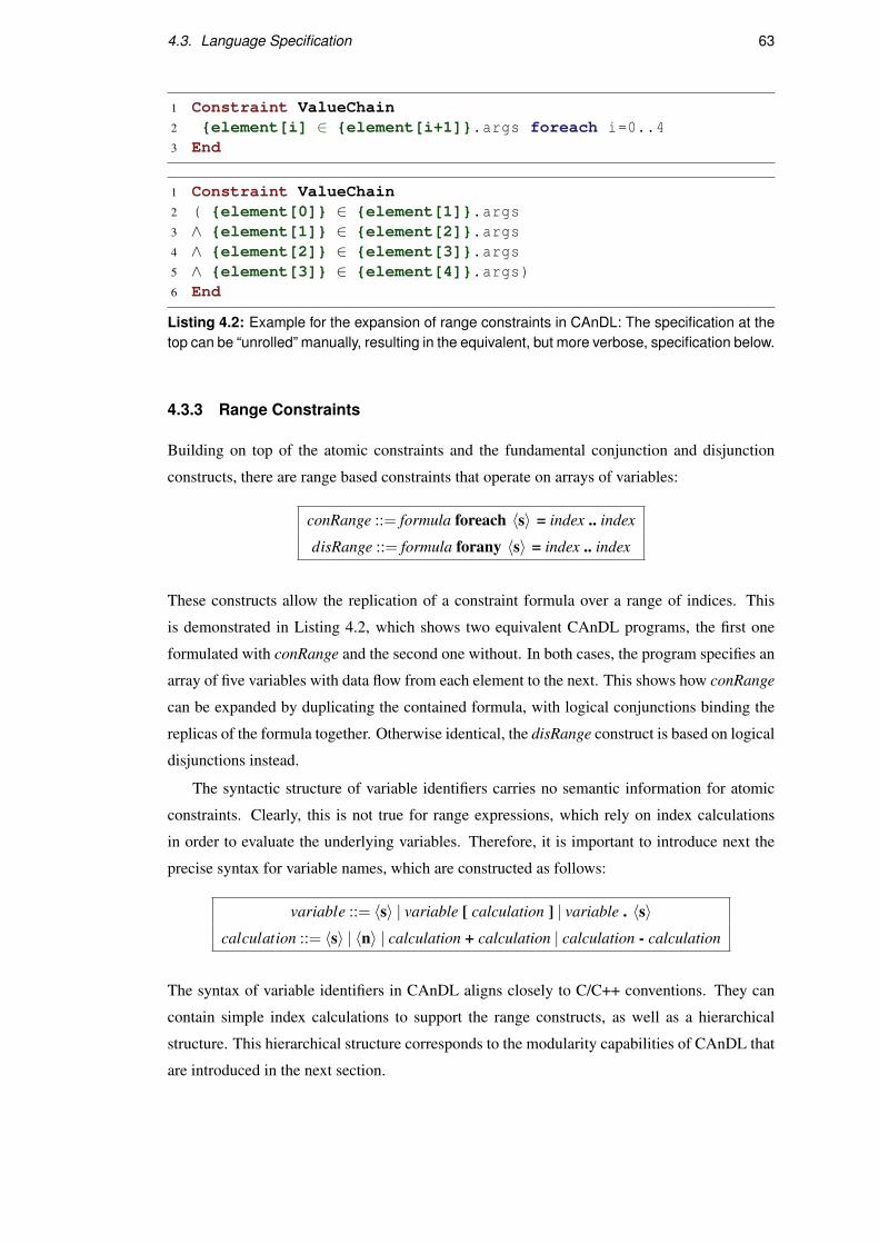
4.3. Language Specification 63
1 Constraint ValueChain2 {element[i] ∈ {element[i+1]}.args foreach i=0..43 End
1 Constraint ValueChain2 ( {element[0]} ∈ {element[1]}.args3 ∧ {element[1]} ∈ {element[2]}.args4 ∧ {element[2]} ∈ {element[3]}.args5 ∧ {element[3]} ∈ {element[4]}.args)6 End
Listing 4.2: Example for the expansion of range constraints in CAnDL: The specification at thetop can be “unrolled” manually, resulting in the equivalent, but more verbose, specification below.
4.3.3 Range Constraints
Building on top of the atomic constraints and the fundamental conjunction and disjunction
constructs, there are range based constraints that operate on arrays of variables:
conRange ::= formula foreach 〈s〉 = index .. index
disRange ::= formula forany 〈s〉 = index .. index
These constructs allow the replication of a constraint formula over a range of indices. This
is demonstrated in Listing 4.2, which shows two equivalent CAnDL programs, the first one
formulated with conRange and the second one without. In both cases, the program specifies an
array of five variables with data flow from each element to the next. This shows how conRange
can be expanded by duplicating the contained formula, with logical conjunctions binding the
replicas of the formula together. Otherwise identical, the disRange construct is based on logical
disjunctions instead.
The syntactic structure of variable identifiers carries no semantic information for atomic
constraints. Clearly, this is not true for range expressions, which rely on index calculations
in order to evaluate the underlying variables. Therefore, it is important to introduce next the
precise syntax for variable names, which are constructed as follows:
variable ::= 〈s〉 | variable [ calculation ] | variable . 〈s〉calculation ::= 〈s〉 | 〈n〉 | calculation + calculation | calculation - calculation
The syntax of variable identifiers in CAnDL aligns closely to C/C++ conventions. They can
contain simple index calculations to support the range constructs, as well as a hierarchical
structure. This hierarchical structure corresponds to the modularity capabilities of CAnDL that
are introduced in the next section.

64 Chapter 4. The Compiler Analysis Description Language
4.3.4 Modularity
Modularity is central to CAnDL, and it is achieved using the include construct.
include 〈s〉 [ (variable -> variable { , variable -> variable } ) ] [ @ variable ]
Note that the syntax in square brackets is optional and the syntax in curly brackets may be
repeated. The basic version of include, using neither of the two optional structures, is simple.
It copies the formula that corresponds to the identifier verbatim into the current specification.
If “[@variable]” is specified, then all the variable names of the inserted constraint formula
are prefixed with the given variable name, separated by a dot. This namespaces the inserted
formula and prevents unwanted interactions with surrounding constraints. The other optional
syntax is used to rename variables in the included formula. In contrast to the prefix syntax, this
increases the interaction with surrounding constraints by injecting other variables. Accordingly,
if both optional constructs are used, the prefix is only applied to variables that are not renamed.
Listing 4.3 illustrates this with two equivalent constraint programs. Both programs specify
an addition of four values, first adding pairwise and then adding the intermediate results. In the
code at the top, a formula for the addition of two values is bound to the name “Sum”. This is then
included three times in another formula named “SumOfSums”. Using the optional grammatical
constructs, the formula operates on a different set of variables each time, such that the third
addition takes the results of the previous two as input.
1 Constraint Sum2 ( opcode{out} = add3 ∧ {in1} = {out}.args[0]4 ∧ {in2} = {out}.args[1])5 End6 Constraint SumOfSums7 ( include Sum@{sum1}8 ∧ include Sum@{sum2}9 ∧ include Sum({sum1.out}->{in1},{sum2.out}->{in2}))
10 End
1 Constraint SumOfSums2 ( opcode{sum1.out} = add3 ∧ {sum1.in1} = {sum1.out}.args[0]4 ∧ {sum1.in2} = {sum1.out}.args[1]5 ∧ opcode{sum2.out} = add6 ∧ {sum2.in1} = {sum2.out}.args[0]7 ∧ {sum2.in2} = {sum2.out}.args[1]8 ∧ opcode{out} = add9 ∧ {sum1.out} = {out}.args[0]
10 ∧ {sum2.out} = {out}.args[1])11 End
Listing 4.3: Example for expansion of the include construct: Both specifications are equivalent.

4.3. Language Specification 65
1 Constraint CollectArguments2 ( ir_type{ins} = instruction3 ∧ collect i 8 ({arg[i]} ∈ {ins}.args))4 End
Listing 4.4: Simple collect example in CAnDL: Direct data dependencies of “ins” are collected.
4.3.4.1 Collect-all Constraints
The collect construct captures all possible solutions of a given formula, as in Definition 2.16.
collect 〈s〉 index formula
In Listing 4.4, the variables “arg[0]”,. . . ,“arg[7]” are specified to contain all of the direct
data dependencies of “ins”. In this example, solutions of “arg[i]” for a given value of “ins”
are identified. The second argument gives an upper limit to the number of collected variables.
The constant upper bound “8” is required here to keep the dimensionality of the search space
finite. If “ins” has less than 8 arguments, the remaining “arg[]” are constrainted to unused.
The first argument of collect specifies the name of an index variable that is used to detect which
variables belong to the collected set.
This example is now extended to show how collect can be used to implement quantifiers.
Consider the task of detecting instructions with only floating-point arguments. This involves
the “∀” quantifier, as it is equivalent to the following equation:
ins has only float arguments ⇐⇒ [∀x : (x,ins) ∈ DFG∗F =⇒ (float,x) ∈ IF ] (4.2)
This can be rewritten to an equivalent formulation on sets:
S1 = select(ins,rev(DFG∗F ))⊂ select(float,TF ) = S2.
Elementary set theory gives S1 ⊆ S2 ⇐⇒ S1 = S1∩S2. Therefore, if a set S is constrained
to be equal to both S1 and S1∩S2, then Equation (4.2) gives that this is satisfiable if and only
if “ins” has only floating-point arguments. This condition can be expressed in CAnDL, as is
shown in Listing 4.5. With the first collect statement at line 3, the set “arg” is constrained to
be equal to S1 and with the second one at lines 4-5, it is constrained to be equal to S1∩S2.
1 Constraint FloatingPointInstruction2 ( ir_type{ins} = instruction3 ∧ collect i 8 ( {ins} ∈ {arg[i]}.args)4 ∧ collect i 8 ( {ins} ∈ {arg[i]}.args5 ∧ data_type{arg[i]} = float))6 End
Listing 4.5: Collect restricts “ins” to instructions with only (up to 8) floating-point operands.

66 Chapter 4. The Compiler Analysis Description Language
The exact same approach can be used for much more complex analysis tasks. For example,
the final case study at the end of this chapter uses collect statements to restrict all array accesses
within a loop to be affine in the loop iterators. First, collect all memory accesses in the loop
(i.e. all “load” and “store” instructions), and then use a second collect statement to enforce
affine calculations of the access indices that are used for these instructions.
4.3.5 Expressing Larger Structures
The modularity of CAnDL allows for the creation of building blocks that are used by multiple
CAnDL specifications. This includes classic control flow structures, such as single-entry
single-exit (SESE) regions and different classes of loops, as well as memory access patterns.
These definitions a standard library that enables higher-level programming with CAnDL. This
section gives an overview of how some of these standard building blocks are defined.
Listing 4.6 gives the specification of SESE regions in CAnDL. Such regions are spanned
by the variables “begin” and “end”, with an incoming control flow edge from “precursor”
to “begin” (line 3) and an outgoing control flow edge from “end” to “successor” (line 5).
Graph domination constraints at lines 8 and 9 guarantee that these are the only entry and exit
of the region. Additional domination constraints at lines 6–7 and lines 10–13 make sure that
there are no jumps from outside the region into an instruction of the region that is not “begin”,
and similarly that there are no early exits of the region. Finally, regions are restricted to align
with basic block boundaries in lines 2 and 4.
Note that the use of variables “precursor” and “successor” prevents the detection of
SESE regions without a precursor or successor. These two special cases could easily be
captured with additional constraints that account for the possibility of an unused successor
or precursor. However, this situation is only relevant in the case of basic blocks that end
with a return statement or that are the entry point of a function. In the context of the loop-
based algorithmic structures that this thesis focuses on, basic blocks can be assumed to have a
precursor and successor.
Natural loops are easily defined in CAnDL, as shown in Listing 4.7. The specification
includes “SESE” and adds only a single additional constraint for the back edge of the loop
at line 3. Additional extensions to this specification are added to define more restricted loop
structures, such as for-loops. This involves the identification of the loop iterator, the breaking
condition, and the corresponding iteration space boundaries. In order to be a valid for-loop, the
end of the iteration space must be determined before the loop is entered. This is expressed in
Listing 4.8, restricting “value” to be either a function argument, a constant, or an instruction
that strictly dominates the loop entry. Note that this formula is underspecified on its own. In
order to get a useful constraint specification, it has to be included in larger CAnDL programs
that also include “Loop”.
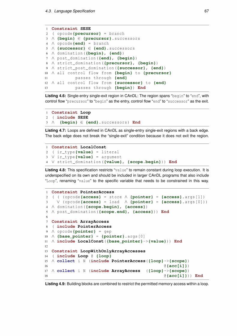
4.3. Language Specification 67
1 Constraint SESE2 ( opcode{precursor} = branch3 ∧ {begin} ∈ {precursor}.successors4 ∧ opcode{end} = branch5 ∧ {successor} ∈ {end}.successors6 ∧ domination({begin}, {end})7 ∧ post_domination({end}, {begin})8 ∧ strict_domination({precursor}, {begin})9 ∧ strict_post_domination({successor}, {end})
10 ∧ all control flow from {begin} to {precursor}11 passes through {end}12 ∧ all control flow from {successor} to {end}13 passes through {begin}) End
Listing 4.6: Single-entry single-exit region in CAnDL: The region spans “begin” to “end”, withcontrol flow “precursor” to “begin” as the entry, control flow “end” to “successor” as the exit.
1 Constraint Loop2 ( include SESE3 ∧ {begin} ∈ {end}.successors) End
Listing 4.7: Loops are defined in CAnDL as single-entry single-exit regions with a back edge.The back edge does not break the “single-exit” condition because it does not exit the region.
1 Constraint LocalConst2 ( ir_type{value} = literal3 ∨ ir_type{value} = argument4 ∨ strict_domination({value}, {scope.begin})) End
Listing 4.8: This specification restricts “value” to remain constant during loop execution. It isunderspecified on its own and should be included in larger CAnDL programs that also include“Loop”, renaming “value” to the specific variable that needs to be constrained in this way.
1 Constraint PointerAccess2 ( ( (opcode{access} = store ∧ {pointer} = {access}.args[1])3 ∨ (opcode{access} = load ∧ {pointer} = {access}.args[0]))4 ∧ domination({scope.begin}, {access})5 ∧ post_domination({scope.end}, {access})) End6
7 Constraint ArrayAccess8 ( include PointerAccess9 ∧ opcode{pointer} = gep
10 ∧ {base_pointer} = {pointer}.args[0]11 ∧ include LocalConst({base_pointer}->{value})) End12
13 Constraint LoopWithOnlyArrayAccesses14 ( include Loop @ {loop}15 ∧ collect i N (include PointerAccess({loop}->{scope})16 @{acc[i]})17 ∧ collect i N (include ArrayAccess ({loop}->{scope})18 @{acc[i]})) End
Listing 4.9: Building blocks are combined to restrict the permitted memory access within a loop.
68 Chapter 4. The Compiler Analysis Description Language
Another class of important building blocks is different categories of memory access. These
form a hierarchy of restrictiveness and include multi-dimensional array access and array access
that is affine in some loop iterators. Listing 4.9 combines several of the introduced building
blocks to specify a loop in which all memory access locations are calculated as offsets from
base pointers that are constant within the loop. This, for example, excludes loops with pointer-
chasing. The “ArrayAccess” specification can be extended with more restrictive memory
access patterns as previously mentioned. This is crucial to define advanced compiler analysis
passes, such as the detection of regions suitable for polyhedral code analysis.
4.4 Implementation
CAnDL is integrated into the LLVM framework. CAnDL programs are read by the CAnDL
compiler during LLVM build time, which then generates C++ source code to implement the
specified LLVM analysis functionality. This code depends on the generic backtracking solver
derived in Chapter 2, which is incorporated directly into the LLVM codebase. The generated
code is compiled and linked together with the existing LLVM libraries. The Clang compiler,
which is built on LLVM, then automatically invokes this solver during the compilation of user
programs, after the optimisation passes.
The resulting Clang binary, built on the modified version LLVM, uses the solver to search
for the specified computational structures and outputs the found instances into report files. It
also makes the results available to ensuing transformation passes in the form of C++ structures.
4.4.1 Normalisation of LLVM IR
For reliable detection of code structures, the normalisation of LLVM IR via optimisation passes
is critical. The promotion of memory to registers, loop-independent code motion, constant
folding, loop normalisations, inlining, and other standard transformations result in predictable
code structures that simplify the formulation of CAnDL specifications.
For example, elements of C++ vectors are accessed via the overloaded operator[].
Such operators appear in LLVM IR as opaque function calls and potentially hinder analysis
with CAnDL specifications. However, these operators are inlined during optimisation, and
parts of the resulting code are propagated out of loops by loop-independent code motion. The
remaining array access can easily be captured by CAnDL using the same specifications that
treat C code. Listing 4.10 demonstrates this normalising effect of optimisations. The top of
the figure shows the C++ implementation of a function that computes a reduction over two
sequences of integers. The first sequence is stored in a plain C array, whereas the second is in
an instance of the vector class. In the optimised LLVM IR code, the difference between these
implementations has disappeared from the reduction loops at lines 24–32 and 39–47.

4.4. Implementation 69
1 int reduce(int* input1 , size_t input1_size ,2 std::vector<int> input2) {3 int result1 = 0, result2 = 0;4 for(size_t i = 0; i != input1_size; i++)5 result1 += input1[i];6 for(size_t i = 0; i != input2.size(); i++)7 result2 += input2[i];8 return result1 + result2;9 }
1 define i32 @_Z23reducePimSt6vectorIiSaIiEE(i32*, i64,2 %"class.std::vector"* ) {3 %4 = icmp eq i64 %1, 04 br i1 %4, label %5, label %1756 ; <label>:5:7 %6 = phi i32 [ 0, %3 ], [ %22, %17 ]8 %7 = getelementptr inbounds %"class.std::vector",9 %"class.std::vector"* %2,
10 i64 0, i32 0, i32 0, i32 0, i32 111 %8 = bitcast i32** %7 to i64*12 %9 = load i64, i64* %8, align 813 %10 = bitcast %"class.std::vector"* %2 to i64*14 %11 = load i64, i64* %115 %12 = icmp eq i64 %9, %1116 %13 = inttoptr i64 %11 to i32*17 br i1 %12, label %25, label %141819 ; <label>:14:20 %15 = sub i64 %9, %1121 %16 = ashr exact i64 %15, 222 br label %282324 ; <label>:17:25 %18 = phi i64 [ %23, %17 ], [ 0, %3 ]26 %19 = phi i32 [ %22, %17 ], [ 0, %3 ]27 %20 = getelementptr inbounds i32, i32* %0, i64 %1828 %21 = load i32, i32* %2029 %22 = add nsw i32 %21, %1930 %23 = add nuw i64 %18, 131 %24 = icmp eq i64 %23, %132 br i1 %24, label %5, label %173334 ; <label>:25:35 %26 = phi i32 [ 0, %5 ], [ %33, %28 ]36 %27 = add nsw i32 %26, %637 ret i32 %273839 ; <label>:28:40 %29 = phi i64 [ 0, %14 ], [ %34, %28 ]41 %30 = phi i32 [ 0, %14 ], [ %33, %28 ]42 %31 = getelementptr inbounds i32, i32* %13, i64 %2943 %32 = load i32, i32* %3144 %33 = add nsw i32 %32, %3045 %34 = add i64 %29, 146 %35 = icmp eq i64 %34, %1647 br i1 %35, label %25, label %2848 }
Listing 4.10: Standard LLVM optimisations as normalising passes: The same computationis expressed with a plain C array and a C++ std::vector respectively. During compilation,the interaction of function inlining and loop-independent code motion results in equivalentintermediate representation code for the reduction loops at lines 24–32 and at lines 39–47.

70 Chapter 4. The Compiler Analysis Description Language
Most standard optimisations that LLVM provides have this implicit effect of normalising
the code, but there are some notable exceptions. Most importantly, this involves optimisations
that are not reliably applied uniformly on all code but utilise opaque cost heuristics or that
require complex preconditions. Notably, this includes loop unrolling and vectorization, which
are hence disabled. The CAnDL-enabled compiler invokes the detection functionality directly
after optimisations and expects the pipeline to be configured with the command-line options
“-Os -fno-unroll-loops -fno-vectorize -fno-slp-vectorize -ffast-math”.
Some other LLVM optimisations also obfuscate the resulting LLVM IR but cannot be
disabled via command-line options. Furthermore, there is some semantic information about
multidimensional arrays that LLVM retains from the input language that effectively results in
multiple distinct ways to express array accesses that are equivalent. To alleviate this, in addition
to standard optimisations, the CAnDL-enabled compiler applies some custom transformations
in order to pass on predictable LLVM IR code to the solver:
• Strength reductions result in special cases that would have to be covered explicitly by
CAnDL specifications. To remove the requirement of considering these special cases,
two strength reduction optimisations are reversed: add 7→or and mul 7→shift. Such
instruction specialisations run counter to the goal of normalising the IR.
• Multi-dimensional array access can be expressed directly in LLVM IR. However, this
only works for statically allocated arrays. As CAnDL should work on dynamically-
sized arrays as well, this representation cannot be relied on and, in effect, introduces
additional complexity. In order to remove this complication, complex “getelementptr”
instructions are simplified to add an offset to a raw pointer. The index calculations are
then performed entirely as integer arithmetic on the indices. This process effectively
flattens multi-dimensional arrays. Chains of “getelementptr” instructions are merged,
again resulting in integer arithmetic instead.
• Some interactions of “select” and “getelementptr” instructions are transformed as
(c?a[i]:a[j])7→a[c?i:j] to minimise the number of “getelementptr” instructions.
Finally, some structures in the LLVM IR are not modified by normalising transformations, but
they are omitted in the SSA model that underpins the CAnDL specifications. This applies to
all integer extension instructions and pointer conversions. These constructs are represented in
LLVM IR as instructions with a single argument. In the SSA model, data flow edges skip these
instructions, pointing from the argument of the instruction to any use of it. The conventional
use of 32-bit integers on 64-bit systems obfuscates the SSA model without these omissions,
particularly in the context of 32-bit loop interators that are automatically elevated to 64-bit
integers during optimisation but then have to be downcast in every iteration before applying a
comparison operator.
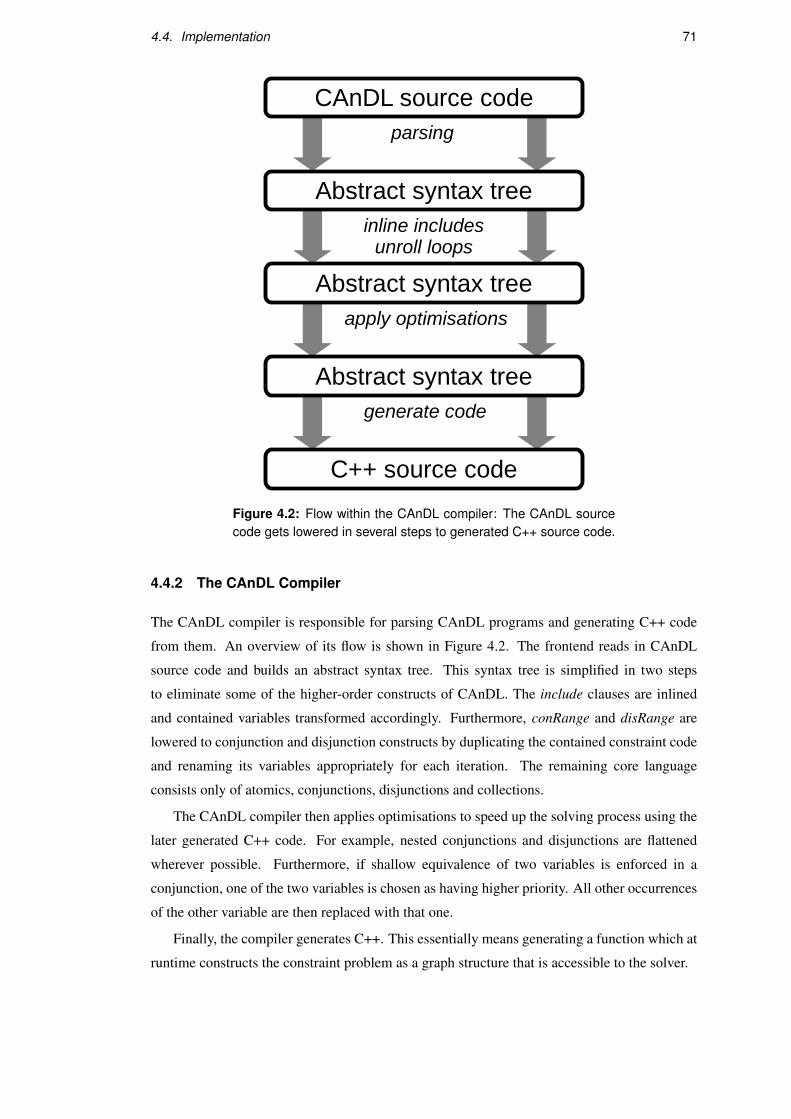
4.4. Implementation 71
Abstract syntax tree
Abstract syntax tree
Abstract syntax tree
C++ source code
CAnDL source code
inline includesunroll loops
parsing
apply optimisations
generate code
Figure 4.2: Flow within the CAnDL compiler: The CAnDL sourcecode gets lowered in several steps to generated C++ source code.
4.4.2 The CAnDL Compiler
The CAnDL compiler is responsible for parsing CAnDL programs and generating C++ code
from them. An overview of its flow is shown in Figure 4.2. The frontend reads in CAnDL
source code and builds an abstract syntax tree. This syntax tree is simplified in two steps
to eliminate some of the higher-order constructs of CAnDL. The include clauses are inlined
and contained variables transformed accordingly. Furthermore, conRange and disRange are
lowered to conjunction and disjunction constructs by duplicating the contained constraint code
and renaming its variables appropriately for each iteration. The remaining core language
consists only of atomics, conjunctions, disjunctions and collections.
The CAnDL compiler then applies optimisations to speed up the solving process using the
later generated C++ code. For example, nested conjunctions and disjunctions are flattened
wherever possible. Furthermore, if shallow equivalence of two variables is enforced in a
conjunction, one of the two variables is chosen as having higher priority. All other occurrences
of the other variable are then replaced with that one.
Finally, the compiler generates C++. This essentially means generating a function which at
runtime constructs the constraint problem as a graph structure that is accessible to the solver.
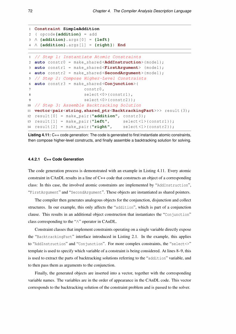
72 Chapter 4. The Compiler Analysis Description Language
1 Constraint SimpleAddition2 ( opcode{addition} = add3 ∧ {addition}.args[0] = {left}4 ∧ {addition}.args[1] = {right}) End
1 // Step 1: Instantiate Atomic Constraints2 auto constr0 = make_shared <AddInstruction>(model);3 auto constr1 = make_shared <FirstArgument> (model);4 auto constr2 = make_shared <SecondArgument>(model);5 // Step 2: Compose Higher-Level Constraints6 auto constr3 = make_shared <Conjunction>(7 constr0 ,8 select <0>(constr1),9 select <0>(constr2));
10 // Step 3: Assemble Backtracking Solution11 vector<pair<string,shared_ptr<BacktrackingPart>>> result(3);12 result[0] = make_pair("addition", constr3);13 result[1] = make_pair("left", select <1>(constr1));14 result[2] = make_pair("right", select <1>(constr2));
Listing 4.11: C++ code generation: The code is generated to first instantiate atomic constraints,then compose higher-level constructs, and finally assemble a backtracking solution for solving.
4.4.2.1 C++ Code Generation
The code generation process is demonstrated with an example in Listing 4.11. Every atomic
constraint in CAnDL results in a line of C++ code that constructs an object of a corresponding
class: In this case, the involved atomic constraints are implemented by “AddInstruction”,
“FirstArgument” and “SecondArgument”. These objects are instantiated as shared pointers.
The compiler then generates analogous objects for the conjunction, disjunction and collect
structures. In our example, this only affects the “addition”, which is part of a conjunction
clause. This results in an additional object construction that instantiates the “Conjunction”
class corresponding to the “∧” operator in CAnDL.
Constraint classes that implement constraints operating on a single variable directly expose
the “BacktrackingPart” interface introduced in Listing 2.1. In the example, this applies
to “AddInstruction” and “Conjunction”. For more complex constraints, the “select<>”
template is used to specify which variable of a constraint is being considered. At lines 8–9, this
is used to extract the parts of backtracking solutions referring to the “addition” variable, and
to then pass them as arguments to the conjunction.
Finally, the generated objects are inserted into a vector, together with the corresponding
variable names. The variables are in the order of appearance in the CAnDL code. This vector
corresponds to the backtracking solution of the constraint problem and is passed to the solver.

4.4. Implementation 73
Figure 4.3: Interactive CAnDL test tool: The left hand panel shows a Static Control Part (SCoP)in Polybench jacobi-2d, the right hand panel shows the constraint solutions found by the solver.
4.4.3 Developer Tools
CAnDL simplifies the construction of compiler analysis functionality, but reasoning about
the semantics of compiler intermediate representation remains difficult. The solver detects
whatever the programmer specifies, without any additional effort, but it is difficult to ensure
that the CAnDL code actually specifies the structures that the programmer intended. Generally,
the accuracy of CAnDL programs can only be ensured with thorough testing, and it is important
to keep in mind that CAnDL is targeted at expert compiler developers.
In order to make the debugging of CAnDL programs more feasible, supporting tools are
provided. Most importantly, this includes an interactive GUI, where developers can test out
corner cases of their CAnDL programs to find false positives and false negatives. This GUI is
shown in Figure 4.3, with an example from one of the use cases presented in Section 4.5.
In the left half, part of a C program from the PolyBench benchmark suite is visible, which
implements a two-dimensional Jacobi stencil. The GUI was configured to look for Static
Control Parts (SCoPs), as described later. The user has clicked the “analyze” button, which
triggered the analysis to run by invoking the modified Clang compiler. The GUI then read the
report file and printed the results in the right-hand part of the figure.
The solver found a SCoP in the IR code (corresponding to lines 459–468 of the C program).
The text on the right shows the hierarchical structure of the solution, with IR values assigned
to every variable. The corresponding C entities can be recovered using the debug information
that is contained in the generated LLVM IR code. By modifying the C code, the developer can
test the detection and verify that no SCoP is detected if irregular control flow is introduced.

74 Chapter 4. The Compiler Analysis Description Language
1 Constraint ComplexFactorisation2 ( opcode{value} = add3 ∧ {sum1.value} = {value}.args[0]4 ∧ {sum2.value} = {value}.args[1]5 ∧ include SumChain @ {sum1}6 ∧ {product1.value} = {sum1.last_factor}7 ∧ include MulChain @ {product1}8 ∧ {product1.last_factor} = {product2.last_factor}9 ∧ include SumChain @ {sum2}
10 ∧ {product2.value} = {sum2.last_factor}11 ∧ include MulChain @ {product2}) End
Listing 4.12: Factorisation opportunities in CAnDL: This captures some opportunities that LLVM“instcombine” misses. “SumChain”, “MulChain” are themselves specified in CAnDL (16 LoC).
4.5 Case Studies
The effectiveness of CAnDL was evaluated in three different use cases. Firstly, it was used
for detecting opportunities to apply a simple peephole optimisation. Secondly, CAnDL was
applied to graphics shader code optimisation. Finally, the detection of Static Control Parts
(SCoPs) that are amenable for polyhedral code transformations was implemented in CAnDL.
Where possible, the evaluation compares the number of lines of CAnDL code, the program
coverage achieved and performance against prior approaches.
4.5.1 Case Study 1: Simple Optimisations
Arithmetic simplifications in LLVM are implemented in the “instcombine” pass. An example
of this is the standard factorisation optimisation that uses the law of distributivity to simplify
integer calculations, as shown in Equation (4.3). Within “instcombine”, this is implemented
in 203 lines of code (commit 7de5f26d, InstructionCombining.cpp lines 549-756 excluding
lines 637-641), and additionally uses supporting functionality shared with other optimisations.
a∗b+a∗ c→ a∗ (b+ c) (4.3)
This analysis problem can be formulated in CAnDL, as shown in Listing 4.12. Crucially,
at lines 5,7,9,11, the specification makes use of “SumChain” and “MulChain”, which allows
the CAnDL program to capture a large, generalised class of opportunities for factorisation.
The “instcombine” pass has limited support for this, and first requires the application of
associative and commutative laws to reorder the values. For example, this is needed for
Equation (4.4), and only partially supported by LLVM with the additional “reassociate”
pass.
a∗b+ c+d ∗a∗ e−> a∗ (b+d ∗ e)+ c (4.4)

4.5. Case Studies 75
LLVM CAnDL
Lines of Code 203 12
Detected in NPB 1 1 + 2
Detected in Parboil 0 0 + 1
Detected in Rodinia 24 24 + 4
Total Compilation time 152.2s 152.2s+7.8s
Table 4.3: Factorisations enabled by LLVM vs CAnDL
4.5.1.1 Experimental Setup
The specification in Listing 4.12 was evaluated against the default factorisation optimisation
in “instcombine” on three different benchmark collections: the sequential C versions of the
NAS Parallel Benchmarks [139], as provided by Seo et al. [140]; the C/C++ Parboil programs
by Stratton et al. [141]; and the OpenMP C/C++ programs of the Rodinia benchmark suite
[142]. The existing LLVM “instcombine” pass was extended, so that it automatically logs
every time that it successfully applied the “tryFactorization” function.
The individual benchmark programs in the three benchmark suites consist of 94915 lines
of code in total. For each benchmark suite, the total number of reported factorisations, as
well as the total compilation time, were measured. The standard LLVM optimisation was
then disabled, and the CAnDL-generated detection functionality was used instead. The same
application programs were compiled with the same version of Clang and identical compiler
options, reporting the number of factorisations found and measuring the total compilation time
again. This timing includes all the other passes within LLVM, plus the CAnDL code path.
4.5.1.2 Results
The results of the evaluation are shown in Table 4.3. In two of the benchmark collections –
NPB and Parboil – there are only a limited number of factorisation opportunities. LLVM was
unable to perform any factorisation in the entire Parboil suite. However, the Rodinia suite
contains more opportunities, mostly in the “particlefilter” and “mummergpu” programs.
In all three benchmarks suites, the CAnDL system found all factorisation opportunities
that the “instcombine” pass identified. In addition, it detected an additional 7 cases across all
programs. Just 12 lines of CAnDL code were able to capture more factorisation opportunities
than 200 lines of C++ code in LLVM.
Using CAnDL on large benchmark suites increased total compilation time by ∼5%. Given
the small impact of individual peephole optimisations, an evaluation of the performance or
code size impact vs “instcombine” is unlikely to yield significant results.

76 Chapter 4. The Compiler Analysis Description Language
1 Constraint FloatingPointAssociativeReorder2 ( include VectorMulChain3 ∧ collect j N4 ( {hoisted[k]} = {factors[i]} forany i=0..N5 ∧ include ScalarHoist({hoisted[j]}->{out},6 {scalar[j]}->{in})@{hoist[j]})7 ∧ collect j N8 ( {nonhoisted[j]} = {factors[i]} forany i=0..N9 ∧ {nonhoisted[j]} != {hoisted[i]} foreach i=0..N))
10 End
Listing 4.13: CAnDL defines multiplication chains with genuine vectors and hoisted scalars:After separating the two cases, some of the multiplications can be performed on scalars instead.
4.5.2 Case Study 2: Graphics Shader Optimisations
Graphics computations often involve arithmetic on vectors of single-precision floating-point
values, which can represent vertex positions in space or colour values. Established graphics
shader compilers utilise the LLVM intermediate representation internally [143].
In real shader code, there are often element-wise products of several floating-point vectors,
where some of the factors are actually scalars that were hoisted to vectors. By reordering the
factors and delaying the hoisting to vectors, some of the element-wise vector products can be
simplified to products on scalars, as shown by example in the following equation.
~x =~a∗v~b∗v vec3(c)∗v ~d ∗v vec3(e)
= vec3(c∗ e)∗~a∗v~b∗v ~d
For general-purpose code, such reordering can be problematic. This is due to computation
artefacts in floating-point arithmetic. However, this is generally no problem in the domain of
graphics processing. Instead, associative reordering can result in performance improvements
when combined with lowering to scalar multiplications as discussed above.
The required analysis functionality for this optimisation was implemented with CAnDL,
as shown in Listing 4.13. Firstly, the specification uses “VectorMulChain” to detect chains
of floating-point vector multiplications. At lines 4–6, all the factors that are hoisted from
some scalar are collected into the array “hoisted”. Correspondingly, all the other factors are
collected into the array “nonhoisted” at lines 7–9.
“VectorMulChain” and “ScalarHoist” are in turn implemented as CAnDL programs.
“VectorMulChain” discovers chains of floating-point vector multiplications in the IR code. It
is defined very similarly to “SumChain” and “MulChain”, which were used in the previous case
study. It guarantees chains of maximal length by checking that neither of the first two factors
is a multiplication itself and that the last factor is not used in any multiplication.

4.5. Case Studies 77
shader programs0 0
1 1
2 2
3 3
4 4
spee
du
pin
per
cen
t
Figure 4.4: Speedup on Qualcomm Adreno 530 (evaluated on HTC 10, running Android 7.0)
“ScalarHoist” operates on “in” and “out”, as well as some hidden internal variables. It
specifies that “out” is a vector generated from “in” by setting all vector dimensions equal to
“in”. The precise implementation of this is highly specific to LLVM and involves combinations
of the LLVM IR instructions “insertelement” and “shufflevector”.
4.5.2.1 Experimental Setup
The LunarGLASS project [144] was used in this work to transform shaders into LLVM IR
and back after optimisation. The CAnDL specification was applied to all fragment shaders in
the GFXBench 4.0 suite taken from Kishonti [145]. A corresponding transformation pass was
added to LLVM, which uses the detected solutions to implement the described optimisation.
This was done by constructing the appropriate scalar and vector multiplications from the arrays
“hoisted” and “nonhoisted”, and then replacing the result of the original multiplication
chain with the final multiplication in these newly generated instructions. Standard dead code
elimination automatically removes the remnants of the original calculation.
The performance impact was evaluated on the Qualcomm Adreno 530 GPU. To measure
the baseline of benchmark performance, all shaders were compiled with the default Qualcomm
graphics stack. They were then compiled with LunarGLASS into LLVM, CAnDL was applied,
and they were transformed back into GLSL code [146]. To evaluate the impact, the result was
passed through the default graphics stack again, and the performance measured.
4.5.2.2 Results
There were 19 solutions to the specification across the benchmarks, and the transformation
had an impact on the performance of 8 fragment shaders. The resulting performance impact
is shown in Figure 4.4. Evidently, there are opportunities for such associative reordering that
the default graphics stack misses. Although the performance impact was moderate with 1–4%
speedup on 8 of the fragment shaders, it shows how new analysis can be rapidly prototyped
and evaluated with only a few lines of code.

78 Chapter 4. The Compiler Analysis Description Language
4.5.3 Case Study 3: Detection of Polyhedral SCoPs
The polyhedral model [27, 28] allows compilers to utilise powerful mathematical reasoning
to detect parallelism opportunities in sequential code and to implement code transformations.
However, this applies only for a restrictive class of well-structured loop nests. More precisely,
conventional polyhedral code transformations are applicable to Static Control Parts (SCoPs).
Detecting SCoPs is a fundamental and necessary first step for any later polyhedral optimisation.
Implementations of the polyhedral model may differ in their precise definition of SCoPs.
The definition of Semantic SCoPs from the Polly compiler by Grosser et al. [26] was used
for reference here. SCoP detection functionality was implemented in CAnDL and compared
against Polly, which is also implemented as an extension to LLVM. The use of the same
definition for SCoPS and the implementation in the same compiler infrastructure allow for
a direct comparison between Polly and CAnDL. The specification of SCoPs is significantly
more complex than the required CAnDL code for the previous case studies. However, it can
be broken into several components, with some of them shown in Listing 4.14.* The integer
constants “10” and “20” in the collect statements are required for the solver to restrict the
search space to a finite set of variables.
Structured Control Flow SCoPs require well-structured control flow. This means that each
conditional jump within the corresponding piece of LLVM IR is accounted for by for-loops
and conditionals. This is ensured with the collect constraints, as in Listing 4.5. The construct
is used with the CAnDL specifications “For” (lines 21–25) and “IfBlock” (lines 26–30) that
describe the control flow of for-loops and conditionals. All the involved conditional jump
instructions are extracted, and it is checked that these are indeed all conditional jumps within
the potential SCoP (lines 14–24 and lines 31-33).
Once the control flow has been established, the iterators of the loops (lines 4–5) are used to
define affine integer computations in the loop (lines 6–9). This is done in a brute-force fashion
with a recursive constraint program “AffineCalc” (line 50). It is checked that the iteration
domain of all the for-loops is well-behaved, i.e. the boundaries are affine in the loop iterators.
Affine Memory Access All memory accesses in the SCoP must be affine. For this to be true,
it needs to be verified that for each “load” and “store” instruction, the base pointer is loop-
invariant, and the index is calculated affinely. The loop-invariant base pointer is easily checked
in “MemoryAccess with the “LocalConst” program from Listing 4.8.
Checking the index calculations is more involved and is again based on the method that
was demonstrated in Listing 4.5. The collect construct is used to find all of the affine memory
accesses in all the loop nests (lines 43–54). Another collect gathers all “load” and “store”
instructions (36–42), guaranteeing that both collections are identical.
*The complete CAnDL code for this section is in Appendix B.
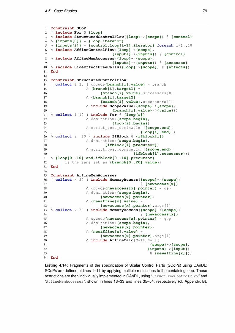
4.5. Case Studies 79
1 Constraint SCoP2 ( include For @ {loop}3 ∧ include StructuredControlFlow({loop}->{scope}) @ {control}4 ∧ {inputs[0]} = {loop.iterator}5 ∧ {inputs[i]} = {control.loop[i-1].iterator} foreach i=1..106 ∧ include AffineControlFlow({loop}->{scope},7 {inputs}->{inputs}) @ {control}8 ∧ include AffineMemAccesses({loop}->{scope},9 {inputs}->{inputs}) @ {accesses}
10 ∧ include SideEffectFreeCalls({loop}->{scope}) @ {effects})11 End1213 Constraint StructuredControlFlow14 ( collect i 20 ( opcode{branch[i].value} = branch15 ∧ {branch[i].target1} =16 {branch[i].value}.successors[0]17 ∧ {branch[i].target2} =18 {branch[i].value}.successors[1]19 ∧ include ScopeValue({scope}->{scope},20 {branch[i].value}->{value}))21 ∧ collect i 10 ( include For @ {loop[i]}22 ∧ domination({scope.begin},23 {loop[i].begin})24 ∧ strict_post_domination({scope.end},25 {loop[i].end}))26 ∧ collect i 10 ( include IfBlock @ {ifblock[i]}27 ∧ domination({scope.begin},28 {ifblock[i].precursor})29 ∧ strict_post_domination({scope.end},30 {ifblock[i].successor}))31 ∧ {loop[0..10].end,ifblock[0..10].precursor}32 is the same set as {branch[0..20].value})33 End3435 Constraint AffineMemAccesses36 ( collect x 20 ( include MemoryAccess({scope}->{scope})37 @ {newaccess[x]}38 ∧ opcode{newaccess[x].pointer} = gep39 ∧ domination({scope.begin},40 {newaccess[x].pointer})41 ∧ {newaffine[x].value} =42 {newaccess[x].pointer}.args[1])43 ∧ collect x 20 ( include MemoryAccess({scope}->{scope})44 @ {newaccess[x]}45 ∧ opcode{newaccess[x].pointer} = gep46 ∧ domination({scope.begin},47 {newaccess[x].pointer})48 ∧ {newaffine[x].value} =49 {newaccess[x].pointer}.args[1]50 ∧ include AffineCalc[M=10,N=6](51 {scope}->{scope},52 {inputs}->{input})53 @ {newaffine[x]}))54 End
Listing 4.14: Fragments of the specification of Scalar Control Parts (SCoPs) using CAnDL:SCoPs are defined at lines 1–11 by applying multiple restrictions to the containing loop. Theserestrictions are then individually implemented in CAnDL, using “StructuredControlFlow” and“AffineMemAccesses”, shown in lines 13–33 and lines 35–54, respectively (cf. Appendix B).

80 Chapter 4. The Compiler Analysis Description Language
Polly CAnDL
Lines of Code 1903 45
Detected in datamining 2 2
Detected in Linear-algebra 19 19
Detected in medley 3 3
Detected in stencils 6 6
Table 4.4: Polly and CAnDL detected all SCoPs.
4.5.3.1 Experimental Setup
The reliable detection of SCoPs was evaluated on the PolyBench suite [147], a collection of
31 benchmark programs that contain SCoPs of differing complexity from several application
domains. For both the CAnDL-based approach and for the evaluation of Polly, it was counted
how many of the computational kernels contained in the benchmark suite were captured in their
entirety by the respective analysis.
Some post-processing of the generated constraint solutions was required to compare the
results of CAnDL and Polly. This was needed because the output of CAnDL was not in the
JSCoP format that Polly generates, but contained the raw constraint solution encoded as a
JSON file. Furthermore, the CAnDL implementation did not merge consecutive outer level
loops into a single SCoP of maximum size. Therefore, the detected loops from the CAnDL
solver were extracted and grouped together. A Python script was then used to verify that they
precisely covered the SCoPs detected by Polly.
4.5.3.2 Results
Table 4.4 shows that the CAnDL specification captured all the SCoPs that Polly detected. To
measure the lines of code required, the CAnDL version was compared with the amount of code
in ScopDetection.cpp of Polly. The same detection results were achieved with much fewer
lines of code in CAnDL. Note that the line count that is given for the CAnDL program does
not include all the CAnDL code involved in the detection of polyhedral regions. Code that is
not specific to this idiom (such as loop structures) is considered as part of the CAnDL standard
library. In the same way, the line count for Polly does not account for additional code that Polly
relies on when detecting SCoPS, e.g. the expansive “ScalarEvolution” pass.
Detecting SCoPs with CAnDL incurred a significant overhead, but compile times remained
below one second for each PolyBench program on an Intel i7-8665U processor. Detailed
compile time results are presented in Table 4.5. The geomean overhead of enabling the CAnDL
detection of SCoPS during compilation was 556%, mostly due to the large number of variables
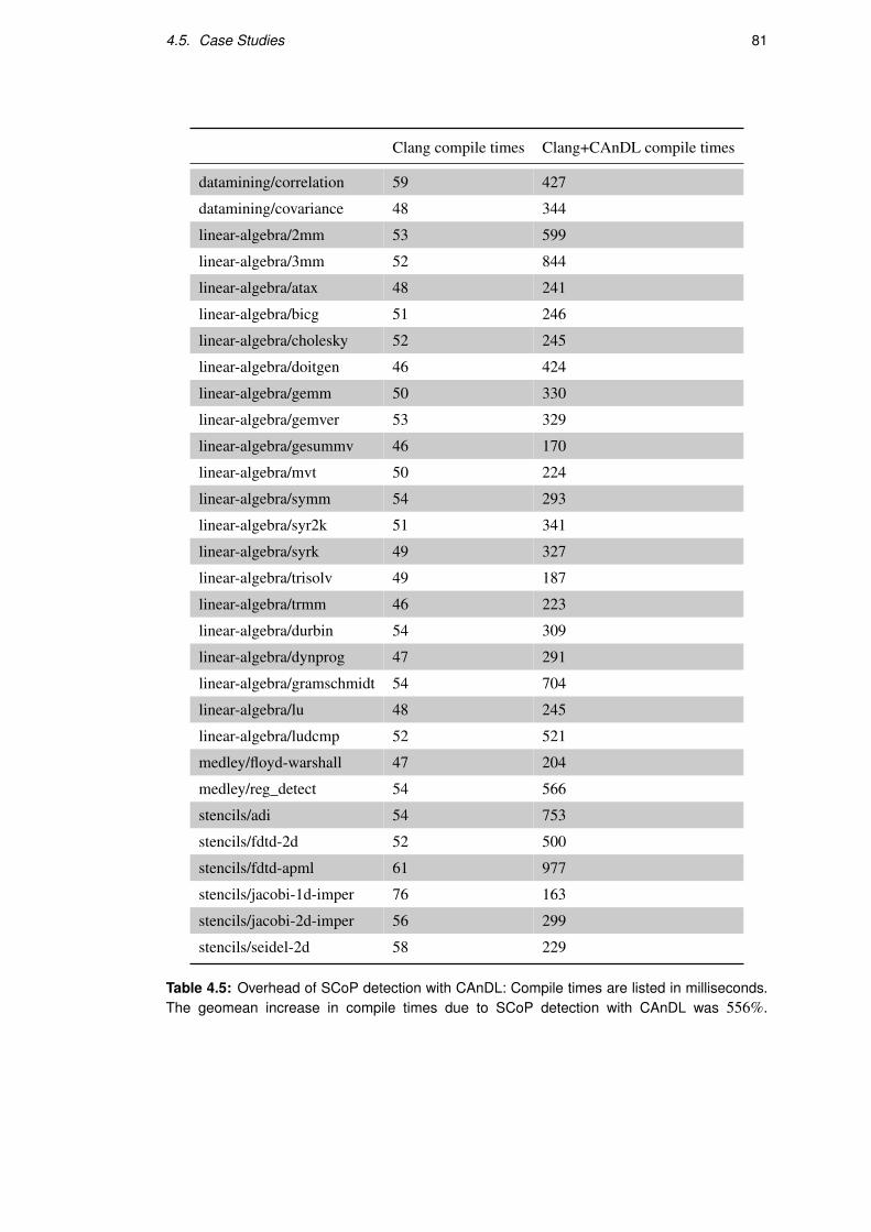
4.5. Case Studies 81
Clang compile times Clang+CAnDL compile times
datamining/correlation 59 427
datamining/covariance 48 344
linear-algebra/2mm 53 599
linear-algebra/3mm 52 844
linear-algebra/atax 48 241
linear-algebra/bicg 51 246
linear-algebra/cholesky 52 245
linear-algebra/doitgen 46 424
linear-algebra/gemm 50 330
linear-algebra/gemver 53 329
linear-algebra/gesummv 46 170
linear-algebra/mvt 50 224
linear-algebra/symm 54 293
linear-algebra/syr2k 51 341
linear-algebra/syrk 49 327
linear-algebra/trisolv 49 187
linear-algebra/trmm 46 223
linear-algebra/durbin 54 309
linear-algebra/dynprog 47 291
linear-algebra/gramschmidt 54 704
linear-algebra/lu 48 245
linear-algebra/ludcmp 52 521
medley/floyd-warshall 47 204
medley/reg_detect 54 566
stencils/adi 54 753
stencils/fdtd-2d 52 500
stencils/fdtd-apml 61 977
stencils/jacobi-1d-imper 76 163
stencils/jacobi-2d-imper 56 299
stencils/seidel-2d 58 229
Table 4.5: Overhead of SCoP detection with CAnDL: Compile times are listed in milliseconds.The geomean increase in compile times due to SCoP detection with CAnDL was 556%.

82 Chapter 4. The Compiler Analysis Description Language
that are required for expressing affine calculations. The compile time impact of all other idioms
discussed in this thesis is much more moderate (compare Table 6.3). This overhead can be
prohibitive during software development when frequent recompilation is required. However, it
pales in comparison to autotuners, superoptimisation, and many other compiler techniques that
involve constraint solvers and should be unproblematic in many contexts.
With a high-level representation of SCoPs, CAnDL allows polyhedral compiler researchers
to explore the impact of relaxing or tightening the exact definition of SCoPs in a straightforward
manner, enabling rapid prototyping. Simple commenting out of constraint statements in the
CAnDL specification relaxes the conditions.
4.6 Conclusions
Optimising compilers require sophisticated program analysis in order to generate performant
code. The state-of-the-art approach for implementing this functionality manually in C++ is
not satisfactory, as exemplified by the complicated and error-prone “instcombine” pass in the
LLVM compiler infrastructure.
The domain-specific Compiler Analysis Description Language (CAnDL) provides a more
efficient approach. CAnDL specifications can automatically generate compiler analysis passes
from a declarative description. They are easier to program and significantly reduce the code
size and complexity when comparing against manual C++ implementations. Although CAnDL
is based on a constraint programming paradigm and uses a backtracking solver to analyse the
LLVM IR code, compile times never exceeded one second.
Many compiler analysis tasks are suitable for implementation with CAnDL. It can be used
for the detection of standard peephole optimisation opportunities and the rapid prototyping
of graphics shader optimisations. Despite its general approach, CAnDL scales to complex
domain-specific code structures and can efficiently recognise large code regions suitable for
polyhedral transformations.
Outlook The final case study showed that CAnDL can express the algorithmic structure of
complex loop nests, not just peephole optimisation opportunities. This enables the capturing
of entire loops at a time. The following chapters expand on this observation by investigating
how the recognition of computational idioms can be leveraged for performance. While SCoPs
were reported without informing additional compiler transformations, Chapter 5 applies auto-
parallelisation techniques to a broad generalisation of reduction computations.

Chapter 5
Automatic Parallelisation of
Reductions and Histograms*
The Compiler Analysis Description Language (CAnDL) makes the constraint methodology
from Chapter 2 accessible to the Clang compiler within the LLVM compiler infrastructure.
The previous chapter showed how this enables compiler analysis tools to be generated from
declarative specifications, replicating and extending established compiler abilities. This chapter
goes beyond restating and improving existing functionality. Instead, it implements automatic
parallelisation methods for programs that were previously inaccessible to compiler reasoning.
Complex Reduction and Histogram Computations (CReHCs) are identified as a previously
overlooked computational idiom. CReHCs constitute performance bottlenecks of important
benchmark programs and share algorithmic structure that allows for targeted acceleration and
parallelisation approaches. In contrast to the better-understood scalar reductions, CReHCs may
contain indirect memory accesses and non-trivial control flow. Such loops have not typically
been studied as a single class of calculations, but this chapter demonstrates that grouping them
together allows for automatic detection and parallelisation using shared methods.
After introducing CReHCs, this chapter presents the Idiom Description Language (IDL) as
an extension of CAnDL and uses it to implement the detection of this idiom. The additional
language features of IDL enable capturing well-behaved kernel functions. CReHCs contain
reduction operators that are modelled as kernel functions, but kernel functions are also required
in the formulation of other computational idioms, such as stencil codes.
Grouping reductions and histograms together and formulating CReHCs in IDL enables
their automatic recognition in C/C++ program code. The evaluation section shows results from
benchmarking the outcomes of parallelisation routines that were implemented to complement
the detection. Significant speedups were achieved on several programs from the NAS Parallel
Benchmark suite, the Parboil Benchmarks, and Rodinia.
*This chapter is based on published research: Ginsbach and O’Boyle [2].
83
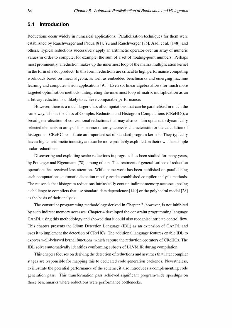
84 Chapter 5. Automatic Parallelisation of Reductions and Histograms
5.1 Introduction
Reductions occur widely in numerical applications. Parallelisation techniques for them were
established by Rauchwerger and Padua [81], Yu and Rauchwerger [85], Jradi et al. [148], and
others. Typical reductions successively apply an arithmetic operator over an array of numeric
values in order to compute, for example, the sum of a set of floating-point numbers. Perhaps
most prominently, a reduction makes up the innermost loop of the matrix multiplication kernel
in the form of a dot product. In this form, reductions are critical to high performance computing
workloads based on linear algebra, as well as embedded benchmarks and emerging machine
learning and computer vision applications [91]. Even so, linear algebra allows for much more
targeted optimisation methods. Interpreting the innermost loop of matrix multiplication as an
arbitrary reduction is unlikely to achieve comparable performance.
However, there is a much larger class of computations that can be parallelised in much the
same way. This is the class of Complex Reduction and Histogram Computations (CReHCs), a
broad generalisation of conventional reductions that may also contain updates to dynamically
selected elements in arrays. This manner of array access is characteristic for the calculation of
histograms. CReHCs constitute an important set of standard program kernels. They typically
have a higher arithmetic intensity and can be more profitably exploited on their own than simple
scalar reductions.
Discovering and exploiting scalar reductions in programs has been studied for many years,
by Pottenger and Eigenmann [78], among others. The treatment of generalisations of reduction
operations has received less attention. While some work has been published on parallelising
such computations, automatic detection mostly evades established compiler analysis methods.
The reason is that histogram reductions intrinsically contain indirect memory accesses, posing
a challenge to compilers that use standard data dependence [149] or the polyhedral model [28]
as the basis of their analysis.
The constraint programming methodology derived in Chapter 2, however, is not inhibited
by such indirect memory accesses. Chapter 4 developed the constraint programming language
CAnDL using this methodology and showed that it could also recognise intricate control flow.
This chapter presents the Idiom Detection Language (IDL) as an extension of CAnDL and
uses it to implement the detection of CReHCs. The additional language features enable IDL to
express well-behaved kernel functions, which capture the reduction operators of CReHCs. The
IDL solver automatically identifies conforming subsets of LLVM IR during compilation.
This chapter focuses on deriving the detection of reductions and assumes that later compiler
stages are responsible for mapping this to dedicated code generation backends. Nevertheless,
to illustrate the potential performance of the scheme, it also introduces a complementing code
generation pass. This transformation pass achieved significant program-wide speedups on
those benchmarks where reductions were performance bottlenecks.
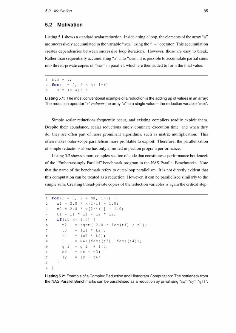
5.2. Motivation 85
5.2 Motivation
Listing 5.1 shows a standard scalar reduction. Inside a single loop, the elements of the array “a”
are successively accumulated in the variable “sum” using the “+=” operator. This accumulation
creates dependencies between successive loop iterations. However, those are easy to break.
Rather than sequentially accumulating “a” into “sum”, it is possible to accumulate partial sums
into thread-private copies of “sum” in parallel, which are then added to form the final value.
1 sum = 0;2 for(i = 0; i < n; i++)3 sum += a[i];
Listing 5.1: The most conventional example of a reduction is the adding up of values in an array:The reduction operator “+” reduces the array “a” to a single value – the reduction variable “sum”.
Simple scalar reductions frequently occur, and existing compilers readily exploit them.
Despite their abundance, scalar reductions rarely dominate execution time, and when they
do, they are often part of more prominent algorithms, such as matrix multiplication. This
often makes outer-scope parallelism more profitable to exploit. Therefore, the parallelisation
of simple reductions alone has only a limited impact on program performance.
Listing 5.2 shows a more complex section of code that constitutes a performance bottleneck
of the “Embarrassingly Parallel” benchmark program in the NAS Parallel Benchmarks. Note
that the name of the benchmark refers to outer-loop parallelism. It is not directly evident that
this computation can be treated as a reduction. However, it can be parallelised similarly to the
simple sum. Creating thread-private copies of the reduction variables is again the critical step.
1 for(i = 0; i < NK; i++) {2 x1 = 2.0 * x[2*i] - 1.0;3 x2 = 2.0 * x[2*i+1] - 1.0;4 t1 = x1 * x1 + x2 * x2;5 if(t1 <= 1.0) {6 t2 = sqrt(-2.0 * log(t1) / t1);7 t3 = (x1 * t2);8 t4 = (x2 * t2);9 l = MAX(fabs(t3), fabs(t4));
10 q[l] = q[l] + 1.0;11 sx = sx + t3;12 sy = sy + t4;13 }14 }
Listing 5.2: Example of a Complex Reduction and Histogram Computation: The bottleneck fromthe NAS Parallel Benchmarks can be parallelised as a reduction by privatising “sx”, “sy”, “q[]”.

86 Chapter 5. Automatic Parallelisation of Reductions and Histograms
sx sy
x=
q=
sx sy
x=
q=
sx’ sy’
q’=
sx += sx’
sy += sy’
q=
q’=
+=
+=
+=
synchronisation
Figure 5.1: Parallelisation of Listing 5.2: The input “x[]” is split over two threads (red/blue) thatoperate on private copies of “sx”, “sy”, “q[]”. These are merged after a synchronisation barrier.
The loop in Listing 5.2 is considered a CReHC for the following reasons: Firstly, there is
an input array “x[]”, from which values are read successively in each iteration. Secondly, the
values “sx” and “sy” are scalar reduction variables, as is evident from lines 11–12. They are
incremented conditionally, and the added value is not merely “x[i]” but the result of a complex
calculation with control flow. Nonetheless, the calculation and the branching condition only
depend on the input values “x[2*i]” and “x[2*i+1]”. Thirdly, the array “q[]” is updated as
a histogram array at line 10. The index “l” is not directly read from an input array, as in a
conventional histogram, but again the calculation only depends on the input values.
As in the case of the simple sum, the parallelisation of this code requires the computation
of partial results in separate memory locations before merging the partial results. The whole
process is illustrated in Figure 5.1, with different colours on the right showing the distribution
of the program over two threads. The scalar variables “sx”, “sy” and the array “q[]” are
privatised. Partial results are then accumulated in the local copies by partitioning the input
array equally across the two threads. Finally, the threads are synchronised, and partial results
merged. This is done by adding the local copies of “sx”, “sy” and performing an element-wise
addition of the local copies of “q[]”.
Figure 5.2 gives an insight into why existing schemes do not detect such reductions by
showing the compiler representation of this program. The histogram update occurs in the third
basic block with the “load”, assignment and “store” operations, but it is by no means obvious
that this is a safe reduction. In fact, accurately detecting reductions is non-trivial. If in the
original program, shown in Listing 5.2, the condition on line 5 was changed to “t1 <= sx”,
this would be no longer be a sound reduction, as there would now be a control dependence on
an intermediate result. This, in turn, would manifest itself as an additional data dependence
edge from block 3 to block 2 in Figure 5.2. Moreover, the code segment can only be classified
as a reduction because all the function calls that are present are pure. Such details have to be
checked to ensure correctness. What is needed is a way to specify these conditions precisely
and to then automatically identify code regions that satisfy the constraints.
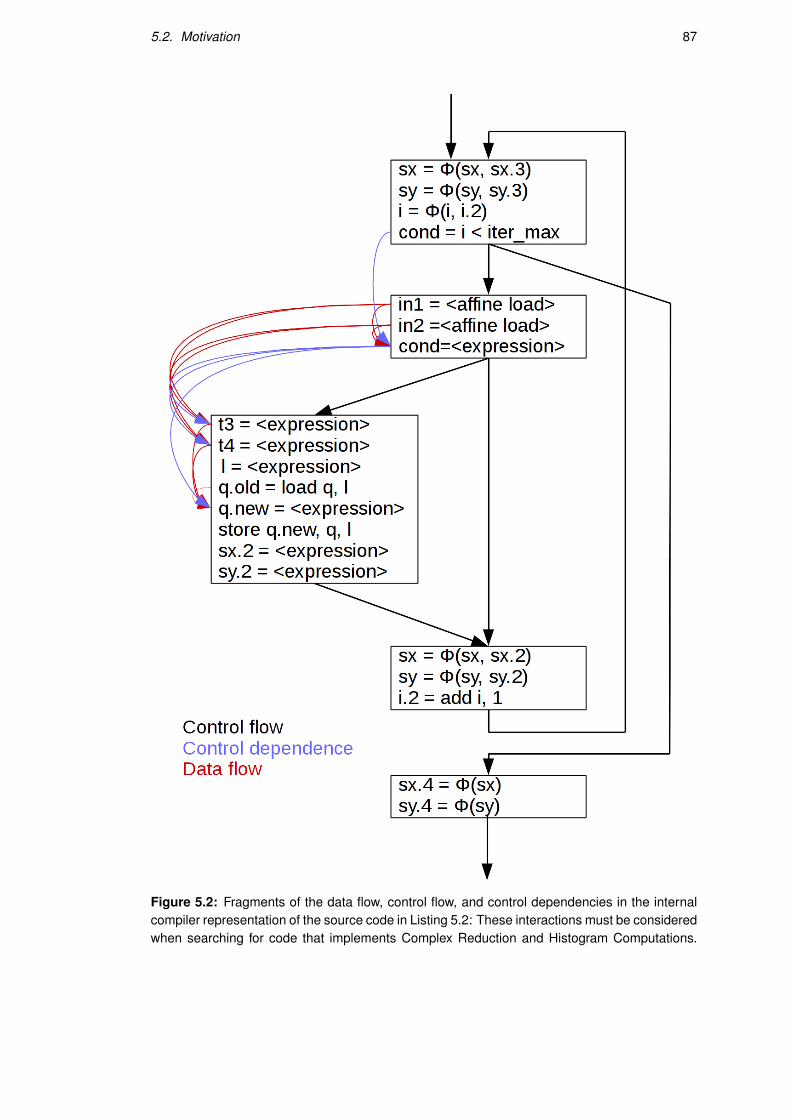
5.2. Motivation 87
Figure 5.2: Fragments of the data flow, control flow, and control dependencies in the internalcompiler representation of the source code in Listing 5.2: These interactions must be consideredwhen searching for code that implements Complex Reduction and Histogram Computations.
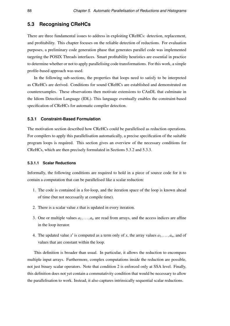
88 Chapter 5. Automatic Parallelisation of Reductions and Histograms
5.3 Recognising CReHCs
There are three fundamental issues to address in exploiting CReHCs: detection, replacement,
and profitability. This chapter focuses on the reliable detection of reductions. For evaluation
purposes, a preliminary code generation phase that generates parallel code was implemented
targeting the POSIX Threads interfaces. Smart profitability heuristics are essential in practice
to determine whether or not to apply parallelising code transformations. For this work, a simple
profile-based approach was used.
In the following sub-sections, the properties that loops need to satisfy to be interpreted
as CReHCs are derived. Conditions for sound CReHCs are established and demonstrated on
counterexamples. These observations then motivate extensions to CAnDL that culminate in
the Idiom Detection Language (IDL). This language eventually enables the constraint-based
specification of CReHCs for automatic compiler detection.
5.3.1 Constraint-Based Formulation
The motivation section described how CReHCs could be parallelised as reduction operations.
For compilers to apply this parallelisation automatically, a precise specification of the suitable
program loops is required. This section gives an overview of the necessary conditions for
CReHCs, which are then precisely formulated in Sections 5.3.2 and 5.3.3.
5.3.1.1 Scalar Reductions
Informally, the following conditions are required to hold in a piece of source code for it to
contain a computation that can be parallelised like a scalar reduction:
1. The code is contained in a for-loop, and the iteration space of the loop is known ahead
of time (but not necessarily at compile time).
2. There is a scalar value x that is updated in every iteration.
3. One or multiple values a1, . . . ,an are read from arrays, and the access indices are affine
in the loop iterator.
4. The updated value x′ is computed as a term only of x, the array values a1, . . . ,an, and of
values that are constant within the loop.
This definition is broader than usual. In particular, it allows the reduction to encompass
multiple input arrays. Furthermore, complex computations inside the reduction are possible,
not just binary scalar operators. Note that condition 2 is enforced only at SSA level. Finally,
this definition does not yet contain a commutativity condition that would be necessary to allow
the parallelisation to work. Instead, it also captures intrinsically sequential scalar reductions.

5.3. Recognising CReHCs 89
1 sum = 0;2 for(i = 0; i < n && sum < 10; i++)3 sum += a[i];
1 sum = 0;2 for(i = 0; i < n; i++)3 b[i] += a[i];
1 chase = 0;2 for(i = 0; i < n; i++)3 chase = a[chase];
1 sum = 0;2 active = true;3 for(i = 0; i < n; i++) {4 sum += active?a[i]:0;5 active = active && (sum < 10);6 }
Listing 5.3: Counterexamples to the four conditions: None of these computations can beparallelised as scalar reductions. The first and last example implement the same program.
Example Both “sx” and “sy” in Listing 5.2 satisfy the conditions. Firstly, the iteration space
of the loop is bounded by “NK”, which is constant. Secondly, within the SSA representation,
both “sx” and “sy” are unconditionally updated via Φ-instructions, shown in Figure 5.2. This
is despite the conditional statement in the original C representation of the program. Thirdly,
two values are read from the single input array “x[]” in every iteration, and the indices “2*i”
and “2*i+1” are affine in “i”. Finally, the updated values depend only on their respective old
values, the two values read from “x[]”, and the constants “1.0” and “2.0”. This also relies on
the fact that all functions used in the computation are pure functions.
Counterexamples Listing 5.3 shows counterexamples to the four conditions, demonstrating
why they are all needed in order to parallelise a given computation as a scalar reduction.
In the first example, the iteration space is not known in advance, as the computation can
be terminated depending on the input data. This makes it impossible to compute partial sums
in parallel. The second example is straightforward, as there is no reduction variable that could
be privatised. The loop could still be computed in parallel – but not as a scalar reduction. The
third example uses index calculations that are not affine in “i”. This prevents a straightforward
distribution of the input array across threads. In this particular case, the index calculation also
involves values other than “i”, preventing the computation of partial results entirely. The final
example is equivalent to the first but breaks the fourth condition instead of the first.

90 Chapter 5. Automatic Parallelisation of Reductions and Histograms
5.3.1.2 Histogram Reductions
The conditions that apply to histogram reductions are similar to those for scalar reductions.
However, instead of one function parameter, there are two:
1. The code is contained in a for-loop, and the iteration space of the loop is known ahead
of time (but not necessarily at compile time).
2. One or multiple values a1, . . . ,an are read from arrays, and the access indices are affine
in the loop iterator.
3. An integer k is computed as a term only of the array values a1, . . . ,an, and of values that
are constant within the loop.
4. A value x is read from an array at index k and a modified value x′ is written at the same
index. The writing may be control-dependent only on a1, . . . ,an and it may not be in a
nested loop.
5. The updated value x′ is computed as a term only of x, the array values a1, . . . ,an, and of
values that are constant within the loop.
Histogram reductions are only parallelisable if their update operator is commutative, just as
is the case for scalar reductions. However, checking this condition requires a post-processing
step, which is independent of the detection of the algorithmic structure. For this research,
checking commutativity was considered the responsibility of code generation.
Example The first two conditions are the same as those in the previous discussion of scalar
reductions and were shown to hold for the loop in Listing 5.2. The array “q[]” also satisfies
the remaining conditions. Firstly, the variable “l” corresponds to the index k. Secondly, the
element “q[l]” is read, modified and written. Lastly, the updated value is computed in an
allowed fashion, as it is obtained by merely adding a constant “1.0” to the previous value.
Counterexamples Again, counterexamples are given in Listing 5.4 to develop an intuition
about the significance of conditions 3–5.
In the first example, the index of the histogram is not computed from an input array but
instead read from an input stream. This makes parallelisation as a histogram impossible, as
the stream is only available sequentially. In the second and third examples, the computation
effectively stops when an index beyond a threshold size occurs. This can only be accounted for
by sequentially going through the array. Therefore, the parallel computation of partial results
is not efficiently possible. This behaviour is evoked in two different ways, by breaking the
conditions 4 and 5, respectively. This shows the need to restrict both the data flow and control
flow of the histogram kernel.
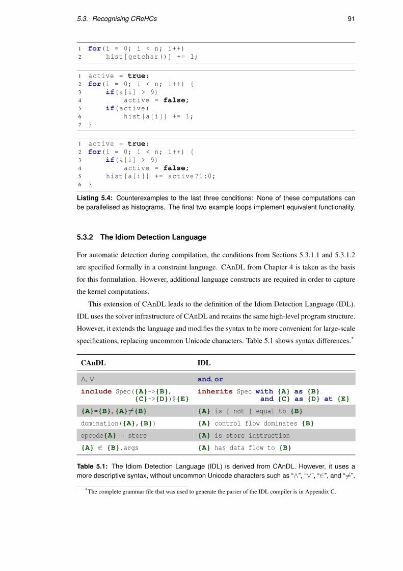
5.3. Recognising CReHCs 91
1 for(i = 0; i < n; i++)2 hist[getchar()] += 1;
1 active = true;2 for(i = 0; i < n; i++) {3 if(a[i] > 9)4 active = false;5 if(active)6 hist[a[i]] += 1;7 }
1 active = true;2 for(i = 0; i < n; i++) {3 if(a[i] > 9)4 active = false;5 hist[a[i]] += active?1:0;6 }
Listing 5.4: Counterexamples to the last three conditions: None of these computations canbe parallelised as histograms. The final two example loops implement equivalent functionality.
5.3.2 The Idiom Detection Language
For automatic detection during compilation, the conditions from Sections 5.3.1.1 and 5.3.1.2
are specified formally in a constraint language. CAnDL from Chapter 4 is taken as the basis
for this formulation. However, additional language constructs are required in order to capture
the kernel computations.
This extension of CAnDL leads to the definition of the Idiom Detection Language (IDL).
IDL uses the solver infrastructure of CAnDL and retains the same high-level program structure.
However, it extends the language and modifies the syntax to be more convenient for large-scale
specifications, replacing uncommon Unicode characters. Table 5.1 shows syntax differences.*
CAnDL IDL
∧, ∨ and, or
include Spec({A}->{B},{C}->{D})@{E}
inherits Spec with {A} as {B}and {C} as {D} at {E}
{A}={B}, {A} 6={B} {A} is [ not ] equal to {B}
domination({A},{B}) {A} control flow dominates {B}
opcode{A} = store {A} is store instruction
{A} ∈ {B}.args {A} has data flow to {B}
Table 5.1: The Idiom Detection Language (IDL) is derived from CAnDL. However, it uses amore descriptive syntax, without uncommon Unicode characters such as “∧”, “∨”, “∈”, and “ 6=”.
*The complete grammar file that was used to generate the parser of the IDL compiler is in Appendix C.

92 Chapter 5. Automatic Parallelisation of Reductions and Histograms
5.3.2.1 Kernel Functions as Generalised Domination
Complex Reduction and Histogram Computations can be expressed as a higher-order function.
This means that the computational idiom is not just parameterised with numerical values, such
as array dimensions, but contains kernel functions as parameters. To enable the capture of such
higher-order functions in IDL, additional constraint expressions are required that go beyond
what CAnDL provided. Specifically, IDL adds another atomic constraint based on generalised
graph domination, as previously described in Definition 2.15, using the following syntax:
all flow from variable_tuple or any origin to any of variable_tuple
passes through at least one of variable_tuple
The syntax of this atomic constraint is quite descriptive, but some details require explanation.
Firstly, “flow” in this constraint does not only capture data flow. To cover kernel functions with
non-trivial control flow, the underlying graph on which this constraint operates is formed as an
extension of the data flow graph DFG∗F . In addition to the data flow edges, it has an edge from
each branch instruction to every instruction within all its targeted basic blocks. This encodes
control dependence information and also guarantees that all relevant control flow is retained
when flushing the graph in reverse direction from the result of a computation. This is needed
for identifying the required instructions to implement a kernel as a separate function.
Secondly, as opposed to the control flow graph that is typically considered for dominance
relationships, the resulting graph has no single “origin”. Aside from the control entry, all non-
pure function calls and reads from memory are considered graph origins.
Figure 5.3 demonstrates the significance of this definition. At the top is an SSA pseudocode
representation of the complex reduction and histogram calculation from Listing 5.2, annotated
in the right column with all the dependencies described above. It is now possible to check the
validity of the kernel function that is used within the loop for the reduction on “sx” as follows:
1 all flow from {loop_carried[0..3]} or any origin2 to any of {sx’’} passes through at least one of3 {sx,t2,t5,precursor,backedge,outside[0..N]}}
This use of the new atomic constraint requires several additional conditions: “precursor” and
“backedge” should be determined and “outside[0..N]” should contain all origins that lie
outside the SESE region within which the kernel functions is considered. Furthermore, the
array “loop_carried” needs to be constrained to contain all loop-carried Φ-instructions.
With this setup, it is straightforward to check that the constraint is satisfied. Control flow
can only reach sx′′ via the precursor at line 1 and the back edge at line 28. The other relevant
graph origins for this example are the load instructions at lines 6,9,18 and the explicitly added
Φ-instructions. The three of these that can reach sx′′ through the graph are explicitly killed as
generalised dominators “sx”, “t2”, and “t5”.

5.3. Recognising CReHCs 93
Block Operation Dependencies
entry 1: goto loop outside the considered region
loop
2: i←Φ(entry : 0, loop : i′) loop carried data flow3: sx←Φ(entry : 0.0, loop : sx′′) loop carried data flow4: sy←Φ(entry : 0.0, loop : sy′′) loop carried data flow5: t1← 2 · i control(1, 28), data(2)6: t2← load x[t1] origin of data flow7: t3← 2.0 · t2−1.0 control(1, 28), data(6)8: t4← 2 · i+1 control(1, 28), data(2)9: t5← load x[t4] origin of data flow
10: t6← 2.0 · t5−1.0 control(1, 28), data(9)11: t7← t3 · t3 + t6 · t6 control(1, 28), data(7, 10)12: t8← t7 ≤ 1.0 control(1, 28), data(11)13: if t8 goto i f block else uncond control(1, 28), data(12)
ifblock
14: t9← sqrt(−2.0 · log(t7)/t7) control(13), data(11)15: t10← t3 ∗ t9 control(13), data(7, 14)16: t11← t6 · t9 control(13), data(10, 14)17: l←MAX( f abs(t10), f abs(t11)) control(13), data(15, 16)18: t12← load q[l] origin of data flow19: t13← t12 +1 control(13), data(18)20: store q[l]← t13 control(13), data(19)21: sx′← sx+ t10 control(13), data(3, 15)22: sy′← sy+ t11 control(13), data(4, 16)23: goto uncond control(13)
uncond
24: sx′′←Φ(loop : sx, i f block : sx′) control(13, 23), data(3, 21)25: sy′′←Φ(loop : sy, i f block : sy′) control(13, 23), data(4, 22)26: i′← i+1 control(13, 23), data(2)27: t14← i′ < NK control(13, 23), data(26)28: if t14 goto loop else exit outside the considered region
function kernel(sx, t2, t5)
entry
t3← 2.0 · t2−1.0t6← 2.0 · t5−1.0t7← t3 · t3 + t6 · t6t8← t7 ≤ 1.0if t8 goto i f block else uncond
ifblock
t9← sqrt(−2.0 · log(t7)/t7)t10← t3 · t9sx′← sx+ t10goto uncond
uncond sx′′←Φ(entry : sx, i f block : sx′)return sx′′
Figure 5.3: A kernel function is identified within the SSA pseudocode at the top (cf. Listing 5.2):The value of sx′′ is calculated in the SESE region spanning lines 2–27 as a pure function of onlysx, t2, and t5. This is determined by starting from sx′′ (blue) and following the dependencies onthe right, checking that all paths end in the predetermined function arguments sx, t1 and t5 (red).The kernel function can then be extracted and valid SSA reconstructed, as shown at the bottom.

94 Chapter 5. Automatic Parallelisation of Reductions and Histograms
1 Constraint KernelFunction
2 ( collect i 4 ( {entries[i]} has control
3 flow to {scope.begin}) and
4 collect i 24 ( inherits LocalConst
5 with {scope} as {scope}
6 at {outside[i]} and
7 {outside[i].value}
8 is not a numeric constant and
9 {outside[i].value} has data
10 flow to {outside[i].use} and
11 {scope.begin} control flow
12 dominates {outside[i].use}) and
13 collect i 8 ( {loop_carried[i].update} reaches
14 phi node {loop_carried[i].value}
15 from {scope.end} and
16 {scope.begin} control flow
17 dominates {loop_carried[i].value}) and
18 all flow from {loop_carried[0..8].value} or any origin
19 to any of {result} passes through at least one of
20 {inputs[0..32],entries[0..4],outside[0..24].value})
21 End
1 Constraint ScalarPart
2 ( {kernel.result} reaches phi node
3 {old_value} from {loop.end} and
4 inherits ScopeValue
5 with {loop} as {scope}
6 and {old_value} as {value} and
7 {kernel.result} has data flow to {final_value} and
8 {loop.end} strictly control flow
9 dominates {final_value} and
10 inherits KernelFunction
11 with {loop} as {scope} at {kernel} and
12 inherits Concat(N1=31,N2=1)
13 with {read_values} as {in1}
14 and {old_value} as {in2}
15 and {kernel.inputs} as {out})
16 End
Listing 5.5: IDL specifications of a kernel function and a scalar reduction within a CReHC: In“ScalarPart”, the kernel function operates in a loop. Its input “kernel.inputs” is composedof “read_values” and the reduction value of the previous iteration, concatenated with “Concat”.

5.3. Recognising CReHCs 95
5.3.2.2 Expressing Kernel Functions in IDL
Listing 5.5 encapsulates kernel functions as an IDL constraint specification in the top half. The
specification is built around the previously introduced generalised graph domination constraint,
which is invoked at lines 18–20. The arrays that are used in these final lines of the specification
are filled with several collect-all statements at lines 2–17. Lines 2–3 collect all the entry points
of the control flow. In the previous example, these were “precursor” and “backedge”. All
values from outside the scope that are used within the scope are collected at lines 4–12. These
values can be considered the closure of the kernel function. Finally, lines 13–17 collect all the
loop-carried Φ-instructions, which only exist in case the scope is a loop.
The bottom of Listing 5.5 shows the IDL specification of a scalar reduction component
within a CReHC loop. This IDL specification is built around a kernel function, incorporating
the specification at lines 10–11. The arguments to this kernel are set using the “Concat”
specification at lines 12–15. This kernel function is connected with a loop-carried Φ-instruction
at lines 2–6. Finally, lines 7–9 make sure that the reduction value eventually leaves the loop,
excluding loop-carried iterators that are only used within the loop.
Listing 5.6 shows how histogram reductions are specified similarly. Two kernel functions
calculate the index of the bin in the histogram (lines 7–9) and the updated value of its contents
(lines 10–15). The histogram update in each iteration may be conditional, as expressed with
“ConditionalReadModifyWrite” in lines 2–6. Crucially, the kernel functions use the scope
of the loop and already restrict this conditional to only depend on the allowed values.
1 Constraint HistoPart2 ( inherits ConditionalReadModifyWrite3 with {loop} as {scope}4 and {idx_kernel.result} as {address}5 and {val_kernel.result} as {new_value}6 at {update} and7 inherits KernelFunction8 with {loop} as {scope}9 and {read_values} as {inputs} at {idx_kernel} and
10 inherits KernelFunction11 with {loop} as {scope} at {val_kernel} and12 inherits Concat(N1=31,N2=1)13 with {read_values} as {in1}14 and {update.old_value} as {in2}15 and {val_kernel.inputs} as {out})16 End
Listing 5.6: IDL specification of a histogram reduction in a Complex Reduction and HistogramComputation: Two kernel functions are present. Lines 7–9 calculate the index into the histogramarray, lines 10–11 generate the updated value. The read-modify-write step may be conditional.

96 Chapter 5. Automatic Parallelisation of Reductions and Histograms
5.3.3 Specification of CReHCs in IDL
Listing 5.7 shows how the previously described IDL specifications can be assembled to define
the class of Complex Reduction and Histogram Computations.*
Such computations are always encapsulated by a single for-loop, as stipulated at line 2.
Lines 3–7 specify that input values “read_values” are read from one or several input arrays,
according to the specification “VectorRead”. These values are then passed at lines 12,17 to
the “HistoPart” and “ScalarPart” invocations. Note that the seemingly redundant variable
name assignments prevent prefixing with “histo[k]” and “scalar[k]”, respectively.
Lines 19–24 make sure that there are no array writes aside from the histogram updates.
Furthermore, lines 27–28 eliminate the possibility of effectful function calls within the loop.
Together, these constraints rule out any unwanted side effects of the loop.
Lines 25–26 enforce that the loop contains at least one reduction or histogram computation.
This is guaranteed indirectly because the two compared variables can only be the same if they
are both unused.
5.4 Code Generation for CReHCs
Parallel code generation immediately follows the CAnDL-generated detection pass. It uses the
detected constraint solutions to reimplement the corresponding loops with divide-and-conquer
parallelism based on POSIX Threads.
For each Complex Reduction and Histogram Computation loop that is found, the relevant
input arrays and closure variables are taken from the solution. They are packed into a data
structure together with any histogram arrays and the iteration space boundaries.
A new function is generated that takes this data structure as its only parameter. Depending
on the number of processors and recursion depth, the function decides whether to bisect its
workload recursively. If not, the loop is executed as before, using the arguments in the structure.
Otherwise, the function uses “pthread_create” to offload half of its workload onto another
thread. For this, it copies its parameter array, replacing histogram arrays with newly allocated
copies. After both threads finished their work, the copy is merged with the original histogram
element-wise and then deallocated.
In general, determining the size of the histogram at compile time is not possible with
static methods. All the branched-off threads, therefore, use dynamic boundary checking and
reallocate the histogram array when necessary. This on-demand enlargement introduces some
overhead but proved acceptable for many benchmark programs. The exceptions to this were
“IS” and “histo”, where the reduction arrays were large and the algorithmic intensity of the
reduction operators low. For these two programs, the reduction array sizes had to be predefined
*The complete IDL code for this section is in Appendix D.
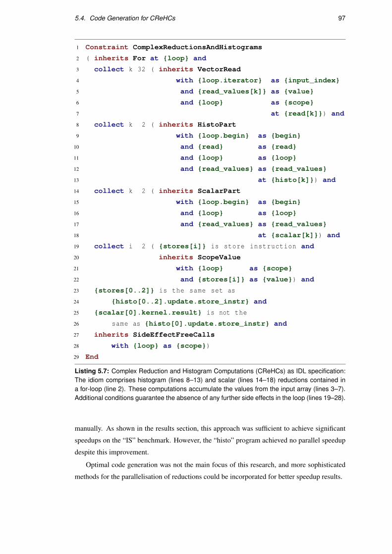
5.4. Code Generation for CReHCs 97
1 Constraint ComplexReductionsAndHistograms
2 ( inherits For at {loop} and
3 collect k 32 ( inherits VectorRead
4 with {loop.iterator} as {input_index}
5 and {read_values[k]} as {value}
6 and {loop} as {scope}
7 at {read[k]}) and
8 collect k 2 ( inherits HistoPart
9 with {loop.begin} as {begin}
10 and {read} as {read}
11 and {loop} as {loop}
12 and {read_values} as {read_values}
13 at {histo[k]}) and
14 collect k 2 ( inherits ScalarPart
15 with {loop.begin} as {begin}
16 and {loop} as {loop}
17 and {read_values} as {read_values}
18 at {scalar[k]}) and
19 collect i 2 ( {stores[i]} is store instruction and
20 inherits ScopeValue
21 with {loop} as {scope}
22 and {stores[i]} as {value}) and
23 {stores[0..2]} is the same set as
24 {histo[0..2].update.store_instr} and
25 {scalar[0].kernel.result} is not the
26 same as {histo[0].update.store_instr} and
27 inherits SideEffectFreeCalls
28 with {loop} as {scope})
29 End
Listing 5.7: Complex Reduction and Histogram Computations (CReHCs) as IDL specification:The idiom comprises histogram (lines 8–13) and scalar (lines 14–18) reductions contained ina for-loop (line 2). These computations accumulate the values from the input array (lines 3–7).Additional conditions guarantee the absence of any further side effects in the loop (lines 19–28).
manually. As shown in the results section, this approach was sufficient to achieve significant
speedups on the “IS” benchmark. However, the “histo” program achieved no parallel speedup
despite this improvement.
Optimal code generation was not the main focus of this research, and more sophisticated
methods for the parallelisation of reductions could be incorporated for better speedup results.

98 Chapter 5. Automatic Parallelisation of Reductions and Histograms
5.5 Experimental Setup
5.5.1 Benchmarks and Platform
The prototype idiom detection pass was applied to C versions of the NAS Parallel Benchmarks
(NPB) [139], which were developed by the NASA Advanced Supercomputing Division (NAS).
Specifically, the Seoul National University (SNU NPB) implementation by Seo et al. [140]
was used, containing the original 8 NAS benchmarks plus 2 of the more recent unstructured
components “UA” and “DC”.
The approach was also evaluated on all of the Parboil [150] and Rodinia [142] benchmark
programs. In total, this constitutes 40 programs of varying complexity, shown in Table 5.2.
The “Embarrassingly Parallel” program in NPB, for instance, is a single file of 324 lines of
code. By contrast, the source code of “Leukocyte” in Rodinia is distributed over more than 50
files. For each of the individual benchmark programs, the total number of scalar and histogram
reductions found was captured.
To determine runtime coverage and performance, all of the benchmarks were evaluated on
the same platform. This was a 64-core machine with 4 AMD Opteron 6376 processors and one
terabyte of RAM.
5.5.2 Competing Approaches
To provide a useful comparison, the IDL approach was evaluated against two state-of-the-art
competitors. The first is a recently-published approach that transforms reductions within the
polyhedral framework; the second is a mature industrial compiler.
Polly-Reduction Doerfert et al. [30] developed a compiler analysis and transformation tool
that detects reductions within code captured by the polyhedral model. This system augments
Polly, an LLVM-based polyhedral compiler [26]. The polyhedral model is powerful when
applicable, and Polly being based on LLVM IR allows for comparison of IDL against another
approach that uses the same compiler infrastructure.
The sequential benchmark programs were compiled by version 3.9 of the Clang compiler,
built with the Polly-enabled LLVM. The SCoPs that Polly detected with the compiler options
“-O3 -mllvm -polly -mllvm -polly-export” were considered. Any Polly-based method
only works within these SCoPs. Therefore, this gives an upper bound for the “Polly-Reduction”
method. Reductions within the SCoPS were then manually identified. Any reduction within
a SCoP was counted as a hit for “Polly-Reduction”. This gives an optimistic estimate as to
what coverage a polyhedral-based approach to reduction operations, such as the one presented
in Doerfert et al. [30], can achieve.
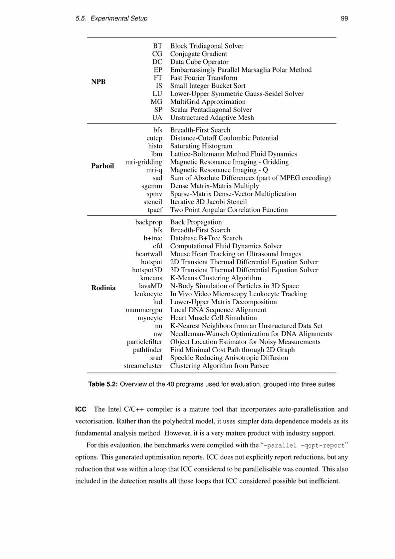
5.5. Experimental Setup 99
NPB
BT Block Tridiagonal SolverCG Conjugate GradientDC Data Cube OperatorEP Embarrassingly Parallel Marsaglia Polar MethodFT Fast Fourier TransformIS Small Integer Bucket Sort
LU Lower-Upper Symmetric Gauss-Seidel SolverMG MultiGrid ApproximationSP Scalar Pentadiagonal Solver
UA Unstructured Adaptive Mesh
Parboil
bfs Breadth-First Searchcutcp Distance-Cutoff Coulombic Potentialhisto Saturating Histogramlbm Lattice-Boltzmann Method Fluid Dynamics
mri-gridding Magnetic Resonance Imaging - Griddingmri-q Magnetic Resonance Imaging - Q
sad Sum of Absolute Differences (part of MPEG encoding)sgemm Dense Matrix-Matrix Multiply
spmv Sparse-Matrix Dense-Vector Multiplicationstencil Iterative 3D Jacobi Stencil
tpacf Two Point Angular Correlation Function
Rodinia
backprop Back Propagationbfs Breadth-First Search
b+tree Database B+Tree Searchcfd Computational Fluid Dynamics Solver
heartwall Mouse Heart Tracking on Ultrasound Imageshotspot 2D Transient Thermal Differential Equation Solver
hotspot3D 3D Transient Thermal Differential Equation Solverkmeans K-Means Clustering AlgorithmlavaMD N-Body Simulation of Particles in 3D Space
leukocyte In Vivo Video Microscopy Leukocyte Trackinglud Lower-Upper Matrix Decomposition
mummergpu Local DNA Sequence Alignmentmyocyte Heart Muscle Cell Simulation
nn K-Nearest Neighbors from an Unstructured Data Setnw Needleman-Wunsch Optimization for DNA Alignments
particlefilter Object Location Estimator for Noisy Measurementspathfinder Find Minimal Cost Path through 2D Graph
srad Speckle Reducing Anisotropic Diffusionstreamcluster Clustering Algorithm from Parsec
Table 5.2: Overview of the 40 programs used for evaluation, grouped into three suites
ICC The Intel C/C++ compiler is a mature tool that incorporates auto-parallelisation and
vectorisation. Rather than the polyhedral model, it uses simpler data dependence models as its
fundamental analysis method. However, it is a very mature product with industry support.
For this evaluation, the benchmarks were compiled with the “-parallel -qopt-report”
options. This generated optimisation reports. ICC does not explicitly report reductions, but any
reduction that was within a loop that ICC considered to be parallelisable was counted. This also
included in the detection results all those loops that ICC considered possible but inefficient.

100 Chapter 5. Automatic Parallelisation of Reductions and Histograms
5.6 Results
This section first presents the number of reductions found by the various different schemes.
This is followed by an analysis of how significant each reduction was. Finally, the performance
impact of the IDL-based parallelisation method was evaluated.
5.6.1 Discovery
The detection schemes were applied to the three benchmark suites, with the results shown in
Figures 5.4 to 5.6. Across all the benchmark programs, the IDL specification captured a total
of 90 reductions: 84 scalar reductions and 6 histogram reductions.
Discovered by IDL There were scalar reductions detected in nearly all of the individual NPB
programs, with “UA” having the highest number at 11. Scalar reductions were less prevalent
in Parboil with only 3 out of 11 benchmarks containing any. Furthermore, these were unevenly
distributed: out of a total of 9 scalar reductions across all Parboil programs, 7 were in “cutcp”.
The Rodinia benchmark collection contained many more identifiable reductions than Parboil.
The IDL solver detected scalar reductions in 15 out of the 19 benchmarks, with 9 reductions in
the “particlefilter” program alone.
Every reduction captured by the other two competing approaches was also identified by the
IDL solver. However, there were some regions that could be classified as reductions manually,
but that did not adhere to the used IDL specification, and thus remained unrecognised. This was
generally the case when the reduction loop was not the innermost loop, as is the case for the
example in Listing 5.8. The three outer loops of this code section from the “SP” benchmark
are reduction loops, but this is obfuscated by the innermost loop. None of the competing
approaches were able to detect this reduction either.
1 for (k = 1; k <= nz2; k++) {2 for (j = 1; j <= ny2; j++) {3 for (i = 1; i <= nx2; i++) {4 for (m = 0; m < 5; m++) {5 add = rhs[k][j][i][m];6 rms[m] = rms[m] + add*add;7 }8 }9 }
10 }
Listing 5.8: Some reductions were missed by all detection approaches. In this loop from “SP”,the outer loops are reduction loops, accumulating into scalar variables “rms[0]”,. . . ,“rms[4]”,but the innermost loop is not a reduction, and it is therefore not captured by the IDL specification.

5.6. Results 101
BT CG DC EP FT IS LU MG SP UA0
2
4
6
8
10
12
2
9
6
4
0
5
01
2
11IDL histogram reductionsIDL scalar reductionsICC reductionsPolly reductions
Figure 5.4: Reductions and histograms detected by the three competing approaches in NPB:Most programs contain scalar reductions, of which IDL consistently recognised more than ICC.Only IDL detected histograms. Most of the benchmarks were unsuitable for analysis with Polly.
bfs cutcphisto lbm
mri-gridding
mri-q sadsgemm
spmvstencil
tpacf0
2
4
6
8
0
7
10 0 0
1 10 0
1
IDL histogram reductionsIDL scalar reductionsICC reductionsPolly reductions
Figure 5.5: Reductions and histograms detected by the three competing methods in Parboil:In half of the benchmark components, no scheme detected any reductions. Nevertheless, IDLidentified two histograms in “histo” and “tpacf”, and was not outperformed on scalar reductions.
back
prop bfs
b+tre
ecf
dhe
artw
all
hotsp
otho
tspot
3Dkm
eans
lava
MD
leuk
ocyt
elu
dm
umm
ergp
um
yocy
te nn nwpa
rticl
efilte
rpa
thfin
der
srad
strea
mcl
uste
r
0
2
4
6
8
10
2
0
2
0
3
12
5
12
3
12
10
9
0
23
IDL histogram reductionsIDL scalar reductionsICC reductionsPolly reductions
Figure 5.6: Reductions and histograms detected by the 3 competing approaches in Rodinia:Most programs contained scalar reductions. ICC matched by IDL only on “heartwall” and “srad”.

102 Chapter 5. Automatic Parallelisation of Reductions and Histograms
Histogram reductions were rarer than scalar reductions. However, the IDL solver was able
to detect 3 in NAS, 2 in Parboil, and 1 in Rodinia. All of them eventually updated the bin value
with an addition, but some contained complex expressions in the kernel function to compute the
addend, as previously seen in Listing 5.2 for the “EP” program. Another interesting example
was “tpacf” from the Parboil benchmarks. In this histogram reduction, the histogram index
kernel function contained a binary search. At the other extreme, the performance bottleneck of
“IS” was a plain histogram without any complications:
1 for( i=0; i<NUM_KEYS; i++ )2 key_buff_ptr[key_buff_ptr2[i]]++;
Polly-Reduction The Polly compiler captured only four relevant code regions across all
benchmark programs that contained a single scalar reduction each. These are in “BT” and “SP”
from the NAS Parallel Benchmarks, “sgemm” from the Parboil Benchmarks, and “leukocte”
from Rodinia. As expected, all loops that contain histogram computations were unsuitable for
polyhedral analysis with Polly. Indirect memory access forms an integral part of any histogram
computation but violates assumptions of the polyhedral model.
Aside from the fundamental limitation for histogram computations, Polly struggled with
the more complex codebases of Rodinia and Parboil. This was not always due to fundamental
limitations of the polyhedral model. Instead, it was often because of loop iteration boundaries
that Polly could not statically determine and the use of flat array structures.
Figures 5.7 to 5.9 show the number of Static Control Parts (SCoPs) that Polly finds across
the 40 individual programs. Detecting such SCoPs is the first part of any polyhedral analysis.
As program code outside of SCoPs is left untouched by Polly, this provides an upper bound
for the detection of reductions. In 23 of the 40 benchmarks, Polly found no SCoPs at all. This
corresponded to 40% of NPB, 63.6% of the Parboil Benchmarks and 63.2% of Rodinia.
The majority of the SCoPs that Polly detected were in stencil computations. The stencil-
based programs “LU”, “BT”, “SP” and “MG” in the NAS Parallel Benchmarks alone accounted
for 37 of the 62 SCoPs that were found across all benchmarks (59.6%).
ICC The Intel C/C++ compiler was more successful than Polly at recognising reductions. It
detected 25 out of 37 reductions in NPB, 3 out of 9 in Parboil and 23 out of 38 in Rodinia.
However, these were all scalar reductions; no histograms were identified.
ICC was more robust and did not require SCoPs as a precondition for its analysis. On the
well-structured NAS benchmarks, it performed well but failed to detect any reductions in “IS”.
Surprisingly, it also did not detect reductions in “SP”, while Polly did. On closer inspection,
this is again due to a deep perfectly nested loop where the reduction iterator is in the middle of
the loop nest.

5.6. Results 103
BT CG DC EP FT IS LU MG SP UA02468
1012141618 reduction SCoPs
other SCoPs
Figure 5.7: Static Control Parts (SCoPs) identified by Polly in NPB: Six of the programs hadcode regions that were representable in the polyhedral model; two of them contained reductions.
bfs cutcphisto lbm
mri-gridding
mri-q sadsgemm
spmvstencil
tpacf0
1
2
3
4
5 reduction SCoPsother SCoPs
Figure 5.8: Static Control Parts (SCoPs) identified by Polly in Parboil: Most of the programswere unsuitable for Polly, only the reduction of the matrix multiplication in “sgemm” was captured.
back
prop bfs
b+tre
ecf
dhe
artw
all
hotsp
otho
tspot
3Dkm
eans
lava
MD
leuk
ocyt
elu
dm
umm
ergp
um
yocy
te nn nwpa
rticl
efilte
rpa
thfin
der
srad
strea
mcl
uste
r
0
1
2
3
4
5 reduction SCoPsother SCoPs
Figure 5.9: Static Control Parts (SCoPs) identified by Polly in Rodinia: Seven programs hadcode regions that were representable in the polyhedral model, but only one captured a reduction.

104 Chapter 5. Automatic Parallelisation of Reductions and Histograms
On the less well-structured Parboil benchmarks, ICC failed to detect many of the scalar
reductions in “cutcp”. This was because these reductions use the functions “fmin” and “fmax”,
which our system recognised as pure, but ICC did not. Finally, ICC recognised many of the
scalar reductions in Rodinia but was outperformed on six of the programs, with IDL finding one
additional reduction in each of them. It is clear that ICC did not attempt to detect histograms,
as it missed all instances of them.
5.6.2 Runtime Coverage
Detecting large numbers of reductions is encouraging but does not address whether or not such
detection is useful. To measure the potential impact, each program was profiled, examining the
time spent in the different types of reduction loops. These measurements from these profiling
runs are shown in Figures 5.10 and 5.11.
The two different classes of reductions behaved very differently. While there were many
more scalar reductions than histogram reductions in total, histogram reductions were much
more likely to constitute performance bottlenecks. In the benchmark programs that contained
histogram reductions, they accounted for an average of 68% of the runtime.
Scalar reductions, on the other hand, were generally irrelevant to program runtime, with
the one exception of the “sgemm” benchmark. Initial profiling already showed that none of the
scalar reductions in Rodinia were significant. Therefore, precise measurements were omitted
and are not shown in Figure 5.11.
It is evident that exploiting reduction parallelism for performance gains was promising only
for histogram reductions. While the “sgemm” program was bottlenecked by a scalar reduction
– the dot product inside the matrix multiplication – treating this loop as an arbitrary reduction
was unlikely to yield optimal results. Instead, Chapter 6 shows how to accelerate this with a
more targeted approach.
5.6.3 Performance
The speedup that was achieved by exploiting reduction parallelism on histograms is detailed
in Figure 5.12. This was only evaluated for benchmarks with significant runtime coverage of
reductions. The speedup from the IDL-based exploiting of reduction parallelism is compared
against the manually optimised parallel benchmark versions that were shipped by the original
implementors. The baseline is the sequential version of the respective benchmark program.
The IDL-based approach achieved 62% speedup on “EP” over the whole program. This
was limited by the runtime coverage of the histogram. Following Amdahl’s Law [151, 152],
parallelisation on 48 cores has a theoretical limit of 1/((1− 46%) + 46%/48)− 1 = 82%
speedup. The manually implemented parallel version, on the other hand, exploits outer-loop
parallelism and outperforms the reduction-based method.
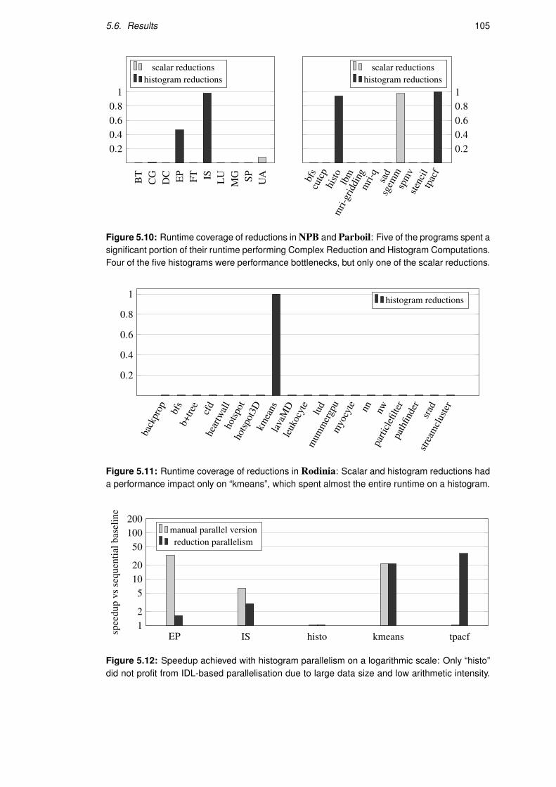
5.6. Results 105
BT
CG
DC EP
FT IS LU
MG SP UA
0.20.40.60.8
1
scalar reductionshistogram reductions
bfs
cutc
phi
sto lbm
mri-
grid
ding
mri-
qsa
dsg
emm
spm
vste
ncil
tpac
f
0.20.40.60.81
scalar reductionshistogram reductions
Figure 5.10: Runtime coverage of reductions in NPB and Parboil: Five of the programs spent asignificant portion of their runtime performing Complex Reduction and Histogram Computations.Four of the five histograms were performance bottlenecks, but only one of the scalar reductions.
back
prop bfs
b+tre
ecf
dhe
artw
all
hotsp
otho
tspot
3Dkm
eans
lava
MD
leuk
ocyt
elu
dm
umm
ergp
um
yocy
te nn nwpa
rticl
efilte
rpa
thfin
der
srad
strea
mcl
uste
r
0.2
0.4
0.6
0.8
1 histogram reductions
Figure 5.11: Runtime coverage of reductions in Rodinia: Scalar and histogram reductions hada performance impact only on “kmeans”, which spent almost the entire runtime on a histogram.
EP IS histo tpacfkmeans12
51020
50100200
spee
dup
vsse
quen
tialb
asel
ine
manual parallel versionreduction parallelism
Figure 5.12: Speedup achieved with histogram parallelism on a logarithmic scale: Only “histo”did not profit from IDL-based parallelisation due to large data size and low arithmetic intensity.
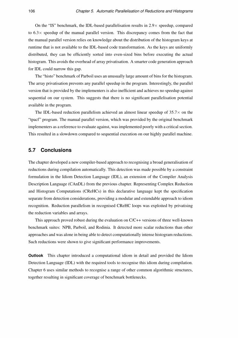
106 Chapter 5. Automatic Parallelisation of Reductions and Histograms
On the “IS” benchmark, the IDL-based parallelisation results in 2.9× speedup, compared
to 6.3× speedup of the manual parallel version. This discrepancy comes from the fact that
the manual parallel version relies on knowledge about the distribution of the histogram keys at
runtime that is not available to the IDL-based code transformation. As the keys are uniformly
distributed, they can be efficiently sorted into even-sized bins before executing the actual
histogram. This avoids the overhead of array privatisation. A smarter code generation approach
for IDL could narrow this gap.
The “histo” benchmark of Parboil uses an unusually large amount of bins for the histogram.
The array privatisation prevents any parallel speedup in the program. Interestingly, the parallel
version that is provided by the implementers is also inefficient and achieves no speedup against
sequential on our system. This suggests that there is no significant parallelisation potential
available in the program.
The IDL-based reduction parallelism achieved an almost linear speedup of 35.7× on the
“tpacf” program. The manual parallel version, which was provided by the original benchmark
implementers as a reference to evaluate against, was implemented poorly with a critical section.
This resulted in a slowdown compared to sequential execution on our highly parallel machine.
5.7 Conclusions
The chapter developed a new compiler-based approach to recognising a broad generalisation of
reductions during compilation automatically. This detection was made possible by a constraint
formulation in the Idiom Detection Language (IDL), an extension of the Compiler Analysis
Description Language (CAnDL) from the previous chapter. Representing Complex Reduction
and Histogram Computations (CReHCs) in this declarative language kept the specification
separate from detection considerations, providing a modular and extendable approach to idiom
recognition. Reduction parallelism in recognised CReHC loops was exploited by privatising
the reduction variables and arrays.
This approach proved robust during the evaluation on C/C++ versions of three well-known
benchmark suites: NPB, Parboil, and Rodinia. It detected more scalar reductions than other
approaches and was alone in being able to detect computationally intense histogram reductions.
Such reductions were shown to give significant performance improvements.
Outlook This chapter introduced a computational idiom in detail and provided the Idiom
Detection Language (IDL) with the required tools to recognise this idiom during compilation.
Chapter 6 uses similar methods to recognise a range of other common algorithmic structures,
together resulting in significant coverage of benchmark bottlenecks.

Chapter 6
Heterogeneous Acceleration via
Computational Idioms*
The previous chapter introduced a computational idiom – Complex Reduction and Histogram
Computations (CReHCs) – and showed how the Idiom Detection Language (IDL) enabled
its discovery and automatic parallelisation. This chapter takes a broader view of automatic
idiom recognition and also includes common linear algebra computations and stencil codes.
Instead of implementing bespoke parallelisation passes, this chapter follows the vision laid out
in the introduction: the detected idioms are translated into stronger models, and external code
generators are then used to leverage the implied domain knowledge.
To facilitate this, the chapter takes abstract algorithmic concepts that are conventionally
explored outside the context of compiler analysis – computational idioms – and formalises
them as IDL specifications. This enables detection and manipulation in optimising compilers.
Heterogeneous acceleration serves as the motivation for this effort. As many scientific codes
are structured around idiomatic performance bottlenecks, efforts that focus on computational
idioms can greatly improve performance, especially on accelerators that were designed with
such computations in mind. The focus is therefore on calculations that are well-supported by
accelerators and their software ecosystems: linear algebra, stencil codes and CReHCs.
The IDL specifications were used for a prototype compiler that automatically detects the
idioms and uses them to circumvent standard code generation via libraries and domain-specific
languages: BLAS implementations, cuSPARSE, clSPARSE, Halide, Lift. This functionality
is directly accessible from a modified version of the widely used Clang C/C++ compiler. The
evaluation could, therefore, be performed on the well-established benchmark suites NAS and
Parboil. 60 idiom instances were detected. In those cases where idioms were a significant part
of the sequential execution time, the generated heterogeneous code achieved 1.26× to over
20× speedup on integrated and external GPUs.
*This chapter is based on published research: Ginsbach et al. [3].
107

108 Chapter 6. Heterogeneous Acceleration via Computational Idioms
6.1 Introduction
Heterogeneous accelerators provide the potential for superior performance. However, realising
this potential in practice is difficult and requires significant programmer effort. Programs have
to be partially rewritten to target heterogeneous systems, using a diverse range of broad and
narrow interfaces. General-purpose languages such as OpenCL [153] provide some portability
across heterogeneous devices, but the achieved performance often disappoints [154]. Despite
the functional portability, rewrites are required in practice to achieve competitive performance.
Optimised numerical libraries provide more reliable performance, but they are more specialised
and often provided by hardware vendors without portability in mind [16, 15, 105, 106]. More
narrow domain-specific languages (DSLs) have been proposed by Ragan-Kelley et al. [11],
Franchetti et al. [155], Rompf and Odersky [156], among others in attempts to deliver both
portability and performance.
Hardware is becoming increasingly heterogeneous, most recently with the development of
deep neural network accelerators such as the Google TPU [20]. This means that library or DSL
based programming is likely to become far more common. The problems with this trend that
arise due to the aforementioned tradeoffs are evident. Firstly, application developers have to
learn multiple specialised DSLs and vendor-specific libraries if they want good performance.
Secondly, they have to rewrite their existing applications to use them. Thirdly, this ties code
into ecosystems that might soon become obsolete. Accelerator DSLs are quickly evolving, and
the adoption and long-term support of academic projects remain unclear. This situation is a
severe impediment to the wide-spread efficient exploitation of heterogeneous hardware.
The ideal would be a compiler that automatically maps existing code to heterogeneous
hardware, with full performance, and requiring no directions from the application programmer.
While this remains an ambitious goal for the general case, this chapter presents a system that
approximates such a general-purpose solution by utilising expertise that is already available
and encapsulated in existing backend interfaces. Instead of implementing code generation for
each heterogeneous accelerator, the system maps user code to heterogeneous hardware via
existing libraries and domain-specific languages, effectively outsourcing the code generation
to hardware and domain specialists.
The approach is based on detecting specific computational idioms in application code that
correspond to the functionality of existing interfaces – libraries and DSLs – for heterogeneous
acceleration. In addition to the Complex Reduction and Histogram Computations (CReHCs)
introduced in Chapter 5, the focus is on sparse and dense linear algebra, as well as stencils. The
covered idioms are a reflection of both the most relevant program bottlenecks and the available
interfaces. Some computational idioms were more widely supported than others, potentially
pointing to gaps in the accelerator landscape. Nonetheless, at least one backend existed per
idiom. The Idiom Detection Language (IDL) then enabled the automatic detection of idioms.

6.1. Introduction 109
Once detected, the idioms were translated into the matching DSL or replaced with an available
library call. The optimised DSL output code, or the pre-built optimised library, was then linked
into the original program.
The libraries cuSPARSE, clSPARSE, cuBLAS, clBLAS for sparse and dense linear algebra
and the DSLs Halide [11] and Lift [157] were used as backends in the evaluation. The Lift
language is a data-parallel functional language that supports generalised reductions as well as
stencils and linear algebra. The wide range of backends allowed the freedom to target many
APIs per idiom and pick the implementation that best suited the target platform.
New computational idioms could easily be added thanks to the flexibility of IDL. This
also provides a powerful means of determining whether a proposed heterogeneous interface
matches existing code, without touching the core compiler. The idioms addressed in this paper
were expressed in less than 500 lines of IDL code. The approach was also highly robust, was
applied to the entire NPB and Parboil benchmark suites and was evaluated on three platforms.
This chapter presents a novel approach that
• uses the Idiom Detection Language (IDL) for detecting idiomatic code sections that can
be accelerated by domain-specific backends;
• implements several common computational idioms in IDL to automatically discover
opportunities for accelerator exploitation;
• efficiently translates and maps the detected idioms to APIs for heterogeneous systems.
The work most similar in approach discovers stencil computations and maps them to the
Halide DSL for acceleration. The Helium tool [44] recovers stencils from image-processing
binaries. This requires large-scale dynamic analysis of binary traces and replacing them with
Halide calls. This was significantly extended by Kamil et al. [45], detecting stencils in Fortran
code. The focus of that work was on inferring post invariants based on syntax-guided synthesis
in translation to Halide. However, it used a narrow approach to code snippet selection and relied
on well-structured Fortran with occasional user annotations. The IDL approach is distinct in
its use of an external programming language for the flexibility of describing arbitrary idioms.
This allows an unbounded set of idioms to be considered and is not restricted to stencils.
To summarise, this chapter presents an automatic approach that discovers idioms in legacy
code and maps them to heterogeneous platforms via libraries and DSLs. The tool was applied
to 21 C/C++ programs from the NPB and Parboil benchmark suites, where it detected more
reductions, stencils, matrix multiplications and sparse matrix-vector computations than existing
schemes. For the programs where idioms dominate execution time, accelerator code was
generated and evaluated on 3 platforms: a multi-core CPU, an integrated APU, and an external
GPU. Overall, 60 idioms were detected, which dominated execution time in 10 programs.
Speedup results for the accelerated code ranged from 1.26× to over 20×.

110 Chapter 6. Heterogeneous Acceleration via Computational Idioms
6.2 Overview
The approach is automatic and was implemented inside the LLVM compiler infrastructure.
It takes arbitrary sequential C/C++ programs as input. Using the Clang compiler, the input
source code is compiled into a Static Single Assignment (SSA) intermediate representation
(LLVM IR). In this representation, the specified idioms are identified and replaced with calls to
specific APIs. Finally, the code generated by the LLVM compiler and the output of the idiom
specific code generators/libraries are linked together into a binary, producing an optimised
program. LLVM was chosen as it is the best supported SSA-based compiler. The methodology
could easily be transferred to other infrastructures, such as GCC.
6.2.1 Compiler Flow
Figure 6.1 gives a detailed overview of the compiler flow that underlies the approach of this
chapter. The grey box at the bottom left is the IDL-enabled compiler. It takes two programs as
inputs: the first is the source code of the user program, the second specifies the computational
idioms that are to be detected. The same idioms can be discovered in many user programs.
Therefore, the IDL program does not have to change from one run to the next.
The source code of the user program at the top left is compiled into optimised LLVM IR
code. The idiom description is parsed and represented internally as a C++ object, as previously
described in Chapter 2, Section 2.4.3. The solver takes the optimised LLVM IR code and
the internal C++ representation of the constraint formula as inputs. It uses backtracking to
recognises all idiomatic parts in the user program.
The recognised idioms and the LLVM IR code are then passed on to the transformation
phase of the system. This phase extracts the idiomatic code sections from the user program and
reformulates them for appropriate heterogeneous backends. For libraries, this means replacing
the code covered by the idiom with a library call.
For DSL interfaces, the process is a little more involved. The user code captured by idioms
is extracted and replaced with function calls to shim interfaces. The extracted code features are
translated into the appropriate DSL. External DSL compilers are responsible for optimising this
DSL code and generating library objects that implement the required function interfaces. The
translation to DSL mainly involves representing the kernel functions. Idioms without kernel
functions correspond to fixed DSL programs and require no additional work. The generated
code is linked with the object code from the user program.
Determining the best heterogeneous API to target for a given platform, and the best of
several overlapping idioms to exploit, will become an essential consideration as the number of
idioms and APIs grows. For the results in this chapter, all applicable libraries and DSLs were
evaluated, and the best-performing versions selected after profiling.
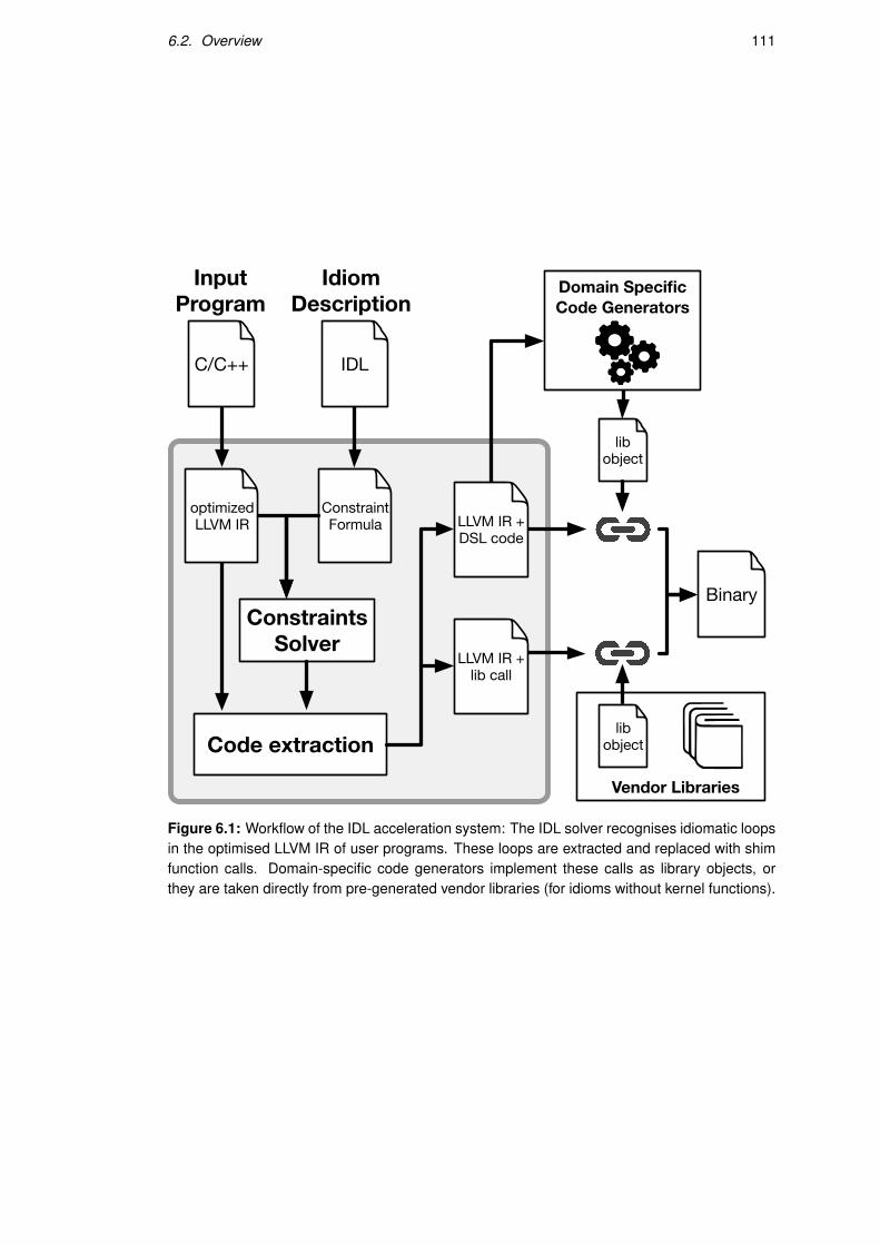
6.2. Overview 111
C/C++ IDL
optimizedLLVM IR
InputProgram
IdiomDescription
ConstraintFormula
ConstraintsSolver
Code extraction
LLVM IR +lib call
Binary
libobject
libobject
Vendor Libraries
Domain SpecificCode Generators
LLVM IR +DSL code
Figure 6.1: Workflow of the IDL acceleration system: The IDL solver recognises idiomatic loopsin the optimised LLVM IR of user programs. These loops are extracted and replaced with shimfunction calls. Domain-specific code generators implement these calls as library objects, orthey are taken directly from pre-generated vendor libraries (for idioms without kernel functions).

112 Chapter 6. Heterogeneous Acceleration via Computational Idioms
6.2.2 Accelerating Sparse Linear Algebra
Sparse linear algebra is central to many scientific codes and increasingly important as a basis
for graph algorithms and data analytics [158], but it contains indirect data accesses that limit
compiler optimisation. Instead of relying on tooling support, programmers use numerical
libraries that are hand-optimised and target accelerator hardware. This reliance on libraries
comes at a cost, however, as it ties programs into vendor-specific software ecosystems and
results in non-portable code. The IDL approach offers an alternative by recognising sparse
linear algebra kernels in compiler intermediate representation and incorporating the domain-
specific backends without source code changes.
The code at the top of Listing 6.1 is the performance bottleneck of the “Conjugate Gradient”
program from the NAS Parallel Benchmarks, with the corresponding LLVM IR code shown
underneath. This bottleneck loop implements a standard operation from sparse linear algebra,
namely the multiplication of a sparse matrix in Compressed Sparse Row (CSR) format with
a dense vector. This computation is supported on accelerator hardware, using well-optimised
libraries such as cuSPARSE and clSPARSE. However, compilers are unable to recognise and
accelerate the computation automatically.
The structure of this sparse linear algebra computation has several features that make it
unsuitable for most established compiler optimisations. Firstly, the iteration domain of the
nested loop is memory-dependent (line 3). Secondly, there is indirect memory access (line 4).
This makes the iteration domain of the loop nest non-polyhedral and the access structure to
memory non-affine. Under these conditions, not only do simple data dependence models fail,
but so do sophisticated analyses based on the polyhedral model.
IDL can express this sparse idiom, as derived in Section 6.3, Figure 6.3. The “Conjugate
Gradient” LLVM IR code, together with the “SPMV_CSR” IDL specification, are input to the
constraint solver, which outputs a constraint solution, as shown in Figure 6.2. In the solution,
different values from the LLVM IR have been assigned to all IDL variables in the “SPMV_CSR”
specification.
Listing 6.2 shows how this solution is used to generate a call to a cuSPARSE procedure.
The individual solution variables are inserted into the “cusparseDcsrmv” code template as
function arguments. The original code is then cut out and replaced with this function call. In
practice, this involved a shim function that manages the device context and memory transfers
from and to the GPU. Finally, the cuSPARSE library was linked with the object code produced
by the Clang compiler, resulting in a speedup of 17× on a GPU as described in more detail in
Section 6.8.
Central to this approach is the ability to detect computational idioms reliably. The next
section derives in detail the formulation of sparse and dense linear algebra, as well as stencils,
in the Idiom Detection Language.
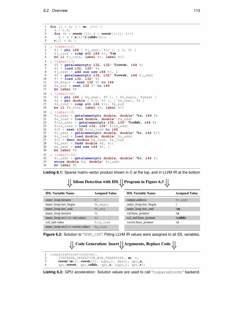
6.2. Overview 113
1 for (j = 0; j < m; j++) {2 d = 0.0;3 for (k = rowstr [j]; k < rowstr[j+1]; k++)4 d = d + a[k]*z[colidx[k]];5 r[j] = d; }
1 ; <label>:2:2 %j = phi i64 [ %j_next , %12 ], [ 0, %1 ]3 %j_cond = icmp slt i64 %j, %m4 br i1 %j_cond , label %3, label %13
5 ; <label>:3:6 %4 = getelementptr i32, i32* %rowstr, i64 %j7 %5 = load i32, i32* %48 %j_next = add nuw nsw i64 %j, 19 %6 = getelementptr i32, i32* %rowstr, i64 %j_next
10 %7 = load i32, i32* %611 %k_begin = sext i32 %5 to i6412 %k_end = sext i32 %7 to i6413 br label %8
14 ; <label>:8:15 %k = phi i64 [ %k_next , %9 ], [ %k_begin , %dnext ]16 %d = phi double [ 0.0, %3 ], [ %d_next , %9 ]17 %k_cond = icmp slt i64 %iv, %k_end18 br i1 %k_cond , label %9, label %12
19 ; <label>:9:20 %a_addr = getelementptr double, double* %a, i64 %k21 %a_load = load double, double* %a_addr22 %cix_addr = getelementptr i32, i32* %colidx, i64 %k23 %cix_load = load i32, i32* %cix_addr24 %10 = sext i32 %cix_load to i6425 %z_addr = getelementptr double, double* %z, i64 %1026 %z_load = load double, double* %z_addr27 %11 = fmul double %a_load , %z_load28 %d_next = fadd double %d, %1129 %k_next = add nsw i64 %k, 130 br label %8
31 ; <label>:12:32 %r_addr = getelementptr double, double* %r, i64 %j33 store double %d, double* %r_addr34 br label %2
Listing 6.1: Sparse matrix-vector product shown in C at the top, and in LLVM IR at the bottom
⇓ ⇓ ⇓Idiom Detection with IDL Program in Figure 6.3
IDL Variable Name Assigned Value
outer_loop.iterator %jinner_loop.iter_begin %k_begininner_loop.iter_end %k_endinner_loop.iterator %kinner_loop.src1 (≈ val.value) %zcol_ind.value %cix_loadinner_loop.src2 (≈ vector.value) %a_load
IDL Variable Name Assigned Value
output.address %r_addrouter_loop.iter_begin 0outer_loop.iter_end %mval.base_pointer %acol_ind.base_pointer %colidxvector.base_pointer %z. . . . . .
Figure 6.2: Solution to “SPMV_CSR”: Fitting LLVM IR values were assigned to all IDL variables.
⇓ ⇓ ⇓Code Generation: Insert Arguments, Replace Code
1 cusparseDcsrmv(context ,2 CUSPARSE_OPERATION_NON_TRANSPOSE , m, n,3 rowstr[m+1]-rowstr[0], &gpu_1 , descr , gpu_a,4 gpu_rowstr, gpu_colidx, gpu_z, &gpu_0 , gpu_r);
Listing 6.2: GPU acceleration: Solution values are used to call “cusparseDcsrmv” backend.

114 Chapter 6. Heterogeneous Acceleration via Computational Idioms
6.3 Specification of Idioms in IDL
The specification of computational idioms in IDL requires careful handling of the arising
complexity, using the modularity features that the language provides. Control flow constructs,
memory access patterns, and additional data flow constraints are defined independently and
then combined to form the complete specifications. This section extends upon the previously
defined building blocks from Chapters 4 and 5.
6.3.1 Sparse Linear Algebra
The most frequently used performance-critical sparse linear algebra routines are variations on
the multiplication of a sparse matrix with a dense vector (SPMV). Capturing the many different
memory access patterns is crucial for these sparse linear algebra routines. On the other hand,
the control flow is very rigid.
Listing 6.3 shows the basic skeleton of the SPMV idiom: there are two for-loops, the
“outer_loop” and the “inner_loop”. Naturally, “outer_loop” contains “inner_loop”
(lines 4–7). The outer loop is a standard for-loop (line 2), while the inner loop is a for-loop
contains a generalised dot product (line 3). Specifically, the “DotProductFor” specification
requires that the loop contains a scalar reduction variable that is incremented by the result of a
floating-point multiplication of two values “src1” and “src2” in every iteration. This skeleton
is completed depending on the sparse matrix format, defining the specific computations and
data flow that yields “src1” and “src2”.
6.3.1.1 Compressed Sparse Row
The Compressed Sparse Row (CSR) format is one of the most widely used formats for sparse
matrices [159]. An example matrix stored in CSR format is shown at the top of Figure 6.3. The
5×5 matrix at the top left is stored in the three separate arrays at the top right: “val”, “col_ind”,
and “row_ptr”.
All non-zero entries of the matrix are stored in a flat array “val” in a row-by-row order. The
“col_ind” array stores the column position for each value. Finally, the “row_ptr” array stores
the beginning of each row of the matrix as an offset into the other two arrays. The number of
rows in the matrix is given directly by the length of the “row_ptr” array minus one. However,
the number of columns is not explicitly stored.
The middle row of Figure 6.3 shows the corresponding SPMV computation in pseudocode.
Finally, the bottom of the figure shows the continuation of the “SPMV” specification for CSR
matrices in IDL. This continuation is immediately derived by walking through the pseudocode
expressions and emitting “inherits” directives to the corresponding IDL subprograms.

6.3. Specification of Idioms in IDL 115
1 Constraint SPMV2 ( inherits For at {outer_loop} and3 inherits DotProductFor at {inner_loop} and4 {outer_loop.begin} strictly5 control flow dominates {inner_loop.begin} and6 {outer_loop.end} strictly7 control flow post dominates {inner_loop.end} and8 ...
Listing 6.3: Skeleton of the sparse matrix-vector product (SPMV) constraint specification in IDL:The precise sparse access patterns are specific to chosen storage formats for sparse matrices.
val =[1 1 2 2 -1 3 2 2 -1 1
]col_ind =
[0 2 1 3 1 2 3 3 2 4
]row_ptr =
[0 2 4 7 8 10
]������������ �����
������������������ ���
��������������� �������������������������������
������������������������������������������� �!
7 ... # Set top-level expression: output[<1>]= <2> * <3> stack=(1,2,3)8 inherits VectorStore # 1: output[i] stack=(2,3)9 with {outer_loop} as {scope}
10 and {outer_loop.iterator} as {input_index} at {output} and11 inherits VectorRead # 2: val[j] stack=(3)12 with {outer_loop} as {scope}13 and {inner_loop.src1} as {value}#<-case <2>14 and {inner_loop.iterator} as {input_index} at {val} and15 inherits VectorRead # 3: vector[col_ind[<4>]] stack=(4)16 with {outer_loop} as {scope}17 and {inner_loop.src2} as {value}#<-case <3>18 and {col_ind.value} as {input_index} at {vector} and19 inherits VectorRead # 4: col_ind[j] stack=()20 with {outer_loop} as {scope}21 and {inner_loop.iterator} as {input_index} at {col_ind} and22 inherits ReadForLoopRanges23 with {outer_loop} as {scope}24 and {inner_loop} as {for}25 and {outer_loop.iterator} as {input_index} at {row_ptr})26 End
Figure 6.3: Compressed Sparse Row in IDL: The top section of the figure shows the differentarrays involved. The pseudocode in the middle of the figure informs the completion of Listing 6.3at the bottom. Walking through the expressions and emitting IDL code one-by-one is sufficient.

116 Chapter 6. Heterogeneous Acceleration via Computational Idioms
6.3.1.2 Jagged Diagonal Storage
For Jagged Diagonal Storage (JDS) [160], the rows of the matrix are permuted such that the
number of nonzeros per row decreases. The permutation is stored in a vector “perm”, the
number of nonzeros per row in “nzcnt”. The nonzero entries are then stored in an array “val”
in the following order: the first nonzero entry in each row, then the second nonzero entry in
each row and so on. The array “col_ind” stores the column for each of the values and “jd_ptr”
stores offsets into “val” and “col_idx”.
Figure 6.4 demonstrates this format on the example sparse matrix from Figure 6.3, and
derives the corresponding IDL code for the “SPMV_JDS” idiom underneath. Note that the sparse
matrix in this example is shown after the permutation operation that JDS requires.
6.3.2 Dense Linear Algebra
Describing dense linear algebra does not require storage format consideration aside from the
simple row-major and column-major distinction. The generalised matrix multiplication idiom
is shown in Listing 6.4. The control flow is captured by three nested for-loops. Inside these
loops, the memory access is characterised by three matrix accesses, each with a different subset
of the loop iterators. The corresponding “MatrixRead” and “MatrixWrite” idioms model
generic access to matrices, allowing strides and transpositions. The floating-point calculations
in the inner loop are encapsulated by the “DotProductForAlphaBeta” idiom. This extends
the “DotProductFor” specification with the linear combination that is part of the generalised
matrix multiplication idiom (C← αAB+βC).
1 Constraint GEMM2 ( inherits ForNest(N=3) and3 inherits MatrixStore4 with {iterator[0]} as {col}5 and {iterator[1]} as {row}6 and {begin} as {begin} at {output} and7 inherits MatrixRead8 with {iterator[0]} as {col}9 and {iterator[2]} as {row}
10 and {begin} as {begin} at {input1} and11 inherits MatrixRead12 with {iterator[1]} as {col}13 and {iterator[2]} as {row}14 and {begin} as {begin} at {input2} and15 inherits DotProductForAlphaBeta16 with {loop[2]} as {loop}17 and {input1.value} as {src1}18 and {input2.value} as {src2}19 and {output.address} as {update_address})20 End
Listing 6.4: IDL specification of the generalised dense matrix-vector multiplication (GEMM)

6.3. Specification of Idioms in IDL 117
perm =[1 2 0 4 3
]val =
[-1 1 2 -1 2 3 1 2 1 2
]col_ind =
[1 0 1 2 3 2 2 3 4 3
]jd_ptr =
[0 5 9 10
]nzcnt =
[3 2 2 2 1
]������������ �����
������������������ ���
��������������������� ������������������
����������������������������������������������������� �!
7 ... # Set top-level expression: output[<1>] = <2> * <3> stack=(1,2,3)
8 inherits VectorStore # 1: output[perm[<4>]] stack=(4,2,3)
9 with {outer_loop} as {scope}
10 and {perm.value} as {input_index} at {output} and
11 inherits VectorRead # 4: perm[i] stack=(2,3)
12 with {outer_loop} as {scope}
13 and {outer_loop.iterator} as {input_index} at {perm} and
14 inherits VectorRead # 2: val[(tmp1)=<5>] stack=(5,3)
15 with {outer_loop} as {scope}
16 and {inner_loop.src1} as {value}#<-case <2>
17 and {tmp1.value} as {input_index} at {val} and
18 inherits Addition # 5: (tmp1)=jd_ptr[<6>]+i stack=(6,3)
19 with {jd_ptr.value} as {input}
20 and {outer_loop.iterator} as {addend} at {tmp1} and
21 inherits VectorRead # 6: jd_ptr[i] stack=(3)
22 with {outer_loop} as {scope}
23 and {inner_loop.iterator} as {input_index} at {jd_ptr} and
24 inherits VectorRead # 3: vector[<7>] stack=(7)
25 with {outer_loop} as {scope}
26 and {inner_loop.src2} as {value}#<-case <3>
27 and {col_ind.value} as {input_index} at {vector} and
28 inherits VectorRead # 7: col_ind[(tmp1)=<5>] stack=()
29 with {outer_loop} as {scope}
30 and {tmp1.value} as {input_index} at {col_ind} and
31 inherits ReadForLoopIterations
32 with {outer_loop} as {scope}
33 and {inner_loop} as {for}
34 and {outer_loop.iterator} as {input_index} at {read_range}
Figure 6.4: Jagged Diagonal Storage in IDL: The top section of the figure shows the differentarrays involved. The pseudocode in the middle of the figure informs the completion of Listing 6.3at the bottom. Walking through the expressions and emitting IDL code one-by-one is sufficient.
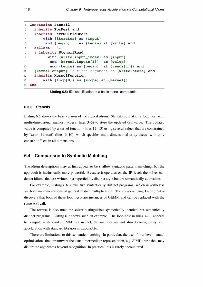
118 Chapter 6. Heterogeneous Acceleration via Computational Idioms
1 Constraint Stencil2 ( inherits ForNest and3 inherits PermMultidStore4 with {iterator} as {input}5 and {begin} as {begin} at {write} and6 collect i 327 ( inherits StencilRead8 with {write.input_index} as {input}9 and {kernel.inputs[i]} as {value}
10 and {begin} as {begin} at {reads[i]}) and11 {kernel.output} is first argument of {write.store} and12 inherits KernelFunction13 with {loop[0]} as {scope} at {kernel})14 End
Listing 6.5: IDL specification of a basic stencil computation
6.3.3 Stencils
Listing 6.5 shows the base version of the stencil idiom. Stencils consist of a loop nest with
multi-dimensional memory access (lines 3–5) to store the updated cell value. The updated
value is computed by a kernel function (lines 12–13) using several values that are constrained
by “StencilRead” (lines 6–10), which specifies multi-dimensional array access with only
constant offsets in all dimensions.
6.4 Comparison to Syntactic Matching
The idiom descriptions may at first appear to be shallow syntactic pattern matching, but the
approach is intrinsically more powerful. Because it operates on the IR level, the solver can
detect idioms that are written in a superficially distinct style but are semantically equivalent.
For example, Listing 6.6 shows two syntactically distinct programs, which nevertheless
are both implementations of general matrix multiplication. The solver – using Listing 6.4 –
discovers that both of these loop nests are instances of GEMM and can be replaced with the
same API call.
The reverse is also true: the solver distinguishes syntactically identical but semantically
distinct programs. Listing 6.7 shows such an example. The loop nest in lines 7–11 appears
to compute a standard GEMM, but in fact, the matrices are not stored contiguously, and
acceleration with standard libraries is impossible.
There are limitations to this semantic matching. In particular, the use of low-level manual
optimisations that circumvent the usual intermediate representation, e.g. SIMD intrinsics, may
distort the algorithms beyond recognition. In practice, this is rarely encountered.

6.4. Comparison to Syntactic Matching 119
1 for (int mm = 0; mm < m; ++mm) {
2 for (int nn = 0; nn < n; ++nn) {
3 float c = 0.0f;
4 for (int i = 0; i < k; ++i) {
5 float a = A[mm + i * lda];
6 float b = B[nn + i * ldb];
7 c += a * b;
8 }
9 C[mm+nn*ldc] =
10 C[mm+nn*ldc] * beta + alpha * c;
11 }
12 }
1 double M1[1000][1000];
2 double M2[1000][1000];
3 double M2[1000][1000];
4
5 //...
6
7 for(int i = 0; i < 1000; i++)
8 for(int j = 0; j < 1000; j++) {
9 M3[i][j] = 0.0f;
10 for(int k = 0; k < 1000; k++)
11 M3[i][j]+=M1[i][k]*M2[k][j]; }
Listing 6.6: Two matching instances of “GEMM”: Although both loop nests are implementedvery differently, they both match the same IDL specification and can be accelerated identically.
1 double *M1[1000];
2 double *M2[1000];
3 double *M2[1000];
4
5 //...
6
7 for(int i = 0; i < 1000; i++)
8 for(int j = 0; j < 1000; j++) {
9 M3[i][j] = 0.0f;
10 for(int k = 0; k < 1000; k++)
11 M3[i][j]+=M1[i][k]*M2[k][j]; }
Listing 6.7: This C program that does not match “GEMM”. Although the loop syntax is identical tothe matching example from Listing 6.6, the different types of the matrices prevent detection. Thisis desirable: Established backends are incompatible with such non-contiguous memory layout.
120 Chapter 6. Heterogeneous Acceleration via Computational Idioms
6.5 Targeting Heterogeneous Backends
After idiom detection, user programs must be transformed to exploit the relevant APIs. Two
types of heterogeneous APIs were targeted: libraries and domain-specific languages with their
optimising compilers.
6.5.1 Domain-Specific Libraries
Libraries provide narrow interfaces but are often highly optimised. For example, the cuBLAS
library is only suitable for a limited set of dense linear algebra operations and only works
on Nvidia GPUs, but its implementation provides outstanding performance. For sparse linear
algebra, the vendor-provided cuSPARSE, clSPARSE, and Intel MKL libraries were used. For
dense BLAS routines, the available backends were cuBLAS, clBLAS, CLBlast, and MKL.
6.5.2 Domain-Specific Code Generators
Domain-Specific Languages provide wider interfaces than libraries and allow problems to be
expressed as compositions of dedicated language constructs. Most importantly, this allows
DSLs to capture kernel functions of idioms that are higher-order functions, e.g. stencils and
reductions. The domain-specific optimising compiler then specialises the program for the target
hardware.
The end result is a library object, which can then be treated identically to pre-generated
vendor libraries. For this research, domain-specific code generators are, therefore, effectively
used as on-demand library generators. The evaluation used Halide and Lift as domain-specific
code generators.
Halide Ragan-Kelley et al. [11] introduced a language and optimising compiler targeted at
image processing applications. Optimised code is generated for CPUs as well as GPUs. Halide
separates the functional description of the problem from the description of the implementation.
This involves a separate execution schedule. This separation allows retargeting of Halide
programs to different platforms without touching the core program. Some of the stencil and
linear algebra idioms were translated into Halide. However, stencils involving control flow in
their kernel were not expressible in Halide and excluded for this backend.
Lift Steuwer et al. [109] introduced an optimising code generator based on rewrite rules [157,
161]. The Lift language consists of functional parallel patterns such as “map” and “reduce”
that express a range of parallel applications. Stencil idioms, complex reductions and linear
algebra idioms were translated to Lift.

6.6. Translating Computational Idioms 121
6.6 Translating Computational Idioms
This section describes how the detected idioms are mapped to the previously described library
APIs and domain-specific languages. The two types of APIs (library interfaces and domain-
specific languages) are treated individually.
6.6.1 Domain-Specific Libraries
For library call interfaces, the original code is removed, and an appropriate function call is
inserted. The solution that is generated by the solver using the IDL program contains both the
IR instructions to remove as well as the arguments that are to be used for the function call.
For example, in the case of the “GEMM” program that was shown in Listing 6.4, the original
code is removed by deleting the IR instruction at “output.store_instr” explicitly, which
captures the store instruction of the “MatrixStore” subprogram. The remaining cleanup
is left to the standard dead code elimination pass. The arguments that specify the matrix
dimensions are taken from “ForNest” in combination with the stride and offset determined
by “MatrixRead” and “MatrixWrite”.
The mapping of solution variables to the arguments of the generated function call needs to
be implemented individually for each backend, as it cannot be described using IDL itself. Once
the code is replaced, LLVM continues with code generation as usual.
6.6.2 Domain-Specific Code Generators
For domain-specific code generators, the situation is a bit more involved than for libraries.
Stencils and Complex Reduction and Histogram Computations are higher-order functions,
containing kernel functions or reduction operators that have to be represented for the DSL.
For each combination of idiom and DSL, there is a parameterised skeleton program. This
skeleton is then specialised for the appropriate data types and numeric parameters as well as
the kernel function or reduction operator.
Numerical parameters are picked from the constraint solution in the same way as previously
described for library call interfaces. Also, from the constraint solution, the loop body that
contains the kernel function or reduction operator is accessible, as well as the input values and
the result value used. This information is enough to cut out the kernel function, which is then
used to generate code appropriate for the DSL backends.
Halide is a language embedded in C++. It requires a syntax tree of the kernel functions
that built using a class hierarchy. However, Halide does not support control flow in the kernel
functions, making code generation easier than for Lift in practice. The relevant kernel functions
contain only a few LLVM IR instructions, which are easily assembled into Halide expressions.
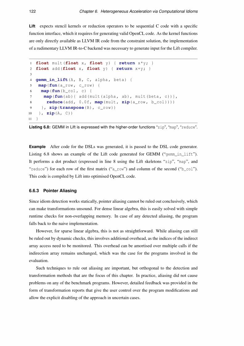
122 Chapter 6. Heterogeneous Acceleration via Computational Idioms
Lift expects stencil kernels or reduction operators to be sequential C code with a specific
function interface, which it requires for generating valid OpenCL code. As the kernel functions
are only directly available as LLVM IR code from the constraint solution, the implementation
of a rudimentary LLVM IR-to-C backend was necessary to generate input for the Lift compiler.
1 float mult(float x, float y) { return x*y; }2 float add(float x, float y) { return x+y; }3
4 gemm_in_lift(A, B, C, alpha , beta) {5 map(fun(a_row , c_row) {6 map(fun(b_col , c) {7 map(fun(ab){ add(mult(alpha , ab), mult(beta , c))},8 reduce(add , 0.0f, map(mult , zip(a_row , b_col))))9 }, zip(transpose(B), c_row))
10 }, zip(A, C))11 }
Listing 6.8: GEMM in Lift is expressed with the higher-order functions “zip”, “map”, “reduce”.
Example After code for the DSLs was generated, it is passed to the DSL code generator.
Listing 6.8 shows an example of the Lift code generated for GEMM (“gemm_in_lift”).
It performs a dot product (expressed in line 8 using the Lift skeletons “zip”, “map”, and
“reduce”) for each row of the first matrix (“a_row”) and column of the second (“b_col”).
This code is compiled by Lift into optimised OpenCL code.
6.6.3 Pointer Aliasing
Since idiom detection works statically, pointer aliasing cannot be ruled out conclusively, which
can make transformations unsound. For dense linear algebra, this is easily solved with simple
runtime checks for non-overlapping memory. In case of any detected aliasing, the program
falls back to the naive implementation.
However, for sparse linear algebra, this is not as straightforward. While aliasing can still
be ruled out by dynamic checks, this involves additional overhead, as the indices of the indirect
array access need to be monitored. This overhead can be amortised over multiple calls if the
indirection array remains unchanged, which was the case for the programs involved in the
evaluation.
Such techniques to rule out aliasing are important, but orthogonal to the detection and
transformation methods that are the focus of this chapter. In practice, aliasing did not cause
problems on any of the benchmark programs. However, detailed feedback was provided in the
form of transformation reports that give the user control over the program modifications and
allow the explicit disabling of the approach in uncertain cases.
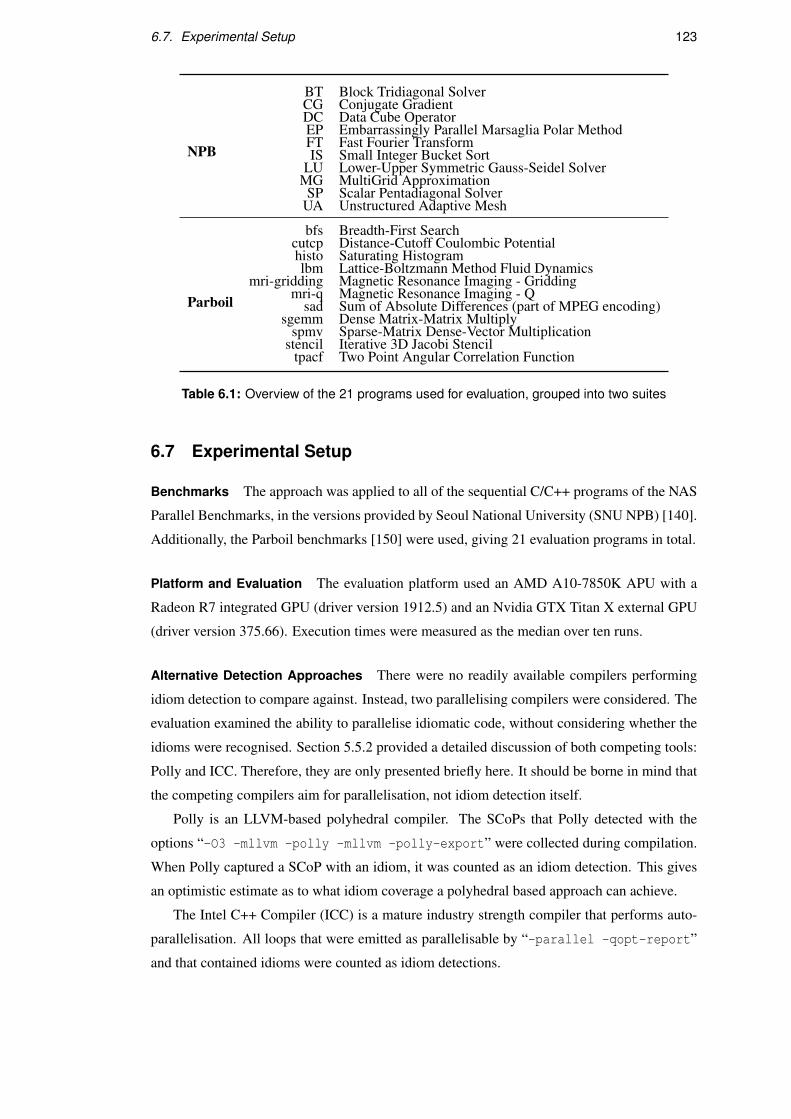
6.7. Experimental Setup 123
NPB
BT Block Tridiagonal SolverCG Conjugate GradientDC Data Cube OperatorEP Embarrassingly Parallel Marsaglia Polar MethodFT Fast Fourier TransformIS Small Integer Bucket Sort
LU Lower-Upper Symmetric Gauss-Seidel SolverMG MultiGrid ApproximationSP Scalar Pentadiagonal Solver
UA Unstructured Adaptive Mesh
Parboil
bfs Breadth-First Searchcutcp Distance-Cutoff Coulombic Potentialhisto Saturating Histogramlbm Lattice-Boltzmann Method Fluid Dynamics
mri-gridding Magnetic Resonance Imaging - Griddingmri-q Magnetic Resonance Imaging - Q
sad Sum of Absolute Differences (part of MPEG encoding)sgemm Dense Matrix-Matrix Multiply
spmv Sparse-Matrix Dense-Vector Multiplicationstencil Iterative 3D Jacobi Stencil
tpacf Two Point Angular Correlation Function
Table 6.1: Overview of the 21 programs used for evaluation, grouped into two suites
6.7 Experimental Setup
Benchmarks The approach was applied to all of the sequential C/C++ programs of the NAS
Parallel Benchmarks, in the versions provided by Seoul National University (SNU NPB) [140].
Additionally, the Parboil benchmarks [150] were used, giving 21 evaluation programs in total.
Platform and Evaluation The evaluation platform used an AMD A10-7850K APU with a
Radeon R7 integrated GPU (driver version 1912.5) and an Nvidia GTX Titan X external GPU
(driver version 375.66). Execution times were measured as the median over ten runs.
Alternative Detection Approaches There were no readily available compilers performing
idiom detection to compare against. Instead, two parallelising compilers were considered. The
evaluation examined the ability to parallelise idiomatic code, without considering whether the
idioms were recognised. Section 5.5.2 provided a detailed discussion of both competing tools:
Polly and ICC. Therefore, they are only presented briefly here. It should be borne in mind that
the competing compilers aim for parallelisation, not idiom detection itself.
Polly is an LLVM-based polyhedral compiler. The SCoPs that Polly detected with the
options “-O3 -mllvm -polly -mllvm -polly-export” were collected during compilation.
When Polly captured a SCoP with an idiom, it was counted as an idiom detection. This gives
an optimistic estimate as to what idiom coverage a polyhedral based approach can achieve.
The Intel C++ Compiler (ICC) is a mature industry strength compiler that performs auto-
parallelisation. All loops that were emitted as parallelisable by “-parallel -qopt-report”
and that contained idioms were counted as idiom detections.

124 Chapter 6. Heterogeneous Acceleration via Computational Idioms
6.8 Results
The approach was evaluated in several steps. First, the number of detected idioms and their
distribution over the benchmark programs was established. During this analysis, the runtime
of the IDL-enabled Clang compiler was measured, and the compile time overhead of the solver
over standard compilation evaluated. Next, the runtime coverage of the idioms was determined
for each benchmark program to see where exploitation might be beneficial.
Where runtime coverage was substantial, speedups over the sequential C code are reported.
Detailed results are given for the performance of each targeted backend interface. Finally, the
evaluation included comparisons to the handwritten OpenMP and OpenCL implementations
that were provided with the benchmark suites as reference implementations. These versions
provide suitable estimates for the upper bound of available performance.
6.8.1 Idiom Detection
Figure 6.5 shows the different idioms detected across all the individual benchmark programs.
IDL detected both scalar and histogram reductions, as well as stencils, dense matrix operations
and sparse matrix-vector multiplication. 16 of the 21 programs contained computational idioms
that IDL was able to identify. The most frequently occurring idiom was the scalar reduction,
present in 10 of the programs. Five of the benchmarks contained histograms; three contained
stencils; two contained SPMV; and only a single program calculated GEMM.
Table 6.2 summarises the number of computational idioms found by IDL, Polly, and ICC.
Polly found three scalar reductions and five stencils, and also detected the GEMM operation
as a generic SCoP. This was counted as a detected idiom, although Polly was unable to apply
any domain-specific knowledge from linear algebra. ICC only recognised scalar reductions,
but was much more successful at it than Polly, detecting a total of 28 instances.
Other approaches than IDL did not detect any histogram loops or sparse matrix operations.
IDL detected 60 idioms overall with the impact on the compilation times shown in Table 6.3.
On average, the compilation times were increased by 82%. This compilation overhead was due
to the solver and could be reduced further by optimising its implementation.
6.8.2 Runtime Coverage
To determine if the detected idioms were impactful, Figure 6.6 shows the percentage of runtime
spent in the detected computational idiom for each benchmark program. This data shows that
either the detected idioms have a low runtime contribution or they dominate almost the entire
execution. EP is the only exception with∼50% runtime coverage. Heterogeneous acceleration
was evaluated on the ten programs that spend a significant amount of time in the detected
idioms. Only these can reasonably expect a performance gain.

6.8. Results 125
BT CG DC EP FT IS LU MG SP UA bfs cutcp histo lbm mri−g mri−q sad sgemm spmv stencil tpacf
0
2
4
6
8
10
# D
ete
cte
d I
dio
ms
Idiom Type Scalar Reduction Histogram Reduction Stencil Matrix Operations Sparse Matrix Operations
Figure 6.5: The different computational idioms found across the benchmark programs: Scalarreductions were the most common, with 10 out of 21 programs containing some. Other idiomswere found in 1–5 programs each. Only five of the benchmarks contained no idiomatic code.
BT CG DC EP FT IS LU MG SP UA bfs cutcp histo lbm mri−g mri−q sad sgemm spmv stencil tpacf
0
25
50
75
100
Runtim
e C
ove
rage (
%)
Figure 6.6: Runtime coverage: 10 of the 21 programs have idiomatic performance bottlenecks.
Scalar
Reduction
Histogram
Reduction
Stencil Matrix Op. Sparse
Matrix Op.
Polly 3 — 5 1 —
ICC 28 — — — —
IDL 45 5 6 1 3
Table 6.2: Comparison of the number of idiom instances detected by IDL, ICC, and Polly: ICCdetected 60% of IDL’s reductions, but no other idioms. Polly focused mostly on stencil programs,but detected only 3 scalars. Both idioms with indirect memory access were exclusive to IDL.
BT CG DC EP FT IS LU MG SP UA bfs cutcp
without IDL 1.9 0.5 1.0 0.3 0.6 0.3 1.9 0.8 1.6 2.7 0.4 0.4
with IDL 4.0 0.8 1.6 0.6 1.2 0.5 3.9 4.5 3.2 7.3 0.5 0.6
overhead in % 116 77 57 77 93 62 103 484 97 169 30 65
histo lbm mri-g mri-q sad sgemm spmv stencil tpacf
without IDL 0.2 0.3 0.2 0.2 0.4 0.6 0.3 0.2 0.2
with IDL 0.2 0.6 0.4 0.3 0.6 0.7 0.7 0.2 0.4
overhead in % 35 87 100 52 58 24 115 36 54
Table 6.3: Compile time cost of IDL solver in seconds: Compilation took 82% longer on average.

126 Chapter 6. Heterogeneous Acceleration via Computational Idioms
CG EP IS MG histo lbm sgemm spmv stencil tpacf
CPUiGPU
GPUCPU
iGPUGPU
CPUiGPU
GPUCPU
iGPUGPU
CPUiGPU
GPUCPU
iGPUGPU
CPUiGPU
GPUCPU
iGPUGPU
CPUiGPU
GPUCPU
iGPUGPU
0
1
2
0
10
20
30
0
10
20
30
40
50
0
50
100
150
200
250
0
10
20
30
0
1
0
1
2
0
1
2
3
4
0
1
0
5
10
15S
pe
ed
up
vs.
Se
qu
en
tia
l
Figure 6.7: Speedup over sequential: Results for the best-performing backend on each platformare shown. The red bars indicate a manual modification for minimising redundant data transfers.
0.25 0.00 0.07 0.02
CG EP IS MG histo lbm sgemm spmv stencil tpacf
IDLO
penCL
OpenM
P
IDLO
penCL
OpenM
P
IDLO
penCL
OpenM
P
IDLO
penCL
OpenM
P
IDLO
penCL
OpenM
P
IDLO
penCL
OpenM
P
IDLO
penCL
OpenM
P
IDLO
penCL
OpenM
P
IDLO
penCL
OpenM
P
IDLO
penCL
OpenM
P
1
10
100
1000
Sp
ee
du
p v
s.
Se
qu
en
tia
l
Figure 6.8: IDL versus manual expert parallelisation: Speedup over the sequential baseline wasmeasured for IDL (selecting best performing backend; red bars) and the handwritten referenceOpenCL and OpenMP implementations (provided by the benchmark developers; yellow bars).
6.8.3 Performance Results
Speedup over Sequential Figure 6.7 shows the end-to-end speedup obtained by accelerating
idioms via heterogeneous APIs on a CPU, an integrated GPU, an external GPU, respectively.
All of the results include data transfer overhead to and from the GPUs, where required. This
overhead was intrinsic to the external GPU, which operates on distinct physical memory. The
integrated GPU, on the other hand, only incurred this cost when APIs enforced additional data
copies. Each bar shows the best-performing API for the given platform; Table 6.4 provides
detailed results also for the other API backends.
Moderate speedups were obtained for five of the benchmarks, from 1.26× for “histo” up to
4.5× for ‘IS”. Besides “MG”, all of these benchmarks had a scalar or histogram reduction as
their performance bottleneck. Interestingly, it emerges that for different benchmarks, different
hardware was beneficial. For “tpcaf”, the CPU was the best platform, beating the GPU, for
which the data transfer time dominated; for “MG” and “histo”, the integrated GPU struck
the right balance between computational power and avoiding data movement to the external
GPU; and for “EP” and “IS”, the data transfer to the GPU was amortised by its superior raw
performance. The results emphasise the significance of flexible heterogeneous code generation.
Committing to any one of the three hardware platforms in the source code would have always
resulted in less-than-optimal performance for at least some of the programs.
For five of the benchmarks, IDL enabled significantly higher performance gains, from
17× for “CG” and up to over 275× for “sgemm”. These benchmarks were computationally
expensive, and the external GPU was always the fastest architecture by a considerable margin.
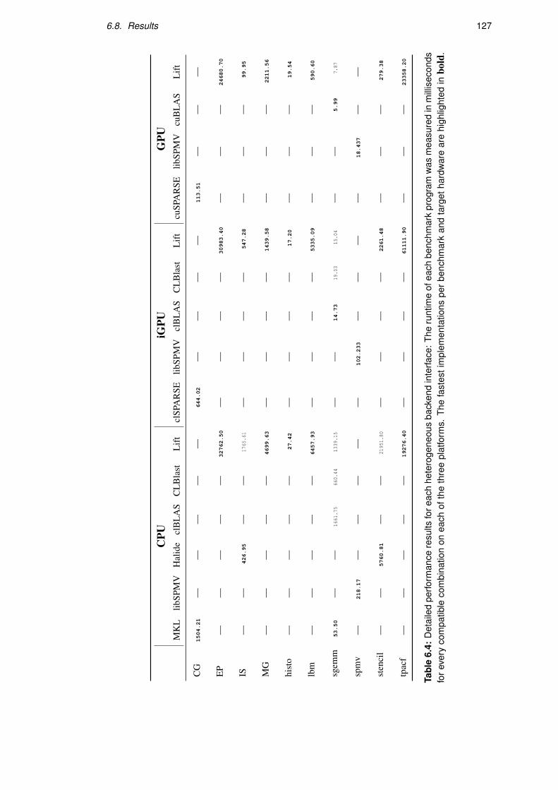
6.8. Results 127
CPU
iGPU
GPU
MK
Llib
SPM
VH
alid
ecl
BL
AS
CL
Bla
stL
ift
clSP
AR
SElib
SPM
Vcl
BL
AS
CL
Bla
stL
ift
cuSP
AR
SElib
SPM
Vcu
BL
AS
Lif
t
CG
1504.21
——
——
—644.02
——
——
113.51
——
—
EP
——
——
—32762.50
——
——
30983.40
——
—24680.70
IS—
—426.95
——
1765
.61
——
——
547.28
——
—99.95
MG
——
——
—4699.63
——
——
1439.58
——
—2211.56
hist
o—
——
——
27.42
——
——
17.20
——
—19.54
lbm
——
——
—6457.93
——
——
5335.09
——
—590.60
sgem
m53.50
——
1661
.75
660.
4413
39.1
5—
—14.73
19.0
315
.04
——
5.99
7.87
spm
v—
218.17
——
——
—102.233
——
——
18.437
——
sten
cil
——
5760.81
——
2195
1.80
——
——
2261.48
——
—279.38
tpac
f—
——
——
19276.40
——
——
61111.90
——
—23358.20
Tabl
e6.
4:D
etai
led
perfo
rman
cere
sults
fore
ach
hete
roge
neou
sba
cken
din
terfa
ce:T
heru
ntim
eof
each
benc
hmar
kpr
ogra
mw
asm
easu
red
inm
illis
econ
dsfo
rev
ery
com
patib
leco
mbi
natio
non
each
ofth
eth
ree
plat
form
s.Th
efa
stes
tim
plem
enta
tions
per
benc
hmar
kan
dta
rget
hard
war
ear
ehi
ghlig
hted
inbo
ld.

128 Chapter 6. Heterogeneous Acceleration via Computational Idioms
The red highlighting in Figure 6.7 indicates an important runtime optimisation: Redundant
data transfers for the iterative “CG”, “lbm”, “spmv” and “stencil” benchmarks were manually
eliminated. All of these benchmarks executed computations inside a for-loop, and did not
require access to the data on the CPU between iterations. A straightforward lazy copying
technique was manually applied by flagging memory objects to avoid redundant transfers,
similar to work by Jablin et al. [162]. This runtime optimisation was crucial for achieving
high performance on some of the benchmark programs.
API Performance Comparison Table 6.4 shows a breakdown of the performance of each API
on each program and platform. Not all APIs target all platforms, e.g. cuSPARSE only targets
NVIDIA GPUs. The version of Halide that was used for this evaluation failed to generate
valid GPU code for any of the benchmarks. Therefore, only the CPU platform was evaluated
with Halide. The best-performing backend is highlighted in bold in the table entries. None
of the previously existing backends supported “SPMV-JDS, which was detected in the “spmv”
benchmark. The libSPMV library was implemented as an ad-hoc solution to this, providing
straightforward parallelisation of the idiom.
On the multi-core CPU, Intel MKL gave the best linear algebra performance, outperforming
the other libraries and Lift. Halide achieved good performance for the NPB “IS” and Parboil
“stencil” benchmarks on the CPU, outperforming Lift due to its more advanced vectorisation
capabilities. In programs that were dominated by scalar reductions, Lift performed well.
On the internal GPU, clBLAS provided a better matrix multiplication implementation than
CLBlast and Lift. On the external GPUs, library backends provided the best linear algebra
implementations, while Lift performed well on stencils and reductions.
Speedup vs Handwritten Parallel Implementations Figure 6.8 shows the performance of
the IDL approach compared to handwritten reference OpenMP and OpenCL implementations.
For some of the benchmarks, the parallel versions were significantly modified beyond the
reach of automation and used entirely different algorithms. For benchmarks where the parallel
reference implementation did not make profound algorithmic changes (“CG”, “histo”, “lbm”,
“sgemm”, “spmv”, “stencil”), IDL enabled comparable – or better – performance. On four of
the benchmarks (“EP”, “IS”, “MG”, “tpacf”) it was more beneficial to parallelise the entire
application, which is beyond the scope of this work.
The handwritten versions of “sgemm” and “stencil’ were outperformed by IDL. This was
due to implementation flaws; a loop interchange already improved performance by almost 20×.
Summary 60 idioms were detected across the benchmark suites, and significant performance
improvements were achieved by targeting different heterogeneous APIs for those benchmarks
where idioms dominate execution time.
6.9. Conclusions 129
6.9 Conclusions
This chapter developed an approach for automatically detecting a broad class of computational
idioms during compilation. These idioms are supported by existing numerical libraries and
domain-specific languages that implement code generation for heterogeneous accelerators.
Once detected, the idiomatic loops are replaced by function calls to code generated by these
external tools.
The detection approach is based on the declarative Idiom Detection Language (IDL) that
identifies program subsets that adhere to idiom specifications with a constraint solver. The
evaluation showed that the ability of IDL to cover irregular idioms improved significantly over
the state-of-the-art implemented by Polly and ICC. Of the 10 benchmark applications where
IDL captured the majority of execution time as idiomatic, more than half implemented idioms
with indirect memory accesses. The incorporation of specialised code generators for idiomatic
code enabled reliable performance gains: speedups were achieved on all 10 programs. This
shows that idiom detection is a promising path to heterogeneous acceleration.


Chapter 7
Conclusions
This thesis introduced a constraint programming methodology that operates on SSA compiler
intermediate representation. The Compiler Analysis Description Language (CAnDL) and the
extended Idiom Detection Language (IDL) were developed, and implemented in the LLVM
framework. This made the constraint programming method available for program analysis.
Several computational idioms were specified using CAnDL and IDL, enabling automatic
recognition of adhering user code sections during compilation. The well-studied kernels among
these idioms were stencils and varied forms of sparse and dense linear algebra. Complementing
these established kernels, Complex Reduction and Histogram Computations (CReHCs) were
introduced as a new grouping of calculations. The evaluation on the established benchmark
suites NPB and Parboil demonstrated that all of these computational idioms covered significant
performance bottlenecks.
Recognising these computational idioms enabled generic compilers to apply idiom-specific
optimising transformations, which are traditionally available only within domain-specific tools.
Such transformations included the automatic parallelisation of programs that were inaccessible
to previous analysis approaches.
Given this background, the idiom detection was performed on sequential C/C++ programs,
achieving automatic heterogeneous parallelisation. Idiomatic loops in the code were redirected
to domain-specific code generators. These specialised tools leveraged the domain knowledge
that is available for code in restrictive idioms. This approach was applicable to 10 of the 21
benchmark programs from NPB and Parboil, resulting in speedups between 1.26× and 275×over the sequential baseline versions.
In summary, this thesis demonstrated that computational idioms are a suitable interface
to heterogeneous acceleration, and developed approaches for automatically recognising them.
The main contributions are the methodology of constraint programming on SSA intermediate
representation, the design and implementation of CAnDL and IDL, and the identification of
generalised reductions as a significant class of benchmark bottlenecks.
131

132 Chapter 7. Conclusions
7.1 Contributions
Constraint Programming on Compiler Intermediate Representation Chapter 2 introduced
constraint programming on SSA form intermediate code. Using a characterisation of the static
structure of SSA programs, SSA constraint problems were defined. These are formulas that
impose restrictions on compiler intermediate code, turning the detection of adhering program
parts into a constraint satisfiability problem. This thesis derived efficient algorithms for solving
SSA constraint problems and discussed significant classes of constraint formulas, reflecting
compiler analysis methods such as data flow and dominance relationships.
The constraint programming methodology was derived starting from algebraic formulation
through to developing the implementation in C++. It applies to any SSA compiler intermediate
representation and is suitable for a wide range of analysis problems.
Specification Languages Chapters 4 and 5 designed and implemented two novel declarative
specification languages: CAnDL (Compiler Analysis Description Language) and its extension
IDL (Idiom Detection Langauge). These languages make the constraint programming method
available in the LLVM framework. This enables constraint programming on the intermediate
code of user programs during compilation with the Clang C/C++ compiler.
Complex Reduction and Histogram Computations Complex Reduction and Histogram
Computations (CReHCs) were introduced in Chapter 5 as a computational idiom. CReHCs are
a generalisation of the well-understood scalar reduction, that additionally covers the indirect
array accesses typically found in histogram calculations. This type of loop was not previously
studied, but this thesis showed that shared parallelisation opportunities exist. Moreover, an
evaluation on established benchmark suites demonstrated that several performance bottlenecks
in each of NPB, Parboil, and Rodinia are, in fact, CReHCs.
Specification of Computational Idioms Chapters 4 to 6 specified a range of computational
idioms in CAnDL and IDL. These included stencils, different forms of sparse and dense linear
algebra, polyhedral Static Control Parts (SCoPs), and CReHCs. The constraint formulations
enabled the automatic recognition of high-level algorithmic structure during compilation. This
enabled generic compilers to apply domain-specific reasoning.
Heterogeneous Acceleration Pipeline Chapter 6 implemented a heterogeneous acceleration
pipeline. The user code sections recognised by IDL specifications were redirected to domain-
specific code generators for heterogeneous accelerator hardware. The evaluation demonstrated
significant heterogeneous parallelisation speedups on established benchmark programs.
7.2. Critical Analysis 133
7.2 Critical Analysis
The approaches of this thesis were built on the derivation of Chapter 2 and evaluated in
several scenarios on C/C++ program code. Despite the effort of bridging between the algebraic
formulation and the application in real-world scenarios, the work remains a prototype, and
several issues need to be addressed before it becomes viable for productive use. Importantly,
this includes questions about the prevalence of idiomatic code, the affordability of significant
compile time overhead, and the ability to compensate for limitations of the underlying solver
technology.
Universality of Computational Idioms Computational idioms were specified in Chapters 5
and 6 and evaluated successfully on a range of established benchmark collections. However,
the NPB and Parboil collections are both from areas of scientific computing. It remains unclear
how generally applicable these idioms are on codebases from other domains. Similar concerns
are faced by competing approaches, including the polyhedral model.
More generally, it is unclear how much code in large-scale applications could be captured
as “idiomatic” even with a more extensive set of idioms. Even some benchmark programs
within NPB and Parboil contain idiosyncratic computations that are unlikely to reoccur in other
contexts. An example is the “sad” program that computes the “Sum of Absolute Differences”
algorithm used by the reference H.264 video encoder.
Compile Time Cost The compile time cost of idiom detection was evaluated in Chapter 6,
showing that overheads between 35% and 115% occurred across the benchmark programs.
Given that the approach is built on constraint satisfiability methods, this is a reassuring result, as
the compile times remain within one order of magnitude. Nonetheless, from the perspective of
compiler optimisations, this might be a prohibitive cost. Moreover, the compile time overhead
is unevenly distributed, with disproportionately longer solver times on large functions and
especially on code sections that are near misses to satisfying the specifications.
Bounded Number of Solver Variables The specification languages were restricted by the
solver to a finite number of variables in the underlying constraint problems. Moreover, each
additional variable incurred a slight overhead, introducing a tradeoff between solver speed
and the generality of the specifications. This caused upper bounds for the number of features
within many idiom specifications: The definition of CReHCs only allowed a maximum of two
histograms, stencils only allowed a neighbourhood of up to 32 elements, and so on.
Similar shortcomings are well-known in other research disciplines using solvers, and some
techniques for resolving them have been suggested by Krings and Leuschel [163] in the context
of constraint logic programming.

134 Chapter 7. Conclusions
7.3 Future Work
Directions for future work include the specification of more computational idioms, usability
improvements of the specification languages, and the application of dynamic analysis and
machine learning to complement the static analysis. Moreover, constraint specifications could
eventually be generated from examples, eliminating the difficulty of writing them manually.
Complementing Dynamic and Machine Learning Approaches The static methods in this
thesis could be enhanced with dynamic approaches and machine learning. Such methods would
naturally complement the entirely static reasoning of constraint programming, but were outside
the scope of this work.
Dynamic profiling could preselect candidate hot loops, drastically reducing the compile
time overhead. More advanced dynamic analysis could collect program features to be fed into
machine learning algorithms. The use of neural networks to guide compiler optimisations has
been successfully studied in the relevant literature [164].
Dynamic methods are also suitable for automating the efficient memory transfers required
between cooperating hardware in heterogeneous computing, and to rule out pointer aliasing.
Unbounded Number of Variables Related research disciplines found ways around some
limitations of their underlying solvers. For example, Bounded Model Checking [165] uses SAT
solvers and involves the unrolling of loops to generate formulas. In order to fit the underlying
solver, this requires the introduction of a certain finite iteration limit k. However, the checking
process can be repeated with increasing values for k, successively ruling out possible violations.
The same approach could be applied to constraint solving on SSA. The solver would be
invoked repeatedly with a gradually increasing number of variables. When no collect constraint
exceeds variable capacity anymore, the process would be terminated. This would ensure that
small solutions are found without unnecessary overhead, yet solutions requiring many variables
would not be discarded entirely. No upper limits for collect statements would be required with
this scheme.
Pointer-Chasing Idioms The ability to recognise sparse linear algebra sets the methods of
this work apart from previous approaches. Going beyond a single data access indirection, IDL
could be used to capture data access patterns that involve pointer chases. This would allow it
to analyse graph operations, such as depth-first graph traversal and the PageRank algorithm.
Parboil implements the breadth-first search program “bfs” that could be accelerated this way.
Moreover, IDL could detect iterations over lists, and the insertion and removal of list items,
extending work by Manilov et al. [97]. Such patterns are not usually performance-critical, but
this would be another step toward an understanding of dynamic data structures in compilers.

7.3. Future Work 135
Higher-level Specification Languages Compared to previous approaches, the specification
languages CAnDL and IDL simplify the implementation of compiler analysis functionality and
enable the detection of more sophisticated idiomatic structures. Nonetheless, knowledge of the
compiler internals is still required to write correct specifications. Furthermore, the precise
extent to which the customisation of the specification languages to LLVM IR was necessary
has not been explored thoroughly.
Future work could investigate languages that abstract away the compiler-specific nature of
CAnDL and IDL, providing an improved programming experience. The pseudocode and the
corresponding specifications in Figures 6.3 and 6.4 suggest how this could be achieved. They
show that for restricted domains (e.g. SPMV), generating IDL from high-level expressions is
straightforward.
Phase-Ordering for Normalisation The presented methods for constraint programming on
LLVM IR relied on preceding optimisation passes for the normalisation of the intermediate
code generated from user programs. The relationship between normalisation and optimisation
in compiler transformation passes poses interesting research questions.
To allow the specification of idioms on predictable intermediate code structures, the solver
was invoked after the Clang optimisation pipeline. Optimisations such as loop-independent
code motion helped eliminate the artefacts of superficial implementation decisions by mapping
many different input programs onto the same optimised intermediate code.
While this approach was effective in practice, the existing LLVM optimisation passes
were not designed for this purpose. Instead, they aim to maximise runtime performance and
minimise code size. Incidentally, these two goals often coincide with normalising behaviour.
However, there are clear exceptions to this rule. The outcome of loop unrolling introduces
unpredictability, as the decision to unroll is based on opaque heuristics and threshold values
that depend on command-line options. Similarly, threshold values for loop unswitching interact
with the loop inversion transformation in obfuscating ways. The surrounding conditionals of
inverted loops within loop nests are sometimes – but not always – propagated out. Finally,
strength reduction changes the opcodes of instructions in special cases.
These challenges were resolved pragmatically in this research. High threshold values were
set, some optimisations were disabled (loop unrolling, vectorisation), and others were partially
reversed (strength reduction).
Instead of pruning the “-Os” or “-O2” presets, future work could establish special-purpose
normalisation compilers by re-evaluating the phase-ordering from scratch. According to a new
metric, individual compiler optimisations could be evaluated on a spectrum from “distorting” to
“normalising”. The highly-scoring passes would then selected for a dedicated phase-ordering
for intermediate code normalisation.

136 Chapter 7. Conclusions
Generating Specifications from Examples The automatic generation of specifications from
examples is another direction for follow-up research. Initial attempts were successful [166].
Using a graph-matching algorithm that operates on SSA code, implementation variations of
the same idiom were overlayed, exposing the common structure. This was guided by a quality
metric for the matching. Code structures that were shared between the examples were turned
into constraints, and features that were unique to specific samples were discarded.
Suitable quality metrics for graph-matching are critical to the success of this approach and
could eventually be tuned with machine learning approaches, such as neural networks. The
manually implemented idioms from this thesis would provide suitable training data.
Eventually, the manual curation of example codes that group together into computational
idioms could become redundant. Automatic profiling of large quantities of code would allow
for the automatic identification of all the relevant hot loops. These loops could then be grouped
into computational idioms by an automatic clustering algorithm using a distance metric. The
success score for the previously discussed graph-matching approach would be a suitable basis
for deriving such a metric for the distance between different candidate loops.
7.4 Summary
This chapter gave a brief overview of the thesis, outlining the development of the approaches
and putting the achieved results into context. The core contributions of this work were listed
individually in a dedicated section. Furthermore, the critical analysis discussed implementation
issues and brought attention to details that could profit from further evaluation.
Interesting challenges remain for future work. The suggested topics include improvements
of the basic methodology for constraint programming, enhanced usability of the specification
languages, and the application to novel domains.

Bibliography
[1] Philip Ginsbach, Lewis Crawford, and Michael F. P. O’Boyle. CAnDL: A Domain
Specific Language for Compiler Analysis. In Proceedings of the 27th International
Conference on Compiler Construction, CC ’18, pages 151–162, New York, NY, USA,
2018. ACM. ISBN 978-1-4503-5644-2. doi: 10.1145/3178372.3179515. URL http:
//doi.acm.org/10.1145/3178372.3179515.
[2] Philip Ginsbach and Michael F. P. O’Boyle. Discovery and Exploitation of General
Reductions: A Constraint Based Approach. In Proceedings of the 2017 International
Symposium on Code Generation and Optimization, CGO ’17, pages 269–280,
Piscataway, NJ, USA, 2017. IEEE Press. ISBN 978-1-5090-4931-8. URL http:
//dl.acm.org/citation.cfm?id=3049832.3049862.
[3] Philip Ginsbach, Toomas Remmelg, Michel Steuwer, Bruno Bodin, Christophe Dubach,
and Michael F. P. O’Boyle. Automatic Matching of Legacy Code to Heterogeneous
APIs: An Idiomatic Approach. In Proceedings of the Twenty-Third International
Conference on Architectural Support for Programming Languages and Operating
Systems, ASPLOS ’18, pages 139–153, New York, NY, USA, 2018. ACM. ISBN 978-1-
4503-4911-6. doi: 10.1145/3173162.3173182. URL http://doi.acm.org/10.1145/
3173162.3173182.
[4] G. E. Moore. Cramming more components onto integrated circuits, reprinted from
electronics, volume 38, number 8, april 19, 1965, pp.114 ff. IEEE Solid-State Circuits
Society Newsletter, 11(3):33–35, Sep. 2006. doi: 10.1109/N-SSC.2006.4785860.
[5] R. H. Dennard, F. H. Gaensslen, V. L. Rideout, E. Bassous, and A. R. LeBlanc. Design
of ion-implanted mosfet’s with very small physical dimensions. IEEE Journal of Solid-
State Circuits, 9(5):256–268, Oct 1974. doi: 10.1109/JSSC.1974.1050511.
[6] G. D. Hutcheson. Moore’s law, lithography, and how optics drive the semiconductor
industry. In Society of Photo-Optical Instrumentation Engineers (SPIE) Conference
Series, volume 10583 of Society of Photo-Optical Instrumentation Engineers (SPIE)
Conference Series, page 1058303, Mar 2018. doi: 10.1117/12.2308299.
137

138 Bibliography
[7] D. Patterson. 50 years of computer architecture: From the mainframe cpu to the domain-
specific tpu and the open risc-v instruction set. In 2018 IEEE International Solid - State
Circuits Conference - (ISSCC), pages 27–31, Feb 2018. doi: 10.1109/ISSCC.2018.
8310168.
[8] H. Esmaeilzadeh, E. Blem, R. S. Amant, K. Sankaralingam, and D. Burger. Dark silicon
and the end of multicore scaling. In 2011 38th Annual International Symposium on
Computer Architecture (ISCA), pages 365–376, June 2011.
[9] Thomas N. Theis and H.-S. Philip Wong. The end of moore’s law: A new beginning for
information technology. Computing in Science Engineering, 19(2):41–50, Mar 2017.
doi: 10.1109/MCSE.2017.29.
[10] H. Andrade and I. Crnkovic. A review on software architectures for heterogeneous
platforms. In 2018 25th Asia-Pacific Software Engineering Conference (APSEC), pages
209–218, Dec 2018. doi: 10.1109/APSEC.2018.00035.
[11] Jonathan Ragan-Kelley, Connelly Barnes, Andrew Adams, Sylvain Paris, Frédo Durand,
and Saman Amarasinghe. Halide: A language and compiler for optimizing parallelism,
locality, and recomputation in image processing pipelines. In Proceedings of the 34th
ACM SIGPLAN Conference on Programming Language Design and Implementation,
PLDI ’13, pages 519–530, New York, NY, USA, 2013. ACM. ISBN 978-1-4503-2014-
6. doi: 10.1145/2491956.2462176. URL http://doi.acm.org/10.1145/2491956.
2462176.
[12] L. Susan Blackford, James Demmel, Jack Dongarra, Iain Duff, Sven Hammarling, Greg
Henry, Michael Heroux, Linda Kaufman, Andrew Lumsdaine, Antoine Petitet, Roland
Pozo, Karin Remington, and R. Clint Whaley. An updated set of basic linear algebra
subprograms (blas). ACM Trans. Math. Softw., 28(2):135–151, June 2002. ISSN 0098-
3500. doi: 10.1145/567806.567807. URL http://doi.acm.org/10.1145/567806.
567807.
[13] C. L. Lawson, R. J. Hanson, D. R. Kincaid, and F. T. Krogh. Basic linear algebra
subprograms for fortran usage. ACM Trans. Math. Softw., 5(3):308–323, September
1979. ISSN 0098-3500. doi: 10.1145/355841.355847. URL http://doi.acm.org/
10.1145/355841.355847.
[14] Intel. Math Kernel Library, 2003. URL https://software.intel.com/en-us/
intel-mkl.
[15] Nvidia. cuBLAS, 2012. URL http://developer.nvidia.com/cublas.

Bibliography 139
[16] AMD. clBLAS, 2013. URL https://github.com/clMathLibraries/clBLAS.
[17] Arm. Performance Libraries, 2017. URL https://developer.arm.com/tools-and-
software/server-and-hpc/arm-architecture-tools/arm-performance-libra
ries.
[18] Qualcomm. Math Library, 2017. URL https://developer.qualcomm.com/
software/qualcomm-math-library.
[19] Qian Wang, Xianyi Zhang, Yunquan Zhang, and Qing Yi. Augem: Automatically
generate high performance dense linear algebra kernels on x86 cpus. In Proceedings
of the International Conference on High Performance Computing, Networking, Storage
and Analysis, SC ’13, pages 25:1–25:12, New York, NY, USA, 2013. ACM. ISBN
978-1-4503-2378-9. doi: 10.1145/2503210.2503219. URL http://doi.acm.org/10.
1145/2503210.2503219.
[20] Norman P. Jouppi, Cliff Young, Nishant Patil, David Patterson, Gaurav Agrawal,
Raminder Bajwa, Sarah Bates, Suresh Bhatia, Nan Boden, Al Borchers, Rick Boyle,
Pierre-luc Cantin, Clifford Chao, Chris Clark, Jeremy Coriell, Mike Daley, Matt Dau,
Jeffrey Dean, Ben Gelb, Tara Vazir Ghaemmaghami, Rajendra Gottipati, William
Gulland, Robert Hagmann, C. Richard Ho, Doug Hogberg, John Hu, Robert Hundt, Dan
Hurt, Julian Ibarz, Aaron Jaffey, Alek Jaworski, Alexander Kaplan, Harshit Khaitan,
Daniel Killebrew, Andy Koch, Naveen Kumar, Steve Lacy, James Laudon, James
Law, Diemthu Le, Chris Leary, Zhuyuan Liu, Kyle Lucke, Alan Lundin, Gordon
MacKean, Adriana Maggiore, Maire Mahony, Kieran Miller, Rahul Nagarajan, Ravi
Narayanaswami, Ray Ni, Kathy Nix, Thomas Norrie, Mark Omernick, Narayana
Penukonda, Andy Phelps, Jonathan Ross, Matt Ross, Amir Salek, Emad Samadiani,
Chris Severn, Gregory Sizikov, Matthew Snelham, Jed Souter, Dan Steinberg, Andy
Swing, Mercedes Tan, Gregory Thorson, Bo Tian, Horia Toma, Erick Tuttle, Vijay
Vasudevan, Richard Walter, Walter Wang, Eric Wilcox, and Doe Hyun Yoon. In-
datacenter performance analysis of a tensor processing unit. In Proceedings of the 44th
Annual International Symposium on Computer Architecture, ISCA 2017, Toronto, ON,
Canada, June 24-28, 2017, pages 1–12, 2017. doi: 10.1145/3079856.3080246. URL
http://doi.acm.org/10.1145/3079856.3080246.
[21] Niall Murphy, Timothy Jones, and Robert Mullins. Limits of dependence analysis
for automatic parallelization. In Proceedings of the 18th International Workshop on
Compilers for Parallel Computing, CPC 2015, 2015.
[22] Saeed Maleki, Yaoqing Gao, Maria J. Garzarán, Tommy Wong, and David A. Padua.
An evaluation of vectorizing compilers. In Proceedings of the 2011 International

140 Bibliography
Conference on Parallel Architectures and Compilation Techniques, PACT ’11, pages
372–382, Washington, DC, USA, 2011. IEEE Computer Society. ISBN 978-0-7695-
4566-0. doi: 10.1109/PACT.2011.68. URL https://doi.org/10.1109/PACT.2011.
68.
[23] Michel Steuwer, Toomas Remmelg, and Christophe Dubach. Lift: A Functional Data-
parallel IR for High-performance GPU Code Generation. In Proceedings of the 2017
International Symposium on Code Generation and Optimization, CGO ’17, pages 74–
85, Piscataway, NJ, USA, 2017. IEEE Press. ISBN 978-1-5090-4931-8. URL http:
//dl.acm.org/citation.cfm?id=3049832.3049841.
[24] Jason Ansel, Shoaib Kamil, Kalyan Veeramachaneni, Jonathan Ragan-Kelley, Jeffrey
Bosboom, Una-May O’Reilly, and Saman Amarasinghe. Opentuner: An extensible
framework for program autotuning. In Proceedings of the 23rd International Conference
on Parallel Architectures and Compilation, PACT ’14, pages 303–316, New York, NY,
USA, 2014. ACM. ISBN 978-1-4503-2809-8. doi: 10.1145/2628071.2628092. URL
http://doi.acm.org/10.1145/2628071.2628092.
[25] Thomas L. Falch and Anne C. Elster. Machine learning based auto-tuning for enhanced
opencl performance portability. In Proceedings of the 2015 IEEE International Parallel
and Distributed Processing Symposium Workshop, IPDPSW ’15, pages 1231–1240,
Washington, DC, USA, 2015. IEEE Computer Society. ISBN 978-1-4673-7684-6. doi:
10.1109/IPDPSW.2015.85. URL https://doi.org/10.1109/IPDPSW.2015.85.
[26] Tobias Grosser, Armin Größlinger, and Christian Lengauer. Polly - performing
polyhedral optimizations on a low-level intermediate representation. Parallel Processing
Letters, 22(4), 2012. URL http://dblp.uni-trier.de/db/journals/ppl/ppl22.
html#GrosserGL12.
[27] Richard M. Karp, Raymond E. Miller, and Shmuel Winograd. The organization of
computations for uniform recurrence equations. J. ACM, 14(3):563–590, July 1967.
ISSN 0004-5411. doi: 10.1145/321406.321418. URL http://doi.acm.org/10.
1145/321406.321418.
[28] Mohamed-Walid Benabderrahmane, Louis-Noël Pouchet, Albert Cohen, and Cédric
Bastoul. The polyhedral model is more widely applicable than you think. In
International Conference on Compiler Construction, pages 283–303. Springer, 2010.
[29] Simon Moll, Johannes Doerfert, and Sebastian Hack. Input space splitting for opencl. In
Proceedings of the 25th International Conference on Compiler Construction, CC 2016,
Bibliography 141
pages 251–260, New York, NY, USA, 2016. ACM. ISBN 978-1-4503-4241-4. doi: 10.
1145/2892208.2892217. URL http://doi.acm.org/10.1145/2892208.2892217.
[30] Johannes Doerfert, Kevin Streit, Sebastian Hack, and Zino Benaissa. Polly’s polyhedral
scheduling in the presence of reductions. CoRR, abs/1505.07716, 2015. URL http:
//arxiv.org/abs/1505.07716.
[31] B. K. Rosen, M. N. Wegman, and F. K. Zadeck. Global value numbers and redundant
computations. In Proceedings of the 15th ACM SIGPLAN-SIGACT Symposium on
Principles of Programming Languages, POPL ’88, pages 12–27, New York, NY,
USA, 1988. ACM. ISBN 0-89791-252-7. doi: 10.1145/73560.73562. URL http:
//doi.acm.org/10.1145/73560.73562.
[32] Linda Torczon and Keith Cooper. Engineering A Compiler. Morgan Kaufmann
Publishers Inc., San Francisco, CA, USA, 2nd edition, 2011. ISBN 012088478X.
[33] Chris Lattner and Vikram Adve. Llvm: A compilation framework for lifelong program
analysis & transformation. In Code Generation and Optimization, 2004. CGO 2004.
International Symposium on, pages 75–86. IEEE, 2004.
[34] Stephen A. Cook. The complexity of theorem-proving procedures. In Proceedings of
the Third Annual ACM Symposium on Theory of Computing, STOC ’71, pages 151–
158, New York, NY, USA, 1971. ACM. doi: 10.1145/800157.805047. URL http:
//doi.acm.org/10.1145/800157.805047.
[35] Jan V. Leeuwen. Handbook of Theoretical Computer Science: Algorithms and
Complexity. MIT Press, Cambridge, MA, USA, 1990. ISBN 0262220385.
[36] Alexander Aiken. Introduction to set constraint-based program analysis. Sci. Comput.
Program., 35(2-3):79–111, November 1999. doi: 10.1016/S0167-6423(99)00007-6.
URL http://dx.doi.org/10.1016/S0167-6423(99)00007-6.
[37] Sumit Gulwani, Saurabh Srivastava, and Ramarathnam Venkatesan. Program analysis
as constraint solving. In Proceedings of the 29th ACM SIGPLAN Conference on
Programming Language Design and Implementation, PLDI ’08, pages 281–292, New
York, NY, USA, 2008. ACM. ISBN 978-1-59593-860-2. doi: 10.1145/1375581.
1375616. URL http://doi.acm.org/10.1145/1375581.1375616.
[38] Sudipta Kundu, Zachary Tatlock, and Sorin Lerner. Proving optimizations correct using
parameterized program equivalence. SIGPLAN Not., 44(6):327–337, June 2009. ISSN
0362-1340. doi: 10.1145/1543135.1542513. URL http://doi.acm.org/10.1145/
1543135.1542513.
142 Bibliography
[39] Jianzhou Zhao, Santosh Nagarakatte, Milo M. K. Martin, and Steve Zdancewic.
Formalizing the llvm intermediate representation for verified program transformations.
In Proceedings of the 39th Annual ACM SIGPLAN-SIGACT Symposium on Principles
of Programming Languages, POPL ’12, pages 427–440, New York, NY, USA, 2012.
ACM. ISBN 978-1-4503-1083-3. doi: 10.1145/2103656.2103709. URL http:
//doi.acm.org/10.1145/2103656.2103709.
[40] Nuno P. Lopes, David Menendez, Santosh Nagarakatte, and John Regehr. Provably
correct peephole optimizations with alive. In Proceedings of the 36th ACM SIGPLAN
Conference on Programming Language Design and Implementation, PLDI ’15, pages
22–32, New York, NY, USA, 2015. ACM. ISBN 978-1-4503-3468-6. doi: 10.1145/
2737924.2737965. URL http://doi.acm.org/10.1145/2737924.2737965.
[41] Andres Nötzli and Fraser Brown. LifeJacket: Verifying precise floating-point
optimizations in llvm. In Proceedings of the 5th ACM SIGPLAN International Workshop
on State Of the Art in Program Analysis, SOAP 2016, pages 24–29, New York, NY,
USA, 2016. ACM. ISBN 978-1-4503-4385-5. doi: 10.1145/2931021.2931024. URL
http://doi.acm.org/10.1145/2931021.2931024.
[42] David Menendez, Santosh Nagarakatte, and Aarti Gupta. Alive-FP: Automated
Verification of Floating Point Based Peephole Optimizations in LLVM, pages 317–
337. Springer Berlin Heidelberg, Berlin, Heidelberg, 2016. ISBN 978-3-662-
53413-7. doi: 10.1007/978-3-662-53413-7_16. URL https://doi.org/10.1007/
978-3-662-53413-7_16.
[43] David Menendez and Santosh Nagarakatte. Alive-infer: Data-driven precondition
inference for peephole optimizations in llvm. In Proceedings of the 38th ACM SIGPLAN
Conference on Programming Language Design and Implementation, PLDI 2017, pages
49–63, New York, NY, USA, 2017. ACM. ISBN 978-1-4503-4988-8. doi: 10.1145/
3062341.3062372. URL http://doi.acm.org/10.1145/3062341.3062372.
[44] Charith Mendis, Jeffrey Bosboom, Kevin Wu, Shoaib Kamil, Jonathan Ragan-Kelley,
Sylvain Paris, Qin Zhao, and Saman Amarasinghe. Helium: Lifting high-performance
stencil kernels from stripped x86 binaries to Halide DSL code. In Proceedings
of the 36th ACM SIGPLAN Conference on Programming Language Design and
Implementation, PLDI ’15, pages 391–402, New York, NY, USA, 2015. ACM. ISBN
978-1-4503-3468-6. doi: 10.1145/2737924.2737974. URL http://doi.acm.org/10.
1145/2737924.2737974.
[45] Shoaib Kamil, Alvin Cheung, Shachar Itzhaky, and Armando Solar-Lezama. Verified
lifting of stencil computations. In Proceedings of the 37th ACM SIGPLAN Conference

Bibliography 143
on Programming Language Design and Implementation, PLDI ’16, pages 711–726,
New York, NY, USA, 2016. ACM. ISBN 978-1-4503-4261-2. doi: 10.1145/2908080.
2908117. URL http://doi.acm.org/10.1145/2908080.2908117.
[46] Eric Mullen, Daryl Zuniga, Zachary Tatlock, and Dan Grossman. Verified peephole
optimizations for compcert. In Proceedings of the 37th ACM SIGPLAN Conference
on Programming Language Design and Implementation, PLDI ’16, pages 448–461,
New York, NY, USA, 2016. ACM. ISBN 978-1-4503-4261-2. doi: 10.1145/2908080.
2908109. URL http://doi.acm.org/10.1145/2908080.2908109.
[47] Daniel Kästner, Ulrich Wünsche, Jörg Barrho, Marc Schlickling, Bernhard Schommer,
Michael Schmidt, Christian Ferdinand, Xavier Leroy, and Sandrine Blazy. CompCert:
Practical experience on integrating and qualifying a formally verified optimizing
compiler. In ERTS 2018: Embedded Real Time Software and Systems. SEE, January
2018. URL http://xavierleroy.org/publi/erts2018_compcert.pdf.
[48] Alain Colmerauer and Philippe Roussel. The birth of prolog. In The Second ACM
SIGPLAN Conference on History of Programming Languages, HOPL-II, pages 37–52,
New York, NY, USA, 1993. ACM. ISBN 0-89791-570-4. doi: 10.1145/154766.155362.
URL http://doi.acm.org/10.1145/154766.155362.
[49] Donald D. Chamberlin and Raymond F. Boyce. Sequel: A structured english query
language. In Proceedings of the 1974 ACM SIGFIDET (Now SIGMOD) Workshop on
Data Description, Access and Control, SIGFIDET ’74, pages 249–264, New York, NY,
USA, 1974. ACM. doi: 10.1145/800296.811515. URL http://doi.acm.org/10.
1145/800296.811515.
[50] Mark A. Linton. Queries and Views of Programs Using a Relational Database System.
PhD thesis, EECS Department, University of California, Berkeley, Dec 1983. URL
http://www2.eecs.berkeley.edu/Pubs/TechRpts/1983/5296.html.
[51] Michael Stonebraker, Gerald Held, Eugene Wong, and Peter Kreps. The design and
implementation of ingres. ACM Trans. Database Syst., 1(3):189–222, September 1976.
ISSN 0362-5915. doi: 10.1145/320473.320476. URL http://doi.acm.org/10.
1145/320473.320476.
[52] Elnar Hajiyev, Mathieu Verbaere, and Oege de Moor. Codequest: Scalable source code
queries with datalog. In Proceedings of the 20th European Conference on Object-
Oriented Programming, ECOOP’06, pages 2–27, Berlin, Heidelberg, 2006. Springer-
Verlag. ISBN 3-540-35726-2, 978-3-540-35726-1. doi: 10.1007/11785477_2. URL
http://dx.doi.org/10.1007/11785477_2.

144 Bibliography
[53] Florian Martin. Pag – an efficient program analyzer generator. International Journal on
Software Tools for Technology Transfer, 2(1):46–67, Nov 1998. ISSN 1433-2779. doi:
10.1007/s100090050017. URL https://doi.org/10.1007/s100090050017.
[54] Karina Olmos and Eelco Visser. Composing source-to-source data-flow transformations
with rewriting strategies and dependent dynamic rewrite rules. In Proceedings of
the 14th International Conference on Compiler Construction, CC’05, pages 204–
220, Berlin, Heidelberg, 2005. Springer-Verlag. ISBN 3-540-25411-0, 978-3-540-
25411-9. doi: 10.1007/978-3-540-31985-6_14. URL http://dx.doi.org/10.1007/
978-3-540-31985-6_14.
[55] Peter Lipps, Ulrich Möncke, and Reinhard Wilhelm. OPTRAN - A language/system
for the specification of program transformations: System overview and experiences,
pages 52–65. Springer Berlin Heidelberg, Berlin, Heidelberg, 1989. ISBN 978-3-
540-46200-2. doi: 10.1007/3-540-51364-7_4. URL https://doi.org/10.1007/
3-540-51364-7_4.
[56] Uwe Aßmann. How to uniformly specify program analysis and transformation with
graph rewrite systems, pages 121–135. Springer Berlin Heidelberg, Berlin, Heidelberg,
1996. ISBN 978-3-540-49939-8. doi: 10.1007/3-540-61053-7_57. URL https://
doi.org/10.1007/3-540-61053-7_57.
[57] Uwe Assmann. Optimix - a tool for rewriting and optimizing programs. In Handbook
of Graph Grammars and Computing by Graph Transformation. Volume 2: Applications,
Languages and Tools, pages 307–318. World Scientific, 1998.
[58] Martin Alt, Uwe Aßmann, and Hans van Someren. Cosy compiler phase embedding
with the CoSy compiler model, pages 278–293. Springer Berlin Heidelberg, Berlin,
Heidelberg, 1994. ISBN 978-3-540-48371-7. doi: 10.1007/3-540-57877-3_19. URL
https://doi.org/10.1007/3-540-57877-3_19.
[59] Vanya Yaneva, Ajitha Rajan, and Christophe Dubach. Compiler-Assisted Test
Acceleration on GPUs for Embedded Software, pages 35–45. ACM, 7 2017. ISBN
978-1-4503-5076-1. doi: 10.1145/3092703.3092720.
[60] Jeremiah James Willcock, Andrew Lumsdaine, and Daniel J. Quinlan. Reusable, generic
program analyses and transformations. In Proceedings of the Eighth International
Conference on Generative Programming and Component Engineering, GPCE ’09, pages
5–14, New York, NY, USA, 2009. ACM. ISBN 978-1-60558-494-2. doi: 10.1145/
1621607.1621611. URL http://doi.acm.org/10.1145/1621607.1621611.

Bibliography 145
[61] Deborah L. Whitfield and Mary Lou Soffa. An approach for exploring code improving
transformations. ACM Trans. Program. Lang. Syst., 19(6):1053–1084, November 1997.
ISSN 0164-0925. doi: 10.1145/267959.267960. URL http://doi.acm.org/10.
1145/267959.267960.
[62] Sorin Lerner, Todd Millstein, Erika Rice, and Craig Chambers. Automated soundness
proofs for dataflow analyses and transformations via local rules. In Proceedings of the
32Nd ACM SIGPLAN-SIGACT Symposium on Principles of Programming Languages,
POPL ’05, pages 364–377, New York, NY, USA, 2005. ACM. ISBN 1-58113-830-
X. doi: 10.1145/1040305.1040335. URL http://doi.acm.org/10.1145/1040305.
1040335.
[63] Uday Bondhugula, Albert Hartono, J. Ramanujam, and P. Sadayappan. A practical
automatic polyhedral parallelizer and locality optimizer. In Proceedings of the 29th
ACM SIGPLAN Conference on Programming Language Design and Implementation,
PLDI ’08, pages 101–113, New York, NY, USA, 2008. ACM. ISBN 978-1-59593-860-
2. doi: 10.1145/1375581.1375595. URL http://doi.acm.org/10.1145/1375581.
1375595.
[64] Tobias Grosser and Torsten Hoefler. Polly-ACC: Transparent compilation to
heterogeneous hardware. In Proceedings of the the 30th International Conference on
Supercomputing (ICS’16), 06 2016.
[65] Johannes Doerfert, Tobias Grosser, and Sebastian Hack. Optimistic loop optimization.
In Proceedings of the 2017 International Symposium on Code Generation and
Optimization, CGO ’17, pages 292–304, Piscataway, NJ, USA, 2017. IEEE Press.
ISBN 978-1-5090-4931-8. URL http://dl.acm.org/citation.cfm?id=3049832.
3049864.
[66] Sven Verdoolaege, Juan Carlos Juega, Albert Cohen, José Ignacio Gómez, Christian
Tenllado, and Francky Catthoor. Polyhedral parallel code generation for cuda. ACM
Trans. Archit. Code Optim., 9(4):54:1–54:23, January 2013. ISSN 1544-3566. doi: 10.
1145/2400682.2400713. URL http://doi.acm.org/10.1145/2400682.2400713.
[67] Sven Verdoolaege and Tobias Grosser. Polyhedral extraction tool. In In Second
International Workshop on Polyhedral Compilation Techniques (IMPACT’12, 2012.
[68] Muthu Manikandan Baskaran, J. Ramanujam, and P. Sadayappan. Automatic C-to-
CUDA code generation for affine programs. In Proceedings of the 19th Joint European
Conference on Theory and Practice of Software, International Conference on Compiler

146 Bibliography
Construction, CC’10/ETAPS’10, pages 244–263, Berlin, Heidelberg, 2010. Springer-
Verlag. ISBN 3-642-11969-7, 978-3-642-11969-9. doi: 10.1007/978-3-642-11970-5_
14. URL http://dx.doi.org/10.1007/978-3-642-11970-5_14.
[69] Riyadh Baghdadi, Albert Cohen, Tobias Grosser, Sven Verdoolaege, Anton Lokhmotov,
Javed Absar, Sven Van Haastregt, Alexey Kravets, and Alastair Donaldson. PENCIL
Language Specification. Research Report RR-8706, INRIA, May 2015. URL https:
//hal.inria.fr/hal-01154812.
[70] Jie Zhao, Michael Kruse, and Albert Cohen. A polyhedral compilation framework for
loops with dynamic data-dependent bounds. In Proceedings of the 27th International
Conference on Compiler Construction, CC 2018, pages 14–24, New York, NY, USA,
2018. ACM. ISBN 978-1-4503-5644-2. doi: 10.1145/3178372.3179509. URL http:
//doi.acm.org/10.1145/3178372.3179509.
[71] Riyadh Baghdadi, Jessica Ray, Malek Ben Romdhane, Emanuele Del Sozzo,
Abdurrahman Akkas, Yunming Zhang, Patricia Suriana, Shoaib Kamil, and Saman
Amarasinghe. Tiramisu: A Polyhedral Compiler for Expressing Fast and Portable Code.
In Proceedings of the 2019 IEEE/ACM International Symposium on Code Generation
and Optimization, CGO 2019, pages 193–205, Piscataway, NJ, USA, 2019. IEEE Press.
ISBN 978-1-7281-1436-1. URL http://dl.acm.org/citation.cfm?id=3314872.
3314896.
[72] Huihui Zhang, Anand Venkat, and Mary Hall. Compiler transformation to generate
hybrid sparse computations. In Proceedings of the Sixth Workshop on Irregular
Applications: Architectures and Algorithms, IA3’16, pages 34–41, Piscataway, NJ,
USA, 2016. IEEE Press. ISBN 978-1-5090-3867-1. doi: 10.1109/IA3.2016.11. URL
https://doi.org/10.1109/IA3.2016.11.
[73] Pierre Jouvelot and Babak Dehbonei. A unified semantic approach for the vectorization
and parallelization of generalized reductions. In Proceedings of the 3rd international
conference on Supercomputing, pages 186–194. ACM, 1989.
[74] Xavier Redon and Paul Feautrier. Scheduling reductions. In Proceedings of the 8th
international conference on Supercomputing, pages 117–125. ACM, 1994.
[75] Lam Chi-Chung, P Sadayappan, and Rephael Wenger. On optimizing a class of multi-
dimensional loops with reduction for parallel execution. Parallel Processing Letters, 7
(02):157–168, 1997.
[76] Gautam Gupta and Sanjay V Rajopadhye. Simplifying reductions. In POPL, volume 6,
pages 30–41, 2006.

Bibliography 147
[77] Kevin Stock, Martin Kong, Tobias Grosser, Louis-Noël Pouchet, Fabrice Rastello,
J. Ramanujam, and P. Sadayappan. A framework for enhancing data reuse via associative
reordering. In Proceedings of the 35th ACM SIGPLAN Conference on Programming
Language Design and Implementation, PLDI ’14, pages 65–76, New York, NY, USA,
2014. ACM. ISBN 978-1-4503-2784-8. doi: 10.1145/2594291.2594342. URL http:
//doi.acm.org/10.1145/2594291.2594342.
[78] Bill Pottenger and Rudolf Eigenmann. Idiom recognition in the polaris parallelizing
compiler. In Proceedings of the 9th international conference on Supercomputing, pages
444–448. ACM, 1995.
[79] Toshio Suganuma, Hideaki Komatsu, and Toshio Nakatani. Detection and global
optimization of reduction operations for distributed parallel machines. In Proceedings
of the 10th international conference on Supercomputing, pages 18–25. ACM, 1996.
[80] Allan L Fisher and Anwar M Ghuloum. Parallelizing complex scans and reductions. In
ACM SIGPLAN Notices, volume 29, pages 135–146. ACM, 1994.
[81] Lawrence Rauchwerger and David A Padua. The LRPD test: Speculative run-
time parallelization of loops with privatization and reduction parallelization. IEEE
Transactions on Parallel and Distributed Systems, 10(2):160–180, 1999.
[82] E. Gutiérrez, O. Plata, and E. L. Zapata. A compiler method for the parallel execution of
irregular reductions in scalable shared memory multiprocessors. In Proceedings of the
14th International Conference on Supercomputing, ICS ’00, pages 78–87, New York,
NY, USA, 2000. ACM. ISBN 1-58113-270-0. doi: 10.1145/335231.335239. URL
http://doi.acm.org/10.1145/335231.335239.
[83] Eladio Gutiérrez, O Plata, and Emilio L Zapata. Optimization techniques for parallel
irregular reductions. Journal of systems architecture, 49(3):63–74, 2003.
[84] Eladio Gutiérrez, Oscar Plata, and Emilio L Zapata. An analytical model of locality-
based parallel irregular reductions. Parallel Computing, 34(3):133–157, 2008.
[85] Hao Yu and Lawrence Rauchwerger. An adaptive algorithm selection framework for
reduction parallelization. IEEE Transactions on Parallel and Distributed Systems, 17
(10):1084–1096, 2006.
[86] Vignesh T Ravi, Wenjing Ma, David Chiu, and Gagan Agrawal. Compiler and
runtime support for enabling generalized reduction computations on heterogeneous
parallel configurations. In Proceedings of the 24th ACM international conference on
supercomputing, pages 137–146. ACM, 2010.

148 Bibliography
[87] X. Huo, V. Ravi, and G. Agrawal. Porting irregular reductions on heterogeneous CPU-
GPU configurations. In Proceedings of the 18th IEEE International Conference on High
Performance Computing, 2011.
[88] D. Das and Peng Wu. Experiences of using a dependence profiler to assist parallelization
for multi-cores. In 2010 IEEE International Symposium on Parallel Distributed
Processing, Workshops and Phd Forum (IPDPSW), pages 1–8, April 2010. doi:
10.1109/IPDPSW.2010.5470884.
[89] Minjang Kim. Dynamic program analysis algorithms to assist parallelization. PhD
thesis, Georgia Institute of Technology, 2012.
[90] Steven J Deitz, Bradford L Chamberlain, and Lawrence Snyder. High-level language
support for user-defined reductions. The Journal of Supercomputing, 23(1):23–37, 2002.
[91] Michael Kruse Chandan Reddy and Albert Cohen. Reduction drawing: Language
constructs and polyhedral compilation for reductions on GPUs. In Proceedings of the
25rd International Conference on Parallel Architectures and Compilation, PACT ’16,
2016.
[92] Miguel Angel Aguilar and Rainer Leupers. Unified identification of multiple forms of
parallelism in embedded applications. In 2015 International Conference on Parallel
Architecture and Compilation (PACT), pages 482–483. IEEE, 2015.
[93] Liang Han, Wei Liu, and James M. Tuck. Speculative parallelization of partial reduction
variables. In Proceedings of the 8th Annual IEEE/ACM International Symposium on
Code Generation and Optimization, CGO ’10, pages 141–150, New York, NY, USA,
2010. ACM. ISBN 978-1-60558-635-9. doi: 10.1145/1772954.1772975. URL http:
//doi.acm.org/10.1145/1772954.1772975.
[94] Nick P. Johnson, Hanjun Kim, Prakash Prabhu, Ayal Zaks, and David I. August.
Speculative separation for privatization and reductions. In Proceedings of the 33rd
ACM SIGPLAN Conference on Programming Language Design and Implementation,
PLDI ’12, pages 359–370, New York, NY, USA, 2012. ACM. ISBN 978-1-4503-1205-
9. doi: 10.1145/2254064.2254107. URL http://doi.acm.org/10.1145/2254064.
2254107.
[95] Georgios Tournavitis, Zheng Wang, Björn Franke, and Michael F.P. O’Boyle. Towards a
holistic approach to auto-parallelization: Integrating profile-driven parallelism detection
and machine-learning based mapping. In Proceedings of the 30th ACM SIGPLAN
Conference on Programming Language Design and Implementation, PLDI ’09, pages

Bibliography 149
177–187, New York, NY, USA, 2009. ACM. ISBN 978-1-60558-392-1. doi: 10.1145/
1542476.1542496. URL http://doi.acm.org/10.1145/1542476.1542496.
[96] Zheng Wang, Georgios Tournavitis, Björn Franke, and Michael F. P. O’boyle.
Integrating profile-driven parallelism detection and machine-learning-based mapping.
ACM Trans. Archit. Code Optim., 11(1):2:1–2:26, February 2014. ISSN 1544-3566.
doi: 10.1145/2579561. URL http://doi.acm.org/10.1145/2579561.
[97] Stanislav Manilov, Christos Vasiladiotis, and Björn Franke. Generalized profile-guided
iterator recognition. In Proceedings of the 27th International Conference on Compiler
Construction, CC 2018, pages 185–195, New York, NY, USA, 2018. ACM. ISBN 978-1-
4503-5644-2. doi: 10.1145/3178372.3179511. URL http://doi.acm.org/10.1145/
3178372.3179511.
[98] Yuan Wen and Michael F.P. O’Boyle. Merge or separate?: Multi-job scheduling for
opencl kernels on cpu/gpu platforms. In Proceedings of the General Purpose GPUs,
GPGPU-10, pages 22–31, New York, NY, USA, 2017. ACM. ISBN 978-1-4503-4915-
4. doi: 10.1145/3038228.3038235. URL http://doi.acm.org/10.1145/3038228.
3038235.
[99] Y. Wen, Z. Wang, and M. F. P. O’Boyle. Smart multi-task scheduling for opencl
programs on cpu/gpu heterogeneous platforms. In 2014 21st International Conference
on High Performance Computing (HiPC), pages 1–10, Dec 2014. doi: 10.1109/HiPC.
2014.7116910.
[100] William F. Ogilvie, Pavlos Petoumenos, Zheng Wang, and Hugh Leather. Active
learning accelerated automatic heuristic construction for parallel program mapping.
In Proceedings of the 23rd International Conference on Parallel Architectures and
Compilation, PACT ’14, pages 481–482, New York, NY, USA, 2014. ACM. ISBN
978-1-4503-2809-8. doi: 10.1145/2628071.2628128. URL http://doi.acm.org/10.
1145/2628071.2628128.
[101] Erik Tomusk, Christophe Dubach, and Michael O’boyle. Selecting heterogeneous cores
for diversity. ACM Trans. Archit. Code Optim., 13(4):49:1–49:25, December 2016. ISSN
1544-3566. doi: 10.1145/3014165. URL http://doi.acm.org/10.1145/3014165.
[102] Linnan Wang, Wei Wu, Zenglin Xu, Jianxiong Xiao, and Yi Yang. Blasx: A
high performance level-3 blas library for heterogeneous multi-gpu computing. In
Proceedings of the 2016 International Conference on Supercomputing, ICS ’16, pages
20:1–20:11, New York, NY, USA, 2016. ACM. ISBN 978-1-4503-4361-9. doi: 10.
1145/2925426.2926256. URL http://doi.acm.org/10.1145/2925426.2926256.

150 Bibliography
[103] Ana Moreton-Fernandez, Eduardo Rodriguez-Gutiez, Arturo Gonzalez-Escribano, and
Diego R. Llanos. Supporting the xeon phi coprocessor in a heterogeneous programming
model. In Francisco F. Rivera, Tomás F. Pena, and José C. Cabaleiro, editors, Euro-
Par 2017: Parallel Processing, pages 457–469, Cham, 2017. Springer International
Publishing. ISBN 978-3-319-64203-1.
[104] Ana Moreton-Fernandez, Arturo Gonzalez-Escribano, and Diego Ferraris. Multi-device
controllers: A library to simplify parallel heterogeneous programming. International
Journal of Parallel Programming, 12 2017.
[105] NVIDIA. NVIDIA CUDA Sparse Matrix library (cuSPARSE). https://developer.
nvidia.com/cusparse, 2010.
[106] AMD. clSPARSE. https://github.com/clMathLibraries/clSPARSE, 2015.
[107] Thomas B. Jablin, Prakash Prabhu, James A. Jablin, Nick P. Johnson, Stephen R. Beard,
and David I. August. Automatic cpu-gpu communication management and optimization.
SIGPLAN Not., 46(6):142–151, June 2011. ISSN 0362-1340. doi: 10.1145/1993316.
1993516. URL http://doi.acm.org/10.1145/1993316.1993516.
[108] Seyong Lee, Seung-Jai Min, and Rudolf Eigenmann. Openmp to gpgpu: A compiler
framework for automatic translation and optimization. SIGPLAN Not., 44(4):101–110,
February 2009. ISSN 0362-1340. doi: 10.1145/1594835.1504194. URL http://doi.
acm.org/10.1145/1594835.1504194.
[109] Michel Steuwer, Christian Fensch, Sam Lindley, and Christophe Dubach. Generating
performance portable code using rewrite rules: From high-level functional expressions
to high-performance OpenCL code. SIGPLAN Not., 50(9):205–217, August 2015. ISSN
0362-1340. doi: 10.1145/2858949.2784754. URL http://doi.acm.org/10.1145/
2858949.2784754.
[110] Michel Steuwer, Toomas Remmelg, and Christophe Dubach. Matrix multiplication
beyond auto-tuning: Rewrite-based gpu code generation. In Proceedings of the
International Conference on Compilers, Architectures and Synthesis for Embedded
Systems, CASES ’16, pages 15:1–15:10, New York, NY, USA, 2016. ACM. ISBN
978-1-4503-4482-1. doi: 10.1145/2968455.2968521. URL http://doi.acm.org/10.
1145/2968455.2968521.
[111] Bastian Hagedorn, Larisa Stoltzfus, Michel Steuwer, Sergei Gorlatch, and Christophe
Dubach. High performance stencil code generation with lift. In Proceedings of the
2018 International Symposium on Code Generation and Optimization, CGO 2018,

Bibliography 151
pages 100–112, New York, NY, USA, 2018. ACM. ISBN 978-1-4503-5617-6. doi:
10.1145/3168824. URL http://doi.acm.org/10.1145/3168824.
[112] Federico Pizzuti, Michel Steuwer, and Christophe Dubach. Position-dependent arrays
and their application for high performance code generation. In Proceedings of the
8th ACM SIGPLAN International Workshop on Functional High-Performance and
Numerical Computing, FHPNC 2019, pages 14–26, New York, NY, USA, 2019. ACM.
ISBN 978-1-4503-6814-8. doi: 10.1145/3331553.3342614. URL http://doi.acm.
org/10.1145/3331553.3342614.
[113] Manuel M.T. Chakravarty, Gabriele Keller, Sean Lee, Trevor L. McDonell, and Vinod
Grover. Accelerating haskell array codes with multicore GPUs. In Proceedings of the
Sixth Workshop on Declarative Aspects of Multicore Programming, DAMP ’11, pages
3–14, New York, NY, USA, 2011. ACM. ISBN 978-1-4503-0486-3. doi: 10.1145/
1926354.1926358. URL http://doi.acm.org/10.1145/1926354.1926358.
[114] Trevor L. McDonell, Manuel M.T. Chakravarty, Gabriele Keller, and Ben Lippmeier.
Optimising purely functional GPU programs. In Proceedings of the 18th ACM SIGPLAN
International Conference on Functional Programming, ICFP ’13, pages 49–60, New
York, NY, USA, 2013. ACM. ISBN 978-1-4503-2326-0. doi: 10.1145/2500365.
2500595. URL http://doi.acm.org/10.1145/2500365.2500595.
[115] Bryan Catanzaro, Michael Garland, and Kurt Keutzer. Copperhead: Compiling an
embedded data parallel language. Technical Report UCB/EECS-2010-124, EECS
Department, University of California, Berkeley, Sep 2010. URL http://www2.eecs.
berkeley.edu/Pubs/TechRpts/2010/EECS-2010-124.html.
[116] Alexander Collins, Dominik Grewe, Vinod Grover, Sean Lee, and Adriana Susnea.
NOVA: A functional language for data parallelism. In Proceedings of ACM
SIGPLAN International Workshop on Libraries, Languages, and Compilers for Array
Programming, ARRAY’14, pages 8:8–8:13, New York, NY, USA, 2014. ACM. ISBN
978-1-4503-2937-8. doi: 10.1145/2627373.2627375. URL http://doi.acm.org/10.
1145/2627373.2627375.
[117] Arvind K. Sujeeth, Kevin J. Brown, Hyoukjoong Lee, Tiark Rompf, Hassan Chafi,
Martin Odersky, and Kunle Olukotun. Delite: A compiler architecture for performance-
oriented embedded domain-specific languages. ACM TECS, 13(4s), 2014.
[118] Jonathan Ragan-Kelley, Connelly Barnes, Andrew Adams, Sylvain Paris, Frédo Durand,
and Saman Amarasinghe. Halide: A language and compiler for optimizing parallelism,
152 Bibliography
locality, and recomputation in image processing pipelines. SIGPLAN Not., 48(6):519–
530, June 2013. ISSN 0362-1340. doi: 10.1145/2499370.2462176. URL http://doi.
acm.org/10.1145/2499370.2462176.
[119] Patricia Suriana, Andrew Adams, and Shoaib Kamil. Parallel associative reductions
in halide. In Proceedings of the 2017 International Symposium on Code Generation
and Optimization, CGO ’17, pages 281–291, Piscataway, NJ, USA, 2017. IEEE Press.
ISBN 978-1-5090-4931-8. URL http://dl.acm.org/citation.cfm?id=3049832.
3049863.
[120] Ravi Teja Mullapudi, Andrew Adams, Dillon Sharlet, Jonathan Ragan-Kelley, and
Kayvon Fatahalian. Automatically scheduling halide image processing pipelines. ACM
Trans. Graph., 35(4):83:1–83:11, July 2016. ISSN 0730-0301. doi: 10.1145/2897824.
2925952. URL http://doi.acm.org/10.1145/2897824.2925952.
[121] Vladimir Kiriansky, Yunming Zhang, and Saman Amarasinghe. Optimizing indirect
memory references with milk. In Proceedings of the 2016 International Conference
on Parallel Architectures and Compilation, PACT ’16, pages 299–312, New York, NY,
USA, 2016. ACM. ISBN 978-1-4503-4121-9. doi: 10.1145/2967938.2967948. URL
http://doi.acm.org/10.1145/2967938.2967948.
[122] David Koeplinger, Matthew Feldman, Raghu Prabhakar, Yaqi Zhang, Stefan Hadjis,
Ruben Fiszel, Tian Zhao, Luigi Nardi, Ardavan Pedram, Christos Kozyrakis, and
Kunle Olukotun. Spatial: A language and compiler for application accelerators. In
Proceedings of the 39th ACM SIGPLAN Conference on Programming Language Design
and Implementation, PLDI 2018, pages 296–311, New York, NY, USA, 2018. ACM.
ISBN 978-1-4503-5698-5. doi: 10.1145/3192366.3192379. URL http://doi.acm.
org/10.1145/3192366.3192379.
[123] Daniele G. Spampinato and Markus Püschel. A basic linear algebra compiler. In
Proceedings of Annual IEEE/ACM International Symposium on Code Generation and
Optimization, CGO ’14, pages 23:23–23:32, New York, NY, USA, 2014. ACM. ISBN
978-1-4503-2670-4. doi: 10.1145/2581122.2544155. URL http://doi.acm.org/10.
1145/2581122.2544155.
[124] Daniele G. Spampinato and Markus Püschel. A basic linear algebra compiler for
structured matrices. In Proceedings of the 2016 International Symposium on Code
Generation and Optimization, CGO ’16, pages 117–127, New York, NY, USA, 2016.
ACM. ISBN 978-1-4503-3778-6. doi: 10.1145/2854038.2854060. URL http:
//doi.acm.org/10.1145/2854038.2854060.
Bibliography 153
[125] Jason Ansel, Cy Chan, Yee Lok Wong, Marek Olszewski, Qin Zhao, Alan Edelman, and
Saman Amarasinghe. Petabricks: A language and compiler for algorithmic choice. In
Proceedings of the 30th ACM SIGPLAN Conference on Programming Language Design
and Implementation, PLDI ’09, pages 38–49, New York, NY, USA, 2009. ACM. ISBN
978-1-60558-392-1. doi: 10.1145/1542476.1542481. URL http://doi.acm.org/10.
1145/1542476.1542481.
[126] Phitchaya Mangpo Phothilimthana, Jason Ansel, Jonathan Ragan-Kelley, and Saman P.
Amarasinghe. Portable performance on heterogeneous architectures. In ASPLOS, pages
431–444. ACM, 2013.
[127] Saurav Muralidharan, Amit Roy, Mary W. Hall, Michael Garland, and Piyush Rai.
Architecture-adaptive code variant tuning. In ASPLOS, pages 325–338. ACM, 2016.
[128] J. Hughes. Why functional programming matters. Comput. J., 32(2):98–107, April
1989. ISSN 0010-4620. doi: 10.1093/comjnl/32.2.98. URL http://dx.doi.org/10.
1093/comjnl/32.2.98.
[129] Jeffrey Dean and Sanjay Ghemawat. Mapreduce: Simplified data processing on large
clusters. Commun. ACM, 51(1):107–113, January 2008. ISSN 0001-0782. doi: 10.
1145/1327452.1327492. URL http://doi.acm.org/10.1145/1327452.1327492.
[130] Krste Asanovic, Ras Bodik, Bryan Christopher Catanzaro, Joseph James Gebis, Parry
Husbands, Kurt Keutzer, David A. Patterson, William Lester Plishker, John Shalf,
Samuel Webb Williams, and Katherine A. Yelick. The landscape of parallel computing
research: A view from berkeley. Technical report, TECHNICAL REPORT, UC
BERKELEY, 2006.
[131] Murray Cole. Algorithmic Skeletons: Structured Management of Parallel Computation.
MIT Press, Cambridge, MA, USA, 1991. ISBN 0-262-53086-4.
[132] Murray Cole. Bringing skeletons out of the closet: A pragmatic manifesto for skeletal
parallel programming. Parallel Comput., 30(3):389–406, March 2004. ISSN 0167-
8191. doi: 10.1016/j.parco.2003.12.002. URL http://dx.doi.org/10.1016/j.
parco.2003.12.002.
[133] M. Leyton and J. M. Piquer. Skandium: Multi-core programming with algorithmic
skeletons. In 2010 18th Euromicro Conference on Parallel, Distributed and Network-
based Processing, pages 289–296, Feb 2010. doi: 10.1109/PDP.2010.26.
[134] Rita Loogen, Yolanda Ortega-mallén, and Ricardo Peña marí. Parallel functional
programming in eden. J. Funct. Program., 15(3):431–475, May 2005. ISSN 0956-

154 Bibliography
7968. doi: 10.1017/S0956796805005526. URL http://dx.doi.org/10.1017/
S0956796805005526.
[135] M. Steuwer, P. Kegel, and S. Gorlatch. Skelcl - a portable skeleton library for high-level
gpu programming. In Parallel and Distributed Processing Workshops and Phd Forum
(IPDPSW), 2011 IEEE International Symposium on, pages 1176–1182, May 2011. doi:
10.1109/IPDPS.2011.269.
[136] James Reinders. Intel Threading Building Blocks. O’Reilly & Associates, Inc.,
Sebastopol, CA, USA, first edition, 2007. ISBN 9780596514808.
[137] Xuejun Yang, Yang Chen, Eric Eide, and John Regehr. Finding and understanding bugs
in c compilers. SIGPLAN Not., 46(6):283–294, June 2011. ISSN 0362-1340. doi: 10.
1145/1993316.1993532. URL http://doi.acm.org/10.1145/1993316.1993532.
[138] R. Cytron, M. Hind, and W. Hsieh. Automatic generation of dag parallelism. In
Proceedings of the ACM SIGPLAN 1989 Conference on Programming Language Design
and Implementation, PLDI ’89, pages 54–68, New York, NY, USA, 1989. ACM. ISBN
0-89791-306-X. doi: 10.1145/73141.74823. URL http://doi.acm.org/10.1145/
73141.74823.
[139] D. H. Bailey, E. Barszcz, J. T. Barton, D. S. Browning, R. L. Carter, L. Dagum,
R. A. Fatoohi, P. O. Frederickson, T. A. Lasinski, R. S. Schreiber, H. D. Simon,
V. Venkatakrishnan, and S. K. Weeratunga. The NAS parallel benchmarks. In
Proceedings of the 1991 ACM/IEEE Conference on Supercomputing, Supercomputing
’91, pages 158–165, New York, NY, USA, 1991. ACM. ISBN 0-89791-459-7. doi:
10.1145/125826.125925. URL http://doi.acm.org/10.1145/125826.125925.
[140] Sangmin Seo, Gangwon Jo, and Jaejin Lee. Performance characterization of the nas
parallel benchmarks in opencl. In Workload Characterization (IISWC), 2011 IEEE
International Symposium on, pages 137–148. IEEE, 2011.
[141] John A Stratton, Christopher Rodrigues, I-Jui Sung, Nady Obeid, Li-Wen Chang, Nasser
Anssari, Geng Daniel Liu, and Wen-mei W Hwu. Parboil: A revised benchmark suite
for scientific and commercial throughput computing. Center for Reliable and High-
Performance Computing, 127, 2012.
[142] Shuai Che, Michael Boyer, Jiayuan Meng, David Tarjan, Jeremy W. Sheaffer, Sang-Ha
Lee, and Kevin Skadron. Rodinia: A benchmark suite for heterogeneous computing. In
Proceedings of the 2009 IEEE International Symposium on Workload Characterization
(IISWC), IISWC ’09, pages 44–54, Washington, DC, USA, 2009. IEEE Computer

Bibliography 155
Society. ISBN 978-1-4244-5156-2. doi: 10.1109/IISWC.2009.5306797. URL http:
//dx.doi.org/10.1109/IISWC.2009.5306797.
[143] Nvidia. NVCC, 2007. URL https://developer.nvidia.com/cuda-llvm-compi
ler.
[144] LunarG. LunarGLASS, 2015. URL https://lunarg.com/shadercompiler-
technologies/lunarglass.
[145] Kishonti. Gfxbench 4.0, 2016. URL https://gfxbench.com.
[146] Randi J. Rost, Bill Licea-Kane, Dan Ginsburg, John M. Kessenich, Barthold Lichtenbelt,
Hugh Malan, and Mike Weiblen. OpenGL Shading Language. Addison-Wesley
Professional, 3rd edition, 2009. ISBN 0321637631, 9780321637635.
[147] Louis-Noel Pouchet. Polybench v2.0, 2011. URL http://web.cse.ohio-state.
edu/~pouchet.2/software/polybench.
[148] Walid Abdala Rfaei Jradi, Hugo A. D. do Nascimento, and Wellington Martins. A fast
and generic gpu-based parallel reduction implementation. CoRR, abs/1710.07358, 2017.
URL http://arxiv.org/abs/1710.07358.
[149] David J Kuck, Robert H Kuhn, David A Padua, Bruce Leasure, and Michael Wolfe.
Dependence graphs and compiler optimizations. In Proceedings of the 8th ACM
SIGPLAN-SIGACT symposium on Principles of programming languages, pages 207–
218. ACM, 1981.
[150] John Stratton, Christopher Rodrigues, I-Jui Sung, Nady Obeid, Li-Wen Chang, Nasser
Anssari, Daniel Geng, Wen-Mei Liu, and Wen-mei Hwu. Parboil: A Revised Benchmark
Suite for Scientific and Commercial Throughput Computing. IMPACT Technical Report,
2018.
[151] Gene M. Amdahl. Validity of the single processor approach to achieving large scale
computing capabilities. In Proceedings of the April 18-20, 1967, Spring Joint Computer
Conference, AFIPS ’67 (Spring), pages 483–485, New York, NY, USA, 1967. ACM.
doi: 10.1145/1465482.1465560. URL http://doi.acm.org/10.1145/1465482.
1465560.
[152] Mark D. Hill and Michael R. Marty. Amdahl’s law in the multicore era. Computer,
41(7):33–38, July 2008. ISSN 0018-9162. doi: 10.1109/MC.2008.209. URL https:
//doi.org/10.1109/MC.2008.209.
[153] Nvidia. Nvidia OpenCL best practices guide, 2011.
156 Bibliography
[154] Seyong Lee, Seung-Jai Min, and Rudolf Eigenmann. OpenMP to GPGPU: A compiler
framework for automatic translation and optimization. SIGPLAN Not., 44(4):101–110,
February 2009. ISSN 0362-1340. doi: 10.1145/1594835.1504194. URL http://doi.
acm.org/10.1145/1594835.1504194.
[155] Franz Franchetti, Frédéric de Mesmay, Daniel McFarlin, and Markus Püschel. Operator
language: A program generation framework for fast kernels. In IFIP TC 2 Working
Conference on Domain-Specific Languages. Springer, 2009.
[156] Tiark Rompf and Martin Odersky. Lightweight modular staging: A pragmatic approach
to runtime code generation and compiled DSLs. Commun. ACM, 55(6), 2012.
[157] Michel Steuwer, Toomas Remmelg, and Christophe Dubach. Lift: a functional data-
parallel IR for high-performance GPU code generation. In CGO, pages 74–85. ACM,
2017.
[158] Jeremy Kepner, David A. Bader, Aydin Buluç, John R. Gilbert, Timothy G. Mattson,
and Henning Meyerhenke. Graphs, matrices, and the graphblas: Seven good reasons. In
ICCS, 2015.
[159] Y. Saad. Iterative Methods for Sparse Linear Systems. Society for Industrial and Applied
Mathematics, second edition, 2003. doi: 10.1137/1.9780898718003. URL https:
//epubs.siam.org/doi/abs/10.1137/1.9780898718003.
[160] Y. Saad. Krylov subspace methods on supercomputers. SIAM Journal on Scientific and
Statistical Computing, 10(6):1200–1232, 1989. doi: 10.1137/0910073. URL https:
//doi.org/10.1137/0910073.
[161] Bastian Hagedorn, Larisa Stoltzfus, Michel Steuwer, Sergei Gorlatch, and Christophe
Dubach. High performance stencil code generation with Lift. In CGO. ACM, 2018.
[162] Thomas B. Jablin, Prakash Prabhu, James A. Jablin, Nick P. Johnson, Stephen R.
Beard, and David I. August. Automatic CPU-GPU communication management and
optimization. In PLDI, 2011.
[163] Sebastian Krings and Michael Leuschel. Constraint logic programming over infinite
domains with an application to proof. Electronic Proceedings in Theoretical Computer
Science, 234:73–87, 12 2016. doi: 10.4204/EPTCS.234.6.
[164] Zheng Wang and Michael F. P. O’Boyle. Machine learning in compiler optimization.
Proceedings of the IEEE, 106(11):1879–1901, 2018. doi: 10.1109/JPROC.2018.
2817118. URL https://doi.org/10.1109/JPROC.2018.2817118.

Bibliography 157
[165] Edmund Clarke, Armin Biere, Richard Raimi, Yunshan Zhu, and Yunshan Zhu.
Bounded model checking using satisfiability solving. Form. Methods Syst. Des., 19
(1):7–34, July 2001. ISSN 0925-9856. doi: 10.1023/A:1011276507260. URL
https://doi.org/10.1023/A:1011276507260.
[166] Bruce Collie, Philip Ginsbach, and Michael F. P. O’Boyle. Type-Directed Program
Synthesis and Constraint Generation for Library Portability. In 28th International
Conference on Parallel Architectures and Compilation Techniques, PACT 2019, Seattle,
WA, USA, September 23-26, 2019, pages 55–67, 2019. doi: 10.1109/PACT.2019.00013.
URL https://doi.org/10.1109/PACT.2019.00013.


Appendix A
Full Grammar of CAnDL
Listing A.1: Verbatim display of the grammar file that was used to generate the CAnDL parser:The file is in a custom version of Backus–Naur form. In the parse tree, all expressions that startwith “@” are automatically expanded. The character “#” marks the top-level language construct.Any expression that does not ultimately become part of this construct constitutes a syntax error.
1 # ::= <specification>2
3 specification ::= Constraint <s> <@formula> End4
5 @formula ::= <atom> | <conjunction> | <disjunction>6 | <rename> | <collect> | <if> | <default> | <@nested>7
8 conjunction ::= ’(’ <@formula> ∧ <@formula>9 { ∧ <@formula> } ’)’
10
11 disjunction ::= ’(’ <@formula> ∨ <@formula>12 { ∨ <@formula> } ’)’13
14 rename ::= ( <conRange> | <disRange> | <include> | <for> )15 [ ’(’ <@variable> -> <@variable>16 { , <@variable> -> <@variable> } ’)’ ]17 [ @ <@variable> ]18
19 include ::= include <s> [ ’[’ <s> = <@index>20 { , <s> = <@index> } ’]’ ]21
22 conRange ::= <@formula> foreach <s> = <@index> .. <@index>23 disRange ::= <@formula> forany <s> = <@index> .. <@index>24 for ::= <@formula> for <s> = <@index>25
26 collect ::= collect <s> <n> <@formula>27
28 if ::= if <@index> = <@index> then <@formula>29 else <@formula> endif30
31 default ::= <@formula> for <s> = <@index>32 if not otherwise specified
159

160 Appendix A. Full Grammar of CAnDL
34 @nested ::= ’(’ <@formula> ’)’35
36 atom ::= <IntegerType> | <FloatType>37 | <VectorType> | <PointerType>38 | <Unused> | <IntZero> | <FloatZero>39 | <Constant> | <Preexecution> | <Argument> | <Instruction>40 | <Same> | <Distinct>41 | <DFGEdge> | <CFGEdge> | <CDGEdge> | <PDGEdge>42 | <FirstOperand> | <SecondOperand>43 | <ThirdOperand> | <FourthOperand>44 | <FirstSuccessor> | <SecondSuccessor>45 | <ThirdSuccessor> | <FourthSuccessor>46 | <Dominate> | <DominateStrict>47 | <Postdom> | <PostdomStrict> | <Blocked>48 | <IncomingValue> | <FunctionAttribute>49 | <Opcode> | <SameSets>50
51 IntegerType ::= data_type <@variable> = integer52 FloatType ::= data_type <@variable> = float53 VectorType ::= data_type <@variable> = vector54 PointerType ::= data_type <@variable> = pointer55
56 Unused ::= <@variable> is unused57 Opcode ::= opcode <@variable> = <s>58
59 IntZero ::= <@variable> is integer zero60 FloatZero ::= <@variable> is floating point zero61
62 Constant ::= ir_type <@variable> = constant63 Preexecution ::= ir_type <@variable> = preexecution64 Argument ::= ir_type <@variable> = argument65 Instruction ::= ir_type <@variable> = instruction66
67 Same ::= <@variable> = <@variable>68 Distinct ::= <@variable> 6= <@variable>69
70 DFGEdge ::= <@variable> ∈ <@variable> . args71 CFGEdge ::= <@variable> ∈ <@variable> . successors72 CDGEdge ::= <@variable> has control dominance to <@variable>73 PDGEdge ::= <@variable> has dependence edge to <@variable>74
75 FirstOperand ::= <@variable> =76 <@variable> . args ’[’ 0 ’]’77 SecondOperand ::= <@variable> =78 <@variable> . args ’[’ 1 ’]’79 ThirdOperand ::= <@variable> =80 <@variable> . args ’[’ 2 ’]’81 FourthOperand ::= <@variable> =82 <@variable> . args ’[’ 3 ’]’
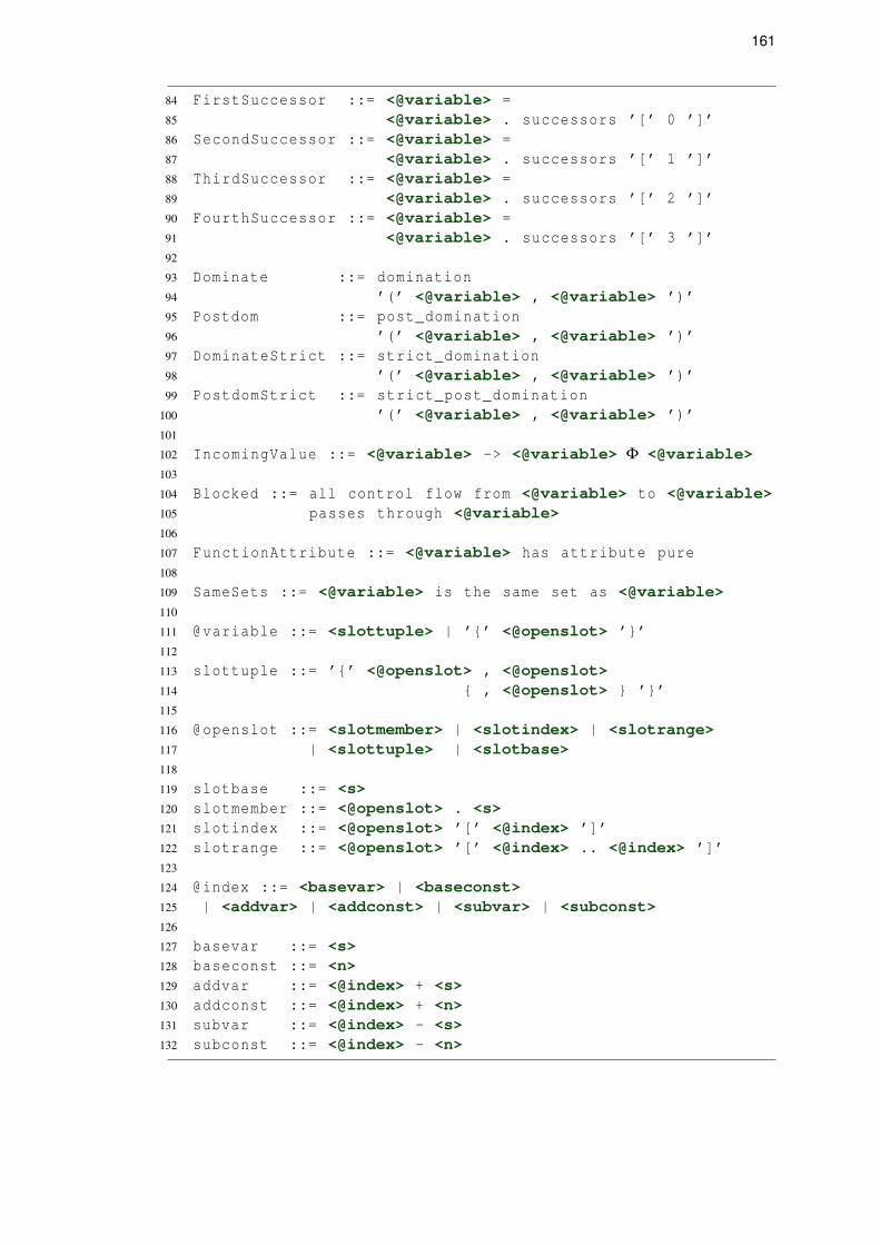
161
84 FirstSuccessor ::= <@variable> =85 <@variable> . successors ’[’ 0 ’]’86 SecondSuccessor ::= <@variable> =87 <@variable> . successors ’[’ 1 ’]’88 ThirdSuccessor ::= <@variable> =89 <@variable> . successors ’[’ 2 ’]’90 FourthSuccessor ::= <@variable> =91 <@variable> . successors ’[’ 3 ’]’92
93 Dominate ::= domination94 ’(’ <@variable> , <@variable> ’)’95 Postdom ::= post_domination96 ’(’ <@variable> , <@variable> ’)’97 DominateStrict ::= strict_domination98 ’(’ <@variable> , <@variable> ’)’99 PostdomStrict ::= strict_post_domination
100 ’(’ <@variable> , <@variable> ’)’101
102 IncomingValue ::= <@variable> -> <@variable> Φ <@variable>103
104 Blocked ::= all control flow from <@variable> to <@variable>105 passes through <@variable>106
107 FunctionAttribute ::= <@variable> has attribute pure108
109 SameSets ::= <@variable> is the same set as <@variable>110
111 @variable ::= <slottuple> | ’{’ <@openslot> ’}’112
113 slottuple ::= ’{’ <@openslot> , <@openslot>114 { , <@openslot> } ’}’115
116 @openslot ::= <slotmember> | <slotindex> | <slotrange>117 | <slottuple> | <slotbase>118
119 slotbase ::= <s>120 slotmember ::= <@openslot> . <s>121 slotindex ::= <@openslot> ’[’ <@index> ’]’122 slotrange ::= <@openslot> ’[’ <@index> .. <@index> ’]’123
124 @index ::= <basevar> | <baseconst>125 | <addvar> | <addconst> | <subvar> | <subconst>126
127 basevar ::= <s>128 baseconst ::= <n>129 addvar ::= <@index> + <s>130 addconst ::= <@index> + <n>131 subvar ::= <@index> - <s>132 subconst ::= <@index> - <n>


Appendix B
Polyhedral Code Sections in CAnDL
Listing B.1: Constraint specification in CAnDL of Scalar Control Parts (SCoPs): These regularloop nests enable polyhedral transformations to be applied, due to their structured control flow,side effect free function calls, and well-behaved memory access that is affine in loop iterators.The entire CAnDL code is displayed, including the relevant parts of the CAnDL standard library.
1 Constraint SCoP2 ( include For @ {loop}3 ∧ include StructuredControlFlow({loop}->{scope}) @ {control}4 ∧ {inputs[0]} = {loop.iterator}5 ∧ {inputs[i]} = {control.loop[i-1].iterator} foreach i=1..106 ∧ include AffineControlFlow({loop}->{scope},7 {inputs}->{inputs}) @ {control}8 ∧ include AffineMemAccesses({loop}->{scope},9 {inputs}->{inputs}) @ {accesses}
10 ∧ include SideEffectFreeCalls({loop}->{scope}) @ {effects})11 End1213 Constraint StructuredControlFlow14 ( collect i 20 ( opcode{branch[i].value} = branch15 ∧ {branch[i].target1} =16 {branch[i].value}.successors[0]17 ∧ {branch[i].target2} =18 {branch[i].value}.successors[1]19 ∧ include ScopeValue({scope}->{scope},20 {branch[i].value}->{value}))21 ∧ collect i 10 ( include For @ {loop[i]}22 ∧ domination({scope.begin},23 {loop[i].begin})24 ∧ strict_post_domination({scope.end},25 {loop[i].end}))26 ∧ collect i 10 ( include IfBlock @ {ifblock[i]}27 ∧ domination({scope.begin},28 {ifblock[i].precursor})29 ∧ strict_post_domination({scope.end},30 {ifblock[i].successor}))31 ∧ {loop[0..10].end,ifblock[0..10].precursor}32 is the same set as {branch[0..20].value})33 End
163

164 Appendix B. Polyhedral Code Sections in CAnDL
35 Constraint AffineControlFlow36 ( include AffineCalc[M=10,N=1](37 {scope}->{scope},38 {loop[i].iter_begin}->{value},39 {inputs}->{input})40 @ {forloop_affine_begin[i]} foreach i=0..1041 ∧ include AffineCalc[M=10,N=1](42 {scope}->{scope},43 {loop[i].iter_end}->{value},44 {inputs}->{input})45 @ {forloop_affine_end[i]} foreach i=0..1046 ∧ include AffineCalc[M=10,N=1](47 {scope}->{scope},48 {ifblock[i].compare_left}->{value},49 {inputs}->{input})50 @ {ifblock_affine_left[i]} foreach i=0..1051 ∧ include AffineCalc[M=10,N=1](52 {scope}->{scope},53 {ifblock[i].compare_right}->{value},54 {inputs}->{input})55 @ {ifblock_affine_right[i]} foreach i=0..10)56 End57
58 Constraint AffineMemAccesses59 ( collect x 20 ( include MemoryAccess({scope}->{scope})60 @ {newaccess[x]}61 ∧ opcode{newaccess[x].pointer} = gep62 ∧ domination({scope.begin},63 {newaccess[x].pointer})64 ∧ {newaffine[x].value} =65 {newaccess[x].pointer}.args[1])66 ∧ collect x 20 ( include MemoryAccess({scope}->{scope})67 @ {newaccess[x]}68 ∧ opcode{newaccess[x].pointer} = gep69 ∧ domination({scope.begin},70 {newaccess[x].pointer})71 ∧ {newaffine[x].value} =72 {newaccess[x].pointer}.args[1]73 ∧ include AffineCalc[M=10,N=6](74 {scope}->{scope},75 {inputs}->{input})76 @ {newaffine[x]}))77 End78
79 Constraint SideEffectFreeCalls80 ( collect i 20 ( opcode{callsite[i]} = call81 ∧ include ScopeValue({callsite[i]}->{value}))82 ∧ collect i 20 ( opcode{callsite[i]} = call83 ∧ include ScopeValue({callsite[i]}->{value})84 ∧ {function[i]} = {callsite[i]}.args[0]85 ∧ {function[i]} has attribute pure))86 End

165
88 Constraint For89 ( include Loop90 ∧ {increment} -> {body.end} Φ {iterator}91 ∧ {increment} ∈ {comparison}.args92 ∧ opcode{comparison} = icmp93 ∧ {comparison} ∈ {end}.args94 ∧ {increment} ∈ {iterator}.args95 ∧ opcode{increment} = add96 ∧ {iterator} ∈ {increment}.args97 ∧ {iter_end} ∈ {comparison}.args98 ∧ include LocalConst({begin}->{scope.begin},99 {iter_end}->{value})
100 ∧ {iter_begin} ∈ {iterator}.args101 ∧ include LocalConst({begin}->{scope.begin},102 {iter_begin}->{value})103 ∧ {iter_step} ∈ {increment}.args104 ∧ include LocalConst({begin}->{scope.begin},105 {iter_step}->{value}))106 End107
108 Constraint Loop109 ( include SESE110 ∧ {begin} ∈ {end}.successors)111 End112
113 Constraint SESE114 ( opcode{precursor} = branch115 ∧ {begin} ∈ {precursor}.successors116 ∧ opcode{end} = branch117 ∧ {successor} ∈ {end}.successors118 ∧ domination({begin}, {end})119 ∧ post_domination({end}, {begin})120 ∧ strict_domination({precursor}, {begin})121 ∧ strict_post_domination({successor}, {end})122 ∧ all control flow from {begin} to {precursor}123 passes through {end}124 ∧ all control flow from {successor} to {end}125 passes through {begin})126 End127
128 Constraint IfBlock129 ( include PotentialSESE({truebegin}->{begin},130 {trueend}->{end})131 ∧ {truebegin} = {precursor}.successors[0]132 ∧ {falsebegin} = {precursor}.successors[1]133 ∧ include PotentialSESE({falsebegin}->{begin},134 {falseend}->{end})135 ∧ {trueend} 6= {falseend}136 ∧ {condition} = {precursor}.args[0]137 ∧ opcode{condition} = icmp138 ∧ {compare_left} = {condition}.args[0]139 ∧ {compare_right} = {condition}.args[1])140 End

166 Appendix B. Polyhedral Code Sections in CAnDL
142 Constraint AffineCalc143 if N=0 then144 ( ( ( include LocalConst145 ∨ ( {value} is unused146 ∧ ir_type{scope.begin} = instruction))147 ∧ ( data_type{input[j]} = integer148 ∨ {input[j]} is unused) foreach j=0..M)149 ∨ ( ( {value} = {input[i]}150 ∧ ir_type{scope.begin} = instruction151 ∧ ( data_type{input[j]} = integer152 ∨ {input[j]} is unused) foreach j=0..M)153 forany i=0..M))154 else155 ( ( ( include AffineCalc[M=M,N=0]156 ∧ {l.value} is unused157 ∧ {r.value} is unused)158 ∨ ( ( ( ( opcode{value} = add159 ∨ opcode{value} = sub)160 ∧ {l.value} = {value}.args[0]161 ∧ {r.value} = {value}.args[1])162 ∨ ( opcode{value} = select163 ∧ {l.value} = {value}.args[1]164 ∧ {r.value} = {value}.args[2])165 ∨ ( opcode{value} = mul166 ∧ include ArgumentsPermuted({l.value}->{src1},167 {r.value}->{src2},168 {value}->{dst})169 ∧ ir_type{l.value} = preexecution170 ∧ ir_type{r.value} = instruction))171 ∧ ir_type{scope.begin} = instruction172 ∧ domination({scope.begin}, {value})173 ∧ ( data_type{input[j]} = integer174 ∨ {input[j]} is unused) foreach j=0..M))175 ∧ include AffineCalc[M=M,N=N-1]({input}->{input},176 {scope}->{scope}) @ {l}177 ∧ include AffineCalc[M=M,N=N-1]({input}->{input},178 {scope}->{scope}) @ {r})179 endif180 End181
182 Constraint ArgumentsPermuted183 ( ( {src1} = {dst}.args[0]184 ∧ {src2} = {dst}.args[1])185 ∨ ( {src2} = {dst}.args[0]186 ∧ {src1} = {dst}.args[1]))187 End188
189 Constraint LocalConst190 ( ( ir_type{scope.begin} = instruction191 ∧ ir_type{value} = preexecution)192 ∨ strict_domination({value}, {scope.begin}))193 End

167
195 Constraint MemoryAccess196 ( ( ( opcode{access} = store197 ∧ {pointer} = {access}.args[1])198 ∨ ( opcode{access} = load199 ∧ {pointer} = {access}.args[0]))200 ∧ domination({scope.begin}, {access})201 ∧ post_domination({scope.end}, {access}))202 End203
204 Constraint ScopeValue205 ( domination({scope.begin}, {value})206 ∧ strict_post_domination({scope.end}, {value}))207 End208
209 Constraint PotentialSESE210 ( opcode{precursor} = branch211 ∧ {begin} ∈ {precursor}.successors212 ∧ opcode{end} = branch213 ∧ {successor} ∈ {end}.successors214 ∧ ( ( domination({begin}, {end})215 ∧ post_domination({end}, {begin})216 ∧ all control flow from {begin} to {precursor}217 passes through {end}218 ∧ all control flow from {successor} to {end}219 passes through {begin})220 ∨ ( {begin} = {end}221 ∧ {begin} ∈ {precursor}.successors222 ∧ {successor} ∈ {end}.successors)223 ∨ ( {precursor} = {end}224 ∧ {begin} = {successor})))225 End

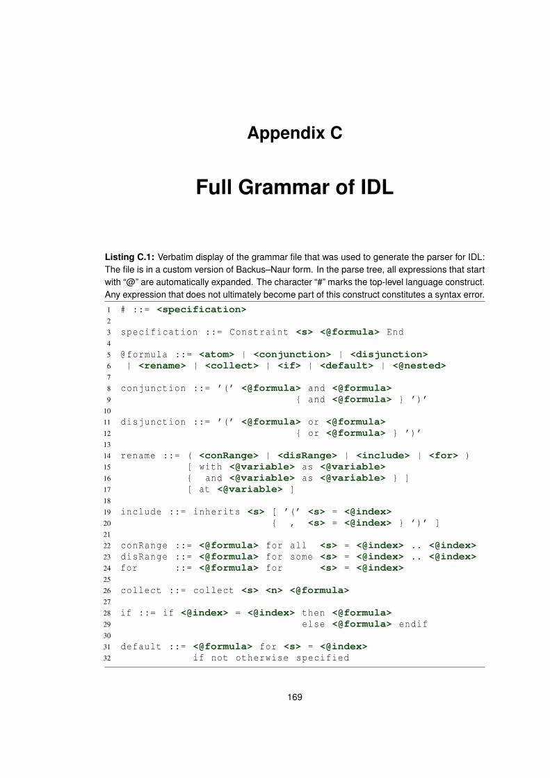
Appendix C
Full Grammar of IDL
Listing C.1: Verbatim display of the grammar file that was used to generate the parser for IDL:The file is in a custom version of Backus–Naur form. In the parse tree, all expressions that startwith “@” are automatically expanded. The character “#” marks the top-level language construct.Any expression that does not ultimately become part of this construct constitutes a syntax error.
1 # ::= <specification>2
3 specification ::= Constraint <s> <@formula> End4
5 @formula ::= <atom> | <conjunction> | <disjunction>6 | <rename> | <collect> | <if> | <default> | <@nested>7
8 conjunction ::= ’(’ <@formula> and <@formula>9 { and <@formula> } ’)’
10
11 disjunction ::= ’(’ <@formula> or <@formula>12 { or <@formula> } ’)’13
14 rename ::= ( <conRange> | <disRange> | <include> | <for> )15 [ with <@variable> as <@variable>16 { and <@variable> as <@variable> } ]17 [ at <@variable> ]18
19 include ::= inherits <s> [ ’(’ <s> = <@index>20 { , <s> = <@index> } ’)’ ]21
22 conRange ::= <@formula> for all <s> = <@index> .. <@index>23 disRange ::= <@formula> for some <s> = <@index> .. <@index>24 for ::= <@formula> for <s> = <@index>25
26 collect ::= collect <s> <n> <@formula>27
28 if ::= if <@index> = <@index> then <@formula>29 else <@formula> endif30
31 default ::= <@formula> for <s> = <@index>32 if not otherwise specified
169

170 Appendix C. Full Grammar of IDL
34 @nested ::= ’(’ <@formula> ’)’35
36 atom ::= <IntegerType> | <FloatType>37 | <VectorType> | <PointerType>38 | <Unused> | <IntZero> | <FloatZero>39 | <Constant> | <Preexecution> | <Argument> | <Instruction>40 | <Same> | <Distinct>41 | <DFGEdge> | <CFGEdge> | <CDGEdge> | <PDGEdge>42 | <FirstOperand> | <SecondOperand>43 | <ThirdOperand> | <FourthOperand>44 | <FirstSuccessor> | <SecondSuccessor>45 | <ThirdSuccessor> | <FourthSuccessor>46 | <Dominate> | <DominateStrict>47 | <Postdom> | <PostdomStrict> | <Blocked>48 | <IncomingValue> | <FunctionAttribute>49 | <Opcode> | <SameSets>50 | <GeneralizedDominance> | <NotNumericConstant> | <Block>51
52 IntegerType ::= <@variable> is an integer53 FloatType ::= <@variable> is a float54 VectorType ::= <@variable> is a vector55 PointerType ::= <@variable> is a pointer56
57 Unused ::= <@variable> is unused58 Opcode ::= <@variable> is <s> instruction59
60 IntZero ::= <@variable> is integer zero61 FloatZero ::= <@variable> is floating point zero62
63 Constant ::= <@variable> is a constant64 Preexecution ::= <@variable> is preexecution65 Argument ::= <@variable> is an argument66 Instruction ::= <@variable> is instruction67 NotNumericConstant ::= <@variable> is not a numeric constant68
69 Same ::= <@variable> is the same as <@variable>70 Distinct ::= <@variable> is not the same as <@variable>71 Block ::= <@variable> spans block to <@variable>72
73 DFGEdge ::= <@variable> has data flow to <@variable>74 CFGEdge ::= <@variable> has control flow to <@variable>75 CDGEdge ::= <@variable> has control dominance to <@variable>76 PDGEdge ::= <@variable> has dependence edge to <@variable>77
78 FirstOperand ::= <@variable> is first79 argument of <@variable>80 SecondOperand ::= <@variable> is second81 argument of <@variable>82 ThirdOperand ::= <@variable> is third83 argument of <@variable>84 FourthOperand ::= <@variable> is fourth85 argument of <@variable>

171
87 FirstSuccessor ::= <@variable> is first88 successor of <@variable>89 SecondSuccessor ::= <@variable> is second90 successor of <@variable>91 ThirdSuccessor ::= <@variable> is third92 successor of <@variable>93 FourthSuccessor ::= <@variable> is fourth94 successor of <@variable>95
96 Dominate ::= <@variable> control flow97 dominates <@variable>98 Postdom ::= <@variable> control flow99 post dominates <@variable>
100 DominateStrict ::= <@variable> strictly control flow101 dominates <@variable>102 PostdomStrict ::= <@variable> strictly control flow103 post dominates <@variable>104
105 IncomingValue ::= <@variable> reaches phi node106 <@variable> from <@variable>107
108 Blocked ::= all control flow from <@variable> to <@variable>109 passes through <@variable>110
111 FunctionAttribute ::= <@variable> has attribute pure112
113 SameSets ::= <@variable> is the same set as <@variable>114
115 GeneralizedDominance ::= all flow from <@variable> or any116 origin to any of <@variable> passes117 through at least one of <@variable>118
119 @variable ::= <slottuple> | ’{’ <@openslot> ’}’120
121 slottuple ::= ’{’ <@openslot> , <@openslot>122 { , <@openslot> } ’}’123
124 @openslot ::= <slotmember> | <slotindex> | <slotrange>125 | <slottuple> | <slotbase>126
127 slotbase ::= <s>128 slotmember ::= <@openslot> . <s>129 slotindex ::= <@openslot> ’[’ <@index> ’]’130 slotrange ::= <@openslot> ’[’ <@index> .. <@index> ’]’131
132 @index ::= <basevar> | <baseconst>133 | <addvar> | <addconst> | <subvar> | <subconst>134
135 basevar ::= <s>136 baseconst ::= <n>137 addvar ::= <@index> + <s>138 addconst ::= <@index> + <n>139 subvar ::= <@index> - <s>140 subconst ::= <@index> - <n>

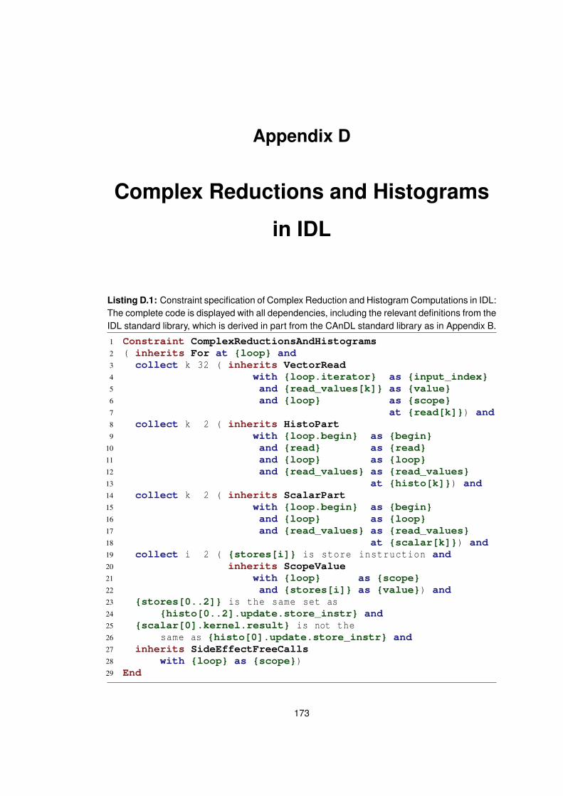
Appendix D
Complex Reductions and Histograms
in IDL
Listing D.1: Constraint specification of Complex Reduction and Histogram Computations in IDL:The complete code is displayed with all dependencies, including the relevant definitions from theIDL standard library, which is derived in part from the CAnDL standard library as in Appendix B.
1 Constraint ComplexReductionsAndHistograms2 ( inherits For at {loop} and3 collect k 32 ( inherits VectorRead4 with {loop.iterator} as {input_index}5 and {read_values[k]} as {value}6 and {loop} as {scope}7 at {read[k]}) and8 collect k 2 ( inherits HistoPart9 with {loop.begin} as {begin}
10 and {read} as {read}11 and {loop} as {loop}12 and {read_values} as {read_values}13 at {histo[k]}) and14 collect k 2 ( inherits ScalarPart15 with {loop.begin} as {begin}16 and {loop} as {loop}17 and {read_values} as {read_values}18 at {scalar[k]}) and19 collect i 2 ( {stores[i]} is store instruction and20 inherits ScopeValue21 with {loop} as {scope}22 and {stores[i]} as {value}) and23 {stores[0..2]} is the same set as24 {histo[0..2].update.store_instr} and25 {scalar[0].kernel.result} is not the26 same as {histo[0].update.store_instr} and27 inherits SideEffectFreeCalls28 with {loop} as {scope})29 End
173
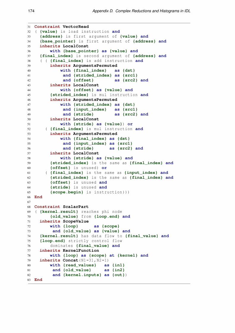
174 Appendix D. Complex Reductions and Histograms in IDL
31 Constraint VectorRead32 ( {value} is load instruction and33 {address} is first argument of {value} and34 {base_pointer} is first argument of {address} and35 inherits LocalConst36 with {base_pointer} as {value} and37 {final_index} is second argument of {address} and38 ( ( {final_index} is add instruction and39 inherits ArgumentsPermuted40 with {final_index} as {dst}41 and {strided_index} as {src1}42 and {offset} as {src2} and43 inherits LocalConst44 with {offset} as {value} and45 {strided_index} is mul instruction and46 inherits ArgumentsPermuted47 with {strided_index} as {dst}48 and {input_index} as {src1}49 and {stride} as {src2} and50 inherits LocalConst51 with {stride} as {value}) or52 ( {final_index} is mul instruction and53 inherits ArgumentsPermuted54 with {final_index} as {dst}55 and {input_index} as {src1}56 and {stride} as {src2} and57 inherits LocalConst58 with {stride} as {value} and59 {strided_index} is the same as {final_index} and60 {offset} is unused) or61 ( {final_index} is the same as {input_index} and62 {strided_index} is the same as {final_index} and63 {offset} is unused and64 {stride} is unused and65 {scope.begin} is instruction)))66 End67
68 Constraint ScalarPart69 ( {kernel.result} reaches phi node70 {old_value} from {loop.end} and71 inherits ScopeValue72 with {loop} as {scope}73 and {old_value} as {value} and74 {kernel.result} has data flow to {final_value} and75 {loop.end} strictly control flow76 dominates {final_value} and77 inherits KernelFunction78 with {loop} as {scope} at {kernel} and79 inherits Concat(N1=31,N2=1)80 with {read_values} as {in1}81 and {old_value} as {in2}82 and {kernel.inputs} as {out})83 End

175
85 Constraint HistoPart86 ( inherits ConditionalReadModifyWrite87 with {loop} as {scope}88 and {idx_kernel.result} as {address}89 and {val_kernel.result} as {new_value}90 at {update} and91 inherits KernelFunction92 with {loop} as {scope}93 and {read_values} as {inputs} at {idx_kernel} and94 inherits KernelFunction95 with {loop} as {scope} at {val_kernel} and96 inherits Concat(N1=31,N2=1)97 with {read_values} as {in1}98 and {update.old_value} as {in2}99 and {val_kernel.inputs} as {out})
100 End101
102 Constraint ConditionalReadModifyWrite103 ( {store_instr} is store instruction and104 inherits MaxOnceInScope105 with {scope} as {scope}106 and {store_instr} as {value} at {maxonce} and107 {address} is second argument of {store_instr} and108 {address} is gep instruction and109 {address} is first argument of {old_value} and110 {old_value} is load instruction and111 {new_value} is first argument of {store_instr})112 End113
114 Constraint MaxOnceInScope115 ( inherits ScopeValue and116 {value} has control flow to {value_after} and117 all control flow from {value_after} to118 {value} passes through {scope.end} and119 all control flow from {value_after} to120 {value} passes through {scope.begin})121 End122
123 Constraint ScopeValue124 ( {scope.begin} control flow dominates {value} and125 {scope.end} strictly control flow post dominates {value})126 End127
128 Constraint SideEffectFreeCalls129 ( collect i 20 ( {callsite[i]} is call instruction and130 inherits ScopeValue131 with {callsite[i]} as {value}) and132 collect i 20 ( {callsite[i]} is call instruction and133 inherits ScopeValue134 with {callsite[i]} as {value} and135 {function[i]} is first136 argument of {callsite[i]} and137 {function[i]} has attribute pure))138 End

176 Appendix D. Complex Reductions and Histograms in IDL
140 Constraint For141 ( inherits Loop and142 {increment} reaches phi node {iterator} from {end} and143 {increment} is first argument of {comparison} and144 {comparison} is icmp instruction and145 {comparison} is first argument of {end} and146 {increment} is add instruction and147 {iterator} is first argument of {increment} and148 {iter_end} is second argument of {comparison} and149 inherits LocalConst150 with {begin} as {scope.begin}151 and {iter_end} as {value} and152 {iter_begin} reaches phi node153 {iterator} from {precursor} and154 inherits LocalConst155 with {begin} as {scope.begin}156 and {iter_begin} as {value} and157 {iter_step} is second argument of {increment} and158 inherits LocalConst159 with {begin} as {scope.begin}160 and {iter_step} as {value})161 End162
163 Constraint Loop164 ( inherits SESE and165 {end} has control flow to {begin})166 End167
168 Constraint SESE169 ( {precursor} is branch instruction and170 {precursor} has control flow to {begin} and171 {end} is branch instruction and172 {end} has control flow to {successor} and173 {begin} control flow dominates {end} and174 {end} control flow post dominates {begin} and175 {precursor} strictly control flow dominates {begin} and176 {successor} strictly control flow post dominates {end} and177 all control flow from {begin} to {precursor}178 passes through {end} and179 all control flow from {successor} to {end}180 passes through {begin})181 End182
183 Constraint LocalConst184 ( ( {scope.begin} is instruction and185 {value} is preexecution) or186 {value} strictly control flow dominates {scope.begin})187 End
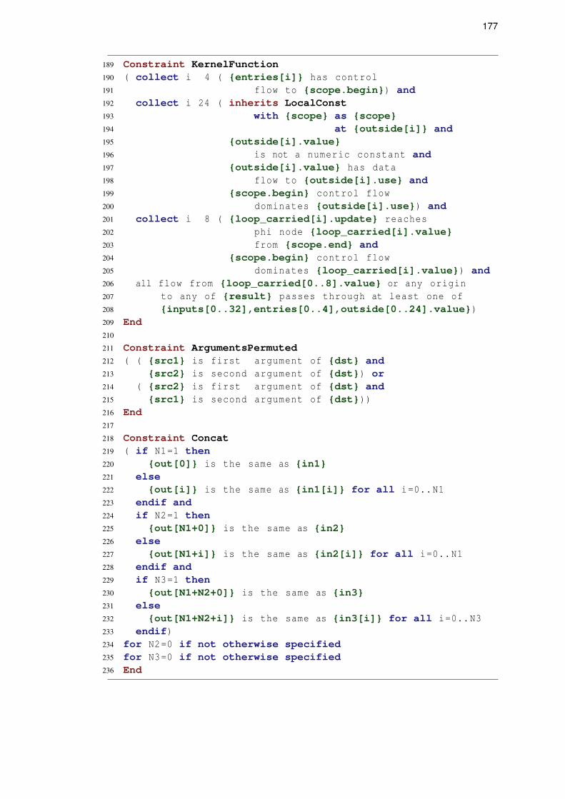
177
189 Constraint KernelFunction190 ( collect i 4 ( {entries[i]} has control191 flow to {scope.begin}) and192 collect i 24 ( inherits LocalConst193 with {scope} as {scope}194 at {outside[i]} and195 {outside[i].value}196 is not a numeric constant and197 {outside[i].value} has data198 flow to {outside[i].use} and199 {scope.begin} control flow200 dominates {outside[i].use}) and201 collect i 8 ( {loop_carried[i].update} reaches202 phi node {loop_carried[i].value}203 from {scope.end} and204 {scope.begin} control flow205 dominates {loop_carried[i].value}) and206 all flow from {loop_carried[0..8].value} or any origin207 to any of {result} passes through at least one of208 {inputs[0..32],entries[0..4],outside[0..24].value})209 End210
211 Constraint ArgumentsPermuted212 ( ( {src1} is first argument of {dst} and213 {src2} is second argument of {dst}) or214 ( {src2} is first argument of {dst} and215 {src1} is second argument of {dst}))216 End217
218 Constraint Concat219 ( if N1=1 then220 {out[0]} is the same as {in1}221 else222 {out[i]} is the same as {in1[i]} for all i=0..N1223 endif and224 if N2=1 then225 {out[N1+0]} is the same as {in2}226 else227 {out[N1+i]} is the same as {in2[i]} for all i=0..N1228 endif and229 if N3=1 then230 {out[N1+N2+0]} is the same as {in3}231 else232 {out[N1+N2+i]} is the same as {in3[i]} for all i=0..N3233 endif)234 for N2=0 if not otherwise specified235 for N3=0 if not otherwise specified236 End