:

ORIGINAL

Geometry and evolution of Holocene transgressiveand regressive barriers on the semi-arid coast of NE Brazil

Luciano Henrique de Oliveira Caldas &

Josibel Gomes de Oliveira Jr &

Walter Eugênio de Medeiros & Karl Stattegger &

Helenice Vital

Received: 10 April 2006 /Accepted: 19 July 2006 / Published online: 19 August 2006# Springer-Verlag 2006

Abstract An integrated study based on ground penetratingradar (GPR) profiles, vibracore descriptions, water-welllogs, and radiocarbon dating in a coastal deposit located inthe northern region of Rio Grande do Norte State,northeastern Brazil, allowed us to identify Holocenetransgressive and regressive barriers. The constructionprocess for the studied coastal barrier is different from thatproposed for the Holocene coastal plains along the easternBrazilian coast, where the hydraulic barrier set up by largerivers for sediments transported by longshore currents hascaused a strongly positive longshore sediment imbalance.In the study area, interpretation of the GPR images, withinthe constraints of vibracores data, allowed us to interpretfive radar facies and four radar boundary sequences for

these coastal deposits, which were built up during theHolocene coastal evolution of the region. As a result, thegeometry of the coastal barrier was reconstructed. Based onbarrier geometry, sediment ages, stratigraphic records, andsedimentation patterns, we propose a barrier evolutionarymodel for the Holocene for the study region. During theHolocene highstand, a transgressive barrier was depositedand a lagoon extended landward. During the sea-level fallsoon after the Holocene highstand, the deposition of aregressive barrier (forced regression) started. This deposi-tion was induced by the coastal geometry and high amountsof eolian sediments supplied by east-northeast winds. Alsoduring this period of sea-level fall, the beach face becamewider, and thus more subjected to wind action, facilitatingthe deposition of the first eolian deposits. These sedimentswere transported to the nearly formed embayment, provid-ing a surplus for the construction of the regressive barrier.During the regressive phase, tidal channels closed and thelagoon became isolated from the open sea. The geometry ofboth the regressive and transgressive barriers as well as thestratigraphic relation between the sedimentary depositssuggest that the Holocene highstand in this region was notmore than 1.4 m above present-day mean sea level.

Introduction

Transgressive and regressive coastal barriers are built up byprocesses involving sea-level changes, wave dominance,seabed inclination, tidal range, sediment input, coastlinegeometry, and ancient geology (Curray 1964; Davis andHayes 1984; Hayes 1994; Lessa et al. 2000). The regressivebarriers are the most likely to be preserved in the geologicalrecord, since transgressive barriers are overridden andreworked by the shoreface ravinement surface, and during

Geo-Mar Lett (2006) 26:249–263DOI 10.1007/s00367-006-0034-2

L. Henrique de Oliveira Caldas : J. Gomes de Oliveira Jr :W. Eugênio de Medeiros (*) :H. VitalPrograma de Pesquisa e Pós-graduação em Geodinâmica eGeofísica, Universidade Federal do Rio Grande do Norte,Campus Universitário UFRN,P.O. Box 1596, 59078-970 Natal/RN, Brazile-mail: walter@dfte.ufrn.br

K. StatteggerInstitute of Geoscience, University of Kiel,Olshausenstr 40,24118 Kiel, Germany

L. Henrique de Oliveira CaldasPETROBRAS,Av. General Canabarro 500,20271-900 Rio de Janeiro/RJ, Brazil

J. Gomes de Oliveira JrCGG do Brasil Ltda,Av. Presidente Wilson 231, sala 1501,20030-021 Rio de Janeiro/RJ, Brazil

Present address:

Present address:

sea-level fall, subsequently excavated by a wave diastem,or a regressive surface of erosion (Kraft and Chrzastowski1985; Roy et al. 1995).

Along the eastern coast of Brazil, large regressiveand transgressive sequences exist. They are associatedmainly to sea-level oscillations during the Pleistoceneand Holocene (Dominguez et al. 1987; Martin et al.1993). Because these barriers are generally adjacent tolarge river mouths along the eastern Brazilian coast, theirgenesis has been attributed to the hydraulic barrier thatthese rivers impose on sediments transported by longshorecurrents, thus causing a strongly positive longshoresediment imbalance (Dominguez et al. 1987, 1992;Dominguez and Wanless 1991; Martin et al. 1993). Inthe cases of regressive barriers that are not positioned nearriver mouths, Dominguez et al. (1987) proposed that theyare built up from the reworking of inner shelf sedimentsduring sea-level fall, corresponding to Bruun’s coastalretreat (Bruun 1962). Dominguez et al. (1987) stated thatduring a falling sea-level scenario, sediments transportedby longshore currents can be captured in river mouths, re-entrances along the coast, and areas protected by offshoreobstacles.

Between the cities of São Bento do Norte andCaiçara do Norte along the north coast of Rio Grandedo Norte State (Fig. 1), where the semi-arid settingreaches the littoral zone, a coastal deposit exists. Based onan evaluation of aerial photographs, it has been interpretedas a regressive barrier, associated to the Holocene sea-level history of the region (Caldas 1996). In this studyarea, no river mouths exist that would capture sedimentstransported by longshore currents. Besides Caldas (1996),there is no other study about the origin of this barrier andits evolution.

The aim of this paper is to provide a stratigraphicoverview of this barrier system, as well as to identify itsgeometry and to propose a framework for the evolutionof the north coastal plain of Rio Grande do Norte Stateduring the mid- to late Holocene. The new aspect of thepresent study is that the barrier system is not associatedto river mouths, in contrast to the coastal plains of theBrazilian east coast. The investigation of this barrierwill also contribute to our knowledge of the Holocenesea-level history of the north coastal region of RioGrande do Norte State, for which some sea-level curveshave been proposed (Barreto et al. 2001; Bezerra et al.2003; Caldas et al. 2006). The sequence of sedimentarydeposits was evaluated based upon an integration ofground penetrating radar (GPR) profiles (morphostratig-raphy), data on depositional cycles obtained from vibra-cores and water-well logs (allostratigraphy), and 14C agesindicating when the sedimentary units were deposited(chronostratigraphy).

Study area and regional setting

Geography, geomorphology and geology

The study area is located along the northern coast of RioGrande do Norte State, northeast Brazil (Fig. 1), about140 km northwest of the state capital, Natal. This coastalregion comprises a plain showing a maximum gradient ofaround 5°, except where dunes occur (Vilaça et al. 1991).The coast is open, wave-dominated, with a shallow innercontinental shelf (maximum 25 m depth) that has anaverage width of 18 km. The region is strongly influencedby oceanic and wind-driven currents from the N and E–NE,which promote local erosion as well as deposition in theshore zone. A large lagoonal channel system is located onthe backside of the sand spit of Galinhos (Fig. 1). Someclosed lagoons occur near the towns of São Bento do Norteand Caiçara do Norte. In the beach zone, several beachrocklines occur along the present foreshore zone, and also in thebackshore zone. Dune fields increase both inland and alongthe shore; dunes close to the shore are constantly reworkedby permanent wind action (Tabosa et al. 2001; Caldas2002; Lima et al. 2002; Vital et al. 2003).

The study area is located in the Potiguar Basin, which ispart of the Northeast Brazilian Rift System (Matos 1994).According to Neves (1987), this Cretaceous basin representsa continental rift in its onshore portion (∼21,500 km2) and apull-apart basin in its offshore portion (∼26,000 km2). TheQuaternary geology of the north coastal zone of Rio Grandedo Norte State is still poorly investigated. Several litho-stratigraphic domains are present, such as sandy dunes,sandbanks, shell middens, tidal flats, beaches, and beachrock(Caldas 1996; Tabosa 2000; Tabosa et al. 2001). Previousstudies have focused mainly on onshore interpretations, off-shore surveys being areally restricted (Vianna and Solewicz1988; Costa-Neto 1997; Testa and Bosence 1999a,b; Barretoet al. 2000; Suguio et al. 2001; Oliveira et al. 2003).

Climate and winds

The climate is tropical, hot and semi-arid (Nimer 1989), andinfluenced by the intertropical convergence zone. A dry periodof about 8 months extends from June to January, and a rainyperiod of 4 months from February to May. The mean annualair temperature is 26.8°C, with a minimum value of 25.0°C atthe end of the rainy period (June–July) and a maximum of28.6°C in February during the summer (Cestaro 1994).

The mean wind velocity in late summer (March) is4.8 m/s, and from late winter to mid-summer (August–December) the values can reach 9.0 m/s (Tabosa et al.2001). These meteorological conditions strongly influencedune migration. Along the north coast, dune migration isrestricted to the dry period when the stronger NE winds

250 Geo-Mar Lett (2006) 26:249–263

blow. Dune field morphology shows a predominantNE–SW direction (Figs. 1 and 2).

Hydrography and wave climate

Small rivers oriented mainly NW–N–NE are common,flowing intermittently and draining into lakes (paleo-lagoons) or tidal flats. Some lakes have been formed bythe damming of rivers by coastal dunes, as well as by theoutcropping of the water table (Oliveira et al. 1990). Fortes(1987) characterized some of these lakes as tidal flats.

Wave measurements collected during 1 year along thecoast near the town of Macau (∼50 km westward of thestudy area) show that mean wave height is 0.8 m(Brazilian Navy 2004). At the coast near the town of SãoBento do Norte (Fig. 1), Tabosa (2000) measured waveheights that varied between 1.4 and 0.2 m. For the coastnear the town of Guamaré (∼50 km eastward of the studyarea), Silveira (2002) reported wave heights of around0.8 m during the rainy season and 0.5 m during the dryseason.

Waves approach the coast from the NNE–ENE.Westerly longshore currents are produced by ENE waverefraction along the EW-oriented coast (Gorini et al.1982). The migration of the sand spits to the west (Fig. 1) isanother indicator of the predominant longshore current(Caldas 2002).

The study area has a semidiurnal mesotidal regime, andthe spring tidal range reaches 3.0 m. In the harbor ofMacau, the tides reach 2.9 m at spring tide and 2.2 m atneap tide (Brazilian Navy 2004).

Sea-level history

Based on radiocarbon dating of paleo-sea-level indicators,Van Andel and Laborel (1964) and Delibrias and Laborel(1969) published the first attempts to establish regionalHolocene sea-level changes for the eastern Brazilian coast.According to Delibrias and Laborel (1969), sea level wassimilar to that of the present day at 6,000 years B.P.; then, itrose to 3 m above present mean sea level at 4,500 years B.P.,

Fig. 1 Location of the study area and geological map (extracted from Caldas 2002) of the coastal zone between Ponta dos Três Irmãos and Galinhos

Fig. 2 Aerial photograph of 1950, showing the locations of the GPRsections (thick lines A1–3, C1, and D1), topographic transects (thinlines A–D), vibracores (BB1–BB5) and water wells (3–12)

Geo-Mar Lett (2006) 26:249–263 251

and since that time, sea level has fallen gradually to itspresent position.

After the pioneer works of Van Andel and Laborel(1964) and Delibrias and Laborel (1969), better-constrainedHolocene sea-level curves were proposed for the Brazilianeastern coast by Suguio et al. (1985). They constructed theso-called Salvador Curve, providing evidence that for thenortheastern region of Brazil, sea level started to rise abovethe present-day level shortly before 7,000 years B.P., andreached a highstand of 5 m above present sea level approxi-mately 5,100 years B.P. Recently, this age has beencalibrated to 5,660 cal. years B.P. (Martin et al. 2003).Furthermore, two negative oscillations were proposed: oneat 4,200–3,700 cal. years B.P., and another at 2,600–2,200 cal. years B.P. Here, it is important to note that adebate remains regarding the existence of these secondarysea-level oscillations (Angulo and Lessa 1997; Martin et al.2003; Ybert et al. 2003).

For the north coast of Brazil, in particular for the northcoast of Rio Grande do Norte State, some investigations onHolocene sea-level changes have been published during thelast 5 years, based on 14C datings in coastal deposit shells(from beachrock) and organic remnants from lagoonalsediments (Barreto et al. 2001; Caldas 2002; Bezerra et al.2003; Caldas et al. 2006). The sea-level curve proposed byCaldas (2002; see also Caldas et al. 2006) and the sea-levelcurve envelope proposed by Bezerra et al. (2003) are shownin Fig. 3. Similarly to the east Brazilian coast, thediscussions here have focused on the height of theHolocene highstand and on the occurrence of secondarysea-level oscillations. According to Bezerra et al. (2003),the Holocene highstand reached 2.5–4.0 m above today’smean sea level, whereas Caldas et al. (2006) proposed ahighstand of 1.3 m. Furthermore, Bezerra et al. (2003)described at least two secondary sea-level oscillationsduring the Holocene regression, whereas Caldas et al.(2006) argued that any small-scale high-frequency oscil-lations could not be easily recognized because today’s tidalrange at the north coast (2.8 m) is greater than the observed

Holocene sea-level highstand (+1.3 m). This highstandvalue is in good accordance with the estimate of sea-levelfall obtained in the present work; we elaborate below onthis aspect within the context of the new data presented andtheir interpretation.

Materials and methods

GPR and topography

GPR is a tool of exploration geophysics that images theshallow subsurface of the Earth (usually up to 30 m), usingelectromagnetic waves with frequencies in the range10 MHz–1 GHz. Because measured data are two-waywave propagation times, data interpretation and processingare done in a manner similar to that for seismic data. Detailsabout the GPR method and its application for sedimentsmay be obtained in, for example, Bristow and Jol (2003).Using GPR technology, subsurface barrier architectures canbe imaged quickly and in detail (e.g., Moore et al. 2004;Engels and Roberts 2005; Rodriguez and Meyer 2006).

Using a 200-MHz antenna, we collected three GPRprofiles in the study area, covering 1.5 km orientedperpendicular to the coastline (profiles A, C, and D inFig. 2). The equipment used was a SIR System 2,manufactured by Geophysical Survey Systems Inc. Wechose a continuous mode of acquisition, where distanceswere measured by means of an odometer and each tracewas collected at steps of 5 cm. The field data wereprocessed using the routine described in Xavier Neto andMedeiros (2006), in order to improve the visualization ofsedimentary features.

All GPR data were corrected for topography, which wassurveyed using theodolite leveling. The topographic pro-files were corrected for present-day mean sea level andspring tide level (Brazilian Navy 2004; own measure-ments). Examples of processed GPR profiles are shown inFigs. 4a, 5a, 6a, 7a, and 8a. In all GPR figures, the left

Fig. 3 a, b Proposed sea-level curves for the study area: a Caldas (2002) and Caldas et al. (2006); b sea-level curve envelope of Bezerra et al.(2003). Elevations are indicated relative to mean sea level

252 Geo-Mar Lett (2006) 26:249–263

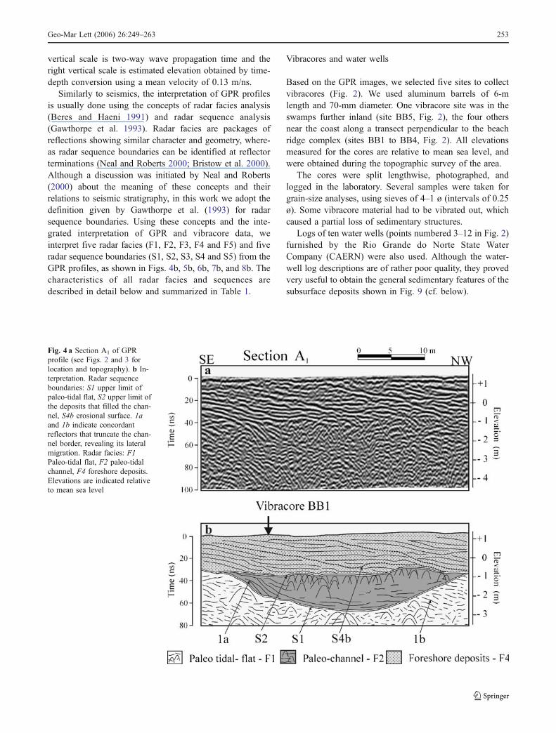
vertical scale is two-way wave propagation time and theright vertical scale is estimated elevation obtained by time-depth conversion using a mean velocity of 0.13 m/ns.

Similarly to seismics, the interpretation of GPR profilesis usually done using the concepts of radar facies analysis(Beres and Haeni 1991) and radar sequence analysis(Gawthorpe et al. 1993). Radar facies are packages ofreflections showing similar character and geometry, where-as radar sequence boundaries can be identified at reflectorterminations (Neal and Roberts 2000; Bristow et al. 2000).Although a discussion was initiated by Neal and Roberts(2000) about the meaning of these concepts and theirrelations to seismic stratigraphy, in this work we adopt thedefinition given by Gawthorpe et al. (1993) for radarsequence boundaries. Using these concepts and the inte-grated interpretation of GPR and vibracore data, weinterpret five radar facies (F1, F2, F3, F4 and F5) and fiveradar sequence boundaries (S1, S2, S3, S4 and S5) from theGPR profiles, as shown in Figs. 4b, 5b, 6b, 7b, and 8b. Thecharacteristics of all radar facies and sequences aredescribed in detail below and summarized in Table 1.

Vibracores and water wells

Based on the GPR images, we selected five sites to collectvibracores (Fig. 2). We used aluminum barrels of 6-mlength and 70-mm diameter. One vibracore site was in theswamps further inland (site BB5, Fig. 2), the four othersnear the coast along a transect perpendicular to the beachridge complex (sites BB1 to BB4, Fig. 2). All elevationsmeasured for the cores are relative to mean sea level, andwere obtained during the topographic survey of the area.

The cores were split lengthwise, photographed, andlogged in the laboratory. Several samples were taken forgrain-size analyses, using sieves of 4–1 ø (intervals of 0.25ø). Some vibracore material had to be vibrated out, whichcaused a partial loss of sedimentary structures.

Logs of ten water wells (points numbered 3–12 in Fig. 2)furnished by the Rio Grande do Norte State WaterCompany (CAERN) were also used. Although the water-well log descriptions are of rather poor quality, they provedvery useful to obtain the general sedimentary features of thesubsurface deposits shown in Fig. 9 (cf. below).

Fig. 4 a Section A1 of GPRprofile (see Figs. 2 and 3 forlocation and topography). b In-terpretation. Radar sequenceboundaries: S1 upper limit ofpaleo-tidal flat, S2 upper limit ofthe deposits that filled the chan-nel, S4b erosional surface. 1aand 1b indicate concordantreflectors that truncate the chan-nel border, revealing its lateralmigration. Radar facies: F1Paleo-tidal flat, F2 paleo-tidalchannel, F4 foreshore deposits.Elevations are indicated relativeto mean sea level

Geo-Mar Lett (2006) 26:249–263 253

AMS radiocarbon dating

AMS radiocarbon dating was carried out on both terrestrialorganic material and mollusk shells collected from vibra-core BB5. A careful selection and a detailed pretreatment of

the bivalve shells allowed us to eliminate or to control forany confounding effects of contamination.

The AMS radiocarbon ages were determined using theAMS system of the Leibniz Laboratory, Kiel University,Germany. The standard procedures are described in Nadeau et

Fig. 5 a Section A2 of GPRprofile (see Figs. 2 and 3 forlocation and topography). b In-terpretation. Radar sequenceboundaries: S1 upper limit ofpaleo-tidal flat (note the irregu-lar form of S1, evidence oferosion at the top of the tidal flatdeposits), S3a erosional surfaceseparating different bodies ofwashover deposits, S4a deposi-tional surface indicating differ-ent events of coastalprogradation seaward, S5 con-tact between eolian and beachdeposits. Radar facies: F1 Paleo-tidal flat, F3 washover deposits,F4 foreshore deposits, F5 eoliandeposits. Elevations are indicat-ed relative to mean sea level

Fig. 6 a Section A3 of GPRprofile (see Figs. 2 and 3 forlocation and topography). b In-terpretation. Radar sequenceboundaries: S1 Upper limit ofthe paleo-tidal flat, S3b erosion-al surface separating differentbodies of washover sediments,S5 contact between washoverdeposits and eolian sediments.Radar facies: F1 Paleo-tidal flat,F3 washover deposits, F5 eoliandeposits. Elevations are indicat-ed relative to mean sea level

254 Geo-Mar Lett (2006) 26:249–263

al. (1997) and Schleicher et al. (1998). The system presents anaverage zero background of 0.3%. Values for AMS 14Ccarbonate ages were not corrected for any standard meanocean reservoir effect. The values were converted to calendarages using version 4.1.2 of the CALIB radiocarbon software(Stuiver and Reimer 1993), updated with recent calibrationdatasets (Stuiver et al. 1998). All calibrated ages were roundedup or down to the nearest multiple of ten.

Results

Topography

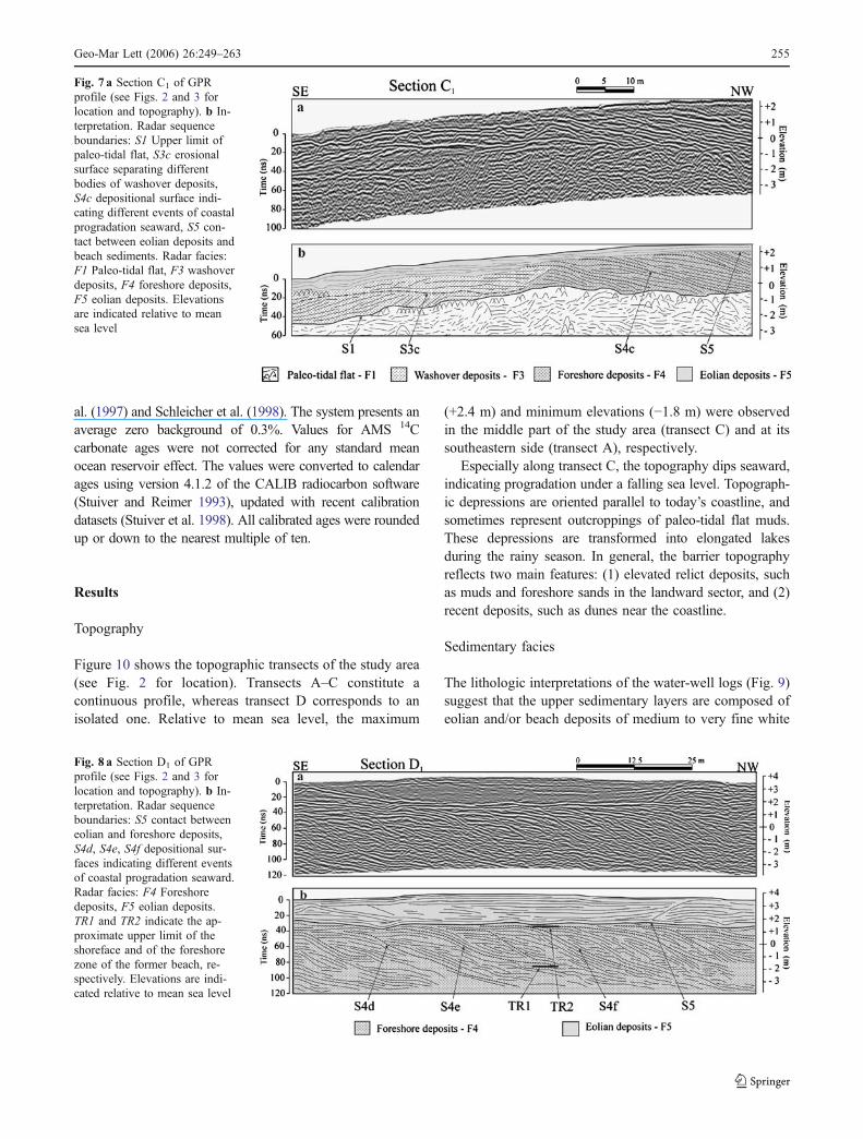
Figure 10 shows the topographic transects of the study area(see Fig. 2 for location). Transects A–C constitute acontinuous profile, whereas transect D corresponds to anisolated one. Relative to mean sea level, the maximum

(+2.4 m) and minimum elevations (−1.8 m) were observedin the middle part of the study area (transect C) and at itssoutheastern side (transect A), respectively.

Especially along transect C, the topography dips seaward,indicating progradation under a falling sea level. Topograph-ic depressions are oriented parallel to today’s coastline, andsometimes represent outcroppings of paleo-tidal flat muds.These depressions are transformed into elongated lakesduring the rainy season. In general, the barrier topographyreflects two main features: (1) elevated relict deposits, suchas muds and foreshore sands in the landward sector, and (2)recent deposits, such as dunes near the coastline.

Sedimentary facies

The lithologic interpretations of the water-well logs (Fig. 9)suggest that the upper sedimentary layers are composed ofeolian and/or beach deposits of medium to very fine white

Fig. 7 a Section C1 of GPRprofile (see Figs. 2 and 3 forlocation and topography). b In-terpretation. Radar sequenceboundaries: S1 Upper limit ofpaleo-tidal flat, S3c erosionalsurface separating differentbodies of washover deposits,S4c depositional surface indi-cating different events of coastalprogradation seaward, S5 con-tact between eolian deposits andbeach sediments. Radar facies:F1 Paleo-tidal flat, F3 washoverdeposits, F4 foreshore deposits,F5 eolian deposits. Elevationsare indicated relative to meansea level

Fig. 8 a Section D1 of GPRprofile (see Figs. 2 and 3 forlocation and topography). b In-terpretation. Radar sequenceboundaries: S5 contact betweeneolian and foreshore deposits,S4d, S4e, S4f depositional sur-faces indicating different eventsof coastal progradation seaward.Radar facies: F4 Foreshoredeposits, F5 eolian deposits.TR1 and TR2 indicate the ap-proximate upper limit of theshoreface and of the foreshorezone of the former beach, re-spectively. Elevations are indi-cated relative to mean sea level

Geo-Mar Lett (2006) 26:249–263 255

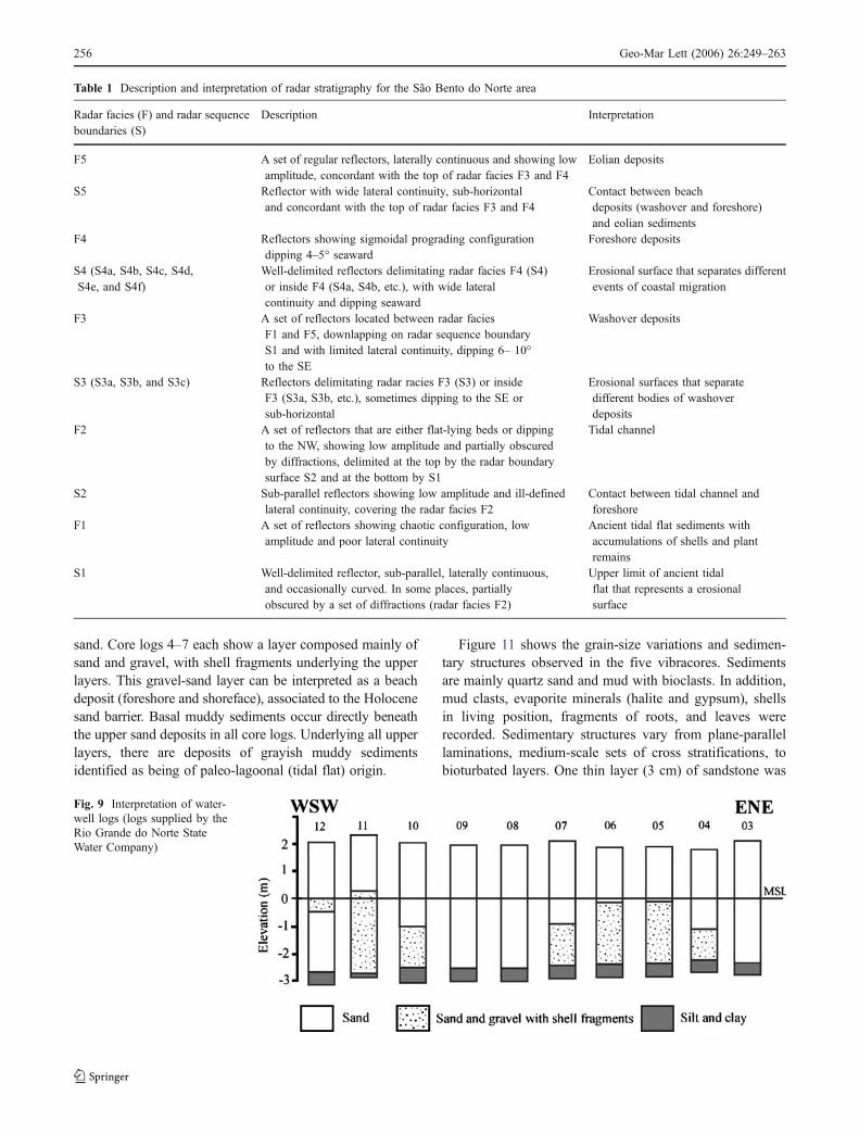
sand. Core logs 4–7 each show a layer composed mainly ofsand and gravel, with shell fragments underlying the upperlayers. This gravel-sand layer can be interpreted as a beachdeposit (foreshore and shoreface), associated to the Holocenesand barrier. Basal muddy sediments occur directly beneaththe upper sand deposits in all core logs. Underlying all upperlayers, there are deposits of grayish muddy sedimentsidentified as being of paleo-lagoonal (tidal flat) origin.

Figure 11 shows the grain-size variations and sedimen-tary structures observed in the five vibracores. Sedimentsare mainly quartz sand and mud with bioclasts. In addition,mud clasts, evaporite minerals (halite and gypsum), shellsin living position, fragments of roots, and leaves wererecorded. Sedimentary structures vary from plane-parallellaminations, medium-scale sets of cross stratifications, tobioturbated layers. One thin layer (3 cm) of sandstone was

Table 1 Description and interpretation of radar stratigraphy for the São Bento do Norte area

Radar facies (F) and radar sequenceboundaries (S)

Description Interpretation

F5 A set of regular reflectors, laterally continuous and showing lowamplitude, concordant with the top of radar facies F3 and F4

Eolian deposits

S5 Reflector with wide lateral continuity, sub-horizontaland concordant with the top of radar facies F3 and F4

Contact between beachdeposits (washover and foreshore)and eolian sediments

F4 Reflectors showing sigmoidal prograding configurationdipping 4–5° seaward

Foreshore deposits

S4 (S4a, S4b, S4c, S4d,S4e, and S4f)

Well-delimited reflectors delimitating radar facies F4 (S4)or inside F4 (S4a, S4b, etc.), with wide lateralcontinuity and dipping seaward

Erosional surface that separates differentevents of coastal migration

F3 A set of reflectors located between radar faciesF1 and F5, downlapping on radar sequence boundaryS1 and with limited lateral continuity, dipping 6– 10°to the SE

Washover deposits

S3 (S3a, S3b, and S3c) Reflectors delimitating radar racies F3 (S3) or insideF3 (S3a, S3b, etc.), sometimes dipping to the SE orsub-horizontal

Erosional surfaces that separatedifferent bodies of washoverdeposits

F2 A set of reflectors that are either flat-lying beds or dippingto the NW, showing low amplitude and partially obscuredby diffractions, delimited at the top by the radar boundarysurface S2 and at the bottom by S1

Tidal channel

S2 Sub-parallel reflectors showing low amplitude and ill-definedlateral continuity, covering the radar facies F2

Contact between tidal channel andforeshore

F1 A set of reflectors showing chaotic configuration, lowamplitude and poor lateral continuity

Ancient tidal flat sediments withaccumulations of shells and plantremains

S1 Well-delimited reflector, sub-parallel, laterally continuous,and occasionally curved. In some places, partiallyobscured by a set of diffractions (radar facies F2)

Upper limit of ancient tidalflat that represents a erosionalsurface

Fig. 9 Interpretation of water-well logs (logs supplied by theRio Grande do Norte StateWater Company)

256 Geo-Mar Lett (2006) 26:249–263

found at the base of vibracore BB4. Based on sedimentarystructures and bounding surfaces, textural and mineralogi-cal composition, color, and distance from the shoreline,three sedimentary facies were distinguished in the vibra-cores, these being detailed below.

Tidal flats, facies a

Facies a was deposited on the intertidal flat, dominated byvertical accretion. In the more inland cores BB5, BB4, andBB3 (Figs. 2 and 11), this facies is comprised of parallel

Fig. 10 Topographic transects (A–D) perpendicular and parallel to the coastline (see Fig. 2 for location). A1–3, C1, and D1 are parts of longer GPRprofiles obtained along topographic transects

Fig. 11 Grain-size variations,sedimentary structures, andinterpreted sedimentary facies(between arrows at the left sideof each column) for vibracoresBB1 to BB5 (see location inFig. 2): a tidal flat, b washover,c undifferentiated. Sedimentarystructures are either plane-paral-lel, horizontal, or inclined. 1–4indicate depths of 14C datings incore BB5. MSL Mean sea level

Geo-Mar Lett (2006) 26:249–263 257

laminations of very fine sand, mud and organic layers,sometimes bioturbated. The mud has a greenish-blackcolor, and some evaporite mineral (halite and gypsum)and mud clasts occur mainly at the top of core BB5. Theyare probably related to a semi-enclosed lagoon during itsfinal stage of evolution. Fossils of roots, shell fragments,and leaves (probably from mangrove trees) also occur.Some shells in living position form banks on the paleo-tidalflat surface. The basal contact with sediments of facies b(cf. below) in cores BB5 and BB4 is abrupt, and defined byan increase in grain size and change in color from greenish-black to gray.

Washover deposits, facies b

Washover deposits are built up through overtopping of thesand barrier. In the cores, facies b is comprised ofmoderately sorted medium to coarse gray sand (Fig. 11).The sedimentary structure is a plane-parallel laminationdipping landward at 5–7° (150–180° azimuth). Furthestinland, in vibracore BB5, its maximum thickness reaches0.2 m at the base, the corresponding value being 0.3 m invibracore BB3. Along some modern spits on the north coastof Rio Grande do Norte State, washover sediments can bedeposited during spring tides.

Undifferentiated deposits, facies c

Facies c is comprised of very fine to very coarse sand,sometimes associated with shells fragments and organiclayers (Fig. 11). No sedimentary structures were observed,probably because they had been destructed by vibrationduring material extraction. Thus, it was not possible toperform accurate facies interpretation in this case. Despitethis problem, at the top of vibracore BB1, the sediments arewell sorted and can be correlated to the covering eoliansediments, whereas in the middle of core BB2, the amountof shells and bioturbation, associated with medium to coarsesand, allow us to infer that they are related to beach sands.

Radar stratigraphy

Radar facies F1

Radar facies F1 was identified in all GPR profiles (Figs. 4,5, 6, 7, and 8), and can be associated to the paleo-tidal flatsedimentary facies described above (facies a). This radarfacies is limited in the upper part by the radar sequenceboundary S1 (Figs. 4b, 5b, 6b, 7b, and 8b), and ischaracterized by a set of reflections with chaotic configu-ration, low amplitude and poor lateral continuity. Moreover,the GPR data show a series of diffraction patterns, whichare concentrated below S1. Based on these findings, and

using also the information of vibracores BB1 and BB3 aswell as the water-well description presented above, weinterpret radar facies F1 as a paleo-tidal flat composed ofmuddy sediments, layered plant remnants and bioclasts; thelatter can be associated to the diffraction patterns.

Radar facies F2

This radar facies is characterized by a set of reflectors thatare either flat-lying or dipping to the NW (Fig. 4). Thereflectors show low amplitudes (compared with radar faciesF3, described below), and are partially obscured bydiffractions. Radar facies F2 is limited at the top by theradar sequence boundary S2, and at the bottom by S1. Thelatter shows a concave geometry in GPR section A1

(Fig. 4). Radar facies F2 is interpreted as a small tidalchannel (located on the tidal flat), parallel to the presentcoastline; this channel was probably a tributary of theformer main tidal channel.

Radar facies F3

Radar facies F3 consists of a set of reflectors with limitedlateral continuity, and dipping 6–10° landward. It is locatedbetween radar facies F1 and radar facies F5 (Figs. 5b, 6b,and 7b). Radar facies F3 shows internal subdivisions intoseveral washover packages separated by radar sequenceboundaries S3a, S3b, and S3c in Figs. 5b, 6b, and 7b,respectively. Furthermore, radar facies F3 downlaps on theradar sequence boundary S1.

Radar facies F3 is interpreted as a washover deposit(cf. sedimentary facies b) because the reflectors diplandward. The radar sequence boundaries S3a, S3b, andS3c can be associated with successive events related to theformation of the washover deposits. Furthermore, the GPRimages show that the younger washover deposits have minordips, compared to those sediments positioned immediatelyabove the radar sequence boundary S1 (see Fig. 7b). Figure 7shows also that the reflectors inside the washover depositsthat are separated by the radar sequence boundary S3cshow very different landward dips. We propose that thesevariations of reflector dips (inside the washover deposits)are due to irregularities on ancient surfaces of deposition.Presently, along this coast, washover deposits are frequentlyformed during spring tides, and may also be associated withstorm surges.

Radar facies F4

This facies comprises a set of reflections showing a pro-gradational configuration (Figs. 4, 5, 7, and 8), with highamplitude, and lateral continuity that may exceed 30 m.The reflectors inside radar facies F4 dip 4–5° seaward, are

258 Geo-Mar Lett (2006) 26:249–263

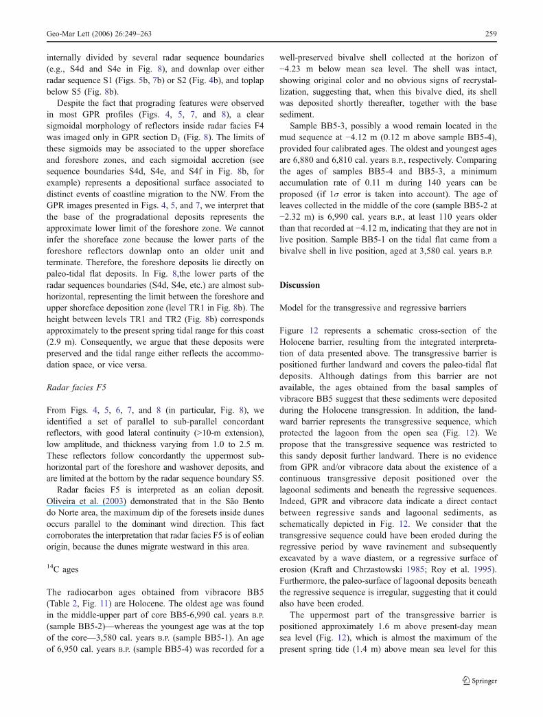
internally divided by several radar sequence boundaries(e.g., S4d and S4e in Fig. 8), and downlap over eitherradar sequence S1 (Figs. 5b, 7b) or S2 (Fig. 4b), and toplapbelow S5 (Fig. 8b).

Despite the fact that prograding features were observedin most GPR profiles (Figs. 4, 5, 7, and 8), a clearsigmoidal morphology of reflectors inside radar facies F4was imaged only in GPR section D1 (Fig. 8). The limits ofthese sigmoids may be associated to the upper shorefaceand foreshore zones, and each sigmoidal accretion (seesequence boundaries S4d, S4e, and S4f in Fig. 8b, forexample) represents a depositional surface associated todistinct events of coastline migration to the NW. From theGPR images presented in Figs. 4, 5, and 7, we interpret thatthe base of the progradational deposits represents theapproximate lower limit of the foreshore zone. We cannotinfer the shoreface zone because the lower parts of theforeshore reflectors downlap onto an older unit andterminate. Therefore, the foreshore deposits lie directly onpaleo-tidal flat deposits. In Fig. 8,the lower parts of theradar sequences boundaries (S4d, S4e, etc.) are almost sub-horizontal, representing the limit between the foreshore andupper shoreface deposition zone (level TR1 in Fig. 8b). Theheight between levels TR1 and TR2 (Fig. 8b) correspondsapproximately to the present spring tidal range for this coast(2.9 m). Consequently, we argue that these deposits werepreserved and the tidal range either reflects the accommo-dation space, or vice versa.

Radar facies F5

From Figs. 4, 5, 6, 7, and 8 (in particular, Fig. 8), weidentified a set of parallel to sub-parallel concordantreflectors, with good lateral continuity (>10-m extension),low amplitude, and thickness varying from 1.0 to 2.5 m.These reflectors follow concordantly the uppermost sub-horizontal part of the foreshore and washover deposits, andare limited at the bottom by the radar sequence boundary S5.

Radar facies F5 is interpreted as an eolian deposit.Oliveira et al. (2003) demonstrated that in the São Bentodo Norte area, the maximum dip of the foresets inside dunesoccurs parallel to the dominant wind direction. This factcorroborates the interpretation that radar facies F5 is of eolianorigin, because the dunes migrate westward in this area.

14C ages

The radiocarbon ages obtained from vibracore BB5(Table 2, Fig. 11) are Holocene. The oldest age was foundin the middle-upper part of core BB5-6,990 cal. years B.P.(sample BB5-2)—whereas the youngest age was at the topof the core—3,580 cal. years B.P. (sample BB5-1). An ageof 6,950 cal. years B.P. (sample BB5-4) was recorded for a

well-preserved bivalve shell collected at the horizon of−4.23 m below mean sea level. The shell was intact,showing original color and no obvious signs of recrystal-lization, suggesting that, when this bivalve died, its shellwas deposited shortly thereafter, together with the basesediment.

Sample BB5-3, possibly a wood remain located in themud sequence at −4.12 m (0.12 m above sample BB5-4),provided four calibrated ages. The oldest and youngest agesare 6,880 and 6,810 cal. years B.P., respectively. Comparingthe ages of samples BB5-4 and BB5-3, a minimumaccumulation rate of 0.11 m during 140 years can beproposed (if 1σ error is taken into account). The age ofleaves collected in the middle of the core (sample BB5-2 at−2.32 m) is 6,990 cal. years B.P., at least 110 years olderthan that recorded at −4.12 m, indicating that they are not inlive position. Sample BB5-1 on the tidal flat came from abivalve shell in live position, aged at 3,580 cal. years B.P.

Discussion

Model for the transgressive and regressive barriers

Figure 12 represents a schematic cross-section of theHolocene barrier, resulting from the integrated interpreta-tion of data presented above. The transgressive barrier ispositioned further landward and covers the paleo-tidal flatdeposits. Although datings from this barrier are notavailable, the ages obtained from the basal samples ofvibracore BB5 suggest that these sediments were depositedduring the Holocene transgression. In addition, the land-ward barrier represents the transgressive sequence, whichprotected the lagoon from the open sea (Fig. 12). Wepropose that the transgressive sequence was restricted tothis sandy deposit further landward. There is no evidencefrom GPR and/or vibracore data about the existence of acontinuous transgressive deposit positioned over thelagoonal sediments and beneath the regressive sequences.Indeed, GPR and vibracore data indicate a direct contactbetween regressive sands and lagoonal sediments, asschematically depicted in Fig. 12. We consider that thetransgressive sequence could have been eroded during theregressive period by wave ravinement and subsequentlyexcavated by a wave diastem, or a regressive surface oferosion (Kraft and Chrzastowski 1985; Roy et al. 1995).Furthermore, the paleo-surface of lagoonal deposits beneaththe regressive sequence is irregular, suggesting that it couldalso have been eroded.

The uppermost part of the transgressive barrier ispositioned approximately 1.6 m above present-day meansea level (Fig. 12), which is almost the maximum of thepresent spring tide (1.4 m) above mean sea level for this

Geo-Mar Lett (2006) 26:249–263 259

coast. However, the top of the transgressive barrier cannotbe used as a reliable sea-level indicator because theelevation of these deposits is determined not only by sealevel, but also by sedimentation rate, incidence of cut andfill, and the upper limit of wave action (Taylor and Stone1996). Furthermore, the top of this barrier could have beeneroded. The maximum elevation we observed in the GPRimages did not exceed 1.4 m. Also, some reflectorsassociated with foreshore deposits are truncated at theirtoplap ends, suggesting that the top of the deposit waseroded, or accommodation space was restricted. Nonethe-less, the geometry of all regressive sequences arguesagainst a sea level that was much higher than the presentone. Deposition space is obviously larger seaward becauseof greater water depth. Well-preserved deposition space canbe observed in GPR section D1 (Fig. 8), where the beachdeposits (foreshore and upper shoreface) are still preserved.If we compare the elevations of the base of the foreshoredeposits with the elevations of the tidal flat, paleo-channel,and upper shoreface in a SE–NW segment, we observe acontinuous slope downward and seaward of the contact.This contact is positioned approximately −0.5 m belowmean sea level (see Fig. 7), whereas in Fig. 4 this contact issituated at −0.8 m. In Fig. 8, the contact between theforeshore and upper shoreface can be inferred at −1.6 mbelow mean sea level. Based only on the elevation of the

base of the foreshore deposits, a sea-level fall of approxi-mately 1.1 m would have occurred in the time span ofbarrier progradation, a value very close to the Holocenehighstand of +1.3 m proposed by Caldas et al. (2006).

Washover deposits occur in some places on the barrier.They are not necessarily transgressive, but they could havebeen generated by hurricanes or storms as well. Unfortu-nately, historical records of hurricanes or storms do notexist for the study area. Alternatively, the washoverdeposits might be associated with spring tides, which couldhave been high enough (+1.4 m) to overwash the barrier.Washover deposits do occur at two points of the GPRsections in the regressive sector (Figs. 5, 6, and 7). Someparts of the washover deposits are delimited by reflectorsthat probably indicate erosive events (cf. radar sequencesboundaries S3a, S3b, and S3c in Figs. 5b, 6b, and 7b,respectively) The radargram shown in Fig. 6 was obtainedover the regressive barrier, seaward of the transgressivebarrier (Fig. 12). The washover sediments, in this case,were deposited during the regression of the barrier.

Evolutionary model for the Holocene barrier

Based on barrier geometry, sediment ages, stratigraphicrecords, and sedimentation patterns, we propose a barrierevolutionary model for the Holocene for the study region

Table 2 AMS radiocarbon ages for samples from vibracore BB5

Lab. no.a Vibracoresample

Elevationb

(mbmsl)Materials δ13C (‰) Conventional age

(14C years B.P.)1σ(years)

Calibratedage(cal. years B.P.)

1σ rangec

(cal. years B.P.)

KIA14743 BB5-1 (top) −1.3 Biv. shell −3.08 ± 0.15 3,575 30 3,580 3,630–3,550KIA13957 BB5-2 −2.32 Leaf −26.33 ± 0.20 6,125 40 6,990 7,090–6,910KIA13958 BB5-3 −4.12 Plant debris −27.19 ± 0.13 6,035 35 6,880; 6,870;

6,820; 6,8106,840–6,760

KIA16093 BB5-4 (bottom) −4.23 Biv. shell −3.09 ± 0.41 6,355 45 6,950 7,010–6,890

aLeibniz Laboratory, Kiel, Germanybmbmsl, meters below today’s mean sea levelc 68.3% of probability distribution

Fig. 12 Schematic stratigraphic cross section perpendicular to the transgressive and regressive Holocene barriers

260 Geo-Mar Lett (2006) 26:249–263

(Fig. 13). During the Holocene highstand, the transgres-sive barrier was deposited and the lagoon could extendlandward (Fig. 13a). This phase of the evolution modelfor the transgressive barrier is similar to that proposedby Dominguez et al. (1987) and Martin et al. (1993) forthe eastern Brazilian coast, where barrier islands andlagoons were built up during the Holocene highstand.

During the sea-level fall soon after the Holocene high-stand, the deposition of the regressive barrier (forcedregression) started. This deposition was induced by thecoastal geometry and high amounts of eolian sedimentssupplied by the east-northeast winds (Fig. 13b). This phaseof the evolution is different from the one proposed for theeastern Brazilian coast, where the hydraulic barrier set upby rivers for sediments transported by longshore currentshas caused a strongly positive longshore sediment imbal-ance (Dominguez et al. 1987, 1992; Dominguez andWanless 1991; Martin et al. 1993). In the study area, thecoastal geometry of a retrograding shoreline to the south,forming a small embayment extending toward the west,resulted from the formation of beachrock eastward. Thisbeachrock was dated at 6,790 cal. years B.P. (Caldas et al.2006) and 6,460 cal. years B.P. (Bezerra et al. 2003). Theseages imply that the beachrock was cemented during thetransgressive phase. When sea level started to fall, thesandy beach face became wider, and consequently moreexposed to wind action, which induced the formation of thefirst eolian deposits. The main wind direction in the region,associated with the embayment of the coastline, favored themigration of the eolian deposits into the embayment. Wepropose that a considerable amount of the regressive barriersediments originated from eolian sediments, as well as fromoffshore areas, consistent with Bruun’s coastal retreatmodel (Bruun 1962). All eolian sediments from the easternpart (Fig. 13b) were transported in the direction of the bay,thus supplying enough sediment for coastal progradation.

Shells in live positions forming banks in the paleo-lagoon were dated at 3,580 cal. years B.P., consistent with alagoonal environment at this age when the last pulses ofseawater reached the lagoon. With the exception of the ageobtained for the upper part of core BB5 (sample BB5-1,Table 2), all other ages, when compared with the sea-levelcurves proposed for this region (Fig. 3), indicate lagoonalsedimentation during the Holocene transgression. The ageobtained from the in situ bivalve from the top of BB5-1(3,580 cal. years B.P.) suggests that the lagoon was activeduring the marine regression. At that time, the lagoon wassemi-enclosed, with high salinity and precipitation of saltminerals, as observed at the top of vibracore BB5.

Along today’s coastline (Fig. 13c), eolian sediments, consist-ing of small blowouts and large dunes, cover at least 2/3 of theregressive barrier in the western sector of the study area, andprobably the whole transgressive barrier in the eastern sector.

Conclusions

Geophysical, sedimentological and geochronological datafor the São Bento do Norte area reveal the existence ofregressive and transgressive deposits built at times ofHolocene sea-level changes. Geophysical, vibracore andwater-well log data suggest that the barrier deposits arearound 3- to 4-m thick, overlaying lagoonal muds. Nocontinuous transgressive layer was observed in the barrier

Fig. 13 a–c Schematic model proposed for the Holocene evolution ofthe São Bento do Norte study area. a Holocene highstand and the finalstage of transgressive barrier deposition above lagoonal sediments. bGeneration of eolian deposits in the eastern part of the area wasconcomitant with sea-level fall. Since then, eolian sediments havebeen transported into the embayment that, during sea-level fall,experienced surplus of sediments, resulting in the deposition of aregressive barrier. c Present-day coast, where the covering of basalsequences by eolian sediments is still occurring today, thus creatinglarge dunes

Geo-Mar Lett (2006) 26:249–263 261

system, because it was probably eroded by wave ravine-ment or regressive surface during the regressive period.

The difference in the elevations of the transgressivedeposit and of the base of the foreshore sediments, whencompared with the proposed sea-level curves for the region,does not corroborate the hypothesis of a sea level beingmuch higher than the present one. Thus, the Holocenehighstand probably was not higher than +1.4 m abovepresent mean sea level.

Coastal progradation and longshore barrier growthoccurred during the regressive barrier phase, when sealevel was falling and the embayment of Sao Bento do Nortearea experienced the supply of sediments associated mainlywith eolian deposits coming from the east. This construc-tion process is different from that proposed for theHolocene coastal plains along the eastern Brazilian coast,where the hydraulic barrier set up by large rivers forsediments transported by longshore currents has caused astrongly positive longshore sediment imbalance.

Acknowledgements This paper is based on the PhD theses ofLuciano Caldas (CNPq grant 201041-97.9) and Josibel G. Oliveira Jr.Financial support was provided by the Deutsche Forschungsgemein-schaft (grant number Sta 401/7-2), MARPETRO (FINEP/CTPETRO/PETROBRAS), and Programa Brasil-Alemanha 150-02 (CAPES-DAAD). CAERN (Companhia de Água e Esgotos do Rio Grande doNorte) provided the water-well logs. Walter E. Medeiros and HeleniceVital thank the Brazilian Agency CNPq for research grants (PQ).Werner Tabosa, Jean Carlos and Mofchet Birnenbaum helped duringfieldwork. We acknowledge two anonymous referees and the journaleditor Monique T. Delafontaine for valuable suggestions and languagecorrections to the original draft. Aderson do Nascimento is thanked forkindly polishing the final English text.

References

Angulo RJ, Lessa GC (1997) The Brazilian sea-level curves: a criticalreview with emphasis on the curves from Paranaguá andCananéia regions. Mar Geol 140:141–166

Barreto AMF, Bezerra FHR, Suguio K, Tatumi SH (2000) Algumasevidências de níveis marinhos Pleistocênicos no litoral do RioGrande do Norte, Brasil. In: Proc XVIII Simp Geologia do Nordeste,Sociedade Brasileira de Geologia, Recife, Boletim 16, pp 16

Barreto AMF, Suguio K, Bezerra FHR (2001) Comparação das curvasde variação do nível relativo do mar no Holoceno do litoral norte-riograndense entre si e com outras curvas do Brasil. In: Proc VIIICongr ABEQUA-Mudanças Globais e o Quaternário, AssociaçãoBrasileira de Estudos do Quaternário, Imbé, pp 106–108

Beres M Jr, Haeni FP (1991) Application of ground penetrating radarmethods in hydrogeologic studies. Ground Water 29:375–386

Bezerra FHR, Barreto AMF, Suguio K (2003) Holocene sea-levelhistory on the Rio Grande do Norte State Coast, Brazil. Mar Geol196:73–89

Brazilian Navy (2004) Tide tables for Brazilian ports. http://www.dhn.mar.mil.br

Bristow CS, Jol HM (eds) (2003) Ground penetrating radar insediments. Geol Soc Lond Spec Publ 211

Bristow CS, Chroston PN, Bailey SD (2000) The structure anddevelopment of foredunes on a locally prograding coast: insights

from ground-penetrating radar surveys, Norfolk, UK. Sedimentology47:923–944

Bruun P (1962) Sea level rise as a cause of shore erosion. AmericanSociety of Civil Engineers Proceedings, J Waterways HaborDivision 88:117–130

Caldas LHO (1996) Geologia costeira da região de São Bento doNorte e Caiçara do Norte, Litoral Norte Potiguar. RepUniversidade Federal do Rio Grande do Norte, Natal

Caldas LHO (2002) Late Quaternary coastal evolution of the northernRio Grande do Norte coast, NE Brazil. PhD Thesis, Institute ofGeosciences, University of Kiel, Kiel

Caldas LHO, Stattegger K, Vital H (2006) Holocene sea-level history:evidence from coastal sediments of the northern Rio Grande doNorte coast, NE Brazil. Mar Geol 228:39–53

Cestaro LA (1994) Os elementos do clima de Galinhos, RN, comorecursos naturais à disposição do Homem. Cadernos Norte-rio-grandense de Temas Geográficos 8:13–28

Costa-Neto LXD (1997) Evolucão geológica-geomorfológica recente daplataforma continental interna ao largo do delta do Rio Açu,Macau-RN. MSc Thesis, Universidade Federal Fluminense,Niterói

Curray JR (1964) Transgression and regression. In: Miller RL (ed)Marine Geology Shepard Commemorative volume. MacMillan,London, pp 175–203

Davis RA, Hayes MO (1984) What is a wave-dominated coast? MarGeol 60:313–329

Delibrias C, Laborel J (1969) Recent variations of the sea level alongthe Brazilian coast. Quaternaria 14:45–49

Dominguez JML, Wanless HR (1991) Facies architecture of a fallingsea-level strandplain, Doce River coast, Brazil. Spec Publ IntAssoc Sediment 14:259–281

Dominguez JML, Martin L, Bittencourt ACSP (1987) Sea-levelhistory and Quaternary evolution of river mouth associatedbeach-ridge plains along the east-southeast Brazilian coast: asummary. In: Nummedal D, Pilkey OH, Howard JD (eds)Sea-level fluctuation and coastal evolution. Soc Econ PaleontolMineral Spec Publ, pp 115–127

Dominguez JML, Bittencourt ACDSP, Martin L (1992) Controls onQuaternary coastal evolution of the east-northeastern coast ofBrazil: roles of sea-level history, trade winds and climate.Sediment Geol 80:213–232

Engels S, Roberts MC (2005) The architecture of prograding sandy-gravelbeach ridges formed during the last Holocene highstand: southwest-ern British Columbia, Canada. J Sediment Res 75:1052–1064

Fortes F (1987) Mapa geológico da Bacia Potiguar (1:1000.000).PETROBRAS, Natal, Internal Rep

Gawthorpe RL, Collier REL, Alexander J, Leeder MR, Bridge JS(1993) Ground penetration radar: application to sand bodygeometry and heterogeneity studies. In: North CP, Prosser DJ(eds) Characterization of fluvial and aeolian reservoirs. Geol SocLond Spec Publ 73:421–432

Gorini MA, Dias GTM, Mello SLM, Espíndola CRS, Gallea CG,Dellapiazza H, Castro JRJC (1982) Estudos ambientais paraimplantação de gasoduto na área de Guamaré (RN). In: ProcXXXII Congr Brasileiro de Geologia, Sociedade Brasileira deGeologia, Salvador, vol 4, pp 1531–1539

Hayes MO (1994) Geology of Holocene barrier system. Springer,Berlin Heidelberg New York

Kraft JC, Chrzastowski MJ (1985) Coastal stratigraphy sequences. In:Davis RA Jr (ed) Coastal sedimentary environments. Springer,Berlin Heidelberg New York

Lessa GC, Angulo RJ, Giannini PC, Araújo AD (2000) Stratigraphyand Holocene evolution of a regressive barrier in south Brazil.Mar Geol 165:87–108

Lima ZMC, Andrade PRO, Xavier Neto P, Vital H, Amaro VE,Medeiros WE (2002) Sand spit from NE Brazil: high-resolution

262 Geo-Mar Lett (2006) 26:249–263

Quaternary analogs for reservoir models. In: Proc AAPG AnnuMeet, 10–13 March 2002, Houston, TX, pp 1–7

Martin L, Suguio K, Flexor J-M (1993) As flutuações de nível do mardurante o Quaternário superior e a evolução geológica de “deltas”Brasileiros. Bol IG-USP 15:1–186

Martin L, Dominguez JML, Bittencourt ACSP (2003) FluctuatingHolocene sea-levels in eastern and southeastern Brazil: evidencefrom multiple fossil and geometric indicators. J Coastal Res19:101–124

Matos RMD (1994) The Northeastern Brazilian Rift System.Tectonics 11:767–790

Moore LJ, Jol HM, Kruse S, Vanderburgh S, Kaminsky GM (2004)Annual layers revealed by GPR in the subsurface of a progradingcoastal barrier, southwest Washington, U.S.A. J Sediment Res74:690–696

Nadeau M-J, Schleicher M, Grootes PM, Erlenkeuser H, Gottang A,Mous DJW, Sarntheim M, Willkomm H (1997) The Leibniz-Labor AMS facility at the Christian-Albrechts University, Kiel,Germany. Nuclear Instruments Methods Phys Res 123:22–30

Neal A, Roberts CL (2000) Applications of ground penetrating radar(GPR) to sedimentological and geomorphological studies incoastal environments. In: Pye K, Allen JRL (eds) Coastal andestuarine environments: sedimentology, geomorphology andgeoarchaeology. Geol Soc Lond Spec Publ 175:139–171

Neves CAO (1987) Análise regional do trinômio geração-migração-acumulação de hidrocarbonetos na Seqüência ContinentalEocretácica da Bacia Potiguar emersa, NE Brasil. MSc Thesis,Universidade Federal de Minas Gerais, Belo Horizonte

Nimer E (1989) Climatologia do Brasil. IBGE, Rio de JaneiroOliveira MIMD, Bagnoli E, Farias CC, Nogueira AMB, Santiago M

(1990) Considerações sobre a geometria, petrografia, sedimento-logia, diagênese e idade dos beachrocks do Rio Grande do Norte.In: Proc XXXVI Congr Brasileiro de Geologia, SociedadeBrasileira de Geologia, Natal, vol 2, pp 621–634

Oliveira JG Jr, Medeiros WE, Vital H, Xavier Neto P, Stattegger K(2003) GPR imaging of the internal structure of a sand dune inRio Grande do Norte State, Brazil. J Coastal Res Spec Issue35:271–278

Rodriguez AB, Meyer CT (2006) Sea-level variation during theHolocene highstand from the morphologic and stratigraphicevolution of Morgan Peninsula, Alabama, USA. J SedimentRes 76:257–269

Roy P, Cowell PJ, Ferland MA, Thom BG (1995) Wave dominatedcoasts. In: Carter RWG, Woodroffe CD (eds) Coastal evolution.Cambridge University Press, Cambridge, pp 121–186

Schleicher M, Gootes PM, Nadeau M-J, Scoon A (1998) Thecarbonate 14C background and its components at the LeibnizAMS facility. Radiocarbon 40:85–93

Silveira IM (2002) Estudo evolutivo das condições ambientais daregião costeira do município de Guamaré-RN. MSc Thesis,Universidade Federal do Rio Grande do Norte, Natal

Stuiver M, Reimer PJ (1993) Extended 14C database and revisedCALIB radiocarbon calibration program. Radiocarbon 35:215–230

Stuiver M, Reimer PJ, Bard E, Beck JW, Burr GS, Hughen KA,Kromer B, McCormac G, Van der Pflicht J, Spurk M (1998)INTECAL98 radiocarbon age calibration, 24,000–0 cal BP.Radiocarbon 40:1041–1083

Suguio K, Martin L, Bittencourt ACSP, Dominguez JML, Flexor J-M,Azevedo AEG (1985) Flutuações do nível relativo do mardurante o Quaternário Superior ao longo do litoral Brasileiro esuas implicações na sedimentação costeira. Rev Bras Geociênc15:273–286

Suguio K, Barreto AMF, Bezerra FHR (2001) Formações Barra deTabatinga e Touros: evidências de paleoníveis do mar Pleistocê-nicos da costa Norte-riograndense. In: Proc VIII Congr ABE-QUA-Mudanças Globais e o Quaternário, Associação Brasileirade Estudos do Quaternário, Imbé, pp 108–109

Tabosa WF (2000) Dinâmica costeira da Região de São Bento doNorte e Caiçara do Norte-RN. Rep Universidade Federal do RioGrande do Norte, Natal

Tabosa WF, Lima ZMC, Vital H, Guedes IMG (2001) Monitoramentocosteiro das praias de São Bento do Norte e Caiçara do Norte-NE/Brasil. In: Proc VII Congr Associação Brasileira de Estudosdo Quaternário, Imbé, pp 383–392

Taylor M, Stone GW (1996) Beach ridge: a review. J Coastal Res12:612–621

Testa V, Bosence DWJ (1999a) Carbonate–siliciclastic sedimentationon high-energy, ocean-facing, tropical ramp, NE Brazil. In:Wright VP, Burchette TP (eds) Carbonate ramps. Geol Soc LondSpec Publ 149:55–71

Testa V, Bosence DWJ (1999b) Physical and biological controls onthe formation of carbonate and siliciclastic bedforms on thenorth-east Brazilian shelf. Sedimentology 46:279–301

Van Andel TH, Laborel J (1964) Recent high relative sea level standnear Recife, Brazil. Science 145:580–581

Vianna ML, Solewicz R (1988) Feições fisiográficas submarinas daplataforma continental do RN visíveis por imagens de satélite. In:Proc Simp Sensoriamento Remoto, Universidade Federal do RioGrande do Norte, Natal, vol 3, pp 581–587

Vilaça JG, Cunha EMS, Silveira IM (1991) Levantamento hidrogeo-lógico do Município de Galinhos. In: Proc IV Congr Nordestinode Ecologia, Sociedade Nordestina de Ecologia, Recife, pp 56

Vital H, Stattegger V, Tabosa WF, Riedel K (2003) Why does erosionoccur on the Northeastern coast of Brazil? The Caiçara do Nortebeach example. J Coastal Res 35:525–529

Xavier Neto P, Medeiros WE (2006) A practical approach to correctattenuation effects in GPR data. J Appl Geophys 59:140–151

Ybert J-P, Bissa WM, Catharino ELM, Kutner M (2003) Environ-mental and sea-level variations on the southeastern Braziliancoast during the Late Holocene with comments on prehistorichuman occupation. Palaeogeogr Palaeoclimatol Palaeoecol189:11–24

Geo-Mar Lett (2006) 26:249–263 263