From rainfall to farm incomes—transforming advice for Australian drought policy. I. Development...

CSIRO PUBLISHING

www.publish.csiro.au/journals/ajar Australian Journal of Agricultural Research, 2007, 58, 993–1003

From rainfall to farm incomes—transforming advice for Australiandrought policy. I. Development and testing of a bioeconomicmodelling system

Philip KokicA, Rohan NelsonB,F, Holger MeinkeC, Andries PotgieterD, and John CarterE

AABARE, GPO Box 1563, Canberra, ACT 2601, Australia, and CSIRO Wealth from Oceans Flagship,GPO Box 284, Canberra, ACT 2601, Australia.

BCSIRO Wealth from Oceans Flagship, GPO Box 284, Canberra, ACT 2601, Australia, and formerly ABARE,GPO Box 1563, Canberra, ACT 2601, Australia.

CCrop and Weed Ecology, Department of Plant Sciences, Wageningen University, PO Box 430,6700 AK Wageningen, The Netherlands.

DQueensland Department of Primary Industries, PO Box 102, Toowoomba, Qld 4350, Australia.EQueensland Department of Natural Resources and Water, GPO Box 2454, Brisbane, Qld 4001, Australia.FCorrespondence author. Email: [email protected]

Abstract. In this paper we report the development of a bioeconomic modelling system, AgFIRM, designed to helpclose a relevance gap between climate science and policy in Australia. We do this by making a simple econometric farmincome model responsive to seasonal forecasts of crop and pasture growth for the coming season. The key quantitativeinnovation was the use of multiple and M-quantile regression to calibrate the farm income model, using simulated cropand pasture growth from 2 agroecological models. The results of model testing demonstrated a capability to reliablyforecast the direction of movement in Australian farm incomes in July at the beginning of the financial year (July–June).The structure of the model, and the seasonal climate forecasting system used, meant that its predictive accuracy wasgreatest across Australia’s cropping regions. In a second paper, Nelson et al. (2007, this issue), we have demonstrated howthe bioeconomic modelling system developed here could be used to enhance the value of climate science to Australiandrought policy.

Introduction

The economic impacts of climate variability and change areof significant concern to governments and rural communities.Changing seasonal patterns of rainfall and temperature affectthe incomes of rural businesses directly through changes inproduction, and indirectly through the variability of internationalcommodity prices (Chapman et al. 2000; White 2000; Hillet al. 2001). In the longer term, climate change has potentialto influence the productivity and profitability of agriculturalsystems, altering patterns of land use and regional economicoutcomes (Kokic et al. 2005; Heyhoe et al. 2007). The concernthat governments and communities share in terms of the socialand economic impacts of drought arises from the welfareimplications for rural households and others in the communityfaced with a risk of catastrophic loss (Hardaker et al. 1997;Anderson 2003).

The impacts of climate variability and change on humansystems are ultimately social and economic in nature. Drought,for example, is largely a social construct representing therisk of agricultural activity being substantially disrupted byspatial and temporal variation in rainfall and temperature(Botterill 2003; Meinke et al. 2006). In Australia, a drought in2002–03 reduced farm incomes by 60–80%, albeit from therelatively high income levels in 2001–02 (Martin et al. 2007).

Economic effects of this kind have been linked to dramaticsocial impacts on rural communities, such as divorce, illness,and suicide (Hayman and Cox 2005; Perry 2006). Reduced farmincomes can have significant flow-on effects on the nationaleconomy and society more generally. Estimates of the impact ofthe 2002–03 drought on the Australian economy range between0.75 and 1.6% of GDP, with significant effects on employment(Penm and Fisher 2003; Horridge et al. 2005).

In contrast, the information systems used to supportclimate-related policy in Australian agriculture focus almostexclusively on biophysical measures of climate variability andits impacts on agricultural production. Traditional droughtscience, for example, has been heavily dominated by reductionistmeasures of variability in rainfall, temperature, soil moisture,and plant growth (Laughlin and Clark 2000). At the beginningof 2007, this narrow biophysical emphasis remained in thenewly developed National Agricultural Monitoring System(www.nams.gov.au), nearly 10 years after this divergencebetween drought science and policy in Australia was firstpointed out (Thompson and Powell 1998). Meinke et al. (2006)refer to this misalignment of drought science and policy inAustralia as a policy relevance gap, highlighting a range ofpotential disciplinary and institutional causes that need tobe addressed.

© CSIRO 2007 10.1071/AR06193 0004-9409/07/100993

994 Australian Journal of Agricultural Research P. Kokic et al.

In this paper and its sequel we explore the potential ofbioeconomic modelling to address a dimension of this policyrelevance gap: the ability of multi-disciplinary science to informpolicy makers of the likely impact of climate variability on farmincomes in the coming season. The key quantitative innovationdescribed in this paper is the use of M-quantile regressionto calibrate a simple econometric model of farm incomes toagroecological models providing probabilistic forecasts of cropand pasture growth for the coming season. We then test thepredictive capability of the model by using it to hindcast farmincomes across Australia from 1990–91 to 2002–03. Potentialpolicy applications of this bioeconomic modelling system, theAgricultural Farm Income Risk Model (AgFIRM), are exploredin a second paper (Nelson et al. 2007, this issue).

Background

Past approaches

Most policy-related analyses of income variability in Australianagriculture have been based on information provided by farmersthrough the Australian Agricultural and Grazing IndustriesSurvey (AAGIS) (ABARE 2003). AAGIS is a large-scale,stratified sample survey conducted annually since 1978–79 for770–1654 farms in Australia’s broadacre cropping, beef, andsheep industries. A range of information has been collectedfrom each sample farm including its production and physicalcharacteristics as well as its financial performance. Informationfor individual farms is aggregated to provide national, regional,and industry statistics.

Previous attempts to empirically relate the seasonalvariability of farm incomes reported in AAGIS to theseasonal variability of rainfall have been hindered by othersources of income variability (Kokic et al. 1993; Scoccimarroet al. 1994). In addition to climate, the variability of farmincomes is influenced by seasonal and longer term trends incommodity prices, and multiple influences on productivity suchas differences in soils, past land management, and enterprisemix. Attempts to regress farm incomes against seasonalrainfall inevitably also need to contend with a high degree ofintrinsic heterogeneity between farms in similar locations andwith apparently similar physical characteristics. These includedifferences in management, aversion to risk, family composition,and lifestyle goals. This has been exacerbated by a rotatingpanel of sample farms in AAGIS representing each industry andregion, with around 80% of farms remaining in the sample fromone year to the next (Kokic et al. 1993).

With multiple sources of variability, the 27 years (1978–79 to2004–05) of data provided by farmers via AAGIS are a relativelyshort period when it comes to isolating the effects of climate onfarm income variability. This is because extreme climate eventssuch as droughts and floods may only be represented once ortwice during this period, and because the effect of a droughtdepends on the profitability and wealth of farm businesses inpreceding years.

The potential of bioeconomic modelling

Bioeconomic modelling has potential to improve ourunderstanding of the impacts of climate variability onfarm incomes. Policy-relevant bioeconomic modelling of

agricultural systems has been comprehensively reviewedby Kruseman (2000). According to Kruseman (p. 15):‘An important role of bio-economic modelling is to makecomplex interactions between agro-ecological and socio-economic phenomena transparent in policy debates’. Fromthis perspective, bioeconomic modelling is a quantitive wayof integrating alternative disciplinary approaches to provideconsistent and intuitively meaningful decision support forpolicy advisers.

Kruseman classifies bioeconomic models for agriculturalsystems research according to their temporal scale and spatialaggregation, and the extent to which they are descriptive,explanatory, or predictive. Descriptive models are by definitionqualitative, explaining interactions within a system using aconsistent set of terms and definitions. Explanatory modelsprovide interpretative insight into past relationships betweenmeasurable indicators. Predictive models take this explanatorypower one step further, providing interpretive insights intothe likely future relationships between measurable indicators.Models of all 3 kinds can provide intuitively meaningful policy-relevant insights by enhancing the mental models used by policyadvisers to design and implement policy.

The model developed by Kokic et al. (1993, 2000) isan econometric farm-scale supply-response model that iscalibrated and applied at a regional scale. The model (describedbelow) is explanatory by design, because it is used to abstractfrom farm to farm variability in the way that managementdecisions are made. It is not a farm household model inthe classic sense described by Singh et al. (1986) becauseconsumption is not incorporated. Most farm household modelshave been designed to model the delicate balance of householdsupply and demand for food in subsistence agriculture(Kruseman 2000). Omitting consumption is consistent withthe commercial nature of Australian farm businesses in whichhousehold consumption is largely separate from supply-responsedecisions.

As the model is explanatory by design, we concentrated ourevaluative testing on its ability to provide explanatory insightinto the likely direction of farm income variability in the comingseason. For completeness, we also tested the model’s predictiveperformance. In previous forecast applications, the modelaccurately predicted the direction of change in production andfarm incomes in response to changes in commodity prices (Kokicet al. 1993, 2000). However, Kokic et al. (1993) showed that notmodelling the dynamic aspects of decision making and supplyresponse reduced the precision with which the model couldpredict the magnitude of these changes. In this paper, we enhancethe dynamic response of the model to seasonal climate variabilityby incorporating forecasts of crop yield and pasture growthfrom previously published and long-operational agroecologicalmodelling systems.

MethodsOverview: linking the modelsTwo methodological steps are reported in this paper. The firstis the use of ordinary least-squares and M-quantile regressionto calibrate the farm income model (FIM) to agroecologicalmodels providing probabilistic forecasts of crop and pasture

Bioeconomic modelling for drought policy Australian Journal of Agricultural Research 995

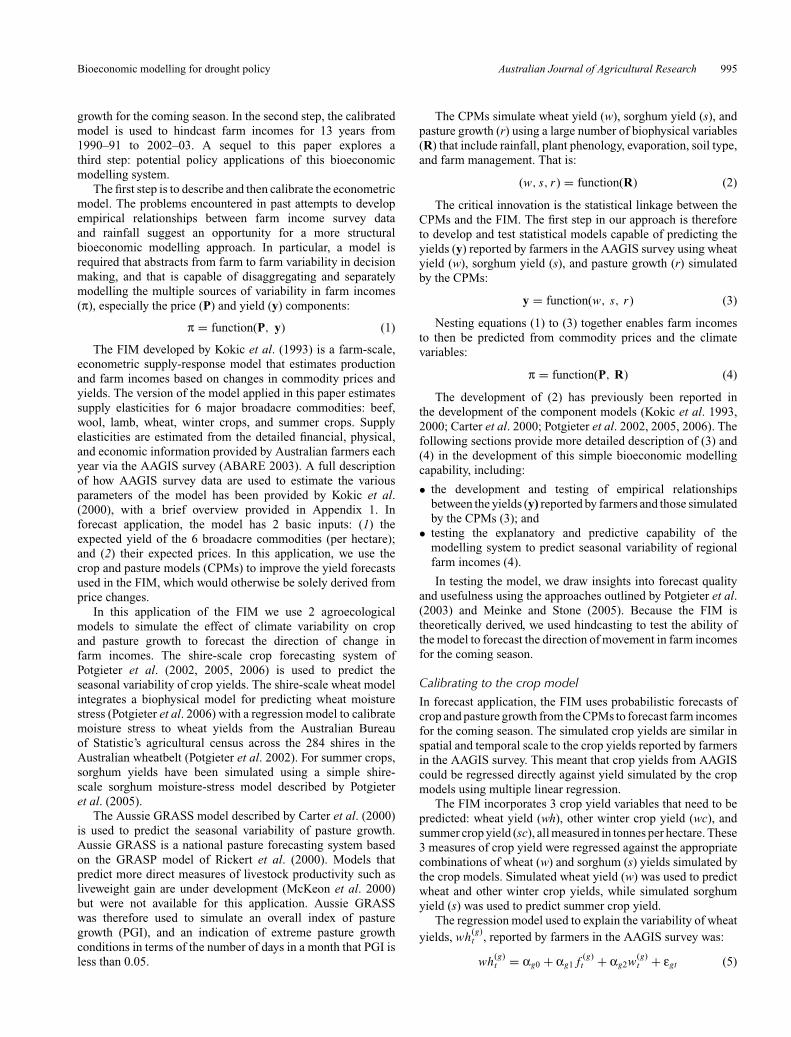
growth for the coming season. In the second step, the calibratedmodel is used to hindcast farm incomes for 13 years from1990–91 to 2002–03. A sequel to this paper explores athird step: potential policy applications of this bioeconomicmodelling system.

The first step is to describe and then calibrate the econometricmodel. The problems encountered in past attempts to developempirical relationships between farm income survey dataand rainfall suggest an opportunity for a more structuralbioeconomic modelling approach. In particular, a model isrequired that abstracts from farm to farm variability in decisionmaking, and that is capable of disaggregating and separatelymodelling the multiple sources of variability in farm incomes(π), especially the price (P) and yield (y) components:

π = function(P, y) (1)

The FIM developed by Kokic et al. (1993) is a farm-scale,econometric supply-response model that estimates productionand farm incomes based on changes in commodity prices andyields. The version of the model applied in this paper estimatessupply elasticities for 6 major broadacre commodities: beef,wool, lamb, wheat, winter crops, and summer crops. Supplyelasticities are estimated from the detailed financial, physical,and economic information provided by Australian farmers eachyear via the AAGIS survey (ABARE 2003). A full descriptionof how AAGIS survey data are used to estimate the variousparameters of the model has been provided by Kokic et al.(2000), with a brief overview provided in Appendix 1. Inforecast application, the model has 2 basic inputs: (1) theexpected yield of the 6 broadacre commodities (per hectare);and (2) their expected prices. In this application, we use thecrop and pasture models (CPMs) to improve the yield forecastsused in the FIM, which would otherwise be solely derived fromprice changes.

In this application of the FIM we use 2 agroecologicalmodels to simulate the effect of climate variability on cropand pasture growth to forecast the direction of change infarm incomes. The shire-scale crop forecasting system ofPotgieter et al. (2002, 2005, 2006) is used to predict theseasonal variability of crop yields. The shire-scale wheat modelintegrates a biophysical model for predicting wheat moisturestress (Potgieter et al. 2006) with a regression model to calibratemoisture stress to wheat yields from the Australian Bureauof Statistic’s agricultural census across the 284 shires in theAustralian wheatbelt (Potgieter et al. 2002). For summer crops,sorghum yields have been simulated using a simple shire-scale sorghum moisture-stress model described by Potgieteret al. (2005).

The Aussie GRASS model described by Carter et al. (2000)is used to predict the seasonal variability of pasture growth.Aussie GRASS is a national pasture forecasting system basedon the GRASP model of Rickert et al. (2000). Models thatpredict more direct measures of livestock productivity such asliveweight gain are under development (McKeon et al. 2000)but were not available for this application. Aussie GRASSwas therefore used to simulate an overall index of pasturegrowth (PGI), and an indication of extreme pasture growthconditions in terms of the number of days in a month that PGI isless than 0.05.

The CPMs simulate wheat yield (w), sorghum yield (s), andpasture growth (r) using a large number of biophysical variables(R) that include rainfall, plant phenology, evaporation, soil type,and farm management. That is:

(w, s, r) = function(R) (2)

The critical innovation is the statistical linkage between theCPMs and the FIM. The first step in our approach is thereforeto develop and test statistical models capable of predicting theyields (y) reported by farmers in the AAGIS survey using wheatyield (w), sorghum yield (s), and pasture growth (r) simulatedby the CPMs:

y = function(w, s, r) (3)

Nesting equations (1) to (3) together enables farm incomesto then be predicted from commodity prices and the climatevariables:

π = function(P, R) (4)

The development of (2) has previously been reported inthe development of the component models (Kokic et al. 1993,2000; Carter et al. 2000; Potgieter et al. 2002, 2005, 2006). Thefollowing sections provide more detailed description of (3) and(4) in the development of this simple bioeconomic modellingcapability, including:

• the development and testing of empirical relationshipsbetween the yields (y) reported by farmers and those simulatedby the CPMs (3); and

• testing the explanatory and predictive capability of themodelling system to predict seasonal variability of regionalfarm incomes (4).

In testing the model, we draw insights into forecast qualityand usefulness using the approaches outlined by Potgieter et al.(2003) and Meinke and Stone (2005). Because the FIM istheoretically derived, we used hindcasting to test the ability ofthe model to forecast the direction of movement in farm incomesfor the coming season.

Calibrating to the crop modelIn forecast application, the FIM uses probabilistic forecasts ofcrop and pasture growth from the CPMs to forecast farm incomesfor the coming season. The simulated crop yields are similar inspatial and temporal scale to the crop yields reported by farmersin the AAGIS survey. This meant that crop yields from AAGIScould be regressed directly against yield simulated by the cropmodels using multiple linear regression.

The FIM incorporates 3 crop yield variables that need to bepredicted: wheat yield (wh), other winter crop yield (wc), andsummer crop yield (sc), all measured in tonnes per hectare. These3 measures of crop yield were regressed against the appropriatecombinations of wheat (w) and sorghum (s) yields simulated bythe crop models. Simulated wheat yield (w) was used to predictwheat and other winter crop yields, while simulated sorghumyield (s) was used to predict summer crop yield.

The regression model used to explain the variability of wheatyields, wh

(g)t , reported by farmers in the AAGIS survey was:

wh(g)t = αg0 + αg1f

(g)t + αg2w(g)

t + εgt (5)


where f (g)t is fertiliser costs in year t, w(g)

t is simulated wheatyield, and εgt is a residual random error term with mean zero andvariance σ2

gt , while αg0, αg1, and αg2 are unknown regressioncoefficients. Here and throughout the paper the variable g isused to signal the level of aggregation used. This is discussed inmore detail below. At an early stage of model development, itwas found that incorporating fertiliser costs in (5) significantlyimproved the ability of the regression model to explain thevariability of wheat yields reported by farmers in the AAGISsurvey.

The corresponding regression models for winter, wc(g)t , and

summer crop yields, sc(g)t , were, respectively:

wc(g)t = βg0 + βg1f

(g)t + βg2w(g)

t + δgt (6)

and

sc(g)t = γg0 + γg1f

(g)t + γg2s

(g)t + ζgt (7)

where s(g)t is simulated sorghum yield, and δgt and ζgt are residual

random error terms with zero means and constant, but different,variances.

Calibrating to the pasture growth modelA statistical relationship between the livestock yields in the FIM(beef, wool, and lamb) was estimated from the pasture growthindices produced by the Aussie GRASS model using M-quantileregression (Breckling and Chambers 1988, Appendix 2). Itresults in a single livestock yield index, q, which is predictedfrom the pasture growth index using the logistic-linear regressionmodel (8):

log

(1 − q

(g)t

q(g)t

)= λg0 +

4∑j=1

λgj r(g)j t +

8∑j=5

λgjp(g)j t + ηgt (8)

where r(g)j t is the average of the pasture growth index in quarter

j of the current financial year t, p(g)j t is the average proportion of

days in quarter j that the pasture growth index is less than 0.05,and ηgt is a residual error term with mean zero and constantvariance. As described in Appendix 2, M-quantile regressionproduces non-parametric functions that relate q to each of thelivestock yields, which together with (8), provides a method ofconstructing the yield function (3).

The dependent and independent variables in the regressionEqns 5–8 correspond to a particular level of aggregation, orgeographic stratification, denoted by g. Two regional scales weretested in the course of model development: local governmentareas, also known as shires, and ABARE farm survey regions,which are considerably larger than shires (ABARE 2003, Fig. 1).

Early results of fitting models 5–8 to shire-scale data canonly be described as moderately acceptable, at best. For wheat(Eqn 5), for example, the average R2 value across all regions was47% and, in several of the wheat-growing regions, substantiallysmaller values than this were obtained. Consequently it wasdecided to only consider linking the models at a regional scale(Fig. 1).

Fig. 1. Australian broadacre regions: first digit represents state; seconddigit represents zone (1, pastoral zone; 2, wheat–sheep zone; 3, high-rainfallzone); third digit represents region within state and zone.

Forecasting farm incomesIn forecast application, the FIM was recalibrated each yearto the areas of land allocated by farmers to each commodity,and then used to forecast farm incomes 1 year into the future.This accounts for trends and dynamic responses, particularlyin livestock herds, which are not incorporated into the simpleeconometric model. For example, supply elasticities tend belower in years when prices are relatively high, yield is high,or when relatively few commodities contribute to farm income.For this application, the FIM was recalibrated each year from1989–90 to 2001–02, and used to forecast income in the years1990–91 to 2002–03. Kokic et al. (1993) found that hindcastingfarm incomes in years before 1990–91 was difficult becauseof the significant structural changes in Australian agriculturebrought about by the end of a wool floor-price scheme in 1987.The actual prices realised in each year were used for hindcastingin order to isolate the explanatory power of the crop and pasturegrowth simulations for forecasting farm incomes. In forecastmode, anticipated commodity prices for the coming seasonwould be used, introducing an additional source of variabilityinto the forecasts.

For each of the 32 agricultural regions, crop and pastureyields were simulated 103 times using historical climate datafrom 1900–01 to 2002–03. A unique set of 103 simulations ofcrop and pasture growth was generated with the antecedent soilmoisture conditions that prevailed across Australia for each ofthe 13 years between 1990–91 and 2002–03. An assumptionof current technology means that these simulations show whatcrop and pasture growth would have been across each regionif the climate for each year between 1900–01 and 2002–03had been experienced. These simulations of crop and pasturegrowth were then used to simulate climate-responsive, regionalfarm income distributions for each of the 13 years over thehindcast period.


Forecasts of annual seasonal conditions are not yet routinelyavailable in Australia (Meinke and Stone 2005). In lieu of areliable, annual forecasting system, annual farm incomes wereassumed to be closely related to seasonal conditions in autumnand winter. Australia’s rainfall variability is strongly influencedby the dynamics of the El Nino/Southern Oscillation (ENSO)phenomena, and the Southern Oscillation Index (SOI) is aconvenient method of indexing the state of the ENSO system.Prolonged periods of negative (positive) SOI values are oftenindicative of El Nino (La Nina) type climatic conditions thatgenerally result in decreased (increased) rainfall probabilitiesover much of Australia (McBride and Nicholls 1983; Stoneet al. 1996).

The SOI phase forecasting system was used to developa leading indicator of winter seasonal conditions, which isavailable at the end of June. To forecast farm incomes, each ofthe distributions of farm income was subdivided into 3 groupsof historical analogue years, using the SOI phase forecastingsystem of Stone et al. (1996). Each year of simulated farmincome was classified as positive/rising (negative/falling) ifthe SOI phases were consistently positive or rapidly rising(consistently negative or rapidly falling) at the end of bothMay and June. All other years were defined as SOI neutral.This results in a stricter classification of year types than theuse of an SOI phase at the end of a single month, with26 years classified as positive/rising, 14 years negative/falling,and 63 years considered SOI neutral.

The result is a probabilistic forecast of annual farm incomesconditional on the SOI for each of the 13 years from 1990–91to 2002–03 across Australia’s 32 agricultural regions. Theseprobabilistic forecasts can then be validated against therealised farm incomes that occurred in each region forthese years.

Testing the bioeconomic model

The model was tested in 2 steps. First, calibration of theeconometric model using simulated crop and pasture growth wastested using standard regression statistics. Second, the abilityof the bioeconomic modelling system to forecast farm incomeswas tested using explanatory and predictive measures of forecastquality.

Calibrating to the CPMs

The crop and livestock regression models (Eqns 5–8) werefitted using 24 years of farm survey data from 1978–79 to2001–02. The predictive accuracy of each regression modelwas assessed using estimates of R2 and mean absolute error(MAE) of fit. The proportion of variability in yield explained bythe simulated crop and pasture yields was reported separatelyas the R2 difference. This statistic was calculated as thedifference in R2 achieved by models 5–8 compared withthe corresponding models excluding the simulated crop andpasture growth variables. Note that because we are interestedin the predictive accuracy of the regression models, thestatistical significance of the coefficients was of less concernthan measures of the actual fit of the model (see Chambers2001).

Forecasting farm incomes

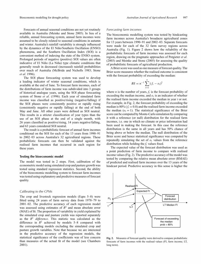
The bioeconomic modelling system was tested by hindcastingfarm incomes across Australia’s broadacre agricultural zonesfor 13 years between 1990–91 and 2002–03. Separate forecastswere made for each of the 32 farm survey regions acrossAustralia (Fig. 1). Figure 2 shows how the reliability of theprobabilistic forecasts of farm incomes was assessed for eachregion, drawing on the pragmatic approaches of Potgieter et al.(2003) and Meinke and Stone (2005) for assessing the qualityof probabilistic forecasts of agricultural production.

A Brier score was used as one measure of forecast quality. TheBrier score measures whether the realised outcome is consistentwith the forecast probability of exceeding the median:

BS = n−1n∑

t=1

(ft − ot )2

where n is the number of years, ft is the forecast probability ofexceeding the median income, and ot is an indicator of whetherthe realised farm income exceeded the median in year t or not.For example, in Fig. 2, the forecast probability of exceeding themedian is 80% ( ft = 0.8) and the realised farm income exceededthe median (ot = 1). The statistical significance of the Brierscore can be computed by Monte-Carlo simulation by comparingit with a reference (or null) distribution for the realised farmincomes, i.e. one in which no climate or price information hadbeen used in making the forecast. In this case the referencedistribution is the same in all years and has 50% chance ofbeing above or below the median. The null distribution of theBrier score and hence statistical significance was computed byrepeatedly simulating the set of ot values from the referencedistribution while holding the ft values fixed.

The expected value of the forecast distribution was used asa point prediction of farm income to compare with realisedincome values (Fig. 2). The predictive accuracy of the model wastested by comparing the relative mean absolute error (RMAE)of predicted and realised farm incomes over the 13 years of thehindcast period. Predictive accuracy in this sense is higher the

Realised FI

Forecast of exceedingthe medianprob = 80%

Forecastdistribution

Expected FI

t t+1

FIt

LT Median FI

Fig. 2. Measures of forecast quality were derived to compare probabilisticforecasts of farm incomes with the realised values (FI, farm income; LT,long term).


closer this statistic is to zero. RMAE is one of the measuresof distributional shift described by Potgieter et al. (2003).RMAE needs to be interpreted alongside the Pearson correlationcoefficient, with skill improving towards 1.0, in order to includethe potential effects of mean reverting processes.

Predictive accuracy is a demanding criterion to satisfy,particularly for a simple descriptive model such as this one,and a forecast can still carry valuable information even whenthe ability to predict point outcomes with precision is poor(Potgieter et al. 2003; Meinke and Stone 2005). For this reason,the following 2 simpler tests of forecast quality were used toassess how often the direction of the forecast was accurate.

• Direction: the proportion of years in which both the predictedand realised values of farm income were on the same side ofthe long-term median. In Fig. 2, for example, they are bothabove the median at time t + 1.

• Change: the proportion of years in which the predicted changein farm income from the previous year was in the samedirection as the realised change. In Fig. 2, both arrows arepointing upwards and so, in this case, the change is in thesame direction.

Skill in either of these statistics is indicated by a valuesignificantly greater than 0.50. The statistical significance ofboth these statistics was assessed relative to the same referencedistribution used for the Brier score.

Results

Calibrating to the crop model

Table 1 shows summary fit statistics for the 3 crop yieldregression models (Eqns 5–7) by farm survey region. As canbe seen from Table 1, the fit of the wheat yield model asmeasured by R2 exceeded 71% across most of Australia’s maincrop-producing regions (zone 2; second digit of region). Theproportion of variation explained by simulated wheat yieldwas very high across zone 2. While simulated wheat yieldexplained only 26–27% of the variation of wheat yields fromAAGIS in Western Australian, the overall R2 exceeded 77%.

Table 1. Fit of winter and summer crop yield models (Eqns 5–7)to survey region level data

Region Obs. Wheat Other winter Summer crops(wh) crops (wc) (sc)

R2 R2 diff. R2 R2 diff. R2 R2 diff.

121 24 0.76 0.51 0.65 0.22 0.60 0.01122 24 0.79 0.60 0.72 0.11123 24 0.73 0.43 0.61 0.29221 24 0.82 0.76 0.64 0.42222 24 0.75 0.65 0.65 0.62223 24 0.72 0.46 0.49 0.38321 24 0.76 0.62 0.51 0.09 0.55 0.27322 24 0.56 0.56 0.34 0.01 0.48 0.42421 24 0.85 0.66 0.78 0.30422 24 0.74 0.30 0.71 0.25521 24 0.77 0.27 0.14 0.09522 24 0.80 0.26 0.58 0.16

The performance of the model was poor in the coastal regions(zone 1) where there is less crop production.

The fit of the other winter crops model at the survey regionlevel was, as expected, not as good as for the wheat model, withthe average R2 value across all regions of 56% compared with75% for wheat. Given the fact that wheat makes up 64% oftotal winter crop production, the performance of the other wintercrops model was considered adequate to proceed with testing theability of the model to predict the direction of change in farmincomes. The fit for summer crops to simulated sorghum yieldswas also considered adequate.

Calibrating to the pasture growth model

One consequence of aggregating the data to region level wasthat this resulted in only 24 observations per farm survey region,one for each survey year. For the crop models, which only have2 dependent variables, this is not an important issue, but forthe livestock model (Eqn 8) there was a risk of over-fitting.Consequently, steps were taken to reduce this risk. Thesesteps included forming higher level groupings of regions inagronomically related zones. In order to maintain the generalityof the livestock model, separate pasture growth variables foreach region were included. Backward step-wise regression wasthen used to remove statistically non-significant terms. Thisreduced the number of dependent variables to less than 7 inmost cases.

Table 2 shows the results of fitting the livestock model asdescribed above. Clearly the pasture growth variables explain areasonable proportion of variation of the livestock yield indexin most regions, 55% on average across all survey regions.In addition, nearly all coefficient estimates selected by thebackward elimination procedure were highly significant.

Forecasting farm incomes

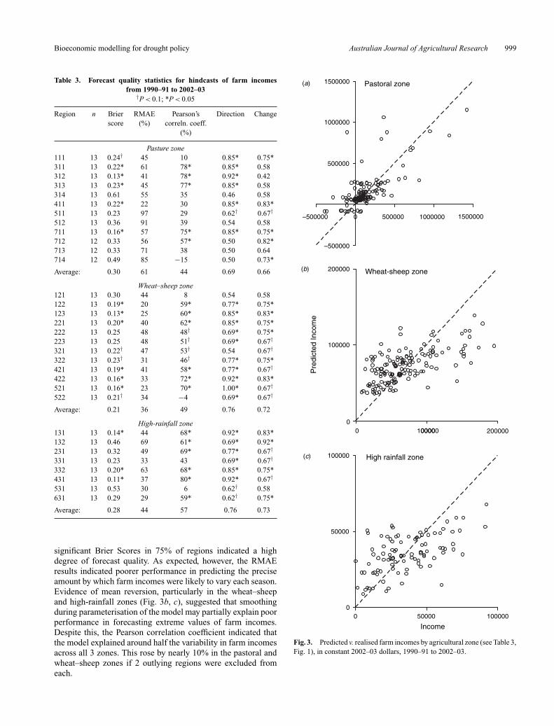
The results of model validation demonstrated that the model canreliably hindcast the direction of movement of farm incomes forthe coming financial year at the beginning of July. The Directionand Change indicators were statistically significant across mostregions of the wheat–sheep and high-rainfall zones, and in morethan half of the regions of the pastoral zone (Table 3).

The predictive performance of the model was highest inthe wheat–sheep zone (Fig. 3a–c, Table 3), where statistically

Table 2. Fit of the livestock yield index model (Eqn 8)

Region Obs. d.f. R2 MAE

111, 411 48 2 0.19 0.07121, 122, 123 72 5 0.65 0.05131, 132 48 3 0.30 0.06221, 222, 223 72 6 0.75 0.06231, 631 48 3 0.44 0.04311, 312, 313, 314 96 6 0.76 0.07321, 322 48 2 0.66 0.05331, 332 48 5 0.32 0.08421, 422, 431 72 6 0.84 0.06511, 512 48 9 0.50 0.08521, 522, 531 72 5 0.91 0.05711, 712, 713, 714 63 2 0.31 0.07


Table 3. Forecast quality statistics for hindcasts of farm incomesfrom 1990–91 to 2002–03

†P < 0.1; *P < 0.05

Region n Brier RMAE Pearson’s Direction Changescore (%) correln. coeff.

(%)

Pasture zone111 13 0.24† 45 10 0.85* 0.75*311 13 0.22* 61 78* 0.85* 0.58312 13 0.13* 41 78* 0.92* 0.42313 13 0.23* 45 77* 0.85* 0.58314 13 0.61 55 35 0.46 0.58411 13 0.22* 22 30 0.85* 0.83*511 13 0.23 97 29 0.62† 0.67†512 13 0.36 91 39 0.54 0.58711 13 0.16* 57 75* 0.85* 0.75*712 12 0.33 56 57* 0.50 0.82*713 12 0.33 71 38 0.50 0.64714 12 0.49 85 −15 0.50 0.73*

Average: 0.30 61 44 0.69 0.66

Wheat–sheep zone121 13 0.30 44 8 0.54 0.58122 13 0.19* 20 59* 0.77* 0.75*123 13 0.13* 25 60* 0.85* 0.83*221 13 0.20* 40 62* 0.85* 0.75*222 13 0.25 48 48† 0.69* 0.75*223 13 0.25 48 51† 0.69* 0.67†321 13 0.22† 47 53† 0.54 0.67†322 13 0.23† 31 46† 0.77* 0.75*421 13 0.19* 41 58* 0.77* 0.67†422 13 0.16* 33 72* 0.92* 0.83*521 13 0.16* 23 70* 1.00* 0.67†522 13 0.21† 34 −4 0.69* 0.67†

Average: 0.21 36 49 0.76 0.72

High-rainfall zone131 13 0.14* 44 68* 0.92* 0.83*132 13 0.46 69 61* 0.69* 0.92*231 13 0.32 49 69* 0.77* 0.67†331 13 0.23 33 43 0.69* 0.67†332 13 0.20* 63 68* 0.85* 0.75*431 13 0.11* 37 80* 0.92* 0.67†531 13 0.53 30 6 0.62† 0.58631 13 0.29 29 59* 0.62† 0.75*

Average: 0.28 44 57 0.76 0.73

significant Brier Scores in 75% of regions indicated a highdegree of forecast quality. As expected, however, the RMAEresults indicated poorer performance in predicting the preciseamount by which farm incomes were likely to vary each season.Evidence of mean reversion, particularly in the wheat–sheepand high-rainfall zones (Fig. 3b, c), suggested that smoothingduring parameterisation of the model may partially explain poorperformance in forecasting extreme values of farm incomes.Despite this, the Pearson correlation coefficient indicated thatthe model explained around half the variability in farm incomesacross all 3 zones. This rose by nearly 10% in the pastoral andwheat–sheep zones if 2 outlying regions were excluded fromeach.

Pastoral zone(a)

(b)

(c)

–500000

0

500000

1000000

1500000

–500000 0 500000 1000000

Wheat-sheep zone

00

100000

200000

0000100000

Pre

dict

ed In

com

e

High rainfall zone

0

50000

100000

0 50000 100000

Income

200000

1500000

Fig. 3. Predicted v. realised farm incomes by agricultural zone (see Table 3,Fig. 1), in constant 2002–03 dollars, 1990–91 to 2002–03.


DiscussionSeveral factors contributed to the superior performance ofthe bioeconomic model AgFIRM in the wheat–sheep zonecompared with the pastoral and high-rainfall zones. Thesefactors include the structure of this version of the model, andthe way it was applied.

In terms of the structure of AgFIRM, a much moredirect link was able to be established between the FIM andthe crop model because crop yields contribute directly tofarm incomes. For livestock regions, operational forecastingsystems such as Aussie GRASS currently predict pasturegrowth, rather than animal production on which farm incomesdirectly depend. Development of models such as AussieGRASS to predict the liveweight gain for sheep and cattleacross Australia continues, hampered by data limitations(McKeon et al. 2000). Data limitations include tracking ofinter-regional transfers of animals and the influence of feed-lots, changes in herd structure, and uncertainty about birth anddeath rates.

The current verson of the FIM is not dynamic, with structuralchanges in the rural sector addressed by recalibrating the modeleach year and only forecasting 1 year into the future. Livestockproduction responds dynamically to climatic and other shocksover several years, and it was not possible to use a completeset of lagged covariates to link the FIM to the pasture modelbecause of the risk of over-fitting. The bioeconomic modelcould be improved significantly in future by incorporating thedynamic adjustment of livestock herds from year to year withinthe econometric model. Models of this kind have already beendeveloped for Australian agriculture, including Beef-BEM (Caoet al. 2003), which shares a similar heritage in being calibratedusing AAGIS data.

The econometric model could also be improved by capturingthe key interactions between livestock and cropping enterpriseson mixed farms. Livestock can be moved around the farm,and fed in combinations of pasture grazing, grazing on-farmforage crops, and/or grain imported from off-farm. Accuratelypredicting the dynamic response of livestock production tofactors such as climate variability may therefore require muchmore explicit modelling of the dynamic linkages amongenterprises than the simple econometric model used in this paper(Pengelly et al. 2004).

A challenge for future applications of AgFIRM is toincorporate price forecasts, which are routinely available andforecast each quarter (e.g. Brown et al. 2007; Drum et al. 2007).Incorporating price forecasts would introduce an additionalsource of variability to farm income forecasts; one that iscurrently faced by decision makers without the aid of model-based income forecasts.

The performance of AgFIRM in cropping relative topastoral regions can partly be explained by the way it wasapplied. The FIM at the core of AgFIRM works on an annualtime step. There are currently no operational forecastingsystems for forecasting annual climate conditions relevant toAustralian agriculture (Meinke and Stone 2005). In lieu ofan operational annual forecast system, the proven SOI-basedseasonal forecasting system of Stone et al. (1996) was used.This choice of forecast system meant that the performanceof the current version of AgFIRM depended on the extent

to which winter seasonal conditions during the months ofJuly–August influence annual farm incomes. Winter seasonalconditions contribute more to annual farm incomes in thecropping systems of southern Australia than in the pastoralsystems or high-rainfall zones in which grazing depends moreon autumn and spring conditions. Winter crop productiondominates farm incomes in southern Australia because hot,dry summers prevent summer cropping without irrigation,and sheep numbers, formerly a major alternative source ofincome, have fallen dramatically since the early 1990s (Nelson2002; Nelson and Lawrance 2004). However, given thatENSO is the major, single source of climate variability inAustralia and the fact that the ENSO cycle roughly correspondsto the Australian financial year (July–June), our approachremains valid.

Many of the model’s shortcomings could be addressed infuture operational versions. Its design is consistent with thesystems approach to applications of seasonal climate forecastingoutlined by Hammer (2000), with a modular design enablingalternative models and forecasting methods to be readily applied.It can be modified to include improved combinations of CPMs indifferent regions for modelling crop and pasture growth. It canalso be modified to include improved forecast systems as theyevolve, and to use different forecast systems in different regions.Improvements to the econometric and livestock modellingoutlined above would enable anticipated improvementsin seasonal, annual, and inter-annual climate forecastingsystems from global climate models (Hunt and Hirst 2000) tobe incorporated.

Conclusions

In this paper we have reported the development of a bioeconomicmodelling system, AgFIRM, capable of forecasting the directionof movement in Australian farm incomes at the beginning ofthe financial year (July–June). The structure of the model, andthe seasonal climate forecasting system used, mean that thepredictive accuracy of the current version of the model is greatestacross Australia’s cropping regions. Numerous opportunitiesexist to enhance the model using existing econometrictechniques, and anticipated developments in livestock modellingand seasonal climate forecasting.

Effectively recruiting climate science to inform decisionmaking and policy surrounding climate variability and changeis becoming an increasingly topical issue. In a sequel to thispaper, Nelson et al. (2007, this issue) demonstrate how thebioeconomic modelling system developed in this paper canbe used to enhance the value of climate science to Australiandrought policy. We provide 3 simple examples of how forecastsof farm financial performance can be used to enhance or replaceadvice to decision makers and policy processes that currentlyrely mostly, if not exclusively, on analyses of rainfall andtemperature. By doing this we seek to close the policy-relevancegap between climate science and decision making, in order toenhance both.

Acknowledgments

The research carried out in this project was partially funded by theManaging Climate Variability Research and Development Program, and theGrains Research and Development Corporation. Their support is gratefully


acknowledged. The authors acknowledge helpful comments on earlierdrafts by Graeme Hammer, Fred Chudleigh, Beverly Henry, Ken Day,Grant Stone, Jozef Syktus, Greg Griffiths, Ahmed Hafi, David Pannell, andan anonymous referee. For their efforts in preparing data, the authors alsothank Caroline Levantis and Dorine Bruget.

References

ABARE (2003) Australian farm survey report. Australian Bureau ofAgriculture and Resource Economics, Canberra, ACT.

Anderson JR (2003) Risk in rural development: challenges for managers andpolicy makers. Agricultural Systems 75, 161–197. doi: 10.1016/S0308-521X(02)00064-1

Botterill L (2003) Uncertain climate—the recent history of drought policyin Australia. The Australian Journal of Politics and History 49, 61–74.doi: 10.1111/1467-8497.00281

Breckling J, Chambers R (1988) M-quantiles. Biometrika 75, 761–771.Brown A, Lawrance L, O’Donnell V (2007) Grains—outlook for wheat,

coarse grains and oilseeds to 2011–12. Australian Commodities 14,27–41.

Cao L, Klijn N, Gleeson T (2003) Modelling the effects of a temporaryloss of export markets in case of a foot and mouth disease outbreak inAustralia: preliminary results on costs to Australian beef producers andconsumers. Agribusiness Review 11, 1–18.

Carter JO, Hall WB, Brook KD, Mc Keon GM, Day KA, Paull CJ(2000) Aussie GRASS: Australian Grassland and RangelandAssessment by Spatial Simulation. In ‘Applications of seasonalclimate forecasting in agricultural and natural ecosystems—theAustralian experience’. Atmospheric and Oceanographic SciencesLibrary. Vol. 21. (Eds GL Hammer, N Nicholls, C Mitchell) (KluwerAcademic Publishers: Dordrecht, The Netherlands)

Chambers R (2001) Evaluation criteria for statistical editing andimputation. UK Office for National Statistics, Methodology Report 28:(www.statistics.gov.uk/downloads/theme other/GSSMethodology No28 v2.pdf).

Chapman SC, Imray RJ, Hammer GL (2000) Can seasonal forecastspredict movements in grain prices? In ‘Applications of seasonal climateforecasting in agricultural and natural ecosystems—the Australianexperience’. Atmospheric and Oceanographic Sciences Library. Vol. 21.(Eds GL Hammer, N Nicholls, C Mitchell) (Kluwer AcademicPublishers: Dordrecht, The Netherlands)

Drum F, Shaw I, Wood A, Ashton D, Lindsay P (2007) Meat—outlookfor beef and veal, sheep meat, pigs and poultry to 2011–12. AustralianCommodities 14, 62–72.

Hammer G (2000) A general systems approach to applying seasonal climateforecasts. In ‘Applications of seasonal climate forecasting in agriculturaland natural ecosystems—the Australian experience’. Atmospheric andOceanographic Sciences Library. Vol. 21. (Eds GL Hammer, N Nicholls,C Mitchell) (Kluwer Academic Publishers: Dordrecht, The Netherlands)

Hardaker JB, Huirne RBM, Anderson JR (1997) ‘Coping with risk inagriculture.’ (CAB International: Wallingford, UK)

Hayman P, Cox P (2005) Drought risk as a negotiated construct.In ‘From disaster response to risk management: Australia’s nationaldrought policy’. (Eds LC Botterill, D Wilhite) (Springer: Dordrecht,The Netherlands)

Heyhoe E, Kim Y, Kokic P, Levantis C, Ahammad H, Schneider K, Crimp S,Nelson R, Flood N, Carter J (2007) Adapting to climate change—issuesand challenges in the agriculture sector. Australian Commodities 14,167–178.

Hill HSJ, Butler D, Fuller SW, Hammer GL, Holzworth D, Love HA,Meinke H, Mjelde JW, Park J, Rosenthal W (2001) Effects of seasonalclimate variability and the use of climate forecasts on wheat supplyin the United States, Australia, and Canada. Impact of El Nino andClimate Variability on Agriculture, ASA Special Publication No. 63.pp. 101–123. (American Society of Agronomy: Madison, WI)

Horridge M, Madden J, Wittwer G (2005) The impact of the 2002–2003drought on Australia. Journal of Policy Modeling 27, 285–308.doi: 10.1016/j.jpolmod.2005.01.008

Hunt B, Hirst AC (2000) Global climate models and their potentialfor seasonal climate forecasting. In ‘Applications of seasonal climateforecasting in agricultural and natural ecosystems—the Australianexperience’. Atmospheric and Oceanographic Sciences Library. Vol. 21.(Eds GL Hammer, N Nicholls, C Mitchell) (Kluwer AcademicPublishers: Dordrecht, The Netherlands)

Kokic P, Beare S, Topp V, Tulpule V (1993) Australian broadacre agriculture:forecasting supply at the farm level. ABARE Research Report 93.7.,Canberra, ACT, Australia.

Kokic P, Chambers R, Beare S (2000) Microsimulation of businessperformance. International Statistical Review. Revue Internationale deStatistique 68, 259–276. doi: 10.2307/1403413

Kokic P, Heaney A, Pechey L, Crimp S, Fisher B (2005) Climatechange. Predicting the impacts on agriculture: a case study. AustralianCommodities 12, 161–170.

Kruseman G (2000) Bio-economic household modelling for agriculturalintensification. PhD thesis, Wageningen University, The Netherlands,Mansholt Studies No. 20.

Laughlin G, Clark A (2000) Drought science and drought policy in Australia:a risk management perspective. In ‘Early warning systems for droughtpreparedness and drought management. Proceedings of an Expert GroupMeeting’. Lisbon. (Eds A Wilhite, MVK Sivakumar, DA Wood) (WorldMeteorological Organisation: Geneva)

Martin P, Mues C, Phillips P, Shafron W, Van Mellor T, Kokic P,Nelson R, Treadwell R (2007) Farm financial performance—Australianfarm income, debt and investment, 2004–05 to 2006–07. AustralianCommodities 14, 179–200.

McBride J, Nicholls N (1983) Seasonal relationships betweenAustralian rainfall and the Southern Oscillation. Monthly WeatherReview 111, 1998–2004. doi: 10.1175/1520-0493(1983)111<1998:SRBARA>2.0.CO;2

McKeon G, Ash A, Hall W, Stafford Smith M (2000) Simulation of grazingstrategies for beef production in north-east Queensland. In ‘Applicationsof seasonal climate forecasting in agricultural and natural ecosystems—the Australian experience’. Atmospheric and Oceanographic SciencesLibrary. Vol. 21. (Eds GL Hammer, N Nicholls, C Mitchell) (KluwerAcademic Publishers: Dordrecht, The Netherlands)

Meinke H, Nelson R, Kokic P, Stone R, Selvaraju R, Baethgen W (2006)Actionable climate knowledge: from analysis to synthesis. ClimateResearch 33, 101–110. doi: 10.3354/cr033101

Meinke H, Stone R (2005) Seasonal and inter-annual climate forecasting: thenew tool for increasing preparedness to climate variability and changein agricultural planning and operations. Climatic Change 70, 221–253.doi: 10.1007/s10584-005-5948-6

Nelson R (2002) Projecting resource use in Australian broadacre agriculture.Australian Commodities 9, 23–28.

Nelson R, Kokic P, Meinke H (2007) From rainfall to farm incomes—transforming advice for Australian drought policy. II. Forecasting farmincomes. Australian Journal of Agricultural Research 58, 1004–1012.

Nelson R, Lawrance L (2004) Resource use in Agriculture. AustralianCommodities 11, 27–29.

Pengelly B, Whitbread A, Mazaiwana P, Mukombe N (2004) Tropicalforage research for the future—better use of research resources todeliver adoption and benefits to farmers. In ‘Tropical legumes forsustainable farming systems in southern Africa and Australia’. ACIARProceedings No. 115. (Eds A Whitbread, B Pengelly) (ACIAR:Canberra, ACT)

Penm J, Fisher B (2003) Economic overview—prospects for world economicrecovery in 2003. Australian Commodities 10, 5–19.

Perry M (2006) Drought-hit Australia battles climate change. Reuters,2 November (www.planetark.org/dailynewsstory.cfm/newsid/38776/story.htm).


Potgieter A, Everingham Y, Hammer G (2003) On measuring the qualityof a probabilistic commodity forecast for a system that incorporatesseasonal climate forecasts. International Journal of Climatology 23,1195–1210. doi: 10.1002/joc.932

Potgieter A, Hammer G, Doherty A (2006) Oz-Wheat a regional-scale cropyield simulation model for Australian wheat. Queensland GovernmentDepartment of Primary Industries and Fisheries, Brisbane.

Potgieter A, Hammer G, Doherty A, de Voil P (2005) A simple regional-scale model for forecasting sorghum yield across North-EasternAustralia. Agricultural and Forest Meteorology 132, 143–153.doi: 10.1016/j.agrformet.2005.07.009

Potgieter AB, Hammer GL, Butler D (2002) Spatial and temporal patternsin Australian wheat yield and their relationship with ENSO. AustralianJournal of Agricultural Research 53, 77–89. doi: 10.1071/AR01002

Rickert KG, Stuth JW, Mc Keon GM (2000) Modelling pasture and animalproduction. In ‘Field and laboratory methods for grassland and animalproduction research’. (Eds L’t Mannetje, RM Jones) (CABI Publishing:New York)

Scoccimarro M, Mues C, Topp V (1994) Climatic variability and farmrisk, Occasional Paper. Land and Water Resources Research andDevelopment Corporation, no. CV01/95.

Appendix 1. The Farm Income Model (FIM)

The FIM model is theoretically derived. Its design assumes that farmers have maximised net income in a base year subject to a landarea constraint. The profit function for farm is:

πi =m∑

j=1

PijQij − Ci(Qi1, . . . , Qim), (A1)

where m is the number of commodities produced by the population of farms of interest, Pij is the price received for commodity j byfarm i, Qij is the quantity of commodity sold by farm i, and Ci is the cost function.

As the size of farms increases, the costs of producing a unit of any commodity will generally also increase due to constraints onthe availability of land. To capture this effect, a convex cost function of the form:

Ci = bi0 +m∑

j=1

bijQµij

ij

is used, where µij >1 and bij are unknown parameters.The operating area Ai of the farm is assumed to be fixed over time and is written as the following functional form of the quantities

of commodity sold:

Ai = di0 +m∑

j=1

dijQij , (A2)

where dij represents the inverse of the per-hectare yield, yij , for commodity j by farm i.Subject to the constraint that the operating area on farm is fixed, Kokic et al. (2000) obtained optimum values of Qij , which

maximise the profit function (A1) subject to (A2) given a set of expected prices {P∗ij ; j = 1, . . ., m} at the forecast time point. At this

optimum the cost function reduces to:

Ci = ci0 +m∑

j=1

cijQij , (A3)

where

cij = P ∗ij + λidij

µij

= P ∗ij + λi/yij

µij

(A4)

is the farm’s unit cost of producing commodity, and λi is a Lagrange multiplier from constraint (A2).

Singh I, Squire L, Strauss J (1986) A survey of agricultural householdmodels: recent findings and policy implications. The World BankEconomic Review 1, 149–179. doi: 10.1093/wber/1.1.149

Stone RC, Hammer GL, Marcussen T (1996) Prediction of global rainfallprobabilities using phases of the Southern Oscillation Index. Nature384, 252–255. doi: 10.1038/384252a0

Thompson D, Powell R (1998) Exceptional circumstances provisionsin Australia—is there too much emphasis on drought? AgriculturalSystems 57, 469–488. doi: 10.1016/S0308-521X(98)00027-4

White B (2000) The importance of climate variability and seasonalforecasting to the Australian economy. In ‘Applications of seasonalclimate forecasting in agricultural and natural ecosystems—theAustralian experience’. Atmospheric and Oceanographic SciencesLibrary. Vol. 21. (Eds GL Hammer, N Nicholls, C Mitchell) (KluwerAcademic Publishers: Dordrecht, The Netherlands)

Manuscript received 14 June 2006, accepted 21 June 2007


Predicting income when commodity prices change

Partial derivatives of the quantity of each commodity produced (Qij ) and λi with respect to expected prices (P∗ij ) are used to simulate

the production of each commodity given an expected price change between the base and forecast time points. This means that theresulting change in unit costs can also be predicted (using Eqn A4). Profit is simulated by using Eqns A1 and A3 and the realisedprice. In other words, provided that a farm is managed so that its outputs are always adjusted to maximise its expected profit subjectto Eqn A2, its micro-level supply response (change in its outputs) to price changes can be simulated.

Details of the estimation and application of the model to forecast incomes in response to changes in commodity prices have beenpresented by Kokic et al. (1993, 2000).

Predicting income when yields change

The CPMs were used to forecast the quantity of each commodity in the FIM (beef, wool, lamb, wheat, winter crops, and summercrops). The quantity of each commodity in the FIM is adjusted in proportion to yields forecast by the CPMs (y∗

ij ) relative to the baseyear (yij ):

Q∗ij = y∗

ij

yij

Qij .

Unit costs are modified using Eqn A3, and profit is simulated by using Eqns A1 and A3.

Appendix 2. M-quantile regression

The role of M-quantile regression in predicting farm incomes has been discussed in detail by Kokic et al. (2000). The productivity ofindividual farms varies with farm-specific factors such as soil moisture availability, soil fertility, management practices, and on-farminfrastructure. This means that productivity can vary dramatically among farms that share broadly similar characteristics such aslocation, size, and enterprise mix. The use of standard regression methods implicitly assumes that the parameters relating productivityto farm incomes are the same for all farms, resulting in aggregation or averaging bias. This can be partly overcome using M-quantileregression (Breckling and Chambers 1988) to estimate farm-specific productivity coefficients.

M-quantile regression is a method of modelling that implicitly allows for ‘missing variables’ in a regression specification, effectivelyreplacing the conventional OLS ‘average line plus noise’ model by a family of lines indexed by a coefficient q (Fig. B1). Differentvalues of q then correspond to different levels of the missing variables. The regression surface passing through the ith dependentvalue corresponds to a particular quantile value qi and a set of regression coefficients di . The advantage of this approach over OLSregression is that the regression coefficients are disaggregated down to each data point. While this disaggregation may not be completebecause of the smoothing effect of regression, M-quantile regression has the advantage that it is non-parametric and so the estimatesof regression coefficients are dictated solely by the data.

In research reported in this paper, M-quantile regression was applied to the livestock components of Eqn A2. Corresponding toeach value of q there are regression coefficient estimates dj (q) for j = 1, . . ., m. These regression coefficients can be interpreted asa set of non-parametric functions dj (q), which map the livestock productivity index q to estimates of the yields of lamb, beef, andwool from the AAGIS survey data. The value qi for any given farm is chosen so as to equate the livestock component of Eqn A2 tothe area of the farm used for livestock production. The estimates of yield for that farm i are given by:

yij = {dj (qi)

}−1

Production (Q )

Ope

ratin

g ar

ea (

ha)

q = 0.75

q = 0.50

q = 0.25

Fig. B1. Example of M-quantile regressions.

http://www.publish.csiro.au/journals/ajar

From rainfall to farm incomes—transforming advice for Australian drought policy. I. Development...

Documents

Transcript of From rainfall to farm incomes—transforming advice for Australian drought policy. I. Development...