Finite element analysis of materials for aquaculture net cages
54
Department of Engineering and Safety Finite element analysis of materials for aquaculture net cages FEA of materials for aquaculture net cages using ANSYS Workbench® — Odd Einar Lockertsen Myrli Master in Technology and Safety in the High North, June 2017
-
Upload
khangminh22 -
Category
Documents
-
view
0 -
download
0
Transcript of Finite element analysis of materials for aquaculture net cages
Department of Engineering and Safety
Finite element analysis of materials for
aquaculture net cages FEA of materials for aquaculture net cages using ANSYS Workbench®
—
Odd Einar Lockertsen Myrli
Master in Technology and Safety in the High North, June 2017

i
Preface
This thesis is the completion of my master’s degree in Technology and Safety in the High
North at UiT – the Arctic University of Norway, Tromsø, Norway. The work described in this
report was carried out at the Department of Engineering and Safety in 2016-17. It is the
original and independent work of the author except where specially acknowledged in the text.
This thesis contains approximately 12504 words, 37 figures and 7 tables.
Odd Einar Lockertsen Myrli
Department of Engineering and Safety
UiT – the Arctic University of Norway
June 2017

ii
Acknowledgement
I would like to thank my supervisor, Dr. Hassan A. Khawaja for his guidance throughout the
work on the simulations. I would also like to thank the members of my study group; Sondre
Ludvigsen, Cathrine H. Strand and Simon K. Skaga, for encouraging professional discussions
during the two years of studying.
Odd Einar Lockertsen Myrli
Department of Engineering and Safety
UiT – the Arctic University of Norway
June 2017

iii
Abstract
The number of good sites in less exposed locations for aquaculture farming is limited. Trends
are now that the fish cages are increasing in both width and depth as well as more weather-
exposed locations are taken into use. As the net cages continues to increase in size, so does
the material costs. The design of the sea cages should be modified for safe and reliable use in
remote offshore locations. Fish farms located in more exposed areas will be subject to more
energetic waves and stronger currents, which will cause large net deformations. This is a
challenge as fish welfare depends on a certain minimum volume within the net cage.
Changing and maintaining net cages are some of the main expenses for fish farms. If the life
time of the net cages are extended by introducing stronger, longer lasting materials, the
overall costs of the nets would be reduced.
The traditional nets are produced in nylon, while the promising solid PET-wire has been
introduced to the aquaculture industry. In this paper, we introduce polyurethane to the
aquaculture net cages, which will be studied together with nylon and PET-wire. The study is
carried out using fluid-structure interaction (FSI) simulation, which is coupling of fluid
dynamics (CFD) and structure mechanics (FEM). ANSYS® software is employed in the
study. We will look at the materials that shows the most promising results for aquaculture
purposes.

iv
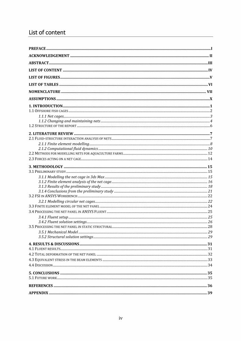
List of content
PREFACE .................................................................................................................................................................................. I
ACKNOWLEDGEMENT ...................................................................................................................................................... II
ABSTRACT ............................................................................................................................................................................ III
LIST OF CONTENT ............................................................................................................................................................. IV
LIST OF FIGURES ..................................................................................................................................................................V
LIST OF TABLES ................................................................................................................................................................. VI
NOMENCLATURE ............................................................................................................................................................. VII
ASSUMPTIONS ...................................................................................................................................................................... X
1. INTRODUCTION ............................................................................................................................................................... 1 1.1 OFFSHORE FISH CAGES ........................................................................................................................................................................... 2
1.1.1 Net cages................................................................................................................................................................................. 3 1.1.2 Changing and maintaining nets .................................................................................................................................... 4
1.2 STRUCTURE OF THE REPORT ................................................................................................................................................................. 6
2. LITERATURE REVIEW ................................................................................................................................................... 7 2.1 FLUID-STRUCTURE INTERACTION ANALYSIS OF NETS ....................................................................................................................... 7
2.1.1 Finite element modelling .................................................................................................................................................. 8 2.1.2 Computational fluid dynamics .................................................................................................................................... 10
2.2 METHODS FOR MODELLING NETS FOR AQUACULTURE FARMS ...................................................................................................... 12 2.3 FORCES ACTING ON A NET CAGE ......................................................................................................................................................... 14
3. METHODOLOGY ........................................................................................................................................................... 15 3.1 PRELIMINARY STUDY ........................................................................................................................................................................... 15
3.1.1 Modelling the net cage in 3ds Max ............................................................................................................................ 15 3.1.2 Finite element analysis of the net cage .................................................................................................................... 16 3.1.3 Results of the preliminary study ................................................................................................................................. 18 3.1.4 Conclusions from the preliminary study ................................................................................................................. 21
3.2 FSI IN ANSYS WORKBENCH ............................................................................................................................................................. 22 3.2.1 Modelling circular net cages ........................................................................................................................................ 22
3.3 FINITE ELEMENT MODEL OF THE NET PANEL .................................................................................................................................. 24 3.4 PROCESSING THE NET PANEL IN ANSYS FLUENT .......................................................................................................................... 25
3.4.1 Fluent setup ........................................................................................................................................................................ 25 3.4.2 Fluent solution settings .................................................................................................................................................. 26
3.5 PROCESSING THE NET PANEL IN STATIC STRUCTURAL ................................................................................................................... 28 3.5.1 Mechanical Model ............................................................................................................................................................ 29 3.5.2 Structural solution settings .......................................................................................................................................... 29
4. RESULTS & DISCUSSIONS .......................................................................................................................................... 31 4.1 FLUENT RESULTS.................................................................................................................................................................................. 31 4.2 TOTAL DEFORMATION OF THE NET PANEL ...................................................................................................................................... 32 4.3 EQUIVALENT STRESS IN THE BEAM ELEMENTS ............................................................................................................................... 33 4.4 DISCUSSION ........................................................................................................................................................................................... 34
5. CONCLUSIONS ............................................................................................................................................................... 35 5.1 FUTURE WORK ...................................................................................................................................................................................... 35
REFERENCES ...................................................................................................................................................................... 36
APPENDIX ........................................................................................................................................................................... 39
v
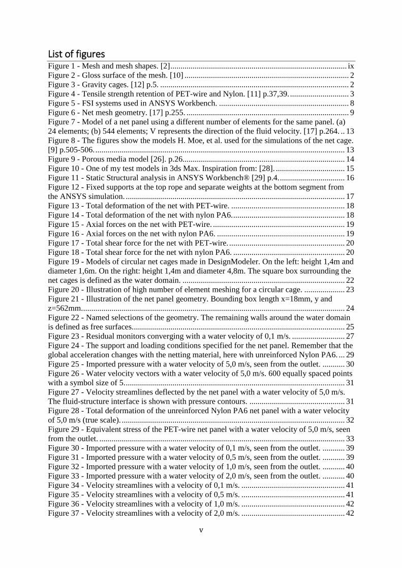
List of figures Figure 1 - Mesh and mesh shapes. [2] ....................................................................................... ix Figure 2 - Gloss surface of the mesh. [10] ................................................................................. 2 Figure 3 - Gravity cages. [12] p.5. ............................................................................................. 2 Figure 4 - Tensile strength retention of PET-wire and Nylon. [11] p.37,39. ............................. 3
Figure 5 - FSI systems used in ANSYS Workbench. ................................................................ 8 Figure 6 - Net mesh geometry. [17] p.255. ................................................................................ 9 Figure 7 - Model of a net panel using a different number of elements for the same panel. (a)
24 elements; (b) 544 elements; V represents the direction of the fluid velocity. [17] p.264. .. 13 Figure 8 - The figures show the models H. Moe, et al. used for the simulations of the net cage.
[9] p.505-506. ........................................................................................................................... 13 Figure 9 - Porous media model [26]. p.26................................................................................ 14 Figure 10 - One of my test models in 3ds Max. Inspiration from: [28]. .................................. 15
Figure 11 - Static Structural analysis in ANSYS Workbench® [29] p.4. ................................ 16 Figure 12 - Fixed supports at the top rope and separate weights at the bottom segment from
the ANSYS simulation. ............................................................................................................ 17 Figure 13 - Total deformation of the net with PET-wire. ........................................................ 18
Figure 14 - Total deformation of the net with nylon PA6. ....................................................... 18 Figure 15 - Axial forces on the net with PET-wire. ................................................................. 19 Figure 16 - Axial forces on the net with nylon PA6. ............................................................... 19 Figure 17 - Total shear force for the net with PET-wire. ......................................................... 20
Figure 18 - Total shear force for the net with nylon PA6. ....................................................... 20 Figure 19 - Models of circular net cages made in DesignModeler. On the left: height 1,4m and
diameter 1,6m. On the right: height 1,4m and diameter 4,8m. The square box surrounding the
net cages is defined as the water domain. ................................................................................ 22 Figure 20 - Illustration of high number of element meshing for a circular cage. .................... 23
Figure 21 - Illustration of the net panel geometry. Bounding box length x=18mm, y and
z=562mm. ................................................................................................................................. 24 Figure 22 - Named selections of the geometry. The remaining walls around the water domain
is defined as free surfaces. ........................................................................................................ 25
Figure 23 - Residual monitors converging with a water velocity of 0,1 m/s. .......................... 27 Figure 24 - The support and loading conditions specified for the net panel. Remember that the
global acceleration changes with the netting material, here with unreinforced Nylon PA6. ... 29
Figure 25 - Imported pressure with a water velocity of 5,0 m/s, seen from the outlet. ........... 30 Figure 26 - Water velocity vectors with a water velocity of 5,0 m/s. 600 equally spaced points
with a symbol size of 5. ............................................................................................................ 31 Figure 27 - Velocity streamlines deflected by the net panel with a water velocity of 5,0 m/s.
The fluid-structure interface is shown with pressure contours. ............................................... 31
Figure 28 - Total deformation of the unreinforced Nylon PA6 net panel with a water velocity
of 5,0 m/s (true scale). .............................................................................................................. 32
Figure 29 - Equivalent stress of the PET-wire net panel with a water velocity of 5,0 m/s, seen
from the outlet. ......................................................................................................................... 33
Figure 30 - Imported pressure with a water velocity of 0,1 m/s, seen from the outlet. ........... 39 Figure 31 - Imported pressure with a water velocity of 0,5 m/s, seen from the outlet. ........... 39 Figure 32 - Imported pressure with a water velocity of 1,0 m/s, seen from the outlet. ........... 40
Figure 33 - Imported pressure with a water velocity of 2,0 m/s, seen from the outlet. ........... 40 Figure 34 - Velocity streamlines with a velocity of 0,1 m/s. ................................................... 41 Figure 35 - Velocity streamlines with a velocity of 0,5 m/s. ................................................... 41 Figure 36 - Velocity streamlines with a velocity of 1,0 m/s. ................................................... 42 Figure 37 - Velocity streamlines with a velocity of 2,0 m/s. ................................................... 42

vi
List of tables Table 1 - Material properties for the preliminary project. Ref. PET-wire: [20] p.36. Ref.
Nylon: [31] and [32]. ................................................................................................................ 17
Table 2 - Geometric properties of the net cage modelled in the preliminary study, with
inspiration from Table 1, H. Moe, et al. [9] p.505. .................................................................. 17 Table 3 - Geometric properties of the net panel. ...................................................................... 24 Table 4 - Material properties retrieved from RTP Company. Ref: unreinforced Nylon [37],
glass fiber reinforced Nylon [38], PET [39], Polyurethane [40]. ............................................. 28
Table 5 - Maximum total deformation of the net panel. .......................................................... 32 Table 6 - Maximum equivalent stress of the net panel. ........................................................... 33 Table 7 - Safety factor for the net panel with the different materials. Tensile strength limits
retrieved from RTP Company. Ref: unreinforced Nylon [37], glass fiber reinforced Nylon
[38], PET [39], Polyurethane [40]. ........................................................................................... 33

vii
Nomenclature
Symbols
𝑆𝑛 -- Solidity ratio
𝜎𝑒 [Pa] Equivalent stress
𝜎1 [Pa] Maximum principal stress
𝜎2 [Pa] Middle principal stress
𝜎3 [Pa] Minimum principal stress
𝐹𝑠 -- Safety factor
𝑆𝑙𝑖𝑚𝑖𝑡 [Pa] Specific stress limit where failure occurs if the maximum
equivalent stress in the structure equals or exceeds this
limit
W [kg] Weight of the beam elements
B [N] Buoyancy of the beam elements
𝜌𝑚 [kg/m3] Material mass density
𝜌𝑤 [kg/m3] Seawater density
g [m/s2] Gravity
𝐿𝑡𝑜𝑡𝑎𝑙 [m] Total strand length of the rectangular net panel
d [m] Diameter of the beam elements
𝐴𝑝𝑟𝑜𝑗𝑒𝑐𝑡𝑒𝑑 [m2] Projected area of the beam elements
𝑎𝑔 [m/s2] Global acceleration boundary condition for the net panel
M [Nm] Applied bending moment of the beam elements
E [Pa] Modulus of elasticity
𝐼 [m4] Area moment of inertia of the beam cross section
𝜅 -- Resulting curvature of the beam
𝑤𝑏 [m] Deflection of the beam elements
𝑥𝑏 [m] Distance along the beam
𝜎𝑎𝑥𝑖𝑎𝑙 [Pa] Axial stress
F [N] Applied force on the beam elements
A [m2] Cross-sectional area
𝛿 [m] Deflection
L [m] Length of the beam element
𝜏 [Pa] Shear stress of beam elements
𝑉 [N] Total shear force at the location
Q [m3] Static moment of inertia
𝑡𝑚 [m] Thickness of the material perpendicular to the shear
𝑽 [m/s] Velocity vector in Cartesian space
∇ -- Vector operator in Cartesian space
(x, y, z) [m] Spatial coordinates of some domain
t [s] Time
u [m/s] Velocity component in the x-direction
v [m/s] Velocity component in the y-direction

viii
w [m/s] Velocity component in the z-direction
𝜇𝑀 [Pa∙s] Molecular viscosity coefficient
𝜆 [Pa∙s] Second viscosity coefficient
p [Pa] Pressure
(𝑓𝑥, 𝑓𝑦, 𝑓𝑧) [N] Body force per unit mass acting on the fluid element
k [J/kg] Turbulent kinetic energy
휀 [J/(kg∙s)] Dissipation rate
𝐺𝑘 [kg/(m∙s3)] Generation of turbulence kinetic energy due to the mean
velocity gradients
𝐺𝑏 [kg/(m∙s3)] Generation of turbulence kinetic energy due to buoyancy
𝑌𝑀 [kg/(m∙s3)] Contribution of the fluctuating dilatation in compressible
turbulence to the overall dissipation rate
(𝐶2, 𝐶1𝜀 , 𝐶3𝜀) -- Constants in the epsilon equation
𝜇 [Pa∙s] Viscosity of the fluid
𝜇𝑡 [Pa∙s] Eddy viscosity
𝜎𝑘 -- Turbulent Prandtl number for the k equation
𝜎𝜀 -- Turbulent Prandtl number for the epsilon equation
𝑆𝑘 and 𝑆𝜀 -- User-defined source terms in the modelled transport
equations for the realizable k-epsilon model
𝑢𝑗 [m/s] Average velocity component
S -- Modulus of the mean rate-of-strain tensor
𝑭𝐷 [N] Drag force
𝑭𝐼 [N] Inertia force
𝐶𝐷 -- Drag coefficient
𝐴𝑟𝑒𝑓 [m2] Reference area
𝑼𝑅 [m/s] Relative flow velocity
𝐶𝑎 -- Added mass coefficient
V [m3] Body volume
U [m/s] Flow velocity
𝑽𝐵 [m/s] Body velocity
𝑆𝐺𝑚𝑎𝑡𝑒𝑟𝑖𝑎𝑙 -- Specific gravity of the material
Abbreviations
CFD Computational fluid dynamics
FEA Finite element analysis
FEM Finite element method
FSI Fluid-structure interaction
PA Polyamide (nylon)
PET Polyethylene terephthalate

ix
Definitions
Diadromous species
Diadromous fishes can both live in freshwater and in saltwater.
Floating collar
The frame which provides buoyancy and attachment for the net cages.
Fouling of the net
Fouling increases the weight of the net and decreases the water flow in and out of the net
cage. Antifouling and/or frequent cleaning will prevent the fouling from building up, but you
must still include a volume of fouling when dimensioning the net (see assumptions).
Mooring
Mooring is the system of lines and bottom attachments for keeping the floating collar in the
desired position.
Fluid-structure interface
The solid surfaces of the net panel act as interfaces between the fluid and the solid domains,
providing the means to transfer the pressure load from ANSYS Fluent to Structural
mechanical.
Realizable k-epsilon model
The realizable model “means that the model satisfies certain mathematical constraints on the
Reynolds stresses, consistent with the physics of turbulent flows.” [1]
Mesh and mesh shapes
Figure 1 - Mesh and mesh shapes. [2]
x
Assumptions
• In this paper, the fish cage is not dimensioned to support a specific type of fish breed,
as there are limitations in terms of water quality and temperatures for each breed. An
analysis of environmental impact and conditions of the site must be performed before
selecting the dimensions of the fish farms.
• When dimensioning the net, one should take the mutual influence between the main
components, such as the floating collar and net cage, the net cage and mooring, etc.
[3] p.33. As we are mainly looking at the materials of the net, the influences
mentioned above have been neglected in the ANSYS® simulation. We are only
looking at the nets used in aquaculture farms.
• The twine thickness is set to 4,5 mm (3mm + 50 % fouling) [4]. Several other
aquaculture suppliers (together with Maccaferri KikkoNet) states that the twine
thickness is 2-3 mm. Then, we must add a volume of fouling: “The calculations of the
net pen shall at a minimum include a volume of fouling which gives up to 50 %
increase of the twine diameter in the net pen as a whole.” [5] p.45.
• The toxicity of the materials has not been considered in this thesis. The toxicity affects
both the fish welfare as well as the marine ecosystem.
• In this paper, we assume that the fish farm is in an area with negligible shipping traffic
to avoid the creation of waves from boats.
• The environmental temperature is set to 2,8°C, which is the lowest recorded seawater
temperature in Tromsø according to seatemperature.org [6].
• We assume constant density and pressure for the water domain.
Page 1 of 42
1. Introduction
“Cage aquaculture may date back to as early as the 1200s in some areas of Asia, and is
currently a major form of aquaculture in countries including Canada, Chile, Japan, Norway
and Scotland, where it has been used mainly for salmonid farming. However, a large variety
of species are grown in cages today and include seawater, freshwater and diadromous species.
Today, therefore, cages are used worldwide in the sea, in lakes and large rivers.” [7] p.249.
The number of good sites in less exposed locations for aquaculture farming are limited.
Trends are now that the fish cages are increasing in both width and depth as well as more
weather-exposed locations are taken into use. The design of the sea cages should be modified
for safe and reliable use in more remote offshore locations. Fish farms located in more
exposed areas will be subject to more energetic waves and stronger currents, which will cause
large net deformations. This is a challenge as fish welfare depends on a certain minimum
volume within the net cage.
“The introduction of the Norwegian standard NS 9415 in 2003 resulted in legal requirements
for strength analysis of fish farms. Up until then, all net cages had been dimensioned using
trade standards based on empirical data. NS 9415 requires strength analysis to validate the
dimensioning of large net cages and net cages subjected to large environmental loads.” [8]
p.180-181. As simulation programs for finite element methods are advancing, the engineering
analysis of the nets can contribute to improve the design, performance and reliability of the
net cages. “An analysis involving a complete fluid and structure interaction model (CFD and
FEA) will be complex and extremely demanding on computational resources, and to our
knowledge attempts to perform such analysis on net cages have not been performed. There is
ongoing work to verify and develop CFD methods for flow around net structures.” [9] p.504.
“Modelling the hydrodynamic loads acting on a net cage is challenging due to hydroelasticity,
i.e., fluid-structure interaction between moving sea-water and the flexible net.” [8] p.181. The
non-linear effects, detailed geometry and dynamic loads involved when analyzing a net cage
makes it both complex and time consuming. Although computational power has increased
immensely during the past decades, a full-scale analysis of aquaculture net cages using CFD
methods is still unrealistic today, since the net consists of thousands of thin twines. The thin
net twines make the water around the interface to divide down into many small elements by
meshing in ANSYS Fluent (see figure 20).
“In open production units in the sea there will always be possibilities for fish escape as a
result of construction failure. The weather is unpredictable and large waves can result in
breakage of the production unit.” [7] p.215. “The material strength of net panels exposed to
sunlight (UV), wind, rain, acid rain, etc. is reduced. This process is called weathering.” [7]
p.263. To test the lifetime of the nets, you could implement a Xenon lamp aging test to see the
elongation at break and time duration of the materials.
Page 2 of 42
Figure 2 - Gloss surface of the mesh. [10]
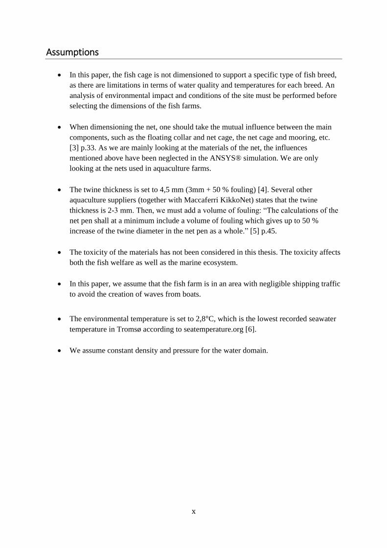
“The lifetime of net cages can be increased by adding a colored (black) antioxidant, so the
development of weathering is reduced. Today, however, white untreated material is
commonly used for net bags.” [7] p.263. “The normal life time of a net bag will vary with site
conditions; in Norway, for example, the life time of a net bag is usually set as 5 years.” [7]
p.263. According to AkvaGroup®, the EcoNet PET-wire nets can stay in the water for up to
14 years. “This eliminates costly net changes and reduce the risk of net damage and fish
escape during net handling.” [11] p.37.
1.1 Offshore fish cages
The offshore fish cages can be floating, submerged or submersible. Where the nets used in the
cages can be rigid or flexible. “Rigid nets may be created by using a flexible net attached to a
stiff framework to distend it, or a rigid metal net that will maintain its original shape
regardless of the waves.” [7] p.249.
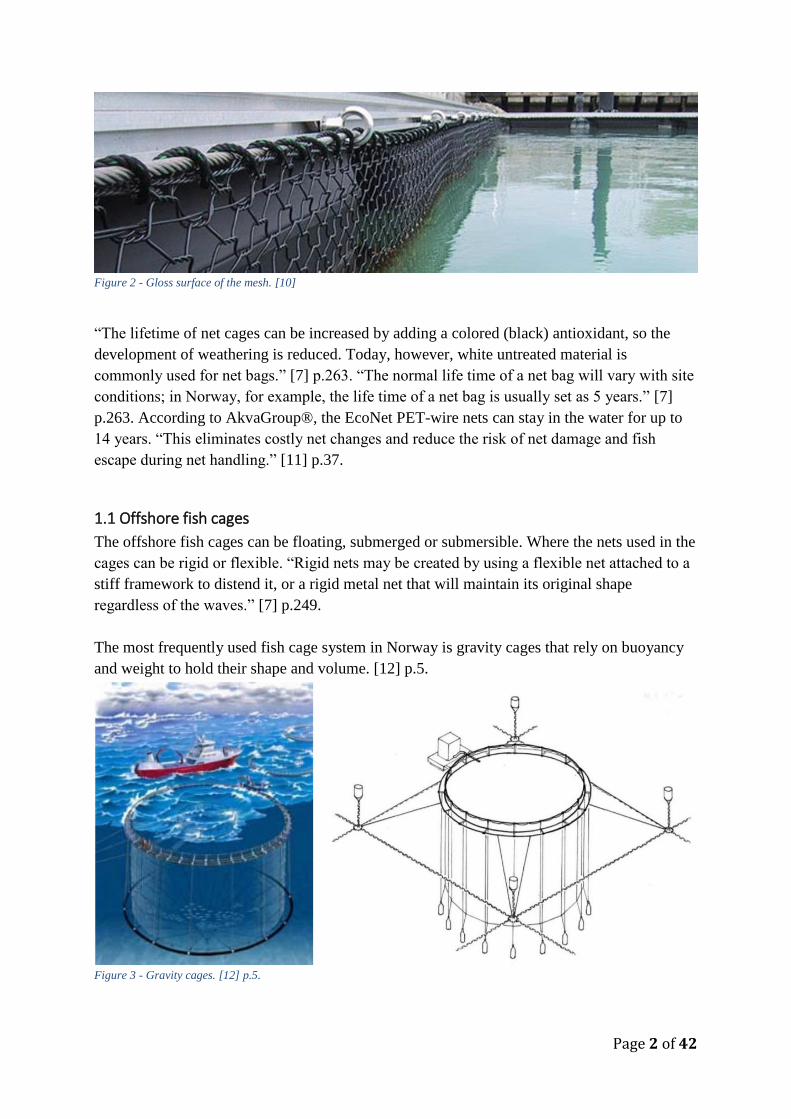
The most frequently used fish cage system in Norway is gravity cages that rely on buoyancy
and weight to hold their shape and volume. [12] p.5.
Figure 3 - Gravity cages. [12] p.5.

Page 3 of 42
In this paper, the focus is on gravity cages, which are most used for intensive aquaculture.
These cages usually consists of a mooring system, a jumping net to prevent fish escaping, a
net cage with a plumb fixed directly or indirectly to the net cage to stretch the net, and a
floating collar to provide buoyancy and attachment for the net cage. [7] p.250. The model
used in the simulations consists of a net panel that refers to a section of the netting, with a
force load to represent the separate weights in the bottom. The weights in the bottom maintain
the shape of the net, either by separate weights or by a heavy bottom ring/sinker tube as you
can see on the picture above.
1.1.1 Net cages
Net cages are built as a system of ropes and netting that can be constructed in various shapes,
sizes and materials. The net cages are designed to transfer and carry all major forces through
the ropes. The net cage is also supported by the mooring system that keeps the farm in a fixed
position and to avoid transfer of excessive forces to the net cage. It is important to take
account for the loads from current, waves, weights and handling of the net when
dimensioning the net cage.
“In the past, materials such as cotton and flax were used for the net bags. These materials
become heavy in water and their strength is rapidly reduced; in addition, they are not very
durable. Nowadays, synthetic plastic materials such as polyamide (PA, nylon) predominate.
This material is cheap, strong and not too stiff to work with.” [7] p.262. The last decade, other
materials like PET-wire (Polyethylene terephthalate) have been taken into use. PET-wire nets
are semi-rigid, and requires less weights to keep the nets in place. The benefits of PET-wire
are that it offers more protection against storm damage and predators like seals. Stronger
materials also enable the net to better maintain its shape and may have a longer life span. This
results in reduced deformation and drag, so the risk of rifts and other damage from adjacent
equipment is reduced. PET-wire nets also have a reduced overall weight displacement for the
cage system, which means less load on the mooring system and a reserve buoyancy for the
cages. According to AkvaGroup®, the tensile strength of the EcoNet PET-wire is superior to
Nylon and retains a high tensile strength for decades both below and above water. [13]
Figure 4 - Tensile strength retention of PET-wire and Nylon. [11] p.37,39.

Page 4 of 42
However, the traditional nylon is a cheaper material, even though PET-wire may have a
longer lifetime. PET-wire also weigh more, which can complicate the handling of large nets.
Handling, together with other human errors and structural errors, are highlighted as some of
the main challenges when it comes to fish escaping. [14] p.33.
In this thesis, polyurethane is also analyzed for use in net cages to compare with Nylon PA6
and PET-wire. China Institute of Water Resources & Hydropower Research in Beijing shows
promising results for a material called the ‘SK one component polyurea’ (polyurethane base
resin). They want to find new applications for the material together with UiT – the Arctic
University of Norway. The advantages of polyurea are listed as the following [15] p.5.;
(1) good aging resistance;
(2) non-toxic;
(3) good anti-seepage and anti-abrasion performance;
(4) high strength, high elongation and good bonding with base concrete;
(5) good chemical resistance;
(6) good anti-freezing performance;
(7) simple and convenient construction.
The materials properties for the SK one component polyurea was analyzed by a fellow
student, Hans-Kristian Norum Eidesen, at the University of Tromsø. The analysis was
performed in a cold room at -30°C, so the results are not applicable for this project. That is
why the material properties for the ester-based thermoplastic polyurethane was retrieved from
RTP Company® as a guideline for what the behavior might look like [16]. To my knowledge,
the material has not been tested for use in aquaculture net cages.
1.1.2 Changing and maintaining nets
“Net handling presents a major part of the total workload on a sea cage farm, and requires
additional equipment.”[7] p.391. Marine fouling is a problem for sea cages, and the degree of
fouling can be reduced by having the mesh size as large as possible. “One or two sizes are
typically used per year, but this depends on fish growth and species.” [7] p.391. On more
fouling-exposed sites, the nets may have to be changed more frequently. Changing the nets is
heavy work and may require cranes to safely lift the nets during harvesting and cleaning to
prevent rifts and other failures that may lead to escape. Netting of stronger materials like
PET-wire may stay in the water until it is damaged, and can remain intact if a single wire is
cut. According to AkvaGroup, the mesh shape will still be relatively stable with little effects
on the structural strength. You can also do maintenance work like cleaning or antifouling on
PET-wire nets while submerged, which greatly reduces the risk of net damage because of net
handling. [11]
The hydrodynamic loads acting on a net cage depends slightly on the solidity of the netting
material. “The solidity ratio (Sn) is used to describe how ‘tight’ a net is and is defined as the
ratio between the area covered by the twines in the net and the total area of the net.” [7] p.262.
𝑆𝑛 = 2 ∙𝑇𝑤𝑖𝑛𝑒 𝑑𝑖𝑎𝑚𝑒𝑡𝑒𝑟
𝐿𝑒𝑛𝑔𝑡ℎ 𝑜𝑓 𝑚𝑒𝑠ℎ 𝑠𝑖𝑑𝑒 𝑜𝑟
𝑇𝑤𝑖𝑛𝑒 𝑎𝑟𝑒𝑎
𝑇𝑜𝑡𝑎𝑙 𝑎𝑟𝑒𝑎 (1)

Page 5 of 42
This relation is important when we want to find the resistance against the water flow through
and around the net, which again determines the hydrodynamic loads acting on the cage. The
solidity will increase because of fouling on the net, which leads to an increase in the covered
area and reduces the oxygen supply for the fish. Algae growth can also increase bacterial
loads and cause diseases and stress. The marine fouling can be removed by using filtered
high-pressure seawater.

Page 6 of 42
1.2 Structure of the report
In this thesis, I analyze the responses of the net panel subject to the environmental conditions,
described by the displacements and the stresses, through analytical/numerical predictions and
fluid-structure interaction simulation. The following points are focused on in this study:
• Literature review of fluid-structure interaction modelling of net cages. How the
research with the finite elements analysis of net cages progresses, and how to model
the behavior of nets subject to environmental loads.
• The methodology of how the study progresses from my preliminary study to how it
was solved using FSI simulation, and some of the challenges I faced during the work
on my simulations.
• Results and discussion of the fluid-structure interaction analysis for the various
materials.
• Conclusion that sums up the discussion of this report.
• Future work, which highlights my thoughts on what ideas that could be initiated based
on this study.
Page 7 of 42
2. Literature review “Research into the mechanical performance of nets has a long history. It progresses along two
major lines: experimental studies (sometimes combined with in-situ observations) and
analytical/numerical predictions.” [17] p.251. Usually, aquaculture suppliers like Aqualine®
use a combination of both, where they build a prototype and place it in a water pool that
generates waves for the final testing. (Jørn Vidar Jakobsen, Aqualine Manager Northern
Norway, personal communication, October 8, 2016)
2.1 Fluid-structure interaction analysis of nets
A fluid-structure interaction (FSI) simulation is a coupled fluid dynamics (CFD) and structure
mechanics (FEM) case where we want to see how the fluid flow exerts the hydrodynamic
forces on the net. The fluid flow calculates and pass flow fields from the CFD to the FEM
code. The fluid elements in the fluid flow field will each undergo three different effects;
translation, deformation and rotation. The hydrodynamic forces exerted on the net will deform
and/or translate the net before the deformed/translated net imparts the velocity to the fluid
domain and changes its shape, as well as the fluid flow. In a FSI analysis we study the
interaction between two different physics phenomena, done in separate analyses/solvers.
There are different modes of FSI modeling; rigid body FSI, one-way FSI and two-way FSI.
With the rigid body FSI, we assume that there is no deformation in the solid structure and
only the motions of the structure in the fluid are considered. This can be done in ANSYS
Fluent alone, but it is not applicable for this project as we want to analyze the deformation for
the net panel to compare the materials used. Two-way FSI is done in an iterative loop, i.e. the
results of the CFD analysis at the fluid-structure interface are transferred to the mechanical
model and applied as loads. Within the same analysis, the subsequently calculated
displacements at the fluid-structure interface are mapped back to the CFD analysis. The loop
continues until convergence is found, and often involves the changes to the mesh of the
model. As we are working with thin twines that divides the water around the interface down
into small elements, a two-way FSI will be too demanding for the computational resources
with several twines. So, the one-way FSI mode is used for this study. [18]
In ANSYS, we can choose between two solvers for a fluid-structure interaction analysis. The
CFX solver uses an element-based finite volume method, while Fluent uses the standard finite
volume method and cell-centered solution to discretize the domain. The Fluent solver is used
in this paper, as it may obtain better accuracy due to the increased number of data points
compared to CFX that uses cell vertex numerics. Fluent allows us to import variables like
temperature or pressure, in this case, from the cell or face zones in the Fluent solver to the
structural finite element analysis. The ANSYS custom system Fluid Flow (Fluent) -> Static
Structural (see figure below) is used for the one-way transfer FSI analysis. The system had to
be modified, as the custom system you see at the top did not import the pressure. One-way
FSI can also be done by system coupling.

Page 8 of 42
Figure 5 - FSI systems used in ANSYS Workbench.
In the custom FSI system, the CFD results are imported to the structural solver as a pressure
load applied on the fluid-structure interface presented in figure 25. In a one-way FSI, the
subsequently calculated displacements at the interface are not transferred back to the CFD
analysis. The two models do not rely on matching meshes or include any modification of the
meshes. The force applied at the interface allows us to investigate the hydrodynamic effects
seawater have on the net panel.
2.1.1 Finite element modelling
A basic idea of the finite element method (FEM) is to divide a complex structure down into
finitely small and geometrically simple bodies, called elements. These elements will in some
sense model the behavior of the structure. Then we can describe the behavior of physical
quantities at each element, and solve the system of equations at the nodes between each
element. (FEM Book given as curriculum in TEK-3015 Multiphysics Simulation at UiT – the
Arctic University of Norway by Hassan A. Khawaja, 2015) p.2.
In mechanical, the stress solutions allow us to predict the safety factors, stresses and
displacements of the net panel and compare the results for the various materials. The ANSYS
yield criterion is based on the Von Mises equivalent stress, which is given as;
𝜎𝑒 = √1
2[(𝜎1 − 𝜎2)2 + (𝜎2 − 𝜎3)2 + (𝜎3 − 𝜎1)2] (2)

Page 9 of 42
Where 𝜎𝑒 is called the equivalent stress, while 𝜎1, 𝜎2 and 𝜎3 are referred to as the principal
stresses. In mechanical, the principal stresses are always ordered such that 𝜎1 is the maximum,
𝜎2 is the middle and 𝜎3 is the minimum stress. The yield occurs when the Von Mises
equivalent stress exceeds the uniaxial material yield strength. The safety factor is;
𝐹𝑠 =𝑆𝑙𝑖𝑚𝑖𝑡
𝜎𝑒 (3)
where 𝑆𝑙𝑖𝑚𝑖𝑡 is the specific stress limit where failure occurs if the maximum equivalent stress
in the structure equals or exceeds this limit. [19] p.883, 906.
2.1.1.1 Forces acting on the beam elements
Figure 6 - Net mesh geometry. [17] p.255.
The weight, buoyancy and projected area of each of the beam elements are:
𝑾 = 𝜋𝒈𝜌𝑚𝐿𝑡𝑜𝑡𝑎𝑙𝑑2
4 (4)
𝑩 = 𝜋𝒈(𝜌𝑤 − 𝜌𝑚)𝐿𝑡𝑜𝑡𝑎𝑙𝑑2
4 (5)
𝐴𝑝𝑟𝑜𝑗𝑒𝑐𝑡𝑒𝑑 = 𝐿𝑡𝑜𝑡𝑎𝑙 ∙ 𝑑 (6)
Where 𝜌𝑚 is the material mass density, 𝜌𝑤 is the seawater density, g is the gravity, d is the
diameter of the beam element and 𝐿𝑡𝑜𝑡𝑎𝑙 is the total strand length of the rectangular net panel.
[17] p.256.
The global acceleration boundary condition for the net panel is calculated by the buoyancy of
the net and the gravity.
𝑎𝑔 =𝜌𝑚𝑎𝑡𝑒𝑟𝑖𝑎𝑙−𝜌𝑤𝑎𝑡𝑒𝑟
𝜌𝑤𝑎𝑡𝑒𝑟∙ 𝑔 (7)
The bending stiffness of the beam elements is a function of the modulus of elasticity and the
area moment of inertia: .
𝑀 = 𝐸𝐼𝜅 = 𝐸𝐼𝜕2𝑤𝑏
𝜕𝑥𝑏2 (8)
Where M is the applied bending moment, 𝑤𝑏 is the deflection of the beam and 𝑥𝑏 is the
distance along the beam. E is the modulus of elasticity, where small values means a flexible
material and large values indicate rigid material. I is the area moment of inertia of the beam
cross section. [20] p.6-7.

Page 10 of 42
S.B.A. Invent [21] defines the axial stress and the deflection of beam elements.
The axial stress is defined as:
𝜎𝑎𝑥𝑖𝑎𝑙 =𝐹
𝐴 (9)
Where F is the applied force and A is the cross-sectional area resisting the load.
“Typically, the stress on a part under axial loading is constant when the cross-sectional area is
constant. However, at the fixed point it can be seen that the stress can vary. This is known as
Saint Venant's Principle, and can only be seen through Finite Element Analysis.” [21]
The deflection 𝛿 is defined as:
𝛿 =𝐹𝐿
𝐴𝐸 (10)
Where F is the applied force, L is the length of the beam element, A is the cross-sectional area
resisting the load and E is the modulus of elasticity.
The formula to calculate the shear stress of beams is defined “as the internal shear stress of a
beam caused by the shear force applied to the beam.” [22]
𝜏 =𝑉𝑄
𝐼𝑡𝑚 (11)
Where V is the total shear force at the location, Q is the static moment of area, I is the
moment of inertia of the entire cross-sectional area and 𝑡𝑚 is the thickness in the material
perpendicular to the shear.
2.1.2 Computational fluid dynamics
Computational fluid dynamics (CFD) is a design tool for fluid dynamics and aerodynamics.
CFD was developed in the 1960s by military research with the needs of the aerospace
community. The central basis of CFD is a) mass is conserved, b) conservation of momentum
(Newton’s second law, 𝐹 = 𝑚𝑎) and c) energy is conserved. When solving fluid-structure
interaction problems, the CFD solver uses the Navier-Stokes equations to import the pressure
from the fluid domain over to the structural domain.
Navier-Stokes equations are a set of coupled differential equations that “consists of a time-
dependent continuity equation for conservation of mass, three time-dependent conservation of
momentum equations and a time-dependent conservation of energy equation.” [23] High-
speed computers can solve approximations to the equations by using a variety of techniques
like the finite difference, finite volume, finite element and spectral methods. Only the
continuity equation and the momentum equation are presented, as the energy equation for
analyzing thermal conditions is disabled for this problem.
The continuity equation in conservation form, from [24] p. 55;
𝜕𝜌
𝜕𝑡+ [
𝜕(𝜌𝑢)
𝜕𝑥+
𝜕(𝜌𝑣)
𝜕𝑦+
𝜕(𝜌𝑤)
𝜕𝑧] = 0 (12.1)
𝜕𝜌
𝜕𝑡+ ∇ ∙ (𝜌𝑽) = 0 (12.2)
Page 11 of 42
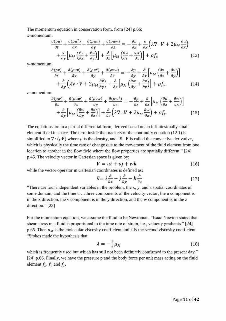
The momentum equation in conservation form, from [24] p.66;
x-momentum:
𝜕(𝜌𝑢)
𝜕𝑡+
𝜕(𝜌𝑢2)
𝜕𝑥+
𝜕(𝜌𝑢𝑣)
𝜕𝑦+
𝜕(𝜌𝑢𝑤)
𝜕𝑧= −
𝜕𝑝
𝜕𝑥+
𝜕
𝜕𝑥(𝜆∇ ∙ 𝑽 + 2𝜇𝑀
𝜕𝑢
𝜕𝑥)
+𝜕
𝜕𝑦[𝜇𝑀 (
𝜕𝑣
𝜕𝑥+
𝜕𝑢
𝜕𝑦)] +
𝜕
𝜕𝑧[𝜇𝑀 (
𝜕𝑢
𝜕𝑧+
𝜕𝑤
𝜕𝑥)] + 𝜌𝑓𝑥 (13)
y-momentum:
𝜕(𝜌𝑣)
𝜕𝑡+
𝜕(𝜌𝑢𝑣)
𝜕𝑥+
𝜕(𝜌𝑣2)
𝜕𝑦+
𝜕(𝜌𝑣𝑤)
𝜕𝑧= −
𝜕𝑝
𝜕𝑦+
𝜕
𝜕𝑥[𝜇𝑀 (
𝜕𝑣
𝜕𝑥+
𝜕𝑢
𝜕𝑦)]
+𝜕
𝜕𝑦(𝜆∇ ∙ 𝑽 + 2𝜇𝑀
𝜕𝑣
𝜕𝑦) +
𝜕
𝜕𝑧[𝜇𝑀 (
𝜕𝑤
𝜕𝑦+
𝜕𝑣
𝜕𝑧)] + 𝜌𝑓𝑦 (14)
z-momentum:
𝜕(𝜌𝑤)
𝜕𝑡+
𝜕(𝜌𝑢𝑤)
𝜕𝑥+
𝜕(𝜌𝑣𝑤)
𝜕𝑦+
𝜕(𝜌𝑤2)
𝜕𝑧= −
𝜕𝑝
𝜕𝑧+
𝜕
𝜕𝑥[𝜇𝑀 (
𝜕𝑢
𝜕𝑧+
𝜕𝑤
𝜕𝑥)]
+𝜕
𝜕𝑦[𝜇𝑀 (
𝜕𝑤
𝜕𝑦+
𝜕𝑣
𝜕𝑧)] +
𝜕
𝜕𝑧(𝜆∇ ∙ 𝑽 + 2𝜇𝑀
𝜕𝑤
𝜕𝑧) + 𝜌𝑓𝑧 (15)
The equations are in a partial differential form, derived based on an infinitesimally small
element fixed in space. The term inside the brackets of the continuity equation (12.1) is
simplified to ∇ ∙ (𝜌𝑽) where 𝜌 is the density, and “∇ ∙ 𝑽 is called the convective derivative,
which is physically the time rate of change due to the movement of the fluid element from one
location to another in the flow field where the flow properties are spatially different.” [24]
p.45. The velocity vector in Cartesian space is given by;
𝑽 = 𝑢𝒊 + 𝑣𝒋 + 𝑤𝒌 (16)
while the vector operator in Cartesian coordinates is defined as;
∇= 𝒊𝜕
𝜕𝑥+ 𝒋
𝜕
𝜕𝑦+ 𝒌
𝜕
𝜕𝑧 (17)
“There are four independent variables in the problem, the x, y, and z spatial coordinates of
some domain, and the time t. …three components of the velocity vector; the u component is
in the x direction, the v component is in the y direction, and the w component is in the z
direction.” [23]
For the momentum equation, we assume the fluid to be Newtonian. “Isaac Newton stated that
shear stress in a fluid is proportional to the time rate of strain, i.e., velocity gradients.” [24]
p.65. Then 𝜇𝑀 is the molecular viscosity coefficient and 𝜆 is the second viscosity coefficient.
“Stokes made the hypothesis that
𝜆 = −2
3𝜇𝑀 (18)
which is frequently used but which has still not been definitely confirmed to the present day.”
[24] p.66. Finally, we have the pressure p and the body force per unit mass acting on the fluid
element 𝑓𝑥, 𝑓𝑦 and 𝑓𝑧.

Page 12 of 42
The modelled transport equations for the realizable k-epsilon model are presented by ANSYS
Help Viewer [25]:
k equation:
𝜕
𝜕𝑡(𝜌𝑘) +
𝜕
𝜕𝑥𝑗(𝜌𝑘𝑢𝑗) =
𝜕
𝜕𝑥𝑗[(𝜇 +
𝜇𝑡
𝜎𝑘)
𝜕𝑘
𝜕𝑥𝑗] + 𝐺𝑘 + 𝐺𝑏 − 𝜌휀 − 𝑌𝑀 + 𝑆𝑘 (19)
Epsilon equation:
𝜕
𝜕𝑡(𝜌휀) +
𝜕
𝜕𝑥𝑗(𝜌휀𝑢𝑗) =
𝜕
𝜕𝑥𝑗[(𝜇 +
𝜇𝑡
𝜎𝜀)
𝜕𝜀
𝜕𝑥𝑗] + 𝜌𝐶1𝑆휀 − 𝜌𝐶2
𝜀2
𝑘+√𝜈𝜀
+𝐶1𝜀𝜀
𝑘𝐶3𝜀𝐺𝑏 + 𝑆𝜀 (20)
Where
𝐶1 = 𝑚𝑎𝑥 [0.43,𝜂
𝜂+5] , 𝜂 = 𝑆
𝑘
𝜀, 𝑆 = √2𝑆𝑖𝑗𝑆𝑖𝑗 𝑎𝑛𝑑 𝑆𝑖𝑗 =
1
2(
𝜕𝑢𝑗
𝜕𝑥𝑖+
𝜕𝑢𝑖
𝜕𝑥𝑗)
“In these equations, t is time, 𝜌 is the density of the fluid, k is the turbulent kinetic energy and
휀 is the dissipation rate. 𝐺𝑘 represents the generation of turbulence kinetic energy due to the
mean velocity gradients. 𝐺𝑏 is the generation of turbulence kinetic energy due to buoyancy.
𝑌𝑀 represents the contribution of the fluctuating dilatation in compressible turbulence to the
overall dissipation rate. 𝐶2, 𝐶1𝜀 and 𝐶3𝜀 are constants. 𝜎𝑘 and 𝜎𝜀 are the turbulent Prandtl
numbers for 𝑘 and 휀, respectively. 𝑆𝑘 and 𝑆𝜀 are user-defined source terms. 𝜇 is the viscosity
of the fluid, while 𝜇𝑡 is the eddy viscosity. 𝑢𝑗 is the average velocity component. S is the
modulus of the mean rate-of-strain tensor.” [25]
The continuity equation, momentum equations, k- and epsilon equation are the equations
ANSYS Fluent solves as seen in figure 23.
2.2 Methods for modelling nets for aquaculture farms
“Today, load models for net cages are typically based on Morison's equation, 2D panel tow-
tests and so-called screen models.” [8] p.181.
I. Tsukrov, et al. [17] propose a consistent one-dimensional net element to be used in the
finite element method to model the dynamic response of net panels to open ocean
environmental loading. The net panel refers to a section of netting between supports, see
picture below. Their focus is centered on the numerical modelling of deformation and overall
dynamic behavior of nets subjected to wave and current loading. The simulations were done
in the AQUA-FE program that is developed at the University of New Hampshire. This “is an
advanced computer design and analysis tool to model the dynamic response of partially or
completely submerged structures in an ocean environment.” [17] p.260.
Page 13 of 42
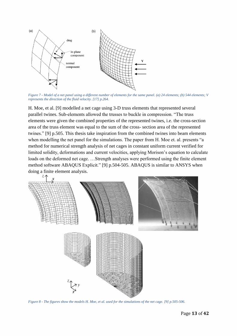
Figure 7 - Model of a net panel using a different number of elements for the same panel. (a) 24 elements; (b) 544 elements; V
represents the direction of the fluid velocity. [17] p.264.
H. Moe, et al. [9] modelled a net cage using 3-D truss elements that represented several
parallel twines. Sub-elements allowed the trusses to buckle in compression. “The truss
elements were given the combined properties of the represented twines, i.e. the cross-section
area of the truss element was equal to the sum of the cross- section area of the represented
twines.” [9] p.505. This thesis take inspiration from the combined twines into beam elements
when modelling the net panel for the simulations. The paper from H. Moe et. al. presents “a
method for numerical strength analysis of net cages in constant uniform current verified for
limited solidity, deformations and current velocities, applying Morison’s equation to calculate
loads on the deformed net cage. …Strength analyses were performed using the finite element
method software ABAQUS Explicit.” [9] p.504-505. ABAQUS is similar to ANSYS when
doing a finite element analysis.
Figure 8 - The figures show the models H. Moe, et al. used for the simulations of the net cage. [9] p.505-506.

Page 14 of 42
Another applied approach presented by Zhao, Y.-P., et al. [26] was to model the net as a
porous medium. Here, the solidity of the net is decided by the porosity to make the structure
affect the flow pattern in the fluid domain. The finite volume method was used to solve the
governing equations of the numerical model using ANSYS Fluent 6.3.
Figure 9 - Porous media model [26]. p.26.
2.3 Forces acting on a net cage
When dimensioning a net cage, the net should be constructed to reproduce the drag,
buoyancy, inertial and elastic forces exerted on the netting by current and waves. “On
ordinary sites it will be the current that causes the highest forces, while on more exposed sites
the wave forces will be considerable.” [7] p.274-275.
“The resulting forces on a moving body in an unsteady viscous flow can be determined using
Morrison equation, which is a combination of an inertial term and a drag term:
𝑭 = 𝑭𝐷 + 𝑭𝐼 (21)
Where the drag force is given by:
𝑭𝐷 =1
2𝜌𝑤𝐶𝐷𝐴𝑟𝑒𝑓𝑼𝑅|𝑼𝑅| (22)
𝜌𝑤 is the water density, 𝐶𝐷 is the drag coefficient, 𝐴𝑟𝑒𝑓 is the reference area and 𝑼𝑅 = 𝑼 −
𝑽𝐵 is the relative flow velocity, U is the flow velocity and 𝑽𝐵 is the body velocity.
And the inertia force is given by:
𝑭𝐼 = 𝜌𝑤𝐶𝑎𝑉�̇�𝑅 + 𝜌𝑤𝑉�̇� (23)
Where 𝐶𝑎 is the added mass coefficient and V is the body volume. Bold letters denote
vectors.” [27] p.1003.

Page 15 of 42
3. Methodology This chapter discusses the methodology used to design the net panel and to study the materials
used in fish cages. The study is carried out using ANSYS Workbench® version 18.1 on a
Lenovo ThinkStation P910. The chapter gives a detailed overview of how the study
progressed from my preliminary study to how it was solved in the mentioned simulation
program.
3.1 Preliminary study
The preliminary study was carried out using ANSYS Workbench® version 17.1 and
postprocessing in Autodesk 3ds Max®. The study was a purely mechanical (FEM) analysis of
nylon PA6 and PET-wire; it did not include the hydrodynamic loads acting on the net cage.
So, the only forces defined on the net was the weights and the fixed supports. Note that the
material properties used in the preliminary study are not the same as for this thesis.
3.1.1 Modelling the net cage in 3ds Max
Figure 10 - One of my test models in 3ds Max. Inspiration from: [28].
The program is user-friendly with many different modifiers that makes the modelling process
easier. With the editable poly function, a primitive object like a cylinder can be divided into
sub-objects (in the form of polygons) that you can modify. With the editable poly function,
you can build any model you can imagine, and this is the method I used to model the net cage.

Page 16 of 42
Before importing the geometry file into ANSYS Workbench, the file must be saved as type:
AutoCad (*.DWG). For an accurate export to ANSYS Workbench, the unit setup must be
customized to metric meters in 3ds Max. The import to ANSYS only contained line bodies, as
the surface bodies will make a volume inside the mesh twines (this is the blue shades between
the twines as you can see in the figure above). So, over 8000 different parts were reduced to
38 parts when imported to ANSYS DesignModeler. After importing the CAD file to ANSYS
workbench, I had to define the cross-section area for the twines, as line bodies do not have a
surface area or volume. Finally, the parts were united into one body using the Boolean body
operation in ANSYS Geometry.
Postprocessing in 3ds Max proved to be incompatible with ANSYS Fluent as the imported
model did not have any faces, which are needed for selecting the fluid-structure interface and
to subtract the solid body from the water. This problem may have been possible to solve
within 3ds Max settings and/or by saving the file as another file type.
I described the bodies by the materials and the imported geometry in ANSYS workbench.
Figure 11 - Static Structural analysis in ANSYS Workbench® [29] p.4.
Transient structural analysis was used in ANSYS Workbench® for a dynamic analysis. The
illustration above still describes the main elements when performing the simulation. In
Engineering Data, the material properties are defined for each of the materials, with Young’s
Modulus, Poisson’s ratio and density (which must be specified when inertia forces are
involved e.g., dynamic simulations). As the net cage with a diamond shaped mesh is difficult
to design in the built-in DesignModeler geometry, the geometric model was created in 3ds
Max.
3.1.2 Finite element analysis of the net cage
By creating a mesh, we create a mesh of nodes, and the results are calculated by solving the
governing equations numerically at each of the nodes using the finite element method.
In the preliminary study, a mechanical physics preference was used for the mesh which
transformed the single body into 6737 nodes and 3584 elements. As the external flows around
the net were yet to be modelled, a Lagrangian formulation is used. The Lagrangian

Page 17 of 42
formulation is usually used for finite element analysis (FEA) of solids, and the nodes are
associated with material points. [30] p.21.
The material properties used for the preliminary project are presented in table 1. The values
differ from the material properties used in this paper, as obtained from RTP Company.
Nylon PA6 PET-wire
Young’s Modulus 2900 MPa 3000 MPa
Poisson’s ratio 0,39 0,39
Density 1158,25 kg/m3 1380 kg/m3
Table 1 - Material properties for the preliminary project. Ref. PET-wire: [20] p.36. Ref. Nylon: [31] and [32].
The net cage was created with the following properties:
Diameter 4.48 m = 16x Truss length
Depth 1.40 m = 5x Truss length
Truss length 0.28 m
Twine thickness 3 mm+50% fouling = 0.0045 m
Truss thickness 4x Twine thickness = 0.018 m
Truss cross-section area 254.47 mm2
Table 2 - Geometric properties of the net cage modelled in the preliminary study, with inspiration from Table 1, H. Moe, et
al. [9] p.505.
The model was constraint by setting a fixed support in all vertexes on the top rope as you can
see on the figure below. Then, the separate weights were set at the bottom rope as well as one
in the middle. Each weight was set to be 800g with inspiration from H. Moe, et al. Model M1
[9] p.505.
Figure 12 - Fixed supports at the top rope and separate weights at the bottom segment from the ANSYS simulation.
Next, the model was solved for both Nylon (PA6) and PET-wire, where the results is
discussed below.
Page 18 of 42
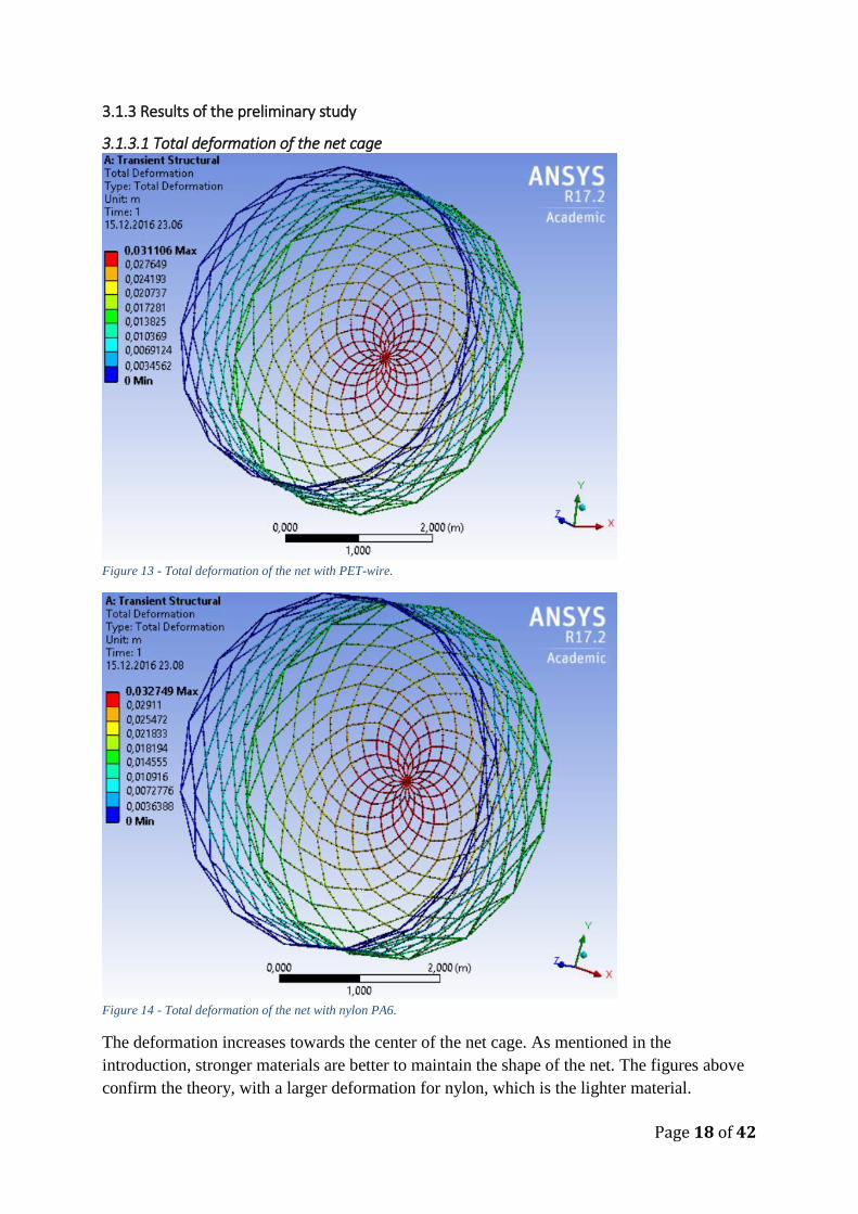
3.1.3 Results of the preliminary study
3.1.3.1 Total deformation of the net cage
Figure 13 - Total deformation of the net with PET-wire.
Figure 14 - Total deformation of the net with nylon PA6.
The deformation increases towards the center of the net cage. As mentioned in the
introduction, stronger materials are better to maintain the shape of the net. The figures above
confirm the theory, with a larger deformation for nylon, which is the lighter material.

Page 19 of 42
3.1.3.2 Axial forces
Figure 15 - Axial forces on the net with PET-wire.
Figure 16 - Axial forces on the net with nylon PA6.
The axial forces are largest near the top and bottom ropes (marked in red and orange) which
means we have the most tension here. This is because of the weights that was placed around
the bottom segment. The maximum tension force is larger for nylon, and nylon also have the
largest compression on the opposite side of the scale.

Page 20 of 42
3.1.3.3 Total shear force
Figure 17 - Total shear force for the net with PET-wire.
Figure 18 - Total shear force for the net with nylon PA6.
The total shear force is largest around the center of the net sides. The force was yet again
largest for nylon PA6.

Page 21 of 42
3.1.4 Conclusions from the preliminary study
Following conclusions were drawn from the preliminary study:
• PET-wire proved to be the strongest material, however, nylon PA6 is a cheaper option
and the results did not differ enough to say that using PET-wire would pay off.
• The material properties chosen for the study are quite similar for the two materials,
this is the reason why the results are so similar for both materials.
• The net should have been constructed to reproduce the drag, buoyancy, inertial and
elastic forces exerted on the netting by current and waves. The fact that we are lacking
the environmental loads from current and waves do not make the results comparable to
the reality.

Page 22 of 42
3.2 FSI in ANSYS Workbench
Following the preliminary study, new models are designed for the fluid-structure interaction
analysis. The net is constructed to reproduce the hydrodynamic forces exerted on the netting
by currents and waves. We describe the bodies by geometries and materials in ANSYS
Workbench. The environmental conditions will include support and loading conditions, and
the responses of the net panel subject to the environmental conditions are described by the
displacements and the stresses.
3.2.1 Modelling circular net cages
Some simplifications had to be made to the circular net cages when modelling in the built-in
DesignModeler geometry. The diamond shaped mesh was replaced by a square mesh to
reduce the number of twines/elements.
Figure 19 - Models of circular net cages made in DesignModeler. On the left: height 1,4m and diameter 1,6m. On the right:
height 1,4m and diameter 4,8m. The square box surrounding the net cages is defined as the water domain.
The circular net cages were made of three-dimensional cylinders and tori with a diameter of
18 mm. The coordinates for the 16 points around the circular cages were found from vertexes
I extracted from 3ds Max models I made for the two cages. The bottom was made by making
a new plane placed at one of the end points of the circle and rotating cylinders around the
circular cage.
The Fluent solution diverged while using a coarse mesh for these detailed geometries. The
problem with these models is the number of elements generated from a finer mesh. Starting
with the largest cage with a diameter of 4,8m, the number of elements/cells ranges from ~50
million with a freeboard and a draft, to over 70 million elements for a fully submerged cage.
The high number of elements comes from the fluid-structure interface where the thin twines
separates the water elements around the interface, as you can see on the illustration in figure
20. Before being able to process the net cages in ANSYS Fluent, both a ANSYS Academic
Research license and the Lenovo ThinkStation P910 had to be acquired, as a ANSYS Student
Page 23 of 42
License has a numerical limit of 512000 nodes/cells. The P910 was brought in to give
additional computational power.
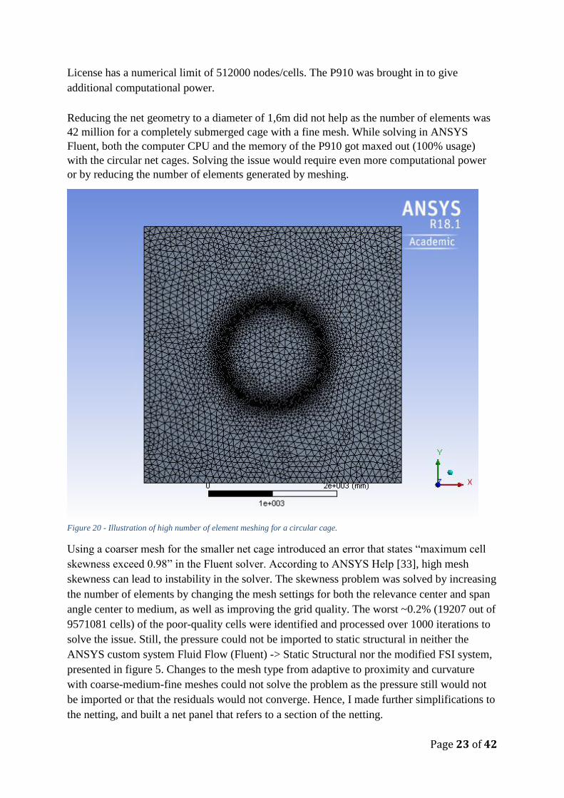
Reducing the net geometry to a diameter of 1,6m did not help as the number of elements was
42 million for a completely submerged cage with a fine mesh. While solving in ANSYS
Fluent, both the computer CPU and the memory of the P910 got maxed out (100% usage)
with the circular net cages. Solving the issue would require even more computational power
or by reducing the number of elements generated by meshing.
Figure 20 - Illustration of high number of element meshing for a circular cage.
Using a coarser mesh for the smaller net cage introduced an error that states “maximum cell
skewness exceed 0.98” in the Fluent solver. According to ANSYS Help [33], high mesh
skewness can lead to instability in the solver. The skewness problem was solved by increasing
the number of elements by changing the mesh settings for both the relevance center and span
angle center to medium, as well as improving the grid quality. The worst ~0.2% (19207 out of
9571081 cells) of the poor-quality cells were identified and processed over 1000 iterations to
solve the issue. Still, the pressure could not be imported to static structural in neither the
ANSYS custom system Fluid Flow (Fluent) -> Static Structural nor the modified FSI system,
presented in figure 5. Changes to the mesh type from adaptive to proximity and curvature
with coarse-medium-fine meshes could not solve the problem as the pressure still would not
be imported or that the residuals would not converge. Hence, I made further simplifications to
the netting, and built a net panel that refers to a section of the netting.

Page 24 of 42
3.3 Finite element model of the net panel
The net panel is built as three-dimensional cylinders in DesignModeler geometry.
The net panel was created with the following properties:
Length of mesh side 54,4 mm
Twine thickness 3 mm+50% fouling = 4,5 mm
Beam thickness 4x Twine thickness = 18 mm
Twine cross-section area 254.47 mm2
Table 3 - Geometric properties of the net panel.
Note that the length of mesh side is twice the maximum length presented in “Tabell 1” [34]
p.20. As I combined 4 twines into each beam element, I increased the length so the mesh
openings/solidity would not be too small.
Figure 21 - Illustration of the net panel geometry. Bounding box length x=18mm, y and z=562mm.
The finite element model of the water mesh consists of 2767284 elements and 3858390 nodes.
The mesh is generated with a CFD physics preference in the Fluent solver. Element sizing is
decided by the size function proximity and curvature, with a medium relevance center, slow
transition and a fine span angle center. The quality target skewness is by default 0.9, with
medium smoothing. While meshing the water domain, the net panel is suppressed. Still, we
can see an increased number of elements due to the fluid-structure interface which consists of
194 faces with a surface area of 0.54698 m2 and a volume of 0.0026527 m3. If the structure is
not subtracted from the water domain, the water domain would just be a square mesh. The
square mesh would have a small number of elements compared to the water domain with the
fluid-structure interface. Another point to add to this is that, if the structure is not subtracted
from the water, the water flow would not flow through the net.

Page 25 of 42
Figure 22 - Named selections of the geometry. The remaining walls around the water domain is defined as free surfaces.
The inlet is defined so that the flow travels in the direction of the positive x-axis, the y-axis is
horizontal and the z-axis is vertical. The corners at each edge of the net panel are cut into one
face to reduce the number of elements generated by meshing, as the circular end-points of the
cylinders would further divide the water elements around the interface. Then, the Boolean
unite operation is used to assemble all cylinders into one body; the net panel. The water
domain is made in a rectangular shape with dimensions 4000x2544x1594 mm to make it
symmetric around each side of the net, except in the x-direction where there is more space
after the netting section to see the behavior of the flow lines. If the walls of the water domain
are too close to the net panel, the flow lines will swirl more after deflection, which will affect
the results. Finally, the Boolean subtract operation is used to subtract the net panel from the
water domain, so ANSYS Fluent knows there is a solid body inside the water in Fluent
meshing. If the net is not subtracted from the water domain, there is no CFD surface to import
the pressure from Fluent to structural.
3.4 Processing the net panel in ANSYS Fluent
3.4.1 Fluent setup
The governing equations are discretized using the finite volume method (cell-centered) and
solved using the CFD software ANSYS Fluent. A steady time simulation is used with a 3D
pressure-based solver to enable the pressure-based Navier-Stokes solution algorithm. “The

Page 26 of 42
pressure-based solver uses a solution algorithm where the governing equations are solved
sequentially (i.e., segregated from one another). Because the governing equations are non-
linear and coupled, the solution loop must be carried out iteratively in order to obtain a
converged numerical solution.” [35] Double-precision is specified in the Fluent launcher, this
means that the residuals can drop as many as 12 orders of magnitude instead of the 6 orders of
magnitude with single-precision before the residuals are converging. Parallel processing is
enabled to make use of all 16 processors of the P910 and to reduce the computing time.
The turbulence/viscous model used is the realizable k-epsilon model with standard wall
functions and default model constants; 𝐶1𝜀 = 1.44, 𝐶2 = 1.9, 𝜎𝑘 = 1.0 and 𝜎𝜀 = 1.2. The
realizable k-epsilon model “is likely to provide superior performance for flow involving
strong pressure gradients. For flow through and around a plane net, strong pressure gradients
exist because of the blockage effect of the fishing net.” [26] p.26.
Water-liquid is found from the Fluent material database, with a default constant viscosity of
0.001003 𝑘𝑔/(𝑚 ∙ 𝑠) and a density of 1025 𝑘𝑔/𝑚3, for the cell zone conditions of the water
domain. For the boundary conditions, the pressure is specified as constant, while the water
velocity from the inlet is set to 0.1, 0.5, 1.0, 2.0 and 5.0 𝑚/𝑠 to compare the behavior of the
net panel of various materials at different flow rates. The inlet velocity is specified with
default values, where the turbulent intensity set to 5% (medium intensity) and the turbulent
viscosity ratio given by 𝜇𝑡/𝜇 is set to 10. The pressure outlet is specified with the same values
for the backflow turbulent intensity and the backflow turbulent viscosity ratio.
The model has two mesh interfaces, one for the water cell zone and one for the solid net
panel. Even though the interfaces have the same position and shape, the interface selected on
the solid net panel will correspond to the solid cell zone, while the interface selected after
suppressing the solid body in Fluent will only correspond to the fluid cell zone. The Fluent
console states that the interface zones overlap for the mesh interfaces, and that this could
adversely affect the solution. The two interface zones must be merged together into a single
mesh before running the Fluent calculation. To merge the zones together, the coupled wall
option is enabled in Mesh Interfaces under fluent setup. The coupled wall boundary at the
interface is acting as a wall zone so the fluid cannot pass across the fluid-structure interface.
Before going on with the solution, the reference values are computed from the inlet and the
seawater temperature is set to 275.95K (2.8°C, see assumptions) with the water domain as the
reference zone.
3.4.2 Fluent solution settings
The pressure-velocity coupling method chosen is the default SIMPLE algorithm. “The
SIMPLE algorithm uses a relationship between velocity and pressure corrections to enforce
mass conservation and to obtain the pressure field.” [36] The spatial discretization scheme for
the gradient method is the default least squares cell based, while the pressure is defined with
the default second-order scheme. The momentum, turbulent kinetic energy and turbulent

Page 27 of 42
dissipation rate are carried out using a second order upwind scheme to improve the accuracy,
as suggested by ANSYS Fluent when checking the case.
Figure 23 - Residual monitors converging with a water velocity of 0,1 m/s.
Note that the turbulent kinetic energy (𝑘) and the turbulent dissipation rate (휀) are initialized
with a first order upwind scheme. I did not use the second order upwind scheme for the cases
where a good convergence was found by using a first order upwind scheme. Take the plot
above as an example; I did not see the residuals converging with an inlet velocity of 0.1 m/s
after 1000 iterations with first order, so I changed the spatial discretization scheme for the
turbulent kinetic energy and the turbulent dissipation rate to second order for another 1000
iterations. Then, the solution met the convergence criteria at iteration step 1857. The solution
is specified as having reached a converged solution when all residuals changes their value by
less or equal to 0.001. The residuals did not meet the specified absolute criteria of 0.001 for
the other velocities analyzed in this project, but they ran for 1000-2000 iterations until a
converging behavior was found.
The first calculations were done with default under-relaxation factors for the solution controls,
but the continuity equation did not converge. “For most flows, the default under-relaxation
factors do not usually require modification. If unstable or divergent behavior is observed,
however, you need to reduce the under-relaxation factors for pressure, momentum, k,
and epsilon from their default values to about 0.2, 0.5, 0.5, and 0.5.” [37].
As these values for the under-relaxation factors still gave a divergent behavior, the under-
relaxation factors were all reduced to 0,1. This solved the issue, and the solution converged.
The solution limits and the advanced solution controls are set as default, where the V-cycle is
used for the pressure equation in the pressure-based segregated algorithm and the flexible
cycle is used for the momentum, turbulent kinetic energy and turbulent dissipation rate
equations. A standard initialization method is used, computed from the inlet. The x-velocity is

Page 28 of 42
the same as for the boundary conditions (0.1, 0.5, 1.0, 2.0 and 5.0 𝑚/𝑠), while the initial y-
and z-velocity are set to 0 m/s, as the angle of attack for the flow is set perpendicular to the
net panel.
3.5 Processing the net panel in static structural
Static structural analysis is used in ANSYS Workbench® to model the structural mechanics.
The material properties are defined for each of the materials in Engineering Data, with
Young’s Modulus, Poisson’s ratio and density (which must be specified when inertia forces
are involved). The material properties used in this project are retrieved from RTP Company.
Note that RTP Company list that: “This information is intended to be used only as a guideline
for designers and processors of modified thermoplastics” for the properties of all materials
used in this project.
Base
polymer
Description Specific
gravity
[-]
Density
[kg/m3]
Tensile
Modulus
[MPa]
Global
acc. (𝒂𝒈)
[m/s2]
Mass of
net panel
[kg]
Nylon PA6 Unreinforced
base resin
1,13 1158,25 2758 1,2753 3,0725
Nylon PA6 30% glass fiber
reinforced,
heat stabilized
-- 1350 9800 3,1105 3,5811
Polyethylene
Terephthalate
(PET)
30% glass fiber
reinforced
1,56 1599 11032 5,4936 4,2416
Ester-based
thermoplastic
Polyurethane
elastomer
30% glass fiber
reinforced
1,44 1476 3103 4,3164 3,9154
Table 4 - Material properties retrieved from RTP Company. Ref: unreinforced Nylon [37], glass fiber reinforced Nylon [38],
PET [39], Polyurethane [40].
goodfellow.com [32], professionalplastics.com [31] and Casanova, C. and W. Dwikartika [20]
p.36. set the Poisson’s ratio for nylon PA6 and PET-wire to 0.39, so the Poisson’s ratio is
assumed to be 0.39 for all materials in this project. The density of the materials is found from
the specific gravity of the materials, except from nylon PA6 30% glass fiber reinforced as the
density was given from RTP Company, using the following relation:
𝜌𝑚𝑎𝑡𝑒𝑟𝑖𝑎𝑙 = 𝑆𝐺𝑚𝑎𝑡𝑒𝑟𝑖𝑎𝑙 ∙ 𝜌𝑤 (24)
Where 𝑆𝐺𝑚𝑎𝑡𝑒𝑟𝑖𝑎𝑙 is the specific gravity of the materials, while 𝜌𝑤 is the density of seawater.
“The behaviour of the net cage can be dominated by non-linear effects due to very large
deformations and materials with non-linear properties.” [38] Synopsis p.4.
The pressure could not be imported with a nonlinear mechanical physics preference as the
following error occurred; “An error occurred while transferring the load. The add-in did not
generate any data to import.” So, I made the following simplifications to the materials
properties; each material is defined as linear elastic with isotropic elasticity derived from the
Young’s Modulus and the Poisson’s Ratio. Now, by using the default mechanical physics

Page 29 of 42
preference, the pressure imported without making any changes to the upstream component
(Fluent solution).
3.5.1 Mechanical Model
The water domain is suppressed in the structural solver, so only the net panel is processed in
the mechanical mesh. Using a fine mesh increases the computational time for importing the
pressure, so I used a coarser mesh to reduce the computational time. The results are only
affected by the mesh settings in a small scale because the net panel geometry is not as
complex as the net cages. Element sizing is decided by the adaptive size function, with
medium relevance center, slow transition and a coarse span angle center. Target quality is by
default 0.05, with medium smoothing. The mesh transforms the single body into 32079 nodes
and 15399 elements.
3.5.2 Structural solution settings
The governing equations are discretized using the finite element method (FEM) with the
mechanical APDL solver target. The environment temperature is specified as 2.8°C. For the
water velocities from 1.0 m/s and above, large deflection must be toggled on, since the
deformation of the net panel is large compared to the model bounding box. “The message is
displayed any time the software detects nodal deformations exceeding 10% of the model
diagonal.” [39]. The remaining analysis settings are left to default.
Figure 24 - The support and loading conditions specified for the net panel. Remember that the global acceleration changes
with the netting material, here with unreinforced Nylon PA6.

Page 30 of 42
The fixed support boundary condition is located at the top and at the two cut corners at the
topside of the net panel, and keeps the selected faces from moving or deforming. The global
acceleration boundary condition for the net panel is calculated by the buoyancy of the net and
the gravity, presented in equation (7). The acceleration changes with the density of the
materials used, and must be defined in the positive z-direction in the global coordinate
system. The force represents a weight of 800 grams, with inspiration from H. Moe, et al.
Model M1 [9] p.505, as used in the preliminary study.
The imported pressure is loaded to the net panel geometry by specifying the 194 faces of the
net panel, and the fluid-structure interface is defined as the CFD surface.
Figure 25 - Imported pressure with a water velocity of 5,0 m/s, seen from the outlet.
The imported pressure profiles for the remaining velocities can be found in the appendix.
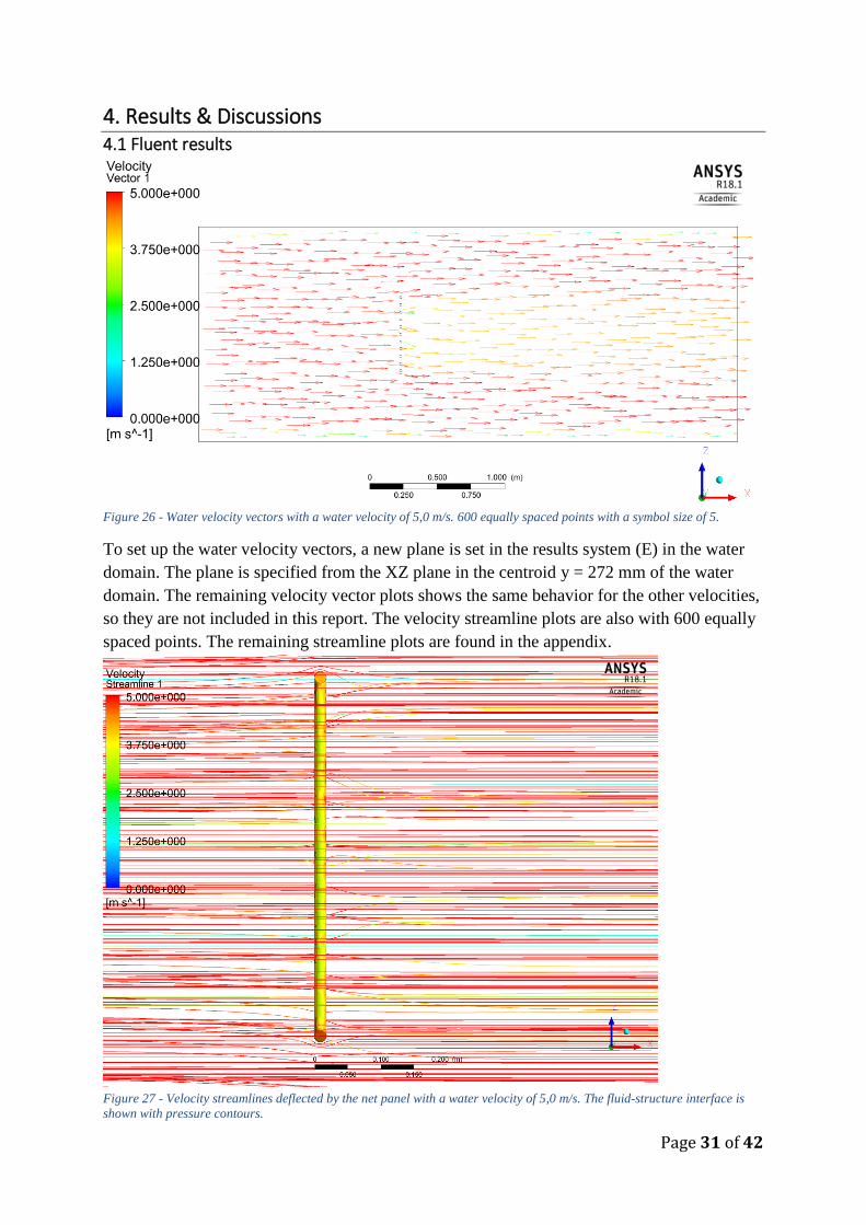
Page 31 of 42
4. Results & Discussions 4.1 Fluent results
Figure 26 - Water velocity vectors with a water velocity of 5,0 m/s. 600 equally spaced points with a symbol size of 5.
To set up the water velocity vectors, a new plane is set in the results system (E) in the water
domain. The plane is specified from the XZ plane in the centroid y = 272 mm of the water
domain. The remaining velocity vector plots shows the same behavior for the other velocities,
so they are not included in this report. The velocity streamline plots are also with 600 equally
spaced points. The remaining streamline plots are found in the appendix.
Figure 27 - Velocity streamlines deflected by the net panel with a water velocity of 5,0 m/s. The fluid-structure interface is
shown with pressure contours.

Page 32 of 42
4.2 Total deformation of the net panel
Figure 28 - Total deformation of the unreinforced Nylon PA6 net panel with a water velocity of 5,0 m/s (true scale).
The table below shows the maximum total deformation of the net panel with different
materials, at each of the velocities:
Max. total
deformation [mm]
Velocities
0,1 m/s 0,5 m/s 1,0 m/s 2,0 m/s 5,0 m/s
Nylon PA6
unreinforced
0,059388 1,0576 3,8757 15,053 86,326
Nylon PA6
reinforced
0,016781 0,29876 1,0912 4,2364 26,085
PET-wire 0,014903 0,26529 0,96898 3,7633 23,212
Polyurethane 0,052694 0,93837 3,441 13,38 77,452 Table 5 - Maximum total deformation of the net panel.
Note that: “A good water exchange will occur with a water velocity above 0.1 m/s. This is
normally sufficient to supply enough oxygen and to remove fish excrement. However, the
water currents should be below 1 m/s because velocities above this will result in very large
forces on the cage structure and mooring system; in these situations, specially designed
systems must be used.” [7] p.250.
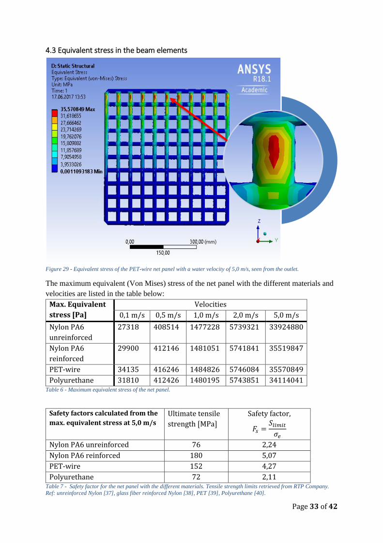
Page 33 of 42
4.3 Equivalent stress in the beam elements
Figure 29 - Equivalent stress of the PET-wire net panel with a water velocity of 5,0 m/s, seen from the outlet.
The maximum equivalent (Von Mises) stress of the net panel with the different materials and
velocities are listed in the table below:
Max. Equivalent
stress [Pa]
Velocities
0,1 m/s 0,5 m/s 1,0 m/s 2,0 m/s 5,0 m/s
Nylon PA6
unreinforced
27318 408514 1477228 5739321 33924880
Nylon PA6
reinforced
29900 412146 1481051 5741841 35519847
PET-wire 34135 416246 1484826 5746084 35570849
Polyurethane 31810 412426 1480195 5743851 34114041 Table 6 - Maximum equivalent stress of the net panel.
Safety factors calculated from the
max. equivalent stress at 5,0 m/s
Ultimate tensile
strength [MPa]
Safety factor,
𝐹𝑠 =𝑆𝑙𝑖𝑚𝑖𝑡
𝜎𝑒
Nylon PA6 unreinforced 76 2,24
Nylon PA6 reinforced 180 5,07
PET-wire 152 4,27
Polyurethane 72 2,11 Table 7 - Safety factor for the net panel with the different materials. Tensile strength limits retrieved from RTP Company.
Ref: unreinforced Nylon [37], glass fiber reinforced Nylon [38], PET [39], Polyurethane [40].
.

Page 34 of 42
4.4 Discussion
The water velocity would not be as linear as we have seen on the velocity streamlines in this
study. In reality, components such as “tidewater current, wind-induced surface current,
outbreak from the coastal current and spring flood because of snow and ice melting” [40]
p.21. would contribute to the total current overview. The angle of attack of the water would
most likely not be set perpendicular to the net panel. The fixed supports that holds the top
faces in a fixed position during loading would also be able to move a bit in a real situation.
These are all factors that could change how the deformation of the net looks like if we were to
install it in a fish farm.
Judging by the results of this study, all the materials could be used for net cages. As
mentioned in the introduction, fish welfare depends on a certain minimum volume within the
net cage. For the more remote areas with higher velocities, the stronger materials like
reinforced nylon PA6 and PET-wire would enable the net to better maintain its shape.
According to the Norwegian Standards NS9415, the breaking strength of the net pens below
surface must not fall below 65% of the initial strength of the net. In areas where there are less
environmental loads in form of currents and waves, economic analyses should be performed
to see what material is the most reasonable by considering the material costs and the total life
span of the nets.
The materials must also be analyzed for toxicity. The toxicity affects both the fish welfare as
well as the marine ecosystem. Finally, the problems I faced by importing the pressure could
possibly be solved with an update to the ANSYS simulation program. There may be a bug in
the system as I’ve used the same method for the circular cages and the net panels, while the
import only worked for the net panels.
Page 35 of 42
5. Conclusions The following conclusions can be drawn from this study:
• Reinforced nylon PA6 and PET-wire have proven to be the strongest materials. In
exposed areas with larger forces on the cage structure, you would benefit from
choosing one of the two.
• I recommend further analyses of the SK one component polyurea from China Institute
of Water Resources & Hydropower Research in Beijing for use in less exposed areas.
The material has shown good qualities for aquaculture purposes compared with the
untreated Nylon PA6, which is commonly used for net cages. However, cost to benefit
analysis is required.
• Companies that supply net cage systems to the aquaculture industry do not openly
share information about the material properties used in the net cages. So, the material
properties used in this study may only be used as a guideline for how the different
materials behaves when the fluid flow exerts the hydrodynamic forces on the net.
5.1 Future work
After the completion of my master’s thesis, the following ideas could be initiated based on
this study:
• Develop a method for a non-linear FSI analysis of net cages, using non-linear material
properties. Possibly with the floating collar and bottom ring/sinker tube installed.
• Perform new analyses in co-operation with one of the suppliers of aquaculture
technology with the material properties used in the industry and to test prototypes.
Another possibility is to buy some material samples and analyze the material
properties, as well as to perform a Xenon lamp aging test to see the elongation at break
and time duration of the materials.
• Perform a mooring analysis with AquaSim (FEA) simulations to determine the
environmental loads the mooring system are exposed to, in compliance with the
Norwegian Standard NS9415.
Page 36 of 42
References
1. SHARCNET:www.sharcnet.ca. 12.4.3 Realizable k-epsilon Model. FLUENT 6.3 User's Guide 2006; Available from: https://www.sharcnet.ca/Software/Fluent6/html/ug/node480.htm.
2. Norge, S. Fishing nets. Netting. Basic terms and definitions. NS-EN ISO 1107 2003. 3. Norge, S., Marine fish farms. Requirements for site survey, risk analyses, design,
dimensioning, production, installation and operation., in Planning and production of main components: General. 2009, Standard Norge: standard.no. p. 33.
4. kikkonet.com. Net Rolls & Panels. 2016 [cited 2016 December 3]; Available from: http://www.kikkonet.com/net_rolls.php.
5. Norge, S., Marine fish farms. Requirements for site survey, risk analyses, design, dimensioning, production, installation and operation., in Use of environmental parameters. 2009, Standard Norge: standard.no. p. 45.
6. www.seatemperature.org. Tromsø average March sea temperature. 2017; Available from: https://www.seatemperature.org/europe/norway/tromso-march.htm.
7. Lekang, O., Aquaculture Engineering, Second Edition. 2013: John Wiley & Sons, Ltd. 8. Moe-Føre, H., et al. Structural response of high solidity net cage models in uniform
flow. Journal of Fluids and Structures, 65 2016; 180-195]. Available from: http://www.sciencedirect.com/science/article/pii/S0889974616303279.
9. Moe, H., A. Fredheim, and O.S. Hopperstad. Structural analysis of aquaculture net cages in current. Journal of Fluids and Structures, 26(3) 2010; 503-516]. Available from: http://www.sciencedirect.com/science/article/pii/S0889974610000289.
10. Maccaferri. Aquaculture Nets/Cages. 2016; Available from: http://www.maccaferri.com/applications/aquaculture-netscages/.
11. AkvaGroup. Cage Farming Aquaculture. 2016; Available from: http://www.akvagroup.com/Downloads/Cage%20farming%20%20EN.pdf.
12. I.J. Aarhus, e.a., Kartlegging av ulike teknologiske løsninger for å møte de miljømessige utfordringene i havbruksnæringen. 2011, SINTEF.
13. AkvaGroup. Cage Farming Aquaculture. 2015; Available from: http://www.akvagroup.com/downloads/cat_%20cage%20-%20engelsk%203_7.pdf.
14. T. Thorvaldsen, e.a., The escape of fish from Norwegian fish farms: Causes, risks and the influence of organisational aspects, in Marine Policy. 2015, Elsevier.
15. Zhiheng, S. The SK one component polyurea and its application in hydraulic and hydropower project structures. Available from: China Institute of Water Resources & Hydropower Research Beijing IWHR-KHL Co., Ltd.
16. Company, R. RTP 1205 S-65D - Ester-based Thermoplastic Polyurethane Elastomer (TPUR/TPU) - Glass Fiber. 2007; Available from: http://web.rtpcompany.com/info/data/1200S/RTP1205S-65D.htm.
17. I. Tsukrov, e.a. Finite element modeling of net panels using a consistent net element. Ocean Engineering, 30(2) 2003 [cited 251-271; Available from: https://www.researchgate.net/publication/223240933_Finite_element_modeling_of_net_panel_using_a_consistent_net_element.
18. Perng, Y.-Y., Modeling Fluid Structure Interactions. 2011, ANSYS, Inc. 19. ANSYS, I. ANSYS Mechanical User's Guide. 2013; Available from:
http://148.204.81.206/Ansys/150/ANSYS%20Mechanical%20Users%20Guide.pdf.

Page 37 of 42
20. Casanova, C. and W. Dwikartika. Modeling of Aquaculture PET Net with the Use of Finite Element Method. 2013; Available from: https://brage.bibsys.no/xmlui/bitstream/handle/11250/238738/653349_FULLTEXT01.pdf?sequence=3&isAllowed=y.
21. Invent, S.B.A. Strength of Materials: Axial Loading. 2016 December 15; Available from: http://engineering-references.sbainvent.com/strength_of_materials/axial-loading.php#.WFMAR_nhDyQ.
22. Edge, E. Shear Stress Equations and Applications. 2016 December 15; Available from: http://www.engineersedge.com/material_science/shear-stress.htm.
23. Hall, N. Navier-Stokes Equations - 3-dimensional-unsteady. 2015; Available from: https://www.grc.nasa.gov/WWW/k-12/airplane/nseqs.html.
24. Anderson, J.D., Computional fluid dynamics - The Basics with Applications. 1995: McGraw-Hill, Inc. 547.
25. ANSYS, I. 4.3.3.2. Transport equations for the realizable k-ε equation. Theory Guide 4.3.3. Realizable k-ε Model Release 18.1; Available from: https://ansyshelp.ansys.com.
26. Zhao, Y.-P., et al. Numerical simulation of the flow around fishing plane nets using the porous media model. Ocean Engineering 2013 [cited 62; 25-37]. Available from: http://www.sciencedirect.com/science/article/pii/S0029801813000243.
27. Potyagaylo, S. and S.G. Loizou. Online Adaptive Geometry Predictor of Aquaculture Fish-Nets. 2014; Available from: http://ieeexplore.ieee.org/stamp/stamp.jsp?arnumber=6961505.
28. myn3wname(YouTube). 3ds max: Mesh modeling tutorial. 2009 [cited 2016 December 3]; Available from: https://www.youtube.com/watch?v=aS5Axs3-RjM.
29. Lee, H.-H. Finite Element Simulations with ANSYS Workbench 16 Chapter 1: Introduction 2016; Available from:
http://myweb.ncku.edu.tw/~hhlee/Myweb_at_NCKU/ANSYS16.html. 30. W. Dwikartika, C.C., in Modeling of Aquaculture PET Net with the Use of Finite
Element Method. 2013. 31. professionalplastics.com. Mechanical Properties of Plastic Materials. 2017; Available
from: http://www.professionalplastics.com/professionalplastics/MechanicalPropertiesofPlastics.pdf.
32. goodfellow.com. Polyamide - Nylon 6 (PA 6) - Material Information. 2017; Available from: http://www.goodfellow.com/E/Polyamide-Nylon-6.html.
33. ANSYS, I. 28.3.1.1. SIMPLE vs. SIMPLEC. Fluent 28.3.1. Choosing the Pressure-Velocity Coupling Method Release 18.1; Available from: https://ansyshelp.ansys.com.
34. Harboe, T. and O.F. Skulstad. Maskeåpning, rømningsfare og fiskevelferd. 2014; Available from: https://www.imr.no/filarkiv/2014/03/maskeapning_romningsfare_og_fiskevelferd.pdf/nb-no.
35. SHARCNET:www.sharcnet.ca. 25.1.1 Pressure-Based Solver. FLUENT 6.3 User's Guide 2006; Available from: https://www.sharcnet.ca/Software/Fluent6/html/ug/node987.htm.
36. SHARCNET:www.sharcnet.ca. 21.4.3. Pressure-Velocity Coupling. Release 17.0 [cited 2017 June 4]; Available from: https://www.sharcnet.ca/Software/Ansys/17.0/en-us/help/flu_th/flu_th_sec_uns_solve_pv.html.
Page 38 of 42
37. SHARCNET:www.sharcnet.ca. 25.9.2 Setting Under-Relaxation Factors. FLUENT 6.3 User's Guide 2006; Available from: https://www.sharcnet.ca/Software/Fluent6/html/ug/node1022.htm.
38. Moe, H. Strength analysis of net structures. Doktoravhandlinger ved NTNU, 1503-8181; 2009:48 2009; Available from: http://hdl.handle.net/11250/236414.
39. ANSYS, I. The Deformation is Large Compared to the Model Bounding Box. Mechanical User's Guide - Troubleshooting v.18.1; Available from: https://ansyshelp.ansys.com.
40. Norge, S., Marine fish farms. Requirements for site survey, risk analyses, design, dimensioning, production, installation and operation., in Site surveys: General. 2009, Standard Norge: standard.no. p. 21.

Page 39 of 42
Appendix
Figure 30 - Imported pressure with a water velocity of 0,1 m/s, seen from the outlet.
Figure 31 - Imported pressure with a water velocity of 0,5 m/s, seen from the outlet.

Page 40 of 42
Figure 32 - Imported pressure with a water velocity of 1,0 m/s, seen from the outlet.
Figure 33 - Imported pressure with a water velocity of 2,0 m/s, seen from the outlet.

Page 41 of 42
Figure 34 - Velocity streamlines with a velocity of 0,1 m/s.
Figure 35 - Velocity streamlines with a velocity of 0,5 m/s.

Page 42 of 42
Figure 36 - Velocity streamlines with a velocity of 1,0 m/s.
Figure 37 - Velocity streamlines with a velocity of 2,0 m/s.