Study 2 – Relative Performance of Surface-Deployed and Bottom-Mounted Echosounders in a Tidal Channel

FINAL REPORT Project number: SDP 200-207 Start date: November 1, 2019 Reporting period: November 1, 2019 – December 31, 2020 Recipient name: Fundy Ocean Research Center for Energy Project lead: Daniel J. Hasselman Prepared by Daniel J. Hasselman Dan Hasselman1*, Louise McGarry2, Tyler Boucher1, Jessica Douglas1 and Shannon MacNeil1 1Fundy Ocean Research Center for Energy, Halifax, NS *Corresponding author: dan.hasselman@fundyforce.ca Submission Date: December 31, 2020 Revision Date: March 19, 2021

1

Table of Contents

1 Executive Summary ............................................................................................................ 2

2 Introduction and Objectives ............................................................................................... 6

3 Methodology ..................................................................................................................... 9

3.1 Tidal Flow Rate Data ............................................................................................................ 10

3.2 Study 2A – WBAT and optical camera .................................................................................. 12

3.3 Study 2B – WBAT, optical camera, and multibeam imaging sonar ........................................ 15

3.4 Study 2C – WBAT and EK80 .................................................................................................. 18

3.5 Data Analysis ....................................................................................................................... 21

3.6 Notes on Setting Minimum and Maximum Sv Thresholds for Fish ........................................ 24

4 Results and Discussion ..................................................................................................... 25

4.1 Study 2A – WBAT and optical camera .................................................................................. 25

4.2 Study 2B – WBAT, optical camera, and multibeam imaging sonar ........................................ 27

4.3 Study 2C – WBAT and EK80 .................................................................................................. 31

4.4 Findings Specific to PLAT-I Rotor Swept Depth – Across All Three Studies ............................ 42

5 Conclusions ...................................................................................................................... 45

6 References ....................................................................................................................... 46

Appendix A. Envirosphere Consultants Limited: Review of Underwater Video ..................... 49

Appendix B. Study Period Post-Processed Echogram Images ................................................63

Appendix C. Future Considerations .......................................................................................66

2

1 Executive Summary Motivation Scientific echosounders are the standard tool in fisheries science for investigating the abundance, distribution, behavior, and ecology of fish, and have been used for monitoring around tidal energy devices. Echosounders have been deployed on the sea floor in a stationary upward-facing orientation for monitoring around gravity-based tidal energy devices but have also been deployed at the sea surface in a downward-facing orientation, either for mobile surveys or on ships at anchor. The advent of floating tidal energy platforms provides an opportunity to deploy echosounders at the sea surface in a long-term, stationary, downward-facing orientation for monitoring. However, the strong currents that make tidal channels attractive for energy production are often dominated by turbulent hydrodynamic features and associated artefacts that can vary over the course of tidal cycles and may hinder the use of echosounders and other active acoustic technologies. Understanding the extent to which turbulent hydrodynamic features impact the use of a bottom-mounted or surface-deployed echosounder is important for designing effective monitoring systems. In partnership with the Pathway Program, Sustainable Marine Energy (Canada) Ltd. and the Fundy Ocean Research Center for Energy, undertook a series of studies to understand whether deployment location impacted the efficacy of echosounder technology for monitoring by assessing the relative performance of surface-deployed instruments and a bottom-mounted echosounder. The bottom-mounted echosounder was the Simrad Wideband Autonomous Transceiver (WBAT: from the Simrad EK80 suite of echosounders) mounted on the Fundy Advanced Sensory Technology (FAST) autonomous underwater platform and deployed in Grand Passage, NS in the vicinity of the Sustainable Marine floating tidal energy platform (i.e., PLAT-I). The surface-deployed instruments were deployed via pole mount attached to the leading edge of the starboard pontoon of the PLAT-I platform and included a Sculpin HDC-SubC optical video camera, a Gemini 720is multibeam imaging sonar, and a downward-facing Simrad Wideband Transceiver (WBT: from the Simrad EK80 suite of echosounders). The primary goal was to collect data to compare target detections for identifying the best placement of echosounders for monitoring in the vicinity of the PLAT-I deployed in a high flow environment. Thus, the objectives of the three studies were to i) investigate the near-surface target detection capabilities of a bottom-mounted, upward-facing, echosounder using a surface-deployed optical video camera (Study 2A), ii) address this same objective over a greater detection range using a multibeam imaging sonar (Study 2B), and iii) investigate the relative performance of a bottom-mounted upward-facing, and a surface-deployed downward-facing echosounder for target detection (Study 2C). This final goal was addressed by identifying the extent of target detection interference due to air entrained in the water by surface waves and turbulence. The PLAT-I rotors were parked during data collection for all three studies. Because of safety concerns for personnel, the PLAT-I and instruments, the FAST platform was deployed at locations in the vicinity of the PLAT-I, but at distances that precluded the possibility of

3

overlapping sampling volumes between the instruments mounted on the PLAT-I and the FAST platform. Summary of Findings No fish images were captured in the 170 hours of optical video data examined for Study 2A and Study 2B. This result was unexpected given that during Study 2A, within the water depths interrogated by the optical camera, the upward-facing echosounder recorded signals consistent with the presence of fish in 55% of the 8.3 hours of echosounder data not obfuscated by entrained air. The images captured by the video camera were of sufficiently high-resolution that the absence of fish likely reflected a lack of fish passing within the camera’s field-of-view. Although the optical video data could not be used to cross-reference targets detected by the echosounder, the echosounder data collected during Study 2A contributed to our understanding of the importance of localized hydrodynamic regimes on the ability to collect useable data. For Study 2B, the image resolution of the imaging sonar was insufficient to identify targets beyond two ambiguous categories: “single fish/debris” and “turbulence/fish/school of fish”. A third category denoted instances when the PLAT-I mooring chain was within the imaging sonar field-of-view. During this study, in nominally 100% of the echosounder observation time periods, signals that could be interpreted as fish were detected at depths that coincided with the depth range interrogated by the imaging sonar (i.e., the top 11 m of the water column). However, the imaging sonar identified potential detections for only 22% of the observation periods. The source of this discrepancy likely stems from non-overlapping sample volumes due to FAST platform deployment location for this study. Although the lack of overlapping sample volumes precluded definitive cross-referencing between the two instruments, optical cameras and imaging sonars have been shown to be valuable monitoring tools elsewhere and have value for monitoring in Grand Passage. As with Study 2A, the echosounder data collected during Study 2B contributed to our understanding of the importance of localized hydrodynamics for the collection of useable data. Analyses of signal interference due to entrained air (Study 2C) suggested a strong difference in the hydrodynamic regimes at the deployment locations of the PLAT-I and the FAST platform with consequences for the proportion of useable data at each site. Signal interference manifested in several ways: i) the presence (PLAT-I site) or absence (FAST site) of a pronounced tide-phase asymmetry in the proportion of data excluded from analyses (due to the persistence and depth penetration of entrained air), ii) the presence (PLAT-I site: flood) or absence (PLAT-I: ebb, FAST site: flood and ebb) of a pronounced negative relationship between flow-speed and the proportion of useable data, and iii) the presence (FAST site) or absence (PLAT-I site) of a reduction in the proportion of useable observation periods with increasingly restrictive minimum acceptable proportions of useable water column. The pronounced tide-phase asymmetry at the PLAT-I site appears to be a consequence of its deployment location downstream from Peter’s Island on the flood tide (upstream on the ebb tide). Consequently, the PLAT-I was deployed within the turbulent field generated by the interaction of the flood-tide with Peter’s Island and its associated bathymetry. The turbulence

4

and associated entrained air had significant consequences for the collection of useable data on the flood tide, reducing the useable proportion of 10-minute observation periods to ≤ 30% on the flood tide; the proportion of useable observation periods on the ebb tide ranged from 85-95%. Going forward, this pronounced asymmetry indicates that useable data collected on the flood tide will be minimal at the current PLAT-I deployment location and will have important consequences for understanding the risk to fish during the flood tide phase. Although comparative echosounder data were not available for Study 2A or Study 2B, analyses of the proportion of “useable” data collected at the FAST deployment sites for all three studies support the hypothesis that bathymetry associated with Peter’s Island creates a pronounced difference in the hydrodynamic regimes associated with the flood and ebb tides at the PLAT-I site and nearby locales (Study 2A and 2B). During Study 2C, the FAST platform was deployed just outside the direct downstream flow associated with Peter’s Island and the echosounder data showed little tide-phase asymmetry but did reveal a deterioration in the proportion of useable observation periods on both the flood and ebb tide when increasing the minimum proportion of the water column deemed as “useable”. While the lack of a pronounced asymmetry for the FAST site in Study 2C indicated that more data was useable on the flood tide relative to the echosounder placed at the PLAT-I, it should be noted that on the ebb tide, the PLAT-I site had more “useable” data as highlighted above. Analysis of the useable proportion of individual observations (pings) within 1-m depth bins in the depths-of-interest for the PLAT-I (i.e., 1-8 m depth) revealed the same pattern found in the data analyzed across the entire water column for the presence (FAST site: Study 2A and 2B; PLAT-I site: Study 2C) or absence (FAST site: Study 2C) of tide-phase asymmetry. Given that the echosounders used here were from the same Simrad EK80 suite of echosounders and deployed with identical data collection parameters, the ability to detect or define the boundary of entrained air was not affected by which echosounder was used. Nor was it affected by deployment at the sea surface in a downward-facing orientation, or on the sea floor in an upward-facing orientation. The sea surface vs. sea floor positioning of the echosounders does, however, have important data collection and analytical consequences that must be considered. The ensonification beam emitted by a transducer is cone-shaped with the apex at the transducer and the diameter of the cone increasing with distance. It follows then that the region closest to the transducer will result in a highly restricted sampling volume and leave substantial proportions of water unsampled. Therefore, to maximize the volume of sampled water, the transducer should be placed furthest from the region of interest. As with the considerations of the hydrodynamic regime when selecting a deployment location, one must also consider the consequences in the vertical dimension. If the entrained air so common to tidal energy sites is between the transducer and the target of interest, the acoustic beam will be scattered before encountering the target and will compromise the collection of quantitative data for estimating density and abundance.

5

Major Take-Aways These studies demonstrate the importance of the influence of hydrodynamics on the ability to collect useable quantitative data required for analyses and reporting on fish abundance and distribution. Deployment location of an echosounder can have a profound impact on the ability to monitor throughout the tidal cycle, such that the hydrodynamic regime will influence when and where you can observe. To obtain quantifiable and comparable data on targets of interest, the echosounder must be deployed such that the acoustic beam encounters the targets before encountering entrained air. Additionally, to maximize the sampling volume, and thereby the likelihood of a fish encountering the acoustic beam, the echosounder should be deployed furthest from the region of interest. Topics for Continued Research Because of the fast-flowing and turbulent waters found in tidal streams, the in situ sampling (e.g., via net tows/trawl surveys) of acoustic targets (fish) commonly done in open waters is not possible in tidal streams. Therefore, ground-truthing the identity and size of acoustic targets observed in tidal streams remains an unresolved and ongoing topic of research in the hydroacoustics community. The presence of entrained air makes monitoring fish in tidal channels particularly problematic. Currently, there is no proven strategy to observe fish with sufficient field-of-view or resolution within a highly turbulent environment. Without the ability to observe fish throughout the entire tidal cycle, quantifying risks of turbines to fish will remain difficult. Therefore, to understand potential risks, it is important to continue to focus on developing methods to detect and observe fish, or establish means by which to infer fish presence and behavior, within turbulent tidal channels.

6

2 Introduction and Objectives Scientific echosounders are the standard tool in fisheries science for quantifying the abundance and distribution of fish, and for investigating fish behaviour and ecology (Fernandes et al. 2002). They are also valuable for monitoring interactions of fish with instream tidal energy turbines. However, monitoring in tidal channels using echosounders has its own inherent challenges, as the high-flow regimes that make tidal channels desirable for tidal power development are often characterized by complex and turbulent hydrodynamic features that can entrain significant amounts of air in the water column affecting their efficacy for monitoring. Echosounders function by listening for echo returns from interfaces with densities that differ from seawater. Because the density of entrained air differs from the surrounding seawater, it returns echoes that interfere with the ability to identify those that are returned from fish and challenges the ability to collect quantitative data about fish abundance and distribution and undermining efforts to effectively monitor around tidal energy devices. When used for monitoring around tidal energy turbines, echosounders have most often been deployed on the sea floor (either mounted on an autonomous or cabled subsea platform or integrated into the device substructure) with their ensonification cone oriented upwards for monitoring around gravity-based tidal energy turbines (Williamson et al., 2016a, 2017; Fraser et al., 2017). However, deploying and recovering bottom-mounted instruments involves considerable costs (e.g., specialized vessels and complex marine operations) and risks for monitoring (e.g., instrument malfunction and/or loss of data, loss of the instrument itself). The advent of floating tidal energy platforms provides logistical advantages (e.g., easy access to instruments and monitoring data) that can offset some of these risks, and affords new opportunities for monitoring from the surface using echosounders in a downward-facing orientation. However, the applicability of this configuration, or the more conventional bottom-mounted upward-facing orientation, for monitoring around floating tidal energy platforms have yet to be assessed. Sustainable Marine Energy (Canada) Ltd. (hereafter Sustainable Marine) operates a floating tidal energy platform (i.e., “PLAT-I”: PLATform for Inshore energy) at its tidal energy demonstration site in Grand Passage, Nova Scotia (Figure 2.1 and Figure 2.2), and conducts a series of monitoring activities using instruments deployed from the sea surface. As such, PLAT-I provides an excellent opportunity to conduct an in situ assessment of the performance of a bottom-mounted upward-facing echosounder for monitoring near-surface waters by comparison with data collected using surface-deployed instruments, including a downward-facing echosounder. Such an assessment is within the scope of the Pathway Program1 – a collaborative effort between the Offshore Energy Research Association (OERA) and the Fundy Ocean Research Center for Energy (FORCE) – to establish a regulator-approved monitoring solution that can be used by tidal energy developers for monitoring the near-field (0 - 100 m) region of their tidal energy device at the FORCE demonstration site.

1 https://oera.ca/research/pathway-program-towards-regulatory-certainty-instream-tidal-energy-projects

7

In partnership with the Pathway Program, Sustainable Marine undertook a project in Grand Passage to investigate target detection capabilities using a bottom-mounted echosounder, and to investigate the relative performance of echosounders deployed on sea floor and at the sea surface. The objectives of the project were to i) investigate the near-surface target detection capabilities of a bottom-mounted upward-facing echosounder using a surface-deployed optical video camera (Study 2A), ii) address the same objective as (i) but over a greater detection range using a multibeam imaging sonar (Study 2B), and iii) investigate the relative performance of a bottom-mounted upward-facing, and a surface-deployed downward-facing echosounder for target detection, and identify the extent of interference due to air entrained from surface waves and turbulence (Study 2C). These studies were designed to assess the efficacy of bottom-mounted and surface-deployed echosounders for target detections and to help guide best practices for monitoring in high flow environments. These studies were not intended to address interactions of fish with tidal turbines and were therefore not designed to assess likelihood of harm to fish from encountering a tidal device, nor to assess avoidance behaviour. Similarly, these studies were not intended to generate data that could be used to quantify fish abundance, distribution or behaviour around tidal energy turbines. While the results of this project are intended to assist in identifying the best placement of echosounders for monitoring fish around tidal turbines in high flow environments, readers should consider these studies as ‘proof of concept’ only given the experimental nature of this work.

8

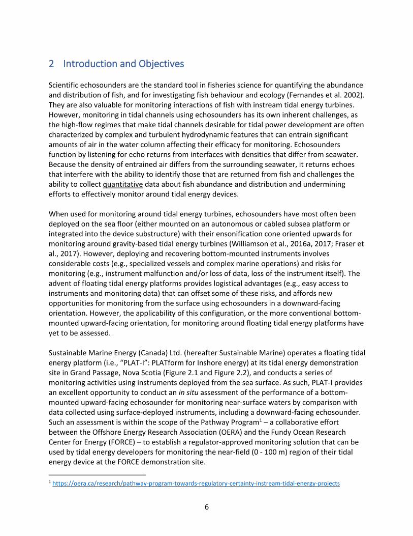
Figure 2.1: Sustainable Marine PLAT-I Platform deployed in Grand Passage.

PLAT-I 4.63 DIMENSIONS (mm)

PLAT-I 4.63 MOORING CONFIGURATION

TOP VIEW

STARBOARD VIEW STERN VIEW

9

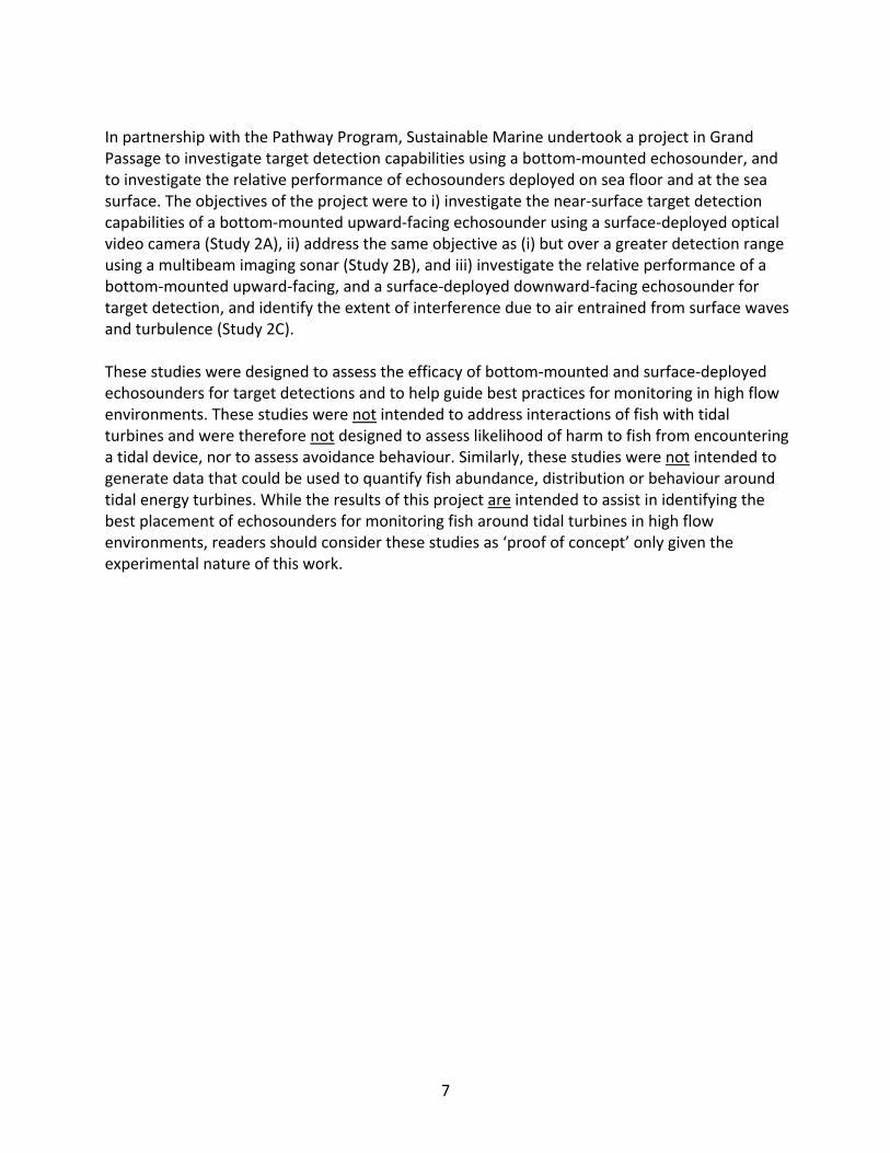
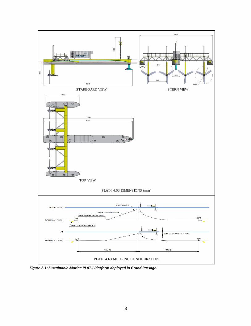
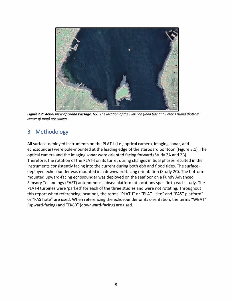
Figure 2.2: Aerial view of Grand Passage, NS. The location of the Plat-I on flood tide and Peter’s Island (bottom center of map) are shown.

3 Methodology All surface-deployed instruments on the PLAT-I (i.e., optical camera, imaging sonar, and echosounder) were pole-mounted at the leading edge of the starboard pontoon (Figure 3.1). The optical camera and the imaging sonar were oriented facing forward (Study 2A and 2B). Therefore, the rotation of the PLAT-I on its turret during changes in tidal phases resulted in the instruments consistently facing into the current during both ebb and flood tides. The surface-deployed echosounder was mounted in a downward-facing orientation (Study 2C). The bottom-mounted upward-facing echosounder was deployed on the seafloor on a Fundy Advanced Sensory Technology (FAST) autonomous subsea platform at locations specific to each study. The PLAT-I turbines were ‘parked’ for each of the three studies and were not rotating. Throughout this report when referencing locations, the terms “PLAT-I” or “PLAT-I site” and “FAST platform” or “FAST site” are used. When referencing the echosounder or its orientation, the terms “WBAT” (upward-facing) and “EK80” (downward-facing) are used.

10

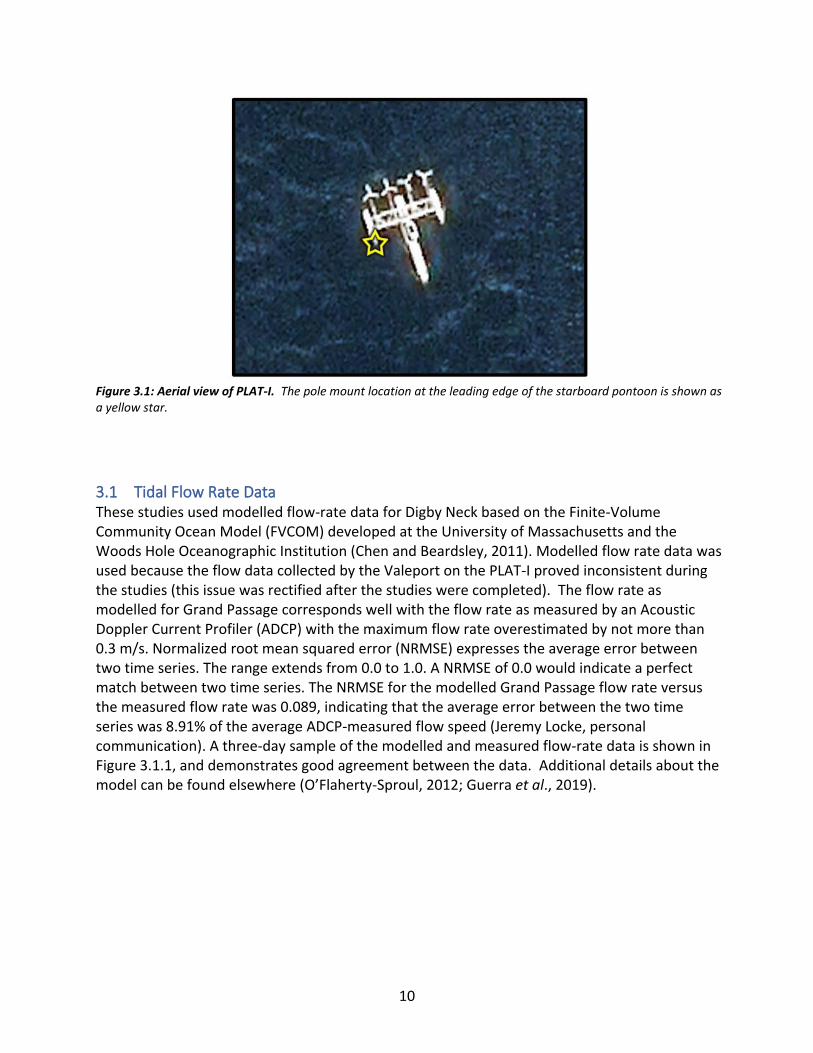
Figure 3.1: Aerial view of PLAT-I. The pole mount location at the leading edge of the starboard pontoon is shown as a yellow star.

3.1 Tidal Flow Rate Data These studies used modelled flow-rate data for Digby Neck based on the Finite-Volume Community Ocean Model (FVCOM) developed at the University of Massachusetts and the Woods Hole Oceanographic Institution (Chen and Beardsley, 2011). Modelled flow rate data was used because the flow data collected by the Valeport on the PLAT-I proved inconsistent during the studies (this issue was rectified after the studies were completed). The flow rate as modelled for Grand Passage corresponds well with the flow rate as measured by an Acoustic Doppler Current Profiler (ADCP) with the maximum flow rate overestimated by not more than 0.3 m/s. Normalized root mean squared error (NRMSE) expresses the average error between two time series. The range extends from 0.0 to 1.0. A NRMSE of 0.0 would indicate a perfect match between two time series. The NRMSE for the modelled Grand Passage flow rate versus the measured flow rate was 0.089, indicating that the average error between the two time series was 8.91% of the average ADCP-measured flow speed (Jeremy Locke, personal communication). A three-day sample of the modelled and measured flow-rate data is shown in Figure 3.1.1, and demonstrates good agreement between the data. Additional details about the model can be found elsewhere (O’Flaherty-Sproul, 2012; Guerra et al., 2019).

11

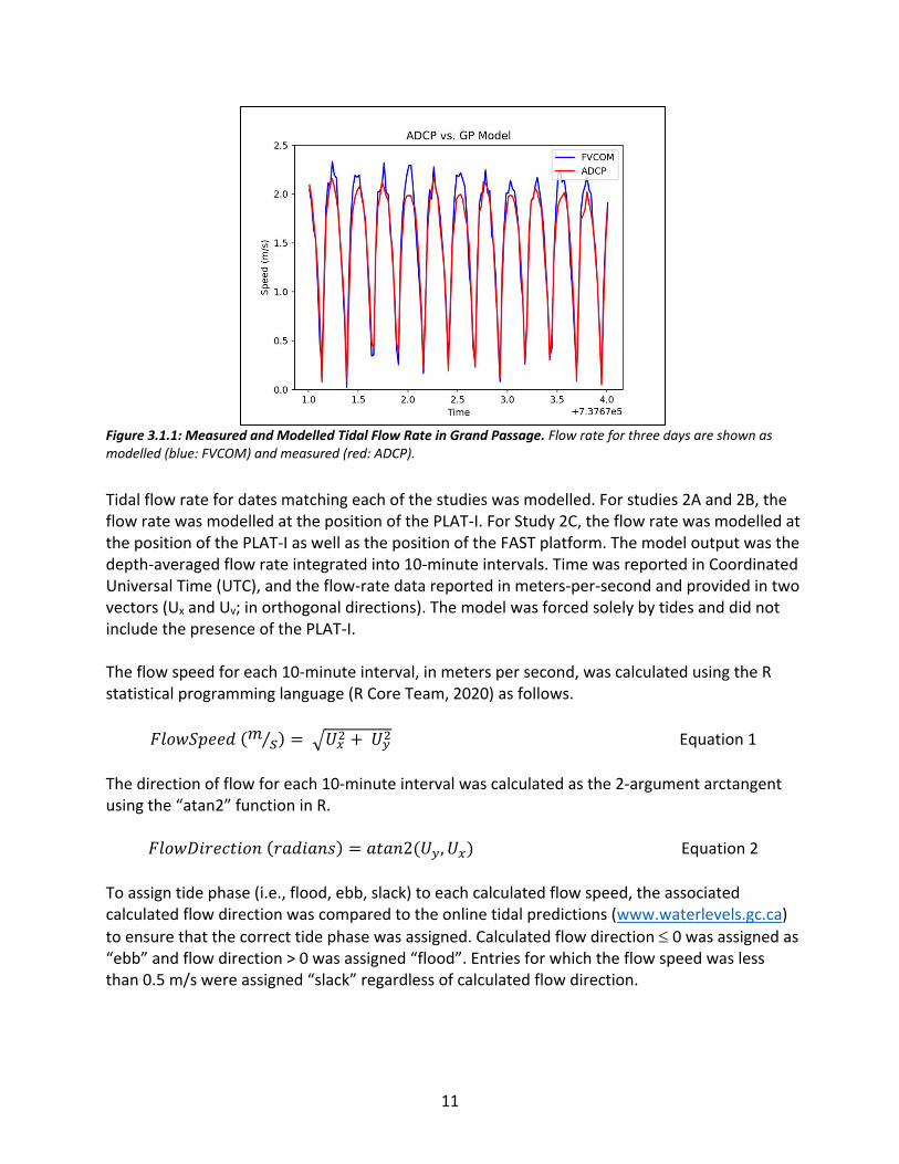
Figure 3.1.1: Measured and Modelled Tidal Flow Rate in Grand Passage. Flow rate for three days are shown as modelled (blue: FVCOM) and measured (red: ADCP).

Tidal flow rate for dates matching each of the studies was modelled. For studies 2A and 2B, the flow rate was modelled at the position of the PLAT-I. For Study 2C, the flow rate was modelled at the position of the PLAT-I as well as the position of the FAST platform. The model output was the depth-averaged flow rate integrated into 10-minute intervals. Time was reported in Coordinated Universal Time (UTC), and the flow-rate data reported in meters-per-second and provided in two vectors (Ux and Uv; in orthogonal directions). The model was forced solely by tides and did not include the presence of the PLAT-I. The flow speed for each 10-minute interval, in meters per second, was calculated using the R statistical programming language (R Core Team, 2020) as follows.

𝐹𝑙𝑜𝑤𝑆𝑝𝑒𝑒𝑑 (𝑚𝑠⁄ ) = √𝑈𝑥

2 + 𝑈𝑦2 Equation 1

The direction of flow for each 10-minute interval was calculated as the 2-argument arctangent using the “atan2” function in R.

𝐹𝑙𝑜𝑤𝐷𝑖𝑟𝑒𝑐𝑡𝑖𝑜𝑛 (𝑟𝑎𝑑𝑖𝑎𝑛𝑠) = 𝑎𝑡𝑎𝑛2(𝑈𝑦, 𝑈𝑥) Equation 2

To assign tide phase (i.e., flood, ebb, slack) to each calculated flow speed, the associated calculated flow direction was compared to the online tidal predictions (www.waterlevels.gc.ca)

to ensure that the correct tide phase was assigned. Calculated flow direction 0 was assigned as “ebb” and flow direction > 0 was assigned “flood”. Entries for which the flow speed was less than 0.5 m/s were assigned “slack” regardless of calculated flow direction.

12

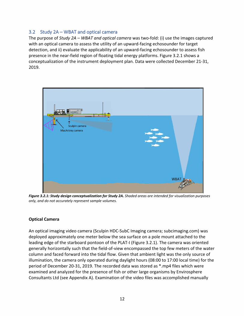
3.2 Study 2A – WBAT and optical camera The purpose of Study 2A – WBAT and optical camera was two-fold: (i) use the images captured with an optical camera to assess the utility of an upward-facing echosounder for target detection, and ii) evaluate the applicability of an upward-facing echosounder to assess fish presence in the near-field region of floating tidal energy platforms. Figure 3.2.1 shows a conceptualization of the instrument deployment plan. Data were collected December 21-31, 2019.

Figure 3.2.1: Study design conceptualization for Study 2A. Shaded areas are intended for visualization purposes only, and do not accurately represent sample volumes.

Optical Camera An optical imaging video camera (Sculpin HDC-SubC Imaging camera; subcimaging.com) was deployed approximately one meter below the sea surface on a pole mount attached to the leading edge of the starboard pontoon of the PLAT-I (Figure 3.2.1). The camera was oriented generally horizontally such that the field-of-view encompassed the top few meters of the water column and faced forward into the tidal flow. Given that ambient light was the only source of illumination, the camera only operated during daylight hours (08:00 to 17:00 local time) for the period of December 20-31, 2019. The recorded data was stored as *.mp4 files which were examined and analyzed for the presence of fish or other large organisms by Envirosphere Consultants Ltd (see Appendix A). Examination of the video files was accomplished manually

13

using VLC media player software (VideoLAN: videolan.org). The results were integrated into 10-minute time bins to match the integration period of the echosounder data. Echosounder Hydroacoustic data were recorded using a Simrad EK80 Wideband Autonomous Transceiver

(WBAT; Kongsberg Maritime, Horten, Norway) operating a 7 split-beam transducer at a frequency of 120 kHz in continuous-wave mode. WBAT data collection settings used at the tidal energy demonstration site in Minas Passage (Viehman et al., 2019) were used here (ping rate: 1 Hz; pulse length: 0.128 ms, power: 125 W). The echosounder was calibrated after the instrument was recovered following the completion of data collection for Study 2A. The resulting calibration parameters were used for all three studies in Grand Passage. The WBAT was mounted to the FAST platform in an upward-facing orientation and deployed on the seafloor approximately 30 m distant from the optical camera on the flood tide (approximately 53 m on the ebb tide as the PLAT-I rotates on its turret; Figure 3.2.2 and Table 3.2.1).

Figure 3.2.2: Deployment location of the WBAT echosounder mounted on the FAST platform, shown for Study 2A relative to the PLAT-I on a flooding tide. Length of yellow line represents the horizontal length from the optical camera deployed at the leading edge of the starboard pontoon to the position of the FAST platform: ~30 m.

14

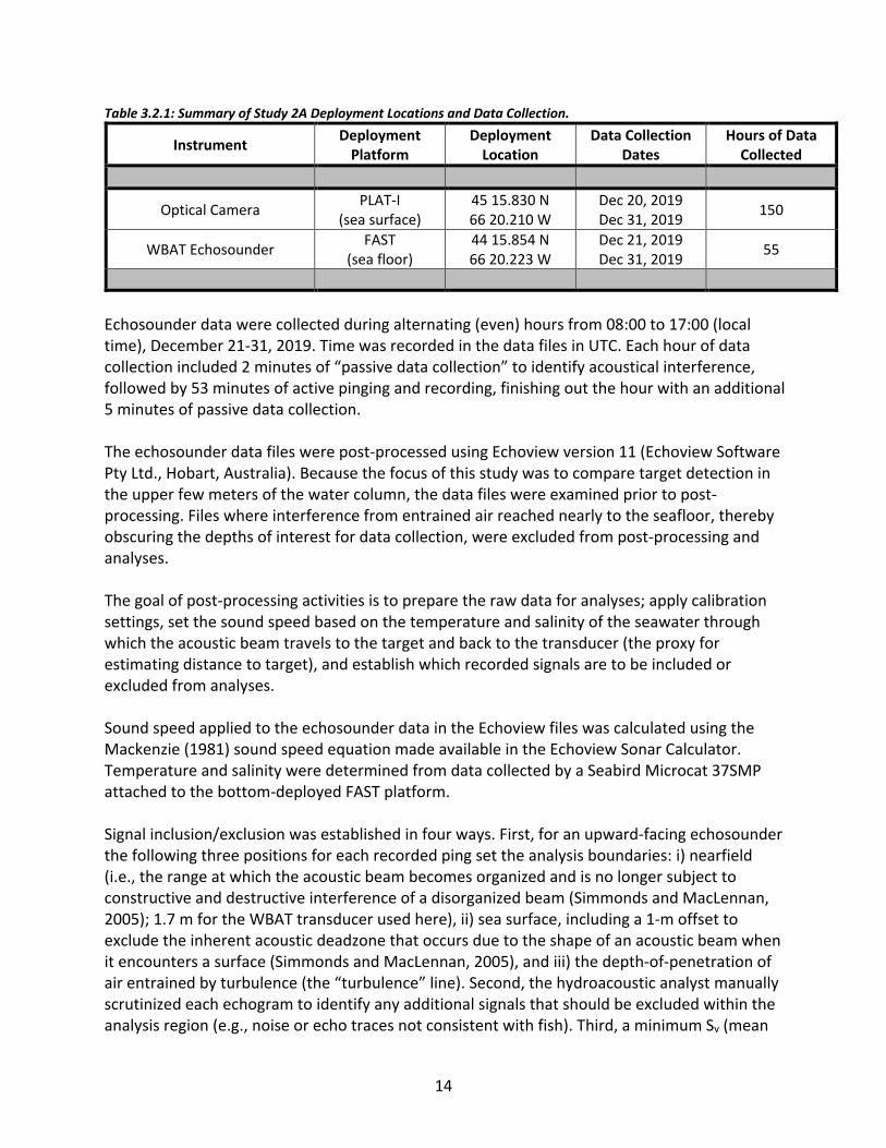
Table 3.2.1: Summary of Study 2A Deployment Locations and Data Collection.

Instrument Deployment

Platform Deployment

Location Data Collection

Dates Hours of Data

Collected

Optical Camera PLAT-I

(sea surface) 45 15.830 N 66 20.210 W

Dec 20, 2019 Dec 31, 2019

150

WBAT Echosounder FAST

(sea floor) 44 15.854 N 66 20.223 W

Dec 21, 2019 Dec 31, 2019

55

Echosounder data were collected during alternating (even) hours from 08:00 to 17:00 (local time), December 21-31, 2019. Time was recorded in the data files in UTC. Each hour of data collection included 2 minutes of “passive data collection” to identify acoustical interference, followed by 53 minutes of active pinging and recording, finishing out the hour with an additional 5 minutes of passive data collection. The echosounder data files were post-processed using Echoview version 11 (Echoview Software Pty Ltd., Hobart, Australia). Because the focus of this study was to compare target detection in the upper few meters of the water column, the data files were examined prior to post-processing. Files where interference from entrained air reached nearly to the seafloor, thereby obscuring the depths of interest for data collection, were excluded from post-processing and analyses. The goal of post-processing activities is to prepare the raw data for analyses; apply calibration settings, set the sound speed based on the temperature and salinity of the seawater through which the acoustic beam travels to the target and back to the transducer (the proxy for estimating distance to target), and establish which recorded signals are to be included or excluded from analyses. Sound speed applied to the echosounder data in the Echoview files was calculated using the Mackenzie (1981) sound speed equation made available in the Echoview Sonar Calculator. Temperature and salinity were determined from data collected by a Seabird Microcat 37SMP attached to the bottom-deployed FAST platform. Signal inclusion/exclusion was established in four ways. First, for an upward-facing echosounder the following three positions for each recorded ping set the analysis boundaries: i) nearfield (i.e., the range at which the acoustic beam becomes organized and is no longer subject to constructive and destructive interference of a disorganized beam (Simmonds and MacLennan, 2005); 1.7 m for the WBAT transducer used here), ii) sea surface, including a 1-m offset to exclude the inherent acoustic deadzone that occurs due to the shape of an acoustic beam when it encounters a surface (Simmonds and MacLennan, 2005), and iii) the depth-of-penetration of air entrained by turbulence (the “turbulence” line). Second, the hydroacoustic analyst manually scrutinized each echogram to identify any additional signals that should be excluded within the analysis region (e.g., noise or echo traces not consistent with fish). Third, a minimum Sv (mean

15

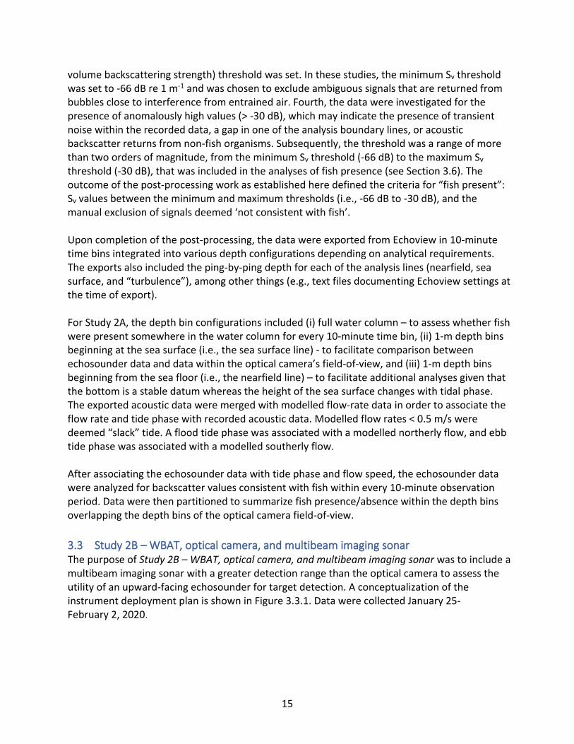
volume backscattering strength) threshold was set. In these studies, the minimum Sv threshold was set to -66 dB re 1 m-1 and was chosen to exclude ambiguous signals that are returned from bubbles close to interference from entrained air. Fourth, the data were investigated for the presence of anomalously high values (> -30 dB), which may indicate the presence of transient noise within the recorded data, a gap in one of the analysis boundary lines, or acoustic backscatter returns from non-fish organisms. Subsequently, the threshold was a range of more than two orders of magnitude, from the minimum Sv threshold (-66 dB) to the maximum Sv threshold (-30 dB), that was included in the analyses of fish presence (see Section 3.6). The outcome of the post-processing work as established here defined the criteria for “fish present”: Sv values between the minimum and maximum thresholds (i.e., -66 dB to -30 dB), and the manual exclusion of signals deemed ‘not consistent with fish’. Upon completion of the post-processing, the data were exported from Echoview in 10-minute time bins integrated into various depth configurations depending on analytical requirements. The exports also included the ping-by-ping depth for each of the analysis lines (nearfield, sea surface, and “turbulence”), among other things (e.g., text files documenting Echoview settings at the time of export). For Study 2A, the depth bin configurations included (i) full water column – to assess whether fish were present somewhere in the water column for every 10-minute time bin, (ii) 1-m depth bins beginning at the sea surface (i.e., the sea surface line) - to facilitate comparison between echosounder data and data within the optical camera’s field-of-view, and (iii) 1-m depth bins beginning from the sea floor (i.e., the nearfield line) – to facilitate additional analyses given that the bottom is a stable datum whereas the height of the sea surface changes with tidal phase. The exported acoustic data were merged with modelled flow-rate data in order to associate the flow rate and tide phase with recorded acoustic data. Modelled flow rates < 0.5 m/s were deemed “slack” tide. A flood tide phase was associated with a modelled northerly flow, and ebb tide phase was associated with a modelled southerly flow. After associating the echosounder data with tide phase and flow speed, the echosounder data were analyzed for backscatter values consistent with fish within every 10-minute observation period. Data were then partitioned to summarize fish presence/absence within the depth bins overlapping the depth bins of the optical camera field-of-view.

3.3 Study 2B – WBAT, optical camera, and multibeam imaging sonar The purpose of Study 2B – WBAT, optical camera, and multibeam imaging sonar was to include a multibeam imaging sonar with a greater detection range than the optical camera to assess the utility of an upward-facing echosounder for target detection. A conceptualization of the instrument deployment plan is shown in Figure 3.3.1. Data were collected January 25-February 2, 2020.

16

Figure 3.3.1: Study design conceptualization for Study 2B. Shaded areas are intended for visualization purposes only, and do not accurately represent sample volumes.

Optical Camera The optical camera was deployed as described for Study 2A, but due to instrumentation failure only 20 hours of data were collected during this study. The data were analyzed for the presence of fish or other large organisms as described for Study 2A. Imaging Sonar A Gemini 720is imaging sonar (Tritech International Ltd. Westhill, Aberdeenshire, UK) was pole-mounted and deployed approximately two meters below the sea surface at the leading edge of the starboard pontoon of the PLAT-I (Figure 3.3.1). The orientation of the imaging sonar was

such that the 120 field-of-view encompassed a horizontal distance of 30 meters (limited by interference beyond that distance), and a maximum depth range of 11 m (limited by the PLAT-I mooring chain in the field of view causing false positive target detections). The frame rate was 12-15 frames per second. Data were recorded on alternate (odd) hours to avoid acoustic interference between the imaging sonar and the echosounder. The imaging sonar data were processed using SEATEC analysis software (Tritech International Ltd.) to detect targets for evaluation. Frames marked with potential detections were scrutinized for fish presence. Potential detections were classified as follows: (1) single fish/debris, (2) turbulence/fish/school of fish, and (3) mooring. Potential detections were marked by tide phase and classified into 10-minute intervals for comparison with echosounder data.

17

Echosounder Echosounder setup, post-processing, and modelled flow-rate data were as described in Section 3.2: Study 2A – WBAT and optical camera with the following exceptions. First, the FAST platform on which the WBAT was mounted was recovered after collection of data for Study 2A and redeployed for Study 2B. Therefore, the location at which the echosounder data were collected changed between Study 2A and Study 2B (Figure 3.3.2 and Table 3.3.1). The deployment location of the FAST platform during Study 2A was in-line with the PLAT-I and very close to its mooring lines (a safety concern that was highlighted upon FAST platform recovery). Thus, for Study 2B the FAST platform was deployed approximately 30 m distant from the optical camera and

Gemini (as per Study 2A), but 40 m to the northeast (heading: ~70 from the Study 2A location) for a total distance of 60 m (Figure 3.3.2). This location kept the FAST platform outside the rotation radius of the PLAT-I, and away from the mooring lines. Second, data collection for Study 2B was not restricted to daylight hours. Data were therefore collected ‘round-the-clock’. Third, the Echoview exports were modified to include an export of data in cells defined by the 10-minute time bins, but with a depth interval of the top 11 m coinciding with the imaging sonar depth-range field of view. Fourth, because the depth-range of interest (11 m) for Study 2B constituted nearly the entire water column available for analyses, no data files were excluded from import into Echoview even when interference from entrained air penetrated nearly to the seafloor.

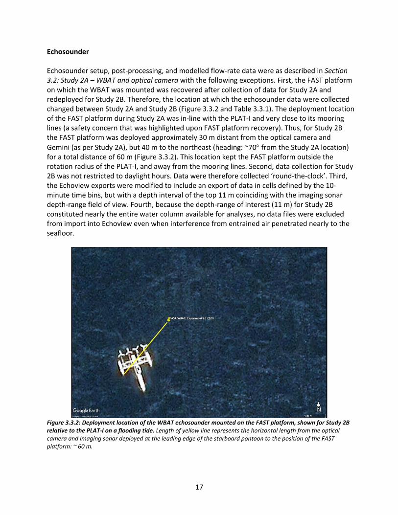
Figure 3.3.2: Deployment location of the WBAT echosounder mounted on the FAST platform, shown for Study 2B relative to the PLAT-I on a flooding tide. Length of yellow line represents the horizontal length from the optical camera and imaging sonar deployed at the leading edge of the starboard pontoon to the position of the FAST platform: ~ 60 m.

18

Table 3.3.1: Summary of Study 2B Deployment Locations and Data Collection.

Instrument Deployment

Platform

Deployment

Location

Data Collection

Dates

Hours of Data

Collected

Optical Camera PLAT-I

(sea surface)

45 15.830 N

66 20.210 W

Jan 31, 2020

Feb 02, 2020 ~ 20

Imaging Sonar PLAT-I

(sea surface)

45 15.830 N

66 20.210 W

Jan 25, 2020

Feb 02, 2020 ~ 91

WBAT Echosounder FAST

(sea floor)

45 15.861 N

66 20.195 W

Jan 25, 2020

Feb 02, 2020 97

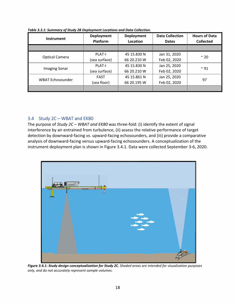
3.4 Study 2C – WBAT and EK80 The purpose of Study 2C – WBAT and EK80 was three-fold: (i) identify the extent of signal interference by air entrained from turbulence, (ii) assess the relative performance of target detection by downward-facing vs. upward-facing echosounders, and (iii) provide a comparative analysis of downward-facing versus upward-facing echosounders. A conceptualization of the instrument deployment plan is shown in Figure 3.4.1. Data were collected September 3-6, 2020.

Figure 3.4.1: Study design conceptualization for Study 2C. Shaded areas are intended for visualization purposes only, and do not accurately represent sample volumes.

19

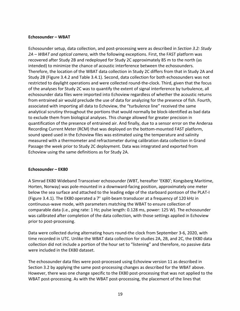
Echosounder – WBAT Echosounder setup, data collection, and post-processing were as described in Section 3.2: Study 2A – WBAT and optical camera, with the following exceptions. First, the FAST platform was recovered after Study 2B and redeployed for Study 2C approximately 85 m to the north (as intended) to minimize the chance of acoustic interference between the echosounders. Therefore, the location of the WBAT data collection in Study 2C differs from that in Study 2A and Study 2B (Figure 3.4.2 and Table 3.4.1). Second, data collection for both echosounders was not restricted to daylight operations and were collected round-the-clock. Third, given that the focus of the analyses for Study 2C was to quantify the extent of signal interference by turbulence, all echosounder data files were imported into Echoview regardless of whether the acoustic returns from entrained air would preclude the use of data for analyzing for the presence of fish. Fourth, associated with importing all data to Echoview, the “turbulence line” received the same analytical scrutiny throughout the portions that would normally be block-identified as bad data to exclude them from biological analyses. This change allowed for greater precision in quantification of the presence of entrained air. And finally, due to a sensor error on the Anderaa Recording Current Meter (RCM) that was deployed on the bottom-mounted FAST platform, sound speed used in the Echoview files was estimated using the temperature and salinity measured with a thermometer and refractometer during calibration data collection in Grand Passage the week prior to Study 2C deployment. Data was integrated and exported from Echoview using the same definitions as for Study 2A. Echosounder – EK80 A Simrad EK80 Wideband Transceiver echosounder (WBT, hereafter ‘EK80’; Kongsberg Maritime, Horten, Norway) was pole-mounted in a downward-facing position, approximately one meter below the sea surface and attached to the leading edge of the starboard pontoon of the PLAT-I

(Figure 3.4.1). The EK80 operated a 7 split-beam transducer at a frequency of 120 kHz in continuous-wave mode, with parameters matching the WBAT to ensure collection of comparable data (i.e., ping rate: 1 Hz; pulse length: 0.128 ms, power: 125 W). The echosounder was calibrated after completion of the data collection, with those settings applied in Echoview prior to post-processing. Data were collected during alternating hours round-the clock from September 3-6, 2020, with time recorded in UTC. Unlike the WBAT data collection for studies 2A, 2B, and 2C, the EK80 data collection did not include a portion of the hour set to “listening” and therefore, no passive data were included in the EK80 dataset. The echosounder data files were post-processed using Echoview version 11 as described in Section 3.2 by applying the same post-processing changes as described for the WBAT above. However, there was one change specific to the EK80 post-processing that was not applied to the WBAT post-processing. As with the WBAT post-processing, the placement of the lines that

20

define the boundaries of the data to be used for analyses are initially computed by software and then scrutinized by a hydroacoustics analyst. For all three studies described here, the initial placement of the lines for the WBAT data was done using the algorithms built in Echoview and available to any user. However, given the extreme dominance of interference from entrained air in the EK80 data set, the built-in Echoview algorithms failed to provide a reasonably placed turbulence line from which to start the post-processing. Instead, the initial placement of the turbulence line (and bottom line) was calculated using Echofilter – a new software developed through the Pathway Program and designed to work with Echoview (Lowe and McGarry, 2020; McGarry et al., 2020). An additional change required for post-processing because of the downward-facing orientation of the EK80 transducer was that the nearfield line (1.7 m from the transducer face) defined the upper limit of the water column data available for analyses; rather than the bottom limit for the upward-facing WBAT. Likewise, the limit that defines the furthest range from the transducer to be included for analyses is the detected sea floor with a 1-m offset to remove the portion affected by the acoustic deadzone; rather than the detected sea surface with the 1-m offset for the upward-facing WBAT. Importantly, the turbulence line is equivalent in the data collected from either an upward-facing or downward-facing echosounder. As with all hydroacoustic post-processing, once the placement of the boundary lines has been estimated through an automated process, the hydroacoustic analyst inspects the line placement for each Echoview file, sets thresholds, and scrutinize for “bad data” as described for the WBAT data. As per the WBAT data for Study 2C, the placement of the turbulence line for the EK80 data was treated as though all of the recorded data would be used for analyses. Data were integrated and exported from Echoview using the same definitions as per the WBAT data.

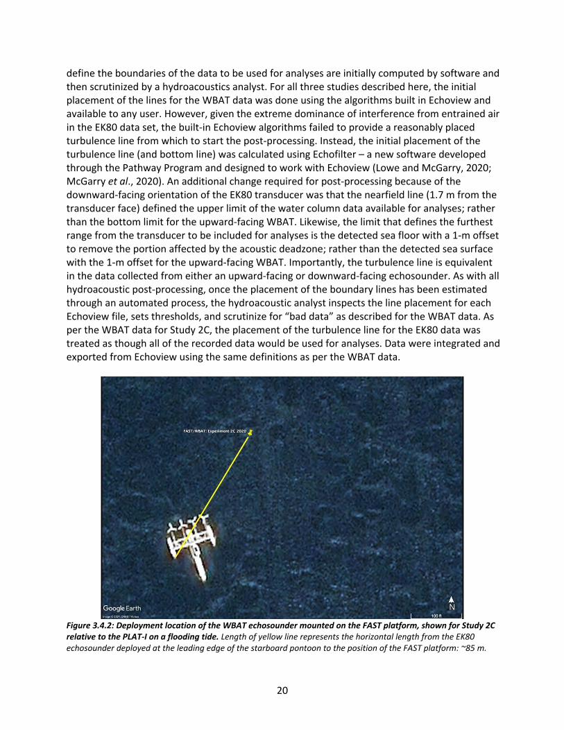
Figure 3.4.2: Deployment location of the WBAT echosounder mounted on the FAST platform, shown for Study 2C relative to the PLAT-I on a flooding tide. Length of yellow line represents the horizontal length from the EK80 echosounder deployed at the leading edge of the starboard pontoon to the position of the FAST platform: ~85 m.

21

Table 3.4.1: Summary of Study 2C Deployment Locations and Data Collection.

Instrument Deployment

Platform

Deployment

Location*

Data Collection

Dates

Hours of Data

Collected

EK80 Echosounder PLAT-I

(sea surface)

45 15.830 N

66 20.210 W

Sep 03, 2020

Sep 06, 2020 33

WBAT Echosounder FAST

(sea floor)

45 15.876 N

66 20.190 W

Sep 03, 2020

Sep 06, 2020 36

* the deployment location noted here for the PLAT-I is the location as shown for Study 2A and 2B. However, it should be noted that prior to the data collection for Study 2C, the PLAT-I was repositioned in generally the same locale. Modelled tidal flow rate data were as described in Section 3.1, but with the model output updated to coincide with the data collection period for this study, and produced for the location of the FAST platform and the location of the PLAT-I. Flow rate data was produced for both locations so that quantification of the associated extent of entrained air was unambiguously associated with the flow rate modelled for each site.

3.5 Data Analysis Merge Metadata with Hydroacoustic Data Scripts were programmed in R to merge the modelled flow rate data with the exported echosounder data. The merge associated the echosounder data, the 10-minute observation periods and the lines defining the boundaries of the analysis region, with the corresponding flow rate and tide phase. Calculate Proportion of Useable Water Column To quantify the extent of signal interference due to entrained air, the proportion of useable water column was calculated, first for every data point (i.e., for each “ping”) included in the exported line files (surface/nearfield, turbulence, bottom/nearfield) that define the analysis region within the datasets for both the upward-facing and the downward-facing echosounders. Then the useable proportion by ping was averaged for each of the 10-minute observation periods. A visualization using data collected by an upward-facing echosounder in Minas Passage is included here (Figure 3.4.3).

22

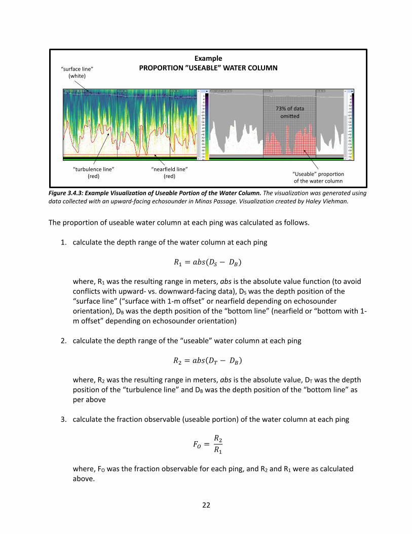
Figure 3.4.3: Example Visualization of Useable Portion of the Water Column. The visualization was generated using data collected with an upward-facing echosounder in Minas Passage. Visualization created by Haley Viehman.

The proportion of useable water column at each ping was calculated as follows.

1. calculate the depth range of the water column at each ping

𝑅1 = 𝑎𝑏𝑠(𝐷𝑆 − 𝐷𝐵)

where, R1 was the resulting range in meters, abs is the absolute value function (to avoid conflicts with upward- vs. downward-facing data), DS was the depth position of the “surface line” (“surface with 1-m offset” or nearfield depending on echosounder orientation), DB was the depth position of the “bottom line” (nearfield or “bottom with 1-m offset” depending on echosounder orientation)

2. calculate the depth range of the “useable” water column at each ping

𝑅2 = 𝑎𝑏𝑠(𝐷𝑇 − 𝐷𝐵)

where, R2 was the resulting range in meters, abs is the absolute value, DT was the depth position of the “turbulence line” and DB was the depth position of the “bottom line” as per above

3. calculate the fraction observable (useable portion) of the water column at each ping

𝐹𝑂 = 𝑅2

𝑅1

where, FO was the fraction observable for each ping, and R2 and R1 were as calculated above.

Example PROPORTION ”USEABLE” WATER COLUMN

73% of data

omi ed

“surface line”(white)

“turbulence line”(red)

“nearfield line”(red) “Useable” propor on

of the water column

23

The ping-by-ping detail of useable water column was then averaged for each 10-minute observation period as follows:

4. calculate the mean of the fraction observable for each 10-minute observation period

𝐹10,𝑗 = ∑ 𝐹𝑂,𝑗

𝑛,𝑗1

𝑛𝑗

where, F10 is the mean fraction-observable for the 10-minute interval, j is the 10-minute interval, nj is the number of datapoints (pings) within the 10-minute interval j, and FO,j are the fraction-observable values for each ping within the 10-minute interval j

5. the tidal flow rate and tide phase associated with each “useable portion” were the flow

rate and tide phase from the modelled tidal flow-rate data for each 10-minute observation period.

The result of these calculations was a dataset of the mean proportion of useable water column for each 10-minute observation period associated with the corresponding modelled tidal flow rate and tide phase. To understand the relationship between tidal flow rate and the proportion of useable observations periods on the flood and ebb tide, a simple linear regression model (function: lm in R) was fit to the data. To gain insights into the influence of tide phase on the amount of data available for analyses (i.e., whether the proportion of useable 10-minute observation periods differed between a flood and ebb tide) and the associated sensitivity to the criteria that defines “useable for analyses”, the count of 10-minute observation periods meeting the criteria was calculated as a proportion of all 10-minute observation periods by tide phase (i.e., if we set criteria to include only those 10-minute observations periods for which the “useable water column” proportion met or exceeded some minimum proportion, does the count of useable 10-minute observations change?). Calculate Proportion of Useable Data within Rotor Swept Depth for Each Data Collection Site While assembling the results of the useable-data analyses, it became apparent that site-specific hydrodynamics, and the consequences for the extent of entrained in the water column, likely played a role in the availability of useable data. Therefore, to take advantage of the opportunity to investigate the potential influence that site-selection may have on data useability within the depths of interest, additional analyses were undertaken to document the useability of data, by site, within the swept depth of the PLAT-I rotors (1.5 to 7.8 m from surface; Sustainable Marine personal communication).

24

The same exported line files used for the Proportion of Useable Water Column analyses were analyzed on a ping-by-ping basis, rather than the 10-minute intervals above. Each ping within each 1-m depth bin, starting 1 m below the surface and ending at 8 m below the surface, was designated as “useable” or “unusable” based on whether the depth of the turbulence line was less than or greater than the depth bin, respectively. Using the same tide phase assignment as above, each ping with its designation of usable or unusable was then aggregated by tide phase. The result was that for each 1-m depth bin from 1 m to 8 m below the surface, the count of pings useable and unusable by tide phase was enumerated. From that data the proportion of useable pings was calculated by depth bin and tide phase. For Study 2A, the proportion of unusable pings needed to be estimated for the data files which were excluded from Echoview. Those files were the hour-long files for which interference from entrained air dominated nearly the entire water column. Because those files were excluded from Echoview, they were therefore not included in the line-data exports. The number of excluded pings at 1 Hz was estimated and included in the results.

3.6 Notes on Setting Minimum and Maximum Sv Thresholds for Fish As described in Section 3.2, one of the objectives of post-processing hydroacoustic data was to establish which recorded signals of returned echo energy were to be included or excluded from analyses. Setting a minimum and a maximum threshold defines the range of signal amplitudes that are accepted for inclusion in analyses. With a dynamic range of 14 orders of magnitude (140 dB: Simrad, 2020), the EK80 suite of echosounders are capable of receiving both very weak and very strong echo returns. The dynamic range is orders of magnitude greater than the range of echo returns found for fish and fish aggregations. Setting minimum and maximum thresholds is therefore warranted. Because the amount of energy returned by fish (individuals or aggregations) is not a static characteristic, setting thresholds can be as much an art as a science. Without in situ sampling to act as a guide (e.g., net tows/trawl surveys to verify species identification and fish size), the thresholds here were based on visual scrutiny of the echograms and consultation with subject-matter experts. The goal was to select a threshold sufficiently low to exclude plankton without excluding fish sizes that should reasonably be included. A minimum volume backscattering strength (Sv) threshold of -66 dB was selected, which at 120 kHz in seawater, is “equivalent” to a “generic” fish of length ~ 1 cm (Love 1971). This minimum threshold was entered into the Echoview software such that Sv values below this value were excluded from analyses, making the minimum threshold a “hard” threshold. In an effort to exclude marine mammals (lungs generate very strong echo returns) and other strong non-fish echo returns without excluding dense aggregations of fish with swim bladders, the maximum threshold was a “soft” threshold. Because this threshold was “soft”, no maximum value was entered into Echoview, but after completing post-processing, the data was examined using scripts in R for Sv values ≥ -30 dB. The script output included the name of the Echoview file and the ping numbers therein which included values ≥ -30 dB. Those echograms were then examined

25

by an analyst to determine whether the values ≥ -30 dB were consistent with fish aggregations (included in analyses) or not (excluded from analyses).

4 Results and Discussion

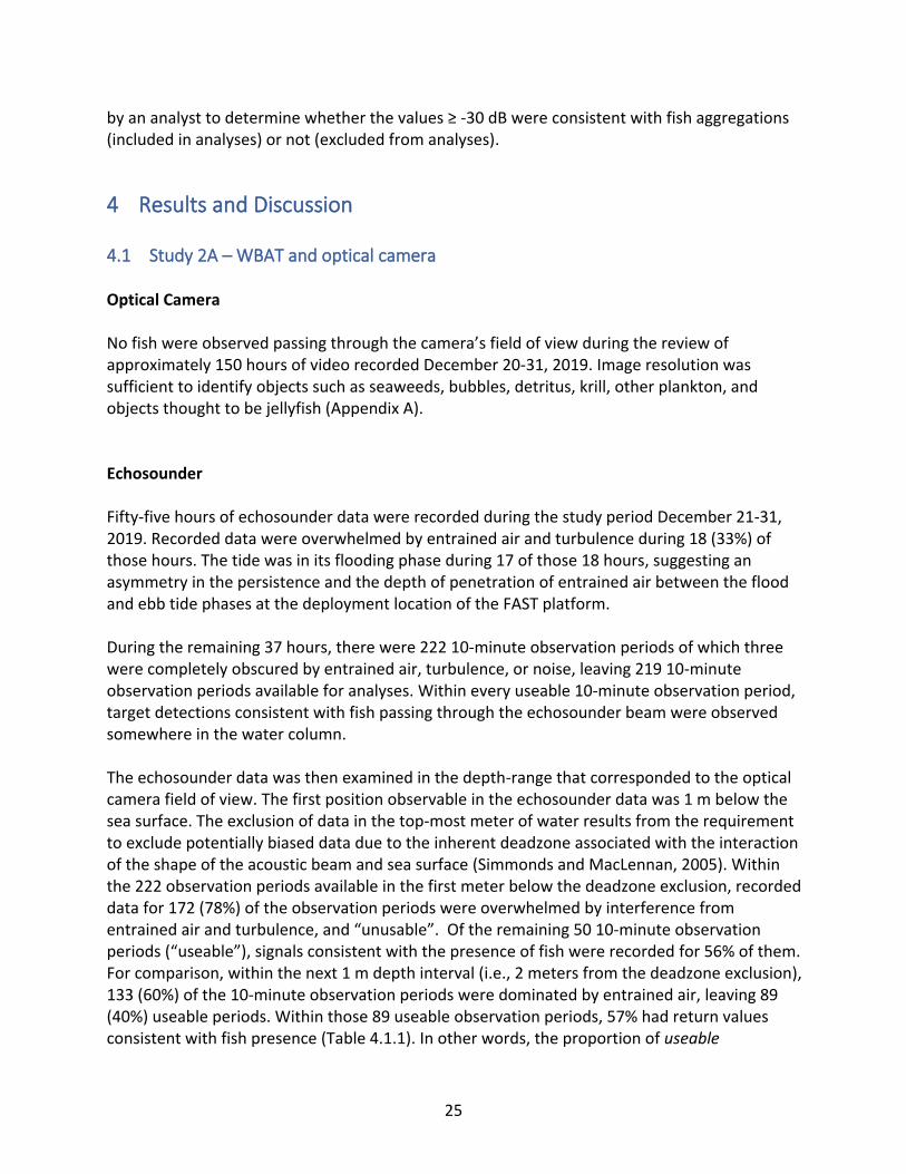
4.1 Study 2A – WBAT and optical camera Optical Camera No fish were observed passing through the camera’s field of view during the review of approximately 150 hours of video recorded December 20-31, 2019. Image resolution was sufficient to identify objects such as seaweeds, bubbles, detritus, krill, other plankton, and objects thought to be jellyfish (Appendix A). Echosounder Fifty-five hours of echosounder data were recorded during the study period December 21-31, 2019. Recorded data were overwhelmed by entrained air and turbulence during 18 (33%) of those hours. The tide was in its flooding phase during 17 of those 18 hours, suggesting an asymmetry in the persistence and the depth of penetration of entrained air between the flood and ebb tide phases at the deployment location of the FAST platform. During the remaining 37 hours, there were 222 10-minute observation periods of which three were completely obscured by entrained air, turbulence, or noise, leaving 219 10-minute observation periods available for analyses. Within every useable 10-minute observation period, target detections consistent with fish passing through the echosounder beam were observed somewhere in the water column. The echosounder data was then examined in the depth-range that corresponded to the optical camera field of view. The first position observable in the echosounder data was 1 m below the sea surface. The exclusion of data in the top-most meter of water results from the requirement to exclude potentially biased data due to the inherent deadzone associated with the interaction of the shape of the acoustic beam and sea surface (Simmonds and MacLennan, 2005). Within the 222 observation periods available in the first meter below the deadzone exclusion, recorded data for 172 (78%) of the observation periods were overwhelmed by interference from entrained air and turbulence, and “unusable”. Of the remaining 50 10-minute observation periods (“useable”), signals consistent with the presence of fish were recorded for 56% of them. For comparison, within the next 1 m depth interval (i.e., 2 meters from the deadzone exclusion), 133 (60%) of the 10-minute observation periods were dominated by entrained air, leaving 89 (40%) useable periods. Within those 89 useable observation periods, 57% had return values consistent with fish presence (Table 4.1.1). In other words, the proportion of useable

26

observation periods that contained echo return values consistent with fish presence was nominally 55% within each of the first two observable meters of water. Table 4.1.1: Summary of Study 2A Useable 10-minute Hydroacoustic Observation Periods (37 out of 55 hours of

data collection). Data in this table includes only those data files which were not fully excluded due to entrained air.

The remaining individual observation periods were designated as “unusable” when signals recorded from within the

observation depth were dominated by entrained air and turbulence, obfuscating signals returned from fish. Each

10-minute observation period for which recorded Sv values greater than -66 dB are reported as “fish present”. “Fish

absent” observation periods indicate that no Sv values greater than -66 dB were observed within the useable data

during the entirety of the observation period.

Of the 222 10-minute observation periods (37 hours out of 55 hours collected)…

Fish Present Fish Absent Unusable

(n) (%) (n) (%) (n) (%)

At Any Depth (full water column) 219 100 % 0 0 % 3 1 %

Within 1-2 Meter from the Surface 28 56 % 22 44 % 172 78 %

Within 2-3 Meter from the Surface 51 57 % 38 43 % 133 60 %

Study 2A Discussion The findings from the optical camera and echosounder starkly differ. Although no fish were observed for the 150 hours of optical camera data collected, signals consistent with the presence of fish were detected by the echosounder in depths coinciding with the cameras field-of-view for approximately 55% of the useable 10-minute time bins. Given that the camera image resolution was sufficient to identify krill, other plankton, jellyfish, seaweed, and detritus, the lack of fish being observed likely stems from fish not passing within the camera’s field-of-view. Without additional sources of information, it is difficult to resolve this discrepancy, but there are several possibilities that could have contributed to the differing results. For instance, the fields-of-view for each instrument were not co-located, nor of equal volume, and were in different deployment conditions. While co-location of the sampling volume would have been ideal, it was not feasible or safe for personnel, instruments, or the PLAT-I structure to attempt a closer deployment. Given that the diameter of the acoustic beam was approximately 1.6 m at the sea “surface” (see discussion in Section 4.3 and Figure 4.3.5) and the field-of-view of the optical camera was only a few meters, there was no opportunity to co-locate the sampling volumes. The camera was pole mounted and attached to the PLAT-I starboard pontoon, while the echosounder was deployed on a FAST platform approximately 30 m distant from the camera on the flood tide (~53 m on ebb tide due to PLAT-I rotation on turret; Figure 3.2.2 and Table 3.2.1). As such, the echosounder field-of-view was in a more “open water” setting than the optical camera. Given the distance between the position of the two instruments, we cannot rule out the possibility that the hydrodynamic conditions at these locations, or the presence of the

27

PLAT-I structure itself, influenced fish presence/absence. However, we have no information by which to address fish behaviour and cannot address this question. The primary goal of this study was to investigate the near-surface target detection capabilities of a bottom-mounted upward-facing echosounder using a surface-deployed optical video camera. In this case, the echosounder recorded signals that were consistent with the presence of fish, but the camera did not. While the identity of the targets registered with the echosounder could not be discerned, this likely resulted from non-overlapping fields of view between the instruments. Nonetheless, the bottom-mounted upward-facing echosounder was shown to be effective at detecting echo returns consistent with the presence of fish in the near surface waters of Grand Passage when turbulence and entrained air did not interfere with acoustic signal transmission.

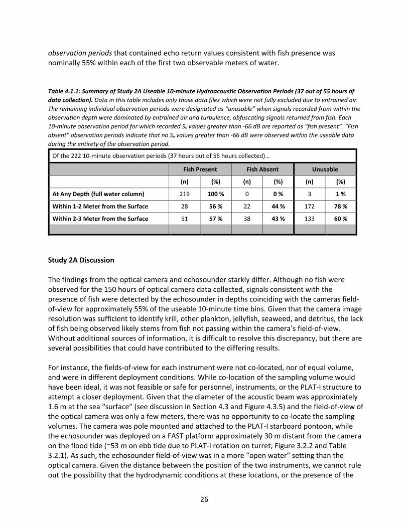
4.2 Study 2B – WBAT, optical camera, and multibeam imaging sonar Optical Camera No fish were observed to pass thorough the field of view of the optical camera during the review of approximately 20 hours of data collected during January 31-February 2, 2020. However, image resolution was sufficient to identify objects such as seaweeds, bubbles, detritus, krill, other plankton, and objects thought to be jellyfish (Appendix A). See Section 4.1: Study 2A – WBAT and optical camera for more discussion. The remainder of this section will focus on the results from the Gemini imaging sonar and echosounder data collections and results. Imaging Sonar Approximately 91 hours of Gemini Imaging Sonar data were collected during January 25–February 2, 2020, resulting in 546 10-minute observation periods. During 121 (22%) of the 10-minute observation periods, 336 potential targets were detected by the SEATEC software, but their identity could not be confirmed. Where direction of movement could be determined, the targets were moving in the same direction as the tidal flow. Image resolution was insufficient to definitively classify potential targets, so they were classified into three categories: “turbulence/fish/school of fish” (n = 229), “single fish/debris” (n = 97), and “mooring” (n = 10) (Table 4.2.1).

28

Table 4.2.1: Classification of 336 Potential Detections Using Gemini Imaging Sonar

(n) (%) ebb flood slack

Potential Detections 336 100 % 94 213 29

“Mooring” 10 3 % 5 1 4

“Single Fish/Debris” 97 29 % 43 32 22

“Turbulence/Fish/School of Fish” 229 68 % 46 180 3

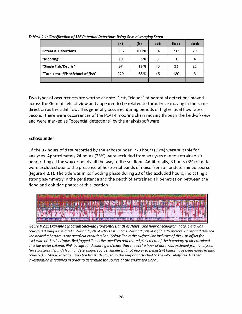
Two types of occurrences are worthy of note. First, “clouds” of potential detections moved across the Gemini field of view and appeared to be related to turbulence moving in the same direction as the tidal flow. This generally occurred during periods of higher tidal flow rates. Second, there were occurrences of the PLAT-I mooring chain moving through the field-of-view and were marked as “potential detections” by the analysis software. Echosounder Of the 97 hours of data recorded by the echosounder, ~70 hours (72%) were suitable for analyses. Approximately 24 hours (25%) were excluded from analyses due to entrained air penetrating all the way or nearly all the way to the seafloor. Additionally, 3 hours (3%) of data were excluded due to the presence of horizontal bands of noise from an undetermined source (Figure 4.2.1). The tide was in its flooding phase during 20 of the excluded hours, indicating a strong asymmetry in the persistence and the depth of entrained air penetration between the flood and ebb tide phases at this location.

Figure 4.2.1: Example Echogram Showing Horizontal Bands of Noise. One hour of echogram data. Data was collected during a rising tide. Water depth at left is 14 meters. Water depth at right is 15 meters. Horizontal thin red line near the bottom is the nearfield exclusion line. Yellow line is the surface line inclusive of the 1-m offset for exclusion of the deadzone. Red jagged line is the unedited automated placement of the boundary of air entrained into the water column. Pink background coloring indicates that the entire hour of data was excluded from analyses. Note horizontal bands from undetermined source. Similar but not nearly so persistent bands have been noted in data collected in Minas Passage using the WBAT deployed to the seafloor attached to the FAST platform. Further investigation is required in order to determine the source of the unwanted signal.

29

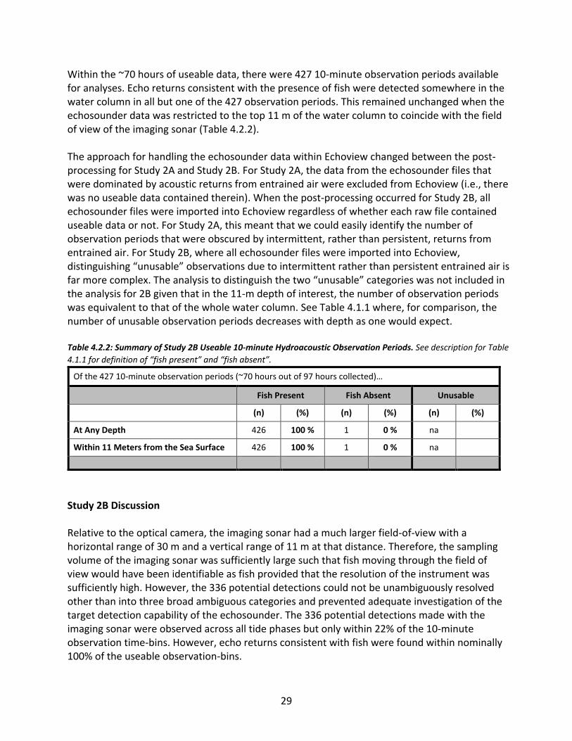
Within the ~70 hours of useable data, there were 427 10-minute observation periods available for analyses. Echo returns consistent with the presence of fish were detected somewhere in the water column in all but one of the 427 observation periods. This remained unchanged when the echosounder data was restricted to the top 11 m of the water column to coincide with the field of view of the imaging sonar (Table 4.2.2). The approach for handling the echosounder data within Echoview changed between the post-processing for Study 2A and Study 2B. For Study 2A, the data from the echosounder files that were dominated by acoustic returns from entrained air were excluded from Echoview (i.e., there was no useable data contained therein). When the post-processing occurred for Study 2B, all echosounder files were imported into Echoview regardless of whether each raw file contained useable data or not. For Study 2A, this meant that we could easily identify the number of observation periods that were obscured by intermittent, rather than persistent, returns from entrained air. For Study 2B, where all echosounder files were imported into Echoview, distinguishing “unusable” observations due to intermittent rather than persistent entrained air is far more complex. The analysis to distinguish the two “unusable” categories was not included in the analysis for 2B given that in the 11-m depth of interest, the number of observation periods was equivalent to that of the whole water column. See Table 4.1.1 where, for comparison, the number of unusable observation periods decreases with depth as one would expect. Table 4.2.2: Summary of Study 2B Useable 10-minute Hydroacoustic Observation Periods. See description for Table

4.1.1 for definition of “fish present” and “fish absent”.

Of the 427 10-minute observation periods (~70 hours out of 97 hours collected)…

Fish Present Fish Absent Unusable

(n) (%) (n) (%) (n) (%)

At Any Depth 426 100 % 1 0 % na

Within 11 Meters from the Sea Surface 426 100 % 1 0 % na

Study 2B Discussion Relative to the optical camera, the imaging sonar had a much larger field-of-view with a horizontal range of 30 m and a vertical range of 11 m at that distance. Therefore, the sampling volume of the imaging sonar was sufficiently large such that fish moving through the field of view would have been identifiable as fish provided that the resolution of the instrument was sufficiently high. However, the 336 potential detections could not be unambiguously resolved other than into three broad ambiguous categories and prevented adequate investigation of the target detection capability of the echosounder. The 336 potential detections made with the imaging sonar were observed across all tide phases but only within 22% of the 10-minute observation time-bins. However, echo returns consistent with fish were found within nominally 100% of the useable observation-bins.

30

While the difference in the proportion of observation bins with potential fish detections (22%: imaging sonar; 100%: echosounder) is notable, there are three factors that may have influenced this difference: (i) the tide phase – given that observations during ebb tide are over-represented in the echosounder data (due to the exclusion of data overwhelmed by entrained air), (ii) non-overlapping sample volumes between instruments (not co-located), and (iii) different deployment locations. The strong asymmetry of tidal phase associated with the exclusion of hydroacoustic data due to entrained air suggests important differences in the hydrodynamic regimes at the deployment location of the FAST platform and the PLAT-I. Because of the tidal asymmetry in the persistence and extent of entrained air, flood-tide data were proportionally under-represented in the echosounder data relative to the imaging sonar data. We examined the distribution of potential detections by tide phase in order to determine whether the partial exclusion of flood tide data from the echosounder dataset affected the proportional comparison of total observation periods. In other words, if flood phase is under-represented in the echosounder data, then the ~ 100% “fish present” time bins may be overstated relative to the imaging sonar proportion of “potential detection” time bins (22%). However, the flood tide was strongly represented in the imaging sonar potential detections (Table 4.2.1), accounting for 65% of the potential detections that were categorized as “single fish/debris” or “turbulence/fish/school of fish” (i.e., excluding the “mooring” category). Therefore, the proportional difference (100% vs. 22%) of observations with potential fish detections does not appear to be a function of the difference in the proportion of tide phase observations. The repositioning of the FAST platform for Study 2B, the diameter of the echosounder acoustic beam at the sea surface (1.6 m) and the useable horizontal range of the imaging sonar (30 m), resulted in non-overlapping sample volumes. Although the lack of overlapping sample volumes precluded definitive cross-referencing between the two instruments, optical cameras and imaging sonars have been shown to be valuable monitoring tools elsewhere (Mueller et al., 2006; Hastie et al., 2019a, 2019b; Williamson et al., 2016b) and have value for monitoring in Grand Passage. As a result of the repositioning of the FAST platform, the echosounder field-of-view was in a more “open water” setting than the imaging sonar mounted on the PLAT-I. Given the distance between the position of the two instruments, we cannot rule out that the possibility that hydrodynamic conditions at these locations, or the presence of the PLAT-I structure itself, influenced fish presence/absence. However, we have no information by which to address fish behaviour and cannot address this question. The primary goal of this study was to investigate the target detection capabilities of a bottom-mounted upward-facing echosounder using a surface-deployed imaging sonar. As observed in Study 2A, the echosounder recorded signals that were consistent with the presence of fish, but the resolution of the imaging sonar was insufficient to unambiguously identify detections beyond three broad categories. Nonetheless, the bottom-mounted upward-facing echosounder

31

was shown to be effective at detecting echo returns consistent with the presence of fish in the depth range of the imaging sonar when turbulence and entrained air did not interfere with acoustic signal transmission.

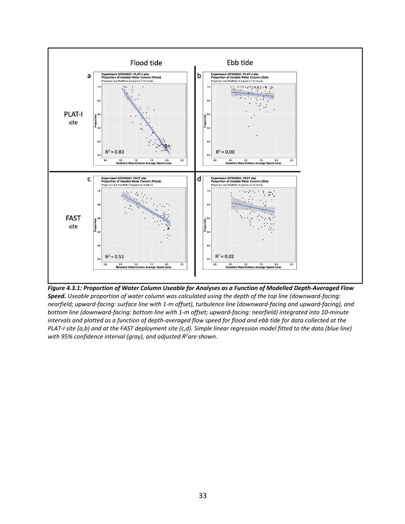
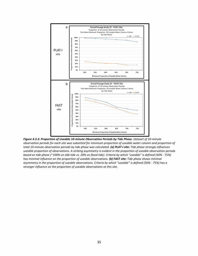
4.3 Study 2C – WBAT and EK80 Echosounders Hydroacoustic data were recorded at the PLAT-I site (33 hours: surface-deployed EK80) and at the FAST-platform site (36 hours: bottom-mounted WBAT) during a spring tide from September 3-6, 2020. There were 244 10-minute observation periods available for analyses from the PLAT-I site and 203 observation periods from the FAST site. Because the purpose of these data collections was to quantify the extent of signal interference from entrained air, all data were post-processed demarcating the boundary of the entrained air (“turbulence line”) in Echoview without using “bad data” regions that would fully exclude data from analyses (i.e., all data were available for the analyses). Signal Interference by Entrained Air Hydroacoustic data from the “PLAT-I” and “FAST” sites suggests important differences in the hydrodynamic regimes at the two locations. For the PLAT-I site, the proportion of useable data decreased markedly with increasing flow speed on the flood tide (adjusted R2 = 0.83; Figure 4.3.1 “a”); the influence of flow speed was much less pronounced on the ebb tide (adjusted R2 = 0.00; Figure 4.3.1 “b”). This phenomenon is well illustrated in a set of echograms typical to the PLAT-I site (Figure 4.3.2 “a” and “b”). The flood tide echogram from the PLAT-I site (“a”), is dominated by persistent, strong signals of entrained air (red colors) throughout the water column, whereas the ebb tide echogram (“b”) shows instances of entrained air near the sea surface but is largely dominated by echo returns from the water column not contaminated by entrained air. The asymmetry in the proportion of useable data for analyses between flood and ebb tide phases at the PLAT-I site is particularly evident when the proportion of useable data is partitioned using a minimum “useable” threshold, regardless of flow speed (Figure 4.3.3 “a”). The proportion of useable data for each tide phase shows little change (ebb: ~100 %; flood: ~20%) regardless of how the “useable” criteria is defined. In other words, Figure 4.3.3a answers the question “how much of the data available on the flood or ebb tide are useable if we set the minimum ‘useable’ criteria to at least 50% of the water column (or 55%, or 60%, etc.,) regardless of flow speed?”. At the PLAT-I site, the amount of useable data is strongly influenced by tide phase – useable on the ebb (~100%) but not on the flood (~20%) – and minimally influenced by tightening the criteria by which “useable” is defined. Conversely, at the FAST deployment site for Study 2C, the amount of useable data was more influenced by how the criteria for “useable” was defined and minimally influenced by tide phase

32

(Figure 4.3.3 “b”). In other words, the two lines representing flood and ebb tide data track tightly together with minimal difference between the useable proportion on the flood vs. the ebb tide and show a distinct reduction in the proportion of useable data that is negatively correlated with increasing minimum criteria for “useable”. When plotted relative to flow rate, there is some reduction in the proportion of “useable” data with increasing flow rate on the flood tide (adjusted R2 = 0.51; Figure 4.3.1 “c”), but not as pronounced at the higher flow rates observed at the PLAT-I site. There is no evidence for a reduction in the proportion of useable data with increasing flow rate at the FAST deployment site on the ebb tide (adjusted R2 = 0.02; Figure 4.3.1 “d”). The relative symmetry of useable data at the FAST site on the ebb and flood tide is illustrated in the echograms (Figure 4.3.2 “c” and “d”). These findings are consistent with the work of Hay (2017) in that the strong tidal currents in Grand Passage can be accompanied by high levels of turbulence resulting from the interaction of the currents with the channel’s bathymetric features and Peter’s Island (Figure 2.1). The PLAT-I is downstream from Peter’s Island during the flood tide. In addition, Hay (2017) notes that spatial scales in a turbulent tidal flow can span many orders of magnitude and local seabed conditions are not sufficient from which to predict levels of turbulence with any degree of accuracy. Therefore, the presence, or absence, of turbulence capable of entraining air minimally or deeply into the water column is site-specific and dependent on the upstream conditions. A satellite image of the PLAT-I on a flood tide (Figure 4.3.4) suggests that the PLAT-I is deployed within a particularly turbulent portion of the channel; a possible consequence of its location relative to Peter’s Island. If the location of the PLAT-I during a flood tide is downstream from bathymetric features generating sufficiently strong turbulence to entrain air from surface to seafloor for large portions of the flood tidal phase, but downstream from less dynamic bathymetric features on the ebb tide, the strong asymmetry in the extent of entrained air we observed would be expected. It appears that the placement of the FAST platform for Study 2C was outside the region of strong and persistent air entrainment throughout the water column. Descriptive statistics of the modelled flow rates for the two echosounder sites for Study 2C are provided in Table 4.3.1 and Table 4.3.2 and show similar flow rates at the sites. Although comparative echosounder data were not available within Study 2A or 2B, the asymmetry in the tidal phase of the data excluded from analyses due to entrained air also suggests strong asymmetry in the extent of entrained air in the vicinity of the PLAT-I location (see Appendix B). The asymmetry suggests that the hydrodynamic regimes at the FAST site locations for Study 2A and Study 2B were more similar to that of the PLAT-I location than the FAST site for Study 2C. During Study 2A, the position of echosounder data collection was directly behind the PLAT-I on the flooding tide and during Study 2B nearby to the PLAT-I on the flooding tide. In both studies, all but one of the hours excluded due to entrained air were data collected during the flood tide. Given that the PLAT-I rotors were parked during both Study 2A and 2B, the tide-phase asymmetry of the entrained air again appears to be a function of the hydrodynamics in locations downstream from Peter’s Island.

33

Figure 4.3.1: Proportion of Water Column Useable for Analyses as a Function of Modelled Depth-Averaged Flow Speed. Useable proportion of water column was calculated using the depth of the top line (downward-facing: nearfield; upward-facing: surface line with 1-m offset), turbulence line (downward-facing and upward-facing), and bottom line (downward-facing: bottom line with 1-m offset; upward-facing: nearfield) integrated into 10-minute intervals and plotted as a function of depth-averaged flow speed for flood and ebb tide for data collected at the PLAT-I site (a,b) and at the FAST deployment site (c,d). Simple linear regression model fitted to the data (blue line) with 95% confidence interval (gray), and adjusted R2are shown.

34

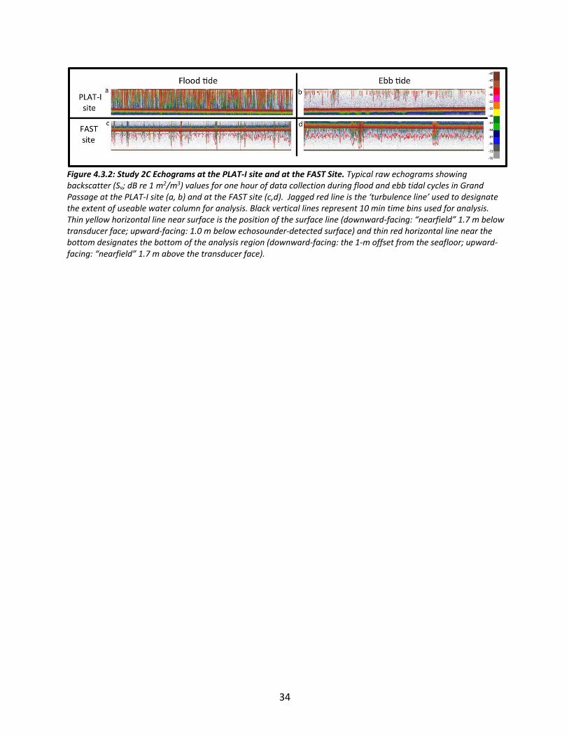
Figure 4.3.2: Study 2C Echograms at the PLAT-I site and at the FAST Site. Typical raw echograms showing backscatter (Sv; dB re 1 m2/m3) values for one hour of data collection during flood and ebb tidal cycles in Grand Passage at the PLAT-I site (a, b) and at the FAST site (c,d). Jagged red line is the ‘turbulence line’ used to designate the extent of useable water column for analysis. Black vertical lines represent 10 min time bins used for analysis. Thin yellow horizontal line near surface is the position of the surface line (downward-facing: “nearfield” 1.7 m below transducer face; upward-facing: 1.0 m below echosounder-detected surface) and thin red horizontal line near the bottom designates the bottom of the analysis region (downward-facing: the 1-m offset from the seafloor; upward-facing: “nearfield” 1.7 m above the transducer face).

35

Figure 4.3.3: Proportion of Useable 10-minute Observation Periods by Tide Phase. Dataset of 10-minute observation periods for each site was subsetted for minimum proportion of useable water column and proportion of total 10-minute observation periods by tide phase was calculated. (a) PLAT-I site: Tide phase strongly influences useable proportion of observations. A striking asymmetry is evident in the proportion of useable observation periods based on tide phase (~100% on ebb tide vs. 20% on flood tide). Criteria by which “useable” is defined (50% - 75%) has minimal influence on the proportion of useable observations. (b) FAST site: Tide phase shows minimal asymmetry in the proportion of useable observations. Criteria by which “useable” is defined (50% - 75%) has a stronger influence on the proportion of useable observations at this site.

a

b

PLAT-Isite

FASTsite

0%

10%

20%

30%

40%

50%

60%

70%

80%

90%

100%

50% 55% 60% 65% 70% 75%P

rop

ort

ion

of

10

-min

ute

Ob

serv

ati

on

Per

iod

s

M in im um Proportion of Useable Water Colum n

Grand Passage Study 2C - PLAT-I SiteProportion of 10-minute Observation Periods

That Meet Minimum Proportion Of Useable Water Column CriteriaBy Tide Phase

EBB FLOOD

0%

10%

20%

30%

40%

50%

60%

70%

80%

90%

100%

50% 55% 60% 65% 70% 75%

Pro

po

rtio

n o

f 10

-min

ute

Ob

serv

ati

on

Per

iod

s

M in imum Proportion of Useable Water Column

Grand Passage Study 2C - FAST3 SiteProportion of 10-minute Observation Periods

That Meet Minimum Proportion Of Useable Water Column CriteriaBy Tide Phase

EBB FLOOD

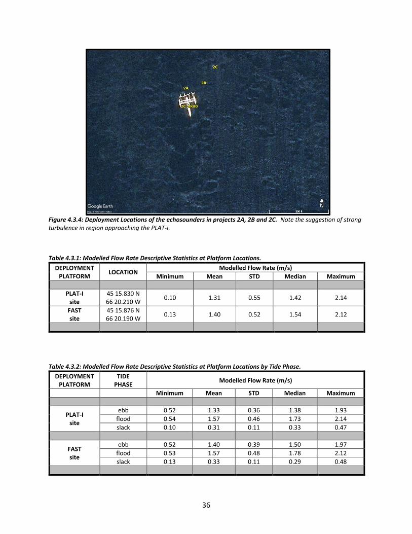
36

Figure 4.3.4: Deployment Locations of the echosounders in projects 2A, 2B and 2C. Note the suggestion of strong turbulence in region approaching the PLAT-I.

Table 4.3.1: Modelled Flow Rate Descriptive Statistics at Platform Locations.

DEPLOYMENT PLATFORM

LOCATION Modelled Flow Rate (m/s)

Minimum Mean STD Median Maximum

PLAT-I site

45 15.830 N 66 20.210 W

0.10 1.31 0.55 1.42 2.14

FAST site

45 15.876 N 66 20.190 W

0.13 1.40 0.52 1.54 2.12

Table 4.3.2: Modelled Flow Rate Descriptive Statistics at Platform Locations by Tide Phase.

DEPLOYMENT PLATFORM

TIDE PHASE

Modelled Flow Rate (m/s)

Minimum Mean STD Median Maximum

PLAT-I site

ebb 0.52 1.33 0.36 1.38 1.93

flood 0.54 1.57 0.46 1.73 2.14

slack 0.10 0.31 0.11 0.33 0.47

FAST site

ebb 0.52 1.40 0.39 1.50 1.97

flood 0.53 1.57 0.48 1.78 2.12

slack 0.13 0.33 0.11 0.29 0.48

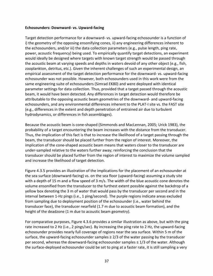
37

Echosounders: Downward- vs. Upward-facing Target detection performance for a downward- vs. upward-facing echosounder is a function of i) the geometry of the opposing ensonifying cones, ii) any engineering differences inherent to the echosounders, and/or iii) the data collection parameters (e.g., pulse length, ping rate, power, acoustic frequency) being used. To empirically quantify target detections, an experiment would ideally be designed where targets with known target strength would be passed through the acoustic beam at varying speeds and depths in waters devoid of any other object (e.g., fish, zooplankton, detritus, etc.). Given the inherent challenges of such an experimental design, an empirical assessment of the target detection performance for the downward- vs. upward-facing echosounder was not possible. However, both echosounders used in this work were from the same engineering suite of echosounders (Simrad EK80) and were deployed with identical parameter settings for data collection. Thus, provided that a target passed through the acoustic beam, it would have been detected. Any differences in target detection would therefore be attributable to the opposing acoustic beam geometries of the downward- and upward-facing echosounders, and any environmental differences inherent to the PLAT-I site vs. the FAST site (e.g., differences in the extent and depth penetration of entrained air due to turbulent hydrodynamics, or differences in fish assemblages). Because the acoustic beam is cone-shaped (Simmonds and MacLennan, 2005; Urick 1983), the probability of a target encountering the beam increases with the distance from the transducer. Thus, the implication of this fact is that to increase the likelihood of a target passing through the beam, the transducer should be placed further from the region of interest. Moreover, the implication of the cone-shaped acoustic beam means that waters closer to the transducer are under-sampled relative to the waters further away; reinforcing the conclusion that the transducer should be placed further from the region of interest to maximize the volume sampled and increase the likelihood of target detection. Figure 4.3.5 provides an illustration of the implications for the placement of an echosounder at the sea surface (downward-facing) vs. on the sea floor (upward-facing) assuming a study site with a depth of 15 m and a flow speed of 3 m/s. The width of the blue acoustic cone denotes the volume ensonified from the transducer to the furthest extent possible against the backdrop of a yellow box denoting the 3 m of water that would pass by the transducer per second and in the interval between 1-Hz pings (i.e., 1 ping/second). The purple regions indicate areas excluded from sampling due to deployment position of the echosounder (i.e., water behind the transducer face), the transducer nearfield (1.7 m due to acoustic beam formation), and the height of the deadzone (1 m due to acoustic beam geometry). For comparative purposes, Figure 4.3.6 provides a similar illustration as above, but with the ping rate increased to 2 Hz (i.e., 2 pings/sec). By increasing the ping rate to 2 Hz, the upward-facing echosounder provides nearly full coverage of regions near the sea surface. Within 5 m of the surface, the upward-facing echosounder samples ≥ 2/3 of the water passing by the transducer per second, whereas the downward-facing echosounder samples ≤ 1/3 of the water. Although the surface-deployed echosounder could be set to ping at a faster rate, it is still sampling a very

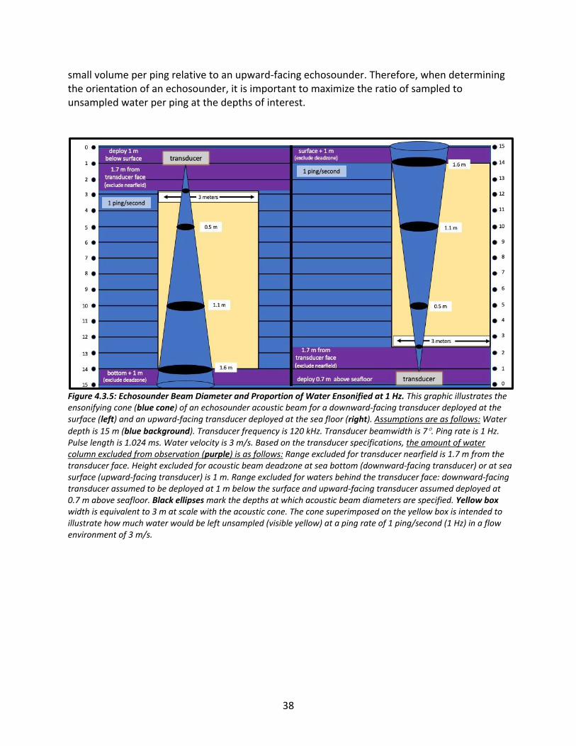
38

small volume per ping relative to an upward-facing echosounder. Therefore, when determining the orientation of an echosounder, it is important to maximize the ratio of sampled to unsampled water per ping at the depths of interest.

Figure 4.3.5: Echosounder Beam Diameter and Proportion of Water Ensonified at 1 Hz. This graphic illustrates the ensonifying cone (blue cone) of an echosounder acoustic beam for a downward-facing transducer deployed at the surface (left) and an upward-facing transducer deployed at the sea floor (right). Assumptions are as follows: Water

depth is 15 m (blue background). Transducer frequency is 120 kHz. Transducer beamwidth is 7. Ping rate is 1 Hz. Pulse length is 1.024 ms. Water velocity is 3 m/s. Based on the transducer specifications, the amount of water column excluded from observation (purple) is as follows: Range excluded for transducer nearfield is 1.7 m from the transducer face. Height excluded for acoustic beam deadzone at sea bottom (downward-facing transducer) or at sea surface (upward-facing transducer) is 1 m. Range excluded for waters behind the transducer face: downward-facing transducer assumed to be deployed at 1 m below the surface and upward-facing transducer assumed deployed at 0.7 m above seafloor. Black ellipses mark the depths at which acoustic beam diameters are specified. Yellow box width is equivalent to 3 m at scale with the acoustic cone. The cone superimposed on the yellow box is intended to illustrate how much water would be left unsampled (visible yellow) at a ping rate of 1 ping/second (1 Hz) in a flow environment of 3 m/s.

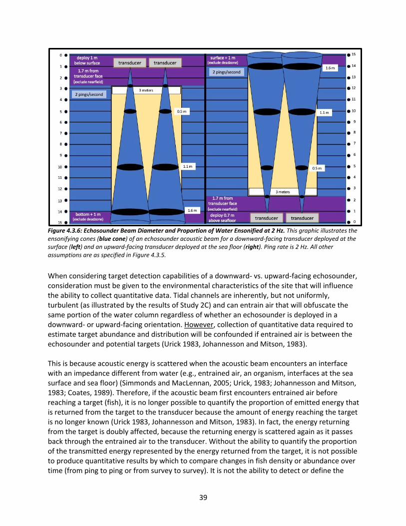
39

Figure 4.3.6: Echosounder Beam Diameter and Proportion of Water Ensonified at 2 Hz. This graphic illustrates the ensonifying cones (blue cone) of an echosounder acoustic beam for a downward-facing transducer deployed at the surface (left) and an upward-facing transducer deployed at the sea floor (right). Ping rate is 2 Hz. All other assumptions are as specified in Figure 4.3.5.

When considering target detection capabilities of a downward- vs. upward-facing echosounder, consideration must be given to the environmental characteristics of the site that will influence the ability to collect quantitative data. Tidal channels are inherently, but not uniformly, turbulent (as illustrated by the results of Study 2C) and can entrain air that will obfuscate the same portion of the water column regardless of whether an echosounder is deployed in a downward- or upward-facing orientation. However, collection of quantitative data required to estimate target abundance and distribution will be confounded if entrained air is between the echosounder and potential targets (Urick 1983, Johannesson and Mitson, 1983). This is because acoustic energy is scattered when the acoustic beam encounters an interface with an impedance different from water (e.g., entrained air, an organism, interfaces at the sea surface and sea floor) (Simmonds and MacLennan, 2005; Urick, 1983; Johannesson and Mitson, 1983; Coates, 1989). Therefore, if the acoustic beam first encounters entrained air before reaching a target (fish), it is no longer possible to quantify the proportion of emitted energy that is returned from the target to the transducer because the amount of energy reaching the target is no longer known (Urick 1983, Johannesson and Mitson, 1983). In fact, the energy returning from the target is doubly affected, because the returning energy is scattered again as it passes back through the entrained air to the transducer. Without the ability to quantify the proportion of the transmitted energy represented by the energy returned from the target, it is not possible to produce quantitative results by which to compare changes in fish density or abundance over time (from ping to ping or from survey to survey). It is not the ability to detect or define the

40

boundary of entrained air that is affected by the placement of an echosounder at the sea surface or sea floor, but rather the quantification of target detections that is impacted; the comparability of any analytical results is irretrievably compromised (Urick 1983, Johannesson and Mitson, 1983). Thus, to achieve quantitative results, the orientation of a transducer needs to be such that the acoustic beam encounters a target before it encounters entrained air. For turbulent tidal channels, this means that the collection of quantitative data necessitates bottom-mounted echosounders with upward-facing transducers. There are additional factors beyond data collection and data quality that contribute to survey-design decisions, and there are both advantages and disadvantages for surface-deployed and bottom-mounted echosounders. These trade-offs include logistical, financial and operational considerations that need to be accounted for during the development of data collection campaigns (see Table 4.3.3). For instance, surface deployments provide greater certainty about the deployment position and the location of the sampled volume of water, and access to data in (near) real-time. Surface deployments also provide logistical advantages (reduced deployment and recovery costs, instrument servicing) and reduced risks for instrument loss or damage. However, where the region of interest is near the sea surface, a downward-facing echosounder will leave most of that region unsampled due to acoustic beam geometry, and the data collected cannot be used for quantitative analyses if the acoustic beam encounters entrained air before targets of interest. Although trade-offs must be weighed when making deployment decisions, the purpose of investing time, money, and resources towards data collection must be the driving motivation for those decisions, because if the data is not collected in a way that supports the analytical needs, then those investments will have been wasted. The challenge is to correctly identify and weigh these trade-offs while keeping the justification and data requirements for the purpose of the data collection firmly in mind. Additional considerations when designing echosounder data collection campaigns can be found in Appendix C.

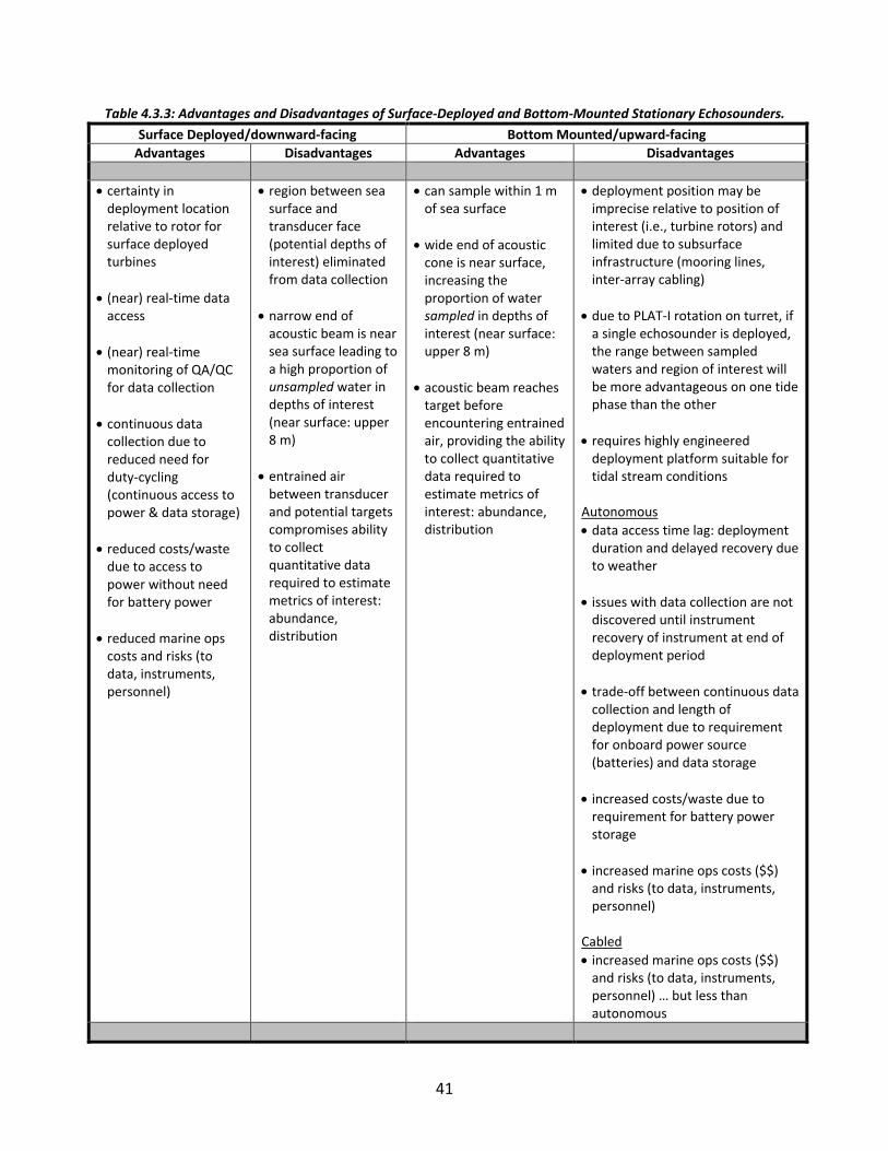
41

Table 4.3.3: Advantages and Disadvantages of Surface-Deployed and Bottom-Mounted Stationary Echosounders.

Surface Deployed/downward-facing Bottom Mounted/upward-facing

Advantages Disadvantages Advantages Disadvantages

• certainty in deployment location relative to rotor for surface deployed turbines

• (near) real-time data access

• (near) real-time monitoring of QA/QC for data collection

• continuous data collection due to reduced need for duty-cycling (continuous access to power & data storage)

• reduced costs/waste due to access to power without need for battery power

• reduced marine ops costs and risks (to data, instruments, personnel)

• region between sea surface and transducer face (potential depths of interest) eliminated from data collection

• narrow end of acoustic beam is near sea surface leading to a high proportion of unsampled water in depths of interest (near surface: upper 8 m)

• entrained air between transducer and potential targets compromises ability to collect quantitative data required to estimate metrics of interest: abundance, distribution

• can sample within 1 m of sea surface

• wide end of acoustic cone is near surface, increasing the proportion of water sampled in depths of interest (near surface: upper 8 m)

• acoustic beam reaches target before encountering entrained air, providing the ability to collect quantitative data required to estimate metrics of interest: abundance, distribution

• deployment position may be imprecise relative to position of interest (i.e., turbine rotors) and limited due to subsurface infrastructure (mooring lines, inter-array cabling)

• due to PLAT-I rotation on turret, if a single echosounder is deployed, the range between sampled waters and region of interest will be more advantageous on one tide phase than the other

• requires highly engineered deployment platform suitable for tidal stream conditions

Autonomous

• data access time lag: deployment duration and delayed recovery due to weather

• issues with data collection are not discovered until instrument recovery of instrument at end of deployment period

• trade-off between continuous data collection and length of deployment due to requirement for onboard power source (batteries) and data storage

• increased costs/waste due to requirement for battery power storage

• increased marine ops costs ($$) and risks (to data, instruments, personnel)

Cabled

• increased marine ops costs ($$) and risks (to data, instruments, personnel) … but less than autonomous

42

Study 2C Discussion The results of this study suggest that the extent of signal interference from air entrained due to turbulence is location specific, and a consequence of local hydrodynamic features in Grand Passage. This is consistent with previous work that found that the strong tidal currents in Grand Passage can be accompanied by high levels of turbulence resulting from the interaction of tidal currents with the channel’s bathymetric features and Peter’s Island (Hay 2017). While the extent of entrained air was strongly asymmetrical with tidal phase at the PLAT-I site, this was not observed for FAST site. Conversely, how ‘useable’ water column was defined did not alter the proportion of useable observation periods at the PLAT-I site, but strongly influenced the number of useable observation periods at the FAST site. Collectively, these results suggest that location-specific hydrodynamic regimes, and their influence on the collection of useable data, must be considered when selecting deployment sites for the collection of data required to meet analytical needs. Therefore, if the purpose of data collection is to document fish presence, abundance, and distribution throughout the tidal cycle (to meet regulatory expectations or satisfy ecosystem protection purposes), it is important to choose sites where the hydrodynamic regime does not preclude data collection for most or all of one tidal phase. If that is not feasible, then complementary data collection methods may be required to meet analytical requirements. However, this needs to be balanced against the possibility that a location with strong tidal phase turbulence asymmetry may be a site where data collection is suitable on the alternative tide phase (as found here). Under those circumstances, the analytical needs may require data collection at more than one location to obtain data to draw inferences when useable data cannot be obtained at the site of interest. Results of this study, and due consideration to the fundamental principles of hydroacoustics (Simmonds and MacLennan, 2005; Urick, 1983; Johannesson and Mitson, 1983; Coates, 1989), make it clear that maximizing the sampling volume and the collection of quantitative hydroacoustic data near the sea surface requires a bottom-mounted upward-facing echosounder. However, there are substantial trade-offs (logistical, operational) relative to a surface-deployed echosounder that require consideration, including increased costs and risks associated with subsea instrument deployment and recovery in tidal channels. When weighing deployment options, the purpose of the data collection campaign should be the driving force behind the decisions that are made. Otherwise, if the data is not collected in a way that satisfies the analytical requirements, the investment of resources in the data collection effort will have been wasted. The challenge is to correctly identify and weigh the trade-offs while prioritizing the data requirements for the purpose of the data collection effort.

4.4 Findings Specific to PLAT-I Rotor Swept Depth – Across All Three Studies The results of the by-ping analyses of the useable water in the upper 8 m of the water column are consistent with findings herein about site-specific hydrodynamic features (Table 4.4.1). The blue shaded cells highlight each tide phase and depth bin for which the proportion of useable

43

data was >50% of the pings collected within that tide phase. The shading intensifies in 10% increments as the proportion of useable pings increases. For the data collected at the PLAT-I site for Study 2C, there were no depth bins during the flood tide achieving 50% useable pings (shown as all white cells). However, for data collected on the ebb tide, every visible depth bin (4 - 8 m) is shaded blue with the useable proportion of pings increasing with depth (blue shading intensifies: 71% to 89% useable). The tidal asymmetry at the PLAT-I site is readily apparent and may be due to turbulence from Peter’s Island. Conversely, the data collected at the FAST site for Study 2C shows a general absence of tidal asymmetry and is evident in the equivalent shading of the depth bins on the flood and ebb tides. At the FAST site for Study 2A (when the FAST platform was much closer to the PLAT-I), the tide phase asymmetry is clearly evident, although the useable data never achieved 50% on either tide phase within the top 8 m of the water column. However, readers should note that the useable proportion of pings was generally an order of magnitude greater on the ebb than on the flood tide. At the FAST site during Study 2B, the tidal asymmetry is still evident, but not as strong as the asymmetry at the site for Study 2A.

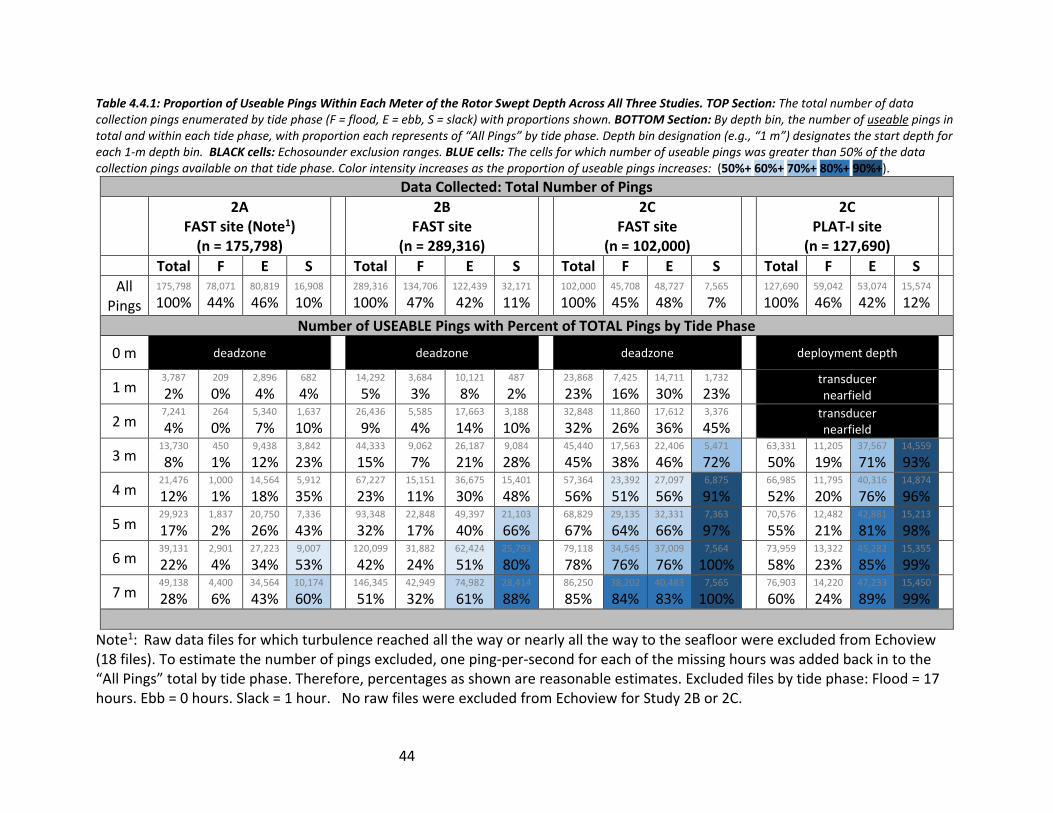
44

Table 4.4.1: Proportion of Useable Pings Within Each Meter of the Rotor Swept Depth Across All Three Studies. TOP Section: The total number of data collection pings enumerated by tide phase (F = flood, E = ebb, S = slack) with proportions shown. BOTTOM Section: By depth bin, the number of useable pings in total and within each tide phase, with proportion each represents of “All Pings” by tide phase. Depth bin designation (e.g., “1 m”) designates the start depth for each 1-m depth bin. BLACK cells: Echosounder exclusion ranges. BLUE cells: The cells for which number of useable pings was greater than 50% of the data collection pings available on that tide phase. Color intensity increases as the proportion of useable pings increases: (50%+ 60%+ 70%+ 80%+ 90%+).

Data Collected: Total Number of Pings

2A

FAST site (Note1) (n = 175,798)

2B

FAST site (n = 289,316)

2C

FAST site (n = 102,000)

2C

PLAT-I site (n = 127,690)

Total F E S Total F E S Total F E S Total F E S

All Pings

175,798

100% 78,071

44% 80,819

46% 16,908

10% 289,316

100% 134,706

47% 122,439

42% 32,171

11% 102,000

100% 45,708

45% 48,727

48% 7,565

7% 127,690

100% 59,042

46% 53,074

42% 15,574

12%

Number of USEABLE Pings with Percent of TOTAL Pings by Tide Phase

0 m deadzone deadzone deadzone deployment depth

1 m 3,787

2% 209

0% 2,896

4% 682

4% 14,292

5% 3,684

3% 10,121

8% 487

2% 23,868

23% 7,425

16% 14,711

30% 1,732

23% transducer nearfield

2 m 7,241

4% 264

0% 5,340

7% 1,637

10% 26,436

9% 5,585

4% 17,663

14% 3,188

10% 32,848

32% 11,860

26% 17,612

36% 3,376

45% transducer nearfield

3 m 13,730

8% 450

1% 9,438

12% 3,842

23% 44,333

15% 9,062

7% 26,187

21% 9,084

28% 45,440

45% 17,563

38% 22,406

46% 5,471

72% 63,331

50% 11,205

19% 37,567

71% 14,559

93%

4 m 21,476

12% 1,000

1% 14,564

18% 5,912

35% 67,227

23% 15,151

11% 36,675

30% 15,401

48% 57,364

56% 23,392

51% 27,097

56% 6,875

91% 66,985

52% 11,795

20% 40,316

76% 14,874

96%

5 m 29,923

17% 1,837

2% 20,750

26% 7,336

43% 93,348

32% 22,848

17% 49,397

40% 21,103

66% 68,829

67% 29,135

64% 32,331

66% 7,363

97% 70,576

55% 12,482

21% 42,881

81% 15,213

98%

6 m 39,131

22% 2,901

4% 27,223

34% 9,007

53% 120,099

42% 31,882

24% 62,424

51% 25,793

80% 79,118

78% 34,545

76% 37,009

76% 7,564

100% 73,959

58% 13,322

23% 45,282

85% 15,355

99%

7 m 49,138

28% 4,400

6% 34,564

43% 10,174

60% 146,345

51% 42,949

32% 74,982

61% 28,414

88% 86,250

85% 38,202

84% 40,483

83% 7,565

100% 76,903

60% 14,220

24% 47,233

89% 15,450

99%

Note1: Raw data files for which turbulence reached all the way or nearly all the way to the seafloor were excluded from Echoview (18 files). To estimate the number of pings excluded, one ping-per-second for each of the missing hours was added back in to the “All Pings” total by tide phase. Therefore, percentages as shown are reasonable estimates. Excluded files by tide phase: Flood = 17 hours. Ebb = 0 hours. Slack = 1 hour. No raw files were excluded from Echoview for Study 2B or 2C.

45

Rotor Swept Depth Discussion For the echosounder data collected during the studies reported herein, the results of the useable data analyses by 1-m depth bins within the top 8 m of the water column were consistent with the earlier results suggesting site-specific hydrodynamic regimes. The contrasts among the results demonstrate that it is not only important to understand the hydrodynamic regime among sites, but also in the depth range of interest. The implication is that none of these sites on either tide phase would have facilitated the collection of 100% useable data within the 8-m depths of interest. However, some sites are more favorable than others, and criteria for site selection, based on some minimum acceptable proportion of useable pings, should be defined by tidal phase and documented during the site selection process.

5 Conclusions These studies were designed to assess the efficacy of bottom-mounted and surface-deployed echosounders for target detections and to help guide best practices for monitoring in high flow environments. In all three studies the bottom-mounted echosounder detected targets consistent with the presence of fish in the portion of the water column not obscured by entrained air. However, the optical camera and the imaging sonar failed to provide data by which to corroborate target identity. This may have partially resulted from non-overlapping sampling volumes between the instruments. However, the repositioning of the bottom-mounted echosounder between studies was fortuitous in the sense that it facilitated examination of how turbulence varies in space, and lead to new insights about the implications of hydrodynamics for data collection. Specifically, knowledge of local hydrodynamics is important in site selection for data collection campaigns and for meeting analytical needs to meet regulatory needs or expectations or to satisfy ecosystem protection purposes. In addition to selecting site location for echosounder deployment, there are trade-offs inherent in selecting the positioning of the echosounder at the site (e.g., surface-deployed downward-facing versus bottom-mounted upward-facing). The trade-offs include implications for data collection (e.g., maximizing volume sampled at the depths of interest, recording echo returns that are uncontaminated by the presence of entrained air between the transducer and the targets of interest) and logistical, financial, and operational considerations. Although trade-offs must be weighed when making deployment decisions, the purpose of investing time, money, and resources towards data collection must be the driving motivation for those decisions. The challenge is to correctly identify and weigh these trade-offs while keeping the data requirements for the purpose of the data collection firmly in mind.

46

6 References Chen, C., and Beardsley, R.C. (2011). An Unstructured Grid, Finite-Volume Coastal Ocean Model.

SMAST/UMASSD-11-1101. http://fvcomo.smast.umassd.edu/fvcom/

Coates, R.F.W. (1989). Underwater Acoustic Systems. Wiley & Sons, Inc. New York. Fernandes, P.G., Gerlatto, F., Holliday, D.V., Nakken, D.V., and Simmonds, E.J. (2002). Acoustic

applications in fisheries science: the ICES contribution. ICES Marine Science Symposia 215: 483-492.

Fisheries and Ocean Canada (1996). Krill on the Scotian Shelf. Stock status report 96/106E.

Catalogue number Fs76-1/1996-106E-PDF.

Fraser, S., Nikora, V., Williamson, B.J., and Scott, B.E. (2017). Automatic active acoustic target detection in turbulent aquatic environments. Limnol. Oceanogr. Methods 15(2): 184-199.

Guerra, M., Hay, A.E., Cheel, R.A., Trowse, G., and Karsten R. (2019). Turbulent flow mapping around a floating in-stream tidal energy platform, in: Proc. of the 13th European Wave and Tidal Energy Conference, Napoli, Italy.

Hastie, G.D., Bivins, M., Coram, A., Gordon, J., Jepp, P., MacAulay, J., Sparling C., and Gillespie, D. (2019a). Three-dimensional movements of harbour seals in a tidally energetic channel: Application of a novel sonar tracking system. Aquatic Conservation: Marine and Freshwater Ecosystems 29(4), 564-575.

Hastie, G.D., Wu, G.-M., Moss, S., Jepp, P., MacAulay, J., Lee, A., Sparling, C.E., Evers, C., and

Gillespie, D. (2019b). Automated detection and tracking of marine mammals: A novel sonar tool for monitoring effects of marine industry. Aquatic Conservation: Marine and Freshwater Ecosystems 29(S1), 119-130.

Hay, A. (2017). Turbulence in Grand Passage, Nova Scotia: Measures of Intermittency. Report

submitted to Offshore Energy Research Association.

Johannesson, K.A. and Mitson, R.B. (1983). Fisheries Acoustics: A practical manual for aquatic biomass estimation. FAO Fisheries Technical Paper 240. Food and Agriculture Organization of the United Nations. Rome.

Love, R.H. (1971). Measurements of Fish Target Strength: A Review. Fishery Bulletin 69(4): 703-

715.

47

Lowe, S.C. and McGarry, L.P. (2020). Echofilter Usage Guide Release 1.0.0. Submitted to Offshore Energy Research Association and the Pathway Program.

MacKenzie, K.V. (1981). Nine-term equation for sound speed in the ocean. Journal of the Acoustical Society of America. 70: 807-812. https://doi.org/10.1121/1.38690

McGarry, L.P., Douglas, J., and Lowe, S. (2020). Improving Automated Post-Processing of

Echosounder Data with Machine Learning Models. Report submitted to Offshore Energy Research Association and the Pathway Program.

McMillan, J., Hay, A., Karsten, R., Trowse, G., Schillinger, D., and O’Flaherty-Sproul, M. (2013). Comprehensive tidal energy resource assessment in the lower Bay of Fundy, Canada, in: Proc. 10th European Wave and Tidal Energy Conference.

Mueller, R.P., Brown, R.S., Hop, H., and Moulton, L. (2006). Video and acoustic camera techniques for studying fish under ice: a review and comparison. Reviews in Fish Biology and Fisheries 16(2): 213-226.

O’Flaherty-Sproul, M. (2012). New high and low resolution numerical models of the tidal

current through the Digby Neck passages, Master’s thesis, Acadia University.

R Core Team (2020). R: A Language and Environment for Statistical Computing. R Foundation for Statistical Computing, Vienna, Austria. https://www.R-project.org.

Simmonds, J. and MacLennan, D. (2005). Fisheries Acoustics Theory and Practice, 2nd edition.

Blackwell Publishing, Oxford, UK.

Simrad (2020). Simrad EK80 Scientific Wide Band Echo Sounder Reference Manual (395234/H). Kongsberg Maritime AS.

Urick, R.J. (1983). Principles of Underwater Sound, 3rd edition. Peninsula Publishing, Los Altos,

California. Viehman, H.A., and Zydlewski, G.B. (2014). Fish Interactions with a Commercial-Scale Tidal

Energy Device in the Natural Environment. Estuaries and Coasts 38(Suppl 1): S241-252.

Viehman, H., Hasselman, D., Boucher, T., Douglas, J., and Bennett, L. (2019). Integrating Hydroacoustic Approaches to Predict Fish Interactions with In-stream Tidal Turbines. Report submitted to Fundy Ocean Research Center for Energy. Project number 300-208.

Williamson, B., Fraser, S., Blondel, P., Bell, P., Waggitt, J., and Scott B. (2016a). Integrating a

multibeam and multifrequency echosounder on the FLOWBEC seabed platform to track fish and seabird behavior around tidal turbine structures. In 4th Marine Energy Technology Symposium (METS). Washington, D.C. p.5.

48

Williamson, B., Blondel, P., Armstrong, E., Bell, P.S., Hall, C., Waggitt, J.J., and Scott, B.E. (2016b). A Self-Contained Subsea Platform for Acoustic Monitoring of the Environment Around Marine Renewable Energy Devices – Field Deployment at Wave and Tidal Energy Sites in Orkney, Scotland. IEEE Journal of Oceanic Engineering 41(1): 67-81.

Williamson, B., Fraser, S., Blondel, P., Bell, P.S., Waggitt, J.J., and Scott, B.E. (2017). Multisensor

Acoustic Tracking of Fish and Seabird Behavior Around Tidal Turbine Structures in Scotland. IEEE Journal of Oceanic Engineering 42(4): 948-965.

49

Appendix A. Envirosphere Consultants Limited: Review of Underwater Video

 

 

 

 

   

Review of Underwater Videos from  Grand Passage, Nova Scotia—  Test Videos December 2019‐January 2020   

Prepared for: 

Fundy Ocean Research Center for Energy 1690 Hollis Street, Unit 1001 Halifax, Nova Scotia B3J 1V7 

Prepared by: 

Envirosphere Consultants Limited   120 Morison Drive, Windsor Nova Scotia Unit 5 B0N 2T0  902 798 4022 | enviroco@ns.sympatico.ca | www.envirosphere.ca 

March 12, 2020 

Review of Underwater Videos from Grand Passage  

Fundy Ocean Research Centre for Energy (FORCE) – March 2020    1 

 

Envirosphere Consultants Limited 120‐5 Morison Drive, Windsor, Nova Scotia B0N 2T0 | 902 798 4022 | enviroco@ns.sympatico.ca | www.envirosphere.ca 

EXECUTIVE SUMMARY  As part of a test program for an underwater acoustic imaging sonar, the Fundy Ocean Research Centre 

for Energy (FORCE) recorded underwater video from a camera co‐located and coincident with the sonar 

equipment. Envirosphere Consultants Limited screened the approximately 170 hours of video for the 

occurrence of fish and other large marine organisms. No fish were observed. Videos were clear enough 

to determine occurrence of fish (if present), tidal state, and presence of detritus and detritus as well as 

occasional marine invertebrate organisms.   

INTRODUCTION AND BACKGROUND The Fundy Ocean Research Centre for Energy (FORCE) has been participating in tests of acoustic imaging 

equipment  intended  for monitoring movements  and  behaviour  of  fish  around  instream  tidal  energy 

devices. Its participation has included use of underwater video equipment (a Deep Blue surface‐connected 

underwater camera system) deployed in the vicinity of an experimental acoustic imaging sonar, in Grand 

Passage, Digby Neck, Nova Scotia. The project was  intended to provide  information to  identify targets 

potentially occurring in the vicinity, to assist in interpreting the sonar record.  Video records were obtained 

in experiments in December 2019 (primary data collection period) and for a short period in February 2020. 

Videos obtained were submitted to Envirosphere Consultants Limited, a marine environmental consultant 

located in Windsor, Nova Scotia, which has experience in underwater video interpretation, for review and 

documentation. 

METHODOLOGY Videos  for both periods  (December 2019 and February 2020) were provided on portable hard drives. 

Videos were  typically  fifteen minutes  long but occasionally  longer  (up  to 30 minutes) or  shorter  (1‐2 

minutes), a period presumably set by the video capture system. The majority were recorded in daylight; 

however  some night periods were  captured but were disregarded  in  the  analysis. The  camera had a 

‘normal’  perspective  and  field  of  view,  so  that  targets  at  some  distance would  be  detected  (FORCE 

personal communication). 

Video was viewed in the VLC video viewer (VLC is an open‐source media player made by the VideoLAN 

organization—www.videolan.org)  on  personal  computers with  the MicroSoft Windows  10  operating 

system.  VLC allows viewing to be speeded up without loss of frames and a speed of 2x was typically used 

in viewing. Initially the video was viewed at normal speed, but it was almost immediately decided to use 

a faster speed, particularly since it was discovered that there was little in the videos, to ensure the project 

could be completed within timelines required.  Also initially, image captures were made of miscellaneous 

objects (e.g. seaweed, objects thought to be jellyfish, detritus etc.), but the practice was excessively time‐

consuming and was dropped after approximately the second day. Occasionally videos were examined by 

another member of the team, with a view to  locating and capturing  images to  illustrate miscellaneous 

objects seen in the videos.  

For each video viewed, the viewer recorded the file name on paper, and any observations. FORCE had 

provided an Excel spreadsheet  listing  the  file names,  the  times and durations of  the videos. The data 

logging system had an intrinsic start date and time, which was translated to actual dates and times using 

a conversion factor provided by FORCE.  The list of videos also indicated the video clips obtained at night 

Review of Underwater Videos from Grand Passage  

Fundy Ocean Research Centre for Energy (FORCE) – March 2020    2 

 

Envirosphere Consultants Limited 120‐5 Morison Drive, Windsor, Nova Scotia B0N 2T0 | 902 798 4022 | enviroco@ns.sympatico.ca | www.envirosphere.ca 

and  therefore which were  to  be  omitted.  Videos were  in MP4  video  format.  The  video  record was 

continuous over the times analyzed.  

RESULTS 

Occurrence of Fish Video coverage consisted of approximately 150 hours of video in 755 separate clips, typically 15‐minutes 

in duration,  as well as 152  clips  taken overnight  (the  latter were not examined). None of  the  videos 

detected fish or other large organisms. 

Occurrence of Miscellaneous Objects Miscellaneous objects seen included seaweeds, bubbles, objects thought to be jellyfish, detritus, krill, and 

other plankton (Figures 1‐20).  

General Quality of Video Typically  the video captured  the movements of particles, bubbles and other objects suspended  in  the 

water in the camera’s field of view. Tidal motion could be observed by the movement towards or away 

from the camera of particles, or periods of slack tide. Images were mostly grey although changes in colour 

could be observed in individual video clips, including brief shifts to ‘warmer’ tones (yellowish or orange) 

thought  to be  changes  in  sunlight  reaching  the water  surface.  In most videos, due  to  the absence of 

reference points, it was not possible to assess the field of view. However several of the objects captured 

in images were estimated to be at several metres distance (e.g. see Figure 15 & 16), indicating that the 

camera was adequately covering the required field of view.  At times, objects passing through appeared 

to be coloured due to the  incident light, while some objects, for example those thought to be jellyfish, 

were naturally reddish. Ctenophores were bright reflective white. A red seaweed, as well as an euphausiid 

(krill) caught in one of the images were their natural colour.  

Conclusions and Recommendations The video was of sufficient quality to detect  fish and  larger organisms  in  the  field of view.    It did not, 

however, include reference points or scales (for example part of a physical device or a ruler) to assist in 

determining size of objects if observed, and it is suggested that this be attempted in future.  

Positioning of the camera, which appears to have a horizontal field of view, may not be ideal for detecting 

fish furthest from it, due to overall turbidity and presence of particles in the water. Orienting the camera 

towards the water surface, which would appear bright from below, may improve the detection of distant 

occurrences of fish.  

The  frame rate and compression used  in producing MP4  files  from  the video excessively blurs objects 

occurring  near  the  camera,  although more  distant  objects  were  clear.  Occurrence  of  large  objects 

including fish can probably readily be detected both near and at some distance from the camera. 

   

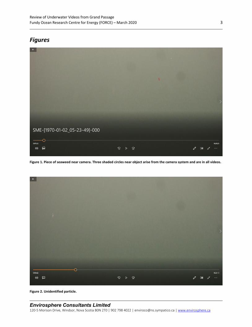
Review of Underwater Videos from Grand Passage  

Fundy Ocean Research Centre for Energy (FORCE) – March 2020    3 

 

Envirosphere Consultants Limited 120‐5 Morison Drive, Windsor, Nova Scotia B0N 2T0 | 902 798 4022 | enviroco@ns.sympatico.ca | www.envirosphere.ca 

Figures 

 

Figure 1. Piece of seaweed near camera. Three shaded circles near object arise from the camera system and are in all videos. 

 

 

Figure 2. Unidentified particle. 

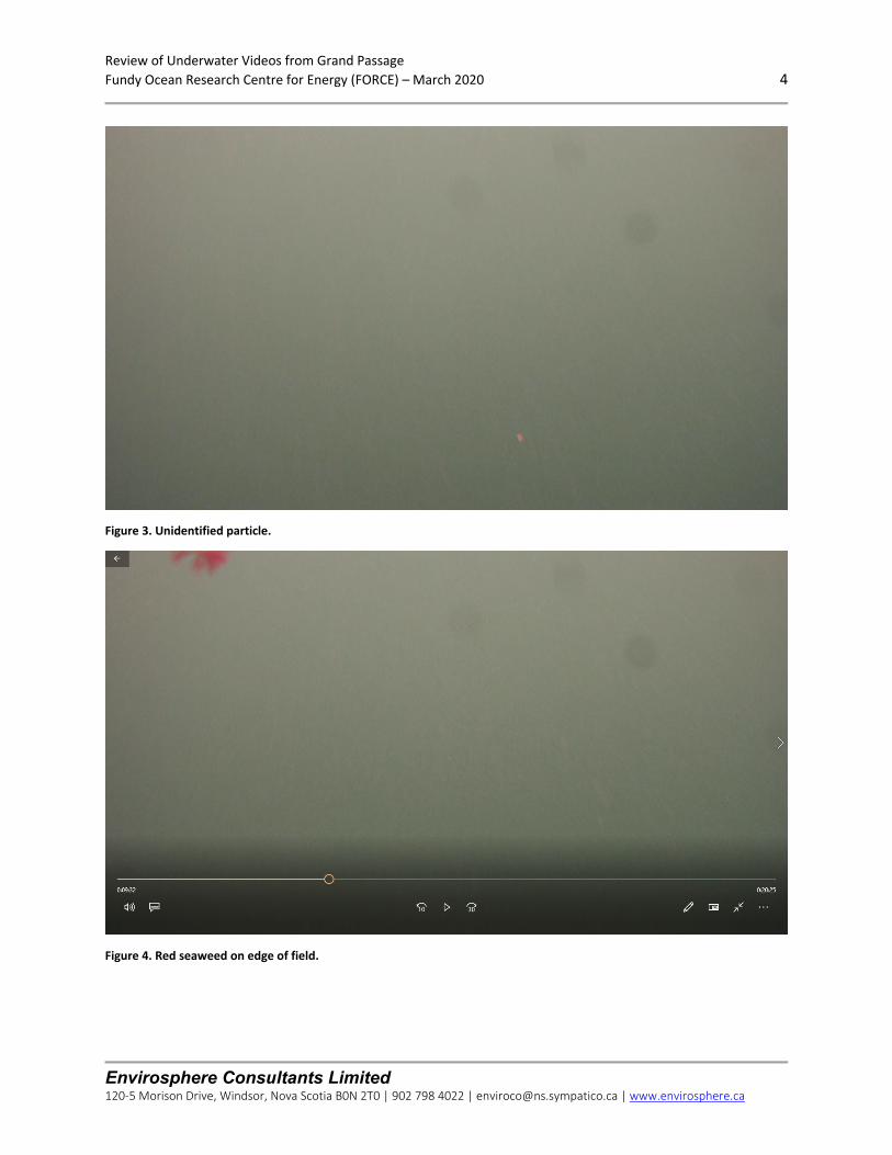
Review of Underwater Videos from Grand Passage  

Fundy Ocean Research Centre for Energy (FORCE) – March 2020    4 

 

Envirosphere Consultants Limited 120‐5 Morison Drive, Windsor, Nova Scotia B0N 2T0 | 902 798 4022 | enviroco@ns.sympatico.ca | www.envirosphere.ca 

 

Figure 3. Unidentified particle. 

 

Figure 4. Red seaweed on edge of field. 

 

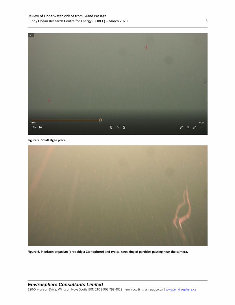
Review of Underwater Videos from Grand Passage  

Fundy Ocean Research Centre for Energy (FORCE) – March 2020    5 

 

Envirosphere Consultants Limited 120‐5 Morison Drive, Windsor, Nova Scotia B0N 2T0 | 902 798 4022 | enviroco@ns.sympatico.ca | www.envirosphere.ca 

 

Figure 5. Small algae piece. 

 

Figure 6. Plankton organism (probably a Ctenophore) and typical streaking of particles passing near the camera. 

 

Review of Underwater Videos from Grand Passage  

Fundy Ocean Research Centre for Energy (FORCE) – March 2020    6 

 

Envirosphere Consultants Limited 120‐5 Morison Drive, Windsor, Nova Scotia B0N 2T0 | 902 798 4022 | enviroco@ns.sympatico.ca | www.envirosphere.ca 

 

Figure 7. Plankton organism (upper left), probably Ctenophore) passing near camera. 

 

Figure 8. Piece of seaweed. 

 

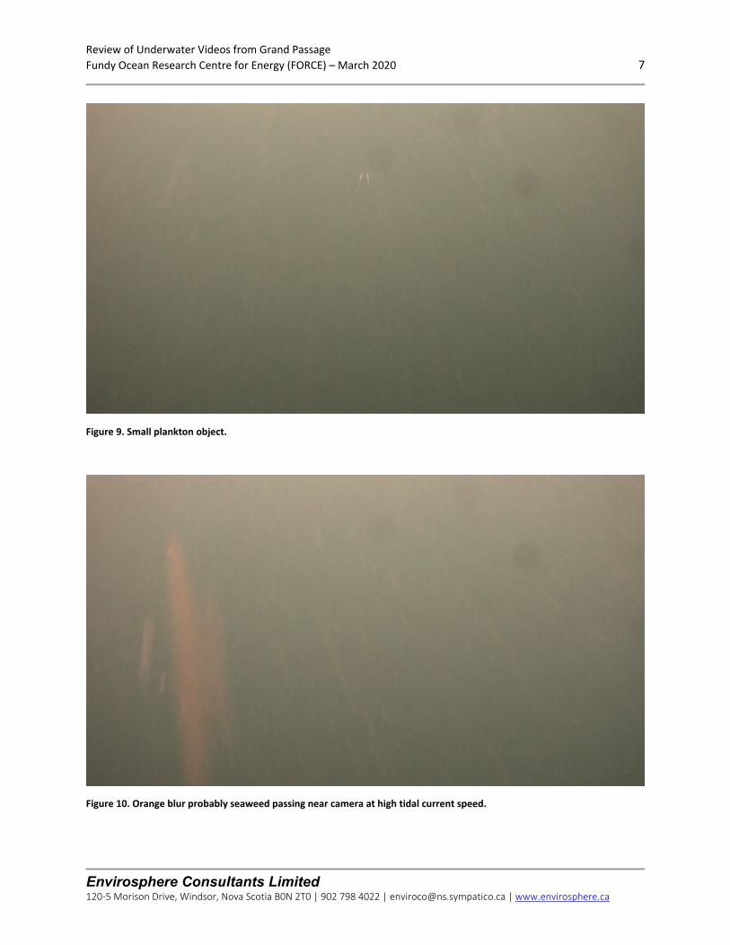
Review of Underwater Videos from Grand Passage  

Fundy Ocean Research Centre for Energy (FORCE) – March 2020    7 

 

Envirosphere Consultants Limited 120‐5 Morison Drive, Windsor, Nova Scotia B0N 2T0 | 902 798 4022 | enviroco@ns.sympatico.ca | www.envirosphere.ca 

 

Figure 9. Small plankton object. 

 

 

Figure 10. Orange blur probably seaweed passing near camera at high tidal current speed. 

 

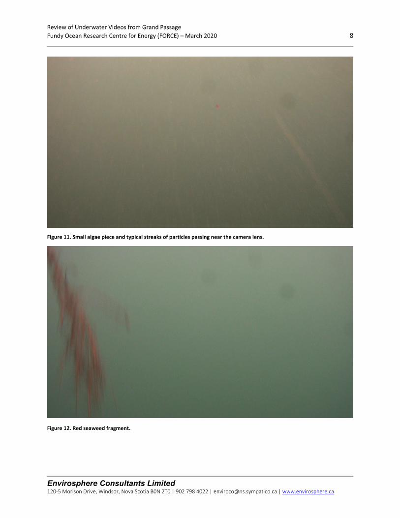
Review of Underwater Videos from Grand Passage  

Fundy Ocean Research Centre for Energy (FORCE) – March 2020    8 

 

Envirosphere Consultants Limited 120‐5 Morison Drive, Windsor, Nova Scotia B0N 2T0 | 902 798 4022 | enviroco@ns.sympatico.ca | www.envirosphere.ca 

 

Figure 11. Small algae piece and typical streaks of particles passing near the camera lens. 

 

Figure 12. Red seaweed fragment. 

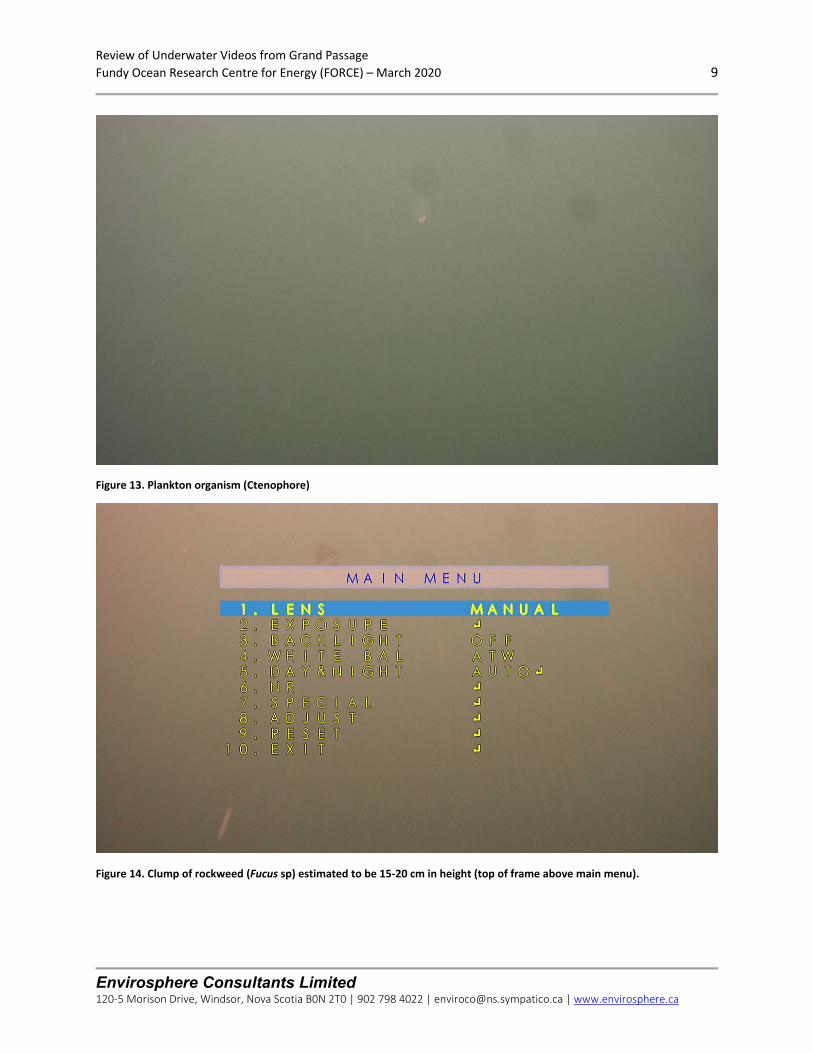
Review of Underwater Videos from Grand Passage  

Fundy Ocean Research Centre for Energy (FORCE) – March 2020    9 

 

Envirosphere Consultants Limited 120‐5 Morison Drive, Windsor, Nova Scotia B0N 2T0 | 902 798 4022 | enviroco@ns.sympatico.ca | www.envirosphere.ca 

 

Figure 13. Plankton organism (Ctenophore) 

 

Figure 14. Clump of rockweed (Fucus sp) estimated to be 15‐20 cm in height (top of frame above main menu).  

Review of Underwater Videos from Grand Passage  

Fundy Ocean Research Centre for Energy (FORCE) – March 2020    10 

 

Envirosphere Consultants Limited 120‐5 Morison Drive, Windsor, Nova Scotia B0N 2T0 | 902 798 4022 | enviroco@ns.sympatico.ca | www.envirosphere.ca 

 

Figure 15. Same clump of rockweed (Fucus sp) as in Figure 14 passing by camera. 

 

Figure 16. Plankton (euphausiid (krill) (upper left). 

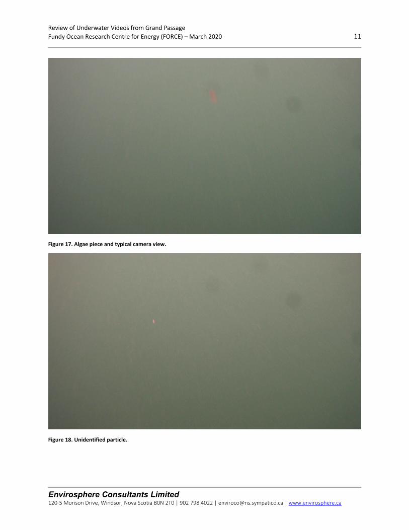
Review of Underwater Videos from Grand Passage  

Fundy Ocean Research Centre for Energy (FORCE) – March 2020    11 

 

Envirosphere Consultants Limited 120‐5 Morison Drive, Windsor, Nova Scotia B0N 2T0 | 902 798 4022 | enviroco@ns.sympatico.ca | www.envirosphere.ca 

 

Figure 17. Algae piece and typical camera view. 

 

Figure 18. Unidentified particle. 

 

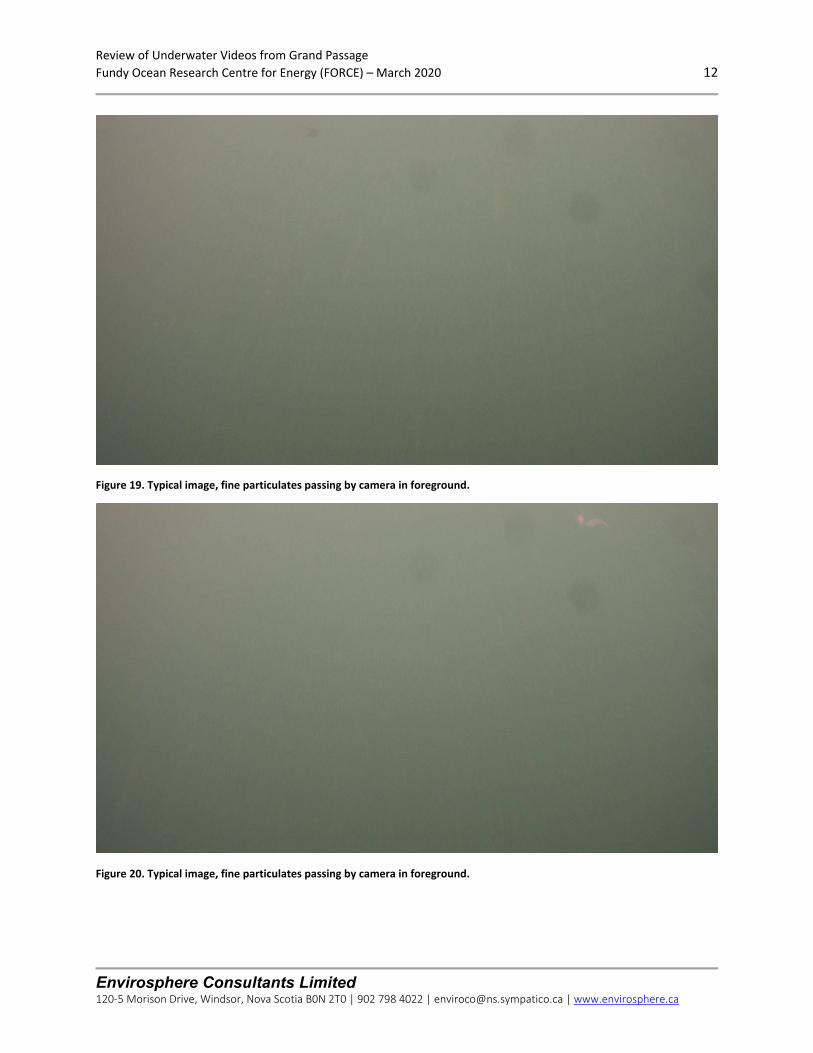
Review of Underwater Videos from Grand Passage  

Fundy Ocean Research Centre for Energy (FORCE) – March 2020    12 

 

Envirosphere Consultants Limited 120‐5 Morison Drive, Windsor, Nova Scotia B0N 2T0 | 902 798 4022 | enviroco@ns.sympatico.ca | www.envirosphere.ca 

 

Figure 19. Typical image, fine particulates passing by camera in foreground. 

 

Figure 20. Typical image, fine particulates passing by camera in foreground. 

 

 

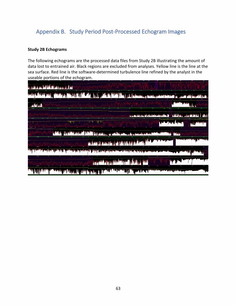
  63 

Appendix B.  Study Period Post‐Processed Echogram Images   Study 2B Echograms  The following echograms are the processed data files from Study 2B illustrating the amount of data lost to entrained air. Black regions are excluded from analyses. Yellow line is the line at the sea surface. Red line is the software‐determined turbulence line refined by the analyst in the useable portions of the echogram.  

 

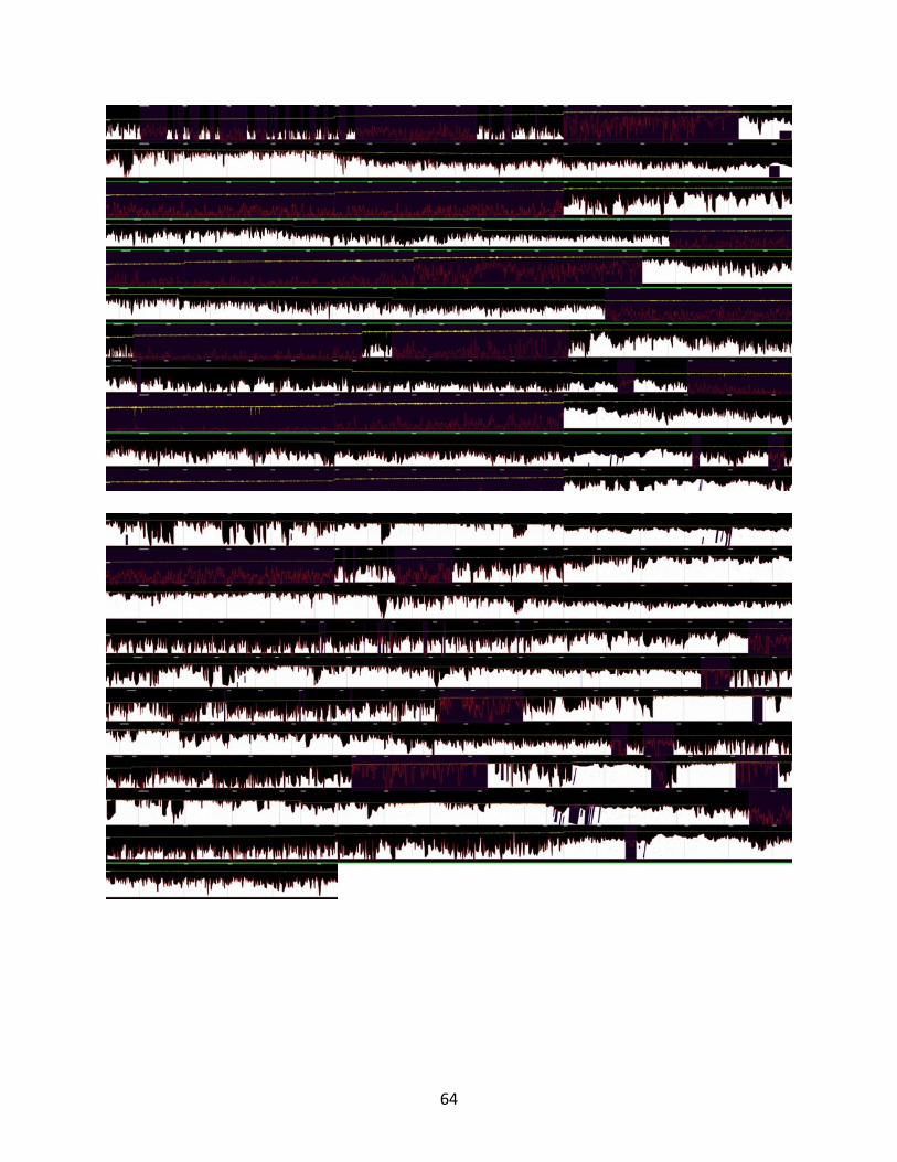
  64 

  

  

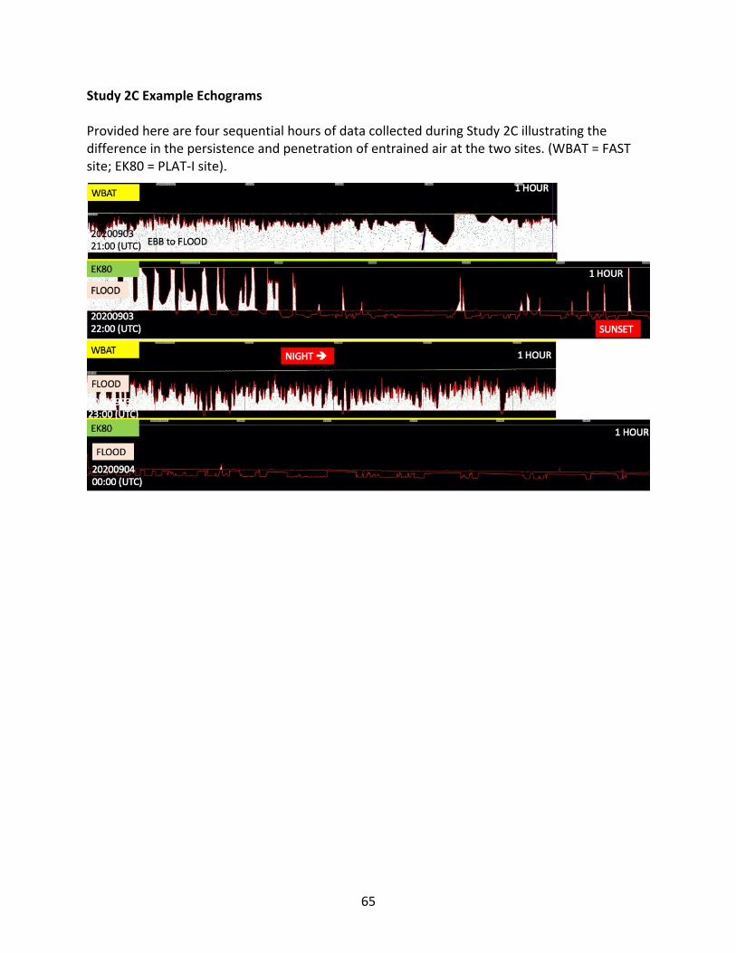
  65 

Study 2C Example Echograms  Provided here are four sequential hours of data collected during Study 2C illustrating the difference in the persistence and penetration of entrained air at the two sites. (WBAT = FAST site; EK80 = PLAT‐I site). 

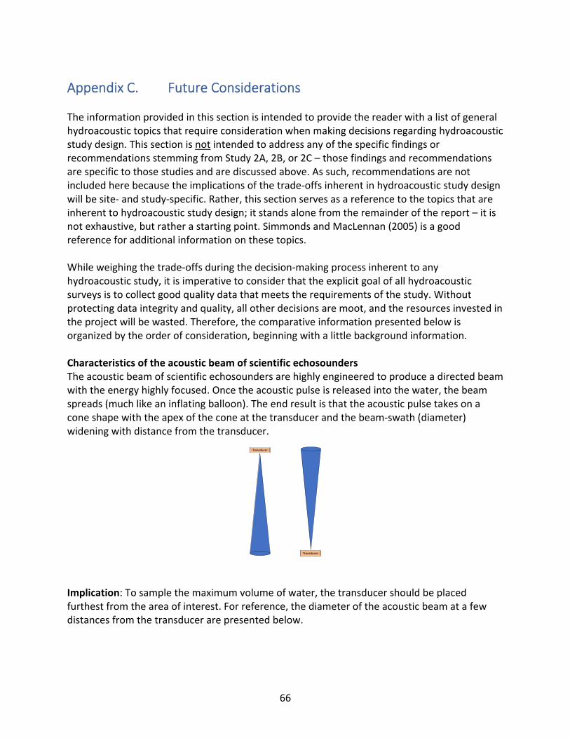
  66 

Appendix C.  Future Considerations   The information provided in this section is intended to provide the reader with a list of general hydroacoustic topics that require consideration when making decisions regarding hydroacoustic study design. This section is not intended to address any of the specific findings or recommendations stemming from Study 2A, 2B, or 2C – those findings and recommendations are specific to those studies and are discussed above. As such, recommendations are not included here because the implications of the trade‐offs inherent in hydroacoustic study design will be site‐ and study‐specific. Rather, this section serves as a reference to the topics that are inherent to hydroacoustic study design; it stands alone from the remainder of the report – it is not exhaustive, but rather a starting point. Simmonds and MacLennan (2005) is a good reference for additional information on these topics.   While weighing the trade‐offs during the decision‐making process inherent to any hydroacoustic study, it is imperative to consider that the explicit goal of all hydroacoustic surveys is to collect good quality data that meets the requirements of the study. Without protecting data integrity and quality, all other decisions are moot, and the resources invested in the project will be wasted. Therefore, the comparative information presented below is organized by the order of consideration, beginning with a little background information.  Characteristics of the acoustic beam of scientific echosounders The acoustic beam of scientific echosounders are highly engineered to produce a directed beam with the energy highly focused. Once the acoustic pulse is released into the water, the beam spreads (much like an inflating balloon). The end result is that the acoustic pulse takes on a cone shape with the apex of the cone at the transducer and the beam‐swath (diameter) widening with distance from the transducer. 

  Implication: To sample the maximum volume of water, the transducer should be placed furthest from the area of interest. For reference, the diameter of the acoustic beam at a few distances from the transducer are presented below.    

Transducer

Transducer

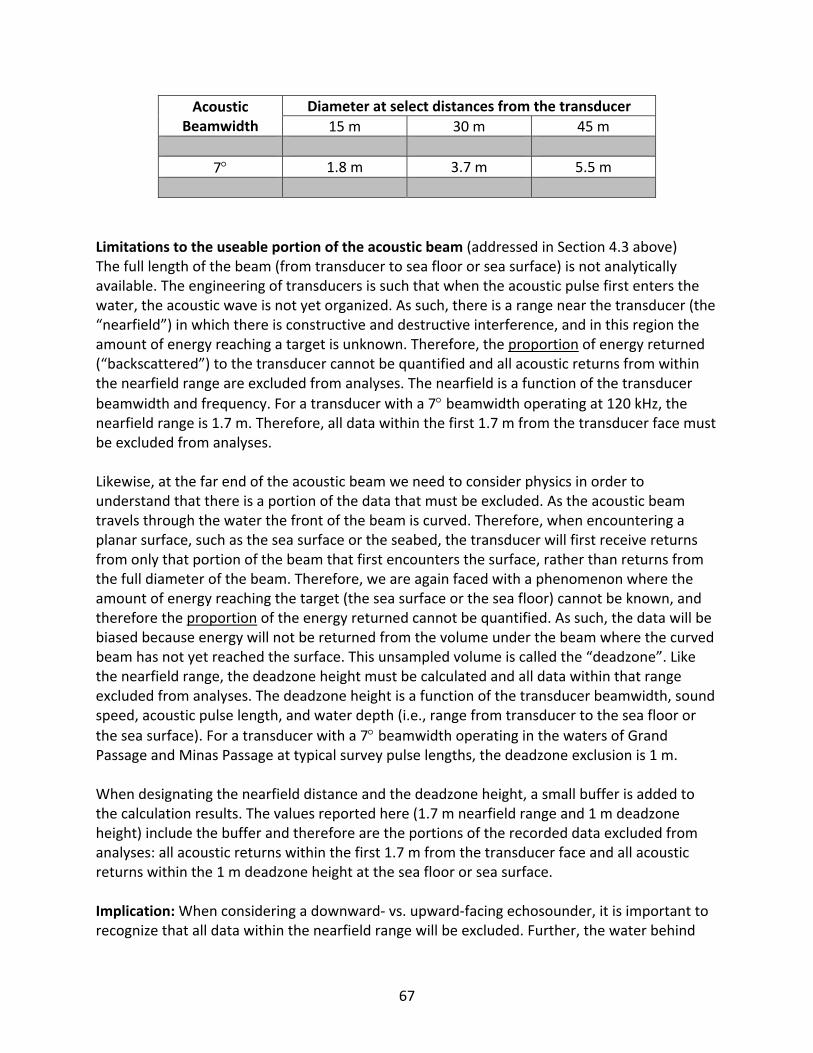
  67 

Acoustic Beamwidth 

Diameter at select distances from the transducer 

15 m  30 m  45 m 

       

7  1.8 m  3.7 m  5.5 m 

       

  Limitations to the useable portion of the acoustic beam (addressed in Section 4.3 above) The full length of the beam (from transducer to sea floor or sea surface) is not analytically available. The engineering of transducers is such that when the acoustic pulse first enters the water, the acoustic wave is not yet organized. As such, there is a range near the transducer (the “nearfield”) in which there is constructive and destructive interference, and in this region the amount of energy reaching a target is unknown. Therefore, the proportion of energy returned (“backscattered”) to the transducer cannot be quantified and all acoustic returns from within the nearfield range are excluded from analyses. The nearfield is a function of the transducer 

beamwidth and frequency. For a transducer with a 7 beamwidth operating at 120 kHz, the nearfield range is 1.7 m. Therefore, all data within the first 1.7 m from the transducer face must be excluded from analyses.  Likewise, at the far end of the acoustic beam we need to consider physics in order to understand that there is a portion of the data that must be excluded. As the acoustic beam travels through the water the front of the beam is curved. Therefore, when encountering a planar surface, such as the sea surface or the seabed, the transducer will first receive returns from only that portion of the beam that first encounters the surface, rather than returns from the full diameter of the beam. Therefore, we are again faced with a phenomenon where the amount of energy reaching the target (the sea surface or the sea floor) cannot be known, and therefore the proportion of the energy returned cannot be quantified. As such, the data will be biased because energy will not be returned from the volume under the beam where the curved beam has not yet reached the surface. This unsampled volume is called the “deadzone”. Like the nearfield range, the deadzone height must be calculated and all data within that range excluded from analyses. The deadzone height is a function of the transducer beamwidth, sound speed, acoustic pulse length, and water depth (i.e., range from transducer to the sea floor or 

the sea surface). For a transducer with a 7 beamwidth operating in the waters of Grand Passage and Minas Passage at typical survey pulse lengths, the deadzone exclusion is 1 m.  When designating the nearfield distance and the deadzone height, a small buffer is added to the calculation results. The values reported here (1.7 m nearfield range and 1 m deadzone height) include the buffer and therefore are the portions of the recorded data excluded from analyses: all acoustic returns within the first 1.7 m from the transducer face and all acoustic returns within the 1 m deadzone height at the sea floor or sea surface.  Implication: When considering a downward‐ vs. upward‐facing echosounder, it is important to recognize that all data within the nearfield range will be excluded. Further, the water behind 

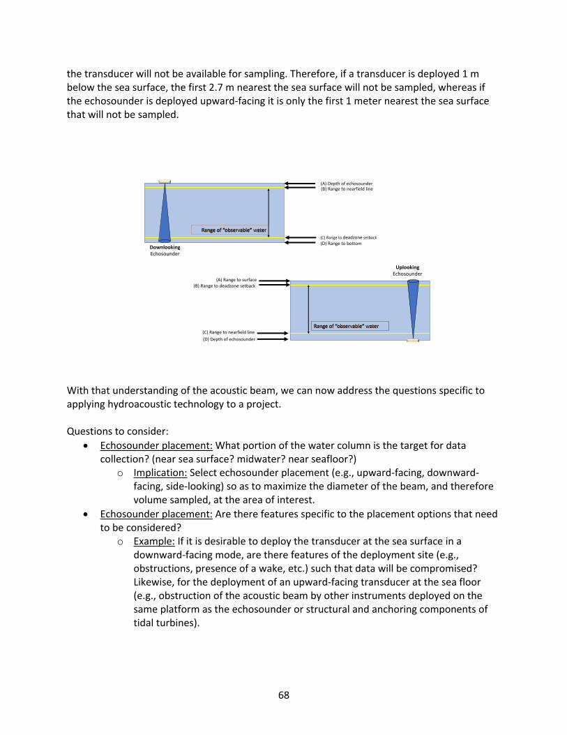
  68 

the transducer will not be available for sampling. Therefore, if a transducer is deployed 1 m below the sea surface, the first 2.7 m nearest the sea surface will not be sampled, whereas if the echosounder is deployed upward‐facing it is only the first 1 meter nearest the sea surface that will not be sampled.     

    With that understanding of the acoustic beam, we can now address the questions specific to applying hydroacoustic technology to a project.  Questions to consider: 

Echosounder placement: What portion of the water column is the target for data collection? (near sea surface? midwater? near seafloor?) 

o Implication: Select echosounder placement (e.g., upward‐facing, downward‐facing, side‐looking) so as to maximize the diameter of the beam, and therefore volume sampled, at the area of interest. 

Echosounder placement: Are there features specific to the placement options that need to be considered? 

o Example: If it is desirable to deploy the transducer at the sea surface in a downward‐facing mode, are there features of the deployment site (e.g., obstructions, presence of a wake, etc.) such that data will be compromised? Likewise, for the deployment of an upward‐facing transducer at the sea floor (e.g., obstruction of the acoustic beam by other instruments deployed on the same platform as the echosounder or structural and anchoring components of tidal turbines). 

DownlookingEchosounder

(A) Depth of echosounder(B) Range to nearfield line

(D) Range to bottom(C) Range to deadzone setback

(D) Depth of echosounder

(C) Range to nearfield line

(A) Range to surface(B) Range to deadzone setback

UplookingEchosounder

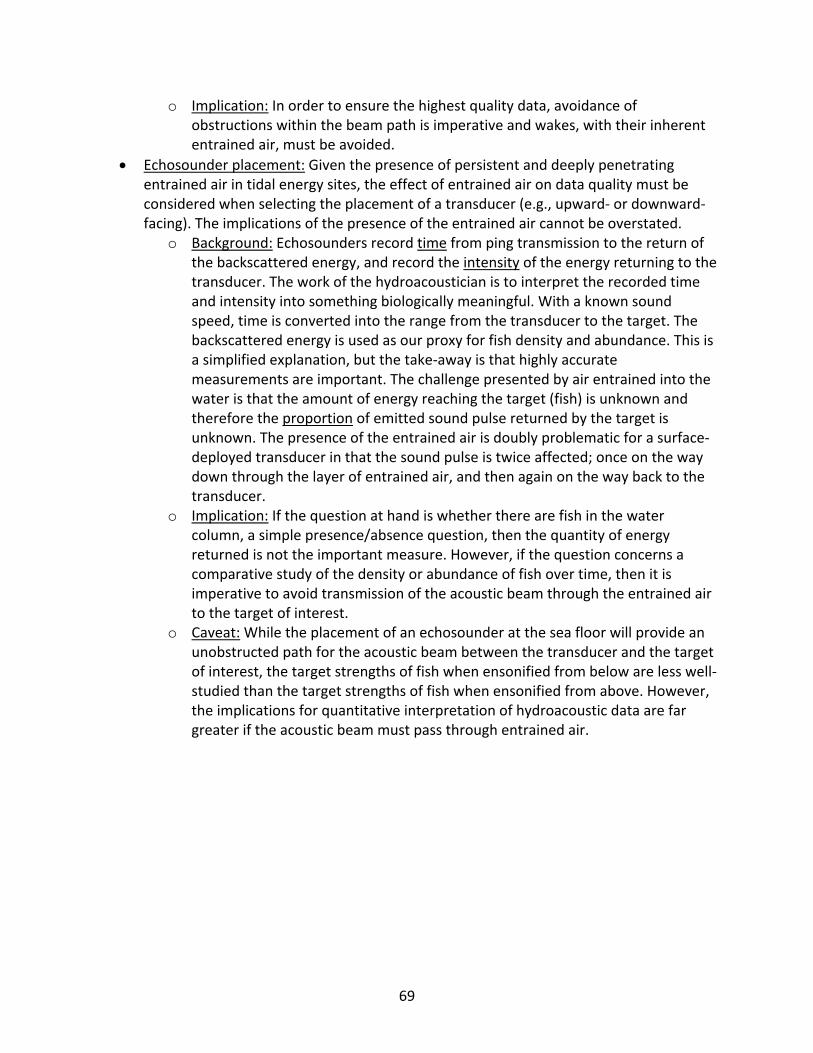
  69 

o Implication: In order to ensure the highest quality data, avoidance of obstructions within the beam path is imperative and wakes, with their inherent entrained air, must be avoided. 

Echosounder placement: Given the presence of persistent and deeply penetrating entrained air in tidal energy sites, the effect of entrained air on data quality must be considered when selecting the placement of a transducer (e.g., upward‐ or downward‐facing). The implications of the presence of the entrained air cannot be overstated. 

o Background: Echosounders record time from ping transmission to the return of the backscattered energy, and record the intensity of the energy returning to the transducer. The work of the hydroacoustician is to interpret the recorded time and intensity into something biologically meaningful. With a known sound speed, time is converted into the range from the transducer to the target. The backscattered energy is used as our proxy for fish density and abundance. This is a simplified explanation, but the take‐away is that highly accurate measurements are important. The challenge presented by air entrained into the water is that the amount of energy reaching the target (fish) is unknown and therefore the proportion of emitted sound pulse returned by the target is unknown. The presence of the entrained air is doubly problematic for a surface‐deployed transducer in that the sound pulse is twice affected; once on the way down through the layer of entrained air, and then again on the way back to the transducer.  

o Implication: If the question at hand is whether there are fish in the water column, a simple presence/absence question, then the quantity of energy returned is not the important measure. However, if the question concerns a comparative study of the density or abundance of fish over time, then it is imperative to avoid transmission of the acoustic beam through the entrained air to the target of interest.  

o Caveat: While the placement of an echosounder at the sea floor will provide an unobstructed path for the acoustic beam between the transducer and the target of interest, the target strengths of fish when ensonified from below are less well‐studied than the target strengths of fish when ensonified from above. However, the implications for quantitative interpretation of hydroacoustic data are far greater if the acoustic beam must pass through entrained air.  

 

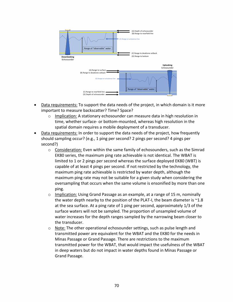
  70 

  

Data requirements: To support the data needs of the project, in which domain is it more important to measure backscatter? Time? Space? 

o Implication: A stationary echosounder can measure data in high resolution in time, whether surface‐ or bottom‐mounted, whereas high resolution in the spatial domain requires a mobile deployment of a transducer. 

Data requirements: In order to support the data needs of the project, how frequently should sampling occur? (e.g., 1 ping per second? 2 pings per second? 4 pings per second?) 

o Consideration: Even within the same family of echosounders, such as the Simrad EK80 series, the maximum ping rate achievable is not identical. The WBAT is limited to 1 or 2 pings per second whereas the surface deployed EK80 (WBT) is capable of at least 4 pings per second. If not restricted by the technology, the maximum ping rate achievable is restricted by water depth, although the maximum ping rate may not be suitable for a given study when considering the oversampling that occurs when the same volume is ensonified by more than one ping. 

o Implication: Using Grand Passage as an example, at a range of 15 m, nominally the water depth nearby to the position of the PLAT‐I, the beam diameter is ~1.8 at the sea surface. At a ping rate of 1 ping per second, approximately 1/3 of the surface waters will not be sampled. The proportion of unsampled volume of water increases for the depth ranges sampled by the narrowing beam closer to the transducer. 

o Note: The other operational echosounder settings, such as pulse length and transmitted power are equivalent for the WBAT and the EK80 for the needs in Minas Passage or Grand Passage. There are restrictions to the maximum transmitted power for the WBAT, that would impact the usefulness of the WBAT in deep waters but do not impact in water depths found in Minas Passage or Grand Passage. 

(A) Depth of echosounder(B) Range to nearfield line

(D) Range to bottom

Range of “observable” water

(E) Range to turbulence line

(C) Range to deadzone setback

(D) Depth of echosounder

(C) Range to nearfield line

(E) Range to turbulence line

(A) Range to surface

(B) Range to deadzone setback

Range of “observable” water

UplookingEchosounder

DownlookingEchosounder

  71 

Data requirements: To support the data needs of the project, will the restrictions imposed by data storage and power needs of an autonomous echosounder deployed on the sea floor be acceptable? If unacceptable, is a cabled solution an option? 

o Note: Technological solutions in addition to a cabled solution exist but are costly and the robustness of the systems for operation in the vigorous environment of a tidal energy site would need to be investigated. 

Analysis requirements: Given that the data can be readily retrieved, processed, analyzed for a surface‐deployed echosounder, will the lag in data processing and analyses inherent with bottom‐mounted echosounders be acceptable? 

o Note: Technology exists by which to relay data from autonomous echosounders to the surface for transmission over the internet. However, substantial upfront investment is required, and their robustness for operation in the vigorous environments of tidal energy sites would need to be investigated. 

Deployment considerations: A sea floor deployment of an echosounder system requires a substantial investment in procuring a suitable deployment platform and the logistical needs and expense with each deployment and retrieval. 

 The above is a list of the initial factors that need to be considered when selecting the placement (surface or sea floor) for deployment of a scientific echosounder. They are interrelated and need to be prioritized and evaluated given the resources (financial, logistical, etc.) that are available. It needs to be stressed that the data and analytical needs of any project must be identified so that inherent trade‐offs can be evaluated in terms of consequence to the project success.