Feature Selection and Molecular Classification of Cancer Using Genetic Programming1

Feature Selection and Molecular Classification of CancerUsing Genetic Programming1

Jianjun Yu*,y, Jindan Yu y, Arpit A. Almal z, Saravana M. Dhanasekaran y, Debashis Ghosh§,William P. Worzel z and Arul M. Chinnaiyan y,b,#

*Bioinformatics Program, University of Michigan Medical School, Ann Arbor, MI 48109, USA; yDepartmentof Pathology, University of Michigan Medical School, Ann Arbor, MI 48109, USA; zGenetics Squared Inc.,210 South 5th Avenue, Suite A, Ann Arbor, MI 48104, USA; §Department of Biostatistics, University of MichiganMedical School, Ann Arbor, MI 48109, USA; bDepartment of Urology, University of Michigan Medical School,Ann Arbor, MI 48109, USA; #The Comprehensive Cancer Center, University of Michigan Medical School,Ann Arbor, MI 48109, USA

Abstract

Despite important advances in microarray-based mo-

lecular classification of tumors, its application in

clinical settings remains formidable. This is in part

due to the limitation of current analysis programs in

discovering robust biomarkers and developing classi-

fiers with a practical set of genes. Genetic program-

ming (GP) is a type of machine learning technique that

uses evolutionary algorithm to simulate natural selec-

tion as well as population dynamics, hence leading

to simple and comprehensible classifiers. Here we

applied GP to cancer expression profiling data to

select feature genes and build molecular classifiers

by mathematical integration of these genes. Analysis

of thousands of GP classifiers generated for a pros-

tate cancer data set revealed repetitive use of a set of

highly discriminative feature genes, many of which are

known to be disease associated. GP classifiers often

comprise five or less genes and successfully predict

cancer types and subtypes. More importantly, GP clas-

sifiers generated in one study are able to predict

samples from an independent study, which may have

used different microarray platforms. In addition, GP

yielded classification accuracy better than or similar

to conventional classification methods. Furthermore,

the mathematical expression of GP classifiers pro-

vides insights into relationships between classifier

genes. Taken together, our results demonstrate that

GP may be valuable for generating effective classi-

fiers containing a practical set of genes for diagnostic/

prognostic cancer classification.

Neoplasia (2007) 9, 292–303

Keywords: Molecular diagnostics, biomarkers, prostate cancer, evolu-tionary algorithm, microarray profiling.

Introduction

The development of high-throughput microarray-based

technology will potentially revolutionize cancer research in

a number of areas including cancer classification, diagnosis,

and treatment. Expression profiling at the mRNA level can

be used in the molecular characterization of cancer by simul-

taneous assessment of a large number of genes [1–5]. This

approach can be used to determine gene expression alter-

ations between different tissue types such as those obtained

from healthy controls and patients with cancer. Analysis of such

large-scale gene expression profiles of cancer will facilitate

the identification of a subset of genes that could function as

diagnostic or prognostic biomarkers. The development of mo-

lecular classifiers that allow segregation of tumors into clinically

relevant molecular subtypes beyond those possible by patho-

logic classification may subsequently serve to classify tumors

with unknown origin into different cancer types or subtypes.

However, due to the large number of genes and the relatively

small number of patient cases available from such studies,

finding a robust gene signature for reliable prediction remains

a challenge.

A number of computational and statistical models have

been developed for molecular classification of tumors. Golub

et al. [3] proposed a weighted voting scheme to identify a

subset of 50 genes that can discriminate acute myeloid leuke-

mia from acute lymphoblastic leukemia, and subsequently

predict class membership of new leukemia cases. Using the

same data set, Mukherjee et al. [6] developed a kernel-based

support vector machine (SVM) classifier and achieved a higher

performance in term of the accuracy of assigning leukemia

Address all correspondence to: Arul M. Chinnaiyan, MD, PhD, Department of Pathology,

University of Michigan Medical School, 1400 E. Medical Center Drive 5316 CCGC, Ann Arbor,

MI 48109-0602. E-mail: [email protected]. William P. Worzel, Bill, Genetics Squared Inc., 210

South 5th Avenue, Suite A, Ann Arbor, MI 48104. E-mail: [email protected] research was supported in part by the National Institutes of Health (R01 CA97063 to

A.M.C. and D.G., U54 DA021519-01A1 to A.M.C., Prostate SPORE P50CA69568 to A.M.C.),

the Early Detection Research Network (UO1 CA111275 to A.M.C. and D.G.), the National

Institutes of General Medical Sciences (GM 72007 to D.G.), the Department of Defense

(W81XWH-06-1-0224 to A.M.C., PC060266 to J.Y.), and the Cancer Center Bioinformatics

Core (support grant 5P30 CA46592 to A.M.C.). A.M.C. is supported by a Clinical Translational

Research Award from the Burroughs Welcome Foundation.

Received 10 January 2007; Revised 20 February 2007; Accepted 22 February 2007.

Copyright D 2007 Neoplasia Press, Inc. All rights reserved 1522-8002/07/$25.00

DOI 10.1593/neo.07121

Neoplasia . Vol. 9, No. 4, April 2007, pp. 292 – 303 292

www.neoplasia.com

RESEARCH ARTICLE

samples into acute myeloid leukemia or acute lymphoblastic

leukemia. van’t Veer et al. [7] developed a 70-gene predictor

that was highly correlated with breast cancer prognosis.

Khan et al. [8] introduced an artificial neural network to

classify different histopathologic types of small round blue

cell tumors (SRBCTs) and identified 96 most discriminative

genes for classification. A deterministic tree-based method

was also introduced by Zhang et al. [9] in 2003 to con-

struct random forests for classifications of leukemia and lym-

phoma. Although these methods have had some success in

classifying tumors, they are often developed by using para-

metric statistical techniques and thus have difficulty in finding

nonlinear relationships between genes. Alternatively, com-

plex models are used that deliver ‘‘black box’’ solutions for

classification and do not give insight into relationships be-

tween genes.

In this study, we present a machine learning approach

called genetic programming (GP) for molecular classification

of cancer. GP belongs to a class of evolutionary algorithms

and was first introduced by Koza [10] in 1992. Recently,

evolutionary algorithms have been used to analyze gene

expression data and select molecular signatures for sample

classification [11–17]. For example, GP has been shown to

be a promising approach for discovering comprehensible

rule-based classifiers from medical data [11,16] as well as

gene expression profiling data [12,14,17–20]. However, the

potential of GP in cancer classification has not been fully

explored. For example, GP classifiers identified from one

data set have not been validated in independent data sets.

Here, we applied GP algorithm to cancer expression profiling

data to identify potentially informative feature genes, build

molecular classifiers, and classify tumor samples. We tested

GP in one SRBCT, one lung adenocarcinoma, and five

prostate cancer data sets and evaluated the generality of

GP classifiers within and across data sets. In addition, we

compared the performance of GP with that of other common

classification techniques, such as linear discriminant analy-

sis and SVMs, for prediction accuracy.

Materials and Methods

Data Sets

All data sets were obtained from ONCOMINE [21] or

requested from the original authors. The SRBCT data [8]

contained 88 samples from four types of cancer cells:

neuroblastoma (NB), rhabdomyosarcoma (RMS), the Ewing

family of tumors (EWS), and Burkitt lymphoma (BL). The

entire data set, excluding five non-SRBCT samples, was

divided into a training set (63 samples) and a validation set

(20 samples) as described in the original study.

The lung adenocarcinoma data set [22] contains 86 lung

cancer samples. The raw CEL files were preprocessed

using RMAExpress (2003, UC Berkeley, http://rmaexpress.

bmbolstad.com/) [23] and normalized so that each array had

zero mean and unit variance. The samples were then sub-

divided into a high- or low-risk group as requested from

the authors. Twenty-eight high-risk and 38 low-risk sam-

ples were included in the training set and the remaining

20 samples were considered as the validation set.

Three prostate cancer data sets [2,24,25] from the Uni-

versity of Michigan (UM), Stanford University (Stanford) and

the University of Pittsburgh (Pittsburgh), respectively, were

used to classify primary prostate cancer (PCA) from benign

prostate samples. A total of 56 samples were randomly

selected from Stanford data set as the training set. The rest

of the Stanford samples and UM and Pittsburgh sets were

treated as validation sets.

In addition, two prostate cancer data sets including

the Pittsburgh and the LaTulippe et al. (Memorial Sloan-

Kettering Cancer Center, MSKCC) data sets [25,26] were

retrieved to distinguish metastatic prostate cancer (MET)

and PCA. Detailed study information is shown in Table 1.

Genetic Programming for Classification

Genetic programming [10] is an evolutionary algorithm

that simulates natural selection and population dynamics to

search for intelligible relationships among the constituents in

a system (classifiers in this study). A basic flowchart for the

GP system is given in Figure 1A. Briefly, the system ran-

domly selects inputs such as gene identifiers and constant

values, which are used to represent the expression values of

corresponding genes. Such selected inputs are then com-

bined with the function operators such as arithmetic or

Boolean operators to compose tree-based GP classifiers,

an example of which is given in Figure 1B. Such classifiers

are eventually accumulated to form an initial population,

where a small subgroup of classifiers is then selected to

create a ‘‘mating group.’’ Each classifier in this mating group

is assessed by a fitness function defined as the area under

the receiver operating characteristic curve (ROC-AUC),

which is widely used to assess the accuracy of a diagnostic

test that yields continuous test results in clinical research

areas. The two fittest classifiers are then selected as

‘‘mating’’ parents by a tournament selection scheme and

‘‘mated’’ to produce ‘‘offspring’’ through selective genetic

Table 1. Gene Expression Data Sets Used in This Study.

Class Description Authors Journal Array Type No. of Genes

Four classes: NB, RMS, BL, EWS Khan et al. [8] Nat Med 7:673 cDNA 2,308

Two classes: high-risk group and low-risk group Beer et al. [22] Nat Med 30:41 Affymetrix Hu6800 7,070

Two classes: PCA and MET LaTulippe et al. [26] Cancer Res 62:4499 Affymetrix HG_U95A 3,547

Yu et al. [25] J Clin Oncol 22:2790 Affymetrix HG_U95A 3,547

Two classes: benign prostate samples (BENIGN) and PCA Lapointe et al. [24] Proc Natl Acad Sci USA 101:811 cDNA 4,168

Dhanasekaran et al. [2] Nature 412:822 cDNA 16,965

Yu et al. [25] J Clin Oncol 22:2790 Affymetrix HG_U95A 12,558

Classification of Cancer Using Genetic Programming Yu et al. 293

Neoplasia . Vol. 9, No. 4, 2007

operators such as crossover, or mutation. The crossover

operator exchanges a subtree of one parent with the other

to generate offspring (Figure 1C), whereas the mutation

operator probabilistically chooses a node in a subtree and

replaces it with a new created subtree randomly. The gen-

erated offspring then replaces the least-fit parent classifiers

in the population. Once new offspring fully replaces parent

classifiers in the entire population, a new generation that in

general contains better classifiers is created. This process

of mating pool selection, fitness assessment, mating, and

replacement is repeated over generations, progressively

creating better classifiers until a termination criterion is met

Figure 1. (A) Flowchart for the GP process. Briefly, a population of tree-based classifiers is first created by randomly choosing gene expression data or con-

stant values and combining with arithmetic or Boolean operators. An example of tree-based classifiers is represented in (B). A small subgroup of classifiers

is then selected as a ‘‘mating group’’ and each classifier in this mating group is assessed by a fitness function, which is defined as the area under the ROC-AUC

in this study. The two fittest classifiers are then selected as ‘‘mating’’ parents and ‘‘mated’’ to produce ‘‘offspring’’ by genetic operators (crossover or mutation).

The generated offspring then replace the least-fit parent classifiers within the population. A new generation of populations is generated once the offspring fully

replaced parent classifiers in the population. This process of mating pool selection, fitness assessment, mating, and replacement is repeated over generations,

progressively creating better classifiers until a completion criterion is met. After the best classifiers are outputted, post-GP analyses are carried out to compute

gene occurrence in the classifiers as well as to predict on new unknown samples. (B) The representation of a GP tree structure for an exemplified classifier,

Gene[A]/Gene[B] > 3. In general, a GP classifier is represented as a tree-based structure composed of the terminal set and function set. The terminal set, in tree

terminology, is composed of leaves (nodes without branches) and may represent as genes or constants. The function set is a set of operators such as arithmetic

operators (+, �, �, H) or Boolean operators (AND, OR, NOT), acting as the branch points in the tree, linking other functions or terminals. (C) The representation of a

crossover operator of GP tree.

294 Classification of Cancer Using Genetic Programming Yu et al.


(e.g., a perfect classifier with a fitness score of 1 or the

maximum number of ‘‘generations’’ is reached).

Table 2 shows an example of primary GP parameters

used to analyze the prostate cancer data set from the

LaTulippe et al. (MSKCC) study [26]. Given the limited

sample size of each data set, we used n-fold cross-validation

procedure to estimate the generalization of classifiers in

predicting samples with unknown class membership. For

example, when a data set is selected as the training set, it

is randomly subdivided into n parts (or folds), wherein

classifiers are developed as described in the above GP

process using samples in n � 1 folds. These classifiers are

then tested on samples in the left-out fold to assess their

potential generalization capability because such samples are

not involved in the development of the classifiers. A good

classifier is expected to classify well in the training samples

as well as the samples in the left-out fold. This process is

repeated n times with each fold taking turns as the testing

fold and the best classifiers are then selected based on

overall performance on the training folds and the test fold.

Overall Methodology for Classifier Validation

In this study, we used GP to discover classifiers that are

capable of classifying samples into different cancer types

based on gene expression patterns. Typically, a classifier is

evolved from a training data set and then validated against

independent validation sets to assess its prediction capacity

on samples with unknown labels. A generic GP classifier-

based prediction is shown as: IF ’(GENE[A]/GENE[B] �GENE[C]) > D’ THEN ’TARGET CLASS’, where the IF clause

is generated by GP, ‘‘TARGET CLASS’’ is predefined in the

initial configuration file, D is a constant, and GENE[A],

GENE[B], and GENE[C] represent the expression levels of

genes A, B, and C, respectively. A continuous prediction

score is preferred for certain analysis like the ROC curve

analysis. To implement that, the classifier can be converted

to the form of ’GENE[A]/GENE[B] � GENE[C]’, where the

calculated mathematical expression values can be then

treated as a continuous variable for ROC test.

Implementation and Running Time

We implemented parallel GP algorithm in C (patented

by Genetics Squared, Inc., Ann Arbor, MI; http://www.

genetics2.com). The analyses were performed on a parallel

computer cluster (7 Dell 1850 1U racks with 2� 3.2-GHz

Xeon processor and 1 Dell 1750 1U rack with 1� 3.06-GHz

Xeon processor; Dell Inc., Round Rock, TX; http://www.dell.

com) running the Debian Linux operating system. The run-

ning times for different data sets varied from a few minutes

to a few days, depending on a large number of parameters

such as the complexity of the problem, size of population

used in the evolution, number of generations, cost of fitness

calculation, number of classifiers, and size of the data set.

For the LaTulippe et al. [26] prostate cancer data set with the

Table 2. Settings for Primary GP Parameters Used to Analyze the Latulippe et al. Prostate Cancer Data.

Parameter Setting Description*

Terminal set All inputs including gene expression values,

and constant values

A set where all end (leaf) nodes in the parse trees representing the programs

must be drawn. A terminal could be a variable, a constant, or a function

with no arguments.

Function set Boolean and floating point operators:

<, >, <=, =>, *, /, +, �A set of operators, e.g., +, �, *, H. These act as the branch points in the

parse tree, linking other functions or terminals.

Selection Generational, tournament size 5 An evolution is called ‘‘generational’’ when the entire existing population of

classifiers is replaced by a new created population at every generation.

Tournament selection is a mechanism for choosing classifiers from a

population. A group of classifiers are selected at random from the

population and the best ones are chosen.

Elitism 1 Property of selection methods, which keeps the best classifier(s) into the

next generation.

Initial population Each tree was created by ramped half-and-half Ramped half-and-half operates by creating an equal number of trees with

each depth between a predetermined minimum and maximum.

Population size 20,000 The number of candidate classifiers in a population.

Number of demes 12 A deme is a separately evolving subset of the whole population. The subsets

may be evolved on different computers. Emigration between subset may

occur every generation.

Crossover probability 0.2 The probability of creating a new individual from parts of its parents.

Mutation probability 0.2 The probability of a subtree replaced by another, some or all of which is

created at random.

Termination criteria Fitness score reaches 1 or max generations (50) A statement or condition to stop the GP cycle.

Initial tree depth 3 The initial distance of any leaf from the root of a tree.

Initial node count 3 The initial number of nodes in a tree.

Maximum tree depth 7 The maximum distance of any leaf from the root of a tree.

Maximum node count 8 The maximum number of nodes in a tree.

Number of folds 4 The number of parts a training set will be subdivided into.

Deme migration frequency Every generation The frequency of moving classifiers between isolated demes.

Deme migration percentage 5% of individuals The percentage of classifiers moving between two demes.

Fitness ROC-AUC A process that evaluates a member of a population and gives it a score

or fitness.

*Source of some term descriptions: Langdon WB (1998). Genetic Programming and Data Structures: Genetic Programming + Data Structures = Automatic

Programming! Amsterdam: Kluwer.



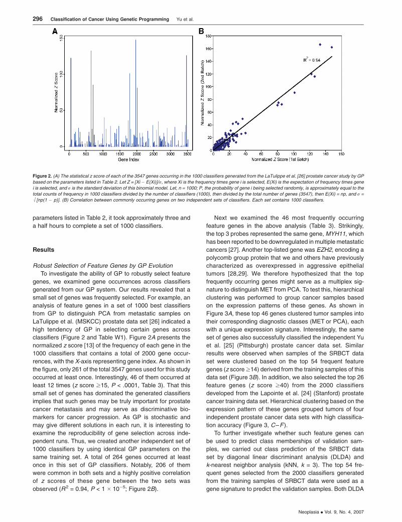
parameters listed in Table 2, it took approximately three and

a half hours to complete a set of 1000 classifiers.

Results

Robust Selection of Feature Genes by GP Evolution

To investigate the ability of GP to robustly select feature

genes, we examined gene occurrences across classifiers

generated from our GP system. Our results revealed that a

small set of genes was frequently selected. For example, an

analysis of feature genes in a set of 1000 best classifiers

from GP to distinguish PCA from metastatic samples on

LaTulippe et al. (MSKCC) prostate data set [26] indicated a

high tendency of GP in selecting certain genes across

classifiers (Figure 2 and Table W1). Figure 2A presents the

normalized z score [13] of the frequency of each gene in the

1000 classifiers that contains a total of 2000 gene occur-

rences, with the X-axis representing gene index. As shown in

the figure, only 261 of the total 3547 genes used for this study

occurred at least once. Interestingly, 46 of them occurred at

least 12 times (z score z15, P < .0001, Table 3). That this

small set of genes has dominated the generated classifiers

implies that such genes may be truly important for prostate

cancer metastasis and may serve as discriminative bio-

markers for cancer progression. As GP is stochastic and

may give different solutions in each run, it is interesting to

examine the reproducibility of gene selection across inde-

pendent runs. Thus, we created another independent set of

1000 classifiers by using identical GP parameters on the

same training set. A total of 264 genes occurred at least

once in this set of GP classifiers. Notably, 206 of them

were common in both sets and a highly positive correlation

of z scores of these gene between the two sets was

observed (R2 = 0.94, P < 1 � 10�5; Figure 2B).

Next we examined the 46 most frequently occurring

feature genes in the above analysis (Table 3). Strikingly,

the top 3 probes represented the same gene, MYH11, which

has been reported to be downregulated in multiple metastatic

cancers [27]. Another top-listed gene was EZH2, encoding a

polycomb group protein that we and others have previously

characterized as overexpressed in aggressive epithelial

tumors [28,29]. We therefore hypothesized that the top

frequently occurring genes might serve as a multiplex sig-

nature to distinguish MET from PCA. To test this, hierarchical

clustering was performed to group cancer samples based

on the expression patterns of these genes. As shown in

Figure 3A, these top 46 genes clustered tumor samples into

their corresponding diagnostic classes (MET or PCA), each

with a unique expression signature. Interestingly, the same

set of genes also successfully classified the independent Yu

et al. [25] (Pittsburgh) prostate cancer data set. Similar

results were observed when samples of the SRBCT data

set were clustered based on the top 54 frequent feature

genes (z score z14) derived from the training samples of this

data set (Figure 3B). In addition, we also selected the top 26

feature genes (z score z40) from the 2000 classifiers

developed from the Lapointe et al. [24] (Stanford) prostate

cancer training data set. Hierarchical clustering based on the

expression pattern of these genes grouped tumors of four

independent prostate cancer data sets with high classifica-

tion accuracy (Figure 3, C–F ).

To further investigate whether such feature genes can

be used to predict class memberships of validation sam-

ples, we carried out class prediction of the SRBCT data

set by diagonal linear discriminant analysis (DLDA) and

k-nearest neighbor analysis (kNN, k = 3). The top 54 fre-

quent genes selected from the 2000 classifiers generated

from the training samples of SRBCT data were used as a

gene signature to predict the validation samples. Both DLDA

Figure 2. (A) The statistical z score of each of the 3547 genes occurring in the 1000 classifiers generated from the LaTulippe et al. [26] prostate cancer study by GP

based on the parameters listed in Table 2. Let Z = [Xi � E(Xi)]/r, where Xi is the frequency times gene i is selected, E(Xi) is the expectation of frequency times gene

i is selected, and r is the standard deviation of this binomial model. Let, n = 1000; P, the probability of gene i being selected randomly, is approximately equal to the

total counts of frequency in 1000 classifiers divided by the number of classifiers (1000), then divided by the total number of genes (3547), then E(Xi) = np, and r =

M[np(1 � p)]. (B) Correlation between commonly occurring genes on two independent sets of classifiers. Each set contains 1000 classifiers.



and kNN analysis predicted all of the 20 validation samples

with 100% accuracy (data not shown), confirming that the

frequent genes derived from GP are truly discriminative

genes and capable of predicting unknown samples.

GP Classifiers Successfully Predict Validation Sample Sets

Next we sought to examine the performance of GP clas-

sifiers comprising only a handful of feature genes. We first

evaluated the ability of GP classifiers to accurately classify

four diagnostic classes of cancers (NB, RMS, EWS, and BL)

within the SRBCT data set [8]. A set of 63 training samples

was used by GP to generate distinguishing classifiers through

cross-validation. Classification was performed in a binary

mode (target vs. nontarget class). For each target class, the

top 10 best classifiers (Table W2) were selected and used to

predict a validation set of 20 samples. Most of the classifiers

achieved 100% sensitivity and specificity on the training set.

Similar prediction accuracy was observed when these clas-

sifiers were applied to the 20 blinded validation samples. The

best classifiers (Table 4) perfectly predicted all of the valida-

tion samples. The average prediction accuracy of the top

10 classifiers for each target class was 98.5% for BL

(95% confidence interval [CI], 0.97–1.00), 92.5% for EWS

(95% CI, 0.89–0.96), 95.5% for NB (95% CI, 0.91–1.00), and

95.5% for RMS (95% CI, 0.92–0.99). Overall, GP classifiers

achieved comparable classification and prediction per-

formance as the method described in the original study,

although using much less genes. This high prediction accu-

racy, however, might be partially due to the fact that the

four cancer types here are much more heterogeneous than

the subtypes of any single cancer.

Thus, we next examined GP in classifying subtypes of

lung adenocarcinoma, wherein samples were designated as

‘‘high risk’’ or ‘‘low risk’’ based on the original publication

Table 3. Frequency of Gene Occurrences in the 1000 Classifiers for the Latulippe et al. Prostate Study.

Probe Set Gene Symbol Gene Title Count* Z Score

37407_s_at MYH11 Myosin, heavy polypeptide 11, smooth muscle 112 147.59

32582_at MYH11 Myosin, heavy polypeptide 11, smooth muscle 101 133.02


1197_at ACTG2 Actin, gamma 2, smooth muscle, enteric 93 122.42

36931_at TAGLN Transgelin 77 101.23

32755_at ACTA2 Actin, alpha 2, smooth muscle, aorta 65 85.34

37576_at PCP4 Purkinje cell protein 4 62 81.36

774_g_at MYH11 Myosin, heavy polypeptide 11, smooth muscle 61 80.04

34203_at CNN1 Calponin 1, basic, smooth muscle 31 40.30

36834_at MOXD1 Monooxygenase, DBH-like 1 28 36.33

39333_at COL4A1 Collagen, type IV, alpha 1 27 35.01


38834_at TOPBP1 Topoisomerase (DNA) II binding protein 1 23 29.71

685_f_at LOC112714 Similar to alpha tubulin 23 29.71

34878_at SMC4L1 SMC4 structural maintenance of chromosomes 4-like 1 22 28.38

35970_g_at MPHOSPH9 M-phase phosphoprotein 9 22 28.38

41137_at PPP1R12B Protein phosphatase 1, regulatory (inhibitor) subunit 12B 21 27.06

1884_s_at PCNA Proliferating cell nuclear antigen 20 25.73

40407_at KPNA2 Karyopherin alpha 2 (RAG cohort 1, importin alpha 1) 20 25.73

32662_at MDC1 Mediator of DNA damage checkpoint 1 19 24.41

34376_at PKIG Protein kinase (cAMP-dependent, catalytic) inhibitor gamma 19 24.41

35742_at C16orf45 Chromosome 16 open reading frame 45 19 24.41

36987_at LMNB2 Lamin B2 19 24.41

39145_at MYL9 Myosin, light polypeptide 9, regulatory 18 23.09

38430_at FABP4 Fatty acid binding protein 4, adipocyte 17 21.76

1599_at CDKN3 Cyclin-dependent kinase inhibitor 3 16 20.44

2012_s_at PRKDC Protein kinase, DNA-activated, catalytic polypeptide 16 20.44

32305_at COL1A2 Collagen, type I, alpha 2 16 20.44

418_at MKI67 Antigen identified by monoclonal antibody Ki-67 16 20.44

651_at RPA3 Replication protein A3, 14kDa 16 20.44

35474_s_at COL1A1 Collagen, type I, alpha 1 15 19.11

37749_at MEST Mesoderm specific transcript homolog (mouse) 15 19.11

38031_at DDX48 DEAD (Asp-Glu-Ala-Asp) box polypeptide 48 15 19.11

39990_at ISL1 ISL1 transcription factor, LIM/homeodomain (islet-1) 15 19.11

1505_at TYMS Thymidylate synthetase 14 17.79

33924_at RAB6IP1 RAB6 interacting protein 1 14 17.79

35694_at MAP4K4 Mitogen-activated protein kinase kinase kinase kinase 4 14 17.79

32306_g_at COL1A2 Collagen, type I, alpha 2 13 16.46

32847_at MYLK Myosin, light polypeptide kinase 13 16.46

37305_at EZH2 Enhancer of zeste homolog 2 (Drosophila) 13 16.46

41081_at BUB1 BUB1 budding uninhibited by benzimidazoles 1 homolog 13 16.46

32272_at K-ALPHA-1 Tubulin, alpha, ubiquitous 12 15.14

36627_at SPARCL1 SPARC-like 1 (mast9, hevin) 12 15.14

37347_at CKS1B CDC28 protein kinase regulatory subunit 1B 12 15.14

39519_at KIAA0692 KIAA0692 protein 12 15.14

40845_at ILF3 Interleukin enhancer binding factor 3, 90 kDa 12 15.14

*Count is the number of occurrences of each gene in 1000 rules.



information [22]. One hundred classifiers were generated

by GP from 66 training samples and the top 5 were found to

have the highest training accuracy of 98.5%. When these

5 classifiers were applied to the 20 test samples, we found

a maximal prediction accuracy of 98.5% and an average

prediction rate of 84.0% (95% CI, 0.70–0.99), comparable

with that of other classification methods as described in the

later session.

A more challenging work is to validate classifiers across

independent data sets. We thus investigated whether GP

could distinguish molecular subtypes of a single cancer class

from independent data sets. Two prostate cancer data sets

(Pittsburgh and MSKCC sets, respectively) were used to

evaluate GP in classifying PCA or MET. Genes within each

data set were standardized to have zero mean and unit vari-

ance, given that similar proportion of metastatic samples was

observed in both data sets. The MSKCC samples were used

as a training set to generate GP classifiers. The 20 classifiers

that perfectly classified PCA from MET in the training set were

selected for prediction. When these classifiers were applied

to predict the independent Pittsburgh prostate cancer sam-

ples, the best classifiers (Table 4) correctly predicted all METs,

and 58 of 62 clinically localized PCAs. This led to 100%

sensitivity and 93.5% specificity. The average prediction ac-

curacy of all of the 20 classifiers was 95.2% sensitivity (95% CI,

0.87–1.00) and 82.1% specificity (95% CI, 0.65–0.99).

The above two prostate cancer data sets were hybridized

by using the same Affymetrix HG-U95Av2 platform (Affymetrix

Inc., Santa Clara, CA) and shared similar proportion ratios

of target/nontarget samples. Next, we examined whether

classifiers generated by GP could predict samples from inde-

pendent studies that have used different microarray platforms.

Figure 3. Top feature genes derived from GP separate tumors into their corresponding diagnostic classes. (A) Hierarchical clustering using the top 46 most

frequent genes derived from the 1000 classifiers generated for the LaTulippe et al. (MSKCC) data set [26]. Genes were ranked by the frequency of their

occurrences in the classifiers. The top 46 frequent genes (z score z15, see Figure 2) were selected for hierarchical clustering. The left panel is the clustering

of metastatic samples and PCA samples for the MSKCC data, and the right panel is for the Yu et al. [25] (Pittsburgh) validation data set. Rows represent genes and

columns represent samples. The green lines in the dendrogram indicate PCA and the red lines represent MET samples. (B) Hierachical clustering of the entire

SRBCT data set using the top 54 feature genes obtained from the training set. (C–F) The top 26 most frequent genes from the 2000 classifiers generated from

Lapointe et al. [24] (Stanford) training set was used to separate 34 benign/control prostate samples from PCA samples in the Stanford training set (C), Stanford

validation set (D), Yu et al. [25] (Pittsburgh) validation set (E), and Dhanasekaran et al. [2] (UM) validation set (F), respectively. The green lines in the dendrogram

indicate benign/control prostate samples and the black lines represent PCA samples.



Three prostate cancer data sets [2,24,25] (UM, Stanford,

and Pittsburgh) were used to test GP classifiers in pre-

dicting benign prostate and PCA samples. Among them, the

Stanford and UM data sets used spot cDNA microarrays,

whereas the Pittsburgh data used Affymetrix HG-U95Av2

oligonucleotide arrays. Two thirds of the Stanford samples

were used as a training set to generate GP classifiers, whereas

the other one third, the UM and Pittsburgh samples, were all

considered as validation samples. We used GP to generate

2000 classifiers and selected the top 26 frequently occurring

genes (z score z40) as potential feature genes. To examine

whether these genes are present in all three microarray plat-

forms we cross-referenced them to the UM and Pittsburgh

data sets using gene symbols. Of these 26 genes, 12 are

present in all three data sets. We thus entered these 12 genes

into the GP system to start a new round of five-fold cross-

validation on the Stanford training set. Five perfect classifiers

were achieved and applied to the validation set. Prediction

accuracy in the Stanford validation samples ranged from

84.4% to 90%. However, the classifiers performed poorly on

UM and Pittsburgh data sets. We suspected that this might

be due to the discrepancy in the proportion ratio of PCA/benign

samples and/or the probe intensity difference across array

platforms, which led to divergence in the constant D of a clas-

sifier (e.g., GENE[A]/GENE[B] � GENE[C] > D). However, we

believe that the relationships between the classifier genes,

although with varying values of D, may still be predictive across

studies, given that the classifier genes are putative dis-

criminative genes. For instance, one of the classifiers, formu-

lated as ‘‘IF (MYO6 + AMACR) >= �2.6776 THEN PCA’’ (see

Table 5), did not predict well on the validation sets. However,

the expression value of ‘‘MYO6 + AMACR’’ might still be

predictive. To test this, we transformed the five classifiers

individually as described in Materials and Methods and calcu-

lated a prediction score for each validation sample by com-

puting the left side of each classifier inequality on a continuous

scale. The predictive ability of each classifier on each valida-

tion set was then assessed by using the ROC-AUC. Notably,

all classifiers were strongly significant (P < 5 � 10�4; Figure 4,

Table 5) in both the Stanford and Pittsburgh validation sets.

The lowest AUC values were 0.91 (95% CI, 0.80–1.00) and

0.87 (95% CI, 0.79–0.95), respectively. For UM data set,

except for one classifier being marginally significant (AUC =

0.64, P = 0.09), all other classifiers were also strongly sig-

nificant (P < 5 � 10�4).

An ensemble ‘‘metaclassifier’’ combining multiple classi-

fiers in general yields better prediction performance, as it

involves more genes and multiple predictive signatures.

Thus, we composed a metaclassifier based on the above

five classifiers. For each sample, the calculated prediction

scores of the five classifiers were totaled to an overall

prediction score, which was then defined as the prediction

score of the metaclassifier for that sample. As expected, this

metaclassifier revealed higher AUCs in each data set (0.96,

0.99, and 0.99 for the Stanford, UM, and Pittsburgh set,

respectively; P < 5 � 10�4; see Figure 4 and Table 5).

Feature Genes of a Classifier Are Correlated

with Each Other

Examination of classifier genes have revealed that GP

classifiers (Tables 4 and 5) are much simpler than predictors

reported by other approaches [1,3,5,6,8,22,30–32], where

Table 5. Classifiers That Classify Benign Prostate and Primary Prostate Cancer.

Classifier ROC-AUC (95% CI)

Lapointe et al. Validation Set (Stanford) Dhanasekaran et al. (UM) Yu et al. (Pittsburgh)

IF (ENC1 + GJB1) >= �0.8902 THEN PCA 0.95 (0.87 –1.00) 0.95 (0.90 –1.00) 0.92 (0.85 – 1.00)

IF (MYO6 + AMACR) >= �2.6776 THEN PCA 0.95 (0.88 –1.00) 0.99 (0.97 –1.00) 0.95 (0.90 – 1.00)

IF (TSPAN13 + PRKCBP1 >= �0.4172 THEN PCA 0.94 (0.85 –1.00) 0.88 (0.78 –0.98) 0.94 (0.90 – 0.99)

IF (C20ORF74 + DAPK1) >= �0.7765 THEN PCA 0.91 (0.80 –1.00) 0.64 (0.49 –0.80) 0.87 (0.79 – 0.95)

IF (IMAGE:396839 + ENC1) >= �0.5513 THEN PCA 0.97 (0.91 –1.00) 0.82 (0.70 –0.94) 0.89 (0.81 – 0.98)

Metaclassifier 0.96 (0.87 –1.00) 0.99 (0.96 –1.00) 0.99 (0.98 – 1.00)

Table 4. Classifiers That Distinguish Different Cancer Classes of SRBCT, Subtypes of Prostate Cancer, or Lung Cancer.

Analysis Classifier Training Errors Test Set Errors

FN FP FN FP

Small, round blue-cell tumor IF (HCLS1 � GSTA4 > XPO6) THEN BL 0 0 0 0

IF (PTPN13/COX8A > CDK6) THEN EWS 0 0 0 0

IF (SATB1 > CSDA^2) THEN NB 0 0 0 0

IF (CDH17/FGFR4 <= MYL4) THEN RMS 0 0 0 0

Primary prostate cancer vs. metastatic

prostate cancer

IF (ARL6IP > MYH11) THEN MET 0 0 0 4

IF (MYH11 < MYH11) THEN MET 0 0 0 4

Lung cancer (high risk vs. low risk) IF (LTBP2 � IARS) <= (ADM + (CCT2 * FCGR2A))

THEN High-Risk

0 1 1 0

IF (GYPB � MN1) < (ADM + (MCFD2 + CKS2))

THEN High-Risk

1 0 3 0

Only one or two classifiers per class per analysis are listed in the table. FN, number of false negatives; FP, number of false positives.



more than 10 genes are often required to build an effec-

tive predictor. GP, by contrast, can use only 2 to 5 genes to

produce effective classifiers and achieve high prediction

power. This simplicity may owe to the relatively strict expres-

sion constraints (Table 2) and the use of a nonparametric

method in selecting informative genes rather than usual

parametric statistical techniques. Furthermore, unlike some

other nonparametric approaches such as neural networks

and SVMs, GP is transparent in that the entire procedure for

classifier generation and evolution is readily available for

inspection and adjustment.

A major difference between GP and other machine learn-

ing techniques is its mathematical connections between

genes within a classifier. Studying the specific genes used

by a classifier and the relationship between these genes

may provide valuable information about gene interactions,

transcriptional regulatory pathways, and clinical diagnosis. A

quick examination of the classifiers revealed a consistent

relationship between the expression levels of classifier

genes. That is, a high (positive/negative) correlation between

genes is preferred for a classifier. For example, within

the classifier of ‘‘IF [MYO6] + [AMACR] >= �2.6776 THEN

’Primary Prostate Cancer’,’’ the expression level of MYO6

was highly positively correlated with AMACR (r = 0.68,

P < .0001). Furthermore, a two-sample t test revealed

that both MYO6 and AMACR were significantly overex-

pressed in PCA relative to benign prostate (both Ps < .001

by t test), demonstrating that genes selected by the GP

system were indeed potential discriminative biomarkers.

Similar relationships were also observed in other classifiers.

Figure 4. The ROCs of five classifiers and one metaclassifier for three prostate cancer validation sets. The classifiers were generated from the Lapointe et al. [24]

(Stanford) training set to distinguish benign prostate from PCA. The ROCs are based on continuous prediction scores computed from the left side of the classifier

inequality (see Materials and Methods). The scores of the metaclassifier are the mean values of prediction scores from each individual classifier. (A, B, C) ROC

curves for Lapointe et al. [24] (Stanford), Dhanasekaran et al. [2] (UM), and Yu et al. [25] (Pittsburgh) validation set, respectively.



GP Outperforms Other Molecular Classification Methods

One important criterion to assess a classification ap-

proach is how it performs in comparison to other commonly

used algorithms in the same research area. To evaluate the

performance of GP, the Burkitt lymphomas (‘‘BL’’) in the

SRBCT data set and the high-risk class in the lung adeno-

carcinoma data were chosen as the target classes, and

five classification methods including compound covariate

predictor, 3-nearest neighbors, nearest centroid, SVMs,

and DLDA were selected as comparing counterparts of the

GP method. To produce a fair comparison, we took into

account the small number of genes used by GP classifiers

and conducted the comparison tests based on either 5- or

10-gene classifiers.

The same training and validation sets as described pre-

viously were used to evaluate the performance of each

classification method. The basic procedure was defined by

two steps: 1) two-sample Student t test was conducted for

each gene in the training set, and the 5 or 10 genes with the

smallest P values were selected as test classifiers; 2)

expression data of the selected 5 or 10 genes across the

training samples were used to build a training model, which

was subsequently applied to the validation samples. Each

individual validation sample was predicted as either ‘‘target

class’’ or ‘‘nontarget class.’’ Misclassification rate was de-

fined as the percentage of validation samples that were

misclassified by a test classifier. Because GP generates

multiple classifiers, the average of the misclassification rates

of the top GP classifiers derived from the training set was

used to represent the misclassification rate of a typical well-

performing GP classifier. For the SRBCT data, we used the

averaged misclassification rate of the top 10 classifiers

because there were 10 perfect classifiers generated from

the training samples to classify ‘‘BL’’ and ‘‘non-BL.’’ Similarly,

the 5 classifiers having the least classification error in the

training set were used for the lung adenocarcinoma data set.

As shown in Table 6, the error rates were comparable across

different methods. The GP system ranked the second and

the third in the SRBCT and the lung adenocarcinoma data

sets, respectively, when 5-gene classifiers were evaluated.

We believe that this may reflect the general prediction

strength of GP system when only a small number of genes

are chosen. Considering the additional advantages of GP in

predicting samples across data sets and in revealing inter-

relationships between classifier genes, we concluded that

GP outperforms other classification method.

Discussion

Although molecular classification has been successfully

used to group tumors based on their gene expression

patterns in retrospective research [1,3,6–9,15,22,32], its

application in clinical settings has been greatly hindered.

This is in part due to the large number of feature genes

required to build a discriminative classifier. Therefore, there

is a strong need to build molecular classifiers made of a

small number of genes, especially in clinical diagnosis,

where it would not be practical to have a diagnostic assay

evaluate hundreds of genes in one test. In this study we

developed a GP system to generate effective classifiers with

a handful of genes.

An intrinsic advantage of GP is that it automatically

selects a small number of feature genes during ‘‘evolution’’

[19]. The evolution of classifiers from the initial population

seamlessly integrates the process of gene selection and

classifier construction. By contrast, gene selection must be

performed in a separate stage for many other classification

algorithms such as kNN, weighted voting, and DLDA. More-

over, it is relatively easier for GP to keep the number of genes

used in one classifier small. As GP searches a larger space

than most traditional classification approaches, there is an

increased chance of GP in finding a better performing

classifier. By identifying and using a small number of genes

and developing transparent and human-comprehensible

rule-based classifiers, GP stands as a good algorithm

of choice.

For each run of GP, it can generate tens to hundreds

of classifiers. However, our data have shown that most of

these classifiers used a limited set of feature genes (Fig-

ure 2). In addition, classifiers generated by different runs of

GP also used a similar set of feature genes. Furthermore,

we have observed that a number of these feature genes

have been previously reported to be disease associated.

Interestingly, the expression profile of the top selected fea-

ture genes easily classified cancer samples into their cor-

responding diagnostic groups as well as predicted validation

sets of samples with high accuracy. These results strongly

indicate that GP is very likely selecting the true discrimina-

tive feature genes, supporting the strong power of GP in

feature selection.

The challenge of the field of molecular classification lies in

the tradeoff of prediction power and the number of genes

used. We have therefore stringently tested GP classifiers,

composed of five genes or fewer, in achieving high predic-

tion accuracy in data sets with varying levels of classifi-

cation complexity. Unlike other studies [17,33] validating

their classifiers using cross-validation within a data set, our

result not only demonstrated that the top GP classifiers

easily classified and predicted the SRBCT data set, which

contained four classes of physiologically heterogeneous

Table 6. Misclassification Error Rates of GP and Other Common Classi-

fication Models.

Algorithm Error Rate (%)

SRBCT (BL vs.

NON-BL)

Lung Cancer (High Risk vs.

Low Risk)

5 Genes 10 Genes 5 Genes 10 Genes

GP 1.5 NA 16 NA

Compound covariate

predictor

5 5 20 25

3-Nearest neighbors 5 5 15 30

Nearest centroid 5 5 20 25

SVMs 0 5 20 25

DLDA 5 5 10 20

NA, not available.



cancers, with 100% accuracy, but also showed optimal per-

formance in classifying and predicting subtypes of pros-

tate cancer for samples either of the same study or of a

different study that used the same microarray platform. In

addition, GP-selected feature genes stay discriminative

even for cancer samples examined in different studies that

used greatly different microarray platforms. Because of this

robustness and stability of GP feature genes, we expect GP

classifier to be highly applicable to clinical diagnosis.

We have found that GP identifiers have prediction accu-

racy comparable with small-gene-number classifiers gener-

ated by other classification methods. However, GP has

added advantages over other algorithms. Its special features

include the following: 1) the ability to automatically select a

small number of genes as potential discriminative genes, 2)

the ability to combine such genes and construct a simple and

comprehensible classifier, and 3) the capability to generate

multiple candidate classifiers.

A major issue in GP as well as other machine learning

systems is data overfitting due to a large number of variables

and a small number of cases in microarray profiling. This

occurs when the classifier is strongly biased toward the

training set and generates poor prediction generality in

validation samples. To address this, our study restricted

the complexity of classifiers and adopted an n-fold cross-

validation strategy. By limiting the size and complexity of

classifiers using the minimum description length principle of

risk minimization [34], the system was forced to generate the

most salient features likely to be the most general solutions

[35]. By resampling using n-fold cross-validation, classifiers

derived from the training samples were reexamined in the

test-fold samples to test how well the learning algorithm

could be generalized. If the fitness on the training data in

one fold is significantly better than the fitness on the test

data, it may indicate that there is an issue of overfitting in the

data. Therefore, a careful examination of the samples may

be necessary.

Another issue for GP is that it is computationally intensive.

The estimated running time increases along with the com-

plexity of the problem and the number of variables. This can

be partially resolved by using parallel processing, which

segments the problem into parts running on different pro-

cessors simultaneously and then synchronizes among them.

In addition, variable prefiltering may also reduce the running

time. As described in the Result section, GP typically selects

those inherently discriminative genes and usually a small set

of genes dominates the selection. Thus, a prefiltering, such

as excluding genes with small variances, may significantly

reduce the running time yet not affect the performance of

classifiers.

Taken together, in this study we systematically evaluated

the feasibility of GP in feature selection and cancer classifi-

cation. By examining the feature genes used by GP classi-

fiers we have demonstrated that GP is able to robustly select

a set of highly discriminative genes. In addition, the mathe-

matical expression of GP classifiers reveals interesting

quantitative relationships between genes. By testing GP

classifiers generated from training sets in validation sets,

we have shown that GP classifiers can successfully predict

tumor classes and outperform most of other classification

methods when only a limited number of genes are allowed to

build a classifier. Our work suggests that GP may be useful

for feature selection and molecular classification of cancer

using a practical set of genes.

References[1] Alizadeh AA, Eisen MB, Davis RE, Ma C, Lossos IS, Rosenwald A,

Boldrick JC, Sabet H, Tran T, Yu X, et al. (2000). Distinct types of diffuse

large B-cell lymphoma identified by gene expression profiling. Nature

403, 503 – 511.

[2] Dhanasekaran SM, Barrette TR, Ghosh D, Shah R, Varambally S,

Kurachi K, Pienta KJ, Rubin MA, and Chinnaiyan AM (2001). Delineation

of prognostic biomarkers in prostate cancer. Nature 412, 822 –826.

[3] Golub TR, Slonim DK, Tamayo P, Huard C, Gaasenbeek M, Mesirov JP,

Coller H, Loh ML, Downing JR, Caligiuri MA, et al. (1999). Molecular

classification of cancer: class discovery and class prediction by gene

expression monitoring. Science 286, 531 – 537.

[4] Hedenfalk I, Duggan D, Chen Y, Radmacher M, Bittner M, Simon R,

Meltzer P, Gusterson B, Esteller M, Kallioniemi OP, et al. (2001). Gene-

expression profiles in hereditary breast cancer. N Engl J Med 344,

539 –548.

[5] Perou CM, Sorlie T, Eisen MB, van de Rijn M, Jeffrey SS, Rees CA,

Pollack JR, Ross DT, Johnsen H, Akslen LA, et al. (2000). Molecular

portraits of human breast tumours. Nature 406, 747 – 752.

[6] Mukherjee S, Tamayo P, Mesirov JP, Slonim D, Verri A, and Poggio T

(1999). Support Vector Machine Classification of Microarray Data.

MIT, CBCL.

[7] van’t Veer LJ, Dai H, van de Vijver MJ, He YD, Hart AA, Mao M, Peterse

HL, van der Kooy K, Marton MJ, Witteveen AT, et al. (2002). Gene

expression profiling predicts clinical outcome of breast cancer. Nature

415, 530 –536.

[8] Khan J, Wei JS, Ringner M, Saal LH, Ladanyi M, Westermann F,

Berthold F, Schwab M, Antonescu CR, Peterson C, et al. (2001).

Classification and diagnostic prediction of cancers using gene expres-

sion profiling and artificial neural networks. Nat Med 7, 673 –679.

[9] Zhang H, Yu CY, and Singer B (2003). Cell and tumor classification

using gene expression data: construction of forests. Proc Natl Acad

Sci USA 100, 4168 –4172.

[10] Koza JR (1992). Genetic Programming: On the Programming of Com-

puters by Means of Natural Selection. MIT Press, Cambridge.

[11] Bojarczuk CC, Lopes HS, and Freitas AA (2001). Data mining with

constrained-syntax genetic programming: applications to medical data

sets. Proceedings Intelligent Data Analysis in Medicine and Pharma-

cology ({IDAMAP}-2001).

[12] Hong JH and Cho SB (2006). The classification of cancer based on

DNA microarray data that uses diverse ensemble genetic programming.

Artif Intell Med 36, 43– 58.

[13] Li L, Weinberg CR, Darden TA, and Pedersen LG (2001). Gene selec-

tion for sample classification based on gene expression data: study of

sensitivity to choice of parameters of the GA/KNN method. Bioinfor-

matics 17, 1131 – 1142.

[14] Mitra AP, Almal AA, George B, Fry DW, Lenehan PF, Pagliarulo V, Cote

RJ, Datar RH, and Worzel WP (2006). The use of genetic programming

in the analysis of quantitative gene expression profiles for identification

of nodal status in bladder cancer. BMC Cancer 6, 159.

[15] Ooi CH and Tan P (2003). Genetic algorithms applied to multi-class

prediction for the analysis of gene expression data. Bioinformatics 19,

37– 44.

[16] Tan KC, Yu Q, Heng CM, and Lee TH (2003). Evolutionary computing

for knowledge discovery in medical diagnosis. Artif Intell Med 27,

129 – 154.

[17] Ho SY, Hsieh CH, Chen HM, and Huang HL (2006). Interpretable gene

expression classifier with an accurate and compact fuzzy rule base for

microarray data analysis. Biosystems 85, 165 –176.

[18] Langdon WB and Buxton BF (2004). Genetic programming for mining

DNA chip data from cancer patients. Genetic Programming and Evolv-

able Machines 5, 251 –257.

[19] Moore JH, Parker JS, and Hahn LW (2001). Symbolic discriminant

analysis for mining gene expression patterns. Lecture Notes Artif Intell

2167, 372 –381.

[20] Moore JH, Parker JS, Olsen NJ, and Aune TM (2002). Symbolic



discriminant analysis of microarray data in autoimmune disease. Genet

Epidemiol 23, 57– 69.

[21] Rhodes DR, Yu J, Shanker K, Deshpande N, Varambally R, Ghosh D,

Barrette T, Pandey A, and Chinnaiyan AM (2004). ONCOMINE: a cancer

microarray database and integrated data-mining platform. Neoplasia 6,

1–6.

[22] Beer DG, Kardia SL, Huang CC, Giordano TJ, Levin AM, Misek DE,

Lin L, Chen G, Gharib TG, Thomas DG, et al. (2002). Gene-expression

profiles predict survival of patients with lung adenocarcinoma. Nat Med

8, 816 – 824.

[23] Bolstad BM, Irizarry RA, Astrand M, and Speed TP (2003). A comparison

of normalization methods for high density oligonucleotide array data

based on variance and bias. Bioinformatics 19, 185–193.

[24] Lapointe J, Li C, Higgins JP, van de Rijn M, Bair E, Montgomery K,

Ferrari M, Egevad L, Rayford W, Bergerheim U, et al. (2004). Gene

expression profiling identifies clinically relevant subtypes of prostate

cancer. Proc Natl Acad Sci USA 101, 811 –816.

[25] Yu YP, Landsittel D, Jing L, Nelson J, Ren B, Liu L, McDonald C,

Thomas R, Dhir R, Finkelstein S, et al. (2004). Gene expression alter-

ations in prostate cancer predicting tumor aggression and preceding

development of malignancy. J Clin Oncol 22, 2790 – 2799.

[26] LaTulippe E, Satagopan J, Smith A, Scher H, Scardino P, Reuter V, and

Gerald WL (2002). Comprehensive gene expression analysis of pros-

tate cancer reveals distinct transcriptional programs associated with

metastatic disease. Cancer Res 62, 4499 –4506.

[27] Ramaswamy S, Ross KN, Lander ES, and Golub TR (2003). A mo-

lecular signature of metastasis in primary solid tumors. Nat Genet 33,

49 –54.

[28] Kleer CG, Cao Q, Varambally S, Shen R, Ota I, Tomlins SA, Ghosh

D, Sewalt RG, Otte AP, Hayes DF, et al. (2003). EZH2 is a marker

of aggressive breast cancer and promotes neoplastic transfor-

mation of breast epithelial cells. Proc Natl Acad Sci USA 100,

11606 – 11611.

[29] Varambally S, Dhanasekaran SM, Zhou M, Barrette TR, Kumar-Sinha

C, Sanda MG, Ghosh D, Pienta KJ, Sewalt RG, Otte AP, et al. (2002).

The polycomb group protein EZH2 is involved in progression of prostate

cancer. Nature 419, 624 – 629.

[30] Armstrong SA, Staunton JE, Silverman LB, Pieters R, den Boer ML,

Minden MD, Sallan SE, Lander ES, Golub TR, and Korsmeyer SJ

(2002). MLL translocations specify a distinct gene expression profile

that distinguishes a unique leukemia. Nat Genet 30, 41– 47.

[31] Gruvberger SK, Ringner M, Eden P, Borg A, Ferno M, Peterson C,

and Meltzer PS (2002). Expression profiling to predict outcome in

breast cancer: the influence of sample selection. Breast Cancer Res

5, 23 – 26.

[32] Shipp MA, Ross KN, Tamayo P, Weng AP, Kutok JL, Aguiar RC,

Gaasenbeek M, Angelo M, Reich M, Pinkus GS, et al. (2002). Diffuse

large B-cell lymphoma outcome prediction by gene-expression pro-

filing and supervised machine learning. Nat Med 8, 68– 74.

[33] Bhattacharyya C, Grate LR, Jordan MI, El Ghaoui L, and Mian IS

(2004). Robust sparse hyperplane classifiers: application to uncertain

molecular profiling data. J Comput Biol 11, 1073 – 1089.

[34] Rissanen J (1978). Modeling by shortest data description. Automatica

14, 465 –471.

[35] Vapnik VN (1995). The Nature of Statistical Learning Theory. Springer-

Verlag, Berlin.



Table W1. Frequency Analysis of Gene Occurrence on Training Data Sets.

A. Frequency of Gene Occurrences in the 2000 Classifiers for the Khan

et al. SRBCT Study

Index Clone_ID Symbol Z Score

1 784224 FGFR4 52.17

122 812105 AF1Q 48.16

128 814260 FVT1 48.16

173 796258 SGCA 46.43

186 1435862 CD99 45.29

245 770394 FCGRT 45.29

254 377461 CAV1 43.57

367 207274 NULL 42.99

421 866702 PTPN13 39.55

482 244618 FRCP2 39.55

508 298062 TNNT2 34.96

544 52076 OLFM1 33.82

553 769716 NF2 32.67

565 491565 CITED2 31.52

602 325182 CDH2 30.95

606 296448 IGF2 29.80

741 143306 NULL 28.65

822 25725 FDFT1 28.08

835 308231 MYO1B 27.51

845 43733 GYG2 25.79

909 236282 WAS 25.21

975 859359 TP53I3 25.21

1002 1471841 ATP1A1 24.64

1054 839552 NCOA1 24.07

1065 461425 MYL4 22.92

1073 629896 MAP1B 22.92

1083 486110 PFN2 22.34

1104 788107 BIN1 22.34

1193 42558 GATM 21.20

1206 241412 ELF1 21.20

1318 713922 GSTM2 21.20

1326 878652 PCOLCE 20.62

1388 786084 CBX1 20.05

1426 1409509 TNNT1 19.48

1600 244637 CRI1 19.48

1644 789253 PSEN2 18.33

1661 357031 TNFAIP6 17.76

1707 134748 GCSH 17.76

1722 183337 HLA-DMA 17.76

1737 813841 PLAT 17.76

1771 814444 CRSP9 17.18

1798 377048 MYO1B 17.18

1885 771323 PLOD 17.18

1895 897788 PTPRF 17.18

1910 214572 CDK6 16.61

1953 142134 ARHGAP8 16.61

1954 756401 RHEB 16.03

1979 293500 FLJ90440 16.03

2045 811108 TRIP6 15.46

2049 504791 GSTA4 15.46

2143 1473131 TLE2 14.89

2145 898219 MEST 14.89

2156 841641 CCND1 14.89

2158 295985 NULL 14.89

B. Frequency of Gene Occurrences in the 1000 Classifiers for the Latulippe

et al. Prostate Study

Probe Set Symbol Z Score

37407_s_at MYH11 147.59

32582_at MYH11 133.02

767_at MYH11 126.4

1197_at ACTG2 122.42

36931_at TAGLN 101.23

32755_at ACTA2 85.34

37576_at PCP4 81.36

774_g_at MYH11 80.04

34203_at CNN1 40.3

Table W1. (continued )

B. Frequency of Gene Occurrences in the 1000 Classifiers for the

Latulippe et al. Prostate Study

Probe Set Symbol Z Score

36834_at MOXD1 36.33

39333_at COL4A1 35.01

773_at MYH11 31.03

38834_at TOPBP1 29.71

685_f_at LOC112714 29.71

34878_at SMC4L1 28.38

35970_g_at MPHOSPH9 28.38

41137_at PPP1R12B 27.06

1884_s_at PCNA 25.73

40407_at KPNA2 25.73

32662_at MDC1 24.41

34376_at PKIG 24.41

35742_at C16orf45 24.41

36987_at LMNB2 24.41

39145_at MYL9 23.09

38430_at FABP4 21.76

1599_at CDKN3 20.44

2012_s_at PRKDC 20.44

32305_at COL1A2 20.44

418_at MKI67 20.44

651_at RPA3 20.44

35474_s_at COL1A1 19.11

37749_at MEST 19.11

38031_at DDX48 19.11

39990_at ISL1 19.11

1505_at TYMS 17.79

33924_at RAB6IP1 17.79

35694_at MAP4K4 17.79

32306_g_at COL1A2 16.46

32847_at MYLK 16.46

37305_at EZH2 16.46

41081_at BUB1 16.46

32272_at K-ALPHA-1 15.14

36627_at SPARCL1 15.14

37347_at CKS1B 15.14

39519_at KIAA0692 15.14

40845_at ILF3 15.14

C. Frequency of Gene Occurrences in the 2000 Classifiers for the

Lapointe et al. Prostate Cancer Study

Index CLID Symbol Z Score

1590 IMAGE:288663 GJB1 282.87

250 IMAGE:136605 POMP 264.49

3388 IMAGE:788180 AMACR 225.69

812 IMAGE:179211 GPR160 222.63

44 IMAGE:1034473 AMACR 205.27

1094 IMAGE:2057931 TACSTD1 182.81

2817 IMAGE:685516 GPR160 174.64

2330 IMAGE:470216 MYO6 154.22

2072 IMAGE:396839 NULL 118.48

782 IMAGE:1709503 NULL 96.02

2109 IMAGE:415962 PCSK6 86.83

3017 IMAGE:745283 DKFZp779O175 86.83

1592 IMAGE:288770 TMEM144 76.62

1098 IMAGE:2062404 MON1B 68.45

1295 IMAGE:244391 PRKCBP1 68.45

2277 IMAGE:460164 C20orf74 64.37

4104 IMAGE:898286 CDC2 54.16

1076 IMAGE:2043415 DAPK1 52.11

3951 IMAGE:855406 NULL 52.11

2116 IMAGE:416374 TSPAN13 52.11

2583 IMAGE:510534 TACSTD1 51.09

1294 IMAGE:244350 NULL 48.03

2589 IMAGE:510856 ENC1 47.01

3580 IMAGE:811101 SH3RF1 43.95

1249 IMAGE:23819 ABCG1 42.92

1173 IMAGE:2244718 GCNT1 40.16

Table W2. Classifiers Generated by GP for Each Training Data Set.

Classification Rules Gene Description

A. Classifiers that distinguish different cancer classes of SRBCT

IF IMAGE:183337 > exp(IMAGE:796613) THEN BL IMAGE:183337 is HLA-DMB; IMAGE:796613 is COL5A2;

IF (IMAGE:767183 � IMAGE:504791) > IMAGE:813742 THEN BL IMAGE:767183 is HCLS1; IMAGE:504791 is GSTA4; IMAGE:813742

is XPO6;

IF (IMAGE:767183/IMAGE:810408 � IMAGE:504791) >

IMAGE:809383 THEN BL

IMAGE:767183 is HCLS1; IMAGE:810408 is ERGIC3; IMAGE:504791

is GSTA4; IMAGE:809383 is PPAN;

IF log(sqrt(IMAGE:183337)) > tanh(IMAGE:308746) THEN BL IMAGE:183337 is HLA-DMB; IMAGE:308746 is EXT2;

IF (IMAGE:740604ÎMAGE:183462 � IMAGE:250654) >

(IMAGE:325155 * IMAGE:813444)ÎMAGE:815555 THEN BL

IMAGE:740604 is ISG20; IMAGE:183462 is MAN2C1; IMAGE:250654

is SPARC; IMAGE:325155 is KRT34; IMAGE:813444 is SLC12A8;

IMAGE:815555 is DGKA;

IF (IMAGE:767183 � IMAGE:504791) >= IMAGE:813742 THEN BL IMAGE:767183 is HCLS1; IMAGE:504791 is GSTA4; IMAGE:813742

is XPO6;

IF (sin(IMAGE:140171) > IMAGE:854899^2) && ((IMAGE:767183 �IMAGE:504791) > IMAGE:486110^2) THEN BL

IMAGE:140171 is THTPA; IMAGE:854899 is DUSP6; IMAGE:767183

is HCLS1; IMAGE:504791 is GSTA4; IMAGE:486110 is PFN2;

IF (IMAGE:740604^cos(IMAGE:897632) � IMAGE:250654) >

IMAGE:183462 THEN BL

IMAGE:740604 is ISG20; IMAGE:897632 is ATP2A2; IMAGE:250654

is SPARC; IMAGE:183462 is MAN2C1;

IF tanh(IMAGE:203003) <= IMAGE:740604 THEN BL IMAGE:203003 is DECR2; IMAGE:740604 is ISG20;

IF (IMAGE:740604^tanh(IMAGE:563673)) > (2.0 * IMAGE:250654)

THEN BL

IMAGE:740604 is ISG20; IMAGE:563673 is ALDH7A1; IMAGE:250654

is SPARC

IF (IMAGE:866702 * IMAGE:814260) > IMAGE:295985 THEN EWS IMAGE:866702 is PTPN13; IMAGE:814260 is FVT1; IMAGE:295985

is CDK6;

IF (IMAGE:866702/IMAGE:1469230) > IMAGE:295985 THEN EWS IMAGE:866702 is PTPN13; IMAGE:1469230 is COX8A; IMAGE:295985

is CDK6;

IF sqrt(IMAGE:770394/IMAGE:52076) <= IMAGE:770394 THEN EWS IMAGE:770394 is FCGRT; IMAGE:52076 is OLFM1; IMAGE:770394

is FCGRT;

IF (IMAGE:178825 * IMAGE:52076) > IMAGE:295985 THEN EWS IMAGE:178825 is NRGN; IMAGE:52076 is OLFM1; IMAGE:295985

is CDK6;

IF (IMAGE:866702 * IMAGE:80338) > IMAGE:295985 THEN EWS IMAGE:866702 is PTPN13; IMAGE:80338 is SELENBP1;

IMAGE:295985 is CDK6;

IF IMAGE:770394 > (sqrt(IMAGE:244951)/(IMAGE:357031/IMAGE:855391))

THEN EWS

IMAGE:770394 is FCGRT; IMAGE:244951 is HIF3A; IMAGE:357031

is TNFAIP6; IMAGE:855391 is STK25;

IF IMAGE:43733 > IMAGE:295985 THEN EWS IMAGE:43733 is GYG2; IMAGE:295985 is CDK6;

IF (IMAGE:770394 + IMAGE:214906) > IMAGE:842820 THEN EWS IMAGE:770394 is FCGRT; IMAGE:214906 is SPEN; IMAGE:842820

is PABPC4;

IF IMAGE:866702 * sqrt(IMAGE:138550) > IMAGE:295985 THEN EWS IMAGE:866702 is PTPN13; IMAGE:138550 is ZNF444; IMAGE:295985

is CDK6;

IF IMAGE:377461 > sqrt(IMAGE:132911) THEN EWS IMAGE:377461 is CAV1; IMAGE:132911 is PPP1CB;

IF IMAGE:364510 > IMAGE:810057^2 THEN NB IMAGE:364510 is SATB1; IMAGE:810057 is CSDA;

IF (3.951/sqrt(IMAGE:1409509)) > (exp(IMAGE:810057)^2)/(IMAGE:135688^2 +

sqrt(IMAGE:1472775)^2) THEN NB

IMAGE:1409509 is TNNT1; IMAGE:810057 is CSDA; IMAGE:135688

is GATA2; IMAGE:1472775 is COL8A1;

IF ((8.714/exp(IMAGE:121521))/exp(IMAGE:546600)) > ((IMAGE:810057^2)/

(IMAGE:325182^2)) THEN NB

IMAGE:121521 is ZNF764; IMAGE:546600 is DNAJB4; IMAGE:810057

is CSDA; IMAGE:325182 is CDH2;

IF IMAGE:364510 > (IMAGE:810057 + ((IMAGE:759200^2)/(4.276/

sin(IMAGE:24415)))) THEN NB

IMAGE:364510 is SATB1; IMAGE:810057 is CSDA; IMAGE:759200

is DHPS; IMAGE:24415 is TP53;

IF (IMAGE:811956 > IMAGE:810057) AND (IMAGE:23132 > cos(IMAGE:491001))

THEN NB

IMAGE:811956 is RAN; IMAGE:810057 is CSDA; IMAGE:23132

is SF3A1; IMAGE:491001 is GLO1;

IF IMAGE:325182^((exp(IMAGE:840942))^2) > ((IMAGE:789376^(�1.222))/1.791)

THEN NB

IMAGE:325182 is CDH2; IMAGE:840942 is HLA-DPB1; IMAGE:789376

is TXNRD1;

IF IMAGE:823886 > IMAGE:810057 THEN NB IMAGE:823886 is NDEL1; IMAGE:810057 is CSDA;

IF ((exp(IMAGE:812105)/5.506)^2) > (IMAGE:323577 + IMAGE:824426 *

IMAGE:814266) THEN NB

IMAGE:812105 is MLLT11; IMAGE:323577 is SLC4A2; IMAGE:824426

is PDAP1; IMAGE:814266 is PRKCZ;

IF exp(IMAGE:810057) <= (IMAGE:395708 + IMAGE:788205 + IMAGE:383188)

THEN NB

IMAGE:810057 is CSDA; IMAGE:395708 is DPYSL4; IMAGE:788205

is SOX4; IMAGE:383188 is RCVRN;

IF IMAGE:810057 <= IMAGE:29054 THEN NB IMAGE:810057 is CSDA; IMAGE:29054 is SCGN;

IF (IMAGE:298062/IMAGE:40017) > (IMAGE:549146ÎMAGE:784224) THEN RMS IMAGE:298062 is TNNT2; IMAGE:40017 is CYCS; IMAGE:549146

is TRIM22; IMAGE:784224 is FGFR4;

IF (IMAGE:511909/IMAGE:784224) <= IMAGE:461425 THEN RMS IMAGE:511909 is CDH17; IMAGE:784224 is FGFR4; IMAGE:461425

is MYL4;

IF (IMAGE:898219^2 + IMAGE:461425)^2 > IMAGE:82131 THEN RMS IMAGE:898219 is MEST; IMAGE:461425 is MYL4; IMAGE:82131

is PSMB1;

IF ((IMAGE:265102 + IMAGE:207274) > IMAGE:244618) AND ((IMAGE:784224 +

IMAGE:244618) > 1.8594) THEN RMS

IMAGE:265102 is ABI2; IMAGE:207274 is IGF2; IMAGE:244618

is FNDC5; IMAGE:784224 is FGFR4; IMAGE:244618 is FNDC5;

IF IMAGE:796258 > (IMAGE:340630/IMAGE:784224) THEN RMS IMAGE:796258 is SGCA; IMAGE:340630 is MAP3K8; IMAGE:784224

is FGFR4;

IF (IMAGE:244618/IMAGE:52076) > (IMAGE:809939/IMAGE:813841) THEN RMS IMAGE:244618 is FNDC5; IMAGE:52076 is OLFM1; IMAGE:809939

is C6orf48; IMAGE:813841 is PLAT;

IF (IMAGE:950367/(IMAGE:244618/IMAGE:52076)) <= (IMAGE:142134 +

IMAGE:143306^2) THEN RMS

IMAGE:950367 is ADAR; IMAGE:244618 is FNDC5; IMAGE:52076

is OLFM1; IMAGE:142134 is PRR5; IMAGE:143306 is LOC645166;

Table W2. (continued )

Classification Rules Gene Description

A. Classifiers that distinguish different cancer classes of SRBCT

IF IMAGE:784224 > IMAGE:781341 THEN RMS IMAGE:784224 is FGFR4; IMAGE:781341 is TULP4;

IF (IMAGE:461425 + IMAGE:898219^2) > IMAGE:825312 THEN RMS IMAGE:461425 is MYL4; IMAGE:898219 is MEST; IMAGE:825312

is ATP5J;

IF IMAGE:298062 > (0.045022 + IMAGE:110467 + sin(IMAGE:784224))

THEN RMS

IMAGE:298062 is TNNT2; IMAGE:110467 is CAV2; IMAGE:784224

is FGFR4;

B. Classifiers that distinguish metastatic prostate cancer from primary prostate cancer

IF (36987_at >= 767_at) THEN MET 36987_at is LMNB2; 767_at is MYH11

IF (40145_at >= 32582_at) THEN MET 40145_at is TOP2A; 32582_at is MYH11

IF (40398_s_at > 32755_at) THEN MET 40398_s_at is MEOX2; 32755_at is ACTA2

IF (39145_at <= 39333_at) THEN MET 39145_at is MYL9; 39333_at is COL4A1

IF (767_at < 37263_at) THEN MET 767_at is MYH11; 37263_at is GGH

IF (38505_at >= 37576_at) THEN MET 38505_at is EIF2C2; 37576_at is PCP4

IF (36931_at < 418_at) THEN MET 36931_at is TAGLN; 418_at is MKI67

IF (774_g_at <= 1232_s_at) THEN MET 774_g_at is MYH11; 1232_s_at is IGFBP1

IF (1276_g_at < 32120_at) THEN MET 1276_g_at is RBPMS; 32120_at is SPAG5

IF (32582_at < 38430_at) THEN MET 32582_at is MYH11; 38430_at is FABP4

IF (37407_s_at < 1648_at) THEN MET 37407_s_at is MYH11; 1648_at is OSMR

IF (773_at <= 32306_g_at) THEN MET 773_at is MYH11; 32306_g_at is COL1A2

IF (39714_at <= 1260_s_at) THEN MET 39714_at is SH3BGRL; 1260_s_at is GSTA1

IF (39109_at >= 828_at) THEN MET 39109_at is TPX2; 828_at is PTGER2

IF (36572_r_at > 37407_s_at) THEN MET 36572_r_at is ARL6IP1; 37407_s_at is MYH11

IF (774_g_at < 35970_g_at) THEN MET 774_g_at is MYH11; 35970_g_at is MPHOSPH9

IF (767_at <= 546_at) THEN MET 767_at is MYH11; 546_at is PKIA

IF (773_at <= 37749_at) THEN MET 773_at is MYH11; 37749_at is MEST

IF (418_at > 36931_at) THEN MET 418_at is MKI67; 36931_at is TAGLN

IF (32272_at >= 32582_at) THEN MET 32272_at is TUBA3; 32582_at is MYH11

C. Classifiers that distinguish primary prostate cancer from benign control

IF (IMAGE:510856 + IMAGE:288663) >= �0.890150 THEN PCA IMAGE:510856 is ENC1; IMAGE:288663 is GJB1

IF (IMAGE:470216 + IMAGE:788180) >= �2.677600 THEN PCA IMAGE:470216 is MYO6; IMAGE:788180 is AMACR

IF (IMAGE:416374 + IMAGE:244391) >= �0.417200 THEN PCA IMAGE:416374 is TSPAN13; IMAGE:244391 is PRKCBP1

IF (IMAGE:460164 + IMAGE:2043415) >= �0.776500 THEN PCA IMAGE:460164 is C20ORF74; IMAGE:2043415 is DAPK1

IF (IMAGE:396839 + IMAGE:510856) >= �0.551250 THEN PCA IMAGE:396839 is UniGene Hs.601168, transcribed locus;

IMAGE:510856 is ENC1

D. Classifiers that distinguish high-risk lung adenocarcinomas from low-risk ones

IF (Z37976_at �D28473_s_at) <= (D14874_at + (U91327_at * X68090_s_at))

THEN High-Risk

Z37976_at is LTBP2; D28473_s_at is IARS; D14874_at is ADM;

U91327_at is CCT2; X68090_s_at is FCGR2A;

IF (M29610_at �Z70218_s_at) < (D14874_at + (M23161_at + X54942_at))

THEN High-Risk

M29610_at is GYPB; Z70218_s_at is MN1; D14874_at is ADM;

M23161_at is MCFD2; X54942_at is CKS2;

IF (D87465_at �U57721_at) < (HG4114-HT4384_at �(D26155_s_at �D21090_at))

THEN High-Risk

D87465_at is SPOCK2; U57721_at is KYNU; HG4114-HT4384_at

is unknown transcript; D26155_s_at is SMARCA2; D21090_at

is RAD23B;

IF (L38486_at �M63180_at) <= (X68090_s_at �(D31888_at * D14874_at))

THEN High-Risk

L38486_at is MFAP4; M63180_at is TARS; X68090_s_at is FCGR2A;

D31888_at is RCOR1; D14874_at is ADM;

IF (L24804_at + L20320_at) >= (U70867_at + (L38486_at / Z49254_at))

THEN High-Risk

L24804_at is PTGES3; L20320_at is CDK7; U70867_at is SLCO2A1;

L38486_at is MFAP4; Z49254_at is MRPL23;

Feature Selection and Molecular Classification of Cancer Using Genetic Programming1

Documents

Transcript of Feature Selection and Molecular Classification of Cancer Using Genetic Programming1