PERFORMANCE TRADE-OFFS IN A PARALLEL TEST GENERATION/FAULT SIMULATION ENVIRONMENT

Srinivas Patil and Prithviraj Banerjee

ii

ABSTRACT

As parallel processing hardware becomes more common and affordable, multiprocessors are being increasingly

used to accelerate VLSI CAD algorithms. The problem of partitioning faults in a parallel test generation/ fault

simulation (TG/FS) environment has received very little attention in the past. In a parallel TG/FS environment, the

fault partitioning method used can have a significant impact on the overall test length and speedup. We propose

heuristics to partition faults for parallel test generation with minimization of both the overall run time and test length

as an objective. Also, for efficient utilization of available processors, the work load has to be balanced at all times.

Since it is very difficult to predict a priori how difficult it is to generate a test for a particular fault, we propose a

load balancing method which uses static partitioning initially and then uses dynamic allocation of work for proces-

sors which become idle. We present a theoretical model to predict the performance of the parallel test generation/

fault simulation process. Finally, we present experimental results based on an implementation on the Intel iPSC/2

hypercube multiprocessor using the ISCAS combinational benchmark circuits.

iii

LIST OF FOOTNOTES

Affiliation of authors:

S. Patil is with IBM Corporation, P.O. Box 950, Poughkeepsie, NY 12602.

P. Banerjee is with the Department of Electrical Engineering and the Coordinated Science Laboratory, University of

Illinois at Urbana-Champaign, Urbana, IL 61801.

Acknowledgment of financial support:

This research was supported in part by the Semiconductor Research Corporation under Contract SRC 88 DP-109

and in part by the National Science Foundation under grant NSF CCR 87-05240.

iv

ADDRESS FOR CORRESPONDENCE

Prithviraj BanerjeeCenter for Reliable and High-Performance Computing

Coordinated Science Laboratory1101 West Springfield Avenue

Urbana, IL 61801

Phone: (217) 333-6564Email: banerjee@crhc.uiuc.edu

FAX: (217) 244-1764

v

LIST OF INDEX TERMS

Test generation, fault simulation, fault partitioning, performance analysis, parallel algorithms.

vi

LIST OF FIGURE CAPTIONS

Figure 1. Compatible fault sets

Figure 2. Mandatory constraint propagation

Figure 3. TG/FS profile

Figure 4. Actual and theoretical TG/FS profiles for c6288

Figure 5. Load profile without load balancing

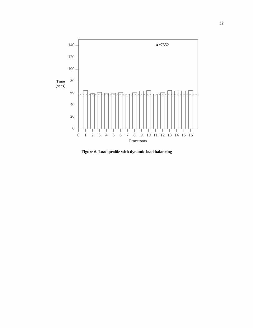
Figure 6. Load profile with dynamic load balancing

Figure 7. Test lengths for c7552

Figure 8. Speedups for c7552

Figure 9. Communication of test vectors for random and MACP partitioning

Figure 10. Communication of test vectors for input partitioning

vii

LIST OF TABLE CAPTIONS

Table I. Parameters in the performance model

Table II. Uniprocessor results with fault simulation

Table III. Results without fault simulation

Table IV. Run times for different partitioning methods

Table V. Results without dynamic load balancing

Table VI. Results with dynamic load balancing

Table VII. Results with pc = 0.6

1

1. INTRODUCTION

Generating a test for a fault in a logic network requires searching the input space of a network for a vector or

a vector sequence which distinguishes the faulty network from the fault-free one. The search space grows exponen-

tially with the number of primary inputs of the logic circuit. The problem of test generation has been shown to be

NP-hard [1, 2] even for combinational circuits. Most test generation algorithms use heuristics for search [3, 4]. For

circuits of VLSI complexity, the test generation time can be prohibitive. Test generation for a VLSI chip can take

days even weeks to complete. Efficient heuristics to speed up test generation have been proposed [5, 6] but such

heuristics are useful only to a limited extent. Multiprocessing hardware has to be used to get orders of magnitude

speedup for a variety of VLSI CAD applications such as placement, routing, design rule checking, extraction and

simulation [7, 8]. Unfortunately, not much work has been done in the utilization of general-purpose multiprocessors

for test generation. With multiprocessing hardware becoming more common and affordable, this seems to be a very

attractive and cost-effective alternative.

The types of parallelism inherent in a test generation/ fault simulation (TG/FS) application can be classified

into the following:

1. Fault Parallelism

2. Heuristic Parallelism

3. Simulation Parallelism

4. AND/OR Parallelism

A detailed discussion of the above types of parallelism may be found in [9]. Though the above types of paral-

lelism may not be identified as such, many examples of the above types of parallelism may be found in work done

previously. Fault Parallelism refers to the concurrent evaluation of the given fault set in parallel. The given faults

are distributed across the available processors so that the TG/FS process can proceed concurrently. Fault parallel-

ism is the focus of this paper and is discussed in more detail in the following sections. The implementation reported

in [10] uses fault parallelism in a loosely-coupled multiprocessor environment. A central server was used which dis-

tributes the fault set and keeps track of the TG/FS activity. A theoretical analysis of the performance of such a distri-

buted TG/FS system was presented in [11] for the parallel test generation system implemented in [10]. An empiri-

cal estimate of the speedups possible through fault parallelism was provided in [12]. Heuristic Parallelism refers to

the use of multiple heuristics (or testability measures) for search concurrently. Based on an empirical model of a

2

loosely coupled system and based on measurements made on a uniprocessor, an estimate of the speedups possible

due to heuristic parallelism on a loosely coupled multiprocessing system was provided in [12]. We can speedup for-

ward implication of logic values by using simulation parallelism. The implementation reported in [13] tries to

speedup exhaustive enumeration for test generation by using the massive parallelism available on an SIMD machine

like the Connection Machine [14]. AND/OR parallelism [15] is a very general model of a parallel algorithm and

encompasses many of the previously discussed techniques. AND-parallel tasks are set of mandatory tasks which can

be executed in parallel. OR-parallel tasks are a set of optional tasks of which only some of the tasks have to be com-

pleted to generate a test. For example, parallel search for a test vector in the input space of a logic circuit can be

termed as OR-parallelism. The parallel search techniques employed in [9, 10, 16] are examples of OR-parallel tech-

niques. In all cases, it was found that the parallel processing of the input search space was able to accelerate the test

generation for faults which required a large number of backtracks (or hard-to-detect faults). Parallel fault simulation

has been an active area of research and methods to exploit parallelism in fault simulation have been proposed and

implemented on a variety of machines [17-24].

This paper examines the performance trade-offs in the implementation of a parallel TG/FS system for combi-

national circuits based on fault parallelism. We assume that complex VLSI circuits are designed using full scan

methodologies, hence the size of the resultant combinational blocks are very large. We show that the overall test

length and speedup are strongly dependent on the fault partitioning method used. Heuristic methods for partitioning

faults are presented and evaluated. We examine the advantages and disadvantages of communicating test vectors

among processors for fault simulation. We propose a dynamic work load distribution strategy based on a distributed

work load allocation and termination detection scheme. We propose a theoretical model to predict the behavior of

the parallel test generation process. Finally, we present experimental results based on an implementation on the Intel

iPSC/2 hypercube using the ISCAS [25] combinational benchmark circuits. Preliminary results based on the

research reported in this paper appeared in [26].

2. EXPLOITING FAULT PARALLELISM

If fault simulation is not a part of a test generation system i.e., only a deterministic test pattern generation pro-

gram is used, the problem of partitioning faults for test generation is relatively straight-forward. To get the max-

imum amount of speedup on a multiprocessor, all one needs to make sure is that the work load is balanced on all

3

processors at all times. A simple dynamic allocation scheme in which an idle processor requests for a target fault

from some other processor/host would suffice. It is then very easy to predict linear speedups as reported in [12].

But most test generation systems use a test generation/ fault simulation loop. Each test generation step is followed

by a fault simulation step to detect additional faults from the fault list. The purpose of this step is two-fold. First,

since the complexity of fault simulation is much less than that of test generation, the fault simulation step saves the

effort in test generation for faults having the same test vector. Second, the overall test length is reduced due to the

additional faults detected during the fault simulation phase (also referred to as dynamic test compaction). The

overall test generation time for the fault set is much less if fault simulation is used.

Due to the use of fault simulation, the problem of fault partitioning in a parallel TG/FS environment becomes

non-trivial. A simple dynamic scheme where each processor is allocated one target fault at a time reduces to the

case where no fault simulation is used at all. Thus for fault simulation to be useful, each processor has to be allo-

cated more than one fault at a time. The best allocation strategy should minimize the overall run time and test

length. An ideal allocation would be such that (a) if a test vector for fault f i can also be a test for f j then they are

assigned to the same processor and (b) the load on all processors is balanced. If fault f i is assigned to processor pi

and fault f j is assigned to processor pj and both have a common test vector, then pi and pj might end up doing

some redundant work which could otherwise have been avoided on the uniprocessor by using fault simulation. Two

faults are called compatible if there exists a vector which can detect both the faults. It is easy to see that a compati-

bility relationship is much weaker than a fault dominance or equivalence relationship. If fault f i is dominant over f j

or f i is equivalent to f j then f i and f j are compatible but not vice versa.

As an example, consider the six faults shown in Figure 1. An edge between f i and f j means that fault f i is

compatible with fault f j . It should however be noted that compatibility is not a transitive relation i.e., if f i is compa-

tible with f j and if f j is compatible with f k it does not mean that f i and f k are compatible. For our example we

shall assume that if fault f i is compatible with faults f j and f k , there exists at least one vector which is a test for all

the faults f i ,f j ,f k which in the general case may not be possible. Also, we shall assume that whenever the test gen-

erator generates a test for a fault f i it generates a vector which detects not only fault f i but also all faults which are

compatible with f i . These assumptions are just for illustration purposes and may not hold true in the general case.

Assume the faults are processed on the uniprocessor as listed i.e., { f 1,f 2,..............,f 6}. Now assume it takes 10

time units to generate a test for a fault and after each test generation step it takes R time units for fault simulation

4

where R is the number of remaining faults. So, if the faults are considered in the order f 1 followed by f 2 and so on,

it takes 10 time units to generate a test for f 1 and 5 time units to do fault simulation for the remaining faults. Fault

f 4 is deleted from the fault list assuming it is detected during fault simulation. It takes 10 times units to generate a

test for f 2 and 3 time units for fault simulation and faults f 3 and f 5 get deleted from the fault list. It takes another 10

units to generate a test for the fault f 6 and the TG/FS process terminates. Thus, the total time for TG/FS on the

uniprocessor is: 10 + 5 + 10 + 3 + 10 = 38 time units and the test length is 3. Now assume there are two processors

p 1 and p 2. Let faults {f 1,f 2,f 6} be assigned to p 1 and faults {f 3,f 4,f 5} be assigned to p 2. Using the compatibility

relationships shown in Figure 1, p 1 takes 30 time units to complete TG/FS for its own fault list and p 2 takes 12 time

units for its own fault list. Thus the overall completion time is 30 time units and the test length is 4. Here it has been

assumed that the processors are computing test vectors independent of each other and have no knowledge of vectors

generated by other processors. This restriction will be relaxed later. Now consider another assignment. Let

{f 1,f 4,f 6} be assigned to p 1 and {f 2,f 3,f 5} be assigned to p 2. The completion time now is 22 time units and the

test length is 3, same as that on the uniprocessor. Since { f 2,f 3,f 5} belong to the same compatible fault set, they

were assigned to the same processor thus reducing the overall run time.

We define a compatible fault set as follows:

Definition: A set of faults is called a compatible fault set if for every pair of faults belonging to the same fault set,

there exists at least one test vector which detects both the faults. Thus all faults in a compatible fault set are pair-

wise compatible.

A compatible set is a complete subgraph in the graph shown in Figure 1 (or a clique) [27]. A complete sub-

graph is one where there is an edge between any two distinct vertices which belong to the subgraph. Finding out

whether two faults f i and f j have a test vector in common is a computationally hard problem and is as difficult as

test generation itself. In the worst case, it might be necessary to enumerate all possible test vectors for f i to find out

whether there is a vector which detects f j also. Since our objective is to find out compatible fault sets without actu-

ally using test generation and fault simulation, approximate heuristic methods have to be used. If heuristic methods

are used, it cannot be guaranteed that two faults belonging to the same partition or set will have a test vector in com-

mon. Due to this reason, the partitions generated by any of the heuristic partitioning methods will be referred to as

pseudo-compatible fault sets. Assigning each pseudo-compatible fault set to a different processor results in a lesser

run time and test length due to more faults being detected during the fault simulation phase.

5

We consider the overall run time to be more important than the test length because the test length in deter-

ministic test pattern generation is orders of magnitude lower than that generated using random patterns. Since the

test length affects the memory utilization for storage of test vectors as well as the test application time, because of

low test lengths obtained using deterministic test pattern generation, the memory utilization as well as the test appli-

cation time are going to be very low. Thus, even an order of magnitude increase in the test length is not going to

affect the memory utilization and test application time significantly. In the case of random pattern testing however,

since the test length is of the order of a few hundred thousand vectors (sometimes more), test length plays a very

important part. The run time for test generation on the other hand, plays a very important part in the overall turn-

around time during the design phase when parts of a circuit may have to be redesigned due to low fault coverage or

testability to reduce the defect rate in the field.

As the number of processors is increased, since we consider minimization of the overall run time for TG/FS

as our primary objective, some pseudo-compatible fault sets may have to be split across processors to keep the load

balanced. Thus, with increase in number of processors, it can be expected that the test length is also increased. The

heuristic partitioning algorithms presented in this paper try to minimize this increase. As the number of processors

approaches the number of faults, it can be expected that the test length approaches the number of faults also (since

we assume the primary objective is to reduce the run time).

Apart from using better partitioning methods to reduce the test lengths, test length can also be reduced by

broadcasting the vectors generated on one processor (through test generation) to all other processors. These test

vectors can be used during the fault simulation process by each processor to reduce the test length as long as the

associated overheads are not high. Due to the approximate nature of the fault partitioning techniques used, it is still

very likely that a test vector generated for a target fault f i assigned to processor pi is also a test for a fault f j

assigned to processor pj . Thus, if we communicate the test vector to processor pj then it does not have to generate a

test for fault f j . Since each processor is using test vectors generated on its own and those sent by other processors,

the number of test vectors used for fault simulation by each processor may be greater than or equal to the number of

vectors used for fault simulation on the uniprocessor. It can so happen that fault simulation phase dominates the

overall run time and each processor ends up spending about the same time as the uniprocessor. Also the communi-

cation overhead is increased and the multiprocessor may quickly run out of buffer space for messages because of

test vectors arriving from other processors at a rate faster than the fault simulation rate. This can cause further

6

degradation in performance. Thus, we have to find an optimal value of some communication parameter pc called

the communication cutoff (defined later) factor which results in a small test length without producing a severe

degradation in run time.

Partitioning methods which are used as a pre-processing step before the actual TG/FS phase will be referred

to as static partitioning methods. A static partitioning method may not result in balanced work loads on all the pro-

cessors. A dynamic load balancing technique may have to be used to keep the processor loads balanced at run time.

Based on our discussions above, we come to the following conclusion:

A good partitioning method to exploit fault parallelism should do the following:

(1) Avoid potential increase in test length by assigning all faults in the same compatible fault set to the same pro-

cessor.

(2) Control the degree of communication based on an optimal value of the communication cutoff factor pc .

(3) Use dynamic load balancing if necessary to keep the load balanced on all processors.

(4) The time for static partitioning should be very small compared to the actual TG/FS time.

It should be noted however that test length and run time anomalies can occur due to faults being processed in

an order different than on the uniprocessor. To reduce the likelihood of such artifacts in our experimental results, we

used the following ordering of faults on the multiprocessor:

If fault f i and f j are assigned to the same processor, fault f i occurs earlier in the fault list than f j if f i occurred

earlier than f j in the fault list of the uniprocessor.

As an example, consider again the six faults shown in Figure 1. Consider the following assignment:

p 1 ← {f 1,f 4} and p 2 ← {f 3,f 2,f 5,f 6}. The order of the faults in each fault list are the order in which they are pro-

cessed. Using this particular partition, processor p 1 takes 11 time units and p 2 takes 13 time units and the overall

completion time is 13 time units. Since it took 38 time units on the uniprocessor, we have a speedup greater than the

number of processors. Also, the test length is 2 which is less than that on the uniprocessor. If we follow the ordering

given above, the test length would have been 3 and the run time would be 22 time units.

7

3. STATIC FAULT PARTITIONING METHODS

All the methods described below were used in the static partitioning or the pre-processing step to initially

assign faults to the processors before the parallel TG/FS process is started. Each of the methods assignsRJJ N

nfhhhHJJ

or

JJQ N

nfhhhJJP

faults to each processor where nf is the total number of faults and N is the number of processors. Since each

processor is assigned equal number of faults, if the number of sets generated by any of the following methods is

greater then the number of processors, sets are assigned to each processor till it gets Nnfhhh faults. In some cases, this

may necessitate splitting the sets between two processors.

3.1 Random

Faults are assigned randomly to the processors. This method is used for comparison with other approaches.

3.2 Input Cones

Since each processor has to be assigned approximately Nnfhhh faults, each processor is allocated a bucket of size

Nnfhhh . A depth-first search is conducted starting from the inputs, where each input is selected in some arbitrary order.

This method assumes that all compatible faults lie in the same fanout cone of an input. In the process of traversal

from some other input, if it is found that a node (or fault) has already been visited, the depth-first search does not

proceed any further for that node since faults in the fanout cone of that node have already been assigned. Thus,

faults belonging to more than one topological input cone will be assigned to only one processor. During the traver-

sal of the circuit using depth-first search, the parity of the gates during the search is taken into account. For example,

if a s-a-0 fault was selected at the input of an inverting gate, then a s-a-1 fault will be selected at the output. This

approach tries to avoid assigning a s-a-0 and a s-a-1 fault on the same line to the same processor (since a s-a-0 and a

s-a-1 fault on the same line cannot be detected by the same test vector). As the bucket for a processor becomes filled

during the depth-first traversal, another processor is selected for assignment. Thus, input cones may be split across

processors during the depth-first traversal.

8

3.3 Output Cones

This method is similar to that for input cones except that the depth-first search traversal of the network is per-

formed starting at the outputs and proceeding towards the inputs.

3.4 Mandatory Constraint Propagation (MACP)

A set of constraints is derived based on the testing requirements imposed by each fault. Two faults are con-

sidered compatible if their testing constraints match i.e., the testing requirements do not conflict. A combination of

techniques proposed in[5, 28, 29] are used. The method involves the following key steps:

(1) A pre-processing phase in which the flow dominators of all the gates are generated [30]. Gate G is a domina-

tor of a gate g if all paths from g to any output in the logic circuit pass through G .

(2) Starting at the fault site and by using backward and forward implication, a set of uniquely implied logic

values is generated. The initial assignments which trigger backward and forward implication are based on

both the excitation and propagation requirements of a fault. For example, if we are testing for a stuck-at-0

fault at the output of a gate, then a logic value 1 will be required at the gate output to excite the fault. This

procedure also gives a set of faults in the vicinity of a fault α which may be detected by a test for α. All such

faults are put in the same pseudo-compatible fault set as α (pseudo-compatible since two faults in the same set

may not really be compatible). This procedure is very similar to the backward and forward implication pro-

cedures described in [28]. Also, from information about the flow dominators of the gate under test, additional

initial assignments are found as discussed under Step 3.

(3) This particular step tries to generate more constraints from the global flow dominator information. If G is a

dominator of g and we are testing for a fault α at the output of g then it must be observed at G . Also, all

inputs of G which are not reachable from the fault site must be set to non-controlling values. A test for a fault

at the output of g thus must detect at least one fault at the output of G (either s-a-0 or s-a-1). Backward and

forward implication is performed for G and its inputs. This is repeated for all dominators G of g and addi-

tional faults are added to the pseudo-compatible set for α generated in Step 2.

As an example consider the circuit C17 shown in Figure 2 which is an example circuit for the ISCAS bench-

marks. Assume we are trying to generate a compatible fault set for the fault 11 s-a-1. After forward and backward

implication of logic values, the sensitive values on various lines is shown in Figure 2. By a line being sensitive we

9

mean that a fault associated with that line will be detected. A ’+’ indicates a line is sensitive and ’-’ indicates a line

is not. The polarity of the fault detected depends on the logic value implied on that line. Thus a s-a-0 fault will be

detected for a line labeled ’1+’ and a s-a-1 fault will be detected on a line labeled ’0+’. Either a s-a-1 or s-a-0 fault

may be detected on a line labeled ’+’. Using the sensitivity values shown in Figure 2, we have the following

pseudo-compatible fault set: {1 s-a-0, 1 s-a-1, 8 s-a-0, 8 s-a-1, 16 s-a-0, 16 s-a-1, 12 s-a-0, 14 s-a-0, 17 s-a-1, 15 s-

a-0, 11 s-a-1}. It can be seen that s-a-0 and s-a-1 fault on the same line may be included in the same pseudo-

compatible fault set even though they are not compatible (and hence the name pseudo-compatible.).

If faults f i and f j are in the same pseudo-compatible fault set, it is very likely that they have a common test

vector. But the heuristic procedures given above do not guarantee that two faults will be compatible if they are

included in the same pseudo-compatible set (by definition). For example, in the example shown in Figure 2, the

faults 8 s-a-1 and 8 s-a-0 are included in the same pseudo-compatible faults set while clearly they are not compati-

ble. All faults belonging to the same pseudo-compatible fault set are assigned to the same processor. It can be seen

that finding pseudo-compatible faults sets by mandatory constraint propagation requires much more computation

time than any of the methods discussed above. All partitioning methods presented in this section require O (n ) com-

putation time, where n is the number of lines in the logic network, except partitioning by MACP. Partitioning by

MACP takes O (n 2) time which is equivalent to one pass for fault simulation. From the above discussion, it would

seem that partitioning by MACP is the best static partitioning method. However, due to its computational complex-

ity, it may take large amount of pre-processing time for large circuits. This will be validated in the experimental

results presented in Section 5. It is easy to see that partitioning by input cones has some inherent advantages over

partitioning by output cones if one considers the test generation process itself. During test generation, starting at the

fault site, sensitized paths are created which fan out from the fault site towards the output. Thus, additional faults

will be detected during fault simulation along these sensitized paths. Since partitioning by input cones will lump all

these faults in the same set, it can be expected that partitioning by input cones will do better than partitioning by out-

put cones on the average. We shall validate this claim through experimental results presented in Section 5. Also, the

partitioning methods presented above may have a tendency to lump all the hard-to-detect or redundant faults into the

same set. Thus, a processor may end up spending too much time on such faults resulting in skewed work loads.

Since it is difficult to come up with an a priori estimate of how difficult it is to generate a test for a particular fault,

additional load balancing is done at the run time by using techniques described in the next section. If a processor

10

ends up spending too much time on redundant or hard-to-detect faults, it will be left with a backlog of faults yet to

be processed. In such a case, the faults will be reallocated to processors which are idle if the dynamic load balancing

technique detailed in the next section is used, thus improving the overall system performance. The dynamic load

balancing technique would be effective irrespective of what the backtrack limit is.

4. LOAD BALANCING

We shall show through experiments that the number of faults is a very poor estimate of the work load. It was

found that even if an equal number of faults is allocated to different processors, the variation in work load (meas-

ured as the amount of time spent doing fault simulation and test generation) was substantial. Since it is very difficult

to judge a priori how difficult it is to generate a test for a particular fault, a static work load allocation scheme may

result in unbalanced work loads. Some processors may become idle before others. However, a dynamic work load

distribution scheme may result in excessive communication which may offset any performance gains due to

dynamic load balancing. We propose a method which is a compromise between static and dynamic load balancing

and combines the advantages of both. Initially, the fault list is distributed using one of the static partitioning

schemes given above. If a processor is done with its own fault list, it broadcasts a request for additional work to

other processors. Each of the processors receiving such a message sends the number of faults still to be processed

(an estimate of the remaining work load) to the processor requesting work. The processor requesting work then

sends an explicit work request message to the processor having the largest fault list. The processor having the larg-

est fault list then splits its own fault list into half and sends it off to the requesting processor. When splitting the

fault list, care is taken to ensure that faults are partitioned according to the static partitioning criterion used initially

i.e., for example, if the static fault partitioning criterion was partitioning by input cones, the idle processor gets

faults which are in the same input cone. Termination detection is very simple in this scheme. When all the fault lists

have been exhausted, all processors will try to request work from each other. When a particular processor finds that

all other processors have exhausted their own fault lists, it terminates. This particular load distribution and distri-

buted termination detection algorithm results in a high message traffic only at the end of the TG/FS process.

The exact algorithmic details of the load balancing algorithm follow. There are two types of messages which

are used by an idle processor when requesting for work: a QUERY message which is broadcast by an idle processor

to query the other processors for the length of the remaining fault list and a WRK_REQ message which is an expli-

11

cit message requesting for work from a busy processor. A parameter τ called the threshold is maintained which

controls the granularity of the load balancing algorithm and prevents excessive communication at the end of the

TG/FS process. Each of the busy processors checks for messages after each TG/FS step by executing the procedure

check_msgs given below:

procedure check_msgs;

(1) If there are no pending messages then return.

(2) If there is a message of the type QUERY then send the length of the remaining fault list to the requesting pro-

cessor if the length is greater than the threshold τ else send zero as the length.

(3) If there is a message of type WRK_REQ, then split the remaining fault list into half and send it to the request-

ing processor.

end check_msgs.

An idle processor pi enters a waiting phase when it exhausts its own fault list. The actions performed during

the waiting phase are given by the procedure get_work given below:

procedure get_work;

(1) Broadcast a QUERY message to all other processors.

(2) Get the length of the remaining fault list on all other processors. Let pd be the processor ID of the processor

having the largest fault list. If the length of the largest fault list is zero, then exit from the TG/FS process.

(3) Send a WRK_REQ message to processor pd and wait for work from pd . If the length of the fault list received

from pd is null, then exit from the TG/FS process else enter the TG/FS loop with the new fault list.

(4) If a QUERY message is received from some other processor then send zero as the length of the fault list to the

requesting processor.

(5) Go to 2.

end get_work;

In the procedure get_work, the idle processor pi exits the TG/FS loop if the fault list received from the

selected donor processor pd is null. This is done for two basic reasons. First, since the processor with the longest

fault list has exhausted its own fault list, it is very likely that the remaining processors have also exhausted their

12

fault lists. Second, this saves the extra communication overhead in termination of the TG/FS loop. Otherwise, each

processor will have to send at least (N −1) WRK_REQ messages before terminating. All message passing is done in

an asynchronous fashion so that a processor does not busy wait for a message at any time as long as it has some

other work to do. Thus, a busy processor is able to overlap computation with communication. The efficiency of the

load balancing method will be evident when we present experimental results.

5. PERFORMANCE ANALYSIS

It is possible to come up with a theoretical model for performance analysis based on the discussions given in

the previous sections. First, we shall try to model the TG/FS process on the uniprocessor based on some simplifying

assumptions. Figure 3 shows a plot of the fraction of faults left versus the fraction of total number of test vectors

generated for four of the ISCAS benchmark circuits. T 1 is the uniprocessor test length. It can be seen that the curve

closely resembles a decaying exponential for each of the circuits. In[31] , a combination of a decaying exponential

and a straight line was used to approximate the number of untested faults versus number of tests curve. The reason-

ing behind this assumption is that in a TG/FS process, initially a large number of faults are detected by the first few

vectors. These are usually the faults amenable to random pattern testing. This initial phase (called Phase I in [31] )

closely resembles a decaying exponential. After Phase I, the faults remaining are random pattern resistant faults.

For such faults, test generation has to be done explicitly and very few additional faults are detected with each addi-

tional test vector apart from the fault for which the test vector was explicitly generated. The curve in this portion

(called Phase II in [31] ) closely resembles a straight line. In Figure 3 the vertical dashed line segment approxi-

mately shows the regions of the curve corresponding to Phase I and II. It can be seen that Phase I ends when

approximately 20-30% of the test vectors have been generated and a fault coverage of 60-80% has been reached.

Though this would model the actual TG/FS process more accurately, the error incurred by modeling the whole

TG/FS curve by a decaying exponential is quite small as is apparent from the actual TG/FS curves shown in Figure

3. Thus, for the sake of simplicity, we shall assume that the TG/FS curve can be approximated by a decaying

exponential. Throughout our analysis, we shall use the CPU time estimates as an estimate of the cost. The terms

’cost’ and ’time’ will be used interchangeably.

13

5.1 Estimating Uniprocessor Run Time

Assuming an exponential fault simulation profile, let the fraction of faults left after t test vectors have been

generated (i.e., after t TG/FS steps) be given by:

F 0e−kt /T 1

where F 0 and k are constants and T 1 is the number of tests required to achieve the maximum possible fault cover-

age on the uniprocessor. The constants F 0 and k can be chosen according some error minimization criterion. For

example, F 0 and k could be chosen so that the sum of squares of errors

i =1ΣT 1

(f i −F 0e−kt /T 1)2

is minimized where f i is the actual fraction of faults left after the i’th test vector.

Let G be the number of gates in the circuit under test and let nf be the number of faults for which tests have

to be generated. Let nI be the number of primary inputs of the circuit under test and α be the fraction of gates

evaluated after each primary input assignment. Let bav be the average number of backtracks per fault and let β be

the fraction of gates evaluated after each backtrack. Hence, the time spent at each test generation step on the unipro-

cessor is:

αnI G + βbav G = (αnI + βbav )G

In the process of generating T 1 test vectors, the test pattern generator may abort test generation for faults for

which the backtrack limit is exceeded and also declare a few faults to be redundant. Let the number of faults

dropped on the uniprocessor be D 1 and the number of faults found redundant be R 1. Thus, the total number of faults

processed by the test pattern generator is (T 1 + R 1 + D 1) and the total time spent in test generation on the uniproces-

sor, denoted by Ctest (1), is given by (αnI + βbav )G (T 1 + R 1 + D 1 ). The number of faults to be simulated for the

t ’th test vector is the number of faults left after simulating the (t −1)’th vector which is:

F 0nf e −k (t −1)/T 1

Let the fraction of gates evaluated at each fault simulation step for each fault being simulated be γ and the fault

simulation cost for the t ’th vector is given by:

F 0nf e −k (t −1)/T 1×γG

The total fault simulation cost on the uniprocessor (Csim (1)) is:

14

i =1ΣT 1

F 0nf e −k (t −1)/T 1γG

which simplifies to:

Csim (1) = F 0nf γG1 − e −k /T 1

1 − e −khhhhhhhhh

and the total uniprocessor run time (for test generation and fault simulation) is given by:

(αnI + βbav )G (T 1 + R 1 + D 1) + F 0nf γG1 − e −k /T 1

1 − e −khhhhhhhhh

5.2 Estimating the Speedup on a Multiprocessor

To calculate the multiprocessor run time, assume there are N processors. Let the test length on N processors

be TN . The ratio of test lengths T 1

TNhhh is in some sense a measure of the redundant work done on the multiprocessor.

The higher the value of T 1

TNhhh, the more the amount of redundant work. In general, TN is dependent on the following:

(1) The static partitioning strategy: the better the strategy, the lower is the test length.

(2) The number of processors N : Excluding test length anomalies of the kind discussed in Section 2, the test

length normally increases with increase in N . Later we present experimental data to support this claim.

(3) The degree of communication allowed for test vectors among processors: the higher the communication, the

lower is the value of test length. We shall validate this claim using experimental data later.

Let each processor broadcast vectors to other processors for fault simulation until it has reached pc fault cov-

erage for its own faults. The parameter pc is called the communication cutoff factor. Thus, each processor not only

uses the test vectors generated during its own test generation phase for fault simulation, but also the ones generated

by other processors. Until each processor reaches a fault coverage of pc , it uses N vectors, where N is the number

of processors, at each fault simulation step. We referred to the parameter pc as the communication cutoff factor in

Section 2. Since pc is calculated relative to each processor’s own fault list, no communication is required to decide

when to stop sending test vectors to other processors. Also, at each fault simulation step, there is no explicit wait for

vectors from other processors. Each processor processes whatever vectors have arrived at that time from other pro-

cessors (all of them may not have arrived) in an asynchronous fashion.

Under perfect load balancing conditions, assume that each processor processes the same number of faults dur-

ing the test generation phase. Also assume that each processor generates TN /N vectors for nf /N of the faults. In

15

general, the above assumptions will not be true so the speedup estimates will be optimistic which will serve as an

upper bound on the actual speedups on the multiprocessor. In reality, the speedup depends on the maximum work

done by any processor rather than the average work load. The test generation time for each processor is given by:

Ctest (N ) = (αnI + βb )G (TN + R 1 + DN )/N

DN is the total number of dropped faults on N processors. The number of faults found redundant on the mul-

tiprocessor will be the same as that on the uniprocessor since the backtrack limit is the same. Until the coverage

reaches pc , each processor also uses test vectors generated by other processors for fault simulation. The fault simu-

lation cost is thus multiplied by a factor of N till a coverage of pc is reached. Assuming an exponential relationship

between the number of untested faults and the number of tests, the number of test vectors generated when a cover-

age of pc is reached is given by:

1 − F 0e−Nkt /TN = pc

or

t = tc =RJJ kN

TNhhhlog 1−pc

F 0hhhhhHJJ

The total fault simulation cost is found by adding the costs for the first tc vectors separately with that of the final

TN − tc vectors. The fault simulation cost is thus:

Ni =1Σtc

F 0 Nnfhhhγe −Nk (t −1)/TN +

i =tc +1ΣTN

F 0 NnfhhhγGe −Nk (t −1)/TN

which simplifies to:

Csim (N ) = F 0nf γGRJQ 1 − e −Nk /TN

1 − e −Nktc /TNhhhhhhhhhhh + N1hhe −ktc /TN

1 − e −kN /TN

1 − e −Nk (TN −tc )/TNhhhhhhhhhhhhhhHJP

We now try to estimate the communication overheads on the multiprocessor. The cost of communicating a

test vector can be denoted by δnI where nI is the number of primary inputs. The cost of broadcasting a test vector is

thus (N −1)×δnI . The analytical expression for communication we are going to obtain below is on the pessimistic

side since we are assuming communication cannot be overlapped. The cost for communicating vectors using this

expression should be considered an upper bound on the actual communication cost. Since each processor broad-

casts tc vectors, the total communication cost is:

Cvect (N ) = N ×(N −1)δnI tc = N ×(N −1)δnI

RJJ kN

TNhhhlog 1−pc

F 0hhhhhHJJ

16

It can be seen that every time a processor becomes idle, it initiates the dialog given in Section 4 under the pro-

cedure get_work which results in 2N messages where N is the number of processors. Of the 2N messages, 2N −1

are short messages of the type QUERY, WRK_REQ or messages giving the length of the fault list. Only one mes-

sage requires sending a part of the fault list. If the latency for short messages is Cshort and the average delay in

sending the fault list is proportional to the total number of faults nf , the communication overhead when the dialog

given above is invoked is given by:

(2N −1)Cshort + ωnf

where ω is some proportionality constant. For the parallel TG/FS process to terminate successfully, each processor

has to execute the procedure get_work at least once. Thus, the total communication overhead due to dynamic load

balancing is at least:

Cload (N ) = N ×[(2N −1)Cshort + ωnf ]

If the latency due to short messages is ignored, the communication overhead for load balancing grows only as fast

as the number of processors N .

In calculating the communication cost above we have again ignored the fact that communication can be over-

lapped with computation and it can also take place in parallel. The communication cost expressions we obtain are

biased more towards the pessimistic side. The speedup on N processors is given by:

SN = Ctest (N ) + Csim (N ) + Cload (N ) + Cvect (N )Ctest (1) + Csim (1)hhhhhhhhhhhhhhhhhhhhhhhhhhhhhhhhhhh

where Ctest (1) and Csim (1) are test generation and fault simulation costs respectively, on the uniprocessor and

Ctest (N ) and Csim (N ) are the corresponding values on N processors. Cload (N ) is the cost of dynamic load balancing

on N processors and Cvect (N ) is the cost of communicating test vectors for fault simulation. To simplify the final

speedup expression, assume tc = 0 for the time being (i.e., no communication for test vectors takes place). Substi-

tuting expressions for the quantities given above, we get:

SN = RJQ(αnI + βbav )G N

TN + R 1 + DNhhhhhhhhhhhh + F 0 NnfhhhγG

1 − e −Nk /TN

1 − e −Nkhhhhhhhhhh + N [(2N −1)Cshort + ωnf ]HJP

RJQ(αnI + βbav )G (T 1 + R 1 + D 1) + F 0nf γG

1 − e −k /T 1

1 − e −khhhhhhhhhHJPhhhhhhhhhhhhhhhhhhhhhhhhhhhhhhhhhhhhhhhhhhhhhhhhhhhhhhhhhhhhhhhhhhhh

It can be seen from the discussion here that the analysis presented is quite different from the one presented in

[11]. The analysis in [11] primarily dealt with the estimation of the size of the target faults that needs to be sent by

the central server so as to minimize communication and maximize speedup. The analysis is thus based on speedup

17

alone and not the quality of the solution (e.g., test length). The analysis presented in this section tries to take into

account both the speedup and the resultant effect on the quality. While a central scheduler is assumed in [11] we

make no such assumptions and assume a completely distributed environment for load balancing and fault partition-

ing. By judicious combination of static and dynamic load balancing and by overlapping computation with communi-

cation, the communication overheads are kept low. Also, the above analysis can accommodate most multiprocessor

MIMD architectures (shared or distributed memory). Architecture dependent parameters can in fact be absorbed as

a part of different constants presented above. However, for architectures based on synchronous communication and

execution e.g., an SIMD architecture like the Connection Machine, an analysis different from the one presented

above will have to be adopted. The parameters used in the above analysis are summarized in Table I.

5.3 Example

To demonstrate the utility of the analysis presented above, consider the following simple example. The TG/FS

program was run on the uniprocessor on 10 randomly selected faults for the circuit c6288 from the ISCAS combina-

tional benchmark suite [32]. All parameters calculated here are with respect an Intel iPSC/2 hypercube. The test

vectors generated during the test generation phase were used in the fault simulation phase for the whole fault list

which consisted of 7744 faults (nf = 7744). It was found that the test pattern generator was able to generate tests for

all the 10 faults without any backtracks (bav = 0). The average test generation time was found to be 0.4 seconds per

fault ([αnI + βbav ]G = 0.4 secs ). Also, the total fault simulation time for all the 10 vectors was found to be 28.65

seconds at the end of which 93.23% of the faults were detected. The number of faults simulated during each fault

simulation step were added up for all the 10 vectors and the time for fault simulation per fault per vector was found

to be 0.0012 seconds (γG = 0.0012 secs ). Thus, based on parameters obtained from this partial TG/FS profile on a

uniprocessor we are trying to estimate the speedup on a multiprocessor. The exponential fault simulation curve will

not be able to fit cases where the final fault coverage is 100% because the exponential model will predict the test

length to be infinite. In such a case the exponential-linear model of [31] will have to be used. However, the pure

exponential model can be used if we assume the fault coverage to be less than but very close to 100%. Let us

assume that the final fault coverage for c6288 is 99.99%. Thus, at t = T 1, the fraction of faults left is 0.0001.

Assume the value F 0 is 1 so that F 0e−kt /T 1 becomes 1 when t is 0. Since, at t = T 1 the fraction of faults left is

0.0001,

18

e −k =0.0001

which means

k = 9.21.

Having estimated the value of k , let us now try to estimate the uniprocessor test length (T 1) for c6288. Since a fault

coverage of 93.23% was reached using 10 vectors, the fraction of faults left at the end of 10 vectors is 0.0677 which

means

F 0e−10k /T 1=0.0677.

Substituting the values of F 0 and k we get the value of T 1 to be 34 which was found to be very close to the actual

uniprocessor test length of 39 (for a fault coverage of 99.94%). Figure 4 compares the theoretical fault simulation

profile with the actual profile for the circuit c6288. It can be seen that the theoretical fault simulation profile matches

the actual one very well. Assume there are no dropped or redundant faults, i.e., R 1 = D 1 = 0. Thus the uniprocessor

test generation time is:

Ctest (1) = (αnI + γbav )GT 1 = 0.4 × 34 = 13.6 seconds

The uniprocessor fault simulation time is:

Csim (1) = F 0γGnf1 − e −k /T 1

1 − e −khhhhhhhhh = 1×0.0012×77441 − e −9.21/34

1−e −9.21hhhhhhhhhh = 39.16 seconds

Thus the total TG/FS time on the uniprocessor is 13.6 + 39.16 = 52.76 seconds. Let us now estimate the run time on

16 processors. Assume there is a ten-fold increase in test length on the multiprocessor i.e., T 16 = 340. Thus,

Ctest (16) = 0.4× 16340hhhh = 8.5 seconds . The fault simulation time is given by

Csim (16) = 1×0.0012× 167744hhhhh×

1 − e−16× 340

9.21hhhhh1−e −9.21×16hhhhhhhhhhh = 1.65 seconds.

To estimate the communication overhead, for the purpose of analysis, ignore the overhead in transferring the fault

list (ω =0). On the Intel i PSC/2 hypercube, the value of Cshort is 0.3 milliseconds or 0.0003 seconds. Thus, com-

munication overhead for load balancing is:

Cload (16) = N (2N −1)Cshort = 16×31×0.0003 = 0.1488 seconds.

Assume that there is no communication for vectors, i.e., pc = 0. Thus, the total run time on 16 processors is

8.5+1.65+0.15 = 10.30 seconds and the speedup is:

S 16 = C (16)C (1)hhhhhh = 10.30

52.76hhhhhh = 5.12.

This is a rather surprising result since we would expect much more parallelism from fault partitioning. The speedup

19

calculated above is rather on the optimistic side since we have ignored the communication overhead for communi-

cating the fault list and the relative skew in test generation work loads because of unequal faults processed during

the test generation phase. We have also not considered the effect of dropped or redundant faults. The highest actual

speedup for the circuit c6288 for any partitioning heuristic (without communication for test vectors) was found to be

3.74. The partitioning heuristic which resulted in this speedup was found to be MACP. Also, the values of T 1 and

TN for MACP were found to be 39 and 367 respectively which are very close to the assumptions made above. In our

experimental results, as discussed later, the communication overhead played a negligible part in determining the

speedup. The term which determined the speedup was the test generation term Ctest (N ) which in turn is dependent

on TN . The domination of the Ctest (N ) with increase in N is also evident from the above calculations for C (1) and

C (16). Thus, the test length is a dominant parameter in determining the speedup.

5.4 Memory Overhead

The above analysis is based on examining the run time trade-offs. Another major component in the perfor-

mance of any algorithm is the memory utilization. Since our implementation is based on a distributed-memory

architecture, the circuit has to be replicated across processors to keep the communication cost low. Thus, it would

seem like the memory requirements of the parallel algorithm are N times the memory requirements of the unipro-

cessor algorithm, where N is the number of processors. However, on closer examination the memory requirements

of the parallel algorithm turn out to be much lower. Only the circuit graph has to be replicated across processors and

the dynamic lists generated during test generation normally consume very less memory due to the low memory

requirements of an algorithm like PODEM [4]. The memory consumed during fault simulation per processor is

however reduced as the number of processors is increased since the fault list is now partitioned across several pro-

cessors and the resultant dynamic lists generated during fault simulation will be shorter. Most present day distri-

buted memory machines lack virtual memory. Thus, memory utilization can become a bottleneck for very large cir-

cuits if the circuit graph cannot fit into the physical memory of each processor. It may not even be possible to run

the parallel algorithm for very large circuits (larger than 50,000 gates) by simple replication. In such a case, the cir-

cuit graph may have to be partitioned on the basis of high-level modules or input/output cones so that test generation

and fault simulation for different modules can proceed concurrently. In case the circuit is partitioned by input/output

cones, only the regions belonging to more than one cone need be replicated. However, virtual memory for distri-

buted memory machines is a very active area of research [33] and we feel that the demands on physical memory

20

will go down as new distributed-memory machines are introduced which incorporate virtual memory. In the case of

shared-memory machines, where ’messages’ are basically read and write operations to the shared memory, the cir-

cuit graph need not be replicated and can be resident in the shared memory which can be accessed by all processors.

Only the processor specific dynamic information need be replicated.

However, the above observations should not detract from the fact that the memory overhead is the main draw-

back of our approach. As a part of future research, we intend to investigate efficient circuit partitioning techniques

to reduce the memory overhead.

6. EXPERIMENTAL RESULTS

6.1 Implementation

A parallel TG/FS program using PODEM[4] as a deterministic test pattern generator, and a deductive fault

simulator[34] was implemented in the C programming language on a 16 processor Intel iPSC/2 hypercube. The

SCOAP[35] heuristic was used for guidance. The ISCAS combinational benchmark suite[25] was used to evaluate

the TG/FS program. A backtrack limit of 25 was used for the deterministic test pattern generator. The performance

of the program on a single node (80386 CPU) of the hypercube is given in Table II. All times are in seconds and

include fault simulation and test generation times. All speedup results will be calculated relative to the times shown

in Table II. Random fill-in was used during fault simulation for primary inputs with unspecified logic values. It can

be seen that the number of test vectors are well below the total number of faults considered. The fault coverage (in

percent) figure is the fraction of faults which were detected or were declared redundant.

Table III shows the uniprocessor and the parallel processor results for some of the ISCAS circuits when no

fault simulation was used. It can be seen that the uniprocessor results are much inferior to those obtained in Table II

by using fault simulation, both in terms of the test lengths and run times. Also, even though random partitioning

was used to partition the faults, the results show almost linear speedups. For the remaining part of our discussion,

we shall assume that fault simulation is always used with deterministic test pattern generation.

6.2 Static Fault Partitioning and Dynamic Load Balancing

Table IV shows the time taken by the partitioning methods discussed in Section 3. It can be seen that except

for partitioning by MACP, most partitioning methods (which constitutes a pre-processing overhead) take a

21

negligible time compared to the total test generation time. However, for large circuits, partitioning by MACP takes a

time comparable to that of test generation. These run times should be kept in mind while comparing the speedup

figures presented for various partitioning methods since the speedups do not include the fault partitioning time.

Table V shows the speedups obtained by using different partitioning methods on 16 processors. The test lengths are

higher than the corresponding figures shown in Table II for the uniprocessor in all cases. No communication for test

vectors was allowed and only static partitioning was used. The fault coverage figures are sometimes marginally

lower than those on the uniprocessor since each processor is doing only local fault simulation i.e., it is not using test

vectors generated by other processors. The actual fault coverage figures may be much higher than just a simple sum

of coverage figures obtained by different processors. The multiprocessor fault coverage figures may in fact be equal

to or greater than the corresponding numbers on the uniprocessor.

Despite the reason given above, the variation in fault coverages from the uniprocessor and across different

partitioning methods is only marginal. Table V also shows the ranks for each partitioning method for test lengths

and speedups. Each partitioning method was given a separate rank for test length and speedup for each of the

ISCAS benchmark circuits. Thus a partitioning method which leads to a lower test length gets a higher rank for test

length. Similarly, a partitioning method which results in higher speedups is given a higher rank. The ranks were then

averaged for all of the ISCAS circuits for each of the partitioning techniques resulting in the composite rank given at

the bottom of each column in Table V. For example, consider the row for circuit c432 in Table V. The ranks

assigned to each of the partitioning methods with respect to the test lengths are 4, 1, 3, and 2 for random, input

cones, output cones and MACP partitioning respectively (the ranks assigned in each row are not shown because of

lack of space). Similarly, the ranks assigned for speedups are 3, 1, 3 and 2 for random, input cones, output cones and

MACP respectively. After assigning ranks in each of the rows, the composite rank is obtained by averaging the rank

in each of the columns. For example, the composite rank of 3.7 for the test length for random partitioning (bottom of

second column in Table V) was found by averaging all ranks for test length for random partitioning across all the

circuits. Partitioning by input cones has the highest rank for the test length and random partitioning has the highest

rank for the speedup even though it has the lowest rank for test length. These results are in some sense counter-

intuitive since one would expect that speedup should be higher for the partitioning method which produces a lower

test length. This particular behavior is in fact not due to a deficiency in the partitioning technique but due to unbal-

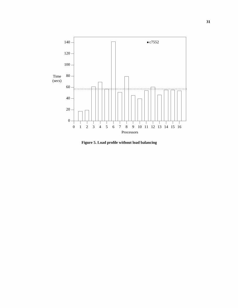
anced loads on different processors. Consider the load profile shown in Figure 5 for the circuit c7552 when output

22

partitioning was used. The load was measured as the sum of fault simulation and test generation times including the

time for communication. The dotted line shows the average of the load on all processors which is 57.77 seconds. If

the processor loads were perfectly balanced, all processor loads would have been near the dotted line. The ideal

speedup in case of balanced loads would have been 57.77437hhhhhh = 7.56. It can be seen that even though equal number of

faults were assigned to each processor, the processor loads are widely skewed with the ratio of maximum to

minimum load being about 8.

Table VI shows the results obtained when the dynamic load balancing scheme discussed in Section 4 was

used. The value of parameter τ was fixed at 10 i.e., the fault list was not split if the length of the remaining fault list

was less than or equal to 10. The results show a significant change in speedups obtained for various partitioning

techniques. Since we have two separate ranks for each partitioning method, we can measure the ’goodness’ of each

partitioning technique by assigning proper weights which reflect the relative importance of the test length and

speedup. If we assign equal weights to test length and speedup, partitioning by input cones and MACP turns out to

be the best partitioning methods with overall ranks of (1.5+2.1)/2 = 1.8 and (2.0+1.7)/2 = 1.85 respectively. How-

ever, considering the large amount of pre-processing time required by MACP, which is an order of magnitude

higher than the total TG/FS time on a multiprocessor, partitioning by input cones turns out to be the best partitioning

method. Figure 6 shows the load profile after the dynamic load balancing technique described in Section 4 was used

with output partitioning. Comparing with Figure 5, the change in the load profile is dramatic. The processor loads

are slightly higher than the ideal load of 57.77 seconds due to the communication overheads of dynamic load

balancing. The speedup obtained in this case is 6.79 which is very close to the ideal speedup of 7.56. Thus, the

dynamic load balancing scheme is able to achieve uniform loads with very little communication overhead. Figures 7

and 8 show the variation in test length and speedup with the number of processors for c7552 when dynamic load

balancing is used. It can be seen that partitioning by input cones does much better than all other methods.

6.3 Communication of Test Vectors Among Processors

As pointed out earlier, most partitioning methods do not guarantee that all faults in the same compatible fault

set are assigned to the same processor. Thus, it may be possible to lower the test length by broadcasting the test vec-

tors derived on one processor to all other processors. However, for large values of the communication cutoff factor

pc , the terms Csim (N ) and Cvect (N ) may become dominant resulting in an a decrease in speedup. However, there

23

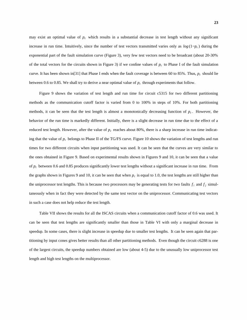
may exist an optimal value of pc which results in a substantial decrease in test length without any significant

increase in run time. Intuitively, since the number of test vectors transmitted varies only as log (1−pc ) during the

exponential part of the fault simulation curve (Figure 3), very few test vectors need to be broadcast (about 20-30%

of the total vectors for the circuits shown in Figure 3) if we confine values of pc to Phase I of the fault simulation

curve. It has been shown in[31] that Phase I ends when the fault coverage is between 60 to 85%. Thus, pc should lie

between 0.6 to 0.85. We shall try to derive a near optimal value of pc through experiments that follow.

Figure 9 shows the variation of test length and run time for circuit c5315 for two different partitioning

methods as the communication cutoff factor is varied from 0 to 100% in steps of 10%. For both partitioning

methods, it can be seen that the test length is almost a monotonically decreasing function of pc . However, the

behavior of the run time is markedly different. Initially, there is a slight decrease in run time due to the effect of a

reduced test length. However, after the value of pc reaches about 80%, there is a sharp increase in run time indicat-

ing that the value of pc belongs to Phase II of the TG/FS curve. Figure 10 shows the variation of test lengths and run

times for two different circuits when input partitioning was used. It can be seen that the curves are very similar to

the ones obtained in Figure 9. Based on experimental results shown in Figures 9 and 10, it can be seen that a value

of pc between 0.6 and 0.85 produces significantly lower test lengths without a significant increase in run time. From

the graphs shown in Figures 9 and 10, it can be seen that when pc is equal to 1.0, the test lengths are still higher than

the uniprocessor test lengths. This is because two processors may be generating tests for two faults f i and f j simul-

taneously when in fact they were detected by the same test vector on the uniprocessor. Communicating test vectors

in such a case does not help reduce the test length.

Table VII shows the results for all the ISCAS circuits when a communication cutoff factor of 0.6 was used. It

can be seen that test lengths are significantly smaller than those in Table VI with only a marginal decrease in

speedup. In some cases, there is slight increase in speedup due to smaller test lengths. It can be seen again that par-

titioning by input cones gives better results than all other partitioning methods. Even though the circuit c6288 is one

of the largest circuits, the speedup numbers obtained are low (about 4-5) due to the unusually low uniprocessor test

length and high test lengths on the multiprocessor.

24

7. CONCLUSIONS

As parallel processing hardware becomes more common and affordable, the use of parallel processing for

speeding up VLSI CAD applications is becoming more appropriate. This paper addressed the issues involved in pro-

viding an integrated test generation/ faults simulation environment on a parallel processor. The aim of this paper

was to show that if one is not careful in the design of a parallel algorithm, apart from inefficient utilization of avail-

able processors, degradation in the quality of solutions can occur. The concepts presented here are not specific to a

particular architecture and can be used on any MIMD parallel processing system. Issues in exploiting fault parallel-

ism for parallel test generation/ fault simulation were identified and discussed. It was shown that coupling fault

simulation with test generation results in a better utilization of the available processors. Requirements of an

efficient fault partitioning scheme were discussed and heuristic schemes for partitioning faults were presented. Also

a theoretical model for the TG/FS process was proposed to estimate the speedup in a parallel TG/FS environment.

Finally, experimental results based on an implementation of our parallel TG/FS algorithm on an Intel iPSC/2 hyper-

cube were presented. It was found that fault partitioning using input cones yielded better results both with respect to

the overall test length as well as the overall run time. A dynamic load balancing scheme which exploits the advan-

tages of both static and full dynamic load balancing was discussed. It was shown that the dynamic load balancing

scheme resulted in a more efficient utilization of the available processors. Also, a near optimal value of communi-

cation cutoff factor was found experimentally which results in smaller test lengths without a significant increase in

run time. The algorithm presented in this paper along with those presented in[9] are used in a very high perfor-

mance parallel test generation system called HIPERTEST.

ACKNOWLEDGMENT

The authors would like to thank all the reviewers for their helpful comments. We would particularly like to

acknowledge the detailed comments provided by Reviewer #3 which helped remove ambiguities and improve the

readability of the original manuscript.

25

REFERENCES

[1] O. H. Ibarra and S. K. Sahni, ‘‘Polynomially complete fault detection problems,’’ IEEE Trans. Computers,vol. C-31, pp. 555-560, June 1982.

[2] H. Fujiwara and S. Toida, ‘‘The complexity of fault fetection: An approach to design for testability,’’ Proc.12th Int. Symp. Fault Tolerant Computing, pp. 101-108, June 1982.

[3] J. P. Roth, ‘‘Diagnosis of automata failures: A calculus and a method,’’ IBM J. Research Development, vol.10, pp. 278-291, July 1966.

[4] P. Goel, ‘‘An implicit enumeration algorithm to generate tests for combinational logic circuits,’’ IEEETrans. Computers, vol. C-30, pp. 215-222, March 1981.

[5] H. Fujiwara and T. Shimono, ‘‘On the acceleration of test generation algorithms,’’ IEEE Trans. Computers,vol. C-32, pp. 1137-1144, December 1983.

[6] M. H. Schulz, E. Trischler, and T. M. Sarfert, ‘‘SOCRATES: A highly efficient ATPG system,’’ IEEETrans. Computer-Aided Design, vol. 7, pp. 126-137, January 1988.

[7] K. T. Tam, ‘‘Parallel processing for CAD applications,’’ IEEE Design and Test, pp. 13-17, October 1987.

[8] P. Banerjee, M. Jones, J. Sargent, R. J. Brouwer, K. P. Belkhale, and S. Patil, ‘‘Parallel algorithms for VLSIcomputer-aided design tools on hypercube multiprocessors,’’ in Advances in VLSI Computer-Aided Design,ed., I. N. Hajj. England: JAI Press, 1988.

[9] S. Patil and P. Banerjee, ‘‘A parallel branch and bound algorithm for test generation,’’ in Proc. 26th DesignAutomation Conf., Las Vegas, NV, pp. 339-344, June 1989.

[10] A. Motohara, K. Nishimura, H. Fujiwara, and I. Shirakawa, ‘‘A parallel scheme for test-pattern generation,’’Proc. Int. Conf. Computer-Aided Design, pp. 156-159, November 1986.

[11] H. Fujiwara and T. Inoue, ‘‘Optimal granularity of test generation in a distributed system,’’ IEEE Trans.Computer-Aided Design, vol. 9, pp. 885-892, August 1990.

[12] S. J. Chandra and J. H. Patel, ‘‘Test generation in a parallel processing environment,’’ Proc. IEEE Int. Conf.Computer Design, October 1988.

[13] G. A. Kramer, ‘‘Employing massive parallelism in digital ATPG algorithms,’’ Proc. Int. Test Conf., pp.108-114, 1983.

[14] W. D. Hillis, in The Connection Machine. Cambridge, MA: MIT Press, 1986.

[15] J. S. Conery, ‘‘The AND/OR process model for parallel interpretation of logic programs,’’ Technical Report204, University of California - Irvine, June 1983.

[16] S. Arvindam, V. Kumar, V. N. Rao, and V. Singh, ‘‘Automatic test pattern generation on multiprocessors,’’Proc. Int. Conf. Knowledge-Based Computer Systems, December 1989.

[17] D. L. Ostapko and Z. Barzilai, ‘‘Fast fault simulation in a parallel processing environment,’’ Proc. Int. TestConf., pp. 293-298, 1987.

[18] P. A. Duba, R. K. Roy, J. A. Abraham, and W. A. Rogers, ‘‘Fault simulation in a distributed environment,’’Proc. 25th Design Automation Conf., pp. 686-691, June 1988.

[19] V. Narayanan and V. Pitchumani, ‘‘A parallel algorithm for fault simulation on the connection machine,’’Proc. Int. Test Conf., pp. 89-93, September 1988.

[20] F. Ozguner, C. Aykanat, and O. Khalid, ‘‘Logic fault simulation on a vector hypercube multiprocessor,’’Proc. 3rd Int. Conf. Hypercube and Concurrent Computers and Applications, vol. II, pp. 1108-1116,January 1988.

[21] P. Agrawal et al, ‘‘MARS: A multiprocessor-based programmable accellerator,’’ IEEE Design and Test ofComputers, vol. 4, pp. 28-36, October 1987.

[22] P. Agrawal, V. D. Agrawal, K. T. Cheng, and R. Tutundjian, ‘‘Fault simulation in a pipelined multiprocessorsystem,’’ in Proc. International Test Conf., Washington, D.C., pp. 727-734, August, 1989.

26

[23] R. B. Mueller-Thuns, D. G. Saab, R. F. Damiano, and J. A. Abraham, ‘‘Portable parallel logic and faultsimulation,’’ in Proc. Int. Conf. Computer-Aided Design, Santa Clara, CA, pp. 506-509, November 1989.

[24] L. Huisman, I. Nair, and R. Daoud, ‘‘Fault simulation of logic designs on parallel processors with distributedmemory,’’ in Proc. International Test Conf., Washington, D.C., pp. 690-697, September, 1990.

[25] F. Brglez and H. Fujiwara, ‘‘Neutral netlist of ten combinational benchmark circuits and a target translator inFORTRAN,’’ Special session on ATPG and fault simulation, Proc. IEEE Int. Symp. Circuits and Systems,June 1985.

[26] S. Patil and P. Banerjee, ‘‘Fault partitioning issues in an integrated parallel test generation/fault simulationenvironment,’’ in Proc. Int. Test Conf., Washington D.C., pp. 718-726, August 1989.

[27] J. A. Bondy and U. S. R. Murty, in Graph Theory With Applications. New York: North-Holland, 1976.

[28] S. B. Akers, C. Joseph, and B. Krishnamurthy, ‘‘On the role of independent fault sets in the generation ofminimal test sets,’’ Proc. Int. Test Conf., pp. 1100-1107, 1987.

[29] T. Kirkland and M. Ray Mercer, ‘‘A topological search algorithm for ATPG,’’ Proc. 24th DesignAutomation Conf., pp. 502-508, 1987.

[30] D. Harel, ‘‘A linear time algorithm for finding dominators in flow graphs and related problems,’’ Proc. 17thACM Symp. Computing, pp. 183-184, May 1985.

[31] P. Goel, ‘‘Test generation cost analysis and projections,’’ Proc. 17th Design Automation Conf., pp. 77-84,June 1980.

[32] F. Brglez, D. Bryan, and K. Kozminski, ‘‘Combinational profiles of sequential benchmark circuits,’’ Proc.Int. Symp. Circuits and Systems, pp. 1929-1934, May 1989.

[33] K. Li and R. Schaefer, ‘‘A hypercube shared virtual memory system,’’ Proc. Int. Conf. Parallel Processing,vol. I, pp. 125-132, August 1989.

[34] D. B. Armstrong, ‘‘A deductive method for simulating faults in logic circuits,’’ IEEE Trans. Computers, vol.C-21, pp. 462-471, May 1972.

[35] L. H. Goldstein and E. L. Thigpen, ‘‘SCOAP: Sandia controllability/observability analysis program,’’ Proc.17th Design Automation Conf., 1980.

27

f 3

f 6

f 5

f 2

f 4

f 1

Figure 1. Compatible fault sets

28

1

++

1

0+

1+

1+

1+

-

+

1

1

1

0

0

1-

0+sa1

1

2

3

6

7

4

5

8

9

10

11

12

13

14

15

16

17

Figure 2. Mandatory constraint propagation

29

0 0.2 0.4 0.6 0.8 1

0

20

40

60

80

100

UntestedFaults (%)

t /T1

∆

∆

∆

∆

∆∆

∆

∆

∆∆

∆∆ ∆

∆∆ ∆ ∆ ∆ ∆ ∆ ∆

∆ ∆ ∆ ∆ ∆ ∆ ∆ ∆ ∆ ∆ ∆ ∆ ∆ ∆ ∆∆

g

g

g

g

g

gg g

gg g g

gg

gg

g gg

gg g g g g g g g g g g g g

gg g g g g g g g g

`

`

`

`

`

``

``

` ` ` ` ` ` ` ` ` ` ` ` ` ` ` ` ` ` ` ` ` ` ` ` ` ` ` ` ` ` `

∆

g

`

PHASE I PHASE II c432

c1908

c6288

c7552

Figure 3. TG/FS profile

30

0 0.2 0.4 0.6 0.8 1

0

20

40

60

80

100

UntestedFaults (%)

t /T1

.................................................................................

PHASE I PHASE II c6288 (theoretical)

c6288 (actual)

Figure 4. Actual and theoretical TG/FS profiles for c6288

31

Processors

Time(secs)

0 1 2 3 4 5 6 7 8 9 10 11 12 13 14 15 16

0

20

40

60

80

100

120

140

. . . . . . . . . . . . . . . . . . . . . . . . . . . . . . . . . . . . . . . . . . . . . . . . . . . . . . . . . . . . . . . . . . . . . . . . . . . . . . . . .

g c7552

Figure 5. Load profile without load balancing

32

Processors

Time(secs)

0 1 2 3 4 5 6 7 8 9 10 11 12 13 14 15 16

0

20

40

60

80

100

120

140

. . . . . . . . . . . . . . . . . . . . . . . . . . . . . . . . . . . . . . . . . . . . . . . . . . . . . . . . . . . . . . . . . . . . . . . . . . . . . . . . .

g c7552

Figure 6. Load profile with dynamic load balancing

33

0

2

4

6

8

Speedup

Processors1 2 4 8 16

g

g

g

g

g

`

`

`

`

`

..........

......

.......

......

......

......

.......

......

......

......

......

......

....

. . . . . . . . .

g`

Random

Input Cones

Output Cones

MACP

c7552

Figure 7. Test lengths for c7552

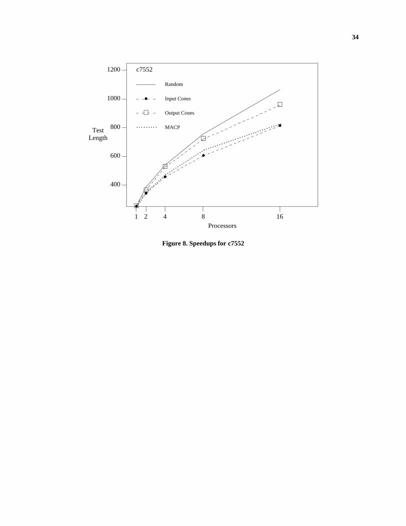
34

400

600

800

1000

1200

TestLength

Processors1 2 4 8 16

g

g

g

g

g

`

`

`

`

`

..........

......

.......

......

......

...... . . .

. . . . .. . . . .

. . . . .. . . . .

. . . . .. . . . .

.. . . . . . . . .

g

`

Random

Input Cones

Output Cones

MACP

c7552

Figure 8. Speedups for c7552

35

Timein secs

Communication Cutoff (pc )

TestLength

20

25

30

35

40

45

50

55

150

250

350

450

550

650

750

850

0 0.1 0.2 0.3 0.4 0.5 0.6 0.7 0.8 0.9 1

g c5315, Random Partitioning

Test Length

Time

Timein secs

Communication Cutoff (pc )

TestLength

20

25

30

35

40

45

50

55

150

250

350

450

550

650

750

850

0 0.1 0.2 0.3 0.4 0.5 0.6 0.7 0.8 0.9 1

g c5315, MACP Partitioning

Test Length

Time

Figure 9. Communication of test vectors for random and MACP partitioning

36

Timein secs

Communication Cutoff (pc )

TestLength

1.2

1.7

2.2

80

105

130

155

180

205

0 0.1 0.2 0.3 0.4 0.5 0.6 0.7 0.8 0.9 1

g c432, Input partitioning

Test Length

Time

Timein secs

Communication Cutoff (pc )

TestLength

50

62.5

75

87.5

100

250

350

450

550

650

750

0 0.1 0.2 0.3 0.4 0.5 0.6 0.7 0.8 0.9 1

g c7552, Input partitioning

Test Length

Time

Figure 10. Communication of test vectors for input partitioning

37

Table I. Parameters in the performance model

iiiiiiiiiiiiiiiiiiiiiiiiiiiiiiiiiiiiiiiiiiiiiiiiiiiiiG Number of gates in the logic circuit

nI Number of primary inputs (PIs) of the logic circuit

nf Number of faults in the fault list

N Number of processors

TN Test length on N processors

R 1 Number of faults found redundant

DN Number of faults dropped on N processors

F 0, k Constants in the exponential fault simulation curve

α Fraction of gates evaluated after each PI assignment

β Fraction of gates evaluated after each backtrack

bav Average number of backtracks during test generation

pc Communication cutoff factor

Cshort Message latency for short messages

ω Communication cost per fault for load balancingiiiiiiiiiiiiiiiiiiiiiiiiiiiiiiiiiiiiiiiiiiiiiiiiiiiiicccccccccccccccccccc

cccccccccccccccccccc

38

Table II. Uniprocessor results with fault simulation

iiiiiiiiiiiiiiiiiiiiiiiiiiiiiiiiiiiiiiiiiiiiiiiiiiiCircuit Faults Test vectors Coverage Time(s)iiiiiiiiiiiiiiiiiiiiiiiiiiiiiiiiiiiiiiiiiiiiiiiiiiiiiiiiiiiiiiiiiiiiiiiiiiiiiiiiiiiiiiiiiiiiiiiiiiiiiic432 524 71 99.24 6.76iiiiiiiiiiiiiiiiiiiiiiiiiiiiiiiiiiiiiiiiiiiiiiiiiiic499 758 72 98.95 9.23iiiiiiiiiiiiiiiiiiiiiiiiiiiiiiiiiiiiiiiiiiiiiiiiiiic880 942 85 100.00 9.05iiiiiiiiiiiiiiiiiiiiiiiiiiiiiiiiiiiiiiiiiiiiiiiiiiic1355 1574 145 99.49 38.02iiiiiiiiiiiiiiiiiiiiiiiiiiiiiiiiiiiiiiiiiiiiiiiiiiic1908 1879 150 99.73 49.42iiiiiiiiiiiiiiiiiiiiiiiiiiiiiiiiiiiiiiiiiiiiiiiiiiic2670 2747 141 95.52 116.81iiiiiiiiiiiiiiiiiiiiiiiiiiiiiiiiiiiiiiiiiiiiiiiiiiic3540 3428 206 96.82 235.38iiiiiiiiiiiiiiiiiiiiiiiiiiiiiiiiiiiiiiiiiiiiiiiiiiic5315 5350 161 99.20 150.41iiiiiiiiiiiiiiiiiiiiiiiiiiiiiiiiiiiiiiiiiiiiiiiiiiic6288 7744 39 99.94 70.81iiiiiiiiiiiiiiiiiiiiiiiiiiiiiiiiiiiiiiiiiiiiiiiiiiic7552 7550 251 97.71 437.00iiiiiiiiiiiiiiiiiiiiiiiiiiiiiiiiiiiiiiiiiiiiiiiiiiic

cccccccccccccccccccc

ccccccccccccccccccccc

ccccccccccccccccccccc

ccccccccccccccccccccc

ccccccccccccccccccccc

ccccccccccccccccccccc

ccccccccccccccccccccc

39

Table III. Results without fault simulation

iiiiiiiiiiiiiiiiiiiiiiiiiiiiiiiiiiiiiiiiiiiiiiiiiiiiiiiiiiiiiiiiiiiiiiiiiiTime (seconds)iiiiiiiiiiiiiiiiiiiiiiiiiiiiiiiiiiiiiiiiiiii

Circuit Vectors Coverage p = 1 p = 2 p = 4 p = 8 p = 16iiiiiiiiiiiiiiiiiiiiiiiiiiiiiiiiiiiiiiiiiiiiiiiiiiiiiiiiiiiiiiiiiiiiiiiiiiiiiiiiiiiiiiiiiiiiiiiiiiiiiiiiiiiiiiiiiiiiiiiiiiiiiiiiiiiiiiiiiiiiiiiiiiiic432 519 99.05 14.74 7.46 3.88 2.52 1.53iiiiiiiiiiiiiiiiiiiiiiiiiiiiiiiiiiiiiiiiiiiiiiiiiiiiiiiiiiiiiiiiiiiiiiiiiic499 750 98.95 43.14 22.56 11.28 6.23 3.23iiiiiiiiiiiiiiiiiiiiiiiiiiiiiiiiiiiiiiiiiiiiiiiiiiiiiiiiiiiiiiiiiiiiiiiiiic880 942 100.00 22.12 11.55 5.77 3.13 1.75iiiiiiiiiiiiiiiiiiiiiiiiiiiiiiiiiiiiiiiiiiiiiiiiiiiiiiiiiiiiiiiiiiiiiiiiiic1355 1560 99.11 220.75 115.58 59.36 30.34 16.22iiiiiiiiiiiiiiiiiiiiiiiiiiiiiiiiiiiiiiiiiiiiiiiiiiiiiiiiiiiiiiiiiiiiiiiiiic1908 1863 99.47 164.36 84.06 46.23 23.74 12.32iiiiiiiiiiiiiiiiiiiiiiiiiiiiiiiiiiiiiiiiiiiiiiiiiiiiiiiiiiiiiiiiiiiiiiiiiic6288 7688 99.69 2920.05 1498.71 756.64 386.60 198.14iiiiiiiiiiiiiiiiiiiiiiiiiiiiiiiiiiiiiiiiiiiiiiiiiiiiiiiiiiiiiiiiiiiiiiiiiicc

cccccccccccccc

cccccccccccccccc

cccccccccccccccc

cccccccccccccccc

cccccccccccccccc

cccccccccccccc

cccccccccccccc

cccccccccccccc

cccccccccccccc

cccccccccccccccc

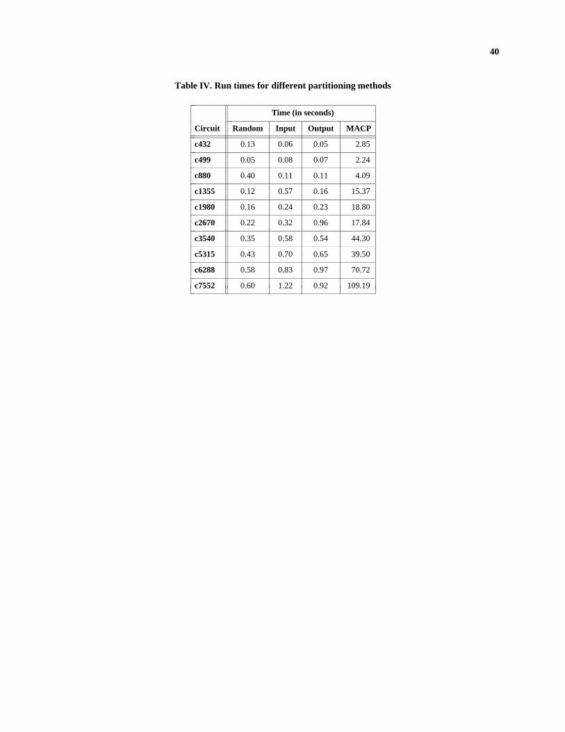
40

Table IV. Run times for different partitioning methods

iiiiiiiiiiiiiiiiiiiiiiiiiiiiiiiiiiiiiiiiiiiiiTime (in seconds)iiiiiiiiiiiiiiiiiiiiiiiiiiiiiiiiiiii

Circuit Random Input Output MACPiiiiiiiiiiiiiiiiiiiiiiiiiiiiiiiiiiiiiiiiiiiiiiiiiiiiiiiiiiiiiiiiiiiiiiiiiiiiiiiiiiiiiiiiiic432 0.13 0.06 0.05 2.85iiiiiiiiiiiiiiiiiiiiiiiiiiiiiiiiiiiiiiiiiiiiic499 0.05 0.08 0.07 2.24iiiiiiiiiiiiiiiiiiiiiiiiiiiiiiiiiiiiiiiiiiiiic880 0.40 0.11 0.11 4.09iiiiiiiiiiiiiiiiiiiiiiiiiiiiiiiiiiiiiiiiiiiiic1355 0.12 0.57 0.16 15.37iiiiiiiiiiiiiiiiiiiiiiiiiiiiiiiiiiiiiiiiiiiiic1980 0.16 0.24 0.23 18.80iiiiiiiiiiiiiiiiiiiiiiiiiiiiiiiiiiiiiiiiiiiiic2670 0.22 0.32 0.96 17.84iiiiiiiiiiiiiiiiiiiiiiiiiiiiiiiiiiiiiiiiiiiiic3540 0.35 0.58 0.54 44.30iiiiiiiiiiiiiiiiiiiiiiiiiiiiiiiiiiiiiiiiiiiiic5315 0.43 0.70 0.65 39.50iiiiiiiiiiiiiiiiiiiiiiiiiiiiiiiiiiiiiiiiiiiiic6288 0.58 0.83 0.97 70.72iiiiiiiiiiiiiiiiiiiiiiiiiiiiiiiiiiiiiiiiiiiiic7552 0.60 1.22 0.92 109.19iiiiiiiiiiiiiiiiiiiiiiiiiiiiiiiiiiiiiiiiiiiiic

cccccccccccccccccccccc

ccccccccccccccccccccccc

ccccccccccccccccccccccc

ccccccccccccccccccccc

ccccccccccccccccccccc

ccccccccccccccccccccc

ccccccccccccccccccccccc

41

Table V. Results without dynamic load balancing

iiiiiiiiiiiiiiiiiiiiiiiiiiiiiiiiiiiiiiiiiiiiiiiiiiiiiiiiiiiiiiiiiiiiiiiiiiiiiiiiiiiiiiiiiiiiiiiiiRandom Input Cones Output Cones MACPiiiiiiiiiiiiiiiiiiiiiiiiiiiiiiiiiiiiiiiiiiiiiiiiiiiiiiiiiiiiiiiiiiiiiiiiiiiiiiiiiiiiiiiii

Ckts Tests Cov S 16 Tests Cov S 16 Tests Cov S 16 Tests Cov S 16iiiiiiiiiiiiiiiiiiiiiiiiiiiiiiiiiiiiiiiiiiiiiiiiiiiiiiiiiiiiiiiiiiiiiiiiiiiiiiiiiiiiiiiiiiiiiiiiiiiiiiiiiiiiiiiiiiiiiiiiiiiiiiiiiiiiiiiiiiiiiiiiiiiiiiiiiiiiiiiiiiiiiiiiiiiiiiiiiiiiiiiiiiiiiiiiiic432 285 99.05 4.0 209 99.05 4.97 249 99.05 4.0 239 99.05 4.66iiiiiiiiiiiiiiiiiiiiiiiiiiiiiiiiiiiiiiiiiiiiiiiiiiiiiiiiiiiiiiiiiiiiiiiiiiiiiiiiiiiiiiiiiiiiiiiiic499 240 98.95 4.73 195 98.95 3.69 192 98.95 3.86 216 98.95 2.95iiiiiiiiiiiiiiiiiiiiiiiiiiiiiiiiiiiiiiiiiiiiiiiiiiiiiiiiiiiiiiiiiiiiiiiiiiiiiiiiiiiiiiiiiiiiiiiiic880 290 100.00 5.06 248 100.00 4.66 292 100.00 4.31 251 100.00 3.69iiiiiiiiiiiiiiiiiiiiiiiiiiiiiiiiiiiiiiiiiiiiiiiiiiiiiiiiiiiiiiiiiiiiiiiiiiiiiiiiiiiiiiiiiiiiiiiiic1355 580 99.11 4.37 362 99.11 5.94 325 99.49 6.48 361 99.49 6.72iiiiiiiiiiiiiiiiiiiiiiiiiiiiiiiiiiiiiiiiiiiiiiiiiiiiiiiiiiiiiiiiiiiiiiiiiiiiiiiiiiiiiiiiiiiiiiiiic1908 535 99.52 5.79 381 99.63 5.59 453 99.73 4.25 420 99.68 5.90iiiiiiiiiiiiiiiiiiiiiiiiiiiiiiiiiiiiiiiiiiiiiiiiiiiiiiiiiiiiiiiiiiiiiiiiiiiiiiiiiiiiiiiiiiiiiiiiic2670 622 94.25 6.55 442 93.99 4.24 489 94.36 3.71 448 94.39 3.88iiiiiiiiiiiiiiiiiiiiiiiiiiiiiiiiiiiiiiiiiiiiiiiiiiiiiiiiiiiiiiiiiiiiiiiiiiiiiiiiiiiiiiiiiiiiiiiiic3540 869 94.81 6.72 608 94.69 4.04 672 95.60 6.68 549 95.71 4.11iiiiiiiiiiiiiiiiiiiiiiiiiiiiiiiiiiiiiiiiiiiiiiiiiiiiiiiiiiiiiiiiiiiiiiiiiiiiiiiiiiiiiiiiiiiiiiiiic5315 846 98.99 5.02 653 99.08 5.60 711 99.01 3.97 592 99.22 5.55iiiiiiiiiiiiiiiiiiiiiiiiiiiiiiiiiiiiiiiiiiiiiiiiiiiiiiiiiiiiiiiiiiiiiiiiiiiiiiiiiiiiiiiiiiiiiiiiic6288 323 99.87 3.36 311 99.90 2.50 408 99.86 2.56 337 99.90 2.53iiiiiiiiiiiiiiiiiiiiiiiiiiiiiiiiiiiiiiiiiiiiiiiiiiiiiiiiiiiiiiiiiiiiiiiiiiiiiiiiiiiiiiiiiiiiiiiiic7552 1061 96.49 6.04 762 96.46 6.01 925 96.64 3.09 790 96.37 4.38iiiiiiiiiiiiiiiiiiiiiiiiiiiiiiiiiiiiiiiiiiiiiiiiiiiiiiiiiiiiiiiiiiiiiiiiiiiiiiiiiiiiiiiiiiiiiiiiiiiiiiiiiiiiiiiiiiiiiiiiiiiiiiiiiiiiiiiiiiiiiiiiiiiiiiiiiiiiiiiiiiiiiiiiiiiiiiiiiiiiiiiiiiiiiiiiiiRank 3.7 1.8 1.5 2.5 2.8 3.0 2.0 2.6iiiiiiiiiiiiiiiiiiiiiiiiiiiiiiiiiiiiiiiiiiiiiiiiiiiiiiiiiiiiiiiiiiiiiiiiiiiiiiiiiiiiiiiiiiiiiiiiicc

ccccccccccccccccccccccc

ccccccccccccccccccccccccc

ccccccccccccccccccccccccc

ccccccccccccccccccccccc

ccccccccccccccccccccccc

ccccccccccccccccccccccccc

ccccccccccccccccccccccccc

ccccccccccccccccccccccc

ccccccccccccccccccccccc

ccccccccccccccccccccccccc

ccccccccccccccccccccccccc

ccccccccccccccccccccccc

ccccccccccccccccccccccc

ccccccccccccccccccccccccc

ccccccccccccccccccccccccc

ccccccccccccccccccccccc

ccccccccccccccccccccccc

ccccccccccccccccccccccccc

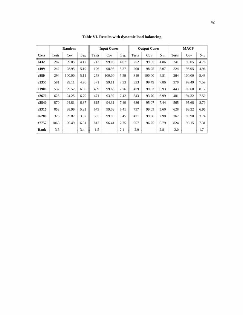
42

Table VI. Results with dynamic load balancing

iiiiiiiiiiiiiiiiiiiiiiiiiiiiiiiiiiiiiiiiiiiiiiiiiiiiiiiiiiiiiiiiiiiiiiiiiiiiiiiiiiiiiiiiiiiiiiiiRandom Input Cones Output Cones MACPiiiiiiiiiiiiiiiiiiiiiiiiiiiiiiiiiiiiiiiiiiiiiiiiiiiiiiiiiiiiiiiiiiiiiiiiiiiiiiiiiiiiiiiii

Ckts Tests Cov S 16 Tests Cov S 16 Tests Cov S 16 Tests Cov S 16iiiiiiiiiiiiiiiiiiiiiiiiiiiiiiiiiiiiiiiiiiiiiiiiiiiiiiiiiiiiiiiiiiiiiiiiiiiiiiiiiiiiiiiiiiiiiiiiiiiiiiiiiiiiiiiiiiiiiiiiiiiiiiiiiiiiiiiiiiiiiiiiiiiiiiiiiiiiiiiiiiiiiiiiiiiiiiiiiiiiiiiiiiiiiiiic432 287 99.05 4.17 213 99.05 4.07 252 99.05 4.86 241 99.05 4.76iiiiiiiiiiiiiiiiiiiiiiiiiiiiiiiiiiiiiiiiiiiiiiiiiiiiiiiiiiiiiiiiiiiiiiiiiiiiiiiiiiiiiiiiiiiiiiiic499 242 98.95 5.19 196 98.95 5.27 200 98.95 5.07 224 98.95 4.96iiiiiiiiiiiiiiiiiiiiiiiiiiiiiiiiiiiiiiiiiiiiiiiiiiiiiiiiiiiiiiiiiiiiiiiiiiiiiiiiiiiiiiiiiiiiiiiic880 294 100.00 5.11 258 100.00 5.59 310 100.00 4.81 264 100.00 5.48iiiiiiiiiiiiiiiiiiiiiiiiiiiiiiiiiiiiiiiiiiiiiiiiiiiiiiiiiiiiiiiiiiiiiiiiiiiiiiiiiiiiiiiiiiiiiiiic1355 581 99.11 4.96 371 99.11 7.33 333 99.49 7.86 370 99.49 7.59iiiiiiiiiiiiiiiiiiiiiiiiiiiiiiiiiiiiiiiiiiiiiiiiiiiiiiiiiiiiiiiiiiiiiiiiiiiiiiiiiiiiiiiiiiiiiiiic1908 537 99.52 6.55 409 99.63 7.76 479 99.63 6.93 443 99.68 8.17iiiiiiiiiiiiiiiiiiiiiiiiiiiiiiiiiiiiiiiiiiiiiiiiiiiiiiiiiiiiiiiiiiiiiiiiiiiiiiiiiiiiiiiiiiiiiiiic2670 625 94.25 6.79 471 93.92 7.42 543 93.70 6.99 481 94.32 7.50iiiiiiiiiiiiiiiiiiiiiiiiiiiiiiiiiiiiiiiiiiiiiiiiiiiiiiiiiiiiiiiiiiiiiiiiiiiiiiiiiiiiiiiiiiiiiiiic3540 870 94.81 6.87 615 94.31 7.49 686 95.07 7.44 565 95.68 8.79iiiiiiiiiiiiiiiiiiiiiiiiiiiiiiiiiiiiiiiiiiiiiiiiiiiiiiiiiiiiiiiiiiiiiiiiiiiiiiiiiiiiiiiiiiiiiiiic5315 852 98.99 5.21 673 99.08 6.41 757 99.03 5.60 628 99.22 6.95iiiiiiiiiiiiiiiiiiiiiiiiiiiiiiiiiiiiiiiiiiiiiiiiiiiiiiiiiiiiiiiiiiiiiiiiiiiiiiiiiiiiiiiiiiiiiiiic6288 323 99.87 3.57 335 99.90 3.45 431 99.86 2.98 367 99.90 3.74iiiiiiiiiiiiiiiiiiiiiiiiiiiiiiiiiiiiiiiiiiiiiiiiiiiiiiiiiiiiiiiiiiiiiiiiiiiiiiiiiiiiiiiiiiiiiiiic7752 1066 96.49 6.51 812 96.41 7.75 957 96.25 6.79 824 96.15 7.31iiiiiiiiiiiiiiiiiiiiiiiiiiiiiiiiiiiiiiiiiiiiiiiiiiiiiiiiiiiiiiiiiiiiiiiiiiiiiiiiiiiiiiiiiiiiiiiiiiiiiiiiiiiiiiiiiiiiiiiiiiiiiiiiiiiiiiiiiiiiiiiiiiiiiiiiiiiiiiiiiiiiiiiiiiiiiiiiiiiiiiiiiiiiiiiiRank 3.6 3.4 1.5 2.1 2.9 2.8 2.0 1.7iiiiiiiiiiiiiiiiiiiiiiiiiiiiiiiiiiiiiiiiiiiiiiiiiiiiiiiiiiiiiiiiiiiiiiiiiiiiiiiiiiiiiiiiiiiiiiiicc

ccccccccccccccccccccccc

ccccccccccccccccccccccccc

ccccccccccccccccccccccccc

ccccccccccccccccccccccc

ccccccccccccccccccccccc

ccccccccccccccccccccccccc

ccccccccccccccccccccccccc

ccccccccccccccccccccccc

ccccccccccccccccccccccc

ccccccccccccccccccccccccc

ccccccccccccccccccccccccc

ccccccccccccccccccccccc

ccccccccccccccccccccccc

ccccccccccccccccccccccccc

ccccccccccccccccccccccccc

ccccccccccccccccccccccc

ccccccccccccccccccccccc

ccccccccccccccccccccccccc

43

Table VII. Results with pc = 0.6

iiiiiiiiiiiiiiiiiiiiiiiiiiiiiiiiiiiiiiiiiiiiiiiiiiiiiiiiiiiiiiiiiiiiiiiiiiiiiiiiiiiiiiiiiiiiiiiiRandom Input Cones Output Cones MACPiiiiiiiiiiiiiiiiiiiiiiiiiiiiiiiiiiiiiiiiiiiiiiiiiiiiiiiiiiiiiiiiiiiiiiiiiiiiiiiiiiiiiiiii

Ckts Tests Cov S 16 Tests Cov S 16 Tests Cov S 16 Tests Cov S 16iiiiiiiiiiiiiiiiiiiiiiiiiiiiiiiiiiiiiiiiiiiiiiiiiiiiiiiiiiiiiiiiiiiiiiiiiiiiiiiiiiiiiiiiiiiiiiiiiiiiiiiiiiiiiiiiiiiiiiiiiiiiiiiiiiiiiiiiiiiiiiiiiiiiiiiiiiiiiiiiiiiiiiiiiiiiiiiiiiiiiiiiiiiiiiiic432 155 99.05 4.12 125 99.05 4.76 151 99.05 3.80 141 99.05 4.00iiiiiiiiiiiiiiiiiiiiiiiiiiiiiiiiiiiiiiiiiiiiiiiiiiiiiiiiiiiiiiiiiiiiiiiiiiiiiiiiiiiiiiiiiiiiiiiic499 143 98.95 5.24 123 98.95 5.30 121 98.95 5.33 125 98.95 4.55iiiiiiiiiiiiiiiiiiiiiiiiiiiiiiiiiiiiiiiiiiiiiiiiiiiiiiiiiiiiiiiiiiiiiiiiiiiiiiiiiiiiiiiiiiiiiiiic880 214 100.00 4.27 169 100.00 5.14 184 100.00 4.41 151 100.00 4.69iiiiiiiiiiiiiiiiiiiiiiiiiiiiiiiiiiiiiiiiiiiiiiiiiiiiiiiiiiiiiiiiiiiiiiiiiiiiiiiiiiiiiiiiiiiiiiiic1355 440 99.24 5.46 250 99.17 6.67 235 99.49 8.07 239 99.37 7.51iiiiiiiiiiiiiiiiiiiiiiiiiiiiiiiiiiiiiiiiiiiiiiiiiiiiiiiiiiiiiiiiiiiiiiiiiiiiiiiiiiiiiiiiiiiiiiiic1908 418 99.57 5.65 289 99.68 6.97 325 99.63 5.34 296 99.68 6.84iiiiiiiiiiiiiiiiiiiiiiiiiiiiiiiiiiiiiiiiiiiiiiiiiiiiiiiiiiiiiiiiiiiiiiiiiiiiiiiiiiiiiiiiiiiiiiiic2670 435 93.96 6.95 280 94.14 6.88 311 93.67 6.82 279 94.54 7.67iiiiiiiiiiiiiiiiiiiiiiiiiiiiiiiiiiiiiiiiiiiiiiiiiiiiiiiiiiiiiiiiiiiiiiiiiiiiiiiiiiiiiiiiiiiiiiiic3540 639 95.48 7.31 407 96.03 8.96 417 95.48 7.42 368 95.80 8.00iiiiiiiiiiiiiiiiiiiiiiiiiiiiiiiiiiiiiiiiiiiiiiiiiiiiiiiiiiiiiiiiiiiiiiiiiiiiiiiiiiiiiiiiiiiiiiiic5315 646 98.95 5.26 486 99.10 6.57 504 99.01 6.09 440 99.10 6.65iiiiiiiiiiiiiiiiiiiiiiiiiiiiiiiiiiiiiiiiiiiiiiiiiiiiiiiiiiiiiiiiiiiiiiiiiiiiiiiiiiiiiiiiiiiiiiiic6288 119 99.90 4.60 121 99.94 4.92 162 99.88 4.54 97 99.94 5.28iiiiiiiiiiiiiiiiiiiiiiiiiiiiiiiiiiiiiiiiiiiiiiiiiiiiiiiiiiiiiiiiiiiiiiiiiiiiiiiiiiiiiiiiiiiiiiiic7552 924 96.25 6.32 556 96.52 8.13 561 96.46 7.38 511 96.46 7.73iiiiiiiiiiiiiiiiiiiiiiiiiiiiiiiiiiiiiiiiiiiiiiiiiiiiiiiiiiiiiiiiiiiiiiiiiiiiiiiiiiiiiiiiiiiiiiiiiiiiiiiiiiiiiiiiiiiiiiiiiiiiiiiiiiiiiiiiiiiiiiiiiiiiiiiiiiiiiiiiiiiiiiiiiiiiiiiiiiiiiiiiiiiiiiiiRank 3.9 3.3 1.9 1.7 2.7 3.0 1.5 2.0iiiiiiiiiiiiiiiiiiiiiiiiiiiiiiiiiiiiiiiiiiiiiiiiiiiiiiiiiiiiiiiiiiiiiiiiiiiiiiiiiiiiiiiiiiiiiiiicc

ccccccccccccccccccccccc

ccccccccccccccccccccccccc

ccccccccccccccccccccccccc

ccccccccccccccccccccccc

ccccccccccccccccccccccc

ccccccccccccccccccccccccc

ccccccccccccccccccccccccc

ccccccccccccccccccccccc

ccccccccccccccccccccccc

ccccccccccccccccccccccccc

ccccccccccccccccccccccccc

ccccccccccccccccccccccc

ccccccccccccccccccccccc

ccccccccccccccccccccccccc

ccccccccccccccccccccccccc

ccccccccccccccccccccccc

ccccccccccccccccccccccc

ccccccccccccccccccccccccc

d d