Research Collection

Doctoral Thesis

Eye Reconstruction and Modeling for Digital Humans

Author(s): Bérard, Pascal

Publication Date: 2018

Permanent Link: https://doi.org/10.3929/ethz-b-000271976

Rights / License: In Copyright - Non-Commercial Use Permitted

This page was generated automatically upon download from the ETH Zurich Research Collection. For moreinformation please consult the Terms of use.

ETH Library

Diss. ETH No. 25064

Eye Reconstruction and Modelingfor Digital Humans

A thesis submitted to attain the degree of

Doctor of Sciences of ETH Zurich(Dr. sc. ETH Zurich)

Presented by

Pascal BerardMSc in Microengineering, EPFL, SwitzerlandBorn 24.11.1987Citizen of Volleges (VS), Switzerland

Accepted on the recommendation of

Prof. Dr. Markus Gross, examinerProf. Dr. Christian Theobalt, co-examinerDr. Thabo Beeler, co-examiner

2018

ii

Abstract

The creation of digital humans is a long-standing challenge of computer graph-ics. Digital humans are tremendously important for applications in visual effectsand virtual reality. The traditional way to generate digital humans is throughscanning. Facial scanning in general has become ubiquitous in digital media, butmost efforts have focused on reconstructing the skin only. The most importantpart of a digital human are arguably the eyes. Even though the human eye isone of the central features of an individual’s appearance, its shape and motionhave so far been mostly approximated in the computer graphics community withgross simplifications. To fill this gap, we investigate in this thesis methods forthe creation of eyes for digital humans. We present algorithms for the reconstruc-tion, the modeling, and the rigging of eyes for computer animation and trackingapplications.

To faithfully reproduce all the intricacies of the human eye we propose a novelcapture system that is capable of accurately reconstructing all the visible parts ofthe eye: the white sclera, the transparent cornea and the non-rigidly deformingcolored iris. These components exhibit very different appearance properties andthus we propose a hybrid reconstruction method that addresses them individu-ally, resulting in a complete model of both spatio-temporal shape and texture atan unprecedented level of detail.

This capture system is time-consuming to use and cumbersome for the actor mak-ing it impractical for general use. To address these constraints we present the firstapproach for high-quality lightweight eye capture, which leverages a database ofpre-captured eyes to guide the reconstruction of new eyes from much less con-strained inputs, such as traditional single-shot face scanners or even a singlephoto from the internet. This is accomplished with a new parametric model ofthe eye built from the database, and a novel image-based model fitting algorithm.

For eye animation we present a novel eye rig informed by ophthalmology find-ings and based on accurate measurements from a new multi-view imaging systemthat can reconstruct eye poses at submillimeter accuracy. Our goal is to raise theawareness in the computer graphics and vision communities that eye movementis more complex than typically assumed, and provide a new eye rig for animationthat models this complexity.

iii

Finally, we believe that the findings of this thesis will alter current assumptionsin computer graphics regarding human eyes, and our work has the potential tosignificantly impact the way that eyes of digital humans will be modelled in thefuture.

iv

Zusammenfassung

Das Erstellen von digitalen Doppelgangern ist eine Herausforderung, die das Ge-biet der Computergrafik schon lange beschaftigt. Digitale Doppelganger sind es-sentiell fur Anwendungen in der virtuellen Realitat oder in visuellen Effektenin Filmen und werden klassischerweise durch Scannen erstellt. Insbesondere Ge-sichtsscanning ist in digitalen Medien allgegenwartig geworden. Die meisten For-schungsarbeiten haben sich jedoch auf die Rekonstruktion der Haut beschrankt.Obwohl das Auge vermutlich das wichtigste Gesichtsmerkmal ist und eine zen-trale Rolle im Erscheinungsbild eines Individuums darstellt, wurde seine Formund Bewegung in der Computergrafik mit groben Vereinfachungen angenahert.Um diese Lucke zu schliessen, untersuchen wir in dieser Arbeit Methoden zumErstellen von Augen fur digitale Doppelganger. Wir prasentieren Algorithmenfur die Rekonstruktion, die Modellierung und das Rigging von Augen fur Com-puteranimationen und Tracking-Anwendungen.

Um alle Feinheiten des menschlichen Auges originalgetreu wiederzugeben, schla-gen wir ein neuartiges Erfassungssystem vor, das in der Lage ist alle sichtbarenTeile des Auges exakt zu rekonstruieren: die weisse Lederhaut, die transparenteHornhaut und die sich deformierende farbige Iris. Diese Teile weisen alle sehr un-terschiedliche visuelle und optische Eigenschaften auf und deshalb schlagen wireine hybride Rekonstruktionsmethode vor, die die verschiedenen Eigenschaftenberucksichtigt. Daraus resultiert ein vollstandiges Augenmodell, das die Formund die Deformation als auch die Textur in einem noch nie dagewesenen Detail-lierungsgrad modelliert.

Dieses Erfassungssystem ist zeitaufwandig und umstandlich in der Benutzungund in der Anwendung fur den Darsteller, womit es sich fur den allgemeinen Ge-brauch nicht eignet. Um diese Einschrankungen zu beheben, stellen wir einenneuen Ansatz fur eine benutzerfreundlichere Augenerfassung vor, die weiterhinhochwertige Augen generiert. Dabei verwenden wir eine Datenbank mit hoch-qualitativen Augenscans, aus der neue Augen generiert werden. Dieser Prozesswird durch einfache Eingaben gelenkt. Dazu kann z.B. ein traditioneller Ge-sichtsscan oder sogar ein einziges Foto aus dem Internet verwendet werden. DieRobustheit vom System wird mit einem neuen parametrischen Augenmodell undeinem neuartigen bildbasierten Algorithmus zum Anpassen der Modellparame-ter erreicht.

v

Fur die Augenanimation stellen wir ein neuartiges Augen-Rig vor, das auf denErkenntnissen der Ophthalmologie und auf genauen Messungen eines neu-en Multikamerasystems basiert, mit dem sich Augenpositionen mit Submilli-metergenauigkeit bestimmen lassen. Unser Ziel ist es, das Bewusstsein in denComputergrafik- und Computervision-Gemeinschaften zu scharfen, dass Augen-bewegungen komplexer sind als ublicherweise angenommen. Dazu fuhren wirein neues Augen-Rig fur die Animation ein, das diese Komplexitat modelliert.

Wir glauben, dass die Resultate dieser Arbeit die aktuellen Annahmen in derComputergrafik in Bezug auf die menschlichen Augen beeinflussen werden undwir glauben, dass unsere Arbeit das Potenzial hat signifikante Auswirkungen aufden Modellierungsprozess von Augen von digitalen Doppelgangern zu haben.

vi

Acknowledgments

Since I was very little, my parents allowed me to experiment and tinker witheverything, even if that meant leaving behind a gigantic mess. I am immenselygrateful for their tolerance and I believe this allowed me to become who I am. Ialso want to thank my sister, Stephanie, my brother, Michel, and my sister-in-law,Karima, for supporting me throughout this PhD.

I would like to sincerely thank my adviser Prof. Markus Gross. He gave me theopportunity to work in this exciting field and gave me the freedom to investigatemy own ideas. He also believed that I can do a PhD in computer graphics withouta strong background in computer science. I am immensely grateful for that.

The same is true for Thabo Beeler and Derek Bradley who supervised me since thevery beginning of my PhD. Their advice and guidance was invaluable and helpedme not to forget the big picture of what we want to achieve. There is nothing betterthan to learn from the best in the field, and this work wouldn’t have been possiblewithout their ideas and it wouldn’t have been possible if I wasn’t able to build ontop of what they have built. I’m also grateful for the countless hours they spentrewording and polishing the papers that make up this thesis.

Thank you, Christian Theobalt, for refereeing my examination and reviewing mythesis.

I would have published nothing without my coauthors. I am grateful to haveworked with all of them: Thabo Beeler, Amit Bermano, Derek Bradley, Alexan-dre Chapiro, Markus Gross, Maurizio Nitti, Mattia Ryffel, Stefan Schmid, RobertSumner, and Fabio Zund.

Many thanks go to my collaborators Maurizio Nitti and Alessia Marra for creat-ing the illustrations and renders that made our papers so much nicer to look at.Special thanks go to Maurizio Nitti for his endless patience.

I wish to thank Dr. med. Peter Maloca and Prof. Dr. Dr. Jens Funk and his teamat UniversitatsSpital Zurich for the helpful discussions and their eye-opening re-marks.

I would like to thank Lewis Siegel and Michael Koperwas for their industry per-spective.

vii

Prof. Gaudenz Danuser introduced me to world of research. I am grateful that heencouraged me to do a PhD.

I would also like to thank all of our eye models, who spent countless hours inuncomfortable positions and made this work possible.

Thank you, Jan Wezel and Ronnie Gansli, for your support in building the hard-ware required for these projects.

I am fortunate to have worked and spent time with people of the ComputerGraphics Lab, Disney Research Zurich, as well as the members of the Interac-tive Geometry Lab who inspired me with their works. They all made the PhD soenjoyable and deadlines so much more human.

I was lucky to share an office during my first year at ETH with Fabian Hahn. Heis an exceptional researcher and friend, who taught me how to code.

Thank you, Antoine Milliez, for making the dull days so much more enjoyablewith your great jokes!

Special thanks for my collaborators and friends: Simone Meyer, Fabio Zund,Tanja Kaser, Yeara Kozlov, Virag Varga, Paulo Gothardo, Severin Klingler, Chris-tian Schuller, Oliver Glauser, Leo Helminger, Christian Schumacher, AlexandreChapiro, Loıc Ciccone, Vittorio Megaro, Riccardo Roveri, Ivan Ovinnikov, EndriDibra, Romain Prevost, Kaan Yucer. I will miss the great time and the refreshingcoffee breaks.

Finally, I would like to thank all my friends who supported and kept me goingduring my PhD.

viii

“Discovery consists not in seeking new lands but in seeing with new eyes.”

— Marcel Proust

ix

x

Contents

Introduction 11.1 Contributions . . . . . . . . . . . . . . . . . . . . . . . . . . . . . . . 81.2 Publications . . . . . . . . . . . . . . . . . . . . . . . . . . . . . . . . 9

Related Work 112.1 Reconstruction and Modeling . . . . . . . . . . . . . . . . . . . . . . 112.2 Iris Deformation . . . . . . . . . . . . . . . . . . . . . . . . . . . . . . 122.3 Medical Instruments . . . . . . . . . . . . . . . . . . . . . . . . . . . 132.4 Facial Capture . . . . . . . . . . . . . . . . . . . . . . . . . . . . . . . 132.5 Non-Rigid Alignment . . . . . . . . . . . . . . . . . . . . . . . . . . 142.6 Texture and Geometry Synthesis . . . . . . . . . . . . . . . . . . . . 142.7 Eye Tracking and Gaze Estimation . . . . . . . . . . . . . . . . . . . 152.8 Eye Rigging and Animation . . . . . . . . . . . . . . . . . . . . . . . 16

Eye Anatomy 173.1 Eyeball . . . . . . . . . . . . . . . . . . . . . . . . . . . . . . . . . . . 173.2 Sclera and Conjunctiva . . . . . . . . . . . . . . . . . . . . . . . . . . 193.3 Cornea . . . . . . . . . . . . . . . . . . . . . . . . . . . . . . . . . . . 193.4 Limbus . . . . . . . . . . . . . . . . . . . . . . . . . . . . . . . . . . . 203.5 Iris . . . . . . . . . . . . . . . . . . . . . . . . . . . . . . . . . . . . . . 213.6 Pupil . . . . . . . . . . . . . . . . . . . . . . . . . . . . . . . . . . . . 223.7 Muscles . . . . . . . . . . . . . . . . . . . . . . . . . . . . . . . . . . . 22

Eye Reconstruction 234.1 Data Acquisition . . . . . . . . . . . . . . . . . . . . . . . . . . . . . 25

4.1.1 Capture Setup . . . . . . . . . . . . . . . . . . . . . . . . . . . 254.1.2 Calibration . . . . . . . . . . . . . . . . . . . . . . . . . . . . . 264.1.3 Image Acquisition . . . . . . . . . . . . . . . . . . . . . . . . 274.1.4 Initial Reconstruction . . . . . . . . . . . . . . . . . . . . . . 27

4.2 Sclera . . . . . . . . . . . . . . . . . . . . . . . . . . . . . . . . . . . . 274.2.1 Image Segmentation . . . . . . . . . . . . . . . . . . . . . . . 284.2.2 Mesh Segmentation . . . . . . . . . . . . . . . . . . . . . . . 294.2.3 Pose Registration . . . . . . . . . . . . . . . . . . . . . . . . . 304.2.4 Sclera Merging . . . . . . . . . . . . . . . . . . . . . . . . . . 31

xi

Contents

4.2.5 Sclera Texturing . . . . . . . . . . . . . . . . . . . . . . . . . . 324.3 Cornea . . . . . . . . . . . . . . . . . . . . . . . . . . . . . . . . . . . 33

4.3.1 Theory . . . . . . . . . . . . . . . . . . . . . . . . . . . . . . . 344.3.2 Constraint Initalization . . . . . . . . . . . . . . . . . . . . . 344.3.3 Surface Reconstruction . . . . . . . . . . . . . . . . . . . . . . 364.3.4 Cornea-Eyeball Merging . . . . . . . . . . . . . . . . . . . . . 37

4.4 Iris . . . . . . . . . . . . . . . . . . . . . . . . . . . . . . . . . . . . . . 374.4.1 Pupil Reconstruction . . . . . . . . . . . . . . . . . . . . . . . 374.4.2 Iris mesh generation . . . . . . . . . . . . . . . . . . . . . . . 394.4.3 Mesh cleanup . . . . . . . . . . . . . . . . . . . . . . . . . . . 404.4.4 Mesh Propagation . . . . . . . . . . . . . . . . . . . . . . . . 414.4.5 Temporal Smoothing and Interpolation . . . . . . . . . . . . 414.4.6 Iris Texturing . . . . . . . . . . . . . . . . . . . . . . . . . . . 42

4.5 Results . . . . . . . . . . . . . . . . . . . . . . . . . . . . . . . . . . . 42

Parametric Eye Model 555.1 Input Data . . . . . . . . . . . . . . . . . . . . . . . . . . . . . . . . . 565.2 Eyeball Model . . . . . . . . . . . . . . . . . . . . . . . . . . . . . . . 565.3 Iris Model . . . . . . . . . . . . . . . . . . . . . . . . . . . . . . . . . 60

5.3.1 Iris Texture Synthesis . . . . . . . . . . . . . . . . . . . . . . . 615.3.2 Iris Geometry Synthesis . . . . . . . . . . . . . . . . . . . . . 64

5.4 Sclera Vein Model . . . . . . . . . . . . . . . . . . . . . . . . . . . . . 655.4.1 Vein Model . . . . . . . . . . . . . . . . . . . . . . . . . . . . 665.4.2 Vein Rendering . . . . . . . . . . . . . . . . . . . . . . . . . . 68

5.5 Model Fitting . . . . . . . . . . . . . . . . . . . . . . . . . . . . . . . 705.5.1 Multi-View Fitting . . . . . . . . . . . . . . . . . . . . . . . . 705.5.2 Single Image Fitting . . . . . . . . . . . . . . . . . . . . . . . 73

5.6 Results . . . . . . . . . . . . . . . . . . . . . . . . . . . . . . . . . . . 73

Eye Rigging 856.1 Eye Rig . . . . . . . . . . . . . . . . . . . . . . . . . . . . . . . . . . . 86

6.1.1 Eye Shape . . . . . . . . . . . . . . . . . . . . . . . . . . . . . 866.1.2 Eye Motion . . . . . . . . . . . . . . . . . . . . . . . . . . . . 886.1.3 Eye Positioning . . . . . . . . . . . . . . . . . . . . . . . . . . 906.1.4 Eye Control . . . . . . . . . . . . . . . . . . . . . . . . . . . . 91

6.2 Data Acquisition . . . . . . . . . . . . . . . . . . . . . . . . . . . . . 916.3 Eye Configuration Reconstruction . . . . . . . . . . . . . . . . . . . 93

6.3.1 Annotation Fitting . . . . . . . . . . . . . . . . . . . . . . . . 956.3.2 Photometric Refinement . . . . . . . . . . . . . . . . . . . . . 98

6.4 Eye Rig Fitting . . . . . . . . . . . . . . . . . . . . . . . . . . . . . . . 1026.4.1 Listing’s Model . . . . . . . . . . . . . . . . . . . . . . . . . . 1026.4.2 Translation Model . . . . . . . . . . . . . . . . . . . . . . . . 103

xii

Contents

6.4.3 Eye Rig . . . . . . . . . . . . . . . . . . . . . . . . . . . . . . . 1036.4.4 Visual Axis . . . . . . . . . . . . . . . . . . . . . . . . . . . . 105

6.5 Results . . . . . . . . . . . . . . . . . . . . . . . . . . . . . . . . . . . 105

Conclusion 1137.1 Limitations . . . . . . . . . . . . . . . . . . . . . . . . . . . . . . . . . 1147.2 Outlook . . . . . . . . . . . . . . . . . . . . . . . . . . . . . . . . . . . 115

Appendix 117

References 119

xiii

C H A P T E R 1Introduction

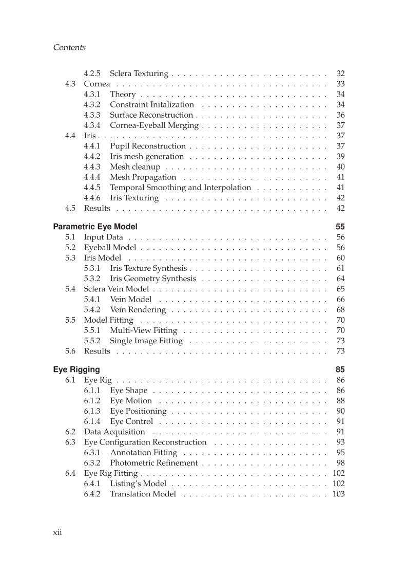
Creating photo-realistic digital humans is a long-standing grand challengein computer graphics. Applications for digital humans include video games,visual effects in films, medical applications and personalized figurines. Oneof the cornerstones of producing digital doubles is capturing an actor’s face.Several decades of research have pushed facial capture technology to anincredible level of quality, where it is becoming difficult to distinguish thedifference between digital faces and real ones. An example for such a dig-ital human is Mike depicted in Fig. 1.1. The members of the wikihuman.orgproject created Mike to demonstrate state-of-the-art methods for the creationof digital humans.

A lot of research went into better models and simpler capture methods fordigital humans. However, most research has focused on the facial skin, ig-noring other important characteristics like the eyes. The eyes are arguablythe most important part of the face, as this is where humans tend to focuswhen looking at someone. Eyes can convey emotions and foretell the actionsof a person and subtle inaccuracies in the eyes of a character can make thedifference between realistic and uncanny.

In this thesis we present methods for the entire digital eye creation pipeline.This includes reconstructing the visible parts of the eye, modeling the vari-ability of human eyes with a parametric model, and rigging the position andmotion for animation and tracking applications.

While a simple modeled or simulated eye may be sufficient for backgroundcharacters, current industry practices spend significant effort to manuallycreate eyes of hero characters. In this thesis, we argue that generic eye mod-

1

Introduction

a) b)

c)

Figure 1.1: Mike is a state-of-the-art digital human. He is the result of an industry-wide collaboration of researchers, visual effect specialists, and artists thatcame together in the wikihuman project with the goal to create an open, andpublicly available data set of a digital human. The methods presented inthis thesis have been used to scan Mike’s eyes. The figure shows a referencephotograph (a), a photo-realistic render from the same view (b) and a close-up render of the right eye (c) reconstructed with the methods presented inthis thesis. Images courtesy of wikihuman.org.

2

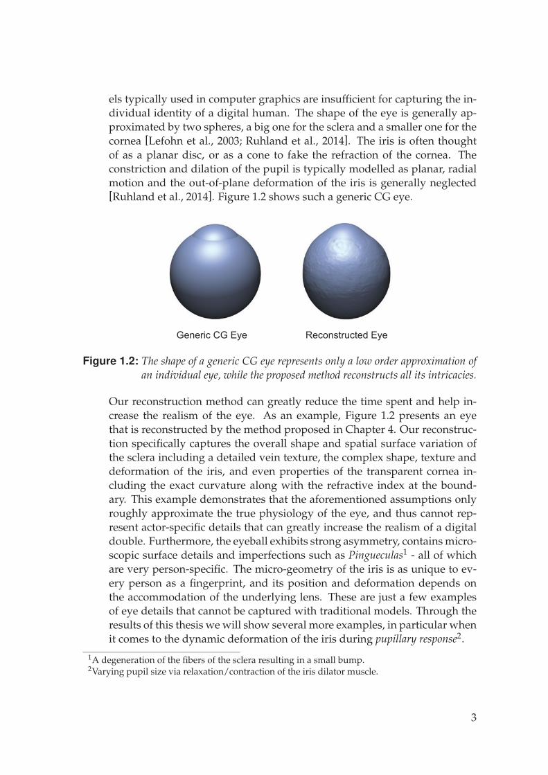
els typically used in computer graphics are insufficient for capturing the in-dividual identity of a digital human. The shape of the eye is generally ap-proximated by two spheres, a big one for the sclera and a smaller one for thecornea [Lefohn et al., 2003; Ruhland et al., 2014]. The iris is often thoughtof as a planar disc, or as a cone to fake the refraction of the cornea. Theconstriction and dilation of the pupil is typically modelled as planar, radialmotion and the out-of-plane deformation of the iris is generally neglected[Ruhland et al., 2014]. Figure 1.2 shows such a generic CG eye.

Generic CG Eye Reconstructed Eye

Figure 1.2: The shape of a generic CG eye represents only a low order approximation ofan individual eye, while the proposed method reconstructs all its intricacies.

Our reconstruction method can greatly reduce the time spent and help in-crease the realism of the eye. As an example, Figure 1.2 presents an eyethat is reconstructed by the method proposed in Chapter 4. Our reconstruc-tion specifically captures the overall shape and spatial surface variation ofthe sclera including a detailed vein texture, the complex shape, texture anddeformation of the iris, and even properties of the transparent cornea in-cluding the exact curvature along with the refractive index at the bound-ary. This example demonstrates that the aforementioned assumptions onlyroughly approximate the true physiology of the eye, and thus cannot rep-resent actor-specific details that can greatly increase the realism of a digitaldouble. Furthermore, the eyeball exhibits strong asymmetry, contains micro-scopic surface details and imperfections such as Pingueculas1 - all of whichare very person-specific. The micro-geometry of the iris is as unique to ev-ery person as a fingerprint, and its position and deformation depends onthe accommodation of the underlying lens. These are just a few examplesof eye details that cannot be captured with traditional models. Through theresults of this thesis we will show several more examples, in particular whenit comes to the dynamic deformation of the iris during pupillary response2.

1A degeneration of the fibers of the sclera resulting in a small bump.2Varying pupil size via relaxation/contraction of the iris dilator muscle.

3

Introduction

To overcome the limitations of generic eye models and accurately reproducethe intricacies of a human eye, we argue that eyes should be captured andreconstructed from images of real actors, analogous to the established prac-tice of skin reconstruction through facial scanning. The eye, however, ismore complex than skin, which is often assumed to be a diffuse Lambertiansurface in most reconstruction methods. The human eye is a heterogeneouscompound of opaque and transparent surfaces with a continuous transitionbetween the two, and even surfaces that are visually distorted due to re-fraction. This complexity makes capturing an eye very challenging, requir-ing a novel algorithm that combines several complementary techniques forimage-based reconstruction. In this work, we propose the first system capa-ble of reconstructing the spatio-temporal shape of all visible parts of the eye;the sclera, the cornea, and the iris, representing a large step forward in real-istic eye modeling. Our approach not only allows us to create more realisticdigital humans for visual effects and computer games by scanning actors,but it also provides the ability to capture the accurate spatio-temporal shapeof an eye in-vivo.

While the results of our eye reconstruction system are compelling, the ac-quisition process is both time consuming and uncomfortable for the actors,as they must lie horizontally with a constraining neck brace while manuallyholding their eye open for dozens of photos over a 20 minute period for eacheye. The physical burden of that approach is quite far from the single shotface scanners that exist today, which are as easy as taking a single photo ina comfortable setting, and thus the applicability of their method is largelylimited.

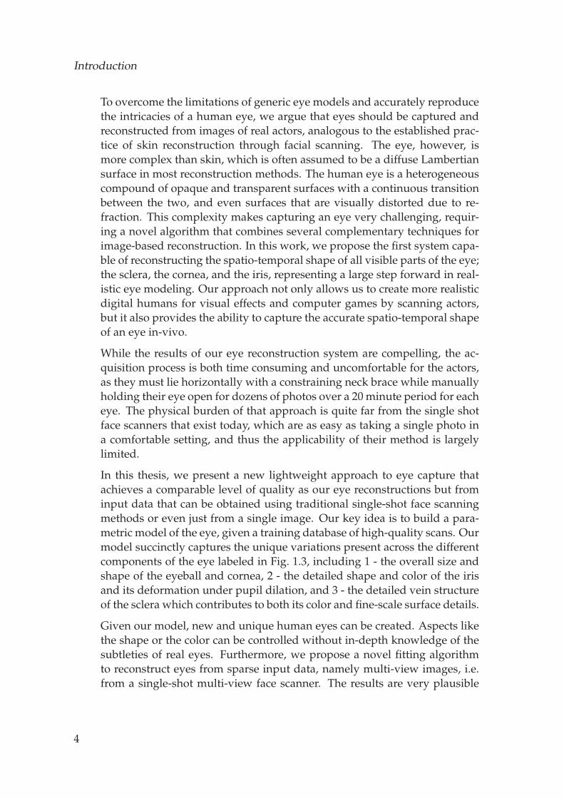
In this thesis, we present a new lightweight approach to eye capture thatachieves a comparable level of quality as our eye reconstructions but frominput data that can be obtained using traditional single-shot face scanningmethods or even just from a single image. Our key idea is to build a para-metric model of the eye, given a training database of high-quality scans. Ourmodel succinctly captures the unique variations present across the differentcomponents of the eye labeled in Fig. 1.3, including 1 - the overall size andshape of the eyeball and cornea, 2 - the detailed shape and color of the irisand its deformation under pupil dilation, and 3 - the detailed vein structureof the sclera which contributes to both its color and fine-scale surface details.

Given our model, new and unique human eyes can be created. Aspects likethe shape or the color can be controlled without in-depth knowledge of thesubtleties of real eyes. Furthermore, we propose a novel fitting algorithmto reconstruct eyes from sparse input data, namely multi-view images, i.e.from a single-shot multi-view face scanner. The results are very plausible

4

scleralimbus

irispupil

Figure 1.3: The visually salient parts of a human eye include the black pupil, the colorediris, and the limbus that demarcates the transition from the white sclera tothe transparent cornea.

eye reconstructions with realistic details from a simple capture setup, whichcan be combined with the face scan to provide a more complete digital facemodel. In this work we demonstrate results using the face scanner of Beeleret al. [2010], however our fitting approach is flexible and can be applied toany traditional face capture setup. Furthermore, by reducing the complexityto a few intuitive parameters, we show that our model can be fit to just singleimages of eyes or even artistic renditions, providing an invaluable tool forfast eye modeling or reconstruction from internet photos. We demonstratethe versatility of our model and fitting approach by reconstructing severaldifferent eyes ranging in size, shape, iris color and vein structure.

Besides fitting single frames and poses the system can also be extended tofit entire sequences. This allows for the analysis of the three-dimensionalposition and orientation during gaze motion. An accurate eyeball pose isimportant since it directly affects the eye region through the interaction withsurrounding tissues and muscles. Humans have been primed by evolutionto scrutinize the eye region, spending about 40% of our attention to that areawhen looking at a face [Janik et al., 1978]. One of the main reasons to doso is to estimate where others are looking in order to anticipate their actions.Once vital to survival, nowadays this is paramount for social interaction andhence it is important to faithfully model and reproduce the way our eyesmove for digital characters.

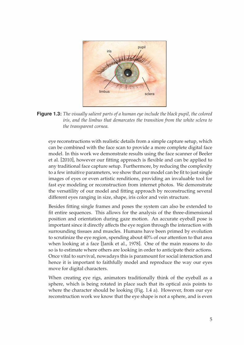
When creating eye rigs, animators traditionally think of the eyeball as asphere, which is being rotated in place such that its optical axis points towhere the character should be looking (Fig. 1.4 a). However, from our eyereconstruction work we know that the eye shape is not a sphere, and is even

5

Introduction

a) b)

Figure 1.4: Eye Model: a) Traditional eye models assume the eye to be roughly sphericaland rotating around its center. The gaze direction is assumed to correspondto the optical axis of the eye (black arrows). b) The proposed eye model takesinto account that the eye is not perfectly spherical and does not simply rotatearound its center. Furthermore it respects the fact that the gaze direction istilted towards the nose (see also Fig. 3.1 (b)).

asymmetric around the optical axis. This, of course, begs the question ofhow correct these other assumptions are, and answering this question is themain focus of Chapter 6 of this thesis. We explore ophthalmological modelsfor eye motion and assess their relevancy and applicability in the context ofcomputer graphics.

The eye is not a rotational apparatus but instead is being pulled into placeby six muscles, two for each degree of rotation (Fig. 3.1 a). These muscles areactivated in an orchestrated manner to control the gaze of the eye. As a con-sequence, the eyeball actually does translate within its socket, meaning thatits rotational pivot is not a single point but actually lies on a manifold. Fur-thermore, the eye is not simply rotated horizontally and vertically but alsoexhibits considerable rotation around its optical axis, called torsion. Withthe emersion of head mounted displays for augmented and virtual realityapplications, modeling these phenomena may become central to allow foroptimal foveal rendering.

A very important fact that is not captured in naıve eye rigs is the fact that thegaze direction does not align with the optical axis of the eye but rather withits visual axis. The visual axis is the ray going through the center of the pupilstarting from the fovea at the back of the eye, which is the location where theeye has the highest resolution. As depicted in Fig. 3.1 b, the fovea is slightlyshifted away from the nose, causing the visual axis to be tilted towards thenose (Fig. 1.4 b), on average around five degrees for adults [LeGrand andElHage, 2013]. This is an extremely important detail that cannot be neglectedas otherwise the digital character will appear slightly cross-eyed, causinguncanny gazes.

6

To be relevant for computer vision and computer graphics applications, aphenomenon must be visible outside of ophthalmologic equipment, i.e. inimagery captured by ordinary cameras. We employ a passive multi-viewacquisition system to reconstruct high-quality eye poses over time, com-plete with accurate high-resolution eye geometry. We demonstrate that bothtranslation and torsion is clearly visible in the acquired data and hence in-vestigate the importance of modeling these phenomena, along with the cor-rect visual axis, in an eye rig for computer graphics applications.

We believe that the work presented in this thesis on eye reconstruction, eyemodeling, and eye rigging has the potential to change how eyes are modeledin computer graphics applications.

7

Introduction

1.1 Contributions

This thesis makes the following main contributions:

• An eyeball reconstruction algorithm for the coupled reconstructions ofsclera, cornea, and iris including the deformation of the iris.

• A parametric eyeball shape model created from a database of eyes. Thismodel allows us to generate a wide range of plausible human eyeballshapes by defining only a few shape parameters.

• A parametric iris model which generates iris shapes including its de-formation. The method requires only a photo or an artist sketch ofan iris as input.

• A parametric vein model that synthesizes realistic vein networks. Thevarious synthesized vein properties are fed to a renderer that lever-ages vein samples from an eye database to render a sclera texture.

• A parametric model fitting algorithm that allow us to determine the besteye model parameters to match input images and scans. Fitting to asingle image is possible.

• A parametric eye rig describing the positions and orientations of theeyeballs. The rig can be configured to match a specific person, in-cluding parameters for the interocular distance, the center of rota-tion, and the visual axis.

• An eye rig fitting algorithm that estimates the best person-specific rigparameters from a multi-view image sequence.

8

1.2 Publications

1.2 Publications

This thesis is based on the following peer-reviewed publications:

• P. BERARD, D. BRADLEY, M. NITTI, T. BEELER, and M. GROSS.High-Quality Capture of Eyes. In Proceedings of ACM SIGGRAPHAsia (Shenzhen, China, December 3-6, 2014). ACM Transactions onGraphics, Volume 33, Issue 6, Pages 223:1–223:12.

• P. BERARD, D. BRADLEY, M. GROSS, and T. BEELER. LightweightEye Capture Using a Parametric Model. In Proceedings of ACMSIGGRAPH (Anaheim, USA, July 24-28, 2016). ACM Transactions onGraphics, Volume 35, Issue 4, Pages 117:1–117:12.

The thesis is also based on the following submitted publication:

• P. BERARD, D. BRADLEY, M. GROSS, and T. BEELER. PhysiologicallyAccurate Eye Rigging. Submitted to ACM SIGGRAPH (Vancouver,Canada, August 12-16, 2018).

During the course of this thesis, the following peer-reviewed papers werepublished, which are not directly related to the presented work:

• F. ZUND, P. BERARD, A. CHAPIRO, S. SCHMID, M. RYFFEL, M.GROSS, A. BERMANO, and R. SUMNER. Unfolding the 8-bit era.In Proceedings of the 12th European Conference on Visual MediaProduction (CVMP) (London, UK, November 24-25, 2015). Pages9:1–9:10.

9

Introduction

10

C H A P T E R 2Related Work

The eye is an important part of the human and this is reflected by the widespectrum of work related to eyes in various disciplines such as medicine,psychology, philosophy, and computer graphics. The requirements for ap-plications in computer graphics are however very different from other fields.This chapter presents some of the related works that are relevant to digitalhumans and computer graphics in general.

The amount of work related to reconstructing and modeling the human eyeis within limits. Our work is related to medical instruments, and facial cap-ture methods, so we also provide a brief overview of these techniques, fol-lowed by a description of other methods that are related to our approach at alower level. Specifically, the algorithms presented in this thesis touch on var-ious fields including non-rigid alignment to find correspondences betweeneye meshes, data driven fitting to adjust an eye model to a given eye mesh,as well as constrained texture and geometry synthesis to create iris details.

These methods focus on modeling shape and appearance of eyes, whichprovides a great starting point to our rigging and tracking work, which isrelated to eye tracking and gaze estimation in images, capturing and mod-eling 3D eye geometry and appearance, and rigging and animating eyes forvirtual characters. In the following we will discuss related work in each area.

2.1 Reconstruction and Modeling

Reconstructing and modeling eye geometry and appearance have so far re-ceived only very little attention in the graphics community, as a recent sur-

11

Related Work

vey of Ruhland et al. [2014] shows. Most research so far has focused solelyon acquiring the iris, the most prominent part of an eye, typically only con-sidering the color variation and neglecting its shape. An exception is theseminal work by Francois et al. [2009], which proposes to estimate the shapebased on the color variation. Guided by the physiology of the iris, they de-velop a bright-is-deep model to hallucinate the microscopic details. Whileimpressive and simple, the results are not physically correct and they haveto manually remove spots from the iris, since these do not conform withtheir model. Lam et al. [2006] propose a biophysically-based light transportmodel to simulate the light scattering and absorption processes occurringwithin the iridal tissues for image synthesis applications, whereas Lefohn etal. [2003] mimic an ocularist’s workflow, where different layers of paint areapplied to reproduce the look of an iris from a photograph. Their method istailored to manufacture eye prosthetics, and only considers the synthesis ofthe iris color, neglecting its shape.

One of the first to model the entire eye were Sagar et al. [1994], who model acomplete eye including the surrounding face for use in a surgical simulator.However, the model is not based on captured data and only approximatesthe shape of a real eye. More recently, Wood et al. [2016a] presented a para-metric eyeball model and a 3D morphable model of the eye region and thenfit the models to images using analysis-by-synthesis.

While there has been a substantial amount of research regarding the recon-struction of shape of various materials [Seitz et al., 2006; Ihrke et al., 2008;Hernandez et al., 2008], none of these methods seem particularly suited toreconstruct the heterogeneous combination of materials present in the eye.As the individual components of the eye are all coupled, they require a uni-fied reconstruction framework, which is what we propose in this thesis.

2.2 Iris Deformation

Other authors have looked into the motion patterns of the iris, such as di-lation or hippus3 [Hachol et al., 2007]. Pamplona and colleagues study thedeformation of the iris when the pupil dilates in 2D [Pamplona et al., 2009].They manually annotate a sparse set of features on a sequence of imagestaken while the pupil dilates. The recovered tracks show that the individualstructures present in the iris prevent it from dilating purely radially on lineartrajectories. Our method tracks the deformation of the iris densely since we

3A rhythmic but irregular continuous change of pupil dilation.

12

2.3 Medical Instruments

do not require manual annotation and our measurements confirm these find-ings. More importantly, we capture the full three-dimensional deformationof the iris, which conveys the detailed shape changes during pupil dilation.In one of our proposed applications we complement our deformation modelwith the temporal model proposed by Pamplona et al. [2009].

More importantly, we do capture the full three dimensional motion, whichnot only conveys how the shape of the iris changes during dilation but alsoshows that the iris moves on the curved surface of the underlying lens. Aswe demonstrate in this thesis, the lens changes its shape for accommodationand as a consequence, the shape of the iris is a function of both dilation andaccommodation - a feature not considered in our community so far.

2.3 Medical Instruments

In the medical community the situation is different. There, accurate eyemeasurements are fundamental, and thus several studies exist. These ei-ther analyze the eye ex-vivo [Eagle Jr, 1988] or employ dedicated devicessuch as MRI to acquire the eye shape [Atchison et al., 2004] and slit lampsor keratography for the cornea [Vivino et al., 1993]. Optical coherencetomography (OCT) [Huang et al., 1991], in ophthalmology mostly em-ployed to image the retina, can also be used to acquire the shape of corneaand iris at high accuracy. An overview of the current corneal assessmentmethods can be found in recent surveys [Rio-Cristobal and Martin, 2014;Pinero, 2013]. Such devices however are not readily available and the datathey produce is oftentimes less suited for graphics applications. We there-fore chose to construct our own setup using commodity hardware and em-ploy passive and active photogrammetry methods for the reconstruction.

2.4 Facial Capture

Unlike eye reconstruction, the area of facial performance capture has re-ceived a lot of attention over the past decades, with a clear trend to-wards more lightweight and less constrained acquisition setups. Theuse of passive multi-view stereo [Beeler et al., 2010; Bradley et al., 2010;Beeler et al., 2011] has greatly reduced the hardware complexity and acqui-sition time required by active systems [Ma et al., 2007; Ghosh et al., 2011;Fyffe et al., 2011]. The amount of cameras employed was subsequentlyfurther reduced to binocular [Valgaerts et al., 2012] and finally monocular

13

Related Work

acquisition [Blanz and Vetter, 1999; Garrido et al., 2013; Cao et al., 2014;Suwajanakorn et al., 2014; Fyffe et al., 2014].

To overcome the inherent ill-posedness of these lightweight acquisition de-vices, people usually employ a strong parametric prior to regularize theproblem. Following this trend to more lightweight acquisition using para-metric priors, we propose to leverage data provided by our high-resolutioncapture technique and build up a parametric eye-model, which can then befit to input images acquired from more lightweight setups, such as face scan-ners, monocular cameras or even from artistically created images.

2.5 Non-Rigid Alignment

A vast amount of work has been performed in the area of non-rigid align-ment, ranging from alignment of rigid object scans with low-frequencywarps, noise, and incomplete data [Ikemoto et al., 2003; Haehnel et al., 2003;Brown and Rusinkiewicz, 2004; Amberg et al., 2007; Li et al., 2008] toalgorithms that find shape matches in a database [Kazhdan et al., 2004;Funkhouser et al., 2004]. Another class of algorithms registers a set ofdifferent meshes that all have the same overall structure, like a face ora human body, with a template-based approach [Blanz and Vetter, 1999;Allen et al., 2003; Anguelov et al., 2005; Vlasic et al., 2005]. In this workwe use a variant of the non-rigid registration algorithm of Li et al. [2008]in order to align multiple reconstructed eyes and build a deformable eyemodel [Blanz and Vetter, 1999]. Although Li et al.’s method is designed foraligning a mesh to depth scans, we will show how to re-formulate the prob-lem in the context of eyes, operating in a spherical domain rather than the2D domain of depth scans.

2.6 Texture and Geometry Synthesis

In this work, texture synthesis is used to generate realistic and detailediris textures and also geometry from low-resolution input images. A verybroad overview of related work on texture synthesis is presented in the sur-vey of Wei et al [2009]. Specific topics relevant for our work include con-strained texture synthesis [Ramanarayanan and Bala, 2007] and example-based image super resolution [Tai et al., 2010], which both aim to producea higher resolution output of an input image given exemplars. With patch-based synthesis methods [Praun et al., 2000; Liang et al., 2001; Efros and

14

2.7 Eye Tracking and Gaze Estimation

Freeman, 2001], controlled upscaling can be achieved easily by constrain-ing each output patch to a smaller patch from the low-resolution input.These algorithms sequentially copy patches from the exemplars to the out-put texture. They were further refined with graph cuts, blending, deforma-tion, and optimization for improved patch-boundaries [Kwatra et al., 2003;Mohammed et al., 2009; Chen et al., 2013]. Dedicated geometry synthesisalgorithms also exist [Wei et al., 2009], however geometry can often be ex-pressed as a texture and conventional texture synthesis algorithms can beapplied. In our work we take inspiration from Li et al. [2015], who proposeto use gradient texture and height map pairs as exemplars where in theirwork the height map encodes facial wrinkles. We expand on their methodand propose to encode color, geometry and also shape deformation in a pla-nar parameterization, allowing us to jointly synthesize texture, shape anddeformation to produce realistic irises that allow dynamic pupil dilation.

2.7 Eye Tracking and Gaze Estimation

The first methods for photographic eye tracking date back over 100years [Dodge and Cline, 1901; Judd et al., 1905], and since thendozens of tracking techniques have emerged, including the introduc-tion of head-mounted eye trackers [Hartridge and Thompson, 1948;Mackworth and Thomas, 1962]. We refer to detailed surveys onhistorical and more modern eye recording devices [Collewijn, 1999;Eggert, 2007]. Such devices have been widely utilized in human-computerinteraction applications. Some examples were to study the usability of newinterfaces [Benel et al., 1991], to use gaze as a means to reduce renderingcosts [Levoy and Whitaker, 1990], or as a direct input pointing device [Zhaiet al., 1999]. These types of eye trackers typically involve specialized hard-ware and dedicated calibration procedures.

Nowadays, people are interested in computing 3D gaze from images inthe wild. Gaze estimation is a fairly mature field (see [Hansen and Ji,2010] for a survey), but a recent trend is to employ appearance-basedgaze estimators. Popular among these approaches are machine learningtechniques that attempt to learn eye position and gaze from a single im-age given a large amount of labeled training data [Sugano et al., 2014;Zhang et al., 2015], which can be created synthetically through realistic ren-dering [Wood et al., 2015; Wood et al., 2016b]. Another approach is model-fitting, for example Wood et al. [2016a] create a parametric eyeball modeland a 3D morphable model of the eye region and then fit the models to im-ages using analysis-by-synthesis. Other authors propose real-time 3D eye

15

Related Work

capture methods that couple eye gaze estimation with facial performancecapture from video input [Wang et al., 2016] or from RGBD camera input[Wen et al., 2017b] including an extension to eyelids [Wen et al., 2017a].However, these techniques use rather simple eye rigs and do not considerophthalmological studies for modeling the true motion patterns of eyes,which is the focus of our work.

2.8 Eye Rigging and Animation

Eye animation is of central importance for the creation of realistic virtualcharacters, and many researchers have studied this topic [Ruhland et al.,2014]. On the one hand, some of the research explores the coupling ofeye animation and head motion [Pejsa et al., 2016; Ma and Deng, 2009]or speech [Zoric et al., 2011; Le et al., 2012; Marsella et al., 2013], whereother work focuses on gaze patterns [Chopra-Khullar and Badler, 2001;Vertegaal et al., 2001], statistical movement models for saccades [Lee et al.,2002], or synthesizing new eye motion from examples [Deng et al., 2005].These studies focus on properties like saccade direction, duration, and ve-locity, and do not consider the 3D rigging and animation required to performthe saccades.

When it comes to rigging eye animations, simplifications are often made.Generally speaking, a common assumption is that an eye is comprised ofa spherical shape, rotating about its center, with the gaze direction cor-responding to the optical axis, which is the vector from the sphere cen-ter through the pupil center [Itti et al., 2003; Pinskiy and Miller, 2009;Weissenfeld et al., 2010; Wood et al., 2016a; Pejsa et al., 2016] (Fig. 1.4 (a)).While easy to construct and animate, this simple eye rig is not anatomicallyaccurate and, as we will show, can lead to uncanny eye gazes. In this work,we show that several of the basic assumptions of 3D eye rigging do not holdwhen fitting eyes to imagery of real humans, and we demonstrate that in-corporating several models from the field of ophthalmology can improve therealism of eye animation in computer graphics.

16

C H A P T E R 3Eye Anatomy

In this chapter we provide an overview of the anatomy of the human eyeviewed through the lens of computer graphics. Medical books [Hogan et al.,1971] describe it in much greater detail, but in this chapter we want to sum-marize what is relevant to this thesis and to computer graphics in general.

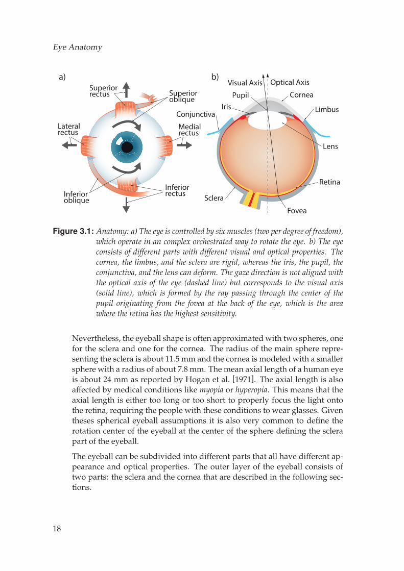
The human eye consists of several different parts as shown in Fig. 3.1. Thewhite sclera and the transparent cornea define the overall shape of the eye-ball. The colored iris, located behind the cornea, acts like a diaphragm con-trolling the light going through the pupil at the center of the iris, and behindthe iris is the lens. It focuses the light and forms an image at the back ofthe eyeball on the retina. The eyeball is connected to muscles that control itsposition and orientation.

In the following sections we will provide more details about each individualpart of the eye.

3.1 Eyeball

The eyeball is the rigid and hard part of the eye. It is located inside the eyesocket that holds the eye in place with muscles as shown in Fig. 3.1 a. Thespherical eyeball shape allows for smooth rotations, however, its shape isnot perfectly spherical. The transparent cornea protrudes from the sphericalshape. Besides the cornea the front part of the eyeball is flatter towards thenose and rounder towards the outer side of the face as depicted in Fig. 4.11.

17

Eye Anatomy

Cornea

Lens

Sclera

LimbusConjunctiva

Iris

Retina

Fovea

Pupil

Visual Axis Optical Axisa) b)

Superiorrectus Superior

oblique

Inferioroblique

Inferiorrectus

Medialrectus

Lateralrectus

Figure 3.1: Anatomy: a) The eye is controlled by six muscles (two per degree of freedom),which operate in an complex orchestrated way to rotate the eye. b) The eyeconsists of different parts with different visual and optical properties. Thecornea, the limbus, and the sclera are rigid, whereas the iris, the pupil, theconjunctiva, and the lens can deform. The gaze direction is not aligned withthe optical axis of the eye (dashed line) but corresponds to the visual axis(solid line), which is formed by the ray passing through the center of thepupil originating from the fovea at the back of the eye, which is the areawhere the retina has the highest sensitivity.

Nevertheless, the eyeball shape is often approximated with two spheres, onefor the sclera and one for the cornea. The radius of the main sphere repre-senting the sclera is about 11.5 mm and the cornea is modeled with a smallersphere with a radius of about 7.8 mm. The mean axial length of a human eyeis about 24 mm as reported by Hogan et al. [1971]. The axial length is alsoaffected by medical conditions like myopia or hyperopia. This means that theaxial length is either too long or too short to properly focus the light ontothe retina, requiring the people with these conditions to wear glasses. Giventheses spherical eyeball assumptions it is also very common to define therotation center of the eyeball at the center of the sphere defining the sclerapart of the eyeball.

The eyeball can be subdivided into different parts that all have different ap-pearance and optical properties. The outer layer of the eyeball consists oftwo parts: the sclera and the cornea that are described in the following sec-tions.

18

3.2 Sclera and Conjunctiva

3.2 Sclera and Conjunctiva

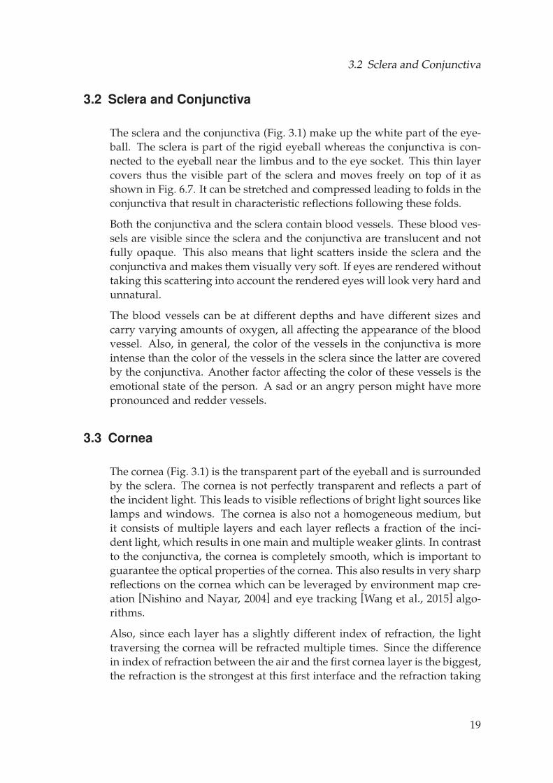
The sclera and the conjunctiva (Fig. 3.1) make up the white part of the eye-ball. The sclera is part of the rigid eyeball whereas the conjunctiva is con-nected to the eyeball near the limbus and to the eye socket. This thin layercovers thus the visible part of the sclera and moves freely on top of it asshown in Fig. 6.7. It can be stretched and compressed leading to folds in theconjunctiva that result in characteristic reflections following these folds.

Both the conjunctiva and the sclera contain blood vessels. These blood ves-sels are visible since the sclera and the conjunctiva are translucent and notfully opaque. This also means that light scatters inside the sclera and theconjunctiva and makes them visually very soft. If eyes are rendered withouttaking this scattering into account the rendered eyes will look very hard andunnatural.

The blood vessels can be at different depths and have different sizes andcarry varying amounts of oxygen, all affecting the appearance of the bloodvessel. Also, in general, the color of the vessels in the conjunctiva is moreintense than the color of the vessels in the sclera since the latter are coveredby the conjunctiva. Another factor affecting the color of these vessels is theemotional state of the person. A sad or an angry person might have morepronounced and redder vessels.

3.3 Cornea

The cornea (Fig. 3.1) is the transparent part of the eyeball and is surroundedby the sclera. The cornea is not perfectly transparent and reflects a part ofthe incident light. This leads to visible reflections of bright light sources likelamps and windows. The cornea is also not a homogeneous medium, butit consists of multiple layers and each layer reflects a fraction of the inci-dent light, which results in one main and multiple weaker glints. In contrastto the conjunctiva, the cornea is completely smooth, which is important toguarantee the optical properties of the cornea. This also results in very sharpreflections on the cornea which can be leveraged by environment map cre-ation [Nishino and Nayar, 2004] and eye tracking [Wang et al., 2015] algo-rithms.

Also, since each layer has a slightly different index of refraction, the lighttraversing the cornea will be refracted multiple times. Since the differencein index of refraction between the air and the first cornea layer is the biggest,the refraction is the strongest at this first interface and the refraction taking

19

Eye Anatomy

place at the other interfaces can often be neglected. In this thesis we willsimplify the cornea and approximate it with a single homogeneous medium.

Structurally, the cornea and the sclera are very similar. However, while oneis transparent the other has an opaque white color. Even though they bothconsist of a similar composition of collagen fibers. The reason for the dif-ferent optical properties lies in the arrangement of theses fibers. The regularalignment of the collagen fibers in the cornea leads to transparency. Whereasthe random alignment of the fibers in the sclera scatters the light and makesthe sclera white.

3.4 Limbus

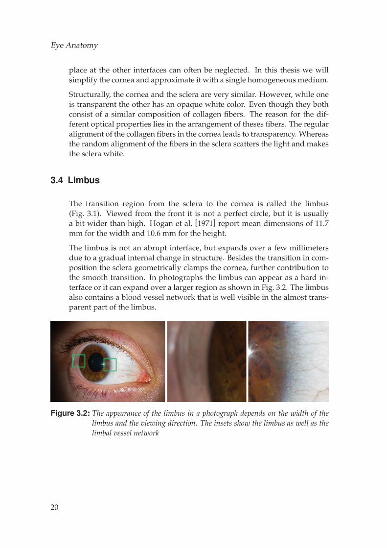
The transition region from the sclera to the cornea is called the limbus(Fig. 3.1). Viewed from the front it is not a perfect circle, but it is usuallya bit wider than high. Hogan et al. [1971] report mean dimensions of 11.7mm for the width and 10.6 mm for the height.

The limbus is not an abrupt interface, but expands over a few millimetersdue to a gradual internal change in structure. Besides the transition in com-position the sclera geometrically clamps the cornea, further contribution tothe smooth transition. In photographs the limbus can appear as a hard in-terface or it can expand over a larger region as shown in Fig. 3.2. The limbusalso contains a blood vessel network that is well visible in the almost trans-parent part of the limbus.

Figure 3.2: The appearance of the limbus in a photograph depends on the width of thelimbus and the viewing direction. The insets show the limbus as well as thelimbal vessel network

20

3.5 Iris

3.5 Iris

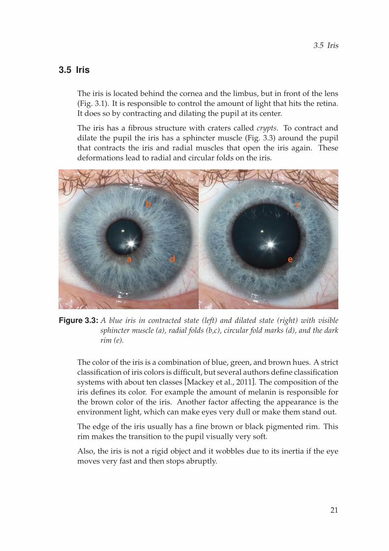
The iris is located behind the cornea and the limbus, but in front of the lens(Fig. 3.1). It is responsible to control the amount of light that hits the retina.It does so by contracting and dilating the pupil at its center.

The iris has a fibrous structure with craters called crypts. To contract anddilate the pupil the iris has a sphincter muscle (Fig. 3.3) around the pupilthat contracts the iris and radial muscles that open the iris again. Thesedeformations lead to radial and circular folds on the iris.

a

b c

d e

Figure 3.3: A blue iris in contracted state (left) and dilated state (right) with visiblesphincter muscle (a), radial folds (b,c), circular fold marks (d), and the darkrim (e).

The color of the iris is a combination of blue, green, and brown hues. A strictclassification of iris colors is difficult, but several authors define classificationsystems with about ten classes [Mackey et al., 2011]. The composition of theiris defines its color. For example the amount of melanin is responsible forthe brown color of the iris. Another factor affecting the appearance is theenvironment light, which can make eyes very dull or make them stand out.

The edge of the iris usually has a fine brown or black pigmented rim. Thisrim makes the transition to the pupil visually very soft.

Also, the iris is not a rigid object and it wobbles due to its inertia if the eyemoves very fast and then stops abruptly.

21

Eye Anatomy

3.6 Pupil

The pupil (Fig. 3.1) is the opening at the center of the iris and controls theamount of light entering the eye. The pupil is not exactly at the center of theiris and this center can even shift during contraction and dilation.

Through contraction and dilation the pupil adjusts it size constantly to ac-count for the amount of environment light (direct response). But there areother factors affecting its size. Due to the accommodation reflex the pupil con-tracts when looking at a close object to guarantee the best possible sharpness.Also, the pupil of the right and the left eye react in a coordinated way (con-sensual response). Thus, if light is shone into one eye, the pupil of the othereye will contract as well. This phenomenon is leveraged in Chapter 4 of thisthesis.

Visually, the pupil is almost never pitch black in a photograph. Light is re-flected on the back of the eye and makes the pupil appear in a shade of gray.If light is projected co-axially to the view axis the pupil becomes very bright,since the light is directly reflected off the back of the eyeball. This effectin combination with infrared light is employed by various pupil detectionalgorithms.

3.7 Muscles

The muscles are responsible to orient the eyeball within the eye socket. Thereare six muscles per eye (Fig. 3.1), which can be grouped in three pairs: supe-rior rectus/inferior rectus, lateral rectus/medial rectus, and superior oblique/inferioroblique. These six muscles move the eye in an orchestrated way. The musclehave multiple functions depending on the current eyeball pose. If the eyeis in the neutral position (looking straight ahead) the superior rectus is themuscle exerting the primary action responsible for looking up. If howeverthe eye is adducted (eye moving nasally) the inferior oblique becomes the pri-mary muscle for looking up. For a more detailed analysis of the functions ofthe individual muscles we refer to the medical literature [Hogan et al., 1971].

22

C H A P T E R 4Eye Reconstruction

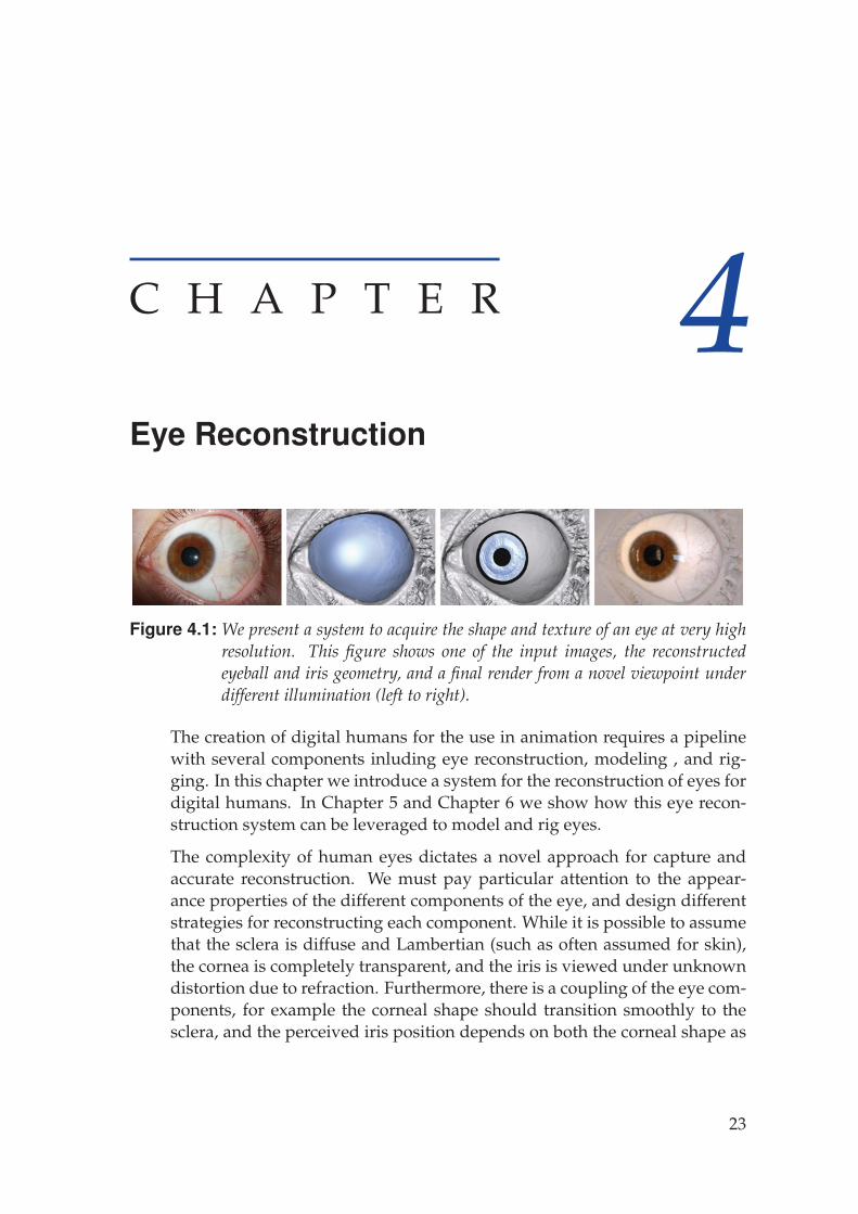
Figure 4.1: We present a system to acquire the shape and texture of an eye at very highresolution. This figure shows one of the input images, the reconstructedeyeball and iris geometry, and a final render from a novel viewpoint underdifferent illumination (left to right).

The creation of digital humans for the use in animation requires a pipelinewith several components inluding eye reconstruction, modeling , and rig-ging. In this chapter we introduce a system for the reconstruction of eyes fordigital humans. In Chapter 5 and Chapter 6 we show how this eye recon-struction system can be leveraged to model and rig eyes.

The complexity of human eyes dictates a novel approach for capture andaccurate reconstruction. We must pay particular attention to the appear-ance properties of the different components of the eye, and design differentstrategies for reconstructing each component. While it is possible to assumethat the sclera is diffuse and Lambertian (such as often assumed for skin),the cornea is completely transparent, and the iris is viewed under unknowndistortion due to refraction. Furthermore, there is a coupling of the eye com-ponents, for example the corneal shape should transition smoothly to thesclera, and the perceived iris position depends on both the corneal shape as

23

Eye Reconstruction

well as the exact index of refraction (both of which do vary from person toperson).

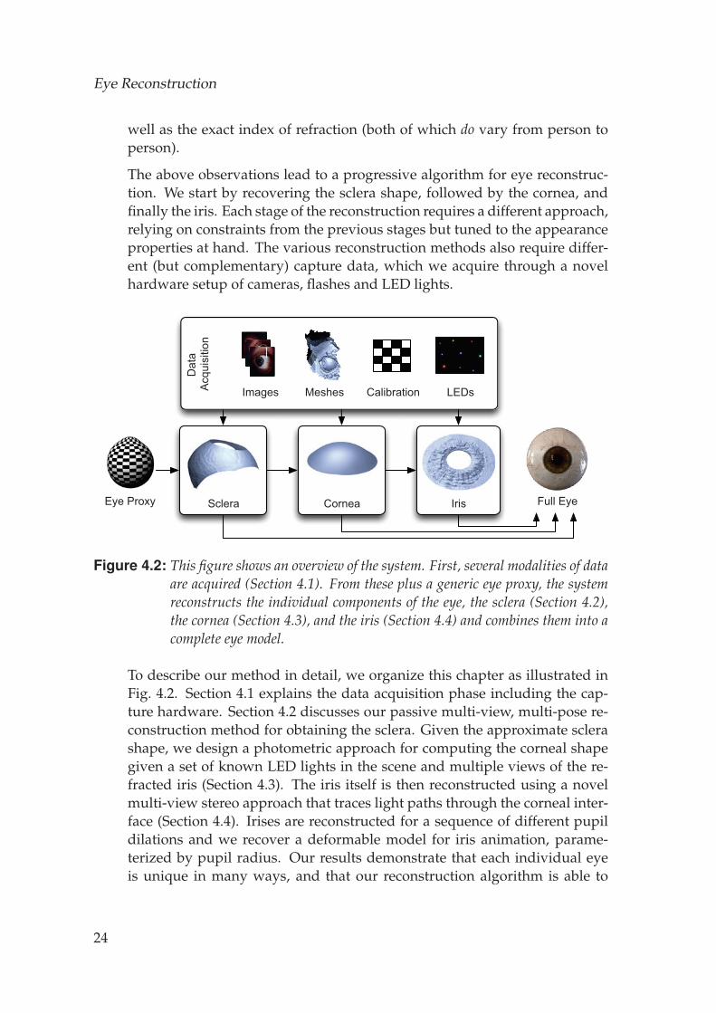
The above observations lead to a progressive algorithm for eye reconstruc-tion. We start by recovering the sclera shape, followed by the cornea, andfinally the iris. Each stage of the reconstruction requires a different approach,relying on constraints from the previous stages but tuned to the appearanceproperties at hand. The various reconstruction methods also require differ-ent (but complementary) capture data, which we acquire through a novelhardware setup of cameras, flashes and LED lights.

Dat

aA

cqui

sitio

n

Full EyeEye Proxy CorneaSclera Iris

Images Meshes Calibration LEDs

Figure 4.2: This figure shows an overview of the system. First, several modalities of dataare acquired (Section 4.1). From these plus a generic eye proxy, the systemreconstructs the individual components of the eye, the sclera (Section 4.2),the cornea (Section 4.3), and the iris (Section 4.4) and combines them into acomplete eye model.

To describe our method in detail, we organize this chapter as illustrated inFig. 4.2. Section 4.1 explains the data acquisition phase including the cap-ture hardware. Section 4.2 discusses our passive multi-view, multi-pose re-construction method for obtaining the sclera. Given the approximate sclerashape, we design a photometric approach for computing the corneal shapegiven a set of known LED lights in the scene and multiple views of the re-fracted iris (Section 4.3). The iris itself is then reconstructed using a novelmulti-view stereo approach that traces light paths through the corneal inter-face (Section 4.4). Irises are reconstructed for a sequence of different pupildilations and we recover a deformable model for iris animation, parame-terized by pupil radius. Our results demonstrate that each individual eyeis unique in many ways, and that our reconstruction algorithm is able to

24

4.1 Data Acquisition

capture the main characteristics required for rendering digital doubles (Sec-tion 4.5).

4.1 Data Acquisition

The first challenge in eye reconstruction is obtaining high-quality imageryof the eye. Human eyes are small, mostly occluded by the face, and havecomplex appearance properties. Additionally, it is difficult for a subject tokeep their eye position fixed for extended periods of time. All of this makescapture challenging, and for these reasons we have designed a novel acqui-sition setup, and we image the eye with variation in gaze, focus and pupildilation.

4.1.1 Capture Setup

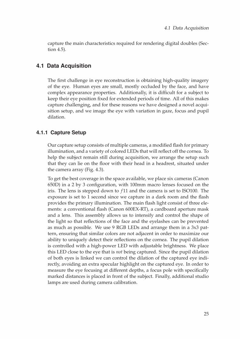
Our capture setup consists of multiple cameras, a modified flash for primaryillumination, and a variety of colored LEDs that will reflect off the cornea. Tohelp the subject remain still during acquisition, we arrange the setup suchthat they can lie on the floor with their head in a headrest, situated underthe camera array (Fig. 4.3).

To get the best coverage in the space available, we place six cameras (Canon650D) in a 2 by 3 configuration, with 100mm macro lenses focused on theiris. The lens is stepped down to f 11 and the camera is set to ISO100. Theexposure is set to 1 second since we capture in a dark room and the flashprovides the primary illumination. The main flash light consist of three ele-ments: a conventional flash (Canon 600EX-RT), a cardboard aperture maskand a lens. This assembly allows us to intensify and control the shape ofthe light so that reflections of the face and the eyelashes can be preventedas much as possible. We use 9 RGB LEDs and arrange them in a 3x3 pat-tern, ensuring that similar colors are not adjacent in order to maximize ourability to uniquely detect their reflections on the cornea. The pupil dilationis controlled with a high-power LED with adjustable brightness. We placethis LED close to the eye that is not being captured. Since the pupil dilationof both eyes is linked we can control the dilation of the captured eye indi-rectly, avoiding an extra specular highlight on the captured eye. In order tomeasure the eye focusing at different depths, a focus pole with specificallymarked distances is placed in front of the subject. Finally, additional studiolamps are used during camera calibration.

25

Eye Reconstruction

1

5

2 6

33 4

6

Figure 4.3: Overview of the capture setup consisting of a camera array (1), a focusedflash light (2), two high-power white LEDs (3) used to control the pupildilation, and color LEDs (4) that produce highlights on the cornea. Thesubject is positioned in a headrest (5). The studio lamps (6) are used duringcamera calibration.

4.1.2 Calibration

Cameras are calibrated using a checkerboard of CALTag markers [Atchesonet al., 2010], which is acquired in approximately 15 positions throughout thecapture volume. We calibrate the positions of the LEDs by imaging a mir-rored sphere, which is also placed at several locations in the scene, close towhere the eyeball is during acquisition. The highlights of the LEDs on thesphere are detected in each image by first applying a Difference-of-Gaussianfilter followed by a non-maximum suppression operator, resulting in singlepixels marking the positions of the highlights. The detected highlight posi-tions from a specific LED in the different cameras form rays that should allintersect at the 3D position of that LED after reflection on the sphere withknown radius (15mm). Thus, we can formulate a nonlinear optimizationproblem where the residuals are the distances between the reflected raysand the position estimates of the LEDs. We solve for the unknown LED andsphere positions with the Levenberg-Marquardt algorithm.

26

4.2 Sclera

4.1.3 Image Acquisition

We wish to reconstruct as much of the visible eye as possible, so the subjectis asked to open their eyes very wide. Even then, much of the sclera is oc-cluded in any single view, so we acquire a series of images that contain avariety of eye poses, covering the possible gaze directions. Specifically weused 11 poses: straight, left, left-up, up, right-up, right, right-down, down, left-down, far-left, and far-right. The straight pose will be used as reference pose,as it neighbors all other poses except far-left and far-right.

We then acquire a second series of images, this time varying the pupil dila-tion. The intricate geometry of the iris deforms non-rigidly as the iris dilatormuscle contracts and expands to open and close the pupil. The dilation isvery person-specific, so we explicitly capture different amounts of dilationfor each actor by gradually increasing the brightness of the high-power LED.In practice, we found that a series of 10 images was sufficient to capture theiris deformation parametrized by pupil dilation.

The acquisition of a complete data set takes approximately 5 minutes forpositioning the hardware, 10 minutes for image acquisition, and 5 minutesfor calibration, during which time the subject lies comfortably on a cushionplaced on the floor.

4.1.4 Initial Reconstruction

To initialize our eye capture method, we pre-compute partial reconstructionsfor each eye gaze using the facial scanning technique of Beeler et al. [2010].Although this reconstruction method is designed for skin, the sclera regionof the eye is similarly diffuse, and so partial sclera geometry is obtainable.These per-gaze reconstructions will be used in later stages of the pipeline.Additionally, the surrounding facial geometry that is visible will be used forproviding context when rendering the eye in Section 4.5.

4.2 Sclera

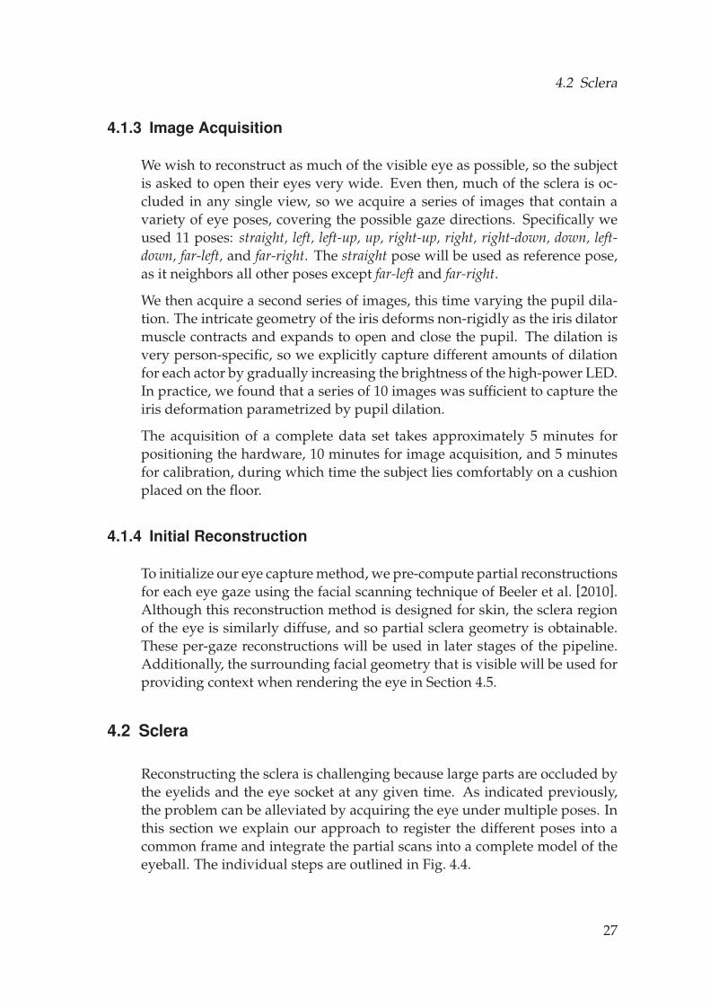
Reconstructing the sclera is challenging because large parts are occluded bythe eyelids and the eye socket at any given time. As indicated previously,the problem can be alleviated by acquiring the eye under multiple poses. Inthis section we explain our approach to register the different poses into acommon frame and integrate the partial scans into a complete model of theeyeball. The individual steps are outlined in Fig. 4.4.

27

Eye Reconstruction

SegmentImages

SegmentMeshes

Images

ScleraGeometryScans

Parameterize Match

Merge

TextureGeneration

ScleraTexture

Mes

h D

omai

nIm

age

Dom

ain

Section 4.2.3 Section 4.2.1

Section 4.2.2

Section 4.2.5

Section 4.2.4

OptimizeAlignment

RoughAlignment

Figure 4.4: The sclera reconstruction operates in both image and mesh domains. The in-put images and meshes are segmented (Section 4.2.1 and Section 4.2.2). Thepartial scans from several eye poses are registered (Section 4.2.3) and com-bined into a single model of the sclera using a generic proxy (Section 4.2.4).A high-resolution texture of the sclera is acquired and extended via texturesynthesis (Section 4.2.5).

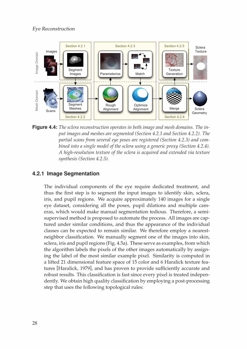
4.2.1 Image Segmentation

The individual components of the eye require dedicated treatment, andthus the first step is to segment the input images to identify skin, sclera,iris, and pupil regions. We acquire approximately 140 images for a singleeye dataset, considering all the poses, pupil dilations and multiple cam-eras, which would make manual segmentation tedious. Therefore, a semi-supervised method is proposed to automate the process. All images are cap-tured under similar conditions, and thus the appearance of the individualclasses can be expected to remain similar. We therefore employ a nearest-neighbor classification. We manually segment one of the images into skin,sclera, iris and pupil regions (Fig. 4.5a). These serve as examples, from whichthe algorithm labels the pixels of the other images automatically by assign-ing the label of the most similar example pixel. Similarity is computed ina lifted 21 dimensional feature space of 15 color and 6 Haralick texture fea-tures [Haralick, 1979], and has proven to provide sufficiently accurate androbust results. This classification is fast since every pixel is treated indepen-dently. We obtain high quality classification by employing a post-processingstep that uses the following topological rules:

28

4.2 Sclera

• The iris is the largest connected component of iris pixels.

• There is only a single pupil and the pupil is inside the iris.

• The sclera part(s) are directly adjacent to the iris.

Fig. 4.5b shows the final classification results for a subset of images, basedon the manually annotated exemplar shown in (a).

a) b)

Figure 4.5: Pupil, iris, sclera, and skin classification with manual labels (a) and exam-ples of automatically labeled images (b).

4.2.2 Mesh Segmentation

Given the image-based classification, we wish to extract the geometry of thesclera from the initial mesh reconstructions from Section 4.1.4. While thegeometry is mostly accurate, the interface to the iris and skin may containartifacts or exhibit over-smoothing, both of which are unwanted propertiesthat we remove as follows.

While a single sphere only poorly approximates the shape of the eyeballglobally (refer to Fig. 4.11 in the results), locally the surface of the sclera maybe approximated sufficiently well. We thus over-segment the sclera meshinto clusters of about 50mm2 using k-means and fit a sphere with a 12.5mmradius (radius of the average eye) to each cluster. We then prune vertices thatdo not conform with the estimated spheres, either in that they are too far offsurface or their normal deviates strongly from the normal of the sphere. Wefound empirically that a distance threshold of 0.3mm and normal thresholdof 10 degrees provide good results in practice and we use these values forall examples in this chapter. We iterate these steps of clustering, sphere fit-ting, and pruning until convergence, which is typically reached in less than5 iterations. The result is a set of partial sclera meshes, one for each capturedgaze direction.

29

Eye Reconstruction

4.2.3 Pose Registration

The poses are captured with different gaze directions and slightly differenthead positions, since it is difficult for the subject to remain perfectly still,even in the custom acquisition setup. To combine the partial sclera meshesinto a single model, we must recover their rigid transformation with respectto the reference pose. ICP [Besl and McKay, 1992] or other mesh-based align-ment methods perform poorly due to the lack of mid-frequency geometricdetail of the sclera. Feature-based methods like SIFT, FAST, etc. fail to ex-tract reliable feature correspondences because the image consists mainly ofedge-like structures instead of point-like or corner-like structures requiredby the aforementioned algorithms. Instead, we rely on optical flow [Brox etal., 2004] to compute dense pairwise correspondences.

Optical flow is an image based technique and typically only reliable on smalldisplacements. We therefore align the poses first using the gaze directionand then parameterize the individual meshes jointly to a uv-plane. The cor-respondences provided by the flow are then employed to compute the rigidtransformations of the individual meshes with respect to the reference pose.These steps are iterated, and convergence is typically reached in 4-5 itera-tions. In the following we will explain the individual steps.

Initial Alignment: The gaze direction is estimated for every pose using thesegmented pupil. Since the head does not remain still during acquisition,the pose transformations are estimated by fitting a sphere to the referencemesh and aligning all other meshes so that their gaze directions match.

Joint Parameterization: The aligned meshes are parameterized to a com-mon uv-space using spherical coordinates. Given the uv-parameterization,we compute textures for the individual poses by projecting them onto theimage of the camera that is closest to the line of sight of the original pose.This naive texturing approach is sufficient for pose registration, and reducesview-dependent effects that could adversely impact the matching.

Correspondence Matching: We compute optical flow [Brox et al., 2004] ofthe individual sclera textures using the blue channel only, since it offers thehighest contrast between the veins and the white of the sclera. The resultingflow field is sub-sampled to extract 3D correspondence constraints betweenany two neighboring sclera meshes. We only extract constraints which areboth well localized and well matched. Matching quality is assessed using

30

4.2 Sclera

the normalized cross-correlation (NCC) within a k × k patch. Localizationis directly related to the spatial frequency content present within this patch,quantified by the standard deviation (SD) of the intensity values. We setk = 21 pixels, NCC > 0, and SD < 0.015 in all our examples.

Optimization: The rigid transformations of all the poses are jointly opti-mized with a Levenberg-Marquardt optimizer so that the weighted squareddistances between the correspondences are minimized. The weights reflectthe local rigidity of the detected correspondences and are computed from theEuclidean residuals that remain when aligning a correspondence plus its 5neighbors rigidly. The optimization is followed by a single ICP iteration tominimize the perpendicular distances between all the meshes.

4.2.4 Sclera Merging

After registering all partial scans of the sclera, they are combined into a sin-gle model of the eyeball. A generic eyeball proxy mesh, sculpted by an artist,is fit to the aligned meshes and the partial scans are merged into a singlemesh, which is then combined with the proxy to complete the missing backof the eyeball.

Proxy Fitting: Due to the anatomy of the face, less of the sclera is recoveredin the vertical direction and as a result the vertical shape is less constrained.We thus fit the proxy in a two step optimization. In the first step we optimizefor uniform and in the second step for horizontal scaling only. In both stepswe optimize for translation and rotation of the eyeball while keeping therotation around the optical axis fixed.

Sclera Merging: The proxy geometry prescribes the topology of the eye-ball. For every vertex of the proxy, a ray is cast along its normal and inter-sected with all sclera meshes. The weighted average position of all intersec-tions along this ray is considered to be the target position for the vertex andthe standard deviation of the intersections will serve as a confidence mea-sure. The weights are a function of the distance of the intersection to theborder of the mesh patch and provide continuity in the contributions.

Eyeball Merging: The previous step only deforms the proxy where scandata is available. To ensure a smooth eyeball, we propagate the deformation

31

Eye Reconstruction

to the back of the eyeball using a Laplacian deformation framework [Sorkineet al., 2004]. The target vertex positions and confidences found in the pre-vious step are included as weighted soft-constraints. The result is a singleeyeball mesh that fits the captured sclera regions including the fine scaledetails and surface variation, and also smoothly completes the back of theeye.

4.2.5 Sclera Texturing

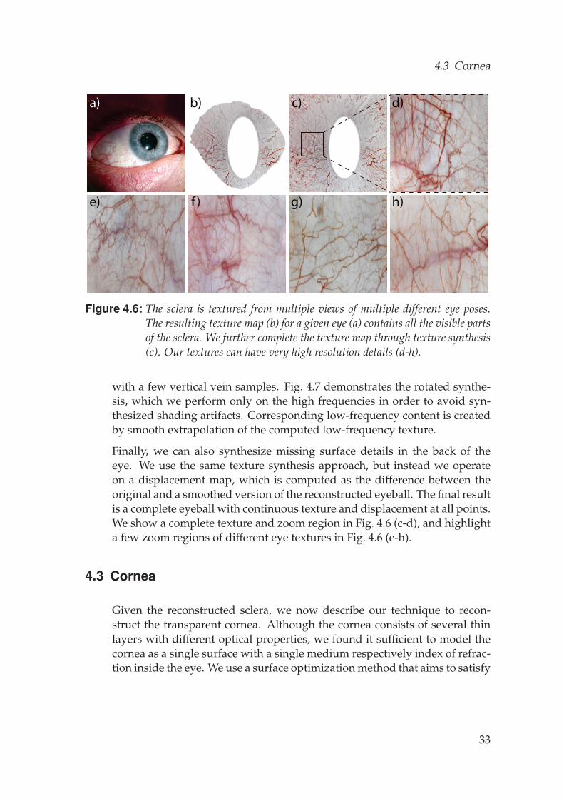
As a final step, we compute a color for each point on the reconstructed sclerasurface by following traditional texture mapping approaches that projectthe 3D object onto multiple camera images. In our case, we must con-sider all images for all eye poses and use the computed sclera segmentationto identify occlusion. One approach is to naively choose the most front-facing viewpoint for each surface point, however this leads to visible seamswhen switching between views. Seams can be avoided by averaging over allviews, but this then leads to texture blurring. An alternative is to solve thePoisson equation to combine patches from different views while enforcingthe gradient between patches to be zero [Bradley et al., 2010], but this canlead to strong artifacts when neighboring pixels at the seam have high gra-dients - a situation that often occurs in our case due to the high contrast of ared blood vessel and white sclera. Our solution is to separate the high andlow frequency content of the images. We then apply the Poisson patch com-bination approach only for the low frequency information, which is guar-anteed to have low gradients. We use the naive best-view approach for thehigh frequencies, where seams are less noticeable because most seams comefrom shading differences and the shading on a smooth eye is low-frequencyby nature. After texture mapping, the frequencies are recombined. Fig. 4.6bshows the computed texture map for the eye in Fig. 4.6a.

Our texturing approach will compute a color for each point that was seen byat least one camera, but the occluded points will remain colorless. Depend-ing on the intended application of the eye reconstruction, it is possible thatwe may require texture at additional regions of the sclera, for example if anartist poses the eye into an extreme gaze direction that reveals part of thesclera that was never observed during capture. For this reason, we synthet-ically complete the sclera texture, using texture synthesis [Efros and Leung,1999]. In our setting, we wish to ensure consistency of blood vessels, whichshould naturally continue from the iris towards the back of the eye. Weaccomplish this by performing synthesis in Polar coordinates, where mostveins traverse consistently in a vertical direction, and we seed the synthesis

32

4.3 Cornea

a) b) c) d)

e) f ) g) h)

Figure 4.6: The sclera is textured from multiple views of multiple different eye poses.The resulting texture map (b) for a given eye (a) contains all the visible partsof the sclera. We further complete the texture map through texture synthesis(c). Our textures can have very high resolution details (d-h).

with a few vertical vein samples. Fig. 4.7 demonstrates the rotated synthe-sis, which we perform only on the high frequencies in order to avoid syn-thesized shading artifacts. Corresponding low-frequency content is createdby smooth extrapolation of the computed low-frequency texture.

Finally, we can also synthesize missing surface details in the back of theeye. We use the same texture synthesis approach, but instead we operateon a displacement map, which is computed as the difference between theoriginal and a smoothed version of the reconstructed eyeball. The final resultis a complete eyeball with continuous texture and displacement at all points.We show a complete texture and zoom region in Fig. 4.6 (c-d), and highlighta few zoom regions of different eye textures in Fig. 4.6 (e-h).

4.3 Cornea

Given the reconstructed sclera, we now describe our technique to recon-struct the transparent cornea. Although the cornea consists of several thinlayers with different optical properties, we found it sufficient to model thecornea as a single surface with a single medium respectively index of refrac-tion inside the eye. We use a surface optimization method that aims to satisfy

33

Eye Reconstruction

constraints from features that are either reflected off or refracted through thecornea.

4.3.1 Theory

Reconstructing transparent surfaces requires different approaches than dif-fuse surface reconstruction since the surface is not directly visible. Trans-parent surfaces are generally not completely transmissive, but a fraction oflight is reflected if the refractive indices of the media involved differ. Thus,a bright light placed in front of the cornea will cause a visible highlight thatprovides a cue about the surface. Unfortunately, the position of the highlightis view-dependent and cannot directly be used in a mulit-view setting.

On the other hand, for a single view there is an ambiguity between the depthalong the viewing ray corresponding to a highlight and the normal of thesurface. For every position along a viewing ray there exists a surface normalreflecting the ray to the origin of the light (Fig. 4.8a, green). This creates asurface normal field defined by all possible viewing ray direction and depthcombinations. A similar surface normal field is produced from refractions(Fig. 4.8a, red).

The reflection and refraction surface normal fields of different views onlycoincide at the position of the actual surface as illustrated in Fig. 4.8b. Weuse this property to reconstruct the cornea.

Our system however produces only a sparse sampling of the normal fieldsas we employ only a few LEDs. We therefore need to add regularizationto ensure a unique solution, which is provided through the chosen sur-face representation. We employ an open uniform B-spline surface with 100control points. This surface has more representation power than the tra-ditionally employed 4th order Zernike polynomials [Ares and Royo, 2006;Smolek and Klyce, 2003] yet can be controlled locally, which is beneficial foroptimization. The control points are spaced regularly and initialized to thesurface of the eyeball proxy introduced in Section 4.2.4. The position of theboundary control points are optimized such that the surface boundaries fitthe proxy geometry. The boundary control points are kept fixed and are notpart of the following surface optimization.

4.3.2 Constraint Initalization

The corneal surface is optimized using three different types of constraints:reflection, refraction and position constraints.

34

4.3 Cornea

Reflection Constraints: The 9 calibrated LEDs placed in front of thecornea are imaged as highlights in the different views. From these high-lights we extract reflection constraints, which prescribe the normal for anypoint along the viewing ray through the highlight. Since the cornea is con-vex, every LED-view pair contributes one constraint assuming the reflectionof the LED is visible in the view. In addition, since we registered the posesin Section 4.2.3 we can combine constraints from all different poses. Thehighlights are detected and identified similarly as in the calibration phase(Section 4.1.2). While the highlights in the calibration images are acquired incomplete darkness, now they appear superimposed on the iris in the inputimages, which can lead to false positive detections. Thus, we remove theseunwanted detections by fitting a 2D Gaussian curve to the intensity profilesof all the highlight candidates to determine their width. Since all the LEDhighlights have a constant size we can remove false positives with a lower(3px) and upper (15px) threshold on the standard deviation of the Gaussian.

Refraction Constraints: Conceptually refraction constraints are very sim-ilar to reflection constraints. Instead of observing the reflected highlight ofa known LED, we instead observe the refraction of a feature on the iris atunknown position. Furthermore, the angle of refraction depends on the re-fractive index. Both the position of the feature and the refractive index areincluded as unknowns into the optimization and solved for. A feature pointon the iris contributes one refractive constraint per view. The correspondingimage location in the different views is estimated via optical flow [Brox etal., 2004]. Features are filtered as described in Section 4.2.3 using NCC>0.6and SD<0.02.

As for reflection constraints, we can combine refraction constraints from allposes. The distribution density of the features varies substantially, as wewont have any in the pupil for example. To account for this we weigh theconstraints by the local density, approximated by the distance d to the 10thnearest constraint as wre f r = NCC/d2 where NCC is the average normal-ized cross correlation score between corresponding image patches used as ameasurement of the quality of the constraint.

Position Constraints: Position constraints are extracted from the mergedsclera mesh (Section 4.2.4). Their purpose is to provide a continuous transi-tion from the cornea to the sclera. We randomly sample position constraintson the sclera in the vicinity of the corneal boundary. To ensure a good distri-bution, we reject constraints that are closer than 1mm to each other.

35

Eye Reconstruction

4.3.3 Surface Reconstruction

With a given set of reflection, refraction and position constraints and an ini-tial guess of the surface, the unknown parameters are optimized with a twostage approach. More specifically, we optimize the control points of the B-Spline, the refractive index and the unknown positions of the feature pointson the iris which are used for the refraction constraints. This amounts toa non-linear optimization which we solve using the Levenberg-Marquardtalgorithm by minimizing the error

Etot = λposEpos + λre f lEre f l + λre f rEre f r, (4.1)

where λpos = 0.1, λre f l = 1, and λre f r = 1 are user-defined parameters. Theerror for the position constraints P is given as

Epos =1|P| ∑

i∈P

∥∥pi − pposi

∥∥2, (4.2)

where ppos denotes the position of the constraint and p the nearest point onthe corneal surface. The error for the reflection constraints Q is given as

Ere f l =1|Q| ∑

i∈Q

∥∥∥ni − nre f li

∥∥∥2, (4.3)

where n is the current and nre f l the targeted surface normal. The error forthe refraction constraintsR is given as

Ere f r =1|R| ∑

i∈Rwre f r

i

∥∥∥pirisi − pre f r

i

∥∥∥2, (4.4)

where piris is the point on the iris, pre f r the closest point on the refracted rayand wre f r its corresponding weight. Optimizing the distance to the closestpoint has proven to be more stable than optimizing the mismatch of thenormals analogously to Equation 4.3.

In the first step we optimize for the control point positions of the B-splinesurface. They are optimized only along the opical axis of the eye and theboundary control points are kept fixed at all times. After convergence thesurface is kept fixed and we optimize for the refraction constraint points onthe iris (piris) and the refractive index. We iterate by alternating the two stepsuntil the overall improvement drops below 10e−10. The initial and optimizedcorneal surface plus constraints are visualized in Fig. 4.9 for one dataset.

36

4.4 Iris

4.3.4 Cornea-Eyeball Merging

We update the eyeball mesh with the optimized cornea by smoothly blend-ing the corneal surface into the eyeball mesh. First, corneal samples are com-puted for each eyeball vertex by intersecting the cornea in the direction ofthe eyeball normals. Second, the iris masks are dilated, blurred, projectedonto the cornea, and averaged to compute blending weights. Finally, theeyeball vertices are combined with the corneal samples by weighting themwith the weights.

4.4 Iris

We now move to the final component of the eye, the iris. In contrast to thesclera, we cannot perform traditional multi-view reconstruction to obtainthe iris geometry because the refractive cornea distorts the views of the iris.Additionally, the cornea transitions smoothly in opacity from fully trans-parent to fully opaque at the sclera, and this smooth transition can confusemulti-view correspondence matching. For these reasons, we create a specificiris reconstruction algorithm that is designed to handle these constraints.Since the iris is coupled with the pupil, our method begins by localizing thepupil in 3D. The iris geometry is then reconstructed and filtered, using thepupil as initialization. Finally, we combine iris reconstructions from captureswith different pupil dilations, allowing us to parameterize and animate thedeformation of the iris during pupillary response.

4.4.1 Pupil Reconstruction

The pupil has a very prominent position at the center of the eye, whichmakes it visually important and artifacts on its boundary would be clearlyvisible. Therefore, we require a reconstruction method for the pupil bound-ary that is robust with respect to perturbations like, for example, thosecaused by the flash highlight. This robust boundary is used to constrainthe iris and also to guide the initial meshing of the iris.

Initialization: The pupil is initialized with the pupil mask boundaries thatwe detect in image space. Each boundary is triangulated from multipleviews, taking into account refraction at the cornea, and we fit a circle to the

37

Eye Reconstruction

triangulated points. The required image correspondences for the triangula-tion are obtained from the optical flow, which we already computed for therefraction constraints of the cornea optimization.

Refinement: As this initial estimate tends to be rather inaccurate due toinconsistencies between pupil masks, we refine the estimated 3D circle in anoptimization that uses two data terms and two regularization terms. Thedata terms come from two additional cues about the pupil location, 1) animage term that incorporates the result of an image-based pupil detectionalgorithm, and 2) a mesh term that incorporates an approximate 3D surfacereconstruction of the pupil region, triangulated from image correspondencesfound using optical flow. The two regularization terms control the overallshape and smoothness of the pupil. Based on these terms, we define anenergy function for the pupil as

E = λIEI + λMEM + λCEC + λSES, (4.5)

which we minimize for a set of n = 50 pupil samples taken on the initialcircle, with weights of λI = 10, λM = 1000, λC = 10000, and λS = 1000 forall data sets. In the following, we will describe each of the energy terms inmore detail.

Image Term: We project the initial pupil circle into the cameras and blurthe images radially along the produced ellipses. We then use a radial edgedetector to locate the edge between the pupil and the iris, and we applyradial non-maximum suppression (NMS) to the response. We define theimage data term as

EI =1n

n

∑i=1

∥∥∥P(pi)− pedgei

∥∥∥2, (4.6)

where P(p) is the projection of sample point p into the image plane throughthe cornea, and pedge is the position of the closest point on the detected edge.

Mesh Term: We create an approximate 3D surface mesh in the vicinity ofthe pupil by triangulating rays from multiple views refracted at the cornealinterface, again with the help of optical flow to provide correspondences.The mesh term for the pupil location then consists of the distances betweenthe pupil samples and the generated mesh, given by

38

4.4 Iris

EM =1

∑ni=1 ci

n

∑i=1

ci

∥∥∥pi − pmeshi

∥∥∥2, (4.7)

where the distances are weighted with the triangulation confidences c of themesh. The triangulation confidence is defined as a linear function of thetriangulation residuals, which maps a residual of 0mm to a confidence of1 and a residual of 0.05mm to a confidence of 0 and clamps all the valuesoutside this range.

Regularization Terms: We allow the samples to deviate orthogonallyfrom the perfect circle, but we penalize these deviations with

EC =1n

n

∑i=1

∥∥∥pi − pcirclei

∥∥∥2, (4.8)

where pcircle is the corresponding point of p on the circle. To obtain a smoothpupil we also penalize strong changes in the deviations from one sample tothe next, using the following smoothness term, where r is the radial and othe orthogonal component of the offset with respect to the circle.

ES =1n

n

∑i=1

[(2ri−ri+1−ri−1)

2 + (2oi−oi+1−oi−1)2]

, (4.9)

Finally, we minimize the sum of all these terms with the Levenberg-Marquardt algorithm to find the position, the radius, and the per-sampledeviations from a circle of the pupil. During the optimization, we constrainthe normal of the pupil circle to the normal of the plane fit to iris mesh sam-ples taken 1 mm away from the initial pupil boundary estimate to be morerobust. Fig. 4.10 illustrates the resulting sample positions both in 3D andprojected onto an image (in green), given the initial estimate (in red).

4.4.2 Iris mesh generation

We use the reconstructed pupil boundary to initialize the iris mesh. Startingwith a closed uniform B-Spline that we fit to the optimized pupil samples,we scale the spline radially in 0.025mm steps to create a sequence of largerand larger rings up to an iris radius of 7mm. These rings are sampled 600times and a triangle mesh is created. This will serve as the topology for theiris.

39

Eye Reconstruction

In a second step, we reconstruct the correct position of each iris vertex. Eachvertex is projected (through the cornea) into a reference camera, where flow-based correspondences to other views are computed. We triangulate the ver-tex position by minimizing the squared distances between the vertex and therefracted rays formed by the correspondences. This minimization is equiva-lent to minimizing the surface error defined in Section 4.3.3. In addition, therays are weighted by the root mean square difference of the corresponding7x7 pixel blocks in image space. In order to reduce high frequency noise, theentire mesh reconstruction process is repeated for a second reference cam-era to obtain a second mesh hypothesis which is combined with the first onethrough weighted averaging.

4.4.3 Mesh cleanup

The reconstructed iris mesh can be noisy and distorted at the boundariesdue to the translucent sclera affecting the optical flow. We perform fouroperations to filter the iris mesh.

Spike Filtering: Spikes are detected by computing a 3-ring neighborhoodaround each vertex. If the distance between the vertex and the mean of theneighboring vertices exceeds a threshold (set to 0.05mm), then the verticesinside the ring are smoothed by solving a Laplacian system, keeping the restof the vertices fixed.

Boundary Deformation: Two criteria are used to label distorted bound-ary vertices: a threshold on the triangulation residuals (set to 0.05mm) andan angle threshold between the smoothed vertex normal and the normal ofthe pupil set to 30 degrees. We dilate the labeled region and smooth thosevertices in the normal direction.

Mesh Relaxation: The mesh is relaxed locally to improve the triangulationby removing skinny or overlapping triangles.

Pupil Constraint: The vertices at the pupil boundary are constrained tothe detected pupil shape. The constraint is enforced with a local Laplaciansystem, where the pupil vertices as well as all mesh vertices farther than1mm from the pupil are constrained. The vertices in-between are deformedbut the local shape is preserved.

40

4.4 Iris

Finally, the two independently triangulated and cleaned mesh hypothesesare averaged to create the iris mesh.

4.4.4 Mesh Propagation

We now combine iris reconstructions from captures with different pupil di-lations. Each mesh is reconstructed independently, with different topologyand vertex counts. We wish to compute a new set of iris meshes that arein vertex-correspondence, allowing us to compute a per vertex deformationmodel.

We begin by computing per camera optical flow [Brox et al., 2004] betweenneighboring poses. Since the vertices are propagated from one pose to thenext, drift might accumulate. To minimize the total amount of drift we se-lect a reference pose in the middle of the dilation sequence and compute theoptical flow in both dilation directions from there. To find the vertex corre-spondences we project each vertex from the source mesh into all the targetpose cameras taking into account the refraction at the cornea. With the re-sulting image positions and the optical flows we compute a set of rays thatwe refract at the cornea and intersect with the iris of the target pose. The tar-get pose vertex is computed as the median of all the intersections. To ensurea clean pupil we enforce the pupil constraint and relax the mesh in the sameway as described in Section 4.4.3.

4.4.5 Temporal Smoothing and Interpolation

In order to animate the pupil dilation, we will use the captured pupil posesas keyframes and interpolate linearly in-between. In practice we found thatthe dilation of the pupil cannot be accurately controlled, and so the pupil di-ameter tends to decrease in irregular steps. This can lead to multiple poseswith very similar diameters and geometry, but with different high frequencyreconstruction noise, which leads to artifacts when interpolating. In order tosmoothly integrate meshes from similar pupil radii, we compute two linearregression models for all poses within a distance of 1mm pupil radius. Thefirst regression model expresses the vertex position and the second modelthe Laplacian vector as a function of the pupil radius. We solve for thesmoothed mesh by evaluating both models and solving the resulting Lapla-cian system with equal weights given to the Laplacians and the positions.

41

Eye Reconstruction

4.4.6 Iris Texturing

Iris textures can be computed from a single view, but these textures willcontain undesired artifacts like highlights, washed out regions close to theboundary, dust on the cornea, etc. These artifacts can be attenuated by com-bining the textures from multiple views of the same iris dilation. We com-pute a contribution map for each view which is set to 1 if the pixel is themost saturated from all the candidates and to 0 otherwise. These maps arethen blurred with a small Gaussian kernel of 3 pixels. Based on these contri-bution maps, the textures from the different views are blended into a singletexture. Picking the most saturated pixels will reduce artefacts caused byillumination pollution from the flash light and by superposition of the whitesclera at the semi-transparent sclera-cornea transition alike. Then, we com-bine the textures from several iris dilations using the median to attenuateshading changes caused by the deforming iris.

4.5 Results

In this section we highlight the results of our eye capture technique by il-lustrating the reconstructions of a variety of human eyes, each with its ownintricacies and details.

We begin by analyzing the common assumption that eyes can be modelledas two spheres, a large one for the eyeball and a smaller one for the cornea.In our work we show that this assumption is inaccurate, which we can il-lustrate by overlaying a cross-section of a captured eye on top of the simplemodel (Fig. 4.11, left). Furthermore, it is often assumed that an eye is sym-metric about the view vector and that the left and right eye can be modelledsimilarly. By capturing both the left and right eye of an actor, we demon-strate that each eye is in fact unique and shows strong asymmetry individu-ally, but when combined the expected left/right symmetry is clearly visible.We believe these results have the potential to change how eyes are tradition-ally modelled in computer graphics.

Our eye capture method is robust, which we highlight by reconstructing 9different eyes from 6 different actors. The full set of reconstructions, shownin Fig. 4.12, contains a variety of different iris colors, surface details, textures,and overall eye shapes. Each eye has unique details, but we observed thatthe differences between people are more significant than the differences be-tween the two eyes of the same person, an expected phenomenon that helpsto validate our reconstruction results. For example, the two brown eyes in

42

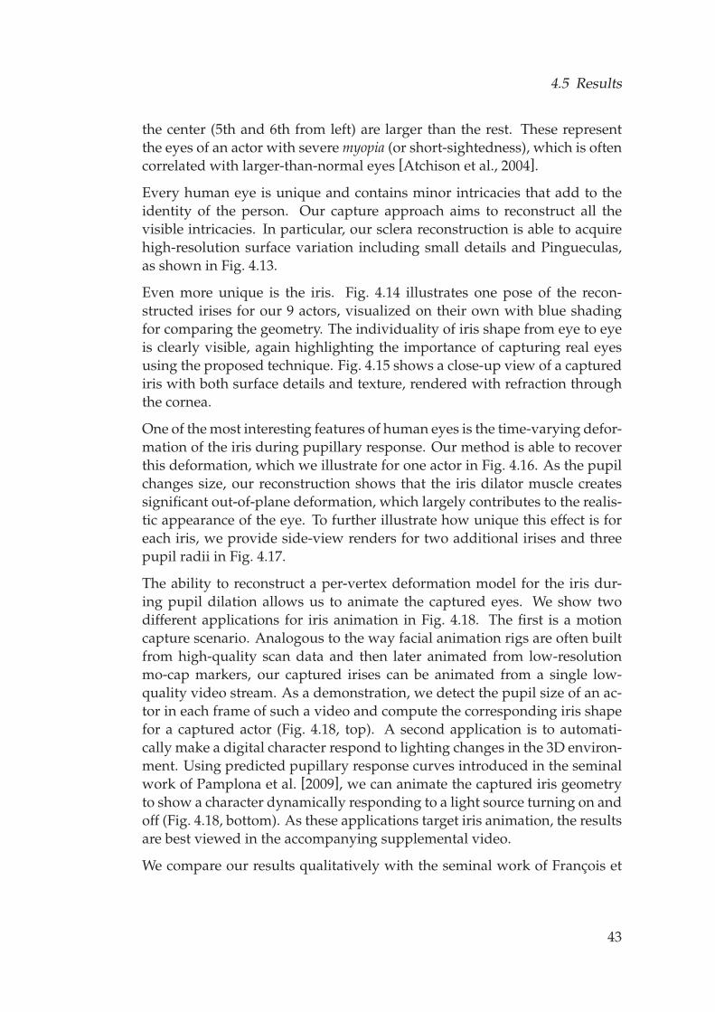
4.5 Results

the center (5th and 6th from left) are larger than the rest. These representthe eyes of an actor with severe myopia (or short-sightedness), which is oftencorrelated with larger-than-normal eyes [Atchison et al., 2004].

Every human eye is unique and contains minor intricacies that add to theidentity of the person. Our capture approach aims to reconstruct all thevisible intricacies. In particular, our sclera reconstruction is able to acquirehigh-resolution surface variation including small details and Pingueculas,as shown in Fig. 4.13.

Even more unique is the iris. Fig. 4.14 illustrates one pose of the recon-structed irises for our 9 actors, visualized on their own with blue shadingfor comparing the geometry. The individuality of iris shape from eye to eyeis clearly visible, again highlighting the importance of capturing real eyesusing the proposed technique. Fig. 4.15 shows a close-up view of a capturediris with both surface details and texture, rendered with refraction throughthe cornea.

One of the most interesting features of human eyes is the time-varying defor-mation of the iris during pupillary response. Our method is able to recoverthis deformation, which we illustrate for one actor in Fig. 4.16. As the pupilchanges size, our reconstruction shows that the iris dilator muscle createssignificant out-of-plane deformation, which largely contributes to the realis-tic appearance of the eye. To further illustrate how unique this effect is foreach iris, we provide side-view renders for two additional irises and threepupil radii in Fig. 4.17.

The ability to reconstruct a per-vertex deformation model for the iris dur-ing pupil dilation allows us to animate the captured eyes. We show twodifferent applications for iris animation in Fig. 4.18. The first is a motioncapture scenario. Analogous to the way facial animation rigs are often builtfrom high-quality scan data and then later animated from low-resolutionmo-cap markers, our captured irises can be animated from a single low-quality video stream. As a demonstration, we detect the pupil size of an ac-tor in each frame of such a video and compute the corresponding iris shapefor a captured actor (Fig. 4.18, top). A second application is to automati-cally make a digital character respond to lighting changes in the 3D environ-ment. Using predicted pupillary response curves introduced in the seminalwork of Pamplona et al. [2009], we can animate the captured iris geometryto show a character dynamically responding to a light source turning on andoff (Fig. 4.18, bottom). As these applications target iris animation, the resultsare best viewed in the accompanying supplemental video.

We compare our results qualitatively with the seminal work of Francois et

43

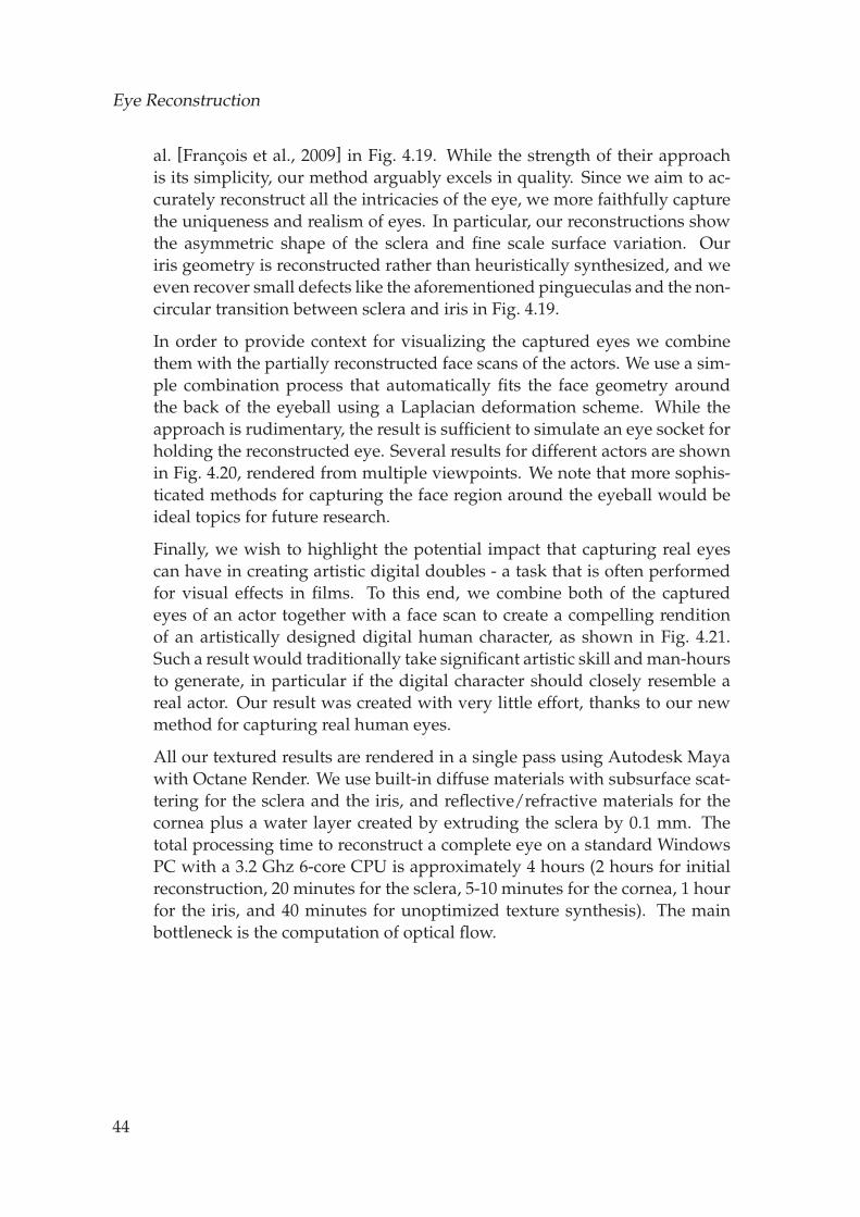
Eye Reconstruction

al. [Francois et al., 2009] in Fig. 4.19. While the strength of their approachis its simplicity, our method arguably excels in quality. Since we aim to ac-curately reconstruct all the intricacies of the eye, we more faithfully capturethe uniqueness and realism of eyes. In particular, our reconstructions showthe asymmetric shape of the sclera and fine scale surface variation. Ouriris geometry is reconstructed rather than heuristically synthesized, and weeven recover small defects like the aforementioned pingueculas and the non-circular transition between sclera and iris in Fig. 4.19.

In order to provide context for visualizing the captured eyes we combinethem with the partially reconstructed face scans of the actors. We use a sim-ple combination process that automatically fits the face geometry aroundthe back of the eyeball using a Laplacian deformation scheme. While theapproach is rudimentary, the result is sufficient to simulate an eye socket forholding the reconstructed eye. Several results for different actors are shownin Fig. 4.20, rendered from multiple viewpoints. We note that more sophis-ticated methods for capturing the face region around the eyeball would beideal topics for future research.

Finally, we wish to highlight the potential impact that capturing real eyescan have in creating artistic digital doubles - a task that is often performedfor visual effects in films. To this end, we combine both of the capturedeyes of an actor together with a face scan to create a compelling renditionof an artistically designed digital human character, as shown in Fig. 4.21.Such a result would traditionally take significant artistic skill and man-hoursto generate, in particular if the digital character should closely resemble areal actor. Our result was created with very little effort, thanks to our newmethod for capturing real human eyes.

All our textured results are rendered in a single pass using Autodesk Mayawith Octane Render. We use built-in diffuse materials with subsurface scat-tering for the sclera and the iris, and reflective/refractive materials for thecornea plus a water layer created by extruding the sclera by 0.1 mm. Thetotal processing time to reconstruct a complete eye on a standard WindowsPC with a 3.2 Ghz 6-core CPU is approximately 4 hours (2 hours for initialreconstruction, 20 minutes for the sclera, 5-10 minutes for the cornea, 1 hourfor the iris, and 40 minutes for unoptimized texture synthesis). The mainbottleneck is the computation of optical flow.

44

4.5 Results

a) b)

c) d)

Figure 4.7: Texture synthesis is performed on the high frequency information in order tocomplete the texture. A captured texture (a) is rotated to polar coordinates(b) and synthesis is performed in a way that preserves vein orientation (c).The final texture is rotated back to Cartesian coordinates (d).

45

Eye Reconstruction

a) b)

c) d)

p

pirisppos prefr

n nrefl nrefr

Figure 4.8: The depth/normal ambiguity of a highlight (a) and the sparse normal field ina multi-view setting (b). Corneal constraints before (c) and after optimiza-tion (d).

46

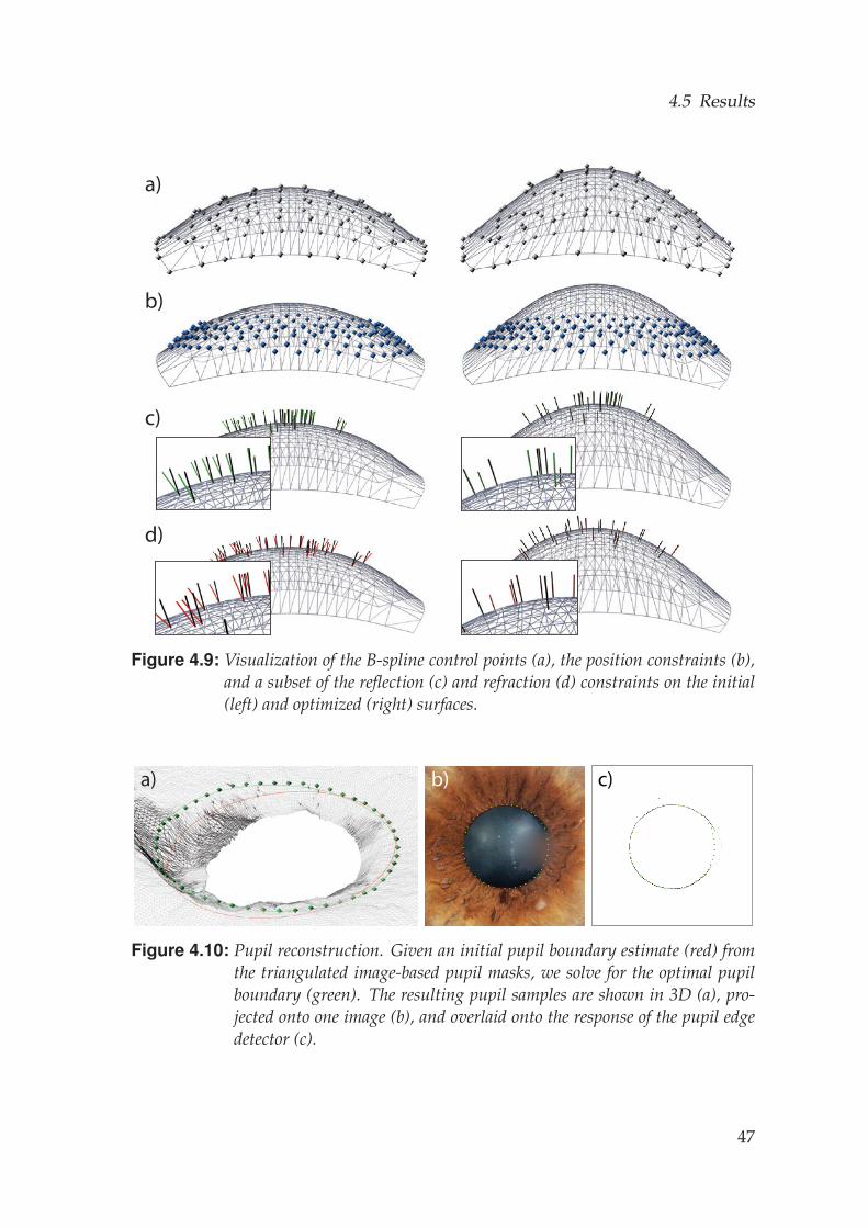
4.5 Results

a)

b)

c)

d)

Figure 4.9: Visualization of the B-spline control points (a), the position constraints (b),and a subset of the reflection (c) and refraction (d) constraints on the initial(left) and optimized (right) surfaces.

c)b)a)

Figure 4.10: Pupil reconstruction. Given an initial pupil boundary estimate (red) fromthe triangulated image-based pupil masks, we solve for the optimal pupilboundary (green). The resulting pupil samples are shown in 3D (a), pro-jected onto one image (b), and overlaid onto the response of the pupil edgedetector (c).

47

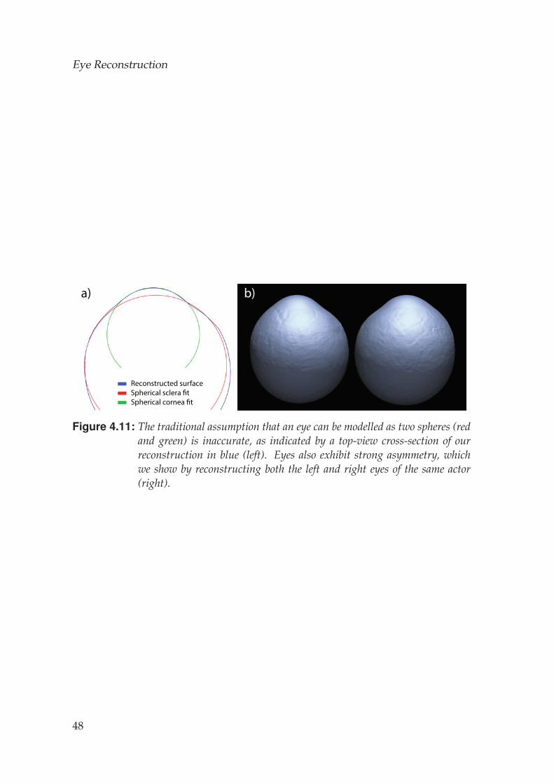
Eye Reconstruction

Reconstructed surfaceSpherical sclera fitSpherical cornea fit

a) b)

Figure 4.11: The traditional assumption that an eye can be modelled as two spheres (redand green) is inaccurate, as indicated by a top-view cross-section of ourreconstruction in blue (left). Eyes also exhibit strong asymmetry, whichwe show by reconstructing both the left and right eyes of the same actor(right).

48

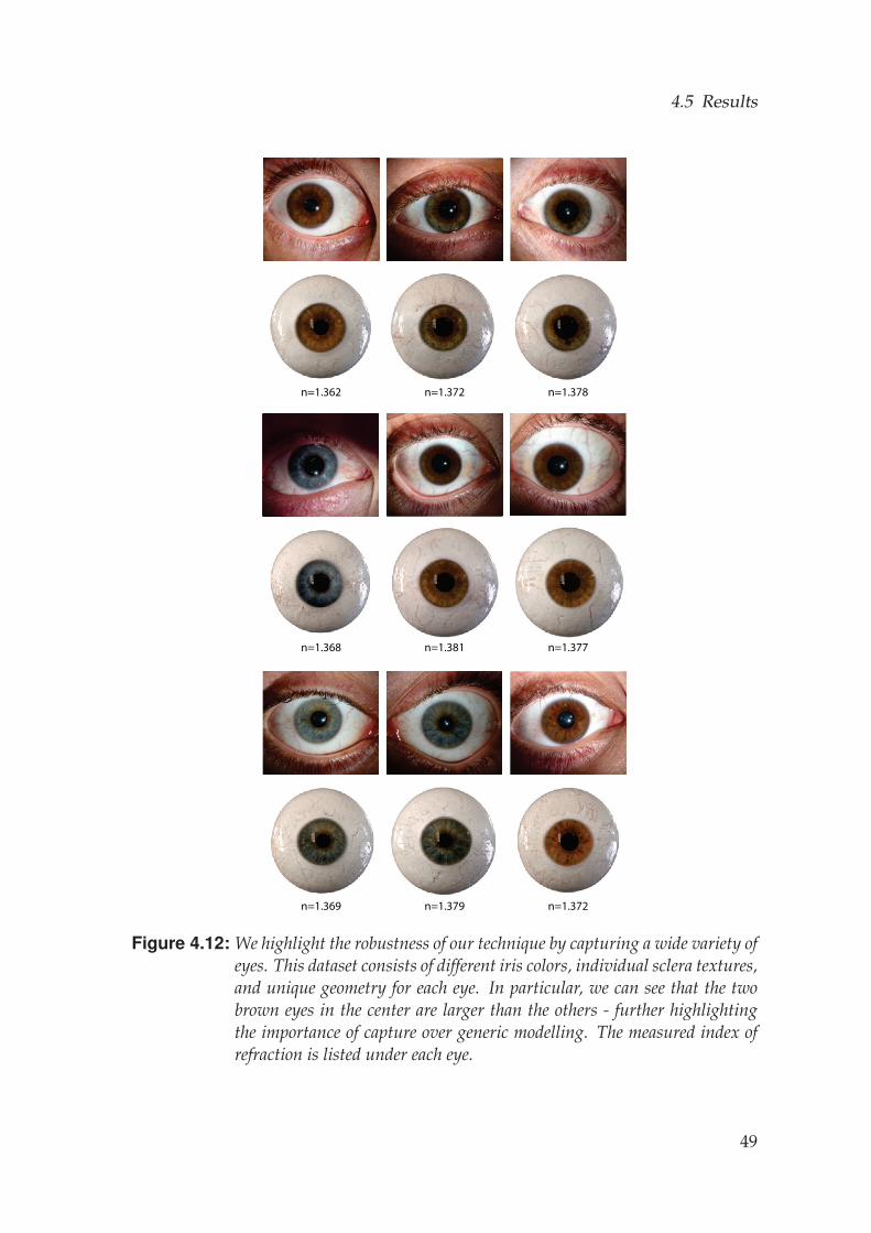
4.5 Results

n=1.362 n=1.372 n=1.378

n=1.368 n=1.381 n=1.377

n=1.369 n=1.379 n=1.372

Figure 4.12: We highlight the robustness of our technique by capturing a wide variety ofeyes. This dataset consists of different iris colors, individual sclera textures,and unique geometry for each eye. In particular, we can see that the twobrown eyes in the center are larger than the others - further highlightingthe importance of capture over generic modelling. The measured index ofrefraction is listed under each eye.

49

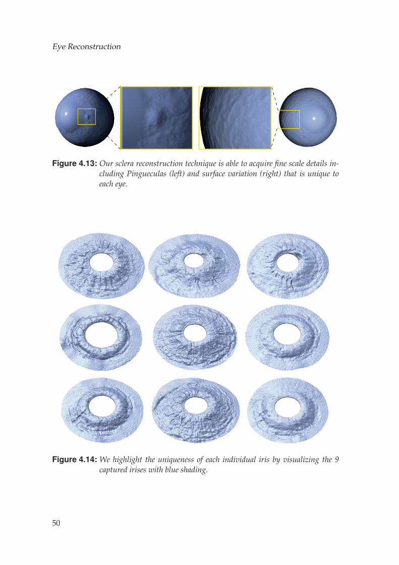
Eye Reconstruction

Figure 4.13: Our sclera reconstruction technique is able to acquire fine scale details in-cluding Pingueculas (left) and surface variation (right) that is unique toeach eye.

Figure 4.14: We highlight the uniqueness of each individual iris by visualizing the 9captured irises with blue shading.

50

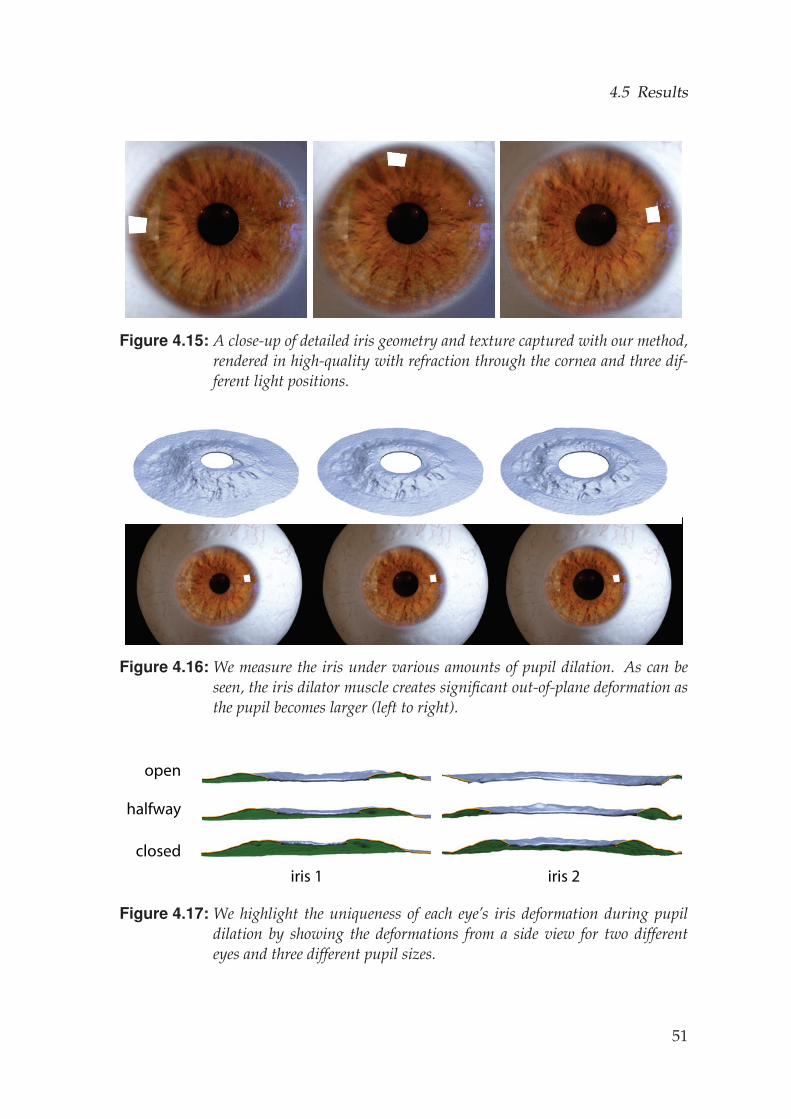
4.5 Results

Figure 4.15: A close-up of detailed iris geometry and texture captured with our method,rendered in high-quality with refraction through the cornea and three dif-ferent light positions.

Figure 4.16: We measure the iris under various amounts of pupil dilation. As can beseen, the iris dilator muscle creates significant out-of-plane deformation asthe pupil becomes larger (left to right).

closed

halfway

open

iris 1 iris 2

Figure 4.17: We highlight the uniqueness of each eye’s iris deformation during pupildilation by showing the deformations from a side view for two differenteyes and three different pupil sizes.

51

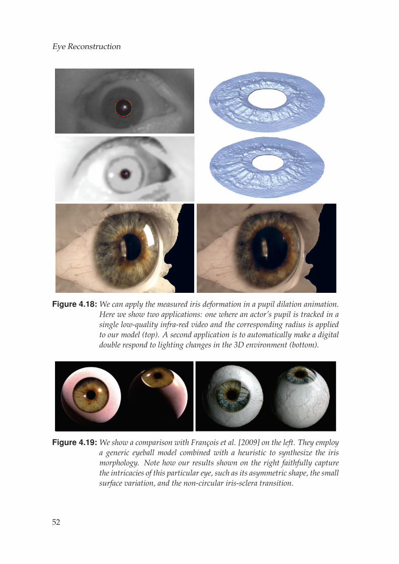
Eye Reconstruction

Figure 4.18: We can apply the measured iris deformation in a pupil dilation animation.Here we show two applications: one where an actor’s pupil is tracked in asingle low-quality infra-red video and the corresponding radius is appliedto our model (top). A second application is to automatically make a digitaldouble respond to lighting changes in the 3D environment (bottom).

Figure 4.19: We show a comparison with Francois et al. [2009] on the left. They employa generic eyeball model combined with a heuristic to synthesize the irismorphology. Note how our results shown on the right faithfully capturethe intricacies of this particular eye, such as its asymmetric shape, the smallsurface variation, and the non-circular iris-sclera transition.

52

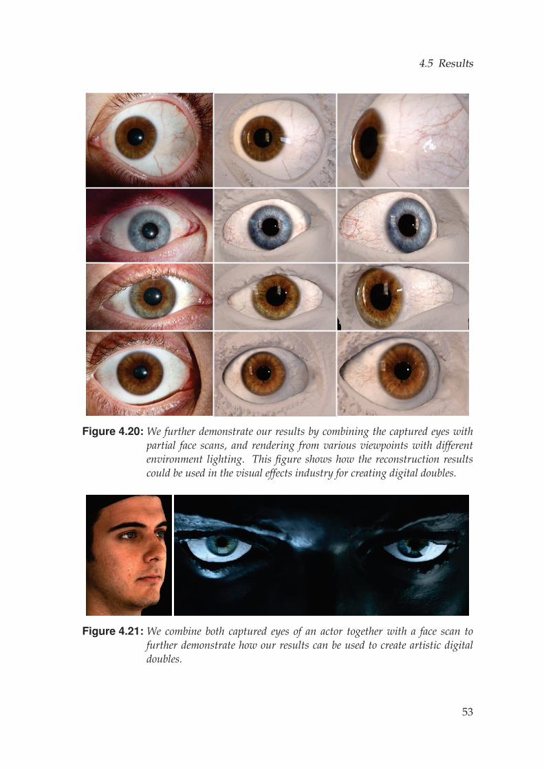
4.5 Results

Figure 4.20: We further demonstrate our results by combining the captured eyes withpartial face scans, and rendering from various viewpoints with differentenvironment lighting. This figure shows how the reconstruction resultscould be used in the visual effects industry for creating digital doubles.

Figure 4.21: We combine both captured eyes of an actor together with a face scan tofurther demonstrate how our results can be used to create artistic digitaldoubles.

53

Eye Reconstruction

54

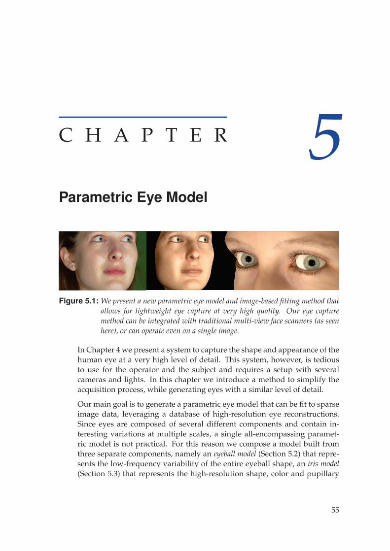
C H A P T E R 5Parametric Eye Model

Figure 5.1: We present a new parametric eye model and image-based fitting method thatallows for lightweight eye capture at very high quality. Our eye capturemethod can be integrated with traditional multi-view face scanners (as seenhere), or can operate even on a single image.

In Chapter 4 we present a system to capture the shape and appearance of thehuman eye at a very high level of detail. This system, however, is tediousto use for the operator and the subject and requires a setup with severalcameras and lights. In this chapter we introduce a method to simplify theacquisition process, while generating eyes with a similar level of detail.

Our main goal is to generate a parametric eye model that can be fit to sparseimage data, leveraging a database of high-resolution eye reconstructions.Since eyes are composed of several different components and contain in-teresting variations at multiple scales, a single all-encompassing paramet-ric model is not practical. For this reason we compose a model built fromthree separate components, namely an eyeball model (Section 5.2) that repre-sents the low-frequency variability of the entire eyeball shape, an iris model(Section 5.3) that represents the high-resolution shape, color and pupillary

55

Parametric Eye Model

deformation of the iris, and a sclera vein model (Section 5.4) that representsthe detailed vein structure in the sclera, including the vein network and thewidth and depth of individual veins, as well as fine-scale geometric surfacedetails. In Section 5.5 we show how the model parameters can be estimatedby fitting the model to 3D face scans, single images, or even artistic portraits,drastically simplifying the process of creating 3D high-quality eyes.

5.1 Input Data

With our eye reconstruction method we captured an eye database containing30 high-quality eyes. This database provides high-resolution meshes andtextures for the white sclera and the colored iris (please refer to the schematicin Fig. 1.3). The iris geometry is provided as a deformation model making itpossible to create meshes for an entire range of pupil dilations. The databasecontains eyes of different iris colors ranging from brown to green-brown toblue, and the high resolution geometry captures intricate eye-specific surfacedetails. A subset of the database eyes are shown in Fig. 5.2. We assume thatright and left eyes are anti-symmetric and we thus mirror the left eyes whenbuilding the model for the right eye. Similarly, a mirrored version of themodel can be used to represent the left eye. The data provided contains alsoa limbus opacity mask defining the transparency transition from sclera tocornea, from which the position of the limbus can be extracted by mappingthe 50 percent opacity level to the mesh.

5.2 Eyeball Model

The eyeball is represented by a morphable model [Blanz and Vetter, 1999],which has been demonstrated to be a good representation to capture low-frequency variation. A morphable model is a linear combination of a set ofsamples. To avoid overfitting to the samples, the dimensionality is often-times reduced using methods such as principal component analysis (PCA).PCA computes the mean shape plus a set of mutually orthogonal basis vec-tors from the samples, ordered according to their variance. Truncating thedimensions with lower variance leads to a subspace that captures the majorvariation in the samples and is resilient to noise. In addition to the shapevariation, our model also includes a rigid transformation for the eyeball aswell as a uniform scale factor.

A morphable model requires all samples to be in perfect correspondence,which is unfortunately not the case for our database of eyes. In our case,

56

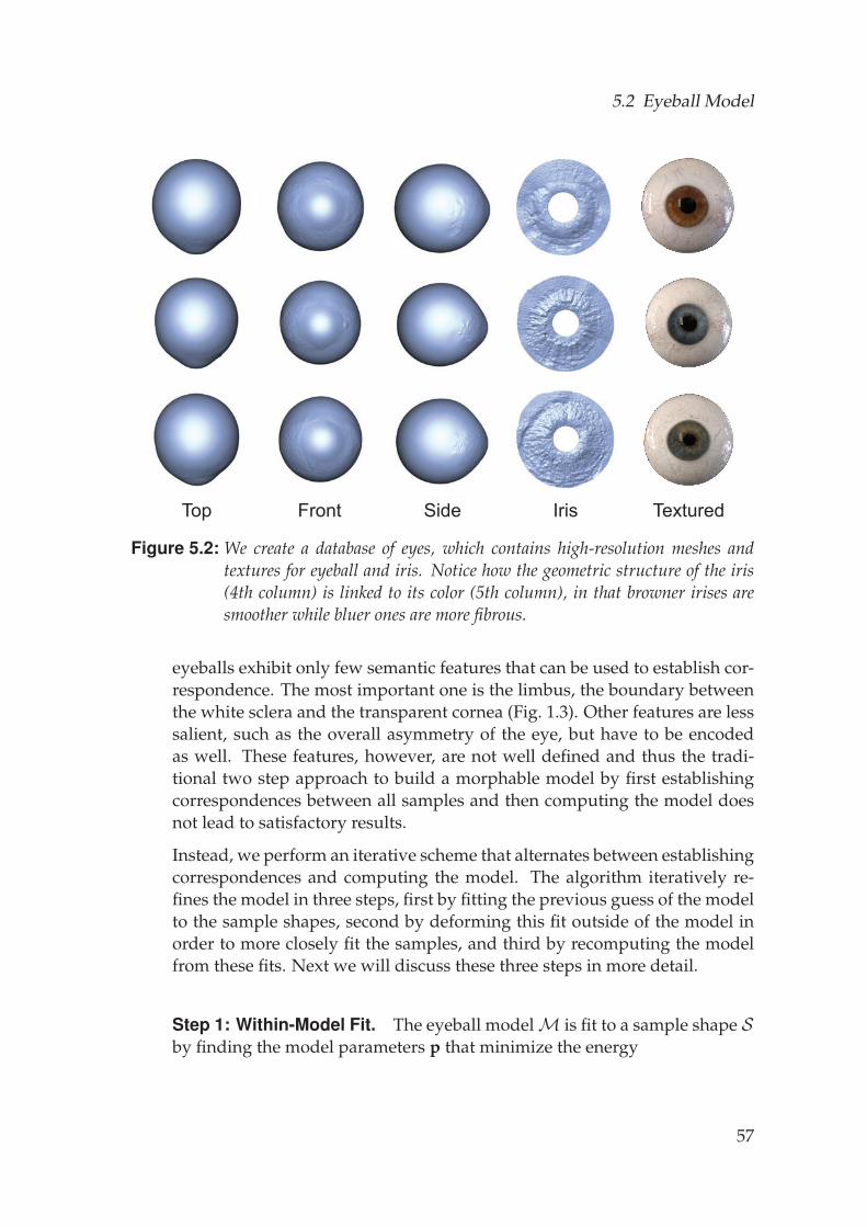
5.2 Eyeball Model

Top Front Side Iris Textured

Figure 5.2: We create a database of eyes, which contains high-resolution meshes andtextures for eyeball and iris. Notice how the geometric structure of the iris(4th column) is linked to its color (5th column), in that browner irises aresmoother while bluer ones are more fibrous.

eyeballs exhibit only few semantic features that can be used to establish cor-respondence. The most important one is the limbus, the boundary betweenthe white sclera and the transparent cornea (Fig. 1.3). Other features are lesssalient, such as the overall asymmetry of the eye, but have to be encodedas well. These features, however, are not well defined and thus the tradi-tional two step approach to build a morphable model by first establishingcorrespondences between all samples and then computing the model doesnot lead to satisfactory results.

Instead, we perform an iterative scheme that alternates between establishingcorrespondences and computing the model. The algorithm iteratively re-fines the model in three steps, first by fitting the previous guess of the modelto the sample shapes, second by deforming this fit outside of the model inorder to more closely fit the samples, and third by recomputing the modelfrom these fits. Next we will discuss these three steps in more detail.

Step 1: Within-Model Fit. The eyeball modelM is fit to a sample shape Sby finding the model parameters p that minimize the energy

57

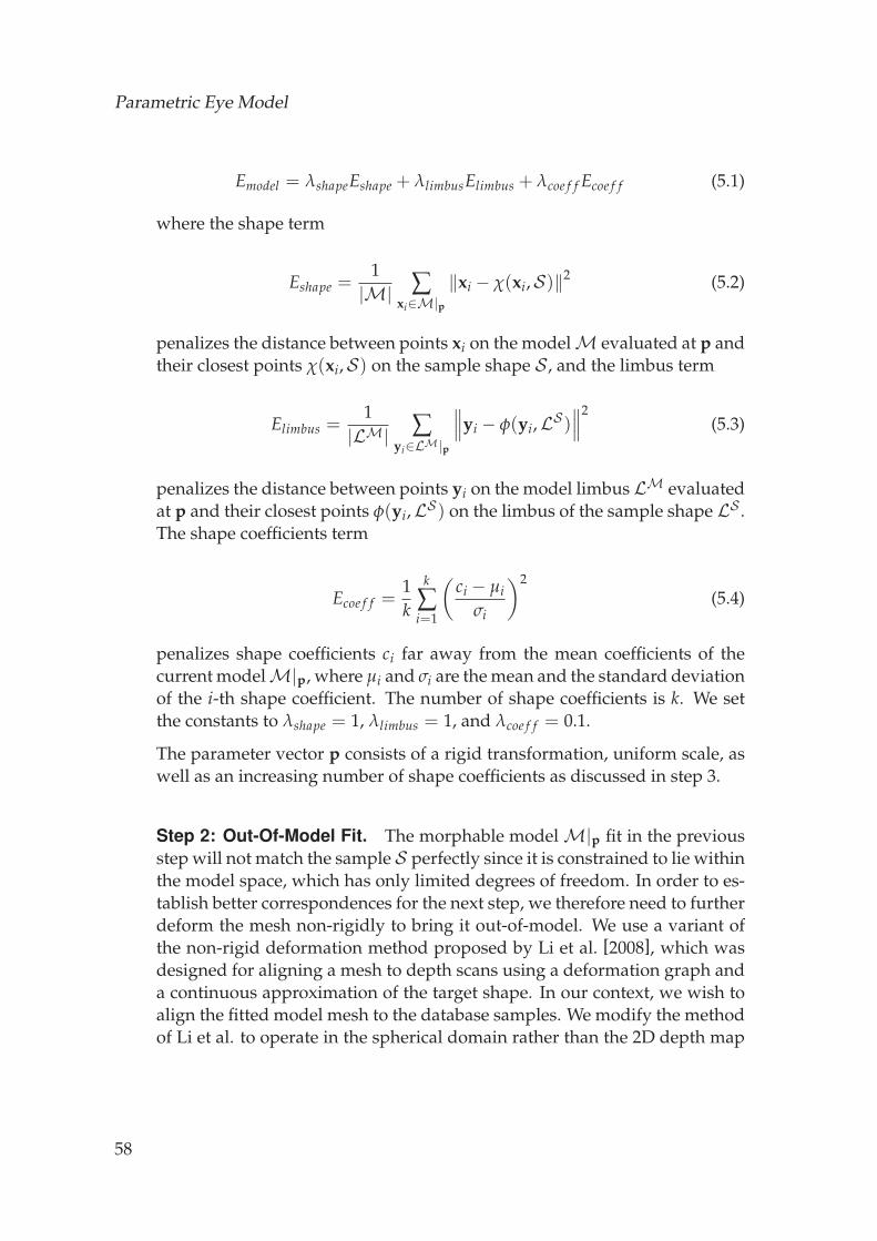
Parametric Eye Model

Emodel = λshapeEshape + λlimbusElimbus + λcoe f f Ecoe f f (5.1)

where the shape term

Eshape =1|M| ∑

xi∈M|p‖xi − χ(xi,S)‖2 (5.2)

penalizes the distance between points xi on the modelM evaluated at p andtheir closest points χ(xi,S) on the sample shape S , and the limbus term

Elimbus =1

|LM| ∑yi∈LM|p

∥∥∥yi − φ(yi,LS)∥∥∥2

(5.3)

penalizes the distance between points yi on the model limbus LM evaluatedat p and their closest points φ(yi,LS) on the limbus of the sample shape LS .The shape coefficients term

Ecoe f f =1k

k

∑i=1

(ci − μi

σi

)2

(5.4)

penalizes shape coefficients ci far away from the mean coefficients of thecurrent modelM|p, where μi and σi are the mean and the standard deviationof the i-th shape coefficient. The number of shape coefficients is k. We setthe constants to λshape = 1, λlimbus = 1, and λcoe f f = 0.1.

The parameter vector p consists of a rigid transformation, uniform scale, aswell as an increasing number of shape coefficients as discussed in step 3.

Step 2: Out-Of-Model Fit. The morphable model M|p fit in the previousstep will not match the sample S perfectly since it is constrained to lie withinthe model space, which has only limited degrees of freedom. In order to es-tablish better correspondences for the next step, we therefore need to furtherdeform the mesh non-rigidly to bring it out-of-model. We use a variant ofthe non-rigid deformation method proposed by Li et al. [2008], which wasdesigned for aligning a mesh to depth scans using a deformation graph anda continuous approximation of the target shape. In our context, we wish toalign the fitted model mesh to the database samples. We modify the methodof Li et al. to operate in the spherical domain rather than the 2D depth map

58

5.2 Eyeball Model

domain, and we add additional constraints to match both the limbus bound-ary and the mesh normals during deformation. We use two spherical coor-dinate parameterizations which are wrapped like the patches of a tennis ballso that the distortion in the domains is minimal. Closely following Li et al.,the energy that is minimized by the algorithm can be expressed as the sumof the following terms:

Enonrigid = λrEr + λsEs + λ f E f + λnEn + λlEl, (5.5)

where Er and Es correspond to the rigid and smooth energies as defined inthe original paper of Li et al. [2008]. We set the constants to λr,s = 0.01 andλ f ,n,l = 1. The shape and limbus energies Es and El correspond to the onesused in the previous step as defined in Equation 5.2 and Equation 5.3, respec-tively. The normal energy En is defined analogously to the shape energy asthe Euclidean difference between the normals of the model and the normalsof the respective closest points on the sample shapes. The non-rigid defor-mation produces meshes {M}which closely resemble the database samples{S} but have the same topology as the eyeball model.

Step 3: Update Eyeball Model. From the non-rigidly aligned shapes{M} an updated version of the model is computed using PCA and keep-ing only the mean shape plus the k most significant dimensions. In orderto be robust towards initial misalignment, the algorithm starts with a veryconstrained model that consists of the mean shape only (k = 0).

The proposed algorithm iterates these three steps and increases the dimen-sionality k of the model every 10 iterations by including the next most signif-icant PCA vector. Increasing the dimensionality allows the model to betterexplain the data and by doing so gradually provides robustness. We usea fixed amount of iterations because the error is not comparable from oneiteration to the other since the model has been updated at the end of eachiteration. After expanding the model three times (k = 3), we found that thefirst mode of the deformable model accounts for 92 percent of the variance,the first two for 96 percent, and the first three for 98 percent of the varia-tion, which covers the low-frequency variation we are targeting with thismodel. The final eyeball model thus contains 10 dimensions, six of whichaccount for rigid transformation, one for uniform scale, and three for shapevariation. Fig. 5.3 shows the deformation modes of our eyeball model.

59

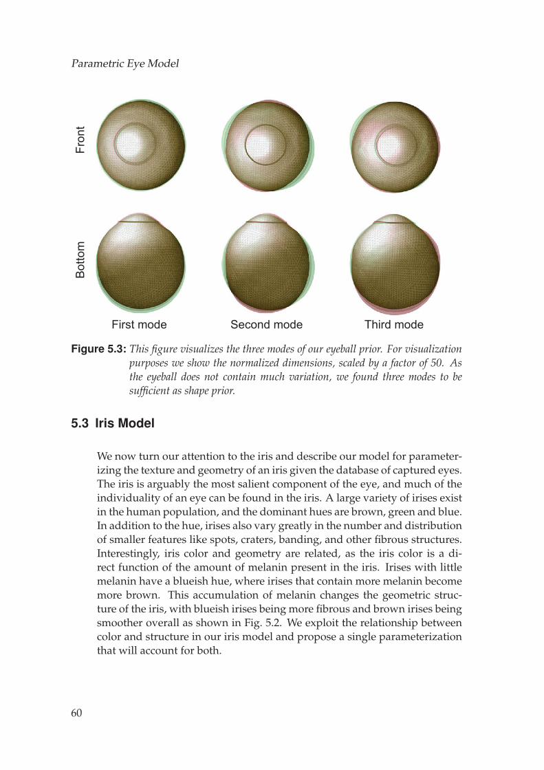
Parametric Eye Model

First mode Second mode Third mode

Fron

tB

otto

m

Figure 5.3: This figure visualizes the three modes of our eyeball prior. For visualizationpurposes we show the normalized dimensions, scaled by a factor of 50. Asthe eyeball does not contain much variation, we found three modes to besufficient as shape prior.

5.3 Iris Model

We now turn our attention to the iris and describe our model for parameter-izing the texture and geometry of an iris given the database of captured eyes.The iris is arguably the most salient component of the eye, and much of theindividuality of an eye can be found in the iris. A large variety of irises existin the human population, and the dominant hues are brown, green and blue.In addition to the hue, irises also vary greatly in the number and distributionof smaller features like spots, craters, banding, and other fibrous structures.Interestingly, iris color and geometry are related, as the iris color is a di-rect function of the amount of melanin present in the iris. Irises with littlemelanin have a blueish hue, where irises that contain more melanin becomemore brown. This accumulation of melanin changes the geometric struc-ture of the iris, with blueish irises being more fibrous and brown irises beingsmoother overall as shown in Fig. 5.2. We exploit the relationship betweencolor and structure in our iris model and propose a single parameterizationthat will account for both.

60

5.3 Iris Model

Since irises have such a wide range of variation, it would be impractical toparameterize them using a Guassian-distributed PCA space as we do for theeyeball. Instead, we account for the variability by parameterizing the iris us-ing a low-resolution control map, which represents the spatially varying hueand the approximate distribution of finer-scale features (see Fig. 5.4.b for anexample control map). The control map will guide the creation of a detailedhigh-resolution iris through constrained texture synthesis, using the irises inthe database as exemplars. The use of a control map is a very intuitive andconvenient way to describe an iris, as it can be extracted from a photographwhen reconstructing the eye of a specific person, or it can be sketched by anartist when creating fictional eyes. Based on the low-resolution control map,we propose a constrained synthesis algorithm to generate a detailed colortexture in high resolution (Section 5.3.1), and then extend the synthesis toadditionally create the geometric iris structure (Section 5.3.2).

5.3.1 Iris Texture Synthesis

Guided by the low-resolution control map our goal is to synthesize a high-resolution texture for the iris based on our eye database, similar to example-based super resolution [Tai et al., 2010] and constrained texture synthe-sis [Ramanarayanan and Bala, 2007]. We achieve this by composing thehigh-resolution texture from exemplar patches from the database, follow-ing the well-studied image quilting approach introduced by Efros and Free-man [2001]. In our application the process is guided by the control map andselects suitable patches from the database ensuring they conform both withthe control map and the already synthesized parts of the texture. Once thepatches have been selected, they are stitched together using graph cuts andcombined to a seamless texture using Poisson blending. Finally, this textureis merged with the intial control map in order to augment the low-res con-trol map with high-res detail. Fig. 5.4 shows the individual steps, which wewill describe in more detail in the following.

Patch Layout. The structure of an iris is arranged radially around thepupil. Operating in polar coordinates (angle/radius) unwraps the radialstructure (Fig. 5.4) and presents itself well for synthesis with rectangularpatches. We synthesize textures of resolution 1024x256 pixels with patchsizes of 64x64 pixels that overlap each other by 31 pixels in both dimensions.While iris features are distributed without angular dependency, they do ex-hibit a radial dependency since the structure close to the pupil (pupillaryzone) differs substantially from the one closer to the limbus (ciliary zone).

61

Parametric Eye Model

To synthesize a specific patch in the output, the algorithm can thus considersample patches at any angle with similar radii (±10%). The only drawbackof the polar coordinate representation is that the synthesized texture mustwrap smoothly in the angular dimension (i.e. across the left and right imageboundaries), which is handled by temporarily extending the texture by oneblock in the angular direction. To guarantee a consistent wrapping the firstand last block are updated as pairs.

Output Patch Selection. The iris is synthesized by iteratively placingpatches from the database iris textures. In each iteration, we first need todecide where to synthesize the next patch in the output texture. Many syn-thesis algorithms employ a sequential order, typically left to right and topto bottom. We found that this leads to unsatisfactory results since importantfeatures, such as spots or freckles, can easily be missed because neighbor-ing patches in the output may provide a stronger constraint than the controlmap. Instead we select the next patch based on control map saliency, whichsynthesizes patches in visually important areas first, thus allowing them tobe more faithful to the control map and spreading the control map resid-ual error into less salient areas. Saliency is computed via steerable filters asproposed by [Jacob and Unser, 2004].

Exemplar Selection. Once the location for the next patch to be synthe-sized has been determined, a suitable patch exemplar has to be retrievedfrom the database. This exemplar should be faithful to both the control mapand any neighboring patches that have already been chosen. Similarity tothe control map, denoted ec, is computed as the mean squared error be-tween a downscaled version of the exemplar and the patch of the controlmap. To gain invariance over differences in exposure and because the mostimportant quantity at this stage is faithful color reproduction, the error iscomputed over the RGB channels, but the mean intensity of the exemplar isscaled globally to match the mean intensity of the control patch. Similarityto the already synthesized texture, denoted en, is computed as mean squarederror over the overlapping pixels. The two similarity measures are linearlycombined into a single quantity

e = αen + (1− α)ec, (5.6)

where we use α = 0.25 for all examples in this chapter. The exemplar patchwith the smallest error is chosen.

62

5.3 Iris Model

Patch Merging. The end result of the above steps is a set of overlappingpatches that cover the entire texture. Even though the patches have beencarefully selected they will still exhibit seams. To alleviate this we followKwatra et al [2003] and employ a graph cut to find seams between patchesthat better respect the underlying image structure, i.e. finding a seam thatminimizes the color difference across the cut. For each patch, pixels at theboundary of the patch that overlap neighboring patches are labeled as sinksand the pixel at the center of the patch as a source. A graph for the currentblock is constructed with horizontal and vertical edges. The capacity of eachedge is set to be the difference of the two connected pixels. We use the max-flow/min-cut algorithm of Boykov et al. [2004] to solve for the cut.

Patch Blending. Once merged, the texture has a unique color per pixelwith minimal, yet still visible seams between patches. To completely re-move the seams we employ Poisson blending [Perez et al., 2003], setting thedesired color gradients across patch seams to be zero while preserving colordetail within patches.

Texture Blending. By definition, the synthesized texture T should well-match the control map C and contain more high frequency detail. However,the control map itself already contains a lot of structural information thatwe wish to preserve. Therefore we propose to blend the synthesized texturewith the control map, however we need to take care not to superimpose thesame frequencies. Assuming the captured image is in focus, the frequencycontent of the control map is determined by the resolution at which it wasacquired. If we base our synthesis on a low resolution image that capturesthe complete face, then we want to add a larger range of spatial frequenciesthan if the original input image was focused onto the eye and hence of highresolution. To avoid superimposing the same frequency bands we thus needto bandpass filter the synthesized texture before blending with the controlmap. We model the bandpass filter as a Gaussian G with the standard devi-ation computed from the ratio in width of the synthesized texture Twidth andthe control map Cwidth as

σ =TwidthCwidth

σ′, (5.7)

where σ′ is the standard deviation of the Gaussian at the resolution of thecontrol map, typically set to 1px. In some cases it makes sense to pick a

63

Parametric Eye Model

larger σ′ to account for noise or defocus of the control map. The high-passfiltered texture and low-pass filtered control map are then combined as

T ← (T − G ∗ T) + G ∗ C, (5.8)

and then re-converted from polar coordinates to create the final texture ofthe iris.

5.3.2 Iris Geometry Synthesis

As mentioned above, there is an inherent coupling between iris texture andgeometric structure. The idea is thus to exploit this coupling and synthesizegeometric details alongside the iris texture. The database is created with oureye reconstruction method and contains both high-res iris textures and irisdeformation models, which encode iris geometry as a function of the pupildilation. Since the iris structure changes substantially under deformation,we aim to synthesize the geometry at the observed pupil dilation. In addi-tion, the algorithm will also provide extrapolations to other pupil dilations,allowing us to control the iris virtually after reconstructing the eye.

Geometry Representation. The iris geometries in the database are en-coded in cylindrical coordinates (angle/radius/height), which renders themcompatible to the domain used for texture synthesis. Spatially, the iris de-formation model is discretized such that it has one vertex per pixel of thecorresponding texture, with full connectivity to its 8 neighbors. Temporally,the deformation model is discretized at four different pupil dilations, spacedequally to span the maximum dilation range common to all exemplars. Oneof the pupil dilations is picked to match the dilation of the input image.

Synthesizing geometry cannot be performed using absolute spatial coordi-nates since patches are physically copied from one spatial location in theexemplar to another in the output texture. For this reason, we find it con-venient to encode the geometry using differential coordinates that encodethe difference in angle, radius and height between neighboring vertices, andthen the synthesized geometry can be reconstructed. Specifically, for everyvertex, the iris geometry is encoded by the eight differential vectors to itsspatial neighbors (in practice, to avoid redundant storage we only need thefour vectors corresponding to top, top-right, right, and bottom-right), plusthree differential vectors forward in time, which we refer to as trajectories inthe following. See Fig. 5.5 for a schematic. These seven differential vectors

64

5.4 Sclera Vein Model

result in 21 additional dimensions that are added to the three color channelsfor synthesis.

Trajectory Scaling. The synthesis algorithm can place patches at differentradii than they were taken from in the exemplar. Even though this radiusdifference is limited to ±10%, we still need to adjust for the fact that defor-mation trajectories closer to the pupil are longer than trajectories closer tothe limbus (see Fig. 5.5 for a schematic explanation). Therefore, we scale thedifference vectors of each trajectory by

ρ =rl − rto

rl − r f rom, (5.9)

where r f rom is the radius at which the patch is extracted and rto the radiuswhere it is placed. rl is the limbus radius at which we assume no deforma-tion.

Reconstruction. The synthesized differential vectors in the final iris tex-ture are assembled to a linear Laplacian system for generating the final irisgeometry similarly to Sorkine et. al [2004]. Since all vectors are relative, thesystem is under-constrained and we need to provide some additional con-straints. The most natural choice is to constrain the positions of the pupil,which ensures a faithful fit to the observed pupil. Since the geometry is en-coded in cylindrical coordinates, we need to scale the angular dimension(radians) to render it compatible with the radial (mm) and height (mm) di-mensions. Thus, the angular dimension is multiplied by 5 mm, which corre-sponds to the average iris radius present in the database.

The result of this section is an iris model parameterized by a low-resolutioncontrol map, which allows high-resolution geometric and texture recon-structions using constrained synthesis given the database of eyes as exem-plars.

5.4 Sclera Vein Model

Finally, we complete the eye by presenting a model for synthesizing thesclera. By far the most dominant features of the sclera are the veins, whichcontribute substantially to the visual appearance of the eye. Depending onthe physical and emotional state, the appearance of these veins changes. Forexample they swell when the eye is irritated or when we are tired, causing

65

Parametric Eye Model

the infamous ”red eye” effect. Veins also travel under the surface at vary-ing depths, and deeper veins appear thicker and softer, while veins at thesurface appear more pronounced.

We propose to model the different states of veins with a parametric veinmodel. Such a model allows us to continuously change parameters andblend between different states. Also, besides modeling changes we can cre-ate additional detail not visible in the input data. Our model grows veinsfrom seed points following a parameter configuration. In the following, wefirst describe our vein model and how the vein network is synthesized, andthen describe how the synthesized veins are rendered to create the scleratexture, including a synthesized normal map to provide fine-scale surfacedetails.

5.4.1 Vein Model

When scrutinizing the veins of a real sclera, one can see that they exhibitan enormous visual richness and complexity (see Fig. 5.6.d), caused by thesuperposition of a large number of veins with varying properties such ascolor, thickness, scale, shape, and sharpness. To resemble this complexstructure, we model the sclera vein network as a forest, where an individ-ual tree corresponds the the vein network generated from a single largevein. The large veins are the most salient structures when looking from afar,and will be referred to as primary level veins. These veins branches off intosmaller second, third and lower level veins. Similar to L-Systems [Rozen-berg and Salomaa, 1976] and tree growing methods [Palubicki et al., 2009;Sagar et al., 1994] we create the vein network based on a set of rules, whichcontrol the vein properties described next.

Vein Properties. A single vein is represented by a series of control points,which are interpolated with a spline to provide a smooth and continuouscurve in the texture domain. These positional control points govern theshape of the vein. Similarly, other spatially varying properties can also bediscretized along this spline and interpolated when required. The proper-ties we synthesize include position offsets along the curve normals, the veinthickness, the vein depth, which relates to its visibility, and vein branchingpoints. Note that the discretization is independent per property, as someproperties vary more quickly when traversing a vein network. To accountfor the irregularity present in nature, we define the properties with a cer-tain amount of randomness. We employ two types of random functions,where one follows a Gaussian distribution N , parameterized by the mean

66

5.4 Sclera Vein Model

and standard deviation. The second one is a colored noise function C, whichis parameterized by the amplitude controlling the amount of perturbationand the spectral power density, which is controlled by the exponent in 1/ f x

and specifies the noise color.

The position offsets are defined by the colored noise function Co f f set in therange of pink (x = 1) and red (x = 2) noise. Thickness is specified at thestarting point ρthickSeed, along with a decay factor ρthickDecay, again perturbedwith a colored noise function (Cthick). Depth is computed as an offset to agiven average depth ρdepth, created by adding colored noise (Cdepth). Fi-nally, the locations of the branching points and the corresponding branch-ing angles are determined by two Gaussian distributions, NbranchPos andNbranchAngle, respectively.

Vein Recipes. Our model allows us to generate veins given a set of param-eters (a vein recipe) describing the properties of the vein (width, depth, crip-pling, noise, etc.). Multiple veins can be synthesized with the same recipe.However, a single recipe does not account for the variation observed in na-ture. Therefore, we empirically create multiple vein recipes that describeveins belonging to different branching levels (primary, secondary, tertiary).. We found that a set of 24 recipes (10 primary, 6 secondary, and 12 tertiary)can produce vein networks of adequate visual complexity. In addition to theparameters described above, the recipes will also prescribe the parametersused for vein growing described below.

Vein Growing. Vein synthesis takes place in an unwrapped texture do-main, with the limbus at the top and the back of the eyeball at the bottom.Veins on the sclera grow from the back of the eyeball to the front, and hencewe grow them from bottom to top.

Growth is governed by a step size ρstep and a direction d at every point.The step size is attenuated during growth by a decay factor ρstepDecay. Thegrowing direction is influenced by three factors, 1 - a Gaussian distributionNβ that provides a general growth bias towards the top of the domain, 2 -a second Gaussian distribution Nγ that controls how much the vein mean-ders, and 3 - a repulsion term that discourages veins from growing over eachother. The repulsion term stems from a repulsion map R that is computedwhile growing the veins, by rendering the veins into an image, indicatingthat a particular area has become occupied. The best growing angle can becomputed with the distributions defined above as

67

Parametric Eye Model

α = maxα

(Nβ(α) + ε)(Nγ(α) + ε)(1−R(x + d) + ε). (5.10)

The direction d is computed from the angle α and current step size, and xdenotes the current position. Also, Nγ is evaluated relative to the last grow-ing angle. Since the terms could fully deactivate each other in pathologicalcases, we add a ε to the terms (ε = 0.001).

Vein Seeds. Veins start growing at seed points at the bottom of the texturefor primary veins, or at branching points for higher levels, and growing isterminated if they reach a predescribed length or grow past the limbus. Theprimary vein seeds are generated at random positions at the bottom of thetexture. We use 10 seeds in all our results. The seeds are generated sequen-tially. To prevent that two seeds are too close to each other we reject theseeds that are closer than 300 pixels. The final texture is 4096 by 2048 pixels.

5.4.2 Vein Rendering

Given a synthesized network of veins with spatially varying properties, wenow render the veins into the texture using an appearance model learnedfrom the database of eyes.

The appearance of a vein is influenced by many different factors, such asits diameter, how shallow it grows, its oxygenation, and others. The mostimportant factor is the depth, which influences the color since the sclera hasa higher absorption coefficient in the red wavelengths and as a consequencedeeper veins appear blueish. The depth also influences the sharpness of thevein, since more subsurface scattering blurs out the cross-profile. Next todepth, thickness plays a central role since thin and thick veins are visuallyquite different. Note that the two parameters are not independent, sincethin veins for example can only appear close to the surface as they wouldbe washed out further in, and consequently have to be of reddish color. Weuse a data-driven approach to map depth and thickness to appearance, de-termined from exemplary textures in the eye database, as described in thefollowing.

Cross-Section Model. We manually label 60 short vein segments in ex-emplary textures, which span the vein appearance. From these segmentswe sample cross-section profiles of the RGB space by fitting an exponentialalong the profile:

68

5.4 Sclera Vein Model

c(r) = cbkgnd − δ exp(−‖r‖1

2ψ

), (5.11)

where r is the distance from the labeled vein along the profile, in pixels. Thefitting estimates thickness ψ, depth δ and background color cbkgnd of thesecross-sections. Subtracting the background from the cross-section will allowus to add the model to any background.

Given the synthesized thickness ψ and depth δ, we retrieve all samples withsimilar depth and thicknesses from the labeled veins, where similarity iscomputed as Euclidean distances on normalized tickness and depth values.A similarity threshold th is set to 1.1 times the distance to the third nearestneighbour. The retrieved cross-profiles are scaled to match to the query pa-rameters, and the final cross-profile used for rendering is computed as theirweighted average, where the weights are set to 1− distance

th .

This model allows us to compute a cross-section for any pair of thicknessand depth parameters. Finally, the cross-section model is evaluated for eachpixel in the neighborhood of a vein with the local width and depth, andadded to the backplate.

Backplate. Our vein model describes the vein network but not the back-ground into which the veins are to be rendered. This background containstwo components: the low frequency variation and the high-frequency struc-ture of the sclera texture. The mid-frequency features are provided by thevein model.

The high-frequency component accounts for visual noise and imperfections.This high-frequency texture is created manually by copying sclera patchesthat contain no veins from the database textures. Since it does not containany recognizeable structures we can employ the same high-frequency com-ponents for every eye.

The low-frequency component is extracted from the smoothed input imageswith the intent to match the perceived overall color variation. Since onlyparts of the sclera texture can be computed from the images, we extrapolatethe low-frequency component of the sclera to the entire eyeball by fitting asmooth spline surface to the visible parts of the texture. The spline surfaceis cyclic in the horizontal direction so that the left and right border matchseamlessly. We also constrain the bottom of the texture to a reddish huesince there is no data present at the back of the eyeball and visually eyesappear more red near the back.

69

Parametric Eye Model

The high- and low-frequency components are combined into a single back-plate image, into which the veins are rendered. An example of a final veintexture is shown in Fig. 5.6 (a), which additionally shows the impact of thedepth (b,c) and thickness (e,f) parameters.

Geometric Surface Details. The geometric surface details of the scleraare important for the visual appearance of the eye since these little bumpsaffect the shape of specular highlights. The bumps consist of a mix of ran-dom bumps and displacements that correlate with the positions of big veins.Thus, we create a normal map based on a combination of procedural noiseand displacements that follow the thick veins to render all our results.

This concludes the parametric model, which is able to synthesize all visibleparts of the eye, including the eyeball, the iris, and the veins.

5.5 Model Fitting

The model described in the previous sections allows us to create a widerange of realistic eyes based on a few parameters and an iris control map.In this section we describe how these parameters can be estimated auto-matically and how the required iris control map is extracted from varioussources. We focus on two different use-case scenarios. In a first use-case,we demonstrate how the proposed method may be used to complement ex-isting photogrammetric face scanners to augment the facial geometry thatis inaccurate for the eye itself with high-quality eye reconstructions, and ina second use-case we show how our method can be used to compute eyegeometry and textures from single, uncalibrated input images.

5.5.1 Multi-View Fitting

In the multi-view scenario we fit our eye model to a 3D face scan providedby a multi-view stereo (MVS) reconstruction algorithm. In this work weleverage the system of Beeler et al. [2010], but any other system that pro-vides calibrated cameras and 3D geometry would also work. The MVS algo-rithm reconstructs the white sclera reasonably well since its surface is mostlydiffuse, albeit at lower quality than skin due to strong specular reflectionswhich result in a noisier surface. Here, our model will serve as a regularizerto get rid of the noise. Most other parts of the eye, such as the cornea orthe iris, pose greater challenge to the system, as they are either invisible orheavily distorted. Here, our model will fully replace any existing 3D data

70

5.5 Model Fitting

and rely solely on the imagery to reconstruct geometry and texture. In thefollowing we will describe fitting of the model to a single or even multipleface scans with different eye gazes simultaneously.

Eyeball Fitting. The input images are annotated by labelling the limbus(red), the pupil (black), the sclera (white), and the iris (green) as shown inFig. 1.3. Manually labelling these features is quick and could potentially beautomated with existing eye detection techniques. Based on the input meshand the labels we estimate the parameters for each eye. Specifically, we es-timate the rigid transformation, the scale, the coefficients of the deformablemodel, as well as the radius and position of the pupil, yielding a total of 14unknowns for a single eye. The orientation of the pupil is constrained byour model to the average pupil orientation of the database. Fitting is basedon four weighted energy terms, which form the total energy Etotal to be min-imized:

Etotal = λsEsclera + λlElimbus + λpEpupil + λcEcoe f f . (5.12)

The sclera energy term (Esclera) penalizes the distance between the modelmeshM and the sclera mesh Z from the face scan, and is defined as

Esclera =1|Z| ∑

xi,ni∈Z‖〈(xi − χ(xi,M)) , ni〉‖2 , (5.13)

where xi are the sclera mesh points and their closest points on the model areχ(xi,M). Distance is only constrained along the normal ni, which allowstangential motion. The sclera mesh is segmented from the full face meshusing the sclera and limbus annotations.

The limbus energy term (Elimbus) penalizes the distance between the projec-tion of the model limbus into the viewpoint and the limbus:

Elimbus =1|LS | ∑

yi∈LS

∥∥∥yi − φ(yi,LM)∥∥∥2

, (5.14)

where yi are the limbus annotations and their closest points to the projectedmodel limbus are φ(yi,LM).

Similarly, the pupil energy term (Epupil) penalizes deviation of the projectedmodel pupil from the pupil annotations. Unlike the limbus energy, this en-ergy has to take into account the refraction taking place at the cornea inter-

71

Parametric Eye Model

face when projecting the pupil into the camera. For the refraction computa-tion we use a continuous spline approximation of the cornea surface.

The last term corresponds to the coefficient term defined in Equation 5.4. Allterms are weighted equally, i.e. all lambdas are set to 1.

Since this is a highly non-linear energy, we optimize it iteratively followingan Expectation-Maximization (EM) schema. In the E-step we recompute allthe correspondences based on the current estimate of the model, and in theM-step we fix the correspondences and optimize for the parameters usingthe Levenberg-Marquart algorithm. Typically, the optimization convergesin about 5 iterations.

Iris Control Map. The optimization above yields the eyeball geometry anda disk centered at the fitted pupil, which will serve as proxy to compute theiris control map. As this disk only approximately corresponds to the realiris geometry, each view will produce a slightly different iris texture. Sincethe cameras of the MVS system frame the full head and lack resolution inthe eye area, we employ two zoomed in cameras to compute the iris texture.From the two, we manually select the one producing the sharpest textureas our primary view. The other view is used to inpaint the highlights only.The algorithm computes a highlight probability using the method of Shen etal. [2009] for each view and combines the iris texture maps according to

C =Cpwp + Cs(1− wp)ws

wp + (1− wp)ws, (5.15)

where Cp and Cs are the colors of the primary and secondary textures, andwp and ws are the highlight confidence maps. As discussed in Section 5.3,the resolution of the control map depends on the resolution of the inputimages. In our particular setup, the resolution of the control map in polarcoordinates is 256x64 pixels.

Eye Pair Fitting. The properties of a pair of eyes are typically highly corre-lated, as was also shown in our eye reconstruction work. This correlation canbe leveraged to reduce the dimensionality of the fitting task from naıvely 28dimensions to 21. Since it is reasonable to assume that the eyes have a similar(but antisymmetric) shape we can use the same shape coefficients and scalefor the second eye. Furthermore, the rigid transformation of the second eyeis linked to the first and can be reduced from 6 to 3 degrees of freedom, onefor the vergence angle and two for the inter-ocular vector. The remaining

72

5.6 Results

parameters are then pupil radius and position, which may differ betweenthe two eyes.

Multi-Pose Fitting. If we assume that the shape of the eyeball is rigid, wecan leverage multiple eye poses to better constrain the optimization. Theshape coefficients and global scale, as well as the inter-ocular vector are thenshared amongst all poses, as are the pupil positions. Fig. 5.7 shows an ex-ample of multi-pose fitting, where we jointly optimize the parameters basedon three poses.

5.5.2 Single Image Fitting

Fitting our eye model to a single image is much less constrained than themulti-view scan fitting since less data is available. Neither can we rely ondepth information nor do we have multiple views to constrain the optimiza-tion. Still, by making some assumptions we are able to extract plausiblemodel parameters for a given image.

The optimization for single image fitting is based on the same energy for-mulation as the multi-view case, described in Equation 5.12, but since wedo not have 3D information, the sclera term is removed. Thus the proposedmethod requires just limbus and pupil annotations, and relies stronger onthe model prior. For example, we fix the scale of the eye to 1 due to the in-herent depth/scale ambiguity in the monocular case. Furthermore, we relyon the position of the model pupil and optimize for pupil radius only. Toproject the limbus and pupil into the image, the method requires a roughguess of the camera parameters (focal length, and sensor size), which can beprovided manually or extracted from meta-data (EXIF).

5.6 Results

In this section we will demonstrate the performance of the proposed methodon a variety of input modalities, ranging from constrained multi-view sce-narios to lightweight reconstruction from single images. Before showingfitting results, we will demonstrate the benefits of the parametric eye modelfor manipulation.

The appearance of the vein network in the sclera varies as a function of thephysiological state of the person, leading to effects such as red eyes caused

73

Parametric Eye Model

by fatigue. The proposed parametric vein model can account for such ef-fects (and others) as shown in Fig. 5.8, where we globally change the depthat which veins grow from shallow (a) to deep (b), which influences theirvisibility, as well as the overall vein thickness from thick (c) to thin (d).

Since we do reconstruct the complete dilation stack of an iris, the pupil sizecan be manipulated to account for virtual illumination conditions or to sim-ulate some physiological effects, such as hippus, which is an oscillation ofthe pupil diameter. Fig. 5.9 shows three different irises at four different dila-tion stages. Our method nicely models the geometric detail that varies as thethe pupil dilates (left to right). The three irises differ in color, ranging frombrown (top) to blue (middle) to dichromatic (bottom). One can clearly seethe different surface structure, which is inherently linked to the color, withbrown irises being smoother and blueish more fibrous. Since our methodgenerates the structure as a function of the iris color, one can indirectly con-trol the structure by changing the color of the iris. In the special case of thedichromatic iris (bottom), the method produces structural details that varyspatially and match the color. The dichromatic iris corresponds to the rightiris in Fig. 5.10.

Fig. 5.11 shows reconstruction results on a variety of different eyes, all cap-tured in the multi-view setup and reconstructed using multi-view fitting.The eyes exhibit varying iris color and structure, eyeball shape and scleravein networks. Since we operate on the same input data as multi-view facereconstruction algorithms, namely a set of calibrated images, our methodseamlessly integrates with existing facial capture pipelines and augmentsthe face by adding eyes, one of the most critical components, as can be seenin Fig. 5.1.

Fig. 5.12 demonstrates the robustness of our method. It shows the resultof a single image fit and the effect of reducing the resolution of the inputimage by a factor of 35. Credible high-frequency detail missing in the low-resolution image is synthesized by our method to produce similar qualityoutputs.

Fig. 5.13 shows a comparison of our eye reconstruction method with ourlightweight fitting approach for an eye not contained in the eye database.The results are generated from the same multi-view data from which alsothe image for the comparison in Fig. 5.12 stems. Despite fitting the model tojust a single pose our approach produces results which are very close to themore laborious eye reconstruction method. The mismatch of the back parts

74

5.6 Results

of the eyeballs is of little significance since neither of the methods producesan accurate reconstruction of these hidden parts.

The computational effort required to reconstruct an eye is about 20 minutes.The most time intense parts are the iris synthesis and the reconstruction ofthe Laplacian system formed by the iris stack. Labelling a single image takesabout 3 minutes, which is the only user input required.

Being able to reconstruct eyes from single images as shown in Fig. 5.14 pro-vides a truly lightweight method to create high-quality CG eyes, not onlyfrom photographs but also from artistic renditions, such as sketches or paint-ings and even extending beyond human eyes, as shown in Fig. 5.15.

75

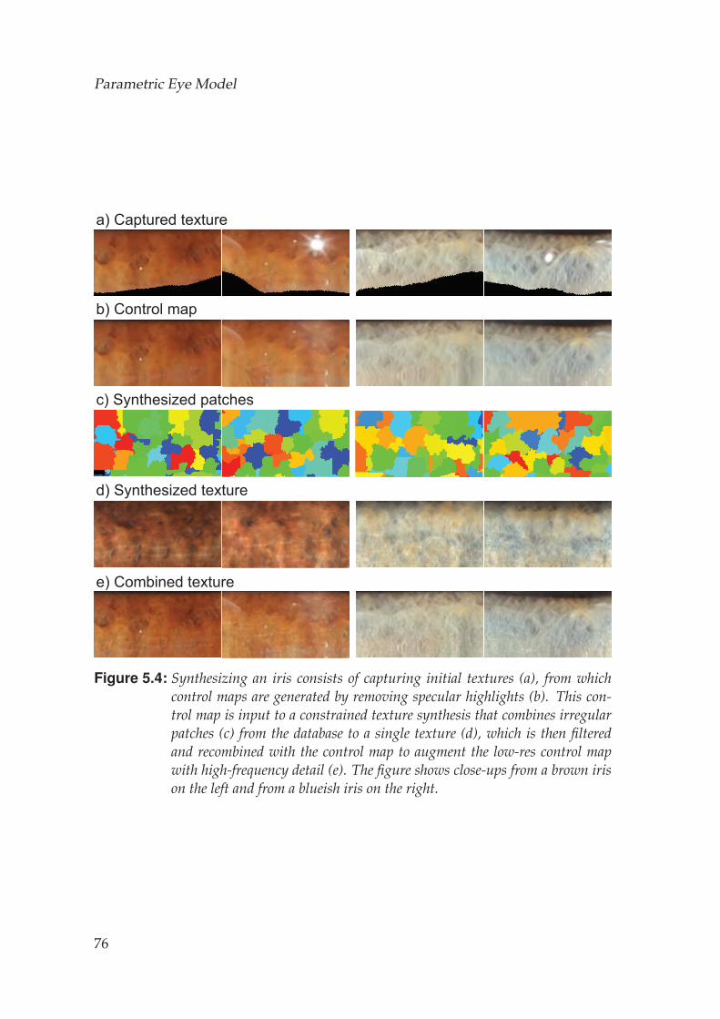
Parametric Eye Model

a) Captured texture

e) Combined texture

b) Control map

c) Synthesized patches

d) Synthesized texture

Figure 5.4: Synthesizing an iris consists of capturing initial textures (a), from whichcontrol maps are generated by removing specular highlights (b). This con-trol map is input to a constrained texture synthesis that combines irregularpatches (c) from the database to a single texture (d), which is then filteredand recombined with the control map to augment the low-res control mapwith high-frequency detail (e). The figure shows close-ups from a brown irison the left and from a blueish iris on the right.

76

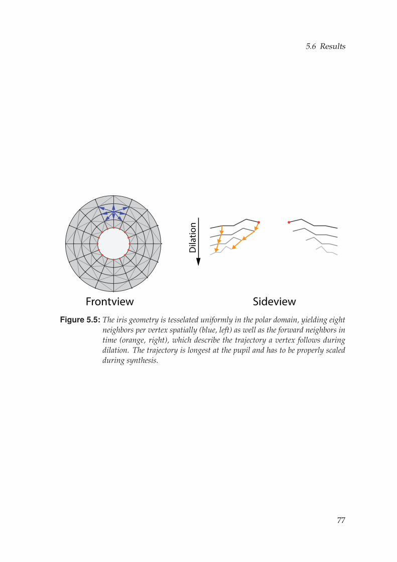
5.6 Results

Frontview Sideview

Dila

tion

Figure 5.5: The iris geometry is tesselated uniformly in the polar domain, yielding eightneighbors per vertex spatially (blue, left) as well as the forward neighbors intime (orange, right), which describe the trajectory a vertex follows duringdilation. The trajectory is longest at the pupil and has to be properly scaledduring synthesis.

77

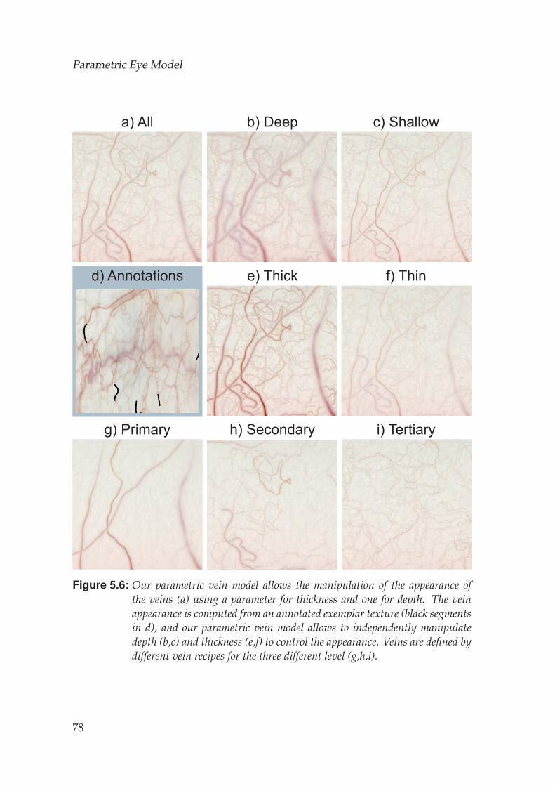
Parametric Eye Model

g) Primary h) Secondary i) Tertiary

b) Deep c) Shallowa) All

d) Annotations e) Thick f) Thin

Figure 5.6: Our parametric vein model allows the manipulation of the appearance ofthe veins (a) using a parameter for thickness and one for depth. The veinappearance is computed from an annotated exemplar texture (black segmentsin d), and our parametric vein model allows to independently manipulatedepth (b,c) and thickness (e,f) to control the appearance. Veins are defined bydifferent vein recipes for the three different level (g,h,i).

78

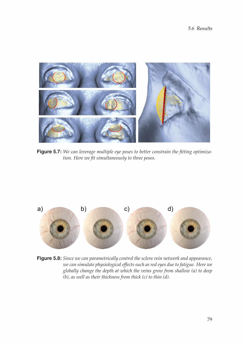
5.6 Results

Figure 5.7: We can leverage multiple eye poses to better constrain the fitting optimiza-tion. Here we fit simultaneously to three poses.

a) b) d)c)

Figure 5.8: Since we can parametrically control the sclera vein network and appearance,we can simulate physiological effects such as red eyes due to fatigue. Here weglobally change the depth at which the veins grow from shallow (a) to deep(b), as well as their thickness from thick (c) to thin (d).

79

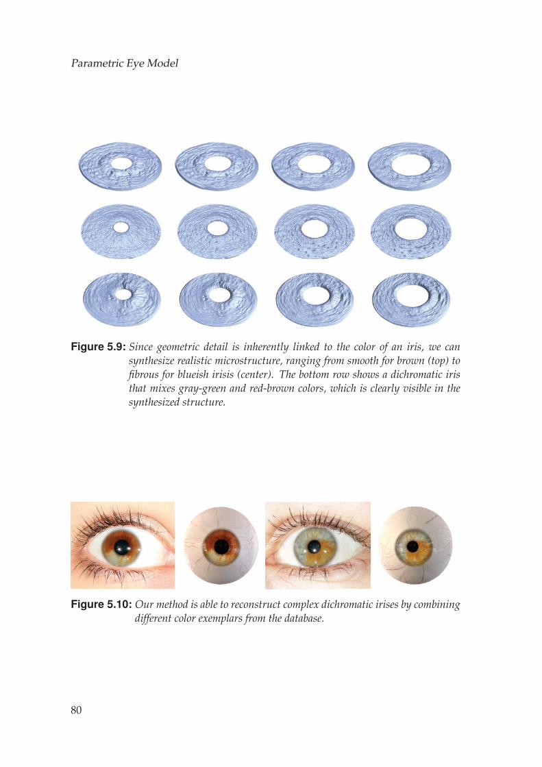
Parametric Eye Model

Figure 5.9: Since geometric detail is inherently linked to the color of an iris, we cansynthesize realistic microstructure, ranging from smooth for brown (top) tofibrous for blueish irisis (center). The bottom row shows a dichromatic iristhat mixes gray-green and red-brown colors, which is clearly visible in thesynthesized structure.

Figure 5.10: Our method is able to reconstruct complex dichromatic irises by combiningdifferent color exemplars from the database.

80

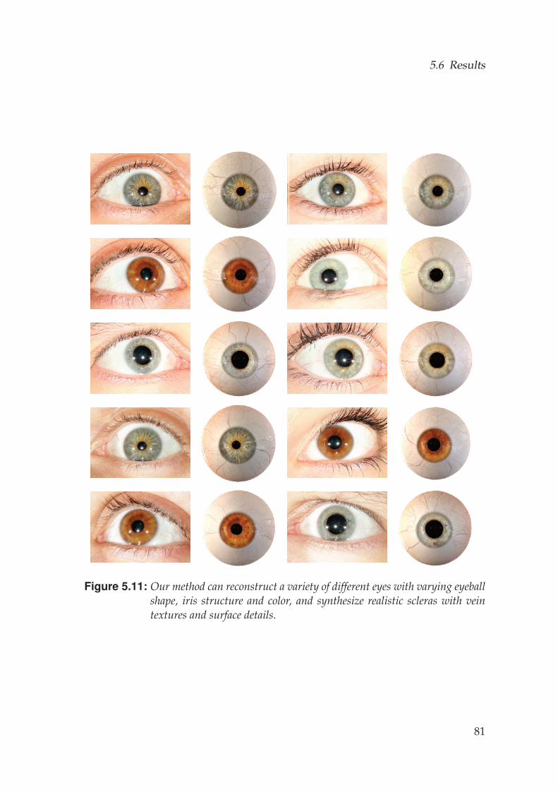
5.6 Results

Figure 5.11: Our method can reconstruct a variety of different eyes with varying eyeballshape, iris structure and color, and synthesize realistic scleras with veintextures and surface details.

81

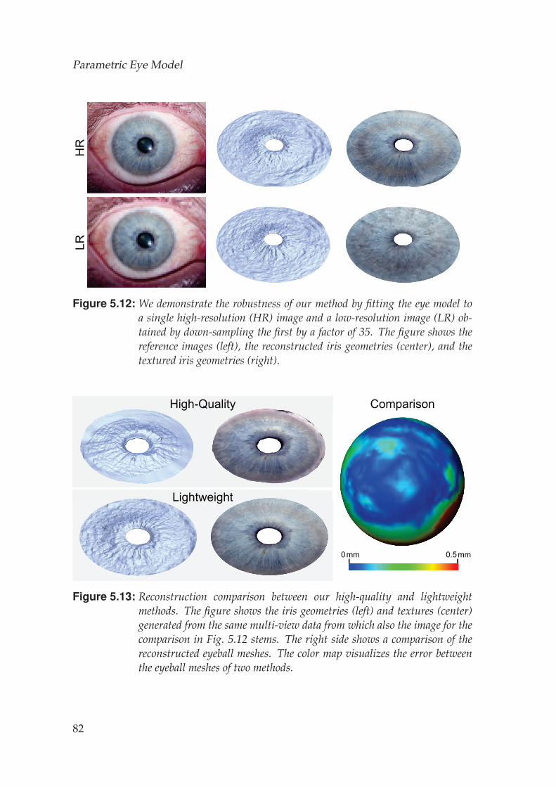
Parametric Eye ModelH

RLR

Figure 5.12: We demonstrate the robustness of our method by fitting the eye model toa single high-resolution (HR) image and a low-resolution image (LR) ob-tained by down-sampling the first by a factor of 35. The figure shows thereference images (left), the reconstructed iris geometries (center), and thetextured iris geometries (right).

Comparison

Lightweight

High-Quality

0.5mm0mm

Figure 5.13: Reconstruction comparison between our high-quality and lightweightmethods. The figure shows the iris geometries (left) and textures (center)generated from the same multi-view data from which also the image for thecomparison in Fig. 5.12 stems. The right side shows a comparison of thereconstructed eyeball meshes. The color map visualizes the error betweenthe eyeball meshes of two methods.

82

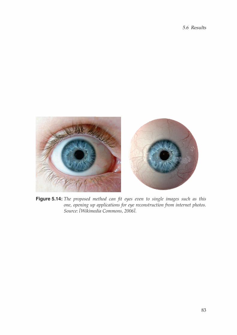
5.6 Results

Figure 5.14: The proposed method can fit eyes even to single images such as thisone, opening up applications for eye reconstruction from internet photos.Source: [Wikimedia Commons, 2006].

83

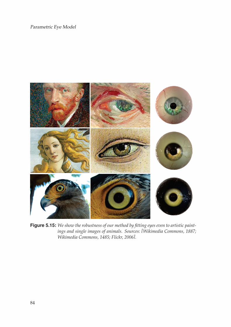
Parametric Eye Model

Figure 5.15: We show the robustness of our method by fitting eyes even to artistic paint-ings and single images of animals. Sources: [Wikimedia Commons, 1887;Wikimedia Commons, 1485; Flickr, 2006].

84

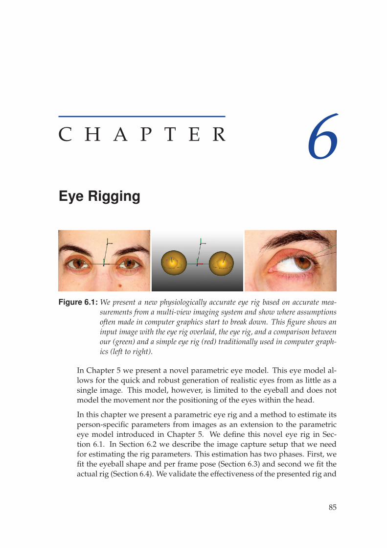
C H A P T E R 6Eye Rigging

Figure 6.1: We present a new physiologically accurate eye rig based on accurate mea-surements from a multi-view imaging system and show where assumptionsoften made in computer graphics start to break down. This figure shows aninput image with the eye rig overlaid, the eye rig, and a comparison betweenour (green) and a simple eye rig (red) traditionally used in computer graph-ics (left to right).

In Chapter 5 we present a novel parametric eye model. This eye model al-lows for the quick and robust generation of realistic eyes from as little as asingle image. This model, however, is limited to the eyeball and does notmodel the movement nor the positioning of the eyes within the head.

In this chapter we present a parametric eye rig and a method to estimate itsperson-specific parameters from images as an extension to the parametriceye model introduced in Chapter 5. We define this novel eye rig in Sec-tion 6.1. In Section 6.2 we describe the image capture setup that we needfor estimating the rig parameters. This estimation has two phases. First, wefit the eyeball shape and per frame pose (Section 6.3) and second we fit theactual rig (Section 6.4). We validate the effectiveness of the presented rig and

85

Eye Rigging

investigate the importance of accurate eye motion modeling in the contextof computer animation (Section 6.5).

6.1 Eye Rig

Our eye rig consists of several parameters that define the rig configuration.We differentiate between static and dynamic parameters, where static param-eters are person-specific but do not change during animation, and dynamicparameters can change over time. The static configuration describes the ge-ometry of the rig, such as, for example the interocular distance or the shapeof the eyeballs. We attribute the static variables with a bar (x). The dynamicconfiguration defines the motion of the eyes, and we attribute dynamic vari-ables with a dot (x). The entire configuration containing both static and dy-namic parameters is denoted as ˙P .

In the following we describe the individual rig parameters. Without lossof generality, we will consistently refer to a right-handed coordinate systemwhere the x-axis points left, the y-axis points up, and the z-axis points for-ward, all with respect to the character.

6.1.1 Eye Shape

Fig. 3.1 (b) shows a cross-section of the eye and labels the most importantfeatures in our context, which we will discuss in more detail below.

Eyeball shape For the eyeball shape we use the parametric eye model in-truduced in chapter Chapter 5. This model represents the eyeball shape witha PCA model with six modes plus a global scale. Since the two eyes of anindividual are similar in shape, we employ a set of six symmetric coefficientscoupled with a set of six antisymmetric coefficients that model the differenceand are regularized to be small.

It will become convenient to model certain parameters as splines on the eye-ball surface (e.g. the limbus, as described next), and so in order to allow forsimple and efficient evaluation of splines on the eyeball surface, we transi-tion from the irregular mesh domain to the regular image domain and storethe mean shape and difference vectors as texture maps. The texture param-eterization is based on spherical coordinates and chosen such that the polesare on the top and bottom of the eye, and the texture resolution is 2048x1024

86

6.1 Eye Rig

pixels. Given the rig configuration ˙P , any point xuv ∈ R2 in texture spacecan be transformed to a point xworld ∈ R3 in world space via

xworld = Eyeball(xuv, ˙P), (6.1)

which applies the inverse texture parameterization at xuv followed by a for-ward evaluation of the rig configuration ˙P .

Limbus The limbus refers to the boundary between the cornea and sclera.Its shape and position is tightly coupled with the shape of the eyeball andhas no additional degrees of freedom. We represent the limbus in texturespace as a closed B-spline that is directly mapped to the eyeball surface. Wedefine the mapping of points xctr ∈ R1 on the spline to points xuv ∈ R2 intexture space as

xuv = Limbus(xctr). (6.2)

Pupil Our parametric eye also contains a pupil. However, it is the meanpupil of a captured dataset and does not account for any person-dependentexcentricity of the pupil. To address this we add three translation parame-ters that are static and common to both eyes, which describe the offset fromthe mean pupil. Analogous to the eyeball shape coefficients we control theradius of the two pupils via a symmetric parameter and an antisymmetricone that accounts for the fact that the two pupils will be similar in radiusbut not exactly the same. The pupil radius parameters vary per pose and arethus dynamic.

Visual axis The gaze direction of an eye does not coincide with the opticalaxis, but with the visual axis of the eye, which is defined as the ray passingthrough the center of the pupil and originating at the point on the retinawith the sharpest vision, the fovea. Since we do not know the location of thefovea, we model the visual axis by a ray originating at the center of the pupil.The direction of the ray is defined in spherical coordinates, as the inclinationrelative to the z-axis. The pair of visual axes for the two eyes is given by fourstatic parameters, a symmetric polar angle and antisymmetric azimuth thatprovide the main directions, coupled with an antisymmetric polar angle andsymmetric azimuth that model slight deviations between the left and righteyes.

87

Eye Rigging

Eyelid interface The eyelid interface defines the location where the skinof the eyelid touches the eyeball. We extend the parametric eye model witha parametric model of the eyelid interface. Similar to the limbus, this inter-face is represented by curves in texture space, one for the upper and one forthe lower eyelid interface. The shape of the curves is based on two fourthorder B-splines whose six middle control points are constrained as shownin Fig. 6.2. The control points are constrained to lie on equidistant linesperpendicular to the horizontal line connecting the two corners of the eye.Each perpendicular line contains two control points that are parametrizedby the opening of the eyelid (computed as the signed distance between thetwo points) and the vertical offset of the points (parameterized by the signeddistance between their mean and the horizontal line). The opening param-eter is constrained to positive values which prevents the upper curve fromcrossing over the lower curve. The eye rotation relative to the eyelid inter-face is accounted for by warping the eyelid curves in texture space. Sincethe texture coordinates are based on spherical coordinates, the warp can becomputed analytically. Given the rig configuration ˙P , we define the map-ping of points xctr ∈ R1 on the spline to points xuv ∈ R2 in texture spaceas

xuv = Eyelid(xctr, ˙P). (6.3)

Tear duct We model the tear duct as a line segment between the last pointon the upper eyelid interface curve and the last point on the lower eyelidinterface curve.

6.1.2 Eye Motion

As depicted in Fig. 3.1 (a), the eye is driven by a set of muscles that exerttranslational forces on the eyeball in order to rotate it. Two muscles are re-sponsible for one rotational degree of freedom (one for each direction), butfor any actual motion there is always several of these muscles being acti-vated in a complex and orchestrated way. An in-depth discussion of themuscular eye actuation is beyond the scope of this thesis and we refer theinterested reader to medical textbooks [Carpenter, 1988]. To name just oneexample, when the eye is rotated horizontally away from the nose (abducted),most of the work to rotate the eye upwards (elevation) will be done by the su-perior rectus muscle. On the other hand, when the eye is rotated horizontallytowards the nose (adducted), it will be the inferior oblique muscle that is re-sponsible for elevating the eye. As a consequence, the typical assumption

88

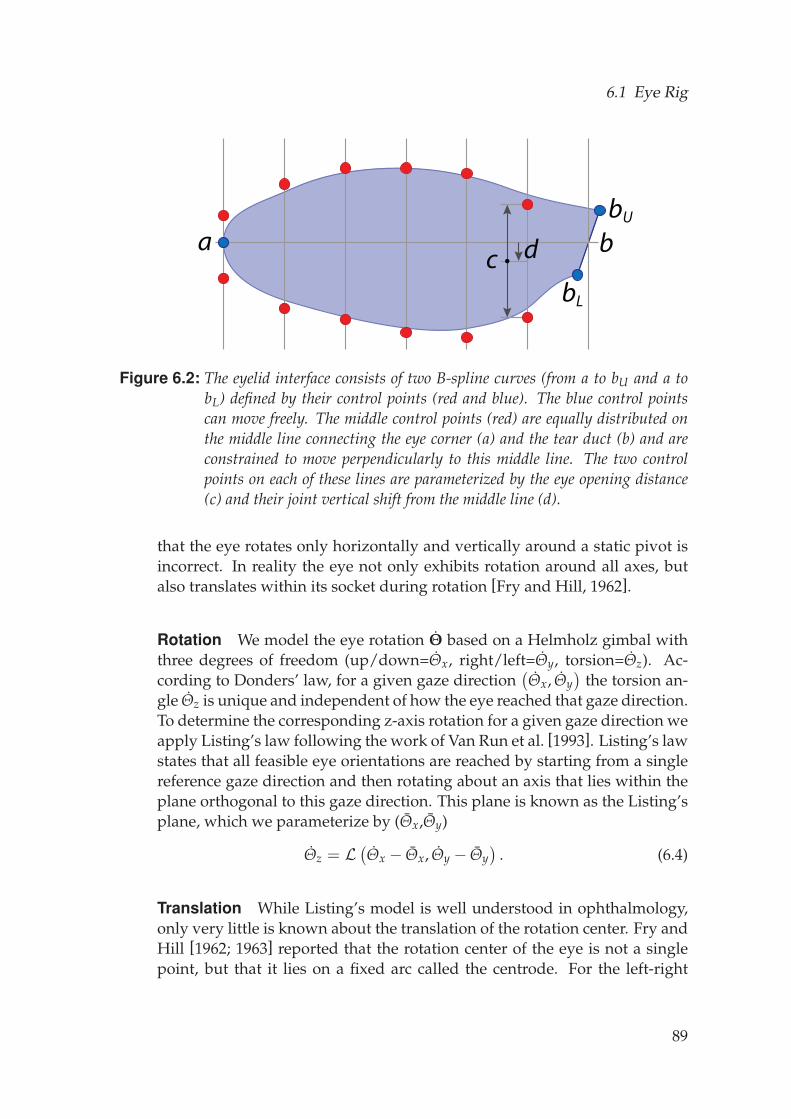
6.1 Eye Rig

ac d b

bU

bL

Figure 6.2: The eyelid interface consists of two B-spline curves (from a to bU and a tobL) defined by their control points (red and blue). The blue control pointscan move freely. The middle control points (red) are equally distributed onthe middle line connecting the eye corner (a) and the tear duct (b) and areconstrained to move perpendicularly to this middle line. The two controlpoints on each of these lines are parameterized by the eye opening distance(c) and their joint vertical shift from the middle line (d).

that the eye rotates only horizontally and vertically around a static pivot isincorrect. In reality the eye not only exhibits rotation around all axes, butalso translates within its socket during rotation [Fry and Hill, 1962].

Rotation We model the eye rotation Θ based on a Helmholz gimbal withthree degrees of freedom (up/down=Θx, right/left=Θy, torsion=Θz). Ac-cording to Donders’ law, for a given gaze direction

(Θx, Θy

)the torsion an-

gle Θz is unique and independent of how the eye reached that gaze direction.To determine the corresponding z-axis rotation for a given gaze direction weapply Listing’s law following the work of Van Run et al. [1993]. Listing’s lawstates that all feasible eye orientations are reached by starting from a singlereference gaze direction and then rotating about an axis that lies within theplane orthogonal to this gaze direction. This plane is known as the Listing’splane, which we parameterize by (Θx,Θy)

Θz = L(Θx − Θx, Θy − Θy

). (6.4)

Translation While Listing’s model is well understood in ophthalmology,only very little is known about the translation of the rotation center. Fry andHill [1962; 1963] reported that the rotation center of the eye is not a singlepoint, but that it lies on a fixed arc called the centrode. For the left-right

89

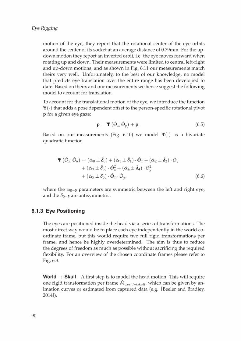
Eye Rigging

motion of the eye, they report that the rotational center of the eye orbitsaround the center of its socket at an average distance of 0.79mm. For the up-down motion they report an inverted orbit, i.e. the eye moves forward whenrotating up and down. Their measurements were limited to central left-rightand up-down motions, and as shown in Fig. 6.11 our measurements matchtheirs very well. Unfortunately, to the best of our knowledge, no modelthat predicts eye translation over the entire range has been developed todate. Based on theirs and our measurements we hence suggest the followingmodel to account for translation.

To account for the translational motion of the eye, we introduce the functionΨ(·) that adds a pose dependent offset to the person-specific rotational pivotp for a given eye gaze:

p = Ψ(Θx, Θy

)+ p. (6.5)

Based on our measurements (Fig. 6.10) we model Ψ(·) as a bivariatequadratic function

Ψ(Θx, Θy

)= (α0 ± δ0) + (α1 ± δ1) · Θx + (α2 ± δ2) · Θy

+ (α3 ± δ3) · Θ2x + (α4 ± δ4) · Θ2

y

+ (α5 ± δ5) · Θx · Θy, (6.6)

where the α0−5 parameters are symmetric between the left and right eye,and the δ0−5 are antisymmetric.

6.1.3 Eye Positioning

The eyes are positioned inside the head via a series of transformations. Themost direct way would be to place each eye independently in the world co-ordinate frame, but this would require two full rigid transformations perframe, and hence be highly overdetermined. The aim is thus to reducethe degrees of freedom as much as possible without sacrificing the requiredflexibility. For an overview of the chosen coordinate frames please refer toFig. 6.3.

World → Skull A first step is to model the head motion. This will requireone rigid transformation per frame Mworld→skull, which can be given by an-imation curves or estimated from captured data (e.g. [Beeler and Bradley,2014]).

90

6.2 Data Acquisition

Skull → Pair Relative to the skull we create an eye pair coordinate frame,defined via the reduced rigid transformation Mskull→pair. This coordinateframe is chosen such that its origin is in the middle between the left andright eyes, with the x-axis going through their rotational pivots p, and thex-axis rotation is kept identical with the x-axis rotation of the skull. The paircoordinate frame is person-specific but static as it does not change duringanimation.

Pair → Socket The left and right eye sockets are defined relative to theeye pair coordinate frame via a static transform Mpair→socket. The sockets aretranslated by plus/minus half the interocular distance along the x-axis andplus/minus half the vertical eye offset along the y-axis.

World → Socket The ultimate socket transformation per eye is given bythe concatenation of the individual transformations. The total number ofdegrees of freedom is 6n (World → Skull) + 5 (Skull → Pair) + 2 (Pair →Socket) = 6n + 7, where n is the number of frames, versus the 12n of the mostnaıve model.

6.1.4 Eye Control

Once fit to a person (Section 6.4), the proposed rig exposes the eye gazes ascontrol parameters for the eye pose. Consistent with industry grade eye rigs,an animator may animate the eye gazes of the left and right eyes individu-ally, or couple them via a controllable look-at point of the character. In theformer case the rig exposes four degrees of freedom (one 2D gaze per eye),which are reduced to three in the latter case (one 3D lookat point). Further-more, the opening of the pupil can be controlled by a single user parameterduring animation.

6.2 Data Acquisition

In order to develop our eye rig we depend on high-quality data of real eyemotion. We employ a multiview capture setup consisting of 12 DSLR cam-eras (Canon 1200D) for taking photographs of static eye poses, from whichwe can reconstruct the shape of the skin surface using the system proposedby Beeler et al. [2010]. For a given subject, we record approximately 60 dif-ferent eye positions, corresponding to one set of gaze points approximately 1meter from the subject, which span three horizontal rows at various heights,

91

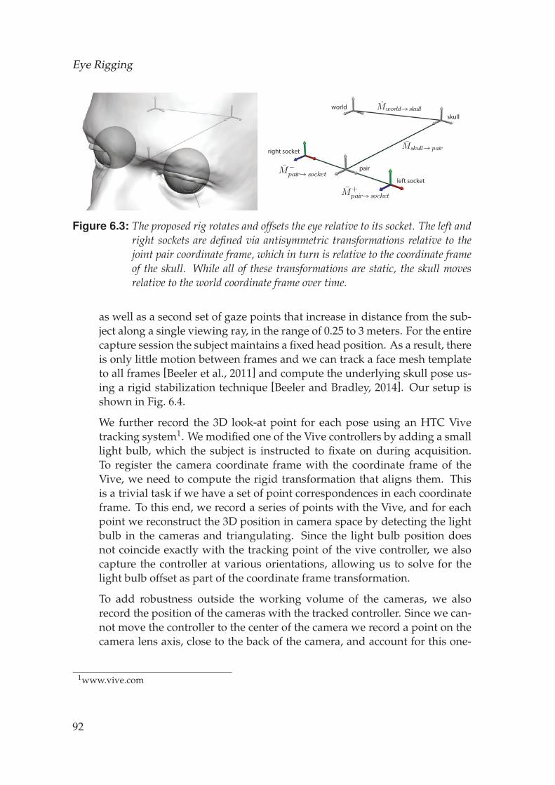
Eye Rigging

Mskull pair

Mworld skull

M+pair socket

M−pair socket

worldskull

pair

left socket

right socket

Figure 6.3: The proposed rig rotates and offsets the eye relative to its socket. The left andright sockets are defined via antisymmetric transformations relative to thejoint pair coordinate frame, which in turn is relative to the coordinate frameof the skull. While all of these transformations are static, the skull movesrelative to the world coordinate frame over time.

as well as a second set of gaze points that increase in distance from the sub-ject along a single viewing ray, in the range of 0.25 to 3 meters. For the entirecapture session the subject maintains a fixed head position. As a result, thereis only little motion between frames and we can track a face mesh templateto all frames [Beeler et al., 2011] and compute the underlying skull pose us-ing a rigid stabilization technique [Beeler and Bradley, 2014]. Our setup isshown in Fig. 6.4.

We further record the 3D look-at point for each pose using an HTC Vivetracking system1. We modified one of the Vive controllers by adding a smalllight bulb, which the subject is instructed to fixate on during acquisition.To register the camera coordinate frame with the coordinate frame of theVive, we need to compute the rigid transformation that aligns them. Thisis a trivial task if we have a set of point correspondences in each coordinateframe. To this end, we record a series of points with the Vive, and for eachpoint we reconstruct the 3D position in camera space by detecting the lightbulb in the cameras and triangulating. Since the light bulb position doesnot coincide exactly with the tracking point of the vive controller, we alsocapture the controller at various orientations, allowing us to solve for thelight bulb offset as part of the coordinate frame transformation.

To add robustness outside the working volume of the cameras, we alsorecord the position of the cameras with the tracked controller. Since we can-not move the controller to the center of the camera we record a point on thecamera lens axis, close to the back of the camera, and account for this one-

1www.vive.com

92

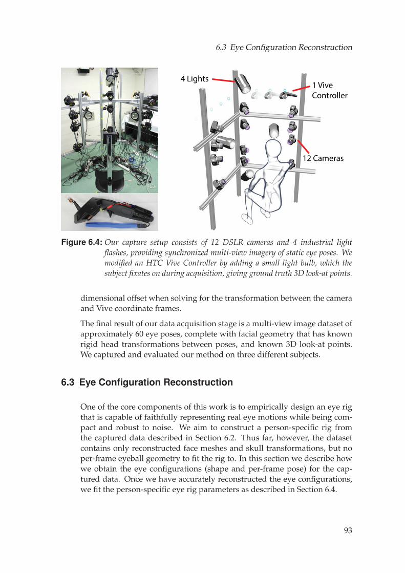
6.3 Eye Configuration Reconstruction

4 Lights

12 Cameras

1 ViveController

Figure 6.4: Our capture setup consists of 12 DSLR cameras and 4 industrial lightflashes, providing synchronized multi-view imagery of static eye poses. Wemodified an HTC Vive Controller by adding a small light bulb, which thesubject fixates on during acquisition, giving ground truth 3D look-at points.

dimensional offset when solving for the transformation between the cameraand Vive coordinate frames.

The final result of our data acquisition stage is a multi-view image dataset ofapproximately 60 eye poses, complete with facial geometry that has knownrigid head transformations between poses, and known 3D look-at points.We captured and evaluated our method on three different subjects.

6.3 Eye Configuration Reconstruction

One of the core components of this work is to empirically design an eye rigthat is capable of faithfully representing real eye motions while being com-pact and robust to noise. We aim to construct a person-specific rig fromthe captured data described in Section 6.2. Thus far, however, the datasetcontains only reconstructed face meshes and skull transformations, but noper-frame eyeball geometry to fit the rig to. In this section we describe howwe obtain the eye configurations (shape and per-frame pose) for the cap-tured data. Once we have accurately reconstructed the eye configurations,we fit the person-specific eye rig parameters as described in Section 6.4.

93

Eye Rigging

We wish to reconstruct eye configurations with as little regularization as pos-sible in order to remain faithful to the data. For the shape, fortunately wecan rely on the parametric eye model introduced in Chapter 5, which wasitself generated from measured data acquired with the system presented inChapter 4. This alleviates the problem considerably and leaves us only withthe need to recover the six degrees of freedom of the eye pose, which wedenote M ∈ R6, for each pose of each eye. One viable option would be to es-timate M independently per frame per eye without any a-priori knowledge.On the other hand, we do know certain things about eye movements fromthe medical literature, such as Listing’s model, and it will be helpful to beable to rely on such information where possible. Therefore, we propose toactually use a subset of our rig introduced in Section 6.1 to reconstruct theindividual eye poses of the dataset.

As with most applications of parametric model fitting to real world data, ourrig will only explain the captured imagery up to a certain error. In order toimprove the fit we introduce two slack variables in the eye pose computa-tion. First, we add a per pose torsion residual Θε

z to Equation 6.4, yielding

Θz = L(Θx − Θx, Θy − Θy

)+ Θε

z . (6.7)

Secondly, we add a per-pose residual pε for the rotational pivot point inEquation 6.5, yielding

p = Ψ(Θx, Θy

)+ p + pε. (6.8)

As we did not know the general shape of Ψ(·) initially, we simply set itto 0. However, when reconstructing the poses for future subjects, one canuse Equation 6.6 instead as a-priori information. These slack variables areweakly regularized to be small, incentivising the other variables to captureas much of the signal as possible and only represent the residual. Togetherwith the gaze direction (Θx, Θy), this amounts to six dynamic degrees offreedom per eye and allows to accurately reconstruct eye poses while stillleveraging prior knowledge.

We obtain the eye configurations by fitting to manual annotations (Sec-tion 6.3.1), which makes fitting very robust. Automatic labelling is chal-lenging due to the complexity of the eye region in terms of geometry andappearance. Manual annotations, however, are not pixel-perfect and there-fore the fits contain errors. Thus, we refine the positions with photometricconstraints (Section 6.3.2). The final eye configurations will be passed on to

94

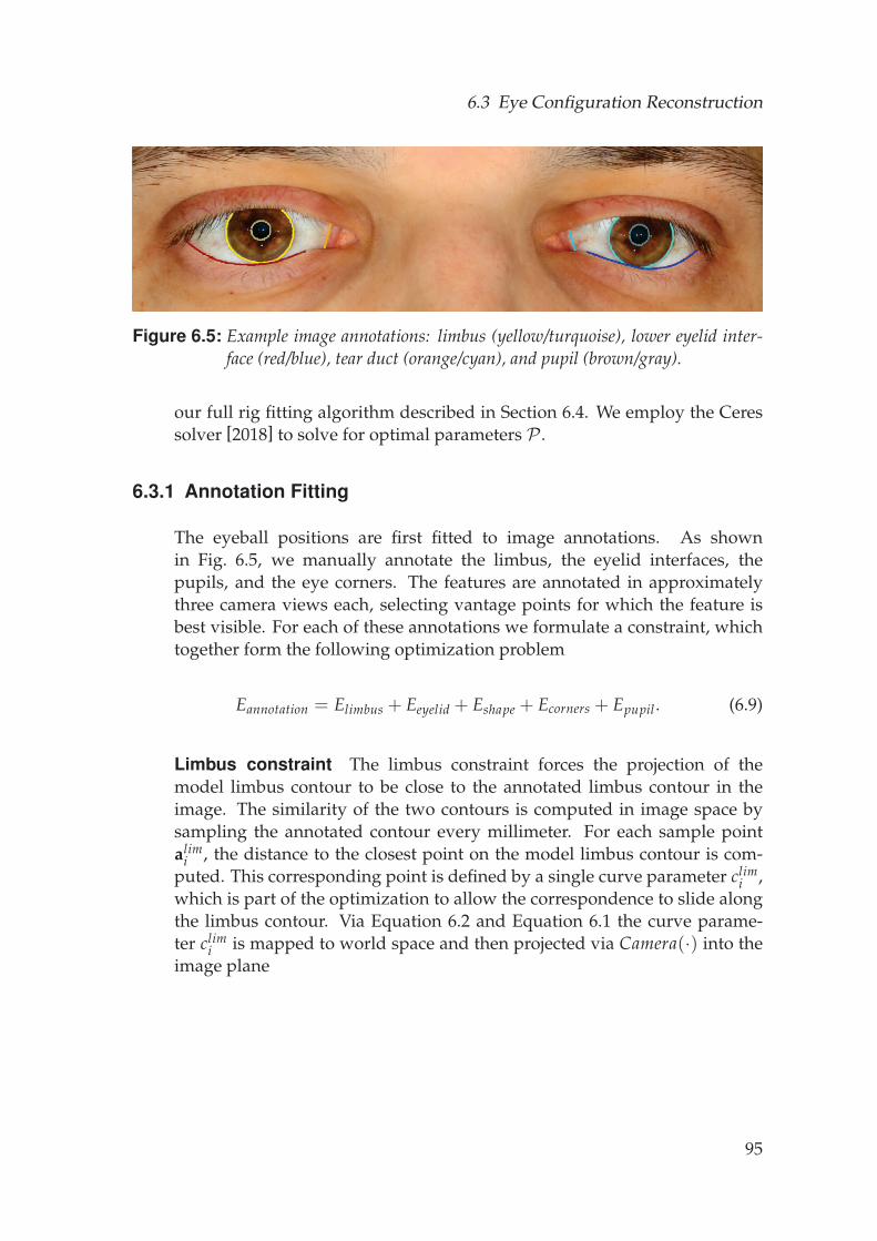
6.3 Eye Configuration Reconstruction

Figure 6.5: Example image annotations: limbus (yellow/turquoise), lower eyelid inter-face (red/blue), tear duct (orange/cyan), and pupil (brown/gray).

our full rig fitting algorithm described in Section 6.4. We employ the Ceressolver [2018] to solve for optimal parameters P .

6.3.1 Annotation Fitting

The eyeball positions are first fitted to image annotations. As shownin Fig. 6.5, we manually annotate the limbus, the eyelid interfaces, thepupils, and the eye corners. The features are annotated in approximatelythree camera views each, selecting vantage points for which the feature isbest visible. For each of these annotations we formulate a constraint, whichtogether form the following optimization problem

Eannotation = Elimbus + Eeyelid + Eshape + Ecorners + Epupil. (6.9)

Limbus constraint The limbus constraint forces the projection of themodel limbus contour to be close to the annotated limbus contour in theimage. The similarity of the two contours is computed in image space bysampling the annotated contour every millimeter. For each sample pointalim

i , the distance to the closest point on the model limbus contour is com-puted. This corresponding point is defined by a single curve parameter clim

i ,which is part of the optimization to allow the correspondence to slide alongthe limbus contour. Via Equation 6.2 and Equation 6.1 the curve parame-ter clim

i is mapped to world space and then projected via Camera(·) into theimage plane

95

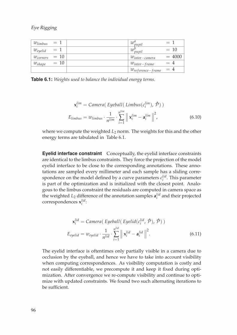
Eye Rigging

wlimbus = 1 wapupil = 1

weyelid = 1 wbpupil = 10

wcorners = 10 winter−camera = 4000wshape = 10 winter− f rame = 4

wre f erence− f rame = 4

Table 6.1: Weights used to balance the individual energy terms.

xlimi = Camera( Eyeball( Limbus(clim

i ), ˙P) )

Elimbus = wlimbus · 1nlim ·

nlim

∑i=1

∥∥∥ xlimi − alim

i

∥∥∥2, (6.10)

where we compute the weighted L2 norm. The weights for this and the otherenergy terms are tabulated in Table 6.1.

Eyelid interface constraint Conceptually, the eyelid interface constraintsare identical to the limbus constraints. They force the projection of the modeleyelid interface to be close to the corresponding annotations. These anno-tations are sampled every millimeter and each sample has a sliding corre-spondence on the model defined by a curve parameters clid

i . This parameteris part of the optimization and is initialized with the closest point. Analo-gous to the limbus constraint the residuals are computed in camera space asthe weighted L2 difference of the annotation samples alid

i and their projectedcorrespondences xlid

i :

xlidi = Camera( Eyeball( Eyelid(clid

i , ˙P), ˙P) )

Eeyelid = weyelid · 1nlid ·

nlid

∑i=1

∥∥∥ xlidi − alid

i

∥∥∥2. (6.11)

The eyelid interface is oftentimes only partially visible in a camera due toocclusion by the eyeball, and hence we have to take into account visibilitywhen computing correspondences. As visibility computation is costly andnot easily differentiable, we precompute it and keep it fixed during opti-mization. After convergence we re-compute visibility and continue to opti-mize with updated constraints. We found two such alternating iterations tobe sufficient.

96

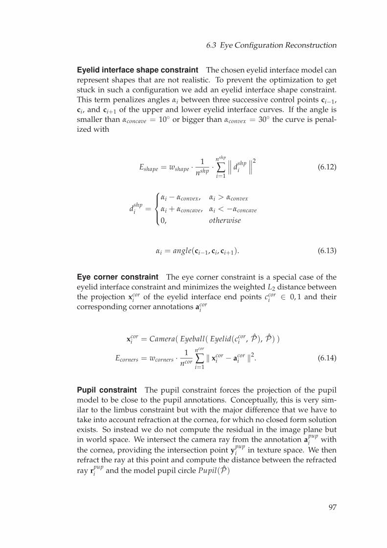
6.3 Eye Configuration Reconstruction

Eyelid interface shape constraint The chosen eyelid interface model canrepresent shapes that are not realistic. To prevent the optimization to getstuck in such a configuration we add an eyelid interface shape constraint.This term penalizes angles αi between three successive control points ci−1,ci, and ci+1 of the upper and lower eyelid interface curves. If the angle issmaller than αconcave = 10◦ or bigger than αconvex = 30◦ the curve is penal-ized with

Eshape = wshape · 1nshp ·

nshp

∑i=1

∥∥∥ dshpi

∥∥∥2(6.12)

dshpi =

⎧⎪⎨⎪⎩

αi − αconvex, αi > αconvex

αi + αconcave, αi < −αconcave

0, otherwise

αi = angle(ci−1, ci, ci+1). (6.13)

Eye corner constraint The eye corner constraint is a special case of theeyelid interface constraint and minimizes the weighted L2 distance betweenthe projection xcor

i of the eyelid interface end points ccori ∈ 0, 1 and their

corresponding corner annotations acori

xcori = Camera( Eyeball( Eyelid(ccor

i , ˙P), ˙P) )

Ecorners = wcorners · 1ncor

ncor

∑i=1‖ xcor

i − acori ‖2. (6.14)

Pupil constraint The pupil constraint forces the projection of the pupilmodel to be close to the pupil annotations. Conceptually, this is very sim-ilar to the limbus constraint but with the major difference that we have totake into account refraction at the cornea, for which no closed form solutionexists. So instead we do not compute the residual in the image plane butin world space. We intersect the camera ray from the annotation apup

i withthe cornea, providing the intersection point ypup

i in texture space. We thenrefract the ray at this point and compute the distance between the refractedray rpup

i and the model pupil circle Pupil( ˙P)

97

Eye Rigging

rpupi = Re f ract( Camera−1(apup

i ), Eyeball(ypupi , ˙P) )

Eapupil = wa

pupil ·1

npup ·npup

∑i=1

∥∥∥ rpupi , Pupil( ˙P)

∥∥∥2

ray−circle. (6.15)

However, since the shape of the cornea changes during the optimization,we cannot keep ypup

i fixed but allow it to slide on the surface of the eyeball,such that its projection back into the image plane always coincides with thesample apup

i

xpupi = Camera( Eyeball(ypup

i , ˙P) )

Ebpupil = wb

pupil ·1

npup ·npup

∑i=1

∥∥ xpupi − apup

i

∥∥2. (6.16)

The final pupil energy is given by the sum of Equation 6.15 and Equa-tion 6.16.

6.3.2 Photometric Refinement

The annotation-based fitting presented in section 6.3.1 produces a first esti-mate of the eye positions, but manual annotations are not pixel-perfect andlead to inaccuracies. To overcome these we introduce an image-based re-finement term that does not depend on manual annotations, but can highlybenefit from the close initial guess they provide. The idea is to incorpo-rate additional constraints that enforce photoconsistency across cameras andacross frames by projecting 3D patches of the eye into the different imagesto compute the discrepancy. These constraints are defined only on the unob-structed parts of the sclera and we first describe how we mask out occluders,such as skin or eyelashes, and introduce the photometric inter-camera andthe inter-frame constraints subsequently. The constraints are formulated inthe same framework and are integrated with the Eannotation energy

Ere f inement = Eannotation

+ winter−camera · Einter−camera

+ winter− f rame · Einter− f rame

+ wre f erence− f rame · Ere f erence− f rame. (6.17)

98

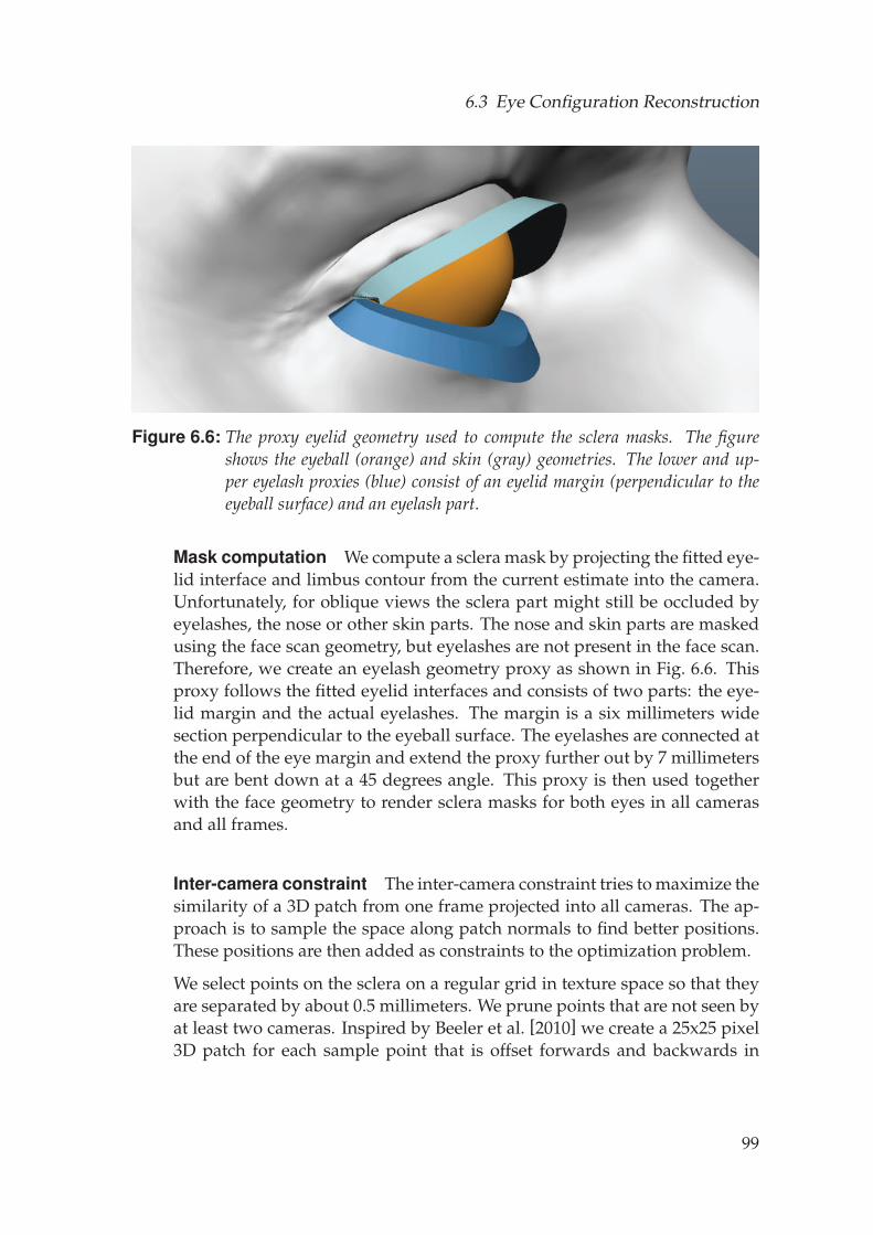
6.3 Eye Configuration Reconstruction

Figure 6.6: The proxy eyelid geometry used to compute the sclera masks. The figureshows the eyeball (orange) and skin (gray) geometries. The lower and up-per eyelash proxies (blue) consist of an eyelid margin (perpendicular to theeyeball surface) and an eyelash part.

Mask computation We compute a sclera mask by projecting the fitted eye-lid interface and limbus contour from the current estimate into the camera.Unfortunately, for oblique views the sclera part might still be occluded byeyelashes, the nose or other skin parts. The nose and skin parts are maskedusing the face scan geometry, but eyelashes are not present in the face scan.Therefore, we create an eyelash geometry proxy as shown in Fig. 6.6. Thisproxy follows the fitted eyelid interfaces and consists of two parts: the eye-lid margin and the actual eyelashes. The margin is a six millimeters widesection perpendicular to the eyeball surface. The eyelashes are connected atthe end of the eye margin and extend the proxy further out by 7 millimetersbut are bent down at a 45 degrees angle. This proxy is then used togetherwith the face geometry to render sclera masks for both eyes in all camerasand all frames.

Inter-camera constraint The inter-camera constraint tries to maximize thesimilarity of a 3D patch from one frame projected into all cameras. The ap-proach is to sample the space along patch normals to find better positions.These positions are then added as constraints to the optimization problem.

We select points on the sclera on a regular grid in texture space so that theyare separated by about 0.5 millimeters. We prune points that are not seen byat least two cameras. Inspired by Beeler et al. [2010] we create a 25x25 pixel3D patch for each sample point that is offset forwards and backwards in

99

Eye Rigging

steps of 0.1 millimeters up to ±1.5 millimeters. These patches are not planarbut have the local shape of the eyeball. At each offset the algorithm com-putes the normalized cross-correlation between a reference camera and allthe other cameras and weights the correlations by the foreshortening angle.We use the masks to evaluate the visibility of the patches in each camera.

The algorithm chooses the reference camera based on a structure measure,which is the sum of neighbor pixel differences. This is required since wecannot solely rely on foreshortening as some cameras might be out-of-focusdue to the shallow depth of field of the cameras.

The optimization residual is formed by the offset position with the smallestphotometric error xopt

i and the corresponding closest point on the eyeballsurface. The closest point is defined by a texture coordinate yinter−camera

i andis part of the optimization parameters.

xinter−camerai = Eyeball(yinter−camera

i , ˙P)Einter−camera =

∥∥∥ xinter−camerai − xopt

i

∥∥∥2. (6.18)

Inter-frame constraint For a given camera the inter-frame constrainttracks and links the same features of two adjacent frames, for which thegaze direction differs by no more than 20 degrees. To compute correspon-dences between the frames for a given camera, we compute a texture forboth frames. The veins are the features which are the easiest to track. Thus,we band-pass filter one of the textures and pick only a small percentage(0.05%) of the pixels with the highest response as samples. Then, the featuredensity is reduced such that features are separated by at least one millime-ter using a non-maxima suppression strategy. For the remaining features wecompute a correspondence in the other texture with a brute force search. Thesearch window is 21 pixels wide and we search up to a maximum distance of30 pixels. To speed up the search we use an image pyramid with three levelsand initialize the next layer with the result of the coarser one. We filter thecorrespondences using RANSAC [Fischler and Bolles, 1981] as follows. Forevery two features in one texture we compute the similarity transform thattransforms the features into the corresponding features of the other texture.Given this transformation we measure how well all the features map ontotheir corresponding features. Features with a distance bigger than 0.25 mil-limeters to their correspondences are considered to be outliers and ignored.Ultimately, the transformation with the overall highest score is used to filter

100

6.3 Eye Configuration Reconstruction

outliers. If there are less than six correspondences we completely ignore theframe.

When these features in texture space between two frames match up, then theeye configurations are reconstructed correctly. To constrain the optimizationtowards that configuration, we project for every feature j the texture loca-tions fj

i and fjk into the camera yielding aj

i and ajk for frames i and k, respec-

tively:

aji = Camera( Eyeball(fj

i ,˙Pi) ). (6.19)

We now add a free variable fj to the optimization, with the intent that thisrepresents the true feature location on the eyeball, and hence projects ontoall aj

i in the respective frames.

xji = Camera( Eyeball(fj, ˙Pi) )

Einter− f rame = ∑i,j

∥∥∥ xji − aj

i

∥∥∥2. (6.20)

Reference-frame rotation constraint The sclera is covered by a protec-tive, mostly transparent skin called the conjunctiva. This skin is not firmlyattached to the eyeball, but actually slides over it, stretching and folding dur-ing eye rotations. Since both sclera and conjunctiva contain veins and otherfeatures, these features move relative to each other (Fig. 6.7) which poses achallenge for the inter-frame constraints and might cause drift as the inter-frame constraints are only concerned with neighboring poses. To preventthis drift we add a rotation constraint that constrains the axial rotation ofa pose with respect to the pose in the reference frame. Since every pose isconstrained to the same reference pose the drift can be eliminated. The rel-ative motion of conjunctiva and sclera is minimal at the limbus, where theconjunctiva is thinnest and more firmly connected to the sclera. We com-pute a photometric residual from this area inside the texture map, whichwill constrain the torsion Θz to align the two poses.

With this final refinement step we can accurately compute the poses of theeyes in all frames individually. In the next section we describe how eye rigsmay be fitted to this data and in Section 6.5 we discuss the captured data indetail and elaborate how it has informed the design of the proposed eye rig.

101

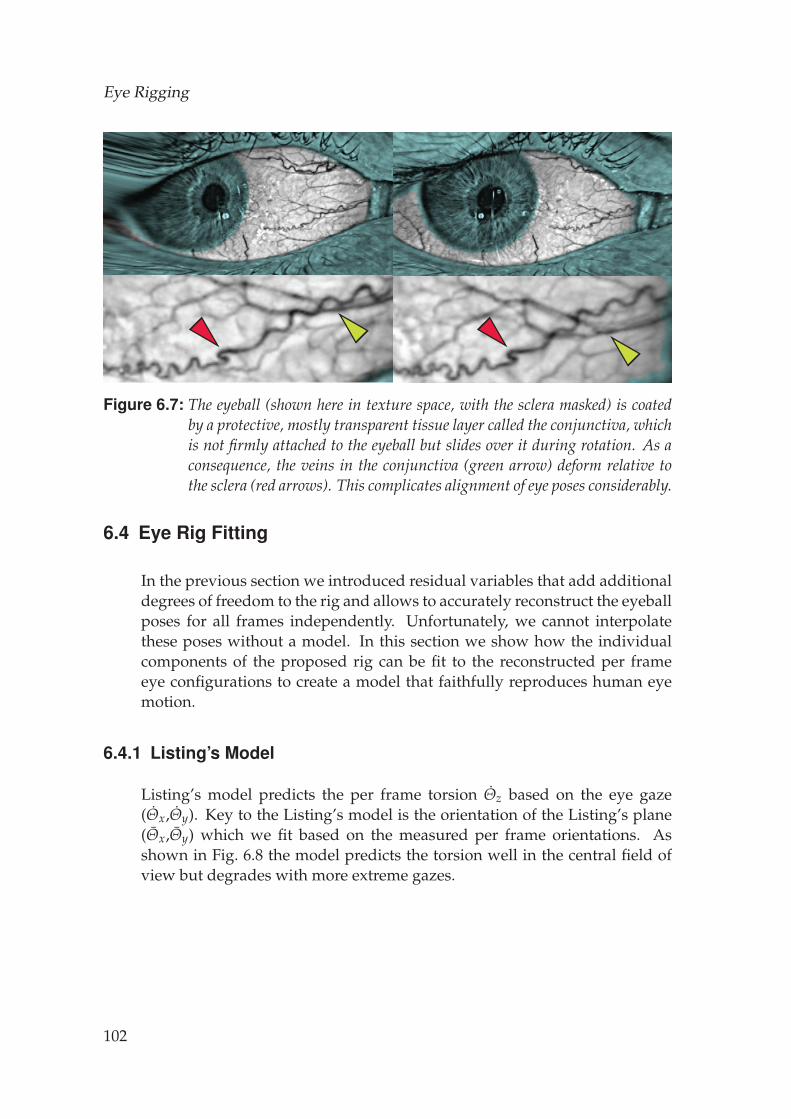
Eye Rigging

Figure 6.7: The eyeball (shown here in texture space, with the sclera masked) is coatedby a protective, mostly transparent tissue layer called the conjunctiva, whichis not firmly attached to the eyeball but slides over it during rotation. As aconsequence, the veins in the conjunctiva (green arrow) deform relative tothe sclera (red arrows). This complicates alignment of eye poses considerably.

6.4 Eye Rig Fitting

In the previous section we introduced residual variables that add additionaldegrees of freedom to the rig and allows to accurately reconstruct the eyeballposes for all frames independently. Unfortunately, we cannot interpolatethese poses without a model. In this section we show how the individualcomponents of the proposed rig can be fit to the reconstructed per frameeye configurations to create a model that faithfully reproduces human eyemotion.

6.4.1 Listing’s Model

Listing’s model predicts the per frame torsion Θz based on the eye gaze(Θx,Θy). Key to the Listing’s model is the orientation of the Listing’s plane(Θx,Θy) which we fit based on the measured per frame orientations. Asshown in Fig. 6.8 the model predicts the torsion well in the central field ofview but degrades with more extreme gazes.

102

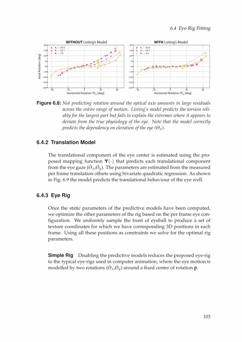
6.4 Eye Rig Fitting

Listings Fit

WITHOUT Listing’s Model WITH Listing’s ModelA

xial

Rot

atio

n [d

eg]

Horizontal Rotation [deg]Θy Horizontal Rotation [deg]Θy

Figure 6.8: Not predicting rotation around the optical axis amounts in large residualsacross the entire range of motion. Listing’s model predicts the torsion reli-ably for the largest part but fails to explain the extremes where it appears todeviate from the true physiology of the eye. Note that the model correctlypredicts the dependency on elevation of the eye (Θx).

6.4.2 Translation Model

The translational component of the eye center is estimated using the pro-posed mapping function Ψ(·) that predicts each translational componentfrom the eye gaze (Θx,Θy). The parameters are estimated from the measuredper frame translation offsets using bivariate quadratic regression. As shownin Fig. 6.9 the model predicts the translational behaviour of the eye well.

6.4.3 Eye Rig

Once the static parameters of the predictive models have been computed,we optimize the other parameters of the rig based on the per frame eye con-figuration. We uniformly sample the front of eyeball to produce a set oftexture coordinates for which we have corresponding 3D positions in eachframe. Using all these positions as constraints we solve for the optimal rigparameters.

Simple Rig Disabling the predictive models reduces the proposed eye-rigto the typical eye-rigs used in computer animation, where the eye motion ismodelled by two rotations (Θx,Θy) around a fixed center of rotation p.

103

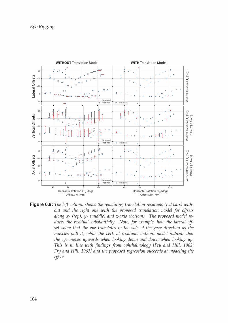
Eye Rigging

Vert

ical

Rot

atio

n

[

deg]

Θx

Offs

et Y

[-0.

1mm

]Ve

rtic

al R

otat

ion

[de

g]Θ

x

Late

ral O

ffset

sVe

rtic

al O

ffset

s

WITHOUT Translation Model WITH Translation Model

Vert

ical

Rot

atio

n

[

deg]

Θx

Offs

et Z

[-0.

1mm

]Horizontal Rotation [deg]ΘyHorizontal Rotation [deg]Θy

Axi

al O

ffset

s

Offset X [0.1mm]Offset X [0.1mm]

Figure 6.9: The left column shows the remaining translation residuals (red bars) with-out and the right one with the proposed translation model for offsetsalong x- (top), y- (middle) and z-axis (bottom). The proposed model re-duces the residual substantially. Note, for example, how the lateral off-set show that the eye translates to the side of the gaze direction as themuscles pull it, while the vertical residuals without model indicate thatthe eye moves upwards when looking down and down when looking up.This is in line with findings from ophthalmology [Fry and Hill, 1962;Fry and Hill, 1963] and the proposed regression succeeds at modeling theeffect.

104

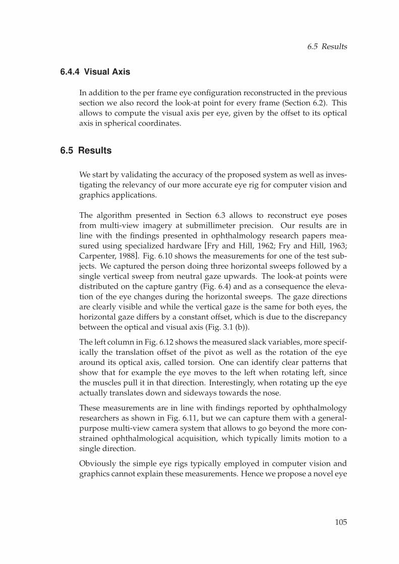
6.5 Results

6.4.4 Visual Axis

In addition to the per frame eye configuration reconstructed in the previoussection we also record the look-at point for every frame (Section 6.2). Thisallows to compute the visual axis per eye, given by the offset to its opticalaxis in spherical coordinates.

6.5 Results

We start by validating the accuracy of the proposed system as well as inves-tigating the relevancy of our more accurate eye rig for computer vision andgraphics applications.

The algorithm presented in Section 6.3 allows to reconstruct eye posesfrom multi-view imagery at submillimeter precision. Our results are inline with the findings presented in ophthalmology research papers mea-sured using specialized hardware [Fry and Hill, 1962; Fry and Hill, 1963;Carpenter, 1988]. Fig. 6.10 shows the measurements for one of the test sub-jects. We captured the person doing three horizontal sweeps followed by asingle vertical sweep from neutral gaze upwards. The look-at points weredistributed on the capture gantry (Fig. 6.4) and as a consequence the eleva-tion of the eye changes during the horizontal sweeps. The gaze directionsare clearly visible and while the vertical gaze is the same for both eyes, thehorizontal gaze differs by a constant offset, which is due to the discrepancybetween the optical and visual axis (Fig. 3.1 (b)).

The left column in Fig. 6.12 shows the measured slack variables, more specif-ically the translation offset of the pivot as well as the rotation of the eyearound its optical axis, called torsion. One can identify clear patterns thatshow that for example the eye moves to the left when rotating left, sincethe muscles pull it in that direction. Interestingly, when rotating up the eyeactually translates down and sideways towards the nose.

These measurements are in line with findings reported by ophthalmologyresearchers as shown in Fig. 6.11, but we can capture them with a general-purpose multi-view camera system that allows to go beyond the more con-strained ophthalmological acquisition, which typically limits motion to asingle direction.

Obviously the simple eye rigs typically employed in computer vision andgraphics cannot explain these measurements. Hence we propose a novel eye

105

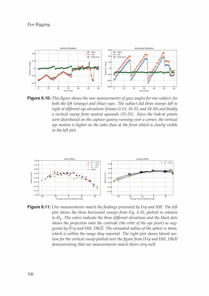
Eye Rigging

Figure 6.10: This figure shows the raw measurements of gaze angles for one subject, forboth the left (orange) and (blue) eyes. The subject did three sweeps left toright at different eye elevations (frames 0-15, 16-33, and 34-50) and finallya vertical sweep from neutral upwards (51-55). Since the look-at pointswere distributed on the capture gantry running over a corner, the verticaleye motion is higher on the sides than at the front which is clearly visiblein the left plot.

Figure 6.11: Our measurements match the findings presented by Fry and Hill. The leftplot shows the three horizontal sweeps from Fig. 6.10, plotted in relationto Θy. The colors indicate the three different elevations and the black dotsshows the projection onto the centrode (the orbit of the eye pivot) as sug-gested by [Fry and Hill, 1962]. The estimated radius of the sphere is 4mm,which is within the range they reported. The right plot shows lateral mo-tion for the vertical sweep plotted over the figure from [Fry and Hill, 1963]demonstrating that our measurements match theirs very well.

106

6.5 Results

rig that incorporates knowledge from ophthalmology, which fits the mea-surements much better as shown in Fig. 6.12. The translation model intro-duced in Section 6.1 succeed at removing most of the signal, leaving justfitting noise behind, which lies in the order of a tenth of a millimeter. TheListings model also predicts the torsion well, except for the extreme gazeposes, where the physiology of the eye motion appears to disagree the theo-retical model.

The fact that these measurements have been computed from ordinary cam-eras is a strong indicator that phenomenons such as torsion and eye transla-tion can be important for computer vision applications, such as accurate eyegaze estimation (Fig. 6.14). Eye gaze is also central for computer animation,where a common mistake is to presume the visual axis to align with the opti-cal axis of the eye, which will lead to cross-eyed characters (Fig. 6.13). As thevisual axis is rotated nasally by about 8 degrees on average relative to oureye model coordinate frame, the optical axis is actually pointing outwardswhen a person is looking at infinity.

To understand the relevancy of our findings for computer graphics applica-tions we synthesize several eye poses with both the presented and a tradi-tional eye rig (Fig. 6.14). The traditional eye rig neglects torsion and transla-tion of the rotational pivot, which leads to subtle yet very noticeable effectsespecially for extreme eye poses resulting in a difference in perceived gazefor the two rigs.

107

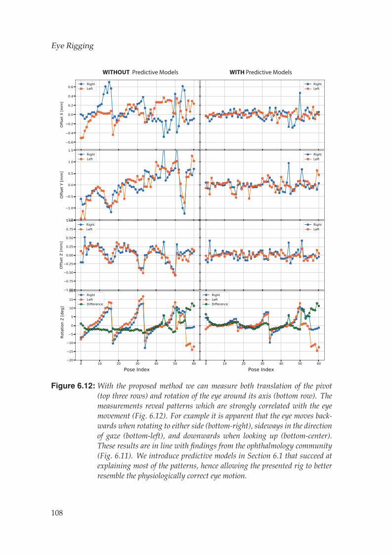
Eye Rigging

WITHOUT Predictive Models WITH Predictive Models

Figure 6.12: With the proposed method we can measure both translation of the pivot(top three rows) and rotation of the eye around its axis (bottom row). Themeasurements reveal patterns which are strongly correlated with the eyemovement (Fig. 6.12). For example it is apparent that the eye moves back-wards when rotating to either side (bottom-right), sideways in the directionof gaze (bottom-left), and downwards when looking up (bottom-center).These results are in line with findings from the ophthalmology community(Fig. 6.11). We introduce predictive models in Section 6.1 that succeed atexplaining most of the patterns, hence allowing the presented rig to betterresemble the physiologically correct eye motion.

108

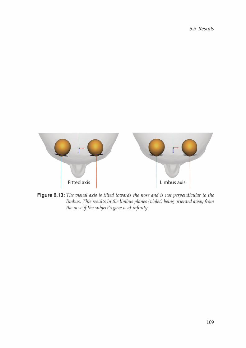
6.5 Results

Fitted axis Limbus axis

Figure 6.13: The visual axis is tilted towards the nose and is not perpendicular to thelimbus. This results in the limbus planes (violet) being oriented away fromthe nose if the subject’s gaze is at infinity.

109

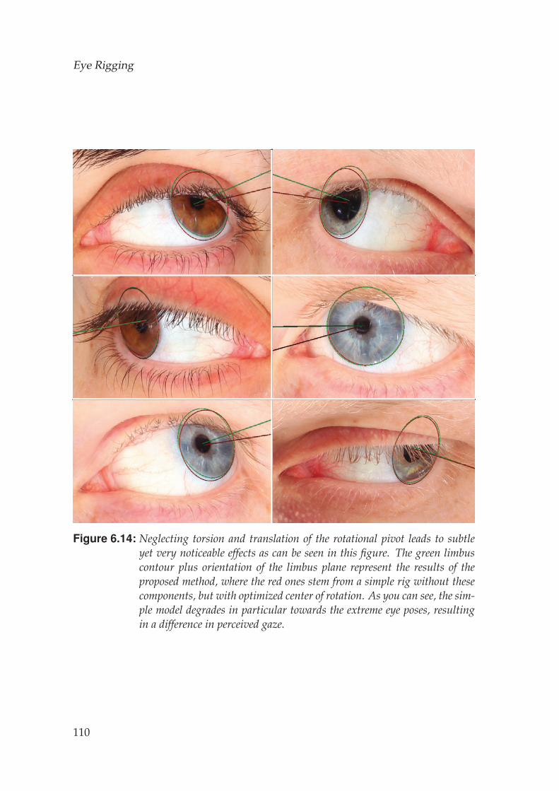
Eye Rigging

Figure 6.14: Neglecting torsion and translation of the rotational pivot leads to subtleyet very noticeable effects as can be seen in this figure. The green limbuscontour plus orientation of the limbus plane represent the results of theproposed method, where the red ones stem from a simple rig without thesecomponents, but with optimized center of rotation. As you can see, the sim-ple model degrades in particular towards the extreme eye poses, resultingin a difference in perceived gaze.

110

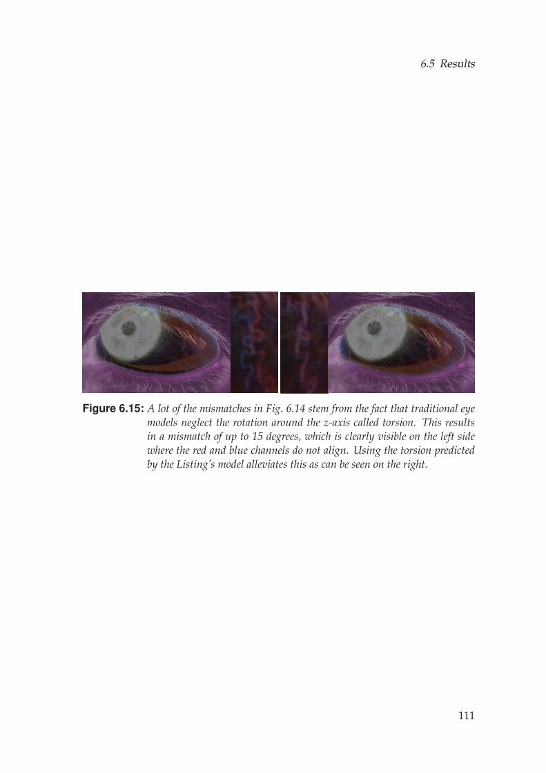
6.5 Results

Figure 6.15: A lot of the mismatches in Fig. 6.14 stem from the fact that traditional eyemodels neglect the rotation around the z-axis called torsion. This resultsin a mismatch of up to 15 degrees, which is clearly visible on the left sidewhere the red and blue channels do not align. Using the torsion predictedby the Listing’s model alleviates this as can be seen on the right.

111

Eye Rigging

112

C H A P T E R 7Conclusion

In this thesis we present methods for the creation of eyes for digital humans.This includes algorithms for the reconstruction, the modeling, and the rig-ging of eyes for animation and tracking applications.

We capture the shape and texture of the most prominent components of theeye at an unprecedented level of detail, including the sclera, the cornea, andthe iris. We demonstrate that the generic eye models typically used in ourcommunity are not sufficient to represent all the intricacies of an eye, whichare very person-specific, and we believe that the findings of this thesis havethe potential to alter our community’s current assumptions regarding hu-man eyes. In addition, we present the first method for reconstructing de-tailed iris deformation during pupil dilation, and demonstrate two applica-tions of how data-driven iris animations can be combined with our high-quality eye reconstructions. A data set has been published on our website1.

These eye reconstructions enable the creation of a new parametric modelof 3D eyes built from a database of high-resolution scans with both geom-etry and texture. Our model contains a shape subspace for the eyeball, acoupled shape and color synthesis method for the iris parameterized by alow-resolution control map, and a sclera vein synthesis approach also withtunable parameters to generate a variety of realistic vein networks. We alsopresent an image-based fitting algorithm that allows our parametric modelto be fit to lightweight inputs, such as common facial scanners, or even singleimages that can be found on the internet. Our parametric model and fittingapproach allow for simple and efficient eye reconstructions, making eye cap-

1https://www.disneyresearch.com/publication/high-quality-capture-of-eyes/

113

Conclusion

ture a more viable approach for industry and home use. Furthermore, themodel allows to manipulate the captured data as it is fully parametric, suchas changing the amount and appearance of sclera veins to simulate physio-logical effects or controlling the pupil size to have the eye react to syntheticillumination.

Based on the parametric eye model we present a novel eye rig informed byophthalmology findings and based on accurate measurements from a multi-view imaging system that can reconstruct eye poses at submillimeter accu-racy. Our goal is to raise the awareness in the computer graphics and visioncommunities that the eye movement is more complex than oftentimes as-sumed. More specifically, we show that the eye is not a purely rotational de-vice but actually translates during rotation and that it also rotates around itsoptical axis. These are important facts, for example, for foveal rendering andhead-mounted display devices, which are gaining a lot of popularity due tothe emerging augmented and virtual reality entertainment. Another impor-tant aspect that animators have to consider is the fact that the visual axis ofthe eye, which defines its gaze, is not identical with the optical axis. Ne-glecting this leads to cross-eyed gazes which quickly lead into the uncannyvalley. We investigate the effect of ignoring or modeling these phenomena inthe context of computer graphics and computer vision to provide the readeran intuition of their potential importance for their application.

We believe that these tools and methods are a valuable contribution to thecurrent eye creation pipeline. These methods allow for the more accurateand realistic creation of eye shape, appearance, and motion on one hand,but they also allow for an easier, faster, and more robust creation on theother hand. We believe that these tools have the potential to change howeyes are being modeled in the visual effects industry and we hope that theywill infuse a soul into a new generation of digital doubles in films.

7.1 Limitations

The methods presented in this thesis are great for various visual effects ap-plications. But unfortunately, they have their limitations.

Our eye reconstruction introduced in Chapter 4 system approximates the irisas a surface. Since the iris is a volumetric object with partially translucenttissue it is difficult to reconstruct accurately. We believe, however, that theoptical flow correspondences used to reconstruct that surface are sufficientlyaccurate to represent the iris with adequate details suitable for rendering,

114

7.2 Outlook

already a step forward from traditional practices that approximate the irisas a plane or cone.

Our parametric eye model (Chapter 5) allows for single-image reconstruc-tions, but unfortunately not without limitations. As can be seen in someof the single-image reconstructions, reflections off the cornea are difficult toidentify and ignore and thus can become baked-in to the iris texture (see thebird example in Fig. 5.15). Additionally, our sclera vein synthesis does notguarantee to produce vein networks that match any partial veins that mightbe visible in the input images. Also, our model is naturally limited by thesize and variation of the input database, and since only a limited number ofscanned high-quality real eyes are currently available, our results may notoptimally match the inputs, but this will be alleviated as more database eyesbecome available.

At this stage our fitted rig is person-specific and we have not investigatedhow it can generalize to others. This would, of course, be highly desirablesince building the rig requires a dedicated capture session and a lot of man-ual annotations, which is realistically only feasible for hero assets in largeproductions. It will, however, enable to acquire a large corpus of eye motionand to create a generalizable model based on that data, which we considerinteresting future work.

Nevertheless, even with these limitations our methods provide a great start-ing point for computer graphics artists to create realistic eyes from images.

7.2 Outlook

Besides addressing the limitations of our system, there are still many oppor-tunities to extend and improve the presented techniques including recon-struction of the eye region, modeling of the eye appearance, and modelingof the eye motion.

Eye region Reconstructing, modeling, and rigging the geometry of the eyeregion is still a remaining challenge. The complex geometries, the variousmaterials, the interfaces between the different parts of the eye, and the oc-clusions make this a very challenging undertaking. Furthermore, the eyesand the surrounding skin substantially influence each other. The eyelid isdeformed as the eye moves underneath it and we expect that opening theeyes wide or firmly closing them does actually influence the position of theeye in the socket, hence affecting its motion. Future work should thus look

115

Conclusion

at ways to couple these two models and provide a rig for the entire eye re-gion. Currently, a digital artist creates an eye region rig by hand based on hisexperience. The model-guided eyelid reconstruction of Bermano et al. [2015]is a first step, but it is limited to the reconstruction of eyelids. The eyelidscannot be animated or modified since there is no underlying rig that allowsfor this interpolation. Wood et al. [2016a] present a model based on the prin-cipal component analysis. We believe that better models can be found, thatare better suited to represent the nonlinear deformations of the eye region.

Eye appearance Capturing and modeling the appearance of the eye aswell as eye rendering are topics that we do not investigate in this thesis.We do not capture reflectance properties of the eyes, such as BRDF or BSS-RDF parameters. Also, the eye consists of various materials, some varyingin space, such as the sclera and the cornea. Anatomically they are the samepart, but the appearance transitions from white to transparent due to a struc-tural change. Also the tear layer, covering the eye, leads to glints, many ofthem close to the eyelids. The amount of liquid of this layer changes de-pending on the physical and emotional state of the person. New appearancecapture methods need to be developed in the future which model the eyewith an even greater attention to detail to produce more realistic digital hu-mans.

Eye dynamics In this thesis, we model the motion of the eye in a staticsense. We model the different poses and states the eyeball and the iris canreach over time, but we do not analyze the temporal characteristics and dy-namic behavior such as saccades, hippus, or tremor. These motions havebeen investigated extensively, but the analysis is often limited to a 2D gazeanalysis. The 3D techniques, presented in this thesis, might reveal previ-ously unknown effects. This might lead to potential applications outside ofour community, for example in ophthalmology, where accurate image-basedeye acquisition could help in discovering, monitoring and treating eye dis-eases.

116

A P P E N D I X A

117

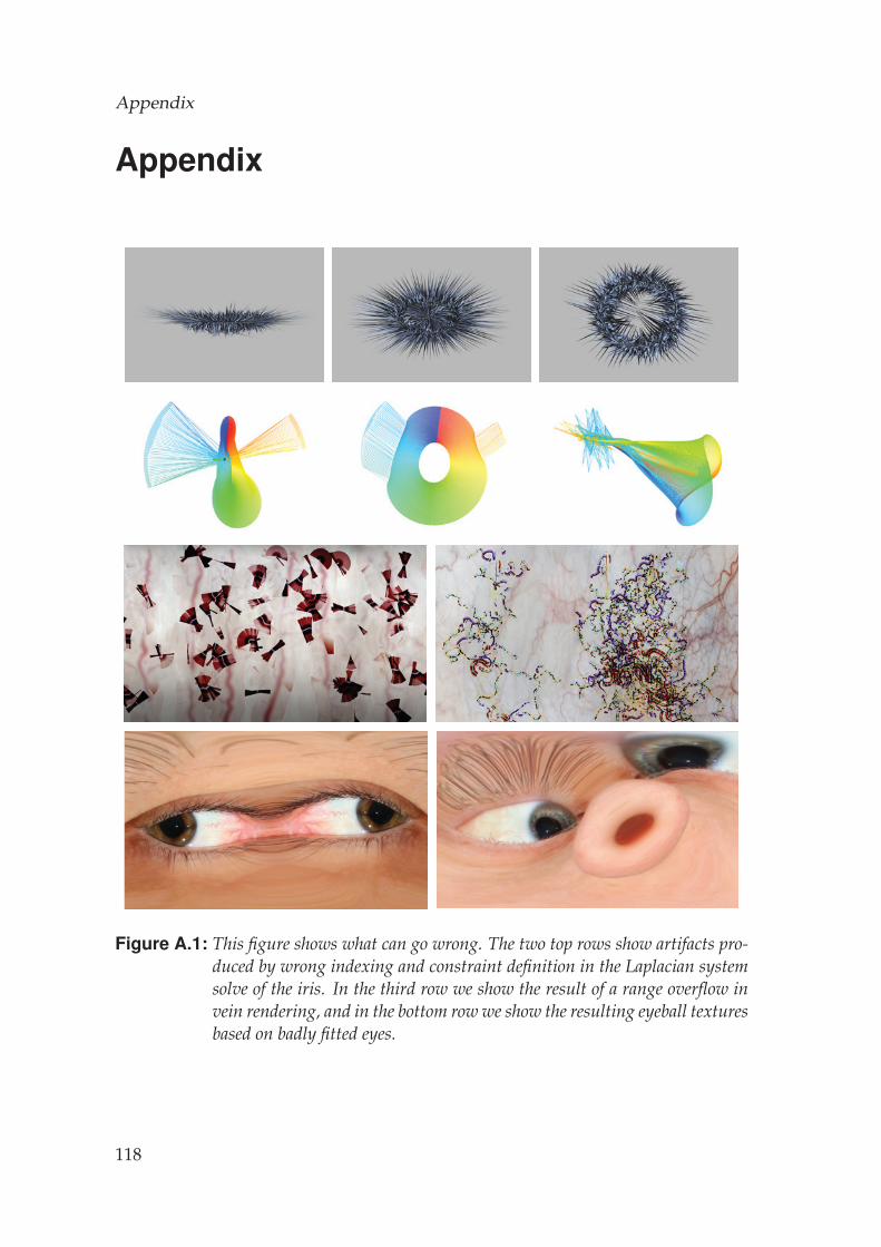
Appendix

Appendix

Figure A.1: This figure shows what can go wrong. The two top rows show artifacts pro-duced by wrong indexing and constraint definition in the Laplacian systemsolve of the iris. In the third row we show the result of a range overflow invein rendering, and in the bottom row we show the resulting eyeball texturesbased on badly fitted eyes.

118

References

[Agarwal et al., 2018] Sameer Agarwal, Keir Mierle, and Others. Ceres solver.http://ceres-solver.org, 2018.

[Allen et al., 2003] Brett Allen, Brian Curless, and Zoran Popovic. The space ofhuman body shapes: reconstruction and parameterization from range scans.In ACM Transactions on Graphics (TOG), volume 22, pages 587–594. ACM, 2003.

[Amberg et al., 2007] Brian Amberg, Sami Romdhani, and Thomas Vetter. Opti-mal step nonrigid icp algorithms for surface registration. In Computer Vision andPattern Recognition, 2007. CVPR’07. IEEE Conference on, pages 1–8. IEEE, 2007.

[Anguelov et al., 2005] Dragomir Anguelov, Praveen Srinivasan, Daphne Koller,Sebastian Thrun, Jim Rodgers, and James Davis. Scape: shape completion andanimation of people. In ACM Transactions on Graphics (TOG), volume 24, pages408–416. ACM, 2005.

[Ares and Royo, 2006] M Ares and S Royo. Comparison of cubic b-spline andzernike-fitting techniques in complex wavefront reconstruction. Applied optics,45(27):6954–6964, 2006.

[Atcheson et al., 2010] Bradley Atcheson, Felix Heide, and Wolfgang Heidrich.CALTag: High precision fiducial markers for camera calibration. In Interna-tional Workshop on Vision, Modeling and Visualization, 2010.

[Atchison et al., 2004] David A Atchison, Catherine E Jones, Katrina L Schmid,Nicola Pritchard, James M Pope, Wendy E Strugnell, and Robyn A Riley. Eyeshape in emmetropia and myopia. Investigative Ophthalmology & Visual Science,45(10):3380–3386, 2004.

References

[Beeler and Bradley, 2014] Thabo Beeler and Derek Bradley. Rigid stabilization offacial expressions. ACM Transactions on Graphics (TOG), 33(4):44, 2014.

[Beeler et al., 2010] T. Beeler, B. Bickel, R. Sumner, P. Beardsley, and M. Gross.High-quality single-shot capture of facial geometry. ACM Trans. Graphics (Proc.SIGGRAPH), 29(4):40, 2010.

[Beeler et al., 2011] Thabo Beeler, Fabian Hahn, Derek Bradley, Bernd Bickel, PaulBeardsley, Craig Gotsman, Robert W Sumner, and Markus Gross. High-qualitypassive facial performance capture using anchor frames. ACM Trans. Graphics(Proc. SIGGRAPH), 30(4):75, 2011.

[Benel et al., 1991] D. C. R. Benel, D. Ottens, and R. Horst. Use of an eye trackingsystem in the usability laboratory. In Proc. of the Human Factors Society 35thAnnual Meeting, pages 461–465, 1991.

[Bermano et al., 2015] Amit Bermano, Thabo Beeler, Yeara Kozlov, Derek Bradley,Bernd Bickel, and Markus Gross. Detailed spatio-temporal reconstruction ofeyelids. ACM Transactions on Graphics (TOG), 34(4):44, 2015.

[Besl and McKay, 1992] P. J. Besl and N. D. McKay. A method for registration of3-d shapes. IEEE Trans. on PAMI, 14(2):239–256, 1992.

[Blanz and Vetter, 1999] Volker Blanz and Thomas Vetter. A morphable modelfor the synthesis of 3d faces. In Proc. of the 26th annual conference on Computergraphics and interactive techniques, pages 187–194, 1999.

[Boykov and Kolmogorov, 2004] Yuri Boykov and Vladimir Kolmogorov. An ex-perimental comparison of min-cut/max-flow algorithms for energy minimiza-tion in vision. Pattern Analysis and Machine Intelligence, IEEE Transactions on,26(9):1124–1137, 2004.

[Bradley et al., 2010] Derek Bradley, Wolfgang Heidrich, Tiberiu Popa, and AllaSheffer. High resolution passive facial performance capture. ACM Trans. Graph-ics (Proc. SIGGRAPH), 29(4):41, 2010.

[Brown and Rusinkiewicz, 2004] Benedict J Brown and Szymon Rusinkiewicz.Non-rigid range-scan alignment using thin-plate splines. In 3D Data Processing,Visualization and Transmission, 2004. 3DPVT 2004. Proceedings. 2nd InternationalSymposium on, pages 759–765. IEEE, 2004.

[Brox et al., 2004] Thomas Brox, Andres Bruhn, Nils Papenberg, and Joachim We-ickert. High accuracy optical flow estimation based on a theory for warping.In ECCV, pages 25–36. Springer, 2004.

[Cao et al., 2014] Chen Cao, Qiming Hou, and Kun Zhou. Displaced dynamic

120

References

expression regression for real-time facial tracking and animation. ACM Trans-actions on Graphics (TOG), 33(4):43, 2014.

[Carpenter, 1988] Roger HS Carpenter. Movements of the Eyes, 2nd Rev. Pion Lim-ited, 1988.

[Chen et al., 2013] Kan Chen, Henry Johan, and Wolfgang Mueller-Wittig. Simpleand efficient example-based texture synthesis using tiling and deformation. InProceedings of the ACM SIGGRAPH Symposium on Interactive 3D Graphics andGames, pages 145–152. ACM, 2013.

[Chopra-Khullar and Badler, 2001] Sonu Chopra-Khullar and Norman I. Badler.Where to look? automating attending behaviors of virtual human characters.Autonomous Agents and Multi-Agent Systems, 4(1):9–23, 2001.

[Collewijn, 1999] H. Collewijn. Eye movement recording. Vision Research: A Prac-tical Guide to Laboratory Methods, pages 245–285, 1999.

[Deng et al., 2005] Zhigang Deng, J. P. Lewis, and U. Neumann. Automated eyemotion using texture synthesis. IEEE CG&A, 25(2):24–30, 2005.

[Dodge and Cline, 1901] R. Dodge and T. S. Cline. The angle velocity of eyemovements. Psychological Review, 8:145–157, 1901.

[Eagle Jr, 1988] RC Eagle Jr. Iris pigmentation and pigmented lesions: an ultra-structural study. Trans. of the American Ophthalmological Society, 86:581, 1988.

[Efros and Freeman, 2001] Alexei A Efros and William T Freeman. Image quiltingfor texture synthesis and transfer. In Proceedings of the 28th annual conference onComputer graphics and interactive techniques, pages 341–346. ACM, 2001.

[Efros and Leung, 1999] Alexei A. Efros and Thomas K. Leung. Texture synthesisby non-parametric sampling. In IEEE ICCV, pages 1033–1038, 1999.

[Eggert, 2007] Thomas Eggert. Eye movement recordings: Methods. Neuro-Ophthalmology, 40:15–34, 2007.

[Fischler and Bolles, 1981] M. Fischler and R. Bolles. Random sample consensus:a paradigm for model fitting with applications to image analysis and auto-mated cartography. Commun. ACM, 24(6):381–395, 1981.

[Flickr, 2006] Flickr. Mohammed Alnaser - Mr. Falcon. Creative Commons - Attri-bution 2.0, 2006. https://www.flickr.com/photos/69er/324313066.

[Francois et al., 2009] Guillaume Francois, Pascal Gautron, Gaspard Breton, andKadi Bouatouch. Image-based modeling of the human eye. IEEE TVCG,15(5):815–827, 2009.

121

References

[Fry and Hill, 1962] GA Fry and WW Hill. The center of rotation of the eye*.Optometry & Vision Science, 39(11):581–595, 1962.

[Fry and Hill, 1963] Glenn A Fry and WW Hill. The mechanics of elevating theeye*. Optometry & Vision Science, 40(12):707–716, 1963.

[Funkhouser et al., 2004] Thomas Funkhouser, Michael Kazhdan, Philip Shilane,Patrick Min, William Kiefer, Ayellet Tal, Szymon Rusinkiewicz, and DavidDobkin. Modeling by example. In ACM Transactions on Graphics (TOG), vol-ume 23, pages 652–663. ACM, 2004.

[Fyffe et al., 2011] Graham Fyffe, Tim Hawkins, Chris Watts, Wan-Chun Ma, andPaul Debevec. Comprehensive facial performance capture. In Eurographics,2011.

[Fyffe et al., 2014] Graham Fyffe, Andrew Jones, Oleg Alexander, RyosukeIchikari, and Paul Debevec. Driving high-resolution facial scans with videoperformance capture. ACM Trans. Graphics, 34(1):8:1–8:14, 2014.

[Garrido et al., 2013] Pablo Garrido, Levi Valgaerts, Chenglei Wu, and ChristianTheobalt. Reconstructing detailed dynamic face geometry from monocularvideo. ACM Trans. Graphics (Proc. SIGGRAPH Asia), 32(6):158, 2013.

[Ghosh et al., 2011] Abhijeet Ghosh, Graham Fyffe, Borom Tunwattanapong, JayBusch, Xueming Yu, and Paul Debevec. Multiview face capture using polarizedspherical gradient illumination. ACM Trans. Graphics (Proc. SIGGRAPH Asia),30(6):129, 2011.

[Hachol et al., 2007] Andrzej Hachol, W Szczepanowska-Nowak, H Kasprzak,I Zawojska, A Dudzinski, R Kinasz, and D Wygledowska-Promienska. Mea-surement of pupil reactivity using fast pupillometry. Physiological measurement,28(1):61, 2007.

[Haehnel et al., 2003] Dirk Haehnel, Sebastian Thrun, and Wolfram Burgard. Anextension of the icp algorithm for modeling nonrigid objects with mobilerobots. In IJCAI, volume 3, pages 915–920, 2003.

[Hansen and Ji, 2010] D. W. Hansen and Q. Ji. In the eye of the beholder: A surveyof models for eyes and gaze. IEEE PAMI, 32(3):478–500, 2010.

[Haralick, 1979] Robert M. Haralick. Statistical and structural approaches to tex-ture. Proc. IEEE, 67(5):786–804, 1979.

[Hartridge and Thompson, 1948] H. Hartridge and L. C. Thompson. Methods ofinvestigating eye movements. British Journal of Ophthalmology, 32:581–591, 1948.

[Hernandez et al., 2008] Carlos Hernandez, George Vogiatzis, and RobertoCipolla. Multiview photometric stereo. IEEE PAMI, 30(3):548–554, 2008.

122

References

[Hogan et al., 1971] Michael J. Hogan, Jorge A. Alvarado, and Joan E. Weddell.Histology of the human eye: an atlas and textbook. Philadelphia: Saunders,pages 393–522, 1971.

[Huang et al., 1991] David Huang, Eric A Swanson, Charles P Lin, Joel S Schu-man, William G Stinson, Warren Chang, Michael R Hee, Thomas Flotte, Ken-ton Gregory, Carmen A Puliafito, et al. Optical coherence tomography. Science,254(5035):1178–1181, 1991.

[Ihrke et al., 2008] Ivo Ihrke, Kiriakos N Kutulakos, Hendrik PA Lensch, MarcusMagnor, and Wolfgang Heidrich. State of the art in transparent and specularobject reconstruction. In Eurographics 2008 - State of the Art Reports, 2008.

[Ikemoto et al., 2003] Leslie Ikemoto, Natasha Gelfand, and Marc Levoy. A hier-archical method for aligning warped meshes. In 3-D Digital Imaging and Model-ing, 2003. 3DIM 2003. Proceedings. Fourth International Conference on, pages 434–441. IEEE, 2003.

[Itti et al., 2003] Laurent Itti, Nitin Dhavale, and Frederic Pighin. Realistic AvatarEye and Head Animation Using a Neurobiological Model of Visual Attention.In Proceedings of SPIE 48th Annual International Symposium on Optical Science andTechnology, 2003.

[Jacob and Unser, 2004] Mathews Jacob and Michael Unser. Design of steerablefilters for feature detection using canny-like criteria. Pattern Analysis and Ma-chine Intelligence, IEEE Transactions on, 26(8):1007–1019, 2004.

[Janik et al., 1978] S. W. Janik, A. R. Wellens, M. L. Goldberg, and L. F. Dell’Osso.Eyes as the center of focus in the visual examination of human faces. Perceptualand Motor Skills, 47(3):857–858, 1978.

[Judd et al., 1905] C. H. Judd, C. N. McAllister, and W. M. Steel. General intro-duction to a series of studies of eye movements by means of kinetoscopic pho-tographs. Psychological Review, Monograph Supplements, 7:1–16, 1905.

[Kazhdan et al., 2004] Michael Kazhdan, Thomas Funkhouser, and SzymonRusinkiewicz. Shape matching and anisotropy. In ACM Transactions on Graphics(TOG), volume 23, pages 623–629. ACM, 2004.

[Kwatra et al., 2003] Vivek Kwatra, Arno Schodl, Irfan Essa, Greg Turk, andAaron Bobick. Graphcut textures: image and video synthesis using graph cuts.In ACM Transactions on Graphics (ToG), volume 22, pages 277–286. ACM, 2003.

[Lam and Baranoski, 2006] M. W. Y. Lam and G. V. G. Baranoski. A predictivelight transport model for the human iris. In Computer Graphics Forum, vol-ume 25, pages 359–368, 2006.

123

References

[Le et al., 2012] B. H. Le, X. Ma, and Z. Deng. Live speech driven head-and-eyemotion generators. IEEE TVCG, 18(11), 2012.

[Lee et al., 2002] Sooha Park Lee, Jeremy B. Badler, and Norman I. Badler. Eyesalive. ACM Trans. Graphics (Proc. SIGGRAPH), 21(3):637–644, 2002.

[Lefohn et al., 2003] Aaron Lefohn, Brian Budge, Peter Shirley, Richard Caruso,and Erik Reinhard. An ocularist’s approach to human iris synthesis. IEEECG&A, 23(6):70–75, 2003.

[LeGrand and ElHage, 2013] Yves LeGrand and Sami G ElHage. Physiological op-tics, volume 13. Springer, 2013.

[Levoy and Whitaker, 1990] M. Levoy and R. Whitaker. Gaze-directed volumerendering. In Symposium on Interactive 3D Graphics, pages 217–223, 1990.

[Li et al., 2008] Hao Li, Robert W Sumner, and Mark Pauly. Global correspon-dence optimization for non-rigid registration of depth scans. In Computer graph-ics forum, volume 27, pages 1421–1430. Wiley Online Library, 2008.

[Li et al., 2015] Jun Li, Weiwei Xu, Zhiquan Cheng, Kai Xu, and Reinhard Klein.Lightweight wrinkle synthesis for 3d facial modeling and animation. Computer-Aided Design, 58:117–122, 2015.

[Liang et al., 2001] Lin Liang, Ce Liu, Ying-Qing Xu, Baining Guo, and Heung-Yeung Shum. Real-time texture synthesis by patch-based sampling. ACMTransactions on Graphics (ToG), 20(3):127–150, 2001.

[Ma and Deng, 2009] Xiaohan Ma and Zhigang Deng. Natural eye motion syn-thesis by modeling gaze-head coupling. In Proc. IEEE VR, pages 143–150, 2009.

[Ma et al., 2007] Wan-Chun Ma, Tim Hawkins, Pieter Peers, Charles-FelixChabert, Malte Weiss, and Paul Debevec. Rapid acquisition of specular anddiffuse normal maps from polarized spherical gradient illumination. In Proc.Rendering Techniques, pages 183–194, 2007.

[Mackey et al., 2011] David A Mackey, Colleen H Wilkinson, Lisa S Kearns, andAlex W Hewitt. Classification of iris colour: review and refinement of a classi-fication schema. Clinical & experimental ophthalmology, 39(5):462–471, 2011.

[Mackworth and Thomas, 1962] N. H. Mackworth and E. L. Thomas. Head-mounted eye-marker camera. Journal of the Optical Society of America, 52:713–716, 1962.

[Marsella et al., 2013] Stacy Marsella, Yuyu Xu, Margaux Lhommet, AndrewFeng, Stefan Scherer, and Ari Shapiro. Virtual character performance fromspeech. In Proc. SCA, pages 25–35, 2013.

124

References

[Mohammed et al., 2009] Umar Mohammed, Simon JD Prince, and Jan Kautz.Visio-lization: generating novel facial images. ACM Transactions on Graphics(TOG), 28(3):57, 2009.

[Nishino and Nayar, 2004] Ko Nishino and Shree K Nayar. Eyes for relighting. InACM Transactions on Graphics (TOG), volume 23, pages 704–711. ACM, 2004.

[Palubicki et al., 2009] Wojciech Palubicki, Kipp Horel, Steven Longay, AdamRunions, Brendan Lane, Radomır Mech, and Przemyslaw Prusinkiewicz. Self-organizing tree models for image synthesis. ACM Trans. Graphics (Proc. SIG-GRAPH), 28(3):58, 2009.

[Pamplona et al., 2009] Vitor F Pamplona, Manuel M Oliveira, and Gladimir VGBaranoski. Photorealistic models for pupil light reflex and iridal pattern defor-mation. ACM Trans. Graphics (TOG), 28(4):106, 2009.

[Pejsa et al., 2016] Tomislav Pejsa, Daniel Rakita, Bilge Mutlu, and Michael Gle-icher. Authoring directed gaze for full-body motion capture. ACM Trans. Graph-ics (Proc. SIGGRAPH Asia, 35(6), 2016.

[Perez et al., 2003] Patrick Perez, Michel Gangnet, and Andrew Blake. Poissonimage editing. ACM Trans. Graphics (Proc. SIGGRAPH), 22(3):313–318, 2003.

[Pinero, 2013] David P Pinero. Technologies for anatomical and geometric char-acterization of the corneal structure and anterior segment: a review. In Seminarsin Ophthalmology, pages 1–10, 2013.

[Pinskiy and Miller, 2009] Dmitriy Pinskiy and Erick Miller. Realistic eye motionusing procedural geometric methods. In SIGGRAPH 2009: Talks, page 75. ACM,2009.

[Praun et al., 2000] Emil Praun, Adam Finkelstein, and Hugues Hoppe. Lappedtextures. In Proceedings of the 27th annual conference on Computer graphics andinteractive techniques, pages 465–470. ACM Press/Addison-Wesley PublishingCo., 2000.

[Ramanarayanan and Bala, 2007] Ganesh Ramanarayanan and Kavita Bala. Con-strained texture synthesis via energy minimization. IEEE TVCG, 13(1), 2007.

[Rio-Cristobal and Martin, 2014] Ana Rio-Cristobal and Raul Martin. Corneal as-sessment technologies: Current status. Survey of Ophthalmology, 2014.

[Rozenberg and Salomaa, 1976] Grzegorz Rozenberg and Arto Salomaa. Themathematical theory of L systems. Springer, 1976.

[Ruhland et al., 2014] K Ruhland, S Andrist, J Badler, C Peters, N Badler, M Gle-icher, B Mutlu, and R McDonnell. Look me in the eyes: A survey of eye and

125

References

gaze animation for virtual agents and artificial systems. In Eurographics State ofthe Art Reports, pages 69–91, 2014.

[Sagar et al., 1994] Mark A. Sagar, David Bullivant, Gordon D. Mallinson, and Pe-ter J. Hunter. A virtual environment and model of the eye for surgical simula-tion. In Proceedings of Computer Graphics and Interactive Techniques, pages 205–212, 1994.

[Seitz et al., 2006] Steven M Seitz, Brian Curless, James Diebel, Daniel Scharstein,and Richard Szeliski. A comparison and evaluation of multi-view stereo recon-struction algorithms. In IEEE CVPR, volume 1, pages 519–528, 2006.

[Shen and Cai, 2009] Hui-Liang Shen and Qing-Yuan Cai. Simple and efficientmethod for specularity removal in an image. Applied optics, 48(14):2711–2719,2009.

[Smolek and Klyce, 2003] Michael K Smolek and Stephen D Klyce. Zernike poly-nomial fitting fails to represent all visually significant corneal aberrations. In-vestigative ophthalmology & visual science, 44(11):4676–4681, 2003.

[Sorkine et al., 2004] Olga Sorkine, Daniel Cohen-Or, Yaron Lipman, Marc Alexa,Christian Rossl, and H-P Seidel. Laplacian surface editing. In Proceedings ofthe 2004 Eurographics/ACM SIGGRAPH symposium on Geometry processing, pages175–184. ACM, 2004.

[Sugano et al., 2014] Y. Sugano, Y. Matsushita, and Y. Sato. Learning-by-synthesisfor appearance-based 3d gaze estimation. In IEEE CVPR, 2014.

[Suwajanakorn et al., 2014] Supasorn Suwajanakorn, Ira Kemelmacher-Shlizerman, and Steven M Seitz. Total moving face reconstruction. InComputer Vision–ECCV 2014, pages 796–812. Springer, 2014.

[Tai et al., 2010] Yu-Wing Tai, Shuaicheng Liu, Michael S. Brown, and StephenLin. Super resolution using edge prior and single image detail synthesis. InCVPR, 2010.

[Valgaerts et al., 2012] Levi Valgaerts, Chenglei Wu, Andres Bruhn, Hans-PeterSeidel, and Christian Theobalt. Lightweight binocular facial performance cap-ture under uncontrolled lighting. ACM Trans. Graph., 31(6):187, 2012.

[Van Run and Van den Berg, 1993] LJ Van Run and AV Van den Berg. Binocu-lar eye orientation during fixations: Listing’s law extended to include eye ver-gence. Vision research, 33(5):691–708, 1993.

[Vertegaal et al., 2001] Roel Vertegaal, Robert Slagter, Gerrit van der Veer, andAnton Nijholt. Eye gaze patterns in conversations: There is more to conversa-

126

References

tional agents than meets the eyes. In Proc. Human Factors in Computing Systems,pages 301–308, 2001.

[Vivino et al., 1993] M.A. Vivino, S. Chintalagiri, B. Trus, and M. Datiles. Devel-opment of a scheimpflug slit lamp camera system for quantitative densitomet-ric analysis. Eye, 7(6):791–798, 1993.

[Vlasic et al., 2005] Daniel Vlasic, Matthew Brand, Hanspeter Pfister, and JovanPopovic. Face transfer with multilinear models. In ACM Transactions on Graph-ics (TOG), volume 24, pages 426–433. ACM, 2005.

[Wang et al., 2015] Jianzhong Wang, Guangyue Zhang, and Jiadong Shi. Pupiland glint detection using wearable camera sensor and near-infrared led array.Sensors, 15(12):30126–30141, 2015.

[Wang et al., 2016] Congyi Wang, Fuhao Shi, Shihong Xia, and Jinxiang Chai. Re-altime 3d eye gaze animation using a single rgb camera. ACM Trans. Graphics(Proc. SIGGRAPH), 35(4), 2016.

[Wei et al., 2009] Li-Yi Wei, Sylvain Lefebvre, Vivek Kwatra, and Greg Turk. Stateof the art in example-based texture synthesis. In Eurographics 2009, State of theArt Report, EG-STAR, pages 93–117. Eurographics Association, 2009.

[Weissenfeld et al., 2010] Axel Weissenfeld, Kang Liu, and J&#x00f6;rn Oster-mann. Video-realistic image-based eye animation via statistically driven statemachines. Vis. Comput., 26(9):1201–1216, 2010.

[Wen et al., 2017a] Quan Wen, Feng Xu, Ming Lu, and Yong Jun-Hai. Real-time3d eyelids tracking from semantic edges. ACM Transactions on Graphics (TOG),2017.

[Wen et al., 2017b] Quan Wen, Feng Xu, and Jun-Hai Yong. Real-time 3d eye per-formance reconstruction for rgbd cameras. IEEE transactions on visualization andcomputer graphics, 23(12):2586–2598, 2017.

[Wikimedia Commons, 1485] Wikimedia Commons. Sandro Botticelli - The Birth ofthe Venus. Public Domain, 1485. https://commons.wikimedia.org/wiki/File:Venus_botticelli_detail.jpg.

[Wikimedia Commons, 1887] Wikimedia Commons. Vincent Van Gogh - Self-Portrait. Public Domain, 1887. https://commons.wikimedia.org/wiki/File:

VanGogh_1887_Selbstbildnis.jpg.

[Wikimedia Commons, 2006] Wikimedia Commons. Blue Eye Image. GNU FreeDocumentation License Version 1.2, 2006. https://commons.wikimedia.org/

wiki/File:Blueye.JPG.

127

References

[Wood et al., 2015] E. Wood, T. Baltrusaitis, X. Zhang, Y. Sugano, P. Robinson, andA. Bulling. Rendering of eyes for eye-shape registration and gaze estimation.In IEEE ICCV, 2015.

[Wood et al., 2016a] E. Wood, T. Baltrusaitis, L. P. Morency, P. Robinson, andA. Bulling. A 3d morphable eye region model for gaze estimation. In ECCV,2016.

[Wood et al., 2016b] E. Wood, T. Baltrusaitis, L. P. Morency, P. Robinson, andA. Bulling. Learning an appearance-based gaze estimator from one millionsynthesized images. In ETRA, 2016.

[Zhai et al., 1999] S. Zhai, C. Morimoto, and S Ihde. Manual and gaze input cas-caded (magic) pointing. In Proc. of the ACM CHI Human Factors in ComputingSystems Conference, pages 246–253, 1999.

[Zhang et al., 2015] X. Zhang, Y. Sugano, M. Fritz, and A. Bulling. Appearance-based gaze estimation in the wild. In IEEE CVPR, 2015.

[Zoric et al., 2011] Goranka Zoric, Rober Forchheimer, and Igor S Pandzic. Oncreating multimodal virtual humans—real time speech driven facial gesturing.Multimedia tools and applications, 54(1):165–179, 2011.

128