San Jose State University San Jose State University

SJSU ScholarWorks SJSU ScholarWorks

Master's Projects Master's Theses and Graduate Research

Winter 2018

Exploratory Data Analysis And Crime Prediction In San Francisco Exploratory Data Analysis And Crime Prediction In San Francisco

Isha Pradhan San Jose State University

Follow this and additional works at: https://scholarworks.sjsu.edu/etd_projects

Part of the Computer Sciences Commons

Recommended Citation Recommended Citation Pradhan, Isha, "Exploratory Data Analysis And Crime Prediction In San Francisco" (2018). Master's Projects. 642. DOI: https://doi.org/10.31979/etd.3usp-3sdy https://scholarworks.sjsu.edu/etd_projects/642

This Master's Project is brought to you for free and open access by the Master's Theses and Graduate Research at SJSU ScholarWorks. It has been accepted for inclusion in Master's Projects by an authorized administrator of SJSU ScholarWorks. For more information, please contact scholarworks@sjsu.edu.

Exploratory Data Analysis And Crime Prediction In San Francisco

A Project

Presented to

The Faculty of the Department of Computer Science

San Jose State University

In Partial Fulfillment

of the Requirements for the Degree

Master of Science

by

Isha Pradhan

May 2018

c○ 2018

Isha Pradhan

ALL RIGHTS RESERVED

The Designated Project Committee Approves the Project Titled

Exploratory Data Analysis And Crime Prediction In San Francisco

by

Isha Pradhan

APPROVED FOR THE DEPARTMENTS OF COMPUTER SCIENCE

SAN JOSE STATE UNIVERSITY

May 2018

Dr. Katerina Potika Department of Computer Science

Dr. Thomas Austin Department of Computer Science

Dr. Robert Chun Department of Computer Science

ABSTRACT

Exploratory Data Analysis And Crime Prediction In San Francisco

by Isha Pradhan

Crime has been prevalent in our society for a very long time and it continues

to be so even today. The San Francisco Police Department has continued to register

numerous such crime cases daily and has released this data to the public as a part

of the open data initiative. In this paper, Big Data analysis is used on this dataset

and a tool that predicts crime in San Francisco is provided. The focus of the project

is to perform an in-depth analysis of the major types of crimes that occurred in the

city, observe the trend over the years, and determine how various attributes, such as

seasons, contribute to specific crimes. Furthermore, the proposed model is described

that builds on the results of the performed predictive analytics, by identifying the

attributes that directly affect the prediction. More specifically, the model predicts

the type of crime that will occur in each district of the city. After preprocessing

the dataset, the problem reduced to a multi-class classification problem. Various

classification techniques such as K-Nearest Neighbor, Multi-class Logistic Regression,

Decision Tree, Random Forest and Naïve Bayes are used. Lastly, our results are

experimentally evaluated and compared against previous work.The proposed model

finds applications in resource allocation of law enforcement in a Smart City.

ACKNOWLEDGMENTS

I want to thank my mentor Dr. Potika for her constant support throughout

this research and for encouraging me to do my best. I would also like to thank my

committee members, Dr. Austin and Dr. Chun for having taken interest in my

research and having agreed to help me as needed.

And last but not the least, I would like to thank my parents for their invaluable

support and for making it possible for me to chase my dreams.

v

TABLE OF CONTENTS

CHAPTER

1 Introduction . . . . . . . . . . . . . . . . . . . . . . . . . . . . . . . 1

1.1 Motivation . . . . . . . . . . . . . . . . . . . . . . . . . . . . . . . 2

1.2 Problem Formulation . . . . . . . . . . . . . . . . . . . . . . . . . 2

2 Definitions and Techniques . . . . . . . . . . . . . . . . . . . . . . 4

2.1 Predictive Analytics . . . . . . . . . . . . . . . . . . . . . . . . . . 4

2.2 Classification Techniques . . . . . . . . . . . . . . . . . . . . . . . 5

2.3 Log Loss Scoring . . . . . . . . . . . . . . . . . . . . . . . . . . . 10

2.4 Parallel Processing using Apache Spark . . . . . . . . . . . . . . . 11

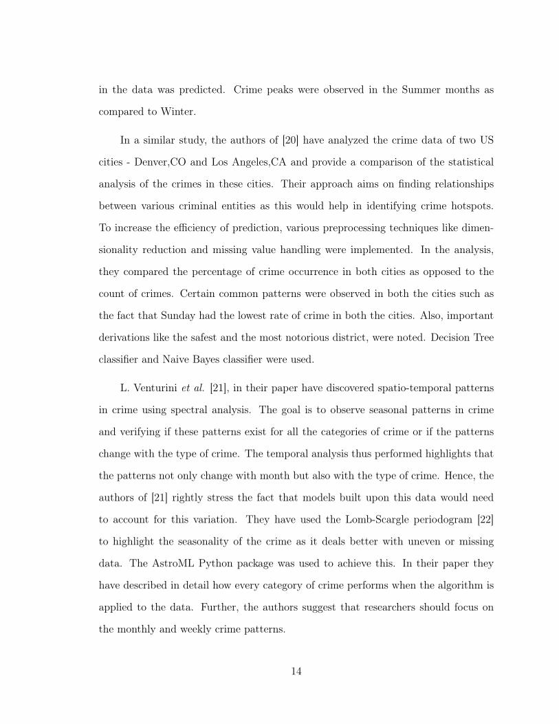
3 Related Work . . . . . . . . . . . . . . . . . . . . . . . . . . . . . . . 13

3.1 Temporal and Spectral Analysis . . . . . . . . . . . . . . . . . . . 13

3.2 Prediction using Clustering and Classification techniques . . . . . 15

3.3 Hotspot Detection . . . . . . . . . . . . . . . . . . . . . . . . . . . 17

4 Design and Implementation . . . . . . . . . . . . . . . . . . . . . . 18

4.1 Overview of the dataset . . . . . . . . . . . . . . . . . . . . . . . . 18

4.2 Data Preprocessing . . . . . . . . . . . . . . . . . . . . . . . . . . 20

4.2.1 Preprocessing using Apache Spark . . . . . . . . . . . . . . 20

4.2.2 Techniques used for preprocessing . . . . . . . . . . . . . . 21

4.3 Software and Technologies Used . . . . . . . . . . . . . . . . . . . 26

5 Experimental Results . . . . . . . . . . . . . . . . . . . . . . . . . . 28

5.1 Comparison of this approach with existing results . . . . . . . . . 28

vi

vii

5.2 Results of Graphical Analysis . . . . . . . . . . . . . . . . . . . . 30

6 Conclusion and Future Work . . . . . . . . . . . . . . . . . . . . . 38

LIST OF REFERENCES . . . . . . . . . . . . . . . . . . . . . . . . . . . 39

LIST OF TABLES

1 Combining Similar Categories . . . . . . . . . . . . . . . . . . . . 23

2 Extracting Information from Description Column . . . . . . . . . 24

3 Results of Experiments . . . . . . . . . . . . . . . . . . . . . . . . 29

viii

LIST OF FIGURES

1 Data mining and predictive analytics. . . . . . . . . . . . . . . . . 4

2 Decision Tree Example . . . . . . . . . . . . . . . . . . . . . . . . 8

3 KNN Classifier Example . . . . . . . . . . . . . . . . . . . . . . . 9

4 Spark Architecture . . . . . . . . . . . . . . . . . . . . . . . . . . 12

5 Snapshot of the actual Dataset . . . . . . . . . . . . . . . . . . . 20

6 Count of Distinct Categories in the Dataset . . . . . . . . . . . . 29

7 Rate of Crime per District by Year . . . . . . . . . . . . . . . . . 30

8 Rate of overall crime every Hour . . . . . . . . . . . . . . . . . . 31

9 Rate of Theft/Larceny by the Hour . . . . . . . . . . . . . . . . . 32

10 Rate of Prostitution by the Hour . . . . . . . . . . . . . . . . . . 32

11 Sum of Drugs/Narcotics cases per Year . . . . . . . . . . . . . . . 33

12 Area of Theft/Larceny by the Year . . . . . . . . . . . . . . . . . 34

13 Area of Drugs/Narcotics by the Year . . . . . . . . . . . . . . . . 35

14 More Balanced Dataset . . . . . . . . . . . . . . . . . . . . . . . 36

15 Recall for old preprocessing . . . . . . . . . . . . . . . . . . . . . 36

16 Recall for more balanced dataset . . . . . . . . . . . . . . . . . . 37

17 Comparison of Precision scores . . . . . . . . . . . . . . . . . . . 37

ix

CHAPTER 1

Introduction

The concept of a smart city has been derived as one of the means to improve

the lives of the people living within the city by taking smart initiatives in a variety

of domains like urban development, safety, energy and so on [1]. One of the factors

that determine the quality of life in the city is the crime rate therein. Although there

could be a lot of technological advancement in the city but the basic requirement of

citizens’ safety still remains [2].

Crime continues to be a threat to us and our society and demands serious consid-

eration if we hope to reduce the onset or the repercussions caused by it. Hundreds of

crimes are recorded daily by the data officers working working alongside the law en-

forcement authorities throughout the United States. Many cities in the United States

have signed the Open Data initiative, thereby making this crime data, among other

types of data, accessible to the general public. The intention behind this initiative

is increasing the citizens’ participation in decision making by utilizing this data to

uncover interesting and useful facts [3].

The city of San Francisco is one amongst the many to have joined this Open Data

movement. The data scientists and engineers working alongside the San Francisco

Police Department (SFPD) have recorded over 100,000 crime cases in the form on

police complaints they have received [4]. With the help of this historical data, many

patterns can be uncovered. This would help us predict the crimes that may happen

in the future and thereby help the city police better safeguard the population of the

city.

1

1.1 Motivation

The motivation behind taking up this topic for the research is that every aware

citizen in today’s modern world wants to live in a safe environment and neighborhood.

However it is a known fact that crime in some form, exists in our society. Although

we cannot control what goes on around us, we can definitely try to take a few steps to

aid the government and police authorities in trying to control it. The SFPD has made

the Police Complaints data from the year 2003 to 2018 (current year) available to the

general public. Hence, taking inspiration from the facts stated above, we decided to

process this data provided and analyze it to identify the trends in crime over the years

as well as make an attempt to predict the crimes in the future.

1.2 Problem Formulation

The problem being tackled in this research can be best explained in two distinct

parts:

1. Performing exploratory analysis of the data to mine patterns in crime:

∙ The first step in determining the safety within different areas in the city

is analyzing the spread and impact of the crime.

∙ We utilize this provided crime dataset by the SFPD and perform ex-

ploratory analysis on it, to observe existing patterns in the crime through-

out the city of San Francisco.

∙ We study the crime spread in the city based on the geographical location

of each crime, the possible areas of victimization on the streets, seasonal

changes in the crime rate and the type, and the hourly variations in crime.

2. Building a prediction model to predict the type of crime that can take place in

2

the city,in the future:

∙ After observing the patterns of crime from the historical data as explained

previous, the next thing is to predict the crimes that can occur in the

future.

∙ Our goal is to build a prediction model that treats this problem as a multi-

class classification problem, by classifying the unseen data into one of the

crime categories (classes) thereby predicting the crime that can occur.

∙ This is expected to help the police plan their patrol and effectively con-

tribute to building a smarter city.

For the first part, we will make use of various data analytics tools along with

Spark for initial data preprocessing, to analyze the spread of the crime in the city.

For the second part, in order to build a prediction model, we build upon the exist-

ing research work and improve their results by experimenting with different types

of algorithms. Summarizing, we present the experimental results using graphs and

statistics.

3

CHAPTER 2

Definitions and Techniques

In this chapter we will go over the details of some concepts and techniques which

will be discussed and implemented throughout this research.

2.1 Predictive Analytics

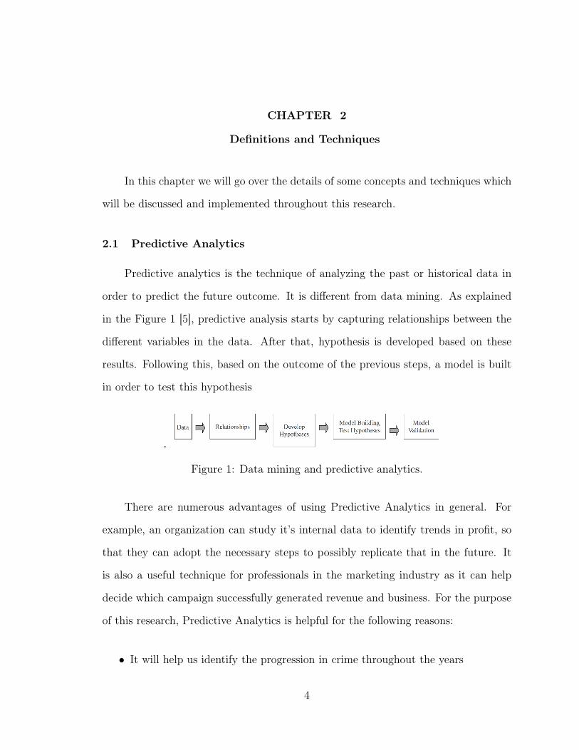
Predictive analytics is the technique of analyzing the past or historical data in

order to predict the future outcome. It is different from data mining. As explained

in the Figure 1 [5], predictive analysis starts by capturing relationships between the

different variables in the data. After that, hypothesis is developed based on these

results. Following this, based on the outcome of the previous steps, a model is built

in order to test this hypothesis

Figure 1: Data mining and predictive analytics.

There are numerous advantages of using Predictive Analytics in general. For

example, an organization can study it’s internal data to identify trends in profit, so

that they can adopt the necessary steps to possibly replicate that in the future. It

is also a useful technique for professionals in the marketing industry as it can help

decide which campaign successfully generated revenue and business. For the purpose

of this research, Predictive Analytics is helpful for the following reasons:

∙ It will help us identify the progression in crime throughout the years

4

∙ It will help us closely observe the variables having highest correlation with the

predictor or target variable

∙ Visualizing the data can even help map potential outliers, which can then be

effectively handled during data preprocessing

∙ The analysis can bring up some interesting facts from the past which might

prove to be useful to the SFPD while planning their patrol or strategies against

crime

2.2 Classification Techniques

Classification techniques are used to segregate the data into one or more cate-

gories also known as class labels. The goal of classification is to create a certain set of

rules that will either make a binary decision, or predict which of the multiple classes

should the data be classified into. Classification can mainly be divided into two types:

1. Binary Classification

In Binary Classification, the goal is to classify the elements into one of the two

categories specified, say, X and X̃ (not X). To determine the efficiency of the

Binary Classifier, we pass a set of inputs to the classifier and examine the output.

There are 4 possible results - True Positive, True Negative, False Positive and

False Negative [6]. Generally, ‘Accuracy’ is used to determine the efficiency of

a binary classifier.

2. Multiclass Classification

Multiclass Classification involves classifying the data into more than two cate-

gories. The most common types of Multiclass Classifiers are [6]:

5

∙ Pigeonhole Classifier: In a pigeonhole classifier every item is classified into

only one of the many categories. Hence, for a given item, there can be

only one output category assigned to it.

∙ Combination Classifier: This type of classifier can place an item into more

than one output categories. Hence, unlike a pigeonhole classifier, this type

of classifier does not assign a unique category to each input.

∙ Fuzzy Classifier: These classifiers not only assign an input to more than

one categories but also assign a degree to each category. This means that

every input belongs to every category by a certain degree. Hence the

output is an N-dimensional vector, where N is the number of categories.

For the purpose of this research, we will focus on the Pigeonhole Multiclass

Classification algorithms.

Below we will look at some of the classification techniques that have been used

in this research.

1. Naïve Bayes

Naïve Bayes classifiers are a set of supervised learning algorithms which are

based on the Bayes’ theorem. The Bayes’ theorem can be stated as shown in

Figure (1),

𝑃 (A|B) = 𝑃 (A)𝑃 (B|A)

𝑃 (B)(1)

Here,

P(A|B) is the conditional probability of A happening given that B is true

6

P(B|A) is the conditional probability of B happening given that A is true and

P(A) and P(B) are the individual probabilities of A and B happening indepen-

dently

All the Naïve Bayes algorithms have the naïve assumption that there exists

independence between all pairs of features. That is, each feature independently

contributes to the probability of the target variable. Although these classifiers

are fairly simple in nature, they tend to work very well in a large number of

real world problems.

2. Decision Trees

Decision Tree classifiers use decision trees to make a prediction about the value

of a target variable. The decision trees are basically functions that successively

determine the class that the input needs to be assigned.

A decision tree contains a root node, interior nodes and terminal or leaf nodes

[7]. The interior nodes are the splitting nodes, i.e. based on the condition spec-

ified in the function at these nodes, the tree is split into two or more branches.

Using decision trees for prediction has many advantages. In a decision tree clas-

sifier, an input is tested against only specific subsets of the data, determined by

the splitting criteria or decision functions. This eliminates unnecessary compu-

tations [8]. Another advantage of Decision Trees is that we can use a feature

selection algorithm in order to decide which features are worth considering for

the decision tree classifier. The lesser the number of features, the better will be

the efficiency of the algorithm [7].

To construct a decision tree, generally a top down approach is applied until some

predefined stopping criterion is met. Figure 2 depicts an example of a decision

7

Figure 2: Decision Tree Example

tree which splits a node based on the best attributes of the Crime Classification

dataset [3], which is what is used in this research.

3. K- Nearest Neighbor

According to the K-Nearest Neighbor (KNN) algorithm, data is classified into

one of the many categories by taking a majority vote of its neighbors. The

label is assigned depending on the most common of the categories among its

neighbors. In other words, we identify the neighbors closest to the new point

we wish to classify and based on these neighbors, we predict the label of this

new point. The number of neighbors to consider can be a user-defined constant

K as in the case of K-nearest neighbors or it can be based on the density of

points in a certain radius specified [9].

The distance metric used can be Euclidean or Manhattan if the target variable is

a continuous variable or Hamming distance if the target variable is a categorical

variable

8

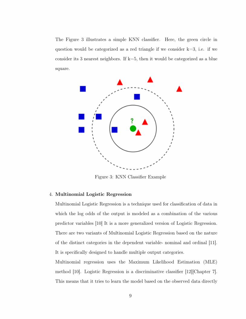
The Figure 3 illustrates a simple KNN classifier. Here, the green circle in

question would be categorized as a red triangle if we consider k=3, i.e. if we

consider its 3 nearest neighbors. If k=5, then it would be categorized as a blue

square.

Figure 3: KNN Classifier Example

4. Multinomial Logistic Regression

Multinomial Logistic Regression is a technique used for classification of data in

which the log odds of the output is modeled as a combination of the various

predictor variables [10] It is a more generalized version of Logistic Regression.

There are two variants of Multinomial Logistic Regression based on the nature

of the distinct categories in the dependent variable- nominal and ordinal [11].

It is specifically designed to handle multiple output categories.

Multinomial regression uses the Maximum Likelihood Estimation (MLE)

method [10]. Logistic Regression is a discriminative classifier [12][Chapter 7].

This means that it tries to learn the model based on the observed data directly

9

and makes less assumptions about the underlying distribution.

5. Random Forest

A Random Forest Classifier generates multiple decision trees on different sub-

samples of the data while training, and then predicts the accuracy or loss score

by taking a mean of these values. This helps to control over-fitting [9].

In the Random Forest algorithm, the split for each node is determined from

a subset of predictor variables which are randomly chosen at the given node

[13]. This is done using the Out-Of-Bag (OOB) approach specified by Breiman

[14]. Here, an inbag dataset is formed using the training set. A few samples

from this training set are set aside (also called the OOB data) for testing the

random learners. The average of the samples misclassified is taken and is used

for judging the performance of the learner [14].

2.3 Log Loss Scoring

In case of multiclass classification, the baseline (or worst-case) accuracy would be:

1𝑁

, where N is the number of distinct categories of the dependent variable. Thus, for

an output variable with 30 different categories, the worst-case would be an accuracy

of 3.33%. In such a case, accuracy might not necessarily be a good measure of the

efficiency of the model. Hence we consider measuring the performance of the model

using Log Loss scoring.

A Log Loss score is used when the model gives out a probability for the prediction

of each class. In this scoring metric, false classifications are penalized. The lesser the

log loss score, the better is the model. For a perfect classifier,the log loss score would

be zero [15].

10

Mathematically, the Log Loss function is defined as follows:

− 1

𝑁

𝑁∑︁𝑖=1

𝑀∑︁𝑗=1

𝑦𝑖𝑗 𝑙𝑜𝑔 𝑝𝑖𝑗 (2)

Here, N is the total number of samples, M denotes the number of distinct cat-

egories present in the output variable, 𝑦𝑖𝑗 takes the value of 0 or 1 indicating if the

label j is the expected label for sample i and 𝑝𝑖𝑗 if the probability that label j will be

assigned to the sample i [15].

The scikit-learn(sklearn) library (written in Python) provides a method for cal-

culating the Log Loss score of a machine learning model, which is defined in the

sklearn.metrics package [16]. In the most simplest form, the method provided by the

sklearn library is given as: 𝑙𝑜𝑔_𝑙𝑜𝑠𝑠(𝑦𝑡𝑟𝑢𝑒, 𝑦𝑝𝑟𝑒𝑑), where 𝑦𝑡𝑟𝑢𝑒 is the expected value of

the output variable and 𝑦𝑝𝑟𝑒𝑑 is the predicted value.

2.4 Parallel Processing using Apache Spark

Apache Spark is a big data tool which distributes the data over a cluster and

achieves parallel processing. It has become popular in the recent few years [17].

Apache Spark has a master-slave architecture.

The SparkContext is the driver program which interacts with a Cluster Manager

as shown in the Figure 4 [18]. The Cluster Manager is connected to the Executors

present on each Worker node. It runs the computations and stores the application

data. Every Spark job is divided into stages and each stage in turn has multiple tasks.

It is the job of the Driver to convert the application data to tasks.

The fundamental feature of Spark is the Resilient Distributed Dataset (RDD). RDDs

are basically a collection of elements which are distributed or partitioned across nodes

11

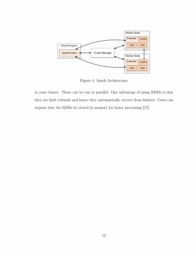
Figure 4: Spark Architecture

in your cluster. These can be run in parallel. One advantage of using RDDs is that

they are fault tolerant and hence they automatically recover from failures. Users can

request that the RDDs be stored in memory for faster processing [17].

12

CHAPTER 3

Related Work

Over the years, there have been a lot of studies involving the use of predictive

analytics to observe patterns in crime. Some of these techniques are more complex

than others and involve the use of more than one datasets. Most of the datasets

used in these researches are taken from the Open Data initiative [3] supported by the

government. In this section we will study the various techniques used by different

authors which will help answer questions such as: What is the role of analytics in

crime prediction?, What techniques are used for data preprocessing? and What are

the classification techniques which have proved to be most efficient?

3.1 Temporal and Spectral Analysis

A lot of research in the area of crime analysis and prediction revolves around the

analysis of spatial and temporal data. The reason for this is fairly obvious as we are

dealing with geographical data spread over the span of many years.

The authors of [19] have studied the fluctuation of crime throughout the year to

see if there exists a pattern with seasons. In their research, they have used the crime

data from three different Canadian cities, focusing on property related crimes. Ac-

cording to their first hypothesis, the peaks in crime during certain time intervals can

be distinctly observed in case of cities where the seasons are more distinct. Their sec-

ond hypothesis is that certain types of crimes will be more frequent in certain seasons

because of their nature. They were able to validate their hypothesis using Ordinary

Least Squares (OLS) Regression for Vancouver and Negative Binomial Regression

for Ottawa. Since their research focused on crime seasonality, quadratic relationship

13

in the data was predicted. Crime peaks were observed in the Summer months as

compared to Winter.

In a similar study, the authors of [20] have analyzed the crime data of two US

cities - Denver,CO and Los Angeles,CA and provide a comparison of the statistical

analysis of the crimes in these cities. Their approach aims on finding relationships

between various criminal entities as this would help in identifying crime hotspots.

To increase the efficiency of prediction, various preprocessing techniques like dimen-

sionality reduction and missing value handling were implemented. In the analysis,

they compared the percentage of crime occurrence in both cities as opposed to the

count of crimes. Certain common patterns were observed in both the cities such as

the fact that Sunday had the lowest rate of crime in both the cities. Also, important

derivations like the safest and the most notorious district, were noted. Decision Tree

classifier and Naive Bayes classifier were used.

L. Venturini et al. [21], in their paper have discovered spatio-temporal patterns

in crime using spectral analysis. The goal is to observe seasonal patterns in crime

and verifying if these patterns exist for all the categories of crime or if the patterns

change with the type of crime. The temporal analysis thus performed highlights that

the patterns not only change with month but also with the type of crime. Hence, the

authors of [21] rightly stress the fact that models built upon this data would need

to account for this variation. They have used the Lomb-Scargle periodogram [22]

to highlight the seasonality of the crime as it deals better with uneven or missing

data. The AstroML Python package was used to achieve this. In their paper they

have described in detail how every category of crime performs when the algorithm is

applied to the data. Further, the authors suggest that researchers should focus on

the monthly and weekly crime patterns.

14

3.2 Prediction using Clustering and Classification techniques

The authors of [23] have described a method to predict the type of crime which

can occur based on the given location and time. Apart from using the data from

the Portland Police Bureau (PPB), they have also included data such as ethnicity

of the population, census data and so on, from other public sources to increase the

accuracy of their results. Further, they have made sure that the data is balanced to

avoid getting skewed results. The machine learning techniques that are applied are

Support Vector Machine (SVM), Random Forest, Gradient Boosting Machines, and

Neural Networks [23]. Before applying the machine learning techniques to predict

the category of the crime, they have applied various preprocessing techniques such as

data transformation, discretization, cleaning and reduction. Due to the large volume

of data, the authors have sampled the data to less than 20,000 rows. They used two

datasets to perform their experiments - one was with the demographic information

used without alterations and in the second case, they used this data to predict the

missing values in the original dataset. In the first case, ensemble techniques like as

Random Forest or Gradient Boosting worked best, while in the second case, SVM

and Neural Networks showed promising results.

Since a smart city should give importance to the safety of their citizens, the

authors of [2] have designed a strategy to construct a network of clusters which can

assign police patrol duties, based on the informational entropy. The idea is to find

patrol locations within the city, such that the entropy is maximized. The reason for

the need to maximize the entropy is that the entropy in this case is mapped to the

variation in the clusters, i.e. more entropy means more cluster coverage [2]. The

dataset used for the research is the Los Angeles County GIS Data. The data has

around 42 different crime categories. Taking the help of a domain expert, the authors

15

have assigned weights to these crimes based on the importance of the crime. Also,

the geocode for each record is taken into consideration and the records that do not

have a geocode are skipped. Because the authors in [2] are trying to maximize the

entropy in this case, consider the equation (3)

𝐻𝑐1 = −p(𝑐1)𝑙𝑛p(𝑐1) (3)

The probability p(c1) is defined as the ratio of weight of the centroid of the crime

to the weight of the system, plus the ratio of the quickest path between two centroids,

to the quickest path in the whole system.

The authors of [24] have taken a unique approach towards crime classification

where unstructured crime reports are classified into one of the many categories of

crime using textual analysis and classification. For achieving this, the data from vari-

ous sources including but not limited to the databases which stores information about

traffic, criminal warrants of New Jersey (NJ) and criminal records from NJ Criminal

History was combined and preprocessed. As a part of the preprocessing activity, all

the stop words, punctuations, case IDs, phone numbers and so on were removed from

the data. Following this, document indexing is performed on the data to convert the

text into its concise representation. In order to identify the topics or specific incident

types from the concise representation, the authors used Latent Semantic Analysis

(LSA). Next, similarity between these topics was identified using the Topic Model-

ing technique where the closer the score is to 1, the more similar it is to the topic

which was followed by Text Categorization. The classification methods used in this

research were Support Vector Machines (SVM), Random Forests, Neural Networks,

MAXENT (Maximum Entropy Classifier), and SLDA (Scaled Linear Discriminant

16

Analysis). However, the authors observed that SVM performed consistently better of

them all.

3.3 Hotspot Detection

A crime hotspot is an area where the occurrence of crime is high as compared to

the other locations [25]. Many researchers have taken an interest in determining crime

hotspots from the given dataset. The authors of [25] mainly discuss two approaches

for detecting hotspots - circular and linear. The authors also discuss the fundamentals

of Spatial Scan Statistics which is a useful tool for hotspot detection. The results on

the Chicago crime dataset are also discussed in detail using both the approaches.

17

CHAPTER 4

Design and Implementation

The fundamental goal of the project is to build a model such that it can predict

the crime category that is more likely to surface given a certain set of characteristics

like the time, location, month and so on. We will also take the help of statistical

and graphical analysis to help determine which attributes contribute to the overall

improvement in the log-loss score.

4.1 Overview of the dataset

The data used in this research project is the San Francisco crime dataset made

available by the San Francisco Police Department on the SF Open Data website [3],

which is a part of the open data initiative. The dataset consists of the following

attributes:

∙ IncidntNum : It is a numerical field. Denotes the incident number of the crime

as recorded in the police logs. It is analogous to the row number.

∙ Descript: It is a text field. Contains a brief description about the crime. This

field provides slightly more information than the Category field but is still quite

limited.

∙ DayOfWeek: It is a text field. Specifies the day of the week when the crime

occurred. It takes on one of the values from: Monday, Tuesday, Wednesday,

Thursday, Friday, Saturday, Sunday

∙ Date: It is a Date-Time field. Specifies the exact date of the crime.

18

∙ PdDistrict: It is a text field. Specifies the police district the crime occurred

in. San Francisco has been divided in 10 police districts. It takes on one of

the values from: Southern, Tenderloin, Mission, Central, Northern, Bayview,

Richmond, Taraval, Ingleside, Park

∙ Resolution: It is a text field. Specifies the resolution for the crime. It takes one

of these values: Arrested, Booked, None

∙ Address: It is a text field. Gives the street address of the crime.

∙ X: It is a geographic field. It gives the longitudinal coordinates of the crime.

∙ Y: It is a geographic field. It gives the latitudinal coordinates of the crime.

∙ Location: It is a location field. It is in the form of a pair of coordinates, i.e.

(X, Y)

∙ PdId: It is a numerical field. It is a unique identifier for each complaint regis-

tered. It is used in the database update or search operations.

∙ Category: It is a text field. Specifies the category of the crime. Originally,

there are 39 distinct values (such as Assault, Larceny/Theft, Prostitution, etc.)

in this field. It is also the dependent variable we will try to predict for the test

set.

There are about 1.4 million rows in the dataset and the size of the dataset is approx-

imately 450 MB. It contains data from the year 2003 to (February) 2018. A snapshot

of the actual dataset [3] is shown in Figure 5.

19

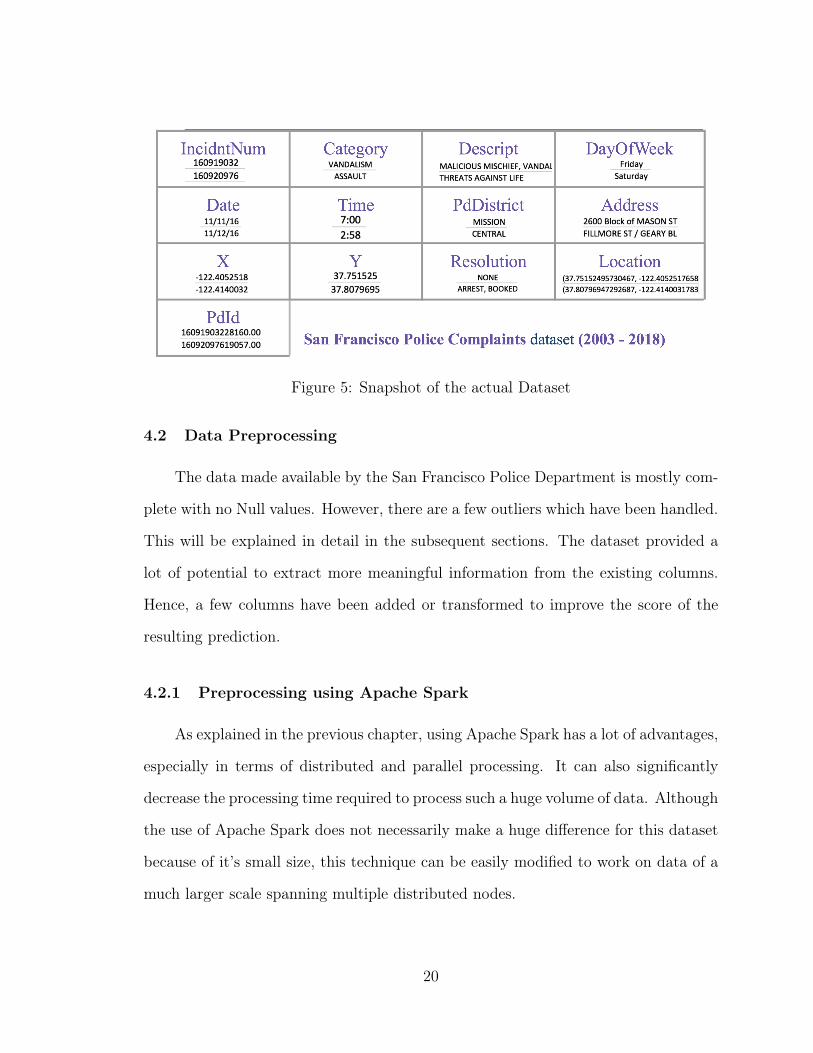
Figure 5: Snapshot of the actual Dataset

4.2 Data Preprocessing

The data made available by the San Francisco Police Department is mostly com-

plete with no Null values. However, there are a few outliers which have been handled.

This will be explained in detail in the subsequent sections. The dataset provided a

lot of potential to extract more meaningful information from the existing columns.

Hence, a few columns have been added or transformed to improve the score of the

resulting prediction.

4.2.1 Preprocessing using Apache Spark

As explained in the previous chapter, using Apache Spark has a lot of advantages,

especially in terms of distributed and parallel processing. It can also significantly

decrease the processing time required to process such a huge volume of data. Although

the use of Apache Spark does not necessarily make a huge difference for this dataset

because of it’s small size, this technique can be easily modified to work on data of a

much larger scale spanning multiple distributed nodes.

20

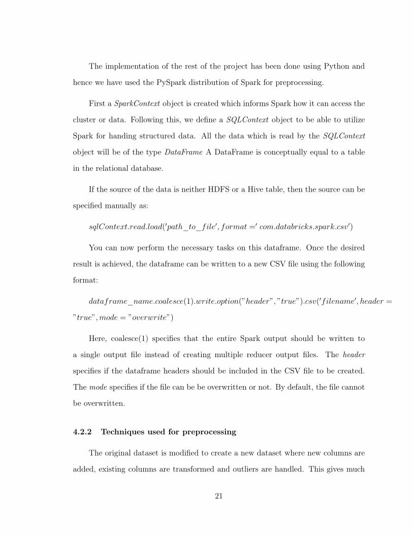
The implementation of the rest of the project has been done using Python and

hence we have used the PySpark distribution of Spark for preprocessing.

First a SparkContext object is created which informs Spark how it can access the

cluster or data. Following this, we define a SQLContext object to be able to utilize

Spark for handing structured data. All the data which is read by the SQLContext

object will be of the type DataFrame A DataFrame is conceptually equal to a table

in the relational database.

If the source of the data is neither HDFS or a Hive table, then the source can be

specified manually as:

𝑠𝑞𝑙𝐶𝑜𝑛𝑡𝑒𝑥𝑡.𝑟𝑒𝑎𝑑.𝑙𝑜𝑎𝑑(′𝑝𝑎𝑡ℎ_𝑡𝑜_𝑓𝑖𝑙𝑒′, 𝑓𝑜𝑟𝑚𝑎𝑡 =′ 𝑐𝑜𝑚.𝑑𝑎𝑡𝑎𝑏𝑟𝑖𝑐𝑘𝑠.𝑠𝑝𝑎𝑟𝑘.𝑐𝑠𝑣′)

You can now perform the necessary tasks on this dataframe. Once the desired

result is achieved, the dataframe can be written to a new CSV file using the following

format:

𝑑𝑎𝑡𝑎𝑓𝑟𝑎𝑚𝑒_𝑛𝑎𝑚𝑒.𝑐𝑜𝑎𝑙𝑒𝑠𝑐𝑒(1).𝑤𝑟𝑖𝑡𝑒.𝑜𝑝𝑡𝑖𝑜𝑛(”ℎ𝑒𝑎𝑑𝑒𝑟”, ”𝑡𝑟𝑢𝑒”).𝑐𝑠𝑣(′𝑓𝑖𝑙𝑒𝑛𝑎𝑚𝑒′, ℎ𝑒𝑎𝑑𝑒𝑟 =

”𝑡𝑟𝑢𝑒”,𝑚𝑜𝑑𝑒 = ”𝑜𝑣𝑒𝑟𝑤𝑟𝑖𝑡𝑒”)

Here, coalesce(1) specifies that the entire Spark output should be written to

a single output file instead of creating multiple reducer output files. The header

specifies if the dataframe headers should be included in the CSV file to be created.

The mode specifies if the file can be be overwritten or not. By default, the file cannot

be overwritten.

4.2.2 Techniques used for preprocessing

The original dataset is modified to create a new dataset where new columns are

added, existing columns are transformed and outliers are handled. This gives much

21

better results than the existing data. The decision to add or transform columns has

been taken by studying the graphical analysis which has been performed on the data

prior to building a model.

4.2.2.1 Data Cleaning

One of the primary steps of Data Cleaning is Outlier Handling. In the San

Francisco Crime dataset, there are a total of 196 outliers as the longitudinal coordinate

exceeds the minimum boundary of San Francisco. The outliers were filtered by the

code below:

𝑑𝑎𝑡𝑎𝑓𝑟𝑎𝑚𝑒.𝑓𝑖𝑙𝑡𝑒𝑟(𝑑𝑎𝑡𝑎𝑓𝑟𝑎𝑚𝑒.𝑋 < −122.3549)

where X is the longitudinal coordinate.

The next step in Data Cleaning is taking care of incorrect or missing data.

Although the dataset does not contain Null values or missing values, the Category

column does contain a few columns which have been incorrectly labeled like the TREA

category which should actually be TRESPASSING.

There are 39 distinct categories in the dataset. However, some of the categories

are very similar to each other. For example, when the Category column contains

values or keywords like: INDECENT EXPOSURE or OBSCENE or DISORDERLY

CONDUCT then return PORNOGRAPHY/OBSCENE MAT. The decision on which

categories should be clubbed together is taken by looking at the Description column

of the dataset which provides more information on what the corresponding Category

column represents. The complete list is presented for reference in Table 1.

22

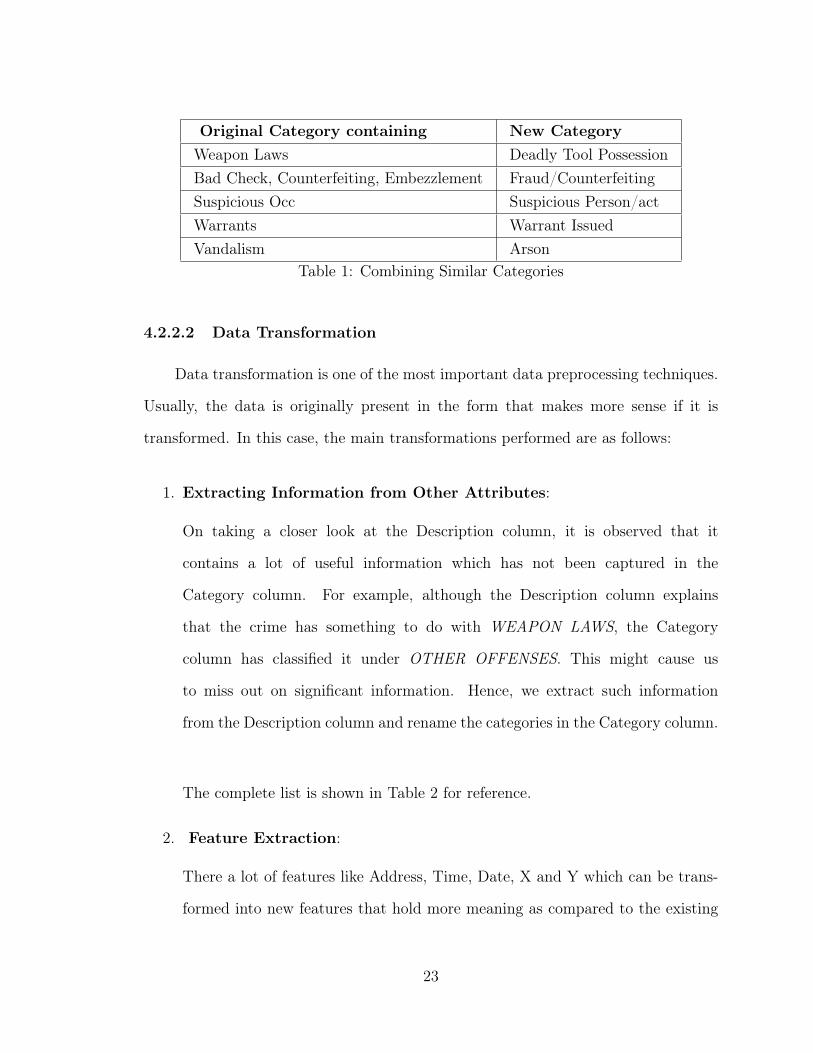
Original Category containing New CategoryWeapon Laws Deadly Tool PossessionBad Check, Counterfeiting, Embezzlement Fraud/CounterfeitingSuspicious Occ Suspicious Person/actWarrants Warrant IssuedVandalism Arson

Table 1: Combining Similar Categories

4.2.2.2 Data Transformation

Data transformation is one of the most important data preprocessing techniques.

Usually, the data is originally present in the form that makes more sense if it is

transformed. In this case, the main transformations performed are as follows:

1. Extracting Information from Other Attributes:

On taking a closer look at the Description column, it is observed that it

contains a lot of useful information which has not been captured in the

Category column. For example, although the Description column explains

that the crime has something to do with WEAPON LAWS, the Category

column has classified it under OTHER OFFENSES. This might cause us

to miss out on significant information. Hence, we extract such information

from the Description column and rename the categories in the Category column.

The complete list is shown in Table 2 for reference.

2. Feature Extraction:

There a lot of features like Address, Time, Date, X and Y which can be trans-

formed into new features that hold more meaning as compared to the existing

23

Description Containing New CategoryLicense, Traffic, speeding, Driving Traffic ViolationBurglary Tools, Air Gun,Tear Gas, Weapon Deadly Tool PossessionSex Sexual OffensesForgery, Fraud Fraud/CounterfeitingTobacco, Drug Drug/narcoticIndecent Exposure, Obscene, Disorderly Conduct Pornography/obscene MatHarassing AssaultInfluence Of Alcohol Drunkenness

Table 2: Extracting Information from Description Column

ones. Hence, all of these features have been used to generate new features and

some of these old features have been eliminated.

Address to BlockOrJunc: In its original form, the Address feature has a

lot of distinct values. Thus, if given a logical consideration, it is not hard to

realize that the exact address of the crime might not be repeated or be useful

in predicting the type of crime in the future. However, this column can be

used to see if the crime occurred on a street corner/junction or on a block.

We can also check if there exists a pattern among certain types of crime to

occur more frequently on a street corner rather than a block. To achieve this,

a simple check of whether ’/’ occurs in the address or not, is performed. If it

does contain the same, it means that the crime occurred on a corner and we

return 1, otherwise it is a block and we return 0. The pseudocode is shown

below:

if address contains ’/’ then

return 1

else

return 0

24

end if

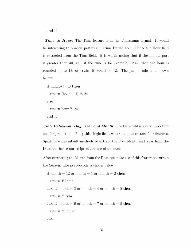
Time to Hour : The Time feature is in the Timestamp format. It would

be interesting to observe patterns in crime by the hour. Hence the Hour field

is extracted from the Time field. It is worth noting that if the minute part

is greater than 40, i.e. if the time is for example, 12:42, then the hour is

rounded off to 13, otherwise it would be 12. The pseudocode is as shown

below:

if minute > 40 then

return (hour + 1) % 24

else

return hour % 24

end if

Date to Season, Day, Year and Month : The Date field is a very important

one for prediction. Using this single field, we are able to extract four features.

Spark provides inbuilt methods to extract the Day, Month and Year from the

Date and hence our script makes use of the same.

After extracting the Month from the Date, we make use of this feature to extract

the Season. The pseudocode is shown below:

if month = 12 or month = 1 or month = 2 then

return Winter

else if month = 3 or month = 4 or month = 5 then

return Spring

else if month = 6 or month = 7 or month = 8 then

return Summer

else

25

return Fall

end if

X and Y to Grid : The X and the Y coordinates provide the exact location

of the crime. However, we can see some interesting patterns on dividing the

entire San Francisco area into grids of 20 X 20. This is inspired from the author

of xyz, which gives specific details on the formula used for generation of these

400 cells.

4.2.2.3 Data Reduction

As previously mentioned, there are 39 categories on crime in the original dataset.

Some of them include labels like NON-CRIMINAL, RECOVERED VEHICLE and

SECONDARY CODES. Since we are trying to predict the future occurrences of

crimes, it is essential to have categories pertaining to actual criminal activities. But

the above labels do not provide any additional information to help us achieve our

goal. Thus, these categories are completely filtered out from our dataset. This re-

duces the number of rows from about 2.1 million to about 1.9 million 38,000 after all

the preprocessing. But with more data in the future, the predictions are expected to

improve.

4.3 Software and Technologies Used

This project is implemented in Python (version 3.6.4). The other libraries used

throughout the project are described below:

PySpark: Apache Spark is a high performance, cluster-computing, open source

framework for data analytics and is capable of handling big data. It is known for its

ability to implicitly handle parallelism and for being fault tolerant. Spark’s Python

26

API, which is known as PySpark exposes the Spark programming model to Python.

In this project, PySpark was used for data preprocessing. The advantage of this

approach is that, large amount of data is processed quickly and the existing code can

be easily modified to support distributed big data in the future, if necessary.

Pandas: Pandas is an open source library that provides tools for data mining and

analysis using Python. It is mainly used in this project to prepare the data for

consumption by specific machine learning algorithms.

NumPy: NumPy is a Python library that can handle multidimensional data and

perform scientific and mathematical operations on the same. NumPy was used in this

project as an accessory to the Pandas library to perform some basic mathematical

operations.

scikit-learn: scikit-learn [16] is an open-source Python machine learning library

which provides numerous classification, regression and clustering algorithms. This

library was used in this project to perform the actual task of model building and

prediction. It provides a variety of evaluation metrics to validate the performance of

the model, which makes it a valuable tool.

Tableau: Tableau is a powerful data analytics tool which is used for building inter-

active dashboards. Tableau was mainly used in the project to generate interactive

graphs and observe patterns in the data. This information proved to be useful in

determining the features that could contribute well to the actual model building. It

also provides a rich map interface for geographical data.

27

CHAPTER 5

Experimental Results

5.1 Comparison of this approach with existing results

In this section a comparative study of our new approach and the results of existing

work, as mentioned in the related work section, is described.

First, we go on to describe the features used for building the various models in

other researches. They are assigned labels of the form Source 1, Source 2 and so on

for easy reference in the subsequent sections.

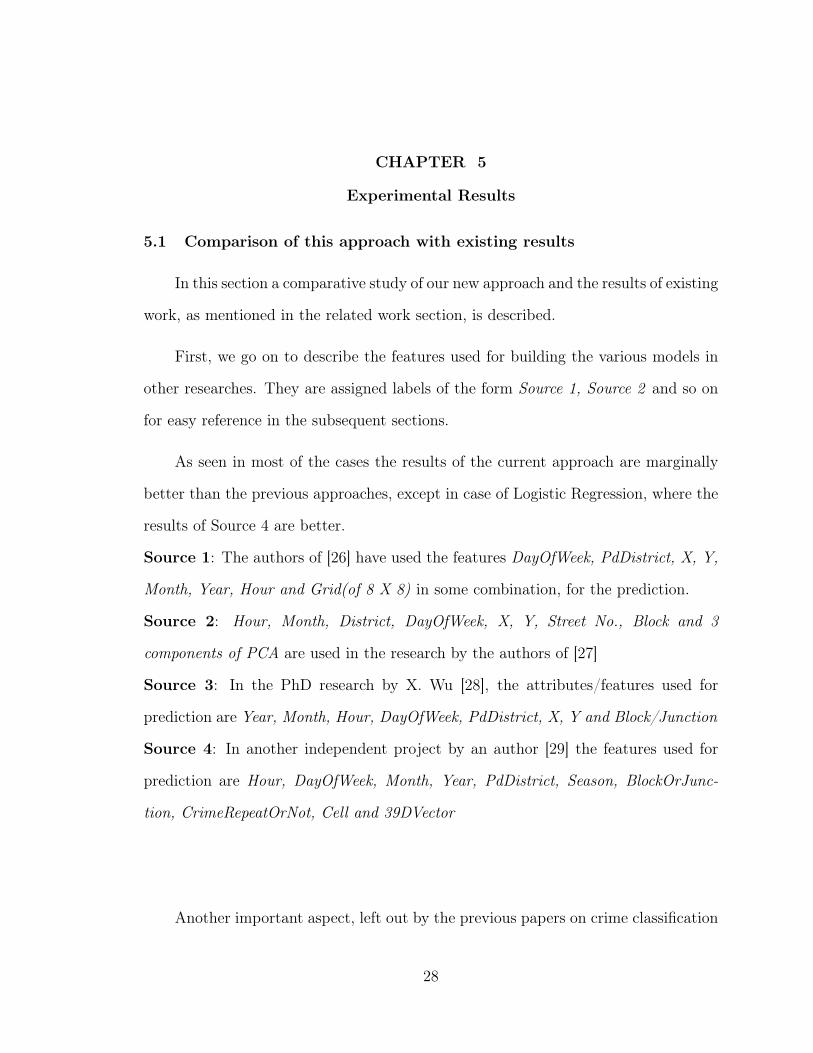
As seen in most of the cases the results of the current approach are marginally

better than the previous approaches, except in case of Logistic Regression, where the

results of Source 4 are better.

Source 1: The authors of [26] have used the features DayOfWeek, PdDistrict, X, Y,

Month, Year, Hour and Grid(of 8 X 8) in some combination, for the prediction.

Source 2: Hour, Month, District, DayOfWeek, X, Y, Street No., Block and 3

components of PCA are used in the research by the authors of [27]

Source 3: In the PhD research by X. Wu [28], the attributes/features used for

prediction are Year, Month, Hour, DayOfWeek, PdDistrict, X, Y and Block/Junction

Source 4: In another independent project by an author [29] the features used for

prediction are Hour, DayOfWeek, Month, Year, PdDistrict, Season, BlockOrJunc-

tion, CrimeRepeatOrNot, Cell and 39DVector

Another important aspect, left out by the previous papers on crime classification

28

Algorithm My Results Source 1 Source 2 Source 3 Source 4

Random Forest 2.2760 2.496 2.366 2.45 -

Naive Bayes 2.5008 2.5821 2.6492 - -

Logistic Regression 2.4042 2.5516 - - 2.365

KNN 2.4634 - 2.621 25.17 -

Decision Tree 2.3928 2.508 - - -

Table 3: Results of Experiments

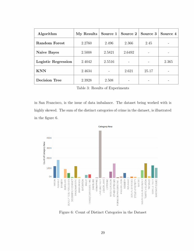
in San Francisco, is the issue of data imbalance. The dataset being worked with is

highly skewed. The sum of the distinct categories of crime in the dataset, is illustrated

in the figure 6.

Figure 6: Count of Distinct Categories in the Dataset

29

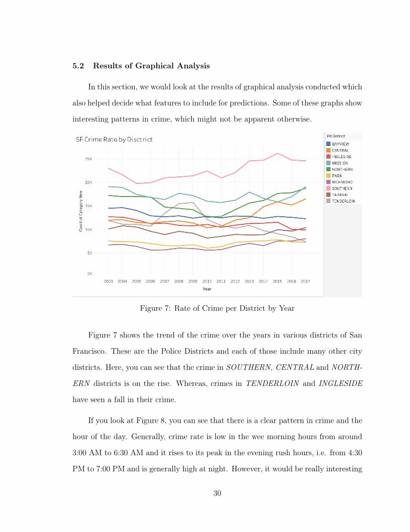
5.2 Results of Graphical Analysis

In this section, we would look at the results of graphical analysis conducted which

also helped decide what features to include for predictions. Some of these graphs show

interesting patterns in crime, which might not be apparent otherwise.

Figure 7: Rate of Crime per District by Year

Figure 7 shows the trend of the crime over the years in various districts of San

Francisco. These are the Police Districts and each of those include many other city

districts. Here, you can see that the crime in SOUTHERN, CENTRAL and NORTH-

ERN districts is on the rise. Whereas, crimes in TENDERLOIN and INGLESIDE

have seen a fall in their crime.

If you look at Figure 8, you can see that there is a clear pattern in crime and the

hour of the day. Generally, crime rate is low in the wee morning hours from around

3:00 AM to 6:30 AM and it rises to its peak in the evening rush hours, i.e. from 4:30

PM to 7:00 PM and is generally high at night. However, it would be really interesting

30

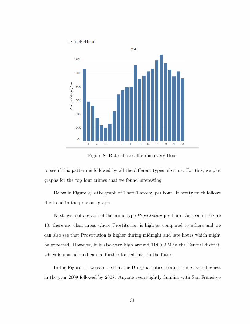
Figure 8: Rate of overall crime every Hour

to see if this pattern is followed by all the different types of crime. For this, we plot

graphs for the top four crimes that we found interesting.

Below in Figure 9, is the graph of Theft/Larceny per hour. It pretty much follows

the trend in the previous graph.

Next, we plot a graph of the crime type Prostitution per hour. As seen in Figure

10, there are clear areas where Prostitution is high as compared to others and we

can also see that Prostitution is higher during midnight and late hours which might

be expected. However, it is also very high around 11:00 AM in the Central district,

which is unusual and can be further looked into, in the future.

In the Figure 11, we can see that the Drug/narcotics related crimes were highest

in the year 2009 followed by 2008. Anyone even slightly familiar with San Francisco

31

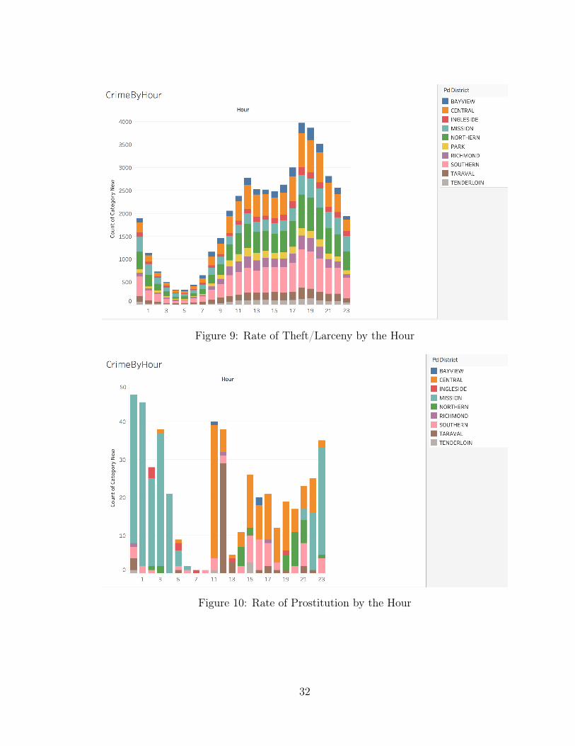
Figure 9: Rate of Theft/Larceny by the Hour

Figure 10: Rate of Prostitution by the Hour

32

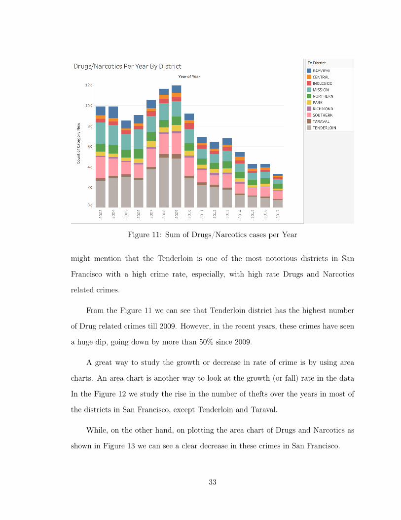
Figure 11: Sum of Drugs/Narcotics cases per Year

might mention that the Tenderloin is one of the most notorious districts in San

Francisco with a high crime rate, especially, with high rate Drugs and Narcotics

related crimes.

From the Figure 11 we can see that Tenderloin district has the highest number

of Drug related crimes till 2009. However, in the recent years, these crimes have seen

a huge dip, going down by more than 50% since 2009.

A great way to study the growth or decrease in rate of crime is by using area

charts. An area chart is another way to look at the growth (or fall) rate in the data

In the Figure 12 we study the rise in the number of thefts over the years in most of

the districts in San Francisco, except Tenderloin and Taraval.

While, on the other hand, on plotting the area chart of Drugs and Narcotics as

shown in Figure 13 we can see a clear decrease in these crimes in San Francisco.

33

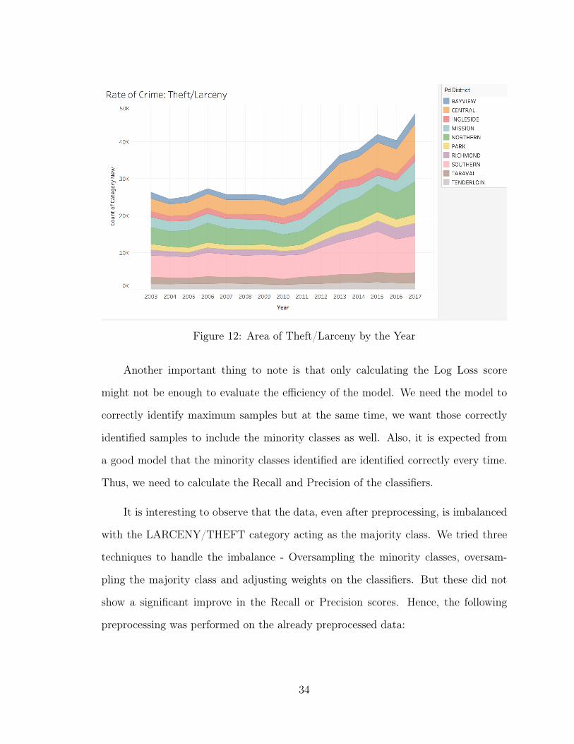
Figure 12: Area of Theft/Larceny by the Year

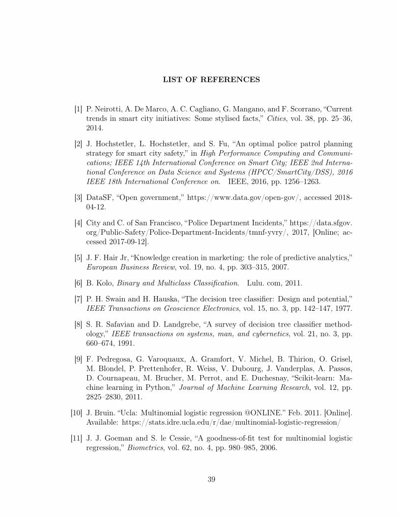
Another important thing to note is that only calculating the Log Loss score

might not be enough to evaluate the efficiency of the model. We need the model to

correctly identify maximum samples but at the same time, we want those correctly

identified samples to include the minority classes as well. Also, it is expected from

a good model that the minority classes identified are identified correctly every time.

Thus, we need to calculate the Recall and Precision of the classifiers.

It is interesting to observe that the data, even after preprocessing, is imbalanced

with the LARCENY/THEFT category acting as the majority class. We tried three

techniques to handle the imbalance - Oversampling the minority classes, oversam-

pling the majority class and adjusting weights on the classifiers. But these did not

show a significant improve in the Recall or Precision scores. Hence, the following

preprocessing was performed on the already preprocessed data:

34

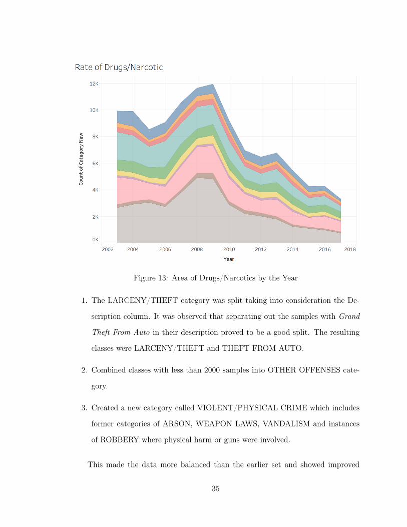
Figure 13: Area of Drugs/Narcotics by the Year

1. The LARCENY/THEFT category was split taking into consideration the De-

scription column. It was observed that separating out the samples with Grand

Theft From Auto in their description proved to be a good split. The resulting

classes were LARCENY/THEFT and THEFT FROM AUTO.

2. Combined classes with less than 2000 samples into OTHER OFFENSES cate-

gory.

3. Created a new category called VIOLENT/PHYSICAL CRIME which includes

former categories of ARSON, WEAPON LAWS, VANDALISM and instances

of ROBBERY where physical harm or guns were involved.

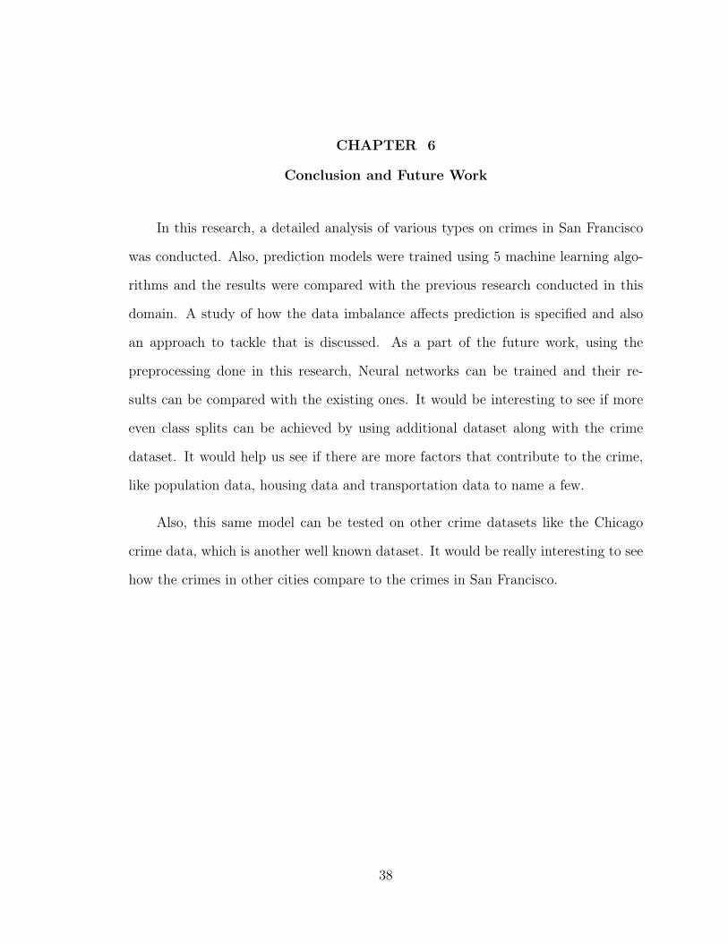
This made the data more balanced than the earlier set and showed improved

35

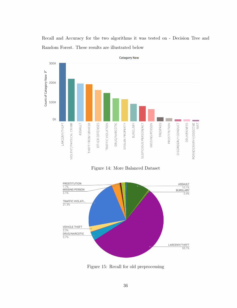
Recall and Accuracy for the two algorithms it was tested on - Decision Tree and

Random Forest. These results are illustrated below

Figure 14: More Balanced Dataset

Figure 15: Recall for old preprocessing

36

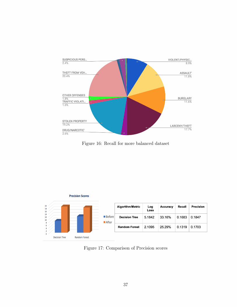
Figure 16: Recall for more balanced dataset

Figure 17: Comparison of Precision scores

37

CHAPTER 6

Conclusion and Future Work

In this research, a detailed analysis of various types on crimes in San Francisco

was conducted. Also, prediction models were trained using 5 machine learning algo-

rithms and the results were compared with the previous research conducted in this

domain. A study of how the data imbalance affects prediction is specified and also

an approach to tackle that is discussed. As a part of the future work, using the

preprocessing done in this research, Neural networks can be trained and their re-

sults can be compared with the existing ones. It would be interesting to see if more

even class splits can be achieved by using additional dataset along with the crime

dataset. It would help us see if there are more factors that contribute to the crime,

like population data, housing data and transportation data to name a few.

Also, this same model can be tested on other crime datasets like the Chicago

crime data, which is another well known dataset. It would be really interesting to see

how the crimes in other cities compare to the crimes in San Francisco.

38

LIST OF REFERENCES

[1] P. Neirotti, A. De Marco, A. C. Cagliano, G. Mangano, and F. Scorrano, “Currenttrends in smart city initiatives: Some stylised facts,” Cities, vol. 38, pp. 25–36,2014.

[2] J. Hochstetler, L. Hochstetler, and S. Fu, “An optimal police patrol planningstrategy for smart city safety,” in High Performance Computing and Communi-cations; IEEE 14th International Conference on Smart City; IEEE 2nd Interna-tional Conference on Data Science and Systems (HPCC/SmartCity/DSS), 2016IEEE 18th International Conference on. IEEE, 2016, pp. 1256–1263.

[3] DataSF, “Open government,” https://www.data.gov/open-gov/, accessed 2018-04-12.

[4] City and C. of San Francisco, “Police Department Incidents,” https://data.sfgov.org/Public-Safety/Police-Department-Incidents/tmnf-yvry/, 2017, [Online; ac-cessed 2017-09-12].

[5] J. F. Hair Jr, “Knowledge creation in marketing: the role of predictive analytics,”European Business Review, vol. 19, no. 4, pp. 303–315, 2007.

[6] B. Kolo, Binary and Multiclass Classification. Lulu. com, 2011.

[7] P. H. Swain and H. Hauska, “The decision tree classifier: Design and potential,”IEEE Transactions on Geoscience Electronics, vol. 15, no. 3, pp. 142–147, 1977.

[8] S. R. Safavian and D. Landgrebe, “A survey of decision tree classifier method-ology,” IEEE transactions on systems, man, and cybernetics, vol. 21, no. 3, pp.660–674, 1991.

[9] F. Pedregosa, G. Varoquaux, A. Gramfort, V. Michel, B. Thirion, O. Grisel,M. Blondel, P. Prettenhofer, R. Weiss, V. Dubourg, J. Vanderplas, A. Passos,D. Cournapeau, M. Brucher, M. Perrot, and E. Duchesnay, “Scikit-learn: Ma-chine learning in Python,” Journal of Machine Learning Research, vol. 12, pp.2825–2830, 2011.

[10] J. Bruin. “Ucla: Multinomial logistic regression @ONLINE.” Feb. 2011. [Online].Available: https://stats.idre.ucla.edu/r/dae/multinomial-logistic-regression/

[11] J. J. Goeman and S. le Cessie, “A goodness-of-fit test for multinomial logisticregression,” Biometrics, vol. 62, no. 4, pp. 980–985, 2006.

39

[12] D. Jurafsky and J. H. Martin, “Speech and language processing: An introductionto natural language processing, computational linguistics, and speech recogni-tion,” pp. 1–1024, 2009.

[13] A. Liaw, M. Wiener, et al., “Classification and regression by randomforest,” Rnews, vol. 2, no. 3, pp. 18–22, 2002.

[14] F. Livingston, “Implementation of breiman’s random forest machine learningalgorithm,” ECE591Q Machine Learning Journal Paper, 2005.

[15] E. Andrew B. Collier, “Making Sense of Logarithmic Loss,” http://www.exegetic.biz/blog/2015/12/making-sense-logarithmic-loss/, 2015, [Online; accessed 2018-19-04].

[16] L. Buitinck, G. Louppe, M. Blondel, F. Pedregosa, A. Mueller, O. Grisel, V. Nic-ulae, P. Prettenhofer, A. Gramfort, J. Grobler, R. Layton, J. VanderPlas, A. Joly,B. Holt, and G. Varoquaux, “API design for machine learning software: experi-ences from the scikit-learn project,” in ECML PKDD Workshop: Languages forData Mining and Machine Learning, 2013, pp. 108–122.

[17] D. Hsu, M. Moh, and T.-S. Moh, “Mining frequency of drug side effects over alarge twitter dataset using apache spark,” in Proceedings of the 2017 IEEE/ACMInternational Conference on Advances in Social Networks Analysis and Mining2017. ACM, 2017, pp. 915–924.

[18] A. Spark, “Apache Spark Cluster Overview,” https://spark.apache.org/docs/latest/cluster-overview.html, [Online; accessed 2018-19-04].

[19] S. J. Linning, M. A. Andresen, and P. J. Brantingham, “Crime seasonality: Ex-amining the temporal fluctuations of property crime in cities with varying cli-mates,” International journal of offender therapy and comparative criminology,vol. 61, no. 16, pp. 1866–1891, 2017.

[20] T. Almanie, R. Mirza, and E. Lor, “Crime prediction based on crime types andusing spatial and temporal criminal hotspots,” arXiv preprint arXiv:1508.02050,2015.

[21] L. Venturini and E. Baralis, “A spectral analysis of crimes in san francisco,” inProceedings of the 2nd ACM SIGSPATIAL Workshop on Smart Cities and UrbanAnalytics. ACM, 2016, p. 4.

[22] N. R. Lomb, “Least-squares frequency analysis of unequally spaced data,” Astro-physics and space science, vol. 39, no. 2, pp. 447–462, 1976.

[23] T. T. Nguyen, A. Hatua, and A. H. Sung, “Building a learning machine classifierwith inadequate data for crime prediction,” Journal of Advances in InformationTechnology Vol, vol. 8, no. 2, 2017.

40

[24] D. Ghosh, S. Chun, B. Shafiq, and N. R. Adam, “Big data-based smart city plat-form: Real-time crime analysis,” in Proceedings of the 17th International DigitalGovernment Research Conference on Digital Government Research. ACM, 2016,pp. 58–66.

[25] E. Eftelioglu, S. Shekhar, and X. Tang, “Crime hotspot detection: A computa-tional perspective,” in Data Mining Trends and Applications in Criminal Scienceand Investigations. IGI Global, 2016, pp. 82–111.

[26] S. T. Ang, W. Wang, and S. Chyou, “San francisco crime classification,” Univer-sity of California San Diego, 2015.

[27] Y. Abouelnaga, “San francisco crime classification,” arXiv preprintarXiv:1607.03626, 2016.

[28] X. Wu, “An informative and predictive analysis of the san francisco police de-partment crime data,” Ph.D. dissertation, UCLA, 2016.

[29] G. H. Larios, “Case study report: San francisco crime classification,” https://gabrielahrlr.github.io/personal-website/docs/SF_crimes.pdf, 2016, [Online; ac-cessed 2018-24-04].

41