Evolution and the Theory of Games

J. Theoret. Biol. (1961) I, 382-403

Evolution and the Theory of Games

R. C. LEWONTIN

Dept. of Biology, University of Rochester, Rochester, New York

(Received 6 March 1961)

The shortcomings of present population genetic theory are discussed as they pertain to problems of speciation, extinction and the evolution of genetic systems. It is suggested that the modern theory of games may be useful in finding exact answers to problems of evolution not covered by the theory of population genetics. An outline of relevant topics in the theory of games is given. It is suggested that the most pertinent utility measure for a population is its one-generation probability of survival and that a strategy or a mixture of strategies corresponding to a maximin strategy will be found in natural populations. These notions are applied to a population segregating for two alleles with different norms of reaction in different environments. For the mode1 chosen the optimal strategy is found to be homozygosis for different alleles in different populations due either to inbreeding or genetic isolation. A segregating polymorphism in such populations would be a detriment to the species, although the heterozygotes are more constant in fitness.

The Present State of Evolutionary Theory

The modern theory of evolutionary dynamics is founded upon the remarkable insights of R. A. Fisher and Sewall Wright and set forth in the loci classici “The Genetical Theory of Natural Selection” (1930) and

“Evolution in Mendelian Populations” (193 I). By the time of the publica- tion of Wright’s paper in 1931 all of the theory of population genetics, as it is presently understood, was established. It is a sign of the extraordinary power of these early formulations, that nothing of equal significance has been added to the theory of population genetics in the thirty years that have passed since that time. Yet we cannot take this period to mean that we now have an adequate theory of evolutionary dynamics. On the con- trary, the theory of population genetics, as complete as it may be in itself, fails to deal with many problems of primary importance for an under- standing of evolution.

The structure of population genetic theory may be briefly summed up as follows, Given an assemblage of organisms defined as a genetic population, given the breeding structure of that population, the frequencies of various

alleles, the phenotypes of the various genotypes, the statistical nature of 382

EVOLUTION AND THE THEORY OF GAMES 383

the environment, the amounts of recombination between loci, the mutation rates and migration rates, then it is possible in theory to predict the genetic structure of the population at some future time. Such a prediction may be unambiguous, as in deterministic theories, or else a statement about the probability that the population will be in a given state, as in stochastic theories. But whether deterministic or stochastic, these theories are restricted to predictions about changes in the genotype composition of a given population with given forces determining the changes of gene frequency. Population genetics is not genetics of populations, but genetics in populations. It is the genetics of phyletic change, of the gradual replace- ment of one set of alleles by another within a phylad genetically continuous in time and space.

A complete, theory of evolution, however, must address itself to other problems besides those of phyletic change within populations. Despite the great amount written about speciation, there is as yet no mathematical theory of species formation nor are there rigorous formulations of the process of phyletic extinction. Yet speciation and extinction stand together with phyletic change as the main features of evolution. What theory will account for the origin and rise of individual homeostasis as an evolutionary mode ? Have we a theory of the waxings and wanings of sexuality, of the variations in amount of recombination, of rates of mutation, of all those factors which enter as parameters in the formulations of population genetics? Except for intuitive theories, the answer to these questions remains, “No”. For example, the genetic conditions which favor species formation have recently been discussed by Mayr (1959), Carson (1959)

and Wallace (1959) and each, while arguing cogently, comes to a different conclusion. Another example is the problem of the relative amounts of genetic variability to be expected in marginal populations as opposed to central populations. Dobzhansky (1955) and Carson (1955, 1959) hold essentially opposing views on this question and a third, closer to that of Carson, is given by Lewontin (1957). It is not the purpose of this introduction to examine these questions in detail, but rather to point out the diversity of conclusions arrived at by evolutionists. This diversity arises not from disagreement about facts, but from the lack of a rigorous theoretical framework for solving problems in which characteristics of a population as a whole are the basic parameters. Disagreements of this nature do not arise in population genetics, sensu strictu, because of the great power of population genetic theory.

Specification of the Problem

The problem that faces the theorist of evolution then, is to account for differences between populations and species in their degrees of

384 R. C. LEWONTIN

inbreeding and outbreeding, in amount of recombination, in mutation rates, in degree of somatic plasticity as opposed to genetic flexibility, in dispersal rates, in short, in all those characteristics of populations which govern adaptation. The solution of this problem requires two things. First, some measure of the success or degree of adaptation of a population must be specified. Thus, it must be possible, in some unambiguous way, to state that a population with free recombination has a success value X, while one with no recombination has a success value Y, when all other conditions are specified. This is analogous to the measure of Darwinian fitness, or adaptive value of a genotype, which is defined in population genetics as the relative probability that an egg of that genotype will produce an egg in the next generation.

Second, given a measure of success or adaptation, it must be possible to construct an adaptive calculus which will predict the kinds of genetic structures that populations will evolve under given environmental conditions. In population genetics the adaptive calculus is built upon the basic rules of mendelism and the mathematical techniques are the standard ones of algebra, the calculus and the theory of stochastic processes. When the population as a whole is the unit of enquiry, however, some new basis must be found. Although the results of population genetic theory will play some part, it is possible that the calculus of population evolution will be a radically different mathematical technique, perhaps one that is yet to be invented by mathematicians. It is the purpose of this article to propose one possible mode of attack, provided by the theory of games developed by von Neuman and Morgenstern (1944).

Outlines of a Relevant Game Theory

Game theory is not well known to biologists so that some of its general outlines must be presented here. What follows is not a strictly conventional description of the theory of games and some new notions have been introduced, There are several reasons for this. First, game theory has its roots in the social sciences and therefore much of the terminology carries connotations of purposive behavior. The notions of a “player”, “choosing a strategy”, “preferring an outcome” are foreign to modern mechanistic biology and so must be either discarded or very carefully redefined. Second, some of the axioms of game theory flow directly from ideas of purposive behavior. The very definition of the important concept of the “utility” of an outcome depends tautologically on human preferences. Third, many of the criteria of optimum solutions to game theoretical problems are inapplicable because they appeal intuitively to human preferences. This last objection is of some help to the evolutionist, because he may reject many of the suggested solutions and narrow down the field of


choice to what may be considered evolutionarily important solutions. Finally, the processes of evolution are eufhciently different from human choice processes, that some new ideas must be introduced into the classical picture of game theory.

In what follows, any divergence from the standard theory of games will be noted when this divergence is significant.

A GAME IN EXTENSIVE FORM

We may imagine one or more players engaged in a game according to a set of rules. Besides the actions of the player or players there are physical conditions, say the order of the cards in a shuffled pack, which determine the events of the game. The game proceeds in discrete steps called mwes and at each move one or more players performs an act A; from a denumer- able set of available acts { A ). The model of discrete moves and acts simplifies the description of the game, but a further extension to tinte- contimous games and games in which ( A > is a continuous set can and must be made for some biological problems.

In the most general game the set of available acts { A } may be different for each player and moreover may change at each move in a way dependent upon the act performed at a previous move. For example, in bridge the cards available to a player in any given trick are determined by the cards he has played in previous tricks.

At each move the physical conditions extraneous to the players’ acts may also change. The set of states of nature { N > is formally identical with asetofacts,(A) d an in this sense nature may be considered simply another player with its own set of possible acts.

After each move has been completed there may be a result which we shall call a local outcome (this term does not exist in standard game theory) which depends upon the Act 4 performed by each player and the state of nature Ni, Whether or not a local outcome does result after every move depends upon the definition of an outcome for each game. In bridge again, the taking of a trick is a local outcome and this will occur only after four moves, rather than one. In addition to local outcomes there will be a terminal outcome which may be either a special local outcome signaling the end of the game or else some function of the local outcome which is not itself a local outcome. In bridge the terminal outcome is the total number of tricks taken by a pair of players, or more generally a function of that total and the total contracted for by the bidding. It is important to notice that the local outcome has an intricate relationship with previous and future outcomes and acts. The set of local outcomes ( o }1 at any time may depend upon past local outcomes, erm though those part outcomes do not

12.. 2s

386 R. C. LEWONTIN

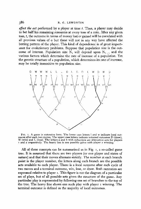
e#ecl the act performed by a player at time t. Thus, a player may decide to bet half his remaining resources at every toss of a coin. After any given toss, t, the outcome in terms of money lost or gained will be correlated with all previous values of o but these will not in any way have affected the betting pattern of the player. This kind of dependence is of great importance for evolutionary problems. Suppose that population size is the outcome of interest. Population size N, will depend upon N, _ 1 and the various factors which determine the rate of increase of a population. Yet the genetic structure of a population, which determines its rate of increase, may be totally insensitive to population size.

DWWWLLLDLGDL WDWD 1. w w w 1. 1.1 w I w w l. w i w 1

FIG. I. A game in extensive form. The lower case letters 1 and w indicate local outcomes after each two moves. The upper case letters indicate terminal outcomes D (draw), W (win) and L (lose). The letters a and b with subscripts are alternative acts for players I and z respectively. The heavy line is one possible game with player I winning.

All of these concepts can be summarized as in Fig. I, a so-called game tree. It is assumed that there are two players (or one player and states of nature) and that their moves alternate strictly. The number at each branch point is the player number, the letters along each branch are the possible acts available to each player. There is a local outcome after each cycle of two moves and a terminal outcome, win, lose, or draw. Both outcomes are expressed relative to player I. This figure is not the diagram of a particular set of plays, but of all possible sets given the structure of the game. Any particular play is represented by following one set of branches to the top of the tree. The heavy line shows one such play with player I winning. The terminal outcome is defined as the majority of local outcomes.


THE NORMAL FORM OF A GAME

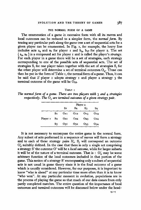
The enumeration of a game in extensive form with all its moves and local outcomes can be reduced to a simpler form, the nurmul form. By tracing any particular path along the game tree a set of sequential acts for a given player can be enumerated. In Fig. I, for example, the heavy line includes acts a, and aQ for player I and b,, bi7 for player 2. The set ( aa, as } is a compound act for player I and is called the player’s strategy. For each player in a game there will be a set of strategies, each strategy corresponding to one of the possible sets of sequential acts. The set of strategies Eli for one player taken together with the set of strategies Sj for the other player will determine a set of terminal outcomes 0,. These can then be put in the form of Table I, the normal form of a game. Thus, it can be said that if player I adopts strategy I and player 2 strategy 3 the terminal outcome of the game will be 01s.

TABLE I

The normal form of a game. There are two players with 3 and 4 strategies respectively. The Oij are terminal outcomes of a given strategy pair.

Player 2

SI sz s3 s4

SI 011 0x2 013 014

Player I Sz 021 022 023 024

S3 031 032 033 034

It is not necessary to encompass the entire game in the normal form. Any subset of acts performed in a sequence of moves will form a strategy and to each of these strategy pairs Sj, Sj will correspond an outcome 0; suitably defined. In the case that there is only a single act comprising a strategy S’ the outcome 0’ will be a local outcome, while for larger subsets it will be of the nature of a terminal outcome. That is : 0; may be some arbitrary function of the local outcomes included in that portion of the game. This notion of a strategy S’ encompassing only a subset of sequential acts is not usual in game theory since it is the final outcome of a game which is usually considered. However, for our purposes, it is important to know “who is ahead” at any particular time more often than it is to know “who won”. At any particular moment in evolution, populations are in the process of playing the game so that much of our data comes from only partly completed matches. The entire question of the importance of local outcomes and terminal outcomes will be discussed below under the head-

388 R. C. LEWONTIN

ing of pay-off functions. What is of importance here is that the normal form allows a game extended in time to be represented as a single step game, the analysis of which is much simpler. The complexity of the model has not been lessened by this procedure, however. In place of a series of simple acts and local outcomes we have a smaller set of complex strategies, and terminal outcomes.

The Game Against Nature

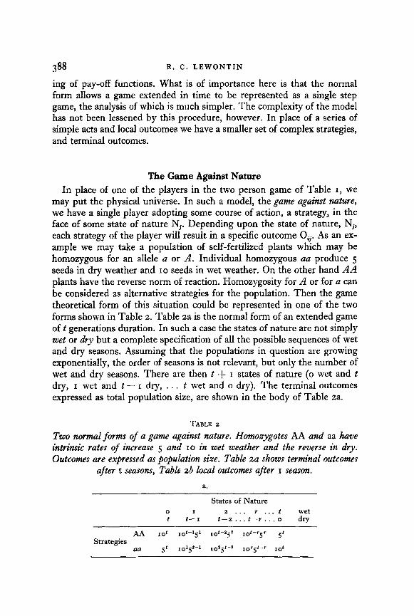
In place of one of the players in the two person game of Table I, we may put the physical universe. In such a model, the game against nature, we have a single player adopting some course of action, a strategy, in the face of some state of nature Nj. Depending upon the state of nature, Nj, each strategy of the player will result in a specific outcome 0,. As an example we may take a population of self-fertilized plants which may be homozygous for an allele a or A. Individual homozygous au produce 5 seeds in dry weather and IO seeds in wet weather. On the other hand AA plants have the reverse norm of reaction. Homozygosity for A or for a can be considered as alternative strategies for the population. Then the game theoretical form of this situation could be represented in one of the two forms shown in Table 2. Table 2a is the normal form of an extended game oft generations duration. In such a case the states of nature are not simply wet or dry but a complete specification of all the possible sequences of wet and dry seasons. Assuming that the populations in question are growing exponentially, the order of seasons is not relevant, but only the number of wet and dry seasons. There are then t + I states of nature (o wet and t dry, I wet and t - I dry, . , . t wet and o dry). The terminal outcomes expressed as total population size, are shown in the body of Table 2a.

TABLE z

Two normal forms of a game against nature. Homozygotes AA and aa have intrinsic rates of increase 5 and IO in wet weather and the reverse in dry. Outcomes are expressed us population size. Table 2u shows terminal outcomes

ufter t seasons, Table zb local outcomes ufter I season.

a.

States of Nature 0 I 2 . . . Y . . . t wet t t-1 t-2.. . t-r.. . 0 dry

AA 1ot 1ot-151 rot-252 x0-5 5’ Strategies

aa .5t IO’+- ,oy-* IO’+ 101

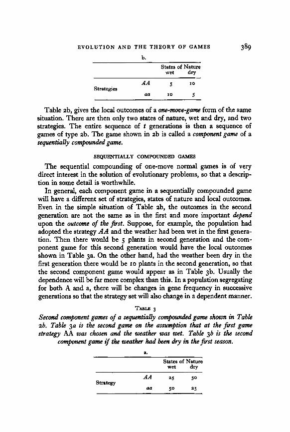
EVOLUTION AND THE THEORY OF GAMES 389 b.

States of Nature wet dry

AA 5 IO Strategies

aa 10 5

Table zb, gives the local outcomes of a one-move-game form of the same situation. There are then only two states of nature, wet and dry, and two strategies. The entire sequence of t generations is then a sequence of games of type zb. The game shown in zb is called a component game of a sequentially compounded game.

SEQURNTIALLY COMPOUNDED GAMES

The sequential compounding of one-move normal games is of very direct interest in the solution of evolutionary problems, so that a description in some detail is worthwhile.

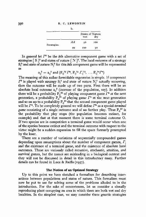
In general, each component game in a sequentially compounded game will have a different set of strategies, states of nature and local outcomes. Even in the simple situation of Table zb, the outcomes in the second generation are not the same as in the first and more important depend upon the outcome of the fist. Suppose, for example, the population had adopted the strategy AA and the weather had been wet in the first generation. Then there would be 5 plants in second generation and the component game for this second generation would have the local outcomes shown in Table ga. On the other hand, had the weather been dry in the first generation there would be IO plants in the second generation, so that the second component game would appear as in Table 3b. Usually the dependence will be far more complex than this. In a population segregating for both A and a, there will be changes in gene frequency in successive generations so that the strategy set will also change in a dependent manner.

TABLE 3

Second component games of a sequentMlly compounded game shown in Table zb. Table 3a is the second game on the assurtrption that at the first game strategy AA was chosen and the weather was wet. Table 3b is the second

component game if the weather had been dty in the first season. a.

Strategy


AA 25 so

aa so 25

390 R. C. LEWONTIN

b.

Strategies AA

aa


-

50 100

100 50

In general let rk be the Kth alternative component game with a set of strategies ( S >” and states of nature { N >“. The local outcome of a strategy St and state of nature NF for this Kth component game will be represented as

oijk = aijk and (Pijko To, Pijkl rijkl, . . . Pijknm)

The meaning of this rather formidable expression is simple. If component TX is played with strategy St and state of nature Njk actually occurring, then the outcome will be made up of two parts. First there will be an absolute local outcome aijk (increase of the population, say). In addition there will be a probability P$” of playing component game To at the next generation, a probability Pijkl of playing game ri at the next generation and so on up to a probability Pijk” that the second component game played will be r”. To be completely general we will define r” as a special terminal game consisting of a single outcome and of no further play. Thus Pijko is the probability that play stops (the population becomes extinct, for example) and that at that moment there is some terminal outcome 0. If two species are in competition a terminal game would occur when one of the species became extinct and the terminal outcome with respect to the victor might be a sudden expansion to fill the space formerly preempted by the loser.

There are a number of variations of sequentially compounded games depending upon assumptions about the number of component games, r, and the existence of a terminal game, and the existence of absolute local outcomes. These are variously called recursive, stochastic, attrition, and survival games, but the names are misleading in a biological context and they will not be discussed in detail in this introductory essay. Further details can be found in Lute & Raiffa (1957).

The Notion of an Optimal Strategy

Up to this point we have sketched a formalism for describing inter- actions between populations and states of nature. This formalism must now be put to use for solving some of the problems alluded to in the introduction. For the sake of concreteness, let us consider a clonally reproducing plant occupying an area in which there are both wet and dry localities. In the simplest case, we may consider three genetic strategies


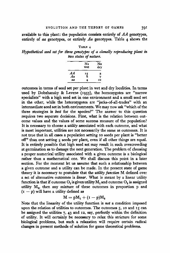
available to this plant: the population consists entirely of AA genotypes, entirely of aa genotypes, or entirely Aa genotypes. Table 4 shows the

TABLB 4

Hypothetical seed set for three genotypes of a clonally reproducing plant in two states of nature.

AA Aa aa

NI N2 wet dry

15 8 ; 4 IO

outcomes in terms of seed set per plant in wet and dry localities. In terms used by Dobzhansky & Levene (rgss), the homozygotes are “narrow specialists” with a high seed set in one environment and a small seed set in the other, while the heterozygotes are “jacks-of-all-trades” with an intermediate seed set in both environments. We may now ask “which of the three strategies is best for the species?” The answer to this question requires two separate decisions. First, what is the relation between outcome values and the values of some success measure of the population? It is necessary to choose a utiZity associated with each outcome, and what is most important, utilities are not necessarily the same as outcomes. It is not true that in all cases a population setting IO seeds per plant is “better off” than one setting 5 seeds per plant, even if all other things are equal. It is entirely possible that high seed set may result in such overcrowding at germination as to damage the next generation. The problem of choosing a proper numerical utility associated with a given outcome is a biological rather than a mathematical one. We shall discuss this point in a later section. For the moment let us assume that such a relationship between a given outcome and a utility can be made. In the present state of game theory it is necessary to postulate that the utility function M defined over a set of alternative outcomes is &rem. What is meant by a linear utility function is that if outcome 0, is given utility M, and outcome 0, is assigned utility M,, then any mixture of these outcomes in proportion p and (I - p) will have a utility defined as

M=pM,+(1 -pp)M, Note that the linearity of the utility function is not a condition imposed upon the relation of utilities to outcomes. The outcomes 5, IO and 15 can be assigned the utilities 7, 43 and 12, say, perfectly within the definition of utility. It will certainly be necessary to relax thii stricture for some biological problems, but such a relaxation will require certain radical changes in present methods of solution for game theoretical problems.

392 R. C. LEWONTIN

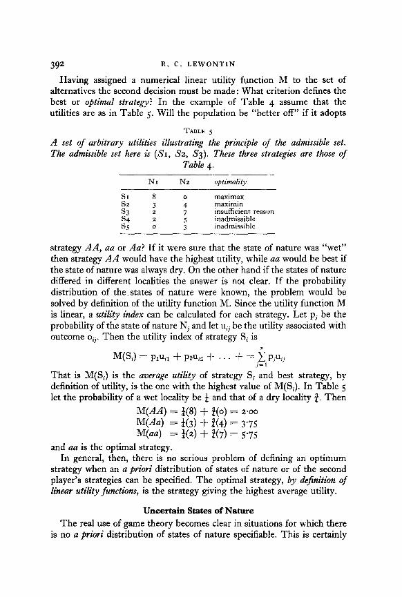
Having assigned a numerical linear utility function M to the set of alternatives the second decision must be made: What criterion defines the best or optimal strategy? In the example of Table 4 assume that the utilities are as in Table 5. Will the population be “better off” if it adopts

TABLE 5

A set of arbitrary utilities illustrating the principle of the admissible set. The admissible set here is (SI, S2, S3). These three strategies are those of

Table 4.

NI Nz optimality

8 0 maximax z: 3 maximin s3 2 ; insufficient reason

2 inadmissible z:

5 0 3 inadmissible

strategy AA, au or Au? If it were sure that the state of nature was “wet” then strategy AA would have the highest utility, while aa would be best if the state of nature was always dry. On the other hand if the states of nature differed in different localities the answer is not clear. If the probability distribution of the, states of nature were known, the problem would be solved by definition of the utility function M. Since the utility function M is linear, a utility index can be calculated for each strategy. Let pj be the probability of the state of nature Nj and let uij be the utility associated with outcome oij. Then the utility index of strategy Si is

II M(S,) = PlUil + PzU~, $- . . . f = C PjUij

j-1

That is M(S) is the average utility of strategy Si and best strategy, by definition of utility, is the one with the highest value of M(S). In Table 5 let the probability of a wet locality be a and that of a dry locality Q. Then

M(AA) = a(S) + g(o) = 2.00

WA4 = t(3) + j(4) = 3’7.5 Mb4 = 6(a) + R7) = 5’75

and au is the optimal strategy. In general, then, there is no serious problem of defining an optimum

strategy when an a priori distribution of states of nature or of the second player’s strategies can be specified. The optimal strategy, by de$nition of linear utility functions, is the strategy giving the highest average utility.

Uncertain States of Nature The real use of game theory becomes clear in situations for which there

is no a priori distribution of states of nature specifiable. This is certainly


the usual, if not universal, case. The empirical definition of probability depends upon large (virtually infinite) numbers of repetitions of given events. In fact the events of nature are so complex that they are seldom if ever repeated in the lifetime of a population or species. With respect to living organisms nature is capricious rather than random. What is the probability of a flood, a succession of dry years, of competition with a new invading species of a particular sort? In general such probabilities cannot be specified (or even defined). Since probabilities cannot be specified for different states of nature, no average utility can be calculated so that other criteria of optimality are needed.

(i) Admhabk strategies Following the notation of Lute & Raiffa (1957) we will say that for two

strategies S and S’ (a) S is equiwaht to S’(S N S’) if they have identical utilities for every

state of nature. (b) S strongly dominates S’( S > S’) if the utilities of S are greater than

for S’ for every state of nature. (c) S weakZy dominates S’(S 2 S’) if S has a higher utility than S’ for at

least one state of nature and never has a lower utility than S’. Then the set of admissabk strategies A* is the set such that no strategy S in I weakly dominates any other strategy S’ in A. Whatever criterion of optimality is used, the optimal strategy, must be in the admissible set S. That is, no reasonable criterion of optimality needs to consider a strategy which is not better than a second strategy in some state of nature. Table 5 makes this notion of an admissible set clear. Sg is first rejected because it is strongly dominated by S2, S3 and S4. It is the worst in every state of nature. S4 is also to be rejected because it never has a higher utility than S2 or S3. It is weakly dominated by S2 and Sg. The admissible set is then { S,, S,, S, ) because none of these is weakly dominated by any other.

(ii) The principle of imfidt reason It is sometimes stated as a principle of probability theory that if there is

no a priori reason for assigning specific probabilities to alternative outcomes of a process, they should all be regarded as equally likely. Using such a principle each state of the possible state of nature would be assigned a probability of I In. With this uniform probability distribution an expected utility can be calculated and the optimal strategy determined. The shortcomings of such a criterion are obvious and have been extensively reviewed in the probability literature. One example will suffice to concretixe these objections. If two indistinguishable coins are tossed, there will be three

394 R. C. LEWONTIN

distinguishable outcomes; 2 heads, 2 tails, I head and I tail. The principle of insufficient reason would result in a probability of 4 for each of these events. If the coins have different dates or one were scratched so that they could now be distinguished, there will be four distinguishable outcomes : head, head ; tail, tail ; head, tail ; tail, head ; and each has a probability of $ by insufficient reason, But this is absurd for either the outcome “two heads” has a probability + or a probability 4 and that probability cannot depend upon whether or not the coins are distinguishable.

The counter-intuitive result of the principle of insufficient reason does not, however, rule it out as a method of solution for organisms. It may very well turn out that some species will be found to employ strategies which are optimal under this criterion. If various combinations of temperature, humidity, soil type, other organisms, and so on, really represent distinguishable environments, then over long periods of time only a small fraction of the possible environmental combination will occur and each will occur essentially once. Even lumping environments that are fairly similar as indistinguishable in order to produce a probability distribution will result in a platykurtic function very similar to a uniform distribution. Within the range of extreme environments, then, an a priori uniform distribution of states of nature may provide a close approximation to an optimal strategy. In Table 5 strategy S3 is optimal under this criterion.

(iii) Strategies based on extreme utilities

If no a priori probabilities can be set for the state of nature or for an opponent’s choice of strategy, then the complete set of utilities will not really provide any criterion for optimality. In such a case we turn to the extreme values of utilities, the greatest and the least utility that a given strategy could yield. One such criterion is to choose that strategy whose greatest possible utility under any alternative state of nature is larger than for any other strategy. This is the maximax optimality criterion. In Table 5 strategy SI is the maximax strategy since it has a utility of 8 under one of the states of nature, which is higher than any utility for any other strategy.

Under what conditions may we expect populations to adopt such a one-sided strategy ? One possibility is in a species expanding into an unoccupied territory or a territory in which competitors are relatively weak. In unfavorable environments the invader would have a small rate of increase or perhaps even lose in competition with the incumbent group. In favorable conditions however, there would be an explosive increase in the population and the setting up of many new populations by migration. Even though some of these populations may be extinguished in unfavorable environments, the maximax strategy would assure in the end successful


spread. Such a maximax strategy would be especially important if rapid colonization were important to eventual success since rapid colonization and occupation of the open niche might preclude later successful invasions of other species.

A second optimum strategy based on extreme utilities is one based on a weighting of the maximum and minimum utilities for each strategy. Let a be the weight assigned to the minimum utility of a given strategy m and I - a the weight assigned to the maximum utility of that strategy, Mi. Then an index due to Lute and Raiffe (1957) is

H(a) = am + (I - a)Mi

and that strategy is optimal which has the highest H(a). Such an index makes it possible to take into account both favorable and unfavorable states of nature, but the precise criterion for the choice of a is not clear and seems to imply some a priori distribution of the best and worst conditions. When a = o we have the maximax criterion discussed above. The most interesting and probably the most useful case for evolutionary problems is the assignment of a = I so that only the minimum utility is considered. This leads to the muxima’n criterion of optimality.

THE MAXIMIN CRITERION OF OPTIMALITY

When a is set to unity, that strategy is optimum whose lowest utility over all states of nature is larger than for any other strategy. That is, the population is guaranteed a utility m, at the very least. In Table 5 the maximin strategy is S2. I propose that this maximin strategy is the one which will be found in most cases for reasons which will be discussed below.

For a given matrix of utilities the maximin strategy or strategies can be seen by examination. However, it is possible to increase the security level of a game (the maximin utility) by extending the strategies to include so- called mixed strategies. In a mixed strategy each of the pure strategy alternatives is assigned a probability pi and it is assumed that the game is played over and over again with strategy Si being chosen pi of the time. The biological analogue of a mixed strategy is a species with many local populations, a proportion pi of these populations adopting a strategy Si. The problem is then to find the values of pi which will maximize the security level of the population. There is a simple method of solution of this problem which guurantees an average utility to the population at least as hQh as the maximin pure strategy, irrespecrive of the distribution of states of nature. This procedure, because it applies irrespective of the probability of various states of nature, is a very powerful one.

We shall demonstrate the method of solution graphically, although

396 R. C. LEWONTIN

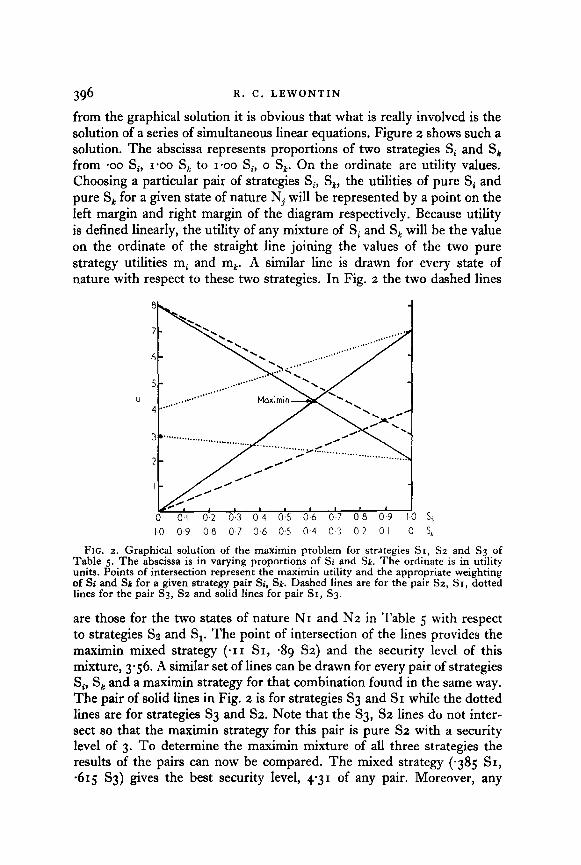
from the graphical solution it is obvious that what is really involved is the solution of a series of simultaneous linear equations. Figure 2 shows such a solution. The abscissa represents proportions of two strategies Si and S, from ‘00 Si, 1.00 S, to 1.00 Si, o S,. On the ordinate are utility values. Choosing a particular pair of strategies Si, S,, the utilities of pure Si and pure S, for a given state of nature Nj will be represented by a point on the left margin and right margin of the diagram respectively. Because utility is defined linearly, the utility of any mixture of Si and S, will be the value on the ordinate of the straight line joining the values of the two pure strategy utilities mi and mk. A similar line is drawn for every state of nature with respect to these two strategies. In Fig. 2 the two dashed lines

u

I 1 I I I 1 0 0.1 0.2 0.3 04 0.5 06 07 08 09 I-O 5,

IO 09 08 07 06 0.5 04 03 02 01 0 5,

FIG. 2. Graphical solution of the maximin problem for strategies SI, Sz and S3 of Table 5. The abscissa is in varying proportions of Si and Sk. The ordinate is in utility units. Points of intersection represent the maximin utility and the appropriate weighting of Si and SE for a given strategy pair Si, Sk. Dashed lines are for the pair Sz, Sr, dotted lines for the pair S3, Sz and solid lines for pair SI, S3.

are those for the two states of nature NI and N2 in Table 5 with respect to strategies Ss and S,. The point of intersection of the lines provides the maximin mixed strategy (*I I SI, 439 SZ) and the security level of this mixture, 3.56. A similar set of lines can be drawn for every pair of strategies S, S, and a maximin strategy for that combination found in the same way. The pair of solid lines in Fig. 2 is for strategies S3 and SI while the dotted lines are for strategies Sg and S2. Note that the S3, S2 lines do not inter- sect so that the maximin strategy for this pair is pure S2 with a security level of 3. To determine the maximin mixture of all three strategies the results of the pairs can now be compared. The mixed strategy (-385 SI, -615 S3) gives the best security level, 4.31 of any pair. Moreover, any


weight given to Sz will lower this security level since substitution of S2 for either SI or S3 always results in a lower security level enen &or& S2 is the pure maximin s&uregy. Thus, no weight should be given this strategy in the optimal strategy mixture and the optimal mixed strategy remains (-385 SI, -615 Sg).

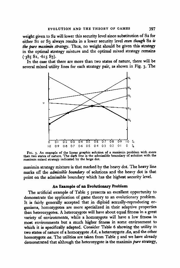
In the case that there are more than two states of nature, there will be several mixed utility lines for each strategy pair, as shown in Fig. 3. The

u

0 0.1 0.2 0.3 0.4 0.5 0.6 0.7 0.8 0.9 I.0 Si I.0 0.9 0.8 0.7 0.6 0.5 0.4 0.3 02 0.1 0 Sk

FIG. 3. An example of the linear graphic solution of a maximin problem with more than two states of nature. The dark line is the admissible boundary of solution with the maximin mixed strategy indicated by the large dot.

maximin strategy mixture is that marked by the heavy dot. The heavy line marks off the admissible boundmy of solutions and the heavy dot is that point on the admissible boundary which has the highest security level.

An Example of an Evolutionary Problem

The artificial example of Table 5 presents an excellent opportunity to demonstrate the application of game theory to an evolutionary problem. It is fairly generally accepted that in diploid sexually-reproducing organisms, homozygotes are more specialized in their adaptive properties than heterozygotes. A heterozygote will have about equal fitness in a great variety of environments, while a homozygote will have a low fitness in most environments but a much higher fitness in some environment to which it is specifically adapted. Consider Table 6 showing the utility in two states of nature of a homozygote AA, a heteroxygote Aa, and the other homozygote ua. The utilities are taken from Table 5 and we have already demonstrated that although the heterozygote is the maximin pure strategy,

398 R. C. LEWONTIN

a greater security level can be obtained by a mixed strategy in which about 40% of the population of the species are homozygous AA and 60% homozygous aa. A population which was heterozygous Aa completely (clonal reproduction) would lower the security level of the entire species. But we may carry the analysis a step further. Nothing has been said about a polymorphic population in which AA, Aa, and au are all present in a segregating mixture. It is quite possible that polymorphism for each population would be a better strategy than the mixed one suggested above. It is important to note that a segregating population is adopting a pure

strategy, not a mixed one in our sense. If segregating populations are allowed, then there are a great number of added pure strategies S4. . . . Sn each representing some set of proportions of AA, Aa and aa in a population.

To solve this problem we will assume that there is no facilitation among genotypes. That is, if there is a proportion X, of AA, X2 of Au and X3 of aa in a population, the utility of this polymorphic population is

m = Xl mAB + X2 m.,, + X3 maa

for any state of nature. Thus for states of nature N, and Ns respectively:

ml = 2X1 + 3X, + 8X, m2 = 7X, + 4X, + 0%

The values of Xi, X, and X, will be determined by the gene frequency of A, say q, and the degree of inbreeding F. In general:

X, = q2( 1 - F) + Fq X, = zq(I - q)( 1 - F) X, = (I - q)2(I -F) + F(I -4)

Table 6 enumerates seven examples (S4 - S9) with the following characteristics :

F 9 S4 0 ‘9 ss 0 ‘5 S6 0.1

S7 ‘9 ‘5 S9 SIO 1:: ::I5

For any value of F there is a continuum of strategies corresponding to a continuum of gene frequencies from o to I. It is obviously not possible to try all possible two-way comparisons of these strategies to find the optimum mixture.

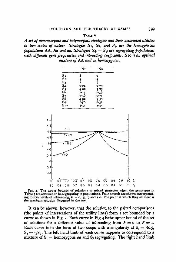
EVOLUTION AND THE THEORY OF GAMES 399 TABLE 6

A set of ?rwmmorphic and polymorphic strategies and their associated utilities in two states of nature. Strategies SI, S2, and S3 are the homogeneous populati AA, Aa and aa. Strategies S4 - S9 are segregating popukatians with different gene frequen&es and inbreeding coe@cients. SIO is an optimal

mixture of AA and aa homoxygotes.

NI N2

E:. 8 3 0 4 s3 7 s4 3.04 0.79 ,"a 4-m 2.24 3.75

6.39 3 7-36 4.90 0.71

3.53 s9 2.56 6-31 SIO 4.31 4.31

F=l

I.0 0.9 0.8 0.7 0.6 0.5 0.4 0.3 0.2 @I 0 Sk

FIG. 4. The upper bounds of solutions to mixed strategies when the genotypes in Table 5 are assumed to be segregating in populations. Four bounds are shown corresponding to four levels of inbreeding, F = o, ‘5, ‘g and 1.0. The point at which they all meet is the maximm solution discussed in the text.

It can be shown, however, that the solution to the paired comparisons (the points of intersections of the utility lines) form a set bounded by a curve as shown in Fig. 4. Each curve in Fig. 4 is the upper bound of the set of solutions for a different value of inbreeding from F = o to F = I. Each curve is in the form of two cusps with a singularity at Si = -615, Sk = -385. The left hand limb of each curve happens to correspond to a mixture of Sj = homozygous aa and Sj segregating. The right hand lib

400 R. C. LEWONTIN

of each corresponds to Si segregating and Sj = homozygous AA. The singularity for each curve then has the identical meaning: a mixture of -615 aa populations and -385 AA populations with no segregating populations. Since the singularity is the highest point with a utility of 4.31, the optimal strategy is one in which there is a mixture of homozygous AA and homozygous au populations in proportions .385 and -615 respectively.

The line for complete inbreeding, F = I, is particularly interesting. It is a horizontal straight line with the utility equal to 4.31 at every point. There is then no unique maximum solution for completely inbred populations. However, all the strategy mixtures on this line have following properties :

(I) There are no heterozygotes. This follows from the complete inbreeding, F = I.

(2) The overall frequency of is aa *615 and of AA is *385 for every point on the line.

The second property is simply a reflection of the fact that completely inbred populations really consist of sub-populations each homozygous for AA or aa.

Thus the optimal strategy for this species consists in possessing only two genotypes aa and AA in the proportions -615 to 0385. This can be accomplished by having all populations homogeneous within themselves, 40 yO being AA population and 60 yO aa populations. It can equally well be accomplished by inbreeding so that each population is a mixture of AA and aa homozygotes with an overall proportion of 40% AA to 60% aa in the species as a whole.

In biological terms, the situation of Table 6 favors genetic isolation between AA and aa genotypes. This means either speciation or complete selfing within one species. Which of these two alternatives is truly optimal depends upon the form of the game for other loci. Complete selfing leads to homozygosity of all the genes in the genome and this may not be optimal. Speciation on the other hand, creates an optimal condition for the new species pair, without forcing homozygosity at other loci.

The Choice of a Utility

I have deferred until last the question of an appropriate choice of a utility function because it is closely related to the question of the criterion of optimality. Population geneticists and ecologists are not in agreement about the parameter or parameters which measure the “success” of a population.

For many population geneticists the average fitness of a population is the appropriate choice. Dobzhansky (1951), Cain & Sheppard (1954) and Li

EVOLUTION AND THE THEORY OF GAMES 40’

(1955) have discussed thii point thoroughly and the result of that discussion may be quickly summed up. The average fitness of a population, @, does tend to a local maximum under the forces of intra-populational selection in most simple cases. However, i@ is defined only within a population and does not, in itself, provide a standard of comparison between populations. All other things being equal, a higher w means greater “success”, but, as always, other things are never equal. In some sense a population riddled with lethal genes is not as “successful” as one free of them since more of its zygotes are being wasted in the elimination of these genes. A large genetic load is a disadvantage to a population, but it is not the whole story. With some kinds of selection an increase in w within a population may actually lower the competitive ability of that population with respect to others of lower G.

Among population ecologists the rate of increase, r, is popular as a measure of success. It is necessary to distinguish two meanings of r. First, there is the rate of increase of a population calculated as the birth rate minus the death rate at any instant of time. An r defined in this way is sensitive to population density and as MacArthur (1960) points out, r is identically zero for all populations which are stable in size, irrespective of that size. Birch (1960) uses the parameter rO (although not always), the rate of increase of a population in its logarithmic growth phase. The chief disadvantage to this measure is that it is independent of population size and measures only the returning power of a decimated population or the rate of increase in newly founded colonies. While these two phases in the life of a population are important, they cannot be the whole measure of success. A great advantage of rs is that it will be increased by natural selection since an individual who leaves more offspring leaves more genes. (This is not necessarily so if there is inter-family selection.) Any parameter under the control of a direct mechanism like natural selection has distinct advantages as a measure of population success.

Thoday (1953) has made the intriguing proposal that the probability of szuw&Z of a population or other evolutionary unit, is the best measure of fitness of that unit. The difliculty of such a parameter is that, as envisioned by Thoday it is virtually impossible to measure. Thoday considered the probability of survival to some distant, unspecified, time, but using the techniques of stochastic game theory, this concept may become more manageable. Consider a population playing a stochastic game extended in time. At each step or move, there is a probability Pi, that the population will contain no individuals at time t + I, given that it contained i individuals at time t. These probabilities will be different for different strategies and states of nature and, in fact, correspond to the probability of playing

T.B. 26

402 R. C. LEWONTIN

the terminal game r” referred to in a previous section. This extinction probability will be a function of both E and r and thus includes both genetic and ecological parameters. I propose, then that (P, = I - Pi&, the probability of survival, is a parameter which it will be of advantage for a population to maximize over the whole stochastic game. Since states of nature are uncertain, however, this maximization must take the form of a maximin criterion. That is, the population’s optimal strategy is to keep the local probability of survival as high as possible under the worst combination of states of nature. The application of the maximin principle to a stochastic game has not been discussed here, but methods are well-known. What is essential here is that if P, is accepted as a measure of utility, then a maximin solution seems called for.

The Adoption of Strategies

The final element needed in a game theoretical approach to evolution is a mechanism. For intra-population genetics, the maximization of E is a good principle because, in fact, the processes of natural selection provide the mechanism for this maximization. Does a similar mechanism exist for “maximinization” of the probability of survival? The answer to this question depends entirely upon the importance of population and species extinction. The notion of natural selection is tautological in that it simply states that those individuals with the highest probability of survival are most fit. A similar tautology holds for population and species. Species which survive are by definition more fit than those which expire. Thus we expect that surviving groups will be those which have, simply by chance, acquired optimal strategies. This is completely analogous to the Dar- winian notion of natural selection of chance variation on the individual level. But what makes natural selection go is the fact that every organism is mortal and the rate of individual extinction is very high. The rate of natural selection within a population is limited by the rate of individual extinction (barring exponentially increasing populations, which are rare). By the same token the effectiveness of inter-deme selection among strategies is bounded by the rate of extinction of demes.

The commonness of population extinction is subject to much discussion. Andrewartha & Birch (1954) believe the rate of extinction of demes to be high while others, notably Nicholson (1957) hold the opposite view. It is extremely difficult to get data on extinction rates of species or higher taxonomic categories because of the confusion of phyletic extinction with taxonomic extinction, the changing of a taxonomic name due to phyletic evolution. Really intensive examination of certain aspects of the fossil record on the lines of Simpson’s elucidation of the Equids would provide the necessary information. If the horse were typical, which is unlikely,


the rate of extinction of distinct phyla would be quite high. Living Equid phyla represent less than I y0 of all known phyla since the Eocene.

On the side of experimentation much can be done. Although the time spans involved in selection among populations is obviously much greater than among individuals, it does not follow that the course of intra- population selection cannot be followed in the laboratory. For example large numbers of experimental bottle or vial populations can be kept simultaneously with organisms like TriboZium or Lhosophila. If different populations were allowed different pure strategies (homozygosity for different alleles, polymorphism, different amounts of recombination, etc.) the extinction of these populations could be followed in fluctuating environments. Mimicking of natural fluctuation in temperature, say, would be relatively easy.

In short, experimentation and observation will reveal the kinds of strategies that promote the longevity of populations and species and thus define biologically the meaning of an optimal strategy.

REFERENCES

ANDREWARTHA, H. G. & BIRCH, L. C. (1954). “The Distribution and Abundance of Animals”. University of Chicago Press.

BIRCH, L. C. (1960). Amer. Nat. 94,s. CARSON, H. L. (1955). Cold Spr. Harb. Symp. quant. Biol. m, 276. CARSON, H. L. (1959). Cold Spr. Harb. Symp. quant. Biol. ~4, 87. CAIN, A. J. & &IEPPARD, P. M. (1954). hfn. Nat. 88, 321. DOBZHANSKY, TH. (1951). “Genetics and the Origin of Species”. 3rd Edition. Columbia

University Press. DOBZHANSRI, TH. (1955). Cold Spr. Harb. Symp. quant. Biol. ZO, I. DOBZHANSKY, TH. & LBVENE, H. (1955). Genetics, 40, 797. FISHER, R. A. (1930). “ The Genetical Theory of Natural Selection.” Clarendon

Press, Oxford. LEWONTIN, R. C. (1957). Cold Spr. Harb. Symp. qumt. Biol. 22, 395. LI, C. C. (1955). Amer. Nat. 89, 281. LUCE, R. D. & RAIFFA, H. (1957). “Games and Decisions”. John Wiley & Sons, New York. MACARTHUR, R. H. (1960). Amer. Nut. 94, 313. MAYR, E. (1959). Cold Spr. Harb. Symp. @&ant. Biol. 24, I. NICHOLSON, A. J. (1957). Cokf Spr. Harb. Symp. qwnt. Biol. ZZ, I 53. THODAY, J. M. (1953). Symp. Sot. exp. Biol. 7, 96. VON NBUMANN, J. & MORGENSTBRN, 0. (1944). “Theory of Games and Economic Be-

havior”. 1st Edition. Princeton University Press. WALLACB, B. (1959). Cold Spr. Harb. Symp. quant. Biol. q, 193. WRIGHT, S. (1931). Genetics, 16, 97.

Evolution and the Theory of Games

Documents

Transcript of Evolution and the Theory of Games