EVALUATION OF FC-5 WITH PG 76-22 HP TO REDUCE ...
219
State of Florida Department of Transportation May 2019 EVALUATION OF FC-5 WITH PG 76-22 HP TO REDUCE RAVELING BE287: FINAL REPORT Submitted by the TEXAS A&M TRANSPORTATION INSTITUTE In collaboration with UNIVERSIDAD DE LOS ANDES
-
Upload
khangminh22 -
Category
Documents
-
view
0 -
download
0
Transcript of EVALUATION OF FC-5 WITH PG 76-22 HP TO REDUCE ...
State of Florida
Department of Transportation
May 2019
EVALUATION OF FC-5 WITH PG 76-22 HP
TO REDUCE RAVELING
BE287: FINAL REPORT
Submitted by the
TEXAS A&M TRANSPORTATION INSTITUTE
In collaboration with
UNIVERSIDAD DE LOS ANDES


ii
DISCLAIMER The opinions, findings, and conclusions expressed in this publication are those of the authors and not necessarily those of the State of Florida Department of Transportation.

iii
UNITS CONVERSION

iv
Technical Report Documentation Page
1. Report No.
2. Government Accession No.
3. Recipient’s Catalog No.
EVALUATION OF FC-5 WITH PG 76-22 HP TO REDUCE RAVELING
5. Report Date May 2019 6. Performing Organization Code
7. Author(s) Edith Arámbula-Mercado, Silvia Caro, Carlos Alberto Rivera Torres, Pravat Karki, Mauricio Sánchez-Silva, and Eun Sug Park
8. Performing Organization Report No.
9. Performing Organization Name and Address Texas A&M Transportation Institute 3135 TAMU College Station, TX 77843-3135
10. Work Unit No. (TRAIS) 11. Contract or Grant No. BE287
12. Sponsoring Agency Name and Address Florida Department of Transportation 605 Suwannee Street, MS 30 Tallahassee, FL 32399
13. Type of Report and Period Covered Final Report November 2016–May 2019 14. Sponsoring Agency Code
15. Supplementary Notes 16. Abstract The objectives of this project were to assess the mechanical performance and durability of open-graded friction course FC-5 mixtures fabricated with a highly polymer-modified (HP) binder (that complied with the requirements of FDOT specifications, Section 916-2), compare the results with those obtained in mixtures fabricated with a conventional polymer-modified asphalt (PMA) binder, and evaluate whether the use of HP binders was a cost-effective alternative to enhance the durability of FC-5 mixtures. The project included a comprehensive experimental plan, as well as computational mechanical simulations in finite elements (FEs) and a life-cycle cost analysis (LCCA). The experimental plan included linear viscoelasticity (LVE), surface free energy (SFE), fatigue cracking, and creep recovery tests on both types of binders under different aging conditions; LVE properties and the SFE of mastics fabricated with both binders and two aggregate types (i.e., limestone and granite); and fracture and durability tests on FC-5 mixtures fabricated with a combination of two binders and two aggregates under different aging conditions. The results showed that the PMA binder and PMA mastics had better LVE properties than the HP binder and mastics. However, the HP binder and HP mastics had superior fatigue cracking and creep recovery in all aging states. The fracture tests conducted on the FC-5 mixtures corroborated these results, and the durability tests—which were conducted using the Cantabro test with multiple cycles—also demonstrated that FC-5 mixtures with HP binder were significantly more durable than those with PMA binder. Numerical FE simulations conducted in a long-term aging state indicated that FC-5 mixtures with HP binder were less prone to raveling under field operational conditions, and the LCCA showed that the extended service life of FC-5 mixtures with HP binder offered a cost-effective alternative. 17. Key Words Open-Graded Friction Course, Raveling, Durability, Polymer-Modified Binder, Highly-Polymer-Modified Binder, HP Binder, HiMA
18. Distribution Statement No restrictions.
19. Security Classif. (of this report) Unclassified.
20. Security Classif. (of this page) Unclassified.
21. No. of Pages 219
22. Price
Form DOT F 1700.7 (8-72) Reproduction of completed page authorized

v
ACKNOWLEDGMENTS The authors would like to extend their gratitude to Greg Sholar, Howie Moseley, Wayne Rilko, Jamie Greene, and Wayne Allick for their guidance and support throughout the execution of this project. Gratitude is also extended to Ah Young Seo, María Alejandra Hernández Sáenz, Vanessa Senior, Laura Manrique-Sánchez, and Geoffrey Giannone for sharing their expertise in support of the laboratory and modeling tasks. Appreciation is also extended to Tony Barbosa and Rick Canatella for their assistance in laboratory-related activities.
Finally, the authors are thankful to Ray Gore from RoadScience, Bob Kluttz from Kraton Polymers, Kevin McGlumphy from Associated Asphalt Partners LLC, and Bryan Atkins from High-Tech Asphalt Solutions for supplying the antistrip additive, highly polymer-modified binder, and cellulose fibers needed to fulfill the experimental test plan.
vi
EXECUTIVE SUMMARY Open-graded friction courses (OGFCs) are thin layers composed of open-graded asphalt mixtures placed on top of regular pavement structures with the goal of improving traffic safety conditions during rainy events and controlling the noise produced by the tire-pavement interaction. One main challenge of this type of mixture is its short durability, which is mainly caused by raveling (i.e., the loss of aggregate particles from the surface of the layer). Efforts to prevent raveling in this type of mixture have included enhanced material selection procedures (e.g., modified binders, increased asphalt binder content, use of mineral or cellulose fibers, and high-quality aggregates), requirements on volumetric properties, and identification of suitable project conditions (e.g., high-speed roads). These efforts have extended the life of OGFC mixtures, but nevertheless, raveling continues to occur, which implies an increase in the costs of maintenance and rehabilitation activities. Thus, the use of new commercially available materials, such as a heavily polymer-modified (HP) binder, which is produced at a polymer dose modification ranging between 6% and 8% by weight of binder, could be a viable option to improve the raveling resistance of OGFCs.
The objective of this project was to evaluate whether the use of performance grade (PG) 76-22 HP binders that satisfied the requirements of FDOT specifications, Section 916-2 could produce more durable FC-5 mixtures than those obtained with a control PG 76-22 polymer-modified asphalt (PMA), as well as their cost effectiveness. To accomplish this goal, the project included a comprehensive experimental plan at the binder, mastic, and mixture levels, as well as computational mechanics simulations and life-cycle cost analysis (LCCA).
The experimental portion of the work plan included two main components:
• Evaluating and comparing the rheological properties of the PMA and HP binders and of mastics obtained from combining both types of binders with two aggregate types (i.e., granite from Junction City Mining and limestone from White Rock Quarries)
• Assessing the cracking performance and durability of FC-5 mixtures that were prepared with these same materials.
The viscoelastic behavior, aging susceptibility, and mechanical performance (i.e., creep recovery and fatigue resistance) of the binders were determined at different aging conditions through:
• The Superpave PG classification • Frequency and temperature sweep tests at low strain levels • The Glover-Rowe parameter • Fourier transform infrared spectroscopy tests • Multi-stress creep recovery tests • Pure linear amplitude sweep tests.
The binder test results showed that both the PMA and HP binders had improved PG grades (i.e., PG 82-22E and PG 82-28E for PMA and HP, respectively) than their commercial labels. The rheology results conducted on both binders and corresponding mastics showed that the PMA binder had improved linear viscoelastic (LVE) properties as compared to the HP binder, which could be due to differences in the base binder used for modification. Nevertheless, the HP binder

vii
had an overall superior performance since it was less prone to aging and had better mechanical response in terms of ductility and cracking susceptibility. Additionally, the results of the LVE properties of the mastics prepared with the combination of the two binders and two aggregates showed that their behavior was more dependent on the type of binder than on the type of aggregate. Also, the inclusion of fillers reduced the differences in the dynamic modulus master curves that were observed for the binders. Surface free energy tests were also conducted on the binders and mastics, and the information was used as input in the numerical models.
In terms of asphalt mixture characterization, FC-5 mixtures were fabricated with the two types of binder and both sources of aggregates to a target air void content of 20±1% and subjected to multiple aging states. The fracture properties of the mixtures were assessed through the indirect tensile asphalt cracking (IDEAL) test and the semicircular bending (SCB) test; the FM 1-T 283 test was performed to evaluate the moisture damage susceptibility of the mixtures; and, finally, the Cantabro abrasion loss test for OGFC mixtures—which corresponds to the Los Angeles abrasion test without the steel balls and with various cycles—was used to evaluate the durability of the mixtures. Overall, the results of the IDEAL and SCB tests showed that the most influential factor on the cracking resistance of the mixtures was the type of binder. Indeed, FC-5 mixtures fabricated with the HP binder showed better performance than those prepared with the PMA binder, regardless of the type of aggregate used. The results of the Cantabro abrasion loss test with multiple cycles demonstrated that aging had a significant impact on the durability of the mixtures, especially for those fabricated with the PMA binder. Overall, the FC-5 mixtures with HP in combination with the granite aggregate showed better durability results than all other mixtures, although the FC-5 with the HP binder and limestone aggregate presented better resistance to degradation up to the first stage of aging. The results of moisture susceptibility were inconclusive in terms of the influence of the aggregate or binder type.
It is noteworthy that these experimental results on binders, mastics, and mixtures correspond to specific PMA and HP binders that were obtained from a single producer source. Moreover, since the PMA binder had an improved PG grade, the relative differences between PMA and HP binders might vary if other sources of these commercial binders are evaluated.
Two-dimensional finite element (FE) models were developed to evaluate the response of the FC-5 mixtures under realistic field operational conditions. The FE models were implemented in Abaqus®, and their goal was to compare the mechanical response and expected raveling susceptibility in two moments of the service life of the OGFC layer:
• In a short-term aging condition (i.e., right after construction) • In a long-term aging condition (i.e., after several years of service).
The susceptibility of the FC-5 mixtures to raveling after short-term field aging was evaluated using a parameter called the raveling index, which measures the susceptibility to raveling based on the amount of energy dissipated at the stone-on-stone contacts during the pass of a wheel load. The susceptibility of the mixtures to raveling after long-term aging was evaluated using cohesive zone modeling (CZM) elements located within the stone-on-stone contacts of the microstructure of the FC-5 mixtures and a new index called energy remaining. These CZM elements use fracture mechanics principles to simulate the actual failure at these contacts; which represent raveling initiation and propagation. The results demonstrated that the long-term aging

viii
condition models that incorporated fracture mechanics principles were more appropriate to simulate the initiation of raveling processes at the stone-on-stone contacts of the OGFC, and the results showed that FC-5 mixtures with HP were less prone to raveling under field conditions.
Finally, an LCCA was conducted using the information obtained from the experimental work to compare the four FC-5 mixtures evaluated. Using available cost data and adding a measure of uncertainty to the values through Monte Carlo simulations, researchers calculated the net present value (NPV) for the four FC-5 mixtures. The results showed that the expected NPV value and its corresponding volatility were smaller for the FC-5 mixtures with the HP binder, suggesting that this type of binder offers a cost-effective alternative for increasing the durability of OGFCs.

ix
TABLE OF CONTENTS DISCLAIMER............................................................................................................................... ii UNITS CONVERSION ............................................................................................................... iii ACKNOWLEDGMENTS ............................................................................................................ v
EXECUTIVE SUMMARY ......................................................................................................... vi LIST OF FIGURES ................................................................................................................... xiii LIST OF TABLES ................................................................................................................... xviii 1.0. INTRODUCTION............................................................................................................. 1
2.0. LITERATURE REVIEW ................................................................................................ 6
2.1. Novel and Recent Research in OGFC .................................................................................. 9
2.2. FDOT Experience with OGFC ........................................................................................... 12
2.3. Computational Models to Evaluate the Durability of OGFC ............................................. 13
2.4. Highly Polymer-Modified Binders ..................................................................................... 15
2.4.1. Definition, Use, and Basic Characteristics............................................................ 15
2.4.2. U.S. Experience Using HP Binders ...................................................................... 18
2.4.3. Latin American Experience Using HP Binders .................................................... 21
2.4.4. European Experience Using Polymer-Modified Materials in OGFC ................... 22
2.4.5. Japanese Experience Using HP Binders in OGFC................................................ 23
3.0. MATERIALS .................................................................................................................. 26
4.0. EXPERIMENTAL TEST PLAN ................................................................................... 28
4.1. Binders and Mastics ........................................................................................................... 28
4.1.1. Binders—PG and MSCR Tests ............................................................................. 30
4.1.2. Binders and Mastics—Temperature and Frequency Sweep Tests ........................ 30
4.1.3. Binders—FTIR Test .............................................................................................. 31
4.1.4. Binders—PLAS Test ............................................................................................ 31
4.1.5. Binders and Mastics—SFE Test ........................................................................... 32
4.2. FC-5 Mixtures .................................................................................................................... 35
4.2.1. Semicircular Bending Test .................................................................................... 36
4.2.2. IDEAL-CT Test .................................................................................................... 37
4.2.3. Cantabro Abrasion Loss Test ................................................................................ 38
4.2.4. Moisture Susceptibility and Tensile Strength ....................................................... 38
4.2.5. Raveling Evolution ............................................................................................... 38
x
5.0. LABORATORY EXPERIMENT RESULTS............................................................... 40
5.1. Binder Characterization ...................................................................................................... 40
5.1.1. Performance Grade ............................................................................................... 40
5.1.2. Linear Viscoelastic Properties .............................................................................. 41
5.1.3. Aging and Cracking Susceptibility ....................................................................... 44
5.1.4. Chemical Changes Due to Oxidative Aging ......................................................... 46
5.1.5. Fatigue Resistance ................................................................................................ 47
5.1.6. Surface Free Energy .............................................................................................. 48
5.2. Mastic Characterization ...................................................................................................... 49
5.2.1. Linear Viscoelastic Properties .............................................................................. 50
5.2.2. Surface Free Energy .............................................................................................. 53
5.3. Mixture Characterization .................................................................................................... 55
5.3.1. Mixture Preparation .............................................................................................. 55
5.3.2. Performance Tests ................................................................................................. 59
5.4. Summary of Experimental Results ..................................................................................... 73
6.0. NUMERICAL MODELING .......................................................................................... 76
6.1. Modeling Methodology and Materials ............................................................................... 78
6.1.1. FC-5 Microstructure Geometry ............................................................................. 78
6.1.2. Pavement Structure ............................................................................................... 81
6.1.3. Loading Conditions ............................................................................................... 82
6.1.4. Aggregate and Pavement Layer Properties ........................................................... 83
6.1.5. Mastic Properties .................................................................................................. 83
6.2. Modeling Cases .................................................................................................................. 85
6.2.1. FE Model for FC-5 Mixtures after Short-Term Aging ......................................... 85
6.2.2. FE Model for FC-5 Mixture after Long-Term Aging ........................................... 86
6.3. Modeling Results ................................................................................................................ 89
6.3.1. Raveling Susceptibility after Short-Term Aging .................................................. 89
6.3.2. Raveling Susceptibility after Long-Term Aging .................................................. 93
6.4. Summary of Modeling Results ........................................................................................... 97
7.0. LIFE-CYCLE COST ANALYSIS ................................................................................. 99
7.1. Deterioration Curves......................................................................................................... 101
7.1.1. Material Loss Functions ...................................................................................... 101
7.1.2. Deterioration Curve Development ...................................................................... 104

xi
7.2. Cost Analysis .................................................................................................................... 107
7.2.1. Cost Estimation ................................................................................................... 108
7.2.2. Uncertainty Evaluation ....................................................................................... 108
7.2.3. Net Present Value ............................................................................................... 108
7.3. LCCA Results ................................................................................................................... 109
8.0. SUMMARY AND CONCLUSIONS ........................................................................... 111
REFERENCES .......................................................................................................................... 115
APPENDIX A—PREVIOUS RESEARCH ON OGFC......................................................... 128
APPENDIX B—AGGREGATE, BINDER, AND MASTIC PROPERTIES ...................... 130
B.1. Morphology ..................................................................................................................... 130
B.2. Surface Free Energy ......................................................................................................... 131
B.2.1. Theory and Calculations ..................................................................................... 131
B.2.2. Results ................................................................................................................ 134
APPENDIX C—SCB EXAMPLES OF TESTED SPECIMENS AND LOAD-DISPLACEMENT CURVES .......................................................................... 146
C.1. Limestone-PMA ............................................................................................................... 146
C.2. Granite-PMA ................................................................................................................... 147
C.3. Limestone-HP .................................................................................................................. 148
C.4. Granite-HP ....................................................................................................................... 149
APPENDIX D—STATISTICAL ANALYSIS SEMICIRCULAR BENDING TEST ........ 150
D.1. Flexibility Index with All Possible Two-Way Interactions Based on 75 Measurements .............................................................................................................. 150
D.2. Flexibility Index: Results of Fitting ANOVA with All Possible Two-Way Interactions Based on 74 Observations after Excluding a Potential Outlier (Observation #28) ........................................................................................................ 154
D.3. Cracking Resistance Index: Results of Fitting ANOVA with All Possible Two-Way Interactions Based on 75 Measurements .................................................... 157
APPENDIX E—STATISTICAL ANALYSIS IDEAL-CT TEST ........................................ 162
APPENDIX F—ASSESSMENT OF THE THREE-WHEEL POLISHER TO QUANTIFY THE EVOLUTION OF RAVELING IN OGFC ................................. 166
F.1. Materials ........................................................................................................................... 166
F.2. Slab Specimen Fabrication ............................................................................................... 167
F.3. Laboratory Experiment..................................................................................................... 168
F.3.1. Three-Wheel Polisher ......................................................................................... 168
xii
F.3.2. Raveling Assessment .......................................................................................... 170
F.4. Test Results ...................................................................................................................... 172
F.4.1. Visual Inspection ................................................................................................ 172
F.4.2. Change in Slab Specimen Weight ...................................................................... 173
F.4.3. Change in Surface Texture ................................................................................. 174
F.4.4. Summary of Results ............................................................................................ 175
F.5. Summary .......................................................................................................................... 176
APPENDIX G—CANTABRO PHOTOGRAPHIC COMPILATION ................................ 177
G.1. Limestone-PMA .............................................................................................................. 177
G.2. Granite-PMA ................................................................................................................... 180
G.3. Limestone-HP .................................................................................................................. 182
G.4. Granite-HP ....................................................................................................................... 185
APPENDIX H—STATISTICAL ANALYSIS CANTABRO TEST..................................... 188
APPENDIX I—STATISTICAL ANALYSIS INDIRECT TENSILE STRENGTH TEST .............................................................................................................................. 193

xiii
LIST OF FIGURES Figure 1-1. Work Plan Components. .............................................................................................. 2
Figure 2-1. Use of OGFC in the United States by State (Hernández-Sáenz et al., 2016). ............. 7
Figure 2-2. Example of Field Specimens in Norway with TLPA (Gibbs et al., 2005). .................. 9
Figure 2-3. 2D OGFC Microstructure Geometry Configuration: (a) Used by TU Delft (Kluttz et al., 2013); (b) Used by TTI/Universidad de Los Andes (Arámbula-Mercado et al., 2016; Manrique-Sánchez et al., 2016). .................................................... 13
Figure 2-4. Timeline of Additives Used in Binders; Adapted from Mundt et al. (2009) and Zhu et al. (2014). ........................................................................................................ 15
Figure 2-5. Microstructure Illustration of PMA with SBS: (a) SBS in an Asphalt Network; (b) HP Binder in an SBS Network (Yellow Represents the SBS Phase, and Black Represents the Asphalt Phase); Adapted from (Kluttz et al., 2014; Vonk and Jellema, 2016). ................................................................................................. 16
Figure 2-6. Worldwide Use of HP Binders. .................................................................................. 17
Figure 2-7. Use of HP Binders in the United States; Modified after Kluttz et al. (2014). ........... 17
Figure 2-8. Master Curve of Various HP Binders; Adapted from Kluttz et al. (2013) and de Bondt et al. (2016)........................................................................................................ 18
Figure 2-9. Dynamic Modulus Testing Results on Plant-Produced Conventional and HP-Modified DGHMA Mixtures; Adapted from Willis et al. (2012). ............................. 21
Figure 4-1. Results of the PLAS Test and Explanation of the Parameters to Compute the FREI Fatigue Parameter (Zhou et al., 2017b). .................................................................. 32
Figure 4-2. Sessile Drop Test Equipment. .................................................................................... 33
Figure 4-3. SFE Test Specimens: (a) Inside the Desiccator; (b) Tested and Untested Specimens. ........................................................................................................................ 34
Figure 4-4. SFE Contact Angle Measurement: (a) Contact Angle < 90°; (b) Contact Angle > 90°. ...................................................................................................................... 35
Figure 4-5. SCB Test Setup: (a) Schematic; (b) Actual Specimen during Testing. ..................... 37
Figure 4-6. (a) Three-Wheel Polisher Equipment Adapted for Evaluating Raveling Evolution; (b) Slab after Testing; (c) Circular Texture Meter. ......................................... 39
Figure 5-1. Master Curves at 45°C (113°F) for PMA Binder in Different Aging States. ............ 42
Figure 5-2. Master Curves at 45°C (113°F) for HP Binder at Different Aging States. ................ 43
Figure 5-3. Original and PAV80 Master Curves at 45°C (113°F) for HP and PMA Binders. ............................................................................................................................. 43
Figure 5-4. G-R Black Space Diagram for PMA, HP, and PG 52-28 Binders. ............................ 45
Figure 5-5. FTIR Results: (a) Carbonyl Area Obtained from FTIR Tests on PMA and HP Binders; (b) Carbonyl Area Growth with Respect to the Carbonyl Area of Original Binder for the PMA and HP Binders. ................................................................ 47
xiv
Figure 5-6. PLAS FREI Results for PMA and HP Binder. .......................................................... 48
Figure 5-7. Normalized Total SFE for HP and PMA Binders in Different Aging States: (a) Effect of Binder Type; (b) Effect of Aging. ................................................................ 49
Figure 5-8. Master Curve for Mastic Samples Using Original HP and PMA Binders. ................ 51
Figure 5-9. Master Curve for Mastic Samples Using Aged HP and PMA Asphalt Binders. ....... 52
Figure 5-10. Dynamic Modulus of Mastic Comparison for the Granite-HP Mastic and the Granite-PMA Mastic. ........................................................................................................ 53
Figure 5-11. Normalized Mastic Total SFE: (a) Effect of Binder Type; (b) Effect of Aggregate Type. ................................................................................................................ 54
Figure 5-12. Normalized Mastic-to-Binder Total SFE. ................................................................ 55
Figure 5-13. Semicircular Bending Test Setup. ............................................................................ 59
Figure 5-14. Specimen of a Granite-HP Binder Mixture in Contact with the Edges of the SCB Loading Frame during Testing. ................................................................................ 60
Figure 5-15. Lateral and Side View of an SCB Notched Test Specimen. .................................... 61
Figure 5-16. Example of Load versus Displacement Curves for Mixtures Tested in the I-FIT. ................................................................................................................................. 61
Figure 5-17. SCB Test Results for All Mixtures with Various Aging States: (a) Flexibility Index; (b) Cracking Resistance Index. .............................................................................. 62
Figure 5-18. IDEAL-CT Test Setup. ............................................................................................ 64
Figure 5-19. Specimen in Contact with the Edge of the IDEAL-CT Loading Frame during Testing............................................................................................................................... 65
Figure 5-20. CTindex Values for the Four Different Mixtures in Unaged and Aged States. .......... 66
Figure 5-21. Cantabro Test Results for Three Aging States. ........................................................ 67
Figure 5-22. Comparison of a Granite-PMA Cantabro Specimen That Reached 80% Mass Loss with Respect to Its Initial Condition......................................................................... 68
Figure 5-23. Cantabro Degradation Curves of Mixtures in Various Aging States (A0, A5, and A10); Each Cantabro Cycle Consists of 300 Revolutions. ........................................ 69
Figure 5-24. Wet and Dry IDT Strength Results for Mixtures Subjected to FM 1-T 283 in Two Aging States.......................................................................................................... 70
Figure 5-25. TSR Results for Mixtures Subjected to FM 1-T 283 in Two Aging States. ............ 72
Figure 5-26. Dry IDT Strength Results for Mixtures in Two Aging States: (a) Subjected to FM 1-T 283; (b) Subjected to the IDEAL Test. ........................................................... 72
Figure 6-1. (a) X-ray Scan of an OGFC Mixture; (b) 2D Section of an OGFC Mixture Obtained from an X-ray CT-Scanned Image and Processed as Input to the FE Model. ............................................................................................................................... 76
Figure 6-2. Characterization of the OGFC Sections: (a) Number of Contacts per Aggregate; (b) Quantification of Aggregate Orientation. ................................................. 77

xv
Figure 6-3. (a) Location of the CZM Elements at the Mastic-on-Mastic Contacts; (b) Traction-Separation Law for the CZM. ............................................................................ 78
Figure 6-4. FC-5 Microstructure Replicates with 20% AV: (a) 2-cm-Thick (0.79-in.); (b) 4-cm-Thick (1.57-in.). ....................................................................................................... 79
Figure 6-5. Particle Orientation. ................................................................................................... 79
Figure 6-6. Pavement Structure for FE Model in Abaqus®. ......................................................... 81
Figure 6-7. Global Mesh of an FE Model with a 4-cm (1.57-in.) FC-5 Mixture. ........................ 82
Figure 6-8. Loading Application and Vertical Displacement for a 2-cm (0.79-in.) FC-5 Mixture. ............................................................................................................................. 82
Figure 6-9. Example of the Threshold RI Value to Be Used for Obtaining the Truncated PDF for the First Replicate of a 4-cm (1.57-in.) Limestone-PMA FC-5 Mixture. .......... 86
Figure 6-10. Traction-Separation Law of the CZM Elements Modified after Caro (2009). ........ 87
Figure 6-11. SDEG Values for Contacts in an FC-5 Microstructure. ........................................... 88
Figure 6-12. PDF of ER for a Replicate of the 2-cm (0.79-in.) Granite-HP FC-5 Mixture. ........ 89
Figure 6-13. Vertical Stress State for a 4-cm (1.57-in.) FC-5 Microstructure with Red Circles Indicating the Location of Maximum Concentration of Stress. ........................... 90
Figure 6-14. Results of (µ+σ)RI for Mode I of Failure of the FC-5 Mixtures with 2-cm (0.79-in.) and 4-cm (1.57-in.). ................................................................................. 92
Figure 6-15. Fracture Evolution of a Contact Using CZM in Replicate of a 4-cm (1.57-in.) Thick Granite-PMA Microstructure Layer: (a) Prior to Crack Initiation; (b) After Crack Propagation at the Mastic-on-Mastic Contact. .............................................. 94
Figure 6-16. (µ+σ)ER Results for the FC-5 Mixtures. ................................................................... 96
Figure 6-17. Correlation between the Results of the Cantabro Abrasion Loss Test and the Numerical ER Results. ...................................................................................................... 97
Figure 7-1. Components of LCCA (after Sánchez-Silva and Klutke 2016). .............................. 100
Figure 7-2. Change in Mass Loss with Cantabro Revolutions for FC-5 Mixtures: (a) A0 Aging State; (b) A5 Aging State; (c) A10 Aging State. ...................................... 102
Figure 7-3. Example of Deterioration Curves for the Limestone-PMA Mixture. ...................... 105
Figure 7-4. Deterioration Curves for the Four FC-5 Mixtures. .................................................. 107
Figure 7-5. Mean NPV versus Standard Deviation of All Mixtures........................................... 109
Figure B-1. Aggregate Morphological Properties and Scale (GR = Granite Aggregate; LS = Limestone Aggregate). ................................................................................................ 131
Figure B-2. Selected Probe Liquids for SFE Testing. ................................................................ 136
Figure B-3. Contact Angles for Replicates of HP Binder in Original State Using Various Probe Liquids: (a) Diiodomethane; (b) Formamide; (c) Glycerol; (d) Water. ............... 137
xvi
Figure B-4. Average Contact Angles Measured with Various Probe Liquids in Different Aging States: (a) HP-OB; (b) HP-RTFO; (c) HP-PAV20; (d) PMA-OB; (e) PMA-RTFO; (f) PMA-PAV20. ................................................................................................ 138
Figure B-5. Normalized Contact Angles Measured with Various Probe Liquids for HP and PMA Binders in Different Aging States: (a) Effect of Binder Type; (b) Effect of Aging. ......................................................................................................................... 141
Figure B-6. Average Contact Angles Measured with Various Probe Liquids: (a) Mastic GH56; (b) Mastic LH59; (c) Mastic GP56; (d) Mastic LP59. ........................................ 142
Figure B-7. Normalized Mastic Contact Angles Measured with Various Probe Liquids: (a) Effect of Binder Type; (b) Effect of Aggregate Type. .............................................. 144
Figure B-8. Normalized Mastic-to-Binder Contact Angles Measured with Various Probe Liquids. ........................................................................................................................... 145
Figure D-1. Flexibility Index: Results of Response of FI and Actual Predicted Plot Based on 75 Measurements. ...................................................................................................... 150
Figure D-2. Residual by Predicted Plot for FI. ........................................................................... 152
Figure D-3. LS Means Plot for Binder Type and FI. .................................................................. 153
Figure D-4. LS Means Plot for Aging State and FI. ................................................................... 153
Figure D-5. Least Squares Fit for Response FI and Actual Predicted Plot without Potential Outlier. ............................................................................................................. 154
Figure D-6. Residual by Predicted Plot without Potential Outlier. ............................................. 155
Figure D-7. Least Square Means Plot for FI and Binder Type without Potential Outlier. ......... 156
Figure D-8. Least Square Means Plot for FI and Aging State without Potential Outlier. .......... 157
Figure D-9. Least Squares Fit Results of Response of CRI and Actual Predicted Plot Based on 75 Measurements. ........................................................................................... 158
Figure D-10. Residual by Predicted Plot for CRI. ...................................................................... 159
Figure D-11. Least Square Means Plot for CRI and Aging State. .............................................. 161
Figure E-1. Least Square Fit for Actual and Predicted Values of Tensile Strength for CTindex. ............................................................................................................................ 162
Figure E-2. Residual and Predicted Plot for CTindex of IDEAL Test. ......................................... 163
Figure E-3. Least Square Means Plot for CTindex and Aging Condition. .................................... 165
Figure F-1. Three-Wheel Polisher. ............................................................................................. 166
Figure F-2. FC-5 Mix Design. .................................................................................................... 167
Figure F-3. Asphalt Roller Compactor and Mold. ...................................................................... 168
Figure F-4. Types of Tires Used in the Three-Wheel Polisher: (a) Rubber Tire (Conventional); (b) Crimped Wire Tire; (c) Studded Tire. ............................................. 169
Figure F-5. Marathon Flat-Free Tire with Zig-Zag Stud Configuration. .................................... 169

xvii
Figure F-6. Studs and Installation Tool. ..................................................................................... 170
Figure F-7. Surface of the Slab after a Test Trial with Studded Tires: (a) Before Cleaning with Compressed Air; (b) After Cleaning with Compressed Air. .................................. 171
Figure F-8. Circular Track Meter Apparatus: (a) Side View; (b) Bottom View. ....................... 172
Figure F-9. Appearance of the Surface of the Slabs after Testing: (a) Trial #1 at 1,700 Load Cycles; (b) Trial #3 at 200 Load Cycles; (c) Trial #4 at 200 Load Cycles; (d) Trial #5 at 100 Load Cycles; (e) Trial #6 at 200 Load Cycles. ................................. 173
Figure F-10. Weight Loss of the Slabs for Different Conditions. .............................................. 174
Figure F-11. Average CTMeter MPD for the Slab Specimens. .................................................. 175
Figure H-1. Percentage Material Loss at Cycle 1 Actual Predicted Plot. ................................... 188
Figure H-2. Residual Predicted Plot Cycle 1 Cantabro Test. ..................................................... 189
Figure H-3. Least Square Means Plot for Aging Condition and Percentage Weight Loss of Cantabro Test. ............................................................................................................. 191
Figure H-4. Least Square Means Plot for Cycle 1 Percentage Weight Loss and Aging Condition......................................................................................................................... 192
Figure I-1. Least Square Fit for Actual and Predicted Values of Tensile Strength for Indirect Tensile Test. ...................................................................................................... 193
Figure I-2. Least Square Means Plot for Tensile Strength and Aging Condition. ...................... 195
Figure I-3. Least Square Means Plot for Tensile Strength and Moisture Condition. ................. 196
xviii
LIST OF TABLES Table 2-1. AV Content Requirements for OGFC Mixtures in Several States in the United
States; Information Partially Compiled from Watson et al. (2018). ................................... 6
Table 2-2. Mix Characteristics for NCHRP Project 9-50 (Watson et al., 2018). ......................... 11
Table 2-3. Properties of Surface Courses in NCAT Phase IV Project (Timm et al., 2012). ........ 20
Table 2-4. Characteristics Required in Japan for Polymer-Modified Binder for OGFC Mixtures; Adapted from Suzuki et al. (2010). .................................................................. 24
Table 2-5. Properties of Two Types of Binder; Adapted from Suzuki et al. (2010). ................... 25
Table 3-1. Characteristics of the FC-5 Mixtures. ......................................................................... 26
Table 4-1. Experimental Plan for Binders and Mastics. ............................................................... 29
Table 4-2. Experimental Tests to Characterize FC-5 Mixtures. ................................................... 35
Table 5-1. PG and MSCR Results for Binders. ............................................................................ 40
Table 5-2. Master Curve Parameters of the PMA Binder at a Reference Temperature (TR) of 45ºC (113ºF) for Different Aging States. ..................................................................... 41
Table 5-3. Master Curve Parameters for the HP Binder at a Reference Temperature (TR) of 45ºC (113ºF) for Different Aging States. ..................................................................... 42
Table 5-4. Average Binder SFE Components. .............................................................................. 48
Table 5-5. WLF Adjustment Coefficients for Unaged Mastic Master Curves. ............................ 50
Table 5-6. WLF Adjustment Coefficients for Aged Mastic Master Curves. ................................ 50
Table 5-7. Mastic Combinations for SFE Characterization. ......................................................... 53
Table 5-8. Average Mastic SFE Components. .............................................................................. 54
Table 5-9. Washed Sieve Analysis Results for Granite and Limestone Mixtures. ....................... 56
Table 5-10. Maximum Specific Gravity for the FC-5 Mixtures. .................................................. 56
Table 5-11. Gmb for Mixtures with PMA Binder. ......................................................................... 57
Table 5-12. Gmb for Mixtures with HP Binder. ............................................................................. 58
Table 5-13. AV Content (%) for the Mixtures with PMA Binder. ............................................... 58
Table 5-14. AV Content (%) for the Mixtures with HP Binder. ................................................... 59
Table 5-15. Ranking of Mixtures Based on SCB Test Results. .................................................... 63
Table 5-16. Ranking of Mixtures Based on the CTindex. ............................................................... 66
Table 5-17. Summary Results for Binder and Mastic Characterization and Ranking. ................. 74
Table 5-18. Summary Results for Mixture Characterization and Ranking. ................................. 75
Table 6-1. Parameters Used as Input in the FE Models. ............................................................... 78
Table 6-2. Characteristics of the Microstructures of the FC-5 Mixtures. ..................................... 80
Table 6-3. Prony Series for Mastic at a Temperature of 30°C after Short-Term Aging............... 84

xix
Table 6-4. Prony Series for Mastic at a Temperature of 30°C after Long-Term Aging. .............. 84
Table 6-5. Input Parameters of the CZM Traction-Separation Law. ............................................ 88
Table 6-6. Raveling Index for Mode I and Mode II of Failure after Short-Term Aging for the FC-5 Mixtures. ............................................................................................................ 91
Table 6-7. Results after Short-Term Aging for (µ+σ)RI Parameter to Evaluate Raveling. ........... 92
Table 6-8. ER Results after Long-Term Aging. ............................................................................ 95
Table 6-9. ER Results after Long-Term Aging to Evaluate Raveling Potential. .......................... 95
Table 6-10. Summary of Numerical Modeling Results after Short- and Long-Term Aging and Ranking of the FC-5 Mixtures to Resist Raveling. .................................................... 98
Table 7-1. Mass Loss Rates of the Different FC-5 Mixtures at A0 Aging State. ....................... 103
Table 7-2. Mass Loss Rates of the Different FC-5 Mixtures at A5 Aging State. ....................... 103
Table 7-3. Mass Loss Rates of the Different FC-5 Mixtures at A10 Aging State. ..................... 104
Table 7-4. Deterioration Rates for the Three Segments of the Deterioration Curves. ................ 106
Table 7-5. Mean Replacement Times for the Four FC-5 Mixtures. ........................................... 106
Table 7-6. Cost of the FC-5 Mixtures used in the LCCA Analysis (𝑪𝑪𝑪𝑪, 𝒌𝒌). ............................... 108
Table 7-7. COV of the Cantabro Abrasion Loss Test Measurements. ....................................... 108
Table 7-8. COV for the NPV Results. ........................................................................................ 109
Table A-1. Projects Funded by FDOT on the Topic of OGFC. .................................................. 128
Table B-1. Aggregate Angularity, Sphericity, and Texture Properties. ...................................... 130
Table B-2. Surface Free Energy of the Aggregates. ................................................................... 135
Table B-3. Characteristics of Selected SFE Probe Liquids. ....................................................... 135
Table B-4. Average Binder Contact Angles 10 Seconds after Test Initiation. ........................... 140
Table B-5. Average Mastic Contact Angles 10 Seconds after Test Initiation. ........................... 143
Table D-1. Summary of Fit FI. ................................................................................................... 150
Table D-2. Parameter Estimates for FI Statistical Analysis. ...................................................... 151
Table D-3. Effect Tests for FI Statistical Analysis. .................................................................... 151
Table D-4. Least Square Means Table for Aggregate Type for Statistical Analysis of FI. ........ 152
Table D-5. Least Square Means Table for Binder Type for Statistical Analysis of FI. .............. 152
Table D-6. Least Square Means Table for Aging State for Statistical Analysis of FI. ............... 152
Table D-7. Least Square Means Table for Combination of Aggregate Type and Binder Type for Statistical Analysis of FI. ................................................................................. 152
Table D-8. Least Square Means Table for Combination of Aggregate Type and Aging State for Statistical Analysis of FI. ................................................................................. 153
Table D-9. Least Square Means Differences Tukey HSD for Alpha = 0.05. ............................. 153

xx
Table D-10. Least Square Means for Combination Binder Type and Aging State for FI Statistical Analysis. ......................................................................................................... 154
Table D-11. Summary Fit for FI without Potential Outlier. ....................................................... 154
Table D-12. Parameter Estimates for FI Statistical Analysis without Potential Outlier. ............ 155
Table D-13. Effect Tests for FI Statistical Analysis without Potential Outlier. ......................... 155
Table D-14. Least Square Means Table for Binder Type for Statistical Analysis of FI without Potential Outlier. ................................................................................................ 156
Table D-15. Least Square Means Table for Combination Aggregate Type and Binder Type for Statistical Analysis of FI without Potential Outlier. ........................................ 156
Table D-16. Least Square Means Table for Combination Aggregate Type and Aging State for Statistical Analysis of FI without Potential Outlier. ........................................ 156
Table D-17. Least Square Means Differences Tukey HSD without Potential Outlier with Alpha = 0.05. .................................................................................................................. 157
Table D-18. Summary of Fit CRI. .............................................................................................. 158
Table D-19. Parameter Estimates for CRI Statistical Analysis. ................................................. 158
Table D-20. Effect Tests for CRI Statistical Analysis. ............................................................... 158
Table D-21. Least Square Means Table for Aggregate Type for Statistical Analysis of CRI. ................................................................................................................................. 159
Table D-22. Least Square Means Table for Binder Type for Statistical Analysis of CRI. ........ 159
Table D-23. Least Square Means Table for Aging State for Statistical Analysis of CRI. .......... 159
Table D-24. Least Square Means Table for Combination of Aggregate Type and Binder Type for Statistical Analysis of CRI. .............................................................................. 160
Table D-25. Least Square Means Table for Combination of Aggregate Type and Aging State for Statistical Analysis of CRI. .............................................................................. 160
Table D-26. Least Square Means Combination of Binder Type and Aging State for CRI. ....... 160
Table D-27. Least Square Means Differences Tukey HSD for CRI with Alpha = 0.05. ........... 160
Table E-1. Summary Fit for IDEAL Test. .................................................................................. 162
Table E-2. Analysis of Variance for IDEAL Test. ..................................................................... 162
Table E-3. Parameter Estimate for IDEAL Test. ........................................................................ 163
Table E-4. Statistical Analysis with Effect Test for IDEAL Test. .............................................. 163
Table E-5. Effect Details with Least Square Means for Aggregate Type of IDEAL Test. ........ 164
Table E-6. Effect Details with Least Square Means for Binder Type of IDEAL Test. .............. 164
Table E-7. Effect Details with Least Square Means for Aging Condition of IDEAL Test. ....... 164
Table E-8. Effect Details with Least Square Means for Combination Aggregate Type and Binder Type of IDEAL Test. .......................................................................................... 164

xxi
Table E-9. Effect Details with Least Square Means for Combination Aggregate Type and Aging Condition of IDEAL Test. ................................................................................... 164
Table E-10. Effect Details with Least Square Means for Combination Aging Condition and Binder Type of IDEAL Test. ................................................................................... 164
Table E-11. Least Square Means Differences Tukey HSD for IDEAL Test with Alpha = 0.05.................................................................................................................................. 165
Table F-1. Test Trials Conducted in the Modified Three-Wheel Polisher. ................................ 170
Table F-2. Summary Results for Modified Three-Wheel Polisher. ............................................ 176
Table H-1. Summary Fit Cycle 1 Cantabro Percentage Loss. .................................................... 188
Table H-2. Analysis of Variance for Percentage Weight Loss for Cantabro Cycle 1. ............... 188
Table H-3. Parameter Estimates for Cantabro Cycle 1 Percentage Wight Loss. ........................ 189
Table H-4. Effect Tests for Cycle 1 Percentage Weight Loss Cantabro Test. ............................ 189
Table H-5. Least Square Means Table for Aggregate Type Cantabro Test. ............................... 190
Table H-6. Least Square Means Table for Binder Type Cantabro Test. .................................... 190
Table H-7. Least Square Means Table for Aging Condition of Cantabro Test. ......................... 190
Table H-8. Least Square Means Table for Combination Aggregate Type and Binder Type of Cantabro Test. ................................................................................................... 190
Table H-9. Least Square Means Table for Combination Aggregate Type and Aging Condition of Cantabro Test. ............................................................................................ 190
Table H-10. Least Square Means Table of Tukey HSD with an Alpha of 0.05 for Combination Aggregate Type and Percentage Weight Loss of Cantabro Test. ............. 191
Table H-11. Least Square Means Table for Combination Binder Type and Aging Condition of Cantabro Test. ............................................................................................ 191
Table H-12. Least Square Means Table of Tukey HSD with an Alpha of 0.05 for Combination Binder Type and Aging Condition of Cantabro Test. ............................... 192
Table I-1. Summary Fit for Tensile Strength of Indirect Tensile Test. ...................................... 193
Table I-2. Analysis of Variance for Tensile Strength of Indirect Tensile Test. .......................... 193
Table I-3. Parameter Estimate for Tensile Strength of Indirect Tensile Test. ............................ 194
Table I-4. Effect Test Statistical Analysis for Tensile Strength of Indirect Tensile Test. .......... 194
Table I-5. Detailed Effect for Aggregate Type with Least Square Means for Tensile Strength of Indirect Tensile Test. .................................................................................... 194
Table I-6. Detailed Effect for Binder Type with Least Square Means for Tensile Strength of Indirect Tensile Test. .................................................................................................. 194
Table I-7. Detailed Effect for Aging Condition with Least Square Means for Tensile Strength of Indirect Tensile Test. .................................................................................... 194

xxii
Table I-8. Detailed Effect for Moisture Condition with Least Square Means for Tensile Strength of Indirect Tensile Test. .................................................................................... 195
Table I-9. Detailed Effect for Combination Aggregate Type and Binder Type with Least Square Means for Tensile Strength of Indirect Tensile Test. ......................................... 195
Table I-10. Detailed Effect for Combination Aggregate Type and Aging Condition with Least Square Means for Tensile Strength of Indirect Tensile Test. ................................ 195
Table I-11. Detailed Effect for Combination Aggregate Type and Moisture Condition with Least Square Means for Tensile Strength of Indirect Tensile Test. ........................ 195
Table I-12. Least Square Means Differences Tukey HSD for Aggregate Type and Moisture Condition with Alpha = 0.05. .......................................................................... 196
Table I-13. Least Square Means Table for Binder Type and Aging Condition. ......................... 196
Table I-14. Least Square Means Table for Binder Type and Moisture Condition. .................... 196
Table I-15. Least Square Means Table for Moisture Condition and Aging Condition. ............. 196
1
1.0. INTRODUCTION Open-graded friction courses (OGFCs) are a particular type of asphalt mixture placed at the surface of conventional pavement structures. These mixtures differ from traditional dense-graded hot mix asphalt (DGHMA) mixtures mainly in their volumetric properties. While conventional DGHMA has air void content in the range of 4% to 7%, the air void content in OGFC is typically between 18% and 22%. These air void contents, which are achieved by controlling the gradation of the mixture and by the compaction effort applied during the construction of the layer in the field, provide high permeability properties, which translate into superior performance of the material under wet weather conditions (i.e., water can be removed from the pavement surface quickly). The existence of large-sized pores in the microstructure of the OGFC also contributes to the reduction of noise generated at the pavement-tire interface caused by passing traffic. Due to these benefits, several states routinely use these mixtures.
Unfortunately, challenges and shortcomings related to the use of OGFC also exist. Several studies have indicated that one main disadvantage of these mixtures is their poor durability and short service life (Cooley et al., 2009). Indeed, the reported average service life of OGFC mixtures is between 6 and 12 years, which is less than the typical service life of DGHMA (i.e., 12 to 18 years), as stated in several studies (Huber, 2000; Huurman et al., 2010; Yildirim et al., 2007). The shorter service lives of these materials compared to DGHMA imply frequent maintenance and rehabilitation interventions. This condition, in conjunction with the fact that the typical cost of OGFC per ton of material is higher than that of DGHMA (according to Root [2009], between 30 to 38% larger), strongly affects the life-cycle cost of OGFC.
Several authors have reported that the main factor affecting the durability of the mixtures is raveling (Huber, 2000; Cooley et al., 2009). Raveling is defined as the continuous loss of aggregate particles from the surface of the OGFC. This degradation may be aggravated by the presence of moisture and/or by intense winter conditions. In general, raveling affects riding quality and accelerates the appearance and evolution of other distresses, causing an overall reduction in the serviceability of the pavement.
To prevent raveling, most state agencies, including the Florida Department of Transportation (FDOT), have restricted the materials that can be used in these mixtures, developed mix design methods, specified construction and maintenance techniques, and limited the operation conditions of the roads where the mixtures can be placed. Although the improvements in the selection of materials and design and construction practices have demonstrated a positive impact on the durability of OGFC, there is still a need to better understand the mechanisms related to this degradation and to explore alternatives to produce more durable mixtures.
Heavily or highly polymer-modified binders (i.e., polymer modification between 6% and 8% by weight of binder) have demonstrated superior performance characteristics in DGHMA. Existing modeling, experimental, and full-scale studies (Willis, 2012, 2016; Kluttz et al., 2009) suggest that these types of binders significantly improve the performance of asphalt mixtures. Therefore, based on the promising results observed in DGHMA, it may be possible that heavily polymer-modified binders could also develop stronger and more durable adhesive aggregate-binder bonds in OGFC, positively improving the resistance of these materials to raveling and increasing the overall durability of the mixture.

2
Therefore, the objectives of this project were to:
• Assess the durability of OGFC mixtures (also called FC-5 mixtures in Florida) prepared with a control performance grade (PG) 76-22 polymer-modified asphalt (PMA) binder (i.e., polymer modification between 2 and 3% by weight of binder) and with a PG 76-22 heavily polymer-modified (HP) asphalt binder (PG 76-22 HP) that complies with FDOT specifications, Section 916-2.
• Conduct a numerical simulation to evaluate the raveling behavior of the FC-5 mixtures under different in-service conditions.
• Perform a life-cycle cost analysis (LCCA) to evaluate whether the differences in FC-5 mixture durability would compensate for the higher initial cost of the PG 76-22 HP binder.
Figure 1-1 illustrates the project’s work plan components.
Figure 1-1. Work Plan Components.
Selection and acquisition of
materials
Characterization of materials and OGFC
mixtures
Mechanical and fracture properties of binders, mastics,
and mixtures
Characterization of raveling evolution on
OGFC mixtures
Phas
e 1
Phas
e 2
Finite element (FE) modeling
Analysis of experimental results
Conclusions regarding the durabil ity of OGFCs with PG 76-22 HP binder
LCCA to evaluate long-term economical benefits of using the material (depending on the results of Phase 1)
Recommendations regarding the use of the new PG 76-22 HP in OGFCs
Analysis of experimental results

3
This report details the results of the three objectives. Chapter 2 presents a summary of the literature review on the topics of OGFC and HP binders. The chapter is divided in several sections, including:
• An overview of OGFC and recent relevant techniques and advances related to this type of mixture.
• Research conducted by FDOT on OGFC. • A brief description of existing computational models in finite elements (FEs) that have
been developed to better understand and quantify raveling in OGFC. • The main characteristics and properties of binders that satisfy the general definition of
HP binders based on their polymer modification dose, including a compilation of experiences in the United States, Europe, Japan, and Latin America, including applications in OGFC.
The literature review includes the opinions and perceptions on the use of HP binders from experts in the United States, Brazil, The Netherlands, Germany, and Japan.
Chapter 3 details the materials used to fulfill the experimental test plan, including two aggregate types and two binder types:
• Aggregates: oolitic limestone and granite. • Binders: PG 76-22 PMA and PG 76-22 HP.
All individual components complied with the specifications defined by FDOT for FC-5 mixtures and are currently being used in the production of FC-5 mixtures in Florida.
Chapter 4 describes the experimental test plan, which includes test procedures aimed at determining critical material properties of binders, mastics, and FC-5 mixtures. The results from these tests were used to identify differences in material properties containing PMA and HP binders, and to estimate service life.
Chapter 5 presents the results of the laboratory experiment results, which had two parts:
• Evaluating and comparing the rheological and surface energy properties of the PMA and HP binders and mastics obtained from combining both types of binders and aggregates.
• Assessing the cracking performance and durability of FC-5 mixtures that were prepared with these same materials.
The aging susceptibility and mechanical performance (i.e., creep recovery and fatigue resistance) of the binders were determined through:
• The Superpave PG classification. • The Glover-Rowe parameter (G-R). • Fourier transform infrared spectroscopy (FTIR) tests. • Multiple stress creep recovery (MSCR) tests. • Pure linear amplitude sweep (PLAS) tests.

4
For the binders and mastics, the viscoelastic behavior and adhesive/cohesive characteristics were evaluated using:
• Frequency and temperature sweep tests at low strain levels. • Surface free energy (SFE) tests.
In terms of asphalt mixture characterization, FC-5 mixtures were fabricated with the two types of binder and both sources of aggregates to a target air void (AV) content of 20±1% and were subjected to multiple aging states. The fracture properties of the mixtures were assessed through the indirect tensile asphalt cracking test (IDEAL-CT) and the semicircular bending (SCB) test; the moisture damage susceptibility of the mixtures was evaluated per FM 1-T 283; and the durability of the mixtures was evaluated with the Cantabro abrasion loss test for OGFC mixtures—which corresponds to the Los Angeles abrasion test without the steel balls—and, in the case of this project, with various test cycles.
Chapter 6 details the numerical FE models used to quantify the raveling susceptibility of the FC-5 mixtures under various conditions. To complement the experimental portion of the work plan, two-dimensional (2D) FE models of a pavement structure with realistic OGFC with two thicknesses were used to assess the expected durability of the FC-5 mixtures. The main objective of these FE models was to evaluate the response of the different FC-5 mixtures under realistic field operational conditions. The models were implemented in Abaqus®, and their goal was to compare the mechanical response and expected raveling susceptibility at two moments of the pavement service life: after short-term aging (i.e., right after construction) and after long-term aging (i.e., after several years of service). The susceptibility of the FC-5 mixtures to raveling after short-term field aging was evaluated through the raveling index (RI), a parameter that uses the linear viscoelastic properties of the mastics coating the coarse aggregates of the OGFC to quantify raveling susceptibility based on the amount of energy dissipated at the stone-on-stone contacts during the pass of a wheel load (Manrique-Sánchez et al., 2016). The susceptibility of the mixtures to raveling after long-term aging condition was evaluated using cohesive zone modeling (CZM) elements located in the FE geometries within the stone-on-stone contacts of the microstructure of the FC-5 mixtures, and a new index called energy remaining (ER). These CZM elements use fracture mechanics principles and were useful to simulate actual failure at these contacts, which represent raveling initiation and propagation. Some of the material properties measured experimentally were used as input parameters to the FE models (i.e., linear viscoelastic properties of the mastics and fracture properties of the mixtures at different aging conditions), while others (i.e., Cantabro abrasion test results) were used to validate the results obtained from the simulations.
Chapter 7 describes the LCCA of the different FC-5 mixtures. The goal of the LCCA was to evaluate whether the expected long-term benefit of the FC-5 mixtures fabricated with the HP binder justified the added cost compared to mixtures prepared with the conventional PG 76-22 PMA binder. The results from the experimental work (i.e., durability through Cantabro tests and fracture properties of the OGFCs) and the available cost data were used to estimate degradation curves of the FC-5 mixtures. One important component of these analyses was the inclusion of a measure of uncertainty of the degradation processes through Monte Carlo simulations. The results of the LCCA were the net present value (NPV) of the service life of each FC-5 and the volatility or uncertainty associated with this value.

5
The last chapter, Chapter 8, summarizes the report findings and provides conclusions and recommendations based on the experimental, numerical, and cost analysis observations.

6
2.0. LITERATURE REVIEW OGFC mixtures have been used as part of road infrastructure projects during the past six decades. In Europe, OGFC was first used in 1960, and 10 years later it was introduced in the United States under the name first-generation OGFC (Mallick et al., 2009; Gunaratne and Mejias De Pernia, 2014). OGFC mixtures are thin layers placed on top of pavement structures with the goal of improving the serviceability of the road, mainly in regard to safety and noise reduction. These improvements are achieved by a large AV content in the mixtures, usually between 15 and 20% (Thai, 2005; Hernández-Sáenz et al., 2016), which translates into a highly permeable road surface. The AV content requirements for OGFC mixtures in various states in the United States are listed in Table 2-1.
Table 2-1. AV Content Requirements for OGFC Mixtures in Several States in the United States; Information Partially Compiled from Watson et al. (2018).
State AV Requirement Alabama Min. 12% Florida* Not specified
Georgia 18–20% 20–22% for PEM**
Louisiana 18–26% Maine 18–22%
Maryland Min. 18% Mississippi Min. 15% Nebraska 17–19%
New Jersey Min. 15, 18, or 20% depending on mix North Carolina Min. 18%
Oklahoma Min. 18% Tennessee Min. 20%
Texas 18–22% Virginia Min. 16%
* No ranges or minimum values were identified in the current specification. ** A porous European mix (PEM) is a type of OGFC with stricter requirements for the quality of materials and the minimum AV content.
The main reason OGFC is used in several states in the United States is the safety benefits it provides, especially under raining conditions, including the following:
• Reduced risk of hydroplaning (Dell’acqua et al., 2011). • Increased initial friction resistance (Adam and Shah, 1974; Brunner, 1975; Huddleston et
al., 1991). • Reduced backsplash and spray from vehicle tires (Nicholls, 1997; Rungruangvirojn and
Kanitpong, 2010). • Improved visibility of pavement markings (Lefebvre, 1993). • Improved car speed and traffic capacity (Cooley et al., 2009).

7
Despite these benefits, the use of OGFC in the United States has declined since the 1980s, mainly due to durability issues. In addition, states in the northern portion of the United States face problems related to maintenance during winter seasons, primarily because OGFC tends to freeze and retain the ice longer, and the application of sand, salt, or other treatments that are commonly used to prevent ice formation tend to clog the AV structure of the mixture (Hernández-Sáenz et al., 2016; Watson et al., 2018). Figure 2-1 shows the current use of OGFC in the United States according to a recent survey; most states in the southern portion, including Florida, currently use this type of mixture.
Figure 2-1. Use of OGFC in the United States by State (Hernández-Sáenz et al., 2016).
The ongoing challenge with OGFC is achieving a balance between durability and functionality of the mixture. As previously mentioned, the principal distress affecting the durability of these mixtures is raveling, a degradation process that consists of the loss of aggregates from the surface of the layer (Mo et al., 2008). The principal factor threatening functionality is clogging, which reduces the effective AV content of the mixture and, consequently, its permeability (Kandhal 2002, Rand 2004). Several countries and states in the United States currently using OGFC have actively conducted research to improve the design, construction, and operation of these types of mixtures, with the objective of achieving more durable and functional materials.
Europe has extensive experience using and improving OGFC mixtures, commonly called PEMs. Although PEMs share several common characteristics with OGFC mixtures used in the United States (e.g., the requirement for better materials than those used for DGHMA mixtures, and the specification of a minimum level of AV content), important differences are that PEMs have more gap-graded aggregate gradations and that the requirements for the materials used in their fabrication are, in general, more demanding than those typically specified in the United States (Thai 2005). Furthermore, although the safety benefits obtained with the use of OGFC mixtures

8
motivate the use of these materials, the most important reason for using PEMs in Europe is the environmental benefits achieved in terms of noise reduction (Bendtsen and Larson, 1999; Mitchell, 2000; Keafott et al., 2005; Voskuilen and Elzinga, 2010; Eck et al., 2010).
Most research projects conducted on these mixtures in Europe have focused on achieving higher noise reduction levels and longer durability. Some projects conducted in this area in recent years include:
• Roads to the Future, a project conducted in The Netherlands between 1996 and 2010. • Silent Roads for Urban and Extra-Urban Use, a joint program from the European Union
conducted between 1998 and 2002 (CORDIS, 2017). • Program of Research, Experimentation, and Innovation in Land Transport, a project
funded by the French Government that included three phases between 1990 and 2006 (Centre d’Etudes et d’Expertise sur les Risques, l’Environnement, la Mobilité et l’Aménagement and Ministère des Transports France, 2017).
• Sustainable Road Surfaces for Traffic Noise Control, a joint research European program conducted between 2002 and 2005 (Pucher et al., 2017).
• Harmonoise, a joint research of the European Union conducted between 2001 and 2004 (Peeters and Blokland, 2007).
Some of the European countries that were identified during this literature review as having extensive experience in OGFC are The Netherlands, Denmark, Italy, the United Kingdom, France, and Germany. Also, countries like Belgium have decreased the use of OGFC due to raveling, clogging, and maintenance costs (Gibbs et al., 2005). A U.S. panel of professionals and experts on pavement engineering and road materials that visited Europe in 2004 identified the following aspects as those that should be reviewed and improved in the United States (Gibbs et al., 2005):
• Consider OGFC as a pavement structural layer. • Achieve equivalent OGFC service life as the mixtures observed in Europe. • Determine critical mix design issues that need to be improved. • Establish and quantify incremental costs associated with the use of OGFC in the long
term associated with the use of special equipment for maintenance and the need for earlier rehabilitation activities.
Since The Netherlands applies OGFC extensively in its national road network (i.e., more than 80% of its current road network includes OGFC) (Voskuilen and Elzinga, 2010), The Netherlands has conducted numerous studies on this topic. One example of these efforts includes research developed in 2016 that evaluated the ÖffenPoriger asphalt (OPA) (i.e., the German term for OGFC) design specification that was used at the time in Germany, in order to offer recommendations to improve specifications (de Bondt et al., 2016). Using a series of OGFC mixtures that were fabricated in the laboratory and later constructed in the field at different thickness (50 and 60 mm thickness), the researchers evaluated durability and the capacity of the layer to absorb noise. Among other results, they found that:
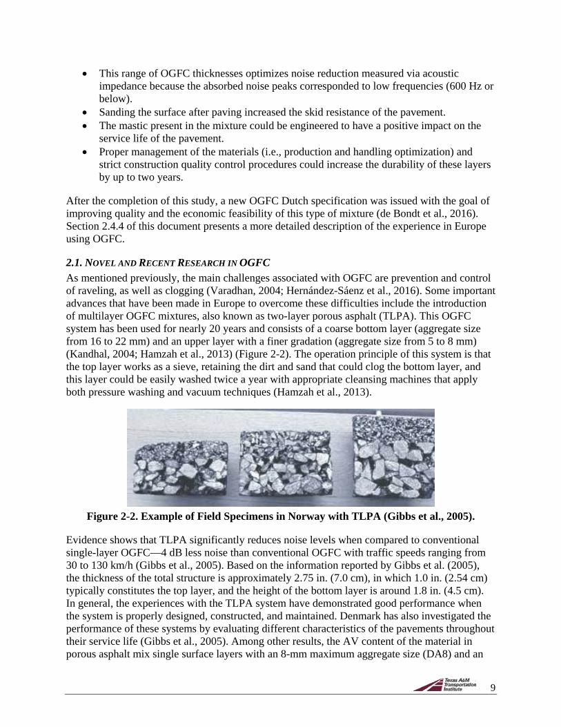
9
• This range of OGFC thicknesses optimizes noise reduction measured via acoustic impedance because the absorbed noise peaks corresponded to low frequencies (600 Hz or below).
• Sanding the surface after paving increased the skid resistance of the pavement. • The mastic present in the mixture could be engineered to have a positive impact on the
service life of the pavement. • Proper management of the materials (i.e., production and handling optimization) and
strict construction quality control procedures could increase the durability of these layers by up to two years.
After the completion of this study, a new OGFC Dutch specification was issued with the goal of improving quality and the economic feasibility of this type of mixture (de Bondt et al., 2016). Section 2.4.4 of this document presents a more detailed description of the experience in Europe using OGFC.
2.1. NOVEL AND RECENT RESEARCH IN OGFC As mentioned previously, the main challenges associated with OGFC are prevention and control of raveling, as well as clogging (Varadhan, 2004; Hernández-Sáenz et al., 2016). Some important advances that have been made in Europe to overcome these difficulties include the introduction of multilayer OGFC mixtures, also known as two-layer porous asphalt (TLPA). This OGFC system has been used for nearly 20 years and consists of a coarse bottom layer (aggregate size from 16 to 22 mm) and an upper layer with a finer gradation (aggregate size from 5 to 8 mm) (Kandhal, 2004; Hamzah et al., 2013) (Figure 2-2). The operation principle of this system is that the top layer works as a sieve, retaining the dirt and sand that could clog the bottom layer, and this layer could be easily washed twice a year with appropriate cleansing machines that apply both pressure washing and vacuum techniques (Hamzah et al., 2013).
Figure 2-2. Example of Field Specimens in Norway with TLPA (Gibbs et al., 2005).
Evidence shows that TLPA significantly reduces noise levels when compared to conventional single-layer OGFC—4 dB less noise than conventional OGFC with traffic speeds ranging from 30 to 130 km/h (Gibbs et al., 2005). Based on the information reported by Gibbs et al. (2005), the thickness of the total structure is approximately 2.75 in. (7.0 cm), in which 1.0 in. (2.54 cm) typically constitutes the top layer, and the height of the bottom layer is around 1.8 in. (4.5 cm). In general, the experiences with the TLPA system have demonstrated good performance when the system is properly designed, constructed, and maintained. Denmark has also investigated the performance of these systems by evaluating different characteristics of the pavements throughout their service life (Gibbs et al., 2005). Among other results, the AV content of the material in porous asphalt mix single surface layers with an 8-mm maximum aggregate size (DA8) and an
10
initial AV content between 18%–22% decreased by about 3% after six years in service; this is an important finding because it could be used as part of life-cycle analyses to evaluate the functionality of the material with time and develop appropriate maintenance strategies.
Another innovation with respect to OGFC is the use of recycled asphalt pavement (RAP) in the design and fabrication of these mixtures. The Netherlands initiated a study in 2010 that is still in progress, in which field validation is being done in order to develop a specification to incorporate up to 50% RAP in OGFC mixtures (Voskuilen and Elzinga 2010). The motivation for the study is the lack of suitable materials for pavement construction and the need to import them from neighboring countries such as Germany (Voskuilen and van de Ven 2010). This study has involved a series of tests (e.g., indirect tensile test, indirect tensile strength ratio, Cantabro loss test, and rotating surface abrasion test, among others), and the laboratory results so far have been promising, which prompted the recently initiated evaluation of the material in field trials.
In the United States, the most recent research effort related to OGFC at the national level include National Cooperative Highway Research Program (NCHRP) project 9-50, conducted by the National Center for Asphalt Technology (NCAT) between 2013 and 2016 (Watson et al., 2018), with the objective of developing an improved design methodology for these mixtures. Some of the findings obtained from the NCHRP project included the following:
• The parameter voids in coarse aggregate (VCA) is not required as part of a successful OGFC design methodology.
• A minimum permeability level of 50 m/day measured via falling head permeability apparatus is related to an OGFC that has 15% AVs in the field.
• The use of fibers is efficient to control draindown. • A maximum value of 20% for Cantabro loss was suggested as a parameter to control
raveling, a condition that was not achieved by some of the mixtures evaluated, including a typical Florida OGFC design.
• The minimum permeability and corresponding AV content should be correlated with the amount of annual rainfall, with a minimum permeability of 100 m/day recommended for places with more than 60 in. of annual rainfall.
• Test procedures to assess the moisture susceptibility of the mixture were recommended based on the tensile strength ratio (TSR) concept.
• The indirect tensile strength test and the Illinois flexibility index (I-FIT) test (based on the SCB test) were recommended to quantify the cracking resistance of the materials.
• The use of modified binders, including a PG 88-22, which is an HP, excelled in performance (i.e., rutting resistance and Cantabro loss) but presented some difficulties related to draindown and decreased permeability.
NCHRP project 9-50 evaluated three types of asphalt binders with the gradation and materials of a Georgia OGFC that had reported good performance in the field. The binders included a 3% polymer-modified asphalt, a 12% modified asphalt rubber (ground tire rubber [GTR] binder classified as PG 76-22), and a 7.5% HP binder as listed in Table 2-2. None of the OGFC mixtures fabricated with these binders included fibers. A control OGFC fabricated with a 2.5% styrene-butadiene-styrene (SBS) modified binder (PG 76-22) and 0.4% fibers by total weight of mixture was also included in the study.

11
Table 2-2. Mix Characteristics for NCHRP Project 9-50 (Watson et al., 2018).
Characteristic Control Mixture
PG 76-22 SBS Mixture
HP Mixture
PG 76-22 GTR Mixture
Binder content (% wt mix) 6.0 6.0 6.0 6.7 Fiber (% wt mix) 0.4 – – – Average AVs (%) 15.4 16.3 14.9 13.9
AVs in mineral aggregate (%) 26.6 26.5 25.5 25.9 Film thickness (microns) 27.1 25.2 26.1 28.2
The results from the Cantabro loss test showed that the mixture containing the HP binder presented a low percentage of mass loss (i.e., 4.7%), and that this value was three to four times smaller than the results obtained for the other mixtures. Specifically, the mixture fabricated with PG 76-22 SBS and with PG 76-22 GTR presented an average mass loss of three specimens of 12.3% and 12.1%, respectively, and the result for the control mix was 19.3%.
Rutting resistance results obtained from the Hamburg wheel tracking test were also encouraging for the HP mixture. The average rut depth obtained for this OGFC was 0.27 in. (6.89 mm), while for the other mixtures, this parameter was between 1.3 and 1.6 times larger (i.e., 0.42 in. [10.56 mm] for the PG 76-22 SBS mixture, 0.43 in. [10.84 mm] for the PG 76-22 GTR, and 0.35 in. [8.99 mm] for the control mixture).
Regarding resistance to moisture damage, the results obtained from the American Association of State Highway and Transportation Officials (AASHTO) T 283 test demonstrated that only the HP and the PG 76-22 GTR mixtures passed both AASHTO and ASTM criteria (i.e., TSR of 0.7 and 0.8, respectively).
Draindown tests were also conducted as part of the project to evaluate if the use of modified binders could obviate the need for fibers. The tests were conducted at temperatures of 166°C and 181°C (330°F and 357°F), except for the HP mixture, for which the test temperatures were set at 171°C and 186°C (340°F and 367°F). The HP mixture was the only one that did not pass the test acceptance criterion (i.e., 0.3% maximum draindown), suggesting that this OGFC required the addition of fibers.
Finally, permeability tests were also conducted according to FM 5-565, Florida Method of Test for Measurement of Water Permeability of Compacted Asphalt Paving Mixtures, on these mixtures, and the results showed similar values for the control and the PG 76-22 SBS mixtures (i.e., 79 m/day). However, the PG 76-22 GTR and the HP mixtures showed decreased permeability (i.e., 33 and 37 m/day, respectively). For the case of the OGFC mixture with PG 76-22 GTR, this result was believed to be partially due to the higher binder content (Table 2-2), while for the HP mixture, no explanation was evident, but the authors speculated that the result could be related to the larger dosage of polymer modification (i.e., about 7.5% SBS polymer, which is roughly double the rate of polymer used in a typical PG 76-22 as reported by the asphalt binder supplier).
In conclusion, the HP mixture performed well in terms of Cantabro mass loss, rutting resistance, and resistance to moisture damage, but the other OGFC mixtures presented superior results in

12
terms of draindown and permeability. The inclusion of fibers in the HP mixture could help improve its draindown.
2.2. FDOT EXPERIENCE WITH OGFC This section summarizes the research conducted by FDOT on the topic of OGFC in recent years. FDOT has been very active in promoting studies to improve the quality of their OGFC FC-5 mixtures. FDOT introduced the use of OGFC in the 1970s, when it developed a 3/8-in. nominal maximum aggregate size (NMAS) OGFC with polish-resistant aggregate that was labeled FC-2. Two decades later, in the 1990s, this type of mixture was replaced by a coarser 1/2-in. NMAS OGFC, which was labeled FC-5 (Musselman, 2015). Currently, as a result of the continuous effort of FDOT to improve the quality of these materials, several FC-5 mixtures with different material types, sources, and requirements are available. Nevertheless, like in other states, some FC-5 mixtures in Florida have displayed durability difficulties (Bennert and Cooley, 2014). This explains the continued interest of FDOT to understand, prevent, and mitigate raveling effects in these mixtures. Indeed, during the last 10 years, FDOT has funded several studies related to this topic, including the following:
• BD-545-53: Introduction of Fracture Resistance to the Design and Evaluation of Open Graded Friction Courses in Florida—Completed in 2009.
• BDS15-977-01: Evaluate the Contribution of the Mixture Components on the Longevity and Performance of FC-5—Completed in 2014.
• BDV25-820-1: Determination of the Optimum Binder Content of Open-Graded Friction Course (OGFC) Mixtures Using Digital Image Processing—Completed in 2015.
• BDV29-820-1: FC-5 Raveling Study—Completed in 2015. • BDR74-977-04: Understanding Mechanisms of Raveling to Extend Open Graded
Friction Course (OGFC) Service Life—Completed in 2016.
These studies involved the following activities and efforts:
• Characterization of the fracture resistance properties of OGFC mixtures (BD-545-53). • Full-scale experiments to evaluate the role of polymer-modified bonding agents between
the OGFC and regular asphalt layers (BD-545-53). • Evaluation of the influence of volumetrics on the durability of OGFC mixtures
(BDS15-977-01). • Review of existing design methods for OGFC using digital imaging techniques as a
support methodology (BDV25-820-1). • Identification of the causes for short-term raveling in FC-5 mixtures in the south of
Florida (BDV29-820-1). • Experimental evaluation of the capability of existing tests to characterize raveling in
FC-5 mixtures based on field performance data and FE modeling, identification of raveling mechanisms, and the most relevant factors influencing this phenomenon (BDR74-977-04).
Appendix A provides additional information regarding the objectives and main results of these projects.

13
2.3. COMPUTATIONAL MODELS TO EVALUATE THE DURABILITY OF OGFC Although the majority of research conducted on OGFC has been focused on laboratory experimental tests or field evaluation activities, another approach that has been less explored is the use of computational modeling to assess and understand the mechanisms associated with the durability of the mixtures (i.e., raveling).
The majority of these works have been conducted by the research groups at TU Delft (The Netherlands) (Mo et al., 2007; 2008; 2010; 2011; Huurman et al., 2009; Kluttz et al., 2013; Jellema and Vonk, 2016), TTI (Alvarez et al., 2010b), and TTI in collaboration with Universidad de Los Andes (Colombia) (Arámbula-Mercado et al., 2016; Manrique-Sánchez et al., 2016). With the exception of the work conducted by Alvarez et al. (2010b), these works have used FE to evaluate the mechanical response of microstructures of OGFC and their susceptibility to raveling, when considering different characteristics of the mixtures (e.g., binder content, particles’ contact network, etc.) and operational and weather factors (e.g., traffic speed, vehicle-interaction friction forces, air temperature, etc.).
The main difference among the FE efforts conducted by the TU Delft and TTI/Universidad de los Andes (Uniandes) research groups is related to the geometry of the OGFC microstructures. In order to represent the aggregate particles of the mixtures, the group at TU Delft has typically used either polygons, spheres, or circles in 2D and 3D (Mo et al., 2007; 2008; 2010; 2011; 2014; Huurman et al., 2009; Kluttz et al., 2013; Jellema and Vonk, 2016), as observed in Figure 2-3a, while Arámbula-Mercado et al. (2016) and Manrique-Sánchez et al. (2016) have used X-ray computed tomography (CT) images to obtain 2D configurations of the actual microstructures of OGFC mixtures, such as those observed in Figure 2-3b. Other differences in the efforts conducted by both research groups include the overall thickness of the OGFC used in the models (i.e., typical total thickness near 3 cm (1.2 in) were used by TU Delft while OGFC models with 2-cm and 4-cm (0.79-in – 1.57-in) were used by TTI/Uniandes), the type of materials used (i.e., OGFC satisfying Dutch specifications versus OGFC satisfying FDOT specifications) and, some specific operational conditions (i.e., wheel speed, vertical and frictional load magnitudes, air temperature). Conversely, equivalent approaches were followed in all models in terms of the boundary conditions of the FE geometry and the techniques used for simulating a moving wheel load on top of the OGFC. In general, the results obtained from these numerical works have permitted researchers to efficiently identify factors that make the mixtures more susceptible to raveling.
(a) (b)
Figure 2-3. 2D OGFC Microstructure Geometry Configuration: (a) Used by TU Delft (Kluttz et al., 2013); (b) Used by TTI/Universidad de Los Andes (Arámbula-Mercado et al.,
2016; Manrique-Sánchez et al., 2016).
In the case of the efforts conducted by the research group at TU Delft, the simplified OGFC microstructures were subjected to different loading conditions and the results were analyzed
14
using a life optimization tool (LOT), which is a meso-mechanistic tool developed that combines the results of stresses and strains with the skeleton of the mixture with a damage accumulation model. Some of the main conclusions that have been obtained from the computational efforts conducted by this group include the following:
• An increase in the binder content is related with a decrease in the magnitude of the stresses at the interfacial zone in the mastic film and, therefore, to a reduction in the raveling susceptibility of the mixture (Mo et al., 2008).
• The main cause for winter damage in OGFC is the decrease in relaxation potential of the mortars present in the mixtures (Huurman et al., 2009).
• Raveling can occur within a wide range of temperatures (Mo et al., 2010).
The numerical efforts conducted by this same research group include two works that are of particular interest for the context of this project since they evaluated the behavior of HP binders when used in OGFC mixtures (i.e., HP-OGFC). These works are titled “Highly Modified Bitumen for Prevention of Winter Damage in OGFCs” (Kluttz et al., 2013) and “Improving Durability and Functionality Retention of Porous Asphalt by Using High Performing Bituminous Binders” (Jellema and Vonk 2016). In both cases, the works used an FE approach with a simplified geometry in combination with the LOT model to evaluate the performance of the material, following a procedure similar to the one used in the previous works conducted by this research group. The numerical results suggested an enhanced performance of the HP-OGFC in winter conditions due to the combination of low modulus and high cohesive strength, and suggested that the presence of low-temperature fluctuations had a severe impact on the durability of the mixture. In the second work, the authors evaluated OGFC using four different binders that presented different modification and toughness, and they concluded that the HP-OGFC modified material presented a longer durability than the other OGFC mixtures and that the best material combination was an HP fabricated with a soft base binder.
In the case of the work conducted by the TTI/Universidad de Los Andes research group (Arámbula-Mercado et al., 2016), FE models containing 0.7- in. and 1.57-in. (2-cm and 4-cm) of realistic type FC-5 OGFC mixtures that are currently used in Florida were located on top of a pavement structure and subjected to the pass of a moving wheel load. Different material combinations and operational conditions were applied to the model, and an energy-based model and probabilistic principles were used to quantify the raveling susceptibility of the material. The four main findings obtained from these numerical models were:
• Raveling is mainly a Mode I fracture process (i.e., opening fracture mode). • Mixtures that were observed to have performed good or poor in the field were also
identified in the models as having the lowest and highest probability to undergo raveling, validating the quality of the model.
• High AV contents and binder contents different from the optimum (i.e., lower or higher) were the two most critical factors in increasing the susceptibility of the mixtures to raveling.
• Low vehicle speeds and zones where vehicles have to brake frequently were the two operational factors identified as increasing the chances of raveling the most.
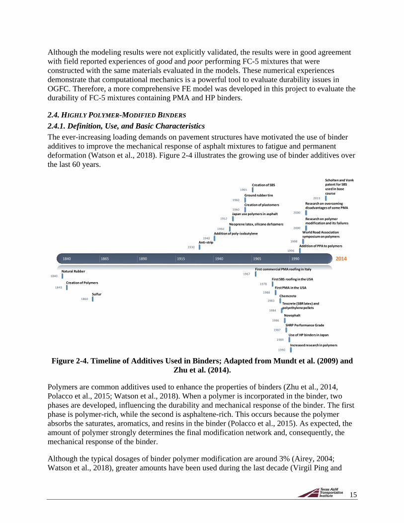
15
Although the modeling results were not explicitly validated, the results were in good agreement with field reported experiences of good and poor performing FC-5 mixtures that were constructed with the same materials evaluated in the models. These numerical experiences demonstrate that computational mechanics is a powerful tool to evaluate durability issues in OGFC. Therefore, a more comprehensive FE model was developed in this project to evaluate the durability of FC-5 mixtures containing PMA and HP binders.
2.4. HIGHLY POLYMER-MODIFIED BINDERS 2.4.1. Definition, Use, and Basic Characteristics The ever-increasing loading demands on pavement structures have motivated the use of binder additives to improve the mechanical response of asphalt mixtures to fatigue and permanent deformation (Watson et al., 2018). Figure 2-4 illustrates the growing use of binder additives over the last 60 years.
Figure 2-4. Timeline of Additives Used in Binders; Adapted from Mundt et al. (2009) and
Zhu et al. (2014).
Polymers are common additives used to enhance the properties of binders (Zhu et al., 2014, Polacco et al., 2015; Watson et al., 2018). When a polymer is incorporated in the binder, two phases are developed, influencing the durability and mechanical response of the binder. The first phase is polymer-rich, while the second is asphaltene-rich. This occurs because the polymer absorbs the saturates, aromatics, and resins in the binder (Polacco et al., 2015). As expected, the amount of polymer strongly determines the final modification network and, consequently, the mechanical response of the binder.
Although the typical dosages of binder polymer modification are around 3% (Airey, 2004; Watson et al., 2018), greater amounts have been used during the last decade (Virgil Ping and
20141840 1865 1890 1915 1940 1965 1990
1840Natural Rubber
1843Creation of Polymers
1860Sulfur
1930Anti-strip
1940Addition of poly-isobutylene
1950Neoprene latex, silicone defoamers
1952Japan use polymers in asphalt1960
Creation of plastomers1960
Ground rubber tire1965
Creation of SBS
1967First commercial PMA roofing in Italy
1978First SBS roofing in the USA
1980First PMA in the USA
1983Chemcrete
1984
Texcrete (SBRlatex) and polyethylene pellets
1986Novophalt
1987SHRP Performance Grade
1989Use of HP binders in Japan
1990Increased research in polymers
1996Addition of PPA to polymers
1998
World Road Association symposium on polymers
2000
Research on polymer modification and its failures
2000
Research on overcoming disadvantages of some PMA
2013
Scholten and Vonk patent for SBS used in base course
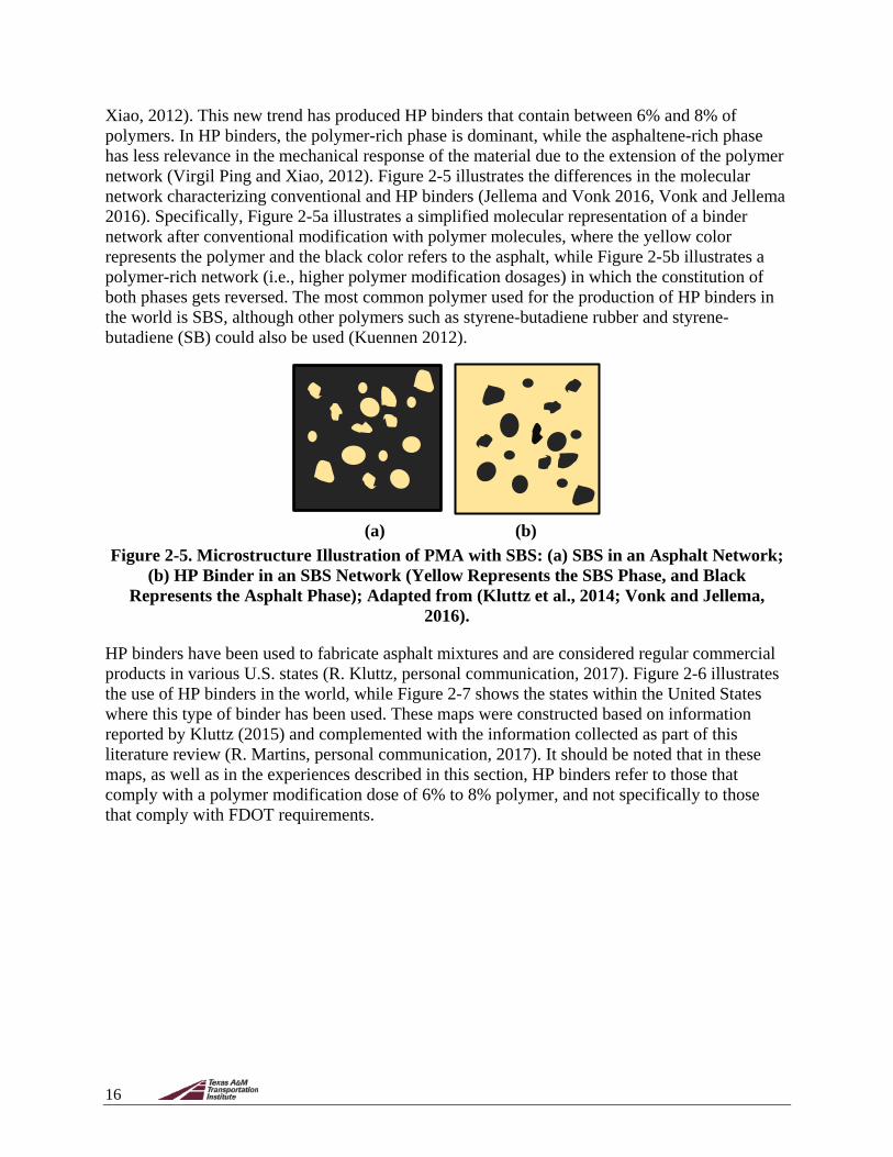
16
Xiao, 2012). This new trend has produced HP binders that contain between 6% and 8% of polymers. In HP binders, the polymer-rich phase is dominant, while the asphaltene-rich phase has less relevance in the mechanical response of the material due to the extension of the polymer network (Virgil Ping and Xiao, 2012). Figure 2-5 illustrates the differences in the molecular network characterizing conventional and HP binders (Jellema and Vonk 2016, Vonk and Jellema 2016). Specifically, Figure 2-5a illustrates a simplified molecular representation of a binder network after conventional modification with polymer molecules, where the yellow color represents the polymer and the black color refers to the asphalt, while Figure 2-5b illustrates a polymer-rich network (i.e., higher polymer modification dosages) in which the constitution of both phases gets reversed. The most common polymer used for the production of HP binders in the world is SBS, although other polymers such as styrene-butadiene rubber and styrene-butadiene (SB) could also be used (Kuennen 2012).
(a) (b) Figure 2-5. Microstructure Illustration of PMA with SBS: (a) SBS in an Asphalt Network;
(b) HP Binder in an SBS Network (Yellow Represents the SBS Phase, and Black Represents the Asphalt Phase); Adapted from (Kluttz et al., 2014; Vonk and Jellema,
2016).
HP binders have been used to fabricate asphalt mixtures and are considered regular commercial products in various U.S. states (R. Kluttz, personal communication, 2017). Figure 2-6 illustrates the use of HP binders in the world, while Figure 2-7 shows the states within the United States where this type of binder has been used. These maps were constructed based on information reported by Kluttz (2015) and complemented with the information collected as part of this literature review (R. Martins, personal communication, 2017). It should be noted that in these maps, as well as in the experiences described in this section, HP binders refer to those that comply with a polymer modification dose of 6% to 8% polymer, and not specifically to those that comply with FDOT requirements.
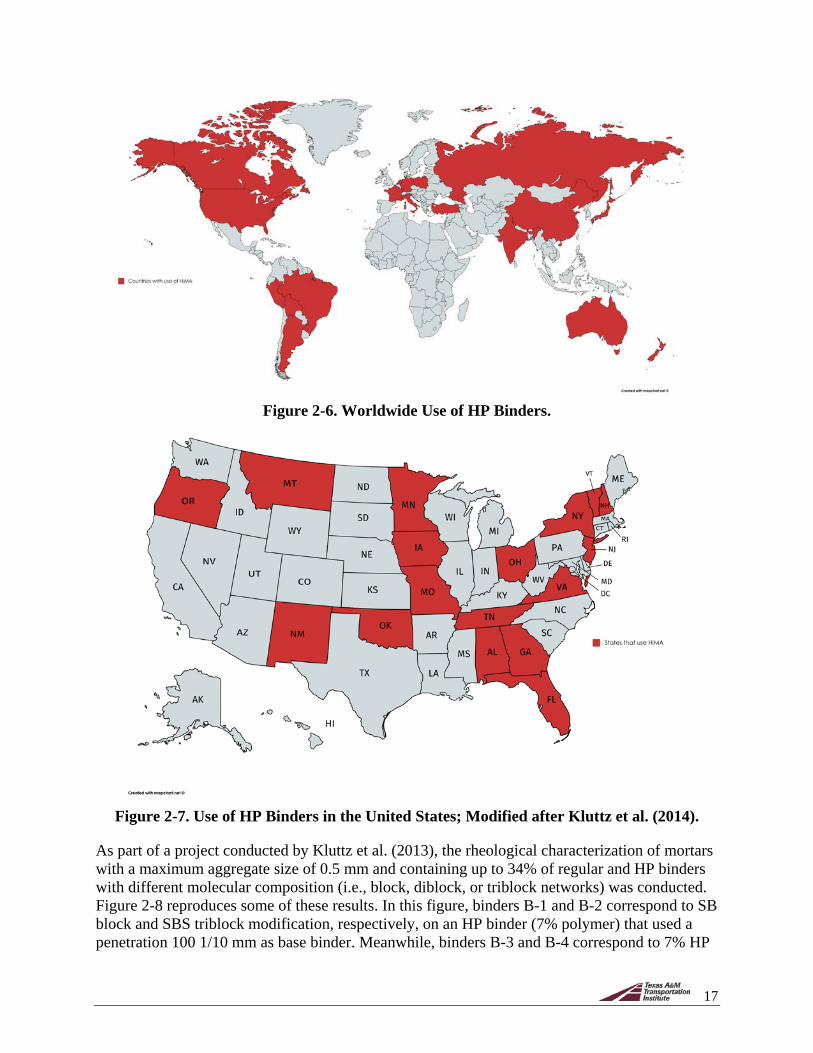
17
Figure 2-6. Worldwide Use of HP Binders.
Figure 2-7. Use of HP Binders in the United States; Modified after Kluttz et al. (2014).
As part of a project conducted by Kluttz et al. (2013), the rheological characterization of mortars with a maximum aggregate size of 0.5 mm and containing up to 34% of regular and HP binders with different molecular composition (i.e., block, diblock, or triblock networks) was conducted. Figure 2-8 reproduces some of these results. In this figure, binders B-1 and B-2 correspond to SB block and SBS triblock modification, respectively, on an HP binder (7% polymer) that used a penetration 100 1/10 mm as base binder. Meanwhile, binders B-3 and B-4 correspond to 7% HP
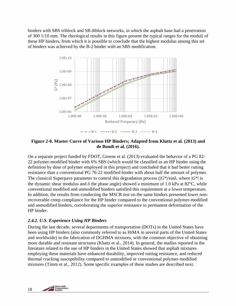
18
binders with SBS triblock and SB diblock networks, in which the asphalt base had a penetration of 300 1/10 mm. The rheological results in this figure present the typical ranges for the moduli of these HP binders, from which it is possible to conclude that the highest modulus among this set of binders was achieved by the B-2 binder with an SBS modification.
Figure 2-8. Master Curve of Various HP Binders; Adapted from Kluttz et al. (2013) and
de Bondt et al. (2016).
On a separate project funded by FDOT, Greene et al. (2013) evaluated the behavior of a PG 82-22 polymer-modified binder with 6% SBS (which would be classified as an HP binder using the definition by dose of polymer employed in this project) and concluded that it had better rutting resistance than a conventional PG 76-22 modified binder with about half the amount of polymer. The classical Superpave parameter to control this degradation process (|G*|/sinδ, where |G*| is the dynamic shear modulus and δ the phase angle) showed a minimum of 1.0 kPa at 82°C, while conventional modified and unmodified binders satisfied this requirement at a lower temperature. In addition, the results from conducting the MSCR test on the same binders presented lower non-recoverable creep compliance for the HP binder compared to the conventional polymer-modified and unmodified binders, corroborating the superior resistance to permanent deformation of the HP binder.
2.4.2. U.S. Experience Using HP Binders During the last decade, several departments of transportation (DOTs) in the United States have been using HP binders (also commonly referred to as HiMA in several parts of the United States and worldwide) in the fabrication of DGHMA mixtures, with the common objective of obtaining more durable and resistant structures (Kluttz et al., 2014). In general, the studies reported in the literature related to the use of HP binders in the United States showed that asphalt mixtures employing these materials have enhanced durability, improved rutting resistance, and reduced thermal cracking susceptibility compared to unmodified or conventional polymer-modified mixtures (Timm et al., 2012). Some specific examples of these studies are described next.
1.0E+06
1.0E+07
1.0E+08
1.0E+09
1.0E+10
1.00E-08 1.00E-06 1.00E-04 1.00E-02 1.00E+00
G* (P
a)
Reduced Frequency [Hz]
B-1 B-2 B-3 B-4

19
In 2013, the New Hampshire DOT developed a project that consisted of constructing and monitoring four trial sections with a variety of mixtures as surface course along a 14.8 mi stretch of road between Auburn and Candia (Lee and Raghunathan, 2015). The surface course in one of the sections included a DGHMA mixture with HP binder and 17% RAP content, while the others contained a surface course with 33.8% RAP content, warm mix asphalt, and asphalt rubber. Some important findings of this study were that the two surface courses with HP-modified or asphalt rubber had the same riding quality as conventional DGHMA adjacent to the trial sections. Moreover, some laboratory experimental tests conducted on these two mixtures showed that they had a better resistance to cracking (i.e., up to three times more cracking resistance) and, consequently, a longer service life. Finally, noise reduction was evaluated in the field following AASHTO TP 76-12, and the results showed that these two mixtures provided quieter surfaces compared to the conventional DGHMA mixture.
Other states, including Missouri and Utah, have expressed interest in using HP binder mixtures and the need for conducting more research on these materials (NCAT 2015). Utah DOT, for example, is developing a new cold-in-place recycling specification and is assessing the performance of trial segments containing mixtures fabricated with HP-modified and fiber-modified binders (NCAT 2015).
Between 2009 and 2012, NCAT conducted a study funded by a series of federal agencies, state DOTs, and private companies (Timm et al., 2012) in which one segment in the NCAT test track aimed at comparing the performance of two trial lanes with HP-modified and regular modified binder mixtures. The pavement structure in one trial lane was composed of a surface course (1.2 in. [30.5 mm]) and an intermediate layer (2.8 in. [71.1 mm]) containing conventional polymer-modified DGHMA, a base layer with an unmodified mixture (3 in. [76.2 mm]), and an unbound aggregate base (5.8 in. [147.3 mm]). The other trial lane included an HP-modified DGHMA mixture for the surface (1.5 in. [38.1 mm]), intermediate (2.8 in. [71.1 mm]), and base (2.6 in. [68.6 mm]) courses, and an unbounded granular base (5.3 in. [134.6 mm]). Table 2-3 summarizes the main properties of the conventional (control) and HP-modified DGHMA mixtures. In the fabrication of the DGHMA mixtures, higher temperatures were used for the HP binder (i.e., the mixing temperature increased between 10–15°F [5.6–8.4ºC] compared to the mixtures with conventional modified binder), while the compaction temperature was almost 30°F (16ºC) higher for these mixtures (Timm et al., 2012). In the same study, the PG of the HP binder was reported as PG 88-22, although the continuous grade was PG 93.5-26.4 (i.e., the binder failed passing the required difference in the non-recoverable creep compliance of the MSCR standard).

20
Table 2-3. Properties of Surface Courses in NCAT Phase IV Project (Timm et al., 2012).
Mixture Type
Pavement with Regular Polymer-Modified and Unmodified
Mixtures (Control) Pavement with HP-DGHMA
Surface Intermediate Base Surface Intermediate and Base
Asphalt PG Grade 76-22 76-22 67-22 88-22* 88-22* % Polymer Modification 2.8 2.8 0 7.5 7.5
Field Air Voids % 6.9 7.2 7.4 6.3 7.3/7.2 Total Combined Binder (Pb),
% wt 5.8 4.7 4.6 5.9 4.6
Asphalt, % 6.1 4.4 4.7 6.3 4.6 Dust Proportion 1.1 0.9 1.1 1.1 0.9
Maximum Specific Gravity (Gmm)
2.483 2.575 2.574 2.474 2.570
* Heavily polymer-modified asphalt.
Back-calculated dynamic modulus values obtained from falling weight deflectometer (FWD) measurements at a service temperature of 40–50°C showed that the modulus of the HP-modified mixtures was greater than the conventional mixture. Additional tests conducted on plant-produced laboratory-compacted specimens suggested that HP modification had a higher impact (i.e., larger values) on the surface HP-DGHMA (9.5 mm NMAS) than in the intermediate and base HP-DGHMA layers (19 mm NMAS) and, in accordance to the FWD results, that the surface HP-DGHMA presented larger values of modulus compared to the control mixture, as observed in Figure 2-9. In addition, bending beam fatigue testing conducted on both mixtures showed that the cycles to failure in the HP-modified mixture (i.e., 6.04×10⁶ cycles) were 45 times more than those required in the control or conventional modified material, indicating that the HP-modified mixture presented a superior fatigue resistance. In terms of rutting susceptibility, the surface HP-modified mixture presented lower flow number values compared to the conventional material. Finally, it was corroborated that the HP-modified mixture used in the surface layer (9.5 mm NMAS) also showed higher resistance to low-temperature cracking and smaller susceptibility to moisture damage (based on TSR results) compared to the conventional mixture.

21
Figure 2-9. Dynamic Modulus Testing Results on Plant-Produced Conventional and
HP-Modified DGHMA Mixtures; Adapted from Willis et al. (2012).
No experiences in the use of HP binders for the fabrication of OGFCs were found in the United States as part of this literature review. Nevertheless, based on the increasing experiences using HP-modified binders, it is expected that several DOTs will explore the use of this type of binder in the near future.
2.4.3. Latin American Experience Using HP Binders The case of Latin America is similar to that of the United States, in the sense that the use of this type of binder is recent (i.e., last five years) and has been limited to the fabrication of DGHMA mixtures. A project in Argentina, for instance, included the use of this type of modified binder in the construction of an airport runway (R. Martins, personal communication, 2017). In addition, there is evidence that Argentina has been conducting some trial sections using HP binder mixtures with the objective of extending the applications of this material in the road networks of the country. This objective responds to the suggestions provided by Quevedo et al. (2016) and Sanziani et al. (2015), who—through a comparative study of the performance of different polymer-modified binders and a specific study on HP modification using Argentinian asphalts—identified some specific benefits in terms of the performance of flexible pavements when using this type of modification.
Other important experiences with this material have been conducted in Brazil. One of the most relevant cases includes a project consisting of the performance assessment of a highway connecting Sao Paulo and the city of Curitiba in the south of Brazil during a 29-month period. This study, led by a research group from the University of Sao Paulo, included the comparison of two pavement structures, one with a 3.0 in. (7.5 cm) HP-modified DGHMA overlay and the other with a 2.0 in. (5.0 cm) DGHMA SBS overlay, both on top of a 1.0 in. (2.5 cm) stress absorbing membrane interlayer (SAMI) located over an in-service pavement structure (Gaspar et al., 2017). The objective of the SAMI layer was to prevent reflective cracking from the existing surface course. So far, the results have shown that the use of the HP-modified DGHMA overlay with the SAMI layer enhanced the response against reflective cracking since only 12.2% reflective cracks were observed on the overlay, while the DGHMA SBS overlay presented 48.1% reflective cracking during the same time period. Moreover, the HP-modified DGHMA overlay has presented a good rutting resistance (Gaspar et al., 2017).
1
10
100
1000
10000
100000
0.000001 0.0001 0.01 1 100 10000
E* (M
Pa)
Reduced Frequency (Hz)
Control SurfaceHiMA Surface

22
Besides these experiences in Argentina and Brazil, it was also possible to identify the use of HP binders as part of DGHMA mixtures in public-private partnership road projects in Peru and Bolivia (D. Gonzalez, personal communication, 2017; R. Martins, personal communication, 2017). In both cases, the motivation for having selected the use of HP binder over conventional polymer-modified binder was the expected increased durability of the material.
Finally, it is worth mentioning that a representative of Kraton in Latin America mentioned in a personal communication that one advantage of using SBS as an additive to fabricate HP binder mixtures is that its implementation is not a challenging process since no additional equipment costs are involved (R. Martins, personal communication, 2017). According to Martins' experience, this condition, in addition to the existing successful experiences on the use of this type of binder, has contributed to the expanded use of HP-modified mixtures in Latin America.
2.4.4. European Experience Using Polymer-Modified Materials in OGFC This section focuses on the varied perception that exists in The Netherlands and Germany about the use of polymer-modified binders, including the use of HP-OGFCs. As mentioned in the initial part of this document, Europe applies OGFC mixtures extensively (J.L.M. Voskuilen, personal communication, 2017). According to a published work about The Netherlands’ experience (Voskuilen et al., 2004), the government expects to implement 100% OGFC in its national road network. An example of the broad experience and research conducted in the last couple of decades on the topic of OGFC is accounting for a significant period of freeze-thaw that occurs in the country about every 10 years. In fact, the deterioration caused by the presence of this periodic climatic condition is considered a normal phase in the life cycle of these mixtures, and no special conservation activities are currently applied to extend the service life of the surface layer (Voskuilen and Elzinga, 2010).
In terms of the materials used in the production of OGFC mixtures, The Netherlands employs a base bitumen classified as penetration 70-100 (1/10 mm) for single OGFC layers and a conventional polymer-modified binder as part of the upper layer in TLPA systems (i.e., two-layer OGFC mixtures) (J.L.M. Voskuilen, personal communication, 2017). For OGFC single layers, the typical thickness is 5.0 cm (2.0 in.), while the typical thicknesses for the TLPA systems are 4.5 cm (1.8 in.) for the bottom layer and 2.5 cm (1.0 in.) for the upper layer. The durability of the OGFC mixture is dependent on the location of placement; single OGFC layers in fast lanes have longer service lives of about 16 years, while in the slow lanes, the average service life is 12 years (Voskuilen and Elzinga, 2010; Voskuilen and van de Ven 2010). According to the same sources, the lifespan of TLPA is about nine years in the slow lanes and 13 years in the fast lanes, on average.
Based on a personal communication via email with Mr. Jan Voskuilen, senior advisor for pavements of the Ministry of Infrastructure and Environment of The Netherlands, it was determined that this country is not considering using HP binders as part of its OGFC mixtures. The reason is that officials believe that the durability of their OGFC mixtures is great enough to be equivalent to that of conventional DGHMA surface mixtures without the need for further polymer modification (J.L.M. Voskuilen, personal communication, 2017). Mr. Voskuilen also suggested that the use of HP-OGFC would not provide improved resistance to raveling compared to their current OGFC mixtures, and therefore, it would not increase the durability of the material. It is noteworthy that this is his personal point of view based on his professional

23
experience but is not supported by written documentation. Nevertheless, this consideration derives from the rationale that, based on the country’s experiences, polymer modification is used as a strategy to prevent rutting in OGFC but not to improve raveling, which according to this expert is mainly a phenomenon related to aging processes.
Contrary to the point of view of experts in The Netherlands, the information gathered as part of this literature review showed that Germany is currently using HP binders in the fabrication of OGFC mixtures. According to a personal communication with Mr. Stefan Ehlert, senior consultant for pavements in the Northrine-Westfalia Federal State in the Road Construction Department, the use of this type of binder enhances durability of OGFC mixtures. In general, OGFC or OPA mixtures in Germany have an average service life between 10 to 12 years, although no specific information about the durability of HP-OGFC was found. The specification for polymer-modified binders in this country corresponds to a binder material classified as PmB 40/100-65-H, in which the first letters refer to binder modification with polymers, the digits refer to the penetration of the base asphalt and the result of the ring-and-ball softening boiling point test, and the letter “H” means that the material is highly polymer modified. According to this specification, the percentage of polymer modification is defined by the contractor and has no specific regulation (ZTV/TL Asphalt—STB 07) (S. Ehlert, personal communication, 2017). The main characteristic of the OPA and HP-OPA mixtures are as follows (Bundesministerium für Verkehr Bau und Stadtentwicklung, 2007):
• AV content between 24 and 28%. • 45 to 50 mm layer thickness. • Different NMASs, usually OPA 8 or OPA 11, which have values of NMAS of 8 mm and
11 mm, respectively. • Presence of waterproof SAMI layer underneath the OPA. • Noise reduction of 6 to 8 dB.
An important difference between the Dutch and the German OGFC mixtures is that the Dutch mixtures have a more continuous gradation that enables more contact points, while the German OGFC gradation is very open. According to information gather via personal communication with Mr. Voskuilen, this could be a major factor explaining the longer lifespan of the Dutch materials (de Bondt et al., 2016). Moreover, the decrease in quality of the contact network of the more open gradation in the German OGFC might partially explain the necessity for using enhanced binders (i.e., conventional and HP binders) in these mixtures in order to guarantee proper performance throughout their service life (J.L.M. Voskuilen, personal communication, 2017). Is important to denote that the high AV content present in the 43German OGFC may reduce the durability of the mixtures.
2.4.5. Japanese Experience Using HP Binders in OGFC Japan has used HP binders in the fabrication of OGFC mixtures for the last 15 years to prevent raveling and, consequently, to increase the durability of these surface layers (Suzuki et al., 2010). Use of polymer-modified binders initiated in 1952 in Japan, and according to Suzuki et al. (2010), OGFC mixtures with 8% polymer modification dosages endure up to 20 years in service. In fact, 11 to 15% polymer modification is used in the OGFC mixtures implemented in the

24
coldest regions of the country, limiting the air voids to 17%, in order to obtain an equivalent durability to conventional HP-OGFC in warmer regions.
According to Suzuki et al. (2010), Japan has used up to 15% SBS modification to overcome major difficulties experienced in OGFC such as durability and functionality in cold winters, bridge pavements, and manipulation and use of small aggregates.
Table 2-4 summarizes the basic properties required for polymer-modified binders used for OGFC, according to the Japan Modified Asphalt Association Standard (Suzuki et al., 2010). Table 2-5 summarizes the typical values obtained for high-viscosity modified binders, which have between 10 and 15% polymer modification, a percentage that is superior to that used in common HP binders (i.e., 7 to 7.5%) and that could be called super highly modified binders. A comparison between this specification and those currently required by FDOT is difficult to pursue, mainly due to the parameters that are used in each case (i.e., Superpave vs. traditional classification).
Table 2-4. Characteristics Required in Japan for Polymer-Modified Binder for OGFC Mixtures; Adapted from Suzuki et al. (2010).
Item/Type H H-F
Softening Point Min. 80.0
Ductility (7°C) – –
Ductility (15°C) Min. 50 –
Toughness Min. 20 –
Tenacity – –
Percentage of bitumen stripped off coarse aggregates – –
Fraass breaking point – Max. 12
Bending workload (−20°C) – Min. 400
Bending stiffness (−20°C) – Max. 100
Penetration 25°C Min. 40
Mass change after TFOT %m 0.6
Retained penetration ratio after TFOT Min. 65
Flash point Min. 260
Density (15°C) To be reported
Optimum mixing temperature °C To be reported
Optimum compaction temperature °C To be reported Note: H = highly polymer-modified binder, H-F = high-viscosity or super highly polymer-modified binders, TFOT = thin-film oven test.

25
Table 2-5. Properties of Two Types of Binder; Adapted from Suzuki et al. (2010).
Test Temperature
Type of Binder Super Highly
Modified Asphalt (10%–15% polymer)
Binder 60/80
Softening point (°C) °C 86 45.5
Ductility (cm) 4°C 21 – 15°C 93 100+
Toughness (n·m) 25°C 37 5 Tenacity (n·m) 25°C 26 1
Fraass breaking point °C −34 −9 Penetration (0.1 mm) 25°C 45 70
Viscosity (Pa·s) 60°C 49,100 250 Density (g/cm3) 15° 1.02 1,035
Kinematic viscosity (mm2/s)
140°C 2,260 309 160°C 921 136 180°C 419 69 200°C 241 40

26
3.0. MATERIALS Two types of binders modified with SBS polymer were included in this study. The first was a polymer-modified binder with an SBS dose between 2–3% by weight of binder (PG 76-22 PMA), which was used as a control binder. The second was a PG 76-22 HP (i.e., SBS polymer modification dose between 6–8%) produced in an asphalt plant in Greensboro, North Carolina. This binder is labeled HP henceforth in this report. With respect to aggregate sources, a limestone from White Rock Quarries, classified with code 87339 and subtype codes C41 (S1A Stone) and C51 (S1B Stone), and a granite from Junction City Mining, with code GA553, subtype codes C47 (S1A Stone) and C53 (S1B Stone), and F22 screenings, were used for the FC-5 mixtures. Four FC-5 mixtures were evaluated using combinations of these materials. The optimum binder content (OBC) by total weight of mixture for the FC-5 with granite was 5.9%, which was determined by FDOT’s State Materials Office, Bituminous Materials Division via the pie plate method. This method consists of preparing several mixtures at different binder contents. The mixtures are placed into clear Pyrex dishes, or pie plates. The dishes containing the mixtures are placed in the oven for about 1–2 hours at the mixing temperature, which is approximately 320°F (160°C). Then, the dishes are removed from the oven and the material is allowed to cool to room temperature. The plate with the mixture is inverted and the bottom surface of the dish is inspected visually. The OBC must show sufficient bonding between the plate and the mix without evidence of excessive drainage. The granite mixture had 1% of hydrated lime by weight of aggregate. The OBC for the FC-5 mixtures with limestone was 6.5% and included 0.5% by weight of binder of a liquid antistrip additive. All mixtures had 0.3% of cellulose fibers by weight of mixture. Table 3-1 summarizes the characteristics of the four FC-5 mixtures.
Table 3-1. Characteristics of the FC-5 Mixtures.
Product Blend Granite Limestone
mm Sieve No. Job Mix Formula Job Mix Formula
Sieve Size
19 3/4 100.0% 100% 12.5 1/2 98.0% 85.5% 9.5 3/8 71.0% 58.2%
4.75 4 23.0% 21.0% 2.36 8 9.0% 8.6% 1.18 16 4.0% 5.7% 0.6 30 4.0% 4.7% 0.3 50 3.0% 3.7%
0.15 100 3.0% 2.2% 0.75 200 2.5% 2.0%
Aggregate Proportion
70% S1A 24% S1B
5% Screenings 1% Lime
65% S1A 35% S1B
OBC 5.9% 6.50% Antistrip (%) 1.0 by weight of aggregate 0.5 by weight of binder
Cellulose Fiber 0.3 by weight of mixture

27
The morphology and SFE characteristics of both aggregate types were obtained from a previous report (Arámbula-Mercado et al., 2016). Since the same aggregate sources were used in the previous report and in this study, it was assumed that the aggregates tested before were representative of the ones used in this project. A summary of the results of this characterization is presented in Appendix B.
For the 2D FE numerical models, the same four mixtures resulting from combining the two types of binders (i.e., PMA and HP asphalt binders) and the two types of aggregate (i.e., limestone and granite) were used. The Cantabro abrasion loss results obtained on these same FC-5 mixtures under various aging states and subjected to multiple cycles of 300 revolutions at 30–33 rpm each, were used to generate deterioration curves to estimate pavement service life to be used as input in the LCCA.

28
4.0. EXPERIMENTAL TEST PLAN Four OGFC mixtures resulting from combining each type of aggregate with each type of binder listed in Chapter 3 were used in the experimental test plan (i.e., granite-PMA, granite-HP, limestone-PMA, and limestone-HP). The following sections describe the tests that were conducted on the binders, mastics, and mixtures.
4.1. BINDERS AND MASTICS The PMA and HP binders were provided by FDOT. Each binder was evaluated under five aging states since the impact of aging on the rheological response and performance of the binder is critical for the durability of the FC-5 mixtures. The five aging states included (a) unaged (i.e., virgin/original binder [OB] state); (b) rolling thin-film oven (RTFO) state; (c) pressure aging vessel (PAV) after 20 hours (i.e., PAV20); (d) PAV after 40 hours (i.e., PAV40); and (e) PAV after 80 hours (i.e., PAV80). RTFO aging was done at 163°C (325°F) for 85 minutes per AASHTO T 240, and PAV aging was at 100°C with a pressure of 2.1 MPa (305 psi) per AASHTO R 28 (AASHTO 2012; 2013a).
According to a study conducted on dense mixtures (Epps-Martin et al., 2017), different PAV aging periods simulate various pavement service life times, depending on the environmental conditions of the location where the pavement is placed and the PG of the virgin binder. If one considers that the climate in Texas and Florida is somewhat similar, for a PG 64-22, the equivalency using rheology-based G-R estimations would be about three, six, and seven years of pavement service life for PAV20, PAV40, and PAV60, respectively (PAV60 is a shorter aging duration than the PAV80 that was used in this study; therefore, an aging of 11 years was assigned to PAV80 based on a projected estimate). However, for FC-5 mixtures, a different virgin binder PG is used, and the total AV content is higher as compared to dense-graded mixtures; therefore, the equivalence in pavement service life could vary.
The tests performed on binders and mastics are listed in Table 4-1. The information about the material properties obtained from these tests allowed researchers to compare them in terms of their stiffness and provided fundamental input for the constitutive models used in the FE numerical simulations. A brief description of these tests is presented next.

29
Table 4-1. Experimental Plan for Binders and Mastics. Material Test Method Standard Parameter Aging State Replicates Outcome
Binder
PG AASHTO M 320
Continuous PG and ∆Tc
OB 1 Stiffness, ductility,
and sensitivity to aging
RTFO 1
PAV20 2
MSCR AASHTO TP 70
% Recovery and non-
recoverable creep
compliance (Jnr)
RTFO 3
Elastic response and stress
dependency
Temperature and Frequency Sweep Tests
— Master curve
and G-R parameter
OB 3 LVE
properties RTFO 3 PAV20-40-80 3 each
FTIR — Carbonyl area OB 3
Chemical aging RTFO 3
PAV20-40-80 3 each
PLAS Test —
Fatigue resistant
energy index (FREI)
OB 2 Fatigue
resistance RTFO 2 PAV20-40-80 2 each
SFE — SFE
components and total SFE
OB RTFO PAV20
5 each Adhesion properties
Mastic
Temperature and Frequency Sweep Tests
— Master curve
and G-R parameter
OB 3 LVE
properties RTFO 3 PAV20 3
SFE — SFE
components and total SFE
OB 5 Adhesion properties
Mastics were prepared by combining the fine portion of the aggregates (i.e., fillers or particles passing No. 200) with the binders. Four mastics were prepared using the combinations of the two binders and two aggregates. The mastics were prepared using a volumetric concentration of 0.24 between binder and filler. This value was based on recommendations provided in the literature (Alvarez et al., 2012; 2018; Massahi et al., 2018). Since the bulk specific gravities of the two types of aggregates (2.77 for granite and 2.41 for limestone, per FDOT mix designs) were different from each other and much higher than the specific gravity of the two types of binders (assumed 1.10), the total binder content for the mastic specimens prepared with granite and limestone fillers totaled 56% and 59% by total weight of the mastic specimen. The following relationships describe how the mastic proportions were developed:
Vc = VfVf+Va
= 0.24 (assumed) (1)
VfVa
= Vc1−Vc
= 0.32 (calculated) (2)
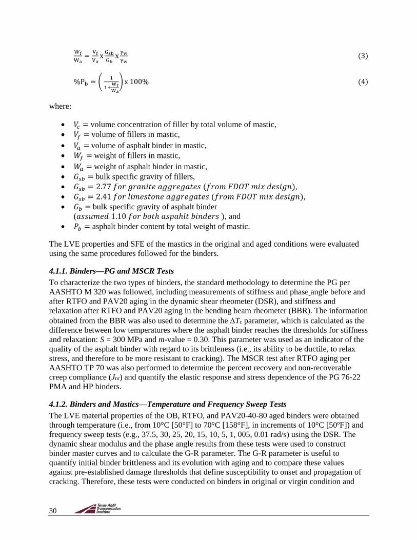
30
WfWa
= VfVa
x GsbGb
x γwγw
(3)
%Pb = � 1
1+WfWa
� x 100% (4)
where:
• 𝑉𝑉𝑐𝑐 = volume concentration of filler by total volume of mastic, • 𝑉𝑉𝑓𝑓 = volume of fillers in mastic, • 𝑉𝑉𝑎𝑎 = volume of asphalt binder in mastic, • 𝑊𝑊𝑓𝑓 = weight of fillers in mastic, • 𝑊𝑊𝑎𝑎 = weight of asphalt binder in mastic, • 𝐺𝐺𝑠𝑠𝑠𝑠 = bulk specific gravity of fillers, • 𝐺𝐺𝑠𝑠𝑠𝑠 = 2.77 𝑓𝑓𝑓𝑓𝑓𝑓 𝑔𝑔𝑓𝑓𝑎𝑎𝑎𝑎𝑎𝑎𝑎𝑎𝑎𝑎 𝑎𝑎𝑔𝑔𝑔𝑔𝑓𝑓𝑎𝑎𝑔𝑔𝑎𝑎𝑎𝑎𝑎𝑎𝑎𝑎 (𝑓𝑓𝑓𝑓𝑓𝑓𝑓𝑓 𝐹𝐹𝐹𝐹𝐹𝐹𝐹𝐹 𝑓𝑓𝑎𝑎𝑚𝑚 𝑑𝑑𝑎𝑎𝑎𝑎𝑎𝑎𝑔𝑔𝑎𝑎), • 𝐺𝐺𝑠𝑠𝑠𝑠 = 2.41 𝑓𝑓𝑓𝑓𝑓𝑓 𝑙𝑙𝑎𝑎𝑓𝑓𝑎𝑎𝑎𝑎𝑎𝑎𝑓𝑓𝑎𝑎𝑎𝑎 𝑎𝑎𝑔𝑔𝑔𝑔𝑓𝑓𝑎𝑎𝑔𝑔𝑎𝑎𝑎𝑎𝑎𝑎𝑎𝑎 (𝑓𝑓𝑓𝑓𝑓𝑓𝑓𝑓 𝐹𝐹𝐹𝐹𝐹𝐹𝐹𝐹 𝑓𝑓𝑎𝑎𝑚𝑚 𝑑𝑑𝑎𝑎𝑎𝑎𝑎𝑎𝑔𝑔𝑎𝑎), • 𝐺𝐺𝑠𝑠 = bulk specific gravity of asphalt binder
(𝑎𝑎𝑎𝑎𝑎𝑎𝑎𝑎𝑓𝑓𝑎𝑎𝑑𝑑 1.10 𝑓𝑓𝑓𝑓𝑓𝑓 𝑏𝑏𝑓𝑓𝑎𝑎ℎ 𝑎𝑎𝑎𝑎𝑎𝑎𝑎𝑎ℎ𝑙𝑙𝑎𝑎 𝑏𝑏𝑎𝑎𝑎𝑎𝑑𝑑𝑎𝑎𝑓𝑓𝑎𝑎 ), and • 𝑃𝑃𝑠𝑠 = asphalt binder content by total weight of mastic.
The LVE properties and SFE of the mastics in the original and aged conditions were evaluated using the same procedures followed for the binders.
4.1.1. Binders—PG and MSCR Tests To characterize the two types of binders, the standard methodology to determine the PG per AASHTO M 320 was followed, including measurements of stiffness and phase angle before and after RTFO and PAV20 aging in the dynamic shear rheometer (DSR), and stiffness and relaxation after RTFO and PAV20 aging in the bending beam rheometer (BBR). The information obtained from the BBR was also used to determine the ∆Tc parameter, which is calculated as the difference between low temperatures where the asphalt binder reaches the thresholds for stiffness and relaxation: S = 300 MPa and m-value = 0.30. This parameter was used as an indicator of the quality of the asphalt binder with regard to its brittleness (i.e., its ability to be ductile, to relax stress, and therefore to be more resistant to cracking). The MSCR test after RTFO aging per AASHTO TP 70 was also performed to determine the percent recovery and non-recoverable creep compliance (Jnr) and quantify the elastic response and stress dependence of the PG 76-22 PMA and HP binders.
4.1.2. Binders and Mastics—Temperature and Frequency Sweep Tests The LVE material properties of the OB, RTFO, and PAV20-40-80 aged binders were obtained through temperature (i.e., from 10°C [50°F] to 70°C [158°F], in increments of 10°C [50ºF]) and frequency sweep tests (e.g., 37.5, 30, 25, 20, 15, 10, 5, 1, 005, 0.01 rad/s) using the DSR. The dynamic shear modulus and the phase angle results from these tests were used to construct binder master curves and to calculate the G-R parameter. The G-R parameter is useful to quantify initial binder brittleness and its evolution with aging and to compare these values against pre-established damage thresholds that define susceptibility to onset and propagation of cracking. Therefore, these tests were conducted on binders in original or virgin condition and
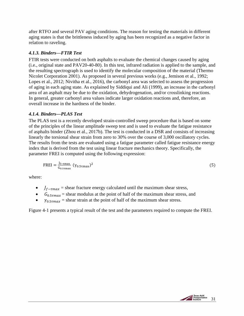
31
after RTFO and several PAV aging conditions. The reason for testing the materials in different aging states is that the brittleness induced by aging has been recognized as a negative factor in relation to raveling.
4.1.3. Binders—FTIR Test FTIR tests were conducted on both asphalts to evaluate the chemical changes caused by aging (i.e., original state and PAV20-40-80). In this test, infrared radiation is applied to the sample, and the resulting spectrograph is used to identify the molecular composition of the material (Thermo Nicolet Corporation 2001). As proposed in several previous works (e.g., Jemison et al., 1992; Lopes et al., 2012; Nivitha et al., 2016), the carbonyl area was selected to assess the progression of aging in each aging state. As explained by Siddiqui and Ali (1999), an increase in the carbonyl area of an asphalt may be due to the oxidation, dehydrogenation, and/or crosslinking reactions. In general, greater carbonyl area values indicate larger oxidation reactions and, therefore, an overall increase in the hardness of the binder.
4.1.4. Binders—PLAS Test The PLAS test is a recently developed strain-controlled sweep procedure that is based on some of the principles of the linear amplitude sweep test and is used to evaluate the fatigue resistance of asphalts binder (Zhou et al., 2017b). The test is conducted in a DSR and consists of increasing linearly the torsional shear strain from zero to 30% over the course of 3,000 oscillatory cycles. The results from the tests are evaluated using a fatigue parameter called fatigue resistance energy index that is derived from the test using linear fracture mechanics theory. Specifically, the parameter FREI is computed using the following expression:
FREI = Jf−τmaxG0.5τmax
(γ0.5τmax)2 (5)
where:
• 𝐽𝐽𝑓𝑓−𝜏𝜏𝜏𝜏𝑎𝑎𝜏𝜏 = shear fracture energy calculated until the maximum shear stress, • 𝐺𝐺0.5𝜏𝜏𝜏𝜏𝑎𝑎𝜏𝜏 = shear modulus at the point of half of the maximum shear stress, and • 𝛾𝛾0.5𝜏𝜏𝜏𝜏𝑎𝑎𝜏𝜏 = shear strain at the point of half of the maximum shear stress.
Figure 4-1 presents a typical result of the test and the parameters required to compute the FREI.

32
Figure 4-1. Results of the PLAS Test and Explanation of the Parameters to Compute the
FREI Fatigue Parameter (Zhou et al., 2017b).
4.1.5. Binders and Mastics—SFE Test SFE refers to the amount of work or energy required to create a new unit of surface of a material under vacuum conditions. Three key components of SFE are used together to determine the work required to separate two different materials at their interface and the work required to create a new interface in a material. These components include the Lifshitz-van der Waals (LW) component, 𝛾𝛾𝐿𝐿𝐿𝐿, Lewis acid component, 𝛾𝛾+, and Lewis base component, 𝛾𝛾− (Van Oss et al., 1988).
Each of these components refers to a different type of property or interaction of material. The LW component of SFE refers to work done for dispersion of atoms or molecules themselves without the transfer of electrons. The Lewis acid or base components refer to a polarity-dependent interaction that involves the transfer of electrons between atoms or molecules without the dispersion of atoms or molecules. Materials with significantly higher 𝛾𝛾𝐿𝐿𝐿𝐿 values (e.g., hydrocarbons) are known as non-polar compounds, whereas materials with significantly higher 𝛾𝛾+or 𝛾𝛾− values are known as polar compounds. These components together determine the work of cohesion between materials A and B, 𝑤𝑤𝐴𝐴𝐴𝐴, and the work of adhesion of material A, 𝑤𝑤𝐴𝐴𝐴𝐴, as described by the following equations (Van Oss et al., 1988):
wAB = Wadhesion2
= �γALW . γB
LW + �γA+. γB
− + �γA−. γB
+ (6)
wAA = Wcohesion2
= γALW + 2�γA
+ γA− (7)
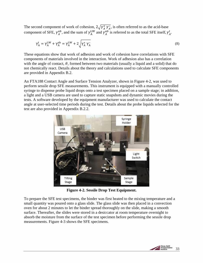
33
The second component of work of cohesion, 2�𝛾𝛾𝐴𝐴+ 𝛾𝛾𝐴𝐴
−, is often referred to as the acid-base component of SFE, 𝛾𝛾𝐴𝐴
𝑎𝑎𝑠𝑠, and the sum of 𝛾𝛾ALW and 𝛾𝛾𝐴𝐴
𝑎𝑎𝑠𝑠 is referred to as the total SFE itself, 𝛾𝛾𝐴𝐴𝑡𝑡 .
γAt = γA
LW + γAab = γA
LW + 2�γA+ γA
− (8)
These equations show that work of adhesion and work of cohesion have correlations with SFE components of materials involved in the interaction. Work of adhesion also has a correlation with the angle of contact, 𝜃𝜃, formed between two materials (usually a liquid and a solid) that do not chemically react. Details about the theory and calculations used to calculate SFE components are provided in Appendix B.2.
An FTA188 Contact Angle and Surface Tension Analyzer, shown in Figure 4-2, was used to perform sessile drop SFE measurements. This instrument is equipped with a manually controlled syringe to dispense probe liquid drops onto a test specimen placed on a sample stage; in addition, a light and a USB camera are used to capture static snapshots and dynamic movies during the tests. A software developed by the equipment manufacturer was used to calculate the contact angle at user-selected time periods during the test. Details about the probe liquids selected for the test are also provided in Appendix B.2.2.
Figure 4-2. Sessile Drop Test Equipment.
To prepare the SFE test specimens, the binder was first heated to the mixing temperature and a small quantity was poured onto a glass slide. The glass slide was then placed in a convection oven for about 2 minutes to let the binder spread thoroughly on the slide, making a smooth surface. Thereafter, the slides were stored in a desiccator at room temperature overnight to absorb the moisture from the surface of the test specimen before performing the sessile drop measurements. Figure 4-3 shows the SFE specimens.
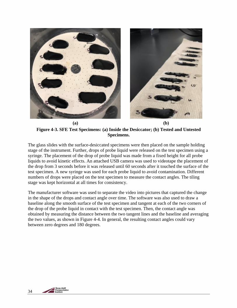
34
(a) (b)
Figure 4-3. SFE Test Specimens: (a) Inside the Desiccator; (b) Tested and Untested Specimens.
The glass slides with the surface-desiccated specimens were then placed on the sample holding stage of the instrument. Further, drops of probe liquid were released on the test specimen using a syringe. The placement of the drop of probe liquid was made from a fixed height for all probe liquids to avoid kinetic effects. An attached USB camera was used to videotape the placement of the drop from 3 seconds before it was released until 60 seconds after it touched the surface of the test specimen. A new syringe was used for each probe liquid to avoid contamination. Different numbers of drops were placed on the test specimen to measure the contact angles. The tiling stage was kept horizontal at all times for consistency.
The manufacturer software was used to separate the video into pictures that captured the change in the shape of the drops and contact angle over time. The software was also used to draw a baseline along the smooth surface of the test specimen and tangent at each of the two corners of the drop of the probe liquid in contact with the test specimen. Then, the contact angle was obtained by measuring the distance between the two tangent lines and the baseline and averaging the two values, as shown in Figure 4-4. In general, the resulting contact angles could vary between zero degrees and 180 degrees.
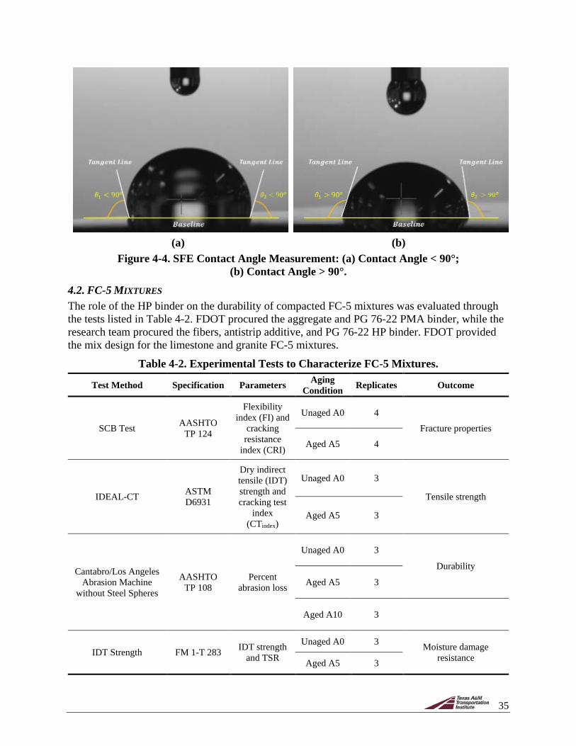
35
(a) (b)
Figure 4-4. SFE Contact Angle Measurement: (a) Contact Angle < 90°; (b) Contact Angle > 90°.
4.2. FC-5 MIXTURES The role of the HP binder on the durability of compacted FC-5 mixtures was evaluated through the tests listed in Table 4-2. FDOT procured the aggregate and PG 76-22 PMA binder, while the research team procured the fibers, antistrip additive, and PG 76-22 HP binder. FDOT provided the mix design for the limestone and granite FC-5 mixtures.
Table 4-2. Experimental Tests to Characterize FC-5 Mixtures.
Test Method Specification Parameters Aging Condition Replicates Outcome
SCB Test AASHTO TP 124
Flexibility index (FI) and
cracking resistance
index (CRI)
Unaged A0 4 Fracture properties
Aged A5 4
IDEAL-CT ASTM D6931
Dry indirect tensile (IDT) strength and cracking test
index (CTindex)
Unaged A0 3
Tensile strength
Aged A5 3
Cantabro/Los Angeles Abrasion Machine
without Steel Spheres
AASHTO TP 108
Percent abrasion loss
Unaged A0 3
Durability
Aged A5 3
Aged A10 3
IDT Strength FM 1-T 283 IDT strength and TSR
Unaged A0 3 Moisture damage resistance Aged A5 3

36
The experimental activities consisted of performing the following tests on the PMA and HP FC-5 compacted specimens: SCB, IDEAL-CT, Cantabro, IDT strength, and TSR. Specimens were prepared following the standard loose mix conditioning of 2 hours at 275°F (135°C) before compaction as recently recommended by NCHRP project 09-52 to simulate aging during production and construction (Newcomb et al., 2015). These conditioned specimens are labeled unaged or A0 in Table 4-2.
Including aging effects in the experimental test plan for the FC-5 mixtures was critical since oxidative hardening is one of the main causes that diminishes durability in these materials (Lin et al., 1995; Alvarez et al., 2006; 2008). Thus, an experimental procedure based on the research conducted as part of NCHRP project 09-54 was herein adopted to age the test specimens (Kim et al., 2017). The aging duration was based on the maps developed as part of NCHRP project 09-54, which indicate the amount of time of loose mix aging at 95°C (203°F) to simulate different years of field aging based on location. Therefore, the second aging state was denoted as A5, and it consisted of subjecting the loose mix prior to compaction to oven aging at 95°C (203°F) for 5 days. According to NCHRP project 09-54 (Kim et al., 2017), this conditioning procedure corresponds to approximately 2–3 years of field aging for dense-graded asphalt mixtures. Although the equivalence of this aging in terms of the actual pavement service life could be different for FC-5 mixtures, it was still considered representative and a significant longer aging period compared to A0. For durability evaluation (i.e., Cantabro abrasion loss test), an additional aging state was included, which consisted of subjecting the loose mix prior to compaction to oven aging at 95°C (203°F) for 10 days. This additional aging state was denoted A10 and would be approximately equivalent to five or more years of pavement service life for dense-graded mixtures (Kim et al., 2017).
4.2.1. Semicircular Bending Test The SCB test was used to quantify fracture properties of the FC-5 mixtures. The SCB test is performed according to AASHTO TP 124-16 (AASHTO, 2016). This test procedure consists of fabricating Superpave gyratory compactor (SGC) specimens 150 mm (5.9 in.) in diameter and 160 mm (6.3 in.) in height. Next, using a diamond-tipped saw blade with a water cooling system, two smaller cylindrical specimens with a height of 50±1 mm (1.97±0.04 in.) are obtained from the SGC specimen. Afterwards, these specimens are cut in half and a notch 15±1 mm (0.59±0.04 in.) deep and 1.5±0.1 mm (0.059±0.04 in.) wide is introduced in the center of the flat side of the specimen. It should be highlighted that although the AV content is controlled in the fabrication of the 160 mm (6.3 in.) height specimen, it is usually not verified in the final SCB specimens.
The specimen is placed on top of two rollers for testing, as observed in Figure 4-5. The test is performed at an intermediate temperature of 77°F (25°C) and consists of applying a monotonic load (F) at a rate of 2.0 in/min (50 mm/min) at the top center of the specimen. This setup produces tensile stresses that induce fracture initiation at the tip of the notch. The load-displacement curve was plotted and the area under the curve was determined (i.e., fracture energy [Gf]), as well as the slope of the fitted curve post-peak load. The output parameters are the FI, which is calculated by dividing the fracture energy by the slope of the post-peak load versus displacement curve, and the CRI, which is obtained by dividing Gf up to the peak load over the magnitude of the peak load. Researchers have demonstrated that FI and CRI provide separation between mixtures with distinct mixture characteristics, binder type in particular (Al-qadi et al., 2015; Zhou et al., 2016; Kaseer et al., 2018).

37
(a) (b)
Figure 4-5. SCB Test Setup: (a) Schematic; (b) Actual Specimen during Testing.
4.2.2. IDEAL-CT Test The IDEAL-CT was performed to obtain the tensile strength of the FC-5 mixtures. The advantages of this test are that it requires no instrumentation, cutting, gluing, drilling, or notching of the specimen. The IDEAL-CT was performed at an intermediate temperature of 77°F (25°C) and consisted of applying a monotonic load (P) at a rate of 50 mm/min (2.0 in/min) at the top center of the specimen using IDT strength test equipment. Zhou et al. (2017a) demonstrated that this test is sensitive to distinct mixture characteristics such as the presence of reclaimed asphalt pavement or asphalt shingles, binder content, aging condition, AV content, and, more importantly, binder type. Although not standard, the dimensions of the specimen that were considered were 6.0 in. (150 mm) in diameter by 2.0 in. (50 mm) in height to match the SCB specimen dimensions. The CTindex was calculated using the following expression for specimens whose thickness differed from 2.4 in. (62 mm):
CTindex = t62
× GfPl
× lD
(9)
where:
• 𝐺𝐺𝑓𝑓 = work of fracture (area under the load-displacement curve), • 𝑎𝑎 = specimen thickness, • P
𝑙𝑙 = slope of the load (P) vs. vertical displacement (l) curve, and
• l𝐷𝐷
= strain tolerance under load (vertical displacement to diameter ratio).
The CTindex is calculated post peak load on the load-displacement curve, where the load corresponded to 75% of the peak load value (i.e., post peak point, or PPP75). P𝑙𝑙 is considered a modulus of the specimen and is calculated as the absolute value of the load-displacement curve
Support rollers
Loading roller
F
r 7.5 cm
2.5 cm
LLD
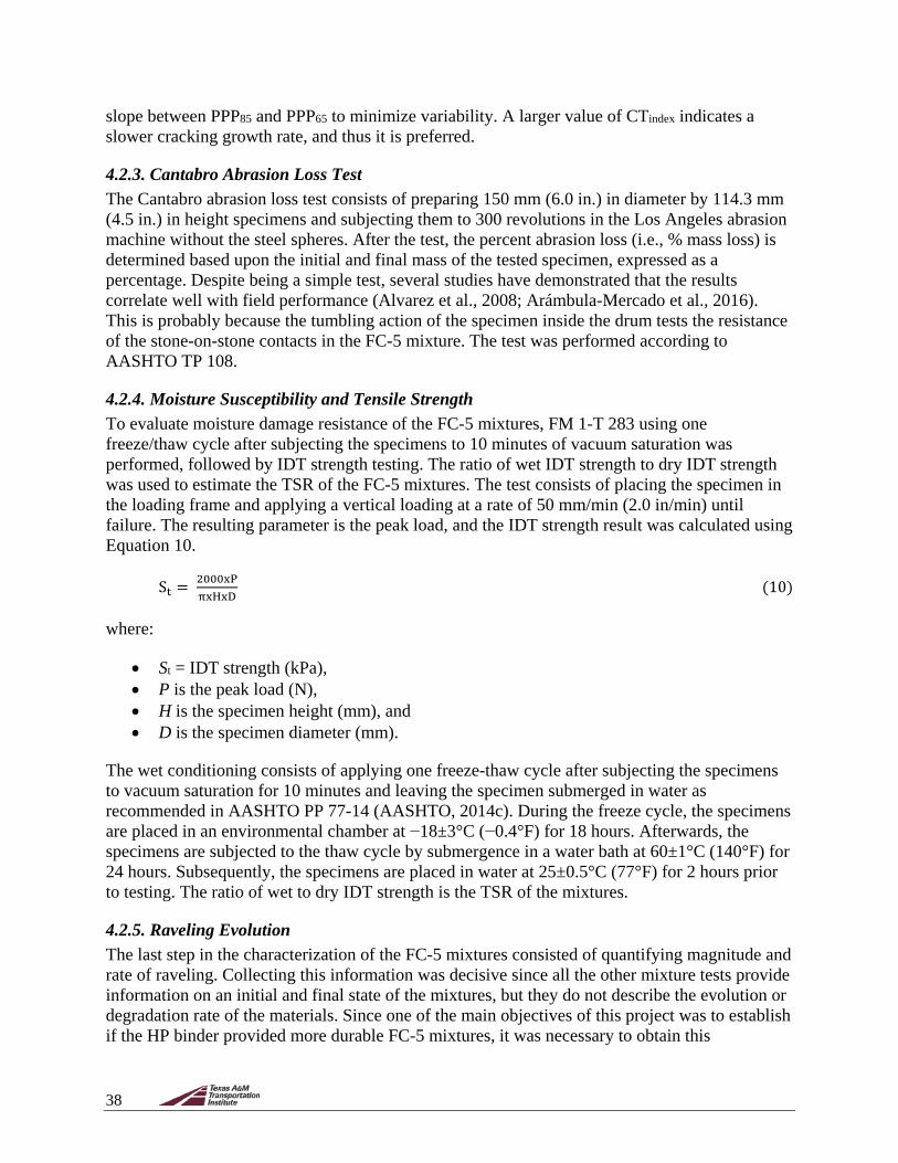
38
slope between PPP85 and PPP65 to minimize variability. A larger value of CTindex indicates a slower cracking growth rate, and thus it is preferred.
4.2.3. Cantabro Abrasion Loss Test The Cantabro abrasion loss test consists of preparing 150 mm (6.0 in.) in diameter by 114.3 mm (4.5 in.) in height specimens and subjecting them to 300 revolutions in the Los Angeles abrasion machine without the steel spheres. After the test, the percent abrasion loss (i.e., % mass loss) is determined based upon the initial and final mass of the tested specimen, expressed as a percentage. Despite being a simple test, several studies have demonstrated that the results correlate well with field performance (Alvarez et al., 2008; Arámbula-Mercado et al., 2016). This is probably because the tumbling action of the specimen inside the drum tests the resistance of the stone-on-stone contacts in the FC-5 mixture. The test was performed according to AASHTO TP 108.
4.2.4. Moisture Susceptibility and Tensile Strength To evaluate moisture damage resistance of the FC-5 mixtures, FM 1-T 283 using one freeze/thaw cycle after subjecting the specimens to 10 minutes of vacuum saturation was performed, followed by IDT strength testing. The ratio of wet IDT strength to dry IDT strength was used to estimate the TSR of the FC-5 mixtures. The test consists of placing the specimen in the loading frame and applying a vertical loading at a rate of 50 mm/min (2.0 in/min) until failure. The resulting parameter is the peak load, and the IDT strength result was calculated using Equation 10.
St = 2000xPπxHxD
(10)
where:
• St = IDT strength (kPa), • P is the peak load (N), • H is the specimen height (mm), and • D is the specimen diameter (mm).
The wet conditioning consists of applying one freeze-thaw cycle after subjecting the specimens to vacuum saturation for 10 minutes and leaving the specimen submerged in water as recommended in AASHTO PP 77-14 (AASHTO, 2014c). During the freeze cycle, the specimens are placed in an environmental chamber at −18±3°C (−0.4°F) for 18 hours. Afterwards, the specimens are subjected to the thaw cycle by submergence in a water bath at 60±1°C (140°F) for 24 hours. Subsequently, the specimens are placed in water at 25±0.5°C (77°F) for 2 hours prior to testing. The ratio of wet to dry IDT strength is the TSR of the mixtures.
4.2.5. Raveling Evolution The last step in the characterization of the FC-5 mixtures consisted of quantifying magnitude and rate of raveling. Collecting this information was decisive since all the other mixture tests provide information on an initial and final state of the mixtures, but they do not describe the evolution or degradation rate of the materials. Since one of the main objectives of this project was to establish if the HP binder provided more durable FC-5 mixtures, it was necessary to obtain this

39
information. For this purpose, trials were initially performed using the three-wheel polisher shown in Figure 4-6a with custom-made studded tires in an effort to promote raveling and not just polishing. The tests were performed at an intermediate room temperature of about 77°F (25°C). Periodically, after a specified number of cycles (e.g., 5,000 load cycles), all dislodged material from the surface of the slab was collected and weighed; in addition, the mean profile depth (MPD) of the slab’s circular track left by the three-wheel polisher (Figure 4-6b) was determined using a portable circular texture meter. This portable device, shown in Figure 4-6c, employs a laser scanner to measure the texture depth along the circular track and was used to quantify changes in the profile of the surface of the slab. Despite multiple efforts, the three-wheel polisher was not able to provide the required evolution of raveling; yet, the various trial attempts and results are still considered valuable and reported in this document.
(a) (b) (c)
Figure 4-6. (a) Three-Wheel Polisher Equipment Adapted for Evaluating Raveling Evolution; (b) Slab after Testing; (c) Circular Texture Meter.
Because the three-wheel polisher was not able to provide the required evolution of raveling, the Cantabro abrasion loss test at various aging conditions—5 and 10 days at 203°F (95°C)—was performed, and the mass of the specimen was measured periodically at every 300 revolutions until a terminal degradation level of 80% abrasion loss was achieved. These results were used to estimate the degradation rate of each FC-5 mixture and used as input in the LCCA.

40
5.0. LABORATORY EXPERIMENT RESULTS 5.1. BINDER CHARACTERIZATION The PMA and HP binders were provided by FDOT in their virgin state. Each binder was evaluated under a total of five aging states since the impact of aging in the rheological response and performance of the binder is critical for the durability of the FC-5 mixtures. As previously mentioned, the five aging states included (a) unaged (OB), (b) RTFO, (c) PAV after 20 hours (i.e., PAV20), (d) PAV after 40 hours (i.e., PAV40), and (e) PAV after 80 hours (i.e., PAV80).
5.1.1. Performance Grade Table 5-1 summarizes the information obtained from the PG testing for both binders. The results showed that the actual PG of both binders differed from their as-received labels because they were classified as PG 82-22E and PG 82-28E for PMA and HP, respectively (i.e., binders that could be used in extreme traffic-related projects). The results of ∆Tc, which is the difference in temperatures of the BBR test when the creep stiffness (S) and the stress relaxation rate (m-value) reach the PG Superpave specification limits of 300 MPa and 0.30, respectively, showed that the HP binder had a wider useful temperature interval and better ductility because this parameter was less negative (i.e., −0.8°C) and only one-fifth of that obtained for the PMA binder (i.e., −4.3°C).
According to FDOT specifications, the MSCR test should be conducted at different temperatures, depending on the level of modification (i.e., 67°C [153°F] for PMA and 76°C [169°F] for HP binders) (FDOT 2018a). Both binders should pass the minimum requirements for a traffic type V, which is (a) the non-recoverable creep compliance at a stress level of 3.2 kPa (Jnr, 3.2) has to be maximum 1.00 kPa-1 and 0.10 kPa-1 for the PMA and HP binders, respectively; (b) the average percent recovery at 3.2 kPa should be larger than 29.37% and 90.0% for the PMA and HP binders, respectively; and (c) the difference in the non-recoverable creep compliance between 0.1 kPa and 3.2 kPa (i.e., Jnr, diff) should be 75% maximum (AASHTO, 2014a; FDOT, 2018a). Based on this information, both binders achieved a grade of E, which means that they can stand the highest level of traffic under that classification (i.e., extremely heavy traffic). It should be noted that due to letter f of section 916 of the Standard Specifications for Road and Bridge Construction (FDOT 2018a), if Jnr, 3.2 is lower than 0.5 kPa-1, %Jnr, diff is not applicable, which is referred to as N/A in Table 5-1.
Table 5-1. PG and MSCR Results for Binders.
Binder Type
Commercial PG Brand
Name
Continuous PG
Rounded PG ∆Tc
MSCR (min Jnr, 3.2)
MSCR (%Recovery)
MSCR (%Jnr, diff)
PMA PG 76-22 PG 83.7-26.5 PG 82-22E −4.3 0.09 kPa-1 (Pass) 70.5% (Pass) N/A
HP PG 76-22 HP PG 87.4-32.4 PG 82-28E −0.8 0.04 kPa-1 (Pass) 93.8% (Pass) N/A
Note: N/A = not applicable.
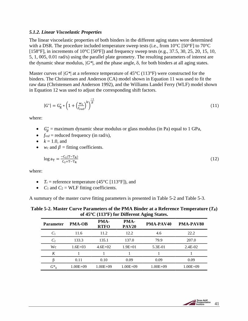
41
5.1.2. Linear Viscoelastic Properties The linear viscoelastic properties of both binders in the different aging states were determined with a DSR. The procedure included temperature sweep tests (i.e., from 10°C [50°F] to 70°C [158°F], in increments of 10°C [50ºF]) and frequency sweep tests (e.g., 37.5, 30, 25, 20, 15, 10, 5, 1, 005, 0.01 rad/s) using the parallel plate geometry. The resulting parameters of interest are the dynamic shear modulus, |G*|, and the phase angle, δ, for both binders at all aging states.
Master curves of |G*| at a reference temperature of 45°C (113°F) were constructed for the binders. The Christensen and Anderson (CA) model shown in Equation 11 was used to fit the raw data (Christensen and Anderson 1992), and the Williams Landel Ferry (WLF) model shown in Equation 12 was used to adjust the corresponding shift factors.
|G∗| = Gg∗ ∗ �1 + � wc
fred�
k�
−1β
(11)
where:
• 𝐺𝐺𝑔𝑔∗ = maximum dynamic shear modulus or glass modulus (in Pa) equal to 1 GPa,
• fred = reduced frequency (in rad/s), • k = 1.0, and • wc and 𝛽𝛽 = fitting coefficients.
log aT = −C1(T−TR)C2+T−TR
(12)
where:
• Tr = reference temperature (45°C [113°F]), and • C1 and C2 = WLF fitting coefficients.
A summary of the master curve fitting parameters is presented in Table 5-2 and Table 5-3.
Table 5-2. Master Curve Parameters of the PMA Binder at a Reference Temperature (TR) of 45ºC (113ºF) for Different Aging States.
Parameter PMA-OB PMA-RTFO
PMA-PAV20 PMA-PAV40 PMA-PAV80
C1 11.6 11.2 12.2 4.6 22.2
C2 133.3 135.1 137.0 79.9 207.0
Wc 1.6E+03 4.6E+02 1.9E+01 5.3E-01 2.4E-02 K 1 1 1 1 1 β 0.11 0.10 0.09 0.09 0.09
G*g 1.00E+09 1.00E+09 1.00E+09 1.00E+09 1.00E+09

42
Table 5-3. Master Curve Parameters for the HP Binder at a Reference Temperature (TR) of 45ºC (113ºF) for Different Aging States.
Parameter HP-OB HP-RTFO HP-PAV20 HP-PAV40 HP-PAV80 C1 6.8 7.3 8.2 10.5 15.6
C2 92.6 97.9 104.6 114.7 162.2 Wc 5.6E+03 3.2E+03 1.4E+02 1.9E+01 8.3E+00 K 1 1 1 1 1 β 0.091 0.098 0.09 0.09 0.09
G*g 1.00E+09 1.00E+09 1.00E+09 1.00E+09 1.00E+09
Figure 5-1 through Figure 5-3 present the master curves obtained for both binders under different aging states at the reference temperature of 45°C (113°F). These curves correspond to the average of the results obtained for three replicates of each binder at each aging state.
Figure 5-1. Master Curves at 45°C (113°F) for PMA Binder in Different Aging States.
1.E+00
1.E+01
1.E+02
1.E+03
1.E+04
1.E+05
1.E+06
1.E+07
1.E+08
1.E+09
1.E-05 1.E-03 1.E-01 1.E+01 1.E+03 1.E+05 1.E+07 1.E+09
Dyn
amic
She
ar M
odul
us (P
a)
Frequency Reduced (Hz)
PMA OB PMA RTFO PMA PAV20 PMA PAV40 PMA PAV80

43
Figure 5-2. Master Curves at 45°C (113°F) for HP Binder at Different Aging States.
Figure 5-3. Original and PAV80 Master Curves at 45°C (113°F) for HP and PMA Binders.
1.E+00
1.E+01
1.E+02
1.E+03
1.E+04
1.E+05
1.E+06
1.E+07
1.E+08
1.E+09
1.E-05 1.E-03 1.E-01 1.E+01 1.E+03 1.E+05 1.E+07 1.E+09
Dyn
amic
She
ar M
odul
us (P
a)
Frequency Reduced (Hz)
HP OB HP RTFO HP PAV20 HP PAV40 HP PAV80
1.E+00
1.E+01
1.E+02
1.E+03
1.E+04
1.E+05
1.E+06
1.E+07
1.E+08
1.E+09
1.E-05 1.E-03 1.E-01 1.E+01 1.E+03 1.E+05 1.E+07 1.E+09
Dyn
amic
She
ar M
odul
us (P
a)
Log Frequency Reduced (Hz)
PMA OB PMA PAV80 HP OB HP PAV80

44
In terms of temperature susceptibility, within a given aging state, the modulus of the HP asphalt binder was not affected as significantly as the PMA binder. This is observed in Figure 5-1 and Figure 5-2, which show smaller values of the slope of the master curves for the HP binder in the five aging states compared to those of the PMA binder (i.e., average slope of 38,609 (Pa/Hz) at a frequency of 10 Hz for the HP binder compared to an average slope of 130,290 (Pa/Hz) for the PMA binder).
The results for the HP binder (Figure 5-2) showed that there are significant differences between aging states. The biggest change in the value of modulus for the HP binder was observed between the RTFO and PAV20 aging states (i.e., an average increase in modulus of 4.29 times with respect to the RTFO state at the reference temperature).
When comparing the OB to the most extreme aging state, the value of |G*| at 10 Hz for the HP binder in the PAV80 state was 20.7 times larger than that of the OB at the same frequency (Figure 5-3). Conversely, the equivalent modulus of the PMA binder in the PAV80 state was only 11.9 times higher than the value of the OB, showing a smaller overall difference in the magnitude of |G*| between these two aging states compared to the HP binder.
An analysis of the differences in the magnitude of |G*| between both binders for each aging state showed that the PMA presents an overall larger modulus than the HP binder, for all aging states. However, a direct comparison between these moduli is inadequate since the base binder used for each modification might be different and unknown. Although in this particular case the PMA binder presents higher moduli than the HP binder, various studies have shown different trends (i.e., PMA modulus equal or less than HP modulus) (Bessa et al., 2018; Gaspar et al., 2017; Chen et al., 2018). In addition, it is known that the inclusion of oils and maltenes before modification is a common industry practice to increase the workability of the heavily modified material (R. Martins, personal communication, 2017). This practice can reduce significantly the dynamic modulus of the base binder, impacting the final modulus of the asphalt (Orlen Asfalt, 2017). Therefore, the focus in this study was to compare the performance and susceptibility to degradation of both binders and not only their linear viscoelastic properties.
5.1.3. Aging and Cracking Susceptibility To explore the influence of aging on the expected cracking performance of both binders, the G-R parameter (Equation 13), a rheological value proposed by Glover et al. (2005) that is considered a good predictor of the binder resistance to degradation due to oxidative hardening, was evaluated. The parameter was obtained from conducting an oscillatory shear test at 15°C (59°F) and 0.005 rad/s with binders under different aging states.
G − R Parameter = G∗(cos δ) 2
sin δ (13)
This parameter presents a good correlation with ductility and has proven to be capable of predicting block cracking performance with aging in the field. In fact, according to existing studies on dense mixtures, G-R parameter values equal to or larger than 180 kPa are related to mixtures that show an onset of early block cracking, while binders with values equal to or larger than 600 kPa are related to mixtures that have a higher probability for developing significant block cracking (Rowe et al., 2014).

45
The G-R parameters were obtained through DSR tests under the aging states previously described. Figure 5-4 presents the Black space diagram (i.e., |G*| vs. δ) with the results of both binders under all aging states; each binder at each aging state represents one point in this graph. The results of an unmodified binder PG 52-28 from Florida were also included in this diagram to show the influence of polymer modification with aging on the mechanical response of the binders (i.e., less change in phase angle). It should be noted that the most aggressive aging state for the unmodified binder PG 52-28 was PAV60 (i.e., there were no available data for PAV80 since these data were part of a different study). Figure 5-4 also includes two curves that represent different damage states related with the G-R parameters. Each curve was computed using the G-R limits previously mentioned. In other words, the damage onset curve shows the threshold for G-R values equal to 180 KPa, and the significant damage curve represents the G-R threshold values equal to 600 KPa. Although those G-R threshold values were determined for dense-graded and not FC-5 mixtures, they are still considered acceptable to evaluate the binders’ potential susceptibility to damage, especially with aging.
Figure 5-4. G-R Black Space Diagram for PMA, HP, and PG 52-28 Binders.
In terms of the modulus, data in Figure 5-4 showed that the value of |G*| at the PAV20 aging state was 13 times larger for the PMA binder compared to the unmodified binder. In contrast, the modulus of the HP binder was eight times larger than that of the unmodified asphalt at the same aging state (i.e., PAV20). With the exception of the OB state, the PMA binder presented larger values of |G*| compared to the other two binders in all other aging states. In fact, |G*| in the PAV40 state was 26.9 and 31.5 times larger than in the original state in the PMA and the

46
unmodified binder, respectively, while it was only 5.8 times larger in the HP binder between these two aging states.
Significant differences caused by aging were also observed in the phase angle. The variations of the phase angle for the unmodified and the PMA binders were 29.7% and 26.1%, respectively, while for the HP binder, the variation was only 2.7%. This result suggests that the viscoelastic behavior, in terms of the magnitude of δ, of the HP binder is expected to be the least susceptible to oxidative aging compared to the other two binders. In fact, the phase angle decreased an average of 18.8% and 17.1% in the PMA and unmodified binders between the different aging states (i.e., original, PAV20, PAV40, and PAV60—for the unmodified binder—or PAV80—for the PMA), respectively, while in the HP binder, this property presented a steady reduction of only 2% between the same aging states.
In terms of the G-R threshold curves, Figure 5-4 shows that the damage onset curve was reached by the unmodified and HP binders after PAV40, while the PMA binder reached this curve earlier than the PAV20 aging state. In fact, the susceptibility to significant cracking for the PMA binder was expected to occur between the PAV20 and PAV40 aging states (about five years of pavement service life), while for the unmodified binder, susceptibility to significant cracking could occur between the PAV40 and PAV60 states. In contrast, the HP binder did not reach the significant cracking curve even after PAV80 aging (i.e., about 11 years of pavement service life). This finding suggests that the cracking resistance due to oxidative aging of the HP binder was notably superior to that of the other two binders. In turn, this could implicate longer durability for FC-5 mixtures fabricated with this type of binder.
5.1.4. Chemical Changes Due to Oxidative Aging Figure 5-5 presents the FTIR results. Figure 5-5a illustrates the carbonyl area for the different aging states, and Figure 5-5b presents the carbonyl area growth data with respect to the original binder value for both binders. It is interesting to note that the HP binder presented larger changes in its chemical structure due to aging (i.e., greater carbonyl area growth over time with respect to the unaged state) compared to the PMA binder, despite those changes not impacting the phase angle of the HP binder or its susceptibility to cracking due to aging, as shown in the previous section. Even though the HP binder seemed to present faster chemical aging processes than the PMA binder, this finding could be due to type or modification of the base binder used to fabricate the PMA and HP binders. Regardless, these results did not seem to affect the expected cracking performance of the material, as discussed previously for the case of cracking susceptibility and described next for the case of fatigue cracking.
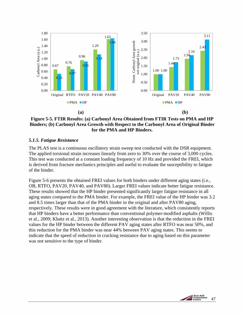
47
(a) (b) Figure 5-5. FTIR Results: (a) Carbonyl Area Obtained from FTIR Tests on PMA and HP Binders; (b) Carbonyl Area Growth with Respect to the Carbonyl Area of Original Binder
for the PMA and HP Binders.
5.1.5. Fatigue Resistance The PLAS test is a continuous oscillatory strain sweep test conducted with the DSR equipment. The applied torsional strain increases linearly from zero to 30% over the course of 3,000 cycles. This test was conducted at a constant loading frequency of 10 Hz and provided the FREI, which is derived from fracture mechanics principles and useful to evaluate the susceptibility to fatigue of the binder.
Figure 5-6 presents the obtained FREI values for both binders under different aging states (i.e., OB, RTFO, PAV20, PAV40, and PAV80). Larger FREI values indicate better fatigue resistance. These results showed that the HP binder presented significantly larger fatigue resistance in all aging states compared to the PMA binder. For example, the FREI value of the HP binder was 3.2 and 8.5 times larger than that of the PMA binder in the original and after PAV80 aging, respectively. These results were in good agreement with the literature, which consistently reports that HP binders have a better performance than conventional polymer-modified asphalts (Willis et al., 2009; Kluttz et al., 2013). Another interesting observation is that the reduction in the FREI values for the HP binder between the different PAV aging states after RTFO was near 50%, and this reduction for the PMA binder was near 44% between PAV aging states. This seems to indicate that the speed of reduction in cracking resistance due to aging based on this parameter was not sensitive to the type of binder.
0.670.76
0.96
1.29
1.62
0.530.67
0.91
1.14
1.64
0.00
0.20
0.40
0.60
0.80
1.00
1.20
1.40
1.60
1.80
Original RTFO PAV20 PAV40 PAV80
Car
bony
l Are
a (a
.u.)
PMA HP
1.00
1.44
1.94
2.43
1.00
1.73
2.16
3.11
0.00
0.50
1.00
1.50
2.00
2.50
3.00
3.50
Original PAV20 PAV40 PAV80
Nor
m. C
arbo
nyl A
rea
grow
th
wrt
orig
inal
(a.u
.)
PMA HP
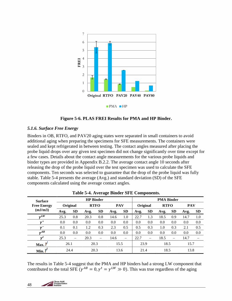
48
Figure 5-6. PLAS FREI Results for PMA and HP Binder.
5.1.6. Surface Free Energy Binders in OB, RTFO, and PAV20 aging states were separated in small containers to avoid additional aging when preparing the specimens for SFE measurements. The containers were sealed and kept refrigerated in between testing. The contact angles measured after placing the probe liquid drops over any given test specimen did not change significantly over time except for a few cases. Details about the contact angle measurements for the various probe liquids and binder types are provided in Appendix B.2.2. The average contact angle 10 seconds after releasing the drop of the probe liquid over the test specimen was used to calculate the SFE components. Ten seconds was selected to guarantee that the drop of the probe liquid was fully stable. Table 5-4 presents the average (Avg.) and standard deviation (SD) of the SFE components calculated using the average contact angles.
Table 5-4. Average Binder SFE Components.
Surface Free Energy
(mJ/m3)
HP Binder PMA Binder Original RTFO PAV Original RTFO PAV
Avg. SD Avg. SD Avg. SD Avg. SD Avg. SD Avg. SD 𝜸𝜸𝑳𝑳𝑳𝑳 25.3 0.8 20.3 0.8 14.6 1.0 22.7 1.3 18.5 0.9 14.7 1.0 𝜸𝜸+ 0.0 0.0 0.0 0.0 0.0 0.0 0.0 0.0 0.0 0.0 0.0 0.0 𝜸𝜸− 0.1 0.1 1.2 0.3 2.3 0.5 0.5 0.3 1.0 0.3 2.1 0.5
𝜸𝜸𝑨𝑨𝑨𝑨 0.0 0.0 0.0 0.0 0.0 0.0 0.0 0.0 0.0 0.0 0.0 0.0 𝜸𝜸𝒕𝒕 25.3 – 20.3 – 14.6 – 22.7 – 18.5 – 14.7 –
Max. 26.1 20.3 15.5 23.9 18.5 15.7
Min. 24.4 20.3 13.6 21.4 18.5 13.8
The results in Table 5-4 suggest that the PMA and HP binders had a strong LW component that contributed to the total SFE (𝛾𝛾𝐴𝐴𝐴𝐴 = 0, 𝛾𝛾𝑡𝑡 = 𝛾𝛾𝐿𝐿𝐿𝐿 ≫ 0). This was true regardless of the aging
0
1
2
3
4
5
6
7
Original RTFO PAV20 PAV40 PAV80
FRE
I
PMA HP

49
state. The near-zero values of LW SFE components strongly suggest that the selected asphalt binders were non-polar in nature. It also indicates that the LW component was the primary factor determining the cohesive and adhesive properties of the selected binders. More importantly, the results presented in Table 5-4 showed that the total SFE was lower for PMA binders than for HP binders, and that the total SFE decreased with aging. Since materials with higher total SFE are more cohesive (work of cohesion = 2 × 𝛾𝛾𝑡𝑡), the HP binder would be expected to be more cohesive than the PMA binder, and for both binders, the cohesiveness was expected to reduce with aging.
Figure 5-7a presents the normalized PMA total SFE with respect to the HP binder total SFE in different aging states. All normalized SFE values (except for one instance) were less than 1.0, indicating that the PMA binder had smaller total SFE (or smaller LW component) than the HP binder. Similarly, Figure 5-7b shows the normalized aged total SFE with respect to the unaged total SFE values. For both HP and PMA, these normalized total SFE values were less than 1.0 in all cases, which indicates that the binders in the aged state had smaller total SFE (or smaller LW component) compared to the ones in the aged state. Figure 5-7b also shows that the total SFE (or LW component) decreased around 20% after RTFO and about 60% after PAV20. Note that the normalized total SFE values are equal to the normalized LW component values because the Lewis acid-base components are zero. The normalized results once again showed that the HP binder had a better resistance to cohesive fracture than the PMA binder, and that binders became less resistant to cohesive damage with aging.
(a) (b)
Figure 5-7. Normalized Total SFE for HP and PMA Binders in Different Aging States: (a) Effect of Binder Type; (b) Effect of Aging.
5.2. MASTIC CHARACTERIZATION In order to prepare the samples, the binders and fillers were independently oven heated to their corresponding FC-5 mixture mixing temperatures (Section 5.3.1.2). Afterwards, the filler was added to the samples of binder and the mixture was stirred with a metal spatula until homogeneous. The mixture was oven heated again for a few minutes until guaranteeing a stable
0.90 0.91
1.01
0.40
0.70
1.00
1.30
Unaged RTFO PAV20
PMA/HP
Nor
mal
ized
T
otal
Sur
face
Fre
e E
nerg
y
0.80
0.58
0.81
0.65
0.40
0.70
1.00
1.30
RTFO/Unaged
PAV20/Unaged
RTFO/Unaged
PAV20/Unaged
HP PMA
Nor
mal
ized
Tot
al S
urfa
ce F
ree
Ene
rgy
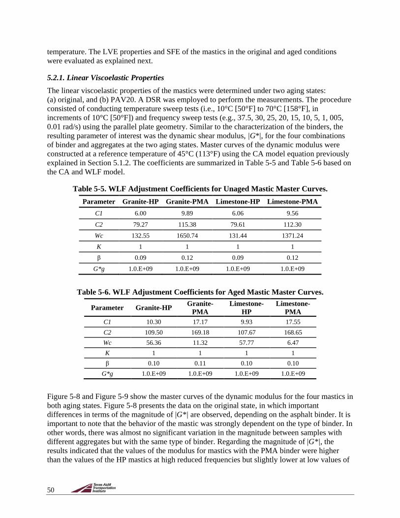
50
temperature. The LVE properties and SFE of the mastics in the original and aged conditions were evaluated as explained next.
5.2.1. Linear Viscoelastic Properties The linear viscoelastic properties of the mastics were determined under two aging states: (a) original, and (b) PAV20. A DSR was employed to perform the measurements. The procedure consisted of conducting temperature sweep tests (i.e., 10°C [50°F] to 70°C [158°F], in increments of 10°C [50°F]) and frequency sweep tests (e.g., 37.5, 30, 25, 20, 15, 10, 5, 1, 005, 0.01 rad/s) using the parallel plate geometry. Similar to the characterization of the binders, the resulting parameter of interest was the dynamic shear modulus, |G*|, for the four combinations of binder and aggregates at the two aging states. Master curves of the dynamic modulus were constructed at a reference temperature of 45°C (113°F) using the CA model equation previously explained in Section 5.1.2. The coefficients are summarized in Table 5-5 and Table 5-6 based on the CA and WLF model.
Table 5-5. WLF Adjustment Coefficients for Unaged Mastic Master Curves. Parameter Granite-HP Granite-PMA Limestone-HP Limestone-PMA
C1 6.00 9.89 6.06 9.56
C2 79.27 115.38 79.61 112.30
Wc 132.55 1650.74 131.44 1371.24
K 1 1 1 1
β 0.09 0.12 0.09 0.12
G*g 1.0.E+09 1.0.E+09 1.0.E+09 1.0.E+09
Table 5-6. WLF Adjustment Coefficients for Aged Mastic Master Curves.
Parameter Granite-HP Granite-PMA
Limestone-HP
Limestone-PMA
C1 10.30 17.17 9.93 17.55 C2 109.50 169.18 107.67 168.65 Wc 56.36 11.32 57.77 6.47 K 1 1 1 1 β 0.10 0.11 0.10 0.10
G*g 1.0.E+09 1.0.E+09 1.0.E+09 1.0.E+09
Figure 5-8 and Figure 5-9 show the master curves of the dynamic modulus for the four mastics in both aging states. Figure 5-8 presents the data on the original state, in which important differences in terms of the magnitude of |G*| are observed, depending on the asphalt binder. It is important to note that the behavior of the mastic was strongly dependent on the type of binder. In other words, there was almost no significant variation in the magnitude between samples with different aggregates but with the same type of binder. Regarding the magnitude of |G*|, the results indicated that the values of the modulus for mastics with the PMA binder were higher than the values of the HP mastics at high reduced frequencies but slightly lower at low values of

51
reduced frequencies. For example, at high frequencies (higher than 1,000 Hz), the magnitude of |G*| of the PMA mastics was 2.31 times greater than the moduli of the HP mastics. In contrast, at low reduced frequencies (lower than 0.01 Hz), the values of |G*| of the mastics with the HP binder were, on average, 1.21 times larger than the PMA mastics.
Figure 5-8. Master Curve for Mastic Samples Using Original HP and PMA Binders.
Regarding the results for the aged mastics (Figure 5-9), the same trend observed for the unaged samples persisted in the sense that the type of binder—and not the aggregate—was the dominating factor affecting the modulus. In this case, and similar to the binders, the values of |G*| were consistently larger for the PMA mastics. In fact, the HP mastics presented a 78.5% reduction in |G*| compared to the PMA mastics at low reduced frequencies (smaller than 0.01 Hz) and 48.4% at high reduced frequencies (greater than 1,000 Hz). When compared to the master curves of |G*| of the aged binders (Figure 5-1 and Figure 5-2), it was observed that the inclusion of the fillers reduced the gap between the curves for the two types of binders, showing the impact of adding this component in the assessment of the response of the material. This result was important since the contacts between particles within the microstructure of an FC-5 mixture are mastic-on-mastic contacts rather than stone-on-stone contacts. Therefore, the durability of the mixture was directly related to the properties of the mastic. The results obtained from these DSR tests were used as input in the numerical models that are detailed in Chapter 4.
1.E+00
1.E+01
1.E+02
1.E+03
1.E+04
1.E+05
1.E+06
1.E+07
1.E+08
1.E+09
1.E-05 1.E-03 1.E-01 1.E+01 1.E+03 1.E+05 1.E+07 1.E+09
Dyn
amic
She
ar M
odul
us (P
a)
Reduced Frequency (Hz)Granite-HP-Unaged Granite-PMA-UnagedLimestone-HP-Unaged Limestone-PMA-Unaged
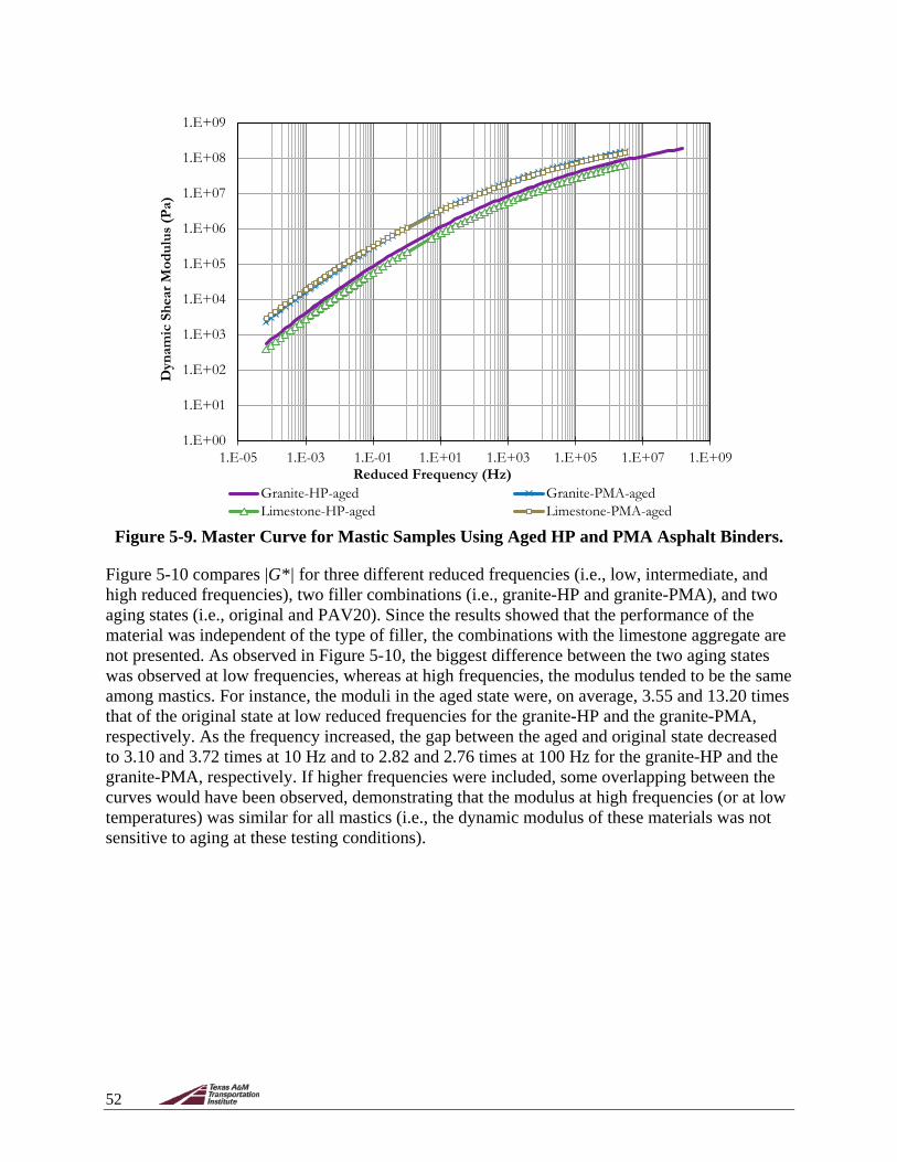
52
Figure 5-9. Master Curve for Mastic Samples Using Aged HP and PMA Asphalt Binders.
Figure 5-10 compares |G*| for three different reduced frequencies (i.e., low, intermediate, and high reduced frequencies), two filler combinations (i.e., granite-HP and granite-PMA), and two aging states (i.e., original and PAV20). Since the results showed that the performance of the material was independent of the type of filler, the combinations with the limestone aggregate are not presented. As observed in Figure 5-10, the biggest difference between the two aging states was observed at low frequencies, whereas at high frequencies, the modulus tended to be the same among mastics. For instance, the moduli in the aged state were, on average, 3.55 and 13.20 times that of the original state at low reduced frequencies for the granite-HP and the granite-PMA, respectively. As the frequency increased, the gap between the aged and original state decreased to 3.10 and 3.72 times at 10 Hz and to 2.82 and 2.76 times at 100 Hz for the granite-HP and the granite-PMA, respectively. If higher frequencies were included, some overlapping between the curves would have been observed, demonstrating that the modulus at high frequencies (or at low temperatures) was similar for all mastics (i.e., the dynamic modulus of these materials was not sensitive to aging at these testing conditions).
1.E+00
1.E+01
1.E+02
1.E+03
1.E+04
1.E+05
1.E+06
1.E+07
1.E+08
1.E+09
1.E-05 1.E-03 1.E-01 1.E+01 1.E+03 1.E+05 1.E+07 1.E+09
Dyn
amic
She
ar M
odul
us (P
a)
Reduced Frequency (Hz)Granite-HP-aged Granite-PMA-agedLimestone-HP-aged Limestone-PMA-aged

53
Figure 5-10. Dynamic Modulus of Mastic Comparison for the Granite-HP Mastic and the
Granite-PMA Mastic.
5.2.2. Surface Free Energy Similar to binders, mastics in the original or unaged state were placed in small containers to avoid additional aging when preparing the specimens for SFE measurements. The containers were sealed and kept refrigerated in between testing. Table 5-7 presents the mastic combinations that were characterized using SFE. All mastic specimens were tested in their original state (i.e., unaged). Appendix B.2.1 details the theory and calculations used to estimate the SFE values, and the procedure followed to conduct the sessile drop test was presented in Section 5.1.6.
The average contact angles over time were derived from a minimum of three tests conducted on the mastics. Like in the case of the binders, the values did not significantly change over time. Therefore, the average contact angle 10 seconds after releasing the drop of the probe liquid over the test specimen was used to calculate the SFE components. As before, 10 seconds was selected to guarantee that the drop of the probe liquid was fully stable.
Table 5-7. Mastic Combinations for SFE Characterization.
Mastic Label Material Combination
GH56 Granite + 56%HP GP56 Granite + 56%PMA LH59 Limestone + 59%HP LP59 Limestone + 59%PMA
Table 5-8 presents the average and standard deviation values of the mastic SFE components calculated using the average contact angles presented in Appendix B.2.2. The mastic specimens had strong non-polar components contributing to the total SFE (𝛾𝛾𝐴𝐴𝐴𝐴 = 0, 𝛾𝛾𝑡𝑡 = 𝛾𝛾𝐿𝐿𝐿𝐿 ≫ 0).
1.0.E+00
1.0.E+01
1.0.E+02
1.0.E+03
1.0.E+04
1.0.E+05
1.0.E+06
1.0.E+07
1.0.E+08
1E-03 1E+01 1E+02
Dyn
amic
Mod
ulus
(Pa)
Reduced Frequency (Hz)
Granite-HP-Unaged Granite-PMA-Unaged Granite-HP-Aged Granite-PMA-Aged

54
Table 5-8. Average Mastic SFE Components. SFE GH56 GP56 LH59 LP59
(mJ/m3) Avg. SD Avg. SD Avg. SD Avg. SD 𝛾𝛾𝐿𝐿𝐿𝐿 21.72 0.62 18.49 0.76 20.31 0.70 18.23 0.62 𝛾𝛾+ 0.00 0.00 0.00 0.00 0.00 0.00 0.00 0.00 𝛾𝛾− 0.02 0.06 0.19 0.18 0.02 0.04 0.76 0.22
𝛾𝛾𝐴𝐴𝐴𝐴 0.00 0.00 0.00 0.00 0.00 0.00 0.00 0.00 𝛾𝛾𝑡𝑡 21.72 – 18.49 – 20.31 – 18.23 –
Max. 22.3 19.3 21.0 18.8
Min. 21.1 17.7 19.6 17.6
Finally, Figure 5-11a presents the normalized PMA mastic total SFE with respect to the HP mastic total SFE. These normalized values were all less than 1.0, indicating that the total SFE of the PMA mastics was smaller compared to the HP mastics. Therefore, the HP mastics are slightly more resistant to cohesive failure than the PMA mastics. Figure 5-11b shows the normalized limestone mastic total SFE with respect to the granite mastic total SFE. The normalized values were marginally smaller than 1.0; therefore, the granite mastics could have a slightly higher cohesive fracture resistance than the limestone mastics.
(a) (b)
Figure 5-11. Normalized Mastic Total SFE: (a) Effect of Binder Type; (b) Effect of Aggregate Type.
Figure 5-12 shows the normalized mastic total SFE with respect to the binder total SFE. All values are less than 1.0, indicating that mastics had less total SFE than binders. This was true regardless of the type of binder or type of aggregate. This finding implies that mastics are more prone to failure by fracture compared to binders without fillers due to reduced cohesiveness.
0.850.90
0.70
1.00
1.30
Granite Limestone
PMA/HP
Nor
mal
ized
T
otal
Sur
face
Fre
e E
nerg
y
0.930.99
0.70
1.00
1.30
HP PMA
Limestone/Granite
Nor
mal
ized
T
otal
Sur
face
Fre
e E
nerg
y

55
Figure 5-12. Normalized Mastic-to-Binder Total SFE.
5.3. MIXTURE CHARACTERIZATION FC-5 mixtures were prepared in the laboratory by combining each type of aggregate with each type of binder, and compacted specimens were tested to compare their expected cracking performance and durability. The results from this experimental stage provided input for the FE and LCCA models that were also conducted as part of this study and detailed in Chapters 6 and 7. The experimental test plan for the FC-5 mixtures was presented in Chapter 4, and the tests to be conducted on the FC-5 mixtures were listed in Table 3-1.
5.3.1. Mixture Preparation 5.3.1.1. Washed Sieve Analysis The first step in the production of the asphalt mixtures was the adjustment in the proportions of the aggregates in accordance with the FC-5 job mix formula provided by FDOT. The two aggregate types, limestone and granite, were provided by FDOT in 5-gal buckets from the original quarries. All the aggregates were oven dried at 110°C (212°F) for 24 hours and later cooled and sieved.
Washed sieve analyses were conducted according to ASTM C117, which requires 2,500 g (5.5 lb.) of batched aggregate samples following the gradations in the job mix formula (AASHTO, 2013b; ASTM, 2017a). Enough water was added to cover the aggregate samples, and the material was agitated by hand with vigor to separate the finer particles from the coarser aggregates. Once the fine aggregates were in suspension, the water was poured into a set of sieves (i.e., No. 8 and No. 200 sieves); when the decantation of materials was complete, the process was repeated until clear water was observed, which indicated that most fines were washed from the larger aggregate particles. The remaining material and the material retained in the two sieves were combined and dried at 110°C (212°F) for 24 hours; then, the material was sieved to determine its washed gradation. If the change with respect to the mix design gradation was larger than 1% and 0.5% for coarse and fine particles, respectively, the aggregate proportions were adjusted, and the process was repeated until a minimum error (i.e., difference between the job mix formula and the washed percent passing amount for all sieves, within the
0.860.80 0.82 0.80
0.70
1.00
1.30
Granite Limestone Granite Limestone
HP PMA
Nor
mal
ized
Sur
face
Fre
e E
nerg
y
γTotal
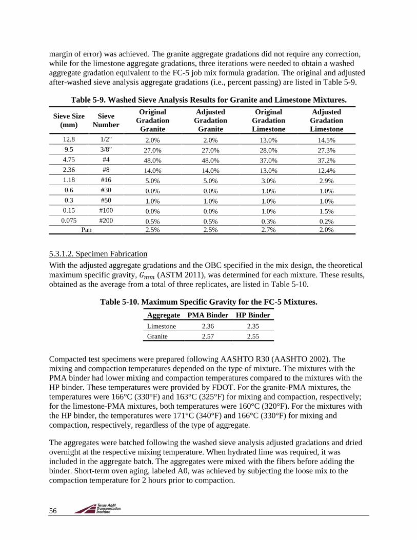
56
margin of error) was achieved. The granite aggregate gradations did not require any correction, while for the limestone aggregate gradations, three iterations were needed to obtain a washed aggregate gradation equivalent to the FC-5 job mix formula gradation. The original and adjusted after-washed sieve analysis aggregate gradations (i.e., percent passing) are listed in Table 5-9.
Table 5-9. Washed Sieve Analysis Results for Granite and Limestone Mixtures.
Sieve Size (mm)
Sieve Number
Original Gradation
Granite
Adjusted Gradation
Granite
Original Gradation Limestone
Adjusted Gradation Limestone
12.8 1/2" 2.0% 2.0% 13.0% 14.5% 9.5 3/8" 27.0% 27.0% 28.0% 27.3%
4.75 #4 48.0% 48.0% 37.0% 37.2% 2.36 #8 14.0% 14.0% 13.0% 12.4% 1.18 #16 5.0% 5.0% 3.0% 2.9% 0.6 #30 0.0% 0.0% 1.0% 1.0% 0.3 #50 1.0% 1.0% 1.0% 1.0%
0.15 #100 0.0% 0.0% 1.0% 1.5% 0.075 #200 0.5% 0.5% 0.3% 0.2%
Pan 2.5% 2.5% 2.7% 2.0%
5.3.1.2. Specimen Fabrication With the adjusted aggregate gradations and the OBC specified in the mix design, the theoretical maximum specific gravity, 𝐺𝐺𝜏𝜏𝜏𝜏 (ASTM 2011), was determined for each mixture. These results, obtained as the average from a total of three replicates, are listed in Table 5-10.
Table 5-10. Maximum Specific Gravity for the FC-5 Mixtures. Aggregate PMA Binder HP Binder Limestone 2.36 2.35 Granite 2.57 2.55
Compacted test specimens were prepared following AASHTO R30 (AASHTO 2002). The mixing and compaction temperatures depended on the type of mixture. The mixtures with the PMA binder had lower mixing and compaction temperatures compared to the mixtures with the HP binder. These temperatures were provided by FDOT. For the granite-PMA mixtures, the temperatures were 166°C (330°F) and 163°C (325°F) for mixing and compaction, respectively; for the limestone-PMA mixtures, both temperatures were 160°C (320°F). For the mixtures with the HP binder, the temperatures were 171°C (340°F) and 166°C (330°F) for mixing and compaction, respectively, regardless of the type of aggregate.
The aggregates were batched following the washed sieve analysis adjusted gradations and dried overnight at the respective mixing temperature. When hydrated lime was required, it was included in the aggregate batch. The aggregates were mixed with the fibers before adding the binder. Short-term oven aging, labeled A0, was achieved by subjecting the loose mix to the compaction temperature for 2 hours prior to compaction.

57
The specimens were compacted using the SGC at a compaction angle of 1.25 degrees and a pressure of 600 kPa with a target AV of 20±1%. The specimens were confined using 150 mm (5.9 in.) polyvinyl chloride (PVC) pipe sleeves as soon as they were extracted from the SGC compaction mold to prevent sagging and crumbling, which was likely to occur in specimens with high AV content. The sleeves were left in place for at least 12 hours while the specimens cooled down in front of a fan. The PVC pipe sleeves were cut on one side to avoid disturbing the sample during extraction from the SGC mold and sealed with duct tape. Even with this precaution, the average diameter of the extracted specimens was not exactly 150.0 mm (5.91 in.) but approximately 150.6 mm (5.93 in.), which was considered acceptable. In addition, the observations by Alvarez et al. (2009), who noted that SGC-compacted FC-5 specimens tend to expand in the vertical direction after extracting from the mold, were taken into consideration. This phenomenon was also reported in the work conducted by Arámbula-Mercado et al. (2016), who observed that SGC-compacted specimens expanded in the vertical direction an average of 1.0 mm (0.04 in.), although this growth depended on the size of the sample (i.e., specimens smaller than 80 mm [3.1 in.] expanded less than the specimens 160 mm [6.3 in.] in height). To prevent these issues, the specimens were compacted 1.0–2.0 mm (0.04–0.08 in.) below the target height required for each test to take into account the vertical expansion. The actual diameter and height measurements per ASTM (2017c) were taken into consideration in the AV content calculation. The AV content was determined between 12–48 hours after the specimen was compacted per ASTM D3203 (ASTM 2017b). All specimens were tested within one week after they were compacted.
The average results and the corresponding variability of the bulk specific gravity, 𝐺𝐺𝜏𝜏𝑠𝑠, of the compacted specimens for the mixtures with PMA and HP binders under all aging states are summarized in Table 5-11 and Table 5-12. In these tables, the term N/A refers to those tests in which the A10 aging state was not considered (i.e., all but the Cantabro abrasion loss tests). As observed, the coefficient of variability (COV) of the 𝐺𝐺𝜏𝜏𝑠𝑠 results were less than or equal to 1% in all cases, proving the high reliability of the specimen fabrication process.
Table 5-11. Gmb for Mixtures with PMA Binder.
Test Aggregate Avg.* A0
Avg. A5
Avg. A10
SD**
A0 SD A5
SD A10
COV A0
COV A5
COV A10
SCB Granite 2.035 2.044 N/A 0.002 0.012 N/A 0.1% 0.6% N/A
Limestone 1.894 1.907 N/A 0.008 0.003 N/A 0.4% 0.2% N/A
IDEAL Granite 2.058 2.032 N/A 0.021 0.002 N/A 1.0% 0.1% N/A
Limestone 1.892 1.897 N/A 0.014 0.019 N/A 0.7% 1.0% N/A
Cantabro Granite 2.066 2.064 2.05 0.013 0.011 0.003 0.6% 0.6% 0%
Limestone 1.903 1.902 1.89 0.008 0.008 0.010 0.4% 0.4% 1% AASHTO
T 283 Granite 2.040 2.047 N/A 0.009 0.012 N/A 0.5% 0.6% N/A
Limestone 1.880 1.895 N/A 0.012 0.010 N/A 0.6% 0.5% N/A * Avg. corresponds to the average of all test replicates. ** SD corresponds to the standard deviation between the test replicates.
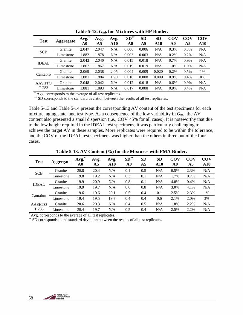
58
Table 5-12. Gmb for Mixtures with HP Binder.
Test Aggregate Avg.* A0
Avg. A5
Avg. A10
SD** A0
SD A5
SD A10
COV A0
COV A5
COV A10
SCB Granite 2.047 2.047 N/A 0.006 0.006 N/A 0.3% 0.3% N/A
Limestone 1.882 1.878 N/A 0.003 0.003 N/A 0.2% 0.2% N/A
IDEAL Granite 2.043 2.040 N/A 0.015 0.018 N/A 0.7% 0.9% N/A
Limestone 1.867 1.867 N/A 0.019 0.019 N/A 1.0% 1.0% N/A
Cantabro Granite 2.069 2.038 2.05 0.004 0.009 0.020 0.2% 0.5% 1%
Limestone 1.881 1.884 1.90 0.016 0.008 0.009 0.9% 0.4% 0% AASHTO
T 283 Granite 2.048 2.042 N/A 0.012 0.018 N/A 0.6% 0.9% N/A
Limestone 1.881 1.893 N/A 0.017 0.008 N/A 0.9% 0.4% N/A * Avg. corresponds to the average of all test replicates. ** SD corresponds to the standard deviation between the results of all test replicates.
Table 5-13 and Table 5-14 present the corresponding AV content of the test specimens for each mixture, aging state, and test type. As a consequence of the low variability in Gmb, the AV content also presented a small dispersion (i.e., COV <5% for all cases). It is noteworthy that due to the low height required in the IDEAL test specimens, it was particularly challenging to achieve the target AV in these samples. More replicates were required to be within the tolerance, and the COV of the IDEAL test specimens was higher than the others in three out of the four cases.
Table 5-13. AV Content (%) for the Mixtures with PMA Binder.
Test Aggregate Avg.* A0
Avg. A5
Avg. A10
SD**
A0 SD A5
SD A10
COV A0
COV A5
COV A10
SCB Granite 20.8 20.4 N/A 0.1 0.5 N/A 0.5% 2.3% N/A
Limestone 19.8 19.2 N/A 0.3 0.1 N/A 1.7% 0.7% N/A
IDEAL Granite 19.9 20.9 N/A 0.8 0.1 N/A 4.0% 0.4% N/A
Limestone 19.9 19.7 N/A 0.6 0.8 N/A 3.0% 4.1% N/A
Cantabro Granite 19.6 19.6 20.1 0.5 0.4 0.1 2.5% 2.3% 1%
Limestone 19.4 19.5 19.7 0.4 0.4 0.6 2.1% 2.0% 3% AASHTO
T 283 Granite 20.6 20.3 N/A 0.4 0.5 N/A 1.8% 2.2% N/A
Limestone 20.4 19.7 N/A 0.5 0.4 N/A 2.5% 2.2% N/A * Avg. corresponds to the average of all test replicates. ** SD corresponds to the standard deviation between the results of all test replicates.

59
Table 5-14. AV Content (%) for the Mixtures with HP Binder.
Test Aggregate Avg.* AV A0
Avg. AV A5
Avg. AV A10
SD** A0
SD A5
SD A10
COV A0
COV A5
COV A10
SCB Granite 19.5 19.5 N/A 0.3 0.3 N/A 1.7% 1.7% N/A
Limestone 19.8 19.9 N/A 0.1 0.1 N/A 0.8% 0.7% N/A
IDEAL Granite 20.0 20.1 N/A 0.6 0.7 N/A 2.9% 3.6% N/A
Limestone 20.0 20.0 N/A 0.5 0.5 N/A 2.3% 2.3% N/A
Cantabro Granite 19.0 20.2 19.8 0.2 0.4 0.8 0.8% 1.8% 4%
Limestone 19.8 19.7 19.2 0.7 0.3 0.4 3.5% 1.7% 2% AASHTO
T 283 Granite 19.8 20.1 N/A 0.5 0.7 N/A 2.3% 3.5% N/A
Limestone 19.8 19.3 N/A 0.7 0.3 N/A 3.6% 1.7% N/A * Avg. corresponds to the average of all test replicates. ** SD corresponds to the standard deviation between the results of all test replicates.
5.3.2. Performance Tests As listed in Table 4-2, the SCB and IDEAL tests were used to determine the fracture properties of the four FC-5 mixtures, the Cantabro abrasion loss test was conducted to assess their durability and degradation, and the FM 1-T 283 test was used to evaluate their susceptibility to moisture damage.
5.3.2.1. Semicircular Bending Test The assembly for the SCB test can be observed in Figure 5-13. After the specimens were conditioned at 25±0.5°C (77°F) for 2 hours ± 10 minutes, they were located in the assembly where they were supported on their flat side. Then, a control load was applied on top of the specimen at a controlled displacement rate of 50 mm/min (1.97 in/min). Two input values were required for the test software: (a) the ligament length, and (b) the total thickness of the specimen to the nearest millimeter. The parameter recorded during the test was the vertical load applied on top of the specimen.
Figure 5-13. Semicircular Bending Test Setup.

60
For the mixtures with the HP binder, a major difficulty was encountered when using the SCB test assembly because the specimen deformed excessively under the test load, and its edges touched the sides of the loading frame toward the end of the test, as shown in Figure 5-14, creating some noise in the recorded data. This was likely due to the high deformability of the HP binder at intermediate temperature. This noise was detected as a second increase in the recorded load, which had to be eliminated during data post-processing to make the results comparable to the mixtures with the PMA binder. A photographic catalog of the cracked specimens and the load-displacement curve can be found in Appendix C.
Figure 5-14. Specimen of a Granite-HP Binder Mixture in Contact with the Edges of the
SCB Loading Frame during Testing.
The I-FIT software from the University of Illinois at Urbana Champaign (https://apps.ict.illinois.edu/software/) was used to determine the test parameters—(a) flexibility index, (b) fracture energy (Gf), and (c) peak load (P max)—which were calculated as follows:
I = Gf / |m| ˟ 0.01 (14)
Gf = Wf / A = ∫(P) du / A (15)
where A is the ligament area (i.e., product of the ligament length and specimen thickness, as shown in Figure 5-15).
FI was obtained by dividing Gf, the fracture energy (J/m2) over the absolute value of the post peak load slope m (kN/mm) times a constant equal to 0.01. Larger values of FI are associated with better cracking resistance and, therefore, a more desirable cracking behavior. Gf was computed as the total area below the vertical displacement at the center of the specimen versus the vertical applied load curve (see work of fracture in Figure 5-16) divided by the ligament area, A. Larger values of Gf are associated with materials with higher resistance to fracture. Finally, the third parameter was defined as the maximum load supported by the specimen during the test; larger values of Pmax (kN) are related with mixtures having improved strength properties.

61
Figure 5-15. Lateral and Side View of an SCB Notched Test Specimen.
Figure 5-16. Example of Load versus Displacement Curves for Mixtures Tested in the
I-FIT.
Based on the results presented by Kaseer et al. (2018), another test parameter was considered in this study, namely the cracking resistance index, shown in Equation 16. It should be noted that although the fracture energy considers both the strength and the ductility of the mixture, it does not differentiate between mixtures that may have different properties but similar fracture energies. The CRI, on the contrary, is able to do so by incorporating the peak load in its calculation. Thus, the CRI is effective in differentiating and ranking the cracking resistance of asphalt mixtures with diverse characteristics, with the additional advantage that it has a reduced variability compared to the FI (Kaseer et al., 2018). Overall, larger values of CRI represent better resistance to cracking, while lower values indicate brittleness.
CRindex = GfPmax
(16)
Out of the available test parameters, the FI and CRI were selected in this study to evaluate the fracture performance of the mixtures.
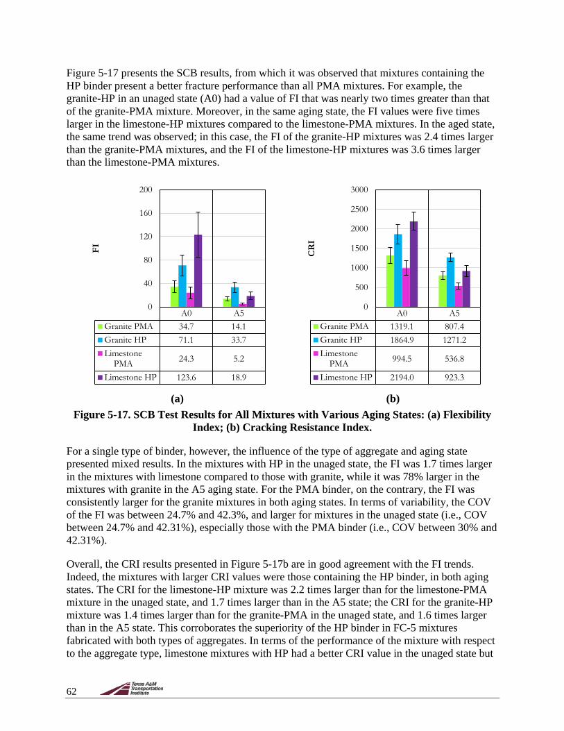
62
Figure 5-17 presents the SCB results, from which it was observed that mixtures containing the HP binder present a better fracture performance than all PMA mixtures. For example, the granite-HP in an unaged state (A0) had a value of FI that was nearly two times greater than that of the granite-PMA mixture. Moreover, in the same aging state, the FI values were five times larger in the limestone-HP mixtures compared to the limestone-PMA mixtures. In the aged state, the same trend was observed; in this case, the FI of the granite-HP mixtures was 2.4 times larger than the granite-PMA mixtures, and the FI of the limestone-HP mixtures was 3.6 times larger than the limestone-PMA mixtures.
(a)
(b)
Figure 5-17. SCB Test Results for All Mixtures with Various Aging States: (a) Flexibility Index; (b) Cracking Resistance Index.
For a single type of binder, however, the influence of the type of aggregate and aging state presented mixed results. In the mixtures with HP in the unaged state, the FI was 1.7 times larger in the mixtures with limestone compared to those with granite, while it was 78% larger in the mixtures with granite in the A5 aging state. For the PMA binder, on the contrary, the FI was consistently larger for the granite mixtures in both aging states. In terms of variability, the COV of the FI was between 24.7% and 42.3%, and larger for mixtures in the unaged state (i.e., COV between 24.7% and 42.31%), especially those with the PMA binder (i.e., COV between 30% and 42.31%).
Overall, the CRI results presented in Figure 5-17b are in good agreement with the FI trends. Indeed, the mixtures with larger CRI values were those containing the HP binder, in both aging states. The CRI for the limestone-HP mixture was 2.2 times larger than for the limestone-PMA mixture in the unaged state, and 1.7 times larger than in the A5 state; the CRI for the granite-HP mixture was 1.4 times larger than for the granite-PMA in the unaged state, and 1.6 times larger than in the A5 state. This corroborates the superiority of the HP binder in FC-5 mixtures fabricated with both types of aggregates. In terms of the performance of the mixture with respect to the aggregate type, limestone mixtures with HP had a better CRI value in the unaged state but
A0 A5Granite PMA 34.7 14.1Granite HP 71.1 33.7Limestone
PMA 24.3 5.2
Limestone HP 123.6 18.9
0
40
80
120
160
200
FI
A0 A5Granite PMA 1319.1 807.4Granite HP 1864.9 1271.2Limestone
PMA 994.5 536.8
Limestone HP 2194.0 923.3
0
500
1000
1500
2000
2500
3000
CR
I

63
a worse CRI value in the A5 state. In the mixtures with PMA, the results were superior when granite was used, independently of the aging state, similar to what was reported for the FI values.
Due to the large amount of data obtained from the experiments, and the number of variables that were considered in this test, a statistical analysis was conducted to identify any outliers in the data and to determine valid relationships between the different variables (e.g., the effect of the aggregate type, binder type, aging state, and/or AV content on the FI and CRI results). Since there is no statistical analysis that can determine an outlier from a sample of a few replicates, an analysis of variance (ANOVA) was performed over the sum of the 75 measurements and the outliers detected at the end based on residuals. A detailed report of this statistical analysis is presented in Appendix D. A single data point was found to be a potential outlier (i.e., replicate 3, for the limestone-HP in the A0 state). However, the results of the statistical analysis indicated that the removal of the value did not significantly affect the results, so the value was kept in all analyses.
Aggregate type, binder type, and aging state as main effects and all possible two-way interactions were included in the ANOVA. The p-value in this analysis is the lowest level at which the observed parameter is significant for the statistic evaluated (Walpole et al., 2009). In this case, a p-value of 0.05 was selected. In terms of the FI results, the only two-way interaction that was statistically significant was aggregate type × aging state. However, the two-way interaction between aggregate type × binder type was borderline significant with a p-value of 0.0573. Thus, the type of binder could also be considered a significant factor determining higher FI values, being larger for the HP binder. The effect of aging on FI was found to be dependent on the type of aggregate: limestone aggregates lead to mixtures with higher values of FI for A0 compared to the A5 state, while no statistical significance was observed when granite was used.
Based on the analysis for CRI, binder type and aging state were statistically significant as well as the two-way interaction between aggregate type × aging state. Specifically, the use of the HP binder was found to provide statistically significant larger CRI values than those obtained with PMA. This result agreed with the ones obtained with the FI parameter. Finally, also similar to the FI results, the effect of aging on CRI was statistically significant for the mixtures with limestone, but not for the mixtures with granite. This could be because the limestone aggregate was more absorptive, and with aging, more binder was absorbed and thus there was less effective binder.
The mixtures were ranked based on the FI and CRI results, as shown in Table 5-15. The ranking of the mixtures depended on their aging state. For instance, for the unaged mixtures, limestone-HP was the best, but it ranked second after aging. Regardless, the mixtures with the HP binder were still superior to the mixtures with the PMA binder.
Table 5-15. Ranking of Mixtures Based on SCB Test Results. Rank Unaged Mixture (A0) Aged Mixture (A5)
1 Limestone-HP Granite-HP 2 Granite-HP Limestone-HP 3 Granite-PMA Granite-PMA 4 Limestone-PMA Limestone-PMA
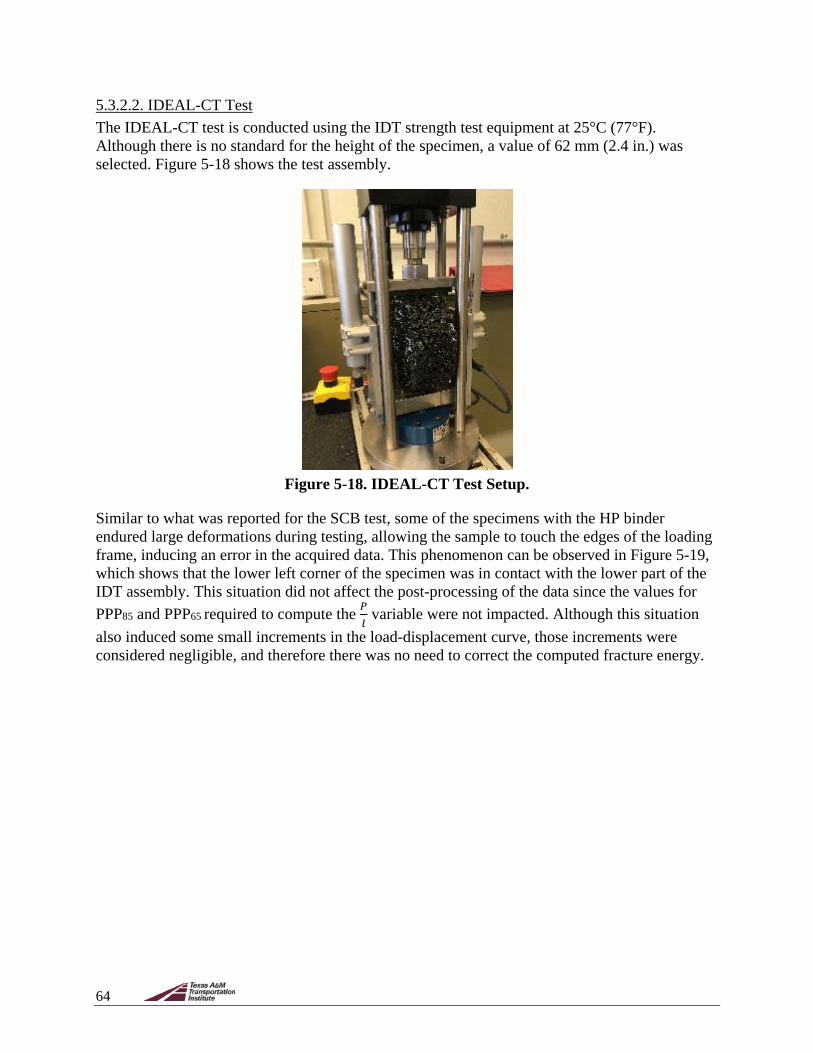
64
5.3.2.2. IDEAL-CT Test The IDEAL-CT test is conducted using the IDT strength test equipment at 25°C (77°F). Although there is no standard for the height of the specimen, a value of 62 mm (2.4 in.) was selected. Figure 5-18 shows the test assembly.
Figure 5-18. IDEAL-CT Test Setup.
Similar to what was reported for the SCB test, some of the specimens with the HP binder endured large deformations during testing, allowing the sample to touch the edges of the loading frame, inducing an error in the acquired data. This phenomenon can be observed in Figure 5-19, which shows that the lower left corner of the specimen was in contact with the lower part of the IDT assembly. This situation did not affect the post-processing of the data since the values for PPP85 and PPP65 required to compute the 𝑃𝑃
𝑙𝑙 variable were not impacted. Although this situation
also induced some small increments in the load-displacement curve, those increments were considered negligible, and therefore there was no need to correct the computed fracture energy.

65
Figure 5-19. Specimen in Contact with the Edge of the IDEAL-CT Loading Frame during
Testing.
The CTindex values (Equation 9) for all mixtures at both aging states are presented in Figure 5-20. In general, larger values of CTindex indicate slower cracking growth rates and, consequently, better cracking performance. The overall trend was consistent in both aging states and shows that, in agreement with the SCB test results, HP mixtures had the best performance. In terms of the aggregate type, granite aggregates provided larger CTindex results in both aging states for both binders. It is worth mentioning that the order of magnitude of the values obtained for the mixtures in the original state significantly differed from those observed in Zhou et al. (2017a) for dense mixtures. However, the IDEAL test is known for being sensitive to the AV content; for example, results for dense mixtures with 9% AV content were found to present values of CTindex that were 1.6 times greater than in mixtures with 5% AV content. Thus, larger differences were expected for the FC-5 specimens that had a target AV content of 20%.
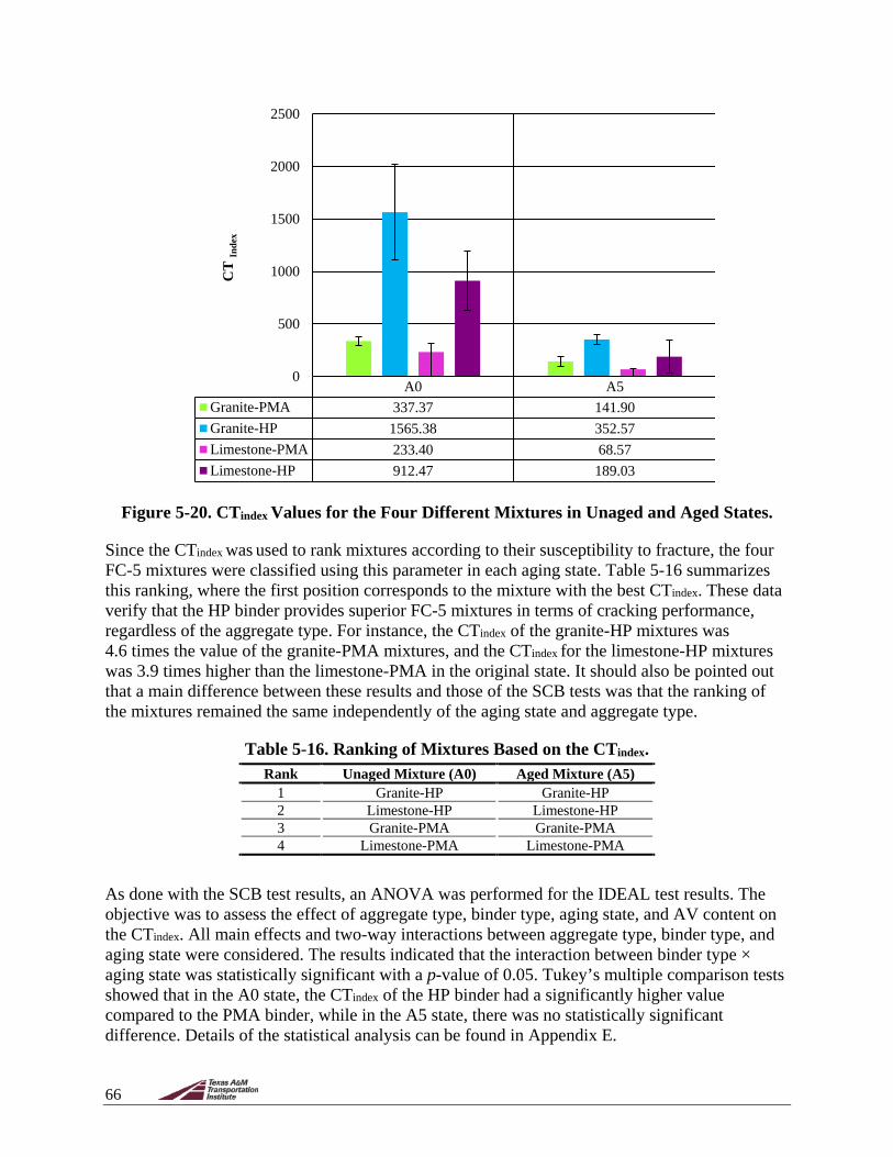
66
Figure 5-20. CTindex Values for the Four Different Mixtures in Unaged and Aged States.
Since the CTindex was used to rank mixtures according to their susceptibility to fracture, the four FC-5 mixtures were classified using this parameter in each aging state. Table 5-16 summarizes this ranking, where the first position corresponds to the mixture with the best CTindex. These data verify that the HP binder provides superior FC-5 mixtures in terms of cracking performance, regardless of the aggregate type. For instance, the CTindex of the granite-HP mixtures was 4.6 times the value of the granite-PMA mixtures, and the CTindex for the limestone-HP mixtures was 3.9 times higher than the limestone-PMA in the original state. It should also be pointed out that a main difference between these results and those of the SCB tests was that the ranking of the mixtures remained the same independently of the aging state and aggregate type.
Table 5-16. Ranking of Mixtures Based on the CTindex. Rank Unaged Mixture (A0) Aged Mixture (A5)
1 Granite-HP Granite-HP 2 Limestone-HP Limestone-HP 3 Granite-PMA Granite-PMA 4 Limestone-PMA Limestone-PMA
As done with the SCB test results, an ANOVA was performed for the IDEAL test results. The objective was to assess the effect of aggregate type, binder type, aging state, and AV content on the CTindex. All main effects and two-way interactions between aggregate type, binder type, and aging state were considered. The results indicated that the interaction between binder type × aging state was statistically significant with a p-value of 0.05. Tukey’s multiple comparison tests showed that in the A0 state, the CTindex of the HP binder had a significantly higher value compared to the PMA binder, while in the A5 state, there was no statistically significant difference. Details of the statistical analysis can be found in Appendix E.
A0 A5Granite-PMA 337.37 141.90Granite-HP 1565.38 352.57Limestone-PMA 233.40 68.57Limestone-HP 912.47 189.03
0
500
1000
1500
2000
2500
CT
Inde
x

67
5.3.2.3. Cantabro Abrasion Loss Test The Cantabro abrasion loss test is specified in AASHTO TP 108 (AASHTO 2014b), as previously detailed in Section 4.2.3. Mixtures with larger mass loss are considered more prone to degradation. The impact of aging was further evaluated in this test by testing specimens in three different aging states: A0, A5, and A10 (Table 4-2). Figure 5-21 summarizes the results for the three aging states.
Figure 5-21. Cantabro Test Results for Three Aging States.
These results demonstrate that the mixtures with the HP binder were consistently less prone to degradation (e.g., small abrasion or % mass loss). Also, the results showed that aging considerably affected the performance of all mixtures. The minimum percentage mass loss suggested in AASHTO TP 108 (i.e., less than 20% mass loss) was easily achieved for every FC-5 mixture in the original state. However, aging fostered the degradation of the mixtures, especially those prepared with the PMA binder, increasing the mass loss. Specifically, the mass loss in the limestone-PMA mixture increased about three times in between aging state (i.e., A0–A5 and A5–A10). This was in accordance with previous experiences of FDOT with FC-5 mixtures, which indicate that after five years of service, some limestone-PMA mixtures experience raveling (Massahi et al., 2018). Conversely, the HP binder FC-5 mixtures passed the standard requirement in both A0 and A5 aging states. Also, the limestone-HP mixtures presented an average of 30% increase in percentage loss compared with the granite mixtures when comparing the A0 and the A10 aging states, suggesting that mixtures with limestone could be less durable (i.e., present a larger abrasion). In terms of the dispersion of the data, the standard deviation of the results increased with aging, which was the opposite of what was observed in other performance tests.
As detailed in Appendix F, an initial unsuccessful attempt was done to assess the evolution in the performance of the FC-5 mixtures (i.e., degradation rate) using compacted slabs in the three-wheel polisher with studded tires. Therefore, an alternative method to evaluate the degradation rate was conducted using compacted specimens in different aging states and subjected to various
A0 A5 A10Granite-PMA 13.4% 15.8% 30.7%Granite-HP 4.3% 10.1% 14.7%Limestone-PMA 7.2% 21.4% 64.9%Limestone-HP 3.9% 8.1% 19.0%
0.0%
10.0%
20.0%
30.0%
40.0%
50.0%
60.0%
70.0%
80.0%
Wei
ght
Los
s
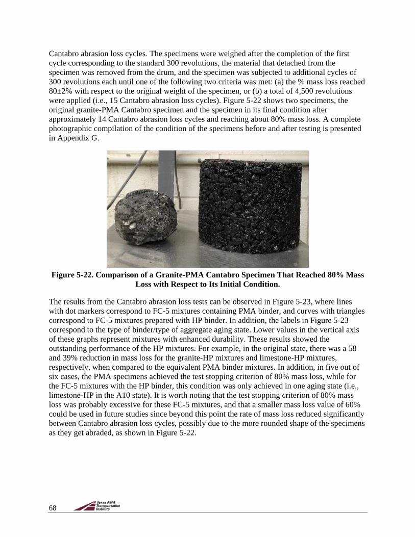
68
Cantabro abrasion loss cycles. The specimens were weighed after the completion of the first cycle corresponding to the standard 300 revolutions, the material that detached from the specimen was removed from the drum, and the specimen was subjected to additional cycles of 300 revolutions each until one of the following two criteria was met: (a) the % mass loss reached 80±2% with respect to the original weight of the specimen, or (b) a total of 4,500 revolutions were applied (i.e., 15 Cantabro abrasion loss cycles). Figure 5-22 shows two specimens, the original granite-PMA Cantabro specimen and the specimen in its final condition after approximately 14 Cantabro abrasion loss cycles and reaching about 80% mass loss. A complete photographic compilation of the condition of the specimens before and after testing is presented in Appendix G.
Figure 5-22. Comparison of a Granite-PMA Cantabro Specimen That Reached 80% Mass
Loss with Respect to Its Initial Condition.
The results from the Cantabro abrasion loss tests can be observed in Figure 5-23, where lines with dot markers correspond to FC-5 mixtures containing PMA binder, and curves with triangles correspond to FC-5 mixtures prepared with HP binder. In addition, the labels in Figure 5-23 correspond to the type of binder/type of aggregate aging state. Lower values in the vertical axis of these graphs represent mixtures with enhanced durability. These results showed the outstanding performance of the HP mixtures. For example, in the original state, there was a 58 and 39% reduction in mass loss for the granite-HP mixtures and limestone-HP mixtures, respectively, when compared to the equivalent PMA binder mixtures. In addition, in five out of six cases, the PMA specimens achieved the test stopping criterion of 80% mass loss, while for the FC-5 mixtures with the HP binder, this condition was only achieved in one aging state (i.e., limestone-HP in the A10 state). It is worth noting that the test stopping criterion of 80% mass loss was probably excessive for these FC-5 mixtures, and that a smaller mass loss value of 60% could be used in future studies since beyond this point the rate of mass loss reduced significantly between Cantabro abrasion loss cycles, possibly due to the more rounded shape of the specimens as they get abraded, as shown in Figure 5-22.

69
Figure 5-23. Cantabro Degradation Curves of Mixtures in Various Aging States
(A0, A5, and A10); Each Cantabro Cycle Consists of 300 Revolutions.
Another major finding from these experiments was the clear effect of aging on the degradation of the mixtures. The influence of the binder in the resistance to abrasion with aging progression was significant since the limestone-HP mixtures in the A10 state were able to withstand five times more Cantabro cycles until reaching the 80% degradation test stopping criterion compared to limestone-PMA mixtures at the same aging state. In accordance with previous results, it was also found that mixtures containing limestone were more susceptible to damage than the mixtures with granite. In fact, the target 80% mass loss test stopping criterion was achieved more rapidly for the PMA mixtures with limestone, except for the PMA in the A0 state, and all limestone-PMA mixtures presented a faster mass loss than those with the granite aggregate.
In general, it was observed that the variability among results decreased with an increase in the applied number of Cantabro abrasion loss cycles. For example, the limestone-HP specimens in the A5 state presented a COV of 16.8% in the first cycle, and this value reduced to 3.8% in the 15th cycle. This trend was similar in the other FC-5 mixtures and might be due to the rounder shape of the specimens as they get abraded, as shown in Figure 5-22.
The Cantabro abrasion loss test results were analyzed statistically using an ANOVA with aggregate type, binder type, aging condition, and AV content as main effects along with their two-way interactions. The results indicated that the two-way interactions between aggregate type × aging condition as well as between binder type × aging condition were significant with a p-value of 0.05. This supports the observations in Figure 5-21 and Figure 5-23, where binder
PMA-G-A0 PMA-G-A5PMA-G-A10 PMA-LS-A0
PMA-LS-A5PMA-LS-A10
HP-G-A0
HP-G-A5
HP-G-A10
HP-LS-A0
HP-LS-A5
HP-LS-A10
0%
10%
20%
30%
40%
50%
60%
70%
80%
90%
1 2 3 4 5 6 7 8 9 10 11 12 13 14 15
% M
ass
Loss
Cantabro CyclesLS = Limestone; G = Granite
PMA-G-A0 PMA-G-A5 PMA-G-A10 PMA-LS-A0
PMA-LS-A5 PMA-LS-A10 HP-G-A0 HP-G-A5
HP-G-A10 HP-LS-A0 HP-LS-A5 HP-LS-A10
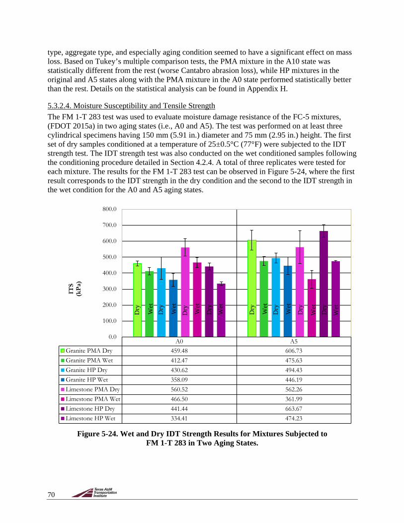
70
type, aggregate type, and especially aging condition seemed to have a significant effect on mass loss. Based on Tukey’s multiple comparison tests, the PMA mixture in the A10 state was statistically different from the rest (worse Cantabro abrasion loss), while HP mixtures in the original and A5 states along with the PMA mixture in the A0 state performed statistically better than the rest. Details on the statistical analysis can be found in Appendix H.
5.3.2.4. Moisture Susceptibility and Tensile Strength The FM 1-T 283 test was used to evaluate moisture damage resistance of the FC-5 mixtures, (FDOT 2015a) in two aging states (i.e., A0 and A5). The test was performed on at least three cylindrical specimens having 150 mm (5.91 in.) diameter and 75 mm (2.95 in.) height. The first set of dry samples conditioned at a temperature of 25±0.5°C (77°F) were subjected to the IDT strength test. The IDT strength test was also conducted on the wet conditioned samples following the conditioning procedure detailed in Section 4.2.4. A total of three replicates were tested for each mixture. The results for the FM 1-T 283 test can be observed in Figure 5-24, where the first result corresponds to the IDT strength in the dry condition and the second to the IDT strength in the wet condition for the A0 and A5 aging states.
Figure 5-24. Wet and Dry IDT Strength Results for Mixtures Subjected to
FM 1-T 283 in Two Aging States.
A0 A5Granite PMA Dry 459.48 606.73Granite PMA Wet 412.47 475.63Granite HP Dry 430.62 494.43Granite HP Wet 358.09 446.19Limestone PMA Dry 560.52 562.26Limestone PMA Wet 466.50 361.99Limestone HP Dry 441.44 663.67Limestone HP Wet 334.41 474.23
0.0
100.0
200.0
300.0
400.0
500.0
600.0
700.0
800.0
ITS
(kPa
)
Dry
Wet
Dry
Dry
Dry
Dry
Dry
Dry
Dry
Wet
Wet
Wet
Wet
Wet
Wet
Wet
71
The results showed considerable variability among replicates (i.e., the COV for the PMA binder in the A0 state was 10% and up to 18% for the specimens in the A5 state, while the COV for the HP binder in the A0 state ranged between 3.2% and 16.4% and between 6–12% in the A5 state). Overall, the IDT strength of the mixtures increased with aging (i.e., between 3 and 32%), with the only exception being the value obtained for the limestone-PMA mixture. The highest IDT strength value in the unaged state obtained from the test corresponded to the mixtures with limestone, and this trend was reversed for the aged state. Mixtures having granite experienced a lesser decrease in the IDT strength from dry to wet condition compared to the limestone mixtures (i.e., the granite-PMA in the A0 state lost 10% from the dry to wet condition). Overall, mixtures with PMA presented higher IDT strength values compared to those fabricated with HP, with the only exception being the limestone-HP mixture in the A5 state. These results were in agreement with the values of the dynamic shear moduli of both asphalts (i.e., PMA presented larger overall values with respect to HP). However, as demonstrated in previous sections, in terms of fracture properties (Sections 5.3.2.1 and 5.3.2.2) and durability (Section 5.3.2.3), the HP mixtures were superior to the PMA mixtures.
Figure 5-25 presents the TSR results. This figure indicates that the susceptibility to moisture damage changes over time due to aging. In the original state, the limestone-PMA mixture had a low TSR value and, contrary to all other mixtures, it did not comply with the typical acceptance criterion of a minimum TSR value of 70% (represented in Figure 5-25 with a red line), based on AASHTO PP 77-14 (AASHTO 2014c). Surprisingly, all mixtures in the aged state (A5) satisfied the minimum TSR of 70%. However, there was not a consistent trend of increase or reduction in the TSR values of the mixtures with respect to the original state. For example, the TSR of the granite-HP mixtures in the A5 state increased 8.5% with respect to the A0 state, while the TSR of the limestone-HP mixtures reduced 5.2% between both aging states. In the case of the PMA mixtures, the TSR in the mixtures with the granite aggregate exhibited a reduction of 13.3% between the A0 and A5 states, while those with limestone had an increase in TSR between these aging states of 27.7%. In terms of the type of aggregate, most mixtures with limestone in both aging states had lower TSR values than those with granite (except for the granite-PMA versus limestone-PMA in the A5 state), independently of the type of binder. As observed, the effects of the asphalt binder or aging state on the susceptibility to moisture damage of these mixtures were diverse.

72
Figure 5-25. TSR Results for Mixtures Subjected to FM 1-T 283 in Two Aging States.
It should be noted that both the IDEAL and FM 1-T 283 tests provided IDT strength values. Figure 5-26 compares the results for both tests in the dry condition. The values were similar with differences smaller than 20%, except for the limestone-HP mixtures in the aged state (A5) and the limestone-PMA mixtures in the original state (A0).
(a)
(b)
Figure 5-26. Dry IDT Strength Results for Mixtures in Two Aging States: (a) Subjected to FM 1-T 283; (b) Subjected to the IDEAL Test.
A0 A5Granite PMA 90% 78%Granite HP 83% 90%limestone-PMA 65% 83%Limestone-HP 76% 72%
0%10%20%30%40%50%60%70%80%90%
100%
Ten
sile
Str
engt
h R
atio
A0 A5Granite PMA 459.48 606.73Granite HP 430.62 494.43Limestone
PMA 560.52 562.26
Limestone HP 441.44 327.44
0
100
200
300
400
500
600
700
800
900
FM 1
-T 2
83 I
DT
Str
engt
h (k
Pa)
A0 A5Granite PMA 385.62 511.85Granite HP 418.60 609.28Limestone
PMA 402.25 617.41
Limestone HP 448.07 724.17
0
100
200
300
400
500
600
700
800
900
IDE
AL
IDT
Str
engt
h(k
Pa)
73
There are several possible explanations for the differences between both test results. According to NCHRP 9-56 (Azari, 2010), it is not appropriate to compare IDT strength results from dense mixtures from different IDT strength tests conducted with different equipment due to calibration issues, even if the specimens and loading conditions are the same. The TSR and the IDEAL tests were conducted with different test equipment, which could partially explain the differences in the results. Also, the height of the specimens was different in both cases (i.e., 62 mm [2.44 in.] in the IDEAL test and 75 mm [2.95 in.] in the FM 1-T 283), which could cause discrepancies in the response of the specimens due to the open structure of FC-5 mixtures. Based on the reasons provided before, detailed analyses of the influence of a specific parameter (i.e., binder or aggregate type) on the IDT strength results were not recommended.
A statistical ANOVA assessing the effects of aggregate type, binder type, aging state, moisture condition, and AV content and their two-way interactions was conducted. The two-way interactions with AV content were insignificant, so they were removed from the model and the ANOVA was conducted again without that variable. The results indicated that the two-way interaction between aggregate type × moisture condition was statistically significant with a p-value = 0.05. This suggests that the effect of aggregate type on the test result depended on whether the material was in the dry or wet condition. Using Tukey’s multiple comparison tests, mixtures with the limestone aggregate in the dry condition had significantly larger IDT strengths compared to mixtures with granite in the dry condition, while for mixtures in the wet condition, there was no statistically significant difference for the two aggregate types. In addition, mixtures in the A5 state had larger values of IDT strength compared to mixtures in the original or A0 state. This result was expected since aging stiffens the binder in the mixture. Details of the statistical analysis can be found in Appendix I.
5.4. SUMMARY OF EXPERIMENTAL RESULTS Table 5-17 and Table 5-18 summarize the results obtained from the different tests. In terms of the binders, as observed in Table 5-17, the HP binder showed a better overall ranking, with the exception of the FTIR test. However, this was not of concern for two reasons: (a) the base binder for each of the modified binders was believed to be different, which could explain some of the changes induced by aging in their chemical composition; and (b) the properties and performance indicators obtained from the other tests showed a better performance for the HP binder. This finding implied that, although the HP binder seemed to have larger carbonyl area growth, this condition did not impact the performance of the HP mixtures.
Table 5-18 shows the ranking of the FC-5 mixtures based on the aging state and the type of mixture. In general, mixtures with the HP binder excelled in performance. More specifically, the HP mixtures with granite were typically ranked better than those with limestone, and in those cases where the limestone-HP mixtures were superior, the corresponding parameter was very similar to the granite-HP.

74
Table 5-17. Summary Results for Binder and Mastic Characterization and Ranking.
Test Property Evaluated
Parameter Evaluated Binder Type Result Ranking Best-Performing
Binder
PG – PG grade PMA PG 82-22 2
HP HP PG 82-28 1
G-R
Cracking susceptibility
due to oxidation
Aging state at which the
damage zone in reached
PMA PAV20 2 HP
HP PAV80 1
FTIR Aging susceptibility
Carbonyl area growth
PMA Slope = 0.2429 1 PMA
HP Slope = 0.2693 2
PLAS Fatigue resistance FREI
PMA HP was consistently better in all aging states
2 HP
HP 1
Sessile Drop
Contact angles Total SFE
PMA Granite-PMA Original 2
HP HP Granite-HP Original 1
In terms of fracture susceptibility, mixtures with the HP binder performed better than those with the PMA binder. Regarding the potential abrasion of the mixture measured through the Cantabro abrasion loss test, the HP mixtures were also consistently superior to the PMA mixtures. Moreover, the granite mixtures were predominantly more resistant to Cantabro abrasion loss compared to the limestone mixtures. Finally, the IDT strength values from the IDEAL test were larger for aged states and for mixtures with the HP binder and, in terms of the moisture damage susceptibility, no conclusive pattern regarding the influence of aging, aggregate type, or binder type was obtained.
Based on the experimental results, the HP binder and corresponding FC-5 mixtures presented an overall better performance compared to those prepared with the PMA binder. Particularly, granite-HP mixtures were more resistant to cracking in both aging states and were also more resistant to abrasion.
Finally, it should be mentioned that this experimental study was conducted on PMA and HP binders obtained from a single producer source. Furthermore, the control PMA binder had an improved PG grade (i.e., PG 82-22E) with respect to its commercial label (i.e., PG 76-22). Thus, the relative differences between the PMA and HP binders might vary if other sources of these commercial binders were evaluated. In this particular case, however, and even when both binders shared the same superior PG grade (i.e., 82), the results were conclusive in demonstrating that the increased polymer amount in the HP binder enhanced the overall performance and durability of the FC-5 mixtures.
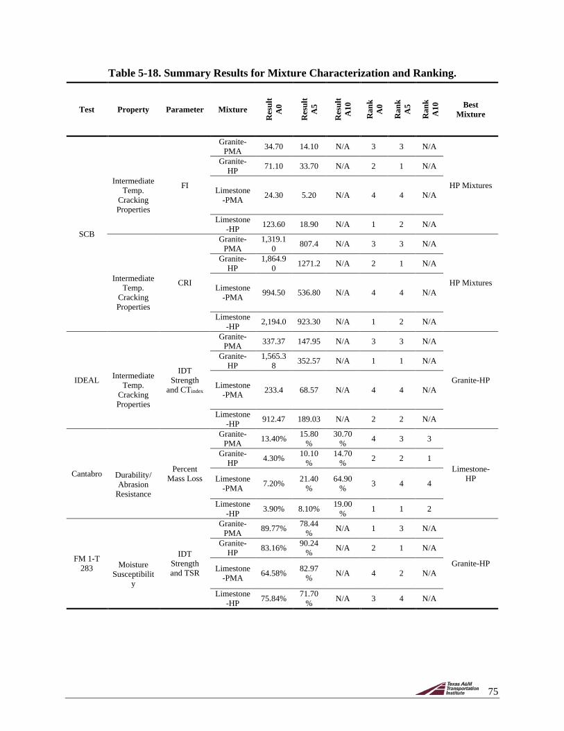
75
Table 5-18. Summary Results for Mixture Characterization and Ranking.
Test Property Parameter Mixture
Res
ult
A0
Res
ult
A5
Res
ult
A10
Ran
k
A0
Ran
k
A5
Ran
k
A10
Best Mixture
SCB
FI
Granite-PMA 34.70 14.10 N/A 3 3 N/A
HP Mixtures
Granite-HP 71.10 33.70 N/A 2 1 N/A
Intermediate Temp.
Cracking Properties
Limestone-PMA 24.30 5.20 N/A 4 4 N/A
Limestone-HP 123.60 18.90 N/A 1 2 N/A
CRI
Granite-PMA
1,319.10 807.4 N/A 3 3 N/A
HP Mixtures
Granite-HP
1,864.90 1271.2 N/A 2 1 N/A
Intermediate Temp.
Cracking Properties
Limestone-PMA 994.50 536.80 N/A 4 4 N/A
Limestone-HP 2,194.0 923.30 N/A 1 2 N/A
IDEAL
IDT Strength
and CTindex
Granite-PMA 337.37 147.95 N/A 3 3 N/A
Granite-HP
Granite-HP
1,565.38 352.57 N/A 1 1 N/A
Intermediate Temp.
Cracking Properties
Limestone-PMA 233.4 68.57 N/A 4 4 N/A
Limestone-HP 912.47 189.03 N/A 2 2 N/A
Cantabro
Percent Mass Loss
Granite-PMA 13.40% 15.80
% 30.70
% 4 3 3
Limestone-HP
Granite-HP 4.30% 10.10
% 14.70
% 2 2 1
Durability/ Abrasion
Resistance
Limestone-PMA 7.20% 21.40
% 64.90
% 3 4 4
Limestone-HP 3.90% 8.10% 19.00
% 1 1 2
FM 1-T 283
IDT Strength and TSR
Granite-PMA 89.77% 78.44
% N/A 1 3 N/A
Granite-HP
Granite-HP 83.16% 90.24
% N/A 2 1 N/A
Moisture Susceptibilit
y
Limestone-PMA 64.58% 82.97
% N/A 4 2 N/A
Limestone-HP 75.84% 71.70
% N/A 3 4 N/A

76
6.0. NUMERICAL MODELING The objective of the 2D FE numerical modeling effort was to complement the experimental work by evaluating the response of the various FC-5 mixtures under short-term and long-term aging conditions. The numerical models included in this project were built based on the previous efforts reported in the literature and on the experience gained by the research team as part of a recently completed FDOT project that aimed at understanding and identifying the mechanisms associated with raveling in these materials (Arámbula-Mercado et al., 2016; Manrique-Sánchez et al., 2016). Since raveling is a stone-on-stone contact phenomenon (Alvarez et al., 2010a), the strength and resistance to raveling of the FC-5 mixture is strongly dependent on the characteristics of the microstructure (Alvarez et al., 2008; Alvarez et al., 2010a; Alvarez et al., 2010b; Manrique-Sánchez et al., 2016). Thus, realistic geometries of the microstructure of the FC-5 mixtures were obtained with X-ray CT and image analysis techniques on specimens fabricated in the laboratory to a target AV content of 20% and used in the FE models, using a similar approach to that used in the previous works. Figure 6-1 presents an example of an X-ray CT cross-section of an FC-5 specimen, as well as the rectangular portion that is used in the FE model. Each one of the sections was fully characterized in order to count with information useful to explain the experimental results (i.e., gradation, AV content, average length of stone-on-stone contacts, aggregate orientation, etc.). Figure 6-2 illustrates an example of the characterization of a cross-section of an FC-5 mixture with respect to the number of stone-on-stone contacts per aggregate and aggregate orientation. Abaqus® was used to perform simulations on the FC-5 geometrical models with distinct material properties.
(a) (b)
Figure 6-1. (a) X-ray Scan of an OGFC Mixture; (b) 2D Section of an OGFC Mixture Obtained from an X-ray CT-Scanned Image and Processed as Input to the FE Model.

77
(a)
(b)
Figure 6-2. Characterization of the OGFC Sections: (a) Number of Contacts per Aggregate; (b) Quantification of Aggregate Orientation.
In the previous FDOT research effort, a rigorous energy-based methodology was designed and used to process the outcome data. This method required processing the results of the stresses and strains within the stone-on-stone contacts of the FC-5 mixture in order to obtain the maximum dissipated energy in both Mode I (opening) and Mode II (shear) of failure at the critical stone-on-stone or mastic-on-mastic contacts where fracture could occur through a parameter named raveling index. In general, larger values of the RI are related with contacts that are more prone to break and, therefore, with a higher susceptibility to raveling. This approach was used to evaluate the raveling susceptibility of the FC-5 mixtures in a short-term aging state.
One difference between the numerical simulations included in this project with respect to previous effort was the evaluation of raveling in the FC-5 mixtures near the end of their service life (i.e., long-term aged condition). This methodology consisted of using aged rheological and fracture properties of the mixtures in order to conduct FE simulations where the actual dislodgement of an aggregate could be represented at the stone-on-stone contacts (i.e., actual simulation of raveling processes). The simulation of fracture was achieved through the use of the CZM technique, a numerical method that has been commonly used to simulate fracture processes in solid materials. Raveling susceptibility was quantified in this long-term aging scenario using the new evaluation parameter ER. This parameter quantifies the energy that the mastic material located at each stone-on-stone contact is still able to dissipate before cracking. Thus, values of ER equal to 0.0 imply that the contact was broken (i.e., raveling initiation), values near 0.0 imply that the contact is near fracture (i.e., raveling is close to initiate), while larger values of ER represent mastic contacts that are far from reaching a fracture condition (i.e., raveling-resistant contacts).
Figure 6-3a illustrates the mastic-on-mastic contact zones where the CZM technique was incorporated, while Figure 6-3b illustrates the bilinear constitutive response that will be used for the cohesive contacts. The mechanical response of these contacts under this traction-separation law is as follows: when the contact is subjected to a certain stress condition, it deforms following a linear elastic response until reaching its maximum tensile strength in any fracture mode (Mode I or II). At this point (δin or σmax in Figure 6-3b), the structural resistance of the contact starts decreasing (i.e., σ after δin in Figure 6-3b) until failure. Once the energy dissipated by the element equals that of the fracture energy of the material, the contact breaks, and the finite

78
elements originally in contact lose that contact and get separated, which represents the initiation of fracture. Afterwards, the propagation of the crack continues through the mastic-on-mastic zone where the cohesive contacts are located, until the point where both aggregates separate from each other (i.e., raveling development).
(a) (b)
Figure 6-3. (a) Location of the CZM Elements at the Mastic-on-Mastic Contacts; (b) Traction-Separation Law for the CZM.
Since the previous FDOT research effort demonstrated that the particular X-ray CT section selected for the FE model strongly influenced the probability of a mixture to raveling, at least three FC-5 microstructures were selected for each type of mixture in order to achieve more reliable results. Table 6-1 summarizes the input data for the FE models and the relationship with the experimental test plan.
Table 6-1. Parameters Used as Input in the FE Models. Input Parameter Method to Obtain the Values
Geometry of the FC-5 microstructure X-ray CT scans and image processing techniques Constitutive relationship for mastics at
different aging conditions Master curves
Traction-separation law of the CZM elements
IDT testing: tensile strength SCB testing: fracture energy
Traffic
Load magnitudes: existing long-term pavement performance (LTPP) data for Florida
or equivalent data from similar databases Longitudinal loading simulating different friction conditions:
reported models in the literature
6.1. MODELING METHODOLOGY AND MATERIALS
6.1.1. FC-5 Microstructure Geometry Portions of 2D vertical cross-sections captured with the X-ray CT scans on OGFC specimens with a target AV of 20% were selected to obtain three FC-5 microstructure replicates with two different thicknesses: 2-cm (0.79-in.) and 4-cm (1.57-in.). Figure 6-4 illustrates the six microstructures used in the FE models. All the aggregates shown in the microstructures in Figure 6-4 are coated with a thin mastic film. The thickness of this mastic film was computed after assuming that the aggregates were spheres covered by a homogeneous film of mastic,
δ (relative displacement)
𝛿𝛿𝑖𝑖𝑛
𝜎𝜏𝜏𝑎𝑎𝜏𝜏
𝐾
𝜎
𝐺𝐺𝑐𝑐
CZM
elements

79
which resulted in a value of 150 µm. This implies that the stone-on-stone contacts in these models are actually mastic-on-mastic contacts.
Figure 6-4. FC-5 Microstructure Replicates with 20% AV: (a) 2-cm-Thick (0.79-in.);
(b) 4-cm-Thick (1.57-in.).
The FC-5 microstructures in Figure 6-4 were characterized in terms of:
• The number of contacts per aggregates. This parameter is correlated with the coordination number of a granular media (i.e., average number of contacts per aggregate) and is considered a good indicator of its network connectivity (Chen and Wong 2016). In this work, two aggregates were considered to be in contact if the distance between their edges was smaller than 0.2 mm (0.008 in.). This value was selected after considering an average binder film thickness for the FC-5 mixtures, and the resolution of the CT image. After obtaining the number of contacts per aggregate, a probability density function (PDF) was adjusted to the results of each microstructure.
• The average orientation of the aggregates. This parameter is defined as the angle between the longest line along the aggregate and the horizontal axis. In a vector image, the longest line corresponds to the highest distance between the two farthest points on the contour or perimeter of the particle (i.e., in a range between −90 degrees to 90 degrees; see Figure 6-5). The orientation of the aggregates for each microstructure was also adjusted to a PDF.
Figure 6-5. Particle Orientation.
• The vector magnitude (Δ) of the microstructure. This is an internal structural index that indicates the average anisotropy of contact orientation on a 2D image (Sefidmazgi et al., 2012), and it is useful to identify the preferred orientation of the particles (i.e., a value of
−46°
Y Axis
X Axis

80
0% indicates a random particle orientation, and a value of 100% indicates a perfect alignment of particles) (Masad et al., 1999; Bessa et al. 2012). The vector magnitude of each microstructure was defined as follows:
∆ = �100N
� ∗ �(∑ sin θk)2 + (∑ cos θk)2 (17)
where:
o Δ = vector magnitude of the microstructure, o θk = angle of each aggregate particle and the horizontal line, and o N = number of aggregates.
Typical values of this parameter for dense asphalt mixtures vary between 40% and 55% (Masad et al., 1999; Sefidmazgi et al., 2012).
• The total length of the stone-on-stone contacts. This parameter, which provides information on the strength of the network, is computed as the sum of the total length of the contacts per aggregate. In general, higher contact lengths indicate stronger networks since this condition is related to better stress distributions and friction properties between aggregates (Sefidmazgi et al., 2012).
A summary of the characteristics of the FC-5 microstructures is presented in Table 6-2.
Table 6-2. Characteristics of the Microstructures of the FC-5 Mixtures.
Layer thickness Replicate
Number of contacts per aggregate Orientation of contacts
Δ (%) Total contact
length (mm [in]) PDF μ* σ** PDF µ (°) σ (°)
2-cm (0.79-in.)
1 Normal 3.0 1.1 Normal −8.0 39.5 33.8 410 (16.1)
2 Log-Logistic 3.3 1.6 Normal −7.7 42.9
37.9 650 (25.6)
3 Normal 2.7 1.5 Normal 4.5 41.0 42.8 591 (23.3)
4-cm (1.57-in.)
1 Weibull 2.6 1.8 Normal −5.1 46.1 57.1 1101 (43.3) 2 Logistic 3.4 1.4 Normal −3.8 44.0 53.6 1083 (42.6) 3 Normal 3.1 1.4 Normal −3.0 42.2 48.1 1077 (42.4)
* Mean value. ** Standard deviation.
Data in Table 6-2 showed that the mean value of the number of contacts in all microstructures was close to 3.0, but it was highly variable within the microstructures (i.e., the minimum COV among all microstructures was 37%). The results also showed that the mean values of the orientation of particles range between −8 degrees and 5 degrees. This indicates that although, on average, the orientation of particles tends to be horizontal, there are several particles within the microstructures presenting a vertical orientation. This result is verified with the vector magnitude of the microstructures, or ∆, which shows that there is not a preferred orientation of the aggregates (i.e., values on average of 45.0%). Finally, in terms of the length of the contacts, the 4-cm (1.57-in.) microstructures had a total contact length that was about two times larger than in

81
the 2-cm (0.79-in.) microstructures, which was an expected result since larger thicknesses can accommodate more aggregates.
6.1.2. Pavement Structure The pavement structure used in the FE model consisted of three layers: (a) an FC-5 mixture, (b) an equivalent base layer, and (c) a subgrade (Figure 6-6). The equivalent base and subgrade layers were assumed continuum, isotropic, and homogenous materials. The use of an equivalent base layer instead of certain specific base and subbase layers representing a more realistic pavement structure is a simplification that allowed a reduction in the computational cost, permitting researchers to focus on the microstructural phenomena occurring within the FC-5 mixture layer. From the mechanical point of view, this simplification is justified based on previous numerical studies showing that the layers beneath the OGFC are not a relevant factor impacting the raveling susceptibility of these mixtures (Arámbula-Mercado et al., 2016). The horizontal direction in the vertical sides of the models was restrained, allowing only movements in the vertical direction, and all degrees of freedom were restrained at the bottom of the models. Figure 6-6 shows the selected pavement geometry with a 4-cm (1.57-in.) FC-5 microstructure and the mastic-on-mastic contacts between the aggregates within the OGFC.
Figure 6-6. Pavement Structure for FE Model in Abaqus®.
The pavement structure used in the FE model included three types of elements. The equivalent pavement base, the subgrade, and the aggregates were meshed using three-node linear elements
4 cm(1.6 in)
Continuum Equivalent Pavement Base
Subgrade
≈70 cm (27.6 in)
OGFC layer
60 cm(23.6 in)
40 cm(15.7 in)

82
(i.e., type CPE3 in Abaqus®). A seed of 15 mm (0.6 in.) was used to mesh the equivalent base and subgrade layers of the pavement, and a seed of 30 mm (1.2 in.) was used to mesh the aggregate particles. The mastic films were meshed using a four-node bilinear quadrilateral element (i.e., type CPE4R in Abaqus®) with a seed of 0.075 mm (0.003 in.). In the models that simulated the long-term field performance of the FC-5 mixture, the mastic-on-mastic contacts were meshed using four-node 2D cohesive elements (i.e., type COH2D4 in Abaqus®). The FC-5 mixture layer was meshed with a total of approximately 460,000 elements, and the pavement structure with a total of about 6,200 elements. Figure 6-7 shows in detail the mesh of a portion of an FC-5 mixture layer of 4-cm (1.57-in.) and part of the mesh of the base layer.
Figure 6-7. Global Mesh of an FE Model with a 4-cm (1.57-in.) FC-5 Mixture.
6.1.3. Loading Conditions The models were subjected to the pass of a half single axle load of 49.7 kN (11,173 lbf) at a speed of 88.5 km/h (55 mph), as observed in Figure 6-8. This loading magnitude and velocity represent typical traffic conditions in highways with FC-5 mixtures in the state of Florida (LTPP 2015). The tire-pavement interaction included a vertical force, which generated the contact pressure on the FC-5 mixture, and a friction force. The friction force was 1.2 kN (270 lbf) and was defined using the data by Milne et al. (2004), who specified that the friction force could be equivalent to 2.5% of the maximum vertical force. Finally, the contact pressure was 0.9 MPa (130.5 psi), which produced a loading contact radius of 12.5 cm (4.9 in.).
Figure 6-8. Loading Application and Vertical Displacement for a 2-cm (0.79-in.) FC-5
Mixture.
OGFC 4cm
Equivalent Base Layer
Displacement [mm]

83
6.1.4. Aggregate and Pavement Layer Properties Both aggregates (limestone and granite) were modeled as linear elastic materials with a Poisson’s ratio of 0.30 and an elastic modulus of 50,000 MPa (7.2×10⁶ psi) for granite and 27,000 MPa (3.9×10⁶ psi) for limestone (Rummel 1991). The layers of the equivalent base layer and subgrade were also modeled as linear elastic materials. The elastic modulus of the equivalent base was 520 MPa (7.5×10⁴ psi) and the Poisson’s ratio was 0.35, and for the subgrade layer, the elastic modulus was 100 MPa (1.4×10⁴ psi) and the Poisson’s ratio was 0.45.
6.1.5. Mastic Properties The mechanical response of the four mastics coating the aggregate particles in the FC-5 mixtures was determined as explained in the Mastic Characterization section of this deliverable. To include this information in the FE models, data in Figure 5-8 and Figure 5-9 were transformed from the frequency (i.e., dynamic modulus) to the time domain (i.e., relaxation modulus). Thus, the parameters of the Prony series of each mastic at a reference temperature of 30°C were determined. These series were normalized with respect to the instantaneous shear modulus to comply with the input requirements of the constitutive linear viscoelastic model of Abaqus®:
g(t) = 1 − ∑ gi(1 − e− t
pini=1 ) (18)
where:
• g(t) = the normalized shear relaxation modulus of the material with respect to the instantaneous shear modulus (G0) as a function of time (t),
• ρi = the ith relaxation time parameter of the Prony series, and • gi = the Prony series parameter Gi divided by the instantaneous shear modulus (i.e., 𝑔𝑔𝑖𝑖 =
𝐺𝐺𝑖𝑖𝐺𝐺0
).
The relationship among the instantaneous modulus, G0, the long-term shear modulus, G∞, and the Prony series parameter, Gi, is:
G0 = G∞ + ∑ Gini=1 (19)
Table 6-3 and Table 6-4 present the Prony series parameters of the four mastics after short-term (i.e., after RTFO) and long-term (i.e., after PAV) aging. In accordance with the experimental results, the mastics with PMA had a higher instantaneous modulus than those prepared using the HP binder. In addition, the instantaneous moduli of the mastics after long-term aging were, on average, 200 MPa (2.9x10⁴ psi) larger than those after short-term aging, independent of the type of binder.
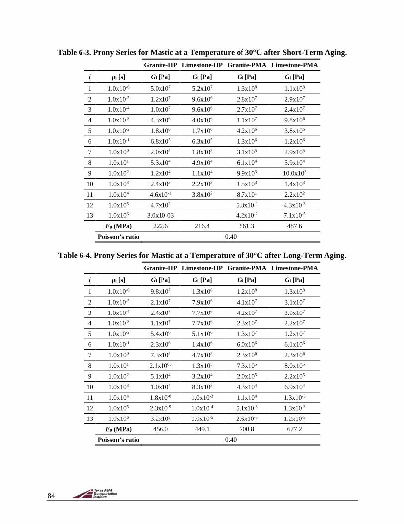
84
Table 6-3. Prony Series for Mastic at a Temperature of 30°C after Short-Term Aging.
Granite-HP Limestone-HP Granite-PMA Limestone-PMA
i ρi [s] Gi [Pa] Gi [Pa] Gi [Pa] Gi [Pa]
1 1.0x10⁻⁶ 5.0x10⁷ 5.2x10⁷ 1.3x10⁸ 1.1x10⁸ 2 1.0x10⁻⁵ 1.2x10⁷ 9.6x10⁶ 2.8x10⁷ 2.9x10⁷ 3 1.0x10⁻⁴ 1.0x10⁷ 9.6x10⁶ 2.7x10⁷ 2.4x10⁷ 4 1.0x10⁻³ 4.3x10⁶ 4.0x10⁶ 1.1x10⁷ 9.8x10⁶ 5 1.0x10⁻² 1.8x10⁶ 1.7x10⁶ 4.2x10⁶ 3.8x10⁶ 6 1.0x10⁻¹ 6.8x10⁵ 6.3x10⁵ 1.3x10⁶ 1.2x10⁶ 7 1.0x100 2.0x10⁵ 1.8x10⁵ 3.1x10⁵ 2.9x10⁵ 8 1.0x101 5.3x10⁴ 4.9x10⁴ 6.1x10⁴ 5.9x10⁴ 9 1.0x10² 1.2x10⁴ 1.1x10⁴ 9.9x10³ 10.0x10³
10 1.0x10³ 2.4x10³ 2.2x10³ 1.5x10³ 1.4x10³ 11 1.0x10⁴ 4.6x10⁻¹ 3.8x10² 8.7x101 2.2x10² 12 1.0x10⁵ 4.7x10² 5.8x10⁻² 4.3x10⁻³ 13 1.0x10⁶ 3.0x10-03 4.2x10⁻² 7.1x10⁻⁵
E0 (MPa) 222.6 216.4 561.3 487.6
Poisson’s ratio 0.40
Table 6-4. Prony Series for Mastic at a Temperature of 30°C after Long-Term Aging.
Granite-HP Limestone-HP Granite-PMA Limestone-PMA
i ρi [s] Gi [Pa] Gi [Pa] Gi [Pa] Gi [Pa]
1 1.0x10⁻⁶ 9.8x10⁷ 1.3x10⁸ 1.2x10⁸ 1.3x10⁸ 2 1.0x10⁻⁵ 2.1x10⁷ 7.9x10⁶ 4.1x10⁷ 3.1x10⁷ 3 1.0x10⁻⁴ 2.4x10⁷ 7.7x10⁶ 4.2x10⁷ 3.9x10⁷ 4 1.0x10⁻³ 1.1x10⁷ 7.7x10⁶ 2.3x10⁷ 2.2x10⁷ 5 1.0x10⁻² 5.4x10⁶ 5.1x10⁶ 1.3x10⁷ 1.2x10⁷ 6 1.0x10⁻¹ 2.3x10⁶ 1.4x10⁶ 6.0x10⁶ 6.1x10⁶ 7 1.0x100 7.3x10⁵ 4.7x10⁵ 2.3x10⁶ 2.3x10⁶ 8 1.0x101 2.1x1005 1.3x10⁵ 7.3x10⁵ 8.0x10⁵ 9 1.0x10² 5.1x10⁴ 3.2x10⁴ 2.0x10⁵ 2.2x10⁵
10 1.0x10³ 1.0x10⁴ 8.3x10³ 4.3x10⁴ 6.9x10⁴ 11 1.0x10⁴ 1.8x10⁻⁸ 1.0x10⁻³ 1.1x10⁴ 1.3x10⁻³ 12 1.0x10⁵ 2.3x10⁻⁹ 1.0x10⁻⁴ 5.1x10⁻³ 1.3x10⁻³ 13 1.0x10⁶ 3.2x10³ 1.0x10⁻⁵ 2.6x10⁻⁵ 1.2x10⁻³
E0 (MPa) 456.0 449.1 700.8 677.2
Poisson’s ratio 0.40

85
6.2. MODELING CASES A total of 24 models were evaluated based on combining six FC-5 mixture microstructures (i.e., three replicates for two different thicknesses); four material combinations (i.e., two aggregate types, granite and limestone, and two binder types, HP and PMA); and two conditions: (a) short-term and (b) long-term aging. As noted previously, the short-term aging resembles the A0 aging state of the mixtures, which is the “as constructed” state, while the long-term aging condition resembles the A5 aging state of the mixtures, or about two to three years of pavement service life.
6.2.1. FE Model for FC-5 Mixtures after Short-Term Aging The RI was the selected parameter to evaluate the raveling susceptibility of the FC-5 mixtures. This index was previously proposed in the research conducted by Arámbula-Mercado et al. (2016). The RI (Equation 20) is a scalar defined as the ratio between the dissipated energy from each mastic element located at the mastic-on-mastic contacts and the cohesive bond energy of the mastic material obtained from the SFE presented in Table 5-8. Higher values of RI indicate higher probability of raveling (i.e., higher chance of reaching the cohesive bond energy of the material). As explained by Masad et al. (2010), the theoretical work of cohesion computed through SFE measurements is various orders of magnitude smaller than the actual work of fracture measured for any material in the laboratory. Thus, the RI is a non-dimensional quantity that would never reach a value of 1.0 but rather a numerical indicator that provides information about the potential fracture of the mastic-on-mastic contacts.
RI =Dissipated energy � J
m3�
Cohesive bond energydry � Jm2�
(20)
To compute the RI, the Mohr’s circle theory is used to transform the data extracted from each finite element in the mastic-on-mastic contacts (e.g., horizontal, vertical, and shear stresses and strains) from global coordinates to local coordinates. This transformation allows for computing the dissipated energy of each element during the pass of the wheel load on top of the FC-5 mixture layer in Mode I and II of failure (i.e., opening and shear fracture modes, respectively). The maximum tensile stress obtained from this coordinate transformation, σ1, is related to Mode I of failure, while the maximum shear stress, τmax, is related to Mode II of failure.
Considering the number of elements located in the mastic-on-mastic contacts (i.e., approximately 4,900 elements for a 2-cm [0.79-in.] FC-5 mixture layer), the RI results for each microstructure and material combination were adjusted to a PDF with a 95% confidence level. As explained later, the PDF presenting the best fit in all cases was a Weibull distribution. However, since raveling constitutes a fracture-related problem, an extreme value analysis was required to quantify the actual chances of fracture in the contacts. In other words, only the elements with very high RI values that had the potential of fracture at a specific mastic-on-mastic contact were considered of interest. Thus, the PDFs of the RI were truncated using a threshold value of RI of 5.0x10- 3 (Figure 6-9). This procedure consisted of defining the PDF of a restricted domain of the original distribution composed of those values higher than the defined threshold. The threshold was selected after guaranteeing that the tail of all the PDFs was correctly represented with a reasonable minimum number of elements in this range (i.e., more than 180 elements). To include the variability of the results, the parameter to evaluate the raveling susceptibility of a mixture
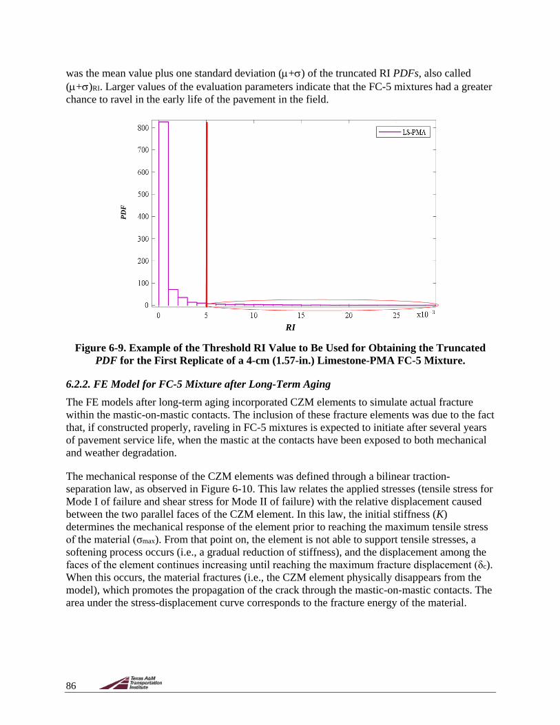
86
was the mean value plus one standard deviation (µ+σ) of the truncated RI PDFs, also called (µ+σ)RI. Larger values of the evaluation parameters indicate that the FC-5 mixtures had a greater chance to ravel in the early life of the pavement in the field.
Figure 6-9. Example of the Threshold RI Value to Be Used for Obtaining the Truncated
PDF for the First Replicate of a 4-cm (1.57-in.) Limestone-PMA FC-5 Mixture.
6.2.2. FE Model for FC-5 Mixture after Long-Term Aging The FE models after long-term aging incorporated CZM elements to simulate actual fracture within the mastic-on-mastic contacts. The inclusion of these fracture elements was due to the fact that, if constructed properly, raveling in FC-5 mixtures is expected to initiate after several years of pavement service life, when the mastic at the contacts have been exposed to both mechanical and weather degradation.
The mechanical response of the CZM elements was defined through a bilinear traction-separation law, as observed in Figure 6-10. This law relates the applied stresses (tensile stress for Mode I of failure and shear stress for Mode II of failure) with the relative displacement caused between the two parallel faces of the CZM element. In this law, the initial stiffness (K) determines the mechanical response of the element prior to reaching the maximum tensile stress of the material (σmax). From that point on, the element is not able to support tensile stresses, a softening process occurs (i.e., a gradual reduction of stiffness), and the displacement among the faces of the element continues increasing until reaching the maximum fracture displacement (δc). When this occurs, the material fractures (i.e., the CZM element physically disappears from the model), which promotes the propagation of the crack through the mastic-on-mastic contacts. The area under the stress-displacement curve corresponds to the fracture energy of the material.
RI

87
Figure 6-10. Traction-Separation Law of the CZM Elements Modified after Caro (2009).
A common problem with CZM elements is that they are incorporated as physical elements in the FE model, but they do not exist in the real world. Therefore, their inclusion in the FE models tends to increase the compliance of the FC-5 microstructures. Thus, the initial stiffness of each mastic material (K) was calibrated after guaranteeing that the mechanical response of each FE model was equivalent to that of the model that did not include CZM elements, but only regular linear viscoelastic mastic elements at the contacts. This process took into consideration the results of the works conducted by Salve and Jalwadi (2015), Aragão and Kim (2012), Aragão et al. (2017), and El Haloui et al. (2018) on this topic. Also, the magnitude of the initial stiffness of each mastic was reduced after considering that after certain years of service, the material had overcome some mechanical degradation (i.e., fatigue damage, based on the FREI parameters obtained from the PLAS tests). Moreover, the calibration of the input parameters of the CZM traction-separation law considered the results reported by Aragão and Kim (2012) and Aragão et al. (2017), in which the effective displacement (i.e., δi /δc from Figure 6-10) of typical asphalt and mastic materials was at least 5x10⁻⁴. Finally, the fracture energy of the CZM was determined using SCB test results, after considering a reduction of near 80% to resemble the critical condition in which raveling should initiate due to the fatigue and other field-related degradation that had occurred in the material. This assumption was justified by existing literature that indicated that aging and field deterioration after five to six years could indicate a reduction of up to 70% of various performance properties (e.g., fracture energy, cohesive bond energy) for dense-graded hot mix asphalt materials (Bhasin et al., 2007a; Saeidi and Aghayan, 2016).
A summary of the input parameters for the traction-separation law of the CZM elements for Mode I of failure is presented in Table 6-5. Since experimental data were not available to define the constitutive response of these elements for Mode II of failure, it was assumed that the mastic materials had isotropic fracture properties.
2 3 54K
σmax
δi δc δ (relative displacement)
σ
Fracture Energy
Prior to damage initiation
Damage Evolution
Crack Propagation
Adhesive Bond Strength
1
1 3 52 4 Cohesive zone
External load

88
Table 6-5. Input Parameters of the CZM Traction-Separation Law.
Mixture Type Stiffness (MPa/mm)
Initial Displacement
(mm)
Fracture Energy (N/mm)
Granite-PMA 15292.97 1.80x10⁻⁴ 0.21 Limestone-PMA 14745.97 1.80x10⁻⁴ 0.24
Granite-HP 45000.00 1.05x10⁻⁴ 0.49 Limestone-HP 44670.06 1.05x10⁻⁴ 0.37
To illustrate the results obtained from the simulations, Figure 6-11 presents the stiffness degradation (SDEG) output variable on three mastic-on-mastic contacts after the wheel load passed over the FC-5 mixture. The SDEG is a state variable with values ranging between 0.0—if no damage has occurred—and 1.0—when the energy dissipated by the material equals its fracture energy. Values closer to 1.0 indicate elements that are near to crack (or near to disappear in the model) since their dissipated energy is close to the fracture capacity of the material. As shown in Figure 6-11, in this particular case, some of the contacts have failed or are close to failure, indicating the potential loss of these two mastic-on-mastic contacts.
Figure 6-11. SDEG Values for Contacts in an FC-5 Microstructure.
As previously mentioned, the susceptibility to raveling in these models was quantified using the new parameter called ER, of the CZM elements. This parameter is defined as the difference between the fracture energy of the material and the energy dissipated by the CZM element after the pass of the wheel load (in N/mm). When the energy dissipated by a CZM element after the pass of the wheel load reaches the fracture energy of the material (i.e., ER = 0.0), a crack appears at that specific location, indicating the initiation of the contact failure. On the contrary, CZM elements that dissipate low amounts of energy after the application of the load (i.e., high ER values) are still resistant to the initiation of raveling. Thus, microstructures having larger ER values in the mastic-on-mastic contacts are more resistant to raveling.
In order to better assess the overall behavior of the microstructures with respect to ER, the results were adjusted to a log-normal distribution with a 95% confidence level. Figure 6-12 presents an example of the frequency distribution of the ER values obtained for one replicate of a 2-cm (0.79-in.) FC-5 microstructure. Moreover, in order to capture not only the mean value of ER but also the variability of these data, the mean plus one standard deviation (µ+σ) of the PDF of ER, or (µ+σ)ER, was selected as the evaluation parameter to compare the susceptibility to raveling of
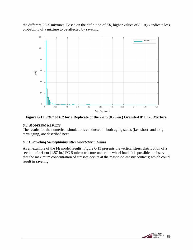
89
the different FC-5 mixtures. Based on the definition of ER, higher values of (µ+σ)ER indicate less probability of a mixture to be affected by raveling.
Figure 6-12. PDF of ER for a Replicate of the 2-cm (0.79-in.) Granite-HP FC-5 Mixture.
6.3. MODELING RESULTS The results for the numerical simulations conducted in both aging states (i.e., short- and long-term aging) are described next.
6.3.1. Raveling Susceptibility after Short-Term Aging As an example of the FE model results, Figure 6-13 presents the vertical stress distribution of a section of a 4-cm (1.57-in.) FC-5 microstructure under the wheel load. It is possible to observe that the maximum concentration of stresses occurs at the mastic-on-mastic contacts; which could result in raveling.
0 0.05 0.1 0.15 0.2 0.25 0.3 0.35 0.4 0.45 0.5
0
20
40
60
80
100
120
Granite-HP

90
Figure 6-13. Vertical Stress State for a 4-cm (1.57-in.) FC-5 Microstructure with Red
Circles Indicating the Location of Maximum Concentration of Stress.
Table 6-6 presents the results of the mean (µ), standard deviation (σ), and mean plus standard deviation (µ+σ) of the RI parameter for the FC-5 mixtures evaluated after short-term aging. As mentioned previously, larger values of (µ+σ)RI obtained from the truncated PDF indicate higher susceptibilities of the mastic-on-mastic contacts to undergo damage and, therefore, higher susceptibility to raveling. This table includes the results for the three replicates of all 2-cm and 4-cm (0.79-in. and 1.57-in.) microstructures, the four FC-5 mixtures (i.e., limestone-PMA, granite-PMA, limestone-HP, and granite-HP), and both modes of failure (i.e., Mode I and Mode II).
Vertical Stress (MPa)

91
Table 6-6. Raveling Index for Mode I and Mode II of Failure after Short-Term Aging for the FC-5 Mixtures.
Micro- structure Replicate Aggregate Binder
Mode I Mode II μRI
(x10-2) σRI
(x10-2) (μ+σ)RI
(x10-2) μRI
(x10-2) σRI
(x10-2) (μ+σ)RI
(x10-2)
2-cm (0.79-in.)
1 Granite
HP 0.9 0.5 1.3 0.6 0.1 0.8 PMA 0.6 0.1 0.7 0.6 0.1 0.7
Limestone HP 0.9 0.6 1.5 0.7 0.2 0.8
PMA 0.8 0.4 1.2 0.6 0.1 0.7
2 Granite
HP 0.9 0.5 1.3 0.6 0.1 0.7 PMA 0.7 0.3 1.0 0.6 0.1 0.7
Limestone HP 0.9 0.6 1.5 0.7 0.2 0.8
PMA 0.9 0.6 1.5 0.6 0.1 0.7
3 Granite
HP 1.6 1.9 3.5 1.0 0.7 1.7 PMA 1.2 1.0 2.1 0.8 0.4 1.2
Limestone HP 1.7 2.1 3.8 1.0 0.7 1.7
PMA 1.2 1.0 2.1 0.9 0.4 1.3
4-cm (1.57-in.)
1 Granite
HP 1.3 1.2 2.5 0.9 0.5 1.4 PMA 1.1 0.8 1.9 0.8 0.4 1.2
Limestone HP 1.4 1.5 2.9 1.0 0.6 1.6
PMA 1.1 0.9 2.0 0.9 0.5 1.3
2 Granite
HP 2.4 3.8 6.2 1.4 1.3 2.7 PMA 1.9 2.5 4.4 1.2 1.0 2.2
Limestone HP 2.7 4.8 7.6 1.5 1.5 3.0
PMA 2.0 2.8 4.8 1.2 1.1 2.3
3 Granite
HP 1.6 1.7 3.3 1.0 0.6 1.5 PMA 1.3 1.2 2.5 0.9 0.5 1.4
Limestone HP 1.7 1.9 3.6 1.0 0.7 1.7
PMA 1.3 1.2 2.6 0.9 0.5 1.5
An initial conclusion from this table is that Mode I of failure is predominant in all cases since (μ+σ)RI is near two times higher than the results for Mode II. Therefore, the analysis will be narrowed to Mode I of failure. As a summary of these results, Table 6-7 and Figure 6-14 present the average values of the raveling parameter and the COV for each mixture at the two thicknesses evaluated.

92
Table 6-7. Results after Short-Term Aging for (µ+σ)RI Parameter to Evaluate Raveling.
Layer Thickness Mixture Type
Average (µ+σ)RI
(x10-2) COV
2-cm (0.79-in.)
Granite-PMA 1.4 45% Limestone-PMA 1.5 34%
Granite-HP 2.0 61% Limestone-HP 2.3 58%
4-cm (1.57-in.)
Granite-PMA 2.9 45% Limestone-PMA 3.1 47%
Granite-HP 4.0 49% Limestone-HP 4.7 54%
Figure 6-14. Results of (µ+σ)RI for Mode I of Failure of the FC-5 Mixtures with
2-cm (0.79-in.) and 4-cm (1.57-in.).
The numerical results were consistent with the experimental findings: since the PMA mastics had a higher modulus than the HP mastics, under the same stress level, mixtures containing PMA presented smaller strains than those fabricated with the HP binder. This implies that the FC-5 mixtures with PMA binder will dissipate less energy (i.e., same stress level but smaller strains) and, consequently, will result in smaller values of the (µ+σ)RI parameter (i.e., lower susceptibility to raveling in the short-term aging state).
More specifically, the results of the 2-cm-thick (0.79-in.) microstructure layers showed that the granite-HP mixture had an (µ+σ)RI that was 47.2% higher than the value in the granite-PMA mixture. This trend prevailed for the mixtures with limestone since the mixture with HP presented 51.3% higher values of (µ+σ)RI than the mixture with PMA. In the case of the 4-cm-thick (1.57 in.) microstructure layers, the (µ+σ)RI values for the granite-PMA mixtures were 36.6% smaller than for the granite-HP mixtures, and 49.0% smaller in the case of limestone-PMA when compared to limestone-HP.
0.E+00
3.E-02
5.E-02
8.E-02
1.E-01
2 cm 4 cm
(µ+σ
) of R
I [-]
Thickness
Granite-PMA Granite-HP Limestone-PMA Limestone-HP

93
In terms of the influence of the aggregate type, the results indicate that the limestone FC-5 mixtures were more prone to raveling in the early stage of service life than the granite FC-5 mixtures, independently of the type of asphalt (i.e., (µ+σ)RI was between 11.7% and 12.4% higher for the limestone FC-5 mixtures 2-cm and 4-cm-thick, respectively).
The numerical simulations also suggest that the 4-cm-thick (1.57 in.) microstructure layers were more prone to raveling than the 2-cm-thick (0.79-in.) microstructure layers since the former resulted in (µ+σ)RI values that were, on average, 2.0 times larger than in the thinner layers. It should be pointed out, however, that this result might be influenced by the quality of the 2D network of the selected microstructures and, consequently, that these results could be inconclusive in this regard. It should also be noted that the results presented high variability independently of the thickness or material (i.e., values of COV of at least 34%). This indicated a strong relationship between the raveling potential and the specific characteristics of the microstructure, which was expected since raveling is a stone-on-stone contact phenomenon.
It should be pointed out that these models exclusively rely on the linear viscoelastic properties of the mastics in other to estimate raveling potential of the mixtures. In other words, they do not include fracture or degradation properties of the materials as part of the analysis. This explains why mixtures with PMA resulted in less raveling susceptibility than mixtures with HP in the early stage of the service life of the pavement, even though the experimental work showed enhanced fracture and durability results for the HP mixtures in this aging state (i.e., A0). This highlighted the necessity for including fracture mechanics-based models in the FE simulations in order to obtain reliable raveling predictions. However, if the construction of the FC-5 mixture complies with the required standards, raveling is expected to occur later in the service life of the pavement. Therefore, a better approach to evaluate raveling susceptibility of the different FC-5 mixtures was to not only consider actual fracture mechanics models (i.e., CZM) but also use the material properties representing an advanced pavement service life of the mixtures. The results of these simulations are presented next.
6.3.2. Raveling Susceptibility after Long-Term Aging In this subsequent numerical modeling effort, a total of 24 FE simulations were conducted. An example of the results is shown in Figure 6-15, which depicts the evolution of the fracture in a mastic-on-mastic contact for the second replicate of a 4-cm-thick (1.57-in.) thick microstructure granite-PMA layer. This figure shows the evolution of a crack at the contact between both aggregates. In this case, the energy remaining to resist fracture or the ER parameter of these CZM elements was zero.

94
Figure 6-15. Fracture Evolution of a Contact Using CZM in Replicate of a 4-cm (1.57-in.) Thick Granite-PMA Microstructure Layer: (a) Prior to Crack Initiation; (b) After Crack
Propagation at the Mastic-on-Mastic Contact.
Table 6-8 presents the results of the mean (µ), standard deviation (σ) of ER, and mean plus standard deviation (µ+σ)ER for the FC-5 mixtures evaluated after long-term aging. As previously noted, ER is the energy remaining of each CZM element after the pass of the wheel load; larger values of this parameter indicate that the element can still resist stresses before failure, values near zero indicate that the element is approaching fracture, and values equal to zero indicate that the CZM element has failed. Table 6-9 and Figure 6-16 summarize the results for each type of mixture and the two microstructure layer thicknesses evaluated.
(a)
(b)

95
Table 6-8. ER Results after Long-Term Aging.
Layer Thickness Replicate Aggregate Binder
Results of ER (N/mm) μER
(×10-3) σER
(×10-3) (μ+σ)ER
(×10-3)
2-cm (0.79-in.)
1 Granite
HP 107 371 478 PMA 45 152 197
Limestone HP 93 469 562
PMA 48 148 196
2 Granite
HP 18 46 102 PMA 14 30 75
Limestone HP 14 33 87
PMA 15 38 74
3 Granite
HP 46 184 229 PMA 30 103 133
Limestone HP 33 166 199
PMA 38 162 200
4-cm (1.57-in.)
1 Granite
HP 71 295 366 PMA 34 105 139
Limestone HP 48 217 264
PMA 38 118 156
2 Granite
HP 54 243 297 PMA 28 98 127
Limestone HP 41 198 239
PMA 33 107 140
3 Granite
HP 30 68 98 PMA 10 102 124
Limestone HP 24 142 167
PMA 27 138 165
Table 6-9. ER Results after Long-Term Aging to Evaluate Raveling Potential.
Layer Thickness Mixture Type
Average ER
(N/mm) (×10-1)
COV
2-cm (0.79-in.)
Granite-PMA 1.3 45.0% Limestone-PMA 1.6 45.7%
Granite-HP 2.7 71.0%
Limestone-HP 2.8 88.0%
4-cm (1.57-in.)
Granite-PMA 1.3 6.0% Limestone-PMA 1.5 8.0%
Granite-HP 2.5 55.0% Limestone-HP 2.2 23.0%

96
Figure 6-16. (µ+σ)ER Results for the FC-5 Mixtures.
Overall, the numerical results after long-term aging showed that there are differences in the resistance to fracture or raveling among the FC-5 mixtures. In terms of the influence of the type of binder, the mixtures with HP present overall higher values of (µ+σ)ER than the mixtures with PMA. This means that FC-5 mixtures fabricated with the HP binder are expected to be more resistant to raveling after several years of pavement service life than the mixtures with the PMA binder. For example, in the 2-cm-thick (0.79-in.) microstructure layer, the overall ER of the mastic-on-mastic contacts (i.e., remaining resistance to failure) in the HP mixtures was between 1.8 and 2.0 times greater than in the PMA mixtures, depending on the type of aggregate. Similarly, in the 4-cm-thick (1.57-in.) microstructure layer, the values of (µ+σ)ER in the HP mixtures were between 1.5 and 2.0 times greater than in the PMA mixtures, depending on the type of aggregate. Figure 6-17 also shows that the results obtained from the different replicates of a single mixture were highly variable, and that this variability was larger for the HP mixtures (COV of 63.0 and 55.0% for granite-HP and limestone-HP, respectively) than for the PMA mixtures (COV of 26.0 and 27.0% for granite-PMA and limestone-PMA, respectively). This is due to the fact that, since the PMA mixtures suffered severe damage after loading, most contacts presented overall low values of ER, independent of the type of microstructure evaluated. On the contrary, contacts in the HP mixtures were in an early stage of damage, and therefore the ER to failure within the contact of each microstructure and among microstructures varied significantly.
In terms of the influence of aggregate type, the results suggested that the limestone-PMA mixtures were 1.2 times less prone to raveling than those fabricated with granite. However, due to the high COV values (Table 6-9), it is difficult to conclude on the significance of the differences in raveling due to aggregate type. In the case of the HP mixtures, these differences varied depending on the thickness of the microstructure: for the 2-cm (0.79-in.) microstructure layers, the results showed that mixtures with limestone were slightly more resistant to raveling than mixtures with granite (i.e., (µ+σ)ER was 1.05 times higher for the limestone mixtures), while for the 4-cm (1.57-in.) microstructure layers, mixtures with granite were more resistant to raveling than those with limestone (i.e., (µ+σ)ER was 12% larger for the granite mixtures).
0.E+00
1.E-01
2.E-01
3.E-01
4.E-01
5.E-01
6.E-01
Granite-HP Limestone-HP Granite-PMA Limestone-PMA
(µ+σ
) ER
(N/m
m)
Mixture Material
2-cm-thick OGFC 4-cm-thick OGFC

97
Figure 6-17. Correlation between the Results of the Cantabro Abrasion Loss Test and the
Numerical ER Results.
Finally, the results also showed that the thickness of the FC-5 mixture was not a factor affecting raveling susceptibility after several years of pavement service life since the evaluation parameter was very similar for the 2-cm and 4-cm-thick (0.79- and 1.57-in.) microstructure layers, with the only exception being the limestone-HP mixtures (i.e., (µ+σ)ER was 20% larger in the 2-cm-thick (0.79-in.) microstructure layer).
In order to validate the numerical results, these findings were compared to those obtained from the Cantabro abrasion loss test. Figure 6-17 presents the Cantabro mass loss of the specimens tested in the A5 and A10 aging states after the first load cycle (i.e., 300 revolutions) versus the selected raveling resistance parameter after long-term aging (i.e., (µ+σ)ER). These results showed a negative correlation between the Cantabro and the ER result; that is, the mixtures that exhibited greater mass loss in the Cantabro test were those showing lower ER values prior to failure in the mastic-on-mastic contacts within the microstructures. This demonstrates an overall good agreement between the experimental and the numerical results, despite the fact that the numerical results were effective in capturing the influence of the type of binder used in the mixture but not the impact of aggregate type. Since Alvarez et al. (2008) demonstrated that the Cantabro abrasion loss test presented a good correlation with the raveling results observed in the field, it is possible to conclude that (µ+σ)ER could be used to obtain a first estimate of the durability of FC-5 mixtures through computation mechanics.
6.4. SUMMARY OF MODELING RESULTS Table 6-10 lists the numerical results of the resistance to raveling obtained after short- and long-term aging of the FC-5 mixtures. The table also presents the ranking of the raveling resistance of the mixtures based on the selected evaluation parameter for each state: (µ+σ)RI for the short-term and (µ+σ)ER for the long-term condition. As can be observed, the trend of the results in each aging state is independent of the thickness of the pavement layer. For the short-term aging
y = -0.136ln(x) - 0.0871R² = 0.6376
y = 0.0269x-1.404
R² = 0.568
1%
10%
100%
0.10 0.15 0.20 0.25 0.30
Mas
s Lo
ss a
fter 1
stC
anta
bro
Cyc
le
(µ+σ)ER (N/mm) Cantabro A5 Cantabro A10
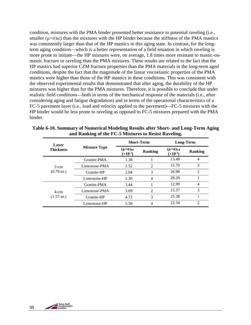
98
condition, mixtures with the PMA binder presented better resistance to potential raveling (i.e., smaller (µ+σ)RI) than the mixtures with the HP binder because the stiffness of the PMA mastics was consistently larger than that of the HP mastics in this aging state. In contrast, for the long-term aging condition—which is a better representation of a field situation in which raveling is more prone to initiate—the HP mixtures were, on average, 1.8 times more resistant to mastic-on-mastic fracture or raveling than the PMA mixtures. These results are related to the fact that the HP mastics had superior CZM fracture properties than the PMA materials in the long-term aged conditions, despite the fact that the magnitude of the linear viscoelastic properties of the PMA mastics were higher than those of the HP mastics in these conditions. This was consistent with the observed experimental results that demonstrated that after aging, the durability of the HP mixtures was higher than for the PMA mixtures. Therefore, it is possible to conclude that under realistic field conditions—both in terms of the mechanical response of the materials (i.e., after considering aging and fatigue degradation) and in terms of the operational characteristics of a FC-5 pavement layer (i.e., load and velocity applied to the pavement)—FC-5 mixtures with the HP binder would be less prone to raveling as opposed to FC-5 mixtures prepared with the PMA binder.
Table 6-10. Summary of Numerical Modeling Results after Short- and Long-Term Aging and Ranking of the FC-5 Mixtures to Resist Raveling.
Layer Thickness Mixture Type
Short-Term Long-Term
(µ+σ)RI
(×10-2) Ranking (µ+σ)ER
(×10-2) Ranking
2-cm (0.79-in.)
Granite-PMA 1.38 1 13.48 4
Limestone-PMA 1.52 2 15.70 3
Granite-HP 2.04 3 26.98 2
Limestone-HP 2.30 4 28.28 1
4-cm (1.57-in.)
Granite-PMA 3.44 1 12.99 4 Limestone-PMA 3.69 2 15.37 3
Granite-HP 4.72 3 25.38 1
Limestone-HP 5.58 4 22.34 2

99
7.0. LIFE-CYCLE COST ANALYSIS The assessment of the use of alternative materials for the construction of new infrastructure should consider aspects such as cost, environmental impact, and social welfare, among others. Life-cycle analysis is a widely used project evaluation strategy that focuses on assessing the evolution of a project, system, or material throughout its lifetime in terms of some specific metrics (Ghosn et al., 2016). For the specific case in which this metric is cost (mainly maintenance and rehabilitation) throughout service life, this technique is called life-cycle cost analysis (Sánchez-Silva and Klutke, 2016). Based on the experimental results, which resulted in enhanced durability of FC-5 mixtures prepared with the HP binder compared to the PMA binder, an LCCA was conducted to compare the four FC-5 mixtures that were studied.
The life-cycle cost objective function of a specific project or system (𝑍𝑍(𝒑𝒑, 𝜽𝜽)) can be written as follows, using the vector parameters p and θ that describe, respectively, the decision variables (e.g., in the case of pavement design, the thicknesses of the layers) and the set of random parameters (e.g., in the case of pavement design, climate and expected loading, among others) that characterize the problem:
Z(𝐩𝐩, 𝛉𝛉) = B(𝐩𝐩, 𝛉𝛉) − �C0(𝐩𝐩, 𝛉𝛉) + ∑ ∑ Cij(𝐩𝐩, 𝛉𝛉)mi=1
nj=1 + ∑ Cq(𝐩𝐩, 𝛉𝛉)Pf(𝐩𝐩, 𝛉𝛉)w
q=1 � (21)
where:
• B(p, θ) = benefit derived from the existence of the project; • C0(p,θ) = initial investment cost; • Cij(p, θ) = cost associated with the j-th investment in the i-th activity type, which might
be, for example, maintenance, insurance payment, etc.; • Cq(p, θ) = cost of failure (or any other unexpected unknown event); and • Pf(p, θ) = corresponding failure probability.
It is important to highlight that in these analyses, all actions related with the operation and the corresponding costs, as well as the costs that the owner or manager may incur, are part of the assessment. The parameters p and θ are specific for each problem, and they depend on both the particular use or purpose of the project under evaluation (e.g., a pavement structure, a pavement segment, a layer within the pavement, etc.) and the overall objective of the LCCA. With respect to the latter, the objectives of the LCCA are to define the feasibility of a particular solution by balancing cost and safety.
It is important to notice that the term safety describes the probability that the system or component under evaluation complies with some specific prescribed criteria, usually defined as a limit state. For the case of pavement structures, this limit state is usually a serviceability level or a performance threshold; for the case of an asphalt mixture, this limit is usually the level of functionality (e.g., a minimum permeability value) and/or the level of performance (e.g., extent and magnitude of raveling). Figure 7-1 illustrates the components of a typical LCCA of a project.

100
Figure 7-1. Components of LCCA (after Sánchez-Silva and Klutke 2016).
In the case of the FC-5 mixtures evaluated in this project, the LCCA included the following:
1. Definition of the parameters used to characterize the performance of the material. 2. Characterization of the material performance over time; in particular, information about
the degradation mechanisms and the uncertainties associated (i.e., evolution of raveling through Cantabro results in different aging conditions).
3. Stochastic model of the material performance (i.e., strategy for uncertainty management). 4. Definition of critical performance criteria; these include serviceability limit state
(performance under conditions that are below required standards) and ultimate limit state (i.e., failure, unacceptable performance). For the particular case of the FC-5, these limits were established based on the raveling performance evaluation obtained from Cantabro test results in different aging states and based on FDOT existing durability criteria for OGFCs and reported service life for these mixtures.
5. Characterization of costs associated with the construction and rehabilitation of OGFCs. 6. Selection of the economic criteria for the cost evaluation (e.g., discount rate, time
mission).
Then, the following general LCCA methodology was applied:
1. Definition of the objective function Z(p, θ) and the parameters that will define the material performance over time.

101
2. Definition of stochastic models that will be used in the analysis, including the selection of the critical variables and the determination of the deterioration curves of the FC-5 mixtures over time.
One relevant aspect that should be stressed about the LCCA used in this project is that it allowed accounting for uncertainty. In other words, through the vector parameter θ, the method recognized that the deterioration of the FC-5 mixtures due to raveling is an uncertain process and, therefore, that the overall NPV of the life service of an FC-5 mixture, with and without the HP binder, is also uncertain. Therefore, the information obtained from this analysis was not only the expected value of the NPV of the service life of different mixtures but also the variability or uncertainty associated with that value.
7.1. DETERIORATION CURVES
7.1.1. Material Loss Functions The deterioration function of the four FC-5 mixtures was measured indirectly using the results of the Cantabro abrasion loss test, which were presented and discussed in Section 5.3.2.3. Although this test was carried out until the weight loss of the specimens reached a predetermined threshold, for the purpose of assessing deterioration, the weight loss curves for the mixtures in different aging conditions were truncated at a value of 20% (Figure 7-2). This is justified by previous works (e.g., Boersman, 2017) and AASHTO TP 108 (2014b), which established that a 20% weight loss in the Cantabro test is an appropriate threshold to guarantee the durability of OGFC mixtures in the field. Data points in Figure 7-2 represent Cantabro revolutions (i.e., 300 revolutions per cycle).

102
(a)
(b)
(c)
Figure 7-2. Change in Mass Loss with Cantabro Revolutions for FC-5 Mixtures: (a) A0 Aging State; (b) A5 Aging State; (c) A10 Aging State.
Figure 7-2 shows that the change in mass loss of all mixtures, in all aging states, can be approximated using linear functions, and consequently, curves in Figure 7-2 consist of segments with different slopes. Under this assumption, the mass loss rate per revolution for any mixture i,
80%
85%
90%
95%
100%
0 500 1000 1500 2000
100%
Mas
s Los
s (%
)
Number of Revolutions
Granite PMA Granite HP
Limestone-PMA Limestone-HP
80%
85%
90%
95%
100%
0 500 1000
100%
Mas
s Los
s (%
)
Number of Revolutions
Granite PMA Granite HP
Limestone-PMA Limestone-HP
80%
85%
90%
95%
100%
0 100 200 300 400 500
100%
Mas
s Los
s (%
)
Number of Revolutions
Granite PMA Granite HP
Limestone-PMA Limestone-HP

103
at a specific aging condition between any two cycles (i.e., 300 revolutions per cycle) in the Cantabro abrasion loss test can be computed as:
δi,k = mi,k−mi,k−1300
(22)
where 𝑓𝑓𝑖𝑖,𝑘𝑘 = weight lost in cycle k (measured in percentage), and 𝑓𝑓𝑖𝑖,0 = 0.
Then, the average mass loss rate within the range of interest (0% to 20%), for a given mixture at a given aging state, can be computed as:
δ�i = 1n
∑ δi,knk=1 (23)
where n = minimum number of cycles in the Cantabro test required for the mixture to exceed the 20% mass loss threshold.
A summary of the results of the mass loss rates for the different mixtures at A0, A5, and A10 aging states is presented in Table 7-1, Table 7-2, and Table 7-3, respectively. The rate analysis shows that mixtures with the HP binder presented smaller mass loss rates than those with the PMA binder, for all aging states.
Table 7-1. Mass Loss Rates of the Different FC-5 Mixtures at A0 Aging State.
Mixture Type
Rates for Aging Condition A0 (% mass loss per revolution) 𝜹𝜹�𝑪𝑪,𝑨𝑨𝑨𝑨
(×10-4) 𝜹𝜹𝑪𝑪,𝟏𝟏 (×10-4)
𝜹𝜹𝑪𝑪,𝟐𝟐 (×10-4)
𝜹𝜹𝑪𝑪,𝟑𝟑 (×10-4)
𝜹𝜹𝑪𝑪,𝟒𝟒 (×10-4)
𝜹𝜹𝑪𝑪,𝟓𝟓 (×10-4)
𝜹𝜹𝑪𝑪,𝟔𝟔 (×10-4)
Limestone-PMA 2.4 2.9 2.7 – – – 2.7
Granite-PMA 4.5 4.6 – – – – 4.5
Limestone-HP 1.3 1.4 1.6 1.5 1.5 – 1.5
Granite- HP 1.4 1.5 1.3 1.2 1.2 1.2 1.3
Table 7-2. Mass Loss Rates of the Different FC-5 Mixtures at A5 Aging State.
Mixture Type
Rates for Aging Condition A5 (% mass loss per revolution) 𝜹𝜹�𝑪𝑪,𝑨𝑨𝟓𝟓
(×10-4) 𝜹𝜹𝑪𝑪,𝟏𝟏 (×10-4)
𝜹𝜹𝑪𝑪,𝟐𝟐 (×10-4)
𝜹𝜹𝑪𝑪,𝟑𝟑 (×10-4)
𝜹𝜹𝑪𝑪,𝟒𝟒 (×10-4)
𝜹𝜹𝑪𝑪,𝟓𝟓 (×10-4)
𝜹𝜹𝑪𝑪,𝟔𝟔 (×10-4)
Limestone-PMA 7.1 7.0 – – – – 7.0
Granite-PMA 5.3 4.9 – – – – 5.1
Limestone-HP 2.7 2.8 2.5 – – – 2.7
Granite- HP 3.4 3.0 2.5 – – – 3.0

104
Table 7-3. Mass Loss Rates of the Different FC-5 Mixtures at A10 Aging State.
Mixture Type
Rates for Aging Condition A10 (% mass loss per revolution) 𝜹𝜹�𝑪𝑪,𝑨𝑨𝟏𝟏𝑨𝑨
(x10-4) 𝜹𝜹𝑪𝑪,𝟏𝟏 (×10-4)
𝜹𝜹𝑪𝑪,𝟐𝟐 (×10-4)
𝜹𝜹𝑪𝑪,𝟑𝟑 (×10-4)
𝜹𝜹𝑪𝑪,𝟒𝟒 (×10-4)
𝜹𝜹𝑪𝑪,𝟓𝟓 (×10-4)
𝜹𝜹𝑪𝑪,𝟔𝟔 (×10-4)
Limestone-PMA 21.6 13.4 – – – – 17.5
Granite-PMA 10.2 8.3 – – – – 9.3
Limestone-HP 6.3 5.1 – – – – 5.7
Granite- HP 4.9 4.5 – – – – 4.7
Then, for a given aging state, Ax, the mass loss after a specific number of revolutions, r, L(r| Ax), can be computed as follows:
L(r|Ax) = δ�i,xr (24)
where:
• 𝛿𝛿�̅�𝑖,𝜏𝜏 = average rate of mass loss of mixture i (see last column in Table 7-1, Table 7-2, and Table 7-3);
• x = aging state A0, A5, A10; and • r = number of revolutions.
7.1.2. Deterioration Curve Development In the previous section, the function describing the mass loss for a specific number of revolutions (i.e., Equation 23) was developed for each mixture at each aging state. Then, the deterioration curves that describe the mass loss with time (i.e., D(t)) were developed. Although there is not a well-established approach that relates the number of Cantabro abrasion loss revolutions with time, the mass loss as a function of the number of cycles or revolutions can be used to make some inferences regarding the degradation of the FC-5 mixtures in the field.
The form of the deterioration function Di(t) (for material i) was defined as piece-wise with constant rates. These curves are characterized by three segments, j = 1, 2, 3, which describe different aging states (Figure 7-3). In each segment j, deterioration occurs at a constant rate, 𝛿𝛿𝑖𝑖,𝑗𝑗
∗ .

105
Figure 7-3. Example of Deterioration Curves for the Limestone-PMA Mixture.
Because deterioration rates were not measured directly, the rates, 𝛿𝛿𝑖𝑖,𝑗𝑗∗ , were different from those
defined in Equation 22 and reported in Table 7-1, Table 7-2, and Table 7-3. These new rates were calculated based on the relative change in mass loss among different FC-5 mixtures. Therefore, the deterioration rate of mixture i in segment j (i.e., 𝛿𝛿𝑖𝑖,𝑗𝑗
∗ ) was computed as follows:
δi,j∗ = βj � δ�i,x
δ�LS−PMA,x�
η (25)
where:
• 𝛽𝛽𝑗𝑗 and 𝜂𝜂 = model parameters; • 𝛿𝛿�̅�𝑖,𝜏𝜏 = average rate of weight loss of material i under the aging state x (Equation 22); and • 𝛿𝛿�̅�𝐿𝐿𝐿−𝑃𝑃𝑃𝑃𝐴𝐴,𝜏𝜏 = average rate of weight loss for limestone-PMA.
The parameters 𝛽𝛽𝑗𝑗 and 𝜂𝜂 were selected considering observed field data and past experiences. The parameter 𝛽𝛽𝑗𝑗 puts a limit on durability, while 𝜂𝜂 takes into consideration the fact that deterioration rates should not be scaled linearly with respect to the limestone-PMA using the Cantabro abrasion loss results because this will lead to unrealistic service lifetimes for certain mixtures. In this study, 𝛽𝛽1 = 0.45, 𝛽𝛽2 = 1.15, 𝛽𝛽3 = 2.23, and 𝜂𝜂 = 0.7. The parameter 𝛽𝛽𝑗𝑗 was selected after assuming that the pavement service life (time to reach a 20% mass loss) for the limestone-PMA FC-5 mixture was 12 years. This assumption is justified in existing literature indicating that the expected life of OGFC mixtures is between 8–12 years (Putman, 2012; Bennert and Cooley, 2014; Hernández-Sáenz et al., 2016; Massahi et al., 2018) and, particularly, based on the fact that FC-5 mixtures in Florida typically last between 10 and 14 years according to information provided by FDOT. In fact, Massahi et al. (2018) argued that limestone-PMA mixtures in southeast Florida have sporadically presented early evidence of raveling. It should be highlighted that the selection of a particular pavement service life (e.g., 12 years for limestone-PMA) is not
0 2 4 6 8 10 12
Time (year)
70%
75%
80%
85%
90%
95%
100%
1-W
eigh
t Los
s
A10A5A0

106
critical for the life-cycle cost assessment because all curves are constructed relative to each other and the objective of the study is to make a comparative cost analysis among the various FC-5 mixtures.
In summary, the piece-wise deterioration curve for mixture i can be written as follows:
Di(t) = �100 − tδi,1
∗ t ≤ 2100 − (2δi,1
∗ + (t − 2)δi,2∗ ) 2 < t ≤ 5
100 − (2δi,1∗ + 3δi,2
∗ + (t − 5)δi,3∗ ) t > 5
(26)
where:
• 𝛿𝛿∗𝑖𝑖,1, 𝛿𝛿∗
𝑖𝑖,2, and 𝛿𝛿∗𝑖𝑖,3 = deterioration rate of mixture i, for each of the three aging
conditions (i.e., segments in Figure 7-3 [Table 7-4]), and • t = pavement service life in years.
Table 7-4. Deterioration Rates for the Three Segments of the Deterioration Curves.
Mixture Deterioration Rates (% loss material/year)
𝜹𝜹∗𝑪𝑪,𝟏𝟏 𝜹𝜹∗
𝑪𝑪,𝟐𝟐 𝜹𝜹∗𝑪𝑪,𝟑𝟑
Granite-HP 0.25 0.56 1.04
Limestone-HP 0.30 0.56 1.12
Granite-PMA 0.65 0.90 1.59
Limestone-PMA 0.45 1.15 2.23
The mean time to replacement of the four FC-5 mixtures considered is presented in Table 7-5. Note that these times are all relative to the predefined service life of the limestone-PMA, which was assumed to be 12 years based only on raveling without regard to other distresses like cracking or rutting. The deterioration curves for the four mixtures are presented in Figure 7-4.
Table 7-5. Mean Replacement Times for the Four FC-5 Mixtures.
Mixture Type Average Lifetime (years)
Granite-HP 22.1 Limestone-HP 20.8 Granite-PMA 15.0
Limestone-PMA 12.0
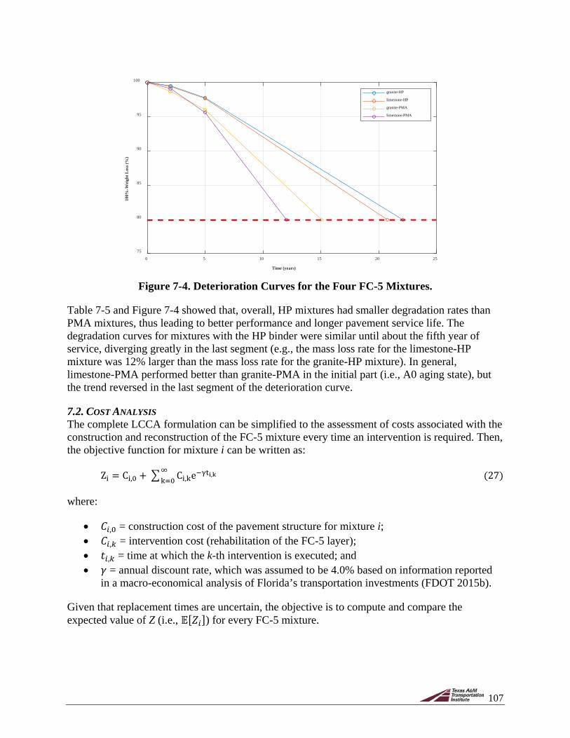
107
Figure 7-4. Deterioration Curves for the Four FC-5 Mixtures.
Table 7-5 and Figure 7-4 showed that, overall, HP mixtures had smaller degradation rates than PMA mixtures, thus leading to better performance and longer pavement service life. The degradation curves for mixtures with the HP binder were similar until about the fifth year of service, diverging greatly in the last segment (e.g., the mass loss rate for the limestone-HP mixture was 12% larger than the mass loss rate for the granite-HP mixture). In general, limestone-PMA performed better than granite-PMA in the initial part (i.e., A0 aging state), but the trend reversed in the last segment of the deterioration curve.
7.2. COST ANALYSIS The complete LCCA formulation can be simplified to the assessment of costs associated with the construction and reconstruction of the FC-5 mixture every time an intervention is required. Then, the objective function for mixture i can be written as:
Zi = Ci,0 + � Ci,ke−γti,k∞k=0 (27)
where:
• 𝐶𝐶𝑖𝑖,0 = construction cost of the pavement structure for mixture i; • 𝐶𝐶𝑖𝑖,𝑘𝑘 = intervention cost (rehabilitation of the FC-5 layer); • 𝑎𝑎𝑖𝑖,𝑘𝑘 = time at which the k-th intervention is executed; and • 𝛾𝛾 = annual discount rate, which was assumed to be 4.0% based on information reported
in a macro-economical analysis of Florida’s transportation investments (FDOT 2015b).
Given that replacement times are uncertain, the objective is to compute and compare the expected value of Z (i.e., 𝔼𝔼[𝑍𝑍𝑖𝑖]) for every FC-5 mixture.
0 5 10 15 20 25
Time (years)
75
80
85
90
95
100
100%
-Wei
ght L
oss (
%)
granite-HP
limestone-HP
granite-PMA
limestone-PMA

108
7.2.1. Cost Estimation The LCCA was carried out based on the cost per metric ton of an FC-5 mixture. The prices used in this study were obtained directly from FDOT’s online page Historical Cost and Other (FDOT 2018b) and based on the information from Moseley and Taylor (2018). All other costs (e.g. Ci,0) were assumed to be equal among FC-5 mixtures and, therefore, not relevant for the comparative study. The costs per ton used in the study are shown in Table 7-6.
Table 7-6. Cost of the FC-5 Mixtures used in the LCCA Analysis (𝑪𝑪𝑪𝑪,𝒌𝒌).
Mixture Type Cost per Ton (USD)
Granite-HP 130.0 Granite-PMA 110.0 Limestone-HP 130.0
Limestone-PMA 110.0
7.2.2. Uncertainty Evaluation
The uncertainty in the deterioration curves, 𝐹𝐹𝑖𝑖(𝑎𝑎), was estimated from the Cantabro abrasion loss tests. Table 7-7 presents the COV associated with the mass loss among replicates for all FC-5 mixtures in different aging states. The average COV is also reported in Table 7-7. In the LCCA simulations, the service life of every FC-5 mixture was taken as normally distributed, with the mean as reported in Table 7-5 and standard deviation defined by the average COV reported in Table 7-7 multiplied by the mean.
Table 7-7. COV of the Cantabro Abrasion Loss Test Measurements. Mixture
Type COV A0
(%) COVA5
(%) COV A10
(%) Average COV
(%) Granite-HP 9.8 8.6 34.5 17.6
Granite-PMA 16.4 13.0 26.3 18.6 Limestone-HP 43.0 9.4 12.7 21.7
Limestone-PMA 24.1 32.3 7.5 21.3
7.2.3. Net Present Value The LCCA was conducted using Monte Carlo simulations. The process consisted of generating a large number of possible realizations or sample paths corresponding to an FC-5 mixture that is replaced every time its mass loss reaches a value of 20%. In every sample path, the times at which replacements occur differ due to the randomness in the deterioration curves (Table 7-7). The model assumes that the pavement structure remains always functional, even if it is repaired or modified during the pavement service life. In other words, in the model, only the FC-5 mixture is replaced. The LCCA was assumed over an infinite time horizon; note that the influence of this infinite life span is small due to the form of the discount function. For example, a replacement made 40 or 50 years after construction has a very small contribution to the objective function Z.
The ultimate purpose of the LCCA was to compare the costs associated with the four FC-5 mixtures included in the study. Then, for every realization of the pavement’s performance (i.e., a

109
possible history of operation and replacement), it is possible to compute the NPV (i.e., function Z) using Equation 25. Since every realization is different, the LCCA of any mixture is characterized by its expected value and the standard deviation of the NPV; in this study, a total of 10,000 LCCA simulations for each FC-5 mixture were performed.
7.3. LCCA RESULTS In terms of life-cycle costs, the FC-5 mixtures can be compared in a space defined by the expected NPV, and the corresponding standard deviations that result from evaluating the 10,000 possible scenarios. These results are presented in Figure 7-5. In this figure, the closer the result to the lower left corner, the better (i.e., low expected NPV and low standard deviation), and the closer the results to the upper-right corner, the worse (i.e., high expected NPV and high standard deviation). Note that the standard deviation is a measure of the volatility in the life-cycle cost, so it is only important when comparing two or more cases with similar mean NPV. Furthermore, given that these values are related with small coefficients of variation, as observed in Table 7-8, the analysis can be simplified and focused on the expected NPV as a criterion for comparison.
Figure 7-5. Mean NPV versus Standard Deviation of All Mixtures.
Table 7-8. COV for the NPV Results. Mixture Type COV (%)
Granite-HP 7.27 Limestone-HP 7.61 Granite-PMA 8.77
Limestone-PMA 8.24
12 14 16 18 20 22 24 26 28 30
Standard Deviation (USD)
200
210
220
230
240
250
260
270
280
290
300
Exp
ecte
d N
PV (U
SD)
Granite-HP
Limestone-PMA
Limestone-HP
Granite-PMA

110
Figure 7-5 shows that the granite-HP mixture had the lowest NPV (i.e., 223.4 USD) and the lowest volatility. In fact, the NPV of the granite-HP mixture was 9% smaller than the granite-PMA mixture, and 23% smaller than the limestone-PMA mixture. Conversely, the results showed that the limestone-PMA mixture led to the largest discounted cost with high volatility (i.e., NPV of 290.5 USD and standard deviation of 23.9 USD). In terms of the influence of the type of aggregate, the results showed that mixtures fabricated with granite presented a lower NPV in contrast to those fabricated with limestone, showing the importance of proper aggregate selection on the durability and cost of the FC-5 mixtures.
Using these criteria for comparing the LCCA results, the order of priority or ranking of the mixtures is as follows:
1. Granite-HP. 2. Limestone-HP. 3. Granite-PMA. 4. Limestone-PMA.

111
8.0. SUMMARY AND CONCLUSIONS The use of OGFC mixtures is associated with numerous safety and environmental advantages, but the need to have more cost-effective layers with improved durability is still a challenge. The most common approaches to prevent raveling have been the use of high-quality aggregates in combination with modified binders, the requisite of specific volumetric properties of the mixture, and the requirement of certain minimum conditions of the roads where the mixture will be placed (e.g., use on high-speed roads). Existing numerical models conducted in FE have proved to be efficient tools to assess raveling mechanisms, and they have also suggested the effectiveness of several of the abovementioned requirements. Consequently, computational mechanics should be further used to explore the role of other factors or conditions that are typically difficult or pricy to assess in the laboratory, like the combination of new materials, the role of mortar oxidation, and pavement-vehicle interactions, among others.
In terms of the type and amount of additives that have been used to improve the durability of OGFC mixtures, it was found that they differ significantly among agencies. For example, even though Germany and The Netherlands use aggregates obtained from Germany, their OGFC mixtures have different gradations and binders, which generates differences in the durability of the materials. In the case of The Netherlands, it uses unmodified binders for single OGFC layers and conventional polymer-modified binders for the surface course of double-OGFC layers or TLPA systems, resulting in materials that have achieved service lives between 12 and 16 years. Due to these excellent results, this country does not plan to incorporate HP binders for the fabrication of their OGFC mixtures. In Germany, OGFC mixtures have more open aggregate gradations compared to The Netherlands, and the country uses both conventional polymer-modified and HP binders as part of the mixtures, achieving service lives between 8 to 12 years. It is noteworthy that both countries use, on average, greater thickness for their OGFC layers compared to the United States, and that they have been successful in implementing double-layer OGFC systems to improve their noise reduction capacity. Finally, Japan was identified as a country having a broad experience in the use of OGFC that incorporates binder polymer modification in dosages up to 15%. This country has achieved durability for these mixtures of about 20 years, overcoming some difficulties related with the durability and functionality of the mixtures during winter periods.
Based on the literature review, it is possible to conclude that there are two main factors required to obtain high-quality OGFC layers. The first factor is related with the gradation of the mixture and its total AV content. This aspect strongly impacts the quality of the stone-on-stone skeleton within the microstructure of the mixture and, consequently, its resistance to raveling. In the case of The Netherlands, it was found that OGFC mixtures have longer service lives compared to their counterparts in Germany, which could be directly related to this aspect. The second factor is related to the benefits of using binder modification, mainly with polymers, to enhance the performance and durability of OGFC mixtures. Nevertheless, it seems that there is no consensus among experts regarding the actual impact of polymer modification and the role of the modification dosage on the overall durability of OGFC mixtures. In addition, regarding the mix design, there is a current shift from methods that focus on determining the OBC for a given gradation guaranteeing good aggregate coating without draindown, to performance-based methods that aim at balancing durability and functionality of the mixture. These mix design methods will likely help produce longer-lasting OGFC layers.

112
To assess the specific case of the OGFC used in Florida (i.e., FC-5 mixtures), experimental, numerical, and cost analyses were performed as part of this study. Two types of aggregates—limestone and granite—and two SBS modified binders—a control PMA and an HP—were employed and compared. Four mixtures were evaluated using the combinations of those materials, including granite-PMA, limestone-PMA, granite-HP, and limestone-HP in different aging states. The experimental portion of the work plan included binders and mastics using various standard test methods. The performance of the mixtures was assessed using the SCB test, the IDEAL-CT test, the Cantabro abrasion loss test, and the IDT strength test before and after moisture conditioning.
The experimental results showed that although the HP binder had lower dynamic modulus values compared to the control PMA binder, the use of the HP binder improved the cracking performance through aging and, therefore, the overall behavior and durability of the FC-5 mixtures. More specifically, the characterization of the binders showed that the PG grade was higher than the one reported for both binders (i.e., PG 82-22E for PMA and PG 82-28E for HP). In addition, the average MSCR %Recovery for the HP binder was 93.8% compared to 70.5% for the PMA binder. Also, the linear viscoelastic properties showed that the PMA binder had larger dynamic shear moduli. In contrast, the HP binder showed, with the computation of the Glover-Rowe parameter, that it was less susceptible to cracking at all aging states. In fact, the results demonstrated that the susceptibility of the PMA binder to damage onset happened before aging for 20 hours in the PAV, while the HP binder reached this cracking limit after 40 hours aging in the PAV. These PAV aging states could be equivalent to about three to seven years of pavement service life. FTIR results indicated that the chemical changes due to aging (i.e., carbonyl area growth) occurred faster in the HP binder; however, this condition did not affect the HP mixture mechanical response and performance. The PLAS test was conducted to evaluate the fatigue resistance of both binders through the FREI parameter. Once again, the results showed a superior fatigue resistance in the HP binder in all aging states. With regard to the total SFE, the HP binder also showed superior cohesive fracture resistance (i.e., larger total SFE); aging affected both PMA and HP binders, reducing the total SFE, although for every aging state, the HP binder was still superior in terms of total SFE compared to the PMA binder.
The rheological properties of the mastics were in good agreement with the observations obtained from the binder characterization, with the only difference being that the inclusion of the aggregate material reduced the gap in modulus between the two binders. With respect to the total SFE, the mastics showed less total SFE compared to the binders. Among the mastic specimens, the granite-HP showed the best cohesive fracture resistance (i.e., larger total SFE). It should be noted, however, that these results were done under dry conditions, and the conclusions may be different in the presence of water.
With regard to the FC-5 mixtures, cracking resistance, abrasion resistance, tensile strength, and moisture susceptibility were evaluated through SCB and IDEAL, Cantabro, and TSR tests, respectively, in two to three aging states. SCB and IDEAL test results showed that the mixtures with HP were less prone to fracture. It was also observed that, in general, the granite FC-5 mixtures had a better resistance to fracture than the limestone FC-5 mixtures. In terms of durability, the Cantabro abrasion loss test was conducted using three aging states and multiple cycles (i.e., sets of 300 revolutions per cycle). The results indicated that the mixtures with the HP binder had a better performance. For example, limestone-HP mixtures aged for 10 days at 95°C

113
(203ºF) withstood twice as many Cantabro cycles before reaching a critical value of 80% mass loss than the mixtures with the PMA binder. Moisture susceptibility tests following FM 1-T 283 did not provide conclusive results regarding the influence of binder, aggregate type, or aging state on affecting the propensity of the mixtures to undergo moisture damage. Finally, the IDT strength results obtained from the IDEAL and the FM 1-T 283 were not consistent in determining the influence of the type of binder. In both cases, the IDT strength values were larger in aged states for all mixtures. IDT strength values obtained from the IDEAL test presented consistent results with those of the SCB test. However, the SCB test results were used as input parameters for the fracture models used in the FE numerical models.
The following was the general ranking of the performance of the FC-5 mixtures evaluated:
1. Granite-HP. 2. Limestone-HP. 3. Granite-PMA. 4. Limestone-PMA.
The experimental results support the fact that FC-5 mixtures with HP binders could provide longer pavement life than conventional FC-5 mixtures fabricated with PMA binders. However, these experimental results were not enough to recommend the use of the HP binder. Numerical modeling and the LCCA were done to verify if the enhanced properties of FC-5 mixtures fabricated with the HP binder compensated for the higher costs associated with the HP binder.
FE numerical models were implemented in the commercial software Abaqus® to assess the effects of the type of binder on the susceptibility to raveling of FC-5 mixtures after short- and long-term aging under realistic field conditions. Three replicates of FC-5 mixtures with two microstructure layer thicknesses (2-cm [0.79-in.] and 4-cm [1.57-in.]) were obtained from X-ray CT images. The FE model indicated that the stiffness of the PMA mastics in the initial state of the service life (i.e., dynamic modulus) provided better raveling potential resistance for the PMA FC-5 mixtures compared to the HP FC-5 mixtures. Conversely, after considering fracture mechanics models in the FE simulations and long-term aging properties, the HP FC-5 mixtures were more resistant to raveling and, therefore, expected to have better pavement service life. More specifically, the results showed that the granite-HP mixture had the best resistance to raveling, followed by limestone-HP, and then by the mixtures with the PMA binder. A good correlation was also found between the Cantabro abrasion loss test results and the numerical results after long-term aging. This indicated that the use of computational mechanics tools that include fracture mechanics models and appropriate input material properties (i.e., linear viscoelastic and fracture properties in aged conditions) is a reasonable alternative to assess the durability of FC-5 mixtures under realistic field conditions.
An economic analysis to evaluate the expected NPV and the uncertainty associated with the durability of the FC-5 mixtures fabricated with both types of binder concluded the work plan. The four FC-5 mixtures were evaluated through LCCA to make a relative comparison of the expected NPV. The LCCA did not only consider the NPV associated with each FC-5 mixture but also evaluated the volatility of the resulting value using Monte Carlo simulations. The results indicated that, in terms of NPV, FC-5 mixtures with the HP binder had better results. This was mainly due to the fact that this mixture presented smaller Cantabro abrasion loss degradation

114
rates compared to the other FC-5 mixtures and, consequently, better durability. Based on the LCCA conducted as part of this project, it was possible to conclude that the increased durability of the FC-5 mixtures fabricated with the HP binder observed as part of the experimental and numerical efforts conducted in this project was cost effective.
115
REFERENCES AASHTO, 2002. Standard Practice for Mixture Conditioning of Hot Mix Asphalts (AASHTO
R 30). American Association of State Highway and Transportation Officials, Washington, D.C.
AASHTO, 2012. Standard Practice for Accelerated Aging of Asphalt Binder Using a Pressurized Aging Vessel (AASHTO R 28). American Association of State Highway and Transportation Officials, Washington, D.C.
AASHTO, 2013a. Standard Method of Test for Effect of Heat and Air on a Moving Film of Asphalt (AASHTO T 240). American Association of State Highway and Transportation Officials, Washington, D.C.
AASHTO, 2013b. Standard Method of Test for Materials Finer Than No. 200 Sieve in Mineral Aggregates by Washing (AASHTO T 11). American Association of State Highway and Transportation Officials, Washington, D.C.
AASHTO, 2014a. Standard Specification for Performance-Graded Asphalt Binder Using Multiple Stress Creep Recovery (MSCR) (AASHTO M 332). American Association of State Highway and Transportation Officials, Washington, D.C.
AASHTO, 2014b. Standard Method of Test for Determining the Abrasion Loss of Asphalt Mixture Specimens. (AASHTO TP 108). American Association of State Highway and Transportation Officials, Washington, D.C.
AASHTO, 2014c. Standard Practice for Materials Selection and Mixture Design of Permeable Friction Courses (PFCs) (AASHTO PP 77). American Association of State Highway and Transportation Officials, Washington, D.C.
AASHTO, 2016. Standard Method of Test for Determining the Fracture Potential of Asphalt Mixtures Using Semicircular Bend Geometry (SCB) at Intermediate Temperature Standard Method of Test for Mixtures Using Semicircular Bend Geometry (AASHTO TP 124). American Association of State Highway and Transportation Officials, Washington, D.C.
Adam, V., and Shah, S.C., 1974. Evaluation of Open-Graded Plant Mix Seal Surfaces for Correction of Slippery Pavements. Transportation Research Record, 523, 88–96.
Airey, G., 2004. Styrene Butadiene Styrene Polymer Modification of Road Bitumen. Journal of Materials Science, 39 (3), 951–959.
Al-Qadi, I.L., Ozer, H., Lambros, J., El Khatib, A., Singhvi, P., Khan, T., and Doll, B., 2015. Testing Protocols to Ensure Performance of High Asphalt Binder Replacement Mixes Using RAP and RAS (Research Report No. FHWA-ICT-15-017). Illinois Center for Transportation, Urbana, IL.

116
Alvarez, A.E., Martin, A.E., Estakhri, C.K., Button, J.W., Glover, C.J., and Jung, S.H., 2006. Synthesis of Current Practice on the Design, Construction, and Maintenance of Porous Friction Courses (Texas Department of Transportation Research Report FHWA/TX-06/0-5262-1). Texas Transportation Institute, College Station, Texas.
Alvarez, A.E., Epps-Martin, A., Estakhri, C.K., and Izzo, R., 2008. Evaluation of Durability Tools for Porous Friction Courses. In Proceedings of the Transportation Research Board 87th Annual Meeting, January 13-17, 2008, Washington, D.C. Transportation Research Board, Washington, D.C.
Alvarez, A.E., Epps-Martin, A., Estakhri, C., and Izzo, R., 2009. Determination of Volumetric Properties for Permeable Friction Course Mixtures. Journal of Testing and Evaluation, 37 (1), 1–10.
Alvarez, A.E., Epps, A., and Estakhri, C., 2010a. Internal Structure of Compacted Permeable Friction Course Mixtures. Construction and Building Materials, 24 (6), 1027–1035.
Alvarez, A.E., Mahmoud, E., Martin, A.E., Masad, E., and Estakhri, C., 2010b. Stone-on-Stone Contact of Permeable Friction Course Mixtures. Journal of Materials in Civil Engineering, 22 (11), 1129–1138.
Alvarez, A.E., Ovalles, E., and Caro, S., 2012. Assessment of the Effect of Mineral Filler on Asphalt-Aggregate Interfaces Based on Thermodynamic Properties. Construction and Building Materials, 28 (1), 599–606.
Alvarez, A.E., Gomez, K.L., Gomez, D.C., and Reyes-Ortiz, O.J., 2018. Optimising the Effect of Natural Filler on Asphalt-Aggregate Interfaces Based on Surface Free Energy Measurements. Road Materials and Pavement Design, DOI: 10.1080/14680629.2018.1465451.
Aragão, F.T.S., and Kim, Y.R., 2012. Mode I Fracture Characterization of Bituminous Paving Mixtures at Intermediate Service Temperatures. Experimental Mechanics, 52 (9), 1423–1434.
Aragão, F.T.S., Badilla-Vargas, G.A., Hartmann, D.A., de Oliveira, A.D., and Kim, Y.R., 2017. Characterization of Temperature- and Rate-Dependent Fracture Properties of Fine Aggregate Bituminous Mixtures Using an Integrated Numerical-Experimental Approach. Engineering Fracture Mechanics, 180, 195–212.
Arámbula-Mercado, E., Hill, R.A., Caro, S., Manrique-Sanchez, L., Park, E.S., and Fernando, E., 2016. Understanding Mechanisms of Raveling to Extend Open Graded Friction Courses (OGFC) Service Life (Florida Department of Transportation Research Report BDR74–977–04). Texas A&M Transportation Institute, College Station, Texas.
ASTM, 2011. Standard Test Method for Theoretical Maximum Specific Gravity and Density of Bituminous Paving Mixtures (ASTM D2041 / D2041M-11). ASTM International, West Conshohocken, PA.

117
ASTM, 2015a. Standard Practice for Calculating Pavement Macrotexture Mean Profile Depth (ASTM E1845-15). ASTM International, West Conshohocken, PA,
ASTM, 2015b. Standard Test Method for Measuring Pavement Macrotexture Properties Using the Circular Track Meter (ASTM E2157-15). ASTM International, West Conshohocken, PA.
ASTM, 2017a. Standard Test Method for Materials Finer than 75-µm (No. 200) Sieve in Mineral Aggregates by Washing (ASTM C117-17). ASTM International, West Conshohocken, PA.
ASTM, 2017b. Standard Test Method for Percent Air Voids in Compacted Asphalt Mixtures (ASTM D3203 / D3203M-17). ASTM International, West Conshohocken, PA.
ASTM, 2017c. Standard Test Method for Thickness or Height of Compacted Asphalt Mixture Specimens (ASTM D3549 / D3549M-18). ASTM International, West Conshohocken, PA.
Azari, H., 2010. Precision Estimates of AASHTO T283: Resistance of Compacted Hot-Mix Asphalt (HMA) to Moisture-Induced Damage (NCHRP Web-Only Document 166). National Cooperative Highway Research Program, Transportation Research Board, Washington, D.C.
Bendtsen, H.C., and Larson, L.E., 1999. Noise-Reducing Pavements for Urban Roads. Nordic Road and Transport Research, 11 (3).
Bennert, T., and Cooley, A., 2014. Evaluate the Contribution of the Mixture Components on the Longevity and Performance of FC-5 (Florida Department of Transportation Research Report BDS15 977-01). Center for Advanced Infrastructure and Transportation (CAIT), Piscataway, NJ.
Bessa, I.S., Castelo Branco, V.T.F., and Soares, J.B., 2012. Evaluation of Different Digital Image Processing Software for Aggregates and Hot Mix Asphalt Characterizations. Construction and Building Materials, 37, 370–378.
Bessa, I., Vasconcelos, K., Bernucci, L., and Castelo Branco, V., 2018. Evaluation of Neat and Modified Asphalt Binders in Relation to Fatigue Cracking by Means of Rheological Characterization. International Society for Asphalt Pavements, 2, 1–8.
Bhasin, A., Howson, J., Masad, E., Little, D., and Lytton, R., 2007a. Effect of Modification Processes on Bond Energy of Asphalt Binders. Transportation Research Record, 1998 (1), 29–37.
Bhasin, A., Little, D.N., Vasconcelos, K.L., and Masad, E., 2007b. Surface Free Energy to Identify Moisture Sensitivity of Materials for Asphalt Mixes. Transportation Research Record, 2001 (1), 37–45.

118
Boersman, J., 2017. Predicting the Degradation of Surface Pavement Due to Raveling. M.Sc. Thesis. Technische Universiteit Eindhoven, Eindhoven, Netherlands.
Brunner, R.J., 1975. Open-Graded Asphalt Friction Course (Pennsylvania DOT Research Project 74-8), Pennsylvania Department of Transportation, Bureau of Materials, Testing and Research, Harrisburg, PA.
Bundesministerium für Verkehr Bau und Stadtentwicklung, 2007. ZTV/TL Asphalt—STB 07. Cologne.
Caro, S., 2009. A Coupled Micromechanical Model of Moisture-Induced Damage in Asphalt Mixtures: Formulation and Applications. Ph.D. Dissertation. Texas A&M University, College Station, TX.
Centre d’Etudes et d’Expertise sur les Risques, l’Environnement, la Mobilité et l’Aménagement and Ministère des Transports France, 2017. Programme de Recherche et Dínnovation dans les Transports Terrestres. Available from https://www.mobilite-intelligente.com/en/node/539.
Chen, M.J., and Wong, Y.D., 2016. Evaluation of the Development of Aggregate Packing in Porous Asphalt Mixture Using Discrete Element Method Simulation. Road Materials and Pavement Design, 18 (1), 64–85.
Chen, J.-S., Wang, T.J., and Lee, C.-T., 2018. Evaluation of a Highly Modified Asphalt Binder for Field Performance. Construction and Building Materials, 171, 539–545.
Christensen, D.W., and Anderson, D.A., 1992. Interpretation of Dynamic Mechanical Test Data for Paving Grade Asphalt Cements (with Discussion). Journal of the Association of Asphalt Paving Technologists, 61, 67–116.
Community Research and Development Information Service (CORDIS), 2017. Silent Road for Urban and Extra-Urban Use: SIRUUS, Grant agreement ID: BRPR980659, 1998-2002. Available from: https://cordis.europa.eu/project/rcn/44821/factsheet/en
Cooley, Jr., L.A., Brumfield, J.W., Mallick, R.B., Mogawer, W.S., Partl, M., Pulikakos, L., and Hicks, G., 2009. Construction and Maintenance Practices for Permeable Friction Courses (National Cooperative Research Program Report 640). National Cooperative Highway Research Program, Transportation Research Board, Washington, D.C.
De Bondt, A., Plug, K., van de Water, J., The, P., and Voskuilen, J., 2016. Development of a Durable Third Generation Porous Asphalt with a High Noise. In Proceedings of the 6th Eurasphalt & Eurobitume Congress, 1-3 June 2016, Prague, Czech Republic.
Dell’acqua, G., De Luca, M., and Lamberti, R., 2011. Indirect Skid Resistance Measurement for Porous Asphalt Pavement Management. Transportation Research Record, 2205, 147–164.

119
Eck, B., Klenzendorf, B., Randall, C., and Barret, M., 2010. Permeable Friction Course for Sustainable Highways. In Proceedings of Green Streets Highway Conference 2010, November 14–17, 2010, Denver, Colorado.
El Haloui, Y., El Omari, M., Absi, J., and Tehrani, F., 2018. Numerical Simulation of Fracture at Asphalt Mastic Materials. In Proceedings of the 3rd International Conference on Optimization and Application (ICOA 2017), April 2017, Meknès, Morocco.
Epps-Martin, A., Arámbula-Mercado, E., Epps, J., Newcomb, D., Glover, C., Chowdury, A., Yin, F., Kaseer, F., Garcia Cucalon, L., Bajaj, A., Hajj, E., Morian, N., Pournoman, S., Daniel, J., Rahbar-Rastegar, R., and King, G., 2017. The Effects of Recycling Agents of Asphalt Mixtures with High RAS and RAP Binder Ratios (NCHRP 09-58 Quarterly Progress Report). Texas A&M Transportation Institute, College Station, Texas, September.
FDOT, 2015a. Florida Method of Test for Resistance of Compacted Bituminous Mixture to Moisture-Induced Damage (FM 1-T 283). Florida Department of Transportation, Tallahassee, Florida.
FDOT, 2015b. Macroeconomic Analysis of Florida’s Transportation Investments. FDOT Work Program, Fiscal Years 2014-2018. Available from https://fdotwww.blob.core.windows.net/sitefinity/docs/default-source/content/planning/policy/economic/macroimpacts0115.pdf?sfvrsn=5d49079b_0
FDOT, 2018a. Standard Specifications for Road and Bridge Construction. Florida Department of Transportation, Tallahassee, Florida.
FDOT, 2018b. Program Management. Historical Cost and Other Information. Available from http://www.fdot.gov/programmanagement/Estimates/HistoricalCostInformation/HistoricalCost.shtm.
Gaspar, M.S., Vasconcelos, K.L., da Silva, A.H.M., and Bernucci, L.L.B., 2017. Highly Modified Asphalt Binder for Asphalt Crack Relief Mix. Transportation Research Record: Journal of the Transportation Research Board, 2630 (1), 110–117.
Ghosn, M., Frangopol, D.M., McAllister T.P., Shah, M., Diniz, S.M.C., Ellingwood B.R., Manuel, L., Biondini, F., Catbas, N., Strauss, A., and Zhao, X.L., 2016. Reliability-Based Performance Indicators for Structural Members. Journal of Structural Engineering, 142 (9), F4016002-1– F4016002-13.
Gibbs, D.C., Iwasaki, R.H., Bernhard, R.J., Bledsoe, J.F., Carlson, D.D., Corbisier, C., Fults, K.W., Hearne, T.M.J., McMullen, K.W., Newcomb, D.E., Roberts, J.H., Rochat, J.L., Scofield, L.A., and Swanlund, M.E., 2005. Quiet Pavement Systems in Europe (Federal Highway Administration Research Report FHWA-PL-05-011). American Trade Initiatives, Alexandria, VA.

120
Glover, C., Davison, R.R., Domke, C.H., Ruan, Y., Juristyarini, P., Knorr, D.B., and Jung, S.H., 2005. Development of a New Method for Assessing Asphalt Binder Durability with Field Validation (Texas Department of Transportation Research Report FHWA/TX-05/1872-2). Texas Transportation Institute, College Station, Texas.
Greene, J., Choubane, B., Chun, S., 2013. Evaluation of a Heavy Polymer Modified Binder through Accelerated Pavement Testing. In Proceeding of the Transportation Research Board 92nd Annual Meeting, January 13-17, 2013, Washington, D.C. Transportation Research Board, Washington, D.C.
Gunaratne, Y.M., and Mejias De Pernia, Y., 2014. Determination of the Optimum Binder Content of Open-Graded Friction Course (OGFC) Mixtures Using Digital Image Processing (Florida Department of Transportation Research Report BDV25-TWO 820-1). University of South Florida, Tampa, Florida.
Hamzah, M.O., Abdullah, N.H., Voskuilen, J.L.M., and van Bochove, G., 2013. Laboratory Simulation of the Clogging Behaviour of Single-Layer and Two-Layer Porous Asphalt. Road Materials and Pavement Design, 14 (1), 107–125.
Hernández-Sáenz, M.A., Caro, S., Arámbula-Mercado, E., and Epps Martin, A., 2016. Mix Design, Performance and Maintenance of Permeable Friction Courses (PFC) in the United States: State of the Art. Construction and Building Materials, 111, 358–367.
Huber, G., 2000. Performance Survey on Open-Graded Friction Course Mixes (Synthesis of Highway Practice 284). Transportation Research Board, National Research Council, Washington, D.C.
Huddleston, I.J., Zhou, H., and Hicks, R.G., 1991. Performance Evaluation of Open-Graded Asphalt Concrete Mixtures Used in Oregon. Journal of the Association of Asphalt Paving Technologists, 3, 110–118.
Huurman, M., Moore, L., and Woldekidan, M.F., 2009. Porous Asphalt Raveling in Cold Weather. Pavement Research and Technology, 3, 110–118.
Huurman, M., Mo, L. T., and Woldekidan, M. F., 2010. Porous asphalt ravelling in cold weather conditions. Pavement Research and Technology, 3(3), 110-118.
Jackson, N.M., 2008. Harmonization of Texture and Skid-Resistance Measurements (Florida Department of Transportation Research Report FL/DOT/SMO/08-BDH-23). University of North Florida, Jacksonville, Florida.
Jellema, E., and Vonk, W., 2016. Improving Durability and Functionality Retention of Porous Asphalt by Using High Performing Bituminous Binders. In Proceedings of the 6th Eurasphalt & Eurobitume Congress, 1-3 June 2016, Prague, Czech Republic.
Jemison, H.B., Burr, B.L., Davison, R.R., Bullin, J.A., and Glover, C.J., 1992. Application and Use of the ATR, FT_IR Method to Asphalt Aging Studies. Fuel Science and Technology International, 10 (4–6), 795–808.
121
Kandhal, P.S., 2002. Design, Construction and Maintenance of Open-Graded Asphalt Friction Courses (Information Series 115). National Asphalt Pavement Association, Lanham, Maryland.
Kandhal, P.S., 2004. Asphalt Pavement Mitigate Tire/Pavement Noise. HMA Technology, 9 (2), 22–31, March/April.
Kaseer, F., Yin, F., Arámbula-Mercado, E., Epps Martin, A., Daniel, J.S., and Salari, S., 2018. Development of an Index to Evaluate the Cracking Potential of Asphalt Mixtures Using the Semi-circular Bending Test. Construction and Building Materials, 167, 286–298.
Keafott, P.J., Barret, M.E., and Malina, Jr., J.F., 2005. Stormwater Quality Documentation of Roadside Shoulders Borrow Ditches (CRWR Online Report 05-02). Center for Research in Water Resources, The University of Texas at Austin, Austin, Texas. Available from http://hdl.handle.net/2152/6996
Kim, Y.R., Castorena, C., Elwardany, M., Rad, F.Y., Underwood, S., Gundha, A., Gudipudi, P., Farrar, M.J., and Glaser, R.R., 2017. Long-Term Aging of Asphalt Mixtures for Performance Testing and Prediction (NCHRP Report 871). National Cooperative Highway Research Program, Transportation Research Board, Washington, D.C.
Kluttz, R., Molenaar, A. A. A., van de Ven, M. F. C., Poot, M. R., Liu, X. Scarpas, A., and Scholten, E. J., 2009. Modified Base Courses for Reduced Pavement Thickness and Improved Longevity. In Proceedings of the International Conference on Perpetual Pavement, Columbus, Ohio.
Kluttz, R., Jellema, E., Woldekidan, M.F., and Hurrman, M., 2013. Highly Modified Bitumen for Prevention of Winter Damage in OGFCs. Airfield and Highway Pavement 2013: Sustainable and Efficient Pavements. Proceedings of the 2013 Airfield & Highway Pavement Conference, June 9–12, 2013, Los Angeles, California. American Society of Civil Engineers (ASCE), Al-Qadi, I.L., and Murrell, S., eds., Reston, VA, 1075–1087.
Kluttz, R., Dongré, R., Buzz Powell, R., Willis, J.R., and Timm, D.H., 2014. Performance and Rational Design of Thin, Highly Modified Structural Pavements. Presentation at the Association of Modified Asphalt Producers (AMAP) Annual Conference, February 18-20, 2014, New Orleans, Louisiana.
Kluttz, R., 2015. Use of Highly Polymer Modified HMA (HiMA). Presentation at the Ohio Asphalt Paving Conference, February 2015, Columbus, Ohio.
Ku, H., 1966. Notes on the Propagation of Error Formulas. Journal of Research of National Bureau of Standards—C, Engineering and Instrumentation, 70C (4), 263–273.
Kuennen, T., 2012. The chemistry of Road Building Materials: Asphalt a la Carte-Modifiers Control Mix Performance. Better Roads, Road Science, 16-27, April.
Kwok, D.Y., and Neumann, A.W., 1999. Contact Angle Measurement and Contact Angle Interpretation. Advances in Colloid and Interface Science, 81, 167–249.

122
Lee, H., Raghunathan, D., 2015. New Hampshire Demonstration Project: Auburn-Candia Resurfacing Project (Federal Highway Administration Final Technical Brief). Applied Research Associates, Inc., Champaign, Illinois, 24p.
Lefebvre, G., 1993. Porous Asphalt. Permanent International Association of Road Congresses (PIARC), Paris, France, 161p.
Lin, M.S., Lunsford, K.M., Glover, C.J., Davison, R.R., and Bullin, J.A., 1995. The Effects of Asphaltenes on the Chemical and Physical Characteristics of Asphalt BT. E.Y. Sheu and O.C. Mullins, eds., Asphaltenes: Fundamentals and Applications, Springer US, Boston, Massachusetts, 155–176.
Little, D.N., and Bhasin, A., 2006. Using Surface Energy Measurements to Select Materials for Asphalt Pavement (Web-Only Document 104). National Cooperative, Highway Research Program, Transportation Research Board, Washington, D.C.
Lopes, M., Zhao, D., Chailleux, E., Kane, M., and Gabet, T., 2012. Characterization of Aging Processes on the Asphalt Mixture Surface. Transportation Research Board, ed., 2nd International Symposium on Asphalt Pavements and Environment, France.
LTPP, 2015. Traffic MEPDG Axle Distribution—States AL to IL. Available from https://infopave.fhwa.dot.gov/Data/StandardDataRelease
Mallick, R.B., Mogawer, W.S., Poulikakos, L.D., Partl, M.N., Cooley, L.A., Brumfield, J.W., and Hicks, G., 2009. Construction and Maintenance Practices for Permeable Friction Courses (NCHRP Report 640). National Cooperative Highway Research Program, Transportation Research Board, Washington, D.C.
Manrique-Sánchez, L., Caro, S., and Arámbula-Mercado, E., 2016. Numerical Modelling of Ravelling in Porous Friction Courses (PFC). Road Materials and Pavement Design, 19 (3), 668–689.
Masad, E., Muhunthan, B., Shashidhar, N., and Harman, T., 1999. Internal Structure Characterization of Asphalt Concrete Using Image Analysis. Journal of Computing in Civil Engineering, 13 (2), 88–95.
Masad, E., Howson, J.E., Bhasin, A., Caro, S., and Little, D.N., 2010. Relationship of Ideal Work of Fracture to Practical Work of Fracture: Background and Experimental Results. Journal of the Association of Asphalt Paving Technologists, 79, 81–118.
Massahi, A., Ali, H., Koohifar, F., Baqersad, M., and Mohammadafzali, M., 2018. Investigation of Pavement Raveling Performance Using Smartphone. International Journal of Pavement Research and Technology, 11 (6), 553–563.
Milne, T.I., Huurman, M., van de Ven, M.F.C., Jenkins, K.J., Scarpas, A., and Kasbergen, C., 2004. Towards Mechanistic Behaviour of Flexible Road Surfacing Seals Using a Prototype FEM Model. In Proceedings of the 8th Conference on Asphalt Pavements for Southern Africa (CAPSA'04), 12–16 September, 2004, Sun City, South Africa.

123
Mitchell, T., 2000. WesTrack Track Roughness, Fuel Consumption, and Maintenance Costs (Tech Brief). Federal Highway Administration, McLean, Virginia.
Mo, L.T., Huurman, M., Woldekidan, M.F., Wu, S.P., and Molenaar, A.A.A., 2010. Investigation into Material Optimization and Development for Improved Ravelling Resistant Porous Asphalt Concrete. Materials and Design, 31 (7), 3194–3206.
Mo, L.T., Huurman, M., Wu, S., and Molenaar, A.A.A., 2014. Mortar Fatigue Model for Meso-mechanistic Mixture Design of Ravelling Resistant Porous Asphalt Concrete. Materials and Structures, 947–961.
Mo, L.T., Huurman, M., Wu, S.P., and Molenaar, A.A.A., 2007. Investigation into Stress States in Porous Asphalt Concrete on the Basis of FE Modelling. Finite Elements in Analysis and Design, 43, 333–343.
Mo, L.T., Huurman, M., Wu, S.P., and Molenaar, A.A.A., 2008. 2D and 3D Meso-scale Finite Element Models for Ravelling Analysis of Porous Asphalt Concrete. Finite Elements in Analysis and Design, 44, 186–196.
Mo, L.T., Huurman, M., Wu, S.P., and Molenaar, A.A.A., 2011. Bitumen-Stone Adhesive Zone Damage Model for the Meso-mechanical Mixture Design of Ravelling Resistant Porous Asphalt Concrete. International Journal of Fatigue, 33, 1490–1503.
Moseley, H., and Taylor, R., 2018. High Polymer Binder and Other Asphalt Considerations for Design. Presentation at the FDOT 2018 Transportation Symposium, June 18–20, Orlando, Florida.
Mundt, D.J., Adams, R.C., Marano, K.M., 2009. A Historical Review of Additives and Modifiers Used in Paving Asphalt Refining Processes in the United States. Journal of Occupational and Environmental Hygiene, 6, 37–41.
Musselman, J., 2015. Pavement Surface Raveling—Recent Experience and Research. Presentation at the Florida Transportation Builders Association (FTBA) Annual Convention, August 6–9, 2015, Naples, Florida.
NCAT, 2015. Asphalt Technology News. A Commitment to Conservation and Sustainability: Exploring Japan’s Asphalt Pavement Innovations, 27 (2), 1–16.
Newcomb, D., Epps-Martin, A., Yin, F., Arámbula, E., Park, E.S., Chowdury, A., Brown, R., Rodezno, C., Tran, N.H., Coleri, E., Jones, D., Harvey, J.T., and Signore, J.M., 2015. Short-Term Laboratory Conditioning of Asphalt Mixtures (NCHRP Report 815). National Cooperative Highway Research Program, Transportation Research Board, Washington, D.C.
Nicholls, J.C., 1997. Review of UK Porous Asphalt Trials (TRL Report 264). Transport Research Laboratory, Crowthorne, UK.

124
Nivitha, M.R., Prasad, E., and Krishnan, J.M., 2016. Ageing in Modified Bitumen Using FTIR Spectroscopy. International Journal of Pavement Engineering, 17 (7), 565–577.
Orlen Asfalt, 2017. Highly Modified Binders—Orbiton HiMA. Available from http://www.orlen-asfalt.pl/PL/InformacjeTechniczne/PortalWiedzy/Documents/flipbook/2015-HIMA-EN/files/assets/basic-html/index.html#12.
Peeters, B., and Blokland, G.V., 2007. The Noise Emission Model for European Road Traffic (Deliverable 11 of the Improved Methods for the Assessment of the Generic Impact of Noise in the Environment [IMAGINE] Project). M+P Consulting Engineers, Vught, The Netherlands.
Polacco, G., Filippi, S., Merusi, F., and Stastna, G., 2015. A Review of the Fundamentals of Polymer-Modified Asphalts: Asphalt/Polymer Interactions and Principles of Compatibility. Advances in Colloid and Interface Science, 224, 72–112.
Pucher, E., Litzka, J., Haberl, J., Girard, J., Ejsmont, J., Lelong, J., Hamet, J.-F., Sandberg, U., Bendtsen, H., Watts, G., Parry, A., Blockland, G., and Kuijpers, A., 2017. Recommendations on Specifications for Tyre and Vehicle Requirements (SILVA Project Deliverable SILVIA-TUW-039-02-WP5-120304). European Commission, Belgian Road Research Centre, Brussels, Belgium. Available from https://trimis.ec.europa.eu/project/sustainable-road-surfaces-traffic-noise-control#tab-docs.
Putman, B.J., 2012. Evaluation of Open-Graded Friction Courses: Construction, Maintenance, and Performance (South Carolina Department of Transportation Research Report FHWA-SC-12-04). Clemson University, Clemson, South Carolina.
Quevedo, C., Sanziani, M., Muzzulini, J., and Alasia, F., 2016. Experiencia en la Modificación de Asfaltos con Diferentes Tipos de Polimeros. In Proceedings of the XVII Congreso Argentino de Vialidad y Tránsito, 24–28 October, Rosario, Santa Fe, Argentina.
Rand, D.A., 2004. Permeable Friction Courses TxDOT Experiences. Presentation at the Southeastern Asphalt User/Producer Group (SEAUPG), November 18-21, Baton Rouge, Louisiana.
Root, R.E. 2009. Investigation of the use of Open-Graded Friction Courses in Wisconsin (Wisconsin Department of Transportation Research Report WHRP 09-01). Root Pavement Technology, Inc., Madison, Wisconsin.
Rowe, G.M., King, G., and Anderson, M., 2014. The Influence of Binder Rheology on the Cracking of Asphalt Mixes in Airport and Highway Projects. Journal of Testing and Evaluation, 42 (5), 1063–1072.
Rummel, R., 1991. Physical Properties of the Rock in the Granitic Section of Borehole GPK1. Geothermal Science and Technology, 3, 199–216.

125
Rungruangvirojn, P., and Kanitpong, K., 2010. Measurement of Visibility Loss due to Splash and Spray: Porous, SMA and Conventional Asphalt Pavements. International Journal Pavement Engineering, 11, 499–510.
Saeidi, H., and Aghayan, I., 2016. Investigating the Effects of Aging and Loading Rate on Low Temperature Cracking Resistance of Core-Based Asphalt Samples Using Semi-circular Bending Test. Construction and Building Materials, 126, 9.
Salve, A.K., and Jalwadi, S.N., 2015. Implementation of Cohesive Zone in ABAQUS to Investigate Fracture Problems. In Proceedings of the National Conference for Engineering Post Graduates RIT, NConPG–15, November. ISBN-13:978-1512094169, 60–66.
Sánchez-Silva, M., and Klutke, G.-A., 2016. Reliability and Life-Cycle Analysis of Deteriorating Systems. Springer International Publishing, 355p.
Sanziani, M., Quevedo, C., Muzzulini, J., Alasia, F., Araujo, M., Volken, M., and Dalla Benetta, O., 2015. Asfaltos Altamente Modificados (HiMA-Highly Modified Asphalts). In Proceedings of the XVIII Congreso Ibero Latinoamericano del Asfalto (CILA), 16-20 November, 2015, Bariloche, Patagonia, Argentina.
Sefidmazgi, N.R., Tashman, L., and Bahia, H., 2012. Internal Structure Characterization of Asphalt Mixtures for Rutting Performance Using Imaging Analysis. Road Materials and Pavement Design, 13 (SUPPL. 1), 21–37.
Siddiqui, M.N., and Ali, M.F., 1999. Studies on the Aging Behavior of the Arabian Asphalts. Fuel, 78 (October 1998), 1005–1015.
Suzuki, T., Hirato, T., Kiya, T., Takahashi, T., Watanabe, M., and Uesaka, K., 2010. Development and Study of Polymer Modified Asphalt in Japan. In Proceedings of the 11th International Conference on Asphalt Pavements, 1–6 August, 2010, Nagoya, Aichi, Japan. International Society of Asphalt Pavements (ISAP), Lino Lakes, MN.
Thai, T., 2005. Approaches for Using Open-Graded Friction Courses for Paving Florida’s Highways. M.Sc. Thesis. University of Florida, Gainesville, Florida.
Thermo Nicolet Corporation, 2001. Introduction to Fourier Transform Infrared Spectrometry. Available from http://www.eng.uc.edu/~beaucag/Classes/Characterization/FTIRintro.pdf.
Timm, D.H., Robbins, M.M., and Willis, J.R., 2012. Field and Laboratory Study of High-Polymer Mixtures at the NCAT Test Track - Interim Report (NCAT Report 12-08). National Center for Asphalt Technology, Auburn, AL.
Van Oss, C.J., Chaudhury, M.K., and Good, R.J., 1988. Interfacial Lifshitz-van der Waals and Polar Interactions in Macroscopic Systems. Chemical Reviews, 88 (6), 927–941.
Varadhan, A., 2004. Evaluation of Open-Graded and Bonded Friction Courses for Florida. M.Eng. Thesis. University of Florida, Gainesville, Florida.

126
Virgil Ping, W., and Xiao, Y., 2012. Effect of Polymer Binder Content on Fracture Mechanics Properties of Hot Mix Asphalt Concrete. Sustainable Transportation Systems: Plan, Design, Build, Manage, and Maintain. Proceedings of the 9th Asian Pacific Transportation Development Conference, June 29–July 1, 2012, Chongqing, China. America Society of Civil Engineers (ASCE), Bai, Y., Virgil Ping, W.-S., Shen, L.D., and Chen, X. eds., Reston, VA.
Vollor, T.W., and Hanson, D.I., 2006. Development of Laboratory Procedure for Measuring Friction of HMA Mixtures - Phase I (NCAT Report 06-06). National Center for Asphalt Technology, Auburn, AL.
Vonk, W., and Jellema, E., 2016. There Is More to Say about Fatigue and Healing of Polymer Modified Asphalt. In Proceedings of the 6th Eurasphalt & Eurobitume Congress, 1-3 June 2016, Prague, Czech Republic.
Voskuilen, J.L.M., van de Ven, M.F.C., and van Wieringen, J., 2004. Two-Layer Porous Asphalt for Noise Reduction. In Proceeding of the 8th Conference on Asphalt Pavements for Southern Africa (CAPSA’04), 12–16 September, 2004, Sun City, South Africa.
Voskuilen, J., and Elzinga, F., 2010. New Life for Porous Asphalt RAP in New Porous Asphalt. In Proceedings of the 11th International Conference on Asphalt Pavements, 1–6 August, 2010, Nagoya, Aichi, Japan. International Society of Asphalt Pavements (ISAP), Lino Lakes, MN.
Voskuilen, J., and van de Ven, M.F.C., 2010. Winter Problems with Porous Asphalt in The Netherlands. In Proceedings of the 11th International Conference on Asphalt Pavements, 1–6 August, 2010, Nagoya, Aichi, Japan. International Society of Asphalt Pavements (ISAP), Lino Lakes, MN.
Walpole, R.E., Myers, R.H., Myers, S.L., and Ye, K., 2009. Probability and Statistics for Engineering and Science. 8th ed., Prentice Hall, Inc., Naucalpan de Juarez.
Watson, D., Tran, N.H., Rodezno, C., Taylor, A.J., and James, T.M. Jr., 2018. Performance-Based Mix Design of Porous Friction Courses (NCHRP Report 877). National Cooperative Highway Research Program, Transportation Research Board, Washington, D.C.
Willis, R., Timm, D., West, R., Powell, B., Robbins, M., Taylor, A., Smit, A., Tran, N., Heitzman, M., and Bianchini, A., 2009. Phase III NCAT Test Track Findings (NCAT Report 09-08). National Center for Asphalt Technology, Auburn, AL.
Willis, J., A. Taylor, A., Tran, N., Kluttz, R., and Timm, D., 2012. Laboratory Evaluation of High Polymer Plant-Produced Mixtures. Road Materials and Pavement Design, 13 (1), 260-280.

127
Willis, J.R., Timm, D.H., and Kluttz, R., 2016. Performance of a Highly Polymer-Modified Asphalt Binder Test Section at the National Center for Asphalt Technology Pavement Test Track. Transportation Research Record: Journal of the Transportation Research Board, 2575, 1-9.
Wu, Z., 2013. Evaluation of Friction Characteristics of Wearing Course Mixtures in Louisiana. Presentation at the Louisiana Transportation Conference, 17–20 February, 2013, Baton Rouge, Louisiana. Available from http://www.ltrc.lsu.edu/ltc_13/pdf/presentations/S64_Evaluation of Friction Characteristics of Wearing Course Mixtures in Louisiana_LTC2013.pdf
Yildirim, Y., T. Dossey, K. Fults, M. Tahmoressi, and Trevino, M., 2007. Winter Maintenance Issues Associated with New Generation of Open-Graded Friction Courses (Texas Department of Transportation Research Report FHWA/TX-08-0-4834-2). Center for Transportation Research, Austin, TX.
Zhou, F., Im. S., Hu, S., Newcomb, D., and Scullion, T., 2016. Selection and Preliminary Evaluation of Laboratory Cracking Tests for Routine Asphalt Mix Designs. Journal of the Association of Asphalt Paving Technologists, 85, 77–108.
Zhou, F., Im, S., Sun, L., and Scullion, T., 2017a. Development of an IDEAL Cracking Test for Asphalt Mix Design and QC/QA. Road Materials and Pavement Design, 18, 405–427.
Zhou, F., Karki, P., and Im, S., 2017b. Development of a Simple Fatigue Cracking Test for Asphalt Binders. Transportation Research Record, 2632, 79–87.
Zhu, J., Birgisson, B., and Kringos, N., 2014. Polymer Modification of Bitumen: Advances and Challenges. European Polymer Journal, 54, 18–38.

128
APPENDIX A—PREVIOUS RESEARCH ON OGFC Table A-1. Projects Funded by FDOT on the Topic of OGFC.
Project Number
Institution Date Completed
Scope Main Findings
BDS15 977-01
Rutgers University
May 2014
▪ Look at various mixtures’ parameters
(binder content, gradation, mix design procedure) and their relationship to field
performance. ▪ Identify possible
changes to the design procedure and
specifications for improved performance.
▪ According to lab and field data, higher binder contents provide
better durability. ▪ Finer gradations seemed to
provide slightly better performance. ▪ It was recommended to include Cantabro and draindown tests as part of the design process, and to use modified binders during the
design process.
BDV29 TWO#820-1
Florida International University
March 2015 ▪ Assess good- and poor-performing OGFC
projects and identify mixture and construction
characteristics (binder content, gradation,
temperature, spread rate, tack rate, etc.) that could
be affecting performance.
▪ Survey key personnel for their opinion on (a)
the extent of the problem, and (b) potential sources.
▪ A method for quantifying the amount of raveling occurring based
on video images was identified. ▪ The majority of observed raveling
(by area) was small.
Best correlations to raveling: ▪ Lower pavement mix
temperatures. ▪ Longer haul times.
▪ Low and high spread rates.
BDV 25 820-2A
University of South Florida
May 2015
▪ Develop, refine, and validate an imaging
process to determine the optimum binder content in the design of OGFC. ▪ Potentially eliminate
the human element of the pie plate procedure
(FM 5-588). ▪ Investigate a
perception-based image model to obtain a reliable
determination of the OBC of the mixture.
▪ The design process is not as simple as originally thought since it is not just a black-area/white-area
issue. ▪ There is a need to replicate how the human brain works and teach the computer via neural network.
▪ A method to assess the following aspects from the images was
identified: total black area and black area, connectivity, centroids and area, aggregate distribution and orientation, uniformity of OBC. ▪ Used in developing a neural
network model.

129
Table A-1. Projects Funded by FDOT on the Topic of OGFC (Continued). Project Number
Institution Date Completed
Scope Main Findings
BDR 74 977-04
TTI December 2015
▪ Understand the mechanisms of raveling
of Florida’s OGFC mixtures through
experimental evaluation and computational mechanics models. ▪ Recommend, if
possible, changes to Florida’s design and
construction guidelines for OGFC mixtures to
improve raveling resistance.
▪ Raveling is associated with a mechanical surface contact problem associated with Mode I of failure. ▪ The quality of microstructures
depends on three factors: the gradation, the compaction process that determines air voids, and the
amount of binder. ▪ Different value of binder content
to OBC increases chances to develop raveling (either above or
below this value). ▪ Not only a minimum but also a
maximum value of air void content could contribute to prevent raveling
degradation.

130
APPENDIX B—AGGREGATE, BINDER, AND MASTIC PROPERTIES B.1. MORPHOLOGY The Aggregate Image Measurement System 2 (AIMS2) was used to analyze 50 particles from each aggregate type and output the distribution of values for angularity, sphericity, and texture as well as summary tables with the average value for each property.
The AIMS2 software provided the results for each variable using predetermined indices as follows:
• Angularity: 1 (perfect circle) to 10,000: o 1 to 2100 is rounded. o Greater than 2100 to 3975 is moderate. o Greater than 3975 to 5400 is high. o Greater than 5400 to 10,000 is extremely angular.
• Sphericity: 0 to 1 (perfect sphere). • Texture: 0 to 1000:
o 0 to 200 is smooth. o 200 to 500 is moderate. o 500 to 750 is high. o 750 to 1000 is extreme.
The angularity, sphericity, and texture values for each aggregate size were combined into a single value for each aggregate through Equation B-1 (i.e., by weighting the parameter value for each aggregate size based on the individual percent retained for that sieve size as a portion of the total coarse aggregate fraction). The final weighted averages for the three parameters for each aggregate type are shown in Table B-1 and illustrated in Figure B-1 with the scale of each parameter.
∑(% Ret.i×Angularityi/Textureei/Sphericityyi)∑ % RetainedCoarse Agg.
(B-1)
Table B-1. Aggregate Angularity, Sphericity, and Texture Properties. Property Limestone Granite
Angularity 2,900.2 3,047.2
Sphericity 0.73 0.67
Texture 142.7 227.6

131
Figure B-1. Aggregate Morphological Properties and Scale (GR = Granite Aggregate; LS =
Limestone Aggregate).
The AIMS2 results showed that limestone has moderate angularity, high sphericity, and low texture, while granite also has moderate angularity and high sphericity but high texture, even though on the low end of the range. A comparison of these morphological properties revealed limited differences between the limestone and granite.
B.2. SURFACE FREE ENERGY
B.2.1. Theory and Calculations
SFE (γTotal) is the amount of work or energy required to create a new unit of surface of that material under vacuum conditions. SFE components include the LW component, ΓLW; the Lewis acid component, Γ+; and the Lewis base component, Γ-. Work of adhesion between two materials A and B can be expressed as (Van Oss et al., 1988):
wAB = Wadhesion2
= �γALW . γB
LW + �γA+. γB
− − + �γA−. γB
+ (B-2)
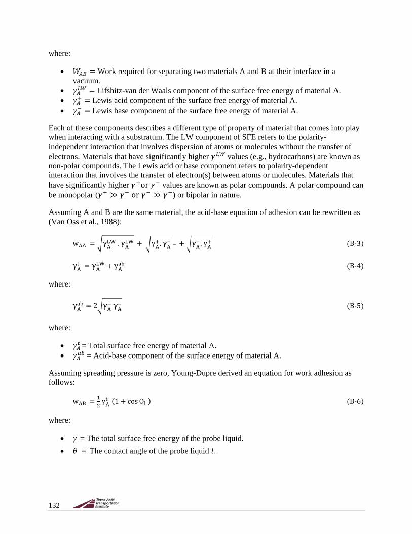
132
where:
• 𝑊𝑊𝐴𝐴𝐴𝐴 = Work required for separating two materials A and B at their interface in a vacuum.
• 𝛾𝛾𝐴𝐴𝐿𝐿𝐿𝐿 = Lifshitz-van der Waals component of the surface free energy of material A.
• 𝛾𝛾𝐴𝐴+ = Lewis acid component of the surface free energy of material A.
• 𝛾𝛾𝐴𝐴− = Lewis base component of the surface free energy of material A.
Each of these components describes a different type of property of material that comes into play when interacting with a substratum. The LW component of SFE refers to the polarity-independent interaction that involves dispersion of atoms or molecules without the transfer of electrons. Materials that have significantly higher 𝛾𝛾𝐿𝐿𝐿𝐿 values (e.g., hydrocarbons) are known as non-polar compounds. The Lewis acid or base component refers to polarity-dependent interaction that involves the transfer of electron(s) between atoms or molecules. Materials that have significantly higher 𝛾𝛾+or 𝛾𝛾− values are known as polar compounds. A polar compound can be monopolar (𝛾𝛾+ ≫ 𝛾𝛾− or 𝛾𝛾− ≫ 𝛾𝛾−) or bipolar in nature.
Assuming A and B are the same material, the acid-base equation of adhesion can be rewritten as (Van Oss et al., 1988):
wAA = �γALW . γA
LW + �γA+. γA
− − + �γA−. γA
+ (B-3)
γAt = γA
LW + γAab (B-4)
where:
γAab = 2�γA
+ γA− (B-5)
where:
• 𝛾𝛾𝐴𝐴𝑡𝑡 = Total surface free energy of material A.
• 𝛾𝛾𝐴𝐴𝑎𝑎𝑠𝑠 = Acid-base component of the surface energy of material A.
Assuming spreading pressure is zero, Young-Dupre derived an equation for work adhesion as follows:
wAB = 12
γAt (1 + cos ϴl ) (B-6)
where:
• 𝛾𝛾 = The total surface free energy of the probe liquid. • 𝜃𝜃 = The contact angle of the probe liquid 𝑙𝑙.

133
If material A is a liquid 𝑙𝑙 and material B is a test sample 𝑎𝑎, the acid-base and the Young-Dupre’s equations for work of adhesion can be expressed as:
wl.s = Wl.s2
= �γlLW . γs
LW + �γl+. γs
− − + �γl−. γs
+ (B-7)
wl.s = Wadhesion2
= 12
γlt (1 + Cosϴl ) (B-8)
where:
γlt = γl
LW + γlab (B-9)
γlab = 2�γl
+ γl− (B-10)
The expressions can then be combined as:
�γlLW . γs
LW + �γl+. γs
− − + �γl−. γs
+ = 12
γlt (1 + Cosϴl ) (B-11)
For n number of probe liquids, the equation of contact angle can be modified as (Bhasin et al., 2007b):
�γliLW . γs
LW + �γli+. γs
− − + �γli−. γs
+ = 12
γlt (1 + Cosϴli ) (B-12)
This relationship can be generalized as:
A. X = B (B-13)
where:
A = ��γl1
LW �γl1+ �γl1
− ⋮ ⋮ ⋮
�γlnLW �γln
+ �γln−
�
n x 3
(B-14)
X = ��γs
LW �γs
+ �γs
− �
3 x 1
(B-15)
B = �
12
γl1t (1 + Cosϴl1 )
⋮12
γlnt (1 + Cosϴln )
�
n x 1
(B-16)

134
If surface free energy components of the probe liquids 𝑙𝑙𝑎𝑎 are already known, this equation can be used to determine the surface free energy components of the test sample 𝑎𝑎 as:
X = A−1. B (B-17)
The measurement errors of surface free energy components can be propagated into the work of adhesion using the following equation (Ku 1966):
σ�w�2 = σγt
2 �∂w∂γ
�2
+ σ�θ�2 �∂w
∂θ�
2 (B-18)
where:
σγt = Error in γt from literature or 0.1 ergs. cm−2
∂w∂γ
= 12
(1 + cos θ�) (B-19)
σ�θ��2 = Error in average contact angle = 1
r. σ�θ
2 = �1r� . � 1
r−1� ∑ �θj − θ��2r
j=1 (B-20)
∂w∂θ
= 12
γt sin θ� (B-21)
where:
• θ� = Average contact angle from replicate measurements, expressed in radians. • 𝑓𝑓 = Number of replicates.
Since there are only three parameters to solve from the combined equation of work of adhesion, a minimum of three liquids is required for these tests. If more than three liquids are used, the above equations can be solved using singular value decomposition techniques.
Researchers have reported that the plot of 𝛾𝛾𝑙𝑙𝑡𝑡𝑐𝑐𝑓𝑓𝑎𝑎𝜃𝜃 𝑚𝑚 𝛾𝛾𝑙𝑙
𝑡𝑡 can be used to identify whether a certain probe liquid anomalously interacted with the test specimen. Generally, the plot of 𝛾𝛾𝑙𝑙
𝑡𝑡𝑐𝑐𝑓𝑓𝑎𝑎𝜃𝜃 𝑚𝑚 𝛾𝛾𝑙𝑙𝑡𝑡
should result in a smooth curve; if the data point from a certain liquid is noticeably outside this curve, contact angles measured from this particular liquid should not be used to analyze surface free energy components (Little and Bhasin 2006). This elimination is important because selection of improper probe liquids can yield inaccuracy of calculated surface energy components.
B.2.2. Results
B.2.2.1. Aggregates The SFE components of each aggregate were determined by researchers at the University of Oklahoma using a universal sorption device, which operates under the principle of static vapor sorption, and the results are presented in Table B-2.
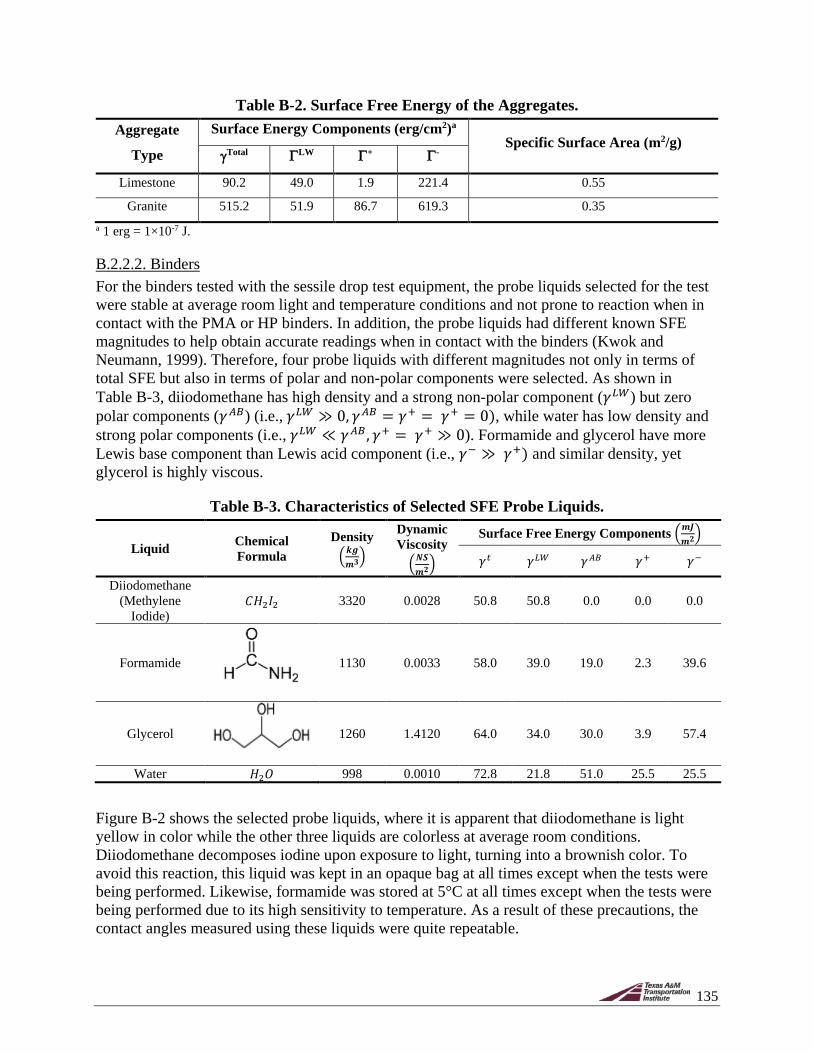
135
Table B-2. Surface Free Energy of the Aggregates. Aggregate
Type
Surface Energy Components (erg/cm2)a
Specific Surface Area (m2/g)
γTotal ΓLW Γ+ Γ-
Limestone 90.2 49.0 1.9 221.4 0.55 Granite 515.2 51.9 86.7 619.3 0.35
a 1 erg = 1×10⁻⁷ J.
B.2.2.2. Binders For the binders tested with the sessile drop test equipment, the probe liquids selected for the test were stable at average room light and temperature conditions and not prone to reaction when in contact with the PMA or HP binders. In addition, the probe liquids had different known SFE magnitudes to help obtain accurate readings when in contact with the binders (Kwok and Neumann, 1999). Therefore, four probe liquids with different magnitudes not only in terms of total SFE but also in terms of polar and non-polar components were selected. As shown in Table B-3, diiodomethane has high density and a strong non-polar component (𝛾𝛾𝐿𝐿𝐿𝐿) but zero polar components (𝛾𝛾𝐴𝐴𝐴𝐴) (i.e., 𝛾𝛾𝐿𝐿𝐿𝐿 ≫ 0, 𝛾𝛾𝐴𝐴𝐴𝐴 = 𝛾𝛾+ = 𝛾𝛾+ = 0), while water has low density and strong polar components (i.e., 𝛾𝛾𝐿𝐿𝐿𝐿 ≪ 𝛾𝛾𝐴𝐴𝐴𝐴, 𝛾𝛾+ = 𝛾𝛾+ ≫ 0). Formamide and glycerol have more Lewis base component than Lewis acid component (i.e., 𝛾𝛾− ≫ 𝛾𝛾+) and similar density, yet glycerol is highly viscous.
Table B-3. Characteristics of Selected SFE Probe Liquids.
Liquid Chemical Formula
Density �𝒌𝒌𝒌𝒌
𝒎𝒎𝟑𝟑�
Dynamic Viscosity
�𝑵𝑵𝑵𝑵𝒎𝒎𝟐𝟐�
Surface Free Energy Components �𝒎𝒎𝒎𝒎𝒎𝒎𝟐𝟐�
𝛾𝛾𝑡𝑡 𝛾𝛾𝐿𝐿𝐿𝐿 𝛾𝛾𝐴𝐴𝐴𝐴 𝛾𝛾+ 𝛾𝛾−
Diiodomethane (Methylene
Iodide) 𝐶𝐶𝐻𝐻2𝐼𝐼2 3320 0.0028 50.8 50.8 0.0 0.0 0.0
Formamide
1130 0.0033 58.0 39.0 19.0 2.3 39.6
Glycerol
1260 1.4120 64.0 34.0 30.0 3.9 57.4
Water 𝐻𝐻2𝐹𝐹 998 0.0010 72.8 21.8 51.0 25.5 25.5
Figure B-2 shows the selected probe liquids, where it is apparent that diiodomethane is light yellow in color while the other three liquids are colorless at average room conditions. Diiodomethane decomposes iodine upon exposure to light, turning into a brownish color. To avoid this reaction, this liquid was kept in an opaque bag at all times except when the tests were being performed. Likewise, formamide was stored at 5°C at all times except when the tests were being performed due to its high sensitivity to temperature. As a result of these precautions, the contact angles measured using these liquids were quite repeatable.

136
Figure B-2. Selected Probe Liquids for SFE Testing.
The contact angles measured after placing the probe liquid drops over any given test specimen did not change significantly over time except for a few cases. These instances in which the contact angles varied over time involved cases where the probe liquid drops took longer to stabilize after initial contact with the surface of the specimen due to the effect of kinetic energy, or when probe liquids were sensitive to average room light (e.g., diiodomethane) or temperature (e.g., water) conditions were used. Figure B-3 shows the contact angles measured on the HP binder in its original state with four probe liquids and illustrates how those values changed over time for some of the replicates. To avoid using the contact angle results that varied with time, seven test replicates were subjected to each probe liquid, and the ones that showed constant trends were used to estimate the average contact angles.

137
(a) (b)
(c) (d)
Figure B-3. Contact Angles for Replicates of HP Binder in Original State Using Various Probe Liquids: (a) Diiodomethane; (b) Formamide; (c) Glycerol; (d) Water.
Figure B-4 shows the average contact angles with time that resulted from testing the HP and PMA binders in OB, RTFO, and PAV20 states using a minimum of three test replicates. For both binders, the probe liquid with the highest density and the weakest acid-base component (i.e., diiodomethane) resulted in the smallest contact angles, while the probe liquid with the lowest density and the strongest acid-base component (i.e., water) resulted in the largest contact angles.
50
60
70
80
90
100
110
120
0 20 40 60
Con
tact
Ang
le (d
eg.)
Time (sec)
Diiodomethane
D1-1
D1-2
D1-3
D2-1
D3-150
60
70
80
90
100
110
120
0 20 40 60
Con
tact
Ang
le (d
eg.)
Time (sec)
Formamide
F1-1
F1-2
F1-3
F2-1
F3-1
50
60
70
80
90
100
110
0 20 40 60
Con
tact
Ang
le (d
eg.)
Time (sec)
Glycerol
G1-1
G1-2
G1-3
G2-1
G3-150
60
70
80
90
100
110
120
0 20 40 60
Con
tact
Ang
le (d
eg.)
Time (sec)
Water
W1-1
W1-2
W1-3
W2-2
W3-1

138
(a)
(b)
(c)
Figure B-4. Average Contact Angles Measured with Various Probe Liquids in Different Aging States: (a) HP-OB; (b) HP-RTFO; (c) HP-PAV20; (d) PMA-OB; (e) PMA-RTFO;
(f) PMA-PAV20.
0
20
40
60
80
100
120
0 10 20 30 40 50 60
Con
tact
Ang
le (d
eg.)
Time (sec)
HP-Unaged
Water
Glycerol
Formamide
Diiodomethane
0
20
40
60
80
100
120
0 10 20 30 40 50 60
Con
tact
Ang
le (d
eg.)
Time (sec)
HP-RTFO
Water
Glycerol
Formamide
Diiodomethane
0
20
40
60
80
100
120
0 10 20 30 40 50 60
Con
tact
Ang
le (d
eg.)
Time (sec)
HP-PAV20
Water
Glycerol
Formamide
Diiodomethane

139
(d)
(e)
(f)
Figure B-4 (Continued). Average Contact Angles Measured with Various Probe Liquids in Different Aging States: (a) HP-OB; (b) HP-RTFO; (c) HP-PAV20; (d) PMA-OB; (e) PMA-
RTFO; (f) PMA-PAV20.
0
20
40
60
80
100
120
0 10 20 30 40 50 60
Con
tact
Ang
le (d
eg.)
Time (sec)
PMA-Unaged
Water
Glycerol
Formamide
Diiodomethane
0
20
40
60
80
100
120
0 10 20 30 40 50 60
Con
tact
Ang
le (d
eg.)
Time (sec)
PMA-RTFO
Water
Glycerol
Formamide
Diiodomethane
0
20
40
60
80
100
120
0 10 20 30 40 50 60
Con
tact
Ang
le (d
eg.)
Time (sec)
PMA-PAV20
Water
Glycerol
Formamide
Diiodomethane

140
Figure B-4 also shows that the liquids with intermediate densities and intermediate acid-base components (i.e., formamide and glycerol) resulted in intermediate contact angle values. In other words, the binder contact angles ranked in the same order as the acid-base component of the probe liquids, suggesting a correlation between the measured contact angles and this SFE component. The ranking of the resulting contact angles (and acid-base component) was as follows: water > glycerol > formamide > diiodomethane.
After a careful analysis of the resulting contact angles from the sessile drop tests, it was determined that only the PMA binder in the original state tested with formamide did not follow this ranking. Therefore, only the results from the remaining probe liquids were employed to estimate the SFE of this binder in the original state. For the PMA binder in RTFO and PAV20 and the HP binders in all three aging states, all four probe liquids were used to calculate the SFE components.
Table B-4 lists the 10-second average contact angles and their standard deviation obtained from at least five test replicates (three replicates with one drop and two replicates with two drops) for both binders under different aging states.
Table B-4. Average Binder Contact Angles 10 Seconds after Test Initiation.
Probe Liquid HP Binder PMA Binder
Original RTFO PAV20 Original RTFO PAV20 Avg. SD Avg. SD Avg. SD Avg. SD Avg. SD Avg. SD
Diiodomethane 58.8 1.3 67.1 1.5 68.6 3.1 65.3 3.9 62.5 2.7 79.5 3.4 Formamide 86.5 1.0 93.4 1.7 91.7 1.7 - - 94.8 1.1 95.5 0.8
Glycerol 100.1 1.5 104.4 1.8 105.8 1.0 100.2 2.9 108.9 2.0 109.5 2.2 Water 103.6 1.5 104.7 0.9 105.3 1.5 106.5 1.0 107.1 0.7 107.2 1.4
Figure B-5a shows the normalized PMA binder contact angles with respect to the HP binder contact angles in different aging states. The data in this figure demonstrate that, for any given aging state, the normalized values are greater than 1.0 in all but one case, suggesting the resulting contact angles of the selected probe liquids in contact with the PMA binder were larger than when in contact with the HP binder. Therefore, less work of adhesion would be needed to separate a given liquid from the PMA binder compared to the HP binder.
Similarly, Figure B-5b presents the normalized original state contact angles with respect to the aged contact angles. For both the HP and PMA binders, the original to aged normalized contact angles were greater than 1.0 in all but two cases, also suggesting that the resulting contact angles of the selected probe liquids in contact with the aged binders were larger than when in contact with the binder in the original state. Figure B-5b also shows that the normalized PAV20/RTFO contact angles were smaller than the RTFO/original normalized contact angles, suggesting an initial significant increase in contact angle with aging but less change with further aging.

141
(a)
(b)
Figure B-5. Normalized Contact Angles Measured with Various Probe Liquids for HP and PMA Binders in Different Aging States: (a) Effect of Binder Type; (b) Effect of Aging.
B.2.2.3. Mastics Figure B-6 shows the average contact angles over time from a minimum of three tests conducted on the mastics. Like in the case of the binders, the values did not significantly change over time. Therefore, the average contact angle 10 seconds after releasing the drop of the probe liquid over the test specimen was used to calculate the SFE components. As before, 10 seconds was selected to guarantee that the drop of the probe liquid was fully stable.
0.70
1.00
1.30
Unaged RTFO PAV20
PMA/HP
Nor
mal
ized
Con
tact
Ang
le
Diiodomethane
Formamide
Glycerol
Water
0.70
1.00
1.30
RTFO/Unaged PAV20/RTFO RTFO/Unaged PAV20/RTFO
HP PMA
Nor
mal
ized
Con
tact
Ang
le
Diiodomethane
Formamide
Glycerol
Water

142
(a) (b)
(c) (d)
Figure B-6. Average Contact Angles Measured with Various Probe Liquids: (a) Mastic GH56; (b) Mastic LH59; (c) Mastic GP56; (d) Mastic LP59.
Table B-5 lists the 10-second average contact angles and their standard deviation for the mastics. Similar to the binder results, the resulting contact angles for the mastics were ranked according to the acid-based SFE component of the probe liquids (Table B-3), confirming the strong correlation between these two values.
0
20
40
60
80
100
120
0 20 40 60
Con
tact
Ang
le (d
eg.)
Time (sec)
GH56
WaterGlycerolFormamideDiisomethaneDiiodomethane
0
20
40
60
80
100
120
0 20 40 60
Con
tact
Ang
le (d
eg.)
Time (sec)
LH59
WaterGlycerolFormamideDiisomethaneDiiodomethane
0
20
40
60
80
100
120
0 20 40 60
Con
tact
Ang
le (d
eg.)
Time (sec)
GP56
Water
Glycerol
Formamide
Diiodomethane0
20
40
60
80
100
120
0 20 40 60
Con
tact
Ang
le (d
eg.)
Time (sec)
LP59
WaterGlycerolFormamideDiiodomethane

143
Table B-5. Average Mastic Contact Angles 10 Seconds after Test Initiation.
Contact Angles (deg.)
GH56 GP56 LH59 LP59 Avg. SD Avg. SD Avg. SD Avg. SD
Diiodomethane 69.5 1.1 72.7 2.1 63.1 1.3 73.3 0.9 Formamide 95.7 1.8 96.1 2.1 96.7 1.6 98.3 1.6
Glycerol 104.8 1.5 107.0 1.8 105.3 1.0 105.6 1.3 Water 107.6 2.0 109.1 1.7 106.1 1.3 108.7 0.3
Figure B-7a shows normalized PMA mastic contact angles with respect to HP mastic contact angles, which are greater than 1.0 in all but two cases, suggesting the probe liquids in contact with the mastics prepared with the PMA binder result in larger contact angles compared to the mastics prepared with the HP binder. Figure B-7b shows normalized limestone mastic contact angles with respect to granite mastic contact angles. The results demonstrate that the normalized values are only slightly greater or smaller than 1.0 in all but one case, suggesting the type of aggregate does not significantly affect the resulting contact angles.
Figure B-8 shows the normalized mastic contact angles with respect to the binder contact angles. These values are all larger than 1.0, suggesting the resulting contact angles of the mastic specimens are larger than the ones obtained for the binder specimens. Therefore, less work of adhesion would be needed to separate a given liquid from the mastics as opposed to the binder without any filler. Figure B-8 also shows that the ranking of the normalized mastic-to-binder contact angles follows the acid-based SFE ranking of the probe liquids.

144
(a)
(b)
Figure B-7. Normalized Mastic Contact Angles Measured with Various Probe Liquids: (a) Effect of Binder Type; (b) Effect of Aggregate Type.
0.950.960.970.980.991.001.011.021.031.041.051.06
Granite Limestone
PMA/HP
Nor
mal
ized
Con
tact
Ang
le
Diiodomethane
Formamide
Glycerol
Water
0.840.860.880.900.920.940.960.981.001.021.04
HP PMA
Limestone/Granite
Nor
mal
ized
Con
tact
Ang
le
Diiodomethane
Formamide
Glycerol
Water
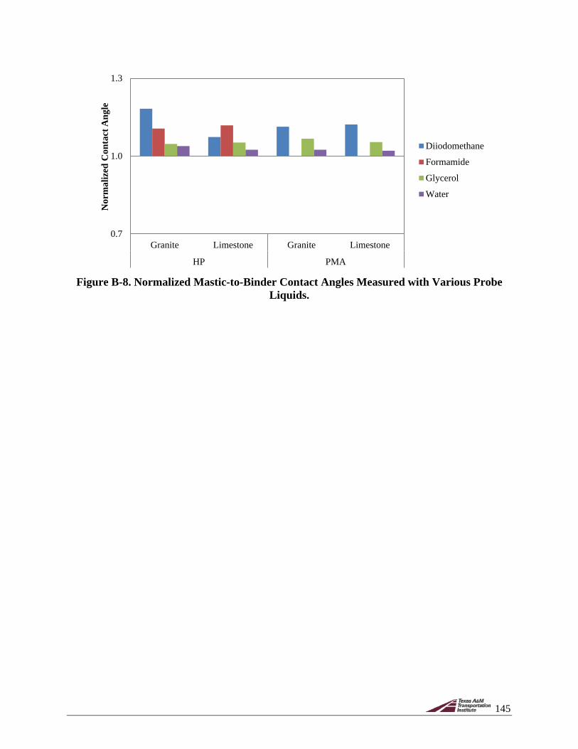
145
Figure B-8. Normalized Mastic-to-Binder Contact Angles Measured with Various Probe
Liquids.
0.7
1.0
1.3
Granite Limestone Granite Limestone
HP PMA
Nor
mal
ized
Con
tact
Ang
le
Diiodomethane
Formamide
Glycerol
Water
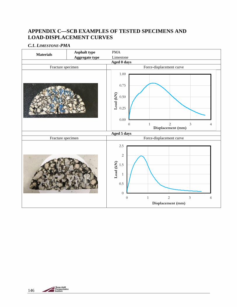
146
APPENDIX C—SCB EXAMPLES OF TESTED SPECIMENS AND LOAD-DISPLACEMENT CURVES C.1. LIMESTONE-PMA
Materials Asphalt type PMA Aggregate type Limestone
Aged 0 days Fracture specimen Force-displacement curve
Aged 5 days Fracture specimen Force-displacement curve
0.00
0.25
0.50
0.75
1.00
0 1 2 3 4
Load
(kN
)
Displacement (mm)
0
0.5
1
1.5
2
2.5
0 1 2 3 4
Load
(kN
)
Displacement (mm)

147
C.2. GRANITE-PMA
Materials Asphalt type PMA Aggregate type Granite
Aged 0 days Fracture specimen Force-displacement curve
No Picture Taken
Aged 5 days
Fracture specimen Force-displacement curve
0.00
0.25
0.50
0.75
1.00
0 2 4 6 8
Load
(kN
)Displacement (mm)
0.00
0.25
0.50
0.75
1.00
1.25
1.50
0 2 4 6 8
Load
(kN
)
Displacement (mm)
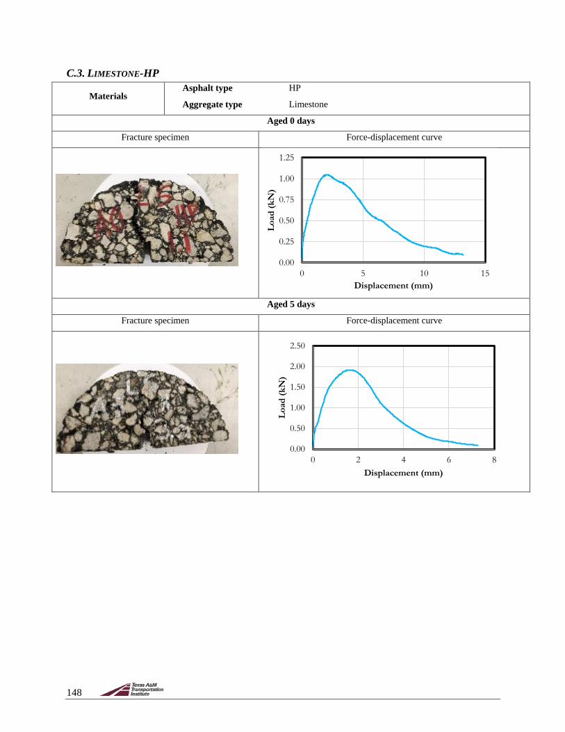
148
C.3. LIMESTONE-HP
Materials Asphalt type HP
Aggregate type Limestone
Aged 0 days
Fracture specimen Force-displacement curve
Aged 5 days
Fracture specimen Force-displacement curve
0.00
0.25
0.50
0.75
1.00
1.25
0 5 10 15Lo
ad (k
N)
Displacement (mm)
0.00
0.50
1.00
1.50
2.00
2.50
0 2 4 6 8
Load
(kN
)
Displacement (mm)

149
C.4. GRANITE-HP
Materials Asphalt type HP
Aggregate type Granite
Aged 0 days
Fracture specimen Force-displacement curve
Aged 5 days
Fracture specimen Force-displacement curve
0.00
0.50
1.00
1.50
2.00
0 5 10 15Lo
ad (k
N)
Displacement (mm)
0.00
0.25
0.50
0.75
1.00
1.25
1.50
0 5 10 15 20
Load
(kN
)
Displacement (mm)

150
APPENDIX D—STATISTICAL ANALYSIS SEMICIRCULAR BENDING TEST D.1. FLEXIBILITY INDEX WITH ALL POSSIBLE TWO-WAY INTERACTIONS BASED ON 75 MEASUREMENTS Figure D-1 presents the information related to the response of the FI, in which the predicted values are plotted against the actual experimental values based on 75 measurements. Table D-1 presents the summarized fit for the results obtained in the previous graphed data (e.g., R-squared, or mean of response). Table D-2 and Table D-3 present the information related to the different parameters and present the information related to a t-student test and F-test analysis, respectively.
Figure D-1. Flexibility Index: Results of Response of FI and Actual Predicted Plot Based on
75 Measurements.
Table D-1. Summary of Fit FI. Parameter Value R-Squared 0.67
R-Squared Adj 0.63 Root Mean Squared Error 26.00
Mean of Response 46.32 Observations (or Sum Wgts) 75
0
50
100
150
200
250
Flex
ibili
ty In
dex
FI A
ctua
l
28
0 50 100 150 200 250
exibility IndexFI Predicted P<.0001 RSq=0.67 RMSE=26.001

151
Table D-2. Parameter Estimates for FI Statistical Analysis. Term Estimate Std. Error t Ratio Prob>|t|
Intercept 254.59 291.93 0.87 0.3863 Aggregate Type [GR] −0.98 4.79 −0.20 0.8388
Binder Type [HP] 21.56 3.67 5.87 <.0001*
Aging State [A0] 11.81 3.11 3.79 0.0003*
Aggregate Type [GR]×Binder Type [HP]
−10.82 5.59 −1.93 0.0573
Aggregate Type [GR] ×Aging State [A0]
−21.17 3.13 −6.75 <.0001*
Binder Type [HP] ×Aging State [A0]
2.15 3.76 0.57 0.5705
Air Voids −10.76 14.67 −0.73 0.4657 * indicates the term is statistically significant at a level of alpha = 0.05
Table D-3. Effect Tests for FI Statistical Analysis. Source Nparm DF Sum of
Squares F Ratio Prob > F
Aggregate Type 1 1 28.21 0.042 0.8388 Binder Type 1 1 23290.72 34.45 <.0001* Aging State 1 1 9712.11 14.37 0.0003*
Aggregate Type×Binder Type 1 1 2529.68 3.74 0.0573 Aggregate Type×Aging State 1 1 30823.50 45.59 <.0001*
Binder Type×Aging State 1 1 219.78 0.33 0.5705 Air Voids 1 1 363.84 0.54 0.4657
* indicates the term is statistically significant at a level of alpha = 0.05
Figure D-2 shows the residual by predicted plot for the values concerning the FI. Table D-4, Table D-5, Table D-6, Table D-7, and Table D-8 present the results of the least square means statistical analysis for the aggregate type, binder, aging state, combination aggregate type and binder, and combination aggregate type and aging state, respectively. Figure D-3 and Figure D-4 present the plotted information for the least square means plot for binder type and FI, and the aging state and FI. Table D-9 presents the information related to the least square means differences for the Tukey honest significant difference (HSD) with an alpha equal to 5%. Finally, Table D-10 presents the information on the combination of binder type and aging state with the least square means statistical analysis.

152
Figure D-2. Residual by Predicted Plot for FI.
Table D-4. Least Square Means Table for Aggregate Type for Statistical Analysis of FI. Level Least Sq Mean Std. Error Mean GR 40.04 6.26 41.56 LS 42.00 5.20 51.21
Table D-5. Least Square Means Table for Binder Type for Statistical Analysis of FI. Level Least Sq
Mean Std. Error Mean
HP 62.58 4.156 65.72 PMA 19.45 5.48 18.78
Table D-6. Least Square Means Table for Aging State for Statistical Analysis of FI. Level Least Sq
Mean Std. Error Mean
A0 52.82 4.51 59.33 A5 29.21 4.40 32.22
Table D-7. Least Square Means Table for Combination of Aggregate Type and Binder Type for Statistical Analysis of FI.
Level Least Sq Mean Std. Error GR,HP 50.78 5.75
GR,PMA 29.29 13.16 LS,HP 74.37 5.91
LS,PMA 9.61 8.39

153
Table D-8. Least Square Means Table for Combination of Aggregate Type and Aging State for Statistical Analysis of FI.
Level Least Sq Mean Std. Error GR,A0 30.68 7.68 GR,A5 49.40 7.54 LS,A0 74.97 5.94 LS,A5 9.02 7.72
Figure D-3. LS Means Plot for Binder Type and FI.
Figure D-4. LS Means Plot for Aging State and FI.
Table D-9. Least Square Means Differences Tukey HSD for Alpha = 0.05. Mixture Level1 Least Sq
Mean LS,A0 A 74.97 GR,A5 A,B 49.40 GR,A0 B,C 30.68 LS,A5 C 9.02
1 Levels not connected by same letter are significantly different.
0
50
100
150
200
250
Flex
ibili
ty In
dex
FI L
S M
eans
HP PMA
Binder Type
GR
LS
0
50
100
150
200
250
Flex
ibili
ty In
dex
FI L
S M
eans
A0 A5
Aging Condition
GR
LS
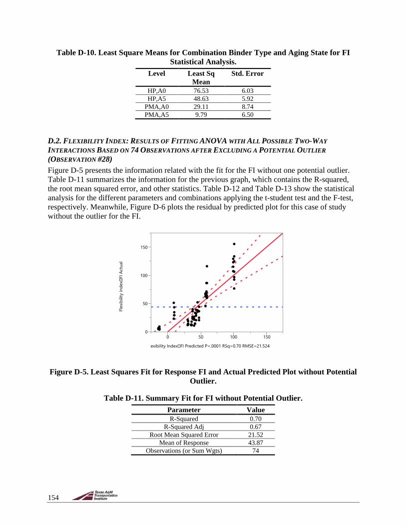
154
Table D-10. Least Square Means for Combination Binder Type and Aging State for FI Statistical Analysis.
Level Least Sq Mean
Std. Error
HP,A0 76.53 6.03 HP,A5 48.63 5.92
PMA,A0 29.11 8.74 PMA,A5 9.79 6.50
D.2. FLEXIBILITY INDEX: RESULTS OF FITTING ANOVA WITH ALL POSSIBLE TWO-WAY INTERACTIONS BASED ON 74 OBSERVATIONS AFTER EXCLUDING A POTENTIAL OUTLIER (OBSERVATION #28) Figure D-5 presents the information related with the fit for the FI without one potential outlier. Table D-11 summarizes the information for the previous graph, which contains the R-squared, the root mean squared error, and other statistics. Table D-12 and Table D-13 show the statistical analysis for the different parameters and combinations applying the t-student test and the F-test, respectively. Meanwhile, Figure D-6 plots the residual by predicted plot for this case of study without the outlier for the FI.
Figure D-5. Least Squares Fit for Response FI and Actual Predicted Plot without Potential
Outlier.
Table D-11. Summary Fit for FI without Potential Outlier. Parameter Value R-Squared 0.70
R-Squared Adj 0.67 Root Mean Squared Error 21.52
Mean of Response 43.87 Observations (or Sum Wgts) 74
0
50
100
150
Flex
ibili
ty In
dex
FI A
ctua
l
0 50 100 150
exibility IndexFI Predicted P<.0001 RSq=0.70 RMSE=21.524

155
Table D-12. Parameter Estimates for FI Statistical Analysis without Potential Outlier. Term Estimate Std. Error t Ratio Prob>|t|
Intercept 164.94 242.19 0.68 0.4982 Aggregate Type [GR] −0.67 3.97 −0.17 0.8659
Binder Type [HP] 20.71 3.04 6.80 <.0001* Aging State [A0] 10.47 2.59 4.04 0.0001*
Aggregate Type [GR] ×Binder Type [HP] −8.07 4.66 −1.73 0.0877 Aggregate Type [GR] ×Aging State [A0] −19.40 2.61 −7.42 <.0001*
Binder Type [HP] ×Aging State [A0] 1.46 3.12 0.47 0.6412 Air Voids −6.32 12.17 −0.52 0.6052
* indicates the term is statistically significant at a level of alpha = 0.05
Table D-13. Effect Tests for FI Statistical Analysis without Potential Outlier. Source Nparm DF Sum of
Squares F Ratio Prob > F
Aggregate Type 1 1 13.305 0.03 0.8659 Binder Type 1 1 21441.53 46.28 <.0001* Aging State 1 1 7576.48 16.35 0.0001*
Aggregate Type×Binder Type 1 1 1392.0 3.00 0.0877 Aggregate Type×Aging State 1 1 25518.48 55.08 <.0001*
Binder Type×Aging State 1 1 101.52 0.21 0.6412 Air Voids 1 1 125.02 0.26 0.6052
* indicates the term is statistically significant at a level of alpha = 0.05
Figure D-6. Residual by Predicted Plot without Potential Outlier.
Table D-14, Table D-15, and Table D-16 present the information for the least square means for the binder type, the combination of aggregate and binder type, and aggregate type and age state, respectively. Figure D-7 presents the least square means plot for FI and binder type, while Figure D-8 presents the information related to the FI and the aging state. Table D-17 presents the information on the least square means differences for the Tukey HSD with an alpha equal to 5% for the FI parameter without the potential outlier.
-40
-20
0
20
40
60
Flex
ibili
ty In
dex
FI R
esid
ual
0 50 100 150
Flexibility IndexFI Predicted

156
Table D-14. Least Square Means Table for Binder Type for Statistical Analysis of FI without Potential Outlier.
Level Least Sq Mean
Std. Error
Mean
HP 60.17 3.47 61.95 PMA 18.75 4.52 18.78
Table D-15. Least Square Means Table for Combination Aggregate Type and Binder Type for Statistical Analysis of FI without Potential Outlier.
Level Least Sq Mean
Std. Error
GR,HP 51.43 4.77 GR,PMA 26.14 10.88
LS,HP 68.92 4.98 LS,PMA 11.35 6.97
Table D-16. Least Square Means Table for Combination Aggregate Type and Aging State for Statistical Analysis of FI without Potential Outlier.
Level Least Sq Mean Std. Error GR,A0 29.86 6.34 GR,A5 47.72 6.23 LS,A0 70.01 5.00 LS,A5 10.27 6.41
Figure D-7. Least Square Means Plot for FI and Binder Type without Potential Outlier.
0
50
100
150
Flex
ibili
ty In
dex
FI L
S M
eans
HP PMA
Binder Type
GR
LS

157
Figure D-8. Least Square Means Plot for FI and Aging State without Potential Outlier.
Table D-17. Least Square Means Differences Tukey HSD without Potential Outlier with Alpha = 0.05.
Mixture Level1 Least Sq Mean
LS,A0 A 70.01 GR,A5 A,B 47.72 GR,A0 B,C 29.86 LS,A5 C 10.27
1 Levels not connected by the same letter are significantly different.
D.3. CRACKING RESISTANCE INDEX: RESULTS OF FITTING ANOVA WITH ALL POSSIBLE TWO-WAY INTERACTIONS BASED ON 75 MEASUREMENTS Figure D-9 presents the results obtained from plotting the experimental CRI and the actual predicted plot based on the 75 conducted measurements. Table D-18 summarizes the fit for the results from the previous graph. Table D-19 shows the results of the statistical analysis of the parameters as well as the t-student test for each of the parameters or combination. Moreover, Table D-20 presents the effect test (i.e., F-test results) for the same parameters and two-way interactions. Finally, Figure D-10 plots the residual by predicted plot versus the experimental values for the CRI.
0
50
100
150
Flex
ibili
ty In
dex
FI L
S M
eans
A0 A5
Aging Condition
GR
LS

158
Figure D-9. Least Squares Fit Results of Response of CRI and Actual Predicted Plot Based
on 75 Measurements.
Table D-18. Summary of Fit CRI. Parameter Value R-Squared 0.74
R-Squared Adj 0.72 Root Mean Squared Error 304.06
Mean of Response 1319.54 Observations (or Sum Wgts) 75
Table D-19. Parameter Estimates for CRI Statistical Analysis. Term Estimate Std. Error t Ratio Prob>|t|
Intercept 3662.02 3413.89 1.07 0.2873 Aggregate Type [GR] 88.84 56.05 1.58 0.1177
Binder Type [HP] 333.49 42.96 7.76 <.0001* Aging State [A0] 184.33 36.43 5.06 <.0001*
Aggregate Type [GR]×Binder Type [HP] −114.52 65.41 −1.75 0.0845 Aggregate Type [GR] ×Aging State [A0] −273.12 36.66 −7.45 <.0001*
Binder Type [HP] ×Aging State [A0] −50.75 44.01 −1.15 0.2530 Air Voids −121.95 171.54 −0.71 0.4796
* indicates the term is statistically significant at a level of alpha = 0.05
Table D-20. Effect Tests for CRI Statistical Analysis. Source Nparm DF Sum of
Squares F Ratio Prob > F
Aggregate Type 1 1 232211.10 2.51 0.1177 Binder Type 1 1 5570709.40 60.26 <.0001* Aging State 1 1 2367429.10 25.61 <.0001*
Aggregate Type×Binder Type 1 1 283404.20 3.07 0.0845 Aggregate Type×Aging State 1 1 5131831.90 55.51 <.0001*
Binder Type×Aging State 1 1 122933.00 1.33 0.25 Air Voids 1 1 46722.60 0.51 0.48
* indicates the term is statistically significant at a level of alpha = 0.05
500
1000
1500
2000
2500
Crac
king
Res
istan
ce In
dex
CRI
Act
ual
500 1000 1500 2000 2500
Resistance Index CRI Predicted P<.0001 RSq=0.74 RMSE=304.06

159
Figure D-10. Residual by Predicted Plot for CRI.
The effect details of the different parameters for the CRindex are presented in the following tables. Table D-21, Table D-22, and Table D-23 present the statistical information for the aggregate type, the asphalt type, and the aging state, respectively. The subsequent tables present the information for the statistical analysis of the combination (i.e., interaction) of the different parameters evaluated, such as the aggregate type and binder or aging state (i.e., Table D-24, Table D-25, and Table D-26). Meanwhile, Table D-27 presents the least square means differences for the Tukey HSD with an alpha equal to 5% for the CRI, and Figure D-11 displays the least square means plot of aging state versus CRI.
Table D-21. Least Square Means Table for Aggregate Type for Statistical Analysis of CRI. Level Least Sq
Mean Std.
Error Mean
GR 1330.60 73.21 1368.59 LS 1152.92 60.84 1269.17
Table D-22. Least Square Means Table for Binder Type for Statistical Analysis of CRI. Level Least Sq
Mean Std. Error Mean
HP 1575.25 48.60 1621.51 PMA 908.27 64.08 890.93
Table D-23. Least Square Means Table for Aging State for Statistical Analysis of CRI. Level Least Sq
Mean Std. Error Mean
A0 1426.09 52.77 1498.62 A5 1057.43 51.44 1125.53
-600
-400
-200
0
200
400
600
Crac
king
Res
istan
ce In
dex
CRI
Res
idua
l
500 1000 1500 2000 2500
Cracking Resistance Index CRI Predicted

160
Table D-24. Least Square Means Table for Combination of Aggregate Type and Binder Type for Statistical Analysis of CRI.
Level Least Sq Mean
Std. Error
GR,HP 1,549.57 67.27 GR,PMA 1,111.62 153.88
LS,HP 1,600.92 69.13 LS,PMA 704.92 98.16
Table D-25. Least Square Means Table for Combination of Aggregate Type and Aging State for Statistical Analysis of CRI.
Level Least Sq Mean
Std. Error
GR,A0 1241.81 89.76 GR,A5 1419.39 88.17 LS,A0 1610.37 69.48 LS,A5 695.47 90.26
Table D-26. Least Square Means Combination of Binder Type and Aging State for CRI. Level Least Sq
Mean Std. Error
HP,A0 1708.83 70.47 HP,A5 1441.67 69.22
PMA,A0 1143.35 102.24 PMA,A5 673.19 76.03
Table D-27. Least Square Means Differences Tukey HSD for CRI with Alpha = 0.05. Mixture Level1 Least Sq
Mean LS,A0 A 1610.37 GR,A5 A,B 1419.39 GR,A0 B 1241.81 LS,A5 C 695.47
1 Levels not connected by same letter are significantly different.

161
Figure D-11. Least Square Means Plot for CRI and Aging State.
500
1000
1500
2000
2500
Crac
king
Res
istan
ce In
dex
CRI L
S M
eans
A0 A5
Aging Condition
GR
LS
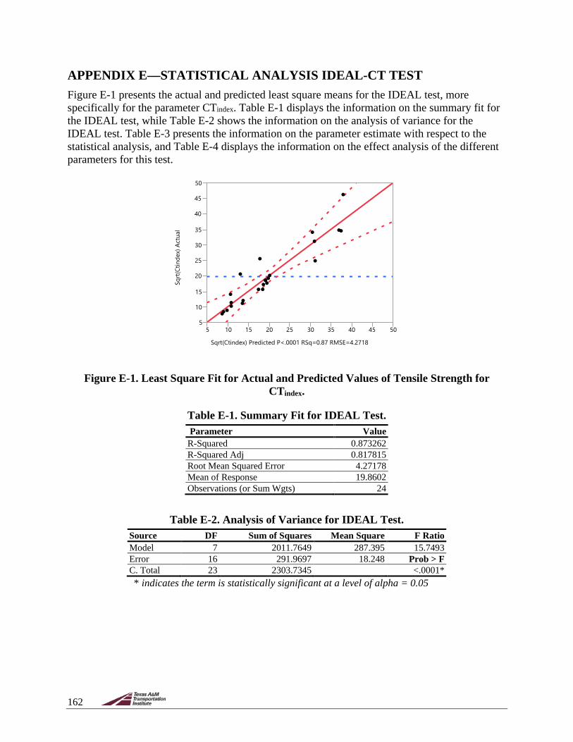
162
APPENDIX E—STATISTICAL ANALYSIS IDEAL-CT TEST Figure E-1 presents the actual and predicted least square means for the IDEAL test, more specifically for the parameter CTindex. Table E-1 displays the information on the summary fit for the IDEAL test, while Table E-2 shows the information on the analysis of variance for the IDEAL test. Table E-3 presents the information on the parameter estimate with respect to the statistical analysis, and Table E-4 displays the information on the effect analysis of the different parameters for this test.
Figure E-1. Least Square Fit for Actual and Predicted Values of Tensile Strength for
CTindex.
Table E-1. Summary Fit for IDEAL Test. Parameter Value R-Squared 0.873262 R-Squared Adj 0.817815 Root Mean Squared Error 4.27178 Mean of Response 19.8602 Observations (or Sum Wgts) 24
Table E-2. Analysis of Variance for IDEAL Test. Source DF Sum of Squares Mean Square F Ratio Model 7 2011.7649 287.395 15.7493 Error 16 291.9697 18.248 Prob > F C. Total 23 2303.7345 <.0001*
* indicates the term is statistically significant at a level of alpha = 0.05
5
10
15
20
25
30
35
40
45
50Sq
rt(Ct
inde
x) A
ctua
l
5 10 15 20 25 30 35 40 45 50
Sqrt(Ctindex) Predicted P<.0001 RSq=0.87 RMSE=4.2718

163
Table E-3. Parameter Estimate for IDEAL Test. Term Estimate Std. Error t Ratio Prob>|t| Intercept 4.0865447 34.42547 0.12 0.9070 Aggregate Type [GR] 1.8118587 0.931399 1.95 0.0695 Binder Type [HP] 5.5587722 0.873792 6.36 <.0001* Aging Condition [A0] 6.6522253 0.909191 7.32 <.0001* Air Voids (%) 0.7845478 1.711699 0.46 0.6529 Aggregate Type [GR]×Binder Type [HP] 1.3060397 0.895351 1.46 0.1640 Aggregate Type [GR] ×Aging Condition [A0] 0.1964099 0.959984 0.20 0.8405 Binder Type [HP] ×Aging Condition [A0] 2.2204552 0.873443 2.54 0.0217* * indicates the term is statistically significant at a level of alpha = 0.05
Table E-4. Statistical Analysis with Effect Test for IDEAL Test. Source Nparm DF Sum of Squares F Ratio Prob > F
Aggregate Type 1 1 69.05498 3.7842 0.0695 Binder Type 1 1 738.51529 40.4708 <.0001*
Aging Condition 1 1 976.88133 53.5333 <.0001* Air Voids 1 1 3.83355 0.2101 0.6529
Aggregate Type×Binder Type 1 1 38.82787 2.1278 0.1640 Aggregate Type×Aging Condition 1 1 0.76386 0.0419 0.8405
Binder Type×Aging Condition 1 1 117.93239 6.4627 0.0217* * indicates the term is statistically significant at a level of alpha = 0.05
Figure E-2 presents the information on the residual and predicted plot of the CTindex for the ideal test result of the statistical analysis. Table E-5, Table E-6, and Table E-7 show the detailed effect analysis of the least square means for the different parameters (e.g., aggregate type, binder type, and aging condition), while Table E-8, Table E-9, and Table E-10 present the detailed effect analysis of the least square means for different combinations of parameters. Furthermore, Figure E-3 displays the least square means of the CTindex and aging condition. Finally, Table E-11 indicates the least square means differences Tukey HSD for the IDEAL test with alpha = 0.05.
Figure E-2. Residual and Predicted Plot for CTindex of IDEAL Test.
-5
0
5
10
Sqrt(
Ctin
dex)
Res
idua
l
5 10 15 20 25 30 35 40 45 50
Sqrt(Ctindex) Predicted

164
Table E-5. Effect Details with Least Square Means for Aggregate Type of IDEAL Test. Level Least Sq Mean Std. Error Mean GR 21.672063 1.2758689 21.8221 LS 18.048346 1.2758689 17.8983
Table E-6. Effect Details with Least Square Means for Binder Type of IDEAL Test. Level Least Sq Mean Std. Error Mean HP 25.418977 1.2344432 25.3932 PMA 14.301432 1.2344432 14.3273
Table E-7. Effect Details with Least Square Means for Aging Condition of IDEAL Test. Level Least Sq Mean Std. Error Mean A0 26.512430 1.2597480 26.3944 A5 13.207979 1.2597480 13.3260
Table E-8. Effect Details with Least Square Means for Combination Aggregate Type and Binder Type of IDEAL Test.
Level Least Sq Mean Std. Error GR,HP 28.536875 1.7452625 GR,PMA 14.807251 1.8400773 LS,HP 22.301078 1.7532569 LS,PMA 13.795613 1.8072895
Table E-9. Effect Details with Least Square Means for Combination Aggregate Type and Aging Condition of IDEAL Test.
Level Least Sq Mean Std. Error GR,A0 28.520698 1.7752005 GR,A5 14.823428 2.0035643 LS,A0 24.504161 1.7535528 LS,A5 11.592530 1.8065429
Table E-10. Effect Details with Least Square Means for Combination Aging Condition and Binder Type of IDEAL Test.
Level Least Sq Mean Std. Error HP,A0 34.291657 1.7636924 HP,A5 16.546296 1.7504276 PMA,A0 18.733203 1.7620258 PMA,A5 9.869662 1.7816211

165
Figure E-3. Least Square Means Plot for CTindex and Aging Condition.
Table E-11. Least Square Means Differences Tukey HSD for IDEAL Test with Alpha = 0.05.
Mixture Level1 Least Sq Mean HP,A0 A 34.291657 PMA,A0 B 18.733203 HP,A5 B,C 16.546296 PMA,A5 C 9.869662 1 Levels not connected by the same letter are significantly different.
510
152025
303540
4550
Sqrt(
Ctin
dex)
LS M
eans
A0 A5
Aging Condition
HP
PMA

166
APPENDIX F—ASSESSMENT OF THE THREE-WHEEL POLISHER TO QUANTIFY THE EVOLUTION OF RAVELING IN OGFC This appendix details the results of the evaluation of the three-wheel polisher to quantify the magnitude and rate of raveling in OGFC mixtures. This information is important to describe the evolution or degradation rate of the mixtures.
The three-wheel polisher, shown in Figure F-1, was developed by NCAT in 2006 (Vollor and Hanson, 2006). It employs load-bearing rubber tires that move in a circular motion over the surface of a slab in the presence of water for a given number of load cycles. The test is performed at room temperature of about 77°F (25°C). Measurements of texture and/or friction before and after the polishing action are usually obtained to assess the susceptibility of the mixture to abrasion. Further details on the equipment are given herein.
Figure F-1. Three-Wheel Polisher.
The objective of this part of the study was to attempt the quantification of the initiation and evolution of raveling in OGFC mixtures by modifying the three-wheel polisher. The modifications done to the standard equipment are detailed in a subsequent section. As initially considered in the work plan, the variables used to quantify the evolution of raveling after a specified number of load cycles included the weight loss during testing and the change in texture.
F.1. MATERIALS To fulfill the objective of this part of the study, an existing plant-produced OGFC mixture obtained as part of a separate research project was employed. The friction course mixture (FC-5) was produced during the construction of a 30-mile-long segment of Interstate Highway 95 in Broward and Miami Dade Counties, Florida. Construction commenced in December 2014, and the plant-produced mixture was collected by TTI in January 2015. The mixture was produced with limestone aggregate from White Rock Quarries and a PG 76-22 binder modified with SBS polymer supplied by South Florida Materials (Riviera Beach terminal). An anti-stripping agent was added to the binder at the terminal. Mineral fibers were also incorporated into the mixture.

167
The mix design gradation can be found in Figure F-2. The mixture conformed to FDOT specifications for OGFC.
Figure F-2. FC-5 Mix Design.
F.2. SLAB SPECIMEN FABRICATION The procedure to prepare the OGFC slab specimens started by placing the plant-produced mixture in the oven for 2 hours at a temperature of 325°F (135°C). Afterwards, the mixture was poured in the asphalt roller compactor (ARC) slab mold to compact specimens 16 L × 20 W × 1 H in. (40.6 L × 50.8 W × 2.5 H cm) (see Figure F-3). The ARC uses an electro-mechanical system, which employs a segmented roller with alternate rotation to simulate field compaction. The temperature during compaction was 300°F (149°C). The target air void content was 20% with a maximum specific gravity (Gmm) of 2.3, which was obtained through laboratory testing. In order to facilitate the extraction of the slabs, oil was poured inside the mold; afterwards, the mold was disassembled and the slab extracted. After compaction, the slabs were left to cool down, labeled, and weighed in preparation for testing.
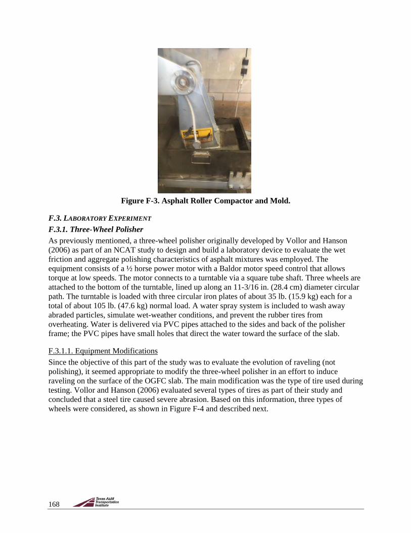
168
Figure F-3. Asphalt Roller Compactor and Mold.
F.3. LABORATORY EXPERIMENT F.3.1. Three-Wheel Polisher As previously mentioned, a three-wheel polisher originally developed by Vollor and Hanson (2006) as part of an NCAT study to design and build a laboratory device to evaluate the wet friction and aggregate polishing characteristics of asphalt mixtures was employed. The equipment consists of a ½ horse power motor with a Baldor motor speed control that allows torque at low speeds. The motor connects to a turntable via a square tube shaft. Three wheels are attached to the bottom of the turntable, lined up along an 11-3/16 in. (28.4 cm) diameter circular path. The turntable is loaded with three circular iron plates of about 35 lb. (15.9 kg) each for a total of about 105 lb. (47.6 kg) normal load. A water spray system is included to wash away abraded particles, simulate wet-weather conditions, and prevent the rubber tires from overheating. Water is delivered via PVC pipes attached to the sides and back of the polisher frame; the PVC pipes have small holes that direct the water toward the surface of the slab.
F.3.1.1. Equipment Modifications
Since the objective of this part of the study was to evaluate the evolution of raveling (not polishing), it seemed appropriate to modify the three-wheel polisher in an effort to induce raveling on the surface of the OGFC slab. The main modification was the type of tire used during testing. Vollor and Hanson (2006) evaluated several types of tires as part of their study and concluded that a steel tire caused severe abrasion. Based on this information, three types of wheels were considered, as shown in Figure F-4 and described next.
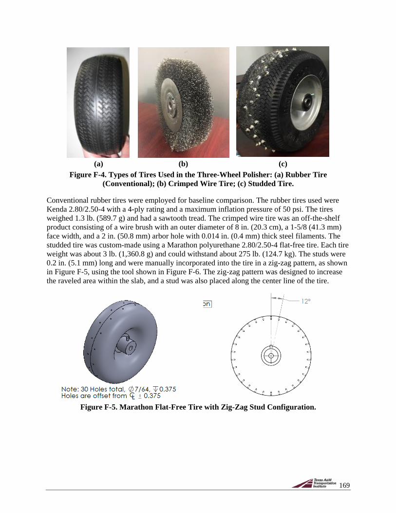
169
(a) (b) (c)
Figure F-4. Types of Tires Used in the Three-Wheel Polisher: (a) Rubber Tire (Conventional); (b) Crimped Wire Tire; (c) Studded Tire.
Conventional rubber tires were employed for baseline comparison. The rubber tires used were Kenda 2.80/2.50-4 with a 4-ply rating and a maximum inflation pressure of 50 psi. The tires weighed 1.3 lb. (589.7 g) and had a sawtooth tread. The crimped wire tire was an off-the-shelf product consisting of a wire brush with an outer diameter of 8 in. (20.3 cm), a 1-5/8 (41.3 mm) face width, and a 2 in. (50.8 mm) arbor hole with 0.014 in. (0.4 mm) thick steel filaments. The studded tire was custom-made using a Marathon polyurethane 2.80/2.50-4 flat-free tire. Each tire weight was about 3 lb. (1,360.8 g) and could withstand about 275 lb. (124.7 kg). The studs were 0.2 in. (5.1 mm) long and were manually incorporated into the tire in a zig-zag pattern, as shown in Figure F-5, using the tool shown in Figure F-6. The zig-zag pattern was designed to increase the raveled area within the slab, and a stud was also placed along the center line of the tire.
Figure F-5. Marathon Flat-Free Tire with Zig-Zag Stud Configuration.

170
Figure F-6. Studs and Installation Tool.
F.3.1.2. Experimental Variables In addition to the different tires used to test the OGFC slab specimens, changes to the total vertical load applied to the three-wheel assembly and the number of load cycles varied for different trials. Table F-1 describes the various trials considered as part of the laboratory experiment. The speed used for all the tests was 0.75 mph (1.2 km/h). Each of the trials presented different conditions of testing except between Trial #4 and #5 that corresponded to replicates. Initially, 100 cycles (about 4 minutes and 50 seconds) were conducted, and depending on the observed behavior, the total number of cycles varied.
Table F-1. Test Trials Conducted in the Modified Three-Wheel Polisher. Trial No. Vertical Load Tire Type
Number of Load Cycles 100 200 1,000 1,700 10,000
1 94.0 lb. (42.6 kg) Rubber X X X 2 127.3 lb. (57.7 kg) Rubber X X X 3 127.3 lb. (57.7 kg) Wire X X 4 94.0 lb. (42.6 kg) Studded X X 5 94.0 lb. (42.6 kg) Studded X 6 61.3 lb. (27.8 kg) Studded X X
F.3.2. Raveling Assessment To quantify the evolution of raveling in OGFC mixtures, two parameters were measured before and after a given number of load cycles as listed in Table F-1: (a) the weight of the material dislodged from the surface of the slab, and (b) the texture or mean profile depth of the slab’s circular track left by the polisher wheels, using a portable circular texture meter (CTMeter), which is described below. The change in friction was not considered critical in the assessment of the evolution of raveling.
F.3.2.1. Change in Slab Specimen Weight In order to quantify the amount of material dislodged from the surface of the slab, a simple protocol was established. After a certain number of cycles were applied, the slab was extracted from the three-wheel polisher machine. Using a compressed air gun, the surface of the slab was cleared of all dust and loose aggregate particles. The compressed air gun was used with care to

171
avoid dislodging additional aggregates from the surface of the slab. Afterwards, the slab was weighed and the information recorded.
The slabs subjected to loading with the studded tires exhibited unexpected crushing of the aggregates rather than raveling. Figure F-7a shows the surface of a slab with crushed aggregates before being cleaned with the compressed air gun, and Figure F-7b shows the surface of the slab after it was cleaned. In Figure F-7b, the path of the studded tires is visible as three separate traces on the surface of the slab, which corresponds to the zig-zag pattern of the studs as can be observed in Figure F-4c. This was possibly exacerbated because all three wheels had the same zig-zag stud configuration and the three-wheel polisher does not allow for wander. The other two types of tires (i.e., rubber and wire) did not crush the aggregates; the details of the dislodging mechanisms for these two tires are described in the results section.
(a) (b)
Figure F-7. Surface of the Slab after a Test Trial with Studded Tires: (a) Before Cleaning with Compressed Air; (b) After Cleaning with Compressed Air.
F.3.2.2. Change in Surface Texture The CTMeter consists of a laser-displacement sensor device mounted on an arm that rotates following a circular track of 11-3/16 in. (28.4 cm), which has the same dimension as the three-wheel polisher track. The sensor has a spot size of 0.003 in. (70 µm) with a vertical resolution of 1.1×10⁻⁴ in. (3 µm). The arm rotates 3.1 in. (80 mm) above the surface with a tangential velocity of 3.9 in/s (6 m/min) in a counterclockwise direction, providing a sample spacing of 0.03 in. (0.87 mm). The recorded profile is divided into eight 4.4 in. (111.5 mm) segment arcs of 128 samples each for analysis. The CTMeter software provides the MPD per ASTM E1845 (ASTM 2015a) and the root mean square per ASTM E2157 (ASTM 2015b) for each segment. Typical MPD values obtained using the CTMeter on dense-graded hot mix asphalt range between 0.016–0.023 in. (0.4–0.6 mm), while values for OGFC mixtures are usually about 0.04 in. (1.0 mm) for both field and test specimens (Jackson, 2008; Wu, 2013). The equipment is shown in Figure F-8.

172
(a) (b)
Figure F-8. Circular Track Meter Apparatus: (a) Side View; (b) Bottom View.
During testing, the CTMeter is placed over the slab surface before and after applying the loading cycles with the three-wheel polisher. The surface of the slab is cleared from debris, especially if the test is being performed after a certain number of load cycles have already been applied to the slab specimen. The location of the CTMeter is marked on the slab to measure on the same place, and the orientation of the apparatus is also the same. Three measurements are obtained on the surface of the slab specimen as follows:
1. Center measurement. 2. About 1 in. (25.4 mm) to the back of the first measurement. 3. About 1 in. (25.4 mm) to the front of the first measurement.
F.4. TEST RESULTS This section includes the results and analysis obtained from the experiments. It is subdivided in three sections. The first section corresponds to the visual inspection of the trials obtained with the different types of tires, and it analyzes the mechanisms that affected the surface of the slab. The second section presents the weight loss during the application of loading cycles in the different trials. Finally, the third section describes the data obtained with the use of the CTMeter, and it includes the MPD of the surface of the slab before testing with the three-wheel polisher and at the end of each trial.
F.4.1. Visual Inspection A visual inspection of the surface of the slab specimens after being subjected to loading with the three-wheel polisher was performed. Figure F-9a (Trial #1) shows a polished surface with no evidence of aggregate crushing. In this case, dislodging of a few aggregate particles passing sieve No. 8 (0.09 in. [2.38 mm]) or smaller was observed, but the extent and evolution of this damage process was very limited. Figure F-9b corresponds to the slab for Trial #3, which shows how the crimped wire tire brushed and abraded the surface of the slab more aggressively, but with no apparent raveling. In Figure F-9c and Figure F-9d, which correspond to the results of Trials #4 and #5 with the studded tires, the path of the stud can be observed as well as some holes in the surface of the slab that are the results of aggregate crushing. After 200 load cycles
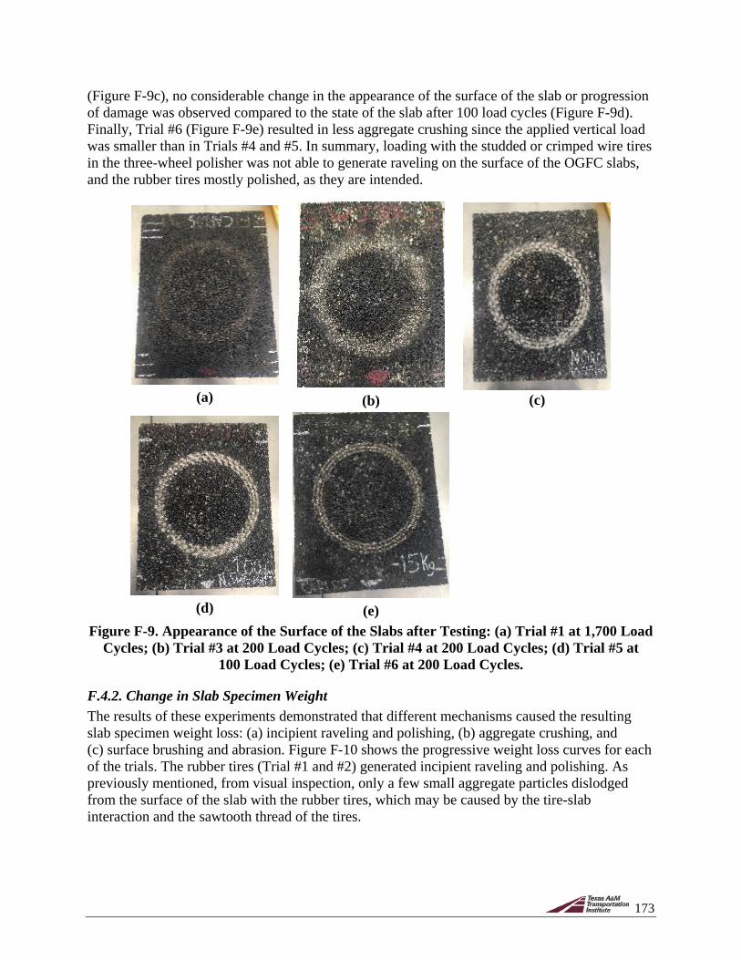
173
(Figure F-9c), no considerable change in the appearance of the surface of the slab or progression of damage was observed compared to the state of the slab after 100 load cycles (Figure F-9d). Finally, Trial #6 (Figure F-9e) resulted in less aggregate crushing since the applied vertical load was smaller than in Trials #4 and #5. In summary, loading with the studded or crimped wire tires in the three-wheel polisher was not able to generate raveling on the surface of the OGFC slabs, and the rubber tires mostly polished, as they are intended.
(a)
(b)
(c)
(d)
(e)
Figure F-9. Appearance of the Surface of the Slabs after Testing: (a) Trial #1 at 1,700 Load Cycles; (b) Trial #3 at 200 Load Cycles; (c) Trial #4 at 200 Load Cycles; (d) Trial #5 at
100 Load Cycles; (e) Trial #6 at 200 Load Cycles.
F.4.2. Change in Slab Specimen Weight The results of these experiments demonstrated that different mechanisms caused the resulting slab specimen weight loss: (a) incipient raveling and polishing, (b) aggregate crushing, and (c) surface brushing and abrasion. Figure F-10 shows the progressive weight loss curves for each of the trials. The rubber tires (Trial #1 and #2) generated incipient raveling and polishing. As previously mentioned, from visual inspection, only a few small aggregate particles dislodged from the surface of the slab with the rubber tires, which may be caused by the tire-slab interaction and the sawtooth thread of the tires.

174
Figure F-10. Weight Loss of the Slabs for Different Conditions.
The application of different vertical loads for the same type of tire type (Trial #1 vs. Trial #2, and Trial #4 vs. Trial #6) had an effect on the weight loss. The weight loss with the change in the vertical load for the rubber tires showed that a higher vertical load produced less weight loss. For instance, after 1,700 load cycles, Trial #1 (i.e., vertical load of 94 lb. [42.6 kg]) had 2.3 times the weight loss as Trial #2 (i.e., vertical load of 127.3 lb. [57.7 kg]) at 10,000 load cycles. This could be caused by a “compaction effect” that prevents the aggregates from dislodging under the increased vertical load.
For the trials with studded tires, there was a positive relationship between weight loss and applied vertical load. In these cases, higher vertical loads generated more weight loss mainly due to an increase in aggregate crushing (e.g., Trial #4 had 1.7 times the weight loss as Trial #6 at 200 cycles). It is noticeable that the weight loss in the trials that used the crimped wire and studded tires was significantly higher than the weight loss obtained with the rubber tires. In addition, the crimped wire and studded tires produced similar weight loss (i.e., 36.2 g and 36.5 g for Trials #3 and #4, respectively, at 200 cycles), despite the difference in vertical load and the fact that the mechanism causing weight loss for the studded tire trials was aggregate crushing while the mechanism causing weight loss for the crimped wire tires was brushing/abrasion.
F.4.3. Change in Surface Texture Figure F-11 presents the average of the three MPD measurements for the different trials. The average MPD changed depending on the trial test conditions and damage mechanisms previously described. The initial MPD (MPDinitial) for the slabs varied but was close to values reported in the literature (Jackson, 2008; Wu, 2013). For the rubber tires (Trials #1 and #2), the MPD decreased with added load cycles, which is consistent with the results obtained from Wu (2013). For the trials conducted with the crimped wire tires (Trial #3), no significant change was observed in MPD with the progression of the test, even though this trial resulted in significant material weight loss. This is possibly due to the brushing/abrasion mechanism caused by this type of tire, as previously explained. Conversely, the aggregate crushing observed in the trials conducted
0
5
10
15
20
25
30
35
40
0 100 200 1000 1700 10000
Wei
ght L
oss (
g)
Number of Cycles
Trial 1 Trial 2 Trial 3
Trial 4 Trial 5 Trial 6

175
with studded tires (Trials #4, #5, and #6) caused an increase in MPD with added load cycles. The MPD100cycles for those three trials were between 11% and 24% times larger than the MPDinitial.
Figure F-11. Average CTMeter MPD for the Slab Specimens.
The variation in vertical load for the rubber tires impacted the MPD results. For example, the relative difference in MPD1700cycles versus the MPDinitial for Trial #1 was about 6%, while for Trial #2 with a heavier vertical load, it was about 20%. The change in vertical load with the studded tires (Trials #5 and #6) presented a less significant change in MPD100cycles versus MPDinitial: about 24% for Trial #5 with a heavier vertical load and 17% for Trial #6. This could be due to the size of the studs creating a similar imprint in the surface of the slab regardless of the vertical load.
F.4.4. Summary of Results Table F-2 summarizes the results obtained for the different trials. The different types of tires used in the three-wheel polisher caused damage to the surface of the OGFC slabs through various mechanisms. The rubber tires generated some raveling, but the extent and evolution of damage was not sufficient to obtain the raveling degradation curves needed for the project. The crimp wire tires induced brushing and abrasion but not raveling. Finally, the studded tires caused aggregate crushing rather than raveling.
0.60.70.80.9
11.11.21.31.41.51.6
0 100 200 1000 1700 10000
MPD
(mm
)
Number of Cycles
Trial 1 Trial 2 Trial 3
Trial 4 Trial 5 Trial 6

176
Table F-2. Summary Results for Modified Three-Wheel Polisher.
Trial Number
Observed Raveling Crushing
Final Material Loss (g)
% Weight Loss
MPD Trend
1 Yes No 23.9 0.25% Steady 2 Yes No 10.4 0.11% Decrease 3 No No 36.2 0.38% Steady 4 No Yes 36.5 0.38% Increase 5 No Yes 22.1 0.23% Increase 6 No Yes 21.4 0.22% Increase
F.5. SUMMARY Based on the results of this part of the study, the conclusion is that the three-wheel polisher (even with modifications) is not adequate to quantify the initiation and evolution of raveling in OGFC mixtures. Despite the modifications of the equipment that were attempted, including using different types of tires and increasing the vertical load of the assembly, the slab specimens exhibited minimal raveling or none at all. The assembly with rubber tires produced mainly polishing with incipient raveling. The rubber tires were effective in dislodging small-sized aggregate particles from the surface of the slab, probably due to the sawtooth thread of the tires. Unfortunately, the damage was not significant for the purpose of obtaining a raveling degradation curve. The crimped wire tire effect on the surface of the slab was a combined brushing/abrasion mechanism but proved ineffective in generating raveling. The custom-made studded tires, although initially more promising than the previous two options, still failed to generate aggregate raveling, crushing the aggregates instead of dislodging them from the surface of the slab.
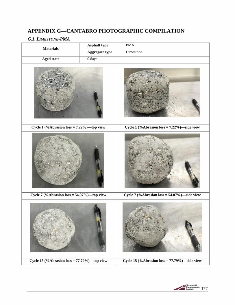
177
APPENDIX G—CANTABRO PHOTOGRAPHIC COMPILATION G.1. LIMESTONE-PMA
Materials Asphalt type PMA
Aggregate type Limestone
Aged state 0 days
Cycle 1 (%Abrasion loss = 7.22%)—top view Cycle 1 (%Abrasion loss = 7.22%)—side view
Cycle 7 (%Abrasion loss = 54.07%)—top view Cycle 7 (%Abrasion loss = 54.07%)—side view
Cycle 15 (%Abrasion loss = 77.79%)—top view Cycle 15 (%Abrasion loss = 77.79%)—side view
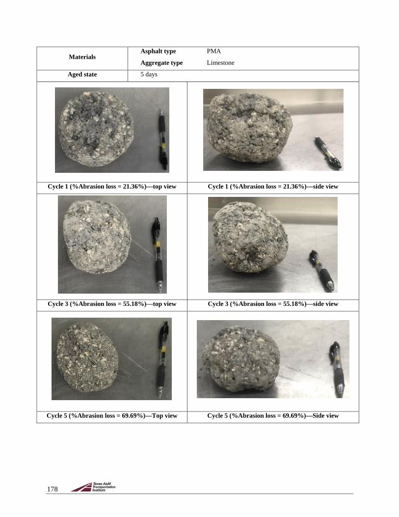
178
Materials Asphalt type PMA
Aggregate type Limestone
Aged state 5 days
Cycle 1 (%Abrasion loss = 21.36%)—top view Cycle 1 (%Abrasion loss = 21.36%)—side view
Cycle 3 (%Abrasion loss = 55.18%)—top view Cycle 3 (%Abrasion loss = 55.18%)—side view
Cycle 5 (%Abrasion loss = 69.69%)—Top view Cycle 5 (%Abrasion loss = 69.69%)—Side view

179
Materials Asphalt type PMA
Aggregate type Limestone
Aged state 10 days
Cycle 1 (%Abrasion loss = 64.92%)—top view Cycle 1 (%Abrasion loss = 64.92%)—side view
Cycle 2 (%Abrasion loss = 80.66%)—top view Cycle 2 (%Abrasion loss = 80.66%)—side view
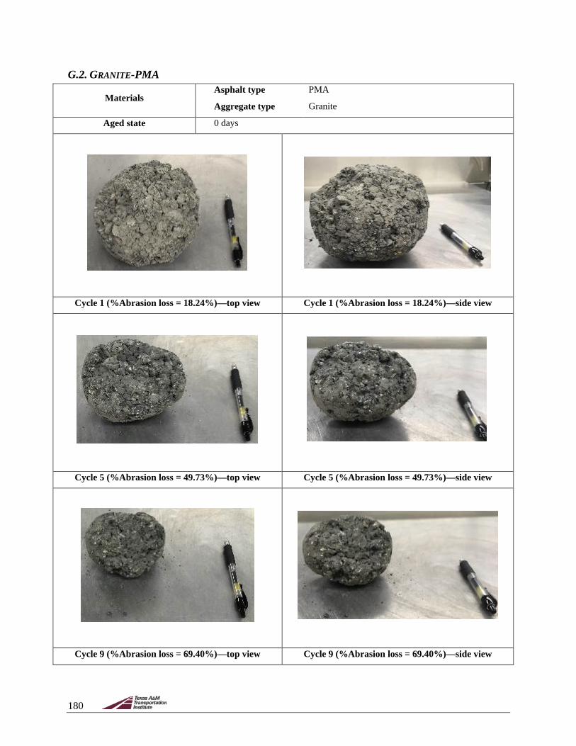
180
G.2. GRANITE-PMA
Materials Asphalt type PMA
Aggregate type Granite
Aged state 0 days
Cycle 1 (%Abrasion loss = 18.24%)—top view Cycle 1 (%Abrasion loss = 18.24%)—side view
Cycle 5 (%Abrasion loss = 49.73%)—top view Cycle 5 (%Abrasion loss = 49.73%)—side view
Cycle 9 (%Abrasion loss = 69.40%)—top view Cycle 9 (%Abrasion loss = 69.40%)—side view

181
Materials Asphalt type PMA
Aggregate type Granite
Aged state 5 days
Cycle 1 (%Abrasion loss = 15.76%)—top view Cycle 1 (%Abrasion loss = 15.76%)—side view
Cycle 5 (%Abrasion loss = 62.43%)—top view Cycle 5 (%Abrasion loss = 62.43%)—side view
Cycle 10 (%Abrasion loss = 81.74%)—top view Cycle 10 (%Abrasion loss = 81.74%)—side view

182
G.3. LIMESTONE-HP
Materials Asphalt type HP
Aggregate type Limestone
Aged state 0 days
Cycle 1 (%Abrasion loss = 3.86%)—top view Cycle 1 (%Abrasion loss = 3.86%)—side view
Cycle 7 (%Abrasion loss = 30.05%)—top view Cycle 7 (%Abrasion loss = 30.05%)—side view
Cycle 15 (%Abrasion loss = 59.33%)—top view Cycle 15 (%Abrasion loss = 59.33%)—side view

183
Materials Asphalt type HP
Aggregate type Limestone
Aged state 5 days
Cycle 1 (%Abrasion loss = 8.08%)—top view Cycle 1 (%Abrasion loss = 8.08%)—side view
Cycle 7 (%Abrasion loss = 45.84%)—top view Cycle 7 (%Abrasion loss = 45.84%)—side view
Cycle 15 (%Abrasion loss = 71.98%)—top view Cycle 15 (%Abrasion loss = 71.98%)—side view
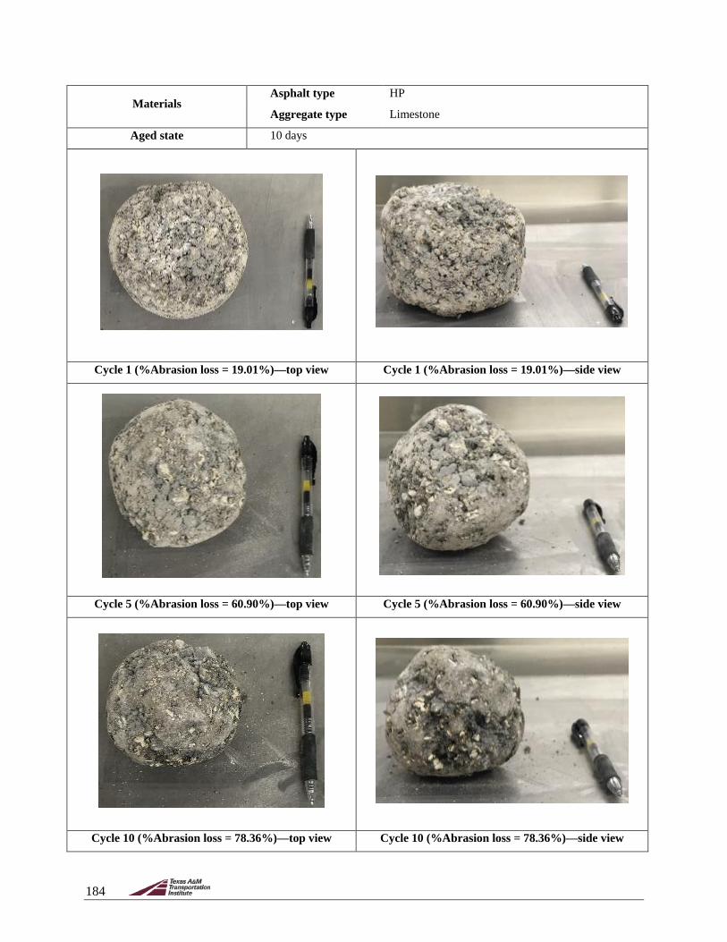
184
Materials Asphalt type HP
Aggregate type Limestone
Aged state 10 days
Cycle 1 (%Abrasion loss = 19.01%)—top view Cycle 1 (%Abrasion loss = 19.01%)—side view
Cycle 5 (%Abrasion loss = 60.90%)—top view Cycle 5 (%Abrasion loss = 60.90%)—side view
Cycle 10 (%Abrasion loss = 78.36%)—top view Cycle 10 (%Abrasion loss = 78.36%)—side view

185
G.4. GRANITE-HP
Materials Asphalt type HP
Aggregate type Granite
Aged state 0 days
Cycle 1 (%Abrasion loss = 4.29%)—top view Cycle 1 (%Abrasion loss = 4.29%)—side view
Cycle 7 (%Abrasion loss = 24.86%)—top view Cycle 7 (%Abrasion loss = 24.86%)—side view
Cycle 15 (%Abrasion loss = 45.08%)—top view Cycle 15 (%Abrasion loss = 45.08%)—side view

186
Materials Asphalt type HP
Aggregate type Granite
Aged state 5 days
Cycle 1 (%Abrasion loss = 10.12%)—top view Cycle 1 (%Abrasion loss = 10.12%)—side view
Cycle 7 (%Abrasion loss = 45.85%)—top view Cycle 7 (%Abrasion loss = 45.85%)—side view
Cycle 15 (%Abrasion loss = 72.93%)—top view Cycle 15 (%Abrasion loss = 72.93%)—side view

187
Materials Asphalt type HP
Aggregate type Granite
Aged state 10 days
Cycle 1 (%Abrasion loss = 14.75%)—top view Cycle 1 (%Abrasion loss = 14.75%)—side view
Cycle 5 (%Abrasion loss = 51.42%)—top view Cycle 5 (%Abrasion loss = 51.42%)—side view
Cycle 9 (%Abrasion loss = 67.46%)—top view Cycle 9 (%Abrasion loss = 67.46%)—side view
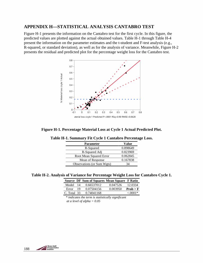
188
APPENDIX H—STATISTICAL ANALYSIS CANTABRO TEST Figure H-1 presents the information on the Cantabro test for the first cycle. In this figure, the predicted values are plotted against the actual obtained values. Table H-1 through Table H-4 present the information on the parameter estimates and the t-student and F-test analysis (e.g., R-squared, or standard deviation), as well as for the analysis of variance. Meanwhile, Figure H-2 presents the residual and predicted plot for the percentage weight loss for the Cantabro test.
Figure H-1. Percentage Material Loss at Cycle 1 Actual Predicted Plot.
Table H-1. Summary Fit Cycle 1 Cantabro Percentage Loss. Parameter Value R-Squared 0.898649
R-Squared Adj 0.823969 Root Mean Squared Error 0.062845
Mean of Response 0.167838 Observations (or Sum Wgts) 34
Table H-2. Analysis of Variance for Percentage Weight Loss for Cantabro Cycle 1. Source DF Sum of Squares Mean Square F Ratio Model 14 0.66537012 0.047526 12.0334 Error 19 0.07504156 0.003950 Prob > F
C. Total 33 0.74041168 <.0001* * indicates the term is statistically significant at a level of alpha = 0.05
0
0.1
0.2
0.3
0.4
0.5
0.6
0.7
0.8%
Mat
eria
l los
s cic
yle
1 Ac
tual
-0.1 0 0.1 0.2 0.3 0.4 0.5 0.6 0.7 0.8
Material loss cicyle 1 Predicted P<.0001 RSq=0.90 RMSE=0.0628

189
Table H-3. Parameter Estimates for Cantabro Cycle 1 Percentage Wight Loss. Term Estimate Std. Error t Ratio Prob>|t|
Intercept 0.5983288 0.44129 1.36 0.1910 Aggregate Type [GR] −0.004116 0.014116 −0.29 0.7738
Binder Type [HP] −0.08938 0.01587 −5.63 <.0001* Aging Condition [A0] −0.112657 0.018027 −6.25 <.0001*
Aging Condition [A10] 0.16514 0.023229 7.11 <.0001* Air Voids (%) −0.021015 0.02249 −0.93 0.3618
Aggregate Type [GR]*Binder Type [HP] 0.0126389 0.012401 1.02 0.3209 Aggregate Type [GR]×Aging Condition [A0] 0.0446927 0.017692 2.53 0.0206*
Aggregate Type [GR] ×Aging Condition [A10] −0.067446 0.018606 −3.62 0.0018* Aggregate Type [GR] × (Air Voids: 19.35%) −0.04732 0.024358 −1.94 0.0670
Binder Type [HP] ×Aging Condition [A0] 0.0306851 0.018382 1.67 0.1114 Binder Type [HP] ×Aging Condition [A10] −0.074688 0.017558 −4.25 0.0004* Binder Type [HP] × (Air Voids: 19.35%) 0.0367253 0.027544 1.33 0.1982
Aging Condition [A0] × (Air Voids: 19.35%) 0.0149392 0.034837 0.43 0.6729 Aging Condition [A10] × (Air Voids: 19.35%) −0.01504 0.040997 −0.37 0.7178
* indicates the term is statistically significant at a level of alpha = 0.05
Table H-4. Effect Tests for Cycle 1 Percentage Weight Loss Cantabro Test. Source Nparm DF Sum of Squares F Ratio Prob > F
Aggregate Type 1 1 0.00033577 0.0850 0.7738 Binder Type 1 1 0.12528380 31.7210 <.0001*
Aging Condition 2 2 0.25285689 32.0108 <.0001* Air Voids (%) 1 1 0.00344838 0.8731 0.3618
Aggregate Type×Binder Type 1 1 0.00410226 1.0387 0.3209 Aggregate Type×Aging Condition 2 2 0.05560550 7.0395 0.0052*
Aggregate Type×Air Voids (%) 1 1 0.01490650 3.7742 0.0670 Binder Type×Aging Condition 2 2 0.07317529 9.2637 0.0016*
Binder Type×Air Voids (%) 1 1 0.00702132 1.7777 0.1982 Aging Condition×Air Voids (%) 2 2 0.00083000 0.1051 0.9008
* indicates the term is statistically significant at a level of alpha = 0.05
Figure H-2. Residual Predicted Plot Cycle 1 Cantabro Test.
-0.10
-0.05
0.00
0.05
0.10
% M
ater
ial l
oss c
icyl
e 1
Resid
ual
-0.1 0 0.1 0.2 0.3 0.4 0.5 0.6 0.7 0.8
% Material loss cicyle 1 Predicted

190
Table H-5, Table H-6, and Table H-7 present the information on the least square means for the aggregate type, binder type, and aging condition, respectively, while Table H-8 and Table H-9 show the information on the combination of aggregate type–binder type and aggregate type–aging condition. Figure H-3 plots the least square means for the percentage weight loss and the aging condition.
Table H-5. Least Square Means Table for Aggregate Type Cantabro Test. Level Least Sq Mean Std. Error Mean GR 0.18757629 0.02135290 0.156244 LS 0.19580796 0.01699757 0.180881
Table H-6. Least Square Means Table for Binder Type Cantabro Test. Level Least Sq Mean Std. Error Mean HP 0.10231202 0.01944856 0.094671 PMA 0.28107224 0.02172068 0.241006
Table H-7. Least Square Means Table for Aging Condition of Cantabro Test. Level Least Sq Mean Std. Error Mean A0 0.07903505 0.01884248 0.083725 A10 0.35683214 0.02957525 0.304270 A5 0.13920920 0.02603399 0.138258
Table H-8. Least Square Means Table for Combination Aggregate Type and Binder Type of Cantabro Test.
Level Least Sq Mean Std. Error GR,HP 0.11083512 0.02861942 GR,PMA 0.26431746 0.03192849 LS,HP 0.09378892 0.02504049 LS,PMA 0.29782701 0.02543170
Table H-9. Least Square Means Table for Combination Aggregate Type and Aging Condition of Cantabro Test.
Level Least Sq Mean Std. Error GR,A0 0.11961189 0.02673398 GR,A10 0.28527063 0.04393187 GR,A5 0.15784635 0.04091905 LS,A0 0.03845820 0.02805528 LS,A10 0.42839365 0.03288936 LS,A5 0.12057204 0.02923384

191
Figure H-3. Least Square Means Plot for Aging Condition and
Percentage Weight Loss of Cantabro Test.
Table H-10 presents the information on the least square means for the Tukey HSD with an α = 0.05 for the percentage weight loss of the first cycle of the Cantabro test. Table H-11 presents the information on the least square means for the combination binder type–aging condition. Figure H-4 illustrates the least square means of the aging condition and the percentage weight loss of material. Finally, Table H-12 presents the least square means table of the Tukey HSD for an alpha of 0.05 for the combination binder type and aging condition.
Table H-10. Least Square Means Table of Tukey HSD with an Alpha of 0.05 for Combination Aggregate Type and Percentage Weight Loss of Cantabro Test.
Level Level1 Least Sq Mean LS,A10 A 0.42839365 GR,A10 A,B 0.28527063 GR,A5 B,C 0.15784635 LS,A5 B,C 0.12057204 GR,A0 C 0.11961189 LS,A0 C 0.03845820
1 Levels not connected by same letter are significantly different.
Table H-11. Least Square Means Table for Combination Binder Type and Aging Condition of Cantabro Test.
Level Least Sq Mean Std. Error HP,A0 0.02034007 0.02739758 HP,A10 0.19276417 0.02988252 HP,A5 0.09383182 0.04254806 PMA,A0 0.13773002 0.02718688 PMA,A10 0.52090010 0.04714721 PMA,A5 0.18458658 0.02860428
0
0.1
0.2
0.3
0.4
0.5
0.6
0.7
0.8
% M
ater
ial l
oss
cicyl
e 1
LS M
eans
A0 A10 A5
Aging Condition
GR
LS
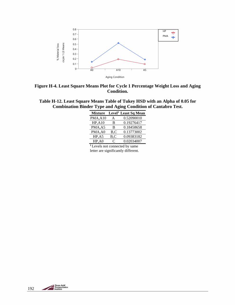
192
Figure H-4. Least Square Means Plot for Cycle 1 Percentage Weight Loss and Aging
Condition.
Table H-12. Least Square Means Table of Tukey HSD with an Alpha of 0.05 for Combination Binder Type and Aging Condition of Cantabro Test.
Mixture Level1 Least Sq Mean PMA,A10 A 0.52090010 HP,A10 B 0.19276417 PMA,A5 B 0.18458658 PMA,A0 B,C 0.13773002 HP,A5 B,C 0.09383182 HP,A0 C 0.02034007
1 Levels not connected by same letter are significantly different.
0
0.1
0.2
0.3
0.4
0.5
0.6
0.7
0.8
% M
ater
ial l
oss
cicyl
e 1
LS M
eans
A0 A10 A5
Aging Condition
HP
PMA

193
APPENDIX I—STATISTICAL ANALYSIS INDIRECT TENSILE STRENGTH TEST Figure I-1 presents the information on the least square fit for the actual and predicted values obtained for the tensile strength for the indirect tensile strength test. Table I-1 presents the information on the summary fit for the tensile strength of the same test. Table I-2 displays the information on the analysis of variance conducted for the same test for the tensile strength. The parameter estimate for the statistical analysis can be observed in Table I-3, while Table I-4 presents the information on the effect test of the statistical analysis. Detailed information on the effect of the different isolated parameters can be observed in Table I-5, Table I-6, Table I-7, and Table I-8, whereas Table I-9, Table I-10, and Table I-11 present the detailed effect of the combination of two parameters. Figure I-2 presents the least square means plotted for the aging condition and tensile strength for the indirect tensile strength.
Figure I-1. Least Square Fit for Actual and Predicted Values of Tensile Strength for
Indirect Tensile Test.
Table I-1. Summary Fit for Tensile Strength of Indirect Tensile Test. Parameter Value R-Squared 0.761707
R-Squared Adj 0.688896 Root Mean Squared Error 54.76332
Mean of Response 471.8441 Observations (or Sum Wgts) 48
Table I-2. Analysis of Variance for Tensile Strength of Indirect Tensile Test. Source DF Sum of Squares Mean Square F Ratio Model 11 345,111.54 31,373.8 10.4613 Error 36 107,964.76 2,999.0 Prob > F
C. Total 47 453,076.29 <.0001* * indicates the term is statistically significant at a level of alpha = 0.05
300
350
400
450
500
550
600
650
700
750
Tens
ile S
treng
th A
ctua
l
300 350 400 450 500 550 600 650 700 750
Tensile Strength Predicted P<.0001 RSq=0.76 RMSE=54.763P<0.0001

194
Table I-3. Parameter Estimate for Tensile Strength of Indirect Tensile Test. Term Estimate Std. Error t Ratio Prob>|t|
Intercept 500.27544 402.237 1.24 0.2216 Aggregate Type [GR] −13.25852 9.25545 −1.43 0.1606
Binder Type [HP] −17.44862 9.447879 −1.85 0.0730 Aging Condition [A0] −54.06924 8.529959 −6.34 <.0001*
Moisture Condition [Dry] 55.43145 8.310548 6.67 <.0001* Air Voids (%) −1.421545 20.10767 −0.07 0.9440
Aggregate Type [GR] ×Binder Type [HP] −8.866855 7.922401 −1.12 0.2705 Aggregate Type [GR] ×Aging Condition [A0] 6.5649082 8.188695 0.80 0.4280
Aggregate Type [GR] ×Moisture Condition [Dry] −20.53218 7.905795 −2.60 0.0135* Binder Type [HP] ×Aging Condition [A0] −9.440921 8.065926 −1.17 0.2495
Binder Type [HP] ×Moisture Condition [Dry] −3.910888 8.292625 −0.47 0.6401 Aging Condition [A0] ×Moisture Condition [Dry] −4.600565 8.447529 −0.54 0.5894
* indicates the term is statistically significant at a level of alpha = 0.05
Table I-4. Effect Test Statistical Analysis for Tensile Strength of Indirect Tensile Test. Source Nparm DF Sum of Squares F Ratio Prob > F
Aggregate Type 1 1 6154.24 2.0521 0.1606 Binder Type 1 1 10229.00 3.4108 0.0730
Aging Condition 1 1 120499.76 40.1797 <.0001* Moisture Condition 1 1 133423.62 44.4891 <.0001*
Air Voids (%) 1 1 14.99 0.0050 0.9440 Aggregate Type*Binder Type 1 1 3756.69 1.2526 0.2705
Aggregate Type×Aging Condition 1 1 1927.56 0.6427 0.4280 Aggregate Type×Moisture Condition 1 1 20228.27 6.7450 0.0135*
Binder Type×Aging Condition 1 1 4108.66 1.3700 0.2495 Binder Type×Moisture Condition 1 1 667.03 0.2224 0.6401
Aging Condition×Moisture Condition 1 1 889.49 0.2966 0.5894 * indicates the term is statistically significant at a level of alpha = 0.05
Table I-5. Detailed Effect for Aggregate Type with Least Square Means for Tensile Strength of Indirect Tensile Test.
Level Least Sq Mean Std. Error Mean GR 458.58561 12.171399 458.245 LS 485.10264 12.171399 485.443
Table I-6. Detailed Effect for Binder Type with Least Square Means for Tensile Strength of Indirect Tensile Test.
Level Least Sq Mean Std. Error Mean HP 454.39550 12.318362 454.761
PMA 489.29275 12.318362 488.927
Table I-7. Detailed Effect for Aging Condition with Least Square Means for Tensile Strength of Indirect Tensile Test.
Level Least Sq Mean Std. Error Mean A0 417.77489 11.629265 417.548 A5 525.91336 11.629265 526.140

195
Table I-8. Detailed Effect for Moisture Condition with Least Square Means for Tensile Strength of Indirect Tensile Test.
Level Least Sq Mean Std. Error Mean Dry 527.27558 11.469298 527.457 Wet 416.41267 11.469298 416.231
Table I-9. Detailed Effect for Combination Aggregate Type and Binder Type with Least Square Means for Tensile Strength of Indirect Tensile Test.
Level Least Sq Mean Std. Error GR,HP 432.27013 15.834064
GR,PMA 484.90108 18.991311 LS,HP 476.52088 18.421272
LS,PMA 493.68441 15.809760
Table I-10. Detailed Effect for Combination Aggregate Type and Aging Condition with Least Square Means for Tensile Strength of Indirect Tensile Test.
Level Least Sq Mean Std. Error GR,A0 411.08128 16.867728 GR,A5 506.08994 16.246928 LS,A0 424.46849 15.817702 LS,A5 545.73679 18.792256
Table I-11. Detailed Effect for Combination Aggregate Type and Moisture Condition with Least Square Means for Tensile Strength of Indirect Tensile Test.
Level Least Sq Mean Std. Error GR,Dry 493.48488 15.989498 GR,Wet 423.68634 17.384856 LS,Dry 561.06627 17.510328 LS,Wet 409.13901 15.947732
Figure I-2. Least Square Means Plot for Tensile Strength and Aging Condition.
300350
400450500
550600650
700750
Tens
ile
Stre
ngth
LS
Mea
ns
A0 A5
Aging Condition

196
Figure I-3 displays the plot for the least square means of the tensile strength versus the moisture condition of the replicates of the indirect tensile test. Table I-12 presents the least square means for the Tukey HSD with an α = 0.05 for aggregate type and moisture condition. Table I-13, Table I-14, and Table I-15 present the least square means for the combination of two parameters.
Figure I-3. Least Square Means Plot for Tensile Strength and Moisture Condition.
Table I-12. Least Square Means Differences Tukey HSD for Aggregate Type and Moisture Condition with Alpha = 0.05.
Mixture Level1 Least Sq Mean LS,Dry A 561.06627 GR,Dry B 493.48488 GR,Wet C 423.68634 LS,Wet C 409.13901
1 Levels not connected by same letter are significantly different.
Table I-13. Least Square Means Table for Binder Type and Aging Condition. Level Least Sq Mean Std. Error HP,A0 390.88534 16.207988 HP,A5 517.90567 17.199567
PMA,A0 444.66443 18.699507 PMA,A5 533.92106 15.812970
Table I-14. Least Square Means Table for Binder Type and Moisture Condition. Level Least Sq Mean Std. Error
HP,Dry 505.91607 16.652679 HP,Wet 402.87494 16.616187
PMA,Dry 548.63508 15.809133 PMA,Wet 429.95041 18.840420
Table I-15. Least Square Means Table for Moisture Condition and Aging Condition. Level Least Sq Mean Std. Error
A0,Dry 468.60577 16.218027 A0,Wet 366.94400 16.053542 A5,Dry 585.94538 18.070092 A5,Wet 465.88135 15.981056
300350
400450500
550600650
700750
Tens
ile
Stre
ngth
LS
Mea
ns
Dry Wet
Replicate #
GR
LS
Moisture Condition