EVALUATION OF FACE RECOGNITION ALGORITHMS ...

EVALUATION OF FACERECOGNITION ALGORITHMS

UNDER NOISE

By

Ansam Almatarneh

A dissertation submitted to the School of Graduate StudiesIn partial fulfillment of the requirements for the degree of

Master of Electrical and Computer EngineeringFaculty of Engineering & Applied ScienceMemorial University of Newfoundland

October 2019

St. John’s, NL

AbstractOne of the major applications of computer vision and image processing is face recog-

nition, where a computerized algorithm automatically identifies a person’s face from

a large image dataset or even from a live video. This thesis addresses facial recogni-

tion, a topic that has been widely studied due to its importance in many applications

in both civilian and military domains. The application of face recognition systems

has expanded from security purposes to social networking sites, managing fraud, and

improving user experience. Numerous algorithms have been designed to perform face

recognition with good accuracy. This problem is challenging due to the dynamic na-

ture of the human face and the different poses that it can take. Regardless of the

algorithm, facial recognition accuracy can be heavily affected by the presence of noise.

This thesis presents a comparison of traditional and deep learning face recognition

algorithms under the presence of noise. For this purpose, Gaussian and salt-and-

pepper noises are applied to the face images drawn from the ORL Dataset. The

image recognition is performed using each of the following eight algorithms: princi-

pal component analysis (PCA), two-dimensional PCA (2D-PCA), linear discriminant

analysis (LDA), independent component analysis (ICA), discrete cosine transform

(DCT), support vector machine (SVM), convolution neural network (CNN) and Alex

Net. The ORL dataset was used in the experiments to calculate the evaluation ac-

curacy for each of the investigated algorithms. Each algorithm is evaluated with two

experiments; in the first experiment only one image per person is used for training,

whereas in the second experiment, five images per person are used for training. The

ii

investigated traditional algorithms are implemented with MATLAB and the deep

learning algorithms approaches are implemented with Python. The results show that

the best performance was obtained using the DCT algorithm with 92% dominant

eigenvalues and 95.25 % accuracy, whereas for deep learning, the best performance

was using a CNN with accuracy of 97.95%, which makes it the best choice under noisy

conditions.

iii

“Thank you my kids, because you gaveme the strength to complete the study”

iv

Table of Contents

Abstract ii

Table of Contents vii

List of Tables viii

List of Figures xi

1 Introduction 1

1.1 Overview . . . . . . . . . . . . . . . . . . . . . . . . . . . . . . . . . . 1

1.2 Main Challenges in Automatic Face Recognition Algorithms . . . . . 4

1.3 Objective of thesis . . . . . . . . . . . . . . . . . . . . . . . . . . . . 5

1.4 Main Contributions of the Thesis . . . . . . . . . . . . . . . . . . . . 7

1.4.1 Taxonomy on Face Recognition . . . . . . . . . . . . . . . . . 7

1.4.2 Effect of Noise on Face Recognition Algorithms . . . . . . . . 8

1.4.3 Compare Traditional Methods to Deep Learning Method . . . 8

1.5 Publications . . . . . . . . . . . . . . . . . . . . . . . . . . . . . . . . 8

1.6 Thesis Organization . . . . . . . . . . . . . . . . . . . . . . . . . . . . 9

2 Literature Review 10

2.1 Introduction . . . . . . . . . . . . . . . . . . . . . . . . . . . . . . . . 10

v

2.2 Surveys Published on Automatic Facial Recognition Algorithms . . . 12

2.3 Examples of Existing Face Recognition Taxonomies . . . . . . . . . . 14

2.3.1 Example one: Multilevel Face Recognition Taxonomy [3]. . . . 14

2.3.2 Example Two: Face Recognition: Status Quo [44] . . . . . . . 20

2.3.3 Example three: Taxonomy of Deep Face Recognition [95] . . . 23

3 Face Recognition Approaches Used in the Study 24

3.1 Introduction . . . . . . . . . . . . . . . . . . . . . . . . . . . . . . . . 24

3.2 Traditional Approach . . . . . . . . . . . . . . . . . . . . . . . . . . 25

3.2.1 Holistic Approach . . . . . . . . . . . . . . . . . . . . . . . . . 26

3.2.1.1 Linear Holistic Approaches . . . . . . . . . . . . . . 29

3.2.1.1.1 Principle Components Analysis (PCA) . . . 30

3.2.1.1.2 2DPCA (two-dimensional PCA) algorithm . 32

3.2.1.1.3 Independent Component Analysis (ICA) . . 37

3.2.1.1.4 Linear Discriminant Analysis (LDA) . . . . 40

3.2.1.2 Non-linear Holistic Approaches . . . . . . . . . . . . 44

3.2.1.2.1 Support Vector Machine (SVM) . . . . . . . 44

3.2.2 Hybrid Approach . . . . . . . . . . . . . . . . . . . . . . . . . 47

3.2.2.1 Discrete Cosine Transform (DCT) . . . . . . . . . . 48

3.3 Deep Learning Methods . . . . . . . . . . . . . . . . . . . . . . . . . 50

3.3.1 Deep Learning-Based Approaches . . . . . . . . . . . . . . . . 50

3.3.2 Convolution Neural Networks (CNN) . . . . . . . . . . . . . . 53

3.3.3 Face Recognition with CNN . . . . . . . . . . . . . . . . . . . 56

4 Comparison of Face Recognition Approaches Under Noise 61

4.1 Introduction . . . . . . . . . . . . . . . . . . . . . . . . . . . . . . . . 61

4.2 Dataset Preparation . . . . . . . . . . . . . . . . . . . . . . . . . . . 62

vi

4.3 Implementation . . . . . . . . . . . . . . . . . . . . . . . . . . . . . . 64

4.4 Experiments . . . . . . . . . . . . . . . . . . . . . . . . . . . . . . . . 64

4.5 Evaluation Metrics . . . . . . . . . . . . . . . . . . . . . . . . . . . . 66

4.6 Noise . . . . . . . . . . . . . . . . . . . . . . . . . . . . . . . . . . . . 66

4.7 Results . . . . . . . . . . . . . . . . . . . . . . . . . . . . . . . . . . . 67

4.7.1 Traditional algorithms . . . . . . . . . . . . . . . . . . . . . . 67

4.7.2 Deep learning . . . . . . . . . . . . . . . . . . . . . . . . . . . 71

4.8 Conclusion and Discussion . . . . . . . . . . . . . . . . . . . . . . . . 78

5 Conclusions and Future Work 81

5.1 Conclusions . . . . . . . . . . . . . . . . . . . . . . . . . . . . . . . . 81

5.2 Future Work . . . . . . . . . . . . . . . . . . . . . . . . . . . . . . . . 83

References 83

vii

List of Tables

2.1 Classification of a selection of representative face recognition solutions

based on the proposed taxonomy. Abbreviations used in this table are

defined in the footnote1 [44]. . . . . . . . . . . . . . . . . . . . . . . . 22

3.1 Backward Propagation vs. Convolution neural network (CNN) . . . . 54

3.2 Public large-scale face datasets [193] . . . . . . . . . . . . . . . . . . 59

4.1 Phase Explanation . . . . . . . . . . . . . . . . . . . . . . . . . . . . 66

4.2 For dominant eigenvalues of 80%. . . . . . . . . . . . . . . . . . . . . 68



4.5 Accuracy of CNN vs AlexNet in different cases . . . . . . . . . . . . . 71

viii

List of Figures

2.1 steps of Face Recognition process [70] . . . . . . . . . . . . . . . . . . 12

2.2 Proposed multi-level face recognition taxonomy [3]. . . . . . . . . . . 14

2.3 Face structure level: (a) global; (b) component +structure; and (c)

component representation face structures [44]. . . . . . . . . . . . . . 15

2.4 Feature support level: Universal feature support with (a) global and

(b) component face structures; Local feature support with (c) global

and (d) component face structures. The square blocks in (c) and (d)

represent the local (spatial) support significant for feature extraction

[44]. . . . . . . . . . . . . . . . . . . . . . . . . . . . . . . . . . . . . 16

2.5 Representative set of four levels of the proposed taxonomy and publi-

cation date of Taxonomy face recognition solutions [44]. . . . . . . . . 17

2.6 Hierarchical Architecture and Taxonomy of Deep Face Recognition [92]. 23

3.1 Categories of the face recognition algorithms studied in the thesis. . . 25

3.2 LBP-based face description [101]. . . . . . . . . . . . . . . . . . . . . 26

3.3 Face recognition algorithms [102] . . . . . . . . . . . . . . . . . . . . 27

3.4 Flow chart of the eigenface-based algorithm [103] . . . . . . . . . . . 29

3.5 Accuracy of Recognition based on Number of training sample [114] . 33

3.6 2DPCA Algorithm Flow chart [115] . . . . . . . . . . . . . . . . . . . 34

3.7 Block Diagram for the Proposed Face Recognition Method [134] . . . 39

ix

3.8 Sample images reconstructed using ICA algorithm (derived from the

ORL face database [132]). . . . . . . . . . . . . . . . . . . . . . . . . 40

3.9 First seven LDA basis vectors shown as p*p images (derived from the

ORL face database [132]). . . . . . . . . . . . . . . . . . . . . . . . . 41

3.10 Test phase of the LDA approach [139]. . . . . . . . . . . . . . . . . . 43

3.11 type of eight classes of binary tree structure [140] . . . . . . . . . . . 45

3.12 face images Binary tree [140] . . . . . . . . . . . . . . . . . . . . . . . 45

3.13 Typical hybrid face representation [145]. . . . . . . . . . . . . . . . . 48

3.14 (a) A face image from ORL database, (b) its DCT transformed image,

and (c) Top-left (low frequency) rectangle carries maximum informa-

tion [150] . . . . . . . . . . . . . . . . . . . . . . . . . . . . . . . . . 49

3.15 Architecture of Alex Net [154] . . . . . . . . . . . . . . . . . . . . . . 54

3.16 Single layer feed forward neural network [155] . . . . . . . . . . . . . 55

4.1 ORL Database [201]. . . . . . . . . . . . . . . . . . . . . . . . . . . . 63

4.2 Training and Testing framework. . . . . . . . . . . . . . . . . . . . . 65

4.3 (a) Sample of original image from ORL dataset, (b) Image with Gaus-

sian noise, and (c) image with salt and pepper noise. . . . . . . . . . 66

4.4 Image corrupted with Gaussian and (b) Image corrupted with salt-and-

pepper [36]. . . . . . . . . . . . . . . . . . . . . . . . . . . . . . . . . 67

4.5 Eigenvalues vs Accuracy for traditional six algorithms in experimental

one with no noise. . . . . . . . . . . . . . . . . . . . . . . . . . . . . . 72


one with adding Gaussian noise. . . . . . . . . . . . . . . . . . . . . . 72


one with adding salt and pepper noise. . . . . . . . . . . . . . . . . . 73

x


two with no noise. . . . . . . . . . . . . . . . . . . . . . . . . . . . . . 74


two with adding Gaussian. . . . . . . . . . . . . . . . . . . . . . . . . 74


two with adding salt and pepper. . . . . . . . . . . . . . . . . . . . . 75

4.11 Deep learning approach vs AlexNet in experiment one and two in case

of no noise. . . . . . . . . . . . . . . . . . . . . . . . . . . . . . . . . 76

4.12 Deep learning approach and AlexNet comparison in experiment one

and two in case of adding Gaussian noise. . . . . . . . . . . . . . . . 76

4.13 Deep learning approach and AlexNet comparison in experiment one

and two in case of adding salt and pepper noise. . . . . . . . . . . . . 77

4.14 Best results of deep learning approach, AlexNet and DCT comparison

under noise. . . . . . . . . . . . . . . . . . . . . . . . . . . . . . . . . 77

xi

List of Acronyms

FR Face Recognition

PCA Principal Component Analysis

2D-PCA Two-Dimensional Principle Components Analysis

LDA Linear Discriminant Analysis

SVM Support Vector Machines

DCT Discrete Cosine Transform

ICA Independent Component Analysis

CNN Convolutional Neural Networks

NN Neural Networks

ORL Olivetti Research Lab

RBF Radial Basis Function

LNMF Local Non-negative Matrix Factorization

NMF Non-negative Matrix Factorization

EBGM Elastic Bunch Graph Matching

3DMM 3D Morphable Model

KED Kernel Extended Dictionary

DP Decision Pyramid

LR Logistic Regression

BPR Bayesian Patch Representation

xii

LSM Local Shape Map

LBP Local Binary Patterns

LPQ Local Phase Quantization

LS-SVM Least Square Support Vector Machine

KLT Karhunen-Loeve Transform

DC Direct Current

DNN Deep Neural Network

ANN Artificial Neural Network

DL Deep learning

LRN Local Response Normalization

SLFFNN Single Layer Feed Forward Neural Network

PDBNN probabilistic decision based neural network

SOM Self Organising Map

RCNN Recurrent Convolution Neural Network

IRCNN Inception Convolutional Recurrent Neural Networks

FCN Fully Convolutional Network

ATM Automated Teller Machine

FDDB Face Detection Data Set and Benchmark

AC Alternate Current

SSD Single Shot Detector

YOLO You Only Look Once

RSA key cryptosystem by Rivest, Shamir, and Adleman in 1978

MTCNN Multi-Task Convolutional Neural Network

R-CNN Region with Convolutional Neural Network

CMS-RCNN Contextual Multi-Scale Region-based CNN

xiii

Chapter 1

Introduction

1.1 Overview

Image processing utilizes a set of algorithms developed to process video footage for

numerous functions such as image and video compression, quality improvement, or

extraction of useful knowledge from the multimedia [1]. Footage can be processed

using either analoge or digital algorithms. Analog image methods are primarily used

for applications like processing hard copies (e.g., pictures and printouts) [2]. On the

other hand, digital image methods use mathematical models to process digital footage

and videos; so, it is usually implemented in exploitation portable computer algorithms

[2].

Facial recognition is one of the most important applications of digital image pro-

cessing. It is essential for verification and identification purposes in many law en-

forcement and commercial applications [3]. For example, a wanted suspect can be

automatically identified from surveillance video footage using a facial recognition sys-

tem from a dataset of suspect photos [4]. Some of the main applications of automatic

face recognition algorithms are as follows:

1

1. Face recognition for security systems. Security is a big issue nowadays more

than ever before. For security purpose, face recognition is able to act as a “key”.

Safety system supported face recognition is often deployed in any place where a

high level of security is required (e.g., banks, airports, schools, offices and air-

ports). Security systems which support faces as a biometric are providing better

results than different biometric systems. Therefore, applying face recognition

capabilities to pc systems could greatly improve the overall security.

2. Face recognition (FR) for access control. To manage the access of individuals

to offices, buildings , laptop systems, airports, ocean ports, email accounts, and

ATM machines, the FR is often used. Therefore, to achieve a very high success

rate for such systems, the quantity of individuals is proscribing, and photos

taken for the image gallery are underneath controlled conditions that prohibit

user contribution. For instance, if the user leaves the system for a specified time,

a design covers the screen. As a result, this system will not check unendingly

who is employing a bound terminal. Thus, access of any unauthorized user

will be denied, whereas the system resumes from the previous session for the

licensed user once they return. Another example, when a person uses an ATM

machines rather than using an ATM card or pass code, the machine would take

an image of the user and then compare it with the one attached to the user’s

bank information to approve access.

3. Face recognition is pervasive computing systems as it refers to the increasing

drift of setting within the microprocessor of existent objects. It is a potential

field where FR will work in the future. Though several machines, like cars, have

such devices installed in them, most of them possess straightforward interfaces

with input on the part of the users. However, considering a bit of human

2

awareness, the pervasive computing could enable devices (like cars) to identify

the character of the person near it.

Although humans can generally perform facial recognition with greater accuracy

than any computer, the human memory is less adept at memorizing a large dataset

of faces, which makes automatic facial recognition algorithms vital [5, 6]. Automatic

facial recognition requires several tasks such as detecting faces in a given image,

extracting facial features, and finally identifying the detected faces using the extracted

features. Over the past twenty years, great deal of research has been carried out to

develop advanced automatic facial recognition algorithms. Most of the existing facial

recognition algorithms fall into two groups: template-based and geometrical feature-

based methods. Template-based algorithms find the correlation between the sample

image and the ones in the dataset to find the nearest match [7]. In geometry based

methods, geometrical features are extracted from the images and, instead of finding

the face, it finds the images with the closest match in feature space.

Statistical tools such as support vector machines (SVM) [8–10], principal com-

ponent analysis (PCA) [11–13], linear discriminant analysis (LDA) [14–16], kernel

techniques [13–16], and artificial neural networks [17, 18] have been widely proposed

and used for automatic facial recognition. These statistical tools can also be used as

hybrid approaches, for example, combination of PCA and radial basis function (RBF)

neural networks [19–21]. Generally, these algorithms map a vector representation of

each face image to a set of images in a dataset. The mapping function is usually a

discriminant function [22, 23] that will result in a positive identification based on a

predefined similarity measure.

3

1.2 Main Challenges in Automatic Face Recogni-

tion Algorithms

The main challenges in popular automatic facial recognition algorithms are described

as follows:

1. Facial expression change: an automatic facial recognition algorithm must be

able to follow facial changes due to the subject’s emotional states [24, 25].

2. Illumination change: Facial images can be recorded under different illumination

levels and hence, automatic facial recognition algorithms must extract features

that are robust to illumination level [26–28].

3. Pose change: Automatic algorithms must be adaptive to the pose of the subject’s

head [29–31].

4. Scaling factor: The new image that is compared with the images in the data

set might have a different size or resolution, and hence an automatic algorithm

must adapt themselves to these kind of differences [32, 33].

5. Obstacles can be either physical obstacles that can occlude the face such as other

objects in the scene, or a subject’s personal obstacles such as glasses, beard or

mustache [34].

6. Noise: The most common problem in automatic face recognition algorithms [35].

Due to its Prevalence, as a part of this thesis, we have investigated its impact

on facial recognition algorithms.

Noise is one of the most common problem in image processing, and it can heavily

affect the performance of facial recognition algorithms, particularly statistical meth-

ods. Two common types of noises that are often found in face images are additive

4

Gaussian noise and salt-and-pepper noise [36]. Gaussian noise is modeled as the sum

of the input signal and a Gaussian distributed noise, whereas the salt-and-pepper is

modelled as random occurrences of spikes in the input signal with random amplitudes

[37]. The level of noise in an image can be reduced by filtering methods. Since Gaus-

sian noise and salt-and-pepper noise affect images in different ways, they cannot be

minimized using the same filters. Gaussian noise is traditionally minimized using av-

eraging filters, while the effect of salt and pepper noise is minimized by median filters.

Both filters minimize the effect of noise in facial images; unfortunately, the averaging

filter can also suppress useful content in images that would affect the performance

of facial recognition algorithms. For example, the averaging filter blurs the images

which results in obscured edges and the resultant loss of important defining features.

Budiman et al. [38] mentioned that the existence of noise in images with varying

illumination has a lower effect on the recognition rate. Moreover, they found that the

effect of noise is more significant and can be easily handled in the recognition rate in

ORL dataset. Their experiments in the ORL dataset showed that some filters could

handle specific noise better than others. In the case of applying salt and pepper noise

to images, the median filter and gaussian filter give 90.35% and 85.80% recognition

rates, respectively. In the case of applying gaussian noise to images the median filter

and gaussian filter give 89.65% and 90.00% recognition rates, respectively. In case of

applying gaussian noise on images the median filter and gaussian filter give (89.65%)

and (90.00%) as a recognition rate, respectively.

1.3 Objective of thesis

This thesis aims to study the performance of face recognition algorithms under noise.

In order to achieve this objective, we study traditional algorithms and recent deep

5

learning algorithms first. We develop a taxonomy for different methods from the

two categories (traditional and deep learning), and then we compare the performance

of these methods under the presence of common noise, namely: Gaussian and salt-

and- pepper. In our proposed taxonomy, face recognition algorithms are the thesis

objectives in detail:

1. Study and discus the existing different face recognition taxonomies. This point

has been done in the thesis in the literature chapter.

2. Detailed comparison for traditional algorithms and deep learning algorithms.

The comparison is based on the mathematical formulation for each algorithm,

the face matrix construction, noise effect, advantages and disadvantages for

each algorithm. This leads to a clear map for face recognition by traditional

algorithms and deep learning algorithms.

3. Detailed study and comparison for accuracy of traditional algorithms and deep

learning algorithms under noise presence. To achieve this point, each algorithm

is evaluated with two experiments where for the training in the first experiment

only one image per person is used and in the second experiment, five images per

person is used [18, 39]. The investigated traditional algorithms are implements

with MATLAB and the deep learning algorithms approaches are implemented

by python, The reason for that is python can be easily integrated with the

most recent deep learning frameworks such as TensorFlow. These frameworks

provide parallel programming in efficient way. The comparison of traditional

and deep learning face recognition algorithms under the presence of Gaussian

and salt-and-pepper noises are applied to the face images drawn from the ORL

Dataset

6

1.4 Main Contributions of the Thesis

1.4.1 Taxonomy on Face Recognition

In this research, we developed a taxonomy for face recognition with categories of

Holistic and Hybrid approaches under traditional approaches and then subsequently

introduced different evaluation for deep learning approaches as follows:

1. Discrete cosine transform (DCT): Commonly used in image compression. In this

survey, we investigated its application for facial recognition problem [40, 41].

2. LDA: A dimensionality reduction technique that is commonly used in different

pattern recognition problems including face recognition [14–16, 42–45].

3. Support vector machine (SVM): Commonly used as a powerful machine learning

tool for classification purposes. SVMs can be either linear or kernel-based [8–

10, 46–48].

4. ICA: Used with applications dealing with multivariate statistical information.

5. PCA: Extracts main features from the data and like LDA, commonly used for

dimensionality reduction [11–13, 49–52].

6. 2D-PCA: A modified version of the PCA techniques [53–56].

7. CNN: A class of deep neural networks, generally applied to analyze visible im-

agery [19–21, 57].

8. AlexNet: An architectural design, composed of nine layers, which was com-

pleted by Alex Krishevsky. The design won an ImageNet Large Scale Visual

Recognition award [58]. This research has been presented previously as [59].

7

1.4.2 Effect of Noise on Face Recognition Algorithms

In this work, the influence of noise on statistical face recognition algorithms including

PCA, 2DPCA, LDA, ICA, and DCT, was investigated. For this purpose, we set

up two different, experiments in which Gaussian noise or salt and pepper noise was

added to the facial images. The results obtained from both experiments show that

the DCT-based algorithm provides the best accuracy of 95.25 %, compared to above

algorithms. In the case of using the strongest eigenvalue 92%, which has the most

dominate information about the object, this will give the maximum accuracy of this

work that has been submitted to “Voice and Vision Processing: New Approaches and

Applications’ Journal.

1.4.3 Compare Traditional Methods to Deep Learning Method

The comparison between traditional algorithms and deep learning algorithms leads

to clear understanding of the performance of each algorithm, and correct choice for

applying each algorithm in different cases and different noise variance. The compari-

son concluded that the accuracy of deep learning is higher than traditional algorithms

with accuracy tends to 99% with 1% error which is high accuracy results until this

time in face recognition. It will help the researchers generate points in how to use

and apply deep learning in face recognition in wide area.

1.5 Publications

• [P1] Ansam Almatarneh and Mohamed S. Shehata, “Facial Recognition Tech-

niques Comparison: Principle Component Analysis (PCA), Two-Dimensional

(2D-PCA), and discrete cosine transform (DCT)”, 26th Annual Newfoundland

Electrical and Computer Engineering Conference (NECEC 2017).

8

• [P2] Ansam Almatarneh and Mohamed S. Shehata, “A Comparison of Facial

Recognition Techniques”, https://easychair.org/publications/preprint/XbLs, July

15, 2018.

• [P3] Ansam Almatarneh and Mohamed S. Shehata, “A Comparison of Facial

Recognition Techniques”, 27th Annual Newfoundland Electrical and Computer

Engineering Conference (NECEC 2018).

• [P4] Ansam Almatarneh, Mohamed S. Shehata, Mohamed H. Ahmad, “Evalu-

ating Statistical Face Recognition Methods Under Noise”, submitted to Voice

and Vision Processing: New Approaches and Applications Journal (2019).

1.6 Thesis Organization

The rest of this thesis is organized as follows:

• Section 2 presents literature review.

• Section 3 face recognition approaches used in the study.

• Section 4 result and discussion.

• Section 5 concludes the thesis research and presents the future work.

9

Chapter 2

Literature Review

2.1 Introduction

Face recognition systems have gained significance in recent years, as they can be ap-

plied to various fields that include entertainment, trading forensics, monitoring and

surveillance. In order to understand the levels of abstraction and landscape of face

recognition, taxonomies of face recognition help in providing a detailed analysis with

evaluating the current state – of -the- art- solutions. This chapter provides a compre-

hensive face recognition taxonomy enriched with different variables, which facilitate

introducing organized categories of solutions for face recognition. In addition, the

taxonomy shall help the researchers in developing further efficient solutions for face

recognition. Face recognitions play a significant role in our daily life. Unfortunately,

this causes dilemma with regard to the ethical and privacy issues relating to how

personal information captured from face recognition shall be used, stored and shared.

According to many definitions, " taxonomy is the practice and science of classifica-

tion of things or concepts, including the principles that underlie such classification"

[60]. The presented multi-level taxonomy includes levels of face structure, feature

10

extraction and feature support. Systems of face recognition have been successfully

introduced universality in various fields with high acceptability [61, 62]. After face

recognition automatic system stands out more than four years ago, the face recogni-

tion field has incredible progress in research [63]. These researches contributed a large

number of face recognition problems in different applications. The research allows us

to classify, organize and abstract the face recognition algorithms which provide two

main advantages.

1. At the present time, it helps more easily analyze the solutions, while establish-

ing a relationship between them, when and provides a deeper knowledge and

conception of the full landscape.

2. It provides best guidance for research directions regarding items such as the

face recognition solutions. Therefore, those items will not be isolated, but items

will be taxonomical network, strengths and weaknesses from their taxonomy

parents and peers and features of inheriting. In addition, it organizes a com-

prehensive overview of current face recognition solutions. This is not an easy

task, as it covers the many variables of face recognition solutions that have

been developed in recent years. Various taxonomies of face recognition have

been introduced [64–75], in order to understand the structure and abstraction

level of face recognition solutions. This chapter proposes a multi-level taxon-

omy which is more comprehensive and focus on face recognition. The following

presented multilevel taxonomy is concerned with four main levels: face struc-

ture, the feature extraction approach, feature support and the sub approach of

feature extraction. Many different approaches are already available to perform

this comparison. However, the basic steps remain the same. The following steps

explain a general automate face recognition model [76].

11

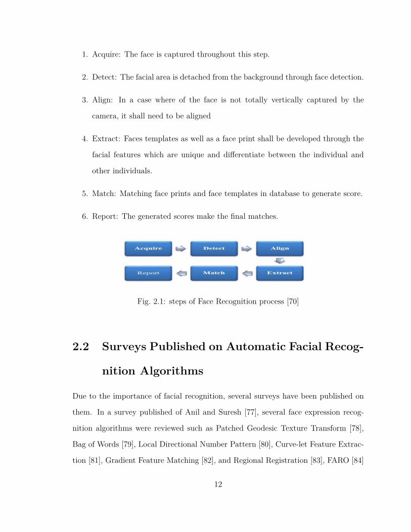
1. Acquire: The face is captured throughout this step.

2. Detect: The facial area is detached from the background through face detection.

3. Align: In a case where of the face is not totally vertically captured by the

camera, it shall need to be aligned

4. Extract: Faces templates as well as a face print shall be developed through the

facial features which are unique and differentiate between the individual and

other individuals.

5. Match: Matching face prints and face templates in database to generate score.

6. Report: The generated scores make the final matches.

Fig. 2.1: steps of Face Recognition process [70]

2.2 Surveys Published on Automatic Facial Recog-

nition Algorithms

Due to the importance of facial recognition, several surveys have been published on

them. In a survey published of Anil and Suresh [77], several face expression recog-

nition algorithms were reviewed such as Patched Geodesic Texture Transform [78],

Bag of Words [79], Local Directional Number Pattern [80], Curve-let Feature Extrac-

tion [81], Gradient Feature Matching [82], and Regional Registration [83], FARO [84]

12

Furthermore, in this survey, several techniques to recognize facial expressions such as

happiness, sadness, fear, surprise, anger, and disgust were presented .

In another survey published by Azeem et al. [85], the effect of partial occlusion

on the performance of face recognition algorithms were studied. These algorithms

mostly employ techniques such as principal component analysis (PCA) [42], local non-

negative matrix Factorization (LNMF) [86], non-negative matrix factorization (NMF)

[87], independent component analysis (ICA) [42], [88, 89], linear discriminate analysis

(LDA) [42, 90], and other variations of these methods. Furthermore, in [3] details

about the experiments, the datasets used, and the results produced after performing

a diverse set of analysis were presented.

Zhou et al. [91] also published a survey on the current state-of-the-art face de-

tectors and their performance on benchmark dataset FDDB [92]. They investigated

the performance of face detection methods such as Haar-like AdaBoost cascade [93]

and HoG-SVM [94] as representatives of traditional methods, and faster R-CNN [95]

and S3FD [96] as deep learning methods on the setting of low-quality images. They

investigated the performance degradation of these algorithms when either the contrast

level or the blur noise is changed. They showed that hand-crafted and deeply learned

features are extremely sensitive and hence, unsuitable for low-quality images. Their

results helped other researchers develop facial recognition algorithms that are more

practical than previous algorithms.

13

2.3 Examples of Existing Face Recognition Tax-

onomies

2.3.1 Example one: Multilevel Face Recognition Taxonomy

[3].

The taxonomy presented in [3] is illustrated in Fig. 2.2 this taxonomy contains four

different levels, which are illustrated below.

Fig. 2.2: Proposed multi-level face recognition taxonomy [3].

1. Face structure

This level illustrates how the recognition solution interacts with face structure,

regarding three classes:

• Global representation which focuses on the face as a whole unit (see Fig.

2.3.a).

• Component structure representation depending on the different elements

14

of the face for example, the eyes, mouth, nose as well as their relationship

(see Fig. 2.3.b).

• Component representation, deals with the selection of specific facial com-

ponent separately without linking it with the other components (see Fig.

2.3.c).

Fig. 2.3: Face structure level: (a) global; (b) component +structure; and (c) compo-nent representation face structures [44].

2. Feature support

This level is concerned with the locational (spatial) support which is considered

for the feature extraction. It can be local or universal. According to Global

feature support which is implies that the area of all selected facial structure

is considered support region for feature extraction, According to full face (Fig.

2.4.a) or a full face component (Fig. 2.4.b). On the other side, the region

of support that of the feature extraction has been viewed as small unit from

the whole face or the (Fig. 2.4.c) or a face component by the local feature

support. In addition, the local regions of support have multiple elements such a

topological standard, overlapping and the size, which simply refers to dividing

the face or the components with squares.

15

Fig. 2.4: Feature support level: Universal feature support with (a) global and (b)component face structures; Local feature support with (c) global and (d) componentface structures. The square blocks in (c) and (d) represent the local (spatial) supportsignificant for feature extraction [44].

3. Feature extraction approach

This level is concerned with the special feature extraction approach which may

be identified as follows [75]

• Appearance based - Statistical transformations from intense data were used

to derive the features.

• Model based -The geometrical elements of the face were used in order to

obtain the features.

• learning based- Features were derived using the learning relationship and

modeling from the inputted data.

• hand-crafted based- Elementary preselected characteristics derived the fea-

tures.

4. Feature extraction sub-approach

The final level within the taxonomy [3] is subordinate to the previous, in order

to identify the exact group of techniques that are used by the selected approach

of feature extraction Fig. 2.5. However, appearance-based Face Recognition

solutions record and map the input data into a lower dimensional space; thus,

16

retaining the most relevant and useful information. Generally, to consider the

face variations, such as occlusions along with scale, pose, and expression changes,

these solutions are sensitive as they do not reflect any specific knowledge about

the structure of the face.

Fig. 2.5: Representative set of four levels of the proposed taxonomy and publicationdate of Taxonomy face recognition solutions [44].

(a) Feature extraction solutions that are based on appearance are divided as

follows:

• Linear solutions, like Principle Component Analysis (PCA) [49] and

Independent Component Analysis (ICA) [50], perform a typical linear

analysis to reach a space with lower dimension in order to exclude the

representative features.

• Non-linear solutions, such as kernel PCA [51], use the structure that

is non-linear in order to achieve a non- linear mapping.

• Multi-linear, such as generalized PCA [52], works on extracting data

from high dimensional data yet preserves its original structure. Con-

sequently, it provides more concentrated representation as compared

to the linear solutions.

17

(b) Model based solutions generate features that are built on the geometric

elements of the face, however, they have less sensitivity to the facial varia-

tions as they are concerned with the structural data from the face. They,

therefore, need accuracy in defining the localization of landmarks before

the feature extraction.

The division of Model based feature extraction solutions is presented as

follows:

• Graph based solutions, such as Elastic Bunch Graph Matching (EBGM)

[97], represent facial feature in the form of a graph as the local informa-

tion of the facial landmarks is stored in nodes. The matching between

these nodes can extract information.

• Shape based solutions, such as the 3D Morphable Model (3DMM)

[98] use landmarks in order to identify facial components. The model

controls landmarks while adopting the functions of shape similarity to

achieve matching.

(c) Learning based: solutions identify features by identifying the relationship

and then modeling them from the inputted data. Compared to different

facial variations could emerge within these solutions. Which is mainly

depend on the given data, however, they can be more flexible than solutions

that depend on the other approaches of face extraction. This is because

they need to tune, train and initialize the hyper parameter.

Recently, solutions with deep learning bases are strongly encouraged for

tasks of face recognition. For instance, deep neural networks dominated

innovative model of face recognition with, Convolutional Neural Networks

(CNNs) being the most significant example.

Solutions of face recognition that are learning based are divided into five

18

technique families which include:

• Deep neural networks, such as the VGG-Face descriptor [99], helps in

handling the input data with high abstraction level and deep processing

layers. This helps in extraction features from this input data.

• Dictionary learning solutions, such as Kernel Extended Dictionary

(KED) [100], based on linear arranged factors helps in feature extrac-

tion from input data.

• Decision tree solutions, for instance the Decision Pyramid (DP) [101],

features are represented as a consequence to a group of decisions

• Regression solutions, such as Logistic Regression (LR) [102], identify

the links between the different factors through adopting the measured

error and compare it with prediction model

• Bayesian solutions, like Bayesian Patch Representation (BPR) [103],

apply the theorem of Bayes in order to extract the features. A proba-

bilistic measure of similarity is then used.

(d) Hand-crafted based solutions conducted features by extracting elements.

Generally, these solutions are not very sensitive to face variations, such

as pose, occlusion, illumination aging, and expression changes. They can

meditate multiple scales, frequency bands, and orientations.

The division of hand- craft based feature extraction solutions is presented

as follows:

• Shape-based: use local shape descriptors to define feature vectors, for

example Local Shape Map (LSM) [104].

• Texture-based: explore structure of local spatial neighborhoods, for

example Local Binary Patterns (LBP) [105].

19

• Frequency-based: explore the local structure from frequency domain,

for example Local Phase Quantization (LPQ) [106]

2.3.2 Example Two: Face Recognition: Status Quo [44]

The work in [64] presented a taxonomy for face recognition solutions and their rep-

resentative, which are organized and sorted depending on the applied face extraction

approach and its subordinate approach while identifying the date when they were

applied.

Table 2.1 presents data about the taxonomy and the performance evaluation that

is suggested.

20

Table 2.1: Classification of a selection of representative face recognition solutions

based on the proposed taxonomy. Abbreviations used in this table are defined in the

footnote1 [44].

22

2.3.3 Example three: Taxonomy of Deep Face Recognition

[95]

In 2014 research focus has developed to deep-learning approaches on the face recogni-

tion performance, such as CNN architectures, include Alex Net [58], VGG-Face [107],

Squeeze Net [108], Google Net [109]. Fig. 2.6 illustrate the Taxonomy added to deep

learning approach; the pipeline explains the flow of deep learning [110].

Fig. 2.6: Hierarchical Architecture and Taxonomy of Deep Face Recognition [92].

Finally, taxonomies with multilevel analysis is more beneficial for a comprehensive

organization and identification the face recognition solutions. Consequently, multi-

level taxonomies have been regarded as considering the two levels of abstraction that

organizes face recognition solutions spicily dependency and matching features, which

are equal to feature extraction [3].

23

Chapter 3

Face Recognition Approaches Used

in the Study

3.1 Introduction

In chapter 2, we presented various examples of current existing taxonomies. In this

chapter we present a suggested taxonomy as shown in Fig. 3.1. This chapter is

concerned with investigating the main three groups which are: holistic (linear and

nonlinear), hybrid, and deep learning-based approach. In addition, these categories

as well as the algorithms that are associated with them shall be introduced.

24

Fig. 3.1: Categories of the face recognition algorithms studied in the thesis.

3.2 Traditional Approach

Despite the great advances that have occurred in the face recognition as various algo-

rithms have been applied, there remain some challenges that needs to be addressed.

These include facial expressions, illumination, face rotation and face occlusion.

Certain visual descriptors are being adapted to solve these challenges. One texture

descriptor which has been used is Local Binary Pattern. (LBP) [111]. This is a

method that depends on pixel-based texture extraction [112]. With the development

of local feature descriptors in other computer vision applications [113], the popularity

of feature-based methods will be increased face recognition. As it can be seen in Fig.

3.2, histograms of LBP descriptors were taken out from local regions and then forming

a global feature vector [114, 115].

25

Fig. 3.2: LBP-based face description [101].

3.2.1 Holistic Approach

In the holistic approach a linear transformation is applied to the face images to con-

vert it into smaller dimensions. This kind of transformations has some significant

drawbacks. The main drawback of linear holistic approaches is that they do not pre-

serve distinctive features. Eigenfaces, Fisher faces, and support vector machines are

important examples of holistic approaches [116]. Fig. 3.3 illustrate the comparison

of PCA (which is the most common technique in face recognition) and other face

recognition techniques based on holistic approaches. Some of the main linear holistic

approaches are represented in Fig. 3.3.

26

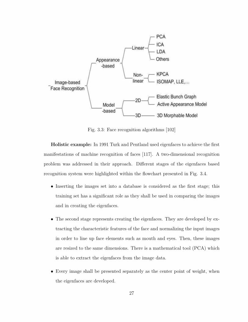
Fig. 3.3: Face recognition algorithms [102]

Holistic example: In 1991 Turk and Pentland used eigenfaces to achieve the first

manifestations of machine recognition of faces [117]. A two-dimensional recognition

problem was addressed in their approach. Different stages of the eigenfaces based

recognition system were highlighted within the flowchart presented in Fig. 3.4.

• Inserting the images set into a database is considered as the first stage; this

training set has a significant role as they shall be used in comparing the images

and in creating the eigenfaces.

• The second stage represents creating the eigenfaces. They are developed by ex-

tracting the characteristic features of the face and normalizing the input images

in order to line up face elements such as mouth and eyes. Then, these images

are resized to the same dimensions. There is a mathematical tool (PCA) which

is able to extract the eigenfaces from the image data.

• Every image shall be presented separately as the center point of weight, when

the eigenfaces are developed.

27

• System indication by accepting the queries of entering or rejection.

• A comparison is made between the weight of the incoming unknown images and

the weight of the other images that are existing on the system. In the case of the

weight of the input images was greater it has to be considered as unidentified.

When the system finds the images, that have a close weight to those images

in the database, the identification of the images is complete. The image input

in the database which has a very close weight shall be kept as a “hit” of the

system’s user [117].

28

Fig. 3.4: Flow chart of the eigenface-based algorithm [103]

3.2.1.1 Linear Holistic Approaches

In these approaches, a linear transformation is applied to the face images to convert

it to smaller dimensions. This kind of transformations has some drawbacks. The

main drawback of linear holistic approaches is that they do not preserve distinctive

features. Some of the main linear holistic approaches are discussed below.

29

3.2.1.1.1 Principle Components Analysis (PCA)

Principle Components Analysis (PCA) is a powerful statistical method and one of

the most popular algorithms used in image processing for decreasing the number of

values in images while keeping unique values needed to identify faces and is useful in

reducing large datasets of images [118]. Before exploring the details of PCA method,

it is important to mention some important mathematical definitions.

This analysis is derived from the transformation of Karhunen ¬Loeve [119, 120].

A representation of s- dimensional vector is given within training image set, PCA

aims to develop a subordinate space of a t-dimension whose vectors are matching the

highest direction of variance in the original space image. The new subordinate space

has usually a lower dimension (t«s). The PCA fundamental vectors are identified as

eigenvectors of the squander matrix in case of the elements of the image are valued

as random variables [120].

In probability theory and statistics, variance measures how far a set of numbers are

spread out from their mean. In the word, variance gives us a measure representing

whether a set of numbers are similar or different [118]. In probability theory and

statistics, covariance is a measure representing how two variables are correlated with

each other. If the covariance is positive, the greater values of one variable mainly

correspond with the greater values of the other variable and vice versa [118].

The basic step in PCA depends on the transformation of Karhumen ¬Loeve [119].

The image could be viewed as an example on a stochastic process, if the elements of

the image were considered as random variables. The PCA basis vectors are indicated

as the eigenvectors of the scatter matrix ST ,[116]

St =N∑

i=1(Xi − µ)(Xi − µ)T (3.1)

30

Where µ is the mean of all images in the training set (the mean face) and Xi is

the ith image with it is columns concatenated in vector.

PCA Training Steps:

1. Normalize the face vector:

Calculate the average the face vector Ψ

Ψ = 1n

M∑i=1

Γi (3.2)

Subtract an average face vector from each face vector (each face image)

Φi = Γi −Ψ (3.3)

2. Reduce the dimensionally of training set.

To calculate eigenvectors, we need calculate covariance matrix C

C = AAT , whereA = [Φ1,Φ2, ...Φi] (3.4)

then

C = N2XN2 (3.5)

Matrix AAT is very large. Must be dimensionally reduction, the solution is

C = ATA (3.6)

then

C = MXM (3.7)

31

3. Calculate eigenvectors Vi from covariance matrix C

ATAVi = µiVi (3.8)

where eigenvectors Vi

eigenvalue µi

“ATA have M eigenvectors

4. Select K best Eigen face, such that K < M and can represent whole training set

select K Eigen face must be in original dimensionally.

5. convert lower dimensionally K eigenvectors to original face dimensionally

ViXA (3.9)

6. represent each face image a linear combination of all K eigenvectors.

3.2.1.1.2 2DPCA (two-dimensional PCA) algorithm

As we look at the PCA technique, we can see that it is very useful in the field

of image recognition and it contains many linear discrimination methods, but there

are some weaken points in the traditional PCA. A new PCA was developed to get

better performance than the traditional one. Increasing data scatter is not enough

to discriminate between clusters, so we present approaches based on new PCA that

consider data labeling and enhances the performance of recognition systems. These

approaches were proved experimentally and were better than traditional PCA and

almost the same complexity. In face recognition, the 2DPCA has been used in large

areas, but it has high sensitivity to outliers, , so a novel robust 2DPCA with F-norm

minimization (F-2DPCA) is proposed to avoid the problem of usual 2DPCA. In face

32

recognition applications, two-dimensional principal component analysis (2DPCA) has

been widely applied [121]. 2DPCA is different from PCA, as it takes a 2D matrix

rather than simply one vector. From the 2D image matrices, the image covariance

matrix is constructed. This makes the image covariance matrix size much smaller.

2DPCA evaluates the matrix mare accurately and efficiently than PCA [122].

The F-2DPCA is robust and rotational invariant, because distance is measured in

F-norm while summation over various data points used 1-norm [53].

As shown Fig. 3.5 when the number of training data increases the accuracy in-

creases accordingly.

Fig. 3.5: Accuracy of Recognition based on Number of training sample [114]

We describe the steps of 2DPCA algorithm in Fig. 3.6 where the flow chart starts

with Face Acquisition and it goes through multiple processing, finally it ends with the

output face image.

PCA, LDA, LPP, NPE are the most common methods in face recognition, ex-

33

Fig. 3.6: 2DPCA Algorithm Flow chart [115]

tracting the most expressive features is done by PCA while LDA is able to extract

discriminating features. LPP and NPE are quite different from PCA and LDA as

they keep on the geometric structure of data.

Tensor (matrix) methods or 2D subspaces learning methods were created. The

two-dimensional subspace learning methods extract features from image matrix di-

rectly and consider the variation among rows and columns which is unlike previ-

ously mentioned methods. The 2DPCA and 2DLDA are contained in the represen-

34

tative two-dimensional methods. Although the 2DPCA and 2DLDA motivations of

two-dimensional methods, they can be unified during the embedding framework also

squared F-norm is used to measure the similarity between images. It is known that

squared F-norm is not robust in the existence of outliers as the outlying measurements

can skew the solution from desired solution [54–56].

The 1-norm subspace-based approach has the ability to obtain robust projection

vectors and it became essential in dimensionality reduction. For example, the use of

L1-PCA was proposed by [123] to measure reconstruction error. In contrast to the

basic property of Euclidean space with 2-norm, the 1-norm is not rotational invariant

[124].

In 2006, Ding et al. proposed the 1-norm rotational invariant for feature extraction

and invented R1-PCA based on the content of learning algorithms [125], that can

measure similarity between data by R1-norm which is 2,1-norm of a matrix. The 1-

norm was extended to p-norm and p-norm was proposed by [125] based on subspace

learning methods [125, 126] to analyze the robustness of subspace learning techniques.

The aforementioned methods cannot well exploit the spatial structure information of

data [93], although they are robust to outliers, they need to change the image form

from 2-D to vector by concatenating all rows of image. To avoid this problem, in 2010,

PCA-L1 was extended to 2DPCAL1 with greedy algorithm [127]. Sparse constraint in

2DPCA-L1 was imposed by [128] and he presented 2DPCAL1-S. 1-norm based tensor

subspace learning was invented [129]. In 2015, 2DPCA-L1with non-greedy algorithm

was developed by [130].

However, all these approaches were developed, yet none were rotational invari-

ant, so they are not adequate for the fundamental goal of PCA because they cannot

measure the error of reconstruction.

To overcome this, robust 2DPCA with F-norm minimization named F-2DPCA

35

for extracting features was used. In this approach, distance as attribute dimension is

measured in F-norm while 1-norm is used for summation over different data points [11].

F-2DPCA is solved by non-greedy iterative algorithm which has a closed form solution

in each single iteration. The neighborhood information during the transformation of

the image into a single vector is not preserved in the Eigenface algorithm that is based

on one-dimensional PCA.

To control such a problem, 2DPCA algorithm based on 2-D images was developed

by [131], that calculates covariance matrix directly. Because the number of 2DPCA

algorithm training samples and its computational complexity is drastically less than

one-dimensional PCA [121], its covariance matrix size is less than one-dimensional

PCA.

2DPCA Training Steps:

In the original 2DPCA method [132], there is only one transformation matrix

computed from one image covariance (scatter) matrix and the dimension of the matrix

can only be reduced from one side. In the complete 2DPCA, let X denote an n-

dimensional unitary column vector. m× n random matrix onto X:

Y = AX (3.10)

variance of each image, is appended to form an array represented by A. get an m-

dimensional projected vector Y which is called the projected feature vector of image

J(s) = tr(Sx) (3.11)

S denotes the covariance matrix of the projected feature vectors of the training sam-

36

ples and tr(Sx) denotes the trace of Sx

Sx = E(Y − EY )(Y − EY )T (3.12)

In summary, 2DPCA algorithm can be described as follows:

1. Computing feature space: N images are sampled by the training image where

each image is decomposed from m rows and n columns pixels, then the mean

(average) of training set and covariance matrix of all images are calculated.

2. Recognition: training image vector for every image is extracted from projected

feature subspace and similarity measurement among two images is shown by the

difference between their projection.

3.2.1.1.3 Independent Component Analysis (ICA) Independent Component

Analysis (ICA) is mostly the same as PCA, except in the distribution of the compo-

nents. In PCA the distribution is designed to be Gaussian, but in ICA it is designed

to be non-Gaussian. ICA depends on minimization of higher order and second order

in the input data (Matrix dimensions), trying to find the basis along the data [133]

For face recognition task, there are two architecture that are provided by [50] of

ICA.

• Architecture I statistically independent basis images,

• Architecture II factorial code representation.

ICA is the general model from which PCA is extracted. With respect to ICA, for

both linear transformation and linear combination, ICA identifies the independent

variables. Because ICA works on higher order statistics, it can provide better data

representation than PCA [134].

37

ICA searches for directions where noticeable concentrations of data are watched

when the source models are sparse in face detection. So, the ICA can be regarded as

a type of cluster analysis when using sparse sources of face recognition [135].

Algorithm: Face determination and Recognition Using Independent

Component Analysis (ICA)[134]

As shown in Fig. 3.7

• Input a video stream (stream of frames).

• Get all frames from the input video sequence and regard the first video frame

as key frame.

• In the key frame, apply the suitable searching algorithm on the face region using

basic face features as mouth and eyes for face determination.

• Then apply the ICA and by combining independent pixels in linear combinations

for definite face recognition.

• Draw the rectangular box for the detected face in the frame.

• Repeat the Step from 3 to 5 till the end of the input video sequence, which

results in the detection and recognition of human face in the video sequence

frame.

38

Fig. 3.7: Block Diagram for the Proposed Face Recognition Method [134]

ICA is used when dealing with multivariate statistical information that is used in

finding covered factors or parts for multidimensional statistical information. For the

case of face images having face orientations in different illumination conditions, we

use ICA as face recognition system.

Performance presented by ICA is better than existing techniques mentioned in

this literature. ICA components are formed from both statistically autonomous and

non-Gaussian [50] which is the main advantage of ICA among other techniques. The

ICA is related to blind source separation problem in the work of Hyvärinen et al.

The use of the ICA for face recognition with massive rotation angles was proposed

by [136] under different illumination conditions. A novel subspace technique was re-

ported by Baek et al. for face recognition named consecutive row column independent

component analysis [137]. Transferring this image into a vector before manipulating

the independent elements is the first step that is carried out for every face image.

There was another technique that was developed by [138] in which both the inno-

vative component analysis model and the optical correlation technique are combined.

In the ICA approach, a collection of random variables is expressed as linear combi-

nations of statistically independent supply variables [139] using linear transformation

that is why ICA attracts attention in linear transformation. The high-order moments

39

of the input are separated by ICA from the second-order moments used in PCA. We

get almost same performance for both approaches.

In Fig. 3.8, it shows ICA factorial code representation. Fast fixed-point algorithm

on which obtained basis vectors are based for that code [140].

Fig. 3.8: Sample images reconstructed using ICA algorithm (derived from the ORLface database [132]).

3.2.1.1.4 Linear Discriminant Analysis (LDA)

LDA is a technique based on linear projection from space of image to low dimensional

space by maximizing the between class scatter and minimizing the within-class scatter,

it achieved great success when applied in face recognition [43].

In LDA, objective evaluation of the significance of visual information in different

features of the face is allowed for recognition. Also, LDA brings us a small set of

features that contain the important information for classification. The LDA approach

overcomes the PCA limitation using the linear discriminant standard.

LDA maximizes the ratio between projected samples between-class scatter matrix

determinant to the projected samples within-class scatter matrix determinant. The

same class images are put together, and the different classes images are separated by

Linear discriminant [45].

The projected test image is compared to each projected training in order to identify

an input test image. This test image is then classified as the closest training image.

Fisher’s criterion is the backbone of this technique in finding a projection A, which is

done by increasing the ratio between-class scatter with respect to within-class scatter

40

(SB and SW, respectively). The original well separated information area will be

linearly transformed into a low-dimensional feature space, and it is provided by LDA.

It must be mentioned that the SW matrix will be singular in face recognition; thus,

traditional LDA can not be applied here because the small sample size obstacle [43–

45]. Generally, LDA is used in reducing dimensionality. There will be many problems

that will stand against traditional LDA in case of dealing with an image with very

high-dimensional data.

For example, if we consider the case in which the face image of size 64*64, it implies

a feature space of 64*64=4096 dimensions; thus, the scatter matrices become of the

size of 4096*4096=16M. Eigenvalues determination is the biggest difficulty as they

are represented in very big matrices. The other challenge is related to the number of

training images that needs to be at least 16M [43],[45].

Face space is constructed by both ICA and PCA without using the face class

(category) information as the whole face training data is taken as a whole. The main

target of LDA is to get an effective method to propose the face vector space. However,

the identification and exploiting the class information is useful in this case. The most

helpful method to discriminate between classes, LDA will be the choice to find the

vectors. All samples of all classes between SW and SB are identified, maximizing

det(SB)/det(SW) ratio is the LDA main target. This is achieved when the projection

matrix column vectors are the eigenvectors of (SW × SB) [43–45], shown Fig. 3.9.

Fig. 3.9: First seven LDA basis vectors shown as p*p images (derived from the ORLface database [132]).

Linear Discriminant Analysis (LDA) Methodology as shown steps on Fig. 3.10:

41

1. A training set consisting of relatively large group of subjects with diverse facial

characteristics is needed. Several examples of face images for each subject in

the training set should be included in the data base which represent different

frontal views of subjects with minor variations in view angle also the test set

should include at least one example.

Assume M is the total number of images, and is equal to K ×N

2. We start by the 2-D intensity array I(x, y) for each image and sub image, then

vector expansion is formed φR(k × n) which points to the face initial repre-

sentation. So, in feature space, all faces are considered as high dimensional

vectors.

Represent the Nx ×Ny. matrices in the form of Ti = Nx ×Ny × 1 vectors.

3. We set a work environment for performing a cluster separation analysis in the

feature space by defining details of the same person’s face as being in one class

and other subject faces being in another different class for all subjects existed in

the training set. We compute the within-class and between-class scatter matrices

after labelling all instances in the training set and defining al the presented

classes.

The testing phase of the Linear Discriminant Analysis is as shown as in Fig.

3.10.

• Subtract the mean of the entire set of images to each face, and then find

the eigenvalues and eigenvectors:

Φi = Γi −1M

(3.13)

42

Fig. 3.10: Test phase of the LDA approach [139].

The covariance matrix:

C = AAT , whereA = [Φ1,Φ2, ...Φi] (3.14)

• To obtain the eigenvalues and eigenvectors of C, the eigenvectors of the

alternative matrix AAT , are obtained, and the eigenvectors of C are given

by ui = A ∗ Vi.

• Each face in the training set (minus the mean) can be represented as a linear

combination of the eigenvectors, with the weights given by Wi = ui × Φi

Each normalized image is then represented as a collection of these weights

W = [Wi...WK ] (3.15)

Once the images are represented in face space by the weights obtained, the

method of linear discriminant can be applied to maximize the ratio of the

43

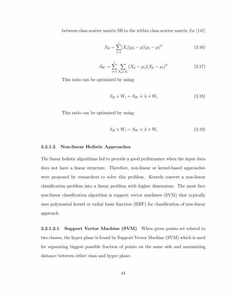
between class scatter matrix SB to the within class scatter matrix Sw [141]

SB =c∑

i=1|Xi|(µi − µ)(µi − µ)T (3.16)

SW =c∑

i=1

∑Xk∈Xi

(Xk − µi)(Xk − µi)T (3.17)

This ratio can be optimized by using:

SB ×Wi = SW × λ×Wi (3.18)

This ratio can be optimized by using:

SB ×Wi = SW × λ×Wi (3.19)

3.2.1.2 Non-linear Holistic Approaches

The linear holistic algorithms fail to provide a good performance when the input data

does not have a linear structure. Therefore, non-linear or kernel-based approaches

were proposed by researchers to solve this problem. Kernels convert a non-linear

classification problem into a linear problem with higher dimensions. The most face

non-linear classification algorithm is support vector machines (SVM) that typically

uses polynomial kernel or radial basis function (RBF) for classification of non-linear

approach.

3.2.1.2.1 Support Vector Machine (SVM) When given points set related to

two classes, the hyper plane is found by Support Vector Machine (SVM) which is used

for separating biggest possible fraction of points on the same side and maximizing

distance between either class and hyper plane.

44

Generally, support vector machine (SVM) deals with problems of two-class clas-

sifications. It belongs to the classifiers of maximum margin type, shown in Fig. 3.11

and 3.12. These classifiers separate two classes by performing pattern recognition

between two classes by finding a decision surface that has maximum distance to the

closest points in the training set which are termed support vectors [46].

Fig. 3.11: type of eight classes of binary tree structure [140]

Fig. 3.12: face images Binary tree [140]

Feature extraction from face images is done first by PCA while discrimination

between each pair of images is then done by means of SVM. Classification task can be

achieved by various means. The case of SVM is different from other methods as it is a

45

machine learning approach in which the classifier is trained well for dealing with face

recognition problems. The SVM takes out the related discriminatory information from

the training data. In SVM, the condition for applying it is that the missing entries

should not be there in the samples defined by feature vectors. It applies to find the

classification hyperplane. We must put into consideration that SVM is presented to

deal with two-class predicament and Face Recognition is not two-class problem, it is

Multi-class problem [48].

Usage of SVM in face recognition comes after extracting facial features, also SVM

can be used individually or with other techniques. As the case of hybrid method in

which ICA extracts facial features and SVM accomplished recognition issue. Using

this technique, we will obtain good results but both ICA and SVM methods are slow

in classification and selecting features. Integrating binary tree recognition approach

with SVM can crack Multi-class FR matter.

Selecting the training sample points with bigger values directly manages Fast

Least Squares SVM quickly locates the optimization classification hyperplanes for

tackling FR [47]. There are different methods, such as 2DPCA, PCA, LDA or angular

LDA, can be considered for feature extraction, most importantly, SVM is used for

classification.

Approaches based on SVM such as global approaches and component-based ap-

proach are effective approaches for face recognition. Least Square Support Vector

Machine (LS-SVM) is considered as one of different methods that can manage face

recognition task successfully with the advantage of fast computational speed with

good recognition rate [47]. Also, component based SVM classifier is regarded as SVM

type used in face recognition.

46

3.2.2 Hybrid Approach

The basic idea behind the hybrid approach is how human eye perceives both local

feature and whole face, there are modular eigenfaces, hybrid local feature, shape

normalized, component-based methods in hybrid approach.

The image taken in 3-D are used in hybrid methods as hybrid FR systems apply

a mixture between holistic and feature extraction methods. The 3D Images manage

the system to detect curves of the eyes and chin and the shape of forehead and many

other details. This is due to the fact that the system used depth and an axis of

measurement which provides adequate information to construct the full face [142].

Detection, Position, Measurement, Representation and Matching are proceeded in

the 3-D system [143].

Detection- catching a face either by scanning photograph or capturing image for the

face at real time.

Position- determining the location, size and angle of the head.

Measurement- each curve in the face is given a measurement to make a template

with high focus on the nose angle, inside the eye and outside the eye.

Representation- transforming the template into a code.

Matching - operation of comparing the received data with those presented in the

data base. In the case of the 3-D images that are compared with the existing 3-D

existing images, there must be no changes. Typically, however, photos that are put

in 2D, and in that case, the 3D image need a few alterations, and this is one of the

hugest challenges in these days [143].

Holistic and feature-based methods are mixed when using hybrid methods, before

the large spread of deep learning, the hybrid methods were the base of most state-

of-the-art face recognition systems. Some hybrid methods are used to combine two

different approaches without occurring any interaction in between. The most common

47

hybrid technique is accomplished by extracting local features (e.g. LBP and projecting

them onto a lower-dimensional and discriminative subspace (e.g. using PCA or LDA).

Different hybrid methods based on Gabor wavelet features combined with different

subspaces methods are proposed [144, 145, 13]. In these methods, the output of Gabor

kernel is convolved with the image and concatenated to form the feature vector. The

feature vector is then down sampled to reduce the dimensionality.

The enhanced linear discriminant model proposed in [146] is used for processing

feature vector [144]. For down sampling the feature vector, PCA followed by ICA

were applied in [145]. Classification whether two images relate to the same subject is

done using the probabilistic reasoning model in [146]. In [13], for encoding high-order

statistics, kernel PCA with polynomial kernels was applied to the feature vector, as

shown Fig. 3.13 [147].

Fig. 3.13: Typical hybrid face representation [145].

3.2.2.1 Discrete Cosine Transform (DCT)

Discrete cosine transform (DCT) is used widely in image processing in general and

face recognition specifically due to high energy compacting [40]. DCT compresses

information of signal in the form of coefficients. As shown in Fig. 3.14.a, DCT is

applied on entire face image shown in Fig. 3.14 a, b and c which gives a low- and high-

frequency coefficients feature matrix of same dimensions. Then, some low frequency

DCT coefficients are selected as a feature vector from each image to construct a feature

space [40].

48

Fig. 3.14: (a) A face image from ORL database, (b) its DCT transformed image, and(c) Top-left (low frequency) rectangle carries maximum information [150]

Face recognition system using the DCT was discussed in a study by [41] including

both geometrical and illumination normalization techniques. This study assumes that

this technique will show high performance for the system better than other approaches

also it claims high recognition rates, and the received results will be compared to

results obtained by holistic approach called Karhunen-Loeve transform (KLT).

Using 49 coefficients in the feature vector, the recognition rate was 84.58%, it

is discovered that the best threshold reached for distance measure between features

would agree the standard of the performance of the system and would give a chance

to be 100% true positives (faces correctly accepted as known) and 0% false positives

(faces incorrectly accepted as known) [41].

The following steps outline the mathematical form of the DCT.

1. Assuming a face image can be considered as a matrix f(x, y) of dimensions

M ×N

2. Then its DCT transform f(u, v) with dimensionsM×N which can be calculated

49

by :

f(u, v) = 1MN

α(u)α(v)×M−1∑x=0

N−1∑y=0

f(x, y)× cos((2x+ 1)uπ2M )cos((2y + 1)vπ

2N )

(3.20)

where

u = 0, 1, 2, ...,M (3.21)

v = 0, 1, 2, ..., N (3.22)

α(w) can be obtained:

a(w) =

1√2 , w < 0

1, otherwise(3.23)

Here, x and y are coordinates in special domain while u and v are the frequency

coordinates in transformed domain. The first coefficient F (1, 1) is named as DC

(Direct Current) while the remaining coefficients are AC (Alternate Current).

The DC coefficient depends on the average image brightness while the AC co-

efficients indicate the amplitude corresponding to the frequency components of

f(x, y) [11].

3.3 Deep Learning Methods

3.3.1 Deep Learning-Based Approaches

In the last few years, deep learning had achieved a very bright success in many areas,

also the machine learning field has a very fast growth rate and is applied to many

traditional and new domains. Based on different classifications of learning, includ-

50

ing supervised, semi-supervised, and un-supervised learning, various approaches have

been presented. Therefore, a brief survey will be presented in this thesis providing

progress occurred in the field of DL taking Deep Neural Network (DNN) as a start.

Deep learning which is based on deep multi-layer neural network can deal with high

dimensional data, when DL is trained on large amount of data, it can effectively detect

large variances of faces, so the most difficult part transformed to capture groups of tiny

faces with variance. Deep learning methods are categorized into three classes, these

three classes are cascade CNN, faster R-CNN [148] and SSD [149] based algorithms.

Some new approaches like generic object detection like YOLO [150], RSA [151], and

UnitBox [152] were developed which are face detectors method with potential base.

Addressing the high computational cost and high variances of face detection was

the reason for proposing cascade CNN [57], the cascaded structure is chosen to remove

simple negative samples at first ages. Joint Cascade CNN [153] and MTCNN [154]

almost have the same work except that they make the detection better by applying

other facial tasks.

For removing samples in various layers within a single CNN, Zhang et al. developed

an ICC-CNN [155]. The fast computation is the best gain of all these approaches,

but also these methods require multi-scale proposals using of discrete image pyramid.

finding crowded, tiny and blurry faces still possess a problem to these approaches.

A scale-invariant detector is applied by algorithms based on Faster R-CNN [148],

[156], [157] or RFCN [158], [159] by extracting features from ROI method of pooling

maps in the higher layer and deploying detectors on top of that.

In faster R-CNN, both the background and the objects will be projected to the

same pixel position in the high-level feature map (this called overlapping) of respective

fields so determining small targets is not the easy task. CMS-RCNN [160] and Deep-IR

[161] integrated features from lower-level convolutional layers to train the detector.

51

Different visual cues used by larger and smaller faces result in utilizing low level

features.

Faster R-CNN based techniques made a great success, but still suffer from slow

computation [162]. Scale-variant detectors on different layers are trained by Algo-

rithms based on SSD [149] to take the best of the multi-scale feature maps like in

SSH [163]. But the SSD is not useful in determining small compact targets. Improv-

ing the matching strategy and anchor densities or assigning layers with specific scale

ranges have proposed S3FD [164], Face Boxes [165], Scale face [166], and HR-ER [167]

to address the anchor mismatching problem and increase the recall rate of tiny faces,

the state-of-the-art recall in FDDB [92] dataset is accomplished by S3FD.In the last

few decades, a small part of artificial intelligence called machine learning has involved

in many several areas. Estimating the model parameters is the main component of

learning procedures so that the learned model can accomplish a specific task. For

example, the parameters are the weight matrices (wi,s) in artificial neural network

(ANN).In DL structure, there are many layers between input and output layer which

permit non-linear processing units for information to present with its hierarchical

architectures which is used in feature learning and pattern categorization [168].

Representations of data on which learning methods are based can also be called

representative learning [168]. It was emphasized in the last literatures that deep

learning based on representative learning imposes features or concept hierarchy, where

the low-level concepts define high level ones and the high-level concepts define the low-

level ones. DL is regarded in some articles as a global technique and can solve almost

all problems types in several domains. In other words, DL is not task specific [168].

52

3.3.2 Convolution Neural Networks (CNN)

Convolution neural network (CNN) has been proposed to train single-hidden layer feed

forward neural networks. A CNN tends to provide good generalization performance at

extremely fast learning speed. AlexNet [58] is a famous architecture of CNN that has

60 million parameters and 500000 neurons. AlexNet was originally trained to classify

the images from 1000 different classes, but it can be re-trained for other applications

using transfer learning mechanism. Transfer learning means training a pre-trained

deep neural network for a different application only by modifying the last layer of

the pre-trained network. This mechanism reduces the required training time as the

parameters of the pre-trained networks have already been learned using millions of

images.

There are two different techniques for Local Response Normalization (LRN) [169]

application:

• First, the LRN is applied on the feature map or on single channel, where N×N

patch are chosen from the same feature map and based one the neighborhood

values, the patch is normalized.

• Second, LRN is applied across the feature maps or channels (neighborhood along

the third dimension but a single location or pixel). There are 3 convolution layers

and 2 fully connected layers in AlexNet.

Computation of the total number of parameters for AlexNet is allowed when pro-

cessing the ImageNet dataset, it can be computed for the first layer as follows: input

samples are 224×224×3, filters (kernels or masks) or a receptive field that has a size

11, the stride is 4, and the output of the first convolution layer is 55×55×96. Accord-

ing to the equations in section 3.1.4, we can calculate that this first layer has 290400

(55× 55× 96) neurons and 364 (11× 11× 3 = 363 + 1bias) weights. The parameters

53

for the first convolution layer are 290400 × 364 = 105705600. The total number of

weights and MACs for the whole network are 61M and 724M respectively.

In general, CNN model consists of six layers in the following order: convolution

layer, max pool layer, convolution layer, max pool layer, fully connected layer and

fully connected layer. AlexNet is deeper than CNN in layer construction, as shown in

Fig. 3.15 and table 3.1. It consists of nine layers as following: convolution layer, max

pool layer, convolution layer, max pool, convolution, convolution, convolution, max

pool and fully connected layer.

Fig. 3.15: Architecture of Alex Net [154]

The Backward Propagation vs. Convolution Neural Network (CNN) comparison:

Algorithms Faster Simpler Less complexity code MultilayerBackward Propagation of Errors X

Convolution Neural Network (CNN) X X X

Table 3.1: Backward Propagation vs. Convolution neural network (CNN)

CNN Methodology:

CNN method is based on a single layer feed forward neural network (SLFNN) as

shown in Fig. 3.16 [170].

54

Fig. 3.16: Single layer feed forward neural network [155]

Suppose that there are N samples (xi, ti) ∈ RnXRm, with L hidden nodes and

activation function g(.). This can be mathematically modeled as

tj =L∑

i=1βg(wi × xj + bi), j = 1, 2, ...N (3.24)

The previous equation could be rewritten in the following form:

T = βH (3.25)

Where, the input-weights matrix W, the bias of hidden layer is b, and the output-

weights are β,

m: the number of hidden neurons

n: the length of input vector (number of features) = number of input neurons

l: the length of output vector = number of output neurons

55

H is the output matrix of hidden layer and defined as:

g(W1.X1 + b1) . . . g(W1.XN + b1)

... . . . ...

g(WM .X1 + bM) . . . g(WM .XN + bM)

(3.26)

CNN could be summarized as follow:

• Randomly assign the input weights matrix WM×N and the bias matrix bmxl.

• Calculate the output matrix H of the hidden layer by 3.26

• Calculate the ouput weight matrix from the following equation:

β = THT (HHT )−1 (3.27)

3.3.3 Face Recognition with CNN

The most popular type of face recognition in deep learning is convolutional neural

networks (CNNs). Deep learning techniques accept training with large amounts of

data for face representation task and this is robust to the training dataset changes.

CNNs can learn specialized features from training instead of designing them.

Training with very huge data sets that contain enough variations to generalize to

unseen samples is the basic disadvantage of deep learning methods. To train CNN

models, large dataset containing face images have been released in the public field [168]

- [171]. In addition to learning discriminative features, CNN used metric learning ap-

proaches for dimensionality reduction. CNNs do not need to be mixed with other

techniques, they are regarded as end-to-end trainable systems. One of the different

approaches that are used in training CNN models consists of treating the problem as

a classification one, where every subject is regarded as a class.

56

After training, subject’s recognition by the model that are not existed in the data

set is accomplished by using the features of the previous layer as the face represen-

tation [172] and discarding the classification layer. These features are referred as

bottleneck features in deep learning. The other techniques, that follows the first

training stage, such as using joint Bayesian [168] or fine-tuning the CNN model with

a different loss function [173, 22, 174–176])can be used for training the model for

enhancing the bottleneck features for the target application.

The most common approach in learning face representation is learning bottleneck

features that is optimizing a distance metric between pairs of faces or triplets of

faces. There was an early method that was proposed in 1997 for face detection, FR,

and eye localization, which is based on a probabilistic decision based neural network

(PDBNN)[177] that was proposed in 1997 for face detection, eye localization and face

recognition, so the idea behind face recognition in neural network is not new.

PDBNN was classified into one fully connected subnet per training subject for

reduction of number of invisible units and overfitting avoiding. Two PBDNNs were

trained using intensity and edge features respectively and the final classification deci-

sion is given from their mixed outputs. There was another early method consisting of

a mixture of a self organising map (SOM) [178] and a convolutional neural network.

A self-organizing map is a sort of neural network that has unsupervised training in

which projection of input data is done onto a lower dimensional space that keeps the

topological properties of the input space. For the two early methods, the proposed

neural network architectures were shallow because none of them was trained end-

to-end. An end-to-end face recognition CNN proposed this method used a siamese

architecture trained with a contrastive loss function [179]. A metric learning proce-

dure is implemented by the contrastive loss whose target is minimizing the distance

between pairs of feature vectors corresponding to the same subject and maximizing

57

the distance between pairs of feature vectors corresponding to different subjects. The

CNN architecture used in this method was shallow and trained using small datasets.

Ground-breaking results were not achieved by any of the methods mentioned above

because of small used training datasets and the low capacity of networks [58].

Once these methods were trained by huge datasets and scaled up, the first deep

learning method for face recognition was developed which is Facebook’s DeepFace

[172] , one of the first CNN-based approaches for face recognition using high capacity

models, achieving an accuracy of 97.35% on the LFW benchmark and minimizing the

error of the previous state-of-the-art by 27%. Two novel contributions were made in

facebook deep face [180, 181]

• build 3-D face modeling on which an essential facial alignment system

• locally connected layers contained in a CNN architecture that will learn various

features from each image region.

Similar results were obtained by the DeepID system [168] using training 60 different

CNNs on patches in which ten regions were comprised. 160 bottleneck features were

extracted during testing from each patch and it is flipped horizontally counterpart

to form a 19,200-dimensional feature vector (160 × 2 × 60). Similar to [172], lo-

cally connected layers are used in the presented CNN architecture. Training a joint

Bayesian classifier [182] on the 19,200- dimensional feature vectors extracted by the

CNNs, gives the verification result. Dataset containing 202,599 face images of 10,177

celebrities [168] is used for system training, show table 3.2.

The accuracy of CNN-based methods for face recognition is affected by three

elements: training data, CNN architecture, and loss function.

Overfitting is prevented by using large datasets which is known in deep learning

applications. As the number of samples per class increases, the trained CNN for

58

Table 3.2: Public large-scale face datasets [193]

classification becomes more definite.

Extracting features generalizing to subjects not existing in the training set is the

most interesting thing about face recognition. The model is exposed to more inter-

class variations via containing large number of subjects in datasets used for face

recognition In [183], the effect of subject number contained in a data set in face

recognition is studied.

According to this effect, the datasets are ordered according to number of images

per subject in a decreasing order, then the CNN model is trained using different

datasets in a gradual manner by increasing subject number. When the first 10,000

subjects with the most images were used for training, best accuracy was obtained. As

number of subject increases, accuracy decreases. A recent advance in the research in

face recognition is the choice of loss function for training CNN based methods. Even

though CNNs trained with SoftMax loss have been very successful [168, 173], it has

been argued that use of loss function for CNN training does not generalize well to

subjects not existed in training set. This is due to the SoftMax loss is encouraged to

learn features that increase inter-class differences but does not minimize intra-class

fluctuations.

There are many network architectures that are common in computer vision such

as such as fast region-based CNN [183] and Xception [184]. Recurrent Convolution

59

Neural Network (RCNN) [185] model was invented in 2015 using recurrent convolution

layers. The mixture of two most popular architectures in the Inception network and

Recurrent Convolutional Network results in the improved version which is named

Inception Convolutional Recurrent Neural Networks (IRCNN) [186], that has better

accuracy than RCNN and almost same network parameters. In 2016, for segmentation

tasks, fully convolutional network (FCN) was developed and it is now popular. There

are recent CNN models containing ladder networks, deeply supervised network and

deep network with stochastic depth [13, 146, 187].

60

Chapter 4

Comparison of Face Recognition

Approaches Under Noise

4.1 Introduction

Computer vision algorithms tackle a number of complex problems in face recognition,

especially noisy imagery. Although the problem definition may be simple, it is chal-

lenging to apply facial recognition systems to noisy images and get accurate results,

because facial recognition accuracy can be heavily affected by the presence of noise.

In this chapter, a comparison of traditional and deep learning face recognition algo-

rithms under the presence of noise are presented and discussed in details in context

of facial recognition. The comparison was performed using each of the following eight

algorithms: principal component analysis (PCA), two-dimensional PCA (2D-PCA),

linear discriminant analysis (LDA), independent component analysis (ICA), discrete

cosine transform (DCT), support vector machine (SVM), convolution neural network

(CNN) and AlexNet. Each algorithm is discussed in details. This chapter summarises

the various aspects of the design and experimental test for each algorithm based on

61

ORL Dataset.

4.2 Dataset Preparation

In this work, the experiment was done using ORL dataset. The database was used

for evaluation and comparison of different algorithms [188]. The ORL dataset is a

popular face recognition dataset that contains a set of face images for 40 persons taken

between April 1992 and April 1994 at Olivetti Research Lab Cambridge University

Engineering Department. It is composed of 400 images (10 poses per person) of size

112 × 92 with 256 grey levels per pixel. Fig. 4.1 shows some sample images from this

dataset. The database images were taken at different positions with different facial

expressions and features (smiling, open eye, closed eye, glasses on and off, etc.), with

varied lighting at different times of day. All images were taken with the same dark

homogenous background. Since the eight algorithms generally require the same scale

of the images and angle of view, ORL database was culled to be suitable for each

algorithm. All images inside the database are the same scale and the same view to be

easy in comparison. The database files are in standard PGM format. The traditional

algorithms have been implemented using Matlab and database format is PGM. For

AlexNet, algorithms have been implemented in Python and the database format is

PMP.

62

Fig. 4.1: ORL Database [201].

63

4.3 Implementation

In this thesis, implementation and testing were performed using Matlab-2016a running

on a desktop with core I5 CPU, 3.20 GHz processor and 8 GB Memory for traditional

approach. We implemented Deep learning using python in TensorFlow and tested on

a PC with a Xeon E5 2.20 GHz CPU and a Titan XP GPU.

4.4 Experiments

This work consists of two experiments. Each experiment consists of two phases, a

training phase to train the classifier in the face recognition method being investigated,

and then a testing phase to test the method’s performance on new face images. The

training phase uses images directly from the ORL dataset without any added noise,

whereas in the testing phase we consider both the cases with no noise added and with

synthesized noise added. Fig. 4.2 shows the two phases used in the experiments.

1. First experiment: Only one image per person used for the training. Thus, the

total number of images used in the training phase is 40 images. During the

testing phase of this experiment, we check three different use-cases for the test

images:

• A test image (different from the training images) is used with no added

noise.

• Gaussian noise is synthesized into the test images and the resulting noisy

images are used for testing.

• Salt-and-pepper noise is added to the test images, similar to the method

for adding Gaussian noise.

64

2. Second experiment: In the second experiment, five images per person are used

for training. Thus, the total number of images in the training phase is 200

images. During the testing, three different use-cases are checked:

• A test image (different from the training images) is used with no added

noise.

• The Gaussian noise is synthesized into to the test images and the result

noisy images are used for testing. The salt and pepper noise is added to

the test images similar to the Gaussian noise.

We added salt and pepper noise with 10 % each. We also add Gaussian noise with

a mean of 0, and sigma2 of 20, Figure 4.3 a, b and c shown three different use cases

from ORL dataset [189–195].

Fig. 4.2: Training and Testing framework.

65

Phase DescriptionImage acquisition Retrieving an image from ORL database

Pre-processing Preprocessing images commonly involves removingbackground noise, scale, dimensioning if needed

Feature extraction In this step, analyze specific facial features.Classification Recognize the face.

Table 4.1: Phase Explanation

Fig. 4.3: (a) Sample of original image from ORL dataset, (b) Image with Gaussiannoise, and (c) image with salt and pepper noise.

4.5 Evaluation Metrics

Accuracy metric for evaluation was used. Accuracy is defined as the number of pre-

dicted correct classes divided by the total number of actual correct classes [5, 6].

A = cL∑k cL

(4.1)

Where A is the accuracy, K is the number of images in the dataset, and CL is the

number of correct labels.

4.6 Noise

Traditional and deep learning methods are some of the earliest and most established

in the area of face recognition. The general idea is to map a vector representation of

each face image to a set of images in a dataset. The mapping function is usually a

66

discriminant function [37, 38, 5, 6, 36] that will result in a positive identification based

on a similarity measure. However, noise can heavily affect the performance of face

recognition methods. Two common noises often found in facial images are Gaussian

(additive noise) which is shown in Fig. 4.4.a, and salt-and-pepper (impulsive noise)

which is shown in Fig. 4.4.b. Gaussian noise is modelled as the sum of the input

signal and Gaussian distribution, whereas salt-and-pepper is modelled as random

occurrences of spikes in the input signal with random amplitudes.

Fig. 4.4: Image corrupted with Gaussian and (b) Image corrupted with salt-and-pepper [36].

4.7 Results

4.7.1 Traditional algorithms

Six traditional algorithms were evaluated for eigenvalues 0 through to 99. Tables 4.2,

4.3, and 4.4 shows the results of the two experiments for the six traditional algorithms

67

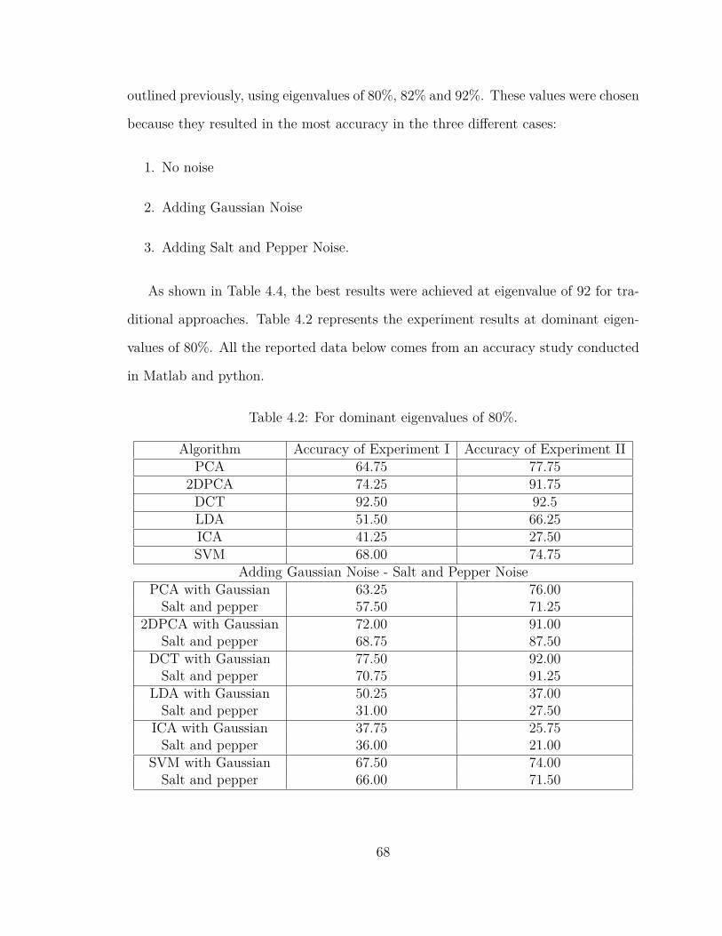
outlined previously, using eigenvalues of 80%, 82% and 92%. These values were chosen

because they resulted in the most accuracy in the three different cases:

1. No noise

2. Adding Gaussian Noise

3. Adding Salt and Pepper Noise.

As shown in Table 4.4, the best results were achieved at eigenvalue of 92 for tra-

ditional approaches. Table 4.2 represents the experiment results at dominant eigen-

values of 80%. All the reported data below comes from an accuracy study conducted

in Matlab and python.

Table 4.2: For dominant eigenvalues of 80%.

Algorithm Accuracy of Experiment I Accuracy of Experiment IIPCA 64.75 77.75

2DPCA 74.25 91.75DCT 92.50 92.5LDA 51.50 66.25ICA 41.25 27.50SVM 68.00 74.75

Adding Gaussian Noise - Salt and Pepper NoisePCA with Gaussian 63.25 76.00Salt and pepper 57.50 71.25

2DPCA with Gaussian 72.00 91.00Salt and pepper 68.75 87.50

DCT with Gaussian 77.50 92.00Salt and pepper 70.75 91.25

LDA with Gaussian 50.25 37.00Salt and pepper 31.00 27.50

ICA with Gaussian 37.75 25.75Salt and pepper 36.00 21.00

SVM with Gaussian 67.50 74.00Salt and pepper 66.00 71.50

68

The accuracy of six algorithms was calculated at dominant eigenvalues of 82% as

shown in table 4.3 in the three cases. The accuracy was presented for experiment I

and II which can be used for comparison.


Algorithm Accuracy of Experiment I Accuracy of Experiment IIPCA 65.00 78.50

2DPCA 74.50 92.50DCT 77.00 92.75LDA 53.00 66.75ICA 39.00 28.75SVM 70.25 78.00







69


Algorithm Accuracy of Experiment I Accuracy of Experiment II2DPCA 73.00 94.75DCT 75.25 95.25LDA 58.25 84.25ICA 54.75 48.00SVM 74.50 89.75







70

4.7.2 Deep learning

Table 4.5 represent the accuracy compassion in experiment I and II for CNN (No noise,

adding Gaussian noise and adding salt-and-pepper noise) and the accuracy results for

AlexNet (No noise, adding Gaussian noise as well as salt-and-pepper noise).

Table 4.5: Accuracy of CNN vs AlexNet in different cases

Algorithm Accuracy of Experiment I Accuracy of Experiment IICNN(without Noise) 59 99.50

Gaussian 55.49 97.95Salt and pepper 45.50 95.25

AlexNet (without Noise) 57.49 96.99Gaussian 57.00 95.99

Salt and pepper 45.99 95.00

Fig. 4.5 illustrates the effect of eigenvalues changing on the accuracy of PCA,

2DPCA, DCT, LDA, ICA and SVM algorithms during experiment one with no noise

adding. As shown in Fig. 4.6, the comparison of six algorithms were represented as

well for experiment one but in case of adding Gaussian noise. Fig. 4.7 illustrates the

test results of experiment one for eigenvalues vs accuracy for traditional six algorithms.

71

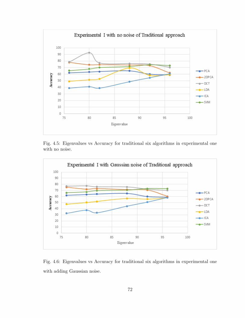
Fig. 4.5: Eigenvalues vs Accuracy for traditional six algorithms in experimental onewith no noise.

Fig. 4.6: Eigenvalues vs Accuracy for traditional six algorithms in experimental one

with adding Gaussian noise.

72

Fig. 4.7: Eigenvalues vs Accuracy for traditional six algorithms in experimental one

with adding salt and pepper noise.

Fig. 4.8, 4.9, and 4.10 illustrate the effect of changing eigenvalues on the accuracy

of PCA, 2DPCAD, DCT, LDA, ICA and SVM algorithms during experiment two in

different three cases (with no noise, Gaussian and salt-and-pepper)

73

Fig. 4.8: Eigenvalues vs Accuracy for traditional six algorithms in experimental two

with no noise.


with adding Gaussian.

74


with adding salt and pepper.

The accuracy of deep learning and AlexNet were represented in Figures 4.11,

4.12 and 4.13. Figure 4.11 illustrates the accuracy comparison of deep learning and

AlexNet in experiment one and two in case of no noise. Figure 4.12 illustrates the

accuracy comparison in case of adding Gaussian noise and Figure 4.13 illustrates the

accuracy comparison in case of adding Salt and pepper noise. Figure 4.14 illustrates

the best results of accuracy for deep learning approach, AlexNet and DCT comparison

under noise.

75

Fig. 4.11: Deep learning approach vs AlexNet in experiment one and two in case of

no noise.

Fig. 4.12: Deep learning approach and AlexNet comparison in experiment one and

two in case of adding Gaussian noise.

76

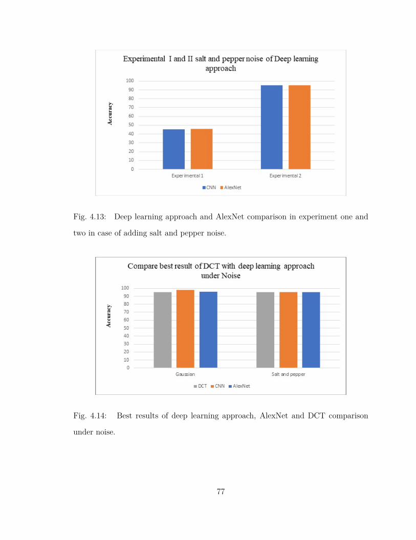
Fig. 4.13: Deep learning approach and AlexNet comparison in experiment one and

two in case of adding salt and pepper noise.

Fig. 4.14: Best results of deep learning approach, AlexNet and DCT comparison

under noise.

77

4.8 Conclusion and Discussion

This last section summarizes the conclusions about face recognition techniques and the

effect of noise on the performance of different techniques. This chapter discussed the

technical aspects of using traditional and deep learning algorithms face recognition

under noise. Each of the eight algorithms had been discussed in details, with the

mathematical form for each algorithm represented as well. Machine learning (neural

networks) was discussed in terms of the number of layers, input layers, hidden layers

and output layer. The ORL database used for experimental data was explained as

well. Face recognition was carried out in two experiments. Each experiment was

implemented for three cases: no noise, added Gaussian noise, and added salt-and-

pepper noise. The performance of each algorithm was measured by the accuracy of

the algorithm. The accuracy of traditional algorithms was obtained and represented

previously in Tables 4.2 – 4.4 and Fig. 4.5 – Fig. 4.10 with dominant eigenvalues of

80%, 82% and 92%. The accuracy of deep learning approach CNN and AlexNet were

carried out in two experiments (experiment one and two), again with three cases in

each: no noise, added Gaussian noise, and added salt-and-pepper noise. The results

of these algorithms illustrated in table 4.4 and Fig. 4.8 – Fig. 4.10. In case of no

noise, it was noticed that DCT is the higher accuracy value with 92.25 % and ICA

is the lowest one with accuracy 41.25. Also, 2DPCA is higher than PCA but with

small change in accuracy with ratio tends to 10%. And the same eigenvalue but

adding Gaussian Noise - Salt and Pepper Noise. It was noticed that the accuracy

of all algorithms in case of Gaussian noise is higher than Salt and pepper noise. In

case of noise with dominant eigenvalues of 80%, the accuracy of DCT is the highest

accuracy with 92% and ICA is the lowest. But in experiment two the value of 2DPCA

is higher than PCA with a 15%. And In case of adding Gaussian Noise and Salt-and-

Pepper Noise, it was noticed that the accuracy of all algorithms in case of Gaussian

78

noise is higher than Salt and pepper noise. Comparing experiment I accuracy results

with experiment II accuracy results in traditional algorithms in case of no noise, it was

noticed that the accuracy of experiment II for all algorithms is higher than experiment

I except ICA. And the same value of eigenvalues but Adding Gaussian Noise - Salt and

Pepper Noise, it was noticed that the accuracy in experiment two was also higher than

accuracy in experiment one except ICA and LDA around 10% to 13%, it was less than

experiment one with 3%. It comes an acceptable value for LDA and normal because

LDA mainly reduce dimensionality of the face. Related with the face recognitions

traditional algorithms the following facts worth to notice at dominant eigenvalues of

82% in experiment one. In case of no noise, accuracy of DCT is the highest accuracy

compared to five algorithms with accuracy 77 %. it was noticed that when changing

the Eigen values from 80% to 82%, the accuracy of DCT changed from 92.25% to

77%. Like the previous accuracy values at 80%, ICA is the lowest accuracy with

value 39%, in case of adding Gaussian noise the best Accuracy of DCT is 76% which

is the highest accuracy compared with another traditional algorithm. And case of

adding salt and pepper noise also, DCT the highest value of 71.75 % and ICA is the

lowest value with 32.50%. In case of no noise with dominant eigenvalues of 82%, the

accuracy of DCT is 92.75 % and ICA 28% which is the lowest accuracy compared to

the rest of traditional algorithms, in case of adding Gaussian noise, the accuracy of

DCT and 2DPCA are the same accuracy with 92%. And in case of adding salt and

pepper noise, the accuracy of DCT is 92% which is best value. Related with the face

recognitions traditional algorithms the following facts worth to notice at dominant

eigenvalues of 92% in experiment one: In case of no noise, DCT is the highest value

of 75.25% and ICA is the lowest accuracy results with 54.75. When adding Gaussian

noise, the SVM best accuracy decrease to 73% and DCT 70.25 % in case of salt-and-

pepper noise. On experimental two all cases of notice at dominant eigenvalues of 92%,

79

the DCT recorded accuracy around 95.25 which is the highest accuracy of noises and

without noise. Related with the face recognitions traditional algorithms the following

facts worth to notice at different dominant eigenvalues in experiment one and two:

DCT was always the highest one at different eigenvalues in experiment one and two

and ICA is the lowest one. It noticed and highlighted that the accuracy of the DCT

algorithm at different Eigenvalues is the highest value compared to SVM, LDA, PCA

,2DPCA and ICA.

Convolutional neural networks (CNNs) with AlexNet

In this experiment, the CNN model for face recognition has been tested using

AlexNet, which is a popular network architecture for face recognition. The interme-

diate representations through stride convolutions and max-pooling layers in AlexNet

results in very rapid down sampling, which is one of the main characteristics of the

network. The faces of ORL dataset are fed as an input for AlexNet. The accuracy of

CNN using AlexNet architecture has been obtained. It was noticed that the CNN in

all cases is the best algorithm. The accuracy of CNN, all cases in experiment two is

better than of all cases in experimental one, because the CNN Works better when in-

creasing the number of images trained. And we note that it has achieved success and

accuracy in the cases of noise, when adding Gaussian is 97.95% and salt-and-pepper

is 95.25%.

80

Chapter 5

Conclusions and Future Work

5.1 Conclusions

Face recognition is important in many fields such as image processing, computer

vision, pattern recognition, and neural networks. Therefore, it has received a high

amount of attention in recent years. In face recognition, there are many obstacles

and challenges that make it difficult to reliably find high-speed solutions. One of

these obstacles is image noise, which effects the accuracy of any algorithm for face

recognition.

Nowadays, modern technology has reached new heights in developing new face

recognition algorithms such as neural networks, CNN, AlexNet, etc. to combat noise

previously challenging to early traditional algorithms such as principal component

analysis (PCA), two-dimensional PCA (2D-PCA), linear discriminant analysis (LDA),

independent component analysis (ICA), discrete cosine transform (DCT) and support

vector machine (SVM).

In this thesis, the influence of noise on traditional face recognition algorithms

including PCA, 2DPCA, LDA, ICA, and DCT and SVM modem algorithms (con-

81

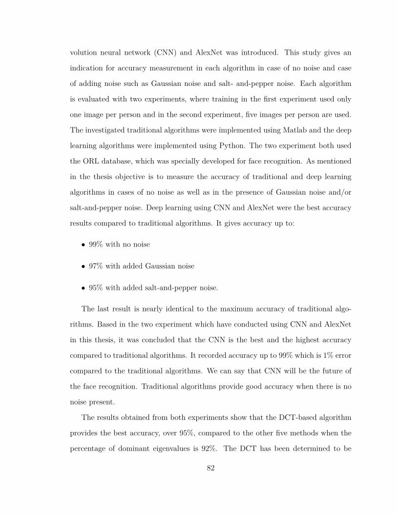
volution neural network (CNN) and AlexNet was introduced. This study gives an

indication for accuracy measurement in each algorithm in case of no noise and case

of adding noise such as Gaussian noise and salt- and-pepper noise. Each algorithm

is evaluated with two experiments, where training in the first experiment used only

one image per person and in the second experiment, five images per person are used.

The investigated traditional algorithms were implemented using Matlab and the deep

learning algorithms were implemented using Python. The two experiment both used

the ORL database, which was specially developed for face recognition. As mentioned

in the thesis objective is to measure the accuracy of traditional and deep learning

algorithms in cases of no noise as well as in the presence of Gaussian noise and/or

salt-and-pepper noise. Deep learning using CNN and AlexNet were the best accuracy

results compared to traditional algorithms. It gives accuracy up to:

• 99% with no noise

• 97% with added Gaussian noise

• 95% with added salt-and-pepper noise.

The last result is nearly identical to the maximum accuracy of traditional algo-

rithms. Based in the two experiment which have conducted using CNN and AlexNet

in this thesis, it was concluded that the CNN is the best and the highest accuracy

compared to traditional algorithms. It recorded accuracy up to 99% which is 1% error

compared to the traditional algorithms. We can say that CNN will be the future of

the face recognition. Traditional algorithms provide good accuracy when there is no

noise present.

The results obtained from both experiments show that the DCT-based algorithm

provides the best accuracy, over 95%, compared to the other five methods when the

percentage of dominant eigenvalues is 92%. The DCT has been determined to be

82

the suitable approach in traditional algorithms for face recognition both when no

noise is present or when noise is added, based on this research results. It should

be highlighted that, when changing the eigenvalues, DCT is always the highest one

in accuracy compared to six traditional algorithms. Also, the accuracy of all eight

algorithms is higher in case of added Gaussian noise when compared to salt-and-

pepper noise.

5.2 Future Work

1. we will investigate face recognition problem with deeper network such as VGG16

and other architecture such as inception network.

2. more noises will be added to investigate the robustness of face recognition algo-

rithms such as Speckle noise as well as Gaussian and salt-and-pepper with each

other at the same time.

3. we will use benchmark large-scale and more data cleaning methods such as

whitening. More hyperparameters setting will be investigated to study the effect

of each one on the performance.

4. The comparison of face recognition algorithms metrics such as performance met-

rics, computational time and complexity will be investigated on the future work.

83

References

[1] J. C. Russ, The image processing handbook. CRC press, 2016.

[2] A. M. Tekalp, Digital video processing. Prentice Hall Press, 2015.

[3] A. K. Jain and Z. L. Stan, Handbook of face recognition. New York: springer,

2011.

[4] A. Mike Burton, S. Wilson, M. Cowan, and V. Bruce, “Face recognition in

poor-quality video; evidence from security surveillance,” Psychological Science,

vol. 10, 05 1999.

[5] S. Z. Li, Xin Wen Hou, Hong Jiang Zhang, and Qian Sheng Cheng, “Learning

spatially localized, parts-based representation,” vol. 1, pp. I–I, Dec 2001.

[6] V. Kazemi and J. Sullivan, “One millisecond face alignment with an ensemble

of regression trees,” pp. 1867–1874, June 2014.

[7] R. J. Baron, “Mechanisms of human facial recognition,” International Journal

of Man-Machine Studies, vol. 15, pp. 137–178, 08 1981.

[8] G. Guo, S. Z. Li, and K. Chan, “Face recognition by support vector machines,”

pp. 196–, 2000. [Online]. Available: http://dl.acm.org/citation.cfm?id=795661.

796198

84

http://dl.acm.org/citation.cfm?id=795661.796198


[9] P. J. Phillips, “Support vector machines applied to face recognition,” Advances

in Neural Information Processing Systems, vol. 11, 12 2001.

[10] J. Huang, X. Shao, and H. Wechsler, “Face pose discrimination using support

vector machines (svm),” vol. 1, pp. 154–156 vol.1, Aug 1998.

[11] Jian Yang, D. Zhang, A. F. Frangi, and Jing-yu Yang, “Two-dimensional pca: a

new approach to appearance-based face representation and recognition,” IEEE

Transactions on Pattern Analysis and Machine Intelligence, vol. 26, no. 1, pp.

131–137, Jan 2004.

[12] R. Gottumukkal and V. Asari, “An improved face recognition technique based

on modular pca approach,” Pattern Recognition Letters, vol. 25, pp. 429–436,

03 2004.

[13] Chengjun Liu, “Gabor-based kernel pca with fractional power polynomial mod-

els for face recognition,” IEEE Transactions on Pattern Analysis and Machine

Intelligence, vol. 26, no. 5, pp. 572–581, May 2004.

[14] W. Zhao, R. Chellappa, and A. Krishnaswamy, “Discriminant analysis of princi-

pal components for face recognition,” in Proceedings Third IEEE International

Conference on Automatic Face and Gesture Recognition, April 1998, pp. 336–

341.

[15] W. Zhao, R. Chellappa, and P. Phillips, “Subspace linear discriminant analysis

for face recognition,” Tech. Rep., 1999.

[16] Juwei Lu, K. N. Plataniotis, and A. N. Venetsanopoulos, “Face recognition using

kernel direct discriminant analysis algorithms,” IEEE Transactions on Neural

Networks, vol. 14, no. 1, pp. 117–126, Jan 2003.

85

[17] X. Li and S. Areibi, “A hardware/software co-design approach for face recogni-

tion,” 01 2005, pp. 55 – 58.

[18] A. Kaushal and J. P. S. Raina, “Face detection using neural network and gabor

wavelet transform,” International Journal of Computer Science and Technology,

vol. 1, Sep 2010.

[19] O. S. Kwun, Y. S. Hoon, and P. Witold, “Design of face recognition algorithm

using pca and lda combined for data pre processing and polynomial based rbf

neural networks,” Expert Systems with Applications, vol. 40, p. 1451–1466, 04

2013.

[20] J. Haddadnia, K. Faez, and M. Ahmadi, “A fuzzy hybrid learning algorithm

for radial basis function neural network with application in human face recog-

nition,” Pattern Recognition, vol. 36, pp. 1187–1202, 2003.

[21] E. Gumus, N. Kilic, A. Sertbas, and O. N. Ucan, “Evaluation of

face recognition techniques using pca, wavelets and svm,” Expert Syst.

Appl., vol. 37, no. 9, pp. 6404–6408, Sep. 2010. [Online]. Available:

http://dx.doi.org/10.1016/j.eswa.2010.02.079

[22] M. Naeem, I. Qureshi, and F. Azam, “Face recognition techniques and ap-

proaches: A survey,” Science International (Lahore), vol. 27, pp. 301–305, 02

2015.

[23] P. F. D. Carrera and I. Marques, “Face recognition algorithms,” Masters thesis

in Computer Science, Universidad Euskal Herriko, 2010.

[24] Kyong I. Chang, K. W. Bowyer, and P. J. Flynn, “Multiple nose region matching

for 3d face recognition under varying facial expression,” IEEE Transactions on

86

http://dx.doi.org/10.1016/j.eswa.2010.02.079

Pattern Analysis and Machine Intelligence, vol. 28, no. 10, pp. 1695–1700, Oct

2006.

[25] Y. . Tian, T. Kanade, and J. F. Cohn, “Recognizing action units for facial

expression analysis,” IEEE Transactions on Pattern Analysis and Machine In-

telligence, vol. 23, no. 2, pp. 97–115, Feb 2001.

[26] Y. Adini, Y. Moses, and S. Ullman, “Face recognition: the problem of com-

pensating for changes in illumination direction,” IEEE Transactions on Pattern

Analysis and Machine Intelligence, vol. 19, no. 7, pp. 721–732, July 1997.

[27] Y. Moses, Y. Adini, and S. Ullman, “Face recognition: the problem of compen-

sating for changes in illumination direction,” in ECCV, 1994.

[28] U. Park, Y. Tong, and A. K. Jain, “Age-invariant face recognition,” IEEE Trans-

actions on Pattern Analysis and Machine Intelligence, vol. 32, no. 5, pp. 947–

954, May 2010.

[29] A. C. Lamont, S. Stewart-Williams, and J. Podd, “Face recognition and aging:

effects of target age and memory load.” Memory and cognition, vol. 33 6, pp.

1017–24, 2005.

[30] F. L. Krouse, “Effects of pose, pose change, and delay on face recognition per-

formance,” Journal of Applied Psychology, vol. 66, pp. 651–654, 10 1981.

[31] R. H. Logie, A. D. Baddeley, and M. M. Woodhead, “Face recognition,

pose and ecological validity,” Applied Cognitive Psychology, vol. 1, no. 1, pp.

53–69, 1987. [Online]. Available: https://onlinelibrary.wiley.com/doi/abs/10.

1002/acp.2350010108

87

https://onlinelibrary.wiley.com/doi/abs/10.1002/acp.2350010108

https://onlinelibrary.wiley.com/doi/abs/10.1002/acp.2350010108

[32] A. M. Bronstein, M. M. Bronstein, and R. Kimmel, “Expression-invariant 3d

face recognition,” pp. 62–70, 2003.

[33] H. Ekenel and B. Sankur, “Multiresolution face recognition,” Image and Vision

Computing, vol. 23, pp. 469–477, 05 2005.

[34] M. Paleari, C. Velardo, B. Huet, and J. Dugelay, “Face dynamics for biometric

people recognition,” pp. 1–5, Oct 2009.

[35] T. Tanskanen, R. Nasanen, T. Montez, J. Paallysaho, and R. Hari, “Face recog-

nition and cortical responses show similar sensitivity to noise spatial frequency,”

Cerebral Cortex, vol. 15, no. 5, pp. 526–534, 08 2004.

[36] R. C. Gonzalez and R. E. Woods, Digital Image Processing. USA: Prentice-

Hall, 2006.

[37] A. Ahmed and M. S. Shehata, “Effect of denoising algorithms on video stabi-

lization,” pp. 299–306, May 2017.

[38] I. Budiman, Herlianto, D. Suhartono, F. Purnomo, and M. Shodiq, “The effec-

tive noise removal techniques and illumination effect in face recognition using

gabor and non-negative matrix factorization,” pp. 32–36, Oct 2016.

[39] B. Jozer, F. Matej, O. Luboš, O. Miloš, and P. Jarmila, “Face recognition under

partial occlusion and noise,” in Eurocon 2013. IEEE, 2013, pp. 2072–2079.

[40] P. Khanna and S. Kant Tyagi, “Face recognition using discrete cosine transform

and nearest neighbor discriminant analysis,” International Journal of Engineer-

ing and Technology, vol. 4, pp. 311–314, 01 2012.

[41] Z. M. Hafed and M. D. Levine, “Face recognition using the discrete cosine

88

transform,” International Journal of Computer Vision, vol. 43, pp. 167–188, 01

2001.

[42] H. Zhao and P. C. Yuen, “Incremental linear discriminant analysis for face

recognition,” IEEE Transactions on Systems, Man, and Cybernetics, Part B

(Cybernetics), vol. 38, no. 1, pp. 210–221, Feb 2008.

[43] H. Yu and J. Yang, “A direct lda algorithm for high dimensional data with

application to face recognition,” Pattern Recognition, vol. 34, pp. 2067–2070,

2001.

[44] R. Sutar, S. Rokadia, and A. Shah, “A survey on face recognition technologies

and techniques,” International Journal of Technology and Computing (IJTC),

vol. 2, 2016.

[45] Z. Lei, M. Pietikainen, and S. Z. Li, “Learning discriminant face descriptor,”

IEEE Transactions on Pattern Analysis and Machine Intelligence, vol. 36, no. 2,

pp. 289–302, Feb 2014.

[46] B. Heisele, P. Ho, and T. Poggio, “Face recognition with support vector ma-

chines: global versus component-based approach,” in Proceedings Eighth IEEE

International Conference on Computer Vision. ICCV 2001, vol. 2, July 2001,

pp. 688–694 vol.2.

[47] Haifeng Wang and Dejin Hu, “Comparison of svm and ls-svm for regression,” in

2005 International Conference on Neural Networks and Brain, vol. 1, Oct 2005,

pp. 279–283.

[48] K.-C. Chou and Y.-D. Cai, “Using functional domain composition and support

vector machines for prediction of protein subcellular location,” The Journal of

biological chemistry, vol. 277, pp. 45 765–9, 12 2002.

89

[49] M. Turk and A. Pentland, “Eigenfaces for recognition,” J. Cognitive

Neuroscience, vol. 3, no. 1, pp. 71–86, Jan. 1991. [Online]. Available:

http://dx.doi.org/10.1162/jocn.1991.3.1.71

[50] M. S. Bartlett, J. R. Movellan, and T. J. Sejnowski, “Face recognition by inde-

pendent component analysis,” IEEE Transactions on Neural Networks, vol. 13,

no. 6, pp. 1450–1464, Nov 2002.

[51] S. Ahmadkhani and P. Adibi, “Face recognition using supervised probabilistic

principal component analysis mixture model in dimensionality reduction with-

out loss framework,” IET Computer Vision, vol. 10, pp. 193–201, 2016.

[52] J. Ye, R. Janardan, and Q. Li, “Gpca: An efficient dimension reduction scheme

for image compression and retrieval,” in Proceedings of the Tenth ACM SIGKDD

International Conference on Knowledge Discovery and Data Mining, ser. KDD

’04, 2004, pp. 354–363.

[53] K. Mikolajczyk and C. Schmid, “A performance evaluation of local descrip-

tors,” IEEE Transactions on Pattern Analysis and Machine Intelligence, vol. 27,

no. 10, pp. 1615–1630, Oct 2005.

[54] Qifa Ke and T. Kanade, “Robust l/sub 1/ norm factorization in the presence of

outliers and missing data by alternative convex programming,” in 2005 IEEE

Computer Society Conference on Computer Vision and Pattern Recognition

(CVPR05), vol. 1, June 2005, pp. 739–746 vol. 1.

[55] M. Collins, S. Dasgupta, and R. E. Schapire, “A generalization of principal

component analysis to the exponential family,” in Proceedings of the 14th

International Conference on Neural Information Processing Systems: Natural

90

http://dx.doi.org/10.1162/jocn.1991.3.1.71

and Synthetic, ser. NIPS’01. Cambridge, MA, USA: MIT Press, 2001, pp. 617–

624. [Online]. Available: http://dl.acm.org/citation.cfm?id=2980539.2980620

[56] C. Gao, J. Zhou, and Q. Pu, “Theory of fractional covariance matrix and its

applications in pca and 2d-pca,” Expert Systems with Applications, vol. 40, p.

5395–5401, 10 2013.

[57] H. Li, Z. Lin, X. Shen, J. Brandt, and G. Hua, “A convolutional neural network

cascade for face detection,” in The IEEE Conference on Computer Vision and

Pattern Recognition (CVPR), June 2015.

[58] A. Krizhevsky, I. Sutskever, and G. E. Hinton, “Imagenet classification with

deep convolutional neural networks,” in Proceedings of the 25th International

Conference on Neural Information Processing Systems - Volume 1, ser.

NIPS’12. USA: Curran Associates Inc., 2012, pp. 1097–1105. [Online].

Available: http://dl.acm.org/citation.cfm?id=2999134.2999257

[59] A. Almatarneh and M. S. Shehata, “A comparison of facial recognition tech-

niques,” in 27th Annual Newfoundland Electrical and Computer Engineering

Conference, 2018, pp. 57 – 87.

[60] C. Brooks, Introduction to classification, taxonomy and file plans – foundational

elements of information governance: Part 1. IMERGE Consulting, Madison,

WI, USA, 2017.

[61] A. K. Jain, A. Ross, and S. Prabhakar, “An introduction to biometric recogni-

tion,” IEEE Transactions on Circuits and Systems for Video Technology, vol. 14,

no. 1, pp. 4–20, Jan 2004.

[62] M. Günther, L. El Shafey, and S. Marcel, “2d face recognition: An experimental

and reproducible research survey,” Idiap, Idiap-RR Idiap-RR-13-2017, 4 2017.

91



[63] A. J. Goldstein, L. D. Harmon, and A. B. Lesk, “Identification of human faces,”

Proceedings of the IEEE, vol. 59, no. 5, pp. 748–760, May 1971.

[64] A. Sepas-Moghaddam, F. Pereira, and P. Correia, “Face recognition: A novel

multi-level taxonomy based survey,” 01 2019.

[65] W.-Y. Zhao, R. Chellappa, P. J. Phillips, and A. Rosenfeld, “Face recognition:

A literature survey,” ACM Comput. Surv., vol. 35, pp. 399–458, 12 2003.

[66] X. Tan, S. Chen, Z.-H. Zhou, and F. Zhang, “Face recognition from a single

image per person: A survey,” Pattern Recognition, vol. 39, pp. 1725–1745, 09

2006.

[67] R. Jafri and H. Arabnia, “A survey of face recognition techniques,” JIPS, vol. 5,

pp. 41–68, 06 2009.

[68] K. Ouji, B. Ben Amor, M. Ardabilian, L. Chen, and F. Ghorbel, “3d face

recognition using r-icp and geodesic coupled approach,” vol. 5371, 06 2009, pp.

390–400.

[69] B. Klare and A. K. Jain, “On a taxonomy of facial features,” 10 2010, pp. 1 –

8.

[70] S. Li and A. Jain, Handbook of face recognition. London, UK: Springer-Verlag

London, 2011.

[71] M. M. Goyani, “Performance analysis of fda based face recognition using corre-

lation , ann and svm,” vol. 1, no. 1, 2012, pp. 108–111.

[72] R. Shyam and Y. N. Singh, “A taxonomy of 2d and 3d face recognition meth-

ods,” 2014 International Conference on Signal Processing and Integrated Net-

works (SPIN), pp. 749–754, 2014.

92

[73] S. Karamizadeh, S. Abdullah, M. Zamani, J. Shayan, and P. Nooralishahi, “Face

recognition via taxonomy of illumination normalization,” Multimedia Forensics

and Security, Springer, pp. 139–160, 2016.

[74] C. Ding and D. Tao, “A comprehensive survey on pose-invariant face recogni-

tion,” ACM Transactions on Intelligent Systems and Technology, vol. 7, no. 3,

pp. 1–37, 2016.

[75] N. Mark and A. S. Aguado, Feature extraction and image processing for com-

puter vision. Academic Press, 2012.

[76] S. Sanjula and C. Gowrishankar, “A novel approach for recognizing facial struc-

tures using extreme learning machine algorithm.” in International Journal of

Innovative Research in Science, no. 2, 2014.

[77] J. Anil and L. P. Suresh, “Literature survey on face and face expression recog-

nition,” in 2016 International Conference on Circuit, Power and Computing

Technologies (ICCPCT), March 2016, pp. 1–6.

[78] F. Hajati, A. A. Raie, and Y. Gao, “Expression-invariant 3d face recognition

using patched geodesic texture transform,” in 2010 International Conference on

Digital Image Computing: Techniques and Applications, Dec 2010, pp. 249–254.

[79] Z. Li, J. Imai, and M. Kaneko, “Face and expression recognition based on bag

of words method considering holistic and local image features,” in 2010 10th

International Symposium on Communications and Information Technologies,

Oct 2010, pp. 1–6.

[80] A. Ramirez Rivera, J. Rojas Castillo, and O. Oksam Chae, “Local directional

number pattern for face analysis: Face and expression recognition,” IEEE Trans-

actions on Image Processing, vol. 22, no. 5, pp. 1740–1752, May 2013.

93

[81] X. Wu and J. Zhao, “Curvelet feature extraction for face recognition and fa-

cial expression recognition,” in 2010 Sixth International Conference on Natural

Computation, vol. 3, Aug 2010, pp. 1212–1216.

[82] A. T. Alex, V. K. Asari, and A. Mathew, “Gradient feature matching for ex-

pression invariant face recognition using single reference image,” in 2012 IEEE

International Conference on Systems, Man, and Cybernetics (SMC), Oct 2012,

pp. 851–856.

[83] N. Alyuz, B. Gokberk, and L. Akarun, “Regional registration for expression

resistant 3-d face recognition,” IEEE Transactions on Information Forensics

and Security, vol. 5, no. 3, pp. 425–440, Sep. 2010.

[84] M. De Marsico, M. Nappi, and D. Riccio, “Faro: Face recognition against oc-

clusions and expression variations,” IEEE Transactions on Systems, Man, and

Cybernetics - Part A: Systems and Humans, vol. 40, no. 1, pp. 121–132, Jan

2010.

[85] A. Azeem, M. Sharif, M. Raza, and M. Murtaza, “A survey: Face recognition

techniques under partial occlusion,” vol. 11, 01 2014.

[86] J. Kim, J. Choi, J. Yi, and M. Turk, “Effective representation using ica for

face recognition robust to local distortion and partial occlusion,” IEEE Trans.

Pattern Anal. Mach. Intell., vol. 27, no. 12, pp. 1977–1981, Dec. 2005. [Online].

Available: https://doi.org/10.1109/TPAMI.2005.242

[87] I. B. Ciocoiu, “Occluded face recognition using parts-based representation meth-

ods,” in Proceedings of the 2005 European Conference on Circuit Theory and

Design, 2005., vol. 1, Sep. 2005, pp. I/315–I/318 vol. 1.

94

https://doi.org/10.1109/TPAMI.2005.242

[88] S. G. Bhele and V. H. Mankar, “A review paper on face recognition techniques,”

in International Journal of Advanced Research in Computer Engineering and

Technology (IJARCET), vol. 1, 2012.

[89] P. Comon, “Independent component analysis, a new concept?” Signal Process-

ing, vol. 36, no. 3, pp. 287 – 314, 1994, higher Order Statistics. [Online]. Avail-

able: http://www.sciencedirect.com/science/article/pii/0165168494900299

[90] Haitao Zhao, Pong Chi Yuen, and J. T. Kwok, “A novel incremental principal

component analysis and its application for face recognition,” IEEE Transactions

on Systems, Man, and Cybernetics, Part B (Cybernetics), vol. 36, no. 4, pp.

873–886, Aug 2006.

[91] Y. Zhou, D. Liu, and T. Huang, “Survey of face detection on low-quality im-

ages,” in 2018 13th IEEE International Conference on Automatic Face Gesture

Recognition (FG 2018), May 2018, pp. 769–773.

[92] V. Jain and E. Learned-Miller, “Fddb: A benchmark for face detection in un-

constrained settings,” 12 2010.

[93] P. Viola and M. J. Jones, “Robust real-time face detection,” International

Journal of Computer Vision, vol. 57, no. 2, pp. 137–154, May 2004. [Online].

Available: https://doi.org/10.1023/B:VISI.0000013087.49260.fb

[94] V. Kazemi and J. Sullivan, “One millisecond face alignment with an ensemble

of regression trees,” 06 2014.

[95] S. Ren, K. He, R. Girshick, and J. Sun, “Faster r-cnn: Towards real-time ob-

ject detection with region proposal networks,” IEEE Transactions on Pattern

Analysis and Machine Intelligence, vol. 39, 06 2015.

95

http://www.sciencedirect.com/science/article/pii/0165168494900299

https://doi.org/10.1023/B:VISI.0000013087.49260.fb

[96] S. Zhang, X. Zhu, Z. Lei, H. Shi, X. Wang, and S. Li, “S3fd: Single shot scale-

invariant face detector,” 10 2017.

[97] L. Wiskott, J. . Fellous, N. Kruger, and C. von der Malsburg, “Face recognition

by elastic bunch graph matching,” in Proceedings of International Conference

on Image Processing, vol. 1, Oct 1997, pp. 129–132 vol.1.

[98] V. Blanz and T. Vetter, “Face recognition based on fitting a 3d morphable

model,” IEEE Transactions on Pattern Analysis and Machine Intelligence,

vol. 25, no. 9, pp. 1063–1074, Sep. 2003.

[99] O. Parkhi, A. Vedaldi, and A. Zisserman, “Deep face recognition,” British Ma-

chine Vision Conference, Sep 2015.

[100] K.-K. Huang, D.-Q. Dai, C.-X. Ren, and Z.-R. Lai, “Learning kernel extended

dictionary for face recognition,” IEEE Transactions on Neural Networks and

Learning Systems, vol. 28, pp. 1–13, 02 2016.

[101] T. Pei, L. Zhang, B. Wang, F. Li, and Z. Zhang, “Decision pyramid

classifier for face recognition under complex variations using single sample per

person,” Pattern Recognition, vol. 64, pp. 305 – 313, 2017. [Online]. Available:

http://www.sciencedirect.com/science/article/pii/S0031320316303740

[102] C. Zhou, L. Wang, Q. Zhang, and X. Wei, “Face recognition based on pca

and logistic regression analysis,” Optik, vol. 125, no. 20, pp. 5916 – 5919,

2014. [Online]. Available: http://www.sciencedirect.com/science/article/pii/

S0030402614008511

[103] H. Li, F. Shen, C. Shen, Y. Yang, and Y. Gao, “Face recognition

using linear representation ensembles,” Pattern Recognition, vol. 59,

96




pp. 72 – 87, 2016, compositional Models and Structured Learning

for Visual Recognition. [Online]. Available: http://www.sciencedirect.com/

science/article/pii/S0031320315004707

[104] Zhaohui Wu, Yueming Wang, and Gang Pan, “3d face recognition using local

shape map,” in 2004 International Conference on Image Processing, 2004. ICIP

’04., vol. 3, Oct 2004, pp. 2003–2006 Vol. 3.

[105] T. Ahonen, A. Hadid, and M. Pietikainen, “Face description with local binary

patterns: Application to face recognition,” IEEE Transactions on Pattern Anal-

ysis and Machine Intelligence, vol. 28, no. 12, pp. 2037–2041, Dec 2006.

[106] T. Ahonen, E. Rahtu, V. Ojansivu, and J. Heikkila, “Recognition of blurred

faces using local phase quantization,” in 2008 19th International Conference on

Pattern Recognition, Dec 2008, pp. 1–4.

[107] O. M. Parkhi, A. Vedaldi, and A. Zisserman, “Deep face recognition,” in BMVC,

2015.

[108] K. Grm, V. Struc, A. Artiges, M. Caron, and H. K. Ekenel, “Strengths and

weaknesses of deep learning models for face recognition against image degrada-

tions,” IET Biometrics, vol. 7, no. 1, pp. 81–89, 2018.

[109] C. Szegedy, Wei Liu, Yangqing Jia, P. Sermanet, S. Reed, D. Anguelov, D. Er-

han, V. Vanhoucke, and A. Rabinovich, “Going deeper with convolutions,” in

2015 IEEE Conference on Computer Vision and Pattern Recognition (CVPR),

June 2015, pp. 1–9.

[110] M. Wang and W. Deng, “Deep face recognition: A survey,” CoRR, vol.

abs/1804.06655, 2018.

97



[111] T. Ojala, M. Pietikäinen, and T. Mäenpää, “Gray scale and rotation invariant

texture classification with local binary patterns,” in Computer Vision - ECCV

2000. Berlin, Heidelberg: Springer Berlin Heidelberg, 2000, pp. 404–420.

[112] K. S. M. Reddy, “Comparison of various face recognition algorithms,” Interna-

tional Journal of Advanced Research in Science, Engineering and Technology,

vol. 4, 2017.

[113] K. Mikolajczyk and C. Schmid, “A performance evaluation of local

descriptors,” IEEE Transactions on Pattern Analysis and Machine Intelligence,

vol. 27, no. 10, pp. 1615–1630, Oct. 2005. [Online]. Available: https:

//hal.inria.fr/inria-00548529

[114] T. Ahonen, A. Hadid, and M. Pietikainen, “Face description with local binary

patterns: Application to face recognition,” IEEE Transactions on Pattern Anal-

ysis and Machine Intelligence, vol. 28, no. 12, pp. 2037–2041, Dec 2006.

[115] D. Huang, C. Shan, M. Ardabilian, Y. Wang, and L. Chen, “Local binary pat-

terns and its application to facial image analysis: A survey,” IEEE Transactions

on Systems, Man, and Cybernetics, Part C (Applications and Reviews), vol. 41,

no. 6, pp. 765–781, Nov 2011.

[116] F. S. Islam and S. Ahmed, “Literature survey of automatic face recognition

system and eigenface based implementation,” BRAC University, 2008.

[117] M. A. Turk and A. P. Pentland, “Face recognition using eigenfaces,” in Pro-

ceedings. 1991 IEEE Computer Society Conference on Computer Vision and

Pattern Recognition, June 1991, pp. 586–591.

[118] J. Fagertun, “Face recognition,” Master’s thesis, Informatics and Mathematical

Modelling, Technical University of Denmark, DTU, 2008.

98

https://hal.inria.fr/inria-00548529

https://hal.inria.fr/inria-00548529

[119] M. Kirby and L. Sirovich, “Application of the karhunen-loeve procedure for the

characterization of human faces,” IEEE Transactions on Pattern Analysis and

Machine Intelligence, vol. 12, no. 1, pp. 103–108, Jan 1990.

[120] R. Everson and L. Sirovich, “Karhunen–loève procedure for gappy data,” J.

Opt. Soc. Am. A, vol. 12, no. 8, pp. 1657–1664, Aug 1995. [Online]. Available:

http://josaa.osa.org/abstract.cfm?URI=josaa-12-8-1657

[121] V. D. M. Nhat and S. Lee, “Improvement on pca and 2dpca algorithms for face

recognition,” in Image and Video Retrieval, W.-K. Leow, M. S. Lew, T.-S. Chua,

W.-Y. Ma, L. Chaisorn, and E. M. Bakker, Eds. Berlin, Heidelberg: Springer

Berlin Heidelberg, 2005, pp. 568–577.

[122] D. Zhang and Z.-H. Zhou, “(2d)2pca: Two-directional two-dimensional pca for

efficient face representation and recognition,” Neurocomputing, vol. 69, no. 1,

pp. 224 – 231, 2005, neural Networks in Signal Processing. [Online]. Available:


[123] Qifa Ke and T. Kanade, “Robust l/sub 1/ norm factorization in the presence of

outliers and missing data by alternative convex programming,” in 2005 IEEE

Computer Society Conference on Computer Vision and Pattern Recognition

(CVPR05), vol. 1, June 2005, pp. 739–746 vol. 1.

[124] C. Ding, D. Zhou, X. He, and H. Zha, “R1-pca: Rotational invariant

l1-norm principal component analysis for robust subspace factorization,” in

Proceedings of the 23rd International Conference on Machine Learning, ser.

ICML ’06. New York, NY, USA: ACM, 2006, pp. 281–288. [Online]. Available:

http://doi.acm.org/10.1145/1143844.1143880

99

http://josaa.osa.org/abstract.cfm?URI=josaa-12-8-1657


http://doi.acm.org/10.1145/1143844.1143880

[125] N. Kwak, “Principal component analysis by lp -norm maximization,” IEEE

Transactions on Cybernetics, vol. 44, no. 5, pp. 594–609, May 2014.

[126] J. Oh and N. Kwak, “Generalized mean for robust principal component

analysis,” Pattern Recognition, vol. 54, pp. 116 – 127, 2016. [Online]. Available:


[127] X. Li, Y. Pang, and Y. Yuan, “L1-norm-based 2dpca,” IEEE Transactions on

Systems, Man, and Cybernetics, Part B (Cybernetics), vol. 40, no. 4, pp. 1170–

1175, Aug 2010.

[128] H. Wang and J. Wang, “2dpca with l1−norm for simultaneously robust and

sparse modelling,” Neural Networks, vol. 46, pp. 190 – 198, 2013.

[129] Y. Pang, X. Li, and Y. Yuan, “Robust tensor analysis with l1-norm,” IEEE

Transactions on Circuits and Systems for Video Technology, vol. 20, no. 2, pp.

172–178, Feb 2010.

[130] R. Wang, F. Nie, X. Yang, F. Gao, and M. Yao, “Robust 2dpca with non−greedy

l1 norm maximization for image analysis,” IEEE Transactions on Cybernetics,

vol. 45, no. 5, pp. 1108–1112, May 2015.

[131] J. Yang, D. Zhang, X. Yong, and J. yu Yang, “Two-dimensional discriminant

transform for face recognition,” Pattern Recognition, vol. 38, no. 7, pp. 1125 –

1129, 2005. [Online]. Available: http://www.sciencedirect.com/science/article/

pii/S0031320305000026

[132] S. Shilpi and R. K. Sahu, “Face recognition based on two dimensional principal

component analysis (2dpca) and result comparison with different classifiers,”

International Journal of Advanced Research in Computer and Communication

Engineering, 2013.

100




[133] G.-B. Huang, Q.-Y. Zhu, and C.-K. Siew, “Extreme learning machine: Theory

and applications,” Neurocomputing, vol. 70, no. 1, pp. 489 – 501, 2006, neural

Networks. [Online]. Available: http://www.sciencedirect.com/science/article/

pii/S0925231206000385

[134] S. Narmatha and K. Mahesh, “Independent component analysis (ica) based face

recognition system,” International journal for advance research in engineering

and technology, vol. 3, pp. 4–8, 2015.

[135] K. S. Sodhi and M. Lal, “Comparative analysis of pca-based face recognition

system using different distance classifiers,” 2013.

[136] K. J. Karande and S. N. Talbar, “Face recognition under variation of pose and

illumination using independent component analysis,” vol. 8, pp. 1–6, 10 2008.

[137] K. Baek, B. Draper, J. Beveridge, and K. She, “Pca vs. ica: A comparison on the

feret data set,” Proceedings of the Joint Conference on Information Sciences,

vol. 6, 03 2004.

[138] A. Alfalou and C. Brosseau, “Robust and discriminating method for face

recognition based on correlation technique and independent component analysis

model,” Opt. Lett., vol. 36, no. 5, pp. 645–647, Mar 2011. [Online]. Available:

http://ol.osa.org/abstract.cfm?URI=ol-36-5-645

[139] P. Comon, “Independent component analysis, a new concept?” Signal Process-

ing, vol. 36, no. 3, pp. 287 – 314, 1994, higher Order Statistics. [Online]. Avail-

able: http://www.sciencedirect.com/science/article/pii/0165168494900299

[140] O. face database, “http://www.uk.research.att.com/facedatabase.html.”

101



http://ol.osa.org/abstract.cfm?URI=ol-36-5-645

http://www.sciencedirect.com/science/article/pii/0165168494900299

[141] M. Bala, P. Singh, and M. S. Meena, “Face recognition using discriminate anal-

ysis,” International Journal of Electrical and Electronics Research, vol. 4, pp.

96–103, 2016.

[142] A. Mian, M. Bennamoun, and R. Owens, “An efficient multimodal 2d-3d hy-

brid approach to automatic face recognition,” IEEE Transactions on Pattern

Analysis and Machine Intelligence, vol. 29, no. 11, pp. 1927–1943, Nov 2007.

[143] K. S. P. Reddy and K. N. Raju, “Design and implementation of an algorithm

for face recognition by using principal component analysis (pca) in matlab,”

International Journal of Advanced Research in Computer Science and Software

Engineering, vol. 6, 2016.

[144] Chengjun Liu and H. Wechsler, “Gabor feature based classification using the

enhanced fisher linear discriminant model for face recognition,” IEEE Transac-

tions on Image Processing, vol. 11, no. 4, pp. 467–476, April 2002.

[145] C. Liu and H. Wechsler, “Independent component analysis of gabor features for

face recognition,” IEEE Transactions on Neural Networks, vol. 14, no. 4, pp.

919–928, July 2003.

[146] Chengjun Liu and H. Wechsler, “Robust coding schemes for indexing and re-

trieval from large face databases,” IEEE Transactions on Image Processing,

vol. 9, no. 1, pp. 132–137, Jan 2000.

[147] D. Sáez Trigueros, L. Meng, and M. Hartnett, “Face recognition: From tradi-

tional to deep learning methods,” 10 2018.

[148] S. Ren, K. He, R. Girshick, and J. Sun, “Faster r-cnn: Towards real-time ob-

ject detection with region proposal networks,” IEEE Transactions on Pattern

Analysis and Machine Intelligence, vol. 39, no. 6, pp. 1137–1149, June 2017.

102

[149] W. Liu, D. Anguelov, D. Erhan, C. Szegedy, S. Reed, C.-Y. Fu, and A. C.

Berg, “Ssd: Single shot multibox detector,” in Computer Vision – ECCV 2016,

B. Leibe, J. Matas, N. Sebe, and M. Welling, Eds. Cham: Springer Interna-

tional Publishing, 2016, pp. 21–37.

[150] J. Redmon, S. Divvala, R. Girshick, and A. Farhadi, “You only look once:

Unified, real-time object detection,” in The IEEE Conference on Computer

Vision and Pattern Recognition (CVPR), June 2016.

[151] Y. Liu, H. Li, J. Yan, F. Wei, X. Wang, and X. Tang, “Recurrent scale approx-

imation for object detection in cnn,” in The IEEE International Conference on

Computer Vision (ICCV), Oct 2017.

[152] J. Yu, Y. Jiang, Z. Wang, Z. Cao, and T. Huang, “Unitbox: An advanced

object detection network,” in Proceedings of the 24th ACM International

Conference on Multimedia, ser. MM ’16. New York, NY, USA: ACM, 2016,

pp. 516–520. [Online]. Available: http://doi.acm.org/10.1145/2964284.2967274

[153] H. Qin, J. Yan, X. Li, and X. Hu, “Joint training of cascaded cnn for face detec-

tion,” in The IEEE Conference on Computer Vision and Pattern Recognition

(CVPR), June 2016.

[154] K. Zhang, Z. Zhang, Z. Li, and Y. Qiao, “Joint face detection and alignment

using multitask cascaded convolutional networks,” IEEE Signal Processing Let-

ters, vol. 23, no. 10, pp. 1499–1503, Oct 2016.

[155] K. Zhang, Z. Zhang, H. Wang, Z. Li, Y. Qiao, and W. Liu, “Detecting faces

using inside cascaded contextual cnn,” in The IEEE International Conference

on Computer Vision (ICCV), Oct 2017.

103

http://doi.acm.org/10.1145/2964284.2967274

[156] H. Jiang and E. Learned-Miller, “Face detection with the faster r-cnn,” in 2017

12th IEEE International Conference on Automatic Face Gesture Recognition

(FG 2017), May 2017, pp. 650–657.

[157] H. Wang, Z. Li, X. Ji, and Y. Wang, “Face r−cnn,” in Computer Vision and

Pattern Recognition, 2017.

[158] J. Dai, Y. Li, K. He, and J. Sun, “R-fcn: Object detection

via region-based fully convolutional networks,” in Advances in Neu-

ral Information Processing Systems 29, D. D. Lee, M. Sugiyama,

U. V. Luxburg, I. Guyon, and R. Garnett, Eds. Curran Associates,

Inc., 2016, pp. 379–387. [Online]. Available: http://papers.nips.cc/paper/

6465-r-fcn-object-detection-via-region-based-fully-convolutional-networks.pdf

[159] Y. Wang, X. Ji, Z. Zhou, H. Wang, and Z. Li, “Detecting faces using region-

based fully convolutional networks,” 09 2017.

[160] C. Zhu, Y. Zheng, K. Luu, and M. Savvides, CMS-RCNN: Contextual

Multi-Scale Region-Based CNN for Unconstrained Face Detection. Cham:

Springer International Publishing, 2017, pp. 57–79. [Online]. Available:

https://doi.org/10.1007/978-3-319-61657-5_3

[161] X. Sun, P. Wu, and S. C. Hoi, “Face detection using deep learning: An

improved faster rcnn approach,” Neurocomputing, vol. 299, pp. 42 – 50,

2018. [Online]. Available: http://www.sciencedirect.com/science/article/pii/

S0925231218303229

[162] J. Huang, V. Rathod, C. Sun, M. Zhu, A. Korattikara, A. Fathi, I. Fischer,

Z. Wojna, Y. Song, S. Guadarrama, and K. Murphy, “Speed/accuracy trade-

104

http://papers.nips.cc/paper/6465-r-fcn-object-detection-via-region-based-fully-convolutional-networks.pdf

http://papers.nips.cc/paper/6465-r-fcn-object-detection-via-region-based-fully-convolutional-networks.pdf

https://doi.org/10.1007/978-3-319-61657-5_3



offs for modern convolutional object detectors,” in The IEEE Conference on

Computer Vision and Pattern Recognition (CVPR), July 2017.

[163] M. Najibi, P. Samangouei, R. Chellappa, and L. S. Davis, “Ssh: Single stage

headless face detector,” in The IEEE International Conference on Computer

Vision (ICCV), Oct 2017.

[164] S. Zhang, X. Zhu, Z. Lei, H. Shi, X. Wang, and S. Z. Li, “S3fd: Single shot scale-

invariant face detector,” in The IEEE International Conference on Computer

Vision (ICCV), Oct 2017.

[165] S. Zhang, X. Zhu, Z. Lei, H. Shi, X. Wang, and S. Z. Li, “Faceboxes: A cpu

real-time face detector with high accuracy,” in 2017 IEEE International Joint

Conference on Biometrics (IJCB), Oct 2017, pp. 1–9.

[166] S. Yang, Y. Xiong, C. C. Loy, and X. Tang, “Face detection through scale-

friendly deep convolutional networks,” CoRR, vol. abs/1706.02863, 2017.

[167] P. Hu and D. Ramanan, “Finding tiny faces,” in The IEEE Conference on

Computer Vision and Pattern Recognition (CVPR), July 2017.

[168] Y. Sun, X. Wang, and X. Tang, “Deep learning face representation from predict-

ing 10,000 classes,” in The IEEE Conference on Computer Vision and Pattern

Recognition (CVPR), June 2014.

[169] M. Z. Alom, T. M. Taha, C. Yakopcic, S. Westberg, P. Sidike, M. S. Nasrin,

M. Hasan, B. C. Van Essen, A. A. S. Awwal, and V. K. Asari, “A state-of-

the-art survey on deep learning theory and architectures,” Electronics, vol. 8,

no. 3, 2019. [Online]. Available: https://www.mdpi.com/2079-9292/8/3/292

[170] in https://brilliant.org/wiki/feedforward-neural-networks/.

105

https://www.mdpi.com/2079-9292/8/3/292

[171] Q. Cao, L. Shen, W. Xie, O. M. Parkhi, and A. Zisserman, “Vggface2: A dataset

for recognising faces across pose and age,” in 2018 13th IEEE International

Conference on Automatic Face Gesture Recognition (FG 2018), May 2018, pp.

67–74.

[172] Y. Taigman, M. Yang, M. Ranzato, and L. Wolf, “Deepface: Closing the gap

to human-level performance in face verification,” in The IEEE Conference on

Computer Vision and Pattern Recognition (CVPR), June 2014.

[173] D. Yi, Z. Lei, S. Liao, and S. Li, “Learning face representation from scratch,”

11 2014.

[174] Y. Guo, L. Zhang, Y. Hu, X. He, and J. Gao, “Ms-celeb-1m: A dataset and

benchmark for large-scale face recognition,” in Computer Vision – ECCV 2016,

B. Leibe, J. Matas, N. Sebe, and M. Welling, Eds. Cham: Springer Interna-

tional Publishing, 2016, pp. 87–102.

[175] A. Nech and I. Kemelmacher-Shlizerman, “Level playing field for million scale

face recognition,” in The IEEE Conference on Computer Vision and Pattern

Recognition (CVPR), July 2017.

[176] A. Bansal, A. Nanduri, C. D. Castillo, R. Ranjan, and R. Chellappa, “Umd-

faces: An annotated face dataset for training deep networks,” in 2017 IEEE

International Joint Conference on Biometrics (IJCB), Oct 2017, pp. 464–473.

[177] Shang-Hung Lin, Sun-Yuan Kung, and Long-Ji Lin, “Face recognition/detection

by probabilistic decision-based neural network,” IEEE Transactions on Neural

Networks, vol. 8, no. 1, pp. 114–132, Jan 1997.

[178] T. Kohonen, “The self−organizing map,” Neurocomputing, vol. 21, no. 1-3, pp.

1–6, 1998.

106

[179] S. Chopra, R. Hadsell, and Y. LeCun, “Learning a similarity metric discrimi-

natively, with application to face verification,” in 2005 IEEE Computer Society

Conference on Computer Vision and Pattern Recognition (CVPR’05), vol. 1,

June 2005, pp. 539–546 vol. 1.

[180] K. Gregor and Y. LeCun, “Emergence of complex-like cells in a temporal prod-

uct network with local receptive fields,” CoRR, vol. abs/1006.0448, 2010.

[181] G. B. Huang, H. Lee, and E. Learned Miller, “Learning hierarchical represen-

tations for face verification with convolutional deep belief networks,” in 2012

IEEE Conference on Computer Vision and Pattern Recognition, June 2012, pp.

2518–2525.

[182] D. Chen, X. Cao, L. Wang, F. Wen, and J. Sun, “Bayesian face revisited: A joint

formulation,” in Computer Vision – ECCV 2012, A. Fitzgibbon, S. Lazebnik,

P. Perona, Y. Sato, and C. Schmid, Eds. Berlin, Heidelberg: Springer Berlin

Heidelberg, 2012, pp. 566–579.

[183] Cong Geng and X. Jiang, “Face recognition using sift features,” in 2009 16th

IEEE International Conference on Image Processing (ICIP), Nov 2009, pp.

3313–3316.

[184] Z. Cao, Q. Yin, X. Tang, and J. Sun, “Face recognition with learning−based

descriptor,” in 2010 IEEE Computer Society Conference on Computer Vision

and Pattern Recognition, June 2010, pp. 2707–2714.

[185] S. Lloyd, “Least squares quantization in pcm,” IEEE Transactions on Informa-

tion Theory, vol. 28, no. 2, pp. 129–137, March 1982.

[186] Y. Freund, S. Dasgupta, M. Kabra, and N. Verma, “Learn-

ing the structure of manifolds using random projections,” in Ad-

107

vances in Neural Information Processing Systems 20, J. C. Platt,

D. Koller, Y. Singer, and S. T. Roweis, Eds. Curran Associates,

Inc., 2008, pp. 473–480. [Online]. Available: http://papers.nips.cc/paper/

3195-learning-the-structure-of-manifolds-using-random-projections.pdf

[187] C.-H. Chan, J. Kittler, and K. Messer, “Multi−scale local binary pattern his-

tograms for face recognition,” in Advances in Biometrics, S.-W. Lee and S. Z.

Li, Eds. Berlin, Heidelberg: Springer Berlin Heidelberg, 2007, pp. 809–818.

[188] R. Gross, S. Baker, I. Matthews, and T. Kanade, Handbook of face recognition.

LiS. Z. JainA. K.(Eds.), 2005.

[189] B. J. Frey, A. Colmenarez, and T. S. Huang, “Mixtures of local linear subspaces

for face recognition,” in Proceedings. 1998 IEEE Computer Society Conference

on Computer Vision and Pattern Recognition (Cat. No. 98CB36231). IEEE,

1998, pp. 32–37.

[190] X. Wang and X. Tang, “Hallucinating face by eigentransformation,” IEEE

Transactions on Systems, Man, and Cybernetics, Part C (Applications and Re-

views), vol. 35, no. 3, pp. 425–434, 2005.

[191] Q. Shi, A. Eriksson, A. Van Den Hengel, and C. Shen, “Is face recognition really

a compressive sensing problem?” in CVPR 2011. IEEE, 2011, pp. 553–560.

[192] A. R. Rivera, J. R. Castillo, and O. O. Chae, “Local directional number pattern

for face analysis: Face and expression recognition,” IEEE transactions on image

processing, vol. 22, no. 5, pp. 1740–1752, 2012.

[193] R. Gopalan, S. Taheri, P. Turaga, and R. Chellappa, “A blur-robust descriptor

with applications to face recognition,” IEEE transactions on pattern analysis

and machine intelligence, vol. 34, no. 6, pp. 1220–1226, 2012.

108

http://papers.nips.cc/paper/3195-learning-the-structure-of-manifolds-using-random-projections.pdf

http://papers.nips.cc/paper/3195-learning-the-structure-of-manifolds-using-random-projections.pdf

[194] J. Ren, X. Jiang, and J. Yuan, “Noise-resistant local binary pattern with an em-

bedded error-correction mechanism,” IEEE Transactions on Image Processing,

vol. 22, no. 10, pp. 4049–4060, 2013.

[195] K. Grm, V. Štruc, A. Artiges, M. Caron, and H. K. Ekenel, “Strengths and

weaknesses of deep learning models for face recognition against image degrada-

tions,” IET Biometrics, vol. 7, no. 1, pp. 81–89, 2017.

109

EVALUATION OF FACE RECOGNITION ALGORITHMS ...

Documents

Transcript of EVALUATION OF FACE RECOGNITION ALGORITHMS ...