Jean-Claude ThiU Joel L. Horowitz

Estimating a Destination-Choice Model from a Choice- based Sample with Limited Information

In most applications of multinomial logit and other probabilistic discrete-choice models, the estimation data set is either a simple random sample ofthe population of interest or an exogenously stratijied sample. Often, however, it is cheaper and easier to sample individuals while they are carrying out the chosen activity of concern. This produces a choice-based sample, which presents important prob- lems of estimation and inference. This paper is concerned with estimation of destination-choice models from choice-based samples when neither the aggregate market shares of alternatives nor the probability distribution of explanatory var- iables in the population is known. The method of Cosslett (1981) for estimating multinomial logit models from such data is summarized, and the limitations on information about choice behavior that can be recovered from the sample are explained. An empirical model of pharmacy choice in the Namur, Belgium, area is presented. It is shown that useful and important information about destination- choice behavior can be obtained from a choice-based sample, even without knowl- edge of aggregate market shares and the probability distribution of explanatory variables.

1. INTRODUCTION

In most applications of multinomial logit and other probabilistic discrete-choice models, the estimation data set has one of two designs. Either it is a simple random sample of the population of interest or it is a stratified random sample in which the strata are defined by easily observed characteristics of individuals such as residential location. In a simple random sample, each member of the population has an equal chance of being sampled. In a stratified random sample, each mem- ber of a stratum has an equal chance of being sampled; the proportion of the total

The authors thank Gerard Rushton for comments on a draft of this pa e r and the National Fund for Scientific Research (Belgium) for support in collecting the data u s e f i n their research. Joel L. Horowitz’s research was supported in part by NSF grant no. SES-8520076.

Jean-Claude Thill is assistant professor of geography at the Uniuwsity of Georgia. Joel L. Horowitz is professor of geography and economics at the Univorsity of Zowa.

Geographical Analysis, Vol. 23, No. 4 (October 1991) 0 1991 Ohio State University Press Submitted 9/90.

Jean-Claude Thill andloel L. Horowitz I 299

sample drawn from each stratum is determined by the analyst. These sample designs are easy to understand, and they make estimating the parameters of models a relatively easy task. In particular, classical maximum likelihood yields consistent, asymptotically efficient parameter estimators.

Simple random samples and samples that are stratified on population character- istics such as residential location have the disadvantage that they can be difficult and costly to obtain. Often, it is easier and cheaper to sample individuals while they are carrying out the chosen activity of interest. For example, data for devel- oping a model of destination choice might be obtained by interviewing individuals at their chosen destinations. Similarly, data for a model of transportation mode choice can be obtained by interviewing transit travelers on board their vehicles and interviewing automobile travelers at the roadside. Interviewing individuals at their chosen destinations or in vehicles gives rise to a sample that is stratified according to the choice variable. Such samples are called “choice-based.” By contrast, samples that are unstratified or stratified on population characteristics other than choice are called “exogenous.” Choice-based sampling can offer signif- icant savings of effort and cost over exogenous sampling if some alternatives are infrequently used, individuals who do not participate in the activity of interest form a large fraction of the population, or the residences of individuals of interest are dispersed over a large geographical area.

Choice-based samples are useful for discrete-choice modeling only if they can be used to estimate a model’s parameters. It is easy to show that the application of conventional maximum-likelihood methods to choice-based samples produces inconsistent parameter estimators. A variety of other estimation techniques have been devised to remedy this problem (Lerman and Manski 1975; Manski and Lerman 1977; Lerman and Manski 1979; Cosslett 1981; Manski and McFadden 1981). The details of these techniques depend on the analyst’s information regard- ing the aggregate market shares of the choice alternatives and the probability distribution of the model’s explanatory variables. Moreover, in the circumstances most likely to exist in practice, the amount of information about choice behavior that can be recovered from a choice-based sample depends on whether the analyst knows the aggregate market shares of the alternatives.

It is often the case in destination-choice modeling that the analyst does not know either the market shares of the choice alternatives or the probability distri- bution of the model’s explanatory variables. For example, in a study of store choice, neither the market shares of individual stores nor the joint distribution of relevant population characteristics (for example, income, age, residential location, employment location) are likely to be known. The situation is similar for destina- tion choice in intercity and vacation travel, patients’ choices of health care facili- ties, and migration. In each case, it is often difficult and expensive to cany out exogenous sampling and to acquire accurate information on either aggregate mar- ket shares for a specified population or the distribution of explanatory variables. The purpose of this paper is to demonstrate the uses and limitations of choice- based samples for modeling destination-choice behavior in the absence of a priori information on market shares and the distribution of explanatory variables.

The remainder of the paper is organized as follows. In section 2, we explain the problem of estimating structural parameters from choice-based samples and sum- marize some important estimation methods. Section 3 describes an empirical model of choice of pharmacy that is estimated from a choice-based sample. The empirical analysis illustrates the feasibility of the estimation methods as well as certain limits on what can be achieved without a priori information on market shares. Concluding comments are presented in section 4.

300 I Geographical Analysis

2. ESTIMATING DISCRETE-CHOICE MODELS WITH CHOICE-BASED SAMPLES

The purpose of this section is to explain why estimating a model from a choice- based sample presents special difficulties and to describe some methods for over- coming these difficulties. Since a choice-based sample is a special kind of stratified sample, we begin with a discussion of estimation from stratified samples generally.

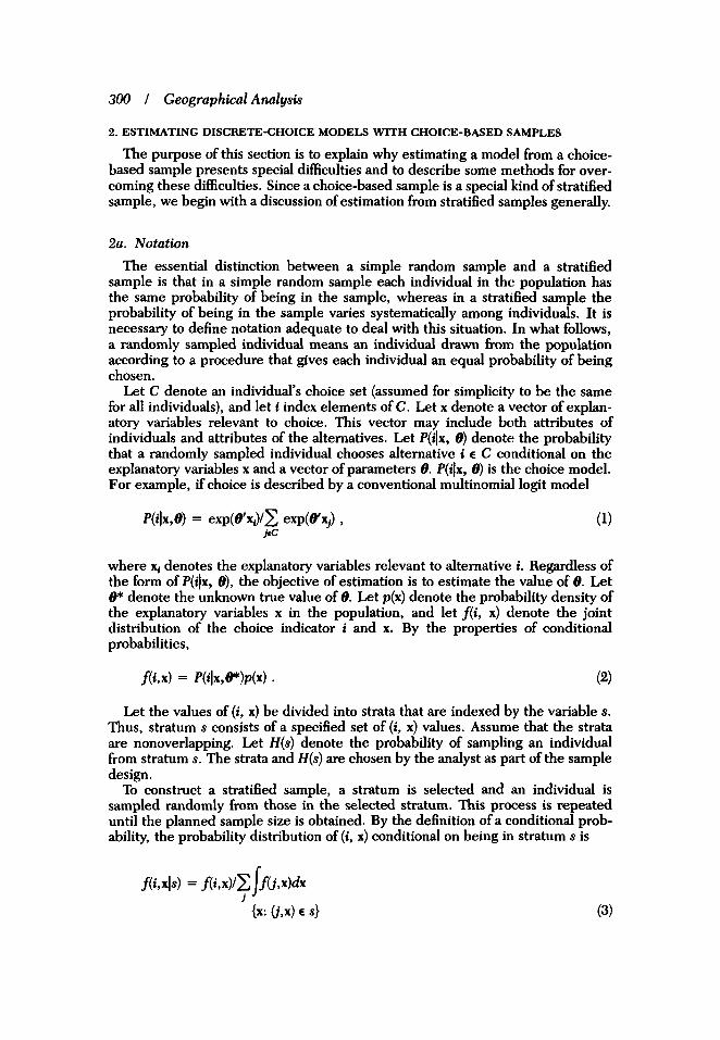
2a. Notation The essential distinction between a simple random sample and a stratified

sample is that in a simple random sample each individual in the population has the same probability of being in the sample, whereas in a stratified sample the probability of being in the sample varies systematically among individuals. It is necessary to define notation adequate to deal with this situation. In what follows, a randomly sampled individual means an individual drawn from the population according to a procedure that gives each individual an equal probability of being chosen.

Let C denote an individual’s choice set (assumed for simplicity to be the same for all individuals), and let i index elements of C. Let x denote a vector of explan- atory variables relevant to choice. This vector may include both attributes of individuals and attributes of the alternatives. Let P(ilx, 8) denote the probability that a randomly sampled individual chooses alternative i E C conditional on the explanatory variables x and a vector of parameters 8. P(ilx, 8) is the choice model. For example, if choice is described by a conventional multinomial logit model

where x, denotes the explanatory variables relevant to alternative i . Regardless of the form of P(i)x, e), the objective of estimation is to estimate the value of 8. Let 8* denote the unknown true value of 8. Let p(x) denote the probability density of the explanatory variables x in the population, and let f ( i , x ) denote the joint distribution of the choice indicator i and x . By the properties of conditional probabilities,

Let the values of (i , x ) be divided into strata that are indexed by the variable s. Thus, stratum s consists of a specified set of (i, x ) values. Assume that the strata are nonoverlapping. Let H(s) denote the probability of sampling an individual from stratum s. The strata and H(s) are chosen by the analyst as part of the sample design.

To construct a stratified sample, a stratum is selected and an individual is sampled randomly from those in the selected stratum. This process is repeated until the planned sample size is obtained. By the definition of a conditional prob- ability, the probability distribution of (i , x) conditional on being in stratum s is

Jean-Claude Thill and Joel L. Horowitz I 301

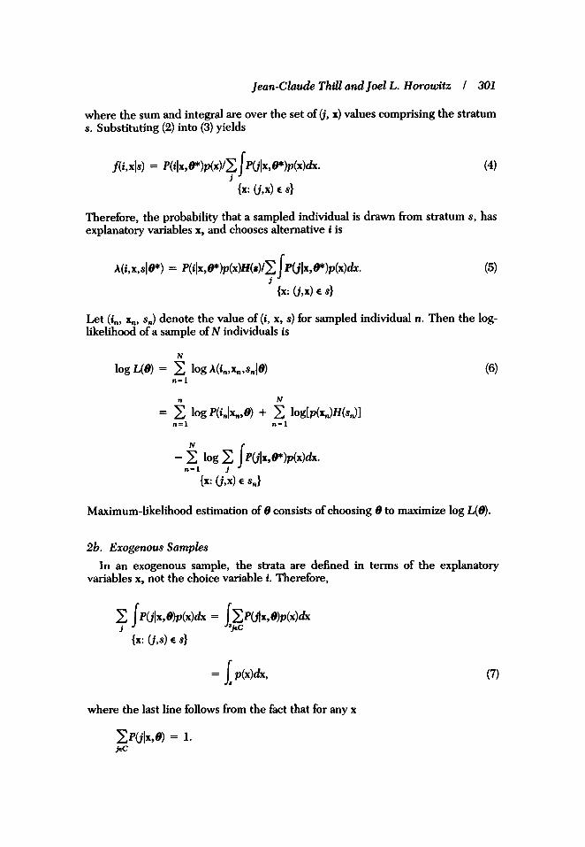
where the sum and integral are over the set of 0, x) values comprising the stratum s. Substituting (2) into (3) yields

Therefore, the probability that a sampled individual is drawn from stratum s, has explanatory variables x, and chooses alternative i is

Let (in, xn, sn) denote the value of ( i , x, s) for sampled individual n. Then the log- likelihood of a sample of N individuals is

Maximum-likelihood estimation of 8 consists of choosing 8 to maximize log L(8).

2b. Exogenous Samples

variables x, not the choice variable i. Therefore, In an exogenous sample, the strata are defined in terms of the explanatory

where the last line follows from the fact that for any x

cp(jlx,e) = 1. W

302 I Geographical Analysis

Substitution of (7) into (6) yields

for any exogenous sample, where s, is the stratum to which individual n belongs. Maximum-likelihood estimation consists of choosing 8 to maximize the right-hand side of (8). Only the first term on the right-hand side depends on 8. Therefore, with an exogenous sample it suffices to maximize

Equation (9) does not involve H(x) or p(x). Therefore, if the estimation data set consists of an exogenous stratified sample or simple random sample, 8 can be estimated by classical maximum likelihood, and no information about H(x) or p(x) is needed. Any stratification of the sample can be ignored.

2c. Choice-based Samples

When the data are choice-based, each stratum consists choice variable i. Therefore, the log-likelihood function is

N N

of a single value of the

( 10)

where the integral is over all values of x. Maximum-likelihood estimation consists of choosing 8 to maximize the right-hand side of (10). Since the second term on the right-hand side does not depend on 8, it suffices to maximize

N N

log L,(e) = log P(inlxn,8) - 2 log I P(i,lx,B)p(x)dx . (11) n = l n = l

By comparing (11) and (9) it can be seen that the log-likelihood function of a choice-based sample consists of the exogenous-sample log-likelihood function plus an additional term. Because of the additional term, the classical, exogenous-sam- ple log-likelihood function is the wrong log-likelihood function for a choice-based sample.

The additional term in (11) is the main soume of difficulty in estimating param- eters from a choice-based sample. The problem is that the term contains p(x), the joint distribution of the explanatory variables in the sampled population. In most applications p(x) is not known. Therefore, the log-likelihood function cannot be

Jean-Chude Thill and Joel L. Horowitz / 303

evaluated, and classical maximum-likelihood estimation cannot be carried out when the sample is choice-based.

One solution to this problem consists of replacing log L, with a function that does not depend on p(x) . To do this, let Q(i) denote the aggregate market share of alternative i . That is,

Q(i) = fP(ilx,8)p(x)dx .

Suppose for the moment that the value of Q(i) is known for each alternative. For example, in transportation mode choice Q(i) often can be estimated quite accu- rately from traffic counts or census data. Recall that H(i) is determined by the design of the sample and, therefore, is known for each i . Define w(i) (i C ) by w(i) = Q(i) /H(i) . Consider estimating 8 by maximizing the weighted exogenous-sample log likelihood

Maximizing log & is feasible if Q(i) is known since log & does not depend on the unknown function p(x) . The resulting estimator of 8 is called the "weighted exogenous-sample maximum likelihood (WESML) estimator." Manski and Ler- man (1977) proved that the WESML estimator is consistent and asymptotically normally distributed with a covariance matrix that can be estimated from the data. Thus, the WESML estimator makes estimation from a choice-based sample pos- sible when Q(i) is known for each i . Manski and McFadden (1981) and Cosslett (1981) discuss a variety of other estimators for the case of known Q(i).

If neither p(x ) nor Q(i) is known, one can estimate p(x ) along with 8 by maximiz- ing (11) over both 8 and p. Cosslett (1981) gives the formal justification of this approach and the details of how it is implemented. If P(ilx, 8) is a multinomial logit model, the resulting estimator of 8 is easy to obtain. Let 8 include a full set of alternative-specific intercepts along with the coefficients of the components of x. That is, the number of intercept terms is one less than the number of alter- natives in C . Then all identified components of 8 except the intercepts can be estimated consistently by maximizing the classical, exogenous-sample log- likelihood function (9). No special modifications of the log-likelihood function are needed to estimate a logit model from a choice-based sample with unknown p(x ) and Q(8). The estimator of 8 is asymptotically normally distributed with covari- ance matrix z, = J-'M]-' , where

and log L is giyen by (9). The derivatives are evaluated at the probability limit of the estimator . In applications, 2, can be estimated consistently by evaluating the derivatives in (13) and (14) at b N and replacing the expected values with sample averages.

The requirement that 8 contain a full set of alternative-specific intercepts places important restrictions on what can be identified in a model estimated from choice-

304 I Geographical Analysis

based data with unknown p(x) and Q(i). This, in turn, limits the information about choice behavior that can be recovered from such data. To illustrate, let the system- atic component of the logit utility function have the linear-in-parameters form that is usually used in applications. Then the systematic component of the utility of alternative i and individual n is

where 8, is the intercept for alternative i , 8, (k = 1, . . . , K ) is the kth component of 8, qn is a K-dimensional vector of explanatory variables for alternative i and individual n, and Xin& is the kth component of qn. It is not possible to identify 6, if the associated explanatory variable $d has the same value for all individuals n- that is, if Xink is an attribute of alternative i that is the same for all individuals. Such variables are perfectly collinear with the alternative-specific intercepts. Con- versely, 8, is identified if%,& varies among both alternatives and individuals. For example, two variables that likely are relevant to destination choice in shopping travel are the distance din from the traveler’s trip origin to destination i , and the price p i of goods at destination i. Since different travelers have different trip origins, din varies among travelers for each destination i , so the 8 coefficient of dni is identified. By contrast, pi is not identified. If pi interacts with an attribute of individuals, then the 8 component associated with the resulting composite vari- able is identified. For example, if shoppers with high incomes are less sensitive to price variations than are shoppers with low incomes, a way to represent the effects of price on destination choice is through the variable pJZn, where Z , is the income of individual n. The composite variable pJZ, varies among both individuals and alternatives, so the 8 coefficient associated with it is identified.

The identification restrictions imply that in general, if the data are choice-based and p and Q are unknown, one cannot identify all the coefficients of a multinomial logit choice model. All the coefficients can be identified only if it is known a priori that the systematic component of the utility function contains no variables that vary among alternatives but not individuals. If this highly restrictive condition does not hold, it is possible to estimate only a subset of the coefficients of the utility function, namely the coefficients of variables that vary among both individ- uals and alternatives. In such cases the full-choice model is neither known nor estimable, so the estimated model cannot be used to predict either aggregate market shares or changes in choices and aggregate shares that would occur if attributes of individuals or alternatives changed. Nonetheless, as is illustrated in section 3, it is possible to make useful inferences on the basis of the identifiable coefficients.

In summary, useful information about choice behavior can be obtained even when the data are choice-based and p and Q are unknown. But one cannot learn as much about choice behavior as could be learned from an exogenously stratified sample or a choice-based sample with known p or Q .

3. A MODEL OF CHOICE OF PHARMACY IN NAMUR BELGIUM

In this section, the methods described in section 2 are illustrated by using them to estimate a multinomial logit model of choice of pharmacy in the Namur, Bel- gium, region.-The model is estimated from a choice-based sample in which nei- ther p nor Q is known.

Jean-Claude Thill and Joel L. Horowitz I 305

3a. Background The data for this analysis were collected during the fall of 1984. At that time,

fifty-two pharmacies were open in the Namur area. They served a population of some 65,OOO residents as well as several thousand commuters.

The pharmacy business in Belgium, as in most West European countries, is heavily regulated by the government. Pharmacies have a monopoly on the retail sale of drugs. In addition to drugs, pharmacies may choose to sell certain “para- pharmacy” items such as cosmetics, personal hygiene items, baby and dietary food, and eyeglasses if prescribed by an ophthalmologist. On average, paraphar- macy items account for 10 percent of sales of Belgian pharmacies, but some pharmacies in the Namur area obtain 40 percent of their sales through such items.

The government regulates the prices pharmacies charge for drugs. Pharmacies may charge the government-established ceiling price or they may offer a discount of up to 10 percent of the cost to the consumer (that is, the list price net of any payment from health insurance). In the Namur area, pharmacies either offer no discounts or offer 10 percent discounts on all of their drug items. Moreover, pharmacies that offer 10 percent discount on drug items offer equal discounts on parapharmacy items.

In Belgium, though allopathic medicine is dominant, there are also practitioners of homeopathic medicine. Accordingly, many pharmacies offer a limited assort- ment of homeopathic drugs. A few pharmacies specialize in the preparation and sale of homeopathic medications. A survey of pharmacies in the Namur area (Thill 1989) showed that on average, homeopathic drugs accounted for 2.8 percent of sales but that some pharmacies obtained 30 percent of their sales from such drugs.

3b. Sample Design The design of the sample used to estimate the model of choice of pharmacy was

conditioned by certain factors that frequently occur in destination-choice analysis. There was no exhaustive record of the population of pharmacy customers from which to randomly sample individuals. Sampling residents of Namur at random was ruled out because it would omit pharmacy customers who are commuters or visitors from outside the city and its immediate environs. This decision was justi- fied a posteriori by the results of the survey we conducted to acquire data on pharmacy choice: 30 percent of surveyed customers lived outside of the Namur area (Thill 1986).

To deal with this situation, we adopted a choice-based sample design. Sampling was carried out on five days during the four-week period of September 23- October 20, 1984. This period was selected to enable the sample to capture day-to-day and week-to-week variability in the spatial behavior of individuals (Huff and Hanson 1986). The five days on which sampling occurred were selected using a method based on the principles of Latin-square selection and suggested originally by Frankel and Stock (1942). See, also, Hansen, Hurwitz, and Madow (1953). The method guarantees that the four weeks of the period and five separate days of the week (Monday, Wednesday, Thursday, Friday, and Saturday) are rep- resented in the sample.’ This design is appropriate when there are day-to-day and week-to-week variations in individual travel patterns (Herz 1983; Hirsh, Prashker, and Ben-Akiva 1986; Huff and Hanson 1986).

Individuals were sampled on the selected days at twenty-three of the fifty-two pharmacies in the study area. The twenty-three pharmacies are well distributed

‘Tuesdays and Thursdays are ex ected to be similar in terms of spatial behavior. Therefore, a Thursday was included in the sampfe but no Tuesday. All pharmacies are closed on Sunday.

306 I Geographical Analysis

in the area and provide an adequate representation of the various types of phar- macies. A trained interviewer was assigned to each pharmacy and was instructed to interview the first customer leaving the shop following completion of the pre- vious interview. Interviews took place on the sidewalk. Interviewed individuals were asked to provide information relevant to destination choice such as their locations of residence and employment and their employment status. A total of 2,156 valid interviews were conducted.

For reasons of computational cost, the model of pharmacy choice was estimated from a subsample of the 2,156 respondents to the survey. A set of fifteen pharma- cies was randomly selected from the twenty-three included in the survey. The 1,694 customers that were interviewed at these pharmacies form the data set used to estimate the choice model. This approach does not affect the consistency and asymptotic normality of the parameter estimator.2

3c. Explanatory Variables of the Model The selection of candidate variables for inclusion in the model was guided by

an analysis of shoppers’ motivations as reported in the interviews (Thill 1986) and by relevant literature (Gagnon 1977; McGoldrick 1981 a, b; Ritchie, Jacoby, and Bone 1981; Thouez 1983; Shannon, Cromley, and Fink 1985). It appears that proximity to the origin or destination base of a customer’s trip is a very important factor in pharmacy ~ h o i c e . ~ This variable is denoted in the model by DIST and is measured by the shortest distance from the origin or final destination of the trip to the pharmacy, whichever is less. Distances were measured on a 534-node transportation network covering the Namur metropolitan area. The shortest routes were found by means of an algorithm of Dijkstra (1959).

Other attributes of pharmacies that are included in our data and that may be relevant to choice include measures of accessibility of the pharmacy to retail, service, and leisure facilities; measures of proximity to a major highway and to bus and train stations; weekly hours of business; whether parapharmacy items and homeopathic drugs are available, and measures of prices and the variety of prod- ucts offered by an establishment. In addition, factors such as the courtesy and competence of the sales personnel were often mentioned in the interviews as choice motivations (Thilll986). They are not variables of the model reported here and, therefore, contribute to the random component of the logit utility function, owing to the difficulty of defining and measuring them.

The proximity of a pharmacy to other retail, service, and leisure facilities indi- cates the potential for economies of scope in travel in cases where an individual decides to link other activities with a trip to the pharmacy (Hanson 1980; Thill and Thomas 1987). Thus, for example, a pharmacy located on a major shopping street is likely to be more attractive ceteris paribus than a pharmacy in a residen- tial neighborhood because the relative proximity of potential trip destinations reduces the travel time and cost involved in reaching them. To capture this effect in the choice model, we use several gravity-type accessibility measures similar to those of Fotheringham and Knudsen (1986). In an attempt to isolate the role of the types of possible trip of destinations, we constructed measures of accessibility to four different types of destinations: retail stores, businesses performing service functions, leisure activities, and all activities combined. The corresponding acces-

2McFadden (1978) proved that in exogenous sam ling, the coefficients of a logit model can be estimated consistently using a randomly selected sutset of the full choice set. McFadden’s proof applies without change to choice-based sampling, thereby justifying the assertion in the text.

%rigin and destination bases of a trip can be home, work, or school.

Jean-Claude Thill andJoel L. Horowitz I 307

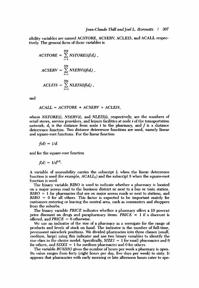
sibility variables are named ACSTORE, ACSERV, ACLEIS, and ACALL respec- tively. The general form of these variables is

534

ACSTORE = c NSTORE(ilf(di), i = l

534

ACSERV = c NSERV(i)f(d,), i = 1

534

ACLElS = c NLEIS(ilf(di), i = l

and

ACALL = ACSTORE + ACSERV + ACLEIS,

where NSTORE(i), NSERV(i), and NLElS(i), respectively, are the numbers of retail stores, service providers, and leisure facilities at node i of the transportation network; di is the distance from node i to the pharmacy, and f is a distance deterrence function. Two distance deterrence functions are used, namely linear and square-root functions. For the linear function

f ( d ) = Ild.

and for the square-root function

A d ) =

A variable of accessibility carries the subscript L when the linear deterrence function is used (for example, ACALLL) and the subscript S when the square-root function is used.

The binary variable RIB0 is used to indicate whether a pharmacy is located on a major access road to the business district or next to a bus or train station. RlBO = 1 for pharmacies that are on major access roads or next to stations, and R I B 0 = 0 for all others. This factor is expected to be important mainly for customers entering or leaving the central area, such as commuters and shoppers from the suburbs.

The binary variable PRICE indicates whether a pharmacy offers a 10 percent price discount on drugs and parapharmacy items. PRlCE = 1 if a discount is offered, and PRlCE = 0 otherwise.

We use an indicator of the size of a pharmacy as a surrogate for the range of products and levels of stock on hand. The indicator is the number of full-time, permanent salesclerk positions. We divided pharmacies into three classes (small, medium, large) using this indicator and use two binary variables to identify the size class in the choice model. Specifically, S l Z E l = 1 for small pharmacies and 0 for others, and SlZE2 = 1 for medium pharmacies and 0 for others.

The variable BUSlHO gives the number of hours per week a pharmacy is open. Its value ranges from forty (eight hours per day, five days per week) to sixty. It appears that pharmacies with early morning or late afternoon hours cater to spe-

308 I Geographical Analysis

cific segments of the population, especially commuters and parents driving chil- dren to school.

The binary variable PARAPH indicates whether a pharmacy provides paraphar- macy items. PARAPH = 1 if such items are available and 0 otherwise. Its value is based on the proportion of a pharmacy’s sales generated by parapharmacy items. This information was obtained in the survey of pharmacies in the Namur area (Thill 1989), which showed that the average proportion is 7.6 percent. We define PARAPH = 1 if parapharmacy items account for more than 7.6 percent of a pharmacy’s sales and 0 otherwise.

The binary variable HOMEO indicates the availability of homeopathic medi- cines in a pharmacy. The data from the survey of pharmacies (Thilll989) indicated that on average, homeopathic products account for 2.8 percent of the sales in the study area. We define HOMEO = 1 if homeopathic products account for more than 2.8 percent of a pharmacy’s sales and HOMEO = 0 otherwise.

A consumer’s preferences among pharmacies is likely to depend on his or her own attributes in addition to those of pharmacies. Three attributes of individuals are used in our model. They are the age of the individual (AGE), the sex of the individual (SEX = 0 for females and 1 for males) and professional status. The variables for professional status are PROF1 = 1 for white-collar workers and 0 for others, PROF2 = 1 for blue-collar workers and 0 for others, and PROF3 = 1 for retired people and 0 for others. Nonworking, nonretired individuals (unemployed, students, housewives) form a fourth class that is indicated when all three of the PROF variables are 0.

Finally, three binary variables are used to identify the bases of tours on which pharmacies are visited. RWOl = 1 for tours that originate and terminate at home, and RWOl = 0 for other tours; RW02 = 1 for tours that originate and terminate at work, and RW02 = 0 otherwise; and RW03 = 1 that originate at home and terminate at work or vice versa, and RW03 = 0 otherwise. The RWO variables are all 0 for tours that do not belong to any of these categories.

The complete set of variables used in the models is summarized in Table 1.

3d. Estimation Methods The estimation sample described in section 3b is choice-based, and we have no

information on the functions p or Q for pharmacies in Namur. Therefore, in a multinomial logit model of pharmacy choice, we can identify only the utility function coefficients of variables that vary among both pharmacies and individuals. Variables that vary among pharmacies but not individuals may affect choice, but their effects cannot be separated from those of the alternative-specific intercepts. Accordingly, the estimated choice model includes only variables that depend on both the pharmacy and the individual. These were constructed from the variables listed in Table 1 by forming products of attributes of alternatives (for example, PRICE) with attributes of individuals (for example, AGE). The effects of other variables are not identified and are absorbed into the alternative-specific intercepts.

An arbitrarily large number of utility-function specifications can be constructed by forming linear combinations of products of the variables listed in Table 1. Only a small subset of these specifications can be estimated in practice, and there is no statistically rigorous or generally accepted method to conduct a specification search. We adopted a stepwise approach. We began by specifying and estimating a relatively simple model. This became the initial maintained model. In subse- quent steps, alternative specifications were estimated and tested against the cur- rent maintained model. A specification that was statistically significantly better

lean-Claude Thill andJoel L. Horowitz I 309

TABLE 1

DlST

ACSTORE

ACSERV

ACLEIS

A C A U

RIB0 PRICE SIZE1 SIZE2 BUSlHO PARAPH HOME0 AGE S E X PROF1 PROF2 PROF3 RWOl RW02 RW03

Definitions of Variables Name Definition

The distance from the trip’s origin or final destination to the pharmacy, whichever is less. Accessibility to retail stores, subscripted L for linear and S for square-root distance decay function. Accessibility to service providers, subscripted L for linear and S for square-root distance d&y function: Accessibility to leisure Facilities, subscripted L for linear and S for square-root distance decay funcGon. Sum of ACSTORE, ACSERV, and ACLEIS, subscripted L for linear and S for square- root distance decay function. 1 if pharmacy is on a major access road or next to a bus or train station, 0 otherwise. 1 if pharmacy offers a 10 percent discount on drugs, 0 otherwise. 1 if pharmacy is small, 0 otherwise. 1 if pharmacy is medium-size, 0 otherwise. Number of hours per week pharmacy is open. 1 i f r p h a r m a c y items account for more than 7.6 percent of sales, 0 otherwise. 1 if omeopathic items account for more than 2.8 percent of sales, 0 otherwise. Age of traveler. 1 if traveler is male, 0 otherwise. 1 if traveler is white-collar worker, 0 otherwise. 1 if traveler is blue-collar worker, 0 Otherwise. 1 if traveler is retired, 0 otherwise. 1 if tour originates and terminates at home, 0 otherwise. 1 if tour originates and terminates at work, 0 otherwise. 1 if tour originates at home and terminates at work or vice versa, 0 otherwise.

than the current maintained model (according to a criterion described below) became the new maintained model. This process continued until we obtained a maintained model that could not be rejected against a reasonable set of alternatives.

The estimated models all are multinomial logit with linear-in-parameters utility functions. Parameter estimation is from a choice-based sample with unknown Q and p functions, and estimation consisted of maximizing the right-hand side of equation (9), as is explained in section 2c. The estimated specifications and the corresponding maximized log-likelihood values are listed in the appendix.

It can easily be shown that as the size of the estimation data set increases toward infinity, the log-likelihood of a correct model exceeds that of any incorrect model with probability approaching 1. Therefore, a maintained model can be tested against an alternative by testing whether the alternative has a log-likelihood that is statistically significantly greater than that of the maintained model. Since none of our specifications is a parametric special case of another, our tests involve non- nested hypotheses. Horowitz (1983) has developed a simple test for this class of problems. According to this test, the maintained model can be rejected against the alternative at a significance level not exceeding 0.01 if the log-likelihood of the alternative model, adjusted for degrees of freedom, exceeds that of the main- tained model by more than 2.71. See Horowitz (1983) for details. We replaced the maintained model with the alternative when the maintained model was rejected by this criterion.

3e. Estimation Results The foregoing specification search procedure led to the selection of model 20 of

the appendix as providing the best description of pharmacy choice among the models we investigated. The variables and estimated parameters of this model are given in Table 2. Estimates of alternative-specific intercepts are not given since, for reasons explained in section 2, they have no behavioral significance. It can be

310 I Geographical Analysis

TABLE 2 Estimation Results

Estimated Variable Coefficient S t a n d d Error &Statist*.

DIST~" - 0.1517 0.00372 -40.802 PRICE*ACE 0.01929 0.00372 5.186

PARAPH*ACE - O.OO997 0.00467 - 2.136 SlZEl*RWOl 0.7190 0.35686 2.015 SlZEl*RW02 0.8729 0.46674 1.870 S l Z E l *RW03 0.8452 0.4133 1.959 SlZE2* RWOl 1.7635 0.46004 3.833 SlZE2* RW02 1.9239 0.54852 3.507 SlZE2*RW03 1.7769 0.51800 3.430 BUSlHO*PROFl 0.01917 0.01303 1.471 BUSlHO*PROF2 0.01243 0.01895 0.656 BUSlHO*PROF3 0.01378 0.01557 0.885 RIBO*RWOl 1.4116 1.0448 1.351 RIBO*RWOZ 1.7142 1.1976 1.431 RIBO*RW03 1.9363 1.0897 1.777 ACA LL,* SEX -6.089 10-5 1.290 10-5 -4.719 Number of observations: 1,694 Log-likelihood at convergence: 2408.07 Log-likelihood of model with only alternative-specific intercepts: - 494.83

HOMEO*(AGE - AGE*/100) 0.09579 0.02914 3.287

.Coefficients whose t statistics exceed 1 .96 in absolute value are significantly different from 0 at the 0.&5 level.

seen from Table 2 that nine of the seventeen parameters of the selected model are statistically significantly different from 0 at the 0.05 level. The remaining param- eters are kept in the model to minimize the chance of omitted-variable bias in the estimation results.

In most respects, the estimation results indicate relations between choice prob- abilities and independent variables that are consistent with expectations. Distance has the expected negative effect on utility and, therefore, on the probability of choosing a given pharmacy. The distance effect on utility is proportional to the square-root of trip length and is independent of the attributes of the traveler.

Price discounting has a statistically significant effect on choice. The variable PRICE*AGE is positive and statistically significant, indicating that discounting is especially effective in attracting older people to a pharmacy. The availability of homeopathic drugs in a pharmacy especially attracts customers of middle ages. Young customers are more responsive than older ones to the availability of para- pharmacy items.

Other things being equal, proximity to other possible trip destinations enhances the utility of a pharmacy. As discussed earlier, this effect is well documented in the literature on destination choice. We found that the various accessibility mea- sures described in section 3c were indistinguishable in terms of their contribution to the model's log-likelihood. Neither the type of trip destination nor the form of the distance deterrence function matters, apparently because the eight accessibil- ity measures are highly correlated with one another. However, the effect on choice of accessibility to other destinations appears to depend on the sex of the traveler. Good access adds more to the utility of a pharmacy if the traveler is female than if the traveler is male.

We have no a priori expectations about the signs or magnitudes of the remaining twelve variables in Table 2.

4. CONCLUSIONS

In most applications of probabilistic discrete-choice models, the estimation data set is an exogenous random sample of the population of interest. However, choice-

Jean-Claude Thill andJoel L. Horowitz I 311

based samples are often easier and cheaper to obtain than exogenous ones. The amount of information about choice behavior that can be recovered from a choice- based sample depends on whether the analyst knows the aggregate market shares of the choice alternatives and the joint probability distribution of any relevant explanatory variables. In this paper, we have been particularly concerned with the case in which neither is known. This is a likely situation when a choice-based sample is used to estimate a model of choice of travel destination choice.

A multinomial logit model can easily be estimated from choice-based data when the aggregate shares and distribution of explanatory variables are unknown. The estimated model can yield useful information about choice behavior, although not as much as can be obtained from an exogenous sample or a choice-based sample with known market shares. In the case of destination-choice behavior, it is possible to test for effects on choice of travel cost and of interactions between attributes of alternatives and attributes of individuals. It is also possible to estimate marginal rates of substitution among these effects. It is not necessary to sample all destina- tions to achieve these results. Thus, choice-based sampling provides a relatively easy and inexpensive means of acquiring information about destination-choice behavior, even when aggregate market shares and the distribution of explanatory variables are unknown.

We have illustrated the use of choice-based sampling with an empirical model of choice of pharmacy in the Namur, Belgium, area. The model was estimated from a choice-based sample without knowledge of aggregate shares or the distri- bution of explanatory variables. Other applications in which choice-based sam- pling may be particularly useful include studies of choice of intercity and vacation travel destinations, patients’ choices of health care facilities, and migration. In each of these settings, low travel frequencies, widely dispersed trip origins and, in the case of migration, lack of a return trip to the origin make exogenous sampling virtually impossible.

LITERATURE CITED

Cosslett, S. R. (1981). “Efficient Estimation of Discrete-Choice Models.” In Structural Analysis of Discrete Data with Econometric Applications, edited by C. F. Manski and D. McFadden, pp. 51-111. Cambridge, Mass.: M.I.T. Press.

Dijkstra, E. (1959). “A Note on Two Problems in Connection with Graphs.” Numerische Mathematik 1, 269-71.

Fotheringham, A. S., and D. C. Knudsen (1986). “Modeling Discontinuous Change in the Spatial Pattern of Retail Outlets: A Methodology.” In Transformations through Space and Time: An Analysis of Nonlinear Structures, Bifurcation Points and Autoregressive De endencies, edited by D. A. Griffith and R. P. Haining, pp. 273-92. Dordrecht: Martinus Ni jho l

Frankel, L. R., and J. S. Stock (1942). “On the Sample Survey of Unemployment.”Journal of the American Statistical Association 37, 77-80.

Gagnon, J . P. (1977). “Factors Affectin Pharmacy Patronage Motives-A Literature Review.”Jour- nal of the American PharmaceuticafAssociation, New Series 17, 556-59.

Hansen, M. H., W. N. Hunvitz, and W. G. Madow (1953). Sample Survey Methods and Theory, vol. 1. New York: John Wiley & Sons.

Hansop, S. (1980). “Spatial Diversification and Multipurpose Travel: Implications for Choice The- ory. Geographical Analysis 12, 245-57.

Herz, R. (1983). “Stability, Variability and Flexibility in Everyday Behavior.” In Recent Advances in Travel Demand Analysis, edited by S. Carpenter and P. Jones, pp. 385-400. Aldershot: Gower Publishing Co.

Hirsh, M., J. N. Prashker, and M. Ben-Akiva (1986). “Day-of-the-Week Models of Shopping Activ- ity Patterns.” Transportation Research Record 1985, 63-69.

Horowitz, J. L. (1983). “Statistical Comparison of Non-Nested Probabilistic Discrete Choice Models.” Transportation Science 17, 319-50.

Huff, O., and S. Hanson (1986). “Repetition and Variability in Urban Travel.” Geographical Anajysis 18, 97-114.

312 I Geographical Analysis

Lerman, S. R., and C. F. Manski (1975). “Alternative Sampling Procedures for Calibrating Disag- gregate Choice Models.” Transportation Research Record 592, 24-28.

. (1979). “Sample Design for Discrete Choice Analysis of Travel Behavior: The State of the Art.” Transportation Research 13A, 2944.

Manski, C. F., and S. R. Lerman (1977). “The Estimation of Choice Probabilities from Choice- Based Samples.” Econometrica 45, 1977-88.

Manski, C. F., and D. McFadden (1981). “Alternative Estimators and Sample Desi ns for Discrete Choice Analysis.” In Structural Analysis of Discrete Data with Econometric Appkations, edited by C. F. Manski and D. McFadden, pp. 1-50. Cambridge, Mass.: M.I.T. Press.

McFadden, D. (1978). “Modelling the Choice of Residential Location.” In Spatial Interaction Theory and Residential Location, edited b A. Karlquist, L. Lunquist, F. Snickars, and J. L. Weibull, pp. 75-96. Amsterdam: North Holyand.

McGoldrick. P. J. (1981a). “Customer Behavior.” Pharmaceutical journal 227, 64243. . (1981b). Retail Pharmacy Customers: Their Motioations and Their Decisions to Make

Purchases. Occasional Paper 8107, Department of Management Science, University of Manch- ester, Manchester, UK.

Ritchie, J., A. Jacoby, and M. Bone (1981). Access to Primary Health Care. London: Office of Population Censuses and Surveys, Social Survey Division, UK Health Department.

Shannon, G., E. Cromley, and J. Fizk (1985). “Pharmacy Patronage among the Elderly: Selected Racial and Geographical Patterns. Social Science and Medicine 20.85-93.

Thill, J. C. (1986). “La clientele des officines pharmaceutiques en milieu iirbain.” Cahiers de Sociologie et de Demographie Medicales 26, 329-51.

. (1989). Shopping Behaoior and Urban Retailing: the Structuring Role of Multipurpose, Multistop Traoeling. Collection de I’Institut de Mathematiques Economiques, n. 35, Universite de Bourgogne, Dijon, France.

Thill, J. C., and I. Thomas (1987). “Toward Conceptualizing Trip-Chaining Behavior: A Review.” Geographical Analysis 19, 1-17.

Thouez, J. P. (1983); “La consommation des medicaments et la localisation des pharmacies a Sher- brooke, Quebec. Cahiers de Sociologie et de Demographie Medicales 23, 57-77.

APPENDIX Selection of the Best Specification of the Systematic Utility

For each model specification, L(B) is the log-likelihood at conver ence and P is the total number of estimated parameters, including the interce ts. A star (*) in the &st column indicates a specification that significantly improves the Eg-likelihood of the maintained model at the 0.01 level.

x

1

2’

3

4

5

Model specification P

Step 1: Transformation of DIST DIST’Ie*AGE, PRICE*SEX, HOMEO*AGE, PARAPH*ACE, SIZE1 *SEX, SIZE2*SEX, BUSIHO*PROFl, BUSIHO*PROF2, BUSIHO*PROF3, RIBO*RWOI, RIBO*RW02, RIBO’RW03, ACALL,*SEX Log(DIST)*AGE, PRICE*SEX, HOMEO*AGE, PARAPH*ACE, SIZEl *SEX, SIZE2*SEX, BUSIHO*PROFI, BUSIHO*PROF2, BUSZHO*PROF3, RIBO*RWOI, RIBO*RW02, RIBO*RW03, ACALL,*SEX Step 2: Variations on DIST’“ DIST’Ie*SEX, PRICE*SEX, HOMEO*ACE, PARAPH*AGE, SIZEl *SEX. SIZE2*SEX. BUSIHO*PROFl. BUSIHO*PROF2. BUSIHO*PROF3, RIBO*RWOI, RIBO*RW02, RIBO*RW03; ACA LL,* S EX - DIST’”*RWOl, DIST’“*RW02, DIST’”*RW03, PRICE*SEX, HOMEO*AGE, PARAPH*ACE, SIZEI*SEX, SIZE2*SEX, BUSIHO*PROFI, BUSIHO*PROF2, BUSIHO*PROF3, RIBO*RWOI, RIBO*RW02,RIBO*RW03, ACALL,*SEX

27 -2597.68

27 - 2707.14

27 -3542.81

29 -2461.83

APPENDIX # Model s d a t i o n P UB)

~

6

7*

8*

9

10*

11

12

13

14

15

16

17

18

19

20*

DIST'"*PROFl, DlST'"*PROF2, DIST'"*PROF3, PRlCE*SEX, HOMEO*AGE, PARAPH*AGE, SlZEl*SEX, SlZE2*SEX, BUSlHO*PROFl , BUSIHO*PROF2, BUSZHO*PROF3, RlBO*RWOl, RlBO*RW02, RlBO*RW03, ACALL,*SEX

29 -3138.73

DlST'", PRZCE*SEX, HOMEO*ACE, PARAPH*ACE, SlZEl*SEX, SlZE2*SEX, BUSlHO*PROFl , BUSlHO*PROF2, BUSlHO*PROF3, RlBO*RWOl, RlBO*RWO2, RlBO*RW03, ACALL,*SEX Step 3: Variations on PRlCE DIST'", PRlCE*AGE, HOMEO*ACE. PARAPH*AGE, SlZEl*SEX, SlZE2*SEX, BUSlHO*PROFl, BUSZHO*PROF2, BUSIHO*PROF3, RlBO*RWOl, RlBO*RW02, RlBO*RW03. ACALL,*SEX DIST'". PRICE*PROFI. PRlCE*PROF2. PRlCE*PROF3.

RlBO*RWOl, RlBO*RW02, RIB @RW03, ACAU,*SEX Step 4: Variations on HOME0 DIST'", PRlCE*AGE, HOMEO*(ACE-ACE21100), PARAPH*AGE, SlZEl *SEX, SlZE2*SEX, BUSlHO*PROFl, BUSZHO*PROF2, BUSIHO*PROF3, RlBO*RWOl, RlBO*RW02, RlBO*RW03, ACALL,*SEX DlST'", PRlCE*AGE. HOMEO*SEX, PARAPH*ACE, SlZEl*SEX, SlZE2*SEX, BUSlHO*PROFl, BUSZHO*PROF2, BUSlHO*PROF3, RlBO*RWOl, RlBO*RW02, €UBO*RW03, ACALL.*SEX DlSTl", PRlCE*ACE, HOMEO*PROFl, HOMEO*PROF2, HOMEO'PROF3, PARAPH*AGE. SlZEl *SEX, SlZE2*SEX, BUSlHO*PROFl , BUSlHO*PROF2, BUSlHO*PROF3, RlBO*RWOl, RZBO*RW02, RlBO*RW03, ACALL,*SEX Step 5: Variations on PARAPH DIST'", PRlCE*ACE, HOMEO*(ACE-AGE21100), PARAPHIAGE, SlZEl *SEX, SlZE2*SEX, BUSlHO*PROFl, BUSlHO*PROF2, BUSlHO*PROF3, RlBO*RWOl, RlBO*RW02, RlBO*RW03, ACALL,*SEX DIST'", PRlCE*AGE, HOMEO*(ACE-ACE21100), PARAPH*SEX. SlZEl *SEX, SlZE2*SEX, BUSlHO*PROFl, BUSlHO*PROF2, BUSlHO*PROF3, RlBO*RWOl, RlBO*RW02, tUBO*RW03, ACALL,*S EX DlST"2, PRlCE*ACE, HOMEO*(ACE-AGE21100), PARAPH*PROFl, PARAPH*PROF2, PARAPH*PROF3, SIZE1 *SEX, SlZE2*SEX, BUSlHO*PROFl, BUSlHO*PROF2, BUSlHO*PROF3, RlBO*RWOl, RlBO*RW03, tUBO*RW03, ACALL,*SEX DIST'", PRlCE*AGE, HOMEO*(ACE-AGE21100), PARAPH*RWOl, PARAPH*RW02, PARAPH*RW03, S l Z E l *SEX, SlZE2*SEX, BUSlHO*PROFl, BUSIHO*PROF2, BUSlHO*PROF3, RlBO*RWOl, RlBO*RW02, RlBO*RW03, ACALL,*SEX Step 6 Variations on SlZEl, SUE2 DIST'", PRlCE*ACE, HOMEO*(ACE-ACE21100), PARAPH*ACE, SIZE1 *ACE, SlZE2*AGE, BUSlHO*PROFl, BUSZHO*PROF2, BUSlHO*PROF3, RlBO*RWOl, RlBO*RW02, tUBO*RW03, ACALL,*SEX DlSTl", PRlCE*AGE, HOMEO*(AGE-AGEe/lOO), PARAPH*ACE,

BUSZHO*PROFl , BUSlHO*PROF2, BUSIHO*PROF3, RlBO*RWOl, RlBO*RW02, RlBO*RW03, ACALL+*SEX

SlZEl *(ACE-ACEYlOO), SZZE2*(ACE-ACE21100),

DZST'", PRlCE*AGE, HOMEO*(AGE-AGE21100), PARAPH*AGE, SlZEl *PROFl, SlZEl *PROF2, SlZEl *PROF3, SlZE2*PROFl, SZZE2*PROF2, SlZE2*PROF3, BUSIHO*PROFl, BUSlHO*PROF2, BUSZHO*PROF3, RlBO*RWOl, RlBO*RW02, RlBO*RW03, ACALL,*SEX

SZZEl*RWOl, SlZEl*RW02, SIZEl*RW03, SlZE2*RWOl, SlZE2*RWO2, SlZE2*RW03, BUSlHO*PROFl, BUSlHO*PROF2, BUSlHO*PROF3, RlBO*RWOl, RZBO*RW02, RlBO*RW03, ACALL,*SEX

DIST'", PRZCE*AGE, HOMEO*(ACE-ACE21100), PARAPH*AGE,

27 -2435.70

27 - 2419.55

29 -2423.71

27 - 2416.17

27 - 2419.57

29 - 2419.89

27

27

29

29

27

27

31

31

-2417.80

-2418.65

-2417.93

- 2417.37

-2415.86

-2415.54

-2414.62

- 2408.07

APPENDIX # Model speci6cation P L(B)

21

22

23

24

25

26

27

28

29

30

31

32

33

34

ACALL,*SEX DIST'", PRICE*AGE, HOMEO*(AGE-AGE2/100), PARAPHIAGE, SIZEI*RWOl, SIZEI*RW02, SIZEl*RW03, SIZE2*RWOI. SIZE2*RW02, SIZE2*RW03, BUSIHO*AGE, RIBO*RWOI, RIBO*RW02, RIBO*RW03, ACALL.*SEX DIST'", PRICE*AGE, HOMEO*(AGE-ACE2/100), PARAPH*AGE, SIZEl*RWOI, SIZEI*RW02, SIZEI*RW03, SIZE2*RWOI,

RIBO*RWOl, RIBO*RW02, RIBO*RW03, ACALL.*SEX

SIZEl*RWOl, SIZEl*RW02, SIZEl*RW03, SIZE2*RWOI, SIZE2*RW02, SIZE2*RW03, BUSIHO*SEX, RIBO*RWOI, RIBO*RWO2, RIBO*RW03, ACALL,*SEX Step 8: Variations on RIB0 DIST'", PRICE*AGE, HOMEO*(AGE-AGE2/100), PARAPH*AGE, SIZEl*RWOl, SIZEl*RW02, SIZEl*RW03, SIZE2*RWOl, SIZE2*RW02, SIZE2*RW03, BUSIHO*PROFI, BUSIHO*PROF2, BUSIHO*PROF3, RIBO*PROFI, RIBO'PROF2, RIBO*PROF3, ACALL,*SEX DISTLt2, PRICE*AGE, HOMEO*(AGE-AGE2/100), PARAPH*AGE. SIZEl*RWOl, SIZEl*RW02, SIZEI*RW03, SIZE2*RWOl, SIZE2*RW02, SIZE2*RWO3, BUSIHO*PROFl, BUSIHO*PROF2, BUSIHO*PROF3, RIBO*SEX, ACALL,*SEX DISTLn, PRICE *AGE, HO MEO*(AG E-AGE2/100), PARA PH*AG E , SIZEI*RWOI, SIZEl*RW02, SIZEI*RW03, SIZE2*RWOI, SIZE2*RW02, SIZE2*RW03, BUSIHO*PROFl, BUSIHO*PROF2, BUSIHO*PROF3, RIBO*AGE, ACAU,*SEX

SIZE2*RWO2, SIZE2*RW03, BUSlHO*(AGE-ACE2ll00),

DISTw, PRICE*AGE, HOMEO*(AGE-AGE2/100), PARAPH*AGE,

DlST'". PRICE*ACE, HOMEO*(ACE-AGE2/100), PARAPH*AGE, SIZEI*RWOI, SIZEl*RW02, SIZEl*RW03. SlZE2*RWOI, SIZE2*RW02. SIZE2*RW03. BUSlHO*PROFI, BUSlHO*PROF2, BUSIHO*PROF3, RIBO*DIST'", ACALL,*SEX DIST'", PRICE*AGE, HOMEO*(AGE-AGE2/100), PARAPH*AGE, SIZEl*RWOl, SIZEl*RW02, SIZEl*RW03, SIZE2*RWOI. SIZE2*RW02, SIZE2*RW03, BUSIHO*PROFl, BUSIHO*PROF2, BUSIHO*PROF3, RIBO*(AGE-AGE2/100), ACALL,*SEX Step 9 Variations on ACALL DIST'", PRICE*AGE, HOMEO*(AGE-ACEp/lOO), PARAPH*AGE, SIZEl*RWOl, SIZEI*RWO2, SIZEI*RW03, SIZE2*RWOI, SIZE2*RW02, SIZE2*RWO3, BUSIHO*PROFI, BUSIHO*PROF2, BUSIHO*PROF3, RIBO*RWOI, RIBO*RW02, RIBO*RW03, ACALL.*AC E DIST'", PRICE*AGE, HOMEO*(AGE-ACE2/100), PARAPH*AGE, SlZEl*RWOI, SIZEl*RWO2, SIZEl*RW03, SIZE2*RWOl, SIZE2*RW02, SIZ32*RW03, BUSIHO*PROFI, BUSIHO*PROF2, BUSIHO*PROF3, RIBO*RWOl, RIBO*RW02, RIBO*RW03,

DIST'", PRICE*AGE, HOMEO*(AGE-ACE2/100), PARAPH*AGE, SIZEl*RWOl, SIZEl*RWO2, SIZEl*RW03, SIZE2*RWOl, SIZE2*RW02, SIZE2*RW03, BUSIHO*PROFl, BUSIHO*PROF2, BUSIHO*PROF3, RIBO*RWOl, RIBO*RW02, RIBO*RW03, ACALL.*RWOl, ACALL,*RW02, ACALL,*RW03

ACALL,*(AGE-AGE~/~~~)

DIST'", PRICE*AGE, HOMEO*(AGE-AGE2/100), PARAPH*ACE, SIZEl*RWOl, SIZEl*RW02, SIZEl*RW03, SIZE2*RWOI, SIZE2*RW02, SIZE2*RW03, BUSIHO*PROFl, BUSIHO'PROF2, BUSIHO*PROF3, RIBO*RWOI, RIBO*RW02, RIBO*RW03, ACALL,*PROFl , ACALL,*PROF2, ACALL,*PROF3

31

29

29

29

31

29

29

29

29

31

31

33

33

31

-2406.67

- 2408.95

- 2408.84

-2408.15

- 2408.45

-2409.39

- 2410.38

- 2407.70

- 2410.42

- 2419.33

- 2417.98

-2411.76

- 2417.46

- 2408.07

SIZE2*RW02, SIZE2' BUSIHO*PROF3, RIBO*RWO. (ACALL,*SEX?

APPENDIX # Model soeci6cption P LIB)

35

36

37

38

39

- 1

DIST'", PRICE*AGE, HOMEO*(AGE-AGE2/100), PARAPH*AGE, 31 -2407.89 SlZEl*RWOl. SlZEl*RW02. SlZEl*RW03, SlZE2*RWOl, SlZE2*RWO2; SlZE2*RW03; BUSIHO*PROFl, BUSlHO*PROF2, BUSlHO*PROF3,RlBO*RWOl, RlBO*RW02, RlBO*RW03, IACALL-*SEX )Im \------. ----I

DIST'", PRlCE*AGE, HOMEO*(AGE-AGE2/100), PARAPH*AGE, 31 - 2408.34 SlZEl*RWOl, SlZEl*RW02, SlZEl*RW03, SlZE2*RWOl, SlZE2*RW02, SlZE2*RW03, BUSlHO*PROFl, BUSlHO*PROF2, BUSlHO*PROF3, RlBO*RWOl, RlBO*RW02, RlBO*RW03, ACAUL* SEX D1STLm, PRlCE *AG E , HO MEO*(AG E-AGE2/100), PARAPH*AG E , 33 -2407.29 SlZEl*RWOl, SlZEl*RW02, SlZEl*RW03, SlZE2*RWOl, SlZE2*RW02. SlZE2*RW03, BUSIHO*PROFl, BUSlHO*PROF2, BUSlHO*PROF3,RlBO*RWOl, RlBO*RW02, RlBO*RW03, ACSTOR.*SEX, ACSERV.*SEX, ACLElS.*SEX D Z S T ' ~ , PRZCE*AGE, HOMEO*(AGE-ACEY~OO), PARAPH*AGE, 31 - 2407.78 SlZEl *RWOl, SlZEl*RW02, SlZEl*RW03, SlZE2*RWOl, SlZE2*RW02, SlZE2*RW03, BUSlHO*PROFl, BUSlHO*PROF2, BUSIHO*PROF3, RlBO*RWOl, RlBO*RW02, RlBO*RW03, ACSTOR.*SEX

SlZEl*RWOl, SlZEl*RWO2, SlZEl*RW03, SlZE2*RWOl, SlZE2*RW02, SlZE2*RW03. BUSlHO*PROFl, BUSlHO*PROF2, BUSlHO*PROF3, RlBO*RWOl, RlBO*RW02, RlBO*RW03, ACSTORL*SEX, ACSERVL*SEX, ACLEISL*SEX

DIST"z, PRlCE*AGE, HOMEO*(ACE-ACE2/100), PARAPH*AGE, 33 -2408.30