Citation: Hennessy, B.; Rutten, M.;

Tingay, S.; Summers, A.; Gustainis,

D.; Crosse, B.; Sokolowski, M.

Establishing the Capabilities of the

Murchison Widefield Array as a

Passive Radar for the Surveillance of

Space. Remote Sens. 2022, 14, 2571.

https://doi.org/10.3390/rs14112571

Academic Editor: Ali Khenchaf

Received: 14 April 2022

Accepted: 22 May 2022

Published: 27 May 2022

Publisher’s Note: MDPI stays neutral

with regard to jurisdictional claims in

published maps and institutional affil-

iations.

Copyright: © 2022 by the authors.

Licensee MDPI, Basel, Switzerland.

This article is an open access article

distributed under the terms and

conditions of the Creative Commons

Attribution (CC BY) license (https://

creativecommons.org/licenses/by/

4.0/).

remote sensing

Article

Establishing the Capabilities of the Murchison Widefield Arrayas a Passive Radar for the Surveillance of SpaceBrendan Hennessy 1,2,* , Mark Rutten 3, Robert Young 2 , Steven Tingay 1 , Ashley Summers 2,Daniel Gustainis 2, Brian Crosse 1 and Marcin Sokolowski 1

1 International Centre for Radio Astronomy Research, Curtin University, Bentley, WA 6102, Australia;s.tingay@curtin.edu.au (S.T.); brian.crosse@curtin.edu.au (B.C.); marcin.sokolowski@curtin.edu.au (M.S.)

2 Defence Science and Technology Group, Edinburgh, SA 5111, Australia;robert.young@dst.defence.gov.au (R.Y.); ashley.summers@dst.defence.gov.au (A.S.);daniel.gustainis@dst.defence.gov.au (D.G.)

3 InTrack Solutions, Adelaide, SA 5000, Australia; mark@intrack.solutions* Correspondence: brendan.hennessy@icrar.org

Abstract: This paper describes the use of the Murchison Widefield Array, a low-frequency radiotelescope at a radio-quiet Western Australian site, as a radar receiver forming part of a continent-spanning multistatic radar network for the surveillance of space. This paper details the systemgeometry employed, the orbit-specific radar signal processing, and the orbit determination algorithmsnecessary to ensure resident space objects are detected, tracked, and propagated. Finally, the paperincludes the results processed after a short collection campaign utilising several FM radio transmittersacross the country, up to a maximum baseline distance of over 2500 km. The results demonstrate theMurchison Widefield Array is able to provide widefield and persistent coverage of objects in lowEarth orbit.

Keywords: passive radar; radar signal processing; space surveillance; multistatic radar; space domainawareness

1. Introduction

Radio telescopes, sensitive instruments designed to detect the faintest signals fromthe most distant cosmic objects, are proving to be capable receivers for the purpose ofradar. Although radio telescope arrays have been used as imaging interferometers, recentinterest in phenomena such as pulsars, fast radio bursts, and cosmic rays, is motivating thedevelopment of high time-resolution capabilities for interferometric arrays [1–3]. These hightime-resolution observation modes allow the direct implementation of radar functionality.Thus, researchers are investigating the use of arrays of radio telescopes as radar receiversfor the surveillance of space [4–7].

This is certainly true for the Murchison Widefield Array (MWA), a low-frequency radiotelescope in remote Western Australia, a precursor to the forthcoming Square KilometreArray (SKA) [8]. Even before the MWA commenced operations in 2013, its use as a passiveradar for the surveillance of space has been considered and planned [9]. Over the lastdecade, work has been undertaken to investigate the MWA’s ability to detect and trackresident space objects (RSOs) in low Earth orbit (LEO) from the reflections of terrestrialtransmissions, particularly FM radio [4,10,11]. Initial simulations predicted the MWAwould be able to detect FM radio reflections from an RSO of a radar cross-section that is assmall as 0.5 m2 at a range of 1000 km [10].

Rather than relying upon pre-existing sources of illumination, many radio telescopesare being utilised as active radar receivers as part of a bistatic system in conjunction with acooperative radar transmitter [6,12]. This configuration is beneficial, as the radar transmitteris ideal for the purpose of providing high-powered illumination of the RSOs. However,

Remote Sens. 2022, 14, 2571. https://doi.org/10.3390/rs14112571 https://www.mdpi.com/journal/remotesensing

Remote Sens. 2022, 14, 2571 2 of 25

this is often achieved through the use of narrow-beam transmitter antennas. A direct beamwill illuminate only a narrow volume and so the system will only be capable of surveillinga small region, especially when combined with a narrow receiver beam. This is congruouswith the operation of the vast majority of space-surveillance radar systems which operatewith a single narrow beam, or a fence, configuration [13].

Passive radar systems are being used for space surveillance purposes with wide-areareceiver systems, utilising a (non-cooperative) broad-beam transmitter at a considerablestandoff distance. Such systems include the Low-Frequency Array (LOFAR) radiotelescope,among others [14–17]. When combined with a receiver with a wide field of regard, awide area of broadcast transmission ensures a significant volume above the receiver isilluminated. However, this broad coverage also means the relative power directed towardRSOs can be reduced when compared to the cooperative bistatic configuration. Despitethis lower directed power, there are benefits to utilising these types of transmitters. Avast coverage volume ensures RSOs may be detected for a significant amount of time,enough to provide accurate orbit estimates from a single pass without any prior knowledge.Additionally, terrestrial broadcasters, such as TV or radio, consist of a distributed networkof many transmitters, allowing multiple transmitters to be used as simultaneous sources ofradar illumination of the volume above the receiver.

This paper details the use of the MWA as a passive radar for the surveillance ofspace, illustrated in Figure 1, and is structured as follows: Section 2 describes the MWAconfiguration and its unique aspects as a passive radar receiver. Section 3 covers the signalprocessing pipeline and includes the techniques to integrate range-compressed pulses toefficiently match objects in orbit, as well as detailing the complete orbit determination (OD)step in Section 4. This OD work builds on earlier work investigating uncued detectionand initial orbit determination (IOD) [18]. The steps taken to overcome the challenges ofusing non-cooperative FM radio transmitters (an analogue broadcasting method) amidstthe network’s unique configuration in Australia are covered in Section 5. The paperincludes some illustrative results in Section 6 from a short collection campaign utilisingfour transmitters around the country at various baseline distances of over 2500 km. Thepaper concludes with Section 7.

Figure 1. Illustration of the use of the Murchison Widefield Array (MWA) as a passive radar, showingtwo transmitters, one satellite and three MWA tiles. The two transmitters’ elevation beampatterns (inblue) and the signal path (in green) are also shown.

2. The Murchison Widefield Array Used as a Radar Receiver

The MWA is the low-frequency precursor to the SKA, operating in the frequencyrange of 70–300 MHz. The main scientific goals of the MWA are to detect radio emissionsfrom neutral hydrogen during the Epoch of Reionisation, to study the Earth’s Sun and itsheliosphere, Earth’s ionosphere, and radio transient phenomena, as well as to map thegalactic and extragalactic radio sky [19].

Remote Sens. 2022, 14, 2571 3 of 25

The telescope is strategically located in a legislated radio-quiet zone, the Murchison Radio-astronomy Observatory, far from cities and other sources of electromagnetic interference.

The MWA consists of 4096 dual-polarised wideband dipoles configured into subarraysof 4 × 4 square grids, referred to as tiles. The grid spacing for each tile is 1.1 m (corre-sponding to a half-wavelength separation for 136 MHz), and the 16 dipoles are attachedto a 5 m × 5 m steel mesh ground plane. These 256 tiles are distributed over ∼15 squarekilometres. The current phase of the MWA, Phase II, allows for the use of half of the tiles atany one time, in compact or extended configurations [20]. Figure 2 shows the layout of thecompact configuration of the Phase II MWA.

Figure 2. A plan view of the Murchison Widefield Array’s compact configuration of Phase II, showingthe location of the 128 tiles.

Each tile’s 16 antennas are combined with an analogue beamformer to form a tile beamin a particular direction in the sky. The beamwidth is approximately 40° at the zenith forFM frequencies.

The full frequency of each tile is directly sampled at 327.78 MHz covering the array’sfrequency range of interest, and a polyphase filter bank (PFB) channelises this data to256 × 1.28 MHz-wide critically sampled coarse channels. The MWA is able to transfera user-defined subset of 24 of these 256 channels in real time through to the high time-resolution voltage capture system (HTR-VCS), allowing for an instantaneous bandwidth of30.72 MHz.

The coarse channels, consisting of 1.28 MHz HTR-VCS data, are then further down-sampled to select the various FM frequencies of interest for radar processing.

For typical space surveillance applications, the standard utilisation is a (wide) beam-stare mode, with the tile’s analogue beam directed near the zenith. The net output is128 channels with a bandwith of (typically) 100 kHz. These data are then calibrated toremove any impact of the distributed array and phase-align each channel to the antenna.Once calibrated, the data are able to be used for precise electronic beamforming with thedistributed array forming a large aperture providing very narrow surveillance beams.The transmitter reference signals are collected directly at sites close to the transmitterwith a small software-defined radio (SDR) system. These SDR reference systems are GPS-disciplined to allow synchronisation with the MWA’s surveillance data. Additionally,despite its location in a radio-quiet zone, the MWA is able to detect transmissions from

Remote Sens. 2022, 14, 2571 4 of 25

the nearest radio transmitters 300 km away, allowing for the direct observation of nearbyreference signals.

3. Signal Processing

An issue faced when using a sensor such as the MWA as a space-surveillance radaris the tradeoff between needing to integrate for a longer amount of time for increasedsensitivity, and the changing geometry that orbital motion imparts. The precise and narrowbeamwidth, resulting from such a large aperture, means that RSOs in LEO will occupya beam for only a brief instant. For even a short coherent processing interval (CPI), theobject in orbit will need to be tracked spatially throughout the CPI. Similarly, the object willneed to be tracked in delay and Doppler parameter space as well. This is the fundamentalchallenge with the detection of RSOs with the MWA; the need to extend the CPI to detectsmaller and more distant RSOs is balanced against the difficulty of coherently formingdetection signals. This section covers efficient and scalable methods for dealing withthis problem by matching the radar-receiver parameters to the orbital motion. This typeof track-processing is achievable given the a priori information on orbits, whereas foruncued detection and searches, earlier studies have detailed practical methods for forminghypothesised orbits [18].

Given a large number of potential orbits, either from known tracks, searching a volumeof orbits around known tracks, or uncued search hypotheses, the surveillance data detailedin Section 2, and the collected reference signals, are able to be coherently matched to detectan RSO in that orbit.

Rather than directly processing across the received signals, range-compressed pulsesare formed for each antenna. These pulses are then matched to the RSO motion [21,22].The signals are split into M pulses, each with a duration of τ, such that the CPI length isgiven by Mτ. The pulse length, τ, needs to be sufficiently short to ensure that any changein the Doppler frequency across the pulse is insignificant [22]. Decreasing the pulse lengthis equivalent to increasing the maximum unambiguous velocity coverage. For a CPI lengthof 3 s, M will need to be in the order of 40,000 pulses in order to unambiguously spanpotential orbital velocities.

Given a reference signal sr and N tiles that each have a received signal sn (n rangingfrom 0 to N − 1), the range-compressed pulses are formed by correlation. Given thesample rate B, each pulse consists of Bτ samples, and the pulse compression forming therange-compressed pulse stack is obtained with the following formula:

χn[t, m] =Bτ−1

∑t′=0

sn[mBτ + t′]sr∗[mBτ + t′ − t] , (1)

where t is the fast-time (or delay) sample index, m is the slow-time pulse index, and t′ isthe fast-time correlation index for the two pulses. Note that the sample rate, B, is treatedhere as equal to the signal bandwidth, although in practice the true signal bandwidth willvary with the analogue content.

This pulse stack is formed for each tile, n, creating a compressed pulse cuboid. Typi-cally these pulses are coherently integrated simply with a Fourier transform (FT), resolvingDoppler. However, for rapidly changing geometries, this will not be sufficient, and insteadthe phase resulting from the target’s motion needs to be matched from pulse to pulse.

Constant radial motion will result in a linear phase rate across subsequent pulses,which will be coherently matched by the FT. However, with orbital motion, the target’sradial slant range changes rapidly, as will its Doppler signal. This results in a complicatedsignal with the Doppler changing rapidly, which is typically treated as a polynomial phasesignal. For orbital motion, matching higher-order terms in this polynomial phase signalresults in significant increases in the signal-to-noise ratio (SNR) [23,24]. The moving object’sphase will be different for each antenna as well, resulting in differing polynomial phasesignals from each tile which need to be matched in order to be combined.

Remote Sens. 2022, 14, 2571 5 of 25

Although it is possible to form a single beam (and even a moving beam), and thensearch in Doppler-rate terms (or indeed vice versa), the parameter space is far too largeand this approach is intractable. Instead, each tile’s matching polynomial phase signalis determined from a hypothesised orbit in order to best match the orbital motion. Thisessentially matches the Doppler phase signal and the spatial phase signal in one process.

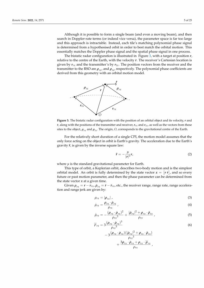
The bistatic radar configuration is illustrated in Figure 3, with a target at position r,relative to the centre of the Earth, with the velocity r. The receiver’s Cartesian location isgiven by rrx and the transmitter’s by rtx. The position vectors from the receiver and thetransmitter to the RSO are ρrx, and ρtx, respectively. The polynomial phase coefficients arederived from this geometry with an orbital motion model.

r

rrxrtx

ρrxρtx

r

O

Figure 3. The bistatic radar configuration with the position of an orbital object and its velocity, r andr, along with the positions of the transmitter and receiver, rrx and rtx, as well as the vectors from thesesites to the object, ρrx and ρtx. The origin, O, corresponds to the gravitational centre of the Earth.

For the relatively short duration of a single CPI, the motion model assumes that theonly force acting on the object in orbit is Earth’s gravity. The acceleration due to the Earth’sgravity r, is given by the inverse square law:

r = − µ

|r|3 r, (2)

where µ is the standard gravitational parameter for Earth.This type of orbit, a Keplerian orbit, describes two-body motion and is the simplest

orbital model. An orbit is fully determined by the state vector x =[r r], and so every

future or past motion parameter, and then the phase parameter can be determined fromthe state vector x at a given time.

Given ρrx = r− rrx, ρrx = r− rrx, etc., the receiver range, range rate, range accelera-tion and range jerk are given by:

ρrx = |ρrx| , (3)

ρrx =ρrx · ρrx

ρrx, (4)

ρrx = − (ρrx · ρrx)2

ρrx3 +|ρrx|2 + ρrx · ρrx

ρrx, (5)

...ρ rx = 3

(ρrx · ρrx)3

ρrx5

− 3(ρrx · ρrx)(|ρrx|2 + ρrx · ρrx)

ρrx3

+3ρrx · ρrx + ρrx ·

...ρ rx

ρrx,

(6)

Remote Sens. 2022, 14, 2571 6 of 25

and this is similarly the case for the transmitter’s terms ρtx, ˙ρtx, ρtx and...ρ tx. Additionally,

...r is determined from (2) and is given by:

...r =3µr · r|r|5 r− µ

|r|3 r . (7)

Note that rrx, rrx and ...r rx are the (known) motion terms for the receiver on the Earth’ssurface, and this is similarly the case for rtx, rtx and ...r tx for the transmitter. In this referenceframe with a rotating Earth, the MWA is travelling (instantaneously) 47 m/s faster than thesouthern-most transmitter used in Section 6.

The expressions for the instantaneous bistatic delay and Doppler are

tD =1c(ρrx + ρtx − |rrx − rtx|) , (8)

fD =− 1λ(ρrx + ρtx) . (9)

The spatial parameters, azimuth and elevation, and their rates, are determined directlyfrom the orbit as well, ensuring that any RSO is spatially tracked throughout the CPI.These parameters are determined from the receiver’s slant range vector rotated from anEarth-centred inertial (ECI) geocentric equatorial reference frame to a south-east zenith(SEZ) topocentric-horizon frame. The rotated vector q and its subsequent rates q and q aregiven by the following formula:

q = D−1ρrx , (10)

q = D−1ρrx , (11)

q = D−1ρrx , (12)

where D is the SEZ to ECI rotation matrix [25]. Note in some publications q and ρ areinstead written as ρsez and ρeci respectively.

From these topocentric pointings, the azimuth and elevation, θ and φ, respectively,and their rates, are determined. Given q = [qS, qE, qZ]

T , the expressions for the spatialparameters are:

θ =π

2− tan−1

(qEqS

), (13)

θ =qSqE − qEqS

qS2 + qE2 , (14)

θ =1

(qS2 + qE2)2

((qSqE − qEqS)(qS

2 + qE2) (15)

− 2(qSqS + qEqE)(qSqE − qEqS))

,

and

φ = tan−1

(qZ√

qS2 + qE2

), (16)

φ =qZ − q sin φ√

qS2 + qE2

, (17)

φ =1

qS2 + qE2

((q sin φ− qZ)(qSqS + qEqE)√

qS2 + qE2

(18)

+ (qZ − q sin φ− qφ cos φ)√

qS2 + qE2

).

Remote Sens. 2022, 14, 2571 7 of 25

Note that the slant ranges (and their rates) will be unchanged by the rotation,q = |q| = ρrx, and again, this is also the case for the subsequent rates.

A previous study assumed that two terms for each of the spatial parameters weresufficient [24]. However, some particularly fast moving objects, such as rocket bodies ingeosynchronous transfer orbits, require additional parameters. The full angular accelera-tions were required to detect an SL-12 rocket body (NORAD 20082) travelling at 9.6 km/s(in the ECI reference frame).

An equivalent approach is to rotate the tile locations to the ECI frame, in which casethe spatial parameters and subsequent beamforming will have a topocentric right ascensionand topocentric declination (rather than the azimuth and elevation) [18].

Given these spatial parameters, the polynomial phase coefficients can be determinedfor both Doppler and spatial aspects. The Doppler phase coefficients for the first four termsare given by their respective-order Taylor series terms:

d0 = −2π

λ(ρrx + ρtx − |rrx − rtx|) , (19)

d1 = −2π

λ(ρrx + ρtx) , (20)

d2 = − π

λ(ρrx + ρtx) , (21)

d3 = − π

3λ(...ρ rx +

...ρ tx) . (22)

Similarly, the expression for the spatial coefficients is given by:

bn,0 = −2π

λ(k · un) , (23)

bn,1 = −2π

λ(k · un) , (24)

bn,2 = − π

λ(k · un) , (25)

where un is the location of the nth tile, and k, k and k are the wavevector and its ratesdetermined from (13)–(18).

Finally, the resulting matched phase signal for each antenna can be formed by samplingeach antenna’s polynomial phase signal at time instances mτ, for m ∈ [−M−1

2 , . . . , M−12 ]:

Pn[m] = e−j(bn,0+(bn,1+d1)mτ+(bn,2+d2)(mτ)2+d3(mτ)3). (26)

This full set of matching phase signals ensures that a potential orbit determined bythe state vector [r, r] will be completely tracked both spatially and in Doppler across everypulse and every tile.

This phase-matching matrix can then be applied to the data, by applying the polyno-mial phase signal correction to each tile by forming the Hadamard product between thetwo. These signals are then coherently combined by summing across each tile to form asingle, fully matched, slow time-series for a single range bin, χ[m]. The range bin delaysample is determined by the time delay tD, from (8), as well as the sample rate B.

χ[m] =N−1

∑n=0

(Pn[m]� χn[t, m])|t=BtD . (27)

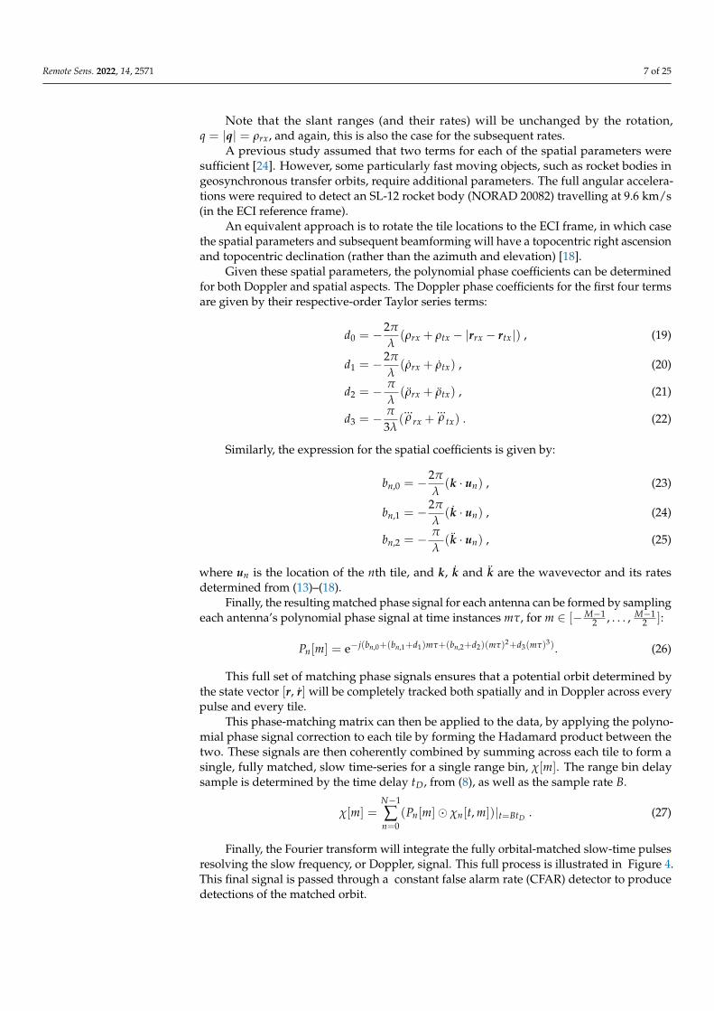
Finally, the Fourier transform will integrate the fully orbital-matched slow-time pulsesresolving the slow frequency, or Doppler, signal. This full process is illustrated in Figure 4.This final signal is passed through a constant false alarm rate (CFAR) detector to producedetections of the matched orbit.

Remote Sens. 2022, 14, 2571 8 of 25

χ[ f ] =

∣∣∣∣∣∣M−1

2

∑m=−M−1

2

χ[m]e−j2πf mM

∣∣∣∣∣∣2

. (28)

d1d1

d2d2

d3d3

b0,0b0,0

b0,1b0,1

b0,2b0,2

b1,0b1,0

b1,1b1,1

b1,2b1,2

bN-1,0bN-1,0

... bN-1,1bN-1,1

bN-1,2bN-1,2

phase coefficients

...

pulse stack for N tiles [ r, r ]orbit description

⊙single range slice phase matching matrix

Σ

FT

Doppler signal

Figure 4. Illustration of the signal processing steps outlined in Section 3. An orbital state vector isused to determine the polynomial phase signal coefficients to form a phase-matching matrix. A singlerange’s slow-time signals are matched to the orbit, and combined using this matrix before detection.

Remote Sens. 2022, 14, 2571 9 of 25

Note that the d0 term is not included, since the final phase is not of immediate interest;however, the inclusion of d1 ensures any matched target returns will be close to zeroDoppler. This allows for a pruned FT implementation. That is, only those frequency binssufficiently close to zero Doppler need to be determined to cover any potential orbitalvelocity offset, and also large enough to encompass sufficient bins allowing for accuratethreshold estimation for the CFAR detector.

The process in (27) and Figure 4 only samples a single range bin; creating an entiredelay–Doppler map would serve little purpose, since the orbit-derived parameters usedto generate that map would only be relevant to a single range. A common pitfall withpassive radar and analogue signals is that the ambiguity function is content-dependant;depending on the specific audio signal, the range resolution can be quite poor [26]. Byprocessing a single range bin, this issue can be avoided, or at least moderated. Althoughsignal content might result in a poor ambiguity function, by matching orbits directly, theorbit-derived parameters will vary across range bins and only one orbit will have thebest-matched parameters.

By forming detections with orbit-derived parameters, every detection will be asso-ciated with an orbital track with some confidence, since the beamforming has followedthe orbit through the CPI. This associated trajectory greatly assists ongoing tracking anddetection-track association. Additionally, having a known trajectory estimate is requiredfor the OD step outlined in Section 4.

This process is entirely flexible and the motion model can be extended to more compli-cated orbital models, such as incorporating an oblate Earth or other perturbing forces. Themeasurement model can also be tailored, rather than applying far-field beamforming whichis suitable for the MWA’s compact configuration. The matched signals are able to be readilyextended to near-field beamforming. Instead of calculating beamforming coefficients aswell as Doppler coefficients, Doppler coefficients ((19)–(22)) can be determined for eachtile’s location and the resulting matched signal can be determined as before.

4. Orbit Determination

Given an orbital track, either from an RSO catalogue or an initial orbit hypothesis, thesix dimensional positions and velocities are determined and the processing steps describedin Section 3 are applied. The position and velocity state vectors, or indeed the orbitalelements, can be adjusted to form search volumes for RSOs, either to detect manoeuvredtargets or to update an old track. If an RSO is detected, a series of associated measurementswill be produced, although the process utilises the six-dimensional state vectors. Themeasurements are produced in the standard radar measurements of azimuth, elevation,bistatic-range, and Doppler.

The number of measurement parameters is extendable in many measurement dimen-sions. As covered in previous sections, there is a need to account for higher-order motionparameters such as Doppler rates as well as spatial rates. These dimensions are not searchedin the processing steps, as that would result in an intractable search space. Instead, onlyazimuth, elevation, bistatic range, and Doppler are the adjusted measurement parameters(either directly or via the orbital elements); the first three are searched over as part of theCartesian location and the latter, Doppler, is searched over via the FT as part of the finalDoppler-resolving step. If sufficient computational resources existed, it may be possibleto independently search through higher-order parameters, which would allow them to beincluded as part of the OD step.

Orbit determination is achieved using the batch least-squares method outlined in [27].This method fits an orbit to a track (or collection) of measurements z. The measurementsvector z consists of k measurements such that z =

[z0 z1 . . . zk−1

]T , each observedat times t0, t1 ... tk−1, with each measurement consisting of the detected delay, Doppler,azimuth and elevation such that zi =

[tDi fDi θi φi

]T .If the function f maps a state vector x to its respective measurement parameters at

times t0, t1 . . . tk−1 (for a single pass, two-body orbit propagation is used such that f consists

Remote Sens. 2022, 14, 2571 10 of 25

of Equations (8), (9), (13) and (16); for longer-term orbit determination, more complicatedmodels need to be used), the best orbital fit is the state vector which, when propagated,minimises the residuals between the measurements and the predicted measurements:

x = argminx

(|z− f (x)|2) (29)

As f is highly non-linear, finding a general minima is not trivial and instead a solutionis found by linearising all quantities around an initial state vector x0. This initial solutionmay be provided a priori from a source such as a previous pass or a space catalogue, orinstead from the detections directly using an IOD method. The residuals, ε, can thenbe approximated:

ε = z− f (x) (30)

≈ z− f (x0)−∂ f∂x

(x− x0) (31)

= ∆z− F∆x , (32)

with ∆x = x − x0 being the difference between x and the reference state vector, and∆z = z− f (x0) being the difference between the actual measurements and the predictedmeasurements for the reference orbit. Additionally, the Jacobian F = ∂ f (x)

∂x |x=x0 consists ofthe partial derivatives of the modelled observations with respect to the state vector.

Now, the orbit determination step is achieved by solving a linear least-square problem,with Equation (29) simplified as:

∆xls = argmin∆x

(|∆z− F∆x|2) . (33)

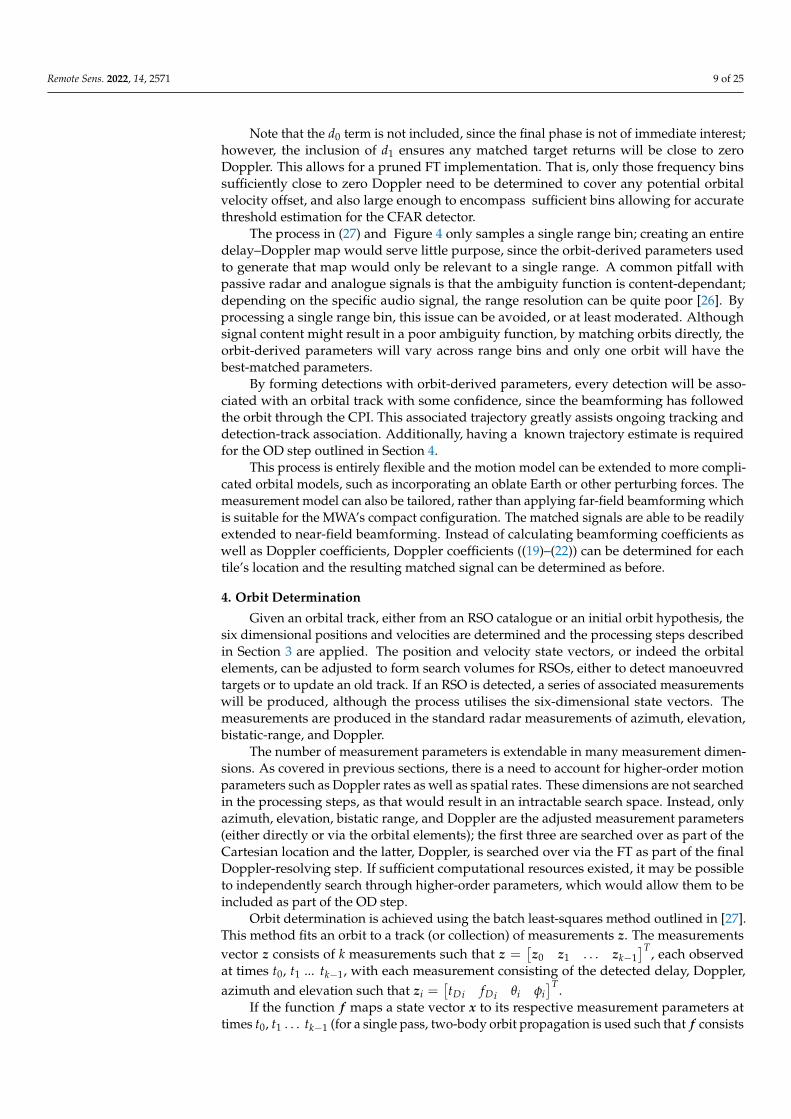
With each detection and track associated with a state vector, x0, a solution to Equation (33)is readily determined [28]. This process is illustrated in Figure 5.

x0

Reference Orbit∆xls

xls

Estimated Orbit

Measurements

Figure 5. Illustration of the orbit determination process, starting with a reference orbit and thenestimating an orbit adjustment to best fit the measurements.

In order to compare different measurement types equally, the residuals are normalisedby scaling the measurements (and thus, the Jacobians) by the mean measurement errorσi. In Equation (33), F and ∆z are replaced by F ′ = ΣF and ∆z′ = Σ∆z, with Σ beingthe diagonal matrix Σ = diag(σ−1

0 , σ−11 , . . . , σ−1

k−1). The mean measurement errors inΣ are determined experimentally and also from the measurement resolutions, with therange measurement accuracy determined by the signal bandwidth, the Doppler resolutiondetermined by the CPI length, and the azimuth and elevation resolutions determined bythe size of the array aperture. In terms of signal processing, the only aspect that is withinthe system’s control is the Doppler resolution through adjusting the CPI length. It is alsopossible to further scale the errors using each detection’s SNR, such that stronger detectionscontribute to the orbital fit to a greater extent than the weaker detections [29].

Remote Sens. 2022, 14, 2571 11 of 25

With this process, the linearised error covariance matrix is now obtained with thefollowing formula:

cov(xls, xls) = (FTΣ2F)−1 . (34)

The diagonal elements of this covariance matrix yield the standard deviation of theestimate of each element of the state vector.

4.1. Multistatic Orbit Determination

The OD approach is readily extendable to incorporate multistatic returns, with thedetections from additional transmitters simply providing extra measurement parametersto fit the orbit. Having each detection associated with a state vector allows for the easyassociation of multistatic measurements.

A given detection’s position is defined by the narrow beamwidth of the electronicallysteered beam and its intersection with the isorange ellipsoid defined by the time delayfrom Equation (8). However, the range resolution achievable using FM radio signals isquite poor, and although the large aperture allows spatially accurate beams, the volumeof the intersection will extend radially. This segment, when intersected with subsequentellipsoids, will not dramatically improve the estimation, as each subsequent coarse ellipsoidwill still be intersected with the identical narrow beam.

Conversely, the target’s velocity estimate can be dramatically improved. By express-ing (9) in terms of the orbital velocity, r, it is clear that every Doppler measurement fDdefines a plane of potential velocities:(

ρrxρrx

+ρtxρtx

)· r = −λ fD +

ρrx · rrx

ρrx+

ρtx · rtx

ρtx. (35)

Additional Doppler returns from different sensors will drastically constrain the extentof possible velocities. Two measurements will define a line, and three or more detectionswill completely determine (or even overdetermine) the velocity. An accurate velocity esti-mate is the most important aspect of the orbital state vector estimate, as errors in the velocityestimation will produce increasingly erroneous position estimates when propagated for-ward. Even if multistatic detections are not coincident, the resulting orbit will be improvedfor having multiple Doppler measurements to constrain the region of possible velocities.

Other benefits of multistatic observations include the diversity of coverage, bothspatially and in terms of signal content, as well as resilience by making the most of thevast amount of energy being radiated outward. If the bistatic configuration is relying onnarrow elevation sidelobes, there will be gaps in illumination. Using multiple transmitterswill help ensure any gaps are covered by at least one other sensor. Additionally, analogueFM radio is not necessarily ideal for radar due to the content-dependant nature of theambiguity function, and diverse options (even multiple stations from the one tower) willprovide resilience in the event one station’s content is not suitable. FM radio signals havebeen shown to be well suited for distributed bistatic radar systems [30].

4.2. Initial Orbit Determination

The process outlined in Section 3 requires an orbit to match the parameters in orderto form detections. Although these orbits can come from a catalogue of tracks, there willstill need to be additional work for uncued detection. The six-dimensional search space ofall potential orbit state vectors is currently an unreasonably large search space. However,earlier work has shown that the application of radar constraints can greatly simplify theprocess. By looking for RSOs at their point of minimum bistatic range, and constrainingranges in orbital eccentricity, this search space can be reduced further [31]. Akin to creatinga spatial fence with receiver beams, this approach only searches a narrow region in orbitalparameter space. RSOs that do not pass through the right parameter space on one pass will

Remote Sens. 2022, 14, 2571 12 of 25

pass through eventually. Tracked RSOs can then be treated as normal, per the general stepsin this section.

There may be thousands of objects from a typical space catalogue observable fromthe MWA at any one point in time, and matching these tracks (and also searching a regionaround these tracks) would potentially require matching a hundred thousand orbits. Anuncued search of a region, even including a constrained orbital search space, will potentiallyrequire matching one million orbits.

Depending on the available computer memory, a region’s hypothesised orbits andresulting parameters can be stored. The phase matrix coefficients, or indeed the full phasematrices, are applicable for all subsequent CPIs and thus, storing them saves on ongoingcomputation.

5. Continental Radar

The Australian continent provides a unique context for large-scale FM radio-basedpassive radar. The majority of the population is concentrated in cities near the coast,particularly in the south-east of the country. The FM radio transmitters are similarly locatedin the population centres. This is illustrated by a map of the most powerful FM transmittersin Figure 6. The MWA is naturally situated far away from these powerful transmitters.This isolation benefits the MWA’s astrophysics goals by reducing incident radio frequencyinterference (RFI). Such a location would ordinarily be less than ideal for terrestrial passiveradar purposes, with most passive radar systems designed to be located within the footprintof the illuminating transmitter. However, for detecting satellites at LEO altitudes, such aseparation becomes a significant advantage.

Figure 6. A map of all the powerful (greater than 50 kW) FM radio transmitters in Australia.

Remote Sens. 2022, 14, 2571 13 of 25

Typical FM radio transmitting antennas consist of six to eight antennas combined toform a beam. These antennas are typically angled (as well as electronically beam-steered)towards the ground in order to direct the maximum amount of energy to the population [32].This can pose a challenge for satellite illumination, as every effort is made to minimisethe amount of wasted energy being radiated outward from Earth, with the main elevationsidelobes being as low as −15 dB compared to the main lobe [32]. However, these sidelobeswill still provide sufficient illumination, and perhaps some Australian transmitters are notso directive, especially given the widespread and low population density found in somerural areas. Figure 7 details a typical FM transmitter pattern. The main beam is directedto the ground; however, sidelobe levels are not insignificant at elevations of up to 15°.At higher elevations, considerable energy is still being radiated in some sidelobes. Thepatterns of other transmitters may not be so directional.

Figure 7. Typical FM array’s in situ measured antenna pattern via the SixArms airborne radiomeasurement system [33].

Instead of relying on sufficient sidelobes for target illumination, it is possible to makeuse of the main lobe for illumination. Given the number of transmitters in the south-eastof Australia, and the lack of large interfering transmitters in between that region and theMWA, a target above the MWA will be illuminated by the main beam of potentially dozensof significant sources. This is illustrated in Figure 8, showing the incident power on an RSOat various altitudes above a receiver with a wide range of potential transmitter–receiverseparation distances. It shows that the loss incurred by the increased transmitter to targetdistance, ρtx, is more than offset by the transmitter gain of the main lobe, from Figure 7.Indeed, the MWA has been used to detect FM radio returns from the moon, undoubtedlyfrom transmitters half-way around the world [34].

Remote Sens. 2022, 14, 2571 14 of 25

Figure 8. Incident power on an object above a receiver, for an equivalent isotropically radiated power(EIRP) of 100 kW, with a beam pattern as shown in Figure 7. Note that this figure is based on aspherical Earth model.

The use of the main lobe is illustrated in Figure 9, showing the SNR of the InternationalSpace Station (ISS), utilising a transmitter in Mount Gambier, over 2500 km away from theMWA. This shows that the strongest detections occur at the lowest transmitter elevationangles (despite the larger signal path loss); it even highlights the diffraction of signals alongthe Earth’s surface with detections occurring at transmitter elevations of almost 2° belowthe horizon.

Figure 9. An example pass showing the detections of the International Space Station utilising adistant transmitter versus the elevation of the target. The blue line shows the detected signal tonoise ratio and the red line shows the signal path length and the reflected range. The reflected rangeis given by ρrx + ρtx and does not include the baseline length to give the full bistatic range, as inEquation (8).

Finally, the majority of FM transmitters transmit a vertically polarised signal, so thedirection relative to the MWA will determine the best receiver polarisation. The verticalpolarisation to the south will be coplanar with the MWA’s north–south polarisation, andthere is a similar situation for transmitters to the east and the MWA’s east–west polarisation.However, impacts from effects such as Faraday rotation due to the ionosphere and otherfactors mean that the presence of matching transmitter and receiver polarisations is notnecessarily a decisive factor in the detected SNR.

Remote Sens. 2022, 14, 2571 15 of 25

6. Results

The results in this section are obtained from 20 min of data consisting of a series offive minute dwells collected in December 2019. As detailed in Section 2, these dwells wererecorded and channelised in real-time and transferred to storage in Perth. Subchannelswere selected such that the full national FM band of approximately 20 MHz was collected.The MWA’s analogue beamformer was directed to point at the zenith. In addition to MWAobservations, several transmitter reference signals were collected from around the country.These are outlined in Table 1 and shown in Figure 10. Despite being located in a radio-quiet observatory, a sufficient signal is able to be observed from the nearby transmittersin Geraldton, some 300 km to the south-west of the MWA. Reference observations werecollected in Perth utilising receiver hardware identical to that used in the MWA. Locatedat the Curtin Institute of Radio Astronomy (CIRA), this MWA-like reference receiver issynchronised with the MWA via GPS.

Transmitter reference signals were also collected at locations near Albany and MountGambier with a SDR setup. These remote SDR nodes are all GPS-disciplined in order tomaintain synchronisation, the collections were manually triggered, and each node was ableto record a reference with a bandwidth of 10 MHz. Although 10 MHz is insufficient tocollect the full FM band, it is generally sufficient to collect every high-powered FM stationfrom a single site. The transmitter near Mount Gambier, over 2500 km away from theMWA and situated in the south-east of South Australia, is one of the highest power radiotransmitters in the country. It should be noted that for each transmitter there are manydifferent FM radio stations, all potentially being broadcast at different power levels. Thefigures in Table 1 are simply the maximum licensed power level from that tower, and thetrue levels may, in fact, be lower.

Data from these remote SDR devices were then transferred to servers at CIRA in Perth,alongside the MWA-collected data, allowing offline space surveillance processing. Thisis achieved by downsampling the MWA data, as well as the SDR transmitter referencedata, to narrowband signals (typically 100 kHz) matching known FM stations, and thenundertaking radar processing as detailed in Section 3, utilising a 3 s CPI.

Figure 10. A map showing the Murchison Widefield Array as well as the transmitters used to generatethe results in Section 6. Details of the transmitters are given in Table 1.

Remote Sens. 2022, 14, 2571 16 of 25

Table 1. Transmitters utilised in this section’s results.

Name (Locale) Maximum Power Distance from MWA

Geraldton 30 kW 295 kmPerth 100 kW 591 km

Albany 50 kW 886 kmMount Gambier 240 kW 2524 km

Figures 11 and 12 illustrate some of the aggregate detections from these observa-tions. These detections are formed by parsing the Doppler signal data (from Equation (28))through a cell-averaging CFAR detector. In passive radar processing (and indeed, noiseradar), target signals exist against a noise/clutter pedestal floor formed by the cross cor-relation of the reference signal against other unwanted/mismatched signals. The CFARdetector estimates this floor from a local threshold region around the cell that is beingevaluated, and the SNR is determined by the peak signal against this floor. For these results,we have used a very conservative threshold of 16 dB, greatly minimising the presence of anyfalse detections. System performance would be improved with a more realistic threshold;however, care would need to be taken to ensure false detections are not incorporated intoorbital estimates.

Figure 11. Example results showing dozens of tracks’ detections above the Murchison WidefieldArray (MWA), with each detection’s colour corresponding to its altitude. The location of theMWA is shown, denoted by an X. The transmitters are also shown, denoted by the black triangles.Additionally, rings denoting a 1000-km range (from the MWA) are included.

Remote Sens. 2022, 14, 2571 17 of 25

Figure 12. Example results, matching Figure 11, showing dozens of tracks’ detections above theMurchison Widefield Array (MWA) with each detection’s colour corresponding to its altitude. Thelocation of the MWA is shown, denoted by an X. The transmitters are also shown, denoted by theblack triangles. Additionally, a ring denoting a 1000-km range (from the MWA) is included.

The MWA is able to maintain tracks of many targets at various ranges. During theseshort and targeted dwells, the MWA was able to detect every large RSO that was withinthe MWA’s main beam at a range of less than 1000 km. The USSPACECOM cataloguedefines a large object as having a median radar cross section (RCS) of 1 m2 or greater anda medium object having a median RCS between 0.1 m2 and 1 m2; however, these valuesare for microwave frequencies which differ from those used in this paper, and shouldonly be taken as a general indicator of size [35]. Additionally, many detections are foundoutside these limits, including the detection of medium RSOs, RSOs at longer ranges, andindeed RSOs well outside of the main receiver beam. This is consistent with the earliertheorised performance [10]. Predictions of the large RSOs with a closest approach of lessthan 1000 km indicate the MWA would detect over 1800 RSO passes per day, when used ina beam-stare mode pointing at the zenith. However, detections outside these conservativelimits, as well as the ability to rapidly adjust the analogue beamforming, suggest the truenumber will be larger.

Figure 13 shows the detections of an outbound pass of COSMOS 1707 (NORAD 16326),a large (now defunct) satellite. The detections were formed utilising the transmitter nearAlbany and show the bistatic range, bistatic Doppler, azimuth and elevation. Tracked foralmost 90 s, the RSO passes the closest bistatic approach (at zero Doppler) and moves northto the closest approach to the receiver (at its maximum elevation). Figure 14 shows theaccuracy of the orbit generated from the COSMOS 1707 measurements. The top row showsthe accuracy of the positional and the velocity covariance, from (34). The bottom row showsthe accuracy of the position and velocity estimate in comparison to the two-line element(TLE) ephemeris. The two rows are in general agreement as to the resulting accuracy andthe results are significantly improved when compared to the initial study [4]. These resultsare typical of most of the objects the MWA detects with a bistatic configuration.

Remote Sens. 2022, 14, 2571 18 of 25

Figure 13. The four measurement parameters from the detections of an outbound COSMOS 1707detected using an FM transmitter in Albany.

With many more transmitters at the radar’s disposal, there is a scope for increasedcoverage. Figure 15 shows the SNR of a pass of the International Space Station for everytransmitter collected in this campaign. It shows three minutes of detections with almost 50 sof complete overlap for each bistatic pair. The SNR fluctuations shown (for all transmitters)highlight the variable nature of the illuminator coverage due to changes in the transmitterbeampattern as well as variations in bistatic RCS. There may be additional contributingfactors such as Faraday rotation. The ISS is detected well outside of the MWA’s receiverbeam, to an elevation of as low as 5° above the horizon.

Figure 14. The resulting orbit predictions from the measurements from Figure 13. The top row showsthe covariance of the position estimate and the velocity estimate; the bottom row shows the meanerror when compared with the TLE.

Although only the ISS and the Hubble Space Telescope were large enough to bedetected simultaneously using all transmitters, approximately three quarters of all thedetected targets had associated detections from another transmitter. Additionally, everytransmitter was able to detect objects that were not detected by any other transmitter,including the comparatively weaker Geraldton site. This highlights that FM broadcasttransmissions do not uniformly cover the volume above the MWA, and results will improvewith more transmitters being utilised. Despite only being licensed to transmit up to a

Remote Sens. 2022, 14, 2571 19 of 25

maximum of 50 kW, the particular configuration of the Albany transmitter, and its elevationsidelobes, produced the largest number of detections of all the transmitters listed in Table 1.

Figure 15. An example pass showing the signal to noise ratio (SNR) of International Space Stationdetections utilising all the transmitters covered in this section.

Figure 16 shows the detection’s measurements for the same RSO pass as in Figure 13;however, this time, the detections from the Perth transmitter are included. The spatialparameters are near-identical as expected, with the differing geometry resulting in differingdelay and Doppler tracks. When these are combined together in the OD stage, the resultsare significantly improved.

Figure 17 shows the accuracy of the combined orbit, equivalent to Figure 14 showing asingle bistatic case. The combined orbit is significantly more accurate than either individualbistatic pairs, particularly the determined velocity. A single detection from Perth (at the 17 smark) reduces the velocity covariance by an order of magnitude, matching the expectationsoutlined in Section 4.1.

Figure 16. The four measurement parameters from the detections of COSMOS 1707 detected usingFM transmitters in both Albany and Perth.

Remote Sens. 2022, 14, 2571 20 of 25

Figure 17. The resulting orbit predictions from the multistatic measurements from Figure 16. Thetop panels show the covariance of the position estimate and the velocity estimate. The bottom panelsshow the mean errors when compared with the two-line element (TLE).

As mentioned earlier, multistatic detections do not need to be coincident to improvethe overall orbit. Figures 18 and 19 show the results from the detections of NADEZHDA 5(NORAD 25567), a far smaller (albeit still classified as large) RSO at a range of 1000 km. Thefigures again show detections from both the Albany and Perth bistatic pairs, but instead ofbeing coincident, the set of the detections are separated by over a minute. However, just asbefore, the multistatic detections greatly improve the accuracy of the orbit, confirmed bothby the reduced covariance as well as compared to the TLE.

Figure 18. The four measurement parameters from the detections of NADEZHDA 5 detected usingFM transmitters in both Albany and Perth.

Remote Sens. 2022, 14, 2571 21 of 25

Figure 19. The resulting orbit predictions from the multistatic measurements from Figure 18. Thetop panels show the covariance of the position estimate and the velocity estimate. As the detectionsfrom each bistatic pair are not coincident, the combined errors will be initially identical to Perth’s.The bottom panels show the mean errors when compared with the two-line element (TLE).

An example of the three transmitters is simultaneously shown in Figures 20 and 21. Inthis example, the satellite OPS 5721 (NORAD 9415) is detected for approximately 20 s withthe Albany illuminator; however, these detections are supplemented by a small numberof detections achieved utilising the Perth and Mount Gambier illuminators. Despite theshort period of detections, the resulting orbit is very accurate when compared against theTLE. Indeed, after only five seconds, the resulting orbit utilising detections across all threetransmitters is very accurate.

There are complications when comparing and assessing determined orbits, especiallywhen comparing them to the TLEs. Looking at the covariance of the multistatic results inFigure 17, the increasing number of detections improves the estimate, especially for velocity.However, when compared to the TLE, the error does not improve; rather, it plateaus. Thiscould be due to many factors; however, these results are within the accuracy of the TLEsthemselves, as positional errors generally vary from a minimum error of approximately1 km at the TLE’s epoch up to 5 km, depending on the age of the TLE [36,37]. Theseuncertainties could potentially mask any systematic biases or offsets, either from the systemitself or from the ionosphere [38,39]. Longer surveillance campaigns are needed to properlyassess any potential systemic issues and to fully evaluate the accuracy of short-arc orbitdetermination.

The true RCS sizes of objects are challenging to estimate, particularly for a passiveradar. Without knowing the precise details of transmitter characteristics, the amount ofincident power is not known. Additionally, bistatic RCS is typically a complicated functionand without accurate knowledge of the precise size and attitude of RSOs, the bistatic RCSis difficult to determine.

The RCS values for known RSOs can be coarsely estimated with simple shapes, suchas cylinders. Comparing the estimates of the detected objects provides additional datapoints to match against the earlier performance predictions. For example, the mediumRCS satellite OV1-5 (NORAD 2122) was detected at a range of 1150 km from the MWA(the corresponding bistatic range was 1600 km) with an SNR of 21 dB. The maximummonostatic RCS of a cylinder of matching dimensions (1.387 m length and 0.69 m diameter)is approximately 0.7 m2. For OV1-5, the RSO’s length is less than half a wavelength,meaning that for smaller RSOs, the scattering will cause the RCS to decrease rapidly [40].Conversely, for RSOs that possess trailing antennas that have low RCS at high frequencies,these structures can produce a large RCS at MWA frequencies. Examples such as OV1-5

Remote Sens. 2022, 14, 2571 22 of 25

agree strongly with the initial predictions that the MWA, used as a passive radar, is able todetect objects with an RCS of 0.5 m2 to a range of 1000 km [10].

Figure 20. The four measurement parameters from detections of OPS 5721 detected using FMtransmitters in Albany, Perth and Mount Gambier.

Figure 21. The resulting orbit predictions from the multistatic measurements from Figure 20. Thetop panels show the covariance of the position estimate and the velocity estimate. The bottom panelsshow the mean errors when compared with the two-line element (TLE).

7. Conclusions

This paper has described the use of the MWA as a passive radar for the surveillanceof space with FM radio illumination. The MWA’s high time-resolution and receivingcapabilities have been described, and the orbital-specific signal processing methods to formradar products have been detailed, from pulse compression through to forming detections.These orbital-specific methods are required to track an RSO’s motion throughout long CPIsto increase SNR. Following detection, the paper details the orbit determination methods,and how multistatic detections can greatly improve the orbital estimate. To demonstrateand verify these methods, this paper includes the results of a short collection campaign,utilising four transmitters across the country. With the data collected during this campaignthe MWA was able to detect and accurately track every large object that passed throughits main beam at a range of 1000 km or less. It additionally tracked many other objects

Remote Sens. 2022, 14, 2571 23 of 25

outside these limits. These results are in agreement with earlier predictions made of thespace surveillance capabilities of the MWA when used as a passive radar receiver.

Multiple transmitters were used to form a multistatic radar network, with multistaticdetections allowing for rapid and accurate orbit determination, with additional transmittersalso providing greater coverage and resilience. By utilising these many transmitters, theMWA is able to provide persistent and widefield coverage of satellites in low Earth orbit.The MWA is able to achieve this coverage using scalable and efficient signal processingmatching the radar processing to the RSO’s orbit. The widefield coverage ensures thatRSOs are tracked for sufficient time to accurately determine an orbit from a single pass.

Although it is not the SKA’s intended purpose, using the techniques described here, theSKA will be a highly capable space surveillance sensor when used as a radar [41]. The SKA willbe significantly more sensitive than the MWA, and even a modest increase in sensitivity wouldenable the detection of signals from a higher altitude (for example, from 1000 km to 2000 km).As shown in Figure 8, higher altitudes would intrinsically allow the utilisation of transmittersat even greater distances, including along Australia’s eastern seaboard. Conversely, sincetransmissions reflected from RSOs are a source of interference for astrophysical observations,knowledge of which RSOs are above the horizon will be important information for the removalof RSO effects from SKA observations. Incorporating a system to remove interference reflectedfrom RSOs would be a natural extension for any radio telescope space surveillance radar.

Author Contributions: Conceptualisation: B.H., S.T. Data Curation: B.H., A.S., D.G., B.C., M.S.Formal analysis: B.H. Investigation: B.H., A.S. Methodology: B.H. Resources: R.Y., S.T. Software:B.H. Supervision: M.R., R.Y., S.T. Writing—original draft: B.H. Writing—review and editing: B.H.,M.R., R.Y., S.T. Visualisation: B.H., R.Y. All authors have read and agreed to the published version ofthe manuscript.

Funding: This research received no external funding.

Data Availability Statement: The data sets were derived from sources in the MWA Data Archive(project ID D0020) at https://asvo.mwatelescope.org/, and can be made available.

Acknowledgments: This scientific work makes use of the Murchison Radio-astronomy Observatory,operated by CSIRO. We acknowledge the Wajarri Yamatji people as the traditional owners of theobservatory’s site. Support for the operation of the MWA is provided by the Australian Govern-ment, under a contract to Curtin University administered by Astronomy Australia Limited. Weacknowledge the Pawsey Supercomputing Centre which is supported by the Western Australian andAustralian Governments. The authors would like to thank David Holdsworth and Nick Spencer fortheir invaluable feedback and reviews of the manuscript. This work is supported by the DefenceScience and Technology Group.

Conflicts of Interest: The authors declare no conflict of interest.

References1. Tremblay, S.; Ord, S.; Bhat, N.; Tingay, S.; Crosse, B.; Pallot, D.; Oronsaye, S.; Bernardi, G.; Bowman, J.; Briggs, F.; et al. The high

time and frequency resolution capabilities of the Murchison Widefield Array. Publ. Astron. Soc. Aust. 2015, 32, e005 . [CrossRef]2. McSweeney, S.; Ord, S.; Kaur, D.; Bhat, N.; Meyers, B.; Tremblay, S.; Jones, J.; Crosse, B.; Smith, K. MWA tied-array processing III:

Microsecond time resolution via a polyphase synthesis filter. Publ. Astron. Soc. Aust. 2020, 37, e034. [CrossRef]3. Williamson, A.; James, C.; Tingay, S.; McSweeney, S.; Ord, S. An Ultra-High Time Resolution Cosmic-Ray Detection Mode for the

Murchison Widefield Array. J. Astron. Instrum. 2021, 10, 2150003. [CrossRef]4. Palmer, J.E.; Hennessy, B.; Rutten, M.; Merrett, D.; Tingay, S.; Kaplan, D.; Tremblay, S.; Ord, S.M.; Morgan, J.; Wayth, R.B.

Surveillance of Space using Passive Radar and the Murchison Widefield Array. In Proceedings of the 2017 IEEE Radar Conference(RadarConf), Seattle, WA, USA, 8–12 May 2017; pp. 1715–1720. [CrossRef]

5. Losacco, M.; Di Lizia, P.; Massari, M.; Naldi, G.; Pupillo, G.; Bianchi, G.; Siminski, J. Initial orbit determination with the multibeamradar sensor BIRALES. Acta Astronaut. 2020, 167, 374–390. [CrossRef]

6. Dhondea, A.; Inggs, M. Mission Planning Tool for Space Debris Detection and Tracking with the MeerKAT Radar. In Proceedingsof the 2019 IEEE Radar Conference (RadarConf), Boston, MA, USA, 22–26 April 2019; pp. 1–6.

7. Malanowski, M.; Jedrzejewski, K.; Misiurewicz, J.; Kulpa, K.; Gromek, A.; Klos, J.; Droszcz, A.; Pozoga, M. Passive Radar Basedon LOFAR Radio Telescope for Air and Space Target Detection. In Proceedings of the 2021 IEEE Radar Conference (RadarConf21),Atlanta, GA, USA, 7–14 May 2021; pp. 1–6. [CrossRef]

Remote Sens. 2022, 14, 2571 24 of 25

8. McMullin, J.; Diamond, P.; McPherson, A.; Laing, R.; Dewdney, P.; Casson, A.; Stringhetti, L.; Rees, N.; Stevenson, T.; Lilley, M.;et al. The Square Kilometre Array project. Soc. Photo-Opt. Instrum. Eng. (SPIE) Conf. Ser. 2020, 11445, 1144512. [CrossRef]

9. Lind, F.D. Passive Radar and Ionospheric Irregularities. In Proceedings of the Solar Heliospheric and Ionospheric Workshop forthe MWA, Cambridge, MA, USA, 1 November 2006.

10. Tingay, S.J.; Kaplan, D.L.; McKinley, B.; Briggs, F.; Wayth, R.B.; Hurley-Walker, N.; Kennewell, J.; Smith, C.; Zhang, K.; Arcus, W.;et al. On the Detection and Tracking of Space Debris Using the Murchison Widefield Array. I: Simulations and Test ObservationsDemonstrate Feasibility. Astron. J. 2013, 146, 103. [CrossRef]

11. Prabu, S.; Hancock, P.J.; Zhang, X.; Tingay, S.J. The development of non-coherent passive radar techniques for space situationalawareness with the Murchison Widefield Array. Publ. Astron. Soc. Aust. 2020, 37, e010. [CrossRef]

12. Losacco, M.; Di Lizia, P.; Massari, M.; Bianchi, G.; Pupillo, G.; Mattana, A.; Naldi, G.; Bertolotti, C.; Roma, M.; Schiaffino, M.; et al.The Multibeam Radar Sensor BIRALES: Performance Assessment for Space Surveillance and Tracking. In Proceedings of the 2019IEEE Aerospace Conference, Big Sky, MT, USA, 2–9 March 2019; pp. 1–13. [CrossRef]

13. National Research Council and others. Continuing Kepler’s Quest: Assessing Air Force Space Command’s Astrodynamics Standards;National Academies Press: Washington, DC, USA, 2012.

14. Jedrzejewski, K.; Kulpa, K.; Malanowski, M.; Pozoga, M. Experimental Trials of Space Object Detection using LOFAR RadioTelescope as a Receiver in Passive Radar. In Proceedings of the 2022 IEEE Radar Conference (RadarConf22), New York, NY, USA,21–25 March 2022; pp. 1–6.

15. Sahr, J.D.; Lind, F.D. The Manastash Ridge radar: A passive bistatic radar for upper atmospheric radio science. Radio Sci. 1997,32, 2345–2358. [CrossRef]

16. Clarkson, V.; Palmer, J. New Frontiers in Passive Radar. IEEE Potentials 2019, 38, 9–15. [CrossRef]17. Hennessy, B.; Gustainis, D.; Misaghi, N.; Young, R.; Somers, B. Deployable Long Range Passive Radar for Space Surveillance. In

Proceedings of the 2022 IEEE Radar Conference (RadarConf22), New York, NY, USA, 21–25 March 2022; pp. 1–6.18. Hennessy, B.; Tingay, S.; Young, R.; Rutten, M.; Crosse, B.; Hancock, P.; Sokolowski, M.; Johnston-Hollitt, M.; Kaplan, D.L. Uncued

Detection and Initial Orbit Determination From Short Observations With the Murchison Widefield Array. IEEE Aerosp. Electron.Syst. Mag. 2021, 36, 16–30. [CrossRef]

19. Beardsley, A.P.; Johnston-Hollitt, M.; Trott, C.M.; Pober, J.C.; Morgan, J.; Oberoi, D.; Kaplan, D.L.; Lynch, C.; Anderson, G.E.;McCauley, P.I.; et al. Science with the Murchison Widefield Array: Phase I results and Phase II opportunities. Publ. Astron. Soc.Aust. 2019, 36, e050. [CrossRef]

20. Wayth, R.B.; Tingay, S.J.; Trott, C.M.; Emrich, D.; Johnston-Hollitt, M.; McKinley, B.; Gaensler, B.M.; Beardsley, A.P.; Booler, T.;Crosse, B.; et al. The Phase II Murchison Widefield Array: Design overview. Publ. Astron. Soc. Aust. 2018, 35, e033. [CrossRef]

21. Stein, S. Algorithms for ambiguity function processing. IEEE Trans. Acoust. Speech Signal Process. 1981, 29, 588–599. [CrossRef]22. Palmer, J.; Palumbo, S.; Summers, A.; Merrett, D.; Searle, S.; Howard, S. An Overview of an Illuminator of Opportunity Passive

Radar Research Project and its Signal Processing Research Directions. Digit. Signal Process. 2011, 21, 593 – 599. [CrossRef]23. Malanowski, M.; Kulpa, K. Analysis of Integration Gain in Passive Radar. In Proceedings of the 2008 International Conference on

Radar, Adelaide, SA, Australia, 2–5 September 2008; pp. 323–328. [CrossRef]24. Hennessy, B.; Tingay, S.; Hancock, P.; Young, R.; Tremblay, S.; Wayth, R.B.; Morgan, J.; McSweeney, S.; Crosse, B.; Johnston-Hollitt,

M.; et al. Improved Techniques for the Surveillance of the Near Earth Space Environment with the Murchison Widefield Array.In Proceedings of the 2019 IEEE Radar Conference (RadarConf), Boston, MA, USA, 22–26 April 2019; pp. 1–6. [CrossRef]

25. Vallado, D.; McClain, W. Fundamentals of Astrodynamics and Applications; Space Technology Library, Springer: Dordrecht,The Netherlands, 2001.

26. Ringer, M.; Frazer, G.; Anderson, S. Waveform analysis of transmissions of opportunity for Passive Radar. In Proceedings of theFifth International Symposium on Signal Processing and Its Applications (IEEE Cat. No.99EX359), Brisbane, QLD, Australia,22–25 August 1999; Research Report Defence Science and Technology Organisation (Australia) DSTO-TR-0809.

27. Montenbruck, O.; Gill, E. Satellite Orbits: Models, Methods and Applications; Springer Science & Business Media: Berlin/Heidelberg,Germany, 2012.

28. Madsen, K.; Nielsen, H.B.; Tingleff, O. Methods for Non-Linear Least Squares Problems. Available online: https://www.researchgate.net/publication/261652064_Methods_for_Non-Linear_Least_Squares_Problems_2nd_ed (accessedon 13 April 2022).

29. Vierinen, J.; Markkanen, J.; Krag, H.; Siminski, J.; Mancas, A. Use of EISCAT 3D for Observations of Space Debris; ESA: Nakano,Japan, 2017.

30. Sahr, J.D. Lossy compression of voltage level samples before detection in distributed passive bistatic radar systems. In Proceedingsof the 2007 IET International Conference on Radar Systems, Edinburgh, UK, 15–18 October 2007; pp. 1–4.

31. Hennessy, B.; Rutten, M.; Tingay, S.; Young, R. Orbit Determination Before Detect: Orbital Parameter Matched Filtering forUncued Detection. In Proceedings of the 2020 IEEE International Radar Conference (RADAR), Washington, DC, USA, 28–30April 2020; pp. 889–894. [CrossRef]

32. O’Hagan, D.W.; Griffiths, H.D.; Ummenhofer, S.M.; Paine, S.T. Elevation Pattern Analysis of Common Passive Bistatic RadarIlluminators of Opportunity. IEEE Trans. Aerosp. Electron. Syst. 2017, 53, 3008–3019. [CrossRef]

33. SixArms. Available online: www.sixarms.com (accessed on 13 April 2022).

Remote Sens. 2022, 14, 2571 25 of 25

34. McKinley, B.; Briggs, F.; Kaplan, D.L.; Greenhill, L.; Bernardi, G.; Bowman, J.D.; de Oliveira-Costa, A.; Tingay, S.J.; Gaensler,B.M.; Oberoi, D.; et al. Low-frequency observations of the Moon with the Murchison Widefield Array. Astron. J. 2012, 145, 23.[CrossRef]

35. USSPACECOM. Space-Track. Available online: www.space-track.org (accessed on 13 April 2022).36. Vallado, D.A.; Crawford, P.; Hujsak, R.; Kelso, T. Revisiting spacetrack report# 3. AIAA 2006, 6753, 446.37. Ly, D.; Lucken, R.; Giolito, D. Correcting TLEs at epoch: Application to the GPS constellation. J. Space Saf. Eng. 2020, 7, 302–306.

[CrossRef]38. Hapgood, M. Ionospheric correction of space radar data. Acta Geophys. 2010, 58, 453–467. [CrossRef]39. Holdsworth, D.A.; Spargo, A.J.; Reid, I.M.; Adami, C. Low Earth Orbit object observations using the Buckland Park VHF radar.

Radio Sci. 2020, 55, 1–19. [CrossRef]40. Knott, E.F.; Schaeffer, J.F.; Tulley, M.T. Radar Cross Section; SciTech Publishing: Raleigh, NC , USA, 2004.41. Stove, A.G. Radar considered as a fine art. In Proceedings of the 2013 International Conference on Radar, Xi’an, China, 14–16

April 2013; pp. 542–547. [CrossRef]