Energy Policy 39 (2011) 334–348

Contents lists available at ScienceDirect

Energy Policy

0301-42

doi:10.1

� Corr

E-m

journal homepage: www.elsevier.com/locate/enpol

Energy policies avoiding a tipping point in the climate system

Olivier Bahn a,�, Neil R. Edwards b, Reto Knutti c, Thomas F. Stocker d

a GERAD and Department of Management Sciences, HEC Montreal, Montreal (Qc), Canada H3T 2A7b Earth and Environmental Sciences, CEPSAR, Open University, Milton Keynes MK7 6AA, UKc Institute for Atmospheric and Climate Science, ETH Zurich, CH-8092 Zurich, Switzerlandd Climate and Environmental Physics, Physics Institute, and Oeschger Centre for Climate Change Research, University of Bern, CH-3012 Bern, Switzerland

a r t i c l e i n f o

Article history:

Received 2 November 2009

Accepted 1 October 2010Available online 25 October 2010

Keywords:

Climate tipping points

GHG emission reduction

Integrated assessment modeling

15/$ - see front matter & 2010 Elsevier Ltd. A

016/j.enpol.2010.10.002

esponding author. Tel.: +1 5143406503; fax:

ail address: olivier.bahn@hec.ca (O. Bahn).

a b s t r a c t

Paleoclimate evidence and climate models indicate that certain elements of the climate system may

exhibit thresholds, with small changes in greenhouse gas emissions resulting in non-linear and

potentially irreversible regime shifts with serious consequences for socio-economic systems. Such

thresholds or tipping points in the climate system are likely to depend on both the magnitude and rate

of change of surface warming. The collapse of the Atlantic thermohaline circulation (THC) is one

example of such a threshold. To evaluate mitigation policies that curb greenhouse gas emissions to

levels that prevent such a climate threshold being reached, we use the MERGE model of Manne,

Mendelsohn and Richels. Depending on assumptions on climate sensitivity and technological progress,

our analysis shows that preserving the THC may require a fast and strong greenhouse gas emission

reduction from today’s level, with transition to nuclear and/or renewable energy, possibly combined

with the use of carbon capture and sequestration systems.

& 2010 Elsevier Ltd. All rights reserved.

1. Introduction

While it remains extremely difficult to define the level of‘dangerous anthropogenic interference with the climate system’as referred to in Article 2 of the United Nations FrameworkConvention on Climate Change (UNFCCC, 1992), it is becomingincreasingly clear that certain elements of the climate system maybe particularly vulnerable to human activities (in particulargreenhouse gas—GHG—emissions), with relatively small changesin emissions above a certain threshold potentially resulting inirreversible regime shifts and significant losses to human welfare.Such elements are referred to by Lenton et al. (2008) as tippingelements, and the associated thresholds as tipping points.Examples include dieback of the Amazon rainforest, loss ofArctic summer sea ice, melting of the West Antarctic ice sheet,and a collapse of the Atlantic thermohaline circulation (THC).Here we choose to focus on the latter possibility, the dynamics ofwhich are relatively well understood, if not well quantified, butour approach could equally well be applied to any other tippingpoint for which a threshold could be identified in a climate model.

The present-day circulation of the Atlantic features a strongsurface current, the Gulf Stream and its extension, whichtransports warm water into high northern latitudes and is largelyresponsible for the relatively mild climate of western Europe. This

ll rights reserved.

+1 5143405634.

wind-driven circulation pattern is strongly connected with theformation and sinking of dense water in the North Atlantic, drivenby strong heat loss to the atmosphere and by changes in salinitydue to precipitation and ice formation, hence the term ‘thermoha-line circulation’. Changes in surface density in the North Atlantic,driven by anthropogenic surface warming, increased precipitationand glacial meltwater runoff from Greenland, thus have thepotential to cause a drastic reduction in the strength of thisthermohaline circulation on a decadal timescale, with ensuingchanges in climate in the North Atlantic region and beyond, asindicated by paleodata (Stocker, 2000) and model simulations(Stouffer and Manabe, 1999; Vellinga and Wood, 2002; Knuttiet al., 2004; Stouffer et al., 2006; Meehl et al., 2007).

The potential impacts of a collapse in the THC could includeregional changes in climate of the order of several degrees (Schaefferet al., 2002; Vellinga and Wood, 2002), and global and local changesin sea level of up to 25–80 cm (Knutti and Stocker, 2000; Levermannet al., 2005; Vellinga and Wood, 2008; Kuhlbrodt et al., 2009; Yinet al., 2009). Initial estimates of THC-induced changes in oceancarbon uptake and in oceanic and terrestrial primary productivity(Joos et al., 1999b; Obata, 2007; Swingedouw et al., 2007; Zickfeldet al., 2008; Kuhlbrodt et al., 2009) suggest that these would besmall compared to warming-induced changes, but changes inregional current patterns could lead to the collapse of certainAtlantic fish stocks (Kuhlbrodt et al., 2009).

A comprehensive risk analysis must weigh the potentiallydrastic impacts of a collapse of the THC against its relatively lowprobability according to the IPCC (Meehl et al., 2007). However,

O. Bahn et al. / Energy Policy 39 (2011) 334–348 335

several points should be noted in this respect. Firstly, THCprojections are highly uncertain, with model responses rangingfrom 10% to 50% weakening over 140 years in response to anincrease of carbon dioxide (CO2) levels to four times preindustrial(Gregory et al., 2005). Secondly, IPCC modeling has so far ignoredthe effects of Greenland meltwater input, considered by someexperts to be the main determinant of future THC behavior(Zickfeld et al., 2007). Furthermore, the IPCC projections relate tothe possibility of collapse before 2100, whereas the inertia of theclimate system is such that emissions in the coming decades mayrender a collapse inevitable on a longer time horizon. Finally, theelicitation study of Zickfeld et al. (2007) revealed that leadingexperts believe the range of likely behavior to be significantlywider than the range of model predictions, partly because ofknown model inadequacies, with a quarter of those interviewedciting a probability greater than 40% of triggering a collapsebefore 2100 under reasonable forcing scenarios.

To avoid such drastic and potentially irreversible changes, onemay design energy policies preserving the THC. Indeed theUNFCCC explicitly states that where there are threats of seriousor irreversible damage, lack of full scientific certainty should notbe used as a reason for postponing measures to anticipate,prevent or minimize such effects. To design such policies, onemay rely on integrated assessment, an interdisciplinary approachthat uses information from different fields of knowledge, inparticular socio-economy and climatology. Integrated AssessmentModels (IAMs) are tools for conducting an integrated assessment,as they typically combine key elements of the economic andbiophysical systems, elements that underlie the anthropogenicglobal climate change phenomenon.

Several studies conducted with IAMs have already considered thegeneric possibility of ‘catastrophic’ climate changes, but withoutfocusing on any of the specific geophysical ‘catastrophes’ listed bythe IPCC (2001); see for instance Wright and Erickson (2003) for acritical discussion of these studies. By contrast, only a few papershave taken explicitly into account a possible collapse of the THC.

Zickfeld and Bruckner (2003, 2008) use a ‘tolerable windowsapproach’ (TWA—Bruckner et al., 1999; Petschel-Held et al., 1999)to compute emission corridors preserving the THC. Their IAMconsists of a simple, impulse-response climate model from theICLIPS toolbox (Bruckner et al., 2003) coupled to a dynamic, four-boxmodel of the Atlantic THC. Socio-economic considerations appearonly as constraints (maximum rate of emission reduction andminimum time span for the transition towards a decarbonizingeconomy). This TWA is enhanced in particular in Bruckner andZickfeld (2009) where cost-effective trajectories are derived toreduce the risk of a THC collapse, and in Kuhlbrodt et al. (2009)where the THC and climate modules are coupled to the DICE modelof the world economy (Nordhaus, 1994). Several other studies makeuse of the DICE model in their integrated assessment of a possibleTHC collapse (Keller et al., 2000; Mastrandrea and Schneider, 2001;Keller et al., 2004; Yohe et al., 2006; McInerney and Keller, 2008).DICE is indeed frequently used in the integrated assessmentliterature, but it has also been strongly criticized for its over-simplicity, see for instance Kaufmann (1997). In particular,possibilities to curb energy-related GHG emissions are onlydescribed in DICE in an aggregated way.

In a first attempt to detail energy choices preserving the THC,we use in this paper the MERGE model of Manne et al. (1995),another well-established IAM. It uses in particular an energymodule that details several technological options to curb energy-related GHG emissions (see Sections 2.1 and 4.1, below). Besidesthis energy module, MERGE consists of another three interrelatedmodules: macro-economy, climate and damage. The climatemodule of MERGE is a rather simple one and does not contain adescription of the THC as some of the studies mentioned before. It

is, however, possible to incorporate within MERGE informationderived from other climate models in the form of constraints ontemperature change. Our approach is thus similar to the one ofKeller et al. (2000, 2004) and McInerney and Keller (2008) wherethe possibility of THC collapse is accounted for by incorporatingconstraints on CO2 concentrations (and thus implicitly also onemission rates) derived from the work of Stocker and Schmittner(1997) using the Bern 2.5-D climate model (Stocker et al., 1992).

In this study we design such constraints to avoid the collapse ofthe THC. Although the reduction of complex natural climatedynamics to a simple set of constraints constitutes a drasticsimplification, our approach allows us to investigate the basicresponse of MERGE in avoiding such a threshold. Furthermore, wecan assess the extent to which the response is sensitive to theprincipal uncertain parameters of the climate module, within theapproximate range to which such parameters are known. We thusincorporate information from relatively sophisticated climatemodels pertaining to a complex, non-linear mode of climate systembehavior, into an IAM with a relatively sophisticated representationof the energy economy, and also address, in a limited way, theimportant issue of modeling uncertainty. Although other integratedassessment studies have included much more complex climatemodels (Bahn et al., 2006; Drouet et al., 2006), or more advancedstatistical methods (Keller et al., 2004; McInerney and Keller, 2008),the consideration of uncertain non-linear climate thresholds in asophisticated energy-economy model represents an important steptowards fully integrated assessments with sophisticated treatmentof both climate and economic dynamics.

Uncertainty regarding the future behavior of the naturalclimate system, even for a given, fixed emissions scenario is, toa large extent, inevitable due to the uncertainty of many forcingsand feedback processes in the climate system. Quantitativeassessment of the uncertainties associated with climate projec-tion typically involves large ensembles of runs (Knutti et al., 2002)(although other techniques can be applied; Allen et al., 2000;Forest et al., 2002; Annan et al., 2005) and therefore requireshighly efficient models. In addition, the THC could responddramatically to climate change on a decadal timescale, but alsorespond to past conditions on a millennial timescale. The simula-tion of future THC behavior, and the quantification of relateduncertainties, is thus highly challenging, and a combination ofmany models and approaches has been used (Rahmstorf et al.,2005; Stouffer et al., 2006).

In this study we make use of results from two types of climatemodels in addition to MERGE’s climate module. To estimateconstraints on total warming and on the rate of warming requiredto avoid a THC collapse, we use results from a large ensemble ofruns of the Bern 2.5-D climate model. In updating parameters ofthe climate module of MERGE, we also make use of results fromC-GOLDSTEIN (Edwards and Marsh, 2005) a slightly morecomputationally demanding model with simplified but three-dimensional ocean dynamics.

The remainder of this paper is organized as follows. In Sections 2and 3, we recall the main characteristics of MERGE (2.1), describeour setting of some key climate module parameters (2.2) and definenecessary conditions for the preservation of the THC (3). Section 4presents some numerical results and finally Section 5 someconcluding remarks.

2. Modeling framework

2.1. MERGE

MERGE is a M odel for E valuating the R egional and G lobal E

ffects of GHG reduction policies. As far as the regional

O. Bahn et al. / Energy Policy 39 (2011) 334–348336

disaggregation is concerned, MERGE distinguishes among ninegeopolitical regions. The first five regions constitute Annex B ofthe Kyoto Protocol to the UNFCCC (United Nations, 1997), namely,those countries who had agreed in 1997 to GHG emissionreduction targets: Canada, Australia and New Zealand (CANZ);Eastern Europe and the former Soviet Union (EEFSU); Japan; theUSA; and Western Europe (WEUR). The last four correspond to thenon-Annex B regions: China; India; Mexico and OPEC (MOPEC);and the rest of the world (ROW).

Fig. 1 displays the four modules of MERGE (energy, macro-economic, climate and damage modules) that enables one toperform integrated assessment of climate and energy policies.

The first module (ETA) corresponds to a bottom-up engineer-ing model. It describes the energy supply sector of a given region,in particular the production of non-electric energy (fossil fuels,hydrogen, synthetic fuels and renewables) and the generation ofelectricity. It captures substitutions of energy carriers (e.g.,switching to low-carbon fossil fuels) and energy technologies(e.g., use of renewable power plants instead of fossil ones) tocomply with GHG emission reduction requirements.

The second module (MACRO) corresponds to a top-downmacro-economic growth model. It balances the rest of theeconomy of a given region using a nested constant elasticity ofsubstitution production function. The latter allows substitutionsbetween a value-added aggregate (capital and labor) and anenergy aggregate (electric and non-electric energy). MACROcaptures macro-economic feedbacks between the energy systemand the rest of the economy, for instance impacts of higher energyprices (due to GHG emission control) on economic activities.

The resulting regional ETA-MACRO models are cast asoptimization problems, where economic equilibrium is deter-mined by a single optimization. More precisely, an ETA-MACROmodel maximizes a welfare function defined as the net presentvalue of regional consumption. Notice that the wealth of eachregion includes capital, labor, fossil fuels (viewed as exhaustibleresources) as well as its initial endowment in emission permits (ifany). MERGE then links the regional ETA-MACRO models byaggregating the regional welfare functions into a global welfarefunction. Regional ETA-MACRO models are further connected byinternational trade of oil, gas, emission permits, energy-intensivegoods as well as an aggregate good in monetary unit (‘numeraire’good) that represents all the other traded goods. A globalconstraint ensures that international trade of these commoditiesis balanced.

ETA-MACRO models yield anthropogenic emissions of CO2,CH4 (methane), N2O (nitrous oxide), HFCs (hydrofluorocarbons)

Energymodule (ETA)

Temperaturechanges

Damagemodule

Climatemodule

Non-Energyrelated GHG

emissions

Energy

Energy costs

Macroeconomicmodule (MACRO)

Energy-related GHG emissions

Damagecosts

Fig. 1. Overview of the MERGE modules.

and SF6 (sulfur hexafluoride). A third module, the climate module,describes how GHG increases in the atmosphere affect tempera-ture. More precisely, it first computes changes in atmosphericGHG concentrations, then the impacts on the earth’s radiativeforcing balance and finally atmospheric temperature changes. Wehave revised this climate module updating two key parameters;see Section 2.2 for more details.

Finally, the fourth module is a damage module that quantifieseconomic losses caused by temperature changes, distinguishingamong market damages (damages that can be valued usingmarket prices) and non-market damages (to elements likebiodiversity that do not have direct market value). More detailson the evaluation of climate change damage in MERGE can befound in Manne and Richels (2005).

Using its four modules, MERGE may be used to perform ‘cost-benefit’ analysis to determine GHG emission trajectories thatbalance costs of GHG reduction with benefits of avoiding climatechanges. To perform such an analysis for a THC collapse woulddemand that a financial value be placed on the specific damagesassociated with THC collapse. In this paper, we follow thealternative ‘cost-effectiveness’ approach which is to require thatcollapse is avoided, or at least that constraints designed to avoidcollapse are satisfied, and derive the GHG emission trajectoriesthat optimize global welfare while remaining within the con-straints. Such an analysis relies only on the first three modules ofMERGE, strictly confining all evaluation of climate damages to theavoidance of a single, catastrophic event.

2.2. Climate evolution

This section recalls briefly the climate module of MERGE andindicates the parameter update we have performed from version5. For a detailed presentation of this module, the reader is referredto Manne et al. (1995). In updating parameters, we take thesimplest possible approach to uncertainty in their values. Theproblem is reduced to the uncertainty in two governingparameters representing climate sensitivity and a lag timescaledependent on ocean dynamics.

As mentioned before, MERGE considers five GHGs: CO2, CH4,N2O, HFCs and SF6 whose emissions come from energy as well as(exogenously assumed) non-energy sources. Based on theseemissions, the climate module computes future atmosphericstocks of these GHGs.

Atmospheric stocks of CO2 are computed using the carbon-cycle model of Maier-Reimer and Hasselmann (1987). This modelrepresents the natural removal of carbon from the atmosphere bya sum of exponential decay terms, calibrated by reference tothree-dimensional model results. Note that MERGE uses a single,fixed impulse-response function and does not include climate-carbon cycle feedbacks. The policy implications of using a similar,albeit somewhat more advanced, empirically fitted model havebeen discussed by Joos et al. (1999a). Note, however, that we takethe carbon-cycle representation as given, and thus do notconsider uncertainties in the response of the carbon cycle toglobal warming. Atmospheric stocks of the other GHGs arecomputed using simple dynamic equations based on a retentionfactor (applied on the current stock level) and actual emissions.

The climate module then computes the impact of futureatmospheric GHG concentrations on the earth’s radiative forcingbalance. More precisely, it computes the radiative RFi (in W m�2)for each of the GHG i considered.

The radiative forcing effect on the atmospheric equilibriumtemperature ET (in 1C) is next computed as follows:

ETðtÞ ¼ ds �X

iAG

RF i�ESðtÞ ð1Þ

O. Bahn et al. / Energy Policy 39 (2011) 334–348 337

where ES(t) corresponds to a cooling effect (in 1C) of exogenouslyassumed sulfur emissions, G to the set of the five GHGs consideredand ds to a parameter (in 1C W�1 m2) depending on the assumedclimate sensitivity s (in 1C). This parameter ds is estimated asfollows:

ds ¼s

5:35� lnð2Þð2Þ

where we choose s as follows1: s¼2 1C for a ‘low’ climatesensitivity, s¼3 1C for a ‘medium’ sensitivity and s¼4.5 1C for a‘high’ sensitivity. This corresponds to the ‘likely’ range of 2–4.5 1Cwith a best estimate of 3 1C given by the IPCC (Meehl et al., 2007).This is also consistent with the most recent review of all lines ofevidence constraining climate sensitivity (Knutti and Hegerl,2008). However, it must be emphasized that the range ofpossible values of climate sensitivity may be much wider thanthose used here; see for instance Stainforth and et al. (2005).

Finally, the actual temperature AT (in 1C) will lag behind theequilibrium temperature as follows:

ATðtþ1Þ�ATðtÞ ¼ cs � ðETðtÞ�ATðtÞÞ ð3Þ

where cs¼1/lags. Over the next century or so the atmospheric lagtimescale lags is essentially controlled by the uptake and transportof heat by the global ocean circulation. Over longer periods, thetimescale for equilibration between AT and imposed changes inGHG forcing (ET), as well as the value of the equilibriumtemperature itself, will be affected by ocean and terrestrialcarbon dynamics as well as cryospheric changes (Knutti andHegerl, 2008).

This timescale is likely to be more realistically estimated by amodel which includes fully three-dimensional ocean dynamics.This estimate is expected to be highly sensitive to ocean mixingparameters, and long integrations are required to evaluate it forany given parameter set. Thus an efficient model is still requiredto estimate the range of possible values of lags.

A suitable model is C-GOLDSTEIN (Edwards and Marsh, 2005,EM henceforth) which features a three-dimensional ocean and athermodynamic and dynamic sea-ice component coupled to aone-layer energy and moisture balance representation of theatmosphere. C-GOLDSTEIN is an order of magnitude less efficientthan the Bern 2.5-D model, but still several orders of magnitudefaster than comprehensive climate models. From a randomlygenerated set of 1000 runs of this model, each with differentmodel parameter values, EM have considered the effect ofuncertainty in ocean and atmospheric mixing parameters onidealized equilibrium solutions (representing the preindustrialclimate) and on global warming simulations. EM define a subsetof 21 of these simulations for which the agreement between long-term averages of spatially resolved atmospheric and oceanic dataand equilibrium solutions unforced by anthropogenic emissionslies within an heuristically defined acceptable range. The meanand range of values for the lag timescale lags is derived from thissubset for an idealized warming scenario with 1% increase of CO2

concentration per year. The parameter lags is thus chosen asfollows2: lags¼45 years when s¼2 1C, 57 years when s¼3 1C and77 years when s¼4.5 1C. The combination of a low sensitivity andshort lag timescale results in a similar warming in the year 2000as the case with a high sensitivity and a long lag timescale. Whileboth the lag and sensitivity are uncertain, the observed warmingover the past century provides a constraint on the combination ofthese two parameters. In matching sensitivity and lag timescalesin this way we are effectively constraining future projectionsusing the past warming (Forest et al., 2002; Knutti et al., 2002,

1 Notice that in MERGE, s is set by default to around 3.3 1C.2 Notice that in MERGE, lag is set by default to around 26 years.

2003). This is akin to a Bayesian approach although no explicitlikelihood function is derived.

The warming rates of the three cases considered are between0.15 and 0.2 1C per decade, in good agreement with the observedtrend of 0:1770:05 3C per decade (the linear trend over the last25 years derived in Trenberth et al., 2007) and future trends ofabout 0.2 1C per decade for the next few decades simulated bycomprehensive climate models (Meehl et al., 2007).

Values for the lag timescale obtained from C-GOLDSTEINshould not depend sensitively on the choice of scenario orwarming rate, since we assume that the timescale is a funda-mental property of the ocean dynamics, but they are found to berelatively sensitive to the period over which the lag time isdetermined, increasing with the length of the period considered.This indicates that over longer timescales the model behavior isnot well fitted by Eq. (3). Indeed, the real system response iscontrolled by a combination of processes with a range of differenttimescales, in particular an atmospheric adjustment within a fewyears is followed by an ocean-dominated response characterizedby decadal to centennial timescales (see, for instance Hasselmannet al., 1993; Stouffer, 2004; Knutti et al., 2008). Using only asingle-timescale model, such a response can only be fittedapproximately. In view of the broad range of parameter valuesconsidered, however, we neglect errors induced by the structuralsimplicity of the climate module. Nevertheless, this indicates theneed to incorporate improved ocean and climate dynamics infuture integrated assessment studies.

It should also be pointed out that in reducing our considerationof uncertainty to two extreme scenarios relating to the climaticresponse to atmospheric GHG concentrations, we are notexplicitly considering uncertainties in the carbon-cycle compo-nent which controls the relation between atmospheric GHGconcentrations and emissions. But by allowing for uncertainty inlag and climate sensitivity we do allow for variations in both thetransient and equilibrium behavior of the climate component. Wealso ignore the uncertainty in the large number of coefficients inthe economic modules of MERGE and, as noted above, in thestructural form of all of the representations.

3. Preserving the THC

To estimate the level and rate of GHG emissions likely toinduce a collapse of the THC we use the Bern 2.5-D climate model.This model is based on two-dimensional (latitude-depth) repre-sentations of the flow in each of the Pacific, Atlantic and IndianOceans. These three basins are connected via a two-dimensional(longitude-depth) representation of the Southern Ocean (Stockeret al., 1992). The model also includes a one-layer energy andmoisture balance representation of the atmosphere (Schmittnerand Stocker, 1999) and a thermodynamic representation of seaice. Some model versions also include a carbon cycle, but we donot make use of it in this study, since the relationship betweenatmospheric temperature and THC behavior should not depend onthe carbon cycle response. In the version used here, GHG forcingsare parameterized as changes in radiative forcing at the top of theatmosphere.

Constraints are derived from a Monte-Carlo ensemble of25,000 global warming simulations with values of climatesensitivity and of all radiative forcing components variedrandomly within their uncertainties (Knutti et al., 2002)(see also Table 1 of Knutti et al., 2003). Future emissions wereprescribed according to SRES scenario B1 (results were verysimilar for scenario A2), and five different sets of ocean modelparameters were used. Only simulations which matched observedglobal mean surface warming from 1900 to 2000 and observed

1.00

1.50

2.00

2.50

3.00

[deg

C]

0.00

0.50

0.15

0.20

0.25

0.30

0.35

0.40

0.00

20102000 2020 2030 2040 2050 2060 2070 2080 2090 2100

2010 2020 2030 2040 2050 2060 2070 2080 2090 2100

0.05

0.10

[deg

C p

er d

ecad

e]

BHBMBL

KHKMKL

BHBMBLCondition on THC KHKMKL

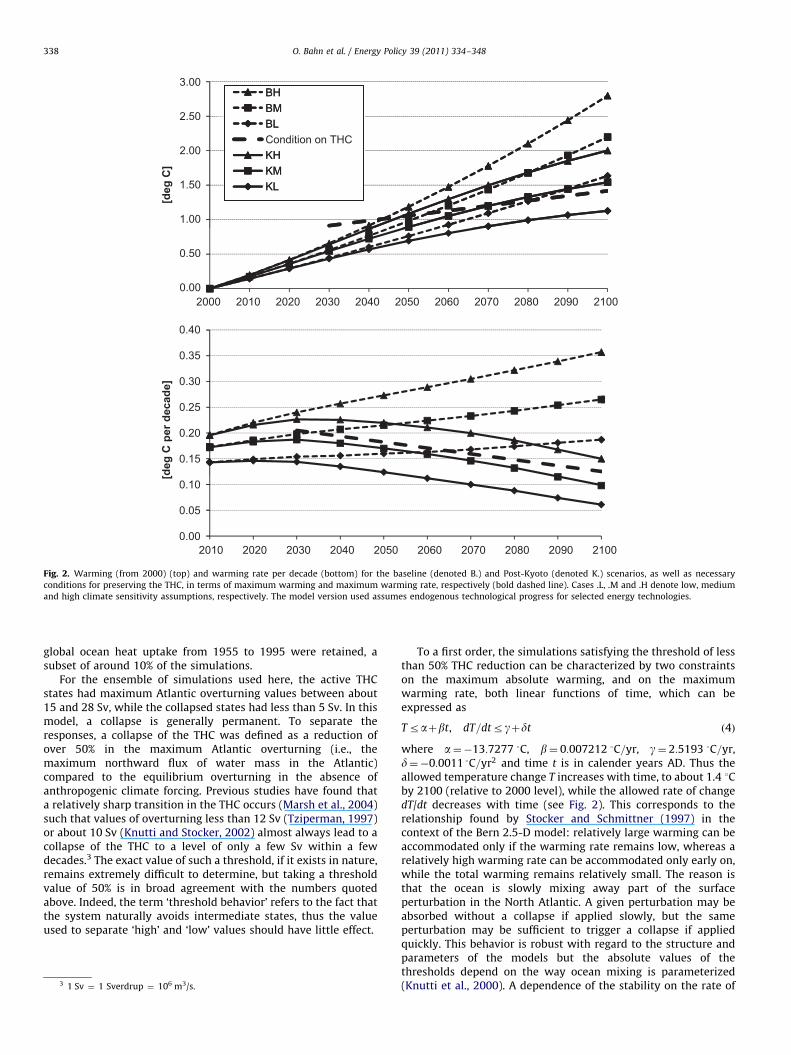
Fig. 2. Warming (from 2000) (top) and warming rate per decade (bottom) for the baseline (denoted B.) and Post-Kyoto (denoted K.) scenarios, as well as necessary

conditions for preserving the THC, in terms of maximum warming and maximum warming rate, respectively (bold dashed line). Cases .L, .M and .H denote low, medium

and high climate sensitivity assumptions, respectively. The model version used assumes endogenous technological progress for selected energy technologies.

O. Bahn et al. / Energy Policy 39 (2011) 334–348338

global ocean heat uptake from 1955 to 1995 were retained, asubset of around 10% of the simulations.

For the ensemble of simulations used here, the active THCstates had maximum Atlantic overturning values between about15 and 28 Sv, while the collapsed states had less than 5 Sv. In thismodel, a collapse is generally permanent. To separate theresponses, a collapse of the THC was defined as a reduction ofover 50% in the maximum Atlantic overturning (i.e., themaximum northward flux of water mass in the Atlantic)compared to the equilibrium overturning in the absence ofanthropogenic climate forcing. Previous studies have found thata relatively sharp transition in the THC occurs (Marsh et al., 2004)such that values of overturning less than 12 Sv (Tziperman, 1997)or about 10 Sv (Knutti and Stocker, 2002) almost always lead to acollapse of the THC to a level of only a few Sv within a fewdecades.3 The exact value of such a threshold, if it exists in nature,remains extremely difficult to determine, but taking a thresholdvalue of 50% is in broad agreement with the numbers quotedabove. Indeed, the term ‘threshold behavior’ refers to the fact thatthe system naturally avoids intermediate states, thus the valueused to separate ‘high’ and ‘low’ values should have little effect.

3 1 Sv ¼ 1 Sverdrup ¼ 106 m3/s.

To a first order, the simulations satisfying the threshold of lessthan 50% THC reduction can be characterized by two constraintson the maximum absolute warming, and on the maximumwarming rate, both linear functions of time, which can beexpressed as

Traþbt, dT=dtrgþdt ð4Þ

where a¼�13:7277 3C, b¼ 0:007212 3C=yr, g¼ 2:5193 3C=yr,d¼�0:0011 3C=yr2 and time t is in calender years AD. Thus theallowed temperature change T increases with time, to about 1.4 1Cby 2100 (relative to 2000 level), while the allowed rate of changedT/dt decreases with time (see Fig. 2). This corresponds to therelationship found by Stocker and Schmittner (1997) in thecontext of the Bern 2.5-D model: relatively large warming can beaccommodated only if the warming rate remains low, whereas arelatively high warming rate can be accommodated only early on,while the total warming remains relatively small. The reason isthat the ocean is slowly mixing away part of the surfaceperturbation in the North Atlantic. A given perturbation may beabsorbed without a collapse if applied slowly, but the sameperturbation may be sufficient to trigger a collapse if appliedquickly. This behavior is robust with regard to the structure andparameters of the models but the absolute values of thethresholds depend on the way ocean mixing is parameterized(Knutti et al., 2000). A dependence of the stability on the rate of

4 Data are given for Western Europe. Introduction dates and costs may vary by

region.5 Note, however, that advanced nuclear energy power plants (which should

provide increased safety and generate a reduced amount of nuclear waste) are

represented in the model by generic technologies (ADV-HC and LBDE, see below)

whose capacity is not limited. In addition, the authors acknowledge that the

characteristics of the NUC technology, reported in Table 1 for Western Europe but

assumed to be the same in all regions, are such that it would, in the absence of its

assumed limited capacity, significantly contribute to electricity generation when

forced to decarbonize the energy sector.6 This corresponds to the modeling philosophy of MERGE that avoids picking

specific winners (Manne and Richels, 2004) among advanced carbon-free

technologies, but has the drawback of not allowing here the distinction between

nuclear and renewable energies.7 In the short term, one could envision water electrolysis using low-cost

renewable electricity. As the potential for the (current) low-cost renewables is

limited, clean production of hydrogen would have to rely after some time on other

sources of carbon-free electricity or on other carbon-free processes. For the latter

one could for instance envision, in the medium term, coal gasification with CCS or

natural gas reforming with CCS, and in the longer term, biomass gasification or

high-temperature water splitting using nuclear heat; see for example OECD/IEA

(2005).8 LBDE: learning part is 50 mills/kWh. LDBN: learning part is 6 US$/GJ.

Learning costs decline by 20% for each doubling of cumulative installed capacity.

O. Bahn et al. / Energy Policy 39 (2011) 334–348 339

change is also seen in some other models (Stouffer and Manabe,1999). Note that the model version used here incorporates severalmodifications compared to Stocker and Schmittner (1997), inparticular the inclusion of a meridional moisture transport andseveral changes to ocean mixing parametrization. The thresholdfor a THC collapse is known to be highly sensitive to both of thesefactors: Knutti et al. (2000) showed that the threshold could varyby an order of magnitude as a function of the vertical diffusivity(their Fig. 9). The strong dependence of THC stability on moisturetransport is explored by Marsh et al. (2004). The THC in the modelused here is relatively sensitive compared to other models(Plattner et al., 2008); however, some experts ascribe aprobability of up to 30% to THC collapse for a warming of lessthan 2 1C compared to preindustrial (Kriegler et al., 2009). Giventhe uncertainty in the value of a possible THC threshold, weregard our results as illustrative of the possible implications ifsuch alow threshold is found to exist.

The constraints are derived by regression, and thus represent thebest-estimate linear functions which separate the collapsed andnon-collapsed states, in other words, the best estimate of theconditions required to preserve the THC in the Bern 2.5-D model.Note that they cannot guarantee its preservation in the model, andcertainly not in the real world. The constraints describe a relation-ship which should not depend on carbon-cycle behavior, nor onemissions scenario. The ensemble considers a wide range of GHGsensitivity behavior and some range of ocean mixing behavior.Uncertainties in atmospheric dynamics, including hydrologicalsensitivity, are not directly addressed by the ensemble, although itmust be noted that further uncertainties are unlikely to beindependent and thus will not be additive. Recall that havingderived the constraints, however, we take them to be fixed, and allsubsequent consideration of uncertainty in our analysis is reduced tothe consideration of high, moderate and low sensitivity cases.

These constraints are then introduced in MERGE in order todetermine policies designed to optimize global welfare whilepreserving the THC. Note, though, that the cost-effectivenessanalysis neglects any economic benefits of such preservation.More accurate assessment of the policy implications of preservingthe THC will clearly require the development of more advanced,fully integrated assessment models and better quantification ofmodeling uncertainties, but the approach chosen here is a firststep towards such a goal.

A similar concept of limiting the overall magnitude and therate of change may apply to other thresholds or tipping elementsin the climate system (Lenton et al., 2008; Kriegler et al., 2009).Ecosystems, for example, are likely to be able to tolerate morewarming when changes are slow and adaptation or migration cancompensate for some of the changes, while high rates of changeswill decrease the overall magnitude of change that can betolerated. The threshold for global temperature in 2100 relativeto 2000 in this study is about 1.4 1C, i.e., equivalent to about 2 1Cwarming from preindustrial, the target that many countries haveadopted to avoid dangerous impacts from climate change. Thuseven if an absolute threshold of the THC is difficult to determineand is model-dependent, the results would also apply to othercomponents in the climate system that exhibit threshold behaviornear 2 1C warming. The implications for energy policies derivedhere are therefore in line with recent estimates of allowed GHGemissions for a 2 1C warming target (Allen et al., 2009;Meinshausen et al., 2009). However, it is essential to note thatthe widely used 2 1C target relates to the maximum warming,rather than the warming experienced by 2100. Uncertainty intechnological developments prevents analysis much beyond2100, but in the solutions derived here the warming rate at2100 remains significant. Stricter constraints would therefore berequired to satisfy the 2 1C maximum limit.

4. Numerical results

This section will analyze energy policies preserving the AtlanticTHC and compare them to alternative policies (business-as-usualand a ‘Post-Kyoto’ policy).

4.1. Scenario characterization

The database of MERGE corresponds to version 5, with theexception of the climate module, as explained in Section 2.2.Table 1 lists the different sources of electric and non-electricenergy supply within the model.4

Remaining fossil fuel power plants (COAL-R, OIL-R and GAS-R)are progressively phased out over time. HYDRO has limitedcapacity reflecting the (limited) potential of the low-cost renew-ables it represents. MERGE assumes also that existing nucleartechnology (NUC) has limited capacity reflecting somehow thecurrent public acceptance of this energy carrier.5 Conversely,ADV-HC and LBDE represent generic6 advanced ‘high-cost’electricity generation technologies (relying on biomass, nuclear,solar and/or wind) and correspond to ‘backstop’ technologies(their capacity is not limited). Similarly, in terms of non-electriccarbon-free supply, RNEW corresponds to a limited supply of low-cost renewables, such as ethanol from biomass. Whereas NEB-HCand LBDN correspond to an unlimited carbon-free supply of non-electric energy. These technologies are again defined in a genericway, but could refer for instance to hydrogen production usingcarbon-free processes.7

To capture alternative energy futures consistent with preservingthe THC, we consider two versions of the model: one withendogenous technological progress in the energy sector, the otherone without. In the latter version, neither LBDE nor LBDN areavailable and costs are assumed to decline every year at a rate of0.5%. The same cost reduction trend applies in the former version(with learning-by-doing—LBD), except for LBDE and LBDN (thatreplace, respectively, ADV-HC and NEB-HC). For these two technol-ogies, only a fraction of the cost is exogenously reduced. Theremaining part of the cost (learning part) is reduced throughaccumulation of knowledge in manufacturing and operation, knowl-edge measured through cumulative installed capacities.8 For anextensive discussion of the modeling of endogenous technologicalprogress in MERGE, the reader is referred in particular to Kypreosand Bahn (2003) and Manne and Barreto (2004).

Table 1Electric and non-electric energy supply in MERGE5.

Name Description Introduction date Cost in 2000 (mills/kW h) Carbon emissions (kg C/kW h)

Electric energy supply

COAL-R Remaining initial coal fired Existing 25.3 0.2364

COAL-N Pulverized coal without CCS 2010 55.0 0.1955

IGCC IGCC with CCS 2015 62.0 0.0240

COAL-A Coal-fuel cell with CCS 2040 65.9 0.0068

OIL-R Remaining initial oil fired Existing 37.8 0.1795

GAS-R Remaining initial gas fired Existing 35.7 0.1044

GAS-N Advanced combined cycle 2005 30.3 0.0935

GAS-A Gas-fuel cell with CCS 2020 47.7 0.0000

HYDRO Hydroelectric and geothermal Existing 40.0 0.0000

NUC Remaining initial nuclear Existing 50.0 0.0000

LBDE Carbon-free technologies with LBD 2005 100.0 0.0000

ADV-HC Carbon-free technologies without LBD 2010 100.0 0.0000

Name Description Introduction date Cost in 2000 (US$/GJ) Carbon emissions (t C/GJ)

Non-electric energy supply

CLDU Coal direct use Existing 3.0 0.0241

OIL1–OIL10 Oil cost categories Existing 3.0–5.25 0.0199

GAS1–GAS10 Gas cost categories Existing 2.0–4.25 0.0137

SYNF Synthetic fuels 2010 9.0 0.0400

RNEW Renewables Existing 6.0 0.0000

LBDN Carbon-free technologies with LBD 2005 14.0 0.0000

NEB-HC Carbon-free technologies without LBD 2010 14.0 0.0000

CCS stands for carbon capture and sequestration. IGCC stands for integrated gasification combined cycle. LDB stands for learning-by-doing.

O. Bahn et al. / Energy Policy 39 (2011) 334–348340

For each of these two MERGE versions (with and withoutlearning), several scenarios are analyzed. The first scenariosconsidered are baseline cases where GHG emissions are notlimited. They assume a world population level of 8.7 billion by2050 and 9.5 by 2100. Between 2000 and 2100, world GDP grows11 times (up to 382 trillion USD 2000), whereas primary energysupply and carbon emissions increase about four times each (upto around 1600 EJ/year and 27 Gt C, respectively). In terms of CO2

emissions, our baseline scenario is then close to the SRES A2scenario (IPCC, 2000).9 We present here three baseline cases: BL, acase with low climate sensitivity (s¼2 1C) and short mean lag forthe ocean warming (lags¼45 years); BM with medium climatesensitivity (3 1C) and mean lag (57 years); and BH with highclimate sensitivity (4.5 1C) and long mean lag (77 years).10

The next scenario is a ‘Post-Kyoto’ scenario, where constraintsare imposed on GHG emissions (instead of temperature changes)as follows.11 Annex B regions of the Kyoto Protocol (except USA)must comply with their Kyoto target by 2010. Afterwards,Western Europe takes the lead in the reduction effort by abatingits GHG emissions by 20% by 2020 (from the 1990 level for CO2

and from the 2000 levels for the other GHGs) and then reducingits emissions by 10% per decade. The other Annex B regions(including USA) abate their GHG emissions by 10% per decade(from the 2010 levels) from 2020 on. Non-annex B regions join theabatement effort in 2030, reducing their GHG emissions by 5% perdecade (from the 2020 levels). As a consequence of these emissionconstraints, world carbon emissions peak in 2020 at 7.5 Gt C anddecrease afterwards to 1.4 Gt C by 2100. Depending again on the

9 Note that MERGE makes further assumptions regarding aerosol forcing,

sulfur emissions being based on the IIASA B2 marker scenario, and regarding non-

CO2 GHGs following the Energy Modeling Forum 21 (De La Chesnaye and Weyant,

2006); see also Manne and Richels (2005) pp. 180–181.10 Notice that for each model version used (with and without learning),

respectively, socio-economic development paths and resulting GHG emissions are

identical in all three baseline cases. But these cases differ by temperature changes

associated with emissions.11 This is among several others a possible scenario for ‘Post-Kyoto’ commit-

ments to result from the current climate negotiations and we have selected it for

illustration purposes only.

assumed (low, medium or high) climate sensitivity and mean lagfor the ocean warming, we present three Post-Kyoto scenarios: KL(2 1C, 45 years), KM (3 1C, 57 years) and KH (4.5 1C, 77 years).12

Recall now that Section 3 has defined constraints on maximumabsolute warming and maximum warming rate that correspondto necessary conditions for preserving the THC. Fig. 2 assesseswhether our baseline and Post-Kyoto scenarios satisfy theseconditions, using the LBD model version for illustration (withsimilar results for the non-learning model version).

Fig. 2 reveals first that whatever climate sensitivity is chosenour baseline scenario fails to preserve the THC, as both constraintson maximum warming and maximum warming rate are violated.In other words, a ‘laissez-faire’ policy is here most likely to make afuture THC collapse inevitable. Fig. 2 shows next that our Post-Kyoto scenario would only prevent a THC shutdown under a lowclimate sensitivity. When the climate sensitivity is medium, theimplemented emission reductions would merely postpone by afew decades (compared to our baseline) the situation where afuture collapse can no longer be avoided. It is also striking to notethat under a high climate sensitivity, in the KH scenario (as in theBH scenario), the constraint on maximum warming rate isviolated before 2030. In other words, a delay in implementing‘ambitious’13 emission reductions by only a few decades would,under some conditions, very likely make a future THC collapseinevitable.

Finally, the last scenario corresponds to a ‘THC preservation’policy, where a collapse is prevented by imposing our constraintson maximum absolute warming and maximum warming rate.Depending once more on the assumed climate sensitivity andmean lag for the ocean warming, we present three THCpreservation scenarios: PL (2 1C, 45 years), PM (3 1C, 57 years)and PH (4.5 1C, 77 years).

12 Note again that for the two model versions used, respectively, socio-

economic development paths and resulting GHG emissions are identical for all

these Post-Kyoto scenarios. But these scenarios differ by temperature changes

associated with emissions. Notice also that emission trajectories are dictated by

their constraints and are thus identical for both model versions.13 See also Fig. 4 next section.

0.60

0.80

1.00

1.20

1.40

1.60

1.80

2.00

[deg

C]

on THC

0.00

0.20

0.40

2000

Condition on THCPH

PM

PL

2010 2020 2030 2040 2050 2060 2070 2080 2090 2100

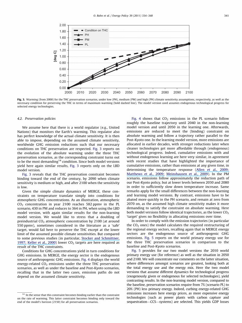
Fig. 3. Warming (from 2000) for the THC preservation scenarios, under low (PH), medium (PM) and high (PH) climate sensitivity assumptions, respectively, as well as the

necessary condition for preserving the THC in terms of maximum warming (bold dashed line). The model version used assumes endogenous technological progress for

selected energy technologies.

O. Bahn et al. / Energy Policy 39 (2011) 334–348 341

4.2. Preservation policies

We assume here that there is a world regulator (e.g., UnitedNations) that monitors the Earth’s warming. This regulator alsohas perfect knowledge of the actual climate sensitivity. It is thenable to impose, depending on the assumed climate sensitivity,worldwide GHG emission reductions such that our necessaryconditions on THC preservation are respected. Fig. 3 reports onthe evolution of the absolute warming under the three THCpreservation scenarios, as the corresponding constraint turns outto be the most demanding14 condition. Since both model versionsyield here again similar results, Fig. 3 reports only on the LBDmodel version.

Fig. 3 reveals that the THC preservation constraint becomesbinding toward the end of the century, by 2090 when climatesensitivity is medium or high, and after 2100 when the sensitivityis low.

Given the simple climate dynamics of MERGE, these con-straints on temperature translate simply into conditions foratmospheric GHG concentrations. As an illustration, atmosphericCO2 concentration in year 2100 reaches 582 ppmv in the PLscenario, 430 in PM and reduces to 364 in PH, when using the LBDmodel version, with again similar results for the non-learningmodel version. We would like to stress that a doubling ofpreindustrial CO2 atmospheric concentration by 2100 (at around550 ppmv), sometimes considered in the literature as a ‘safe’target, would fail here to preserve the THC except at the lowerlimit of the assumed possible climate sensitivities. But comparedto some previous studies (in particular, Stocker and Schmittner,1997; Keller et al., 2000) lower CO2 targets are here required asresult of the THC constraints.

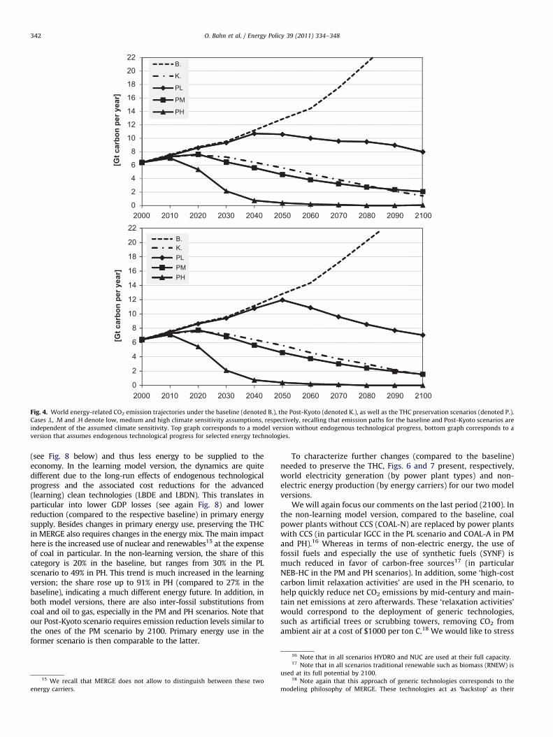
Conditions for GHG concentrations yield in turn conditions forGHG emissions. In MERGE, the energy sector is the endogenoussource of anthropogenic GHG emissions. Fig. 4 displays the worldenergy-related CO2 emissions under the three THC preservationscenarios, as well as under the baseline and Post-Kyoto scenarios,recalling that in the latter two cases, emission paths do notdepend on the assumed climate sensitivity.

14 In the sense that this constraint becomes binding earlier than the constraint

on the rate of warming. This latter constraint becomes binding only toward the

end of the model’s horizon (2150) for all preservation scenarios.

Fig. 4 shows that CO2 emissions in the PL scenario followroughly the baseline trajectory until 2040 in the non-learningmodel version and until 2050 in the learning one. Afterwards,emissions are reduced to meet the (binding) constraint onabsolute warming and follow a trajectory rather parallel to thePost-Kyoto one. In the learning model version, more emissions areallocated in earlier decades, with stronger reductions later whencleaner technologies get more affordable through (endogenous)technological progress. Indeed, cumulative emissions with andwithout endogenous learning are here very similar, in agreementwith recent studies that have highlighted the importance ofcumulative emissions, rather than emissions at any given time, indetermining the temperature response (Allen et al., 2009;Matthews et al., 2009; Meinshausen et al., 2009). In the PMscenario, emissions follow approximately the reduction path ofour Post-Kyoto policy, but at lower levels between 2030 and 2080in order to sufficiently slow down temperature increase. Sameremarks apply for the small differences between the non-learningand learning model versions. By contrast, emissions have to beabated more quickly in the PH scenario, and remain at zero from2070 on, as the assumed high climate sensitivity makes it moredemanding to satisfy the constraint on absolute warming. Hereboth model versions follow identical trajectories, as the lower CO2

‘target’ gives no flexibility in allocating emissions over time.In order to comply with the emission trajectories (in particular

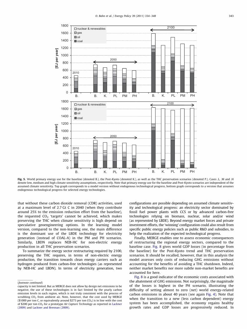
the CO2 ones) the model calculates the required restructuring ofthe regional energy sectors, recalling again that in MERGE energysectors are the endogenous source of anthropogenic GHGemissions. Fig. 5 reports on the world primary energy use forthe three THC preservation scenarios in comparison to thebaseline and Post-Kyoto scenarios.

Fig. 5 provides for our two model versions the 2010 worldprimary energy use (for reference) as well as the situation in 2050and 2100. We will concentrate our comments on the latter situation,where differences amongst scenarios are greatest, looking both atthe total energy use and the energy mix. Here the two modelversions that assume different dynamics for technological progress(exogenously given or endogenous for selected technologies), yieldcontrasting results. In the non-learning model version, compared tothe baseline, preservation scenarios require from 7% (scenario PL) to20% (PH) less primary energy. Indeed, curbing energy-related GHGemissions increases here energy prices, as more expensive energytechnologies (such as power plants with carbon capture andsequestration—CCS—systems) are selected. This yields GDP losses

6

8

10

12

14

16

18

20

22

[Gt c

arbo

n pe

r yea

r]

B.

K.

PL

PM

PH

0

2

4

2000

B.

K.

PL

PM

PH

8

10

12

14

16

18

20

22

[Gt c

arbo

n pe

r yea

r]

0

2

4

6

2010 2020 2030 2040 2050 2060 2070 2080 2090 2100

2000 2010 2020 2030 2040 2050 2060 2070 2080 2090 2100

B.K.PLPMPH

Fig. 4. World energy-related CO2 emission trajectories under the baseline (denoted B.), the Post-Kyoto (denoted K.), as well as the THC preservation scenarios (denoted P.).

Cases .L, .M and .H denote low, medium and high climate sensitivity assumptions, respectively, recalling that emission paths for the baseline and Post-Kyoto scenarios are

independent of the assumed climate sensitivity. Top graph corresponds to a model version without endogenous technological progress, bottom graph corresponds to a

version that assumes endogenous technological progress for selected energy technologies.

O. Bahn et al. / Energy Policy 39 (2011) 334–348342

(see Fig. 8 below) and thus less energy to be supplied to theeconomy. In the learning model version, the dynamics are quitedifferent due to the long-run effects of endogenous technologicalprogress and the associated cost reductions for the advanced(learning) clean technologies (LBDE and LBDN). This translates inparticular into lower GDP losses (see again Fig. 8) and lowerreduction (compared to the respective baseline) in primary energysupply. Besides changes in primary energy use, preserving the THCin MERGE also requires changes in the energy mix. The main impacthere is the increased use of nuclear and renewables15 at the expenseof coal in particular. In the non-learning version, the share of thiscategory is 20% in the baseline, but ranges from 30% in the PLscenario to 49% in PH. This trend is much increased in the learningversion; the share rose up to 91% in PH (compared to 27% in thebaseline), indicating a much different energy future. In addition, inboth model versions, there are also inter-fossil substitutions fromcoal and oil to gas, especially in the PM and PH scenarios. Note thatour Post-Kyoto scenario requires emission reduction levels similar tothe ones of the PM scenario by 2100. Primary energy use in theformer scenario is then comparable to the latter.

15 We recall that MERGE does not allow to distinguish between these two

energy carriers.

To characterize further changes (compared to the baseline)needed to preserve the THC, Figs. 6 and 7 present, respectively,world electricity generation (by power plant types) and non-electric energy production (by energy carriers) for our two modelversions.

We will again focus our comments on the last period (2100). Inthe non-learning model version, compared to the baseline, coalpower plants without CCS (COAL-N) are replaced by power plantswith CCS (in particular IGCC in the PL scenario and COAL-A in PMand PH).16 Whereas in terms of non-electric energy, the use offossil fuels and especially the use of synthetic fuels (SYNF) ismuch reduced in favor of carbon-free sources17 (in particularNEB-HC in the PM and PH scenarios). In addition, some ‘high-costcarbon limit relaxation activities’ are used in the PH scenario, tohelp quickly reduce net CO2 emissions by mid-century and main-tain net emissions at zero afterwards. These ‘relaxation activities’would correspond to the deployment of generic technologies,such as artificial trees or scrubbing towers, removing CO2 fromambient air at a cost of $1000 per ton C.18 We would like to stress

16 Note that in all scenarios HYDRO and NUC are used at their full capacity.17 Note that in all scenarios traditional renewable such as biomass (RNEW) is

used at its full potential by 2100.18 Note again that this approach of generic technologies corresponds to the

modeling philosophy of MERGE. These technologies act as ‘backstop’ as their

2050

1800

1600

2010

2100

0

200

400

600

800

1000

1200

1400

B.

[EJ

per y

ear]

nuclear & renewablesgasoilcoal

0

200

400

600

800

1000

1200

1400

1600

1800

[EJ

per y

ear]

nuclear & renewablesgasoilcoal

2010

2050

2100

B. K. PL PM PH B. K. PL PM PH

B. B. K. PL PM PH B. K. PL PM PH

Fig. 5. World primary energy use for the baseline (denoted B.), the Post-Kyoto (denoted K.), as well as the THC preservation scenarios (denoted P.). Cases .L, .M and .H

denote low, medium and high climate sensitivity assumptions, respectively. Note that primary energy use for the baseline and Post-Kyoto scenarios are independent of the

assumed climate sensitivity. Top graph corresponds to a model version without endogenous technological progress, bottom graph corresponds to a version that assumes

endogenous technological progress for selected energy technologies.

O. Bahn et al. / Energy Policy 39 (2011) 334–348 343

that without these carbon dioxide removal (CDR) activities, usedat a maximum level of 2.7 Gt C in 2040 (when they contributearound 25% to the emission reduction effort from the baseline),the requested CO2 ‘targets’ cannot be achieved, which makespreserving the THC when climate sensitivity is high depend onspeculative geoengineering options. In the learning modelversion, compared to the non-learning one, the main differenceis the dominant use of the LBDE technology for electricitygeneration (instead of COAL-A) in the PM and PH scenarios.Similarly, LBDN replaces NEB-HC for non-electric energyproduction in all THC preservation scenarios.

To summarize the energy sector restructuring required by 2100,preserving the THC requires, in terms of non-electric energyproduction, the transition towards clean energy carriers such ashydrogen produced from carbon-free technologies (as representedby NEB-HC and LBDN). In terms of electricity generation, two

(footnote continued)

capacity is not limited. But as MERGE does not allow by design net emissions to be

negative, the use of these technologies is in fact limited by the yearly carbon

emission levels in each region, which is not truly consistent with the process of

scrubbing CO2 from ambient air. Note, however, that the cost used by MERGE

($1000 per ton C, or equivalently around $273 per ton CO2) is in line with the cost

of $200 per ton CO2 for a prototype Air Capture Technology as reported in Lackner

(2009) and Lackner and Brennan (2009).

configurations are possible depending on assumed climate sensitiv-ity and technological progress: an electricity sector dominated byfossil fuel power plants with CCS or by advanced carbon-freetechnologies relying on biomass, nuclear, solar and/or wind(as represented by LBDE). Beyond energy market forces and privateinvestment efforts, the ‘winning’ configuration could also result fromspecific public energy policies such as public R&D and subsidies, tohelp the realization of the expected technological progress.

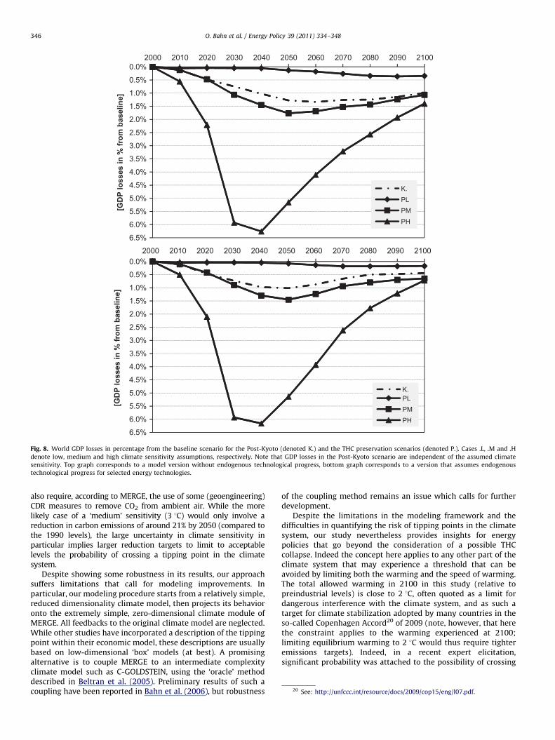
Finally, MERGE enables one to assess economic consequencesof restructuring the regional energy sectors, compared to thebaseline case. Fig. 8 gives world GDP losses (in percentage fromthe baseline) for the Post-Kyoto trend and THC preservationscenarios. It should be recalled, however, that in this analysis themodel assesses only costs of reducing GHG emissions withoutaccounting for the benefits of avoiding a THC shutdown. Indeed,neither market benefits nor more subtle non-market benefits areaccounted for here.

Fig. 8 is a good indicator of the economic costs associated withthe abatement of GHG emissions. Not surprisingly, the magnitudeof the losses is highest in the PH scenario, illustrating thedifficulty of setting almost to zero (net) world energy-relatedcarbon emissions in about 40 years (see again Fig. 4). Note thatwhen the transition to a new (less carbon dependent) energysystem has been accomplished, the economy regains healthygrowth rates and GDP losses are progressively reduced. In

0

20

40

60

80

100

120

[PW

h pe

r yea

r]

adv-hchydronucgas-acoal-aigccgas-ngas-rcoal-ncoal-r

2050

2100

2010

40

60

80

100

120

[PW

h pe

r yea

r]

0

20

40

60

80

100

120lbdehydronucgas-acoal-aigccgas-ngas-rcoal-ncoal-r

2010

2050

2100

B. B. K. PL PM PH B. K. PL PM PH

B. B. K. PL PM PH B. K. PL PM PH

Fig. 6. World electricity generation by power plant types for the baseline (denoted B.), the Post-Kyoto (denoted K.), as well as the THC preservation scenarios (denoted P.).

Cases .L, .M and .H denote low, medium and high climate sensitivity assumptions, respectively. Note that electricity generation for the baseline and Post-Kyoto scenarios

are independent of the assumed climate sensitivity. Power plant types are: adv-hc and lbde (advanced high-cost carbon-free technologies such as advanced nuclear,

biomass, solar and wind), hydro (hydroelectric, geothermal and other existing low-cost renewables), nuc (existing nuclear technology), gas-a & coal-a and igcc (advanced

gas and coal plants, respectively, with carbon capture and sequestration), gas-n (advanced gas combined cycle), gas-r and coal-r (remaining gas and coal plants,

respectively) and coal-n (pulverized coal plant without CO2 recovery). Top graph corresponds to a model version without endogenous technological progress, bottom graph

corresponds to a version that assumes endogenous technological progress for selected energy technologies.

O. Bahn et al. / Energy Policy 39 (2011) 334–348344

addition, compared to the model version without learning, GDPlosses are reduced in the long run in the version with learning, asregional economies benefit from cost reductions in someadvanced clean technologies (resulting from investments overtime, following the endogenous representation of technologicalprogress). Now looking at regional economic impacts of THCpreservation, some regions suffer more GDP losses than the worldaverage; by decreasing order: MOPEC (Mexico and OPEC) andEEFSU (Eastern Europe and the former Soviet Union) that have thelargest endowments of oil and gas, and in the learning modelversion China that has the largest endowments of coal.

4.3. Comparison to previous studies

Our paper follows a cost-effective approach to determine anoptimal configuration of the regional economies and energysystems that respects necessary conditions for preserving theTHC. By contrast, several previous studies (Keller et al., 2000,2004; Mastrandrea and Schneider, 2001; McInerney and Keller,2008) have followed (at least partly) a cost-benefit approach thatbalances costs of reducing GHG emissions with benefitsassociated with avoiding a THC collapse.

A cost-effective approach to the THC issue has severallimitations (Keller et al., 2004). Indeed, it does not in particularconsider the possibility of only postponing a collapse (and theassociated damages) and considers implicitly (from a cost-benefitperspective) infinite damages associated with a collapse. But acost-benefit approach to abrupt climate changes itself suffersseveral limitations (see, e.g., Wright and Erickson, 2003) due inparticular to large uncertainties associated with the magnitude ofdamages a THC collapse would cause and to the controversialissue of choosing a discount rate (in particular for accounting thefuture benefits of avoiding a collapse).

Because of these different approaches, our results do notcompare easily to those of studies following a cost-benefitapproach. Indeed, in the above-mentioned studies the THC iseither allowed to collapse under certain conditions, or theproposed optimal policy does not significantly reduce the oddsof a collapse. We can, however, compare to some extent ourresults with: those of Keller et al. (2000) and Bruckner andZickfeld (2009) when they follow a cost-effective approach, thoseof McInerney and Keller (2008) when they assess the magnitudeof GHG reduction that would preserve the THC, those of Yoheet al. (2006), and those obtained with a tolerable window

rnewsynfgasnonoilnon

0

100

200

300

400

500

600

700

[EJ

per y

ear]

neb-hc

cldu

2010

2050

2100

lbdnrnewsynfgasnonoilnoncldu

0

100

200

300

400

500

600

700

800

[EJ

per y

ear]

2010

2050

2100

B. B. K. PL PM PH B. K. PL PM PH

B. B. K. PL PM PH B. K. PL PM PH

Fig. 7. World non-electric energy production by energy carriers for the baseline (denoted B.), the Post-Kyoto (denoted K.), as well as the THC preservation scenarios

(denoted P.). Cases .L, .M and .H denote low, medium and high climate sensitivity assumptions, respectively. Note that non-electric energy production for the baseline and

Post-Kyoto scenarios are independent of the assumed climate sensitivity. Energy carriers are: neb-hc and lbdn (advanced high-cost clean carriers such as hydrogen

produced using carbon-free processes), rnew (low-cost renewables such as ethanol from biomass), synf (synthetic fuels), gasnon (gas for non-electric use), oilnon (oil for

non-electric use) and cldu (coal for non-electric use). Top graph corresponds to a model version without endogenous technological progress, bottom graph corresponds to a

version that assumes endogenous technological progress for selected energy technologies.

O. Bahn et al. / Energy Policy 39 (2011) 334–348 345

approach (reported in particular in Zickfeld and Bruckner, 2008;Bruckner and Zickfeld, 2009).

Our results present several similarities with these latterstudies. In particular, results show a strong influence of theclimate sensitivity on the optimal GHG emission trajectories;the higher the assumed climate sensitivity, the sooner and thestronger the emission reductions necessary to avoid a THCcollapse. Similarly, when considering ‘high’ settings for theuncertain climate parameters (such as the climate sensitivity)most of the studies indicate that even a modest increase in GHGemissions during the next few decades would yield a situationwhere a future collapse of the THC could no longer be avoided.

However, our results present also some differences comparedto the latter mentioned studies. In particular, our approach topreserve the THC generally implies stronger GHG emissionreductions (owing to the tighter THC constraints) with thenotable exception of McInerney and Keller (2008) that sharewith us the limitation of not modeling explicitly the THC.19

Differences may indeed result from the modeling frameworks. But

19 They rather impose, as we do, constraints that correspond to necessary

conditions for preserving the THC.

to some extent, they also reflect our imperfect knowledge ofcritical THC thresholds.

5. Conclusions

In this paper, we have estimated, using the MERGE model, cost-effective energy policies yielding GHG emission trajectories thatwould preserve the Atlantic thermohaline circulation (THC) underdifferent settings for uncertain climate parameters (climate sensi-tivity and rate of ocean warming). Our results are consistent withthe existing literature with respect to the finding that under some‘high’ settings for the uncertain climate parameters (in particular aclimate sensitivity set at 4.5 1C, the upper end of the likely rangeprovided by the IPCC) a small increase in GHG emissions during thenext decades would be enough to yield a situation where crossing aparticular tipping point in the climate system (here, a collapse of theTHC) can no longer be avoided in the (possibly distant) future. Ourresults also illustrate the possible energy challenges (e.g., almostcomplete decarbonization of the energy sectors in about 40 years)that would need to be overcome to ensure avoiding a THC collapse ifthe climate sensitivity (in particular) turns out to be ‘high’. Themagnitude and speed of the decarbonization requested here would

2000

K.PLPMPH

0.0%

0.5%

1.0%

1.5%

2.0%

2.5%

3.0%

3.5%

4.0%

4.5%

5.0%

5.5%

6.0%

6.5%

K.PLPMPH

K.PLPMPH

0.0%

0.5%

1.0%

1.5%

2.0%

2.5%

3.0%

3.5%

4.0%

4.5%

5.0%

5.5%

6.0%

6.5%

K.PLPMPH

2010 2020 2030 2040 2050 2060 2070 2080 2090 2100

2000 2010 2020 2030 2040 2050 2060 2070 2080 2090 2100

[GD

P lo

sses

in %

from

bas

elin

e][G

DP

loss

es in

% fr

om b

asel

ine]

Fig. 8. World GDP losses in percentage from the baseline scenario for the Post-Kyoto (denoted K.) and the THC preservation scenarios (denoted P.). Cases .L, .M and .H

denote low, medium and high climate sensitivity assumptions, respectively. Note that GDP losses in the Post-Kyoto scenario are independent of the assumed climate

sensitivity. Top graph corresponds to a model version without endogenous technological progress, bottom graph corresponds to a version that assumes endogenous

technological progress for selected energy technologies.

20 See: http://unfccc.int/resource/docs/2009/cop15/eng/l07.pdf.

O. Bahn et al. / Energy Policy 39 (2011) 334–348346

also require, according to MERGE, the use of some (geoengineering)CDR measures to remove CO2 from ambient air. While the morelikely case of a ‘medium’ sensitivity (3 1C) would only involve areduction in carbon emissions of around 21% by 2050 (compared tothe 1990 levels), the large uncertainty in climate sensitivity inparticular implies larger reduction targets to limit to acceptablelevels the probability of crossing a tipping point in the climatesystem.

Despite showing some robustness in its results, our approachsuffers limitations that call for modeling improvements. Inparticular, our modeling procedure starts from a relatively simple,reduced dimensionality climate model, then projects its behavioronto the extremely simple, zero-dimensional climate module ofMERGE. All feedbacks to the original climate model are neglected.While other studies have incorporated a description of the tippingpoint within their economic model, these descriptions are usuallybased on low-dimensional ‘box’ models (at best). A promisingalternative is to couple MERGE to an intermediate complexityclimate model such as C-GOLDSTEIN, using the ‘oracle’ methoddescribed in Beltran et al. (2005). Preliminary results of such acoupling have been reported in Bahn et al. (2006), but robustness

of the coupling method remains an issue which calls for furtherdevelopment.

Despite the limitations in the modeling framework and thedifficulties in quantifying the risk of tipping points in the climatesystem, our study nevertheless provides insights for energypolicies that go beyond the consideration of a possible THCcollapse. Indeed the concept here applies to any other part of theclimate system that may experience a threshold that can beavoided by limiting both the warming and the speed of warming.The total allowed warming in 2100 in this study (relative topreindustrial levels) is close to 2 1C, often quoted as a limit fordangerous interference with the climate system, and as such atarget for climate stabilization adopted by many countries in theso-called Copenhagen Accord20 of 2009 (note, however, that herethe constraint applies to the warming experienced at 2100;limiting equilibrium warming to 2 1C would thus require tighteremissions targets). Indeed, in a recent expert elicitation,significant probability was attached to the possibility of crossing

O. Bahn et al. / Energy Policy 39 (2011) 334–348 347

major tipping points (e.g., dieback of the Amazon rainforest,melting of Greenland, collapse of the West Antarctic ice sheet,shutdown of the THC) for a warming of about 2 1C (Kriegler et al.,2009). Some impacts and tipping points are likely to depend onthe rate of warming (Stocker and Schmittner, 1997; O’Neill andOppenheimer, 2004), in particular those characterizing ecosystemshifts. This has largely been ignored in international negotiationsof GHG reduction targets, that focus more on absolute warming.The results of this study are therefore not limited to thediscussion of the THC, but are an illustration of the energypolicy implications in a case where the total warming is limited tonear 2 1C, with the additional condition that the rate oftemperature change, and hence the rate of adaptation required,is limited.

Acknowledgments

The authors wish to acknowledge financial support from theNatural Sciences and Engineering Research Council of Canada, theprogramme Gestion et Impacts du Changement Climatique (France),the Swiss National Science Foundation through NCCR Climate andthe UK Natural Environment Research Council.

References

Allen, M.R., Frame, D.J., Huntingford, C., Jones, C.D., Lowe, J.A., Meinshausen, M.,Meinshausen, N., 2009. Warming caused by cumulative carbon emissionstowards the trillionth tonne. Nature 458, 1163–1166.

Allen, M.R., Stott, P.A., Mitchell, J.F., Schnur, R., Delworth, T.L., 2000. Quantifyingthe uncertainty in forecasts of anthropogenic climate change. Nature 407,617–620.

Annan, J.D., Hargreaves, J.C., Edwards, N.R., Marsh, R., 2005. Parameter estimationin an intermediate complexity earth system model using an ensemble kalmanfilter. Ocean Modelling 8, 135–154.

Bahn, O., Drouet, L., Edwards, N.R., Haurie, A., Knutti, R., Kypreos, S., Stocker, T.F.,Vial, J.-P., 2006. The coupling of optimal economic growth and climatedynamics. Climatic Change 79, 103–119.

Beltran, C., Drouet, L., Edwards, N.R., Haurie, A., Vial, J.-P., Zachary, D., 2005. Anoracle method to couple climate and economic dynamics. In: Haurie, A.,Viguier, L. (Eds.), The Coupling of Climate and Economic Dynamics. Springer,pp. 69–95.

Bruckner, T., Zickfeld, K., 2009. Emissions corridors for reducing the risk of acollapse of the Atlantic thermohaline circulation. Mitigation and AdaptationStrategies of Global Change 14, 61–83.

Bruckner, T., Hooss, G., Fuessel, H.M., Hasselmann, K., 2003. Climate systemmodeling in the framework of the tolerable windows approach: the ICLIPSclimate model. Climatic Change 56, 119–137.

Bruckner, T., Petschel-Held, G., Toth, F., Fuessel, H.M., Helm, C., Leimbach, M.,Schellnhuber, H., 1999. Climate change decision support and the tolerablewindows approach. Environmental Modeling and Assessment 4, 217–234.

De La Chesnaye, F.C., Weyant, J.P. (Eds.), 2006. Multi-Greenhouse Gas Mitigationand Climate Policy. The Energy Journal (special issue 3, 520 pp.).

Drouet, L., Edwards, N.R., Haurie, A., 2006. Coupling climate and economic modelsin a cost-benefit framework: a convex optimisation approach. EnvironmentalModeling and Assessment 11, 101–114.

Edwards, N.R., Marsh, R., 2005. Uncertainties due to transport-parametersensitivity in an efficient 3-D ocean-climate model. Climate Dynamics 24,415–433.

Forest, C.E., Stone, P.H., Sokolov, A.P., Allen, M.R., Webster, M.D., 2002. Quantifyinguncertainties in climate system properties with the use of recent climateobservations. Science 295, 113–117.

Gregory, J.M., Dixon, K.W., Stouffer, R.J., Weaver, A.J., Driesschaert, E., Eby, M.,Fichefet, T., Hasumi, H., Hu, A., Jungclaus, J.H., Kamenkovich, I.V., Levermann,A., Montoya, M., Murakami, S., Nawrath, S., Oka, A., Sokolov, A.P., Thorpe, R.B.,2005. A model intercomparison of changes in the Atlantic thermohalinecirculation in response to increasing atmospheric CO2 concentration. Geophy-sical Research Letters 32. doi:10.1029/2005GL023209.

Hasselmann, K., Sausen, R., Maier-Reimer, E., Voss, R., 1993. On the cold startproblem in transient simulations with coupled atmosphere-ocean models.Climate Dynamics 9, 53–61.

IPCC, 2001. Climate change 2001: impacts, adaptation and vulnerability. In:McCarthy, J.J. (Ed.), Contribution of Working Group II to the Third AssessmentReport of the Intergovernmental Panel on Climate Change. CambridgeUniversity Press, Cambridge, UK.

IPCC, 2000. Special report on Emissions Scenarios, Cambridge University Press,Cambridge, UK.

Joos, F., Muller-Furstenberger, G., Stephan, G., 1999a. Correcting the carbon cyclerepresentation: how important is it for the economics of climate change?Environmental Modeling and Assessment 4 133–140.

Joos, F., Plattner, G.-K., Stocker, T.F., Marchal, O., Schmittner, A., 1999b. Globalwarming and marine carbon cycle feedbacks on future atmospheric CO2.Science 284, 464–467.

Kaufmann, R.K., 1997. Assessing the DICE model: uncertainty associated with theemissions and retention of greenhouse gases. Climatic Change 35, 435–448.

Keller, K., Bolker, B.M., Bradford, D.F., 2004. Uncertain climate thresholds andoptimal economic growth. Journal of Environmental Economics and Manage-ment 48, 723–741.

Keller, K., Tan, K., Morel, F.M.M., Bradford, D.F., 2000. Preserving the oceancirculation: implications for climate policy. Climatic Change 47, 17–43.

Knutti, R., Hegerl, G.C., 2008. The equilibrium sensitivity of the Earth’s temperatureto radiation changes. Nature Geoscience 1, 735–743.

Knutti, R., Krahenmann, S., Frame, D.J., Allen, M.R., 2008. Comment on ‘‘Heatcapacity, time constant, and sensitivity of Earth’s climate system’’ by S. E.Schwartz. J. Geophys. Res. 113, D15103 . doi:10.1029/2007JD009473.

Knutti, R., Fluckiger, J., Stocker, T.F., Timmerman, A., 2004. Strong hemisphericcoupling of glacial climate through freshwater discharge and ocean circulation.Nature 430, 851–856.

Knutti, R., Stocker, T.F., Joos, F., Plattner, G.-K., 2003. Probabilistic climate changeprojections using neural networks. Climate Dynamics 21, 257–272.

Knutti, R., Stocker, T.F., 2002. Limited predictability of the future thermohalinecirculation close to an instability threshold. Journal of Climate 15, 179–186.

Knutti, R., Stocker, T.F., Joos, F., Plattner, G.-K., 2002. Constraints on radiativeforcing and future climate change from observations and climate modelensembles. Nature 416, 719–723.

Knutti, R., Stocker, T.F., Wright, D.G., 2000. The effects of sub-grid-scaleparameterizations in a zonally averaged ocean model. Journal of PhysicalOceanography 30, 2738–2752.

Knutti, R., Stocker, T.F., 2000. Influence of the thermohaline circulation onprojected sea level rise. Journal of Climate 13, 1997–2001.

Kriegler, E., Hall, J.W., Held, H., Dawson, R., Schellnhuber, H.-J., 2009. Impreciseprobability assessment of tipping points in the climate system. Proceedings ofthe National Academy of Sciences 106, 5041–5046.

Kuhlbrodt, T., Rahmstorf, S., Zickfeld, K., Bendiksen Vikebo, F., Sundby, S., Hofmann,M., Link, P.M., Bondeau, A., Cramer, W., Jaeger, C., 2009. An integrated assessmentof changes in the thermohaline circulation. Climatic Change 96, 489–537.

Kypreos, S., Bahn, O., 2003. A MERGE model with endogenous technologicalprogress. Environmental Modeling and Assessment 8, 249–259.

Lackner, K.S., 2009. Capture of carbon dioxide from ambient air. European PhysicsJournal Special Topics 176, 93–106.

Lackner, K.S., Brennan, S., 2009. Envisioning carbon capture and storage: expandedpossibilities due to air capture, leakage insurance, and C-14 monitoring.Climatic Change 96, 357–378.

Lenton, T.M., Held, H., Kriegler, E., Hall, J.W., Lucht, W., Rahmstorf, S., Schellnhuber,H.-J., 2008. Tipping elements in the Earth’s climate system. Proceedings of theNational Academy of Sciences 105, 1786–1793.

Levermann, A., Griesel, A., Hofmann, M., Montoya, M., Rahmstorf, S., 2005.Dynamic sea level changes following changes in the thermohaline circulation.Climate Dynamics 24, 347–354.

Maier-Reimer, E., Hasselmann, K., 1987. Transport and storage of carbon dioxide inthe ocean: an inorganic ocean-circulation carbon cycle model. ClimateDynamics 2, 63–90.

Manne, A.S., Richels, R.G., 2005. MERGE: an integrated assessment model for globalclimate change. In: Loulou, R., Waaub, J.-P., Zaccour, G. (Eds.), Energy andEnvironment. GERAD 25th Anniversary Series. Springer, pp. 175–189.

Manne, A.S., Barreto, L., 2004. Learn-by-doing and carbon dioxide abatement.Energy Economics 26, 621–633.

Manne, A.S., Richels, R.G., 2004. The impact of learning-by-doing on the timing andcosts of CO2 abatement. Energy Economics 26, 603–619.

Manne, A.S., Mendelsohn, R., Richels, R.G., 1995. MERGE: a model for evaluatingregional and global effects of GHG reduction policies. Energy Policy 23, 17–34.

Marsh, R., Yool, A., Lenton, T.M., Gulamali, M.Y., Edwards, N.R., Shepherd, J.G.,Krznaric, M., Newhouse, S., Cox, S.J., 2004. Bistability of the thermohalinecirculation identified through comprehensive 2-parameter sweeps of anefficient climate model. Climate Dynamics 23, 761–777.

Mastrandrea, M.D., Schneider, S.H., 2001. Integrated assessment of abrupt climaticchange. Climate Policy 1, 433–449.

Matthews, H.D., Gillett, N.P., Stott, P.A., Zickfeld, K., 2009. The proportionality ofglobal warming to cumulative carbon emissions. Nature 459, 829–833.

McInerney, D., Keller, K., 2008. Economically optimal risk reduction strategies inthe face of uncertain climate thresholds. Climatic Change 91, 29–41.

Meehl, G.A., Stocker, T.F., Collins, W.D., Friedlingstein, P., Gaye, A.T., Gregory, J.M.,Kitoh, A., Knutti, R., Murphy, J.M., Noda, A., Raper, S.C.B., Watterson, I.G.,Weaver, A.J., Zhao, Z.-C., 2007. Global climate projections. In: Solomon, S., Qin,D., Manning, M., Chen, Z., Marquis, M., Averyt, K.B., Tignor, M., Miller, H.L.(Eds.), Climate Change 2007: The Physical Science Basis. Contribution ofWorking Group I to the Fourth Assessment Report of the IntergovernmentalPanel on Climate Change. Cambridge University Press, Cambridge, UnitedKingdom and New York, NY, USA, pp. 747–845.

Meinshausen, M., Meinshausen, N., Hare, W., Raper, S.C., Frieler, K., Knutti, R.,Frame, D.J., Allen, M.R., 2009. Greenhouse-gas emission targets for limitingglobal warming to 2 1C. Nature 458, 1158–1162.

O. Bahn et al. / Energy Policy 39 (2011) 334–348348

Nordhaus, W.D., 1994. Managing the Global Commons: The Economics of ClimateChange. MIT Press, Cambridge, MA.

Obata, A., 2007. Climate-carbon cycle model response to freshwater discharge intothe North Atlantic. Journal of Climate 20, 5962–5976.

OECD/IEA, 2005. Energy Technology Analysis Prospects for Hydrogen and FuelCells. International Energy Agency Publications, Paris, France.

O’Neill, B.C., Oppenheimer, M., 2004. Climate change impacts are sensitive to theconcentration stabilization path. Proceedings of the National Academy ofSciences 101, 16411–16416.

Petschel-Held, G., Schellnhuber, H.-J., Bruckner, T., Toth, F., Hasselmann, K., 1999.The tolerable windows approach: theoretical and methodological foundations.Climatic Change 41, 303–331.

Plattner, G.K., Knutti, R., Joos, F., Stocker, T.F., von Bloh, W., Brovkin, V., Cameron,D., Driesschaert, E., Dutkiewicz, M., Edwards, N.R., Fichefet, T., Hargreaves, J.C.,Jones, C.D., Loutre, M.F., Matthews, H.D., Mouchet, A., Muller, S.A., Nawrath, S.,Price, A., Sokolov, A., Strassmann, K.M., Weaver, A., 2008. Long-term climatecommitments projected with climate-carbon cycle model. Journal of Climate21, 2721–2751.

Rahmstorf, S., Crucifix, M., Ganopolski, A., Goosse, H., Kamenkovich, I., Knutti, R.,Lohmann, G., Marsh, R., Mysak, L.A., Wang, Z., Weaver, A.J., 2005. Thermohalinecirculation hysteresis: a model intercomparison. Geophysical Research Letters32. doi:10.1029/2005GL023655.

Schaeffer, M., Selten, M., Opsteegh, D., Goosse, H., 2002. Intrinsic limits topredictability of abrupt regional climate change in IPCC SRES scenarios.Geophysical Research Letters 29. doi:10.1029/ 2002GL01524.

Schmittner, A., Stocker, T.F., 1999. The stability of the thermohaline circulation inglobal warming experiments. Journal of Climate 12, 1117–1133.

Stainforth, D.A., et al., 2005. Uncertainty in predictions of the climate response torising levels of greenhouse gases. Nature 433, 403–406.

Stocker, T.F., 2000. Past and future reorganizations in the climate system.Quaternary Science Reviews 19, 301–319.

Stocker, T.F., Schmittner, A., 1997. Influence of CO2 emissions rates on the stabilityof the thermohaline circulation. Nature 388, 862–865.

Stocker, T.F., Wright, D.G., Mysak, L.A., 1992. A zonally averaged, coupled ocean-atmosphere model for paleoclimate studies. Journal of Climate 5, 773–797.

Stouffer, R.J., Yin, J., Gregory, J.M., Dixon, K.W., Spelman, M.J., Hurlin, W., Weaver,A.J., Eby, M., Flato, G.M., Hasumi, H., Hu, A., Jungclaus, J.H., Kamenkovich, I.V.,Levermann, Montoya, M., Murakami, S., Nawrath, S., Oka, A., Peltier, W.R.,Robitaille, D.W., Sokolov, A., Vettoretti, G., Weber, S.L., 2006. Investigating thecauses of the response of the thermohaline circulation to past and futureclimate changes. Journal of Climate 19, 1365–1387.

Stouffer, R.J., 2004. Time scales of climate response. Journal of Climate 17,209–217.

Stouffer, R.J., Manabe, S., 1999. Response of a coupled ocean-atmosphere model toincreasing atmospheric carbon dioxide: sensitivity to the rate of increase.Journal of Climate 12, 2224–2237.

Swingedouw, D., Bopp, L., Matras, A., Braconnot, P., 2007. Effect of land-ice meltingand associated changes in the AMOC result in little overall impact on oceanicCO2 uptake. Geophysical Research Letters 34 Art no. L23706.

Trenberth, K.E., Jones, P.D., Ambenje, P., Bojariu, R., Easterling, D., KleinTank, A.,Parker, D., Rahimzadeh, F., Renwick, J.A., Rusticucci, M., Soden, B., Zhai, P.,2007. Observations: surface and atmospheric climate change. In: Solomon, S.,Qin, D., Manning, M., Chen, Z., Marquis, M., Averyt, K.B., Tignor, M., Miller, H.L.(Eds.), Climate Change 2007: The Physical Science Basis. Contribution ofWorking Group I to the Fourth Assessment Report of the IntergovernmentalPanel on Climate Change. Cambridge University Press, Cambridge, UnitedKingdom and New York, NY, USA, pp. 235–336.

Tziperman, E., 1997. Inherently unstable climate behaviour due to weakthermohaline ocean circulation. Nature 386, 592–595.

United Nations, 1997. Kyoto Protocol to the United Nations Framework Conven-tion on Climate Change, Climate Change Secretariat, Bonn.

UNFCCC, 1992. United Nations Framework Convention on Climate Change.International Legal Materials 31, 849–873.

Vellinga, M., Wood, R.A., 2008. Impacts of thermohaline circulation shutdown inthe twenty-first century. Climatic Change 91, 43–63.

Vellinga, M., Wood, R.A., 2002. Global climatic impacts of a collapse of the Atlanticthermohaline circulation. Climatic Change 54, 251–267.

Wright, E.L., Erickson, J.D., 2003. Incorporating catastrophes into integratedassessment: science, impacts, and adaptation. Climatic Change 57, 265–286.

Yin, J., Schlesinger, M.E., Stouffer, R.J., 2009. Model projections of rapid sea-levelrise on the northeast coast of the United States. Nature Geoscience 2, 262–266.

Yohe, G., Schlesinger, M.E., Andronova, N.G., 2006. Reducing the risk of a collapseof the Atlantic thermohaline circulation. The Integrated Assessment Journal 6,57–73.

Zickfeld, K., Bruckner, T., 2008. Reducing the risk of Atlantic thermohalinecirculation collapse: sensitivity analysis of emissions corridors. ClimaticChange 91, 291–315.

Zickfeld, K., Eby, M., Weaver, A.J., 2008. Carbon-cycle feedbacks of changes in theAtlantic meridional overturning circulation under future atmospheric CO2.Global Biogeochemical Cycles 22, GB3024 . doi:10.1029/2007GB003118.

Zickfeld, K., Levermann, A., Granger Morgan, M., Kuhlbrodt, T., Rahmstorf, S., Keith,D.W., 2007. Expert judgements on the response of the Atlantic meridionaloverturning circulation to climate change. Climatic Change 82, 235–265.

Zickfeld, K., Bruckner, T., 2003. Reducing the risk of abrupt climate change:emission corridors preserving the Atlantic thermohaline circulation. Inte-grated Assessment 4, 106–115.