arX

iv:h

ep-t

h/05

0718

1v2

2 S

ep 2

005

Electromagnetic Interaction in the System of Multimonopoles

and Vortex Rings

Yasha ShnirInstitut fur Physik, Universitat Oldenburg, D-26111, Oldenburg, Germany

Behavior of static axially symmetric monopole-antimonopole and vortex ring solutions of theSU(2) Yang-Mills-Higgs theory in an external uniform magnetic field is considered. It is argued thatthe axially symmetric monopole-antimonopole chains and vortex rings can be treated as a boundedelectromagnetic system of the magnetic charges and the electric current rings. The magnitude ofthe external field is a parameter which may be used to test the structure of the static potentialof the effective electromagnetic interaction between the monopoles with opposite orientation in thegroup space. It is shown that for a non-BPS solutions there is a local minimum of this potential.

PACS numbers: 14.80.Hv,11.15Kc

I. INTRODUCTION

The structure of the vacuum of the SU(2) Yang-Mills-Higgs (YMH) theory is rather nontrivial (see. e.g., [1, 2]), thereare spherically symmetric monopoles with unit topological charge [3], axially symmetrical multimonopoles of highertopological charge [4, 5, 6], and solutions with platonic symmetry [1, 7]. There is also a monopole-antimonopole (M-A)pair static solution, which is a deformation of the topologically trivial sector [8, 9]. Recently, another deformationsof this sector, which represented monopole-antimonopole chains and vortex rings, were discussed [10]. There are alsoelectrically charged generalizations of these solutions [11, 12, 13], which appear due to excitation of the gauge zeromodes of the underlying electrically neutral solutions.

These solutions are characterized by two integers, the winding number m in polar angle θ and the winding numbern in azimuthal angle ϕ. The structure of the nodes of the Higgs field depends on the values of these integers, thereare both chains of zeros and rings. However, only the winding number n has a meaning of the topological charge ofthe configuration.

In the Bogomol’nyi-Prasad-Sommerfield (BPS) limit of vanishing Higgs potential the spherically symmetricmonopole and axially symmetric multimonopole solutions, which satisfy the first order Bogomol’nyi equations [14] aswell as the second order field equations, are known analytically [6].

Taubes proved that in the SU(2) YMH theory a smooth, finite energy magnetic dipole solution of the second orderfield equations, which do not satisfy the Bogomol’nyi equations, could exist [16]. In his consideration the space ofthe field configurations and the energy functional are considered as the manifold and the function, respectively. For amonopole-antimonopole pair (M-A) the map S2 → S2 has a degree zero, thus it is a deformation of the topologicallytrivial sector. A generator for the corresponding homotopy group is a non-contractible loop which describes creationof a monopole-antimonopole pair with relative orientation in the isospace δ = −π from the vacuum, separation ofthe pair, rotation of the monopole by 2π and annihilation of the pair back into vacuum. Minimization of the energyfunctional along such a loop yields an equilibrium state in the middle of the loop where the monopole is rotated byπ and δ = 0. Such an axially symmetric configuration, with two zeros of the Higgs field located symmetrically on thepositive and negative z-axis, corresponds to a saddlepoint of the energy functional, a monopole and antimonopole instatic equilibrium, a magnetic dipole [8, 9].

It is interesting to compare the situation with the case of two monopoles. It was shown long ago [17], that there isa balance of two long-range interactions between the BPS monopoles, which are mediated by the massless photon andthe massless scalar particle, respectively. The balance of interactions, which yields the magnetic dipole solution, is abit more subtle. Indeed, a monopole and an antimonopole can only be in static equilibrium, if they are close enoughto experience a repulsive force [9, 10] which may balance the electromagnetic and scalar attractions. In this casewe have a complicated pattern of short-range interactions and the structure of the nodes of the Higgs fields stronglydepends on the scalar coupling [10]. All these Yukawa interactions result in an effective potential of interaction whoselocal minimum corresponds, for example, to the static dipole solution.

Evidently, an external electromagnetic field may be used as a “dipstick” to test the structure of the net potentialof the interaction between the poles. In this note I argue that one can make use of an effective electromagneticinteraction in such solutions, which encompasses the complicated picture of the short-range Yukawa forces above.Further, to support this interpretation, I study the interaction of different static axially symmetric deformations ofthe topologically trivial sector, both monopoles and vortex rings, with an external uniform magnetic field.

In section II we present the action, the axially symmetric Ansatz and the boundary conditions. In section III wediscuss the effect of coupling of the system with an external homogeneous magnetic field and consider the behavior

2

of the forced monopole-antimonopole pairs and vortex rings. We present our conclusions in section IV.

II. YANG-MILLS-HIGGS SOLUTIONS: MONOPOLE-ANTIMONOPOLE CHAINS AND VORTEX

RINGS

The Lagrangian of the Yang-Mills-Higgs model is given by

−L0 =

∫{

1

2Tr (FµνFµν) +

1

4Tr (DµΦDµΦ) +

λ

8Tr[

(

Φ2 − η2)2]

}

d3r , (1)

with su(2) gauge potential Aµ = Aaµτa/2, field strength tensor Fµν = ∂µAν − ∂νAµ + ie[Aµ, Aν ], and covariant

derivative of the Higgs field Φ = φaτa in the adjoint representation DµΦ = ∂µΦ+ ie[Aµ, Φ]. Here e denotes the gaugecoupling constant, η the vacuum expectation value of the Higgs field and λ the strength of the Higgs selfcoupling.

The static regular solutions of the corresponding field equations were constructed numerically by employing of theaxially symmetric Ansatz [10] for the gauge and the Higgs fields

Aµdxµ =

(

K1

rdr + (1 − K2)dθ

)

τ(n)ϕ

2e− n sin θ

(

K3τ

(n,m)r

2e+ (1 − K4)

τ(n,m)θ

2e

)

dϕ

Φ = Φ1τ(n,m)r + Φ2τ

(n,m)θ . (2)

The Ansatz is written in the basis of su(2) matrices τ(n,m)r , τ

(n,m)θ and τ

(n)ϕ which are defined as the dot product of

the Cartesian vector of Pauli matrices ~τ and the spacial unit vectors

e(n,m)r = (sin(mθ) cos(nϕ), sin(mθ) sin(nϕ), cos(mθ)) ,

e(n,m)θ = (cos(mθ) cos(nϕ), cos(mθ) sin(nϕ),− sin(mθ)) ,

e(n)ϕ = (− sin(nϕ), cos(nϕ), 0) , (3)

respectively. The gauge field functions Ki, i = 1, . . . , 4 and two Higgs field functions Φ1, Φ2 depend on the coordinatesr and θ. The axial symmetry of the configuration allows also to consider the system in cylindrical coordinates withthe planar radius ρ = r sin θ.

The Ansatz (2) is axially symmetric in a sense that a spacial rotation around the z-axis can be compensated by

Abelian gauge transformation U = exp{iω(r, θ)τ(n)ϕ /2} which leaves the Ansatz form-invariant. However the gauge

potential and the scalar field transform as

A′µ = UAµU † +

i

e(∂µU)U †, Φ′ = UΦU †

respectively. Then the structure functions of the Ansatz transforming as [9]

K1 → K1 − r∂rω ; K2 → K2 + ∂θω ;(

K3 +cos(mθ)

sin θ

)

→

(

K3 +cos(mθ)

sin θ

)

cos ω +

(

1 − K4 −

sin(mθ)

sin θ

)

sin ω ;

(

1 − K4 −

sin(mθ)

sin θ

)

→ −

(

K3 +cos(mθ)

sin θ

)

sin ω +

(

1 − K4 −

sin(mθ)

sin θ

)

cos ω ;

Φ1 → Φ1 cos ω + Φ2 sin ω ; Φ2 → −Φ1 sin ω + Φ2 cos ω .

(4)

To obtain a regular solution we make use of the U(1) gauge symmetry to fix the gauge [15]. We impose thecondition

Gf =1

r2(r∂rK1 − ∂θK2) = 0 .

The regular solutions with finite energy density and correct asymptotic behavior are constructed numerically byimposing the boundary conditions. The regularity of the energy density functional at the origin requires

K1(0, θ) = 0 , K2(0, θ) = 1 , K3(0, θ) = 0 , K4(0, θ) = 1 ,

sin(kθ)Φ1(0, θ) + cos(kθ)Φ2(0, θ) = 0 ,

3

∂r [cos(kθ)Φ1(r, θ) − sin(kθ)Φ2(r, θ)]|r=0 = 0

that is Φρ(0, θ) = 0 and ∂rΦz(0, θ) = 0.Since here we are discussing only the topologically trivial sector of the model, the related configurations at infinity

required to tend to a pure gauge

Φ −→ UτzU† , Aµ −→ i∂µUU † , (5)

where U = exp{−ikθτ(n)ϕ } and m = 2k. Therefore in terms of the functions K1 − K4, Φ1, Φ2 these boundary

conditions read [26]

K1 −→ 0 , K2 −→ 1 − 2k , K3 −→ 0 , K4 −→ 1 −2 sin(kθ)

sin θ, (6)

Φ1 −→ cos(kθ) , Φ2 −→ sin(kθ) . (7)

Regularity on the z-axis, finally, requires

K1 = K3 = Φ2 = 0 , ∂θK2 = ∂θK4 = ∂θΦ1 = 0 ,

for θ = 0 and θ = π.Thus, the deformations of the topologically trivial sector are classified according to the values of the winding

numbers k and n. The branch of solutions with k = 1 corresponds to the monopole-antimonopole pair M-A (n = 1)[9], the charge-2 monopole-antimonopole pair (n = 2) [10, 21] and a single vortex ring (n ≥ 3). Another branchwith k = 2 corresponds to the monopole-antimonopole chain M-A-M-A with 4 nodes of the Higgs field on the z-axis(n = 1), chain of 4 double nodes (n = 2) and the system of two vortex rings (n ≥ 3) [9]. The energy of theseconfigurations increases with n.

The axially symmetric solutions under consideration are characterised by a non-vanishing magnetic dipole moment[9, 10]. It can be read off from the asymptotic form of the gauge field at infinity

Aµdxµ = µsin2 θ

2rτzdϕ , (8)

where µ is a (dimensionless) magnetic dipole moment.Note that the pattern of interaction between the monopoles is very different from a naive picture of electromagnetic

interaction of point-like charges [1, 2, 17]. Indeed, there is such an attractive force between well separated monopoleand antimonopole, in the singular gauge, it is mediated by the A3 component of the vector field. However, this field ismassless only outside of the monopole core. On the other hand, it is known that the BPS monopoles do not interactat any separation which allows us to make use of the powerful moduli space approach (see, e.g., [1]). The reason isthat the repulsive vector interaction between the poles is always balanced by the scalar interaction.

However, the axially symmetric configurations which we are discussing, are not solutions of the first order Bogo-mol’nyi equation, even in the limit of vanishing scalar coupling where scalar interaction also becomes long-range.They are deformation of the topologically trivial sector and, on the scale of characteristic size of the axially symmetricsolutions, both the scalar particle and the A3

µ vector boson remain massive. Furthermore, the vector bosons A±µ

also mediate the short-range Yukawa interactions between the monopoles and we have to take into account all thesecontributions.

Taubes pointed out [16] that the latter contribution to the net potential depends on the relative orientation of themonopoles in the group space which is parametrised by an angle δ. Magnetic dipole solution above corresponds tothe saddle point configuration where the attractive short-range forces, mediated both by the A3

µ vector boson and theHiggs boson, are balanced by the repulsive interaction. The latter forces are mediated by the massive vector bosonsA±

µ with opposite orientation in the group space. There is a difference from a system of two identically charged BPSmonopoles where the scalar attraction is cancelled due to contribution of the repulsive gauge interaction. Note thatthe boundary conditions on the fields at the spatial asymptotic (5) above, for example for M-A pair k = 1, yield therotation of the fields on the negative semi-axis z by π, with respect to the fields on the positive semi-axis z. Evidently,this corresponds to the Taubes conjecture for a magnetic dipole.

4

III. ELECTOMAGNETIC PROPERTIES OF THE CONFIGURATIONS

A. Effective electromagnetic interaction

Thus, the pattern of interaction between the monopoles is very different from a naive picture of Coulomb long-rangeelectromagnetic interaction of point-like charges. It looks a bit surprising, but there is also a possibility to describethis system in terms of an effective electromagnetic interaction associated with the regular Abelian electromagneticfield strength tensor

Fµν = Tr

{

ΦFµν −i

2eΦDµΦDνΦ

}

. (9)

Here we make use of the normalization Φ = Φ/η. Thus, in a regular gauge all the components of the vector fieldare projected there onto direction of the Higgs field and corresponding excitation, a photon, is massive inside of themonopole core.

This gauge-invariant definition of the electromagnetic field strength tensor Fµν , given in [22], is close to the original

definition of the ’t Hooft tensor [3], up to replacement Φ with a normalized Higgs field Φ/|Φ|. Obviously, bothdefinitions coincide on the spacial boundary. The difference is that the ’t Hooft tensor is singular at the zeros of theHiggs field, while (9) is regular everywhere. In both cases the zeros are associated with positions of the monopoles.

Note that the definition of an electromagnetic field strength tensor is always somewhat arbitrary in a non-Abelian

gauge theory, for example one can also consider Fµν = φaF aµν [22, 23].

Let us briefly recapitulate the electromagnetic properties of the solutions [10]. The electromagnetic field strengthtensor (9) yields both the electric current jν

el

∂µFµν = 4πjν

el , (10)

and the magnetic current jνmag

∂µ∗Fµν = 4πjν

mag . (11)

The magnetic charge of the configuration is defined as

g =1

4πη

∫

1

2Tr (FijDkΦ) εijkd3r . (12)

In the topologically trivial sector it vanishes, however the charge density distribution g(x) = 12Tr (FijDkΦ) εijk is not

trivial. Evidently, the electric current jνel is vanishing for the spherically symmetric ‘t Hooft–Polyakov solution.

As mentioned above, the axially symmetric configurations posess a magnetic dipole moment which, in such aneffective electomagnetic framework, can be evaluated from the magnetic charge density and the electric currentdensity as [24],

~µ = (µcharge + µcurrent)~ez =

∫(

~r g(x) −1

2~r ×~jel

)

d3r . (13)

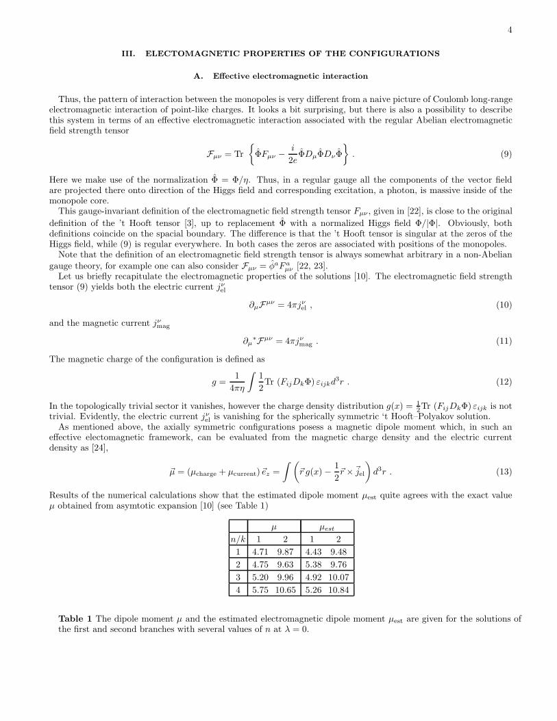
Results of the numerical calculations show that the estimated dipole moment µest quite agrees with the exact valueµ obtained from asymtotic expansion [10] (see Table 1)

µ µest

n/k 1 2 1 2

1 4.71 9.87 4.43 9.48

2 4.75 9.63 5.38 9.76

3 5.20 9.96 4.92 10.07

4 5.75 10.65 5.26 10.84

Table 1 The dipole moment µ and the estimated electromagnetic dipole moment µest are given for the solutions ofthe first and second branches with several values of n at λ = 0.

5

z ρ

m=2, n=3 configuration: topological charge density at λ=0

02

46

810

1214

16

-10-5

05

10

-1.5

-1

-0.5

0

0.5

1

1.5

ρz

m=2, n=3 configuration: U(1) current density at λ=0

0 2 4 6 8 10 12 14 16 -10-8

-6-4

-20

24

68

10

-0.020

0.020.040.060.080.1

0.120.140.16

Figure 1: The charge density (left) and electric current density (right) are shown for solution with k = 1, n = 3 at λ = 0 asfunctions of the coordinates z, ρ.

j

B j−g

g

B g

Figure 2: Electomagnetic picture of an equilibrium state of two opposite magnetic charges in the magnetic field of the electriccurrent ring.

Thus, the physical picture of the source of the dipole moment is that it originates both from a distribution of themagnetic charges and the electric currents [10]. Because of axial symmetry of the configurations, ~µ = µ~ez.

Let us consider the charge and current density distributions given by the relations (12) and (10), respectively. Wecan evaluate these electromagnetic quantities by straightforward substitution of the numerical solutions with given kand n into the definitions above.

To construct solutions subject to the above boundary conditions, we map the infinite interval of the variable r ontothe unit interval of the compactified radial variable x ∈ [0 : 1],

x =r

1 + r,

i.e., the partial derivative with respect to the radial coordinate changes according to ∂r → (1− x)2∂x . The numericalcalculations are then performed with the help of the FIDISOL package based on the Newton-Raphson iterativeprocedure [25]. The equations are discretized on a non-equidistant grid in x and θ with typical grids sizes of 70× 60.The estimates of the relative error for the functions are of the order of 10−4. The results were presented in [9, 10].

Making use of these solutions, we can see that there is a single electric current ring for the first branch of thesolutions with k = 1 (see Fig. 1). This current is circulating exactly between the maxima of distributions of thepositive and negative charge density. For n = 1 the latter are located at the z axis and coincide with positions of thenodes of the Higgs field. For solution with n = 2 the maxima of the charge density distribution form two rings parallelto xy-plane where the current ring is placed. Also the energy density of the configuration represents two tori. Howevertwo (double) zeroes of the Higgs field still are on the z axis. The energy density tori are located symmetrically withrespect to the nodes of the Higgs field.

As winding number n increases further, i.e., n ≥ 3, instead of isolated nodes on the symmetry axis, the closed vortexsolution arises [10]. For this configuration the Higgs field vanishes on a closed ring centered around the symmetry axis.This ring coincides with position of maxima of the current density distribution. Thus, one may conjecture that the

6

ρ z

m=4, n=1 configuration: charge density at λ=0

01

23

45

67 -10

-8-6

-4-2

02

46

810

-0.4-0.3-0.2-0.1

00.10.20.30.4

ρz

m=4, n=1 configuration: U(1) current density at λ=0

05

1015

2025 -20

-15-10

-50

510

1520

-0.8

-0.6

-0.4

-0.2

0

0.2

0.4

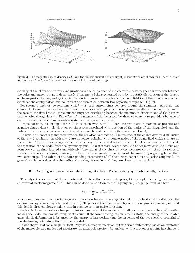
Figure 3: The magnetic charge density (left) and the electric current density (right) distributions are shown for M-A-M-A chainsolution with k = 2, n = 1 at λ = 0 as functions of the coordinates z, ρ.

stability of the chain and vortex configurations is due to balance of the effective electromagnetic interaction betweenthe poles and current rings. Indeed, the U(1) magnetic field is generated both by the static distribution of the densityof the magnetic charges, and by the circular electric current. There is the magnetic field Bk of the current loop whichstabilizes the configuration and counteract the attraction between two opposite charges (cf. Fig. 2).

For second branch of the solutions with k = 2 three current rings centered around the symmetry axis arise, onecounterclockwise in the xy-plane, and two outer clockwise rings which lie in planes parallel to the xy-plane. As inthe case of the first branch, these current rings are circulating between the maxima of distributions of the positiveand negative charge density. The effect of the magnetic field generated by these currents is to provide a balance ofelectromagnetic interactions in such a system of charges and currents.

Let us consider, for example the M-A-M-A chain with n = 1. There are two pairs of maxima of positive andnegative charge density distribution on the z axis associated with position of the nodes of the Higgs field and theradius of the inner current ring is a bit smaller than the radius of two other rings (see Fig. 3).

As winding number n is increases further, the situation is changing. The maxima of the charge density distributionof the k = 2 configuration with n = 2 are no longer coincide with double nodes of the Higgs field which still are onthe z axis. They form four rings with current density tori squeezed between them. Further increasement of n leadsto separation of the nodes from the symmetry axis. As n increases beyond two, the nodes move onto the ρ axis andform two vortex rings located symmetrically. The radius of the rings of nodes increases with n. Also the radius ofthree current loops increases, however, for the vortex configuration the radius of the inner ring is getting larger thantwo outer rings. The values of the corresponding parameters of all these rings depend on the scalar coupling λ. Ingeneral, for larger values of λ the radius of the rings is smaller and they are closer to the xy-plane.

B. Coupling with an external electromagnetic field: Forced axially symmetric configurations

To analyse the structure of the net potential of interaction between the poles, let us couple the configurations withan external electromagnetic field. This can be done by addition to the Lagrangian (1) a gauge invariant term

Lint =1

2εnmkFmkBext

n ,

which describes the direct electromagnetic interaction between the magnetic field of the field configuration and theexternal homogeneous magnetic field Bext [18]. To preserve the axial symmetry of the configuration, we suppose thatthis field is directed along z axis, either in positive or in negative direction.

Such a field can be used as a free perturbation parameter of the model which allows to manipulate the configurationmoving the nodes and transforming its structure. If the forced configuration remains static, the energy of the relatedquasi-elastic deformation is balanced by the energy of interaction, thus the structure of the net effective potential ofthe electromagnetic interaction may be revealed.

It was shown that for a single ‘t Hooft-Polyakov monopole inclusion of this term of interaction yields an excitationof the monopole zero modes and accelerate the monopole precisely by analogy with a motion of a point-like charge in

7

0

0.1

0.2

0.3

0.4

0.5

0.6

-0.3 -0.2 -0.1 0 0.1 0.2 0.3 0.4 0.5 0.6 0.7 0.8 0.9

Vin

t

Bext

k=1 branch: Energy of interaction at λ=0.5

n=1

n=2

n=3

n=4

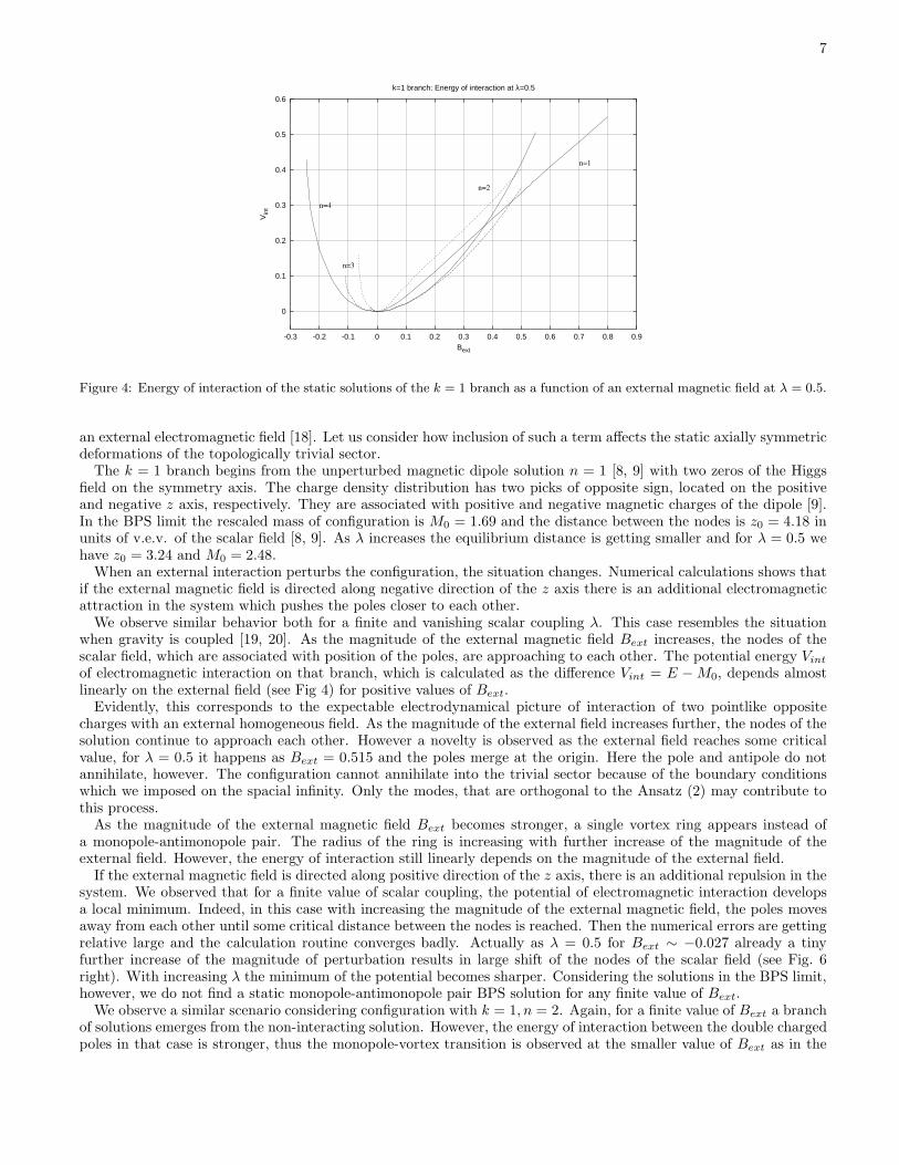
Figure 4: Energy of interaction of the static solutions of the k = 1 branch as a function of an external magnetic field at λ = 0.5.

an external electromagnetic field [18]. Let us consider how inclusion of such a term affects the static axially symmetricdeformations of the topologically trivial sector.

The k = 1 branch begins from the unperturbed magnetic dipole solution n = 1 [8, 9] with two zeros of the Higgsfield on the symmetry axis. The charge density distribution has two picks of opposite sign, located on the positiveand negative z axis, respectively. They are associated with positive and negative magnetic charges of the dipole [9].In the BPS limit the rescaled mass of configuration is M0 = 1.69 and the distance between the nodes is z0 = 4.18 inunits of v.e.v. of the scalar field [8, 9]. As λ increases the equilibrium distance is getting smaller and for λ = 0.5 wehave z0 = 3.24 and M0 = 2.48.

When an external interaction perturbs the configuration, the situation changes. Numerical calculations shows thatif the external magnetic field is directed along negative direction of the z axis there is an additional electromagneticattraction in the system which pushes the poles closer to each other.

We observe similar behavior both for a finite and vanishing scalar coupling λ. This case resembles the situationwhen gravity is coupled [19, 20]. As the magnitude of the external magnetic field Bext increases, the nodes of thescalar field, which are associated with position of the poles, are approaching to each other. The potential energy Vint

of electromagnetic interaction on that branch, which is calculated as the difference Vint = E − M0, depends almostlinearly on the external field (see Fig 4) for positive values of Bext.

Evidently, this corresponds to the expectable electrodynamical picture of interaction of two pointlike oppositecharges with an external homogeneous field. As the magnitude of the external field increases further, the nodes of thesolution continue to approach each other. However a novelty is observed as the external field reaches some criticalvalue, for λ = 0.5 it happens as Bext = 0.515 and the poles merge at the origin. Here the pole and antipole do notannihilate, however. The configuration cannot annihilate into the trivial sector because of the boundary conditionswhich we imposed on the spacial infinity. Only the modes, that are orthogonal to the Ansatz (2) may contribute tothis process.

As the magnitude of the external magnetic field Bext becomes stronger, a single vortex ring appears instead ofa monopole-antimonopole pair. The radius of the ring is increasing with further increase of the magnitude of theexternal field. However, the energy of interaction still linearly depends on the magnitude of the external field.

If the external magnetic field is directed along positive direction of the z axis, there is an additional repulsion in thesystem. We observed that for a finite value of scalar coupling, the potential of electromagnetic interaction developsa local minimum. Indeed, in this case with increasing the magnitude of the external magnetic field, the poles movesaway from each other until some critical distance between the nodes is reached. Then the numerical errors are gettingrelative large and the calculation routine converges badly. Actually as λ = 0.5 for Bext ∼ −0.027 already a tinyfurther increase of the magnitude of perturbation results in large shift of the nodes of the scalar field (see Fig. 6right). With increasing λ the minimum of the potential becomes sharper. Considering the solutions in the BPS limit,however, we do not find a static monopole-antimonopole pair BPS solution for any finite value of Bext.

We observe a similar scenario considering configuration with k = 1, n = 2. Again, for a finite value of Bext a branchof solutions emerges from the non-interacting solution. However, the energy of interaction between the double chargedpoles in that case is stronger, thus the monopole-vortex transition is observed at the smaller value of Bext as in the

8

0

0.2

0.4

0.6

0.8

1

1.2

1.4

1.6

1.8

2

2.2

-0.1 0 0.1 0.2 0.3 0.4 0.5 0.6 0.7 0.8

z 0, ρ

0

Bext

k=1 branch: positive node as function of Bext at λ=0.5

n=2

n=1

1.2

1.4

1.6

1.8

2

2.2

2.4

2.6

2.8

-0.2 -0.1 0 0.1 0.2 0.3 0.4 0.5

ρ 0

Bext

k=1 branch: positive node as function of Bext at λ=0.5

n=3

n=4

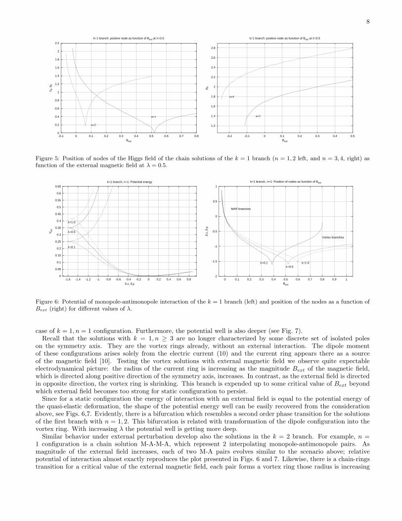
Figure 5: Position of nodes of the Higgs field of the chain solutions of the k = 1 branch (n = 1, 2 left, and n = 3, 4, right) asfunction of the external magnetic field at λ = 0.5.

0

0.05

0.1

0.15

0.2

0.25

0.3

0.35

0.4

0.45

0.5

0.55

0.6

0.65

-1.6 -1.4 -1.2 -1 -0.8 -0.6 -0.4 -0.2 0 0.2 0.4 0.6 0.8

Vin

t

δ z, δ ρ

k=1 branch, n=1: Potential energy

λ=0.1

λ=0.5

λ=1.0

-2

-1.5

-1

-0.5

0

0.5

1

0 0.1 0.2 0.3 0.4 0.5 0.6 0.7 0.8 0.9 1

δ z,

δ ρ

Bext

k=1 branch, n=1: Position of nodes as function of Bext

λ=0.1λ=0.5

λ=1.0

MAP branches

Vortex branches

Figure 6: Potential of monopole-antimonopole interaction of the k = 1 branch (left) and position of the nodes as a function ofBext (right) for different values of λ.

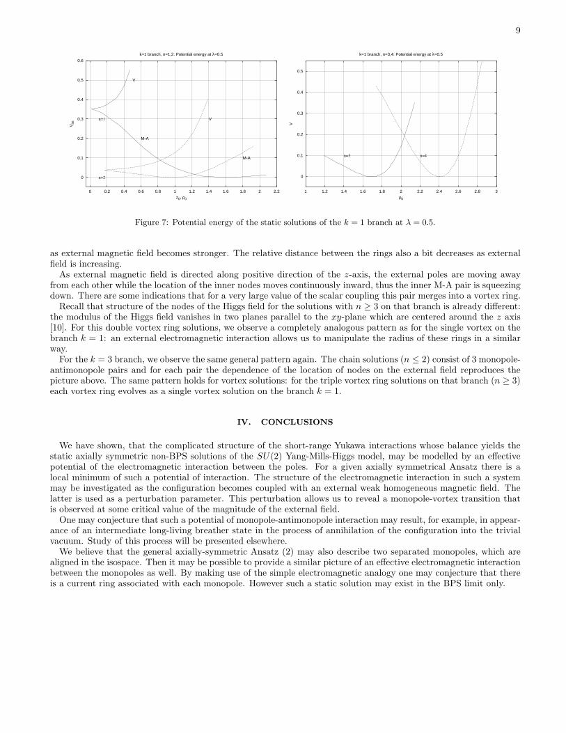
case of k = 1, n = 1 configuration. Furthermore, the potential well is also deeper (see Fig. 7).Recall that the solutions with k = 1, n ≥ 3 are no longer characterized by some discrete set of isolated poles

on the symmetry axis. They are the vortex rings already, without an external interaction. The dipole momentof these configurations arises solely from the electric current (10) and the current ring appears there as a sourceof the magnetic field [10]. Testing the vortex solutions with external magnetic field we observe quite expectableelectrodynamical picture: the radius of the current ring is increasing as the magnitude Bext of the magnetic field,which is directed along positive direction of the symmetry axis, increases. In contrast, as the external field is directedin opposite direction, the vortex ring is shrinking. This branch is expended up to some critical value of Bext beyondwhich external field becomes too strong for static configuration to persist.

Since for a static configuration the energy of interaction with an external field is equal to the potential energy ofthe quasi-elastic deformation, the shape of the potential energy well can be easily recovered from the considerationabove, see Figs. 6,7. Evidently, there is a bifurcation which resembles a second order phase transition for the solutionsof the first branch with n = 1, 2. This bifurcation is related with transformation of the dipole configuration into thevortex ring. With increasing λ the potential well is getting more deep.

Similar behavior under external perturbation develop also the solutions in the k = 2 branch. For example, n =1 configuration is a chain solution M-A-M-A, which represent 2 interpolating monopole-antimonopole pairs. Asmagnitude of the external field increases, each of two M-A pairs evolves similar to the scenario above; relativepotential of interaction almost exactly reproduces the plot presented in Figs. 6 and 7. Likewise, there is a chain-ringstransition for a critical value of the external magnetic field, each pair forms a vortex ring those radius is increasing

9

0

0.1

0.2

0.3

0.4

0.5

0.6

0 0.2 0.4 0.6 0.8 1 1.2 1.4 1.6 1.8 2 2.2

Vin

t

z0, ρ0

k=1 branch, n=1,2: Potential energy at λ=0.5

n=1

n=2

V

V

M-A

M-A

0

0.1

0.2

0.3

0.4

0.5

1 1.2 1.4 1.6 1.8 2 2.2 2.4 2.6 2.8 3

V

ρ0

k=1 branch, n=3,4: Potential energy at λ=0.5

n=3 n=4

Figure 7: Potential energy of the static solutions of the k = 1 branch at λ = 0.5.

as external magnetic field becomes stronger. The relative distance between the rings also a bit decreases as externalfield is increasing.

As external magnetic field is directed along positive direction of the z-axis, the external poles are moving awayfrom each other while the location of the inner nodes moves continuously inward, thus the inner M-A pair is squeezingdown. There are some indications that for a very large value of the scalar coupling this pair merges into a vortex ring.

Recall that structure of the nodes of the Higgs field for the solutions with n ≥ 3 on that branch is already different:the modulus of the Higgs field vanishes in two planes parallel to the xy-plane which are centered around the z axis[10]. For this double vortex ring solutions, we observe a completely analogous pattern as for the single vortex on thebranch k = 1: an external electromagnetic interaction allows us to manipulate the radius of these rings in a similarway.

For the k = 3 branch, we observe the same general pattern again. The chain solutions (n ≤ 2) consist of 3 monopole-antimonopole pairs and for each pair the dependence of the location of nodes on the external field reproduces thepicture above. The same pattern holds for vortex solutions: for the triple vortex ring solutions on that branch (n ≥ 3)each vortex ring evolves as a single vortex solution on the branch k = 1.

IV. CONCLUSIONS

We have shown, that the complicated structure of the short-range Yukawa interactions whose balance yields thestatic axially symmetric non-BPS solutions of the SU(2) Yang-Mills-Higgs model, may be modelled by an effectivepotential of the electromagnetic interaction between the poles. For a given axially symmetrical Ansatz there is alocal minimum of such a potential of interaction. The structure of the electromagnetic interaction in such a systemmay be investigated as the configuration becomes coupled with an external weak homogeneous magnetic field. Thelatter is used as a perturbation parameter. This perturbation allows us to reveal a monopole-vortex transition thatis observed at some critical value of the magnitude of the external field.

One may conjecture that such a potential of monopole-antimonopole interaction may result, for example, in appear-ance of an intermediate long-living breather state in the process of annihilation of the configuration into the trivialvacuum. Study of this process will be presented elsewhere.

We believe that the general axially-symmetric Ansatz (2) may also describe two separated monopoles, which arealigned in the isospace. Then it may be possible to provide a similar picture of an effective electromagnetic interactionbetween the monopoles as well. By making use of the simple electromagnetic analogy one may conjecture that thereis a current ring associated with each monopole. However such a static solution may exist in the BPS limit only.

10

Acknowledgments

I am grateful to B. Kleihaus, J. Kunz and P. Sutcliffe for useful discussions and comments. I would like to acknowl-edge the hospitality at the Bogoliubov Laboratory of Theoretical Physics, JINR where this work was completed.

[1] N.S. Manton and P.M. Sutcliffe, Topological Solitons (Cambridge University Press 2004)[2] Ya.M. Shnir, Magnetic Monopoles (Springer, Berlin Heidelberg New York 2005)[3] G. ‘t Hooft, Nucl. Phys. B 79, 276 (1974);

A.M. Polyakov, Pis’ma JETP 20, 430 (1974).[4] E.J. Weinberg and A.H. Guth, Phys. Rev. D D14, 1660 (1976).[5] C. Rebbi and P. Rossi, Phys. Rev. D 22, 2010 (1980).[6] R.S. Ward, Comm. Math. Phys. 79, 317 (1981);

P. Forgacs, Z. Horvath and L. Palla, Phys. Lett. B 99, 232 (1981);M.K. Prasad, Comm. Math. Phys. 80, 137 (1981);M.K. Prasad and P. Rossi, Phys. Rev. D 24, 2182 (1981).

[7] see e.g. P.M. Sutcliffe, Int. J. Mod. Phys. A 12, 4663 (1997);C. J. Houghton, N. S. Manton and P. M. Sutcliffe, Nucl. Phys. B 510, 507 (1998).

[8] Bernhard Ruber, Thesis, University of Bonn 1985.[9] B. Kleihaus and J. Kunz, Phys. Rev. D 61, 025003 (2000).

[10] B. Kleihaus, J. Kunz and Ya. Shnir, Phys. Lett. B 570, 237 (2003);B. Kleihaus, J. Kunz and Ya. Shnir, Phys. Rev. D 68, 101701 (2003);B. Kleihaus, J. Kunz and Ya. Shnir, Phys. Rev. D 70, 065010 (2004).

[11] B. Julia and A. Zee, Phys. Rev. D 11, 2227 (1975).[12] E.J. Weinberg, Phys. Rev. D 20 936 (1979).[13] B. Hartmann, B. Kleihaus, and J. Kunz, Mod. Phys. Lett. A 15, 1003 (2000);

B. Kleihaus, J. Kunz and Ulrike Neemann, arXiv: gr-qc/0507047.[14] E.B. Bogomol’nyi, Yad. Fiz. 24, 861 (1976);

M.K. Prasad and C.M. Sommerfeld, Phys. Rev. Lett. 35, 760 (1975).[15] B. Kleihaus, J. Kunz and D.H. Tchrakian, Mod. Phys. Lett. A 13 2523 (1998).[16] C.H. Taubes, Commun. Math. Phys. 97, 473 (1985); ibid 86, 257 (1982); ibid 86, 299 (1982).[17] N.S. Manton, Nucl. Phys. B 126, 525 (1977).[18] V.G. Kiselev and Ya. Shnir, Phys. Rev. D 57, 5174 (1998);

Ya. Shnir, Mod. Phys. Lett. A 19, 287 (2004).[19] B. Kleihaus and J. Kunz, Phys. Rev. Lett. 85, 2430 (2000).[20] B. Kleihaus, J. Kunz, and Ya. Shnir, Phys. Rev. D 71, (2005) 024013.[21] V. Paturyan, and D.H. Tchrakian, J. Math. Phys. 45, 302 (2004).[22] P. Goddard and D. Olive, Rep. Prog. Phys. 41, 1357 (1978).[23] N.S. Manton, Nucl. Phys. B135, 319 (1978).[24] M. Hindmarsh and M. James, Phys. Rev. D 49, 6109 (1994).[25] W. Schonauer, and R. Weiß, J. Comput. Appl. Math. 27, 279 (1989);

M. Schauder, R. Weiß, and W. Schonauer, The CADSOL Program Package, Universitat Karlsruhe, Interner Bericht Nr.46/92 (1992).

[26] In earliest study of the axially symmetric configurations, we worked in the gauge where the scalar field components on thespacial asymptotic do not depend on the polar angle [9, 10].