E�cient Dynamic Programming Algorithmsfor Ordering Expensive Joins and SelectionsWolfgang Scheufele? Guido MoerkotteUniversit�at MannheimLehrstuhl f�ur Praktische Informatik III68131 Mannheim, Germanye-mail: fws j moerg@pi3.informatik.uni-mannheim.deAbstract. The generally accepted optimization heuristics of pushing se-lections down does not yield optimal plans in the presence of expensivepredicates. Therefore, several researchers have proposed algorithms tocompute optimal processing trees for queries with expensive predicates.All these approaches are incorrect|with one exception [3]. Our contri-bution is as follows. We present a formally derived and correct dynamicprogramming algorithm to compute optimal bushy processing trees forqueries with expensive predicates. This algorithm is then enhanced tobe able to (1) handle several join algorithms including sort merge witha correct handling of interesting sort orders, to (2) perform predicatesplitting, to (3) exploit structural information about the query graph tocut down the search space. Further, we present e�cient implementationsof the algorithms. More speci�cally we introduce unique solutions fore�ciently computing the cost of the intermediate plans and for savingmemory space by utilizing bitvector contraction. Our implementationsimpose no restrictions on the type of query graphs, the shape of pro-cessing trees or the class of cost functions. We establish the correctnessof our algorithms and derive tight asymptotic bounds on the worst casetime and space complexities. We also report on a series of benchmarksshowing that queries of sizes which are likely to occur in practice can beoptimized over the unconstrained search space in less than a second.1 IntroductionTraditional work on algebraic query optimization has mainly focused on theproblem of ordering joins in a query. Restrictions like selections and projec-tions are generally treated by \push-down rules". According to these, selectionsand projections should be pushed down the query plan as far as possible. Theseheuristic rules worked quite well for traditional relational database systems wherethe evaluation of selection predicates is of neglectable cost and every selection re-duces the cost of subsequent joins. As pointed out by Hellerstein, Stonebraker [5],this is no longer true for modern database systems like object-oriented DBMSs? Research supported by the German Research Association (DFG) under contractMo 507/6-1.

that allow users to implement arbitrary complex functions in a general-purposeprogramming language. In this paper we present a dynamic programming al-gorithm for computing optimal bushy processing trees with cross products forconjunctive queries with expensive join and selection predicates. The algorithmis then enhanced to (1) handle several join algorithms including sort merge witha correct handling of interesting sort orders, to (2) perform predicate splitting,to (3) exploit structural information about the query graph to cut down thesearch space. There are no restrictions on the shape of the processing trees, thestructure of the query graph or the type of cost functions. We then focus on ef-�cient algorithms with respect to both the asymptotic time complexity and thehidden constants in the implementation. Our dynamic programming algorithmand its enhancements were formally derived by means of recurrences and timeand space complexities are analyzed carefully. We present details of an e�cientimplementation and sketch possible generalizations. More speci�cally we intro-duce unique solutions for e�ciently computing the cost of the intermediate plansand for saving memory space by utilizing bitvector contraction. A more detaileddescription of our algorithm can be found in our technical report [10].The rest of the paper is organized as follows. Section 2 summarizes relatedwork and clari�es the contribution of our approach over existing approaches. Sec-tion 3 covers the background for the rest of the paper. In section 4 we presentthe dynamic programming algorithm for ordering expensive selections and joins.Section 5 discusses the problems to be solved in an e�cient implementation ofthese solutions. One of its main contributions is to o�er a possibility for a fastcomputation of cost functions. This is a major point, since most of the opti-mization time in a dynamic programming approach is often spent on computingcosts. A second major point introduces techniques for space saving measures. Insection 6 we discuss several possible generalizations of our algorithm accountingfor interesting sort orders, the option to split conjunctive predicates, and theexploitation of structural information from the join graph. Section 7 shows theresults of timing measurements and section 8 concludes the paper.2 Related Work and ContributionOnly few approaches exist to the problem of ordering joins and selections withexpensive predicates. In the LDL system [4] and later on in the Papyrus project[1] expensive selections are modelled as arti�cial relations which are then or-dered by a traditional join ordering algorithm producing left-deep trees. Thisapproach su�ers from two disadvantages. First, the time complexity of the algo-rithm cannot compete with the complexity of approaches which do not modelselections and joins alike and, second, left-deep trees do not admit plans wheremore than one cheap selection is \pushed down". Another approach is basedupon the \predicate migration algorithm" [5, 6] which solves the simpler problemof interleaving expensive selections in an existing join tree. The authors of [5, 6]suggest to solve the general problem by enumerating all join orders while placingthe expensive selections with the predicate migration algorithm|in combination

with a system R style dynamic programming algorithm endowed with pruning.The predicate migration approach has several severe shortcomings. It may de-generate to exhaustive enumeration, it assumes a linear cost model and it doesnot always yield optimal results [2]. Recently, Chaudhuri and Shim presented adynamic programming algorithm for ordering joins and expensive selections [2].Although they claim that their algorithm computes optimal plans for all costfunctions, all query graphs, and even when the algorithm is generalized to bushyprocessing trees and expensive join predicates, the alleged correctness has notbeen proved at all. In fact, it is not di�cult to �nd counterexamples disprov-ing the correctness for even the simplest cost functions and processing trees.This bug was later discovered and the algorithm restricted to work on regularcost functions only [3]. Further, it does not generate plans that contain crossproducts. The algorithm is not able to consider di�erent join implementations.Especially the sort merge join is out of the scope of the algorithm due to its re-striction to regular cost functions. A further disadvantage is that the algorithmdoes not perform predicate splitting. The contribution of our algorithm and itsenhancements are: (1) It works on arbitrary cost functions. (2) It generates planswith cross products. (3) It can handle di�erent join algorithms. (4) It is capableof exploiting interesting sort orders. (5) It employs predicate splitting. (6) Ituses structural information to restrict the search space. Our �nal contributionare tight time and space bounds.3 PreliminariesWe consider simple conjunctive queries [12] involving only single table selectionsand binary joins (selection-join-queries). A query is represented by a set of re-lations R1; : : : ; Rn and a set of query predicates p1; : : : ; pn, where pk is either ajoin predicate connecting two relations Ri and Rj or a selection predicate whichrefers to a single relation Rk (henceforth denoted by �k). All predicates areassumed to be either basic predicates or conjunctions of basic predicates (con-junctive predicates). Basic predicates are simple built-in predicates or predicatesde�ned via user-de�ned functions which may be expensive to compute.Let R1; : : : ; Rn be the relations involved in the query. Associated with eachrelation is its cardinality ni = jRij. The predicates in the query induce a joingraph G = (fR1; : : : ; Rng; E), where E contains all pairs fRi; Rjg for whichexists a predicate pk relating Ri and Rj . For every join or selection predicatepk 2 P , we assume the existence of a selectivity fk [12] and a cost factor ckdenoting the costs for a single evaluation of the predicate.A processing tree for a select-join-query is a rooted binary tree with its in-ternal nodes having either one or two sons. In the �rst case the node representsa selection operation and in the latter case it represents a binary join operation.The tree has exactly n leaves, which are the relations R1; : : : ; Rn. Processingtrees are classi�ed according to their shape. The main distinction is betweenleft-deep trees and bushy trees. In a left-deep tree the right subtree of an internalnode does not contain joins. Otherwise it is called a bushy tree.

There are di�erent implementations of the join operator each leading to dif-ferent cost functions for the join and hence to di�erent cost functions for thewhole processing tree. We do not want to commit ourselves to a particular costfunction, instead the reader may select his favorite cost function from a large classof admissible cost functions which are subject to the following two requirements.First, the cost function is decomposable and thus can be computed by means ofrecurrences. Second, the costs of a processing tree are (strictly) monotonouslyincreasing with respect to the costs of its subtrees. This seems to be no majorrestriction for \reasonable" cost functions. It can be shown [9] that such costfunctions guarantee that every optimal solution satis�es the \principle of opti-mality" which we state in the next section. In order to discuss some details of ane�cient implementation we assume that the cost function can be written as arecurrence involving several auxiliary functions, an example is the size function(the number of tuples in the result of a subquery).4 The Dynamic Programming AlgorithmLet us denote the set of relations occurring in a bushy plan P by Rel(P ) andthe set of relations to which selections in P refer by Sel(P ). Let R denote aset of relations. We denote by Sel(R) the set of all selections referring to somerelation in R. Each subset V � R de�nes an induced subquery which contains allthe joins and selections that refer to relations in V only. A subplan P 0 of a planP corresponds to a subtree of the expression tree associated with P . A partitionof a set S is a pair of nonempty disjoint subsets of S whose union is exactly S.For a partition S1; S2 of S we write S = S1 ] S2. By a k-set we simply mean aset with exactly k elements.Consider an optimal plan P for an induced subquery involving the nonemptyset of relations Rel(P ) and the set of selections Sel(P ). Obviously, P has eitherthe form P � (P1 1 P2) for subplans P1 and P2 of P , or the form P � �i(P 0)for a subplan P 0 of P and a selection �i 2 Sel(P ). The important fact isnow that the subplans P1; P2 are necessarily optimal plans for the relationsRel(P1); Rel(P2) and the selections Sel(P1); Sel(P2), where Rel(P1)]Rel(P2) =Rel(P ); Sel(P1) = Sel(P )\ Sel(R1); Sel(P2) = Sel(P )\ Sel(R2): Similarly, P 0is an optimal bushy plan for the relations Rel(P 0) and the selections Sel(P ),where Rel(P 0) = Rel(P ); Sel(P 0) = Sel(P )� f�ig. Otherwise we could obtaina cheaper plan by replacing the suboptimal part by an optimal one which wouldbe a contradiction to the assumed optimality of P (note that our cost function isdecomposable and monotone). The property that optimal solutions of a problemcan be decomposed into a number of \smaller", likewise optimal solutions of thesame problem, is known as Bellman's optimality principle. This leads immedi-ately to the following recurrence for computing an optimal bushy plan1 for a setof relations R and a set of selections S.1 min() is the operation which yields a plan with minimal costs among the addressedset of plans. Convention: min;(: : : ) := � where � denotes some arti�cial plan withcost 1.

opt(R;S) = 8>>><>>>:min(min;�R0�R(opt(R0; S \ Sel(R0)) 1 if ; � S � R;opt(R nR0; S \ Sel(R n R0)))min�i2S(�i(opt(R; S n f�ig))))Ri if R = fRig;S = ; (1)The join symbol 1 denotes a join with the conjunction of all join predicatesthat relate relations in R0 to relations in R n R0. Considering the join graph,the conjuncts of the join predicate correspond to the predicates associated withthe edges in the cut (R0; R nR0). If the cut is empty the join is actually a crossproduct.In our �rst algorithm we will treat such joins and selections with conjunctivepredicates as single operations with according accumulated costs. The option tosplit such predicates will be discussed in section 6.2 where we present a secondalgorithm.Based on recurrence (1), there is an obvious recursive algorithm to solve ourproblem but this solution would be very ine�cient since many subproblems aresolved more than once. A much more e�cient way to solve this recurrence isby means of a table and is known under the name of dynamic programming[8, 11]. Instead of solving subproblems recursively, we solve them one after theother in some appropriate order and store their solutions in a table. The overalltime complexity then becomes (typically) a function of the number of distinctsubproblems rather than of the larger number of recursive calls. Obviously, thesubproblems have to be solved in the right order so that whenever the solutionto a subproblem is needed it is already available in the table. A straightforwardsolution is the following. We enumerate all subsets of relations by increasing size,and for each subset R we then enumerate all subsets S of the set of selectionsoccurring in R by increasing size. For each such pair (R;S) we evaluate therecurrence (1) and store the solution associated with (R;S).For the following algorithm we assume a given select-join-query involving nrelations R = fR1; : : : ; Rng and m � n selections S = f�1; : : : ; �mg. In thefollowing, we identify selections and relations to which they refer. Let P be theset of all join predicates pi;j relating two relations Ri and Rj . By RS we denotethe set fRi 2 R j 9�j 2 S : �j relates to Rig which consists of all relationsin R to which some selection in S relates. For all U � R and V � U \ RS , atthe end of the algorithm T [U; V ] stores an optimal bushy plan for the subquery(U; V ).

proc Optimal-Bushy-Tree(R;P )1 for k = 1 to n do2 for all k-subsets Mk of R do3 for l = 0 to min(k;m) do4 for all l-subsets Pl of Mk \RS do5 best cost so far =1;6 for all subsets L of Mk with 0 < jLj < k do7 L0 =Mk n L, V = Pl \ L, V 0 = Pl \ L0;8 p = Vfpi;j j pi;j 2 P; Ri 2 V; Rj 2 V 0g; // p=true might hold9 T = (T [L; V ] 1p T [L0; V 0]);10 if Cost(T) < best cost so far then11 best cost so far = Cost(T);12 T [Mk; Pl] = T ;13 �;14 od;15 for all R 2 Pl do16 T = �R(T [Mk; Pl n fRg]);17 if Cost(T) < best cost so far then18 best cost so far = Cost(T);19 T [Mk; Pl] = T ;20 �;21 od;22 od;23 od;24 od;25 od;26 return T [R; S];Complexity of the algorithm: In [10] we show that the number of consideredpartial plans is 3n(5=3)m + (2m=3 � 2) � 2n(3=2)m + 1 which we can rewriteas [3(5=3)c]n + (2cn=3 � 2)[2(3=2)c]n + 1 if we replace m by the fraction ofselections c = m=n. Assuming an asymptotic optimal implementation of theenumeration part of the algorithm (see section 5), the amount of work per con-sidered plan is constant and the asymptotic time complexity of our algorithm isO([3 (5=3)c]n + n[2 (3=2)c]n). Assuming that the relations are re-numbered suchthat all selections refer to relations in fR1; : : : ; Rmg, the space complexity of thealgorithm is O(2n+m). Note that not every table entry T [i; j]; 0 � i < n; 0 � j <m represents a valid subproblem. In fact, the number of table entries used bythe algorithm to store the solutions of subproblems is 2n(3=2)m � 1. In section5.3 we discuss techniques to save space.5 An E�cient Implementation5.1 Fast Enumeration of SubproblemsThe frame of our dynamic programming algorithm is the systematic enumerationof subproblems consisting of three nested loops iterating over subsets of relationsand predicates, respectively.

The �rst loop enumerates all nonempty subsets of the set of all relations inthe query. It turns out that enumerating all subsets strictly by increasing sizeseems not to be the most e�cient way. The whole point is that the order ofenumeration only has to guarantee that for every enumerated set S, all subsetsof S have already been enumerated. One of such orderings, which is probablythe most suitable, is the following. We use the standard representation of n-sets,namely bitvectors of length n. A subset of a set S is then characterized by abitvector which is component-wise smaller than the bitvector of S. This leadsto the obvious ordering in which the bitvectors are arranged according to theirvalue as binary numbers. This simple and very e�ective enumeration scheme(binary counting method) is successfully used in [13]. The major advantage isthat we can pass over to the next subset by merely incrementing an integer,which is an extremely fast hardwired operation.The next problem is to enumerate subsets S of a �xed subset M of a set Q. If Qhas n elements then we can represent M by a bitvector m of length n. Since Mis a subset of Q some bit positions of m may be zero. Vance and Maier proposein [13] a very e�cient and elegant way to solve this problem. In fact, they showthat the following loop enumerates all bitvectors S being a subset of M , whereM � Q.S = 0;repeat: : :S =M &(S �M);until S = 0We assume two's-complement arithmetic. Bit-operations are denoted as in thelanguage C. As an important special case, we mention that M & �M yields thebit with the smallest index in M . Similarily, one can count downward using theoperation S =M &(S � 1). Combining these operations, one can show that theoperation S =M &((S j (M &(S� 1)))�M) (with initial value S =M & �M)iterates through each single bit in the bitvectorM in order of increasing indices.5.2 E�cient Computation of the Cost FunctionNow, we discuss the e�cient evaluation of the cost function within the nestedloops. Obviously, for a given plan we can compute the costs and the size in (typ-ically) linear time but there is a even more e�cient way using the recurrences forthese functions. If R0; R00 and S0; S00 are the partitions of R and S, respectively,for which the recurrence (1) assumes a minimum, we haveSize(R;S) = Size(R0; S0) � Size(R00; S00) � Sel(R0; R00);where Sel(R0; R00) := YRi2R0;Rj2R00 fi;j

is the product of all selectivities between relations in R0 and R00. Note thatthe last equation holds for every partition R0; R00 of R independent of the rootoperator in an optimal plan. Hence we may choose a certain partition in orderto simplify the computations. Now if R0 = U1 ] U2 and R00 = V1 ] V2, we havethe following recurrence for Sel(R0; R00)Sel(U1 ] U2; V1 ] V2) = Sel(U1; V1) � Sel(U1; V2) � Sel(U2; V1) � Sel(U2; V2)Choosing U1 = �(R); U2 := ;; V1 = �(R nU1); and V2 := R nU1 n V2, where thefunction � is given by �(A) := fRkg; k = minfi jRi 2 Agleads toSel(�(R); R n �(R)) =Sel(�(R); �(R n �(R))) � Sel(�(R); (R n �(R)) n �(R n �(R))) =Sel(�(R); �(R n �(R))) � Sel(�(R); (R n �(R n �(R))) n �(R))De�ning the fan-selectivity Fan Sel(R) as Sel(�(R); Rn�(R)), gives the simplerrecurrenceFan Sel(R) = Sel(�(R); �(R n �(R))) � Fan Sel(R n �(R))= fi;j � Fan Sel(R n �(R n �(R))) (2)where we assumed �(R) = fRig and �(R n �(R)) = fRjg.As a consequence, we can compute Size(R;S) with the following recurrenceSize(R;S) = Size(�(R); S \ �(R)) � Size(R n �(R); (R n �(R)) \ S) (3)� Fan Sel(R)We remind that the single relation in �(R) can be computed very e�cientlyvia the operation a& � a on the bitvector of R. Recurrences (2) and (3) areillustrated in the following �gure. The encircled sets of relations denote thenested partitions along which the sizes and selectivities are computed......

R_i1

R_i2

R_i3f_i1,i2

R_ikFan_Sel

.

.

.

.

.

R_i3

R_ik

f_i2,i3

f_i1,i2

R_i1

R_i2

i1 < i2 < ... < iki1 < i2 < ... < ik

(3)(2)

5.3 Space Saving MeasuresAnother problem is how to store the tables without wasting space. For example,suppose n = 10; m = 10 and let r and s denote the bitvectors correspondingto the sets R and S, respectively. If we use r and s directly as indices of atwo-dimensional array cost[ ][ ], about 90% of the entries in the table will not beaccessed by the algorithm. To avoid this immense waste of space we have to usea contracted version of the second bitvector s.De�nition 1. (bitvector contraction)Let r and s be two bitvectors consisting of the bits r0r1 : : : rn and s0s1 : : : sn,respectively. We de�ne the contraction of s with respect to r as follows:contrr(s) = 8<: � if s = �contrr1:::rn(s1 : : : sn) if s 6= � and r0 = 0s0 contrr1:::rn(s1 : : : sn) if s 6= � and r0 = 1Example Let us contract the bitvector s = 0101001111 with respect to thebitvector r = 1110110100. For each bit si of s, we examine the correspondingbit ri in r. If ri is zero we \delete" si in s, otherwise we retain it. The result isthe contracted bitvector 010001.The following �gure shows the structure of the two-dimensional ragged ar-rays. The �rst dimension is of �xed size 2n, whereas the second dimension is ofsize 2k where k is the number of common nonzero bits in the value of the �rstindex i and the bitvector of all selections sels. The number of entries in such aragged array is Pmk=0 �mk �2k2n�m = [2( 32 )c]n. Note that this number equals 2nfor m = 0 and 3n for m = n. A simple array would require 4n entries. The �gurebelow shows the worst case where the number of selections equals the numberof relations.

0 1 2 3 4 5 6 7 8 9 10 11 12 13 14 15

0000 0010 0100 0110

01000000

0000 0001 0010 0011 1000 1001 1010 1011

0

1

2

3

4

5

6

7

8

9

10

11

12

13

15

14

0000

0001

0010

0100

0011

0101

0111

0110

1000

1001

1100

1101

1110

1111

1011

1010

The simplest way would be to contract the second index on the y for eachaccess of the array. This would slow down the algorithm by a factor of n. Itwould be much better if we could contract all relevant values in the course of theother computations|therefore not changing the asymptotic time complexity.Note that within our algorithm the �rst and second indices are enumerated byincreasing values which makes a contraction easy. We simply use pairs of indicesi; ic, one uncontracted index i and its contracted version ic and count up theirvalues independently.As mentioned before, in the two outermost loops bitvector contraction is easydue to the order of enumeration of the bitvectors. Unfortunately, this does notwork in the innermost loop where we have to contract the result of a conjunc-tion of two contracted bitvectors again. Such a \double contraction" cannot beachieved by simple counting or other combinations of arithmetic and bit oper-ations. One possible solution is to contract the index in the innermost loop onthe y, another is to tabulate the contraction function. Since tabulation seemsslightly more e�cient, we apply the second method. Before entering the inner-most loop we compute and store the results of all contraction operations whichwill occur in the innermost loop. The computation of contraction values can nowbe done more e�ciently since we do not depend on the speci�c order of enumer-ation in the innermost loop. The values in the table can be computed bottom-upusing the recurrence given in De�nition 1. Due to contraction the new time com-plexity of the algorithm is O((n+1)[3(5=3)c]n +n[2(3=2)c]n+ (cn)22n) whereasthe new space complexity is O([2(3=2)c]n + 2n).6 Some Generalizations6.1 Di�erent Join AlgorithmsIn addition to the problem of optimal ordering expensive selections and joinsthe optimizer eventually has to select a join algorithm for each of the join op-erators in the processing tree. Let us call processing trees where a join methodfrom a certain pool of join implementations is assigned to each join operatoran annotated processing tree. We now describe how our dynamic programmingalgorithm can be generalized to determine optimal annotated bushy processingtrees in one integrated step.The central point is that the application of a certain join method can changethe physical representation of an intermediate relation such that the join costsin subsequent steps may change. For example, the application of a sort-mergejoin leaves a result which is sorted with respect to the join attribute. Nested loopjoins are order preserving, that is if the outer relation is sorted with respect toan attribute A then the join result is also sorted with respect to A. A join orselection may take advantage of the sorted attribute. In the following discussionwe restrict ourselves to the case where only nested-loop joins and sort-mergejoins are available. Furthermore, we assume that all join predicates in the queryare equi-joins so that both join methods can be applied for every join that occurs.

This is not a restriction of the algorithm but makes the following discussion lesscomplex.Consider an optimal bushy plan P for the relations in Rel(P ) and the selec-tions in Sel(P ). Again we can distinguish between a join operator representingthe root of the plan tree and a selection operator representing the root. In caseof a join operator we further distinguish between the join algorithms nested-loop(nl) and sort-merge (sm). Let Ca(R;S) be the costs of an optimal subplan forthe relations in R and selections in S, where the result is sorted with respectto the attribute a (of some relation r 2 R). C(R;S) is similar de�ned, but theresult is not necessarily sorted with respect to any attribute. Now, the opti-mality principle holds both for C(R;S) and Cx(R;S) for all attributes x in theresult of the query (R;S) and one can easily specify two recurrences which com-pute C(R;S) and Cajb(R;S) in terms of C(R0; S0); Ca(R0; S0) and Cb(R0; S0) for\smaller" subproblems (R0; S0), respectively. Here ajb denotes the join attributein the result of an equi-join with respect to the attributes a and b.Time Complexity: The number of considered partial plans is O(n2[3(5=3)c]n +cn3[2(3=2)c]n). Similarly, the asymptotic number of table entries in our newalgorithm is O(n2[2(3=2)c]n).6.2 Splitting Conjunctive PredicatesSo far our algorithm does consider joins and selections over conjunctive predicateswhich may occur in the course of the algorithm as indivisible operators of theplan. For example, consider a query on three relations with three join predicatesrelating all the relations. Then, every join operator in the root of a processingtree has a join predicate which is the conjunction of two basic join predicates.In the presence of expensive predicates this may lead to suboptimal2 plans sincethere may be a cheaper plan which splits a conjunctive join predicate into a joinwith high selectivity and low costs and a number of (secondary) selections withlower selectivities and higher costs. Consequently, we do henceforth considerthe larger search space of all queries formed by joins and selections with basicpredicates which are equivalent to our original query.The approach is similar to our �rst approach but this time we have to takeinto account the basic predicates involved in a partial solution. First, we replaceall conjunctive selection and join predicates in the original query by all its con-juncts. Note that this makes our query graph a multigraph. Let p1; : : : ; pm bethe resulting set of basic predicates. We shall henceforth use bitvectors of lengthm to represent sets of basic predicates. Let us now consider an optimal plan Pwhich involves the relations in R and the predicates in P . We denote the costsof such an optimal plan by C(R;P ). Obviously, the root operator in P is eithera cross product, a join with a basic predicate h1 or a selection with a basicpredicate h2. Hence, exactly one of the following four cases holds:2 with respect to the larger search space de�ned next

P � P1 � P2 (cross product): Rel(P ) = Rel(P1) ] Rel(P2); P red(P ) =Pred(P1) ] Pred(P2). The induced join graphs of P1 and P2 are not con-nected in the induced join graph of P . Besides, the subplans Pi (i = 1; 2)are optimal with respect to the corresponding sets Rel(Pi); P red(Pi).P � P1 1h1 P2 (join): Rel(P ) = Rel(P1) ] Rel(P2) and Pred(P ) = Pred(P1)] Pred(P2) ] fh1g. The induced join graphs of P1 and P2 are connected bya bridge h1 in the induced join graph of P . Furthermore, the subplans P1; P2are optimal with respect to the corresponding sets Rel(Pi); P red(Pi).P � �h1(P1) (secondary selection): Rel(P ) = Rel(P1) and Pred(P ) =Pred(P1) ] fh1g. The subplan P1 is optimal with respect to the corre-sponding sets Rel(P1) and Pred(P1).P � �h2(P1) (single table selection): Rel(P ) = Rel(P1) and Pred(P ) =Pred(P1) ] fh2g. The subplan P1 is optimal with respect to the corre-sponding sets Rel(P1) and Pred(P1).Again, it is not di�cult to see that the optimality principle holds and onecan give a recurrence which determines an optimal plan opt(R;P ) for the prob-lem (R;P ) by iterating over all partitions of R applying the corresponding costfunction according to one of the above cases. More details can be found in thetechnical report [10].Complexity Issues: Let m > 0 be the number of di�erent basic predicates (joinsand selections) and n the number of base relations. We derived the followingupper bound on the number of considered partial plans m2m3n � 3m2m+n�1 +m2m�1 = O(m2m3n).As to the space complexity, one can easily give an upper bound of 2n+m on thenumber of table entries used by the algorithm.6.3 Using Structural Information from the Join GraphSo far we concentrated on fast enumeration without analyzing structural in-formation about the problem instance at hand. To give an example, supposeour query graph to be 2-connected. Then every cut contains at least two edges;therefore the topmost operator in a processing tree can neither be a join nor across product. Hence, our second algorithm iterates in vain over all 2n partitionsof the set of all n relations.We will now describe the approach in our third algorithm which uses struc-tural information from the join graph to avoid the enumeration of unnecessarysubproblems. Suppose that a given query relates the relations in R and thepredicates in P . We denote the number of relations in R by n, the number ofpredicates in P by m and the number of selections by s. Consider any optimalprocessing tree T for a subquery induced by the subset of relations R0 � R andthe subset of predicates P 0 � P . The join graph induced by the relations R andthe predicates P is denoted by G(R;P ). Obviously, the root operator in T iseither a cross product, a join, a secondary selection or a single table selection.Depending on the operation in the root of the processing tree, we can classify

the graph G(R0; P 0) as follows. If the root operation is a cross product, thenG(R0; P 0) decomposes into two components. Otherwise, if it is a join with (ba-sic) predicate h then G(R0; P 0) contains a bridge h. If it is a secondary selectionwith (basic) predicate h then G(R0; P 0) contains an edge h. And, if it is a singletable selection with predicate h then G(R0; P 0) contains a loop h.Consequently, we can enumerate all possible cross products by building all par-titions of the set of components of G(R0; P 0). All joins can be enumerated byconsidering all bridges of G(R0; P 0) as follows. Suppose that the bridge is thebasic predicate h and denote the set of components resulting from removing thebridge by C. Now, every possible join can be obtained by building all partitionsof the components in C and joining them with the predicate h. All secondaryselections can be enumerated by just considering every edge (no loops) as se-lection predicate. And, if we step through all loops in G(R0; P 0) we enumerateall single table selections. In a sense we are tackling subproblems in the reversedirection than we did before. Instead of enumerating all partitions and analyzingthe type of operation it admits we consider types of operations and enumeratethe respective subproblems.Complexity: One can show that the number of considered partial plans is atmost 2m�1(3n� 1)+ 2m(3=2)m�1(3n� 1)+m2m�1(2n� 1) and the asymptoticworst-case time complexity is O(2m3n + m(3=2)m3n + (m + n)2m+n � m2m).Furthermore, the number of table entries used by the algorithm is 2n+m.The above time and space complexities are generous upper bounds whichdo not account for the structure of a query graph. For an acyclic join graphG with n nodes, m = n � 1 edges (no loops and multiple edges) and s loops(possibly some multiple loops) the number of considered partial plans is boundby 2s[4n(n=2�1=4)+3n(2n=9�2=9+s=6)] and the asymptotic time complexityis O(2s(n24n + (n2 + s)3n)).7 Performance MeasurementsIn this section we investigate how our dynamic programming algorithms per-form in practice. Note that we give no results of the quality of the generatedplans, since they are optimal. The only remaining question is whether the al-gorithm can be applied in practice since the time bounds seem quite high. Webegin with algorithm Optimal-Bushy-Tree(R,P ) without enhancements. The ta-ble below shows the timings for random queries with n = 10 relations and querygraphs with 50% of all possible edges having selectivity factors less than 1. Joinpredicates are cheap (i.e. cp = 1) whereas selection predicates are expensive(i.e. cp > 1). All timings in this section were measured on a lightly loaded SunSPARCstation 20 with 128 MB of main memory. They represent averages overa few hundred runs with randomly generated queries.10 relations sel : 0 1 2 3 4 5 6 7 8 9 10time [s]: < 0:1 < 0:1 < 0:1 0.1 0.2 0.5 0.9 2.1 4.3 8.1 13.5

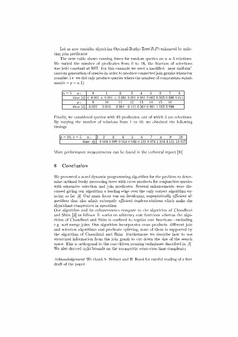
Let us now consider algorithm Optimal-Bushy-Tree(R,P ) enhanced by split-ting join predicates.The next table shows running times for random queries on n = 5 relations.We varied the number of predicates from 0 to 16, the fraction of selectionswas held constant at 50%. For this example we used a modi�ed \near-uniform"random generation of queries in order to produce connected join graphs wheneverpossible, i.e. we did only produce queries where the number of components equalsmax(n� p+ s; 1).n = 5 p : 0 1 2 3 4 5 6 7 8time [s]: < 0.001 < 0.001 < 0.001 0.001 0.001 0.002 0.003 0.006 0.011p : 9 10 11 12 13 14 15 16time [s]: 0.022 0.043 0.084 0.177 0.364 0.801 1.763 3.899Finally, we considered queries with 10 predicates, out of which 5 are selections.By varying the number of relations from 1 to 10, we obtained the followingtimings.p = 10; s = 5 n : 1 2 3 4 5 6 7 8 9 10time [s]: - 0.004 0.008 0.018 0.043 0.122 0.374 1.204 4.151 13.927More performance measurements can be found in the technical report [10].8 ConclusionWe presented a novel dynamic programming algorithm for the problem to deter-mine optimal bushy processing trees with cross products for conjunctive querieswith expensive selection and join predicates. Several enhancements were dis-cussed giving our algorithm a leading edge over the only correct algorithm ex-isting so far [3]. Our main focus was on developing asymptotically e�cient al-gorithms that also admit extremely e�cient implementations which make thealgorithms competitive in operation.Our algorithm and its enhancements compare to the algorithm of Chaudhuriand Shim [3] as follows. It works on arbitrary cost functions whereas the algo-rithm of Chaudhuri and Shim is con�ned to regular cost functions|excludinge.g. sort-merge joins. Our algorithm incorporates cross products, di�erent joinand selection algorithms and predicate splitting, none of them is supported bythe algorithm of Chaudhuri and Shim. Furthermore we describe how to usestructural information from the join graph to cut down the size of the searchspace. This is orthogonal to the cost-driven pruning techniques described in [3].We also derived tight bounds on the asymptotic worst-case time complexity.Acknowledgement We thank S. Helmer and B. Rossi for careful reading of a �rstdraft of the paper.

References1. S. Chaudhuri and K. Shim. Query optimization in the presence of foreign functions.In Proc. Int. Conf. on Very Large Data Bases (VLDB), pages 529{542, Dublin,Ireland, 1993.2. S. Chaudhuri and K. Shim. Optimization of queries with user-de�ned predicates.In Proc. Int. Conf. on Very Large Data Bases (VLDB), pages 87{98, Bombay,India, 1996.3. S. Chaudhuri and K. Shim. Optimization of queries with user-de�ned predicates.Technical report, Microsoft Research, Advanced Technology Division, One Mi-crosoft Way, Redmond, WA 98052, USA, 1997.4. R. Gamboa D. Chimenti and R. Krishnamurthy. Towards an open architecturefor LDL. In Proc. Int. Conf. on Very Large Data Bases (VLDB), pages 195{203,Amsterdam, Netherlands, August 1989.5. J. Hellerstein and M. Stonebraker. Predicate migration: Optimizing queries withexpensive predicates. In Proc. of the ACM SIGMOD Conf. on Management ofData, pages 267{277, Washington, DC, 1993.6. J. M. Hellerstein. Practical predicate placement. In Proc. of the ACM SIGMODConf. on Management of Data, pages 325{335, Minneapolis, Minnesota, USA, May1994.7. A. Kemper, G. Moerkotte, and M. Steinbrunn. Optimization of boolean expressionsin object bases. In Proc. Int. Conf. on Very Large Data Bases (VLDB), pages 79{90, 1992.8. M. Minoux. Mathematical Programming. Theory and Algorithms. Wiley, 1986.9. T. L. Morin. Monotonicity and the principle of optimality. J. Math. Anal. andAppl., 1977.10. W. Scheufele and G. Moerkotte. E�cient dynamic programming algorithms forordering expensive joins and selections. Forthcoming Technical Report, Lehrstuhlf�ur Praktische Informatik III, Universit�at Mannheim, 68131 Mannheim, Germany,1998.11. C. E. Leiserson T. H. Cormen and R. L. Rivest. Introduction to Algorithms. MITPress, Cambridge, Massachusetts, USA, 1990.12. J. D. Ullman. Principles of Database and Knowledge-Base Systems, volume II:The New Technologies. Computer Science Press, 1989.13. B. Vance and D. Maier. Rapid bushy join-order optimization with cartesian prod-ucts. In Proc. of the ACM SIGMOD Conf. on Management of Data, pages 35{46,Toronto, Canada, 1996.