Effects of Information about Invasive Species on Risk Perception and Seafood Demand by Gender and Race1

Timothy C. Haab Department of Agricultural, Environmental and Development Economics

The Ohio State University Columbus, OH 43210

haab.1@osu.edu

John C. Whitehead Department of Economics

Appalachian State University Boone, NC 28608

whiteheadjc@appstate.edu

George R. Parsons Department of Economics

University of Delaware Newark, DE 19716 gparsons@udel.edu

Jammie Price

Department of Sociology and Social Work Appalachian State University

Boone, NC 28608 pricejl@appstate.edu

January 28, 2008

1 A previous version of this paper was presented at the 2001 AERE Workshop, Assessing and Managing Environmental and Public Health Risks, and the 2007 Michigan State University Invasive Species Workshop. We thank participants in those workshops for their comments. This work was (partially) supported by Grant NA86RG0036 from the National Sea Grant College Program, National Oceanic and Atmospheric Administration to the North Carolina Sea Grant College Program.

Effects of Information about Invasive Species on Risk Perception and Seafood Demand by Gender and Race

Abstract: In this paper we consider the effects of negative and positive risk information on

perceived seafood risks and seafood consumption by gender and race. The data is from a Mid-

Atlantic survey of coastal seafood consumers. We elicit risk perceptions in three risk scenarios

with a dichotomous choice with a follow-up question format. We elicit continuous revealed and

stated preference seafood consumption in nine risk and price scenarios. Analysis in four gender

and race categories indicates that demographic groups respond to the positive and negative

information in different ways. Communication of risk information as risk mitigation policy is a

challenge.

1

Introduction

In 1992 researchers at North Carolina State University identified Pfiesteria Piscicida

(Pfiesteria) as one possible cause of fish kills in eastern North Carolina’s estuarine systems

(Burkholder, Noga and Hobbs, 1992). Pfiesteria is a single-celled microorganism that lies

dormant in the sediment of fresh and brackish water estuaries, but in combination with high

nutrient concentrations potentially becomes a toxic predator of a number of local fish species.

Pfiesteria has also been linked to fish kills in Virginia, Maryland and Delaware.

Public perception of Pfiesteria and other harmful algal blooms (e.g., red and brown tides)

has the potential to impose significant economic losses on the mid-Atlantic region (Lipton 1998).

Public concern over harmful algal blooms and, in particular, Pfiesteria can lead to a significant

decrease in demand for seafood in affected areas, despite a lack of scientific evidence linking any

illness from seafood consumption to Pfiesteria. Past research suggests that information about

seafood safety may change behavior, consumers may self protect against seafood risk by

reducing consumption, and self protection behavior may differ across different socioeconomic

groups.

The general population tends to produce inaccurate estimates of risk (McIntosh and Acuff

1994, Johnson and Griffith 1996, Almas 1999). Most people receive information about

environmental risks and food safety from the mass media and often ignore or disregard these

warnings (Velicer and Knuth 1994). People may believe that a warning does not pertain to food

in their area, or that they can limit the danger by various cooking methods. This is of particular

concern for pregnant women and small children who are at higher risk for foodborne pathogens

such as mercury in fish. When people receive information on food safety from individuals such

2

as family and friends it is often incorrect (McIntosh and Acuff 1994), and these sources tend to

convey the benefits of eating seafood rather than the risks (Burger 2005).

Past economic research finds that negative information about food safety tends to

decrease consumption, while counter-information does not necessarily have the opposite effect

(Smith, van Ravenswaay, and Thompson 1988, Brown and Schrader 1990, Lin and Milon 1993).

On the other hand, Wessells, Kline, and Anderson (1996) and Parsons et al. (forthcoming) find

that seafood consumption decreases with negative information about seafood safety and

increases with some types of positive information.

Some of these results concerning the effect of information may be masked by

socioeconomic factors. Social location and access to social resources strongly influence how

people perceive, accept, and manage risk (Lupton, 1999; Slovic, 1999). For example, women,

people of color, working classes, children, the less educated, and the elderly have all been argued

to be “at risk” because of their limited abilities to communicate and control social situations, in

part via reduced access to information (Luhmann, 1993). Women perceive higher food safety

risks than men (Burger, Sanchez and Gochfeld, 1998) and are more concerned about the effects

of food on health and the effect of the environment on food (Davidson and Freudenburg, 1996).

Hersh (1996) determined that women and whites engage in safer behaviors than men and

nonwhites including higher rates of non smoking, seat belt use, brushing and flossing teeth,

exercise, and checking blood pressure. Similarly, Burger et al (1999) found whites, with much

higher median incomes, have more accurate knowledge of seafood safety than blacks and

hispanics.

3

In contrast, Burger, Sanchez and Gochfeld (1998) find no differences among men and

women anglers in awareness of seafood safety information, perceptions of whether seafood was

safe to eat, and seafood consumption. Jakus and Shaw (2003) find no gender or race effects in

the decision of whether to keep fish caught from reservoirs with fish consumption advisories.

Many of the gender and race effects found, and not found, could be a result of the

interaction between gender, race, and social class (Flynn, Slovic, and Mertz (1994)). White men

perceived lower risks than others on nearly all hazards in Finucane et al.’s (2003) study,

including hand guns, nuclear power, cigarette smoke, sexually transmitted diseases, drugs, blood

transfusions, pesticides, lead poisoning, and food hazards. Nonwhite females tend to perceive the

highest risk for most hazards. Other studies have found that white women eat less seafood than

white men (Burger 2000). To examine these interactions, social researchers need to include

interaction effects in their statistical models.

To our knowledge no study of food safety and consumption to date has considered the

interaction of socioeconomic factors, particularly gender and race. We consider the effects of

negative and positive risk information on perceived seafood risks from Pfiesteria Piscicida

(hereafter, Pfiesteria) associated fish kills and seafood consumption by gender and race. The data

is from a Mid-Atlantic survey of coastal seafood consumers (Whitehead et al. 2003). Previous

research has examined the effects of information about Pfiesteria-related fish kills and seafood

safety on seafood demand in a stated preference framework (Parsons et al. 2006). In this paper

we examine the effect of Pfiesteria-related fish kills and health risk information on risk

perception and seafood demand in a jointly estimating revealed and stated preference framework.

4

The Survey

To study the effects of health risk information on seafood risk perceptions and demand,

we conducted a phone-mail-phone survey of mid-Atlantic residents. The sample frame included

seafood eaters in Delaware, the eastern parts of Maryland (including the District of Columbia),

North Carolina and Virginia. The sample frame was stratified with a 50/50 urban/rural split and a

50/50 North Carolina/rest of sample split.

The survey was conducted during fish kill season: June through November. The East

Carolina University Survey Research Laboratory conducted the first telephone interviews from

August to October. Almost nine thousand calls were made in an attempt to reach 2000

respondents. One thousand eight hundred and seven interviews were completed. Dividing the

completed interviews by eligible contacts (i.e., refusals plus completed interviews) yields a

response rate of 60.7%. This response rate varies significantly by state. The response rate in

North Carolina was highest with 69% and 1085 completed interviews. The response rates in

Delaware, District of Columbia, Maryland and Virginia were 52.9%, 46.2%, 48.7%, and 54.4%.

The number of completed interviews was 237, 47, 216, and 222 respectively. These differences

are probably attributable to the name recognition of East Carolina University in eastern North

Carolina and the lack thereof for the rest of the sample.

An information brochure was mailed to respondents who agreed to participate in the

second telephone survey. The information mail-out consists of four parts. The major part is the

Pfiesteria brochure titled “What you should know about Pfiesteria” which was based on the

brochure published by the U.S. Environmental Protection Agency’s Office of Water titled “What

5

you should know about Pfiesteria Piscicida.”2 The brochure and the “counter information” insert

followed the same format with the same headings and edited text. Each mail packet also included

a combination of inserts we will refer to as: “fish kill information,” “seafood inspection

program,” “hypothetical fish kill” and “counter information.” The brochures were full color and

included contact information for more information.

Each section of the Pfiesteria brochure includes one or two short paragraphs. Full color

photographs accompany the text. The first page included three sections. The first section of the

brochure began with a simple definition of Pfiesteria. The second section explains that Pfiesteria

stuns with released toxins and that the toxins are believed to cause sores on fish. The third

section states that toxic outbreaks of Pfiesteria are short but Pfiesteria-associated fish kills can

last for days or weeks. The second page included three sections. The fourth section of the

brochure describes other sources of fish kills and sores. The fifth section then describes more

fully where Pfiesteria has and has not been found with an illustrative map. The sixth section

emphasizes the scientific uncertainty about Pfiesteria by using qualifiers to describe each source

of outbreaks including the presence of a large number of fish, pollutants and excess nutrients.

The back page of the brochure contained three sections. The seventh section of the brochure

discusses health effects and included the statement: “There is no evidence that Pfiesteria-

associated illnesses are associated with eating finfish or shellfish.” The eighth section stated that

2The fact sheet formerly resided at http://www.epa.gov/owow/estuaries/pfiesteria/fact.html. It

has since been taken down from the EPA’s website. The brochure and insert information was

simplified by the authors and revised based on comments received from focus groups and from a

review by an ecologist familiar with the Pfiesteria scientific literature. All survey materials are

available upon request.

6

brown and red tides and Pfiesteria are types of harmful algal blooms. The ninth section provided

state Pfiesteria hotline numbers.

In the hypothetical fish kill insert, respondents in North Carolina were asked to consider a

hypothetical press release about fish kill in the Neuse River near New Bern, NC. The wording

for the hypothetical press release followed closely the wording of actual government press

releases describing fish kill events. Respondents in Delaware, Maryland, and Virginia were

asked to consider a hypothetical fish kill in the Pokomoke River on the eastern shore of

Maryland. There were major and minor versions for the hypothetical fish kills. The major fish

kill is described to affect approximately 300,000 Menhaden, 10,000 Croaker and 5,000 Flounder.

The minor fish kill is described to affect approximately 10,000 Menhaden.

Another insert provided further information about fish kills and a proposed mandatory

seafood inspection program. The fish kill information included a bar chart defining major and

minor fish kills. The other side of the insert proposed a mandatory inspection program by the

U.S. Department of Commerce (USDC) instead of the voluntary inspection services of seafood

producers and processors (under the authority of the Agricultural Marketing Act of 1946).

The final insert, “counter information” is intended to enforce the notion of the safety of

seafood. The information states “YES. In general it IS safe to eat seafood”. It further reports that

there has never been a case of illness from eating finfish and shellfish exposed to Pfiesteria and

that swimming and boating and other recreational activities in costal waters are generally safe.

Finally, it has information on what is being done about Pfiesteria by the collaboration of state,

federal, and local government and academic institutions. The expectation is that respondents who

received this counter information are less likely to worry about seafood safety. Eighty percent of

7

the sample were to receive the Pfiesteria brochure and 40 percent of these were to receive the

counter information. Twenty-percent were to receive neither source of information. All

respondents receive either the major or minor fish kill insert.

About three weeks after the information was mailed, interviewers attempted to contact

the respondents. The second telephone interviews were conducted from October through

November. One thousand four hundred and three respondents agreed to participate in the second

survey. This represents 77 percent of respondents to the first survey and 46.9 percent of those

contacted for the first survey. Of these, 1149 were contacted with 846 completing the interview.

After deleting coding errors between the first and second survey, 835 completed interviews

remain. The response rate to the second survey is 72.7 percent of those who were contacted for

the second survey and 27.9 percent of those contacted for the first survey. The response rate of

those who agreed to participate and were contacted for the second survey is 70.1 percent for

Delaware, 43.5 percent for Washington D.C., 81.7 percent for Maryland, 73.5 percent for North

Carolina and 76.9 percent for Virginia. Deletion of ineligible respondents and those who did not

answer all of the risk perception and demand questions leaves a sample of 646.

The Questionnaires

The first telephone interview collected information on seafood consumption patterns and

costs, revealed and stated seafood demand under a variety of pricing scenarios, seafood health

risk, attitudes and perceptions about seafood and Pfiesteria, and socioeconomic information. A

series of questions were asked to gather qualitative and quantitative perceived risk information.

The qualitative risk question is: “To get a better idea of how safe you think you are from eating

seafood, consider the seafood meals you expect to eat next month. What do you think are your

8

chances of getting sick from eating these meals? Do you think they are very likely, somewhat

likely, somewhat not likely, or not likely at all?”

A quantitative risk question was asked immediately after the qualitative question and

presents a dichotomous choice with a follow-up: “Do you think your chances are greater or less

than 1 percent?” The interviewers accepted the potential answer categories “more,” “less,” or

“about 1 percent.” Respondents who perceive that the chance of getting sick is less than one

percent were asked a follow-up question with a lower risk amount: “This means that you think

your chance of getting sick is less than one in 100. We’d like to know how low you think your

chances are. Do you think your chances of getting sick are greater or less than 1 in D?” The

denominator D took on one of four possible values: 1000, 10,000, 100,000, or 1,000,000.

Respondents answered a set of four questions about the number of seafood meals they

consumed each month. They were first asked how many seafood meals they ate the previous

month (revealed behavior) and how many they would eat the next month (stated behavior). They

were asked how many seafood meals they would eat next month if seafood meal prices went up

by one of four different prices ($1, $3, $5, $7) while all other food prices remain the same. Also

they were asked how many seafood meals they would eat next month if price went down by one

of four different prices ($1, $2, $3, $4) while all other food prices remain the same. Price

changes were randomly assigned to respondents.

The second (follow-up) interview was designed to collect information on seafood

demand, seafood health risk, and attitudes about seafood and Pfiesteria. Most of the questions

were identical or similar to questions asked in the first survey. The main purpose of these

9

questions is to determine if seafood demand, perceived health risk and attitudes about Pfiesteria

change after receiving the informational inserts.

Respondents were asked to assess their perceived risk of eating seafood under two

different scenarios. First, they were asked for their qualitative and quantitative risk assessment

after the hypothetical fish kill. Then they were asked for their qualitative and quantitative risk

perceptions after the mandatory seafood inspection program is implemented. The qualitative and

quantitative risk questions are the same as those in the first interview.

Respondents were asked five additional seafood consumption questions: how much

seafood they ate during the past month (revealed preference), how much they would eat next

month, how much they would eat next month after the fish kill, how much they would eat next

month after the fish kill and with the seafood inspection program and, finally, how much they

would eat next month after the fish kill, with the seafood inspection program and a higher price

for seafood meals ($1, $3, $5, or $7).

Data Summary

The data summary for four groups of respondents is presented in Table 1. Thirty-one

percent of the sample is white male, 7 percent is nonwhite male, 45 percent is white female and

17 percent is nonwhite female. A key difference across group is in income with white male

respondents reporting substantially greater household income. Nonwhite males and females are

more likely to live in an urban county.

The quantitative risk perception data is summarized in Table 2. The variable SICK is

equal to one if respondents thought there chances of getting sick are greater than the suggested

probability. In the baseline scenario, 37 percent of respondents thought that their chance of

10

getting sick from eating seafood meals during a month was greater than 1 percent. After a fish

kill, 57 percent of respondents thought their chances of getting sick were greater than 1 percent.

After a fish kill but with a seafood inspection program, 31 percent of respondents thought their

chances of getting sick were greater than 1 percent. For those respondents who thought their

chances of getting sick were less than 1 percent, the percentage that thinks their chances of

getting sick are greater than the randomly assigned probability rises as the probability falls. In

the baseline sample the probability rises from 34 percent to 59 percent as the probability falls

from p = .001 to p = .000001. In the fish kill scenario the probability rises from 30 percent to 42

percent. In the fish kill with the seafood inspection scenario, the probability rises from 21 percent

to 39 percent.

Seafood consumption choices and seafood prices are presented in Table 3. Scenarios 1-4

were elicited in the first telephone survey. The seafood meal price is defined as the product of the

average price of seafood meal at a restaurant and the quantity of seafood meals at a restaurant

plus the product of the average price of seafood meals cooked at home and the quantity of

seafood meals at home. This is then divided by the sum of quantity of seafood meals at a

restaurant and quantity of seafood meals at home to give the average price of a seafood meal for

each respondent. The average, or typical, prices of seafood at restaurants and at home were

obtained during the survey. The average price of all meals is about $10. The randomly assigned

price changes are added to this price where appropriate.

The first question elicited seafood consumption for the past month (revealed behavior).

The second question elicited stated preference seafood consumption for the next month. The

third question elicited stated preference seafood consumption for the next month with a price

increase. The fourth question elicited stated preference seafood consumption for the next month

11

with a price decrease. As expected, seafood consumption decreases with the price increase and

decreases with the price increase. There are no significant differences between the baseline

revealed and stated preference data. Scenarios 5- 9 were elicited in the second telephone survey.

Comparing across surveys, seafood consumption is higher in the baseline revealed and stated

preference scenarios. This suggests that information, specifically participation in a seafood safety

survey, negatively influenced seafood consumption. As expected, seafood consumption

decreases with the fish kill, increases with the seafood inspection program (with the fish kill) and

decreases with the price increase (with the fish kill and seafood inspection program).

Empirical Models

To analyze the dichotomous responses to the quantitative risk question we first briefly

describe the empirical modeling strategy. Let r be the risk of getting sick from eating seafood in

a typical month. In general:

(1) ( )ε,srr =

where s is a vector of socio-demographic, attitudinal and information variables, and ε is an

unobservable error term assumed to be mean zero. The function ),( εsr is bound between zero

and 1.

If the probability of getting sick per seafood meal, π , is independent of all other seafood

meals eaten then the probability of getting sick in a given month is the binomial probability:

(2) ( ) xTxr −−= ππ 1

12

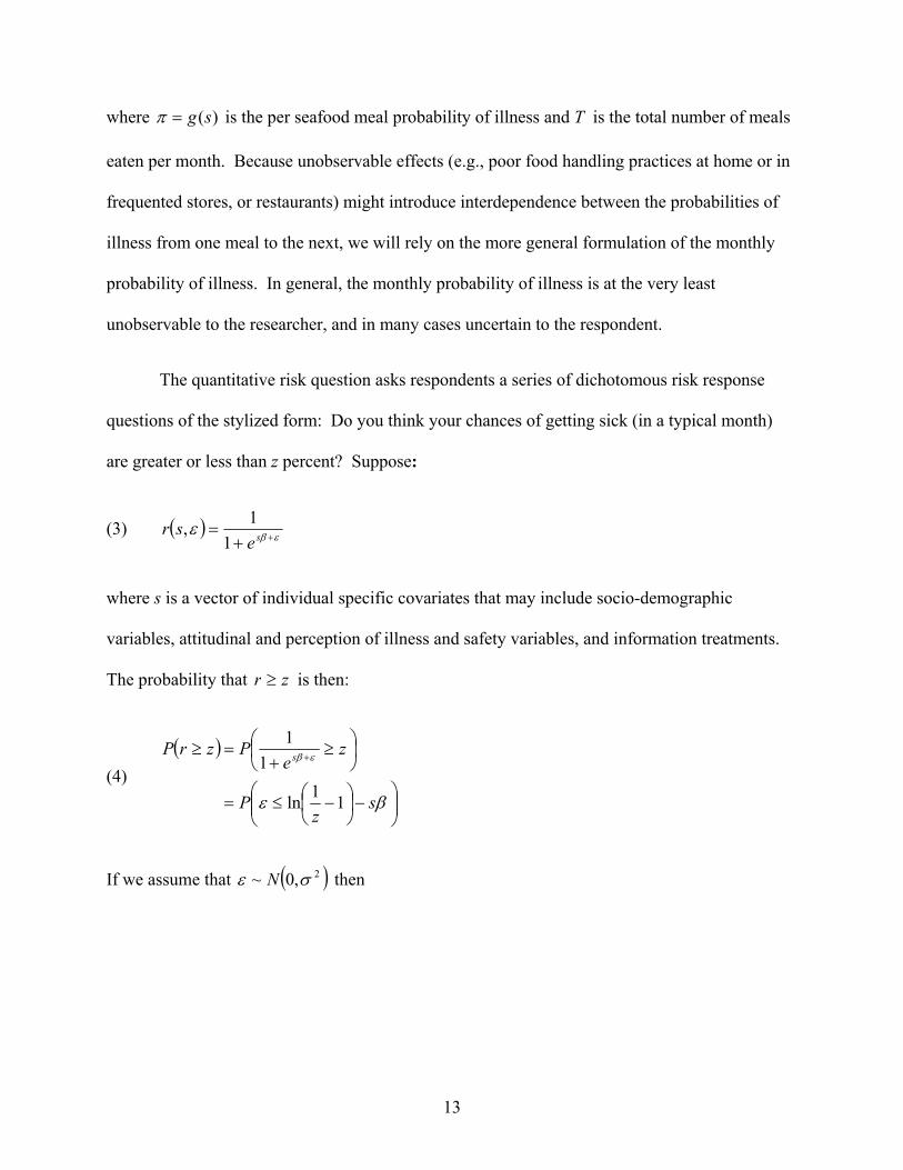
where )(sg=π is the per seafood meal probability of illness and T is the total number of meals

eaten per month. Because unobservable effects (e.g., poor food handling practices at home or in

frequented stores, or restaurants) might introduce interdependence between the probabilities of

illness from one meal to the next, we will rely on the more general formulation of the monthly

probability of illness. In general, the monthly probability of illness is at the very least

unobservable to the researcher, and in many cases uncertain to the respondent.

The quantitative risk question asks respondents a series of dichotomous risk response

questions of the stylized form: Do you think your chances of getting sick (in a typical month)

are greater or less than z percent? Suppose:

(3) ( ) εβε ++= se

sr1

1,

where s is a vector of individual specific covariates that may include socio-demographic

variables, attitudinal and perception of illness and safety variables, and information treatments.

The probability that zr ≥ is then:

(4) ( )

⎟⎟⎠

⎞⎜⎜⎝

⎛−⎟

⎠⎞

⎜⎝⎛ −≤=

⎟⎠⎞

⎜⎝⎛ ≥+

=≥ +

βε

εβ

sz

P

ze

PzrP s

11ln

11

If we assume that ( )2,0~ σε N then

13

(5)

( )

⎟⎟⎟⎟

⎠

⎞

⎜⎜⎜⎜

⎝

⎛

−⎟⎠⎞

⎜⎝⎛ −

Φ=

⎟⎟⎟⎟

⎠

⎞

⎜⎜⎜⎜

⎝

⎛

−⎟⎠⎞

⎜⎝⎛ −

≤=≥

σβ

σ

σβ

σσε

sz

szPzrP

11ln

11ln

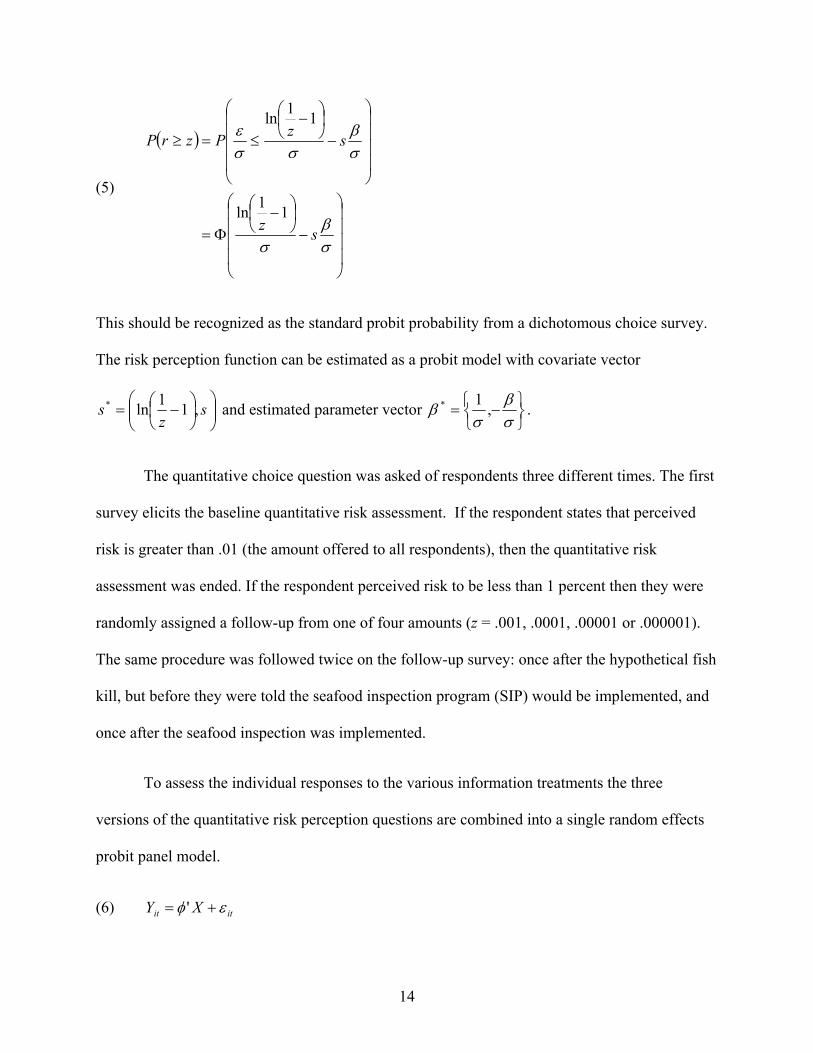
This should be recognized as the standard probit probability from a dichotomous choice survey.

The risk perception function can be estimated as a probit model with covariate vector

⎟⎟⎠

⎞⎜⎜⎝

⎛⎟⎠⎞

⎜⎝⎛ −= s

zs ,11ln* and estimated parameter vector

⎭⎬⎫

⎩⎨⎧ −=

σβ

σβ ,1* .

The quantitative choice question was asked of respondents three different times. The first

survey elicits the baseline quantitative risk assessment. If the respondent states that perceived

risk is greater than .01 (the amount offered to all respondents), then the quantitative risk

assessment was ended. If the respondent perceived risk to be less than 1 percent then they were

randomly assigned a follow-up from one of four amounts (z = .001, .0001, .00001 or .000001).

The same procedure was followed twice on the follow-up survey: once after the hypothetical fish

kill, but before they were told the seafood inspection program (SIP) would be implemented, and

once after the seafood inspection was implemented.

To assess the individual responses to the various information treatments the three

versions of the quantitative risk perception questions are combined into a single random effects

probit panel model.

(6) itit XY εφ += '

14

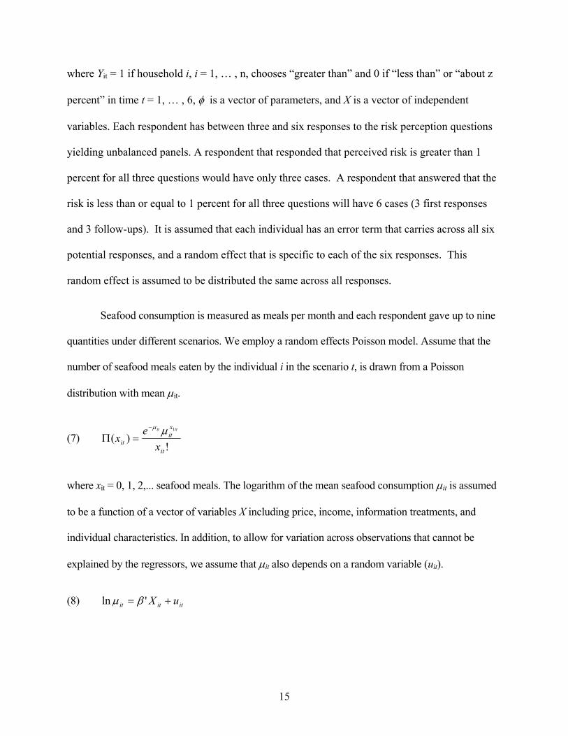
where Yit = 1 if household i, i = 1, … , n, chooses “greater than” and 0 if “less than” or “about z

percent” in time t = 1, … , 6, φ is a vector of parameters, and X is a vector of independent

variables. Each respondent has between three and six responses to the risk perception questions

yielding unbalanced panels. A respondent that responded that perceived risk is greater than 1

percent for all three questions would have only three cases. A respondent that answered that the

risk is less than or equal to 1 percent for all three questions will have 6 cases (3 first responses

and 3 follow-ups). It is assumed that each individual has an error term that carries across all six

potential responses, and a random effect that is specific to each of the six responses. This

random effect is assumed to be distributed the same across all responses.

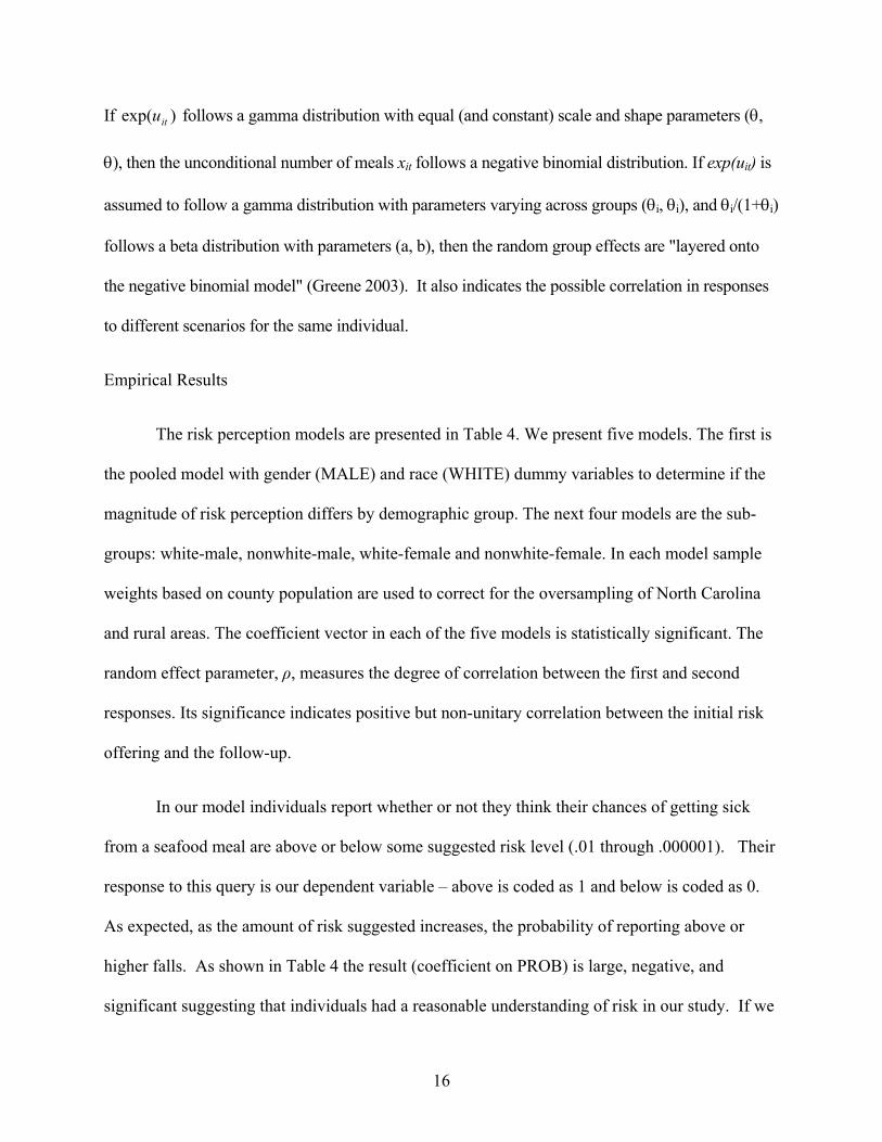
Seafood consumption is measured as meals per month and each respondent gave up to nine

quantities under different scenarios. We employ a random effects Poisson model. Assume that the

number of seafood meals eaten by the individual i in the scenario t, is drawn from a Poisson

distribution with mean μit.

(7) !

)(1

it

xit

it xe

xitit μμ−

=Π

where xit = 0, 1, 2,... seafood meals. The logarithm of the mean seafood consumption μit is assumed

to be a function of a vector of variables X including price, income, information treatments, and

individual characteristics. In addition, to allow for variation across observations that cannot be

explained by the regressors, we assume that μit also depends on a random variable (uit).

(8) ititit uX += 'ln βμ

15

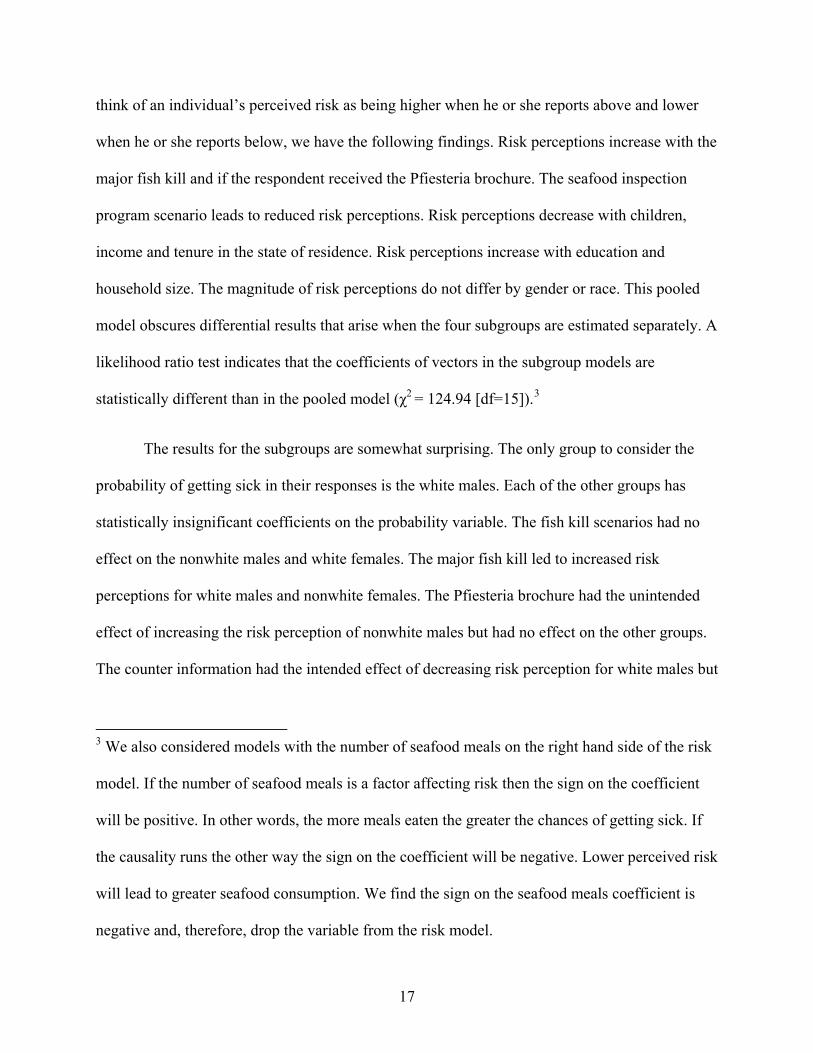
If follows a gamma distribution with equal (and constant) scale and shape parameters (θ,

θ), then the unconditional number of meals xit follows a negative binomial distribution. If exp(uit) is

assumed to follow a gamma distribution with parameters varying across groups (θi, θi), and θi/(1+θi)

follows a beta distribution with parameters (a, b), then the random group effects are "layered onto

the negative binomial model" (Greene 2003). It also indicates the possible correlation in responses

to different scenarios for the same individual.

)exp( itu

Empirical Results

The risk perception models are presented in Table 4. We present five models. The first is

the pooled model with gender (MALE) and race (WHITE) dummy variables to determine if the

magnitude of risk perception differs by demographic group. The next four models are the sub-

groups: white-male, nonwhite-male, white-female and nonwhite-female. In each model sample

weights based on county population are used to correct for the oversampling of North Carolina

and rural areas. The coefficient vector in each of the five models is statistically significant. The

random effect parameter, ρ, measures the degree of correlation between the first and second

responses. Its significance indicates positive but non-unitary correlation between the initial risk

offering and the follow-up.

In our model individuals report whether or not they think their chances of getting sick

from a seafood meal are above or below some suggested risk level (.01 through .000001). Their

response to this query is our dependent variable – above is coded as 1 and below is coded as 0.

As expected, as the amount of risk suggested increases, the probability of reporting above or

higher falls. As shown in Table 4 the result (coefficient on PROB) is large, negative, and

significant suggesting that individuals had a reasonable understanding of risk in our study. If we

16

think of an individual’s perceived risk as being higher when he or she reports above and lower

when he or she reports below, we have the following findings. Risk perceptions increase with the

major fish kill and if the respondent received the Pfiesteria brochure. The seafood inspection

program scenario leads to reduced risk perceptions. Risk perceptions decrease with children,

income and tenure in the state of residence. Risk perceptions increase with education and

household size. The magnitude of risk perceptions do not differ by gender or race. This pooled

model obscures differential results that arise when the four subgroups are estimated separately. A

likelihood ratio test indicates that the coefficients of vectors in the subgroup models are

statistically different than in the pooled model (χ2 = 124.94 [df=15]).3

The results for the subgroups are somewhat surprising. The only group to consider the

probability of getting sick in their responses is the white males. Each of the other groups has

statistically insignificant coefficients on the probability variable. The fish kill scenarios had no

effect on the nonwhite males and white females. The major fish kill led to increased risk

perceptions for white males and nonwhite females. The Pfiesteria brochure had the unintended

effect of increasing the risk perception of nonwhite males but had no effect on the other groups.

The counter information had the intended effect of decreasing risk perception for white males but

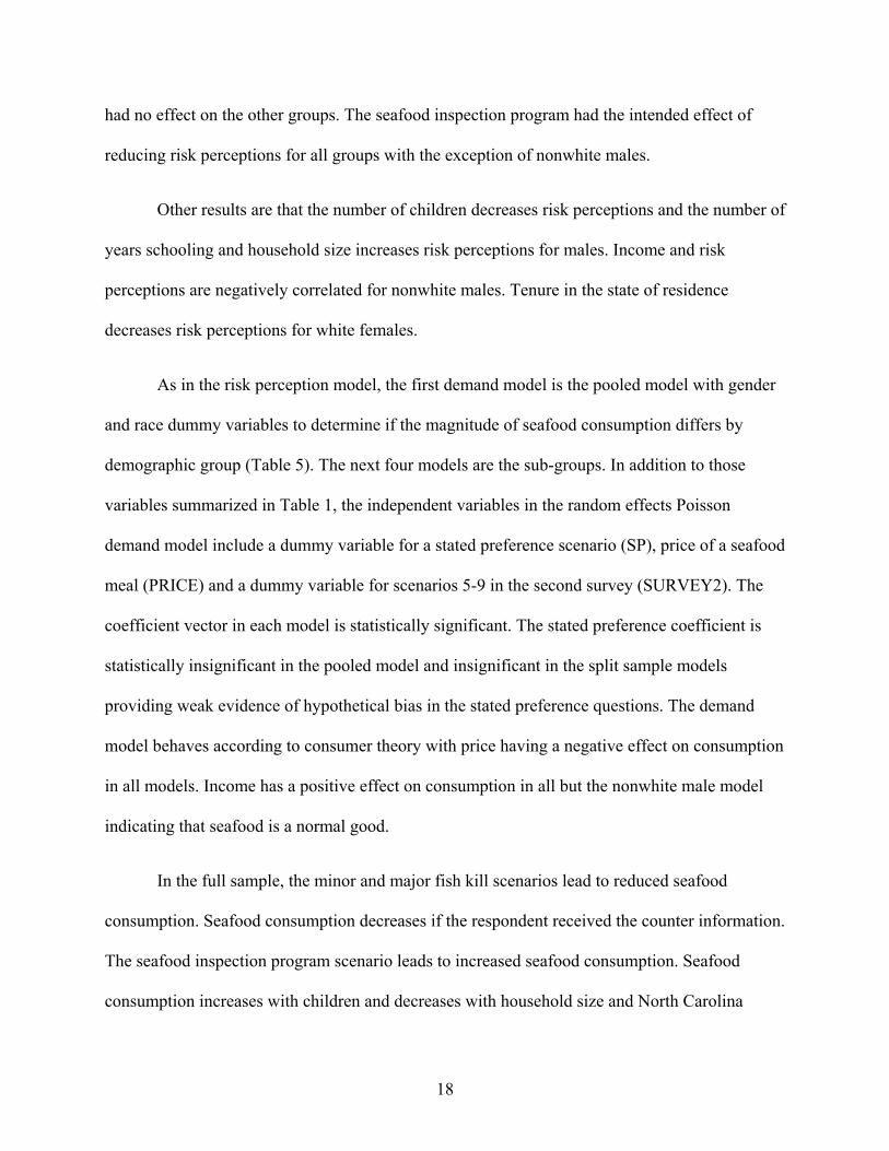
3 We also considered models with the number of seafood meals on the right hand side of the risk

model. If the number of seafood meals is a factor affecting risk then the sign on the coefficient

will be positive. In other words, the more meals eaten the greater the chances of getting sick. If

the causality runs the other way the sign on the coefficient will be negative. Lower perceived risk

will lead to greater seafood consumption. We find the sign on the seafood meals coefficient is

negative and, therefore, drop the variable from the risk model.

17

had no effect on the other groups. The seafood inspection program had the intended effect of

reducing risk perceptions for all groups with the exception of nonwhite males.

Other results are that the number of children decreases risk perceptions and the number of

years schooling and household size increases risk perceptions for males. Income and risk

perceptions are negatively correlated for nonwhite males. Tenure in the state of residence

decreases risk perceptions for white females.

As in the risk perception model, the first demand model is the pooled model with gender

and race dummy variables to determine if the magnitude of seafood consumption differs by

demographic group (Table 5). The next four models are the sub-groups. In addition to those

variables summarized in Table 1, the independent variables in the random effects Poisson

demand model include a dummy variable for a stated preference scenario (SP), price of a seafood

meal (PRICE) and a dummy variable for scenarios 5-9 in the second survey (SURVEY2). The

coefficient vector in each model is statistically significant. The stated preference coefficient is

statistically insignificant in the pooled model and insignificant in the split sample models

providing weak evidence of hypothetical bias in the stated preference questions. The demand

model behaves according to consumer theory with price having a negative effect on consumption

in all models. Income has a positive effect on consumption in all but the nonwhite male model

indicating that seafood is a normal good.

In the full sample, the minor and major fish kill scenarios lead to reduced seafood

consumption. Seafood consumption decreases if the respondent received the counter information.

The seafood inspection program scenario leads to increased seafood consumption. Seafood

consumption increases with children and decreases with household size and North Carolina

18

residence. White respondents consume less seafood while male respondents consumer more.

This pooled model obscures differential results that arise when the four subgroups are estimated

separately. A likelihood ratio test indicates that the coefficients of vectors in the subgroup

models are statistically different than in the pooled model (χ2 = 107.73 [df=17]).

The minor and major fish kill scenarios have negative effects on seafood consumption in

all sub-sample models (the minor coefficient in the nonwhite male model is statistically

insignificant). But, the magnitude of each statistically significant coefficient is similar. The

Pfiesteria brochure has the intended positive effect on consumption for males and a negative

effect for nonwhite females. The counter information had the intended positive effect on the

female groups. The seafood inspection program had the intended positive effect on consumption

for each group. Other results are sparse. North Carolina residents eat less seafood except for

nonwhite males. White females who have more children, education and smaller households eat

more seafood.

Conclusions

In this paper we consider the effects of negative and positive risk information on

perceived seafood risks and seafood consumption by gender and race. The data is from a Mid-

Atlantic survey of coastal seafood consumers. We elicit risk perceptions in three risk scenarios

with a dichotomous choice with a follow-up question format. We elicit revealed and stated

preference seafood consumption in nine risk and price scenarios. We find that risk information

(fish kills) and countervailing information have differential effects on different demographic

groups. Analysis in four gender and race categories indicates that demographic groups respond to

the positive and negative risk information in different ways.

19

Based on the information provided in our surveys, after controlling for other factors, only

white males consistently accurately perceive, accept, and manage seafood risk. For example,

only white males perceived a substantial probability of becoming ill from eating a month of

seafood meals. Fish kill scenarios had no effect on the risk perceived by nonwhite males and

white females. Initial information intended to ease Pfiesteria concerns actually increased

perceived risk of nonwhite males, though it increased their estimates for likely seafood

consumption. Oddly, the same initial Pfiesteria information decreased estimates of seafood

consumption among nonwhite females. After hearing additional information intended to further

ease Pfiesteria concerns, white males were the only group with decreased perceived risk, though

this additional information did increase estimates of seafood consumption among white and

nonwhite women. The proposed seafood inspection programs had no impact on perceived risk

among nonwhite males, though it did, as with all other groups, increase their estimates of

seafood consumption.

Apparently, only white males trust the information provided on seafood risk. White men

may perceive less risk because they have more power and control over their lives, communities,

and institutions. Subsequently, they have more trust in institutions associated with food safety,

fisheries, and public health. As Slovic (1999) points out, “danger is real, but risk is socially

constructed” (p.689). To truly inform people of seafood safety and risk, we need to build trust in

less advantaged groups (Slovic 1999). Public health leaders should consider using different

media and voices to convey information about seafood risk across diverse groups of people

(Burger et al. 1999).

We need improved educational campaigns, with more use of newspapers and television

advisories (Burger, Sanchez and Gochfeld, 1998) and face-to-face communications among

20

community members (Burger et al. 2003; Bettman et al., 1987). These campaigns should be

repeated frequently (McIntosh and Acuff, 1994) and target younger people (Burger, 2005).

Health advisories should include the benefits and the risks associated with eating seafood and

should include specific information pertaining to children, child-bearing age women, and

pregnant women (Knuth et al., 2003).

Our results suggest that risk communication continues to be a challenge. Our primary risk

communication device did not change risk perceptions and it changed behavior in the intended

direction for males only. Worse, it changed behavior in the unintended direction for nonwhite

females. Our secondary risk communication device changed risk perceptions for only one of four

demographic groups, white males, and changed behavior for females only. Future research into

risk communication and mitigation policy should consider the differential impact of risk

information on demographic groups. This research should consider the joint role of gender, race

and class on the effectiveness of risk communication instruments.

21

References

Bettman, J.R., Payne, J.W., and Staelin, R. 1987. Cognitive considerations in designing effective

labels for presenting risk information, in: K. Viscusi and W. Magat (Eds) Learning about

Risk: Evidence on the Economic Responses to Risk Information, pp.1-28. Cambridge:

Harvard University Press.

Brown, Deborah J. and Lee F. Schrader. 1990. Cholesterol information and shell egg

consumption, American Journal of Agricultural Economics 72(August):548-555.

Burger, J. 2000. Gender differences in meal patterns: Role of self-caught fish and wild game in

meat and fish diets. Environmental Research Section A 83:140-149.

Burger, J. 2005. Fishing, fish consumption, and knowledge about advisories in college students

and others in central New Jersey. Environmental Research 98:268-275.

Burger, J., McDermott, M.H., Chess, C., Bochenek, E., Perez-Logo, M. and Pflugh,K. K. 2003.

Evaluating risk communication about fish consumption advisories: Efficacy of a brochure

versus a classroom lesson in Spanish and English. Risk Analysis 23(4):791-803.

Burger, J., Pflugh, K. K., Lurig, L., Von Hagen, L. A., and Von Hagen, S. 1999. Fishing in

urban New Jersey: Ethnicity affects information sources, perception, and compliance.

Risk Analysis 19(2):217-229.

Burger, J., Sanchez, S. and Gochfeld, M. 1998. Fishing, consumption, and risk perception in

fisherfolk along an east coast estuary. Environmental Research 77:25-35.

Burkholder, J., E. Noga, and C. Hobbs. 1992. New “phantom” dinoflagellate is the causative

agent of major estuarine fish kills. Nature, July 30. v350.

Davidson, D. J. and Freudenburg, W. R. 1996. Gender and environmental risk concerns.

Environment & Behavior 28(3):302-340.

22

Fincucane, M. L., Slovic, P., Mertz, C. K., Flynn, J. and Satterfield, T. A. 2000. Gender, race,

and perceived risk: The “white male” effect. Healthy Risk and Society 2(2):159-172.

Flynn, J., Slovic, P., and Mertz, C. K. 1994. Gender, race and perception of environmental

health risks. Risk Analysis 14:1101-1108.

Greene, William H. 2003.Econometric Analysis, Fifth Edition, Upper Saddle River, NJ: Prentice

Hall.

Hersh, Joni. 1996. Smoking, seat belts, and other risky consumer decisions: Differences by

gender and race. Managerial and Decision Economics 17:471-481.

Jakus, Paul M., and W. Douglass Shaw. 2003. Perceived hazard and product choice: An

application to recreational site choice. Journal of Risk and Uncertainty 26(1):77-92.

Joffe, H. 1999. Risk and the “Other.” Cambridge: University Press.

Johnson, J. C. and Griffith, D. C. 1996. Pollution, food safety, and the distribution of knowledge.

Human Ecology 24(1):87-108.

Knuth, B. A., Connelly, N. A., Sheeshka, J., and Patterson, J. 2003. Weighing health benefit and

health risk information when consuming sport-caught fish. Risk Analysis 23(6):1185-

1197.

Lin, C.-T. Jordon, and J. Walter Milon. 1993. Attribute and safety perceptions in a double-hurdle

model of shellfish consumption, American Journal of Agricultural Economics,

75(August):724-729.

Lipton, D. W. 1998. Pfiesteria’s economic impact on seafood industry sales and recreational

fishing. Proceedings of the University of Maryland Center for Agricultural and Natural

Resource Policy Conference, Economics of Policy Options for Nutrient Management and

Dinoflagellates, Laurel, MD.

23

24

Luhmann, N. 1993. Risk: A Sociological Theory. New York: Aldine De Gruyter.

Lupton, D. 1999. Risk. London: Routledge.

McIntosh, W. A. and Acuff, G. R. 1994. Public perceptions of food safety. Social Science

Journal 31(3):285-289.

Parsons, George, R., Ash O. Morgan, John C. Whitehead and Timothy C. Haab. 2006. The

welfare effects of Pfiesteria-related fish kills: A contingent behavior analysis of seafood

consumers, Agricultural and Resource Economic Review.

Slovic, Paul. 1999. Trust, emotion, sex, politics, and science: Surveying the risk-assessment

battlefield. Risk Analysis 19(4):689-701.

Smith, Mark E., Eileen van Ravenswaay, and Stanley R. Thompson. 1988. Sales loss

determination in food contamination incidents: An application to milk bans in Hawaii,

American Journal of Agricultural Economics 70(August):513-520.

Velicer, C. M., and Knuth, B. A. 1994. Communicating contaminant risks from sport-caught

fish: The importance of target audience assessment. Risk Analysis 14:833-841.

Wessells, Cathy Roheim, Jeffrey Kline, and Joan Gray Anderson, 1996. Seafood safety

perceptions on anticipated consumption under varying information treatments,

Agricultural and Resource Economics Review 25(1):12-21.

Whitehead, John C., Timothy C. Haab, George R. Parsons. 2003. Economic effects of Pfiesteria,

Ocean and Coastal Management 46:845-858.

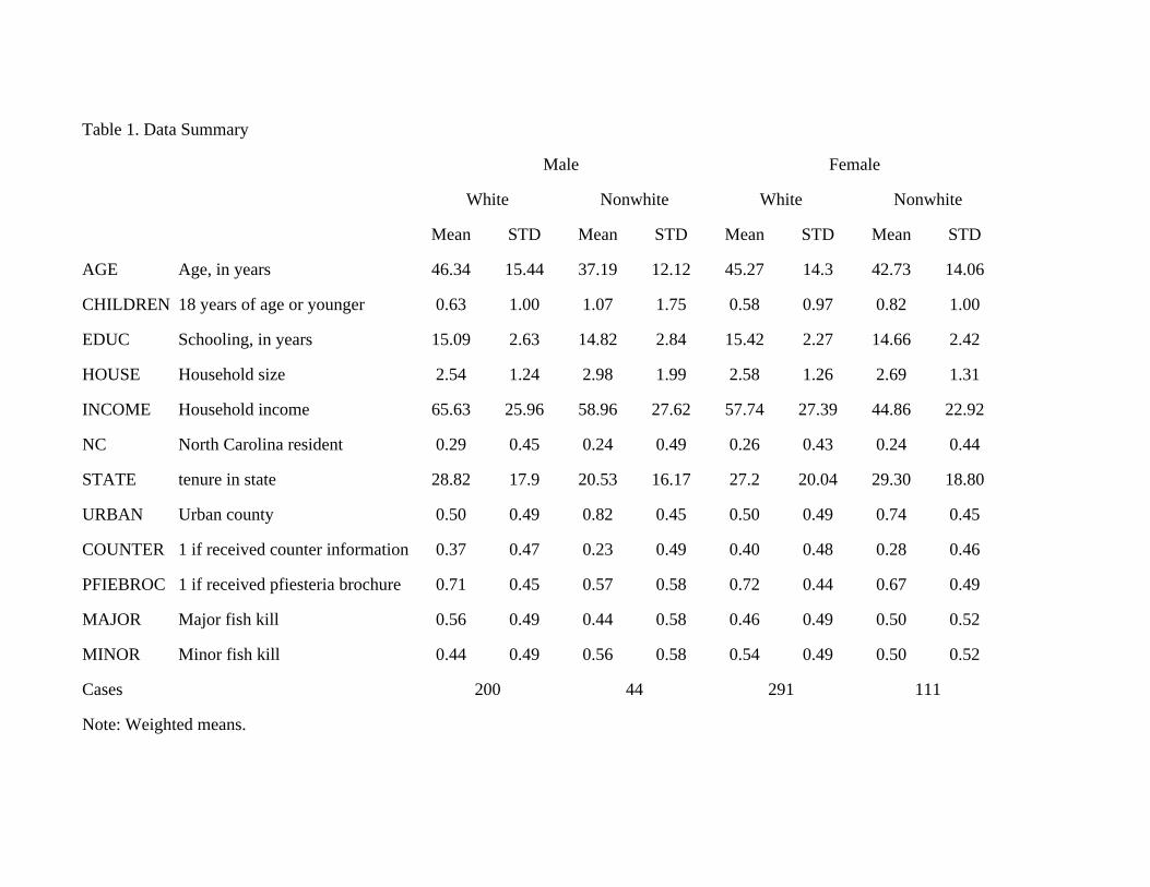
Table 1. Data Summary

Male Female

White Nonwhite White Nonwhite

Mean STD Mean STD Mean STD Mean STD

AGE Age, in years 46.34 15.44 37.19 12.12 45.27 14.3 42.73 14.06

CHILDREN 18 years of age or younger 0.63 1.00 1.07 1.75 0.58 0.97 0.82 1.00

EDUC Schooling, in years 15.09 2.63 14.82 2.84 15.42 2.27 14.66 2.42

HOUSE Household size 2.54 1.24 2.98 1.99 2.58 1.26 2.69 1.31

INCOME Household income 65.63 25.96 58.96 27.62 57.74 27.39 44.86 22.92

NC North Carolina resident 0.29 0.45 0.24 0.49 0.26 0.43 0.24 0.44

STATE tenure in state 28.82 17.9 20.53 16.17 27.2 20.04 29.30 18.80

URBAN Urban county 0.50 0.49 0.82 0.45 0.50 0.49 0.74 0.45

COUNTER 1 if received counter information 0.37 0.47 0.23 0.49 0.40 0.48 0.28 0.46

PFIEBROC 1 if received pfiesteria brochure 0.71 0.45 0.57 0.58 0.72 0.44 0.67 0.49

MAJOR Major fish kill 0.56 0.49 0.44 0.58 0.46 0.49 0.50 0.52

MINOR Minor fish kill 0.44 0.49 0.56 0.58 0.54 0.49 0.50 0.52

Cases 200 44 291 111

Note: Weighted means.

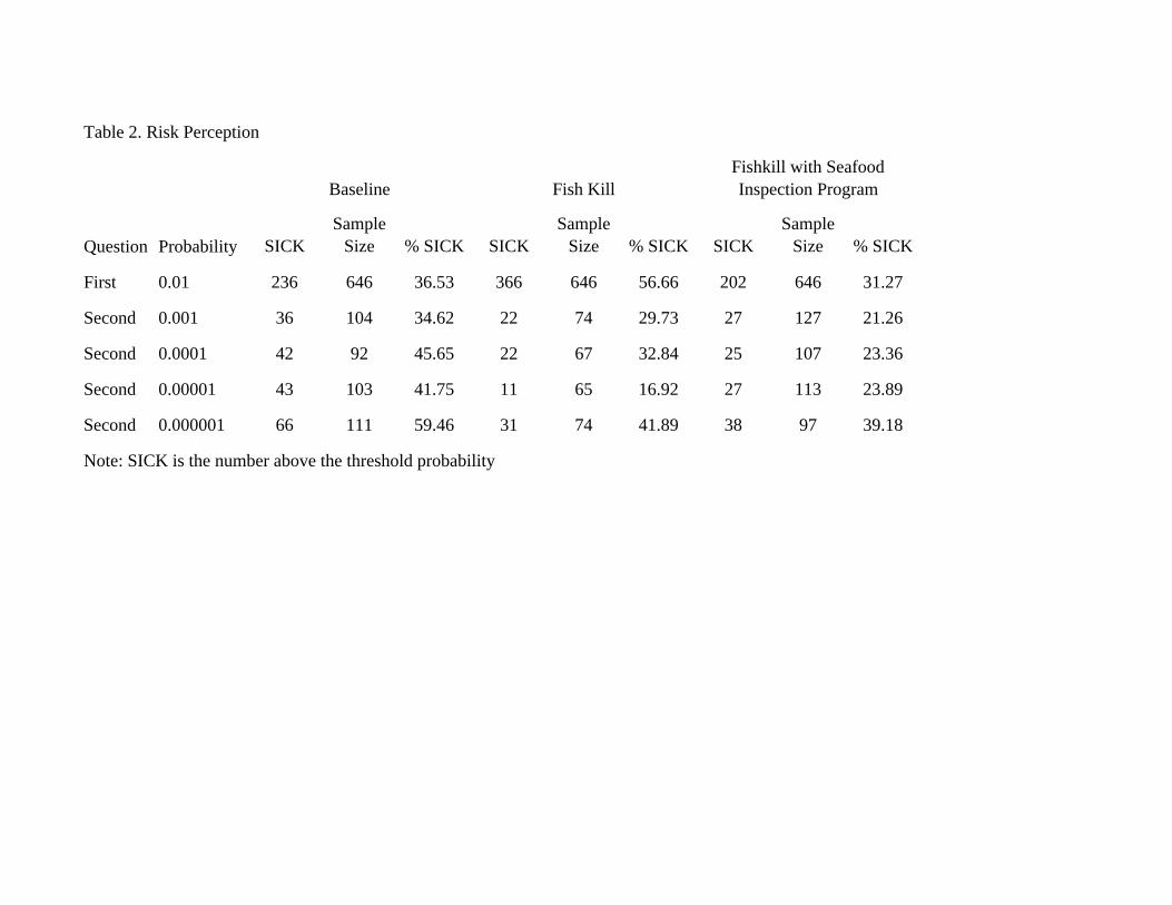
Table 2. Risk Perception

Baseline Fish KillFishkill with Seafood Inspection Program

Question Probability SICKSample

Size % SICK SICKSample

Size % SICK SICKSample

Size % SICK

First 0.01 236 646 36.53 366 646 56.66 202 646 31.27

Second 0.001 36 104 34.62 22 74 29.73 27 127 21.26

Second 0.0001 42 92 45.65 22 67 32.84 25 107 23.36

Second 0.00001 43 103 41.75 11 65 16.92 27 113 23.89

Second 0.000001 66 111 59.46 31 74 41.89 38 97 39.18

Note: SICK is the number above the threshold probability

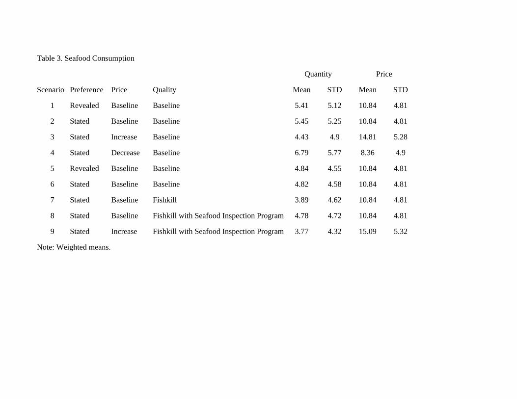
Table 3. Seafood Consumption

Quantity Price

Scenario Preference Price Quality Mean STD Mean STD

1 Revealed Baseline Baseline 5.41 5.12 10.84 4.81

2 Stated Baseline Baseline 5.45 5.25 10.84 4.81

3 Stated Increase Baseline 4.43 4.9 14.81 5.28

4 Stated Decrease Baseline 6.79 5.77 8.36 4.9

5 Revealed Baseline Baseline 4.84 4.55 10.84 4.81

6 Stated Baseline Baseline 4.82 4.58 10.84 4.81

7 Stated Baseline Fishkill 3.89 4.62 10.84 4.81

8 Stated Baseline Fishkill with Seafood Inspection Program 4.78 4.72 10.84 4.81

9 Stated Increase Fishkill with Seafood Inspection Program 3.77 4.32 15.09 5.32

Note: Weighted means.

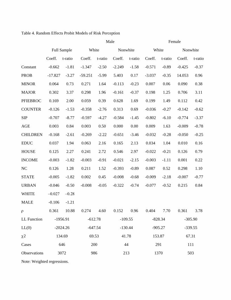
Table 4. Random Effects Probit Models of Risk Perception

Male Female

Full Sample White Nonwhite White Nonwhite

Coeff. t-ratio Coeff. t-ratio Coeff. t-ratio Coeff. t-ratio Coeff. t-ratio

Constant -0.662 -1.81 -1.347 -2.50 -2.249 -1.58 -0.571 -0.89 -0.425 -0.37

PROB -17.827 -3.27 -59.251 -5.99 5.403 0.17 -3.037 -0.35 14.053 0.96

MINOR 0.064 0.73 0.271 1.64 -0.113 -0.23 0.007 0.06 0.090 0.38

MAJOR 0.302 3.37 0.298 1.96 -0.161 -0.37 0.198 1.25 0.706 3.11

PFIEBROC 0.169 2.00 0.059 0.39 0.628 1.69 0.199 1.49 0.112 0.42

COUNTER -0.126 -1.53 -0.358 -2.76 0.313 0.69 -0.036 -0.27 -0.142 -0.62

SIP -0.707 -8.77 -0.597 -4.27 -0.584 -1.45 -0.802 -6.10 -0.774 -3.37

AGE 0.003 0.84 0.003 0.50 0.000 0.00 0.009 1.63 -0.009 -0.78

CHILDREN -0.168 -2.61 -0.269 -2.22 -0.651 -3.46 -0.032 -0.28 -0.050 -0.25

EDUC 0.037 1.94 0.063 2.16 0.165 2.13 0.034 1.04 0.010 0.16

HOUSE 0.125 2.27 0.241 2.72 0.546 2.97 -0.022 -0.21 0.126 0.79

INCOME -0.003 -1.82 -0.003 -0.91 -0.021 -2.15 -0.003 -1.11 0.001 0.22

NC 0.126 1.28 0.211 1.52 -0.393 -0.89 0.087 0.52 0.298 1.10

STATE -0.005 -1.82 0.002 0.45 -0.008 -0.68 -0.009 -2.18 -0.007 -0.77

URBAN -0.046 -0.50 -0.008 -0.05 -0.322 -0.74 -0.077 -0.52 0.215 0.84

WHITE −0.027 −0.28

MALE -0.106 -1.21

ρ 0.361 10.88 0.274 4.60 0.152 0.96 0.404 7.70 0.361 3.78

LL Function -1956.91 -612.78 -109.55 -828.34 -305.90

LL(0) -2024.26 -647.54 -130.44 -905.27 -339.55

χ2 134.69 69.53 41.78 153.87 67.31

Cases 646 200 44 291 111

Observations 3072 986 213 1370 503

Note: Weighted regressions.

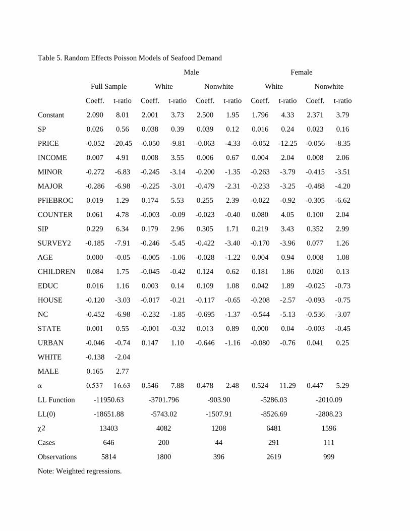
Table 5. Random Effects Poisson Models of Seafood Demand

Male Female

Full Sample White Nonwhite White Nonwhite

Coeff. t-ratio Coeff. t-ratio Coeff. t-ratio Coeff. t-ratio Coeff. t-ratio

Constant 2.090 8.01 2.001 3.73 2.500 1.95 1.796 4.33 2.371 3.79

SP 0.026 0.56 0.038 0.39 0.039 0.12 0.016 0.24 0.023 0.16

PRICE -0.052 -20.45 -0.050 -9.81 -0.063 -4.33 -0.052 -12.25 -0.056 -8.35

INCOME 0.007 4.91 0.008 3.55 0.006 0.67 0.004 2.04 0.008 2.06

MINOR -0.272 -6.83 -0.245 -3.14 -0.200 -1.35 -0.263 -3.79 -0.415 -3.51

MAJOR -0.286 -6.98 -0.225 -3.01 -0.479 -2.31 -0.233 -3.25 -0.488 -4.20

PFIEBROC 0.019 1.29 0.174 5.53 0.255 2.39 -0.022 -0.92 -0.305 -6.62

COUNTER 0.061 4.78 -0.003 -0.09 -0.023 -0.40 0.080 4.05 0.100 2.04

SIP 0.229 6.34 0.179 2.96 0.305 1.71 0.219 3.43 0.352 2.99

SURVEY2 -0.185 -7.91 -0.246 -5.45 -0.422 -3.40 -0.170 -3.96 0.077 1.26

AGE 0.000 -0.05 -0.005 -1.06 -0.028 -1.22 0.004 0.94 0.008 1.08

CHILDREN 0.084 1.75 -0.045 -0.42 0.124 0.62 0.181 1.86 0.020 0.13

EDUC 0.016 1.16 0.003 0.14 0.109 1.08 0.042 1.89 -0.025 -0.73

HOUSE -0.120 -3.03 -0.017 -0.21 -0.117 -0.65 -0.208 -2.57 -0.093 -0.75

NC -0.452 -6.98 -0.232 -1.85 -0.695 -1.37 -0.544 -5.13 -0.536 -3.07

STATE 0.001 0.55 -0.001 -0.32 0.013 0.89 0.000 0.04 -0.003 -0.45

URBAN -0.046 -0.74 0.147 1.10 -0.646 -1.16 -0.080 -0.76 0.041 0.25

WHITE -0.138 -2.04

MALE 0.165 2.77

α 0.537 16.63 0.546 7.88 0.478 2.48 0.524 11.29 0.447 5.29

LL Function -11950.63 -3701.796 -903.90 -5286.03 -2010.09

LL(0) -18651.88 -5743.02 -1507.91 -8526.69 -2808.23

χ2 13403 4082 1208 6481 1596

Cases 646 200 44 291 111

Observations 5814 1800 396 2619 999

Note: Weighted regressions.