Dynamic Optimization and Conformity in Health Behavior and Life Enjoyment over the Life Cycle

Hernán Bejarano Hillard Kaplanᶲ Stephen Rassenti

Abstract

This article examines individual and social influences on investments in health and enjoyment from immediate consumption. We report the results of a lab experiment that mimics the problem of health investment over a lifetime, building on Grossman’s (1972a, 1972b) theoretical framework. Subjects earn money through the experiment in proportion to the sum of the life enjoyment they have consumed. However, income in each period is a function of previous health investments, so there is a dynamic optimum for maximizing earnings through the appropriate expenditures on life enjoyment and health in each period. In order to model social effects in the experiment, we randomly assigned individuals to chat/observation groups, composed of four subjects each. Two treatments were employed: In the Independent treatment, an individual’s rewards from investments in life enjoyment depend only on his choice and in the Interdependent treatment, rewards not only depend on an individual’s choices but also on their similarity to the choices of the others in their group. Seven predictions were tested and each was supported by the data. We found: 1) Subjects engaged in helpful chat in both treatments; 2) there was significant heterogeneity among both subjects and groups in chat frequencies; and 3) chat was most common early in the experiment. The interdependent treatment 4) increased strategic chat frequency, 5) decreased within-group variance, 6) increased between-group variance, and 7) increased the likelihood of behavior far from the optimum with respect to the dynamic problem. Individual incentives explain a large part, but not all, of the variance in prosocial behavior in the form of strategic advice. Incentives for conformity appear to promote prosocial behavior, but also increase variance among groups in equilibrium outcomes, leading to convergence on suboptimal strategies for some groups.

Economic Science Institute, Chapman University, Orange, CA ᶲUniversity of New Mexico, Albuquerque, NM

1. Introduction

Inequalities in health, across and within populations, are a major public concern

that demand attention (Murray et al. 1999). For example, the life expectancy of Native

American males is 56 years in some counties, while that of Asian American women is 95

years in other counties (Murray et al. 1998). While several critical variables such as income

and education help explain these differences, significant variance remains unexplained

(Cutler and Lleras-Muney 2010). Other explanatory variables are related to health

behavior, exercise, and dietary habits. In fact, health behavior explains about 40 percent of

premature mortality, as well as substantial morbidity and disability, in the United States

(McGinnis et al. 2002).

Empirical evidence shows that social groups influence health behavior in complex

ways. Peer pressure can help individuals control health habits (Umberson et al. 2010). For

example, spouses or religious communities may monitor, inhibit, regulate, or facilitate the

health behavior of their partners or members of their community (Waite 1995, Ellison and

Levin 1998). Group effects alternatively might lead individuals to engage in risk-taking and

increased alcohol consumption. In addition, there seem to be matching effects; for example,

having an obese spouse or friend can increase an individual’s likelihood of being obese

(Christakis and Fowler 2007; Crosnoe et al. 2004). Despite the extensive evidence of group

influence in health behavior, little is known of the precise mechanisms by which groups

influence individual choices. Identifying the social causes of behavioral change from

naturally occurring data is difficult due to selection biases and unobserved heterogeneity

associated with group formation (Fowler et al. 2011). In addition, interactions between

individuals and groups that affect health behavior are usually unobserved.

This article examines individual and social influences on investments in health and

enjoyment from immediate consumption. We do this in a specially framed lab experiment

that mimics the problem of health investment over a lifetime, building on Grossman’s

(1972a, 1972b) theoretical framework to study health investment choices. Choosing

optimal health investments over the life course is a complex task. Individuals might

estimate well the current costs and benefits of their actions but be less certain of their long-

run effects. In essence, to determine how much time, income and effort to invest in healthy

behavior, individuals have to solve a dynamic programing problem addressing uncertainty

concerning future income and progressive health degeneration.

In the lab, our subjects experienced an experimental environment that mimics the

previously described health-investment problem. Each subject lives a nine-period life,

during each period of which he earns income and then invests some proportion of that

income in health and some in life enjoyment. Subjects earn money through the experiment

in proportion to the sum of the life enjoyment they have consumed. However, income in

each period is a function of previous health investments, so there is a dynamic optimum for

maximizing earnings through the appropriate expenditures on life enjoyment and health in

each period. Subjects live eight lives during the experiment with identical parameter

values, so they can learn from experience.

In order to model social effects in the experiment, we randomly assigned individuals

to chat/observation groups, composed of four subjects each. Between lives, subjects were

allowed to chat with and observe the choices of others in their chat group. We employed

the chat room discussions during the experiments to study how advice and queries about

the appropriate investment strategies affected behavior. Our experimental approach in

which chat/observation groups are formed randomly and in which interactions between

the individuals of the groups are recorded, allow us to analyze whether a mechanism exists

that links health behavior and group communication.

Our experimental design presents two treatments to investigate social impacts on

health. In our baseline Independent treatment, an individual’s rewards from investments

in life enjoyment depend only on his choices. When rewards are independent of others’

choices, individuals do not have monetary incentives to provide any advice. However,

individuals still have an incentive to search for advice, and particularly, might be willing to

post queries about strategies, hoping that those who perform better will voluntarily

provide some guidance. Therefore, in the independent treatment, an individual’s

willingness to provide advice is mostly generated by their intrinsic motivation to help

others.

In the second Interdependent treatment, rewards not only depend on an

individual’s choices but also on their similarity to the choices of the others in their group.

Individuals have a payoff function that provides them incentive to make behavioral choices

similar to the other members of their group (a conformity coefficient). Therefore, in the

interdependent treatment, individuals have an extrinsic motivation to discuss, agree, and

coordinate on health behavior.

In keeping with the theme of this special issue, the goal of this article is to utilize this

experimental design to test a series of hypotheses about social influences on health

behavior. We propose that social effects derive from two principle routes. First, people

utilize observation of behavior and engage in direct communication about practices and

strategies in order to be better able to achieve their goals. Providing advice and educating

others is an intrinsically human and pro-social activity. Humans have been providing

advice regarding health behavior for millennia (Kleinman 1980), and now they can even

provide advice to strangers on the Internet (Constant et al. 1996, Swan 2012). A second

route for social effects derives from the increased utility people gain by the extent to which

their choices conform to those of others, with whom they interact and identify. This second

route may reinforce the optimizing effects of the first route, but may also lead to multiple

equilibria. In other words, communication, queries and advice regarding health behavior,

can improve health investment and life-enjoyment choices, but also can lead to suboptimal

habits. From this logic, we test the following predictions:

1) In both treatments, subjects will make queries and provide strategic advice during

chat.

2) Significant chat heterogeneity will exist between groups, above the individual

heterogeneity of its members, through processes of observation and information

exchange.

3) Advice and queries will be most common during the first few lives of the experiment

while individuals are most focused on learning.

4) Due to incentives, chat about investment behavior will be more frequent in the

interdependent treatment than in the independent treatment.

5) The conformity payoff in the interdependent treatment will decrease within-group

variance in behavior.

6) Due to the possibility of multiple equilibria, the interdependent treatment will

increase among-group variance in behavior.

7) As a result of 5, the worst performing groups, in terms of optimizing investments

per period over the life course, will be more common in the interdependent rewards

treatment.

2. The Health Investment Problem: Theory and Experimental Environment

In the experiments to be reported each individual participant worked in a real effort

harvesting task to earn income and made a sequence of investment decisions in a series of

unrelated lifetimes. Each lifetime was comprised of a sequence of 9 periods (t =1, 2,…9) of

real effort earnings activity followed by investment decision making. Every lifetime ended

after nine periods unless the participant’s ‘health’ had degenerated to the point of death

before then. After each lifetime ended, every participant was ‘reincarnated’ into his next

unrelated lifetime.

Once the participant finished the real effort harvesting task in period t, from which

effort she had secured harvest revenue1, Rt, proportional to current health, she was

required to make investment decisions: how much to invest, It, in preserving health for

future harvesting, how much to invest in life enjoyment, Lt, in order to be paid for her

efforts, and how much (if any) to leave uninvested in a bank account, Bt, that would become

available for future investments in life enjoyment or health. All participants were endowed

with a beginning bank balance, B0, of 0, and should end with a final bank balance, B9, of 0, if

1 For a complete description of the real effort harvesting task, the revenue possible, and the optimal harvesting

strategy see Appendix 1.

they maximize their total gains from life enjoyment. The budget constraints governing

investment in each period were given by:

It + Lt + Bt = Bt-1 + Rt t=1, 2, …9

The non-linear return functions for investments in health and life enjoyment are

given below. They were designed to have diminishing returns to scale, so that the optimal

investment pattern across time would display properties similar to a Grossman model. The

transition equation in our experimental system relating final health in period t (Ht) to final

health in the previous period (Ht-1), given an investment (It) in preserving health, and a

natural degeneration (dt) of health that occurred during period t, was given by:

𝐻𝑡 = 𝑀𝑖𝑛 [100, 𝐻𝑡−1 − d𝑡 + 301 − ⅇ−.025It

1 + ⅇ−.025It ]

A participant could theoretically regenerate health by up to 30 points in any given

period if she had accumulated an ‘infinite’ amount of harvest revenue to invest, but an

upper bound was imposed that prevented the next state of health from ever exceeding 100.

Furthermore, the parameters in the experimental environment were chosen such that the

boundary condition, Ht+1 = 100, was never approached under optimal or ‘reasonable’

decision making. Given the interior solution was always active, the marginal rate of return

on health investment each period was given by:

𝑑𝐻𝑡

𝑑𝐼𝑡=

1.5ⅇ−.025It

1 + 2ⅇ−.025It + ⅇ−.05It

Note that at It= 0, dHt/dIt = 3/8 and the rate of return on each subsequent revenue

unit invested in health is independent of initial state of health (Ht) until health reaches 100.

Over many periods and lifetimes, participants could become very familiar with the fixed

function governing diminishing returns on health investment.

The earnings equation relating investment in life enjoyment (Lt) to cash earned (Et)

in period t, by a socially independent participant was given by:

Socially Independent Earnings: 𝐸𝑡 = 250(1 + 𝐻𝑡/100)(1 − ⅇ−.028𝐿𝑡)

By convention, in any given period t, degradation of health occurred after

harvesting. Then health investment, Ht, selected was implemented prior to the life

enjoyment investment, Lt, so that the upgraded state of health would be incorporated into

the life enjoyment computation. The participants were given graphical representations of

the health and life enjoyment investments that made it very clear that both had diminishing

returns.2 The participant’s job was to correctly balance investment of harvesting revenue

between health and life enjoyment, each period of her lifetime. To maximize her earnings

across her entire life (periods 1-9) the participant had to solve the following nonlinear

program:

Maximize: ∑ 𝐸𝑡𝑡=1,9 = ∑ 𝑡=1,9 250(1 + 𝐻𝑡/100)(1 − ⅇ−.028𝐿𝑡)

Subject to: 𝐵𝑡−1 + 𝑅𝑡 = 𝐼𝑡 + 𝐿𝑡 ∀ 𝑡 = 1, … 9

𝐻𝑡 = 𝐻𝑡−1 − d𝑡 + 301−ⅇ−.025It

1+ⅇ−.025t ∀ 𝑡 = 1, … 93

𝑅𝑡 = 𝑟ⅇ𝑣(Ht/100) during any active harvest period4

2 The second derivatives are calculated in the Appendix 2. 3 Health degeneration dt= {-16, -17, … -23, -24} 4 Rev is a fixed parameter that indicates participant harvesting proficiency. See Appendix 2 for further discussion.

The main treatment variable in the experiments reported determined whether each

subject’s earnings from investing in life enjoyment were interdependent or independent of

the decisions made by other subjects in his social group. The earnings equation for socially

interdependent participants, relating investment in life enjoyment (Lt) to cash earned (Et)

in period t given the mean investment, Ot, made by all other subjects in the subject’s social

group, is given by:

Socially Interdependent Earnings: 𝐸𝑡 = 1.5 ∗𝑀𝑖𝑛(𝐿𝑡,𝑂𝑡)

𝑀𝑎𝑥(𝐿𝑡,𝑂𝑡)∗ 250(1 + 𝐻𝑡/100)(1 − ⅇ−.028𝐿𝑡)

Note, these earnings were simply computed as the Socially Independent Earnings

multiplied by a ‘conformity multiplier,’ 1.5 ∗𝑀𝑖𝑛(𝐿𝑡,𝑂𝑡)

𝑀𝑎𝑥(𝐿𝑡,𝑂𝑡) . The ratio

𝑀𝑖𝑛(𝐿𝑡,𝑂𝑡)

𝑀𝑎𝑥(𝐿𝑡,𝑂𝑡) measures the

proportion by which the subject’s life enjoyment investment, Lt, matches the mean life

enjoyment investment, Ot, of other members of her social group. Under interdependence, a

subject who conforms to the group mean in making her life investment choices could earn a

premium of up to 50%, while one that strayed from her group’s mean (more than 33%

below or above) would find herself earning less than she would if she were not socially

bound.

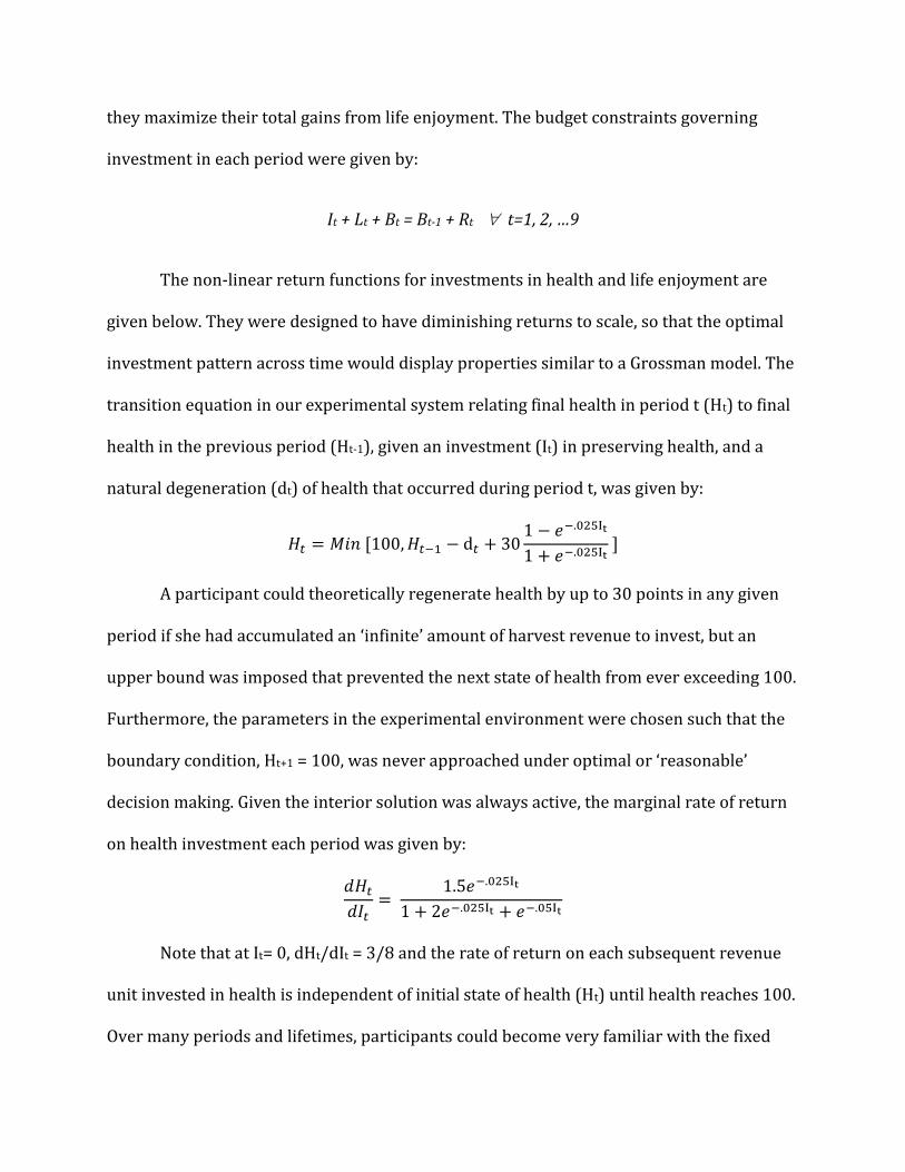
The Health graph below indicates that starting from her current health of 50, the

participant could possibly increase her next period’s health up to level 80 by making a large

health investment. Meanwhile, the Enjoyment graph below shows two lines: the dashed

line represents enjoyment earnings under social Independence, while the solid line

represents enjoyment earnings under social Interdependence when other members of the

subject’s group make a mean investment of 60. In experiments where subjects are

Independent they only see the dashed line. In experiments where subjects are

Interdependent they see both lines and can adjust the location of the apex of the solid line

according to their premonition concerning their group’s mean investment. The enjoyment

graph shows that under Independence a subject who invests 60 in life enjoyment would

receive a payoff of ~333, which would be translated to a cash reward at experiment’s end.

Under Interdependence if the group mean were 60 and the subject made the same

investment, she would earn 500 = 1.5 x 333, while if she chose to invest 40 or 130 she

would only earn ~3005.

In our environments, the shape of the Health investment graph would never alter:

only the starting point on the Y-axis, current health, would adjust from period to period.

However the shape of the Enjoyment Investment graph would get steeper if health

deteriorated or flatten if health improved.

Note that in the constrained dynamic maximization problem the subject must solve, Ht can

be rewritten as a function of her initial health, H0, and investments, It, in health.

5 In order to make investments, the participant used reciprocating scroll bars on the x-axis of each graph that would

not allow her to spend more than the revenue she had accumulated.

𝐻𝑡 = 𝐻0 + ∑ −𝑑𝑘 + 𝑘=1,𝑡

301 − ⅇ−.025Ik

1 + ⅇ−.025Ik

So solving the participant’s constrained life enjoyment optimization can be

rewritten as an unconstrained optimization that is a function of the sequence of health

investments Ii and bank deposits Bt6:

∑ 𝐸𝑡

𝑡=1,9

= ∑

𝑡=1,9

250(1 + [𝐻0 + ∑ −𝑑𝑘 + 𝑘=1,𝑡

301 − ⅇ−.025Ik

1 + ⅇ−.025Ik] /100)(1 − ⅇ−.028(𝐵𝑡−1+𝑅𝑡−𝐼𝑡))

This problem is easy to solve numerically for any given period t when Ht-1, Bt-1, Rt

and Bt are known.7 The initial conditions for health and bank balance were given by H0 = 85

and B0 = 0, the final bank balance B9 must be zero, and Rt is always a linear function, rev(Ht-

1/100), of previous period’s health. We can either apply non-linear optimization or

dynamic programming techniques to find the optimal sequence of health investments, It,

and the corresponding maximal aggregate life enjoyment ∑ 𝐸𝑡𝑖=1,9 .

It is important to note that under Interdependence, even with its premium for investment

conformity and penalty for non-conformity, the optimal investment pattern for like-skilled

harvesters is exactly the same as it is under Independence. The best that any group can do

6 The parameters in the environments we designed were such that the optimal Bt* was rarely anything other than 0. This considerably reduced the dimension of the decision making problem faced by participants. On rare occasions, during the move from harvesting to retirement (periods 6 to 7), there was a minor improvement in overall life enjoyment by banking some harvest income to smooth investment in life enjoyment. 7 Appendix 2 provides the example of period 9.

is for all individuals to conform to what would otherwise be the optimal investment pattern

for each under Independence: resulting earnings would simply be multiplied by 1.5.

Using Rt = 87(Ht-1/100) (we found that 87 was the low variance, mean skill parameter of all

participants), the period by period optimal Health (Ht) profile that participants should

maintain in order to make health investments (It) that maximize total life enjoyment (Et)

is given in the following table:

Optimal Health (Ht) by period: 1 2 3 4 5 6 7 8 9 89 91 92 90 86 78 65 42 18

The table below captures a quantitative representation of what is necessary to

maintain this optimal health vector, and hints at some behavioral difficulties participants

might encounter if their perception of optimal strategy requirements is less than perfect. It

shows the marginal rates of return for optimal investments in life enjoyment in each period

of life, and implicitly the rate of return on investment in health and banking for current and

future enjoyment maximization.8 It also shows the percentage of income earned (plus

banked9) that must be devoted to optimal health maintenance in each period of life.

Optimal Marginal Rate of Return, % of Income Invested in Health, by period: 1 2 3 4 5 6 7 8 9 10.0, 86 8.6, 80 7.4, 73 6.3, 67 5.3, 59 4.3, 50 3.3, 35 2.5, 0 2.5, 0

8 This is true for all periods except where a boundary condition is met (only in periods 8 and/or 9) and the marginal return on any investment in health is dominated by investment in life enjoyment (Lt) so the optimal investment in health is zero (It=0). 9 There are only 2 periods in the 36 displayed where it behooves subjects to bank some earned revenue for the purpose income smoothing: in period 8 of the Flat No Retirement regime where health will fall precipitously in period 9, and in period 6 of the Tiered Retirement regime where income falls precipitously in period 7, the first period of retirement.

Savvy participants must recognize that 86% of earned revenue from harvesting

must be spent on health in period 1, and 80% in period 2, while the marginal rates of

return on investments are 4 times larger than later in life: that skewed optimal investment

strategy is a requirement to be reckoned with in splitting earned harvest revenues between

health and life enjoyment. Late in life (periods 8 and 9), participants must let go of their

health and spend entirely on life enjoyment. The complete solution for all decision and

state variables are provided in Appendix I.

Multiple Lives and Chat Groups

This nine period dynamic optimization problem is difficult to solve, due to the

nonlinearities and interactions in the health and life enjoyment functions. In order to allow

subjects to learn about the environment and to adjust their strategies accordingly, subjects

lived eight nine-period lives under identical conditions. This ‘reincarnation’ can be thought

of as a way of modeling cultural traditions in which individuals learn from previous

generations how to best perform in the environment. In addition, we proposed that in

response to difficult dynamic problems, people would use observational learning and

information exchange to help solve those problems. To model that process, subjects were

divided in four-person chat-observation groups. Subjects could observe the behavior of

three other subjects (the same three people in each life) and could chat with them, using

text messages, between lives.

Under Social Independence the chat group provided nothing more than a venue to

exchange information concerning individual strategy, but under Social Interdependence,

the mean investment in Life Enjoyment by other members of a chat group became the

norm by which investment of each group member was evaluated and translated into

earnings. Interdependence allowed conformity in investment strategies to enhance

earnings and non-conformity to penalize them. Under Interdependence, chat provided a

venue for both optimizing and conforming strategies to evolve.

A total of 156 subjects, who were randomly allocated to 39 chat/observation

groups, 68 subjects (17 chat groups) in the Independent treatment, 88 subjects (22 chat

groups) in the Interdependent treatment. Members of each chat-group were free to

observe and discuss (or not) each other’s performances for 90 seconds at the end of each

lifetime.

Subjects’ conversations were captured by the messages written in chat window.

Chat lines were classified independently by two independent research assistants that acted

as coders10. Coders were trained to apply a classification criterion that captures the

presence of strategic advice and queries.

To achieve this goal, coders classified lines into one of four thematic categories and

into one of two linguistic categories. The thematic categories captured message’s meaning,

while the linguistic category captured the message’s direction and intention. The four

thematic categories were: Income Generation, Income Allocation, Other Experimental

Issues, Non-Experimental chat. In this article we focus on the second category: this

10 The chat lines of the Independent treatment were classified by four coders. To be consistent with the classification of chat lines in the Interdependent treatment, we used for this paper a classification based on hose codifiers with similar interelaiability rates to the codifiers of the Interdependent treatment.

category includes all those messages in which subjects expressed ideas or concerns

regarding the allocation of their income to health and life enjoyment. The two linguistic

categories were: Statements or Queries. Chat lines were assigned to particular class only if

both coders agreed on their classification.

3. Statistical Approach

In order to handle the repeated and clustered nature of the experimental design, we

employed a mixed fixed and random effects linear model to analyze the data. Each subject

lived eight lifetimes, having the opportunity to chat with others in her chat/observation

group seven times. During the experiment, each subject chose 72 times (8 lives x 9 periods)

how to allocate her income between health and life enjoyment investments. The empirical

model takes into account the lack of independence among observations within and among

individuals in groups. To do this, the model estimates the fixed effects of lifetime,

experimental treatment, and interaction terms, while assessing the random effects for chat

group and individual.

4. Results

Descriptive Statistics

Descriptive statistics for the main variables to be analyzed are presented in Table 1.

For each of the eight ‘lives’ in the experiment, the table shows the means for total

enjoyment purchased and the number of strategic queries and advice made per subject

during the rest phase following that life during which chat was allowed. Total enjoyment

purchased is the sum of the amount purchased in each of the nine periods and is

proportional to the actual amount the subject is paid. Those data are presented in three

columns. The first column shows the means for the treatment group in which each subject’s

rewards from investments in life enjoyment are independent (that is, the rewards are

unaffected by the behavior of other subjects in the chat group). There are two columns for

the other treatment group in which rewards are interdependent. The first of those columns

(column 2) presents the counterfactual independent rewards (for comparability purposes)

that the subjects in the interdependent chat groups would have received if their rewards

were independent. The second of those columns (column 3) presents the rewards they

actually received from their investments, after their interdependence is taken into account

through the conformity multiplier. It is evident from the table that for both treatment

groups, Total Enjoyment Purchased increases with each life, indicating that their

performance increasingly approached the optimal investment profile across lives. It is also

evident that subjects in the interdependent rewards treatment group achieved increasingly

high levels of conformity across lives to maximize the multiplier on their investments. The

regression models discussed below will examine these effects in detail.

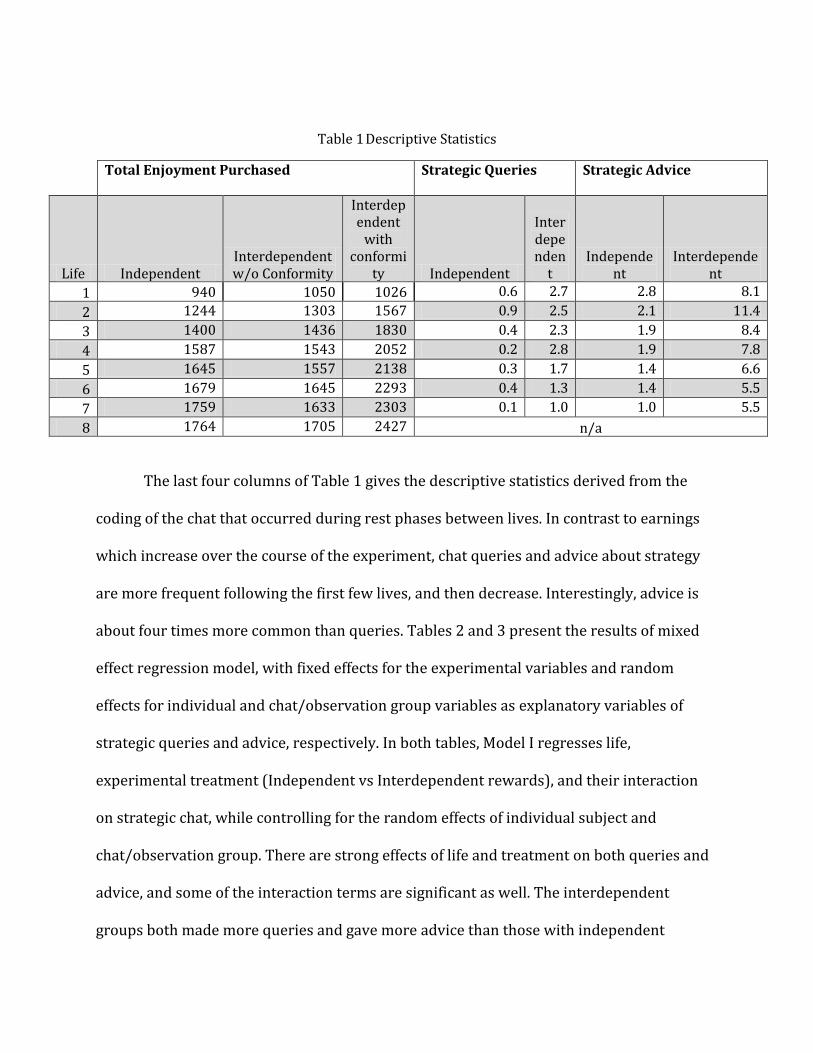
Table 1 Descriptive Statistics

Total Enjoyment Purchased Strategic Queries Strategic Advice

Life Independent Interdependent w/o Conformity

Interdependent

with conformi

ty Independent

Interdependen

t Independe

nt Interdepende

nt

1 940 1050 1026 0.6 2.7 2.8 8.1

2 1244 1303 1567 0.9 2.5 2.1 11.4

3 1400 1436 1830 0.4 2.3 1.9 8.4

4 1587 1543 2052 0.2 2.8 1.9 7.8

5 1645 1557 2138 0.3 1.7 1.4 6.6

6 1679 1645 2293 0.4 1.3 1.4 5.5

7 1759 1633 2303 0.1 1.0 1.0 5.5

8 1764 1705 2427 n/a

The last four columns of Table 1 gives the descriptive statistics derived from the

coding of the chat that occurred during rest phases between lives. In contrast to earnings

which increase over the course of the experiment, chat queries and advice about strategy

are more frequent following the first few lives, and then decrease. Interestingly, advice is

about four times more common than queries. Tables 2 and 3 present the results of mixed

effect regression model, with fixed effects for the experimental variables and random

effects for individual and chat/observation group variables as explanatory variables of

strategic queries and advice, respectively. In both tables, Model I regresses life,

experimental treatment (Independent vs Interdependent rewards), and their interaction

on strategic chat, while controlling for the random effects of individual subject and

chat/observation group. There are strong effects of life and treatment on both queries and

advice, and some of the interaction terms are significant as well. The interdependent

groups both made more queries and gave more advice than those with independent

rewards, as would be expected by the gains from coordination and conformity. Relative to

the last lives, strategic chat of both types was greatest early in the experiment when

learning and behavior change was greatest.

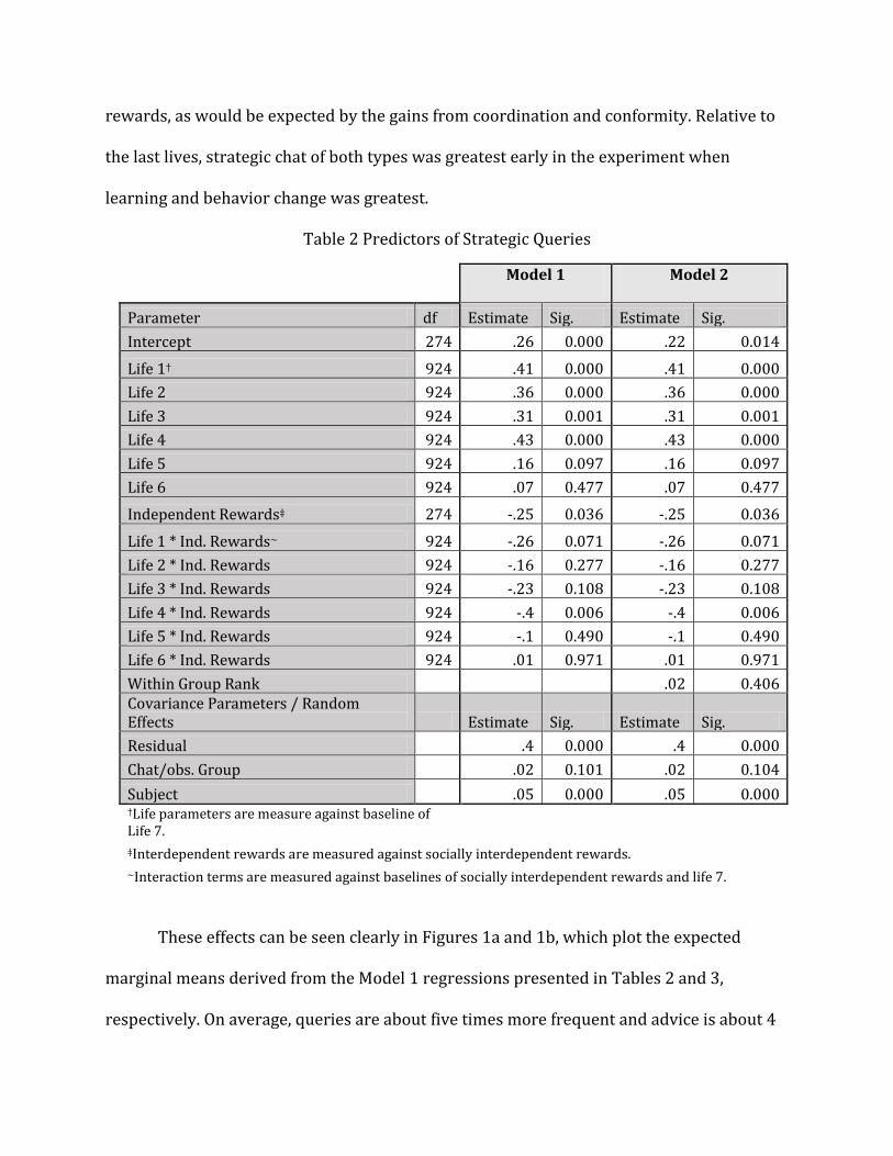
Table 2 Predictors of Strategic Queries

Model 1 Model 2

Parameter df Estimate Sig. Estimate Sig.

Intercept 274 .26 0.000 .22 0.014

Life 1† 924 .41 0.000 .41 0.000

Life 2 924 .36 0.000 .36 0.000

Life 3 924 .31 0.001 .31 0.001

Life 4 924 .43 0.000 .43 0.000

Life 5 924 .16 0.097 .16 0.097

Life 6 924 .07 0.477 .07 0.477

Independent Rewards‡ 274 -.25 0.036 -.25 0.036

Life 1 * Ind. Rewards~ 924 -.26 0.071 -.26 0.071

Life 2 * Ind. Rewards 924 -.16 0.277 -.16 0.277

Life 3 * Ind. Rewards 924 -.23 0.108 -.23 0.108

Life 4 * Ind. Rewards 924 -.4 0.006 -.4 0.006

Life 5 * Ind. Rewards 924 -.1 0.490 -.1 0.490

Life 6 * Ind. Rewards 924 .01 0.971 .01 0.971

Within Group Rank .02 0.406 Covariance Parameters / Random Effects Estimate Sig. Estimate Sig.

Residual .4 0.000 .4 0.000

Chat/obs. Group .02 0.101 .02 0.104

Subject .05 0.000 .05 0.000 †Life parameters are measure against baseline of Life 7.

‡Interdependent rewards are measured against socially interdependent rewards.

~Interaction terms are measured against baselines of socially interdependent rewards and life 7.

These effects can be seen clearly in Figures 1a and 1b, which plot the expected

marginal means derived from the Model 1 regressions presented in Tables 2 and 3,

respectively. On average, queries are about five times more frequent and advice is about 4

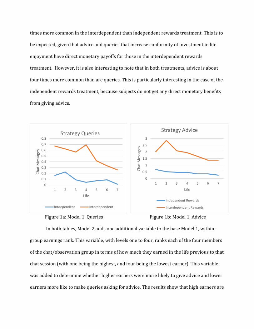
times more common in the interdependent than independent rewards treatment. This is to

be expected, given that advice and queries that increase conformity of investment in life

enjoyment have direct monetary payoffs for those in the interdependent rewards

treatment. However, it is also interesting to note that in both treatments, advice is about

four times more common than are queries. This is particularly interesting in the case of the

independent rewards treatment, because subjects do not get any direct monetary benefits

from giving advice.

Figure 1a: Model 1, Queries Figure 1b: Model 1, Advice

In both tables, Model 2 adds one additional variable to the base Model 1, within-

group earnings rank. This variable, with levels one to four, ranks each of the four members

of the chat/observation group in terms of how much they earned in the life previous to that

chat session (with one being the highest, and four being the lowest earner). This variable

was added to determine whether higher earners were more likely to give advice and lower

earners more like to make queries asking for advice. The results show that high earners are

0

0.5

1

1.5

2

2.5

3

1 2 3 4 5 6 7

Ch

at M

essa

ges

Life

Strategy Advice

Independent Rewards

Interdependent Rewards

0

0.1

0.2

0.3

0.4

0.5

0.6

0.7

0.8

1 2 3 4 5 6 7

Ch

at M

essa

ges

Life

Strategy Queries

Intdependent Interdependent

more likely to give advice, with advice statements decreasing by about .24 with each

successive rank. However, rank did not have a significant effect on queries. It would appear

that subjects that did well relative to others whom they could observe and engage in chat

were more motivated to offer advice, but asking for advice, which was less common, did

not depend on rank.

Table3: Predictors of Strategic Statements

Model 1 Model 2

Parameter df Estimate Sig. Estimate Sig.

Intercept 76 1.38 0.000 1.98 0.000

Life 1† 924 0.65 0.008 0.65 0.008

Life 2 924 1.48 0.000 1.48 0.000

Life 3 924 0.72 0.004 0.72 0.003

Life 4 924 0.58 0.018 0.58 0.018

Life 5 924 0.28 0.247 0.28 0.244

Life 6 924 0.00 1.000 0.00 1.000

Independent Rewards‡ 274 -1.13 0.013 -1.13 0.013

Life 1 * Ind. Rewards~ 924 -0.21 0.578 -0.21 0.576

Life 2 * Ind. Rewards 924 -1.20 0.001 -1.20 0.001

Life 3 * Ind. Rewards 924 -0.50 0.182 -0.50 0.180

Life 4 * Ind. Rewards 924 -0.36 0.334 -0.36 0.331

Life 5 * Ind. Rewards 924 -0.18 0.626 -0.18 0.624

Life 6 * Ind. Rewards 924 0.10 0.782 0.10 0.780

Within Group Rank -0.24 0.000

Covariance Parameters / Random Effects Estimate Sig. Estimate Sig.

Residual 2.64 0.000 2.62 0.000

Chat/obs. Group 1.03 0.001 1.06 0.001

Subject 0.71 0.000 0.60 0.000

†Life parameters are measure against baseline of Life7

‡Interdependent rewards are measured against socially interdependent rewards

~Interaction terms are measured against baselines of socially interdependent rewards and life 7.

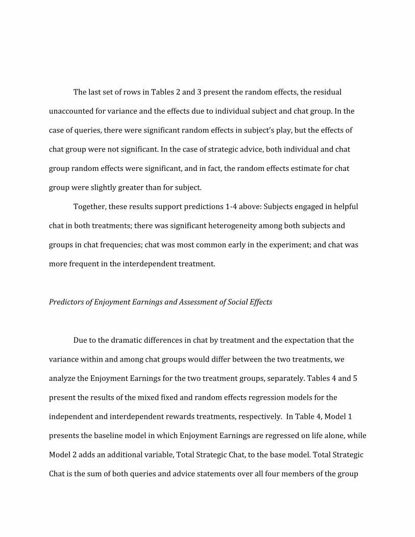
The last set of rows in Tables 2 and 3 present the random effects, the residual

unaccounted for variance and the effects due to individual subject and chat group. In the

case of queries, there were significant random effects in subject’s play, but the effects of

chat group were not significant. In the case of strategic advice, both individual and chat

group random effects were significant, and in fact, the random effects estimate for chat

group were slightly greater than for subject.

Together, these results support predictions 1-4 above: Subjects engaged in helpful

chat in both treatments; there was significant heterogeneity among both subjects and

groups in chat frequencies; chat was most common early in the experiment; and chat was

more frequent in the interdependent treatment.

Predictors of Enjoyment Earnings and Assessment of Social Effects

Due to the dramatic differences in chat by treatment and the expectation that the

variance within and among chat groups would differ between the two treatments, we

analyze the Enjoyment Earnings for the two treatment groups, separately. Tables 4 and 5

present the results of the mixed fixed and random effects regression models for the

independent and interdependent rewards treatments, respectively. In Table 4, Model 1

presents the baseline model in which Enjoyment Earnings are regressed on life alone, while

Model 2 adds an additional variable, Total Strategic Chat, to the base model. Total Strategic

Chat is the sum of both queries and advice statements over all four members of the group

following a given life. This variable was added as an attempt to examine whether verbal

exchanges over strategy improved earnings in the next life.

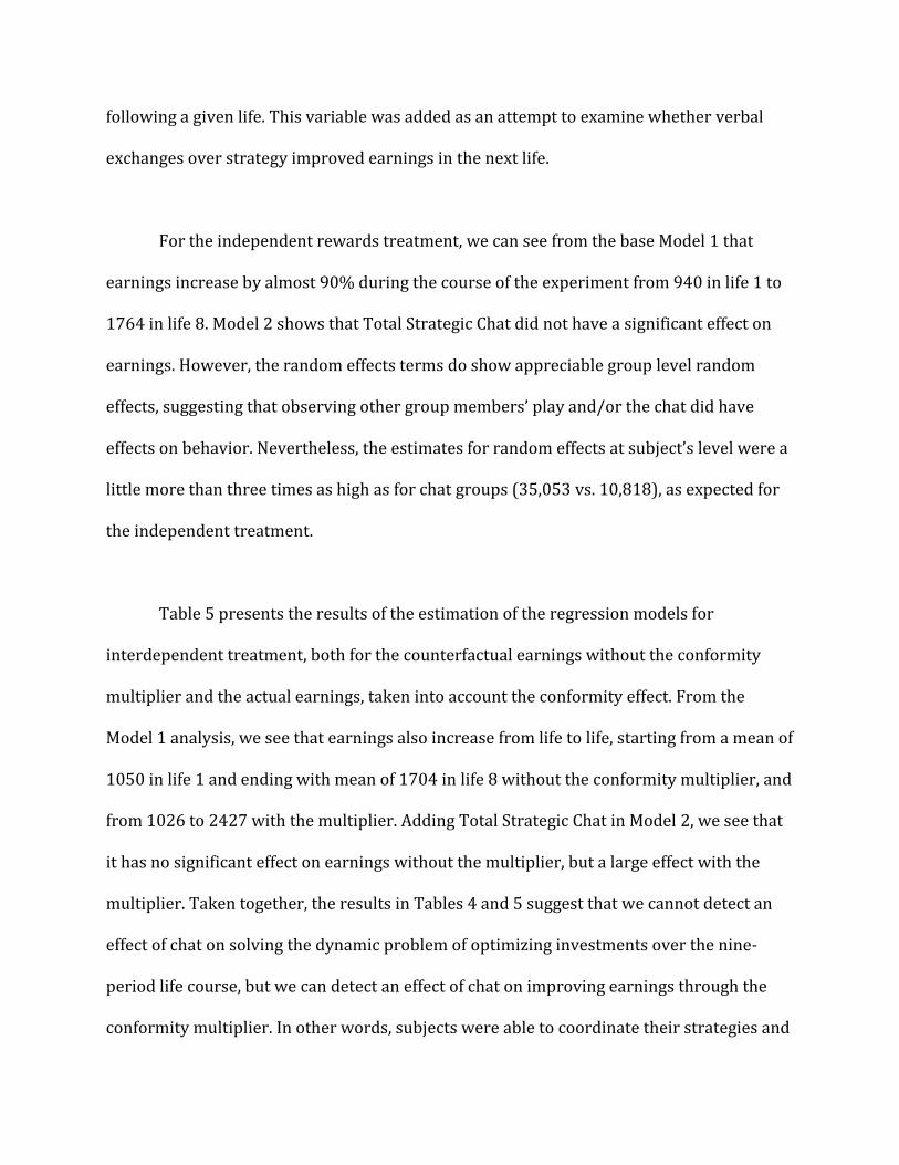
For the independent rewards treatment, we can see from the base Model 1 that

earnings increase by almost 90% during the course of the experiment from 940 in life 1 to

1764 in life 8. Model 2 shows that Total Strategic Chat did not have a significant effect on

earnings. However, the random effects terms do show appreciable group level random

effects, suggesting that observing other group members’ play and/or the chat did have

effects on behavior. Nevertheless, the estimates for random effects at subject’s level were a

little more than three times as high as for chat groups (35,053 vs. 10,818), as expected for

the independent treatment.

Table 5 presents the results of the estimation of the regression models for

interdependent treatment, both for the counterfactual earnings without the conformity

multiplier and the actual earnings, taken into account the conformity effect. From the

Model 1 analysis, we see that earnings also increase from life to life, starting from a mean of

1050 in life 1 and ending with mean of 1704 in life 8 without the conformity multiplier, and

from 1026 to 2427 with the multiplier. Adding Total Strategic Chat in Model 2, we see that

it has no significant effect on earnings without the multiplier, but a large effect with the

multiplier. Taken together, the results in Tables 4 and 5 suggest that we cannot detect an

effect of chat on solving the dynamic problem of optimizing investments over the nine-

period life course, but we can detect an effect of chat on improving earnings through the

conformity multiplier. In other words, subjects were able to coordinate their strategies and

make similar investments in each period; the chat appears to have facilitated this

coordination.

Table 4 Enjoyment Earnings without Socially Dependent Rewards

Model 1 Model 2

Parameter df Estimate Sig. df Estimate Sig.

Intercept 39 1764 0.000 36 1761 0.000

Life 1 469 -824 0.000

Life 2 469 -520 0.000 407 -526 0.000

Life 3 469 -364 0.000 405 -369 0.000

Life 4 469 -176 0.000 403 -179 0.000

Life 5 469 -119 0.004 402 -122 0.003

Life 6 469 -85 0.037 402 -86 0.031

Life 7 469 -5 0.896 402 -7 0.860

theme2_sum 397 2 0.638 Covariance Parameters / Random Effects Estimate Sig. Estimate Sig.

Residual 56204 0.000 53691 0.000

Chat/obs. Group 35053 0.000 41606 0.000

Subject 10817 0.167 11095 0.199

Table 5 Enjoyment Earnings with Socially Dependent Rewards

Model I Model 2

Interdependent w/o conformity

Interdependent with conformity

Interdependent w/o conformity

Interdependent with conformity

Parameter df Estimate Sig. Est. Sig. df Est. Sig. Est. Sig.

Intercept 39 1705 0.000 2427 0.000 36 1698 0.000 2390 0.000

Life 1 469 -655 0.000 -1401 0.000

Life 2 469 -402 0.000 -860 0.000 407 -406 0.000 -882 0.000

Life 3 469 -269 0.000 -597 0.000 405 -276 0.000 -639 0.000

Life 4 469 -162 0.000 -375 0.000 403 -166 0.000 -399 0.000

Life 5 469 -148 0.000 -289 0.000 402 -152 0.000 -310 0.000

Life 6 469 -60 0.080 -134 0.006 402 -62 0.055 -143 0.002

Life 7 469 -72 0.036 -124 0.011 402 -72 0.025 -124 0.007

theme2_sum 397 1 0.473 5 0.005

Covariance Parameters / Random Effects Est. Sig. Est. Sig. Est. Sig. Est. Sig.

Residual 51678 0.000 102943 0.000 45205 0.000 92560 0.000

Chat/obs. Group

11533 0.000 10179 0.013 13567 0.000 14248 0.003

Subject 42449 0.003 133297 0.002 51138 0.003 157171 0.002

Figure 2 illustrates these effects by plotting the expected marginal means for

enjoyment earnings from the Model 1 regressions in Tables 4 and 5. Earnings for both

treatments increase with each progressive life, and are very similar on average for the two

treatments, when the conformity bias is not taken into account. However, the

interdependent chat groups also increasingly took advantage of the conformity multiplier

(as can be seen by the increasing distance between the red and orange lines).

The dramatic effects of introducing interdependence in rewards can be seen from the

variance decomposition of the random effects. As opposed to the independent rewards

case where the chat group random effects were one third as large as the individual subject

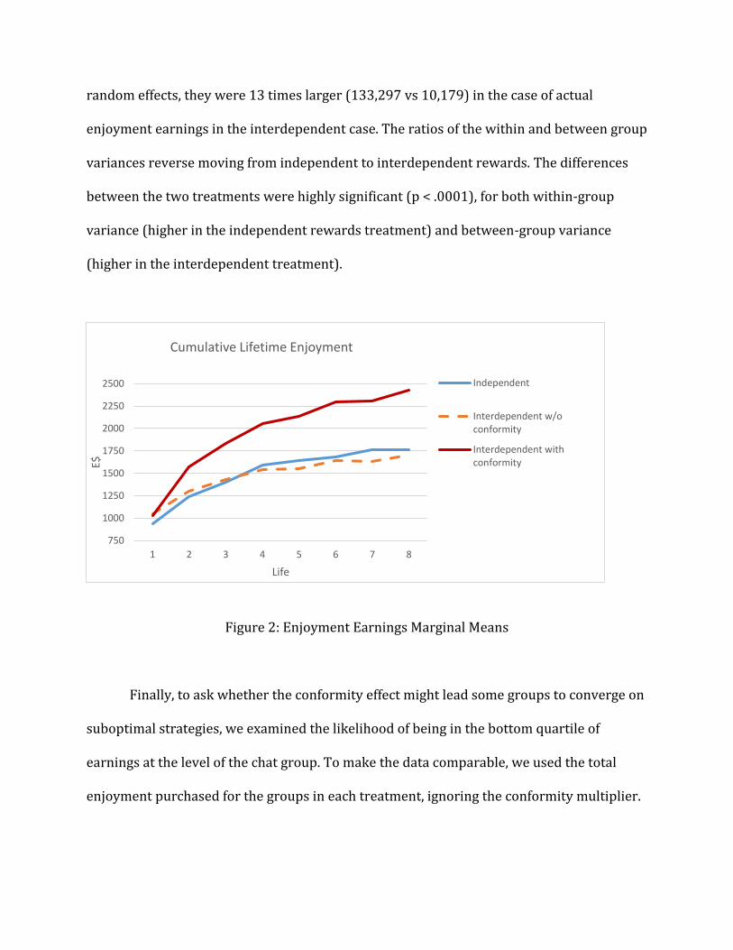
random effects, they were 13 times larger (133,297 vs 10,179) in the case of actual

enjoyment earnings in the interdependent case. The ratios of the within and between group

variances reverse moving from independent to interdependent rewards. The differences

between the two treatments were highly significant (p < .0001), for both within-group

variance (higher in the independent rewards treatment) and between-group variance

(higher in the interdependent treatment).

Figure 2: Enjoyment Earnings Marginal Means

Finally, to ask whether the conformity effect might lead some groups to converge on

suboptimal strategies, we examined the likelihood of being in the bottom quartile of

earnings at the level of the chat group. To make the data comparable, we used the total

enjoyment purchased for the groups in each treatment, ignoring the conformity multiplier.

750

1000

1250

1500

1750

2000

2250

2500

1 2 3 4 5 6 7 8

E$

Life

Cumulative Lifetime Enjoyment

Independent

Interdependent w/oconformity

Interdependent withconformity

Those results are presented in Table 6, using data from lives 7 and 8 when earnings in both

treatments were highest.

Table 6 Cumulative Earnings in the Lowest Quartile

Lowest Quartile Enjoyment Earnings

Treatment Group

Total Independent Interdependent

No 30 29 59

Yes 4 15 19

Total 34 44 78

Table 6 shows that just over a third of the chat groups in the interdependent

rewards treatment were in the lowest quartile of mean earnings (15/44), whereas only

11% were in the lowest quartile in the independent treatment, leading to an odds ratio of

about 3. These results suggest that the focus on social conformity in investment in life

enjoyment can increase variance among groups, with some groups stabilizing at behavioral

strategies quite far from optimal dynamic performance.

Together, these results support predictions 5-7 with the interdependent treatment

decreasing within-group variance but increasing between-group variance, sometimes

resulting in behavior far from the optimum with respect to the dynamic problem.

5. Discussion and Conclusions

There are two large scale implications of these findings. First, in keeping with the

theme of this special issue, individual incentives explain a large part, but not all, of the

variance in prosocial behavior in the form of strategic advice. Second, incentives for

conformity promote prosocial behavior, but also increase variance among groups in

equilibrium outcomes, leading to convergence on suboptimal strategies for some groups.

We discuss each in turn.

The independent rewards treatment provides insights into ‘non-selfish’ prosocial

behavior. In that case, there were no monetary incentives for subjects to help others find

the optimal strategy of investments, but there were also no monetary incentives to defect

or mislead them. Nor were subjects given instructions about what they could talk about

between lives. Nevertheless, about one third of chat messages were about strategies of how

to perform in the experiment, two thirds of which were directed to optimal investment

(about 2 messages per life). Moreover, most messages were advice rather than queries

about strategy. Individual monetary incentives might explain queries, but are less likely to

explain advice. In addition, subjects who did relatively better than other in their group in

terms of earnings were more likely to provide strategic advice, but were no more likely to

make queries. This suggests that better earners were motivated to help those who did

worse.

We were unable to show that in the independent rewards treatment, quantity of

strategy messages was associated with earnings. There are several possible explanations of

this finding. One is that quantity of messages without reference to quality is a poor measure

of information flow. This explanation would be consistent with the finding that there were

significant random effects of chat groups on earnings, and on both health investments and

enjoyment investments. Another possible explanation is that the dynamic optimization

problem subjects faced was particularly complex and nonlinear. They showed through

their behavior that they were able to improve their performance over time, but it may have

been difficult to put those improvements into words in simple chat messages.

The interdependent rewards treatment provided strong monetary incentives for

subjects to coordinate on behavior. These motivations resulted in both absolutely more

strategy chat and a greater relative emphasis on strategy than on other topics. People in the

interdependent group sent about four times as many strategy messages as the independent

rewards group, but they sent fewer messages about topics outside the experiment (1.2

versus 3 messages on average per life per chat group). Just as in the independent

treatment, higher earners (relative to other chat group members) in the socially dependent

treatment offered more strategic advice than lower earners, and advice was much more

common than queries.

With respect to the impacts of chat on earnings, we found mixed results for the

interdependent treatment. As in the case of the independent rewards, we found no

significant effects of chat on earnings without taking into account the conformity

multiplier. However, actual earnings, taking into account the multiplier, were positively

associated with the number of strategy chat messages sent in a life. One interpretation of

this finding is that the chat served more to facilitate conformity on one strategy, rather than

to optimize investments over the life course. Figure 3 examines this possibility by

comparing observed investment behavior with optimal investment behavior. A visual

inspection of the figure suggests that subjects in the independent rewards treatment

converged more on the optimal strategy on average than those in the interdependent

treatment. Unlike the theoretical optimum, investments in life enjoyment in the

interdependent treatment tend to remain flat rather than increase throughout life, and

investments in health decrease much less than is optimal. This suggests that subjects may

have converged on rules of thumb that were easily transmissible. Also, in support of this

interpretation that conformity can conflict with optimizing are (1) the increasing

divergence of the actual earnings from earnings without the multiplier in Figure 2; and (2)

the increased likelihood of being in the bottom quartile of earnings for subjects in the

socially interdependent treatment, when the conformity bias is not taken into account.

Figure 3. Observed and Theoretically Optimal Investment strategies.

This last finding, when coupled with the massively greater random effects at the

chat group level for the socially interdependent treatment than for the independent

rewards treatment, may imply that conformity biases can compete with other strategic

problems individuals face. In the face of uncertainty, doing what most others do (positive

frequency dependent modeling) can often be the best strategy, since it integrates

information across individuals and over time (Boyd and Richersen 1988). Moreover,

0

10

20

30

40

50

60

70

1 2 3 4 5 6 7 8 9

E$

Period

Enjoyment Investment

Theoretical Independent

Interdependent

0

10

20

30

40

50

60

70

1 2 3 4 5 6 7 8 9

Period

Health Investment

Theoretical Independent

Interdependent

activities that provide enjoyment utility at a potential cost to health, such as smoking,

alcohol consumption, and excessive eating, are often done in social contexts. Thus, the

variant individual who chooses to avoid those activities and invest in health will forego

opportunities for social exchange at the same time.

This tension between gains from conformity and individual optimization may help

explain the striking variability in health behavior across regions, ethnic groups and

socioeconomic strata. The social costs and benefits of cigarette smoking, alcohol

consumption, physical exercise, and eating patterns are likely to vary with respect to their

frequency in the networks in which individuals are embedded. From a social perspective,

overweight or over-exercise, for that matter, may be relative terms.

The processes generating varying social equilibria in health behavior and status

merit further investigation. Behavioral economic experiments that focus on the interplay

of dynamic optimization problems and social forces are likely to provide new insights into

why so many different equilibria are observed, and may be particularly productive in

explaining changing patterns of health.

6. Bibliography

Christakis, N. A., & Fowler, J. H. (2007). The spread of obesity in a large social network over

32 years. New England Journal of Medicine, 357(4), 370-379

Constant, D., Sproull, L., & Kiesler, S. (1996). The kindness of strangers: The usefulness of

electronic weak ties for technical advice. Organization Science, 7(2), 119-135.

Cutler, D. M., & Lleras-Muney, A. (2010). Understanding differences in health behaviors by

education. Journal of Health Economics, 29(1), 1-28.

Flocke, S. A., & Stange, K. C. (2004). Direct observation and patient recall of health behavior

advice. Preventive Medicine, 38(3), 343-349.

Ellison, C. G., & Levin, J. S. (1998). The religion-health connection: Evidence, theory, and

future directions. Health Education & Behavior, 25(6), 700-720.

Flocke, S. A., Clark, A., Schlessman, K., & Pomiecko, G. (2005). Exercise, diet, and weight loss

advice in the family medicine outpatient setting. Family Medicine, 37(6), 415-421.

Fowler, J. H., Settle, J. E., & Christakis, N. A. (2011). Correlated genotypes in friendship

networks. Proceedings of the National Academy of Sciences, 108(5), 1993-1997.

Fuchs, V. (2004). Reflections on the socio-economic correlates of health. Journal of health

economics, 23(4), pp. 653-661.Grossman, M. (1972a) The Demand for Health: A

Theoretical and Empirical Investigation. Columbia University Press for the National

Bureau of Economic Research, New York.

Grossman, M. (1972b). On the concept of health capital and the demand for health. The

Journal of Political Economy, 80(2), pp. 223-255.

Kenkel, D. S. (1991). Health behavior, health knowledge, and schooling. Journal of Political

Economy, 287-305.

Kleinman, A. (1980). Patients and healers in the context of culture: An exploration of the

borderland between anthropology, medicine, and psychiatry (Vol. 3). University of

California Press.

McGinnis, J. M., Williams-Russo, P., & Knickman, J. R. (2002). The case for more active policy

attention to health promotion. Health Affairs, 21(2), 78-93.

Murray, C. J. L., Gakidou, E. E., & Frenk, J. (1999). Critical Reflection-Health inequalities and

social group differences: What should we measure?. Bulletin of the World Health

Organization, 77(7), 537-544.

Swan, M. (2012). Crowdsourced health research studies: an important emerging

complement to clinical trials in the public health research ecosystem. Journal of

medical Internet research, 14(2).

Umberson, D., Crosnoe, R., & Reczek, C. (2010). Social relationships and health behavior

across life course. Annual review of sociology, 36, 139.

Waite L. (1995). Does Marriage Matter? Demography, 32:483–508

Appendix 1: Real Effort Harvesting

During the first part of each period in each life, participants were required to undertake a

real-effort harvesting task in which the participant could earn revenue, Rt, that she could

subsequently invest in either life enjoyment (a cash reward) or health preservation for

subsequent periods of the current lifetime. The amount of time allowed for the harvesting

task during each period (maximum 30 seconds) was directly proportional to the

participant’s current level of health, Ht, (between 0 and 100), so investment in upgrading

health enabled a higher levels of harvesting in future periods. The initial health condition,

85, and the natural degeneration of health across all periods of life {-16, -17, … -23, -24}

were preprogrammed and identical for all participants in all lifetimes in all experimental

treatments. The health degeneration occurred after harvesting just before investment for

the current period began. Never investing in health would result in the participant dying

(not being able to continue to harvesting and investing) in period 5.

The harvesting task assigned to participants required vigilance and some manual dexterity

but was designed so that most participants could perform at a high enough level that their

harvest earnings and optimal investment strategies would be quite comparable. The task

involved a sequence of 30 targets that would skirt across a circular harvesting field. Each

target had a one of four different harvest values, and each target took two seconds to skirt

across the field, after which it disappeared. To harvest the target the participant simply

needed to click on the harvesting field while that target was viable. Once a click was made it

would take 2 seconds to process the harvested target during which time the participant

could harvest no other targets although she could see the unavailable targets as they

skirted by. If the participant’s current health were at level Ht [0,100], then during the first

30x(100- Ht)/100 seconds of the harvest period she would see targets go by that she was

unable to harvest due to her deteriorated health. Similarly, if a target were only partially

processed by the end of the previous period, processing would complete at the beginning of

the next period adding a small increment to any downtime due to deteriorated health.

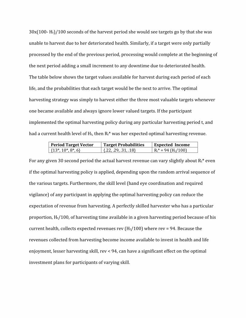
The table below shows the target values available for harvest during each period of each

life, and the probabilities that each target would be the next to arrive. The optimal

harvesting strategy was simply to harvest either the three most valuable targets whenever

one became available and always ignore lower valued targets. If the participant

implemented the optimal harvesting policy during any particular harvesting period t, and

had a current health level of Ht, then Rt* was her expected optimal harvesting revenue.

Period Target Vector Target Probabilities Expected Income {13*, 10*, 8*, 6} {.22, .29, .31, .18} Rt* = 94 (Ht/100)

For any given 30 second period the actual harvest revenue can vary slightly about Rt* even

if the optimal harvesting policy is applied, depending upon the random arrival sequence of

the various targets. Furthermore, the skill level (hand eye coordination and required

vigilance) of any participant in applying the optimal harvesting policy can reduce the

expectation of revenue from harvesting. A perfectly skilled harvester who has a particular

proportion, Ht/100, of harvesting time available in a given harvesting period because of his

current health, collects expected revenues rev (Ht/100) where rev = 94. Because the

revenues collected from harvesting become income available to invest in health and life

enjoyment, lesser harvesting skill, rev < 94, can have a significant effect on the optimal

investment plans for participants of varying skill.

To compute the optimal harvesting strategy, consider, for example, the target set V= {13,

10, 8, 6} where the probability of encountering each target type during the next second is

given by p={.22, .29, .31, .18}. Given it takes 2 seconds of handling time to process any

target, the harvest value per second for each type of target is given by V/2 = {6.5, 5, 4, 3}.

The total value per second derived by harvesting only the n most valuable targets is given

by vipi = {2.86, 5.76, 8.24, 9.32}. The total handling time for the n most valuable targets is

given by 1+ 2pi = {1.44, 2.02, 2.64, 3}. And finally, the total value per second of total

handling time is given by vipi / (1+ 2pi) = {1.99, 2.85, 3.12, 3.1}. The optimal harvesting

policy is to always take whichever of the first three targets shows up next. In a 30 second

harvesting period this policy would generate a total harvest value of 30 x 3.12 = 94 units of

value.

The parameters in the experiment are set such that rev= 94 is the expected revenue per

period for a perfectly skilled harvester who is 100% healthy. In the experiments reported,

the participants displayed mean harvesting skills that were less than perfect (rev= 87), but

with low variance. Because the revenues Rt collected from harvesting become the income

available to invest in health and life enjoyment, lesser harvesting skill can have a significant

effect on the optimal investment schedule. We use rev= 87, the mean harvesting skill of all

subjects, as the baseline parameter for computing optimal investment planning

throughout this paper.

Appendix 2: Computation

The transition equation relating health at the end of period t to health at the end of period t-1 is

given by:

𝐻𝑡 = 𝑀𝑖𝑛 [100, 𝐻𝑡−1 − d𝑡 + 301 − ⅇ−.025It

1 + ⅇ−.025It ]

The first derivative of health w.r.t. investment in health is given by:

𝑑𝐻𝑡

𝑑𝐼𝑡= 30 ∙ .025ⅇ−.025It [

1

1 + ⅇ−.025It+

(1 − ⅇ−.025It)

(1 + ⅇ−.025It)2]

or,

𝑑𝐻𝑡

𝑑𝐼𝑡=

1.5ⅇ−.025It

1 + 2ⅇ−.025It + ⅇ−.05It

The second derivative of health w.r.t. investment in health is given by:

𝑑2𝐻𝑡

𝑑𝐼𝑡2 = 1.5 [

−.025ⅇ−.025It

1 + 2ⅇ−.025It + ⅇ−.05It+

. 05(ⅇ−.025It)(ⅇ−.025It + ⅇ−.05It)

(1 + 2ⅇ−.025It + ⅇ−.05It)2]

or,

𝑑2𝐻𝑡

𝑑𝐼𝑡2 = 1.5 [

−.025ⅇ−.025It − .05ⅇ−.05It − .025ⅇ−.075It

(1 + 2ⅇ−.025It + ⅇ−.05It)2+

. 05(ⅇ−.05It + ⅇ−.075It)

(1 + 2ⅇ−.025It + ⅇ−.05It)2]

𝑑2𝐻𝑡

𝑑𝐼𝑡2 = −.025 [

ⅇ−.025It − ⅇ−.075It

(1 + 2ⅇ−.025It + ⅇ−.05It)2]

The consumption function which gives subject earnings, Et, from life enjoyment in period t as a

function of the portion of harvest and retirement returns that are invested in life enjoyment, Lt, is

given by:

𝐸𝑡 = 250(1 + 𝐻𝑡/100)(1 − ⅇ−.028𝐿𝑡)

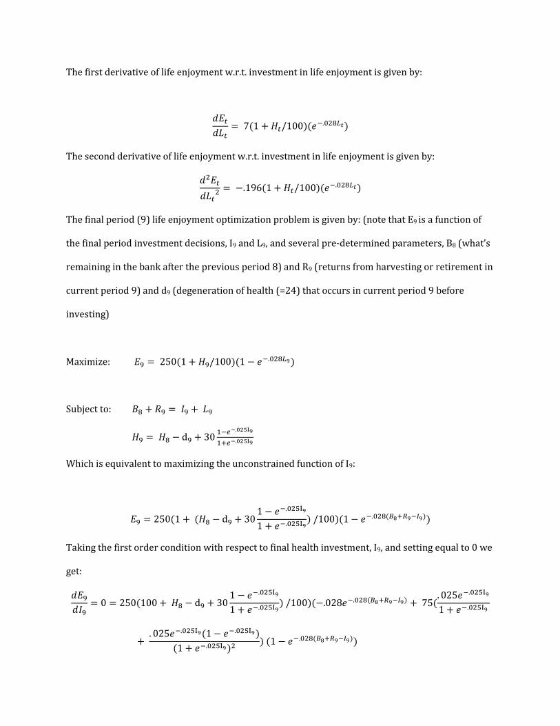
The first derivative of life enjoyment w.r.t. investment in life enjoyment is given by:

𝑑𝐸𝑡

𝑑𝐿𝑡= 7(1 + 𝐻𝑡/100)(ⅇ−.028𝐿𝑡)

The second derivative of life enjoyment w.r.t. investment in life enjoyment is given by:

𝑑2𝐸𝑡

𝑑𝐿𝑡2 = −.196(1 + 𝐻𝑡/100)(ⅇ−.028𝐿𝑡)

The final period (9) life enjoyment optimization problem is given by: (note that E9 is a function of

the final period investment decisions, I9 and L9, and several pre-determined parameters, B8 (what’s

remaining in the bank after the previous period 8) and R9 (returns from harvesting or retirement in

current period 9) and d9 (degeneration of health (=24) that occurs in current period 9 before

investing)

Maximize: 𝐸9 = 250(1 + 𝐻9/100)(1 − ⅇ−.028𝐿9)

Subject to: 𝐵8 + 𝑅9 = 𝐼9 + 𝐿9

𝐻9 = 𝐻8 − d9 + 301−ⅇ−.025I9

1+ⅇ−.025I9

Which is equivalent to maximizing the unconstrained function of I9:

𝐸9 = 250(1 + (𝐻8 − d9 + 301 − ⅇ−.025I9

1 + ⅇ−.025I9) /100)(1 − ⅇ−.028(𝐵8+𝑅9−𝐼9))

Taking the first order condition with respect to final health investment, I9, and setting equal to 0 we

get:

𝑑𝐸9

𝑑𝐼9= 0 = 250(100 + 𝐻8 − d9 + 30

1 − ⅇ−.025I9

1 + ⅇ−.025I9) /100)(−.028ⅇ−.028(𝐵8+𝑅9−𝐼9) + 75(

. 025ⅇ−.025I9

1 + ⅇ−.025I9

+ . 025ⅇ−.025I9(1 − ⅇ−.025I9)

(1 + ⅇ−.025I9)2) (1 − ⅇ−.028(𝐵8+𝑅9−𝐼9))

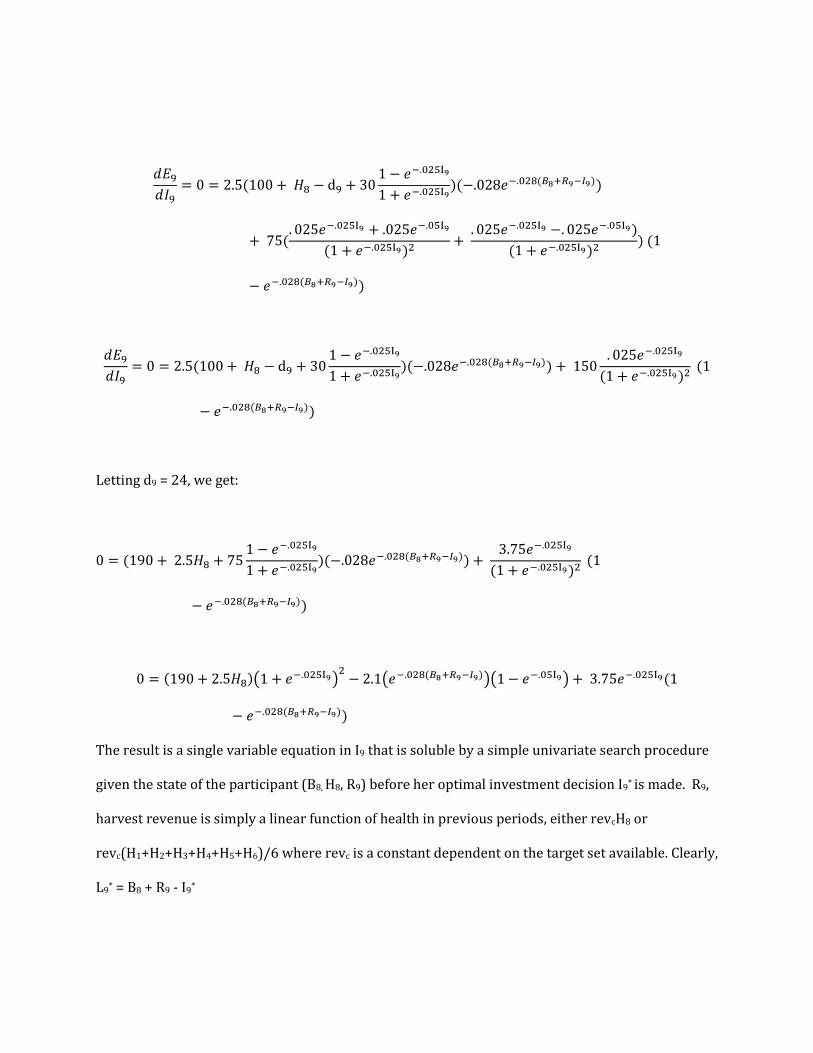
𝑑𝐸9

𝑑𝐼9= 0 = 2.5(100 + 𝐻8 − d9 + 30

1 − ⅇ−.025I9

1 + ⅇ−.025I9)(−.028ⅇ−.028(𝐵8+𝑅9−𝐼9))

+ 75(. 025ⅇ−.025I9 + .025ⅇ−.05I9

(1 + ⅇ−.025I9)2+

. 025ⅇ−.025I9 −. 025ⅇ−.05I9)

(1 + ⅇ−.025I9)2) (1

− ⅇ−.028(𝐵8+𝑅9−𝐼9))

𝑑𝐸9

𝑑𝐼9= 0 = 2.5(100 + 𝐻8 − d9 + 30

1 − ⅇ−.025I9

1 + ⅇ−.025I9)(−.028ⅇ−.028(𝐵8+𝑅9−𝐼9)) + 150

. 025ⅇ−.025I9

(1 + ⅇ−.025I9)2 (1

− ⅇ−.028(𝐵8+𝑅9−𝐼9))

Letting d9 = 24, we get:

0 = (190 + 2.5𝐻8 + 751 − ⅇ−.025I9

1 + ⅇ−.025I9)(−.028ⅇ−.028(𝐵8+𝑅9−𝐼9)) +

3.75ⅇ−.025I9

(1 + ⅇ−.025I9)2 (1

− ⅇ−.028(𝐵8+𝑅9−𝐼9))

0 = (190 + 2.5𝐻8)(1 + ⅇ−.025I9)2

− 2.1(ⅇ−.028(𝐵8+𝑅9−𝐼9))(1 − ⅇ−.05I9) + 3.75ⅇ−.025I9(1

− ⅇ−.028(𝐵8+𝑅9−𝐼9))

The result is a single variable equation in I9 that is soluble by a simple univariate search procedure

given the state of the participant (B8, H8, R9) before her optimal investment decision I9* is made. R9,

harvest revenue is simply a linear function of health in previous periods, either revcH8 or

revc(H1+H2+H3+H4+H5+H6)/6 where revc is a constant dependent on the target set available. Clearly,

L9* = B8 + R9 - I9*

The following tables provide the complete optimal decision trajectory for decision makers who are

perfect harvesters (rev= 94, given the experiment parameters), and the optimal decision trajectory

for decision makers who possess the average harvesting skill (rev= 87) that was demonstrated by

our experimental subjects.

Independent Harvest Rate Per Health = 0.94

Period 0 1 2 3 4 5 6 7 8 9 Investment Health 85 69 72.7 75.1 75.9 74.7 71.1 64.3 52.8 33.6

End Health 85 89.7 93.1 94.9 94.7 92.1 86.3 75.8 57.6 33.6

Harvest 0 79.9 84.3 87.5 89.2 89 86.6 81.2 71.3 54.2 Health Investment 0 68 66.1 63.3 59.1 53.2 44.6 32.3 12.9 0 Life Investment 0 11.9 18.2 24.2 30.1 35.9 42 48.9 58.4 54.2 Cash On Hand 0 0 0 0 0 0 0 0 0 0 Life Enjoyment 0 202.3 289.3 359.7 415.5 456.5 483.1 491.5 475.8 391.1 Marginal ROR 9.51 8.12 6.93 5.86 4.92 4.02 3.13 2.15 2.05 % Invest in Health 85 78 72 66 60 52 40 18 0

Interdependent Harvest Rate Per Health = 0.87

Period 0 1 2 3 4 5 6 7 8 9 Investment Health 85 69 71.9 73.3 72.9 70.4 65.1 56.1 41.7 17.7

End Health 85 88.9 91.3 91.9 90.4 86.1 78.1 64.7 41.7 17.7

Harvest 0 74 77.3 79.4 80 78.6 74.9 67.9 56.3 36.3 Health Investment 0 63.9 61.5 58.1 53.2 46.5 37.2 23.6 0 0

Life Investment 0 10 15.8 21.4 26.7 32.1 37.7 44.3 49.6 43

Cash On Hand 0 0 0 0 0 0 0 0 6.7 0

Life Enjoyment 0 173.7 256.5 323.9 376.2 414 435.5 439 398.9 309

Marginal ROR 9.99 8.60 7.38 6.31 5.30 4.34 3.33 2.47 2.47 % Invest in Health 86 80 73 67 59 50 35 0 0