Doctoral Thesis Evaluating pre-learner driver, road safety interventions designed for Transition...
530
i Evaluating pre-learner driver road safety education programmes designed for Transition Year (year 12) students in the Republic of Ireland. Margaret Ryan A dissertation submitted for the degree of Doctor of Philosophy of the University of Dublin, Trinity College, Dublin 2, Ireland. February 2013. This research was conducted in the School of Psychology, TCD.
Transcript of Doctoral Thesis Evaluating pre-learner driver, road safety interventions designed for Transition...
i
Evaluating pre-learner driver road
safety education programmes designed for
Transition Year (year 12) students in the
Republic of Ireland.
Margaret Ryan
A dissertation submitted for the degree of Doctor of Philosophy of the University of
Dublin, Trinity College, Dublin 2, Ireland. February 2013.
This research was conducted in the School of Psychology, TCD.


i
1.1 DECLARATION
I hereby declare that:
(a) The work contained in this thesis has not been submitted as an exercise for a degree
at this, or at any other University;
(b) This thesis is the result of my own investigations, and the contributions of others
are duly acknowledged in the text wherever included;
(c) I agree to deposit this thesis in the University’s open access institutional repository
or allow the library to do so on my behalf, subject to Irish Copyright legislation and
Trinity College Library conditions of use and acknowledgement.
Signed:__________________________________
Margaret Ryan
Date: 28 / 02 / 2013
ii
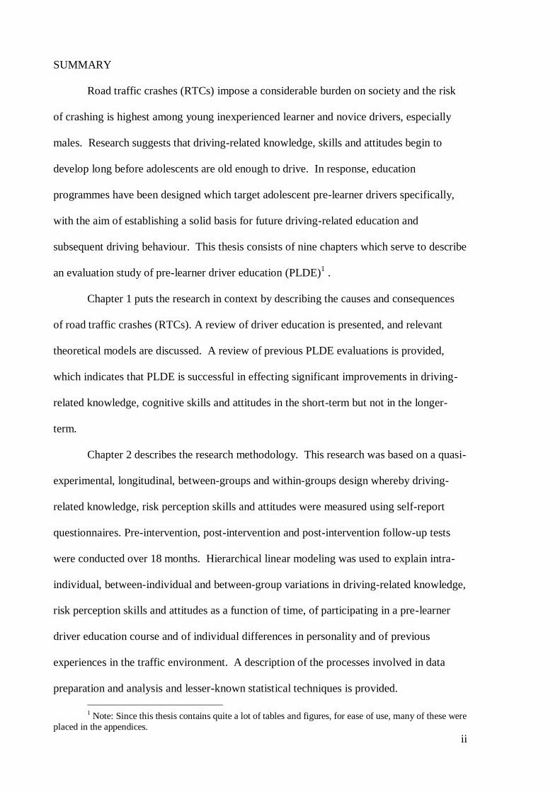
SUMMARY
Road traffic crashes (RTCs) impose a considerable burden on society and the risk
of crashing is highest among young inexperienced learner and novice drivers, especially
males. Research suggests that driving-related knowledge, skills and attitudes begin to
develop long before adolescents are old enough to drive. In response, education
programmes have been designed which target adolescent pre-learner drivers specifically,
with the aim of establishing a solid basis for future driving-related education and
subsequent driving behaviour. This thesis consists of nine chapters which serve to describe
an evaluation study of pre-learner driver education (PLDE)1 .
Chapter 1 puts the research in context by describing the causes and consequences
of road traffic crashes (RTCs). A review of driver education is presented, and relevant
theoretical models are discussed. A review of previous PLDE evaluations is provided,
which indicates that PLDE is successful in effecting significant improvements in driving-
related knowledge, cognitive skills and attitudes in the short-term but not in the longer-
term.
Chapter 2 describes the research methodology. This research was based on a quasi-
experimental, longitudinal, between-groups and within-groups design whereby driving-
related knowledge, risk perception skills and attitudes were measured using self-report
questionnaires. Pre-intervention, post-intervention and post-intervention follow-up tests
were conducted over 18 months. Hierarchical linear modeling was used to explain intra-
individual, between-individual and between-group variations in driving-related knowledge,
risk perception skills and attitudes as a function of time, of participating in a pre-learner
driver education course and of individual differences in personality and of previous
experiences in the traffic environment. A description of the processes involved in data
preparation and analysis and lesser-known statistical techniques is provided.
1 Note: Since this thesis contains quite a lot of tables and figures, for ease of use, many of these were
placed in the appendices.
iii
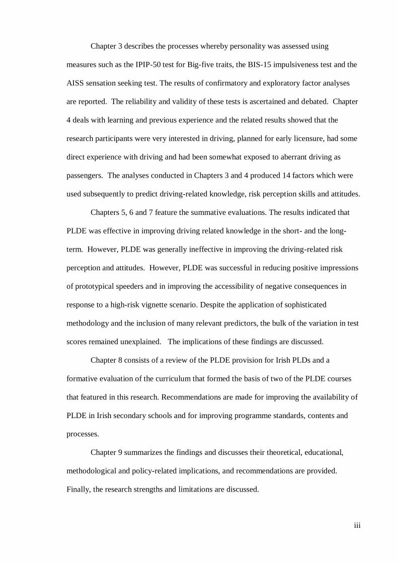
Chapter 3 describes the processes whereby personality was assessed using
measures such as the IPIP-50 test for Big-five traits, the BIS-15 impulsiveness test and the
AISS sensation seeking test. The results of confirmatory and exploratory factor analyses
are reported. The reliability and validity of these tests is ascertained and debated. Chapter
4 deals with learning and previous experience and the related results showed that the
research participants were very interested in driving, planned for early licensure, had some
direct experience with driving and had been somewhat exposed to aberrant driving as
passengers. The analyses conducted in Chapters 3 and 4 produced 14 factors which were
used subsequently to predict driving-related knowledge, risk perception skills and attitudes.
Chapters 5, 6 and 7 feature the summative evaluations. The results indicated that
PLDE was effective in improving driving related knowledge in the short- and the long-
term. However, PLDE was generally ineffective in improving the driving-related risk
perception and attitudes. However, PLDE was successful in reducing positive impressions
of prototypical speeders and in improving the accessibility of negative consequences in
response to a high-risk vignette scenario. Despite the application of sophisticated
methodology and the inclusion of many relevant predictors, the bulk of the variation in test
scores remained unexplained. The implications of these findings are discussed.
Chapter 8 consists of a review of the PLDE provision for Irish PLDs and a
formative evaluation of the curriculum that formed the basis of two of the PLDE courses
that featured in this research. Recommendations are made for improving the availability of
PLDE in Irish secondary schools and for improving programme standards, contents and
processes.
Chapter 9 summarizes the findings and discusses their theoretical, educational,
methodological and policy-related implications, and recommendations are provided.
Finally, the research strengths and limitations are discussed.

iv
ACKNOWLEDGEMENTS
This thesis represents the culmination of 4 years research on the topic of pre-learner
driver education and a lifelong ambition to obtain a university education. Throughout this
process I have been privileged to receive encouragement, support and guidance from a
wide range of individuals and organizations, some of which deserve specific mention.
I am grateful to the Road Safety Authority for funding this research and I would
like to acknowledge the help and support that I received from Michael Rowland, Michael
Brosnan and the staff in the RSA’s education division. I also wish to thank the staff and
students in the schools that participated in this research. This represented a considerable
commitment in terms of time and energy and these were provided with an extraordinary
degree of generosity and graciousness.
I would like to thank my supervisor, Dr. Michael Gormley, who guided this project
from its inception and remained as a constant source of advice, and encouragement
throughout. I would like to acknowledge the help and support that I received from Dr.
Kevin Thomas, who co-supervised this research until he transferred to Bournemouth
University.
I am deeply grateful to Prof. Ray Fuller, without whom none of this would ever
have happened. Not only did he take a chance on me when he recommended that I be
accepted as a mature undergraduate student in TCD in 2004, but his passion for human
factors psychology and his expertise in driver behaviour inspired me to develop a deep and
enduring interest in these areas. Within the School of Psychology, I offer sincere thanks to
my appraisers, Prof. Ian Robertson and Dr. Samuel Cromie, who were a source of valuable
advice and encouragement over the past 4 years. I also applaud the professionalism of the
technical and administrative staff, including Pat Holohan, Lisa Gilroy, Enzar
Hadziselimovic, Michelle Le Good, Siobhan Walsh, Luisa Byrne, June Carpenter and
dearest June Switzer.

v
While I was conducting this research I had the pleasure of working within a vibrant
community of post-graduate researchers in the School of Psychology, whose support at
both a professional and personal level was invaluable and whose friendship and
companionship I deeply cherish. Heartfelt thanks therefore goes to Maria, Fearghal,
Louise, Ashling, Katriona, Kristin and other post-graduates who are too numerous to
mention individually - Ni bheidh bhur leithéidí ann arís.
To my dear husband Michael, whose faith and confidence in my ability to
undertake and complete my university education was at all times far stronger than was my
own. Thank you for believing in me and wanting this for me even more than I wanted it
for myself. Thanks also to my sons Graham and David, my daughters-in-laws Sarah and
Karen and my 6 wonderful grandchildren James, Amy, Kate, Leo, Rose and also Dylan
who arrived just in time to be included here. You are my joy and my inspiration – I love
you dearly.
Thanks also to my friends, especially the “Morgue” crew, who did not let my
socially undesirable status as an aspiring psychologist and an impoverished one at that,
interfere too much with the dynamics in our little group. Thanks to Michael Howard this
thesis has been purged of many gaffs ranging from Freudian slips to split infinitives – beati
sunt oculi tui.
Reflecting on what the time spent as a psychology student has meant to me, this
verse by T. S. Elliott came to mind:
“We shall not cease from exploration
And the end of all our exploring
Will be to arrive where we started
And know the place for the first time”
This has been a truly awesome journey and a fascinating process of discovery!

vi
1.2 Abbreviations2
AISS Arnett Inventory of Sensation Seeking
BIS Barrett Impulsiveness Scale
CRLE Crash risk likelihood estimates scale
CSO Central Statistics Office
DBQ Driver Behaviour Questionnaire
DE Driver education
DT Driver training
DWI Driving while intoxicated.
ECTM European Council of Ministers for Transport
ETS Educational Testing Service
EU European Union
FARS Fatal Analysis Reporting System
GDE Goals for driver education
GDL Graduated driver licence
HLM Hierarchical Linear Modeling
IP Intervention Phase – period inclusive of the T1 and the T2 tests
IPIP International Personality Item Pool
IVF Initial versus final phase - comparisons of T1 and T3 test scores
LDP Learner driver permit
OECD Organization for Economic Cooperation and Development,
PCR Perceived controllability of risk scale
PD Pre-driver
PDE Pre-driver education
PDLC Pre-driver licencing course
PIP Post-intervention phase – period inclusive of the T2 and the T3 tests
PLD Pre-learner driver
PLDE Pre-learner driver education
PRAD Perceived risk for adolescent drivers scale
PWM Prototype willingness model
ROI Republic of Ireland
ROTR Rules of the Road
RSA Road Safety Authority (Ireland)
RTC Road traffic crash
SARTRE Social Attitudes to Road Traffic Risk in Europe
SES Socio-economic status
SPC Safe Performance Curriculum
SS Sensation seeking
SWOV Dutch Institute for Road Safety Research
TCI Task capability interface model
TPB Theory of planned behaviour
TT Theory test (for learner drivers)
TY Transition Year
UNRSC United Nations Road Safety Collaboration
WHO World Health Organization
WTRT Willingness to take risks in traffic scale
2 Note: Statistical abbreviations are not included

vii
1.3 Table of Contents
1.1 DECLARATION ....................................................................................................................... I
1.2 ABBREVIATIONS ....................................................................................................................... VI
1.3 TABLE OF CONTENTS ................................................................................................................ VII
1.4 LIST OF TABLES ...................................................................................................................... XIV
1.5 LIST OF FIGURES .................................................................................................................... XVIII
CHAPTER 1: DRIVER BEHAVIOUR AND DRIVER EDUCATION ...........................................................1
1.1 ROAD TRAFFIC CRASHES ..............................................................................................................2
1.1.1 The human cost of RTCs ................................................................................................2
1.1.2 Financial and social costs of RTCs ..................................................................................4
1.1.3 Causes of RTCs ..............................................................................................................4
1.1.4 The young novice driver problem ...................................................................................7
1.2 DRIVER EDUCATION AND TRAINING .............................................................................................. 11
1.2.1 Defining driver education, driver training, pre-drivers and pre-learner drivers .............. 11
1.2.2 The DeKalb county driver education project ................................................................. 13
1.2.3 The driver education debate ........................................................................................ 16
1.2.4 Reinventing driver education ....................................................................................... 21
1.2.5 Theoretical models of driver behaviour ........................................................................ 22
1.2.6 Pre-learner driver characteristics ................................................................................. 37
1.2.7 Pre-learner driver education (PLDE) ............................................................................. 39
1.2.8 Aim of the present study ............................................................................................. 43
1.2.9 Hypotheses ................................................................................................................. 44
CHAPTER 2: METHODOLOGY........................................................................................................ 46
2.1 DESIGN ................................................................................................................................ 46
2.2 PARTICIPANTS ........................................................................................................................ 48
2.2.1 Attrition ...................................................................................................................... 52
2.3 APPARATUS AND MATERIALS ..................................................................................................... 53
2.4 MEASURES ............................................................................................................................ 53
viii
2.5 PROCEDURE .......................................................................................................................... 55
2.6 DATA PREPARATION AND ANALYSIS ............................................................................................. 56
2.6.2 Hierarchical linear modeling (HLM) ............................................................................ 62
2.6.3 HLM models in longitudinal research .......................................................................... 63
2.6.4 Implementing HLM analysis in this study .................................................................... 64
2.6.5 Modeling strategy ...................................................................................................... 66
2.6.6 Effect size calculations ............................................................................................... 69
2.6.7 Sample size ................................................................................................................ 71
2.6.8 Analysis of knowledge test scores ............................................................................... 72
CHAPTER 3: PERSONAL CHARACTERISTICS .................................................................................. 76
3.1 INTRODUCTION ...................................................................................................................... 76
3.1.1 Big-Five personality traits ........................................................................................... 78
3.1.2 Sensation seeking ...................................................................................................... 80
3.1.3 Impulsiveness............................................................................................................. 81
3.2 AIM .................................................................................................................................... 83
3.2.1 Design ....................................................................................................................... 83
3.2.2 Participants ............................................................................................................... 83
3.2.3 Procedure .................................................................................................................. 83
3.3 MEASURES ........................................................................................................................... 83
3.3.1 AISS ........................................................................................................................... 84
3.3.2 BIS-15 ........................................................................................................................ 84
3.3.3 IPIP-50 ....................................................................................................................... 85
3.4 RESULTS .............................................................................................................................. 86
3.4.1 Confirmatory factor analysis ...................................................................................... 86
3.4.2 Exploratory factor analysis ......................................................................................... 87
3.5 DISCUSSION .......................................................................................................................... 91
CHAPTER 4: LEARNING AND EXPERIENCE .................................................................................... 96
4.1 INTRODUCTION ...................................................................................................................... 96
4.1.1 Learning theories ....................................................................................................... 99

ix
4.1.2 Implications of learning theories for educational practice .......................................... 103
4.1.3 Application of learning theories to driver behaviour .................................................. 105
4.1.4 The role of social influence in the development of risky driving styles ......................... 107
4.2 AIM ................................................................................................................................... 113
4.3 METHODOLOGY .................................................................................................................... 114
4.3.1 Measures .................................................................................................................. 114
4.4 RESULT ............................................................................................................................... 115
4.4.1 Interest in driving ...................................................................................................... 115
4.4.2 Experience with traffic .............................................................................................. 117
4.4.3 Exposure to aberrant driving practices – Parents driving style .................................... 124
4.5 DISCUSSION ......................................................................................................................... 128
CHAPTER 5: KNOWLEDGE .......................................................................................................... 136
5.1 INTRODUCTION..................................................................................................................... 136
5.2 METHOD ............................................................................................................................ 138
5.2.1 Design ...................................................................................................................... 138
5.2.2 Participants .............................................................................................................. 138
5.2.3 Procedure ................................................................................................................. 138
5.2.4 Measures .................................................................................................................. 138
5.2.5 Data analysis ............................................................................................................ 141
5.3 RESULTS OF THE ITEM RESPONSE ANALYSES .................................................................................. 142
5.3.1 Short knowledge tests ............................................................................................... 142
5.3.2 Item response analysis of the supplementary knowledge tests ................................... 148
5.4 RESULTS OF THE DESCRIPTIVE AND HLM ANALYSES ........................................................................ 153
5.4.1 HLM analysis of short knowledge test scores ............................................................. 155
5.4.2 HLM analyses of the supplementary knowledge tests ................................................ 163
5.5 DISCUSSION ......................................................................................................................... 167
CHAPTER 6: RISK PERCEPTION ................................................................................................... 175
6.1 INTRODUCTION..................................................................................................................... 175
x
6.1.1 Objective crash risk ...................................................................................................177
6.1.2 Cognitive biases in risk perception .............................................................................178
6.1.3 Alternative measures of risk perception .....................................................................181
6.1.4 Implicit tests .............................................................................................................182
6.2 METHOD ............................................................................................................................184
6.2.1 Design ......................................................................................................................184
6.2.2 Participants ..............................................................................................................184
6.2.3 Procedure .................................................................................................................184
6.2.4 Measures ..................................................................................................................184
6.3 RESULTS .............................................................................................................................185
6.3.1 Principal component analysis of the repeated measures items ...................................185
6.3.2 Perceived risks for adolescent drivers scale (PRAD) ....................................................187
6.3.3 Likelihood of encountering risk-increasing factors while gaining experience with driving
.......................................................................................................................................................193
6.3.4 Crash risk likelihood estimates scale (CRLE) ...............................................................195
6.3.5 Perceived controllability of risk scale (PCR) ................................................................198
6.3.6 Willingness to take risks in traffic scale (WTRT) .........................................................202
6.3.7 High-risk vignette ......................................................................................................206
6.3.8 Results for vignettes ..................................................................................................208
6.4 DISCUSSION .........................................................................................................................215
6.4.1 Between-student predictors of risk perception ...........................................................217
6.4.2 Perceptions of inexperience .......................................................................................219
6.4.3 Mental representations of risk ...................................................................................221
CHAPTER 7: ATTITUDES TOWARDS SPEEDING ............................................................................225
7.1 INTRODUCTION .....................................................................................................................225
7.2 THEORETICAL PERSPECTIVES ON SPEEDING ...................................................................................227
7.2.1 Speeding and young drivers.......................................................................................230
7.2.2 Attitude development ...............................................................................................231
7.2.3 Measuring attitudes towards speeding in pre-learner drivers .....................................232
xi
7.2.4 Aims and hypotheses ................................................................................................ 234
7.3 METHOD ............................................................................................................................ 234
7.3.1 Design ...................................................................................................................... 234
7.3.2 Participants .............................................................................................................. 235
7.3.3 Procedure ................................................................................................................. 235
7.3.4 Measures .................................................................................................................. 235
7.4 RESULTS ............................................................................................................................. 237
7.4.1 Principal components analysis................................................................................... 239
7.4.2 Descriptive data ........................................................................................................ 241
7.4.3 HLM analysis of attitudes towards speeding scores ................................................... 243
7.5 DISCUSSION ......................................................................................................................... 252
7.5.1 Time effects .............................................................................................................. 253
7.5.2 PLDE effects .............................................................................................................. 254
7.5.3 Pre-existing attitudes towards speeding .................................................................... 254
7.5.4 Factors that influenced pre-existing attitudes, beliefs, expectations and willingness .. 256
7.5.5 Strengths and weaknesses ........................................................................................ 261
CHAPTER 8: FORMATIVE EVALUATION ...................................................................................... 264
8.1 INTRODUCTION..................................................................................................................... 264
8.1.1 Summative and formative evaluations ...................................................................... 265
8.1.2 Stakeholder and user needs ...................................................................................... 266
8.1.3 Programme theory .................................................................................................... 266
8.1.4 Visions, Goals and objectives ..................................................................................... 268
8.1.5 Programme content and delivery .............................................................................. 269
8.1.6 Programme standards and business processes .......................................................... 272
8.1.7 Scope of current evaluation ....................................................................................... 274
8.2 METHOD ............................................................................................................................ 275
8.2.1 Design ...................................................................................................................... 275
8.2.2 Participants .............................................................................................................. 275
8.2.3 Procedure ................................................................................................................. 275
xii
8.2.4 Measures ..................................................................................................................275
8.3 RESULTS .............................................................................................................................276
8.3.1 Overview of the PLDE courses that featured in this study ...........................................276
8.3.2 Student survey – student evaluation of programme elements ....................................278
8.3.3 Administrator survey .................................................................................................288
8.3.4 Teacher interviews ....................................................................................................291
8.4 DISCUSSION .........................................................................................................................296
8.4.1 Review on the provision of PLDE for Irish adolescents ................................................296
8.4.2 Formative evaluation of programmes A and B ...........................................................299
8.4.3 Programme standards, business processes and context .............................................304
CHAPTER 9: GENERAL DISCUSSION ............................................................................................309
9.1 SUMMARY FINDINGS FROM THE SUMMATIVE EVALUATION ...............................................................309
9.2 SUMMARY FINDINGS FROM THE FORMATIVE EVALUATION ................................................................313
9.3 THEORETICAL IMPLICATIONS .....................................................................................................315
9.3.1 Biological development .............................................................................................316
9.3.2 Psychosocial development .........................................................................................317
9.4 IMPLICATIONS FOR PLDE ........................................................................................................322
9.4.1 Improving PLDE .........................................................................................................324
9.5 METHODOLOGICAL STRENGTHS AND LIMITATIONS .........................................................................326
9.5.1 Strengths ..................................................................................................................327
9.5.2 Limitations ................................................................................................................328
9.6 CONCLUDING REMARKS ..........................................................................................................332
9.7 REFERENCES ........................................................................................................................333
CHAPTER 10: APPENDICES ..........................................................................................................361
10.1 APPENDIX A. DETAILS OF PRE-LEARNER DRIVER EDUCATION COURSES ..............................................361
10.1.1 Programmes A and B...............................................................................................361
10.1.2 Programme C ........................................................................................................364
10.1.3 Group D – Programmes developed by individual schools ..........................................365
10.1.4 Group E – One day courses ......................................................................................366
xiii
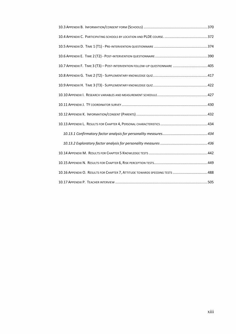
10.3 APPENDIX B. INFORMATION/CONSENT FORM (SCHOOLS) ............................................................. 370
10.4 APPENDIX C. PARTICIPATING SCHOOLS BY LOCATION AND PLDE COURSE. ......................................... 372
10.5 APPENDIX D. TIME 1 (T1) - PRE-INTERVENTION QUESTIONNAIRE ................................................... 374
10.6 APPENDIX E. TIME 2 (T2) - POST-INTERVENTION QUESTIONNAIRE .................................................. 390
10.7 APPENDIX F. TIME 3 (T3) – POST-INTERVENTION FOLLOW-UP QUESTIONNAIRE ................................. 405
10.8 APPENDIX G. TIME 2 (T2) - SUPPLEMENTARY KNOWLEDGE QUIZ .................................................... 417
10.9 APPENDIX H. TIME 3 (T3) - SUPPLEMENTARY KNOWLEDGE QUIZ .................................................... 422
10.10 APPENDIX I. RESEARCH VARIABLES AND MEASUREMENT SCHEDULE ................................................ 427
10.11 APPENDIX J. TY COORDINATOR SURVEY .................................................................................. 430
10.12 APPENDIX K. INFORMATION/CONSENT (PARENTS) .................................................................... 432
10.13 APPENDIX L. RESULTS FOR CHAPTER 4, PERSONAL CHARACTERISTICS ............................................. 434
10.13.1 Confirmatory factor analysis for personality measures........................................... 434
10.13.2 Exploratory factor analysis for personality measures ............................................. 436
10.14 APPENDIX M. RESULTS FOR CHAPTER 5 KNOWLEDGE TESTS ........................................................ 442
10.15 APPENDIX N. RESULTS FOR CHAPTER 6, RISK PERCEPTION TESTS................................................... 449
10.16 APPENDIX O. RESULTS FOR CHAPTER 7, ATTITUDE TOWARDS SPEEDING TESTS ................................. 488
10.17 APPENDIX P. TEACHER INTERVIEW ........................................................................................ 505
xiv
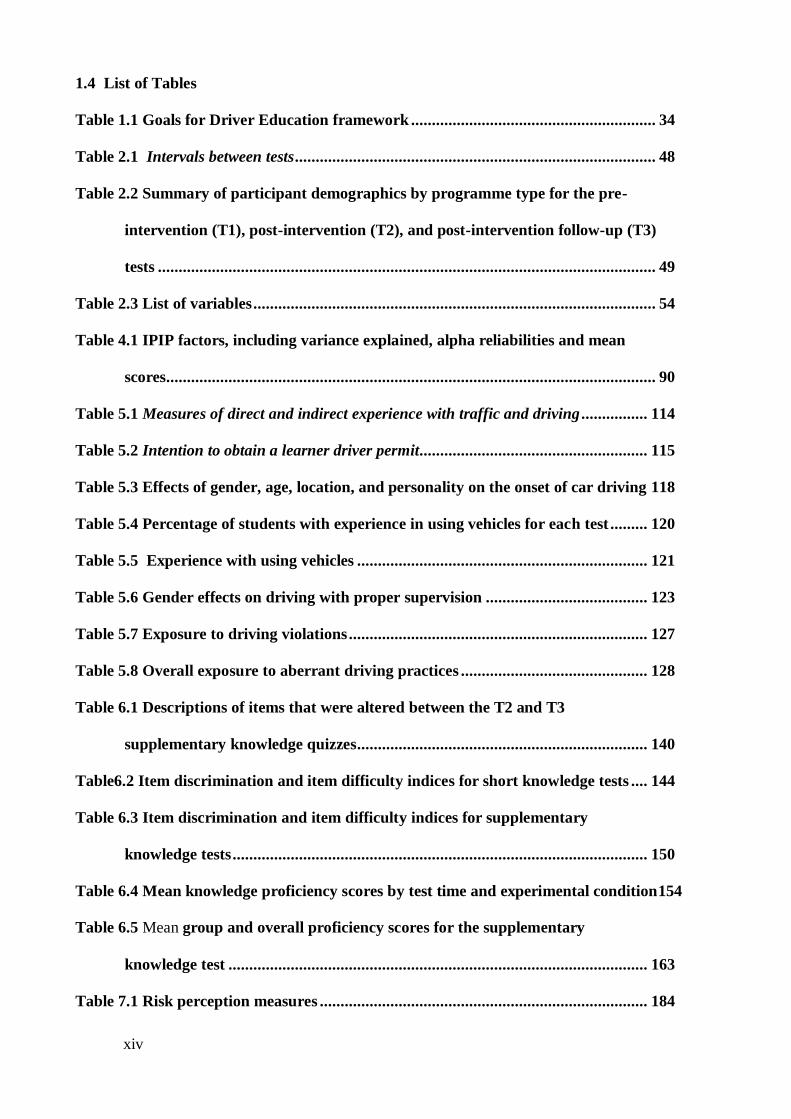
1.4 List of Tables
Table 1.1 Goals for Driver Education framework ........................................................... 34
Table 2.1 Intervals between tests ....................................................................................... 48
Table 2.2 Summary of participant demographics by programme type for the pre-
intervention (T1), post-intervention (T2), and post-intervention follow-up (T3)
tests ........................................................................................................................ 49
Table 2.3 List of variables ................................................................................................. 54
Table 4.1 IPIP factors, including variance explained, alpha reliabilities and mean
scores...................................................................................................................... 90
Table 5.1 Measures of direct and indirect experience with traffic and driving ................ 114
Table 5.2 Intention to obtain a learner driver permit....................................................... 115
Table 5.3 Effects of gender, age, location, and personality on the onset of car driving 118
Table 5.4 Percentage of students with experience in using vehicles for each test ......... 120
Table 5.5 Experience with using vehicles ...................................................................... 121
Table 5.6 Gender effects on driving with proper supervision ....................................... 123
Table 5.7 Exposure to driving violations ........................................................................ 127
Table 5.8 Overall exposure to aberrant driving practices ............................................. 128
Table 6.1 Descriptions of items that were altered between the T2 and T3
supplementary knowledge quizzes...................................................................... 140
Table6.2 Item discrimination and item difficulty indices for short knowledge tests .... 144
Table 6.3 Item discrimination and item difficulty indices for supplementary
knowledge tests .................................................................................................... 150
Table 6.4 Mean knowledge proficiency scores by test time and experimental condition154
Table 6.5 Mean group and overall proficiency scores for the supplementary
knowledge test ..................................................................................................... 163
Table 7.1 Risk perception measures ............................................................................... 184
xv
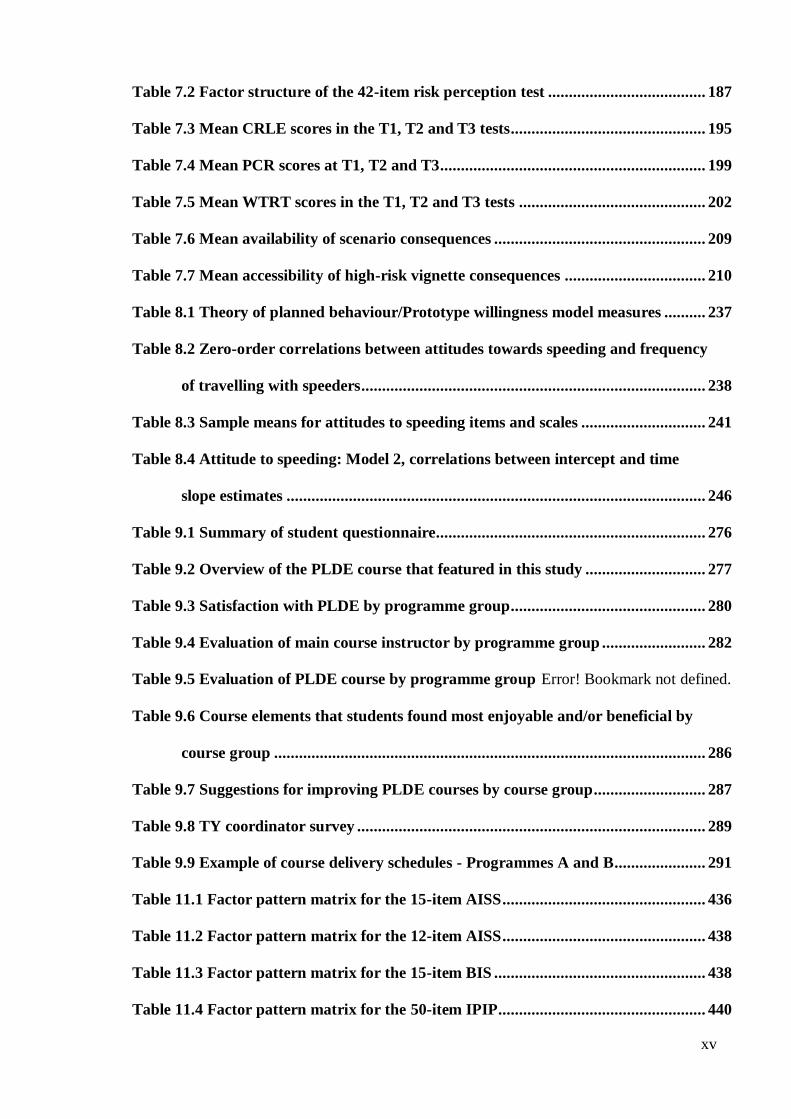
Table 7.2 Factor structure of the 42-item risk perception test ...................................... 187
Table 7.3 Mean CRLE scores in the T1, T2 and T3 tests ............................................... 195
Table 7.4 Mean PCR scores at T1, T2 and T3 ................................................................ 199
Table 7.5 Mean WTRT scores in the T1, T2 and T3 tests ............................................. 202
Table 7.6 Mean availability of scenario consequences ................................................... 209
Table 7.7 Mean accessibility of high-risk vignette consequences .................................. 210
Table 8.1 Theory of planned behaviour/Prototype willingness model measures .......... 237
Table 8.2 Zero-order correlations between attitudes towards speeding and frequency
of travelling with speeders ................................................................................... 238
Table 8.3 Sample means for attitudes to speeding items and scales .............................. 241
Table 8.4 Attitude to speeding: Model 2, correlations between intercept and time
slope estimates ..................................................................................................... 246
Table 9.1 Summary of student questionnaire ................................................................. 276
Table 9.2 Overview of the PLDE course that featured in this study ............................. 277
Table 9.3 Satisfaction with PLDE by programme group ............................................... 280
Table 9.4 Evaluation of main course instructor by programme group ......................... 282
Table 9.5 Evaluation of PLDE course by programme group Error! Bookmark not defined.
Table 9.6 Course elements that students found most enjoyable and/or beneficial by
course group ........................................................................................................ 286
Table 9.7 Suggestions for improving PLDE courses by course group ........................... 287
Table 9.8 TY coordinator survey .................................................................................... 289
Table 9.9 Example of course delivery schedules - Programmes A and B ...................... 291
Table 11.1 Factor pattern matrix for the 15-item AISS ................................................. 436
Table 11.2 Factor pattern matrix for the 12-item AISS ................................................. 438
Table 11.3 Factor pattern matrix for the 15-item BIS ................................................... 438
Table 11.4 Factor pattern matrix for the 50-item IPIP .................................................. 440
xvi
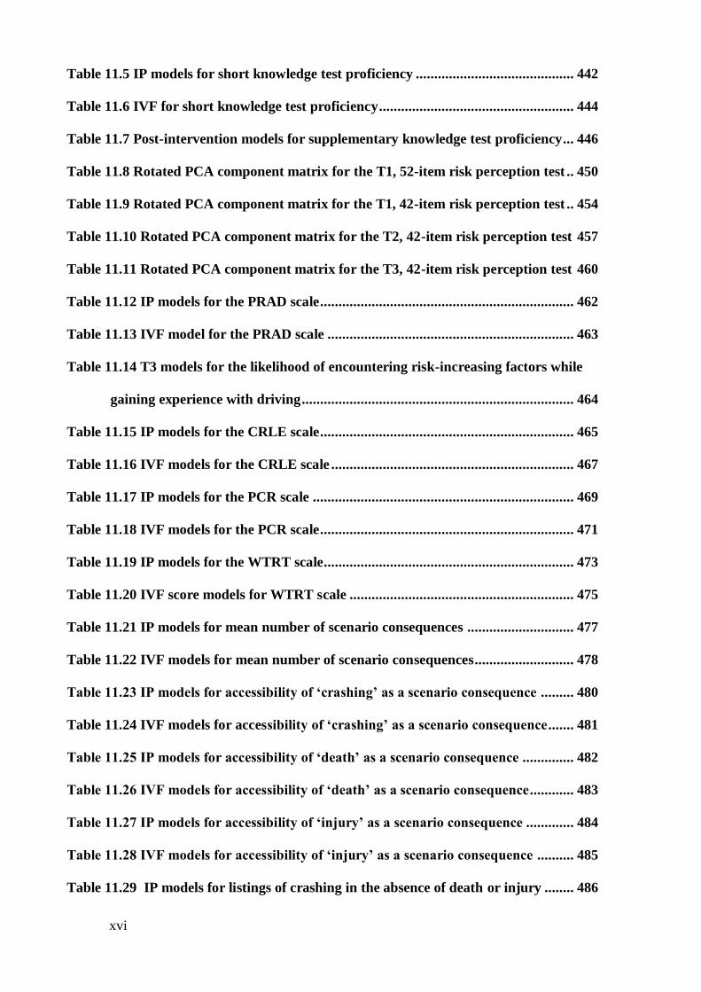
Table 11.5 IP models for short knowledge test proficiency ........................................... 442
Table 11.6 IVF for short knowledge test proficiency ..................................................... 444
Table 11.7 Post-intervention models for supplementary knowledge test proficiency... 446
Table 11.8 Rotated PCA component matrix for the T1, 52-item risk perception test .. 450
Table 11.9 Rotated PCA component matrix for the T1, 42-item risk perception test .. 454
Table 11.10 Rotated PCA component matrix for the T2, 42-item risk perception test 457
Table 11.11 Rotated PCA component matrix for the T3, 42-item risk perception test 460
Table 11.12 IP models for the PRAD scale ..................................................................... 462
Table 11.13 IVF model for the PRAD scale ................................................................... 463
Table 11.14 T3 models for the likelihood of encountering risk-increasing factors while
gaining experience with driving .......................................................................... 464
Table 11.15 IP models for the CRLE scale ..................................................................... 465
Table 11.16 IVF models for the CRLE scale .................................................................. 467
Table 11.17 IP models for the PCR scale ....................................................................... 469
Table 11.18 IVF models for the PCR scale ..................................................................... 471
Table 11.19 IP models for the WTRT scale.................................................................... 473
Table 11.20 IVF score models for WTRT scale ............................................................. 475
Table 11.21 IP models for mean number of scenario consequences ............................. 477
Table 11.22 IVF models for mean number of scenario consequences ........................... 478
Table 11.23 IP models for accessibility of ‘crashing’ as a scenario consequence ......... 480
Table 11.24 IVF models for accessibility of ‘crashing’ as a scenario consequence ....... 481
Table 11.25 IP models for accessibility of ‘death’ as a scenario consequence .............. 482
Table 11.26 IVF models for accessibility of ‘death’ as a scenario consequence............ 483
Table 11.27 IP models for accessibility of ‘injury’ as a scenario consequence ............. 484
Table 11.28 IVF models for accessibility of ‘injury’ as a scenario consequence .......... 485
Table 11.29 IP models for listings of crashing in the absence of death or injury ........ 486
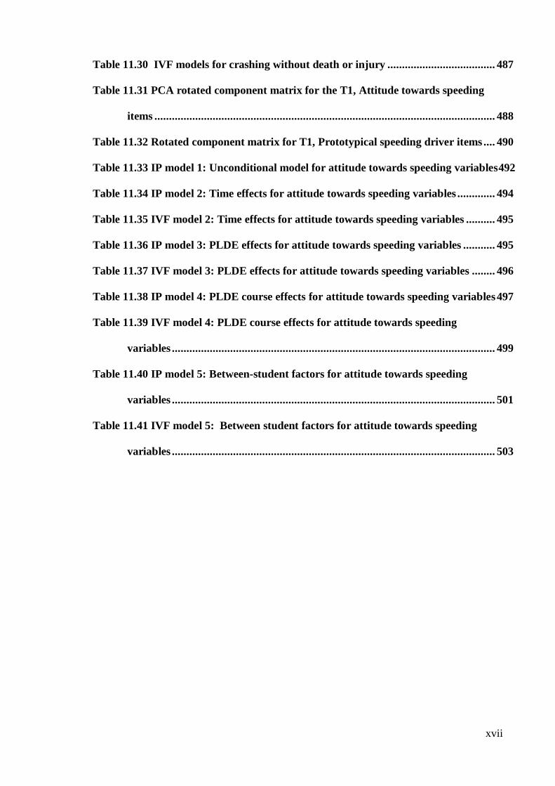
xvii
Table 11.30 IVF models for crashing without death or injury ..................................... 487
Table 11.31 PCA rotated component matrix for the T1, Attitude towards speeding
items ..................................................................................................................... 488
Table 11.32 Rotated component matrix for T1, Prototypical speeding driver items .... 490
Table 11.33 IP model 1: Unconditional model for attitude towards speeding variables492
Table 11.34 IP model 2: Time effects for attitude towards speeding variables ............. 494
Table 11.35 IVF model 2: Time effects for attitude towards speeding variables .......... 495
Table 11.36 IP model 3: PLDE effects for attitude towards speeding variables ........... 495
Table 11.37 IVF model 3: PLDE effects for attitude towards speeding variables ........ 496
Table 11.38 IP model 4: PLDE course effects for attitude towards speeding variables 497
Table 11.39 IVF model 4: PLDE course effects for attitude towards speeding
variables ............................................................................................................... 499
Table 11.40 IP model 5: Between-student factors for attitude towards speeding
variables ............................................................................................................... 501
Table 11.41 IVF model 5: Between student factors for attitude towards speeding
variables ............................................................................................................... 503
xviii
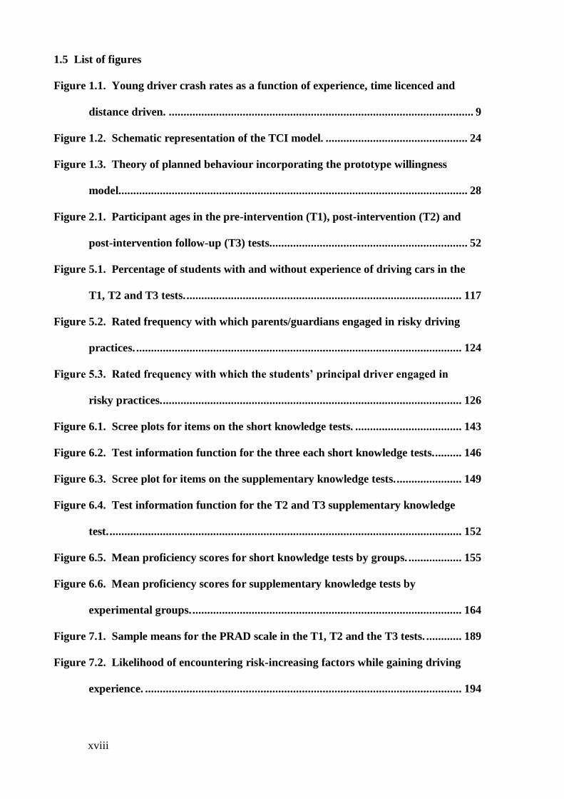
1.5 List of figures
Figure 1.1. Young driver crash rates as a function of experience, time licenced and
distance driven. ....................................................................................................... 9
Figure 1.2. Schematic representation of the TCI model. ................................................ 24
Figure 1.3. Theory of planned behaviour incorporating the prototype willingness
model...................................................................................................................... 28
Figure 2.1. Participant ages in the pre-intervention (T1), post-intervention (T2) and
post-intervention follow-up (T3) tests. .................................................................. 52
Figure 5.1. Percentage of students with and without experience of driving cars in the
T1, T2 and T3 tests. ............................................................................................. 117
Figure 5.2. Rated frequency with which parents/guardians engaged in risky driving
practices. .............................................................................................................. 124
Figure 5.3. Rated frequency with which the students’ principal driver engaged in
risky practices...................................................................................................... 126
Figure 6.1. Scree plots for items on the short knowledge tests. .................................... 143
Figure 6.2. Test information function for the three each short knowledge tests.......... 146
Figure 6.3. Scree plot for items on the supplementary knowledge tests. ...................... 149
Figure 6.4. Test information function for the T2 and T3 supplementary knowledge
test. ....................................................................................................................... 152
Figure 6.5. Mean proficiency scores for short knowledge tests by groups. .................. 155
Figure 6.6. Mean proficiency scores for supplementary knowledge tests by
experimental groups. ........................................................................................... 164
Figure 7.1. Sample means for the PRAD scale in the T1, T2 and the T3 tests. ............ 189
Figure 7.2. Likelihood of encountering risk-increasing factors while gaining driving
experience. ........................................................................................................... 194
xix
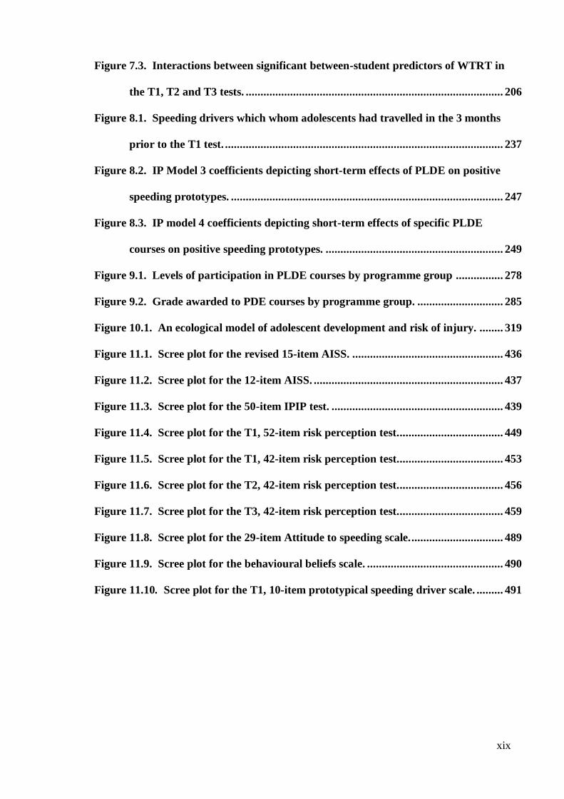
Figure 7.3. Interactions between significant between-student predictors of WTRT in
the T1, T2 and T3 tests. ....................................................................................... 206
Figure 8.1. Speeding drivers which whom adolescents had travelled in the 3 months
prior to the T1 test. .............................................................................................. 237
Figure 8.2. IP Model 3 coefficients depicting short-term effects of PLDE on positive
speeding prototypes. ............................................................................................ 247
Figure 8.3. IP model 4 coefficients depicting short-term effects of specific PLDE
courses on positive speeding prototypes. ............................................................ 249
Figure 9.1. Levels of participation in PLDE courses by programme group ................ 278
Figure 9.2. Grade awarded to PDE courses by programme group. ............................. 285
Figure 10.1. An ecological model of adolescent development and risk of injury. ........ 319
Figure 11.1. Scree plot for the revised 15-item AISS. ................................................... 436
Figure 11.2. Scree plot for the 12-item AISS. ................................................................ 437
Figure 11.3. Scree plot for the 50-item IPIP test. .......................................................... 439
Figure 11.4. Scree plot for the T1, 52-item risk perception test. ................................... 449
Figure 11.5. Scree plot for the T1, 42-item risk perception test. ................................... 453
Figure 11.6. Scree plot for the T2, 42-item risk perception test. ................................... 456
Figure 11.7. Scree plot for the T3, 42-item risk perception test. ................................... 459
Figure 11.8. Scree plot for the 29-item Attitude to speeding scale. ............................... 489
Figure 11.9. Scree plot for the behavioural beliefs scale. .............................................. 490
Figure 11.10. Scree plot for the T1, 10-item prototypical speeding driver scale. ......... 491

1
Chapter 1: Driver behaviour and driver education
Learning to drive is an important milestone for adolescents primarily because
obtaining a driver’s licence constitutes an important rite of passage into adulthood, since it
facilitates increased mobility and independence (Christmas, 2008). As the traffic
environment is inherently risky, the vast majority of learner drivers undertake some form
of driver education and training to provide them with some level (Sagberg, Fosser, &
Saetermo, 1997) of driving competency before they take to the roads (Engstrom,
Gregersen, Hernetkoski, & Nyberg, 2003; Ivers et al., 2006; Shope, 2006; Williams, 2006).
Although traditional forms of driver education (DE) and driver training (DT) generally
succeeded in equipping learners with sufficient knowledge and psychomotor skills to allow
them to become mobile, they have been less successful transmitting safe driving habits
(Elander, West, & French, 1993). This constitutes a considerable problem for newly
fledged drivers, who face considerable challenges when it comes to the balancing their
desire for mobility with the requirement for safety, (Mayhew, 2007).
The sub-discipline of human factors psychology aims to address such problems
using psychological principles as guidelines for designing and creating systems that
enhance performance, increase safety and support user wellbeing. Human factors is a term
used to describe physical, cognitive or behavioural properties of an individual which
impacts on the systems in which they commonly operate and vice versa (Wickens, Lee,
Liu, & Gordon Becker, 2004). In recent years, the development and refinement of theories
which attempt to explain, predict and control risk-taking in drivers exemplifies the
application of human factors principles to improving road safety. These efforts have
focussed mainly on two somewhat complimentary concepts; behavioural adaptation and
risk compensation (Vaa, 2007). On the one hand, behavioural adaptation describes a

2
tendency to consciously adjust behaviour to meet situational contingencies, e.g. to drive
faster when in a hurry (McKenna, 2005). On the other hand, risk compensation theory
posits that behavioural adjustments can also occur as a result of unconscious decision
making (Wilde, 1988). Evidence supporting this latter theory shows, for example, that
drivers using cars with anti-lock brakes drive faster and operate with less headway than
those using cars with standard braking systems (Sagberg et al., 1997). In combination,
both of these theoretical perspectives have made a substantial contribution towards
explaining driver behaviour.
1.1 Road traffic crashes
Driving has always entailed increased exposure to risk. According to Fallon and
O’Neill (2005) it is likely that the first fatal car crash occurred here in Ireland in 1896,
shortly after the development of the internal combustion engine and the subsequent
proliferation of motorised transport. Since then, the numbers of traffic-related deaths and
injuries has risen to such proportions that the World Health Organization (WHO, 2003)
conceptualized road traffic crashes (RTCs) as a “hidden epidemic” because they constitute
a growing, but generally overlooked threat to human health and well-being.
1.1.1 The human cost of RTCs
Following a review of the international RTC data, the United Nations Road Safety
Collaboration (UNRSC) (2011) reported that the global death toll resulting from RTCs had
reached almost 1.3 million people annually by 2010, which equates to approximately 3,500
deaths every day. They also estimated that approximately 50 million people suffer non-
fatal injuries in crashes annually and noted that these injuries frequently result in disability.
Furthermore, they predicted that the global death toll would rise to 2.4 million per year
before 2020 unless improvements are made to the traffic system.
The UNRSC report (2011) also demonstrated that crash involvement represents a
particular risk for younger people: It is among the top three causes of death for 15 –
3
44-year-olds and is the leading cause of death for 15 - 29-year-olds. This general trend is
also reflected within the driver population, where young novices tend to be more crash-
involved than are drivers in other age categories (Drummond, 1989; Elvik, Høye, Vaa, &
Sørensen, 2009; L. Evans, 1991; Gregersen, Nyberg, & Berg, 2003; Mayhew, Simpson, &
Pak, 2003; OECD - ECMT, 2006b; Sagberg, 1998).
Similar patterns of crash-related deaths and injuries emerge from the Irish crash
data. The latest available full set of data shows that there were 26,495 Garda3-reported
collisions in 2009, in which 238 people were killed, 9,742 were injured, 604 of whom were
seriously injured (RSA, 2010a). Alarmingly, however, there is evidence to suggest that
the statistics for injuries following RTCs are underestimated in many countries, including
Ireland. For instance, a recent analysis of trends in acute hospital patient care in Ireland
between 2005 and 2009 showed that the number of people who were admitted to hospital
with serious injuries following RTCs was 3.5 times greater than the number of serious
injuries reported by the Gardaí (Sheridan, Howell, McKeown, & Bedford, 2011).
Although 15- to 24-year-olds constitute 16.5% of the Irish population, and not all of them
drive, motorists in this age group were involved in 37% of crashes in 2009. Thirty percent
of those killed were males, whereas just 6% of those killed were young females. Thus,
young male drivers were five times more likely to be killed than young female drivers.
Age and gender differences in injury crashes were less acute: differences in driver injury
rates between males and females was quite small (males 53% and females 47%) and young
drivers, aged between 15 -24-years were involved in 25% of the total number of injury
crashes and young males constituted 16% of the total whereas young females made up just
10%. However, young female drivers were involved in more property-damage only
crashes (15.5%) than young male drivers (12%) (RSA, 2010a).
3 The official name for the Irish police force is An Garda Síochána and members of the force are
called Gardaí.
4
1.1.2 Financial and social costs of RTCs
Crashes represent a considerable economic and social burden on society (OECD -
ECMT, 2006b). In 2002 the Irish government commissioned Goodbody Consultants to
estimate the financial cost of RTCs. Their report showed that the average cost for each
fatality was just over €2.3 million and the costs for serious injury, minor injury and
property damage only crashes were estimated at €304,600, €30,000, and €2,400,
respectively (Bacon, 2005). After adjusting for inflation, the overall estimated cost of road
traffic crashes in 2009 was €973.5 million; which includes €562.4 million for fatalities,
€158 million for serious crashes, €200 million for minor injury crashes and €53.5 million
for material damage crashes (RSA, 2010a). This represented 0.7% of Gross Domestic
Product in Ireland in 2009. Moreover, the social costs of premature death and injury on the
road and the resulting devastation of the lives of victims and their relatives are impossible
to quantify. Furthermore, a considerable amount of resources are employed dealing with
the aftermath of crashes, which might otherwise be used to support health and well-being
in the community (OECD - ECMT, 2006b).
1.1.3 Causes of RTCs
In light of these considerations, much effort has been expended in investigating the
causes of RTCs and in attempting to devise appropriate remedies (Wickens et al., 2004).
Early studies (e.g. Haddon, 1968) identified three elements that contribute to crashes;
human factors (e.g. behavioural errors and violations), roadway/environmental factors (e.g.
road conditions) and vehicle factors (e.g. bald tyres). Subsequent research conducted in
both the USA and the UK calculated the relative contribution of these factors across a large
number of crashes. The findings suggested that human factors were implicated in 94% -
95% of all crashes (Sabey & Staughton, 1975; Treat, Tumbas, McDonald, & Hume, 1980).
Since driver behaviour was identified as a causal factor in 92% of fatal crashes in Ireland
in 2009 (RSA, 2010a), it seems that human behaviour is also the primary cause of traffic
5
crashes in this jurisdiction. These findings suggest that efforts to reduce RTCs should focus
predominantly on tackling the human contribution to this problem.
1.1.3.1 Driving errors and violations
Human error is defined as “inappropriate human behaviour that lowers levels of
system effectiveness or safety” (Wickens et al., 2004, p. 366). Reason (1990) devised and
empirically tested taxonomy of errors which distinguished between two principal
categories of error; errors of omission which are caused by unintentional failures in
planned action, and errors of commission, which describe deliberate violations of driving
rules and regulations. Based on these findings, Reason and his colleagues developed the
Manchester Driver Behaviour Questionnaire (DBQ) (Reason, Manstead, Stradling, Baxter,
& Campbell, 1990) in an attempt to measure self-reported errors and violations. These
researches believed that driving errors represent performance limitations (e.g. attentional,
perceptual and information processing skills), whereas violations reflect driving style,
which is largely dictated by motivations and also habits established during a driving career
(de Winter & Dodou, 2010). Following an independent review of the behavioural
correlates of variations in crash risk, Elander, West and French (1993) concluded that both
driving skill (what the driver ‘can’ do) and driving style (what the driver ‘does’ do) are
crucial in determining driver safety.
The DBQ has been used extensively to predict RTCs. In a recent meta-analytic
review of 173 DBQ studies, de Winter and Dodou (2010) reported that there was an
medium sized correlation (r = .4) between DBQ scores and self-reported crashes, after
correcting for measurement error. They also showed that errors and violations were
equally strong predictors of crashes, reporting correlations of .07 and .06 for each factor
respectively. This contradicts previous findings that suggested that only errors (deLucia,
Bleckley, Meyer, & Bush, 2003) or only violations (see Stradling, Parker, Lajunen,
6
Meadows, & Xie, 1998) predicted crashes. Gender differences in the propensity to commit
errors and violations were also identified in many of the studies. Males were less
susceptible to errors and more prone to violations than females (de Winter & Dodou, 2010;
Wells, Tong, Sexton, Grayson, & Jones, 2008). In general, the incidence of both errors
and violations decreases with age, although, interestingly, data from studies with younger
samples (e.g. Wells et al., 2008) suggests that the commission of violations actually
increases with age in the shorter term. However, it is assumed that this result represents
the confounding effects of increasing experience rather than age per se. This can be
explained in terms of theories of behavioural adaptation and compensation, which were
outlined earlier, which suggest that drivers alter their behaviour to satisfy personal
motivation and situational demands (Vaa, 2007; Wilde, 1988). Another line of enquiry
examined the effects of antecedent errors and violations on the types of crashes that young
novice drivers suffer. For example, in a study that analysed over 2,000 crashes involving
16—19-year-old American drivers, McKnight and McKnight (2003) found that the vast
majority of non-fatal crashes were due to errors of omission, (i.e. failure to operate safe
routine and failure to recognise the danger in this practice), rather than the result of
deliberate risk taking. Evidence also suggests that the fatal crashes of young drivers have a
distinct aetiology. Gonzales, Dickinson, DiGuiseppi and Lowenstein (2005) examined
fatal crash records for young novice drivers in Colorado, using the U.S. Government’s
Fatal Analysis Reporting System database (FARS) and found that these were characterized
by speeding, recklessness, single-vehicle and rollover crashes, which were mainly
attributable to deliberate violations of traffic laws.
In sum, human behaviour in the form of driving errors (i.e. skill deficits) and/or
violations (i.e. aberrant driving styles) are responsible for a large proportion of RTCs.
Among the novice driver population, the propensity to commit errors tends to increase in
the early stages of driving as a function of increasing experience and this leads to increases
7
in non-fatal collisions in the short-term. Fatal collisions are more strongly associated with
violations of traffic regulations, which are more indicative of aberrant driving habits
(style).
1.1.4 The young novice driver problem
Empirical evidence suggests that three key factors, age, inexperience and gender,
contribute to the commission of errors and violations and therefore to the excessive crash
risk evidenced amongst younger drivers (OECD - ECMT, 2006b). The overrepresentation
of young, novice and male drivers in Irish crash statistics reflects a global phenomenon
which has been described as “so robust and repeatable that it is almost like a law of nature”
(L. Evans, 1991, p. 41).
Since most individuals begin driving when they are young, it is inherently difficult
to assess the absolute effects of either age or inexperience on driver behaviour. Several
studies addressed this problem by estimating the relative risk of crashing for drivers in
different age groups, while simultaneously controlling for driving experience. For
example, using the FARS database, Evans (1991) calculated that the crash rate among
American 16-year-olds was almost three times that of 18-year-olds. Also, in a study that
compared the self-reported crash and violation rates of 28,500 Finnish novices from three
age groups, 18-20-year-olds, 21-30-year-olds and 31-50-year-olds, Laapotti, Keskinen,
Hatakka and Katila (2001) found higher incidences of crashes and offences among the
younger novices, especially males. They also showed that the types of driving incidents
reported by young males related more to risky driving rather than poor vehicle control
skills whereas the opposite was true of young females. Vlakveld (2005; as cited
inWegman & Aarts, 2006) also isolated the effects of age and experience by analysing the
crash records of Dutch drivers who were licenced at either 18-21, 23-27, or 30-40 years of
age and found that for those who started driving at 18, approximately 40% of the reduction
8
in crash risk over time was attributable to increasing age, whereas the remaining 60% was
associated with increasing experience with driving.
Evidence from a wide range of studies supports the view that inexperience is the
primary cause of the young novice driver problem (OECD - ECMT, 2006b). Learning to
drive takes time, because driving is a complex task which involves the coordination of a
range of skills including psychomotor skills which coordinate a wide range of basic tasks
(e.g. steering, braking) and also higher order cognitive skills ( e.g. risk and hazard
perception, problem solving), which underlie safe performance (Hatakka, Keskinen,
Gregersen, Glad, & Hernetkoski, 2002; Mayhew, Simpson, & Robinson, 2002). Thus, it
takes a considerable amount of effortful practice to achieve competency (Dreyfus &
Dreyfus, 1986; Elvik et al., 2009). Research conducted in the U.S. by Edwards (2001)
showed that just 10% of novice crashes were caused by poor vehicle control skills,
whereas 90% of collisions were attributable to deficits in driving-related cognitive
functioning, such as inaccurate risk perception, overestimation of driving skills and
deliberate risk taking, which are largely contingent on inexperience and/or immaturity (see
Arnett, Offer, & Fine, 1997; Drummond, 1989; L. Evans, 1991; McKnight & McKnight,
2003).
The results from longitudinal studies of learner and novice driver performance highlights
the effects of experience and show that there is a dramatic decrease in crash involvement
among young drivers in the 6-8 months immediately after they pass the driving test
(Mayhew et al., 2003; Sagberg, 1998; Wells et al., 2008). For instance, Mayhew et al.
(2003) found that the crash rate among 16-19-year-olds dropped by 42% in their first 7
months of independent driving. This rapid fall in crash rates soon after licencing suggests
that the young driver problem is more related to inexperience than it is to age. This
evidence also supports the view that driving skills develop as a power function of driving
experience, i.e. improvement is rapid at first but decreases as the learner becomes more
9
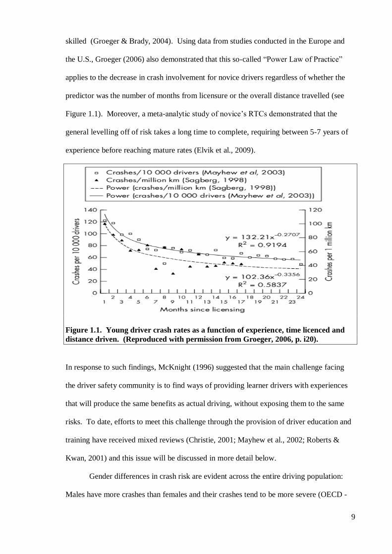
skilled (Groeger & Brady, 2004). Using data from studies conducted in the Europe and
the U.S., Groeger (2006) also demonstrated that this so-called “Power Law of Practice”
applies to the decrease in crash involvement for novice drivers regardless of whether the
predictor was the number of months from licensure or the overall distance travelled (see
Figure 1.1). Moreover, a meta-analytic study of novice’s RTCs demonstrated that the
general levelling off of risk takes a long time to complete, requiring between 5-7 years of
experience before reaching mature rates (Elvik et al., 2009).
Figure 1.1. Young driver crash rates as a function of experience, time licenced and
distance driven. (Reproduced with permission from Groeger, 2006, p. i20).
In response to such findings, McKnight (1996) suggested that the main challenge facing
the driver safety community is to find ways of providing learner drivers with experiences
that will produce the same benefits as actual driving, without exposing them to the same
risks. To date, efforts to meet this challenge through the provision of driver education and
training have received mixed reviews (Christie, 2001; Mayhew et al., 2002; Roberts &
Kwan, 2001) and this issue will be discussed in more detail below.
Gender differences in crash risk are evident across the entire driving population:
Males have more crashes than females and their crashes tend to be more severe (OECD -
10
ECMT, 2006b). Furthermore, this pattern emerges soon after licensure (Engstrom et al.,
2003; Kweon & Knockelman, 2003; Wells et al., 2008). Research also indicates that the
gap between young males and young females is widening over time. Twisk and Stacey
(2007) reported the results of a study that compared relative risk of crashing for younger
drivers against that for older drivers in the Netherlands, Sweden and Great Britain in 1994
and 2001. The results showed that whereas in 1994 young males were between 3.5 and 5
times more likely to crash than older males, by 2001, the relative risk for younger drivers
ranged between 6 and 7.5 times greater than their older counterparts. In the same period,
young females were only twice as likely to crash as older drivers and this ratio of risk
remained stable across time. Twisk and Stacey believe that these findings indicate that
young female drivers tend to profit more from current improvements in road safety to a
greater extent than young men, which suggests that a lot more research needs to be done
into the causes of high-risk driving in young males in order to redress this balance.
In summary, the young novice driver problem arises because this group face
excessive levels of risk on the road which is mainly attributable to a combination of age
and inexperience, which is further exacerbated when the driver is male (OECD - ECMT,
2006b). Inexperience poses a greater risk than age and although it takes 5-7 years to gain
enough experience to achieve risk equalisation with more mature drivers, the most acute
risk phase occurs within the first few months of driving (Groeger, 2006). Because of this,
it is easier to mitigate the risk posed by inexperience than that associated with age-related
factors (Shope, 2006). There is a marked difference in the pattern of crashes for young
males compared to that for young females (Wells et al., 2008). Males have more crashes
than females and their collisions are more likely to be a result of their driving style
(violations), whereas females’ crashes appear to be caused primarily by skill-based deficits
(errors) (de Winter & Dodou, 2010). Alarmingly, the comparative risk for young males in
relation to their female counterparts and also older males seems to have increased in recent
11
years, which suggests that countermeasures, including driver education and training, may
be less effective in mitigating risk for young males (Twisk & Stacey, 2007).
1.2 Driver education and training
Driving is a complex task and learning to drive involves the acquisition and
subsequent coordination of a range of skills, rules and knowledge that help learners to stay
safe in traffic (Dreyfus & Dreyfus, 1986; Rasmussen, 1983). Formal DE and DT have
good face validity; they are popular among learners and their parents (Fuller & Bonney,
2004), and also with the authorities, and other stakeholders (C. Johnson, Hardman, &
Luther, 2009; Lonero et al., 1995) in all countries where this type of instruction is available
(Wegman & Aarts, 2006). This is mainly because they are believed to be effective in
providing aspiring drivers with basic car control skills and knowledge of the rules of the
road which are prerequisites to obtaining a licence (Christie, 2001). However, empirical
evidence suggests that traditional forms of DE and DT have been ineffective generally
when it comes to reducing post-licence crashes (Christie, 2001; McKenna, 2010a; Roberts
& Kwan, 2001). For instance, comparisons between the post-licence crash records of
professionally and informally trained (i.e. instructed by parents and/or friends) novice
drivers indicate that there is no statistical differences in crash outcomes between these
groups (Groeger & Brady, 2004; Lynham & Twisk, 1995; Wells et al., 2008).
1.2.1 Defining driver education, driver training, pre-drivers and pre-learner
drivers
Before reviewing the evidence in the DE debate it is worth making a distinction
between DE, and DT, since these terms are regarded as synonymous in some sections of
the literature (Christie, 2001). In North America for example, DE typically describes
programs for new drivers that consist of both classroom learning and practical in-car
training (Lonero, 2008). The conflation of these terms is not particularly helpful for two
reasons: First, it makes it difficult to differentiate between programmes that provide

12
education or training alone in order to isolate the absolute effects of these somewhat
distinct processes. Second, the overall conclusions reached in some systematic reviews
concerning the efficacy of DE programmes are not as reliable (or informative) as they
might be because they are often based on the results from a range of studies that are not
equivalent because of variations in the relative amounts of education and training in the
curricula of the programmes under investigation. For example, a review published by the
world-renowned Cochrane Collaboration (i.e. Roberts & Kwan, 2001) included the results
from studies where the ratios of practical to classroom instruction ranged between 32 hours
of education and 39 hours of training in the case of the Safe Performance Curriculum
condition in the DeKalb county education project (Stock, Weaver, Ray, Brink, & Safoff,
1983) and 15 hours of education and 8 hours of training for Wynne-Jones and Hurst’s
(1984) study of high school driver education in New Zealand.
Outside of North America, the situation with respect to DT and DE is clearer.
There, researchers commonly distinguish between these two processes, thereby providing
practical options for those who want to examine these processes individually. In this
literature, the term training is used to describe the transmission of practical skills and
competencies, such as accelerating, changing gears, and braking, that are needed to control
and operate a vehicle (Christie, 2001; Woolley, 2000), and education is used to refer to
class-room based instruction which focuses on the broader intellectual/cognitive aspects of
learning to drive, i.e. knowledge (e.g. the rules of the road), attitudes (e.g., over-
confidence) and behaviours (e.g., risk-taking) (Christie, 2001). In the interest of clarity,
these latter definitions were adopted in the current research.
Similar problems beset the nomenclature used for the recipients of DE. The term
pre-driver (PD) is used widely to describe individuals of any age who have not yet learned
to drive (Deighton & Luther, 2007). However, school-based pre-driver education is an
intervention strategy that is aimed at secondary school students between 15 – 16-years-old

13
who are still too young to obtain a learner driver permit, and thus avail of driver training
(Siegrist, 1999). Therefore, this group constitute a special class of pre-drivers, and as such
need their own designation. The present study used the term pre-learner driver (PLD),
(after Senserrick, 2007) to describe its participants, the overwhelming majority of whom
were 16-years old or younger when the study commenced. In addition, the term pre-
learner driver education (PLDE) was adopted to describe educational interventions that
have been designed for these students.
1.2.2 The DeKalb county driver education project
Pre-driver education/training programmes were developed initially in the late
1940s. In 1949, the U.S. National Education Association’s national Commission on Safety
Education recommended a standard for driver education and training based on 30 hours of
classroom training and 6 hours of behind-the-wheel training. This represented a
compromise between the time needed to teach driver education and the time feasible (and
funded) for teaching driving skills during school hours (J. Nicholson, 2003). Although
many evaluations of school-based pre-driver education (PDE) programmes have been
reported in the literature, the DeKalb County Education Project (Stock et al., 1983) is a
particularly interesting example of this genre, because it is acknowledged as the most
comprehensive and methodologically rigorous experiment in school-based PDE ever
undertaken (Lonero et al., 1995). Thus, it has featured in a number of high-profile reviews
of PDE (e.g. Christie, 2001; Deighton & Luther, 2007; Drummond, 1989; Lonero &
Mayhew, 2010; Mayhew et al., 2002; Roberts & Kwan, 2001; Vernick et al., 1999). The
project was conducted in the U.S. state of Georgia in the late 1970s and involved over
16,000 students, who were randomly assigned to one of three experimental groups; two
treatment groups and a control group.
The first treatment group received 72 hours of instruction based on the newly
developed Safe Performance Curriculum (SPC), which involved 32 hours of classroom
14
education, 16 hours in a driving simulator, 16 hours on a driving range, three hours
instruction in evasive manoeuvring and five hours on-road training. The second treatment
group took a pre-driver licencing course (PDLC), which was considered as a minimal
preparation for passing the driving test. This entailed 20 hours of basic driver training,
including classroom instruction, driving range and simulation instruction as well as
practice driving with parents. The control group were given no formal instruction in
school, rather it was expected that they would be taught to drive by their parents and/or by
commercial driving schools. No restrictions were placed on either the type or the amount
of instruction that they could receive (Mayhew & Simpson, 1996).
The students were monitored over the following six years where their uptake of
training and driver licencing was recorded and their crash and violation records were
monitored. Early results from this study showed that contrary to expectations, the SPC
group were involved in more accidents than were those in the PDLC and the control
groups. This outcome was mainly attributed to the fact that students in the SPC group
obtained driving licences earlier than did those in the other groups, which increased their
exposure to risk (Stock et al., 1983). Subsequent analyses, that attempted to control for
differential rates of licencing in the groups by including data from only those students who
had obtained a driving licence, reported that the mean number of collisions was lower in
the SPC group than it was in both the PDLC and control group in the first six months of
licenced driving, albeit that this difference was not statistically significant (Stock et al.,
1983). Nevertheless, because the difference in scores between the SPC group and the
controls approached significance (p = 0.076) Stock and his colleagues suggested that this
indicted that the SPC programme was effective (Stock et al., 1983), although no effect size
was reported. However, these beneficial effects were no longer evident during follow-up
studies using data collected 12, 18 and 24 months after the programmes ended. The results
from a further test, conducted 6 years after the programmes ended, also showed that there
15
were no significant reductions in crashes for the SPC group compared to the controls.
Surprisingly, however, this study revealed a small, but significant reduction in crashes for
students in the PDLC group compared to the controls (Smith & Blatt, 1987). Altogether,
these outcomes, even the positive ones, fell way below expectations and the apparent
superiority of the PDLC remains perplexing (Mayhew & Simpson, 1996).
Aside from prompting a major theoretical debate about the value of DE (which is
discussed in detail below) the various analyses of the DeKalb data served to highlight some
of the methodological problems that can arise, even in well designed and properly executed
studies. Although randomized control designs are widely regarded at the ‘gold standard’ in
scientific research (Donaldson, 2009), it can be difficult to establish and maintain
experimental control. In the DeKalb study for instance, although students were randomly
assigned to the various experimental conditions and stringent efforts were made using
stratified sampling, to balance these groups in terms of group numbers and student
demographics (gender, socio-economic status etc.), inevitably there was differential
attrition in the three groups. Some of the students assigned to the active groups never
actually attended their assigned course and/or did not start driving within the time frame
covered by the various studies. Furthermore, the reliability of the results from the second
analysis (Stock et al., 1983), which showed some positive effects of PDE, was challenged
on the grounds of potential self-selection bias, since it featured the records of just those
students who completed their allotted courses and actually started driving. Finally and
perhaps most importantly, there was a problem with maintaining the status quo among
participants in the control group, which is a well-documented difficulty in applied research
(Lonero & Mayhew, 2010). In laboratory studies it is relatively easy to ensure that the
members of a control group all participate under the exact same conditions. However this
type of standardisation is impossible to achieve when conducting community-based
research, due to the ongoing influence of a myriad of differential factors on individuals in
16
their daily lives (Shaughnessy, Zechmeister, & Zechmeister, 2009). The DeKalb
researchers tried to ameliorate this problem by assuming that rather than not learning how
to drive at all, the participants in the control group would learn in the community using
formal and informal education and training. This situation undoubtedly made it more
difficult for the researchers to identify the absolute effects of school-based education and
training, because rather than being compared with individuals who received no education
or training at all, students in the PDE groups were being compared with individuals who
almost certainly did receive some driver education and/or training, the exact form and
composition of which was not quantified in any systematic way during the study.
1.2.3 The driver education debate
The results from the DeKalb study initiated widespread debate over the safety value
of school-based DE, which not alone polarized opinion, but also led to the near-extinction
of large scale DE projects (Williams, Preusser, & Ledingham, 2009). The sceptics in this
debate, including the majority of the research community, concluded that DE doesn’t
work, because the empirical evidence indicated that it was not effective in reducing RTCs.
In opposition, many practitioners, managers, and more recently, a growing number of
researchers (e.g. Clinton and Lonero (2006c); McKenna (2010a)) argued that just because
individual PDE programmes failed to reduce crash involvement in their graduates, this
does not mean that training and education per se are incapable of producing lasting safety
benefits.
Sceptical opinion was predominantly formulated on the basis of the results from
systematic reviews of empirical evaluations that had been conducted over the past twenty
years in relation to individual DE and DT programmes that had been designed for pre-
drivers, learners and novices (e.g. Christie, 2001; Deighton & Luther, 2007; Drummond,
1989; Lonero & Mayhew, 2010; Mayhew et al., 2002; Roberts & Kwan, 2001; Vernick et
al., 1999). These reviewers were generally disparaging of DE, because many of the studies
17
featured reported minimal and inconsistent safety-related improvements in course
participants. Following their review of 9 studies of school-based PDE programmes that
included two randomised controlled trials, two re-analyses of the DeKalb randomised
controlled study and five ecological studies (i.e. investigations of recorded changes in
crash outcomes following legislative changes to the rules for driving), Vernick et al.,
(1999) concluded that there was no convincing evidence to suggest that students who
completed these courses had fewer car crashes or driving violations than those who did not
take such a course. For instance, they showed that the proportion of high school students
who take PDE courses in individual states in the U.S. was unrelated to the fatal crash
involvement of 16 – 18-years-old adolescent drivers. The potential drawbacks of PDE
were also noted in the conclusion of a review conducted for the Cochrane Collaboration by
Roberts and Kwan (2001), which suggested that driver education may lead to a small but
significant increase in teenage crash involvement due to early licensure. It has also been
suggested that mere participation in such courses may induce unrealistic beliefs and
expectations regarding the subsequent capabilities of PDE graduates in the students
themselves (Wilde, 1994) and in their parents (Waller, 1983). This accumulation of
negative appraisals of school-based PLE by well-respected researchers led seasoned
analysts (e.g. Christie, 2001), to question the wisdom of spending time and money on
interventions that don’t work, rather than using those resources to support measures that do
work, e.g. the enactment of stricter legislation and stricter enforcement of existing
legislation.
Although supporters of DE (e.g. Clinton & Lonero, 2006c; McKenna, 2010a,
2010b) admit that these types of interventions have a poor track record with respect to
crash reduction, they believe that it is wrong to conclude that DE does not work on the
basis of this sole criterion. Instead, they propose that such conclusions are intemperate
because they are based on an oversimplified conceptualisation of the driving task, of the
18
role and functions of the educational process, and of human nature in general. These
observations serve to highlight a fundamental flaw in the rationale (i.e. the logic model)
that underpins a wide range of social programming interventions which aim to prevent or
ameliorate societal problems, i.e. the joint assumptions that (a) specific educational
programmes encompass elements (content and processes) that are both necessary and
sufficient to impart optimal levels of knowledge and skills and instil well-adjusted attitudes
in all students and (b) that there is a relatively lawful, simple and direct relationship
between educational inputs and long-term behavioural outputs (Donaldson, 2003).
However, the complexity of the relationship between knowledge, skills, attitudes and
actual behaviour is well-documented in the psychological literature (Deighton & Luther,
2007; Durkin & Tolmie, 2010), most notably in areas of direct learning (Leslie &
O'Reilly, 2003; Skinner, 1974), social learning (Bandura, 1977), the acquisition and
maintenance of skills (Anderson, 1982; Ericsson, Krampe, & Tesch-Romer, 1993) and also
attitudes (Ajzen, 1991) and attitude change (Prochaska & DiClemente, 1992). This means
that it is harder to achieve lasting desirable and beneficial changes in driver behaviour
than is generally anticipated (Lonero et al., 1995; Lonero & Mayhew, 2010). For instance,
the apparent failure of DE programmes to reduce crashes has been attributed to the fact
that young drivers may be either unable or unwilling to make appropriate decisions using
the skills and the knowledge that they have acquired as a result of having taken these
courses (Vernick et al., 1999). The true scale of this problem was summarised by
Williams, Preusser and Ledingham (2009), as follows: First, PDE courses are too short
and most of the time is spent teaching basic vehicle handling skill, leaving little time for
teaching safety skills. Second, it is likely that the motivation to obtain a licence as soon as
possible outweighs any safety concerns that PDE students may have. Finally, they noted
the difficulties associated with influencing lifestyle and development factors, which
represents a considerable barrier to driver education effectiveness. In this regard, research
19
shows that there is a positive correlation between the driving behaviours of parents and
their adolescent and young adult offspring (Ferguson, Williams, Chapline, Reinfurt, & De
Leonardis, 2001; Miller & Taubman - Ben-Ari, 2010). Studies also show that adolescents
drive faster and take more risks when they are accompanied by peers (Arnett et al., 1997),
especially males (Baxter, Manstead, Stradling, & Campbell, 1990). There is also a well-
documented association between certain personality traits, such as sensation seeking
(Arnett et al., 1997) and impulsiveness (Stanford, Greve, Boudreaux, Mathias, &
Brumbelow, 1996), and risk-taking, including risky driving. Thus, the impact of PDE can
be easily superseded by such strong and persistent influences.
Discouraging as this might seem, Williams et al’s analysis (2009) nevertheless
identified important themes and issues that need to be addressed if DE is to play a useful
role in tackling the young driver problem. Specifically, it (a) questioned the feasibility of
requiring that DE programmes produce demonstrable safety outcomes in terms of a
reduction in crash involvement, (b) highlighted imbalances in existing curricula that seem
to favour the practical aspects of DE over safety aspects, (c) recognized the importance of
motivational factors and (d) emphasised the role that antecedent lifestyle and
developmental factors play in moderating the effectiveness of educational interventions.
Given their relevance to the present research, these issues will now be examined in more
detail.
There has been considerable debate about what should be considered as legitimate
expectations and goals for PDE (Lonero & Mayhew, 2010). The requirement to produce
sustainable and measurable long-term safety benefits is seen as unreasonable for a variety
of reasons. For example, driving involves the balancing to two somewhat conflicting
goals: the desire for mobility and the need for safety (Wickens, 1992). As a method,
school-based education is geared towards achieving results in relation to well-defined topic
areas that are measured over the short-term by means of continuous assessment and exams.
20
Thus, school-based driver training/education is well placed to cater for students’ short-term
mobility (instrumental) needs by focussing mainly on the ‘control’ aspects of driving i.e.
transmitting the skills and knowledge required to pass the driving test and start a life of
independent driving (Lonero et al., 1995). However, Waller believes that it is
unreasonable to hold PDE responsible for the long-term safety performance of students,
since that would be akin to “...holding home economics teachers responsible for whether
the students prepare well-balanced meals two years later (1975, p. 2).” Taking a
behaviourist perspective, Fuller (1992) noted that since the traffic system is very forgiving
of errors and violations, it can inadvertently “shape” undesirable practices by intermittently
but regularly reinforcing them and rarely, if ever, punishing them. Thus, even though PDE
may be able to provide students with the relevant knowledge, skills and attitudes which
serve as a solid foundation for safe driving, subsequent experience gained while driving
tends to erode this foundation. Thus, there is clearly a need to supplement basic PDE with
other forms of extended learning opportunities, such as graduated driving licencing
(GDL)4.
Although it seems that DE is not very effective in increasing road safety by
reducing the number of RTCs, McKenna (2010a) suggests that educational interventions,
including DE, may actually work to increase safety in a more subtle and indirect way e.g.
by promoting the ‘perceived legitimacy’ of actions. Countering Christie’s (2001)
suggestion that DE interventions should be scaled-back in order to divert existing resources
into alternative road safety measures such as enforcement and engineering, McKenna
argued that it is unlikely that there would be much political or public support for such
measures in the absence of the type of psychological priming that educational measures
currently provide. This position assumes that the value of education lies in its (supposed)
4 The issue of graduated driving licences is beyond the scope of this thesis. For a comprehensive
review of GDL see (Williams & Shults, 2010).
21
ability to induce changes in attitudes at a cultural level that “facilitate, enable, or are
necessary for those interventions that do work” (McKenna, 2010a, p. 14).
Support for this hypothesis is provided by an evidential shift in attitudes regarding
driving while intoxicated (DWI) in Ireland following a series of national media campaigns
that highlighted this problem. This research, which was conducted as part of the EU’s
Social Attitudes to Road Traffic Risk in Europe (SARTRE) project, estimated the
effectiveness of the campaigns by comparing the results from the pre-campaign study
(SARTRE 2) (Fuller & Gormley, 1998) with those recorded in the SARTRE 3 study
(Gormley & Fuller, 2005), which was conducted when the campaigns had been running for
over 6 years. The results suggested that some progress was made in improving drivers’
attitudes with respect to DWI during this period. The number of drivers who believed that
the decision about whether or not to drink and drive should not be left up to drivers
themselves decreased by 14% and support for a proposal to decrease the current permitted
maximum blood/alcohol limit had risen by 20% (Gormley & Fuller, 2005). These changes
in attitudes most likely reflect a cultural change that was facilitated by the provision of
educational interventions that aimed, among other things to, increasing awareness of the
social implications of DWI.
1.2.4 Reinventing driver education
The impetus to develop better programme theories and models is evidenced in the
objectives outlined in the AAA Foundation’s “Novice Driver Education Model Curriculum
Outline” position paper (Lonero et al., 1995). This suggested that there was an urgent
requirement to assess the needs of novice drivers comprehensively, to evaluate methods of
instruction and to assess the effectiveness of DE in influencing driver behaviour (Lonero et
al., 1995). In Europe, concerted efforts to improve DE culminated in the formulation of
the EU’s Goals for Driver Education framework (GDE) (Siegrist, 1999), which provided
detailed recommendations regarding the topics that need to be addressed by driver
22
education, including knowledge and skills related to vehicle handling, to operating in the
traffic environment, to trip planning, and to lifestyle planning. The framework also
highlights the importance of providing students with insight regarding risk increasing
factors and also with metacognitive skills which allow them to assess their driving-related
motivations, (e.g. peer pressure) on an ongoing basis (Hatakka et al., 2002).
Both of these approaches were informed by existing theoretical models, such as
Michon’s Hierarchical Control model (1985), and Fuller’s Task-Capability Interface
model (2000), which describe the relationship between a range of distal and proximal
antecedent factors that hypothetically ‘cause’ driving behaviour and thus give rise to
subsequent consequences in the traffic environment. They each describe the hierarchical
ordering of an extensive range of driver characteristics including driving skills, personal
values and motivations, self-management skills and driving behaviours which are regarded
as ‘educable qualities’ and thus seen as legitimate targets for PDE (Lonero, 2008). By
taking this new and more systematic approach to driver instruction, organizations such as
the AAA Foundation and the E. U. Commission for Transport and Road Safety aim to
reduce the numbers of RTCs among learner and novice drivers.
1.2.5 Theoretical models of driver behaviour
Two classes of theoretical models of driver behaviour emerged in the literature; basic
descriptive models and more complex motivational models. Descriptive models, such as
Dreyfus and Dreyfus’s (1986) 5-stage hierarchical model of skill acquisition and Michon’s
Hierarchical Control Model (1985), focus on specifying the driving process itself in terms
of what the driver needs to do. Michon’s model subdivides the driving task into three
hierarchically ordered levels that describe control (e.g. steering, braking), manoeuvring
(e.g. giving right of way in traffic) and strategic (e.g. trip and route planning) operations.
However, whereas descriptive models provide a solid basis for the systematic examination
of driving behaviour, their usefulness is somewhat constrained because they focus solely
23
on the acquisition and maintenance of driving skill, without taking account of important
dynamic interactions between forces that influence driver performance including
motivation, capabilities and situational factors (Carsten, 2007). This view is supported by
evidence presented earlier, which shows that young novice drivers are at the greatest risk
of crashing just after they complete their driving test successfully (Groeger, 2006). Thus, a
range of more complex motivational models were developed which attempt to provide a
more comprehensive explanation of driver behaviour (Oppenheim et al., 2010). The
rationale behind the motivational approach was summarised by Fuller (1984), who noted
that because driving is fundamentally a self-paced task, it is the drivers actions that
determine the degree of difficulty of the driving task from one moment to the next.
Therefore, the driver’s motivations are often more important than are their physical and
perceptual capabilities in determining the safety of their performance.
1.2.5.1 The task-capability interface model
Fuller’s (2005) task-capability interface model (TCI) exemplifies motivational
models of driver behaviour (see Figure 1.2).
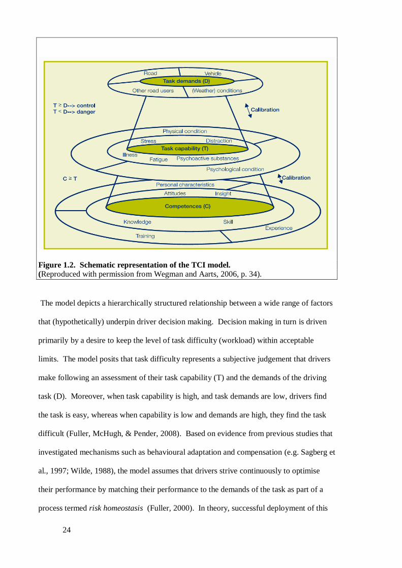
24
Figure 1.2. Schematic representation of the TCI model.
(Reproduced with permission from Wegman and Aarts, 2006, p. 34).
The model depicts a hierarchically structured relationship between a wide range of factors
that (hypothetically) underpin driver decision making. Decision making in turn is driven
primarily by a desire to keep the level of task difficulty (workload) within acceptable
limits. The model posits that task difficulty represents a subjective judgement that drivers
make following an assessment of their task capability (T) and the demands of the driving
task (D). Moreover, when task capability is high, and task demands are low, drivers find
the task is easy, whereas when capability is low and demands are high, they find the task
difficult (Fuller, McHugh, & Pender, 2008). Based on evidence from previous studies that
investigated mechanisms such as behavioural adaptation and compensation (e.g. Sagberg et
al., 1997; Wilde, 1988), the model assumes that drivers strive continuously to optimise
their performance by matching their performance to the demands of the task as part of a
process termed risk homeostasis (Fuller, 2000). In theory, successful deployment of this
25
strategy depends on three things: Accurate assessment of capability and of the complexity
of the task and then the correct selection of behaviours that permit drivers to balance their
capabilities with the demands of the task effectively (de Craen, 2010). In psychological
terms, the process of balancing capabilities and task demands is termed calibration
(Kuiken & Twisk, 2001). The concept of calibration is also particularly interesting in the
context of driver-education because evidence suggests that faulty calibration (i.e.
inaccurate perception of task capability and/or task difficulties) is the root cause of the
young novice driver problem (Arnett, 1996; Deery, 1999; Finn & Bragg, 1986; McKnight
& McKnight, 2003). For instance, data from The U.S. National Young-Driver Survey
suggests that American adolescents have relatively poor awareness of the effects of
inexperience on their safety as drivers (Ginsburg et al., 2008), which suggests that they
tend to overestimate their capabilities. Research also shows that young novice drivers tend
to drive with smaller safety margins (e.g. headway) (Engstrom et al., 2003) and that they
are more prone to engaging in secondary tasks (e.g. using mobile phones) (Sayer,
Devonshire, & Flannagan, 2005) than are older, more experienced drivers. Given their
inexperience, this suggests that they underestimate the demands of the driving task. Thus,
there is general agreement that driver education should focus on providing students with
insight into the limitations of their capabilities, and also into the actual complexity of the
traffic task, thereby enabling them to assess the difficulty of the driving task with greater
accuracy (de Craen, 2010; Hatakka et al., 2002; Lonero et al., 1995).
Fuller’s TCI model (2005) posits that both proximal (e.g. driver fatigue) and distal
factors (e.g. physical characteristics and personality characteristics) influence task
capability. For instance, it suggests that task capability is contingent on a range of
competences (C) which represent the sum total of what a driver is capable of doing (see
Figure 1.2). Competence, in turn, is influenced by personal characteristics, e.g. biological
attributes such as gender, information processing capacity (speed of reactions) and also by
26
learning opportunities that are afforded as a result of experience and training (trial and
error learning, observational learning and the amount and type of driver instruction that an
individual has received) (Wegman & Aarts, 2006). The model assumes that these factors
moderate the processes that are involved in the acquisition of knowledge and skills, and the
development of attitudes and insight, which, subsequently define the upper limits of an
individual’s competence (Fuller, 2005). Thereafter, the behavioural expression of
competence is contingent on drivers’ immediate physiological and/or psychological
condition (e.g. alertness, motivation etc.). Thus task capability can be seen as an
individual’s actual capacity to perform the task on a moment-to-moment basis. Driving
task demands are influenced by a range of extrinsic and intrinsic factors, including
environmental conditions (e.g. road, and weather conditions and the behaviour of other
road users) and also by choices that drivers make. These include strategic choices (trip
planning), tactical choices (manoeuvring), and operational choices (vehicle control) which
were described by Michon (1985).
The TCI model (Fuller, 2005) is useful for explaining a range of phenomena which
are not only associated with the young driver problem e.g. their overrepresentation in
RTCs as a result of increased vulnerability to risk (Shope, 2006), but which are also of
interest from an educational perspective. For instance, the TCI model predicts that
personal characteristics, including antecedent dispositional factors, moderate the learning
process and thus affect competence. This is supported by evidence from studies of
adolescents who have been diagnosed with attention-deficit/hyperactivity disorder
(ADHD). This developmental disorder is characterized by deficits in sustained attention,
persistence and poor behavioural regulation, which makes it more difficult for suffers to
learn at school and also affects their behaviour as drivers (Barkley, 1998). Research
shows that ADHD predisposes drivers to greater risk-taking, for instance adolescents with
ADHD are four times more likely to have a crash than other teenagers (Barkley, 2004).
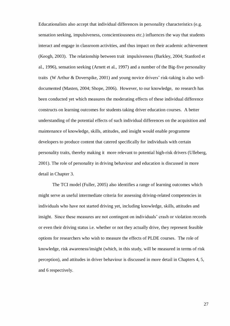
27
Educationalists also accept that individual differences in personality characteristics (e.g.
sensation seeking, impulsiveness, conscientiousness etc.) influences the way that students
interact and engage in classroom activities, and thus impact on their academic achievement
(Keogh, 2003). The relationship between trait impulsiveness (Barkley, 2004; Stanford et
al., 1996), sensation seeking (Arnett et al., 1997) and a number of the Big-five personality
traits (W Arthur & Doverspike, 2001) and young novice drivers’ risk-taking is also well-
documented (Masten, 2004; Shope, 2006). However, to our knowledge, no research has
been conducted yet which measures the moderating effects of these individual difference
constructs on learning outcomes for students taking driver education courses. A better
understanding of the potential effects of such individual differences on the acquisition and
maintenance of knowledge, skills, attitudes, and insight would enable programme
developers to produce content that catered specifically for individuals with certain
personality traits, thereby making it more relevant to potential high-risk drivers (Ulleberg,
2001). The role of personality in driving behaviour and education is discussed in more
detail in Chapter 3.
The TCI model (Fuller, 2005) also identifies a range of learning outcomes which
might serve as useful intermediate criteria for assessing driving-related competencies in
individuals who have not started driving yet, including knowledge, skills, attitudes and
insight. Since these measures are not contingent on individuals’ crash or violation records
or even their driving status i.e. whether or not they actually drive, they represent feasible
options for researchers who wish to measure the effects of PLDE courses. The role of
knowledge, risk awareness/insight (which, in this study, will be measured in terms of risk
perception), and attitudes in driver behaviour is discussed in more detail in Chapters 4, 5,
and 6 respectively.
28
1.2.5.2 The theory of planned behaviour incorporating the prototype willingness
model
In addition to driving-specific theories, such as Fuller’s TCI model (2005), several
non-domain specific theories have been used to explain and predict driver decision making
and behaviour in traffic and thus are of potential interest to those who have a stake in
improving road safety. The best-known of these are Ajzen’s theory of planned behaviour
(TPB) (1991) and Gibbons and Gerrard’s prototype willingness model (PWM) (1995)
(see Figure 1.3). The TPB focuses on rational decision making and models the relationship
between a range of determinants of human behaviour including behavioural beliefs,
normative beliefs, control beliefs and behavioural intentions.
Figure 1.3. Theory of planned behaviour incorporating the prototype willingness
model.
(after Gibbons & Gerrard, 1995).
The PWM augments the TPB by accounting for factors that influence heuristic
decision making, including social images (prototypes) and behavioural willingness (Rivis,
Sheeran, & Armitage, 2006).
29
The TPB posits that behavioural beliefs represent subjective estimates of the likely
consequences of a particular behaviour, which in turn gives rise to an attitude towards that
behaviour. An attitude is a dispositional evaluative response, either favourable or
unfavourable, towards something or someone (Ajzen, 2005). Normative beliefs describe
the normative expectations of others, which give rise to perceptions of social pressure,
which is described in terms of a subjective norm. Control beliefs are derived following an
evaluation of factors that may make the performance of the behaviour either more or less
likely and measurements on this scale describe perceived behavioural control
(Francis et al., 2009). Furthermore, these three determinants operate in tandem to form a
behavioural intention, the strength of which is dictated by variations in attitude and
subjective norm, combined with perceptions of control. The theory posits that behavioural
intentions are the most proximal determinants of behaviour (Ajzen, 1991). In accordance
with learning theory (Bandura, 1977; Pavlov & Thompson, 1902; Skinner, 1974) the TPB
assumes that attitudes, subjective norms and perceptions of control are acquired directly by
means of classical and/or operant conditioning and also indirectly through social learning
(Ajzen, 1991; Eby & Molnar, 1998).
The TPB has been used to investigate a wide range of health-related behaviours,
including exercising (Norman, Conner, & Bell, 2000), smoking and drinking (Spijkerman,
van den Eijnden, Vitale, & Engels, 2004), the commission of driving violations (Forward,
2009), speeding (Conner et al., 2007; M. A. Elliott, Armitage, & Baughan, 2003, 2007)
and adolescents’ behaviour in traffic (M. A. Elliott, 2004). For example, the results of a
study conducted by Elliott et al., (2003) showed that there was a strong relationship
between self-reported intention to speed and speeding behaviour (r = .67), and they also
reported that intentions and perceived behavioural control accounted for 32% of the
variance in behaviour after controlling for demographic factors. In addition, the results of
several meta-analyses support the utility of behavioural intentions as a predictor of
30
subsequent behaviour. For instance, Armitage and Connor (2001) reviewed 185 TPB
studies and found that attitudes, subjective norms and perceived behavioural control
accounted for 39% of the variation in intentions and that intentions accounted for 31% of
the variation in actual behaviour. Thereafter, Armitage and Connor proposed that
educational interventions might legitimately focus on TPB constructs, as a means of
reducing speeding behaviour and of reducing the commission of driving violations
generally. Some work has already been carried out in this regard. Hardeman et al. (2010)
reviewed 30 studies of educational interventions in the areas of health and safety that were
based on TPB principles and reported that 50% of these interventions were effective in
changing intentions and over 65% worked to change behaviour, albeit that the reported
effect sizes were small. Nevertheless, given the high risks faced by young novice drivers,
any reduction in intended or actual aberrant behaviour can be seen as constituting a step in
the right direction.
The path of decision-making described by the TPB assumes that this process
unfolds in an entirely rational way, i.e. that individuals consider all the possible
consequences of their behaviour before they decide to act (Reyna & Rivers, 2008).
However, the fact that health-impairing behaviours such as substance use and risk-taking
in traffic are relatively common, especially among adolescents (Bingham & Shope, 2004;
McKenna & Horswill, 2006; Shope, 2006; Spijkerman et al., 2004) suggests that young
people do not always act rationally. The prototype willingness model (PWM) (Gibbons &
Gerrard, 1995) is dual process theory of decision making and thus describes two paths to
risk-taking; one representing a reasoned route and the other depicting a heuristic route,
which is contingent on reactions to social images. The social reaction path incorporates
two constructs: risk prototypes, and behavioural willingness (Figure 1.3). Risk prototypes
describe mental representations (images) of individuals who engage in risky behaviours,
for example a typical smoker, drinker, or speeder and behavioural willingness describes
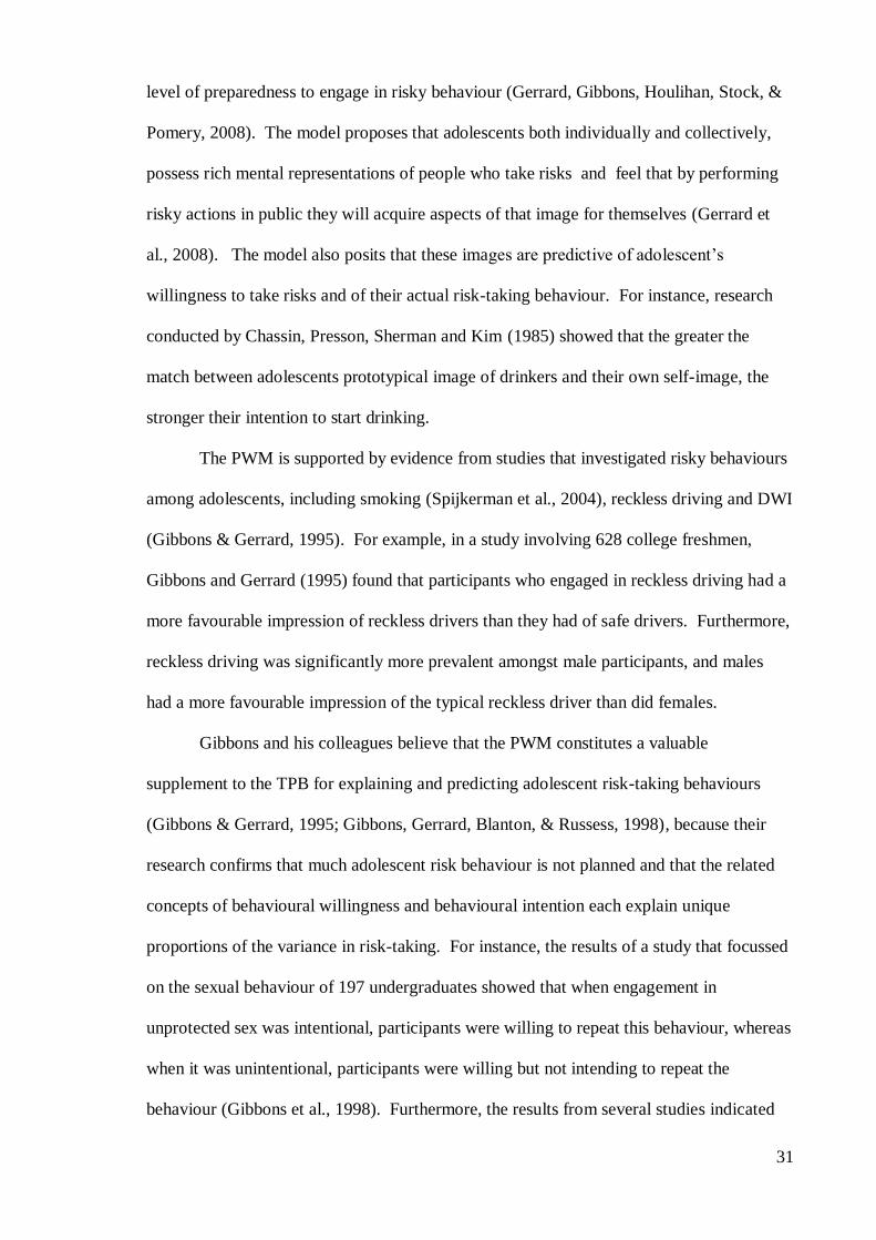
31
level of preparedness to engage in risky behaviour (Gerrard, Gibbons, Houlihan, Stock, &
Pomery, 2008). The model proposes that adolescents both individually and collectively,
possess rich mental representations of people who take risks and feel that by performing
risky actions in public they will acquire aspects of that image for themselves (Gerrard et
al., 2008). The model also posits that these images are predictive of adolescent’s
willingness to take risks and of their actual risk-taking behaviour. For instance, research
conducted by Chassin, Presson, Sherman and Kim (1985) showed that the greater the
match between adolescents prototypical image of drinkers and their own self-image, the
stronger their intention to start drinking.
The PWM is supported by evidence from studies that investigated risky behaviours
among adolescents, including smoking (Spijkerman et al., 2004), reckless driving and DWI
(Gibbons & Gerrard, 1995). For example, in a study involving 628 college freshmen,
Gibbons and Gerrard (1995) found that participants who engaged in reckless driving had a
more favourable impression of reckless drivers than they had of safe drivers. Furthermore,
reckless driving was significantly more prevalent amongst male participants, and males
had a more favourable impression of the typical reckless driver than did females.
Gibbons and his colleagues believe that the PWM constitutes a valuable
supplement to the TPB for explaining and predicting adolescent risk-taking behaviours
(Gibbons & Gerrard, 1995; Gibbons, Gerrard, Blanton, & Russess, 1998), because their
research confirms that much adolescent risk behaviour is not planned and that the related
concepts of behavioural willingness and behavioural intention each explain unique
proportions of the variance in risk-taking. For instance, the results of a study that focussed
on the sexual behaviour of 197 undergraduates showed that when engagement in
unprotected sex was intentional, participants were willing to repeat this behaviour, whereas
when it was unintentional, participants were willing but not intending to repeat the
behaviour (Gibbons et al., 1998). Furthermore, the results from several studies indicated

32
that substance use and condom use in adolescents under 19-years-old were more strongly
correlated with the participants’ willingness rather than with their intentions to do so
(Spijkerman et al., 2004; van Empln & Kok, 2006). Thus it appears that willingness
constitutes a generalised positive attitude towards behaviour, whereas intentions represent
a firmer resolve to engage in that behaviour.
The accumulated evidence presented here suggests that TPB and PWM constructs
constitute useful measures of attitudes, social influence, perceptions of control, behavioural
willingness, intention and actual behaviour among adolescents. In addition, since these
constructs can also be used as proxy measures of behaviour in order to determine the
effectiveness of interventions where actual behaviour cannot be measured (Francis et al.,
2009; Gibbons & Gerrard, 1995), they constitute a valuable resource when it comes to
studying the effects of PLDE.
1.2.5.3 Goals for driver education framework (GDE)
The goals for driver education framework (GDE) (Hatakka et al., 2002) synthesises many
of the principles incorporated in descriptive skill-based models (e.g. the Hierarchical
Control Model (Michon, 1985)) and functional motivation-based models ((e.g. the TCI
(Fuller, 2000), TPB (Ajzen, 1991) and PWM (Gibbons & Gerrard, 1995)) and as such
represents an evolution in thinking with regard to driver behaviour and driver education
(see

33
Table 1.1 for a model description).
The GDE-framework attempts to broaden the scope of driver education and
training by redefining its goals, and methods. For example, although the model retains the
hierarchical framework favoured in earlier skill-based models, the GDE-framework
distinguishes between four, increasingly influential, levels of skills and competencies that
are seen as necessary for optimal performance including (a) vehicle manoeuvring, (b)
mastering traffic situations, (c) goal and context of driving, and (d) goals for life and skills
for living. The GDE-framework also outlines a second dimension, which indicates that
driver education should aim to provide students with (a) basic skills and knowledge; (b)
knowledge and skills related to risk increasing factors; and (c) skills for self-evaluation, at
each level of the hierarchy. In this conceptualisation, basic knowledge, and skills for
manoeuvring a vehicle, and for mastering traffic situations are seen as fundamental for
successful driving. Therefore these competencies should be acquired during driver
training. In addition, the model supposes that the application of these skills is guided by
higher level personal tendencies, goals and motives, which should be addressed as part of
driver education and training courses. The second column in the framework describes the
types of risks that arise when drivers have insufficient knowledge or skills related to the
competencies described at each level of the hierarchy and thus highlights the importance of
accurate risk perception for increasing safety.

34
Table 1.1 Goals for Driver Education framework
(Reproduced with permission from Hatakka, Keskinen, Glad, Gregersen,
Hernetkoski, 2002)
35
Risk judgements feature prominently in most theoretical models of health
behaviour, including the Theory of Planned Behaviour (Ajzen, 1991). These posit that
individuals’ perceptions about the consequences of their behaviour and their perceptions
about their personal vulnerability to those consequences play a crucial role in their decision

36
making. For instance, studies show that whereas adolescents and adults appear to be
equally capable of assessing risk accurately (Millstein & Halpern-Felsher, 2002),
adolescents who take risks perceive themselves as less likely to suffer negative
consequences as a result of such actions than do those who abstain from risky practices
(Arnett, 2002). Furthermore, research conducted by Naatanen and Summala (1974) and
Summala (1987) suggested that in addition to the official goal of the traffic system (i.e.
safety), the behaviour of some young drivers is influenced by “extra motives”, such as
competition, sensation seeking, deliberate risk taking and a desire to conform to perceived
social norms, which may be socially rewarding and satisfy their developmental needs
(Jessor, 1998). For instance, it is well known that adolescence is marked by an increased
desire for independence from familial influences and that this is accompanied by an
increased susceptibility to (perceived) peer influence and (perceived) peer pressure
(Steinberg, 2004). In response, the GDE suggests that driver education programmes
should anticipate and proactively address such factors by providing students with
knowledge about how both their trip-related goals and motives and also their life goals and
personal tendencies affect driving behaviour and by equipping them with the necessary
skills to control these influences. Thus the GDE model provides useful guidelines for
individuals or organizations who wish to develop driver education and training courses.
The third column in the GDE-framework focuses on how drivers assess their
personal situations on each of the four levels and reflects an increasing awareness among
theorists of the role that metacognitive processes play in the development of driver
competency. Metacognition refers to the act of thinking about thinking, and involves the
active monitoring and regulation of cognitive activity (A. L. Brown, 1987). The
relationship between metacognition and learning was first suggested by Flavell (1979),
who proposed that awareness of cognitive processes consisted of both metacognitive
knowledge (self-awareness) and metacognitive skills (self-evaluation and self-regulation).
37
For instance, the GDE-framework posits that pre-drivers and novices should be trained to
examine their attitudes towards aberrant practices, such as speeding, to examine the ways
in which such attitudes can potentially affect their driving behaviour and to develop
strategies that enable them to change their attitudes where necessary. Research suggests
that there are positive associations between increased metacognitive knowledge and
increased learning, improved performance and greater achievement of educational goals
(Tobias & Everson, 2003 ). Both the TCI model of driver behaviour (Fuller, 2005), and
the GDE-framework of driver education and training (Hatakka et al., 2002) stress the
importance of metacognition in establishing and maintaining safe driving practices. For
instance, the concept of calibration, which featutures prominently in the TCI model refers
to the alignment of a driver’s metacognitive judgements about his/her own capabilities and
the demands of the driving task, with objective reality (Kuiken & Twisk, 2001). In the
context of the GDE-framework, accurate calibration describes awareness (insight) of the
ways in which skills, abilities and personal tendences affect decision making with respect
to manoeuvring a vehicle in traffic and also planning trips and life in general (Peräaho,
Keskinen, & Hatakka, 2003). Following a review of driver training in Europe, Lynham
and Twisk (1995) suggested that the provision of training in metacognitive aspects of
driving represent the most promising approach for improving driver education.
Furthermore, since metacognitive training can be provided for individuals who have not
started driving yet, this type of training can be used with pre-learner as well as learner
drivers. Unlike traditional approaches to teaching which focus mainly on providing
students with knowledge, metacognitive training uses a constructivist approach, whereby
students actively construct knowledge and increase their understanding by interacting with
the topic of interest (Bransford, Brown, & Cockling, 2000). This approch necessitates a
move away from lecture-based teaching in favour of more interactive methods such as
discussions and role play. For example, metacognitive training might involve a group
38
discussion that examines the possible consequences of high speed driving, or an enactment
of a situation where participants are being encouraged to drive after consuming alcohol or
drugs. The evidence presented above suggests that, improving driving-related
metacognition constitutes a feasible objective for PLDE courses.
1.2.6 Pre-learner driver characteristics
A growing body of research indicates that risk-taking in traffic follows a
developmental trajectory, which starts in early childhood (Deighton & Luther, 2007;
Durkin & Tolmie, 2010; Waylen & McKenna, 2002, 2008). Empirical evidence show that
that attitudes towards driving are well-established in youngsters long before they are old
enough to obtain a learner permit and thus gain firsthand experience with driving5 (e.g.
Harré, 2000; Harré & Brandt, 2000a, 2000b; Harré, Brandt, & Dawe, 2000; Parker &
Stradling, 2001; Waylen & McKenna, 2002, 2008). For instance, research conducted by
Harré et al. (2000) involving 277 14- and 16-year-old adolescents in New Zealand,
measured their perceptions about the acceptability of a range of reckless and illegal driving
behaviours including; tailgating, risky overtaking, running red lights, chasing and/or racing
other drivers, DWI and speeding. The results showed that over 25% of the participants,
including 49% of males believed that it was safe to travel at 120km/h in a 100km/h zone.
Waylen and McKenna (2002) surveyed 567 UK secondary school students aged between
11- and 16-years regarding their attitudes towards road use and their beliefs about what it
would be like to drive. They found that males had riskier attitudes towards road safety and
driving than did females and the former were most likely to condone driving violations
such as speeding and running red lights and reported an increased tendency to enjoy
travelling at fast speeds. The males in this sample also believed that driving would be
easier and that they would be more influenced by their friends when they were driving than
5 The reported prevalence of unlicenced, under aged driving among adolescents is generally quite
low. Elliott, Ginsburg and Winston (2008) found that just 4.2% of the five and a half thousand 9th to 11th
grade students that they surveyed indicated that they drove for at least 1 hour per week without a licence.
39
did the females. Parker and Stradling (2001) also reported that pre-driving males aged
from 11-years-old onwards had a greater interest in cars, anticipated more thrill-seeking
when they became drivers, rated current speed limits as ‘too slow’ and said that driving
would provide a means for them to express themselves than did their female counterparts.
Another study, by Waylen and McKenna (2008) examined the relationship between
sensation seeking and positive attitudes towards speeding and driving violations among
adolescents and adults. This showed that there were significant age and gender differences
in trait sensation seeking among UK 11-16-year-olds, with boys reporting higher levels of
sensation seeking than girls. These effects peaked in mid-adolescence for both genders
after which the effects levelled-off for boys and declined for girls. The results also showed
that there were significant correlations between trait sensation seeking and favourable
attitudes to speeding and also driving violations. Finally, research conducted in Ireland,
involving over 500 secondary-school students, with an average age of 16-years, showed
that attitudes to road safety expressed by male participants were significantly riskier than
were those expressed by their female counterparts. However, both sexes were equally
tolerant of breaking the speed limit where doing so was perceived as safe (O'Brien,
Rooney, & Fuller, 2001). Taken as a whole, the evidence from these studies suggests that
driving-related beliefs and attitudes develop in the absence of direct experience with actual
driving and may instead be derived as a result of biological and/or social influences. Since
these findings indicate that young males and individuals with a greater propensity for
sensation seeking tend to have more aberrant attitudes towards driving, this suggests that
the task of instilling appropriate attitudes towards driving in adolescents may prove more
difficult in some cases than in others. As a result, there is growing support for the view
that driver education should to be delivered over an extended period, beginning with pre-
learner driver programmes for students aged between 14-17-years old (Christie, 2001;
Lonero et al., 1995; Lonero & Mayhew, 2010; Siegrist, 1999).
40
1.2.7 Pre-learner driver education (PLDE)
Although PLDE programmes constitute a relatively recent addition to the driver
education repertoire, the results from evaluation studies of PLDE have been mildly
encouraging. These suggest that attendance at a PLDE course can result in increased
knowledge, improved thinking skills and better attitudes towards safe driving. For
instance, Harré and Brandt (2000a) assessed the effectiveness of a traffic safety
programme designed for year 10 students (14-year-olds) in New Zealand. The programme
consisted of 16 lessons which covered topics including risk perception, motivations for
risk-taking and the effects of inexperience, peer pressure and impaired driving. Students
were encouraged to analyse their beliefs and attitudes towards these issues using a
specially designed workbook. Self-report questionnaires were used to measure changes in
attitudes and behaviours in this active programme group (n = 61) and a matched control
group (n = 90) on three occasions; pre- and post-intervention, and post-intervention plus 6
months. The measures included attitudes towards DWI, frequency of being a passenger of
a drink-driver, intention to be a passenger of a drink-driver, frequency of seat-belt wearing
and knowledge about the risk of speeding. Participants were also asked to rate the
acceptability of nine risky/illegal behaviours. The results indicated that there was a
significant improvement in attitudes towards risky behaviour in the active group in
comparison with the controls in four of the nine behaviours tested in the second test.
However, these beneficial effects were no longer evident in the follow-up test.
Unfortunately the researchers did not stipulate which specific attitudes improved (Deighton
& Luther, 2007). Although this was a relatively small-scale study to begin with, and there
was a 21% rate of attrition between the post-intervention and the follow-up tests, these
results indicate that pre-driver education can have a positive short-term effect on driving-
related attitudes.
41
Similar positive results were reported in an evaluation of the DRIVE pre-driver
education programme in the UK (H. Simpson, Chinn, Stone, Elliott, & Knowles, 2002).
This intervention consisted of a video, a teacher/student manual and a self-help booklet
that was distributed to Road Safety Officers, and through them to schools and other
interested groups. The evaluation was based on a pre- and post-intervention questionnaire
that assessed students’ knowledge of safe driving and attitudes towards driving. The
sample consisted of 546 year 12 students from 19 schools that delivered the DRIVE
course, and 641 matched controls and most participants were between 16-17-years old.
The knowledge test was based on the course material and consisted of 28 (one mark)
questions, 24 of which involved a “True”, “False” or “Don’t know” answer and the
remaining 4 involved a multiple choice format. The results of the pre-intervention test
indicated that there was very little difference in the mean pre-intervention scores for the
experimental group and the controls (M = 18.1 and 17.8 respectively). However, the
results of the post-intervention test showed that whereas the experimental group recorded
significant gains in knowledge (M = 21.2, p < .001); the mean scores in the control group
had decreased significantly between the two tests (M = 16.9, p < .001). Simpson et al.,
(2002) reported that the students who took the programme showed marked improvement in
knowledge about the fact that accidents mostly happen locally, that reducing speed can
save lives and that young male passengers have a higher risk of being killed in RTCs. The
risk perception measures consisted of list of 14 potentially dangerous driving activities,
which the students had to rate on a four-point scale, ranging from 1 = “not at all
dangerous” to 4 = “very dangerous”, thus the overall scale scores could range between 14 -
56 points. The results showed there was a small increase in the mean scores for the
experimental group between the two tests, from 46.3 to 47.3 (p < .001), whereas there was
a slight, non-significant decrease in the means for the control group, from 45.2 to 44.7
during the same period. On the basis of these results, the researchers concluded that the
42
DRIVE programme was moderately successful in increasing the students’ knowledge
about safe driving and their perception of the risks involved in risky driving activities.
Clearly, however, 1 point increase in the risk-perception scores in the active group hardly
constitutes a meaningful improvement. Furthermore, the information value of this study is
somewhat limited because no follow up test was performed to ascertain the possible long-
term effects of the programme.
More recently, a UK study evaluated a half-day PLDE intervention entitled “Safe
Drive Stay Alive”, which aimed to improve pre-drivers’ attitudes by increasing their
awareness of the consequences of risky driving and their vulnerability on the roads
(Poulter & McKenna, 2010). The intervention involved watching a video that contained a
dramatic reconstruction of a fatal car crash involving youngsters and also testimonials
provided by members of the emergency services, surviving victims and bereaved parents,
each describing their personal experience of a fatal collision. Students from six schools
completed a questionnaire on three occasions: pre-intervention (791 students), post-
intervention (422 students) and a post-intervention follow-up (258 students) five months
after the presentation. As a result of listwise deletion, the overall analyses were based on
the scores for just 199 students; 128 males and 71 females, with a mean age of 15.6 years.
The measures included 13 questions about speeding which were based on TPB constructs
(Ajzen, 1991), including attitudes, subjective norms, perceived behavioural control, and
future intentions. The results showed that the programme had a significant immediate
effect on the overall scores for the items. There was a significant pre-to-post-intervention
improvement in relation to four issues: students’ intentions to drive within the speed limit,
the inevitability that one will exceed the speed limit sometimes, sticking to the speed
regardless of the fact that one is slowing down the flow of traffic and resisting peer
pressure to drive faster. However, with the exception of exceeding the speed limit
sometimes, these improvements were no longer evident during the five-month follow-up
43
study, which suggests that the impact of this one-day intervention was short-lived.
Furthermore, in the absence of a control group, it is difficult to judge the real effects of this
intervention.
This brief review of previous evaluations of PLDE courses suggests that these types
of interventions provide some short-term benefits for pre-learner drivers with respect to
driving-related knowledge, risk perception skills and attitudes, which do not appear to
persist over longer time periods. However, there is some evidence to suggest that PLDE
interventions may function to make students more amenable to subsequent road safety
messages. For instance, O’Brien, Rooney and Fuller (2001) investigated the effects of
attending a drama presentation that concentrated on the negative consequences RTCs on
519 Irish pre-learner adolescents (439 in the experimental group, and 80 controls). In line
with the PLDE evaluations discussed previously, they found that attendance at the drama
resulted in significant short-term improvements in risk perception, but that this effect was
no longer evident in the one-year follow-up test. However, as part of that test, they
exposed all of the participants to a set of media messages which aimed to reinforce the
central themes from the original drama and then re-tested them. Those results showed that
there was a significantly greater increase in positive attitudes towards these messages
among students in the experimental group in comparison to the controls. The implications
of these findings for road safety education, particularly driver preparation courses are clear.
If the effects of these types of educational interventions are cumulative rather than absolute
in nature, then students should be exposed to regular and timely refresher courses in order
to prolong the benefits that accrued from attending the original course. The effects of
reinforcement on learning are well-known in psychological circles and will be discussed in
more detail in Chapter 4.
Whereas the authors of the PLDE evaluations that have been reviewed above
acknowledged the various limitations of their studies, no evidence was found to suggest
44
that they recognized the need to test for clustering effects in their data and to control for
these effects where necessary. Clustering occurs when participants are grouped in some
way, (e.g. within schools) or when repeated measures are used. The data derived in these
cases violates the assumption of independence that underpins the rationale behind
inferential statistical procedures such as analysis of variance (ANOVA) and multivariate
analysis of variance (MANOVA) (Kreft, 1996). In the field of educational psychology,
evaluations of school-based interventions routinely use statistical procedures, such as
hierarchical linear modelling (HLM), to adjust for the effects of clustering (see for example
Flannery et al., 2003; Guo, 2005; Raudenbush & Bryk, 2002). Since failure to adjust for
clustering represents a significant flaw in the design of previous evaluations of driver
education programmes, this study intends to make an important contribution to the
literature by using HLM techniques to improve the psychometric credentials of its
findings. A detailed discussion of HLM techniques is provided in Chapter 2.
To date, very few evaluations of PLDE courses have been conducted and those
have contented themselves with examining a relatively small number of issues and
concepts. However, this study intends to adopt a broader approach in an attempt to gain a
more comprehensive understanding of the factors that influence the formation and
maintenance of knowledge, and good risk perception skills, and safe attitudes towards
driving in PLDs. Not alone would this information allow programme developers to refine
their courses to cater for specific target audiences, but it may also help to identify more
meaningful criteria for use in future programme evaluations (Lonero et al., 1995).
1.2.8 Aim of the present study
The aim of this research is to evaluate PLDE interventions that are provided for
Transition Year (year 12) students in schools in the Republic of Ireland (ROI). The main
part of the project consists of a summative of assessment of student outcomes from a range
of driving-related educational courses that are typically provided for TY students. These

45
range from modular programmes that span the entire school year to one-day courses, all of
which aim to provide PLDs with the types of driving-related knowledge, skills and
attitudes that would assist them in becoming better drivers in the future. In addition, a
formative evaluation of the curriculum which forms the basis of two of these programmes
is conducted in an effort to identify programme features (content and/or processes) that
might be changed in order to improve the efficiency and effectiveness of these
programmes.
1.2.9 Hypotheses
The following hypotheses will be tested as part of the summative evaluation. The
order in which these are presented reflects the statistical modelling strategy that was
adopted in this research rather than relative importance of the predictions:
1. There will be significant variations in driving-related knowledge, risk perception
skills and attitudes of participating students at intra-student, between-student and
between-schools levels.
2. There will be significant short-term changes (i.e. between the pre-intervention
(T1), and post-intervention (T2) tests) in driving-related knowledge, risk perception
skills, and attitudes in the research sample.
3. There will be significant long-term changes (i.e. between the pre-intervention (T1),
and post-intervention follow-up (T3) tests) in driving-related knowledge, risk
perception skills and attitudes in this sample.
4. Students who take a PLDE course during Transition Year (the PLDE group), will
acquire significantly more driving-related knowledge, better risk perception skills
and better attitudes towards driving than will those in who do not take a PLDE
course (the control group).

46
5. Students who attend specific types of PLDE courses will acquire significantly more
driving-related knowledge, better risk perception skills and better attitudes towards
driving than will those in the non-PLDE control group.
6. Both initial levels of, and changes in driving-related knowledge, risk perception
skills and attitudes will be influenced by a range of distal and proximal between-
student factors including;
a) Personal characteristics e.g. gender, domicile location, socio-economic
status (SES) personality (i.e. sensation seeking, impulsiveness and Big-5
personality traits).
b) Previous experience gained through direct interactions with the traffic
system or indirectly, through observational learning (see Table 2.2 for a
comprehensive list.).
47
Chapter 2: Methodology
In the ROI, second-level education is delivered over a 5 or 6 year cycle, from year
9 onwards. In years 9-11, students prepare for the national Junior Certificate Examination,
and in years 13-14, they study for the national Leaving Certificate Examination. Year 12,
which is called “Transition Year” (TY), is an optional part in the second-level cycle. The
curriculum for that year focuses on non-traditional activities with the aim of promoting
“….the personal, social, vocational and educational development of students and preparing
them for their role as autonomous, participative and responsible members of society”
(Second Level Support Services - Department of Education and Skills, 2013, p. 1). Thus,
TY students are encouraged to develop a wide range of transferable critical thinking and
creative problem solving skills by engaging in a wide range of activities, such as
participating in social innovation projects, forming mini companies, gaining work
experience, and, of particular relevance for the current research, preparing to learn how to
drive.
2.1 Design
This study used a quasi-experimental design, whereby students in TY and year
12/136 in participating school were divided across six experimental groups in accordance
with their PLDE status, i.e. five PLDE groups and a non-PLDE control group. This design
was preferred over a randomised controlled experiment for practical reasons (see Levin,
2005), because the majority of the schools that provide PLDE in transition year have
already invested considerable amount of time and effort in specific courses in terms of
providing in-service teacher training, purchasing study materials etc., thus changing these
arrangements would have placed excessive demands on school resources.
6 For the purpose of this study Transition Year (TY) is classified as “year 12” and the next school
year is classified as “year 13”. However, some students skip TY and go directly from year 11 to year 13,
thus some year 13 students were included as matched controls in this study.

48
Students in the PLDE groups took one of five different types of courses, all of
which are commonly used with TY classes (see Appendix A). Students in four of these
groups, (groups A - D) used PLDE programmes that were modular in design, i.e. they
contained a multiple instructional units and were delivered over several weeks or months.
The courses that were taken by groups A-C are used widely in the ROI. Students in group
D took courses that had been developed within their own schools. Students in group E
took one of two types of PLDE course that are delivered in a single day. The control group
consisted of a cohort of TY and Year 13 students who did not take a PLDE course in
school.
Both between-groups and repeated measures were used to ascertain the nature and
levels of driving-related knowledge, cognitive skills and attitudes among students in this
sample. The students were tested on three occasions in 18 months between September
2009 and March 2011. First, a pre-intervention test (T1) was administered in each group
1.5 weeks (on average) before their scheduled PLDE course was delivered. Second, a
post-intervention test (T2) was conducted with each school group within 1 to 4 weeks of
the completion of the individual courses. Third, a post-intervention follow-up test (T3)
was administered between 9 - 12 months after each course had ended. The variability in
the gaps between testing sessions occurred because there were practical limits as to when
testing could take place, due to the number of schools involved, and their diverse locations
and also because the PLDE courses that featured in this study differed considerably in
terms of duration. The average interval between the T1 and theT2 tests was approximately
26 weeks; the average interval between the T2 and the T3 tests was approximately 51
weeks and the average interval between the T1 and the T3 tests was approximately 77
weeks (Table 2.1). The testing schedule used for classes in the control group mirrored this
pattern.

49
Table 2.1 Intervals between tests
Number of weeks
Interval between tests Min. Max. M (SD)
T1 - T2 4 37 25.81 (8.08)
T2 - T3 39 71 50.69 (8.41)
T1 - T3 54 85 76.51 (4.90)
The research was designed to comply with recent guidelines produced by the AAA
Foundation for Traffic Safety (see Clinton & Lonero, 2006a, 2006b; Clinton & Lonero,
2006c), which encapsulate international best practice in evaluation design and
methodology and was approved by the ethics committee in the School of Psychology,
Trinity College, Dublin.
2.2 Participants
The population for this study consisted of all students who were enrolled as TY
students during the 2009-2010 school year. During the previous year, when recruitment
for this study was underway, 335,123 adolescents were enrolled in 731 secondary school in
the Republic of Ireland. TY programmes were being delivered in 71% of these schools,
and students in the remaining schools skipped year 12, and transferred directly into year
13 (Department of Education and Science, 2010). In order to gain access to relevant
population, a list of all schools that were providing TY was obtained from the Second
Level Support Services division in the Department of Education, via a personal
communication from M, O’Leary on March 10, 2009. Thereafter, an invitation was sent,
either by post or by e-mail, to the TY coordinators in these schools, inviting them to
participate in this research. This letter also explained the study aims and outlined the
research procedure and was accompanied by a School Consent Form (Appendix B), that
they could return if they agreed to participate. Fifteen schools were recruited on foot of
this initial request. Thereafter, a stratified opportunity-based approach (Shaughnessy et al.,
2009) was used to recruit additional school groups, whereby successive recruitment drives
increasingly targeted groups that had the potential to balance student numbers with respect

50
to a number of key strata, including PLDE status, gender, socio-economic status (SES),
and school location. In total, 39 schools consented to host the project; however, as a result
of staffing and scheduling problems, testing was conducted in only 34 of these schools.
The ROI is divided into 26 counties (regions). Since the participating schools were located
in14 of these, it was concluded that they constituted a reasonably representative sample of
the target population (see Appendix C). Students in 32 of these schools participated in one
of the active PLDE groups. Seven of those same schools also provided a group of
students, who were not taking a PLDE course, but who were otherwise of equivalent status
to their counterparts, to act as matched controls. This meant that there was a minimal
amount of difference between the type of students who took the PLDE courses and those
who did not. For instance, in the case of the matched groups, some of these students were
unable to take the PLDE course that was provided because it was over-subscribed. Where
this occurred, places were typically allocated on a random basis by the TY coordinator.
Two schools provided students for the control group alone: One of these did not provide
PLDE as a TY option and the other did not provide a TY programme at all. Twenty-three
of the participant groups came from single-sex schools (12 male, 11 female) and the
remainder came from mixed sex schools.
Two thousand and three students participated in the first test (T1). However, 23 of
these were removed from the study because the data that they provided in this initial
survey was deemed as insufficient and/or unreliable. Thus, the actual sample consisted of
1,880 students who took the T1 test, of which 1,324 and 1,412 took the T2 and the T3 tests
respectively (Table 2.2).
Table 2.2 Summary of participant demographics by programme type for the pre-
intervention (T1), post-intervention (T2), and post-intervention follow-up (T3) tests
Group Characteristics Student Characteristics
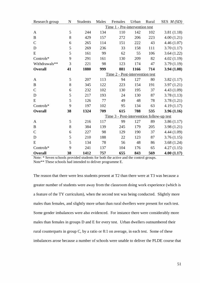
51
Research group N Students Males Females Urban Rural SES M (SD)
Time 1 - Pre-intervention test
A 5 244 134 110 142 102 3.81 (1.18)
B 8 429 157 272 206 223 4.00 (1.21)
C 6 265 114 151 222 43 4.46 (1.07)
D 5 269 236 33 158 111 3.70 (1.17)
E 5 161 99 62 55 106 3.64 (1.22)
Controls* 9 291 161 130 209 82 4.02 (1.19)
Withdrawals** 3 221 98 123 174 47 3.79 (1.19)
Overall 41 1880 999 881 1166 714 3.94 (1.08)
Time 2 - Post-intervention test
A 5 207 113 94 127 80 3.82 (1.17)
B 8 345 122 223 154 191 3.97 (1.21)
C 6 232 102 130 195 37 4.43 (1.09)
D 5 217 193 24 130 87 3.78 (1.13)
E 5 126 77 49 48 78 3.78 (1.21)
Controls* 9 197 102 95 134 63 4.19 (1.17)
Overall 38 1324 709 615 788 535 3.96 (1.16)
Time 3 - Post-intervention follow-up test
A 5 216 117 99 127 89 3.86 (1.17)
B 8 384 139 245 179 205 3.98 (1.21)
C 6 227 98 129 190 37 4.44 (1.09)
D 5 210 188 22 123 87 3.76 (1.15)
E 5 134 78 56 48 86 3.68 (1.24)
Controls* 9 241 137 104 176 65 4.27 (1.15)
Overall 38 1412 757 655 843 569 4.00 (1.17) Note: * Seven schools provided students for both the active and the control groups.
Note** These schools had intended to deliver programme E.
The reason that there were less students present at T2 than there were at T3 was because a
greater number of students were away from the classroom doing work experience (which is
a feature of the TY curriculum), when the second test was being conducted. Slightly more
males than females, and slightly more urban than rural dwellers were present for each test.
Some gender imbalances were also evidenced. For instance there were considerably more
males than females in groups D and E for every test. Urban dwellers outnumbered their
rural counterparts in group C, by a ratio or 8:1 on average, in each test. Some of these
imbalances arose because a number of schools were unable to deliver the PLDE course that
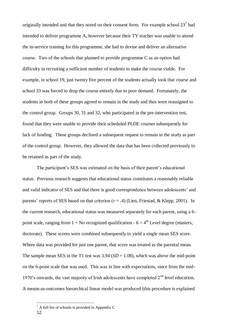
52
originally intended and that they noted on their consent form. For example school 237 had
intended to deliver programme A, however because their TY teacher was unable to attend
the in-service training for this programme, she had to devise and deliver an alternative
course. Two of the schools that planned to provide programme C as an option had
difficulty in recruiting a sufficient number of students to make the course viable. For
example, in school 19, just twenty five percent of the students actually took that course and
school 33 was forced to drop the course entirely due to poor demand. Fortunately, the
students in both of these groups agreed to remain in the study and thus were reassigned to
the control group. Groups 30, 31 and 32, who participated in the pre-intervention test,
found that they were unable to provide their scheduled PLDE courses subsequently for
lack of funding. These groups declined a subsequent request to remain in the study as part
of the control group. However, they allowed the data that has been collected previously to
be retained as part of the study.
The participant’s SES was estimated on the basis of their parent’s educational
status. Previous research suggests that educational status constitutes a reasonably reliable
and valid indicator of SES and that there is good correspondence between adolescents’ and
parents’ reports of SES based on that criterion (r = .4) (Lien, Friestad, & Klepp, 2001). In
the current research, educational status was measured separately for each parent, using a 6-
point scale, ranging from 1 = No recognized qualification - 6 = 4th Level degree (masters,
doctorate). These scores were combined subsequently to yield a single mean SES score.
Where data was provided for just one parent, that score was treated as the parental mean.
The sample mean SES in the T1 test was 3.94 (SD = 1.08), which was above the mid-point
on the 6-point scale that was used. This was in line with expectations, since from the mid-
1970’s onwards, the vast majority of Irish adolescents have completed 2nd
level education.
A means-as-outcomes hierarchical linear model was produced (this procedure is explained
7 A full list of schools is provided in Appendix C
53
in detail later in this chapter), which compared the SES of students in each of the active
groups with the SES of students in the control group, with one notable result. The mean
SES for students in the control group (3.81, SE = 0.15, t(35) = 25.99) was significantly
lower than that for students in group C (4.5, SE = 0.25, t(35) = 2.8, p < .01), however this
difference was quite small (r = .25).
The mean age in the sample at T1, the T2 and the T3 was 16.02 (SD = 0.5), 16.38
(SD = 0.45) and 17.31 (SD = 0.41) respectively. The modal ages are shown in Figure 2.1.
Figure 2.1. Participant ages in the pre-intervention (T1), post-intervention (T2) and
post-intervention follow-up (T3) tests.
2.2.1 Attrition
Attrition is problematic in longitudinal research. Not only does it reduce the
amount of data that can be used for inferential analyses, but differential attrition from
individual experimental groups also constitutes a potential threat to the internal validity of
a study (Levin, 2005). The overall rate of attrition in this research was low, amounting to
approximately 30% between the T1 and T2 tests, and approximately 25% between the T1
and T3 tests. Furthermore, a sizeable proportion of these losses (i.e. 12%) were due to the
loss of three entire school groups that withdrew from the study after taking the T1 test.
0%
10%
20%
30%
40%
50%
60%
70%
80%
T1 T2 T3
Test
Participants' ages
14-year-olds
15-year-olds
16-year-olds
17-year-olds
18-year-olds
19-year-olds
54
After adjusting for those losses, remaining rate of attrition was quite low, amounting to
20% between T1, and T2, and to just 15% between T1, and T3. These losses occurred
mainly because students were away from their classrooms doing work experience, and
other course-related activities when testing was being carried out and thus were not
systematic in character. Furthermore, there were no significant differences in the rates of
attrition between the groups (see Table 2.2). Also, since the main analysis was conducted
using hierarchical linear modelling (HLM), the loss of individual students from within
school groups did not have the same type of detrimental impact that it would have had if
more traditional types of regression analyses were being used (Bryk & Raudenbush, 1992).
These issues are addressed in more detail below.
2.3 Apparatus and Materials
Several software packages were used to analyze the data in this study. The
descriptive analyses were conducted in PAWS (Version 18.0). The confirmatory factor
analyses were performed using Amos (Arbuckle, 2009). The item response analyses of the
knowledge test scores were conducted in JMP (Version 9.0.2), and jMetrik (Meyer,
2011), and the hierarchical linear models were constructed using HLM (Version7)
(Raudenbush, Bryk, & Congdon, 1996-2011).
Self-report questionnaire booklets were used to collect data in the T1, T2, and T3
tests, details of which are provided in Appendices D, E, and F respectively. To help reduce
survey bias, three different booklets were produced for each test, which allowed for a
partial randomisation in the order in which the questions were presented. Additional
questionnaire booklets were used for the supplementary knowledge tests that were used
during the T2 (Appendix G) and the T3 (Appendix H) assessments.
2.4 Measures
The main function of the questionnaires was to measure the participants’ driving-
related knowledge, risk perception skills, and attitude towards speeding. The resulting data
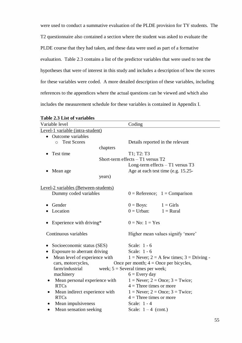
55
were used to conduct a summative evaluation of the PLDE provision for TY students. The
T2 questionnaire also contained a section where the student was asked to evaluate the
PLDE course that they had taken, and these data were used as part of a formative
evaluation. Table 2.3 contains a list of the predictor variables that were used to test the
hypotheses that were of interest in this study and includes a description of how the scores
for these variables were coded. A more detailed description of these variables, including
references to the appendices where the actual questions can be viewed and which also
includes the measurement schedule for these variables is contained in Appendix I.
Table 2.3 List of variables
Variable level Coding
Level-1 variable (intra-student)
Outcome variables
o Test Scores Details reported in the relevant
chapters
Test time T1; T2: T3
Short-term effects – T1 versus T2
Long-term effects – T1 versus T3
Mean age Age at each test time (e.g. 15.25-
years)
Level-2 variables (Between-students)
Dummy coded variables 0 = Reference; 1 = Comparison
Gender 0 = Boys: 1 = Girls
Location 0 = Urban: 1 = Rural
Experience with driving* 0 = No: 1 = Yes
Continuous variables Higher mean values signify ‘more’
Socioeconomic status (SES) Scale: 1 - 6
Exposure to aberrant driving Scale: 1 - 6
Mean level of experience with 1 = Never; 2 = A few times; 3 = Driving -
cars, motorcycles, Once per month; 4 = Once per bicycles,
farm/industrial week; 5 = Several times per week;
machinery 6 = Every day
Mean personal experience with 1 = Never; 2 = Once; 3 = Twice;
RTCs 4 = Three times or more
Mean indirect experience with 1 = Never; 2 = Once; 3 = Twice;
RTCs 4 = Three times or more
Mean impulsiveness Scale: 1 - 4
Mean sensation seeking Scale: 1 – 4 (cont.)
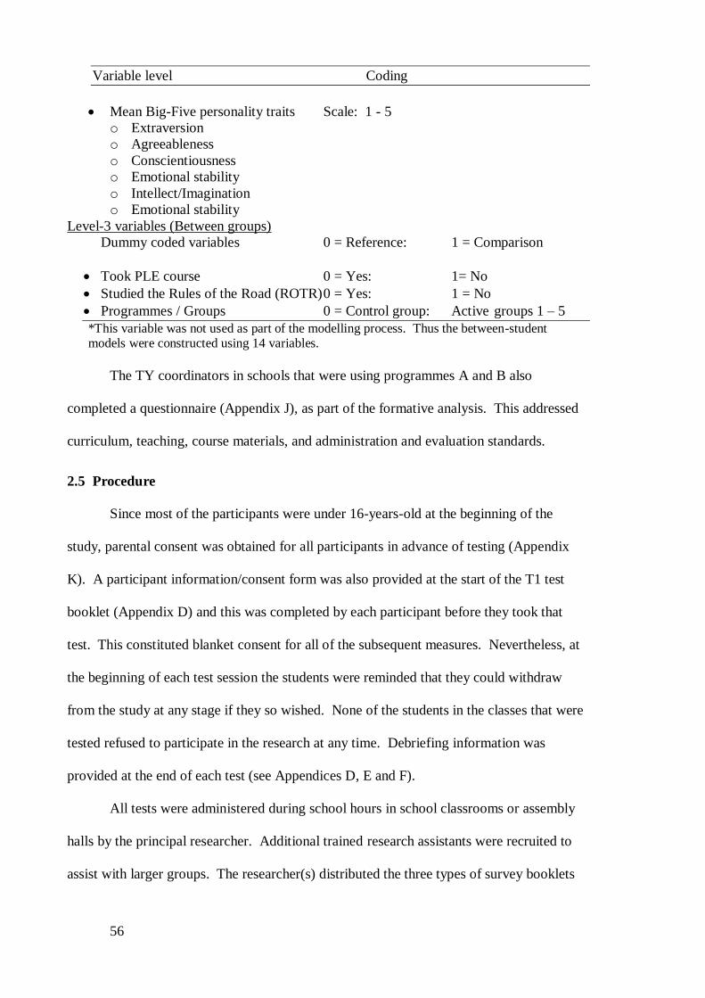
56
Variable level Coding
Mean Big-Five personality traits Scale: 1 - 5
o Extraversion
o Agreeableness
o Conscientiousness
o Emotional stability
o Intellect/Imagination
o Emotional stability
Level-3 variables (Between groups)
Dummy coded variables 0 = Reference: 1 = Comparison
Took PLE course 0 = Yes: 1= No
Studied the Rules of the Road (ROTR) 0 = Yes: 1 = No
Programmes / Groups 0 = Control group: Active groups 1 – 5
*This variable was not used as part of the modelling process. Thus the between-student models were constructed using 14 variables.
The TY coordinators in schools that were using programmes A and B also
completed a questionnaire (Appendix J), as part of the formative analysis. This addressed
curriculum, teaching, course materials, and administration and evaluation standards.
2.5 Procedure
Since most of the participants were under 16-years-old at the beginning of the
study, parental consent was obtained for all participants in advance of testing (Appendix
K). A participant information/consent form was also provided at the start of the T1 test
booklet (Appendix D) and this was completed by each participant before they took that
test. This constituted blanket consent for all of the subsequent measures. Nevertheless, at
the beginning of each test session the students were reminded that they could withdraw
from the study at any stage if they so wished. None of the students in the classes that were
tested refused to participate in the research at any time. Debriefing information was
provided at the end of each test (see Appendices D, E and F).
All tests were administered during school hours in school classrooms or assembly
halls by the principal researcher. Additional trained research assistants were recruited to
assist with larger groups. The researcher(s) distributed the three types of survey booklets
57
randomly among the participants. Before the test began, the following instructions were
read out:
This survey should take you about fifty minutes to complete. Please read the information at the
beginning of the survey before you begin answering the questions. We are interested in your
opinions, so please do not confer with your classmates while completing the survey. If you have
any questions or need any help, please raise your hand and I/we will be glad to provide it. When
you have finished the survey, please take a few minutes to review your answers to ensure that you
have answered all of the questions fully.
Approximately ten minutes before the end of each test, the researcher(s) asked the
participants to ensure that they had not inadvertently skipped a question, which helped to
minimise the incidence of missing or incomplete data.
2.6 Data preparation and analysis
The data from the surveys were entered into PASW, where they were screened for
errors and abnormalities. Transcription errors (e.g. out-of-range values) were corrected, by
referring to the original scripts. The data were then checked for violations of the
assumptions of normality that underlie the various statistical tests that were used and the
results of these tests will be reported in the appropriate sections throughout this thesis.
However, it is expedient to deal with some general issues such as outliers, missing data and
sample size here.
2.6.1.1 Outliers
The presence of outliers (i.e. extreme values in the context of the rest of the data), can
have a detrimental effect on the normality properties of a dataset and thus these values are
sometimes replaced with less extreme ones. The criteria for determining whether or not a
value is an outlier is quite arbitrary, and most statistical software packages, including
PASW, identify values that extend beyond the 25 or the 75th percentiles as outliers (Field,
2009). However, a case can also be made for retaining outliers, on the basis that research
ought to be about describing empirical reality and this cannot be achieved by removing
58
inconvenient values. Extreme values, especially those produced in response to Likert scale
type questions are not necessarily anomalous or invalid and should not be altered solely to
satisfy the assumption that data should be normally distributed (Shittu, 2008).
Furthermore, checking, and correcting for outliers can become an exercise in diminishing
returns because once started the process must be continued. When outliers are deleted,
researchers often find that new outliers emerge in subsequent analyses. The effect of
outliers is lessened where datasets are large and where the values are destined to become
part of a composite score (Langford & Toby, 1998), as was often the case in the present
research. For these reasons, no action was taken to correct for outliers with respect to the
scaled questions in this study. However, there were some extreme responses to question
D/22, whereby students were asked to estimate the number of people killed on Irish roads
in years 2008 or 2009. Preliminary analyses showed that there were 141, 128, and 107
extreme responses to this question in the T1, T2, and T3 tests respectively. Subsequently,
outlying values on this question were replaced with a value that was three standard
deviations away from the mean, as recommended by Field (2009).
2.6.1.2 Missing data
Missing data represents a significant challenge for psychologists and others who
work in the social sciences (Zechmeister, Zechmeister, & Shaughnessy, 2001). Several
options are available to alleviate this problem including; a) complete case analysis (e.g.
listwise deletion) whereby data from cases that have missing values are not used at all in
the analysis; b) imputation, where a plausible value is substituted for the missing one and
c) full maximum likelihood analysis, which uses all the available information “to identify
the parameter values that have the highest probability of producing the sample data”
(Baraldi & Enders, 2010, p. 18).
According to the American Task Force on Statistical Inference, listwise deletion is
one of “the worst methods available for practical applications” (1999, p. 598), since it
59
often results in the loss of large amounts of data. Nevertheless, the HLM software that was
used to produce the hierarchical linear models in this research uses listwise deletion to deal
with missing values at three levels of analysis, the intra-individual level (level-1), the
between-student level (level-2) and the between groups level (level-3). Whereas listwise
deletion is a prudent way of dealing with data from individuals and groups who did not
participate in one or more of the tests in a longitudinal study (i.e. levels 2 and 3), the
wholesale removal of responses where data was missing at the intra-individual level (for
instance where a participant did not provide an answer for one item on a scale, or where
he/she failed to answer individual questions), would have resulted in an unacceptable
depletion of the present sample. As a case in point, the evaluation of the one-day PLDE
course conducted by Poulter and McKenna (Poulter & McKenna, 2010) which was
reported in the Chapter 1, involved the loss of over 67% of the participants during the
course of the study. Moreover, as a result of listwise deletion, their analysis was based on
the scores from just 199 of the 258 individuals who participated in all three studies, which
constitutes an additional loss of almost 23% of that, already reduced sample. For these
reasons, the feasibility of replacing missing values with plausible scores was examined
further.
Before undertaking any form of data imputation, researchers need to know why the
data are missing and what effect this is likely to have on their findings. Little and Rubin
(2002) devised a classification system for missing data mechanisms to describe the
relationship between measured variables and the probability of missing data and the
resulting categories are widely used to decide which type of missing data technique is best
in a given situation. In this system, data can be missing completely at random (MCAR),
missing at random (MAR) and missing not at random (MNAR). These classifications
apply to specific analyses and thus the same data set may feature analysis that are MCAR,
MAR and/or MNAR, depending on which variables are included in the analysis.
60
Data are MCAR when the probability of missing data on a variable is unrelated to
other measured variables or unrelated to the variable with the missing values itself (Little
& Rubin, 2002). Missingnes in this situation is completely unsystematic and the observed
data are perceived as a random subsample of hypothetically complete data. Although
assumptions for MCAR are very difficult to satisfy in practice (Baraldi & Enders, 2010)
several such incidences were evident in this study: For example, since the bulk of the data
was derived using Likert-type scale type questions with multiple response items, it
sometimes happened that a participant either forgot to tick one of the boxes, or ticked two
options for a single item by mistake. Justifiably, these types of action slips could be
classified as MCAR.
Data are MAR if missingnes is related to other measured variables in the dataset,
but not to the underlying values of the incomplete variable (Little & Rubin, 2002). The
loss in such an instance is systematic because the likelihood of missing data is associated
with other variables in the analysis. However, Allison advises researchers to treat MAR,
and ignorability as equivalent where the “parameters that govern the missing data process
are not associated with the parameters to be estimated” (Allison, 2001, p. 5).
Data are classified as MNAR where the probability of missing data is
systematically related to the hypothetical values that are missing. MNAR mechanism
describes data that are missing based on the would-be values of the missing scores
(Baraldi & Enders, 2010). For instance, in this study, it is likely that students who were
not engaged academically, or who were not enthusiastic about PLDE did not answer the
questions in the evaluation section of the questionnaire. In this situation, it would be
wrong to attempt any form of substitution for these missing values, therefore no action was
taken to replace missing values in such instances.
Missing data can be dealt with using some form of imputation whereby the missing
data are replaced with reasonable estimations, which are then treated as if they were real

61
data. However, it should be noted that when imputation is used, both correlations and
variability may be attenuated and mean estimates involving these data can be biased
(Allison, 2001). Several techniques have been developed to impute data, ranging from
relatively simple methods e.g. single imputation, to more complex procedures e.g. multiple
imputation .
The simplest form of single imputation, means substitution, is seen as a crude way
of dealing with missing data (Allison, 2001), therefore this option was not considered for
the present analyses. The most sophisticated form of single imputation, estimation
maximisation (EM), which is implemented in PAWS, uses the maximum likelihood
algorithm to generate a covariance matrix and mean estimates, based on the available data.
As this name suggests, EM consists of an iterative process between two steps, estimation
and maximization. Using a probability function, the process first finds a value which
maximizes the probability of obtaining a value for x given an observed value y, while
making essential use of associated values (Dempster, Laird, & Rubin, 1977).
Multiple imputation (MI) is a Monte Carlo technique for dealing with missing data
where missing values are replaced with plausible values in several simulated versions of
the dataset (Rubin, 1987). This yields estimates that are less biased than are those
produced by single imputation methods. Despite this, from both a theoretical and practical
standpoint, MI is not the single best way to deal with missing data. Rather, decisions about
how to deal with missing data need to be based on considerations about the relative costs
and benefits associated specific techniques. Scheffer (2002) demonstrated that single
imputation methods can work when the data are MAR but only when less than 10% of the
data are missing. Alternatively, multiple imputation works well with this type of data
when up to 25% are missing. However, when data are NMAR nothing short of maximum
likelihood estimation will work and preferably when less than 25% of the data are missing.
62
In this study, individual missing value analyses were conducted on data from each
test and these showed that 1.1%, 4.5% and 0.7% of the data were missing from the T1, T2
and T3 tests respectively8. The largest amount of missing data (8.8%) were from questions
that dealt with parental driving styles and students’ exposure to aberrant driving, which
featured in the T1 test. There are three likely explanations for these omissions; first, since
some students did not provide any data for one of their parents, this probably means they
were living with a lone parent; second, it is possible that students whose parents engaged in
aberrant driving were unwilling to report their behaviour and thus skipped these questions;
third, a small number of students reported that their parents did not drive.
Since the current dataset was large, the cost in terms of computational resources
that would have been required to produce and manipulate multiple imputations of the
entire dataset was deemed prohibitive, especially since the amount of missing data was
small. Having thus opted for single imputation, the EM technique was used because it has
better statistical properties than other single imputation methods (Dempster et al., 1977).
In this way, steps were taken to attenuate the potentially detrimental effect of HLM’s
automatic listwise deletion of missing values. Values were imputed only for discreet
missing variables i.e. values that were either MCAR or MAR. Since accurate EM
estimation requires some knowledge of scores for related items, the availability of such
data was the criterion that was used to decide when a missing value should be imputed.
Separate analyses were conducted to estimate values for specific items or scales. This
entailed identifying items on the relevant scale or sub-scale and using the values reported
there to help predict the missing score. Where such values were also missing, no
imputation was performed.
When EM imputation is performed using PASW, a new data file containing the
imputed scores is created. A comparison of the correlations between scores within the
8 Missing data from the supplementary knowledge tests will be addressed in the Chapter 5.
63
original file and those within the new file was conducted and the results indicated that the
correlations between some variables were reduced after the replacement, probably because
of the increased homogeneity of distributions. However, this reduction, which ranged
from 0.01 to 0.06 was considered as extremely small (see Sümer, 2003).
2.6.2 Hierarchical linear modeling (HLM)
Longitudinal studies conducted in educational settings produce a type of datum that
violates the assumption of independence that underpins most multivariate techniques. This
occurs because a) observations are recorded for the same individuals on several occasions,
and b) because those individuals are nested within schools. In both of these situations, the
chances of committing a Type 1 error are increased (Raudenbush & Bryk, 2002). This in
turn weakens the validity of any statistical conclusions that are reached on the basis of such
data (Levin, 2005). Specialised data analysis techniques such as multilevel modelling
(MM) and hierarchical linear modelling (HLM) have been developed to help alleviate this
problem. Multilevel models have been used effectively in a range education research
studies, including school effectiveness studies (Kreft, 1993; Lee & Bryk, 1989) and
multisite evaluations (Pituch, 2001; Pituch & Miller, 1999), where the use of this technique
allows researchers to provide a close fit to the structure of the data while also accounting
for clustering.
There are other substantive reasons for conducting multilevel modelling.
Researchers are often interested in exploring interactions between individual
characteristics and group characteristics by testing joint effects of these characteristics on
the outcome variable. For example, in educational research, it might be important to assess
the joint effects of students’ SES and their school’s SES on their academic achievement.
This type of cross-level relationship between student-level and school-level factors cannot
be examined easily using conventional approaches (Guo, 2005).
64
Hierarchical models deal with nested data by predicting parameters using separate
regression equations at each level of the model to predict parameters of variables at lower
levels of the model. To illustrate how and why this is done consider the possible effects of
an intervention on different types of adolescents. It is possible that the intervention may
have a much greater effect on males than it does on females. The differing effects of being
in the intervention group would produce different parameters for the intercept and slope of
a regression equation. The intercept for the boys might be lower (lower starting values)
and increase in performance (slope) is likely to be much greater. Hierarchical models take
into account the fact that there are separate intercepts and slopes for different levels in a
model. Therefore, information about higher levels, such as school group, can be used to
predict the slopes and intercept parameters of variables in lower levels in the model
(Raudenbush & Bryk, 2002). In common with more familiar types of regression
techniques, HLM can be used to produce both standard and logistic models. The former is
used for scaled data and the latter are used when the outcomes are categorical in nature (for
an overview of the application of HLM techniques in traffic research see Dupont &
Martensen, 2007).
2.6.3 HLM models in longitudinal research
Where change over time needs to be represented for students within schools, as was
the case with the present research, three-level HLM models, using a full maximum
likelihood estimator, are constructed (Raudenbush & Bryk, 2002). In these analyses, level-
1 represents intra-student estimates and tests for changes in scores for variables that
change over time (e.g. knowledge, skills and attitudes). Level-2 addresses between-
students effects and tests for the influence of individual differences (e.g. gender) on the
model. Level-3 represents the between-schools effects and tests for the effects of mean
group characteristics (e.g. the type of PLDE programme that was used by individual
school groups) on the model. At this level, individual difference variables are aggregated

65
to account for the effects of differences in the classroom environment. For example,
Flannery et al., (2003) used three-level HLMs to test for the impact of a violence
prevention programme (PeaceBuilders) on the aggressive behaviour of over 4,000 primary
school children in the U.S. In these models, level-1 represented changes in aggression
over time, level-2 represented individual differences and level-3 represented differences
between schools. These analyses showed that there was a slight decrease in aggression
over time for all of the participants (level-1). However, they also demonstrated that the
decline in aggression was significantly larger for students who attended schools that used
the PeaceBuilders programme in comparison with those who attended non-programme
schools (level-3). Finally, they indicated that students who had higher baseline levels of
aggression benefitted more from taking the intervention than those who were less
aggressive at the outset (level-2). This study demonstrates the range of analyses that can
be conducted using three-level HLM techniques.
2.6.4 Implementing HLM analysis in this study
HLM analysis for this study was implemented using HLM (Version 7) software
(Raudenbush et al., 1996-2011). In order to separate the data needed for each level of
analysis the required files were generated in PASW (Version 18), and these were used
subsequently to create the necessary files within HLM.
As the name suggests, longitudinal hierarchical linear modeling assumes that there
is a linear relationship between data obtained at a range of time points (e.g. outcomes
measured at T1, at T2 and at T3). However, an accumulation of empirical evidence
suggests that where studies involve some form of intervention, the rate of change over time
will not be consistent across the entire period under investigation. In studies using a
similar data collection schedule to the one used in this research, i.e. a pre-intervention, a
post-intervention and post-intervention follow-up, substantial changes are often found in
the intervention phase (i.e. between T1 and T2), which are followed by a second, post-
66
intervention phase (i.e. between T2 and T3) wherein the rate of change is reduced or even
reversed. For instance, as part of a systematic review investigating the effectiveness of
interventions in changing a range of health behaviours, including smoking, obesity, and
taking physical exercise Jepson, Harris, Platt, and Tannahill (2010) noted that whereas
improvements in the desired direction were often achieved while the interventions were
being provided, these effects often weakened in the post-intervention period. Similar
findings have been reported with respect to interventions designed to improve the
behaviour and attitudes of pre-drivers and novices (Carcary, Power, & Murray, 2001;
Harré & Brandt, 2000a).
Keller et al. (2000), developed a simple strategy to overcome this problem by
modelling change over time using piece-wise linear models, where rates of change were
allowed to differ between the different phases in the study. In the present study this was
achieved by constructing separate models to map changes in scores in the intervention
phase (IP) (i.e. between T1 and T2), in the post-intervention phase (PIP) (i.e. between T2
and T3), and by comparing the initial versus final scores (IVF)( i.e. between T1 and T3).
However, since preliminary analyses of the PIP phase data indicated that that there was
generally very little change in scores between the T2 and the T3 tests and since these
analyses were not central to addressing the study’s hypotheses, only the results of the IP
and the IVF comparisons will be reported in this thesis.
There were advantages and disadvantages associated with this approach. The main
advantage was that since the analyses involved just two time-points, the intercept values
obtained during the analyses represented the estimated mean score for the first time-point
under investigation in the analysis and by adding the slope value, it was easy to calculate
estimated scores for the second time point, having taken the effects of clustering into
account. There were two principal drawbacks to adopting this modelling strategy. First,
HLM modelling normally provides an option whereby the coefficient values for both the
67
intercept and the slope can be allowed to vary randomly. However, when estimating a
model that is based on just two data points (i.e. T1 and T2 scores) one of these values
needs to be specified as “fixed” rather than “random” so that the necessary calculations can
be performed in HLM. In the current research, decisions about whether to “fix” the
intercept or the slope were based on the reliability analyses produced by HLM. According
to Raudenbush (2004) coefficients with low reliability (i.e. < .1) should be fixed because
they are not useful in discriminating between the groups at that particular level. Second,
since the intercepts in both the IP and the IVF models were based on the same T1 test
scores, this gave rise to a considerable amount of redundant information. Although details
of all of the HLM analyses, including the intercepts, slopes and random variances are
provided in table form in the appendices and a full description is provided in the main
thesis for the results of the IP analyses, in the interest of brevity, the intercept results for
the IVF models are not described in detail in the main document.
2.6.5 Modeling strategy
The process of constructing HLMs typically begins by fitting an unconditional
(null) model. In the case of the 3-level models that were used throughout this study, this
unconditional model partitioned the total variability in the outcome into three components:
o σ2, representing the variability in the data at level-1 (intra-student)
o τπ, representing the variability at level-2 (between-student)
o τϐ representing the variability at level-3 (between-groups)
According to Raudenbush and Bryk “This model provides useful empirical
evidence for determining a proper specification of the individual growth equation and
baseline statistics for evaluating subsequent models (2002, p. 29).” This is the simplest
form of HLM and is equivalent to a one-way ANOVA with random effects and the
resulting output is used to calculate the intraclass correlation statistic (ICC), which
quantifies variation at each of the levels and thus identifies the amount of variance
68
potentially to be explained at all levels (Raudenbush, Bryk, Cheong, Congdon, & du Toit,
2011). The ICCs are calculated as follows:
σ
σ τπ τ
τπ
σ τπ τ
τ
σ τπ τ
In educational research with cross-sectional designs level-1 ICCs generally range
between .05 and .20 (Snijders & Bosker, 1999). However, it is not unusual to find level-1
ICCs in excess of .5 in longitudinal studies (Dedrick et al., 2009; Hox & Roberts, 2010).
Opinion is divided about the best modeling strategy to use subsequently (Guo,
2005; Kreft, 1993; Pituch, 2001; Raudenbush & Bryk, 2002). Hox (2002) advocated a
stepwise approach, where analysis begins with the level-one model and proceeds to both
the level-two and level three models and then examines cross-level interactions. Snijders
and Bosker (1999) suggested conducting a direct hypothesis test of the full model or using
an inductive (data-driven) strategy or both.
In the absence of a universally-agreed strategy, data analysis for the three-level
models in this research focussed on answering the research questions in the order of their
importance. Step 1 involved the estimation of the unconditional model, to assess the
variability in the data, thus testing hypothesis 1. In model 2, the longitudinal variable
‘time’ was added as a level-1 predictor, to test hypotheses 2 and 3 (i.e. that there would be
significant short-term and long-term improvements in scores). Model 3 tested for the
effects of exposure to PLDE generally, addressing hypothesis 4. Model 4 tested for the
effects of taking specific PLDE programmes, addressing hypothesis 5. Model 5 involved
testing for the effects of between-student predictor variables at the intercept and at the
slope. These models were trimmed subsequently in accordance with recommendations
provided by Raudenbush & Bryk’s (2002):

69
1. Variables where both the fixed effects coefficients9 and corresponding random
effects were not significant were excluded from the model.
2. Variables with non-significant coefficients but significant random effects were
retained where there were substantive reasons for keeping those predictors.
3. Where there were remaining random slopes with significant variance, additional
cross-level interactions were included to try to explain that variance. Where this
resulted in the random slope becoming non-significant, that slope was estimated as
a non-randomly varying slope.
Since the majority of these tests produced non-significant results, in the interest of
clarity and brevity, the model 5 tables that are reproduced in appendices provide details of
only those between-student predictors that had a significant effect on the outcomes in
question. Finally, in cases where there were significant predictors at all three levels, a
sixth model was constructed to explore cross-level interaction effects.
According to Snijders and Bosker (1999) model specification should then progress
to the testing of the significance of random effects. Two techniques can be used to
distinguish between alternative models with significant random effects and to decide which
one best represented the pattern of variability seen in the data; the loglikelihood ratio test
and the Akaike Information Criterion test. The log likelihood test is used to compare the
goodness-of-fit of alternative nested models (i.e. where one model consists of a subset of
the variables contained in a larger model). This uses the deviance (-2 log likelihood) of the
two models by subtracting the smaller deviance from the larger one. The difference is
expressed as a chi-square statistic with the number of degrees of freedom equal to the
number of different parameters in the two models and is accompanied by a significance
test. When the difference is statistically significant, this indicates that the less restrictive
model (the one with the highest number of variables) fits the data significantly better than
9 The fixed effects reported as part of this research did not include adjustments for robust standard
errors due to the small size of the sample (see Maas & Hox, 2004).
70
does the simpler model. Alternatively, the Akaike Information Criterion (AIC) (Akaike,
1987) can be used to distinguish between non-nested models. For instance one model
might contain a combination of time and gender, whereas another might contain a
combination of time and SES. The AIC also measures goodness of fit and offers a relative
measure of the information lost when a model is used to represent reality, by describing the
trade-off between accuracy and complexity. The AIC is calculated by doubling the
number of parameters in the model and adding this to the deviance statistic produced by
HLM. The model with the lower AIC is seen as the better of the two, although there is
currently no way to test the significance of this result.
2.6.6 Effect size calculations
Effect sizes provide important supplementary information to complement null
hypothesis significance testing because they provide a practical measure of the magnitude
of an effect, which is independent of sample size (Selya, Rose, Dierker, Hedeker, &
Mermelstein, 2012). In ordinary least squares (OLS) regression, the R2 statistic
represents
the proportion of the variance explained by the predictors, however there is no direct
equivalent of this in hierarchical linear regression. Instead, a pseudo- R2
can be calculated,
which compares the log-likelihood from the empty (unconditional) model to the log-
likelihood from fuller models in order to measure the proportional reduction in residual
variance between two nested models using this formula:
( ) ( )
( )
This can also be done for random variation at each of the three levels in the model
(Raudenbush & Bryk, 2002). Since this explained variance is analogous to the R2 change
in OLS regression, Cohen’s (1988) guidelines can be applied i.e. pseudo-R2 values of .02,
.13, and .26 in pseudo-R2 change represent small, medium and large effects respectively.
However, this method can sometimes produce negative values, because the inclusion of
some predictors can increase the magnitude of the variance component, rendering the
71
result uninterruptable (Peugh, 2010). For instance, in the present research, a series of
three-level models were constructed to test for the effects of change over time (level-1),
between-student factors (level-2) and between group factors (level-3), on a range of
outcome variables. The null model in the series accounted for the variance at each of these
three levels. However, the next model, which tested for the effects of time, contained an
additional level of variance (i.e. for the time slope), thus this model is not directly
comparable to the null model using the formula described above. For this reason,
researchers using longitudinal designs commonly calculate the pseudo- R2 with reference
to a basic model which has already accounted for the effects of time, rather than to the null
model itself (Schreiber & Griffin, 2004). Thus in the present research the pseudo- R2
calculations were based on Model 2, which included a time slope.
The calculation of pseudo-R2 values also becomes more complicated in cases where
level-2 predictors are allowed to vary randomly in the model, because this increases the
number of variance coefficients at that level, thus increasing the overall variance in the
model, as indicated by Peugh (2010). This situation renders the pseudo-R2
uninterperatable. In order to avert this problem in the current research, it was decided to
‘fix’ all level-2 coefficients, rather than allow them to vary randomly, because the variance
thus produced is functionally equivalent to that produced by a basic model. This decision
was taken on pragmatic grounds, since the advantages of being able to report effect sizes
for the models concerned outweighed the disadvantages associated with restricting the
variation in the between-student predictors.
The magnitude of the differences in scores between groups and between scores on
different test occasions was assessed as a function of the standardised mean difference
between the relevant scores (i.e. Cohen’s d), using this formula:
( ) ( )
( )
72
The resulting value is equivalent to a z-score of a standard normal distribution. For
example, an effect size of 0.7 means that the score of the average person in the
experimental group is 0.7 standard deviations above the average person in the control
group and hence exceeds the score of 76% of the control group. Using Cohen’s (1988)
guidelines, effect sizes of 0.2, 0.5 and 0.8 were considered as small, medium and large
respectively.
2.6.7 Sample size
The initial sample size calculations for this study were based on the assumption that
mainstream statistical techniques such as multiple regression would be used to analyze the
data. In these circumstances, the present sample would have been more than adequate to
detect statistically significant outcomes. However, when it was recognized that the effects
of clustering in the data needed to be offset by using hierarchical multilevel modeling the
issues of sample size and statistical power had to be re-examined.
Studies involving HLM techniques face two problems in relation to sample size:
Establishing the minimum number of cases needed to use this method and attaining
sufficient statistical power to reach significance. Although Hox and Roberts, (2010)
showed that the estimation of the elements in the fixed part of multilevel models are
unbiased under most conditions, there is general agreement that having more groups is
more important than having more cases per group (Kreft, 1996; Peugh, 2010; Raudenbush,
2008; Snijders & Bosker, 1999). Hox and Roberts (2010) also suggested that the random
variations are best estimated using at least 100 groups, although they highlighted the need
for more work to clarify this issue.
Power requirements vary depending on the particular hypothesis of interest. In
general, fixed effects require fewer cases and main effects require fewer cases than cross-
level interactions. Kreft (1996) found that when using HLM a sample size consisting of at
least 30 groups with 30 participants per group were required to have sufficient power to
73
test fixed effects. However, Hox and Roberts (2010) indicated that when estimating
random variances and cross-level interactions, in excess of 100 groups with ten
participants are needed to power these tests sufficiently. In the context of longitudinal
growth curves, one needs more than 5 groups and the greater the interval between tests the
better (Raudenbush, 2008). In the present study only 25 of the 41groups had more than 30
participants, and although a further 8 groups had between 20 – 30 participants, there were
still some concerns that the study might be underpowered. However these considerations
had to be balanced against the greater threat to validity that would have been posed had
clustering effects not been taken into consideration.
2.6.8 Analysis of knowledge test scores
Several options were considered when calculating the scores on the knowledge
tests in this study. The simplest option would have been to calculate the total number of
correct answers provided by each student, with the further option of introducing a formula
for negative marking. However, since the knowledge tests that were used as part of this
research had not been used previously and since there was considerable heterogeneity in
the sample neither of these solutions was deemed wholly adequate in terms of reliability
and validity. Therefore an alternative method, based on item response theory testing was
used to calculate the knowledge test scores in an effort to improve the psychometric
properties of these tests.
2.6.8.1 Item response theory
The aim of many educational and psychological tests is to measure an underlying
‘latent’ variable, which is often regarded as an ability or a proficiency. Item response
theory (IRT) constitutes a probabilistic model which attempts to explain the response of an
individual to an item on a test (DeMars, 2010; Hambleton, Swaminathan, & Rogers, 1991;
Lord, 1980) in terms of this proficiency. Unlike classical test theory, where examinees’
scores are determined by summing their test scores, IRT examines the quality of items by

74
calculating whether or not an examinee provided the correct answer to individual items.
Lord and Novick (1968) suggested that obtaining the maximum amount of information
from a given set of items depends on three major factors:
The measurement procedure – the manner in which the examinees respond to the
items
The specification of an item scoring rule or formula that is used for each item
The combination of the item scores into a total score by an item weighting formula
IRT assumes that the probability of a random person j with proficiency θj correctly
answering a random item i with a difficulty bi is a function of the interaction between
his/her proficiency and the difficulty of the item. Thus individuals with high proficiency
are more likely to get easy items right, whereas individuals with low proficiency are more
likely to get difficult questions wrong.
The proficiency parameter θ signifies the magnitude of the latent trait (e.g.
knowledge proficiency) for each person who took the test. This score is computed and
interpreted in a way that is very different from traditional scoring methods (e.g. total
number or percentage of correct answers). The examinees’ total number-correct score is
not the actual score, rather the score is based on the item response functions (IRF), leading
to a weighted score when the model contains item discrimination parameters. Thus the
scores generated through an item-response-theory analysis are represented in a logit metric,
which references a person’s proficiency to the log of the odds of a correct response to
items. Proficiency θ is measured on a scale that has a midpoint of zero and a unit of
measurement of one and thus can be classified as an interval level of measurement, where
a value of zero represents an average level of proficiency, positive values indicate levels of
performance that is above average and negative values signify below average proficiency
(Hambleton et al., 1991).
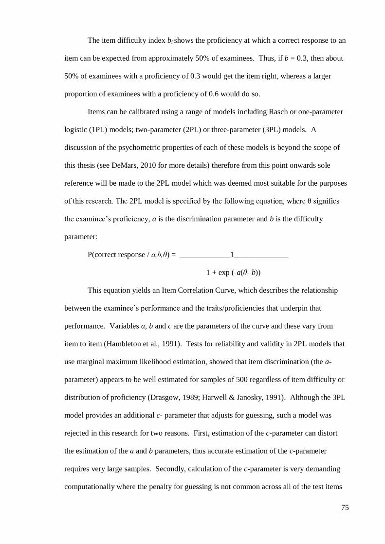
75
The item difficulty index bi shows the proficiency at which a correct response to an
item can be expected from approximately 50% of examinees. Thus, if b = 0.3, then about
50% of examinees with a proficiency of 0.3 would get the item right, whereas a larger
proportion of examinees with a proficiency of 0.6 would do so.
Items can be calibrated using a range of models including Rasch or one-parameter
logistic (1PL) models; two-parameter (2PL) or three-parameter (3PL) models. A
discussion of the psychometric properties of each of these models is beyond the scope of
this thesis (see DeMars, 2010 for more details) therefore from this point onwards sole
reference will be made to the 2PL model which was deemed most suitable for the purposes
of this research. The 2PL model is specified by the following equation, where θ signifies
the examinee’s proficiency, a is the discrimination parameter and b is the difficulty
parameter:
P(correct response / a,b,θ) = _____________1______________
1 + exp (-a(θ- b))
This equation yields an Item Correlation Curve, which describes the relationship
between the examinee’s performance and the traits/proficiencies that underpin that
performance. Variables a, b and c are the parameters of the curve and these vary from
item to item (Hambleton et al., 1991). Tests for reliability and validity in 2PL models that
use marginal maximum likelihood estimation, showed that item discrimination (the a-
parameter) appears to be well estimated for samples of 500 regardless of item difficulty or
distribution of proficiency (Drasgow, 1989; Harwell & Janosky, 1991). Although the 3PL
model provides an additional c- parameter that adjusts for guessing, such a model was
rejected in this research for two reasons. First, estimation of the c-parameter can distort
the estimation of the a and b parameters, thus accurate estimation of the c-parameter
requires very large samples. Secondly, calculation of the c-parameter is very demanding
computationally where the penalty for guessing is not common across all of the test items
76
as was the case with the knowledge tests used in this study. IRT models do not require the
data to be normally distributed, however estimation of IRT parameters requires large
samples and longer tests provide more accurate θ estimates (C. M. Woods, 2008).
Item response analysis uses mathematical models that specify that the probability
that an examinee will supply the correct answer to a given item depends on the examinee’s
proficiency and the characteristics of the item (Hambleton et al., 1991). One major
advantage of using IRT is that when an IRT model fits the test data, the proficiency
estimates for the examinees are not test-dependent, which means that proficiency estimates
derived using different sets of items will be invariant across the tests (except for
measurement error) (Hambleton et al., 1991 ). However, before proceeding with IRT
analysis, several assumptions need to be satisfied about the data used in these models, the
most important of which are unidimensionality and local independence. A test that
measures a single proficiency is deemed unidimensional. Although the outcomes on
knowledge tests are affected by other factors, such as cognition, personality and
motivation, the assumption of unidimensionality is satisfied where there is a single
“dominant” element that influences test performance (Hambleton et al., 1991). This is
established by looking at the scree plot. The assumption of local independence is
established when examinees’ responses to any pair of items are statistically independent
when their abilities are held constant. This is established using Yen’s Q3 Test (1984).
These assumptions were tested in relation to the data produced on each of the knowledge
tests in this research and the outcomes are reported at the beginning of the relevant
sections.
77
Chapter 3: Personal Characteristics
3.1 Introduction
The field of personality research encapsulates two fundamental views of human
nature; an ideographic perspective, which focuses on the uniqueness of individuals and a
nomothetic view, which concerns itself with the human tendency to exhibit consistent
patterns of thinking, feeling and acting in terms of personality traits (McCrae et al., 2000).
In the latter part of the 20th century, the well-publicised person-situation debate between
proponents of the nomothetic, trait-based approach, most notably Costa and McCrae, and
advocates of the ideographic approach, including Mischel and Bandura, highlighted the
strengths and weaknesses of these approaches in explaining and predicting human
behaviour. On the one hand, Mischel condemned, what he saw as an over-reliance on
trait-based explanations, by demonstrating that behaviour varies across situations and that
the correlations reported in studies that used both self-reported trait measures and also
assessed actual behaviour were typically less than .30 (Mischel, 1968). On the other hand,
a range of studies using the five-factor trait model of personality showed that there is
substantial consistency in personality traits across the adult lifespan and that trait scores
were predictive of life-course outcomes (McCrae & Costa, 1989; McCrae et al., 2000).
One such example involved a longitudinal study of Harvard graduates, which showed that
trait measurements taken at the end of their college careers were significantly related to
those taken 45 years later and that higher levels of traits such as conscientiousness,
extraversion and openness to experience were associated with more positive outcomes,
such as career success and general adjustment to variations in life circumstances (Soldz &
Vaillant, 1999).
As a result of the insight gained during the person-situation debate, it is now
generally accepted among theorists that personality constitutes a stable, generalised, distal
influence on behaviour (Beirness, 1993; McCrae & Costa, 2004; Mischel & Shoda, 1995;
78
Ulleberg & Rundmo, 2003), which is mediated through more proximal socio-cognitive
factors such as beliefs, attitudes and intentions (Ajzen, 1991). This view is also enshrined
in TCI model of driving behaviour (Fuller, 2005).
Numerous studies have shown that individual differences in personality traits,
including sensation seeking, impulsiveness and Big-Five markers, are predictive of a range
of behaviours, including academic performance, risk taking, the development and
maintenance of driving styles and crash involvement (Arnett et al., 1997; Winfred Arthur
& Graziano, 1996; Chamorro-Permuzic & Furnham, 2003; Jonah, 1997; Stanford et al.,
2009; Sümer, 2003). These findings have substantive implications for driver education.
First, whereas cognitive ability is clearly an important factor in academic achievement,
ability alone does not provide a sufficient explanation for individual differences in either
the ability to learn or academic achievement. For instance, research conducted by
Chamorro-Permuzic and Furnham, (2003; 2009) indicated that the Big-Five traits (Costa &
McCrae, 1992) accounted for over 10% of the unique variance in exam grades achieved by
university undergraduates over a three-year period. Furthermore, following their
longitudinal study of New Zealandanders aged from 3 – to 21-years-old, which assessed
health risk behaviours, Caspi et al. (1997) noted that since the personality correlates of risk
taking are evident early in life, knowledge of these characteristics would help programme
developers build courses that can adapt to characteristic motivations, attitudes and feelings
of specific audiences. Thus, knowledge about personality could be used to inform the
content of educational interventions and also to customise interventions in order to make
them more efficient and effective (Shope & Bingham, 2008). Whereas it is acknowledged
that it is difficult to change personal dispositions, it also appears that the behavioural
expression of these tendencies is amenable to modification through metacognitive practices
(Flavell, 1979). These ideals are firmly enshrined in the GDE-framework (Hatakka et al.,
2002), which posits that driver education programmes should incorporate metacognitive
79
exercises, for example to encourage students to identify their own personal tendencies, to
understand the effects that these tendencies might have on their driving behaviour and to
provide them with robust strategies to control maladaptive tendencies, thereby increasing
safety.
3.1.1 Big-Five personality traits
In recent years the Big-Five model has come to dominate trait-based research into
individual differences (McAdams & Pals, 2006), because evidence suggests that this
model, encompassing five super traits (extraversion, agreeableness, conscientiousness,
neuroticism, and openness to experience) represents personality at its broadest level of
abstraction (Costa & McCrae, 1992; Goldberg, 2011). As described by the International
Personality Item Pool (Goldberg, 2011), five-factor domains subsume hundreds of traits.
For instance, agreeableness incorporates facets such as trust, compliance and straight-
forwardness. Conscientiousness includes goal-orientation, competence, deliberation and
orderliness. Extraversion is marked by positive affect, excitement seeking and
gregariousness. Neuroticism, which is labelled ‘emotional stability’ is characterised by
anxiety, anger/hostility, impulsiveness and vulnerability. Openness to experience, which is
labelled ‘intellect/imagination’, incorporates intellectual curiosity, fantasy and openness to
aesthetics, feelings and values (Gullone & Moore, 2000).
Links between Big-Five traits and engagement in risky behaviour have been
investigated empirically. For example, Nicholson, Fenton-O’Creevy, Soane, and Willman
(2005) devised an index of risk taking across six life domains (career, health, finance,
recreation, social and safety), which they used subsequently to examine the relationship
between Big-Five traits and risk-taking. Their results showed that high levels of
extraversion and openness, and that low levels of neuroticism, agreeableness and
conscientiousness predicted risk-taking tendencies. However, the associations between
Big-Five traits and risky driving are less clear. Whereas Booth-Kewley and Vickers

80
(1994) found that both low agreeableness and low consciousness were strong predictors of
risky driving, neither neuroticism, openness, nor extraversion predicted this behaviour.
A number of Big-Five traits have also been linked with accident involvement. A
meta-analytic study by Clarke and Robertson (2005) found that low conscientiousness and
low agreeableness were valid and generalizable antecedents of accident involvement
generally, with correlations of .27 and .26 respectively. They also showed that high
extraversion was predictive of RTC involvement. Winifred Arthur and her colleagues (W
Arthur & Doverspike, 2001; Winfred Arthur & Graziano, 1996) have demonstrated links
between low conscientiousness and crash involvement repeatedly. For instance, one study
involving 477 drivers, showed that individuals who rated themselves as more conscientious
(i.e. more dependable, responsible and self-disciplined) were less likely to have been
involved in an RTC than were those with lower scores for that trait (Winfred Arthur &
Graziano, 1996).
Research also suggests that personality traits can influence risk judgements in
adolescents. A study by Gullone and Moore (2000), involving 459 secondary school
pupils aged from 11- to 18-years-old found that those who were more extraverted and/or
more agreeable were also less likely to rate behaviours listed in the Adolescent Risk-
Taking Questionnaire (Gullone, Moore, Moss, & Boyd, 2000) as risky. In addition, those
who were more conscientiousness judged all types of risk, except thrill seeking, as riskier
than did their less conscientious counterparts. The relationship between Big-Five traits and
academic success has also been studied extensively (for a review, see de Raad &
Schouwenburg, 1996). The bulk of this research involves college students, where
consistent positive relations have been found between performance and both
conscientiousness and openness, and negative relations with extraversion, and neuroticism
(Busato, Prins, Elshout, & Hamaker, 1998, 2000; Chamorro-Permuzic & Furnham, 2003;
de Raad & Schouwenburg, 1996). It is also worth noting that conscientiousness is regarded
81
as the most reliable predictor of performance at work (Barrick & Mount, 1991). Among
children and adolescents, it seems that both extraversion and neuroticism act as positive
predictors of achievement (de Raad & Schouwenburg, 1996). Since individual differences
with respect to Big-Five traits appear to influence risk-taking behaviour, accident
involvement, risk judgements and academic performance, then clearly these influences
need to be acknowledged by course developers and suitably addressed as part of a good
PLDE course.
3.1.2 Sensation seeking
Sensation seeking (SS) is a personality disposition that is characterised by a need to
seek novelty and intensity of sensory experience (Arnett, 1994). Tendencies towards
sensation seeking have been identified in the general population, using a variety of
instruments, including the Arnett Inventory of Sensation Seeking (AISS) (Arnett, 1994).
Elevated levels of SS have been associated with greater participation in a variety risky
activities including extreme sports (Ruedl, Abart, Ledochowski, Burtscher, & Kopp, 2012),
substance abuse (Wagner, 2001), risky sexual activities (Donohew et al., 2000) and risk
taking in traffic (Arnett, 1994; Arnett et al., 1997). Both age and sex differences have been
identified in AISS scores (Arnett, 1996; Donohew et al., 2000). For instance, the results
from a German study involving almost 2,000 people aged between 16 - and 79-years,
showed that age was inversely related to SS and that the scores for males were higher than
those for females across all age categories (Roth, Schumacher, & Brähler, 2005). The
same study also found that sociodemographic factors, such as socioeconomic status and
place of residence, only explained a small amount of the variance in SS. Since consistently
higher levels of SS have been found in adolescents when compared to adults (Hoyle,
Stephenson, Palmgreen, Lorch, & Donohew, 2002; Jonah, 1997; Zuckerman, 1996), it has
been proposed that SS might be partly responsible for the disproportionately high rates of
road traffic crashes and fatalities among young drivers (Arnett et al., 1997). Jonah (1997)
82
reviewed 40 studies that investigated the relationship between SS and risky driving, and
found moderate correlations between these factors (r =0.3 to 0.4). Similarly, Rimmö and
Åberg (1999) found that SS explained 27% of the variance in driving violations, which
was 10 times more than the variation accounted for by driving errors. Beirness, and
Simpson (1988) also identified SS as a contributing factor in accident involvement among
American high school students in grades 9 – 11. Since, SS represents a risk-increasing
factor for adolescent drivers, there is an obvious need to provide youngsters with
knowledge about SS and insight into their own SS tendencies and the ways in which SS
can have a negative impact on their safety and well-being.
3.1.3 Impulsiveness
Impulsiveness is characterised as “a predisposition towards, rapid, unplanned
reactions to internal or external stimuli without regard to the negative consequences of
these reactions” (Moeller, Barratt, Dougherty, Schmitz, & Swann, 2001, p. 1783).
Research has shown that individuals who exhibit elevated levels of trait impulsiveness are
prone to a variety of behaviours that have a negative impact on their own health and well-
being, and on society generally. For instance, impulsiveness has been linked with sub-
optimal levels of emotional and behavioural control in areas of educational performance
(Fink & MCCown, 1993; Stanford et al., 1996), mental health (Castellani & Rugle, 1995)
criminal justice (Ireland & Archer, 2008) and general risk-taking (Haase & Silbereisen,
2011). This suggests that individual differences with respect to trait impulsiveness may
also constitute useful predictors of pre-existing levels of knowledge, skills and attitudes
and also of educational outcomes with respect to PLDE.
The Barratt Impulsiveness Scale (BIS), is the most widely used measure of trait
impulsiveness (Stanford et al., 2009). The original BIS scale consisted of 30-items
designed to measure three sub-traits: cognitive impulsiveness (making quick decisions),
motor impulsiveness (acting without thinking) and non-planning impulsiveness (lack of
83
foresight) (Barratt, 1959). Furthermore, Patton, Stanford and Barratt (1995) believe that
the overall item pool constitutes a “homogenous measure of impulsiveness”, which
indicates that a total scale score can also be used to assess overall impulsiveness. The BIS-
30 was designed to clearly differentiate impulsiveness from other action-based personality
characteristics such as extraversion, sensation seeking and risk taking (Stanford et al.,
2009). Using the updated BIS-II, Stanford et al. (1996) found that impulsiveness was
positively correlated with a number of risk taking behaviours including aggression, drug
use, drink driving and not wearing seatbelts. The same study also showed that levels of
impulsiveness were higher in males than females and was higher in high school students
than in college students. Thus, it is possible that excessive impulsiveness may partly
explain the overrepresentation of young male drivers RTCs.
Research also suggests that impulsiveness acts as a moderator between intelligence
and academic success; students with high impulsiveness and high academic ability tend to
have lower grades than do those with low impulsiveness and high ability (Zeidner, 1995).
For example, in a study of 241 Spanish secondary school students aged between 12 – 17-
years, using the BIS-10, Vigil-Colet and Morales-Vives (2005) found significant positive
correlations between academic failure and non-planning (.29), cognitive (.27), and overall
impulsiveness (.31). One likely explanation for these findings is that children and
adolescents with an impulsive problem-solving style do not persist with learning tasks
(Fink & MCCown, 1993). Another explanation focuses on the cognitive aspect of
impulsiveness, suggesting that impulsive individuals tend to respond quickly, with little
analysis or reflection (Vigil-Colet & Morales-Vives, 2005), which may indicate that they
might not apply themselves adequately when responding to surveys. The BIS 15 was
developed by Spinella (2007) to provide a short version of the BIS that would be suitable
for use in larger surveys, such as the present study.

84
Thus, an accumulation of evidence suggests that individual differences in
personality traits constitute a significant antecedent influence on cognition, affect, and
behaviour. In addition, the TCI model (Fuller, 2005) predicts that personality represents a
significant antecedent influence on driver capability and thereby on driving behaviour.
3.2 Aim
This part of the study aims to calculate scores for sensation seeking, impulsiveness
and the Big-Five-personality traits. These scores will be used subsequently to investigate
the impact that these traits might have on driving-related knowledge, skills and attitudes of
PLDs before taking a PLDE course, immediately after taking a course and again 9 months
later. The results of these tests will be reported in chapters 5, 6 and 7 as part of the
summative evaluation. Method
3.2.1 Design
See Chapter 2, subsection 2.3
3.2.2 Participants
See Chapter 2, subsection 2.2.
3.2.3 Procedure
See Chapter 2, subsection 2.5
3.3 Measures
Three well-known inventories were used to measure personality characteristics in
this research:
1. Arnett Inventory of Sensation Seeking (AISS) (Arnett, 1994).
2. Barrett Impulsiveness Scale-15 (BIS-15) (Spinella, 2007).
3. International Personality Item Pool-50 item set of Big-Five traits (IPIP-50)
(Goldberg, 2011).
85
3.3.1 AISS
The 20-item AISS (Arnett, 1994) incorporates 2 sub-scales; Novelty (10 items) and
Intensity (10 items). Responses were given on a 4-point Likert scale (1 = Describes me
very well – 4 = Does not describe me at all), (Appendix D, Question 14) and these scores
were reversed subsequently such that higher scores suggested a greater tendency towards
sensation seeking. The AISS is used widely to measure sensation seeking, however,
although some studies showed that Arnett’s two-factor model of sensation seeking
provided a reasonably good fit for the data (Ferrando & Chico, 2001), others found that
the internal consistency of the model was low (Arnett, 1994; Haynes, Miles, & Clements,
2000; Roth & Hertzberg, 2004). For example Arnett himself (1994) reported poor
Cronbach’s α values for both the intensity (.64) and the novelty sub-scales (.5), and the
value of the overall scale was barely adequate (.7). Furthermore, the results from studies
conducted by Haynes et al. (2000), and Roth and Hertzberg (2004)10
, who used
confirmatory factor analysis (CFA) to test the factor structure of the AISS, highlighted
problems with respect to some of the AISS items because they failed to load onto their
designated sub-scales, which suggests that the current test may need some revision.
3.3.2 BIS-15
The BIS-15 (Spinella, 2007) consists of a 15-item scale comprising 3 sub-scales,
i.e. motor and attentional impulsiveness and non-planning (5 items for each). Responses
were measured on a 4-point Likert scale (1 = Rarely/never – 4 = Almost always) (see
Appendix D, Question 34). Although there are six positively valanced items in this scale,
scores for these items are reversed prior to data analysis, thus a higher score on this scale
indicates a stronger tendency towards impulsiveness Although Spinella reported good
internal consistency for the entire scale (a = .81), no alpha values were provided for the
three sub-scales. However he also reported that scores on the BIS 15 correlated highly
10 Note the mean participant ages in these studies were 24.8 and 14.9 years respectively.

86
with those on the BIS-30 (r = .94, p<.001). In addition, scores on the BIS 15 were
inversely related to age and the instrument related to other measures that assess executive
functions and impulsiveness. Thus, Spinella concluded this shorter scale serves as a useful
alternative to the BIS-II, while retaining good psychometric properties. In their review of
50 years of research using the 30-item BIS, Stanford et al., (2009), reported alpha values of
.74, .59 and .72 respectively for the Attentional, Motor and Non-planning subscales and
.83 for the overall scale.
3.3.3 IPIP-50
The IPIP-50 test (Goldberg, 2011) provides a public-domain alternative for
measuring Big-Five personality constructs which feature in major commercial inventories
(e.g. Costa and McCrae’s Neo-Pi-R(1992)). The inventory uses 10 items to measure each
of the 5 personality factors: Extraversion, Agreeableness, Conscientiousness, Emotional
Stability and Intellect/Imagination. Responses were recorded using a 5-point Likert scale
(1 = Very Inaccurate – 5 = Very Accurate), (Appendix E, Question 46). Scores for
negatively valanced items were reversed subsequently, thus higher scores indicate a
stronger tendency towards these dispositions
The IPIP-50 scale has good internal consistency, with a reported Cronbach’s alpha
coefficient of .84 for the 50-item scale and alphas of .87 for extraversion, .82 for
agreeableness, .79 for conscientiousness, .86 for emotional stability and .84 for
intellect/imagination (Goldberg, 2011).
In the current research, both the AISS and the BIS-15 tests were conducted at T1, and
the IPIP test was conducted at T2. This was done in order to balance the sizes of the
questionnaires that were used in both tests and to avoid overtaxing the participants in any
one test.
87
3.4 Results
3.4.1 Confirmatory factor analysis
The data from each inventory was subjected to separate confirmatory factor
analyses (CFA) using Amos (Version 18.0) (Arbuckle, 2009), to ascertain the
psychometric properties of these tests. Preliminary analyses revealed excessive kurtosis in
some of the data, thus further analysis was conducted using asymptotic distribution free
estimation, which makes no distributional assumptions and can be used where sample sizes
exceed 1,000 (Muthēn, 1993). The following well-established criteria were used to judge
the acceptability of each model in this research:
The Goodness of Fit Index (GFI) exceeds .90 (Byrne, 2010)
The Comparative Fit Index (CFI) exceeds .93 (Byrne, 2010)
The Root Mean Square of Approximation (RMSA) is less than .08 (M. W.
Brown & Cudeck, 1993) and ideally less than .05 (Steiger, 1990).
The Expected Cross Validation Index (ECVI) should be less than 2 or 3
(Kline, 2011).
Attempts to fit unidimensional models and a range of multi-dimensional models for
each of the three inventories were unsuccessful (see Appendix L for full details). The
following results from the final attempt to fit unidimensional models for each instrument
show that ECVI and the CFI indices were outside of acceptable levels.
AISS: (χ2 (1880) = 605.65 [p < .001]; RMSEA = .06 [.05-.06]; GFI = .95;
CFI = .67: ECVI = .36 [.32-.40])
BIS: (χ2 (1880) = 551.75 [p < .001]; RMSEA = .05 [.049-.058]; GFI = .94;
CFI = .61: ECVI = .33 [.291-.370])
IPIP: (χ2 (1880) = 10196.26 [p < .001]; RMSEA = .06 [.06-.06]; GFI = .79; CFI
= .60: ECVI = 5.54 [5.37-5.72].
88
3.4.2 Exploratory factor analysis
As an alternative, the scores on these tests were subjected to separate exploratory
factor analyses (EFA) using principal component analysis (PCA). The suitability of the
data for factor analysis was assessed independently for each test. Inspection of the
correlation matrices for each test revealed the presence of many coefficients of .3 and
above, the Kaiser-Meyer-Olkin (Kaiser, 1974) values exceeded .80 and Bartlett’s Tests of
Sphericity (Bartlett, 1954) reached statistical significance (p < .05), supporting the
factorability of the correlation matrices. To aid the interpretation the resulting
components, oblique (promax) rotations were performed in an attempt to achieve the most
parsimonious simple structure, while permitting the factors to correlate, since the results of
the CFAs had established that there was some overlap between the latent constructs in each
test (see Appendix L). Having identified the relevant factors in each test, the Cronbach’s
alpha (a) (Cronbach, 1990) was computed to assess the internal consistency of the
individual scales and sub-scales. The following rule-of-thumb outlined by Nunally (1978)
was used to categorise a; > . 9 – Excellent, > .8 – Good, > .7 – Acceptable, > .6 –
Questionable, > .5 – Poor, and < .5 – Unacceptable. Then mean score were calculated for
each scale. According to Tabachnick, and Fidell (2001), this method preserves the
variation in the original data and is generally acceptable for most exploratory research
designs.
3.4.2.1 AISS
The CFA of the 20-item AISS inventory showed that 4 of the observed variables
that Arnett (1994) proposed should load on to the Novelty factor (items 3, 5, 13, and 15)
and 1 observed variable that should load on to the Intensity scale (item 4) failed to load
significantly on to these factors. Similar problems with these items have been reported in
previous studies (e.g. Haynes et al., 2000; Roth & Hertzberg, 2004). In order to improve
the validity of this scale in the present study, the PCA was conducted using only the
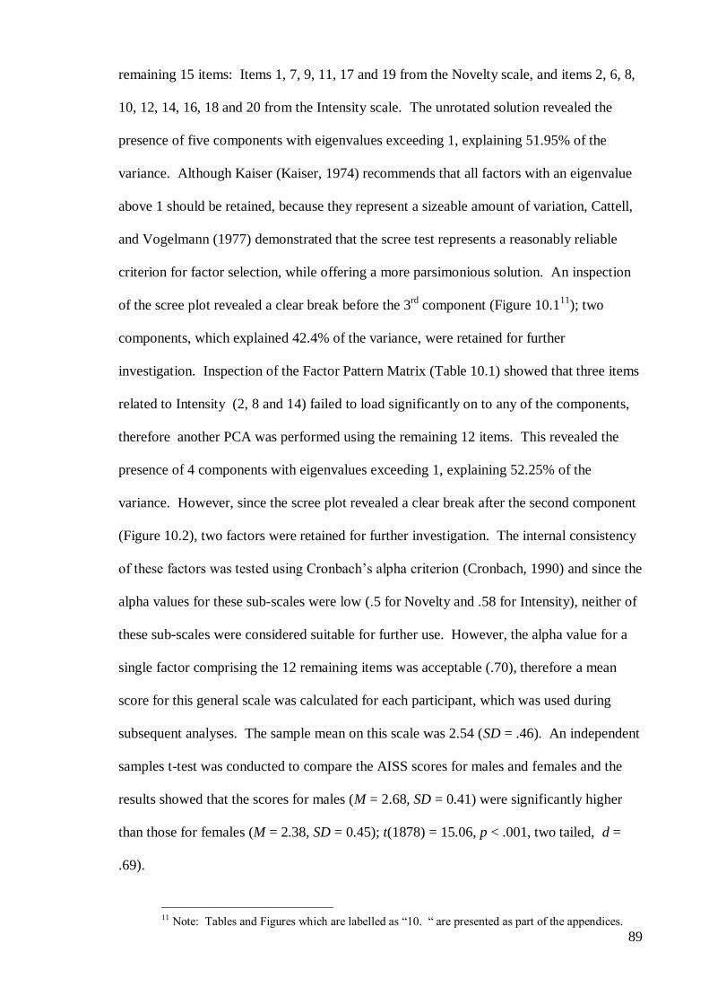
89
remaining 15 items: Items 1, 7, 9, 11, 17 and 19 from the Novelty scale, and items 2, 6, 8,
10, 12, 14, 16, 18 and 20 from the Intensity scale. The unrotated solution revealed the
presence of five components with eigenvalues exceeding 1, explaining 51.95% of the
variance. Although Kaiser (Kaiser, 1974) recommends that all factors with an eigenvalue
above 1 should be retained, because they represent a sizeable amount of variation, Cattell,
and Vogelmann (1977) demonstrated that the scree test represents a reasonably reliable
criterion for factor selection, while offering a more parsimonious solution. An inspection
of the scree plot revealed a clear break before the 3rd
component (Figure 10.111
); two
components, which explained 42.4% of the variance, were retained for further
investigation. Inspection of the Factor Pattern Matrix (Table 10.1) showed that three items
related to Intensity (2, 8 and 14) failed to load significantly on to any of the components,
therefore another PCA was performed using the remaining 12 items. This revealed the
presence of 4 components with eigenvalues exceeding 1, explaining 52.25% of the
variance. However, since the scree plot revealed a clear break after the second component
(Figure 10.2), two factors were retained for further investigation. The internal consistency
of these factors was tested using Cronbach’s alpha criterion (Cronbach, 1990) and since the
alpha values for these sub-scales were low (.5 for Novelty and .58 for Intensity), neither of
these sub-scales were considered suitable for further use. However, the alpha value for a
single factor comprising the 12 remaining items was acceptable (.70), therefore a mean
score for this general scale was calculated for each participant, which was used during
subsequent analyses. The sample mean on this scale was 2.54 (SD = .46). An independent
samples t-test was conducted to compare the AISS scores for males and females and the
results showed that the scores for males (M = 2.68, SD = 0.41) were significantly higher
than those for females (M = 2.38, SD = 0.45); t(1878) = 15.06, p < .001, two tailed, d =
.69).
11 Note: Tables and Figures which are labelled as “10. “ are presented as part of the appendices.
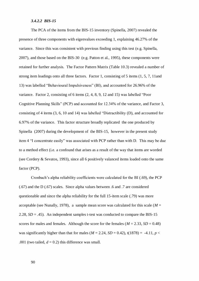
90
3.4.2.2 BIS-15
The PCA of the items from the BIS-15 inventory (Spinella, 2007) revealed the
presence of three components with eigenvalues exceeding 1, explaining 46.27% of the
variance. Since this was consistent with previous finding using this test (e.g. Spinella,
2007), and those based on the BIS-30 (e.g. Patton et al., 1995), these components were
retained for further analysis. The Factor Pattern Matrix (Table 10.3) revealed a number of
strong item loadings onto all three factors. Factor 1, consisting of 5 items (1, 5, 7, 11and
13) was labelled “Behavioural Impulsiveness” (BI), and accounted for 26.96% of the
variance. Factor 2, consisting of 6 items (2, 4, 8, 9, 12 and 15) was labelled “Poor
Cognitive Planning Skills” (PCP) and accounted for 12.34% of the variance, and Factor 3,
consisting of 4 items (3, 6, 10 and 14) was labelled “Distractibility (D), and accounted for
6.97% of the variance. This factor structure broadly replicated the one produced by
Spinella (2007) during the development of the BIS-15, however in the present study
item 4 “I concentrate easily” was associated with PCP rather than with D. This may be due
to a method effect (i.e. a confound that arises as a result of the way that items are worded
(see Cordery & Sevatos, 1993), since all 6 positively valanced items loaded onto the same
factor (PCP).
Cronbach’s alpha reliability coefficients were calculated for the BI (.69), the PCP
(.67) and the D (.67) scales. Since alpha values between .6 and .7 are considered
questionable and since the alpha reliability for the full 15-item scale (.79) was more
acceptable (see Nunally, 1978), a sample mean score was calculated for this scale (M =
2.28, SD = .45). An independent samples t-test was conducted to compare the BIS-15
scores for males and females. Although the score for the females (M = 2.33, SD = 0.48)
was significantly higher than that for males (M = 2.24, SD = 0.42), t(1878) = -4.11, p <
.001 (two tailed, d = 0.2) this difference was small.
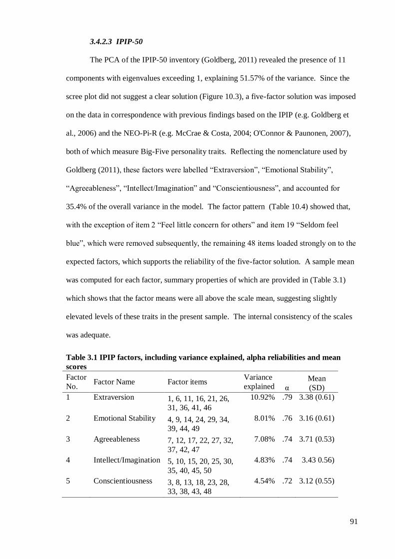
91
3.4.2.3 IPIP-50
The PCA of the IPIP-50 inventory (Goldberg, 2011) revealed the presence of 11
components with eigenvalues exceeding 1, explaining 51.57% of the variance. Since the
scree plot did not suggest a clear solution (Figure 10.3), a five-factor solution was imposed
on the data in correspondence with previous findings based on the IPIP (e.g. Goldberg et
al., 2006) and the NEO-Pi-R (e.g. McCrae & Costa, 2004; O'Connor & Paunonen, 2007),
both of which measure Big-Five personality traits. Reflecting the nomenclature used by
Goldberg (2011), these factors were labelled “Extraversion”, “Emotional Stability”,
“Agreeableness”, “Intellect/Imagination” and “Conscientiousness”, and accounted for
35.4% of the overall variance in the model. The factor pattern (Table 10.4) showed that,
with the exception of item 2 “Feel little concern for others” and item 19 “Seldom feel
blue”, which were removed subsequently, the remaining 48 items loaded strongly on to the
expected factors, which supports the reliability of the five-factor solution. A sample mean
was computed for each factor, summary properties of which are provided in (Table 3.1)
which shows that the factor means were all above the scale mean, suggesting slightly
elevated levels of these traits in the present sample. The internal consistency of the scales
was adequate.
Table 3.1 IPIP factors, including variance explained, alpha reliabilities and mean
scores
Factor
No. Factor Name Factor items
Variance
explained α
Mean
(SD)
1 Extraversion 1, 6, 11, 16, 21, 26,
31, 36, 41, 46
10.92% .79 3.38 (0.61)
2 Emotional Stability 4, 9, 14, 24, 29, 34,
39, 44, 49
8.01% .76 3.16 (0.61)
3 Agreeableness 7, 12, 17, 22, 27, 32,
37, 42, 47
7.08% .74 3.71 (0.53)
4 Intellect/Imagination 5, 10, 15, 20, 25, 30,
35, 40, 45, 50
4.83% .74 3.43 0.56)
5 Conscientiousness 3, 8, 13, 18, 23, 28,
33, 38, 43, 48
4.54% .72 3.12 (0.55)
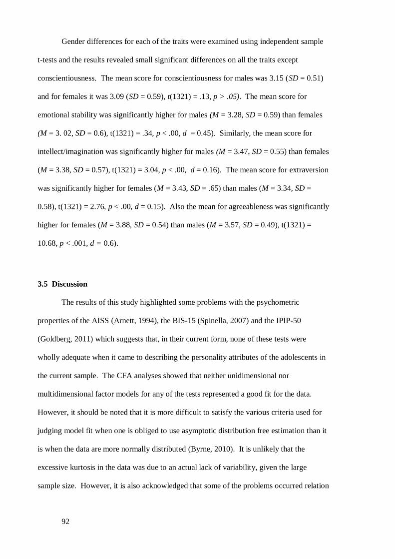
92
Gender differences for each of the traits were examined using independent sample
t-tests and the results revealed small significant differences on all the traits except
conscientiousness. The mean score for conscientiousness for males was 3.15 (SD = 0.51)
and for females it was 3.09 (SD = 0.59), t(1321) = .13, p > .05). The mean score for
emotional stability was significantly higher for males (M = 3.28, SD = 0.59) than females
(M = 3. 02, SD = 0.6), t(1321) = .34, p < .00, d = 0.45). Similarly, the mean score for
intellect/imagination was significantly higher for males (M = 3.47, SD = 0.55) than females
(M = 3.38, SD = 0.57), t(1321) = 3.04, p < .00, d = 0.16). The mean score for extraversion
was significantly higher for females (M = 3.43, SD = .65) than males (M = 3.34, SD =
0.58), t(1321) = 2.76, p < .00, d = 0.15). Also the mean for agreeableness was significantly
higher for females (M = 3.88, SD = 0.54) than males (M = 3.57, SD = 0.49), t(1321) =
10.68, p < .001, d =
0.6).
3.5 Discussion
The results of this study highlighted some problems with the psychometric
properties of the AISS (Arnett, 1994), the BIS-15 (Spinella, 2007) and the IPIP-50
(Goldberg, 2011) which suggests that, in their current form, none of these tests were
wholly adequate when it came to describing the personality attributes of the adolescents in
the current sample. The CFA analyses showed that neither unidimensional nor
multidimensional factor models for any of the tests represented a good fit for the data.
However, it should be noted that it is more difficult to satisfy the various criteria used for
judging model fit when one is obliged to use asymptotic distribution free estimation than it
is when the data are more normally distributed (Byrne, 2010). It is unlikely that the
excessive kurtosis in the data was due to an actual lack of variability, given the large
sample size. However, it is also acknowledged that some of the problems occurred relation
93
to factor analyses in this study might have arisen because the scales that were used were
developed for adults rather than for adolescents.
Nevertheless, the results for the PCAs for the IPIP and the BIS-15 showed that,
with minor exceptions, all of the items loaded onto the expected factors and that the
resulting scales had good internal consistency, which accords with findings from research
with adult samples (Goldberg et al., 2006; Spinella, 2007). This suggests that both the
IPIP-50 and the BIS-15 instruments are capable of measuring Big-Five personality traits
and impulsiveness in adolescents, which may be of some interest to the research
community, given that both of these tests are short and are available free of charge.
However, the various difficulties outlined above with respect to the original 20-
item AISS scale suggest that this test did not constitute a valid measure of sensation
seeking in the current sample. The combined results of the CFA and the EFA showed that
over 40% of the items failed to load properly on to the correct sub-scales and the internal
consistency reliability of these sub-scales was poor also. Similar results have been
reported in previous studies that examined the factor structure of the AISS using CFA. For
example, in a study involving 822 US undergraduates, with a mean age of < 25-years (SD
= 8.3), Haynes et al, (2000) needed to remove 7 items due to low factor loadings (items 3,
13, 15 and 17 from the Novelty sub- scale, and items 10, 14, and 16 from the Intensity sub-
scale) to derive a version of the AISS which fitted the data adequately. Similarly, research
conducted by Roth, and Hertzberg (2004) with a sample of 1,949 German adolescents aged
between 14 – 16-years, also produced low factor loadings with respect to 8 AISS items
(items 3,5,13, 15 and 17 from the Novelty sub-scale, and items 2, 10 and 14 from the
Intensity sub-scale), prompting their removal. It is interesting to note that 4 items, that
proved problematic in those studies were also problematic in the present study; item 3 “If I
have to wait a long time, I am usually patient about it”, item 13 “I do not like extremely
hot and spicy food”, item 14 “In general, I work better when I am under pressure” and item
94
15 “I often like to have the TV on while I am doing something”. Given that all three
studies were conducted in different countries, with different aged samples and also that
Roth and Hertzberg used a German translation of the AISS, it is clear that these particular
items do not constitute valid generalized measures of their respective sub-scales and should
perhaps be removed from the AISS inventory. For instance, it is likely that item 3 assesses
patience as opposed to a low desire for novelty. Younger adolescents may have limited
experience with making the decisions described in items 13 and 15, depending on their
families’ lifestyles. Given that 7 further items (2, 4, 5, 8, 10, 16 and 17) have proved
problematic in the U.S, the German and/or the present study, this suggests that over 50% of
the items on the AISS do not measure the construct that they were designed to measure on
a consistent basis and thus warrant further investigation.
The poor performance of the AISS is generally attributed to Arnett’s failure to
establish the psychometric properties of the test at the outset, devising the test instead on
the basis of the face validity of the constituent items (Haynes et al., 2000; Roth &
Hertzberg, 2004). The best-studied alternative, Zuckerman’s Sensation Seeking Scale,
Form V (Zuckerman 1996), appeared unsuitable for the current research, since it requires
that participants adjudicate on activities such as flying an airplane, homosexuality and
sexual experiences, which not only describe behavioural willingness rather than sensation
seeking (Mallet & Vignoli, 2007), but are also plainly unsuitable for measuring of
sensation seeking in younger adolescents. Thus, further research is warranted to
investigate the underlying structure of sensation seeking as a personality trait and to
formulate a test that can measure that construct more accurately than can the present
formulation of the AISS, especially in young adolescents.
3.5.1.1 Gender effects
Gender differences in the scales on the IPIP=50 were broadly in line with
expectations. Differences in agreeableness and emotional stability (opp. neuroticism)
95
evidenced in this study were consistent with those reported in previous studies of adults
and adolescents (Costa & McCrae, 2001; Gullone & Moore, 2000). Females had
significantly higher levels of agreeableness and significantly lower levels of emotional
stability than males. Also in accord with Gullone and Moore’s findings, males reported
higher levels of conscientiousness than females, albeit that these differences were non-
significant. Moreover, whereas males scored higher on intellect/imagination (openness to
experience), the females in this study appeared to be more extraverted than the males. It is
notable however, that the magnitude of gender differences that were found was quite small.
Males also recorded significantly higher levels of sensation seeking and gender
differences accounted for 11% of the variation in the scores on that scale. Although Arnett
(Arnett, 1994) did not provide effect size calculations for his research, the present results
accord with findings from the Roth and Hertzberg study reported earlier (2004) which
recorded a medium sized gender effect in favour of males using Cohen’s d test. Although
significant gender differences were also evident for impulsiveness in this research, these
effects were very small. Moreover, whereas significant gender differences were found
with respect to several of the traits that feature in this study, the magnitude of most of these
differences was so small as to render them negligible. Similar outcomes are common in
studies featuring large sample sizes. In sum, the results of this study indicate that there
were meaningful gender differences in the levels of sensation seeking, emotional stability,
and agreeableness in the current sample, where males exhibited higher levels of the former
two traits and females reported higher levels of the latter trait.
The principal aim of this part of the study was to measure personality traits that
(theoretically) constitute antecedent influences on behaviour (i.e. the Big-Five) and also on
risk-taking (i.e. sensation seeking and impulsiveness). Despite the large sample size, a
number of problems were identified regarding the validity of these tests, most notably with
the AISS (Arnett, 1994). Nevertheless, scores on these scales were calculated for each

96
participant and these were used during the remainder of this study to test for the possible
effects of these traits on driving-related knowledge, risk perception skills and attitudes.
However, since the TCI model (Fuller, 2005) also posits that prior learning represents a
significant influence on knowledge, skills and attitudes and thereby on driver capability,
the next chapter will examine that issue in some detail.
97
Chapter 4: Learning and experience
4.1 Introduction
An understanding of the phenomena and principles of learning is an essential
prerequisite in any study of human behaviour (Levin, 2005). This is especially true when
that behaviour occurs in an educational setting as is the case with the present research.
There is general agreement among practitioners and researchers across a wide range of
disciplines, including educationalists, psychologists and neuropsychologists, that learning
is a process whereby experience produces a relatively enduring change in an organism’s
behaviour or capabilities (Bandura, 1977; Bransford et al., 2000; Brunner, 1966; E. R.
Kandel, Schwartz, & Thomas, 2000; Piaget, 1971; Skinner, 1974). The scientific literature
on human learning, development, cognition, brain functioning and culture is colossal, thus
a detailed explication of these principles is beyond the scope of this study. Instead, there
follows a brief review of theories and research that are pertinent to driver behaviour on the
one hand and that have specific implications for the design, implementation and
assessment of school-based educational interventions on the other.
Learning entails the acquisition of some type of knowledge, which is then stored in
the form of memory (Reber & Reber, 2001). Schacter, Wagner and Buckner (2000)
identified four long-term memory systems; episodic memory, semantic memory,
perceptual-representation system and procedural memory. One of the main ways in which
memory systems differ is in their reliance on explicit or implicit memory processes; the
former involves conscious recollection of previous experience whereas the latter is
evidenced when performance on a memory task relies mainly on unconscious mental
processes. Much of the evidence supporting the existence of separate memory systems
was derived from studying patients with memory deficits. For example, Vargha-Khadem
98
et al. (1997) studied children who sustained bilateral hippocampal damage before they had
the opportunity to develop semantic memories. Although these children had poor recall of
the day’s events, e.g. television programmes that they watched, their speech and language
development, literacy and factual knowledge were all within the normal range.
Episodic and semantic memories involve explicit memory processes, and as such,
are often subsumed under the heading of declarative memory. Episodic memory involves
the conscious recall of personal events from the past and semantic memory refers to
knowledge about the world (Eysenck & Keane, 2010). The cognitive processes that occur
during explicit learning have a substantial influence on subsequent long-term memory.
Craik and Lockhart’s levels-of-processing theory (1972) posited that the depth of
processing of a stimulus has a sizeable impact on its memorability and that deeper levels of
analysis produce stronger memory traces than do superficial levels of processing. Craik
and Tulving (1975) demonstrated that the elaboration of processing is important for
encoding memories. Over a number of trials they presented participants with a word and a
sentence where a word was missing, and the task was to decide whether or not the word
fitted into the blank space. Elaboration was varied by the complexity of the sentences, for
example, “She cooked the........” and “The great bird swooped down, and carried off the
struggling........” Cued recall in a subsequent test was twice as high for words
accompanying more complex sentences, indicating that elaboration facilitates long-term
memory.
The distinctiveness of a stimulus also affects memorability and two interesting
phenomena have been studied in this regard; the self-reference effect, and flashbulb
memories. The self-reference effect is tested by comparing participants’ self-judgements
with those that they make about others and tests the hypothesis that stimuli involving the
former will be better recalled than those involving the latter. In a meta-analysis of 60 self-
reference studies, Symons and Johnson (1997) found clear evidence supporting the
99
existence of this effect. They also showed that self-references worked best to facilitate
memory when the stimuli used are commonly organized and elaborated through self-
reference. For instance there was a stronger self-reference effect for personality traits than
for nouns describing parts of the body. Flashbulb memory (R. Brown & Kulik, 1977)
describes long lasting vivid memories that people have for dramatic events, for instance,
the assassination of President Kennedy, or being involved in a car crash. Research shows
that flashbulb memories depend on three main factors; (a) prior knowledge, which helps to
relate the event to existing memory structures, (b) personal importance, as predicted by
self-reference theory and (c) a feeling of surprise and an emotional reaction (Conway et
al., 1994). Evidence supporting the memory enhancing effects of levels of processing,
self-reference and flashbulb phenomena supports the assumption that individuals who have
been directly or indirectly involved in a RTC should remember that event and thus their
crash histories may have some bearing on their subsequent knowledge, risk perceptions
and attitudes, and thereby on their amenability to the road safety messages delivered as
part of a PLDE course.
Learning also involves implicit memory processes such as the acquisition of
procedural memory and perceptual representations. Procedural memory is used in
acquiring cognitive and motor skills (Schacter et al., 2000), such as learning to drive. The
perceptual representation system is best described in terms of the repetition priming effect.
For example, evidence shows that stimulus processing occurs faster and/or more easily on
successive presentations of a stimulus (Schacter et al., 2000). Some of the theories
presented above have implications for the development and refinement of driver education
courses. They show that learning is enhanced by repetition and elaboration and when the
material is distinctive and/or has personal relevance to the students.

100
4.1.1 Learning theories
Psychologists distinguish between two modes of learning: Direct learning, which
happens as a result of trial-and error, and indirect learning, which is based on observation
or instruction (Fuller, 2002). In practice, learning can, and often does, entail both of these
processes. The behaviourist movement focused almost exclusively on explaining direct
learning, the social learning and constructivists paradigms mainly concerned with indirect
learning and the cognitivist approach addressed both of these types of learning.
4.1.1.1 Behavioural theories
Modern-day theorising about how people learn began in earnest with the advent of
the behaviourist movement (Bransford et al., 2000). Behaviourism is an empirical
approach to learning that focuses on observable behaviour and on the stimuli that elicit it,
without reference to the mind or mental processes (Skinner, 1974). The central tenet of
behaviourism is that almost all behaviours are learned by means of conditioning, which
occurs as a result of interacting with the environment. During the learning process,
associations are formed between environmental stimuli and behavioural responses, which
are fuelled by primal drives, such as hunger and also the presence of external forces, such
as rewards and punishments (Leslie & O'Reilly, 2003; Skinner, 1974). Mainstream
behaviourism focuses on two types of learning: classical and operant conditioning.
Classical conditioning, describes a type of incidental learning that occurs automatically
when a stimulus (unconditioned) that elicits a response becomes associated with another
stimulus (conditioned) which subsequently acquires the capacity to evoke the same
response (Leslie & O'Reilly, 2003). Operant conditioning describes the modification of
voluntary behaviour on the basis of conseqences, most notably through a process of trial-
and-error (Thorndike, 1966). Skinner (1974) viewed operant conditioning in terms of
relations between antecedents, behaviours and consequences (ABC) and this so-called
101
“three-term-contingency” provides a reasonably comprehensive account of the acquisition
and maintenance of a wide range of behaviours (Leslie & O'Reilly, 2003).
4.1.1.2 Cognitive theories
Alternatively, cognitive theories focus on the changes that occur in thinking in
response to learning. Cognitive scientists specialise in describing and explaining the
mental structures and processes that underlie the acquisition, adaptation and regulation of
behaviour, including attention (Treisman & Gelade, 1980), perception (Gibson, 1979;
Milner & Goodale, 1995), memory (Atkinson & Shiffrin, 1968; Baddeley, 1982) and
general information processing (Shiffrin & Schneider, 1977a). They also address more
complex cognitive processes which are involved in using or transforming previously
acquired knowledge and skills, for example, adapting existing concepts (Piaget, 1978),
problem solving (Newell & Simon, 1972), the development of expertise (Anderson, 1996;
Ericsson et al., 1993), transfer of training (Barnett & Ceci, 2002) and metacognition
(Flavell, 1979).
4.1.1.3 Social cognitive theory
The social cognitive approach to learning attempts to synthesise ideas from the
behaviourist, cognitive and social paradigms within psychology (Bandura, 1989). The
theory was built around the concept of the triadic reciprocal determinism, whereby
behaviour, personal factors (including cognition) and environmental influences “all operate
as interacting determinants that influence each other bi-directionally” (Bandura, 1989, p.
2). As part of this project, Bandura pioneered the study of indirect, observational
learning, which he termed modelling, and this concept has made a significant contribution
to current thinking about learning processes. According to Bandura (1989) almost all
learning which occurs as a result of direct experience can also occur vicariously by
observing people’s behaviour and noting the consequences. Furthermore, Bandura’s
research on vicarious learning showed that whereas children acquire the knowledge and the

102
capability to emulate the behaviour of a role model quite easily, they are selective in the
way that they express this learning behaviourally. For example, studies on the acquisition
of gender-role learning, showed although children learned from observing both male and
female role models, they did not ordinarily express all of these behaviours because they
judged that some of them are inappropriate for their sex (Bandura, 1965). Observational
learning also exerts a distal influence on behaviour. For example Bandura and Walters’
Bobo doll experiments (1963) suggested that acquired knowledge and behavioural
capabilities may not be translated into action until an suitable opportunity presents itself.
This suggests, for example, that children and young adolescents begin learning to drive by
observing their parents actions and emulate this behaviour when they themselves start to
drive.
The social cognitive perspective also provides some insight into the differential effects
of parental socioeconomic status on outcomes for their children. An abundance of
evidence suggests that there is a strong relationship between parental socioeconomic status
and a range of adolescent outcomes, including educational attainment (Zwick & Greif
Green, 2007), lower levels of health-related knowledge (La Torre, Perna, De Vitto,
Langiano, & Ricciard, 2002), crash involvement when driving (Hasselberg & Laflamme,
2003, 2008, 2009). In the field of education, for example, the association between
standardised test scores and socioeconomic status (SES) is well-established (Zwick &
Greif Green, 2007). In the U.S., prospective college entrants are required to take the
Scholastic Assessment Test (SAT), which tests their capacity for mathematics, critical
reading and writing and test results show that there is a consistent, positive relationship
between SES and SAT test scores. For instance, data from the 2005 test, indicated that
test scores for students whose family income exceeded $100,000 per annum were
approximately 1 standard deviation unit above those for students whose family income was
less than €10,000 (College Entrance Examination Board, 2005). Similarly, the results from
103
a study investigating the relationship between health-related knowledge and socio-
economic status of Italian adolescents, found that youngsters from lower socioeconomic
backgrounds knew significantly less about proper dietary requirements, sexually
transmitted diseases and the effects of psychoactive drugs on perception and consciousness
(La Torre et al., 2002). Finally, the relationship between parental SES and the crash
involvement of their young novice driver offspring was examined in a series of Swedish
studies (Hasselberg & Laflamme, 2003, 2008, 2009), which reported that there was a
negative relationship between these factors: The higher the SES of the parents, the lower
the crash involvement of their children. It is generally supposed that the detrimental
effects of being brought up in a low-SES family are due to the combination of relative
deprivation within the family and within the low-SES neighbourhoods. Adolescents from
such backgrounds usually have more limited exposure to positive role models and more
limited access to material resources than their better-off counterparts (Gordon et al., 2000).
Thus SES constitutes a significant environmental influence on adolescent learning and
behaviour, which suggests that the existence of individual differences in SES should be
considered by PLDE course developers and evaluators.
4.1.1.4 Constructivist theories
Constructivism expands on the social cognition model by describing and explaining
the various ways that individuals actively construct their knowledge as a result of
interacting with other people and the environment (G. Simpson, 2001). Early constructive
approaches viewed learning as a process of organising, assimilating, and accommodating
new information into their existing cognitive structures (schemas) (Piaget, Inhelder, &
Weaver, 1969). Constructivism also emphasises the role of social context in the
formulation of knowledge and mutual understanding. For example Vygotsky’s zone of
proximal development theory, posits that individuals can, with help from someone who has

104
more advanced knowledge, master concepts and ideas that they would not be able to
understand on their own (Vytgosky, 1978).
4.1.2 Implications of learning theories for educational practice
Behaviourist, cognitivists, social cognitivists and constructivist theories have
contributed to increasing understanding about the processes that are involved in learning
and in teaching. Historically, the main goal of primary and post-primary school education
was to provide students with knowledge, thus success was demonstrated through being
able to remember, and repeat information (Bransford et al., 2000). Today, however, as a
result of advanced understanding of learning and memory processes, ‘knowing’ is
construed in terms of being able to find and use information (Simon, 1996). To illustrate,
when driving, it is one thing to know the physical laws that dictate the breaking distance of
a vehicle under any given condition, but it is quite another thing to access and use this
information to establish and maintain a safe distance from the vehicle in front. This
change in educational focus reflects the growing influence of cognitivist and constructivist
ideas (Moreno, 2010). Today’s educationalists concentrate on helping students to develop
the necessary tools and strategies that will enable them to acquire knowledge and that
allow them to to think productively about subject matter ranging from mathematics to
social, personal and health education (Bransford et al., 2000). These latter would
encompass road safety education and PLDE. Such developments have implications for
educational practice. The recent overhaul of the mathematics syllabus in Irish secondary
school represents a good example of this change in emphasis from rote learning to insight
learning. Whereas the old syllabus focussed almost entirely on memorising theorems and
formulae, the new “Project Maths” syllabus requires that students actively apply these
principles to solving mathematics problems in a real-world context (Lubienski, 2011).
Following a detailed examination of the accumulated literature on learning and
teaching, the American National Research Council’s Committee on Developments in the

105
Science of Learning (Bransford et al., 2000) arrived at three main conclusions about the
conditions under which formal learning takes place.
(1) Students come to the classroom with preconceptions about how the world
works. If their initial understanding is not engaged, they may fail to grasp the
new concepts and information that they are taught or they may learn them for
the purposes of a test but revert to their preconceptions outside the classroom.
(2) To develop competence in an area of inquiry, students must: (a) have a deep
foundation of factual knowledge, (b) understand facts and ideas in the context
of a conceptual framework and (c) organize knowledge in ways that facilitate
retrieval and application.
(3) A metacognitive approach to instruction can help students learn to take
control of their learning by defining learning goals and monitoring their
progress in achieving them.
Current theorising in the driver education field has also kept abreast of these developments.
For instance, the GDE-framework (Hatakka et al., 2002), recognizes that whereas
declarative knowledge and procedural skill are necessary for driving, metacognitive
processes play a vital role in the acquisition and maintenance of safe driving habits.
Bransford et al’s (2000) findings also have important implications for both the
development and evaluation of driver education programmes. For example, evidence
presented in Chapter 1 suggests that young road users, including children, adolescent pre-
learners and pre-drivers have a range of well-established attitudes towards driving before
they have had any direct experience with driving (M. A. Elliott, 2004; Harré et al., 2000;
Lonero, 2008; Waylen & McKenna, 2002). The learning theories reviewed in this chapter
suggest that these attitudes have most likely been acquired as a result of exposure to
differential learning opportunities. Thus it is almost certain that students embarking on
PLDE courses constitute a heterogeneous group. It follows therefore that a one-size-fits-

106
all approach to driver education does not constitute an efficient strategy when it comes to
increasing knowledge and improving cognitive skills and attitudes towards driving. The
constructivist approach to learning suggests that in order to be effective, social
programmes needs to identify and take account of, the knowledge and cognitive structures
(schemas) that students possess when they embark on an educational intervention. Only
then can they provide the types of mildly challenging experiences which promote
assimilation and accommodation which supports increased understanding (Piaget, 1978;
Vytgosky, 1978) and metacognition (Siegrist, 1999). This implies that the efficiency and
effectiveness of educational interventions would be improved were they to incorporate
features (e.g. tests and/or exercises) that would allow both teachers and pupils to explore
the range of pre-existing driving-related knowledge, risk perception skills and attitudes
within a class and use this as a basis for further learning.
Behaviourism also provides prescriptive advice for programme developers and
evaluators. According to Skinner (1974), learning proceeds most effectively when
The information to be learned is presented in small steps
The learners are given rapid feedback concerning the accuracy of their learning
The learners are able to learn at their own pace
Interestingly, the most commonly used teaching technique in secondary schools, i.e. the
teacher lead approach, often violates all three of these principles.
4.1.3 Application of learning theories to driver behaviour
The behaviourist approach provides a relatively simple model for explaining driver
behaviour and the motivations that underlie that behaviour in terms of stimulus-response
mechanisms. For instance, Fuller and Bonney (2004) outlined the problems that novice
drivers face when it comes to learning the vast array of A-B-C contingencies which prevail
in traffic, and which might explain their over-representation in crashes. These include;
“Inadequate exposure to the contingences of safe driving
107
Discrepencies between experienced contingencies and contingencies represented in
the ‘Rules of the Road’
Few opportunities to learn directly the relationship between low probability events
The reinforcement of unsafe driving behaviour and the punishment or at the least
non-reinforcement of safe-driving behaviour” (p.26)
Since many of these problems are not specific to learner and novice drivers, it is obvious
that learning through direct experience can have detrimental as well as beneficial effects on
driving behaviour. For example, many experienced drivers persist with driving at
inappropriately high speeds, disregarding the accumulated evidence showing that this
behaviour seriously increases the risk of crashing (see Aarts & Van Schagen, 2006;
SWOV, 2007; Wallén Warner & Aberg, 2008). From a behaviourist perspective, speeding
can be construed as reinforcing: On the one hand it reduces the perceived cost of driving
(e.g. the expenditure of effort), and on the other hand it confers apparent benefits
(e.g.saving time) especially in the short-term (Fuller, 2002).
Cognitive science focused on explaining changes in mental representations
(thinking) that occur as a result of learning, and Dreyfus and Dreyfuss’ (1986) 5-stage
hierarchical model of general skill acquisition is an interesting example of this approach.
The model describes changes in the perception of the task environment that were reported
by performers as they acquired complex skills by means of instruction and experience.
This model outlines progress through five developmental stages: Novice, advanced
beginner, competent, proficient and expert (Tronsmoen, 2010). During the initial stage
novices learn the relevant abstract rules (e.g. the Rules of the Road) and stick to them
rigidly. In time and given some experience in coping with real situations, advanced
beginners begin to formulate guidelines for action based on specific aspects of a situation
(e.g. in wet conditions, drive more slowly). The development of competency is marked by
an increasing ability to see actions in terms of longer-term goals and to read traffic
108
intuitively. Behaviour is increasingly based on emotional responses, both posit ive and
negative, to situations derived from past experience. During this stage, learners develop
maxims, which take account of situational aspects and also their salience to determine the
appropriate action (e.g. when pressured for time and at low risk of official sanction, exceed
the speed limit). Experts have an intuitive grasp of situations based on deep tacit
understanding and only revert to using rules, guidelines or maxims to guide behaviour
when problems arise or in novel situations. Dreyfus and Defuses’ (1986) ethnographic
research provides additional evidence supporting the existence of a number of cognitive
sub-processes that contribute to the development of skilled performance: including the
gradual change from controlled to automatic processing (Shiffrin & Schneider, 1977a,
1977b), the development of expertise (Erickson et al., 2007) and transfer of training
(Barnett & Ceci, 2002). Such findings can be used to inform the content of driver
education courses and to improve the processes whereby they are delivered.
4.1.4 The role of social influence in the development of risky driving styles
Socioenvironmental perspectives, including social learning theory (Akers, 1973;
Bandura, 1989) and primary socialization theory (Oetting & Donnermeyer, 1998; Taubman
- Ben-Ari, Mikulincer, & Gillath, 2005) highlight the effect that familial and peer
influences have on the development of problem behaviour in adolescence (D. B. Kandel &
Andrews, 1987). Aker’s social learning theory (Akers, 1973) proposes that parental, and
peer influences operate by means of differential association with “groups which control
(their) major sources of reinforcement and punishment, and expose them to behavioural
models and normative definitions” (Akers, Krohn, Lanza-Kaduce, & Radosevich, 1979, p.
638). Aker’s theory was used to investigate the influence of peers and parents on the risky
behaviour of young drivers aged from 17 to 24-years (Scott-Parker, Watson, & King,
2009). The results showed that peer norms, and anticipated peer and parent rewards
significantly predicted self-reported risky driving behaviour. Green, and Dorn (2008),
109
investigated the pre-driving experiences of British 17-19-year-old pre-drivers and novice
drivers using focus groups, and reported that two main themes emerged: one concerned
modelling people’s behaviour and the other was ‘distancing from other’s driving
behaviour’. Parental driving was carefully monitored by many of the participants. Fathers
were admired because they were confident, made driving seem like fun and liked speeding,
whereas mothers were perceived as less competent, and less assured as drivers. Some
adolescent, whose parents regularly combined drinking and driving, believed that they
themselves would be likely to emulate this practice. This study shows that pre-drivers do,
in fact, critically assess the skills and behaviours of their parents.
Parental influence on driving operates through the family socialization process,
both in terms of how they themselves drive (Taubman - Ben-Ari et al., 2005) and how they
supervise their offspring in the learner and novice stages of driving (Simons-Morton &
Ouimet, 2006). Since a discussion of this latter aspect of driver socialisation is beyond the
scope of this present research, this thesis will focus on the influence of parental driving
habits on driving behaviour of their offspring. It is also worth noting here that associations
between parents and offsprings’ behaviours, attitudes and beliefs are most likely due to the
combined influences of shared genetics, parental role modelling and parental socializing
practices (Maccoby, 2000). Mindful of this caveat, research has demonstrated some
degree of correspondence between the driving practices of parents and their offspring.
Findings from a study that examined the official driving records of over 140,000 families
in the US suggested that during the first few years of licensure, the driving records of
adolescents were related to those of their parents: Youngsters whose parents had three or
more recorded crashes were 22% more likely to have had a crash themselves. Those
whose parents had three or more violations were 38% more likely to have had a violation
when compared to those whose parents had a clean driving record (Ferguson et al.,
110
2001)12
. Further research on the inter-generational transmission of driving styles within
families showed that there was some correspondence between the self-reported driving
styles (habits) of parents and those of their recently licenced offspring (Miller & Taubman
- Ben-Ari, 2010). This study indicated that parental anxious and angry driving styles were
mirrored in the driving styles of their children. Maternal anxious driving style predicted a
similar driving style in their daughters and paternal recklessness was also associated with
reckless driving styles in their daughters. However, maternal careful driving styles were
reflected in the styles of both their sons and daughters. Earlier research conducted by
Taubman-Ben-Ari, Mikulincer, and Gallath (2005) also found a high correspondence
between maternal driving styles, adaptive and maladaptive, and the corresponding styles in
their offspring. Thus, it appears that whereas maternal driving styles predicted a wide
range of driving behaviours in their offspring, paternal driving styles were mainly
associated with the aberrant driving habits of their children. Since children inherit genetic
characteristics from both of their parents, this evidence supports the view that driving
habits are mainly acquired through social learning processes.
Similarly, evidence suggests that driving behaviours and attitudes can be
transmitted horizontally within families. A French study featuring over 1,200, 27- to 30-
year-olds and their parents found that although parental behaviours and attitudes predicted
those of their adult children, these influences were attenuated in the presence of siblings
who drove (Lahatte & Le Pape, 2008). When the young driver was an only child, or when
they were the only driver in a sibship, they were significantly more likely to be influenced
by parents than a young person with siblings, or with siblings who held a full driving
licence. The study also compared the results for young inexperienced drivers with those
of drivers with 4 or more years of driving experience and found that parental influence on
12 Whereas no attempt was made in this study to control for the amount of driving or type of driving
that either the parents or their offspring did, given the large sample size such factors were unlikely to
influence these results significantly.
111
driving behaviours and attitudes decreased gradually over time, which provides support
for primacy of direct experience over indirect learning in affecting behaviour and attitudes.
Peers effects with respect to adolescents’ risk-taking behaviours, and attitudes are
well- documented (Allen & Brown, 2008; Steinberg & Monahan, 2007). The tendency for
individuals to take more risks in groups than when alone is termed ‘the risky shift’
(Vinokur, 1971). Gardner and Steinberg (2005) investigated this phenomenon in three
groups: 13 – 16-year-old adolescents, 18 – 20-year-old youths and adults over 24-years-
old. Participants completed questionnaires that measured risk preference, risky decision
making and risk taking when alone, or in the company of 2 same-aged peers. The results
showed participants took more risks, focussed less on the costs of risky behaviour and
more on the benefits, and made riskier decisions when accompanied by peers than when
they were alone, and also that peer influence decreased with age. Peer influence on
adolescents driving behaviour and attitudes towards driving has been studied extensively.
Reflecting on the ways in which peers influence adolescent driving behaviour Allen and
Bown (2008) proposed that developmental, driving-specific and social factors often
combine to create a “perfect storm” of risks for adolescent drivers. Adolesence is
associated with an increased tendency towards risk-taking (Arnett, 2002), some of which is
associated with a need to achieve autonomy from parents and gain social acceptance from
peers (Allen, Aber, & Leadbetter, 1990). Research shows that adolescents driving
behaviour changes depending on whom they are carrying as passengers. Teenages drive
faster and take more risks when accompanied by peers as opposed to adult passengers
(Arnett et al., 1997), especially if the peers are young males (Baxter et al., 1990).
Evidence also suggests that adolescents who believe that risky driving and DWI is
acceptable and who have friends who engage in these deviant behaviours, are more likely
to engage in these practices than those who do not (e.g. Jessor, Turbin, & Costa, 1997).
112
Although relatively few studies have examined peer influences on the perceptions
and attitudes of pre-drivers, there is some evidence to suggest that adolescents perceive
peer norms as being quite tolerant of risk. In a study involving over 5,000 American 12 –
17-year-olds, the participants were asked to judge how much people of a similar age cared
about a range of behaviours, including avoiding drugs, cigarettes, heavy drinking, physical
fitness, DWI and seatbelt use (N. Evans, Gilpin, Farkas, Shenassa, & Pierce, 1995). The
results showed that whereas almost 85% of the sample believed that their peers cared a lot
about weight control, just 40% thought that their peers were concerned about DWI.
Furthermore, just 15% perceived seatbelt use as a major concern for their peers. However,
Green, and Dorn (2008) showed that adolescents believed that certain undesirable driving
practices that they had observed in young drivers, including agressive, careless and
reckless behaviour, should be avoided. Thus, it seems that although adolescents perceive
the peer norm in relation to driving as risky, these norms do not always influence their
attitudes towards risky driving practices.
4.1.4.1 Experience with road traffic crashes
The relationship between experience with driving and crash involvement was
established in Chapter 1, and the pervasive nature of this relationship was outlined earlier
in this chapter. In Ajzen’s Theory of Planned Behaviour (1991) previous experience is
regarded as a general antecedent, influencing beliefs, attitudes, norms, perceived
behavioural control, and thence actual behaviour. Research conducted by Fazio and his
collaborators found that attitudes formed through direct experience were better predictors
of behaviour than those formed through indirect experience (Fazio, Powell, & Williams,
1989; Fazio, Zanna, & Cooper, 1978). Direct experience produces attitudes that are based
on affective appraisals of the attitude object, whereas indirect experience gives rise to
cognitive evaluations of that object (Millar & Millar, 1996). It is therefore reasonable to
predict that experience (direct or indirect) with crucial events, such as car crashes, would
113
leave a strong impression on peoples’ thinking, feelings and actions. Lucas (2003)
investigated the psychological effects of crash involvement on a group of 124 American
drivers, 42 of whom had been involved in at least one crash. The results showed that
drivers who were involved in a collision in the five years preceding the study had greater
concerns for their personal safety, worried more about driving and reported higher levels of
driving-related stress and negative physiological symptoms than those who were not crash-
involved. A study conducted by McKenna and Albery (2001) revealed that drivers who
had been hospitalised as a result of a RTC judged their driving skills more negatively and
expressed less intentions to speed in the future than did those who were accident free.
However, the same study indicated that involvement in a minor accident or an accident
where someone else was injured had no significant effect on skill evaluations or intentions.
Furthermore, longitudinal research based on the driving records of over 13,000 US young
novice drivers showed that those who had been involved in an at-fault crash were just as
likely to be involved in another collision as they were before they had the first one (Waller,
Elliott, Shope, Raghunathan, & Little, 2001). A recent meta-analysis of drivers’ crash
records also showed that the frequency of crash involvement for individuals is remarkably
stable over time (A. E. af Wåhlberg, 2009). This seems to suggest that if crash experience
has any influence on the way that drivers feel and act, these effects are short-lived.
However, very little is known currently about how either direct or indirect involvement in
crashes affects the beliefs and attitudes of PLDs.
In addition, there is a dearth of research investigating the possible effects that direct
experience with traffic, exposure to the driving behaviour of parents or other influential
role models might have on knowledge, risk perception skills, and attitudes in PLDs. Given
the well-established links between direct and indirect experience, and the acquisition and
maintenance of knowledge, skills, attitudes and behaviour generally, and also with respect
to driving behaviour, this constitutes a significant gap in the literature. Increased

114
understanding about the effects that prior learning might have on driving-related
knowledge, skills and attitudes would contribute towards the future development and
evaluation of PLDE programmes. Current thinking in educational circles suggests that
generic types of educational interventions, which do not address pre-existing levels of
knowledge, cognitive skills and attitudes are unlikely to contribute substantially to
increasing road safety (Bransford et al., 2000). Evaluators also need to account for the
effects of moderating influences that are extrinsic to the programmes themselves in order
to increase the validity of their findings.
4.2 Aim
The aims of this part of the study were to measure:
1. Interest in driving in this PLD sample.
2. Direct experience with using vehicles, including bicycles, motorcycles, cars
and farm/industrial machinery.
3. Direct and indirect experience with crash involvement
4. Exposure to aberrant driving practices.
The results of these tests will then be used to ascertain whether or not these factors
influences driving related knowledge, risk perception skills and attitudes towards speeding
as part of the summative evaluation which is reported in Chapters 5, 6 and 7. It is
predicted that:
1. Students who have a greater amount of direct experience with using vehicles
will have demonstrably better knowledge and risk perception skills than will
those with little or no direct experience with vehicle use.
2. Students with greater exposure to aberrant driving practices, will be less
knowledgeable and have poorer risk perception skills and have a more positive
attitude towards speeding than will those with less exposure to maladaptive
driving habits.
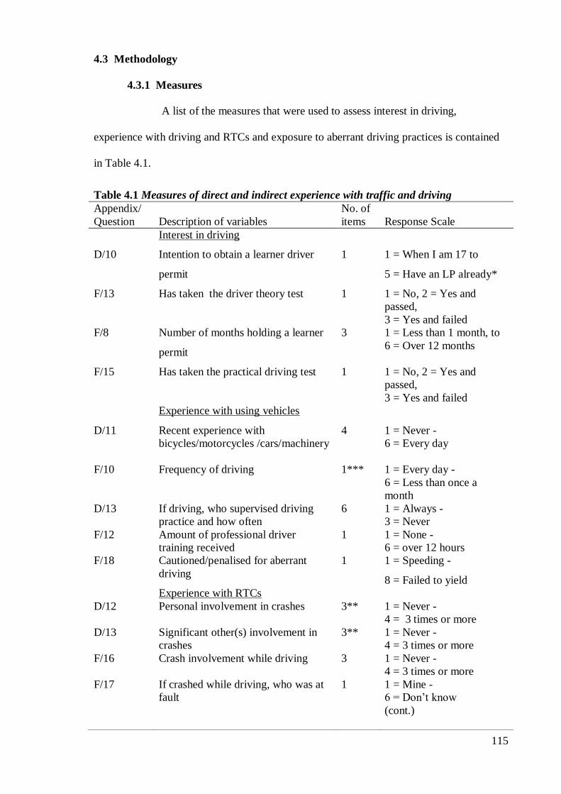
115
4.3 Methodology
4.3.1 Measures
A list of the measures that were used to assess interest in driving,
experience with driving and RTCs and exposure to aberrant driving practices is contained
in Table 4.1.
Table 4.1 Measures of direct and indirect experience with traffic and driving
Appendix/
Question Description of variables
No. of
items Response Scale
Interest in driving
D/10 Intention to obtain a learner driver
permit
1 1 = When I am 17 to
5 = Have an LP already*
F/13 Has taken the driver theory test 1 1 = No, 2 = Yes and
passed,
3 = Yes and failed
F/8 Number of months holding a learner
permit
3 1 = Less than 1 month, to
6 = Over 12 months
F/15 Has taken the practical driving test 1 1 = No, 2 = Yes and
passed,
3 = Yes and failed
Experience with using vehicles
D/11 Recent experience with
bicycles/motorcycles /cars/machinery
4 1 = Never -
6 = Every day
F/10 Frequency of driving 1*** 1 = Every day -
6 = Less than once a
month
D/13 If driving, who supervised driving
practice and how often
6 1 = Always -
3 = Never
F/12 Amount of professional driver
training received
1 1 = None -
6 = over 12 hours
F/18 Cautioned/penalised for aberrant
driving
1 1 = Speeding -
8 = Failed to yield
Experience with RTCs
D/12 Personal involvement in crashes 3** 1 = Never -
4 = 3 times or more
D/13 Significant other(s) involvement in
crashes
3** 1 = Never -
4 = 3 times or more
F/16 Crash involvement while driving 3 1 = Never -
4 = 3 times or more
F/17 If crashed while driving, who was at
fault
1 1 = Mine -
6 = Don’t know
(cont.)
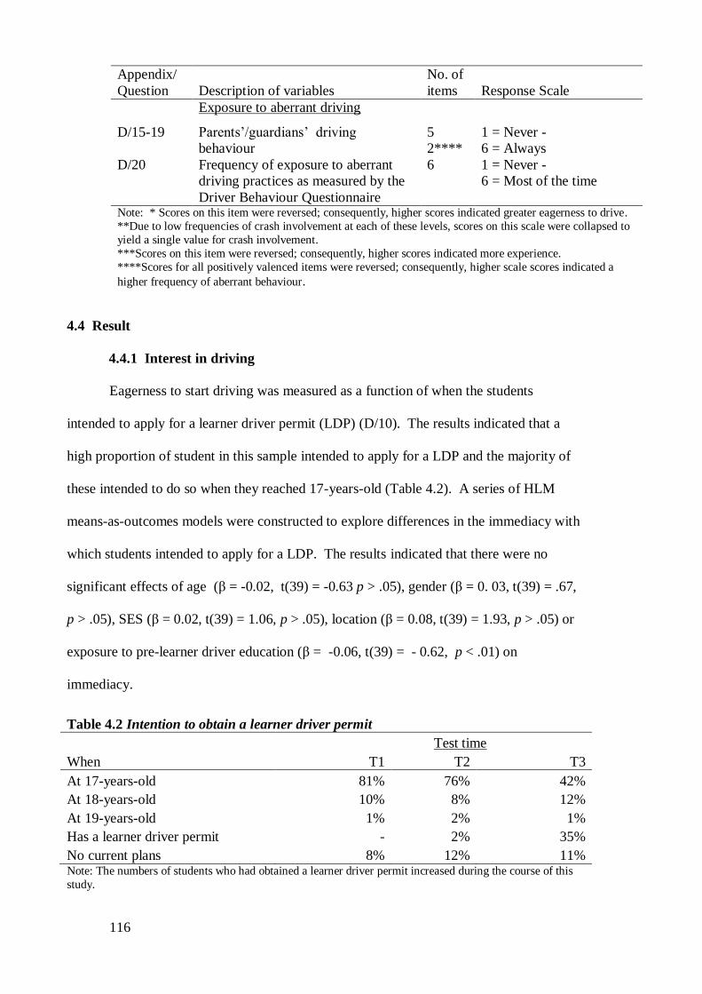
116
4.4 Result
4.4.1 Interest in driving
Eagerness to start driving was measured as a function of when the students
intended to apply for a learner driver permit (LDP) (D/10). The results indicated that a
high proportion of student in this sample intended to apply for a LDP and the majority of
these intended to do so when they reached 17-years-old (Table 4.2). A series of HLM
means-as-outcomes models were constructed to explore differences in the immediacy with
which students intended to apply for a LDP. The results indicated that there were no
significant effects of age (β = -0.02, t(39) = -0.63 p > .05), gender (β = 0. 03, t(39) = .67,
p > .05), SES (β = 0.02, t(39) = 1.06, p > .05), location (β = 0.08, t(39) = 1.93, p > .05) or
exposure to pre-learner driver education (β = -0.06, t(39) = - 0.62, p < .01) on
immediacy.
Table 4.2 Intention to obtain a learner driver permit
Test time
When T1 T2 T3
At 17-years-old 81% 76% 42%
At 18-years-old 10% 8% 12%
At 19-years-old 1% 2% 1%
Has a learner driver permit - 2% 35%
No current plans 8% 12% 11% Note: The numbers of students who had obtained a learner driver permit increased during the course of this
study.
Appendix/
Question Description of variables
No. of
items Response Scale
Exposure to aberrant driving
D/15-19 Parents’/guardians’ driving
behaviour
5
2****
1 = Never -
6 = Always
D/20 Frequency of exposure to aberrant
driving practices as measured by the
Driver Behaviour Questionnaire
6 1 = Never -
6 = Most of the time
Note: * Scores on this item were reversed; consequently, higher scores indicated greater eagerness to drive.
**Due to low frequencies of crash involvement at each of these levels, scores on this scale were collapsed to
yield a single value for crash involvement.
***Scores on this item were reversed; consequently, higher scores indicated more experience.
****Scores for all positively valenced items were reversed; consequently, higher scale scores indicated a
higher frequency of aberrant behaviour.
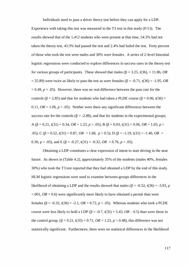
117
Individuals need to pass a driver theory test before they can apply for a LDP.
Experience with taking this test was measured in the T3 test in this study (F/13). The
results showed that of the 1,412 students who were present at that time, 54.3% had not
taken the theory test, 43.3% had passed the test and 2.4% had failed the test. Forty percent
of those who took the test were males and 30% were females. A series of 2-level binomial
logistic regressions were conducted to explore differences in success rates in the theory test
for various groups of participants. These showed that males (β = 3.25, t(36), = 11.86, OR
= 25.89) were twice as likely to pass the test as were females (β = -0.71, t(36) = -1.95, OR
= 0.49, p = .05). However, there was no real difference between the pass rate for the
controls (β = 2.85) and that for students who had taken a PLDE course (β = 0.06, t(36) =
0.11, OR = 1.06, p > .05). Neither were there any significant differences between the
success rate for the controls (β = -2.88), and that for students in the experimental groups;
A (β = 0.21, t(31) = 0.34, OR = 1.23, p > .05); B (β = 0.03, t(31) = 0.06, OR = 1.03, p >
.05); C (β = 0.52, t(31) = 0.87, OR = 1.68, p > 0.5); D (β = -1.19, t(31) = -1.40, OR =
0.30, p > .05), and E (β = -0.27, t(31) = -0.32, OR = 0.76, p > .05).
Obtaining a LDP constitutes a clear expression of intent to start driving in the near
future. As shown in (Table 4.2), approximately 35% of the students (males 40%, females
30%) who took the T3 test reported that they had obtained a LDP by the end of this study.
HLM logistic regressions were used to examine between-groups differences in the
likelihood of obtaining a LDP and the results showed that males (β = -0.52, t(36) = -3.93, p
<.001, OR = 0.6) were significantly more likely to have obtained a permit than were
females (β = -0.32, t(36) = -2.1, OR = 0.72, p < .05). Whereas students who took a PLDE
course were less likely to hold a LDP (β = -0.7, t(35) = 5.43, OR – 0.5) than were those in
the control group, (β = 0.21, t(35) = 0.71, OR = 1.23, p > 0.48), this difference was not
statistically significant. Furthermore, there were no statistical differences in the likelihood
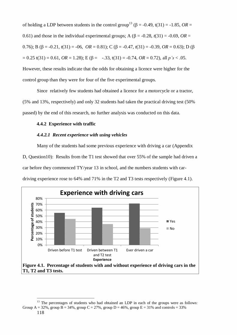
118
of holding a LDP between students in the control group13
(β = -0.49, t(31) = -1.85, OR =
0.61) and those in the individual experimental groups; A (β = -0.28, t(31) = -0.69, OR =
0.76); B (β = -0.21, t(31) = -06, OR = 0.81); C (β = -0.47, t(31) = -0.39, OR = 0.63); D (β
= 0.25 t(31) = 0.61, OR = 1.28); E (β = -.33, t(31) = -0.74, OR = 0.72), all p’s < .05.
However, these results indicate that the odds for obtaining a licence were higher for the
control group than they were for four of the five experimental groups.
Since relatively few students had obtained a licence for a motorcycle or a tractor,
(5% and 13%, respectively) and only 32 students had taken the practical driving test (50%
passed) by the end of this research, no further analysis was conducted on this data.
4.4.2 Experience with traffic
4.4.2.1 Recent experience with using vehicles
Many of the students had some previous experience with driving a car (Appendix
D, Question10): Results from the T1 test showed that over 55% of the sample had driven a
car before they commenced TY/year 13 in school, and the numbers students with car-
driving experience rose to 64% and 71% in the T2 and T3 tests respectively (Figure 4.1).
Figure 4.1. Percentage of students with and without experience of driving cars in the
T1, T2 and T3 tests.
13 The percentages of students who had obtained an LDP in each of the groups were as follows:
Group A = 32%, group B = 34%, group C = 27%, group D = 46%, group E = 31% and controls = 33%
0%
10%
20%
30%
40%
50%
60%
70%
80%
Driven before T1 test Driven between T1and T2 test
Ever driven a car
Per
cen
tage
of
stu
den
ts
Experience
Experience with driving cars
Yes
No
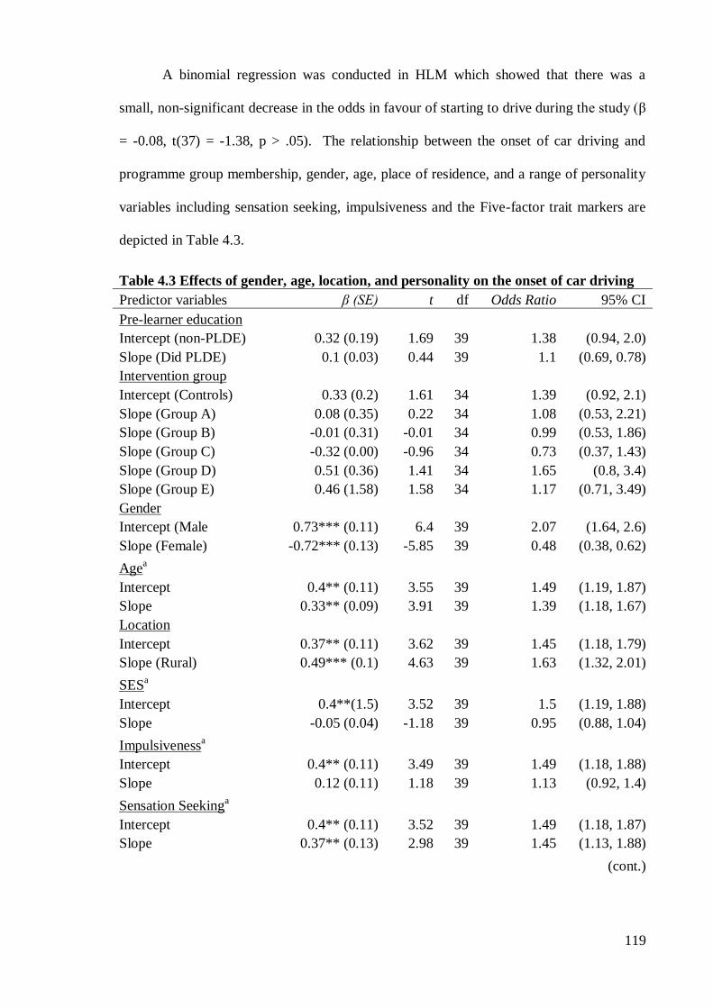
119
A binomial regression was conducted in HLM which showed that there was a
small, non-significant decrease in the odds in favour of starting to drive during the study (β
= -0.08, t(37) = -1.38, p > .05). The relationship between the onset of car driving and
programme group membership, gender, age, place of residence, and a range of personality
variables including sensation seeking, impulsiveness and the Five-factor trait markers are
depicted in Table 4.3.
Table 4.3 Effects of gender, age, location, and personality on the onset of car driving
Predictor variables β (SE) t df Odds Ratio 95% CI
Pre-learner education
Intercept (non-PLDE) 0.32 (0.19) 1.69 39 1.38 (0.94, 2.0)
Slope (Did PLDE) 0.1 (0.03) 0.44 39 1.1 (0.69, 0.78)
Intervention group
Intercept (Controls) 0.33 (0.2) 1.61 34 1.39 (0.92, 2.1)
Slope (Group A) 0.08 (0.35) 0.22 34 1.08 (0.53, 2.21)
Slope (Group B) -0.01 (0.31) -0.01 34 0.99 (0.53, 1.86)
Slope (Group C) -0.32 (0.00) -0.96 34 0.73 (0.37, 1.43)
Slope (Group D) 0.51 (0.36) 1.41 34 1.65 (0.8, 3.4)
Slope (Group E) 0.46 (1.58) 1.58 34 1.17 (0.71, 3.49)
Gender
Intercept (Male 0.73*** (0.11) 6.4 39 2.07 (1.64, 2.6)
Slope (Female) -0.72*** (0.13) -5.85 39 0.48 (0.38, 0.62)
Agea
Intercept 0.4** (0.11) 3.55 39 1.49 (1.19, 1.87)
Slope 0.33** (0.09) 3.91 39 1.39 (1.18, 1.67)
Location
Intercept 0.37** (0.11) 3.62 39 1.45 (1.18, 1.79)
Slope (Rural) 0.49*** (0.1) 4.63 39 1.63 (1.32, 2.01)
SESa
Intercept 0.4**(1.5) 3.52 39 1.5 (1.19, 1.88)
Slope -0.05 (0.04) -1.18 39 0.95 (0.88, 1.04)
Impulsivenessa
Intercept 0.4** (0.11) 3.49 39 1.49 (1.18, 1.88)
Slope 0.12 (0.11) 1.18 39 1.13 (0.92, 1.4)
Sensation Seekinga
Intercept 0.4** (0.11) 3.52 39 1.49 (1.18, 1.87)
Slope 0.37** (0.13) 2.98 39 1.45 (1.13, 1.88)
(cont.)
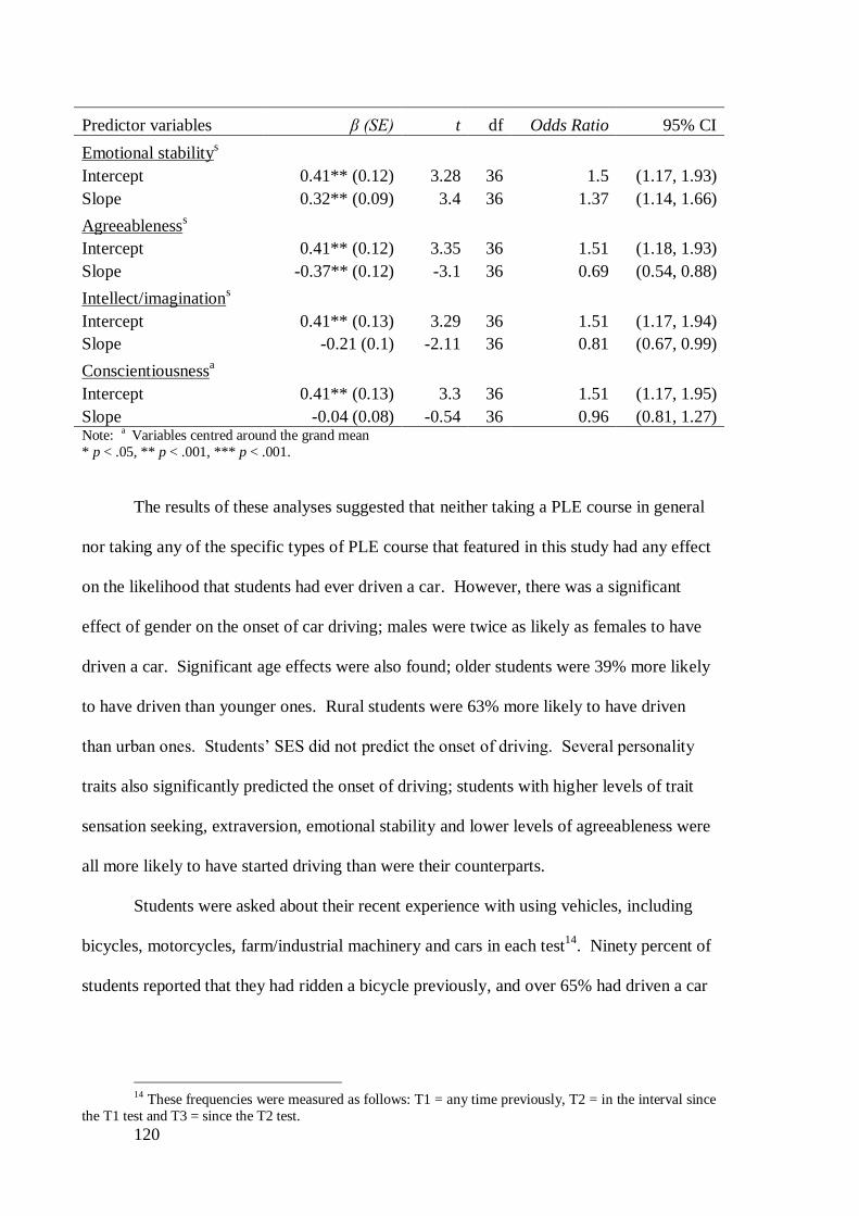
120
Predictor variables β (SE) t df Odds Ratio 95% CI
Emotional stabilitys
Intercept 0.41** (0.12) 3.28 36 1.5 (1.17, 1.93)
Slope 0.32** (0.09) 3.4 36 1.37 (1.14, 1.66)
Agreeablenesss
Intercept 0.41** (0.12) 3.35 36 1.51 (1.18, 1.93)
Slope -0.37** (0.12) -3.1 36 0.69 (0.54, 0.88)
Intellect/imaginations
Intercept 0.41** (0.13) 3.29 36 1.51 (1.17, 1.94)
Slope -0.21 (0.1) -2.11 36 0.81 (0.67, 0.99)
Conscientiousnessa
Intercept 0.41** (0.13) 3.3 36 1.51 (1.17, 1.95)
Slope -0.04 (0.08) -0.54 36 0.96 (0.81, 1.27) Note: a Variables centred around the grand mean
* p < .05, ** p < .001, *** p < .001.
The results of these analyses suggested that neither taking a PLE course in general
nor taking any of the specific types of PLE course that featured in this study had any effect
on the likelihood that students had ever driven a car. However, there was a significant
effect of gender on the onset of car driving; males were twice as likely as females to have
driven a car. Significant age effects were also found; older students were 39% more likely
to have driven than younger ones. Rural students were 63% more likely to have driven
than urban ones. Students’ SES did not predict the onset of driving. Several personality
traits also significantly predicted the onset of driving; students with higher levels of trait
sensation seeking, extraversion, emotional stability and lower levels of agreeableness were
all more likely to have started driving than were their counterparts.
Students were asked about their recent experience with using vehicles, including
bicycles, motorcycles, farm/industrial machinery and cars in each test14
. Ninety percent of
students reported that they had ridden a bicycle previously, and over 65% had driven a car
14 These frequencies were measured as follows: T1 = any time previously, T2 = in the interval since
the T1 test and T3 = since the T2 test.
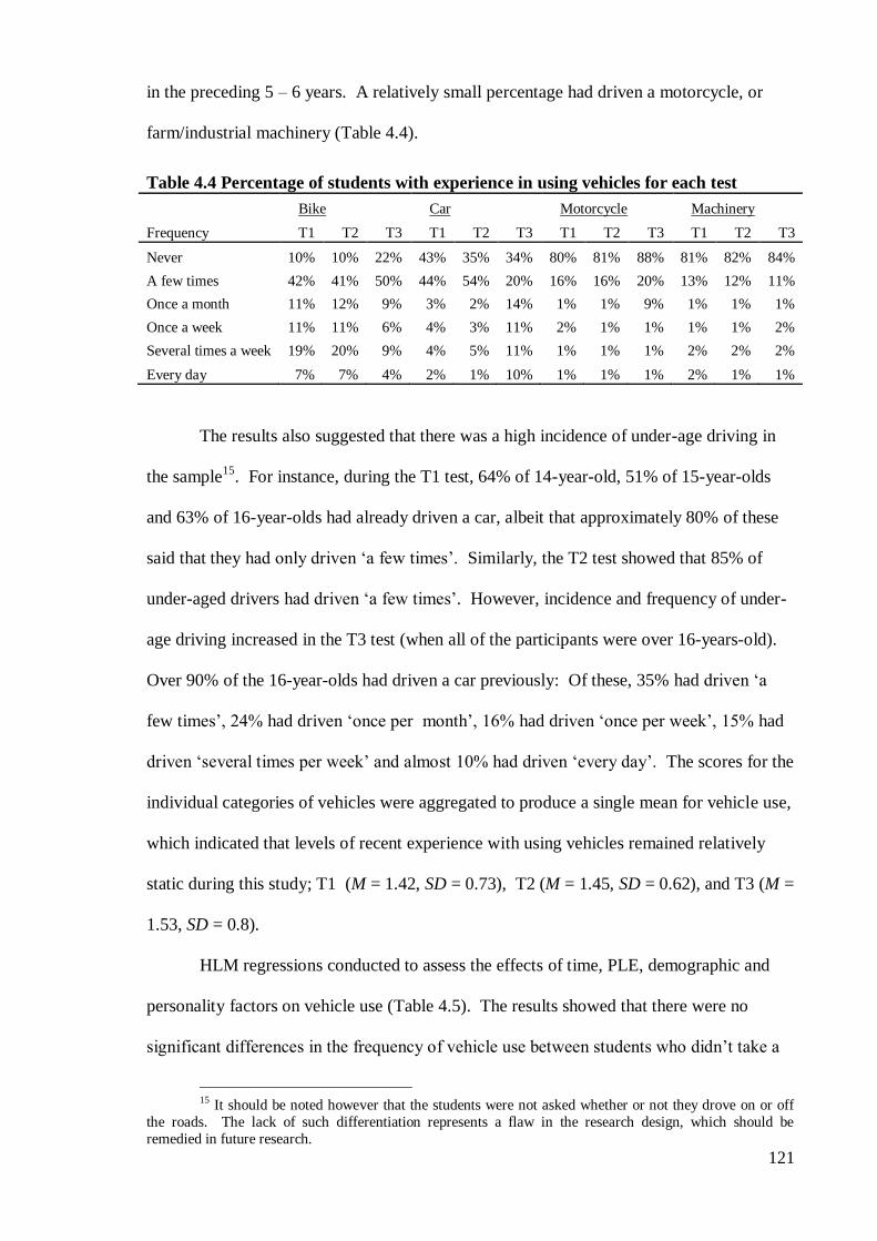
121
in the preceding 5 – 6 years. A relatively small percentage had driven a motorcycle, or
farm/industrial machinery (Table 4.4).
Table 4.4 Percentage of students with experience in using vehicles for each test
Bike Car Motorcycle Machinery
Frequency T1 T2 T3 T1 T2 T3 T1 T2 T3 T1 T2 T3
Never 10% 10% 22% 43% 35% 34% 80% 81% 88% 81% 82% 84%
A few times 42% 41% 50% 44% 54% 20% 16% 16% 20% 13% 12% 11%
Once a month 11% 12% 9% 3% 2% 14% 1% 1% 9% 1% 1% 1%
Once a week 11% 11% 6% 4% 3% 11% 2% 1% 1% 1% 1% 2%
Several times a week 19% 20% 9% 4% 5% 11% 1% 1% 1% 2% 2% 2%
Every day 7% 7% 4% 2% 1% 10% 1% 1% 1% 2% 1% 1%
The results also suggested that there was a high incidence of under-age driving in
the sample15
. For instance, during the T1 test, 64% of 14-year-old, 51% of 15-year-olds
and 63% of 16-year-olds had already driven a car, albeit that approximately 80% of these
said that they had only driven ‘a few times’. Similarly, the T2 test showed that 85% of
under-aged drivers had driven ‘a few times’. However, incidence and frequency of under-
age driving increased in the T3 test (when all of the participants were over 16-years-old).
Over 90% of the 16-year-olds had driven a car previously: Of these, 35% had driven ‘a
few times’, 24% had driven ‘once per month’, 16% had driven ‘once per week’, 15% had
driven ‘several times per week’ and almost 10% had driven ‘every day’. The scores for the
individual categories of vehicles were aggregated to produce a single mean for vehicle use,
which indicated that levels of recent experience with using vehicles remained relatively
static during this study; T1 (M = 1.42, SD = 0.73), T2 (M = 1.45, SD = 0.62), and T3 (M =
1.53, SD = 0.8).
HLM regressions conducted to assess the effects of time, PLE, demographic and
personality factors on vehicle use (Table 4.5). The results showed that there were no
significant differences in the frequency of vehicle use between students who didn’t take a
15 It should be noted however that the students were not asked whether or not they drove on or off
the roads. The lack of such differentiation represents a flaw in the research design, which should be
remedied in future research.
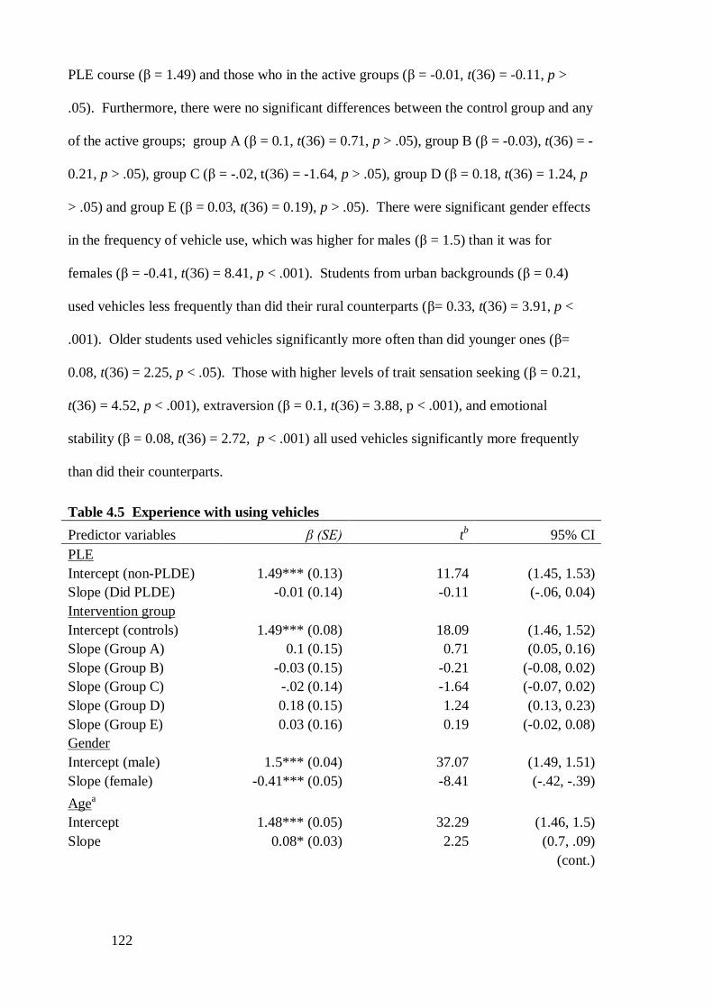
122
PLE course (β = 1.49) and those who in the active groups (β = -0.01, t(36) = -0.11, p >
.05). Furthermore, there were no significant differences between the control group and any
of the active groups; group A (β = 0.1, t(36) = 0.71, p > .05), group B (β = -0.03), t(36) = -
0.21, p > .05), group C (β = -.02, t(36) = -1.64, p > .05), group D (β = 0.18, t(36) = 1.24, p
> .05) and group E (β = 0.03, t(36) = 0.19), p > .05). There were significant gender effects
in the frequency of vehicle use, which was higher for males (β = 1.5) than it was for
females (β = -0.41, t(36) = 8.41, p < .001). Students from urban backgrounds (β = 0.4)
used vehicles less frequently than did their rural counterparts (β= 0.33, t(36) = 3.91, p <
.001). Older students used vehicles significantly more often than did younger ones (β=
0.08, t(36) = 2.25, p < .05). Those with higher levels of trait sensation seeking (β = 0.21,
t(36) = 4.52, p < .001), extraversion (β = 0.1, t(36) = 3.88, p < .001), and emotional
stability (β = 0.08, t(36) = 2.72, p < .001) all used vehicles significantly more frequently
than did their counterparts.
Table 4.5 Experience with using vehicles
Predictor variables β (SE) tb 95% CI
PLE
Intercept (non-PLDE) 1.49*** (0.13) 11.74 (1.45, 1.53)
Slope (Did PLDE) -0.01 (0.14) -0.11 (-.06, 0.04)
Intervention group
Intercept (controls) 1.49*** (0.08) 18.09 (1.46, 1.52)
Slope (Group A) 0.1 (0.15) 0.71 (0.05, 0.16)
Slope (Group B) -0.03 (0.15) -0.21 (-0.08, 0.02)
Slope (Group C) -.02 (0.14) -1.64 (-0.07, 0.02)
Slope (Group D) 0.18 (0.15) 1.24 (0.13, 0.23)
Slope (Group E) 0.03 (0.16) 0.19 (-0.02, 0.08)
Gender
Intercept (male) 1.5*** (0.04) 37.07 (1.49, 1.51)
Slope (female) -0.41*** (0.05) -8.41 (-.42, -.39)
Agea
Intercept 1.48*** (0.05) 32.29 (1.46, 1.5)
Slope 0.08* (0.03) 2.25 (0.7, .09)
(cont.)
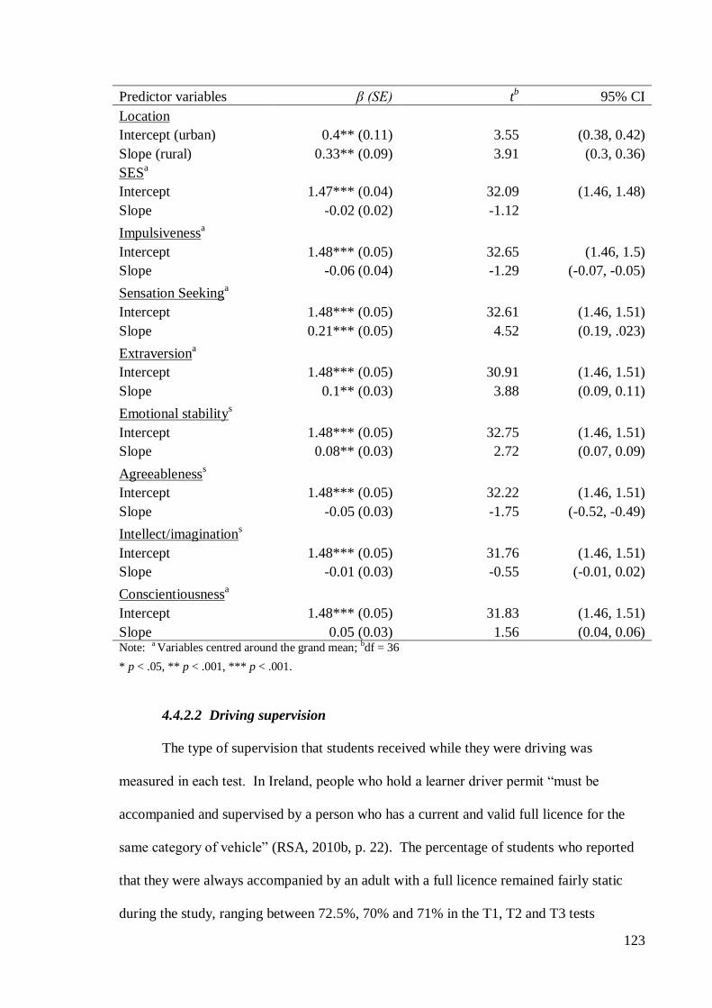
123
Predictor variables β (SE) tb 95% CI
Location
Intercept (urban) 0.4** (0.11) 3.55 (0.38, 0.42)
Slope (rural) 0.33** (0.09) 3.91 (0.3, 0.36)
SESa
Intercept 1.47*** (0.04) 32.09 (1.46, 1.48)
Slope -0.02 (0.02) -1.12
Impulsivenessa
Intercept 1.48*** (0.05) 32.65 (1.46, 1.5)
Slope -0.06 (0.04) -1.29 (-0.07, -0.05)
Sensation Seekinga
Intercept 1.48*** (0.05) 32.61 (1.46, 1.51)
Slope 0.21*** (0.05) 4.52 (0.19, .023)
Extraversiona
Intercept 1.48*** (0.05) 30.91 (1.46, 1.51)
Slope 0.1** (0.03) 3.88 (0.09, 0.11)
Emotional stabilitys
Intercept 1.48*** (0.05) 32.75 (1.46, 1.51)
Slope 0.08** (0.03) 2.72 (0.07, 0.09)
Agreeablenesss
Intercept 1.48*** (0.05) 32.22 (1.46, 1.51)
Slope -0.05 (0.03) -1.75 (-0.52, -0.49)
Intellect/imaginations
Intercept 1.48*** (0.05) 31.76 (1.46, 1.51)
Slope -0.01 (0.03) -0.55 (-0.01, 0.02)
Conscientiousnessa
Intercept 1.48*** (0.05) 31.83 (1.46, 1.51)
Slope 0.05 (0.03) 1.56 (0.04, 0.06) Note: a Variables centred around the grand mean; bdf = 36
* p < .05, ** p < .001, *** p < .001.
4.4.2.2 Driving supervision
The type of supervision that students received while they were driving was
measured in each test. In Ireland, people who hold a learner driver permit “must be
accompanied and supervised by a person who has a current and valid full licence for the
same category of vehicle” (RSA, 2010b, p. 22). The percentage of students who reported
that they were always accompanied by an adult with a full licence remained fairly static
during the study, ranging between 72.5%, 70% and 71% in the T1, T2 and T3 tests
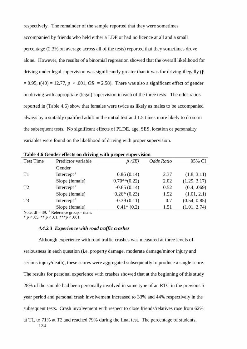
124
respectively. The remainder of the sample reported that they were sometimes
accompanied by friends who held either a LDP or had no licence at all and a small
percentage (2.3% on average across all of the tests) reported that they sometimes drove
alone. However, the results of a binomial regression showed that the overall likelihood for
driving under legal supervision was significantly greater than it was for driving illegally (β
= 0.95, t(40) = 12.77, p < .001, OR = 2.58). There was also a significant effect of gender
on driving with appropriate (legal) supervision in each of the three tests. The odds ratios
reported in (Table 4.6) show that females were twice as likely as males to be accompanied
always by a suitably qualified adult in the initial test and 1.5 times more likely to do so in
the subsequent tests. No significant effects of PLDE, age, SES, location or personality
variables were found on the likelihood of driving with proper supervision.
Table 4.6 Gender effects on driving with proper supervision
Test Time Predictor variable β (SE) Odds Ratio 95% CI
Gender
T1 Intercept a 0.86 (0.14) 2.37 (1.8, 3.11)
Slope (female) 0.70**(0.22) 2.02 (1.29, 3.17)
T2 Intercept a -0.65 (0.14) 0.52 (0.4, .069)
Slope (female) 0.26* (0.23) 1.52 (1.01, 2.1)
T3 Intercept a -0.39 (0.11) 0.7 (0.54, 0.85)
Slope (female) 0.41* (0.2) 1.51 (1.01, 2.74)
Note: df = 39. a Reference group = male.
* p < .05, ** p < .01, ***p < .001.
4.4.2.3 Experience with road traffic crashes
Although experience with road traffic crashes was measured at three levels of
seriousness in each question (i.e. property damage, moderate damage/minor injury and
serious injury/death), these scores were aggregated subsequently to produce a single score.
The results for personal experience with crashes showed that at the beginning of this study
28% of the sample had been personally involved in some type of an RTC in the previous 5-
year period and personal crash involvement increased to 33% and 44% respectively in the
subsequent tests. Crash involvement with respect to close friends/relatives rose from 62%
at T1, to 71% at T2 and reached 79% during the final test. The percentage of students,
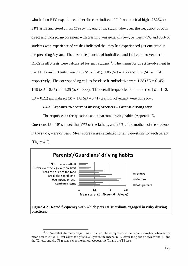
125
who had no RTC experience, either direct or indirect, fell from an initial high of 32%, to
24% at T2 and stood at just 17% by the end of the study. However, the frequency of both
direct and indirect involvement with crashing was generally low, between 75% and 80% of
students with experience of crashes indicated that they had experienced just one crash in
the preceding 5 years. The mean frequencies of both direct and indirect involvement in
RTCs in all 3 tests were calculated for each student16
. The means for direct involvement in
the T1, T2 and T3 tests were 1.28 (SD = 0 .45), 1.05 (SD = 0 .2) and 1.14 (SD = 0 .34),
respectively. The corresponding values for close friend/relative were 1.38 (SD = 0 .45),
1.19 (SD = 0.35) and 1.25 (SD = 0.38). The overall frequencies for both direct (M = 1.12,
SD = 0.21) and indirect (M = 1.8, SD = 0.41) crash involvement were quite low.
4.4.3 Exposure to aberrant driving practices – Parents driving style
The responses to the questions about parental driving habits (Appendix D,
Questions 15 – 19) showed that 97% of the fathers, and 95% of the mothers of the students
in the study, were drivers. Mean scores were calculated for all 5 questions for each parent
(Figure 4.2).
Figure 4.2. Rated frequency with which parents/guardians engaged in risky driving
practices.
16 16 Note that the percentage figures quoted above represent cumulative estimates, whereas the
mean scores in the T1 test cover the previous 5 years, the means in T2 cover the period between the T1 and
the T2 tests and the T3 means cover the period between the T1 and the T3 tests.
1 1.5 2 2.5
Combined itemsUse mobile phone
Break the speed limitBreak the rules of the road
Driver over the legal alcohol limitNot wear a seatbelt
Mean score (1 = Never - 6 = Always)
Parents'/Guardians' driving habits
Fathers
Mothers
Both parents
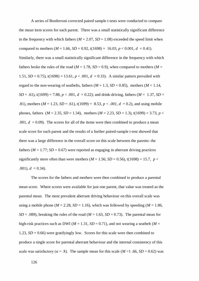
126
A series of Bonferroni corrected paired sample t-tests were conducted to compare
the mean item scores for each parent. There was a small statistically significant difference
in the frequency with which fathers (M = 2.07, SD = 1.08) exceeded the speed limit when
compared to mothers (M = 1.66, SD = 0.92, t(1698) = 16.03, p < 0.001, d = 0.41).
Similarly, there was a small statistically significant difference in the frequency with which
fathers broke the rules of the road (M = 1.78, SD = 0.9), when compared to mothers (M =
1.51, SD = 0.75), t(1698) = 13.61, p < .001, d = 0.33). A similar pattern prevailed with
regard to the non-wearing of seatbelts, fathers (M = 1.3, SD = 0.85), mothers (M = 1.14,
SD = .61), t(1699) = 7.88, p < .001, d = 0.22); and drink-driving, fathers (M = 1.37, SD =
.81), mothers (M = 1.23, SD = .61), t(1699) = 8.53, p < .001, d = 0.2), and using mobile
phones, fathers (M = 2.35, SD = 1.34), mothers (M = 2.23, SD = 1.3), t(1699) = 3.73, p <
.001, d = 0.09). The scores for all of the items were then combined to produce a mean
scale score for each parent and the results of a further paired-sample t-test showed that
there was a large difference in the overall score on this scale between the parents: the
fathers (M = 1.77; SD = 0.67) were reported as engaging in aberrant driving practices
significantly more often than were mothers (M = 1.56; SD = 0.56), t(1698) = 15.7, p <
.001), d = 0.34).
The scores for the fathers and mothers were then combined to produce a parental
mean score. Where scores were available for just one parent, that value was treated as the
parental mean. The most prevalent aberrant driving behaviour on this overall scale was
using a mobile phone (M = 2.28, SD = 1.16), which was followed by speeding (M = 1.86,
SD = .089), breaking the rules of the road (M = 1.63, SD = 0.73). The parental mean for
high-risk practices such as DWI (M = 1.31, SD = 0.71), and not wearing a seatbelt (M =
1.23, SD = 0.66) were gratifyingly low. Scores for this scale were then combined to
produce a single score for parental aberrant behaviour and the internal consistency of this
scale was satisfactory (α = .8). The sample mean for this scale (M =1 .66, SD = 0.62) was
127
low. Given that a score of 1 on this scale represented “Never” and a score of 2 represented
“Hardly ever” this indicated that the students in the sample were not exposed to aberrant
driving behaviour by their parents to any great extent.
4.4.3.1 Exposure to aberrant driving practices – principal driver’s driving style
The levels of student exposure to the aberrant driving practices of the driver that they
travel with most often (i.e. their principal driver, who may or may not have been a parent)
were measured using 6 items (D/20). The reported prevalence of aberrant driving practices
among principal drivers was generally quite low (Figure 4.3).
Figure 4.3. Rated frequency with which the students’ principal driver engaged in
risky practices.
The most prevalent behaviour was sounding the car horn to indicate annoyance with
another road user (M = 2.55, SD = 1.37). The mean score for overtaking slow drivers on
the inside was surprisingly high (M = 2.07, SD = 1.4) in relative terms. The least prevalent
behaviours were crowding slow drivers (M 1.6, SD = 1.07), crossing against traffic lights
(M = 1.66, SD = 0.93) and lane hogging (M 1.68, SD = 1.03). The scores for these 6 items
were combined to form a single scale representing exposure to driving violations, and the
internal consistency of the scale was adequate (α = .71), The mean scale score was
relatively low (M = 1.9, SD = 0.77), given that a score of 1 represented “Never” and a
score of 2 represented “Hardly ever”.
1 1.5 2 2.5 3
Combined items
Sound horn to indicate annoyance
Overtake slow driver on the inside
Display hostility towards some road users
Stay in obstructed lane until the last…
Cross junction after traffic lights turned…
Travel close to slow drivers
Mean score (1 = Never - 6 = Most of the time
Principal drivers' driving style
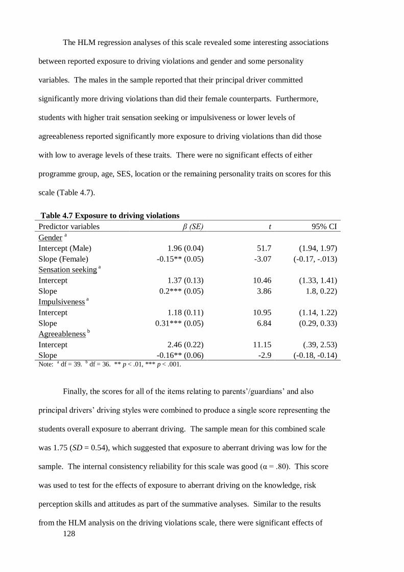
128
The HLM regression analyses of this scale revealed some interesting associations
between reported exposure to driving violations and gender and some personality
variables. The males in the sample reported that their principal driver committed
significantly more driving violations than did their female counterparts. Furthermore,
students with higher trait sensation seeking or impulsiveness or lower levels of
agreeableness reported significantly more exposure to driving violations than did those
with low to average levels of these traits. There were no significant effects of either
programme group, age, SES, location or the remaining personality traits on scores for this
scale (Table 4.7).
Table 4.7 Exposure to driving violations
Predictor variables β (SE) t 95% CI
Gender a
Intercept (Male) 1.96 (0.04) 51.7 (1.94, 1.97)
Slope (Female) -0.15** (0.05) -3.07 (-0.17, -.013)
Sensation seeking a
Intercept 1.37 (0.13) 10.46 (1.33, 1.41)
Slope 0.2*** (0.05) 3.86 1.8, 0.22)
Impulsiveness a
Intercept 1.18 (0.11) 10.95 (1.14, 1.22)
Slope 0.31*** (0.05) 6.84 (0.29, 0.33)
Agreeableness b
Intercept 2.46 (0.22) 11.15 (.39, 2.53)
Slope -0.16** (0.06) -2.9 (-0.18, -0.14) Note: a df = 39. b df = 36. ** p < .01, *** p < .001.
Finally, the scores for all of the items relating to parents’/guardians’ and also
principal drivers’ driving styles were combined to produce a single score representing the
students overall exposure to aberrant driving. The sample mean for this combined scale
was 1.75 (SD = 0.54), which suggested that exposure to aberrant driving was low for the
sample. The internal consistency reliability for this scale was good (α = .80). This score
was used to test for the effects of exposure to aberrant driving on the knowledge, risk
perception skills and attitudes as part of the summative analyses. Similar to the results
from the HLM analysis on the driving violations scale, there were significant effects of
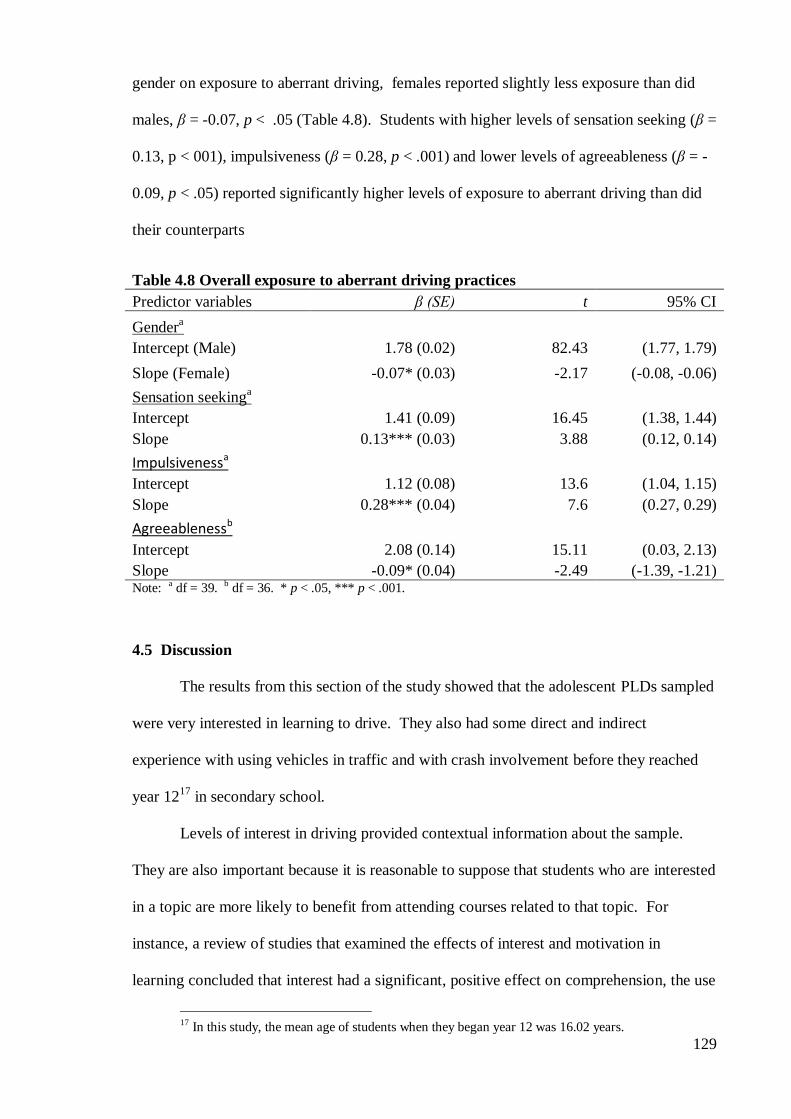
129
gender on exposure to aberrant driving, females reported slightly less exposure than did
males, β = -0.07, p < .05 (Table 4.8). Students with higher levels of sensation seeking (β =
0.13, p < 001), impulsiveness (β = 0.28, p < .001) and lower levels of agreeableness (β = -
0.09, p < .05) reported significantly higher levels of exposure to aberrant driving than did
their counterparts
Table 4.8 Overall exposure to aberrant driving practices
Predictor variables β (SE) t 95% CI
Gendera
Intercept (Male) 1.78 (0.02) 82.43 (1.77, 1.79)
Slope (Female) -0.07* (0.03) -2.17 (-0.08, -0.06)
Sensation seekinga
Intercept 1.41 (0.09) 16.45 (1.38, 1.44)
Slope 0.13*** (0.03) 3.88 (0.12, 0.14)
Impulsivenessa
Intercept 1.12 (0.08) 13.6 (1.04, 1.15)
Slope 0.28*** (0.04) 7.6 (0.27, 0.29)
Agreeablenessb
Intercept 2.08 (0.14) 15.11 (0.03, 2.13)
Slope -0.09* (0.04) -2.49 (-1.39, -1.21) Note: a df = 39. b df = 36. * p < .05, *** p < .001.
4.5 Discussion
The results from this section of the study showed that the adolescent PLDs sampled
were very interested in learning to drive. They also had some direct and indirect
experience with using vehicles in traffic and with crash involvement before they reached
year 1217
in secondary school.
Levels of interest in driving provided contextual information about the sample.
They are also important because it is reasonable to suppose that students who are interested
in a topic are more likely to benefit from attending courses related to that topic. For
instance, a review of studies that examined the effects of interest and motivation in
learning concluded that interest had a significant, positive effect on comprehension, the use
17 In this study, the mean age of students when they began year 12 was 16.02 years.
130
of learning strategies and the quality of the emotional experience while learning (Schiefele,
1991). Eagerness to start driving remained fairly constant during this research: Most of
the students intended to apply for a LDP as soon as they possibly could and only a small
percentage had no plans to obtain a permit at each stage. Furthermore, data from the end
of the study showed that over 45% of the students had taken their driver theory test and
that 35% had obtained a LDP by then. Males in the sample were significantly more likely
to have passed a driver theory test and to have obtained a LDP than were females,
suggesting that males were more eager to start driving than were females. This supports
findings in previous studies which showed that males start driving earlier than females
(e.g. Ferguson, Leaf, Preusser, & Williams, 1994). However, recent Irish data shows that
there was very little difference between the percentages of males (52.5%) and females
(49%) taking the driver theory test between January and October 2011 (personal
communication from Catriona McLaughlin, Prometric Ireland, May 24th
, 2012). There
were no significant effects of taking a PLDE course generally, or of taking one of the
specific PLDE courses that featured in this research, on success with the driver theory test.
However this is not surprising, given the large percentage of students who reported that
they had passed the test. It is worth noting however that the 5.5% failure rate reported in
this study was much lower than the estimated failure rate on the actual theory test, which
was approximately, 30% during the first 6 months of 2011 (personal communication with
Catriona McLaughlin, Prometric Ireland, May 24th
. 2012). There are two possible
explanations for this discrepancy; either people who failed the test indicated that they had
in fact passed, or those who didn’t pass didn’t admit to taking the test in the first place.
Given that participants had been given repeated assurances of their anonymity, the latter
explanation seems somewhat more plausible than the former. Either way this
inconsistency highlights the drawbacks of measuring behaviour and attitudes through self-
report. Nevertheless, Jonah, and Dawson (1987) noted that although people tend to
131
overreport positive behaviour and underreport negative behaviour, the self-report method
is nevertheless useful for making comparisons between groups. Furthermore several
studies indicate that people, including school students tend to provide accurate reports of
their behaviours and attitudes (Killen & Robinson, 1988; Lajunen & Summala, 2003).
However for a contrarian view on self-report methodology in traffic research see af
Wåhlberg (2009).
The majority of the students in the current sample had operated a vehicle in the 12-
month period prior to each test. However, since mean score for vehicle use ranged
between 1 and 2 on a scale where 1 represented “never” and 2 denoted “a few times”, it
appears that overall levels of experience with using vehicles was generally quite low.
Nevertheless, over half of the participants indicated that they had driven a car at least once
before they reached year 12 in secondary school and experience with using vehicles rose to
75% by the end of the study. The results for the post-intervention tests (i.e. T2 and T3)
showed that students who had taken a PLDE course were not more likely to have driven a
car than were those in the control group. One of the major criticisms of PDE is that it
encourages students to start driving at an early age, thus increasing their exposure to risk
(Mayhew et al., 2002; Mayhew, Simpson, Williams, & Ferguson, 1998; Roberts & Kwan,
2001). However, the results of the present study do not support this contention, because
they show that participation in PLDE did not lead to earlier licencing, nor did it precipitate
the early onset of car driving in pre-learners. Furthermore, participation in PLDE did not
affect the frequency with which the students used other vehicles, including cars.
Several demographic factors, such as gender, age, rural domicile and personality
traits, including sensation seeking, extraversion, emotional stability and agreeableness,
were associated with an earlier onset of driving. The finding that rural students were
significantly more likely to have driven a car than their urban counterparts was un-
surprising. Youngsters in rural areas with poor access to public transport are likely to be
132
more strongly motivated to start driving than are those who have regular access to these
services. However, is well known that driving on rural roads poses particular challenges
for all drivers. For instance data from the U.S. shows that whereas just 23% of the
population lives in rural areas, 56% of crashes occur in rural areas (NHTSA, 2010).
Furthermore, researchers agree that teens in rural areas are five to six times more likely to
be involved in a fatal or severe injury crash than teens in urban areas (H. Y. Chen et al.,
2009; Peek-Asa, Britton, Young, Pawlovich, & Falb, 2010). Given that the combination of
youthfulness and rural driving represents a significant threat to safety, and since this study
shows that rural youngsters are more likely to start driving at an early age than their urban
counterparts, there is a clear need to ensure that all teenagers in rural areas are made aware
of the increased risk that they face as learner and novice drivers. This should be addressed
as part of a good PLDE course.
The early onset of driving was also predicted by a range of personality factors
including high sensation seeking, extraversion and emotional stability, and low
agreeableness. Most of the scientific literature examining the relationship between
personality traits and driving focuses on aberrant behaviours, such as deliberate risk taking
(Arnett, 2002; Arnett et al., 1997). However, given that driving clearly represents a
somewhat novel, challenging, and in some instances illegal activity for students in their
mid-teens it is not surprising that students with a stronger tendency towards sensation
seeking, extraversion, emotional stability, and/or lower levels of agreeableness would start
driving sooner than do their counterparts. The GDE-framework (Hatakka et al., 2002)
recommends that driver education should aim to make students aware of risk-increasing
factors and provide them with insight into how personal tendencies might influence their
perceptions of risk and their actual risk-taking behaviour. Thus, these issues should be
addressed in PLDE courses.
133
The reported prevalence of illegal underage driving in the sample was high18
.
Over half of the 15-year-olds and more than 60% of the 16-year-olds reported that they had
driven a car, albeit that most under aged students had only driven “a few times”. However,
the results from the final test indicated that 90% of 16-year-olds had driven a car
previously and over 40% of the 16-year-olds were driving at least once a week. On the
basis of the well-documented links between youthfulness, inexperience and increased crash
risk, which were outlined in Chapter 1, these findings are a cause for concern. Thus, it is
recommended that PLDE courses should pay particular attention to the problem of
underage driving and to explaining why these factors constitute such a high risk for learner
and novice drivers.
The results with respect to driving supervision were also disquieting. In Ireland, it
is illegal for a learner to drive a vehicle unless he/she is under the supervision of a person
who has had a full licence for a minimum of two years. It is expected that this form of
extended supervision will not only help novices to avoid unnecessary risk-taking in the
short-term, but will also help them to acquire good driving habits over the longer-term
(RSA, 2007). In this regard, the results from a new German scheme whereby newly
qualified adolescent drivers agreed to be accompanied by a designated qualified driver,
who does nothing to actively influence their behaviour, showed that participants in this
scheme had fewer crashes than did their counterparts in a control group (Funk, 2010). In
the current research, over a quarter of the drivers surveyed during the initial test, one third
of those who took the post-intervention test and over half of those who completed the final
survey reported that they had driven without proper supervision at some time.
Furthermore, given that the incidence of inadequate supervision appeared to increase over
time and the apparent absence of any significant programme effects relative to the control
18 Although it is acknowledged that the students were not asked to differentiate between off-road
and on-road driving, it is clear nonetheless that underage driving in either setting is problematic and should
be discouraged
134
group, it seems reasonable to conclude that the PLDE courses that featured in this study
were not effective in discouraging this practice. Thus it is recommended that that PLDE
courses should pay more attention to the outlining the problems associated with inadequate
supervision, and the attendant risks in order to discourage this practice.
Although over half of the students had been involved directly in some kind of RTC
in the preceding 5 years and 80% had indirect experience of crashing through a close
friend or relative, the actual frequency of crash involvement was gratifyingly low. In both
instances, over three quarters of those with experience of crashing had only been involved
in one crash in the preceding 5 years. This indicated that it would be difficult to assess the
moderating effects that experience with road traffic crashes might have on knowledge, risk
perception skills and attitudes in the remainder of this research.
The participants reported that their parents generally refrained from engaging in
aberrant driving practices. Since the mean scores for four of the five items in this scale
was below 2.1, this suggests that the parents either “never” or “hardly ever” refrained from
wearing seatbelts, drove while over the legal alcohol limit, broke the speed limit or
contravened the rules of the road. The means for driving while using a mobile phone were
slightly higher; however, it should be noted that the test made no distinction between hand-
held and hands-free instruments. Whereas the use of hands-free mobile phones while
driving does not contravene current traffic legislation in Ireland, it does increase the risk
of crashing (WHO, 2011). Since this fact has been well publicised by the RSA, it is
reasonable to assume that parents who were using hands-free mobile phones had chosen to
do so despite the risks involved. However, when the findings from this part of the study
were examined in terms of the percentage of parents who always complied with driving
regulations it was notable that just 33% of fathers and 53% of mothers always observed the
speed limit, 44% of fathers and 59% of mothers always observed the rules of the road and
84% of fathers and 93% of mothers always wore their seatbelts. In addition, only 76% of
135
fathers and 86% of mothers never drove after drinking alcohol and amazingly only 35% of
fathers and 93% of mothers never used a mobile phone whilst driving. This suggests that
more work needs to be done to improve the driving habits of Irish parents. The finding
that fathers engaged in aberrant driving practices more often than mothers was not
surprising, since an accumulation of evidence in the literature indicates that males have
riskier driving styles than females (de Winter & Dodou, 2010; Miller & Taubman - Ben-
Ari, 2010; Wells et al., 2008).
The current results indicated that students’ general exposure to driving violations
while being driven by their principal driver was also low. This reflects the fact that many
of these drivers either “never” or “hardly ever” crossed an intersection against the traffic
lights, hogged driving lanes, displayed hostility towards, crowded other drivers or overtook
slow drivers on the inside. Although sounding the horn to indicate annoyance with another
road user was the most prevalent type of violation reported by the students, their exposure
to this practice was also moderately low. Since the scores from this test are very similar to
those found in studies featuring drivers’ own self-reported behaviour (Åberg & Rimmö,
1998; Lajunen, Parker, & Summala, 2004), it seems that the commission of driving
violations in Ireland reflects the international average. More importantly in the present
context, these results indicate that pre-learner drivers both notice and are capable of
reporting on the frequency with which their principal drivers commit driving violations
with a reasonable degree of accuracy. In hindsight however, it is regrettable that the
identity of these “principal drivers” was not ascertained, since this would have provided a
clearer picture of the various influences on adolescent passengers. Since male students and
those with higher levels of sensation seeking, and impulsiveness, and lower levels of
agreeableness reported higher levels of exposure to driving violations than did their
counterparts, it seems likely that those former individuals chose to associate with people
who engaged in aberrant driving practices. This assumption is given credence by the fact

136
that no such differences were found in the reporting of parental driving practices.
Furthermore, it is well-known that male drivers and those who are more inclined towards
sensation seeking, impulsiveness and low agreeableness are more likely to commit driving
violations than are their counterparts (Lajunen et al., 2004; Oltedal & Rundmo, 2006;
Owsley, McGwin, & McNeal, 2003; Rimmö & Åberg, 1999).
Having established that, in accordance with the TCI model of driver behaviour
(Fuller, 2005), personal characteristics and previous learning represent important
antecedent influences on personal competence, and having produced personality and
experience indices for each of the participants, these predictors were used to investigate
individual differences in initial levels of knowledge, risk perception skills and attitudes,
and also changes in these outcomes as a function of time and of participating in a PLDE
course in the chapters that follow.
137
Chapter 5: Knowledge
5.1 Introduction
Knowledge about how the traffic system works is an essential precursor of safe
behaviour in the roadway. In Ireland, the traffic system is governed by The Rules of the
Road (ROTR), which enshrines current legislation and describes best practice in road user
behaviour. Compliance with these rules is essential for the ensuring the safety and security
of all road users (RSA, 2010b). Moreover, the behavioural psychologist Skinner once
suggested that rules are society’s way of demonstrating to its citizens how to learn from the
mistakes of others (Bonnie, 1985). In cognitive terms, knowledge about the ROTR is
classified as declarative knowledge, since it entails knowing that something is the case
(Eysenck & Keane, 2010). This type of knowledge is generally acquired either directly as
a result of experience or indirectly by means of formal education (Dong et al., 2011).
Research conducted within the educational sector shows that classroom-based instruction
is a particularly effective way of providing students with declarative knowledge in a
systematic way (Moreno, 2010). For instance, the results from the Irish State Junior
Certificate Examinations in 2011 indicate that less than 2% of the examinees failed the
English section of this test and that the failure rates for History (6%) and Science (3%)
were also very low (Irish State Examinations Commission, 2012). This suggests that the
vast majority of Irish students gain a substantial amount of knowledge during the first three
years in secondary school as a result of education.
As part of their educational strategy, the RSA has developed a range of material to
educate child and adolescent school goers about road safety. Three programmes are
currently in use for primary school students; the “Be Safe” programme, which targets 5 –
12-year-olds and the “Seatbelt Sheriff”, and the “Hi Glo Silver” programme with is aimed
at 7 – 12-year-olds. At secondary school level, the “Streetwise” programme is designed
for 12 – 15-year-olds. Because of this concerted effort to provide road safety education in
138
Irish schools, the vast majority of youngsters who have completed their primary school
and/or post-primary education in Ireland will have received some type of instruction
about how to stay safe in traffic and about the ROTR before they reached year 12 in
secondary school (RSA, 2012).
The current edition of the “Rules of the Road” (RSA, 2010b) uses three methods to
guide behaviour: It draws attention to behaviour that the law requires or forbids; it tells
road users how to act where no legal rule is in place and it describes and illustrates road
signs and markings, traffic lights etc. which serve to regulate traffic. Although the ROTR
apply to all road users, aspiring drivers must demonstrate a satisfactory level of knowledge
of these rules by taking a learner driver theory test (TT) before they can apply for a learner
driver permit (LDP). Since formal study of the ROTR constitutes a recognisable move
towards obtaining a licence and thus becoming a driver, it is expected that this element
would be included as part of a good PLDE course.
In addition to the type of knowledge contained in the ROTR, many driver
preparation courses draw students’ attention to evidence related to statistical risk in traffic.
This typically includes information about the number of people killed each year, the age
groups who are most at risk, the amount of practice that is needed to become a competent
driver and the types of manoeuvres that constitute the highest statistical risk of crashing for
learner and novice drivers. This information is useful for increasing awareness about the
objective risks that are associated with a range of demographic and behavioural factors,
because people’s perceptions of risk are generally quite low since they don’t usually
experience these risks at first hand (Fuller, 2002).
Since the concept of PLDE is relatively new and since those evaluations that have
been carried out to date have mainly focussed on the effects of these courses on driving-
related cognition e.g. beliefs, attitudes and risk perception (e.g. Harré & Brandt, 2000a;
Poulter & McKenna, 2010), very little is known about the effect of PLDE on declarative
139
knowledge i.e. knowledge about the ROTR and statistical risk. However, an evaluation the
1-day Rotary Youth Driver Awareness programme, involving over 1,200 Australian PLDs
in school year 11, showed that this course lead to significant gains in short-term knowledge
with respect to the consequences of risky driving behaviour and drink-driving regulations
for new drivers (Elkington, 2005). However, most of this knowledge was lost over the
subsequent 3-month period.
The aims of this part of the study were to:
1. Devise tests to measure knowledge about the ROTR and statistical risk in PLD
adolescents, and establish their psychometric properties.
2. Use the results of those tests to investigate the 6 hypotheses that form the
centrepiece of this research.
5.2 Method
5.2.1 Design
See Chapter 2, subsection 2.3
5.2.2 Participants
See Chapter 2, subsection 2.2.
5.2.3 Procedure
See Chapter 2, subsection 2.5
5.2.4 Measures
Two different tests were devised and used to measure student knowledge about the
rules of the road and statistical risk in the present study. The first short test was included
as part of the main questionnaires and thus recorded knowledge proficiency in the T1, T2
and T3 tests. A supplementary knowledge test was devised and used during the T2 (see
Appendix G) and T3 (see Appendix H) tests, in an attempt to address the knowledge
construct more adequately.

140
5.2.4.1 Short knowledge test
The short knowledge test was presented as part of the ‘Attitudes and Knowledge’ section
of the questionnaire, whereby the knowledge questions were interspersed among the
attitude questions. This test contained eight questions, which were designed to measure
the students’ knowledge about the ROTR and statistical risk (see Appendix D, questions
22, 23, 25, 26, 28, 29, 31 and 35). Questions about statistical risk were included because
they represent the type of information that should be provided as part of a good PLDE
course, and the inclusion of such measures was required to cater for school groups that did
not study the ROTR formally as part of their PLDE course.
Seven of the questions were presented in multiple-choice formats. Five of the
multiple-choice questions featured response options that included one key (correct)
response and at least three distractor items. Two questions involved multiple key response
items, with several distractors. There was also one free-response question. Thus, each of
the short knowledge tests contained 13 key items. In the following examples, key
responses are denoted by the symbol ‘*’;
Question 22: “How many people were killed on the roads in the Republic of
Ireland in 2008? We are merely interested in your best estimate as opposed to the correct
answer. Please enter your estimate in this box”. One mark was awarded for estimates that
were within 20% of the correct figure. In the T1 and T2 tests, this question specified the
year 2008, when 279 people were killed, therefore answers between 223 and 335 inclusive
were awarded one point. In T3 the specified year was changed to 2010, when 213 people
were killed, therefore one mark was awarded to values between 170 and 257 inclusive.
Question 26: “How much driving experience do you think you will need to have,
before your chances of having a crash are the same as those of the average mature driver?”
Six options were presented: (a) Less than 1 year; (b) Between 1 & 3 years; (c) Between 3
& 5 years; (d) Between 5 & 7 years*; (e) Between 7 & 9 years; (f) More than 9 years.

141
Question 28: “What should you do if you become drowsy while driving?” The 4
response options were; (a) Increase your speed to shorten the journey, (b) Stop and take a
break*, (c) Play some loud music and (d) Open a window or turn on the air conditioning.
A binary code was used to grade the responses, where 1 represented a correct answer and 0
denoted an incorrect answer. Since it was assumed that missing values in these tests
indicated of a deficit in knowledge, these were also awarded a score of 0. The maximum
score for the short knowledge test was 13 points.
5.2.4.2 Supplementary knowledge test
A supplementary knowledge test, consisting of 26 multiple-choice questions was
administered during the T2 (Appendix G), and the T3 (Appendix H) tests. In order to
control for practice effects, the content of 50% of the questions was changed between the
T2 and T3. However, as can be seen in Table 5.1, both the old and the new question
covered the same general categories of knowledge.
Table 5.1 Descriptions of items that were altered between the T2 and T3
supplementary knowledge quizzes
Question
Number T2 Description T3 Description
02 Picture – Hazard perception Picture – Hazard perception
05 Rules for drivers Rules for Pedestrians
06 Rules for drivers Rules for drivers
08 Road signs Road signs
10 Road markings Road markings
12 Stopping distances Stopping distances
13 Road markings Road markings
14 Rules for learner drivers Rules for learner drivers
15 Road signs Road signs
18 Hand signals Hand signals
22 Picture – Hazard perception Picture – Hazard perception
24 Rules for drivers Rules for drivers
25 Picture – Hazard perception Picture – Hazard perception Note: Questions 02 and 25 contained 2 key items, question 05 contained 3 key items, and the rest of the
questions listed above contained 1 key item.
The supplementary tests consisted of 18 questions where the students were required
to pick one key answer from four possible responses, and eight questions where they were
required to choose 2 or more key responses from a list of possible responses. Thus, each
142
test contained 43 key responses, and since the responses from this test were graded in a
similar manner to those on the short knowledge test, the maximum score for this test was
43 points.
5.2.5 Data analysis
Data from the knowledge tests were analysed in two stages: First, an item response
analysis was conducted to establish the reliability and validity of the knowledge tests and
thereafter to calculate a proficiency score for each participant. Second, the resulting scores
were used to build multilevel hierarchical linear models (HLMs), which examined the
effects of a range of predictor variables on the knowledge proficiency scores.
Item response theory represents an important technical development in the field of
measurement (Linn, 1989). The main advantage of IRT over traditional methods for
scoring tests lies in the promise of invariance, which Wright (1968) described as “person-
free item calibration and item-free person measurement”, the basis for which was
described in Chapter 2, sub-section 6.9.1. Because it is able to identify items that do not
differentiate between and/or which discriminate against candidates, IRT is preferred over
classical item analysis when it comes to producing valid achievement proficiencies on the
basis of tests that have not been validated previously (Hambleton et al., 1991), as was the
case for the knowledge tests that were used in this study. IRT has the further advantage of
being able to adjust for changes in the item composition between tests, which allows
researchers to substitute some of the items on a test with items that are similar in terms of
difficulty and discriminatory properties (DeMars, 2010). In the present study, this property
of item invariance allowed us to replace almost 50% of the items from the T2 test in the T3
test. This was done to reduce possible practice effects and thus to improve the validity of
the test further. Previous research with respect to student learning suggest that IRT
provides more stable estimates of item difficulty across samples and across different forms
of the same test, and produces less measurement error than do analyses that are based on
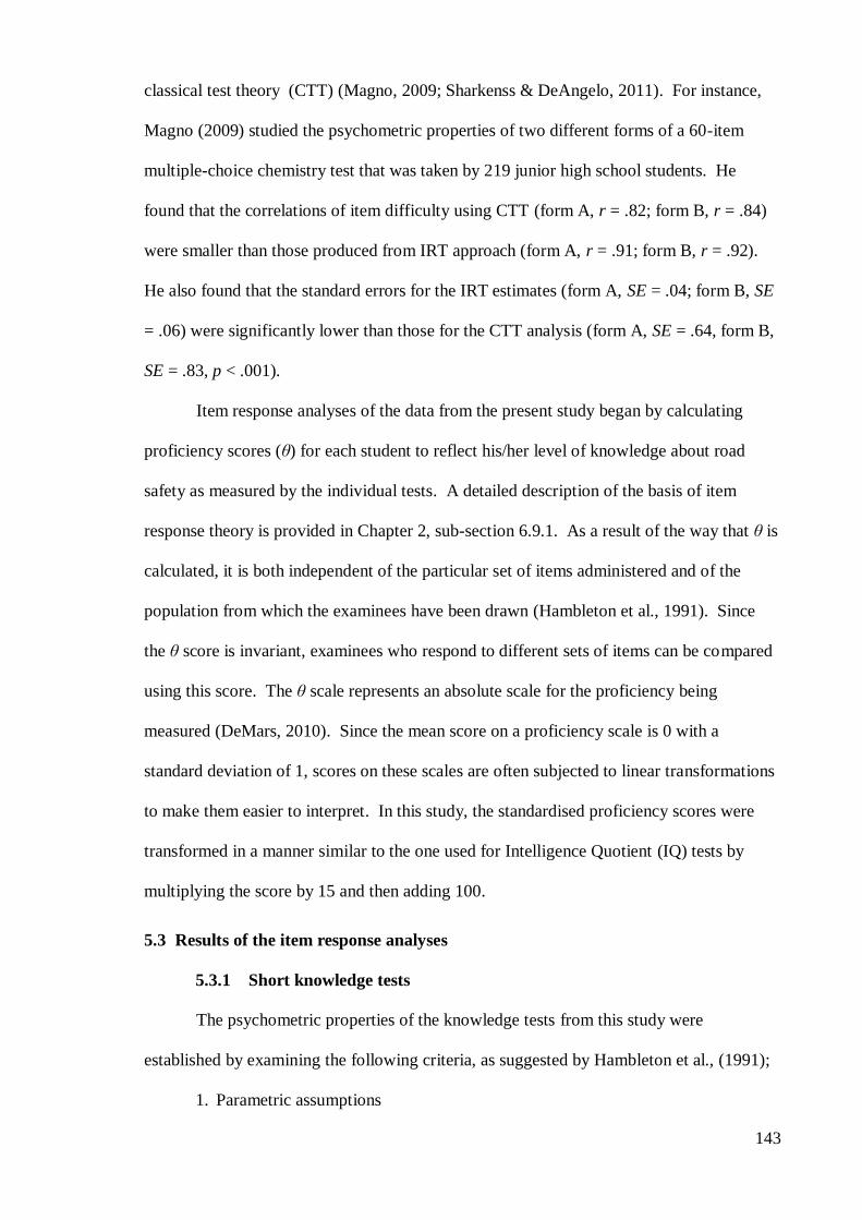
143
classical test theory (CTT) (Magno, 2009; Sharkenss & DeAngelo, 2011). For instance,
Magno (2009) studied the psychometric properties of two different forms of a 60-item
multiple-choice chemistry test that was taken by 219 junior high school students. He
found that the correlations of item difficulty using CTT (form A, r = .82; form B, r = .84)
were smaller than those produced from IRT approach (form A, r = .91; form B, r = .92).
He also found that the standard errors for the IRT estimates (form A, SE = .04; form B, SE
= .06) were significantly lower than those for the CTT analysis (form A, SE = .64, form B,
SE = .83, p < .001).
Item response analyses of the data from the present study began by calculating
proficiency scores (θ) for each student to reflect his/her level of knowledge about road
safety as measured by the individual tests. A detailed description of the basis of item
response theory is provided in Chapter 2, sub-section 6.9.1. As a result of the way that θ is
calculated, it is both independent of the particular set of items administered and of the
population from which the examinees have been drawn (Hambleton et al., 1991). Since
the θ score is invariant, examinees who respond to different sets of items can be compared
using this score. The θ scale represents an absolute scale for the proficiency being
measured (DeMars, 2010). Since the mean score on a proficiency scale is 0 with a
standard deviation of 1, scores on these scales are often subjected to linear transformations
to make them easier to interpret. In this study, the standardised proficiency scores were
transformed in a manner similar to the one used for Intelligence Quotient (IQ) tests by
multiplying the score by 15 and then adding 100.
5.3 Results of the item response analyses
5.3.1 Short knowledge tests
The psychometric properties of the knowledge tests from this study were
established by examining the following criteria, as suggested by Hambleton et al., (1991);
1. Parametric assumptions
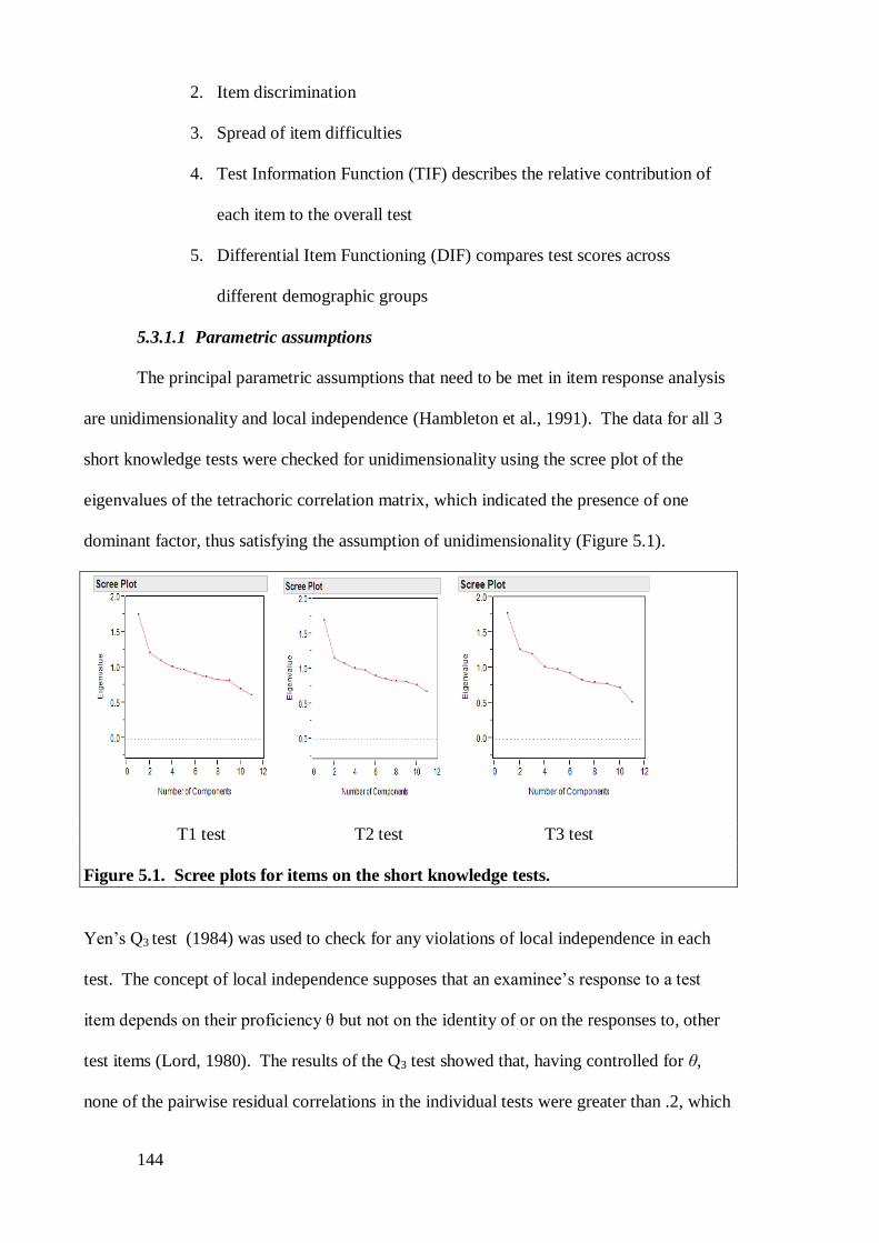
144
2. Item discrimination
3. Spread of item difficulties
4. Test Information Function (TIF) describes the relative contribution of
each item to the overall test
5. Differential Item Functioning (DIF) compares test scores across
different demographic groups
5.3.1.1 Parametric assumptions
The principal parametric assumptions that need to be met in item response analysis
are unidimensionality and local independence (Hambleton et al., 1991). The data for all 3
short knowledge tests were checked for unidimensionality using the scree plot of the
eigenvalues of the tetrachoric correlation matrix, which indicated the presence of one
dominant factor, thus satisfying the assumption of unidimensionality (Figure 5.1).
T1 test T2 test T3 test
Figure 5.1. Scree plots for items on the short knowledge tests.
Yen’s Q3 test (1984) was used to check for any violations of local independence in each
test. The concept of local independence supposes that an examinee’s response to a test
item depends on their proficiency θ but not on the identity of or on the responses to, other
test items (Lord, 1980). The results of the Q3 test showed that, having controlled for θ,
none of the pairwise residual correlations in the individual tests were greater than .2, which
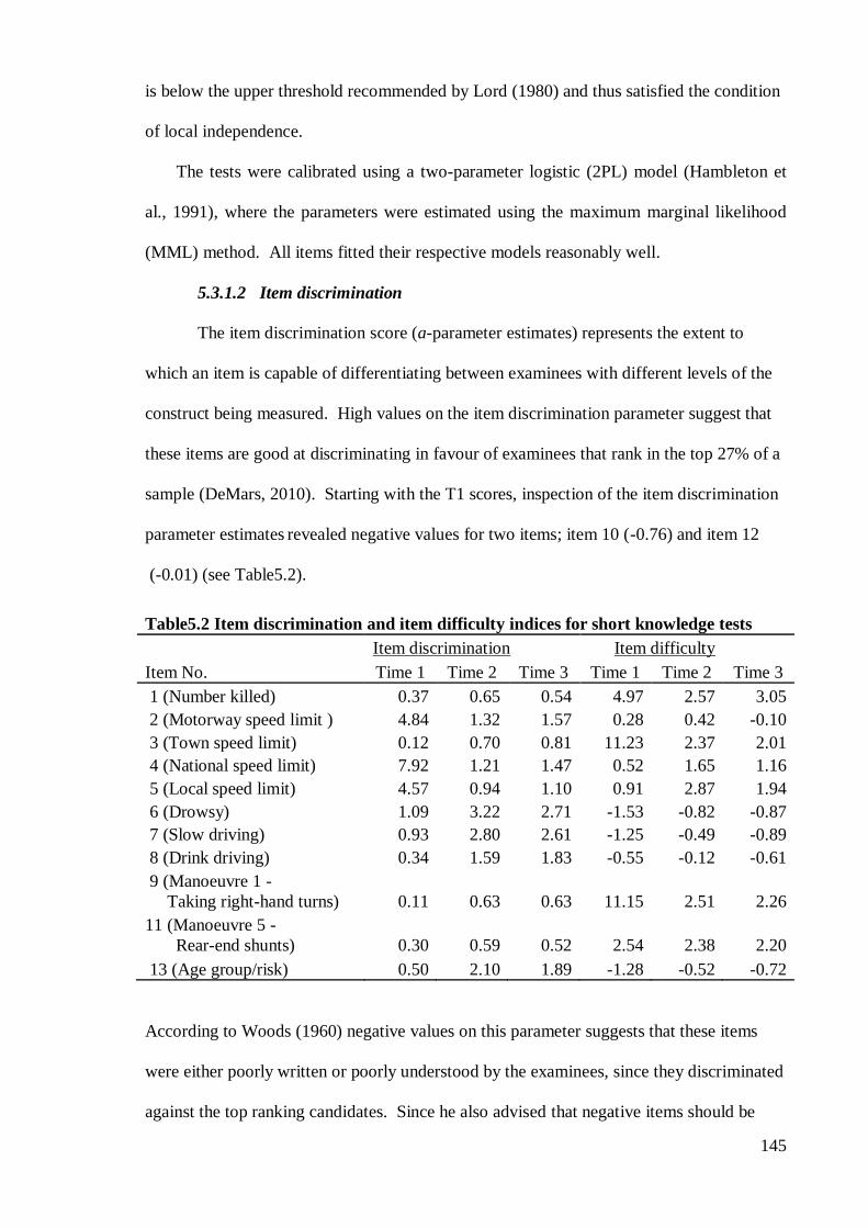
145
is below the upper threshold recommended by Lord (1980) and thus satisfied the condition
of local independence.
The tests were calibrated using a two-parameter logistic (2PL) model (Hambleton et
al., 1991), where the parameters were estimated using the maximum marginal likelihood
(MML) method. All items fitted their respective models reasonably well.
5.3.1.2 Item discrimination
The item discrimination score (a-parameter estimates) represents the extent to
which an item is capable of differentiating between examinees with different levels of the
construct being measured. High values on the item discrimination parameter suggest that
these items are good at discriminating in favour of examinees that rank in the top 27% of a
sample (DeMars, 2010). Starting with the T1 scores, inspection of the item discrimination
parameter estimates revealed negative values for two items; item 10 (-0.76) and item 12
(-0.01) (see Table5.2).
Table5.2 Item discrimination and item difficulty indices for short knowledge tests
Item discrimination Item difficulty
Item No. Time 1 Time 2 Time 3 Time 1 Time 2 Time 3
1 (Number killed) 0.37 0.65 0.54 4.97 2.57 3.05
2 (Motorway speed limit ) 4.84 1.32 1.57 0.28 0.42 -0.10
3 (Town speed limit) 0.12 0.70 0.81 11.23 2.37 2.01
4 (National speed limit) 7.92 1.21 1.47 0.52 1.65 1.16
5 (Local speed limit) 4.57 0.94 1.10 0.91 2.87 1.94
6 (Drowsy) 1.09 3.22 2.71 -1.53 -0.82 -0.87
7 (Slow driving) 0.93 2.80 2.61 -1.25 -0.49 -0.89
8 (Drink driving) 0.34 1.59 1.83 -0.55 -0.12 -0.61
9 (Manoeuvre 1 -
Taking right-hand turns) 0.11 0.63 0.63 11.15 2.51 2.26
11 (Manoeuvre 5 -
Rear-end shunts) 0.30 0.59 0.52 2.54 2.38 2.20
13 (Age group/risk) 0.50 2.10 1.89 -1.28 -0.52 -0.72
According to Woods (1960) negative values on this parameter suggests that these items
were either poorly written or poorly understood by the examinees, since they discriminated
against the top ranking candidates. Since he also advised that negative items should be

146
dropped to improve test validity, items 10 and 12 were dropped from the scale and the
remaining eleven items were used to calculate the proficiency scores in all three tests. The
item discrimination classification system devised by Ebel and Frisbie (1986) indicates that
discrimination values that are ≥ .4 are very good, those ranging between .30 and.39 are
reasonably good, those between .20 to .29 are classified as marginal and those below.19
are regarded as poor discriminators. Based on these criteria, the a-parameter estimates for
the T1 test showed that three of the four items testing knowledge of speed limits (2, 4, and
5) were the best discriminating items on this test. Items 6, 7, and 13 were also good, items
1 and 8 were reasonably good, item 11 was marginal, and items 3 and 9 were poor
discriminators. Analysis of the item discrimination score for both the T2 and T3 tests
show that all items were very good at discriminating between participants (see Table5.2).
The mean discrimination index was higher for the T1 test 1.92 (SD = 2.63), than it was for
the T2 (M =1.43, SD = 0.91) and the T3 (M = 1.43, SD = .079) tests, which suggests that
the gap between the students with high levels of proficiency and those with low levels of
proficiency was becoming narrower during the course of this study.
5.3.1.3 Item difficulty
The item difficulty index represents the proportion of students who identified the
correct answer(s) for each of the questions (Hambleton et al., 1991). These b-parameter
estimates were used to evaluate the tentative difficulty/appropriateness of the test items.
The higher the difficulty score, the harder the item was for the participants to answer
correctly. In accordance with the item difficulty classification system devised by Woods
(1960), items with difficulty values that are ≥.5 were classified as difficult, those with
values ranging between -.5 and +.5 standard deviations from the mean were classified as
moderate and items with values of ≤-.5 were deemed easy. An item difficulty analysis of
the items on the T1 test showed that it contained six difficult items (1, 3, 4, 5, 9 and 11),
one moderate item (2) and four easy items (6, 7, 8 and 13). Item 3, which tested student
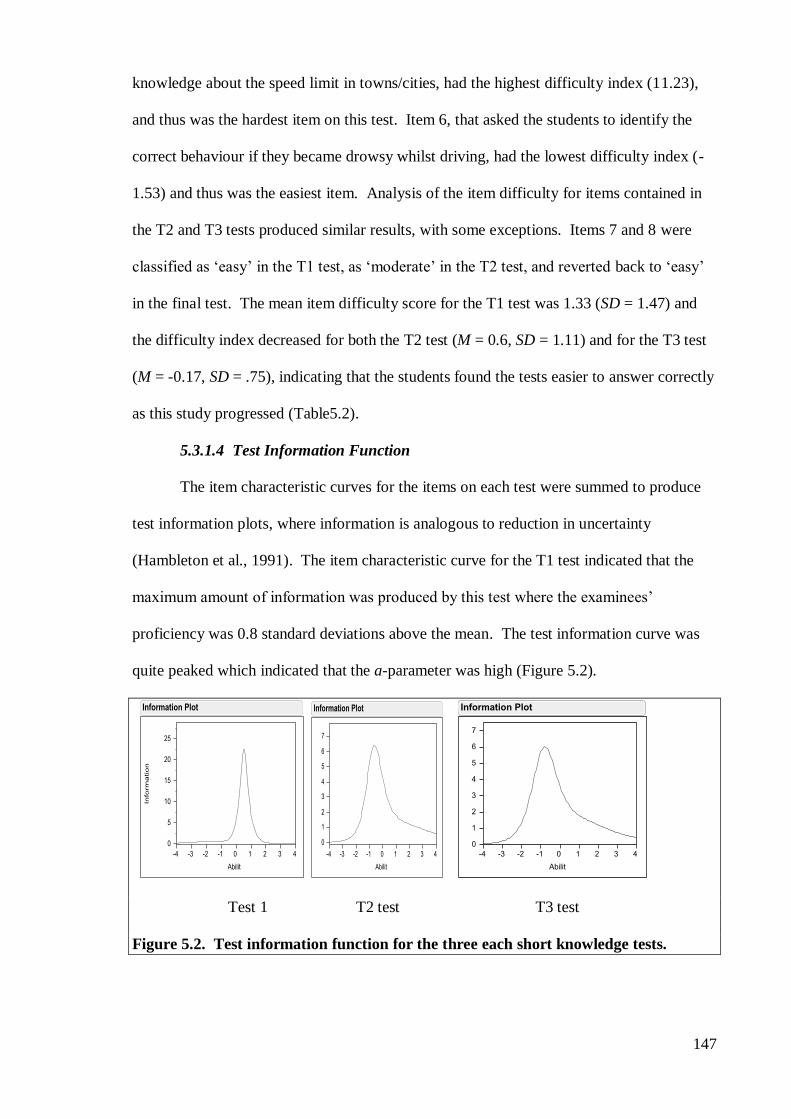
147
knowledge about the speed limit in towns/cities, had the highest difficulty index (11.23),
and thus was the hardest item on this test. Item 6, that asked the students to identify the
correct behaviour if they became drowsy whilst driving, had the lowest difficulty index (-
1.53) and thus was the easiest item. Analysis of the item difficulty for items contained in
the T2 and T3 tests produced similar results, with some exceptions. Items 7 and 8 were
classified as ‘easy’ in the T1 test, as ‘moderate’ in the T2 test, and reverted back to ‘easy’
in the final test. The mean item difficulty score for the T1 test was 1.33 (SD = 1.47) and
the difficulty index decreased for both the T2 test (M = 0.6, SD = 1.11) and for the T3 test
(M = -0.17, SD = .75), indicating that the students found the tests easier to answer correctly
as this study progressed (Table5.2).
5.3.1.4 Test Information Function
The item characteristic curves for the items on each test were summed to produce
test information plots, where information is analogous to reduction in uncertainty
(Hambleton et al., 1991). The item characteristic curve for the T1 test indicated that the
maximum amount of information was produced by this test where the examinees’
proficiency was 0.8 standard deviations above the mean. The test information curve was
quite peaked which indicated that the a-parameter was high (Figure 5.2).
Test 1 T2 test T3 test
Figure 5.2. Test information function for the three each short knowledge tests.
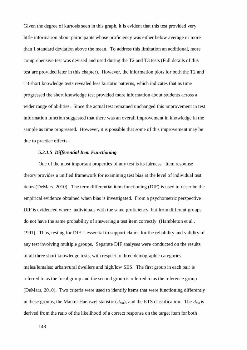
148
Given the degree of kurtosis seen in this graph, it is evident that this test provided very
little information about participants whose proficiency was either below average or more
than 1 standard deviation above the mean. To address this limitation an additional, more
comprehensive test was devised and used during the T2 and T3 tests (Full details of this
test are provided later in this chapter). However, the information plots for both the T2 and
T3 short knowledge tests revealed less kurtotic patterns, which indicates that as time
progressed the short knowledge test provided more information about students across a
wider range of abilities. Since the actual test remained unchanged this improvement in test
information function suggested that there was an overall improvement in knowledge in the
sample as time progressed. However, it is possible that some of this improvement may be
due to practice effects.
5.3.1.5 Differential Item Functioning
One of the most important properties of any test is its fairness. Item response
theory provides a unified framework for examining test bias at the level of individual test
items (DeMars, 2010). The term differential item functioning (DIF) is used to describe the
empirical evidence obtained when bias is investigated. From a psychometric perspective
DIF is evidenced where individuals with the same proficiency, but from different groups,
do not have the same probability of answering a test item correctly (Hambleton et al.,
1991). Thus, testing for DIF is essential to support claims for the reliability and validity of
any test involving multiple groups. Separate DIF analyses were conducted on the results
of all three short knowledge tests, with respect to three demographic categories;
males/females; urban/rural dwellers and high/low SES. The first group in each pair is
referred to as the focal group and the second group is referred to as the reference group
(DeMars, 2010). Two criteria were used to identify items that were functioning differently
in these groups, the Mantel-Haenszel statistic (Δmh), and the ETS classification. The Δmh is
derived from the ratio of the likelihood of a correct response on the target item for both
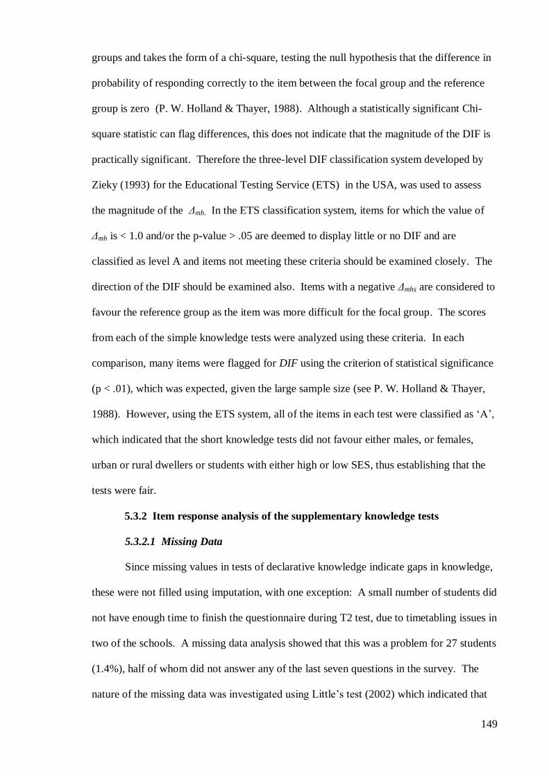
149
groups and takes the form of a chi-square, testing the null hypothesis that the difference in
probability of responding correctly to the item between the focal group and the reference
group is zero (P. W. Holland & Thayer, 1988). Although a statistically significant Chi-
square statistic can flag differences, this does not indicate that the magnitude of the DIF is
practically significant. Therefore the three-level DIF classification system developed by
Zieky (1993) for the Educational Testing Service (ETS) in the USA, was used to assess
the magnitude of the Δmh. In the ETS classification system, items for which the value of
Δmh is < 1.0 and/or the p-value > .05 are deemed to display little or no DIF and are
classified as level A and items not meeting these criteria should be examined closely. The
direction of the DIF should be examined also. Items with a negative Δmhs are considered to
favour the reference group as the item was more difficult for the focal group. The scores
from each of the simple knowledge tests were analyzed using these criteria. In each
comparison, many items were flagged for DIF using the criterion of statistical significance
(p < .01), which was expected, given the large sample size (see P. W. Holland & Thayer,
1988). However, using the ETS system, all of the items in each test were classified as ‘A’,
which indicated that the short knowledge tests did not favour either males, or females,
urban or rural dwellers or students with either high or low SES, thus establishing that the
tests were fair.
5.3.2 Item response analysis of the supplementary knowledge tests
5.3.2.1 Missing Data
Since missing values in tests of declarative knowledge indicate gaps in knowledge,
these were not filled using imputation, with one exception: A small number of students did
not have enough time to finish the questionnaire during T2 test, due to timetabling issues in
two of the schools. A missing data analysis showed that this was a problem for 27 students
(1.4%), half of whom did not answer any of the last seven questions in the survey. The
nature of the missing data was investigated using Little’s test (2002) which indicated that
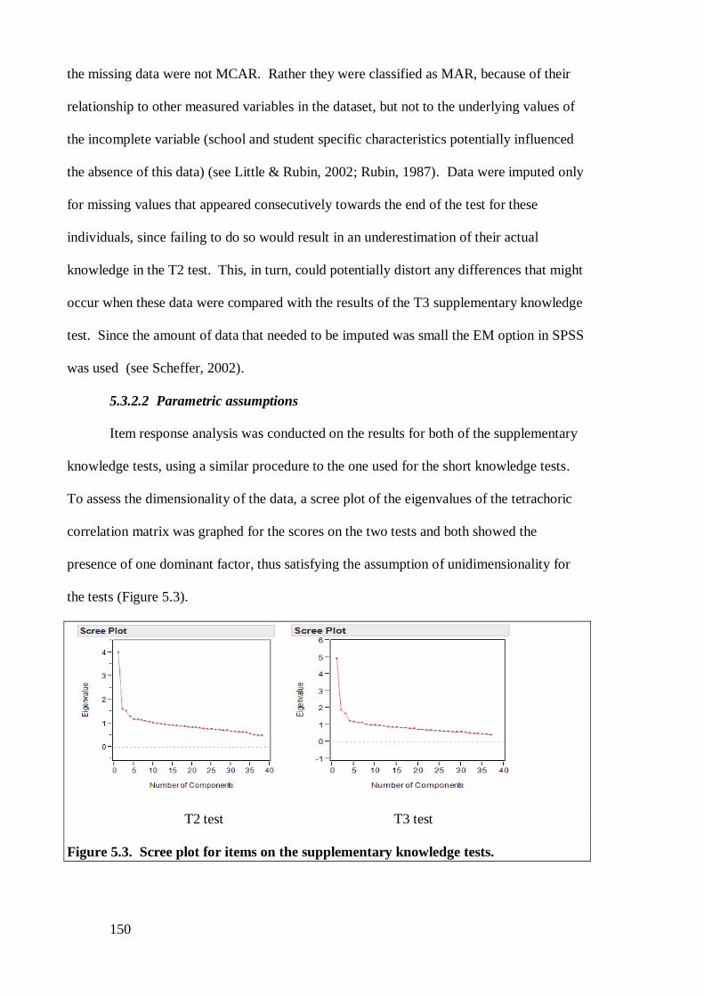
150
the missing data were not MCAR. Rather they were classified as MAR, because of their
relationship to other measured variables in the dataset, but not to the underlying values of
the incomplete variable (school and student specific characteristics potentially influenced
the absence of this data) (see Little & Rubin, 2002; Rubin, 1987). Data were imputed only
for missing values that appeared consecutively towards the end of the test for these
individuals, since failing to do so would result in an underestimation of their actual
knowledge in the T2 test. This, in turn, could potentially distort any differences that might
occur when these data were compared with the results of the T3 supplementary knowledge
test. Since the amount of data that needed to be imputed was small the EM option in SPSS
was used (see Scheffer, 2002).
5.3.2.2 Parametric assumptions
Item response analysis was conducted on the results for both of the supplementary
knowledge tests, using a similar procedure to the one used for the short knowledge tests.
To assess the dimensionality of the data, a scree plot of the eigenvalues of the tetrachoric
correlation matrix was graphed for the scores on the two tests and both showed the
presence of one dominant factor, thus satisfying the assumption of unidimensionality for
the tests (Figure 5.3).
T2 test T3 test
Figure 5.3. Scree plot for items on the supplementary knowledge tests.
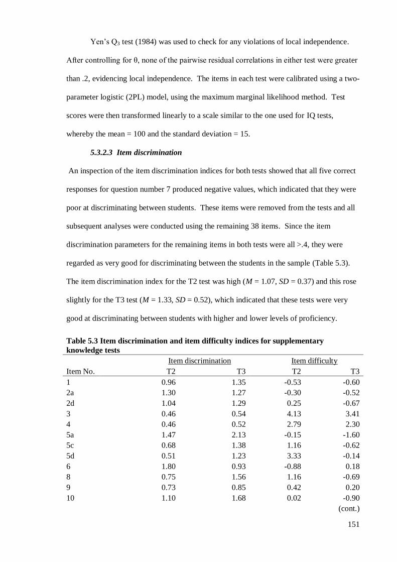
151
Yen’s Q3 test (1984) was used to check for any violations of local independence.
After controlling for θ, none of the pairwise residual correlations in either test were greater
than .2, evidencing local independence. The items in each test were calibrated using a two-
parameter logistic (2PL) model, using the maximum marginal likelihood method. Test
scores were then transformed linearly to a scale similar to the one used for IQ tests,
whereby the mean = 100 and the standard deviation = 15.
5.3.2.3 Item discrimination
An inspection of the item discrimination indices for both tests showed that all five correct
responses for question number 7 produced negative values, which indicated that they were
poor at discriminating between students. These items were removed from the tests and all
subsequent analyses were conducted using the remaining 38 items. Since the item
discrimination parameters for the remaining items in both tests were all >.4, they were
regarded as very good for discriminating between the students in the sample (Table 5.3).
The item discrimination index for the T2 test was high (M = 1.07, SD = 0.37) and this rose
slightly for the T3 test (M = 1.33, SD = 0.52), which indicated that these tests were very
good at discriminating between students with higher and lower levels of proficiency.
Table 5.3 Item discrimination and item difficulty indices for supplementary
knowledge tests
Item discrimination Item difficulty
Item No. T2 T3 T2 T3
1 0.96 1.35 -0.53 -0.60
2a 1.30 1.27 -0.30 -0.52
2d 1.04 1.29 0.25 -0.67
3 0.46 0.54 4.13 3.41
4 0.46 0.52 2.79 2.30
5a 1.47 2.13 -0.15 -1.60
5c 0.68 1.38 1.16 -0.62
5d 0.51 1.23 3.33 -0.14
6 1.80 0.93 -0.88 0.18
8 0.75 1.56 1.16 -0.69
9 0.73 0.85 0.42 0.20
10 1.10 1.68 0.02 -0.90
(cont.)
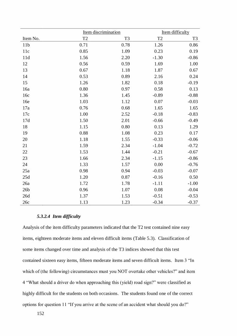
152
Item discrimination Item difficulty
Item No. T2 T3 T2 T3
11b 0.71 0.78 1.26 0.86
11c 0.85 1.09 0.23 0.19
11d 1.56 2.20 -1.30 -0.86
12 0.56 0.59 1.69 1.00
13 0.67 1.18 1.87 0.67
14 0.53 0.89 2.16 0.24
15 1.26 1.82 0.18 -0.19
16a 0.80 0.97 0.58 0.13
16c 1.36 1.45 -0.89 -0.88
16e 1.03 1.12 0.07 -0.03
17a 0.76 0.68 1.65 1.65
17c 1.00 2.52 -0.18 -0.83
17d 1.50 2.01 -0.66 -0.49
18 1.15 0.80 0.13 1.29
19 0.88 1.08 0.23 0.17
20 1.18 1.55 -0.33 -0.06
21 1.59 2.34 -1.04 -0.72
22 1.53 1.44 -0.21 -0.67
23 1.66 2.34 -1.15 -0.86
24 1.33 1.57 0.00 -0.76
25a 0.98 0.94 -0.03 -0.07
25d 1.20 0.87 -0.16 0.50
26a 1.72 1.78 -1.11 -1.00
26b 0.96 1.07 0.08 -0.04
26d 1.37 1.53 -0.51 -0.53
26c 1.13 1.23 -0.34 -0.37
5.3.2.4 Item difficulty
Analysis of the item difficulty parameters indicated that the T2 test contained nine easy
items, eighteen moderate items and eleven difficult items (Table 5.3). Classification of
some items changed over time and analysis of the T3 indices showed that this test
contained sixteen easy items, fifteen moderate items and seven difficult items. Item 3 “In
which of (the following) circumstances must you NOT overtake other vehicles?” and item
4 “What should a driver do when approaching this (yield) road sign?” were classified as
highly difficult for the students on both occasions. The students found one of the correct
options for question 11 “If you arrive at the scene of an accident what should you do?”
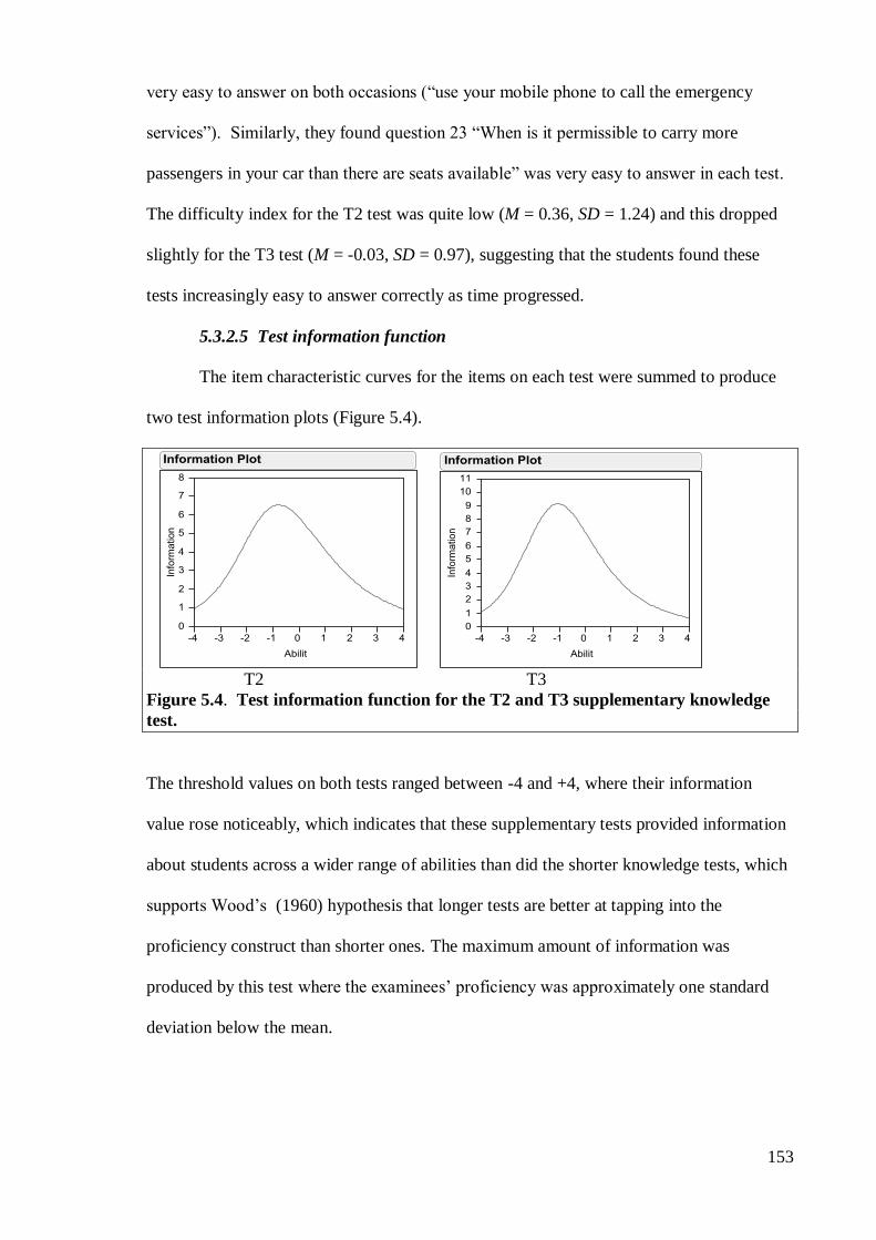
153
very easy to answer on both occasions (“use your mobile phone to call the emergency
services”). Similarly, they found question 23 “When is it permissible to carry more
passengers in your car than there are seats available” was very easy to answer in each test.
The difficulty index for the T2 test was quite low (M = 0.36, SD = 1.24) and this dropped
slightly for the T3 test (M = -0.03, SD = 0.97), suggesting that the students found these
tests increasingly easy to answer correctly as time progressed.
5.3.2.5 Test information function
The item characteristic curves for the items on each test were summed to produce
two test information plots (Figure 5.4).
T2 T3
Figure 5.4. Test information function for the T2 and T3 supplementary knowledge
test.
The threshold values on both tests ranged between -4 and +4, where their information
value rose noticeably, which indicates that these supplementary tests provided information
about students across a wider range of abilities than did the shorter knowledge tests, which
supports Wood’s (1960) hypothesis that longer tests are better at tapping into the
proficiency construct than shorter ones. The maximum amount of information was
produced by this test where the examinees’ proficiency was approximately one standard
deviation below the mean.
154
5.3.2.6 Differential item functioning
Differential item functioning was tested for the scores on the supplementary tests,
using a similar process to the one used for the simple knowledge tests. The results of the
Mantel_Haenszel statistic, (Δmh) (P. W. Holland & Thayer, 1988) and the corresponding
test of significance showed that many items functioned differently between the focal group
and the reference group. However when the ETS criteria (Zieky, 1993) were applied all of
the items on both tests were rated as ‘AA’, suggesting that these tests did not operate
differently between either males/females, or urban/rural dwellers or students classified as
having high or low SES.
Since the results of the item response analyses on the three short knowledge tests
and on the two supplementary knowledge tests met the various criteria used to establish
reliability and validity (Hambleton et al., 1991), the scores from these tests were deemed
suitable for further analysis.
5.4 Results of the descriptive and HLM analyses
This section begins by reporting the results of the analyses of the short knowledge
test scores, which examined patterns of change in knowledge proficiency in the
intervention phase (i.e. between the T1 and T2 tests), and also between the initial and the
final test in the study (i.e. between the T1 and T3 tests). Similar analyses of the
supplementary knowledge test scores are reported in the next section. Since the
supplementary knowledge tests was were conducted only at T2 and T3, just one set of
analyses was needed for these comparisons.
The raw mean number of items that the students answered correctly in the T1 test
was 4.90 (SD = 1.56), and this increased slightly in the T2 test (M = 5.05, SD = 1.1), and
again in the T3 test (M = 5.44, SD =1.65). Since each test contained eleven items, these
results show that, on average, the students in this sample answered less than 50% of the
questions correctly in these tests. Following the linear transformation of the proficiency
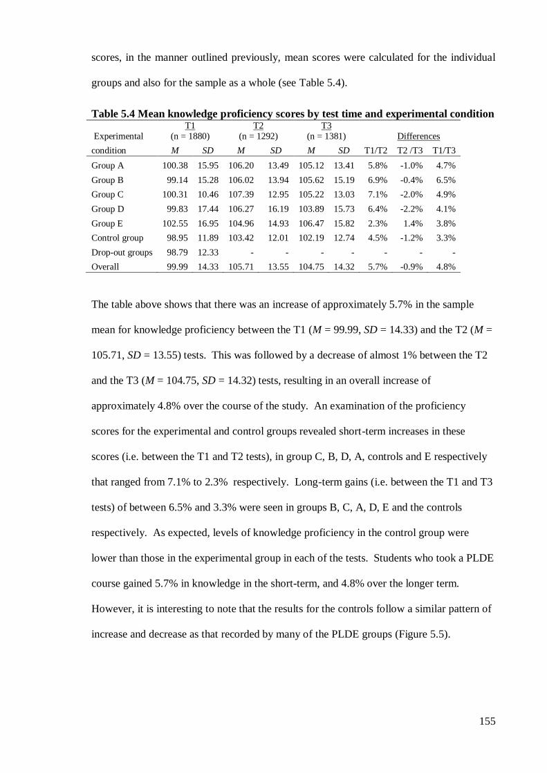
155
scores, in the manner outlined previously, mean scores were calculated for the individual
groups and also for the sample as a whole (see Table 5.4).
Table 5.4 Mean knowledge proficiency scores by test time and experimental condition
Experimental
T1
(n = 1880)
T2
(n = 1292)
T3
(n = 1381) Differences
condition M SD M SD M SD T1/T2 T2 /T3 T1/T3
Group A 100.38 15.95 106.20 13.49 105.12 13.41 5.8% -1.0% 4.7%
Group B 99.14 15.28 106.02 13.94 105.62 15.19 6.9% -0.4% 6.5%
Group C 100.31 10.46 107.39 12.95 105.22 13.03 7.1% -2.0% 4.9%
Group D 99.83 17.44 106.27 16.19 103.89 15.73 6.4% -2.2% 4.1%
Group E 102.55 16.95 104.96 14.93 106.47 15.82 2.3% 1.4% 3.8%
Control group 98.95 11.89 103.42 12.01 102.19 12.74 4.5% -1.2% 3.3%
Drop-out groups 98.79 12.33 - - - - - - -
Overall 99.99 14.33 105.71 13.55 104.75 14.32 5.7% -0.9% 4.8%
The table above shows that there was an increase of approximately 5.7% in the sample
mean for knowledge proficiency between the T1 (M = 99.99, SD = 14.33) and the T2 (M =
105.71, SD = 13.55) tests. This was followed by a decrease of almost 1% between the T2
and the T3 (M = 104.75, SD = 14.32) tests, resulting in an overall increase of
approximately 4.8% over the course of the study. An examination of the proficiency
scores for the experimental and control groups revealed short-term increases in these
scores (i.e. between the T1 and T2 tests), in group C, B, D, A, controls and E respectively
that ranged from 7.1% to 2.3% respectively. Long-term gains (i.e. between the T1 and T3
tests) of between 6.5% and 3.3% were seen in groups B, C, A, D, E and the controls
respectively. As expected, levels of knowledge proficiency in the control group were
lower than those in the experimental group in each of the tests. Students who took a PLDE
course gained 5.7% in knowledge in the short-term, and 4.8% over the longer term.
However, it is interesting to note that the results for the controls follow a similar pattern of
increase and decrease as that recorded by many of the PLDE groups (Figure 5.5).
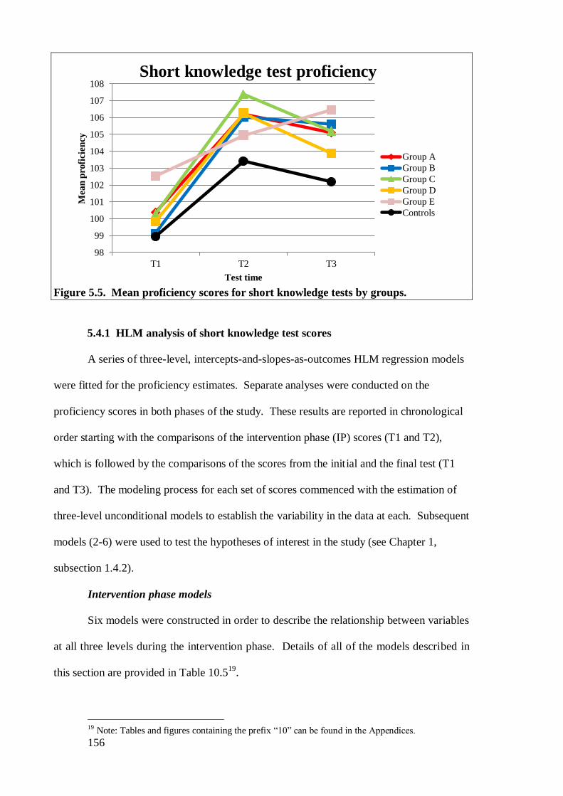
156
Figure 5.5. Mean proficiency scores for short knowledge tests by groups.
5.4.1 HLM analysis of short knowledge test scores
A series of three-level, intercepts-and-slopes-as-outcomes HLM regression models
were fitted for the proficiency estimates. Separate analyses were conducted on the
proficiency scores in both phases of the study. These results are reported in chronological
order starting with the comparisons of the intervention phase (IP) scores (T1 and T2),
which is followed by the comparisons of the scores from the initial and the final test (T1
and T3). The modeling process for each set of scores commenced with the estimation of
three-level unconditional models to establish the variability in the data at each. Subsequent
models (2-6) were used to test the hypotheses of interest in the study (see Chapter 1,
subsection 1.4.2).
Intervention phase models
Six models were constructed in order to describe the relationship between variables
at all three levels during the intervention phase. Details of all of the models described in
this section are provided in Table 10.519
.
19 Note: Tables and figures containing the prefix “10” can be found in the Appendices.
98
99
100
101
102
103
104
105
106
107
108
T1 T2 T3
Mean
profi
cie
ncy
Test time
Short knowledge test proficiency
Group A
Group B
Group C
Group D
Group E
Controls
157
Unconditional model (model 1)
The results for the unconditional model showed that the mean regression
coefficients for this test varied significantly around the grand mean (β = 103.03). The ICC
indicated that most of the variation in the proficiency estimates (81%) was attributable to
intra-student (level-1) factors. Between-student differences (level-2) accounted for an
additional 16% of the variance and between groups differences (level-3) were responsible
for just 3% of the variation in the model. The results of chi-square goodness-of-fit tests
indicated that there was a significant amount of variation in the between students (χ2 =
1689.81, df = 1212, p < 0.001) and in the between schools (χ2 = 5.31, df = 37, p < 0.001)
estimates. To gauge the magnitude of these variations, plausible values ranges, based on
95% confidence intervals (CIs), were calculated for all three levels. These suggested that
there was a small amount of variation in the between-groups scores, 95% CI (98.6,
107.58). The variation in the between-student estimates was over twice as large, 95% CI
(91.52, 114.66) and the within-student variation was almost six times greater than the
between-group variation and twice as large as the student level variation, 95% CI (77.17,
129.01). Thus intra-student factors accounted for the majority of the variation in the data.
Change by time/age (model 2)
The effects of the level-1 predictors i.e. time and mean age were tested in model 2.
Preliminary analysis showed that there was no main effect of age (β = -0.41, t(40) = -0.66,
p > .05 ), therefore ‘age’ was dropped from the model. The subsequent time-only model
showed that there was a significant amount of both between-student variation (χ2 =
1848.02, df = 1212, p < .001) and between groups variation (x2 = 78.51, df = 37, p < .001)
in knowledge proficiency scores at the intercept (i.e. T1), which supports hypothesis 1.
Knowledge proficiency increased significantly in the sample during the intervention phase
(β = 5.50, t(37) = 10.25, p < .001, d = .02), endorsing hypothesis 2. An inspection of the
tau beta ( b ) matrices revealed a negative correlation between the intercept and the slope
158
scores which suggested that students who had less knowledge proficiency in the T1 test
gained more knowledge in the intervention phase than those who demonstrated less
proficiency at T1 (pseudo-R2
= 0.02). For instance, an inspection of the raw data
confirmed that whereas school groups with a mean proficiency score that was below 100
(i.e. the metric mean) in the T1 test gained 7.41 points on average in the T2 test, those
whose mean was above 100 initially only gained 4.48 points on average in the second test.
Since both the intercept and slope estimates were statistically significant, both parameters
were needed to explain the growth trajectory. The inclusion of time as a predictor resulted
in an 8.8% reduction in the explainable variance at the within-student level. A chi-square
goodness-of-fit test showed that the inclusion of time in model significantly improved the
fit of the data when compared to the unconditional model (model 1), χ2 = 112.29, df = 3, p <
0.00, pseudo-R2 = .03. Thus it appears that the increase in proficiency over time
represented a small, but significant factor in explaining variations in knowledge in the
intervention phase.
PLDE effects (model 3)
Model 3 tested the effect of taking a PLDE course in Transition Year on changes in
proficiency scores over time. The results showed that there was no significant difference
between the initial proficiency estimates (T1) for students who took a PLDE course (β =
100.28) and the estimates for those who received no PLDE in school (β = 0.33, t(36) =
0.22, p > .05). However, the slope coefficients showed that the PLDE group gained a
significant amount of proficiency between the T1 and T2 tests (β = 5.96, t(36) = 10.77, p <
.001), and that the gains achieved by the non-PLDE group were significantly lower (β = -
2.91, t(36) = -2.08, p < .05, d = .14). This evidence for a main effect of participating in
PLDE supports hypothesis 4, albeit that the difference was quite small. The results of a
goodness-of-fit comparison between this model and model 2 showed that the inclusion of
159
PLDE group membership as a predictor did not produce a significant reduction in the
variance in the data (χ2 = 4.99, df = 2, p > .05).
PLDE group effects (model 4)
The effects of attending specific types of PLDE courses were tested in model 4.
The results showed that there was no significant difference in knowledge proficiency
between any of the experimental groups before the interventions were delivered. The
outcome for the slope indicated that, students in the control group gained a significant
amount of knowledge between the T1 and T2 tests (β = 3.01, t(32) = 2.34, p < .05).
However the gains in knowledge made by students who took PLDE courses A (β = 2.82,
t(32) = 1.56, p < .05, d = .1), B (β = 3.72, t(32) = 2.67, p < .05, d = .21 ) and C (β = 4.25,
t(32) = 2.41, p < .05, d = .25 ), were significantly larger, providing limited support for
hypothesis 5. However, a goodness of fit comparison between this model and model 2
indicated that the additional specification of programme group membership did not result
in a significant reduction in the unexplained variance in the data when compared to the
simpler model (χ2 = 13.57, df = 10, p > 0.5).
Between-student effects (model 5)
Model 5 estimates involved the addition of the 14 level-2 predictors listed in Table
2.3 to the time-only model (2) and the subsequent trimming of all non-significant
coefficients from the model, as recommended by Raudenbush & Bryk (2002), (see
Chapter 2, sub-section 6.6 for a detailed explanation of this process)20
. The results showed
that several between-students factors significantly influenced the T1 (intercept) and the T2
(slope) estimates for this model. The intercept estimates showed that students with higher
SES (β = 0.96, t(37) = 2.65, p < .05), and more experience with using vehicles (β = 2.47,
t(37) = 3.27, p <.01), had significantly more proficiency in the T1 knowledge test than
students with average to low levels of these attributes, and those with more exposure to
20 Note that all between-student models in this research were constructed using this methodology.
160
aberrant driving practices (β = -3.29. t(37) = -3.33, p < .01) and those with higher trait
impulsiveness (β = -2.37, t(37) = -2.29, p < .05) were significantly less proficient on the T1
test than were their counterparts. However, the differences in scores between students with
high levels of these attributes when compared with those with average to low levels of
these characteristics were small in real terms. This provides very limited support for
hypothesis 6. For instance, the difference in relation to SES was just 1%, and it was 2.5%,
-3.2% and -2.3% for experience, exposure, and impulsiveness respectively. The slope
estimates showed that whereas students gained a significant amount of knowledge
proficiency between the two tests (β = 5.27), those with more exposure to aberrant driving
gained significantly more proficiency during that period (β = 2.64, t(37) = 2.45, p < .05)
than did their counterparts. There was an estimated improvement of 8.1% in the scores for
this group between the two tests. Thus, these results offer limited support for hypothesis 6.
The results of a chi-square goodness-of-fit test showed that when compared to model 2, the
inclusion of significant between-student predictors in model 5 improved the fit of the data
significantly (χ2 = 102.46, df = 60, p < 0.001, pseudo-R
2 = .08).
A final model was built to test for cross-level interactions between significant
predictors from the previous models, however no significant effects were found.
Furthermore, given the small decreases in the -2-log likelihood deviance between
successive models and also the magnitude of the deviance in model 5, it is clear that none
of the models tested represented a particularly good fit for the present data.
5.4.1.1 Initial and final test comparison models
Comparisons of the knowledge proficiency scores recorded in the initial test (T1)
and those recorded in the final test (T3) were made in a similar progression to the one
described for the intervention phase comparisons reported earlier. Details of all of the
models described in this section are contained in Table 10.6.
161
Unconditional model (model 1)
The unconditional model showed that the there was a significant amount of
variation in the grand mean scores for knowledge proficiency during this study (β =
102.78, t(37) = 187.26, p < .001). The estimates indicated that 91% of the explained
variance in scores was accounted for by intra-student (level-1) factors, a further 6% was
associated with between-student (level-2) factors, and the final 3% was attributable to
between-group factors. The results of chi-square goodness-of-fit tests showed that there
was a significant amount of variation in the between-student estimates (χ2 = 1246.73, df =
1105, p < 0.01) and also between schools (χ2 = 96.67, df = 37, p < 0.001). The plausible
values range for proficiency estimates scores at school-level (97.96, 107.60) and the range
at student level (95.45, 110.11) was just 1.5 times wider. However, the range of variation
between the scores on the T1 and T3 tests at intra-student level (74.87, 130.69) was almost
four times greater than those at the between-student level and almost 6 times greater than
that at the between-groups level.
Change over time (model 2)
The level-1 variables ‘time’ and ‘mean age’ were added in model 2. Preliminary
analysis showed that there was no main effect of age (β = -0.22, t(37) = -0.32, p > .05 ),
therefore ‘age’ was dropped from the model. The results for the subsequent time-only
model showed that there was a significant increase in knowledge proficiency in the sample
between the start and the finish of this study (β = 5.04, t(37) = 8.35, p < 0.00, d = .3),
supporting hypothesis 3. However, whereas the tau beta correlations between the intercept
and the slope in the corresponding IP model were negative, which suggests that students
with greater knowledge proficiency during the T1 test, gained less knowledge over the
shorter term, the corresponding correlations between the T1 and T3 tests (R2 = 0.95)
showed a reversal in this trend. Students with better knowledge proficiency on the T1 test,
162
gained more knowledge during the course of the study than did those who had less
proficiency at the outset. The inclusion of ‘time’ as a predictor resulted in a 6% reduction
in the explainable variance in proficiency scores at the within-student level. A chi-square
goodness of fit test indicated that the inclusion of time in model 2 significantly improved
the fit of the data, when compared with the unconditional model (χ2 = 68.00, df = 3, p <
0.00, pseudo-R2 = .03). Thus, the increase in knowledge over time constituted a significant
factor in explaining some of the variation in knowledge during the course of this study.
PLDE effects (model 3)
Model 3 tested the effects of taking a PLDE course in TY on changes in knowledge
proficiency over time. The outcome showed that although students who took a PLDE
course (β = 5.46, t(36) = 8.31, p < .001) gained more knowledge than those who did not
take such a course, this difference was not statistically significant (β = -2.64, t(36) = -1.64,
p > .05). This does not support hypothesis 4. A goodness-of-fit test compared the
explanatory power of models 2 and 3 and the results showed that the addition of PLDE as a
predictor significantly reduced the variance in the data (χ2= 297.15, df = 2, p < .001, R
2 =
0.06, pseudo-R2 = .01).
Programme effects (model 4)
Model 4 tested the effects of attending specific types of PLDE courses on changes
in knowledge between the T1 and T3 tests. The results showed that only the students in
group B (β = 4.17, t(32) = 2.23, p < .05) gained significantly more knowledge proficiency
than did those in the control group (β = 2.79, t(32) = 1.90, p > .05, d = .06) over the longer
term. Furthermore, the magnitude of this difference was quite small. A chi-square
goodness-of-fit test was conducted between the previous model and this fuller model, and
the results showed that the additional differentiation between PLDE group effects did not
significantly reduce the variability in the data (χ2 = 10.50, df = 10, p > .05, pseudo-R
2 = .01).
163
Thus, membership of specific PLDE groups did not constitute a reliable predictor of
knowledge proficiency in this test.
Between-student effects (model 5)
Model 5 involved estimating the effects the 14 level-2 predictors listed in Table
2.3. on the T1 and T3 knowledge proficiency estimates. This model was then trimmed of
all non-significant predictors (see Chapter 2, sub-section 6.6). Similar to the findings from
model 5 in the intervention phase, this trimmed model contained 4 variables that
significantly influenced the proficiency estimates in the T1 test. The slope estimates
showed that there was a significant positive effect for higher exposure to aberrant driving
(β = 3.53, t(37) = 2.68, p < .05), which represented an increase in proficiency of almost 9%
for students in that category over the long-term. Altogether, these findings offer very
limited support for hypothesis 6. The results of a chi-square goodness-of-fit test showed
that, when compared to model 2, the inclusion of significant between-student predictors in
model 5 improved the fit of the data significantly (χ2 = 92.15, df = 60, p < 0.01, pseudo-R
2 =
.02).
Finally, a further model that included all the significant variables from the previous
models showed that there were no significant cross-level interactions between these
predictors over the longer-term. Again, the magnitude of the -2 log likelihood deviance
remained disappointingly high in all models, suggesting that the combination of predictors
that were used to test hypothesis 6 were not very good predictors of knowledge proficiency
in the present sample.
5.4.1.2 Effects of studying the ROTR
Since some of the PLDE courses featured in this study did not entail any formal
study of the ROTR and since it is reasonable to expect that students who studied the ROTR
would have better knowledge proficiency than those who did not, the absolute effects of
studying the ROTR as part of a school-based PLDE course were investigated as a likely
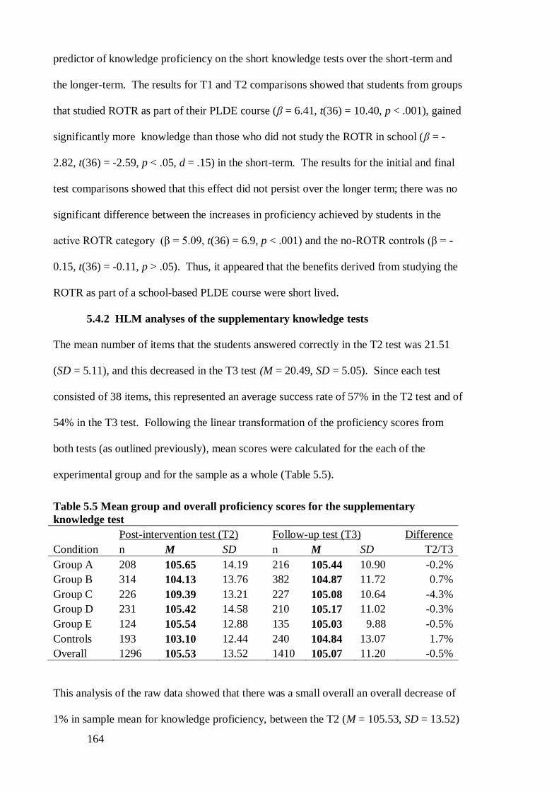
164
predictor of knowledge proficiency on the short knowledge tests over the short-term and
the longer-term. The results for T1 and T2 comparisons showed that students from groups
that studied ROTR as part of their PLDE course (β = 6.41, t(36) = 10.40, p < .001), gained
significantly more knowledge than those who did not study the ROTR in school (β = -
2.82, t(36) = -2.59, p < .05, d = .15) in the short-term. The results for the initial and final
test comparisons showed that this effect did not persist over the longer term; there was no
significant difference between the increases in proficiency achieved by students in the
active ROTR category (β = 5.09, t(36) = 6.9, p < .001) and the no-ROTR controls (β = -
0.15, t(36) = -0.11, p > .05). Thus, it appeared that the benefits derived from studying the
ROTR as part of a school-based PLDE course were short lived.
5.4.2 HLM analyses of the supplementary knowledge tests
The mean number of items that the students answered correctly in the T2 test was 21.51
(SD = 5.11), and this decreased in the T3 test (M = 20.49, SD = 5.05). Since each test
consisted of 38 items, this represented an average success rate of 57% in the T2 test and of
54% in the T3 test. Following the linear transformation of the proficiency scores from
both tests (as outlined previously), mean scores were calculated for the each of the
experimental group and for the sample as a whole (Table 5.5).
Table 5.5 Mean group and overall proficiency scores for the supplementary
knowledge test
Post-intervention test (T2) Follow-up test (T3) Difference
Condition n M SD n M SD T2/T3
Group A 208 105.65 14.19 216 105.44 10.90 -0.2%
Group B 314 104.13 13.76 382 104.87 11.72 0.7%
Group C 226 109.39 13.21 227 105.08 10.64 -4.3%
Group D 231 105.42 14.58 210 105.17 11.02 -0.3%
Group E 124 105.54 12.88 135 105.03 9.88 -0.5%
Controls 193 103.10 12.44 240 104.84 13.07 1.7%
Overall 1296 105.53 13.52 1410 105.07 11.20 -0.5%
This analysis of the raw data showed that there was a small overall an overall decrease of
1% in sample mean for knowledge proficiency, between the T2 (M = 105.53, SD = 13.52)
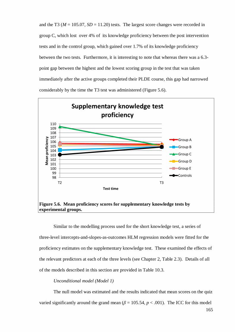
165
and the T3 (M = 105.07, SD = 11.20) tests. The largest score changes were recorded in
group C, which lost over 4% of its knowledge proficiency between the post intervention
tests and in the control group, which gained over 1.7% of its knowledge proficiency
between the two tests. Furthermore, it is interesting to note that whereas there was a 6.3-
point gap between the highest and the lowest scoring group in the test that was taken
immediately after the active groups completed their PLDE course, this gap had narrowed
considerably by the time the T3 test was administered (Figure 5.6).
Figure 5.6. Mean proficiency scores for supplementary knowledge tests by
experimental groups.
Similar to the modelling process used for the short knowledge test, a series of
three-level intercepts-and-slopes-as-outcomes HLM regression models were fitted for the
proficiency estimates on the supplementary knowledge test. These examined the effects of
the relevant predictors at each of the three levels (see Chapter 2, Table 2.3). Details of all
of the models described in this section are provided in Table 10.3.
Unconditional model (Model 1)
The null model was estimated and the results indicated that mean scores on the quiz
varied significantly around the grand mean (β = 105.54, p < .001). The ICC for this model
9899
100101102103104105106107108109110
T2 T3
Mea
n p
rofi
cien
cy
Test time
Supplementary knowledge test proficiency
Group A
Group B
Group C
Group D
Group E
Controls

166
showed that almost 70% of the variation in student proficiency for the supplementary test
was attributable to time factors (level-1), over 27% was associated with students within
schools (level-2) and the final 3% represented between schools variation (level-3).
Separate chi-square tests indicated that there was a significant amount of variation in the
between-student estimates (χ2= 1896.4, df = 1082, p < 0.001) and also between schools
(χ2= 88.147, df = 36, p < 0.001). There was a small amount of variation in scores between
schools, 95% CI (101.60, 110.12). The between-student variance was three times greater,
95% CI (93.06, 118.656) and the intra-student variation was almost five times greater than
the between schools variation CI (99.17, 111.91). The intra-student variation was over
one-and-a-half times greater than the variation between students.
Change over time (model 2)
The level-1 variables ‘time’ and ‘mean age’ were added in model 2. Preliminary
analysis showed that there was no main effect of age (β = -0.02, t(37) = -0.11, p > .05 ),
therefore ‘age’ was dropped from the model. The results for the subsequent time-only
model showed that there was a small, non-significant decrease in knowledge proficiency in
the sample between the T2 and the T3 tests (β = -0.07, t(36) = -1.01, p > .05).
Interestingly, since there was a negative covariance between the intercept and slope
estimates, this suggests that students who knew more in the T2 test, lost less proficiency
than those who knew less during that test (R2 = 0.8). A chi-square goodness-of-fit test
showed that the addition of ‘time’ as a predictor in this model improved the fit of the data
significantly (χ2 = 25.69, df = 3, p < 0.00, pseudo-R
2 = .01). The addition of time as a
predictor resulted in a 5% reduction in the explainable variance in the data at the within-
student level.
PLDE effects (model 3)
The effects of taking a PLDE course were tested in model 3 and the results showed
that there was a significant difference in knowledge proficiency between students who took
167
a PLDE course (β = 105.97) and those who did take such a course (β = -2.51, t(36) = -
2.01, p < .05, d = -0.02) in the T2 test. The slope estimates showed that the subsequent
decrease in proficiency experienced by the PLDE group was not significant (β = -0.46,
t(36) = -0.8, p > .05) and although students in the non-PLDE groups gained some
proficiency in the post-intervention period (β = 2.26, t(35) = 1.17, p > .05), the difference
in the slopes between the two groups was not significant. These results suggest that
although PLDE group membership produced measureable changes in knowledge
proficiency in the short-term, these effects did not persist over time, which provides
support for hypothesis 4, but not for hypothesis 5. Moreover, the chi-square statistic
indicated that the inclusion of PLDE as a predictor did not improve the fit of the data,
when compared with the time-only model (model 2) (x2 = 1.66, df = 2, p > .05).
PLDE group effects (model 4)
The effects of attending specific types of PLDE courses were tested in model 4.
This showed that there was no significant difference in knowledge proficiency between
students in the control those in any of the active programme groups with respect to the T2
intercepts or the T3 slopes. Furthermore, the inclusion of specific PLDE course effects in
this model did not account for any significant reduction in the variance in the data when
compared to the time-only model (x2 = 10.92, df = 10, p > .05). Thus, programme group
membership was not useful predictor of knowledge proficiency in either of the post-
intervention tests.
Between-student effects (model 5)
Model 5 involved the addition of all of the level-2 predictors to the level-1
predictor ‘time’. All non-significant coefficients were then trimmed from the model as per
Chapter 2, subsection 6.6. The final model showed that exposure to aberrant driving (β = -
1.39, t(36) = -2.06, p = .05), and impulsiveness (β = -2.31, t(36) = -3.03, p <.01 )
significantly influenced the T2 proficiency estimates and none of the between-student
168
predictors used in this study influenced the change that occurred between the T2 and T3
tests. However, the results of a chi-square test indicated that this model represented a
significantly better fit for the data than did the time-only model (model 2) (x2 = 16.59, df =
4, p < .01, pseudo-R2 = .02).
Since none of the between-groups variables produced significant changes in scores
in the supplementary knowledge test, there was no need to test for interactions between
predictors at all three levels.
5.4.2.1 Effects of studying the ROTR
The absolute effects of studying the ROTR on knowledge proficiency were
measured and the results showed that although students who studied the ROTR as part of a
PLDE course in school (β = 107.19, t(35) = 116.35, p < .001) had greater proficiency on
the T2 supplementary test than those who did not (β = -2.56, t(35) = -1.71, p > .05), this
difference was not statistically significant. Neither was there any substantial difference in
the loss of proficiency experienced by the ROTR students (β = -1.13) and the non-ROTR
students (β = 0.93, t(35) = 0.61, p > .05) in the post intervention phase. This evidence adds
further weight to the view that studying the ROTR as part of a PLDE course does not have
a significant effect on the gains in proficiency as measured the knowledge tests used in this
study.
5.5 Discussion
In this part of the research, item response analyses were conducted to investigate
the psychometric properties of tests which had been designed to measure declarative
knowledge with respect to the ROTR and specific factors that increase risk in traffic in
PLD adolescents. Having established the reliability and validity of these tests, knowledge
proficiency scores were produced for each student and these were used subsequently to
construct a series of HLMs that tested the hypotheses that were of interest in this study.
169
The results of these hypotheses tests will be reviewed first and a discussion of the item
response analyses and the general methodology will follow thereafter.
The results from the HLM analyses of the T1 short knowledge test indicated that
although there was a considerable amount of variation in knowledge proficiency in the
sample, the students were reasonably knowledgeable about the ROTR and specific risk-
increasing factors when they began in TY/year 13 of secondary school. The reported
variation in knowledge proficiency is explicable in the context of the TCI model (Fuller,
2005), which suggests that personal capability arises as a result of a combination of
physiological attributes, exposure to differential learning experiences and individual
differences in personality.
The results from the null models (model 1) for the short test and for the
supplementary tests indicated that the largest proportion of variation in the data was
located at the intra-student level. The current research included just two predictors, age
and time, that addressed variation at that level directly and it was found that these factors
accounted for just 3% in the overall variation in the short-term and long-term short
knowledge test scores and of just 1% in the supplementary test scores. Moreover, although
a wide range of between-student and between-group predictors were included as part of the
model construction exercises, the -2-log likelihood deviance scores remained stubbornly
high. This suggests that a large proportion of the variation in knowledge scores was
attributable to some factor(s) that were not taken into account in the current research
design. Whereas it is acknowledged that the inclusion of predictors at any level of a HLM
can influence changes in the amount of variation remaining at all levels of the model, it is
clear nonetheless that the factors that were most likely to reduce the variance at the intra-
student level in this research were ones that tend to vary over time. Although between-
student factors such as experience with using vehicles, experience with RTCs were
measured in each test, other factors which had the potential to vary over time were
170
measured just once i.e. personality traits such as impulsiveness, sensation seeking and Big-
Five markers. Whilst it was not expected that these predictors would change substantially
during the course of this project, with hindsight it is clear that the failure to account for the
time-varying properties of trait predictors represents a flaw in the research design. Since
preliminary analysis of the HLM results for the remainder of the study also showed that
most of the variance in the relevant models was attributable to intra-student factors,
possible sources of this will be examined in detail in the general discussion. In the interim,
it is should be noted that lack of an adequate range of significant, time varying intra-
student predictors limited the potential of the current research to explain driving-related
knowledge, risk perception skills and attitudes within the context of the TCI model (Fuller,
2005).
The results from the short tests suggested that sample as a whole gained a small,
but statistically significant amount of knowledge over both the short-term and the long-
term, supporting hypotheses 2 and 3. Furthermore, the results showed that taking a PLDE
course in TY had a positive effect on knowledge acquisition. Students who took a PLDE
course gained significantly more knowledge than did students in the control group in the
short-term but not over the longer-term, offering some support for hypotheses 4. The
current findings provide some support for the efficacy of PLDE in increasing driving-
related declarative knowledge in adolescents, over a short period of time. They also accord
with the results from previous studies which reported short-term improvements in driving-
related cognition (Elkington, 2005; Harré & Brandt, 2000a; Poulter & McKenna, 2010)
and declarative knowledge (Elkington, 2005) as a result of attending a PLDE course.
One surprising aspect of the present results was that the test scores for the control
group followed roughly the same pattern of change across the three tests as did those for
the experimental groups. The unanticipated increase in knowledge proficiency for the
control group during the intervention phase and the subsequent decrease in the post-
171
intervention phase was somewhat perplexing, because it suggested that knowledge
proficiency in this group was being influenced systematically by some extraneous factor.
One possible explanation for this phenomenon was the eagerness to start driving in the
sample, which was evidenced in Chapter 4. Many of the students in this study became
eligible to apply for an LDP during the intervention phase of this study. However, since
one needs to pass the driver theory test in order to get this permit, it seems likely that the
unexpected increase in knowledge proficiency in the control group was due to the fact that
many of these students were studying the ROTR in preparation for taking the theory test.
This assumption is supported by findings that the rate of licensure was significantly higher
for the controls than it was for students in the PLDE groups. The subsequent decline in
proficiency seen in all groups is consistent with current knowledge with respect to the
various processes involved in the acquisition and retention of declarative knowledge (e.g.
Craik and Lockhart’s (1972) levels of processing theory and Anderson’s (1996) adaptive
control of thought architecture). Specifically, memory traces for information that is salient
and that is rehearsed regularly become strengthened, whereas those traces grow weaker
when that knowledge is no longer being accessed on a regular basis. Another plausible
explanation for the pattern in these data concerns the Hawthorne Effect (Parsons, 1974)
which suggests that there would be an increased interest in driving and driving-related
knowledge, risk perception skills and attitudes in the control group as a result of
participating in the study.
The present findings also suggested that some types of PLDE courses were more
effective in equipping students with knowledge proficiency than others. Students who
took the various PLDE courses that featured in this study gained slightly more knowledge
proficiency in the intervention phase and retained more knowledge over the longer term,
than did those in the control group. However, only those students in groups B and C
gained significantly more knowledge in the short term and only those in group B retained
172
significantly more knowledge over the longer term than did those in the control group.
The results from the supplementary knowledge tests also showed that students in the active
PLDE groups knew more about the ROTR at T2 (i.e. in immediately after they completed
their course) than did the controls. However, these differences were only statistically
significant between groups C and the controls. As expected, students from groups that
studied the ROTR as part of their PLDE course gained significantly more knowledge in the
intervention phase than did those who did not. The apparent superiority of programmes B
and C in equipping their students with factual knowledge over the shorter term may be due
to the fact that all of the classes who took these programmes spent time studying the
ROTR, whereas only some of the classes in groups A and D, and none of the classes in
group E studied the ROTR as part of their programme. Furthermore, the average amount
of time spent on focussed study of the ROTR that was reported by teachers in groups A
and D was less than three hours, whereas the average time reported for groups B and C was
more than 5 hours. Although several attempts were made to control statistically for the
amount of time that the groups spent studying the ROTR and statistical, due to the absence
of any sort of uniformity between the groups with respect to this issue, no valid solution to
this problem could be found. The educational and policy implications of the apparent
heterogeneity in the PLDE provision for TY students with respect to course content and
delivery will be discussed in Chapter 8 of this thesis. In the meantime, it is acknowledged
that this situation posed a significant problem when it came to assessing driving-related
knowledge in this study. The current findings could also be critiqued on the basis that
some of the information that would be needed in order to answer questions in the
knowledge tests correctly may not have been provided as part of individual PLDE courses.
In mitigation, it is argued that all of the knowledge questions dealt with important aspects
of the ROTR and factors that are known to increase risk, and as such should have be
addressed as part of a good PLDE course.
173
A large number of between-student predictors, including personal characteristics
and direct and indirect experience in the traffic environment were used in an attempt to
explain individual differences in knowledge proficiency. There were no significant effects
of any of the Big-Five markers or of experience with crashing in any of the tests.
Antecedent factors including SES and experience with using vehicles had a significant
positive effect, and factors including exposure to aberrant driving and trait impulsiveness
had a significant negative effect on knowledge proficiency during the initial test. These
findings are consistent with previous research, which links higher SES with greater
educational proficiency (Zwick & Greif Green, 2007) and higher trait impulsiveness with
poorer academic performance (Fink & MCCown, 1993; Stanford et al., 1996), and
personal direct and indirect experience with the acquisition of knowledge (Bandura, 1977;
Skinner, 1974). Furthermore, students with more exposure to aberrant driving gained
significantly more knowledge in the intervention phase than did their less exposed
classmates. However, this improvement cannot be attributed to the effects of taking
PLDE, since there was no interaction between exposure and PLDE group membership.
These differences in intercept and slope values between students with high exposure to
aberrant driving and those with low exposure may indicate that the former made genuinely
greater gains but it may also reflect measurement error. Since the effects of SES,
experience, impulsiveness, and exposure and were small in real terms, (1%, 2.3%, – 2.4%,
and -3.3% respectively), these factors did not explain the variation in knowledge
proficiency to any great extent.
One of the strengths of the current approach was the use of item response analyses,
which revealed some interesting and potentially useful information. The analyses of the
short knowledge test scores indicated that several of the items on the original tests were
poor at discriminating between students with different abilities, which prompted the
removal of these items to improve validity. The item difficulty indices for the short tests

174
showed that whereas the students found the T1 and T2 tests difficult to answer correctly,
they found the T3 test much easier. The difficulty indices for the supplementary tests
suggest that they found both the T2 and T3 tests easy to answer. The pattern of decrease in
the difficulty indices for the short test, where all of the questions remained the same
throughout the study, and for the supplementary test, where half of the questions were
changed between the T2 and the T 3 tests, were very similar. This suggests that the
increasing ease with which the students answered the questions as time progressed
reflected real increases in knowledge, rather than mere practice effects.
Since item difficulty analysis differentiated clearly between items that students in
this sample found either easy or difficult to answer correctly, these results constitute a
useful barometer of driving-related knowledge in Irish PLD adolescents. This information
is potentially interesting for road safety professionals, who may wish to adapt road safety
interventions and campaigns to better suit this age group. For instance, it is reasonable to
suggest that considerable improvements in the efficiency and effectiveness of PLDE
programmes might be achieved by concentrating less on strengthening student proficiency
in areas where it is already adequate and focussing instead on trying to identify gaps in
student knowledge and filling these gaps using additional content. In fact, there is general
agreement in academic circles that the one-size-fits-all approach that is currently favoured
by the majority of educational interventions is inefficient and ineffective (Durkin &
Tolmie, 2010; McKenna, 2010a). One relatively simple way to address both of these
issues would be for teachers to tailor existing programmes to cater for the needs of
individual classes. In order to do this, teachers would need to conduct a pre-intervention
test to measure pre-existing levels of knowledge (and other relevant competencies), which
would identify the particular strengths and weaknesses in individual classes. This
information could also be fed back to programme developers to help them improve their
courses. For instance, the results from the short knowledge tests in this study suggest that
175
the students were quite knowledgeable about issues such as impaired driving (i.e.
drowsiness, and DWI), dealing with slow drivers, and the fact that 15-24-year-olds are
more likely than any other age group to be involved in a RTC at all times. This suggests
that ongoing campaigns designed to increase awareness about these risk-increasing factors
are having some effect in the general population. However, the present sample knew
considerably less about speed limits, driving manoeuvres that are particularly problematic
for young novice drivers and the number of people that die as a result of RTCs annually.
Similar a review of the results from the supplementary knowledge tests indicated that the
students were well aware of the number of passengers that a driver is allowed to carry,
what to check for when buying a car, what to do at the scene of a RTC and the rules of the
road for cyclists. They were less knowledgeable about the rules regarding overtaking other
vehicles, what to do when approaching a ‘yield’ sign, the rules that apply at pedestrian
crossings, and most importantly, the fact that learner drivers must be accompanied by an
adult. Clearly, the introduction of a mechanism (e.g. an entry test) which would identify
specific deficits in knowledge, both in PLDs in general and within individual class groups
would serve to improve the efficiency and effectiveness of PLDE courses.
176
Chapter 6: Risk perception
6.1 Introduction
Whereas adolescent learner and novice drivers generally acquire the requisite
knowledge and skill to handle a vehicle in traffic quite quickly (Hall & West, 1996), the
higher-order perceptual and cognitive skills that underpin safe driving takes considerably
longer to develop (Arnett, 2002; Deery, 1999; Keating & Halpern-Felsher, 2008). It is
generally accepted that this delay represents a major source risk for adolescent drivers
partially because it promotes overconfidence (Beyth-Marom, Austin, Fischhoff, Palmgren,
& Jacobs-Quadrel, 1993; Finn & Bragg, 1986; Machin & Sankey, 2008; Matthews &
Moran, 1986). One higher-order perceptual skill that has received a lot of attention in the
past is risk perception (Deery, 1999; DeJoy, 1992; Ivers et al., 2009; Johah & Dawson,
1987). In the context of driving, risk perception entails the identification of potential
hazards, assessments of the likelihood that those hazards can be mitigated and a subjective
appraisal of one’s skill to avoid such risks, and thus constitutes “the subjective experience
of risk in potential traffic hazards” (Deery, 1999, p. 226).
The issue of subjective risk judgements is at the core of most theoretical models of
health and risk behaviour including social cognitive theory (Bandura, 1989) the TPB
(Ajzen, 1991), the PWM (Gibbons & Gerrard, 1995), the TCI model (Fuller, 2005) and
GDE- framework (Hatakka et al., 2002) all of which were described in Chapter 1.
Supported by a substantial body of accumulated empirical evidence, these theories posit
that an individual’s beliefs about the consequences of their actions, and their perceptions
about their vulnerability to such consequences exert a strong influence on their behaviour
(Millstein & Halpern-Felsher, 2002), and thereby on their exposure to risk. For instance,
studies suggest that there is a negative relationship between risk perception and risky
behaviour in adults (I. D. Brown & Groeger, 1988; Horwarth, 1988) and in adolescents
177
(Lavery & Siegel, 1993). According to Harrē (2000), driver behaviour, especially that of
young drivers, is contingent on their ‘risk state’, i.e. in situations where objective (actual)
risk is high, but perceived risk is low, drivers behave recklessly, whereas those who
perceive high risk adjust their behaviour to avoid such risks. Research shows that young
drivers perceive less risk in relation to speeding, close-following and night-time driving
than do older drivers, which suggests that the excessive crash risk for youngsters may be
partially due to poor risk perception, rather than deliberate risk-taking (Finn & Bragg,
1986; Johah & Dawson, 1987). However, some studies show that young drivers are more
aware of driving risks than are drivers of other age groups, especially regarding alcohol use
(Ginsburg et al., 2008; Harré et al., 2000; Sarkar & Andreas, 2004). Evidence also
suggests that young males are less proficient when it comes to perceiving driving-related
risk than are young females (DeJoy, 1992). Furthermore, youngsters who undertake or are
exposed to risky driving behaviours also tend to perceive the risks of driving as low
(Ginsburg et al., 2008; Sarkar & Andreas, 2004; Shope, 2006), supporting Fuller’s (1992)
“Learned Riskiness” hypothesis.
Although all novice drivers are exposed to a certain level of unavoidable risk due to
inexperience (OECD - ECMT, 2006a), Fuller’s (2005) TCI model posits that
inexperienced drivers can mitigate this risk to some extent by adapting the demands of the
driving task to their (reduced) capability. However, success with this strategy depends on
the accuracy of a driver’s judgements about his/her own skills and motivations (i.e. state
awareness) and also his/her assessments of the relative dangers that are inherent in an array
of driving situations (i.e. situation awareness) (SWOV, 2010). The process of aligning a
driver’s judgements with objective reality is known as ‘calibration’ (de Craen, 2010). The
dramatic reduction in crash likelihood which occurs during the first six months of solo
driving, which was detailed in Chapter 1, suggests that direct experience with driving
facilitates the calibration process. However, the educational approach to reducing risk-
178
taking is based on the premise that peoples’ subjective perception of risk can be calibrated
in a more forgiving environment than the open road (Masten, 2004). In this regard,
Mayhew and Simpson (1995, 1996) suggested that the effectiveness of pre-learner and pre-
driver education courses might be improved by focussing on addressing skill deficits in
areas such as hazard recognition and risk assessment. However, whereas the available
evidence indicates that hazard perception can be improved by means of off-road training
(Crick & MCKenna, 1992), it remains unclear as to whether risk perception is equally
amenable to educational intervention.
6.1.1 Objective crash risk
In order to conduct valid assessments of an individual’s ability to perceive risk in
any given situation, one first has to know what the actual risks are in that situation. For
instance, crash data from the UK suggests that the one-year odds for dying in a crash in
2004 were 1 in 17,655, on average, with corresponding lifetime odds of approximately 1 in
204 (Bandolier, 2012). Furthermore, according to data published by US motor insurance
providers, drivers submit a collision claim once in every 17.9 years on average. Based on
these calculations an individual who starts driving at 17-years-old might expect to file at
least one claim before they reach 35-years-old (National Safety Council, 2012). Although
recent estimates suggest that novice drivers are 45% more likely to be involved in a crash
than are experienced drivers (Insurance Corporation of British Columbia, 2010) it is clear
nonetheless that there is less than a 50/50 chance that the average young novice will be
crash-involved in his/her first five years of driving. It is also acknowledged that crash risk
increases disproportionately for young learner and novices when driving capability is
impaired due to drinking, taking drugs, fatigue, or where task demands are increased as a
result of speeding, distractions and peer influences (e.g. L. Evans, 1991; Mayhew et al.,
2003; OECD - ECMT, 2006b; Shope & Bingham, 2008).
179
6.1.2 Cognitive biases in risk perception
Numerous studies show that young drivers believe that their risk of crashing while
engaging in a number of dangerous behaviours is lower than do older drivers (Arnett,
2002; Deery, 1999; DeJoy, 1992; Finn & Bragg, 1986). They also tend to rate themselves
as more skilled, less risky and less likely to have a collision then are their peers (Harré,
Foster, & O'Neill, 2005; Horswill, Waylen, & Tofield, 2004; McKenna, 1993). It should
be noted however that research shows that drivers of all ages tend to overestimate their
driving skills (Horswill et al., 2004) and underestimate their vulnerability to crash risk
(DeJoy, 1989; Svenson, 1981), which results in excessive risk taking in the driving
population as a whole (Sundström, 2008). Such errors in judgement are problematic
because evidence suggests that drivers who believe that they are more skilful commit more
driving violations and have more crashes than other drivers (Horswill et al., 2004).
The tendency to overestimate skills, i.e. “...to describe oneself more positively than
normative criteria would predict” (Krueger, 1998, p. 505), is termed ‘self-enhancement
bias’ (J. D. Brown, 1986). The tendency to view the likelihood of negative events as lower
for oneself than it is for others is termed ‘optimism bias’ (Svenson, 1981). Thus far,
efforts to reduce self-enhancement and optimism biases in youngsters have been largely
unsuccessful. For instance, Harrē, Foster and O’Neill (2005) tried to influence risk
judgements in a group of university students by showing some of them advertisements that
featured young drivers driving dangerously, resulting in a crash, and showing others
advertisements of young drivers making safe decisions. The results showed that students
in the former condition displayed more optimism bias than did those in the latter. It has
also been demonstrated that whereas drivers may agree with the messages in road safety
campaigns, they frequently perceive that this information is not personally relevant
(McKenna & Horswill, 2006; Svenson, 1981). Nevertheless, some studies have been
180
partially successful in reducing driver optimism by getting drivers to recall their negative
driving experiences and risky driving behaviour (McKenna & Albery, 2001).
6.1.2.1 Measuring cognitive biases in risk perception
The methodology used to investigate self-enhancement and optimism biases has
been criticised on several grounds (see Sundström, 2008, p. for a review). For instance,
whereas perceptions of driver competence are usually measured by asking drivers to
compare their own driving skill with that of a putative “average” driver, it is inherently
difficult to make reliable assessments regarding the driving ability of such a person
(Sundström, 2011). At best, the term ‘average’ is ill-defined and at worst it has negative
connotations, which may promote feelings of superiority among individuals in the
comparison group (Groeger, 2001). Evidence shows that when the criterion or trait of
interest is clearly defined people are better able to compare their own performance to that
of their peers (Dunning, Heath, & Suls, 2004). Thus, it has been suggested that perceived
capability and likelihood estimates should be measured in terms of clearly defined criteria
to increase reliability (Sundström, 2011).
Risk perception and vulnerability to risk can be conceptualized and measured in a
variety of alternative ways. Millstein, and Halpern-Felsher (2002) suggested that
researchers could find out whether or not an individual recognizes the risks inherent in a
particular situation, or examine the accuracy of their risk judgements in that situation. This
method was used as part of the American National Youth Driver Survey (Ginsburg et al.,
2008), which began by eliciting and prioritizing the beliefs of 443 American adolescents in
response to the question “What makes a difference in whether teenagers are safe in cars” ?
This yielded 25 risk-increasing factors which were then used in a survey of 5,665 9th –
11th grade students, aged approximately 14- 17-years, where participants were asked to
judge how much of a difference each factor makes. In addition, their judgements regarding
the prevalence of those risk-increasing factors in the teenage driving population were
181
measured by asking them how often they were exposed to these behaviours as passengers
of teenage drivers. The results of this study were reported in terms of the percentage of
students who agreed that a factor made a lot of difference to teen safety in cars. The
factors that were believed to make the most difference were, DWI (87%), text-messaging
or using hand-held devices (79%), racing other cars (77%), smoking marijuana (72%),
driver anger/road rage (70%), paying attention to passengers who are acting ‘wild’ (65%).
Inexperience with driving appeared in 10th position (60%) and having other teenagers in
the car (10%) was the judged as the making the least difference to teen safety. The
prevalence results showed that having other teenaged passengers was the most commonly
reported activity (64%) and this was followed by speeding (59%), drivers talking on cell
phones (57%), and selecting music. However, incidences of DWI (16%) and driver
inexperience (15%) were relatively low, as were incidences of teenage drivers and
passengers who had been smoking marijuana or drinking alcohol (12%). These results
demonstrate that American adolescents were aware of the well-documented relative
dangers of DWI (e.g. Shope & Bingham, 2008), driver distraction (e.g. Strayer & Drews,
2004; Strutts, Reinfurt, & Rodgman, 2001) and speeding (e.g. Williams, Preusser, Ulmer,
& Weinstein, 1995). However, the study also revealed noteworthy gaps in the participants’
understanding of driving-related risk for teenagers. For instance, whereas it is well-known
that inexperience is a major contributory factor in crashes involving young novice drivers
(see Chapter 1 for a review), the participants in that study underestimated the importance
of experience. Furthermore, given that the sample consisted entirely of adolescents, all of
whom would be considered as inexperienced drivers, surprisingly few reported frequent
sightings of inexperienced drivers. In addition, whereas observations of teen drivers
carrying peer passengers were commonplace, the participants did not seem to recognize the
inherent danger in this situation. For instance, using the FARS database, Chen, Baker,
Braver and Li (2000) calculated that, the relative risk of dying in a RTC for 17-year-old
182
drivers with one passenger was 1.48 times that for a similarly aged driver without
passengers. This risk increased to 2.58 with two passengers and to 3.07 with three or more
passengers. In sum, the results from the National Youth Driver Survey suggest that the
risk judgements of American adolescents regarding driver inexperience, and carrying peer
passengers were quite inaccurate.
Research also suggests that the relationship between perceived risk and perceived
vulnerability to risk may also be contingent on perceptions regarding the controllability of
such risk (Sjöberg, Moen, & Rundmö, 2004). For example, McKenna (1993) showed that
perceptions of risk are lower amongst drivers than they are amongst passengers. Findings
that people believe that they are more in control than they really are may partly explain
why risk perception tends to be poorly calibrated in the driving population. One study
examined the effects of perceived skill on risk judgements by measuring the extent to
which motorcyclists believed that they could avoid death or injury whilst engaging in a
range of activities, using personal skill alone (Sexton, Hamilton, Baughan, Stradling, &
Broughton, 2006). The results showed that motorcycling was perceived as less risky than
skiing, rock climbing and hang-gliding, and that the participants believed that
motorcycling accidents are more under personal control than are accidents that might occur
while engaging in these other activities. These researchers also reported that a substantial
number of these bikers believed that statistical risk did not apply to them because they
were ‘good riders’. This suggests that the concept of controllability could be used to better
understand risk-related judgements in the general road user population.
6.1.3 Alternative measures of risk perception
Studies investigating driving-related cognitions, such as risk perception, rely
heavily on self-report measures, whereby participants are required to make judgements
about the degree to which they either agree or disagree with propositional statements.
These methods were used in both of the studies described above. However, an increasing
183
body of empirical evidence suggests that such methods are not effective when it comes to
accessing and measuring personally relevant constructs and propositions about the issue at
hand which are stored in memory (Stacy, 1997). Such evidence supports dual-process
explanations of information processing, which demonstrate the existence of two different
modes of processing, a propositional mode and an associative mode (J. S. B. T. Evans,
2003; Gawronski & Bodenhausen, 2007; Wilson, Lindsey, & Schooler, 2000). On the one
hand, the propositional system relies on explicit cognitive processes, which unfold in a
slow, deliberate and largely conscious way and which are amenable to self-report methods.
On the other hand, the associative system relies on implicit, automatic reactions within the
brain, which occur quickly, and remain largely outside of conscious awareness (J. S. B. T.
Evans, 2008), and thus are not accessible using self-report measures. The associative
system has been explained in terms of spreading neural activation, whereby connections
between stimuli and responses are established and subsequently strengthened on the basis
of the frequency of their co-occurrence (Anderson, 1983). Whereas a detailed account of
the associative system is outside the remit of this thesis (see Saling & Phillips, 2007 for a
review of automatic behaviour), it suffices to say that there is general agreement among
cognitive psychologists that experiences become encoded in memory in the form of mental
representations and that strength of these representations can be inferred on the basis of the
relative automaticity with which individuals access these representations (Bargh &
Williams, 2006).
6.1.4 Implicit tests
Measures of implicit cognition, such as the implicit association test (Greenwald,
McGhee, & Schwartz, 1998) capitalize on the notion that implicit associations (i.e. mental
representations) can be identified and measured on the basis of response latency i.e.
accessibility. For example, Stacy, Leigh and Weingardt (1994) demonstrated that whereas
many adults have a variety of positive alcohol-related outcomes stored in their long-term
184
memory, frequent exposure to alcohol increases the accessibility of these consequences.
Free recall memory tasks allow researchers to assess the availability and accessibility of
mental representations in response to particular stimuli, and thus constitute a valuable
resource for revealing such information. To illustrate, research conducted with over 1,000
Irish male drivers, aged between 17 – 28-years aimed to examine their mental
representations in response to the following hypothetical scenario;
“John, a young man of 20, loved driving fast and showing his mates how he could push his car to
the limit. One rainy day, with two of his mates with him in the car, he took a corner too fast, lost
control and slammed into a tree at 120km/h...
What do you think might be the consequences of this crash?” (Gormley & Fuller, 2008, p. 15).
Respondents were encouraged to mention all of the consequences that came to mind. The
results were analysed in terms of the frequency with which a consequence was mentioned,
testing availability, and also with respect to the order in which the responses were given,
testing accessibility. The results showed that seven types of consequences came to mind
for these drivers, namely, in order of frequency, Death, Serious injury, Damage to
car/property, Injury, Impact on friends/family, Legal consequences and Costs. They also
showed that whereas death was mentioned with similar frequency by all of the participants,
younger drivers mentioned death significantly later than did older drivers. These results
suggest that the association between crashing and death may be less strongly established in
younger male drivers, and this might partially explain why some young drivers
underestimate their chances of crashing. Gormley and Fuller also remarked on the relative
inaccessibility of social consequences e.g. impact on family and friends and the absence of
references to consequences such as permanent disability. Such findings can be used to
improve DE interventions by alerting course developers to specific deficits in knowledge
and lack of insight which could not be identified using self-report measures.

185
6.2 Method
6.2.1 Design
See Chapter 2, sub-section 2.1.
6.2.2 Participants
See Chapter 2, sub-section 2.2.
6.2.3 Procedure
See Chapter 2, sub-section 2.5.
6.2.4 Measures
See Chapter 2, sub-section 2.4. An abbreviated description of the items used in this
part of the study, including references to the appendices, where the actual questions can be
seen appears below (Table 6.1). During the final test, the students were also asked to
estimate the likelihood that they would engage in risk-increasing practices, and/or
encounter risk-increasing situations while they were gaining driving experience.
Furthermore, since the results from Tests 1 and 2 suggested that a substantial number of
the students would be driving before they took the final test, a number of measures of
actual driving behaviour were included in the T3 test.
Table 6.1 Risk perception measures
Appendix /
Question Description
No. of
items Scale
D/21 Beliefs about personal self-efficacy and
locus of control
7 1 = Strongly agree -
5 = Strongly disagree
D/24, 30, 33
Estimating crash likelihood for self and
others
9a 1 = Very unlikely -
5 = Very likely
D/27 b Judging the role of skill in mitigating
crash risk (controllability)
8 a 1 = Always -
4 = Never
D/32 Willingness to take risks in traffic 7 1 = Very unwilling -
5 = Very willing
(cont.)
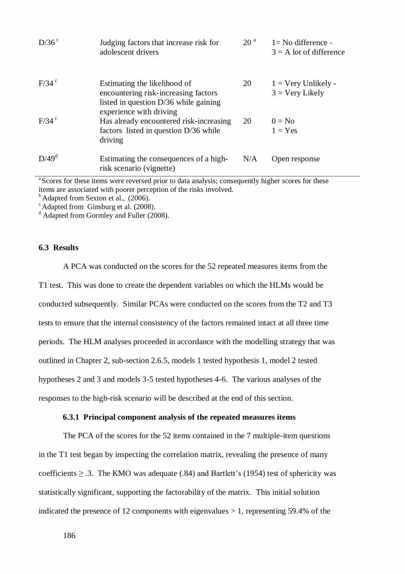
186
D/36 c Judging factors that increase risk for
adolescent drivers
20 a 1= No difference -
3 = A lot of difference
F/34 c Estimating the likelihood of
encountering risk-increasing factors
listed in question D/36 while gaining
experience with driving
20 1 = Very Unlikely -
3 = Very Likely
F/34 c
Has already encountered risk-increasing
factors listed in question D/36 while
driving
20 0 = No
1 = Yes
D/49d Estimating the consequences of a high-
risk scenario (vignette)
N/A Open response
a Scores for these items were reversed prior to data analysis; consequently higher scores for these
items are associated with poorer perception of the risks involved. b Adapted from Sexton et al.,
(2006).
c Adapted from Ginsburg et al. (2008).
d Adapted from Gormley and Fuller (2008).
6.3 Results
A PCA was conducted on the scores for the 52 repeated measures items from the
T1 test. This was done to create the dependent variables on which the HLMs would be
conducted subsequently. Similar PCAs were conducted on the scores from the T2 and T3
tests to ensure that the internal consistency of the factors remained intact at all three time
periods. The HLM analyses proceeded in accordance with the modelling strategy that was
outlined in Chapter 2, sub-section 2.6.5, models 1 tested hypothesis 1, model 2 tested
hypotheses 2 and 3 and models 3-5 tested hypotheses 4-6. The various analyses of the
responses to the high-risk scenario will be described at the end of this section.
6.3.1 Principal component analysis of the repeated measures items
The PCA of the scores for the 52 items contained in the 7 multiple-item questions
in the T1 test began by inspecting the correlation matrix, revealing the presence of many
coefficients ≥ .3. The KMO was adequate (.84) and Bartlett’s (1954) test of sphericity was
statistically significant, supporting the factorability of the matrix. This initial solution
indicated the presence of 12 components with eigenvalues > 1, representing 59.4% of the
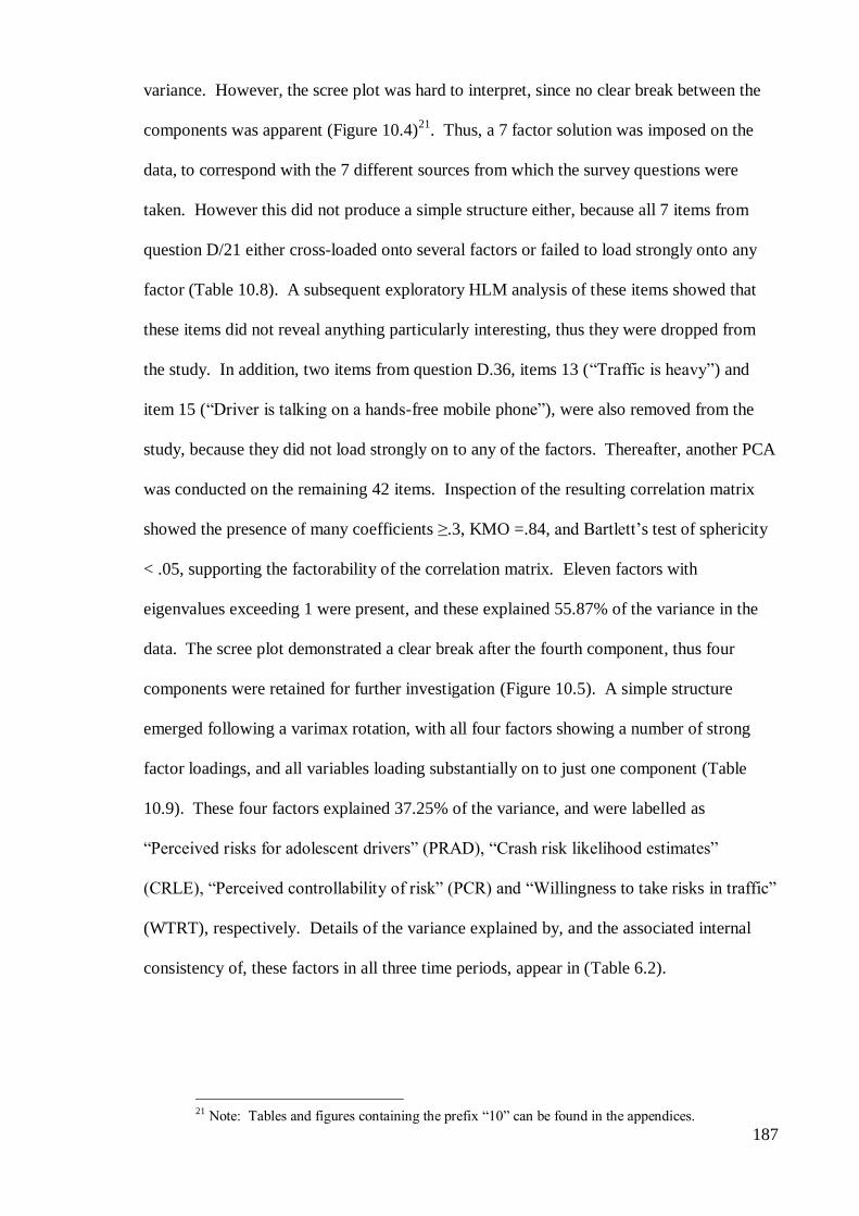
187
variance. However, the scree plot was hard to interpret, since no clear break between the
components was apparent (Figure 10.4)21
. Thus, a 7 factor solution was imposed on the
data, to correspond with the 7 different sources from which the survey questions were
taken. However this did not produce a simple structure either, because all 7 items from
question D/21 either cross-loaded onto several factors or failed to load strongly onto any
factor (Table 10.8). A subsequent exploratory HLM analysis of these items showed that
these items did not reveal anything particularly interesting, thus they were dropped from
the study. In addition, two items from question D.36, items 13 (“Traffic is heavy”) and
item 15 (“Driver is talking on a hands-free mobile phone”), were also removed from the
study, because they did not load strongly on to any of the factors. Thereafter, another PCA
was conducted on the remaining 42 items. Inspection of the resulting correlation matrix
showed the presence of many coefficients ≥.3, KMO =.84, and Bartlett’s test of sphericity
< .05, supporting the factorability of the correlation matrix. Eleven factors with
eigenvalues exceeding 1 were present, and these explained 55.87% of the variance in the
data. The scree plot demonstrated a clear break after the fourth component, thus four
components were retained for further investigation (Figure 10.5). A simple structure
emerged following a varimax rotation, with all four factors showing a number of strong
factor loadings, and all variables loading substantially on to just one component (Table
10.9). These four factors explained 37.25% of the variance, and were labelled as
“Perceived risks for adolescent drivers” (PRAD), “Crash risk likelihood estimates”
(CRLE), “Perceived controllability of risk” (PCR) and “Willingness to take risks in traffic”
(WTRT), respectively. Details of the variance explained by, and the associated internal
consistency of, these factors in all three time periods, appear in (Table 6.2).
21 Note: Tables and figures containing the prefix “10” can be found in the appendices.
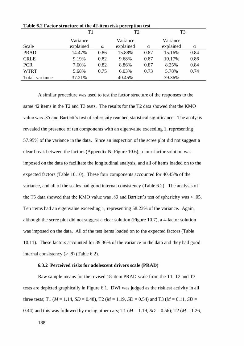
188
Table 6.2 Factor structure of the 42-item risk perception test
Scale
T1 T2 T3
Variance
explained α
Variance
explained α
Variance
explained α
PRAD 14.47% 0.86 15.88% 0.87 15.16% 0.84
CRLE 9.19% 0.82 9.68% 0.87 10.17% 0.86
PCR 7.60% 0.82 8.86% 0.87 8.25% 0.84
WTRT 5.68% 0.75 6.03% 0.73 5.78% 0.74
Total variance 37.21%
40.45%
39.36%
A similar procedure was used to test the factor structure of the responses to the
same 42 items in the T2 and T3 tests. The results for the T2 data showed that the KMO
value was .85 and Bartlett’s test of sphericity reached statistical significance. The analysis
revealed the presence of ten components with an eigenvalue exceeding 1, representing
57.95% of the variance in the data. Since an inspection of the scree plot did not suggest a
clear break between the factors (Appendix N, Figure 10.6), a four-factor solution was
imposed on the data to facilitate the longitudinal analysis, and all of items loaded on to the
expected factors (Table 10.10). These four components accounted for 40.45% of the
variance, and all of the scales had good internal consistency (Table 6.2). The analysis of
the T3 data showed that the KMO value was .83 and Bartlett’s test of sphericity was < .05.
Ten items had an eigenvalue exceeding 1, representing 58.23% of the variance. Again,
although the scree plot did not suggest a clear solution (Figure 10.7), a 4-factor solution
was imposed on the data. All of the test items loaded on to the expected factors (Table
10.11). These factors accounted for 39.36% of the variance in the data and they had good
internal consistency (> .8) (Table 6.2).
6.3.2 Perceived risks for adolescent drivers scale (PRAD)
Raw sample means for the revised 18-item PRAD scale from the T1, T2 and T3
tests are depicted graphically in Figure 6.1. DWI was judged as the riskiest activity in all
three tests; T1 (M = 1.14, SD = 0.48), T2 (M = 1.19, SD = 0.54) and T3 (M = 0.11, SD =
0.44) and this was followed by racing other cars; T1 (M = 1.19, SD = 0.56); T2 (M = 1.26,

189
SD = 0.65); T3 (M = 1.17, SD = 0.53). Driving in the dark was judged as the least risky
activity in the three tests; T1 (M = 2.27, SD = 0.94), T2 (M = 2.12, SD = 0.88), T3 (M =
2.22, SD = 0.95). This was followed by carrying teenage passengers; T1 (M = 2.07, SD =
0.97), T2 (M = 1.76, SD = 0.82), T3 (M = 1.83, SD = 0.8). The means for driver
inexperience at T1 (M = 21.39, SD = 0.55), T2 (M = 1.46, SD = 0.57), T3 (M = 1.38, SD =
0.53) placed this factor in 7th
place in terms of riskiness.
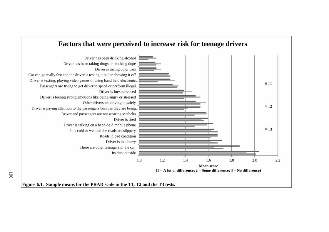
190
Figure 6.1. Sample means for the PRAD scale in the T1, T2 and the T3 tests.
1.0 1.2 1.4 1.6 1.8 2.0 2.2
Its dark outside
There are other teenagers in the car
Driver is in a hurry
Roads in bad condition
It is cold or wet and the roads are slippery
Driver is talking on a hand-held mobile phone
Driver is tired
Driver and passengers are not wearing seatbelts
Driver is paying attention to the passengers because they are being…
Other drivers are driving unsafely
Driver is feeling strong emotions like being angry or stressed
Driver is inexperienced
Passengers are trying to get driver to speed or perform illegal…
Driver is texting, playing video games or using hand held electronic…
Car can go really fast and the driver is testing it out or showing it off
Driver is racing other cars
Driver has been taking drugs or smoking dope
Driver has been drinking alcohol
Mean score
(1 = A lot of difference; 2 = Some difference; 3 = No difference)
Factors that were perceived to increase risk for teenage drivers
T1
T2
T3
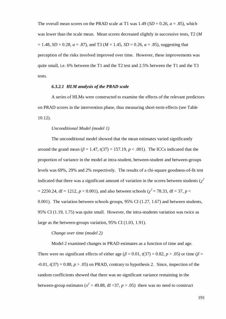
191
The overall mean scores on the PRAD scale at T1 was 1.49 (SD = 0.26, a = .85), which
was lower than the scale mean. Mean scores decreased slightly in successive tests, T2 (M
= 1.48, SD = 0.28, a = .87), and T3 (M = 1.45, SD = 0.26, a = .85), suggesting that
perception of the risks involved improved over time. However, these improvements was
quite small, i.e. 6% between the T1 and the T2 test and 2.5% between the T1 and the T3
tests.
6.3.2.1 HLM analysis of the PRAD scale
A series of HLMs were constructed to examine the effects of the relevant predictors
on PRAD scores in the intervention phase, thus measuring short-term effects (see Table
10.12).
Unconditional Model (model 1)
The unconditional model showed that the mean estimates varied significantly
around the grand mean (β = 1.47, t(37) = 157.19, p < .001). The ICCs indicated that the
proportion of variance in the model at intra-student, between-student and between-groups
levels was 69%, 29% and 2% respectively. The results of a chi-square goodness-of-fit test
indicated that there was a significant amount of variation in the scores between students (χ2
= 2250.24, df = 1212, p < 0.001), and also between schools (χ2 = 78.33, df = 37, p <
0.001). The variation between schools groups, 95% CI (1.27, 1.67) and between students,
95% CI (1.19, 1.75) was quite small. However, the intra-students variation was twice as
large as the between-groups variation, 95% CI (1.03, 1.91).
Change over time (model 2)
Model 2 examined changes in PRAD estimates as a function of time and age.
There were no significant effects of either age (β = 0.01, t(37) = 0.82, p > .05) or time (β =
-0.01, t(37) = 0.88, p > .05) on PRAD, contrary to hypothesis 2. Since, inspection of the
random coefficients showed that there was no significant variance remaining in the
between-group estimates (x2 = 49.88, df =37, p > .05) there was no need to construct
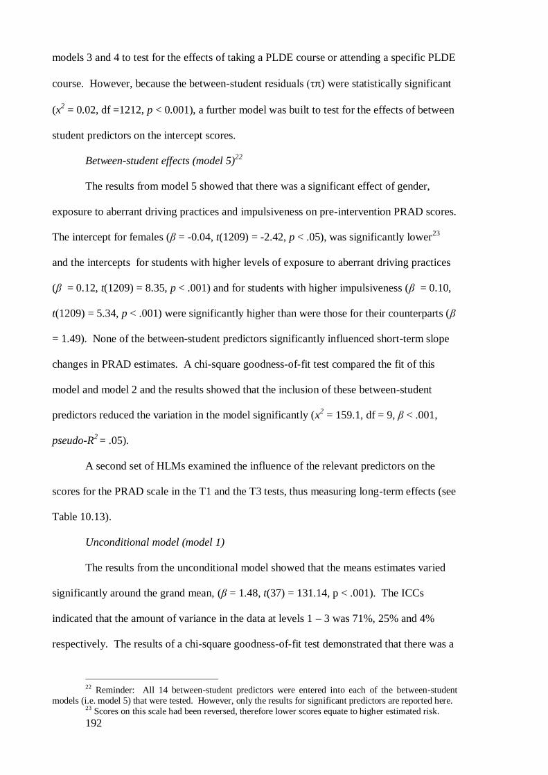
192
models 3 and 4 to test for the effects of taking a PLDE course or attending a specific PLDE
course. However, because the between-student residuals (τπ) were statistically significant
(x2 = 0.02, df =1212, p < 0.001), a further model was built to test for the effects of between
student predictors on the intercept scores.
Between-student effects (model 5)22
The results from model 5 showed that there was a significant effect of gender,
exposure to aberrant driving practices and impulsiveness on pre-intervention PRAD scores.
The intercept for females (β = -0.04, t(1209) = -2.42, p < .05), was significantly lower23
and the intercepts for students with higher levels of exposure to aberrant driving practices
(β = 0.12, t(1209) = 8.35, p < .001) and for students with higher impulsiveness (β = 0.10,
t(1209) = 5.34, p < .001) were significantly higher than were those for their counterparts (β
= 1.49). None of the between-student predictors significantly influenced short-term slope
changes in PRAD estimates. A chi-square goodness-of-fit test compared the fit of this
model and model 2 and the results showed that the inclusion of these between-student
predictors reduced the variation in the model significantly (x2 = 159.1, df = 9, β < .001,
pseudo-R2 = .05).
A second set of HLMs examined the influence of the relevant predictors on the
scores for the PRAD scale in the T1 and the T3 tests, thus measuring long-term effects (see
Table 10.13).
Unconditional model (model 1)
The results from the unconditional model showed that the means estimates varied
significantly around the grand mean, (β = 1.48, t(37) = 131.14, p < .001). The ICCs
indicated that the amount of variance in the data at levels 1 – 3 was 71%, 25% and 4%
respectively. The results of a chi-square goodness-of-fit test demonstrated that there was a
22 Reminder: All 14 between-student predictors were entered into each of the between-student
models (i.e. model 5) that were tested. However, only the results for significant predictors are reported here. 23 Scores on this scale had been reversed, therefore lower scores equate to higher estimated risk.
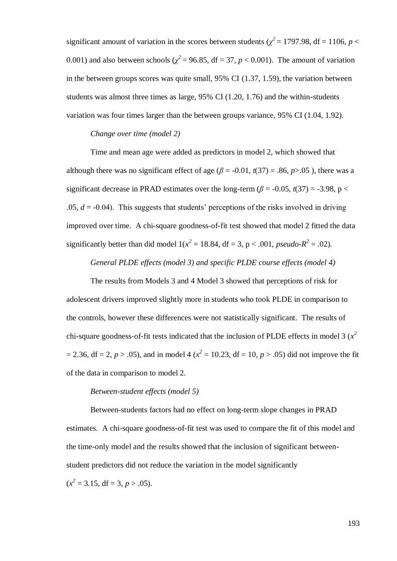
193
significant amount of variation in the scores between students (χ2 = 1797.98, df = 1106, p <
0.001) and also between schools (χ2 = 96.85, df = 37, p < 0.001). The amount of variation
in the between groups scores was quite small, 95% CI (1.37, 1.59), the variation between
students was almost three times as large, 95% CI (1.20, 1.76) and the within-students
variation was four times larger than the between groups variance, 95% CI (1.04, 1.92).
Change over time (model 2)
Time and mean age were added as predictors in model 2, which showed that
although there was no significant effect of age (β = -0.01, t(37) = .86, p>.05 ), there was a
significant decrease in PRAD estimates over the long-term (β = -0.05, t(37) = -3.98, p <
.05, d = -0.04). This suggests that students’ perceptions of the risks involved in driving
improved over time. A chi-square goodness-of-fit test showed that model 2 fitted the data
significantly better than did model 1(x2 = 18.84, df = 3, p < .001, pseudo-R
2 = .02).
General PLDE effects (model 3) and specific PLDE course effects (model 4)
The results from Models 3 and 4 Model 3 showed that perceptions of risk for
adolescent drivers improved slightly more in students who took PLDE in comparison to
the controls, however these differences were not statistically significant. The results of
chi-square goodness-of-fit tests indicated that the inclusion of PLDE effects in model 3 (x2
= 2.36, df = 2, p > .05), and in model 4 (x2 = 10.23, df = 10, p > .05) did not improve the fit
of the data in comparison to model 2.
Between-student effects (model 5)
Between-students factors had no effect on long-term slope changes in PRAD
estimates. A chi-square goodness-of-fit test was used to compare the fit of this model and
the time-only model and the results showed that the inclusion of significant between-
student predictors did not reduce the variation in the model significantly
(x2 = 3.15, df = 3, p > .05).
194
6.3.3 Likelihood of encountering risk-increasing factors while gaining
experience with driving
Since it was estimated that many of the students in this sample would be learning to
drive by the time that the T3 test was conducted, as part of that test, participants were
asked to estimate the likelihood that they would engage in any of the 18 risk-increasing
activities mentioned above while they were gaining driving experience (see question F/34).
Raw sample means for the scale items are graphed in Figure 6.2 which shows that the
likelihood estimates mainly accorded with the seriousness of the risks involved. Students
predicted that they were least likely to drink alcohol (M = 1.24, SD = 0.71), take drugs (M
= 1.3, SD = 0.77), or race other cars (M = 1.35, SD – 0.78) while they were driving.
Students estimated that they were most likely to drive in the dark (M = 2.23, SD = 0.86),
carry teenage passengers (M = 2.21, SD = 0.88), and to drive on poor quality roads (M =
2.16, SD = 0.89). Somewhat surprisingly, given the question wording, the survey item
“The driver is inexperienced” was judged in 7th
position in terms of likelihood, based on
the sample means. The overall mean for this scale was 1.76 (SD= 0.49) and the internal
consistency was good (a = .89). HLM analyses showed that although the likelihood
estimates were higher for the control group than for the active PLDE groups, these
differences were not statistically significant (Table 10.14). There were no significant
effects of any of the relevant between-student predictors on the likelihood estimates
Question F/34 also included a box that the students could tick if they had already
experience that range of risk increasing factors while they were driving. However, not
enough students responded to this section of the question to permit any meaningful
analyses to be conducted on this data.
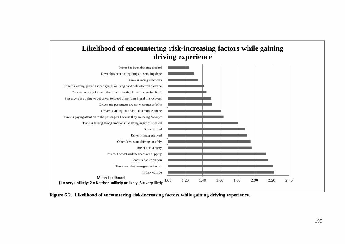
195
Figure 6.2. Likelihood of encountering risk-increasing factors while gaining driving experience.
1.00 1.20 1.40 1.60 1.80 2.00 2.20 2.40
Its dark outside
There are other teenagers in the car
Roads in bad condition
It is cold or wet and the roads are slippery
Driver is in a hurry
Other drivers are driving unsafely
Driver is inexperienced
Driver is tired
Driver is feeling strong emotions like being angry or stressed
Driver is paying attention to the passengers because they are being "rowdy"
Driver is talking on a hand-held mobile phone
Driver and passengers are not wearing seatbelts
Passengers are trying to get driver to speed or perform illegal manoeuvers
Car can go really fast and the driver is testing it out or showing it off
Driver is texting, playing video games or using hand held electronic device
Driver is racing other cars
Driver has been taking drugs or smoking dope
Driver has been drinking alcohol
Mean likelihood (1 = very unlikely; 2 = Neither unlikely or likely; 3 = very likely
Likelihood of encountering risk-increasing factors while gaining
driving experience
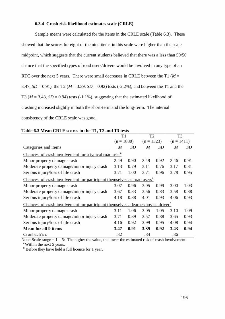
196
6.3.4 Crash risk likelihood estimates scale (CRLE)
Sample means were calculated for the items in the CRLE scale (Table 6.3). These
showed that the scores for eight of the nine items in this scale were higher than the scale
midpoint, which suggests that the current students believed that there was a less than 50/50
chance that the specified types of road users/drivers would be involved in any type of an
RTC over the next 5 years. There were small decreases in CRLE between the T1 (M =
3.47, SD = 0.91), the T2 (M = 3.39, SD = 0.92) tests (-2.2%), and between the T1 and the
T3 (M = 3.43, SD = 0.94) tests (-1.1%), suggesting that the estimated likelihood of
crashing increased slightly in both the short-term and the long-term. The internal
consistency of the CRLE scale was good.
Table 6.3 Mean CRLE scores in the T1, T2 and T3 tests
T1
(n = 1880)
T2
(n = 1323)
T3
(n = 1411)
Categories and items M SD M SD M SD
Chances of crash involvement for a typical road usera
Minor property damage crash 2.49 0.90 2.49 0.92 2.46 0.91
Moderate property damage/minor injury crash 3.13 0.79 3.11 0.76 3.17 0.81
Serious injury/loss of life crash 3.71 1.00 3.71 0.96 3.78 0.95
Chances of crash involvement for participant themselves as road usersa
Minor property damage crash 3.07 0.96 3.05 0.99 3.00 1.03
Moderate property damage/minor injury crash 3.67 0.83 3.56 0.83 3.58 0.88
Serious injury/loss of life crash 4.18 0.88 4.01 0.93 4.06 0.93
Chances of crash involvement for participant themselves a learner/novice driverb
Minor property damage crash 3.11 1.06 3.05 1.05 3.10 1.09
Moderate property damage/minor injury crash 3.71 0.89 3.57 0.88 3.65 0.93
Serious injury/loss of life crash 4.16 0.92 3.99 0.95 4.08 0.94
Mean for all 9 items 3.47 0.91 3.39 0.92 3.43 0.94
Cronbach’s a .82
.84
.86
Note: Scale range = 1 – 5: The higher the value, the lower the estimated risk of crash involvement. a Within the next 5 years.
b Before they have held a full licence for 1 year.
197
6.3.4.1 HLM analyses of the CRLE scale
A series of HLMs were constructed to examine the influence of the relevant
predictors on the CRLE scale estimates in the intervention phase (Table 10.15).
Unconditional Model (model 1)
The unconditional model demonstrated that the mean estimates varied significantly
around the grand mean (b = 3.44, t(37) = 164.47, p < .001). The ICCs indicated that the
variation in the data at levels 1 – 3 was 67%, 31% and 2% respectively. The results of chi-
square goodness-of-fit tests indicated that there was a significant amount of variation in the
scores between students (χ2 = 2250.05, df = 1212, p < 0.001) and also between schools (χ
2
= 74.08, df = 37, p < 0.001). There was a small amount of variation in the between-groups
scores, 95% CI (3.24, 3.64), and the between students variance was three times larger, 95%
CI (2.82, 4.06). The within-students variation was five times larger than the between-
groups variance, 95% CI (2.44, 4.44).
Change over time (model 2)
When time and mean age were included as predictors, the results showed that
although there was no significant effect of age, there was a small, significant decrease in
CRLE values between the T1 (β = 3.46), and the T2 (β = -0.06, t(37) = -3.05, p < .05, d = -
0.07) tests. The results of a chi-square goodness-of-fit test indicated that accounting for
time and mean age in model 2 improved the fit of the data significantly (x2 = 9.91, df = 3, p
< 0.05, pseudo-R2 = .01).
General PLDE effects (model 3) and specific PLDE course effects (model 4)
The results from models 3 and 4 showed that the slopes for students who took
PLDE decreased more than did those for the control group however this effect was not
statistically significant. A chi-square goodness-of-fit test indicated that the inclusion of
PLDE effects in model 3 (x2 = 2.49, df = 2, p > .05), and 4 (x
2 = 6.61, df = 10, p > .05) did
not improve the fit of the data in comparison to model 2.

198
Between-student effects (model 5)
Model 5 tested for the effects of between-student predictors. The results for the
trimmed model indicated that the males (β = 3.52) perceived the likelihood of crashing as
lower than did the females (β = -.14, t(37) = -3.09, p < .01) in the T1 test. However, there
was no significant difference between decreases in CRLE for the males (β = -0.06, t(37) = -
1.93, p > 0.05) and for the females (β = -0.01, t(37) = -0.42, p > .05 ) in the intervention
phase. Whereas the chi-square statistic indicated that this model provided a better fit for
the data than did model 2 (x2 = 14.42, df = 2, p < .001, pseudo- R
2= .01), the amount of
variance accounted for by gender was very small.
Another series of HLMs were constructed to examine the influence of the relevant
predictors on the coefficients produced by comparing the initial and final scores on the
CRLE scale, thus testing long-term effects (Table 10.16).
Unconditional model (model 1)
The unconditional model showed that mean CRLE varied significantly around the
grand mean, (β = 3.46, t(37) = 155.92, p < .001). The ICC estimates showed the amount of
variance in the data at levels 1 – 3 was 70%, 28% and 2% respectively. A chi-square
goodness-of-fit test indicated that there was a significant amount of variation in the scores
between students (χ2
= 1935.69, df = 1106, p < 0.001) and also between schools (χ2 =
76.37, df = 37, p < 0.001). The amount of variation in the between groups scores was quite
small, 95% CI (3.26, 3.66), the variation between students was more than three times
larger, 95% CI (2.84, 4.08). The within-students variation was over four times larger than
the between groups variance, 95% CI (2.46, 4.46).
199
Change over time (model 2)
Model 2 demonstrates that there was no significant effect of time or of mean age on
slope changes in CRLE over the long-term. A chi-square goodness-of-fit test showed that
model 2 did not represented a significantly better fit for the data than did the unconditional
model (x2 = 4.78, df = 3, p > .05).
General PLDE effects (model 3) and specific PLDE course effects (model 4)
Models 3 and 4 demonstrated that there were no significant effects of exposure to
PLDE in general, or of attending specific PLDE courses on the long-term slope values for
CRLE. Chi-square goodness-of-fit tests showed that the inclusion of PLDE effects in
models 3 (x2 = 4.05, df = 2, p > .05), and 4 (x
2 = 12.37, df = 10, p > .05) did not improve
the fit of the data in comparison with model 2.
Between-student effects (model 5)
Model 5 tested for the effects of between-student predictors. The trimmed model
indicated that there were significant gender differences in long-term CRLE slope values.
Whereas the scores for the boys increased slightly (β = 0.02), those for the girls decreased
significantly more in the same period (β = -0.10, t(1067) = -2.33, p < .05). This model
represented a significantly better fit for the data than did model 2 (x2 = 139.34, df = 2, p <
.001, pseudo-R2 = .04).
6.3.5 Perceived controllability of risk scale (PCR)
Raw sample means for the items for the PCR scale appear in (Table 6.4). Since higher
scores on this scale signify stronger beliefs that crash risk is controllable as a function of
skill, these results suggest that the current students believed that skill plays a greater role in
avoiding crashing while speeding and a lesser role in avoiding crashing where capability is
impaired due to the influence of drugs, distraction or alcohol. The overall scale mean was
2.33 (SD = 0.87) at T1, and this decreased in T2 (M = 2.25, SD = 0.93), and then remained
stable in the T3 test (M = 2.25, SD = 0.83).
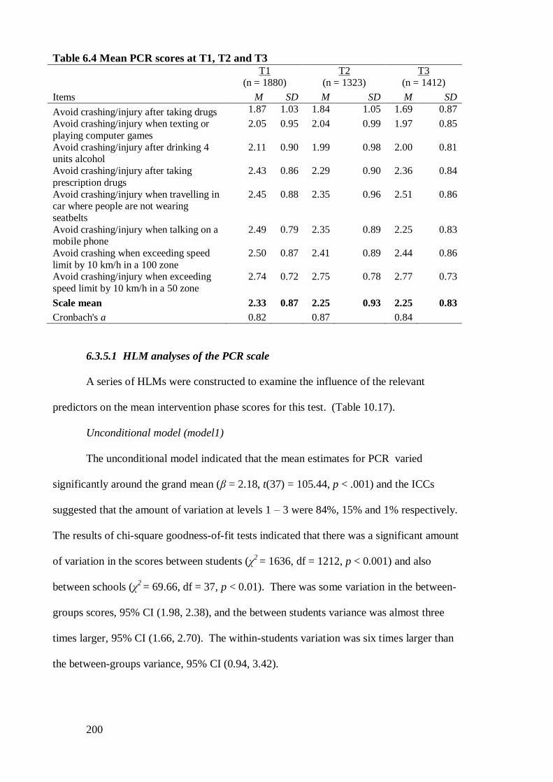
200
Table 6.4 Mean PCR scores at T1, T2 and T3
T1
(n = 1880) T2
(n = 1323) T3
(n = 1412)
Items M SD M SD M SD
Avoid crashing/injury after taking drugs 1.87 1.03 1.84 1.05 1.69 0.87
Avoid crashing/injury when texting or
playing computer games 2.05 0.95 2.04 0.99 1.97 0.85
Avoid crashing/injury after drinking 4 units alcohol
2.11 0.90 1.99 0.98 2.00 0.81
Avoid crashing/injury after taking
prescription drugs 2.43 0.86 2.29 0.90 2.36 0.84
Avoid crashing/injury when travelling in car where people are not wearing
seatbelts
2.45 0.88 2.35 0.96 2.51 0.86
Avoid crashing/injury when talking on a mobile phone
2.49 0.79 2.35 0.89 2.25 0.83
Avoid crashing when exceeding speed
limit by 10 km/h in a 100 zone 2.50 0.87 2.41 0.89 2.44 0.86
Avoid crashing/injury when exceeding
speed limit by 10 km/h in a 50 zone 2.74 0.72 2.75 0.78 2.77 0.73
Scale mean 2.33 0.87 2.25 0.93 2.25 0.83
Cronbach's a 0.82 0.87 0.84
6.3.5.1 HLM analyses of the PCR scale
A series of HLMs were constructed to examine the influence of the relevant
predictors on the mean intervention phase scores for this test. (Table 10.17).
Unconditional model (model1)
The unconditional model indicated that the mean estimates for PCR varied
significantly around the grand mean (β = 2.18, t(37) = 105.44, p < .001) and the ICCs
suggested that the amount of variation at levels 1 – 3 were 84%, 15% and 1% respectively.
The results of chi-square goodness-of-fit tests indicated that there was a significant amount
of variation in the scores between students (χ2
= 1636, df = 1212, p < 0.001) and also
between schools (χ2 = 69.66, df = 37, p < 0.01). There was some variation in the between-
groups scores, 95% CI (1.98, 2.38), and the between students variance was almost three
times larger, 95% CI (1.66, 2.70). The within-students variation was six times larger than
the between-groups variance, 95% CI (0.94, 3.42).
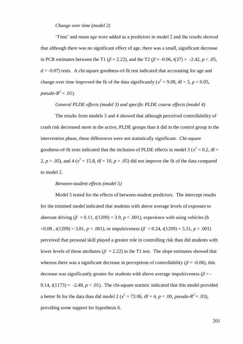
201
Change over time (model 2)
‘Time’ and mean age were added as a predictors in model 2 and the results showed
that although there was no significant effect of age, there was a small, significant decrease
in PCR estimates between the T1 (β = 2.22), and the T2 (β = -0.06, t(37) = -2.42, p < .05,
d = -0.07) tests. A chi-square goodness-of-fit test indicated that accounting for age and
change over time improved the fit of the data significantly (x2 = 9.08, df = 3, p < 0.05,
pseudo-R2 = .01).
General PLDE effects (model 3) and specific PLDE course effects (model 4)
The results from models 3 and 4 showed that although perceived controllability of
crash risk decreased more in the active, PLDE groups than it did in the control group in the
intervention phase, these differences were not statistically significant. Chi-square
goodness-of-fit tests indicated that the inclusion of PLDE effects in model 3 (x2 = 0.2, df =
2, p > .05), and 4 (x2 = 15.8, df = 10, p > .05) did not improve the fit of the data compared
to model 2.
Between-student effects (model 5)
Model 5 tested for the effects of between-student predictors. The intercept results
for the trimmed model indicated that students with above average levels of exposure to
aberrant driving (β = 0.11, t(1209) = 3.9, p < .001), experience with using vehicles (b
=0.08 , t(1209) = 3.81, p < .001), or impulsiveness (β = 0.24, t(1209) = 5.51, p < .001)
perceived that personal skill played a greater role in controlling risk than did students with
lower levels of those attributes (β = 2.22) in the T1 test. The slope estimates showed that
whereas there was a significant decrease in perceptions of controllability (β = -0.06), this
decrease was significantly greater for students with above average impulsiveness (β = -
0.14, t(1173) = -2.48, p < .01). The chi-square statistic indicated that this model provided
a better fit for the data than did model 2 (x2 = 73.06, df = 4, p < .00, pseudo-R
2 = .03),
providing some support for hypothesis 6.
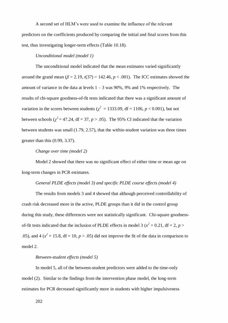
202
A second set of HLM’s were used to examine the influence of the relevant
predictors on the coefficients produced by comparing the initial and final scores from this
test, thus investigating longer-term effects (Table 10.18).
Unconditional model (model 1)
The unconditional model indicated that the mean estimates varied significantly
around the grand mean (β = 2.19, t(37) = 142.46, p < .001). The ICC estimates showed the
amount of variance in the data at levels 1 – 3 was 90%, 9% and 1% respectively. The
results of chi-square goodness-of-fit tests indicated that there was a significant amount of
variation in the scores between students (χ2
= 1333.09, df = 1106, p < 0.001), but not
between schools (χ2 = 47.24, df = 37, p > .05). The 95% CI indicated that the variation
between students was small (1.79, 2.57), that the within-student variation was three times
greater than this (0.99, 3.37).
Change over time (model 2)
Model 2 showed that there was no significant effect of either time or mean age on
long-term changes in PCR estimates.
General PLDE effects (model 3) and specific PLDE course effects (model 4)
The results from models 3 and 4 showed that although perceived controllability of
crash risk decreased more in the active, PLDE groups than it did in the control group
during this study, these differences were not statistically significant. Chi-square goodness-
of-fit tests indicated that the inclusion of PLDE effects in model 3 (x2 = 0.21, df = 2, p >
.05), and 4 (x2 = 15.8, df = 10, p > .05) did not improve the fit of the data in comparison to
model 2.
Between-student effects (model 5)
In model 5, all of the between-student predictors were added to the time-only
model (2). Similar to the findings from the intervention phase model, the long-term
estimates for PCR decreased significantly more in students with higher impulsiveness

203
(β = -0.15, t(1173) = -2.48, p < .05) than it did in the less impulsive counterparts.
Although this model represented a significantly better fit for the data than did model 2 (x2
= 73.06, df = 4, p < .001), the inclusion of significant between-student predictors in this
model did not produce a meaningful reduction in the variance in the data (R2 < .01).
6.3.6 Willingness to take risks in traffic scale (WTRT)
Raw sample means were calculated for the items on the WTRT scale (Table 6.5). These
indicated that students were most willing to cycle without a helmet and to refrain from
wearing a seatbelt in a school bus and least willing to take a lift with a driver who had been
drinking and to ride a motorcycle without a helmet, in each test. There was very little
change in the overall scale means between the T1 (M = 2.48, SD = 1.08), the T2 (M = 2.51,
SD = 1.06) and the T3 (M = 2.51, SD = 1.07). The internal consistency of the willingness
scale was adequate.
Table 6.5 Mean WTRT scores in the T1, T2 and T3 tests
T1
(n = 1880)
T2
(n = 1322)
T3
(n = 1412)
Items M SD M SD M SD
Willing to cycle without a helmet 3.92 1.13 3.80 1.10 3.90 1.10
Willing to refrain from wearing a seatbelt in a
school bus
3.27
1.23
3.31
1.19
3.34
1.23
Willing to cross a busy road from between
parked cars
2.93 1.17 2.98 1.14 3.07 1.19
Willing to take a lift with a driver who speeds 2.56 1.06 2.57 0.98 2.51 1.01
Willing to drive parents car without
permission 2.00 1.19 2.08 1.17 2.13 1.17
Willing to refrain from wearing seatbelt in car 1.88 1.05 1.96 1.07 1.90 1.07
Willing to ride motorcycle without a helmet 1.69 0.92 1.78 0.92 1.75
0.93
Willing to take a lift with a driver who has
been drinking
1.57
0.86
1.63
0.92
1.50
0.84
Scale Mean 2.48 1.08 2.51 1.06 2.51 1.07
Cronbach's alpha reliabilities 0.75 0.73 0.74
6.3.6.1 HLM analyses of the WTRT scale
A series of HLMs were constructed to examine the influence of the relevant predictors on
the intervention phase estimates for this test (Table 10.19).
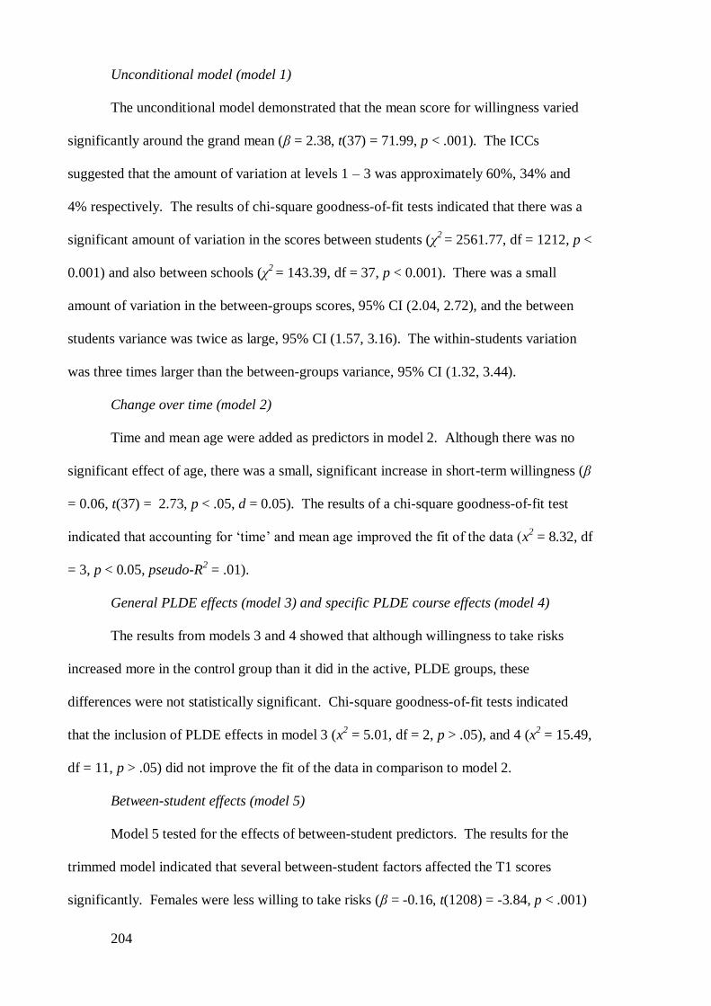
204
Unconditional model (model 1)
The unconditional model demonstrated that the mean score for willingness varied
significantly around the grand mean (β = 2.38, t(37) = 71.99, p < .001). The ICCs
suggested that the amount of variation at levels 1 – 3 was approximately 60%, 34% and
4% respectively. The results of chi-square goodness-of-fit tests indicated that there was a
significant amount of variation in the scores between students (χ2 = 2561.77, df = 1212, p <
0.001) and also between schools (χ2 = 143.39, df = 37, p < 0.001). There was a small
amount of variation in the between-groups scores, 95% CI (2.04, 2.72), and the between
students variance was twice as large, 95% CI (1.57, 3.16). The within-students variation
was three times larger than the between-groups variance, 95% CI (1.32, 3.44).
Change over time (model 2)
Time and mean age were added as predictors in model 2. Although there was no
significant effect of age, there was a small, significant increase in short-term willingness (β
= 0.06, t(37) = 2.73, p < .05, d = 0.05). The results of a chi-square goodness-of-fit test
indicated that accounting for ‘time’ and mean age improved the fit of the data (x2 = 8.32, df
= 3, p < 0.05, pseudo-R2 = .01).
General PLDE effects (model 3) and specific PLDE course effects (model 4)
The results from models 3 and 4 showed that although willingness to take risks
increased more in the control group than it did in the active, PLDE groups, these
differences were not statistically significant. Chi-square goodness-of-fit tests indicated
that the inclusion of PLDE effects in model 3 (x2 = 5.01, df = 2, p > .05), and 4 (x
2 = 15.49,
df = 11, p > .05) did not improve the fit of the data in comparison to model 2.
Between-student effects (model 5)
Model 5 tested for the effects of between-student predictors. The results for the
trimmed model indicated that several between-student factors affected the T1 scores
significantly. Females were less willing to take risks (β = -0.16, t(1208) = -3.84, p < .001)
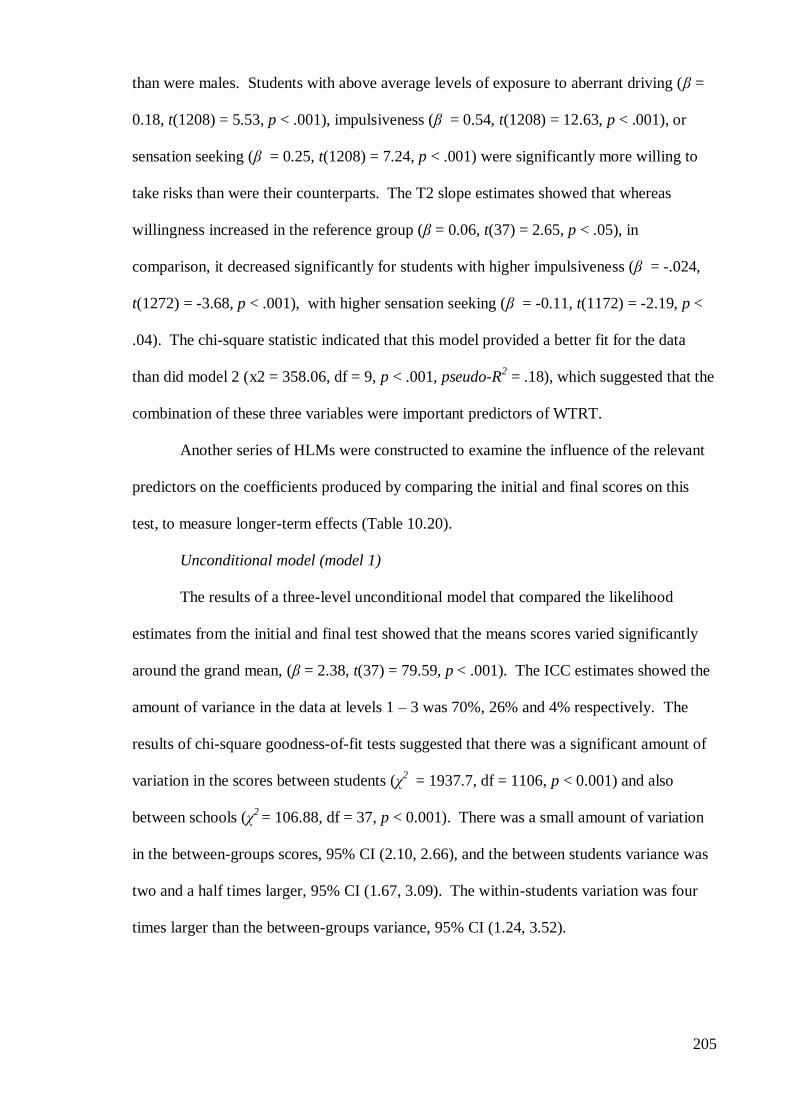
205
than were males. Students with above average levels of exposure to aberrant driving (β =
0.18, t(1208) = 5.53, p < .001), impulsiveness (β = 0.54, t(1208) = 12.63, p < .001), or
sensation seeking (β = 0.25, t(1208) = 7.24, p < .001) were significantly more willing to
take risks than were their counterparts. The T2 slope estimates showed that whereas
willingness increased in the reference group (β = 0.06, t(37) = 2.65, p < .05), in
comparison, it decreased significantly for students with higher impulsiveness (β = -.024,
t(1272) = -3.68, p < .001), with higher sensation seeking (β = -0.11, t(1172) = -2.19, p <
.04). The chi-square statistic indicated that this model provided a better fit for the data
than did model 2 (x2 = 358.06, df = 9, p < .001, pseudo-R2 = .18), which suggested that the
combination of these three variables were important predictors of WTRT.
Another series of HLMs were constructed to examine the influence of the relevant
predictors on the coefficients produced by comparing the initial and final scores on this
test, to measure longer-term effects (Table 10.20).
Unconditional model (model 1)
The results of a three-level unconditional model that compared the likelihood
estimates from the initial and final test showed that the means scores varied significantly
around the grand mean, (β = 2.38, t(37) = 79.59, p < .001). The ICC estimates showed the
amount of variance in the data at levels 1 – 3 was 70%, 26% and 4% respectively. The
results of chi-square goodness-of-fit tests suggested that there was a significant amount of
variation in the scores between students (χ2
= 1937.7, df = 1106, p < 0.001) and also
between schools (χ2 = 106.88, df = 37, p < 0.001). There was a small amount of variation
in the between-groups scores, 95% CI (2.10, 2.66), and the between students variance was
two and a half times larger, 95% CI (1.67, 3.09). The within-students variation was four
times larger than the between-groups variance, 95% CI (1.24, 3.52).
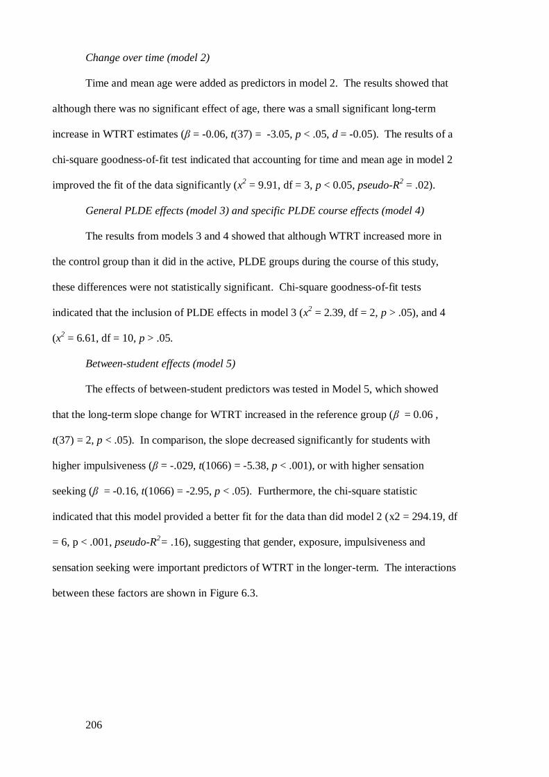
206
Change over time (model 2)
Time and mean age were added as predictors in model 2. The results showed that
although there was no significant effect of age, there was a small significant long-term
increase in WTRT estimates (β = -0.06, t(37) = -3.05, p < .05, d = -0.05). The results of a
chi-square goodness-of-fit test indicated that accounting for time and mean age in model 2
improved the fit of the data significantly (x2 = 9.91, df = 3, p < 0.05, pseudo-R
2 = .02).
General PLDE effects (model 3) and specific PLDE course effects (model 4)
The results from models 3 and 4 showed that although WTRT increased more in
the control group than it did in the active, PLDE groups during the course of this study,
these differences were not statistically significant. Chi-square goodness-of-fit tests
indicated that the inclusion of PLDE effects in model 3 (x2 = 2.39, df = 2, p > .05), and 4
(x2 = 6.61, df = 10, p > .05.
Between-student effects (model 5)
The effects of between-student predictors was tested in Model 5, which showed
that the long-term slope change for WTRT increased in the reference group (β = 0.06 ,
t(37) = 2, p < .05). In comparison, the slope decreased significantly for students with
higher impulsiveness (β = -.029, t(1066) = -5.38, p < .001), or with higher sensation
seeking (β = -0.16, t(1066) = -2.95, p < .05). Furthermore, the chi-square statistic
indicated that this model provided a better fit for the data than did model 2 (x2 = 294.19, df
= 6, p < .001, pseudo-R2= .16), suggesting that gender, exposure, impulsiveness and
sensation seeking were important predictors of WTRT in the longer-term. The interactions
between these factors are shown in Figure 6.3.
207
Figure 6.3. Interactions between significant between-student predictors of WTRT in
the T1, T2 and T3 tests.
Finally, it should be noted that although the available evidence suggested that it
was unlikely that there would be any significant interaction effects for between-student and
between-groups slope changes in the risk perception scale scores, additional models were
nonetheless constructed to test for such interactions. No significant interactions were
indeed found and these models are not presented due to pressure on space.
6.3.7 High-risk vignette
Mental representations of the consequences of high-risk driving-behaviour were
determined by eliciting responses to three almost identical vignettes. These described
scenarios which involved a range of factors which both individually and collectively
increase risk for adolescent drivers and passengers, and other road users i.e. age,
inexperience, speeding, late night driving and the presence of peers. Students were given
the following instructions at the start of each vignette:
2
2.2
2.4
2.6
2.8
3
T1 T2 T3
HL
M c
oeff
icie
nts
Test time
Willingness to take risks in traffic
Reference Group
Higher impulsiveness
Higher sensation seeking
Females
Exposure to aberrant driving

208
“We would like you to consider the situation described below and then answer the question as fully
and honestly as you possibly can. There is no need to worry about projecting a good image because
the answers you give in this survey are totally confidential.”
The T1 vignette:
“Mark is 17 years old and has had a learner permit to drive for 6 months. One Saturday night while
his parents were away he decided to use his dad's car to take some of the lads to a disco in a nearby
town. The disco finished at 2am and on their way home Mark decided to see how fast the car can
go.” (Appendix D, question 49).
The T2 vignette:
“James is 17 years old and has been learning to drive for the past 6 months. After the disco last
Friday night, James brought his mates back to his house because his parents were away. When they
got there they realized that their friend David had been left behind. James decided that they should
take his dad's car and go back to the disco to collect David. Since they were in a hurry he decided to
drive as fast as the car could go.” (Appendix E, question 33).
The T3 vignette:
“David is 17 years old and has been learning to drive for the past 6 months. One Friday night while
his parents were away he decided to use his dad's car to take some of the lads to football training and
afterwards they went to a disco. The disco finished at 2am and on their way home David drove as
fast as the car could go because it was so late.” (Appendix F, question 44).
The instructions provided at the end of each vignette were as follows: “What are
the possible consequences of this? Please write as many things as you can think of,
numbering them as you go along, starting with the number 1.”
The responses were analysed with respect to;
1. The types of consequences listed (testing availability)
2. The number of consequences listed (testing availability)
3. The rank order in which consequences were listed (testing accessibility)
4. The absence of important consequences (testing accessibility)
The first stage of data analysis involved the identification and categorisation of the
listed consequences. The responses provided by 25% of the T1 participants, which had
209
been selected at random, were coded independently by 3 experienced researchers from the
Department of Psychology, TCD. During this process, 12 categories of consequences were
identified and an inter-rater reliability analysis showed that there was good consistency in
agreement between the researchers regarding these categories (Kappa = .73 (p <.001) 95%
CI (.57, .89)). Responses from all three tests were then collapsed into these categories,
while simultaneously preserving the order in which items had been listed. The number of
consequences listed by each student was ascertained by re-coding the responses in these
categories into 12 new binary variables i.e. 0 = not listed, 1 = listed.
6.3.8 Results for vignettes
6.3.8.1 Availability of consequences
A summary of the responses from each test is provided in (Table 6.6) which shows that
serious outcomes, including ‘crashing’, ‘death’ and’ injury’ were cited most frequently in
each test. These were followed in terms of availability by consequences such as being
‘caught by the Gardaí’, ‘damage to cars/property’, and losing control of the car. Although
over 21% of the students listed ‘legal problems’ (e.g. getting penalty points, going to court,
being jailed) as a possible consequence in the T1 test, this figure dropped markedly over
time to 13.9% at T2 and to 3.2% at T3. Listings of ‘trouble with parents’ and ‘increased
risk/danger’ were quite stable across the tests. Between 10% and 12% of students
suggested that there might be no consequences as a result of the high-risk behaviour
described in the vignettes. However, it should be noted that this outcome was rarely listed
as the sole reaction to the vignette. A numbers of students mentioned beneficial
consequences e.g. “They'll get home faster” the driver “could show off his driving skills
and drive safely home”; “...the girls will be impressed....” Here again, very few students
listed only beneficial consequences. Just a small number of students listed social/moral
consequences, e.g. “They will crash and the passengers will be injured or killed and he
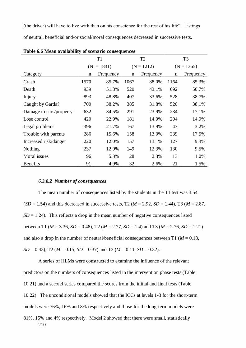
210
(the driver) will have to live with than on his conscience for the rest of his life”. Listings
of neutral, beneficial and/or social/moral consequences decreased in successive tests.
Table 6.6 Mean availability of scenario consequences
T1 T2 T3
(N = 1831) (N = 1212) (N = 1365)
Category n Frequency n Frequency n Frequency
Crash 1570 85.7% 1067 88.0% 1164 85.3%
Death 939 51.3% 520 43.1% 692 50.7%
Injury 893 48.8% 407 33.6% 528 38.7%
Caught by Gardaí 700 38.2% 385 31.8% 520 38.1%
Damage to cars/property 632 34.5% 291 23.9% 234 17.1%
Lose control 420 22.9% 181 14.9% 204 14.9%
Legal problems 396 21.7% 167 13.9% 43 3.2%
Trouble with parents 286 15.6% 158 13.0% 239 17.5%
Increased risk/danger 220 12.0% 157 13.1% 127 9.3%
Nothing 237 12.9% 149 12.3% 130 9.5%
Moral issues 96 5.3% 28 2.3% 13 1.0%
Benefits 91 4.9% 32 2.6% 21 1.5%
6.3.8.2 Number of consequences
The mean number of consequences listed by the students in the T1 test was 3.54
(SD = 1.54) and this decreased in successive tests, T2 (M = 2.92, SD = 1.44), T3 (M = 2.87,
SD = 1.24). This reflects a drop in the mean number of negative consequences listed
between T1 (M = 3.36, SD = 0.48), T2 (M = 2.77, SD = 1.4) and T3 (M = 2.76, SD = 1.21)
and also a drop in the number of neutral/beneficial consequences between T1 (M = 0.18,
SD = 0.43), T2 (M = 0.15, SD = 0.37) and T3 (M = 0.11, SD = 0.32).
A series of HLMs were constructed to examine the influence of the relevant
predictors on the numbers of consequences listed in the intervention phase tests (Table
10.21) and a second series compared the scores from the initial and final tests (Table
10.22). The unconditional models showed that the ICCs at levels 1-3 for the short-term
models were 76%, 16% and 8% respectively and those for the long-term models were
81%, 15% and 4% respectively. Model 2 showed that there were small, statistically
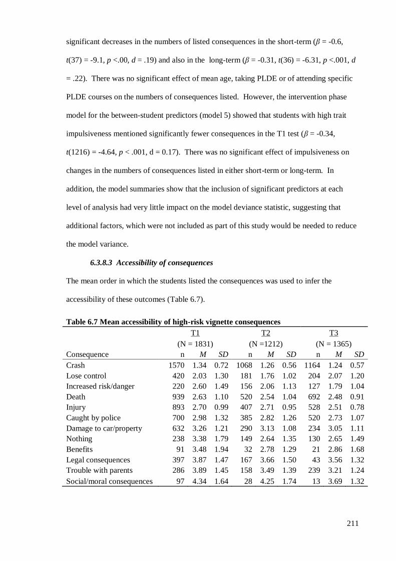
211
significant decreases in the numbers of listed consequences in the short-term (β = -0.6,
t(37) = -9.1, p <.00, d = .19) and also in the long-term (β = -0.31, t(36) = -6.31, p <.001, d
= .22). There was no significant effect of mean age, taking PLDE or of attending specific
PLDE courses on the numbers of consequences listed. However, the intervention phase
model for the between-student predictors (model 5) showed that students with high trait
impulsiveness mentioned significantly fewer consequences in the T1 test (β = -0.34,
t(1216) = -4.64, p < .001, d = 0.17). There was no significant effect of impulsiveness on
changes in the numbers of consequences listed in either short-term or long-term. In
addition, the model summaries show that the inclusion of significant predictors at each
level of analysis had very little impact on the model deviance statistic, suggesting that
additional factors, which were not included as part of this study would be needed to reduce
the model variance.
6.3.8.3 Accessibility of consequences
The mean order in which the students listed the consequences was used to infer the
accessibility of these outcomes (Table 6.7).
Table 6.7 Mean accessibility of high-risk vignette consequences
T1 T2 T3
(N = 1831) (N =1212) (N = 1365)
Consequence n M SD n M SD n M SD
Crash 1570 1.34 0.72 1068 1.26 0.56 1164 1.24 0.57
Lose control 420 2.03 1.30 181 1.76 1.02 204 2.07 1.20
Increased risk/danger 220 2.60 1.49 156 2.06 1.13 127 1.79 1.04
Death 939 2.63 1.10 520 2.54 1.04 692 2.48 0.91
Injury 893 2.70 0.99 407 2.71 0.95 528 2.51 0.78
Caught by police 700 2.98 1.32 385 2.82 1.26 520 2.73 1.07
Damage to car/property 632 3.26 1.21 290 3.13 1.08 234 3.05 1.11
Nothing 238 3.38 1.79 149 2.64 1.35 130 2.65 1.49
Benefits 91 3.48 1.94 32 2.78 1.29 21 2.86 1.68
Legal consequences 397 3.87 1.47 167 3.66 1.50 43 3.56 1.32
Trouble with parents 286 3.89 1.45 158 3.49 1.39 239 3.21 1.24
Social/moral consequences 97 4.34 1.64 28 4.25 1.74 13 3.69 1.32
212
On average, the first consequence that sprang to mind in the current sample in each test
was ‘crashing’; T1 (M = 1.34, SD = 0.72), T2 (M = 1.26, SD = 0.56), T3 (M = 1.24, SD =
0.57). This was followed by non-specific consequences such as ‘losing control’ and
‘increased risk and danger’. Next, came serious consequences, including ‘death’ and’
injury’, and these were followed by ‘getting caught by the police’ and ‘damaging cars or
property’. Next came neutral and beneficial consequences, and these were followed by
legal consequences, getting into trouble with parents and finally social or moral
consequences.
A series of hierarchical linear Poisson distribution models with a log-link function
(Raudenbush & Bryk, 2002) were used to analyse differences in the accessibility of the
three most serious types of consequences, i.e. crash, death, injury. In the Poisson model,
the event rate ratio is the exponential of a coefficient (exp(b), which is a measure of
relative effect size, because it can be interpreted as the percentage change in the dependent
variable associated with an increase of 1 unit in the independent variable, holding other
factors constant (Raudenbush & Bryk, 2002). In the present analyses the exp(b) represents
the relative position in which a consequence was listed. All models were corrected for
over-dispersion of the level-1 variances as recommended by Raudenbush and Bryk (2002).
6.3.8.4 Accessibility of “crashing” as a consequence
Table 10.23 contains the intervention phase results for the accessibility of
‘crashing’. The unconditional model indicated that there was a significant amount of
variance in the log-rate of accessibility between the T1 and the T2 tests (β = 0.25, t(36)
=18.58, p < .001). Model 2 showed that there was a significant increase in accessibility
between T1 (β = 0.28, t(36) = 15.1, p < .001, exp(b) = 1.32) and T2 (β = -0.6, t(36) = -
2.31 , p < .05, exp(b) = 0.94), i.e. crashing was listed 6% sooner in the second test. Model
3 investigated the influence of taking a PLDE course on accessibility and the slope results
showed that students who took PLDE mentioned crashing 12% sooner (β = -0.13, t(36)
213
= -2.20, p < .05, exp(b) = 0.88), than did those in the control group. Model 4 showed that
whereas there was a slight decrease in accessibility in the controls between the T1 and the
T2 tests (β = 0.06, t(31), = 0.99, p > .05, exp(b) = 1.06), there was an increase in
accessibility in all of the PLDE groups. Furthermore, this increase was statistically
significant in the case of groups B (β = -0.18, t(32), = -2.28 , p < .05, exp(b) = 0.84), and C
(β = -0.18, t(31), = -2.23, p < .05, exp(b) = 0.83). This indicated that crashing was
mentioned between 16% and 17% sooner by students in groups B and C respectively than
it was by those in the control group. There were no significant effects of between-student
predictors on crash accessibility.
Long-term changes in the accessibility of crashing as an outcome were tested using
the scores from the T1 and the T3 tests (see Table 10.24). The unconditional model
indicated that there was a significant amount of variance in the log-rate of immediacy
between the two tests, (β = 0.24, t(36) =9.72, p < .001). Model 2 showed that there was a
significant increase in accessibility between T1 (β = 0.28, t(36) = 8.85, p < .001, exp(b) =
1.33) and T2 (β = -0.4, t(36) = -2.04 , p < .05, exp(b) = 0.95), indicating that crashing was
listed 5% sooner in the second test. However, the results from models 3 and 4 and an
additional model that tested for the effects of between-student variables showed that none
of these predictors influenced the accessibility of crashing as a consequence of the high-
risk vignettes in the long-term.
6.3.8.5 Accessibility of ‘death’ as a consequence
The accessibility of ‘death’ as a consequence was tested by comparing the T1 and
T2 scores in a series of models (see Table 10.25). The unconditional model showed that
there was a significant amount of variance in accessibility β = 0.88, t(36), = 47.21, p <
.001, exp(b) = 2.43). However, models 2 and 3 showed that there were no significant
effects of either time, or of taking PLDE on differences in accessibility. Model 4, which
was used to compare estimates for the control group and those for students who attended
214
specific PLDE courses indicated that whereas accessibility decreased in the control group
between the T1 and the T2 tests (β = 0.07, t(31), = 0.84, p > .05, exp(b) = 1.07), it
increased in each of the PLDE groups. However, this difference was only significant with
respect to groups A (β = -0.27, t(31), = -2.17, p < .05, exp(b) = 0.76) and C (β = -0.19,
t(31), = -2.04, p < .05, exp(b) = 0.81). This indicates that students in groups A and C listed
death as a consequence 24% and 19% faster than did those in the control group in the post-
intervention test. There were no significant effects of between-student predictors on the
short-term accessibility of death as a consequence.
The results of the accessibility of ‘death’ over the long-term shown in Table 10.26,
which shows that there were no significant effects of time, taking PLDE, attending a
specific PLDE course or of between-student predictors on changes in the accessibility of
‘death’ as a consequence over the long-term.
6.3.8.6 Accessibility of ‘injury’ as a consequence
The models outlined in Tables 10.27 and 10.28 demonstrate that there were no
significant effects of time, taking PLDE, attending a specific PLDE course, or between-
student factors on intercept or slope change values over the short-term or the long-term
respectively.
6.3.8.7 Accessibility of ‘injury’ and ‘death’ in conjunction with crashing
An inspection of the raw data from the vignettes in (Table 6.6) revealed a large
discrepancy in the frequency with which serious consequences such as crashing, injury of
death were mentioned. When averaged across the three tests, approximately 86% of the
sample listed crashing as consequence of the high-risk scenarios, whereas only 48% listed
injury and 40% listed death as a possible outcome. Since students had been encouraged to
list all possible consequences, and since they listed three consequences on average in each
test, and since crashing was the most accessible of all the listed outcomes (see Table 6.7),
this suggests that the mental representation of crashing was not strongly linked with mental
215
representations for injury and/or death for some students. In fact, during the T1, T2 and T3
tests, approximately 26%, 38% and 28% (respectively) of students who listed crashing as
an outcome made no mention of either injury or death. The strength of this apparent
dissociation between mental representations of crashing and injury/death (i.e. crashing
without death or injury (CWDI) was tested using a series of binomial HLMs.
The HLM models for the T1 and T2 scores for CWDI are outlined in Table 10.29,
which show that whereas there was a 47% likelihood of listing CWDI in the T1 test (β = -
0.76, t(37), = -9.95, p < .001, OR = 0.47), these odds increased by 68% in the T2 test (β =
0.52, t(37), = 5.15, p < .001, OR = 1.68). The results for model 3 show that whereas there
was an increase of 63% in the likelihood of mentioning CWDI for students who took a
PLDE course, the likelihood for the controls was 25% greater. The results for model 4
show that the slope increases with respect to CWDI were lower for in each of the PLDE
groups than it was in the control group, albeit that these differences were not statistically
significant. However, gender differences were evident in the T1 scores: Compared to
males, females were 28% less likely to list CWDI (β = -0.32, t(37), = -2.17, p < .05, OR =
0.72). There was no significant effect of gender on short-term slope changes for CWDI.
The HLM models comparing the T1 and T3 scores for CWDI showed that there was no
significant effect of time, PLDE, PLDE group membership, or gender on changes with
respect to this variable over the long-term (see Table 10.30).
At the close of this results section it is worth reiterating that each of the between-
student models tested here were constructed initially using all of the between-student
predictors listed in Table 2.3 and that non-significant predictors were subsequently
trimmed from the models. These results showed that there were no significant effects of
domicile location, SES, experience with RTCs or any of the Big-Five personality traits on
either the intercept or slope values in any of the tests that were conducted.
216
6.4 Discussion
Risk perception was measured in this part of the study using four self-report scales
and a vignette. The scales measured a) perceived risk for adolescent drivers (PRAD), b)
crash risk likelihood estimates (CRLE), c) perceived controllability of risk (PCR), d)
willingness to take risks in traffic (WTRT). These factors had been derived on the basis of
principal component analyse which showed that collectively, they accounted for
approximately 37%, 40% and 39% of the variance in the T1, T2 and T3 data respectively.
A series of HLMs, were constructed to address the hypotheses outlined in Chapter 1. The
results from the null models indicated that the largest proportion of the variation in risk
perception in this study was located at intra-student level, supporting hypothesis 1.
Hypotheses 2 and 3 predicted that they would be significant changes in risk perception in
the short-term and long-term respectively, and the results provided mixed support for these
propositions. Whereas there were some changes in risk perception in the desired (less
risky) direction in the short- and the long-term, these changes were small in magnitude.
Small, significant short- and long-term increases in willingness to take risks in traffic were
also found.
Hypotheses 4 and 5, which posited that exposure to PLDE would result in
significant improvements in risk perception were not supported. Although greater
improvements were seen in the active PLDE groups than were seen in the control group,
these differences were not statistically significant. The current results also demonstrated
that the inclusion of PLDE in general and of specific PLDE courses as predictors did not
result in significant improvements in the model fit, which suggests that PLDE was not an
important predictor of changes in risk perception during this study. These findings do not
accord with findings from some previous PLDE evaluation studies that tested for risk
perception. For example, evaluations of the UK “Drive” initiative (H. Simpson et al.,
2002), and “Risk management and Road Safety” programme in New Zealand (Harré &
217
Brandt, 2000a) found that risk perception improved significantly for students who attended
these PLDE programmes when compared with no-programme controls. Several factors
may explain the discrepancy between the current findings and those earlier results. For
instance, the assessments that were carried out in previous studies were more limited in
scope and in scientific rigour than were the ones conducted here. As mentioned above, the
Drive study (H. Simpson et al., 2002) used just 14 items to measure risk perception, and
reported very small improvements, the statistical significance of which was almost
certainly influenced by the large sample size. Furthermore, whereas Harre and Brandt’s
evaluation reported small significant short-term improvements in risk perception, and since
only 9 items were used, it is likely that the construct of risk perception was inadequately
represented in that study. In contrast, the current research used 42 items incorporated in 4
scales, each of which had good internal consistency, and thereby constituted a more
reliable and valid test of risk perception. Furthermore, the available evidence suggests that
the vast majority of researchers in the driver education field do not analyze their data using
statistical techniques that adjust for the non-independence of observations in studies using
time-series data. This increases the likely occurrence of Type-1 errors (Shaughnessy et al.,
2009). The use of HLM techniques to control for this problem in the current study
undoubtedly made it more difficult to attribute statistical significance to the findings.
However this was considered as a small price to pay in order to improve the reliability of
such findings. Other steps were taken to improve the validity of risk perception estimates
in this study. Instead of comparing the CRLEs which the students provided for the average
road user, with the estimates that they provided for themselves as road users, and for
themselves as drivers, the scores for these three scales were combined to yield a single
aggregate score. By avoiding the pitfalls associated with measuring comparative risk
judgements which were described earlier, this score represented a more accurate measure
of estimates of crash risk likelihood in the current sample.
218
6.4.1 Between-student predictors of risk perception
A number of between-student factors influenced risk perception in the pre-
intervention (T1) test, including gender, exposure to aberrant driving, experience with
using vehicles, trait impulsiveness and sensation seeking, supporting hypothesis 6. These
findings are consistent with the social learning (Bandura, 1977, 1989) and TCI (Fuller,
2005) perspectives on human (and driver) behaviour, which posit that distal antecedents
such as gender and personality and proximal antecedents such as learning as a result of
direct experience or exposure to role models influence an individual’s capability – in this
instance his/her ability to perceive risk. The expected trends emerged with respect to these
influences: Males perceived less risk than did females on the PRAD and the CRLE scales,
which accords with previous findings regarding pre-learner, learner and novice drivers
(e.g. DeJoy, 1992; Ginsburg et al., 2008; McKenna, 1993). Likewise the findings that
males were more willing to take risks in traffic than were females (e.g. Johah & Dawson,
1987; OECD - ECMT, 2006b; Twisk & Stacey, 2007). High levels of exposure to aberrant
driving predicted poorer perceptions of risk in the T1 test and subsequent attendance at a
PLDE course did little to reverse this trend. Research suggests that perceptions about what
is ‘normal’ or expected behaviour while driving develop as a result of exposure to the
driving behaviours of parents, and a range of other significant others, especially peers
Shope (2006). The results of the present study provide additional evidence to support the
effects of social influence in the development of risk-perception. Furthermore, since there
were no significant interactions between exposure to aberrant driving behaviour and
exposure to PLDE, this further supports the view that social learning represents a far
stronger influence on risk perception in adolescents than does educational learning. Some
researchers believe that one possible way to overcome the strong influence of parents and
friends would be to provide road safety education in a more systematic way and over a
longer period of time (Christie, 2001; Lonero et al., 1995; Lonero & Mayhew, 2010;
219
Siegrist, 1999). An alternative approach would be to provide parents and significant others
with insight into the effects that their driving behaviour can have on the driving-related
thoughts, feelings and actions of children and adolescents. To date, little research has been
conducted to investigate parental awareness of the effect that their behaviour as drivers can
have on driving-related cognition in their offspring. Such research is long overdue.
However, research conducted in Australia by Harrison that investigated parent-focussed
road safety interventions suggests that parents can be influenced to increase their
effectiveness when it comes to improving road safety outcomes for their children
(Harrison, 2009)
High levels of trait impulsiveness also predicted poorer risk perception in relation
to the PRAD, PCR and WTRT scales, and high sensation seeking was also associated with
greater WTRT, which accords with other findings reported in the personality domain (e.g.
Arnett et al., 1997; Beirness & Simpson, 1988; Jonah, Thiessen, & Au-Yeung, 2001;
Stanford et al., 1996). There was significant decline (improvement) in perceptions
regarding the controllability of risk and in willingness to take risks in traffic in students
with above average levels of impulsiveness. There was also a significant decline in
willingness in students with above average levels of sensation seeking. There are two
possible explanations for these results. First, empirical evidence suggests that trait
impulsiveness and sensation seeking levels decline from mid-adolescence onward, i.e.
from age 16 (Steinberg et al., 2008), thus these results may reflect real declines in risk-
perception and willingness for these students. Second, since these traits were only
measured in the initial test the possibility exists that those test scores did not represent an
accurate measure of sensation seeking and impulsiveness in subsequent tests. However,
considering that the mean interval between the T1 and T2 tests was just 26 weeks, and the
mean interval between the T1 and T3 tests was 76 weeks, it was not be expected that these
traits characteristics would have changed significantly over such relatively short time
220
spans. Nevertheless, this does highlight problems regarding the measurement of traits in
adolescents and suggest that researchers conducting research involving children and
adolescents and which involve trait-based predictors should re-measure those traits on each
test occasion.
Similar to the findings reported in the previous chapter with respect to knowledge,
the model summaries for the PRAD, CRLE, PCE and WTRT scales showed that the
inclusion of significant predictors at the intra-student, between-student and between groups
levels did very little to reduce the variation in the data, which suggests that factors other
than the ones stipulated as part of this study were exerting a major influence on risk
perception in the current research.
6.4.2 Perceptions of inexperience
A detailed examination of the scores for the scaled items produced some findings
that could help to inform the future development of PLDE programmes. First, the
adolescents in this study were well aware of the relative risks associated with the
commission of driving violations e.g. impaired driving and speeding. Second, their
estimations of the likelihood that they would engage in these risk-increasing activities
whilst driving were generally commensurate with the seriousness of such risk. Third, the
mean scores from the CRLE scale indicated that student estimates for the likely risk of
crashing were closely aligned with the actual risk of crashing, which was outlined above.
This suggested that insight regarding factors that increase driving risk was generally good
in the sample, even before the PLDE courses were delivered.
Nevertheless, some important errors of judgement were identified, most notably
with respect to inexperience and the presence of peer passengers. A vast accumulation of
evidence shows that inexperience and age constitute major risk-increasing factors for
young novice drivers (Elvik et al., 2009; L. Evans, 1991; Groeger, 2006; Groeger & Brady,
2004; OECD - ECMT, 2006b). It is also known that these state dependent factors serve to
221
amplify the risks associated with the commission of driving violations (e.g. speeding,
impaired driving) and also that it is easier to mitigate risk posed by inexperience than by
age (Shope, 2006; Shope & Bingham, 2008). The PRAD scale results in this study showed
that inexperience was consistently judged as constituting a lesser risk for teenage drivers
than were six other factors including drinking, drugs, racing, speeding, texting and
inappropriate peer influence. Furthermore, when asked to estimate the likelihood that they
would encounter any of those same risk factors while they were gaining driving
experience, the students judged that they were less likely to drive while inexperienced than
they were to drive either in the dark, or with other teenagers, or on bad roads or when in a
hurry. Similar findings have been reported previously as part of the US National Young
Drivers Survey (Ginsburg et al., 2008), where just 60% of the participants viewed
inexperience as a significant hazard, placing it 10th
position in terms of threats to teen
safety. Furthermore, just 15% of the participants reported seeing inexperience often in
teen drivers, apparently because experience was determined on the basis of driving
licensure, which suggested that they did not “ recognize what merits experience”
(Ginsburg et al., 2008, p. 1391).
A review of the PLDE courses that were featured in this study (see Appendix A for
a brief overview) showed that whereas they all devote a great deal of time and effort to
informing students about factors that increase risk for all drivers (e.g. speeding and driver
impairment), far less effort is devoted to overtly addressing state dependent risk factors
which apply specifically to adolescent drivers e.g., inexperience and age. Given that all
PLDs are, by definition, subject to the pervasive influence of inexperience and age, this
constitutes a significant omission; not least because it is clear that adolescents do not grasp
the import of inexperience in increasing their exposure to risk as drivers. Thus, there is a
pressing need to develop programme content and processes that address the concept of
inexperience in a direct and obvious way and thus facilitate the calibration of state
222
awareness in adolescent drivers. For instance, there is an evident need to ensure that all
PLDE courses provide students with a clear definition of what constitutes ‘experience’ in
the context of driving and thereafter, with an adequate understanding of their increased
exposure to driving risk simply by virtue of their age and inexperience.
The PRAD scale results also showed that whereas adolescents seemed aware of the
detrimental effects of carrying aberrant passengers, they appear to be much less aware that
carrying peer passengers per se increases driving risk for young learners and novices: The
former appeared near the top of the risk rankings, whereas the latter appeared close to the
bottom. Similar findings have been reported as part of the US Young National Driver
study (Ginsburg et al., 2008). In addition, results from Australian DRIVE study (Ivers et
al., 2006), which involved over 20,000 young novice drivers showed that whereas over
half of the participants reported driving with multiple passengers, making it the most
prevalent risk increasing behaviour in that group, this behaviour was ranked second lowest
in terms of riskiness by these novices. Thus there appears to be a clear need to better
inform young pre-learners, learners and novices about the potential risks of carrying peer
passengers, and also about why this risk arises in the first place.
6.4.3 Mental representations of risk
A vignette was also used in this research to further explore risk perception
processes in Irish adolescents and thus build on earlier research conducted by Gormley and
Fuller (2008). Responses to these high risk scenarios permitted the availability and
accessibility of mental representations of the consequences of such behaviour to be
inferred. The present results concurred broadly with those reported in Gormley and
Fuller’s study, since it showed that 12 broad categories of outcomes were associated with
such behaviour. In order of frequency these were; crashing, losing control of the car,
death, injury that serious consequences, including crashing, death, injury, getting caught by
the police, damage to cars/property, losing control, legal problems, getting into trouble
223
with parents, increased risk/danger, nothing, moral issues and beneficial consequences.
The numbers of consequences listed decreased significantly over the short- and the long-
term. The magnitude of the decrease was larger over the short-term than it was over the
longer-term. However, since the interval between the first and second test was twice as
short as that between the first and third test it is possible that these decreases may be due in
part to boredom and a contingent lack of effort when it came to thinking about this
question and writing down the responses.
Whereas ‘crashing’ was seen as the most available and accessible consequence in
the sample in all tests, other serious consequences such as death and injury came to mind
less easily. For example, in the T1 test there was an almost 50% chance that a student
would list crashing without mentioning either death or injury. These odds increased to
68% at T2 and dropped back to 50% again in the final test. Since the thought of crashing
did not cue thoughts of highly likely subsequent consequences i.e. death and/or injury, this
suggests that mental representations for crashing and those for death and injury were
weakly linked in the adolescents in this sample. It also appeared that these associations
were more weakly linked in the males than they were in the females: The former were
28% less likely to associate crashing with death and/or injury than were the females in the
pre-intervention test. These findings may help to explain gender differences in driving-
related attitudes (Harré, Field, & Kirkwood, 1996), tendencies to commit driving violations
(de Winter & Dodou, 2010), risk-taking (Ames, Zogg, & Stacy, 2002) and crash
involvement among young novice drivers (OECD - ECMT, 2006b). The current results
also showed that exposure to PLDE in TY did little to strengthen these links.
The relatively poor availability and accessibility of social/moral consequences in
this study was notable, suggesting that the moral and social dimension of high-risk driving
behaviour was poorly represented in the minds of the adolescents in this sample.
Moreover, similar findings were reported in Gormley and Fuller’s earlier study of male
224
drivers aged between 17 – 28-years. Kohlberg’s theory of moral development (Kohlberg,
1984) predicts that by the time an individual reaches adolescence they will have reached
the ‘conventional’ stage of moral development , and thus be capable of discerning
appropriate moral responses with respect to hypothetical situations. This view is supported
by recent psycho-physiological research which shows conclusively that adolescents
become more capable of complex, abstract, deliberative and hypothetical thinking as they
mature from late childhood into mid-adolescence (Steinberg, 2008). Therefore, the fact
that such moral consequences did not come to mind easily for the participants in these
studies suggests that they may not have given sufficient thought to such issues in the past.
This is an area where PLDE had the potential to make a difference.
The current results also demonstrated the absolute accessibility (as opposed to the
relative accessibility which was outlined above) of mental representations of crashing,
death and injury as a consequence of high-risk behaviour. The accessibility of crashing
improved significantly as a function of time, and of exposure to PLDE. Crashing was
mentioned between 7% and 17% faster by students in PLDE groups A-E in the post-
intervention (T2) test than it was by those in the control group. Similarly, death was listed
as a consequence between 2% and 24% faster in the T2 test by students in the active
groups than it was by students in the control group. Although these improvements in
accessibility were generally small in magnitude, they suggest nonetheless that PLDE has
some potential when it comes to improving students’ mental representations of the
consequences of high-risk driving behaviour.
Overall, the use of vignettes to examine the availability and accessibility of explicit
and implicit mental representations of high-risk driving behaviour in this study constituted
a more nuanced approach than that which is commonly used in research involving PLDs
and PDs (e.g., self-report and/or observation). This technique revealed the types of
consequences that adolescents associate with such behaviour, the ways in which these
225
associations changed over time, and subtle differences in the mental representations
between males and females. It also showed that exposure to PLDE served to strengthen
mental representations of the consequences of high risk driving to some extent. Thus, this
methodology represents a promising avenue for future research. However, additional
research would be needed to develop a methodical and efficient approach to the creation of
driving-related vignettes, for instance it would be interesting to see what would happen if
the scenario that was depicted was more ambiguous. One drawback of scenario-based
research concerns the risk that participants will interpret the narrative in unintended ways
(Stecher et al., 2006). In the current research for example, some students included
suggestions that the driver may have been drinking, a factor that was not intended to be
accounted for part of the scenario. However, such problems could be averted by providing
more detailed instructions.
226
Chapter 7: Attitudes towards speeding
7.1 Introduction
Speed is an important component in the traffic system (Aarts & Van Schagen,
2006) because it regulates the interface between the two somewhat conflicting primary
goals of driving i.e. the desire for mobility and the need for safety (Fuller, 2000; Mayhew,
2007). Speeding can be classified as being excessive (i.e. driving above the speed limit)
or inappropriate (i.e. driving too fast for the prevailing conditions) (Fuller, Bates, et al.,
2008). Empirical evidence demonstrates that there is a strong positive relationship
between speed and crash likelihood (Elvik et al., 2009; L. Evans, 1991; OECD-ECTM,
2010; WHO, 2009). This relationship has been mapped with considerable accuracy using
a set of power functions developed by Nilsson (2004), and estimates thus derived suggest
that a mean increase in speed of 5% leads to an increase of approximately 10% in injury
crashes and of approximately 20% in fatal crashes (Aarts & Van Schagen, 2006; Elvik et
al., 2009; OECD - ECMT, 2006a). A review of data from OECD member states showed
that speeding constitutes the biggest road safety problem in many regions, contributing to
approximately one third of fatal accidents, while simultaneously constituting an
aggravating factor in all accidents (OECD - ECMT, 2006a). Similarly, reports from the
ROI suggest that speeding was a contributory factor in almost 40% of all collisions in that
jurisdiction in 2010 (RSA, 2011). Despite the evident risk, speeding is a ubiquitous feature
in most driving cultures (OECD-ECTM, 2010; OECD - ECMT, 2006a; RSA, 2011; United
Nations Road Safety Collaboration, 2011). For instance, OECD (2006a) estimates suggest
that over 50% of individuals who are driving in that region at any given moment are
exceeding legal speed limits.
227
Excessive and inappropriate speed contributes substantially to the disproportionate
crash liability of young adolescent drivers when compared with older motorists (McKnight
& McKnight, 2003; OECD - ECMT, 2006b; Wasielewsky, 1984). Following an analysis
of the official reports from almost 1,300 accidents involving 17 - 25-year-old UK drivers,
Clarke Ward and Truman (2005) reported that voluntary risk-taking, most notably
speeding, was involved in approximately 26% of ‘to blame’ crashes. Similarly, McKnight,
and Mc Knight’s (2003) investigation of non-fatal crashes among 16 – 19-year-olds in
California, and Maryland showed that over 20% of these collisions were due to
inappropriate speed, and that the crash risk of younger drivers in this group was greater
than it was for older drivers. Stradling Meadows, and Beatty (2004) also attested to the
propensity of 17-20-year-olds for speeding, and also noted that up to the age of 50, males
reported a higher affinity for speed than did females.
Given the consistency with which speeding has been shown to increase risk (see
Aarts & Van Schagen, 2006; Ballesteros & Dischinger, 2000; Shope & Bingham, 2008;
Williams, 2003), speeding was identified as a key target in the Irish National Road Safety
Strategy (2007 – 2012). This aimed to ensure that all road users develop appropriate
attitudes and safe behaviour with respect to speed choice, using education as a primary tool
(RSA, 2007). In support of this strategy, the current study aimed to discover what types of
attitudes Irish PLDs hold towards speeding as they entered Transition Year (TY)24
in
secondary school and to measure the effect that taking a PLDE course during that year
might have on changing those attitudes in a desirable direction. Speeding was chosen as a
focus for this study for other pragmatic and substantive reasons. First, since speeding is
the most common driving violation (Reason et al., 1990), adolescent pre-drivers are likely
to have had sufficient exposure to speeding behaviour as passengers, and as general road
users to allow them to form attitudes about speeding. Second, speeding has been described
24 As was explained in Chapter 2, some students in the control group were not taking a TY course
and thus had transferred directly from year 11 into year 13.
228
as ‘an ambivalent dimension’ (Delhomme, Verlhiac, & Martha, 2009), because it
simultaneously allows drivers to minimise the perceived costs of travel, maximise the
perceived benefits in terms of saving time, while remaining as a source of increased risk.
This ambivalence, may explain why it is so difficult to deter individuals, especially
adolescents, from speeding or travelling with drivers who have a tendency towards
speeding. It is reasonable to expect that such ambivalence regarding speeding would be
addressed as part of a good PLDE course.
7.2 Theoretical perspectives on speeding
Several theoretical approaches have been used to explain decision making under
conditions of risk. Since speeding constitutes a well-recognized risk factor for drivers of
all ages, these theories have been used to explain and predict speeding, and to inform the
development of interventions which attempt to reduce this behaviour. Theses includes the
general models such as the TPB (Ajzen, 1991), the PWM (Gibbons & Gerrard, 1995), and
driving specific models such as the TCI (Fuller, 2005) which were outlined in Chapter 1.
In sum, the TPB (Ajzen, 1991) suggests that beliefs about speeding are derived on
the basis of a three-term contingency between antecedent conditions, behavioural
responses to those conditions, and the ensuing consequences (Fuller et al., 2008).
Specifically, where drivers believe that the benefits of speeding outweighs the risks, and
where their significant others (family, friends, peers) approve of speeding, and where they
themselves believe that they have the means and opportunity to speed (or to expose
themselves to speeding), their intention to do so will increase, which in turn increases the
likelihood that they will engage in speeding behaviour (Fylan, Hempel, Grunfeld, Conner,
& Lawton, 2006). Research conducted by Holland and Conner (1996) supports this
prediction: They reported that as a result of past experience, and exposure to societal
norms, many drivers have come to believe that breaking the speed limit is socially
229
acceptable, that their peers approve of speeding, and that the likelihood of being caught by
the police or crash involvement is slim.
The inclusion of PWM constructs contributes additional explanatory power to the
TPB model by suggesting that behaviour is also influenced by prototypical images of
individuals who engage in the behaviour in question (e.g. speeders) and personal
willingness to engage in such behaviour (Gibbons et al., 1998). Regarding young novice
drivers, Gerrard, Gibbons, and Gano (2003) indicated that a willingness to speed,
particularly in the presence of peers, can be a stronger predictor of speeding than actual
intentions. Other research has shown that where a young novice has a favourable socially
shared image (prototype) of a typical risky driver (e.g. speeder), it is more likely that
he/she will speed when the circumstances permit (Ouellette, Gerrard, Gibbons, & Reis-
Bergan, 1999). Since willingness to engage in speeding activity and favourable
prototypical evaluation of speeders predict greater involvement with speeding, this
suggests that these constructs may represent potentially useful targets for the developers of
PLDE courses.
The TCI model (Fuller, 2005) posits that drivers regulate the difficulty of the
driving task on the basis of subjective judgements about their personal capability, and the
ongoing demands of the driving task. Speeding clearly increases task difficulty, since it
reduces the time available to anticipate and perceive oncoming hazards, and to take the
appropriate action. For instance research has shown that whereas drivers are theoretically
capable of reacting to a potential hazard in as little as one second, actual response times
typically range from 1.5 to 4 seconds (L. Evans, 1991). To illustrate the effect of this
delay, consider what might happen if a child runs out into the road 13 metres ahead of a
car. At a speed of 30 km/h the car will stop just before hitting the child, whereas at a speed
of 50 km/h the car will have travelled an additional 14 meters, and the resulting impact
230
would mean that the child would have little chance of survival (Global Road Safety
Partnership, 2008).
The high prevalence of speeding in the driving population suggests that many
drivers lack adequate insight regarding the negative impact that speeding has on their
capability and on task demand, and thereby underestimate the difficulty of driving at
excessive or inappropriate speed, and thereby on the attendant risk of crashing. However,
empirical support for these assumptions has been somewhat equivocal. On the one hand,
research conducted by Walton and Bathurst (1998) showed that drivers rated speeding as
the main factor in unsafe driving. In addition, research by Adams-Guppy, and Guppy
(1995) revealed a modest negative correlation between self-reports of speeding, and the
perceived risk of speeding. Of the 572 British company car drivers surveyed, those who
less frequently exceeded the speed limit were more likely to regard speeding as an
important risk factor. This suggests that drivers are aware of the relationship between
speeding and risk. On the other hand, a study by McKenna and Horswill (2006) indicated
that factors other than increased risk had a substantial influence on speeding behaviour.
They found that while the costs (e.g. legal sanctions, economics) and benefits (e.g.
reduction in journey time, thrill) associated with speeding played a significant role in
predicting this behaviour, concerns about crashing were the worst predictor of speeding.
Furthermore, results from the UK arm of the Social Attitudes to Risk in Europe study
(SARTRE 3) showed that whereas UK drivers were more aware that driving too fast was a
major contributory factor in accidents, than were drivers in most other EU countries, when
it came to their own driving, they did not associate fast driving with dangerous driving
(Quimby, 2005). On balance, these results suggest that drivers’ understanding of the
relationship between speeding and risk is quite poor. Since the most obvious way to
address this deficit is through education, it is clear that this issue should be dealt with as
part of a good PLDE course.
231
7.2.1 Speeding and young drivers
Young novice drivers have limited experience with matching the demands of the
driving task to their (limited) capabilities (de Craen, Twisk, Hagenzieker, Elffers, &
Brookhuis, 2008), therefore speeding is a particularly acute problem in this population
(Sundström, 2008). A recent Australian study investigated the speeding-related beliefs of
398 novice drivers aged between 17- and 24-years who had been classified as either high
intenders or low intenders with respect to speeding on the basis of a median split. The
results showed that high intenders had more positive behavioural beliefs about speeding,
perceived more support from friends for speeding, and perceived that they had more
control over speeding than did low intenders (Horvath, Lewis, & Watson, 2012). The
same study reported that males had greater intentions of speeding than did females. A
Norwegian study involving 4,500 adolescents showed that those with a positive attitude
towards traffic safety were less likely to report risky driving behaviour (r = .79) (Ulleberg
& Rundmo, 2003). A recent study involving over 3,000 French novices aged between 18 –
25-years using TPB and PWM constructs showed that that speeding intention was strongly
correlated with past speeding behaviour, attitudes and also with the participants’ perceived
similarity to deviant prototypes (Cestac, Paran, & Delhomme, 2011). Moreover, scores for
all of the variables tested in that study were all slightly below the mid-point on the scale
that was used, suggesting that attitudes, beliefs and intentions were not particularly risky in
this sample generally. These findings support evidence presented in Chapter 1 which
suggested that TPB and PWM constructs constitute reliable and valid measures of driving-
related beliefs, attitudes, intentions, and behaviour in adults (Conner et al., 2007; M. A.
Elliott & Thomson, 2010; Forward, 2009), and adolescents (M. A. Elliott, 2004; Poulter &
McKenna, 2010). It was also noted in Chapter 1 that interventions based on TPB
principles were somewhat successful in changing intentions and subsequent behaviour
(Hardeman et al., 2010). To date, however, very few studies have used TPB constructs,
232
and none were identified by the current researcher which used PWM constructs to
investigate the attitudes, intentions and behaviour of PLDs. One study of PLDs involving
the TPB model, which was described in Chapter 1, reported changes in the desired
directions with respect to attitudes, peer norms and future intentions in the short-term, but
not over the longer-term (Poulter & McKenna, 2010).
7.2.2 Attitude development
In order to develop effective and efficient PLDE courses, it is important to
understand what types of attitudes young adolescents hold about driving, and to know
when and how these attitudes become established (Deighton & Luther, 2007; Lonero,
Clinton, & Black, 2000). It is generally accepted that attitudes are acquired as a function
of direct experience (classical and operant conditioning) and social learning (observation)
(see Ajzen, 1991; Eby & Molnar, 1998). A detailed description of learning processes was
provided in Chapter 4, where it was established that social influence, notably by parents
and peers, affected the driving-related attitudes and behaviours of children, adolescents and
young adults (Allen & Brown, 2008; DiBlasio, 1988; M. A. Elliott & Baughan, 2004;
Green & Dorn, 2008; Simons-Morton & Ouimet, 2006; Taubman - Ben-Ari et al., 2005).
As part of the review of PLDE in Chapter 1, evidence was presented which showed that
driving-related attitudes were present in children as young as 11-years-of-age (Waylen &
McKenna, 2002, 2008). Findings from similar studies involving school students aged
between 11- 16-years, suggested that a proportion of the participants believed that it was
safe to travel at excessive speed (Harré et al., 2000), or expressed tolerance for breaking
the speed limit where they believed that it was safe to do so (O'Brien et al., 2001). In
addition, the attitudes expressed by young males were consistently riskier than those
expressed by young females (O'Brien et al., 2001; Parker & Stradling, 2001; Waylen &
McKenna, 2002, 2008). Thus it is evident that driving-related beliefs and attitudes develop
233
before children and adolescents have the opportunity to gain direct experience with
driving.
Research also suggests that attitudes towards driving tend to become more risky as
adolescence progresses. For instance, research conducted in New Zealand (Harré et al.,
2000) showed that 14 – 15-year-olds (n = 168) expressed less risky driving-related
attitudes than did 16-17-year-olds (n = 109) with respect to speeding, travelling with a
drink-driver, and back-seat belt usage. Lonero, Clinton and Black (2000) used focus
groups to elicit the beliefs and attitudes that US teenagers had about driving, whereby they
noted that the 15-year-olds in the groups generally believed that they would become
careful and thoughtful drivers, whereas the 16 – 18-year-olds talked more about the laws
that they broke and how much they got away with. These findings suggest that it is
important to ascertain the beliefs of Irish PLDs, because this would assist in the
development of educational interventions that are relevant for this particular group.
7.2.3 Measuring attitudes towards speeding in pre-learner drivers
However, the measurement of attitudes towards speeding in individuals who are
below the legal age for driving represents something of a challenge, because such beliefs,
attitudes, and behavioural intentions are more a matter of conjecture than of fact.
Nevertheless, this direct approach remains popular with researchers who work with PLDs.
For instance, a recent study involving pre-driving adolescents in Scotland and New
Zealand, measured TPB constructs using items such as “My refraining from speeding
would be easy/difficult” (Mann, 2010). Similarly, a UK study that evaluated a PLDE
course, used questions such as “After I pass my test, exceeding the speed limit by more
than 10 mph on a country road outside a built-up area would be (1: exciting; 7 boring)
(Poulter & McKenna, 2010). However, it is debateable as to whether individuals who
don’t already drive can provide well-informed (i.e. valid) responses to such questions. The
authors of a well-respected TPB manual recommend that researchers should use their own
234
judgements regarding the types of questions that seem to make sense in the context of the
behaviour in question and of the sample that is being examined (Francis et al., 2009).
Thus, in the present study, whereas it seemed reasonable to measure the students’
prototypical impressions of speeders, since they had direct and indirect contact with such
individuals, it seemed more sensible to measure their behavioural and normative beliefs,
perceived behavioural control and willingness with reference to speeding-related
behaviours that featured within their current behavioural repertoire. Thus, these TPB and
PWM constructs were measured with respect to travelling as a passenger with a known
speeder.
To date, very few studies have examined the beliefs and attitudes of adolescent
passengers. However a study conducted by Ulleberg (2004) involving 4,397 Norwegian
adolescents showed that the majority of those believed that it was fairly acceptable to
travel with an unsafe driver (M = 3.42, on a 5-point scale). Furthermore, such beliefs
reduced the likelihood that passengers would challenge unsafe driving, and were more
pronounced in adolescents who travelled with friends who drove in a risky manner.
Although Ulleberg did not report any statistical information regarding the frequency with
which these participants travelled with speeders, these findings suggest that exposure to
aberrant driving as a passenger can influence passenger-related beliefs, attitudes and
intentions. This suggests that passenger-related attitudes and behaviours represent
legitimate targets for PLDE courses and also for those who wish to evaluate such courses.
It is worth noting here that because this study was predominantly interested in
ascertaining the attitudes, beliefs and intentions of Irish PLDs both before and after the
delivery of PLDE in Transition Year, no attempt was made to test the actual TPB and
PWM models themselves since such analyses were beyond the scope of this research. This
kind of approach is also endorsed by Francis et al. (2009) who supported the feasibility of

235
using individual TPB items in repeated measures studies to determine the efficacy of
interventions on specific variables.
7.2.4 Aims and hypotheses
The main aims and hypotheses for this part of the study are those expressed in
Chapter 1, sub-section 1.2.7. Thus, consistent with current knowledge regarding TPB and
PWM constructs it is hypothesised that;
H1. Risky attitudes towards travelling with speeders will be present in the current
sample in the pre-intervention test (T1).
H 2 & 3. Attitudes regarding speeding will become riskier over time and
expectations, willingness and perceptions of behavioural control will increase over
time.
H4. Attitudes will change in a desirable direction as a result of exposure to PLDE.
H5. Attitudes will change in a desirable direction as a result of attending specific
PLDE courses.
H6. There will be significant effects of between-student factors on both pre-
intervention levels of these attributes (T1) and on changes that occur in these
attributes over the short-term (T2 slope) and the longer-term (T3 slope) in this
study;
Males will express riskier attitudes than will females
Differential exposure to aberrant driving will predict attitudes
Personality factors including impulsiveness, sensation seeking and Big-
five factors will influence attitudes.
7.3 Method
7.3.1 Design
See Chapter 2, sub-section 2.1.
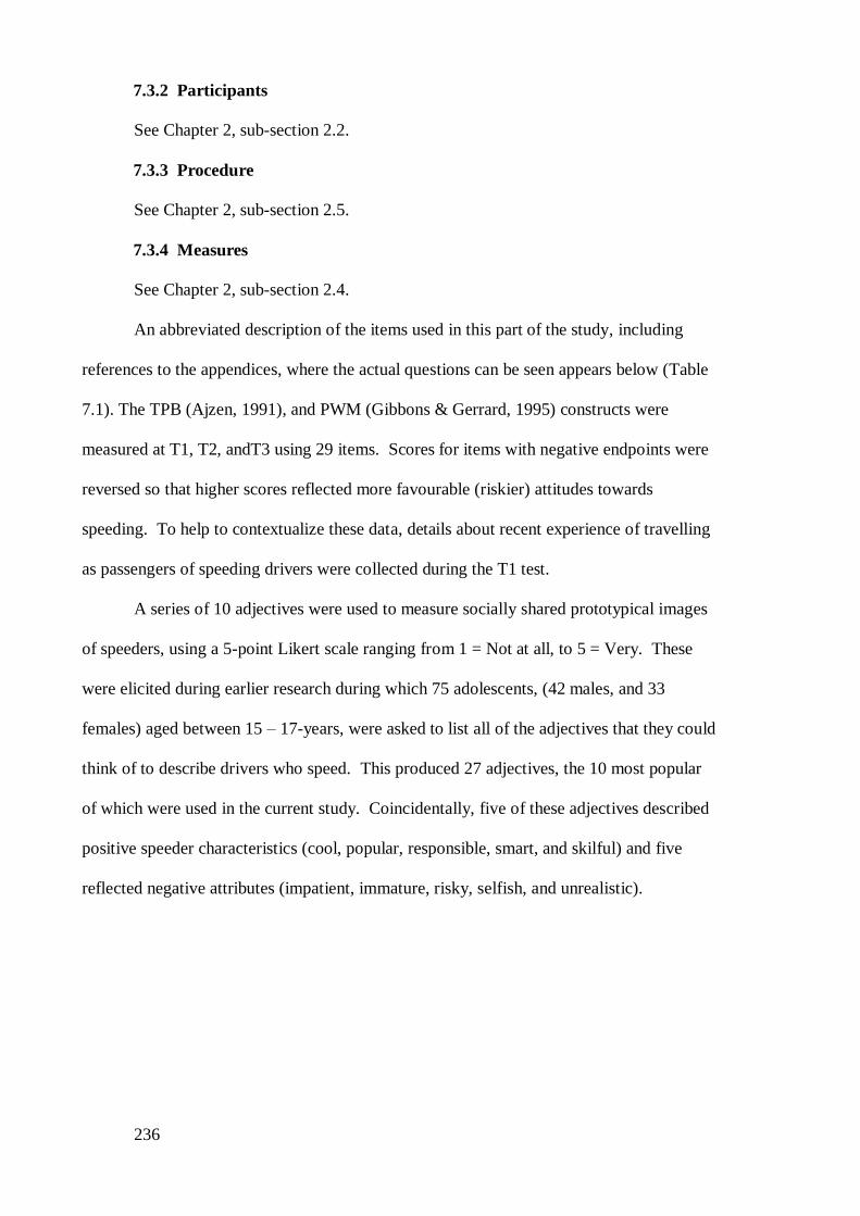
236
7.3.2 Participants
See Chapter 2, sub-section 2.2.
7.3.3 Procedure
See Chapter 2, sub-section 2.5.
7.3.4 Measures
See Chapter 2, sub-section 2.4.
An abbreviated description of the items used in this part of the study, including
references to the appendices, where the actual questions can be seen appears below (Table
7.1). The TPB (Ajzen, 1991), and PWM (Gibbons & Gerrard, 1995) constructs were
measured at T1, T2, andT3 using 29 items. Scores for items with negative endpoints were
reversed so that higher scores reflected more favourable (riskier) attitudes towards
speeding. To help to contextualize these data, details about recent experience of travelling
as passengers of speeding drivers were collected during the T1 test.
A series of 10 adjectives were used to measure socially shared prototypical images
of speeders, using a 5-point Likert scale ranging from 1 = Not at all, to 5 = Very. These
were elicited during earlier research during which 75 adolescents, (42 males, and 33
females) aged between 15 – 17-years, were asked to list all of the adjectives that they could
think of to describe drivers who speed. This produced 27 adjectives, the 10 most popular
of which were used in the current study. Coincidentally, five of these adjectives described
positive speeder characteristics (cool, popular, responsible, smart, and skilful) and five
reflected negative attributes (impatient, immature, risky, selfish, and unrealistic).
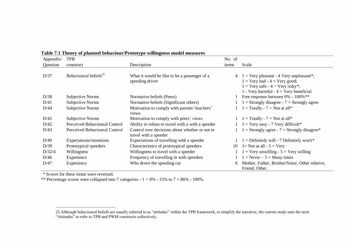
Table 7.1 Theory of planned behaviour/Prototype willingness model measures
Appendix/ TPB No. of
Question construct Description items Scale
D/37
Behavioural beliefs
25
What it would be like to be a passenger of a
speeding driver
4
1 = Very pleasant - 4 Very unpleasant*;
1 = Very bad - 4 = Very good; 1 = Very safe - 4 = Very risky*;
1 - Very harmful - 4 = Very beneficial D/38 Subjective Norms Normative beliefs (Peers) 1 Free response between 0% - 100%**
D/41 Subjective Norms Normative beliefs (Significant others) 1 1 = Strongly disagree - 7 = Strongly agree
D/44 Subjective Norms Motivation to comply with parents’/teachers’ views
1 1 = Totally - 7 = Not at all*
D/45 Subjective Norms Motivation to comply with peers’ views 1 1 = Totally - 7 = Not at all*
D/42 Perceived Behavioural Control Ability to refuse to travel with a with a speeder 1 1 = Very easy - 7 Very difficult*
D/43 Perceived Behavioural Control Control over decisions about whether or not to
travel with a speeder 1 1 = Strongly agree - 7 = Strongly disagree*
D/40 Expectations/intentions Expectations of travelling with a speeder 1 1 = Definitely will - 7 Definitely won't*
D/39 Prototypical speeders Characteristics of prototypical speeders 10 1= Not at all - 5 = Very
D/32/4 Willingness Willingness to travel with a speeder 1 1 = Very unwilling - 5 = Very willing
D/46 Experience Frequency of travelling in with speeders 1 1 = Never – 5 = Many times
D/47 Experience Who drove the speeding car 6 Mother, Father, Brother/Sister, Other relative, Friend, Other.
* Scores for these items were reversed.
** Percentage scores were collapsed into 7 categories - 1 = 0% - 15% to 7 = 86% - 100%.
25 Although behavioural beliefs are usually referred to as “attitudes” within the TPB framework, to simplify the narrative, the current study uses the term
“Attitudes” to refer to TPB and PWM constructs collectively.
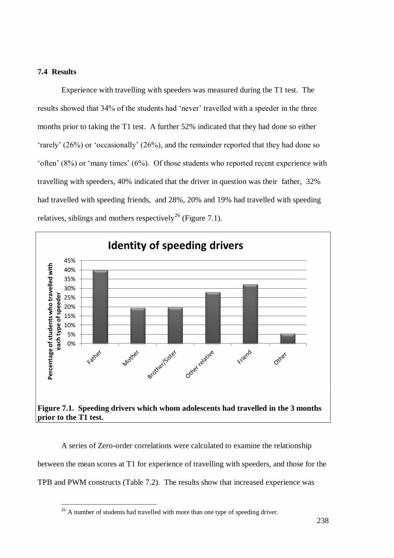
238
7.4 Results
Experience with travelling with speeders was measured during the T1 test. The
results showed that 34% of the students had ‘never’ travelled with a speeder in the three
months prior to taking the T1 test. A further 52% indicated that they had done so either
‘rarely’ (26%) or ‘occasionally’ (26%), and the remainder reported that they had done so
‘often’ (8%) or ‘many times’ (6%). Of those students who reported recent experience with
travelling with speeders, 40% indicated that the driver in question was their father, 32%
had travelled with speeding friends, and 28%, 20% and 19% had travelled with speeding
relatives, siblings and mothers respectively26
(Figure 7.1).
Figure 7.1. Speeding drivers which whom adolescents had travelled in the 3 months
prior to the T1 test.
A series of Zero-order correlations were calculated to examine the relationship
between the mean scores at T1 for experience of travelling with speeders, and those for the
TPB and PWM constructs (Table 7.2). The results show that increased experience was
26 A number of students had travelled with more than one type of speeding driver.
0%
5%
10%
15%
20%
25%
30%
35%
40%
45%
Per
cen
tage
of
stu
den
ts w
ho
tra
velle
d w
ith
ea
ch t
ype
of
spee
der
Identity of speeding drivers
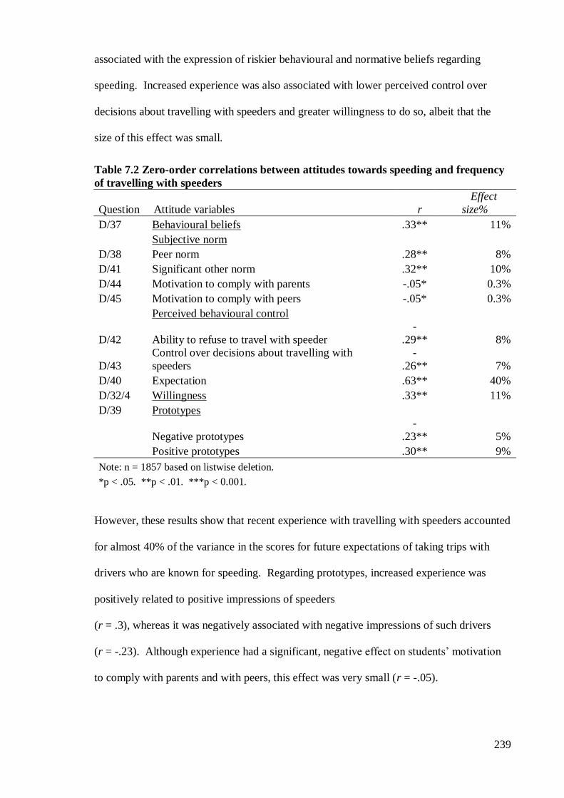
239
associated with the expression of riskier behavioural and normative beliefs regarding
speeding. Increased experience was also associated with lower perceived control over
decisions about travelling with speeders and greater willingness to do so, albeit that the
size of this effect was small.
Table 7.2 Zero-order correlations between attitudes towards speeding and frequency
of travelling with speeders
Question Attitude variables r
Effect
size%
D/37 Behavioural beliefs .33** 11%
Subjective norm
D/38 Peer norm .28** 8%
D/41 Significant other norm .32** 10%
D/44 Motivation to comply with parents -.05* 0.3%
D/45 Motivation to comply with peers -.05* 0.3%
Perceived behavioural control
D/42 Ability to refuse to travel with speeder
-
.29** 8%
D/43
Control over decisions about travelling with
speeders
-
.26** 7%
D/40 Expectation .63** 40%
D/32/4 Willingness .33** 11%
D/39 Prototypes
Negative prototypes
-
.23** 5%
Positive prototypes .30** 9%
Note: n = 1857 based on listwise deletion. *p < .05. **p < .01. ***p < 0.001.
However, these results show that recent experience with travelling with speeders accounted
for almost 40% of the variance in the scores for future expectations of taking trips with
drivers who are known for speeding. Regarding prototypes, increased experience was
positively related to positive impressions of speeders
(r = .3), whereas it was negatively associated with negative impressions of such drivers
(r = -.23). Although experience had a significant, negative effect on students’ motivation
to comply with parents and with peers, this effect was very small (r = -.05).
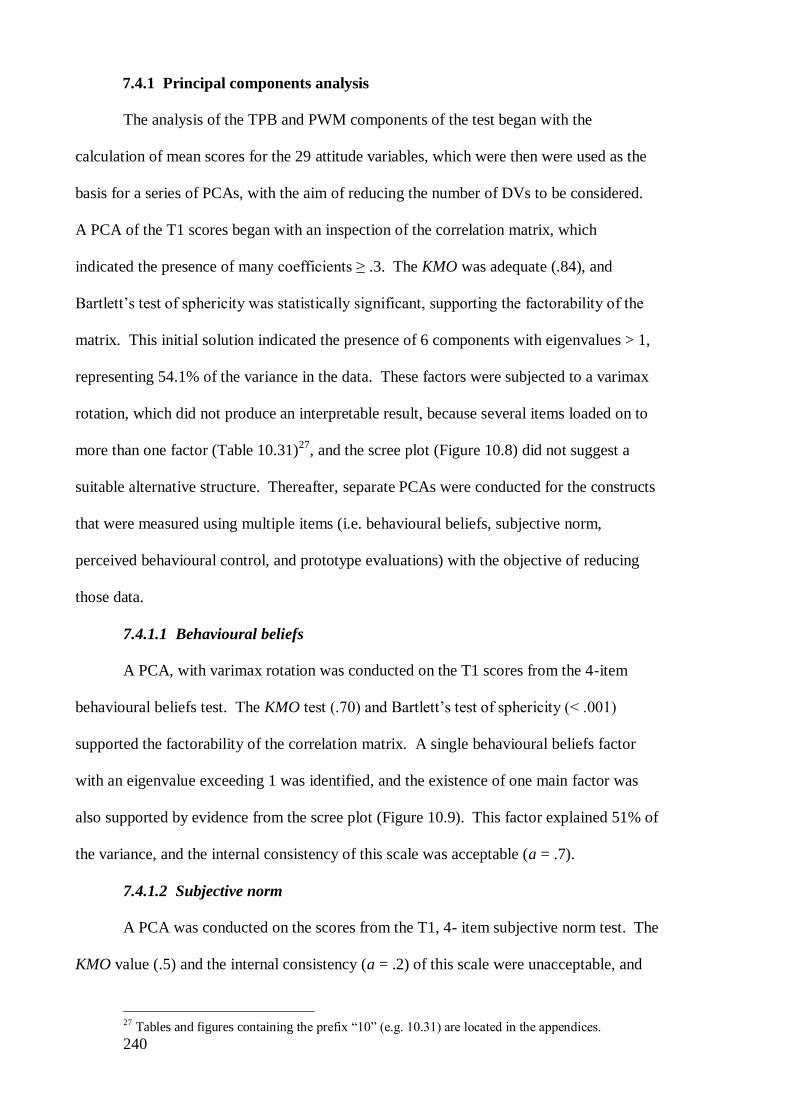
240
7.4.1 Principal components analysis
The analysis of the TPB and PWM components of the test began with the
calculation of mean scores for the 29 attitude variables, which were then were used as the
basis for a series of PCAs, with the aim of reducing the number of DVs to be considered.
A PCA of the T1 scores began with an inspection of the correlation matrix, which
indicated the presence of many coefficients ≥ .3. The KMO was adequate (.84), and
Bartlett’s test of sphericity was statistically significant, supporting the factorability of the
matrix. This initial solution indicated the presence of 6 components with eigenvalues > 1,
representing 54.1% of the variance in the data. These factors were subjected to a varimax
rotation, which did not produce an interpretable result, because several items loaded on to
more than one factor (Table 10.31)27
, and the scree plot (Figure 10.8) did not suggest a
suitable alternative structure. Thereafter, separate PCAs were conducted for the constructs
that were measured using multiple items (i.e. behavioural beliefs, subjective norm,
perceived behavioural control, and prototype evaluations) with the objective of reducing
those data.
7.4.1.1 Behavioural beliefs
A PCA, with varimax rotation was conducted on the T1 scores from the 4-item
behavioural beliefs test. The KMO test (.70) and Bartlett’s test of sphericity (< .001)
supported the factorability of the correlation matrix. A single behavioural beliefs factor
with an eigenvalue exceeding 1 was identified, and the existence of one main factor was
also supported by evidence from the scree plot (Figure 10.9). This factor explained 51% of
the variance, and the internal consistency of this scale was acceptable (a = .7).
7.4.1.2 Subjective norm
A PCA was conducted on the scores from the T1, 4- item subjective norm test. The
KMO value (.5) and the internal consistency (a = .2) of this scale were unacceptable, and
27 Tables and figures containing the prefix “10” (e.g. 10.31) are located in the appendices.
241
could not be improved by deleting any of the items. Consequently these items were
analysed individually for the remainder of the study.
7.4.1.3 Perceived behavioural control
Similarly, the PCA for the T1 scores from the 2-item perceived behavioural control
test revealed unacceptable KMO (.50), and internal consistency (a = .5) values, and these
items were analysed separately thereafter.
7.4.1.4 Prototypes
A PCA was also performed on the T1 scores for the 10-item, prototypical speeding
driver test. Inspection of the correlation matrix revealed the presence of many coefficients
≥ .3, and the results for the KMO (.8), and Bartlett’s (< .05) tests, supported the
factorability of the matrix. PCA revealed the presence of a three factor with eigenvalues
exceeding 1, explaining 61% of the variance, thus these factors were rotated. Although,
the rotated component matrix showed that several items loaded strongly on to more than 1
component (Table 10.32), an inspection of the scree plot suggested the presence of two
dominant components (Figure 10.10). Thus, a 2-factor solution, which explained 50.1% of
the variance, was imposed on the data. Component 1, which consisted of the 5 negative
adjectives from the scale, was labelled Negative Prototypes, and contributed 32.8% of the
variance. Component 2, which consisted of the 5 positive adjectives from the scale, was
labelled Positive Prototypes, and contributed 17.3% of the variance. The internal
consistencies of the Negative Prototype scale (a = .8) and the Positive Prototype scale (a =
.7) were adequate.
As a result of these factor analyses the number of variables in this section of the
study was reduced to 13, 11 of which addressed TPB and PWM constructs and two which
addressed previous experience with travelling with drivers who are known for speeding.

242
7.4.2 Descriptive data
Sample means for the scales and for the individual items from the T1, the T2 and, the T3
tests are summarised in Table 7.3.
Table 7.3 Sample means for attitudes to speeding items and scales
Appendix /
Question Attitudes variables
Time 1* Time 2** Time 3*** Raw score change
M SD M SD M SD T1/T2 T2/T3 T1/T3
D/37 Behavioural Beliefs 2.20 0.80 2.12 0.81 2.15 1.01 -3.6% 1.4% -2.3%
Subjective Norm items
D/38 Percentage of peers who think it's OK
to travel with a speeder (descriptive
norm)
3.93 1.68 4.47 1.83 3.49 1.55 13.7% -21.9% -11.2%
D/41 People who are close to me
(significant others) think it's OK for
me to travel with a speeder
(injunctive norm)
2.54 1.60 2.45 1.54 2.42 1.64 -3.5% -1.2% -4.7%
D/44 Motivation to comply with parents'
opinions
3.85 1.95 4.28 1.46 4.56 1.65 11.2% 6.5% 18.4%
D/45 Motivation to comply with peers'
opinions
4.29 1.93 4.03 1.29 3.73 1.61 -6.1% -7.4% -13.1%
Perceived Behavioural Control
items
D/42 Easy to refuse a lift with a speeder 4.48 1.78 4.52 1.72 4.59 1.76 0.9% 1.5% 2.5%
D/43
Up to me to decide whether or not to
travel with a speeder 5.48 1.60 5.51 1.55 5.84 1.35 0.5% 6.0% 6.6%
Behavioural Intention item
D/40
Expectation of travelling with speeder
in the next 3 months 3.15 1.20 3.25 1.20 3.42 1.23 3.2% 5.2% 8.6%
D/39 Prototypes scales
Negative 3.47 0.92 3.68 0.91 3.36 1.00 6.1% -8.7% -3.2%
Positive 2.33 0.80 2.25 0.76 2.11 0.90 -3.4% -6.2% -9.4%
Willingness item
D/32/4 Willingness to travel with a speeder 2.56 1.06 2.57 0.98 2.51 1.01 0.4% -2.3% -2.0%
* n = 1880. **n = 1322. *** n = 1412.
The T1 scores for the behavioural beliefs scale (M = 2.2, SD = 0.8), indicated that the
students believed that travelling in a speeding car would be somewhat of a negative
experience and these beliefs changed very little in the subsequent tests.
The results for the subjective norm items revealed a disparity between parental and
peer norms. On the one hand, students believed that people who are close to them
(significant others) would not approve of travelling with a speeder at T1 (M = 2.54, SD =
1.6), and perceived approval for this behaviour decreased by 3.5% between the T1 and the
T2 test and by a further 1.2% subsequently. On the other hand, students believed that
243
approximately half of their peers would approve of taking a lift with a speeder at T1 (M =
3.93, SD = 1.68), and perceived peer approval increased by almost 14% between the T1
and the T2 tests, although it decreased by almost 22% during the study as a whole. The
results also suggested that the students were somewhat motivated to comply with their
peers’ opinions at T1 (M = 4.29, SD = 1.93). However, such motivation decreased by over
6% at T2 and by a further 7.4% in the final test. Furthermore, although, students were
slightly less motivated to comply with their parents’ opinions at T1 (M = 3.85, SD = 1.95),
such motivation increased by over 11% in the T2 test and by a further 6.5% in the final test.
The students were ‘unsure’ regarding their expectations (intentions) of being a
passenger in a speeding car at T1 (M = 3.15, SD = 1.2), however expectancy increased by
approximately 3% between the T1, the T2 tests, and by approximately 5% subsequently.
Since the mean scores for both of the PBC items were above the mid-point in the
scale, this indicates that the student tended to believe that they had some control over
whether or not they travelled with speeders. Scores for the T1 test, showed that they
agreed that they were in a position to decide whether or not to travel with speeders (M =
5.48, SD = 1.6), and scores for this item increased by 0.5% between the T1 and the T2
tests, and by 6.5% subsequently. However, the means with respect to refusing to take a lift
from a driver who had a reputation for speeding were slightly lower (T1, M = 4.48, SD =
1.78), decreasing by approximately 1% between the T1 and the T2 tests, and by 1.5%
subsequently.
The results regarding prototypical speeders indicated that the current participants
had a somewhat negative impression of such drivers. The T1 scores on the positive scale
were below the midpoint (M = 2.33, SD = 0.8), and these decreased by 3.4% between the
T1, and the T2 tests, and by 6.2% subsequently. The T1 scores on the negative scale were
above the midpoint (M = 3.47, SD = 0.92,) and negativity increased by over 6% between
the T1, and the T2 tests. However, negativity decreased by 8.7% subsequently.

244
The mean scores for willingness indicated that the students were more willing than
unwilling to take a lift with a speeder at T1 (M = 2.56, SD = 1.06), and that willingness
increased marginally (0.4%) between the T1. and the T2 tests, and decreased by 2.3%
subsequently.
7.4.3 HLM analysis of attitudes towards speeding scores
The HLM analyses proceeded in accordance with the modelling strategy that was
outlined in section 7.3.1 above; models 1 tested hypothesis 1, model 2 tested hypotheses 2
and 3, and models 3-5 tested hypotheses 4-6. Two sets of HLMs, one measuring short-
term changes and the other measuring long-term changes were constructed to examine the
effects of intra-student factors (i.e. time and age), of taking PLDE in general, of taking
specific PLDE courses, and of between-student factors on the mean scores for the 11
attitudes to speeding variables described above. This produced a large quantity of data,
and in the interest of brevity, these results will be reported on a model-by model basis,
rather than on a variable-by-variable basis, as was done previously.
7.4.3.1 Unconditional models (model 1)
The results for the unconditional models for the attitudes towards speeding
variables in both the IP and the IVF phases are summarised in Table 10.33. This indicates
that the fixed effects coefficients for all models varied significantly around the grand mean,
and chi-square goodness of fit tests indicated that there was a significant amount of
variation in the IP and in the IVF scores at the between-students (level-2) and between-
groups (level-3) levels, supporting hypothesis 1. Similar to the previous findings in this
research, these results also indicated that the largest proportion of the variation in risk
perception in this study was located at intra-student level.
7.4.3.2 Change over time (model 2)
The next set of models examined changes in attitudes as a function of time and age.
The IP models indicated that there was no significant effect of age on any of the variables
245
(Table 10.34). However there were some changes over time, including significant
increases in perceived peer approval for speeding (β = 0.15, t(37) = 2.32, p < .05, d =
0.05), motivation to comply with parents (β = 0.36, t(37) = 6.0, p < .001, d = 0.11),
expectations of travelling with a speeder (β = 0.16, t(37) = 4.53, p < .001, d = 0.11), and
negative impressions of prototypical speeders (β = 0.2, t(37) = 5.34, p < .001, d = 0.24).
There were also significant decreases in motivation to comply with peers (β = -0.31, t(37)
= -6.24, p < .001, d = -0.2), and in positive impressions of prototypical speeders (β = -0.18,
t(37) = -1.19, p < .05, d = -0.29). However, there were no significant slope changes with
respect to the following variables; attitude (D/37), perceived views of significant others
(D/41), ability to refuse a lift with a speeder (D/42), personal control over decisions about
travelling with speeders (D/43), and willingness to travel with a speeder (D/32-4).
Hypothesis 2 predicted that there would be significant short-term changes in attitudes in a
more risky direction, and since such changes were evidenced with respect to just two of the
variables that were tested (i.e. percentage of peers who think that it is ‘ok’ to travel with
speeders, and behavioural expectations) these results offer weak support for this
proposition. In addition, the model summaries indicated that time and age in combination
accounted for very little of the variance in all of these models (pseudo-R2 < 0.03).
The slope coefficients for the IVF models (Table 10.35) showed that age was not a
significant predictor of long-term changes with respect to any of the attitudes to speeding.
However, congruent with the IP results, there were significant long-term increases in
motivation to comply with parents (β = 0.68, t(37) = 5.37, p < .001, d = 0.22), and
behavioural expectations (β = 0.37, t(37) = 4.29, p < .001, d = 0.26). Furthermore, whereas
the increase in perceived personal control over decisions regarding travelling with speeders
was non-significant in the short-term, the IVF estimates show that perceived personal
control increased significantly over the longer-term (β = 0.43, t(37) = 4.11, p < .001, d =
0.17). Long-term declines in motivation to comply with peers (β = -0.36, t(37) = -3.1, p <
246
.01, d = -0.13), and support for positive prototypical images of speeders (β = -0.18, t(37) =
-2.66, p < .01, d = -0.29), also reflected the pattern of decline evidenced in the IP short-
term models. However, there was a significant long-term decrease in perceived peer
approval for travelling with speeders (β = -0.34, t(37) = -3.09, p < .01, d = -0.11) and in
negative prototypical images of speeders (β = -0.14, t(37) = -1.64, p < .05, d = -0.14),
which contrasts with the increases recorded for these items during the intervention phase.
Finally, there were no significant long-term changes in behavioural beliefs (D/37),
perceived views of significant others (D/41), ability to refuse a lift with a speeder (D/42),
and willingness to travel with a speeder (D/32-4). Since there was no significant short-
term or long-term change over time with respect to these four variables they were dropped
from the study. Hypothesis 3 predicted that there would be significant change in attitudes
in a risky direction over the long-term, and since these results provided evidence of
undesirable change with respect to just one of the variables tested, these results tend to
refute that proposal. Furthermore, the model fit statistics indicate that both time and age
factors accounted for a very small percentage of the variance in the overall models; the
pseudo-R2 values were < .04 for all variables, with the exception of item D/43 (pseudo-R
2
= .22) which was somewhat larger.
A review of the model summaries for the IP models (Table 10.34) and for the IVF
models (Table 10.35) indicated that these models fitted the data significantly better than
did the unconditional models, i.e. the results of chi-square goodness of fit comparisons
were all statistically significant. However, given that the model deviance values remained
high (> 5700), and that the inclusion of time and age as level-1 predictors had such a small
effect, it appears that age and time alone were not sufficient to explain variations in the
data over either the short- or the long-term.
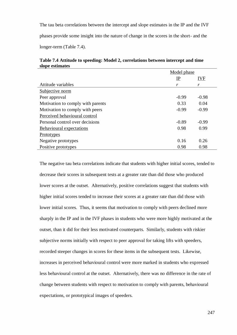
247
The tau beta correlations between the intercept and slope estimates in the IP and the IVF
phases provide some insight into the nature of change in the scores in the short- and the
longer-term (Table 7.4).
Table 7.4 Attitude to speeding: Model 2, correlations between intercept and time
slope estimates
Model phase
IP IVF
Attitude variables r r
Subjective norm
Peer approval -0.99 -0.98
Motivation to comply with parents 0.33 0.04
Motivation to comply with peers -0.99 -0.99
Perceived behavioural control
Personal control over decisions -0.89 -0.99
Behavioural expectations 0.98 0.99
Prototypes
Negative prototypes 0.16 0.26
Positive prototypes 0.98 0.98
The negative tau beta correlations indicate that students with higher initial scores, tended to
decrease their scores in subsequent tests at a greater rate than did those who produced
lower scores at the outset. Alternatively, positive correlations suggest that students with
higher initial scores tended to increase their scores at a greater rate than did those with
lower initial scores. Thus, it seems that motivation to comply with peers declined more
sharply in the IP and in the IVF phases in students who were more highly motivated at the
outset, than it did for their less motivated counterparts. Similarly, students with riskier
subjective norms initially with respect to peer approval for taking lifts with speeders,
recorded steeper changes in scores for these items in the subsequent tests. Likewise,
increases in perceived behavioural control were more marked in students who expressed
less behavioural control at the outset. Alternatively, there was no difference in the rate of
change between students with respect to motivation to comply with parents, behavioural
expectations, or prototypical images of speeders.
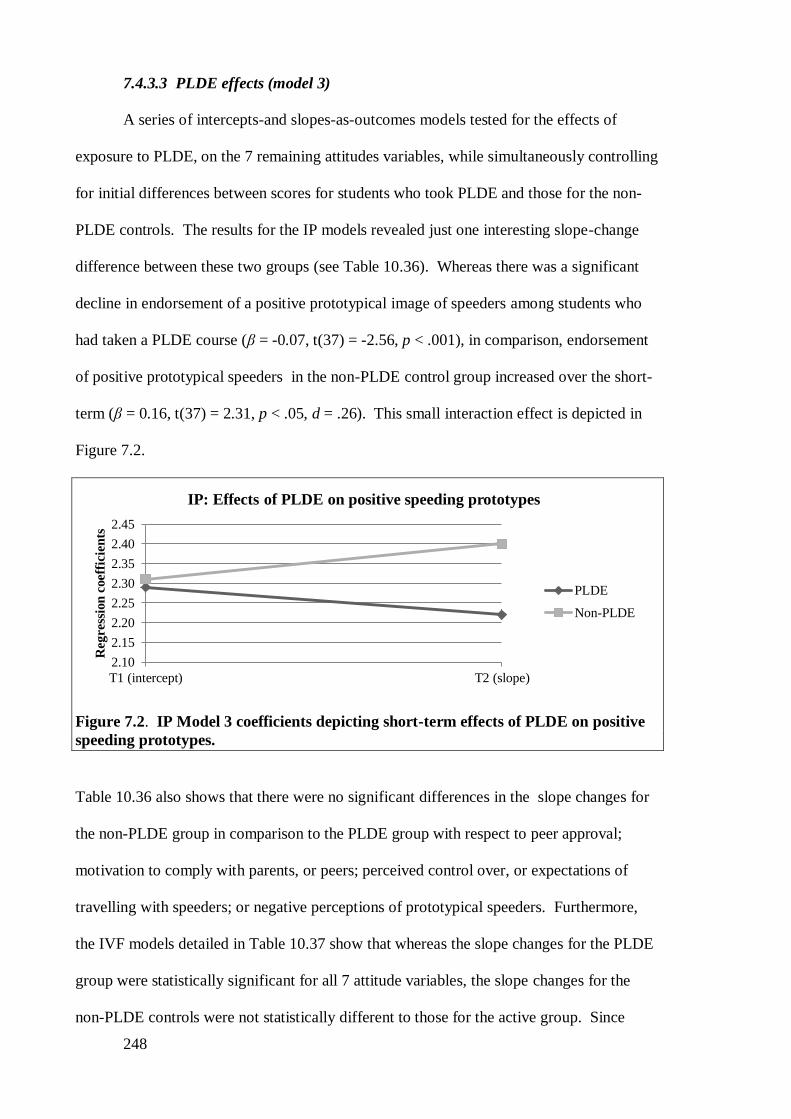
248
7.4.3.3 PLDE effects (model 3)
A series of intercepts-and slopes-as-outcomes models tested for the effects of
exposure to PLDE, on the 7 remaining attitudes variables, while simultaneously controlling
for initial differences between scores for students who took PLDE and those for the non-
PLDE controls. The results for the IP models revealed just one interesting slope-change
difference between these two groups (see Table 10.36). Whereas there was a significant
decline in endorsement of a positive prototypical image of speeders among students who
had taken a PLDE course (β = -0.07, t(37) = -2.56, p < .001), in comparison, endorsement
of positive prototypical speeders in the non-PLDE control group increased over the short-
term (β = 0.16, t(37) = 2.31, p < .05, d = .26). This small interaction effect is depicted in
Figure 7.2.
Figure 7.2. IP Model 3 coefficients depicting short-term effects of PLDE on positive
speeding prototypes.
Table 10.36 also shows that there were no significant differences in the slope changes for
the non-PLDE group in comparison to the PLDE group with respect to peer approval;
motivation to comply with parents, or peers; perceived control over, or expectations of
travelling with speeders; or negative perceptions of prototypical speeders. Furthermore,
the IVF models detailed in Table 10.37 show that whereas the slope changes for the PLDE
group were statistically significant for all 7 attitude variables, the slope changes for the
non-PLDE controls were not statistically different to those for the active group. Since
2.10
2.15
2.20
2.25
2.30
2.35
2.40
2.45
T1 (intercept) T2 (slope)
Reg
ress
ion
coeff
icie
nts
IP: Effects of PLDE on positive speeding prototypes
PLDE
Non-PLDE
249
there were no significant short-term effects of taking PLDE in relation to six of the seven
attitude variables, and no significant effects of PLDE on any of the variables over the long-
term, hypothesis 4 was rejected.
Furthermore, the model summaries for the IP (Table 10.36), and the IVF (Table
10.37) models showed clearly that these models did not represent a better fit for the data
than did the simpler, time-only models (model 2), and that the model deviance remained
high, which suggests that exposure to PLDE was not an important predictor of changes in
attitudes towards speeding in this study.
7.4.3.4 PLDE course effects (model 4)
A series of intercepts-and slopes-as-outcomes models tested for the effects of
exposure to specific PLDE courses, on the 7 remaining attitude variables, while
simultaneously controlling for initial differences in scores between students in the each of
the five PLDE groups and those of students in the control group. The IP models, which
tested short-term effects, are presented in Table 10.38, and these produced just one
noteworthy result: Whereas endorsement of positive prototypical images of speeders
increased significantly between the T1 and the T2 tests for the control group (β = 0.09,
t(37) = 1.39, p < .05), in comparison, it decreased significantly in all of the PLDE groups:
A (β = -0.14, t(1206) = -2.01, p < .04); B (β = -0.17, t(1206) = -2.02, p < .05), C (β = -0.16,
t(1206) = -2.01, p < 0.05), D(β = -0.19, t(1206) = -2.09, p < .05); E (β = -0.23, t(1206) = -
2.17, p < .05). However, the magnitude of the differences in the slopes between the
control group and groups A – E was small, d = 0.13, 0.08, 0.28, 0.15, and 0.16
respectively. These interaction effects are depicted in Figure 7.3.
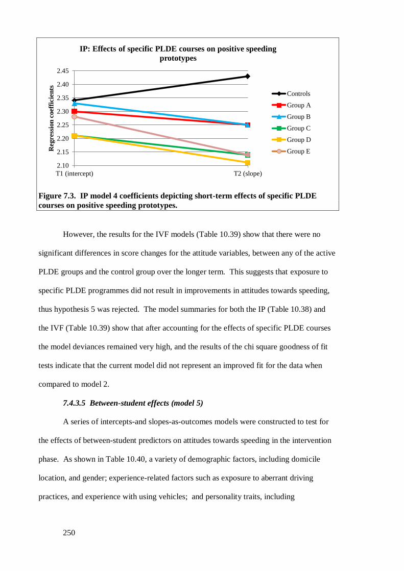
250
Figure 7.3. IP model 4 coefficients depicting short-term effects of specific PLDE
courses on positive speeding prototypes.
However, the results for the IVF models (Table 10.39) show that there were no
significant differences in score changes for the attitude variables, between any of the active
PLDE groups and the control group over the longer term. This suggests that exposure to
specific PLDE programmes did not result in improvements in attitudes towards speeding,
thus hypothesis 5 was rejected. The model summaries for both the IP (Table 10.38) and
the IVF (Table 10.39) show that after accounting for the effects of specific PLDE courses
the model deviances remained very high, and the results of the chi square goodness of fit
tests indicate that the current model did not represent an improved fit for the data when
compared to model 2.
7.4.3.5 Between-student effects (model 5)
A series of intercepts-and slopes-as-outcomes models were constructed to test for
the effects of between-student predictors on attitudes towards speeding in the intervention
phase. As shown in Table 10.40, a variety of demographic factors, including domicile
location, and gender; experience-related factors such as exposure to aberrant driving
practices, and experience with using vehicles; and personality traits, including
2.10
2.15
2.20
2.25
2.30
2.35
2.40
2.45
T1 (intercept) T2 (slope)
Reg
ress
ion
coeff
icie
nts
IP: Effects of specific PLDE courses on positive speeding
prototypes
Controls
Group A
Group B
Group C
Group D
Group E
251
impulsiveness, sensation seeking, and agreeableness impacted significantly on the intercept
estimates (i.e. the T1 test scores).
Exposure to aberrant driving was the strongest and the most consistent predictor of
attitudes towards speeding. Students with higher levels of exposure to aberrant driving
(HE) expressed riskier attitudes towards speeding in response to five of the seven test
items, than did their less exposed counterparts (LE). For example, the IP intercepts for the
HE students with respect to peer approval of speeding (β = 0.43, t(1209) = 4.83, p < .001),
expectations of travelling with speeders (β = 0.64, t(1207) = 10.57, p < .001), and positive
prototypical images of speeders (β = 0.24, t(1208) = 7.35, p < .001) were all significantly
higher, and the intercepts for HE students for perceived behavioural control over decisions
about travelling with speeders (β = -0.38, t(1211) = -4.94, p < .001), and for negative
prototypical images of speeders (β = -0.22, t(1209) = -5.63, p < .001) were significantly
lower, than those recorded for LE students.
Trait impulsiveness also influenced attitudes with some consistency. The intercept
coefficients suggested that initial attitudes towards speeding among students with higher
levels of impulsiveness (HI) were significantly riskier than were those among their less
impulsive peers (LI) with respect to peer approval (β = .04, t(1209) = 4.78, p < .001),
motivation to comply with parents (β = -0.44, t(1210) = -4.74, p < .001), expectations (β =
0.28, t(1207) = 4.61, p < .001), and prototypes, both negative (β = -0.19, t(1209) = -4.2, p
< .001) and positive (β = 0.18, t(1208) = 4.71, p < .001). Sensation seeking also predicted
initial attitude scores for two of the attitude variables. Students with higher levels of
sensation seeking expressed riskier attitudes with respect to peer approval (β = 0.33,
t(1209) = 4.12, p < .001), and positive prototypes (β = 0.16, t(1208) = 4.08, p < .001), than
did those with a lower tendency towards sensation seeking. Trait agreeableness affected
the initial estimates with respect to expectations of travelling with speeders: Students who
252
were high in agreeableness had lower expectations of travelling with speeders (β = -0.14,
t(1207) = -2.89, p < .001) than did their less agreeable peers.
The intercept estimates also indicated that there were significant gender differences
in attitudes towards speeding in the T1 test for some variables, whereby females expressed
significantly less risky attitudes than did males. Females were significantly more
motivated to comply with their parents views on travelling with speeders (β = 0.31, t(1209)
= , p < ), and expressed stronger endorsements of negative prototypical images of speeders
(β = 0.26, t(1209) = 5.5, p < .001), and weaker endorsements of positive prototypical
images (β = -0.18, t(1208) = -4.36, p < .001), than did their male counterparts.
Students with more initial experience with using vehicles expressed significantly
stronger expectations of travelling with a speeder (β = 0.31, t(1210) = 2.97, p < .01) in the
T1 test than did students with less experience in the T1. Finally, there were no significant
effects of any between-student factor on slope chances in the IP models.
The IVF models, depicting the long-term effects of between-student factors are
shown in Table 10.41, which indicates that factors including exposure to aberrant driving
and impulsiveness significantly affected slope changes in attitudes towards speeding over
the longer-term. Although LE students low exposure to aberrant driving practices (LE)
recorded significant long-term increases in expectations of travelling with speeders (β =
0.30, t(37) = 6.81, p < .001), the corresponding increase for HE students was significantly
greater (β = 0.29, t(1066) = -3.85, p < .001). There were significant divergences between
the slope changes for HE and LE students with regards to prototypical speeders. A
significant long-term decrease in support for negative images of speeders among LE
students (β = -0.13, t(37) = -3.2, p < .01), was contrasted with a significant increase in
support among HE students (β = 0.17, t(1067) = 2.42, p < .05). Similarly, whereas support
for positive prototypical images decreased significantly among LE students (β = -0.1,
253
t(1066) = -2.8, p < .05), in comparison, it increased among HE students (β = -0.2, t(1066)
= -3.58, p < .001).
Long-term differences in slope changes were also found between students with
high levels of impulsiveness (HI), and those with lower levels of that trait (LI). Where
there was a significant decrease in motivation to comply with peer attitudes towards
speeding among LI students (β = -0.77, t(37) = -9.12, p < .001), the corresponding decrease
was significantly smaller among HI students (β = 0.34, t(1067) = 2.85, p < .01). In
addition, whereas perceived control over whether or not to travel with speeders increased
significantly among LI students (β = 0.37, t(37) = 3.48, p < .01), the corresponding
increase among HI students was significantly smaller (β = -0.23, t(1067) = -2.37, p < .05).
Thus it appeared that some of the between-student factors that were of interest in
this study did have a significant effect on attitudes towards speeding. However, the model
summaries for the IP models (Table 10.40) and the IVF models (Table10.41) show clearly
that although these models fitted the data significantly better than did the simpler time-only
models (model 2), the model deviances remained stubbornly high and the effect sizes were
very small. It is worth reiterating here that each of the between-student models tested in
this part of the study were constructed initially using all of the between-student predictors
listed in Table 2.3 and that non-significant predictors were subsequently trimmed from the
models. These results showed that there were no significant effects of domicile location,
SES, experience with RTCs or any of the Big-Five personality traits on either the intercept
or slope values in any of the tests that were conducted.
7.5 Discussion
This part of the study examined speeding-related attitudes, beliefs, behavioural
expectancies and willingness of TY students using a range of constructs derived from the
TPB (Ajzen, 1991) and PWM (Gibbons & Gerrard, 1995). A series of HLMs, were
254
constructed to address the various hypotheses which were of interest in this project. The
results of these analyses showed that there was a considerable amount of between-student
variation in the data with respect to those constructs at the beginning of the project,
supporting hypothesis 1. However, hypotheses 2 and 3 were largely unsupported, because
it emerged that the speeding-related attitudes of the current sample became less risky when
measured over the short- and the long- term. Likewise hypotheses 4 and 5 were rejected
because the weight of evidence suggested that neither exposure to PLDE in general, nor
attendance at one of the PLDE courses that featured in this study resulted in significantly
greater improvements (change in a less-risky direction) in speeding-related attitudes in
these active groups when compared with the changes that occurred within the control
group. The results from the pre-intervention (T1) test provided some support for
hypothesis 6, since they showed that a variety of between-student factors influenced pre-
existing speeding-related attitudes, beliefs, expectancies and willingness in the sample.
In line with other findings in this research regarding knowledge and risk
perception, the model summaries for the attitudes towards speeding measures
demonstrated that the inclusion of significant predictors at intra-student, between-student
and between-groups levels did not result in significant reductions in the variation in the
data, which indicates that factors that were not stipulated in this study were exerting a
major influence on attitudes in this research.
7.5.1 Time effects
The results from the short-term and long-term HLMs showed that there were
significant changes over time in 7 of the 11 speeding-related attitudes variables that were
examined in this study. However, since attitudes tended to become less risky over time,
with respect to behavioural beliefs, these findings appear to be somewhat at odds with
those reported in similar studies of pre-driving adolescents which were described earlier
(e.g. Harré et al., 2000; Lonero et al., 2000).
255
7.5.2 PLDE effects
The current results also indicated that attendance at a PLDE course in TY did not
produce significantly greater beneficial changes in attitudes, beliefs, expectations and
willingness in TY students in either the short-term or the longer term, with one exception,
i.e. socially shared prototypical images of speeders. Whereas approval for positive speeder
prototypes increased significantly over the short-term in the control group, in comparison it
decreased significantly among students who took PLDE, albeit that this effect did not
persist over the longer-term. The general absence of short-term effects of PLDE on
attitudes in the current study does not accord with findings reported in previous evaluations
of PLDE programmes (see for example Deighton & Luther, 2007; Harré & Brandt, 2000b;
Poulter & McKenna, 2010). It seems likely that methodological factors may partly explain
this discrepancy and a detailed discussion of these factors will be provided in the latter part
of this chapter. The current results also suggest that PLDE was wholly ineffective in
delivering safety-related benefits over the longer term and these findings accord with those
reported in previous evaluations of PLDE (Harré & Brandt, 2000a; Poulter & McKenna,
2010) and DE (see Christie, 2001; Deighton & Luther, 2007; Roberts & Kwan, 2001;
Vernick et al., 1999).
7.5.3 Pre-existing attitudes towards speeding
Nevertheless, the pre-intervention (T1) test in this study did provide some insights
into the speeding-related attitudes in Irish PLDs as they entered TY/year 12 of secondary
school, and these may be of some interest in the road safety domain. First, the results
showed that mean scores with respect to the TPB and PWM constructs were generally
close to the mid points on their respective scales. This suggests that whereas the current
participants did not have particularly safe attitudes towards speeding at the beginning of
this project, they did not have particularly risky ones either. Thus it appeared that the
scope for PLDE to affect improvements was somewhat limited. Indeed, some of the

256
attitudes expressed in this study were relatively low risk and thus desirable from a safety
perspective. For instance, the students believed that travelling with a driver who was
speeding would be a somewhat negative experience and their evaluations of speeder
prototypes were more negative than they were positive. However, peer opinion with
respect to speeding was perceived as being more risky than were the perceived views of
significant others and motivation to comply with peers was marginally stronger than was
motivation to comply with parents. The students tended to believe that they had some
control over whether or not they travelled with speeders, albeit that they were slightly more
willing than unwilling to do so. Nevertheless, they were unsure regarding their prospects
of travelling with a speeder in the near future. However, due to their young age and thus
their relative reliance on parents and other adults for transport, the extent to which these
students had actual control over decisions about whether or not to travel with speeders
remains uncertain. This constitutes a limitation in the present methodology.
The current findings concur broadly with those reported in Poulter and McKenna’s
(2010) recent study of UK PLDS, which showed that mean values for attitude, parental
norm, behavioural intentions lay close to the mid-point and at the less-risky end of the
scale, whereas the scores for peer norms and motivation to comply with peers occupied the
more risky end of the scale. In addition, those participants believed that they had some
degree of control over whether or not they would engage in speeding when they started to
drive. The present findings also accord with those reported in Cestac, Paran and
Delhomme’s (2011) large-scale study of French novices which was described above and
which found that attitudes towards speeding in that group lay mainly on the less risky end
of the scales that were used. In combination, these results suggest that the scope for
changing attitudes in young pre-learner, learner and novices drivers is rather limited, which
may in part explain why it is so difficult to identify significant beneficial effects as a result
of taking a PLDE course.

257
7.5.4 Factors that influenced pre-existing attitudes, beliefs, expectations and
willingness
The current results also show that a number of between-student factors influenced
pre-existing attitudes, beliefs, expectancies and willingness; these include previous
experience of travelling with speeders, exposure to aberrant driving, impulsiveness,
sensation seeking, and gender, albeit that the magnitude of these effects was quite small.
7.5.4.1 Experience and exposure
The consistency with which previous experience of travelling with speeders and/or
exposure to aberrant driving was seen as having a detrimental effect on speeding-related
attitudes, beliefs, expectations and willingness at the beginning of this study was
noteworthy. Two-thirds of the current sample indicated that they had travelled with a
speeder in the three months prior to the commencement of this study, and the main culprits
were fathers, friends and other relatives respectively. Students who had recent experience
of travelling as a passenger of a speeder expressed riskier beliefs and attitudes towards
speeding and were more willing to travel with speeders and had stronger expectations of
doing so in the near future when compared to their less experienced counterparts.
Moreover, the HLM analyses showed that exposure to aberrant driving was the strongest
and most consistent predictor of attitudes towards speeding in the T1 test. Students with
greater exposure expressed riskier attitudes towards speeding with respect to five of the
seven attitude items that were measured than did their less-exposed counterparts. They
perceived greater peer approval for travelling with speeders. They judged positive speeder
prototypes more leniently and assessed negative speeder prototypes less harshly. They had
greater expectations of travelling with speeders in the following three months and their
perceptions of having control over whether or not they travelled with speeders were lower.
These results suggest that exposure to aberrant driving practices including speeding served
to establish attitudinal and behavioural norms and expectations that are undesirable from a
258
safety perspective. Furthermore, some of these influences (e.g. expectations, undesirable
evaluations of speeder prototypes) persisted over the longer-term. These results concur
with previous findings which indicated that exposure to the aberrant driving practices of
important role models, most notably those of parents (Ferguson et al., 2001; Miller &
Taubman - Ben-Ari, 2010; Taubman - Ben-Ari et al., 2005), and of peers (Allen & Brown,
2008; Jessor et al., 1997; Scott-Parker et al., 2009; Steinberg & Monahan, 2007), has a
negative impact on adolescents beliefs, attitudes, intentions and willingness with respect to
risk-taking in traffic (Waller, 1975; Williams et al., 2009).
7.5.4.2 Social normative influence
This study also revealed some interesting findings regarding social normative
influences on speeding-related beliefs and attitudes in this sample of Irish PLDs. First,
whereas peer norms were perceived as quite risky, the norms for significant others were
construed as safer in comparison. Second, whereas motivation to comply with perceived
peer norms decreased consistently over the course of this study, motivation to comply with
parental/teacher norms increased consistently in the same period.
Evidence presented in Chapter 4 suggested that adolescents tend to perceive the
peer norm as tolerant of risk (N. Evans et al., 1995). It was also suggested that the
increased tendency towards risk-taking in adolescence reflects a need to gain social
acceptance among peers (Allen et al., 1990). This may help to explain findings that
adolescents adopt a riskier driving style when they are accompanied by peers than they do
when they carry adult passengers (Arnett et al., 1997; Baxter et al., 1990). However,
abundant research based on social norms theory (Perkins & Berkowitz, 1986) posits that
individuals are apt to misperceive peer norms to the extent that they assume that peer
attitudes and behaviours are more risky than they actually are (see Prentice, 2008 for a
comprehensive review).

259
Although it is acknowledged that a multitude of psychological and social processes
give rise to such misperceptions, the role of descriptive norms is particularly salient in the
context of this research. Social norm theory suggests that perceptions regarding the
prevalence of risky driving-related attitudes and behaviour among adolescents can become
distorted because the media and social programming interventions tend to focus more on
depicting aberrant behaviour than they do on highlighting safe behaviour. To redress this
balance, approaches such as social marketing have been developed, which concentrate on
providing participants with accurate information about the social context in the form of
positive group norms. A review of the extant literature conducted by Haines, Perking,
Rice and Barker (2005) cited numerous examples that attest to the efficacy of the social
marketing approach in reducing substance use in secondary schools.
Parents and teachers are also seen as important sources of information (and
misinformation) about social norms. Whereas some studies suggest that parental influence
declines and peer influence strengthens as a result of increased extra-familial socialisation
during adolescence (Windle, 2000), a considerable weight of evidence also suggests that
parental influence remains strong through adolescence (Deighton & Luther, 2007; Durkin
& Tolmie, 2010). Indeed the results of the current study show that whereas motivation to
comply with perceived peer norms with respect to travelling with speeders was stronger
than was motivation to comply with parents/teachers norms in the initial test, this trend
reversed during the course of this project. This result accords with findings from a study
of a large and diverse sample of Americans aged between 10 and 30-years old, which
found that resistance to peer influence increased linearly between the ages of 14 and 18
(Steinberg & Monahan, 2007).
When these results are viewed within the context of a social marketing strategy
several recommendations emerge. First, programme developers should consider
capitalizing on the effects of peer influence by providing students with accurate
260
information about how their peers actually think, feel and act, thereby altering the
perceived norm in a less risky direction. Indeed some of the educational interventions that
featured in this research do incorporate some mechanism for ascertaining peer norms and
making them explicit and this aspect of the courses will be discussed in greater detail in
Chapter 8. Second, there is a pressing need to educate parents about the importance of
modelling safe driving attitudes and behaviours for their children from an early age. They
should be reminded that they represent a significant influence in their children’ lives both
as role models and carriers of normative information and they need to be vigilant to guard
against providing their offspring with mixed messages when it comes to road safety. For
instance, it is important that parents both set a good example and also convey to their
offspring that safe driving is the norm. Third, to counteract the obvious threat posed by
aberrant role models, programme developers should seek to develop effective and efficient
means of challenging the actions of such individuals, thereby weakening their potential to
undermine road safety messages. Fourth, efforts should be made to identify adolescent and
adult drivers who might act as positive role models in media campaigns and as part of
educational interventions e.g. entertainers and sportspeople who espouse safe values and
who behave responsibly as drivers. Research suggests that the impact of positive and
negative role models may depend on an individual’s goal orientation in given situations
(Lockwood, Sadler, Fyman, & Tuck, 2004). For instance, a considerable body of research
indicates that people are particularly sensitive to information that fits with their desire to
achieve success or to avoid failure (Higgins, 2000). Apparently, individuals are
particularly amenable to the influence of positive role models when they are pursuing
success, whereas they are more likely to be influenced by negative role models when they
are trying to avoid failure (Lockwood, Jordan, & Kunda, 2002). Thus, there is clearly a
need to depict both types of role models in media and in education programmes. Finally,
the current results suggest that PLDE was effective in reducing the favourability of
261
positive prototypical images of speeders significantly over the short-term. Some non-
significant effects in the desired direction were also evidenced with respect to negative
prototypes. This suggests that the prototypes represent a potentially useful concept when it
comes to developing and evaluating PLDE courses. To date, this construct has received
very little attention in the road safety domain; however the current results suggest that
further research is warranted in this regard.
7.5.4.3 Personality
Personality traits also affected pre-existing attitudes towards speeding in this study.
Students with higher levels of impulsiveness and/or sensation seeking perceived greater
peer approval for travelling with speeders and also viewed positive speeder prototypes
more favourably. Additionally, more impulsive students had greater expectations of
travelling with speeders, were less motivated to comply with parents’/teachers’ views on
this issue and viewed negative speeder prototypes more favourably. It was also notable
that high impulsiveness predicted greater motivation to comply with peer norms and less
perceived behavioural control over travelling with speeders over the longer-term. By
demonstrating that personality characteristics such as impulsiveness and sensation seeking
influence the development of risky speeding-related attitudes in PLDs, these findings
expand on the extant literature which demonstrates that such personality characteristics
tend to have a negative impact on driving behaviour during adolescence (Arnett et al.,
1997; Beirness & Simpson, 1988; Hoyle et al., 2002) and in adulthood (Dahlen, Martin,
Ragan, & Kuhlman, 2005; Dahlen & White, 2006; Jonah, 1997).
Since personality characteristics such as impulsiveness and sensation seeking are
understood to be predominantly biologically based (Roberti, 2004; Stanford et al., 1996;
Steinberg et al., 2008; Zuckerman, 1996), it is unlikely that these traits can be altered by
means of educational interventions. However, the GDE framework suggests that education
can provide students with insight regarding their personal risky tendencies and also provide
262
them with strategies which will help them to ameliorate the detrimental effects that such
tendencies may have on their thoughts, feelings and actions (Hatakka et al., 2002). To
date however, there is no evidence to suggest that this aspect of the GDE framework is
being used by course developers to address the problems that arise as a result of
impulsiveness and sensation seeking in adolescent PLDs, LDs, and novices. Such
developments are long overdue.
7.5.4.4 Gender effects
Whereas previous research suggests that male PLDs have riskier attitudes than do
their female counterparts (Waylen & McKenna, 2002, 2008), in the present study such
differences only reached statistical significance in relation to three of the seven variables
that were tested in the HLM analyses. In the pre-intervention tests females expressed
stronger endorsement of negative speeder prototypes and weaker endorsement of positive
speeder prototypes than did males. These findings are in line with previous reports which
showed that females are less likely to condone driving violations than are males (Waylen
& McKenna, 2002). Females were also more motivated to comply with parents’/teachers’
views about whether or not they should travel with a speeder. These findings are common
in the literature and likely reflect the emergence of gender role identities, whereby
masculinity is associated with risk seeking as a means of expressing autonomy and
bravado (Durkin & Tolmie, 2010).
7.5.5 Strengths and weaknesses
The results from this part of the study need to be evaluated within the context of a
number of methodological factors, some of which were specific to this part of the research
and thus warrant immediate discussion. The main strength of this part of the research was
that it used a wide range of items to measure TPB constructs (Ajzen, 1991), and these are
widely regarded as reliable and valid when it comes to describing, explaining and
predicting driving-related beliefs, attitudes, and expectancies in adolescents (see Poulter &
263
McKenna, 2010) and in adults (see Armitage & Connor, 2001). The current study also
extended findings from previous research with pre-driving adolescents by examining the
PWM constructs (Gibbons et al., 1998). This innovative move revealed the potential
usefulness of the ‘prototype’ concept, both as a measurement tool and also as a target for
PLDE programme developers. The present study also sought to improve the validity of
TPB-based measures for pre-driving samples, by measuring behaviour that is within the
current behavioural repertoire of this group (i.e. travelling with speeders), rather than to
asking them to suppose what they might do when they become drivers, as is usually the
case in such research. The current results indicate that this strategy represented a feasible
option for future studies, since the ensuing results did not depart radically from those
reported in studies that used more traditional methods (e.g. Poulter & McKenna, 2010).
One potential limitation in this study is its dependence on single-item measurement
scales, which have been shown to be less reliable than longer tests (Nunally, 1978)
Although multiple items were used to measure many of the TPB constructs in this study,
with the exception of behavioural beliefs, these could not be formed into scales due to
problems with internal consistency. It is acknowledged that single-item scales have
weaknesses, for instance McKenna and Horswill (2006), caution that the wording in single
item scales may influence the result, thus producing less reliable data. Nevertheless,
several studies have attested to the psychometric properties of single-item scales (see D. G.
Gardner, Cummings, Dunham, & Pierce, 1998; Nagy, 2002).
In summary, the findings from this part of the research provide information about
the speeding-related attitudes, beliefs, expectancies and willingness of a sample of Irish
PLDs. It demonstrated that PLDE was largely ineffective when it came to effecting safety-
related changes in these constructs in both the short- and the long-term. However, it did
produce data that showed that social factors, including experience with speeding and
exposure to aberrant driving, and also personality factors, including impulsiveness and

264
sensation seeking, predicted riskier attitudes, beliefs and expectancies in this sample. As
such, these results may assist in the future development of educational interventions and
contribute towards increasing the knowledge base in the road safety domain regarding pre-
driving adolescents.
265
Chapter 8: Formative evaluation
8.1 Introduction
Evaluation entails ‘the systematic determination of the merit, worth or significance
of an object’ (Scriven, 2003, p. 19). Since the late 1990s there has been a growing global
trend towards incorporating values of accountability and greater professionalism across a
wide range of social enterprises. This has lead to a dramatic increase in the number and
types of evaluations that are commissioned by a wide range of national and international
organizations and an associated rise in the number of professional bodies that represent
evaluation practitioners (Donaldson & Lipsey, 2006b). According to Scriven (2003), these
developments have transformed evaluation practice into a “transdiscipline” that is
concerned with conceiving and refining theories, tools and methodologies that can be used
across a wide range of other disciplines, while simultaneously striving to advance
knowledge about the best ways to practice evaluation.
In light of these developments, the AAA Foundation for Traffic Safety
commissioned Kathryn Clinton and Larry Lonero to produce of a set of guidelines for
evaluating DE programmes, which incorporates best practice from across the evaluation
domain (Clinton & Lonero, 2006a, 2006b, 2006c). These guidelines provide a detailed
background for planning and conducting effective evaluations of learner driver education
and for integrating evaluation into programme development and policy. One of the main
aims of this endeavour was to promote standardisation of evaluation practice to enable
researchers and other stakeholders to properly synthesise the knowledge gathered during
evaluations and thereby to develop better programmes. The absence of a systematic
approach to evaluation in the DE domain is often lamented in the literature (Deighton &
Luther, 2007; Mayhew et al., 2002; Roberts & Kwan, 2001), because it represents a
considerable impediment to the accumulation of knowledge and expertise (Levin, 2005).
266
Clinton and Lonero (2006b) recommend that evaluations of DE programmes should be
based on evaluation theory, the key components of which are: programme description,
identifying the values inherent in the programme, deciding what type of evaluation results
(knowledge) are credible, meaningful and useful to programme users and other
stakeholders.
8.1.1 Summative and formative evaluations
Two types of evaluations, summative and formative, are useful for informing
development of educational interventions. Summative evaluations are conducted to assess
the impact of a programme, thus summative assessments of DE interventions commonly
seek to assess programme efficacy in terms of proximal goals such as student learning of
course content (e.g. improved knowledge, skills and attitudes), and distal outcomes (e.g.
decreased risk taking and crash reduction) (McKenna, 2010b; Waller, 1975). The
summative evaluation that was performed as part of the present research was described in
Chapters 5, 6, and 7. Formative evaluations are used to assess the effectiveness of a
curriculum and to guide users as to which curriculum to adopt and how to improve it
(Dylan, 2006). It is argued that gaining understanding into how an intervention promotes
change, with whom and under what circumstances, is equally important as is knowing
whether or not the desired chance took place, especially when an intervention is designed
to be implemented in a broad range of settings (WHO-European Working Group on Health
Promotion Evaluation, 2008). A typical formative evaluation will examine a programme’s
logic model (theoretical basis), context (environment), standards, processes and products
(Clinton & Lonero, 2006b).
With these considerations in mind, a formative evaluation plan was developed for
this research which aimed to:
1. Describe the programmes.
2. Identify stakeholder and user needs.
267
3. Describe programme theory (logic model).
4. Outline programme goals and objectives.
5. Review programme products and processes (i.e. resources, activities, delivery).
6. Examine programme standards, business processes and context.
Programme descriptions are provided in Appendix A and a general overview of
stakeholder and user needs, programme theory, goals and objective is provided below.
8.1.2 Stakeholder and user needs
Stakeholder and user needs with respect to traffic safety were identified as part of
the literature review that formed the basis of Chapter 1 of this thesis and these have been
further elaborated in subsequent chapters. To recapitulate, stakeholders and road users
alike are motivated fundamentally by two somewhat competing needs; the need for
mobility and the requirement for safety (Mayhew, 2007). The current Irish National Road
Safety Strategy (RSA, 2007) summarises stakeholder needs in terms of reducing the
incidence of RTCs in the population in general and among young drivers in particular. The
results presented in Chapter 4 suggest that a large proportion of Irish adolescents want to
start driving as soon as they are allowed to obtain a learner driver permit. However, it is
widely accepted that the safety status of young novice drivers is compromised as a result of
age, and inexperience (Drummond, 1989; L. Evans, 1991; Groeger & Brady, 2004; OECD
- ECMT, 2006b). More specifically, research suggests that the excessive crash liability of
young novice drivers is mainly due to a lack of basic knowledge and skills, poor
understanding of factors that increase risk in traffic and inadequate insight into their
limited capabilities as inexperienced drivers (Engstrom et al., 2003; Hatakka et al., 2002;
McKnight & McKnight, 2003).
8.1.3 Programme theory
Previous efforts to solve the “Young Driver Problem” using educational
interventions were deemed unsuccessful because they did not yield identifiable safety
268
benefits in terms of crash reduction (Christie, 2001; Roberts & Kwan, 2001). However,
critics (e.g. Lonero, 2008; Lonero et al., 1995; Waller, 1975) argued that many of these
early attempts at DE were doomed to failure because they were developed in the absence
of a coherent programme theory to the extent that “The prevailing culture (was) to think
that....road safety can be delivered on the basis of opinion, folklore, intuition and
experience” (Hauer, 2007, p. 2). A programme theory (logic model) is a set of
assumptions that guide the way that specific programmes are implemented and are
expected to produce results (Donaldson & Lipsey, 2006a). It describes what is supposed
to happen by specifying how the various elements in the programme are expected to induce
change and thus achieve its aims (Clinton & Lonero, 2006c).
In recent times, an increasing number of researchers have come to believe that the
Goals for driver education framework (GDE) (Hatakka et al., 2002) provides a
theoretically sound basis for the future development of driver education (Peräaho et al.,
2003). A detailed description of the GDE model was provided in Chapter 1. To
recapitulate, the GDE- framework consists of a hierarchical model which identifies
competencies that need to be achieved in order to become a safe driver at four operational
levels (vehicle manoeuvring, mastering driving situations, goals and context of driving and
goals for life / skills for living). The GDE-framework assumes that higher level operations
guide and control behaviour at lower levels, thus factors that are addressed at the highest
level are the ones that are most important from a safety perspective (Peräaho et al., 2003).
Whereas it is recognized that basic knowledge and skills serve as a foundation for the
establishment of driver competency (skill), the development of a safe driving practices
(style) requires that learners a) develop safe attitudes towards driving, b) gain an
understanding of risks involved, c) gain insight regarding their personal goals and
motivations and how these might affect their decision making as drivers (Hatakka et al.,
2002; Williams et al., 2009). Following a comprehensive review of the extant literature on
269
young novice driver education and training, Engstrom, Gregersen, Hernetkoski and Nyberg
(2003) recommended that driver education at secondary school level should focus on the
higher levels of the GDE-framework as opposed to providing training in vehicle handling
and control.
It should be noted however that some experts are unconvinced regarding the
feasibility of trying to mould driving styles in pre-driving populations. First, it is unlikely
that PLDE programmes would be able to compensate for biological immaturity which
manifests itself in the form of risk taking (Steinberg, 2004) . This issue will be discussed
in greater detail in the general discussion in this thesis. Second, McKnight (1985) noted
that since adolescents are motivated primarily by a desire to acquire a driving licence, they
tend to focus their attention on gaining the types of knowledge and skills that will help
them to satisfy that goal. However, because the prospect of independent driving is
somewhat remote for pre-learner drivers, these adolescents are likely to be less motivated
when it comes to learning safe driving practices. Given that there is a crucial link between
the success of driver education and student motivation (see Pintrich, 2003), McKnight
believes that DE courses that focus on the development of safe driving styles should be
delivered after students have acquired a learner driver permit because they are more likely
to be motivated to engage with material that deals with driving style when that material
becomes salient i.e. when they actually need it and are in a position to use it.
8.1.4 Visions, Goals and objectives
Evaluation theory indicates that programme goals and objectives should be
formulated on the basis of a programme theory (Clinton & Lonero, 2006b). Thus, on the
basis of the GDE-framework (Hatakka et al., 2002), it follows that PLDE courses should
aim to improve basic knowledge (e.g. knowledge about the ROTR), and also awareness of
factors that increase risk, especially those that increase risk for young learner and novice
drivers, and to increase self awareness with regard to risky attitudes and risky personal
270
tendencies. Whereas the developers of all PLDE programmes envisage that their courses
will contribute towards improving the calibre of PLDs, the programmes that they produce
tend to focus on different objectives in the pursuit of this goal. For example, in this study
most of the courses in group D and course E2 focused on serving students’ instrumental
needs, i.e. on providing them with factual knowledge and skills, whereas programmes A, B
and C placed a lot of emphasis on addressing students’ developmental needs, in terms of
increasing student awareness about the dangers of driving, or on improving students’
driving related beliefs and attitudes.
8.1.5 Programme content and delivery
Whereas it is relatively easy to formulate goals and objectives for PLDE, it has
proved much harder to identify suitable content and delivery methods that will help to
produce the desired outcomes (Lonero, 2008). However, on the basis of the
recommendations that are provided within the GDE-framework (Hatakka et al., 2002) and
the accumulated findings from previous research, some of which have been cited
previously in this thesis, it is clear that a comprehensive PLDE education programme
should aim to address both the instrumental and developmental needs of PLDs. The main
education-based (as opposed to training-based) instrumental needs of PLDs are:
Knowledge about the ROTR
Information regarding the driver licencing process.
Developmental needs of PLDs can be addressed by improving their awareness of state
dependent and situation dependent factors that are known to increase risk for young
drivers, and by providing them with strategies the will help to mitigate these risks. These
factors include:
Age-related immaturity
Inexperience.
Poor risk perception.
271
Risky attitudes towards driving with respect to speeding, driver impairment
and deliberate risk-taking.
Risky personal tendencies including impulsiveness and sensation seeking.
Susceptibility to social influences from peers, parents, and other negative
role models.
The learning theories that were reviewed in Chapter 3 also provided some guidance
with respect the ways in which the acquisition of driving-related competencies can be
supported in an educational context (see sub-section 3.1.1). To recapitulate; education
functions to provide students with information which is translated into knowledge, skills
and attitudes (Bransford et al., 2000). The encoding, and the storage and retrieval of
information in memory is facilitated when: exposure to the to-be-learned material is
repeated and distributed over a period of time (Ericsson & Kintsch, 1995; Schacter et al.,
2000); students are given immediate feedback regarding the accuracy of their learning
(Skinner, 1974); students are given ample opportunity to think about and/or interact with
the material (Craik & Lockhart, 1972; Flavell, 1979); the new information is related in
some way to previously learned material (Bransford et al., 2000; Piaget et al., 1969); the
material has personal importance (Symons & Johnson, 1997); the message is distinctive
(Schacter et al., 2000) and finally when the information evokes an emotional reaction
(Conway et al., 1994).
In addition, Kolb’s Experiential Learning Theory (ELT) (Kolb, 1984) highlights the
key role that reflective practice plays in the development of understanding. The
importance of reflective practice (insight training) in the development of safe driving
habits is acknowledged within the GDE-framework (Hatakka et al., 2002). According to
ELT, four key elements are required for successful experiential learning: concrete
experience, observation and reflection, the subsequent formation of new abstract concepts
and the ability to test these in new situations. The theory posits that it is not sufficient to
272
have an experience in order to learn. It is also necessary to reflect on that experience to
make generalisation and to formulate concepts which can then be applied in new situations.
This suggests that educational interventions should aim to provide students with
opportunities to reflect on what they have learned and to plan how they are going to enact
such learning. This might involve thinking about a situation (e.g. taking a lift with a driver
who is known for speeding or DWI) and trying out new coping strategies or alternative
ways of behaving in that situation (e.g. refusal strategies, planning alternative means of
transport).
The methods that are used to deliver safety messages also have a bearing on their
effectiveness. Petty and Cacioppo’s (1986), elaboration likelihood model posits that
peoples’ motivation and ability to process information varies as a function of situational
and dispositional factors. Where motivation and ability is high, people focus on thinking
about the information that is contained in a message, whereas when motivation and ability
are low, they are more likely to be influenced by peripheral features of the message e.g. the
credibility/attractiveness of the message source, or the way the message is presented. The
peripheral route is used when the audience is unable to process the message fully because
the message is too complex or because they are too immature to understand and/or
appreciate the relevance of the message. The target audience for PLDE courses is quite
diverse, thus it is expected that there will be wide variations in this group with respect to
motivation and ability. In these circumstances, the ELM model of persuasion indicates
that safety messages ought to be presented using both the direct and the peripheral routes
in order to maximise the courses’ potential to achieve the desired results.
An accumulation of evidence, some of which was presented in Chapter 4,
demonstrates that social influence plays a significant role in the development and
maintenance of safety-related attitudes, expectations, intentions and behaviours in
adolescents and that parents and peers constitute the main sources of such influence. The
273
findings from the current research which were presented in Chapters 5, 6 and 7 also
showed that exposure to the aberrant driving practices of parents and significant others had
a negative impact on the participants’ driving-related knowledge, risk perception skills and
attitudes. However, the corollary of these findings is that students whose parents and
significant others drive safely have been influenced positively as a result of exposure to
these positive role models. Research also suggests that social influence can be harnessed
to produce successful outcomes in social programming interventions. For example a meta-
analytic review of 47 peer-based intervention programmes found that these programmes
consistently produced positive effects on peoples’ health-related behaviours (Posavac,
Kattapong, & Dew, 1999). Yates and Dowrick (1991) developed a road safety intervention
which targeted the behaviours of high-risk adolescent drivers using peer influence and
social modelling. Following a three-year evaluation, it was reported that that the
programme was effective in increasing knowledge about and improving attitudes towards
DWI and also in reducing the incidence of DWI. These findings suggest that the inclusion
of content and processes that provide students with exposure to positive social influences
can improve the effectiveness of these interventions.
8.1.6 Programme standards and business processes
PLDE is a relatively new phenomenon, not just in the ROI but worldwide, therefore
no recognizable operating standards exist currently for these courses. However, on the
basis of what is known about programme standards for DE generally it is assumed that the
main areas of concern with respect to PLDE programmes will be those related to
curriculum planning and programme implementation (see Clinton & Lonero, 2006a).
8.1.6.1 Curriculum planning
A review of the TY curriculum was presented in Chapter 2. This revealed that TY
is an optional feature of the secondary school cycle in the ROI which aims to promote
personal, social, educational and vocational development. TY is structured such that

274
individual schools are responsible for setting appropriate goals and defining objectives that
are necessary for achieving these aims (Second Level Support Services - Department of
Education and Skills, 2013). TY coordinators who wish to provide a PLDE course for
their students have to choose between an ever-increasing array of interventions which
range from modular courses that are delivered over weeks or months to one-day courses.
This means that there are considerable between-school variations in terms of the quantity
and the quality of the PLDE programmes which are provided for TY students.
8.1.6.2 Programme implementation
Since it is anticipated that the PLDE education courses which are used in Irish
secondary schools will have been developed from sound theoretical bases and programme
goals and objectives will have been formulated with those bases in mind, it is important
that these programmes are delivered in the manner that was intended by the developers. In
the past, very few evaluations provided information about this aspect of programme
delivery (CARRS-Q, 2009). A review of over 1,200 published studies showed that just 5%
provided information about programme implementation (Durlak & Wells, 1997).
Nevertheless, the existing research suggests that programmes are more effective when they
are delivered according to the original design and that the tendency to preserve programme
integrity is associated with teachers who were enthusiastic and well-prepared and who had
the support and encouragement of their school principal (Rohrbach, Graham, & Hansen,
1993).
Failure to adhere to the implementation standards laid down by programme
developers represents a considerable threat to validity in evaluation studies. For example,
when Williams, Preusser and Ledingham (2009) conducted a study to assess the feasibility
of conducting a comprehensive evaluation of the American Driver and Traffic Safety
Education Association’s (ADTSEA) driver education curriculum they concluded that this
programme could not be evaluated in a completely scientific (valid) way because

275
“...individual schools (with their own guidelines) use what they want, but rarely use the
whole programme” (p 17).
8.1.6.3 Programme context
Programme context refers to the political, economic and social environments in
which a programme is implemented (Clinton & Lonero, 2006c). As discussed previously,
there is strong political will in the ROI to improve road safety and thus school curricula at
both primary and secondary level feature a number of compulsory road safety programmes
which have been developed by the Road Safety Authority (RSA, 2012). However, since
school staff and children are embedded in the shared school environment, an appreciation
of the organisational and cultural context of schools is critical for the implementation and
sustainability of such educational interventions (Ringeisen, Henderson, & Hoagwood,
2003). Evidence suggests that programme implementation is likely to be more successful
where organisations have strong administration and leadership, and support the programme
(Rohrbach, Grana, Sussman, & Valente, 2006).
8.1.7 Scope of current evaluation
Clinton and Lonero’s guidelines (2006b) suggest that an evaluation should aim to
provide a comprehensive assessment of the DE programme(s) under review, while also
taking pragmatic considerations such as the availability of time and resources into account.
With this in mind, and on the basis of a brief review of the five types of programmes that
were used in the schools that participated in this project, the current research aimed to
comment on the PLDE provision for TY students in Irish secondary schools. Thereafter, a
more detailed formative evaluation of the curriculum for programmes A and B will be
conducted.
276
8.2 Method
8.2.1 Design
See Chapter 2, sub-section 2.1.
8.2.2 Participants
See Chapter 2, sub-section 2.2.
8.2.3 Procedure
See Chapter 2, sub-section 2.5.
8.2.4 Measures
This part of the study used both quantative and qualitative methods to evaluate the
PLDE programmes that featured in the current research. These measures were
administered in conjunction with the T2 test and thus were taken shortly after the
individual groups had completed their PLDE courses.
The quantative measures consisted of two self-report questionnaires; a 34-item
student survey and a 20-item TY coordinator survey. The student survey was completed
by all of the students who participated in the T2 test. The survey aimed to measure
students’ reactions to the PLDE course that they had taken. The topics covered in this
survey are summarised in Table 8.1 below and the actual survey items can found in
Appendix E. The TY coordinators in the 13 schools that had used programmes A and B
completed a survey at their own convenience and returned it by post. This examined
programme standards and business processes, including curriculum planning,
teacher/instructor training, course materials, and course administration and evaluation (see
Appendix J for survey).

277
Table 8.1 Summary of student questionnaire
Question
Number Description Items Response Scale
E/34 Has taken a PLDE course 1 Yes / No
E/35 Level of participation in course 1 1 = 76% - 100% -
4 = 0% - 25%
E/36 Satisfaction with course components a
11 1 = Not provided -
2 = Completely satisfied -
6 = Completely dissatisfied*
E/37 Identity of course teacher 1 1 = TY teacher –
5 = Professional instructor
E/38 Evaluation of course teacher a 6 1 = Completely dissatisfied -
10 = Completely satisfied
E/39 Evaluation of course a 10 1 = Completely disagree - 5
= Completely agree
E/40 Grade awarded for the course 1 “A” – “F”
E/41 Most enjoyable part of the course b
1 Open response
E/42 Most beneficial part of the course b 1 Open response
E/43 Things that ought to be changed b 1 Open response
E/44 How to make those changes b
1 Open response
Note: Scores for this item were transformed subsequently: Response 1 “Not provided” was dropped from the scale and the remaining scores were re-coded such that 1 = completely dissatisfied and 5 =
completely satisfied and so forth. a Adapted from Lonero, Clinton, Persaud, Chipman and Smiley (2005)
b Adapted from Clinton and Lonero (2006a).
A series of semi-structured interviews were also conducted to assist with the
formative analysis of the programmes A and B curriculum28
. Although the PLDE teachers
in each of the 13 schools that used this curriculum agreed to be interviewed, due to
scheduling difficulties, interviews were conducted subsequently with teachers in nine of
these schools. The interview schedule that was used to guide these interviews is contained
in Appendix P.
8.3 Results
8.3.1 Overview of the PLDE courses that featured in this study
The course overview that is provided in Table 8.2 shows that all of the courses that
featured in the current research share some common aspirations; to improve driving-related
28 These programmes were based on a single curriculum

278
knowledge, awareness and attitudes of adolescent secondary school students. The
principal methods that were used to achieve these goals were lectures, class discussions,
student projects and courses A – D also used guest speakers.
Table 8.2 Overview of the PLDE course that featured in this study
Programmes
Features* A B C D E1 E2
Type Modular Modular Modular Modular 1-day 1-day
Duration in hours 45 20 20 15-20 7 6
Location of main activity On-
site
On-
site
On-
site
On-
site
On-
site
Off-
site
Teacher School School School School Course Course
Educational criteria
Based on NCCA criteria √ √ √ - - -
Objectives
Increase knowledge √ √ √ √ √ √
Increase awareness √ √ √ √ √ √
Improve attitudes √ √ √ √ √ √
In-car training X X X X X √
Activities
Classroom tuition √ √ √ √ √ √
Provision for class discussions** √ √ √ √ √ √
Provision for student projects √ √ √ √ X X
Provision for guest speakers** √ √ √ √ N/A N/A
Course materials
Teacher manual √ √ √ N/A N/A N/A
Student textbook X X √ X N/A N/A
(cont.)
Programmes
Features* A B C D E1 E2
Additional resources
Road safety DVDs √ √ √ √ √ X
Provision for teaching The Rules of
the Road**
√ √ √ √ √ √
Rewards/incentives
Certificate of attendance X X √ √ √ √
Discounted motor insurance X X √ √ √ X
* Detailed course descriptions are provided in Appendix A. **The extent to which these features were used varied from class to class.
The courses differed with respect to their structure and duration. Courses A – D were
modular in design and were delivered over several weeks or months. Programme A was
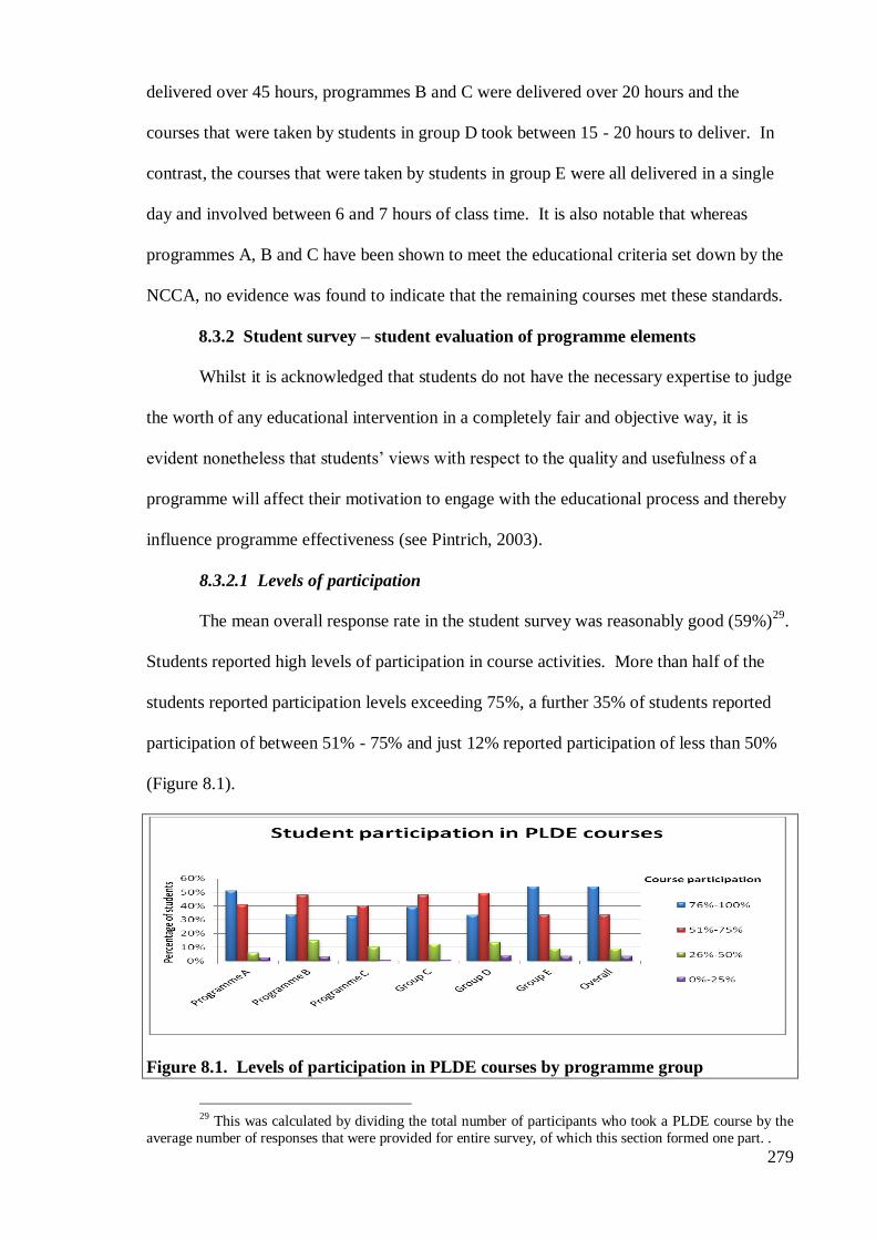
279
delivered over 45 hours, programmes B and C were delivered over 20 hours and the
courses that were taken by students in group D took between 15 - 20 hours to deliver. In
contrast, the courses that were taken by students in group E were all delivered in a single
day and involved between 6 and 7 hours of class time. It is also notable that whereas
programmes A, B and C have been shown to meet the educational criteria set down by the
NCCA, no evidence was found to indicate that the remaining courses met these standards.
8.3.2 Student survey – student evaluation of programme elements
Whilst it is acknowledged that students do not have the necessary expertise to judge
the worth of any educational intervention in a completely fair and objective way, it is
evident nonetheless that students’ views with respect to the quality and usefulness of a
programme will affect their motivation to engage with the educational process and thereby
influence programme effectiveness (see Pintrich, 2003).
8.3.2.1 Levels of participation
The mean overall response rate in the student survey was reasonably good (59%)29
.
Students reported high levels of participation in course activities. More than half of the
students reported participation levels exceeding 75%, a further 35% of students reported
participation of between 51% - 75% and just 12% reported participation of less than 50%
(Figure 8.1).
Figure 8.1. Levels of participation in PLDE courses by programme group
29 This was calculated by dividing the total number of participants who took a PLDE course by the
average number of responses that were provided for entire survey, of which this section formed one part. .
280
8.3.2.2 Satisfaction with the course materials
Whereas student satisfaction with course materials was measured using an 11-item scale,
four items (i.e. CD interactive exercises, in-car instruction, in-car log, and in-car
supervision) were dropped subsequently because very few of the respondents had used
these features as part of their PLDE course. Thereafter, item means and scale means were
calculated for the individual PLDE groups and for the overall sample (Table 8.3).
The group means for the individual items ranged from 4.28 for video presentations
(e.g. DVDs) to 3.81 for course workload/assignments. The sample mean for the scale was
4.08 (SD = 1.02) and the internal consistency of this scale was adequate (α > .7)
(Cronbach, 1990). These results suggest that the current participants were somewhat
satisfied with the materials that were used as part of their courses.
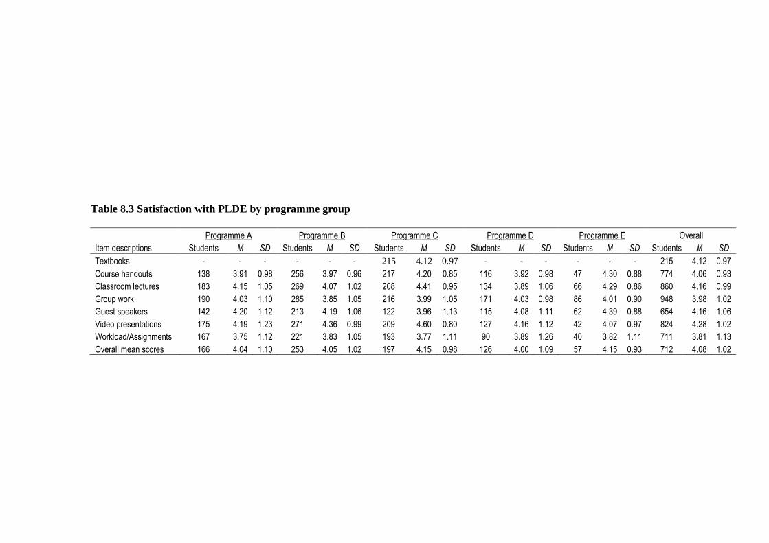
Table 8.3 Satisfaction with PLDE by programme group
Programme A Programme B Programme C Programme D Programme E Overall
Item descriptions Students M SD Students M SD Students M SD Students M SD Students M SD Students M SD
Textbooks - - - - - - 215 4.12 0.97 - - - - - - 215 4.12 0.97
Course handouts 138 3.91 0.98 256 3.97 0.96 217 4.20 0.85 116 3.92 0.98 47 4.30 0.88 774 4.06 0.93
Classroom lectures 183 4.15 1.05 269 4.07 1.02 208 4.41 0.95 134 3.89 1.06 66 4.29 0.86 860 4.16 0.99
Group work 190 4.03 1.10 285 3.85 1.05 216 3.99 1.05 171 4.03 0.98 86 4.01 0.90 948 3.98 1.02
Guest speakers 142 4.20 1.12 213 4.19 1.06 122 3.96 1.13 115 4.08 1.11 62 4.39 0.88 654 4.16 1.06
Video presentations 175 4.19 1.23 271 4.36 0.99 209 4.60 0.80 127 4.16 1.12 42 4.07 0.97 824 4.28 1.02
Workload/Assignments 167 3.75 1.12 221 3.83 1.05 193 3.77 1.11 90 3.89 1.26 40 3.82 1.11 711 3.81 1.13
Overall mean scores 166 4.04 1.10 253 4.05 1.02 197 4.15 0.98 126 4.00 1.09 57 4.15 0.93 712 4.08 1.02

282
8.3.2.3 Evaluation of main course instructor
Item and scale means were calculated for the 6-item course instructor evaluation
scale for each of the PLDE groups and for the overall sample (Table 8.4). An inspection of
the item means suggested that the students were most satisfied with respect to item 1 “The
instructor knew the subject matter (M = 8.04, SD = 2.2), next came item 4 “The instructor
answered the students’ questions satisfactorily (M = 7.59, SD = 2.35), then came item 5
“The instructor provided a good combination of lecture and discussion” (M = 6.73, SD =
2.6), The students were least satisfied with respect to item 2 “The instructor seemed to be
concerned as to whether or not the students learned the material” (M = 6.49, SD = 2.71),
and item 3 “The instructor recognized individual differences in the students’ abilities” (M
= 6.31, SD = 2.6), The scale mean was 6.97 (SD = 2.5). The internal consistency of this
scale was adequate (α > .7) (Cronbach, 1990). Since all of these means above the mid-
point on the scale that was used, this indicates that the students were more satisfied than
dissatisfied with their course instructors.
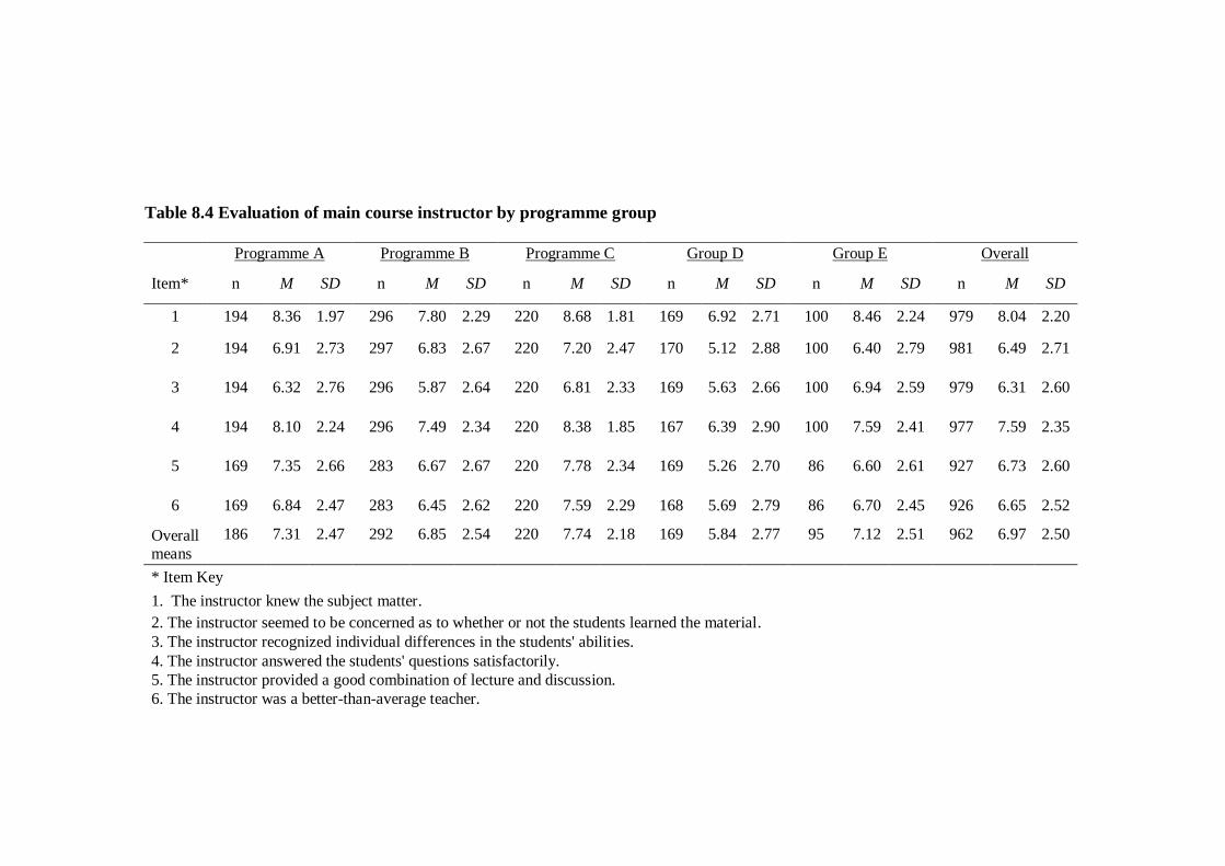
Table 8.4 Evaluation of main course instructor by programme group
Programme A Programme B Programme C Group D Group E Overall
Item* n M SD n M SD n M SD n M SD n M SD n M SD
1 194 8.36 1.97 296 7.80 2.29 220 8.68 1.81 169 6.92 2.71 100 8.46 2.24 979 8.04 2.20
2 194 6.91 2.73 297 6.83 2.67 220 7.20 2.47 170 5.12 2.88 100 6.40 2.79 981 6.49 2.71
3 194 6.32 2.76 296 5.87 2.64 220 6.81 2.33 169 5.63 2.66 100 6.94 2.59 979 6.31 2.60
4 194 8.10 2.24 296 7.49 2.34 220 8.38 1.85 167 6.39 2.90 100 7.59 2.41 977 7.59 2.35
5 169 7.35 2.66 283 6.67 2.67 220 7.78 2.34 169 5.26 2.70 86 6.60 2.61 927 6.73 2.60
6 169 6.84 2.47 283 6.45 2.62 220 7.59 2.29 168 5.69 2.79 86 6.70 2.45 926 6.65 2.52
Overall means
186 7.31 2.47 292 6.85 2.54 220 7.74 2.18 169 5.84 2.77 95 7.12 2.51 962 6.97 2.50
* Item Key
1. The instructor knew the subject matter.
2. The instructor seemed to be concerned as to whether or not the students learned the material. 3. The instructor recognized individual differences in the students' abilities. 4. The instructor answered the students' questions satisfactorily. 5. The instructor provided a good combination of lecture and discussion. 6. The instructor was a better-than-average teacher.
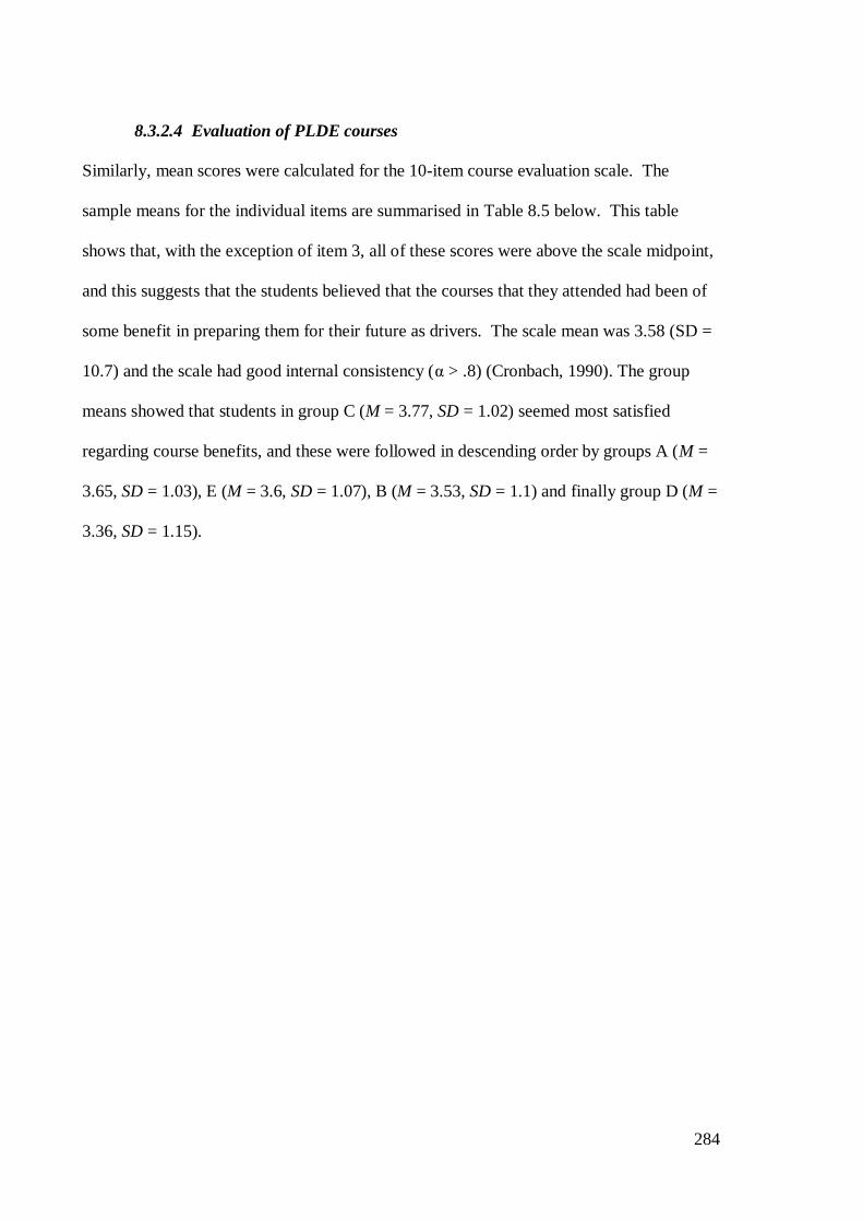
284
8.3.2.4 Evaluation of PLDE courses
Similarly, mean scores were calculated for the 10-item course evaluation scale. The
sample means for the individual items are summarised in Table 8.5 below. This table
shows that, with the exception of item 3, all of these scores were above the scale midpoint,
and this suggests that the students believed that the courses that they attended had been of
some benefit in preparing them for their future as drivers. The scale mean was 3.58 (SD =
10.7) and the scale had good internal consistency (α > .8) (Cronbach, 1990). The group
means showed that students in group C (M = 3.77, SD = 1.02) seemed most satisfied
regarding course benefits, and these were followed in descending order by groups A (M =
3.65, SD = 1.03), E (M = 3.6, SD = 1.07), B (M = 3.53, SD = 1.1) and finally group D (M =
3.36, SD = 1.15).
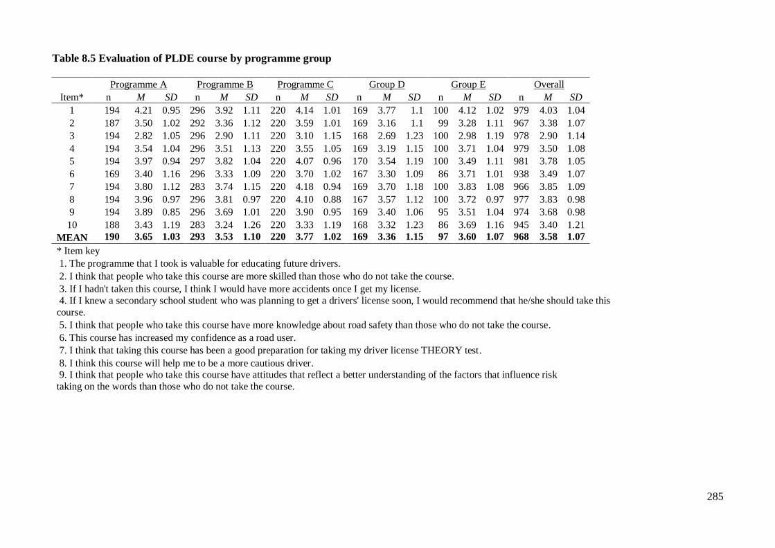
285
Table 8.5 Evaluation of PLDE course by programme group
Programme A Programme B Programme C Group D Group E Overall
Item* n M SD n M SD n M SD n M SD n M SD n M SD 1 194 4.21 0.95 296 3.92 1.11 220 4.14 1.01 169 3.77 1.1 100 4.12 1.02 979 4.03 1.04
2 187 3.50 1.02 292 3.36 1.12 220 3.59 1.01 169 3.16 1.1 99 3.28 1.11 967 3.38 1.07 3 194 2.82 1.05 296 2.90 1.11 220 3.10 1.15 168 2.69 1.23 100 2.98 1.19 978 2.90 1.14
4 194 3.54 1.04 296 3.51 1.13 220 3.55 1.05 169 3.19 1.15 100 3.71 1.04 979 3.50 1.08 5 194 3.97 0.94 297 3.82 1.04 220 4.07 0.96 170 3.54 1.19 100 3.49 1.11 981 3.78 1.05
6 169 3.40 1.16 296 3.33 1.09 220 3.70 1.02 167 3.30 1.09 86 3.71 1.01 938 3.49 1.07 7 194 3.80 1.12 283 3.74 1.15 220 4.18 0.94 169 3.70 1.18 100 3.83 1.08 966 3.85 1.09
8 194 3.96 0.97 296 3.81 0.97 220 4.10 0.88 167 3.57 1.12 100 3.72 0.97 977 3.83 0.98 9 194 3.89 0.85 296 3.69 1.01 220 3.90 0.95 169 3.40 1.06 95 3.51 1.04 974 3.68 0.98
10 188 3.43 1.19 283 3.24 1.26 220 3.33 1.19 168 3.32 1.23 86 3.69 1.16 945 3.40 1.21 MEAN 190 3.65 1.03 293 3.53 1.10 220 3.77 1.02 169 3.36 1.15 97 3.60 1.07 968 3.58 1.07
* Item key 1. The programme that I took is valuable for educating future drivers.
2. I think that people who take this course are more skilled than those who do not take the course. 3. If I hadn't taken this course, I think I would have more accidents once I get my license.
4. If I knew a secondary school student who was planning to get a drivers' license soon, I would recommend that he/she should take this
course.
5. I think that people who take this course have more knowledge about road safety than those who do not take the course.
6. This course has increased my confidence as a road user. 7. I think that taking this course has been a good preparation for taking my driver license THEORY test.
8. I think this course will help me to be a more cautious driver. 9. I think that people who take this course have attitudes that reflect a better understanding of the factors that influence risk
taking on the words than those who do not take the course.
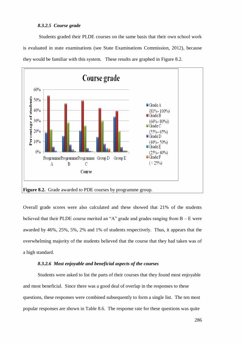
286
8.3.2.5 Course grade
Students graded their PLDE courses on the same basis that their own school work
is evaluated in state examinations (see State Examinations Commission, 2012), because
they would be familiar with this system. These results are graphed in Figure 8.2.
Figure 8.2. Grade awarded to PDE courses by programme group.
Overall grade scores were also calculated and these showed that 21% of the students
believed that their PLDE course merited an “A” grade and grades ranging from B – E were
awarded by 46%, 25%, 5%, 2% and 1% of students respectively. Thus, it appears that the
overwhelming majority of the students believed that the course that they had taken was of
a high standard.
8.3.2.6 Most enjoyable and beneficial aspects of the courses
Students were asked to list the parts of their courses that they found most enjoyable
and most beneficial. Since there was a good deal of overlap in the responses to these
questions, these responses were combined subsequently to form a single list. The ten most
popular responses are shown in Table 8.6. The response rate for these questions was quite
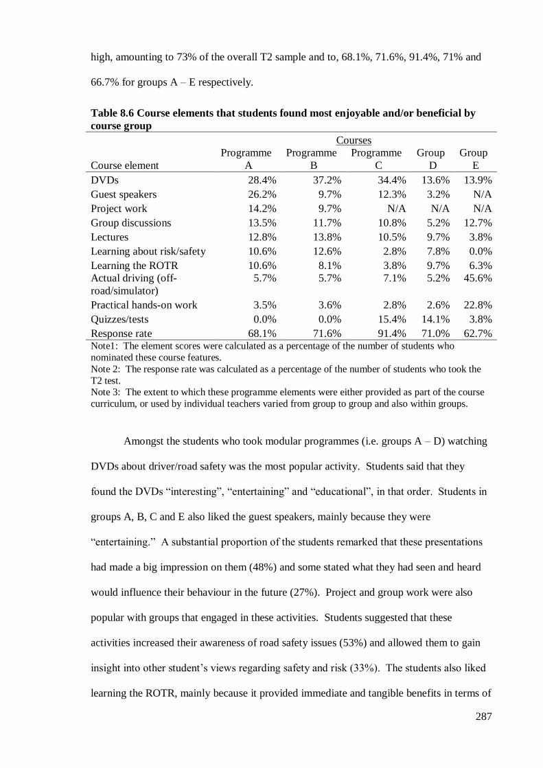
287
high, amounting to 73% of the overall T2 sample and to, 68.1%, 71.6%, 91.4%, 71% and
66.7% for groups A – E respectively.
Table 8.6 Course elements that students found most enjoyable and/or beneficial by
course group
Courses
Course element
Programme
A
Programme
B
Programme
C
Group
D
Group
E
DVDs 28.4% 37.2% 34.4% 13.6% 13.9%
Guest speakers 26.2% 9.7% 12.3% 3.2% N/A
Project work 14.2% 9.7% N/A N/A N/A
Group discussions 13.5% 11.7% 10.8% 5.2% 12.7%
Lectures 12.8% 13.8% 10.5% 9.7% 3.8%
Learning about risk/safety 10.6% 12.6% 2.8% 7.8% 0.0%
Learning the ROTR 10.6% 8.1% 3.8% 9.7% 6.3%
Actual driving (off-
road/simulator)
5.7% 5.7% 7.1% 5.2% 45.6%
Practical hands-on work 3.5% 3.6% 2.8% 2.6% 22.8%
Quizzes/tests 0.0% 0.0% 15.4% 14.1% 3.8%
Response rate 68.1% 71.6% 91.4% 71.0% 62.7% Note1: The element scores were calculated as a percentage of the number of students who
nominated these course features. Note 2: The response rate was calculated as a percentage of the number of students who took the
T2 test. Note 3: The extent to which these programme elements were either provided as part of the course
curriculum, or used by individual teachers varied from group to group and also within groups.
Amongst the students who took modular programmes (i.e. groups A – D) watching
DVDs about driver/road safety was the most popular activity. Students said that they
found the DVDs “interesting”, “entertaining” and “educational”, in that order. Students in
groups A, B, C and E also liked the guest speakers, mainly because they were
“entertaining.” A substantial proportion of the students remarked that these presentations
had made a big impression on them (48%) and some stated what they had seen and heard
would influence their behaviour in the future (27%). Project and group work were also
popular with groups that engaged in these activities. Students suggested that these
activities increased their awareness of road safety issues (53%) and allowed them to gain
insight into other student’s views regarding safety and risk (33%). The students also liked
learning the ROTR, mainly because it provided immediate and tangible benefits in terms of
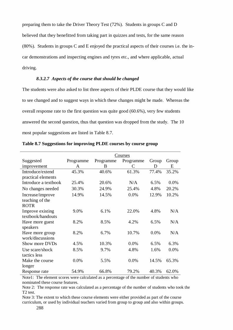
288
preparing them to take the Driver Theory Test (72%). Students in groups C and D
believed that they benefitted from taking part in quizzes and tests, for the same reason
(80%). Students in groups C and E enjoyed the practical aspects of their courses i.e. the in-
car demonstrations and inspecting engines and tyres etc., and where applicable, actual
driving.
8.3.2.7 Aspects of the course that should be changed
The students were also asked to list three aspects of their PLDE course that they would like
to see changed and to suggest ways in which these changes might be made. Whereas the
overall response rate to the first question was quite good (60.6%), very few students
answered the second question, thus that question was dropped from the study. The 10
most popular suggestions are listed in Table 8.7.
Table 8.7 Suggestions for improving PLDE courses by course group
Courses
Suggested
improvement
Programme
A
Programme
B
Programme
C
Group
D
Group
E
Introduce/extend
practical elements
45.3% 40.6% 61.3% 77.4% 35.2%
Introduce a textbook 25.4% 20.6% N/A 6.5% 0.0%
No changes needed 30.3% 24.9% 25.4% 4.8% 20.2%
Increase/improve
teaching of the
ROTR
14.9% 14.5% 0.0% 12.9% 10.2%
Improve existing
textbook/handouts
9.0% 6.1% 22.0% 4.8% N/A
Have more guest
speakers
8.2% 8.5% 4.2% 6.5% N/A
Have more group
work/discussions
8.2% 6.7% 10.7% 0.0% N/A
Show more DVDs 4.5% 10.3% 0.0% 6.5% 6.3%
Use scare/shock
tactics less
8.5% 9.7% 4.8% 1.6% 0.0%
Make the course
longer
0.0% 5.5% 0.0% 14.5% 65.3%
Response rate 54.9% 66.8% 79.2% 40.3% 62.0%
Note1: The element scores were calculated as a percentage of the number of students who
nominated these course features. Note 2: The response rate was calculated as a percentage of the number of students who took the
T2 test. Note 3: The extent to which these course elements were either provided as part of the course curriculum, or used by individual teachers varied from group to group and also within groups.
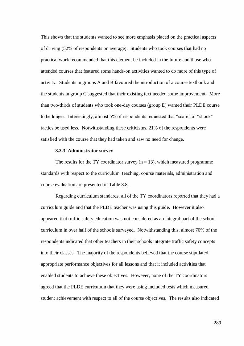
289
This shows that the students wanted to see more emphasis placed on the practical aspects
of driving (52% of respondents on average): Students who took courses that had no
practical work recommended that this element be included in the future and those who
attended courses that featured some hands-on activities wanted to do more of this type of
activity. Students in groups A and B favoured the introduction of a course textbook and
the students in group C suggested that their existing text needed some improvement. More
than two-thirds of students who took one-day courses (group E) wanted their PLDE course
to be longer. Interestingly, almost 5% of respondents requested that “scare” or “shock”
tactics be used less. Notwithstanding these criticisms, 21% of the respondents were
satisfied with the course that they had taken and saw no need for change.
8.3.3 Administrator survey
The results for the TY coordinator survey (n = 13), which measured programme
standards with respect to the curriculum, teaching, course materials, administration and
course evaluation are presented in Table 8.8.
Regarding curriculum standards, all of the TY coordinators reported that they had a
curriculum guide and that the PLDE teacher was using this guide. However it also
appeared that traffic safety education was not considered as an integral part of the school
curriculum in over half of the schools surveyed. Notwithstanding this, almost 70% of the
respondents indicated that other teachers in their schools integrate traffic safety concepts
into their classes. The majority of the respondents believed that the course stipulated
appropriate performance objectives for all lessons and that it included activities that
enabled students to achieve these objectives. However, none of the TY coordinators
agreed that the PLDE curriculum that they were using included tests which measured
student achievement with respect to all of the course objectives. The results also indicated

290
that the majority of schools (77%) did not provide their students with written information
regarding the criteria for the successful completion of the course.
Table 8.8 TY coordinator survey
Item Topic Yes No
CURRICULUM STANDARDS
1 Does the school have a curriculum guide for the TY pre-
learner driver course?
100% 0%
2 Does the course teacher have a copy of the curriculum and
follow it?
100% 0%
3 Is traffic safety education considered as an integral part of
the school curriculum?
46% 54%
4 Does the course stipulate appropriate performance
objectives for all lessons?
62% 38%
5 Does the curriculum include tests which measure student
achievements with respect to all of the course objectives? 69% 31%
6 Does the curriculum include tests for all of the course
objectives?
0% 100%
7 Do teachers of other subjects integrate traffic safety
concepts into their classes?
69% 31%
8 Are written criteria for successful completion of the course
given to all students?
23% 77%
TEACHING STANDARDS
9 Are course teachers selected on the basis of their academic
achievements and/or their experience with teaching traffic
safety education?
46% 54%
10 Have teachers/instructors received any certification before
teaching the course?
77% 23%
11 Is the course-related performance of the teacher/instructor
assessed regularly?
0% 100%
COURSE MATRIAL STANDARDS
12 Does the course contain sufficient amounts of quality
instructional materials to help students achieve the course
objectives?
77% 23%
13 Are supplementary teaching materials, lectures
demonstrations etc. related to driver and traffic safety
education used?
(i.e. elements that are not part of the main road safety
course)
69% 31%
14 If so, are these critically reviewed before use by school
authorities?
54% 46%
ADMINISTRATION AND EVALUATION
STANDARDS
15 Do students receive academic credit for the successful
completion of the course?
54% 46%
16 Are academic standards maintained on a par with those of
other courses?
62% 38%
(cont.)
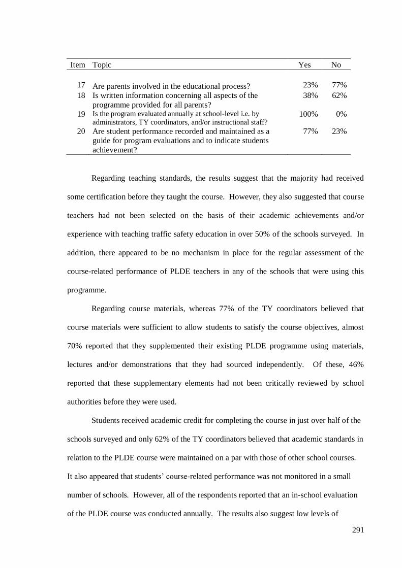
291
Item Topic Yes No
17 Are parents involved in the educational process? 23% 77%
18 Is written information concerning all aspects of the
programme provided for all parents?
38% 62%
19 Is the program evaluated annually at school-level i.e. by
administrators, TY coordinators, and/or instructional staff? 100% 0%
20 Are student performance recorded and maintained as a
guide for program evaluations and to indicate students
achievement?
77% 23%
Regarding teaching standards, the results suggest that the majority had received
some certification before they taught the course. However, they also suggested that course
teachers had not been selected on the basis of their academic achievements and/or
experience with teaching traffic safety education in over 50% of the schools surveyed. In
addition, there appeared to be no mechanism in place for the regular assessment of the
course-related performance of PLDE teachers in any of the schools that were using this
programme.
Regarding course materials, whereas 77% of the TY coordinators believed that
course materials were sufficient to allow students to satisfy the course objectives, almost
70% reported that they supplemented their existing PLDE programme using materials,
lectures and/or demonstrations that they had sourced independently. Of these, 46%
reported that these supplementary elements had not been critically reviewed by school
authorities before they were used.
Students received academic credit for completing the course in just over half of the
schools surveyed and only 62% of the TY coordinators believed that academic standards in
relation to the PLDE course were maintained on a par with those of other school courses.
It also appeared that students’ course-related performance was not monitored in a small
number of schools. However, all of the respondents reported that an in-school evaluation
of the PLDE course was conducted annually. The results also suggest low levels of

292
parental involvement with the PLDE course (23%) and the majority of the schools (62%)
do not provide parents with detailed written information about the course.
8.3.4 Teacher interviews
The semi-structured interviews that were conducted with the class teachers in nine
schools that had delivered programmes A (schools 1, 3, 4, and 5; n = 4) and B (schools 6,
9, 10, 11, and 13; n = 5). These interviews were conducted in private in either empty
classrooms or visitors’ reception rooms, during normal school hours, and lasted for 45
minutes on average. Since the main purpose of these interviews was to gather information
about the running of these courses the narrative that follows was based on a simple content
analysis of these interviews.
8.3.4.1 Course scheduling and implementation
All of the teachers thought that TY was the most suitable time for the delivery of
PLDE programmes such as programmes A and B. Details of scheduling arrangements in
the schools from which the interviewees were drawn are contained in Table 8.9.
Table 8.9 Example of course delivery schedules - Programmes A and B
School ID Programme Course duration Class time Class periods per week
1 A Entire year 45 1 X Single
3 A Entire year 45 1 X Single
4 A Entire year 45 1 X Single
5 A Entire year 45 1 X Single
6 B 12 weeks 20 2 X Single
9 B 8 weeks 20 1 X Single; 1 X Double
10 B 12 weeks 20 2 X Single
11 B 6 weeks 20 2 X Double
13 B 12 weeks 20 2 X Single
Programme A consists of 45 hours of tuition, which was delivered over the entire school
year in the groups that participated in this part of the study. Programme B consists of 20
hours of tuition, and schools varied as to how this time was planned. Teachers using
programme A expressed satisfaction with the course schedule and believed that this course
was neither too short nor too long. However, all of the programme B teachers mentioned

293
that they struggled to cover the entire course in the allotted time. Furthermore, all teachers
reported that course delivery had been disrupted as a result of competing demands from
other school and TY activities. The way that such conflict were typically resolved was
summarised by teacher 5, “Ah, it’s only road safety; let’s take them out of that”. Teacher 3
also noted “It’s very hard to get continuity, because they are doing such a wide range of
subjects here and a lot of them (students) are involved in sports and are off playing
matches when some of the classes are being held.....Then throughout the year we have
work experience, so they are gone for 4 weeks....It’s just a myth that there is loads of time
in TY to get things done” (teacher 3). Other activities that intruded on PLDE class time
included school trips, concerts and plays.
Given that teaching schedules were commonly disrupted, teachers liked the fact
that programmes A and B were designed to provide them with some degree of flexibility
with regard to the parts of the courses that are actually delivered and also with respect to
the amount of time that individual teachers spend focussing on the various aspects of the
course. There was unanimous agreement that this arrangement helped to ensure that their
students gain the maximum amount of exposure to the most important elements in the
courses. However, since the teachers were provided with no clear guidelines as to which
parts of the courses are most important in terms addressing the road safety needs of
adolescents; they had to rely on their own judgement in this regard. In school 1 for
instance “..what we do is pick and choose......what we think is relevant....to the
girls....where the dangers are and what should be highlighted”. Sometimes, however the
agenda was driven by student interests “...often you go in (to the lesson) with an
agenda....but very often somebody will put their hand up and say that they read a story in
the newspaper last week....or that their aunt had a crash, and this takes us in a different
direction...That’s the beauty of the course, it doesn’t have to be fixed” (teacher 3). All of
the teachers reported that they spent a lot of time focussing on programme section 2 -

294
“Killer Behaviours”, especially lessons 8 and 9 “Speed and Speeding” and lessons 9 and
10 “Alcohol and Driving”. All teachers covered lesson 23 “The driving test, motor tax and
insurance” and many reported that students were very interested in this lesson and were
somewhat surprised at the costs involved in motoring. All of the teachers recognized the
value of the various exercises contained in lessons 1 and 2, which seek to ascertain and
challenge student attitudes towards safe driving, “I spend a lot of time dealing with peer
pressure, the temptation of getting a lift home from the pub with a mate....” (teacher 3).
Nevertheless, the interviews revealed that some teachers had not completed all of these
exercises. “I saw the ‘moving debate’ being demonstrated during the in-service training
day, and I thought that it was a good idea, but we never actually got around to doing this in
class” (teacher 13). Eight of the nine teachers said that they spent little or no time on
lessons 26 and 27 “Driving abroad” because they believed that these had very little
immediate or practical relevance for their students. “That kind of stuff probably wouldn’t
appeal to them now.....they just want to get in and start driving from A to B” (teacher 3).
Lessons 6 and 7 “Safety belts/Child restraints/Airbags/Loose objects” was also skipped by
more than half of the teachers. Some reported that they spent very little time on lessons 3
and 4 “Pedestrians and Cyclists”, because “...the kids have had lots of classes on this
before now...” (teacher 13). Lessons 28 – 31 covers the ROTR, with the aim of preparing
students sufficiently to take the “Driver Theory Test” (RSA, 2008). This part of the course
is supported by a CD containing over 1,000 power point slides depicting theory test
questions and a template for testing student knowledge. However, the amount of time that
the teachers devoted to using these resources varied considerably across all 13 schools that
were delivering programmes A and B30
. Irrespective of whether they were delivering
programme A or B, it appeared that some teachers adopted a systematic and thorough
approach when it came to covering the ROTR (30%), others preferred to “dip in and out”
30 This information was derived on the basis of the teacher interviews and also personal
communications with the teachers who did not participate in the interviews.

295
of this material (55%) and the remainder (15%) spent little or no time on this part of the
course. For instance, two teachers said that they didn’t cover anything related to the theory
test because they assumed (incorrectly – see footnote 4) that the students were too young to
benefit from this aspect of the course. “The material is there, but a lot of them are 16,
they’re not ready, so I’m open to correction, if you do get your theory test, you have to
apply for your driving test within 6 months”31
(teacher 1).
8.3.4.2 Programme materials, activities and recourses
All of the teachers who were interviewed were satisfied that the curriculum for
programmes A and B goes a long way towards addressing the needs of PLDs with respect
to driving-related knowledge, risk awareness and attitudes. Several teachers said that they
would like to see a student textbook introduced as part of these courses. They opined that
this would eliminate the “hassle” and the wastefulness involved in photocopying
worksheets and other course materials for every student in their classes. Teacher 6 also
noted that “If they (the students) had a textbook, then at least they would have something
physical, so that they see a progression, and have something to refer back to in the future.”
All of the teachers suggested that the students should receive some form of official
certificate to show that they had attended the course which could then be included as part
of their TY portfolios.
Although all of the interviewees said that they had done some of the group
exercises and project work that was outlined in the course manual, none of them had
completed all of these course elements. For example, whereas lessons 1 and 2 include very
valuable group exercises i.e. a moving debate, which is designed to identify student
misperceptions about road safety and a group discussion about the consequences of an
RTC, just 2 of the teachers that were interviewed said they used the former and only 5 had
used the latter.
31 In actual fact, adolescents are allowed to take the Driver Theory Test at 16-year-of-age and the
outcome remains valid for two years (RSA, 2012).

296
Whereas all of the teachers agreed that the DVD resources for these courses are of
a good standard and that students liked watching them, many teachers reported that they
had also accessed and used additional audio-visual materials in order to reinforce the road
safety messages that are contained in programmes A and B. “What works really well is
my supplementary material; the stuff I use to reinforce the point. You can get clips from
the Rehabilitation Centre and clips with parents who have lost a child in a crash. Stuff that
shows real people, telling real stories about their experiences and its real hard-
hitting....There’s no substitute for this kind of stuff. You can show them three or four
times a year and they (the students) are still glued to it” (teacher 6). All of the teachers
mentioned that they wanted the course providers to make more resources available and
some suggested that this could be done online, using a web portal.
Programmes A and B also contain some provision for inviting guest speakers. For
instance a Garda speaker can be invited to deliver the “It Won’t Happen to Me”
presentation, which deals with the causes and consequences of RTCs, and challenges
perceptions of personal invulnerability. A visit can also be arranged from National Car
Testing Service (NCTS) personnel, who talk about preparing for the NCT test and the
driving test. However, whereas all of the teachers that were interviewed were interested in
inviting these guest speakers to their schools, only three of them actually succeeded in
arranging a visit from the Gardaí and just one had managed to arrange a visit from the
NCTS. Teachers noted the difficulties involved in scheduling such visits, e.g. difficulty in
contacting the relevant individuals and arranging a mutually acceptable time for the
presentations to take place. Thus it appears that these resources are under-utilised.
However, it emerged that some teachers had used their own initiative and sourced
alternative guest speakers and some even provided supplementary courses. For instance,
teachers in schools 1, 3, 5, 6, and 10 reported that they had used the car and road safety
demonstration that is listed in Appendix A (p. 407) as part of their course. Schools 3 and 6

297
had provided course E1 (see Appendix A) in addition to their main PLDE programme.
Students in schools 5 and 6 also attended a driver training session, the former using a
driving simulator and the latter attended course E2 (see Appendix A).
8.3.4.3 Programme context
Three of the teachers commented on the issue of programme context. They spoke
about the efforts that had been made to integrate road safety into the broader second-level
curriculum in their schools. “I think it’s critical to have the science people (teachers) on
board. They can demonstrate important principles such as the effects of speeding, stopping
distances, reaction times....” (teacher 6). The teacher in school 10 spoke about the culture
of road safety that had been developed in that school. “I don’t think it’s a subject, it’s a
moral issue, It is part of what we are, part of our being....I suppose, in tandem with all the
theory, we try to put out awareness and I find it’s the awareness that brings them into the
whole notion of being safe, of knowing.....of a basic understanding”.
8.4 Discussion
This discussion will begin by providing some general observations regarding the
PLDE provision for TY students, placing particular emphasis on the five types of courses
that were delivered in the schools that participated in this research. Thereafter the focus
will shift towards reviewing the curriculum that formed the basis for programmes A and B.
8.4.1 Review on the provision of PLDE for Irish adolescents
TY is an optional feature of second level education in the ROI and during 2008,
when this research was being planned, the TY curriculum was being delivered in 71% of
secondary schools. However, since not all schools provide TY and since some of those
who do provide TY do not deliver PLDE as part of that curriculum, it was noted that a
sizeable proportion of Irish secondary school students are not provided with the
opportunity to attend a PLDE course during their last two years in secondary school.

298
Current thinking within the road safety research community (e.g. Christie, 2001; Fuller &
Bonney, 2004; McKenna, 2010b) suggests that the benefits of taking road safety education
accrue from regular and frequent attendance at these courses. It was noted in Chapter 5 that
the RSA have developed a range of road safety programmes which serve to provide regular
and frequent exposure to road safety messages as part of their educational strategy. Thus,
the failure of some schools to provide PLDE courses for adolescents in the latter part of
their secondary schooling, and at a time when many of these students will be considering
learning to drive, could be regarded as something of a departure from this strategy.
In addition, since TY curriculums are decided at school level rather than at national
level, there is very little uniformity with respect to the quantity or the quality of the PLDE
that is provided for TY students who do take these courses. As a result, there are wide
variations in what PLDE means from one school to the next. Moreover, whereas the
course manuals for programmes A, B and C state clearly that these programmes comply
with NCAA criteria for second level courses, it remained unclear as to whether the
developers of the remaining courses had taken these criteria into account when compiling
their courses. Thus, there appears to be a need to develop an oversight mechanism
whereby courses that are provided for TY students are examined by the relevant authorities
to ensure that better and more uniform curriculum standards are applied in this area.
Lonero (2008) suggests that the development of such standards would serve to help
schools to become more successful in providing and administering uniform PLDE courses
that use the most up-to-date content and delivery techniques This in turn would help to
ensure that TY students get the best available PLD education as part of their secondary
schooling.
The PLDE courses that featured in the current research are used widely in the ROI,
and thus can be considered as reasonably representative of these types of interventions.
However, there were notable differences between these courses with respect to their
299
structure and durations. For instance whereas programme A was delivered across the
entire school year and involved 45hours of class time, programmes B C and D were
delivered in one school term and involved 15 -20 hours of tuition and those taken by
students in group E were completed in just one day. Whereas many students in this study
were satisfied with the course that they had taken, it was notable that over two-thirds of the
students who had taken the one-day courses indicated that they wanted to receive more
PLDE. Although no between-groups comparisons were conducted to test for the effects
that these differences might have had on student outcomes, because this was beyond the
scope of the current research, it is clear nonetheless from a theoretical perspective that
longer courses provide the students with more opportunity to interact with course materials
and processes and for this reason alone they might be more likely to produce desirable
changes in terms of increased knowledge and awareness than are shorter courses (see for
example Ericsson et al., 1993; Kolb, 1984).
The results of the student survey indicated that a substantial proportion of the
students surveyed rated the course that they had taken quite highly. Moreover, the course
evaluation scores suggest that the students believed that the PLDE course that they had
attended was of some value in terms of providing them with the types of driving-related
knowledge, skills and attitudes which would enable them to become good drivers in the
future. However, it was also clear that many students wanted PLDE to address their
instrumental needs more directly by providing content that deals with the practical side of
driving and that would help them to study the ROTR. Empirical evidence suggests that
PLDE courses should focus on addressing student’s developmental needs rather than on
satisfying their instrumental needs because the latter encourages earlier licensure which
increases exposure to risk, and thereby defeats the purpose of such education (Roberts &
Kwan, 2001). Encouragingly, the current results showed that very little, if any practical
hands-on experience was provided as part of the PLDE courses that featured in this study.
300
However, it is clear that student expectations regarding the provision of instruction in the
ROTR were reasonable, given that 80% of the students in this study expressed an intention
to obtain a learner driver permit as soon as they could do so legally (i.e. at 17-years-old)
and that passing a Driver Theory Test is a fundamental requirement for obtaining this
licence. Students were enthusiastic about learning the ROTR and partaking in other
activities that they believed provided immediate benefits, e.g. passing the driver theory
test. A review of syllabuses for the modular courses that featured in this study (A-D)
indicated that these did in fact provide reasonably comprehensive coverage of the ROTR,
albeit that the extent to which this material was covered by individual classes varied
substantially between school groups. This issue will be dealt with in more detail shortly.
The students also reported that they had benefitted from participating in group and
project work, mainly because it provided them with insight into peer opinion regarding risk
taking and road safety generally. They also enjoyed attending presentations by guest
speakers, who seem to have made such a strong and enduring impression on some students,
they reported that what they had seen and heard during these presentations would influence
their future behaviour.
8.4.2 Formative evaluation of programmes A and B
A more detailed analysis of the curriculum that formed the basis of programmes A
and B was conducted. Since these courses differed only in terms of their duration, in the
interest of brevity these will be referred to collectively as “the programme” for most of this
discussion. The review that follows was based on the data from the student surveys, the
TY coordinator surveys and the teacher interviews. All references to TY coordinators,
teachers and students in this part of the discussion are applicable to individuals who used
programmes A and B. It should also be noted that in the absence of an official programme
curriculum, the teacher manual for these programmes served as a de facto curriculum for
the purpose of this review.
301
8.4.2.1 Aims, goals and objectives
The stated mission of the body that developed these programmes is “To make roads
safer for everyone.....to save lives and prevent injuries by reducing the number and severity
of collisions on the road”, and education is regarded as a “key pillar” in achieving these
aims (RSA, 2013a). A detailed inspection of the curriculum, revealed that whereas a clear
set of learning objectives have been provided for the individual lessons, no attempt has
been made to describe the overall aims, goals and objectives of the programme. Further
enquires established that such overall aims, goals and objectives are not communicated
explicitly to course teachers at any stage (i.e. during in-service training or in the form of
supplementary materials) (personal communication with Christine Hegarty, Education
Officer, RSA, on 18/1/2013). Clinton and Lonero (2006c) suggest that good programmes
are developed on the basis of a programme theory, i.e. a set of assumptions that direct the
way the programme is implemented and expected to produce results. This theory is best
expressed in the form of a graphical representation (a logic model) which shows what is
supposed to happen by specifying how the various elements in the programme are
expected to combine to produce change and thus achieve its goals. Such logic models are
also useful for communicating the goals and objectives to stakeholders and thereby help to
develop a common understanding of the programme and its intended outcomes. Since the
current findings indicate that there is a lack of clarity about the ways in which the activities
of this course are expected to improve road safety, it is recommended that a logic model be
developed for this course. This should be included as part of the course introduction and a
copy of this should be provided for all students and stakeholders (e.g. parents, school
authorities, the NCCA).
302
8.4.2.2 Addressing student and stakeholder needs: programme content and
activities
The review of curriculum and the attendant DVD resources revealed that these
contain materials and activities that have been designed to provide for students’
instrumental and developmental needs within the context of the higher levels of the GDE-
framework (see Hatakka et al., 2002). They incorporate content and activities that aim to
increase factual knowledge (e.g. the ROTR and procedural information regarding driver
licencing, motor tax and insurance); to improve awareness of factors that increase risk for
drivers, and to improve attitudes towards driving. When interviewed, the teachers reported
that they were satisfied that this curriculum has the capacity to address student needs as
stated above. However, whereas the students expressed a clear interest in studying the
ROTR to prepare themselves for taking the Driver Theory Test, and some expected that the
course would help them to do so, the majority of the teachers reported that they did not
cover this aspect of the course thoroughly. Nevertheless, all teachers reported that they
covered the material pertaining to driver testing, and motor tax and insurance. Thus,
whereas the course is theoretically capable of addressing students’ instrumental needs in
terms of providing knowledge about the ROTR and information about the practical aspects
of motoring, the results from this study shows that student needs with respect to the ROTR
were not always satisfied in practice.
The curriculum review found that the programme also included a variety of
materials and activities that were relevant to addressing the developmental needs of PLDs.
For instance, it places a lot of emphasis on increasing students’ awareness with respect to a
range of important state- and situation-dependent factors that are known to increase risk for
drivers generally (the so-called “Killer Behaviours” such as speeding, driving after
drinking or taking drugs, driver fatigue). However, given that it is well-established that
inexperience, immaturity, and gender constitute the primary state dependent risk factors
303
for young learner and novice drivers (Arnett et al., 1997; L. Evans, 1991; McKnight &
McKnight, 2003; OECD - ECMT, 2006b; Twisk & Stacey, 2007), it was surprising to find
that the programme does not deal with any of these topics directly i.e. as topics in their
own right. Findings reported in Chapter 6 of this study and also from previous research
(e.g. Ginsburg et al., 2008) show clearly that adolescents do not have a proper
appreciation of what it means to be inexperienced as a driver, thus it is reasonable to
expect that a good PLDE course would address this issue. Likewise, whereas the GDE-
framework (Hatakka et al., 2002) suggests DE programmes ought to include content and
processes that have been designed to help students to gain insight into their personal risk-
increasing tendencies (e.g. impulsiveness, sensation seeking) and should provide them with
strategies to help them to control such motivational states, the issue of personal tendencies
is not dealt with directly in this course. Finally, since it is widely-accepted that young
males are more likely than young females to engage in unsafe driving behaviours, such as
speeding, and DWI (Harré et al., 1996), and that the risk of crashing for young male
drivers is higher than it is for all other groups (Twisk & Stacey, 2007), the failure to
address this topic directly as part of a PLDE programme represents a significant omission.
Evidence suggests that in comparison with young females, young males tend to lack
awareness of their risk status as learner and novice drivers (DeJoy, 1992). For example, in
a study conducted by Gormley and Fuller (2008) with 734 young male drivers, 32
respondents challenged the veracity of some of the questions that were asked, saying that
did not believe that young male drivers are at the most risk of crashing. This suggests that
there is a need to convince young male students about their actual risk status as learner and
novice drivers. Petty and Cacioppo’s ELM theory (1986) suggests that persuasive
materials should be presented though central and peripheral routes. The programme
curriculum appears to rely heavily on the peripheral method when informing students
about the dangers involved in driving (i.e. showing DVDs of RTCs and their
304
consequences). However, the direct route should also be used to provide students with
factual information about the types of risks that they face as young, inexperienced and
where applicable, male drivers. For instance, students should be provided with a detailed
account of where, when, how and most importantly why they are more likely to have an
RTC than are older, more experienced drivers.
The GDE-framework (Hatakka et al., 2002) highlights the importance of reflexive
practice in the development of safe driving habits. Furthermore, Kolb’s ELT (1984)
proposes that students learn best when reflexive practice is combined with the formulation
of enactment strategies. In this regard, it espoused in psychological research that
behavioural intentions, as described within the TPB (Ajzen, 1991), constitute reasonably
reliable predictors of behaviour (Armitage & Connor, 2001). According to Gollwitzer
(1999) the formulation of an implementation strategy helps to crystallize intentions by
specifying when, where and how an intended goal can be achieved. For example, an
implementation intention with respect to speeding might take the form of “When I start
driving, I will adhere to the speed limit.” It is assumed that as a result of having already
formed a mental representation of this situation, the desired response will occur with some
degree of automaticity subsequently (Bargh & Williams, 2006).
A recent meta-analysis of the results of 94 studies involving implementation
intentions indicated that the formulation of implementation intentions had a medium-to-
large positive effect (d = .65) on goal attainment (Gollwitzer & Sheeran, 2005). Research
conducted in the traffic domain also supports the utility of implementation intentions for
improving driver behaviour. Delhomme, Kreel, Ragot (2008) studied 624 of convicted
speeders who attended a rehabilitation training course, some of whom made a public
commitment to observe the speed limits in the future and some who did not. Their results
showed that the incidence of speeding decreased significantly in the active ‘commitment’
group, in comparison to the ‘no commitment’ controls in the short-term and this effect was
305
still evident five months after the intervention ceased. These studies suggest that the
inclusion of mechanisms which encourage students to formulate implementation intentions
in relation to key course objectives is likely to increase the effectiveness of PLDE
programmes. Thus the feasibility of developing such mechanisms and including them as
part of the programme curriculum should be investigated.
Encouragingly, this review found that the curriculum incorporates many elements
that are known to facilitate student learning, some of which were outlined in the
introduction to this chapter. The programmes are delivered over an extended period of
time and the safety messages that they aim to convey are reiterated in a variety of ways
during that time. Since the programmes are relatively long, students are given ample time
to think about the material and to discuss it with their classmates. Some of the materials
and processes (e.g. the DVDs and the media tracking exercise) have the potential to evoke
emotional reactions and students are provided with opportunities to explore these as
individuals and as part of a peer group. Notably however the course does not provide clear
and consistent mechanisms whereby student performance can be assessed in relation to the
course objectives. This apparent failure to produce timely feedback constitutes a
significant weakness in the course structure because it is known that student learning is
improved when they receive regular and timely feedback on their performance (Bransford
et al., 2000; Skinner, 1974).
8.4.3 Programme standards, business processes and context
The results of the part of the study that focussed on programme standards, business
process and context revealed a number of problems, the most notable of which was the
lack of proper programme implementation standards.
For instance, one would have to question the rationale for basing two programmes,
one of which involves more than twice the amount of class time than does the other, on a
single curriculum, when that curriculum provides no guidelines as to how class time ought
306
to be spent. The curriculum was designed such that that the teachers and administrative
staff are given a considerable amount of latitude regarding the way in which the
programme is implemented. In the absence of a programme logic model and clear
guidelines about which parts of the course are central for addressing the driving-related
needs of PLDs and which are more peripheral, teachers are forced to make subjective
judgements about which parts of the programme they should include and which parts they
should leave out. During the teacher interviews it emerged that teachers were in favour of
this arrangement, because it helped them to ensure that their students received maximum
exposure to important content. Whereas it is acknowledged that teachers do have the
required expertise to deliver the programmes, it is clear that few, if any, teachers are
sufficiently expert in the area of road safety to make independent decisions regarding
programme implementation.
The current results also indicate that programme implementation was also disrupted
due to competition for classroom time from other school activities. Research suggests that
such problems are commonplace in the U.K (MVA Consultancy, 2009) and across Europe
(European Commission, 2005). Research also indicates that disputes regarding programme
implementation are more likely to arise where the administrative authority within an
organization is weak and is less supportive of the programme (Rohrbach et al., 2006). The
results of the current study suggest that, in some schools, road safety education is judged as
less important that are other school activities. They show that, in some schools, PLDE is
not regarded as an integral part of the school curriculum and that the standards that are
applied with respect to the content, delivery and assessment of the PLDE curriculum are
lower than those that are commonly applied to other second level courses. None of the
schools in the current research conducted regular evaluations of their PLDE teachers’
course-related performance, which is somewhat worrying, because the results also showed
many schools do not take academic performance or experience with teaching traffic safety

307
courses into account when they appoint a teacher to deliver PLDE. Furthermore, although
the all of the TY coordinators reported that their schools evaluate the programme on an
annual basis, it appeared that the use of supplementary (non-course) materials was
condoned in the majority of the schools and that such materials were not always critically
reviewed by school authorities. These results indicate that contextual factors can have a
major effect on the operation of these PLDE programmes. This suggests that there is a
need to develop proper programme standards for these courses.
The failure to develop programme standards for programmes A and B and the
subsequent findings that there was no real uniformity in the ways that the schools in this
study implemented these programmes, severely limits the ability of the current research to
reach wholly reliable and valid conclusions with respect to the efficacy and effectiveness
of these programmes. This issue will be discussed in more detail in the next chapter.
The main strength of this part of the study was that it used both quantative and
qualitative methods to examine student reactions to their PLDE courses and also the
approaches that school management and staff took to implementation and delivery of the
curriculum that formed the basis of programmes A and B. Whereas the schools that
participated in this research can be considered as being reasonably representative of
schools in the ROI, it is acknowledged nonetheless that due to operational constraints the
school-level sample in this research was quite small and the sample for the teacher
interviews was smaller still.
8.4.3.1 Recommendations
The following recommendations are made on the basis of the findings from this
part of the study:
1. Standards and guidelines should be devised for overseeing courses that are
provided for TY students to ensure programme quality with respect to content,

308
delivery, and monitoring and also programme administration and
teacher/instructor qualifications.
2. A study should be conducted to examine the feasibility of providing PLDE for
all adolescents during the senior cycle of secondary school.
3. A review of the programme A and B curriculum should be conducted with a
view to developing separate curriculums for these two programmes. This needs
to be done so that adequate programme standards can be devised.
4. A programme theory should be developed for programmes A and B; this should
include a logic model, which clearly demonstrates the relationship between
programme objectives, goals and aims. This will help programme users and
other stakeholders to understand how the programme is supposed to work to
produce safety-related outcomes.
5. School is an ideal setting for learning the ROTR and student expectations with
regard to the provision of ROTR training should be met as part of their PLDE
course.
6. PLDE courses should aim to address important state-dependent factors that are
affect the driving-related cognition, affect and behaviour of adolescents i.e.
immaturity, inexperience, and gender.
7. New content and activities should be developed which have a sound basis in
theory and a proven record of success in the field. Such activities might include
work around implementation intentions, the use of social influence and
modelling and greater parental involvement in course activities.
8. Tests of learning outcomes should be developed and used at various intervals
during the course. The results from such tests will provide students with timely
feedback about their progress and will allow teachers and school authorities to
monitor programme effectiveness.

309
9. The feasibility of producing a course textbook should be examined.
10. A web portal should be developed where teachers can access approved
supplementary materials, up-to-date information about road safety issues that
are relevant to the course and course updates.
310
Chapter 9: General discussion
The aim of this research was to evaluate road safety interventions which have been
designed for PLDs and which are delivered as part of the TY curriculum in secondary
schools in the ROI. This chapter serves to summarise key findings from this project and to
consider the possible theoretical, educational, research, and policy-related implications of
those findings.
The theoretical framework for the current research was formulated on the basis of a
review of empirical and theoretical evidence pertaining to driver behaviour, to human
behaviour generally, and to driver education which was presented in Chapter 1. This was
influenced by three behavioural models; the TCI (Fuller, 2005), which exemplifies
motivational models of driving behaviour; the TPB (Ajzen, 1991), which is a widely used
socio-cognitive model of general behaviour and the PWM (Gibbons & Gerrard, 1995),
which focuses on the social reactive route to risk taking. In addition, the GDE-framework
(Hatakka et al., 2002) was used to provide a strong theoretical basis for defining
appropriate goals and targets for driver education. The evaluation strategy that was used
was based on best practice guidelines developed for the AAA Foundation for Traffic
Safety (Clinton & Lonero, 2006a, 2006b, 2006c). Thus informed, the current research
used hierarchical linear modelling techniques (HLM) with the objective of explaining
variations in driving-related knowledge, risk perception skills and attitudes in Irish
adolescents as a function of intra-student (age and time), between-student (demographics
and individual differences) and between-groups factors (differential exposure to PLDE).
9.1 Summary findings from the summative evaluation
The following review of the main findings from the summative evaluation will be
discussed in terms of the research hypotheses. First however, a summary of the findings
from the baseline test will be presented, since these serve to contextualise the research
findings. A review of the item and scale means from the initial test revealed that the
311
students in this sample possessed a moderate amount of declarative knowledge regarding
the ROTR at the start of TY, year 12/year 13 in secondary school (mean age
approximately 16-years). Likewise, since the mean scores recorded for risk perception
were close to the mid-points on the relevant scales, it appeared that the students were
somewhat capable of perceiving driving-related risk. Similarly, mean scores obtained in
tests that measured attitudes towards speeding with respect to behavioural beliefs and
subjective norms were close to the scale mid-points, which indicated that the students in
this sample did not have particularly risky attitudes towards speeding. The results also
suggested that the students perceived that they had some degree of control when it came to
travelling with drivers who have a reputation for speeding, albeit that they were marginally
more willing than unwilling to do so. Moreover, the students’ mental representations
(prototypical images) of drivers who engage in speeding were more negative than they
were positive. Taken as a whole, these findings suggests that although there was some
scope for PLDE to work to produce improvement in knowledge, risk perception and
attitudes towards speeding during the course of this study, such changes were likely to be
small in magnitude. Nevertheless, since this information serves to increase our
understanding of PLDs it should be of interest to stakeholders, traffic safety researchers
and programme developers.
Study hypothesis 1, which posited that there would be significant variations in
driving-related knowledge, risk perception skills and attitudes of participating students at
intra-student, between-student and between-groups levels, at the outset of this study, was
supported. A review of the model fit indices for the null model estimates supported the
latter two predictions. In addition, a review of the plausible values ranges in these models
showed that on average, the intra-student variation estimates were more than double those
of the between-student estimates and over four times greater than the between-group
estimates, supporting the first prediction.
312
Hypotheses 2 and 3 predicted that there would be significant changes in driving-
related knowledge, risk perception skills and attitudes in the sample in both the short-term
(i.e. in the intervention phase) and the long-term (i.e. in the interim between the initial and
the final test). The results derived from the model 2 estimates demonstrated that there was
a small, significant increase in knowledge proficiency in this sample in both the short-term
and the long-term. Small significant improvements in risk perception were also evidenced
in the short-term but not over the longer-term. However, whereas previous research
suggested that attitudes towards driving among adolescents tend to become riskier over
time (Harré et al., 2000; Lonero et al., 2000), the results from this study did not wholly
support such a conclusion. While small short-term increases were seen with respect to
perceptions that the peer norm favoured speeding and expectations of travelling with
speeders, motivation to comply with this norm waned and motivation to comply with
parental perceived parental norms strengthened, as did tendencies to view prototypical
speeders negatively. Although many of these effects did not persist over the longer-term,
small significant decreases in motivation to comply with peers and in positive impressions
of prototypical speeders were evidenced between the initial and the final test in this study.
As a result of these findings it is recommended that PLDE programme developers should
aim to support the positive trends evidenced by these data. This issue will be discussed in
due course.
Hypothesis 4 predicted that students who attended a PLDE course during TY would
gain significantly more driving-related knowledge, better risk perception skills and better
attitudes towards driving than would students in the non-PLDE control group. Likewise,
hypothesis 5 posited that students who attended any of the specific PLDE courses that
featured in this study (i.e. courses A – E) would achieve significantly greater
improvements with respect to driving-related knowledge, risk perception skills and
attitudes than would those in the controls. Regarding knowledge, it was found that
313
students who attended a PLDE course gained significantly more knowledge than did the
controls in the short-term but not over the longer-term. This concurs with previous
findings (e.g. Elkington, 2005; Harré & Brandt, 2000a; Poulter & McKenna, 2010) and
thus lends additional support to the assertion that PLDE is effective in providing students
with driving-related declarative knowledge in the short-term. The present research also
showed that students who attended popular modular PLDE programmes (i.e. programmes
A, B and C) gained significantly more knowledge over the short-term than did the controls.
Furthermore, those who attended programme B gained significantly more knowledge over
the longer-term than did the controls. However, since it was also shown that the amount of
time that was devoted to studying the ROTR by the individual groups in this sample varied
considerably, no firm conclusion could be reached regarding the efficacy of individual
programmes in increasing driving-related knowledge. Predictably, groups that devoted
more attention to studying the ROTR gained significantly more knowledge in the short-
term, albeit that some of this knowledge was lost over the longer term. It was also noted
that the trend in the data with respect to the control group reflected that of the active PLDE
groups, which suggested that the control students were studying the ROTR independently
in order to prepare themselves for the Driver Theory Test.
The results from the current study indicated that attendance at PLDE did not result
in significant changes in driving-related risk perceptions or attitudes towards speeding in
the desired (less-risky) direction for the majority of the analyses that were conducted.
These results do not support the findings from previous studies, which reported small
short-term improvements in attitudes as a result of exposure to PLDE (e.g. Elkington,
2005; Harré & Brandt, 2000a). On the one hand, the present study used a far more
extensive range of predictor and outcome variables than did previous PLDE evaluations,
and thus probably constituted a more valid measure of driving-related risk perception and
attitudes. On the other hand however, the possibility that the present study was somewhat
314
underpowered cannot be ruled out entirely. Whereas the overall sample size was very
large, the number of school groups from which the sample was derived fell just short of the
criteria suggested by (Kreft, 1996). This issue was discussed in detail in Chapter 2.
Interestingly, the current findings indicated that attendance at PLDE resulted in
significant improvements in the cognitive availability and accessibility of some types of
negative outcomes in response to a vignette depicting a high risk scenario over the short-
term but not over the longer-term. Furthermore, attendance at PLDE was also associated
with a significant deterioration in positive sentiment towards prototypical speeders in both
the short- and the long-term. When taken as a whole however, these results suggested that
PLDE was not particularly effective in improving driving-related knowledge, risk
perception skills and attitudes in this sample.
Hypothesis 6 predicted that initial levels of, and changes in, knowledge, risk
perception skills and attitudes in this study would be influenced by a range of distal and
proximal between-student factors. Although 14 between-student variables were examined
as part of this research, only five of these predictors, three distal factors (gender,
impulsiveness and sensation seeking) and two proximal factors (exposure to aberrant
driving practices and experience with using vehicles) were shown to impact significantly
on students’ knowledge, risk perception skills and attitudes. Moreover, the effects were
evident mostly in the pre-intervention tests and were small in magnitude. No significant
effects of SES, the Big-Five personality traits, domicile location or direct and indirect
experience with crashing were found in any of the tests. Contrary to expectations, no
significant interaction effects were found between the between-student and the between-
groups factors.
9.2 Summary findings from the formative evaluation
Formative evaluations are conducted to ensure that the goals of educational
interventions are being achieved and to help to further the development of such
315
interventions by identifying problematic aspects of these interventions and suggesting
possible improvements (Clinton & Lonero, 2006b). The results from the current student
evaluation survey showed that students who had attended PLDE were generally satisfied
with these courses. However, many students requested that PLDE be improved to ensure
that their instrumental needs were catered for more fully through the inclusion of more
content relating to the practical aspects of driving (e.g. in-car driver training, improved
coverage of the ROTR). However, since research suggests that the provision of driver
training promotes early licensure (Roberts & Kwan, 2001) it was encouraging to note that
the majority of the courses in the current research did not provide in-car training as part of
their curricula. However, it was recommended that coverage of the ROTR be introduced
or improved where necessary. Students also reported that they had benefitted from
attending guest speaker presentations (the topic of positive role models will be discussed in
more detail below).
Since the courses that featured in this study differed considerably in terms of
structure, duration and content, no attempt was made to make direct comparisons between
these courses. Instead, the detailed formative analysis was conducted on two programmes
of the featured programmes (i.e. programmes A and B), the results of which were
described in detail in Chapter 8. In sum, it was concluded that these programmes
incorporated many of the features that are suggested in the higher levels of the GDE matrix
(Hatakka et al., 2002). It was recommended that the feasibility of developing new and
improved content and processes be investigated e.g. implementation intentions. Concerns
were raised about the policy of basing two programmes, which differed substantially in
terms of duration on a single curriculum, without providing teachers with a clear indication
of programme goals and detailed instructions about how the programmes should be
implemented. The negative consequences of this policy were evidenced in the teacher
interviews, which showed that teachers routinely made subjective judgements regarding

316
programme implementation. It was acknowledged that this situation posed a serious threat
to the internal validity of the current research (see Onwuegbuzie & McLean, 2003), to the
extent that no firm conclusions could be reached regarding the efficacy of these
programmes at this time. It was recommended that separate curricula be developed for
these programmes and that logic models should be developed in order to communicate
programme aims, goals and objectives to school authorities, teachers, students, parents and
other interested stakeholders. It was noted that some schools do not regard PLDE as an
integral part of the curriculum and that the standards applied regarding programme content,
delivery and assessment are inferior to those that are commonly applied to other second-
level courses, especially with respect to course evaluation, student and teacher assessment
and the use of extracurricular materials that have not been evaluated by school authorities.
All of these problems serve to reduce programme effectiveness and need to be addressed
by the developer of these programmes.
9.3 Theoretical implications
Despite the inclusion of a wide range of relevant predictors as part of the model
construction process, attempts to explain variations in the driving-related knowledge, risk
perception skills and attitudes of the students in this research were largely unsuccessful.
Although this result was somewhat disappointing, it was not entirely unexpected, given the
epistemological complexity of the subject matter. Nevertheless, the present research went
further than did previous evaluation studies of DE (e.g. Stock et al., 1983) and of PLDE
(e.g. Elkington, 2005; Harré & Brandt, 2000a; Poulter & McKenna, 2010) by attempting
to account for some of this complexity by using HLM techniques and by controlling for a
wide range of proximal and distal antecedents which are believed to influence human
behaviour generally and driver behaviour specifically (see Ajzen, 1991; Fuller, 2005). As
a result, a consistent pattern emerged from within these data which suggested that the main
source of the unexplained variation in all of the models that were constructed was located
317
at the intra-student level, rather than at the between-student or the between groups-levels,
and thus was likely to be age/time-related (e.g. biological maturity). Although these
findings are novel in the context of DE research, they accord well with previous findings
which showed that 40% of the reduction in the crash risk for adolescent drivers over time
can be attributed to increasing age Valkveld (2005: as cited in Wegman & Aarts, 2006).
9.3.1 Biological development
Recent research suggests that intra-individual factors, such as neurobiological
development, play a significant role in adolescent cognition, affect and behaviour (Casey,
Getz, & Galvan, 2008; Durkin & Tolmie, 2010; Steinberg, 2005). The dual-systems model
of adolescent development (Steinberg, 2008) posits that adolescent behaviour is contingent
on interactions between changes in two neurobiological systems; a socio-emotional system
and a cognitive control system. Whereas the former becomes activated rather abruptly
around the time of puberty, giving rise to increased reward (sensation) seeking, the
development of cognitive control is characterised by increasing self-regulation and impulse
control, which differs from individual to individual and takes many years to complete
(Paus, 2005). Moreover, whereas research indicates that adolescents have similar
intellectual capabilities to adults (Reyna & Farley, 2006), studies also show that
adolescents lack the capacity to override impulses in emotionally charged situations
(Steinberg, 2005). This suggests that risk-taking in adolescents is less a question of poor
decision making than it is one of poor judgement (Steinberg, 2003).
It is widely accepted within the traffic domain, that the temporal gap between the
development of procedural skills (e.g. vehicle handling) and higher-order cognitive skills
(e.g. state and situational awareness) represents a major source of risk for adolescent
drivers (Beyth-Marom et al., 1993; Finn & Bragg, 1986; Machin & Sankey, 2008;
Matthews & Moran, 1986). In response, the GDE-framework (Hatakka et al., 2002) posits
that driver education programmes ought to include content and processes (e.g. activities)
318
that facilitate the development of metacognitive knowledge (i.e. self-awareness) and
metacognitive skills (i.e. skills for self-evaluation and self-regulation), and thereby support
the accurate calibration of learner drivers (Peräaho et al., 2003). Although this approach
has been welcomed by traffic safety researchers (e.g. Engstrom et al., 2003; Lynham &
Twisk, 1995), the above findings from neurobiological research highlight a potential flaw
in the logic that underpins this strategy when it comes to educating young pre-learner,
learner and novice drivers. Specifically, whereas GDE model assumes that the
development of metacognitive knowledge and metacognitive skills can be accelerated by
means of driver education, given that the development of cognitive control functions
appear to be largely contingent on biological maturational processes, it seems unlikely that
the acquisition of driving-related metacognitive skills can be accelerated any great extent
through exposure to brief educational interventions. The global trend towards the adoption
of graduated driver licencing systems over the past decade suggests that many experts and
policy makers have come to a similar conclusion (see Keating & Halpern-Felsher, 2008;
Lonero et al., 2005; Williams, 2006). However, this does not mean that work on the
development of content and processes related to the remaining aspects of the GDE-
framework should be discontinued.
9.3.2 Psychosocial development
The most consistent findings in the current research were those which indicated that
previous exposure to aberrant driving had a negative effect on driving-related knowledge,
risk perception skills and attitudes in the pre-intervention test. Although the size of this
effect was small, the robustness of this effect across most of the analyses that were
conducted was remarkable, especially since the sample mean (1.75, SD = 0.54) was quite
low on the 5-point scale that was used to measure this predictor. These results support
previous findings which indicated that the development of some driving-related
competencies begins long before youngsters are old enough to drive and occurs

319
predominantly as a result of observational learning (M. A. Elliott & Baughan, 2004; Harré
et al., 2000; Waylen & McKenna, 2008). They also accord with results from previous
studies which showed that exposure to risky role models, most notably parents (Taubman -
Ben-Ari et al., 2005), and peers (Arnett et al., 1997), predicts the development of risky
styles of driving. However, since relatively little is known currently about the ways in
which antecedent influences affect the development of driving-related competencies in
PLDs, these findings make a noteworthy contribution to the literature and more research
along these lines is warranted.
Whereas these findings are compatible with assumptions that are implicit in
behavioural models such as the TCI (Fuller, 2005) and the TPB (Ajzen, 1991), and are also
concur with the social cognition model of learning (Akers, 1973; Bandura, 1989), some
researchers have come to believe that the role that contextual factors play in adolescent
development needs to be explicated more comprehensively in terms of a broader
ecological framework. For instance, Johnson and Jones (2011) recently developed an
ecological model for understanding adolescent development and risk of injury, which
situates the individual within a system of relationships ranging from micro-level
(individual), meso-level (family/peers), community level (locality), and macro-level
(socio-political/cultural) which are reciprocal and therefore “mutually shaping” (Figure
9.1).
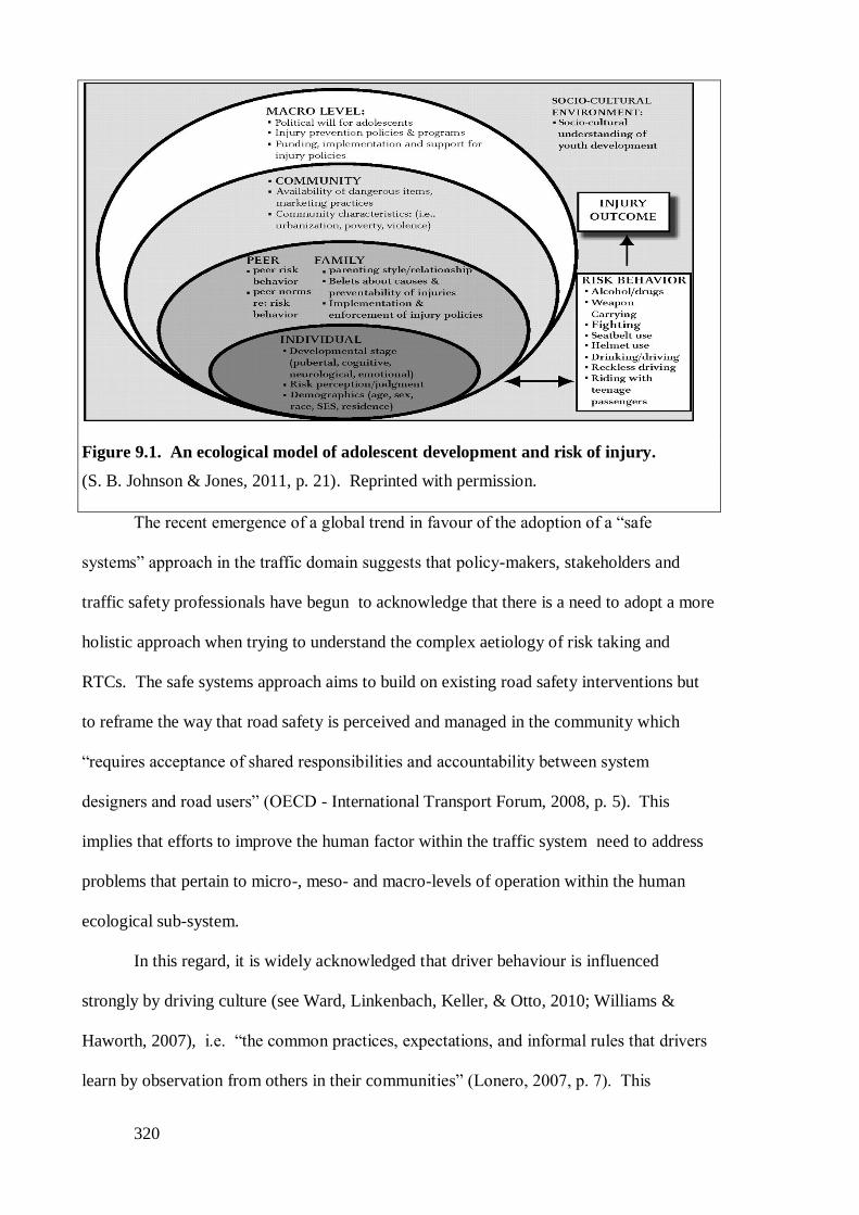
320
Figure 9.1. An ecological model of adolescent development and risk of injury.
(S. B. Johnson & Jones, 2011, p. 21). Reprinted with permission.
The recent emergence of a global trend in favour of the adoption of a “safe
systems” approach in the traffic domain suggests that policy-makers, stakeholders and
traffic safety professionals have begun to acknowledge that there is a need to adopt a more
holistic approach when trying to understand the complex aetiology of risk taking and
RTCs. The safe systems approach aims to build on existing road safety interventions but
to reframe the way that road safety is perceived and managed in the community which
“requires acceptance of shared responsibilities and accountability between system
designers and road users” (OECD - International Transport Forum, 2008, p. 5). This
implies that efforts to improve the human factor within the traffic system need to address
problems that pertain to micro-, meso- and macro-levels of operation within the human
ecological sub-system.
In this regard, it is widely acknowledged that driver behaviour is influenced
strongly by driving culture (see Ward, Linkenbach, Keller, & Otto, 2010; Williams &
Haworth, 2007), i.e. “the common practices, expectations, and informal rules that drivers
learn by observation from others in their communities” (Lonero, 2007, p. 7). This
321
definition pertains not only to behaviours that increase or decrease crash risk but also to
cognitive affective and behavioural responses related to the acceptance or rejection of road
safety interventions (Ward et al., 2010). Much effort has been expended in developing
interventions that focus on altering the perceptions of individual road users regarding the
social norms related to risk taking and driving risk (Berkowitz, 2005; Haines et al., 2005).
Whereas this approach assumes that actual societal norms are oriented predominantly in
the direction of safety, the available evidence does not wholly support such an assumption.
For instance, at a societal level, it is evident that driving culture is negatively impacted by
high-profile role models that “valorise” assertiveness and superiority in drivers, e.g., the
Top Gear presenters, James Bond, etc. (Christmas, 2008). The idea that individuals cannot
be abstracted from the social context is fundamental to social ecological theory
(Bronfenbrenner, 2005). Since cultural influences operate across all levels of the social
sphere, there is a growing realization within the road safety community that continuing
efforts to improve road safety will necessitate the development of intervention strategies
designed to target all levels of the social eco-system (see Ward et al., 2010). Such efforts
would entail addressing the beliefs and attitudes of individual road users, and also
intervening to promote and support the development of safe driving norms among
parents/peers, at community level and in society as a whole. Without such changes, it is
inevitable that the road safety messages that are contained in interventions such as the ones
that featured in this research will be overwhelmed by strong and enduring social
influences which do not reinforce the safety messages contained in these interventions
consistently (for discussions on this point see McKenna, 2010a; Williams et al., 2009).
The results from the current research lend further support to this view because they show
that whereas exposure to aberrant driving had a negative effect on driving-related
knowledge, risk perception and attitudes in the pre-intervention test, attendance at a PLDE
course did little to remedy this problem.
322
An abundance of empirical evidence attests to the role that parents and peers and
prototypical role models play in the psychosocial development of children and adolescents
(Bianchi & Summala, 2004; Miller & Taubman - Ben-Ari, 2010; Ouellette et al., 1999).
Regarding parents, research has shown that whereas parents with adolescent offspring are
acutely aware of their role and responsibilities when their children were learning to drive,
the majority of parents are oblivious to the fact that they play an equally important role in
modelling good and bad driving-related behaviours for their children (Christmas, 2008).
This suggests that there is a pressing need to develop a social marketing campaign to raise
awareness of this issue amongst parents. Regarding peers, the results from this research
supports previous findings which showed that adolescents tend to perceive peer norms as
risky (N. Evans et al., 1995). It is also known that exposure to peers who engage in
deviant behaviours increases the likelihood of such behaviour in adolescents (Jessor et al.,
1997). However, research has also shown that positive peer influence can be harnessed to
produce successful outcomes in social programming interventions and that the inclusion of
content and processes that provide students with exposure to positive social influences can
improve programme effectiveness (Posavac et al., 1999; Yates & Dowrick, 1991).
Regarding prototypes, studies suggest that where young novice drivers have favourable
socially shared images of risky driver prototypes (e.g. speeders) they are more likely to
engage in risky driving, circumstances permitting (Ouellette et al., 1999). Much more
work remains to be done by PLDE programme developers to capitalise on positive peer
influence.
Since all of the available evidence suggests that individuals begin to acquire
driving-related knowledge, cognitive skills and attitudes an early age on the basis of what
they observe as car passengers (e.g. Harré et al., 2000; Waylen & McKenna, 2008), one
obvious way to counteract the detrimental effects of such experiences would be to teach
adolescents to become good passengers. For example, Christmas (2008) suggested that
323
pre-driver education provides a unique opportunity to improve young passengers’ skills in
observing and evaluating the driver behaviour of their parents and significant others. The
findings in this research indicated that students with recent experience of travelling with
speeding drivers were more likely to have a positive impression and less likely to have a
negative impression of such drivers. Encouragingly they also suggest that PLDE was
somewhat effective in reducing positive sentiment towards speeder prototypes, although it
should be noted that it was not equally successful in increasing negative appraisals of such
drivers. Nevertheless, this suggests that the concept of driver prototypes, both positive and
negative, may prove useful in the future development of PLDE programmes. The
challenge for programme developers is to identify suitable positive driver role models
/prototypes who would be willing to participate in such a project.
9.4 Implications for PLDE
The results of the current research contribute to an ever-increasing body of findings
which suggest that driver education is largely ineffective, because it produces minimal and
inconsistent improvements in the safety-related cognitions, affect and behaviours of pre-
drivers (see Christie, 2001; Deighton & Luther, 2007; Mayhew et al., 2002; Roberts &
Kwan, 2001; Stock et al., 1983; Vernick et al., 1999) and of pre-learner drivers (see
Elkington, 2005; Harré & Brandt, 2000a; Poulter & McKenna, 2010; H. Simpson et al.,
2002). Nevertheless, the continued popularity of driver education amongst stakeholders
arises from a socially-shared intuition that DE cannot but help to improve road safety at
some level (McKenna, 2010a). For example, research indicates that DE functions to make
students more amenable to subsequent safety-related messages (O'Brien et al., 2001). It
has also been suggested that the beneficial effects of road safety education most likely
accrue as a result of regular and repeated exposure to programme content (Christie, 2001;
Lonero et al., 1995; Lonero & Mayhew, 2010; Siegrist, 1999). Moreover, it has been
proposed that driver education may operate at a cultural level by functioning to improve

324
public sentiment towards other, more obviously successful road safety interventions
(McKenna, 2010a). If these suppositions are indeed correct, then it would seem that the
effects of road safety interventions are likely to be subtle and therefore difficult to detect.
This represents something of a dilemma for policy makers, since they clearly want to be
seen to be taking action to improve road safety, but they also need to ensure that the
actions that they do take produce tangible results and thereby justify the expenditure of
time, effort and other resources (see Christie & Harrison, 2003). For instance, whereas
McKenna (2010a) proposed that educational interventions could be designed and
evaluated on the basis of their efficacy in changing the perceived legitimacy of policy-
related action (e.g. changes in legislation, stricter enforcement of existing rules), it is
unlikely that such a radical shifts in the focus of DE would receive the support of
stakeholders and policy makers. Nevertheless, the results from the SARTRE studies which
were cited in Chapter 1 (e.g. Fuller & Gormley, 1998; Gormley & Fuller, 2005), suggest
that work remains to be done here in Ireland to improve public perception of road safety
policy and legislation. Thus efforts to improve the perceived legitimacy of traffic safety
policy-related actions using road safety initiatives, including PLDE, should be encouraged
and supported.
There are a number of good reasons for supporting the provision of PLDE as part
of the secondary school curriculum and for funding its future development. First, the
current findings suggest that the vast majority of PLDs are interested in obtaining an LDP
sooner rather than later, and the secondary school system has a proven track record in
addressing students’ instrumental needs by providing them with the wherewithal to pass
knowledge-based tests. Second, since PLDs will have been exposed to factors (e.g.
individuals and/or circumstances) that served to shape their driving-related knowledge, risk
perception skills and attitudes over time, and since the benefits of education tend to accrue
over time, clearly road safety education should be delivered at regular intervals as part of
325
the primary and secondary school curriculum right through to year 14. Third, since the
vast majority of Irish adolescents complete their second-level education, the inclusion of
PLDE as part of the national curriculum would ensure that most Irish adolescents would
continue to be exposed to road safety messages at a crucial juncture i.e. when many of
them are becoming actively interested in driving. Thus, whereas there is a temptation to
focus on traffic safety policies which yield visible results over the short-term (e.g.
engineering, enforcement), the well-being of society may be served better by taking a
long-term approach and by investing in the development of more effective road safety
education initiatives.
9.4.1 Improving PLDE
Many traffic safety professionals support the drive to develop more effective DE
and believe that this might be achieved by broadening the scope of DE (as discussed
previously) and by focussing more intensely on the core problems that confront adolescent
learner and pre-learner drivers (see Christie & Harrison, 2003; Lonero et al., 2005). Since
all of the available evidence suggests that faulty calibration is the root cause of the young
driver problem (Arnett, 1996; Deery, 1999; Finn & Bragg, 1986; McKnight & McKnight,
2003), there is general agreement that driver education should focus on providing students
with insight into the limitations of their capabilities, and also into the actual complexity of
the traffic task, thereby enabling them to assess the difficulty of the driving task with
greater accuracy (de Craen, 2010; Hatakka et al., 2002; Lonero et al., 1995). It has long
since been established that inexperience , age and (male) gender function to reduce task
capability in younger drivers (OECD - ECMT, 2006b). However, one important insight
that was gained from this research was that, in common with their U.S. counterparts (see
Ginsburg et al., 2008), Irish adolescents have a poor appreciation of the magnitude of the
threat that inexperience poses to their safety as drivers. Yet the formative evaluation that
was conducted as part of this research noted that the amount of attention that is devoted to
326
the topic of inexperience in the programmes that featured in this study was in no way
commensurate with the importance of this topic in terms of catering for adolescent
students’ developmental needs as drivers. Whereas it is acknowledged that all of the
programmes reviewed as part of this study did indeed address issues related to
inexperience, age and gender, these issues were normally addressed in the context of other,
more generic safety issues (e.g. speeding, DWI, driver fatigue) rather than as topics in their
own right. Thus, it is recommended that the future development of PLDE should involve
the provision of programme units/lessons that focus specifically on inexperience, age and
gender in order to make PLDs more aware of the effects that these factors have on their
capability as drivers. Adolescents need to know how, where, when and most importantly
why these factors pose a threat to their safety as learner and novice drivers.
The results obtained from the vignettes that were used in this research also
provided some unique insights into the cognitive functioning of PLDs. These suggested
that attendance at a PLDE course increased the accessibility of mental representations of
crashing in response to a high-risk scenario. Intriguingly, since the results showed that
although over 80% of the students surveyed listed “crashing” as a possible consequence of
these scenarios, over 25% of these did not also list attendant consequences such as “injury”
or “death, which suggests that mental associations between these outcomes need to be
strengthened in some PLDs, especially males. Moreover, the current results also indicated
that PLDE may function in some way to improve the accessibility of serious consequences.
Although these results were encouraging, much more work needs to be done to progress
this potentially useful line of enquiry and this issue was discussed in greater detail in
Chapter 6.
The simple descriptive and univariate analyses produced as part of this study
provided valuable information about Irish PLDs, revealing them as diverse, in terms of
their personal characteristics, and their previous experiences with driving and being a
327
passenger. These findings may be of some interest to researchers, programme developers
and policy makers. The results in Chapter 3, which focussed on measuring personality
traits, suggested that relatively short inventories e.g. BIS-15 test of impulsiveness
(Spinella, 2007) and the IPIP-50 test of Big-Five personality factors (Goldberg, 2011) were
suitable for use with adolescents in the 15 – 17-year age group. However, the present
research supported previous findings (e.g. Roth & Hertzberg, 2004) regarding the
inadequacy of the AISS (Arnett, 1994). Given that the research community has been
aware of this problem for some time, and given that the validity of the best-known
alternative i.e. Zuckerman’s Sensation Seeking Scale, Form V (Zuckerman 1996) for
adolescent populations has also been challenged, and given that sensation seeking is a
significant predictor of risk taking in adolescents, it is very surprising that no apparent
effort has been made thus far to develop an improved, adolescent-friendly sensation
seeking scale. This should be done as a matter of urgency.
Over 80% of the students who participated in this research reported that they
intended to obtain an LDP as soon as this was possible, thus the inclusion of PLDE as part
of the senior cycle curriculum in secondary school appears timely. The current research
also suggested that there was an unacceptably high incidence of un-licenced driving and of
driving without proper supervision in the current sample. Such problem should be
addressed as part of PLDE interventions.
9.5 Methodological strengths and limitations
Although issues pertaining to reliability and validity were discussed according as
they arose in the preceding chapters, the following serves to summarise these strengths and
weaknesses for ease of reference.
328
9.5.1 Strengths
Viewed in the context of previous investigations into DE, the current research was
innovative to the extent that it employed a number of sophisticated data analysis
techniques, including IRT and HLM analyses, which served to improve the reliability and
validity of the findings.
IRT analysis employs sophisticated methodology to calculate peoples’ ability to
responding to test items (DeMars, 2010). Evidence presented in Chapter 5 suggested that
IRT analysis is useful for identifying items that do not differentiate between or which
discriminate against testees (Lord, 1980). Research has shown that this method is better
able to produce valid achievement scores than are more traditional scoring mechanisms,
especially where tests that have not been validated previously (see Hambleton et al.,
1991), as was the case in the current research. The results of the IRT analysis in this
research provided information about the strengths and weaknesses in students’ knowledge.
This should assist programme developers to orient their courses to better suit students’
needs and thereby to improve the efficiency and effectiveness of their courses. For
instance, the current results suggested that students were quite knowledgeable about issues
such as impaired driving (e.g. DWI, drowsiness), but knew considerably less about speed
limits and driving manoeuvres which pose problems for young novice drivers.
Researchers in a wide range of disciplines, most notably the educational sphere
(e.g. Flannery et al., 2003; Kreft, 1993) routinely employ multilevel modelling techniques
such as HLM to account for variations in their data whilst simultaneously controlling for
clustering effects (Raudenbush & Bryk, 2002). Clustering occurs when research
participants are nested in groups (e.g. school classes) or where research is based on a
repeated measures design. Although the vast majority of DE research involves the testing
of nested groups, often using longitudinal designs, this researcher was unable to find a
single DE study which reported that steps had been taken to test for and where necessary to
329
control for clustering effects. This suggests that the statistical requirement to control for
clustering is poorly understood in the traffic safety community (seeDupont & Martensen,
2007 for a good description of how multilevel modelling can be used in traffic research).
The various advantages and disadvantages associated with HLM methodology in general
and in its application in the current research were discussed in detail in Chapter 2. In sum,
the main advantage of HLM is that it allows researchers to investigate the inter-
relationships between a wide range of variables which are associated with multiple levels
of analyses (e.g. intra-individual, between-individuals and between-groups factors). The
main disadvantages of this methodology are that the use of these techniques reduce the
likelihood of obtaining statistically significant results and that relatively large samples are
required to provide HLM studies with sufficient statistical power to reveal significant
results where these exist. For example, whereas it is acknowledged that the current study
came very close to satisfying power requirements outlined by Raudenbush (2008), the
possibility that this study did not have sufficient power to detect significant results cannot
be ruled out conclusively. Despite the difficulties that are involved in implementing
multilevel modelling techniques such as HLM, it is nevertheless clear that such techniques
provide mechanisms whereby researchers can make progress in examining the complex
array of factors that influence human cognition, affect and behaviour. Thus, it is
recommended that the traffic research community should embrace the new methodologies,
such as multilevel modelling and IRT analyses in situations where their use is warranted.
9.5.2 Limitations
Despite these strengths, the current results need to be considered in the context of a
number of procedural, conceptual and methodological limitations.
9.5.2.1 Procedural limitations
Although a number of steps were taken to increase reliability and validity in this
research there were some limitations as to what could be done for operational reasons e.g.
330
the availability of human resources, time and funding. First, it is acknowledged that the
ability of the current research to produce results that were generalizable to the PLDE
population as a whole was somewhat constrained since it used a quasi-experimental design
and used opportunity based population sampling methods. Second, although efforts were
made to recruit a large sample of students which would be reasonably representative of the
Irish PLD population in terms of gender, SES and PLDE education status, it is
acknowledged that the resulting sample did contain some imbalances in terms of these
demographics. Furthermore, because testing was conducted in a large number of schools
where the delivery schedules for PLDE differed considerably, it was not possible to
standardise the between-test intervals in a completely rigorous way. However, ever effort
was made to reduce sampling bias through the provision of matched active/control groups
where possible and by ensuring that incidences of attrition were random and low. All of
these issues were discussed in more detail in Chapter 2.
Whereas evaluations of social programming interventions typically involve the
assessment of individual programmes, the current research adopted a broader approach by
including five different programmes in the research design. Despite the obvious advantage
of this strategy in terms of gaining a better understanding of the effects of PLDE on Irish
adolescents, the limitations associated with this approach, which have been outlined
previously, need to be reiterated. First, whereas programme evaluation usually involves
assessing the extent to which programme objectives have been met (Clinton & Lonero,
2006a), since this research involved multiple programmes, each with their own objectives,
this type of assessment was not feasible in the current circumstances. Instead, the various
tests that were used in this research were formulated on the basis of theoretical
considerations with respect to the type of content that should (ideally) be part of a good
PLDE course. Since it is acknowledged that these ideal standards were bound to differ
from the standards adopted by individual course developers, the current results cannot be
331
construed as reflecting positively or negatively on any of the individual programmes that
featured in this research. However, since a wide range of tests, incorporating many test
items were used as part of the summative evaluations in this research it is reasonable to
suggest that the current results represent a reasonably fair and accurate reflection of
driving-related knowledge, risk perception skills and attitudes in the current sample over
time and as a function of PLDE status. It is also argued the content of these tests
addressed important driving-related criteria and that these ought to have been included as
part of a good PLDE course. The educational and policy implications of the apparent
heterogeneity in the PLDE provision for TY students with respect to course content and
delivery were discussed in greater detail in Chapter 8.
9.5.2.2 Conceptual limitations
Although current efforts to explain variations in driving-related knowledge, risk
perception skills and attitudes were unsuccessful the results of the HLM analyses
suggested that a large proportion of the variance in these models was attributable to intra-
student time-dependent factors. Since the inclusion of age and time as predictors did very
little to reduce variations in these models, it was concluded above that the remaining
variations were most likely due to maturational factors. Although it is difficult to see at
present how currently emerging findings with respect to neurobiological development
might be used to develop the kinds of measures that could be applied in the field, it is
nevertheless acknowledged that the lack of such measures represented a considerable
limitation in this research. However, some steps could be taken to begin to address
maturational influences in future research. For example, although measures of trait
impulsiveness and sensation seeking were included as part of the current research, these
were measured just once, because it was not expected that such influences would change
perceptibly within the 18-month period when testing in this project was taking place.
Nevertheless, since previous research suggests that some changes do occur in
332
impulsiveness and sensation seeking during adolescence (Steinberg et al., 2008) it would
be interesting to see if such changes might account for some of the variation in driving-
related outcomes in PLDS at intra-student level. This would necessitate the inclusion of
measures to test these traits at each stage in longitudinal studies.
9.5.2.3 Methodological limitations
This study relied entirely on self-report questionnaires, because this approach was
particularly suited to measuring driving-related knowledge, risk perception skills and
attitudes in this large sample of PLDs. Nevertheless, it is widely-acknowledged that the
validity self-report data can be negatively impacted by confounds, such as social
desirability (Crowne & Marlowe, 1960). Two factors contribute to incidences of socially
desirable responding; impression management and self-deception (Paulhus, 1984).
Impression management occurs where individuals deliberately attempt to present a
favourable image and thus tends to be problematic in group testing sessions. Self-
deception occurs where individuals provides subjectively honest, but positively biased self-
descriptions (Paulhus, 1984). Although research suggests that adolescents may be more
susceptible to the problem of social desirability than adults (J. D. Brown, 1986), it has also
been found that school-going adolescents tend to report their behaviours and attitudes with
reasonable accuracy (Killen & Robinson, 1988). Furthermore, the results from the present
research in relation to the DBQ (Reason et al., 1990) items showed that students’
evaluations of their principal driver were broadly in line with the findings in other DBQ
studies (Åberg & Rimmö, 1998; Lajunen et al., 2004), which supports the validity of the
current findings. Research also indicates that the validity of self-report data can be
improved through the provision of assurances of confidentiality, the establishment of good
rapport and by focussing on relatively recent events (Brener, Billy, & Grady, 2003) and all
of these safeguards were included as part of this research. Moreover, the current students
were provided with regular and timely reminders to refrain from interacting with their
333
classmates and also to respond accurately and openly to the questionnaire items. Although
it is notoriously difficult to address problems associated with self-deception bias, this
research made some attempt to do so by including one item which served as a measure of
implicit cognition (i.e. the vignette) and thus was not subject to self-deceptive influences.
9.6 Concluding remarks
The current results contribute towards an ever-increasing body of evidence which
demonstrate that biological antecedents and subsequent social factors play a defining role
in the establishment and maintenance of driving-related knowledge and cognitions, against
which current forms of driver education remain relatively ineffective. The strongest
conclusion that can be drawn from this research is that educational initiatives that focus on
developing driving-related knowledge, cognitive skills and attitudes in individual PLDs are
unlikely to succeed unless they are supported by initiatives that focus on changing driving
culture at all levels of the society. Nevertheless, by using a broad psychosocial framework,
sophisticated methodologies and a longitudinal design, this research provided unique
insights into the driving-related knowledge, risk perception skills and attitudes of Irish
PLDs and that these can be used to inform the future development of road safety policy for
this age group and also to improve the efficiency and effectiveness of PLDE programmes.
Whereas the current incidence of RTCs and the resulting toll of death and injury,
particularly amongst young novice drivers is socially, morally and financially
unacceptable, it should be remembered that road safety has become a great public health
success story in recent years. In the relatively short lifespan of this project (i.e. from 2009
to 2012), there was a 32% reduction in RTC-related deaths here in Ireland. However, the
sustainability of this downward trend will likely depend on the continued application of a
safe systems approach and attendant efforts to improve engineering, enforcement,
education and evaluation (RSA, 2013b). Hopefully, this research has made some small
contribution with respect to these latter.

334
9.7 References
Aarts, L., & Van Schagen, I. (2006). Driving speed and the risk of road crashes: A review.
Accident Analysis & Prevention, 38(2), 215-224. doi: 10.1016/j.aap.2005.07.004
Åberg, L., & Rimmö, P. A. (1998). Dimensions of aberrant driver behaviour. Erognomics,
41, 39-56. doi: 10.1080/001401398187314
Adams-Guppy, J. R., & Guppy, A. (1995). Speeding in relation to perceptions of risk,
utility and driving style by British company car drivers. Ergonomics, 38(12), 2525-
2535. doi: 10.1080/00140139508925284
af Wåhlberg, A. (2009). Driver behaviour and accident research methodology: Unresolved
problems. Surrey: Ashgate Publishing.
af Wåhlberg, A. E. (2009). Driver behaviour and accident research methodology:
Unsolved problems. Aldershot: Ashgate.
Ajzen, I. (1991). The theory of planned behavior. Organizational Behaviour and Human
Decision Processes, 50, 179-211. doi: 10.1016/0749-5978(91)90020-T
Ajzen, I. (2005). Attitudes, personality and behaviour. Maidenhead: Open University
Press.
Akaike, H. (1987). Factor analysis and the AIC. Psychometrica, 52, 317-332.
Akers, R. L. (1973). Deviant behaviour: A social learning approach. Belmont, CA:
Wadsworth Publishing Co.
Akers, R. L., Krohn, M. D., Lanza-Kaduce, L., & Radosevich, M. (1979). Social learning
and deviant behaviour: A specific test of a general learning theory. American
Sociological Review, 44, 636-655.
Allen, J. P., Aber, J. L., & Leadbetter, B. J. (1990). Adolescent problem behaviours: The
influence of attachment and autonomy. Psychiatry Clinic North America, 13, 455-
467. doi: PMid:2235694
Allen, J. P., & Brown, B. B. (2008). Adolescents, peers, and motor vehicles: The perfect
storm? American Journal of Preventive Medicine, 35(3, Supplement 1), S289-
S293. doi: 10.1016/j.amepre.2008.06.017
Allison, P. D. (2001). Missing data. Thousand Oaks, CA: Sage.
Ames, S. L., Zogg, J. B., & Stacy, A. W. (2002). Implicit cognition, sensation seeking,
marijuana use and driving behavior among drug offenders. Personality and
Individual Differences, 33(7), 1055-1072. doi: 10.1016/s0191-8869(01)00212-4
Anderson, J. R. (1982). Acquisition of cognitive skill. Psychological Review, 89(4), 369-
406. doi: 10.1037/0033-295X.89.4.396
Anderson, J. R. (1983). A spreading activation theory of memory. Journal of Verbal
Learning and Verbal Behaviour, 22, 261-295.
Anderson, J. R. (1996). ACT: A simple theory of complex cognition. American
Psychologist(51), 355-365. doi: 10.1037/0003-066X.51.4.355
Arbuckle, J. L. (2009). Amos (Version 18.0.0 ). Crawfordville FL: Amos Development
Corporation.
Armitage, C. J., & Connor, M. (2001). Efficacy of the theory of planned behaviour: A
meta-analysic review. British Journal of Social Psychology(40), 471-499. doi:
10.1348/014466601164939
Arnett, J. J. (1994). Sensation seeking: A new conceptualization and a new scale.
Personality and Individual Differences, 16(2), 289-296. doi: 10.1016/0191-
8869(94)90165-1
Arnett, J. J. (1996). Sensation seeking, aggressiveness, and adolescent reckless behavior.
Personality and Individual Differences, 20(6), 693-702. doi: 10.1016/0191-
8869(96)00027-X
335
Arnett, J. J. (2002). Developmental sources of crash risk in young drivers. Injury
Prevention, 31, 10-27.
Arnett, J. J., Offer, D., & Fine, M. A. (1997). Reckless driving in adolescence: `State' and
`trait' factors. Accident Analysis & Prevention, 29(1), 57-63. doi: 10.1016/S0001-
4575(97)87007-8
Arthur, W., & Doverspike, D. (2001). Predicting motor vehicle crash involvement from a
personality measure and a driving knowledge test. Journal of Prevention &
Intervention in the Community, 22(1), 35-42. doi: 10.1080/10852350109511209
Arthur, W., & Graziano, W. G. (1996). The five factor model, conscientiousness, and
driving accident involvement. Journal of Personality and Social Psychology(65),
593-618. doi: 10.1111/j.1467-6494.1996.tb00523.x
Atkinson, R. C., & Shiffrin, R. M. (1968). Human memory: A proposed system and its
control processes. In K. W. Spence & J. T. Spence (Eds.), The psychology of
learning and motivation (Vol. 2, pp. 89-195). London: Academic Press.
Bacon, P. (2005). Economic evaluation of the government strategy for road safety, 1998-
2002. Dublin Goodbody Economic Consultants.
Baddeley, A. D. (1982). Domains of recollection. Psychological Review, 89, 708-729. doi:
10.1037/0033-295X.89.6.708
Ballesteros, M. F., & Dischinger, P. (2000). Characteristics of traffic crashes in Maryland
(1996 - 1998). Paper presented at the 44th Annual Conference for the Advancement
of Automotive Medicine, Chicago, IL.
Bandolier. (2012). Risk of death and transportation Retrieved 1st December, 2012, from
http://www.medicine.ox.ac.uk/bandolier/booth/Risk/trasnsportpop.html
Bandura, A. (1965). Influence of models' reinforcement contingencies on the acquisition of
imitated responses. Journal of Personality and Social Psychology, 1, 589-595. doi:
10.1037/h0022070
Bandura, A. (1977). Social learning theory. Englewood Cliffs, NJ: Prentice-Hall.
Bandura, A. (1989). Social cognitive theory. In R. Vasta (Ed.), Annals of child
development. Vol. 6. Six theories of child development (pp. 1-60). Greenwich, CT:
JAI Press.
Bandura, A., & Walters, R. H. (1963). Social learning and personality development. New
York: Holt, Rinehart and Winston.
Baraldi, A. N., & Enders, C. K. (2010). An introduction to modern missing data analyses.
Journal of School Psychology, 48(1), 5-37. doi: 10.1016/j.jsp.2009.10.001
Bargh, J. A., & Williams, E. L. (2006). The automaticity of social life. Current Directions
in Psychological Science, 15(1), 1-4. doi: 10.1111/j.0963-7214.2006.00395.x
Barkley, R. A. (1998). Attention-deficit/hyperactivity disorder: A handbook for diagnosis
and treatment (2nd ed.). New York: Guilford.
Barkley, R. A. (2004). Driving impairments in teens and adults with attention-
deficit/hyperactivity disorder. Psychiatric Clinics of North America, 27, 233-260.
doi: 10.1016/S0193-953X(03)00091-1
Barnett, S. M., & Ceci, S. J. (2002). When and where do we apply what we learn? A
taxonomy for far transfer. Psychological Bulletin(128), 612-637. doi:
10.1037/0033-2909.128.4.612
Barratt, E. S. (1959). Anxiety and impulsiveness related to psychomotor efficiency.
Perceptual and Motor Skills, 9, 191-198.
Barrick, M. R., & Mount, M. K. (1991). The Big Five personality dimensions and job
performance: A meta-analysis. Personnel Psychology, 44(1), 1-26. doi:
10.1111/j.1744-6570.1991.tb00688.x
Bartlett, M. S. (1954). A note on the multiplying factors for various chi-square
approximations. Journal of the Royal Statistical Society, 16 (Series B), 296-298.
336
Baxter, J. S., Manstead, A. S., Stradling, S. G., & Campbell, K. A. (1990). Social
facilitation and driver behaviour. British Journal of Psychology, 81(3), 351-360.
Beirness, D. J. (1993). Do we really drive as we live? Alcohol, Drugs and Driving, 9, 129-
143.
Beirness, D. J., & Simpson, H. M. (1988). Lifestyle correlates of risky driving and accidnet
involvement among youth. Alcohol, Drugs, and Driving, 4, 193-204.
Berkowitz, A. D. (2005). An overview of the social norms approach. In L. Lederman, L.
Stewart, F. Goodhart & L. Laitman (Eds.), Changing the culture of college
drinking: A socially situated prevention campaign (pp. 245-257).
Beyth-Marom, R., Austin, L., Fischhoff, B., Palmgren, C., & Jacobs-Quadrel, M. (1993).
Perceived consequences of risky behaviors: Adults and adolescents. Developmental
Psychology, 29(3), 549-563. doi: 10.1037//0012-1649.29.3.549
Bianchi, A., & Summala, H. (2004). The "genetics" of driving behavior: parents' driving
style predicts their children's driving style. Accident Analysis & Prevention, 36(4),
655-659. doi: Doi: 10.1016/s0001-4575(03)00087-3
Bingham, C. R., & Shope, J. T. (2004). Adolescent problem behavior and problem driving
in young adulthood. Journal of Adolescent Research, 19(2), 205-223. doi:
10.1177/0743558403258269
Bonnie, R. J. (1985). The efficacy of law as a paternalistic instrument. Nebraska
Symposium on Motivation, 33, 131-211.
Booth-Kewley, S., & Vickers, R. R. (1994). Associations between major domains of
personality and health behaviour. Journal of Personality, 62(3), 281-298. doi:
10.1111/j.1467-6494.1994.tb00298.x
Bransford, J. D., Brown, A. L., & Cockling, R. R. (Eds.). (2000). How People Learn:
Brain, Mind, Experience, and School: Expanded Edition. Washington, DC:
National Academy Press.
Brener, N. D., Billy, J. O. G., & Grady, W. R. (2003). Assessment of factors affecting the
validity of self-reported health-risk behaviour among adolescents: Evidencefrom
the scientific literature. Journal of Adolescent Health, 33, 436-457. doi:
10.1016/S1054-139X(03)00052-1
Bronfenbrenner, U. (2005). Making human beings human : bioecological perspectives on
human development. Thousand Oaks ; London: Sage.
Brown, A. L. (1987). Metacognition, executive control, self-regulation, and other more
mysterious mechanisms. Metacognition, Motivation, and Understanding, 65, 116-
123. doi: 10.1016/0010-0277(77)90018-X
Brown, I. D., & Groeger, J. A. (1988). Risk perceptionand decision taking during the
transition between novice and experienced driver status. Ergonomics, 3(4), 585-
593. doi: 10.1080/0014013888966701
Brown, J. D. (1986). Evaluation of self and others: Self-enhancemnt biases in social
judgements. Social Cognition, 3, 353-376. doi: 10.1521/soco.1986.4.4.353
Brown, M. W., & Cudeck, R. (1993). Alternative ways of assessing model fit. In K. A.
Bollen & J. Long (Eds.), Testing structural equation models (pp. 136-162).
Newbury Park, CA: Sage Publications.
Brown, R., & Kulik, J. (1977). Flashbulb memories. Cognition 5, 73-99.
Brunner, J. S. (1966). On knowing: Essays for the left hand New York Atheneum.
Bryk, A. S., & Raudenbush, S. W. (1992). Hiererchical linear models. Newbury Park, CA:
Sage.
Busato, V. V., Prins, F. J., Elshout, J. J., & Hamaker, C. (1998). The relation between
learning styles, the Big Five personality traits and achievement motivation in higher
education. Personality and Individual Differences, 26(1), 129-140. doi:
10.1016/S0191-8869(98)00112-3
337
Busato, V. V., Prins, F. J., Elshout, J. J., & Hamaker, C. (2000). Intellectual ability,
learning style, personality, achievement motivation and academic success of
psychology students in higher education. Personality and Individual Differences,
29(6), 1057-1068. doi: 10.1016/S0191-8869(99)00253-6
Byrne, B. M. (2010). Structural equation modelling with AMOS: Basic concepts,
applications and programming (2 ed.). New York: Routledge.
Carcary, B., Power, K., & Murray, F. (2001). The new driver project: changing driving
beliefs, attitudes and self-reported driving behaviour through classroom based pre
and post driving test interventions. Edinburgh: Scotish Executive Central Research
Unit.
CARRS-Q. (2009). Driver education for senior school students (Years 10-12) and young
novice drivers: Literature review and key elements of a best practice program.
Brisbane: Department of Transport and Main Roads.
Carsten, O. (2007). From driver models to modelling the driver: What do we really need
to know about the driver? In P. C. Cacciabue (Ed.), Modelling driver behaviour in
automotive environments (pp. 105-120). London: Springer.
Casey, B. J., Getz, S., & Galvan, A. (2008). The adolescent brain. Developmental Review,
28(1), 62-77. doi: 10.1016/j.dr.2007.08.003
Caspi, A., Harrington, H., Moffitt, T. E., Begg, D., Dickson, N., Langley, J., & Silva, P. A.
(1997). Personality differences predict health-risk behaviors in young adulthood:
Evidence from a longitudinal study. Journal of Personality and Social Psychology,
73(5), 1052-1063. doi: 10.1037/0022-3514.73.5.1052
Castellani, B., & Rugle, L. (1995). A comparison of pathological gamblers to alcoholics
and cocaine misusers on impulsivity, sensation seeking and craving. Substance Use
& Misuse, 30(3), 275-289. doi: 10.3109/10826089509048726
Cattell, R. B., & Vogelmann, S. (1977). A comprehensive trial of the scree and K-G
criteria for determining the number of factors. Multivariate Behavioral Research,
12(3), 289-325. doi: 10.1207/s15327906mbr1203_2
Cestac, J., Paran, F., & Delhomme, P. (2011). Young drivers' sensation seeking, subjective
norms, and perceived behavioral control and their roles in predicting speeding
intention: How risk-taking motivations evolve with gender and driving experience.
Safety Science, 49(3), 424-432. doi: 10.1016/j.ssci.2010.10.007
Chamorro-Permuzic, T., & Furnham, A. (2003). Personality predicts academic
performance: Evidence from two longitudinal university samples. Journal of
Research in Personality, 37, 319-338. doi: 10.1016/S0092-6566(02)00578-0
Chamorro-Premuzic, T., & Furnham, A. (2009). Mainly Openness: The relationship
between the Big Five personality traits and learning approaches. Learning and
Individual Differences, 19(4), 524-529. doi: 10.1016/j.lindif.2009.06.004
Chassin, L., Presson, C. C., Sherman, S. J., & Kim, K. (1985). Self-image and social-image
factors in adolescent alcohol use. Journal of Studies on Alcohol, 46, 39-47.
Chen, H. Y., Ivers, R. Q., Martiniuk, A. L. C., Boufous, A., Senserrick, T., Woodward, M.,
. . . North, R. (2009). Risk and type of crash among young drivers by rurality of
residence: Findings from the DRIVE study. Accident Analysis & Prevention,
41(4), 676-682. doi: 10.1016/j.aap.2009.03.005
Chen, L., Baker, S. P., Braver, E. R., & Li, G. (2000). Carrying passengers as a risk factor
for crashes fatal to 16- and 17-year-old drivers. JAMA: The Journal of the
American Medical Association, 283(12), 1578-1582. doi:
10.1001/jama.283.12.1578
Christie, R. (2001). The effectiveness of driver training as a road safety measure: A review
of the literature. (01/03). Melbourne: Royal Automobile Club of Victoria (RACV).
Christie, R., & Harrison, W. (2003). Driver training and education programs of the future.
(03/03). Melbourne, Victoria: Royal Automobile Club of Victoria (RACV).
338
Christmas, S. (2008). Feeling safe, itching to drive: Pre-driver and learner perspectives on
driving and learning. (Road Safety Research Report No. 6). London: Department
for Transport.
Clarke, D. D., Ward, P., & Truman, W. (2005). Voluntary risk taking and skill deficits in
young driver accidents in the UK. Accident Analysis & Prevention, 37(3), 523-529.
doi: 10.1016/j.aap.2005.01.007
Clarke, S., & T. Robertson, I. (2005). A meta-analytic review of the Big Five personality
factors and accident involvement in occupational and non-occupational settings.
Journal of Occupational and Organizational Psychology, 78(3), 355-376. doi:
10.1348/096317905x26183
Clinton, K. M., & Lonero, L. P. (2006a). Evaluating driver education programmes: How
to guide. Washington DC: AAA Foundation for Traffic Safety.
Clinton, K. M., & Lonero, L. P. (2006b). Evaluating driver education programs:
Comprehensive guidelines. Washington DC: AAA Foundation for Traffic Safety.
Clinton, K. M., & Lonero, L. P. (2006c). Evaluating driver education programs:
Management overview. Washington DC: AAA Foundation for Traffic Safety.
Cohen, J. (1988). Statistical power analysis for the behavioral sciences (2nd ed.).
Hillsdale, NJ: Lawrence Earlbaum Associates.
College Entrance Examination Board. (2005). 2005 college-bound seniors: A profile of
SAT program test-takers. Retrieved from
http://www.collegeboard.com/prod_downloads/about/news_info/cbsenior/yr2005/2
005-college-bound-seniors.pdf
Conner, M., Lawton, R., Parker, D., Chorlton, K., Manstead, A. S. R., & Stradling, S.
(2007). Application of the theory of planned behaviour to the prediction of
objectively assessed breaking of posted speed limits. British Journal of Psychology,
98, 429-453. doi: 10.1348/000712606X133597
Conway, M. A., Anderson, S. J., Larsen, S. F., Donnelly, C. M., McDaniel, M. A., &
McClelland, A. G. R. (1994). The function of flashbulb memories. Memory and
Cognition, 22, 326-343. doi: 10.3758/BF03200860
Cordery, J. L., & Sevatos, P. P. (1993). Responses to the original and resived job
diagnostic survey: Is education a factor in responses to negatively worded items?
Journal of Applied Psychology, 78, 141-143. doi: 10.1037/0021-9010.78.1.141
Costa, P. T., & McCrae, R. R. (1992). Professional manual for the Neo-Pi-R. Odessa, FL:
Psychological Assessment Resources Inc.
Costa, P. T., & McCrae, R. R. (2001). Gender differences in personality traits across
cultures: Robust and surprising findings. Journal of Personality and Social
Psychology, 81(2), 322-331. doi: 10.1037/0022-3514.81.2.322
Craik, F. I. M., & Lockhart, R. S. (1972). Levels of processing: A framework for memory
research. Journal of Verbal Learning and Verbal Behaviour, 11, 671-684.
Craik, F. I. M., & Tulving, E. (1975). Depth of processing and the retention of words in
eposodic memory. Journal of Experimental Psychology, 104, 268-294.
Crick, J., & MCKenna, F. (1992). Hazard perception: Can it be trained? Crowthorne:
Transport Research Laboratory.
Cronbach, L. J. (1990). Essentials of psychological testing (5th ed.). New York Harper &
Row.
Crowne, D. P., & Marlowe, D. (1960). A new scale of social desirability independent of
psychopathology. Journal of Consulting Psychology, 24(4), 349-354.
Dahlen, E. R., Martin, R. C., Ragan, K., & Kuhlman, M. M. (2005). Driving anger,
sensation seeking, impulsiveness, and boredom proneness in the prediction of
unsafe driving. Accident Analysis & Prevention, 37(2), 341-348. doi:
10.1016/j.aap.2004.10.006
339
Dahlen, E. R., & White, R. P. (2006). The Big Five factors, sensation seeking, and driving
anger in the prediction of unsafe driving. Personality and Individual Differences,
41(5), 903-915. doi: 10.1016/j.paid.2006.03.016
de Craen, S. (2010). The X-factor: A longitudinal study of calibration in young novice
drivers. (Doctoral Dissertation), SWOV, Leidschendam. Retrieved from
http://www.swov.nl/rapport/Proefschriften/Saskia_de_Craen.pdf
de Craen, S., Twisk, D. A. M., Hagenzieker, M. P., Elffers, H., & Brookhuis, K. A. (2008).
The development of a method to measure speed adaptation to traffic complexity:
Identifying novice, unsafe, and overconfident drivers. Accident Analysis &
Prevention, 40(4), 1524-1530. doi: 10.1016/j.aap.2008.03.018
de Raad, B., & Schouwenburg, H. C. (1996). Personality in learning and education: a
review. European Journal of Personality, 10(5), 303-336. doi: 10.1002/(sici)1099-
0984(199612)10:5<303::aid-per262>3.0.co;2-2
de Winter, J. C. F., & Dodou, D. (2010). The Driver Behaviour Questionnaire as a
predictor of accidents: A meta-analysis. Journal of Safety Research, 41(6), 463-
470. doi: 10.1016/j.jsr.2010.10.007
Dedrick, R. F., Ferron, J. M., Hess, M. R., Hogarty, K. Y., Kromrey, J. D., Lang, T. R., . . .
S, L. R. (2009). Multilevel modeling: A review of the methodological issues and
applications. Review of Educational Research, 79(1), 69-102. doi:
10.3102/0034654308325581
Deery, H. A. (1999). Hazard and risk perception among young novice drivers. Journal of
Safety Research, 30(4), 225-236. doi: 10.1016/s0022-4375(99)00018-3
Deighton, C., & Luther, R. (2007). Pre-driver education: A critical review of the literature
on attitude change and development, good practice in pre-driver education and
programme effectiveness. London: Department for Transport UK.
DeJoy, D. M. (1989). The optimism bias and traffic accident risk perception. Accident
Analysis & Prevention, 21(4), 333-340. doi: 10.1016/0001-4575(89)90024-9
DeJoy, D. M. (1992). An examination of gender differences in traffic accident risk
perception. Accident Analysis & Prevention, 24(3), 237-246. doi: 10.1016/0001-
4575(92)90003-2
Delhomme, P., Kreel, V., & Ragot, I. (2008). The effect of the commitment to observe
speed limits during rehabilitation training courses for traffic regulation offenders
in France. Revue Européenne de Psychologie Appliquée/European Review of
Applied Psychology, 58(1), 31-42. doi: 10.1016/j.erap.2005.07.005
Delhomme, P., Verlhiac, J. F., & Martha, C. (2009). Are drivers' comparative risk
judgments about speeding realistic? Journal of Safety Research, 40(5), 333-339.
doi: 10.1016/j.jsr.2009.09.003
deLucia, M. K., Bleckley, L. E., Meyer, L. E., & Bush, J. M. (2003). Judgements about
collisions in younger and older drivers. Transportation Research Part F, 6, 63-80.
doi: 10.1016/S1369-8478(02)00047-5
DeMars, C. (2010). Item response theory. Oxford Oxford University Press.
Dempster, A. P., Laird, N. M., & Rubin, D. B. (1977). Maximum likelihood for incomplete
data via the EM algorithm. Journal of the Royal Statistical Society. Series B
(Methodological), 39(1), 1-38.
Department of Education and Science. (2010). Second level schools and pupils by year,
enrolment size, statistic and type of school. Retrieved from
http://www.cso.ie/px/des/Dialog/Saveshow.asp
DiBlasio, F. A. (1988). Predriving riders and drinking drivers. Journal of Studies on
Alcohol, 49(1), 11-15.
Donaldson, S. I. (2003). Theory-driven program evaluation in the new millenium. In S. I.
Donaldson & M. Scriven (Eds.), Evaluating social programs and proglems: visions
for the new millennium (pp. 104-141). New Jersey: Lawrence Erlbaum Assiciates.
340
Donaldson, S. I. (2009). In search of the blueprint for an evidence-based global society. In
S. I. Donaldson, C. A. Christie & M. M. Melvin (Eds.), What counts as credible
evidence in applied research and evaluation practice (pp. 2-18). Thousand Oaks,
CA: Sage Publications Inc.
Donaldson, S. I., & Lipsey, M. W. (2006a). Roles for theory in contemporary evaluation
practice: Developing practical knowledge. In I. Shaw, G. J. C & M. M. Mark
(Eds.), The handbook of evaluation: Policies, programs and practices (pp. 56-75).
London: Sage.
Donaldson, S. I., & Lipsey, M. W. (2006b). Roles for theory in contemporary evaluation
practice: Developing practical knowledge. In I. Shaw, J. C. Greene & M. M.
Melvin (Eds.), The handbook of evaluation policies, programs and practices (pp.
56-75). London: Sage.
Dong, X., Peek-Asa, C., Yang, J., Wang, S., Chen, X., Chi, G., & Ramirez, M. (2011). The
association of road safety knowledge and risk behaviour with paediatric road traffic
injury in Guangzhou, China. Injury Prevention, 17(1), 15-20. doi:
10.1136/ip.2010.027540
Donohew, L., Zimmerman, R., Cupp, P. S., Novak, S., Colon, S., & Abell, R. (2000).
Sensation seeking, impulsive decision-making, and risky sex: Implications for risk-
taking and design of interventions. Personality and Individual Differences, 28(6),
1079-1091. doi: 10.1016/S0191-8869(99)00158-0
Drasgow, F. (1989). An Evaluation of Marginal Maximum Likelihood Estimation for the
Two-Parameter Logistic Model. Applied Psychological Measurement, 13(1), 77-90.
doi: 10.1177/014662168901300108
Dreyfus, S. E., & Dreyfus, H. L. (1986). Mind over machine. New York: Free Press.
Drummond, A. E. (1989). An overview of novice driver performance issues: A literature
review. Melbourne, Victoria: Monash University Accident Research Centre.
Dunning, D., Heath, C., & Suls, J. M. (2004). Flawed self-assessment. Implications for
health, education and workplace. Psychological Science in the Public Interest, 5(3),
69-131. doi: 10.1111/j.1529-1006.2004.00018.x
Dupont, E., & Martensen, H. (2007). Multilevel modelling and time series analysis in
traffic safety research - Methodology Retrieved 22nd September, 2012, from
http://erso.swov.nl/safetynet/fixed/WP7/D7_4/D7.4.pdf
Durkin, K., & Tolmie, A. (2010). The development of children's and young people's
attitudes to driving: A critical review of the literature. (Road Safety Web
Publication No. 18). London: Department for Transport.
Durlak, J. A., & Wells, A. M. (1997). Primary prevention mental health programes for
children and adolescents: A meta-analytic review. American Journal of
Community Psychology, 25, 207-214. doi: 10.1080/09638239817842
Dylan, W. (2006). Formative assessments: Getting the focus right. Educational
Assessment, 11, 283-289.
Ebel, R. L., & Frisbie, D. A. (1986). Essentials of educational measurement. Englewood
Cliffs, NJ: Prentice-Hall.
Eby, D. W., & Molnar, L. J. (1998). Matching traffic safety strategies to youth
characteristics: A literature review of cognitive development. Ann Arbour, MI:
University of Michican.
Edwards, M. (2001). Standards for notice driver education and licensing Driver education
at the crossoroads. Proceedings from the Committee on Operator Education and
Regulation (Report No. E-C024). Washington, DC: Transportation Research
Board.
Elander, J., West, R., & French, D. (1993). Behavioural correlates of individual differences
in road-traffic crashes: An examination of methodology and findings.
Psychological Bulletin, 113, 279-294. doi: 10.1037/0033-2909.113.2.279

341
Elkington, J. (2005). Evaluation of the Rotary Youth Driver Awareness (RYDA) road safety
education programme. Sydney, NSW: Jane Elkington and Associates.
Elliott, M. A. (2004). The attitudes and behaviour of adolescent road users: An application
of the theory of planned behaviour. (TRL Report Number 601). Crowthorne,
Berkshire: Transport Research Laboratory.
Elliott, M. A., Armitage, C. J., & Baughan, C. (2003). Drivers' compliance with speed
limits: An application of the theory of planned behaviour. Journal of Applied
Psychology, 88(964 - 972). doi: 10.1037/0021-9010.88.5.964
Elliott, M. A., Armitage, C. J., & Baughan, C. (2007). Using the theory of planned
behaviour to predict observed driving behaviour. British Journal of Social
Psychology, 46, 69-90. doi: 10.1348/014466605X90801
Elliott, M. A., & Baughan, C. J. (2004). Developing a self-report method for investigating
adolescent road user behaviour. Transportation Research Part F: Traffic
Psychology and Behaviour, 7(6), 373-393. doi: 10.1016/j.trf.2004.10.002
Elliott, M. A., & Thomson, J. A. (2010). The social cognitive determinants of offending
drivers' speeding behaviour. Accident Analysis & Prevention, 42(6), 1595-1605.
doi: 10.1016/j.aap.2010.03.018
Elliott, M. R., Ginsburg, K. R., & Winston, F. K. (2008). Unlicensed teenaged drivers:
Who are they, and how do they behave when they are behing the wheel? Pediatrics,
122, e994 - e1000. doi: 10.1542/peds.2008-1257
Elvik, R., Høye, A., Vaa, T., & Sørensen, M. (2009). The handbook of road safety
measures. Bingley, Yorkshire: Emerald.
Engstrom, I., Gregersen, N. P., Hernetkoski, K., & Nyberg, A. (2003). Young novice
drivers, driver education and training : literature review. Linkoping: Swedish
National Road and Transport Research Institute.
Erickson, K. I., Colcombe, S. J., Wadhwa, R., Bherer, L., Peterson, M. S., Scalf, P. E., . . .
Kramer, A. F. (2007). Training-induced functional activation changes in dual-task
processing: An fMRI study. Cerebral Cortex, 17(1), 192-204. doi:
10.1093/cercor/bhj137S
Ericsson, K. A., & Kintsch, W. (1995). Long-term working memory. Psychological
Review, 102(2), 211-245. doi: 10.1037/0033-295x.102.2.211
Ericsson, K. A., Krampe, R. T., & Tesch-Romer, C. (1993). The Role of Deliberate
Practice in the Acquisition of Expert Performance. Psychological Review, 100(3),
363-406. doi: 10.1037/0033-295X.100.3.363
European Commission. (2005). ROSE 25 - Good practice guide on road safety education.
Brussels: European Commission.
Evans, J. S. B. T. (2003). In two minds: Dual process accounts of reasoning. Trends in
Cognitive Science, 7, 454-459. doi: 10.1016/j.tics.2003.08.012
Evans, J. S. B. T. (2008). Dual-processing accounts of reasoning, judgement, and social
cognition. Annual Review of Psychology, 59, 255-278. doi:
10.1146/annurev.psych.59.103006.093629
Evans, L. (1991). Traffic safety and the driver. New York: Van Nostrand Reinhold.
Evans, N., Gilpin, E., Farkas, A. J., Shenassa, E., & Pierce, J. P. (1995). Adolescents'
perceptions of their peers' health norms. American Journal of Public Health, 85(8),
1064-1069. doi: 10.2105/AJPH.85.8_Pt_1.1064
Eysenck, M. W., & Keane, M. T. (2010). Cognitive psychology : A student's handbook (6th
ed.). Hove, Sussex: Psychology.
Fallon, I., & O'Neill, D. (2005). The world's first automobile fatality. Accident Analysis &
Prevention, 37(4), 601-603. doi: 10.1016/j.aap.2005.02.002
Fazio, R. H., Powell, M. C., & Williams, C. R. (1989). The Role of Attitude Accessibility
in the Attitude-to-Behavior Process. Journal of Consumer Research, 16(3), 280-
288. doi: 10.1086/209214
342
Fazio, R. H., Zanna, M. P., & Cooper, J. (1978). Direct experience and attitude-behaivour
consistency: An information processing analysis. Personality and Social
Psychology Bulletin, 4, 48-52. doi: 10.1177/014616727800400109
Ferguson, S. A., Leaf, W. A., Preusser, D. F., & Williams, A. F. (1994). Teenage driving
practices and licensing laws: Differences in four states. Arlington, VA: Insurance
institute for Highway Safety.
Ferguson, S. A., Williams, A. F., Chapline, J. F., Reinfurt, D. W., & De Leonardis, D. M.
(2001). Relationship of parent driving records to the driving records of their
children. Accident Analysis & Prevention, 33(2), 229-234. doi: 10.1016/S0001-
4575(00)00036-1
Ferrando, P. J., & Chico, E. (2001). The construct of sensation seeking as measured by
Zuckerman's SSS-V and Arnett's AISS: a structural equation model. Personality
and Individual Differences, 31(7), 1121-1133. doi: 10.1016/S0191-8869(00)00208-
7
Field, A. P. (2009). Discovering statistics using SPSS : (and sex and drugs and rock 'n'
roll) (3rd ed.). Los Angeles, CA: SAGE.
Fink, A. D., & MCCown, W. G. (1993). Impulsivity in children and adolescents:
Measurement, causes and treatment. In W. G. McCown, M. Shure & J. Johnson
(Eds.), The impulsive client, theory, research and treatment (pp. 279-308).
Washington, DC: American Psychological Association.
Finn, P., & Bragg, B. W. E. (1986). Perception of the risk of an accident by young and
older drivers. Accident Analysis & Prevention, 18(4), 289-298. doi: 10.1016/0001-
4575(86)90043-6
Flannery, D. J., Vazsonyi, A. T., Liau, A. K., Guo, S., Powell, K. E., Atha, H., . . . Embry,
D. (2003). Initial behavior outcomes for the PeaceBuilders universal school-based
violence prevention program. Developmental Psychology, 39(2), 292-308. doi:
10.1037/0012-1649.39.2.292
Flavell, J. H. (1979). Metacognition and cognitive monitoring: A new area of cognitive-
developmental inquiry. American Psychologist, 34, 906-911. doi: 10.1037/0033-
2909.128.4.612
Forward, S. E. (2009). The theory of planned behaviour: The role of descriptive norms and
past behaviour in the prediction of drivers' intentions to violate. Transportation
Research Part F: Traffic Psychology and Behaviour, 12(3), 198-207. doi:
10.1016/j.trf.2008.12.002
Francis, J. J., Eccles, M. P., Johnston, M., Walker, A., Grimshaw, J., Roy, R., . . . Bonetti,
D. (2009). Constructing questionnaires based on the theory of planned behaviour,
14 May 2009, from
http://www.people.umass.edu/aizen/pdf/Francis%20etal.TPB%20research%20man
ual.pdf
Fuller, R. (1984). The conceptualization of driving behaviour as threat avoidance.
Ergonomics, 27(11), 1139-1155. doi: 10.1080/00140138408963596
Fuller, R. (1992). Learned Riskiness. Irish Journal of Psychology, 13, 250-257.
Fuller, R. (2000). The task-capability interface model of the driving process. Recherche -
Transports - Sécurité, 66, 47-57. doi: 10.1016/s0761-8980(00)90006-2
Fuller, R. (2002). Learning and the road user. In R. Fuller & J. A. Santos (Eds.), Human
factors for highway engineers (pp. 43-57). Amsterdam Pergamon.
Fuller, R. (2005). Towards a general theory of driver behaviour. Accident Analysis &
Prevention, 37(3), 461-472. doi: 10.1016/j.aap.2004.11.003
Fuller, R., Bates, H., Gormley, M., Hannigan, B., Stradling, S., Broughton, P., . . .
O'Dolan, C. (2008). The conditions for inappropriate high speed: A review of the
research literature from 1995 to 2006. (Road Safety Research Report No. 92).
London: Department for Transport.
343
Fuller, R., & Bonney, D. (2004). Driver education and training in post-primary schools.
Dublin: Irish National Council for Curriculum and Assessment.
Fuller, R., & Gormley, M. (1998). SARTRE 2. Dublin: National Roads Authority.
Fuller, R., McHugh, C., & Pender, S. (2008). Task difficulty and risk in the determination
of driver behaviour. Revue Européenne de Psychologie Appliquée/European
Review of Applied Psychology, 58(1), 13-21. doi: 10.1016/j.erap.2005.07.004
Funk, W. (2010). Accompanied driving from age 17 practical feasibility of a new scheme
for young drivers in Germany. injury Prevention, 16(Suppl 1), A127. doi:
10.1136/ip.2010.029215.455
Fylan, F., Hempel, S., Grunfeld, B., Conner, M., & Lawton, R. (2006). Effective
Interventions for Speeding Motorists. (Road Safety Research Report No. 66).
London: Department for Transport.
Gardner, D. G., Cummings, L. L., Dunham, R. B., & Pierce, J. L. (1998). Single-item
versus multiple-item measurement scales: An empircial comparison. Educational
and Psychological Measurement, 58, 898-915. doi:
10.1177/0013164498058006003S
Gardner, M., & Steinberg, L. (2005). Peer influence on risk taking, risk preference and
risky decision making in adolescence and adulthood: An experimental study.
Developmental Psychology, 41(4), 625-635. doi: 10.1037/0012-1649-.41.1.625
Gawronski, B., & Bodenhausen, G. V. (2007). Unraveling the processes underlying
evaluation: Attitudes from the perspective of the ape model. Social Cognition, 25,
687-717. doi: 10.1521/soco.2007.25.5.687
Gerrard, M., Gibbons, F. X., & Gano, M. L. (2003). Reducing adolescent risk: Toward an
integrated approach. In D. Romer (Ed.), Adolescents' risk perceptions and
behavioral willingness (pp. 75-81). Newbury Park, CA: Sage.
Gerrard, M., Gibbons, F. X., Houlihan, A. E., Stock, M. L., & Pomery, E. A. (2008). A
dual-process approach to health risk decision making: The prototype willingness
model. Developmental Review, 28(1), 29-61. doi: 10.1016/j.dr.2007.10.001
Gibbons, F. X., & Gerrard, M. (1995). Predicting young adult's health risk behaviour.
Journal of Personality and Social Psychology, 69, 505-517. doi: 10.1037//0022-
3514.69.3.505
Gibbons, F. X., Gerrard, M., Blanton, H., & Russess, D. W. (1998). Reasoned action and
social reaction: Willingness and intention as independent predictors of health risk.
Journal of Personality and Social Psychology, 74, 1164-1180. doi: 10.1037/0022-
3514.74.5.1164
Gibson, J. J. (1979). The ecological approach to visual perception. Boston: Houghton
Mifflin.
Ginsburg, K. R., Winston, F. K., Senserrick, T., Garcia-Espana, F., Kinsman, S.,
Quistberg, D. A., . . . Elliott, M. R. (2008). National young-driver survey: Teen
perspective and experience with factors that affect driving safety. Pediatrics, 121,
1391-1403. doi: 10.1542/peds.2007-2595
Global Road Safety Partnership. (2008). Speed management: A road safety manual for
decision-makers and practitioners. Geneva: World Health Organisation.
Goldberg, L. R. (2011). International Personality Item Pool: A scientific collaboratory for
the development of advanced measures of personality traits and other individual
differences Retrieved 18th January, 2011, from http://ipip.ori.org/
Goldberg, L. R., Johnson, J. A., Eber, H. W., Hogan, R., Ashton, M. C., Cloninger, C. R.,
& Gough, H. C. (2006). The International Personality Item Pool and the future of
public-domain personality measures. Journal of Research in Personality(40), 84-
96. doi: 10.1016/j.jrp.2005.08.007
Gollwitzer, P. M. (1999). Implementation intentions: Strong effects of simple plans.
American Psychologist, 54(7), 493-503. doi: 10.1037/0003-066X.54.7.493
344
Gollwitzer, P. M., & Sheeran, P. (2005). Implementation intentions and goal achievement:
A meta-analysis of effects and processes. Advances in Experimental Social
Psychology, 73, 249-268. doi: 10.1016/S0065-2601(06)38002-1
Gonzales, M. M., Dickinson, L. M., DiGuiseppi, C., & Lowenstein, S. R. (2005). Student
drivers: A study of fatal motor crashes involving 16-year-old drivers. Annals of
Emergency Medicine, 45, 140-146. doi: 10.1016/j.annemergmed.2004.08.039
Gordon, D., Adelman, L., Ashworth, K., Bradshaw, J., Levitas, R., Middleton, R., . . .
Williams, J. (2000). Poverty and social exclusion in Brittain. York: Joseph
Rowntree Foundation
Gormley, M., & Fuller, R. (2005). SARTRE 3. Dublin: National Roads Authority.
Gormley, M., & Fuller, R. (2008). Investigation of high risk behaviour in Irish young male
drivers. Ballina: Irish Road Safety Authority.
Green, A., & Dorn, L. (2008). How do 'significant others' influence young people's beliefs
about driving? In L. Dorn (Ed.), Driver Behaviour and Training (Vol. 3, pp. 3-16).
Farnham: Ashgate Publishing.
Greenwald, A. G., McGhee, D. E., & Schwartz, J. L. K. (1998). Measuring individual
differences in implicit cognition: The implicit association test. Journal of
Personality and Social Psychology, 74(6), 1464-1480. doi: 10.1037/0022-
3514.74.6.1464
Gregersen, N. P., Nyberg, A., & Berg, H.-Y. (2003). Accident involvement among learner
drivers: An analysis of the consequences of supervised practice. Accident Analysis
& Prevention, 35(5), 725-730. doi: 10.1016/S0001-4575(02)00051-9
Groeger, J. A. (2001). Understanding driving. Applying cognitive psychology to a complex
everyday task. Philadelphia Taylor & Francis Inc.
Groeger, J. A. (2006). Youthfullness, inexperience, and sleep loss: The problems young
drivers face and those they pose for us. injury Prevention, 12(Suppl 1), 19-24. doi:
10.1136/ip.2006.012070
Groeger, J. A., & Brady, S. J. (2004). The differential effects of formal and informal driver
training. (Road safety research report No 42
). London: U.K. Department for Transport Retrieved from
http://www.dft.gov.uk/pgr/roadsafety/research/rsrr/theme2/thedifferentialeffectsoff
orm.pdf.
Gullone, E., & Moore, S. (2000). Adolescent risk-taking and the five-factor model of
personality. Journal of Adolescence, 23(4), 393-407. doi: 10.1006/jado.2000.0327
Gullone, E., Moore, S., Moss, S., & Boyd, C. (2000). The Adolescent Risk-Taking
Questionnaire: Development and psychometric evaluation. Journal of Adolescent
Research, 15(2), 231-250. doi: 10.1177/0743558400152003
Guo, S. (2005). Analyzing grouped data with hierarchical linear modeling. Children and
Youth Services Review, 27(6), 637-652. doi: 10.1016/j.childyouth.2004.11.017
Haase, C. M., & Silbereisen, R. K. (2011). Effects of positive affect on risk perceptions in
adolescence and young adulthood. Journal of Adolescence, 34(1), 29-37. doi:
10.1016/j.adolescence.2010.03.004
Haddon, W. (1968). The changing approach to the epidemiology, prevention, and
amelioration of trauma: The transition to approaches etiologically rather than
descriptively based. American Journal of Public Health, 58, 1431-1438.
Haines, M. P., Perkins, H. W., Rice, R. M., & Barker, G. (2005). A guide to marketing
social norms for health promotion in schools and communities Retrieved
December 30, 2012, from
http://www.socialnormsresources.org/pdf/Guidebook2.pdf
Hall, J., & West, R. (1996). Role of formal instruction and informal practice in learning to
drive. Ergonomics, 39(4), 693-706. doi: 10.1080/00140139608964490
345
Hambleton, R. K., Swaminathan, H., & Rogers, H. J. (1991). Fundamentals of item
response theory. Newbury Park, CA: Sage Publications.
Hardeman, W., Johnson, M., Johnson, D., Bonetti, D., Wareham, N., & Kinmonth, A. L.
(2010). Application of the theory of planned behaviour in behaviour change
interventions: A systematic review. Psychology and Health, 17(2), 123-158. doi:
10.1080/08870440290013644a
Harré, N. (2000). Risk evaluation, driving, and adolescents: A typology. Developmental
Review, 20(2), 206-226. doi: 10.1006/drev.1999.0498
Harré, N., & Brandt, T. (2000a). The effectiveness of a year 10 traffic safety programme.
New Zealand Journal of Educational Studies, 35(1), 79-83.
Harré, N., & Brandt, T. (2000b). The integration of traffic safety education into Year 10
social studies: An evaluation study. New Zealand Journal of Educational Studies,
35(1), 79-83.
Harré, N., Brandt, T., & Dawe, M. (2000). The development of risky driving in
adolescence. Journal of Safety Research, 31(4), 185-194. doi: 10.1016/S0022-
4375(00)00035-9
Harré, N., Field, J., & Kirkwood, B. (1996). Gender differences and areas of common
concern in the driving behaviors and attitudes of adolescents. Journal of Safety
Research, 27(3), 163-173. doi: 10.1016/0022-4375(96)00013-8
Harré, N., Foster, S., & O'Neill, M. (2005). Self-enhancement, crash-risk optimism and the
impact of safety advertisements on young drivers. British Journal of Psychology,
96(2), 215-230. doi: 10.1348/000712605x36019
Harrison, W. A. (2009). Information to support parent-focussed road safety interventions.
Victoria: RACV.
Harwell, M. R., & Janosky, J. E. (1991). An Empirical Study of the Effects of Small
Datasets and Varying Prior Variances on Item Parameter Estimation in BILOG.
Applied Psychological Measurement, 15(3), 279-291. doi:
10.1177/014662169101500308
Hasselberg, M., & Laflamme, L. (2003). Socioeconomic Background and Road Traffic
Injuries: A Study of Young Car Drivers in Sweden. Traffic Injury Prevention, 4(3),
249-254. doi: 10.1080/15389580309882
Hasselberg, M., & Laflamme, L. (2008). Road traffic injuries among young car drivers by
country of origin and socioeconomic position. International Journal of Public
Health, 53(1), 40-45. doi: 10.1007/s00038-007-6083-0
Hasselberg, M., & Laflamme, L. (2009). How do car crashes happen among young drivers
aged 18-20 years? Typical circumstances in relation to license status, alcohol
impairment and injury consequences. Accident Analysis & Prevention, 41(4), 734-
738. doi: 10.1016/j.aap.2009.03.012
Hatakka, M., Keskinen, E., Gregersen, N. P., Glad, A., & Hernetkoski, K. (2002). From
control of the vehicle to personal self-control; broadening the perspectives to driver
education. Transportation Research Part F: Traffic Psychology and Behaviour,
5(3), 201-216. doi: 10.1016/S1369-8478(02)00018-9
Hauer, E. (2007). A case for evidence-based road safety delivery. Washington, DC: AAA
Foundation for Traffic Safety.
Haynes, C. A., Miles, J. N. V., & Clements, K. (2000). A confirmatory factor analysis of
two models of sensation seeking. Personality and Individual Differences, 29(5),
823-839. doi: 10.1016/s0191-8869(99)00235-4
Higgins, E. T. (2000). Making good decisions: Value from fit. American Psychologist, 55,
1217-1230. doi: 10.1037/0003-066X.55.11.1217
Holland, C. A., & Conner, M. T. (1996). Exceeding the speed limit: An evaluation of the
effectiveness of a police intervention. Accident Analysis & Prevention, 28(5), 587-
597. doi: 10.1016/0001-4575(96)00031-0
346
Holland, P. W., & Thayer, D. T. (1988). Differential item performance and the Mantel-
Haenszel procedure. In H. Wainer & H. I. Braun (Eds.), Test validity (pp. 129-145).
Hillsdale, NJ: Lawrence Erlbaum Associates
Horswill, M. S., Waylen, A. E., & Tofield, M. I. (2004). Drivers' ratings of different
components of their own driving skill: A greater illusion of superiority for skills
that relate to accident involvement. Journal of Applied Social Psychology, 34(1),
177-195. doi: 10.1111/j.1559-1816.2004.tb02543.x
Horvath, C., Lewis, I., & Watson, B. (2012). The beliefs which motivate young male and
female drivers to speed: A comparison of low and high intenders. Accident Analysis
& Prevention, 45(0), 334-341. doi: 10.1016/j.aap.2011.07.023
Horwarth, I. (1988). The relationship between objective risk, subjective risk and behaviour.
Ergonomics, 31, 527-535.
Hox, J. J. (2002). Multilevel analysis. Mahwah, NJ: Erlbaum.
Hox, J. J., & Roberts, J. K. (2010). Handbook of advanced multilevel analysis. New York:
Routledge.
Hoyle, R. H., Stephenson, M. T., Palmgreen, P., Lorch, E. P., & Donohew, R. L. (2002).
Reliability and validity of a brief measure of sensation seeking. Personality and
Individual Differences, 32(3), 401-414. doi: 10.1016/s0191-8869(01)00032-0
Insurance Corporation of British Columbia. (2010). British Columbia Traffic Collision
Statistics Retrieved 15th December, 2012, from http://www.icbc.com/road-
safety/safety-research/collision-statistics
Ireland, J. L., & Archer, J. (2008). Impulsivity among adult prisoners: A confirmatory
factor analysis study of the Barratt Impulsivity Scale. Personality and Individual
Differences, 45(4), 286-292. doi: 10.1016/j.paid.2008.04.012
Irish State Examinations Commission. (2012). Junior certificate examination results
Retrieved September 22, 2012, from
http://www.examinations.ie/index.php?l=en&mc=st&sc=r12
Ivers, R. Q., Blows, S. J., Stevenson, M. R., Norton, R. N., Williamson, A., Eisenbruch,
M., . . . Wang, J. (2006). A cohort study of 20,822 young drivers: the DRIVE study
methods and population. Injury Prevention, 12, 385-389. doi:
10.1136/ip.2006.011825
Ivers, R. Q., Senserrick, T., Boufous, S., Stevenson, M., Chen, H. Y., & Woodward, M.
(2009). Novice drivers' risky driving behaviour, risk perception, and crash risk:
Findings from the DRIVE study. American Journal of Public Health, 99(9), 1638-
1644. doi: 10.2105/AJPH.2008.150367
Jepson, R. G., Harris, F. M., Platt, S., & Tannahill, C. (2010). The effectiveness of
interventions to change six health behaviours: A review of reviews. BMC Public
Health(10), 538-542. doi: 10.1186/1471-2458-10-538
Jessor, R. (1998). New perspectives on adolescent risk behavior. Cambridge, UK:
Cambridge University Press.
Jessor, R., Turbin, M. S., & Costa, F. M. (1997). Predicting developmental change in risky
driving: The transition to young adulthood. Applied Developmental Science, 1(1),
4-16. doi: 10.1207/s1532480xads0101-2
Johah, B. A., & Dawson, N. E. (1987). Youth and risk: Age differences in risky driving,
risk perception and risk utility. Alcohol, Drugs and Driving, 3(3-4), 13-29.
Johnson, C., Hardman, J., & Luther, R. (2009). Enhansing driver education, training and
testing in Ireland. Volume 2: Supporting evidence. Ballina: Road Safety
Authority.
Johnson, S. B., & Jones, V. C. (2011). Adolescent development and risk of injury: using
developmental science to improve interventions. Injury Prevention, 17(1), 50-54.
doi: 10.1136/ip.2010.028126
347
Jonah, B. A. (1997). Sensation seeking and risky driving: A review and synthesis of the
literature. Accident Analysis & Prevention, 29(5), 651-665. doi: 10.1016/S0001-
4575(97)00017-1
Jonah, B. A., Thiessen, R., & Au-Yeung, E. (2001). Sensation seeking, risky driving and
behavioral adaptation. Accident Analysis & Prevention, 33(5), 679-684. doi:
10.1016/S0001-4575(00)00085-3
Kaiser, H. (1974). An index of factorial simplicity. Psychometrika, 39(1), 31-36. doi:
10.1007/bf02291575
Kandel, D. B., & Andrews, K. (1987). Process of adolescent socialization by parents and
peers. Internation Jounal of the Addictions, 22, 319-343.
Kandel, E. R., Schwartz, J. H., & Thomas, M. (2000). Principles of Neural Science (4th
ed.). New York: McGraw-Hill.
Keating, D. P., & Halpern-Felsher, B. L. (2008). Adolescent drivers: A developmental
perspective on risk, proficiency, and safety. American Journal of Preventive
Medicine, 35(3, Supplement 1), S272-S277. doi: 10.1016/j.amepre.2008.06.026
Keller, M. B., McCullough, J. P., Klein, D. N., Arnow, B., Dunner, D. L., Gelenberg, A. J.,
. . . Zajecka, J. (2000). A comparison of Nefazodone, the cognitive behavioural-
analysis system of psychotherapy, and their combination for the treatment of
chronic depression. New England Journal of Medicine, 342, 1462-1470. doi:
10.1056/NEJM200005183422001
Keogh, B. K. (2003). Temperament in the classroom. Baltimore, MA: Brookes.
Killen, J. D., & Robinson, T. N. (1988). School-based research on health behaviour
change: The Standford Adolescent Heart Health Programme as a model for cardio-
vascular disease risk reduction. Review of Educational Research, 15, 176-196.
Kline, R. B. (2011). Prinicples and practice of structural equation modeling (3rd ed.).
New York: Guildford Press.
Kohlberg, L. (1984). The psychology of moral development: The nature and validity of
moral stages. San Fransicco, CA: Harper & Row.
Kolb, D. A. (1984). Experiential learning: Experience as the source of learning and
development. New Jersey: Prentice Hall.
Kreft, I. G. G. (1993). Using Multilevel Analysis to Assess School Effectiveness: A Study
of Dutch Secondary Schools. Sociology of Education, 66(2), 104-129.
Kreft, I. G. G. (1996). Are multilevel techniques necessary? An overview, including
simulation studies Retrieved from
http://www.calstatela.edu/faculty/ikreft/quarterly/quarterly.html
Krueger, J. (1998). Enhancement Bias in Descriptions of Self and Others. Personality and
Social Psychology Bulletin, 24(5), 505-516. doi: 10.1177/0146167298245006
Kuiken, M., & Twisk, D. A. M. (2001). Safe driving and the training of calibration
(Report No. R-2001-29). Leidschendam: SWOV Institute for Road Safety
Research.
Kweon, Y. J., & Knockelman, K. M. (2003). Overall injury risk to differente drivers:
Combining exposure, frequency and severity models. Accident Analysis &
Prevention, 35, 441-450. doi: 10.1016/S0001-4575(02)00021-0
La Torre, G., Perna, P., De Vitto, E., Langiano, E., & Ricciard, G. (2002). Health-related
knowledge and socio economic status: A study of adolescents in central Italy.
Journal of Preventative Medicine and Hygiene, 43, 46-51.
Laapotti, S., Keskinen, E., Hatakka, M., & Katila, A. (2001). Novice drivers' accidents and
violations — a failure on higher or lower hierarchical levels of driving behaviour.
Accident Anslsysis & Prevention, 33(6), 759-769. doi: 10.1016/s0001-
4575(00)00090-7
Lahatte, A., & Le Pape, M. C. (2008). Is the way young people drive a reflection of the
way their parents drive? An econometric study of the relation between parental risk
348
and their children's risk. Risk Analysis, 28(3), 627-634. doi: 10.1111/j.1539-
6924.2008.01044.x
Lajunen, T., Parker, D., & Summala, H. (2004). The Manchester Driver Behaviour
Questionnaire: a cross-cultural study. Accident Analysis & Prevention, 36(2), 231-
238. doi: 10.1016/S0001-4575(02)00152-5
Lajunen, T., & Summala, H. (2003). Can we trust self-reports of driving? Effects of
impression management on driver behaviour questionnaire responses.
Transportation Research Part F: Traffic Psychology and Behaviour, 6(2), 97-107.
doi: 10.1016/S1369-8478(03)00008-1
Langford, I. H., & Toby, L. (1998). Outliers in multilevel data. Journal of the Royal
Statistical Society. Series A (Statistics in Society), 161(2), 121-160. doi:
10.1111/1467-985X.00094
Lavery, B., & Siegel, A. W. (1993). Adolescent risk-taking: An analysis of problem
behaviours in problem children. Journal of Experimental Child Psychology, 55,
277-294. doi: 10.1006/jecp.1993.1016
Lee, V., & Bryk, A. S. (1989). A multilevel model of the social distrubution of high school
achievement. Sociology of Education, 62, 172-192.
Leslie, J. C., & O'Reilly, M. F. (2003). Behavior analysis : foundations and applications to
psychology. Hove, Sussex: Psychology Press.
Levin, J. R. (2005). Framing educational research inquiry to meet today's realities:
Randomized classroom trials on trial. In G. D. Phye, D. H. Robinson & J. R. Levin
(Eds.), Empirical methods for evaluating educational interventions (pp. 3-27). San
Diego, CA: Elsevier Academic Press.
Lien, N., Friestad, C., & Klepp, K. I. (2001). Adolescents' proxy reports of parents'
socioeconomic status: How valid are they? J Epidemiol Community Health, 55(10),
731-742. doi: 10.1136/jech.55.10.731
Linn, R. L. (1989). Has item response theory increased the validity of achievement test
scores? (CSE Technical Report 302). San Francisco: UCLA Centre for Research on
Evaluation, Standards, and Student Testing.
Little, R. J., & Rubin, D. B. (2002). Statistican anslysis with missing data (2nd ed.).
Hoboken, NJ: Wiley.
Lockwood, P., Jordan, C. H., & Kunda, Z. (2002). Motivation by positive or negative role
models: Regulatory focus determines who will best inspire us. Journal of
Personality and Social Psychology, 83(4), 854-864. doi: 10.1037/0022-
3514.83.4.854
Lockwood, P., Sadler, P., Fyman, K., & Tuck, S. (2004). To do or not to do: Using
positive and negative role models to harness motivation. Social Cognition, 22(4),
422-450. doi: 10.1521/soco.22.4.422.38297
Lonero, L. P. (2007). Finding the next cultural paradigm for road safety. In A. F. f. T.
Safety (Ed.), Improving traffic safety culture in the United States: The journey
forward. Washington, DC: AAA Foundation for Traffic Safety
Lonero, L. P. (2008). Trends in driver education and training. American Journal of
Preventive Medicine, 35(3, Supplement 1), S316-S323. doi:
10.1016/j.amepre.2008.06.023
Lonero, L. P., Clinton, K., & Black, D. (2000). Training to improve the decision making of
young novice drivers: Final report. Washington, D C: National Highway Traffic
Safety Administration.
Lonero, L. P., Clinton, K., Brock, J., Wilde, G., Laurie, I., & Black, D. (1995). Novice
driver education model curriculum outline. Washington: AAA Foundation for
Traffic Safety.
349
Lonero, L. P., Clinton, K., Persaud, B. N., Chipman, M. L., & Smiley, A. M. (2005). A
longitudinal analysis of Manitoba Public Insurance driver education program.
(Final Report). Winnipeg, Manitoba: Manitoba Public Insurance.
Lonero, L. P., & Mayhew, D. (2010). Large-scale evaluation of the driver education
review of the literature on driver education evaluation 2010 update. Washington,
DC: AAA Foundation for Traffic Safety.
Lord, F. M. (1980). Application of item response theory to practical testing problems.
Hillsdale, NJ: Erlbaum.
Lord, F. M., & Novick, M. R. (1968). Statistical theories of mental test scores. Reading
MA: Addison-Welsley Publishing Company.
Lubienski, S. (2011). Mathematics education and reform in Ireland. Irish Mathematics
Society Bulletin, 67, 27-55.
Lucas, J. L. (2003). Drivers' psychological and physical reactions after motor vehicle
accidents. Transportation Research Part F: Traffic Psychology and Behaviour,
6(2), 135-145. doi: 10.1016/S1369-8478(03)00021-4
Lynham, D., & Twisk, D. A. M. (1995). Car driver training and licensing systems in
Europe (Report No 145
). Crowthorne: Transport Research Laboratory (TRL).
Maas, C. J. M., & Hox, J. J. (2004). Robustness issues in multilevel regression analysis.
Statistica Neerlandica, 58(2), 127-137. doi: 10.1046/j.0039-0402.2003.00252.x
Maccoby, E. E. (2000). Parenting and its effects on children: On reading and misreading
behaviour genetics. Annual Review of Psychology, 51, 1-27. doi:
10.1146/annurev.psych.51.1.1
Machin, M. A., & Sankey, K. S. (2008). Relationships between young drivers' personality
characteristics, risk perceptions, and driving behaviour. Accident Analysis &
Prevention, 40(2), 541-547. doi: DOI: 10.1016/j.aap.2007.08.010
Magno, C. (2009). Demonstrating the difference between classical test theory and item
response theory using derived test data. International Journal of Educational and
Psychological Assessment, 1(1), 1-11.
Mallet, P., & Vignoli, E. (2007). Intensity seeking and novelty seeking: Their relationship
to adolescent risk behavior and occupational interests. Personality and Individual
Differences, 43(8), 2011-2021. doi: 10.1016/j.paid.2007.06.018
Mann, H. N. (2010). Predicting young driver behaviour from pre-driver attitudes,
intentions and road behaviour. Doctoral dissertation, Heriot-Watt University,
Edinburgh. Retrieved from http://www.ros.hw.ac.uk/handle/10399/2396
Masten, S. V. (2004). Teenage driver risks and interventions. Los Angeles, CA: California
Department of Motor Vehicles.
Matthews, M. L., & Moran, A. R. (1986). Age differences in male drivers' perception of
accident risk: The role of perceived driving ability. Accident Analysis &
Prevention, 18(4), 299-313.
Mayhew, D. R. (2007). Driver education and graduated licensing in North America: Past,
present, and future. Journal of Safety Research, 38(2), 229-235. doi:
10.1016/j.jsr.2007.03.001
Mayhew, D. R., & Simpson, H. M. (1995). The role of driving experience: Implicationf
for the training and licensing of new drivers. Ottawa, Ontario: Traffic Injury
Research Foundation
Mayhew, D. R., & Simpson, H. M. (1996). Effectiveness and role of driver education and
training in a graduated licensing system. (01975897). Ottawa, Ontario: Traffic
Injury Research Foundation Retrieved from http://www.jstor.org/stable/3343089.
Mayhew, D. R., Simpson, H. M., & Pak, A. (2003). Changes in collision rates among
novice drivers during the first months of driving. Accident Analysis & Prevention,
35(5), 683-691. doi: 10.1016/S0001-4575(02)00047-7
350
Mayhew, D. R., Simpson, H. M., & Robinson, A. (2002). The safety value of driver
education and training. Injury Prevention, 8, ii3-ii8. doi: 10.1136/ip.8.suppl_2.ii3
Mayhew, D. R., Simpson, H. M., Williams, A. F., & Ferguson, S. A. (1998). Effectiveness
and role of driver education and training in a graduated licensing system. Journal of
Public Health Policy, 19(1), 51-67. doi: 10.2307/3343089
McAdams, D. P., & Pals, J. L. (2006). A New Big Five: Fundamental Principles for an
Integrative Science of Personality. American Psychologist, 61(3), 204-217. doi:
10.1037/0003-066x.61.3.204
McCrae, R. R., & Costa, P. T. (1989). More reasons to adopt the five-factor model.
American Psychologist, 44(2), 451-452. doi: 10.1037/0003-066x.44.2.451
McCrae, R. R., & Costa, P. T. (2004). A contemplated revision of the NEO Five-Factor
Inventory. Personality and Individual Differences, 36(3), 587-596. doi:
10.1016/S0191-8869(03)00118-1
McCrae, R. R., Costa, P. T., Ostendorf, F., Angleitner, A., Hrebícková, M., Avia, M. D., . .
. Smith, P. B. (2000). Nature Over Nurture: Temperament, Personality, and Life
Span Development. Journal of Personality and Social Psychology, 78(1), 173-186.
doi: 10.1037/0022-3514.78.1.173
McKenna, F. P. (1993). It won't happen to me: Unrealistic optimism or illusion of control?
British Journal of Psychology, 84(1), 39-50. doi: 10.1111/j.2044-
8295.1993.tb02461.x
McKenna, F. P. (2005). What shall we do about speeding-education? In G. Underwood
(Ed.), Traffic and Transport Psychology (pp. 521-528). Oxford: Elsevier.
McKenna, F. P. (2010a). Education in road safety: Are we getting it right? (10/113).
London: RAC Foundation
McKenna, F. P. (2010b). The public health benefits of road safety education for teenagers.
Retrieved December 6, 2012, from www.road-safety.org.uk/.../1281709104-
McKennathinkpiece2.doc
McKenna, F. P., & Albery, I. P. (2001). Does unrealistic optimism change following a
negative experience? Journal of Applied Social Psychology, 31(6), 1146-1157.
McKenna, F. P., & Horswill, M. S. (2006). Risk taking from the participant's perspective:
The case of driving and accident risk. Health Psychology, 25(2), 163-170. doi:
10.1037/0278-6133.25.2.163
McKnight, A. J. (1985). Driver education when? In D. R. Mayhew, H. M. Simpson & A.
C. Donelson (Eds.), Young driver accidents: in search of solutions (pp. 109-115).
Ottawa, Ontario: Traffic Injury Research Foundation of Canada.
McKnight, A. J. (1996). Causes of the problem: The role of experience-related factors in
the collisions of young drivers. Paper presented at the New to the Road: Reducing
the Risks for Young Motorists Conference, Los Angeles, CA.
McKnight, A. J., & McKnight, A. S. (2003). Young novice drivers: Careless or clueless?
Accident Analysis & Prevention, 35(6), 921-923. doi: 10.1016/S0001-
4575(02)00100-8
Meyer, J. P. (2011). jMetrik (Version 2.1.0) [Computer software].
Michon, J. A. (1985). A critical review of driver behaviour models: What do we know,
what should we do? In L. Evans & R. C. Schwing (Eds.), Human behaviour and
raffic safety (pp. 485-520). New York: Plenum.
Millar, M. G., & Millar, K. U. (1996). The effects of direct and indirect experience on
affective and cognitive responses and the attitude-behaviour relation. Journal of
Experimental Social Psychology, 32, 561-579. doi: 10.1006/jesp.1996.0025
Miller, G., & Taubman - Ben-Ari, O. (2010). Driving styles among young novice drivers:
The contribution of parental driving styles and personal characteristics. Accident
Analysis & Prevention, 42(2), 558-570. doi: 10.1016/j.aap.2009.09.024
351
Millstein, S. G., & Halpern-Felsher, B. L. (2002). Perceptions of risk and vulnerability.
Journal of Adolescent Health, 31, 10-27. doi: 10.1016/S1054-139X(02)00412-3
Milner, A. D., & Goodale, M. A. (1995). The visual brain. Oxford: Oxford University
Press.
Mischel, W. (1968). Peraonality and assessment (Vol. Wiley): New York.
Mischel, W., & Shoda, Y. (1995). A cognitive-affective system theory of personality:
Reconceptualizing situations, dispositions, dynamics, and invariance in personality
structure. Psychological Review, 102(2), 246-268. doi: 10.1037/0033-
295X.102.2.246
Moeller, F. G., Barratt, E. S., Dougherty, D. M., Schmitz, J. M., & Swann, A. C. (2001).
Psychiatric Aspects of Impulsivity. American Journal of Psychiatry, 158(11), 1783-
1793. doi: 10.1176/appi.ajp.158.11.1783
Moreno, R. (2010). Educational psychology. Hoboken, NJ: John Wiley & Sons, Inc.
Muthēn, B. O. (1993). Goodness of fit with categorical and other nonnormal variables. In
K. A. Bollen & J. S. Long (Eds.), Testing structural equation models (pp. 205-234).
Newbury Park, CA: Sage Publications.
MVA Consultancy. (2009). Building on success: Improving the delivery of road safety
education, training and publicity. Road safety research report 99. London:
Department for Transport.
Näätänen, R., & Summala, H. (1974). A model for the role of motivational factors in
drivers' decision-making∗. Accident Analysis & Prevention, 6(3–4), 243-261. doi:
10.1016/0001-4575(74)90003-7
Nagy, M. S. (2002). Using single-item approach to measuring facet job satisfaction.
Journal of Occupational and Organizational Psychology, 75, 77-86. doi:
10.1348/096317902167658
National Safety Council. (2012). Safety on the Road Retrieved 1st December 2012, from
http://www.nsc.org/safety_road/Pages/safety_on_the_road.aspx
Newell, B. R., & Simon, H. A. (1972). Human problem solving. Englewood Cliffs, NJ:
Prentice-Hall.
NHTSA. (2010). Traffic safety facts 2008 data. Urban/Rural comparisons Retrieved
August 7th, 2012, from http://www-nrd.nhtsa.dot.gov/Pubs/811164.pdf
Nicholson, J. (2003). Driver education and training: History and research. Paper
presented at the National Transportation Safety Board public forum on driver
education and training. October 28th - 29th, Washington, DC.
Nicholson, N., Fenton-O'Creevy, M., Soane, E., & Willman, P. (2005). Personality and
domain-specific risk taking. Journal of Risk Research, 8(2), 157-176. doi:
10.1080/1366987032000123856
Nilsson, G. (2004). Traffic safety dimensions and the power model to describe the effect of
speed on safety. (Bulletin 221). Lund: Lund Institute of Technology.
Norman, P., Conner, M., & Bell, R. (2000). The Theory of Planned Behaviour and
exercise: Evidence for the moderating role of past behaviour. British Journal of
Health Psychology, 5(3), 249-261. doi: 10.1348/135910700168892
Nunally, J. O. (1978). Psychometric theory. New York: McGraw-Hill.
O'Brien, Rooney, F., & Fuller, R. (2001). The effectiveness of a drama presentation in
improving road safety attitudes Dublin: Dublin City Council Office of the Director
of TrafficDepartment
O'Connor, M., & Paunonen, S. V. (2007). Big Five personality predictors of post-
secondary academic performance. Personality and Individual Differences, 43, 971-
990. doi: 10.1016/j.paid.2007.03.017
OECD-ECTM. (2010). IRTAD Road Safety Report 2010. Paris: OECD International
Traffic Safety Data and Analysis Group Retrieved from Organisation for Economic
352
Co-operation and Development.
http://www.internationaltransportforum.org/irtad/pdf/10IrtadReport.pdf.
OECD - ECMT. (2006a). Speed management. Paris: OECD - Organisation for Economic
co-operation and Development & ECMT - European Conference of Ministers of
Transport.
OECD - ECMT. (2006b). Young drivers: The road to safety. Paris: OECD - Organisation
for Economic co-operation and Development & ECMT - European Conference of
Ministers of Transport.
OECD - International Transport Forum. (2008). Towards zero: Ambitious road safety
targets and the safe systems approach. Geneva: OECD.
Oetting, E. R., & Donnermeyer, J. F. (1998). Primary socialization theory: The etiology of
drug use and deviance. Journal of Substance Use & Misuse, 33, 995-1026. doi:
10.3109/10826089809056252
Oltedal, S., & Rundmo, T. (2006). The effects of personality and gender on risky driving
behaviour and accident involvement. Safety Science, 44(7), 621-628. doi:
10.1016/j.ssci.2005.12.003
Onwuegbuzie, A. J., & McLean, J. E. (2003). Expanding the framework of internal and
external validity in quantative research. Research in Schools, 10(1), 71-89.
Oppenheim, I., Shinar, D., Carsten, O., Barnard, Y., Lai, F., Vanderhaegen, F., . . .
Kecklund, L. (2010). ITERATE: Critical review of models and parameters for
driver models in different surface transport systems and in different safety critical
situations. Brussles: EU.
Ouellette, J. A., Gerrard, M., Gibbons, F. X., & Reis-Bergan, M. (1999). Parents, peers,
and prototypes: Antecedents of adolescent alcohol expectancies, alcohol
consumption, and alcohol-related life problems in rural youth. Psychology of
Addictive Behaviors, 13(3), 183-197. doi: 10.1037/0893-164X.13.3.183
Owsley, C., McGwin, & McNeal, S. F. (2003). Impact of impulsiveness, venturesomeness,
and empathy on driving by older adults. Journal of Safety Research, 34(4), 353-
359. doi: 10.1016/j.jsr.2003.09.013
Parker, D., & Stradling, S. (2001). Influencing driver attitudes and behaviour. (Road
Safety Research Report No. 17). London: Department for Transport.
Parsons, H. M. (1974). What happened at Hawthorne? Science, 183(4128), 922-932. doi:
10.1126/science.183.4128.922
Patton, J. H., Stanford, M. A., & Barratt, E. S. (1995). Factor structure of the Barratt
Impulsiveness Scale. Journal of Clinical Psychology, 51, 768-774. doi:
10.1002/1097-4679(199511)51
Paulhus, D. L. (1984). Two-component models of socially desirable responding. Journal of
Personality and Social Psychology, 46(3), 598-609. doi: 10.1037//0022-
3514.46.3.598
Paus, T. (2005). Mapping brain maturation and cognitive development during adolescence.
Trends in Cognitive Sciences, 9(2), 60-68. doi: 10.1016/j.tics.2004.12.008
Pavlov, I. P., & Thompson, W. H. (1902). The work of the digestive glands. London: C.
Griffin & Company.
Peek-Asa, C., Britton, C., Young, T., Pawlovich, M., & Falb, S. (2010). Teenage driver
crash incidence and factors influencing crash injury by rurality. Journal of Safety
Research, 41(6), 487-492. doi: 10.1016/j.jsr.2010.10.002
Peräaho, M., Keskinen, E., & Hatakka, M. (2003). Driver competence in a hierarchical
perspective, implications for driver education. University of Turku: Report to
Swedish Road Administration Retrieved from http://www.1st-4.org/wp-
content/uploads/2012/02/GDE-Matrix2.pdf.
353
Perkins, H. W., & Berkowitz, A. D. (1986). Perceiving the community norms of alcohol
among students: Some esearch implications for campus alcohol education
programming. Internation Jounal of the Addictions, 21, 961-976.
Petty, R. E., & Cacioppo, J. T. (1986). The elaboration likelihood model of persuasion.
Advances in Experimental Social Psychology, 19, 123-162.
Peugh, J. L. (2010). A practical guide to multilevel modeling. Journal of School
Psychology, 48(1), 85-112. doi: 10.1016/j.jsp.2009.09.002
Piaget, J. (1971). Biology and knowledge: An essay on the relations between organic
regulations and cognitive processes. Edinburgh: Edinburgh University.
Piaget, J. (1978). Success and understanding. Cambridge, MA: Harvard University Press.
Piaget, J., Inhelder, B., & Weaver, H. (1969). The psychology of the child. London: Basic
Books.
Pintrich, P. R. (2003). A motivational science perspective on the role of studnet motivation
in learning and teaching contexts. Journal of Educational Psychology, 95(4), 667-
686. doi: 10.1037/0022-0663.95.4.667
Pituch, K. A. (2001). Using Multilevel Modeling in Large-Scale Planned Variation
Educational Experiments: Improving Understanding of Intervention Effects. The
Journal of Experimental Education, 69(4), 347-372.
Pituch, K. A., & Miller, J. (1999). Strengthening multisite educational interventions: An
illustration with multilevel modeling. Educational Research and Evaluation, 5, 62-
75. doi: 10.1076/edre.5.1.62.3888
Posavac, E. J., Kattapong, K. R., & Dew, D. E. (1999). Peer-based interventions to
influence health-related behaviours and attitudes: A meta-analysis. Psychological
Reports, 85, 1179-1194. doi: 10.2466/PR0.85.7.1179-1194
Poulter, D. R., & McKenna, F. P. (2010). Evaluating the effectiveness of a road safety
education intervention for pre-drivers: An application of the theory of planned
behaviour. British Journal of Educational Psychology(80), 163-181. doi:
10.1348/014466509X468421
Prentice, D. A. (2008). Mobilizing and Weakening Peer Influence as Mechanisms for
Changing Behavior. In M. J. Prinstein & K. A. Dodge (Eds.), Understanding peer
influence in children and adolescents (pp. 161-176). New York: Guildford Press.
Prochaska, J. O., & DiClemente, C. c. (1992). Stages of change in the modification of
problem behaviours. In M. Hersen, P. M. Miller & R. Eisler (Eds.), Progress in
behaviour modification (Vol. 28, pp. 184-218). New York: Wadsworth Publishing
Quimby, A. R. (2005). Comparing UK and European drivers on speed and speeding issues:
Some results from SARTRE 3 survey. Behavioral research in Road Safety:
Fifteenth seminar (pp. 49-68). London: Department for Transport.
Rasmussen, J. (1983). Skills, rules, knowledge: Signals, signs and symbols and other
distrinctions in human performance models. IEEE Transactions on Systems, Man,
and Cybernetics, 13(3), 257-267.
Raudenbush, S. W. (2004). What are value-added models estimating and what does this
imply for statistical practice? Journal of Educational and Behavioural Statistics,
29(1), 121-129. doi: 10.3102/10769986029001121
Raudenbush, S. W. (2008). Many small groups. In J. de Leeuw & E. Meijer (Eds.),
Handbook of multilevel analysis (pp. 207-236). New York: Springer.
Raudenbush, S. W., & Bryk, A. S. (2002). Hierarchical linear models : Applications and
data analysis methods (2nd ed.). Thousand Oaks, CA Sage Publications.
Raudenbush, S. W., Bryk, A. S., Cheong, Y. F., Congdon, R., & du Toit, M. (2011). HLM
7. Lincolnwood, IL: Scientific Software International Inc.
Raudenbush, S. W., Bryk, A. S., & Congdon, R. (1996-2011). HLM for Windows (Version
7) [Computer software]. Chicago, IL: Scientific Software International.
Reason, J. T. (1990). Human error. Cambridge, UK: Cambridge University Press.

354
Reason, J. T., Manstead, A. S. R., Stradling, S. G., Baxter, J. S., & Campbell, K. (1990).
Errors and violations on the road: a real distinction? Ergonomics(33), 1615-1332.
doi: 10.1080/00140139008925335
Reber, A. S., & Reber, E. (2001). The Oxford dictionary of psychology (3rd ed.). London:
Penguin.
Reyna, V. F., & Farley, F. (2006). Risk and rationality in adolescent decision making:
Implications for theory, practice, and public policy. Psychological Science in the
Public Interest, 7(1), 1-44.
Reyna, V. F., & Rivers, S. E. (2008). Current theories of risk and rational decision making.
Developmental Review, 28(1), 1-11. doi: 10.1016/j.dr.2008.01.002
Rimmö, P.-A., & Åberg, L. (1999). On the distinction between violations and errors:
sensation seeking associations. Transportation Research Part F: Traffic
Psychology and Behaviour, 2(3), 151-166. doi: 10.1016/s1369-8478(99)00013-3
Ringeisen, H., Henderson, K., & Hoagwood, K. (2003). Context matters: Schools and the
'research to practice gap' in children's mental health. School Psychology Review,
32(2), 153-168.
Rivis, A., Sheeran, P., & Armitage, C. J. (2006). Augmenting the theory of planned
behaviour with the prototype/willingness model: Predictive validity of actor versus
abstainer prototypes for adolescents' health-protective and health-risk intentions.
British Journal of Health Psychology, 11(3), 483-500. doi:
10.1348/135910705X70327
Roberti, J. W. (2004). A review of behavioral and biological correlates of sensation
seeking. Journal of Research in Personality, 38(3), 256-279. doi: 10.1016/s0092-
6566(03)00067-9
Roberts, I. G., & Kwan, I. (2001). School-based driver education for the prevention of
traffic crashes. Cochrane Database of Systematic Reviews(Issue 3. Art. No.:
CD003201), 1-16. doi: 10.1002/14651858.CD003201
Rohrbach, L. A., Graham, J. W., & Hansen, W. B. (1993). Diffusion of a school-based
substance abuse prevention program: Predictors of program implementation.
Preventative Medicine, 22, 237-260. doi: 10.1006/pmed.1993.1020
Rohrbach, L. A., Grana, R., Sussman, S., & Valente, T. W. (2006). Type II translation:
Transporting prevention interventions from research to real-world settings.
Evaluation and the Health Professions, 29(3), 302-333. doi:
10.1177/0163278706290408
Roth, M., & Hertzberg, P. Y. (2004). A validation and psychometric examination of the
Arnett inventory of sensation seeking (AISS) in German adolescents. European
Journal of Psychological Assessment, 20(3), 205-214. doi: 10.1027/1015-
5759.20.3.205
Roth, M., Schumacher, J., & Brähler, E. (2005). Sensation seeking in the community: Sex,
age and sociodemographic comparisons on a representative German population
sample. Personality and Individual Differences, 39(7), 1261-1271. doi:
10.1016/j.paid.2005.05.003
RSA. (2007). Road Safety Strategy 2007-2012. Ballina: Irish Road Safety Authority.
RSA. (2008). Your Road to Safety: transition year road safety programme manual.
Castlebar,: Irish Road Safety Authority.
RSA. (2010a). Road collision facts 2009. Ballina: Irish Road Safety Authority
RSA. (2010b). The rules of the road. Ballina Irish Road Safety Authority.
RSA. (2011). Deaths and injuries on Irish roads 2010. Retrieved from
http://www.rsa.ie/en/RSA/Road-Safety/Our-Research/Deaths-injuries-on-Irish-
roads/
RSA. (2012). Road Safety Retrieved May 14th, 2012, from
http://www.rsa.ie/en/RSA/Road-Safety/
355
RSA. (2013a). About us. Retrieved January 18, 2013, from
http://www.rsa.ie/en/Utility/About-Us/What-we-do/
RSA. (2013b). Road safety strategy consultation 2013 - 2020. Retrieved 23rd February,
2013, from http://www.rsa.ie/en/Utility/About-Us/Our-strategy/Road-Safety-
Strategy-2013-2020/
Rubin, D. B. (1987). Multiple imputation for nonresponse in surveys. Hoboken, NJ: Wiley.
Ruedl, G., Abart, M., Ledochowski, L., Burtscher, M., & Kopp, M. (2012). Self reported
risk taking and risk compensation in skiers and snowboarders are associated with
sensation seeking. Accident Analysis & Prevention, 48(0), 292-296. doi:
10.1016/j.aap.2012.01.031
Sabey, B., & Staughton, G. (1975). Interacting roles of road environment, vehicle, and
road user. Paper presented at the 5th Conference of the International Association
for Accident and Traffic Medicine, London.
Sagberg, F. (1998). Month by month changes in accident risk. Paper presented at the
International Association of Applied Psychology, San Francisco, CA. 9-14 August.
Sagberg, F., Fosser, S., & Saetermo, I. A. F. (1997). An investigation of behavioural
adaptation to airbags and antilick brakes among taxi drivers. Accident Analysis &
Prevention, 29, 293-302. doi: 10.1016/S0001-4575(96)00083-8
Saling, L. L., & Phillips, J. G. (2007). Automatic behaviour: Efficient not mindless. Brain
Research Bulletin, 73(1–3), 1-20. doi:
http://dx.doi.org/10.1016/j.brainresbull.2007.02.009
Sarkar, S., & Andreas, M. (2004). Acceptance of and engagement in risky driving
behaviors by teenagers. Adolescence, 39(156), 687-700.
Sayer, J. R., Devonshire, J. M., & Flannagan, C. A. (2005). The effects of secondary tasks
on naturalistic driving performance. (Report No. UMTRI-2005-29). Ann Arbor,
Michigan: The University of Michigan, Transportation Research Institute.
Schacter, D. L., Wagner, A. D., & Bruckner, R. L. (Eds.). (2000). Memory systems 1999.
Oxford,: Oxford University Press.
Scheffer, J. (2002). Dealing with missing data. Res Lett Inf Math Sci, (3), 153-160.
Retrieved from
http://www.massey.ac.nz/~wwiims/research/letters.volume3number1
Schiefele, U. (1991). Interest, learning, and motivation. Educational Psychologist, 26(3 -
4), 229-323 doi: 10.1080/00461520.1991.9653136
Schreiber, J. B., & Griffin, B. W. (2004). Review of Multilevel Modeling and Multilevel
Studies in The Journal of Educational Research (1992-2002). [Article]. Journal of
Educational Research, 98(1), 24-33. doi: 10.3200/JOER.98.1.24-34
Scott-Parker, B., Watson, B., & King, M. J. (2009). Exploring how parents and peers
influence the behaviour of young drivers. Paper presented at the Australasian Road
Safety Research, Policing and Education Conference, Sydney.
Scriven, M. (2003). Evaluation in the new millenium: The transdisciplinary vision. In S. I.
Donaldson & M. Scriven (Eds.), Evaluating social programs and problems:
Visions for the new millenium (pp. 19-42). Mahwah, NJ: Erlbaum.
Second Level Support Services - Department of Education and Skills. (2013). Transition
year programmes guidelines for schools Retrieved Jan 2nd, 2013, from
http://ty.slss.ie/resources/guidelines.pdf
Selya, A. S., Rose, J. S., Dierker, L. C., Hedeker, D., & Mermelstein, R. J. (2012). A
practical guide to calculating Cohen's F2, a measure of local effect size from PROC
MIXED. Frontiers in Psychology, 3, 111-120. doi: 10.3389/fpsyg.2012.00111
Senserrick, T. M. (2007). Recent developments in young driver education, training and
licensing in Australia. Journal of Safety Research, 38(2), 237-244. doi:
10.1016/j.jsr.2007.03.002
356
Sexton, B., Hamilton, K., Baughan, C., Stradling, S., & Broughton, P. (2006). Risk and
motorcyclists in Scotland. (Transport Research Series). Edinburgh.
Sharkenss, J., & DeAngelo, L. (2011). Measuring student involvement: A comparison of
classical test theory and item response theory in the construction of scales from
student surveys. Research in Higher Education, 52, 480-507. doi: 10.1007/s1162-
010-920-3
Shaughnessy, J. J., Zechmeister, E. B., & Zechmeister, J. S. (2009). Research methods in
psychology (8th ed.). Boston, MA: McGraw-Hill Higher Education.
Sheridan, A., Howell, F., McKeown, N., & Bedford, D. (2011). Admission to acute
hospitals for injuries as a result of road traffic collisions in Ireland, 2005-2009.
Dublin: Department of Public Health, Irish Health Service Executive. Retrieved
from
http://www.hse.ie/eng/services/Publications/HealthProtection/Public_Health_/RTC
-related_Hospital_Admissions_2005-2009,_A_Report.pdf.
Shiffrin, R. M., & Schneider, W. (1977a). Controlled and automatic human informatin
processing: II. Perceptual learning, automatic attending and a general theory.
Psychological Review, 84, 127-190. doi: 10.1037/0033-295X.84.2.127
Shiffrin, R. M., & Schneider, W. (1977b). Controlled and automatic human information
processing: II. Perceptual learning automatic attending and a general theory.
Psychological Review, 84, 127-190. doi: 10.1037/0033-295X.84.2.127
Shittu, O. I. (2008). Accomodation of outliers in time series data: An alternative method.
Asian Journal of Mathemetics and Statistics, 1(1), 24-33. doi:
10.3923/ajsr.2008.130.137
Shope, J. T. (2006). Influences on youthful driving behavior and their potential for guiding
interventions to reduce crashes. Injury Prevention, 12(suppl_1), i9-14. doi:
10.1136/ip.2006.011874
Shope, J. T., & Bingham, C. R. (2008). Teen driving: Motor-vehicle crashes and factors
that contribute. American Journal of Preventive Medicine, 35(3, Supplement 1),
S261-S271. doi: 10.1016/j.amepre.2008.06.022
Siegrist, S. (1999). GADGET:An EU-project Guarding Automobile Drivers through
Guidance Education and Technonogy. (WP 3 report). Berne: BFU.
Simon, H. A. (1996). Observations on the science of science learning. Washington, DC:
Committee on Developments in the Science of Learning for the Sciences of Science
Learning.
Simons-Morton, B., & Ouimet, M. C. (2006). Parent involvement in novice teen driving: A
review of the literature. Injury Prevention, 12, 130-137. doi:
10.1136/ip.2006.011569
Simpson, G. (2001). Learner characteristics, learning environments, and constructivist
epistemologies. Australian Science Teachers Journal, 47(2), 17-24. doi:
10.1037/0003-066X.34.10.906
Simpson, H., Chinn, L., Stone, J., Elliott, M. A., & Knowles, J. (2002). Monitoring and
evaluation of safety measures for new drivers. (TRL525). Crowthorne: Transport
Research Laboratory.
Sjöberg, L., Moen, B. E., & Rundmö, T. (2004). Explaining risk perception. An evaluation
of the psychometric paradigm in risk perception research. . Trondheim,:
Norwegien University of Science and Technology.
Skinner, B. F. (1974). About behaviourism. London: Cape.
Smith, M. F., & Blatt, J. (1987). Summary of preliminary results: Follow-up evaluation.
Safe Performance Curriculum Driver Education Project. Spokane, WA: American
Drivers and Traffic Safety Education Association.
Snijders, T. A. B., & Bosker, R. J. (1999). Multilevel analysis : an introduction to basic
and advanced multilevel modeling. London: SAGE.
357
Soldz, S., & Vaillant, G. E. (1999). The Big Five personality traits and the life course: A
45-year longitudinal study. Journal of Research in Personality, 33(2), 208-232. doi:
10.1006/jrpe.1999.2243
Spijkerman, R., van den Eijnden, R. J. J. M., Vitale, S., & Engels, R. C. M. E. (2004).
Explaining adolescents' smoking and drinking behavior: The concept of smoker and
drinker prototypes in relation to variables of the theory of planned behavior.
Addictive Behaviors, 29(8), 1615-1622. doi: 10.1016/j.addbeh.2004.02.030
Spinella, M. (2007). Normative data and a short form of the Barratt Impulsiveness Scale.
International Journal of Neuroscience(117), 359-368. doi:
10.1080/00207450600588881
Stacy, A. W. (1997). Memory activation and expectancy as prospective predictors of
alcohol and marijuana use. Journal of Abnormal Psychology, 106(1), 61-73. doi:
10.1037/0021-843X.106.1.61
Stacy, A. W., Leigh, C., & Weingardt, K. R. (1994). Memory accessibility and association
of alcohol use and its positive outcomes. Experimental and Clinical
Psychopharmacology, 2, 269-280. doi: 1064-1297.2.3.269
Stanford, M. S., Greve, K. W., Boudreaux, J. K., Mathias, C. W., & Brumbelow, J. L.
(1996). Impulsiveness and risk-taking behavior: comparison of high-school and
college students using the Barratt Impulsiveness Scale. Personality and Individual
Differences, 21(6), 1073-1075. doi: 10.1016/S0191-8869(96)00151-1
Stanford, M. S., Mathias, C. W., Dougherty, D. M., Lake, S. L., Anderson, N. E., & Patton,
J. H. (2009). Fifty years of the Barratt Impulsiveness Scale: An update and review.
Personality and Individual Differences, 47(5), 385-395. doi:
10.1016/j.paid.2009.04.008
State Examinations Commission. (2012). Junior certificate examination results 2011
Retrieved 5th August, 2012 from
http://www.examinations.ie/index.php?l=en&mc=ca&sc=sb
Stecher, B., Le, V.-N., Hamilton, L., Ryan, G., Robyn, A., & Lockwood, J. R. (2006).
Using Structured Classroom Vignettes to Measure Instructional Practices in
Mathematics. Educational Evaluation and Policy Analysis, 28(2), 101-130. doi:
10.3102/01623737028002101
Steiger, J. H. (1990). Structural model evaluation and modification: An interval estimation
approach. Multivariate Behavioural Research, 25, 173-180.
Steinberg, L. (2003). Is decision making the right framework for research on adolescent
risk taking? In D. Romer (Ed.), Reducing adolescent risk: Towards an intregrated
approach. London: Sage Publications.
Steinberg, L. (2004). Risk taking in adolescence: what changes, and why? NY Acad. Sci. ,
1(2004 June 1), 51-58. doi: 10.1196/annals.1308.005
Steinberg, L. (2005). Cognitive and affective development in adolescence. Trends in
Cognitive Sciences, 9(2), 69-74. doi: 10.1016/j.tics.2004.12.005
Steinberg, L. (2008). A social neuroscience perspective on adolescent risk-taking.
Developmental Review, 28(1), 78-106. doi: 10.1016/j.dr.2007.08.002
Steinberg, L., Albert, D., Cauffman, E., Banich, M., Graham, S., & Woolard, J. (2008).
Age differences in sensation seeking and impulsivity as indexed by behavior and
self-report: Evidence for a dual systems model. [10.1037/a0012955].
Developmental Psychology, 44(6), 1764-1778.
Steinberg, L., & Monahan, K. C. (2007). Age differences in resistance to peer influence.
Developmental Psychology, 43(6), 1531-1543. doi: 10.1037/0012-1649.43.6.1531
Stock, J. R., Weaver, J. K., Ray, H. W., Brink, J. R., & Safoff, M. G. (1983). Evaluation of
safe performance secondary school driver education curriulum demonstration
project. (Final Report. DOT HS 806 568). Washington, DC: U.S. Department for
Transportation.
358
Stradling, S. G., Meadows, M., & Beatty, S. (2004). Characteristics and crash-involvement
of speeding, violating and thrill-seeking drivers. In T. Rothengatter & R. D.
Huguenin (Eds.), Traffic and transport psychology: Theory and application (pp.
177-192). Amsterdam: Elsevier.
Stradling, S. G., Parker, D., Lajunen, T., Meadows, M. L., & Xie, C. Q. (1998). Normal
behaviour and traffic safety: Violations, errors, lapses and crashes. In H. van Hoist,
Å. Nygren & Å. E. Anderson (Eds.), Transportation, traffic safety and health.
Human behaviour. . Berlin: Springer-Verlag.
Strayer, D. L., & Drews, F. A. (2004). Profiles in driver distraction: Effects of cell phone
conversations on younger and older drivers. Human Factors, 46, 640-649. doi:
10.151//hfes.46.4.640.5806
Strutts, J. C., Reinfurt, D. W., & Rodgman, E. A. (2001). The role of driver distraction in
crashes: an analysis of the 1995 - 1999 Crashworthiness Data System data. Annual
Procedure of the Association of Advanced Automotive Medicine, 45, 287-301.
Sümer, N. (2003). Personality and behavioral predictors of traffic accidents: testing a
contextual mediated model. Accident Analysis & Prevention, 35(6), 949-964. doi:
10.1016/s0001-4575(02)00103-3
Summala, H. (1987). Young driver accidents: Risk taking or failure of skills? Alcohol,
Drugs, and Driving, 3(3-4), 79-94.
Sundström, A. (2008). Self-assessment of driving skill - A review from a measurement
perspective. Transportation Research Part F: Traffic Psychology and Behaviour,
11(1), 1-9. doi: 10.1016/j.trf.2007.05.002
Sundström, A. (2011). The validity of self-reported driver competence: Relations between
measures of perceived driver competence and actual driving skill. Transportation
Research Part F: Traffic Psychology and Behaviour, 14(2), 155-163. doi:
10.1016/j.trf.2010.11.011
Svenson, O. (1981). Are we all less risky and more skillful than our fellow drivers? Acta
Psychologica, 47(2), 143-148. doi: 10.1016/0001-6918(81)90005-6
SWOV. (2007). The relation between speed and crashes [Factsheet]. Leidschendam:
SWOV Institute for Road Safety Research.
SWOV. (2010). State awareness, risk awareness and calibration. Leidschendam: SWOV
Institute for Road Safety Research.
Symons, C. S., & Johnson, B. T. (1997). The self-reference effect in memory: A meta-
analysis. Psychological Bulletin, 121, 371-394. doi: 10.1037/0033-2909.121.3.371
Tabachnick, B. G., & Fidell, L. S. (2001). Using multivariate statistics (4 ed.). Needham
Heights, MA: Allyn & Bacon.
Taubman - Ben-Ari, O., Mikulincer, M., & Gillath, O. (2005). From parents to children—
similarity in parents and offspring driving styles. Transportation Research Part F:
Traffic Psychology and Behaviour, 8(1), 19-29. doi: 10.1016/j.trf.2004.11.001
Thorndike, E. L. (1966). Human learning. Cambridge, MA: M.I.T. Press.
Tobias, S., & Everson, H. T. (2003 ). Knowing what you know and what you don't:
Further research on metacognitive knowledge monitoring. (2002-03). New York:
College Entrance Examination Board.
Treat, J. R., Tumbas, N. S., McDonald, S. T., & Hume, R. D. (1980). Tri-level study of the
causes of traffic accidents. Volume 1: Causal factor tabulations and assessments.
Alexandira, VA: Transportation Research Board of the National Academies
Retrieved from http://trid.trb.org/view.aspx?id=144150.
Treisman, A. M., & Gelade, G. (1980). A feature integration theory of attention. Cognitive
Psychology, 12, 97-136. doi: 10.1016/0010-0285(80)90005-5
Tronsmoen, T. (2010). Associations between driver training, determinants of risky driving
behaviour and crash involvement. Safety Science(1), 35-45.
359
Twisk, D. A. M., & Stacey, C. (2007). Trends in young driver risk and countermeasures in
European countries. Journal of Safety Research, 38(2), 245-257. doi:
10.1016/j.jsr.2007.03.006
Ulleberg, P. (2001). Personality subtypes of young drivers. Relationship to risk-taking
preferences, accident involvement, and response to a traffic safety campaign.
Transportation Research Part F: Traffic Psychology and Behaviour, 4(4), 279-297.
doi: 10.1016/S1369-8478(01)00029-8
Ulleberg, P. (2004). Social influence from the back-seat: factors related to adolescent
passengers' willingness to address unsafe drivers. Transportation Research Part F:
Traffic Psychology and Behaviour, 7(1), 17-30. doi: 10.1016/j.trf.2003.09.004
Ulleberg, P., & Rundmo, T. (2003). Personality, attitudes and risk perception as predictors
of risky driving behaviour among young drivers. Safety Science, 41(5), 427-443.
doi: Doi: 10.1016/s0925-7535(01)00077-7
United Nations Road Safety Collaboration. (2011). Global plan for the decade of action for
road safety 2011-2020 Retrieved 24 May, 2011, from World Health Organisation
http://www.who.int/roadsafety/decade_of_action/plan/english.pdf
Vaa, T. (2007). Modelling driver behaviour on the basis of emotions and feelings:
Intelligent transport systems and behavioural adaptations. In C. Cacciabue (Ed.),
Modelling driver behaviour in automotive environments; Critical issues in driver
interactions with intelligent transport systems (pp. 208-232). London: Springer.
van Empln, P., & Kok, G. (2006). Condom use in steady and casual sexual relationships:
Planning, preparation and willingness to take risks among adolescents. Psychology
and Health, 21(2), 165-181. doi: 10.1080/14768320500229898
Vargha-Khadem, F., Gadian, D. G., Watmins, K. E., Connolly, A., Van Paesschen, W., &
Mishkin, M. (1997). Differential effects of early hippocampal pathology on
episodic and semantic memory. Science, 277, 376-380. doi:
10.1126/science.277.5324.376
Vernick, J. S., Li, G., Ogaitis, S., MacKenzie, E. J., Baker, S. P., & Gielen, A. C. (1999).
Effects of high school driver education on motor vehicle crashes, violations, and
licensure. American Journal of Preventive Medicine, 16(1, Supplement 1), 40-46.
doi: 10.1016/s0749-3797(98)00115-9
Vigil-Colet, A., & Morales-Vives, F. (2005). How impulsivity is related to intelligence and
academic achievement. Spanish Journal of Psychology, 8(2), 199-204. doi:
PMid:16255386
Vinokur, A. (1971). Review and theoretical analysis of the effects of group processes upon
individual and groups decisions involving risk. Psychologic 76, 231-250.
Vytgosky, L. S. (1978). Mind in society: The development of higher mental processes.
Cambridge, MA: Harvard University Press.
Wagner, M. K. (2001). Behavioral characteristics related to substance abuse and risk-
taking, sensation-seeking, anxiety sensitivity, and self reinforcement. Addictive
Behaviors, 26(1), 115-120. doi: 10.1016/s0306-4603(00)00071-x
Wallén Warner, H., & Aberg, L. (2008). Drivers' beliefs about exceeding the speed limits.
Transportation Research Part F: Traffic Psychology and Behaviour, 11(5), 376-
389. doi: 10.1016/j.trf.2008.03.002
Waller, P. F. (1975). Education for driving: An exercise in self-delusion? . Paper
presented at the Driver Research Colloquim Ann Arbor, Michigan. June 4-5.
Waller, P. F. (1983). Young Drivers: Reckless or unprepared? Paper presented at the
International Symposium on Young Driver Accidents: In search of solutions, Banff,
NC.
Waller, P. F., Elliott, M. R., Shope, J. T., Raghunathan, T. E., & Little, R. J. A. (2001).
Changes in young adult offense and crash patterns over time. Accident Analysis &
Prevention, 33(1), 117-128. doi: 10.1016/s0001-4575(00)00022-1
360
Walton, D., & Bathurst, J. (1998). An exploration of the perceptions of the average driver's
speed compared to perceived driver safety and driving skill. Accident Analysis &
Prevention, 30(6), 821-830. doi: 10.1016/S0001-4575(98)00035-9
Ward, N. J., Linkenbach, J., Keller, S. N., & Otto, J. (2010). White paper on traffic safety
culture. Washington, DC: U. S. Department for Transportation.
Wasielewsky, P. (1984). Speed as a measure of driver risk: Observed speeds versus driver
and vehicle characteristics. Accident Analysis & Prevention, 16, 89-103.
Waylen, A. E., & McKenna, F. P. (2002). Cradle attitudes - grave consequences: The
development of gender differences in risk attitudes and behaviour in road use.
Basingstoke, Hampshire: AA Foundation for Road Safety Research Retrieved from
http://www.iam.org.uk/Resources/Institute%20Of%20Advanced%20Motorists/Mig
rated%20Resources/Documents/A/AA_foundation_FDN33.pdf.
Waylen, A. E., & McKenna, F. P. (2008). Risky attitudes towards road use in pre-drivers.
Accident Analysis & Prevention, 40(3), 905-911. doi: 10.1016/j.aap.2007.10.005 |
Wegman, F., & Aarts, L. (Eds.). (2006). Advancing sustainable safety: National road
safety outlook for 2005 - 2020. Leidschendam: SWOV Institute for Road Safety
Research.
Wells, P., Tong, S, Sexton, B., Grayson, G., & Jones, E. (2008). Cohort II: A study of
learner and new drivers. Volume 1 - Main report. (Report No. 81). London:
Department for Transport.
WHO-European Working Group on Health Promotion Evaluation. (2008). Health
promotion evaluation: Recommendations for policy-makers, Report fo the WHO
European Working Group on Health Promotion Evaluation. Copenhagen: World
Health Organization.
WHO. (2003). World Health Report. Geneva: World Health Organization.
WHO. (2009). Global status report on road safety: Time for action. Geneva: World
Health Organization.
WHO. (2011). Mobile phone use: A growing problem of driver distraction. Geneva:
World Health Organisation
Wickens, C. D. (1992). Engineering psychology and human performance (2nd ed.). New
York: Harper Collins.
Wickens, C. D., Lee, J. D., Liu, Y., & Gordon Becker, S. E. (2004). Introduction ot human
factors engineering (2nd ed.). Upper Saddle River, NJ: Pearson Education Inc.
Wilde, G. J. S. (1988). Risk homeostasis theory and traffic accident: Proposition,
deductions and discussion of dissension in recent reactions. Ergonomics, 31(4),
441-468. doi: 10.1080/00140138808966691
Wilde, G. J. S. (1994). Risk homeostatis theory and its promise for improved safety. In R.
M. Trimpop & G. J. S. Wilde (Eds.), Challenges to accident prevention: The issue
of risk compensation behaviour (pp. 9-24). Groningen: Styx Publications
Wilkinson, L., & American Psychological Association Task Force on Statistical Inference.
(1999). Statistical methods in psychology journals: Guidelines and explanations.
American Psychologist, 54, 594-604. doi: 10.1037//0003-066X.54.8.594
Williams, A. F. (2003). Teenage drivers: patterns of risk. Journal of Safety Research,
34(1), 5-15. doi: doi:10.1016/S0022-4375(02)00075-0
Williams, A. F. (2006). Young driver risk factors: successful and unsuccessful approaches
for dealing with them and an agenda for the future. Injury Prevention, 12(suppl_1),
i4-8. doi: 10.1136/ip.2006.011783
Williams, A. F., & Haworth, N. (2007). Overcoming barriers to creating a well-functioning
safety coulture: A comparison of Australia and the United States. In AAA
Foundation for Traffic Safety (Ed.), Improving Traffic Safety Culture in the United
States (pp. 77-93). Washington, DC: AAA Foundation for Traffic Safety.
361
Williams, A. F., Preusser, D. F., & Ledingham, K. A. (2009). Feasibility study on
evaluating driver education curriculum. (DOT HS 811 08). Washington, DC: U.S.
Department of Transportation National Highway Traffic Safety Administration.
Williams, A. F., Preusser, D. F., Ulmer, R. G., & Weinstein, H. B. (1995). Characteristics
of fatal crashes of 16-year-old drivers: Implications for licensure policies. Journal
of Public Health Policy, 16(3), 347-360. doi: 10.2307/3342863
Williams, A. F., & Shults, R. A. (2010). Graduated driver licensing research, 2007-present:
A review and commentary. Journal of Safety Research, 41(2), 77-84. doi:
10.1016/j.jsr.2010.03.002
Wilson, T. D., Lindsey, S., & Schooler, T. Y. (2000). A Model of Dual Attitudes.
Psychological Review, 107(1), 101-126. doi: 10.1037//0003-066X.54.8.594
Windle, M. (2000). Parental, sibling and peer influences on adolescent substance use and
alcohol problems. Applied Developmental Science, 4, 98-110. doi:
10.1207/S1532480XADS0402_5
Woods, C. M. (2008). Ramsay-curve item response theory for the three-parameter logistic
item response model. Applied Psychological Measurement, 32(6), 447-465. doi:
10.1177/0146621607308014
Woods, D. A. (1960). Test construction: Development and interpretation of achievement
tests. Columbus, OH: Merrill Books Inc.
Woolley, J. E. (2000). In-car driver training at high schools : A literature review.
Adelaide, South Australia: South Australia Dept. of Transportation.
Wright, B. D. (1968). Sample free test calibration and person measurement. Princeton, NJ:
Educational Testing Service.
Wynne-Jones, J. D., & Hurst, P. M. (1984). The AA driver training evaluation. (Traffic
Research Report No. 33). Wellington, New Zealand: Ministry of Transport.
Yates, B. A., & Dowrick, P. W. (1991). Stop the drinking driver: A behavioural school-
based prevention program. Journal of Alcohol and Drugs Education, 36, 12-19.
Yen, W. M. (1984). Effects of local item dependence on the fit and equating performance
of the three-parameter logistic model. Applied Psychological Measurement, 8, 125-
145.
Zechmeister, J. S., Zechmeister, E. B., & Shaughnessy, J. J. (2001). Essentials of research
methods in psychology. Boston, MA: McGraw-Hill.
Zeidner, M. (1995). Personality trait correlates of intelligence. In D. H. Saklofske & M.
Zeidner (Eds.), International handbook of personality and intelligence (pp. 229-
320). New York: Plenum Press.
Zieky, M. (1993). Practical questions in the use of DIF statistics in test development. In P.
W. Holland & H. Wainer (Eds.), Differential item functioning (pp. 337-348).
Hillsdale, NJ: Lawrence Erlbaum Associates.
Zuckerman , M. (1996). Item revisions in the Sensation Seeking Scale form V (SSS-V).
Personality and Individual Differences, 20, 515. doi: 10.1016/0191-
8869(95)00195-6
Zuckerman, M. (1996). The psychological model for impulsive unsocialized sensation
seeking: A comparative approach. Neuropsychobiology, 34(3), 125-129.
Zwick, R., & Greif Green, J. (2007). New perspectives on the correlation of SAT scores,
high school grades, and socioeconomic factors. Journal of Education Measurement,
44(1), 25-45. Retrieved from
http://search.proquest.com/professional/docview/62029569?accountid=14404
doi:10.1111/j.1745-3984.2007.00025.x

362
Chapter 10: Appendices
10.1 Appendix A. Details of pre-learner driver education courses
The details of the PLDE courses that were used by the school groups who
participated in this study are provided below. However, the names of these courses have
been withheld, for reasons of commercial sensitivity.
10.1.1 Programmes A and B
Programmes A and B were based on a single curriculum and this was developed for
specifically for TY students in collaboration with the NCCA (National Council for
Curriculum Assessment), the Department for Education and Science and the Transition
Year Support Service. It includes lesson plans that were prepared by a multi-agency team
which consisted of teachers, and personnel from the Road Safety Authority (RSA), the
National Ambulance Training Centre, Bus Éireann, An Garda Síochána, the National Car
Test and the Health and Safety Authority. The programme was designed to build on the
work of the Civic, Social and Political Education resource “Streetwise”.
Although both programmes are identical in design, programme A involves forty
five hours of tuition, whereas programme B involves just twenty hours of tuition.
Although the majority of the activity is class-room based there is some degree of flexibility
in the way that time can be used. Suggested timetable arrangements for programme A are;
Across the full school year – 1 x double class period per week
26 hours class time + 9 hours self-directed learning
15 Weeks – 2 x double class periods per week
30 hours class time + 15 hours of self-directed learning

363
10 Weeks – 1 x double plus 1 x single class periods per week
27 hours class time + 18 hours of self-directed learning
Suggested timetable arrangements for programme B are;
15 weeks – 1 x double class period per week
20 hours class time
10.1.1.1 Materials and resources
Lesson plans and support materials (including a DVD) are contained in the course
manual, which is supplied to teachers who have completed in-service training. These
materials include programme instructions, a description of learning outcomes, worksheets,
and time management tools. There is no student textbook for these courses; instead
teachers are encouraged to reproduce worksheets and other study materials using the
teaching manual. A list of approved guest speakers is also provided including:
Garda Síochána presentation “It Won’t Happen to Me” (90 minutes).
National Car Testing Service (90 minutes)
Interactive presentation on the Driving Test.
Health Service Executive, National Ambulance Service (90 minutes)
A DVD covering first aid at the scene of a road crash is also provided.
10.1.1.2 Contents
The course is divided into 4 main sections, each containing a number of lessons
Section 1: About Road Safety
1. Introduction to Road Safety
2. Who’s Who in the Road Safety Business
3 - 4. Pedestrians and Cyclists
5. Motorcyclists
6 - 7. Safety Belts/Child Restraints/Airbags/Loose Objects

364
Section 2: Killer Behaviour
8 - 9. Speed and Speeding
10 - 11. Alcohol and Driving
12 - 13. Drugs and Driving
14 - 15. Hazard Perception
16 - 17. Driver Fatigue
Section 3: The Emergency Services
18 - 19. Garda presentation – “It Won’t Happen to Me”
20 - 21. Action in an Emergency – Road Sense at a Traffic
Collision
22. Living with the Impact of Road Traffic Collisions
Section 4: Getting Ready to Drive
23. The Driving Test, Motor Tax and Insurance
24 - 25. The NCT Test
26 - 27. Driving Abroad
28-31. Driver Theory Test
Teachers are given a considerable amount of latitude with regard course
presentation. They are advised that they do not necessarily need to present these study
units in any particular order and that they should also adapt the course to suit local
contexts since there may not be enough time to complete all activities outlined in the
manual. Teachers can use their own discretion and choose the most appropriate activities
for each class. For instance, the teacher manual also states that the relevant Driver Theory
Test learning can be included at the end of each module.
10.1.1.3 Costs and Benefits
There are no financial costs to either schools or individual pupils who participate in
this course.

365
Students receive no accreditation or financial incentives.
10.1.2 Programme C
The course design incorporates 3 phases of driver instruction:
Education Course - 20 hours classroom based driver education
Driving Instruction - 10 hours of driving tuition
Structured Driving Practice - 40 hours of structured practice with a mentor
10.1.2.1 Course content
The present research focused solely on the Education Course element of this
programme. This 20 hour module was developed specifically to address the needs of Irish
pre-drivers. It focuses on knowledge development in relation to road systems, laws, rules
and regulations. It is structured around NCCA criteria for transition year, targeting
attitudes, motivations and behaviour, which are widely acknowledged as crucial elements
in reducing road related death and injury. Students do no hands-on driving as part of the
course.
10.1.2.2 Course Delivery
The course can be delivered in two different ways:
Staff teachers can be trained to deliver the programme:
Staff teacher deliver the programme during normal school hours
No course fee for Students
Students only pay the value of their textbooks
Course developers deliver the course:
School offers course as an option to students
School provides classroom during or after school hours
Student pays course fee

366
10.1.2.3 Materials and resources
Course teachers are provided with a course manual, a driver theory test CD, DVD
and computer presentations, a workshop activity guide and two sets of review quizzes.
The students receive a student manual, a drivers’ log book, a mentors guide, a driver theory
test CD and manual and an application form for a learner driver permit.
10.1.2.4 Costs and Benefits
Fees when staff teachers deliver the course:
€750 one-off payment for teacher training including teaching resources
€50 per capita fee for each student to cover the cost of student resources.
Fees when course developers deliver the course the fees are;32
€190 per capita for a class of 11-15 students
€155 per capita for a class of 16-20 students
€125 per capita for a class of 21-25 students
On successful completion students receive
€100 voucher off their 1st Motor Insurance Policy with most of Leading Irish
Insurance companies
Students are awarded an attendance certificate for their TY portfolio
10.1.3 Group D – Programmes developed by individual schools
Students in group D participated in one of a variety of pre-driver education
programmes that were developed within their own schools, usually on an ad-hoc basis.
Although the contents of these courses varied slightly from school to school, they each
bore a close resemblance to programmes A, B and C in terms of both content and method
of delivery: They were modular in design, and were delivered in the classroom during a
single school term, by a transition year teacher and occasional guest speakers. Similarly,
32 These details were correct at the beginning of the study i.e. September, 2009.

367
students also watched road safety DVDs, participated in class discussions, and learned the
Rules of the Road. Students in group 21, who took programme D5 (see Appendix B) used
an additional computer-based hazard perception test on several occasions during the course
and progress was monitored by the class teachers.
10.1.4 Group E – One day courses
10.1.4.1 Programme E1: One-day driver education module
This course was developed to educate young adults about the dangers of driving
before they get behind the wheel, and consists of two three-and-a-half hour sessions,
During the first session students are shown the consequences of road traffic crashes and the
later session focuses on demonstrating safer strategies and procedures. Parts of the
programme are interactive and the students are encouraged to participate as much as
possible. The course is delivered by the course developers during school hours, on school
premises.
Materials and resources
The course is delivered via Multi-media including
Video
DVD
PowerPoint
Content
Session 1 consists of graphical depictions of what can happen when a vehicle is in
the hands of an irresponsible driver.
Topics areas covered by the programme include:
The consequences of dangerous driving.
Adopting the correct attitude.

368
Speed Kills
Anticipation and hazard awareness.
Vulnerable road users.
Seat belts.
Mobile phones and driving.
Practical advice on learning to drive and insurance.
Correct procedures for learning how to drive
Picking a driving instructor i.e. how to pick a driving instructor
Mock Driver Theory Test
Costs and Benefits
Cost for the presentation is €370 per day for the entire class.
Students receive a folder with practical advice relating to
o The Rules of the Road
o The Driving Test
Graduates receive a certificate of attendance
On production of this certificate, plus evidence of completion of a series of
driving lessons from a recognized driving instructor, students will receive the
equivalent of their first year’s ‘no claims’ bonus’ immediately from a range of
motor insurers.
10.1.4.2 Programme E2: Driver education and training module
This one-day course was specially designed for TY students, and consists of a one-
day education/training module.
Course Delivery
The course is delivered by programme staff at a specially designed facility and

369
includes;
Classroom education
Behind-the-wheel driver training
Education and training sessions alternate between groups, which means that some students
take the education session first and others take the training session first.
Contents
The following issues are covered by the course
Rules of the Road
Recognizing Road Signs
Anti-Drink/Drugs/Speeding
Motoring Skills
Lane Discipline and Road Rage
Real accident scenarios
Accidents/insurance
Risk Perception Skills
Car Familiarization
Costs and benefits
No details of costs available at the time of printing
Students receive a certificate for participation
10.1.4.3 Car and road safety demonstration
This involved a 3-hour structured lecture and demonstration using a car that has
been modified so that the internal mechanisms were easily visible. Students then received
hands on practice with the various components in the car, while it remained in a stationary
position. This course was delivered in school groups 1, 3, 5, 6, 10, 21, 22, 25, 26 and 27.

370
Contents
Various crash scenarios are explained in detail.
The importance of the adjustment of the head restraint to avoid serious neck injury
in a crash is another safety measure examined.
Proper positioning of the safety belt, dash-board symbols and engine management
lights are examined.
How to identify worn tyre tread depth and worn brakes are also shown.
Costs/Benefits
Cost per day ranges from €350 to €500 per school.
Students are awarded an attendance certificate for their TY portfolio

371
10.3 Appendix B. Information/consent form (Schools)
Information/ Consent Letter for all TY Schools
‘Trinity College Dublin – Transition Year Driver Education Study’ Did you know…?
Traffic crashes are the No 1 Killer of teenagers in the developed world.
279 people were killed on Irish roads in 2008.
One third of those killed were between 16 and 25.
Source: Road Safety Authority (2008)OECD (2006).
The Road Safety Authority is supporting research being conducted by the School of Psychology, Trinity College, Dublin, which aims to evaluate educational interventions being
delivered to Irish adolescents during transition year and compare these to a variety of interventions
which are currently available both nationally and internationally. The research will be questionnaire-based and will commence in September 2009. The study will examine the impact of
transition year education programmes on the road safety-related knowledge, skills, attitudes,
decision-making and consequent behaviour of adolescent students.
It will identify which specific characteristics of the programme’s content and delivery
facilitate or inhibit the assimilation of safety information, and what alternative content, structures and methodology would improve the rate of transfer of knowledge, skills and attitudes in
adolescent road users. Additionally, it will examine the influence of proximal and distal human
factors present during adolescence on: attention to programme content, retention of knowledge, skills learned and subsequent reproduction of behaviours conducive to safe road use and
responsible citizenship.
There are tangible benefits in participating in this study for your pupils, your school and
also the wider community:
The evaluation should enable us to pinpoint those facets of driver education and training which appear to be most effective in improving drivers’ knowledge, skills and attitudes.
Subsequent focus on these elements will help save time, effort and resources for your
students, school and community. Schools will have an opportunity to play an active part in the accumulation of scientific
evidence that will serve to inform best practice in the domain of pre-driver education in
Ireland and internationally. Students will gain valuable experience of participating in socially relevant research
Confidentiality is assured for all participating schools and their students. If you would
consider allowing your school to participate in this research please complete and return the form attached below at your earliest convenience.
Driver Education Evaluation Schools’ Consent Form
School Name:__________________________________________
Address: ___________________________________________

372
___________________________________________
Telephone: _______________________
TY Coordinator Name: __________________________________
Tel/Mobile: _______________________
E-mail: _______________________
School Catchment Mainly Rural Mainly Urban Area (please tick)
Driver Education Programme(s) on TY curriculum (Please tick)
RSA “Your Road to Safety” (Full Programme) RSA “Your Road to Safety” (Fast-track Programme) Other programmes
Name Provider Contact Details
TY Class 2009-2010 Details Female Male Students Under 16 Yrs Total
School Facilities Yes No Students have access to Computers Students have access to Internet We would consider participating online
Students participating in this research will be asked to complete a questionnaire designed to measure their driving-related knowledge, skills and attitudes on three separate occasions; once in
Sept ’09, then again in Apr/May ’10 and finally in Jan/Feb ’11. Sample questionnaires will be
available from August 2009 and can be forwarded on request.
Please tick the box to indicate that you agree to facilitate this research by providing a venue for testing and also by recommending participation to your students.
Your Name: ___________________________________
On behalf of ____________________________________
School Name
Principal Researcher This study is being supervised by
Margaret Ryan, Dr. Michael Gormley
School of Psychology, [email protected]
Aras an Phiarsaigh, Tel: 01-8963903
Trinity College, &
Dublin 2. Dr. Kevin Thomas,
E-mail: [email protected] [email protected]
Tel: 8963083 Tel: 01-8963237

373
10.4 Appendix C. Participating schools by location and PLDE course.
School ID County School gender Course code Participants
1* Kildare Female A 73
2 Louth Mixed A 58
3 Carlow Male A 47
4 Dublin Male A 44
5 Dublin Mixed A 22
Sub-total A
244
6* Cork Mixed B 84
7 Dublin Female B 76
8* Wexford Mixed B 71
9 Wicklow Female B 65
10* Limerick Mixed B 56
11 Cork Mixed B 45
12 Cavan Male B 19
13 Dublin Mixed B 13
Sub-total B
429
14 Dublin Mixed C 68
15 Dublin Mixed C 58
16 Dublin Female C 47
17 Dublin Mixed C 37
18 Dubllin Female C 30
19* Dublin Male C 25
Sub-total C
265
20 Dublin Male D (1) 90
21 Mayo Male D (2) 89
22* Limerick Male D (3) 46
23 Kilkenny Mixed D (4) 24
24 Dublin Female D (5) 20
Sub-total D
269
25 Cavan Mixed E (1) 24
26 Cavan Female E (1) 16
27* Kerry Mixed E (1) 53
28 Meath Female E (2) 27
29 Mayo Male E (2) 41
Sub-total E
161
30 Cork Female Dropped out 117
31 Cork Male Dropped out 71
32 Clare Mixed Dropped out 33
Sub-total dropouts
221
(cont.)

374
School County School gender Course code Participants
33 Dublin Female Controls 89
34 Dublin Male Controls 20
35 Dublin Male Controls 91
36 Kerry Mixed Controls 21
37 Wexford Mixed Controls 19
38 Cork Mixed Controls 19
39 Limerick Male Controls 17
40 Limerick Mixed Controls 8
41 Kildare Female Controls 7
Sub-total Controls
291
Overall total 1880
* These schools provided participants for both the active PLDE groups and for the
control group

375
10.5 Appendix D. Time 1 (T1) - Pre-intervention questionnaire33
33 The original surveys were worded to suit on-line participation. Since subsequent testing was
conducted in person, students were told verbally to apply these instructions to suit that format.

376

377

378

379

380

381

382

383

384

385

386

387

388

389

390

391
10.6 Appendix E. Time 2 (T2) - Post-intervention questionnaire

392

393

394

395
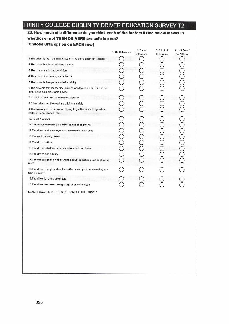
396

397

398

399

400

401

402
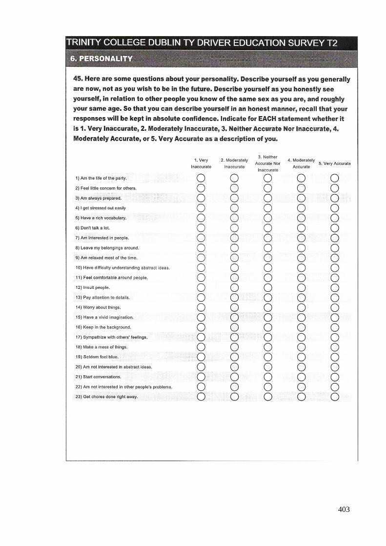
403

404

405

406
10.7 Appendix F. Time 3 (T3) – Post-intervention follow-up questionnaire
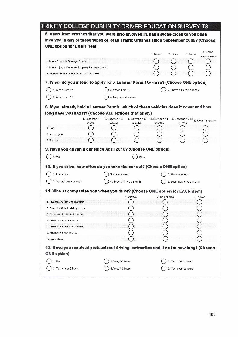
407

408

409

410

411

412

413

414

415

416

417

418
10.8 Appendix G. Time 2 (T2) - Supplementary knowledge quiz
These questions were designed to test your knowledge of the rules of the road.
Please put a circle around the letter opposite the correct answer(s).
1. What do flashing amber lights at a Pelican Crossing mean for drivers? (Circle ONE
option)**34
(a) Danger ahead - you must stop and wait until they stop flashing.
(b) Prepare to slow down.
(c)*35
Stop and give way to pedestrians, but proceed if the way is clear.
(d) Extra vigilance needed – children may be nearby.
2. What are the MOST IMPORTANT things that a driver should be conscious of in this
situation? (Circle TWO options)
(a)* People crossing the street at the rear of the bus.
(b) Caution and proper road conduct on the part of al road users.
(c) The bus driver will always signal before moving off.
(d)* People crossing the street from the left to catch the bus
3. In which of these circumstances must you NOT overtake other vehicles?
(Circle ONE option)**
(a) When you are driving in a residential area.
(b) When the vehicle in front is travelling 10km/h under the speed limit.
(c) When the surrounding traffic is flowing freely.
(d)* When you are in the left-hand lane of a dual carriageway when the traffic is
moving at normal speed.
4. What should a driver do when approaching this road sign? (Circle ONE option)**
(a)* Yield to traffic on the major road.
(b) Yield to traffic coming from the right.
(c) Yield to trucks and buses only.
(d) All vehicles, except bicycles, must yield.
5. Which of these rules apply to PEDESTRIANS using zebra crossings?
(Circle ALL correct options)
(a)* Pedestrians should avoid causing a driver to break suddenly or to swerve.
(b) Pedestrians have the right of way over other traffic while standing at the crossing.
(c)* Pedestrians are responsible for their own safety while using zebra crossings.
(d)* Pedestrians must not cross within or within 15 meters of the crossing.
34 Note: Items marked ** were used in both of the supplementary tests. 35 Note: Items marked * denote correct responses.
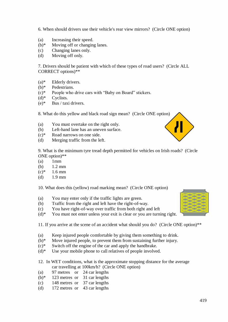
419
6. When should drivers use their vehicle's rear view mirrors? (Circle ONE option)
(a) Increasing their speed.
(b)* Moving off or changing lanes.
(c) Changing lanes only.
(d) Moving off only.
7. Drivers should be patient with which of these types of road users? (Circle ALL
CORRECT options)**
(a)* Elderly drivers.
(b)* Pedestrians.
(c)* People who drive cars with “Baby on Board” stickers.
(d)* Cyclists.
(e)* Bus / taxi drivers.
8. What do this yellow and black road sign mean? (Circle ONE option)
(a) You must overtake on the right only.
(b) Left-hand lane has an uneven surface.
(c)* Road narrows on one side.
(d) Merging traffic from the left.
9. What is the minimum tyre tread depth permitted for vehicles on Irish roads? (Circle
ONE option)**
(a) 1mm
(b) 1.2 mm
(c)* 1.6 mm
(d) 1.9 mm
10. What does this (yellow) road marking mean? (Circle ONE option)
(a) You may enter only if the traffic lights are green.
(b) Traffic from the right and left have the right-of-way.
(c) You have right-of-way over traffic from both right and left
(d)* You must not enter unless your exit is clear or you are turning right.
11. If you arrive at the scene of an accident what should you do? (Circle ONE option)**
(a) Keep injured people comfortable by giving them something to drink.
(b)* Move injured people, to prevent them from sustaining further injury.
(c)* Switch off the engine of the car and apply the handbrake.
(d)* Use your mobile phone to call relatives of people involved.
12. In WET conditions, what is the approximate stopping distance for the average
car travelling at 100km/h? (Circle ONE option)
(a) 97 metres or 24 car lengths
(b)* 123 metres or 31 car lengths
(c) 148 metres or 37 car lengths
(d) 172 metres or 43 car lengths

420
13. If driving from A to B, what do these road markings mean? (Circle ONE option)
(a) You may cross the continuous white line only when performing a ‘U’-turn.
(b)* You may overtake by crossing the continuous white line.
(c) You may not overtake by crossing the continuous white line.
(d) You may not overtake, only motorcyclists may cross the
continuous white line.
14. Which of these statements is NOT TRUE about the conditions under which learner
drivers are allowed to drive a car in a public place? (Circle ONE option)
(a) Driver must be over 17 years of age.
(b) Driver must have passed the driver theory test.
(c) Driver must be in possession of his/her learner permit while driving.
(d)* Driver must be accompanied by an adult.
(e) The vehicle is taxed and insured.
15. What do this (blue) road sign mean? (Circle ONE option)
(a) Crossing onto the opposite carriageway is not allowed.
(b) No overtaking.
(c)* End of motorway.
(d) Stopping under bridge is not allowed.
16. Which of the following actions can cause a vehicle to skid? (Circle THREE options)**
(a)* Harsh acceleration.
(b) Not enough pressure in the tyres.
(c)* Heavy braking.
(d) Too much pressure in the tyres.
(e) The steering wheel being too free or pliable.
(f)* Excessive speed.
17. If stopped by the Gardai, with which of these requests would you, as a driver, be
required to comply? (Circle ONE option)**
(a)* Write out your signature.
(b) Allow them to take your driving licence back to the Garda station.
(c)* Show them a valid motor insurance certificate.
(d)* Demonstrate that you are sober.
18. What does this hand signal mean? (Circle ONE option)
(a) The driver intends to turn left.
(b)* The driver intends to slow down or stop.
(c) The driver intends to turn right.
(d) The driver intends to begin a ‘U’-turn.
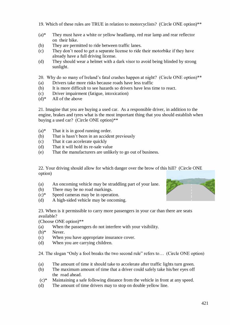
421
19. Which of these rules are TRUE in relation to motorcyclists? (Circle ONE option)**
(a)* They must have a white or yellow headlamp, red rear lamp and rear reflector
on their bike.
(b) They are permitted to ride between traffic lanes.
(c) They don’t need to get a separate license to ride their motorbike if they have
already have a full driving license.
(d) They should wear a helmet with a dark visor to avoid being blinded by strong
sunlight.
20. Why do so many of Ireland’s fatal crashes happen at night? (Circle ONE option)**
(a) Drivers take more risks because roads have less traffic
(b) It is more difficult to see hazards so drivers have less time to react.
(c) Driver impairment (fatigue, intoxication)
(d)* All of the above
21. Imagine that you are buying a used car. As a responsible driver, in addition to the
engine, brakes and tyres what is the most important thing that you should establish when
buying a used car? (Circle ONE option)**
(a)* That it is in good running order.
(b) That is hasn’t been in an accident previously
(c) That it can accelerate quickly
(d) That it will hold its re-sale value
(e) That the manufacturers are unlikely to go out of business.
22. Your driving should allow for which danger over the brow of this hill? (Circle ONE
option)
(a) An oncoming vehicle may be straddling part of your lane.
(b) There may be no road markings.
(c)* Speed cameras may be in operation.
(d) A high-sided vehicle may be oncoming.
23. When is it permissible to carry more passengers in your car than there are seats
available?
(Choose ONE option)**
(a) When the passengers do not interfere with your visibility.
(b)* Never.
(c) When you have appropriate insurance cover.
(d) When you are carrying children.
24. The slogan “Only a fool breaks the two second rule” refers to… (Circle ONE option)
(a) The amount of time it should take to accelerate after traffic lights turn green.
(b) The maximum amount of time that a driver could safely take his/her eyes off
the road ahead.
(c)* Maintaining a safe following distance from the vehicle in front at any speed.
(d) The amount of time drivers may to stop on double yellow line.

422
25. Imagine that you are driving this car approaching the roundabout.
Which conduct is correct? (Circle TWO options)
(a)* I must wait.
(b) The vehicle to the right must wait.
(c)* The vehicle on the roundabout has right of way.
(d) Treat the roundabout as a junction with roads of equal importance.
26. Which of the following rules must CYCLISTS obey? (Circle ALL CORRECT
options)**
(a)* Give proper signals before moving off, changing lanes and making a turn.
(b)* Don’t use mobile phone or personal entertainment system.
(c)* Wear reflective clothing at all times.
(d)* A cyclist must use a cycle track if it is provided

423
10.9 Appendix H. Time 3 (T3) - Supplementary knowledge quiz
These questions were designed to test your knowledge of the rules of the road.
Please put a circle around the letter opposite each correct answer(s).
1. What do flashing amber lights at a Pelican Crossing mean for drivers?
(Circle ONE option)**
(a) Danger ahead - you must stop and wait until they stop flashing.
(b) Prepare to slow down.
(c)* Stop and give way to pedestrians, but proceed if the way is clear.
(d) Extra vigilance needed – children may be nearby.
2. Why must you pay special attention to pedestrians in this situation?
(Circle TWO options)
(a) On side streets, pedestrians have the right of way.
(b)* Parked vehicles restrict the view of the motorists and pedestrians.
(c)* Pedestrians frequently step onto the road way without paying attention.
(d) Pedestrians are only allowed to cross the road at pedestrian crossings.
3. In which of these circumstances must you NOT overtake other vehicles?
(Circle ONE option)**
(a) When you are driving in a residential area.
(b) When the vehicle in front is travelling at 10km/h under the speed limit.
(c) When the surrounding traffic is flowing freely.
(d)* When you are in the left-hand lane of a dual carriageway when the traffic is
moving at normal speed.
4. What should a driver do when approaching this road sign? (Circle ONE option)**
(a)* Yield to traffic coming from the right.
(b) Yield to traffic on the major road.
(c) Yield to trucks and buses only.
(d) All vehicles, except bicycles, must yield.
5. Drivers should always make way for................................
(Circle ALL CORRECT options)
(a)* Emergency vehicles using sirens and flashing lights.
(b)* Pedestrians on or at a zebra crossing.
(c) Cyclists leaving a cycle lane.
(d)* Pedestrians at a junction, if they have started crossing the road.
6. When are ‘lighting up hour’? (Circle ONE option)
(a)* From half an hour after sunset to half an hour before sunrise.
(b) When visibility is less than 300 metres.
(c) From mid-night until 6 a.m.
(d) When visibility is less than 200 metres.

424
7. Drivers should be patient with which of these types of road users?
(Circle ALL CORRECT options)**
(a)* Middle aged drivers.
(b)* Pedestrians.
(c)* People who drive cars with “Baby on Board” stickers.
(d)* Cyclists.
(e)* Bus / taxi drivers.
8. What does this yellow and black road sign mean? (Circle ONE option)
(a) Series of bends ahead.
(b) Crosswinds ahead.
(c) Steep hill ahead.
(d)* Slippery stretch of road ahead.
9. What is the minimum tyre tread depth permitted for vehicles on Irish roads?
(Circle ONE option)**
(a) 1mm.
(b) 1.2 mm.
(c)* 1.6 mm.
(d) 1.9 mm.
10. What does this yellow and black chevron road sign mean? (Circle ONE option)
(a) Series of speed ramps ahead.
(b) Road closed – you must turn back.
(c)* Sharp change of direction ahead.
(d) Traffic from the left has priority.
11. If you arrive at the scene of an accident what should you do?
(Circle ALL CORRECT options)**
(a) Keep injured people comfortable by giving them something to drink.
(b)* Move injured people, if they are in danger of sustaining further injury.
(c)* Switch off the engines of the cars involved and apply the handbrakes.
(d)* Use your mobile phone to call the emergency services.
12. In WET conditions, what is the approximate stopping distance for the average car
travelling at 60km/h? (Circle ONE option)
(a) 35.2 metres or 9 car lengths.
(b)* 48.5 metres or 12 car lengths.
(c) 81.4 metres or 20 car lengths.
(d) 97.1 metres or 24 car lengths.

425
13. What does this road markings mean? (Circle ONE option)
(a) Road surface is uneven.
(b) You may park for a maximum of one hour only.
(c)* Pedestrian crossing is nearby.
(d) You may overtake if the road is clear ahead.
14. Which of these statements is TRUE about the conditions under which learner drivers
are allowed to drive a car in a public place? (Circle the ONE correct option)
(a) Driver must be over 16 years of age.
(b) Driver must have applied for the on-road driving test.
(c)* Driver must be in possession of his/her learner permit while driving.
(d) Driver must be accompanied by an adult.
(e) The vehicle must be under 10 years old.
15. What does this (blue) road sign mean? (Circle ONE option)
(a) Steep climb up ahead for 3 kilometres.
(b) Crossing traffic ahead.
(c) Three lanes ahead.
(d)* Three hundred metres to the next exit.
16. Which of the following actions can cause a vehicle to skid? (Circle THREE options)**
(a)* Harsh acceleration.
(b) Not enough pressure in the tyres.
(c)* Heavy braking.
(d) The steering wheel being too free or pliable.
(e)* Excessive speed.
17. If stopped by the Gardai, with which of these requests would you, as a driver, be
required to comply? (Circle ALL CORRECT options)**
(a)* Write out your signature.
(b) Allow them to take your driving license back to the Garda station.
(c)* Provide evidence that your car is taxed and insured.
(d)* Demonstrate that you are sober.
18. What does this hand signal mean? (Circle ONE option)
(a)* The driver intends to turn left.
(b) The driver intends to slow down or stop.
(c) The driver intends to turn right.
(d) The driver intends to begin a ‘U’-turn.
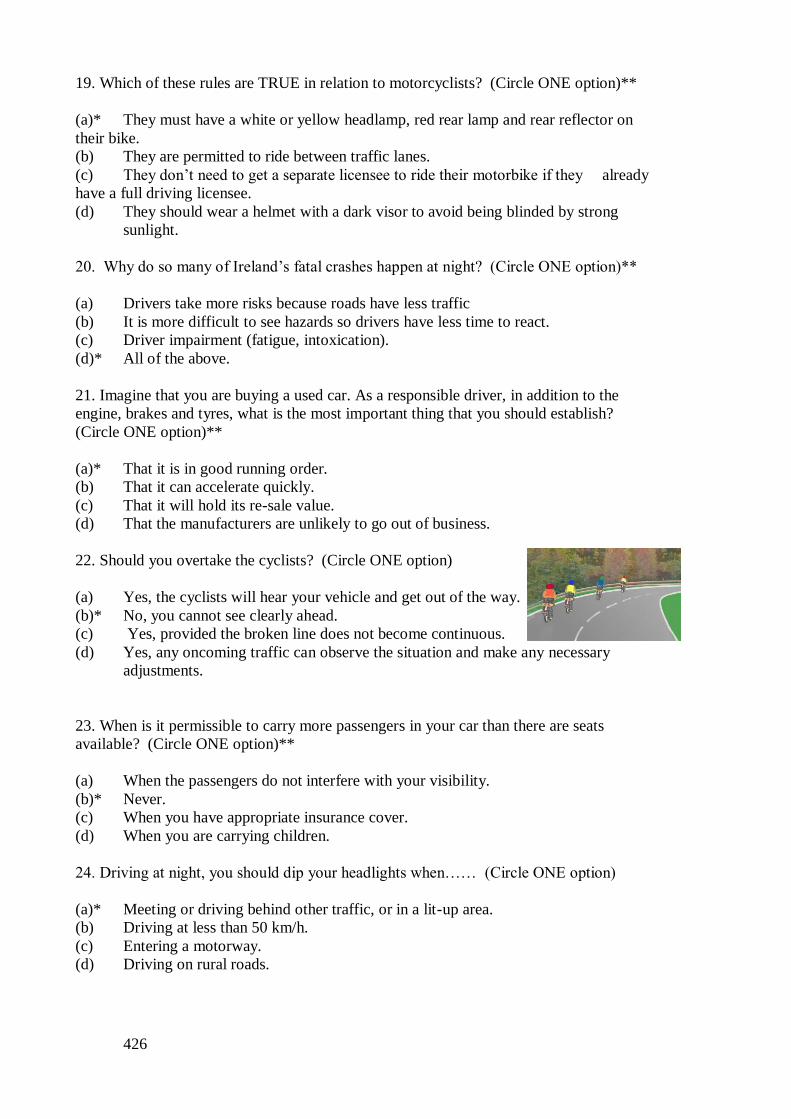
426
19. Which of these rules are TRUE in relation to motorcyclists? (Circle ONE option)**
(a)* They must have a white or yellow headlamp, red rear lamp and rear reflector on
their bike.
(b) They are permitted to ride between traffic lanes.
(c) They don’t need to get a separate licensee to ride their motorbike if they already
have a full driving licensee.
(d) They should wear a helmet with a dark visor to avoid being blinded by strong
sunlight.
20. Why do so many of Ireland’s fatal crashes happen at night? (Circle ONE option)**
(a) Drivers take more risks because roads have less traffic
(b) It is more difficult to see hazards so drivers have less time to react.
(c) Driver impairment (fatigue, intoxication).
(d)* All of the above.
21. Imagine that you are buying a used car. As a responsible driver, in addition to the
engine, brakes and tyres, what is the most important thing that you should establish?
(Circle ONE option)**
(a)* That it is in good running order.
(b) That it can accelerate quickly.
(c) That it will hold its re-sale value.
(d) That the manufacturers are unlikely to go out of business.
22. Should you overtake the cyclists? (Circle ONE option)
(a) Yes, the cyclists will hear your vehicle and get out of the way.
(b)* No, you cannot see clearly ahead.
(c) Yes, provided the broken line does not become continuous.
(d) Yes, any oncoming traffic can observe the situation and make any necessary
adjustments.
23. When is it permissible to carry more passengers in your car than there are seats
available? (Circle ONE option)**
(a) When the passengers do not interfere with your visibility.
(b)* Never.
(c) When you have appropriate insurance cover.
(d) When you are carrying children.
24. Driving at night, you should dip your headlights when…… (Circle ONE option)
(a)* Meeting or driving behind other traffic, or in a lit-up area.
(b) Driving at less than 50 km/h.
(c) Entering a motorway.
(d) Driving on rural roads.

427
25. A strong side wind is blowing from the left. You want to overtake the truck. You are
most exposed to danger…………….. (Circle TWO options)
(a)* On leaving the slipstream of the truck.
(b) If you apply the brakes while in the slipstream of the truck.
(c) Prior to entering the slipstream of the truck.
(d)* When you enter the slipstream of the truck.
26. Which of the following rules must CYCLISTS obey? (Circle ALL CORRECT
options)**
(a)* Give proper signals before moving off, changing lanes and making a turn.
(b)* Don’t use mobile phone or personal entertainment system.
(c)* Wear reflective clothing at all times.
(d)* A cyclist must use a cycle track if it is provided.
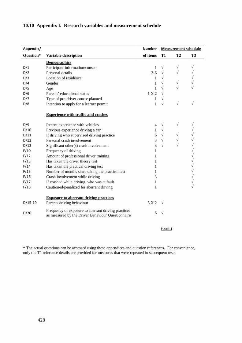
428
10.10 Appendix I. Research variables and measurement schedule
Appendix/ Number Measurement schedule
Question* Variable description of items T1 T2 T3
Demographics
D/1 Participant information/consent 1 √ √ √
D/2 Personal details 3-6 √ √ √
D/3 Location of residence 1 √
√
D/4 Gender 1 √ √ √
D/5 Age 1 √ √ √
D/6 Parents' educational status 1 X 2 √
D/7 Type of pre-driver course planned 1 √
D/8 Intention to apply for a learner permit 1 √ √ √
Experience with traffic and crashes
D/9 Recent experience with vehicles 4 √ √ √
D/10 Previous experience driving a car 1 √
√
D/11 If driving who supervised driving practice 6 √ √ √
D/12 Personal crash involvement 3 √ √ √
D/13 Significant other(s) crash involvement 3 √ √ √
F/10 Frequency of driving 1
√
F/12 Amount of professional driver training 1
√
F/13 Has taken the driver theory test 1
√
F/14 Has taken the practical driving test 1
√
F/15 Number of months since taking the practical test 1
√
F/16 Crash involvement while driving 3
√
F/17 If crashed while driving, who was at fault 1
√
F/18 Cautioned/penalized for aberrant driving 1
√
Exposure to aberrant driving practices
D/15-19 Parents driving behaviour 5 X 2 √
D/20 Frequency of exposure to aberrant driving practices
as measured by the Driver Behaviour Questionnaire 6 √
(cont.)
* The actual questions can be accessed using these appendices and question references. For convenience,
only the T1 reference details are provided for measures that were repeated in subsequent tests.
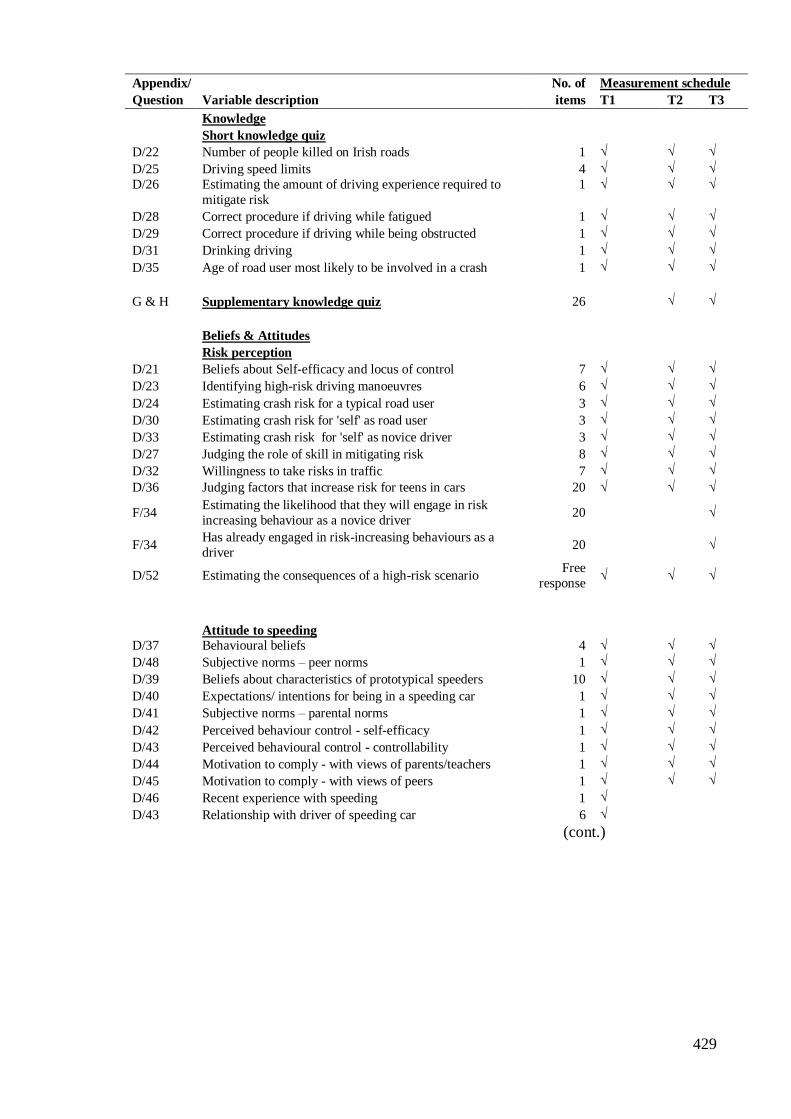
429
Appendix/ No. of Measurement schedule
Question Variable description items T1 T2 T3
Knowledge
Short knowledge quiz
D/22 Number of people killed on Irish roads 1 √ √ √
D/25 Driving speed limits 4 √ √ √
D/26 Estimating the amount of driving experience required to
mitigate risk
1 √ √ √
D/28 Correct procedure if driving while fatigued 1 √ √ √
D/29 Correct procedure if driving while being obstructed 1 √ √ √
D/31 Drinking driving 1 √ √ √
D/35 Age of road user most likely to be involved in a crash 1 √ √ √
G & H Supplementary knowledge quiz 26
√ √
Beliefs & Attitudes
Risk perception
D/21 Beliefs about Self-efficacy and locus of control 7 √ √ √
D/23 Identifying high-risk driving manoeuvres 6 √ √ √
D/24 Estimating crash risk for a typical road user 3 √ √ √
D/30 Estimating crash risk for 'self' as road user 3 √ √ √
D/33 Estimating crash risk for 'self' as novice driver 3 √ √ √
D/27 Judging the role of skill in mitigating risk 8 √ √ √
D/32 Willingness to take risks in traffic 7 √ √ √
D/36 Judging factors that increase risk for teens in cars 20 √ √ √
F/34 Estimating the likelihood that they will engage in risk
increasing behaviour as a novice driver 20
√
F/34 Has already engaged in risk-increasing behaviours as a
driver 20
√
D/52 Estimating the consequences of a high-risk scenario Free
response √ √ √
Attitude to speeding
D/37 Behavioural beliefs 4 √ √ √
D/48 Subjective norms – peer norms 1 √ √ √
D/39 Beliefs about characteristics of prototypical speeders 10 √ √ √
D/40 Expectations/ intentions for being in a speeding car 1 √ √ √
D/41 Subjective norms – parental norms 1 √ √ √
D/42 Perceived behaviour control - self-efficacy 1 √ √ √
D/43 Perceived behavioural control - controllability 1 √ √ √
D/44 Motivation to comply - with views of parents/teachers 1 √ √ √
D/45 Motivation to comply - with views of peers 1 √ √ √
D/46 Recent experience with speeding 1 √
D/43 Relationship with driver of speeding car 6 √
(cont.)
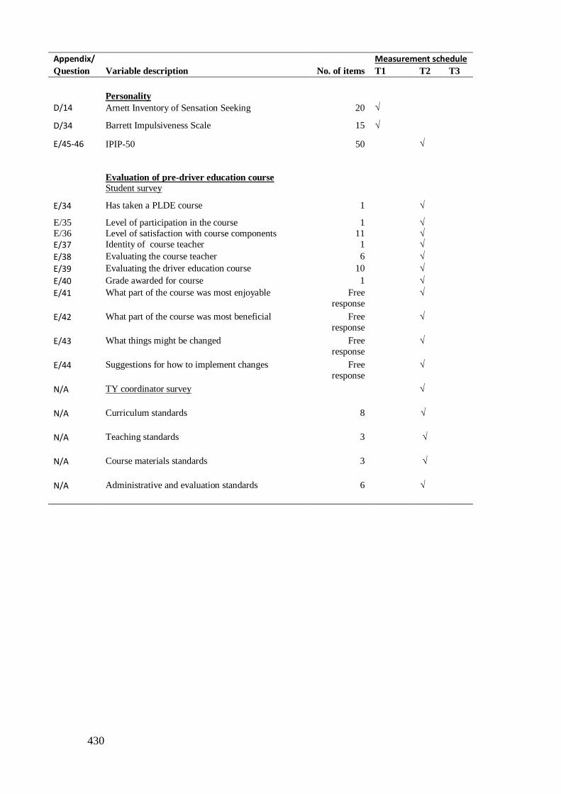
430
Appendix/
Measurement schedule
Question Variable description No. of items T1 T2 T3
Personality
D/14 Arnett Inventory of Sensation Seeking 20 √
D/34 Barrett Impulsiveness Scale 15 √
E/45-46 IPIP-50 50
√
Evaluation of pre-driver education course
Student survey
E/34 Has taken a PLDE course 1 √
E/35 Level of participation in the course 1 √ E/36 Level of satisfaction with course components 11 √ E/37 Identity of course teacher 1 √
E/38 Evaluating the course teacher 6 √
E/39 Evaluating the driver education course 10 √
E/40 Grade awarded for course 1 √
E/41 What part of the course was most enjoyable Free
response √
E/42 What part of the course was most beneficial Free
response √
E/43 What things might be changed Free
response √
E/44 Suggestions for how to implement changes Free
response √
N/A TY coordinator survey √
N/A Curriculum standards 8 √
N/A Teaching standards 3 √
N/A Course materials standards 3
√
N/A Administrative and evaluation standards 6 √

431
10.11 Appendix J. TY coordinator survey
TY COORDINATOR QUESTIONNAIRE
Please answer these questions in relation to the pre-learner driver education course that was delivered to your TY students during the school year 2009-2010.
Item CURRICULUM STANDARDS
Y
YES
N
NO
1 Does the school have a curriculum guide for the course?
2 Do course teachers have a copy of the curriculum and follow it?
3 Is traffic safety education considered an integral part of the school
curriculum?
4 Does the course stipulate appropriate performance objectives for all
lessons?
5 Does the course include activities that enable the student to
accomplish these objectives?
6 Does the curriculum include tests which measure student
achievements with respect to all of the course objectives?
7 Do teachers of other subjects integrate traffic safety concepts into
their classes?
8 Are written criteria for successful completion of the course given to
all students?
TEACHING STANDARDS
Y
YES
N
NO
9 Are course teachers selected on the basis of their academic
achievements and/or their experience with teaching traffic safety
education?
10 Have teachers/instructors received any certification before teaching
the course?
11 Is the course-related performance of the teacher/instructor assessed
regularly?
School:

432
COURSE MATERIAL STANDARDS
Y
YES
N
NO
12 Does the course contain sufficient amounts of quality instructional
materials to help students achieve the course objectives?
13 Are supplementary teaching materials, lectures, demonstrations
etc. related to driver and traffic safety education used?
(i.e. elements that are not part of the main road safety course)
14 If so, are these critically reviewed before use by school authorities?
ADMINISTRATION AND EVALUATION STANDARDS
Y
YES
N
NO
15 Do students receive academic credit for the successful completion
of the course?
16 Are academic standards maintained on a par with those of other
courses?
17 Are parents involved in the educational process?
18
Is written information concerning all aspects of the programme
provided for all parents?
19 Is the program evaluated annually at school-level i.e. by
administrators, TY coordinators, and/or instructional staff?
20 Are student performance recorded and maintained as a guide for
program evaluations and to indicate students achievement?

433
10.12 Appendix K. Information/consent (Parents)
LETTER OF CONSENT (Parents)
Re: Trinity College, Dublin’s Evaluation of Transition Year Pre-driver
Education Programmes.
The school that your son/daughter attends has agreed to participate in this research
project that aims to evaluate the various forms of pre-driver education currently in use by
transition year students in Irish secondary schools. This research is being undertaken by
Margaret Ryan, who a is research student at the School of Psychology, Trinity College,
Dublin.
The study will examine the impact of the driver education that your son/daughter
will receive during Transition Year on their knowledge, skills, attitudes and behaviour over
time. It will also examine factors that influence the ways in which they engage with
programme content. The research will be conducted using questionnaires, which take
approximately 50 minutes to complete. They will be asked to do this on 3 separate
occasions: Once in the Autumn of 2009, then again in April/May 2010 and finally in
January/February 2011.
If you agree to allow your son/daughter to participate in this study their identity
will be coded for anonimity purposes and the information they provide will be securely
stored in the School of Psychology TCD. Only mysef and my supervisors will have access
to these records. Students will be at liberty to withdraw from the study at any time without

434
prejudice. Your/their rights under the Freedom of Information Act 1977 (amended 2003)
will be respected at all times.
Further details can be obtained by contacting the researcher
Margaret Ryan,
c/o School of Psychology, TCD, Dublin 2.
This study is being supervised by
Dr. Michael Gormley, & Dr. Kevin Thomas,
[email protected] [email protected],
Tel: 01-8963093 01-8963237
Please place an X in the box to indicate that you have read and understood the above and
that you agree to participate in this study.
Enter Your Name here
Son/Daughter’s Name
Enter School Name here
Date
435
10.13 Appendix L. Results for Chapter 4, Personal characteristics
10.13.1 Confirmatory factor analysis for personality measures
Separate confirmatory factor analyses (CFAs) were conducted to examine the
structure of the data from the AISS (Arnett, 1994), the BIS-15 (Spinella, 2007) and the
IPIP (Goldberg, 2011), using AMOS software (Arbuckle, 2009).
10.13.1.1 AISS
CAF was used to fit a succession of models based on scores from the AISS
(Arnett, 1994). First, a univariate model was tested where all observed variables loaded
onto a single latent variable. The results revealed non-significant loadings for two items:
Item 3 “If I have to wait a long time, I am usually patient about it” and item 15 “I often like
to have the TV on while I am doing something else, such as reading or cleaning up”.
Despite the removal of these items the univariate model remained a poor fit for the data
(χ2 (1880) = 1007.72 [P=.00]; RMSEA = .06 [.06-.06]; GFI = .93; CFI = .51: ECVI = .57
[.52-.63]). A two-factor model was constructed where twenty observed variables loaded
onto two correlated latent variables, labelled “Novelty” and “Intensity”. Results for this
model showed that four observed variables on the Novelty factor (items 3,5,13 and 15) and
one observed variable in the Intensity factor (item 4) “Intensity” did not load significantly
on to these factors. These items were subsequently deleted and the model was re-evaluated
using the remaining 15 items. Although the model fit improved (χ2 (1880) = 605.65 [P
=.00]; RMSEA = .06 [.05-.06]; GFI = .95; CFI = .67: ECVI = .36 [.32-.40]), both the
RMSEA and the CFI remained below acceptable thresholds. Inspection of the modification
indices highlighted correlations between several of the error terms associated with each of
the factors. However, when these correlations were added the model fit remained poor,
prompting the rejection of this model.
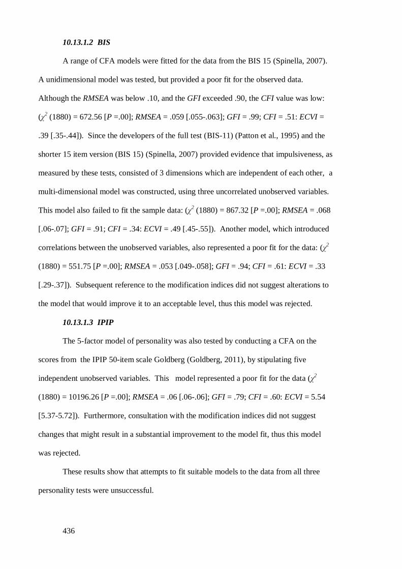
436
10.13.1.2 BIS
A range of CFA models were fitted for the data from the BIS 15 (Spinella, 2007).
A unidimensional model was tested, but provided a poor fit for the observed data.
Although the RMSEA was below .10, and the GFI exceeded .90, the CFI value was low:
(χ2 (1880) = 672.56 [P =.00]; RMSEA = .059 [.055-.063]; GFI = .99; CFI = .51: ECVI =
.39 [.35-.44]). Since the developers of the full test (BIS-11) (Patton et al., 1995) and the
shorter 15 item version (BIS 15) (Spinella, 2007) provided evidence that impulsiveness, as
measured by these tests, consisted of 3 dimensions which are independent of each other, a
multi-dimensional model was constructed, using three uncorrelated unobserved variables.
This model also failed to fit the sample data: (χ2 (1880) = 867.32 [P =.00]; RMSEA = .068
[.06-.07]; GFI = .91; CFI = .34: ECVI = .49 [.45-.55]). Another model, which introduced
correlations between the unobserved variables, also represented a poor fit for the data: (χ2
(1880) = 551.75 [P =.00]; RMSEA = .053 [.049-.058]; GFI = .94; CFI = .61: ECVI = .33
[.29-.37]). Subsequent reference to the modification indices did not suggest alterations to
the model that would improve it to an acceptable level, thus this model was rejected.
10.13.1.3 IPIP
The 5-factor model of personality was also tested by conducting a CFA on the
scores from the IPIP 50-item scale Goldberg (Goldberg, 2011), by stipulating five
independent unobserved variables. This model represented a poor fit for the data (χ2
(1880) = 10196.26 [P =.00]; RMSEA = .06 [.06-.06]; GFI = .79; CFI = .60: ECVI = 5.54
[5.37-5.72]). Furthermore, consultation with the modification indices did not suggest
changes that might result in a substantial improvement to the model fit, thus this model
was rejected.
These results show that attempts to fit suitable models to the data from all three
personality tests were unsuccessful.
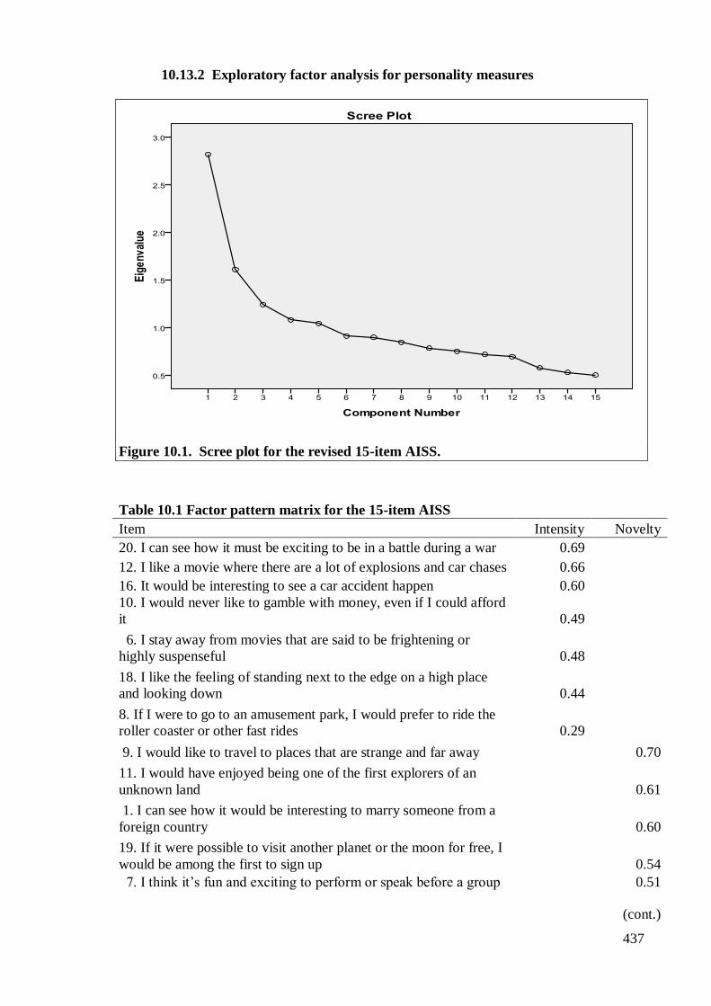
437
10.13.2 Exploratory factor analysis for personality measures
Figure 10.1. Scree plot for the revised 15-item AISS.
Table 10.1 Factor pattern matrix for the 15-item AISS
Item Intensity Novelty
20. I can see how it must be exciting to be in a battle during a war 0.69
12. I like a movie where there are a lot of explosions and car chases 0.66
16. It would be interesting to see a car accident happen 0.60
10. I would never like to gamble with money, even if I could afford
it 0.49
6. I stay away from movies that are said to be frightening or
highly suspenseful 0.48
18. I like the feeling of standing next to the edge on a high place
and looking down 0.44
8. If I were to go to an amusement park, I would prefer to ride the
roller coaster or other fast rides 0.29
9. I would like to travel to places that are strange and far away
0.70
11. I would have enjoyed being one of the first explorers of an
unknown land
0.61
1. I can see how it would be interesting to marry someone from a
foreign country
0.60
19. If it were possible to visit another planet or the moon for free, I
would be among the first to sign up
0.54
7. I think it’s fun and exciting to perform or speak before a group
0.51
(cont.)
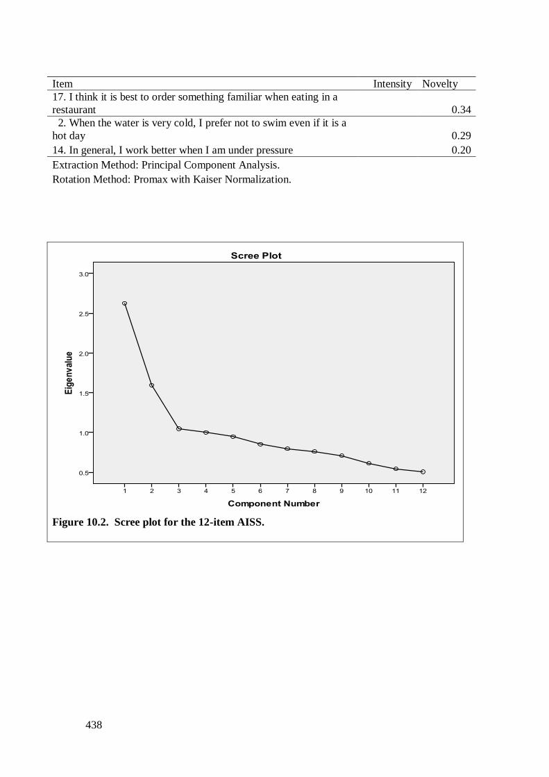
438
Item Intensity Novelty
17. I think it is best to order something familiar when eating in a
restaurant 0.34
2. When the water is very cold, I prefer not to swim even if it is a
hot day 0.29
14. In general, I work better when I am under pressure 0.20
Extraction Method: Principal Component Analysis.
Rotation Method: Promax with Kaiser Normalization.
Figure 10.2. Scree plot for the 12-item AISS.
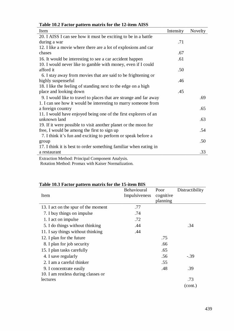
439
Table 10.2 Factor pattern matrix for the 12-item AISS
Item Intensity Novelty
20. I AISS I can see how it must be exciting to be in a battle
during a war .71
12. I like a movie where there are a lot of explosions and car
chases .67
16. It would be interesting to see a car accident happen .61
10. I would never like to gamble with money, even if I could
afford it .50
6. I stay away from movies that are said to be frightening or
highly suspenseful .46
18. I like the feeling of standing next to the edge on a high
place and looking down .45
9. I would like to travel to places that are strange and far away .69
1. I can see how it would be interesting to marry someone from
a foreign country .65
11. I would have enjoyed being one of the first explorers of an
unknown land .63
19. If it were possible to visit another planet or the moon for
free, I would be among the first to sign up .54
7. I think it’s fun and exciting to perform or speak before a
group .50
17. I think it is best to order something familiar when eating in
a restaurant .33
Extraction Method: Principal Component Analysis. Rotation Method: Promax with Kaiser Normalization.
Table 10.3 Factor pattern matrix for the 15-item BIS
Item
Behavioural
Impulsiveness
Poor
cognitive
planning
Distractibility
13. I act on the spur of the moment .77
7. I buy things on impulse .74
1. I act on impulse .72
5. I do things without thinking .44
.34
11. I say things without thinking .44
12. I plan for the future
.75
8. I plan for job security
.66
15. I plan tasks carefully
.65
4. I save regularly
.56 -.39
2. I am a careful thinker
.55
9. I concentrate easily
.48 .39
10. I am restless during classes or
lectures
.73
(cont.)
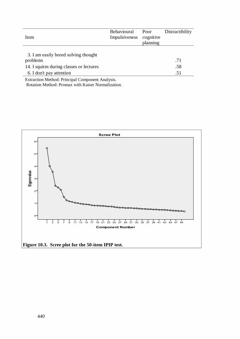
440
Item
Behavioural
Impulsiveness
Poor
cognitive
planning
Distractibility
3. I am easily bored solving thought
problems
.71
14. I squirm during classes or lectures
.58
6. I don't pay attention
.51
Extraction Method: Principal Component Analysis.
Rotation Method: Promax with Kaiser Normalization.
Figure 10.3. Scree plot for the 50-item IPIP test.
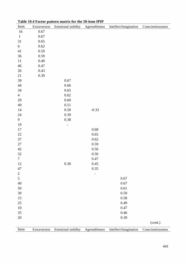
441
Table 10.4 Factor pattern matrix for the 50-item IPIP
Item Extraversion Emotional stability Agreeableness Intellect/Imagination Conscientiousness
16 0.67
1 0.67
31 0.65
6 0.62
41 0.59
36 0.59
11 0.49
46 0.47
26 0.43
21 0.39
39
0.67
44
0.66
34
0.65
4
0.62
29
0.60
49
0.51
14
0.50 -0.33
24
0.39
9
0.38
19
-
17
0.68
22
0.65
37
0.62
27
0.59
42
0.56
32
0.50
7
0.47
12
0.30 0.45
47
0.35
2
-
5
0.67
40
0.67
50
0.61
30
0.59
15
0.58
25
0.49
10
0.47
35
0.46
20
0.39
(cont.)
Item Extraversion Emotional stability Agreeableness Intellect/Imagination Conscientiousness
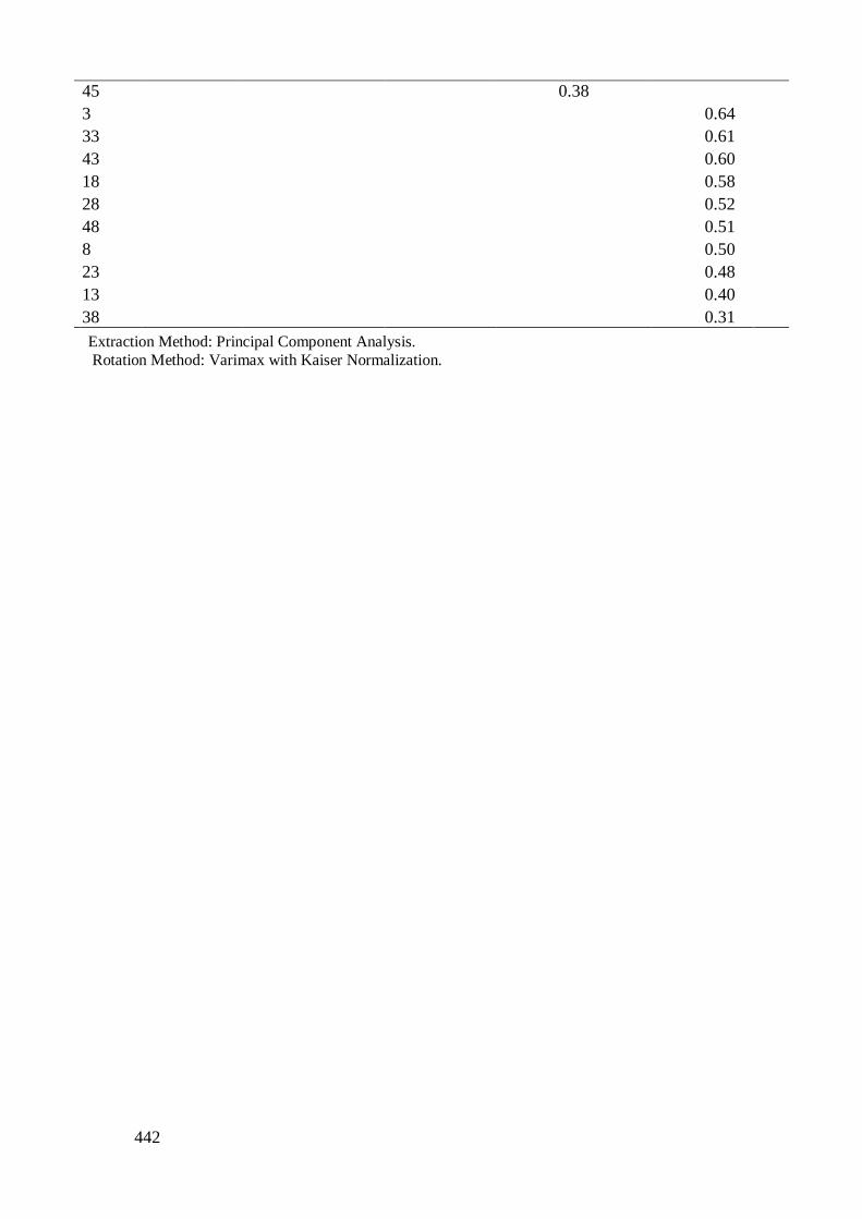
442
45
0.38
3
0.64
33
0.61
43
0.60
18
0.58
28
0.52
48
0.51
8
0.50
23
0.48
13
0.40
38
0.31
Extraction Method: Principal Component Analysis. Rotation Method: Varimax with Kaiser Normalization.
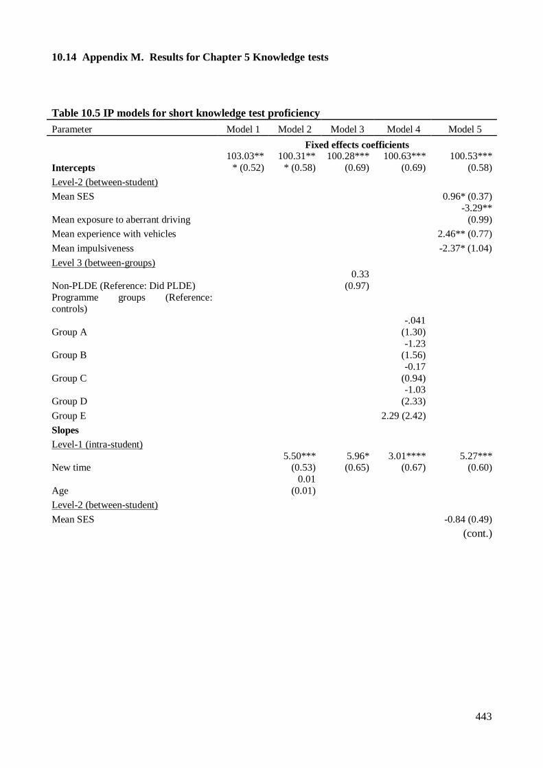
443
10.14 Appendix M. Results for Chapter 5 Knowledge tests
Table 10.5 IP models for short knowledge test proficiency
Parameter Model 1 Model 2 Model 3 Model 4 Model 5
Fixed effects coefficients
Intercepts 103.03**
* (0.52) 100.31**
* (0.58) 100.28***
(0.69) 100.63***
(0.69) 100.53***
(0.58)
Level-2 (between-student) Mean SES
0.96* (0.37)
Mean exposure to aberrant driving
-3.29**
(0.99)
Mean experience with vehicles
2.46** (0.77)
Mean impulsiveness
-2.37* (1.04)
Level 3 (between-groups)
Non-PLDE (Reference: Did PLDE)
0.33
(0.97)
Programme groups (Reference: controls)
Group A
-.041
(1.30)
Group B
-1.23 (1.56)
Group C
-0.17
(0.94)
Group D
-1.03
(2.33)
Group E
2.29 (2.42) Slopes
Level-1 (intra-student)
New time
5.50*** (0.53)
5.96* (0.65)
3.01**** (0.67)
5.27*** (0.60)
Age
0.01
(0.01)
Level-2 (between-student)
Mean SES
-0.84 (0.49)
(cont.)
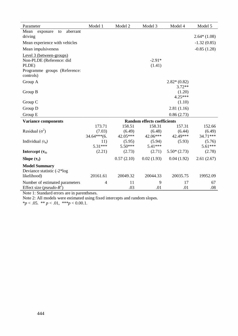
444
Parameter Model 1 Model 2 Model 3 Model 4 Model 5 Mean exposure to aberrant
driving
2.64* (1.08)
Mean experience with vehicles
-1.32 (0.85)
Mean impulsiveness
-0.85 (1.28)
Level 3 (between-groups) Non-PLDE (Reference: did
PLDE)
-2.91*
(1.41)
Programme groups (Reference: controls)
Group A
2.82* (0.82)
Group B
3.72** (1.20)
Group C
4.25***
(1.10)
Group D
2.81 (1.16) Group E
0.86 (2.73)
Variance components Random effects coefficients
Residual (σ2)
173.71 (7.03)
158.51 (6.49)
158.31 (6.48)
157.31 (6.44)
152.66 (6.49)
Individual (τπ) 34.64***(6.
11) 42.05***
(5.95) 42.06***
(5.94) 42.49***
(5.93) 34.71***
(5.76)
Intercept (τϐ) 5.31***
(2.21) 5.50***
(2.73) 5.41***
(2.71) 5.50* (2.73) 5.61***
(2.78)
Slope (τϐ)
0.57 (2.10) 0.02 (1.93) 0.04 (1.92) 2.61 (2.67)
Model Summary
Deviance statistic (-2*log likelihood) 20161.61 20049.32 20044.33 20035.75 19952.09
Number of estimated parameters 4 11 9 17 67 Effect size (pseudo-R
2)
.03 .01 .01 .08
Note 1: Standard errors are in parentheses. Note 2: All models were estimated using fixed intercepts and random slopes.
*p < .05. ** p < .01, ***p < 0.00.1.
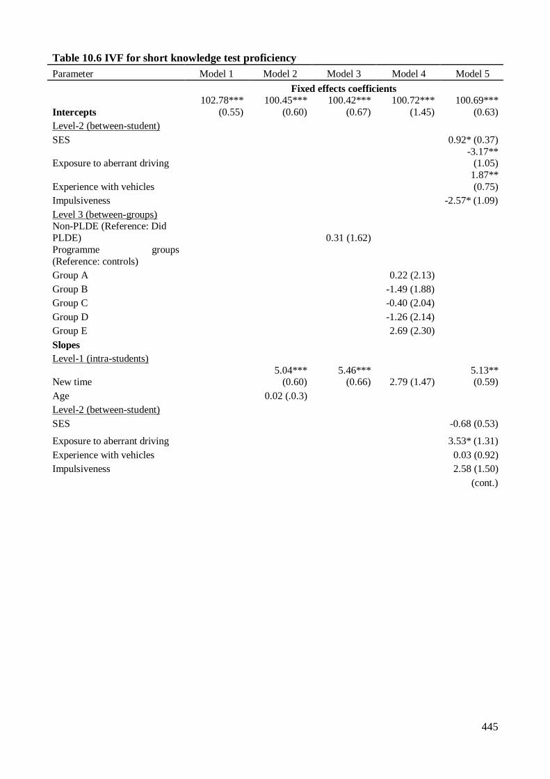
445
Table 10.6 IVF for short knowledge test proficiency
Parameter Model 1 Model 2 Model 3 Model 4 Model 5
Fixed effects coefficients
Intercepts 102.78***
(0.55) 100.45***
(0.60) 100.42***
(0.67) 100.72***
(1.45) 100.69***
(0.63)
Level-2 (between-student)
SES
0.92* (0.37)
Exposure to aberrant driving
-3.17** (1.05)
Experience with vehicles
1.87**
(0.75)
Impulsiveness
-2.57* (1.09)
Level 3 (between-groups) Non-PLDE (Reference: Did
PLDE)
0.31 (1.62)
Programme groups
(Reference: controls) Group A
0.22 (2.13)
Group B
-1.49 (1.88) Group C
-0.40 (2.04)
Group D
-1.26 (2.14) Group E
2.69 (2.30)
Slopes Level-1 (intra-students)
New time
5.04*** (0.60)
5.46*** (0.66) 2.79 (1.47)
5.13** (0.59)
Age
0.02 (.0.3)
Level-2 (between-student)
SES
-0.68 (0.53)
Exposure to aberrant driving
3.53* (1.31)
Experience with vehicles
0.03 (0.92)
Impulsiveness
2.58 (1.50)
(cont.)
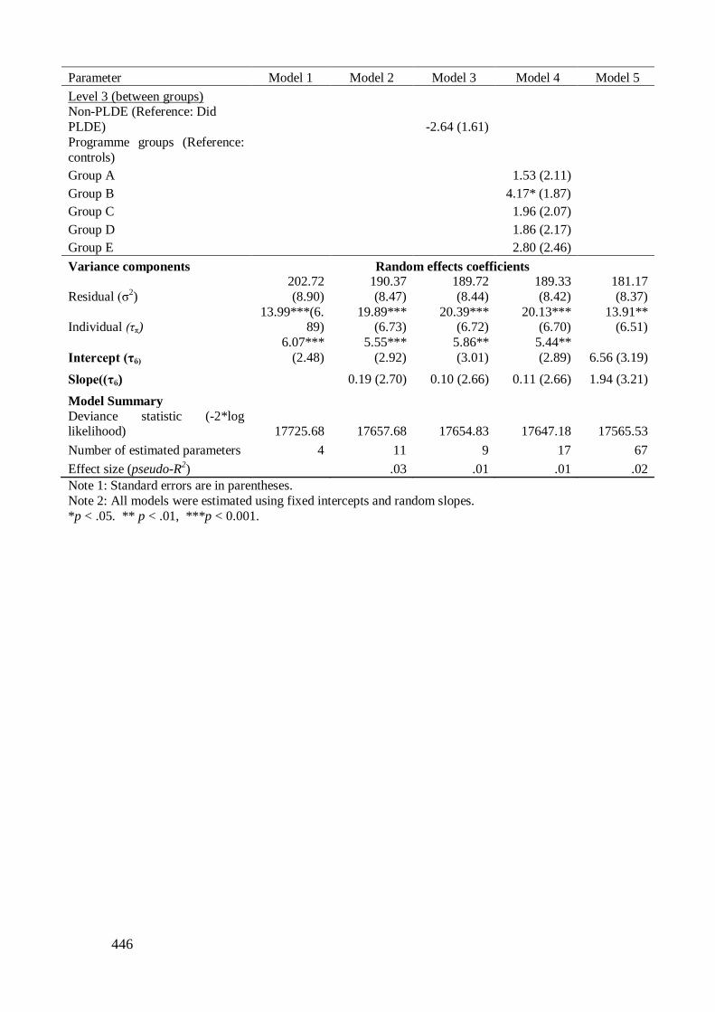
446
Parameter Model 1 Model 2 Model 3 Model 4 Model 5
Level 3 (between groups) Non-PLDE (Reference: Did
PLDE)
-2.64 (1.61)
Programme groups (Reference:
controls) Group A
1.53 (2.11)
Group B
4.17* (1.87) Group C
1.96 (2.07)
Group D
1.86 (2.17) Group E
2.80 (2.46)
Variance components Random effects coefficients
Residual (σ2)
202.72
(8.90) 190.37
(8.47) 189.72
(8.44) 189.33
(8.42) 181.17
(8.37)
Individual (τπ) 13.99***(6.
89) 19.89***
(6.73) 20.39***
(6.72) 20.13***
(6.70) 13.91**
(6.51)
Intercept (τϐ) 6.07***
(2.48) 5.55***
(2.92) 5.86**
(3.01) 5.44**
(2.89) 6.56 (3.19)
Slope((τϐ)
0.19 (2.70) 0.10 (2.66) 0.11 (2.66) 1.94 (3.21)
Model Summary
Deviance statistic (-2*log likelihood) 17725.68 17657.68 17654.83 17647.18 17565.53
Number of estimated parameters 4 11 9 17 67
Effect size (pseudo-R2)
.03 .01 .01 .02
Note 1: Standard errors are in parentheses.
Note 2: All models were estimated using fixed intercepts and random slopes.
*p < .05. ** p < .01, ***p < 0.001.
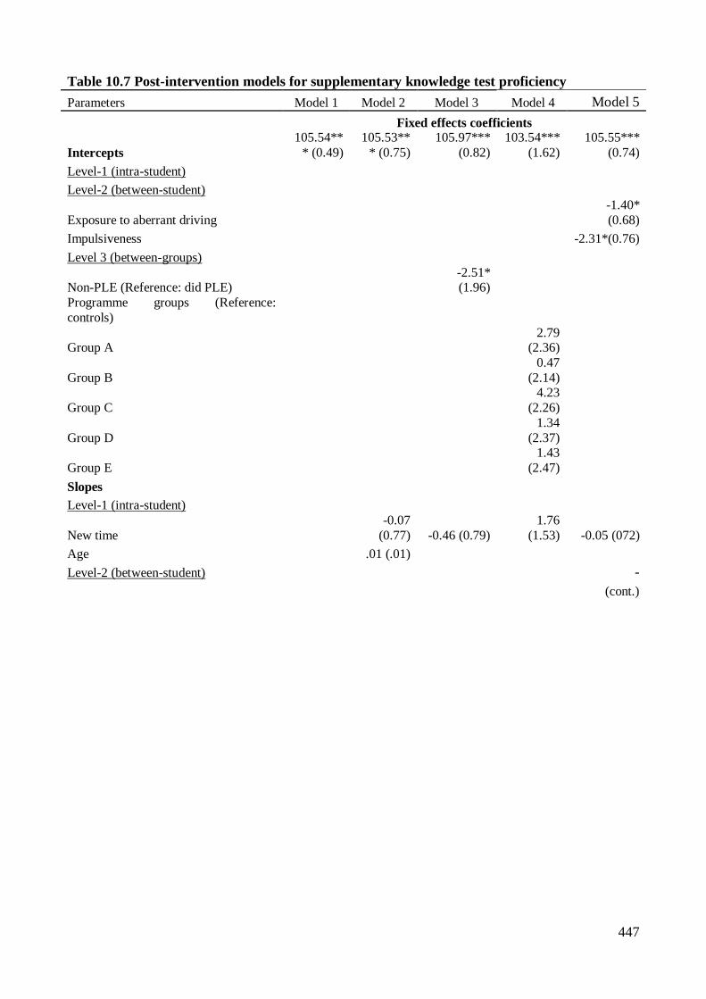
447
Table 10.7 Post-intervention models for supplementary knowledge test proficiency
Parameters Model 1 Model 2 Model 3 Model 4 Model 5
Fixed effects coefficients
Intercepts 105.54**
* (0.49) 105.53**
* (0.75) 105.97***
(0.82) 103.54***
(1.62) 105.55***
(0.74)
Level-1 (intra-student) Level-2 (between-student)
Exposure to aberrant driving
-1.40*
(0.68)
Impulsiveness
-2.31*(0.76)
Level 3 (between-groups)
Non-PLE (Reference: did PLE)
-2.51* (1.96)
Programme groups (Reference:
controls)
Group A
2.79 (2.36)
Group B
0.47
(2.14)
Group C
4.23
(2.26)
Group D
1.34
(2.37)
Group E
1.43
(2.47)
Slopes Level-1 (intra-student)
New time
-0.07
(0.77) -0.46 (0.79) 1.76
(1.53) -0.05 (072)
Age
.01 (.01)
Level-2 (between-student)
-
(cont.)
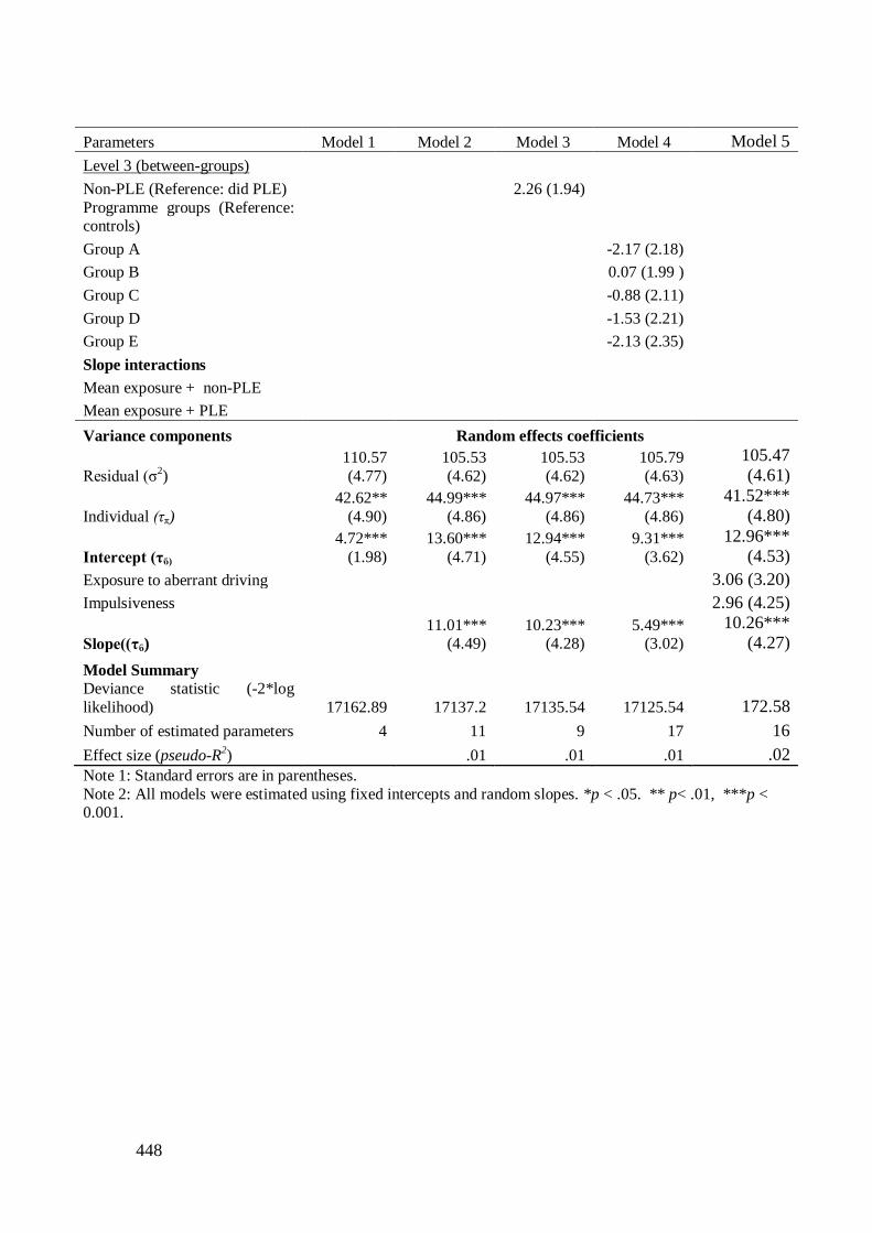
448
Parameters Model 1 Model 2 Model 3 Model 4 Model 5
Level 3 (between-groups)
Non-PLE (Reference: did PLE)
2.26 (1.94)
Programme groups (Reference: controls)
Group A
-2.17 (2.18)
Group B
0.07 (1.99 )
Group C
-0.88 (2.11)
Group D
-1.53 (2.21) Group E
-2.13 (2.35)
Slope interactions
Mean exposure + non-PLE Mean exposure + PLE
Variance components Random effects coefficients
Residual (σ2)
110.57
(4.77) 105.53
(4.62) 105.53
(4.62) 105.79
(4.63)
105.47
(4.61)
Individual (τπ) 42.62**
(4.90) 44.99***
(4.86) 44.97***
(4.86) 44.73***
(4.86)
41.52***
(4.80)
Intercept (τϐ) 4.72***
(1.98) 13.60***
(4.71) 12.94***
(4.55) 9.31***
(3.62)
12.96***
(4.53)
Exposure to aberrant driving
3.06 (3.20)
Impulsiveness
2.96 (4.25)
Slope((τϐ)
11.01*** (4.49)
10.23*** (4.28)
5.49*** (3.02)
10.26***
(4.27)
Model Summary
Deviance statistic (-2*log
likelihood) 17162.89 17137.2 17135.54 17125.54 172.58
Number of estimated parameters 4 11 9 17 16
Effect size (pseudo-R2)
.01 .01 .01 .02
Note 1: Standard errors are in parentheses.
Note 2: All models were estimated using fixed intercepts and random slopes. *p < .05. ** p< .01, ***p < 0.001.

449
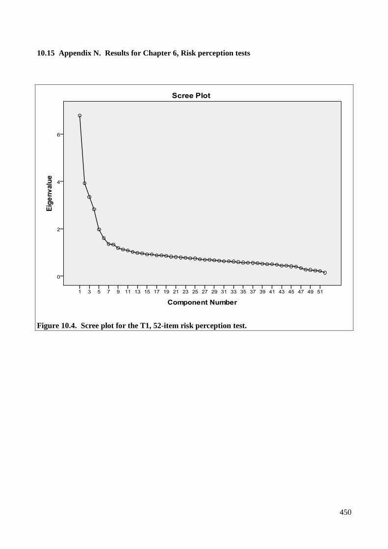
450
10.15 Appendix N. Results for Chapter 6, Risk perception tests
Figure 10.4. Scree plot for the T1, 52-item risk perception test.
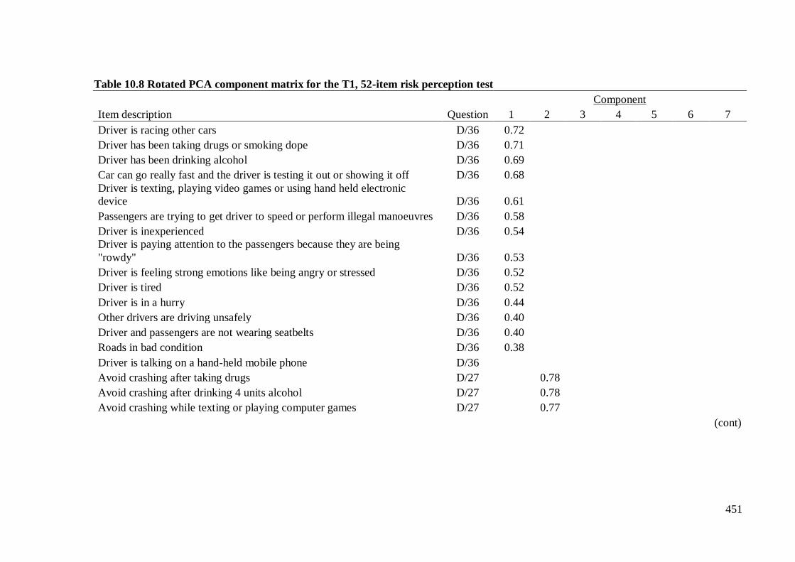
451
Table 10.8 Rotated PCA component matrix for the T1, 52-item risk perception test
Component
Item description Question 1 2 3 4 5 6 7
Driver is racing other cars D/36 0.72
Driver has been taking drugs or smoking dope D/36 0.71
Driver has been drinking alcohol D/36 0.69
Car can go really fast and the driver is testing it out or showing it off D/36 0.68
Driver is texting, playing video games or using hand held electronic
device D/36 0.61
Passengers are trying to get driver to speed or perform illegal manoeuvres D/36 0.58
Driver is inexperienced D/36 0.54 Driver is paying attention to the passengers because they are being
"rowdy" D/36 0.53
Driver is feeling strong emotions like being angry or stressed D/36 0.52
Driver is tired D/36 0.52
Driver is in a hurry D/36 0.44
Other drivers are driving unsafely D/36 0.40
Driver and passengers are not wearing seatbelts D/36 0.40
Roads in bad condition D/36 0.38
Driver is talking on a hand-held mobile phone D/36
Avoid crashing after taking drugs D/27 0.78
Avoid crashing after drinking 4 units alcohol D/27 0.78
Avoid crashing while texting or playing computer games D/27 0.77
(cont)
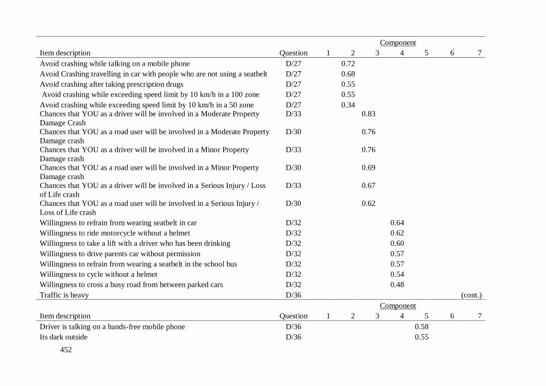
452
Component
Item description Question 1 2 3 4 5 6 7
Avoid crashing while talking on a mobile phone D/27 0.72
Avoid Crashing travelling in car with people who are not using a seatbelt D/27 0.68
Avoid crashing after taking prescription drugs D/27 0.55
Avoid crashing while exceeding speed limit by 10 km/h in a 100 zone D/27 0.55
Avoid crashing while exceeding speed limit by 10 km/h in a 50 zone D/27 0.34 Chances that YOU as a driver will be involved in a Moderate Property
Damage Crash
D/33 0.83
Chances that YOU as a road user will be involved in a Moderate Property
Damage crash
D/30 0.76
Chances that YOU as a driver will be involved in a Minor Property
Damage crash
D/33 0.76
Chances that YOU as a road user will be involved in a Minor Property
Damage crash
D/30 0.69
Chances that YOU as a driver will be involved in a Serious Injury / Loss
of Life crash
D/33 0.67
Chances that YOU as a road user will be involved in a Serious Injury /
Loss of Life crash
D/30 0.62
Willingness to refrain from wearing seatbelt in car D/32 0.64
Willingness to ride motorcycle without a helmet D/32 0.62
Willingness to take a lift with a driver who has been drinking D/32 0.60
Willingness to drive parents car without permission D/32 0.57
Willingness to refrain from wearing a seatbelt in the school bus D/32 0.57
Willingness to cycle without a helmet D/32 0.54
Willingness to cross a busy road from between parked cars D/32 0.48
Traffic is heavy D/36
(cont.)
Component
Item description Question 1 2 3 4 5 6 7
Driver is talking on a hands-free mobile phone D/36 0.58
Its dark outside D/36 0.55

453
It is cold or wet and the roads are slippery D/36
0.44
There are other teenagers in the car D/36 0.32
Chances that a typical road user will be involved in a Serious Injury/Loss
of Life crash
D/24 0.83
Chances that a typical road user will be in a Minor Property Damage crash D/24 0.79
Chances that a typical road user will be involved in a Serious Injury/Loss
of Life crash
D/24 0.38
Lots of drivers are careless. I can't do anything about it if they crash into
me
D/21 0.42 0.52
If we just do what our teachers, parents and the authorities tell us, we will
go through life like robots, never fully enjoying things
D/21 0.31 0.34 0.41
Learning to drive will be easy for me D/21 0.37
Avoiding accidents over a long period is basically down to luck is down
to luck
D/21 0.31 0.35
I will find it very difficult to follow the rules of the road all of the time D/21 0.30 0.32
Even with all the thousands of cars on the roads, there's a lot I can do by
myself to avoid an accident
D/21
The government/authorities are mainly responsible for improving road
safety
D/21
Extraction Method: Principal Component Analysis. Rotation Method: Varimax with Kaiser Normalization.
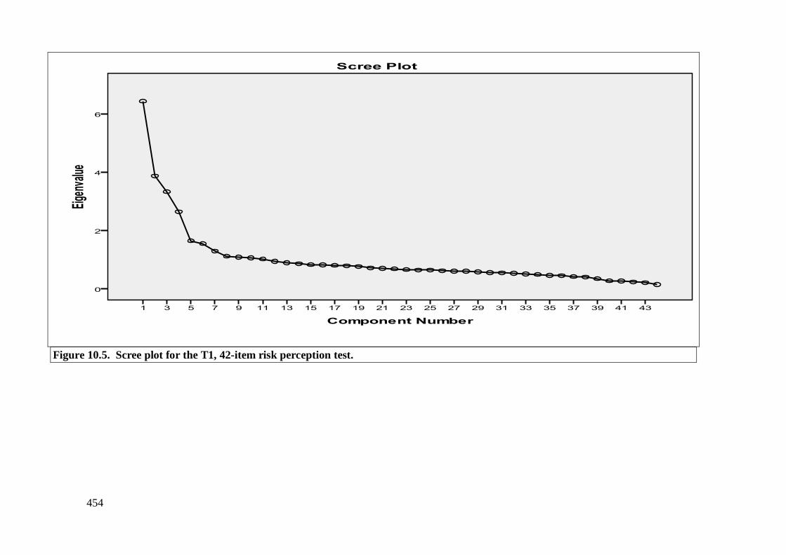
454
Figure 10.5. Scree plot for the T1, 42-item risk perception test.
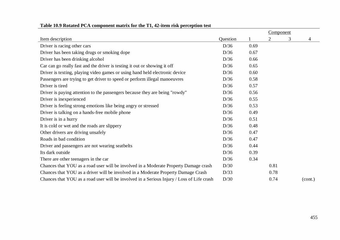
455
Table 10.9 Rotated PCA component matrix for the T1, 42-item risk perception test
Component
Item description Question 1 2 3 4
Driver is racing other cars D/36 0.69
Driver has been taking drugs or smoking dope D/36 0.67
Driver has been drinking alcohol D/36 0.66
Car can go really fast and the driver is testing it out or showing it off D/36 0.65
Driver is texting, playing video games or using hand held electronic device D/36 0.60
Passengers are trying to get driver to speed or perform illegal manoeuvres D/36 0.58
Driver is tired D/36 0.57
Driver is paying attention to the passengers because they are being "rowdy" D/36 0.56
Driver is inexperienced D/36 0.55
Driver is feeling strong emotions like being angry or stressed D/36 0.53
Driver is talking on a hands-free mobile phone D/36 0.49
Driver is in a hurry D/36 0.51
It is cold or wet and the roads are slippery D/36 0.48
Other drivers are driving unsafely D/36 0.47
Roads in bad condition D/36 0.47
Driver and passengers are not wearing seatbelts D/36 0.44
Its dark outside D/36 0.39
There are other teenagers in the car D/36 0.34
Chances that YOU as a road user will be involved in a Moderate Property Damage crash D/30 0.81
Chances that YOU as a driver will be involved in a Moderate Property Damage Crash D/33 0.78
Chances that YOU as a road user will be involved in a Serious Injury / Loss of Life crash D/30 0.74 (cont.)
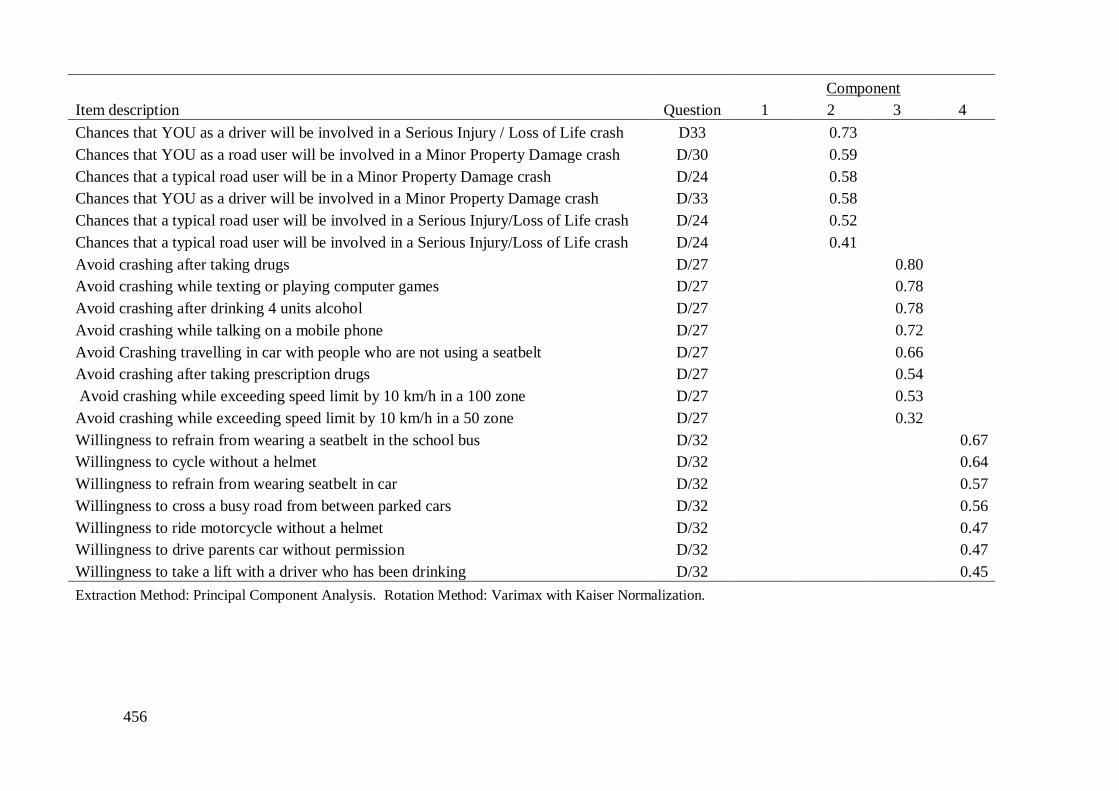
456
Component
Item description Question 1 2 3 4
Chances that YOU as a driver will be involved in a Serious Injury / Loss of Life crash D33 0.73
Chances that YOU as a road user will be involved in a Minor Property Damage crash D/30 0.59
Chances that a typical road user will be in a Minor Property Damage crash D/24 0.58
Chances that YOU as a driver will be involved in a Minor Property Damage crash D/33 0.58
Chances that a typical road user will be involved in a Serious Injury/Loss of Life crash D/24 0.52
Chances that a typical road user will be involved in a Serious Injury/Loss of Life crash D/24 0.41
Avoid crashing after taking drugs D/27 0.80
Avoid crashing while texting or playing computer games D/27 0.78
Avoid crashing after drinking 4 units alcohol D/27 0.78
Avoid crashing while talking on a mobile phone D/27 0.72
Avoid Crashing travelling in car with people who are not using a seatbelt D/27 0.66
Avoid crashing after taking prescription drugs D/27 0.54
Avoid crashing while exceeding speed limit by 10 km/h in a 100 zone D/27 0.53
Avoid crashing while exceeding speed limit by 10 km/h in a 50 zone D/27 0.32
Willingness to refrain from wearing a seatbelt in the school bus D/32 0.67
Willingness to cycle without a helmet D/32 0.64
Willingness to refrain from wearing seatbelt in car D/32 0.57
Willingness to cross a busy road from between parked cars D/32 0.56
Willingness to ride motorcycle without a helmet D/32 0.47
Willingness to drive parents car without permission D/32 0.47
Willingness to take a lift with a driver who has been drinking D/32 0.45
Extraction Method: Principal Component Analysis. Rotation Method: Varimax with Kaiser Normalization.
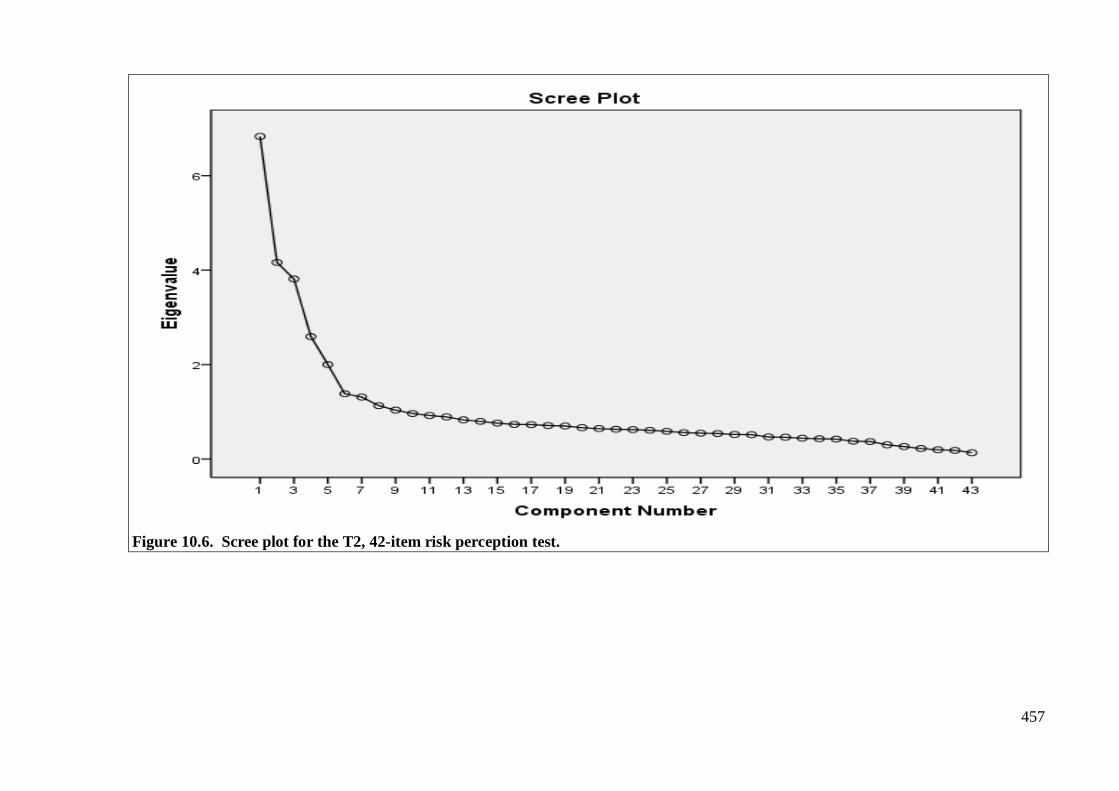
457
Figure 10.6. Scree plot for the T2, 42-item risk perception test.
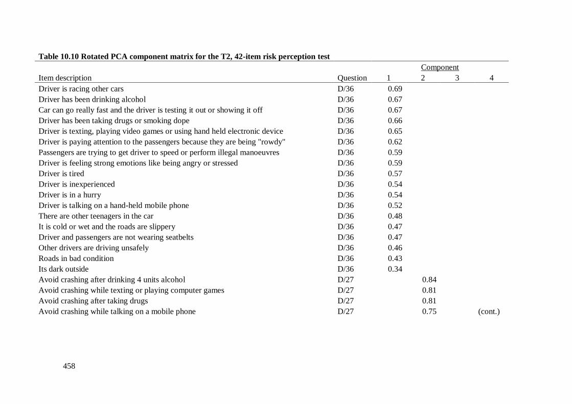
458
Table 10.10 Rotated PCA component matrix for the T2, 42-item risk perception test
Component
Item description Question 1 2 3 4
Driver is racing other cars D/36 0.69
Driver has been drinking alcohol D/36 0.67
Car can go really fast and the driver is testing it out or showing it off D/36 0.67
Driver has been taking drugs or smoking dope D/36 0.66
Driver is texting, playing video games or using hand held electronic device D/36 0.65
Driver is paying attention to the passengers because they are being "rowdy" D/36 0.62
Passengers are trying to get driver to speed or perform illegal manoeuvres D/36 0.59
Driver is feeling strong emotions like being angry or stressed D/36 0.59
Driver is tired D/36 0.57
Driver is inexperienced D/36 0.54
Driver is in a hurry D/36 0.54
Driver is talking on a hand-held mobile phone D/36 0.52
There are other teenagers in the car D/36 0.48
It is cold or wet and the roads are slippery D/36 0.47
Driver and passengers are not wearing seatbelts D/36 0.47
Other drivers are driving unsafely D/36 0.46
Roads in bad condition D/36 0.43
Its dark outside D/36 0.34
Avoid crashing after drinking 4 units alcohol D/27 0.84
Avoid crashing while texting or playing computer games D/27 0.81
Avoid crashing after taking drugs D/27 0.81
Avoid crashing while talking on a mobile phone D/27 0.75
(cont.)
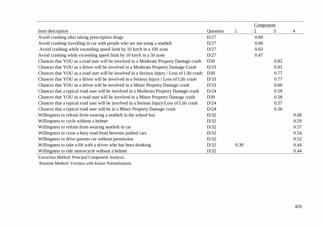
459
Component
Item description Question 1 2 3 4
Avoid crashing after taking prescription drugs D/27 0.69
Avoid crashing travelling in car with people who are not using a seatbelt D/27 0.68
Avoid crashing while exceeding speed limit by 10 km/h in a 100 zone D/27 0.63
Avoid crashing while exceeding speed limit by 10 km/h in a 50 zone D/27 0.47
Chances that YOU as a road user will be involved in a Moderate Property Damage crash D30 0.82
Chances that YOU as a driver will be involved in a Moderate Property Damage Crash D/33 0.81
Chances that YOU as a road user will be involved in a Serious Injury / Loss of Life crash D30 0.77
Chances that YOU as a driver will be involved in a Serious Injury / Loss of Life crash D/33 0.77
Chances that YOU as a driver will be involved in a Minor Property Damage crash D/33 0.60
Chances that a typical road user will be involved in a Moderate Property Damage crash D/24 0.59
Chances that YOU as a road user will be involved in a Minor Property Damage crash D30 0.58
Chances that a typical road user will be involved in a Serious Injury/Loss of Life crash D/24 0.57
Chances that a typical road user will be in a Minor Property Damage crash D/24 0.36
Willingness to refrain from wearing a seatbelt in the school bus D/32 0.68
Willingness to cycle without a helmet D/32 0.59
Willingness to refrain from wearing seatbelt in car D/32 0.57
Willingness to cross a busy road from between parked cars D/32 0.54
Willingness to drive parents car without permission D/32 0.52
Willingness to take a lift with a driver who has been drinking D/32 0.30 0.44
Willingness to ride motorcycle without a helmet D/32 0.44
Extraction Method: Principal Component Analysis.
Rotation Method: Varimax with Kaiser Normalization.
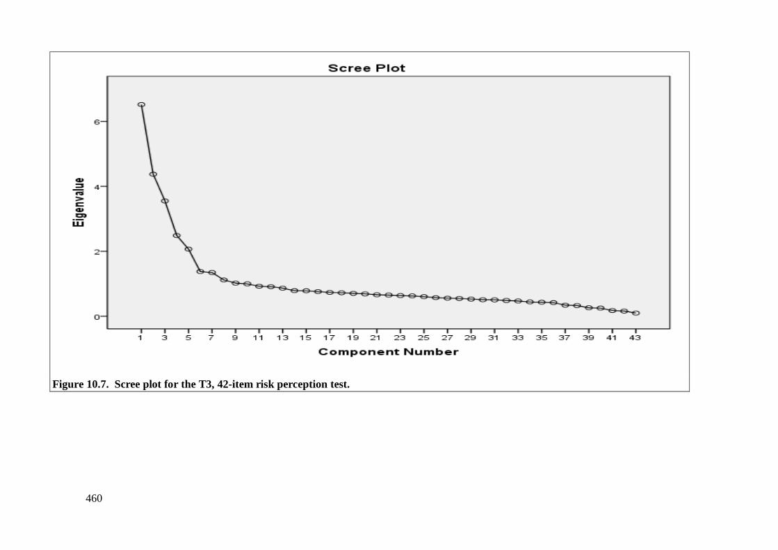
460
Figure 10.7. Scree plot for the T3, 42-item risk perception test.
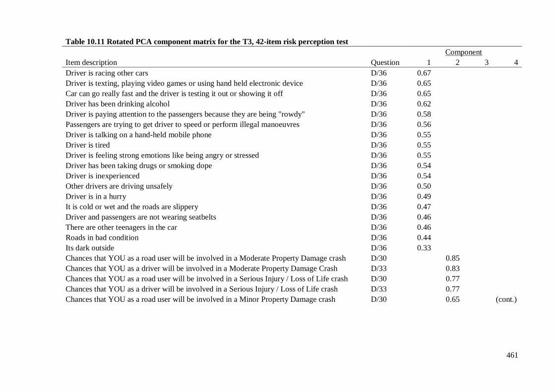
461
Table 10.11 Rotated PCA component matrix for the T3, 42-item risk perception test
Component
Item description Question 1 2 3 4
Driver is racing other cars D/36 0.67
Driver is texting, playing video games or using hand held electronic device D/36 0.65
Car can go really fast and the driver is testing it out or showing it off D/36 0.65
Driver has been drinking alcohol D/36 0.62
Driver is paying attention to the passengers because they are being "rowdy" D/36 0.58
Passengers are trying to get driver to speed or perform illegal manoeuvres D/36 0.56
Driver is talking on a hand-held mobile phone D/36 0.55
Driver is tired D/36 0.55
Driver is feeling strong emotions like being angry or stressed D/36 0.55
Driver has been taking drugs or smoking dope D/36 0.54
Driver is inexperienced D/36 0.54
Other drivers are driving unsafely D/36 0.50
Driver is in a hurry D/36 0.49
It is cold or wet and the roads are slippery D/36 0.47
Driver and passengers are not wearing seatbelts D/36 0.46
There are other teenagers in the car D/36 0.46
Roads in bad condition D/36 0.44
Its dark outside D/36 0.33
Chances that YOU as a road user will be involved in a Moderate Property Damage crash D/30 0.85
Chances that YOU as a driver will be involved in a Moderate Property Damage Crash D/33 0.83
Chances that YOU as a road user will be involved in a Serious Injury / Loss of Life crash D/30 0.77
Chances that YOU as a driver will be involved in a Serious Injury / Loss of Life crash D/33 0.77
Chances that YOU as a road user will be involved in a Minor Property Damage crash D/30 0.65 (cont.)
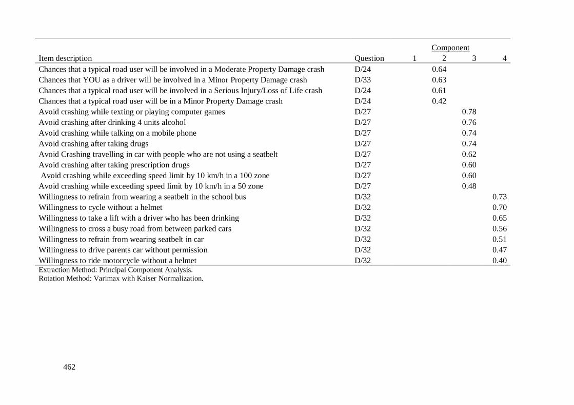
462
Component
Item description Question 1 2 3 4
Chances that a typical road user will be involved in a Moderate Property Damage crash D/24 0.64
Chances that YOU as a driver will be involved in a Minor Property Damage crash D/33 0.63
Chances that a typical road user will be involved in a Serious Injury/Loss of Life crash D/24 0.61
Chances that a typical road user will be in a Minor Property Damage crash D/24 0.42
Avoid crashing while texting or playing computer games D/27 0.78
Avoid crashing after drinking 4 units alcohol D/27 0.76
Avoid crashing while talking on a mobile phone D/27 0.74
Avoid crashing after taking drugs D/27 0.74
Avoid Crashing travelling in car with people who are not using a seatbelt D/27 0.62
Avoid crashing after taking prescription drugs D/27 0.60
Avoid crashing while exceeding speed limit by 10 km/h in a 100 zone D/27 0.60
Avoid crashing while exceeding speed limit by 10 km/h in a 50 zone D/27 0.48
Willingness to refrain from wearing a seatbelt in the school bus D/32 0.73
Willingness to cycle without a helmet D/32 0.70
Willingness to take a lift with a driver who has been drinking D/32 0.65
Willingness to cross a busy road from between parked cars D/32 0.56
Willingness to refrain from wearing seatbelt in car D/32 0.51
Willingness to drive parents car without permission D/32 0.47
Willingness to ride motorcycle without a helmet D/32 0.40 Extraction Method: Principal Component Analysis. Rotation Method: Varimax with Kaiser Normalization.
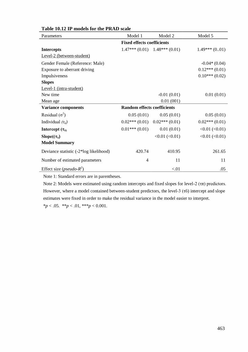
463
Table 10.12 IP models for the PRAD scale
Parameters Model 1 Model 2 Model 5
Fixed effects coefficients
Intercepts 1.47*** (0.01) 1.48*** (0.01) 1.49*** (0..01)
Level-2 (between-student) Gender Female (Reference: Male)
-0.04* (0.04)
Exposure to aberrant driving
0.12*** (0.01)
Impulsiveness
0.10*** (0.02)
Slopes
Level-1 (intra-student) New time
-0.01 (0.01) 0.01 (0.01)
Mean age
0.01 (001) Variance components Random effects coefficients
Residual (σ2) 0.05 (0.01) 0.05 (0.01) 0.05 (0.01)
Individual (τπ) 0.02*** (0.01) 0.02*** (0.01) 0.02*** (0.01)
Intercept (τϐ) 0.01*** (0.01) 0.01 (0.01) <0.01 (<0.01)
Slope((τϐ)
<0.01 (<0.01) <0.01 (<0.01)
Model Summary
Deviance statistic (-2*log likelihood) 420.74 410.95 261.65
Number of estimated parameters 4 11 11
Effect size (pseudo-R2)
<.01 .05
Note 1: Standard errors are in parentheses.
Note 2: Models were estimated using random intercepts and fixed slopes for level-2 (τπ) predictors.
However, where a model contained between-student predictors, the level-3 (τϐ) intercept and slope
estimates were fixed in order to make the residual variance in the model easier to interpret.
*p < .05. **p < .01, ***p < 0.001.
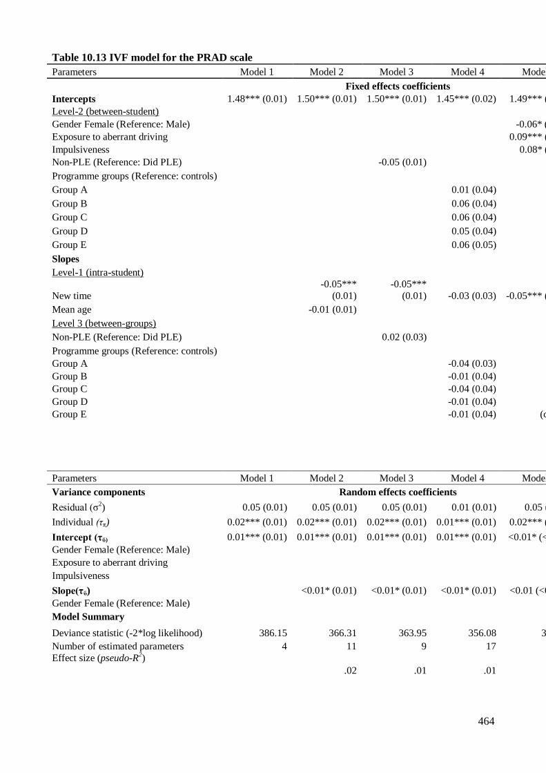
464
Table 10.13 IVF model for the PRAD scale
Parameters Model 1 Model 2 Model 3 Model 4 Model 5
Fixed effects coefficients
Intercepts 1.48*** (0.01) 1.50*** (0.01) 1.50*** (0.01) 1.45*** (0.02) 1.49*** (0.01)
Level-2 (between-student)
Gender Female (Reference: Male)
-0.06* (0.02)
Exposure to aberrant driving
0.09*** (0.01)
Impulsiveness
0.08* (0.02)
Non-PLE (Reference: Did PLE)
-0.05 (0.01)
Programme groups (Reference: controls)
Group A
0.01 (0.04)
Group B
0.06 (0.04)
Group C
0.06 (0.04)
Group D
0.05 (0.04)
Group E
0.06 (0.05)
Slopes
Level-1 (intra-student)
New time
-0.05***
(0.01) -0.05***
(0.01) -0.03 (0.03) -0.05*** (0.01)
Mean age
-0.01 (0.01)
Level 3 (between-groups) Non-PLE (Reference: Did PLE)
0.02 (0.03)
Programme groups (Reference: controls) Group A
-0.04 (0.03)
Group B
-0.01 (0.04) Group C
-0.04 (0.04)
Group D
-0.01 (0.04) Group E -0.01 (0.04) (cont.)
Parameters Model 1 Model 2 Model 3 Model 4 Model 5
Variance components Random effects coefficients
Residual (σ2) 0.05 (0.01) 0.05 (0.01) 0.05 (0.01) 0.01 (0.01) 0.05 (0.01)
Individual (τπ) 0.02*** (0.01) 0.02*** (0.01) 0.02*** (0.01) 0.01*** (0.01) 0.02*** (0.01)
Intercept (τϐ) 0.01*** (0.01) 0.01*** (0.01) 0.01*** (0.01) 0.01*** (0.01) <0.01* (<0.01)
Gender Female (Reference: Male)
Exposure to aberrant driving
Impulsiveness
Slope(τϐ)
<0.01* (0.01) <0.01* (0.01) <0.01* (0.01) <0.01 (<0.01)
Gender Female (Reference: Male)
Model Summary
Deviance statistic (-2*log likelihood) 386.15 366.31 363.95 356.08 363.16
Number of estimated parameters 4 11 9 17 10 Effect size (pseudo-R
2)
.02 .01 .01 .01
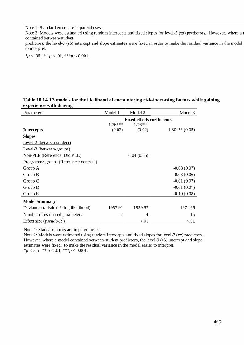
465
Note 1: Standard errors are in parentheses. Note 2: Models were estimated using random intercepts and fixed slopes for level-2 (τπ) predictors. However, where a model
contained between-student predictors, the level-3 (τϐ) intercept and slope estimates were fixed in order to make the residual variance in the model easier
to interpret.
*p < .05. ** p < .01, ***p < 0.001.
Table 10.14 T3 models for the likelihood of encountering risk-increasing factors while gaining
experience with driving
Parameters Model 1 Model 2 Model 3
Fixed effects coefficients
Intercepts 1.76***
(0.02) 1.76***
(0.02) 1.80*** (0.05)
Slopes
Level-2 (between-student)
Level-3 (between-groups)
Non-PLE (Reference: Did PLE)
0.04 (0.05)
Programme groups (Reference: controls)
Group A
-0.08 (0.07)
Group B
-0.03 (0.06)
Group C
-0.01 (0.07)
Group D
-0.01 (0.07)
Group E -0.10 (0.08)
Model Summary
Deviance statistic (-2*log likelihood) 1957.91 1959.57 1971.66
Number of estimated parameters 2 4 15
Effect size (pseudo-R2)
<.01 <.01
Note 1: Standard errors are in parentheses. Note 2: Models were estimated using random intercepts and fixed slopes for level-2 (τπ) predictors. However, where a model contained between-student predictors, the level-3 (τϐ) intercept and slope estimates were fixed, to make the residual variance in the model easier to interpret. *p < .05. ** p < .01, ***p < 0.001.
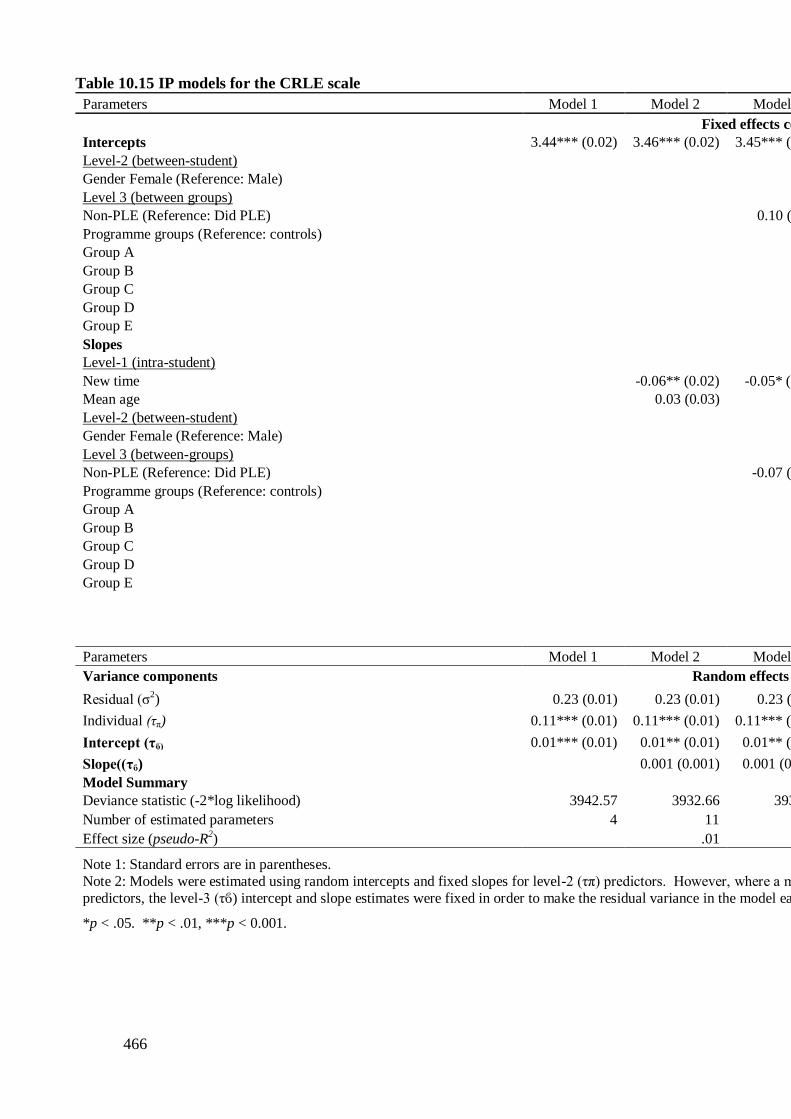
466
Table 10.15 IP models for the CRLE scale
Parameters Model 1 Model 2 Model 3 Model 4 Model 5
Fixed effects coefficients
Intercepts 3.44*** (0.02) 3.46*** (0.02) 3.45*** (0.02) 3.55*** (0.07) 3.52*** (0.03)
Level-2 (between-student)
Gender Female (Reference: Male)
-0.14** (0.04)
Level 3 (between groups)
Non-PLE (Reference: Did PLE)
0.10 (0.06)
Programme groups (Reference: controls)
Group A
0.15 (0.07)
Group B
0.12 (0.07)
Group C
0.12 (0.07)
Group D
0.05 (0.07)
Group E
0.02 (0.08)
Slopes
Level-1 (intra-student)
New time
-0.06** (0.02) -0.05* (0.02) -0.13* (0.06) -0.06 (0.03)
Mean age
0.03 (0.03)
Level-2 (between-student)
Gender Female (Reference: Male)
Level 3 (between-groups)
Non-PLE (Reference: Did PLE)
-0.07 (0.06)
Programme groups (Reference: controls)
Group A
-0.06 (0.07)
Group B
-0.09 (0.07)
Group C
-0.06 (0.07)
Group D
-0.08 (0.08)
Group E -0.09 (0.09) (cont.)
Parameters Model 1 Model 2 Model 3 Model 4 Model 5
Variance components Random effects coefficients
Residual (σ2) 0.23 (0.01) 0.23 (0.01) 0.23 (0.01) 0.23 (0.01) 0.23 (0.01)
Individual (τπ) 0.11*** (0.01) 0.11*** (0.01) 0.11*** (0.01) 0.11*** (0.01) 0.11*** (0.01)
Intercept (τϐ) 0.01*** (0.01) 0.01** (0.01) 0.01** (0.01) 0.01** (0.01) 0.01** (0.01)
Slope((τϐ)
0.001 (0.001) 0.001 (0.001) 0.001 (0.001) 0.001 (0.001)
Model Summary Deviance statistic (-2*log likelihood) 3942.57 3932.66 3930.17 3926.05 3913.24
Number of estimated parameters 4 11 9 17 14
Effect size (pseudo-R2)
.01 .01 .01 .01
Note 1: Standard errors are in parentheses. Note 2: Models were estimated using random intercepts and fixed slopes for level-2 (τπ) predictors. However, where a model contained between-student predictors, the level-3 (τϐ) intercept and slope estimates were fixed in order to make the residual variance in the model easier to interpret.
*p < .05. **p < .01, ***p < 0.001.

467
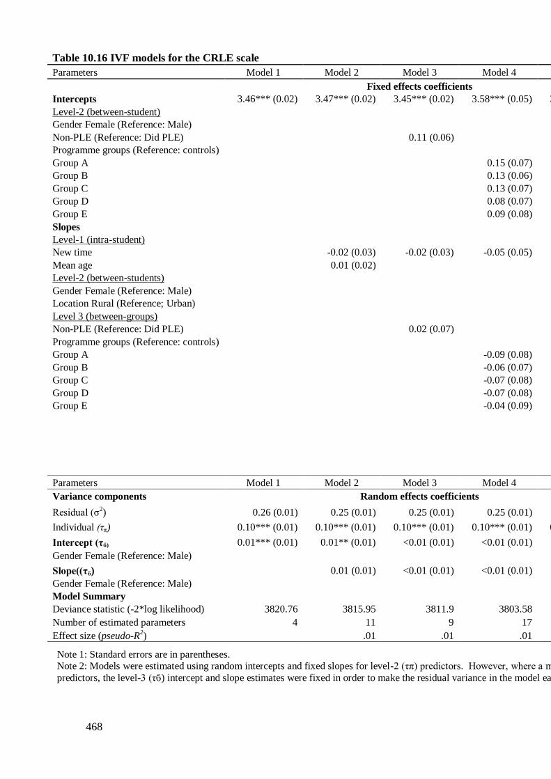
468
Table 10.16 IVF models for the CRLE scale
Parameters Model 1 Model 2 Model 3 Model 4 Model 5
Fixed effects coefficients
Intercepts 3.46*** (0.02) 3.47*** (0.02) 3.45*** (0.02) 3.58*** (0.05) 3.51*** (0.03)
Level-2 (between-student)
Gender Female (Reference: Male)
-0.11* (0.05)
Non-PLE (Reference: Did PLE)
0.11 (0.06)
Programme groups (Reference: controls)
Group A
0.15 (0.07)
Group B
0.13 (0.06)
Group C
0.13 (0.07)
Group D
0.08 (0.07)
Group E
0.09 (0.08)
Slopes
Level-1 (intra-student)
New time
-0.02 (0.03) -0.02 (0.03) -0.05 (0.05) 0.02 (0.03)
Mean age
0.01 (0.02)
Level-2 (between-students)
Gender Female (Reference: Male)
-0.10* (0.05)
Location Rural (Reference; Urban)
Level 3 (between-groups)
Non-PLE (Reference: Did PLE)
0.02 (0.07)
Programme groups (Reference: controls)
Group A
-0.09 (0.08)
Group B
-0.06 (0.07)
Group C
-0.07 (0.08)
Group D
-0.07 (0.08)
Group E -0.04 (0.09)
(cont.)
Parameters Model 1 Model 2 Model 3 Model 4 Model 5
Variance components Random effects coefficients
Residual (σ2) 0.26 (0.01) 0.25 (0.01) 0.25 (0.01) 0.25 (0.01) 0.25 (0.01)
Individual (τπ) 0.10*** (0.01) 0.10*** (0.01) 0.10*** (0.01) 0.10*** (0.01) 0.10*** (0.01)
Intercept (τϐ) 0.01*** (0.01) 0.01** (0.01) <0.01 (0.01) <0.01 (0.01) <0.01 (0.01)
Gender Female (Reference: Male)
0.02 (0.01)
Slope((τϐ)
0.01 (0.01) <0.01 (0.01) <0.01 (0.01) <0.01 (0.01)
Gender Female (Reference: Male)
<0.01 (0.01)
Model Summary
Deviance statistic (-2*log likelihood) 3820.76 3815.95 3811.9 3803.58 3789.48
Number of estimated parameters 4 11 9 17 16
Effect size (pseudo-R2)
.01 .01 .01 .04
Note 1: Standard errors are in parentheses. Note 2: Models were estimated using random intercepts and fixed slopes for level-2 (τπ) predictors. However, where a model contained between-student predictors, the level-3 (τϐ) intercept and slope estimates were fixed in order to make the residual variance in the model easier to interpret.

469
*p < .05. **p < .01, ***p < 0.001.
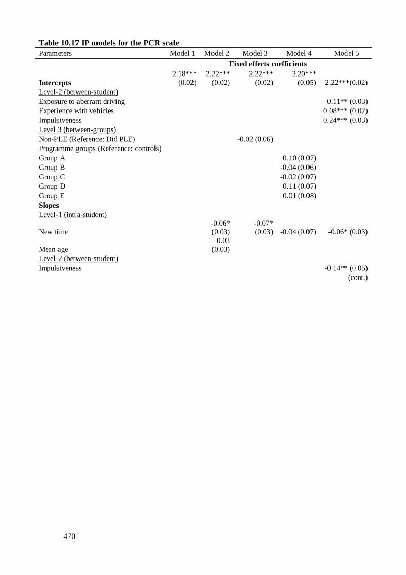
470
Table 10.17 IP models for the PCR scale
Parameters Model 1 Model 2 Model 3 Model 4 Model 5
Fixed effects coefficients
Intercepts 2.18***
(0.02) 2.22***
(0.02) 2.22***
(0.02) 2.20***
(0.05) 2.22***(0.02)
Level-2 (between-student)
Exposure to aberrant driving
0.11** (0.03)
Experience with vehicles
0.08*** (0.02)
Impulsiveness
0.24*** (0.03)
Level 3 (between-groups)
Non-PLE (Reference: Did PLE)
-0.02 (0.06)
Programme groups (Reference: controls)
Group A
0.10 (0.07)
Group B
-0.04 (0.06)
Group C
-0.02 (0.07)
Group D
0.11 (0.07)
Group E
0.01 (0.08)
Slopes
Level-1 (intra-student)
New time
-0.06* (0.03)
-0.07* (0.03) -0.04 (0.07) -0.06* (0.03)
Mean age
0.03
(0.03) Level-2 (between-student)
Impulsiveness
-0.14** (0.05)
(cont.)
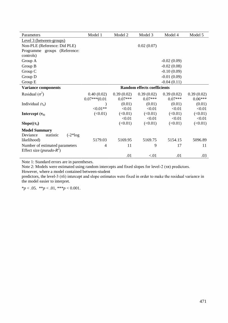
471
Parameters Model 1 Model 2 Model 3 Model 4 Model 5
Level 3 (between-groups) Non-PLE (Reference: Did PLE)
0.02 (0.07)
Programme groups (Reference:
controls) Group A
-0.02 (0.09)
Group B
-0.02 (0.08) Group C
-0.10 (0.09)
Group D
-0.01 (0.09) Group E -0.04 (0.11)
Variance components Random effects coefficients
Residual (σ2) 0.40 (0.02) 0.39 (0.02) 0.39 (0.02) 0.39 (0.02) 0.39 (0.02)
Individual (τπ) 0.07***(0.01
) 0.07***
(0.01) 0.07***
(0.01) 0.07***
(0.01) 0.06***
(0.01)
Intercept (τϐ) <0.01**
(<0.01) <0.01
(<0.01) <0.01
(<0.01) <0.01
(<0.01) <0.01
(<0.01)
Slope((τϐ)
<0.01 (<0.01)
<0.01 (<0.01)
<0.01 (<0.01)
<0.01 (<0.01)
Model Summary
Deviance statistic (-2*log
likelihood) 5179.03 5169.95 5169.75 5154.15 5096.89
Number of estimated parameters 4 11 9 17 11 Effect size (pseudo-R
2)
.01 <.01 .01 .03
Note 1: Standard errors are in parentheses. Note 2: Models were estimated using random intercepts and fixed slopes for level-2 (τπ) predictors.
However, where a model contained between-student predictors, the level-3 (τϐ) intercept and slope estimates were fixed in order to make the residual variance in the model easier to interpret.
*p < .05. **p < .01, ***p < 0.001.
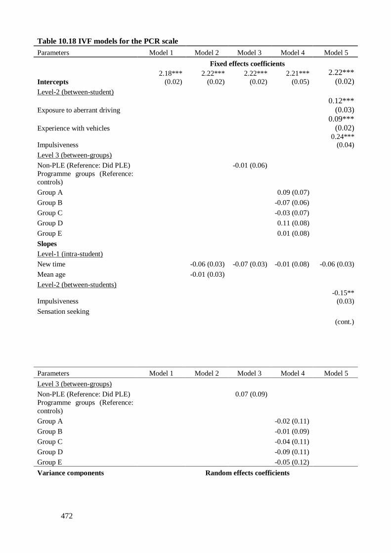
472
Table 10.18 IVF models for the PCR scale
Parameters Model 1 Model 2 Model 3 Model 4 Model 5
Fixed effects coefficients
Intercepts 2.18***
(0.02) 2.22***
(0.02) 2.22***
(0.02) 2.21***
(0.05)
2.22***
(0.02)
Level-2 (between-student)
Exposure to aberrant driving
0.12***
(0.03)
Experience with vehicles
0.09***
(0.02)
Impulsiveness
0.24*** (0.04)
Level 3 (between-groups)
Non-PLE (Reference: Did PLE)
-0.01 (0.06)
Programme groups (Reference:
controls) Group A
0.09 (0.07) Group B
-0.07 (0.06)
Group C
-0.03 (0.07) Group D
0.11 (0.08)
Group E
0.01 (0.08) Slopes
Level-1 (intra-student) New time
-0.06 (0.03) -0.07 (0.03) -0.01 (0.08) -0.06 (0.03)
Mean age
-0.01 (0.03) Level-2 (between-students)
Impulsiveness
-0.15**
(0.03)
Sensation seeking
(cont.)
Parameters Model 1 Model 2 Model 3 Model 4 Model 5
Level 3 (between-groups)
Non-PLE (Reference: Did PLE)
0.07 (0.09)
Programme groups (Reference:
controls) Group A
-0.02 (0.11) Group B
-0.01 (0.09)
Group C
-0.04 (0.11) Group D
-0.09 (0.11)
Group E -0.05 (0.12) Variance components Random effects coefficients
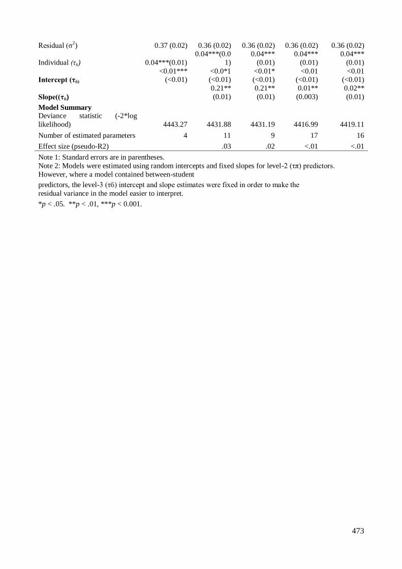
473
Residual (σ2) 0.37 (0.02) 0.36 (0.02) 0.36 (0.02) 0.36 (0.02) 0.36 (0.02)
Individual (τπ) 0.04***(0.01) 0.04***(0.0
1) 0.04***
(0.01) 0.04***
(0.01) 0.04***
(0.01)
Intercept (τϐ) <0.01***
(<0.01) <0.0*1 (<0.01)
<0.01* (<0.01)
<0.01 (<0.01)
<0.01 (<0.01)
Slope((τϐ)
0.21**
(0.01) 0.21**
(0.01) 0.01**
(0.003) 0.02**
(0.01)
Model Summary Deviance statistic (-2*log
likelihood) 4443.27 4431.88 4431.19 4416.99 4419.11
Number of estimated parameters 4 11 9 17 16
Effect size (pseudo-R2)
.03 .02 <.01 <.01
Note 1: Standard errors are in parentheses. Note 2: Models were estimated using random intercepts and fixed slopes for level-2 (τπ) predictors.
However, where a model contained between-student
predictors, the level-3 (τϐ) intercept and slope estimates were fixed in order to make the
residual variance in the model easier to interpret.
*p < .05. **p < .01, ***p < 0.001.
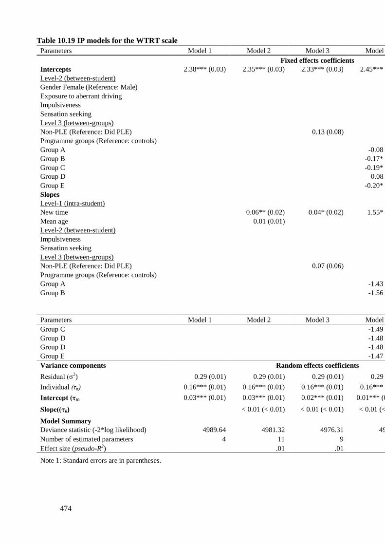
474
Table 10.19 IP models for the WTRT scale
Parameters Model 1 Model 2 Model 3 Model 4 Model 5
Fixed effects coefficients
Intercepts 2.38*** (0.03) 2.35*** (0.03) 2.33*** (0.03) 2.45*** (0.07) 2.43*** (0.03)
Level-2 (between-student)
Gender Female (Reference: Male)
-0.16*** (0.04)
Exposure to aberrant driving
0.18*** (0.03)
Impulsiveness
0.54*** (0.04)
Sensation seeking
0.25*** (0.04)
Level 3 (between-groups)
Non-PLE (Reference: Did PLE)
0.13 (0.08)
Programme groups (Reference: controls)
Group A
-0.08 (0.10)
Group B
-0.17* (0.09)
Group C
-0.19* (0.09)
Group D
0.08 (0.10)
Group E
-0.20* (0.11)
Slopes
Level-1 (intra-student)
New time
0.06** (0.02) 0.04* (0.02) 1.55* (1.24) 0.06* (0.02)
Mean age
0.01 (0.01)
Level-2 (between-student)
Impulsiveness
-0.24*** (0.05)
Sensation seeking
-0.11* (0.05)
Level 3 (between-groups)
Non-PLE (Reference: Did PLE)
0.07 (0.06)
Programme groups (Reference: controls)
Group A
-1.43 (1.24)
Group B
-1.56 (1.24) (cont.)
Parameters Model 1 Model 2 Model 3 Model 4 Model 5
Group C
-1.49 (1.24)
Group D
-1.48 (1.20) Group D
-1.48 (1.20)
Group E -1.47 (1.24) Variance components Random effects coefficients
Residual (σ2) 0.29 (0.01) 0.29 (0.01) 0.29 (0.01) 0.29 (0.01) 0.28 (0.01)
Individual (τπ) 0.16*** (0.01) 0.16*** (0.01) 0.16*** (0.01) 0.16*** (0.01) 0.10*** (0.01)
Intercept (τϐ) 0.03*** (0.01) 0.03*** (0.01) 0.02*** (0.01) 0.01*** (0.001) 0.01* (0.01)
Slope((τϐ)
< 0.01 (< 0.01) < 0.01 (< 0.01) < 0.01 (< 0.01) < 0.01 (< 0.01)
Model Summary Deviance statistic (-2*log likelihood) 4989.64 4981.32 4976.31 4965.83 4623.26
Number of estimated parameters 4 11 9 17 13
Effect size (pseudo-R2)
.01 .01 .03 .18
Note 1: Standard errors are in parentheses.

475
Note 2: Models were estimated using random intercepts and fixed slopes for level-2 (τπ) predictors. However, where a model contained between-
student predictors, the level-3 (τϐ) intercept and slope estimates were fixed in order to make the residual variance in the model easier to interpret.
*p < .05. ** p < .01, ***p < 0.001.
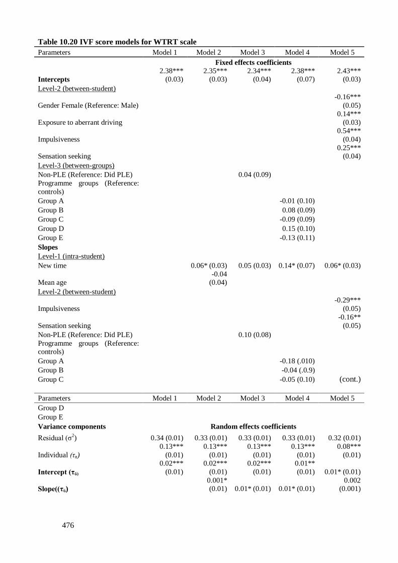
476
Table 10.20 IVF score models for WTRT scale
Parameters Model 1 Model 2 Model 3 Model 4 Model 5
Fixed effects coefficients
Intercepts 2.38***
(0.03) 2.35***
(0.03) 2.34***
(0.04) 2.38***
(0.07) 2.43***
(0.03)
Level-2 (between-student)
Gender Female (Reference: Male)
-0.16***
(0.05)
Exposure to aberrant driving
0.14***
(0.03)
Impulsiveness
0.54***
(0.04)
Sensation seeking
0.25*** (0.04)
Level-3 (between-groups)
Non-PLE (Reference: Did PLE)
0.04 (0.09)
Programme groups (Reference:
controls)
Group A
-0.01 (0.10)
Group B
0.08 (0.09)
Group C
-0.09 (0.09)
Group D
0.15 (0.10)
Group E
-0.13 (0.11)
Slopes
Level-1 (intra-student)
New time
0.06* (0.03) 0.05 (0.03) 0.14* (0.07) 0.06* (0.03)
Mean age
-0.04 (0.04)
Level-2 (between-student)
Impulsiveness
-0.29***
(0.05)
Sensation seeking
-0.16**
(0.05)
Non-PLE (Reference: Did PLE)
0.10 (0.08)
Programme groups (Reference: controls)
Group A
-0.18 (.010)
Group B
-0.04 (.0.9)
Group C
-0.05 (0.10) (cont.)
Parameters Model 1 Model 2 Model 3 Model 4 Model 5
Group D
Group E
Variance components Random effects coefficients
Residual (σ2) 0.34 (0.01) 0.33 (0.01) 0.33 (0.01) 0.33 (0.01) 0.32 (0.01)
Individual (τπ) 0.13***
(0.01) 0.13***
(0.01) 0.13***
(0.01) 0.13***
(0.01) 0.08***
(0.01)
Intercept (τϐ) 0.02***
(0.01) 0.02***
(0.01) 0.02***
(0.01) 0.01**
(0.01) 0.01* (0.01)
Slope((τϐ)
0.001* (0.01) 0.01* (0.01) 0.01* (0.01)
0.002 (0.001)

477
Model Summary
Deviance statistic (-2*log likelihood) 4698.52 4689.48 4687.09 4677.37 4395.29
Number of estimated parameters 4 11 9 17 13
Effect size (pseudo-R2)
.02 .01 .04 .16
Note 1: Standard errors are in parentheses. Note 2: Models were estimated using random intercepts and fixed slopes for level-2 (τπ) predictors. However, where a model contained between-student predictors, the level-3 (τϐ) intercept and slope estimates
were fixed in order to make the residual variance in the model easier to interpret.
*p < .05. ** p < .01, ***p < 0.001.
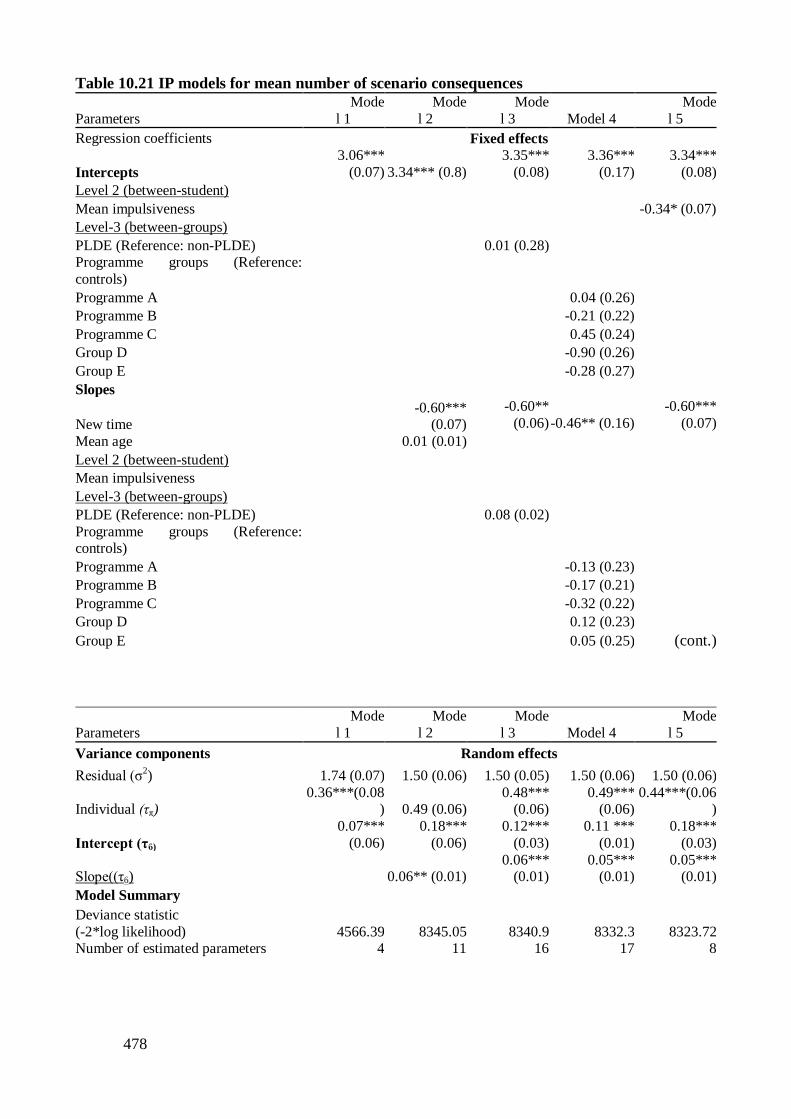
478
Table 10.21 IP models for mean number of scenario consequences
Parameters Mode
l 1 Mode
l 2 Mode
l 3
Model 4 Mode
l 5
Regression coefficients Fixed effects
Intercepts 3.06***
(0.07) 3.34*** (0.8) 3.35***
(0.08) 3.36***
(0.17) 3.34***
(0.08)
Level 2 (between-student)
Mean impulsiveness
-0.34* (0.07)
Level-3 (between-groups)
PLDE (Reference: non-PLDE)
0.01 (0.28) Programme groups (Reference:
controls)
Programme A
0.04 (0.26) Programme B
-0.21 (0.22)
Programme C
0.45 (0.24) Group D
-0.90 (0.26)
Group E
-0.28 (0.27) Slopes
New time Mean age
-0.60*** (0.07)
0.01 (0.01)
-0.60**
(0.06) -0.46** (0.16)
-0.60***
(0.07)
Level 2 (between-student) Mean impulsiveness
Level-3 (between-groups) PLDE (Reference: non-PLDE)
0.08 (0.02)
Programme groups (Reference: controls)
Programme A
-0.13 (0.23)
Programme B
-0.17 (0.21)
Programme C
-0.32 (0.22)
Group D
0.12 (0.23)
Group E
0.05 (0.25) (cont.)
Parameters
Mode
l 1 Mode
l 2 Mode
l 3
Model 4 Mode
l 5
Variance components Random effects
Residual (σ2) 1.74 (0.07) 1.50 (0.06) 1.50 (0.05) 1.50 (0.06) 1.50 (0.06)
Individual (τπ) 0.36***(0.08
) 0.49 (0.06) 0.48***
(0.06) 0.49***
(0.06) 0.44***(0.06
)
Intercept (τϐ) 0.07***
(0.06) 0.18***
(0.06) 0.12***
(0.03) 0.11 ***
(0.01) 0.18***
(0.03)
Slope((τϐ)
0.06** (0.01) 0.06***
(0.01) 0.05***
(0.01) 0.05***
(0.01)
Model Summary Deviance statistic
(-2*log likelihood) 4566.39 8345.05 8340.9 8332.3 8323.72 Number of estimated parameters
4
11
16
17
8
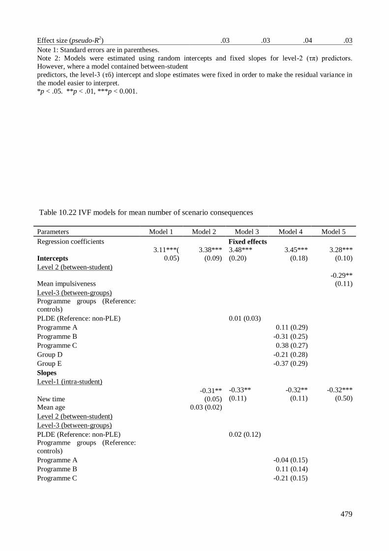
479
Effect size (pseudo-R2)
.03 .03 .04 .03
Note 1: Standard errors are in parentheses. Note 2: Models were estimated using random intercepts and fixed slopes for level-2 (τπ) predictors. However, where a model contained between-student predictors, the level-3 (τϐ) intercept and slope estimates were fixed in order to make the residual variance in
the model easier to interpret. *p < .05. **p < .01, ***p < 0.001.
Table 10.22 IVF models for mean number of scenario consequences
Parameters Model 1 Model 2 Model 3 Model 4 Model 5
Regression coefficients Fixed effects
Intercepts 3.11***(
0.05) 3.38***
(0.09) 3.48***
(0.20) 3.45***
(0.18) 3.28***
(0.10)
Level 2 (between-student)
Mean impulsiveness
-0.29** (0.11)
Level-3 (between-groups)
Programme groups (Reference: controls)
PLDE (Reference: non-PLE)
0.01 (0.03)
Programme A
0.11 (0.29)
Programme B
-0.31 (0.25)
Programme C
0.38 (0.27)
Group D
-0.21 (0.28)
Group E
-0.37 (0.29)
Slopes
Level-1 (intra-student)
New time Mean age
-0.31**
(0.05) 0.03 (0.02)
-0.33**
(0.11)
-0.32**
(0.11)
-0.32***
(0.50)
Level 2 (between-student) Level-3 (between-groups)
PLDE (Reference: non-PLE)
0.02 (0.12) Programme groups (Reference:
controls)
Programme A
-0.04 (0.15) Programme B
0.11 (0.14)
Programme C
-0.21 (0.15)
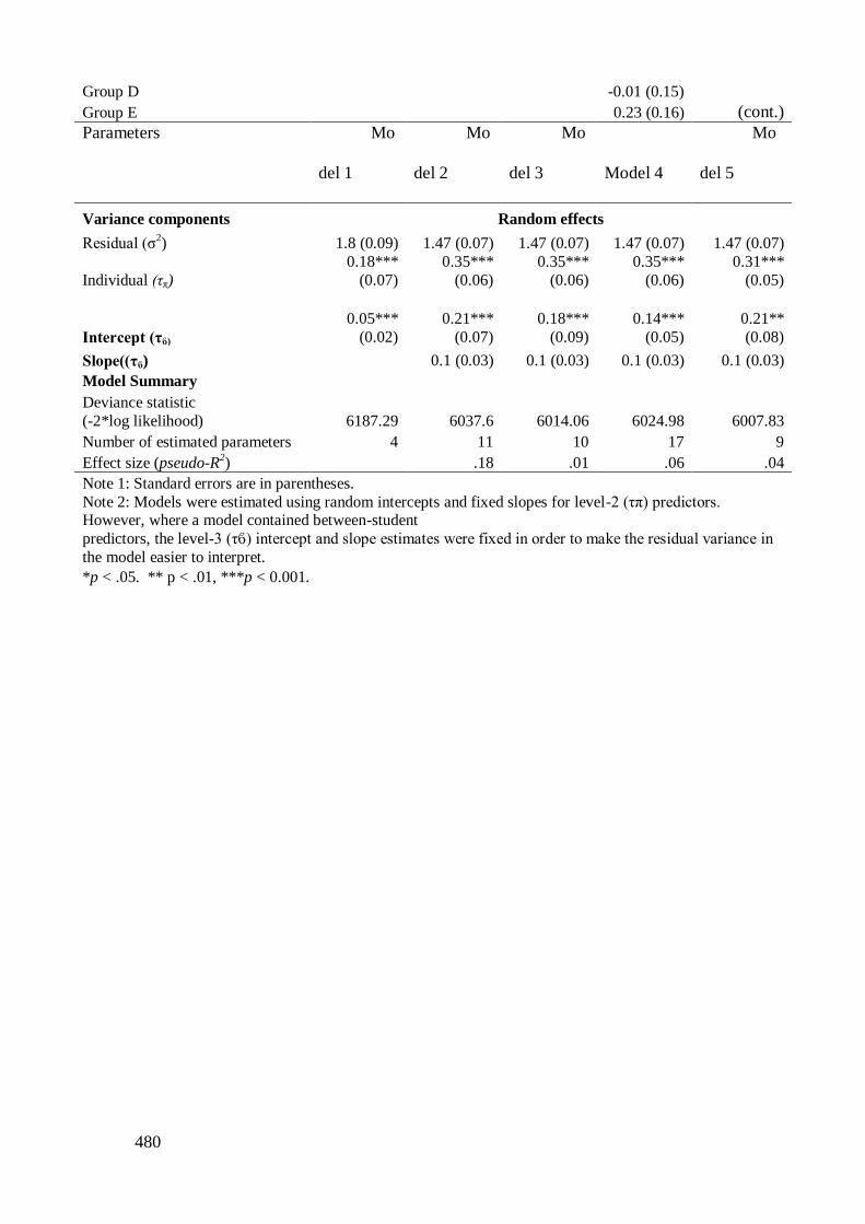
480
Group D
-0.01 (0.15)
Group E
0.23 (0.16) (cont.)
Parameters Mo
del 1
Mo
del 2
Mo
del 3
Model 4
Mo
del 5
Variance components Random effects
Residual (σ2) 1.8 (0.09) 1.47 (0.07) 1.47 (0.07) 1.47 (0.07) 1.47 (0.07)
Individual (τπ)
0.18***
(0.07)
0.35***
(0.06)
0.35***
(0.06)
0.35***
(0.06)
0.31***
(0.05)
Intercept (τϐ) 0.05***
(0.02) 0.21***
(0.07) 0.18***
(0.09) 0.14***
(0.05) 0.21**
(0.08)
Slope((τϐ)
0.1 (0.03) 0.1 (0.03) 0.1 (0.03) 0.1 (0.03)
Model Summary Deviance statistic
(-2*log likelihood) 6187.29 6037.6 6014.06 6024.98 6007.83
Number of estimated parameters 4 11 10 17 9
Effect size (pseudo-R2)
.18 .01 .06 .04
Note 1: Standard errors are in parentheses. Note 2: Models were estimated using random intercepts and fixed slopes for level-2 (τπ) predictors. However, where a model contained between-student predictors, the level-3 (τϐ) intercept and slope estimates were fixed in order to make the residual variance in
the model easier to interpret.
*p < .05. ** p < .01, ***p < 0.001.
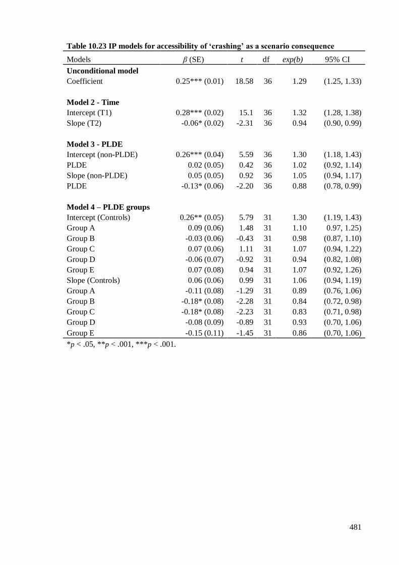
481
Table 10.23 IP models for accessibility of ‘crashing’ as a scenario consequence
Models β (SE) t df exp(b) 95% CI
Unconditional model
Coefficient 0.25*** (0.01) 18.58 36 1.29 (1.25, 1.33)
Model 2 - Time
Intercept (T1) 0.28*** (0.02) 15.1 36 1.32 (1.28, 1.38)
Slope (T2) -0.06* (0.02) -2.31 36 0.94 (0.90, 0.99)
Model 3 - PLDE
Intercept (non-PLDE) 0.26*** (0.04) 5.59 36 1.30 (1.18, 1.43)
PLDE 0.02 (0.05) 0.42 36 1.02 (0.92, 1.14)
Slope (non-PLDE) 0.05 (0.05) 0.92 36 1.05 (0.94, 1.17)
PLDE -0.13* (0.06) -2.20 36 0.88 (0.78, 0.99)
Model 4 – PLDE groups
Intercept (Controls) 0.26** (0.05) 5.79 31 1.30 (1.19, 1.43)
Group A 0.09 (0.06) 1.48 31 1.10 0.97, 1.25)
Group B -0.03 (0.06) -0.43 31 0.98 (0.87, 1.10)
Group C 0.07 (0.06) 1.11 31 1.07 (0.94, 1.22)
Group D -0.06 (0.07) -0.92 31 0.94 (0.82, 1.08)
Group E 0.07 (0.08) 0.94 31 1.07 (0.92, 1.26)
Slope (Controls) 0.06 (0.06) 0.99 31 1.06 (0.94, 1.19)
Group A -0.11 (0.08) -1.29 31 0.89 (0.76, 1.06)
Group B -0.18* (0.08) -2.28 31 0.84 (0.72, 0.98)
Group C -0.18* (0.08) -2.23 31 0.83 (0.71, 0.98)
Group D -0.08 (0.09) -0.89 31 0.93 (0.70, 1.06)
Group E -0.15 (0.11) -1.45 31 0.86 (0.70, 1.06)
*p < .05, **p < .001, ***p < .001.
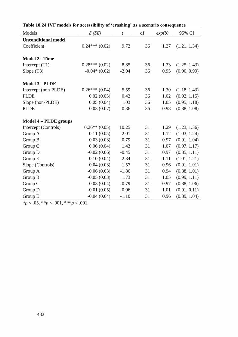
482
Table 10.24 IVF models for accessibility of ‘crashing’ as a scenario consequence
Models β (SE) t df exp(b) 95% CI
Unconditional model
Coefficient 0.24*** (0.02) 9.72 36 1.27 (1.21, 1.34)
Model 2 - Time
Intercept (T1) 0.28*** (0.02) 8.85 36 1.33 (1.25, 1.43)
Slope (T3) -0.04* (0.02) -2.04 36 0.95 (0.90, 0.99)
Model 3 - PLDE
Intercept (non-PLDE) 0.26*** (0.04) 5.59 36 1.30 (1.18, 1.43)
PLDE 0.02 (0.05) 0.42 36 1.02 (0.92, 1.15)
Slope (non-PLDE) 0.05 (0.04) 1.03 36 1.05 (0.95, 1.18)
PLDE -0.03 (0.07) -0.36 36 0.98 (0.88, 1.08)
Model 4 – PLDE groups
Intercept (Controls) 0.26** (0.05) 10.25 31 1.29 (1.23, 1.36)
Group A 0.11 (0.05) 2.01 31 1.12 (1.03, 1.24)
Group B -0.03 (0.03) -0.79 31 0.97 (0.91, 1.04)
Group C 0.06 (0.04) 1.43 31 1.07 (0.97, 1.17)
Group D -0.02 (0.06) -0.45 31 0.97 (0.85, 1.11)
Group E 0.10 (0.04) 2.34 31 1.11 (1.01, 1.21)
Slope (Controls) -0.04 (0.03) -1.57 31 0.96 (0.91, 1.01)
Group A -0.06 (0.03) -1.86 31 0.94 (0.88, 1.01)
Group B -0.05 (0.03) 1.73 31 1.05 (0.99, 1.11)
Group C -0.03 (0.04) -0.79 31 0.97 (0.88, 1.06)
Group D -0.01 (0.05) 0.06 31 1.01 (0.91, 0.11)
Group E -0.04 (0.04) -1.10 31 0.96 (0.89, 1.04)
*p < .05, **p < .001, ***p < .001.
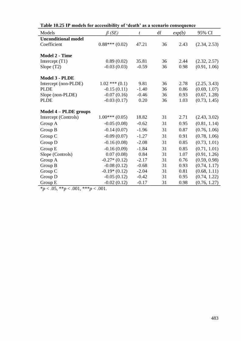
483
Table 10.25 IP models for accessibility of ‘death’ as a scenario consequence
Models β (SE) t df exp(b) 95% CI
Unconditional model
Coefficient 0.88*** (0.02) 47.21 36 2.43 (2.34, 2.53)
Model 2 - Time
Intercept (T1) 0.89 (0.02) 35.81 36 2.44 (2.32, 2.57)
Slope (T2) -0.03 (0.03) -0.59 36 0.98 (0.91, 1.06)
Model 3 - PLDE
Intercept (non-PLDE) 1.02 *** (0.1) 9.81 36 2.78 (2.25, 3.43)
PLDE -0.15 (0.11) -1.40 36 0.86 (0.69, 1.07)
Slope (non-PLDE) -0.07 (0.16) -0.46 36 0.93 (0.67, 1.28)
PLDE -0.03 (0.17) 0.20 36 1.03 (0.73, 1.45)
Model 4 – PLDE groups
Intercept (Controls) 1.00*** (0.05) 18.82 31 2.71 (2.43, 3.02)
Group A -0.05 (0.08) -0.62 31 0.95 (0.81, 1.14)
Group B -0.14 (0.07) -1.96 31 0.87 (0.76, 1.06)
Group C -0.09 (0.07) -1.27 31 0.91 (0.78, 1.06)
Group D -0.16 (0.08) -2.08 31 0.85 (0.73, 1.01)
Group E -0.16 (0.09) -1.84 31 0.85 (0.71, 1.01)
Slope (Controls) 0.07 (0.08) 0.84 31 1.07 (0.91, 1.26)
Group A -0.27* (0.12) -2.17 31 0.76 (0.59, 0.98)
Group B -0.08 (0.12) -0.68 31 0.93 (0.74, 1.17)
Group C -0.19* (0.12) -2.04 31 0.81 (0.68, 1.11)
Group D -0.05 (0.12) -0.42 31 0.95 (0.74, 1.22)
Group E -0.02 (0.12) -0.17 31 0.98 (0.76, 1.27)
*p < .05, **p < .001, ***p < .001.
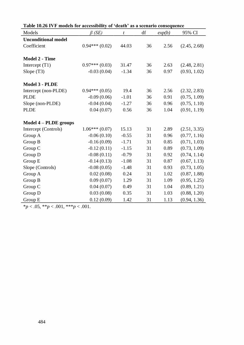
484
Table 10.26 IVF models for accessibility of ‘death’ as a scenario consequence
Models β (SE) t df exp(b) 95% CI
Unconditional model
Coefficient 0.94*** (0.02) 44.03 36 2.56 (2.45, 2.68)
Model 2 - Time
Intercept (T1) 0.97*** (0.03) 31.47 36 2.63 (2.48, 2.81)
Slope (T3) -0.03 (0.04) -1.34 36 0.97 (0.93, 1.02)
Model 3 - PLDE
Intercept (non-PLDE) 0.94*** (0.05) 19.4 36 2.56 (2.32, 2.83)
PLDE -0.09 (0.06) -1.01 36 0.91 (0.75, 1.09)
Slope (non-PLDE) -0.04 (0.04) -1.27 36 0.96 (0.75, 1.10)
PLDE 0.04 (0.07) 0.56 36 1.04 (0.91, 1.19)
Model 4 – PLDE groups
Intercept (Controls) 1.06*** (0.07) 15.13 31 2.89 (2.51, 3.35)
Group A -0.06 (0.10) -0.55 31 0.96 (0.77, 1.16)
Group B -0.16 (0.09) -1.71 31 0.85 (0.71, 1.03)
Group C -0.12 (0.11) -1.15 31 0.89 (0.73, 1.09)
Group D -0.08 (0.11) -0.79 31 0.92 (0.74, 1.14)
Group E -0.14 (0.13) -1.08 31 0.87 (0.67, 1.13)
Slope (Controls) -0.08 (0.05) -1.48 31 0.93 (0.73, 1.05)
Group A 0.02 (0.08) 0.24 31 1.02 (0.87, 1.88)
Group B 0.09 (0.07) 1.29 31 1.09 (0.95, 1.25)
Group C 0.04 (0.07) 0.49 31 1.04 (0.89, 1.21)
Group D 0.03 (0.08) 0.35 31 1.03 (0.88, 1.20)
Group E 0.12 (0.09) 1.42 31 1.13 (0.94, 1.36)
*p < .05, **p < .001, ***p < .001.
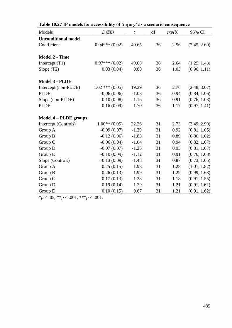
485
Table 10.27 IP models for accessibility of ‘injury’ as a scenario consequence
Models β (SE) t df exp(b) 95% CI
Unconditional model
Coefficient 0.94*** (0.02) 40.65 36 2.56 (2.45, 2.69)
Model 2 - Time
Intercept (T1) 0.97*** (0.02) 49.08 36 2.64 (1.25, 1.43)
Slope (T2) 0.03 (0.04) 0.80 36 1.03 (0.96, 1.11)
Model 3 - PLDE
Intercept (non-PLDE) 1.02 *** (0.05) 19.39 36 2.76 (2.48, 3.07)
PLDE -0.06 (0.06) -1.08 36 0.94 (0.84, 1.06)
Slope (non-PLDE) -0.10 (0.08) -1.16 36 0.91 (0.76, 1.08)
PLDE 0.16 (0.09) 1.70 36 1.17 (0.97, 1.41)
Model 4 – PLDE groups
Intercept (Controls) 1.00** (0.05) 22.26 31 2.73 (2.49, 2.99)
Group A -0.09 (0.07) -1.29 31 0.92 (0.81, 1.05)
Group B -0.12 (0.06) -1.83 31 0.89 (0.86, 1.02)
Group C -0.06 (0.04) -1.04 31 0.94 (0.82, 1.07)
Group D -0.07 (0.07) -1.25 31 0.93 (0.81, 1.07)
Group E -0.10 (0.09) -1.12 31 0.91 (0.76, 1.08)
Slope (Controls) -0.13 (0.09) -1.48 31 0.87 (0.73, 1.05)
Group A 0.25 (0.15) 1.98 31 1.28 (1.01, 1.82)
Group B 0.26 (0.13) 1.99 31 1.29 (0.99, 1.68)
Group C 0.17 (0.13) 1.28 31 1.18 (0.91, 1.55)
Group D 0.19 (0.14) 1.39 31 1.21 (0.91, 1.62)
Group E 0.10 (0.15) 0.67 31 1.21 (0.91, 1.62)
*p < .05, **p < .001, ***p < .001.
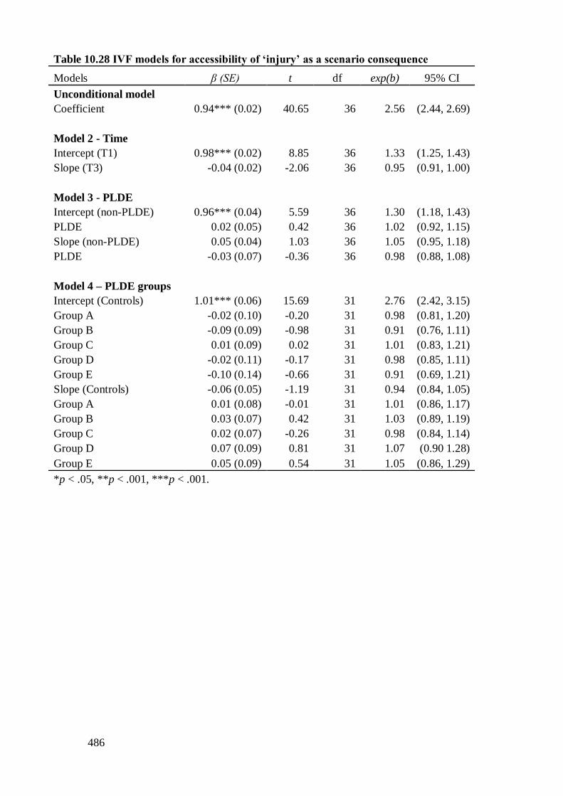
486
Table 10.28 IVF models for accessibility of ‘injury’ as a scenario consequence
Models β (SE) t df exp(b) 95% CI
Unconditional model
Coefficient 0.94*** (0.02) 40.65 36 2.56 (2.44, 2.69)
Model 2 - Time
Intercept (T1) 0.98*** (0.02) 8.85 36 1.33 (1.25, 1.43)
Slope (T3) -0.04 (0.02) -2.06 36 0.95 (0.91, 1.00)
Model 3 - PLDE
Intercept (non-PLDE) 0.96*** (0.04) 5.59 36 1.30 (1.18, 1.43)
PLDE 0.02 (0.05) 0.42 36 1.02 (0.92, 1.15)
Slope (non-PLDE) 0.05 (0.04) 1.03 36 1.05 (0.95, 1.18)
PLDE -0.03 (0.07) -0.36 36 0.98 (0.88, 1.08)
Model 4 – PLDE groups
Intercept (Controls) 1.01*** (0.06) 15.69 31 2.76 (2.42, 3.15)
Group A -0.02 (0.10) -0.20 31 0.98 (0.81, 1.20)
Group B -0.09 (0.09) -0.98 31 0.91 (0.76, 1.11)
Group C 0.01 (0.09) 0.02 31 1.01 (0.83, 1.21)
Group D -0.02 (0.11) -0.17 31 0.98 (0.85, 1.11)
Group E -0.10 (0.14) -0.66 31 0.91 (0.69, 1.21)
Slope (Controls) -0.06 (0.05) -1.19 31 0.94 (0.84, 1.05)
Group A 0.01 (0.08) -0.01 31 1.01 (0.86, 1.17)
Group B 0.03 (0.07) 0.42 31 1.03 (0.89, 1.19)
Group C 0.02 (0.07) -0.26 31 0.98 (0.84, 1.14)
Group D 0.07 (0.09) 0.81 31 1.07 (0.90 1.28)
Group E 0.05 (0.09) 0.54 31 1.05 (0.86, 1.29)
*p < .05, **p < .001, ***p < .001.
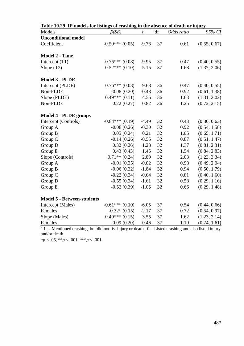
487
Table 10.29 IP models for listings of crashing in the absence of death or injury
Models β(SE) t df Odds ratio 95% CI
Unconditional model
Coefficient -0.50*** (0.05) -9.76 37 0.61 (0.55, 0.67)
Model 2 - Time
Intercept (T1) -0.76*** (0.08) -9.95 37 0.47 (0.40, 0.55)
Slope (T2) 0.52*** (0.10) 5.15 37 1.68 (1.37, 2.06)
Model 3 - PLDE
Intercept (PLDE) -0.76*** (0.08) -9.68 36 0.47 (0.40, 0.55)
Non-PLDE -0.08 (0.20) -0.43 36 0.92 (0.61, 1.38)
Slope (PLDE) 0.49*** (0.11) 4.55 36 1.63 (1.31, 2.02)
Non-PLDE 0.22 (0.27) 0.82 36 1.25 (0.72, 2.15)
Model 4 - PLDE groups
Intercept (Controls) -0.84*** (0.19) -4.49 32 0.43 (0.30, 0.63)
Group A -0.08 (0.26) -0.30 32 0.92 (0.54, 1.58)
Group B 0.05 (0.24) 0.21 32 1.05 (0.65, 1.71)
Group C -0.14 (0.26) -0.55 32 0.87 (0.51, 1.47)
Group D 0.32 (0.26) 1.23 32 1.37 (0.81, 2.31)
Group E 0.43 (0.43) 1.45 32 1.54 (0.84, 2.83)
Slope (Controls) 0.71** (0.24) 2.89 32 2.03 (1.23, 3.34)
Group A -0.01 (0.35) -0.02 32 0.98 (0.49, 2.04)
Group B -0.06 (0.32) -1.84 32 0.94 (0.50, 1.79)
Group C -0.22 (0.34) -0.64 32 0.81 (0.40, 1.60)
Group D -0.55 (0.34) -1.61 32 0.58 (0.29, 1.16)
Group E -0.52 (0.39) -1.05 32 0.66 (0.29, 1.48)
Model 5 - Between-students
Intercept (Males) -0.61*** (0.10) -6.05 37 0.54 (0.44, 0.66)
Females -0.32* (0.15) -2.17 37 0.72 (0.54, 0.97)
Slope (Males) 0.49*** (0.15) 3.55 37 1.62 (1.23, 2.14)
Females 0.09 (0.20) 0.46 37 1.10 (0.74, 1.61) a
1 = Mentioned crashing, but did not list injury or death, 0 = Listed crashing and also listed injury and/or death.
*p < .05, **p < .001, ***p < .001.
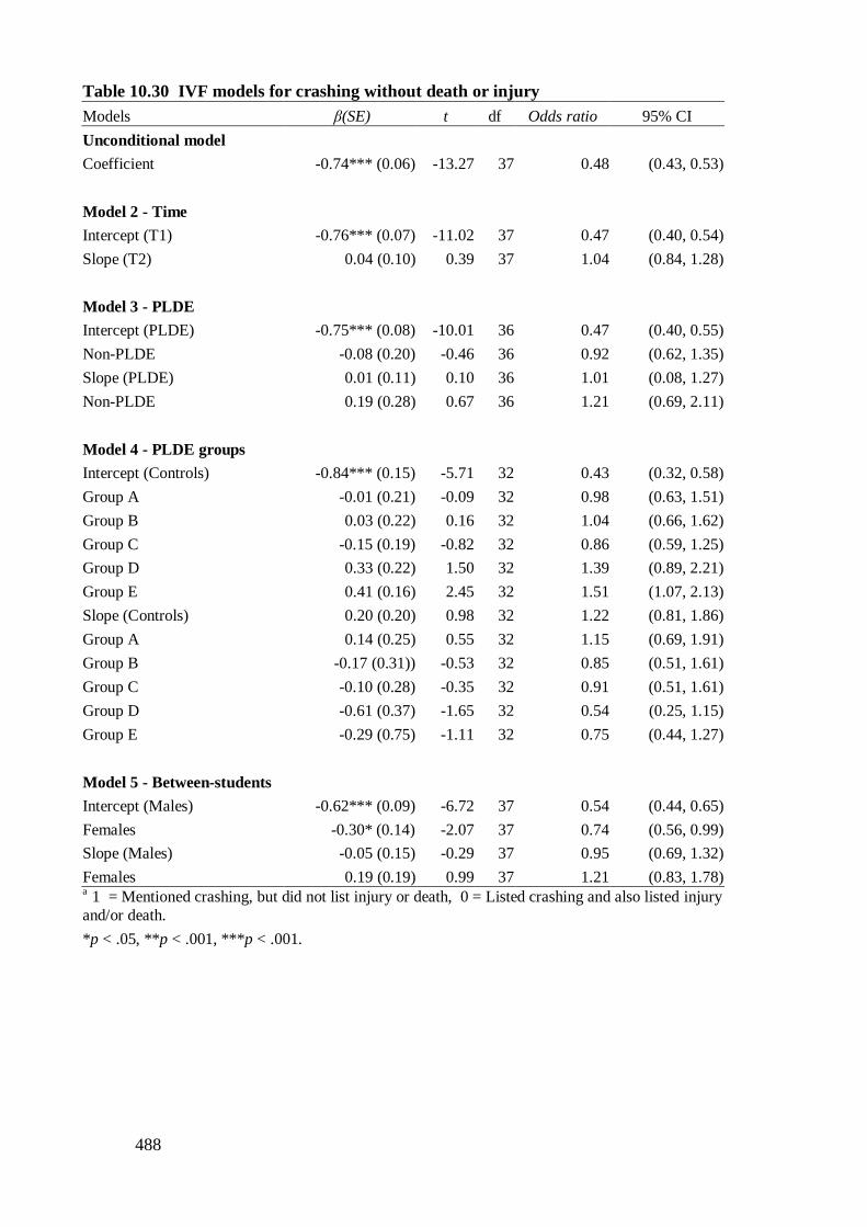
488
Table 10.30 IVF models for crashing without death or injury
Models β(SE) t df Odds ratio 95% CI
Unconditional model
Coefficient -0.74*** (0.06) -13.27 37 0.48 (0.43, 0.53)
Model 2 - Time Intercept (T1) -0.76*** (0.07) -11.02 37 0.47 (0.40, 0.54)
Slope (T2) 0.04 (0.10) 0.39 37 1.04 (0.84, 1.28)
Model 3 - PLDE
Intercept (PLDE) -0.75*** (0.08) -10.01 36 0.47 (0.40, 0.55)
Non-PLDE -0.08 (0.20) -0.46 36 0.92 (0.62, 1.35)
Slope (PLDE) 0.01 (0.11) 0.10 36 1.01 (0.08, 1.27)
Non-PLDE 0.19 (0.28) 0.67 36 1.21 (0.69, 2.11)
Model 4 - PLDE groups
Intercept (Controls) -0.84*** (0.15) -5.71 32 0.43 (0.32, 0.58)
Group A -0.01 (0.21) -0.09 32 0.98 (0.63, 1.51)
Group B 0.03 (0.22) 0.16 32 1.04 (0.66, 1.62)
Group C -0.15 (0.19) -0.82 32 0.86 (0.59, 1.25)
Group D 0.33 (0.22) 1.50 32 1.39 (0.89, 2.21)
Group E 0.41 (0.16) 2.45 32 1.51 (1.07, 2.13)
Slope (Controls) 0.20 (0.20) 0.98 32 1.22 (0.81, 1.86)
Group A 0.14 (0.25) 0.55 32 1.15 (0.69, 1.91)
Group B -0.17 (0.31)) -0.53 32 0.85 (0.51, 1.61)
Group C -0.10 (0.28) -0.35 32 0.91 (0.51, 1.61)
Group D -0.61 (0.37) -1.65 32 0.54 (0.25, 1.15)
Group E -0.29 (0.75) -1.11 32 0.75 (0.44, 1.27)
Model 5 - Between-students Intercept (Males) -0.62*** (0.09) -6.72 37 0.54 (0.44, 0.65)
Females -0.30* (0.14) -2.07 37 0.74 (0.56, 0.99)
Slope (Males) -0.05 (0.15) -0.29 37 0.95 (0.69, 1.32)
Females 0.19 (0.19) 0.99 37 1.21 (0.83, 1.78) a
1 = Mentioned crashing, but did not list injury or death, 0 = Listed crashing and also listed injury
and/or death.
*p < .05, **p < .001, ***p < .001.
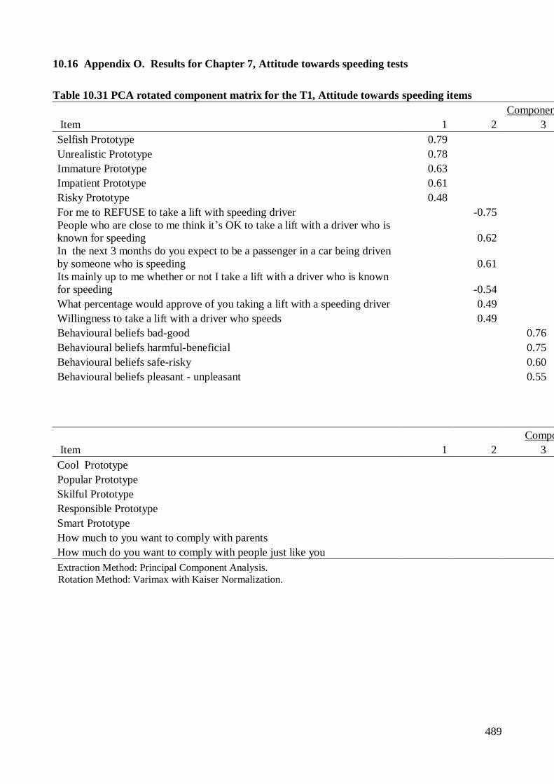
489
10.16 Appendix O. Results for Chapter 7, Attitude towards speeding tests
Table 10.31 PCA rotated component matrix for the T1, Attitude towards speeding items
Component
Item 1 2 3 4 5 6
Selfish Prototype 0.79
Unrealistic Prototype 0.78
Immature Prototype 0.63 -0.38
Impatient Prototype 0.61
Risky Prototype 0.48 -0.38
For me to REFUSE to take a lift with speeding driver -0.75
People who are close to me think it’s OK to take a lift with a driver who is
known for speeding 0.62
In the next 3 months do you expect to be a passenger in a car being driven
by someone who is speeding 0.61
Its mainly up to me whether or not I take a lift with a driver who is known
for speeding -0.54 0.32 -0.31
What percentage would approve of you taking a lift with a speeding driver 0.49
Willingness to take a lift with a driver who speeds 0.49
Behavioural beliefs bad-good 0.76
Behavioural beliefs harmful-beneficial 0.75
Behavioural beliefs safe-risky 0.60
Behavioural beliefs pleasant - unpleasant 0.55 (cont.)
Component
Item 1 2 3 4 5 6
Cool Prototype 0.72
Popular Prototype 0.71
Skilful Prototype 0.60 0.41
Responsible Prototype 0.73
Smart Prototype 0.33 0.70
How much to you want to comply with parents 0.75
How much do you want to comply with people just like you 0.73
Extraction Method: Principal Component Analysis.
Rotation Method: Varimax with Kaiser Normalization.
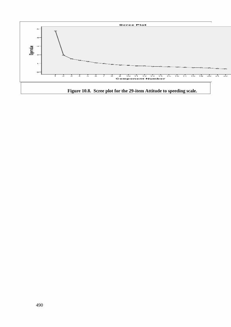
490
Figure 10.8. Scree plot for the 29-item Attitude to speeding scale.
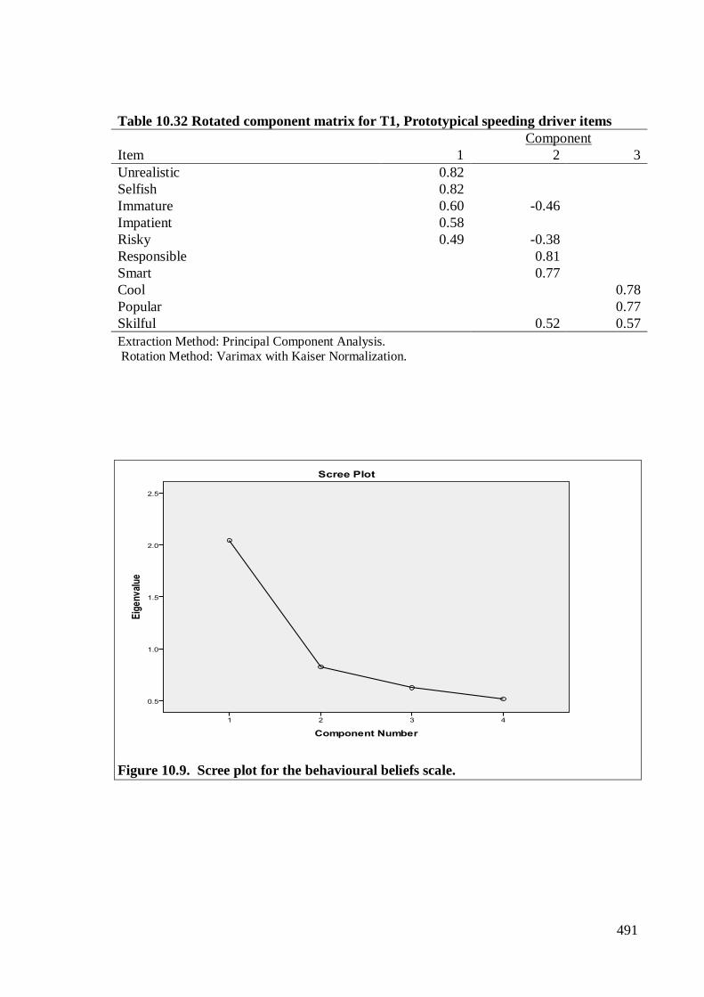
491
Table 10.32 Rotated component matrix for T1, Prototypical speeding driver items
Component
Item 1 2 3
Unrealistic 0.82
Selfish 0.82
Immature 0.60 -0.46
Impatient 0.58
Risky 0.49 -0.38
Responsible 0.81
Smart 0.77
Cool 0.78
Popular 0.77
Skilful 0.52 0.57
Extraction Method: Principal Component Analysis. Rotation Method: Varimax with Kaiser Normalization.
Figure 10.9. Scree plot for the behavioural beliefs scale.
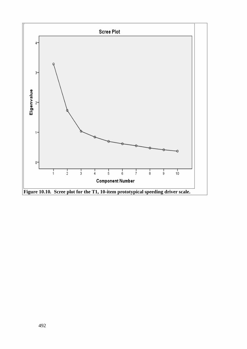
492
Figure 10.10. Scree plot for the T1, 10-item prototypical speeding driver scale.
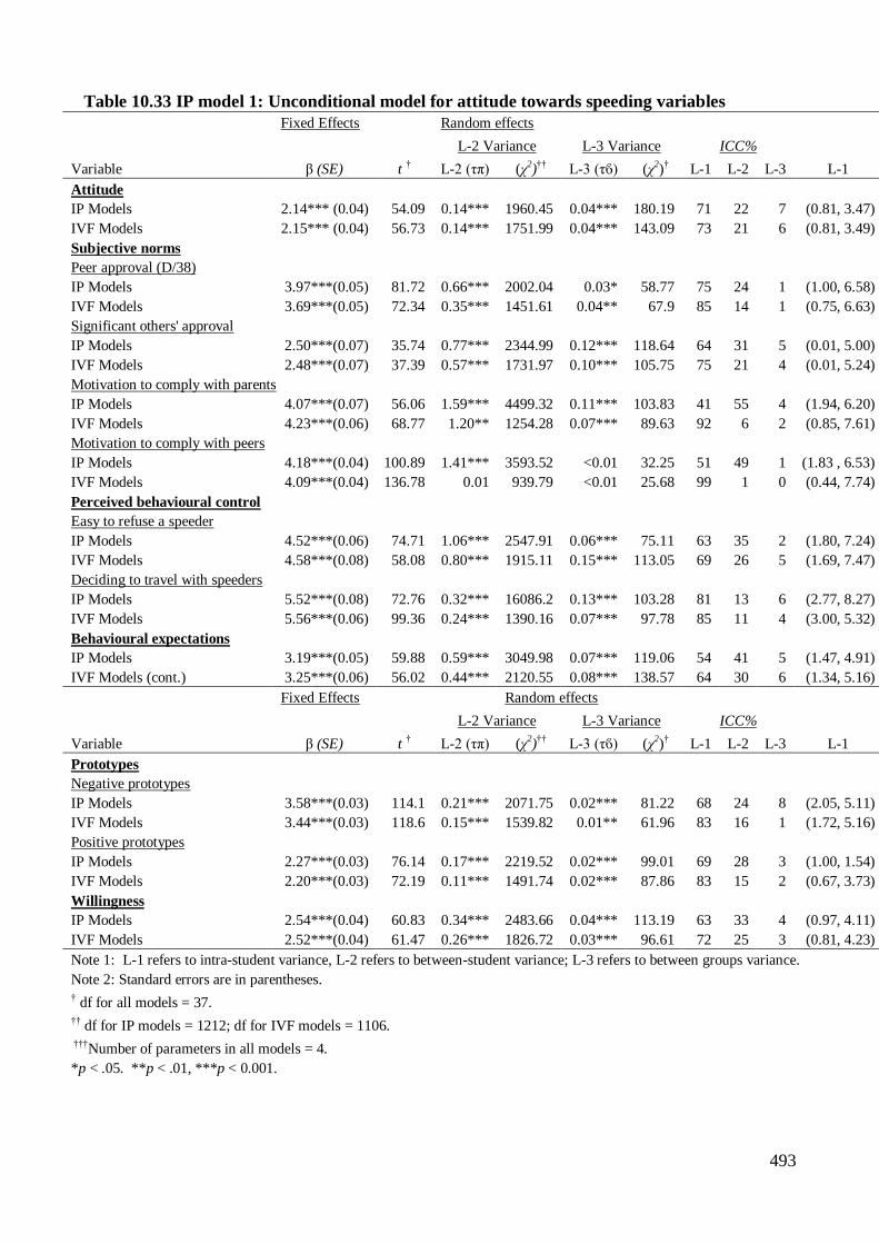
493
Table 10.33 IP model 1: Unconditional model for attitude towards speeding variables
Fixed Effects Random effects
L-2 Variance L-3 Variance ICC% 95% CI Deviance†††
Variable β (SE) t † L-2 (τπ) (χ2)†† L-3 (τϐ) (χ2)† L-1 L-2 L-3 L-1 L-2 L-3
Attitude
IP Models 2.14*** (0.04) 54.09 0.14*** 1960.45 0.04*** 180.19 71 22 7 (0.81, 3.47) (1.41, 2.87) (1.75, 2.53) 5780.73
IVF Models 2.15*** (0.04) 56.73 0.14*** 1751.99 0.04*** 143.09 73 21 6 (0.81, 3.49) (1.42, 2.88) (1.76, 2.54) 5340.76
Subjective norms
Peer approval (D/38)
IP Models 3.97***(0.05) 81.72 0.66*** 2002.04 0.03* 58.77 75 24 1 (1.00, 6.58) (2.20, 5.38) (2.45, 4.13) 9502.69
IVF Models 3.69***(0.05) 72.34 0.35*** 1451.61 0.04** 67.9 85 14 1 (0.75, 6.63) (2.53, 4.85) (3.30, 4.08) 8615.00
Significant others' approval
IP Models 2.50***(0.07) 35.74 0.77*** 2344.99 0.12*** 118.64 64 31 5 (0.01, 5.00) (0.77, 4.23) (1.82, 3.18) 9189.11
IVF Models 2.48***(0.07) 37.39 0.57*** 1731.97 0.10*** 105.75 75 21 4 (0.01, 5.24) (0.99, 3.97) (1.86, 3.10) 8627.44
Motivation to comply with parents
IP Models 4.07***(0.07) 56.06 1.59*** 4499.32 0.11*** 103.83 41 55 4 (1.94, 6.20) (1.59, 6.55) (3.42, 4.72) 9178.12
IVF Models 4.23***(0.06) 68.77 1.20** 1254.28 0.07*** 89.63 92 6 2 (0.85, 7.61) (3.35, 5.11) (3.71, 4.75) 9148.35
Motivation to comply with peers
IP Models 4.18***(0.04) 100.89 1.41*** 3593.52 <0.01 32.25 51 49 1 (1.83 , 6.53) (1.85, 6.51) (3.98, 4.38) 9366.87
IVF Models 4.09***(0.04) 136.78 0.01 939.79 <0.01 25.68 99 1 0 (0.44, 7.74) (3.98, 4.20) (4.08, 4.10) 9324.59
Perceived behavioural control
Easy to refuse a speeder
IP Models 4.52***(0.06) 74.71 1.06*** 2547.91 0.06*** 75.11 63 35 2 (1.80, 7.24) (2.50, 6.54) (4.04, 5.00) 9682.25
IVF Models 4.58***(0.08) 58.08 0.80*** 1915.11 0.15*** 113.05 69 26 5 (1.69, 7.47) (2.83, 6.33) (3.82, 5.34) 8940.88
Deciding to travel with speeders
IP Models 5.52***(0.08) 72.76 0.32*** 16086.2 0.13*** 103.28 81 13 6 (2.77, 8.27) (4.41, 6.63) (4.81, 6.23) 7518.43
IVF Models 5.56***(0.06) 99.36 0.24*** 1390.16 0.07*** 97.78 85 11 4 (3.00, 5.32) (4.70, 6.62) (5.14, 6.18) 8197.86
Behavioural expectations
IP Models 3.19***(0.05) 59.88 0.59*** 3049.98 0.07*** 119.06 54 41 5 (1.47, 4.91) (1.69, 4.69) 2.68, 3.70) 7642.20
IVF Models (cont.) 3.25***(0.06) 56.02 0.44*** 2120.55 0.08*** 138.57 64 30 6 (1.34, 5.16) (1.95, 4.55) (2.68, 3.82) 7178.01
Fixed Effects
Random effects
L-2 Variance L-3 Variance ICC% 95% CI Deviance†††
Variable β (SE) t † L-2 (τπ) (χ2)†† L-3 (τϐ) (χ2)† L-1 L-2 L-3 L-1 L-2 L-3
Prototypes
Negative prototypes
IP Models 3.58***(0.03) 114.1 0.21*** 2071.75 0.02*** 81.22 68 24 8 (2.05, 5.11) (2.67, 4.49) (3.03, 4.13) 6545.88
IVF Models 3.44***(0.03) 118.6 0.15*** 1539.82 0.01** 61.96 83 16 1 (1.72, 5.16) (2.68, 4.20) (3.24, 3.64) 6302.09
Positive prototypes
IP Models 2.27***(0.03) 76.14 0.17*** 2219.52 0.02*** 99.01 69 28 3 (1.00, 1.54) (1.45, 3.09) (2.00, 2.54) 5709.98
IVF Models 2.20***(0.03) 72.19 0.11*** 1491.74 0.02*** 87.86 83 15 2 (0.67, 3.73) (1.56, 2.84) (1.94, 2.46) 5740.40
Willingness
IP Models 2.54***(0.04) 60.83 0.34*** 2483.66 0.04*** 113.19 63 33 4 (0.97, 4.11) (1.40, 3.68) (2.15, 2.93) 6932.85
IVF Models 2.52***(0.04) 61.47 0.26*** 1826.72 0.03*** 96.61 72 25 3 (0.81, 4.23) (1.51, 3.53) (2.16, 2.88) 6084.19
Note 1: L-1 refers to intra-student variance, L-2 refers to between-student variance; L-3 refers to between groups variance.
Note 2: Standard errors are in parentheses.
† df for all models = 37.
†† df for IP models = 1212; df for IVF models = 1106.
†††Number of parameters in all models = 4.
*p < .05. **p < .01, ***p < 0.001.

494
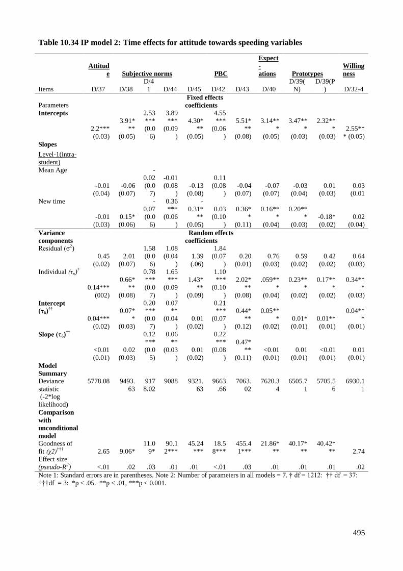
495
Table 10.34 IP model 2: Time effects for attitude towards speeding variables
Attitud
e Subjective norms PBC
Expect
-
ations Prototypes
Willing
ness
Items D/37 D/38
D/4
1 D/44 D/45 D/42 D/43 D/40
D/39(
N)
D/39(P
) D/32-4
Parameters
Fixed effects
coefficients
Intercepts
2.2***
(0.03)
3.91*
**
(0.05)
2.53
***
(0.0
6)
3.89
***
(0.09
)
4.30*
**
(0.05)
4.55
***
(0.06
)
5.51*
**
(0.08)
3.14**
*
(0.05)
3.47**
*
(0.03)
2.32**
*
(0.03)
2.55**
* (0.05)
Slopes
Level-1(intra-
student)
Mean Age
-0.01
(0.04)
-0.06
(0.07)
-
0.02
(0.0
7)
-0.01
(0.08
)
-0.13
(0.08)
0.11
(0.08
)
-0.04
(0.07)
-0.07
(0.07)
-0.03
(0.04)
0.01
(0.03)
0.03
(0.01
New time
-0.01
(0.03)
0.15*
(0.06)
-
0.07 (0.0
6)
0.36
*** (0.06
)
-
0.31***
(0.05)
0.03 (0.10
)
0.36**
(0.11)
0.16***
(0.04)
0.20***
(0.03)
-0.18*
(0.02)
0.02
(0.04)
Variance
components
Random effects
coefficients
Residual (σ2)
0.45
(0.02)
2.01
(0.07)
1.58
(0.0
6)
1.08
(0.04
)
1.39
(.06)
1.84
(0.07
)
0.20
(0.01)
0.76
(0.03)
0.59
(0.02)
0.42
(0.02)
0.64
(0.03)
Individual (τπ)†
0.14***
(002)
0.66*
**
(0.08)
0.78
***
(0.0
7)
1.65
***
(0.09
)
1.43*
**
(0.09)
1.10
***
(0.10
)
2.02*
**
(0.08)
.059**
*
(0.04)
0.23**
*
(0.02)
0.17**
*
(0.02)
0.34**
*
(0.03)
Intercept
(τϐ)††
0.04***
(0.02)
0.07*
*
(0.03)
0.20***
(0.0
7)
0.07**
(0.04
)
0.01
(0.02)
0.21***
(0.07
)
0.44*
**
(0.12)
0.05**
*
(0.02)
0.01*
(0.01)
0.01**
(0.01)
0.04**
*
(0.01)
Slope (τϐ)††
<0.01
(0.01)
0.02
(0.03)
0.12
***
(0.0
5)
0.06
**
(0.03
)
0.01
(0.02)
0.22
***
(0.08
)
0.47*
**
(0.11)
<0.01
(0.01)
0.01
(0.01)
<0.01
(0.01)
0.01
(0.01)
Model
Summary
Deviance
statistic (-2*log
likelihood)
5778.08 9493.
63
917
8.02
9088 9321.
63
9663
.66
7063.
02
7620.3
4
6505.7
1
5705.5
6
6930.1
1
Comparison
with
unconditional
model
Goodness of
fit (χ2)††† 2.65 9.06*
11.0
9*
90.1
2***
45.24
***
18.5
8***
455.4
1***
21.86*
**
40.17*
**
40.42*
** 2.74
Effect size
(pseudo-R2) <.01 .02 .03 .01 .01 <.01 .03 .01 .01 .01 .02
Note 1: Standard errors are in parentheses. Note 2: Number of parameters in all models = 7. † df = 1212: †† df = 37:
†††df = 3: *p < .05. **p < .01, ***p < 0.001.
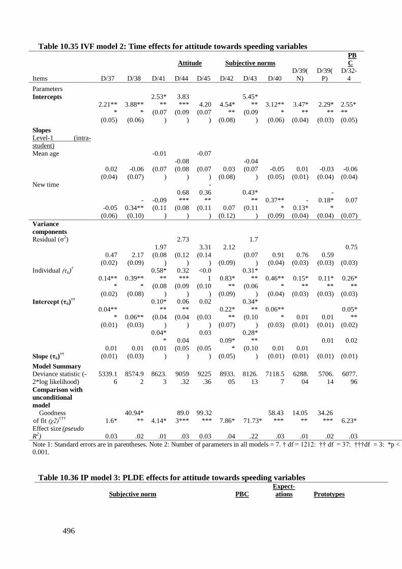
496
Table 10.35 IVF model 2: Time effects for attitude towards speeding variables
Attitude Subjective norms
PB
C
Items D/37 D/38 D/41 D/44 D/45 D/42 D/43 D/40
D/39(
N)
D/39(
P)
D/32-
4
Parameters
Intercepts
2.21**
*
(0.05)
3.88**
*
(0.06)
2.53*
**
(0.07
)
3.83
***
(0.09
)
4.20
(0.07
)
4.54*
**
(0.08)
5.45*
**
(0.09
)
3.12**
*
(0.06)
3.47*
**
(0.04)
2.29*
**
(0.03)
2.55*
**
(0.05)
Slopes
Level-1 (intra-
student)
Mean age
0.02
(0.04)
-0.06
(0.07)
-0.01
(0.07
)
-0.08
(0.08
)
-0.07
(0.07
)
0.03
(0.08)
-0.04
(0.07
)
-0.05
(0.05)
0.01
(0.01)
-0.03
(0.04)
-0.06
(0.04)
New time
-0.05
(0.06)
-0.34**
(0.10)
-0.09 (0.11
)
0.68
*** (0.08
)
-
0.36
** (0.11
)
0.07
(0.12)
0.43*
** (0.11
)
0.37***
(0.09)
-0.13*
(0.04)
-
0.18**
(0.04)
0.07
(0.07)
Variance
components
Residual (σ2)
0.47
(0.02)
2.17
(0.09)
1.97
(0.08
)
2.73
(0.12
)
3.31
(0.14
)
2.12
(0.09)
1.7
(0.07
)
0.91
(0.04)
0.76
(0.03)
0.59
(0.03)
0.75
(0.03)
Individual (τπ)†
0.14**
*
(0.02)
0.39**
*
(0.08)
0.58*
**
(0.08
)
0.32
***
(0.09
)
<0.0
1
(0.10
)
0.83*
**
(0.09)
0.31*
**
(0.06
)
0.46**
*
(0.04)
0.15*
**
(0.03)
0.11*
**
(0.03)
0.26*
**
(0.03)
Intercept (τϐ)††
0.04**
*
(0.01)
0.06**
(0.03)
0.10*
**
(0.04
)
0.06
**
(0.04
)
0.02
(0.03
)
0.22*
**
(0.07)
0.34*
**
(0.10
)
0.06**
*
(0.03)
0.01
(0.01)
0.01
(0.01)
0.05*
**
(0.02)
Slope (τϐ)††
0.01
(0.01)
0.01
(0.03)
0.04*
*
(0.01
)
0.04
(0.05
)
0.03
(0.05
)
0.09*
*
(0.05)
0.28*
**
(0.10
)
0.01
(0.01)
0.01
(0.01)
0.01
(0.01)
0.02
(0.01)
Model Summary
Deviance statistic (-
2*log likelihood)
5339.1
6
8574.9
2
8623.
3
9059
.32
9225
.36
8933.
05
8126.
13
7118.5
7
6288.
04
5706.
14
6077.
96
Comparison with
unconditional
model
Goodness
of fit (χ2)††† 1.6*
40.94*
** 4.14*
89.0
3***
99.32
*** 7.86* 71.73***
58.43
***
14.05
**
34.26
*** 6.23*
Effect size (pseudo
R2) 0.03 .02 .01 .03 0.03 .04 .22 .03 .01 .02 .03
Note 1: Standard errors are in parentheses. Note 2: Number of parameters in all models = 7. † df = 1212: †† df = 37: †††df = 3: *p < .05. **p < .01, ***p < 0.001.
Table 10.36 IP model 3: PLDE effects for attitude towards speeding variables
Subjective norm
PBC
Expect-
ations Prototypes
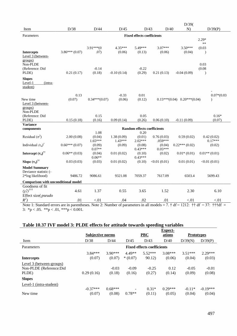
497
Item D/38 D/44 D/45 D/43 D/40
D/39(
N) D/39(P)
Parameters Fixed effects coefficients
Intercepts 3.86*** (0.07) 3.91***(0
.07) 4.35***
(0.06) 5.49***
(0.13) 3.07***
(0.06) 3.50***
(0.04)
2.29***
(0.03)
Level 3 (between-groups)
Non-PLDE
(Reference: Did PLDE) 0.21 (0.17)
-0.14 (0.18) -0.10 (0.14)
-0.22 (0.29) 0.21 (0.13) -0.04 (0.09)
0.03
(0.08)
Slopes Level-1 (intra-
student)
NNew time 0.13
(0.07) 0.0.34***(0.07) -0.33 (0.06)
0.01 (0.12) 0.15***(0.04) 0.20***(0.04)
-
0.07*(0.03)
Level 3 (between-groups)
Non-PLDE (Reference: Did PLDE) 0.15 (0.18)
0.15 (0.16) 0.09 (0.14)
0.05 (0.26) 0.06 (0.10) -0.11 (0.09)
0.16* (0.07)
Variance
components Random effects coefficients
Residual (σ2) 2.00 (0.08) 1.08
(0.04) 1.38 (0.09) 0.20
(0.01) 0.76 (0.03) 0.59 (0.02) 0.42 (0.02)
Individual (τπ)† 0.66*** (0.07)
1.65*** (0.09)
1.43*** (0.09)
2.02*** (0.08)
.059*** (0.04) 0.22*** (0.02)
0.17*** (0.02)
Intercept (τϐ)††
0.06** (0.03) 0.07** (0.04) 0.01 (0.02)
0.43*** (0.10)
0.05*** (0.02) 0.01* (0.01) 0.01** (0.01)
Slope (τϐ)††
0.03 (0.03) 0.06** (0.03) 0.01 (0.02)
0.43*** (0.10) <0.01 (0.01) 0.01 (0.01) <0.01 (0.01)
Model Summary Deviance statistic (-
2*log likelihood) 9486.72 9086.61 9321.08 7059.37 7617.09 6503.4 5699.43
Comparison with unconditional model Goodness of fit
(χ2)††† 4.61 1.37 0.55 3.65 1.52 2.30 6.10
Effect size( pseudo
R2) .01 <.01 .04 .02 .01 <.01 <.01
Note 1: Standard errors are in parentheses. Note 2: Number of parameters in all models = 7. † df = 1212: †† df = 37: †††df =
3: *p < .05. **p < .01, ***p < 0.001.
Table 10.37 IVF model 3: PLDE effects for attitude towards speeding variables
Subjective norms
PBC
Expect-
ations Prototypes
Item D/38 D/44 D/45 D/43 D/40 D/39(N) D/39(P)
Parameters Fixed effects coefficients
Intercepts
3.84***
(0.07)
3.90***
(0.07)
4.49**
* (0.07)
5.52***
90.12)
3.08***
(0.06)
3.51***
(0.04)
2.29***
(0.03)
Level 3 (between-groups)
Non-PLDE (Reference:Did
PLDE) 0.29 (0.16)
-0.03
(0.18)
-0.09
(0.16)
-0.25
(0.27)
0.12
(0.14)
-0.05
(0.09)
-0.01
(0.08)
Slopes
Level-1 (intra-student)
New time
-0.37***
(0.07)
0.68***
(0.08)
-
0.78**
0.31*
(0.11)
0.29***
(0.05)
-0.11*
(0.04)
-0.19***
(0.04)
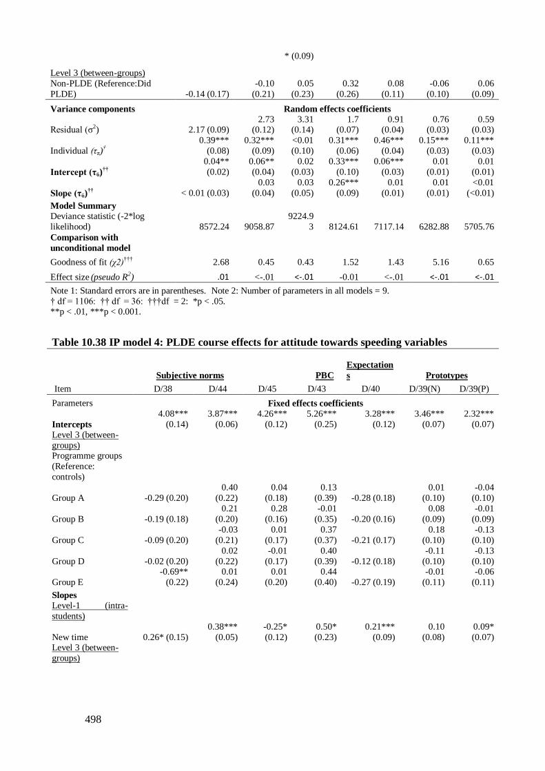
498
* (0.09)
Level 3 (between-groups)
Non-PLDE (Reference:Did
PLDE) -0.14 (0.17)
-0.10
(0.21)
0.05
(0.23)
0.32
(0.26)
0.08
(0.11)
-0.06
(0.10)
0.06
(0.09)
Variance components Random effects coefficients
Residual (σ2) 2.17 (0.09) 2.73
(0.12) 3.31
(0.14) 1.7
(0.07) 0.91
(0.04) 0.76
(0.03) 0.59
(0.03)
Individual (τπ)†
0.39***
(0.08)
0.32***
(0.09)
<0.01
(0.10)
0.31***
(0.06)
0.46***
(0.04)
0.15***
(0.03)
0.11***
(0.03)
Intercept (τϐ)††
0.04**
(0.02)
0.06**
(0.04)
0.02
(0.03)
0.33***
(0.10)
0.06***
(0.03)
0.01
(0.01)
0.01
(0.01)
Slope (τϐ)††
< 0.01 (0.03)
0.03
(0.04)
0.03
(0.05)
0.26***
(0.09)
0.01
(0.01)
0.01
(0.01)
<0.01
(<0.01)
Model Summary
Deviance statistic (-2*log
likelihood) 8572.24 9058.87
9224.9
3 8124.61 7117.14 6282.88 5705.76
Comparison with
unconditional model
Goodness of fit (χ2)††† 2.68 0.45 0.43 1.52 1.43 5.16 0.65
Effect size (pseudo R2) .01 <-.01 <-.01 -0.01 <-.01 <-.01 <-.01
Note 1: Standard errors are in parentheses. Note 2: Number of parameters in all models = 9.
† df = 1106: †† df = 36: †††df = 2: *p < .05. **p < .01, ***p < 0.001.
Table 10.38 IP model 4: PLDE course effects for attitude towards speeding variables
Subjective norms PBC
Expectation
s Prototypes
Item D/38 D/44 D/45 D/43 D/40 D/39(N) D/39(P)
Parameters Fixed effects coefficients
Intercepts
4.08***
(0.14)
3.87***
(0.06)
4.26***
(0.12)
5.26***
(0.25)
3.28***
(0.12)
3.46***
(0.07)
2.32***
(0.07)
Level 3 (between-
groups)
Programme groups
(Reference:
controls)
Group A -0.29 (0.20)
0.40
(0.22)
0.04
(0.18)
0.13
(0.39) -0.28 (0.18)
0.01
(0.10)
-0.04
(0.10)
Group B -0.19 (0.18)
0.21
(0.20)
0.28
(0.16)
-0.01
(0.35) -0.20 (0.16)
0.08
(0.09)
-0.01
(0.09)
Group C -0.09 (0.20)
-0.03
(0.21)
0.01
(0.17)
0.37
(0.37) -0.21 (0.17)
0.18
(0.10)
-0.13
(0.10)
Group D -0.02 (0.20)
0.02
(0.22)
-0.01
(0.17)
0.40
(0.39) -0.12 (0.18)
-0.11
(0.10)
-0.13
(0.10)
Group E
-0.69**
(0.22)
0.01
(0.24)
0.01
(0.20)
0.44
(0.40) -0.27 (0.19)
-0.01
(0.11)
-0.06
(0.11)
Slopes
Level-1 (intra-
students)
New time 0.26* (0.15)
0.38***
(0.05)
-0.25*
(0.12)
0.50*
(0.23)
0.21***
(0.09)
0.10
(0.08)
0.09*
(0.07) Level 3 (between-
groups)
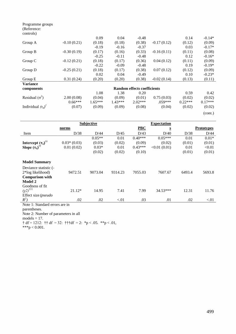
499
Programme groups
(Reference:
controls)
Group A -0.10 (0.21)
0.09
(0.18)
0.04
(0.18)
-0.48
(0.38) -0.17 (0.12)
0.14
(0.12)
-0.14*
(0.09)
Group B -0.30 (0.19)
-0.19
(0.17)
-0.16
(0.16)
-0.37
(0.33) -0.16 (0.11)
0.03
(0.11)
-0.17*
(0.08)
Group C -0.12 (0.21)
-0.25
(0.18)
-0.11
(0.17)
-0.48
(0.36) 0.04 (0.12)
0.12
(0.11)
-0.16*
(0.09)
Group D -0.25 (0.21)
-0.22
(0.18)
-0.09
(0.17)
-0.48
(0.38) 0.07 (0.12)
0.19
(0.12)
-0.19*
(0.09)
Group E 0.31 (0.24)
0.02
(0.20)
0.04
(0.20)
-0.49
(0.38) -0.02 (0.14)
0.10
(0.13)
-0.23*
(0.11)
Variance
components Random effects coefficients
Residual (σ2) 2.00 (0.08)
1.08
(0.04)
1.38
(0.09)
0.20
(0.01) 0.75 (0.03)
0.59
(0.02)
0.42
(0.02)
Individual (τπ)†
0.66***
(0.07)
1.65***
(0.09)
1.43***
(0.09)
2.02***
(0.08)
.059***
(0.04)
0.22***
(0.02)
0.17***
(0.02)
(cont.)
Subjective
norms
PBC
Expectation
s Prototypes
Item D/38 D/44 D/45 D/43 D/40 D/38 D/44
Intercept (τϐ)††
0.03* (0.03)
0.05**
(0.03)
0.01
(0.02)
0.40***
(0.09)
0.05***
(0.02)
0.01
(0.01)
0.01*
(0.01)
Slope (τϐ)††
0.01 (0.02) 0.03*
(0.02)
0.01
(0.02)
0.43***
(0.10)
<0.01 (0.01) 0.01
(0.01)
<0.01
(0.01)
Model Summary
Deviance statistic (-
2*log likelihood) 9472.51 9073.04 9314.23 7055.03 7607.67 6493.4 5693.8
Comparison with
Model 2
Goodness of fit
(χ2)††† 21.12* 14.95 7.41 7.99 34.53*** 12.31 11.76
Effect size (pseudo
R2) .02 .02 <.01 .03 .01 .02 <.01
Note 1: Standard errors are in
parentheses.
Note 2: Number of parameters in all
models = 17. † df = 1212: †† df = 32: †††df = 2: *p < .05. **p < .01,
***p < 0.001.
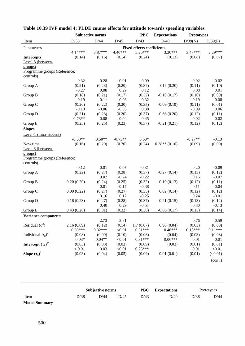
500
Table 10.39 IVF model 4: PLDE course effects for attitude towards speeding variables
Subjective norms PBC Expectations Prototypes
Item D/38 D/44 D/45 D/43 D/40 D/39(N) D/39(P)
Parameters Fixed effects coefficients
Intercepts
4.14***
(0.14)
3.87***
(0.16)
4.40***
(0.14)
5.26***
(0.24)
3.20***
(0.13)
3.47***
(0.08)
2.29***
(0.07)
Level 3 (between-
groups)
Programme groups (Reference:
controls)
Group A
-0.32
(0.21)
0.28
(0.23)
-0.01
(0.20)
0.09
(0.37) -017 (0.20)
0.02
(0.11)
0.02
(0.10)
Group B
-0.27
(0.18)
0.08
(0.21)
0.29
(0.17)
0.12
(0.32) -0.10 (0.17)
0.08
(0.10)
0.01
(0.09)
Group C
-0.19
(0.20)
-0.11
(0.22)
0.08
(0.20)
0.32
(0.35) -0.09 (0.19)
0.19
(0.11)
-0.08
(0.01)
Group D
-0.10
(0.21)
-0.06
(0.23)
-0.05
(0.20)
0.38
(0.37) -0.66 (0.20)
-0.09
(0.12)
0.06
(0.11)
Group E
-0.73**
(0.23)
-0.08
(0.25)
-0.04
(0.23)
0.45
(0.37) -0.21 (0.21)
-0.02
(0.12)
-0.02
(0.12)
Slopes
Level-1 (intra-student)
New time
-0.50**
(0.16)
0.58**
(0.20)
-0.73**
(0.20)
0.63*
(0.24) 0.38** (0.10)
-0.27**
(0.09)
-0.13
(0.09) Level 3 (between-
groups)
Programme groups (Reference:
controls)
Group A
-0.12
(0.22)
0.01
(0.27)
0.05
(0.28)
-0.31
(0.37) -0.27 (0.14)
0.20
(0.13)
-0.09
(0.12)
Group B 0.20 (0.20)
0.02
(0.24)
-0.24
(0.25)
-0.22
(0.32) 0.10 (0.13)
0.15
(0.12)
-0.07
(0.11)
Group C 0.09 (0.22)
0.01
(0.27)
-0.17
(0.27)
-0.38
(0.35) 0.02 (0.14)
0.11
(0.12)
-0.04
(0.12)
Group D 0.16 (0.23) 0.16
(0.27) 0.12
(0.28) -0.25
(0.37) -0.21 (0.15) 0.24
(0.13) -0.01
(0.12)
Group E 0.43 (0.26)
0.40
(0.31)
0.29
(0.32)
-0.51
(0.38) -0.06 (0.17)
0.30
(0.15)
-0.13
(0.14)
Variance components
Residual (σ2) 2.16 (0.09)
2.73
(0.12)
3.31
(0.14) 1.7 (0.07) 0.90 (0.04)
0.76
(0.03)
0.59
(0.03)
Individual (τπ)†
0.39***
(0.08)
0.32***
(0.09)
<0.01
(0.10)
0.31***
(0.06)
0.46***
(0.04)
0.15***
(0.03)
0.11***
(0.03)
Intercept (τϐ)††
0.03*
(0.03)
0.04**
(0.03)
<0.01
(0.02)
0.31***
(0.09)
0.06***
(0.03)
0.01
(0.01)
0.01
(0.01)
Slope (τϐ)††
< 0.01
(0.03)
0.03
(0.04)
<0.01
(0.05)
0.26***
(0.09) 0.01 (0.01)
0.01
(0.01)
<0.01
(<0.01)
(cont.)
Subjective norms PBC
Expectations Prototypes
Item D/38 D/44 D/45 D/43 D/40 D/38 D/44
Model Summary

501
Deviance statistic (-
2*log likelihood) 9472.51 9053.32 9217.45 8118.43 7108.90 6274.56 5702.23
Comparison with
Model 2
Goodness of fit (χ2)††† 18.05 6.00 7.91 7.70 9.67 13.48 4.18
Effect size (pseudo R2) <.01 .01 .01 .02 .01 .02 <.01
Note 1: Standard errors are in
parentheses.
Note 2: Number of parameters in all
models = 17.
† df = 1106: †† df = 32: †††df = 10: *p < .05, **p < .01,
***p < 0.001.
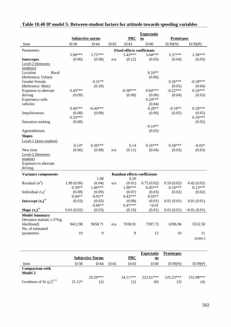
502
Table 10.40 IP model 5: Between-student factors for attitude towards speeding variables
Subjective norms PBC
Expectatio
ns Prototypes
Item D/38 D/44 D/45 D/43 D/40 D/39(N) D/39(P)
Parameters Fixed effects coefficients
Intercepts
3.90***
(0.06)
3.75***
(0.08) n/a
5.43***
(0.12)
3.04***
(0.05)
3.37***
(0.04)
2.38***
(0.03)
Level-2 (between-students)
Location Rural
(Reference; Urban)
0.16**
(0.06)
Gender Female
(Reference: Male)
0.31**
(0.10)
0.26***
(0.05)
-0.18***
(0.04)
Exposure to aberrant
driving
0.43***
(0.09)
-0.38***
(0.08)
0.64***
(0.06)
-0.22***
(0.04)
0.24***
(0.03)
Experience with
vehicles
0.24***
(0.04)
Impulsiveness
0.40***
(0.08)
-0.44***
(0.09)
0.28**
(0.06)
-0.19**
(0.05)
0.18***
(0.05)
Sensation seeking 0.33***
(0.08)
0.16*** (0.05)
Agreeableness
-0.14**
(0.05)
Slopes
Level-1 (intra-student)
New time
0.14*
(0.06)
0.36***
(0.08) n/a
0.14
(0.11)
0.16***
(0.04)
0.18***
(0.03)
-0.05*
(0.03)
Level-2 (between-
student)
Exposure to aberrant
driving
Variance components Random effects coefficients
Residual (σ2) 1.99 (0.09)
1.08
(0.04) n/a
0.20
(0.01) 0.75 (0.02) 0.59 (0.02) 0.42 (0.02)
Individual (τπ)†
0.59** (0.08)
1.60*** (0.09)
1.99*** (0.07)
0.45*** (0.03)
0.19*** (0.02)
0.13*** (0.02)
Intercept (τϐ)††
0.04**
(0.03)
0.05**
(0.03)
0.43***
(0.08)
0.03**
(0.01) 0.01 (0.01) 0.01 (0.01)
Slope (τϐ)††
0.01 (0.02)
0.06**
(0.03)
0.47***
(0.10)
<0.01
(0.01) 0.01 (0.01) <0.01 (0.01)
Model Summary
Deviance statistic (-2*log
likelihood) 9412.98 9058.71 n/a 7038.91 7397.73 6396.96 5552.58
No. of estimated
parameters 10 9
8 12 10 11
(cont.)
Subjective Norms
PBC
Expectatio
ns
Prototypes
Item D/38 D/44 D/45 D/43 D/40 D/39(N) D/39(P)
Comparison with
Model 2
Goodness of fit (χ2)††† 21.12* 29.29***
(2)
24.11*** (1)
222.61*** (6)
125.23*** (3)
152.98*** (4)

503
Effect size (pseudo R2) .02 <.01 <.01 <.01 .05 .08
Note 1: Standard errors are in parentheses. † df = 1212: †† df = 32: †††df = 10: *p < .05. **p < .01, ***p <
0.001.
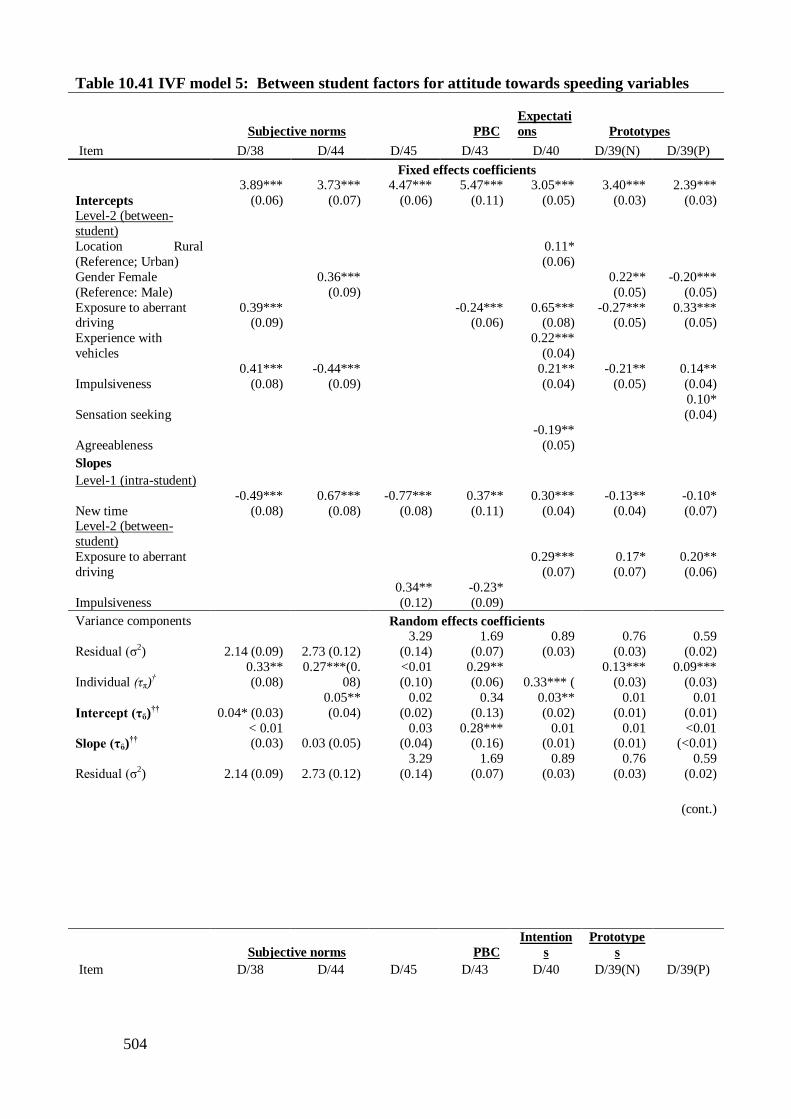
504
Table 10.41 IVF model 5: Between student factors for attitude towards speeding variables
Subjective norms PBC
Expectati
ons Prototypes
Item D/38 D/44 D/45 D/43 D/40 D/39(N) D/39(P)
Fixed effects coefficients
Intercepts
3.89***
(0.06)
3.73***
(0.07)
4.47***
(0.06)
5.47***
(0.11)
3.05***
(0.05)
3.40***
(0.03)
2.39***
(0.03)
Level-2 (between-
student)
Location Rural
(Reference; Urban)
0.11*
(0.06)
Gender Female
(Reference: Male)
0.36***
(0.09)
0.22**
(0.05)
-0.20***
(0.05)
Exposure to aberrant driving
0.39*** (0.09)
-0.24*** (0.06)
0.65*** (0.08)
-0.27*** (0.05)
0.33*** (0.05)
Experience with
vehicles
0.22***
(0.04)
Impulsiveness
0.41***
(0.08)
-0.44***
(0.09)
0.21**
(0.04)
-0.21**
(0.05)
0.14**
(0.04)
Sensation seeking
0.10*
(0.04)
Agreeableness
-0.19**
(0.05)
Slopes
Level-1 (intra-student)
New time
-0.49***
(0.08)
0.67***
(0.08)
-0.77***
(0.08)
0.37**
(0.11)
0.30***
(0.04)
-0.13**
(0.04)
-0.10*
(0.07) Level-2 (between-
student)
Exposure to aberrant
driving
0.29***
(0.07)
0.17*
(0.07)
0.20**
(0.06)
Impulsiveness
0.34**
(0.12)
-0.23*
(0.09)
Variance components Random effects coefficients
Residual (σ2) 2.14 (0.09) 2.73 (0.12)
3.29
(0.14)
1.69
(0.07)
0.89
(0.03)
0.76
(0.03)
0.59
(0.02)
Individual (τπ)†
0.33**
(0.08)
0.27***(0.
08)
<0.01
(0.10)
0.29**
(0.06) 0.33*** (
0.13***
(0.03)
0.09***
(0.03)
Intercept (τϐ)††
0.04* (0.03)
0.05**
(0.04)
0.02
(0.02)
0.34
(0.13)
0.03**
(0.02)
0.01
(0.01)
0.01
(0.01)
Slope (τϐ)††
< 0.01 (0.03) 0.03 (0.05)
0.03 (0.04)
0.28*** (0.16)
0.01 (0.01)
0.01 (0.01)
<0.01 (<0.01)
Residual (σ2) 2.14 (0.09) 2.73 (0.12)
3.29
(0.14)
1.69
(0.07)
0.89
(0.03)
0.76
(0.03)
0.59
(0.02)
(cont.)
Subjective norms PBC
Intention
s
Prototype
s Item D/38 D/44 D/45 D/43 D/40 D/39(N) D/39(P)
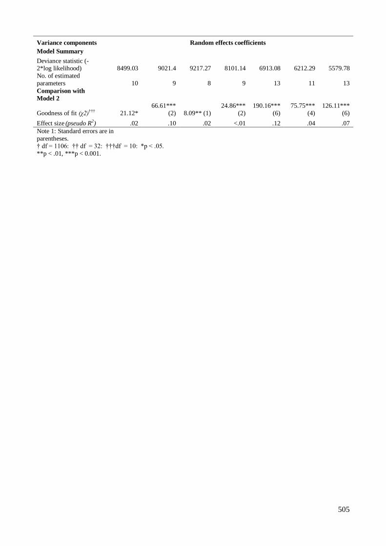
505
Variance components Random effects coefficients
Model Summary
Deviance statistic (-2*log likelihood) 8499.03 9021.4 9217.27 8101.14 6913.08 6212.29 5579.78
No. of estimated
parameters 10 9 8 9 13 11 13
Comparison with
Model 2
Goodness of fit (χ2)††† 21.12*
66.61***
(2) 8.09** (1)
24.86***
(2)
190.16***
(6)
75.75***
(4)
126.11***
(6)
Effect size (pseudo R2) .02 .10 .02 <.01 .12 .04 .07
Note 1: Standard errors are in
parentheses.
† df = 1106: †† df = 32: †††df = 10: *p < .05.
**p < .01, ***p < 0.001.

506
10.17 Appendix P. Teacher interview
The semi-structured teacher interviews were based on 13 questions. At the
beginning of each interview the teacher was informed about the purpose of the interview
and provided with assurances of confidentiality and were informed about their right to
withdraw their consent as follows;
“Thank you for agreeing to do this interview. The questions that I intend to ask are
mainly related to quality of the PLDE programme that you have taught recently. I
appreciate your help and I value your ideas and suggestions. Your name will not appear in
connection with any of the data that you provide and you are at liberty to stop this
interview or to have any data destroyed if you wish to do so in the future.”
Questions
1. Can you tell me a bit about the PLDE course that you taught recently?
Probes
Over how many weeks did it run?
How many class periods per week were scheduled?
Do you feel that this pace was too fast or too slow?
Was there enough to cover the entire course?
Did you leave out any sections/parts? Which sections? Why?
Did you cut short any parts of the programme? Which parts? Why?
Did you cover the Driver Theory Test? To what extent?
Did the students do any other PLDE courses?
2. Now I would like to talk programme materials and activities.
Probes
How satisfied were you with the course materials?
Can you talk a bit about programme activities?
Were those activities beneficial from the perspective of teaching and learning?

507
Which ones worked well? Did any activities not work well?
How could they be improved?
3. Did you use any of the recommended guest speakers during the year and if so what how would
you rate their contribution?
Probes
If not what were the obstacles?
How would you rate the quality of their presentations?
How would you rate their delivery technique?
How did the students react?
4. Which sections of the course were most important in your own opinion? Why?
5. Could you talk a bit about student reactions to the course?
Probes
What sections did they find most interesting? Why?
What did they find least interesting? Why?
Could you suggest anything that would help to capture their interest?
6. Were there any aspects of the programme that need improvement from an instructor’s
perspective?
Probes
Resources?
Time available for teaching the course?
7. Do you feel that there is anything missing from the course?
Is there anything else that you would like to add that might be useful?
Thank you very much that has been really helpful.

508