
Do Differences in Financial Development Explain the Global Pattern of Current Account Imbalances?
68
Do Differences in Financial Development Explain the Global Pattern of Current Account Imbalances? Joseph Gruber and Steven B. Kamin* February 8, 2008 Abstract: This paper addresses the popular view that differences in financial development explain the pattern of global current account imbalances. One strain of thinking explains the net flow of capital from developing to industrial economies on the basis of the industrial economies’ more advanced financial systems and correspondingly more attractive assets. A related view addresses why the United States has attracted the lion’s share of capital flows from developing to industrial economies; it stresses the exceptional depth, breadth, and safety of U.S. financial markets. In this paper we empirically test these hypotheses. Building on Chinn and Prasad (2003) and Gruber and Kamin (2007), we assess econometrically whether different measures of financial development explain the net flow of capital from developing to industrial economies, as well as the concentration of those flows toward the United States. We also assess whether differences in asset returns, an alternative measure of the attractiveness of financial assets, can explain the international pattern of capital flows. We find little evidence that differences in financial development help to explain the global pattern of current account imbalances. The measures of financial development generally do not explain either the net flow of capital from developing to industrial economies or, more specifically, the large U.S. current account deficits. Lower bond yields have been generally associated with lower current account balances (e.g., larger deficits) in industrial countries. However, U.S. bond yields have not been significantly lower than in other industrial economies, nor have expected equity earnings yields. This suggests, contrary to conventional wisdom, that U.S. financial assets have not been demonstrably more attractive than those of other industrial economies, and hence cannot explain the large U.S. deficit. Finally, we consider the alternative but related hypothesis that spending in the United States was uniquely responsive to the lower cost of credit stemming from capital inflows from developing countries, thus accounting for the outsized U.S. deficit. However, we found this hypothesis also to be weak, as household saving rates have declined throughout the industrial economies, not just in the United States. * The views in this paper are solely the responsibility of the authors and should not be interpreted as reflecting the views of the Board of Governors of the Federal Reserve System or of any other person associated with the Federal Reserve System. We would like to thank Joseph Gagnon, Chris Gust, Trevor Reeve, Rob Vigfusson, and participants in the International Finance Workshop for helpful comments and advice. William DeHaven provided excellent research assistance. Corresponding author: Tel: +1 202 452 3339; E-mail:[email protected]
-
Upload
independent -
Category
Documents
-
view
5 -
download
0
Transcript of Do Differences in Financial Development Explain the Global Pattern of Current Account Imbalances?

Do Differences in Financial Development Explain the Global Pattern of
Current Account Imbalances?
Joseph Gruber and Steven B. Kamin*
February 8, 2008 Abstract: This paper addresses the popular view that differences in financial development explain the pattern of global current account imbalances. One strain of thinking explains the net flow of capital from developing to industrial economies on the basis of the industrial economies’ more advanced financial systems and correspondingly more attractive assets. A related view addresses why the United States has attracted the lion’s share of capital flows from developing to industrial economies; it stresses the exceptional depth, breadth, and safety of U.S. financial markets.
In this paper we empirically test these hypotheses. Building on Chinn and Prasad (2003)
and Gruber and Kamin (2007), we assess econometrically whether different measures of financial development explain the net flow of capital from developing to industrial economies, as well as the concentration of those flows toward the United States. We also assess whether differences in asset returns, an alternative measure of the attractiveness of financial assets, can explain the international pattern of capital flows.
We find little evidence that differences in financial development help to explain the
global pattern of current account imbalances. The measures of financial development generally do not explain either the net flow of capital from developing to industrial economies or, more specifically, the large U.S. current account deficits. Lower bond yields have been generally associated with lower current account balances (e.g., larger deficits) in industrial countries. However, U.S. bond yields have not been significantly lower than in other industrial economies, nor have expected equity earnings yields. This suggests, contrary to conventional wisdom, that U.S. financial assets have not been demonstrably more attractive than those of other industrial economies, and hence cannot explain the large U.S. deficit.
Finally, we consider the alternative but related hypothesis that spending in the United
States was uniquely responsive to the lower cost of credit stemming from capital inflows from developing countries, thus accounting for the outsized U.S. deficit. However, we found this hypothesis also to be weak, as household saving rates have declined throughout the industrial economies, not just in the United States. * The views in this paper are solely the responsibility of the authors and should not be interpreted as reflecting the views of the Board of Governors of the Federal Reserve System or of any other person associated with the Federal Reserve System. We would like to thank Joseph Gagnon, Chris Gust, Trevor Reeve, Rob Vigfusson, and participants in the International Finance Workshop for helpful comments and advice. William DeHaven provided excellent research assistance. Corresponding author: Tel: +1 202 452 3339; E-mail:[email protected]

1
I. Introduction
There is, as yet, no consensus as to the factors underlying the emergence of large current
account surpluses and deficits around the world. However, many observers have come to focus
on differences in financial development to explain these imbalances.
One strain of thinking focuses on why net capital is flowing from developing to industrial
economies, the opposite of what conventional theory would predict. It is suggested that
developing countries have inefficient financial systems that encourage saving and discourage
investment (Hubbard, 2006; Prasad, Rajan, and Subramanian, 2006; Ju and Wei, 2006). Another
hypothesis is that developing countries seek the high-quality financial assets that industrial
economies produce, and they are willing to run current account surpluses in order to acquire
those assets (Caballero, Farhi, and Gourinchas, 2006; Mendoza, Quadrini, and Rios-Rull, 2007).
Differences in financial development have been cited not only to explain why capital is
flowing on net from developing to industrial economies—what Bernanke (2005, 2007) referred
to as the “global saving glut”—but also why the United States has attracted the lion’s share of
those flows. The prevalent view is that the prominent depth, breadth, and safety of U.S. financial
markets, combined with a highly entrepreneurial culture and a supportive legal system, explains
why the United States has attracted so much of the world’s savings (Blanchard, Giavazzi, and
Sa, 2005; Clarida, 2005; Cooper, 2005; Hubbard, 2005).
These hypotheses are plausible and are receiving increasing acceptance among observers
and researchers. Yet, they have not been submitted to much rigorous empirical testing. The
focus of this paper is on assessing whether financial-development explanations of the pattern of
global current account imbalances are genuinely consistent with the data.

2
Our research starts by examining the sources of net capital flows from developing to
industrial economies (what some have referred to as the “uphill flow of capital”). Building on
Chinn and Prasad (2003) and Gruber and Kamin (2007), we start with a panel regression model
that, for a wide range of developing and industrial economies over several decades, relates
current account deficits (as a share of GDP) to a selection of standard determinants such as
output growth, fiscal balances, per capita income, and demographic variables. Those variables,
by themselves, cannot explain the uphill flow of capital. We then add to the model different
measures of financial development—e.g., private credit and stock market capitalization—and
determine whether these measures help to explain why so many developing economies have
been running substantial current account surpluses. Our analysis is similar in scope and
methodology to recent research by Chinn and Ito (2007a, 2007b); Chinn and Ito focus on the
interaction between financial development, legal institutions, and financial openness in
influencing current accounts, while our work focuses on the broader relationship between
financial development and the international pattern of current account imbalances.
Whether or not differences in financial development explain why developing countries
are running current account surpluses, they may still explain why the funds generated by those
surpluses are being channeled primarily to the United States. The second part of our research
addresses this hypothesis. We re-estimate the panel regressions described above, but restrict the
sample to industrial economies alone in order to determine whether those industrial economies
with the most developed financial systems are the ones most likely to attract net capital inflows.
As a complement to this research, we also consider the configuration of interest rates
among industrial economies. In principle, the most financially developed economies—those

3
with the deepest, most liquid, and most mature financial markets—should enjoy lower risk
premia on their assets than those issued in less developed financial markets, and thus their
interest rates should be lower. These lower interest rates, in turn, should boost investment and
discourage saving, thereby lowering the current account balance. Accordingly, we test to see
whether industrial economies with relatively large current account deficits, such as the United
States, have enjoyed relatively low interest rates in recent years, and whether the pattern of
interest rates can help explain the pattern of current account imbalances. (See Balakrishnan and
Tulin, 2006, for a related analysis of this issue.) We also examine expected returns on equities.
To provide a plan of the paper and foreshadow our key results, in Section II we provide
evidence that measures of financial development, such as the amount of private credit or scale of
stock markets, do not help to explain the uphill flow of capital from developing to developed
economies. In our panel regressions for a global sample of countries, the coefficients on these
measures generally are neither significant nor of the expected sign. Accordingly, in explaining
the recent current account deficits of developing countries, we fall back on the factors identified
by Bernanke (2005, 2007) and Gruber and Kamin (2007) as causing the global saving glut:
Asian financial crises and the price-driven surge in the revenues of oil exporters.
Section III addresses the question of why the United States absorbed the lion’s share of
capital coming from developing countries. We find no evidence that the pattern of current
account imbalances within industrial economies reflects the pattern of financial development,
either. In a panel regression restricted to industrial economies, the coefficients on financial
development measures for the most part are insignificant and have the wrong sign. Moreover,
4
even after inclusion of financial development measures, these equations fail to explain the large
U.S. current account deficit.
Section IV describes how, when we use interest rate differentials rather than more direct
“quantity” measures of financial development, these differentials do indeed help to explain the
pattern of current account balances among industrial economies: Countries with higher-than-
average real interest rates, whose assets implicitly are less desirable to global investors, tend to
run higher current account balances (smaller deficits).
Even so, these differentials do not help to explain the large U.S. deficit. This is because
U.S. real long-term interest rates have neither been substantially lower than, nor have fallen
further than, those of most other industrial economies in recent years. In fact, econometric
equations relating long-term interest rates to standard determinants such as inflation and GDP
growth are able to explain the decline in U.S. interest rates since the late 1990s reasonably well,
even as they fail to capture declines in interest rates in several other industrial economies. This
is an important and surprising finding, as it contradicts the conventional wisdom that U.S. assets
are demonstrably superior to assets of other industrial nations in the eyes of global investors, and
that U.S. interest rates have been pushed down especially far by capital inflows from developing
countries. This finding is corroborated by an analysis of expected earnings yields on equities,
which shows, again, that such yields have not fallen further in the United States than in other
industrial countries.
If the exceptional attractiveness of U.S. financial markets does not explain why the
United States took greatest advantage of the global saving glut to finance larger deficits, what
does? In Section V, we consider an alternative but related explanation: Spending in the United

5
States is more responsive to the cost and availability of credit than in other industrial countries,
and this has led to an outsized increase in U.S. spending, borrowing, and the current account
deficit.
A key feature of this explanation is that, rather than positing exogenous shocks to
spending in the United States and abroad, it assumes this spending has responded in a consistent
manner to its fundamental determinants. Indeed, we confirm that household saving in the United
States and several other industrial economies has been well explained in recent years by its
fundamental determinants, including two variables likely to reflect the influence of the global
saving glut: interest rates and household wealth. However, we also document that household
saving rates declined in many industrial economies during the past decade, so that the U.S.
experience was not unique in this regard. Rather, what is unique about the United States is that
increases in household spending were not offset by increases in public or corporate saving, as
they were in most other industrial economies. Insofar as the global saving glut should have led
to increased spending in general, we suggest that the experience of other industrial economies is
curious and bears further examination.
II. Do Differences in Financial Development Explain Capital’s Uphill Flow?
In this section we attempt to gauge the importance of financial market development in
determining the recent pattern of current account balances, particularly in regard to the uphill
flow of capital from developing economies to developed economies, via panel regressions in the
style of Chinn and Prasad (2003) and Gruber and Kamin (2007). These regressions relate the
ratio of the current account balance to GDP (defined so that a rise in the balance means a larger

6
surplus) to various indicators of financial development, controlling for a number of other
possible current account determinants.
The sample for the regressions covers up to 84 countries over the period from 1982 to
2006. As in previous work, we consider multi-year averages of annual observations in order to
abstract from dynamics resulting from frictions and adjustment processes related to the business
cycle. Data were averaged over the 1982 – 1986, 1987 – 1991, 1992 – 1996, 1997 – 2001, and
2002 – 2006 periods. Some series entered into the regression with a lagged observation
calculated over the 1977 – 1981 period. In cases of missing annual data, period averages were
calculated based on years for which observations were available.
In order to correctly estimate the impact of financial market development on current
account balances, we control for a number of other possible determinants of current accounts:
the level of per capita income, changes in real GDP growth rates, fiscal balances, the lagged
level of net foreign assets, the dependency ratio, the degree of openness, the nominal oil balance,
and, in some instances, the quality of government institutions. These variables are standard in
the literature, and are motivated and constructed along the lines of Gruber and Kamin (2007).
(See the appendix for sources.) Most variables are entered as deviations from a GDP-weighted
sample mean, as current accounts are relative and should only be affected by the idiosyncratic
country-specific element of the variables. Our regressions also include period fixed effects,
allowing the average current account balance to GDP ratio to vary across time.
The measures of financial development that we consider are taken from the 2006 update
of Beck, Demirgüç-Kunt, and Levine (2000). Financial development may be measured by any
number of criteria including the quality of supervision and regulation, the safety and soundness

7
of institutions, legal protections for market participants, the breadth and depth of markets, and
the scale of the financial sector relative to the overall economy. Beck, Demirgüç-Kunt, and
Levine provide consistent data for a wide range of countries, and although these data do not
address all of the criteria listed above, they most likely are reasonable proxies for the overall
level of financial development. We report results controlling for a variety of measures of
financial development, including private credit/GDP, bank assets/GDP, non-bank financial
assets/GDP, stock market capitalization/GDP, stock market turnover/GDP, and the growth of
stock market capitalization/GDP. As with our other control variables, all the financial
development variables were entered into the regressions as deviations from the GDP-weighted
sample mean, as it is the relative superiority of financial institutions which should attract capital
flows rather than the absolute level of development.
Table 1 reports summary statistics for the measures of financial development that we
consider. Column 1 reports the simple average of the measures across the last period of the
sample. The next two columns report averages for two different sub-samples, those countries
that had current account surpluses in excess of 2 percent of GDP on average over the period
between 2002 and 2006 and those countries that had current account deficits in excess of 2
percent of GDP over the same period. Comparing the two columns provides weak evidence that
greater financial development is actually associated with larger current account surpluses,
contrary to the common conjecture. Period averages for the United States, Column 4, are far
above the total sample average, indicative of the United States’ highly developed markets. For
the most part, the U.S. averages also exceed those of other industrial countries, while developing

8
Asia has fairly advanced financial indicators compared with the total sample averages shown in
the first column.
Before considering the impact of financial development on current account balances,
Table 2 assesses the predictive impact of the non-financial determinants. The regressions
include an unreported constant and fixed period effects. For each explanatory variable, the first
row reports the coefficient estimate and the second row is the associated t-statistic; coefficients
that are statistically significantly different from zero at the 90 percent level or higher are
indicated in bold.
Column 1 reports the coefficient estimates for the simplest non-financial model.
Governance indicators are only available for the last three period averages, and are thus excluded
from this preliminary regression in order to allow the largest number of observations. The
regression produces plausible results, with all variables excluding GDP growth entering
significantly and with the anticipated sign. That is, higher current accounts balances (larger
surpluses or smaller deficits) are associated with higher per capita incomes, higher fiscal
balances, more net foreign assets (which raise net investment income), fewer young or aged
dependents, higher net oil exports, and greater economic openness.
The regression reported in Column 2 includes separate dummy variables for the United
States and for the major developing Asian countries in the sample for both the 1997 – 2001 and
2002 – 2006 periods. We focus on the developing Asian economies because, alongside the oil
exporters, they represent the main source of developing country current account surpluses. The
coefficients on the dummy variables represent the average difference between the actual current
account and the model prediction across the two period averages. As shown in
9
Column 2, the model without indicators of financial market development does quite poorly at
predicting the U.S. deficit and the developing Asian surpluses, with the U.S. prediction error
large, negative, and significant, and the error for the developing Asian countries large, positive,
and significant.
Column 3 adds a measure of the quality of government institutions to the regression, with
a higher value for the indicator indicating superior institutions. Institutions enter significantly
into the regression and, consistent with expectations, have a negative coefficient, indicating that
better institutions are associated with a more negative current account balance. However, as
shown in Column 4, the addition of the government institutions variable does not explain the
U.S. current account deficit, as the coefficient on the dummy variable remains large, negative,
and significant. Institutions also leave the surpluses of developing Asia unexplained.
Given the inability of standard current account determinants to explain the large Asian
surpluses or U.S. deficit, we now examine whether different measures of financial development
can improve the model’s performance. Table 3 reports estimation results from regression
equations that include the measures of financial development discussed earlier. (The sample
changes across the regressions on account of differences in data coverage across the financial
variables.) The non-financial variables generally retain coefficient estimates in the same range
as those reported in the non-financial regressions in Table 2. However, with the exception of the
growth of stock market capitalization, the coefficients on the financial variables are positive,
indicating that greater financial market development is associated with a greater current account
surplus, contrary to theories that associate greater development with larger deficits. Of the
variables considered, only the growth of stock market capitalization has the correct sign and is

10
significant. Table 4 repeats the regressions from Table 3, adding the government institutions
variable (which further reduces the sample size). Again, the financial variables generally enter
with the wrong sign and are insignificant, with the exception of the growth of stock market
capitalization.1
Table 5 examines whether the growth in stock market capitalization, the only financial
market variable to come in significantly and with the right sign in earlier regressions, can explain
both the Asian surpluses and the U.S. deficit. As shown in Column 1, the dummy variable for
the developing Asian economies as well the dummy for the United States remain significant,
such that the Asian surpluses and the U.S. deficit remain unexplained. Column 2, shows that the
U.S. deficit remains inexplicably large when the Asian dummy is excluded from the regression.
Columns 3 and 4 repeat the regressions from Columns 1 and 2 including governance indicators
and over a shorter sample, and display a similar outcome.
Our results suggest that, contrary to what is emerging as conventional wisdom, measures
of financial development are not an important determinant of the international pattern of current
account balances: they can explain neither the large developing Asian surpluses nor the large
U.S. deficit. A brief look at the data shows that this result should not be all that surprising, as
the developing Asian economies have both a relatively high level of financial development as
well as large current account surpluses. As shown in Figure 1, the economies of developing Asia
1 In regressions similar to those reported here, Chinn and Ito (2007a, 2007b) generally do not find measures of financial development such as private credit/GDP, by themselves, to be significant determinants of current account balances. In both papers, Chinn and Ito do report significant results when measures of financial development are interacted with institutional variables, including a measure of legal development and an index of financial market openness. However, their results suggest that financial development leads to lower current account balances only in industrial economies, not developing ones. Moreover, it is unclear from their results whether these interactions between financial development and other structural characteristics importantly explain the developing country surpluses and large U.S. deficit.

11
have some of the highest private credit/GDP ratios in our sample. The developing Asian
economies are also above the norm in terms of bank deposits/GDP, non-bank financial
assets/GDP, stock market capitalization/GDP, and stock market turnover/GDP, as shown in the
last column of Table 1.2
III. Do Differences In Financial Development Explain the Large U.S. Deficit?
As discussed above, differences in financial development do not seem to be able to
explain the uphill flow of capital from developing to developed countries. However, the high
level of financial development in the United States relative to its industrial peers, as evidenced
by Columns 4 and 5 on Table 1, might still be able to explain why capital flowing out of the
developing world seems to have wound up mainly in the United States.
In Table 6 we present panel regressions similar in structure to those reported earlier, but
with the sample constrained to include only 21 industrial countries. None of the financial market
indicators are significant in our industrial country sub-sample. However, unlike with the larger
sample, the coefficients on the private credit/GDP and non-bank financial assets/GDP both have
the right (negative) sign, as does the coefficient on the growth of stock market capitalization.
Even so, inclusion of the two marginally significant variables, private credit/GDP and the
growthof stock market capitalization, does not help the model explain the large U.S. deficit,
which retains its significant negative dummy. 3
2 This finding is consistent with Chinn and Ito’s (2007a, 2007b) findings that in many developing countries, including in Asia, greater financial development is associated with higher, not lower, current account balances. 3 Examining a similar sample, Mendoza, Quadrini, and Rios-Rull (2007) report that private credit/GDP is significantly negatively correlated with the current account balance, controlling for the level of per capita GDP. When we reproduced that regression, we found that the U.S. current account deficit again remained a significant outlier, suggesting that the variable does not explain the large U.S. imbalance.

12
Because of the prominence of the view that the exceptional nature of the U.S. financial
system accounts for the country’s large deficits, Table 7 reports results for still more measures of
financial development that were not reported for the larger sample: financial system
deposits/GDP, bank overhead costs/total assets, the net interest margin, a measure of bank
concentration, and private bond market capitalization/GDP. As with the earlier data, these data
were taken from the 2006 update of Beck, Demirgüç-Kunt, and Levine (2000). As shown in
Column 1, the coefficient on financial system deposits/GDP is significant but of the wrong sign.
In Column 5, the coefficient on private bond market capitalization/GDP is significant and of the
right sign. However, as shown in Column 6, including private bond market capitalization/GDP
in the regression does little to help explain the large U.S. deficit.
IV. Are U.S. Assets Special? Evidence from Asset Prices
In Section III, we tested a battery of different measures of financial development and
found that few of them helped to explain the pattern of current account balances among
industrial economies. The few variables whose coefficients were both significant and of the
expected sign—private credit/GDP, private bond market capitalization/GDP, and the growth in
stock market capitalization—still did not help to explain the large U.S. current account deficit in
recent years.
In this section, we switch from “quantity” measures of financial development—e.g.,
private credit or stock market turnover—to measures based on asset prices. In principle, the
global integration of financial markets should lead expected asset returns around the world to be
equalized. To the extent that differences in expected asset returns remain, these differences likely
reflect differences in asset preferences and/or required risk premia (Orr, Edey, and Kennedy,

13
1995, Balakrishnan and Tulin, 2006). Hence, if, as many argue, the U.S. financial system is
regarded by investors as deep, liquid, and especially safe, one would expect investors to accept
lower rates of return on U.S. assets than on the assets of countries with less effective financial
systems. Accordingly, differentials in asset returns may reflect investor appraisals of the
attractiveness of different financial systems more accurately than the more ad hoc “quantity”
measures analyzed in Section III, and hence have a better chance of explaining the pattern of
current account balances.
IV.1 Do interest-rate differentials explain current account balances?
We begin with the most widely available measure of asset returns, the yield on long-term
government bonds. To abstract from differences in expected inflation (and hence exchange rate
depreciation) across countries, we focus on real interest rates, which we compute by subtracting
the contemporaneous four-quarter inflation rate from the nominal yield.4 Interest rate
differentials are then computed by subtracting from each country’s real interest rate the GDP-
weighted average of real interest rates in the industrial countries.
Table 8 displays the estimates of our panel regression model for industrial countries, once
the interest rate differential is included. The coefficient on that variable is significant and
positive, as expected: Higher-than-average interest rates in a country indicate that investors find
that country’s assets less attractive, and hence are associated with smaller net capital inflows and
larger current account balances.5 Even so, the coefficient on the dummy variable for the U.S.
4 The four-quarter inflation rate in a given quarter is the percent change in the CPI in that quarter relative to its level four quarters earlier. We view this as a reasonable proxy for inflation expectations, insofar as these data are averaged over multi-year periods to compute the real inflation differentials which enter into the panel regressions. 5 Boileau and Normandin (2008) find interest rates to be negatively correlated with current account balances, the opposite of our finding. However, their estimate is based on bivariate correlations using quarterly data, and hence may be capturing short-term demand effects—demand shocks may simultaneously raise interest rates and reduce

14
current account in 1997-2006 remains negative, significant, and large. Thus, inclusion of the
interest rate differential does not help to explain the large U.S. deficit.
IV.2 Trends in long-term interest rates
If industrial countries with relatively lower long-term bond yields tend to experience
relatively larger current account deficits, why don’t the equations shown in Table 8 explain the
large U.S. deficits of recent years? Figures 2 and 3 provide a ready answer to that question: in
recent years, U.S. long-term interest rates neither have averaged significantly below those of
other industrial countries, nor have they declined by a significantly larger extent. Thus, if
investors find U.S. assets particularly attractive, this attractiveness is not apparent in bond
prices.6
Figure 2 presents nominal interest rates on long-term (usually 10-year maturities)
government bonds, comparing those for a range of industrial countries with the GDP-weighted
average of OECD countries (excluding Korea and Mexico). Most countries’ long-term treasury
yields lie above the OECD average, which is depressed by Japan, whose very low nominal
interest rates are weighted highly. Even taking that into account, however, there is no evidence
that U.S. long-term yields have been substantially lower—relative to the OECD average—than
those of most other countries (excluding Japan) in the period since 1996. U.S. nominal yields
have indeed been somewhat lower than those in Australia, U.K., and Norway, but they have
much closer to those in Canada, Germany, Spain, France, Italy, and Belgium.
current account surpluses—that are precluded by our period-average data with controls for output growth and fiscal policy. In an estimated model of real long-term interest rates, Orr, Edey, and Kennedy (1995) also find a negative correlation between interest rates and current account balances, but their model, again, lacks many of the control variables present in our equation. 6 Orr, Edey, and Kennedy (1995) argue that the most common explanation for real interest rate differentials is the existence of financial risk premia. Accordingly, small or negligible real interest rate differentials suggest the

15
Furthermore, there is no evidence that nominal long-term interest rates in the United
States fell by more than those of other countries from the pre-1997 period—before the global
saving glut—to afterward: nominal U.S. and OECD-wide yields have tracked each other closely
for decades. Several other countries—U.K., Australia, Spain, and Italy—exhibited a much
steeper decline in their interest rates since 1996.
Figure 3 repeats the analysis with real long-term interest rates. These charts confirm that
U.S. real interest rates remained very close to those of the OECD average during the past 10
years or so. (The divergence between Japanese and other interest rates was smaller in real terms
than in nominal terms over the period, and hence Japan depresses the OECD average by much
less.) The charts also confirm that, as with nominal interest rates, real interest rates did not
decline any more quickly in the United States than they did in the other industrial economies on
average.
Our findings are consistent with those of Balakrishnan, Bayoumi, and Tulin (2007), who
found little evidence that bond yields in the United States had fallen more than in the euro area
or the United Kingdom in recent years.7 Balakrishnan and Tulin (2006) do find evidence of
negative risk premia for U.S. assets, showing that nominal interest rate differentials between the
United States and other countries were insufficient to compensate for expected exchange rate
depreciation as derived from surveys. However, their study uses short-term interest rates rather
than the longer-term yields most likely to reflect investor preferences, and it remains unclear
absence of negative or positive financial risk premia. 7 Balakrishnan, Bayoumi, and Tulin (2007) also decompose the sources of financing for the U.S. current account deficit and find that declining home bias and financial deepening (increases in investor portfolios) account for most of this financing, rather than an increase in the share of U.S. assets in foreign portfolios. Although they acknowledge a large residual in their calculations, their findings represent further evidence against the view that an increase in preferences for U.S. assets explains the widening deficit.

16
whether survey measures of exchange rate expectations correlate well with the expectations held
by actual traders.
To summarize, the fact that U.S. real long-term interest rates were similar to those of
other industrial economies in the past decade represents prima facie evidence that U.S. assets did
not command an unusually low risk premium among global investors. And the fact that real
interest rates did not decline more in the United States than elsewhere tends to undercut the view
that the expansion of investor portfolios in the past decade (associated with the global saving
glut) was targeted primarily toward U.S. assets.8
IV.3 Comparison of interest-rate trends with model predictions
As noted above, the fact that U.S. yields have behaved very similarly to those in other
countries in the past decade contradicts the view that investors considered U.S. assets to be
especially attractive, and this led them to channel the additional funds associated with the global
saving glut mainly toward U.S. assets. It is possible, however, that the United States may have
experienced other shocks that, in the absence of a special attractiveness of its assets to foreign
investors, would have boosted U.S. interest rates relative to those in other industrial economies.
For example, a decline in household saving or rise in the fiscal deficit would have put upward
pressure on interest rates—the fact that they did not rise relative to other countries could be
taken as evidence that investors were especially attracted to U.S. assets. Additionally, as
suggested in footnote 8 above, even in the absence of exogenous shocks, it is possible that low
8 It might be thought that even if U.S. assets did command a low risk premia, its interest rates might not be lower than those in other countries, because additional issuance of U.S. assets in response to low interest rates might drive that premium back up. Indeed, in principle, a country experiencing a decline in its risk premium—and hence a decline in interest rates—might be encouraged to spend more and borrow more, thus increasing its liabilities and pushing interest rates back up. However, it is unlikely that interest rates would be pushed back all the way to their original level, as that would imply that the country had a perfectly flat demand curve for borrowed funds (that is, a

17
interest rates induced by the special attractiveness of U.S. assets could have led U.S. spending
and output growth to increase endogenously, and that might have pushed U.S. interest rates at
least partway back toward parity with other countries.
To address these possibilities, we estimated some simple econometric models of long-
term yields for the United States and other industrial economies. These models are estimated
separately for each country rather than in the panel data format used in the regressions described
above. They incorporate standard determinants of interest rates, such as real GDP growth,
inflation, and the fiscal balance, along the lines followed by Warnock and Warnock (2006). We
would expect these models to capture the effects of standard shocks to interest rates such as a
rise in household consumption, business investment, or the fiscal deficit. However, such models
would not be expected to capture a shift in portfolio demands for long-term bonds. Accordingly,
if U.S. assets were considered particularly attractive to global investors, and if the bulk of the
global saving glut was being channeled to U.S. markets as a result of that attractiveness, we
would expect U.S. interest rates to fall by more than predicted by our models during the period
after 1996. By the same token, we would expect interest rates in other countries to adhere more
closely to model predictions.
Models without expectational variables Table 9 presents estimation results of our first model,
OLS regressions of quarterly values of nominal long-term sovereign yields on contemporaneous
values of the nominal money market interest rate, the 4-quarter CPI inflation rate, the 4-quarter
growth rate of real GDP, the standard deviation of the quarterly change in the long-term nominal
interest rate over the preceding 12 quarters, the structural (full-employment) fiscal balance as a
willingness to borrow all the funds offered at a given interest rate).

18
ratio to GDP, and two lags of the dependent variable. For most of the countries studied, the
starting point for the estimation is in the 1970s or 1980s; a similar model, discussed below,
includes survey measures of expectations, but owing to data availability, these regressions do not
start until the 1990s. For the United States, the coefficients all have the expected sign and, for
the most part, are significantly different from zero; for other countries, the results are more
mixed but generally consistent with conventional expectations.
Figure 4 uses the estimated equations to present two different measures of the extent to
which actual interest rate behavior may have differed from the models’ predictions over the past
decade. For each country, the figure on the left compares the actual movement in interest rates
with a dynamic simulation of the model from 1998 onwards (with, for this exercise, the model
being estimated only through 1997). The figure on the right represents a test of structural
stability, the “cusum” estimate of the cumulative sum of the model one-step-ahead residuals,
along with the 95 percent confidence interval for this calculation.
The results for the United States suggest, at most, weak evidence that interest rates in the
United States fell more than model predictions since 1997. The interest rate fell more than the
dynamic simulation on the left, but until the end of the sample, remained within the 95 percent
confidence interval. The cusum test indicates that residuals tended to be negative since the mid-
1990s, again suggesting interest rates fell more than model predictions, but not to a statistically
significant extent.
More importantly, the results for other countries suggest that their interest rates also
tended to fall somewhat more in the past decade than model predictions, and to an even greater
extent than in the United States. In a number of countries, the interest rate fell below the
19
confidence interval for the dynamic simulation, and in two countries, the cusum calculation
dropped below the 95 percent confidence bounds. In no countries did interest rates rise above
model predictions by a significant margin.
These results indicate that the behavior of U.S. long-term yields during the past decade
was in no way different from that of yields in other industrial economies. To the extent that U.S.
yields fell somewhat more than predictions of a standard model, this was an experience shared
by many other countries. Accordingly, it is possible that all industrial countries benefited
equally, in terms of their bond yields, from the global saving glut. Other explanations for the
universal decline in bond yields are beyond the bounds of this paper, but could involve, among
other things, reductions in inflation expectations and improvements in central bank practice and
communications.
Models with expectational variables Table 10 presents results of a model that uses survey
expectations of inflation and real GDP growth from Consensus Economics. The specification of
the equation is quite similar to that in Warnock and Warnock’s (2006) analysis of the effects of
capital inflows on U.S. interest rates. The explanatory variables include 10-year inflation
expectations, the spread between 1-year and 10-year inflation expectations, the money market
interest rate, the standard deviation of long-term yields over the preceding 12 quarters,
expectations of real GDP growth over the next year, the structural fiscal balance/GDP ratio, and
two lags of long-term interest rates. As the time series for Consensus Economics forecasts are
much shorter than for non-expectational data, the estimation periods are much shorter as well,
and results are available for only a limited number of countries.

20
For the most part, the signs of the coefficients on the explanatory variables are of the
expected sign, although that on the fiscal balance is more mixed and coefficients are not always
significant. Figure 5 presents several tests of model prediction. Because the estimation samples
start in 1990 at the earliest, it did not seem sensible to show dynamic out-of-sample predictions.
Instead, the left hand panel for each country compares the actual and fitted values of the interest
rates—these move together very closely owing to the lagged dependent variables, but the
residuals plotted at the bottom of the charts may be more informative. The right hand panel for
each country displays the cusum test for the model, as shown (above) for the models without
expectational variables.
Looking first at the United States, it is hard to discern much of a change in the pattern of
residuals between the early and later parts of the sample. The cusum test indicates a pattern of
negative residuals—indicating actual interest rates lower than model prediction—but well within
the confidence bounds. Conversely, for several other countries—U.K., Netherlands, Sweden—
the cusum test indicates a more significant decline in interest rates relative to model prediction.
In sum, as with the models without expectational variables, the models with expectational
variables provide no evidence in support of the view that the global saving glut depressed
interest rates in the United States by a greater extent than in other industrial economies.
IV.4 Other rates of return
Thus far, we have focused on sovereign (that is, government) bond yields as measures of
the rates of return assessed by global investors. This is a sensible strategy, as sovereign bonds
are issued by many countries—they often are widely traded in deep markets, and their yields are
easy to compare with each other. Nevertheless, the U.S. current account has been financed by

21
foreign purchases of corporate bonds and equities as well as government bonds. Accordingly, it
is possible that the U.S. assets which have proven especially attractive to global investors have
been corporate bonds or stocks rather than government bonds.
Is there any evidence that the comparative advantage of the United States is in the
issuance of private rather than public assets? Such evidence would entail yields on U.S.
corporate bonds or stocks either being lower than those on comparable assets in other industrial
economies or falling more steeply since the mid-1990s. Figure 6 presents yields on corporate
AA and BBB rated bonds, respectively, for the relatively few countries and years for which these
data are available. Comparing U.S. corporate bond yields with those of the United Kingdom,
Canada, Japan, and the EU countries in aggregate, there is no evidence that U.S. corporate yields
either are lower than those in other countries or have fallen more rapidly in recent years.
We now turn towards the return on equities. Figure 7 compares the forward earnings
yield on equities in a selection of industrial economies to the GDP-weighted mean for OECD
countries for which these data are available. This yield is calculated as the expected year-ahead
earnings per share, as surveyed by I/B/E/S, divided by the share price. It thus represents the
expected rate of return (abstracting from capital gains) on stocks, and is comparable to the yield
on sovereign or corporate bonds. The U.S. earnings yield moves from tracking above the OECD
average (the red dashed line) for most of the period prior to 2000 to falling below the OECD
average thereafter. In principle, this could suggest that with the advent of the global saving glut,
investors attracted to U.S. stocks could have pushed the U.S. earnings yield down further than
that of other industrial economies.
22
However, many other industrial economies also exhibit declines in their earnings yields
relative to the OECD average. This is explained by the fact that Japanese earnings yields started
the late 1980s at a very low level and have trended up since. Given Japan’s sizeable GDP
weight, its low earnings yield pulled down the OECD average early on and boosted it later in the
sample; this led the earnings yields of many other industrial economies to start out higher than
the OECD average and decline toward it more recently. The blue dotted line indicates the
OECD average excluding Japan. The U.S. earnings yield has moved closely with this average
through 2000 and fallen just a bit below it thereafter. Accordingly, it does not appear that global
investors found U.S. stocks to be significantly more attractive than the equities of other industrial
economies.
V. A Related Hypothesis
To sum up the results described in Sections III and IV, we have found little evidence for
the view that global investors have found U.S. assets to be especially attractive, and that this
attractiveness is what explains the large U.S. current account deficit. Thus, the question of what
explains the deficit remains open.
In this section, we consider an alternative but related hypothesis, which for convenience
we will label the “spending response” hypothesis: Although U.S. rates of return were not pushed
down further than rates in other countries by the global saving glut, U.S. consumption and
investment spending is more sensitive to such rates. Accordingly, U.S. domestic demand
expanded more sharply than demand in other industrial countries in response to the increased
supply of saving from developing countries, and this explains the more pronounced widening of
its current account deficit.

23
Although we have not seen a formal elaboration of the “spending response” hypothesis in
the literature, variants of it arise frequently in general discussions of the U.S. deficit, and it is
consistent with widespread views that the U.S. financial system is more innovative and
aggressive in channeling resources toward users of capital than financial systems in most other
industrial economies. To note one particularly topical example, some argue that the decline in
interest rates earlier in this decade contributed to the sub-prime mortgage boom in the United
States, which, in turn, boosted residential housing investment. An implication of this proposition
is that the global saving glut spurred financial innovation, spending, and a widening of the
current account deficit in the United States, and to a greater extent than in most other industrial
economies.
To evaluate the spending response hypothesis, we began by focusing on the largest
component of spending in most economies, household consumption. Table 11 presents
estimation results for equations relating the quarterly log-change in real household consumption
to several standard explanatory variables (in addition to an unreported constant): the log-ratio of
consumption to household disposable income, the ratio of household wealth to household
disposable income, the real money market interest rate, and the log-change in real household
disposable income. The consumption functions are estimated only for the G7 economies, as
OECD data on household wealth are limited to those economies.
The coefficient estimates for the United States are of the expected sign and most are
significant: real household consumption growth reacts negatively to the ratio of consumption to
disposable income (essentially an error-correction term), positively to the ratio of household
wealth to disposable income, negatively to the real money market interest rate, and positively to

24
the growth of real disposable income. The estimates for the United Kingdom, Canada, and
Germany also are consistent with expectations. Conversely, the estimates for France, Italy, and
Japan indicate aberrant responses of consumption to household wealth or interest rates.
To the extent that the global saving glut boosted consumption, it would have done so
most directly by affecting the money market interest rate and household wealth (which includes
assets such as equities and bonds). The estimation results in Table 11 present some weak
evidence that the responsiveness of consumption to interest rates and wealth is somewhat higher
in the United States than in most of the other G7 countries, and similar to that in Canada.
Figure 8 presents dynamic out-of-sample simulations of these equations, starting in 1998.
For those countries whose coefficient estimates are sensible—U.S., U.K., Canada, and
Germany—the models do a reasonably good job of tracking the path of consumption. This is an
important finding, as it contradicts the widely held view that the expansion of the U.S. current
account deficit reflects an exogenous decline in U.S. household saving. In fact, U.S.
consumption (and hence saving) appears well explained by its fundamental determinants, and
thus seems to have been influenced more by movements in interest rates and wealth than by any
exogenous shocks.
Given the results shown so far, if U.S. household saving rates had declined substantially
more than saving rates in other industrial countries, this would provide support for the
hypothesis that spending in the United States was more responsive than in other countries to the
global saving glut, thus helping to explain the large U.S. deficit. However, as illustrated by
Figure 9, this is not the case. Figure 9 decomposes the changes in the current account/GDP ratio
between 1996 and 2005 for many industrial economies into their respective changes in the

25
components of saving and investment rates.9 In the United States, consistent with conventional
wisdom, the expansion of the current account deficit can be decomposed primarily into a
reduction in household saving and an expansion of residential investment. However, these
developments are by no means unique to the United States. Most of the industrial economies in
the figure also experienced substantial declines in household saving rates, and several of them
also experienced substantial increases in residential investment. (See de Serres and Pelgrin,
2003, for a broad analysis of the decline in private saving rates in industrial economies.) These
shared trends should not be surprising, considering that real interest rates declined and household
wealth ratios rose throughout the industrial economies during the past decade.
Why, then, did the U.S. deficit expand more than that of most other economies during the
past decade? This question cannot be answered definitively from the decomposition shown in
Figure 9. This decomposition merely breaks down the change in current accounts into
corresponding changes in saving and investment rates, which themselves are endogenous with
respect to more fundamental factors.
Nonetheless, the pattern of changes in saving and investment components may offer
some clues. Perhaps most obviously, although the most important changes leading to larger
current account deficits in the United States—the decline in household saving and increase in
residential spending—were not very large, there were few offsetting movements in other U.S.
saving or investment components. By contrast, in Canada and Japan, large declines in household
saving were offset by large increases in corporate saving. Moreover, about half of the countries
9 Complete data for these countries are only available for 2005; see appendix for sources. Changes in the components of saving and investment do not always sum to changes in the current account balance owing to the statistical discrepancy.

26
shown in Figure 9 exhibited substantial increases in public saving—which also offset declines in
household saving in many cases—whereas U.S. public saving marked a small decline.
It is difficult to understand why public and corporate saving increased in so many
countries since the mid-1990s, thereby offsetting increases in household spending.10 To provide
more perspective, Figures 10 and 11 present analogous decompositions of the level of the current
account balance, as contrasted with the decompositions of the change in the current account
shown in Figure 9. Figure 10 indicates that in 1996, a large number of industrial economies
already had corporate saving rates well in excess of the U.S. rate; by 2005, as shown in Figure
11, this gap grew still wider. Additionally, Figures 10 and 11 document how public saving rates
in a number of foreign industrial economies swung from negative to positive, and often
substantially so. Finally, U.S. household saving was already exceptionally low compared with
most other countries in 1996; it generally retained that status as saving rates in the United States
and elsewhere generally declined over the subsequent decade.
Putting these pieces together, we would argue that in response to the glut of saving
coming from developing countries, it would have been natural for most industrial economies to
have increased spending, borrowing, and current account deficits. That such developments did
not materialize in many industrial economies—as declines in household saving and increases in
residential investment were offset by greater public and corporate saving—may be more
anomalous than the widening of the current account deficit experienced in the United States.
The reasons for these offsets lie beyond the scope of this paper but clearly merit further research.
10 Loeys, Mackie, Meggyesi, and Panigirtzoglou (2005) argue that corporations were the primary force behind the global saving glut, and attribute the high rate of corporate saving to a desire to repair previously over-extended balance sheets.

27
VI. Conclusion
In this paper, we evaluated the popular hypothesis that the pattern of current account
imbalances around the world can be explained by differences in the extent of financial
development. Broadly speaking, this hypothesis holds that countries with more advanced
financial systems, and which produce safer and more liquid assets, will be more likely to attract
capital from abroad and hence run current account deficits. Accordingly, because industrial
economies have more advanced financial systems than developing countries, developing
countries have been running current account surpluses vis-à-vis the industrial economies. And
within the industrial economies, the United States, with its exceptionally deep, liquid, and well-
regulated financial markets, has been garnering of lion’s share of these capital inflows.
To test these hypotheses, we estimated panel regressions that related the current account
balance as a share of GDP to a set of standard explanatory variables such as per capital income,
GDP growth, fiscal policy, and demographic variables. We then explored whether, by adding
different measures of financial development (private credit, bank and non-bank assets, stock
market capitalization, and stock market turnover) to our panel regressions, we could explain the
two salient aspects of global capital flows: the large current account surpluses of the developing
economies, and the outsized deficits being run by the United States. In fact, the coefficients on
the financial development variables were generally of the wrong sign, and models including
those variables failed to predict either the large developing country surpluses or the large U.S.
deficit. Hence, these results provide little support for the view that differences in financial
development account for the international pattern of external imbalances.

28
To drill down deeper into this issue, we addressed an alternative indicator of financial
development: differences in asset returns. In principle, economies that produce more desirable
financial assets should have to pay lower premia on those assets, and hence would enjoy lower
financing costs than economies producing less attractive assets. When we added measures of
government bond yields to our panel regressions, we confirmed that countries with lower bond
yields tend to have lower current account balances (i.e., larger deficits). Even so, the models do
not explain the large U.S. deficits. The reason for this is that U.S. government bond yields have
neither been lower than, nor fallen farther than, the returns of other industrial economies in the
past decade; the same is true of U.S. corporate bond yields and forward equity earnings. This
finding surprised us, as it contradicts the conventional wisdom that U.S. financial assets are
exceptionally attractive, even compared with those of other industrial nations.
If differences in financial development do not explain the global pattern of current
account imbalances, then what does? In regards to the surpluses of developing countries, we are
inclined to emphasize the factors highlighted by Bernanke (2005, 2007) and Gruber and Kamin
(2007) as contributing to the “global saving glut”: Asian financial crises and windfall revenues
for oil exporters.
In regards to the outsized U.S. deficits, our initial hypothesis was that U.S. domestic
spending is more responsive to interest rates and asset prices than spending in other industrial
economies, and hence rose more in reaction to the lower cost of credit associated with the global
saving glut. Estimation of consumption functions confirmed that the decline in U.S. household
saving rates did not represent an exogenous shock, but rather was well-explained by movements
in interest rates and household wealth. However, we found that the household saving rates

29
declined in many other industrial economies as well, and that some of these economies also
experienced a boom in residential investment similar to that in the United States.
Therefore, the apparent positive reaction of household spending to the global saving glut
was not confined to the United States, but rather was shared by many industrial countries. What
distinguishes the United States from most other industrial economies was that the rise in U.S.
household spending was not offset by declines in the spending of other sectors, so that the
current account deficit widened substantially. In contrast, in most other industrial economies,
reduced household saving was offset by increased public and/or corporate saving, thus
restraining the widening of current account imbalances in the face of the global saving glut.
These developments suggest that the most salient question for future research may not be “why
did the U.S. deficit widen so much?” but rather “why did the deficits of other industrial
economies widen so little?”

30
References
Balakrishnan, Ravi and Volodymyr Tulin (2006), “U.S. Dollar Risk Premiums and Capital
Flows,” IMF Working Paper WP/06/160. Balakrishnan, Ravi and Tamin Bayoumi, and Volodymyr Tulin (2007), “Globalization, Gluts,
Innovation, or Irrationality: What Explains the Easy Financing of the U.S. Current Account Deficit?” IMF Working Paper WP/07/160.
Beck, Thorsten, Asli Demirgüç-Kunt, and Ross Levine (2000), “A New Database on Financial
Development and Structure,” World Bank Economic Review 14, 597-605. Bernanke, B. (2005), “The global saving glut and the U.S. current account deficit,” Homer Jones
Lecture, St. Louis, Missouri. Bernanke, B. (2007), “Global Imbalances: Recent Developments and Prospects,” Bundesbank
Lecture, Berlin, Germany. Blanchard, O., Giavazzi, F., and Sa, F. (2005), “The U.S. current account and the dollar,” NBER
Working Paper No. 11137. Boileau, Martin and Michel Normandin (2008), “Dynamics of the current account and interest
differentials,” Journal of International Economics 74, 35-52. Caballero, R.J., Farhi, E., and Gourinchas, P.-O. (2006), “An Equilibrium Model of ‘Global
Imbalances’ and Low Interest Rates,” NBER Working Paper 11996. Chinn, M.D. and Ito, H. (2007a), “Current account balances, financial development, and
institutions: assaying the world ‘savings glut’,” Journal of International Money and Finance 26, 546-569.
Chinn, M.D. and Ito, H. (2007b), “East Asia and Global Imbalances: Saving, Investment, and
Financial Development,” Paper prepared for 18th Annual NBER-East Asian Seminar on Economics, “Financial Sector Development in the Pacific Rim,” June.
Chinn, M.D. and Prasad, E.S. (2003), “Medium-term determinants of current accounts in
industrial and developing countries: an empirical exploration,” Journal of International Economics 59, 47-76.
Clarida, Richard H. (2005), “Japan, china, and the U.S. Current Account Deficit,” Cato Journal
25, 111-114.
31
Cooper, R.N. (2005), “Living with Global Imbalances: A Contrarian View,” Institute for International Economics Policy Brief PB05-3, November.
De Serres, Alain and Florian Pelgrin (2003), “The Decline in Private Saving Rates in the 1990s
in OECD Countries: How Much Can Be Explained by Non-wealth Determinants?” OECD Economics Studies No. 26, 2003/1.
Gruber, J.W., Kamin, S.B. (2007), “Explaining the Global Pattern of Current Account
Imbalances,” Journal of International Money and Finance 26, 500-522. Hubbard, R.G. (2005), “A Paradox of Interest,” Wall Street Journal, June 23. Hubbard, R.G. (2006), “The U.S. current account deficit and public policy,” Journal of Policy
Modeling 28, 665-671. Ju, J. and Wei, S-J. (2006), “A solution to two paradoxes of international capital flows,” IMF
Working Paper WP/06/178. Kaufmann, D., Kraay, A., and Mastruzzi, M. 2007. Governance matters VI: governance
indicators for 1996 – 2006. World Bank Policy Research #4280 June 2007 Lane, P. and Milesi-Ferretti, G. 2006. The external wealth of nations mark II: revised and
extended estimates of foreign assets and liabilities, 1970 – 2004. IMF Working Paper 06/69.
Loeys, Jan, David Mackie, Paul Meggyesi, and Nikolaus Panigirtzoglou (2005), “Corporates are
driving the global saving glut,” J.P. Morgan Research, London, June 24. Mendoza, E.G., Quadrini, V., and Rios-Rull, J.-S. (2007), “Financial Integration, Financial
Deepness, and Global Imbalances,” NBER Working Paper 12909. Orr, Drian, Malcom Edey, and Michael Kennedy (1995), “Real Long-Term Interest Rates: The
Evidence from Pooled-Time-Series,” OECD Economic Studies No. 25. Prasad, E.S., Rajan, R., and Subramanian, A. (2006), “Foreign capital and economic growth,”
Paper presented at Federal Reserve Bank of Kansas City Annual Economic Symposium. Warnock, Francis E. and Veronica Cacdac Warnock (2006), “International Capital Flows and
U.S. Interest Rates,” NBER Working Paper 12560, October.

32
Data Appendix
Series Source
Current Account, Nominal GDP, Per Capita Income, Imports, Exports, Age Dependency Ratio
World Development Indicators
Financial Development Variables Thorsten Beck, Asli Demirgüç-Kunt, and Ross Levine (2000 and revised 2006)
Fiscal Balance GFS, OECD, Asian Development Bank, MOF(Taiwan)
Net Foreign Asset Position Lane and Milesi-Ferretti (2006)
Indicators of Institutional Quality Kaufmann, Kraay, and Mastruzzi (2005)
Oil: Imports, Exports, and Prices Energy Information Agency – Department of Energy
Money Market Interest Rate, Real GDP, IFS
AA and BBB Corporate Spreads JP Morgan
Forward Equity Earnings Yields Institutional Brokers Estimate System (I/B/E/S)
Inflation Expectations, GDP Growth Expectations
Consensus Economics
Investment components of national income accounts
BEA (US), OECD (all other countries)
Saving components of national income accounts
BEA (US), Eurostat (euro area, Denmark, Sweden, UK), OECD (Canada), Australian Bureau of Statistics (Australia), Cabinet Office (Japan)
CPI Inflation, Real Consumption, Real Disposable Income, Household Wealth, Long-term Interest Rates
OECD

33
Additional details on the construction of saving ratios shown on Figures 9 through 11: For the United States the data is from NIPA Table 5.1 Saving and Investment. Gross Personal Saving is calculated as Net Personal Saving (Line 4) plus Consumption of Fixed Capital by Households and Institutions (Line 16). Gross Corporate Saving is calculated as Undistributed Corporate Profits with Inventory Valuation and Capital Consumption Adjustments (Line 5) plus Consumption of Fixed Capital by Domestic Business (Line 15) and Wage Accruals less Disbursements (Line 9). Gross Government Saving is calculated as Net Government Saving by Federal, State, and Local (Line 10) plus Consumption of Fixed Capital by Federal, State, and Local Governments (Line 17). For the euro area, Denmark, Sweden, and the United Kingdom, data is taken from Eurostat: Income, Saving, and Lending by Institutional Sector. For each sector Net Saving is added to Consumption of Fixed Capital to calculate Gross Saving. Corporate Saving is the sum of Gross Saving for the Financial and Non-Financial Corporations. Household Saving includes data for non-profit institutions. Data for Australia come from the Australian Bureau of Statistics. Household saving is calculated as Net Saving by Households plus Consumption of Fixed Capital by Households. Corporate Saving is calculated as Non-Household and Government Net Saving plus Non-Household Consumption of Fixed Capital. Government Saving is Net Saving by Government. Data on the consumption of fixed capital by the government sector was not available. As constructed, consumption of fixed capital by the government is implicated assigned to the corporate sector, boosting calculated corporate gross saving. Data for Canada are taken from the OECD. Corporate Saving is constructed as Gross National Saving less Net Household Saving and Net General Government Saving. Implicitly, all consumption of fixed capital is being attributed to the corporate sector, thereby boosted gross corporate saving somewhat. For Japan the data are taken from the Cabinet Office’s Income and Outlay Accounts by Economic Sector. Sample: Albania, Algeria, Argentina, Australia, Austria, Bahrain, Bangladesh, Belgium, Benin, Bolivia, Botswana, Brazil, Bulgaria, Burkina Faso, Cameroon, Canada, Chile, China, Colombia, Congo D.R., Costa Rica, Côte d’Ivoire, Cyprus, Czech Republic, Denmark, Dominican Republic, Egypt, El Salvador, Fiji, Finland, France, Germany, Ghana, Greece, Guatemala, Haiti, Honduras, Hong Kong, Hungary, India, Indonesia, Iran, Ireland, Israel, Italy, Jamaica, Japan, Jordan, Kenya, Korea, Madagascar, Malaysia, Mauritius, Mexico, Morocco, Nepal, Netherlands, New Zealand, Norway, Oman, Pakistan, Panama, Paraguay, Peru, Philippines, Poland, Portugal, South Africa, Spain, Sri Lanka, Sweden, Switzerland, Syria, Taiwan, Thailand, Trinidad and Tobago, Tunisia, Turkey, Uganda, United Kingdom, United States, Uruguay, Venezuela, Zimbabwe.

Table 1: Financial Development Indicators1 2 3 4 5 6
Total Sample Surplus* Deficit* United States Non-US Industrial Developing Asia***2002-2006 2002-2006 2002-2006 2002 - 2006 2002 - 2006 2002 - 2006
Unweighted Sample Averages:
Private Credit / GDP 0.48 0.57 0.42 1.81 1.18 0.89Bank Deposits / GDP 0.49 0.57 0.44 0.68 0.88 1.02Non-Bank Deposits / GDP 0.15 0.13 0.17 1.46 0.66 0.27Stock Market Capitalization/ GDP 0.59 0.77 0.52 1.26 0.79 1.12Stock Market Turnover / GDP 0.51 0.53 0.41 1.44 0.88 0.91
*Large surplus defined as over 2 percent of GDP in 2002 - 2006 period. **Large deficit defined as over 2 percent of GDP in 2002 - 2006 period. ***Developing Asia includes China, Hong Kong, Indonesia, Korea, Malaysia, Philippines, Taiwan, and Thailand

Table 2: Standard Determinants
1 2 3 4Per Capita GDP 0.003 0.005 0.010 0.011
3.200 3.806 4.475 4.628ΔGrowth 0.032 0.066 -0.063 -0.010
0.396 1.043 -0.436 -0.102Fiscal Balance 0.189 0.185 0.214 0.207
2.864 3.333 2.616 3.063NFA 0.018 0.016 0.013 0.011
2.765 2.603 2.526 2.713Age Dependency Ratio -0.025 -0.010 -0.068 -0.041
-1.954 -0.574 -3.233 -1.627Oil Balance / GDP 0.158 0.156 0.165 0.168
3.130 3.038 2.452 2.367Openness 0.012 0.006 0.010 0.000
1.996 1.099 1.012 0.064Governance Indicators -0.018 -0.015
-2.379 -2.133U.S.(1997 - 2006) -0.060 -0.077
-3.752 -4.174Developing Asia (1997-2006) 0.047 0.047
4.666 8.520
#Obs 346 346 221 221R^2 0.313 0.364 0.372 0.445SER 0.035 0.034 0.037 0.034
Panel regression with unreported constant and period fixed effects. 84 cross-sections and 5 periods.t-statistic reported underneath coefficientBold indicates signifance at the 10 percent level.Developing Asia includes China, Hong Kong, Indonesia, Korea, Malaysia, Philippines, Taiwan, and Thailand

Table 3: Financial Variables
1 2 3 4 5 6Per Capita GDP 0.004 0.003 0.002 0.003 0.003 0.004
2.815 2.314 0.924 1.756 2.483 4.342ΔGrowth 0.062 0.076 -0.021 0.035 0.031 -0.037
0.722 0.886 -0.231 0.259 0.239 -0.203Fiscal Balance 0.152 0.162 0.067 0.180 0.181 0.101
2.318 2.426 1.114 1.891 1.820 0.717NFA 0.009 0.009 0.003 0.026 0.022 0.025
1.563 1.552 0.382 2.798 3.484 3.707Age Dependency Ratio -0.005 0.000 -0.037 -0.004 0.012 0.006
-0.297 0.015 -2.738 -0.221 0.637 0.203Oil Balance / GDP 0.212 0.218 0.301 0.175 0.189 0.253
3.047 3.141 4.634 2.477 2.611 3.134Openness 0.014 0.012 0.024 0.008 0.014 0.012
2.162 1.887 1.991 1.233 1.788 1.237Private Credit / GDP 0.006
0.720Bank Assets / GDP 0.016
2.416Non-Bank Financial Assets / GDP 0.018
1.324Stock Market Cap / GDP 0.006
0.747Stock Market Turnover / GDP 0.014
2.540Growth Stock Market Cap -0.005
-4.359
#Obs 327 328 164 260 257 195R^2 0.334 0.342 0.492 0.321 0.343 0.357SER 0.034 0.034 0.032 0.036 0.035 0.036
Panel regression with unreported constant and period fixed effects. 84 cross-sections and 5 periods.t-statistic reported underneath coefficientBold indicates signifance at the 10 percent level.

Table 4: Financial Variables with Governance Indicators
1 2 3 4 5 6Per Capita GDP 0.011 0.010 0.005 0.010 0.011 0.012
4.222 3.921 2.605 4.955 4.386 3.809ΔGrowth -0.045 -0.028 -0.224 -0.117 -0.096 -0.100
-0.323 -0.209 -1.520 -0.633 -0.537 -0.477Fiscal Balance 0.191 0.204 -0.063 0.209 0.213 0.107
2.379 2.402 -0.569 2.058 2.044 0.688NFA 0.004 0.004 -0.010 0.011 0.013 0.016
0.687 0.700 -1.507 1.335 2.065 2.085Age Dependency Ratio -0.056 -0.050 -0.037 -0.048 -0.031 -0.032
-2.317 -2.046 -2.051 -2.250 -1.270 -0.798Oil Balance / GDP 0.210 0.215 0.397 0.173 0.176 0.235
2.705 2.776 6.038 2.202 2.219 2.742Openness 0.013 0.011 0.034 0.008 0.016 0.017
1.262 1.074 1.907 1.059 1.354 1.632Governance Indicators -0.020 -0.021 -0.003 -0.023 -0.021 -0.024
-2.089 -2.124 -0.382 -2.647 -2.562 -2.290Private Credit / GDP 0.006
0.436Bank Assets / GDP 0.015
1.377Non-Bank Financial Assets / GDP 0.011
1.104Stock Market Cap / GDP 0.010
1.144Stock Market Turnover / GDP 0.009
2.039Growth Stock Market Cap -0.149
-1.840
#Obs 213 214 103 194 192 174R^2 0.390 0.397 0.581 0.366 0.361 0.400SER 0.036 0.036 0.032 0.036 0.036 0.035
Panel regression with unreported constant and period fixed effects. 84 cross-sections and 5 periods.t-statistic reported underneath coefficientBold indicates signifance at the 10 percent level.

Table 5: Financial Variables with Governance Indicators
1 2 3 4Per Capita GDP 0.008 0.005 0.013 0.014
8.425 5.566 4.484 4.110ΔGrowth 0.039 -0.030 -0.017 -0.091
0.337 -0.160 -0.132 -0.443Fiscal Balance 0.084 0.093 0.073 0.102
0.841 0.672 0.640 0.673NFA 0.022 0.024 0.015 0.014
3.716 3.697 2.299 1.883Age Dependency Ratio 0.038 0.009 0.021 -0.035
1.046 0.315 0.457 -0.870Oil Balance / GDP 0.254 0.249 0.251 0.225
3.099 3.098 2.643 2.712Openness 0.000 0.010 0.005 0.016
0.002 1.062 0.714 1.527Governance Indicators -0.015 -0.026
-1.797 -2.478Growth Stock Market Cap -0.004 -0.005 -0.119 -0.138
-3.605 -4.453 -2.320 -1.799U.S.(1997 - 2006) -0.072 -0.065 -0.077 -0.076
-4.156 -3.934 -4.591 -4.533Developing Asia (1997-2006) 0.056 0.050
7.055 7.706
#Obs 196 196 175 175R^2 0.467 0.374 0.499 0.427SER 0.033 0.035 0.032 0.035
Panel regression with unreported constant and period fixed effects. 84 cross-sections and 5 periods.t-statistic reported underneath coefficientBold indicates signifance at the 10 percent level.Developing Asia includes China, Hong Kong, Indonesia, Korea, Malaysia, Philippines, Taiwan, and Thailand

Table 6: Financial Variables - Industrial Country Sub-sample
1 2 3 4 5 6 7Per Capita GDP 0.011 0.010 0.009 0.011 0.011 0.012 0.017
3.490 3.274 1.293 3.456 3.456 3.500 4.754ΔGrowth 0.237 0.293 -0.128 0.302 0.302 0.071 0.009
0.806 1.060 -0.460 1.103 1.135 0.243 0.031Fiscal Balance 0.183 0.180 0.313 0.160 0.151 0.349 0.269
1.286 1.223 1.938 1.033 0.979 2.864 2.850NFA 0.042 0.036 0.045 0.033 0.034 0.044 0.041
6.929 5.081 1.175 3.666 4.731 5.362 5.963Age Dependency Ratio -0.025 0.003 -0.044 0.049 0.073 0.044 0.014
-0.211 0.022 -0.305 0.492 0.652 0.377 0.202Openness 0.039 0.040 0.055 0.042 0.045 0.034 0.029
8.339 9.692 2.557 6.261 5.997 2.826 2.072Private Credit / GDP -0.016 -0.021
-1.388 -2.161Bank Assets / GDP 0.005
0.727Non-Bank Financial Assets / GDP -0.002
-0.117Stock Market Cap / GDP 0.005
0.471Stock Market Turnover / GDP 0.012
1.166Growth Stock Market Cap -0.097 -0.067
-1.295 -1.427U.S.(1997 - 2006) -0.057
-3.643
#Obs 105 105 37 85 85 64 64R^2 0.502 0.489 0.540 0.496 0.502 0.516 0.583SER 0.029 0.030 0.029 0.031 0.031 0.033 0.030
Panel regression with unreported constant and period fixed effects. 21 cross-sections and 5 periods.t-statistic reported underneath coefficientBold indicates signifance at the 10 percent level.

Table 7: Industrial Country Sub-sample - Additional Financial Variables
1 2 3 4 5 6Per Capita GDP 0.009 0.015 0.015 0.017 0.017 0.017
2.515 7.377 7.053 4.996 6.440 6.374ΔGrowth 0.151 0.291 0.252 0.251 0.345 0.364
0.659 1.198 1.056 0.948 1.369 1.239Fiscal Balance 0.267 0.261 0.287 0.160 0.247 0.215
2.085 2.192 3.172 1.579 1.667 1.703NFA 0.053 0.060 0.058 0.053 0.050 0.047
5.661 4.667 5.842 6.547 4.658 4.548Age Dependency Ratio -0.003 -0.151 -0.149 -0.183 -0.086 -0.065
-0.031 -1.173 -1.212 -1.328 -0.656 -0.691Openness 0.040 0.036 0.034 0.036 0.039 0.034
8.679 3.981 3.315 3.895 5.572 3.666Real Interest Rate Differential 0.011 0.019 0.019 0.017 0.017 0.017
3.637 3.138 3.064 3.691 3.486 4.462Financial System Deposits / GDP 0.014
1.897Bank Overhead Costs / Total Assets -0.246
-0.768Net Interest Margin -0.357
-0.926Bank Concentration 0.036
1.176Private Bond Market Capitalization / GDP -0.020 -0.005
-2.129 -0.853U.S.(1997 - 2006) -0.064
-6.895
#Obs 102 78 77 78 78 78R^2 0.549 0.626 0.634 0.640 0.615 0.659SER 0.028 0.027 0.027 0.026 0.027 0.025
Panel regression with unreported constant and period fixed effects. 21 cross-sections and 5 periods.t-statistic reported underneath coefficientBold indicates signifance at the 10 percent level.

Table 8: Interest Rate Differentials - Industrial Country Sub-sample
1 2 3 4Per Capita GDP 0.010 0.012 0.017 0.017
3.158 3.074 6.440 6.374ΔGrowth 0.153 0.155 0.345 0.364
0.622 0.600 1.369 1.239Fiscal Balance 0.234 0.190 0.247 0.215
1.730 1.565 1.667 1.703NFA 0.054 0.051 0.050 0.047
6.133 5.712 4.658 0.010Age Dependency Ratio -0.024 -0.008 -0.086 -0.065
-0.228 -0.074 -0.656 -0.691Openness 0.039 0.035 0.039 0.034
7.855 5.468 5.572 3.666Real Interest Rate Differential 0.010 0.010 0.017 0.017
3.132 3.251 3.486 4.462Private Bond Market Capitalization / GDP -0.020 -0.005
-2.129 -0.853U.S.(1997 - 2006) -0.057 -0.064
-3.289 -6.895
#Obs 102 102 78 78R^2 0.544 0.574 0.615 0.659SER 0.028 0.027 0.027 0.025
Panel regression with unreported constant and period fixed effects. 21 cross-sections and 5 periods.t-statistic reported underneath coefficientBold indicates signifance at the 10 percent level.

Table 9Dependent Variable: 10-yr. Nominal Government Bond Yields
(Model Without Expectational Variables)
U.S. U.K. Australia Austria Belgium Canada Denmark Finland France Germany Italy
Money Market Interest Rate 0.126 -0.048 0.076 0.075 0.047 0.135 0.099 0.120 0.095 -0.013 0.183 t-Stat 2.495 -0.565 3.005 3.767 1.605 3.028 3.125 3.690 2.761 -0.290 3.332
Inflation 0.069 0.191 0.035 0.047 0.037 0.051 0.222 0.047 0.068 0.089 0.067 t-Stat 1.889 2.175 2.539 2.715 0.931 1.635 4.354 2.352 2.957 1.492 1.791
Real GDP Growth 0.072 0.142 0.048 0.017 0.038 0.041 0.026 0.002 0.034 0.018 -0.002 t-Stat 3.109 1.997 2.359 1.312 1.936 1.705 0.842 0.097 1.260 1.633 -0.079
Interest Rate Volatility 0.830 0.886 0.250 -0.061 0.049 0.732 0.239 0.842 0.757 0.781 0.340 t-Stat 1.926 1.392 0.591 -0.216 0.074 1.860 0.637 3.478 3.149 0.804 0.901
Fiscal Balance / GDP -0.047 -0.007 -0.038 -0.057 -0.039 -0.031 -0.024 -0.019 0.069 0.057 -0.018 t-Stat -1.282 -0.206 -1.060 -2.621 -2.451 -1.278 -0.623 -0.700 1.502 1.659 -0.634
10-yr. Int. Rate (-1) 0.821 0.962 1.009 1.174 1.188 0.888 1.031 1.156 1.034 1.184 1.190 t-Stat 5.788 8.148 7.781 14.666 12.967 8.233 9.366 16.584 8.552 7.644 12.067
10-yr. Int. Rate (-2) -0.086 -0.111 -0.137 -0.333 -0.301 -0.175 -0.269 -0.398 -0.221 -0.291 -0.479 t-Stat -0.751 -1.187 -1.179 -4.967 -3.830 -1.906 -1.956 -6.467 -2.434 -2.372 -5.860
Adjusted R-squared 0.969 0.969 0.973 0.980 0.988 0.968 0.987 0.978 0.987 0.966 0.988
S.E of Regression 0.464 0.329 0.527 0.275 0.332 0.517 0.605 0.444 0.409 0.277 0.537
Durbin-Watson Statistic 1.745 1.846 1.859 1.802 1.915 1.936 1.748 1.898 1.752 1.739 1.870
Sample 74q2 06q4 91q1 06q4 74q2 06q4 74q2 06q4 81q1 06q4 75q1 06q4 78q1 06q4 78q1 06q4 74q2 06q4 91q1 06q4 81q1 06q4
Number of Observations 131 64 131 131 104 128 116 116 131 64 104

Table 9 (Continued)Dependent Variable: 10-yr. Nominal Government Bond Yields
(Model Without Expectational Variables)
Japan Netherlands New Zealand Norway Portugal Spain Sweden Switzerland
Money Market Interest Rate 0.082 0.060 0.077 0.058 0.145 0.123 0.062 0.063 t-Stat 1.627 1.444 2.100 2.288 2.126 3.107 4.998 3.254
Inflation -0.003 0.064 0.000 0.050 0.167 0.114 0.055 0.052 t-Stat -0.170 1.876 0.015 2.801 4.085 3.540 2.704 2.510
Real GDP Growth 0.031 0.099 -0.003 0.026 0.130 0.037 0.065 0.028 t-Stat 1.312 3.727 -0.113 1.516 2.239 1.122 3.489 2.172
Interest Rate Volatility 0.220 0.505 0.287 0.034 -0.047 0.679 0.201 0.122 t-Stat 0.730 0.934 1.019 0.129 -0.291 1.439 0.748 0.387
Fiscal Balance / GDP -0.026 -0.092 -0.050 0.040 -0.002 -0.043 -0.002 NA t-Stat -1.038 -3.339 -0.820 2.258 -0.048 -0.615 -0.121 NA
10-yr. Int. Rate (-1) 0.842 0.988 0.986 1.093 0.867 1.078 1.261 1.085 t-Stat 7.777 7.489 5.682 10.146 8.793 9.961 22.616 10.175
10-yr. Int. Rate (-2) 0.049 -0.168 -0.171 -0.250 -0.095 -0.353 -0.390 -0.283 t-Stat 0.569 -1.517 -1.171 -2.369 -1.164 -3.293 -6.315 -2.693
Adjusted R-squared 0.973 0.974 0.977 0.985 0.987 0.985 0.980 0.952
S.E of Regression 0.444 0.339 0.505 0.402 1.007 0.556 0.447 0.250
Durbin-Watson Statistic 2.005 1.643 1.858 1.920 2.084 1.847 1.849 1.794
Sample 74q2 06q4 80q1 06q4 86q1 06q4 79q1 06q4 81q1 06q4 80q1 06q4 74q2 06q4 75q4 06q4
Number of Observations 131.000 108.000 84.000 112.000 104.000 108.000 131.000 125.000

Table 10Dependent Variable: 10-yr Nominal Government Bond Yields
(Model with Expectational Variables)
U.S. U.K. Canada France Netherlands Italy Japan Norway Spain Sweden Switzerland
Inflation Expectations (10-yr.) 0.772 0.595 0.050 0.851 NA 0.754 0.214 NA NA NA NA t-Stat 3.611 2.002 0.152 3.560 NA 3.339 1.472 NA NA NA NA
Inflation Expectations (1-yr.) NA NA NA NA -0.053 NA NA 0.198 0.501 0.254 0.221 t-Stat NA NA NA NA -0.587 NA NA 1.308 3.575 2.711 1.450
10-yr. minus 1-yr. Inflation Expectations -0.275 -0.089 -0.257 0.014 NA 0.041 -0.037 NA NA NA NA t-Stat -1.242 -1.659 -1.646 0.046 NA 0.268 -0.220 NA NA NA NA
Money Market Interest Rate 0.014 -0.050 0.168 -0.002 0.053 0.225 0.136 0.114 0.089 0.051 0.108 t-Stat 0.282 -0.581 2.177 -0.064 1.287 4.872 2.874 2.686 1.845 7.108 1.942
Interest Rate Volatility 0.783 0.663 2.383 0.560 0.293 0.560 0.679 0.555 2.950 0.974 0.441 t-Stat 1.337 1.018 3.560 1.380 0.334 1.577 0.972 0.969 5.595 2.853 0.863
GDP Growth Expectations (1-yr.) 0.072 0.192 0.199 0.482 0.052 0.215 0.053 0.169 0.386 0.134 0.196 t-Stat 1.053 1.996 1.833 4.308 0.654 1.998 0.889 1.262 3.708 1.227 1.470
Fiscal Balance 0.060 0.036 -0.055 -0.042 0.006 -0.005 -0.035 0.015 -0.177 -0.039 -0.032 t-Stat 1.490 1.093 -1.304 -0.791 0.257 -0.082 -1.140 0.422 -2.231 -1.269 -0.794
10-yr. Int. Rate (-1) 0.895 0.991 0.781 0.954 1.290 0.970 0.673 1.090 0.938 1.119 0.988 t-Stat 7.734 7.828 6.654 8.975 10.661 9.631 3.638 9.986 11.606 14.466 7.189
10-yr. Int. Rate (-2) -0.320 -0.239 -0.235 -0.295 -0.391 -0.465 0.001 -0.393 -0.511 -0.418 -0.423 t-Stat -2.574 -1.801 -2.053 -3.622 -3.907 -7.183 0.013 -3.060 -6.087 -4.912 -3.749
Adjusted R-squared 0.929 0.969 0.960 0.977 0.968 0.990 0.971 0.958 0.988 0.974 0.967
S.E of Regression 0.345 0.326 0.374 0.287 0.297 0.371 0.313 0.400 0.389 0.453 0.246
Durbin-Watson Statistic 2.011 1.959 1.760 1.892 1.922 1.986 1.836 1.776 2.065 1.886 1.774
Sample 90q2 06q4 91q1 06q4 90q2 06q4 90q2 06q4 90q2 06q4 90q2 06q4 90q2 06q4 90q2 06q4 90q2 06q4 90q2 06q4 90q2 06q4
Number of Observations 67 64 67 67 67 67 67 67 67 67 67

Table 11Dependent Variable: Log Change in Real Household Consumption
U.S. U.K. Canada France Germany Italy Japan
Log (Real Consumption / Real Disposable Income) (-1) -0.123 -0.194 -0.113 -0.001 -0.204 -0.010 -0.051 t-Stat -4.439 -3.176 -1.753 -0.021 -2.433 -0.400 -2.329
Household Wealth / Disposable Income (-1) 0.008 0.007 0.009 -0.001 0.005 -0.001 0.000 t-Stat 5.972 2.698 1.333 -1.621 1.142 -2.558 0.422
Real Money Market Interest Rate (-1) -0.070 -0.040 -0.143 -0.081 -0.015 -0.072 0.022 t-Stat -2.547 -0.493 -2.781 -2.097 -0.171 -1.244 0.319
Change in the Log of Real Disposable Income 0.087 0.127 0.323 0.063 0.797 0.260 0.192 t-Stat 1.155 1.642 2.770 0.902 12.924 1.358 1.756
Adjusted R-squared 0.200 0.098 0.229 0.050 0.768 0.238 0.103
S.E of Regression 0.004 0.006 0.006 0.005 0.005 0.006 0.009
Durbin-Watson Statistic 2.146 1.671 2.188 2.308 2.359 1.978 2.668
Sample 85q2 06q4 91q2 06q1 85q2 06q4 85q2 06q1 91q2 06q1 85q2 05q1 85q2 06q1
Number of Observations 87 60 87 84 60 80 84

Figure 1a
-0.4
-0.3
-0.2
-0.1
0
0.1
0.2
0.3
0.4
0 0.2 0.4 0.6 0.8 1 1.2 1.4 1.6 1.8 2
Cur
rent
Acc
ount
/ G
DP
Private Credit / GDP
Developing Asia
0.2
0.3
0.4
t / G
DP
Bank Deposits / GDP
-0.4
-0.3
-0.2
-0.1
0
0.1
0 0.5 1 1.5 2 2.5 3
Cur
rent
Acc
ount
Developing Asia
-0.15
-0.1
-0.05
0
0.05
0.1
0.15
0.2
0.25
0.3
0.35
0 0.5 1 1.5 2 2.5 3Cur
rent
Acc
ount
/ G
DP
Non-Bank Financial Assets / GDP
-0.2 Developing Asia

Figure 1b
0.35
Stock Market Cap / GDP
0.2
0.25
0.3
P
0.05
0.1
0.15
rren
t Acc
ount
/ G
DP
0 15
-0.1
-0.05
00 0.5 1 1.5 2 2.5 3 3.5 4 4.5
Cur
D l i A i-0.15 Developing Asia
0.3
0.35Stock Market Turnover / GDP
0.15
0.2
0.25
nt /
GD
P
0
0.05
0.1
0 0 5 1 1 5 2 2 5 3 3 5 4
Cur
rent
Acc
ou
-0.15
-0.1
-0.050 0.5 1 1.5 2 2.5 3 3.5 4
Developing Asia

2
4
6
8
10
12
14
16
80 82 84 86 88 90 92 94 96 98 00 02 04 06
United States Nominal Interest RateOECD Weighted Average
2
4
6
8
10
12
14
16
18
80 82 84 86 88 90 92 94 96 98 00 02 04 06
United Kingdom Nominal Interest RateOECD Weighted Average
2
4
6
8
10
12
14
16
18
80 82 84 86 88 90 92 94 96 98 00 02 04 06
Canada Nominal Interest RateCanada OECD Weighted Average
2
4
6
8
10
12
14
16
18
80 82 84 86 88 90 92 94 96 98 00 02 04 06
Australia Nominal Interest RateOECD Weighted Average
2
4
6
8
10
12
14
16
18
80 82 84 86 88 90 92 94 96 98 00 02 04 06
Spain Nominal Interest RateOECD Weighted Average
2
4
6
8
10
12
14
16
18
80 82 84 86 88 90 92 94 96 98 00 02 04 06
France Nominal Interest RateOECD Weighted Average
Long-term Nominal Interest Rates and OECD Weighted AverageFigure 2
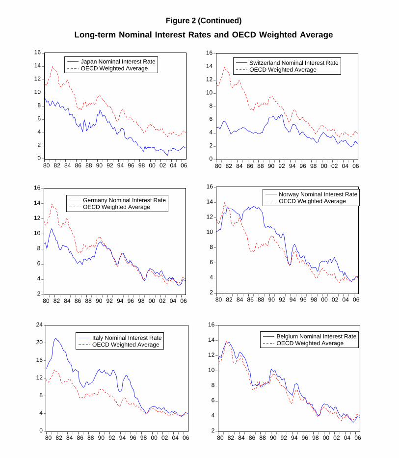
0
2
4
6
8
10
12
14
16
80 82 84 86 88 90 92 94 96 98 00 02 04 06
Japan Nominal Interest RateOECD Weighted Average
0
2
4
6
8
10
12
14
16
80 82 84 86 88 90 92 94 96 98 00 02 04 06
Switzerland Nominal Interest RateOECD Weighted Average
2
4
6
8
10
12
14
16
80 82 84 86 88 90 92 94 96 98 00 02 04 06
Germany Nominal Interest RateOECD Weighted Average
2
4
6
8
10
12
14
16
80 82 84 86 88 90 92 94 96 98 00 02 04 06
Norway Nominal Interest RateOECD Weighted Average
0
4
8
12
16
20
24
80 82 84 86 88 90 92 94 96 98 00 02 04 06
Italy Nominal Interest RateOECD Weighted Average
2
4
6
8
10
12
14
16
80 82 84 86 88 90 92 94 96 98 00 02 04 06
Belgium Nominal Interest RateOECD Weighted Average
Long-term Nominal Interest Rates and OECD Weighted AverageFigure 2 (Continued)

-4
-2
0
2
4
6
8
10
80 82 84 86 88 90 92 94 96 98 00 02 04 06
US Real Interest RateOECD Weighted Average
-1
0
1
2
3
4
5
6
7
8
80 82 84 86 88 90 92 94 96 98 00 02 04 06
UK Real Interest RateOECD Weighted Average
-2
0
2
4
6
8
10
80 82 84 86 88 90 92 94 96 98 00 02 04 06
Canada Real Interest RateOECD Weighted Average
-2
0
2
4
6
8
10
12
80 82 84 86 88 90 92 94 96 98 00 02 04 06
Australia Real Interest RateOECD Weighted Average
-2
0
2
4
6
8
10
80 82 84 86 88 90 92 94 96 98 00 02 04 06
Spain Real Interest RateOECD Weighted Average
-1
0
1
2
3
4
5
6
7
8
80 82 84 86 88 90 92 94 96 98 00 02 04 06
France Real Interest RateOECD Weighted Average
Long-term Real Interest Rates and OECD Weighted AverageFigure 3

-1
0
1
2
3
4
5
6
7
80 82 84 86 88 90 92 94 96 98 00 02 04 06
Japan Real Interest RateOECD Weighted Average
-2
-1
0
1
2
3
4
5
6
7
80 82 84 86 88 90 92 94 96 98 00 02 04 06
Switzerland Real Interest RateOECD Weighted Average
-1
0
1
2
3
4
5
6
7
8
80 82 84 86 88 90 92 94 96 98 00 02 04 06
Germany Real Interest RateOECD Weighted Average
-4
-2
0
2
4
6
8
80 82 84 86 88 90 92 94 96 98 00 02 04 06
Norway Real Interest RateOECD Weighted Average
-6
-4
-2
0
2
4
6
8
10
80 82 84 86 88 90 92 94 96 98 00 02 04 06
Italy Real Interest RateOECD Weighted Average
-1
0
1
2
3
4
5
6
7
8
80 82 84 86 88 90 92 94 96 98 00 02 04 06
Belgium Real Interest RateOECD Weighted Average
Long-term Real Interest Rates and OECD Weighted AverageFigure 3 (Continued)

2
4
6
8
10
12
14
16
1975 1980 1985 1990 1995 2000 2005
Dynamic Forecast*Actual Interest Rate95% Confidence Interval
United States
Nom
inal
Inte
rest
Rat
e
-40
-30
-20
-10
0
10
20
30
40
1980 1985 1990 1995 2000 2005
United States Cusum95% Confidence Interval
2
4
6
8
10
12
14
16
18
1975 1980 1985 1990 1995 2000 2005
Dynamic Forecast*Actual Interest Rate95% Confidence Interval
United Kingdom
Nom
inal
Inte
rest
Rat
e
-30
-20
-10
0
10
20
30
93 94 95 96 97 98 99 00 01 02 03 04 05 06
United Kingdom Cusum95% Confidence Interval
2
4
6
8
10
12
14
16
1975 1980 1985 1990 1995 2000 2005
Dynamic Forecast*Actual Interest Rate95% Confidence Interval
Sweden
Nom
inal
Inte
rest
Rat
e
-40
-30
-20
-10
0
10
20
30
40
1980 1985 1990 1995 2000 2005
Sweden Cusum95% Confidence Interval
1
2
3
4
5
6
7
8
1975 1980 1985 1990 1995 2000 2005
Dynamic Forecast*Actual Interest Rate95% Confidence Interval
Switzerland
Nom
inal
Inte
rest
Rat
e
-40
-30
-20
-10
0
10
20
30
40
1980 1985 1990 1995 2000 2005
Switzerland Cusum95% Confidence Interval
Long-term Nominal Bond-yield Models without Expectational VariablesFigure 4
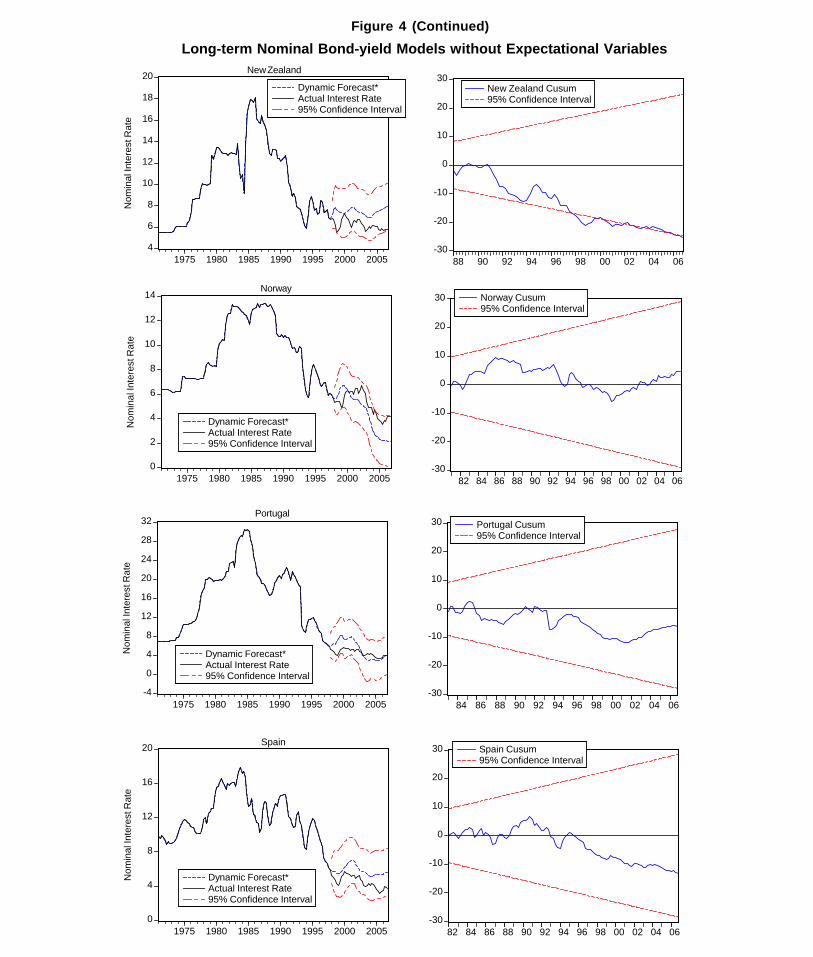
4
6
8
10
12
14
16
18
20
1975 1980 1985 1990 1995 2000 2005
Dynamic Forecast*Actual Interest Rate95% Confidence Interval
New Zealand
Nom
inal
Inte
rest
Rat
e
-30
-20
-10
0
10
20
30
88 90 92 94 96 98 00 02 04 06
New Zealand Cusum95% Confidence Interval
0
2
4
6
8
10
12
14
1975 1980 1985 1990 1995 2000 2005
Dynamic Forecast*Actual Interest Rate95% Confidence Interval
Norway
Nom
inal
Inte
rest
Rat
e
-30
-20
-10
0
10
20
30
82 84 86 88 90 92 94 96 98 00 02 04 06
Norway Cusum95% Confidence Interval
0
4
8
12
16
20
1975 1980 1985 1990 1995 2000 2005
Dynamic Forecast*Actual Interest Rate95% Confidence Interval
Spain
Nom
inal
Inte
rest
Rat
e
-30
-20
-10
0
10
20
30
82 84 86 88 90 92 94 96 98 00 02 04 06
Spain Cusum95% Confidence Interval
-4
0
4
8
12
16
20
24
28
32
1975 1980 1985 1990 1995 2000 2005
Dynamic Forecast*Actual Interest Rate95% Confidence Interval
Portugal
Nom
inal
Inte
rest
Rat
e
-30
-20
-10
0
10
20
30
84 86 88 90 92 94 96 98 00 02 04 06
Portugal Cusum95% Confidence Interval
Long-term Nominal Bond-yield Models without Expectational VariablesFigure 4 (Continued)

3
4
5
6
7
8
9
10
11
12
1975 1980 1985 1990 1995 2000 2005
Dynamic Forecast*Actual Interest Rate95% Confidence Interval
Austria
Nom
inal
Inte
rest
Rat
e
-40
-30
-20
-10
0
10
20
30
40
1980 1985 1990 1995 2000 2005
Austria Cusum95% Confidence Interval
2
4
6
8
10
12
14
16
18
1975 1980 1985 1990 1995 2000 2005
Dynamic Forecast*Actual Interest Rate95% Confidence Interval
Australia
Nom
inal
Inte
rest
Rat
e
-40
-30
-20
-10
0
10
20
30
40
1980 1985 1990 1995 2000 2005
Australia Cusum95% Confidence Interval
2
4
6
8
10
12
14
1975 1980 1985 1990 1995 2000 2005
Dynamic Forecast*Actual Interest Rate95% Confidence Interval
Belgium
Nom
inal
Inte
rest
Rat
e
-60
-50
-40
-30
-20
-10
0
10
20
30
84 86 88 90 92 94 96 98 00 02 04 06
Belgium Cusum95% Confidence Interval
2
4
6
8
10
12
14
16
18
1975 1980 1985 1990 1995 2000 2005
Dynamic Forecast*Actual Interest Rate95% Confidence Interval
Canada
Nom
inal
Inte
rest
Rat
e
-40
-30
-20
-10
0
10
20
30
40
1980 1985 1990 1995 2000 2005
Canada Cusum95% Confidence Interval
Long-term Nominal Bond-yield Models without Expectational VariablesFigure 4 (Continued)

0
4
8
12
16
20
24
1975 1980 1985 1990 1995 2000 2005
Dynamic Forecast*Actual Interest Rate95% Confidence Interval
Denmark
Nom
inal
Inte
rest
Rat
e
-50
-40
-30
-20
-10
0
10
20
30
40
80 82 84 86 88 90 92 94 96 98 00 02 04 06
Denmark Cusum95% Confidence Interval
0
2
4
6
8
10
12
14
1975 1980 1985 1990 1995 2000 2005
Dynamic Forecast*Actual Interest Rate95% Confidence Interval
Finland
Nom
inal
Inte
rest
Rat
e
-40
-30
-20
-10
0
10
20
30
40
80 82 84 86 88 90 92 94 96 98 00 02 04 06
Finland Cusum95% Confidence Interval
0
4
8
12
16
20
1975 1980 1985 1990 1995 2000 2005
Dynamic Forecast*Actual Interest Rate95% Confidence Interval
France
Nom
inal
Inte
rest
Rat
e
-40
-30
-20
-10
0
10
20
30
40
1980 1985 1990 1995 2000 2005
France Cusum95% Confidence Interval
2
3
4
5
6
7
8
9
10
11
1975 1980 1985 1990 1995 2000 2005
Dynamic Forecast*Actual Interest Rate95% Confidence Interval
Germany
Nom
inal
Inte
rest
Rat
e
-30
-20
-10
0
10
20
30
93 94 95 96 97 98 99 00 01 02 03 04 05 06
Germany Cusum95% Confidence Interval
Long-term Nominal Bond-yield Models without Expectational VariablesFigure 4 (Continued)

0
4
8
12
16
20
24
1975 1980 1985 1990 1995 2000 2005
Dynamic Forecast*Actual Interest Rate95% Confidence Interval
Italy
Nom
inal
Inte
rest
Rat
e
-30
-20
-10
0
10
20
30
84 86 88 90 92 94 96 98 00 02 04 06
Italy Cusum95% Confidence Interval
0
2
4
6
8
10
1975 1980 1985 1990 1995 2000 2005
Dynamic Forecast*Actual Interest Rate95% Confidence Interval
Japan
Nom
inal
Inte
rest
Rat
e
-40
-30
-20
-10
0
10
20
30
40
1980 1985 1990 1995 2000 2005
Japan Cusum95% Confidence Interval
2
4
6
8
10
12
14
1975 1980 1985 1990 1995 2000 2005
Dynamic Forecast*Actual Interest Rate95% Confidence Interval
Netherlands
Nom
inal
Inte
rest
Rat
e
-30
-20
-10
0
10
20
30
82 84 86 88 90 92 94 96 98 00 02 04 06
Netherland Cusum95% Confidence Interval
Long-term Nominal Bond-yield Models without Expectational VariablesFigure 4 (Continued)

-2
0
2
4
6
8
10
1990 1992 1994 1996 1998 2000 2002 2004 2006
US ResidualUS ActualUS Fitted
-30
-20
-10
0
10
20
30
93 94 95 96 97 98 99 00 01 02 03 04 05 06
US Cusum95% Confidence Interval
-2
0
2
4
6
8
10
12
1990 1992 1994 1996 1998 2000 2002 2004 2006
UK ResidualUK ActualUK Fitted
-40
-30
-20
-10
0
10
20
30
93 94 95 96 97 98 99 00 01 02 03 04 05 06
UK Cusum95% Confidence Interval
-1
0
1
2
3
4
5
6
7
8
1990 1992 1994 1996 1998 2000 2002 2004 2006
Japan ResidualJapan ActualJapan Fitted
-30
-20
-10
0
10
20
30
93 94 95 96 97 98 99 00 01 02 03 04 05 06
Japan Cusum95% Confidence Interval
Long-term Nominal Bond-yield Models with Expectational VariablesFigure 5

-2
0
2
4
6
8
10
12
14
1990 1992 1994 1996 1998 2000 2002 2004 2006
Sweden ResidualSweden ActualSweden Fitted
-30
-20
-10
0
10
20
30
1992 1994 1996 1998 2000 2002 2004 2006
Sweden Cusum95% Confidence Interval
-1
0
1
2
3
4
5
6
7
1990 1992 1994 1996 1998 2000 2002 2004 2006
Switzerland ResidualSwitzerland ActualSwitzerland Fitted
-30
-20
-10
0
10
20
30
1992 1994 1996 1998 2000 2002 2004 2006
Switzerland Cusum95% Confidence Interval
-2
0
2
4
6
8
10
12
1990 1992 1994 1996 1998 2000 2002 2004 2006
France ResidualFrance ActualFrance Fitted
-30
-20
-10
0
10
20
30
93 94 95 96 97 98 99 00 01 02 03 04 05 06
France Cusum95% Confidence Interval
Long-term Nominal Bond-yield Models with Expectational VariablesFigure 5 (Continued)

-2
0
2
4
6
8
10
1990 1992 1994 1996 1998 2000 2002 2004 2006
Netherlands ResidualNetherlands ActualNetherlands Fitted
-30
-20
-10
0
10
20
30
1992 1994 1996 1998 2000 2002 2004 2006
Netherlands Cusum95% Confidence Interval
-2
0
2
4
6
8
10
12
1990 1992 1994 1996 1998 2000 2002 2004 2006
Canada ResidualCanada ActualCanada Fitted
-30
-20
-10
0
10
20
30
1994 1996 1998 2000 2002 2004 2006
Canada Cusum95% Confidence Interval
-2
0
2
4
6
8
10
12
1990 1992 1994 1996 1998 2000 2002 2004 2006
Norway ResidualNorway ActualNorway Fitted
-30
-20
-10
0
10
20
30
1992 1994 1996 1998 2000 2002 2004 2006
Norway Cusum95% Confidence Interval
-4
0
4
8
12
16
1990 1992 1994 1996 1998 2000 2002 2004 2006
Spain ResidualSpain ActualSpain Fitted
-30
-20
-10
0
10
20
30
1992 1994 1996 1998 2000 2002 2004 2006
Spain Cusum95% Confidence Interval
Long-term Nominal Bond-yield Models with Expectational VariablesFigure 5 (Continued)

1998 2000 2002 2004 20064
5
6
7
8
9
10
Corporate Nominal AA-Rated Bond Yields*
Figure 6
US AA yieldUK AA yield
1998 2000 2002 2004 20064
5
6
7
8
9
10US AA yieldCanada AA yield
1998 2000 2002 2004 20060
1
2
3
4
5
6
7
8
US AA yieldJapan AA yield
1998 2000 2002 2004 20063
4
5
6
7
8US AA yieldEU AA yield
1998 2000 2002 2004 20064
5
6
7
8
9
10
11
Corporate Nominal BBB-Rated Bond Yields*
US BBB yieldUK BBB yield
1998 2000 2002 2004 20064
5
6
7
8
9
10
11US BBB yieldCanada BBB yield
1998 2000 2002 2004 20060123
4567
89
*Yields computed as Long-term government bond yields plus credit spreads on 10-yr. rated corporate bonds.
US BBB yieldJapan BBB yield
1998 2000 2002 2004 20063
4
5
6
7
8
9US BBB yieldEU BBB yield

Forward Earnings Yields on Equities
1990 1995 2000 20054
5
6
7
8
9
10
11
Figure 7
Forward Earnings YieldOECD Weighted AverageOECD Weighted Average exc. Japan
United States
1990 1995 2000 20054
5
6
7
8
9
10
11
Canada
1990 1995 2000 20054567891011121314
Australia
1990 1995 2000 200545678910111213
United Kingdom
1990 1995 2000 200523456789101112
Austria
1990 1995 2000 2005456789101112131415
Belgium
1990 1995 2000 20054
5
6
7
8
9
10
11
12
Denmark
1990 1995 2000 2005-4-2024681012141618
Finland
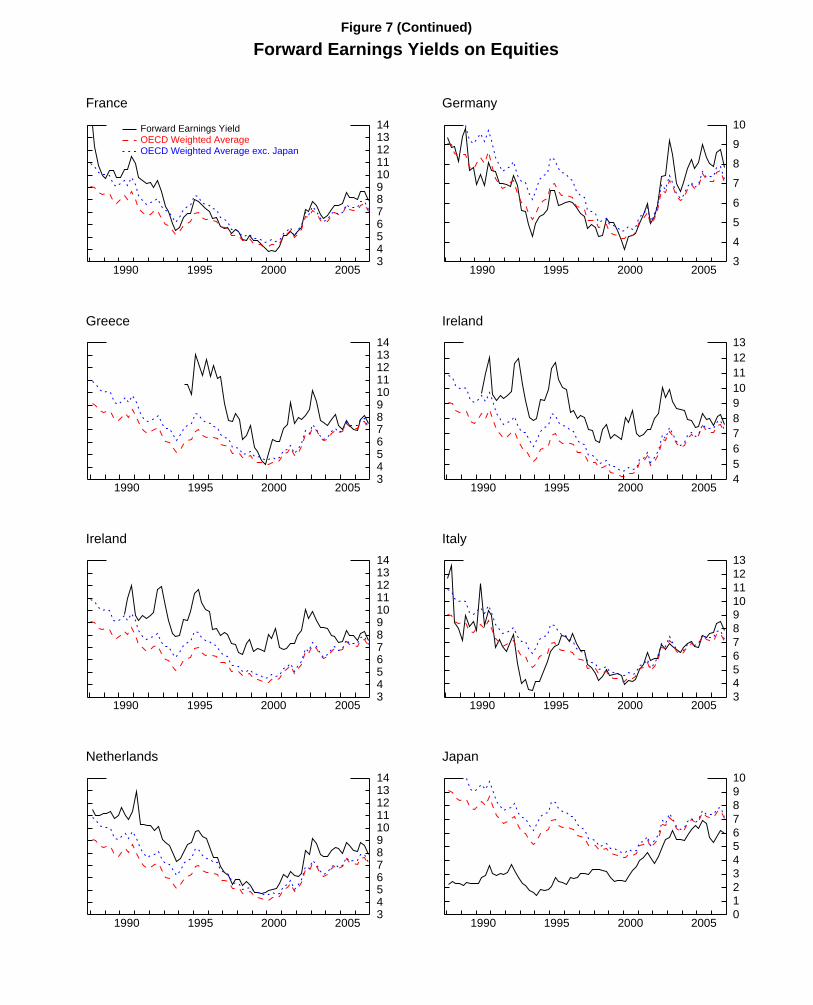
Forward Earnings Yields on Equities
1990 1995 2000 200534567891011121314
Figure 7 (Continued)
Forward Earnings YieldOECD Weighted AverageOECD Weighted Average exc. Japan
France
1990 1995 2000 20053
4
5
6
7
8
9
10
Germany
1990 1995 2000 200534567891011121314
Greece
1990 1995 2000 200545678910111213
Ireland
1990 1995 2000 200534567891011121314
Ireland
1990 1995 2000 2005345678910111213
Italy
1990 1995 2000 200534567891011121314
Netherlands
1990 1995 2000 2005012345678910
Japan
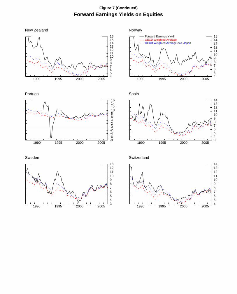
Forward Earnings Yields on Equities
1990 1995 2000 200545678910111213141516
Figure 7 (Continued)
New Zealand
1990 1995 2000 2005456789101112131415Forward Earnings Yield
OECD Weighted AverageOECD Weighted Average exc. Japan
Norway
1990 1995 2000 2005-8-6-4-20246810121416
Portugal
1990 1995 2000 200534567891011121314
Spain
1990 1995 2000 2005345678910111213
Sweden
1990 1995 2000 20054567891011121314
Switzerland

15.4
15.5
15.6
15.7
15.8
15.9
16.0
95 96 97 98 99 00 01 02 03 04 05 06
Dynamic Forecast*Log Real Cons.95% Confidence Interval
United States
Log
Rea
l Con
sum
ptio
n
13.1
13.2
13.3
13.4
13.5
13.6
13.7
95 96 97 98 99 00 01 02 03 04 05 06
Dynamic Forecast*Log Real Cons.95% Confidence Interval
United Kingdom
Log
Rea
l Con
sum
ptio
n
13.0
13.1
13.2
13.3
13.4
13.5
95 96 97 98 99 00 01 02 03 04 05 06
Dynamic Forecast*Log Real Cons.95% Confidence Interval
Canada
Log
Rea
l Con
sum
ptio
n
13.90
13.92
13.94
13.96
13.98
14.00
14.02
14.04
14.06
95 96 97 98 99 00 01 02 03 04 05 06
Dynamic Forecast*Log Real Cons.95% Confidence Interval
Germany
Log
Rea
l Con
sum
ptio
n
13.3
13.4
13.5
13.6
13.7
13.8
95 96 97 98 99 00 01 02 03 04 05 06
Dynamic Forecast*Log Real Cons.95% Confidence Interval
Italy
Log
Rea
l Con
sum
ptio
n
13.40
13.45
13.50
13.55
13.60
13.65
13.70
13.75
95 96 97 98 99 00 01 02 03 04 05 06
Dynamic Forecast*Log Real Cons.95% Confidence Interval
France
Log
Rea
l Con
sum
ptio
n
19.36
19.40
19.44
19.48
19.52
19.56
95 96 97 98 99 00 01 02 03 04 05 06
Dynamic Forecast*Log Real Cons.95% Confidence Interval
Japan
Log
Rea
l Con
sum
ptio
n
Dynamic Simulations of Log Real Household ConsumptionFigure 8

Figure 9: Change in Current Accounts 1996 - 2005*
-0.200
-0.150
-0.100
-0.050
0.000
0.050
0.100
0.150
Spa
in
Italy
US
A
Gre
ece
Por
tuga
l
Fran
ce
Aus
tralia
UK
Finl
and
Can
ada
Japa
n
Den
mar
k
Net
herla
nds
Sw
eden
Aus
tria
Ger
man
y
Public SavingHousehold SavingCorporate SavingNon-Residential InvestmentResidential InvestmentCA/GDP
*2004 for Greece and 2003 for Portugal

Figure 10: Level of Current Accounts in 1996
-0.40
-0.30
-0.20
-0.10
0.00
0.10
0.20
0.30
0.40
Aust
ralia
Portu
gal
Aust
ria
Gre
ece
USA
UK
Ger
man
y
Spai
n
Can
ada
Fran
ce
Japa
n
Den
mar
k
Italy
Swed
en
Finl
and
Net
herla
nds
Public SavingHousehold SavingCorporate SavingNon-Residential InvestmentResidential InvestmentCA

Figure 11: Level of Current Accounts in 2005*
-0.40
-0.30
-0.20
-0.10
0.00
0.10
0.20
0.30
0.40
Spa
in
Por
tuga
l
US
A
Aus
tralia
Gre
ece
UK
Italy
Fran
ce
Can
ada
Aus
tria
Den
mar
k
Japa
n
Ger
man
y
Finl
and
Sw
eden
Net
herla
nds
Public SavingHousehold SavingCorporate SavingNon-Residential InvestmentResidential InvestmentCA
*2004 for Greece and 2003 for Portugal