MPRAMunich Personal RePEc Archive

Divorce and Corruption: New Study,New Data

Oasis Kodila-Tedika and Florentin Azia-Dimbu and Cedrick

Kalemasi-Mosengo

University of Kinshasa, Department of Economics, DemocraticRepublic of Congo (DRC); Institute of African Economics,Universite Pedagogique Nationale, Department of Psychology,Democratic Republic of Congo (DRC), University of Kinshasa,Department of Economics, Democratic Republic of Congo (DRC)

13. May 2012

Online at http://mpra.ub.uni-muenchen.de/39815/MPRA Paper No. 39815, posted 3. July 2012 19:19 UTC

Divorce and Corruption: New Study, New Data

Oasis Kodila-Tedika

Florention Azia-Dimbu

Cedrick Kalemasi-Mosengo

University of Kinshasa Working paper N° 001/12/FASE

1

Divorce and Corruption: New Study, New Data

Oasis Kodila-Tedika1

University of Kinshasa, Department of Economics, Democratic Republic of Congo (DRC)

Institute of African Economics

E-mail : oasiskodila@yahoo.fr

Florention Azia-Dimbu

Université Pédagogique Nationale, Department of Psychology, Democratic Republic of Congo (DRC)

Cedrick Kalemasi-Mosengo

University of Kinshasa, Department of Economics, Democratic Republic of Congo (DRC)

Abstract

This paper aims at identifying the effects of divorce alongside on corruption controlling.

We find no significant effect of divorce on corruption. The same conclusion is found in

cross-section and panel data.

Keys-words: Divorce, corruption, Europe

1. Introduction

Economists have proposed what can be referred to as the traditional causes of corruption

(Lambsdorff, 2006; Kodila Tedika, 2012). However, the interest in nontraditional has been

increasing more and more, recently. These include factors such as age (Torgler & Valev,

2006), gender (Swamy et al., 2001; Dollar & al, 2001; Sung & Chu, 2003; Sung, 2003;

Cheung and Hernandez-Julian, 2006; Lavallée & al., 2010), level of intelligence (Potrafke,

2011), trust (Uslaner, 2004), etc. In the tread, Mocan (2008) documents the bond between

corruption and civil status on microdata. It is considered in the framework of married,

divorced, the widows, the single and the living room together. The fact of being unmarried

appears significant, and the fact of being widowed appears significant in certain regressions.

The question that we put forth in this study is whether one can find any significant

relationship between divorce and corruption. Beyond the need of confirming or disagreeing

with the results in Mocan (2008), this question seems legitimate since it is estimated that

people who want to divorce to be eager to accelerate the things by lubricating the legal

machine. Also, psychological work insinuates a rather significant relation between the divorce

and the level of stress (Lazarus, 1984; Lazarus & al., 1985; Holmes & Rahe, 1967; Kanner &

al, 1981). In such a case, one can insinuate an effective pertubation to scramble reference.

Thus, a relation divorce-marriage could appear. What interests us is the direct effect of the

divorce on corruption.

In this paper we intend to focus more on divorce, better than the above mentioned article. In

1 I thank Emmanuel Martin for data and Isaac Kanyama-Kalonda for lectures.

2

addition, this article uses different data, such as European data. And then the sample is

relatively homogenous. The availability of data conditioned the use of this sample. This focus

on social norms that fit better the interdisciplinary literature on divorce.

The remainder of the paper is structured as follows. Section 2 presents the data and gives

suggestive evidence. Section 3 describes the empirical specification and estimation strategy.

Section 4 examines marriage effect of corruption and the conclusions are given in section 5.

2. Data and Descriptive Evidence

To examine the relationship between divorce and corruption we collected a cross-section from

to average 2002-2009 and panel data over the period from 2002 to 2009 for 25 europeans

countries . The selection of countries as well as the time period is driven by concerns of data

availability. In addition, we try to follow Kalonda-Kanyama and Kodila Tedika (2012) use

relatively the same control variables. The variables used are summarized in Tables 1, 2 and 3.

We describe each variable in turn as following.

2.1 Divorce and corruption

The dependent variable is the yearly corruption level from the Transparency International and

interest variable is the Crude divorce rate (divorces per 1,000 inhabitants), the same data as

used in Kodila Tedika (2012). To measure corruption, I use the Transparency International's

Perception of Corruption Index (CPI) for the year 2010. The index assumes values between

10 (no corruption) and 0 (extreme corruption). The CPI has often been used in empirical

research on corruption (see i.e. the studies mentioned in section 1).

The source is Demography report of Eurostat (to see figure 1 to identify the evolution of the

divorce in time within EU-27). These data have the advantage that they are available for the

whole time period under consideration and for all UE-27 member countries. In addition, the

EuroStat has ensured that divorce rates are comparable across the countries. Divorce is not

legal in Malta. Germany misses certain control variables. Therefore, our estimates are made

on 25 countries.

In 2007, 1.2 million divorces took place in the EU-27. The crude divorce rate was 2.1 per 1

000 inhabitants Eurostat (2011). Regarding the reality of divorce, Ireland (0.8 per 1 000

inhabitants) and several southern European Member States, including Italy (0.9), Slovenia

(1.1) and Greece (1.2) have significantly lower crude divorce rates than Belgium (3.0 per 1

000 inhabitants), Lithuania and the Czech Republic, both with 2.8. According to Figure I, the

rate of divorce for UE-26 was 1,99 in 1990. In 2009, the trend is positive: it is gone to 2,07.

There are thus more divorces.

3

Figure 1. Evolution of crude divorce rate in EU-27 (divorce per 1,000 inhabitants)

On average, UE-25 behaves well in terms of corruption, because it represents an average note

of 6,35. There are nevertheless problematic cases: on the whole, there are 8 nations which

have a note lower than 5, whereas the best note is 10. Danmark has the highest score, while

Greece and Romania divide both the note of 3,8/10.

Table 1: List of countries

This study uses the data from 25 countries : Belgium; Bulgaria; The Czech Republic;

Denmark ; Estonia ; Ireland ; Greece ; Spain ; France, including overseas territories;

'Metropolitan France' excludes overseas territories; Italy ; Cyprus ; Latvia ; Lithuania ;

Luxembourg ; Hungary ; The Netherlands ; Austria ; Poland ; Portugal ; Romania ; Slovenia ;

Slovakia ; Finland ; Sweden and The United Kingdom.

Table 2. Summary statistics (Cross-section)

Variable Obs Mean Std. Dev. Min Max

Divorce 25 2.139 0.6675059 0.775 3.15

Corruption 25 1.089723 0.7686955 -0.1574431 2.35022

UE 25 7.711 2.8678 3.6 14.55

Gender 25 2.248 0.9117697 0.825 4.85

Infla 25 3.283205 2.061051 1.428242 10.44169

Helath 25 77.08036 3.186208 71.6244 80.80093

Density 25 127.1663 103.9401 17.29225 483.9098

Edu 25 59.98888 16.58317 11.27159 90.95385

Log GDP per capit25 10.05355 .4774529 9.174291 11.13314

1,98

1,99

2

2,01

2,02

2,03

2,04

2,05

2,06

2,07

2,08

1985 1990 1995 2000 2005 2010

Divorce

4

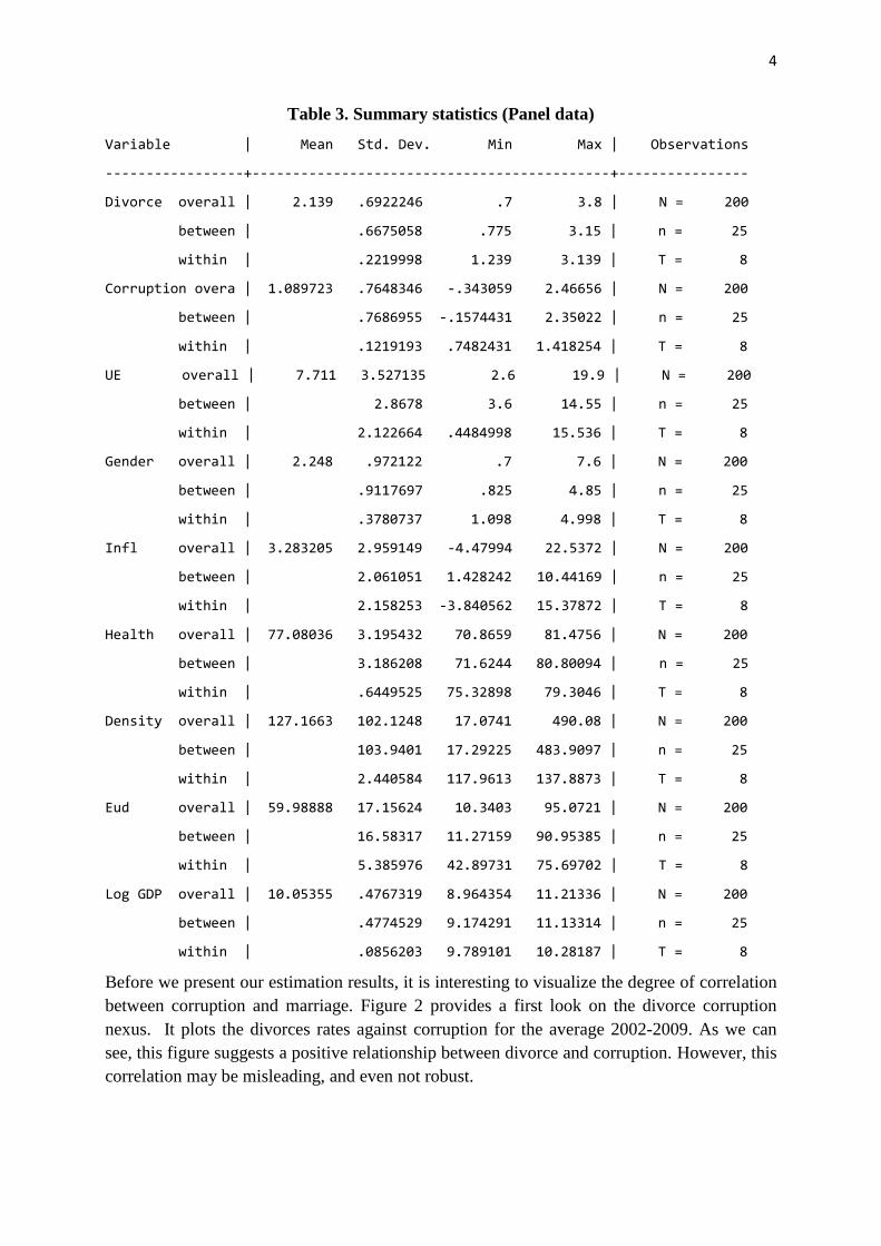
Table 3. Summary statistics (Panel data)

Variable | Mean Std. Dev. Min Max | Observations

-----------------+--------------------------------------------+----------------

Divorce overall | 2.139 .6922246 .7 3.8 | N = 200

between | .6675058 .775 3.15 | n = 25

within | .2219998 1.239 3.139 | T = 8

Corruption overa | 1.089723 .7648346 -.343059 2.46656 | N = 200

between | .7686955 -.1574431 2.35022 | n = 25

within | .1219193 .7482431 1.418254 | T = 8

UE overall | 7.711 3.527135 2.6 19.9 | N = 200

between | 2.8678 3.6 14.55 | n = 25

within | 2.122664 .4484998 15.536 | T = 8

Gender overall | 2.248 .972122 .7 7.6 | N = 200

between | .9117697 .825 4.85 | n = 25

within | .3780737 1.098 4.998 | T = 8

Infl overall | 3.283205 2.959149 -4.47994 22.5372 | N = 200

between | 2.061051 1.428242 10.44169 | n = 25

within | 2.158253 -3.840562 15.37872 | T = 8

Health overall | 77.08036 3.195432 70.8659 81.4756 | N = 200

between | 3.186208 71.6244 80.80094 | n = 25

within | .6449525 75.32898 79.3046 | T = 8

Density overall | 127.1663 102.1248 17.0741 490.08 | N = 200

between | 103.9401 17.29225 483.9097 | n = 25

within | 2.440584 117.9613 137.8873 | T = 8

Eud overall | 59.98888 17.15624 10.3403 95.0721 | N = 200

between | 16.58317 11.27159 90.95385 | n = 25

within | 5.385976 42.89731 75.69702 | T = 8

Log GDP overall | 10.05355 .4767319 8.964354 11.21336 | N = 200

between | .4774529 9.174291 11.13314 | n = 25

within | .0856203 9.789101 10.28187 | T = 8

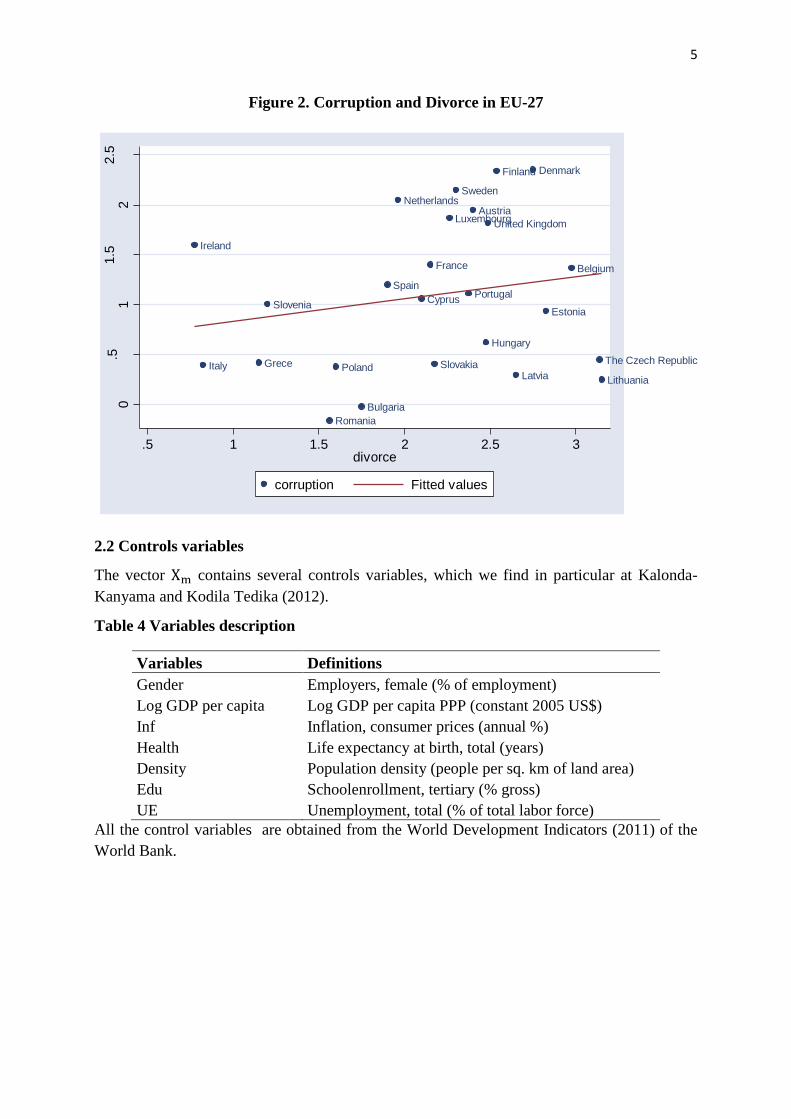
Before we present our estimation results, it is interesting to visualize the degree of correlation

between corruption and marriage. Figure 2 provides a first look on the divorce corruption

nexus. It plots the divorces rates against corruption for the average 2002-2009. As we can

see, this figure suggests a positive relationship between divorce and corruption. However, this

correlation may be misleading, and even not robust.

5

Figure 2. Corruption and Divorce in EU-27

2.2 Controls variables

The vector contains several controls variables, which we find in particular at Kalonda-

Kanyama and Kodila Tedika (2012).

Table 4 Variables description

Variables Definitions

Gender Employers, female (% of employment)

Log GDP per capita Log GDP per capita PPP (constant 2005 US$)

Inf Inflation, consumer prices (annual %)

Health Life expectancy at birth, total (years)

Density Population density (people per sq. km of land area)

Edu Schoolenrollment, tertiary (% gross)

UE Unemployment, total (% of total labor force)

All the control variables are obtained from the World Development Indicators (2011) of the

World Bank.

Sweden

Finland

Slovakia

United Kingdom

Slovenia

Romania

Portugal

Poland

AustriaNetherlands

Hungary

Luxembourg

LithuaniaLatvia

Cyprus

Italy

France

Spain

Grece

Ireland

Estonia

Denmark

The Czech Republic

Bulgaria

Belgium

0.5

11.5

22.5

.5 1 1.5 2 2.5 3divorce

corruption Fitted values

6

3. Empirical Results

3.1 Estimation strategy

The baseline econometric model has the following form:

(1)

With i = 6,… m representing the various listed countries.

We estimate the model with ordinary least squares (OLS) and robust standard errors. This

empirical study uses European cross-sectional data and panel data. For cross-sectional, the

estimate is made for the average enter 2002-2009 and we use the bootstrap. In econometrics,

the principal contribution of Bootstrap relates to the improvement of the inference in the

methods of regression, in particular in small sample in the sense that the estimated parameters

improve.

(2)

With i = 6,… m representing the various listed countries and n represents temporal dimension.

We estimate the model with ordinary least squares (OLS) and robust standard errors (Eicker-

White). We use fixed-effects, after the result of Hausmann test. This empirical study uses data

from 25 european countries over the period from 2002 to 2009.

3.2 Regression results

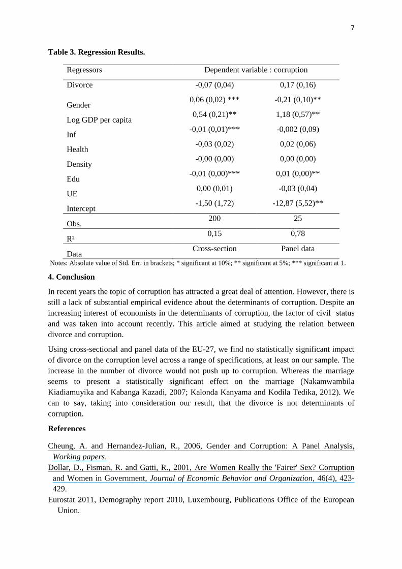
Table 5 shows the baseline regression results. The control variables are statistically significant

in several cases. Within the framework of the relative relevance of our controls of variable,

one notices that it is not significant, except for the shadow.

Within the framework of the absolute relevance of our variable of interest (divorce), one

notices that it is not significant in all the cases. Given the nature of our data and study, to test

the robustness of the results is not obvious. In order to check the robustness of the results we

uses the same variables in panel and cross-section. But the divorce isn’t statistically

significant.

7

Table 3. Regression Results.

Regressors Dependent variable : corruption

Divorce -0,07 (0,04) 0,17 (0,16)

Gender 0,06 (0,02) *** -0,21 (0,10)**

Log GDP per capita 0,54 (0,21)** 1,18 (0,57)**

Inf -0,01 (0,01)*** -0,002 (0,09)

Health -0,03 (0,02) 0,02 (0,06)

Density -0,00 (0,00) 0,00 (0,00)

Edu -0,01 (0,00)*** 0,01 (0,00)**

UE 0,00 (0,01) -0,03 (0,04)

Intercept -1,50 (1,72) -12,87 (5,52)**

Obs. 200 25

R² 0,15 0,78

Data Cross-section Panel data

Notes: Absolute value of Std. Err. in brackets; * significant at 10%; ** significant at 5%; *** significant at 1.

4. Conclusion

In recent years the topic of corruption has attracted a great deal of attention. However, there is

still a lack of substantial empirical evidence about the determinants of corruption. Despite an

increasing interest of economists in the determinants of corruption, the factor of civil status

and was taken into account recently. This article aimed at studying the relation between

divorce and corruption.

Using cross-sectional and panel data of the EU-27, we find no statistically significant impact

of divorce on the corruption level across a range of specifications, at least on our sample. The

increase in the number of divorce would not push up to corruption. Whereas the marriage

seems to present a statistically significant effect on the marriage (Nakamwambila

Kiadiamuyika and Kabanga Kazadi, 2007; Kalonda Kanyama and Kodila Tedika, 2012). We

can to say, taking into consideration our result, that the divorce is not determinants of

corruption.

References

Cheung, A. and Hernandez-Julian, R., 2006, Gender and Corruption: A Panel Analysis,

Working papers.

Dollar, D., Fisman, R. and Gatti, R., 2001, Are Women Really the 'Fairer' Sex? Corruption

and Women in Government, Journal of Economic Behavior and Organization, 46(4), 423-

429.

Eurostat 2011, Demography report 2010, Luxembourg, Publications Office of the European

Union.

8

Holmes, T.H. and Rahe, R.H., 1967, The social read adjustment rating scale, Journal of

Psychosomatic Research, 11:213-218.

Kalonda-Kanyama, I. and Kodila Tedika, O., 2012, Marriage and corruption: An empirical

analysis on European data, submitted.

Kanner, A.D., Coyne, J.C., Schaefer, C. and Lazarus, R.S., 1981, Comparison of two modes

of stress measurement: daily hassles and uptifts of stress measurement, Journal of

Behavioral Medecine, 4: 1-39.

Kodila Tedika, O., 2012, Causes de la corruption : aperçu empirique, Annales de l’Université

Marien-Ngouabi, submitted.

Lambsdorff, J.G., 2006, Consequences and Causes of Corruption: What do We Know from a

Cross-Section of Countries?, In Rose-Ackermann (ed), International Handbook on The

Economics of Corruption, Edward-Elgar, Cheltenham, UK, Northampton, MA, USA, 3-51.

Lavallée, E., Razafindrakoto, M. and Roubaud, F., 2010, Ce qui engendre la corruption : une

analyse microéconomique sur données africaines, Revue d'économie du développement.

24(3) : 5-47.

Lazarus, R.S., 1984, The trivalization of distress, In B.L.Hammonds et C.J. Scheirer (ed.).

Psychology and Health : The master lecture series, Washington DC : American

Psychological Association..

Lazarus, R.S., DeLongis, A., Folkman, S.and Gruen, R., 1985, Stress and adaptational

outcomes: The problem of confounded measures, American Psychologist, 40:770-779.

Mocan, N., 2008, What Determines Corruption? International Evidence from Microdata,

Economic Inquiry. 64(4): 439-510.

Nakamwambila Kiadiamuyika, J. and Kabanga Kazadi, C., 2007, Impact de la pauvreté sur la

corruption chez les magistrats, les policiers de roulage et les taximen à Kinshasa”, ODHS

Rapport de recherche N°7.

Potrafke, N., 2012, Intelligence and Corruption, Economics Letters, 114(1): 109-112.

Sung, H.-E., 2003, Fairer Sex or Fairer System? Gender and Corruption Revisited, Social

Forces, 82(2), 703-723.

Sung, H.-E. and Chu, D., 2003, Does Participation in the Global Economy Reduce Political

Corruption? An Empirical Inquiry, International Journal of Comparative Criminology, 3(2):

94-118.

Swamy, A., Knack, S., Lee, L. and Azfar, O., 2001, Gender and Corruption, Journal of

Development Economics, 64: 25-55.

Uslaner, E., 2004, Trust and Corruption. In The New Institutional Economics of Corruption -

Norms, Trust, and Reciprocity, ed. by J. Graf Lambsdorff, M. Schramm and M. Taube,

Routledge, London: 76-92.