Determinants of Residential Location Choice: How Important Are Local Public Goods in Attracting...

DETERMINANTS OF RESIDENTIAL LOCATION CHOICE:

HOW IMPORTANT ARE LOCAL PUBLIC GOODS IN

ATTRACTING HOMEOWNERS TO CENTRAL CITY

LOCATIONS?*

Isaac Bayoh

Department of Agricultural, Environmental and Development Economics, Ohio StateUniversity, Columbus, OH. [email protected]

Elena G. IrwinDepartment of Agricultural, Environmental and Development Economics, Ohio StateUniversity, Columbus, OH. E-mail: [email protected]

Timothy Haab

Department of Agricultural, Environmental and Development Economics, Ohio StateUniversity, Columbus, OH. [email protected]

ABSTRACT. A hybrid conditional logit choice model is estimated using data on thecharacteristics and destination of homeowners who engaged in intrametropolitanmoves among 17 school districts within the Columbus, Ohio area in 1995. Themodel is used to test the relative influence of local fiscal and public goods versushousehold-level characteristics in determining household location choices acrosscentral city and suburban school districts. Results provide evidence of both a ‘‘nat-ural evolution’’ of households to the suburbs, due to job location, residential filtering,and household income and lifecycle effects, and ‘‘flight from blight,’’ due to lowerschool quality, higher crime levels, and lower average income levels in the city. Incomparing the magnitudes of these variables, we find that school quality exerts thestrongest influence: a 1-percent increase in the school quality of the city districtincreases the probability of choosing a city residence by 3.7 percent. In contrast, theeffects of household income and other individual characteristics are relatively mod-est. The findings provide support for a ‘‘flight from blight’’ suburbanization processthat is dominated by differences in neighborhood quality between the city andsuburbs. An implication is that investments that promote central city developmentand reduce suburbanization are justified on efficiency grounds if negative external-ities are generated by increased concentration of poverty, crime, and low schoolquality.

97

*Paper prepared for the Critical Issues Symposium State and Local GovernmentRegulations and Economic Development, March 4–5, 2005, Florida State University Tallahassee,FL.

Received: 24 February 2004; Revised: 22 June 2004; Accepted: 15 August 2004

JOURNAL OF REGIONAL SCIENCE, VOL. 46, No. 1, 2006, pp. 97–120

# Blackwell Publishing, Inc. 2006.BlackwellPublishing, Inc., 350Main Street, Malden, MA 02148, USA and 9600Garsington Road,Oxford,OX42DQ, UK.

1. INTRODUCTION1

A critical question for regional economic development is the extent towhich central city growth and decline impact suburban and regional metro-politan growth. Some empirical evidence suggests that central city growth ispositively and significantly associated with suburban and metropolitangrowth (Voith, 1992; Savitch et al., 1993; Leichenko, 2001). For example,Leichenko (2001) studies the simultaneous relationships between city–sub-urban growth and population–employment from 1970 to 97. She finds thatsuburban employment growth positively affected city employment growth inthe 1980s and 1990s, but negatively affected city population growth duringthis time, and that city employment growth benefited suburban employmentgrowth in the 1990s. She concludes that a positive feedback between city andsuburban growth existed during this time of relative economic prosperity.Voith (1992) finds a positive association among city and suburban population,income, and employment changes during the 1970s and 1980s. He concludesthat central city decline exerts a slow and cumulative effect on regionalgrowth by draining the region of its ‘‘economic and social vitality.’’

These arguments provide a regional economic development rationale forstate and federal programs to increase the amount of development fundsallocated to central cities relative to their suburban counterparts. However,such a conclusion fails to consider the suburbanization process itself and theextent to which this process is efficient. Provided suburbanization generatessome level of benefits, these benefits should be weighed against the socialwelfare gains from additional central city investments that could slow sub-urbanization. As Mieszkowski and Mills (1993) argue, the efficiency of stateand federal spending that favors central cities depends on the underlyingeconomic and social processes that cause suburbanization. For example, ifsuburbanization is primarily driven by certain ‘‘natural evolution’’ marketprocesses, such as increases in real household incomes, lifecycle effects, joblocation, and technological advances, then it may be by and large an efficientprocess. This is because such changes alter the optimal location choice ofhouseholds by making suburban locations more desirable, for example, bymaking travel to suburban locations less costly through technological innova-tions or by increasing the demand for suburban housing due to rising incomes.Alternatively, if the suburbanization process is associated with externalitiesor public goods or is largely driven by government policies that distort the true

1We are grateful to the Ohio Housing Research Network and Hazel Morrow-Jones,Associate Professor in City and Regional Planning at Ohio State University, for making thedata used in this analysis available. Support for the research was provided by the Ohio StateUniversity Urban Affairs Committee and Ohio Center for Real Estate Education and Research.We are grateful to Don Haurin for valuable feedback on preliminary draft of this paper and toKeith Ihlanfeldt, Stefan Norrbin, an anonymous referee, and other participants at the CriticalIssues Symposium State and Local Government Regulations and Economic Development atFlorida State University.

98 JOURNAL OF REGIONAL SCIENCE, VOL. 46, NO. 1, 2006

# Blackwell Publishing, Inc. 2006.

social costs associated with suburbanization, then the inefficiency of suburba-nization may provide an added justification for state and federal governmentsto increase development funding to central cities.

It is well established that certain government policies have distorted thetrue costs associated with suburban land development. Primary among theseare the government’s subsidization of public road building and of homeowner-ship through federal income tax policy. In the case of roads, congestionexternalities lead to underpricing of road travel and an oversupply of roads,which fosters a more decentralized urban form than what is socially optimal(Brueckner, 2000). The federal income tax housing subsidy promotes subur-banization because it essentially lowers the price of land in areas with elasticland supply, namely the suburbs. Persky and Kurban (2003) present convin-cing evidence of how the price and income effects of this subsidy have led to anoverconsumption of urban land in outer suburban areas of Chicago. Theyestimate that the wealth creation effect of this subsidy, which was distributeddisproportionately to suburban residents due to higher homeownership ratesand incomes and housing values in the suburbs, led to 20 percent moreconsumption of urban land in the outer Chicago area from 1989 to 1996. Incontrast, they find that the increase in central city incomes due to ‘‘pro-city’’federal spending in other programs has only offset suburban land consump-tion by a few percentage points. Although total federal expenditures per capitain the central city were about two-thirds higher than in the suburbs, theyargue that the vast bulk of the difference in these expenditures is due totransfers that subsidize consumption by poorer city residents rather thanprograms that encourage wealth accumulation.

In addition to government subsidies that lower the private cost of sub-urban land, the suburbanization process is associated with several kinds ofexternalities that also have led to suboptimal pricing of suburban develop-ment. As Brueckner (2000) details, the full benefits of open space land are notreflected in agricultural or rural land prices, and thus, the market fails toreflect the full opportunity cost of developing rural land. In addition, the costsof providing local public services, including public utilities, roads, and schools,are not reflected in the private costs and development, and thus, new residen-tial housing is underpriced.

A final externality concerns the ‘‘flight from blight’’ process and the extentto which negative externalities are generated that result in a suboptimaldistribution of poor and nonpoor households. According to the Tiebout-based‘‘flight from blight’’ theory of suburbanization, households move from the cityto the suburbs in response to fiscal and social problems associated with thecentral city, for example, high taxes combined with inferior locally providedpublic goods (Mieszkowski and Mills, 1993). This process is clearly optimal forthe households that move, because they can minimize their disutility from cityblight and lower their tax liability by moving to a suburban community that ismore homogeneous in income. The city is left with a declining tax base, andover time as more middle- and higher-income households move out, an

BAYOH, IRWIN, AND HAAB: DETERMINANTS OF RESIDENTIAL LOCATION CHOICE 99


increased concentration of poverty, low-quality schools, and inferior-city ser-vices. The resulting fiscal disparity leads to an inequitable distribution ofresources, but this is not in itself inefficient and is something that the federalgovernment can attempt to address through a variety of transfer paymentprograms. The question from an efficiency viewpoint is whether the concen-tration of lower-income households that results from such a process generatesadditional social costs. A large literature on neighborhood effects has sought tosort out the extent to which the geographic concentration of poverty and socialills (e.g., crime and low school quality) negatively impacts individual educa-tional or employment outcomes. The empirical evidence is mixed, dependingto some extent on whether the potential endogeneity of neighborhood effects istaken into account. Although in some cases the estimated neighborhoodeffects diminish or even disappear after identification techniques areemployed (e.g., Evans, Oates, and Schwab, 1992), in many other cases theeffects persist. For example, Cutler and Glaeser (1997) find, after controllingfor endogenous neighborhood choice, significantly worse school and employ-ment outcomes for blacks in more-segregated areas than blacks in less-segregated areas. Dills (2005) uses a quasi-experimental design to identifypeer effects on educational attainment and finds that the loss of high-abilitypeers lowers the performance of remaining low-scoring students. Gaviria andRaphael (2001) test for peer-group influences on the propensity of teenagers todrop out of high school, among other behaviors, and find strong evidence ofpeer-group effects at the school level for this and other activities. Thus,although it remains to some extent an unresolved empirical question, atleast some empirical evidence indicates that the concentration of low-incomehouseholds, a natural outcome of the flight-from-blight process, results incertain negative externalities. These negative externalities affect city dwellersand, to the extent that crime and other social problems spill across jurisdic-tional boundaries, adjacent suburban dwellers as well. Such a dynamicimplies that, although some amount of out-migration among higher-incomehouseholds is efficient, an inefficiency arises from the overconcentration offiscal and social problems in the city and results in too many higher-incomehouseholds in the suburbs than what is socially optimal.2

Clearly existing government policy has already introduced a number ofmarket distortions that have influenced suburbanization, and thus, given theimprobability that these distortions perfectly cancel each other out, theobserved suburbanization process is inefficient. Although the complexity ofthese interactions make it hard to identify second-best solutions, it is none-theless useful to examine the extent to which the suburbanization processmay be driven by ‘‘natural evolution’’ versus ‘‘flight from blight’’ processes.Although both sets of factors are potentially at work, the relevant question for

2The reverse dynamic could be possible as well, although there is less empirical support forthis. For example, dispersion of crime may generate even more crime by increasing access tohigher income households beyond what is socially optimal.



policy and regional economic development is whether one set of forces dom-inates the other. Evidence of strong natural evolution processes would implythat the best approach for government is to take steps to ensure that the pricesignals in the city and suburban land and housing markets are correct and asfree from distortions as politically feasible. Strong evidence of a flight-from-blight process, however, would suggest that additional government interven-tions, for example, in the form of additional state and federal developmentfunds to cities, may be warranted.

Interestingly, although much has been written on natural evolution andflight-from-blight processes and the empirical significance of a variety offactors has been demonstrated in isolation, relatively few studies have pro-vided empirical results that identify the relative magnitudes of these variousfactors and none have done so with an explicit focus on the suburbanizationprocess. This paper provides an empirical investigation of the determinants ofthe suburbanization process and the extent to which household decisions vis-a-vis the city are driven by natural evolution forces versus city fiscal andsocial problems. We use a unique dataset on the characteristics, origin, anddestination of homeowners who engaged in intrametropolitan moves in thecentral city county of the Columbus, Ohio metropolitan area to estimate aresidential location choice model that accounts for both neighborhood featuresand household-level characteristics. In addition to shedding light on the nat-ural evolution versus flight-from-blight question, our results provide quanti-tative estimates of the relative magnitudes of various fiscal, social, andhousehold-specific factors. Such estimates can provide useful guidance tolocal policymakers faced with questions of where to invest additional dollarsto spur population growth or ease population decline.

2. RESIDENTIAL LOCATION CHOICE, LOCAL PUBLIC SERVICES ANDSUBURBANIZATION

Empirical evidence of the importance of rising incomes, lifecycle effects,residential filtering, transportation changes, and employment decentraliza-tion supports a ‘‘natural evolution’’ theory of suburbanization in whichchanges in these conditions make suburban locations more attractive to cityresidents. Margo (1992) provides evidence of the role of increasing per capitaincome in the decentralization process using census data on the location ofhouseholds in U.S. urban and suburban areas. Other studies have investi-gated the interdependence between employment and population decentraliza-tion and the extent to which decentralization of employment has led topopulation suburbanization (e.g., Thurston and Yezer, 1994). A separate lit-erature on lifecycle effects has provided empirical evidence that supportsRossi’s (1955) lifecycle hypothesis that people adjust their housing consump-tion to fit changing household needs with their progression through the cycleof life, for example, changes in household size, age of household members, andmarriage status (Clark and Onaka, 1983).



Empirical research also provides evidence of ‘‘flight from blight’’ due tofiscal and social problems in central cities that induce movement out of thecity among more affluent households. Cullen and Levitt (1999) find evidenceof the responsiveness of households to crime rates; specifically, that higherincome, being white, and the presence of a child under age 18 increase theresponsiveness of a household to a change in crime rate. A variety of evidencesupports the theory that schools have a great impact on the residential loca-tion decision of households (Bogart and Cromwell, 2000) and on housingprices. South and Crowder (1997) find that suburbanization is in part drivenby a desire for segregation in which higher-class households will relocate toseparate themselves from lower-class households. Other research has exam-ined similar interactions with urban poverty and its role in inducing outwardmovement among more affluent households (Bradford and Kelejian, 1973).Not all the evidence supports the ‘‘flight from blight’’ hypotheses though. Millsand Price (1984) estimate aggregate population and employment densities forU.S. urban areas between 1960 and 1970 and find no significant relationshipbetween these densities and several urban amenity variables, including crime,educational attainment, and tax rates.

Empirically distinguishing between the natural evolution and flight-from-blight hypotheses has been difficult for a number of reasons. An obviousreason is that these theories are not at all mutually exclusive and it is verylikely that there are a number of interactions among them, as Mieszkowskiand Mills (1993) emphasize. A second difficulty in separating out these effectshas been the historical lack of spatially disaggregated household data. Forexample, the majority of research on suburbanization in the urban economicsliterature describes suburbanization in terms of population density gradients.The shortcomings of this approach, including restrictive assumptions aboutfunctional form and assumptions that the urban spatial structure is mono-centric, have been acknowledged in the literature. Third, to the extent thatboth types of forces are present in the suburbanization process, identifying therelative magnitudes of the two different sets of variables is important. This isbest achieved within the context of a single model or set of models that canisolate these competing effects and control for other variations. For example,distinguishing individual household versus neighborhood effects requires anestimation technique that can incorporate data on both household character-istics and neighborhood features. This implies a discrete choice framework, inwhich data on individual households as well as neighborhood features areused to explain residential choices. Due to computational difficulties in esti-mating such models and the lack of data on both individual and neighborhoodvariables, the number of such studies that have employed such an approach islimited.

To date, most discrete choice models of household location decisions havefocused on the role of housing characteristics in determining a household’slocation choice (e.g., Quigley, 1976) and other aspects of the housing choice,such as transportation mode (e.g., Boehm, Herzog, and Schfottmann, 1991)



and travel costs (e.g., Anas, 1982). Friedman (1981) appears to be the first toestimate a discrete choice model in which the community is the objective ofchoice. He uses a conditional logit model to examine the role of public servicesin community choice, but the results show that housing services are thelargest determinant of community choice and that local public services havelittle or no affect on choice of community. Quigley (1985) considers the role ofpublic services in estimating recent renter’s location choices in the final stageof a three-part estimation framework. His results with respect to local publicservices, which are not the focus of the paper, are counterintuitive: school andpublic expenditures have a small, but negative effect on the probability of ahousehold choosing a community.

More recently, Rapaport (1997) and Nechyba and Strauss (1997) haveincorporated both community and individual variables into models of commu-nity choice to control for heterogeneity in income and other household char-acteristics. Rapaport (1997) goes further and estimates the joint choice ofcommunity, tenure, and housing services using first a mixed logit in whichthe community choice is modeled as a function of community and householdcharacteristics. However, because the focus of her work is on the endogeneityof housing prices when community and housing services are jointly deter-mined, she does not focus on the results concerning the public service vari-ables, which are counterintuitive (e.g., school quality is found to have eitheran insignificant or negative effect on community choice). Most relevant for ourwork, Nechyba and Strauss (1997) estimate both a logit and polytomous modelof community choice in which they explicitly investigate the role of local publicservices and community characteristics using data on homeowners in sixschool districts in Camden County, New Jersey. They find significant andpositive effects of public school spending on community choice: a 1-percentincrease in the level of per pupil spending is found to increase the probabilitythat the average resident chooses that community by anywhere from 1.7 to 3.1percent. Crime is found to have a significant and negative effect: a 1-percentincrease in crime in a community is found to decrease the probability of ahousehold choosing a community by between 0.1 and 0.4 percent. Theseresults are found to be robust across the different models.

Although Nechyba and Strauss provide an important contribution to theexplicit modeling of community choice as a function of local public services, thespecification of their model is lacking in several ways. First, rather thanexploring the question of how local taxes or expenditures influence communitychoice, they are forced to omit local expenditures and obscure differences intax rates by incorporating these differences into a variable that approximateshouseholds’ level of private consumption in a given community. Second, theydo not report the relative magnitudes of individual household features (suchas income and size) that they obtain from the polytomous model, and thus, it isnot possible to evaluate the importance of individual factors, such as incomeand lifecycle effects, relative to the local public goods. Thus, it is not possible toconclude anything with respect to the suburbanization process and the extent



to which factors associated with ‘‘natural evolution’’ versus ‘‘flight from blight’’influence household location decisions.

3. A MODEL OF HOUSEHOLD COMMUNITY CHOICE

In theory, households make a simultaneous decision regarding communitychoice, tenure, and housing services, and thus, a model of household locationshould estimate the influence of housing, household, and community character-istics jointly (e.g., Quigley, 1985; Rapaport, 1997). In addition, the decision tomove to a particular community is unlikely to be independent of the decision tomove from a particular house and community, and thus, a full model wouldestimate the joint decision of moving and destination. However, data limitationsprevent most studies from estimating this full model. We abstract from thedwelling choice and the household’s decision to engage in a move and focus onthe community destination choice. Thus, the model is conditional on a house-hold having made the decision to move and implicitly treats the level of housingservices as constant across all communities. Empirically, we attempt to relaxthe assumption regarding constant housing services by allowing for variationsin average housing services across communities.3

Households are assumed to choose a community by weighing the commu-nity alternatives that are available, estimating the costs and the benefits ofeach, and choosing the neighborhood that maximizes their net benefits. Assuch, the chosen community maximizes the expected utility across all neigh-borhoods subject to a budget constraint. We assume that the set of availablelocations is defined by a finite number of mutually exclusive discrete alter-natives: j ¼ 1, . . . , J, where J is the total number of discrete locations thatcomprise a household’s choice set. Each discrete alternative corresponds to alocal jurisdiction or community that is comprised of a unique bundle of publicservices and (public and private) neighborhood features. Because the budgetconstraint includes the tax burden associated with a particular community,this term varies across communities.

Following the standard random utility model formulation, an individualhousehold (indexed i) will choose community j if the indirect utility of choosingthat alternative Vij exceeds the utility of all other alternatives: Vij ¼ Max[Vi1,Vi2, . . . , ViJ]. Treating the indirect utility function as a random variable andassuming that the deterministic (Wij) and random components ("ij) are addi-tively separable, the probability of a household i choosing community j can beexpressed as:

Pij ¼ ProbðWij þ "ij > Wik þ "ikÞ for all k 6¼ jð1Þ

where k and j are locations indices. Assuming "ij is distributed as a type Iextreme value (Gumbel) random variable with cumulative distribution function

3A similar approach is taken by Nechyba and Strauss (1997).



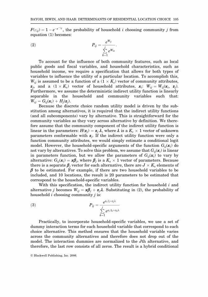
F("ij) ¼ 1� e�e�"ij , the probability of household i choosing community j fromequation (1) becomes:

Pij ¼eWij

Pj

k¼1

eWik

:ð2Þ

To account for the influence of both community features, such as localpublic goods and fiscal variables, and household characteristics, such ashousehold income, we require a specification that allows for both types ofvariables to influence the utility of a particular location. To accomplish this,Wij is assumed to be a function of a (1 � Kz) vector of community attributes,zj, and a (1 � Kx) vector of household attributes, xi: Wij ¼ Wij(xi, zj).Furthermore, we assume the deterministic indirect utility function is linearlyseparable in the household and community variables such that:Wij ¼ Gij(xi) þ Hj(zj).

Because the discrete choice random utility model is driven by the sub-stitution among alternatives, it is required that the indirect utility functions(and all subcomponents) vary by alternative. This is straightforward for thecommunity variables as they vary across alternative by definition. We there-fore assume that the community component of the indirect utility function islinear in the parameters: H(zj) ¼ zj l, where l is a Kz � 1 vector of unknownparameters conformable with zj. If the indirect utility function were only afunction community attributes, we would simply estimate a conditional logitmodel. However, the household-specific arguments of the function Gij(xi) donot vary by alternatives. To solve this problem, we assume that Gij(xi) is linearin parameters function, but we allow the parameters of Gij(xi) to vary byalternative: Gij(xi) ¼ xbj, where bj is a Kx � 1 vector of parameters. Becausethere is a separate bj vector for each alternative, there are J � Kx elements ofb to be estimated. For example, if there are two household variables to beincluded, and 10 locations, the result is 20 parameters to be estimated thatcorrespond to the household-specific variables.

With this specification, the indirect utility function for household i andalternative j becomes Wij ¼ xbj þ zj l. Substituting in (2), the probability ofhousehold i choosing community j is:

Pij ¼exi�jþzjl

Pj

k¼1

exi�kþzkl

ð3Þ

Practically, to incorporate household-specific variables, we use a set ofdummy interaction terms for each household variable that correspond to eachchoice alternative. This method ensures that the household variable variesacross the community alternatives and therefore does not drop out of themodel. The interaction dummies are normalized to the Jth alternative, andtherefore, the last row consists of all zeros. The result is a hybrid conditional



logit model that is able to consider the effects of both alternative-specificfeatures and household-level characteristics on the community choice of ahousehold.

A final estimation issue is the specification of the choice set. For thepurpose of our study, we seek a delineation of geographical space that yieldsa reasonable amount of homogeneity in the characteristics of each location.According to these criteria, the best alternative is to define the school districtsas the unit of community choice. School districts are comprised of one or moretax districts and most often match the boundaries of a local jurisdiction.

4. DATA AND MODEL SPECIFICATION

The multinomial choice model of residential location is estimated usingdata on homeowners living in the central county of the Columbus metropolitanarea, Franklin County. Franklin County comprises 66 percent of the metropo-litan population with just over 1 million (1,068,978) population in 2000. Inaddition to the City of Columbus, which comprises 67 percent of the populationin Franklin County and is almost fully contained within the county, there are44 other local jurisdictions located within the county. These include approxi-mately 10 suburban cities, some of which are highly desirable locations with topschool districts, and 17 unincorporated township areas. Unlike many centralcounties, Franklin County’s population has continued to grow in recent dec-ades, increasing by 11 percent between 1990 and 2000. Just over half thepopulation moved at least once between 1995 and 2000, 65 percent of whichmoved from within Franklin County. Despite population gains, the countyexperienced a modest loss in net migration (2.8 percent) between 1990 and2000 with an estimated 440,000 people moving out of Franklin County.

To estimate the model, we use a unique dataset that was compiled byresearchers at the Ohio State University and Cleveland State University.4

Using deed transfer records for 2,074 households that undertook a movewithin Franklin County in 1995, researchers matched the location of housesbought and sold within this study area. In addition, a survey was conducted ofthese homeowners who undertook a move from one home to another withinFranklin County in 1995. Our model is estimated with data from the 824households that were surveyed. Of these surveyed households, 20 percentare minorities (defined as non-Caucasian households), 77 percent are married,54 percent have one or more children, and the average annual income isbetween $60,000 and $80,000. The average age is 44.5 years and 42.6 yearsfor males and females respectively. Seventy-nine percent of the heads of

4The matched deed transfer data were made available by the Ohio Housing ResearchNetwork. Additional survey data were collected by Hazel Morrow-Jones, Associate Professor inCity and Regional Planning at Ohio State University. Support for the research was provided bythe Ohio State University Urban Affairs Committee and Ohio Center for Real Estate Educationand Research.



households attended college. In comparing the previous and current homes,the average household moved ‘‘up’’ in terms of lot size and house value: lot sizeincreased by an average of 10 percent and house value by an average of 25.6percent. Although almost three-fourths of the households moved ‘‘outward’’from the city to a suburb or from an inner to outer suburb, about one-fifth ofthe households moved to the city. Of these city moves, almost two-thirdsoriginated from the city. Only 6 percent of the households engaged in ‘‘inward’’moves from an outer to inner suburb or from a suburb to the city.

Although data on repeat homeowners are limited in some ways, they areuseful in others. First, they comprise the majority of homebuyers nationwide inany given year and thus their choices have substantial impacts on overall homebuying and residential location trends. Second, because they are more experi-enced and are likely to have higher incomes, they are more likely to have abetter idea of their preferences and the resources to realize those preferences(Morrow-Jones, 2002). However, because the data only include households whosold and bought homes in Franklin County in 1995, it does not contain first-time homebuyers or households who moved across county lines or who movedto, from, or between rental units. Despite these limitations, the data appear tobe reasonably representative. A comparison of selected household characteris-tics with data from the 2002 American Housing Survey on homebuyers living inthe primary central city area of the Columbus MSA revealed no significantdifferences in income, but some significant differences in age (surveyed home-owners were significantly older by 1 to 2.5 years on average) and marital status(a higher proportion of the surveyed households were married). Other researchusing these data compared the geographic distribution and average home salesprice of the surveyed households with that of the buyer–seller matched popula-tion and found no significant differences (Morrow-Jones, 2002).

The empirical choice model is estimated with five types of variables, thefirst four of which are measured at the school district (community) level andthe last of which varies across individual households: (i) level and quality oflocal public service and fiscal variables, (ii) private consumption opportunitiesand job accessibility, (iii) socio-economic characteristics of the population, (iv)physical features of the community, and (v) income and lifecycle characteris-tics of the household. To account for the quality of the services provided bylocal governments, we incorporate variables that are proxies for these mainservices. First, the level of public safety in the school district is proxied by theestimated total number of crimes in the school district.5 Even though nodistinction is made among the types of crimes committed, this aggregatestatistic is expected to be highly negatively correlated with the overall levelof public safety experienced by residents living in each school district. Weexpect that this variable will have a negative effect on the likelihood that a

5This variable was aggregated to the school district level from an estimate of total crimesper block group based on population data and data from the FBI Uniform Crime Report. Theseestimates were obtained from Applied Geographic Systems: http://www.appliedgeographic.com.



household moves to a particular community. Second, the quality of publicschools is measured using an aggregate school performance measure definedas the average test score of students in the ninth grade on standardizedEnglish and mathematics tests.6 Increases in school quality are expected toattract households to a community, and thus, we expect this variable to have apositive effect on the probability of community choice. Finally, the level oftaxes in a jurisdiction reflects the price that households must pay for thevariety of public goods that are locally provided. In Ohio, the major tax paidby households is the property tax. This tax rate is included in the model as apartial measure of the entry price associated living in a particular locality. Inaddition to the local property tax, homeowners are also charged a property taxat the school district level. In Ohio, schools are partially financed throughtaxes levied at the school district level. Holding the quantity and quality oflocal public services (including school quality) constant, it is expected thathigher taxes will deter a household from moving to a particular jurisdiction.

In addition to local public services and fiscal variables, access to privategoods and job opportunities are hypothesized to increase the likelihood that ahousehold chooses a particular community. Access to private goods consump-tion is measured by the number of retail establishments per capita in thecommunity.7 Job accessibility is measured by the number of business estab-lishments per capita in the community and average commuting time toColumbus’ downtown center. Because Columbus is the state capitol and thecapitol building is located downtown, a relatively high proportion of jobs arelocated in the downtown area.8 Thus, although Columbus has its share of edgecities and dispersed employment as well, commuting distance to the citycenter is still a relevant measure of job accessibility. Rather than attemptingto define other employment subcenters and measure proximity to these addi-tional centers, we capture the positive effects of a suburban subcenter withinthe same community by the measure of total business establishments.

Households are hypothesized to have preferences over the socioeconomiccomposition of a community.9 Median per capita household income is includedas a primary characteristic of the existing population. All else equal, we expect

6These data are compiled by the State of Ohio’s Department of Education and madeavailable publicly on their ‘‘Local Report Card’’ website: http://www.ode.state.oh.us.

7Data on the number and of retail and other businesses were obtained from AppliedGeographic Information Systems (AGS): http://www.appliedgeographic.com. These data are esti-mated counts at the block group level, based on data from the Economic Census, sales tax receipts,and other sources.

8Glaeser, Kahn, and Chu (2001) calculate that close to 20 percent of the metropolitan jobs inColumbus are located within a 3-mile ring of the city center and over 60 percent are located withina 10-mile ring. Relative to other metropolitan areas, they rank Columbus as a ‘‘centralizedemployment metro.’’

9The remaining variables are all from the 1990 Census of Population. To construct thesemeasures at the school district level, a spatial aggregation method implemented by ArcView GISsoftware was used to aggregate from block groups to school districts.



that this would have a positive influence on a household’s location choice,although this sign may depend on the particular sample of households thatundertake a move. If households tend to sort themselves into homogeneousgroups within locations, then income would have a positive effect if theobserved sample of movers is above average in income. To account for vari-ations in the distribution of incomes across communities, we include twoadditional measures. The proportion of households with annual incomes of$15,000 or less is included as a measure of the poverty level within a commu-nity. Conversely, the proportion of households with incomes of $75,000 ormore is included to capture the extent to which high-income housing andhouseholds are located in the community. We omit a measure of racial compo-sition because, other than the city district, which is comprised of 27 percentAfrican Americans, the other school districts are relatively homogeneous(ranging from 1 to 6 percent African American composition). This omissionis not because we believe that race is not an issue in the suburbanizationprocess, but rather due to statistical difficulties in estimating a relationshipgiven the lack of variation in racial composition across the choice set.

We include two measures of the physical environment that are hypothe-sized to influence household community choice. First, the literature suggests aclear preference among households for newer housing stock. The proportion ofhousing units that are at least 25 years old (built before 1970) is included as aproxy for the age of the neighborhood’s housing stock. Second, populationdensity is included to control for the varying levels of density that exist acrossschool districts. The sign of this variable is an empirical question: a positivesign could indicate that there are positive agglomeration economies associatedwith higher-density living whereas a negative sign may signal congestioneffects. This variable is specified in its logarithmic form.

The last set of variables are household-specific variables. Because house-holds are not homogeneous in their income levels and because householdsoften sort themselves according to their ability to pay for housing and localpublic services, it is important to include household-specific information onincome levels. Data on the approximate income level of the surveyed house-holds are available to us. This variable is a categorical variable that repre-sents a corresponding range of income for each household. It varies from 2 to12 and represents increasing levels of income in $20,000 increments. In add-ition to income, the presence or absence of school-aged children is included asa measure of a household’s lifecycle stage. Information on the number andages of children within the household is also available to us from the survey.We use this information to construct a dummy variable that is defined as 1 ifthere the household has at least one child between ages 5 and 18 and 0otherwise. Ideally, we would include additional household-specific variables,such as age of head of household and race, but when we include more than twohousehold-specific attributes, the model has problems with convergence.Thus, we focus on what we believe are the two primary sources of heteroge-neity among households, income, and presence of school-aged children and



assume that other characteristics of households in our sample do not system-atically influence their location choices.

There are a total of 17 school districts that are either fully or partiallyencompassed within the Franklin County boundary and that comprise ourchoice set. These districts exhibit a substantial range in terms of size, schoolquality, crime rate, income, and the other features of residential locationdiscussed above. Table 1 reports the median values of selected school districtvariables and the total number of households surveyed that moved to each ofthe locations.

5. ESTIMATION RESULTS AND DISCUSSION

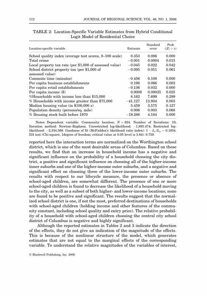
Table 2 reports the estimated coefficients for the community-level vari-ables from the hybrid conditional logit model specified in Equation (3). All fourfiscal variables are found to be significant and of the expected sign. Highercrime levels and higher property taxes (at both the local and the school districtlevels) are estimated to have a negative effect on a household’s probability ofchoosing a locality, whereas school quality is estimated to have a positiveeffect on household choice. Job accessibility, as measured by both commutingtime to the downtown district and total business establishments per capitawithin a community, is positively associated with household location deci-sions. The probability of a household choosing a community increases withshortened commute time to downtown and more business establishments inthe community. Access to private goods, as measured by the number of retailestablishments per capita, is found to have a negative impact on housingchoice. Although this is inconsistent with our prior expectations, it is possiblethat this variable is correlated with congestion levels within a community.Two of the three income variables are found to be significant. Per capitaincome of a community has a positive influence on household choice, whereasthe proportion of high-income households (with incomes of $75,000 or greater)is found to decrease the probability that a household chooses a community.This result likely reflects the fact that many households are priced out ofhigher-income communities, and thus, households with average income levelsare less likely to choose these more exclusive communities. Lastly, populationdensity is found to be positive and significant, as is the proportion of newerhousing stock in a community. The positive sign associated with populationdensity may indicate positive agglomeration economies or may simply be dueto the fact that a place with a larger population is more likely to attractadditional households, all else equal.

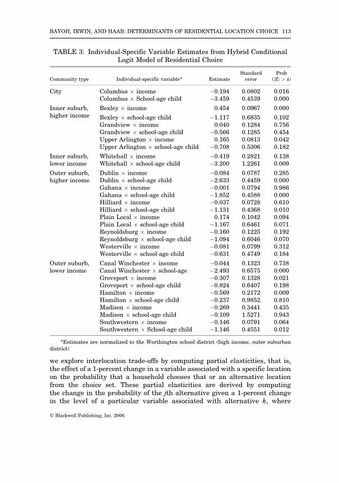
Table 3 reports the influence of the individual-specific terms on householdlocation choices. Because of the dummy interaction approach that allows theseterms to be included in the conditional logit model, the model generatesestimates of location-specific parameters, normalized to a particular location,for each of these individual variables. Therefore each individual-specific vari-able has J � 1 (in this case, 16) estimates associated with it. In the results



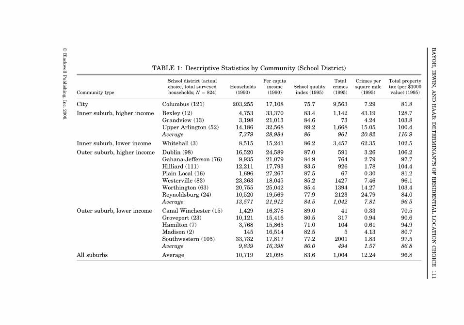
TABLE 1: Descriptive Statistics by Community (School District)

Community type

School district (actualchoice, total surveyedhouseholds; N ¼ 824)

Households(1990)

Per capitaincome(1990)

School qualityindex (1995)

Totalcrimes(1995)

Crimes persquare mile

(1995)

Total propertytax (per $1000value) (1995)

City Columbus (121) 203,255 17,108 75.7 9,563 7.29 81.8

Inner suburb, higher income Bexley (12) 4,753 33,370 83.4 1,142 43.19 128.7Grandview (13) 3,198 21,013 84.6 73 4.24 103.8Upper Arlington (52) 14,186 32,568 89.2 1,668 15.05 100.4Average 7,379 28,984 86 961 20.82 110.9

Inner suburb, lower income Whitehall (3) 8,515 15,241 86.2 3,457 62.35 102.5

Outer suburb, higher income Dublin (98) 16,520 24,589 87.0 591 3.26 106.2Gahana-Jefferson (76) 9,935 21,079 84.9 764 2.79 97.7Hilliard (111) 12,211 17,793 83.5 926 1.78 104.4Plain Local (16) 1,696 27,267 87.5 67 0.30 81.2Westerville (83) 23,363 18,045 85.2 1427 7.46 96.1Worthington (63) 20,755 25,042 85.4 1394 14.27 103.4Reynoldsburg (24) 10,520 19,569 77.9 2123 24.79 84.0Average 13,571 21,912 84.5 1,042 7.81 96.5

Outer suburb, lower income Canal Winchester (15) 1,429 16,378 89.0 41 0.33 70.5Groveport (23) 10,121 15,416 80.5 317 0.94 90.6Hamilton (7) 3,768 15,865 71.0 104 0.61 94.9Madison (2) 145 16,514 82.5 5 4.13 80.7Southwestern (105) 33,732 17,817 77.2 2001 1.83 97.5Average 9,839 16,398 80.0 494 1.57 86.8

All suburbs Average 10,719 21,098 83.6 1,004 12.24 96.8

BA

YO

H,

IRW

IN,

AN

DH

AA

B:

DE

TE

RM

INA

NT

SO

FR

ES

IDE

NT

IAL

LO

CA

TIO

NC

HO

ICE

111

#B

lack

well

Pu

blish

ing,

Inc.

2006.

reported here the interaction terms are normalized on the Worthington schooldistrict, which is one of the most desirable areas of Columbus. Based on theseresults, we find that an increase in household income has a negative andsignificant influence on the probability of a household choosing the city dis-trict, a positive and significant influence on choosing all of the higher-incomeinner suburbs and one of the higher-income outer suburbs, and a negative andsignificant effect on choosing three of the lower-income outer suburbs. Theresults with respect to our lifecycle measure, the presence or absence ofschool-aged children, are somewhat different. The presence of one or moreschool-aged children is found to decrease the likelihood of a household movingto the city, as well as a subset of both higher- and lower-income locations; noneare found to be positive and significant. The results suggest that the normal-ized school district is one, if not the most, preferred destinations of householdswith school-aged children (holding income and other features of the commu-nity constant, including school quality and entry price). The relative probabil-ity of a household with school-aged children choosing the central city schooldistrict of Columbus is negative and highly significant.

Although the reported estimates in Tables 2 and 3 indicate the directionof the effects, they do not give an indication of the magnitude of the effects.This is because of the nonlinear structure of the model, which generatesestimates that are not equal to the marginal effects of the correspondingvariable. To understand the relative magnitudes of the variables of interest,

TABLE 2: Location-Specific Variable Estimates from Hybrid ConditionalLogit Model of Residential Choice

Location-specific variable EstimateStandard

errorProb

(jZj > z)

School quality index (average test scores, 0–100 scale) 0.353 0.086 0.000Total crime �0.001 0.0004 0.015Local property tax rate (per $1,000 of assessed value) �0.045 0.022 0.042School district property tax (per $1,000 ofassessed value)

�0.095 0.051 0.061

Commute time (minutes) �0.456 0.108 0.000Per capita business establishments 0.198 0.066 0.003Per capita retail establishments �0.136 0.032 0.000Per capita income ($) 0.0008 0.00035 0.025%Households with income less than $15,000 8.162 7.699 0.289% Households with income greater than $75,000 �41.127 13.804 0.003Median housing value (in $100,000 s) 5.459 3.575 0.127Population density (persons/sq. mile) 0.006 0.003 0.068% Housing stock built before 1970 �19.286 4.184 0.000

Notes: Dependent variable: Community location; N ¼ 824. Number of Iterations: 10;Iteration method: Newton–Raphson. Unrestricted log-likelihood: �1,895.474; Restricted log-likelihood: �2,334.568. Goodness of fit (McFadden’s likelihood ratio index): 1 � Lr /Lu ¼ 0.1854.IIA test (Chi-square, 1degree of freedom; critical value at 0.05 level is 3.84): 0.759.



we explore interlocation trade-offs by computing partial elasticities, that is,the effect of a 1-percent change in a variable associated with a specific locationon the probability that a household chooses that or an alternative locationfrom the choice set. These partial elasticities are derived by computingthe change in the probability of the jth alternative given a 1-percent changein the level of a particular variable associated with alternative k, where

TABLE 3: Individual-Specific Variable Estimates from Hybrid ConditionalLogit Model of Residential Choice

Community type Individual-specific variable* EstimateStandard

errorProb

(jZj > z)

City Columbus � income �0.194 0.0802 0.016Columbus � School-age child �3.459 0.4539 0.000

Inner suburb,higher income

Bexley � income 0.454 0.0967 0.000

Bexley � school-age child �1.117 0.6835 0.102Grandview � income 0.040 0.1284 0.756Grandview � school-age child �0.566 0.1285 0.454Upper Arlington � income 0.165 0.0813 0.042Upper Arlington � school-age child �0.708 0.5306 0.182

Inner suburb,lower income

Whitehall � income �0.419 0.2821 0.138Whitehall � school-age child �3.200 1.2261 0.009

Outer suburb,higher income

Dublin � income �0.084 0.0787 0.285Dublin � school-age child �2.633 0.4459 0.000Gahana � income �0.001 0.0794 0.986Gahana � school-age child �1.852 0.4588 0.000Hilliard � income �0.037 0.0728 0.610Hilliard � school-age child �1.131 0.4368 0.010Plain Local � income 0.174 0.1042 0.094Plain Local � school-age child �1.167 0.6461 0.071Reynoldsburg � income �0.160 0.1225 0.192Reynoldsburg � school-age child �1.094 0.6046 0.070Westerville � income �0.081 0.0799 0.312Westerville � school-age child �0.631 0.4749 0.184

Outer suburb,lower income

Canal Winchester � income �0.044 0.1323 0.738Canal Winchester � school-age �2.493 0.6575 0.000Groveport � income �0.307 0.1328 0.021Groveport � school-age child �0.824 0.6407 0.198Hamilton � income �0.569 0.2172 0.009Hamilton � school-age child �0.237 0.9852 0.810Madison � income �0.269 0.3441 0.435Madison � school-age child �0.109 1.5271 0.943Southwestern � income �0.146 0.0791 0.064Southwestern � School-age child �1.146 0.4551 0.012

*Estimates are normalized to the Worthington school district (high income, outer suburbandistrict)



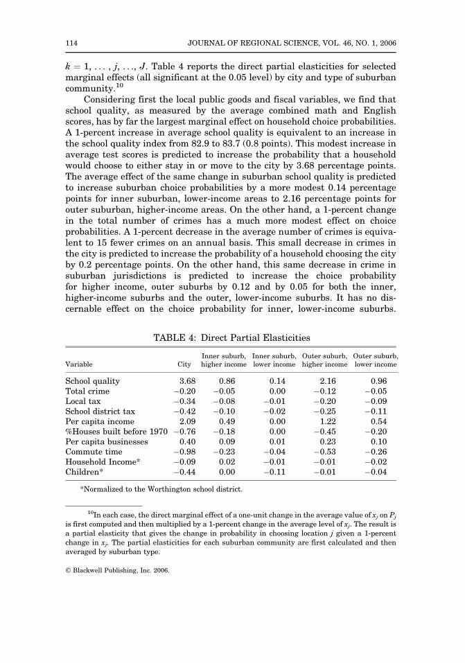
k ¼ 1, . . . , j, . . ., J. Table 4 reports the direct partial elasticities for selectedmarginal effects (all significant at the 0.05 level) by city and type of suburbancommunity.10

Considering first the local public goods and fiscal variables, we find thatschool quality, as measured by the average combined math and Englishscores, has by far the largest marginal effect on household choice probabilities.A 1-percent increase in average school quality is equivalent to an increase inthe school quality index from 82.9 to 83.7 (0.8 points). This modest increase inaverage test scores is predicted to increase the probability that a householdwould choose to either stay in or move to the city by 3.68 percentage points.The average effect of the same change in suburban school quality is predictedto increase suburban choice probabilities by a more modest 0.14 percentagepoints for inner suburban, lower-income areas to 2.16 percentage points forouter suburban, higher-income areas. On the other hand, a 1-percent changein the total number of crimes has a much more modest effect on choiceprobabilities. A 1-percent decrease in the average number of crimes is equiva-lent to 15 fewer crimes on an annual basis. This small decrease in crimes inthe city is predicted to increase the probability of a household choosing the cityby 0.2 percentage points. On the other hand, this same decrease in crime insuburban jurisdictions is predicted to increase the choice probabilityfor higher income, outer suburbs by 0.12 and by 0.05 for both the inner,higher-income suburbs and the outer, lower-income suburbs. It has no dis-cernable effect on the choice probability for inner, lower-income suburbs.

TABLE 4: Direct Partial Elasticities

Variable CityInner suburb,higher income

Inner suburb,lower income

Outer suburb,higher income

Outer suburb,lower income

School quality 3.68 0.86 0.14 2.16 0.96Total crime �0.20 �0.05 0.00 �0.12 �0.05Local tax �0.34 �0.08 �0.01 �0.20 �0.09School district tax �0.42 �0.10 �0.02 �0.25 �0.11Per capita income 2.09 0.49 0.00 1.22 0.54%Houses built before 1970 �0.76 �0.18 0.00 �0.45 �0.20Per capita businesses 0.40 0.09 0.01 0.23 0.10Commute time �0.98 �0.23 �0.04 �0.53 �0.26Household Income* �0.09 0.02 �0.01 �0.01 �0.02Children* �0.44 0.00 �0.11 �0.01 �0.04

*Normalized to the Worthington school district.

10In each case, the direct marginal effect of a one-unit change in the average value of xj on Pj

is first computed and then multiplied by a 1-percent change in the average level of xj. The result isa partial elasticity that gives the change in probability in choosing location j given a 1-percentchange in xj. The partial elasticities for each suburban community are first calculated and thenaveraged by suburban type.



Lastly, a 1-percent change in the local and school district property tax rates isfound to have a moderately negative influence on household choice probabil-ities, ranging from a decrease in the probability of choosing the city of 0.42percentage points given a 1-percent increase in the school district tax toessentially no discernable effect on some of the other choice probabilitiesassociated with suburban areas.

Marginal changes in other neighborhood variables are also found to havea substantial influence on choice probabilities. The marginal effect of a1-percent change in per capita income is relatively large. A 1-percent increasein per capita income levels would raise per capita income levels by $209 onaverage, from $20,863 to $21,071. This increase in the city’s per capita incomelevel would increase the probability a household chooses the city by 2.1percent. This same increase in average per capita income levels for outer,higher-income suburbs would increase the choice probability for these loca-tions by 1.2 percent and would have more moderate effects on the probabilityassociated with other suburban locations. Interestingly, this change in aver-age income levels appears to have no discernable effect on the choice prob-ability associated with inner, lower-income suburbs. A 1-percent increase inthe proportion of houses that are 25 years or older would increase the averagepercent of older homes in a jurisdiction by 0.3 percentage points from 31.5 to31.8. This small increase in the relative number of older homes in the citydecreases the probability that a household chooses the city by an estimated0.76 percent. The same increase in the proportion of older houses in thesuburbs is predicted to have more modest effects, ranging from no discernableeffect on the choice probability associated with inner, lower-income suburbsto a 0.45 decrease in the probability associated with outer, higher-incomesuburbs.

Changes in the distribution of jobs have an impact on household choiceprobabilities. A 1-percent increase in the total number of business establish-ments per capita would increase the average number of businesses per personby 0.16. This effect on the probability of a household choosing a particularcommunity is positive, ranging from an increase in the choice probabilityassociated with the city of 0.4 percentage points to 0.1 for some of the sub-urban areas. A 1-percent increase in the average commute time, from 17.1 to17.3 minutes, has a discernable effect on choice probabilities. Such an increaselowers the probability of a household choosing a city location by about 1percent and lowers the probability of choosing a suburban location by any-where from 0.04 to 0.53 percent.

Comparing the relative influence of the public service variables withother neighborhood variables on the city choice probability, the marginaleffect associated with an increase in school quality in the city is five timesthe magnitude of the negative effect associated with the proportion of olderhouses and almost 20 times the marginal effect of total crimes. In turn, themarginal effect of crime is more than twice the magnitude of the marginaleffect of per capita income levels. On the other hand, the marginal effect of



school district taxes is twice the magnitude of the crime effect and roughly equalin magnitude to the marginal effect of the number of business establishments.

Finally, we consider the partial elasticities associated with the two house-hold-specific variables. A 1-percent increase in average household income(from approximately $77,400 to $78,274) is estimated to decrease the citychoice probability by 0.09 percentage points relative to the Worthington schooldistrict (a higher-income, outer suburb). The effect of the same increase inhousehold income on the choice probability of suburban locations is found tobe relatively negligible, suggesting that these variables do not have a stronginfluence on distinguishing these suburban locations from the normalizedsuburban location. On the other hand, an increase in the household’s numberof school-age children by one decreases the probability a household choosesthe city by 0.44 percentage points (holding school quality and other variablesin the model constant and again, relative to the Worthington school district).The effect of an increase in the number of school-aged children on suburbanchoice probabilities is smaller. Relative to the normalized school district, thechoice probability associated with the higher-income suburbs remains essen-tially unchanged. The effect on the lower income suburbs is to reduce theirchoice probabilities relative to the normalized location by 0.04 to 0.11 percen-tage points.

So far our discussion of the results reveals school quality as being thelargest single explanation of community choice. However, this is based on verysmall, marginal adjustments and ignores the fact that wide variations existbetween city and suburban service levels. Because the ‘‘flight from blight’’hypothesis poses these differences as a substantial driver of suburbanization,it is useful to investigate how equalization of these key community character-istics across the city and suburban areas would influence the city choiceprobability.11 To carry out this exercise, we first calculate the average suburbanvalues of these variables and then calculate the percentage change in the cityvalues of these variables necessary to achieve these average suburban levels.The predicted increases in household choice probabilities are then calculatedusing the estimated partial elasticities reported in Table 4. Table 5 reports theresults of this exercise.

We find that equalization of school quality across, which is 10.2 percentlower in the city than the average suburban school quality, would increase theprobability that a household chooses a city residence by 37.5 percent. Bycomparison, if the total number of crimes committed in the city dropped tothe average suburban level, which is a substantial decrease of almost 90

11If such nonmarginal changes were to occur in reality, land and housing markets wouldadjust by bidding up prices in the city and offsetting the predicted impact on household choiceprobabilities. Because our analysis is limited to a partial equilibrium framework, we are unable toconsider such adjustments. Assuming, however, that markets would react in a similar way to anyimprovement in a city service, then the comparison of the magnitudes of change in predictedchoice probabilities across the different scenarios is nonetheless instructive.



percent, the city choice probability would increase by 18 percent. The greatestincrease in the probability that a household chooses a city location is fromequalization of the per capita income levels. A 23 percent increase in percapita income levels in the city to the average suburban level would increasethe probability that a household chooses the city by almost 65 percent. Thus,even though the variation in city–suburban crime density is larger than thecorresponding variation in school quality or per capita income, eliminatingdifferences in crime across the city and suburbs is not found to have as strongan effect on the city choice probability as is eliminating the school quality orper capita income differences. This is simply because the marginal effectsassociated with these variables are substantially larger. It is interesting tocompare a final equalization scenario: equalization of city and suburban aver-age tax burdens. In this case, Columbus’ combined property taxes from thecity and school district are 18 percent lower than the corresponding averagesuburban tax burden. Raising the city tax rate by this amount decreases theprobability that a household chooses the city by 11 percent, which is substan-tially less in magnitude than the school quality or per capita income equal-ization scenarios. Put differently, suppose an equalization of school qualityacross the city and suburbs induced 1,000 additional households to stay in thecity versus move out. By comparison, an equalization of crime across the cityand suburbs would result in the retention of 477 households in the city,whereas an equalization of average income levels would lead to a total of1,728 households remaining in the city. By comparison, an equalization oftax rates between the city and suburbs would result in a loss of an additional293 households from the city.

6. SUMMARY AND CONCLUSION

We investigate the specific determinants of household location decisionsusing a discrete choice model of household community choice that accounts forboth community characteristics and household-level attributes. The estimatedmarginal effects from the model are used to draw inferences regarding theextent to which suburbanization may be driven by a process of natural

TABLE 5: City–Suburb Equalization Scenarios

Equalization scenario City value

Averagesuburban

value

Hypotheticalpercent change

in city value

Predicted changein city choiceprobability

School quality (0–100 index) 75.7 83.4 10.2 37.5Total crimes 9,563 1,003 �89.5 17.9Per capita income ($) 17,108 21,098 23.3 64.8Total property tax (per $1000 value) 81.8 96.4 17.9 �11.0% Houses built before 1970 44.0 31.0 �30.1 22.9



evolution versus flight from blight. We find strong evidence of the importanceof local public goods—most notably, school quality—as well as taxes andsocioeconomic features of the population. Most of the factors that relate to anatural evolution process of suburbanization, namely job location, accessibil-ity, residential filtering, and individual income and lifecycle effects, were alsofound to be significant determinants of household choice. However, with theexception of the housing stock age and commuting time, both of which werefound to have relatively substantial effects, the magnitudes of the naturalevolution effects were substantially smaller. Based on this evidence, we con-clude that community choice decisions of households in our study area aredriven more by factors associated with a flight-from-blight process of subur-banization than one of natural evolution.

In attempting to discern these effects, there are a number of limitations ofthis study. Primary among these is the fact that we observe only a snapshot intime and therefore cannot account for changes over time that are sure to havelarge effects on the suburbanization process. For example, like all metropolitanareas, the state and federal government has made enormous investments inbuilding highways and roads in the Columbus area. These investments havefundamentally shaped the evolution of urban form over time, but we are unableto capture such effects using cross-sectional data. A second limitation is theconditional nature of the results. Because we do not estimate a full model ofhome selling and buying decisions, the results are conditional on the fact that ahousehold is already a homeowner and has decided to engage in a move. Datameasurement problems are a third limitation. Unfortunately, most of our dataare not available at the school district level. Fortunately, it is available at asmaller unit of geography (Census block groups), which allows us to use aGeographic Information System (GIS) to aggregate to the school district level.However, because school district and block group boundaries do not correspond,this aggregation is inexact and our method almost certainly introduces measure-ment error that could lead to spatial error dependence in our model. Correctingfor spatial error dependence in a multinomial discrete choice model such as oursis computationally quite difficult. So far, there are relatively few attempts in theliterature to do this and none to our knowledge in the housing literature.Because significant spatial error can lead to inconsistent estimates in a discretechoice model, our results must be viewed with this limitation in mind.

Despite these limitations, the study is useful as it is the first to provide acomparison of the relative magnitudes of a number of variables associatedwith the natural evolution and flight from blight theories of suburbanizationwithin the context of a household choice model. In comparison with Nechybaand Strauss (1997), the only other recent household choice study that we areaware of that has explicitly focused on the influence of local fiscal and publicservice variables, our estimated elasticities for school quality and crime areconsistent with their findings both in sign and in approximate magnitude. Inaddition, we find support for a number of other factors not considered in theirmodel, such as neighborhood income levels, the age of the housing stock, and



access to jobs. Lastly, by including household-specific variables, we are able tocompare how heterogeneity in individuals versus communities influenceshouseholds’ choice probabilities.

The results have policy implications at both the city and the regional levels.From a perspective of attracting residents to the city, our results show that thereare a number of policy levers that the city can attempt to manipulate to influencein-migration. Rather than a process of natural evolution, which would imply thatthe suburbanization process may be largely out of the direct reach of localpolicies, the findings show that there are a number of community characteristicsthat are directly determined by local policies that influence the suburbanizationprocess. Second, if the relative magnitudes of the estimated choice elasticitiesand the scenarios are meaningful, these results suggest that the costs (in termsof population loss) of raising city residential property taxes are far less than thebenefits (in terms of population gain) of increasing school quality and publicsafety levels. In other words, if additional tax revenues could be used effectivelyto reduce crime and increase school quality, our results suggest that on net, out-migration to the suburbs will decrease. Third, in comparing the magnitudes ofthe job accessibility measures with those of neighborhood quality, our resultsindicate that high-quality public services and neighborhood quality have astronger pull on potential homeowners than does the location of jobs.

From a regional perspective, the results provide a rationale for centralcity investment by higher governments if negative externalities are associatedwith flight from blight. Although this is ultimately an empirical question thatis yet to be fully answered, the existing empirical literature provides someevidence that concentrating fiscal and social problems generates even higherlevels of poverty, unemployment, and other social problems. If present, thesenegative externalities will increase the social costs associated with living inthe city, and to the extent that spillovers affect adjacent suburbs or that citydecline retards regional growth, they will generate social costs that areabsorbed by suburban residents as well. In this case, the resulting distributionof lower- and higher-income households is inefficient and central city invest-ments to slow suburbanization are warranted on efficiency grounds.

REFERENCES

Anas, A. 1992. Residential Location Markets and Urban Transportation. New York: AcademicPress.

Boehm, T. P., H. W. Herzog, and A. M. Schlottmann. 1991. ‘‘Intra-Urban Mobility, Migration andTenure Choice,’’ Review of Economics and Statistics, 73, 59–68.

Bogart, W. T., and B. A. Cromwell. 2000. ‘‘How Much Is a Neighborhood School Worth?,’’ Journalof Urban Economics, 47, 280–305.

Bradford, D. F., and H. H. Kelejian. 1973. ‘‘An Econometric Model of the Flight to the Suburbs,’’Journal of Political Economy, 81(3), 566–589.

Bruecker, J. 2000. ‘‘Urban Sprawl: Diagnosis and Remedies,’’ International Regional ScienceReview, 23(2), 160–171.



Clark, W., and J. L. Onaka. 1983. ‘‘Life-Cycle And Housing Adjustment as Explanations ofResidential-Mobility,’’ Urban Studies, 20(1), 47.

Cullen, J. B., and S. D. Levitt. 1999. ‘‘Crime, Urban Flight, and the Consequences for Cities,’’Review of Economics and Statistics, 81(2), 159–169.

Cutler, D. M., and E. L. Glaeser. 1997. ‘‘Are Ghettos Good or Bad?,’’ Quarterly Journal ofEconomics, 112(3), 827–872.

Dills, A. K. 2005. ‘‘Does Cream-Skimming Curdle the Milk? A Study of Peer Effects,’’ Economics ofEducation Review, 24(1), 19–28.

Evans, W. N., W. E. Oates, and R. M. Schwab. 1992. ‘‘Measuring Peer Group Effects: A Study ofTeenage Behavior,’’ Journal of Political Economy, 100, 966–991.

Gaviria, A., and S. Raphael. 2001. ‘‘School-Based Peer Effects and Juvenile Behavior,’’ Review ofEconomics and Statistics, 83(2), 257–268.

Glaeser, E., M. Kahn, and C. Chu. 2001. Job Sprawl: Employment Location in U.S. MetropolitanAreas. The Brookings Institute Survey Series, May: 1–8.

Friedman, J. 1981. ‘‘A Conditional Logit Model of the Role of Local Public Services in ResidentialChoices,’’ Urban Studies, 18, 347–358.

Leichenko, R. 2001. ‘‘Growth and Change in U.S. Cities and Suburbs,’’ Growth and Change, 32,326–354.

Margo, R. 1992. ‘‘Explaining the Postwar Suburbanization of Population in the United States: TheRole of Income,’’ Journal of Urban Economics, 31, 301–310.

Mieszkowski, P., and E. Mills. 1993. ‘‘The Causes of Metropolitan Suburbanization,’’ Journal ofEconomics Perspectives, 7(3), 135–147.

Mills, E., and R. Price. 1984. ‘‘Metropolitan Suburbanization and Central City Problems,’’ Journalof Urban Economics, 15(1), 1–17.

Morrow-Jones, H. 2002. ‘‘Homeowner Decisions and the Thinning Metropolis,’’ in Proceedings of theThinning Metropolis Conference, co-sponsored by the Brookings Institution, Cornell Universityand the Lincoln Land Institute. September 2000. CD-ROM available from Cornell University.

Nechyba, T., and R. P. Strauss. 1997. ‘‘Community Choice and Local Public Services: A DiscreteChoice Approach,’’ Regional Science and Urban Economics, 28, 51–73.

Persky, J., and H. Kurban. 2003. ‘‘Do Federal Spending and Tax Policies Build Cities or PromoteSprawl?,’’ Regional Science and Urban Economics, 33, 361–378.

Quigley, J. M. 1976. ‘‘Housing Demand in the Short Run: An Analysis of Polytomous Choice,’’Explorations in Economic Research, 13, 76–102.

———. 1985. ‘‘Consumer Choice of Dwelling, Neighborhood and Public Services,’’ Regional Scienceand Urban Economics, 15, 41–63.

Rapaport, C. 1997. ‘‘Housing Demand and Community Choice: An Empirical Analysis,’’ Journal ofUrban Economics, 42, 243–260.

Rossi, P. 1955. Why Families Move, 2nd ed. Beverly Hills: Sage Publications.Savitch, H. V., D. Collins, C. Sanders, and J. Markham. 1993. ‘‘Ties that Bind: Central Cities,

Suburbs and the New Metropolitan Region,’’ Economic Development Quarterly, 7(4), 341–357.South, S. J., and K. D. Crowder. 1997. ‘‘Residential Mobility Between Cities and Suburbs: Race,

Suburbanization, and Back-to-City Moves,’’ Demography, 34(4), 525–538.Thurston, L., and A. Yezer. 1994. ‘‘Causality in the Suburbanization of Population and

Employment,’’ Journal of Urban Economics, 35, 105–118.Voith, R. 1992. ‘‘City and suburban growth: Substitutes or complements?,’’ Business Review

(Federal Reserve Bank of Philadelphia), September/October, 21–31.



Determinants of Residential Location Choice: How Important Are Local Public Goods in Attracting...

Documents

Transcript of Determinants of Residential Location Choice: How Important Are Local Public Goods in Attracting...