Determinant Expansions of Signed Matrices and of Certain Jacobians
21
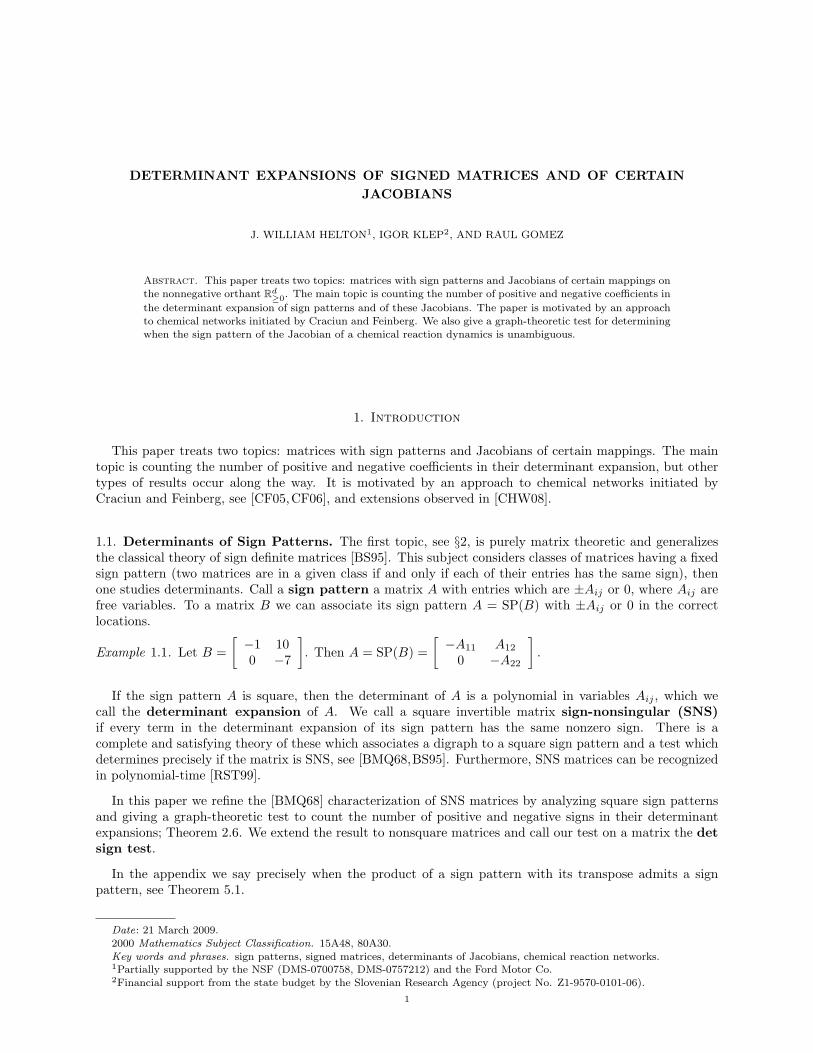
DETERMINANT EXPANSIONS OF SIGNED MATRICES AND OF CERTAIN JACOBIANS J. WILLIAM HELTON 1 , IGOR KLEP 2 , AND RAUL GOMEZ Abstract. This paper treats two topics: matrices with sign patterns and Jacobians of certain mappings on the nonnegative orthant R d ≥0 . The main topic is counting the number of positive and negative coefficients in the determinant expansion of sign patterns and of these Jacobians. The paper is motivated by an approach to chemical networks initiated by Craciun and Feinberg. We also give a graph-theoretic test for determining when the sign pattern of the Jacobian of a chemical reaction dynamics is unambiguous. 1. Introduction This paper treats two topics: matrices with sign patterns and Jacobians of certain mappings. The main topic is counting the number of positive and negative coefficients in their determinant expansion, but other types of results occur along the way. It is motivated by an approach to chemical networks initiated by Craciun and Feinberg, see [CF05,CF06], and extensions observed in [CHW08]. 1.1. Determinants of Sign Patterns. The first topic, see §2, is purely matrix theoretic and generalizes the classical theory of sign definite matrices [BS95]. This subject considers classes of matrices having a fixed sign pattern (two matrices are in a given class if and only if each of their entries has the same sign), then one studies determinants. Call a sign pattern a matrix A with entries which are ±A ij or 0, where A ij are free variables. To a matrix B we can associate its sign pattern A = SP(B) with ±A ij or 0 in the correct locations. Example 1.1. Let B = -1 10 0 -7 . Then A = SP(B)= -A 11 A 12 0 -A 22 . If the sign pattern A is square, then the determinant of A is a polynomial in variables A ij , which we call the determinant expansion of A. We call a square invertible matrix sign-nonsingular (SNS) if every term in the determinant expansion of its sign pattern has the same nonzero sign. There is a complete and satisfying theory of these which associates a digraph to a square sign pattern and a test which determines precisely if the matrix is SNS, see [BMQ68,BS95]. Furthermore, SNS matrices can be recognized in polynomial-time [RST99]. In this paper we refine the [BMQ68] characterization of SNS matrices by analyzing square sign patterns and giving a graph-theoretic test to count the number of positive and negative signs in their determinant expansions; Theorem 2.6. We extend the result to nonsquare matrices and call our test on a matrix the det sign test. In the appendix we say precisely when the product of a sign pattern with its transpose admits a sign pattern, see Theorem 5.1. Date : 21 March 2009. 2000 Mathematics Subject Classification. 15A48, 80A30. Key words and phrases. sign patterns, signed matrices, determinants of Jacobians, chemical reaction networks. 1 Partially supported by the NSF (DMS-0700758, DMS-0757212) and the Ford Motor Co. 2 Financial support from the state budget by the Slovenian Research Agency (project No. Z1-9570-0101-06). 1
-
Upload
independent -
Category
Documents
-
view
3 -
download
0
Transcript of Determinant Expansions of Signed Matrices and of Certain Jacobians
DETERMINANT EXPANSIONS OF SIGNED MATRICES AND OF CERTAINJACOBIANS
J. WILLIAM HELTON1, IGOR KLEP2, AND RAUL GOMEZ
Abstract. This paper treats two topics: matrices with sign patterns and Jacobians of certain mappings on
the nonnegative orthant Rd≥0. The main topic is counting the number of positive and negative coefficients in
the determinant expansion of sign patterns and of these Jacobians. The paper is motivated by an approach
to chemical networks initiated by Craciun and Feinberg. We also give a graph-theoretic test for determiningwhen the sign pattern of the Jacobian of a chemical reaction dynamics is unambiguous.
1. Introduction
This paper treats two topics: matrices with sign patterns and Jacobians of certain mappings. The maintopic is counting the number of positive and negative coefficients in their determinant expansion, but othertypes of results occur along the way. It is motivated by an approach to chemical networks initiated byCraciun and Feinberg, see [CF05,CF06], and extensions observed in [CHW08].
1.1. Determinants of Sign Patterns. The first topic, see §2, is purely matrix theoretic and generalizesthe classical theory of sign definite matrices [BS95]. This subject considers classes of matrices having a fixedsign pattern (two matrices are in a given class if and only if each of their entries has the same sign), thenone studies determinants. Call a sign pattern a matrix A with entries which are ±Aij or 0, where Aij arefree variables. To a matrix B we can associate its sign pattern A = SP(B) with ±Aij or 0 in the correctlocations.
Example 1.1. Let B =[−1 100 −7
]. Then A = SP(B) =
[−A11 A12
0 −A22
].
If the sign pattern A is square, then the determinant of A is a polynomial in variables Aij , which wecall the determinant expansion of A. We call a square invertible matrix sign-nonsingular (SNS)if every term in the determinant expansion of its sign pattern has the same nonzero sign. There is acomplete and satisfying theory of these which associates a digraph to a square sign pattern and a test whichdetermines precisely if the matrix is SNS, see [BMQ68,BS95]. Furthermore, SNS matrices can be recognizedin polynomial-time [RST99].
In this paper we refine the [BMQ68] characterization of SNS matrices by analyzing square sign patternsand giving a graph-theoretic test to count the number of positive and negative signs in their determinantexpansions; Theorem 2.6. We extend the result to nonsquare matrices and call our test on a matrix the detsign test.
In the appendix we say precisely when the product of a sign pattern with its transpose admits a signpattern, see Theorem 5.1.
Date: 21 March 2009.
2000 Mathematics Subject Classification. 15A48, 80A30.
Key words and phrases. sign patterns, signed matrices, determinants of Jacobians, chemical reaction networks.1Partially supported by the NSF (DMS-0700758, DMS-0757212) and the Ford Motor Co.2Financial support from the state budget by the Slovenian Research Agency (project No. Z1-9570-0101-06).
1
2 HELTON, KLEP, AND GOMEZ
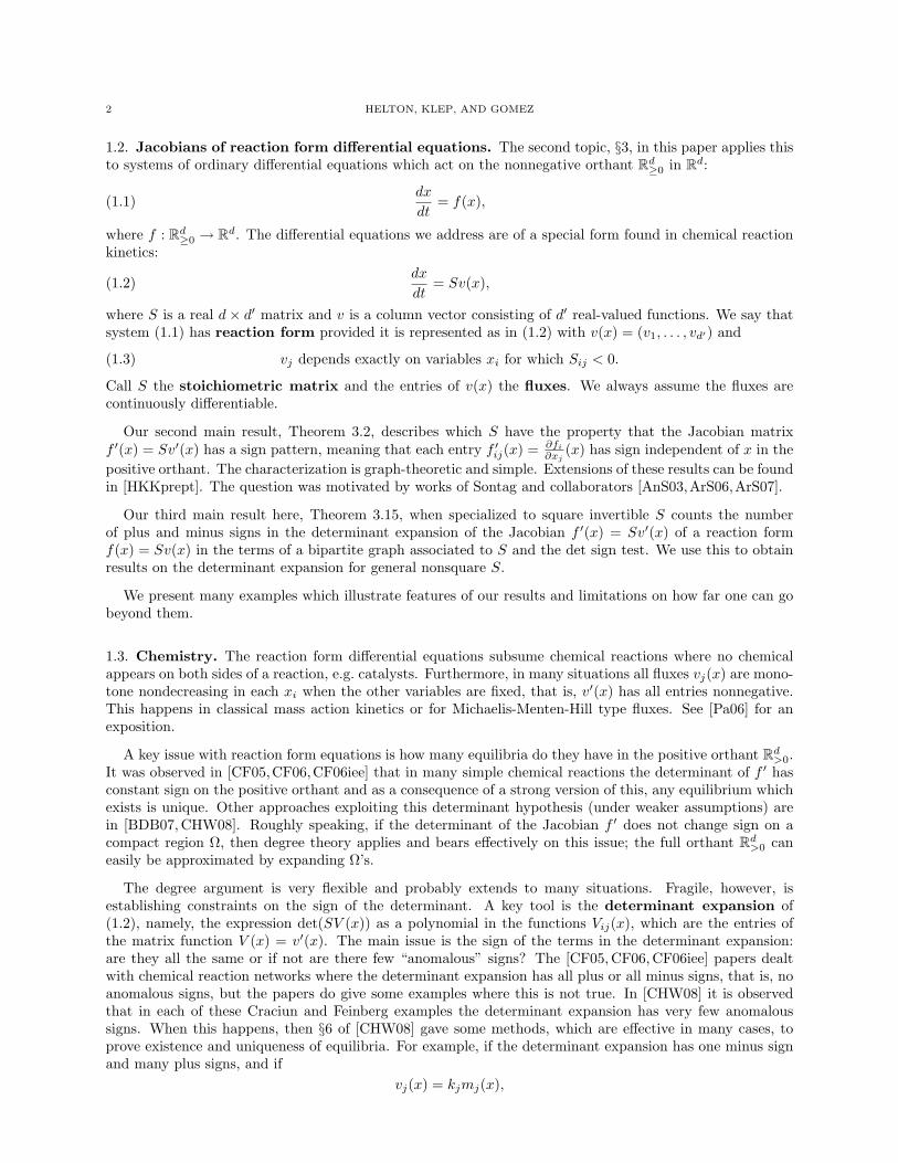
1.2. Jacobians of reaction form differential equations. The second topic, §3, in this paper applies thisto systems of ordinary differential equations which act on the nonnegative orthant Rd≥0 in Rd:
(1.1)dx
dt= f(x),
where f : Rd≥0 → Rd. The differential equations we address are of a special form found in chemical reactionkinetics:
(1.2)dx
dt= Sv(x),
where S is a real d× d′ matrix and v is a column vector consisting of d′ real-valued functions. We say thatsystem (1.1) has reaction form provided it is represented as in (1.2) with v(x) = (v1, . . . , vd′) and
(1.3) vj depends exactly on variables xi for which Sij < 0.
Call S the stoichiometric matrix and the entries of v(x) the fluxes. We always assume the fluxes arecontinuously differentiable.
Our second main result, Theorem 3.2, describes which S have the property that the Jacobian matrixf ′(x) = Sv′(x) has a sign pattern, meaning that each entry f ′ij(x) = ∂fi
∂xj(x) has sign independent of x in the
positive orthant. The characterization is graph-theoretic and simple. Extensions of these results can be foundin [HKKprept]. The question was motivated by works of Sontag and collaborators [AnS03,ArS06,ArS07].
Our third main result here, Theorem 3.15, when specialized to square invertible S counts the numberof plus and minus signs in the determinant expansion of the Jacobian f ′(x) = Sv′(x) of a reaction formf(x) = Sv(x) in the terms of a bipartite graph associated to S and the det sign test. We use this to obtainresults on the determinant expansion for general nonsquare S.
We present many examples which illustrate features of our results and limitations on how far one can gobeyond them.
1.3. Chemistry. The reaction form differential equations subsume chemical reactions where no chemicalappears on both sides of a reaction, e.g. catalysts. Furthermore, in many situations all fluxes vj(x) are mono-tone nondecreasing in each xi when the other variables are fixed, that is, v′(x) has all entries nonnegative.This happens in classical mass action kinetics or for Michaelis-Menten-Hill type fluxes. See [Pa06] for anexposition.
A key issue with reaction form equations is how many equilibria do they have in the positive orthant Rd>0.It was observed in [CF05,CF06,CF06iee] that in many simple chemical reactions the determinant of f ′ hasconstant sign on the positive orthant and as a consequence of a strong version of this, any equilibrium whichexists is unique. Other approaches exploiting this determinant hypothesis (under weaker assumptions) arein [BDB07, CHW08]. Roughly speaking, if the determinant of the Jacobian f ′ does not change sign on acompact region Ω, then degree theory applies and bears effectively on this issue; the full orthant Rd>0 caneasily be approximated by expanding Ω’s.
The degree argument is very flexible and probably extends to many situations. Fragile, however, isestablishing constraints on the sign of the determinant. A key tool is the determinant expansion of(1.2), namely, the expression det(SV (x)) as a polynomial in the functions Vij(x), which are the entries ofthe matrix function V (x) = v′(x). The main issue is the sign of the terms in the determinant expansion:are they all the same or if not are there few “anomalous” signs? The [CF05, CF06, CF06iee] papers dealtwith chemical reaction networks where the determinant expansion has all plus or all minus signs, that is, noanomalous signs, but the papers do give some examples where this is not true. In [CHW08] it is observedthat in each of these Craciun and Feinberg examples the determinant expansion has very few anomaloussigns. When this happens, then §6 of [CHW08] gave some methods, which are effective in many cases, toprove existence and uniqueness of equilibria. For example, if the determinant expansion has one minus signand many plus signs, and if
vj(x) = kjmj(x),
DETERMINANT EXPANSIONS OF SIGNED MATRICES AND OF CERTAIN JACOBIANS 3
where mj is a monomial in x and kj > 0, then for a large collection of kj > 0, we get det(SV (x)) is positiveon large regions (which in particular situations can be estimated).
Our main results, Theorem 3.15 etc., on det(SV (x)) were motivated by a desire to develop tools forcounting anomalous signs. While the paper is not aimed at chemical applications, many of the examples ofmatrices S we use to illustrate our work are stoichiometric matrices for chemical reactions.
The paper [BDB07] identified chemical reaction determinant expansions initiated by [CF05, CF06] withclassical matrix determinant expansion theory and sign patterns. This is described in the book [BS95] andpursued into new directions in a variety of recent papers such as [BJS98,CJ06,KOSD07]. The bipartite graphconventions in this paper are a bit different than conventional, but were chosen to be reasonably consistentwith [CF06].
The authors wish to thank Vitaly Katsnelson for diligent reading and suggestions. We also thank twoanonymous referees whose useful comments improved the presentation of the paper.
2. Matrices with sign patterns
This section gives the set-up and our main results on sign patterns as described in the introduction.
Let t(A), respectively m±(A), denote the number of nonzero terms, respectively positive or negative signs,in the determinant expansion of the square sign pattern A. Recall a sign definite (SD) matrix A is onewith either m−(A) = 0 or m+(A) = 0 or det(A) = 0. The number of anomalous signs m(A) of a squaresign pattern A is defined to be
m(A) := minm−(A),m+(A).We say A is j-sign definite if it has j anomalous signs, that is m(A) = j.
Question (J-sign): Given a sign pattern S is every square submatrix sign definite, or more generallywhat is the largest j for which S contains a j-sign definite square matrix.
We shall convert this question to an equivalent graph theoretic problem and give a more refined result forsquare sign patterns A which counts m±(A).
2.1. Basics on graphs, matrices and determinants. To this end we use the standard notion of bipartitegraphs [HGBM06]. Given a sign pattern S let G(S) denote its signed bipartite graph. It is a signedbipartite graph with one set of vertices C(S) based on columns and the other set of vertices R(S) based onrows. There is an edge joining column c and row r if and only if the (r, c) entry Src of S is nonzero. The signof this edge is the sign of Src. This is a simplified version of the species-reaction (SR) graph in [CF06]. Iftwo edges meeting at the same column have the same sign, they are called a c-pair. By a cycle we mean aclosed (simple) path, with no other repeated vertices than the starting and ending vertices (sometimes alsocalled a simple cycle, circuit, circle, or polygon). A cycle that contains an even (respectively odd) numberof c-pairs is called an e-cycle (respectively o-cycle). Recall a matching in a bipartite graph is a set ofedges without common vertices. Equivalently it is an injective mapping from one of the vertex sets to theother respecting the graph. A matching in a bipartite graph is called perfect if it covers all vertices in thesmaller of the two vertex sets. A k × k square submatrix A of S corresponds to k column nodes C(A) andk row nodes R(A); there is an associated sub-bipartite graph G(A) of G(S).
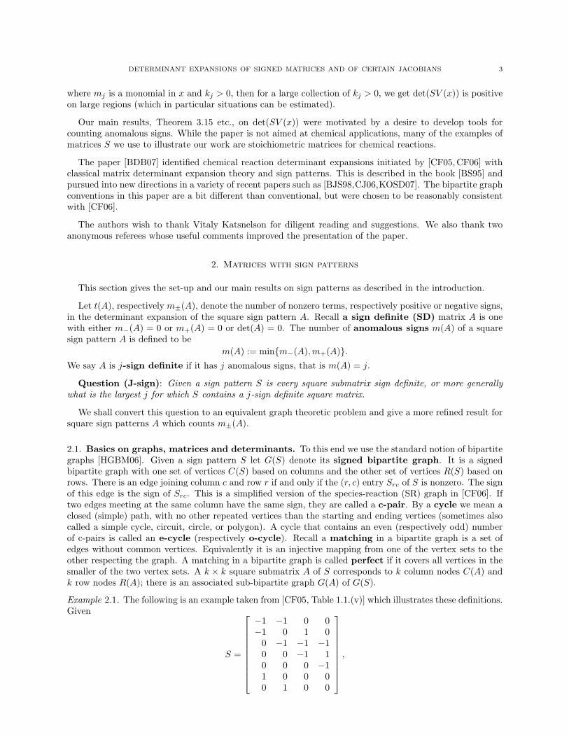
Example 2.1. The following is an example taken from [CF05, Table 1.1.(v)] which illustrates these definitions.Given
S =
−1 −1 0 0−1 0 1 0
0 −1 −1 −10 0 −1 10 0 0 −11 0 0 00 1 0 0
,
4 HELTON, KLEP, AND GOMEZ
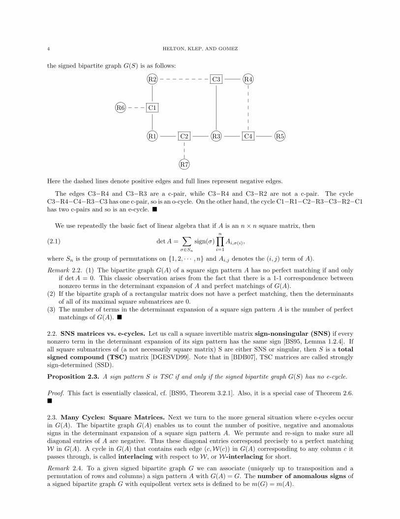
the signed bipartite graph G(S) is as follows:
R2?>=<89:; ________ C3 R4?>=<89:;
R6?>=<89:; ___ C1
R1?>=<89:; C2
R3?>=<89:; C4 R5?>=<89:;
R7?>=<89:;Here the dashed lines denote positive edges and full lines represent negative edges.
The edges C3−R4 and C3−R3 are a c-pair, while C3−R4 and C3−R2 are not a c-pair. The cycleC3−R4−C4−R3−C3 has one c-pair, so is an o-cycle. On the other hand, the cycle C1−R1−C2−R3−C3−R2−C1has two c-pairs and so is an e-cycle.
We use repeatedly the basic fact of linear algebra that if A is an n× n square matrix, then
(2.1) detA =∑σ∈Sn
sign(σ)n∏i=1
Ai,σ(i),
where Sn is the group of permutations on 1, 2, · · · , n and Ai,j denotes the (i, j) term of A).
Remark 2.2. (1) The bipartite graph G(A) of a square sign pattern A has no perfect matching if and onlyif detA = 0. This classic observation arises from the fact that there is a 1-1 correspondence betweennonzero terms in the determinant expansion of A and perfect matchings of G(A).
(2) If the bipartite graph of a rectangular matrix does not have a perfect matching, then the determinantsof all of its maximal square submatrices are 0.
(3) The number of terms in the determinant expansion of a square sign pattern A is the number of perfectmatchings of G(A).
2.2. SNS matrices vs. e-cycles. Let us call a square invertible matrix sign-nonsingular (SNS) if everynonzero term in the determinant expansion of its sign pattern has the same sign [BS95, Lemma 1.2.4]. Ifall square submatrices of (a not necessarily square matrix) S are either SNS or singular, then S is a totalsigned compound (TSC) matrix [DGESVD99]. Note that in [BDB07], TSC matrices are called stronglysign-determined (SSD).
Proposition 2.3. A sign pattern S is TSC if and only if the signed bipartite graph G(S) has no e-cycle.
Proof. This fact is essentially classical, cf. [BS95, Theorem 3.2.1]. Also, it is a special case of Theorem 2.6.
2.3. Many Cycles: Square Matrices. Next we turn to the more general situation where e-cycles occurin G(A). The bipartite graph G(A) enables us to count the number of positive, negative and anomaloussigns in the determinant expansion of a square sign pattern A. We permute and re-sign to make sure alldiagonal entries of A are negative. Thus these diagonal entries correspond precisely to a perfect matchingW in G(A). A cycle in G(A) that contains each edge (c,W(c)) in G(A) corresponding to any column c itpasses through, is called interlacing with respect to W, or W-interlacing for short.
Remark 2.4. To a given signed bipartite graph G we can associate (uniquely up to transposition and apermutation of rows and columns) a sign pattern A with G(A) = G. The number of anomalous signs ofa signed bipartite graph G with equipollent vertex sets is defined to be m(G) = m(A).
DETERMINANT EXPANSIONS OF SIGNED MATRICES AND OF CERTAIN JACOBIANS 5
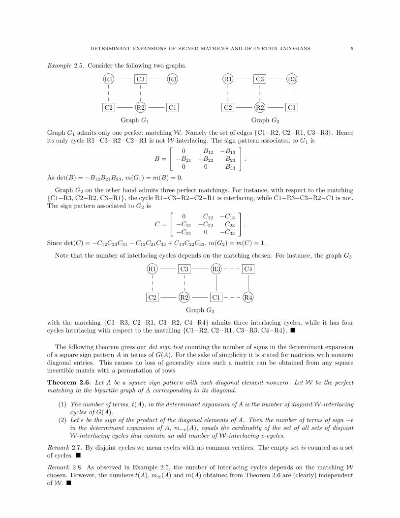
Example 2.5. Consider the following two graphs.
R1?>=<89:;
C3
R3?>=<89:;
C2 R2?>=<89:; C1
R1?>=<89:;
C3
R3?>=<89:;
C2 R2?>=<89:; C1
Graph G1 Graph G2
Graph G1 admits only one perfect matchingW. Namely the set of edges C1−R2, C2−R1, C3−R3. Henceits only cycle R1−C3−R2−C2−R1 is not W-interlacing. The sign pattern associated to G1 is
B =
0 B12 −B13
−B21 −B22 B23
0 0 −B33
.As det(B) = −B12B21B33, m(G1) = m(B) = 0.
Graph G2 on the other hand admits three perfect matchings. For instance, with respect to the matchingC1−R3, C2−R2, C3−R1, the cycle R1−C3−R2−C2−R1 is interlacing, while C1−R3−C3−R2−C1 is not.The sign pattern associated to G2 is
C =
0 C12 −C13
−C21 −C22 C23
−C31 0 −C33
.Since det(C) = −C12C23C31 − C12C21C33 + C13C22C33, m(G2) = m(C) = 1.
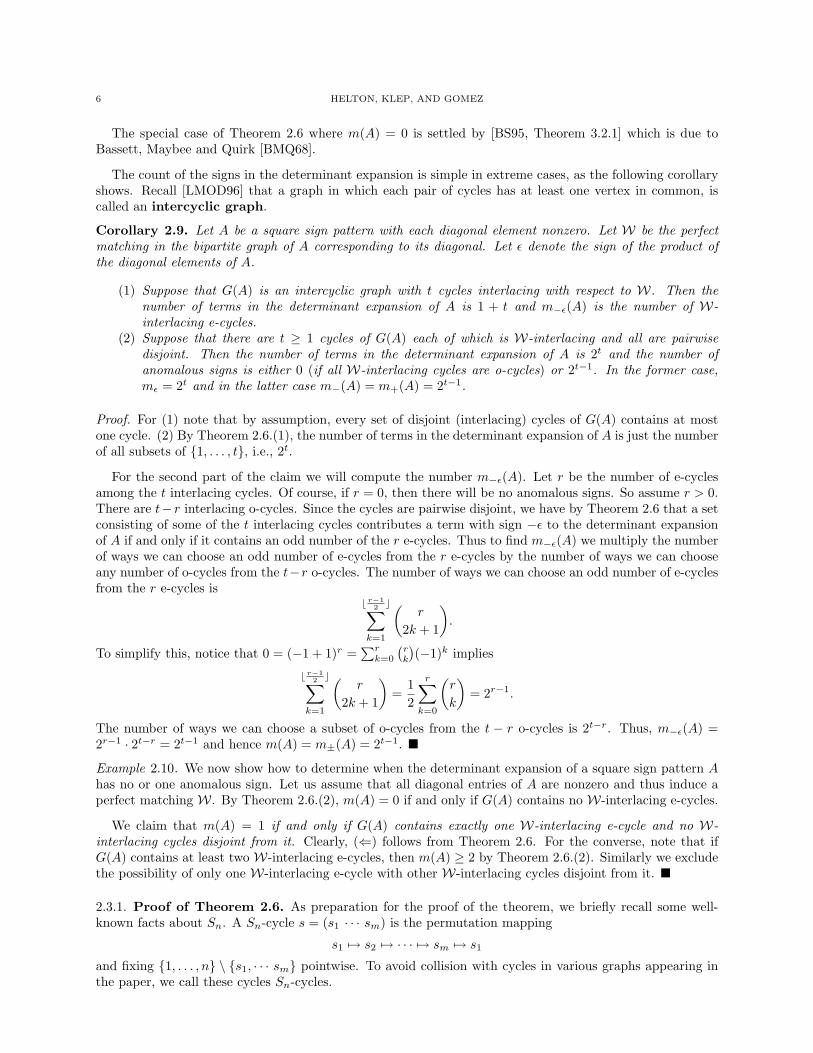
Note that the number of interlacing cycles depends on the matching chosen. For instance, the graph G3
R1?>=<89:;
C3
R3?>=<89:; ___ C4
C2 R2?>=<89:; C1 ___ R4?>=<89:;Graph G3
with the matching C1−R3, C2−R1, C3−R2, C4−R4 admits three interlacing cycles, while it has fourcycles interlacing with respect to the matching C1−R2, C2−R1, C3−R3, C4−R4.
The following theorem gives our det sign test counting the number of signs in the determinant expansionof a square sign pattern A in terms of G(A). For the sake of simplicity it is stated for matrices with nonzerodiagonal entries. This causes no loss of generality since such a matrix can be obtained from any squareinvertible matrix with a permutation of rows.
Theorem 2.6. Let A be a square sign pattern with each diagonal element nonzero. Let W be the perfectmatching in the bipartite graph of A corresponding to its diagonal.
(1) The number of terms, t(A), in the determinant expansion of A is the number of disjointW-interlacingcycles of G(A).
(2) Let ε be the sign of the product of the diagonal elements of A. Then the number of terms of sign −εin the determinant expansion of A, m−ε(A), equals the cardinality of the set of all sets of disjointW-interlacing cycles that contain an odd number of W-interlacing e-cycles.
Remark 2.7. By disjoint cycles we mean cycles with no common vertices. The empty set is counted as a setof cycles.
Remark 2.8. As observed in Example 2.5, the number of interlacing cycles depends on the matching Wchosen. However, the numbers t(A), m±(A) and m(A) obtained from Theorem 2.6 are (clearly) independentof W.
6 HELTON, KLEP, AND GOMEZ
The special case of Theorem 2.6 where m(A) = 0 is settled by [BS95, Theorem 3.2.1] which is due toBassett, Maybee and Quirk [BMQ68].
The count of the signs in the determinant expansion is simple in extreme cases, as the following corollaryshows. Recall [LMOD96] that a graph in which each pair of cycles has at least one vertex in common, iscalled an intercyclic graph.
Corollary 2.9. Let A be a square sign pattern with each diagonal element nonzero. Let W be the perfectmatching in the bipartite graph of A corresponding to its diagonal. Let ε denote the sign of the product ofthe diagonal elements of A.
(1) Suppose that G(A) is an intercyclic graph with t cycles interlacing with respect to W. Then thenumber of terms in the determinant expansion of A is 1 + t and m−ε(A) is the number of W-interlacing e-cycles.
(2) Suppose that there are t ≥ 1 cycles of G(A) each of which is W-interlacing and all are pairwisedisjoint. Then the number of terms in the determinant expansion of A is 2t and the number ofanomalous signs is either 0 (if all W-interlacing cycles are o-cycles) or 2t−1. In the former case,mε = 2t and in the latter case m−(A) = m+(A) = 2t−1.
Proof. For (1) note that by assumption, every set of disjoint (interlacing) cycles of G(A) contains at mostone cycle. (2) By Theorem 2.6.(1), the number of terms in the determinant expansion of A is just the numberof all subsets of 1, . . . , t, i.e., 2t.
For the second part of the claim we will compute the number m−ε(A). Let r be the number of e-cyclesamong the t interlacing cycles. Of course, if r = 0, then there will be no anomalous signs. So assume r > 0.There are t− r interlacing o-cycles. Since the cycles are pairwise disjoint, we have by Theorem 2.6 that a setconsisting of some of the t interlacing cycles contributes a term with sign −ε to the determinant expansionof A if and only if it contains an odd number of the r e-cycles. Thus to find m−ε(A) we multiply the numberof ways we can choose an odd number of e-cycles from the r e-cycles by the number of ways we can chooseany number of o-cycles from the t−r o-cycles. The number of ways we can choose an odd number of e-cyclesfrom the r e-cycles is
b r−12 c∑
k=1
(r
2k + 1
).
To simplify this, notice that 0 = (−1 + 1)r =∑rk=0
(rk
)(−1)k implies
b r−12 c∑
k=1
(r
2k + 1
)=
12
r∑k=0
(r
k
)= 2r−1.
The number of ways we can choose a subset of o-cycles from the t − r o-cycles is 2t−r. Thus, m−ε(A) =2r−1 · 2t−r = 2t−1 and hence m(A) = m±(A) = 2t−1.
Example 2.10. We now show how to determine when the determinant expansion of a square sign pattern Ahas no or one anomalous sign. Let us assume that all diagonal entries of A are nonzero and thus induce aperfect matching W. By Theorem 2.6.(2), m(A) = 0 if and only if G(A) contains no W-interlacing e-cycles.
We claim that m(A) = 1 if and only if G(A) contains exactly one W-interlacing e-cycle and no W-interlacing cycles disjoint from it. Clearly, (⇐) follows from Theorem 2.6. For the converse, note that ifG(A) contains at least two W-interlacing e-cycles, then m(A) ≥ 2 by Theorem 2.6.(2). Similarly we excludethe possibility of only one W-interlacing e-cycle with other W-interlacing cycles disjoint from it.
2.3.1. Proof of Theorem 2.6. As preparation for the proof of the theorem, we briefly recall some well-known facts about Sn. A Sn-cycle s = (s1 · · · sm) is the permutation mapping
s1 7→ s2 7→ · · · 7→ sm 7→ s1
and fixing 1, . . . , n \ s1, · · · sm pointwise. To avoid collision with cycles in various graphs appearing inthe paper, we call these cycles Sn-cycles.
DETERMINANT EXPANSIONS OF SIGNED MATRICES AND OF CERTAIN JACOBIANS 7
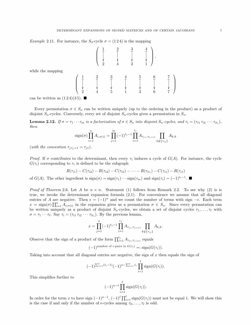
Example 2.11. For instance, the S4-cycle σ = (1 2 4) is the mapping1_
2_
3_
4_
2 4 3 1
,
while the mapping 1_
2_
3_
4_
5_
6_
7_
2 4 5 1 3 6 7
can be written as (1 2 4)(3 5).
Every permutation σ ∈ Sn can be written uniquely (up to the ordering in the product) as a product ofdisjoint Sn-cycles. Conversely, every set of disjoint Sn-cycles gives a permutation in Sn.
Lemma 2.12. If σ = τ1 · · · τm is a factorization of σ ∈ Sn into disjoint Sn-cycles, and τi = (τi1 τi2 · · · τiti),then
sign(σ)n∏i=1
Ai,σ(i) =m∏j=1
(−1)tj−1
tj∏i=1
Aτj i,τj i+1
∏k 6∈τij
Ak,k
(with the convention τj tj+1 = τj1).
Proof. If σ contributes to the determinant, then every τi induces a cycle of G(A). For instance, the cycleG(τi) corresponding to τi is defined to be the subgraph
R(τi1)− C(τi2)−R(τi2)− C(τi3)− · · · −R(τiti)− C(τi1)−R(τi1)
of G(A). The other ingredient is sign(σ) = sign(τ1) · · · sign(τm) and sign(τi) = (−1)ti−1.
Proof of Theorem 2.6. Let A be n × n. Statement (1) follows from Remark 2.2. To see why (2) is istrue, we invoke the determinant expansion formula (2.1). For convenience we assume that all diagonalentries of A are negative. Then ε = (−1)n and we count the number of terms with sign −ε. Each termx = sign(σ)
∏ni=1Ai,σ(i) in the expansion gives us a permutation σ ∈ Sn. Since every permutation can
be written uniquely as a product of disjoint Sn-cycles, we obtain a set of disjoint cycles τ1, . . . , τ` withσ = τ1 · · · τ`. Say τi = (τi1 τi2 · · · τiti). By the previous lemma,
x =∏j=1
(−1)tj−1
tj∏i=1
Aτj i,τj i+1
∏k 6∈τij
Ak,k.
Observe that the sign of a product of the form∏tji=1Aτji,τj i+1 equals
(−1)number of c-pairs in G(τi) =: sign(G(τi)).
Taking into account that all diagonal entries are negative, the sign of x then equals the sign of
(−1)P`i=1(ti−1)(−1)n−
P`i=1 ti
∏i=1
sign(G(τi)).
This simplifies further to
(−1)n−`∏i=1
sign(G(τi)).
In order for the term x to have sign (−1)n−1, (−1)`∏`i=1 sign(G(τi)) must not be equal 1. We will show this
is the case if and only if the number of e-cycles among τ0, . . . , τ` is odd.
8 HELTON, KLEP, AND GOMEZ
Case (1): Suppose ` is odd. Then
(−1)`∏i=1
sign(G(τi)) = −1 ⇐⇒∏i=1
sign(G(τi)) = 1
⇐⇒ (−1)#(o-cycles among τ0,...,τ`) = 1
⇐⇒ # (o-cycles among τ0, . . . , τ`) is even
⇐⇒ # (e-cycles among τ0, . . . , τ`) is odd,
since ` is odd and # (e-cycles) = `−# (o-cycles).
Case (2): Suppose ` is even. Then
(−1)`∏i=1
sign(G(τi)) = −1 ⇐⇒∏i=1
sign(G(τi)) = −1
⇐⇒ (−1)#(o-cycles among τ0,...,τ`) = −1
⇐⇒ # (o-cycles among τ0, . . . , τ`) is odd
⇐⇒ # (e-cycles among τ0, . . . , τ`) is odd,
since ` is even and # (e-cycles) = `−# (o-cycles).
A referee has pointed out that this proof is along the lines of a refinement of the [BMQ68] proof.
2.4. Many Cycles: Nonsquare Matrices. The graph-theoretic test described in §2.3 gives a det sign testsettling Question (J-sign). In this section we extend the det sign test to nonsquare sign patterns S.
A cycle has the property that the number of rows it passes through is the same as the number of columnsit passes through. A set of cycles is called balanced if the number of rows they pass through is the sameas the number of columns they pass through (i.e., if they are incident with the same number of rows andcolumns). Every balanced set of cycles picks out a square submatrix A of S and hence induces a sub-bipartitegraph G(A) of G(S). Such a submatrix and the sub-bipartite graph are both said to be balanced. Noteeach column and row of A appears in at least one cycle in G(A).
Proposition 2.13. For every square invertible submatrix B of a sign pattern S there is a balanced squaresubmatrix A of S with m(A) = m(B). In fact, A can be chosen to be a submatrix of B.
Proof. Suppose B is the smallest square submatrix of S violating the conclusion of the proposition. Afterpermuting rows we assume B has nonzero entries on the diagonal. Since B is not balanced, either a row ora column of B does not appear in any cycle in G(B). Without loss of generality we assume this to be row 1.
Since we assume that row 1 does not appear in any cycle of G(B), for σ ∈ Sn with σ = τ1 · · · τ`, whereτi are disjoint Sn-cycles, the corresponding term in the determinant expansion x = sign(σ)
∏ni=1Bi,σ(i) will
be zero if 1 appears in one of the τi. Hence the nonzero terms x will correspond to permutations σ withσ(1) = 1. In other words, B1,1 will get picked from row one. So by removing row and column one from B weobtain a smaller matrix B0 with m(B0) = m(B). By the minimality assumption on B, there is a balancedsquare submatrix A of B0 with m(A) = m(B0) = m(B), a contradiction.
By this proposition, the answer J to Question (J-sign) equals the maximal number of anomalous signsobtainable from a balanced square submatrix of the sign pattern S. So a procedure for finding the desiredupper bound J is as follows. Consider sets of balanced cycles in G(S). Each of these induces a squaresubmatrix A of S. If G(A) admits no perfect matching, we continue with another set of balanced cycles.Otherwise we count the number of anomalous signs in detA by the procedure described in Theorem 2.6 of§2.3. The highest possible count obtained is the desired sharp upper bound J .
DETERMINANT EXPANSIONS OF SIGNED MATRICES AND OF CERTAIN JACOBIANS 9
3. Reaction form differential equations and the Jacobians
Now we turn to studying systems of reaction form (RF) ordinary differential equations which act on thenonnegative orthant Rd≥0 in Rd:
(3.1)dx
dt= f(x) = Sv(x),
where f : Rd≥0 → Rd, S is a real d×d′ matrix and v is a column vector consisting of d′ real-valued functions.
The differential equation (3.1) has weak reaction form (wRF) provided V (x) := v′(x) satisfies Sij >0⇒ Vji(x) = 0. If a differential equation has wRF, then it has reaction form provided Sij = 0⇒ Vji(x) = 0and Sij < 0 ⇒ Vji(x) 6= 0. The flux vector v(x) is monotone nondecreasing (respectively, monotoneincreasing) if ∂vj
∂xi(x) is either 0 for all x ∈ Rd′≥0 or nonnegative (respectively, positive) for all x ∈ Rd′>0.
This section analyzes two properties the Jacobian of f(x) might have. First we say when f ′(x) has a signpattern (Theorem 3.2 and Corollary 3.1). Secondly we give a method based on §2 for counting the numberof plus and minus coefficients in its determinant expansion.
3.1. Sign pattern of the Jacobian. We first say when the Jacobian of a reaction form dynamics respectsa sign pattern and find that it does surprisingly often.
Corollary 3.1. Given a reaction form differential equationdx
dt= Sv(x)
with monotone increasing flux vector v(x). The Jacobian Sv′(x) respects the same sign pattern for allx ∈ Rn>0 if the bipartite graph G(S) does not contain a cycle of length four with three negative edges.
The corollary is an immediate consequence of Theorem 3.2.(3) which is phrased symbolically. Notethat while the cycle condition is a necessary condition in Corollary 3.1, it is both necessary and sufficientin Theorem 3.1.(3). We now introduce some definitions required to formulate our sign pattern resultssymbolically.
Here and in the sequel, U will denote what we call the flux pattern assigned to S. It is defined to be ad′× d matrix with each entry being 0 or a free variable Uij ; the (i, j)th entry of U is 0 if and only if Sji ≥ 0.In case the differential equation (3.1) satisfies RF and the flux vector v(x) is monotone increasing, U is thesign pattern of V (x). For an illustration, see Example 3.5.
Theorem 3.2. Let S be a real d × d′ matrix and U the corresponding flux pattern. Consider (3.1) andsuppose that the Vij(x) for fixed i are linearly independent. Then:
(1) The differential equation (3.1) has wRF if and only if each diagonal term in SV (x) is a negativelinear combination of the Vij(x).
(2) (Weak reaction form differential equations) If (3.1) has wRF, then SV (x) admits a sign pattern(that is, each entry of SV (x) is a positive or negative linear combination of monomials in the Vij(x))whenever the matrix S does not contain a 2× 2 submatrix with the same sign pattern as
(3.2)[
+1 −1−1, 0 −1, 0
]or
[−1 +1−1, 0 −1, 0
]or
[−1, 0 −1, 0
+1 −1
]or
[−1, 0 −1, 0−1 +1
].
Here −1, 0 stands for either −1 or 0.(3) (Reaction form differential equations)
(a) The product SU admits a sign pattern if and only if the matrix S does not contain a 2 × 2submatrix with the same sign pattern as
(3.3)[
+1 −1−1 −1
]or
[−1 +1−1 −1
]or
[−1 −1+1 −1
]or
[−1 −1−1 +1
].
Equivalently, in terms of the bipartite graph, G(S) does not contain a cycle of length four withthree negative edges.
10 HELTON, KLEP, AND GOMEZ
(b) The entry (SU)ij is nonzero if and only if there is some k with Sik 6= 0 and Sjk < 0. If SUadmits a sign pattern, then sign((SU)ij) = sign(Sik).
Proof. (1) Write S = S+ − S− for real matrices S+, S− with nonnegative coefficients satisfying the compli-mentarity property (S+)ij(S−)ij = 0. Diagonal entries of SV (x) are of the form
∑j SijVji(x) which meets
the negative coefficient condition if and only if∑j(S+)ijVji(x) = 0 if and only if (S+)ijVji(x) = 0 for all
i, j. This uses the linear independence of the Vji(x). so no cancellation can occur. Thus Sij > 0 if and onlyif (S+)ij 6= 0 implies Vji(x) = 0 which is the wRF condition.
(2) The (i, j)th entry of SV (x) does not have a sign pattern if and only if (S+V (x))ij 6= 0 and (S−V (x))ij 6=0. (S+V (x))ij =
∑k(S+)ikVkj(x), so (S+V (x))ij 6= 0 if and only if for some k, Sik > 0 and Vkj(x) 6= 0, so
by wRF, Sjk 6> 0. To summarize: Sik > 0 and Sjk 6> 0. Similarly, (S−V (x))ij 6= 0 if and only if there issome ` with (S−)i` 6= 0 and V`j(x) 6= 0 so Sj` 6> 0. In summary, Si` < 0 and Sj` 6> 0. Taken together thisimplies that the 2 × 2 submatrix of S given by rows i, j and columns k, ` has the same sign pattern as oneof the matrices in (3.2).
(3a) This follows as in (2) by using that Ukj 6= 0 if and only if Sjk < 0.
(3b) From (SU)ij =∑k SikUkj it follows that (SU)ij 6= 0 if and only if there is k with Sik 6= 0 and
Ukj 6= 0. Due to the construction of U , Ukj 6= 0 if and only if Sjk < 0. This proves the first part of thestatement and the second follows immediately since Ukj is “positive”.
The issue in Theorem 3.2 is a variant on a simple characterization of when the product AB of two signpatterns A and B, having “transposed” sign patterns, has a sign pattern, cf. §5.
Our next step is to introduce several different types of determinant expansions.
3.2. The core and other determinant expansions. Now we change to the topic of determinant expan-sions of the Jacobian of f . Such were introduced to the subject of chemical reaction networks in [CF05] andare discussed in §1.3 and §4. The Craciun-Feinberg determinant expansion [CF05] is defined to be
cfd(S) := det(SU − τI) with τ fixed, e.g. τ = 1
for S ∈ Rd×d′ and the corresponding flux pattern U . In this paper we introduce and study the coredeterminant
(3.4) cd(S) := limτ→0
1τd−r
det(SU − τI),
where r := rank(S). It is appropriate for analysis of many chemical reaction networks, see Theorem 4.1. Formore details on the relationship between the Craciun-Feinberg determinant expansion cfd(S) and the coredeterminant cd(S) we refer the reader to §4.
The remainder of this section sets up machinery for the study of determinant expansions. We devotemost of our attention to the core determinant, because our ideas when applied to the Craciun-Feinbergdeterminant are very similar. §3.2, §3.3 and §3.4 introduce definitions and constructions, then §3.5, §3.6 and§3.7 give bounds on the number of anomalous signs as well as examples.
Proposition 3.3. Let C ∈ Rd×d′ , let D be a d′× d matrix with possibly symbolic entries and suppose C hasrank r. Define α to be the determinant of the compression of CD to the range of C. Then
α = limτ→0
1τd−r
det(CD − τI).
Proof. Observe that
CD − τI =[
(CD − τI)|imC ∗0 −τI|(imC)⊥
].
As the size of the second diagonal block is (d− r)× (d− r),1
τd−rdet(CD − τI) = det((CD − τI)|imC).

DETERMINANT EXPANSIONS OF SIGNED MATRICES AND OF CERTAIN JACOBIANS 11
Sending τ → 0 yields the desired conclusion.
Definition 3.4. A column c in S ∈ Rd×d′ is called reversible if −c is also a column of S. (Many matricescoming from chemical reactions have reversible columns.) We call −c the reverse of c.
Example 3.5. Let us consider an example which is a slight modification of [CF05, Table 1.1.(i)]:
R5?>=<89:; ___ C3,C4 R3?>=<89:;
R2?>=<89:; C5
R4?>=<89:; ___ C1,C2 R1?>=<89:;
The corresponding stoichiometric matrix S and the vector v(x) are given by the following:
S =
a11 −a11 0 0 −a13
a21 −a21 a22 −a22 00 0 a32 −a32 a33
−a41 a41 0 0 00 0 −a52 a52 0
, v(x) =
k1x
a414
k2xa111 xa21
2
k3xa525
k4xa222 xa32
3
k5xa131
.Note some of the columns of S are reversible. This phenomenon is captured in the graph by listing twocolumns that are reverses of each other in a common rectangular box. For example, C3 and C4 appear inthe same box and in fact columns 3 and 4 are reverses of each other. The sign of S33 is the same as the signof S23 and both appear in the graph as a solid line. S53 has sign opposite to these and so appears in thegraph as a dashed line. This is also true for C4. Other dashed vs. solid lines of the graph coming from abox with reversible columns follow the same pattern.
The corresponding V (x) and U are as follows:
V (x) =
0 0 0 xa41−1
4 a41k1 0xa11−1
1 xa212 a11k2 xa11
1 xa21−12 a21k2 0 0 0
0 0 0 0 xa52−15 a52k3
0 xa22−12 xa32
3 a22k4 xa222 xa32−1
3 a32k4 0 0xa13−1
1 a13k5 0 0 0 0
,
U =
0 0 0 U14 0U21 U22 0 0 00 0 0 0 U35
0 U42 U43 0 0U51 0 0 0 0
.For generic choices of the numbers aij the matrix S will be of rank 3 and this is what we focus on. Astraightforward computation gives
cd(S) = −2a13a41a52U14U35U51 − 2a13a21a52U22U35U51 − 2a13a22a41U14U42U51
−2a13a32a41U14U43U51 − 2a13a21a32U22U43U51 + 2a11a22a33U22U43U51
Hence there is potentially one anomalous sign in cd(S). However,
−2a13a21a32U22U43U51 + 2a11a22a33U22U43U51 = 2(a11a22a33 − a13a21a32)U22U43U51
so cd(S) has one, respectively no anomalous sign, depending on whether a11a22a33 − a13a21a32 is positive,respectively nonpositive.
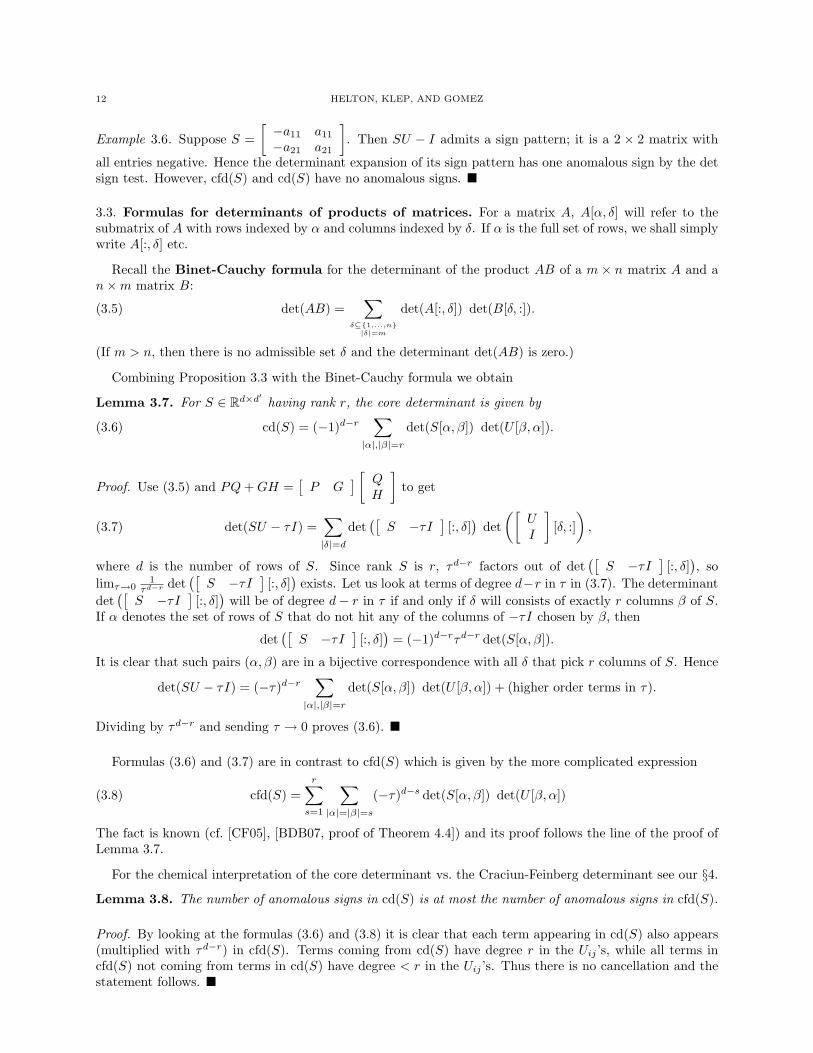
12 HELTON, KLEP, AND GOMEZ
Example 3.6. Suppose S =[−a11 a11
−a21 a21
]. Then SU − I admits a sign pattern; it is a 2 × 2 matrix with
all entries negative. Hence the determinant expansion of its sign pattern has one anomalous sign by the detsign test. However, cfd(S) and cd(S) have no anomalous signs.
3.3. Formulas for determinants of products of matrices. For a matrix A, A[α, δ] will refer to thesubmatrix of A with rows indexed by α and columns indexed by δ. If α is the full set of rows, we shall simplywrite A[:, δ] etc.
Recall the Binet-Cauchy formula for the determinant of the product AB of a m × n matrix A and an×m matrix B:
(3.5) det(AB) =∑
δ⊆1,...,n|δ|=m
det(A[:, δ]) det(B[δ, :]).
(If m > n, then there is no admissible set δ and the determinant det(AB) is zero.)
Combining Proposition 3.3 with the Binet-Cauchy formula we obtain
Lemma 3.7. For S ∈ Rd×d′ having rank r, the core determinant is given by
(3.6) cd(S) = (−1)d−r∑
|α|,|β|=r
det(S[α, β]) det(U [β, α]).
Proof. Use (3.5) and PQ+GH =[P G
] [ QH
]to get
(3.7) det(SU − τI) =∑|δ|=d
det([
S −τI]
[:, δ])
det([
UI
][δ, :]
),
where d is the number of rows of S. Since rank S is r, τd−r factors out of det([
S −τI]
[:, δ]), so
limτ→01
τd−rdet([
S −τI]
[:, δ])
exists. Let us look at terms of degree d−r in τ in (3.7). The determinantdet([
S −τI]
[:, δ])
will be of degree d− r in τ if and only if δ will consists of exactly r columns β of S.If α denotes the set of rows of S that do not hit any of the columns of −τI chosen by β, then
det([
S −τI]
[:, δ])
= (−1)d−rτd−r det(S[α, β]).
It is clear that such pairs (α, β) are in a bijective correspondence with all δ that pick r columns of S. Hence
det(SU − τI) = (−τ)d−r∑
|α|,|β|=r
det(S[α, β]) det(U [β, α]) + (higher order terms in τ).
Dividing by τd−r and sending τ → 0 proves (3.6).
Formulas (3.6) and (3.7) are in contrast to cfd(S) which is given by the more complicated expression
(3.8) cfd(S) =r∑s=1
∑|α|=|β|=s
(−τ)d−s det(S[α, β]) det(U [β, α])
The fact is known (cf. [CF05], [BDB07, proof of Theorem 4.4]) and its proof follows the line of the proof ofLemma 3.7.
For the chemical interpretation of the core determinant vs. the Craciun-Feinberg determinant see our §4.
Lemma 3.8. The number of anomalous signs in cd(S) is at most the number of anomalous signs in cfd(S).
Proof. By looking at the formulas (3.6) and (3.8) it is clear that each term appearing in cd(S) also appears(multiplied with τd−r) in cfd(S). Terms coming from cd(S) have degree r in the Uij ’s, while all terms incfd(S) not coming from terms in cd(S) have degree < r in the Uij ’s. Thus there is no cancellation and thestatement follows.
DETERMINANT EXPANSIONS OF SIGNED MATRICES AND OF CERTAIN JACOBIANS 13
Remark 3.9. Example 3.21 shows that the number of anomalous signs in cd(S) can be strictly smaller thanthe number of anomalous signs in cfd(S).
If B is the sign pattern associated to the graph G1 of Example 2.5, and S =[B −B
], then cd(S) has
no anomalous signs, whereas cfd(S) has one anomalous sign. We leave this as an exercise for the interestedreader.
3.4. Generic matrices and the reduced S-matrix. In this section we introduce some basic definitionsand illustrate them with an example.
Definition 3.10. A matrix A is called weakly generic if its rank r is maximal among all matrices with thesame sign pattern. If, in addition, all r × r submatrices of A are weakly generic, then A is called generic.
The set of all (weakly) generic m×m matrices with a given sign pattern is open and dense in the set ofall m×m matrices with that sign pattern.
Lemma 3.11. The rank r of a generic matrix A with connected graph G(A) is equal to the minimum of thenumber of rows or of columns of A. If G(A) has ` components G1, . . . , G` and ri is the minimal number ofcolumn or row nodes in Gi, then r =
∑`i=1 ri.
Proof. Obvious.
Definition 3.12. For S ∈ Rd×d′ let Sred denote a reduced S-matrix, i.e., a matrix obtained from S byremoving one column out of every pair of columns which are reverses of each other. Clearly, Sred containsno reversible columns. The reduced flux pattern Ured is obtained from S and Sred: it is built from thesign pattern of −STred by setting all entries coming from positive entries in columns nonreversible in S to 0.In particular, if all columns of S are reversible, then Ured is the sign pattern of −STred. If no column of S isreversible, then Sred = S and Ured = U .
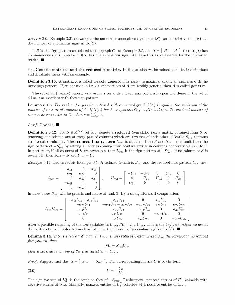
Example 3.13. Let us revisit Example 3.5. A reduced S-matrix Sred and the reduced flux pattern Ured are
Sred =
a11 0 −a13
a21 a22 00 a32 a33
−a41 0 00 −a52 0
, Ured =
−U11 −U12 0 U14 00 −U22 −U23 0 U25
U31 0 0 0 0
.In most cases Sred will be generic and hence of rank 3. By a straightforward computation,
SredUred =
−a11U11 − a13U31 −a11U12 0 a11U14 0
−a21U11 −a21U12 − a22U22 −a22U23 a21U14 a22U25
a33U31 −a32U22 −a32U23 0 a32U25
a41U11 a41U21 0 −a41U14 00 a52U22 a52U23 0 −a52U25
After a possible renaming of the free variables in Ured, SU = SredUred. This is the key observation we use inthe next sections in order to count or estimate the number of anomalous signs in cd(S).
Lemma 3.14. If S is a real d×d′ matrix, if Sred is any reduced S-matrix and Ured the corresponding reducedflux pattern, then
SU = SredUred
after a possible renaming of the free variables in Ured.
Proof. Suppose first that S =[Sred −Sred
]. The corresponding matrix U is of the form
(3.9) U =[U0
U1
].
The sign pattern of UT0 is the same as that of −Sred. Furthermore, nonzero entries of UT0 coincide withnegative entries of Sred. Similarly, nonzero entries of UT1 coincide with positive entries of Sred.
14 HELTON, KLEP, AND GOMEZ
Clearly, SU = Sred(U0 − U1) = SredUred (after a possible renaming of the free variables in Ured).
Let us now look at the general case, where some of the columns do not have reverses in S. We ‘expand’S to S =
[Sred −Sred
]by adding reverses of nonreversible columns. We insert rows of zeros at the
appropriate places in U . Again, we write
U =[U0
U1
].
As before, nonzero entries of UT0 correspond to negative entries of Sred. (Nonzero entries of UT1 correspondto a subset of the set of all positive entries of Sred.) As U0 − U1 = Ured, this concludes the proof.
3.5. Counting anomalous signs when Sred is square. Now we give our main theorem for square reducedS-matrices. The result is strong and effectively reduces the problem to the matrix and graph-theoretic testof §2.4.
Theorem 3.15. Let S be a real d× d′ matrix and suppose Sred is a generic square invertible matrix. Then:
(1) The number of terms in the core determinant cd(S) equals the number of terms in the determinantexpansion of Ured.
(2) The number of anomalous signs of the core determinant cd(S) is the number of anomalous signs inthe determinant expansion of Ured.
Remark 3.16. Note that the theorem gives a count of positive and negative terms in cd(S) when combinedwith Theorem 2.6. The number of (anomalous) signs in the determinant expansion of Ured is bounded aboveby the number of (anomalous) signs in the determinant expansion of the sign pattern of Sred.
Proof of Theorem 3.15. Follows immediately from Lemma 3.14.
3.6. Rectangular Sred matrices. This section gives results and examples for the case of rectangular re-duced S-matrices. Our theorem for complicated situations would not easily yield the precise count. On theother hand, it yields estimates and in various simple cases it is effective.
We can use Lemma 3.14 to provide a Binet-Cauchy expansion with fewer terms than there were in Lemma3.7, namely:
Lemma 3.17. For S ∈ Rd×d′ having rank r, the core determinant is given by
(3.10) cd(S) = (−1)d−r∑
|α|,|β|=r
det(Sred[α, β]) det(Ured[β, α]).
Theorem 3.15 and Remark 3.16 tell us how to count the number of positive, negative or anomalous signsin cd(S) with generic Sred. By the Binet-Cauchy formula (3.10) given in Lemma 3.17 we count the numberof positive and negative terms for each of the det(Ured[β, α]) and take into account the sign of det(Sred[α, β]).The sum of these will give us a count for the number of positive and negative terms in cd(S). Note: due tothe freeness of entries of U , there is no cancellation between the summands. In particular, this count givesus a lower bound and upper bound on the number of anomalous signs in cd(S).
Theorem 3.18. Suppose S ∈ Rd×d′ has rank r. Let Sred be a reduced S-matrix and Ured the reduced fluxpattern. Suppose that Sred is generic.
(1) The number of anomalous signs in cd(S) is at least∑|α|,|β|=r
m(Ured[β, α])
and at most ∑|α|,|β|=r
t(Ured[β, α])−m(Ured[β, α]).
DETERMINANT EXPANSIONS OF SIGNED MATRICES AND OF CERTAIN JACOBIANS 15
(2) The number of terms of sign (−1)d−1 in cd(S) is at least∑Sred[α,β]∈N
m(Ured[β, α])
and at most ∑Sred[α,β]∈N
t(Ured[β, α])−m(Ured[β, α]),
where N is the set of all r × r submatrices of Sred that are not SD.
Proof. (1) follows from the explanation given before the statement of the theorem, so we consider (2). Fora SD matrix S0 = Sred[α, β], all terms in the determinant expansion of the sign pattern of S0 have the samesign. Hence the same holds true for U0 = Ured[β, α] which is the sign pattern of −ST0 with possibly someentries set to 0. If |α| = |β| = r, then the sign of det(U0) is 0 or (−1)r times the sign of det(S0). Hence byLemma 3.17, a term of sign (−1)d−1 in cd(S) cannot come from a r × r SD submatrix of Sred. To concludethe proof, note that given Si = Sred[α, β] ∈ N , the term det(Sred[α, β]) det(Ured[β, α]) will contribute atleast minm−(Ui),m+(Ui) = m(Ui) terms of sign (−1)d−1 in cd(S) and at most maxm−(Ui),m+(Ui) =t(Ui)−m(Ui) terms of sign (−1)d−1. (Here Ui := Ured[β, α].)
These bounds are often tight as the next examples illustrate.
3.6.1. Examples.
Proposition 3.19. Let S be a d× d′ matrix of rank r with generic Sred.
(1) Suppose Sred has no e-cycle interlacing with respect to a perfect matching, then cd(S) has no anomaloussigns.
(2) If cd(S) has no anomalous signs, then G(Ured) has no e-cycles interlacing with respect to a perfectmatching.
Proof. (1) By assumption and Theorem 2.6, any r× r submatrix S0 = Sred[α, β] of Sred is SD. Then N = ∅,so by Theorem 3.18, cd(S) will have no anomalous signs.
To see why (2) is true, we invoke Theorem 2.6. Such an e-cycle and the perfect matching in G(Ured) pickout a r × r submatrix Ured[β, α] of Ured. The corresponding summand in (3.10) will then yield at least oneanomalous sign by Theorem 2.6.
In the fully reversible case this yields a necessary and sufficient condition for cd(S) to have no anomaloussigns.
Remark 3.20. We recall that for cfd(S) what we have just done is known [CF06] in the fully reversible caseS =
[Sred −Sred
]. What is shown in [CF06], implies that cfd(S) has no anomalous signs if and only if
G(Sred) has no e-cycles.
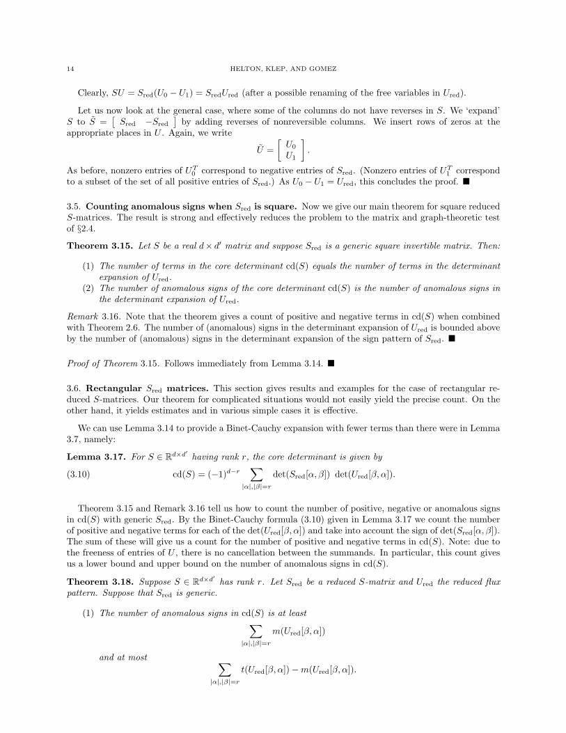
Example 3.21. Suppose Sred is generic, S =[Sred −Sred
]and the graph G(Sred) is:
R1?>=<89:;
C1
C2 R2?>=<89:; C3 ___ R3?>=<89:; · · · Cn ___ Rn?>=<89:;
There are n rows and n columns, so the rank of S (and Sred) is n. G(Sred) supports exactly one rank nsquare matrix, Sred itself.
G(Sred) has one cycle with no c-pairs, so it is an e-cycle. G(Sred) admits 2 perfect matchings: the e-cycleinterlaces both matchings. So by Theorem 2.6, we get N = Sred.
16 HELTON, KLEP, AND GOMEZ
Theorem 3.18 together with Theorem 2.6 imply
1 = m(Ured) =∑Nm(Ui) ≤ m(S) ≤
∑N
[t(Ui)−m(Ui)] = t(Ured)−m(Ured) = 2− 1 = 1.
Thus generically cd(S) has one anomalous sign (independent of n ≥ 2).
Alternative to Theorem 3.18, since Sred is square, we could have used Theorems 3.15 and 2.6 which tellus that cd(S) will have 2 terms, one with a positive and one with a negative sign.
On the other hand, the number of anomalous signs in cfd(S) increases rapidly with n.
n 2 3 4 5 6 7 8 9 10# of anomalous signs in cfd(S) 1 2 5 13 34 89 233 610 1597
This data is consistent withnumber of anomalous signs = Fib(2n− 3)
(see the website http://www.research.att.com/~njas/sequences/), where Fib(k) denotes the kth Fi-bonacci number. We conjecture that the formula is true for all n.
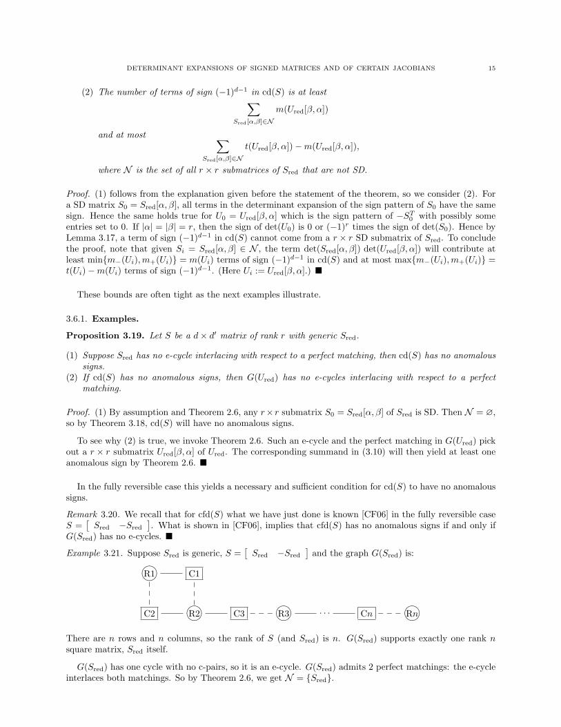
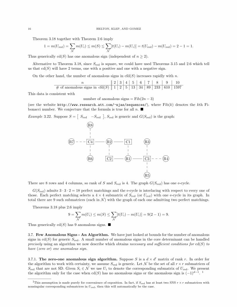
Example 3.22. Suppose S =[Sred −Sred
], Sred is generic and G(Sred) is the graph:
R8?>=<89:;
R7?>=<89:; ___ C4
R2?>=<89:;
C1
R3?>=<89:;
R6?>=<89:; C2 R1?>=<89:; C3 ___
R4?>=<89:;
R5?>=<89:;There are 8 rows and 4 columns, so rank of S and Sred is 4. The graph G(Sred) has one e-cycle.
G(Sred) admits 3 · 3 · 2 = 18 perfect matchings and the e-cycle is interlacing with respect to every one ofthose. Each perfect matching selects a 4 × 4 submatrix of Sred (or Ured) with one e-cycle in its graph. Intotal there are 9 such submatrices (each in N ) with the graph of each one admitting two perfect matchings.
Theorems 3.18 plus 2.6 imply
9 =∑Nm(Ui) ≤ m(S) ≤
∑N
[t(Ui)−m(Ui)] = 9(2− 1) = 9.
Thus generically cd(S) has 9 anomalous signs.
3.7. Few Anomalous Signs - An Algorithm. We have just looked at bounds for the number of anomaloussigns in cd(S) for generic Sred. A small number of anomalous signs in the core determinant can be handledprecisely using an algorithm we now describe which obtains necessary and sufficient conditions for cd(S) tohave (zero or) one anomalous sign.
3.7.1. The zero-one anomalous sign algorithm. Suppose S is a d × d′ matrix of rank r. In order forthe algorithm to work with certainty, we assume Sred is generic. Let N be the set of all r× r submatrices ofSred that are not SD. Given Si ∈ N we use Ui to denote the corresponding submatrix of Ured. We presentthe algorithm only for the case when cd(S) has no anomalous signs or the anomalous sign is (−1)d−1. 1
1This assumption is made purely for convenience of exposition. In fact, if Sred has at least two SNS r× r submatrices withnonsingular corresponding submatrices in Ured, then this will automatically be the case.
DETERMINANT EXPANSIONS OF SIGNED MATRICES AND OF CERTAIN JACOBIANS 17
Case E: N has 0 elements.Then cd(S) has no anomalous signs.
Case N: N is nonempty.Subcase (a): All the Ui corresponding to Si ∈ N are SD.
Take det(Si) det(Ui) and look at its sign. If for all Si ∈ N this sign is (−1)r, then cd(S) has noanomalous signs. Otherwise for some Si ∈ N the sign is (−1)r−1 and the corresponding termdet(Si) det(Ui) contributes t(Ui) terms with sign (−1)r−1 to cd(S). If t(Ui) > 1, then thereis more than one anomalous sign in cd(S). If there is Sj 6= Si with sign(det(Sj) det(Uj)) =(−1)r−1, then cd(S) will have more than one anomalous sign. Otherwise cd(S) has one anoma-lous sign.
Subcase (b): There is exactly one S0 ∈ N for which the corresponding U0 is not SD.If there is Si ∈ N \ S0 with the sign of det(Si) det(Ui) equal to (−1)r, then cd(S) will havemore than one anomalous sign. Otherwise we use the det sign test (Theorem 2.6) to computem(U0).
(i) If m(U0) > 1, then cd(S) will have more than one anomalous sign.(ii) Suppose m(U0) = 1. If t(U0) = 2, cd(S) will have one anomalous sign. So suppose
t(U0) > 2. Let
ε =
+1 | m(U0) = m+(U0)−1 | otherwise.
Now cd(S) will have one anomalous sign if and only if
(3.11) ε sign det(S0) = (−1)r−1.
(If (3.11) fails, cd(S) will have more than one anomalous sign.)Subcase (c): There are at least two Si ∈ N for which the corresponding Ui is not SD.
In this case cd(S) will have at least two anomalous signs.
Lemma 3.23. The zero-one anomalous sign algorithm computes whether or not there is one (respectivelyno) anomalous sign.
Proof. Case E is described in Proposition 3.19. Case N.(a) follows directly from the Binet-Cauchy formula(3.10). For Case N.(b).(i), det(S0) det(U0) has more than one anomalous sign, so cd(S) will have more thanone anomalous sign. The proof of Case N.(b).(ii) is essentially contained in the statement itself. Finally, inthe Case N.(c) two different Si contribute two different terms to the Binet-Cauchy expansion 3.10 for cd(S)each having at least one anomalous sign.
Remark 3.24. The algorithm simplifies considerably in the fully reversible case, as then Ui is SD if and onlyif Si is. Thus Case N.(a) cannot arise. Subcase (b) is equivalent to N having exactly one element andSubcase (c) is equivalent to N containing at least two elements.
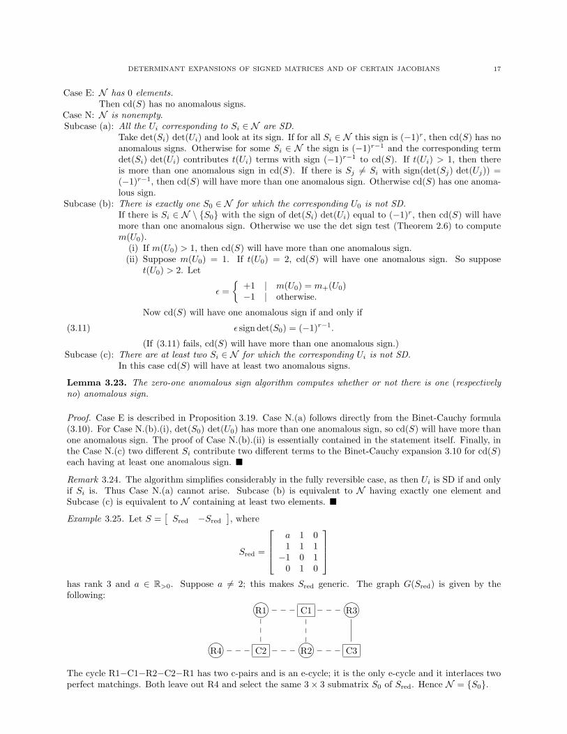
Example 3.25. Let S =[Sred −Sred
], where
Sred =
a 1 01 1 1−1 0 1
0 1 0
has rank 3 and a ∈ R>0. Suppose a 6= 2; this makes Sred generic. The graph G(Sred) is given by thefollowing:
R1?>=<89:;
___ C1
R3?>=<89:;_ _ _
R4?>=<89:; ___ C2 ___ R2?>=<89:; C3_ _ _
The cycle R1−C1−R2−C2−R1 has two c-pairs and is an e-cycle; it is the only e-cycle and it interlaces twoperfect matchings. Both leave out R4 and select the same 3× 3 submatrix S0 of Sred. Hence N = S0.
18 HELTON, KLEP, AND GOMEZ
To count the number of anomalous signs in cd(S) apply the Algorithm 3.7.1. Our situation correspondsto Case N.(b) and we compute m(U0), where U0 is the 3 × 3 submatrix of Ured corresponding to S0. Bythe det sign test, m(U0) = 1 and t(U0) = 3. It is easy to see that m(U0) = m−(U0); thus by the zero-oneanomalous sign algorithm, cd(S) will have one anomalous sign if and only if a− 2 = det(S0) < 0. (If a > 2,cd(S) will have two anomalous signs.)
Another class of examples is solipsistic cycles, a notion we now elucidate. A subgraph Γ of G is said tobe solipsistic provided when edges of Γ are removed from G all paths in the remaining graph starting froma vertex in Γ have length ≤ 1.
Proposition 3.26. Suppose Sred is generic and the graph G(Sred) is connected and contains at most onecycle which is solipsistic (e.g. Example 3.5 or Example [CF05, Table 1.1.(iii)]). Then the number of anomaloussigns in cd(S) is ≤ 1.
Proof. Without loss of generality, G(Sred) contains a cycle E . If E is not an e-cycle, then we are in Case Eof the algorithm and there are no anomalous signs in cd(S). Thus we assume that E is an e-cycle.
By Lemma 3.11, the rank r of Sred is the minimal number of rows or of columns in Sred. If r is biggerthan the number of columns appearing in the cycle, then we are in Case E of the algorithm because anyperfect matching will include some edge not in the cycle, thus making E not interlace it. Hence cd(S) hasno anomalous signs.
Otherwise r equals the number of columns appearing in the cycle. Then N has only one element S0. Thecorresponding submatrix U0 of Ured is either SD or its determinant expansion has two terms of opposite sign.Now the result follows from Case N.(a).
Note that results on the core determinant cd(S) given in this section have parallels for the Craciun-Feinberg determinant expansion cfd(S) which are easy to work out using the techniques in our paper.
4. Chemical Motivation
This matrix theory paper is not directly aimed at producing chemical results but was inspired as anextension of the striking work of Craciun and Feinberg. We hope these extensions might someday provevaluable on chemical network problems and some methods they combine with are described in [CHW08] anda consequence is Theorem 4.1 below.
Now we turn to describing the connection between the core determinant from §3 and chemistry.
A chemical reactor can be thought of as a tank with each chemical species flowing in (assume at a constantrate) and each species flowing out (assume in proportion to its concentration in the tank). If the reactioninside the tank satisfies dx
dt = g(x), then when there are inflows and outflows, the total reaction satisfies
dx
dt= f(x) = g(x) + εxin − δx.
The Craciun-Feinberg determinant is the determinant of the Jacobian f ′ when δ is 1 and it bears on countingthe number of equilibria for this differential equation, cf. [CF05,CF06,CHW08]. There is some discussion ofsmall outflows vs. no outflows in [CF06iee].
The core determinant bears on a different problem. Assume the differential equation has reaction formf(x) = Sv(x). Let R (respectively R⊥) denote the range of S (respectively its orthogonal complement);R is typically called the stoichiometric subspace. Let P be the projection onto R and P⊥ onto R⊥. Withno inflows and outflows, P⊥f(x) = 0 and clearly this implies the solution x(t) to the differential equationpropagates on the affine subspace
(4.1) Mx0 := x | P⊥x(t) = const = P⊥x0.

DETERMINANT EXPANSIONS OF SIGNED MATRICES AND OF CERTAIN JACOBIANS 19
This reflects quantities (like the number of carbon atoms) being conserved. The flow on Mx0 has dynamicsdPxdt = d(Px+P⊥x0)
dt = Pf(Px+ P⊥x0). Proposition 3.3 implies that the determinant of the Jacobian of thisdynamics is the core determinant which we studied in this paper, namely, for any ξ in Mx0
(4.2) cd(S)(ξ) = det(Pf ′(ξ)P ).
When cd(S) has no anomalous signs the degree theory arguments in §3 of [CHW08] give a strong resultfor numbers of equilibria of the differential equation.
Theorem 4.1. Suppose dxdt = fb(x) := Svb(x) has reaction form with vb(x) once continuously differentiable
in x and depending continuously on a parameter 0 ≤ b ≤ 1. Suppose each component vbj(x) of vb(x) ismonotone nondecreasing. Suppose Mx0 is compact. Suppose cd(S) has no anomalous signs.
If there are no zeroes fb(x) = 0 for any b and any x on the boundary of Mx0 , then the number of zeroesfor fb in the interior of Mx0 is independent of b.
The hypothesis that cd(S) has no anomalous signs can be weakened to cd(S)(ξ) does not equal 0 for anyξ in Mx0 .
5. Appendix. A sign pattern times its transpose
This paper derived matrix theoretic results pertaining to a chemistry setup. In this section we describesimilar results in a different mathematical context which some might find more attractive.
Theorem 5.1. Let A be a sign pattern and B its transposed sign pattern. Then AB has a sign pattern ifand only if A does not contain a 2×2 submatrix whose rows and columns can be permuted to obtain a matrixwhose sign pattern is one of
(5.1)[
+1 −1−1 −1
]or
[−1 +1+1 +1
].
Proof. This is easily proved using a straightforward analysis of (AB)ij =∑k AikBkj similar to that found
in the proof of Theorem 3.2.(2).
Remark 5.2. Note that Theorem 5.1 implies Theorem 3.2.(3) in the case S is fully reversible, i.e., S =[Sred −Sred
]. Indeed, by Lemma 3.14, SU = SredUred and Ured is the transpose of the sign pattern of
−Sred. Now apply Theorem 5.1 to Sred.
In a similar vein what we have done bears on the determinant expansions of AB where A is a signpattern and B is its transpose pattern. If A is a total signed compound sign pattern, as in §2.2, and Bis its transpose sign pattern, then AB is sign-nonsingular provided it is invertible. This follows from theBinet-Cauchy formula (similar to §3.3), and the idea is essentially in [CF05, CF06, BDB07]. When AB isnot invertible, then the core determinant expansion introduced here has all coefficients of the same sign.What we do in this paper is more general in that it gives estimates on the number of anomalous signs in theexpansion of det(AB). However, we specialize to A not actually being a sign pattern but having numericalentries, and B being the sign pattern which is the transpose of the signs of A.
6. Appendix. Software
The discovering of the results in this paper was considerably facilitated by computer experiments. Theprograms we wrote to do this might be of value to a broad community, so we documented them and providedtutorial examples. They are found on the web site
http://www.math.ucsd.edu/~chemcomp/
The Mathematica files provided contain software for dealing with equations that come from chemicalreaction networks; dx/dt = f(x) = Sv(x) as in (1.2). Some of our commands focus on the the Jacobian, f ′,of f ; they do the following
20 HELTON, KLEP, AND GOMEZ
(1) compute the Jacobian f ′ of f (given say the stoichiometric matrix S);(2) compute the Craciun-Feinberg determinant of f ′;(3) compute the core determinant of f ′;(4) check existence of a sign pattern for f ′(x) which remains unchanged for all x ≥ 0, using Theorem 5.1 in
this paper;(5) implement the sign fixing algorithm explained in [HKKprept].
Another part of our Mathematica package deals with deficiency of reaction form differential equationsand various representations for these differential equations. Capability to automatically plot planar graphsis under development and should be available soon.
References
[AnS03] D. Angeli, E. D. Sontag: Monotone control systems. New directions on nonlinear control. IEEE Trans. Automat.
Control 48 (2003), no. 10, 1684–1698[ArS06] M. Arcak, E.D. Sontag: Diagonal stability of a class of cyclic systems and its connection with the secant criterion.
Automatica, 42 (2006), no. 9, 1531–1537
[ArS07] M. Arcak, E.D. Sontag: A passivity-based stability criterion for a class of interconnected systems and applicationsto biochemical reaction networks. Mathematical Biosciences and Engineering, to appear.
http://arxiv.org/abs/0705.3188
[BJS98] M. Bakonyi, C.R. Johnson, D.P. Stanford: Sign pattern matrices that require domain-range pairs with given signpatterns, Linear and Multilinear Algebra 44 (1998), no. 2, 165–178
[BDB07] M. Banaji, P. Donnell, S. Baigent: P Matrix Properties, Injectivity, and Stability in Chemical Reaction Systems,
SIAM J. Appl. Math. 67 (2007), no. 6, 1523–1547[BMQ68] L. Bassett, J. Maybee, J. Quirk: Qualitative economics and the scope of the correspondence principle. Econo-
metrica 36 (1968), 544–563[BS95] R.A. Brualdi, B.L. Shader: Matrices of sign-solvable linear systems, Cambridge Univ. Press, 1995
[CJ06] P.J. Cameron, C.R. Johnson: The number of equivalence classes of symmetric sign patterns, Discrete Math. 306
(2006), no. 23, 3074–3077[CF05] G. Craciun, M. Feinberg: Multiple equilibria in complex chemical reaction networks. I. The injectivity property,
SIAM J. Appl. Math. 65 (2005), no. 5, 1526–1546
[CF06] G. Craciun, M. Feinberg: Multiple equilibria in complex chemical reaction networks. II. The species-reactiongraph, SIAM J. Appl. Math. 66 (2006), no. 4, 1321–1338
[CF06iee] G. Craciun, M. Feinberg: Multiple Equilibria in Complex Chemical Reaction Networks: Extensions to Entrapped
Species Models, IEE Proceedings Systems Biology 153:4 (2006), 179–186[CHW08] G. Craciun, J.W. Helton, R.J. Williams: Homotopy methods for counting reaction network equilibria, Math.
Biosci. 216 (2008), 140–149
[DGESVD99] J. Demmel, M. Gu, S. Eisenstat, I. Slapnicar, K. Veselic, Z. Drmac: Computing the singular value decompositionwith high relative accuracy, Linear Algebra Appl. 299 (1999), no. 1-3, 21–80
[HKKprept] J.W. Helton, V. Katsnelson, I. Klep: Sign patterns for chemical reaction networks, preprint (2009)[HGBM06] L. Hogben, R. Brualdi, A. Greenbaum, R. Mathias (Eds.): Handbook of Linear Algebra, Discrete Mathematics
and Applications, vol. 39, CRC Press, 2006
[KOSD07] I.-J. Kim, D.D. Olesky, B. Shader, P. van den Driessche: Sign patterns that allow a positive or nonnegative leftinverse, SIAM J. Matrix Anal. Appl. 29 (2007), no. 2, 554–565
[LMOD96] T. Lundy, J.S. Maybee, D.D. Olesky, P. van den Driessche: Spectra and inverse sign patterns of nearly sign-nonsingular matrices, Linear Algebra Appl. 249 (1996), 325–339
[Pa06] B. Palsson: Systems Biology: Properties of Reconstructed Networks, Cambridge Univ. Press, 2006[RST99] N. Robertson, P.D. Seymour, R. Thomas: Permanents, Pfaffian orientations, and even directed circuits, Ann. of
Math. (2) 150 (1999), no. 3, 929–975
J. William Helton, Mathematics Department, University of California at San Diego, La Jolla CA 92093-0112
E-mail address: [email protected]
Igor Klep, Univerza v Ljubljani, Fakulteta za matematiko in fiziko, Jadranska 19, SI-1111 Ljubljana, and
Univerza v Mariboru, Koroska 160, SI-2000 Maribor, Slovenia
E-mail address: [email protected]
Raul Gomez, Mathematics Department, University of California at San Diego, La Jolla CA 92093-0112
E-mail address: [email protected]
DETERMINANT EXPANSIONS OF SIGNED MATRICES AND OF CERTAIN JACOBIANS 21
NOT FOR PUBLICATION
Contents
1. Introduction 1
1.1. Determinants of Sign Patterns 1
1.2. Jacobians of reaction form differential equations 2
1.3. Chemistry 2
2. Matrices with sign patterns 3
2.1. Basics on graphs, matrices and determinants 3
2.2. SNS matrices vs. e-cycles 4
2.3. Many Cycles: Square Matrices 4
2.3.1. Proof of Theorem 2.6 6
2.4. Many Cycles: Nonsquare Matrices 8
3. Reaction form differential equations and the Jacobians 9
3.1. Sign pattern of the Jacobian 9
3.2. The core and other determinant expansions 10
3.3. Formulas for determinants of products of matrices 12
3.4. Generic matrices and the reduced S-matrix 13
3.5. Counting anomalous signs when Sred is square 14
3.6. Rectangular Sred matrices 14
3.6.1. Examples 15
3.7. Few Anomalous Signs - An Algorithm 16
3.7.1. The zero-one anomalous sign algorithm 16
4. Chemical Motivation 18
5. Appendix. A sign pattern times its transpose 19
6. Appendix. Software 19
References 20