Detecting Activities from Body-Worn Accelerometers

via Instance-based Algorithms

Nicola Bicocchi, Marco Mamei, Franco Zambonelli

Dipartimento di Scienze e Metodi dell’Ingegneria, University of Modena and ReggioEmilia, Italy

Abstract

The automatic and unobtrusive identification of user’s activities is one ofthe challenging goals of context-aware computing. This paper discusses andexperimentally evaluates instance-based algorithms to infer user’s activitieson the basis of data acquired from body-worn accelerometer sensors. Weshow that instance-based algorithms can classify simple and specific activitieswith high accuracy. In addition, due to their low requirements, we show howthey can be implemented on severely resource-constrained devices. Finally,we propose mechanisms to take advantage of the temporal dimension of thesignal, and to identify novel activities at run time.

Key words: Context-aware Computing, Body-worn Sensors, MotionClassification.

1. Introduction

The automatic and unobtrusive identification of user’s activities fromsensor data is one of the key and most challenging goals of context-awarecomputing [1]. Several opportunities can arise from the availability of suchan information. For example, a service would be able to flexibly adapt itsbehavior to di!erent circumstances (e.g., a smart phone application couldturn silent, once recognizing that the user is in a theater watching a movie).As another example, the simple description of user’s activities could auto-matically produce entries in blogs, diaries and social network sites [2].

While advances in hardware technologies (e.g., smart phones, wirelesssensors and RFID tags [3]) are making feasible to collect a vast amount

Preprint submitted to Pervasive Mobile Computing Journal March 23, 2010

of information about the user in an unobtrusive way, it is still di"cult toorganize and aggregate all the collected information in a coherent, expressiveand semantically-rich representation. In other words there is a gap betweenlow-level sensor readings and their high-level context description [4].

In this paper we tackle the problem of turning low-level accelerometerdata acquired from body-worn sensors into high-level activity descriptions.Body-worn accelerometers are suitable for this kind of applications: theyare small and economic, could be easily integrated in everyday objects andclothes, and they are already integrated in a number of smart phones.

To e"ciently classify human activities on the basis of accelerometer datawe focus on instance based mechanisms. Instance-based classifiers do notbuild an explicit, declarative representation of the class of interest but relyon the class labels attached to the training samples similar to the test sampleto be classified. These methods have thus been called lazy learners, since“they defer the decision on how to generalize beyond the training data untileach new query instance is encountered” [5]. We focused on these algorithmsin that they are easy to implement, they o!er state-of-the-art classificationperformance, the classification procedure can be easily understood (it doesnot rely on black-box models like in neural networks), they support on-lineclassification and training and, as detailed in the following sections, they canbe implemented on resource-constrained devices.

Although the problem of classifying user activities on the basis of body-worn accelerometers has already been investigated in several other researches[6, 7, 8, 9] (see Section 2 for details), the contribution of this paper is toshow that simple instance-based algorithms can classify accelerometer datamore accurately than several other approaches employing more complex algo-rithms. In addition, we show that instance-based algorithms can be executedon resource constrained devices like sensor motes.

More in detail, the paper presents the following contributions and insights:

1. We show that simple instance-based (IB) algorithms o!er state-of-the-art classification performance in this scenario (80% classification pre-cision and recall with 16 classes). In addition, we verified that theycan be easily implemented on resource constrained sensors. In partic-ular, the mainstream argument that IB consumes too much memorybecause it stores individual feature vectors (see later) is unfounded. Inthis scenario, IB can be implemented on memory-constrained deviceskeeping state-of-the-art performance.

2

2. We highlight that body-worn accelerometers are not only useful to rec-ognize simple motion/ambulation states (e.g., walking, running) like inmost of the related work. These sensors can also recognize and dis-criminate among specific activities in other scenarios (e.g., use a PC,stir pasta, drive the car). This supports the use of accelerometer dataand IB-algorithms to fulfill the context-awareness vision.

3. We present a mechanism allowing IB classification to take into con-sideration the time series of the acceleration data and to aggregateclassification results over a given time frame to considerably improveclassification precision and recall.

4. We present a mechanism to introduce and identify new activity classesat run time. One of the main problems of IB classifiers is that theyclassify any new pattern as one of the predefined classes, no matter howdi!erent the new pattern is from the ones in the training set. Instead,practical systems require a mechanism to understand that a patterndeviating from the ones seen previously could represent a completelynew activity rather than a di!erent “gait” for the predefined ones.

Accordingly, the remainder of the paper is organized as follows: Section 2surveys related work in this area. Section 3 presents the instance-based algo-rithms we used to classify activities using acceleration data and illustrates thepossible applications enabled by these algorithms. Section 4 presents somenovel mechanisms we introduced to better deal with the sensors’ time seriesand to enable the on-line discovery of new classes. Section 5 describes thecollection of the dataset. Section 6 presents the classification performances ofour proposal. Section 7 details some results illustrating the suitability of theproposed mechanism to resource-constrained sensors. Section 8 concludes.

2. Related work

The problem of recognizing user’s activities on the basis of accelerom-eter data has been studied in a large number of works. Basically, all theapproaches share the same basic framework:

1. A number of accelerometers are worn by the user typically at specificpositions on her body.

2. Data is collected on a device (smart phone, laptop) and the user isasked to label his/her activities to provide ground truth information.

3

3. Feature vectors are extracted from the raw accelerometer data.4. A pattern recognition algorithm (whether instance-based or using other

mechanisms, such as Hidden Markov Model and Support Vector Ma-chine) is used to learn a model to recognize user’s activities on the basisof the feature vectors.

5. Once this training phase is concluded, new data is collected while theuser performs daily activities. Such data is converted in feature vectorsand then classified.

6. Some standard measures (e.g., accuracy, confusion matrices) are usedto evaluate classification performances.

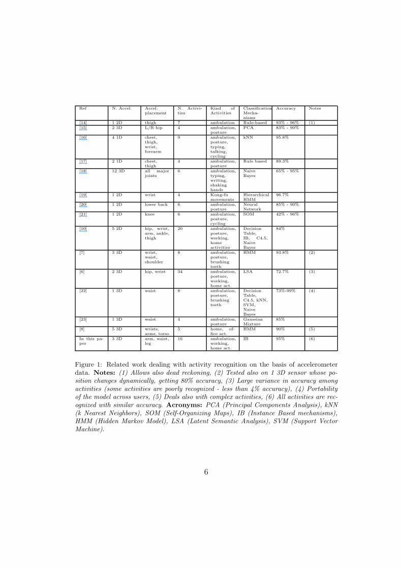
Since the basic framework of all the approaches in the area is almostidentical, we can present their setting and results in a single table (see Figure2). For each of the related works being surveyed, we describe the number ofaccelerometers being used, where they have been located, the number andkind of activities the system tries to recognize, the classification mechanismbeing used, and the resulting classification accuracy.

Looking at the table, it is possible to see that apart from a few proposals[10, 6] most of the literature recognize a rather limited set of ambulatoryactivities. It is also worth emphasizing that in [10] 5 accelerometers are usedinstead of 3. This can obviously provide more data and ease the classifica-tion process. On the other side, [6] exhibits large variance in classificationprecision and recall. Despite a high number of activities is considered, someof them are poorly recognized (less than 4% accuracy).

Although this table is useful to present several related coherently works,it does not allow for simply comparing the reported accuracies and deducethat one work is better than another. These works are applied to di!erentdatasets, thus it is not correct to compare their results: it can be moredi"cult to classify 2 similar activities than to separate 20 “disjunct” ones.Similarly, one work can capture several expressions of the same activity (e.g.,di!erent ways of running), while another one might only capture only a few.Despite these limitations, the table gives an overall view on the classificationtask being addressed by the related work and on the obtained accuracy.

Our approach demonstrates that simple IB algorithms can reliably rec-ognize a fairly large number of (also not ambulatory) activities.

We want also to emphasize that the use of IB approaches has recentlygained a lot of attention in research and applications in several other areas.

4

One of the best known concrete applications developed with IB mecha-nisms is Google’s “Did you mean?” tool. It corrects errors in search queries,not through a complex parsing of the query but by memorizing billions ofquery-answer pairs and suggesting the one closest to the users query.

In [11] a system to classify images on the basis of IB algorithms is pre-sented. The system uses a large dataset of 80 millions images collected fromthe Internet and labeled with one of the English nouns in the WordNet lexicaldatabase. Using IB approaches, new images are classified on the basis of theclosest images in the dataset. This work demonstrates that IB algorithmsobtain state-of-the-art performances also on complex computer vision tasks.

The work presented in [12] applies IB algorithms to bio-informatics. Itcompares di!erent classification algorithms over typical bio-informatics datasets.IB algorithms consistently rank at the top of that list. Similarly, for text-classification, [13] shows that IB algorithms outperforms most of the (morecomplex) mechanisms for text classification.

These results further motivate us in experimenting IB algorithms in thearea of human activity classification.

3. Instance-Based Classification of Human Activities

Instance-based classification algorithms can be generally divided into twobroad categories: (i) approaches based on the distance between the newsample and the closest labeled instances, (ii) approaches based on the localdensity of labeled instances in the area close to the new sample.

In our work we experimented with 4 instance-based classification algo-rithms: K Nearest Neighbors (kNN, or IBk) represents the former category.Direct Density (DD), Class Local Outlier Factor (CLOF), Local Classifica-tion Factor (LCF) represent the latter one.

Density-based approaches have been used also because they provide ef-fective techniques to detect outliers among the samples. As described inthe next section, this characteristic is useful to introduce and identify newactivity classes at run time.

3.1. Feature Vectors ExtractionBefore describing the di!erent instance-based classification algorithms, it

is important to describe how feature vectors have been extracted from theaccelerometer data.

5

Ref N. Accel. Accel.placement

N. Activi-ties

Kind ofActivities

ClassificationMecha-nisms

Accuracy Notes

[14] 1 2D thigh 7 ambulation Rule-based 93% - 96% (1)[15] 2 3D L/R hip 4 ambulation,

posturePCA 83% - 90%

[16] 4 1D chest,thigh,wrist,forearm

9 ambulation,posture,typing,talking,cycling

kNN 95.8%

[17] 2 1D chest,thigh

4 ambulation,posture

Rule based 89.3%

[18] 12 3D all majorjoints

6 ambulation,typing,writing,shakinghands

NaiveBayes

65% - 95%

[19] 1 2D wrist 4 Kung-fumovements

HierarchicalHMM

96.7%

[20] 1 2D lower back 6 ambulation,posture

NeuralNetwork

85% - 90%

[21] 1 2D knee 6 ambulation,posture,cycling

SOM 42% - 96%

[10] 5 2D hip, wrist,arm, ankle,thigh

20 ambulation,posture,working,homeactivities

DecisionTable,IB, C4.5,NaiveBayes

84%

[7] 3 3D wrist,waist,shoulder

8 ambulation,posture,brushingteeth

HMM 93.8% (2)

[6] 2 3D hip, wrist 34 ambulation,posture,working,home act.

LSA 72.7% (3)

[22] 1 3D waist 8 ambulation,posture,brushingteeth

DecisionTable,C4.5, kNN,SVM,NaiveBayes

73%-99% (4)

[23] 1 3D waist 4 ambulation,posture

GaussianMixture

85%

[8] 5 3D wrists,arms, torso

5 home, of-fice act.

HMM 90% (5)

In this pa-per

3 3D arm, waist,leg

16 ambulation,working,home act.

IB 95% (6)

Figure 1: Related work dealing with activity recognition on the basis of accelerometerdata. Notes: (1) Allows also dead reckoning, (2) Tested also on 1 3D sensor whose po-sition changes dynamically, getting 80% accuracy, (3) Large variance in accuracy amongactivities (some activities are poorly recognized - less than 4% accuracy), (4) Portabilityof the model across users, (5) Deals also with complex activities, (6) All activities are rec-ognized with similar accuracy. Acronyms: PCA (Principal Components Analysis), kNN(k Nearest Neighbors), SOM (Self-Organizing Maps), IB (Instance Based mechanisms),HMM (Hidden Markov Model), LSA (Latent Semantic Analysis), SVM (Support VectorMachine).

6

We started by just considering feature vectors consisting of 9 elementscorresponding to the x,y,z components of the acceleration measured by 3body-worn sensors (positioned at right arm, waist and right leg) in a singlesampling (sensors are sampled at 10Hz). Each feature vector has been clas-sified independently. The distance among these vectors have been measuredin terms of Euclidean distance.

It is worth noticing that our sampling rate is lower than that reportedin other related works. For example, the CenceMe project [9] measuredthat 40Hz is the minimum acceptable rate for e!ectively classifying activitiesfrom a single 3D accelerometer embedded in a mobile phone. In our case,the use of 3 well-positioned 3D accelerometers allows to classify e!ectivelyaccelerometer data acquired at lower sampling rates.

In the following Section 4.1, we describe how we extended this vector totake into account the temporal dynamics of the collected data.

3.2. Instance-based Classification

In this section we briefly describe the instance-based classification algo-rithms we adopted in our experiments.

k Nearest Neighbors (kNN, or IBk). The k Nearest Neighbors algo-rithm classifies a new sample p by selecting the k training samples that areclosest to p under some distance function (in this work we used the Euclideandistance). Then, p is given the most frequent label appearing in the selectedk training samples. In the simplest case (k = 1), a new sample is classifiedthe same as the closest instance in the training set.

Direct Density (DD). If the samples in the training set TS are unevenlydistributed (like in most real cases), the kNN algorithm can fail to correctlyclassify a given sample if it falls in a region having a high-density of samplesof another class. To deal with this issue, the Direct Density approach (DD)takes into consideration the average distance between the sample to be clas-sified and the k-nearest neighbors of a given class. The sample is classifiedwith the class of k-nearest neighbors at the minimum distance.

Class Local Outlier Factor (CLOF). While the DD algorithm triesto determine to which extent a new sample is close to the clusters in thetraining sets associated with the di!erent classes, the Class Local OutlierFactor (CLOF) algorithm measures how much the new sample is an outlierwith respect to that clusters. It does so, by considering the ratio between theDD measure of the sample to be classified (q) and the average DD measure

7

of the training samples close to q. If the q sample is within a cluster suchratio will be close to 1. Otherwise it will be much higher.

Local Classification Factor (LCF). The Local Classification Factor(LCF) linearly combines DD and CLOF classification (LCF = DD + w ·CLOF ), trying to get the best trade-o! between the two. The parameter w,used in the linear combination, determines to which degree the outlier factorof a sample q is relevant for its classification. A higher value for w leadsto more correctly classified objects in the sparser classes, at the expense ofincorrectly classified objects in the denser classes.

In Section 6 we will present the results of applying such algorithms tohuman action classification.

4. Refining the Classification

In this section we present some valuable refinements to the classificationprocess. The first contribution allows to improve classification accuracy bytaking into account the time series of the acquired data. The second contri-bution allows to discover new classes of activities at run time.

4.1. Dealing with Time

While some classification algorithms, such as HMM [5], inherently dealwith the temporal relationships among the acquired samples, instance-basedalgorithms do not have such a mechanism built in their conception.

Still, for human activities classification such kind of temporal relation-ships are important. In fact, while individual sensor readings can be am-biguous and noisy, the pattern of a whole time-window of readings can bemuch more recognizable. In addition, assuming that human activities lastfor a minimum amount of time, it is possible to output class labels at a muchlower rate (e.g., 1Hz) than sensor readings (e.g. 10Hz) to save computationalresources (see Section 7.1).

Accordingly, we developed 2 simple yet e!ective mechanisms to representtemporal relationships in instance-based mechanisms.

Embedding Temporal Information in the Samples. This mecha-nism consists of adding elements, encoding temporal aspects, to the featurevector. In particular, starting from the 9-components feature vector (3 3-axisaccelerometers) described in Section 3.1, we added mean and variance of the

8

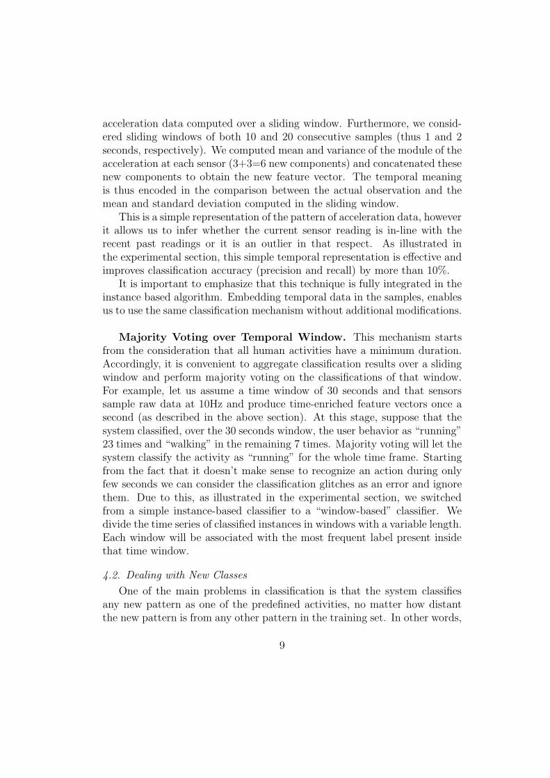
acceleration data computed over a sliding window. Furthermore, we consid-ered sliding windows of both 10 and 20 consecutive samples (thus 1 and 2seconds, respectively). We computed mean and variance of the module of theacceleration at each sensor (3+3=6 new components) and concatenated thesenew components to obtain the new feature vector. The temporal meaningis thus encoded in the comparison between the actual observation and themean and standard deviation computed in the sliding window.

This is a simple representation of the pattern of acceleration data, howeverit allows us to infer whether the current sensor reading is in-line with therecent past readings or it is an outlier in that respect. As illustrated inthe experimental section, this simple temporal representation is e!ective andimproves classification accuracy (precision and recall) by more than 10%.

It is important to emphasize that this technique is fully integrated in theinstance based algorithm. Embedding temporal data in the samples, enablesus to use the same classification mechanism without additional modifications.

Majority Voting over Temporal Window. This mechanism startsfrom the consideration that all human activities have a minimum duration.Accordingly, it is convenient to aggregate classification results over a slidingwindow and perform majority voting on the classifications of that window.For example, let us assume a time window of 30 seconds and that sensorssample raw data at 10Hz and produce time-enriched feature vectors once asecond (as described in the above section). At this stage, suppose that thesystem classified, over the 30 seconds window, the user behavior as “running”23 times and “walking” in the remaining 7 times. Majority voting will let thesystem classify the activity as “running” for the whole time frame. Startingfrom the fact that it doesn’t make sense to recognize an action during onlyfew seconds we can consider the classification glitches as an error and ignorethem. Due to this, as illustrated in the experimental section, we switchedfrom a simple instance-based classifier to a “window-based” classifier. Wedivide the time series of classified instances in windows with a variable length.Each window will be associated with the most frequent label present insidethat time window.

4.2. Dealing with New Classes

One of the main problems in classification is that the system classifiesany new pattern as one of the predefined activities, no matter how distantthe new pattern is from any other pattern in the training set. In other words,

9

the system is able to deal with only a predefined set of classes. Instead, apractical system requires a mechanism to add new classes at run time. Itis worth noting that this problem extends the idea of the NULL class (i.e.,the class that contains all the instances – outliers – that cannot be neatlyclassified in any of the specified classes) [24]. If sensors register a patternsignificantly di!erent form the ones describing the predefined classes, thesystem should create a new class (possibly asking the user for a proper label)and classify the new sensor readings accordingly.

On the one hand, instance-based algorithms are suitable for dynamicallyadding classes at run time. Since they do not have an explicit training phase,but all the computation is deferred at classification time, it is easy to adda new class just by adding samples with the new class label. On the otherhand, it is rather di"cult to decide whether a new sample is an outlier of apreviously existing class or it is the first sample of a new class.

The straightforward solution of creating a new class if the new sample isfarther than a threshold T from all the previously labeled samples does notwork well in practice, producing low classification accuracy.

Thus, we developed a novel solution to this problem. As discussed in Sec-tion 3.2, Local Classification Factor (LCF) is suitable as an outlier detector.After choosing the weight w to be used, for every sample q to be classified,it produces a numeric value LCFi(q) associated with each class i found inthe training set. We modified our classifier to associate to a special classcalled new every item which has min(LCFi(q)) greater than a threshold th.In Section 6 we show that, by properly tuning parameters k, w and th it ispossible to discover new classes at run time rather e!ectively.

A similar approach, grounded on statistical significance tests, has beenpresented in [24, 25]. In our future work we will try to combine this with ourapproach to improve the recognition of new classes.

5. Dataset Collection

To test our proposal we set up a 4-node body-worn sensor network to col-lect acceleration data. The network consists of: 3 Sunspot sensors(http://www.sunspotworld.com) provided with 3D accelerometers attachedto the right arm, waist and right leg of the person, and a back-packed Ultra-Mobile PC (UMPC): Asus EeePC 701SD (http://eeepc.asus.com). The 3Sunspots sample acceleration data at 10Hz and transmit it to the ultra-mobile PC where data is classified on line on the basis of an instance-based

10

algorithm (see Fig. 2). This simple set-up has two main advantages:

1. Simplicity. We developed and debugged classification algorithms onthe ultra-mobile PC, avoiding the complexity in programming with thesensors cumbersome libraries. This complies with the scientific aimof our work: we are not trying to create a ready-to-market solution,but to test models and algorithms. Moreover, high-level profiling toolsto monitor the application memory budget and CPU performance canbe readily used on the ultra-mobile PC. Thus, we can conduct rigor-ous measurements to test whether the proposed approach can fit theresource constraints of the sensors.

2. Repeatability. Although the ultra-mobile PC classifies samples on-line, all the samples are also saved in files. This allows us to repeat ex-periments and re-verify our conclusions. Some of our datasets are avail-able on line: http://pervasive2.morselli.unimo.it/~nicola/humanActions/

On the basis of our set-up, we performed two data acquisition campaigns:

1. Activities Dataset. To create this dataset we asked a group of 6people to wear our sensor network and perform a series of 16 predefinedactivities: stir pasta (while cooking); climb stairs; sleep (lie in bed);run; use pc (type and move the mouse); wash hands; use playstation 3(sat with the joypad in hand); read sat on the sofa; take the elevator;ride a bike; stand still; drive the car; eat pasta; drink at the bar (drinkstanding still); walk; dance (step feet and move hands rhythmically).These activities represent a mix of simple ambulatory activities and ofspecific actions dealing with house- or o"ce-works. Collected sensordata has been clearly labeled with the associated activity.

2. Real-life Dataset. To create this dataset, 2 users (among the au-thors) wear the sensor network for 1 day, as they went about theirnormal lives. Ground-truth labels have been acquired with a separaterecording application roughly synchronized with the sensor clock. Ac-tivities being annotated with the recording application are: chat beingsat; drink standing; set up the table; clean kitchen’s racks; eat; drivethe car; clean the table; chat standing; work at the pc; read on the sofa;wash hands, take something from fridge

While the former dataset has all the sensor data labeled with the corre-sponding activities, the latter dataset has a lot of unlabeled data where theuser did not explicitly indicate any activity.

11

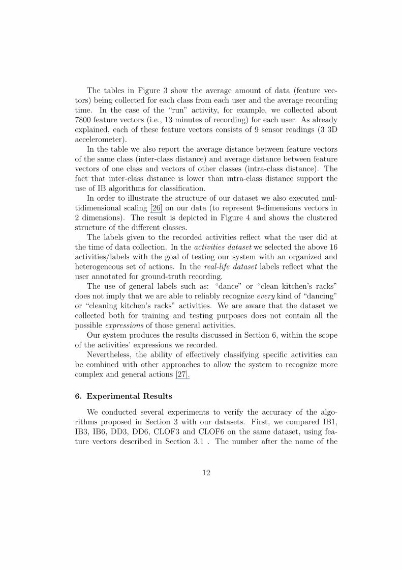
The tables in Figure 3 show the average amount of data (feature vec-tors) being collected for each class from each user and the average recordingtime. In the case of the “run” activity, for example, we collected about7800 feature vectors (i.e., 13 minutes of recording) for each user. As alreadyexplained, each of these feature vectors consists of 9 sensor readings (3 3Daccelerometer).

In the table we also report the average distance between feature vectorsof the same class (inter-class distance) and average distance between featurevectors of one class and vectors of other classes (intra-class distance). Thefact that inter-class distance is lower than intra-class distance support theuse of IB algorithms for classification.

In order to illustrate the structure of our dataset we also executed mul-tidimensional scaling [26] on our data (to represent 9-dimensions vectors in2 dimensions). The result is depicted in Figure 4 and shows the clusteredstructure of the di!erent classes.

The labels given to the recorded activities reflect what the user did atthe time of data collection. In the activities dataset we selected the above 16activities/labels with the goal of testing our system with an organized andheterogeneous set of actions. In the real-life dataset labels reflect what theuser annotated for ground-truth recording.

The use of general labels such as: “dance” or “clean kitchen’s racks”does not imply that we are able to reliably recognize every kind of “dancing”or “cleaning kitchen’s racks” activities. We are aware that the dataset wecollected both for training and testing purposes does not contain all thepossible expressions of those general activities.

Our system produces the results discussed in Section 6, within the scopeof the activities’ expressions we recorded.

Nevertheless, the ability of e!ectively classifying specific activities canbe combined with other approaches to allow the system to recognize morecomplex and general actions [27].

6. Experimental Results

We conducted several experiments to verify the accuracy of the algo-rithms proposed in Section 3 with our datasets. First, we compared IB1,IB3, IB6, DD3, DD6, CLOF3 and CLOF6 on the same dataset, using fea-ture vectors described in Section 3.1 . The number after the name of the

12

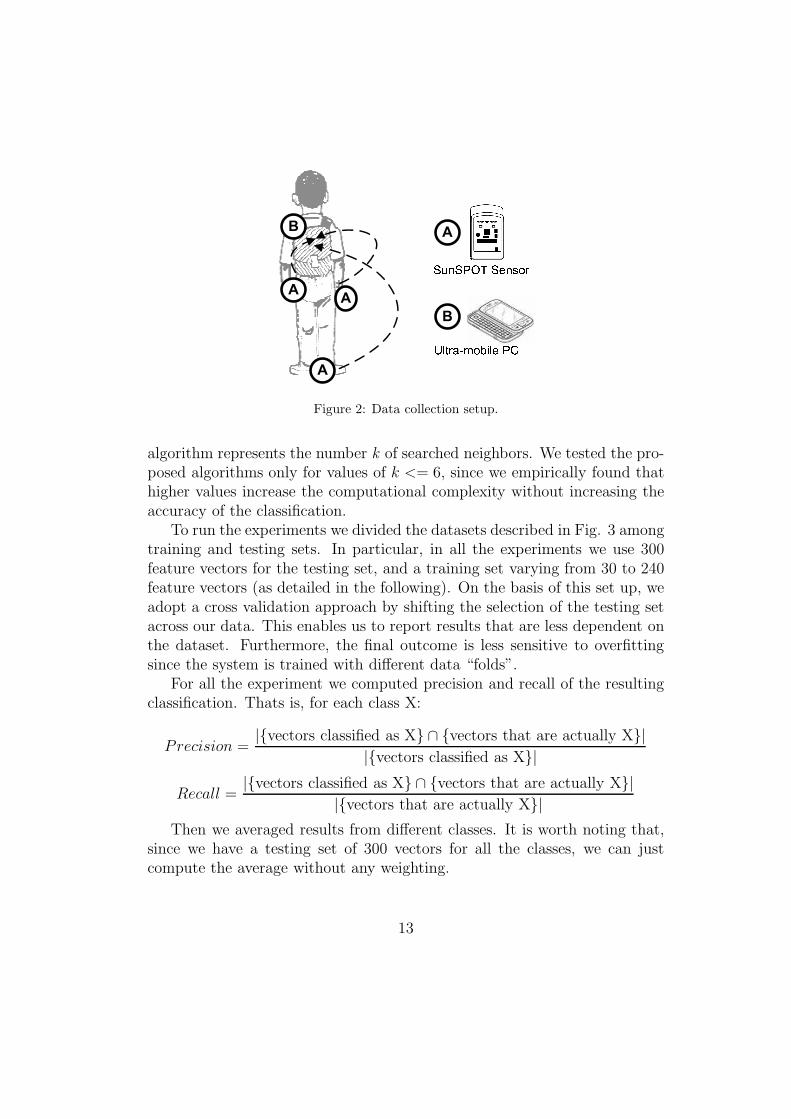
Figure 2: Data collection setup.

algorithm represents the number k of searched neighbors. We tested the pro-posed algorithms only for values of k <= 6, since we empirically found thathigher values increase the computational complexity without increasing theaccuracy of the classification.

To run the experiments we divided the datasets described in Fig. 3 amongtraining and testing sets. In particular, in all the experiments we use 300feature vectors for the testing set, and a training set varying from 30 to 240feature vectors (as detailed in the following). On the basis of this set up, weadopt a cross validation approach by shifting the selection of the testing setacross our data. This enables us to report results that are less dependent onthe dataset. Furthermore, the final outcome is less sensitive to overfittingsince the system is trained with di!erent data “folds”.

For all the experiment we computed precision and recall of the resultingclassification. Thats is, for each class X:

Precision =|{vectors classified as X} ! {vectors that are actually X}|

|{vectors classified as X}|

Recall =|{vectors classified as X} ! {vectors that are actually X}|

|{vectors that are actually X}|

Then we averaged results from di!erent classes. It is worth noting that,since we have a testing set of 300 vectors for all the classes, we can justcompute the average without any weighting.

13

Activity Avg. # vectors Avg. rec. time Avg. inter-class d. Avg. intra-class d.

stir pasta (cooking) 3900 6 min 0.59 1.67climb stairs 10800 18 min 1.41 2.06

sleep (lie in bed) 3700 6 min 0.02 3.39run 7800 13 min 2.82 2.91

use pc 15400 25 min 0.51 2.31wash hands 1900 3 min 0.57 1.66

use ps3 1900 3 min 0.17 1.89read on the sofa 1200 2 min 0.21 1.92take the elevator 2700 4 min 0.35 2.15

ride a bike 3500 6 min 0.87 1.69stand still 8800 14 min 0.21 1.77

drive the car 22500 37 min 0.69 2.47eat pasta 4200 7 min 0.47 1.97

drink standing still (bar) 3900 6 min 0.49 1.83walk 28100 47 min 1.39 2.15dance 3300 5 min 1.48 2.01

Activity Avg. # Samples Avg. rec. time Avg. inter-class d. Avg. intra-class d.

chat being sat 12600 21 min 0.07 2.39drink standing 6000 10 min 0.63 1.44set up the table 15600 26 min 0.86 1.43

clean kitchen racks 3600 6 min 0.84 1.42eat 13800 23 min 1.08 1.5

drive the car 9600 16 min 1.64 1.96clean the table 2400 4 min 1.26 1.86chat standing 26400 44 min 0.79 1.46work at the pc 31800 53 min 1.2 1.51read on the sofa 8400 14 min 0.99 1.65

wash hands 1200 2 min 0.74 1.41take s. from fridge 1800 3 min 0.75 1.48

Figure 3: (top) Activity dataset. (bottom) Real-life dataset

All the experiments except those in Section 6.3 have been conducted byusing, for both training and testing, data coming from the same user. Thus,the measured precision and recall in all the experiments refers to this case.More in detail, we set up the experiment so that during cross validation, the300-vector testing set is always associated with a training set coming fromthe same user.

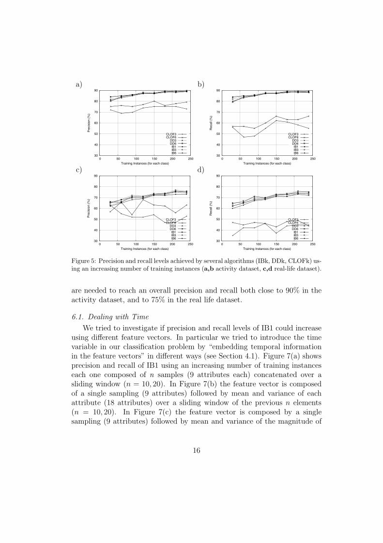
Figure 5 shows the precision and recall levels reached with an increasingnumber of training instances for the various classifiers. It is interesting tonote that even a small number of training instances per class (approximately50) is enough to reach high precision and recall. Moreover, it is clear fromthe graph that IBk and DDk algorithms outperform CLOFk. Consideringthe fact that these algorithms may run on resource constrained devices (seeSection 7), IB1 is clearly the best choice. In fact, even though its performanceis similar to IB3, IB6 and DDk, it is much simpler and, therefore, faster tobe executed. For this reason, we used IB1 in all the experiments reported inthe following of this section.

It is worth mentioning that, without any kind of optimizations, by simplyapplying IB1 to a training set composed of only 200 instances of 9 attributes(3 axis, 3 accelerometers) it is possible to achieve remarkable precision and

14

Figure 4: (top) Activity dataset. (bottom) Real-life dataset

recall levels. In particular, about 85% on the activity dataset while about75% on the real life data set. This experiment supports the contributionclaims made at the beginning of the paper: the simple IB1 algorithm canclassify accelerometer data with about 80% precision and recall, with a lim-ited number of training examples. This fact also supports the idea of usingIB algorithms on resource-constrained sensors (see Section 7).

Although a fair comparison with the state-of-the-art reported in Section2 would require using the same dataset, the obtained results indicate that– at least with regard of the set of action we considered – instance-basedalgorithms exhibit performance in line with the current best practices.

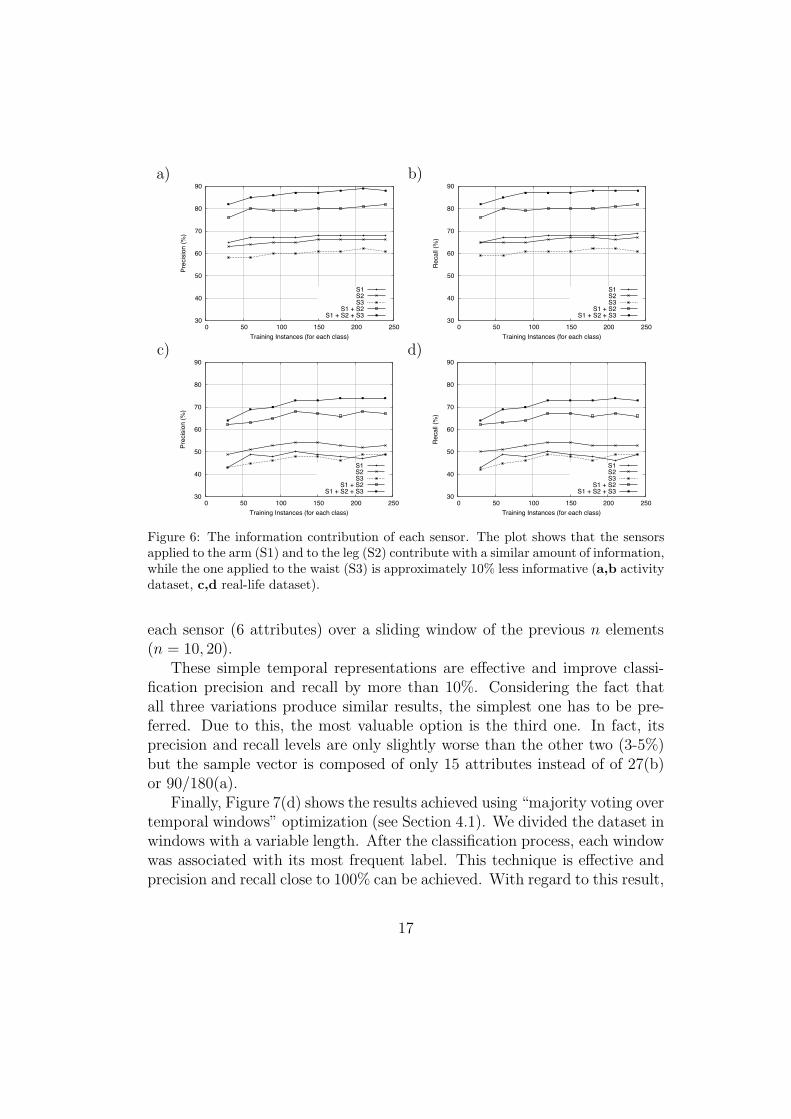
We were also interested in discovering whether the information contribu-tions coming from the three sensors were equal or not. Thus we applied IB1to the same dataset used in the experiments above but modified to suppressthe contribution of one or more sensors. In Figure 6 we plotted precisionand recall reached by IB1, in the activity dataset, increasing the number oftraining instances, using one sensor, two sensors, all three sensors, and eachof them alone. The plot shows that the sensors applied to the arm (S1) andto the leg (S2) provide a similar amount of information, while the one ap-plied to the waist (S3) is 10% less e!ective. In summary, even though thewaist-applied sensor gives a slightly smaller contribution, all three sensors

15

a)

30

40

50

60

70

80

90

0 50 100 150 200 250

Prec

isio

n (%

)

Training Instances (for each class)

CLOF3CLOF6

DD3DD6IB1IB3IB6

b)

30

40

50

60

70

80

90

0 50 100 150 200 250

Rec

all (

%)

Training Instances (for each class)

CLOF3CLOF6

DD3DD6IB1IB3IB6

c)

30

40

50

60

70

80

90

0 50 100 150 200 250

Prec

isio

n (%

)

Training Instances (for each class)

CLOF3CLOF6

DD3DD6IB1IB3IB6

d)

30

40

50

60

70

80

90

0 50 100 150 200 250

Rec

all (

%)

Training Instances (for each class)

CLOF3CLOF6

DD3DD6IB1IB3IB6

Figure 5: Precision and recall levels achieved by several algorithms (IBk, DDk, CLOFk) us-ing an increasing number of training instances (a,b activity dataset, c,d real-life dataset).

are needed to reach an overall precision and recall both close to 90% in theactivity dataset, and to 75% in the real life dataset.

6.1. Dealing with Time

We tried to investigate if precision and recall levels of IB1 could increaseusing di!erent feature vectors. In particular we tried to introduce the timevariable in our classification problem by “embedding temporal informationin the feature vectors” in di!erent ways (see Section 4.1). Figure 7(a) showsprecision and recall of IB1 using an increasing number of training instanceseach one composed of n samples (9 attributes each) concatenated over asliding window (n = 10, 20). In Figure 7(b) the feature vector is composedof a single sampling (9 attributes) followed by mean and variance of eachattribute (18 attributes) over a sliding window of the previous n elements(n = 10, 20). In Figure 7(c) the feature vector is composed by a singlesampling (9 attributes) followed by mean and variance of the magnitude of

16

a)

30

40

50

60

70

80

90

0 50 100 150 200 250

Prec

isio

n (%

)

Training Instances (for each class)

S1S2S3

S1 + S2S1 + S2 + S3

b)

30

40

50

60

70

80

90

0 50 100 150 200 250

Rec

all (

%)

Training Instances (for each class)

S1S2S3

S1 + S2S1 + S2 + S3

c)

30

40

50

60

70

80

90

0 50 100 150 200 250

Prec

isio

n (%

)

Training Instances (for each class)

S1S2S3

S1 + S2S1 + S2 + S3

d)

30

40

50

60

70

80

90

0 50 100 150 200 250

Rec

all (

%)

Training Instances (for each class)

S1S2S3

S1 + S2S1 + S2 + S3

Figure 6: The information contribution of each sensor. The plot shows that the sensorsapplied to the arm (S1) and to the leg (S2) contribute with a similar amount of information,while the one applied to the waist (S3) is approximately 10% less informative (a,b activitydataset, c,d real-life dataset).

each sensor (6 attributes) over a sliding window of the previous n elements(n = 10, 20).

These simple temporal representations are e!ective and improve classi-fication precision and recall by more than 10%. Considering the fact thatall three variations produce similar results, the simplest one has to be pre-ferred. Due to this, the most valuable option is the third one. In fact, itsprecision and recall levels are only slightly worse than the other two (3-5%)but the sample vector is composed of only 15 attributes instead of of 27(b)or 90/180(a).

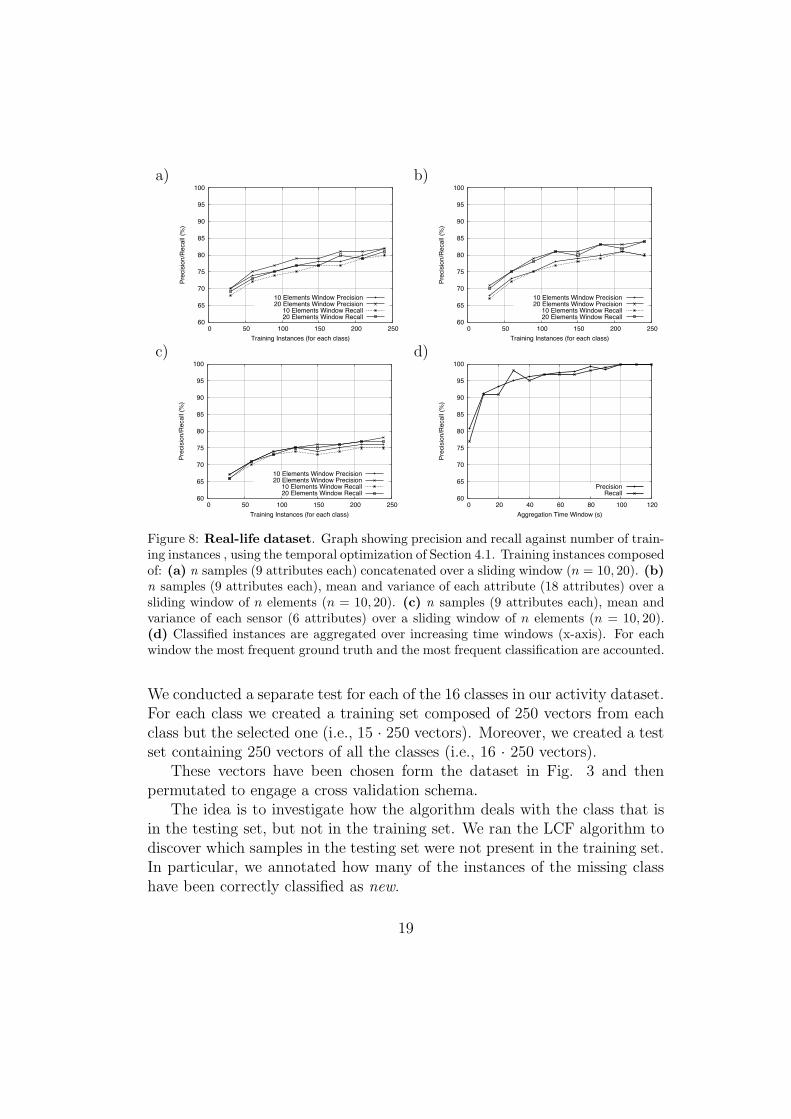
Finally, Figure 7(d) shows the results achieved using “majority voting overtemporal windows” optimization (see Section 4.1). We divided the dataset inwindows with a variable length. After the classification process, each windowwas associated with its most frequent label. This technique is e!ective andprecision and recall close to 100% can be achieved. With regard to this result,

17

a)

80

85

90

95

100

0 50 100 150 200 250

Prec

isio

n/R

ecal

l (%

)

Training Instances (for each class)

10 Elements Window Precision20 Elements Window Precision

10 Elements Window Recall20 Elements Window Recall

b)

80

85

90

95

100

0 50 100 150 200 250

Prec

isio

n/R

ecal

l (%

)

Training Instances (for each class)

10 Elements Window Precision20 Elements Window Precision

10 Elements Window Recall20 Elements Window Recall

c)

80

85

90

95

100

0 50 100 150 200 250

Prec

isio

n/R

ecal

l (%

)

Training Instances (for each class)

10 Elements Window Precision20 Elements Window Precision

10 Elements Window Recall20 Elements Window Recall

d)

80

85

90

95

100

0 20 40 60 80 100 120

Prec

isio

n/R

ecal

l (%

)

Aggregation Time Window (s)

PrecisionRecall

Figure 7: Activity dataset. Graph showing precision and recall against number of train-ing instances, using the temporal optimization of Section 4.1. Training instances composedof: (a) n samples (9 attributes each) concatenated over a sliding window (n = 10, 20). (b)n samples (9 attributes each), mean and variance of each attribute (18 attributes) over asliding window of n elements (n = 10, 20). (c) n samples (9 attributes each), mean andvariance of each sensor (6 attributes) over a sliding window of n elements (n = 10, 20). (d)Graph showing the e!ect of temporal aggregation on the overall precision and recall. Clas-sified instances are aggregated over increasing time windows (x-axis). For each windowthe most frequent ground truth and the most frequent classification are accounted.

it is again worth noticing that this experiment has been conducted using crossvalidation. This indicates that the reported result is less dependent on thedataset and that it is eventually less sensitive to the problem of overfittingsince it derives form training with di!erent data.

Figure 8 illustrates the results of the above experiment conducted overthe real-life data set, and in this case also similar conclusions can be reached.

6.2. Dealing with New Classes

To test the e!ectiveness of the proposed approach to recognize new ac-tivities, described in Section , we performed the following set of experiments.

18

a)

60

65

70

75

80

85

90

95

100

0 50 100 150 200 250

Prec

isio

n/R

ecal

l (%

)

Training Instances (for each class)

10 Elements Window Precision20 Elements Window Precision

10 Elements Window Recall20 Elements Window Recall

b)

60

65

70

75

80

85

90

95

100

0 50 100 150 200 250

Prec

isio

n/R

ecal

l (%

)

Training Instances (for each class)

10 Elements Window Precision20 Elements Window Precision

10 Elements Window Recall20 Elements Window Recall

c)

60

65

70

75

80

85

90

95

100

0 50 100 150 200 250

Prec

isio

n/R

ecal

l (%

)

Training Instances (for each class)

10 Elements Window Precision20 Elements Window Precision

10 Elements Window Recall20 Elements Window Recall

d)

60

65

70

75

80

85

90

95

100

0 20 40 60 80 100 120

Prec

isio

n/R

ecal

l (%

)

Aggregation Time Window (s)

PrecisionRecall

Figure 8: Real-life dataset. Graph showing precision and recall against number of train-ing instances , using the temporal optimization of Section 4.1. Training instances composedof: (a) n samples (9 attributes each) concatenated over a sliding window (n = 10, 20). (b)n samples (9 attributes each), mean and variance of each attribute (18 attributes) over asliding window of n elements (n = 10, 20). (c) n samples (9 attributes each), mean andvariance of each sensor (6 attributes) over a sliding window of n elements (n = 10, 20).(d) Classified instances are aggregated over increasing time windows (x-axis). For eachwindow the most frequent ground truth and the most frequent classification are accounted.

We conducted a separate test for each of the 16 classes in our activity dataset.For each class we created a training set composed of 250 vectors from eachclass but the selected one (i.e., 15 · 250 vectors). Moreover, we created a testset containing 250 vectors of all the classes (i.e., 16 · 250 vectors).

These vectors have been chosen form the dataset in Fig. 3 and thenpermutated to engage a cross validation schema.

The idea is to investigate how the algorithm deals with the class that isin the testing set, but not in the training set. We ran the LCF algorithm todiscover which samples in the testing set were not present in the training set.In particular, we annotated how many of the instances of the missing classhave been correctly classified as new.

19

a b c d e f g h i j k l m n o p0.83 0.56 0.68 0.88 0.57 0.69 0.91 0.51 0.63 0.67 0.73 0.72 0.59 0.80 0.87 0.85

Figure 9: Table describing the precision of LCF in new events classification. Actions usedare: (a) stand still; (b) sleep (lie in bed); (c) read sat on the sofa; (d) walk; (e) run; (f)drive the car; (g) climb stairs; (h) use pc (type and move the mouse); (i) use playstation 3(sat with the joypad in hand); (j) stir pasta (while cooking); (k) eat pasta; (l) drink at thebar (drink standing still); (m) dance (step feet and move hands rhythmically); (n) ride abike; (o) take the elevator; (p) wash hands;

Figure 9 presents the results. It shows the precision of the algorithm inidentifying the new class. The table shows for example that if the action(a) stand still is not in the training set, then the LCF algorithm correctlyclassifies it as new in 83% of the times. In the remaining 17% of the times,the action is incorrectly classified as one of the other activities.

The result shows that, for the most of the actions, more than 50% of theinstances were correctly classified as new. However it is worth mentioningthat these results have a considerable variance and depend on the numberand type of the classes present in the training set. For example, instancesbelonging the dancing class are frequently misclassified as running insteadof new because of the similarities between these two actions. Obviously, ifthe class running was not present in the training set, the number of errorswould be greatly reduced.

In this experiments, we empirically set k = 6, w = 0.5 and th = 4.0by cycling through all the possible values of these parameters to find thebest result. To be more specific we explored 0 < k < 10, 0 < w < 1 and0 < th < 10 using a discrete step of 0.1. We are aware that this methodologyis prone to overfitting and that this result has been biased by the data weused. However, considering the early stage of this part of our work, we aimsimply to show that instance-based algorithms can be a suitable tool forrecognizing novel classes.

Similar approaches, grounded on statistical significance tests, have beenpresented in [24, 25]. The use of statistical tests rather than a single thresholdcan improve the robustness and the correctness of the approach. In [24, 25]authors report 90% precision in identifying new (NULL) classes. In our futurework we will apply statistical significance tests to improve our results.

6.3. Moving the Training Set

A desirable property for every event classification system is to be resistantto overfitting. This property makes a system robust to the “background

20

noise” during the classification and may greatly simplify the deploymentand eventual updates. While a system prone to overfitting has to be tunedfor every user or usage, a less sensitive one can share a common trainingset among di!erent installations. In addition, sharing samples among userswould speed up the training phase of the algorithm. For example, a sportapplication could be provided with a pre-collected set of labeled samplesto classify sport activities. A user of this application could try to classifyhis/her own activities on the basis of the predefined samples, thus zeroingthe bootstrap training phase.

While in all the previous experiments the training and the testing setswere recorded by the same user, in this experiment the training and the testsets were recorded by two di!erent users.

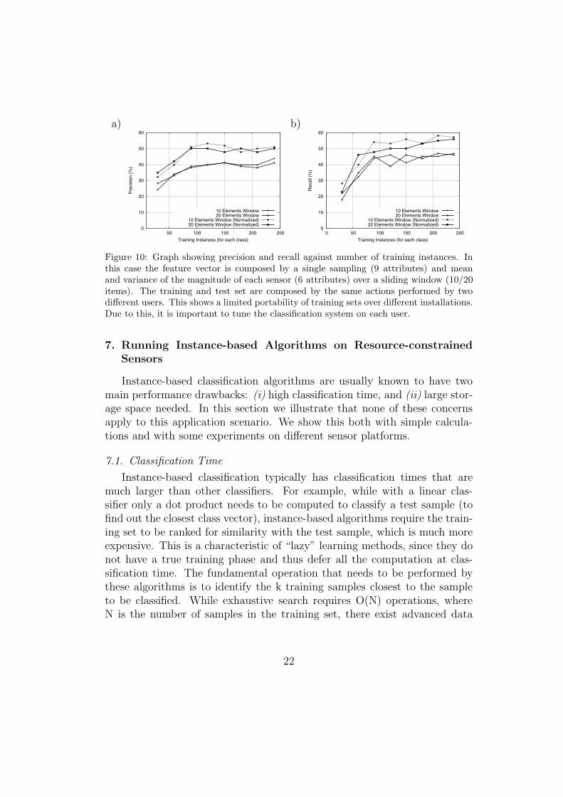
We tested two kinds of feature vectors for this experiment: (i) vectorscomposed by a single sampling (9 attributes) and mean and variance of themagnitude of each sensor (6 attributes) over a sliding window of n elements(n = 10, 20). (ii) The same kind of vectors, but normalized to a fixed range,in order to reduce di!erences across users. Figure 10 shows the precisionand recall levels against the number of training instances. Unfortunately thegraphs show a robust decrease (40%-55% against 90%) in precision and recallsuggesting a limited portability of training sets over di!erent installations.This is due to the inherent idiosyncrasies of each user’s movements that makethe sharing of samples rather inaccurate.

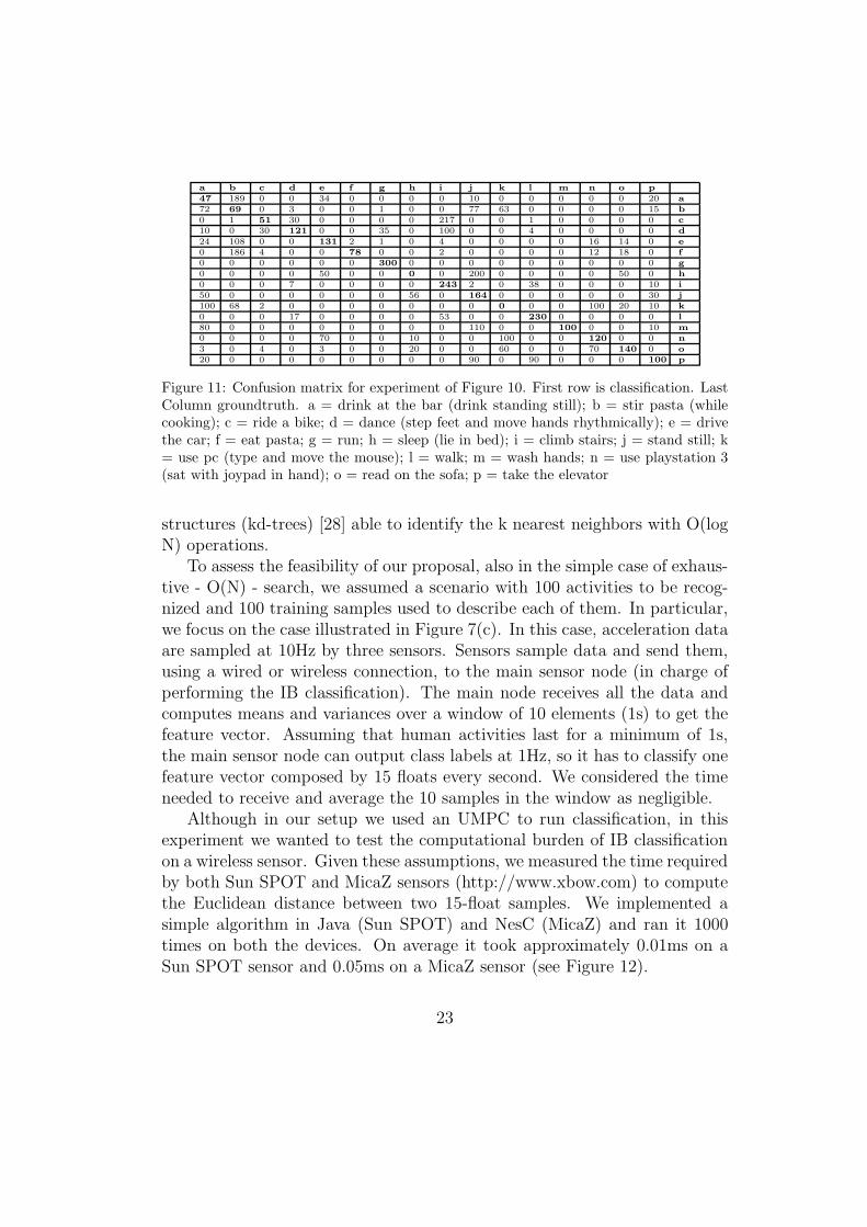
To better illustrate this problem we analyzed the confusion matrix asso-ciated with this classification (see Figure 11). Large errors are mainly asso-ciated to rather similar activities (e.g., looking at the first row, the “drinkat the bar” activity is often misclassified into “stir pasta”. Similarly “eatpasta” is often confused with “stir pasta”).

The main problem here relates to our use of labels to describe activities.As discussed in Section 5, our dataset is rather limited: data representingthe “drink at the bar” activity, for example, does not cover all the possibleexpressions of such an activity, so di!erent users might label “drink at thebar” with some rather di!erent movements. To overcome this limitation,on the one hand a larger dataset comprising more expressions of the sameactivities should be recorded. On the other hand, novel features should beextracted from the sensor data. In particular, the spectral characteristics ofthe data seem to be a good candidate for this kind of application [7]. In ourfuture work we will combine spectral characteristics in the feature vectors soas to allow for training set portability across users.

21

a)

0

10

20

30

40

50

60

50 100 150 200 250

Prec

isio

n (%

)

Training Instances (for each class)

10 Elements Window20 Elements Window

10 Elements Window (Normalized)20 Elements Window (Normalized)

b)

0

10

20

30

40

50

60

0 50 100 150 200 250

Rec

all (

%)

Training Instances (for each class)

10 Elements Window20 Elements Window

10 Elements Window (Normalized)20 Elements Window (Normalized)

Figure 10: Graph showing precision and recall against number of training instances. Inthis case the feature vector is composed by a single sampling (9 attributes) and meanand variance of the magnitude of each sensor (6 attributes) over a sliding window (10/20items). The training and test set are composed by the same actions performed by twodi!erent users. This shows a limited portability of training sets over di!erent installations.Due to this, it is important to tune the classification system on each user.

7. Running Instance-based Algorithms on Resource-constrainedSensors

Instance-based classification algorithms are usually known to have twomain performance drawbacks: (i) high classification time, and (ii) large stor-age space needed. In this section we illustrate that none of these concernsapply to this application scenario. We show this both with simple calcula-tions and with some experiments on di!erent sensor platforms.

7.1. Classification Time

Instance-based classification typically has classification times that aremuch larger than other classifiers. For example, while with a linear clas-sifier only a dot product needs to be computed to classify a test sample (tofind out the closest class vector), instance-based algorithms require the train-ing set to be ranked for similarity with the test sample, which is much moreexpensive. This is a characteristic of “lazy” learning methods, since they donot have a true training phase and thus defer all the computation at clas-sification time. The fundamental operation that needs to be performed bythese algorithms is to identify the k training samples closest to the sampleto be classified. While exhaustive search requires O(N) operations, whereN is the number of samples in the training set, there exist advanced data

22

a b c d e f g h i j k l m n o p

47 189 0 0 34 0 0 0 0 10 0 0 0 0 0 20 a

72 69 0 3 0 0 1 0 0 77 63 0 0 0 0 15 b

0 1 51 30 0 0 0 0 217 0 0 1 0 0 0 0 c

10 0 30 121 0 0 35 0 100 0 0 4 0 0 0 0 d

24 108 0 0 131 2 1 0 4 0 0 0 0 16 14 0 e

0 186 4 0 0 78 0 0 2 0 0 0 0 12 18 0 f

0 0 0 0 0 0 300 0 0 0 0 0 0 0 0 0 g

0 0 0 0 50 0 0 0 0 200 0 0 0 0 50 0 h

0 0 0 7 0 0 0 0 243 2 0 38 0 0 0 10 i

50 0 0 0 0 0 0 56 0 164 0 0 0 0 0 30 j

100 68 2 0 0 0 0 0 0 0 0 0 0 100 20 10 k

0 0 0 17 0 0 0 0 53 0 0 230 0 0 0 0 l

80 0 0 0 0 0 0 0 0 110 0 0 100 0 0 10 m

0 0 0 0 70 0 0 10 0 0 100 0 0 120 0 0 n

3 0 4 0 3 0 0 20 0 0 60 0 0 70 140 0 o

20 0 0 0 0 0 0 0 0 90 0 90 0 0 0 100 p

Figure 11: Confusion matrix for experiment of Figure 10. First row is classification. LastColumn groundtruth. a = drink at the bar (drink standing still); b = stir pasta (whilecooking); c = ride a bike; d = dance (step feet and move hands rhythmically); e = drivethe car; f = eat pasta; g = run; h = sleep (lie in bed); i = climb stairs; j = stand still; k= use pc (type and move the mouse); l = walk; m = wash hands; n = use playstation 3(sat with joypad in hand); o = read on the sofa; p = take the elevator

structures (kd-trees) [28] able to identify the k nearest neighbors with O(logN) operations.

To assess the feasibility of our proposal, also in the simple case of exhaus-tive - O(N) - search, we assumed a scenario with 100 activities to be recog-nized and 100 training samples used to describe each of them. In particular,we focus on the case illustrated in Figure 7(c). In this case, acceleration dataare sampled at 10Hz by three sensors. Sensors sample data and send them,using a wired or wireless connection, to the main sensor node (in charge ofperforming the IB classification). The main node receives all the data andcomputes means and variances over a window of 10 elements (1s) to get thefeature vector. Assuming that human activities last for a minimum of 1s,the main sensor node can output class labels at 1Hz, so it has to classify onefeature vector composed by 15 floats every second. We considered the timeneeded to receive and average the 10 samples in the window as negligible.

Although in our setup we used an UMPC to run classification, in thisexperiment we wanted to test the computational burden of IB classificationon a wireless sensor. Given these assumptions, we measured the time requiredby both Sun SPOT and MicaZ sensors (http://www.xbow.com) to computethe Euclidean distance between two 15-float samples. We implemented asimple algorithm in Java (Sun SPOT) and NesC (MicaZ) and ran it 1000times on both the devices. On average it took approximately 0.01ms on aSun SPOT sensor and 0.05ms on a MicaZ sensor (see Figure 12).

23

0

50

100

150

200

250

0 0.01 0.02 0.03 0.04 0.05 0.06 0.07 0.08

Num

ber o

f Run

s

Execution Time (ms)

Sun SPOTMicaZ

Figure 12: Distribution of time to compute distances among feature vectors in Sun SPOTand MicaZ sensor platforms.

Considering 100 actions, each of them described by 100 samples, and asimple exhaustive search over the whole dataset composed in this case by10000 training samples, we can estimate an overall execution time of 0.1son Sun SPOT sensors and 0.5s on MicaZ sensors. It is worth noting thatthis search has to be done only once every second. Moreover, by exploitinge"cient data structures able to avoid exhaustive searches like kd-trees, theoverall execution time would be in the order of 1ms on both the sensors.

7.2. Memory Requirements

Instance-based classification algorithms tend to require more memorythan other classifiers. While most classifiers (e.g., neural networks andBayesian networks) construct an explicit and declarative representation ofthe class of interest, instance-based algorithms simply store all the samplesin the training set. So, while the class representation can be compact (e.g.,a linear classifier only requires 1 vector per class), the storage of the trainingsamples is much larger.

The above two drawbacks are almost negligible in our scenario. We ver-ified (see Figure 7 and 8) that state-of-the-art classification performancescan be achieved by storing about 100 feature vectors per class and that nosignificant improvement can be expected by increasing that number.

For example, considering the case of Figure 7(c) in which we have samplesof 15 floats: single sensor data (9 floats) followed by mean and variance of themagnitude of each sensor over a sliding window (6 floats). Assuming 4 bytes

24

per float, then we have 60 bytes per feature vector, and thus 6KB per class.In our test-bed, each sensor is a Sun SPOT provided with 512KB RAM and4MB Flash memory. Thus, by storing the feature vectors in the node flashmemory, we can theoretically recognize about 650 activities. Considering atestbed of MicaZ sensor node, each having 512KB Flash memory, we wouldstill be able to represent 85 activities.

8. Conclusions and Future Work

In this paper we described the use of instance-based algorithms to inferuser’s activities on the basis of accelerometer data acquired from body-wornsensors. In particular, we highlighted that instance-based algorithms pro-vide state-of-the-art performance, are simple to implement, and can run onresource-constrained sensor platforms. Furthermore we showed that they canachieve remarkable precision and accuracy levels in classifying simple andspecific activities. As a consequence, this approach is a promising startingpoint for building next-generation systems able to recognize more complexactivities [27].

Despite these encouraging results, further work is needed to improve theportability of training sets across individuals and to better identify newclasses at run time. In addition, larger-scale experiments may be neededto enable the development of practical tools for the automatic recognition ofuser activities.

References

[1] M. Hanson, H. Powell, A. Barth, K. Ringgenberg, B. Calhoun, J. Aylor,J. Lach, Body area sensor networks: Challenges and opportunities, IEEEComputer 42 (1) (2009) 58–65.

[2] A. Campbell, S. Eisenman, N. Lane, E. Miluzzo, R. Peterson, H. Lu,X. Zheng, M. Musolesi, K. Fodor, G. Ahn, The rise of people-centricsensing, IEEE Internet Computing 12 (4) (2008) 12–21.

[3] G. Roussos, V. Kostakos, Rfid in pervasive computing: State-of-the-art and outlook, Elsevier Pervasive and Mobile Computing 5 (1) (2009)110–131.

25

[4] D. Patterson, L. Liao, D. Fox, H. Kautz, Inferring high-level behav-ior from low-level sensors, in: International Conference on UbiquitousComputing, ACM, Seattle (WA), USA, 2003, pp. 73–89.

[5] T. Mitchell, Machine Learning, McGraw Hill, New York (NY), USA,1996.

[6] T. Huynh, M. Fritz, B. Schiele, Discovery of activity patterns using topicmodels, in: International conference on Ubiquitous computing, ACM,Seoul, Korea, 2008, pp. 10–19.

[7] T. Choudhury, S. Consolvo, B. Harrison, J. Hightower, A. LaMarca,L. LeGrand, A. Rahimi, A. Rea, G. Bordello, B. Hemingway, P. Klas-nja, K. Koscher, J. Landay, J. Lester, D. Wyatt, D. Haehnel, The mobilesensing platform: An embedded activity recognition system, IEEE Per-vasive Computing 7 (2) (2008) 32–41.

[8] H. Junker, O. Amft, P. Lukowicz, G. Troster, Gesture spotting withbody-worn inertial sensors to detect user activities, Elsevier PatternRecognition 41 (6) (2008) 2010–2024.

[9] E. Miluzzo, N. D. Lane, K. Fodor, R. Peterson, H. Lu, M. Musolesi,S. B. Eisenman, X. Zheng, A. T. Campbell, Sensing meets mobile socialnetworks: the design, implementation and evaluation of the cencemeapplication, in: Conference on Embedded Networked Sensor Systems,ACM, Raleigh (NC), USA, 2008, pp. 337–350.

[10] L. Bao, S. Intille, Activity recognition from user-annotated accelerationdata, in: International Conference on Pervasive Computing, Springer,Linz, Austria, 2004, pp. 1–17.

[11] A. Torralba, R. Fergus, W. T. Freeman, 80 million tiny images: a largedataset for non-parametric object and scene recognition, IEEE Trans-actions on Pattern Analysis and Machine Intelligence 30 (11) (2008)1958–1970.

[12] C. Plant, C. Bohm, B. Tilg, C. Baumgarten, Enhancing instance-basedclassification with local density: a new algorithm for classifying unbal-anced biomedical data, Oxford Bioinformatics 22 (8) (2006) 981–988.

26

[13] F. Sebastiani, Machine learning in automated text categorization, ACMComputing Surveys 34 (1) (2002) 1–47.

[14] S. Lee, K. Mase, Activity and location recognition using wearable sen-sors, IEEE Pervasive Computing 1 (3) (2002) 24–32.

[15] J. Mantyjarvi, J. Himberg, T. Seppanen, Recognizing human motionwith multiple acceleration sensors, in: International Conference on Sys-tems, Man, and Cybernetics, Vol. 2, IEEE, Tucson (AZ), USA, 2001,pp. 747–752.

[16] F. Foerster, M. Smeja, J. Fahrenberg, Detection of posture and mo-tion by accelerometry: a validation in ambulatory monitoring, ElsevierComputers in Human Behavior 15 (1999) 571–583.

[17] K. Aminian, P. Robert, E. Buchser, B. Rutschmann, D. Hayoz, M. De-pairon, Physical activity monitoring based on accelerometry: validationand comparison with video observation, Springer Medical and BiologicalEngineering and Computing 37 (3) (1999) 304–328.

[18] N. Kern, B. Schiele, A. Schmidt, Multi-sensor activity context detectionfor wearable computing, in: European Symposium on Ambient Intelli-gence, Veldhoven, The Netherlands, 2003, pp. 220–232.

[19] G. Chambers, S. Venkatesh, G. West, H. Bui, Hierarchical recognition ofintentional human gestures for sports video annotation, in: InternationalConference on Pattern Recognition, IEEE, Quebec City, Canada, 2002,pp. 1082–1085.

[20] C. Randell, H. Muller, Context awareness by analysing accelerometerdata, in: International Symposium on Wearable Computers, IEEE, At-lanta (GE), USA, 2000, pp. 175–176.

[21] K. V. Laerhoven, O. Cakmakci, What shall we teach our pants?, in:International Symposium on Wearable Computers, IEEE, Atlanta (GE),USA, 2000, p. 77.

[22] N. Ravi, N. Dandekar, P. Mysore, M. Littman, Activity recognition fromaccelerometer data, in: Innovative Applications of Artificial Intelligence,AAAI Press, Pittsburgh(PA), USA, 2005, pp. 1541–1546.

27

[23] N. Bicocchi, M. Lasagni, M. Mamei, A. Prati, R. Cucchiara, F. Zam-bonelli, Pervasive self-learning with multi-modal distributed sensors, in:PerAda Workshop, Conference on Self-organizing and Self-adaptive Sys-tems, IEEE, Venice, Italy, 2008, pp. 61–66.

[24] D. Barbara, C. Domeniconi, J. Rogers, Detecting outliers using trans-duction and statistical testing, in: International Conference on Knowl-edge Discovery and Data Mining, ACM, Philadelphia (PA), USA, 2006,pp. 55–64.

[25] C. Park, H. Shim, On detecting an emerging class, in: InternationalConference on Granular Computing, IEEE, San Jose (CA), USA, 2007,pp. 265–270.

[26] U. Brandes, C. Pich, Eigensolver methods for progressive multidimen-sional scaling of large data, in: International Symposium on GraphDrawing, Karlsruhe, Germany, 2006, pp. 42–53.

[27] E. Kim, S. Helal, D. Cook, Human activity recognition and patterndiscovery, IEEE Pervasive Computing 9 (1) (2010) 48 –53.

[28] J. Predd, S. Kulkarni, H. Poor, Distributed learning in wireless sensornetworks, IEEE Signal Processing 23 (4) (2006) 56 – 69.

28