Designing `smart' computer-assisted markets : An experimental auction for gas networks

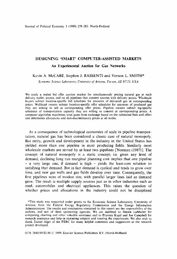
Journal of Political Economy 5 (1989) 259-283. North-Holland

DESIGNING ‘SMART’ COMPUTER-ASSISTED MARKETS

An Experimental Auction for Gas Networks

Kevin A. MCCABE, Stephen J. RASSENTI and Vernon L. SMITH*

Economic Science Laboratory, Unive&ty of Arizona, Tucson, AZ 85721, USA

We study a sealed bid&offer auction market for simultaneously pricing natural gas at each delivery outlet, source, and on all pipelines that connect sources with delivery points. Wholesale buyers submit location-specilic bid schedules for amounts of delivered gas at corresponding prices. Wellhead owners submit location-specilic offer schedules for amounts of produced gas they are willing to sell at corresponding offer prices. Pipeline owners submit leg-specific schedules of transportation capacity they are willing to commit at corresponding prices. A computer algorithm maximizes total gains from exchange based on the submitted bids and offers and determines allocations and non-discriminatory prices at all nodes.

As a consequence of technological economies of scale in pipeline transportation, natural gas has been considered a classic case of natural monopoly. But entry, growth and development in the industry in the United States has yielded more than one pipeline in most producing fields. Similarly most wholesale markets are served by at least two pipelines [Norman (1987)]. The concept of natural monopoly is a static concept; i.e. given any level of demand, declining long run marginal planning cost implies that one pipeline _ a very large one, if demand is high - yields the least-cost solution to satisfying that demand. But in fact demand is cyclical and tends to grow over time, and new gas wells and gas fields develop over time. Consequently, the first pipelines were of modest size, with parallel larger lines laid as demand grew. The result is multiple supply sources just as in other industries such as steel, automobiles and electrical appliances. This raises the question of whether prices and allocations in the industry could not be disciplined

*This study was supported under grants to the Economic Science Laboratory, University of Arizona, from the Federal Energy Regulatory Commission and the Energy Information Administration. The results and conclusions contained in this report are the responsibility of the authors, and not of these sponsoring agencies. We are indebted to Shawn LaMaster for computing, charting and other valuable assistance and to Praveen Kujal and Joe Campbell for research assistance and help in recruiting subjects and running the experiments. We also wish to thank Daniel Alger of the FERC for many helpful comments and suggestions as the research project developed.

01762680/89/$3.50 (3 1989, Elsevier Science Publishers B.V. (North-Holland)

260 K.A. McCabe et al., Computer-assisted markets

satisfactorily by competitive forces as a replacement for some of the public regulatory apparatus.

Historically, in the United States federal regulation of the industry strengthened the monopoly power of gas pipelines. In the early years natural gas was an undeveloped by-product of the search for oil. Therefore it was felt that the industry needed protection from supply and demand risk to encourage pipeline construction. Consequently, before a construction permit was issued to serve a new market, the pipeline company was required to demonstrate that it had sufficient gas reserves under contract. With supplies required to be adequate, the demand side was then protected by limiting access by new pipelines. This created a regulatory system in which wholesale buyers had to purchase all wellhead gas from pipelines. The resulting pipeline monopoly was further strengthened by a requirement that imposed minimum charges (independent of quantity taken), and sole supplier con- ditions on the local distribution companies who were the wholesale pur- chasers of pipeline gas. Thus ‘regulation’ under the old Federal Power Commission actually took the form of government promotion of the natural gas industry [Stalon (1985)].

All this began to change because of the Natural Gas Policy Act (NGPA) of 1978. This legislation initiated a process of phased deregulation of wellhead gas by removing from the Federal Energy Regulatory Commission (FERC) the role of making judgments about the adequacy of price incentives to produce gas. The NGPA together with FERC Order 436, issued in 1985, facilitated a process whereby wholesale buyers could directly contract for, or purchase spot, gas from wellhead producers, and then buy their pipeline transportation. Thus the historic ‘bundling’ of gas production and transportation started to come apart. Although the regulatory process helped to insure pipeline monopoly, and this probably explains their historically high rate of return on investment compared with other industries [Norman (1987, tables 3 and 4, fig. l)], the new competitive forces, strengthened by NGPA and the FERC Order 436, are helping to produce many changes in the

industry. It is against this background that we were asked by the FERC to develop,

and examine the feasibility and properties of, an auction market for the sale and transportation of natural gas. In this article we report our initial research design and experiments based on this objective.

1. Gas auction net: Motivation and distinguishing features

The gas and transport pricing mechanism we examine in this study has been motivated in part by the following potentially desirable properties.

(1) self regulation; i.e. ultimately we seek to explore the feasibility of

substituting a satisfactory market mechanism for rate of return and other

K.A. McCabe et al., Computer-assisted markets 261

regulatory constraints. The wide application of competitive sealed auctions in financial markets suggests that a suitable extension and modifi- cation of this institution may have desirable properties in gas network applications.

(2) Non price-discrimination; i.e. all price differences among wholesalers, producers and pipelines in any given pricing period are justified only on the basis of marginal costs and opportunity costs. It is our interpretation that current law favors this property.

(3) Priority-responsive pricing for curtailments; i.e. in the event of restrictions in pipeline capacity (say due to cold weather) there is an automatic restriction of deliveries to those wholesalers that have the highest consumption priorities (and a corresponding restriction of production schedules to those wellhead producers that have the highest production priorities) as expressed in the bids (offers) each submits to the auction- dispatch center.

(4) Value responsive investment incentives. A good mechanism should

provide incentives for increases in production and transportation capacity where such increases have the highest value.

(5) Simplicity and decentralization. Although network systems may have inherent physical complications, it is desirable to have a price mechamism in which the participants can understand what is required of them and can readily fulfill these requirements. One of the advantages of a decentralized mechanism is that the participants can concentrate on judgments and actions based on the private information each is most directly informed about. Computer assistance is used where it is most appropriate and needed: to generate non-discretionary, consistent, best, but strictly routine results based on the willingness-to-pay and willingness-to-accept judgments of dispersed individual participants.

(6) Compatibility with existing institutions. Present institutions emphasizing

contract precomitments for gas and/or transportation could continue to function simultaneously with a network auction. This could be accom- plished by applying the auction to available capacities above the flows precommitted by contract. Consequently the extent of the use of the auction would be determined by the decisions of the participants, and could grow in response to increased use without the necessity of a possible disruptive discontinuous switchover. When the auction is used for spot trades holders of long gas could resell spot those quantities not needed for current consumption. In this case the auction would supple- ment and increase the efficiency of current institutions.

This paper reports our findings from 9 laboratory experiments designed to study the efficiency and price performance characteristics of a sealed bid- offer auction mechanism for the simultaneous allocation of gas and pipeline

262 K.A. McCabe et al., Computer-assisted markers

capacity rights among buyers of delivered gas, transporters, and sellers of wellhead gas. This computer-assisted mechanism will be called Gas Auction Net.

Some of the salient features of our Gas Auction Net mechanism are as follows.

(1)

(2)

(3)

(4)

(5)

Consumption centers (consisting of primary gas buyers such as local distribution companies and industrial consumers) are connected to producing gas fields (consisting of primary gas sellers) by a capacity- constrained pipeline network. The network we study experimentally is thin, and weakly competitive. In this sense it is intended as a worst-case example for any price mechanism. The auction market uses ‘smart’ computer support to process location- specific bid schedules from gas buyers, location-specific offer schedules from wellhead producers, and segment-specific offer schedules of transfer capacity from pipeline owners. This means that each of the three types of participants is required to make judgments that reflect only their own private circumstances. That is, their willingness to buy gas, sell gas or sell transportation on each pipeline segment. The resulting prices are non-discriminatory; i.e. all sellers at the same location (or line haul pipeline input point) receive the same price, all buyers at the same location (line haul output point) pay the same price, and all pipelines connecting a given source location with a given receiving location obtain the same price. Other pricing mechanisms, such as double auction and posted pricing do not yield non-discriminative prices except in full equilibrium.’ Gas Auction Net yields non- discriminatory prices in each price period. Differences in the price of gas between any two (production or consumption) locations reflect differences in the marginal supply price of transportation and/or pipeline capacity restrictions. The allocation of delivered gas among buyers, of produced gas among sellers, and of the resulting transportation requirements among pipelines maximizes the total system aggregate gains from exchange (surplus) given the schedules of buyer bids, seller offers and pipeline offers. In this sense Gas Auction Net guarantees a maximally efficient, or no waste, competitive market given the submitted bids and offers of all participants. Its first priority is to consume gas from the lowest cost wells, and deliver it to the highest value wholesale user using the lowest cost transportation routes.

The experiments we report evaluate the price and efficiency characteristics

‘See Ketcham, Smith and Williams (1984) for a comparison of the double auction and posted price exchange institutions.


of Gas Auction Net as a mechanism for the exchange of rights. The rights

themselves are not labelled or interpreted in terms of particular possible implementations in the gas industry. Thus the rights actually traded in an implementation of Gas Auction Net might be for spot gas commitments, hourly, monthly or weekly, or for forward commitments next winter (tirm or interruptible). Our primary research task is to evaluate Gas Auction Net as a price mechanism applied to any well-defined set of contractual rights.

Technically, Gas Auction Net is an extension and generalization of the competitive (uniform price) sealed bid, and double sealed bid-offer, auctions. As a price mechanism its distinguishing feature is that all accepted bids to buy are tilled at a price less than or equal to the lowest accepted bid price of buyers - a price that just clears the market by making the total number of units offered equal to the number demanded. This contrasts with the discriminative sealed bid auction where Q units are offered for sale and. the Q highest bids are accepted, but each accepted bid is tilled at a price equal to the amount bid. Consequently, different buyers pay different prices for the same commodity. Also, the discriminative auction provides an incentive for strategic underbidding of full willingness-to-pay as each bidder attempts to avoid having to pay more than the minimum necessary amount (the lowest accepted bid). This incentive is reduced in the competitive auction, and in special cases is in theory eliminated.

There is now a considerable theoretical literature on competitive auctions [see the survey by McAfee and McMillan (1987)] stimulated by Vickrey’s (1961) original contribution, and generalizing the second price sealed bid auction for a single unit to the competitive multiple unit auction. There are also several experimental studies [in chronological order, Smith (1967) Belovicz (1979), Coursey and Smith (1984), Miller and Plott (1985), Cox, Smith and Walker (1985)] of competitive auctions often with empirical comparison to discriminative auctions. The first field experiments comparing competitive and discriminative auctions of long-term bonds were conducted by the U.S. Treasury in the early 1970s.

Also of particular importance to Gas Auction Net as an extension of the competitive sealed bid auction is the fact that variations on this institution have received wide acceptance as price-allocation mechanisms in financial markets. We are therefore considering the extension of an institution that has been thoroughly time-tested for over a decade and found increasing application.

2. Overview of experimental design and procedures

The research design underlying this paper is based on three series of experiments using a simplified gas transmission network. The first series uses parameters which we call Design I, and consisted of three experiments using


inexperienced subjects, two using experienced subjects and one using ‘super’ (or twice) experienced subjects. The second series, Design II, (in addition to the inexperienced training sessions) consisted of two experiments using experienced subjects and one using super experienced subjects. Design II further differs from Design I in that in the former the cost and capacity parameters provide a more contestable and potentially more competitive network than Design I. By comparing the results from Design II with those from Design I we are able to measure the effect of increased network contestability. A third series, Design III, again consisted of two experiments using experienced and one experiment using twice experienced subjects. Design III was based on the same parameters used in Design II. But in Design II each pipeline owner also owned one of the producer wells served by the pipeline, while in Design III no pipeline transported gas from a well owned by that pipeline. By comparing the results of Design II with those of Design III we obtain a measure of the effect of vertical integration on the ability of pipelines to compete for rents with independent producers.

Subjects were recruited from the undergraduate population at the Univer- sity of Arizona. They were paid three dollars upon arrival for an experiment as an incentive to arrive on time. At the end of each experiment subjects were paid their profit earnings in U.S. dollars. These payouts varied from six dollars to sixty dollars, U.S. currency. All experimental earnings are denomi- nated in what are called ‘pesos’, which are then converted into U.S. dollars at a fixed specified rate - one (for experienced subjects) U.S. dollar per hundred pesos depending upon the parameter design. Using a conversion rate facilitates approximate uniformity in individual rewards across experiments with different parameter designs.

All experiments were run on the Plato Computer system. This system was used: to instruct subjects in the experimental institution; to enforce the message rules which define the institution (and thus coordinate subject interaction); and to record profits. Experimenters were on hand both to assist subjects who had difficulty in understanding the rules and to enforce privacy.

After everyone had arrived they were assigned randomly an agent type (as defined in our ‘design’ subsections below). Subjects then went through the instructions at their own pace. When everyone had finished reading the instructions, and all questions were answered, inexperienced subjects were then put through a one-period trial run of the experiment. When the trial period was concluded they were asked to verify their understanding of their profit page in light of their market decisions. After all questions were answered the experiment was begun.

Experience with human subjects suggests that fatigue problems may arise if one runs an experiment for more than two consecutive hours. This constraint prevented the experiments in our inexperienced treatment from lasting more than 15 periods. But experienced players finished the instructions more


Fig. 1. Pipeline system and predicted equilibrium for market network environments.

quickly allowing us to run up to 30 or more periods. To minimize ‘end play’ in all experiments, subjects were not informed as to the actual number of

periods.

3. Parameters: Network design I

The physical layout of our network system is shown in fig. 1. Each pipeline is identified by owner and segment. Thus 2.2 refers to line owner 2, segment 2. Line owners 1 and 2 each own three segments of the system and owner 3 owns four segments.

The top panel of table 1 lists the valuations and capacities of the six

buyers. These are intended to represent opportunity costs faced by bulk buyers. The columns labelled 1/l, Ql and k’2, Q2 in table 1 show the unit values and corresponding quantities at which our experimental buyers can ‘redeem’ their purchases from the experimenter. For example buyer 1 can redeem 2 units/period at a price of 300 pesos/unit and an additional 2 units at 200 pesos/unit. Each buyer has a two-part marginal valuation schedule defined in this manner. The second panel of table 1 lists the cost and output capacities of each of the six producers in the columns labelled WC and Q. For example Well 1 can deliver up to 5 units/period at an out-of-pocket cost of 150 pesos/unit. Note that each pipeline owner is also an owner of one well; lines 1, 2, and 3 own wells W2, W4 and W6 respectively. This is intended to reflect the current condition in the industry in which there are


Table 1

A competitive equilibrium solution with all bids equal to values and all offers equal to costs. Network Design I

Buyer (Node Buyer V 1 Q 1 V2 Q2 Consumption price i.d.) Profit

1 300 2 200 2 2 200 (P3) 200 2 255 3 245 2 5 210 (P4) 205 3 310 2 230 2 4 225 (P5) 180 4 275 3 260 2 5 235 (P8) 170 5 320 2 225 2 2 240 (P9) 160 6 285 2 260 3 5 240 (P9) 150

Well (Node Well WC Q Production price i . d . ) Profit

1065 (59.20/0)

1 150 5 5 180 (P2) 150 2 180 4 2 180 (P2/ 0 3 150 5 5 180 (PI) 150 4 180 4 2 180 (PI) 0 5 160 5 5 200 (P6) 200 6 190 4 4 200 {P6) 40

540 (30.0%)

Line (Node Line LCI Q1 LC2 Q2 Shipment price diff.) Profit

Ceiling price

1.1 15 7 25 3 7 20 (P3 P2) 35 30 1.2 10 5 15 3 5 10 (P4-P3) 0 20 1.3 10 3 15 2 4 15 (P5-P4) 15 20 2.1 25 7 35 4 7 30 (P4~P1) 35 40 2.2 15 6 25 3 3 15 (P7-P4) 0 30 2.3 10 6 15 3 7 15 (P9 P7) 30 20 3.1 15 5 25 2 0 10 (P(~P4) 0 30 3.2 15 8 25 3 9 25 (P7 P6) 80 30 3.3 10 8 15 3 5 10 (P8 P7) 0 20 3.4 t5 6 25 2 0 5 (P9 P8) 0 30

E B- 59.2°o E p - 27.80o E L - 10.8Oo Ep1~ = 2.2°;

195 (10.8%)

Total surplus, 1800 pesos.

b o t h i n d e p e n d e n t w e l l h e a d o w n e r s a n d ' c ap t i ve ' wells o w n e d by, o r u n d e r

c o n t r a c t wi th , the se rv ing p ipe l ine .

The b o t t o m pane l of t ab le 1 lists the t w o - p a r t m a r g i n a l cos t s c h e d u l e for

e a c h o w n e r - s e g m e n t of p ipe l ine in the c o l u m n s l abe l l ed LC1 Q1 a n d L C 2 ,

Q2. T h e last c o l u m n lists the ce i l ing pr ice o n each line s e g m e n t . F o r e x a m p l e

p ipe l ine s e g m e n t 2.2 can t r a n s p o r t up to 6 un i t s at 15 p e s o s / u n i t a n d an


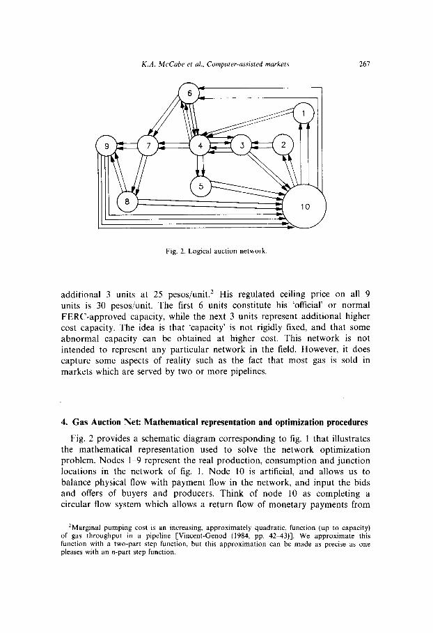
Fig. 2. Logical auction network

additional 3 units at 25 pesos/unit. ’ His regulated ceiling price on all 9

units is 30 pesos/unit. The first 6 units constitute his ‘offtcial’ or normal FERC-approved capacity, while the next 3 units represent additional higher cost capacity. The idea is that ‘capacity’ is not rigidly fixed, and that some abnormal capacity can be obtained at higher cost. This network is not intended to represent any particular network in the field. However, it does capture some aspects of reality such as the fact that most gas is sold in markets which are served by two or more pipelines.

4. Gas Auction Net: Mathematical representation and optimization procedures

Fig. 2 provides a schematic diagram corresponding to fig. 1 that illustrates the mathematical representation used to solve the network optimization problem. Nodes l-9 represent the real production, consumption and junction locations in the network of fig. 1. Node 10 is artificial, and allows us to balance physical flow with payment flow in the network, and input the bids and offers of buyers and producers. Think of node 10 as completing a circular flow system which allows a return flow of monetary payments from

*Marginal pumping cost is an increasing, approximately quadratic, function (up to capacity) of gas throughput in a pipeline [Vincent-Genod (1984, pp. 42%43)]. We approximate this function with a two-part step function, but this approximation can be made as precise as one pleases with an n-part step function.


buyers to producers in exchange for the gas flowing on modes l-9 from producers to buyers.

Each are i in the network is represented by the vector (si,ei, li,ui,ci) with:

si its starting point

ei its end point li the least permissible flow on that arc (zero in our applications)

ui the greatest permissible flow on that arc (as determined by the bid or offer quantity entered by a buyer or a producer)

ci the offer price (bids are signed negative) per unit of flow on that arc.

Each arc represents one bid or offer. If a buyer makes a two-part bid, then it is represented by two parallel arcs. Two-part offers by pipeline owners are represented similarly. Where gas is to be allowed to flow in either direction on a pipeline a two-part offer is represented by four arcs - two arcs in each direction, as in the arcs connecting nodes 3 and 4.

Example I: Buyer 4 bids 300/unit for 3 units and 2OO/unit for 2 more units. Since buyer 4 is at location 8 (fig. 1 and tables 1 and 2) his bids would be

represented by 2 arcs labelled as:

(8, 10, 0, 3, -300); and

(8, 01, 0, 2, -200).

Each arc is defined by its own identifying number from 1 to 42 so there is no problem with parallel arcs between the same nodes.

Example 2. Producer 4 offers to produce 5 units for 95/unit. Then the appropriate arc wo1~!1 be 1Abelled (10, 1, 0, 5, 95).

Example 3. The owner of segment 2.2 offers to carry 6 units at 45/unit and an additional 3 unit at 55/unit. Then the appropriate arcs are labelled (4, 7, 0, 6, 45) and (4, 7, 0, 3, 55).

After all arcs are labelled using the bids and offers of the agents, the revealed surplus in the network is maximized using the following formulation:

maximize: -C cifi (total surplus);

subject to: c fi- c fk=O (V nodesj); isE, keS,

IisLsui (V arcs i);

I

II

where fi is the flow on arc i, and for each node j. Ej is the set of arcs which


end at j, and Sj is the set of arcs which begin at j. Note that constraint set I maintains the balance of flow at each node j. Constraint set II ensures that

the flow on each arc does not exceed the stated bounds. Solving the linear program yields not only the optimal flows (and

production and consumption pattern) but also the set of shadow prices Zj for all nodes in the network.

Since the shadow prices are relative to one another, the difference in shadow prices at the start and end nodes of an arc gives us the value of the marginal unit of flow on that arc, hence the price associated with that flow. For example:

(a) If rci0-rr8 = -250 then buyer 4 (who resides at location 8) pays 250 pesos/unit to receive delivered gas at location 8. It is clear that if two buyers reside at the same location they pay the same price.

(b) If rc, -rc4 =50 then the owner of pipeline segment 2.2 receives 50 pesos/unit to transport between locations 4 and 7.

(c) If 7c6-rcio= 105 then both producers 5 and 6 who reside at location 6 receives the same price, 105 pesos/unit, to produce gas at that location.

With this linear programming formulation the budget is always balanced since the physical flow on each segment represents an activity which is exactly compensated.

A sample solution of the linear program is displayed on the right hand side of table 1 beginning with the columns labelled Consumption, Production and Shipment. The solution prices at each node, and flows on each arc, are also entered on fig. 1. This solution is based on full revelation of demand by buyers and of supply by producers and transporters, and is achieved by applying the linear program with all bids at marginal redemption value and all offers at marginal cost. Our parameters for this design imply that in a competitive equilibrium (ce) solution buyer surplus is 1065 (59.2%) producer surplus is 500 (27.8%) for independent wellhead owners, and 40 (2.2%) for pipeline owned wells, pipeline transportation surplus is 195 (10.8%) and total surplus is 1800 (loo”/,), all measured in experimental pesos. These ideal surplus figures will be used to evaluate the overall efficiency of each experimental market as well as the division of the total surplus among the three constituents. Note that with these particular parameters there are no ce flows on segments 3.1 and 3.4. In effect, Network Design I is less connected than that displayed in fig. 1. Below, in Network Design II, this condition is relaxed by using parameters such that there are ce flows on all legs. Design I was our basic ‘trainer’ for building up a pool of experienced network subjects. Design I provides a measure of the gross behavioral ‘rationality’ of our mechanism in that we should not observe persistent flows on segments 3.1 and 3.4, since these segments do not provide close cost contestability with the alternative path segments with which they compete.


AVERAGE PRICES: GAS AUCTION NET DtSlGN I EM'S 4e, 5e, 6ee z15

r . ‘P3

- - - * _ -. _.............. * . . . . . ..-.-. * __ -.. PzI<ce)

I _ ; _.’ F2ice)

P2 =-=-_““_ ___._--_- -_

2z20

M ZLO ---,

u e zzoo 1 -

mm_--__ _ee4________.__.----- _

‘P3 P4<ce)

-- ---..___ __ --_---------

.- -

5 10 15 20 25 PERIOD

P5 .____----

._---__

-_- -mm-------

P4 _-.------- -mm-

__________-__---

P4<ce)

5 10 15 20 25 PERIOD

Fig. 3

5. Experimental results: Gas Auction Net Design I

The principal results of experiments 4e, 5e and 6ee (the inexperienced sessions li, 2i and 3i are not reported) are provided in the accompanying charts of average prices and average efficiency.

A verage prices

Average prices are charted by period at the head and tail of each pipeline segment in figs. 3-5. The priuces at the top of each chart, plotted as solid ‘dots’, apply to the node at the end point or head to which the pipeline segment is delivering gas. The prices at the bottom, plotted as ‘xs’, refer to the tail node from which the segment is receiving gas. For example, in segment 1.1 delivery is to Bl (fig. l), so the upper prices are observations on

K.A. McCabe et al., Computer-assisted markets

AVEMGE PRICES: GAS AUCTION NET DESIGN 1 EXPS k, 5e, be 225

r 3ECMICNT P.l PIPkLINE CEILIND - 40

P4 _-_---- ---

- -, - - - .y ..-. ; - - - - - - -_.---

P4<ce)

L

r :

__ $=_~____-._-__------- _. _ _ _ ; ._.“’ _

P1<ce)

5 10 PER1ISOD 20 25

=so SEOMENT P.pI PXPkLINB: - 30 CEILING

240 ..

P7 .----- g 330 .. - -

____----- _-_----

= -.- - = _

~zt?o P7(oe) -

P4 ___--- ----

_--_-__.--_-_---- zz10 - - - --

P4<ce)

=cJo

r

I

5 10 15 20 25 PERIOD

SEOM=NT P.3 PIPELINB: CE*LINO - eo

PB ___---

-.--

- - __._---- . _ - -

__--

PQ<ce) -?..---

- _ _P7 .___-----

___----

- I - - P7<ce)

1 5 10

P&SOD 20 25

Fig. 4

271

P, (note 3, figs. 1 and 2) while the lower prices, I’,, are for wells WI and W2 served by segment 1.1; in segment 2.3 the gas is delivered to a buyer node, at price P, (buyers B5 and B6), but the gas source is the junction, J, where price is denoted P,. The price at the output node on the line segment is higher than the price at the input node because gas flows from lower to higher prices (just as electricity flows from low potential nodes to high potential nodes). Price differentials are required to overcome the resistance to (costs of) transporting commodity. The difference between the two series of prices is the observed line segment transportation price, P,. The ce prices are represented by the dotted parallel lines, whose difference is the ce pipeline prices on the indicated segment. Charts are not provided for segments 3.1


AVERAGE PRICES: GAS AUCTION NET DESIGN I EXPS 4~, 5e, 6--e

r-=1 SEOMENT 3.E PIPELINE CEILING - JO

1 230 + py________--_--------‘-I P7(ce)

I I ^^_ .--- z?ocl _.. - ___---

. - _.__----- PG(ce)

P6 1eo

5 10 15 20 z5 PERIOD

.zz:eo SEGMENT 3.3 PIPELINE CEILING - zo

- - 250 -- Pa _-----

_____--_-- __-_-_-

Fig. 5

and 3.4 since, as expected in Design I, the predominant observation was zero flows on these segments in all experiments.

Several characteristics of these price observations should be emphasized.

(1) Except for the first few period in the case of some nodes, prices tend to be quite stable, or to change slowly, from period to period. This is not due to averaging across the three experiments; it is also a characteristic of each individual experiment. This result is a consequence of the bid-offer behavior of the subjects. Over time they tend to settle into a pattern in which bids to buy delivered gas are at, or somewhat above, their respective node prices. Similarly producers offer at, or somewhat below, their node prices, while pipelines offer at, or somewhat below, their transport prices on each segment. Consequently, a small reduction in a buyer’s bid or slight increase in a seller’s offer, is likely to cause the agent to be cut out of the market, or at least have his allocation reduced, but this will have a relatively small effect on prices given this bid-offer pattern. The primary impact is on allocations and therefore efficiency and the distribution of surplus, as will be discussed below.

(2) Buyer Bl typically pays approximately the ce price and consumes the ce allocation. However, producers Wl and W2 who serve Bl tend to receive


less than the ce price. We think this is due in part to the downstream competition between pipelines 1 and 2 to serve buyers B2 to B6. (Because of the transport cost on segment 3.1, pipeline 3 is not in effective competition for buyers B2 and B3.) To be effective in this downstream competition pipeline 1 must resist letting the price of gas flowing into Bl rise much above the ce price. Since well W2 (owned by pipeline 1) is a marginal producer, this means that pipeline 1 must forgo any positive profit on W2. In fact it is typical to observe zero flows and profit for W2 in all three experiments. Instead, we observe the owner of pipeline 1 quoting a transportation price on segment 1.1 that is above the ce price. This leads Wl to accept a wellhead price below the ce. It should be noted that the owner of Wl has no other revenue source whereas the owner of pipeline 1 has other revenue sources on segments 1.2 and 1.3.

(3) Buyers B2 and B4B6 are primarily supplied by wells W3-W6 both in a ce and in the realizations recorded in experiments 4e, 5e and 6ee. Consequently, this part of the network is potentially more contestable than the rest of the network. However, the cost advantage on segment 3.2, with a cost of 25, compared with that on 2.1 plus 2.2, with a combined cost of 45 allows 3.2 to change the ceiling price while 2.1 and 2.2 must offer transportation at prices nearer to cost.

(4) Therefore the net delivered price of gas to buyers B2-B6 tends to exceed the ce price. But the gas flows to these buyers, particularly to buyers B2 and B4, are close to the ce allocations. The deliveries to B5 and B6 appear to be short of the ce because 2.3 is uncontested in supplying two competing buyers. (Notice from table 1 that the high combined cost on segments 3.3 and 3.4, compared with segment 2.3 precludes effective competition from pipeline 3). B3 and B4 receive close to their ce allocation by B4 pays the transport ceiling price, and B3 pays a transport price closer to cost than to the ceiling. We attribute this difference to the fact that the difference between marginal value and the ce pice for B3 (230 minus 225) is much smaller than for B4 (260 minus 235), as can be seen in table 1. Consequently, 83 is likely to be more resistant to increases in pipeline charges than B4.

.?$kiency and the distribution of surplus

The accompanying chart (fig. 6) labeled ‘Average efficiency’ plots the percentage (averaged across experiments 4e, 5e, and 6ee) of the ce total surplus (1800 pesos) actually realized by the participants in each period. An efficiency of 100:/i means the market realized the maximum possible surplus based on the costs and values listed in table 1. The division of this realized average surplus among buyers, pure producers, pipeline transportation and pipeline owned wells is also plotted in each period. The top line (solid) plotted in fig. 6 is the average realized total efftciency. The second line (long


90

t

A/--- w _ TOTAL

__ __ EB 0”

.._._ EW

70 ___ EL K h 60 _________-------- EWL L

?z 50 __ EB(ce)

G

F= 40

‘, ,r\/fi,,,

\,’ ”

r/‘\,-\,--v-,_, EW(ce)

B .-- EL(m)

. .._____...., EWL(ce) .-.

: :,. ‘......,‘.. ...‘... . ..‘._‘~,________-._,

01 ., - ,.,,. ....:.. 5 10 15 20 25

PERIOD

Fig. 6

dashes) plots the average surplus realized by buyers as a percentage of the total, EB. The third line (short dashes) plots the average percentage surplus obtained by the independent wells, EW The fourth line (short and long dashes) represents the average percentage surplus obtained in pipeline transportation, EL. The last line (dotted) near the bottom of the chart is the average percentage surplus obtained from production capacity owned by pipelines, EWL. The horizontal lines, broken to match their corresponding observed values, represent the theoretical percentage surplus, EB(ce), EW(ce), EL(ce) and EWL(ce).

Note the following general characteristics of these observations.

(1) (2) (3)

(4)

(5)

Total efficiency tends to rise over time. Buyer surplus is fairly constant over time, but below the ce prediction. The independent producer surplus rises, approaching the ce prediction over time. Pipeline transportation surplus rises over time and stabilizes above the ce prediction. Wells owned by pipelines show some uptrend in surplus but this surplus is little different than the ce prediction.

6. Parameters: Network Designs II and III

A second set of Network parameters is provided in table 2. The corresponding ce solution is also shown in table 2. Note that in this parameterization the ce solution requires flows on every pipeline segment, although profits are not always positive (segment 3.1). In a ce buyer surplus


Table 2

A competitive equilibrium solution with all bids equal to values and all oNers equal to costs.

Network Design II and III

Buyer (Node Buyer Buyer Vl Ql V2 Q2 Consumption price i.d.) profit

207 2 165 2 2 167 (P3) 80

197 3 182 2 5 175 (P4) 80

230 2 I85 2 3 185 (P5) 90

244 3 211 2 -

4

215 (P8) 91

267 2 225 2 223 (P9) 92

262 2 228 3 5 223 (P9) 93

Well Well WC Q Production price

I 131 5 5 I52 2 144 4 4 152 3 134 5 5 155 4 148 4 4 155 5 157 5 5 180 6 180 4 1 180

Line LCl Ql LC2 Q2

1.1 IO 8 15 3 1.2 5 6 8 3 1.3 6 3 11 2 2.1 14 7 20 3 2.2 29 4 36 3 2.3 I1 4 16 3 3.1 5 4 8 3 3.2 19 7 27 3 3.3 4 7 8 3 3.4 5 4 9 3

526 (45.7%)

(Node Well id.) profit

(P2) I05 (P2) 32

(PI) I05 (Pl) 28

( P6) 115

(P6) 0

Shipment

9 15 (P3-P2) 40 24 7 8 (P4P3) 18 13 3 10 (P55P4) 12 17 9 20 (P4Pl) 42 32 4 32 (P77P4) 12 57 5 I6 (P99P7) 20 24 4 5 (PbP4) 0 13

10 27 (P7-P6) 56 42 9 8 (PS-P7) 28 I3 4 8 (P9-P8) 12 I6

385 (33.4%)

Line (Node price di&)

Line profit

Ceiling

E,=45.7:;, E,=28.2% E, = 20.9% E,, = 5.2%

240 (20.9%)

Total surplus, 1151 pesos, _

is 526 (45.7”/,), producer surplus is 325 (28.2%) for independent wellhead owners and 60 (5.2%) for pipeline owned wells, pipeline transportation surplus is 240 (20.9%) and total surplus is 1151 (100%). Again we use these ideal states to evaluate the efficiency of our experimental markets and the division of surplus among the three agent classes. In comparing Designs I and II we note that, in the latter, segments 3.1 and 3.4 have costs that actively contest alternative pathways for delivering gas. In general the


pipeline parameters in Design II yield greater potential contestability than Design I. Thus in table 2 all the ce pipeline segment prices are at or near their respective second step marginal costs, An important research question is whether this tighter contestability will alter the marked tendency, observed in the Design I experiments, for buyers to do poorly relative to both producers and pipeline owners.

In Design III all value, cost and capacity parameters were identical to those in Design II. The only difference was that in Design III no pipeline owner was allowed to own a well in a field that the pipeline served. Our objective was to measure the allocative effect of ‘captive’ well ownership by pipelines. When pipelines own wells in the fields they serve, are they able to leverage prices to their advantages relative to the independent producers?

7. Experimental results: Gas Auction Net Designs II and III

Average prices

As in section 5, the accompanying charts for experiments le, 2e, 3ee (figs. 7-10) plot the delivery and source prices on each pipeline segment for each period. As in Design I, the period-by-period inertia characterizing these prices is again evident.

In contrast with the results for the Design I parameters, the new results substantially reverse the earlier finding that buyers perform poorly relative to producers and pipelines. Network competition in Design II yields buyer prices that hover more closely to the ce prices. Likewise, observed producer prices and pipeline prices are closer to the theoretical ce prices. An exception is pipeline 1, particularly on segment 1.1 (fig. 7). But this segment is the least contested in network 1, Design II. It makes strategic sense for pipeline owner 1 to price high on segment 1.1, pick off surplus from Bl (or PI), then low on segment 1.2 where he/she is forced to be competitive with 2.1 in the contest for B2 and the long distance customers on the left side of the network. This puts pressure on 2.1 either to price near ce or to exercise some monopsony power against producer P,. As shown in fig. 8 the latter tendency dominates slightly. Pricing high on 1.3 is possible since this segment is the sole source of supply for B3. But this pattern is not uniform across the three experiments because there are significant bilateral negotiation elements in the transportation of gas from B2 to 83.

A similar situation is observed for pipeline 3. That is, on segment 3.3, a price approximately equal to the ce price often prevails as indicated in fig. 9 for average prices on segment 3.3. Consequently prices at the junction, J, which are slightly above the ce price, are reflected in an average delivered price to B4 somewhat above the ce price. But the average transportation price on segment 3.4 is below the ce price because of competition with


AVERAGE PKICES: GAS AUCTION NET DESIGN II CXPS le, Ze, 3- 1eo

,JkOMENT 1.1 PIP&LINH: CEILINO - P1

1eo -- -P3

si 170 .. Pzs<cs) E _- E 160 .. -

E-2 Y...? ._ _ _ - ._ ;’ _ ; _ p=cc->

1BO .. - ” ._

--___“^ -_ ̂ _

*e* ’ I 5 3.0 15 20 25

PERIOD

1eo _ SEGMENT 1.x PIPELZNE CEILING - 13

*=c3 __ - _ P4 P4<ce) _._ - _ * a._ _ * _ .; _ _ -._ _ - _ _ _ i _ _ _ _. f I ._

G 170 .- ”

s

-.____ p =_._y.” ) _ _ _._ _. _

a 160 .. P3

150 t

SEGMENT 1.3 PIPELINH: CRZILINC - 17

. _ -P5 -mm____ _-

--__----__--_-‘_ PS(ce)

-..P4 P4(ce> 4.. -___-__ ___-__-__“_____.__._

5 10 PE&I%D

20 25

Fig. 7

segment 2.3 for the business of buyers B5 and B6. As a result, the average delivered price of gas to I35 and B6 is precisely at the ce price for 18 of 30 pricing periods.

Efficiency and the distribution of surplus

Although the average efficiency plotted in fig. 11 shows some modest improvement over time, efficiency is punctuated with abrupt drops and, especially on experiment 3ee, cycles. The cycles in 3ee were largely due to the ‘bargaining’ action of buyers Bl and B5 whose offers were repeatedly at or just below the prices at their respective nodes causing deliveries to drop sporadically to one or zero units.

J.Po1.E E


PRICES: GAS AUCTION NET DESIGN II EXPS le, Ze, 3ee I

- _ _ P4<ce) ----- **^_;_._.l__--___-*-_-;.

_FI -.- Pl(C.E)

----m--.-m __-______--_--_--

_P4 - - P4(ce) ---_---.____-__--____.-_-__

5 10 15 20 25 PERIOD

I SEGMENT 9.3 PIPELINE CEILING = 2-S

_PB _ ___-_------_-___-_- ______ _y-<=->

_ -I?7 ___----

- - . I

_-_-_---.____.__

P7(ce)

5 10 ,E&I%D

20 25

Fig. 8

We call attention to the following characteristics of the average efkiency shares graphed in fig. 11.

(1)

(2)

(31

(41

Buyer surplus, EB, tends to approach the predicted ce share of surplus over successive periods. The surplus from the independent wells, EB( stabilizes much below its predicted ce share. Pipeline transportation efficiency, EL, stabilizes over time at approximately its predicted ce share. The wells owned by pipelines realize an efficiency level, EWL, tending to decline steadily over all periods.

We conclude that the greater contestability among pipelines in Design II

K.A. McCabe et al., Computer-assisted markets

AVERAGt PRICES: GAS AUCTION NET DESIGN II EXPS le, 2e, 3-

180 --^ - -PC3 ” ” I --__ _._..;...Y...?...?._.. _._ ..~..-.-..~..-.-.- ?. F..?.

P6<ce)

230 --

P6 El 220 .- __ u

___““-‘_‘_.‘._.“___,~____

3 210 -----_____-_--.._ _______ P6<ce)

-_-_--_:__

200 ---p7 P77<ce)

ID0 5 10

P&.ZOl3 20 25

Fig. 9

AVERAGE PRICES: GAS AUCTION NET DESIGN II EXPS le, 2e, 3ee =so SECMENT 3.4 PrP=LaNt CE1LIND - 111

zx40

t I z w30 1 ps

s E

.._ .._._ _ ? _ .-. - -.. _ _ PB<ce~ *---_-_.-___* _-._ ==I3 -- _ _

._-._

-----..-- -” “_.___ _____

“. ..Y. . ..? -

z210 .. -I=6

P6<ce)

coo ’ I 5 10

P&&D 20 25

Fig. 10

279


100

90

60

70 N

6 60

% 50 ‘i; % s 40

30

20

10

0

LEGEND

- TOTAL

-- EB

EW

.__ EL

EWL

-- EB(ce)

EW(ce)

.-- EL(ce)

EWL( ce)

5 10 15 20 25 Period

Fig. 11

relative to I results in a considerable transfer of surplus from pipelines and producers to buyers.

Since the prices results in the Design III experiments are similar to those in Design II, only the average efficiency results are reported (fig. 12) for Design III. Comparing figs. 11 and 12 it is evident that when pipelines do not transport for their own wells, as in Design III, this has no important effect on total efficiency nor on the buyer and independent producer efficiencies. But pipeline transportation profits tend to increase, while the

70

; 60

“y 50

g 40

30

100 r 90

60

/

/ 20

10

0 5 10 15 20 25

PERIOD

Fig. 12

LEGEND

- TOTAL

__ El3

EW

.__ EL

EWL

__ EB(ce)

EW(ce)

.__ EL(m)

EWL(ce)


profits on their own production decreases. Consequently, when pipelines transport their own gas they are able to get better prices for the gas but at the cost of lower prices for line haul transportation.

Efficiency comparisons, Design III versus Design I

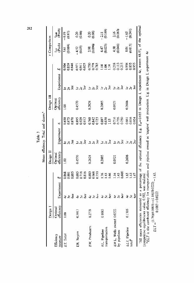
In Table 3 we provide a summary observation of each measure of efficiency for each experiment. This summary measures of efficiency is the mean efficiency across all periods of each experiment,

where E’ is the period t efficiency as defined by each of the measures (ET’, EB’, E W’, EL’, E WL’) for each experiment.

Comparing Designs I and II we observe a small but insignificant decline in total efftciency. But the greater contestability of Design II causes a significant increase in the fraction of optimal surplus realized by buyers, even with our small sample size. Well owners experience a decline in their relative share. Both as transporters and as well-owners pipelines realize a significantly lower relative surplus in Design II. As transporters their share falls as much as 50 percent, and a producers by more than 50 percent. Their combined profit share efficiency, ELT, averages less than 90 percent of its predicted value in Design II.

Efficiency comparisons, Design III versus Design II

Table 3 also provides mean efficiency comparisons with (Design II) and without (Design III) pipeline ability to transport their own gas. Moving from Design II to III we find n important change in E7: EB and EW Pipeline profit efliciency increases somewhat, but prolits on pipeline-owned wells decline considerably although the decline is not statistically significant. The net effect is to increase total pipeline profits, ELT Thus pipelines actually perform somewhat better when they do not transport their own gas.

8. Summary

The high rate of return on investment in gas pipelines, the historical imperatives of a regulatory system that strengthened any inherent monopoly power in pipeline systems, and the increased potential contestability in U.S. natural gas pipeline networks together imply the need to reevaluate federal U.S. regulation of the natural gas industry. In this maiden effort, we propose a new auction market institution for gas pipeline networks. This institution

282

• , . ~ @ . .

o c~ ~ o c5

c5 o o c5

.~ = o

E

t-,

e.0

.o

ab "~

o

o,.,

• c3

~ = ~ + +

,-4


requires computer support. Specifically, the task of the computer is to provide node prices and pipeline flows that maximize the total gains from exchange in the network conditional upon the location-specific bid schedules of all wholesale buyers and the location-specific offer schedules of all gas and pipeline sellers.

Based on laboratory experiments with reward-motivated subjects, our major conclusion is that, where alternative pipeline transportation paths have comparable costs, and capacity is adequate, gas pipeline networks using Gas Auction Net yield substantially competitive outcomes. Gas Auction Net appears to discipline the behavior of the three types of agents, and we find nothing inherently monopolistic about pipelines except in those parts of the networks served by only one pipeline. Even in these cases bargaining appears to be sufficiently symmetric to yield outcomes that do not disadvantage buyers.

References

Belovicz, M.W., 1979, Sealed-bid auctions: Experimental results and applications, in: V.L. Smith, ed., Research in experimental economics, Vol. 1 (JAI Press, Greenwich, CT) 2799338.

Coursey, Don and Vernon L. Smith, 1984, Experimental tests of an allocation mechanism for private, public or externality goods, Scandinavian Journal of Economics 86, no. 4, 4688484.

Cox, James C., Vernon L. Smith and James Walker, 1985, Expected revenue in discriminative and uniform price sealed-bid auctions, in: V.L. Smith, ed., Research in experimental economics, Vol. 3 (JAI Press, Greenwich, CT) 1833232.

Ketcham, Jon, Vernon L. Smith and Arlington W. Williams, 1984, A comparison of posted offer and double auction pricing institutions, Review of Economic Studies 51.

McAfee, R. Preston and John McMillan, 1987, Auctions and bidding, Journal of Economic Literature 25, 699-738.

Miller, Gary and Charles R. Plott, 1985, Revenue-generating properties of sealed-bid auctions, in: V.L. Smith, ed., Research in experimental economics, Vol. 3 (JAI Press, Greenwich, CT) 159-181.

Norman, Donald A., 1987, Competition in the natural gas pipeline industry, Western Inter- national Economic Association meetings (Vancouver, B.C.).

Smith, Vernon L., 1967, Experimental studies of discrimination versus competition in sealed-bid auction markets, Journal of Business 40, 5684.

Stalon, Charles A., (Commissioner, Federal Energy Regulatory Commission), 1985, The dimi- nishing role of regulation in the natural gas industry, Seventh Annual North American Conference, The International Association of Energy Economists (Philadelphia, PA).

Vickrey, William, 1961, Counterspeculation, auctions and competitive sealed tenders, Journal of Finance 16, 8837.

Vincent-Genod, Jacques, 1984, Fundamentals of pipeline engineering (Gulf, Houston, TX).

Designing `smart' computer-assisted markets : An experimental auction for gas networks

Documents

Transcript of Designing `smart' computer-assisted markets : An experimental auction for gas networks