design and implementation of iec 61499 standard-based
269
DESIGN AND IMPLEMENTATION OF IEC 61499 STANDARD-BASED NONLINEAR CONTROLLERS USING FUNCTIONAL BLOCK PROGRAMMING IN DISTRIBUTED CONTROL PLATFORM By JULIUS N’GON’GA MUGA Thesis submitted in partial fulfilment of the requirements for the degree Doctor of Technology: Electrical Engineering In the Faculty of Engineering at the Cape Peninsula University of Technology Supervisor: Prof R. Tzoneva Bellville campus December 2015 i
-
Upload
khangminh22 -
Category
Documents
-
view
3 -
download
0
Transcript of design and implementation of iec 61499 standard-based

0
DESIGN AND IMPLEMENTATION OF IEC 61499 STANDARD-BASED NONLINEAR CONTROLLERS USING FUNCTIONAL BLOCK PROGRAMMING IN DISTRIBUTED CONTROL PLATFORM By JULIUS N’GON’GA MUGA Thesis submitted in partial fulfilment of the requirements for the degree Doctor of Technology: Electrical Engineering In the Faculty of Engineering at the Cape Peninsula University of Technology Supervisor: Prof R. Tzoneva Bellville campus December 2015
i

CPUT copyright information The dissertation/thesis may not be published either in part (in scholarly, scientific or technical journals), or as a whole (as a monograph), unless permission has been obtained from the University
DECLARATION
I, Julius N’gon’ga Muga, declare that the contents of this dissertation/thesis represent my own unaided work, and that the dissertation/thesis has not previously been submitted for academic examination towards any qualification. Furthermore, it represents my own opinions and not necessarily those of the Cape Peninsula University of Technology.
Signed Date
ii

ABSTRACT
Majority of the industrial systems encountered are significantly non-linear in nature, so if they
are synthesised and designed by linear methods, then some of salient features
characterising of their performance may not be captured. Therefore designing a control
system that captures the nonlinearities is important. This research focuses on the control
design strategies for the Continuous Stirred Tank Reactor (CSTR) process. To control such a
process a careful design strategy is required because of the nonlinearities, loop interaction
and the potentially unstable dynamics characterizing the system. In these systems, linear
control methods alone may not perform satisfactorily. Three different control design
strategies (Dynamic decoupling, Decentralized and Input-output feedback linearization
controller) are proposed and implemented .in the Matlab/Simulink platform and the
developed strategies are then deployed to the design of distributed automation control
system configuration using the IEC 61499 standard based functional block programming
language. Twin CAT 3.1 system real-time and Matlab/Simulink (www.mathworks.com)
environment are used to test the effectiveness of the models The simulation results from the
investigation done between Simulink and TwinCAT 3 software (Beckhoff Automation)
platforms in the case of the model transformation and closed loop simulation of the process
for the considered cases have shown the suitability and the potentials of merging the
Matlab/Simulink control function blocks into the TwinCAT 3.1 function blocks in real-time.
The merits derived from such integration imply that the existing software and software
components can be re-used. This is in line with one of the IEC 6144 standard requirements
such as portability and interoperability. Similarly, the simplification of programming
applications is greatly achieved. The investigation has also shown that the integration the of
Matlab/Simulink models running in the TwinCAT 3.1 PLC do not need any modification,
hence confirming that the TwinCAT 3.1 development platform can be used for the design and
implementation of controllers from different platforms. Also, based on the steps required for
model transformation the between the Matlab/Simulink to the TwinCAT 3 functional blocks,
the algorithms of the control design methodologies developed, simulation results are used to
verify the suitability of the controls to find whether the effective set-point tracking control and
disturbance effect minimisation for the output variables can be achieved in real-time using
the transformed Simulink blocks to the TwinCAT 3 functional blocks, then downloaded to the
Beckhoff CX5020 PLC for real-time execution. Good set-point tracking control is achieved for
the MIMO closed loop nonlinear CSTR process for the considered cases of the developed
control methodologies. Similarly, the effects of disturbances are investigated. TwinCAT
functional modules achieved good set-point tracking with these disturbances minimization
under all the cases considered.
iii

ACKNOWLEDGEMENTS
I wish to thank: My employer Technical University of Mombasa for granting me the study leave and
scholarship for this noble undertaking. I will always remain grateful to the support I received during the course of study.
My supervisor Professor Raynitchka Tzoneva for her supervision, guidance, advice and contribution throughout the thesis write up. To her, I say thank you very much.
My wife Liz for the endurance, support, understanding and encouragement during the time of study.
My sons Frank, Yves and Michael Muga for the endurance during my long period absence from home. I love you all.
The financial assistance of the National Research Foundation towards this research is acknowledged. Opinions expressed in this thesis and the conclusions arrived at, are those of the author, and are not necessarily to be attributed to the National Research Foundation.
iv

DEDICATION
I dedicate this thesis to my little boy, Michael Muga
v

TABLE OF CONTENTS
Declaration ii Abstract iii Acknowledgements iv Dedication v Glossary viii CHAPTER ONE: PROBLEM STATEMENT, OBJECTIVES, HYPOTHESIS AND ASSUMPTIONS 1.1 Introduction 1 1.2 Awareness of the problem 2 1.3 Problem statement 4 1.3.1 Sub problem 1(design) 4 1.3.2 Sub problem 2(implementation) 5 1.4 Research Aim and Objectives 5 1.4.1 Aim 5 1.4.2 Specific objectives 5 1.5 Hypothesis 6 1.6 Delimitation of the Research 6 1.7 Motivation of the Research 7 1.8 Assumptions 7 1.9 Contributions of the Research and Deliverables 8 1.10 Outline of the thesis 8 1.11 Conclusion 10 CHAPTER TWO: LITERATURE REVIEW
2.1 Introduction 12 2.2 Nonlinear systems and nonlinear controller design techniques 12 2.3 Review of the existing literature for the CSTR modelling and
control design 14
2.3.1 Model based controller design method 15 2.3.1.1 Differential geometric concepts 18 2.3.1.2 Nonlinear model predictive control 19 2.3.1.3 Nonlinear Internal model control 19 2.3.1.4 Lyapunov based controller design 21 2.3.1.5 Multivariable Control 22 2.3.2 Concluding remarks 30 2.4 Overview of the distributed control and the IEC 61499 standard
application in process industry 42
2.4.1 Basic ideas of the IEC 61499 standard application in the industrial automation control systems
44
2.4.2 The IEC 61499 standard executing tools 46 2.4.3 The IEC 61499 standard and distributed control review 46 2.5 Discussion on the application of the IEC 61499 standard for
Distributed Control 62
2.6
Overall Conclusion regarding this chapter and the way forward 65
vi

CHAPTER THREE: ANALYSIS OF THE STEADY STATE AND DYNAMIC CHARACTERISTICS OF THE CSTR PLANT MODEL
3.1 Introduction 65 3.2 The mathematical description of the nonlinear systems 65 3.3 The CSTR process 66 3.3.1 Derivation of the modelling equations for the CSTR process 67 3.3.2 Mass and Energy balances for the CSTR process 70 3.3.2.1 Overall mathematical balance for the CSTR process (continuity
equation) 70
3.3.2.2 Energy balance of component A for the CSTR process 71 3.3.2.3 Conclusion regarding balance equations for the CSTR process 72 3.4 State space form of the dynamic equations of the CSTR process 72 3.5 Steady state and dynamic equations analysis 74 3.5.1 Simulation of the controlled variables at the steady state
operating conditions 74
3.5.2 Dynamic analysis and Simulation 77 3.6 Discussion and conclusion 81
CHAPTER FOUR: CONTROLLER DESIGN METHODS USING CONVENTIONAL TECHNIQUES
4.1 Introduction 83 4.2 Multivariable controller design 83 4.3 The CSTR model linearization and stability analysis 84 4.4 Decoupling controller design 88 4.4.1 Decoupled concentration control loop transfer function derivation 92 4.4.2 Decoupled temperature control loop transfer function derivation 92 4.5 PI controller design by pole placement technique 93 4.5.1 PI controller design for the concentration loop 94 4.5.2 PI controller design for temperature control loop 98 4.6 Simulated results 100 4.6.1 Concentration loop simulated results 100 4.6.1.1 Investigation of the process performance for variations in
concentration set-point 101
4.6.1.2 Investigation of the process performance for disturbances in the concentration loop
103
4.6.2 Investigation of the process performance for variations in temperature control loop
106
4.6.2.1 Investigation of the process performance for variations in temperature set-point
107
4.6.2.2 Investigation of the process performance for disturbances in the temperature control loop
108
4.6.2.3 Investigation of the process performance in the concentration loop for disturbances in the temperature control loop
110
4.6.2.3 Discussion of the results of simulation 112 4.7 Conclusion 113
CHAPTER FIVE: DECENTRALIZED CONTROLLER DESIGN FOR THE CSTR PROCESS
5.1 Introduction 115 5.2 Decentralized control approach 115 5.3 The Relative Gain Array (RGA) 116
vii

5.4 IMC-based PID feedback control design theory 119 5.4.1 IMC-based PID feedback control design for the concentration
control loop 121
5.4.2 IMC-based PID feedback control design for the temperature control loop
122
5.5 Simulation Results 124 5.5.1 Concentration loop transition behaviour 125 5.5.2 Temperature loop transition behaviour 127 5.5.3 Simulation of the decentralized closed loop MIMO CSTR system 128 5.5.4 Investigation on the disturbance influence on the concentration
output 130
5.5.5 Investigation on the disturbance influence on the temperature output
132
5.6 Decentralized control with detuning factors 134 5.6.1 Comparison of closed loop performance between Decentralized
control with and without detuning factors 135
5.6.2 Investigation on the disturbance interference in the decentralized system with detuning factor over the concentration output
137
5.6.3 Investigation on the disturbance interference in the decentralized system with detuning factor over the temperature output
138
5.7 Discussion of the Results 139 5.8 Concluding remarks on the developed decentralized design
method 140
CHAPTER SIX: INPUT/OUTPUT FEEDBACK LINEARIZATION CONTROLLER DESIGN
6.1 Introduction 142 6.2 Feedback linearization control schemes 142 6.3 Input-Output Feedback linearization control design technique 144 6.4 Input-Output Feedback linearization control design for the CSTR
process 146
6.5 Linear PI controller design 148 6.5.1 Linear PI controller design for the concentration control loop 150 6.5.2 Linear PI controller design for the temperature control loop 151 6.6 Simulation design 153 6.6.1.1 Concentration loop results from simulations for various set
points 155
6.6.1.2 Investigation of the process performance for a disturbance on the concentration control loop
157
6.6.2.1 Temperature loop results from simulations for various set points 158 6.6.2.2 Investigation of the process performance for a disturbance on the
temperature control loop 159
6.7 Discussion of the Results 161 6.8 Concluding remarks on the I/O feedback linearization design
method used 162
CHAPTER SEVEN: FUNCTION BLOCK TRANSFORMATION FROM MATLAB/SIMULINK TO BECKHOFF TwinCAT 3.1 FOR REAL-TIME SIMULATION
AND CONTROL 7.1 Introduction 164 7.2 The Beckhoff TwinCAT 3.1 software for Automation Technology
(Overview) 164
viii

7.2.1 The Beckhoff TwinCAT 3.1 software for Automation Engineering platform
165
7.2.2 The Beckhoff TwinCAT 3.1 software for Automation Runtime 166 7.2.3 The programming Logic Controller 167 7.2.3.1 The Beckhoff TwinCAT 3.1 CX-5020 PLC 168 7.2.3.2 The Beckhoff TwinCAT 3.1 CX-5020 PLC communication with
Ethernet for real-time control 169
7.3 Matlab/Simulink integration with TwinCAT 3.1 170 7.4 Steps for TwinCAT 3.1 module generation from a Simulink model 171 7.5 Closed loop control transformations and the results of real-time
simulations 176
7.5.1 Dynamic decoupling closed loop control implementation in Real-time
176
7.5.1.1 Model transformation and set-point tracking control for the decoupled closed loop system
176
7.5.2.1 Investigation of the process performance for disturbance on the concentration control loop
179
7.5.2.2 Temperature loop results from simulation for various set-points and disturbances
187
7.5.3 Decentralized closed loop control implementation in Real-time 196 7.5.3.1 Model transformation and set-point tracking control for the
decentralized closed loop system 197
7.5.3.2 Investigation of the process performance for disturbance on the concentration control loop under decentralized control
199
7.5.3.3 Temperature loop results from simulation for various set-points and disturbances under decentralized control
203
7.5.4 Input-Output feedback linearization closed loop control implementation in Real-time
208
7.5.4.1 Model transformation and set-point tracking control for the input-output feedback linearization closed loop system
208
7.5.4.2 Investigation of the process performance for disturbance on the concentration control loop under input-output feedback linearization control
211
7.6 Discussion of the Results from the simulations 213 7.7 Conclusion 213
CHAPTER EIGHT: CONCLUSION, DELIVERABLES, APPLICATIONS AND FUTURE WORK
8.1 Introduction 214 8.2 Problems solved in the thesis 215 8.2.1 Design-based 215 8.2.2 Implementation-based sub-problem 215 8.3 The thesis deliverables 216 8.3.1 Comprehensive literature review 216 8.3.2 Mathematical modelling of the nonlinear MIMO CSTR process in
the Matlab/Simulink platform 216
8.3.3 Design of the dynamic decoupling controller for the MIMO CSTR process
217
8.3.4 Design of the decentralized control for the MIMO CSTR process 217 8.3.5 Design of the I/O feedback nonlinear linearized control for the
MIMO CSTR process 217
8.3.6 Development of transformation procedure for the developed software from the Matlab/Simulink environment to Beckhoff TwinCAT 3 real-time environment for real-time simulation
218
ix

8.4 Developed software 218 8.5 Applications of the results from the thesis 220 8.6 Future work 220 8.7 Publications 221 8.8 Conclusion 221 REFERENCES 222 LIST OF FIGURES Figure 3.1: A basic scheme of the CSTR process Black box model of the nonlinear CSTR process
68
Figure 3.2: Black box model of the nonlinear CSTR process 75 Figure 3.3: Simulink block diagram of the nonlinear CSTR model 75 Figure 3.4: Time response of the Concentration values of input at steady state operating point
76
Figure 3.5: Time response of the Temperature for values of input at the steady state operating point
76
Figure 3.6: Response of the concentration for 10%+ step change in q with cqconstant
77
Figure 3.7: Response of the concentration for 10%− step change in q with cqconstant
78
Figure 3.8: Response of the concentration for 10%− step change in cq with qconstant
78
Figure 3.9: Response of the concentration for step change in cq with qconstant
78
Figure 3.10: Time response of the concentration for 10%± step changes in inputs
79
Figure 3.11: Response of the Temperature for step change in q with cqconstant
79
Figure 3.12: Response of the Temperature for 10%− step change in withconstant
79
Figure3.13: Response of the Temperature for step change in withconstant
80
Figure 3.14: Response of the Temperature for 10%− step change in q with cqconstant
80
Figure 3.15: Time response of the Temperature for 10%± step changes in qand cq
80
Figure 4.1: The block diagram of the linearized 2 2x MIMO CSTR system 88 Figure 4.2: The decoupled closed loop control system 89 Figure 4.3: The closed loop system with decouplers 90 Figure 4.4: The block diagram of the decoupled system 94 Figure 4.5: Flow diagram of the summary of the pole selection procedure 98 Figure 4.6: Dynamic decoupling control implemented in Simulink 100 Figure 4.7: Set-point tracking concentration response 101 Figure 4.8: Response of 0.02 /mol l 101 Figure 4.9: Response of 0.04 /mol l 101 Figure 4.10: Response of 0.06 /mol l 101 Figure 4.11: Response of 0.10 /mol l 101
10%+
10%+
cq q
10%+ cq q
x

Figure 4.12: Response of 0.12 /mol l 102 Figure 4.13: Response of 0.14 /mol l 102 Figure 4.14: Frequency response analyses for the concentration control 104 Figure 4.15: Dynamic decoupling controls subject to disturbances at the output 1( )y and the interaction junction 1( )u
103
Figure 4.16: Response under 31 mol/le− noise 103 Figure 4.17: Response under 34 mol/le− noise 103 Figure 4.18: Response under 0.01mol/l noise 104 Figure 4.19: Response under 0.04mol/l noise. 104 Figure 4.20: Response under 10 / minl± .noise 104 Figure 4.21: Response under 40 / minl± noise 104 Figure 4.22: Response under 80 / minl± .noise 105 Figure 4.23: Response under 100 / minl± noise 105 Figure 4.24: Temperature response under 31 mol/le−± .noise on 1y 105
Figure 4.25: Temperature response under 34 mol/le−± .noise on 1y . 105
Figure 4.26: Temperature response under 0.01mol/l± .noise on 1y . 105
Figure 4.27: Temperature response under 0.04mol/l± .noise on 1y . 105
Figure 4.28: Temperature response under 10 / minl± .noise on 1u 106
Figure 4.29: Temperature response under 40 / minl± .noise on 1u 106
Figure 4.30: Temperature response under 80 / minl± .noise on 1u 106
Figure 4.31: Temperature response under 100 / minl± noise on 1u 106 Figure 4.32: Set-point tracking temperature response 107 Figure 4.33: Temperature set-point tracking at 465K 107 Figure 4.34: Temperature set-point tracking at 460K 107 Figure 4.35: Temperature set-point tracking at 450K 108 Figure 4.36: Temperature set-point tracking at 446K 108 Figure 4.37: Temperature set-point tracking at 440K 108 Figure 4.38: Temperature set-point tracking at 435K 108 Figure 4.39: Temperature response under 4K± noise. 109 Figure 4.40: Temperature response under 8K± noise Caption 109 Figure 4.41: Temperature response under 10K± noise 109 Figure 4.42: Temperature response under 20K± noise 109 Figure 4.43: Temperature response under 10 / minl± noise on 2u 110
Figure 4.44: Temperature Response under 40 / minl± noise on 2u 110
Figure 4.45: Temperature response under 80 / minl± noise on 2u 110
Figure 4.46: Temperature response under 100 / minl± noise on 2u 110
Figure 4.47: Concentration response under 4K± noise on 2y 111
Figure 4.48: Concentration response under 8K± noise on 2y 111
Figure 4.49: Concentration response under 10K± noise on 2y 111
Figure 4.50: Concentration response under 20K± noise on 2y 111
Figure 4.51: Concentration response under 10 / minl± noise on 2u 112
Figure 4.52: Concentration response under 40 / minl± noise on 2u 112
Figure 4.53: Concentration response under 80 / minl± noise on 2u 112
Figure 4.54: Concentration response under 100 / minl± noise on 2u 112 xi

Figure 5.1: Block diagram for the decentralized control of the MIMO CSTR 119 Figure 5.2: Classical feedback control scheme 119 Figure 5.3: Internal model control scheme 120 Figure 5.4: Fully decentralized closed loop control scheme for the concentration
125
Figure 5.5: Fully decentralized closed loop control scheme for the temperature
125
Figure 5.6: Decentralized control concentration set point tracking 126 Figure 5.7: Set-point tracking for 0.08mol/l 126 Figure 5.8: Set-point tracking for 0.1mol/l 126 Figure 5.9: Set-point tracking for 0.12mol/l 126 Figure 5.10: Set-point tracking for 0.14mol/l 126 Figure 5.11: Decentralized control temperature set point tracking
127
Figure 5.12: Set-point tracking for 446K 127 Figure 5.13: Set-point tracking for 450K 127 Figure 5.14: Set-point tracking for 455K 128 Figure 5.15: Set-point tracking for 460K 128 Figure 5.16: Decentralized control implemented in Simulink 128 Figure 5.17: Concentration set-point tracking under decentralized control 129 Figure 5.18: Temperature set-point tracking under decentralized control 129 Figure 5.19: Closed loop control with disturbances at the concentration output 1y
130
Figure 5.20: Concentration response under 31 mol/le−± noise on 1y 130
Figure 5.21: Concentration response under 34 mol/le−± noise on 1y 130
Figure 5.22: Concentration response under 0.01mol/l± noise on 1y 130
Figure 5.23: Concentration response under 0.04mol/l± noise on 1y 130
Figure 5.24: Temperature response under 31 mol/le−± noise on 1y 131
Figure 5.25: Temperature response under 34 mol/le−± noise on 1y 131
Figure 5.26: Temperature response under 0.01mol/l± noise on 1y 131
Figure 5.27: Temperature response under 0.04mol/l± noise on 1y 131
Figure 5.28: Closed loop control with disturbances on 2y output 132
Figure 5.29: Temperature response under 4K noise± 132 Figure 5.30: Temperature response under 8K noise± 132 Figure 5.31: Temperature response under 10K noise± 133 Figure 5.32: Temperature response under 20K noise± 133 Figure 5.33: Concentration response under 4K noise± on 2y 133
Figure 5.34: Concentration response under 8K noise± on 2y 133
Figure 5.35: Concentration response under 10K noise± on 2y 133
Figure 5.36: Concentration response under 20K noise± on 2y 133 Figure 5.37: Concentration closed response using the detuning factor 135 Figure 5.38: Temperature loop closed response using the detuning factor 135 Figure 5.39: Comparison for the concentration response without and with the detuning factor
136
Figure 5.40: Comparison for the temperature response without and with the detuning factor
136
Figure 5.41: Response under 31 mol/le−± noise 137
Figure 5.42: Response under 34 mol/le−± noise 137 Figure 5.43: Response under 0.01mol/l± noise 137
xii

Figure 5.44: Response under 0.04mol/l± noise 137 Figure 5.45: Response under 0.01mol/l± noise on 1y 138
Figure 5.46: Response under 0.04mol/l± noise on 1y 138
Figure 5.47: Response under 0.01mol/l± noise on 1y 138
Figure 5.48: Response under 0.04mol/l± noise on 1y 138
Figure 5.49: Response under 4K noise± 139 Figure 5.50: Response under 8K noise± 139 Figure 5.51: Response under 10K noise± 139 Figure 5.52: Response under 20K noise± 139 Figure 5.53: Response under 10K noise± 139 Figure 5.54: Response under 20K noise± 139 Figure 5.55: Response under 10K noise± 139 Figure 5.56: : Response under 20K noise± 139 Figure 6.1: Input-output feedback linearization control structure 146 Figure 6.2: Desired closed loop Input-output feedback linearization for concentration
150
Figure 6.3: Desired closed loop Input-output feedback linearization for temperature
151
Figure 6.4: Simulink CSTR process model 153 Figure 6.5: Control structure using input-output feedback linearization 154 Figure 6.6: Simulink block for the input-output feedback linearization controller
154
Figure 6.7: Input-output feedback linearization controlled concentration set-point tracking
155
Figure 6.8: Response for a set-point of 0.08 /mol l 156 Figure 6.9: Response for a set-point of 0.09 /mol l 156 Figure 6.10: Response for a set-point of 0.1 /mol l 156 Figure 6.11: Response for a set-point of 0.11 /mol l 156 Figure 6.12: Response for a set-point of 0.12 /mol l 156 Figure 6.13: Response for a set-point of 0.13 /mol l 156 Figure 6.14: Concentration response under 31 mol/le−± disturbance magnitude 157 Figure 6.15: Concentration response under 34 mol/le−± disturbance magnitude
157
Figure 6.16: Concentration response under 0.01mol/l± disturbance magnitude
157
Figure 6.17: Concentration response under 0.04mol/l± disturbance magnitude
157
Figure 6.18: Temperature response under 31 mol/le−± disturbance magnitude 158 Figure 6.19: Temperature response under 34 mol/le−± disturbance magnitude 158 Figure 6.20: Temperature response under 0.01mol/l± disturbance magnitude 158 Figure 6.21: Temperature response under 0.04mol/l± disturbance magnitude 158 Figure 6.22: Response for 447K set point 159 Figure 6.23: Response for 450K set point 159 Figure 6.24: Response for 455K set point 159 Figure 6.25: Response for 460K set point 159 Figure 6.26: Temperature response under a disturbance magnitude 0.4K± 160 Figure 6.27: Temperature response under a disturbance magnitude 1K± 160 Figure 6.28: Temperature response under a disturbance magnitude 2K± 160 Figure 6.29: Temperature response under a disturbance magnitude 160 Figure 6.30: Concentration response under a disturbance magnitude 0.4K± 161
xiii

Figure 6.31: Concentration response under a disturbance magnitude 1K± 161 Figure 6.32: Concentration response under a disturbance magnitude 0.4K± 161 Figure 6.33: Concentration response under a disturbance magnitude 1K± 161 Figure 7.1: TwinCAT 3.1 eXtended Automation (http://www.beckhoff.com/english.,2015)
166
Figure 7.2: TwinCAT 3.1. Engineering platform (http://www.beckhoff.com/english.,2015)
167
Figure 7.3: Modular TwinCAT 3.1. Runtime platform (http://www.beckhoff.com/english.,2015)
168
Figure 7.4: Beckhoff CX5020 PLC (www.beckhoff.com/CX5000) 169 Figure 7.5: Real-time control communication with Ethernet 171 Figure 7.6: TcCOM module operation 172 Figure 7.7: Snapshot of the Code generation in Simulink platform 173 Figure 7.8: Snapshot of the model building in Simulink platform 173 Figure 7.9: Snapshot of the Code generated in Simulink platform 173 Figure 7.10: Snapshot of the TwinCAT Microsoft visual studio platform Figure 7.11: Snapshot for creating new TwinCAT project in the visual studio platform
174
Figure 7.12: Snapshot for adding new TcCOM object 174 Figure 7.13: Snapshot for test running TcCOM object 174 Figure 7.14: Snapshot for linking the TcCOM object to the local PLC 175 Figure 7.15: Snapshot for linking the TcCOM object to the task 175 Figure 7.16: Snapshot of the TwinCAT project Microsoft visual studio platform
175
Figure 7.17: Transformed Simulink closed loop model under dynamic decoupling to TwinCAT 3 function blocks
177
Figure 7.18: Concentration Set-point tracking for 0.08moles/litre 177 Figure 7.19: Concentration Set-point tracking for 0.09 moles/litre 177 Figure 7.20: Concentration Set-point tracking for 0.1moles/litre 178 Figure 7.21: Concentration Set-point tracking for 0.11moles/litre 178 Figure 7.22: Concentration Set-point tracking for 0.12 moles/litre 178 Figure 7.23: Concentration Set-point tracking for 0.13moles/litre 179 Figure 7.24: TwinCAT 3 dynamic decoupled function blocks module for CSTR closed loop control with disturbance on 1y
180
Figure 7.25: Set-point tracking under 31e−± moles/litre disturbance on 1y 180
Figure 7.26: Set-point tracking under 34e−± moles/litre disturbance on 1y 181
Figure 7.27: Set-point tracking under 0.01± moles/litre disturbance on 1y 181
Figure 7.28: Set-point tracking under 0.04± moles/litre disturbance on 1y 181
Figure 7.29: Concentration Set-point tracking for 0.13moles/litre Concentration Set-point tracking under 10± litres/min disturbance on 1u e
182
Figure 7.30: Concentration Set-point tracking under 40± litres/min disturbance on 1u
182
Figure 7.31: Concentration Set-point tracking under 80± litres/min disturbance on 1u
183
Figure 7.32: Concentration Set-point tracking under 100± litres/min disturbance on 1u
183
Figure 7.33: Concentration Set-point tracking under 4K± disturbance on 2y 184
Figure 7.34: Concentration Set-point tracking under 8K± disturbance on 2y 184
Figure 7.35: Concentration Set-point tracking under 10K± disturbance on 2y 184
Figure 7.36: Concentration Set-point tracking under 20K± disturbance on 2y 185 xiv

Figure 7.37: Concentration Set-point tracking under 10± litres/min disturbance on 2u
185
Figure 7.38: Concentration Set-point tracking under 40± litres/min disturbance on 2u
186
Figure 7.39: Concentration Set-point tracking under 80± litres/min disturbance on 2u
186
Figure 7.40: Concentration Set-point tracking under 100± litres/min disturbance on 1u
186
Figure 7.41: Temperature Set-point tracking for 450K 187 Figure 7.42: Temperature Set-point tracking for 455K 187 Figure 7.43: Temperature Set-point tracking for 460K 188 Figure 7.44: Temperature Set-point tracking for 465K 188 Figure 7.45: Temperature Set-point tracking under 31e−± mole/litre disturbance on 1y
190
Figure 7.46: Temperature Set-point tracking under 34e−± mole/litre disturbance on 1y
190
Figure 7.47: Temperature Set-point tracking under 0.01± mole/litre disturbance on 1y
191
Figure 7.48: Temperature Set-point tracking under 0.04± mole/litre disturbance on 1y
191
Figure 7.49: Temperature Set-point tracking under 10± litres/min disturbance on 1u
192
Figure 7.50: Temperature Set-point tracking under 40± litres/min disturbance on 1u
192
Figure 7.51: Temperature Set-point tracking under 80± litres/min disturbance on 1u
192
Figure 7.52: Temperature Set-point tracking under 100± litres/min disturbance on 1u
193
Figure 7.53: Temperature Set-point tracking under 4K± disturbance on 2y 193
Figure 7.54: Temperature Set-point tracking under 8K± disturbance on 2y 194
Figure 7.55: Temperature Set-point tracking under 10K± disturbance on 2y 194
Figure 7.56: Temperature Set-point tracking under 20K± disturbance on 2y 194 Figure 7.57: Temperature Set-point tracking under 10± litres/min disturbance on 2u
195
Figure 7.58: Temperature Set-point tracking under 40± litres/min disturbance on 2u
195
Figure 7.59: Temperature Set-point tracking under 80± litres/min disturbance on 2u
196
Figure 7.60: Temperature Set-point tracking under 100± litres/min disturbance on 2u
196
Figure 7.61: Transformed Simulink closed loop control model under decentralized methodology to TwinCAT 3 function blocks
197
Figure 7.62: Concentration Set-point tracking for 0.09 moles/litre 197 Figure 7.63: Concentration Set-point tracking for 0.1moles/litre 198 Figure 7.64: Concentration Set-point tracking for 0.11moles/litre 198
xv

Figure 7.65: Concentration Set-point tracking for 0.12 moles/litre 198 Figure 7.66: Concentration Set-point tracking for 0.13moles/litre 199 Figure 7.67: Concentration Set-point tracking for 31e−± moles/litre 200 Figure 7.68: Concentration Set-point tracking for 34e−± moles/litre 200 Figure 7.69: Concentration Set-point tracking for 0.01± moles/litre 200 Figure 7.70: Concentration Set-point tracking for 0.04± moles/litre 201 Figure 7.71: Concentration Set-point tracking under 4K± disturbance on 2y 201
Figure 7.72: Concentration Set-point tracking under 8K± disturbance on 2y 202
Figure 7.73: Concentration Set-point tracking under 10K± disturbance on 2y 202
Figure 7.74: Concentration Set-point tracking under 20K± disturbance on 2y 202 Figure 7.75: Temperature Set-point tracking under decentralized control for 450K
203
Figure 7.76: Temperature Set-point tracking under decentralized control for 455K
203
Figure 7.77: Temperature Set-point tracking under decentralized control for 460K
204
Figure 7.78: Temperature Set-point tracking under decentralized control for 465K
204
Figure 7.79: Temperature Set-point tracking under 4K± disturbance on 2y 205
Figure 7.80: Temperature Set-point tracking under 8K± disturbance on 2y 205
Figure 7.81: Temperature Set-point tracking under 10K± disturbance on 2y 205
Figure 7.82: Temperature Set-point tracking under 20K± disturbance on 2y 206
Figure 7.83: Temperature Set-point tracking under 31e−± moles/litre disturbance on 2y
206
Figure 7.84: Temperature Set-point tracking under 34e−± moles/litre disturbance on 2y
207
Figure 7.85: Temperature Set-point tracking under 0.01± moles/litre disturbance on 2y
207
Figure 7.86: Temperature Set-point tracking under 0.04± moles/litre disturbance on 2y
207
Figure 7.87: Transformed Simulink closed loop control model under the Input-Output feedback linearization control methodology to TwinCAT 3 function blocks
208
Figure 7.88: Concentration Set-point tracking under I/O feedback linearization for 0.08moles/litre
209
Figure 7.89: Concentration Set-point tracking under I/O feedback linearization for 0.09 moles/litre
209
Figure 7.90: Concentration Set-point tracking under I/O feedback linearization for 0.1moles/litre
209
Figure 7.91: Concentration Set-point tracking under I/O feedback linearization for 0.11moles/litre
210
Figure 7.92: Concentration Set-point tracking under I/O feedback linearization for 0.12 moles/litre
210
Figure 7.93: Concentration Set-point tracking under I/O feedback linearization for 0.13moles/litre
210
Figure 7.94: Concentration Set-point tracking under I/O feedback linearization for 31e−± moles/litre disturbance on 1y
211
Figure 7.95: Concentration Set-point tracking under I/O feedback 212
xvi

linearization for 34e−± moles/litre disturbance on 1y Figure 7.96: Concentration Set-point tracking under I/O feedback linearization for 0.01± moles/litre disturbance on 1y
212
Figure 7.97: Concentration Set-point tracking under I/O feedback linearization for 0.04± moles/litre disturbance on 1y
212
LIST OF TABLES Table 2.1: Number of the reviewed publications for model-based control verses the year
14
Table 2.2: Review papers on model based control design for CSTR. 24 Table 2.3: Number of reviewed publications on the distributed control and the IEC 61499 Standard
46
Table 2.4: Review papers on the distributed control and the IEC 61499 standard
48
Table 3.1: Steady state operating data for the CSTR process 73 Table 3.2: Steady state operating points 73 Table 3.3: 10%± step changes in input volumetric flow rates q and cq 81 Table 4.1: Analysis of the different set-points influence over the concentration response performance indicators under dynamic decoupling control
102
Table 4.2: Analysis of the different set-points influence over the temperature response performance indicators under dynamic decoupling control.
108
Table 5.1: Performance indices for the concentration control loop under decentralized control
126
Table 5.2: Performance indices for temperature control loop under decentralized control
128
Table 5.3: Performance indices for the concentration and the temperature with and without detuning
136
Table 6.1: Performance indices for the concentration control loop using I/O linearization-based control
157
Table 6.2: Performance indices for the temperature control loop using I/O linearizing control
160
Table 7.1: Embedded CX5020 PLC Technical data sheet (www.beckhoff.com/CX5000
169
Table 7.2: Comparison between the performance indicators of the closed loop concentration and temperature responses under the Matlab/Simulink and the TwinCAT PLC real-time for various magnitudes
187
Table 7.3: Comparison between the performance indicators of the closed loop concentration and temperature responses under the Matlab/Simulink and the TwinCAT PLC real-time for various step magnitudes in decentralized control
209
Table 7.4: Comparison between the performance indicators of the closed loop concentration responses under the Matlab/Simulink and the TwinCAT PLC real-time for various step magnitudes in I/O feedback linearization control
216
Table 8.1: Matlab m-files developed for the thesis 222 Table 8.2: Simulink models developed in the thesis 223 Table 8.3: Simulink models transformed to TwinCAT 3 functional blocks 224 Table 8.4: TwinCAT 3 models developed 224
xvii

APPENDICES 234 Appendix A1: Function files openloop_cstr 234 Appendix A2: Script files openloop_cstrsim 235 Appendix B: Script file linearize_mod.m 238 Appendix C: Script file conc_code_3.m 239 Appendix D: Script file dyn_conc_code.m 240 Appendix E1: Script file diag_decentsim.m 241 Appendix E2: Script file conc_code_4.m 242 Appendix F: Simulink models developed for the thesis 243 Appendix G: TwinCAT models developed for the thesis 244 Appendix G1: TwinCAT model under dynamic control 244 Appendix G2: TwinCAT model under dynamic control with disturbances 244 Appendix G3: TwinCAT model under decentralized control 245 Appendix G4: TwinCAT model under I/O feedback linearization control 245 Appendix H1: Beckhoff PLC CX-5020 246 Appendix H2: Beckhoff PLC CX-5020 technical data 246 Appendix I: PID Controller Settings Based On IMC 247
xviii

GLOSSARY
Terms/Acronyms/Abbreviations Definition/Explanation ADACOR Adaptive holonic Control Architecture ADS Automation Device Specification BLT Biggest Log-modulus Transfer function CAEX Computer Aided Engineering Exchange COM Component Object Model CORFU Common Object-oriented Real-time Frame work For
Unified development CSTR Continuous Stirred Tank Reactor CX-5020 PLC Programmable Logic Controller (Beckhoff
Automation Inc.) DCS Distributed Control System DLP Dynamic Linear Part DIAC Framework for Distributed Industrial Automation
and Control EFA Extended Finite Automata ESS Engineering Support System FB Function Block FBench An open source graphical software tool for
automation FBDK Function Block Development Kit FBRT Function Block RunTime FTC Fault Tolerant Control GLC Globally linearizing Control ICP Instrumentation Control Points ICS Triplex ISaGRAF A software platform for development and monitoring
of control applications IEC International Electro-Technical Commission IDE Integrated Development Environment IMC Internal Model Control IO Input/Output IPMCS Industrial Process Measurement and Control
Systems IQC Integral Quadratic Constraint ISA International Standard of Automation ISE Integral Squared Error LMI Linearized Model Infinite-bus system LPV Linear Parameter Varying LQC Linear Quadratic Control MIMO Multi-Input Multi-Output MLD Mixed Logic Dynamic model MPC Model Predictive Control MPP Mini Pulp Process MRAC Model Reference Adaptive Control MVC Model-View-Controller NCES Net Condition/Event Systems NDO Nonlinear Disturbance Observer NI Niederlinski index NIMC Nonlinear Internal Model Control NLPC Nonlinear Predictive Control NMPC Nonlinear Model Predictive Control NPAC Nonlinear Predictive Adaptive Controller
xix

nxtCONTROL The control logic of the nxtSTUDIO nxtSTUDIO Engineering software tool distributed control
systems nxtRT The runtime platform of the nxtSTUDIO OOONEIDA Open Object Oriented knowledge Economy for
Intelligent industrial Automation PI Proportional/Integral PID Proportional/Integral/Derivative PLC Programmable Logic Controller PSO Particle Swarm Optimisation PWA PieceWise Affine RGA Relative Gain Array SESA Signal net system analysis SIFB Service Interface Function Blocks SISO Single-Input Single-Output SNP Static Nonlinear Part SIPN Signal Interpreted Petri Nets SVD Single Value Decomposition TcCOM TwinCAT Component Object Model ThIThO Three-Input Three-Output TINI Tiny Inter-Net Interface TITO Two-Input Two-Output TSMC Terminal Sliding Mode Control TwinCAT The Windows Control Automation UML Unified Modelling Language XAE Extended Automation Engineering XAR Extended Automation Runtime XML Extensible Mark-up Language VEDA Verification Environment for Distributed
Applications VIVE Visual Verifier
MATHEMATICAL NOTATIONS
Symbols/Letters Definition/Explanation W Area for the heat exchange
AC Concentration of the component in the reactor
AOC Concentration of the component in the feed stream
PC Specific heat capacity of component in the reactor
PCC
Specific heat capacity of the coolant q Process volumetric flow rate
inq Process feed input volumetric flow rate
oq Process output volumetric flow rate
inρ Density of the incoming flow
cq Coolant volumetric flow rate
ok Pre-exponential factor
R Ideal gas constant
r Rate of reaction per unit volume T
Reactor temperature
OT Feed temperature
xx

COT Jacket temperature
Overall heat transfer coefficient V
Reactor constant volume E∆
Activation energy ( )H−∆
Heat of reaction
ρ Density of component in the reactor cρ
Density of the coolant
sq Steady state feed flow rate
csq Initial Coolant volumetric flow rate
2u Control input for temperature
1y Controlled output concentration
AinitC Initial value of concentration
2y Controlled output temperature
initT Initial value of temperature
u Vector of control signals Cµ Microcontroller
x State vector variables of the CSTR variables 1x
Concentration state variable
2x Temperature state variable
ox Initial state vector
1u Control input for concentration
( )f x n -dimensional vector of nonlinear functions ( )g x nxm -dimensional matrix of nonlinear functions ( )h x l -dimensional vector of nonlinear functions
A Component in the reactor 1 2,f f
Nonlinear functions of the CSTR
ou Initial control signal vector
PG CSTR plant transfer function matrix
( )D s Decoupler matrix transfer function
( )Q s Diagonal (apparent) transfer function matrix of CSTR
z The power of the IMC filter ( )V s
Control input vector from linear controllers ( )C s
Linear controller vectors Λ Relative Gain Array matrix F Detuning factor ζ Damping factor
PM Maximum (Peak) overshoot
sT Settling time
nω Undamped natural frequency
dω Damped natural frequency
λ Element by element in the RGA β Time constant of the non-invertible element γ Adjustable fitter factor
hA
xxi

( )f s The IMC filter transfer function
xxii

CHAPTER ONE INTRODUCTION
PROBLEM STATEMENT, OBJECTIVES, HYPOTHESIS AND ASSUMPTIONS 1.1 Introduction
Majority of the industrial systems encountered are significantly non-linear in
nature, so if they are synthesised and designed by linear methods, then some of
salient features characterising of their performance may not be captured.
Therefore designing a control system that captures the nonlinearities is important.
Nevertheless, linear controller design methods have proved adequate in many
applications (Schweickhardt and Allgöwer, 2007; O'brien and Carruthers, 2013;
Andrade, et al., 2015). The important nonlinear diversity in practical systems
makes it impossible for a systematic and general theory for the design of
nonlinear control systems (Hunt et al., 1992). Linear systems obey the principles
of homogeneity and superposition. When these two properties are fulfilled for any
linear system then the performance of such system is, guaranteed under any
operating condition. In contrast to the linear case, a nonlinear system having its
best performance for certain input signal may show highly unsatisfactory
performance when the signal amplitude experiences sudden change. Also, the
analysis and synthesis of the control properties for nonlinear systems can be
extremely difficult and time consuming (Hunt et al., 1992). However, the design
and implementation of robust nonlinear controllers that captures the process
nonlinearities, is of great interest. Plenty of research papers for the control of
nonlinear industrial systems are available and different approaches are available.
Approaches such are feedback linearization, back stepping control, sliding mode
control, Linearization based on Lyapunov theory, Differential Geometry concepts,
as well as those based on artificial intelligence etc., have been proposed. A few
examples are (Hunt et al., 1992; Wang and Li., 2005; Schweickhardt and
Allgower, 2007; Marinescu, B., 2010; Vlad et al 2012; Hammer, 2014). Another
challenging aspect is if the system is Multi-Input Multi-Output (MIMO). In MIMO
processes, the coupling between different inputs and outputs makes the design of
the controller difficult. Generally, each input will have an effect on every output of
the process. Because of this coupling, signals can interact in unexpected ways.
One solution is to design additional controllers to compensate for the interactions
(Jevtovic and Matausek, 2010; Sujatha, and Panda, 2013; Leena and Ray, 2014).
This research focuses on the control design strategies for the Continuous Stirred
Tank Reactor (CSTR) process. To control such a process a careful design
strategy is required because of the nonlinearities, loop interaction and the
1

potentially unstable dynamics. In these systems, linear control methods alone
may not perform satisfactorily. The proposed research work is aimed at the
design and implementation of nonlinear controllers and the deployment of the
developed controllers to the design of distributed automation control system
configuration using the IEC 61499 standard based functional block programming
language. Twin CAT 3.1 system real-time (Beckhoff Automation) and
Matlab/Simulink (www.mathworks.com) environment are used to test the
effectiveness of the developed models and methods in realizing the thesis
objectives. The IEC 61499 standard was developed by the International Electro
technical commission and the objective of the standard is to address the
limitations of the popular programmable logic controller (IEC 61131-PLC)
programming languages in implementing real-time control. The standard also
offers benefits such as the ease of configurability, interoperability, portability and
event driven approach to the implementation of control strategy. Comparative
performance analyses using the two platforms (Matlab/Simulink and TwinCAT
3.1) such as configurability and decentralization assessment are carried out.
Simulation will be used to show the suitability of the Distributed control system in
line with the functional block programming concepts. It is envisaged that the
thesis out contributions will provide a platform for understanding the concepts of
the TwinCAT 3.1 software environment, its application to practical distributed
control systems, as well as a guide for model transformation between the two
environments (Matlab/Simulink and TwinCAT 3.1) for modelling, data analysis
and real-time simulation.
This chapter is further subdivided as follows: Section 1.2 shows the awareness of
the research problem, while section 1.3 gives the problem statement. Section 1.4
lists the aims and objectives of the research. Then sections 1.5, 1.6, 1.7
respectively provide the hypothesis, the delimitations of the research work and
the motivation followed by the assumptions in section 1.8. Section 1.9 gives the
thesis contribution and deliverables. Section 1.10 is the outline of the proceeding
chapters and lastly the conclusion is provided in section 1.11.
1.2 Awareness of the problem Research in nonlinear control is motivated by the inherently nonlinear
characteristics of the dynamic systems to be controlled. In reality, virtually most
practical systems encountered are significantly nonlinear in nature so that the
salient features characterising of their performance may be completely
compromised if they are modelled, analysed and designed by linear control
2

methods (Guay at al., 2005). The important nonlinear diversity in practical
systems makes it impossible for a systematic and general theory for the design of
nonlinear control systems (Hahn and Marquardt, 2003). However, the design and
implementation of robust nonlinear controllers that captures the process
nonlinearities, is of great interest. Linear systems obey the principles of
homogeneity and superposition. When these two properties are fulfilled for any
linear system then the performance of such system is guaranteed under any
operating condition. In contrast to the linear case, a nonlinear system having its
best performance for certain input signal may show highly unsatisfactory
performance when the signal amplitude experiences sudden change. Also, the
analysis and synthesis of the control properties for nonlinear systems can be
extremely difficult and time consuming. The increasing tough requirements
imposed on product quality and energy utilization, and also, the safety and
environmental impacts require that industrial processes operate such that their
inherent nonlinearities are emphasized. Thus developing and implementing
controllers which are suitable when process nonlinearities must be accounted for,
is of great interest .It is on this context that the nonlinear theory is suggested for
the design and implementation of nonlinear distributed controllers for the
nonlinear plants. The prototyping environment that is proposed for the
construction, implementation and simulation is the new IEC 61499 function blocks
standard platform (Vyatkin, V.,2011) The IEC 61499 was developed to support
distributed control. The structure developed is integrated with the TwinCAT 3.1.
IEC 61499 based real-time environment and the Matlab/Simulink
(www.mathworks.com) environment to test the suitability of the proposed
methods. Based on the factors mentioned the main research questions of the
thesis can be formulated as follows:
• Linear or nonlinear methods for design of controllers for MIMO nonlinear
processes contribute to better performance of the closed loop system for
various process conditions, as changing set point and disturbances.
• Is the software TwinCAT 3.1 capable for programming of the developed
decentralized distributed closed loop control systems and to perform real-time
simulation.
• Can the real-time Twin CAT 3.1 environment be capable to assure the same
performance characteristics of the closed loop systems through real-time
simulation in comparison with the obtained through the simulation in
Matlab/Simulink environment.
3

1.3 Problem Statement The need for decentralized control in complex manufacturing setup is
tremendously growing because of reasons, such as flexibility and reliability. In
contrast to a centralized controlled system, any failure in any part of the system
results in a breakdown in the system. The IEC 61131-3 standard function block
diagram programming of the PLCs are not suitable for implementation of
distributed control. Also, the increased complexity of present day industrial set-
ups implies that the control design methods like nonlinear controller design which
can overcome limitations on the conventional feedback control design methods
are needed. The IEC 61499 standard-based PLC environment is the solution in
order to achieve distributed control of complex nonlinear industrial systems. The
thesis focuses on nonlinear control design and its real-time implementation in a
distributed set-up that utilizes some of the features of the IEC 61499 standard
using functional block programming in a distributed control platform. Multi-input
Muliti-output (MIMO) Continuous Stirred Tank Reactor (CSTR) model is used as
case study to show the suitability of the algorithms developed. The problem can
be split into: Nonlinear controller design, and real-time implementation of the
developed control system.
The thesis focuses on the development of nonlinear MIMO control system
methodology based on the platforms complaint with the IEC 61499 standard,
thereby exploiting the potentials of this platform for distributed control
applications. MIMO (CSTR) bench mark model is selected as the nonlinear plant
to be controlled.
1.3.1 Sub-problem1 (design). This problem can be addressed through the following steps:
• To formulate the mathematical model for the MIMO nonlinear plant
• To develop methods for the linearization and stability analysis relevant to
MIMO nonlinear plant model.
• To develop methods for the design of linear controllers based on the
conventional decoupling (Jacobian) linearization techniques, relevant to the
MIMO nonlinear plant model
• To develop methods for the design of nonlinear controllers based on dynamic
decoupling techniques relevant to the MIMO nonlinear plant model.
• To develop methods for the design of nonlinear decentralized controllers
techniques relevant to the MIMO nonlinear plant model.
4

• To develop methods for the design of nonlinear controllers based on
input/output feedback linearization techniques relevant to the MIMO nonlinear
plant model.
• To design linear controllers, additional to the dynamic decoupling,
decentralized and input/output linearization controllers to improve the closed
loop system performance.
• To develop Matlab/Simulink software and simulate the MIMO closed loop
systems.
1.3.2 Sub-problem2 (implementation).
• To perform simulations for the developed closed loop decoupled control
system in Matlab/Simulink environment
• To perform simulations for the developed closed loop decoupled control
system in Matlab/Simulink environment
• To perform simulations for the developed closed loop decentralized control
system in Matlab/Simulink environment
• To perform simulations for the developed closed loop input/output feedback
linearization control system in Matlab/Simulink environment
• To transform the developed control software from Matlab/Simulink
environment to the IEC 61499 standard-based TwinCAT 3 simulation
environment (Function blocks).
• To perform real-time simulation of the closed loop systems in the TwinCAT
PLC platform to demonstrate the effectiveness of the transformations.
• To perform real-time distributed control simulations of the closed loop
systems in in the TwinCAT PLC platform
1.4 Research Aim and Objectives The research investigations are looking at the following aim and objectives.
1.4.1 Aim The aim of the investigation is to design nonlinear controllers and implement
them in the functional block based PLC environment in order to achieve real-time
simulation of the distributed closed control of complex industrial systems.
1.4.2 Objectives 1. To model, linearize and simulate the nonlinear MIMO CSTR in
Matlab/Simulink environment.
5

2. To design decoupling control and develop Matlab/Simulink software and
simulate the closed loop system in Matlab/Simulink environment for set-point
tracking control and disturbance rejection.
3. To design decentralized control and develop Matlab/Simulink software and
simulate the closed loop system in Matlab/Simulink environment for set-point
tracking control and disturbance rejection.
4. To design input/output linearized feedback control and develop
Matlab/Simulink software and simulate the closed loop system in
Matlab/Simulink environment for set-point tracking control and disturbance
rejection.
5. To perform comparative analysis of the Dynamic decoupling controller design,
Decentralized control strategy and Input-output state feedback linearization in
terms of set-point tracking capabilities and disturbance rejection.
6. To transform the developed software from Matlab/Simulink environment to
IEC 61499 standard-based TwinCAT 3 simulation environment (Function
blocks).
7. To perform real-time simulation of the closed loop system in order to
demonstrate the effectiveness of the transformation.
1.5 Hypothesis The developing and implementing of controllers which are suitable when process
nonlinearities must be accounted for are of great interest. Hence the designs of
such controllers are preferable. Also the increased degree of distribution and the
type of real-time automation implies that the software tools that would make it
possible to design the control application in a distributed way is needed. On the
bases of the above, the hypotheses are:
1. Design of controllers using the principles of decoupling, decentralization and
input-output linearization can be successfully provided for nonlinear
multivariable systems.
2. The mathematical expression of the designed controllers can be programmed
in the software environment of the TwinCAT 3 software for real-time
simulation and implementation of nonlinear distributed control systems.
Thus, developing a control system methodology based on the new TwinCAT 3
functional block programming complaint with the requirements of the IEC 61499
standard offers great potentials in all those control applications that require real-
time solutions for multivariable nonlinear dynamic processes.
6

1.6 Delimitation of the research The proposed research is focused into the design and implementation of
nonlinear controllers using Matlab functional block programming environment. It
considers a prototype MIMO Continuous Stirred Tank Reactor (CSTR) plant
model with two control loops. The control structures developed are limited to the
methodology adopted by the linear theory (dynamic decoupling control and
decentralized control) and the nonlinear theory (input/output feedback
linearization within the control loops). These structures are implemented both in
the Matlab/Simulink platform and in the TwinCAT 3.1 (Beckhoff Automation)
supporting the IEC 61499 standard as case studies. Simulations are used to
show the suitability of the control systems. A comparative performance analyses
are carried out. Real-time control simulation is carried out by transformation of the
developed Matlab/Simulink closed loop systems into the TwinCAT 3.1 Beckhoff
Automation software and Beckhoff CX-5020 PLC.
1.7 Motivation of the Research Strongly nonlinear systems cannot be controlled optimally by linear feedback
controllers. The increased complexity of present day industrial set-ups implies
that the control design methods like nonlinear controller design which can
overcome limitations on the conventional feedback control design methods are
needed. The IEC 61499 standard based TwinCAT 3.1 environment is the next
generation control design software for the automation industry. It was developed
to support distributed control. The standard is currently evolving and has not been
used in actual factory applications. Thus, the research is motivated by developing
control system design methods based on this new standard requirement that offer
great potentials in all those distributed control applications that require real-time
solutions for MIMO nonlinear dynamic processes.
1.8 Assumptions In order to achieve the objectives of the research, the following assumptions are
made on different parts of the work.
• The process dynamics are highly nonlinear and the operating points are
explicitly stated.
• The nature of the equations describing the process to be controlled allows the
controller to be designed by both linear and feedback linearization techniques.
• The IEC 61499 standard-based function block complaint platform TwinCAT
3.1 should be able to describe both nonlinear control and data relationship for
7

the distributed closed loop control system design for both hardware and
software implementation and real-time simulation.
1.9 Contributions of the Research and Deliverables. 1. Development of the methods for the design of the linear controllers based on
decoupling control philosophy 2. Development of the methods for Design of the linear decentralized controllers for
the nonlinear MIMO system
3. Design of nonlinear controllers based on input/output feedback linearization of
the nonlinear MIMO system
4. Simulations of the control algorithms in Matlab/Simulink for comparative
analysis.
5. Development of a guide or algorithm for transformation of the developed
software from Matlab/Simulink environment to IEC 61499 standard-based
TwinCAT 3.1 simulation environment (Function blocks).
6. Real-time simulation comparison of the various closed loop systems by the
Beckhoff CX-5020 PLC and TwinCAT 3.1 software environment.
7. Publication.
1.10 Outline of the thesis The thesis is made up of eight chapters with a breakdown as follows:
Chapter 1 serves as a foundation for understanding and interpreting the contents
of the thesis. It provides problem awareness, problem statement, aim and
objectives of this research, hypothesis and assumptions, the motivation for the
research as well as the research contribution and deliverables.
Chapter 2 is concerned with the review on the relevant aspects of the areas
which concern this thesis and subdivided into sections as follows: General
nonlinear systems and nonlinear controller design techniques, the nonlinear
MIMO Continuous stirred tank reactor (CSTR) bench mark model, CSTR
modelling and the control design methodologies and tools that have been used,
review of the Distributed control methods, review of the IEC 61499 standard in
process industry, and a review of implementation of the nonlinear control with IEC
61499 functional block programming.
Chapter 3 This chapter discusses the nonlinear MIMO Continuous Stirred Tank
Reactor. This has been chosen as a case study example for this research. The 8

nonlinear CSTR process model’s steady state and dynamic responses are
analysed. The simulations on the developed nonlinear model of the CSTR plant
with a first order exothermic reaction are performed to show the behaviour of the
plant model for step changes in the inputs. This allows for the choosing of optimal
working points for the various controller designs and implementations.
Chapter 4 This chapter presents the multivariable control of the ideal nonlinear
CSTR process model using decoupling controller design strategies to control the
reactor concentration and temperature. First, the nonlinear CSTR plant model is
linearized at one of the operating point and then decoupling control is designed.
Decoupling control ensures that the MIMO closed loop control system is
decoupled so that each output is controlled independent of the other outputs. The
preliminary theory of the method is presented, then the details of the design of
the control schemes are provided, and lastly the developed closed loop system is
tested by simulation in the Matlab/Simulink environment and is evaluated in terms
of the performance specifications for various initial conditions, disturbances and
set points.
Chapter 5 This chapter presents the multivariable control of the linearized ideal
nonlinear CSTR process model using decentralized controller design strategies to
control the reactor temperature and the concentration. For the design of the
decentralized controllers, input output pairing is performed based on the Relative
Gin Array (RGA)-the ratio of the open loop gain to the closed loop gain of the
considered control system. The preliminary theory of the method is presented,
then the details of the design of the control scheme are presented, and lastly the
developed closed loop system is tested by simulation in Matlab/Simulink
environment and is evaluated in terms of the performance specifications for
different system conditions.
Chapter 6 This chapter develops an input/output feedback linearization controller
design method for the nonlinear multi input multi output process of the reactor
temperature and concentration in a CSTR. Input/output feedback linearization is a
type of control design technique that uses feedback signal to cancel the inherent
nonlinearities in a system, and creates linear differential relationship between the
outputs and the newly defined virtual inputs. The preliminary theory of the method
is presented, then the details of the design of the control methodologies are
provided, and lastly the proposed closed loop system is tested by simulation in
9

the Matlab/Simulink environment in terms of the performance specifications for
various system conditions. A comparison with the other conventional methods
developed in chapters four and five is made.
Chapter 7 The concept of real-time control for the MIMO CSTR is introduced.
The chapter introduces the TwinCAT 3.1 software as a tool used for integration
with Matlab/Simulink software in order to implement real time control of the
developed control algorithms. The chapter presents a methodology of
transforming the developed continuous time controller blocks in Chapters 4, 5
and 6 as well as the complete closed loop systems application from
Matlab/Simulink environment to the Beckhoff Embedded PCs using the
capabilities of TwinCAT 3.1 simulation environment. Then the Beckhoff CX-5020
Programmable Logic Controller is used for real-time simulation of the closed loop
systems. It presents the development of the algorithm (guide) for the
transformation therein.
Chapter 8 presents the conclusion of the thesis. It outlines the deliverables
achieved and suggestions for future works in relation to the nonlinear control
based on IEC 61499 standard. In addition the publication derived from the results
of the study is also listed.
1.11 Conclusion This chapter presents the background of the project, the problem statement, the
aims and objectives of the project. The assumptions, the delimitation of the
research and the motivation is also given. It also outlines the contribution and
deliverables expected.
In order to achieve the stated aims and objectives, a comprehensive literature
review on nonlinear systems and nonlinear controller design techniques, and
control of MIMO systems with emphasis on the CSTR plant is essential. Also a
review on Design of distributed control, the IEC 61499 Standard for distributed
control application, and the implementation of the control using the IEC 61499
functional block programming techniques is important.
Chapter 2 presents review on the existing literature on nonlinear systems and
nonlinear controller design techniques, control of MIMO CSTR systems,
distributed control and the IEC61499 standard.
10

CHAPTER TWO LITERATURE REVIEW
2.1 Introduction For enhanced functionality, flexibility and reliability, the tendency of the present
day industrial set-up is to embed the disciplines of computing, communication
and control together to form different levels of information processes and plant
operation. The IEC 61499 standard gives a methodology that embeds computing,
communication and control to model, design and implement the distributed
process measurement and control systems applications. The standard is still new
and evolving. The thesis focuses on the development of nonlinear Multi-input
Multi-output (MIMO) control system philosophies based on the platforms
complaint with this standard thereby exploiting the potentials for distributed
control applications that require real-time solutions. Multi-input Multi-Output
Continuous Stirred Tank Reactor (CSTR) bench mark model has been chosen as
the nonlinear plant to be controlled. This chapter therefore is concerned with the
review on the relevant aspects of the areas which concern this research
investigation subdivided into sections as follows:
Section 2.2 presents an introduction to the General nonlinear systems and
nonlinear controller design techniques. In section 2.3, a review of the existing
literature for the CSTR modelling and the control design is presented. In section
2.4 a review on Distributed control and the IEC 61499 standard in process
industry is presented. In section 2.5 discussion of the comparative review is
presented, and lastly, the conclusion of the chapter is presented in section 2.6.
2.2 Nonlinear systems and nonlinear controller design techniques Research in the field of nonlinear control is motivated by the inherently nonlinear
characteristics of the dynamic systems to be controlled. Strongly nonlinear
systems cannot be controlled in an optimum way by a linear feedback controller.
The increased complexity of present day industrial set-ups implies that the control
design methods like nonlinear controller design which can overcome limitations
on the conventional feedback control design methods are needed. While the
theory of modelling for linear systems is well understood, as well as there is
availability of the mathematical tools for the analysis, there is still a wide gap in
the control theory to analyse and design the nonlinear systems. The distinction
between linear and nonlinear systems is that any system that satisfies the
properties of homogeneity and superposition is a linear system. If the system fails
to satisfy these two properties then it is nonlinear. Thirdly, nonlinear systems may
have many equilibrium points unlike the linear systems which have only one 11

equilibrium point. This therefore means that for nonlinear systems, their stability
needs must be explicitly specified. Majority of the industrial systems encountered
are significantly non-linear in nature, so if they are synthesised and designed by
linear methods, then some of salient features characterising their performance
may not be captured. Therefore designing a feedback control system to capture
these nonlinearities is important and significant. Nevertheless, linear controller
design methods have proved to be adequate in many applications
(Schweickhardt and Allgöwer, 2007). The important nonlinear diversity in practical
systems makes it impossible for a systematic and general theory for the design of
nonlinear control systems (Hunt et al., 1992). As it was mentioned above, linear
systems obey the principles of homogeneity and superposition. When these two
properties are fulfilled for any linear system then the performance of such system
is guaranteed under any operating condition. In contrast to the linear case, a
nonlinear system having its best performance for certain input signal may show
highly unsatisfactory performance when the signal amplitude experiences sudden
change. There is no equivalent mathematical theory, on which base a full theory
of the non-linear control systems can be built. Also, the analysis and synthesis of
the control properties for nonlinear systems can be extremely difficult and time
consuming (Hunt et al., 1992). The increasing tough requirements imposed on
product quality and energy utilization, and also, the safety and environmental
impacts require that industrial processes operate such that their inherent
nonlinearities are emphasized. Thus developing and implementing controllers
which are suitable when process nonlinearities must be accounted for, is of great
interest both academically and for industry. Plenty of research papers on the
analysis and control of nonlinear systems are available and many different
methods have been proposed. Such approaches are feedback linearization, back
stepping control, sliding mode control, trajectory linearization based on Lyapunov
theory, those based on Differential Geometry concepts, as well as those based
on artificial computing approaches etc. A few examples are from (Desoer and
Wang, 1980; Hunt et al., 1992; Enqvist and Ljung, 2004; Schweickhardt and
Allgower, 2007; Marinescu, B., 2010; Zhai and Qian, 2012; Hammer, Jacob,
2014).
Another challenging aspect is if the system to be controlled is Multi-Input Multi-
Output (MIMO). In MIMO systems the coupling between different inputs and
outputs makes the controller design to be difficult. Generally, each input will affect
every output of the system. Because of this coupling, signals can interact in
12

unexpected ways. One solution is to design additional controllers to compensate
for the process and control loop interactions (Meng, Zhao-Jun et al., 2010; Lee, II
Hwan, 2011; Sujatha, and Panda, 2013; Ghosh, A., and Das, S. K., 2012; Leena,
G., and Ray, G., 2014).
2.3 Review of the existing literature for the CSTR modelling and control design The Continuous Stirred Tank Reactor (CSTR) has been selected as a case study
in this thesis. Reactors are the primary focus of many chemical plants. Many
variables must be regulated in a reactor for good process operation. This section
of the chapter presents a review of the control design methods for the nonlinear
MIMO exothermic CSTR process. The control of such a process demands proper
design because of the nonlinearities, the loop interactions and the potentially
unstable dynamics. In these systems, control based on the linear methods for
design alone such as the conventional linear PID controllers may not always yield
satisfactory results. The linear controllers have been the sole selection over the
years even though many other advanced control methods have been developed,
is mainly because of their ability to produce satisfactory results for most control
problems, if these controllers are properly tuned and installed. They are simple,
transparent and feasible. It must also be emphasized that the literature on robust
control, monitoring, and optimization methods is available in plenty, with each
method presenting a solution to a particular problem.
According to (Wayne Bequette, 1991) the following common process
characteristics cause difficulty in the control of both linear and nonlinear systems:
the interactions between the control variables and the controlled variables, the
unmonitored state variables, unmonitored and frequent load disturbances, higher
order and distributed processes, uncertain and time varying variables, constraints
on the control and state variables, and dead time on the inputs and the outputs.
Such features of the multivariable nonlinear systems illustrate the need for and
difficulty of feedback control system design. Research efforts have focused on
presenting control design methodologies that can handle many of these features.
However, it may be accepted that presently there is not one methodology that will
solve all the control problems that can prevail in the modern plants. This is
because; different plants have different problems to be solved.
In general, the nonlinear control algorithms can be classified as:
• Model-Based Control
• Intelligent Control
13

The thesis is focussed on the former method for the design of controllers for
nonlinear systems. These are then reviewed in the following.
2.3.1 Model based controller design method The objective of this section is to review the existing literature on the control
design strategies on model based control based that have been used over the
years for the solution to nonlinear problems, specifically for the CSTR. Table 2.1
provides the number of publications considered and Figure 2.1 illustrates the
graph of the reviewed papers year wise on model based control from 1966 to
2015. For this review a total of 120 papers are considered.
Table 2.1: Number of the reviewed publications for model-based control verses the year
NUMBER OF PUBLICATIONS IN THE YEAR REFERENCE YEAR OF
PUBLICATION NUMBER OF
PUBLICATIONS (Bristol, 1966) 1966 1 (Uppal and Ray, 1974) 1974 1 (Desoer and Wang, 1980). 1980 1 (Economou and Morari, 1986); (Li and Luyben, 1986) 1986 2 (Grosdidier and Morari, 1987); (Luyben, W and. Luyben, M., 1997)
1987 2
(Kravaris and Polanski, 1988) 1988 1 (Skogestad and Morari, 1989); (Daoutidis and Kravaris, 1989)
1989 2
(Kravaris and Kantor, 1990a); (Kravaris and Kantor, 1990b); (Chien and Fruehauf, 1990); (Henson and Seborg., 1990)
1990 4
Bequette., 1991) 1991 1 (Astorga, 1992); (Pottmann and Seborg.,1992) 1992 2 (Seborg, 1994); (Hovd and Skogestad, 1994) 1994 2 (Isidori, 1995) 1995 1 (Viel, et al, 1997) 1997 1 (Marchand and Alamir, 1998); (Marchand et al., 1998); (Gagnon et al., 1998)
1998 3
(Aris and Amundson, 2000) 2000 1 (Antonelli and Astolfi, 2001) 2001 1 (Chen and Seborg, 2002); (Panda et al., 2002); (Rangaiah and Toh, 2002)
2002 3
(Antonelli and Astolfi, 2003); (Chisci, et al, 2003) 2003 2 (Bequette, 2004); (Enqvist and Ljung, 2004);.( Hahn and Marquardt, 2004)
2004 3
(Wang and Li, 2005); (Guay, et al., 2005); (Hedrick and Girard, 2005); (Vojtesek and Dostal, 2005); (Ye Xudong, 2005)
2005 5
(Cai and Xiong, 2006); (Garelli, et al.,2006); (Nordfeldt and Hagglund, 2006); (Selvakumar et al., 2006); (Tavakoli et al., 2006); (Yang, et al.,2006)
2006 6
(Jingjing et al, 2007); (B. Wayne Bequette, 2007) 2007 2 (Rehan, et al, 2008); (Cai, et al., 2008); (Jouili et al., 2008); (Wu, et al.,2008)
2008 4
(López, et, al, 2009); (Bartolini, et al.,2009); (Bakosova and Vasickaninova, 2009)
2009 3
(Rahul and Singla, 2010); (Kamala and Renganathan, 2010 10
14

2010), (Jevtovic and Matausek, 2010); (Vojtesek and Dostal, 2010); (Cai, et al., 2010); (Ganesh and Chiambaram, 2010); (Hadisujoto et al., 2010); (Marinescu, 2010); (Vinodha and Prakash, 2010); (Fikar, 2000) (Allgower et al, 2011); (Dostal, et al, 2011); (Hong, et al., 2011) (Anitha and Subbulekshmi, 2011); (Ge, et al., 2011); (Hirama et al., 2011); (Lee, et al., 2011); (Li, et al., 2011)
2011 8
(Bachir et al, 2012), (Saleh and Mohamed, 2012); (Bachir et al, 2012); (Gholami et al, 2012); (Gao et al., 2012); (Mohamed, et al, 2012); (Hong and Cheng, 2012); (Lopez et al, 2012); (Kamala and Renganathan, 2012); (Ghosh, and Das., 2012,); (Lengare, et al., 2012); (Chen et al., 2012); (Chidambaram and Rajapandiyan, 2012); (Fu et al., 2012); (Mehta and Mahji, 2012); (Kumar and Khanduja, 2012.); (Liu, et al., 2012); (Maghade and Patre, 2012); (Ramzi et al., 2012); (Rosinova, and Kozakova, 2012); (Zhai, et al., 2012)
2012 21
(Hoang et al, 2013); (Yasabie and Sahu, 2013); (Rao and Chimmiri, 2013); (Sujatha, and Panda, 2013); (Chen, et al., 2013); (Dong-Juan et al., 2013); (Kurniawan, et al., 2013)
2013 7
(Wang, et al., 2014); (Ding Li et al., 2014); (Leena, and Ray., 2014); (Jacob, 2014); (Chen and Yun, 2014); (Garrido and Morilla, 2014); (Kwon and Choi, 2014); (Nunes, et al., 2014); (Ulrich and Jurek, 2014); (Yu and Liu, 2014); (Zhu et al. 2014)
2014 11
(Kaldmae and Moog, 2015); (Zhang et al., 2015); (Rehman, and Peterson, 2015); (Vivekananathan and Ponnusamy, 2015); (Yang and, Liu, 2015); (Yang and Wang ,2015); (Dana Copot et al.,2015); (Prashant and Sharad, 2015); (XU Jiao, et al., 2015); (Dongya Zhao et al., 2015)
2015 10
Figure 2.1: Number of publications year by year
1966
19
74
1980
1986
19
87
1988
19
89 19
90
1991
19
92
1994
19
95
1997
1998
2000
20
01
2002
20
03
2004
2005
20
06
2007
2008
20
09
2010
20
11
2012
20
13
2014
20
15
0
5
10
15
20
25
Num
ber o
f pub
licat
ions
YEAR
Number of publications per year
15

Model-based control can be defined as a mathematical and visual technique of
solving the problems associated with complex control systems design. In these
control systems design methods involves four steps: namely: modelling of the
plant, analysing and synthesizing of the controller, simulation of the plant and
controller, and finally, merging all the phases by implementing the closed loop
control. The model-based nonlinear control design techniques are presently the
topic of much interest because of the possibility of employing the process
nonlinearities directly in the control methodology. For example, (Seborg, 1994)
presented an article “perspective on advanced control strategies for process
control” where the controllers are classified according to the degree to which they
have been used in industry and concluded by the remarking that most advanced
control strategies continue to be model based but intelligent control techniques
are receiving widespread attention and that the key research issue is how to
integrate the intelligent control based strategies with the model based
approaches in a practical and cost effective manner Model-Based Control
techniques contain algorithms in which an explicitly separately identifiable
dynamic model of the plant is used. Nonlinear Internal model control (Economou,
et al., 1986; Henson and Seborg, 1991), nonlinear model predictive control (Silva
and Kwong, 1999) Lyapunov based control and those based on Differential
geometric concepts (Kravaris and Kantor, 1990), and Multivariable control (Jones
and Tham, 1987; Tham et al, 1991) are typical examples. These methods share
common characteristics, namely (Seborg, 1994);
• They are all designed on a mathematical model of the plant and hence their
robustness and stability can thus be evaluated analytically.
• All these methods use the inverse of the process model either explicitly or
implicitly to calculate the necessary control action.
A brief introduction of the principle of operation and a review of the model-based
controller design methods are given in the following sections together with a
summary of the applications. The objectives and results of the controller design
methods are presented in Table 2.2. The review is categorized under five
different control schemes: those based on differential geometric concepts,
nonlinear model predictive control, nonlinear internal model control, those based
on Lyapunov stability and those based on multivariable control respectively.
2.3.1.1 Differential geometric concepts: Over the years, differential geometry has been used as an effective tool for the
analysis and design of nonlinear control systems. In these methods, linearity of
16

the closed loop system is sought in some sense. Differential geometric concepts
allow a certain class of systems to be linearized using the state feedback and
coordinate transformations. The primary issue is the design of nonlinear change
of coordinates and nonlinear feedback that make the system behave in a linear
manner. An overview of this approach is given by (Isidori, 1995, Nijmeijer and
Van der Schaft, 1996, Kantor, 1987, Henson and Seborg, 1990, Kravaris and
Kantor, 1990; Yu, Ding Li et al., 2014). Similarly there is a good overview of
general nonlinear approaches to chemical process control system design by
(Bequette, 1991). One of the main contributions of differential geometric
approach is input/output linearization which seeks to reduce the original nonlinear
system to a linear system in an input/output sense via state feedback. There is a
wide range of possible control laws using output and state feedback for output
tracking, input-state and input-output linearization, and decoupling control. These
methods have been applied to the CSTR problem to obtain exact state
linearization, exact input/output linearization and state linearization with
disturbance rejection (Ye Xudong, 2005; Zhang and Chen, 2014; Yu, and Liu,
2014; Zhu et al., 2014; Yang et al., 2006). As an example, the work of (Hong, et
al., 2011) is based on stabilization and tracking control for a class of nonlinear
systems. A nonlinear state feedback stabilization control is proposed which
guarantees global asymptotic output and state tracking with zero tracking error in
the steady state. The proposed methodologies are illustrated using simulation
examples of chaotic and unstable dynamics. The work of (Yang and Liu, 2015) is
based on adaptive output feedback controller design for a MIMO nonlinear
system with unknown nonlinear parameters, uncertain nonlinearities, bounded
disturbance, unmodeled dynamics and uncertain control parameters. Through the
design and the simulation results the effectiveness of the proposed controller is
proved. In (Chen, Z., et al., 2012) robust output tracking control design is
proposed for a general class of uncertain non-affine nonlinear systems. The
design employs feedback linearization, coupled with a high gain filter which is
built to estimate the feedback linearization error. The simulation results show the
effectiveness of the approach. Input-output feedback linearization technique is
used in this study and therefore is covered in detail in Chapter 6. This is a control
design methodology that uses a feedback signal to cancel the inherent nonlinear
dynamics and to create a linear differential relation between the output and a
newly defined synthetic input.
17

2.3.1.2 Nonlinear model predictive control The common way of controlling process systems with strong nonlinearities is to
apply model based predictive controllers where a detailed dynamic process
model is used in an optimization framework. The model predictive control (MPC)
has been used widely in the process industries because of its many appealing
features such as handling multivariable systems with time delays. In addition, the
constraints on manipulated inputs, states and output variables are explicitly
handled in the formulation of the optimization problem (Panjapornpon, 2005).
Model predictive control is a class of computer control algorithms that control the
future behavior of a plant through the explicit use of a dynamic model of the plant.
At each control interval, the model predictive algorithm computes an open loop
sequence of the manipulated variables, for a time termed a control horizon in
order to optimize the process behavior in the time ahead known as the prediction
horizon. Process constraints and any changes in the process objectives or
operating conditions can be implemented on line. A new process measurement is
injected in the control loop and the entire optimization is repeated at subsequent
control intervals. At the heart of the model predictive controller is the model,
which is used not only to forecast the effects of future inputs, but also to estimate
the current state of the plant from the given history of the past measurements and
controls (Khalid, 2006).
MPC technology was originally developed for power plant and petroleum refinery
control applications, but can now be found in a wide variety of manufacturing
environments including chemical, food processing, automotive, aerospace,
metallurgy, and pulp and paper (Thomas Badgwell and Joe Qin, 2001). Further
introductory literature on model predictive control can be found in several text
books such as (Maciejowski, J.M., 2002; Byrd, Richard H. et al, 2006) although
most processes are inherently nonlinear, the vast majority of MPC applications to
date are based on linear dynamic models. Nevertheless, there are cases where
nonlinear effects are significant enough to justify the use of the nonlinear model
predictive control technology. These include regulator control problems where the
process is highly nonlinear and subject to large frequent disturbances like the
continuous stirred reactor or servo control problems where the operating points
change frequently.
Nonlinear Model Predictive Control (NMPC) is an effective strategy for controlling
nonlinear chemical processes with constraints and time delays (Sistu and
18

Bequette, 2004). 2005). NMPC offers great potential in those areas where
process nonlinearities are strong and it is required to improve performance or
even to achieve stable operation. However, (Bequette, 2007) presented a paper
where he provided a concise overview of some of the challenges of developing
and implementing the non-linear predictive control algorithms, with regards to his
experience and the published results. He singled out the optimization problem
which leads to solution with multiple minima, plant mismatch with additive inputs
which result into poor performance when actual disturbances occur in the inputs.
Therefore designers of the NMPC techniques should give more attention to the
problem of disturbance estimation, prediction and compensation. Also, model
development remains an ongoing challenge and it is usually not clear whether the
additional effort of developing a non-linear model, instead of a linear model, will
result in an economic benefit. He noted that while many investigators have
developed non-linearity measures, these are not easy to apply in practice and
usually require the apriori development of a non-linear model. For a more detailed
discussion of the theoretical issues pertaining to the NMPC design methods,
there are review articles by Mayne et al, 2000 and Allgower et al, 1999.This
control strategy is not used in this research project and therefore is not
exhaustively reviewed.
2.3.1.3 Nonlinear Internal model control: The scheme is one of the most popular methodologies in the process industry
because of its simplicity, capability to reject disturbances and robustness. It can
be used both for linear and nonlinear systems. A first step toward a practically
applicable nonlinear controller design technique was proposed (Economou and
Morari, 1986) where it was shown that the nonlinear Internal Model Control (IMC)
works well even in the case where no linear controller can yield stable behavior.
Since then, the IMC has been applied in several areas as chemical processes
such as CSTR (Varshney et al., 2009; Zhang and Li, 2009), batch reactors
(Azwar et al., 2006; Liu et al., 2010), pH control (Jalili-Kharajoo et al., 2003;
Wang and Shi, 2005), and distillation (Han and Clough, 2006; Li et al., 2009). A
unifying review of the internal model control type schemes was first presented by
(Garcia and Morari, 1982) who defined the IMC structure for single-input single-
output, discrete-time systems and further as a nonlinear controller by (Economou
et al, 1986) who developed a nonlinear IMC by employing an approximate
inverse of the model, using local linear approximation. As the name suggests, the
scheme utilizes the inverse of the model of the plant to design the controller. In
19

order for the IMC structure to be stable, certain conditions must be fulfilled
namely; the plant model must be an exact match of the plant and the inverse of
the model must exist. When the model is an exact match of the plant then stability
of both controller and plant is sufficient to guarantee overall system stability.
Similarly, when the model is exact match of the plant, and the controller is the
inverse of the model, then the controller is perfect and the plant output is equal to
the reference signal, hence there will be no offset in the plant output if the
reference signal is asymptotically constant.
IMC is very popular and continues to enjoy widespread popularity in industrial
control applications due to its fine disturbance rejection capabilities and
robustness. More information on the IMC can be found in (Alexander et al, 2002;
Datta and Ochoa, 1996; Henson and Seborg, 1991; Morari. and Zafiriou, 1989;
Patwardhan and Madhavan, 1998; Wang, et al 2001; Xie. and Rad., 2000; Chien
and Fruehauf, 1990; B, Wayne Bequette, 2004). This principle is used in the
design of decentralized controllers for the CSTR model under this study.
2.3.1.4 Lyapunov based controller design: This section gives an overview on some of the approaches of the Lyapunov
design methods that have been used for the CSTR. Lyapunov theory allows in
particular determination of the region of attraction of the stable equilibrium points.
Lyapunov based design has been a primary tool for nonlinear control system
design, stability and performance analysis since its introduction in 1982 by the
Russian mathematician Alexandr Mikkailovich Lyapunov. Lyapunov’s work, titled:
The General Problem of Motion Stability includes two methods for stability
analysis: the linearization method and the direct method The linearization draws
its conclusions about a nonlinear system’s local stability around an equilibrium
point from the stability properties of its linear approximation (Jianying Gao, 2004).
The direct method determines the stability properties of a nonlinear system by
constructing a scalar energy-like function for the system and examining the
functions time variations. The details of these two methods are summarized in
many control engineering books, for example (Slotine and LI, 1991). The
Lyapunov direct method is the most important tool for the analysis and design of
nonlinear systems. The use of Lyapunov-based methods for robust controller
design in conjunction with differential geometric methods was first introduced by
Ha and Gilbert (1987). They addressed the case where the nominal state
feedback provides linearity of both the state equations and the output. For
example, (Antonelli and Astolfi, 2003) made use of methodologies and tools from
20

the Lyapunov theory in the design of bounded output feedback control laws for
the temperature stabilization of a class of CSTRs with exothermic or endothermic
reactions. It is shown that these controllers yield global asymptotic stability and
do not require precise knowledge of the system parameters. In (Ge, S.S. et al.,
2011), adaptive tracking control for a class of uncertain MIMO nonlinear systems
with input constraints is proposed and closed loop bounded stability is achieved
via the Lyapunov synthesis through simulation studies.
2.3.1.5 Multivariable Control: Because of the presence of interactions, the multivariable processes are difficult
to control simply due to several output variables being monitored simultaneously
by manipulating several input channels. There are several multivariable control
techniques available such as those based on the Nyquist arrays which are based
on frequency domain techniques for interaction analysis and for design of pre-
compensators and post compensators (Maciejowski, 1989; Chen and Seborg,
2002), and sequential closing design methods where each controller is designed
sequentially (Hovd and Skogestad, 1994; Rangaiah and Toh, 2002; Rehan, M., et
al, 2008), In this method, the controller of the quickest loop is first tuned. This is
done by considering the case of the selected input-output pair. The loop is the
closed, then tuned after which the other loops are then tuned sequentially and so
on. In the Independent design method, each controller is tuned on the basis of
paired transfer functions while satisfying some specified constraints as a result of
process interactions (Skogestad and Morari, 1989). Then there is the more
popular method known as the Biggest Log-Modulus Tuning (BLT) method of
(Luyben, 1986; Jevtovic and Matausek, 2010; Ghosh, A., and Das, S. K., 2012,
Lengare, et al., 2012; Wang, et al., 2014) where every controller for the multi-loop
system is first designed using the general classical techniques by ignoring the
process coupling from the other loops. After which the couplings are factored in
by detuning each set of controller parameters until some performance index is
reached. The Relay auto-tuning of (Shen and Yu, 1994) applies the relay
feedback methodology to design each corresponding SISO controller. A review of
the three different MIMO controller design strategies is carried out, below:
Decoupling control ensures that the MIMO control system is decoupled by
incorporating a pre-compensator to compensate for the process and loop
interactions, so that each output is controlled independently (Luyben, W. and,
Luyben, M., 1997). This control strategy has been used by several other authors
21

over the years with success, among them (Luyben W. and. Luyben, M., 1997;
Jevtovic and Matausek, 2010; Ghosh and Das, 2012; Lengare, et al., 2012;
Wang, et al., 2014). For example, the work of (Jevtovic and Matausek, 2010) is
focused on an ideal decoupler plus PID controller for optimization in the case of
constraints on robustness and sensitivity to the measurement noise. The validity
of the proposed tuning is confirmed on a TITO test bench process. The study by
(Ghosh and Das, 2012) is based the continuous-time, linear time-invariant, non-
minimum-phase, unstable, MIMO plant. The control strategy is to first perform
input-output decoupling in the open-loop and then effecting zero placements of
the decoupled loops using SISO periodic feedback. The study achieves superior
multi-channel output gain margin compensation and arbitrarily large multi-channel
output gain margin is also found out. An example is provided to demonstrate the
design procedure and the controller capability.
Decentralized control on the other hand tries to control the MIMO process by a
suitable decoupling into SISO control loops. However, the decentralized
controllers cannot eliminate the interactions of the plant. Thus, in order to design
decentralized controllers, input output pairing is performed based on the Relative
Gain Array (RGA) method proposed by (Bristol, E. H., 1966), in which the
decentralized control design is made possible by finding the best control structure
pairing between the controlled and manipulated parameters that tries to reduce
the couplings. This implies that two independent diagonal controllers can be
designed while disregarding the coupling between the input pairs. After that an
interaction measure is designed to account for the effect of the coupling on the
stability and performance of the whole system (Wuhuau et al., 2010; Rosinova
and Kozakova, 2012; Kurniawan, E., et al., 2013).
For example, (Wuhuau et al., 2010) proposed an approach of decentralized PID
controller design for MIMO processes by first finding the input/output pairing by
using the RGA-Niederlinski index criteria; the equivalent transfer functions of the
individual loops are then derived. Based on the equivalent transfer functions
decentralized PID controllers are tuned to stabilize the MIMO processes
independently. To demonstrate the efficiency of the proposed approach, three
industrial MIMO processes with different dimensions and interaction modes are
employed.
(Seborg, D. E, 1994) presented “a perspective on advanced control strategies for
process control” where the controllers are classified according to the degree to
which they have been used in industry and concluded by remarking that the most
22
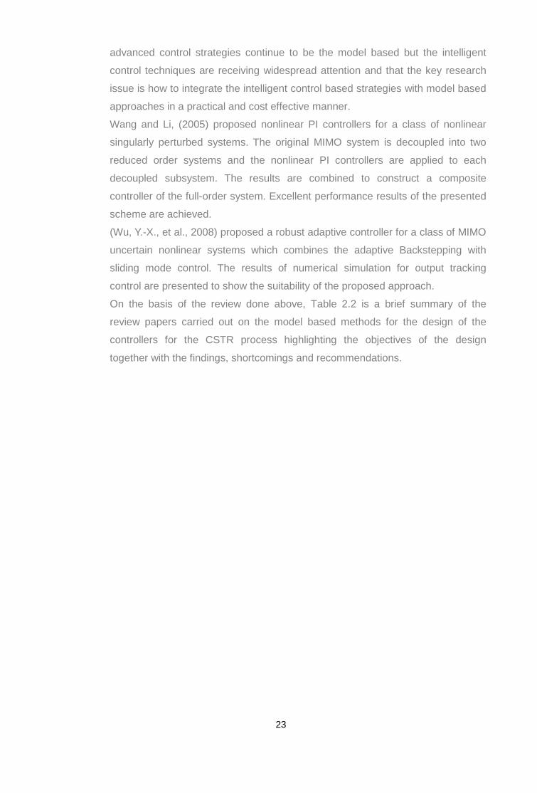
advanced control strategies continue to be the model based but the intelligent
control techniques are receiving widespread attention and that the key research
issue is how to integrate the intelligent control based strategies with model based
approaches in a practical and cost effective manner.
Wang and Li, (2005) proposed nonlinear PI controllers for a class of nonlinear
singularly perturbed systems. The original MIMO system is decoupled into two
reduced order systems and the nonlinear PI controllers are applied to each
decoupled subsystem. The results are combined to construct a composite
controller of the full-order system. Excellent performance results of the presented
scheme are achieved.
(Wu, Y.-X., et al., 2008) proposed a robust adaptive controller for a class of MIMO
uncertain nonlinear systems which combines the adaptive Backstepping with
sliding mode control. The results of numerical simulation for output tracking
control are presented to show the suitability of the proposed approach.
On the basis of the review done above, Table 2.2 is a brief summary of the
review papers carried out on the model based methods for the design of the
controllers for the CSTR process highlighting the objectives of the design
together with the findings, shortcomings and recommendations.
23

Table 2.2: Review papers on model based control design for CSTR. Reference Paper
Controlled variables
constraints Controller Description (methodologies)
Theoretical development Deliverables: Achievements and drawbacks
(Hoang et al, 2013)
Reactor temperature control
steady state multiplicity and the exhibition of minimum phase behavior
Lyapunov Control law Thermodynamics stability analysis and its use for nonlinear stabilization of the CSTR
A description of the thermodynamic availability concept. Its use for open loop dynamic analysis of the non-isothermal CSTR. Its use for Lyapunov based control laws. Derivation of the non-isothermal CSTR. Illustration of the performances of the controller by simulations. Comparison of the controller with a proportional control strategy.
(Yasabie and Sahu, 2013)
Temperature control and Concentration control
Noise in the form of random inputs
1. Model Reference Adaptive Controller(MRAC) 2.Conventional Controller
Provides an understanding of how to implement an adaptive controller and to compare an adaptive controller with conventionally designed controller in various situations.
Demonstrated that while the adaptive controller exhibits superior performance in the presence of noise the convergence time is typically large (greater than 10 seconds) and there is large overshoot.
(Rao and Chimmiri, 2013)
Temperature and concentration control
Deterministic disturbance and stochastic load disturbance generated through random Gaussian noise
PID and a nonlinear internal model control (NIMC) strategy
Nonlinear Model Based Control of Complex Dynamic Chemical Systems which is supported by a nonlinear model based estimator
A nonlinear internal model control (NIMC) with an estimator is designed NIMC strategy is evaluated by applying it for the control of a non-isothermal CSTR and a homo-polymerization reactor. The results show the superior performance of the estimator based NIMC strategy over the conventional PID controllers.
(Bachir Daaou et al, 2012)
Concentration and Reactor temperature
Noise and
model
uncertainties
Linearizing Feedback Controller and Lyapunov stability theorem based controller
Development of an observer-based nonlinear control scheme for a CSTR.
The closed-loop dynamic simulations are developed to illustrate the effectiveness of the proposed approach
24

(Saleh and
Mohamed,
2012)
Tank level and mass concentration control
External disturbances as well as parametric uncertainties are introduced into the model
PI Controller Back stepping controller and Lyapunov function-based controller
Nonlinear control of a three-state CSTR using the back stepping technique. The back stepping controller is first designed. Then an augmented back stepping control law is designed, based on the sliding mode control theory to add robustness to the proposed controller.
The proposed controllers are shown to drive the output trajectories to their respective desired values, hence, ensuring the stability of the closed-loop system. Finally, several simulation studies are presented to illustrate the effectiveness of the proposed control laws.
(Bachir et al, 2012)
Temperature control
Modeling uncertainties and noisy measurements.
Observer-based control scheme using feedback linearization technique and Lyapunov stability technique.
Development of Linearizing Feedback Control with a Variable Structure Observer.
Observer-based control scheme using feedback linearization is addressed. The Lyapunov stability is used to establish the stability of the system. Performance is illustrated via simulations which show that the controller is able to regulate the reactor temperature in the presence of modeling uncertainties and noisy measurements.
(Gholami et al., 2012)
Temperature, and Concentration control
Nonlinear processes imposed by input constraints as: the rate of heat input and the temperature
A Fault-Tolerant Control (FTC) methodology has been presented. The proposed methodology uses a combination of Feedback Linearization and Model Predictive Control (FLMPC) schemes
Fault-Tolerant Control of a Nonlinear Process with Input Constraints
FTC is a challenging issue when the process inputs face constraints. Two sets of fault scenarios were organized to address the two critical input constraints. The obtained results demonstrate the successful activation of the proposed method by replacing the candidate control configurations via the dedicated supervisor.
D. X. Gao et al., 2012
Temperature and density are the state and output variables to be controlled while control variable is
NIL 1.State Feedback Linearization 2.Optimal control
Feedback Linearization and Optimal Control Approach for Bilinear Systems.
State feedback exact linearization approach of optimal control for bilinear systems is designed by solving the Riccati equation and introducing state feedback with state prediction. Simulation results show
25

the flow rate of the cooling.
that the proposed approach is valid and easy to implement
(B. Mohamed, et al., 2012)
Concentration and temperature reactor control with feed low rate and jacket temperature as the manipulated variables.
Noisy measurements and dynamics uncertainty
1.Nonlinear observer design 2.Input-output feedback linearization controller design 3.Lyapunov stability technique
Observer-based input-output linearization control of a multivariable continuous chemical reactor
The observer proposed offers the advantage of only one tuning parameter. The observer is coupled with a nonlinear controller. The controller is constructed through feedback linearization for concentration and temperature control. Lyapunov stability is used to establish the stability of the closed loop system. The proposed control exhibits a satisfactory performance.
(Hong and Cheng, 2012)
The inlet coolant temperature is the input-regulated variable used as the manipulated variable to maintain proper reactor temperature control as the system output.
Parameter uncertainty
Nonlinear Predictive Adaptive Controller and Nonlinear Disturbance Observer (NDO) for CSTR process and a Lyapunov function to analyze the stability
NPAC is presented to solve the presence of parameter uncertainty in strong nonlinear systems. The controller is composed of an optimal NPAC and a NDO. NDO is used to estimate the steady-state response error, and the optimal NPAC improves the system stability.
CSTR tracking with uncertain-parameter problem has been investigated. The NPAC scheme based on NDO was implemented. The presented control laws can guarantee that the steady-state response error asymptotically converges to zero. The proposed compensation method can greatly reduce the effect of disturbances and improve the system tracking accuracy and robustness.
(Ricardo Aguilar Lopez et al., 2012)
The reactor temperature is regulated by means of water flowing through a cooling jacket.
The temperature measurements are corrupted by noise with a ± 5% around the current temperature value.
1.I/O Linearizing Controller; 2. High-order Sliding-mode Controller; 3.Sliding-mode controller. 4. Lyapunov-type analysis
Temperature Control of Continuous Chemical Reactors under noisy measurements and model uncertainties. The design is based on a sliding-mode uncertainty estimator The estimation of convergence is done by the Lyapunov-type analysis
A sliding-mode observer based I/O Linearizing control law is designed. It is considered that the reaction heat is unknown and noisy measurements exist such that an uncertainty estimation methodology is based on algebraic-differential concepts and a sliding-mode frame work. Numerical simulations in which a class of oscillatory chemical system is used as application example to show the
26

effectiveness. (Allgower et al, 2011)
Concentration and Temperature and coolant temperature as the only manipulated variable
multiple hard output constraints imposed on a CSTR
A blending or sliding mode controller is utilized
The objective is to design a control system that can satisfy the three different constraints using only one control input, namely: the coolant temperature.
It is shown analytically and with simulations, that there are critical combinations of constraints, where robust constraint satisfaction cannot be guaranteed. As a consequence violation of at least one constraint has to be allowed.
(P. Dostal, et al., 2011)
The reactant temperature control
Changes of the input signals in strongly nonlinear regions.
Static Nonlinear and Dynamic linear Controller
Nonlinear Control of a Chemical Reactor. The developed control strategy is also suitable for other similar technological processes such as tubular chemical reactors.
The strategy is based on a factorization of the controller into linear and nonlinear part. The nonlinear part is approximated through recursive parameter estimation. Tuning is via pole placement. Simulation demonstrates its usefulness for greater changes of input signals in the strongly nonlinear regions.
(Dostál, et al., 2011)
The coolant flow rate is taken as the control input and the controlled output is the reactant temperature.
Changes of the reactants volumetric flow rate.
Static Nonlinear Part (SNP)and Dynamic Linear Part (DLP) of the controller
Simulation of nonlinear adaptive control of a continuous stirred tank reactor
The control strategy is based on factorization of a controller into the adaptive Dynamic Linear Part (DLP) and the Static Nonlinear Part (SNP). DLP design employs simulated Steady-state characteristics of the process. Then, the DLP and a nonlinear model of the CSTR are approximated by a continuous time external linear model. Simulation results demonstrate the applicability of the control strategy and its usefulness for other similar nonlinear technological processes.
(Rahul and Singla, 2010)
Temperature and Concentration control
Nil Adaptive nonlinear controller and PID controller
Adaptive and PID controllers are tested by using Matlab/Simulink program and their performance is compared
The results prove that adaptive controllers are appropriate to be used under non-linear difficulties.
27

for different temperature and concentration. Adaptive controller exhibits superior control in the presence of a nonlinearities. This is illustrated on the control of non-linear system (CSTR).
(Pablo A. López Pérez, et, al., 2009)
Temperature control
Chattering phenomenon caused by the discontinuity of the input injection
Sliding‐mode controllers under the frame of the differential algebra
Dynamic nonlinear feedback for temperature control of continuous stirred tank reactor with complex behavior
Sliding-mode controllers under the frame of differential algebra are designed. An estimator is coupled to the proposed controller to infer the measured and uncertain terms. The reactor temperature trajectories are controlled successfully in comparison with other nonlinear controllers.in dismissing the chattering of the standard sliding‐ mode controllers.
Jingjing et al., 2007)
Concentration is the output, and the temperature of the coolant is the input of the CSTR system
High nonlinearity, multiple operating points, and a wide operating range.
Model predictive control (MPC). MPC based on Mixed Logical Dynamical (MLD) model
Modeling and Control of a Continuous Stirred Tank Reactor based on a Mixed Logical Dynamical Model (MLD)
A mixed logical dynamical (MLD) model based-Model Predictive Control (MPC) is proposed for CSTR with high nonlinearity, multiple operating points, and a wide operating range. The control law is synthesized by a moving horizon technique for an optimal transition. Drawbacks: Computation complexity which increases with the number of logic variables. More efforts are required to solve these problems.
(B. Wayne Bequette, 2007)
Temperature regulation
Plant mismatch and disturbances in the inputs
Nonlinear model predictive control
An overview of Non-linear Model Predictive Control (NMPC) is presented, with an extreme bias towards the author’s experiences and published results.
Overview of some of the challenges of developing and implementing NMPC algorithms. Optimization problem which leads to multiple minima solution, plant mismatch with additive inputs which resulting in
28

poor performance when disturbances occur in inputs. Therefore designers to give more attention to disturbance estimation, prediction and compensation
(Antonelli and Astolfi, 2003)
Ttemperature stabilization
Input constraints and uncertainty on the kinetic parameters
Output feedback control laws and Lyapunov theory
Lyapunov theory is used in the design of bounded control laws for the temperature stabilization of a class CSTR’s with exothermic and endothermic reactions
The proposed approach offers some important advantages including constraint handling capability and computational simplicity: Some numerical simulations, illustrating the theoretical results, are presented.
(L. Chisci, et al., 2003)
Reactor temperature (controlled output) and the temperature of the coolant stream (manipulated input).
Stringent input and state constraints
Linear Parameter Varying (LPV) embedding techniques in the design of a gain-scheduling controller.
Set-point tracking for a class of constrained nonlinear systems with application to a CSTR
A case-study of constrained nonlinear control relative to the temperature control of a Continuous Stirred Tank Reactor (CSTR). The use of Linear Parameter Varying (LPV) embedding techniques along with an admissible set theory allow fast and safe tracking in presence of stringent input and state constraints
(Antonelli and Astolfi, 2001)
Temperature stabilization
Uncertainty in inputs and kinetic parameters
Lyapunov adaptive Linearizing technique and Global stabilization by state feedback
Stability analysis It is shown that these controllers yield Global Asymptotic Stability and do not require precise knowledge of the system parameters
(Marchand and Alamir, 1998)
Concentration and Temperature control
Nil The design of the feedback is based on the knowledge of a control Lyapunov function.
State feedback is presented for the stabilization of a nonlinear system based on the generation of open-loop trajectories. Lyapunov theory is given applicable to a CSTR case study.
The paper gives conditions on Open-loop trajectory generators in order to use them for the design of a nonlinear feedback. The construction of such a feedback is proposed on a CSTR case study.
(Nicolas Marchand and Mazen Alamir, 1998)
Reactor temperature is the controlled output and the jacketed fluid temperature is
Time lag in the control input.
The state feedback control and Lyapunov theory
The application of the feedback to a Continuous Stirred Tank Reactor, known to exhibit unstable steady states, is provided.
A new state feedback is presented for the stabilization of nonlinear systems. It is based on the generation of open-loop trajectories to design a stabilizing feedback. A
29

the manipulated variable and
general theoretical background based on Lyapunov theory is given. The application of the feedback to a CSTR known to exhibit unstable steady states is provided.
(Kravaris, and Palanki, 1988)
Concentration control
Structured model uncertainty
Robust Nonlinear State Feedback Under Structured Uncertainty and Lyapunov-based approach is to guarantee uniform ultimate Boundedness.
Given upper bounds on the modeling error of the nonlinear process, design a nonlinear state feedback law that guarantees stability and performance for all perturbations within the given bounds.
A robust nonlinear state feedback is proposed for uncertainties considered as a class of bounded perturbations to the state model. A Lyapunov-based approach is used to guarantee uniform ultimate boundedness. The control of the process was simulated using the “true” process, and the robust controller. It is observed that the output of the true process is ultimately bounded, as predicted.
(Viel, et al., 1997)
Temperature and concentration control
Input constraints with strong uncertainties on the dependence of the kinetic function with respect to the temperature.
I/O state feedback linearization and robust state observer
For a general class of CSTR’s, a set of controllers that guarantee the global temperature stabilization in spite of strong uncertainties and the dependence of the kinetic functions with respect to the temperature is proposed. The main feature of these controllers lies in their capability of handling input constraints in some instances
A set of controllers that can guarantee the global temperature stabilization of CSTR in spite of strong uncertainties and the dependence of the kinetic function with respect to the temperature have been proposed. The uniform Boundedness of the concentrations with respect to the temperature was the key point in the proofs. A practical consequence of these results lies in the opportunity of operating chemical reactors at unstable open-loop steady states that correspond to optimal operating conditions.
(Dale
Seborg,
General
perspective of
Nil 1.Conventional strategies. 2. Classical techniques.
The paper provides a personal perspective on the current status of Advanced process
Most prominent methods are discussed critically with emphasis placed on key design issues and
30
1994) process control
variables
3. Advanced control (widely used techniques). 4. Advanced control (new techniques with some industrial applications). 5. Advanced control: proposed strategies with few industrial applications.
control strategies by classifying them according to the degree which they have been used in industry.
unresolved research problems.
(Kravaris and Kantor, 1990)
Concentration and temperature control
Nil Mathematics and systems theory background, including linear tools from differential geometry, nonlinear inversion, and zero dynamics.
Review for geometric methods in nonlinear process control. The concept of feedback linearization of nonlinear systems is introduced. Gives background theory
Reviews theoretical results that are relevant to control applications and provides representative chemical engineering examples on the geometric methods for nonlinear process control
(Kravaris and Kantor, 1990)
Nonlinear pH Control in a CSTR.
Nil The Internal Model Control (IMC) and Globally Linearizing Control (GLC) structures
Review of The Internal Model Control (IMC) and Globally Linearizing Control (GLC) structures for nonlinear processes
The main mission is to solve the feedback linearization problems and to show their application in controlling nonlinear processes (controller synthesis).
(Daoutidis and Kravaris, 1989)
Case 1. The concentration and temperature are the outputs and the manipulated input is the heat input in the third vessel. Case 2. The inlet temperature is controlled and the manipulated input is the heat input in the first vessel. Case 3. The major inlet concentration
Presence of disturbances to inlet concentration and temperature
Feed forward/State feedback control law
The general feedforward/feedback control problem for nonlinear SISO systems is addressed and control laws that lead to elimination of the effect of the measurable disturbances, on the process output and at the same time provides input-output linearity linearity with respect to set point changes are solved for 3 CSTR in series.
The proposed methodology was proven to be a very powerful technique in completely eliminating the effect of the measured disturbances and providing satisfactory servo behavior.
31

is controlled and the manipulated input is the heat input in the first vessel.
(Economou and Morari, 1986)
The inlet stream feed temperature and the desired product output concentrations are selected as manipulated and controlled variables, respectively.
Disturbances and/or unmodeled system dynamics.
Internal Model Control (IMC)
1. An extension of the IMC design for MIMO nonlinear systems. 2. Attractive features of linear IMC are carried over naturally to the nonlinear case. 3. This is a first step toward a practically applicable nonlinear feedback controller design technique.
Operator formalism is used to extend the IMC design approach to nonlinear systems. Simulation examples demonstrate the simplicity of the design procedure and the good performance characteristics, and show that the nonlinear IMC works well even in the case where no linear controller can yield stable behavior.
(Kamala Thyagarajan and Renganathan, 2010)
Effluent concentration and reactor temperature are process outputs and feed flow rate and the coolant flow rates are the manipulated variables
Set-point tracking and Load Disturbance rejection
1. Decentralized controllers design using IMC method and detuning factor
2. Design of decoupling controllers using IMC method and detuning factor
Comparative analysis between decentralized control and decoupling control strategies
It is shown that decoupling controllers provide better set point tracking and load disturbance rejection than the decentralized controllers
(Kamala Thyagarajan and Renganathan, 2012)
Effluent concentration and reactor temperature
Set-point tracking and Load Disturbance rejection
IMC based conventional control scheme Particle Swarm Optimization decentralized PID controller
Comparative analysis between PSO and IMC control strategies PSO is utilized to optimize the coefficients of the decentralized PID controller tuned to cover the nonlinear range of the process. The effectiveness of the control scheme is demonstrated by simulation studies on the CSTR process.
The proposed controller provides better set-point tracking and load disturbance rejection than the IMC based conventional control scheme.
(Wang and Temperature Set-point Two nonlinear PI control Stabilisation of a class of The simplicity and performance of
32

Li, 2005)
control tracking and Load Disturbance rejection
laws to form the composite controller
singularly perturbed systems using nonlinear PI control techniques is addressed by decomposition of the system to overcome the unknown nonlinear uncertainties due to unmodeled dynamics and external disturbances of each subsystem
the proposed methodology is demonstrated through a mathematical example
(Chen and Seborg, 2002)
Level control of distillation column
Disturbance rejection and set-point tracking
IMC with PID controllers based on the direct synthesis approach
Although the PI/ PID controllers are designed for disturbance rejection, the set-point responses are usually satisfactory and can be independently tuned via a standard set-point weighting factor or a set-point filter constant without affecting the disturbance response
Nine simulation examples to demonstrates that very good control for a wide variety of processes including those with integrating and/or non-minimum phase characteristics is possible
(Hovd and Skogestad, 1994)
Methanol, concentration, reflux flow rate and the steam flow rates
Set-point tracking and disturbance rejection
PI controller tuning using Biggest Log Modulus (BLT) approaches and sequential design approaches
A new sequential design procedure that involves minimizing the performance criterion at each design step is proposed. The key basis for design is the factorization of the overall system in terms of the estimates for the complementary sensitivity functions of the loops that are to be designed
A procedure for sequential design of decentralized controllers for linear systems is presented. It is shown how to include a simple estimate of the effect of closing subsequent loops into the design problem for the loop which is to be closed.
(Rehan, M., et al., 2008)
Flow and temperature control of a Coupled Three Tank System
Set-point tracking and Load Disturbance rejection
Use of Integral Quadratic Constraint (IQC), and minimum maximum Linear Quadratic Gain(LQG) control approaches
The scheme uses a copy of the plant nonlinearity along with its inverse function in the controller.
Robust nonlinear output feedback controller design, including copies of the inverses of the nonlinearities in the controller. Compressor surge system is used to show the effectiveness of the proposed
33

scheme (Skogestad and Morari, 1989)
Methanol, concentration, reflux flow rate and the steam flow rates
satisfy robust performance in terms of set-point tracking and reduction of model uncertainties
Diagonal PID controllers Two design methods are addressed: sequential loop-closing design and the independent design of each loop.
The decentralized control problem is formulated as a series of independent designs. Simple bounds on these individual designs are derived, which, guarantee robust performance of the overall system. The results provide a generalization of the interaction measure.
(Jevtovic and Matausek, 2010)
Composition and temperature control
Fast set-point responses and fast disturbance rejection, under constraints on robustness and control effort.
Ideal decouplers and PID control
The validity of the system is confirmed using a test batch consisting of Two-Input Two-Output (TITO) stable, integrating and unstable processes, and one Three-Input Three-Output (ThIThO) stable process
Designing multivariable controller based on ideal decoupler and controller optimization under constraints on the robustness and sensitivity to measurement noise is done
(Ghosh, A., and Das, S. K., 2012)
Frequency response analysis of the transfer function
robustness measures of multi-channel output gain margins for SISO plants
Ideal decouplers and PID control
It is shown that decoupled compensation may be employed to provide good multi-channel output gain margin compensation for MIMO plants even when they are unstable as well as contain non-minimum-phase zeros.
Achieves superior multi-channel output gain margin compensation of continuous-time, non-minimum-phase, unstable, MIMO plants by first input–output decoupling these in open-loop and then effecting zero placements of the decoupled loops using SISO feedback.
(Lengare, et al., 2012)
General Set-point tracking and Load Disturbance rejection
Decentralized PID controller design using IMC theory.
The method has no limitations regarding systems weak or strong interactions, and multiple delays
Direct controller synthesis approach is used. A detuning factor for each loop is specified based on the closed-loop time constant. Then appropriate controller settings are determined using the Maclaurin series expansion. Simulation examples demonstrate the usefulness of the proposed method.
(Wang, et al., 2014)
Product composition control
The improvement of
Smith delay compensator is employed, where PI
PI controllers with two unitary matrices are derived from
Decoupling control based on singular value decomposition. Moreover, the
34

of the Wood berry distillation column
dynamic quality and resistance to model error
controllers are designed via internal model control (IMC
SVD, and then decoupling is obtained. Noteworthy improvements of the method include wide adaptability, i.e., square system and non-square system, but also its convenience of quantitatively regulating response performance
method overcomes the effect of model error caused by parameter perturbation. Two illustrative examples are provided to demonstrate the effectiveness of the proposed method. The integral of squared error (ISE) performance criterion is applied for evaluation.
(Chen, Z., et al., 2012)
The temperature of ceramic kiln
Set-point tracking and Load Disturbance rejection
Feedback linearization, coupled with two high-gain observers
The approach handles the difficulty in controlling non-affine nonlinear systems and also simplifies the stability analysis due to its linear control structure
Control design for a general class of uncertain non-affine nonlinear systems. Simulation results show the effectiveness of the approach.
(Hong, et al., 2011)
Chaos control and state variables control of unstable dynamical systems
Stabilization, tracking control, optimal disturbance rejection
Nonlinear state feedback by means of quadratic Lyapunov function
Guarantees global asymptotic output and state tracking with zero tracking error in the steady state.
Provide, for MIMO nonlinear systems, a tracking control based on nonlinear state feedback. The methodologies are illustrated using two simulations of chaotic and unstable dynamical systems.
(Ding Li et al., 2014)
Effluent concentration is controlled
Set-point tracking and Load Disturbance rejection
Input-output feedback linearization using the theories of differential geometry and linear PID control.
Linearization is realized by input variable-substitution and then, mature linear control theory for the sub linear system is used
Designed a controller for the CSTR system. Simulation results show that the proposed control scheme is efficient and the system contains good static and dynamic performance.
(Vojtesek and Dostal, 2010)
Changes of the heat removal as manipulated variable and the temperature of the reactant as the controlled output
Set-point tracking and Load Disturbance rejection
Proportional Controller Control based on polynomial synthesis and the pole-placement provides good control results in spite of negative control properties such as non-minimum phase behaviour and changes in the sign of the controller gain
A methodology for simulation of a nonlinear CSTR reactor with adaptive control is presented. The results demonstrate the usability of the control method, in terms of stability of the output response
(Ray, G., Torque and voltage Set-point Decentralized PID A linearized model of multi- An LMI optimization problem is
35

2014) control tracking and Load Disturbance rejection
controller based on Hermite Biehler theorem
machine infinite-bus system is considered for simulation to show the effectiveness of the design procedure
formulated to ensure the stability of the composite system while the designed decentralized controllers are employed. A genetic algorithm based search technique is adopted to select an optimal PID controller gains from a designed search space of the stabilizing controllers in order to have an optimum value of the performance index
(Sujatha, and Panda, 2013)
Product composition control, at the top and bottom of the distillation column
Set-point tracking and Load Disturbance rejection
Controller tuning using IMC PI Laurent tuning rule
The proposed method of control configuration selection and closed loop identification can be used to retune the decentralized multi-loop controller for linear MIMO systems.
Uses input/output data from interactive loop to formulate a model using relay feedback and to quantify interaction measures for selection of control configuration. Simulation results have demonstrated the effectiveness of the proposed control configuration.
(Jacob, 2014)
control of a tight neighbourhood of the bounded outputs
Robust asymptotic stabilisation
Static state feedback controllers
A simple methodology for the design of state feedback controllers for nonlinear continuous-time systems is introduced
It is shown that controllers can be derived by solving a set of inequalities obtained directly from system’s equation. The results are applied to the design of controllers that achieve robust asymptotic stabilisation for the general class of nonlinear systems
(Zhang et al., 2015)
desired trajectory of the composition measurements
Stability analysis and trajectory control
an adaptive fuzzy control developed by using backstepping design technique
adaptive fuzzy backstepping control problem of the two-stage chemical reactor with recycle streams
It is shown that all the signals of the resulting closed-loop system are bounded and the tracking error remains at an adjustable neighbourhood of the origin with the prescribed performance bounds.
(Rehman and Peterson, 2015)
output feed control for the compressor surge system
uncertainties and nonlinearities elimination
A robust dynamic state feedback controller based on the use of integral quadratic constraint (IQC)
The scheme uses a copy of the plant nonlinearity along with its inverse function in the controller by. using an integral
A compressor surge system is used to show the effectiveness of the proposed scheme
36

and Linear quadratic regulation (LQR) control.
quadratic constraint (IQC) approach which gives a smaller bound on the closed loop cost function
(Vivekananathan and Ponnusamy, 2015)
Reactor temperature
Servo and regulatory controls
Decentralized PI controllers
The scheme uses auto tuning algorithm for two different cases: the servo and regulatory problems. MATLAB and SIMULINK tools are used for system modelling and control design.
The performance indices for the Multiple Input Multiple Output-based decentralized PI controller for the CSTR system is evaluated and presented
(Yang and Wang ,2015)
Reactor concentration
steady state stability in the presence of disturbances
Explicit Model Predictive Control of CSTR System Based on piecewise affine (PWA ) system
The paper provides a practical method to control the CSTR system
The simulation results show that the CSTR system is capable of running in accordance with the desired index and demonstrate the effectiveness of the presented approach to control the CSTR system.
(Dana Copot et al.,2015)
Reactor temperature control
Constraints such as the propeller speed, preheating of the inlet gases and catalyst basket are analysed
Proportional controller and Internal model control (lMC)-based controller
Development of a control strategy for efficient operation of a CSTR reactor
Two control strategies were designed and tested on the real system
(Prashant and Sharad, 2015)
effluent concentration and temperature of the reaction
stability under circumstances of partial pole-zero cancellation
Decoupling Based model Predictive Control
Loop interactions are compensated for by directly modifying the plant model without changing its response characteristics provided plant and model mismatch is at minimum
The proposed strategy is compared for its simplicity with multi-variable decoupling control strategies Simulations show that proposed technique efficiently reduces loop interactions in CSTR process.
(XU Jiao, et al., 2015)
effluent concentration and temperature of the
Nil State feedback linearization control method based on
A nonlinear control method for a (MIMO) nonlinear non-minimum phase system is
the method is applied to isothermal continuous stirred tank reactor (CSTR) non-minimum phase system,
37

reaction differential geometry provided that can guarantee the stability of the zero dynamics while meeting the performance requirements of external dynamics.
and the simulation results verify the effectiveness of the proposed method
(Dongya Zhao et al., 2015)
Reactor temperature
Set point tracking and external disturbance rejection
Output feedback terminal sliding mode control (TSMC) framework. Lyapunov stability analysis
The paper focuses on the finite time stability of the temperature loop in the presence of an external disturbance in the concentration loop. Compared with the existing sliding mode control approaches, the proposed approach has a much stronger robustness and faster converging speed without requiring high control gain.
Proposes a control mode which can estimate the system states and stabilize the system output tracking error to zero in a finite time. Illustrative examples are demonstrated by using Matlab simulations to validate the effectiveness of the proposed approach.
38

2.3.2 Concluding remarks
Several control strategies that are proposed in the existing literature for the
stabilization, set point tacking, regulatory control and disturbance rejection
problems for the CSTR process are reviewed based on the model-based
control concepts such as the differential geometric concepts, the model predictive
control, the internal model control, the multivariable control and the Lyapunov
stability analysis concepts. These strategies are also demonstrated by several
simulations and practical applications to various types of the CSTR process.
Successful application of these control strategies has been reported with
almost every author posting good results However, it must be noted that the
review is by no means exhaustive. Model predictive control can be viewed as the
most successful practical technique because of the capability of handling multi
variable systems subject to constraints. However, the main intention of the review
is to grasp a general knowledge of the various techniques available for the design
of nonlinear controllers for the MIMO CSTR process. The following conclusions
are drawn:
• Control strategies based on the differential geometric methodology which
allow a certain class of systems to be linearized using state feedback and
coordinate transformation such as I/O linearization, state feedback
linearization, sliding mode control, and back stepping technique for state
transformation, sliding mode control has been considered quite often for the
nonlinear control design of the CSTR process subject to constraints.
Lyapunov based approach has been utilized to guarantee or establish robust
stability. These schemes offer some important advantages including
constraint handling capabilities and computational simplicity. Strategies based
on factorization of the controller into linear and nonlinear parts are also
considered. Tuning is by pole placement techniques. Adaptive control (e.g.
model reference adaptive control) and PID control are also considered in the
presence of constraints. It has been suggested that the strategy eliminate
disturbances.
• Nonlinear model predictive control strategies as well as a combination of
model predictive control and feedback linearization have been also
considered for high nonlinearity, multiple operating points over wide ranges. It
has been noted that there are challenges to be addressed in developing and
implementing nonlinear model predictive control algorithms optimization
leading to multiple minima solution and plant mismatch. Therefore designers
39

are encouraged to give more attention to disturbance estimation, prediction,
and compensation.
• Nonlinear internal model control (NIMC) strategies are also considered for the
control of the CSTR to provide increased process stability when the presence
of constrained inputs and measured disturbances. It has been found through
simulation that NIMC provides superior performance over conventional PID
controllers.
• Another challenging aspect is if the system to be controlled is a MIMO
system. In MIMO systems the coupling between different inputs and outputs
makes the design of the controller difficult. Generally, every input will affect
every output of the system. Because of this coupling, signals can interact in
unexpected ways. One of the solutions is to design additional controllers to
compensate for the process and control loop interactions. This strategy is
known as decoupling control and can be designed in a number of ways
(static, dynamic, and diagonal, block diagonal, triangular or inverted). The
other solution is to design decentralized control for the MIMO system.
Different design methods have been investigated such as; the sequential loop
tuning method, the method of detuning, the method of independent loop
tuning, and the method of Relay auto-tuning. Each method has its merits and
demerits.
• It is noted that getting a desired performance is the major concern, especially
when the system under control (CSTR) inherits nonlinear dynamic
characteristics. Important aspects from these reviews reveal the performance
indices that are important to be evaluated as: the accuracy in changes in set
point tracking (predicting model output response faithfully) in terms of the rise
time, the settling time and the peak overshoot, the regulation control cases,
the model disturbance rejection, the plant model mismatch, wide operating
range conditions and the stability proof of the closed loop system which is
being controlled. This is shown in whichever method that is adopted to ensure
robustness of the system under closed loop.
• It has also been noted that the coolant temperature or the feed flow rate is
usually employed as the control input variables, while either the reactor
temperature and/or concentration are selected as the controlled variables.
Then the purpose is to find the missing state variables that are used in the
control strategy. In the majority of the papers reviewed, Lyapunov based
approaches are used to guarantee or establish robust stability of the CSTR
40

closed loop control system behavior, subject to constraints including
measurement error and/or unmeasured disturbances.
The objective of this thesis is to provide a comparative analysis between three
different control design strategies which are applicable to the control of the
nonlinear MIMO exothermic Continuous Stirred Tank Reactor (CSTR) process.
Dynamic decoupling controller design, Decentralized control strategy and Input-
output state feedback linearization controller design strategies are analysed and
implemented for set-point tracking control of the MIMO CSTR, and a comparison
of their performance is made. These concepts are discussed in detail in Chapters
four five and six
The section that follows is a review on distributed control approach and the IEC
61499 standard application in process industry which are used for real-time
control implementation.
2.4 Overview of the distributed control approach and the IEC 61499 standard application in process industry As the major objective of this work is to design and implement nonlinear
controllers in a distributed control environment by using functional block
programming language satisfying the IEC 61499 standard, this section of
literature review presents related materials on the design and implementation of
distributed control approaches in industrial process and their corresponding
applications based on functional block programming complaint with the IEC
61499 standard that has been successfully implemented in some studies and
thereby exploiting the salient features such as, the interoperability, portability and
configurability of the control system. Present PLCs are conventionally designed
specifically for centralized control systems. However, with the increasing
demands for distributed control in industry, the present PLCs are limited in their
application by the IEC 61131-3 standard. It must also be noted that the current
industrial practice is to have distributed control paradigm to solve complex control
problems by breaking them into smaller modular controls placed throughout the
process set up to control a variety of devices within their jurisdiction while the
main controller oversees the entire operation of the complex process. Distributed
control paradigm is being extensively used for monitoring, regulation, sequential
control, optimization, alarms, and various other tasks. In this way the
control/regulation tasks are being more flexible, manageable and more
responsive to changes. However, (A. Zoitl et al., 2007) notes that although IEC
61499 has been around for some time, the most published articles on it up to now
41

have been more of academic or of prototype case studies. Their paper presents
an overview of the past and present works and the implementation related to the
IEC 61499 standard and explores the potential of the standard for eventual
application scenarios. They argue that the implementation of this new concept to
the distributed control concept is rather too slow. They give the main reasons as
semantic issues which are still unresolved, lack of development guidelines, lack
of clear application arrears and lack of industrial grade platforms for testing the
standard. Similarly, (Vyatkin V, 2011) presented a comprehensive review of the
standard in which he discussed the various industrial and research works in
relation to the IEC 61499 standard architecture for distributed automation
systems. The review concluded that the applicability of the IEC 61499 based
control systems in industry is increasing. With the promising application areas
including flexible material handling, flexible reconfigurable industrial automatic
systems, intelligent power distributed networks and smart Grid, and also different
aspects of embedded networked systems.
(Thramboulidis et al., 2005) presented a paper titled, “IEC 61499 in Factory
Automation”, where he noted that though many research works on the standard
have been on for some time to exploit the new standard in factory automation, its
adoptability in industry has still lacking. The paper surveyed research results
reported on IEC 61499 models and attempted to pinpoint the drawbacks of the
standard in implementing the whole development procedure for distributed control
in industrial applications with regard to software engineering. Then in the
following year, (Thramboulidis et al., 2006) noted that even though the IEC 61499
provides the basic forum towards open market in the control and automation
area, this new standard still possess many open questions that must be
answered before a reasonable design procedure for distributed control systems is
guaranteed. In their article, the inefficiencies of the IEC 61499 with regard to the
design phase are outlined and how these efficiencies could be overcome is
addressed. A laboratory system, “the FESTO, Modular Production System” is
used as a running example to show the alternatives of possible design. Lastly,
(Thramboulidis, K. 2013) presented a comparative analysis between the two
standards (IEC 61499 vs. IEC 61131). His argument was that the claims of the
main features of the IEC 61499 standard, such as the reusability, the portability,
the interoperability, and the event driven execution has been promoted by
academic world based on unsubstantiated findings. A number of misconceptions
are discussed in the paper to demonstrate that the comparison, which appears
between IEC 61499 and 61131 are not always provided with proof. (Wang Chi-
42

Ming, 2003) investigated the use of IEC 61499 function block standard as an
implementation strategy for the solution of system fault-findings and fault
recovery works in distributed systems. In particular, the focus was on how
efficient the IEC 61499 standard is as a modelling tool in comparison to other
modelling approaches like the real-time object oriented modelling approach in
assisting this process. (Strasser et al, 2004) investigated the IEC 61499 standard
concept as a tool for the application in the field of closed loop control. Based on
this investigation, new function blocks types were identified and developed for the
important functionalities that are needed for the design of the closed loop control
systems. The applications and drawbacks of the IEC 61499 for distributed closed
control were effected on a real-time experiment (seesaw problem). (Yang and
Vyatkin, 2012) presented a new approach called model-based engineering which
bridges MATLAB/Simulink block models with IEC 61499 function block models.
To achieve this, a transformation between the two block diagram languages was
proposed. The transformation that supported by these models provided the
fundamentals for the verification and validation frame work for the IEC 61499
function blocks in closed loop with the MATLAB/Simulink block models of the
plant. The frame work also provided the means of running distributed simulations
for complex highbred closed loop control systems. It also paved the way of
building complex models using the satisfactory object installation methodologies
of the IEC 61499. (Reinhardt et al, 2012) proposed an outline on how the closed
loop control systems can be implemented for the industrial automation
applications with regards to IEC 61499 function blocks. In order to find out the
right execution procedure for the closed loop control using the IEC 61499 events,
three different processing methodologies are designed and implemented.
Because of its event based execution concept, the IEC 61499 has some
advantages with regards to the closed loop control. (Thramboulidis et al 2007)
were the first researchers to examine how the IEC 61499 function block model
concepts can be applied for batch process control. They proposed a hybrid
approach that integrates the IEC 61499 function block model with the Unified
Modelling Language (UML) to exploit the current approaches in software
engineering such as object oriented technology, model driven technology, and
component based technology. The FESTO Mini Pulp Process (MPP), which is a
laboratory prototype, was used to implement a transitional methodology that
resulted in a reduction of the switching cost from the ISA SP88 industrially
accepted family of standards for batch process control. (Strasser et al., 2011),
discussed the design and execution matters in the IEC 61499 standard for
43

distributed control and automation systems. They noted that the implementation
of the standard with regards to published work, there are certain ambiguities with
regards to different execution behaviour of the IEC 61499 elements on different
control devices. These are the execution, the resource, and the function blocks.
The article discussed different design strategies and execution matters in relation
to these problems and presented a profile of compliance for the interpretation of
the standard that result on the desired objectives.
The research in the concept of Distributed control system (DCS) encompasses
almost every field as shown by the following examples: (Tsang and Wang, 1994;
Alonso et al., 2000) for development of a distributed control scheme for lighting
control, (Stewart et al., 2003) for the design of feedback controller for a spatially
distributed system with application to paper machine problem, (Vyatkin, 2008) for
the distributed IEC 61499 Intelligent control of a reconfigurable manufacturing
system with application to airport baggage handling systems, (Qiang Yang et al,
2011) on communication structure for distributed control of power distributed
networks with distributed generators, etc. Without loss of the intention of this
review the following sections are based on those practical applications
implementing the IEC 61499 standard concept in a distributed control platform.
2.4.1 Basic ideas of the IEC 61499 standard application in the industrial automation control systems Most of the industrial automation systems are designed using Programmable
Logic Controllers (PLC). Operations of these controllers are based on the
International standard, the IEC 61131-3. However there are challenges of
applying PLCs for large distributed systems based on this standard since these
PLCs are mainly structured for the centralized scan-based architecture control
and the most important factors such as the flexibility, the re-configurability and the
portability of distributed control systems are lacking on the IEC 61131-3 standard.
The IEC 61499 standard is an approach that can handle increased complexity of
the present day automation control systems and which is an improvement of the
IEC 61131 PLC system engineering. The IEC 61499 standard finally got
published in the year 2005 (Christensen et al, 2012). It was initiated by the IEC to
complement the 61131-3 standard and it presents guidelines for the application of
function blocks in the design and implementation of the distributed control in the
industrial process, measurement and control systems. The standard addresses
needs for modular software that is vendor-independent that can be applied for the
distributed industrial process control by defining basic concepts of the design of
44

modular, reusable distributed components The standard also specifies the
software tool requirements. In using the IEC 61499 standard, it is possible to
design and implement distributed control that cover multiple resources and
distributed over multiple devices. The IEC 61499 defines three categories of
function blocks: - Basic function blocks, composite function blocks, and service
interface function blocks-for capturing and saving platform-dependent functions of
devices. Each function block has a set of input and output variable nodes. The
input variables are read by the internal algorithm when it is executed, while the
results from the algorithm are written to the outputs and read at the output
variable nodes.
2.4.2 The IEC 61499 standard executing tools In terms of the software tools, the runtime environments and the libraries of the
software components, that supports IEC 61499 standard, (Christensen et al,
2012) notes that number of software tool vendors that are providing software
tools and runtime environments for the IEC 61499 architecture, which are either
commercially supported or operates as open source and meets the standard
objectives such as portability, configurability and interoperability have increased.
They are: the Function Block Development Kit (FBDK) available as an open
source and widely used in research trial implementation
(http://www.holobloc.com), ICS Triplex ISaGRAF, development tool, which is a
Rockwell Automation Company software tool (http://www.isagraf.com), which is
available as a commercial tool, Distributed Industrial Automation and Control –
Integrated Engineering Environment known as the 4DIAC-IDE
(http://www.eclipse.org) developed at the Vienna University of Technology is an
open source software tool project for research and development, and finally,
nxtSTUDIO is developed by the Australian company nxtControl
(http://www.nxtcontrol.com), as a commercial tool. The other tools developed but
not currently active are such as CORFU ESS, TORERO IDE, OOONEIDA
Workbench or FBench. (http://www.isa.org), and the software platforms
supporting IEC 61499 and available either as open source or commercially
supported are FBRT, ISaGRAF Runtime, FORTE, and nxtRT61499 platforms.
The efforts of making these tools available can make significant contribution to
the on-going development and improvement of the IEC 61499 standard.
However, as noted in (Vyatkin, 2011) state of the art review, these tools have
been successfully applied in many automation projects but mostly in academic
and research labs and not for industrial purposes.
45

Since its inception, there have been several published case studies with various
applications for implementation of distributed control in industry, which are
subsequently reviewed here giving the objectives of the design, supporting tools,
semantic execution, and application together with findings, shortcomings and
recommendations, followed with summary and conclusive remarks on the way
forward.
2.4.3 The IEC 61499 standard and distributed control review
A brief overview and analysis of published materials related to the IEC 61499 with
respect to the design and every aspect of implementation of the distributed
control paradigm is thus given in Table 2.2 and a graph of Figure 2.2 showing
how the field has developed over the years. The Table 2.2 provides the number
of publications considered the reviewed papers year wise from 1966 to 2015. For
this review a total of 116 papers are considered. Table 2.3 show the review done
under the headings: references, control application, supporting tools and
platforms, benefits/usability of their implementations, and finally, the overall
remarks.
Table 2.3: Number of publications on the distributed control and the IEC 61499 Standard
NUMBER OF PUBLICATIONS IN THE YEAR REFERENCE YEAR OF
PUBLICATION NUMBER OF PUBLICATIONS
(Vyatkin and Hanisch, 2001) 2001 1 (Thramboulidis, 2002) 2002 1 (Feng Xia, et al 2004), (Brennan et al, 2004), (Strasser et al 2004), and (Thramboulidis, 2004)
2004 4
(Stromman et al, 2005), (Jose Lastra et al, 2005), (Arndt Luider et al, 2005), (Thramboulidis, 2005), (Olsen et al, 2005), (Dubinin et al, 2005), (Vyatkin and Hanisch, 2005), and (Lastra et al, 2005)
2005 8
(Doukas et al, 2006),and (Thramboulidis, 2006) 2006 2 (Thramboulidis et al, 2007), (Hussain and Frey, 2007), (Sünder, et al, 2007), and (Hamid et al, 2007)
2007 4
(Dimitrova et al, 2008), (Dimitrova et al, 2008), (Goran and Akesson, 2008), (Vyatkin, et al, 2008), (Yang and Vyatkin, 2008), (Vlad and Turcu, 2008), (Vyatkin and Chouinard, 2008), (Black and Vyatkin, 2008), and (Sünder and Vyatkin, 2008)
2008 9
(Hegny et al, 2009), (Sünder and Vyatkin, 2009), and (M. Minhat et al, 2009)
2009 3
(Higgins, et al, 2010), (Preuße et al, 2010), (Strasser et al 2010), (Maryam, 2010), (Li Yoong, 2010), (Dai and Vyatkin, 2010), (Cheng and Vyatkin, 2010), and (Vyatkin and Dubinin, 2010)
2010 8
(D. Hästbacka et al. 2011), (Antonova and Batchkova, 2011), (Yan and Vyatkin, 2011), (Cheng et al, 2011), and (Winkler et al, 2011)
2011 5
(Hegny et al, 2012), (Campanelli et al, 2012), (Yang and 2012 5 46

Vyatkin, 2012), (Sandeep Patil et al, 2012), and (Hametner et all., 2012) (Oana and, Popescu, 2013). (Kleanthis Thramboulidis, 2013), (Mulubika and Basson, 2013), (Robert Feldmann, 2013), (Kruger and Basson, 2013)
2013 5
(Saey et al., 2014) 2014 1 (Stefano Campanelli et al.,2015), (Dimitrova and Dimitrov, 2015), (Volker Renken, 2015)
2015 3
Figure 2.2: Number of publications year by year
2001
2002
2004
2005
2006
2007
2008
2009
2010
2011
2012
2013
2014
2015
0
2
4
6
8
10
NO
OF
PUBL
ICAT
ION
S
YEAR OF PUBLICATION
NO OF PUBLICATIONS VERSES THE YEAR
47

Table 2.4.: Review papers on the distributed control and the IEC 61499 standard. References Control Application
(Case study) Software tools and run-time platforms
Benefits/usability of their implementations
Remarks (Short description of the aim and applications)
(Higgins, et al., 2010)
Smart Grids distributed power system automation
Involves the use of the IEC 61499 as an integration, extension, and verification mechanism for the IEC61850-based systems.
IEC 61850 lacks the specification of functions, and IEC 61499 lacks “standard” communication services. The best features of each standard can satisfy the needs of the other, creating an architecture for truly flexible and adaptable power system automation.
Presents a new approach to power system automation, based on distributed intelligence control. The paper investigates the interplay between IEC 61850 and IEC 61499 standards, and proposes a way of combining the application functions of IEC 61850-compliant devices with IEC 61499-compliant logics using the communication services of IEC 61850-7-2. The results greatly enhance the flexibility and adaptability of automation systems, toward the realization of the smart grid concept.
(Hegny et al., 2012)
Industrial Robotics and smart Energy Systems
Instrumentation-and Control-Points (ICP) as Process Interface in Hierarchical IEC 61499 control application
The analysis and evaluation provided shows that the ICP concept together with the adapter concept greatly improves the control application design and implementation leading to better structured and more reusable control software.
A concept based on a logical grouping of input/output devices (I/O) to so called Instrumentation- and Control-Points and decoupling them from the control application by applying IEC 61499 function blocks based adapter concept is investigated. Two industrial motivated application examples show that this concept fulfills the requirements for increasing the reusability of control code by separating control logic from hardware specific code. Moreover, it leads to a better application software structure which is easier to maintain and to understand.
(Hegny et al., 2009)
Design of control and diagnostic applications for the palette transfer system (PTS) of ACIN’s Odo Struger Lab transport system.
Function Block Development Kit (FBDK)
The hierarchical composition of IEC 61499 applications proved to be useful, if the system consists of many components of the same type. The SIFBs were identified as the central connection element for simulation and implementation
The work analyses existing approaches for designing distributed control applications using plant models. A hierarchical extension of the layered model-view-control design pattern is presented. Furthermore generic Service Interface Function Blocks are presented that allow seamless transition from simulation to implementation.
(Campanelli et al., 2012)
Simple test case consisting of three different personal computers to test the functionalities of the architecture.
Integration of IEC 61131-3 and IEC 61499 runtime environments by using 4DIAC platform
Demonstrated that the system correctly realizes the distributed control
Presents a method for the integration of the two standards (IEC 61131 and 61499), that allows the exploitation of the benefits of both. The proposed architecture is based on the parallel execution of both environments that interact with each other through some specific interfaces. A test implementation of the architecture is presented to demonstrate the feasibility
48

of the proposed solution. (D. Hästbacka et al.. 2011)
AUKOTON development process
IEC 61499 and UML automation profile
Supports industrial practices and are able to utilize existing control system platforms. Successfully applied to small-scale process control applications. The practical applicability and benefits for engineering industrial process control applications are also addressed
Presents model-driven development and domain-specific modeling approach concepts to the development of industrial process control applications. The approach is based on established practices of the industrial automation and control domain, a compatible UML profile, and an integrated and standards-based tool environment for modeling and transformation execution thereby increasing productivity and enhancing platform independent solution reuse.
(Thramboulidis, 2002)
RTLinux as the Industrial Process Control Protocol
Virtual Field Bus (VFB), which is an IEC 61499 compliant field bus as a case study performed by the IPCP Protocol.
The architecture is very helpful in the development process of function block oriented Engineering Support System. It helps to easily identify services for application management, such as function block creation, deletion, inter connection and activation.
Presents Common Object-oriented Real-time Framework for the Unified development (CORFU), an object oriented (OO) framework to improve the engineering process of IPMCSs in terms of reliability, development time and degree of automation. The defined framework embodies an abstract design that is capable to provide solutions for the family of distributed IPMCSs.
Doukas et
al., 2006)
Machine automation (robotic arm)
CORFU Engineering Support System and Archimedes system platform software tools
The system was demonstrated successfully, proving the effectiveness of the FB model as well as the usability of the proposed execution environment.
The applicability of the IEC 61499 model in a well-known PID-based control application for robotic arms is examined. A specific code generator was developed to automatically produce the executable model of the application for a prototype Linux-based FB execution environment.
(Oana and, Popescu, 2013)
Process Control Plants
FBDK and Matlab platforms
Allows portability on equipment from different vendors and on different development environments that conform to the IEC 61499 standard by creating sub-applications and using them either locally or in distributed system configurations.
Designed a process control library of advanced control and optimization algorithms for large – scale industrial plants, written in a standardized format based on IEC 61499. Presents the structure, design and functions of this library including communication mechanisms allowing the integration of its components in a local or distributed application
(Dimitrova et al., 2008)
The approach is illustrated using the Festo Mini Pulp Process (MPP) Laboratory
ISA SP88 and Function Block Development Kit (FBDK) as tool for IEC 61499 implementations
This concept allows re-configuration of the control without altering the function block diagram. Hence the proposed approach offers analyzable formal
A new way to combine the concepts of SP88 for design with the models of IEC 61499 for implementation is proposed. To describe the control sequences Signal Interpreted Petri Nets (SIPN) are used to get a more formal model of the control. Based
49

automation models, re-usable basic components, and easy re-configurability
on these description basic functions based on IEC 61499 for the control as well as the corresponding activation sequences are determined. The interconnection to the required sequences is implemented using a scheduler concept.
(Goran and Akesson, 2008)
The ball sorting process
IEC 61499 runtime environment called Fuber
The control code and the process model are expressed using the IEC 61499 language thus making it easier to use the formal verification in the control software development.
A new control software development method is presented. It uses IEC 61499 function blocks for control software and provides tools for simulation, execution, automatic model generation and formal verification during the development. Simulation and execution are supported by the same tool, the Fuber runtime environment. Formal modeling is done using extended finite automata (EFA) and an automatic model generation tool.
(Stromman et al., 2005)
Control application for a lifter unit of a manufacturing line
FBDK repository The research analyzes alternative solutions developed by automation designers using IEC 61499 and notes that it is very difficult to rate their reuse potential absolutely and also not possible to present detailed guidelines applicable to the entire industry.
Research goal was to increase the understanding of the use of IEC 61499 by industrial practitioners. Need for guidelines were demonstrated by identifying many specific design decisions that must be addressed before the commercial development of reusable software can begin.
(Jose Lastra et al., 2005)
Control of inverted pendulum
CORFU, FBDK and TUT-IPE Visio TM Template
Shows possibility of achieving control of real-time closed loop applications using a Java based industrial controller as runtime platform for IEC 61499 applications.
A software application that enables the deployment of IEC 61499 applications into a chosen scan-based controller to demonstrate how an event-based system implemented with IEC 61499 can be adopted for a scan-based embedded controller.
(Arndt Luider et al., 2005)
A pusher example which can be extended and retracted by valves
Conversion of Function Block Systems to Net-Condition/Event-Systems. and the Integration of model design within the FBSD tool.
Based on the modeling steps provided an automatic Function Block Systems design is possible.
A methodology for automatic modeling of IEC 61499 compliant function block systems by Net-Condition/Event-Systems. Using these models it is possible to formally validate and/or verify the behavior of function block systems to ensure correctness within control systems.
(Feng Xia, et al., 2004)
DC Servo control system
FB control applications modeled as task graphs (TGs) that describe the
The quality of control can be improved by the method, which is illustrated by an example of a DC
The problem of how to allocate Function Blocks onto Real time Distributed Control Systems holding periodicity, time, and precedence and resource
50

logical structure, the communication and precedence constraints among FBs.
Servo control system. systems constraints is investigated. By fully utilizing the pipelined parallelism, a heuristic FB allocation algorithm is proposed to minimize the control period.
(Brennan et al., 2004)
A Dallas Semiconductors Tiny Inter-Net Interface (TINI) board including a microcontroller for prototyping
Function Block Development Kit (FBDK) developed by Rockwell Automation
A simple example of a distributed control application is implemented on a Java-based embedded control platform employed to test this approach
Focuses on the use of software design patterns to assist in the design and development of distributed control software. The Model-View-Controller (MVC) framework is used to develop IEC 61499 function block applications.
(Preuße et al., 2010)
EnAS Project Demonstrator.
Review of various tools like FBDK, 4DIAC-ITE, ISaGRAF, and nxtControl
Development of formal techniques for the IEC 61499 standard
Summarizes the development of formal modeling and verification of Function Blocks following the IEC 61499, provides a critical review on what has been done, and opens the view for further challenges in the development of formal techniques for IEC 61499 standard.
(Vyatkin, et al., 2008)
Manufacturing automation and mechatronic industry
Function blocks (FB), Unified Modelling Language (UML), Simulink, and Net Condition/Event Systems (NCES)
The paper appeals to developers of automation systems and automation software tools via showing the pathway to improve the system development practices by combining several design and validation methodologies and technologies.
A new framework for design and validation for the design of automated manufacturing systems from intelligent mechatronic components complying to the IEC 61499 architecture and the automation object concepts. It is illustrated how to use these with UML, Simulink, and NCES, form a framework that enables pick-and-place design, simulation, formal verification, and deployment with the support of a suite of software tools.
(Yang and Vyatkin, 2012)
An example of a motor Simulink model
Matlab Simulink and Function Blocks of IEC 61499 standard
Main benefits of the approach are: – Automated model transformation reduces time and effort on model development and greatly helps in validating the designs based on IEC61499 Function Blocks – Embedded models extend the capabilities in implementation of model-predictive controls in the IEC 61499 environment;
A mathematically rigorous transformation method from MATLAB Simulink for IEC61499 Function Blocks has been described. The method aims to help in design of complex distributed systems by taking advantage of the simulation and analysis capability of MATLAB Simulink. The proposed approach has been validated on a number of industrial use-cases. Adopting this methodology can make the use of IEC 61499 for commercial development environments advantageous
(Yang and Vyatkin,
Batch Process Reactor and its
A hybrid approach of integration of IEC 61499
An overview of the implementation and challenges of
An overview of the works on design and validation of distributed control in process industry. It is shown that
51

2008) hybrid lab-scale model FESTO MMP (Mini Pulp Process),
with UML and IEC61804 Standard
the new distributed control approaches in the process industry are surveyed
a distributed control can bring benefits such as flexibility, re-configurability and software reusability by implementation of the new approaches based on International standards such as IEC61499 and IEC 61804 newly introduced Function Block (FB) concepts.
(Hametner et al., 2012)
An incinerator for energy production
4DIAC function block library
Through the evaluation of the proposed concepts after implementation, several fields of application could be identified.
The implementation of the closed loop control algorithm is done in IEC 61499 concepts using the open source project called 4DIAC. Two controller instances to control the MIMO plant behavior are done. The requirements applicable for industrial controller algorithm implemented on embedded devices like Programmable Logic Controllers are shown.
(Strasser et al., 2004)
The control of the challenging seesaw balancing problem
FBDK (Function Block Development Kit) and FBRT (Function Black Run Time) from Rockwell Automation were used
From different experiments it turned out that the arrangement of closed loop control experiments is limited: The execution of the whole real-time control is too slow to keep track of the correct position of the cart on the seesaw which can cause instability of the system
Investigated the possibilities for applying the concept of the IEC 61499 standard to the field of closed loop control. New FB types are identified and developed and added to the library to cover the core functionality that is necessary for the implementation in closed loop control systems. The usage and limitations of the IEC 61499 for distributed closed loop control is demonstrated on a real experiment - the control of the challenging seesaw Problem.
(Thramboulidis, 2006)
FESTO Modular Production System
CORFU FBDK It was shown that the use of Function Block Interaction Diagrams (FIDs) with a modified Execution Control Chart can produce more expressive design diagrams that are better understood by the control engineers.
The inefficiencies of IEC 61499, at least as far as the design phase is considered, are highlighted and the way that these inefficiencies can be addressed is discussed. A laboratory system, the FESTO Modular Production System, was used as a running example to demonstrate possible design alternatives.
(Thramboulidis et al., 2007)
Batch control of FESTO Mini Pulp Process (MPP), a laboratory system
The Java-based IEC61499- compliant run-time. The CORFU framework and the Archimedes System Platform
The new approach exploits the best practices of software engineering in the form of UML and IEC 61499, and the goal has been to make this accessible to professional automation designers with minimal retraining.
A hybrid approach that integrates the IEC61499 Function Block Model (FB) with the Unified Modeling Language is exploited and customized to the batch control domain. A toolset was customized and presented to demonstrate the applicability of this approach. Research experience with industrial engineers in the context of IEC 61499 and SP88 is used to motivate the development of the methodology.
52

The Java-based IEC 61499-compliant run-time environment is used for the execution of the control application.
(Hussain and Frey, 2007)
FESTO MPS didactic model of a typical industrial application and a lift control application
FBDK An analytic approach for deployment conforming to the standard and execution semantics realized in certain implementations of the IEC 61499 standard
This work addresses the issue of finding a feasible as well as optimal deployment of IEC 61499 compliant distributed control applications. The proposed work also addresses the context of differing execution semantics and acknowledges that there are still certain points which need to be resolved regarding the execution semantics. Therefore, certain assumptions are made to make the matters simple and intuitive
(Strasser et al., 2010)
Function Blocks (FBs) and Function Block Networks (FBN)
FBDK The investigations are contributions in order to find a compliance profile for an interpretation of the standard that achieves the goals of: portability, (re)configurability, interoperability, and distribution.
This paper discusses different design and execution issues related to IEC 61499 distributed automation and control systems. Different models for the execution of FBs in IEC 61499 devices and resources as well as the execution of CFBs and sub applications are discussed. It is found that stricter and more precise provisions are required in order to achieve the main goals of the IEC 61499 standard as: portability, (re)configurability, interoperability, and distribution. The paper is a contribution in order to find a compliance profile for an interpretation of the standard that achieves these goals.
(Thramboulidis, 2005)
Review study CORFU FBDK Open problems and future challenges are discussed.
This paper surveys research results reported so far about the IEC 61499 model and attempts to highlight the inefficiencies of this paradigm to support the whole development process of distributed control applications as far as the software engineering point of view is considered.
(Vyatkin and Hanisch, 2001)
A Simple plant – Boring station consisting of a boring machine (drill) and a transfer stage that delivers work pieces to the home position of the drill.
Software tool called VEDA
Verification helps to contribute to the improvement of testing of function blocks
In this paper a software tool called VEDA (Verification Environment for Distributed Applications) for modeling and verification of distributed control systems is presented. The tool provides an integrated environment for formal, model-based verification of the execution control of function blocks following the new IEC 61499 standard. The modeling is performed in closed loop way using manually developed models of plants and automatically generated models of the controllers.
53

(Thramboulidis, 2004)
The Teabag Boxing System
CORFU FBDK UML brings in the development process the best software engineering practices
The use of UML in control and automation is examined and a description of the use of a hybrid approach in the development process of distributed control systems is given. The proposed approach integrates UML with the already well accepted by control engineers FB construct, to cover the analysis and design phases of the development process. A model driven approach is adapted from analysis through design, to implementation. The applicability of the UML profile for scheduling, performance and time, to the proposed development process, is examined.
(Maryam, 2010)
Automatic Iron Cutting Device
IEC 61499, Function Block, FBDK, FBRT, Net master software environment, JVM, SIFB
One special feature in this research is the device independent control application design followed by the code distribution among available devices and the communication code integration
IEC61499 Function Blocks concept, Function Block Development Kit (FBDK), Function Block Run Time Environment (FBRT), Net master, and a design pattern for developing the Automatic Iron Cutting Device distributed in two devices using IEC61499 FBs Editor are discussed and benefits are fully described. It is shown that IEC 61499 provides easy communication via network. The Communications between two devices provided by publish and subscribe FBs with an exclusive IP address and a port so that data can be written to and read from a specific address.
(Antonova and Batchkova, 2011)
Distribution Station that is part of didactic test bench, manufactured by FESTO Corp.
Use of UML/SysML, FIPA reference model and IEC-61499 standard
The most essential features of this approach is that control engineers are able to model the closed loop control system and to apply the different type of analysis techniques for performance requirements, without knowledge of the inner techniques.
Suggested a methodology for the development of multi-agent control systems based on the combined use of UML/SysML, FIPA and IEC-61499 standards for development of open, interoperable, re-configurable, and distributed control system. This methodology allows describing the whole life-cycle of the control system and achieving software encapsulation and re-use of the defined entities (agents).
(Vlad and Turcu, 2008)
Manufacturing process of products composed by two components that are first machined and then assembled in an
FBDK licensed by Rockwell Automation MVC - an architectural pattern used in software engineering
Some benefits of this IEC 61499 approach are, Intuitive programming, reutilizing of function blocks and easy debugging.
Describes a modeling application based on the IEC 61499 standard and the modified MVC pattern, for a manufacturing system consisting of two machining lines, one assembly line and the transport system The application represents a first step in a more complex project dealing with the reconfiguration problem of the manufacturing systems.
54

end product (Olsen et al., 2005)
A conveyor belt system for transporting parts to a manufacturing process
Rockwell Automation function blocks development kit (FBDK) for software implementation and Dallas semiconductor Tiny Inter-Net Interface (TINI) for the hardware implementation.
The anticipated advantages of this method is that it should overcome application loading issues and open the door for more intelligent approaches to reconfigurations
A dynamic approach to programmable logic controller (PLC) reconfiguration that is based on IEC 61499 standards for real-time distributed control systems are proposed. With this proposal, contingencies are made for all possible changes that may occur. To illustrate this approach, a simple configuration that uses Rockwell Automation function block development kit (FBDK) for software implementation and Dallas semiconductor Tiny Inter-Net Interface (TINI) for the hardware implementation are used.
(Li Yoong, 2010)
Modeling a baggage handling system
4DIAC-IDE (version 0.3) and FBDK (version 20081003) as well as MHVIS (Material Handling Visualize) tools
The semantics for synchronous execution is proved correct for any arbitrary composition of function blocks and run-time scheduling overhead is eliminated. These semantics further enable formal verification of function blocks using the concept of synchronous observers.
Proposed a formal model for distributed IEC 61499 systems based on the globally asynchronous locally synchronous (GALS) paradigm. For a centralized implementation, function block networks are executed synchronously, while distributed implementations are executed as a collection of synchronous islands that communicate with each other.
(Dai and Vyatkin, 2010)
A Conveyor System of a Simple Airport Baggage Handling System
nxtSTUDIO IEC 61499 Editor
This approach can be also beneficial in terms of performance, as the event flow can be directed only to those FBs which are necessary to be involved in the reaction to a certain input event in the environment.
The paper discusses the problem of migration from the PLC control to the event-driven and component based architecture of IEC 61499 function blocks and illustrate three different migration methods: object-oriented in basic function block, object-oriented in composite function block and class-oriented in basic function block. The advantages and limitations are summarized and guideline for migration is provided.
(Dubinin et al., 2005)
The test bed is a model of modular production system
The tool sets are FBRT that is a Java based run-time platform and Function Block Development Kit (FBDK) – the engineering software tool from Rockwell Automation
The paper presented an approach supporting the automation systems’ engineering that is based on UML and IEC61499. Application of several UML diagrams has been studied that provide a comprehensive support of the engineering process.
Suggests a comprehensive engineering framework for software design for component-based distributed industrial automation based on the combination of UML with the function block concept of the newly emerging international standard IEC61499. Four UML diagram types have been used, namely: class, sequence, cooperation and state-chart diagrams. The UML design is transformed then to the executable function block specification following the IEC61499.
(Cheng and The demonstrative Object-oriented data The demonstrative example Presents the first step to seamlessly incorporate IEC 55

Vyatkin, 2010)
FESTO Distributing Station
format called Computer Aided Engineering Exchange (CAEX) of IEC 62424 and IEC 61499 FBs
illustrates the design flexibility using IMCs. Further research focuses on applying the CAEX templates to more practical engineering tools and standards.
61499 standard with other tools and standards to support the development lifecycle of control program for automation system following a systematic design methodology by addressing two issues: a systematic approach of developing and organizing IMC elements and a seamless and scalable way supporting IMC composition and reconfiguration.
(Sünder and Vyatkin, 2009)
A linear drive system
4DIAC FB networks and runtime environment (FORTE) and Petri Nets modeling language (NCES)
The proposed methodology does not only enhance the expressiveness of model checking for proving the properties of a given system, but may be used also for better analysis during the system design
Focuses on the IEC 61499 control applications for automation objects, the building blocks for intelligent mechatronic systems. A comprehensive approach for their formal description of control behavior incorporating also the operating system policy and physical time as parameter for real-time behavior is given on the basis of Net Condition/Event Systems for a typical control device configuration.
(Vyatkin and Chouinard, 2008)
The ‘LED Chaser’ reference example
FBDK and ISaGRAF structures
The approach has benefits, both for the developer, who did not have to change much the tool and run-time from the IEC61331-3 version, and for the end-user, who, arguably, will easier migrate from IEC 61131- 3 to IEC 61499.
This paper presents first results of comparison of ISaGRAF implementation of IEC 61499 with that of FBDK – the tool traditionally used for experiments with this standard in the research community. The relation of ISaGRAF standard’s compliance for current and future IEC61499 implementations are addressed in terms of migration from cyclic scanned programmable logic controllers (PLC) of IEC61131-3 to the event driven controllers conforming to IEC61499. It is shown how some structures of the ISaGRAF implementation can be mapped to FBDK implementation and vice versa.
(Yan and Vyatkin, 2011)
Modular Baggage Handling System design
The solution was prototyped using ISaGRAF for implementation of IEC 61499 and tested on a network of 50 networked control nodes. The Ethernet communications framework was utilized.
This design approach can be regarded as cyber-physical since it naturally combines simulation models into the design life-cycle, providing ready to use simulation within the design framework
The proposed design methodology leverages IEC 61499 Function Blocks as a supporting architecture feasibility of a fully distributed automation design of Baggage Handling Systems automation. Each physical element of the BHS is represented by a Function Block that encapsulates functionality into a single re-usable module. The proposed solution demonstrates such benefits as flexibility, fault resilience and design re-use. A graph based representation of the system layout was used for rendering of the visualisation.
(Cheng et material handling NxtSTUDIO IEC 61499 The proposed method can be Proposes a method of time-driven control with high-56

al., 2011) system IDE standard with support of the IEEE 1588 protocol.
applied in any domain that requires distributed precision time control despite unpredictable asynchronous nature of IEC 61499 run-time platforms and communication networks like Ethernet.
precision synchronous clocks in distributed control systems built following the IEC 61499 standard on the performance of material handling systems. A time-driven control system is developed using IEC 61499 Function Blocks architecture with support of the IEEE 1588 Precision Time Protocol. Analytic performance is developed and comparisons between the time-driven and two other possible control designs have been conducted and elaborated in terms of costs, logic design, and system throughput.
(M. Minhat et al., 2009)
CNC milling machine
FB Development Kit (FBDK) by Rockwell Automation
Showcased a methodology to facilitate the transition from a centralized system to a distributed system and from a simulated system to a physical system. The STEP-NC controller making use of the IEC 61499 takes maximum advantage of its highly visual nature.
This paper discusses the two new standards, ISO 14649 and IEC 61499, with a focus on the development of a STEP-NC enabled controller. The controller architecture is presented and a prototype system based on this architecture has been developed. The development tools used in this research are also discussed.
(Sandeep Patil et al., 2012)
A re-configurable pick and place robot
NxtSTUDIO (IEC 61499 function blocks) and ViVe and SESA tools.
A new reusable and scalable model for formal verification that is not time consuming, has been proposed, developed and tried on different reconfigurable systems.
Introduces an approach to automatic verification of mechatronic systems designed as plug-and-play of Intelligent Mechatronic Components (IMC) using model-checking by the Vive/SESA model checker. Net Condition Event Systems formalism is used to model the decentralized control logic and discrete-state dynamics of the plant. A multi closed loop model of Plant and Controller is used and controller is extensively verified for safety, liveliness and functional properties of the robot. Computational Tree Logic (CTL) is used to specify these properties.
(Sünder, et al., 2007)
Infineon C167CS microcontroller (μC), mounted on a development board.
IEC 61499 runtime environment C++FBRT. by use of NCES,
We have evaluated our results within a test example with real-world measurements, and we have found very small deviations
This paper investigates on the introduction of the runtime behavior and real-time constraints into the verification process of IEC 61499 based automation systems. It is shown that, the event propagation policies as well as the necessary execution time for all actions within the automation system need to be described for a complete model of the automation system. The basis of the formal description provides an analytic methodology for the event propagation
57

policy of an IEC 61499 runtime implementation. (Vyatkin and Dubinin, 2010)
Pneumatic cylinder-based control system
AGG is a rule-based visual programming environment and nxtControl for the IEC 61499 function block editing tool
The refactoring can help in implementing equivalent transformation of control programs without introducing errors.
This paper deals with refactoring of execution control charts of IEC 61499 basic function blocks as a means to improve the engineering support potential of the standard. The main purpose of the refactoring is removal of arcs without event inputs as well as getting rid of potential deadlock states. The ECC refactoring is implemented as a set of graph transformation rules using the AGG software tool.
(Vyatkin and Hanisch, 2005)
A manufacturing system in laboratory scale.
Execution is by means of FBRT – Function Block Run-Time platform of Function Block Development Kit FBDK of Rockwell Automation and modeling formalism is by Net Condition/Event Systems (NCES).
This closed-loop approach to the modeling enables expression of the specifications directly in terms of the machine behavior (not only input and output signals of the controller).
Describes formal modeling and verification of automation systems from the system engineering point of view by applying the concept of reuse of model components. The reuse is achieved by the combination of modular modeling of automation systems with object-oriented description of models in UML style. This allows benefiting from advantages of both worlds: efficiently manage highly hierarchical complex models with UML tools and end up with efficiently executable models with distributed states that are compatible also with IEC61499 function block specifications.
(Lastra et al., 2005)
FlexLink lifter a pallet-based conveyor system.
IEC 61499-compliant editors (e.g. CORFU, FBDK and TUT-IPE Visio Template
The paper shows that despite the contrasting approaches in the two execution models it is possible to implement the IEC 61499 execution on scan-based controllers of the present industrial systems.
Developed a software tool (IEC 61499 Application Generator) that enables the deployment of IEC 61499 applications to scan-based embedded controllers to demonstrate how an event-based system implemented with IEC 61499 can be adopted for a scan-based embedded controller
(Black and Vyatkin, 2008)
intelligent BHS automation
FBDK from Rockwell automation
Simulation is used to demonstrate the effectiveness of the agent-based control system and a utility is presented for real-time viewing of the system
Presents a multi agent control approach for a baggage handling system using IEC 61499 Function Blocks. It focuses on demonstrating a decentralized control system that is scalable, reconfigurable and fault tolerant.
(Winkler et al., 2011)
Processing station with rotary table, drilling module and testing module
Net Condition/Event Systems (NCES) and their subclass safe NCES (sNCES) as modular modeling language.
Allows system behavior analysis and improves the application of the supposed synthesis method.
A methodology to enhance the synthesis of discrete process control by generating a controller model automatically by the application of new structural analysis methods for the used formal modeling language safe Net Condition/Event Systems, derived from Petri net
58

(Sünder and Vyatkin, 2008)
IEC 61131-3 and IEC 61499 libraries
IEC 61131-3 and IEC 61499
Analyses the capabilities of the both standards IEC 61131-3 and IEC 61499 to be treated as component framework. A Component system architecture is envisaged that is based on an enhanced IEC 61499 runtime environment.
Proposed the mapping approach of software components to the elements of the two standards IEC 61131-3 and IEC 61499 by addressing the following different aspects: (i) enhancement of the possibilities of existing IEC 61131-3 implementations, (ii) tight coupling of IEC 61499 control logic to existing IEC 61131 applications, and (iii) the ability to distribute also IEC 61131-3 FB networks within the same platform.
(Hamid et al., 2007)
Siemens S7 PLC PID function block
Siemens S7 PLC and Matlab Neural network toolbox
The accuracy of the implemented block is investigated regarding to the calculation and programming limits of the PLCs
The aim of this project is to introduce and implement a new function block of a neural network to the function library of PLC. The block can be used in manual or automatic mode. Finally the application of the new block is compared with a classic simulated block and the results are presented.
Stefano Campanelli et al., 2015
IEC 61131-3 and IEC 61499 libraries with LowEffort INTegration architecture
LowEffort INTegration architecture (LE-INT) to realize the coexistence of code modules written in the two standards
The proposed architecture is based on the coexistence of control software of the two standards. Modules written in one standard interact with some particular interfaces that encapsulate functionalities and information to be exchanged with the other standard.
An architecture to integrate IEC 61131-3 systems in an IEC 61499 distributed solution In particular, the architecture permits to utilize available run-times without modification, it allows the reuse of software modules, and it utilizes existing features of the standards. It is described via a case study to prove feasibility and benefits. Experimental results demonstrate that the proposed solution does not add substantial load or delays to the system when compared to an IEC 61131-3 based solution
Kruger and Basson, 2013
Lab-scale Reconfigurable Assembly System (
Java-based FBDK (Function Block Development Kit) and ADACOR (ADAptive holonic COntrol aRchitecture)
The research proposes multi-agent systems and IEC 61499 function blocks (FBs) as possible control strategies for implementation in reconfigurable systems.
Software agents and IEC 61499 function blocks are evaluated as alternative strategies for implementing holonic control for a modular feeder subsystem of an experimental Reconfigurable Assembly System. The strategies are evaluated through four reconfiguration experiments. The results show that agent-based control is more suitable in the specific case study.
Robert Feldmann, 2013
PLC unit in a paper machine model developed in Simulink environment
TwinCAT 2.11 as the platform for compiling to the soft PLC
The research compares the implementations of the different code generation for the PLC unit in terms of complexity The codes are C-Code, Structure Text-Code and the CFC block diagram
An approach for the quality assessment of three different automatically generated controller implementations on a PLC in terms of complexity and performance
Volker Local heat-flow in a Matlab/Simulink platform Investigations of two meta-models An approach for implementation of real-time control 59

Renken, 2015
bridge model and TwinCAT environment
for the purposes of implementing real-time control of a real-simple forming process
systems for manufacturing error-free goods at first time
Mulubika and Basson, 2013
Lab-scale Reconfigurable Assembly System
Java-based FBDK (Function Block Development Kit) and Java Agent Development platform (JADE)
Comparison of IEC 61499 function block control and Agent-based control
Approaches for comparison of the IEC 61499 function blocks and the JADE platforms to implement control of a modular robot are proposed.
Saey et al., 2014
Motion control demonstrator
Matlab/Simulink platform and Simulink coder Target for the PLC
Use of a Matlab generated real-time code to control a torsion drive system
The article proposes a design method that combines a controller, high speed remote input/output Ethernet-based network to control a torsion drive system
Kleanthis Thramboulidis, 2013
Up-counter function block, IEC 61499 Tank function block application and a network of time-triggered function blocks
ISaGRAF model based on IEC 61131 and IEC 61499 standards
The article presents some misperceptions regarding a comparative analysis based on the two standards IEC 61131 and IEC 61499
It is shown that the IEC 61499 standard cannot be considered as an effective successor of the IEC 61131 with regard to the development of industrial automation systems.
Dimitrova and Dimitrov, 2015
SCADA laboratory imitation models
Digital Simulator (DISIM-V) for operational dispatching of the train traffic and Digital Simulator (DISIM)-E for monitoring and control of the electrical equipment
Proposed a simulation model of SCADA system for monitoring and control of train traffic and power supply in Sofia metropolitan
The simulation model is used for training students and personnel in the metropolitan.
60

2.5 Discussion on the application of the IEC 61499 standard for Distributed Control
In the foregoing section, the applicability of the IEC 61499 standard’s function blocks
for embedded distributed control system design approaches was investigated. About
60 related works are cited in this investigation. The discussion in regard to this review
can be drawn as follows:
• In the area of closed loop control, there is a natural link between block diagram
description of closed loop control elements and the function block concepts of the
IEC 61499 standard architecture as investigated by the different researchers,
where closed loop control applications using the popular controller algorithm (PID)
have been implemented with success. However it is found that the IEC 61499
standard function block library for closed loop control applications is not populated
enough with mathematical formalisms for solving different and complex control
problems. In this regard special library block diagram elements for different
control problems and corresponding approaches are needed. For example, the
neural network function block has not been developed in the IEC 61499 PLC
systems. It is therefore envisioned that tools will be developed that will model,
validate and simulate the behaviour of such complex networks of function blocks
specifically in the field of process control.
• Analyses of different software tools that aid in the transformation of closed loop
block diagrams directly to IEC 61499 function blocks have also been researched.
For example very popular tools for modelling and implementation of closed loop
control problems such as Matlab/Simulink from MathWorks and LabView from
National Instruments have been used to help in the design of complex distributed
systems. The proposed approach has been validated on a number of industrial
use-case studies and it is concluded that adopting this transformation
methodology can make the use of the IEC 61499 standard for commercial
development environments advantageous as that automated model
transformation reduces time and effort on model development and greatly helps in
validating the designs based on the IEC61499 Function Blocks environment.
• Another aspect that emanates from this review is the concept of migration from
the legacy IEC 61131 to IEC 61499 where design patterns, migration approaches
and execution semantic rules are discussed. In addition, different aspects: such
as tight coupling of IEC 61499 control logic to existing IEC 61131 applications,
and the ability to distribute also the IEC 61131-3 FB networks within the same
platform that allows the exploitation of the benefits of both standards are
discussed. Other researchers developed a software tool (IEC 61499 Application
Generator) that enables the deployment of IEC 61499 applications to scan-based
61

embedded controllers based on the IEC 61131 to demonstrate how an event-
based system implemented with the IEC 61499 standard can be adopted for a
scan-based embedded controller. Test implementations of the architectures are
presented to demonstrate the feasibility of the proposed solutions. However, from
the literature reviewed it may be noted that different approaches have been
proposed and there is no clear guide on the procedure to effect the migration
since different code representations are used.
• Implementation software tools, run-time platforms and modelling languages and
execution semantics are another factor that emanates from the review. In order to
implement the IEC 61499 standard fully, a compliant tool set that consists of a
work bench for editing function block designs and translating them into executable
form and some kind of run-time environment that supports the execution must be
available. There are open source and commercial Integrated Development
Environments (IDE) that are IEC 61499 complaints which have been developed to
implement distributed control projects and tested them with success. These
environments are such as: the ISaGRAF of ICS Triplex and the nxtControl, for
commercial application environments, the open source projects 4DIAC and the
FBDK from Rockwell Automation tool for research and demonstration, and
CORFU engineering support system software that can be used for the
deployment and execution of the created IEC 61499 standard FB design models.
In addition, to the work bench editors, researchers have proposed other tools and
modeling and verification languages to run parallel to the development
environments using IEC 61499 standard as a vehicle to enhance the synthesis of
control paradigms, thereby demonstrating such benefits of flexibility, fault
resilience and easier implementation methods. However, these proposals are
suitable to specific scheduling policy to execute function blocks and for specific
applications. Such modeling tools and languages proposed in the literature are :
Net Condition/Event Systems (NCES) as a formal graphical language that fits well
for modelling and verification of distributed embedded and control systems,
ViVe/SESA-ViVe is an interactive graphical model-building and analysis tool for
building models of large and complex distributed systems and SESA-a command
line software tool for the analysis of Signal-Net Systems, AGG-a rule based visual
language supporting an algebraic approach to graph transformation, and Unified
Modelling Language (UML) for modelling objects to support the development life-
cycle of control program, are suggested.
• Industrial applicability of projects under the IEC 61499 standard is another factor
to be discussed. From the review it shows that most of the projects undertaken
are on the laboratory equipment’s mostly, from university laboratories, mainly,
62

because the impact of the standard is still minimal due to the limited experience of
trained personnel with the standard, limited knowledge available, very high cost of
implementation, no methodology that guides the definition of the Function Block
network that models the control applications, and no guidance on how to identify
the Function Block types that are required to compose a control application,
among others. However the field of control application is wide ranging from
motion control, material handling, lab scale process control, smart grid distributed
power systems, motor control, building management systems, assembly, machine
tools, monitoring, mechatronic, and agriculture, and food processing, with almost
all the research work trying to demonstrate the potential of the IEC 61499 as
compared to IEC 61131 when used in industrial automation application. ISaGRAF
was the first vendor to implement a commercial project which is IEC 61499
complaint and have demonstrated the usability of the concepts in highly
distributed applications with high speed performance. The company have put on
the market over 10,000 controllers which are IEC 61499 standards complaint.
In conclusion it can be said that experience with IEC 61499 concepts is still lacking
for most control engineers and the challenges of applying the standard in distributed
systems are still on-going. However, it is also worth noting that there is increasing
number of commercially supported tools that are IEC 61499 complaint. There is also
need to formulate application guidelines for use, as well as standardized libraries.
Similarly, the success of the features the standard possess such as component
based, open architecture with event driven functional modules, portability,
interoperability and configurability, can only be measured upon by developing
software tools from multiple vendors which are to be adopted by industry on real
practical and complex plants. For example, portability and interoperability of library
elements features test can only be measured when different vendor library tools can
exchange information in different engineering environments and hardware like
transformation between function block models created under 4DIAC.to Simulink
model of MathWorks environments etc. The proposed research work is aimed at the
deployment of the developed controllers to the design of distributed automation
control system configuration using the IEC 61499 standard based complaint
platforms. Twin CAT 3.1 (Beckhoff automation) system’s real-time and
Matlab/Simulink (www.mathworks.com) environment are used to test the
effectiveness of the models Comparative performance analyses using the two
platforms (Matlab/Simulink and Twin CAT 3.1) such as configurability,
decentralization assessment are presented in chapter 7.
63

2.6 Overall Conclusion regarding this chapter and the way forward Overall, the review considered different aspects of design and implementation of
control systems with specific bias to a nonlinear CSTR plant. In the beginning the
nonlinear plant was introduced and the significance of the plant as the case study as
well as the motivation towards the review of the research objectives was highlighted.
The methodologies adopted over the years to the control of nonlinear plants were
reviewed. As stated earlier, the motivation of this research is to use a combination of
linear and nonlinear based process models of the nonlinear plant with different control
strategies such as decentralized, decoupling control, and feedback linearization
techniques to provide a methodology for design and implementation of the control of
the nonlinear CSTR plant. Table 2.2 provided summary of the review of the general
mode-based design methods employed for the nonlinear control with their
advantages and disadvantages, followed with a discussion on how the conventional
concepts are intended to be applied as part of the thesis objectives.
The control paradigm employing input-output feedback linearization techniques with
emphasis to CSTR model is adopted as method to be developed for the case of the
CSTR process. The reason for feedback realization technique as opposed to the
other control methods .is the simplicity of the technique and also that feedback
linearization technique is suitable and efficient method for controlling a broader class
of nonlinear systems. The nonlinear plant also being a MIMO system requires control
strategies that aim to eliminate interaction between control loops, decentralized
control and decoupling control strategies are proposed based on the linear system
model.
Tables 2.4 presents a summary of the review papers on the new IEC 61499 standard
developed to be adopted for the design and implementation of distributed control, and
automation where several issues regarding the design and implementation rules,
semantic, workbench platforms, software tools, runtime environments, as well as real
time applicability are reviewed and discussed. The approach proposed in this thesis
is to integrate the concepts of the Matlab/Simulink transformation to the Functional
block programming environment of TwinCAT 3.1, and utilize them to design and
implement nonlinear controllers for the CSTR nonlinear plant. This can be achieved
by introducing and implementing a new function blocks of the plant as well as for the
controllers to the function library of PLC system in order to achieve the envisaged
objectives. The approach of the transformation is described in chapter seven.
Chapter three discusses the nonlinear MIMO CSTR process model, its static and
dynamic characteristics and its significance in this research
64

CHAPTER THREE ANALYSIS OF THE STEADY STATE AND DYNAMIC CHARACTERISTICS
OF THE CSTR PLANT MODEL
3.1 Introduction This chapter discusses the Continuous Stirred Tank Reactor (CSTR) which has been
selected as a case study in the thesis. The nonlinear CSTR process model’s steady
state and dynamic characteristics are analysed in order to help in developing a clear
understanding of the steady state and dynamic behaviour of the system for various
changes on the input conditions. The Simulations are performed on the nonlinear
model of the CSTR with a first order exothermic reaction to show the behaviour of the
plant model for step changes in the inputs. This allows for the choosing of optimal
working points for the controller design.
The chapter is structured as follows: In section 3.2, a general problem formulation of
nonlinear systems is presented. In section 3.3 the ideal CSTR process as the case
study is presented. In section 3.3 the modelling equations describing the dynamics of
the CSTR process are derived. In section 3.4 the state space form of the CSTR
dynamic equations is presented. In section 3.5 the steady state performance analysis
is given. In section 3.6 the dynamic analysis and simulation of the CSTR process is
derived. Section 3.7 presents the discussions and conclusion arising from the
analyses and the significance of the obtained results for the next chapter.
3.2 The mathematical description of nonlinear systems Nonlinear control covers a wider class of systems that do not obey the superposition
principle and homogeneity property. It applies to many real-world systems, because
virtually all real systems are nonlinear. While the theory of dynamic modelling for the
linear systems is well understood as well as the mathematical tools for their analysis,
there is still a wide gap in control theory for the analysis of nonlinear systems. Design
methods for designing controllers for the nonlinear systems are not fully developed
and are often difficult to use. The distinction between the linear and nonlinear
systems is that any system that satisfies the properties of homogeneity and
superposition is a linear system. If the system does not satisfy these two properties
then it is nonlinear. Thirdly, nonlinear systems may have many equilibrium points
unlike the linear system which has only one equilibrium point. This therefore means
that for the nonlinear systems, their stability needs must be explicitly specified. Many
physical quantities such as a vehicle’s velocity, thermal, fluidic, chemical, biological or
electrical signals, have upper bound. When that upper bound is reached, the linearity
is lost. The differential equations governing such systems are nonlinear in nature. It is
65

therefore advantageous to consider their nonlinearities directly when analysing and
designing controllers.
Nonlinear continuous time-invariant systems can be generally described by the set of
state-space nonlinear equations of the form:
[ , ][ , ]
x f x uy h x u==
(3.1)
Where, 1 2[ , ,....... ]Tnx x x x= represents state vector, 1 2[ , ,....... ]T
mu u u u= is the input
vector, 1 2[ , ,....... ]Tnf f f f= and 1 2[ , ,....... ]T
lh h h h= are the nonlinear vector functions
while 1 2[ , ,....... ]Tly y y y= represents the output vector. The mathematical model of
Equation (3.1) is then defined with initial conditions. Each state variable needs as
many initial conditions as is the number of the components of the vector of the state.
Equation (3.2) is the initial conditions for the nonlinear system, i.e.
(0) ox x= (3.2)
Where ox is obtained from the steady state analysis.
In the following section, the nonlinear Continuous Stirred Tank Reactor (CSTR)
bench mark model is presented.
3.3 The Ideal CSTR process The CSTR process has been selected as a case study for the design and
implementation of the various control laws, due to the simplicity of the mathematical
representation and because of the inherent nonlinearity property of the model. A
CSTR is a common phenomenon in chemical and petrochemical reaction plants in
which an impeller continuously stirs the content of a tank or reactor, thereby ensuring
proper mixing of the reagents in order to achieve a specific output (product). The
CSTR process is normally run at steady state with continuous flow of reactants and
products. Chemical reactions are either exothermic (release energy) or endothermic
(require energy input) and therefore it is necessary that energy be either removed or
added to a reactor for a constant temperature to be maintained. Exothermic reactions
are the most interesting systems to study because of the potential safety problems
(rapid increase in temperature behaviour) and possibility of the exotic behaviour such
as multiple steady states. This means that for the same value of the input variable
there may be several possible values of the output variable (Uppal and Ray, 1974;
Russo and Bequette, 1998; Aris and. Amundson, 2000; Bequette, 2004; Vojtesek and
Dostal, 2005; Bakosova and Vasickaninova, 2009; Vojtesek and Dostal, 2010; Kumar
and Khanduja, 2012). These features therefore make the CSTR an important model
66

for research. Many practical examples of the CSTR exist in industry including various
types of polymerization reactors which produce polymers that are used for plastic
products such as plastic bottles or polystyrene coolers. Although industrial reactors
typically have more complicated kinetics than an ideal CSTR, the characteristic
behaviour is similar, hence the interesting features can still be realised using the ideal
one. It is also worth noting that most of the reactors, dealt with in the literature for
control purposes, have been modelled as ideal CSTRs. In addition, the CSTR is an
example of a MIMO system in which the formation of the product is dependent upon
the reactor temperature and the feed flow rate. The process has to be controlled by
two loops, a concentration control loop and a temperature control loop. Changes to
the feed flow rate are used to control the product concentration and the changes to
the reactor temperature are made by increasing or decreasing the temperature of the
jacket (varying the coolant flow rate). However, changes made to the feed would
change the reaction mass, and hence temperature, and changes made to
temperature would change the reaction rate, and hence influence the concentration.
This is an example of loop interactions. For control design, loop interactions should
be avoided because changes in one loop might cause destabilizing effects on the
other loop.
3.3.1 Derivation of the modelling equations To describe the dynamic behaviour of the considered CSTR process model from
Figure.3.1, mass, component and energy balance equations are developed. In the
process, an irreversible, exothermic reaction A occurs in a constant volume reactor
that is cooled by a single coolant stream. Proper knowledge of how to manipulate
these equations for control will results in the successful operation and production of
the desired products. For this analysis, the system is assumed to have two state
variables; the reactor temperature and the reactor concentration and these are also
the output variables to be controlled. The manipulated variables are the feed flow rate
and the coolant flow rate.
67

Fresh Feed of A
AC
OT
inq
T
ACT
cq
Inlet coolant temperature
cq
COT Effluent
COT
AOC
q
Stirrer
Coolant jacket
Figure 3.1: A basic scheme of the CSTR Process
A jacket surrounding the reactor also has feed and exit streams. The jacket water is
assumed to be perfectly mixed and at a lower temperature than the temperature of
the reactor. Energy then passes through the reactor walls into the jacket, removing
the heat generated by the reaction.
For simplicity, the following assumptions are made in the development of the CSTR
model:
• Cooling jacket temperature can be directly manipulated, so that an energy
balance around the jacket is not required
• Heat losses from the process (well-insulated) to the atmosphere are negligible.
• Perfect mixing- the mixture density and heat capacity are assumed constant.
• The coolant is perfectly mixed and therefore the temperature everywhere in the
jacket is the same.
• The mass of the material walls is negligible so that the thermal inertia of the metal
need not to be considered.
• Constant volume assumed.
• The exit stream has the same concentration and temperature as the entire reactor
liquid
• Constant parameter values. There are no spatial variations in the concentration
and temperature or reaction rate throughout the reactor.
The parameters and variables that appear in the modelling equations are as listed:
68

W Area for the heat exchange
AC Concentration of the component 𝐴𝐴 in the reactor
AOC Concentration of the component 𝐴𝐴 in the feed stream
,P PCC C Specific heat capacities (Calories/mass*temperature) where PC is the specific
heat capacity of 𝐴𝐴 in the reactor and PCC is the Specific heat capacities of the
coolant
q Process volumetric flow rate (volume/time)
inq Process feed input volumetric flow rate (volume/time)
oq Process output volumetric flow rate (volume/time)
inρ Density of the incoming flow (mass/volume)
cq Coolant volumetric flow rate (volume/time)
ok Pre-exponential factor (time-1)
R Ideal gas constant (Calories/mole*temperature)
r Rate of reaction per unit volume (mole/volume*time)
t Time
T Reactor temperature
OT Feed temperature
COT Jacket temperature
hA Overall heat transfer coefficient (Calories/(time*area*temperature))
V Reactor constant volume
E∆ Activation energy (Calories/mole)
( )H−∆ Heat of reaction (Calories/mole)
, cρ ρ Densities (mass/volume), where ρ is the density of 𝐴𝐴 in the reactor and , cρ is
the density of the coolant
Model development basis is a set of fundamental balance equations which are
mathematical statements of physical laws that require conversion of mass, energy,
momentum and quantities by particular chemical species while introducing
appropriate variables. Chemical processes have important thermal effects hence it is
necessary to develop material and energy balance models for these systems. The
two basic mathematical equations required to describe the CSTR performance are
the mass (material) balance and the energy balance which are explained and derived
as follows:
69

3.3.2 Mass and Energy balances for the CSTR process: The two laws of physics (the law of mass and the law of energy conservation provide
the basic tools which are used in the study of the chemical reaction processes. The
law of mass states that the mass can neither be produced nor destroyed, i.e. mass is
conserved. Similarly, the law of conservation of energy states that energy cannot be
created nor destroyed, although energy can be changed from one form to another
form.
3.3.2.1 Overall and component A material balances for the CSTR process (continuity equation) The material (mass) balance for a reactant can be described in a general first
principles-based derivation of the form applicable to any type of a reactor as follows
(Bequette,1998):
Rate of Rate of generationRate of inflow Rate of outflow
accumulation by chemical reactioninto the system from the system
within the system within the system
= − ±
(3.3)
Equation (3.3) implies that given a constant volume, the rate of accumulation of mass
in the reactor is equal to the sum of mass inflow into the system minus the sum of
mass outflow minus (plus) the mass flow of the consumed or generated mass.
For the CSTR process under investigation, the following are assumed.
• Mass flow rate into the reactor .in inq ρ=
• Mass flow rate out of the reactor .oq ρ=
• Rate of production or consumption of mass within the reactor 0,= and,
• Rate of accumulation of mass within the reactor is .dVdt
ρ
Substituting these terms in the continuity Equation (3.3))
Where for the whole reactor it is obtained:
. in in odV q qdt
ρ ρ ρ= − (3.4)
Assuming that the density of the mass in the reactor remains constant throughout the
reaction then, Equation (3.4) simplifies to:
in odV q qdt
= − (3.5)
The mass balance equation for the component A in the reactor has the same
structure as in Equation (3.3) with the following components.
• Rate of the component A into reactor is .in AOq C
• Rate of the component A out of reactor is .o Aq C 70

• Rate of generation of the component A by a chemical reaction is rV−
• Rate of accumulation of the component A within the reactor is AdCVdt
Here r is the rate of disappearance of the component A . Substituting all these terms
in the mass balance Equation (3.3), the following is obtained.
Ain AO o A
CV q C q C rVdt
= − − (3.6)
Assuming that a constant amount of the material is in the reactor (Denn, 1986), then:
in oq q q= = and equation (3.6) can be written as:
AAO A
dCV qC qC rVdt
= − − (3.7)
Where, r is the rate of the reaction per unit volume and is given by the Arrhenius
equation exp.o AEr k C
R T−∆ =
(3.8)
From Equations (3.7) and (3.8) it is noted that the time rate of change of the
component A is a function of both the reactant concentration of the component Aand the reactant temperature of component A within the CSTR.
Similarly, the Energy Balance equation of the component is derived in the following
subsection.
3.3.2.2 Energy Balance of the component for the CSTR process The forms of energy in a given substance can be divided into two: internal and
external. Internal energy is part of a molecular structure of a substance while external
energy results from motion of a substance. Chemical internal energy is the energy in
the chemical bonds of a substance and is composed of the strengths of the atomic
bonds in the substance and the energy in the bonds between the molecules. For
chemical processes where there are thermal effects, the external energy may be
neglected because their contribution is generally at least two orders of magnitude
less than that of the internal energy (Bequette, 1998).
The energy balance Equation is described in the following way (Bequette, 1998):
Rate of energy Net rate of Rate of energy added byaccumulation energy input exothermic chemical reaction
= +
(3.9)
Where,
Net rate of Rate of heat input from the Rate of heat output frominput energy heating jacket to the reactor reactor to the cooling coil
= −
(3.10)
For the considered CSTR reactor,
• Rate of the energy going into the reactor is P Oq C Tρ
A
A
71

• Rate of the energy going out of the reactor is:
( )( ) 1 expP O c pc c COP c
hAq C T T C q T TC q
ρ ρρ
−− + − −
• Rate of the energy added by the exothermic reaction is:
• ( ) ( ) expo AEH Vr H Vk C
RT−∆ −∆ = −∆
,and the
• Rate of accumulation of energy added by the exothermic reaction is PdTV Cdt
ρ
Here ( )H Vr−∆ is the rate of energy contributed by the exothermic reaction.
Thus using the energy Equations (3.9) and (3.10) the final energy balance equation
for the component derived with the assumption of a constant volume, heat
capacity and density is given as:
( )( ) ( ) 1 expP P o c PC c COP c
dT hAV C q C T T H Vr C q T Tdt C q
ρ ρ ρρ
−= − + −∆ + − −
(3.11)
The energy balance reaction described by the Equation (3.11) is assumed to be of
the first order.
3.3.2.3 Conclusion regarding the Balance Equations for the CSTR process
A methodology for developing dynamic models of the CSTR has been presented.
Two first order nonlinear differential equations are derived from the first principles
based on mass balance and energy balance. Equation (3.7) is the first order equation
describing the mass (material) balance of the component to analyse its
concentration, while Equation (3.11) is the second first order equation describing the
dynamics of the energy balance of the component the reactor temperature for the
CSTR process. In the process of the derivation, the assumptions of the perfectly
stirred constant volume tank reactor are used. With regards to the two Equations
derived, it is noted that there is mutual coupling between the material and energy
balance equations as well as nonlinearities with respect to time. The nonlinearities
can be seen to be due to the exponential relations in the two Equations. These
couplings may lead to complex behaviour of the process and difficulties in its control.
3.4 State space Form of the Dynamic Equations of the CSTR process The mathematical model of the CSTR is composed of the mass and energy balance
equations, plus necessary equations for the calculation of the rate reactior and the
heat transfer. For this analysis, the systems is assumed to have two state variables,
namely the reactor temperature and the reactor concentration and from Equations
A
A
A
72

(3.7) and (3.11) the following two first order differential equations modelled in state
space variable form are obtained:
1( , ) ( )AA AO A
dC qf C T C C rdt V
= = − − (3.12)
( )2( )( , ) ( ) 1 expc PC c
A o COP P P c
C qdT q H r hAf C T T T T Tdt V C C V C q
ρρ ρ ρ
−∆ −= = − + + − −
(3.13)
where each term in the two Equations have already been defined. The nonlinearity of
the model is hidden mainly in the computation of the reaction rate r which is a
nonlinear function of the temperature, T and it is computed from Arrhenius law given
in Equation (3.8). The system is modelled and analysed using the parameters
specified in Tables 3.1 and 3.2. These parameters represent both the steady state
and the dynamic operating conditions (Vinodha et al, 2010; Vojtesek and Dostal,
2012; Prakash and Srinivasan, 2008).
Table 3.1: Steady state operating data
Process variable Nominal operation condition
Process variable Nominal operation condition
Reactor Concentration)( AC
lmol /0989.0 CSTR volume )(V l100
Temperature )(T K7763.438 Heat transfer term )(hA )./(min10*7 5 kcal
Coolant flow rate )( cq min/103l Reaction rate constant)( ok
110 min10*2.7 −
Process flow rate )(q min/0.100 l Activation energy )/( RE K410*1 Feed concentration )( AOC lmol /1 Heat of reaction )( H∆− molcal /10*2 5− Feed temperature )( OT K0.350 Liquid densities ),( cρρ lgal /10*1 3 Coolant temperature )( COT K0.350 Specific heats ),( PCP CC )./(1 kgcal
Table 3.2: Steady state operating points. Operating points )(lpmq )(lpmqC )/( lmolCA )(KT
Operating points 1 102 97 0.0762 444..7 Operating points 2 100 103 0.0989 438.77 Operating points 3 98 109 0.01275 433
The analysis of this system can be performed for both steady state and dynamic
behaviour in order to understand, how the system works in different states and
various changes of the inputs. The steady state values help in fixing of the initial
conditions for the controller design. The steady state analysis shows behaviour of the
system in the steady-state, i.e. as time tends toward infinity and results in an optimal
working point in the sense of maximal effectiveness and concentration yield. Dynamic
analysis means that the state and output variables are observed in time after a step
73

change of some input variable. Before analysing the dynamics of the system, it is
important to understand its steady state behaviour.
3.5 Steady state and dynamic analyses
The steady state solution is obtained when 0AdCdt
= , and dT =0dt
in Equations (3.14)
and (3.15), i.e.:
1( , ) 0 ( )AA AO A
dC qf C T C C rdt V
= = = − − (3.14)
( )2( )( , ) 0 ( ) 1 expc PC c
A o COP P P c
C qdT q H r hAf C T T T T Tdt V C C V C q
ρρ ρ ρ
−∆ −= = = − + + − −
(3.15)
Solution to Equations (3.15) and (3.14) for AC and T is possible if all the numerical
values of the parameters and variables are as given in Table 3.1. Previous studies for
the steady state response (Russo and Bequette, 1995, 1997, 1998; Bequette, 1998;
Bequette, 2007) have shown interesting steady-state behaviours of this reactor. It is
shown that the solution of these equations, whatever the initial guesses for the
concentration and temperature, leads to different steady state values. It is important
also to use physical insight about the possible range of the solutions. For example,
since the feed concentration of 𝐴𝐴 is1mole/litre and the reaction only consumes ,A the
possible range for the concentration of 𝐴𝐴 is 0 1AC< < . Also, it is easy to show that a
lower bound for the temperature is 350 (77 )K C which would occur if there was no
reaction at all, since the feed and jacket temperatures are both350 (77 )K C . There
is a correlation between concentration and temperature meaning that if the
concentration 𝐴𝐴 is high, then not much reaction has taken place and hence little
energy is released by reaction. Therefore the temperature will not be much different
than the feed temperature and jacket temperatures and vice versa. It has been shown
that different initial conditions causes the system to converge to three different steady
state operating points which are as illustrated in Table 3.2 above.
3.5.1 Simulation of the controlled variables at the steady state operating conditions. The model of the CSTR process, whose dynamics are defined by the Equations
(3.12) and (3.13) can represented in a black box form as shown in Figure 3.2.
74

Steady state parameterssT
AsCsq
csq
Figure 3.2: Black box model of the nonlinear CSTR process
where the inputs are the steady state values of the feed flow rate sq and the coolant
flow rate csq respectively. This model is subsequently built in the Matlab/Simulink
environment is shown in Figure 3.3 using parameters of Table 3.1. The simulated
open loop curves of the controlled variables steady at one of the operating points as
indicated in Table 3.2 where the control inputs of the coolant flow rate the feed flow
rate and the initial points of the concentration and the temperature respectively are
selected to have the steady state values for this operating point as:
102 / , 97 / , 0.0762 / , and 444.77s cs As sq mol l q mol l C mol l T K= = = = ,
are re illustrated in Figures 3.4 and 3.5.
Figure 3.3: Simulink block diagram of the nonlinear CSTR model
75

Figure 3.4: Time response of the Concentration values of input at steady state
operating point
Reference to Figure 3.4, the initial condition is at steady state operating point of
0.0762 mole/litre and settles at some value of 0.07623mole/litre with steady state
error of 0.04%
Figure 3.5: Time response of the Temperature for values of input at the steady state
operating point
Reference to Figure 3.4, the initial condition is at the steady state operating point of
444.77K and settles at some value of 444.7K with steady state error of 0.16%
From the simulated time responses of the concentration and the temperature as
illustrated in Figures 3.4 and 3.5, it is noted that in both the outputs, there is a steady
state error implying that if the process is disturbed from the steady state point, it
cannot go back to the steady state without closed loop control. This means that it
needs to be controlled.
0 0.5 1 1.5 2 2.5 3 3.5 4 4.5 50.076
0.0761
0.0761
0.0762
0.0762
0.0763
X: 2.037Y: 0.07624
Time [minutes]
Con
cent
ratio
n of
A [m
ol/L
]
open loop curves for initial conditions selected at operating steady state point
response for steady state values of q and qc
X: 4.537Y: 0.07623
0.0762 initial value
0 0.5 1 1.5 2 2.5 3 3.5 4 4.5 5444.73
444.74
444.75
444.76
444.77
444.78
444.79
444.8
response for steady state of q and qc
X: 0.2123Y: 444.8
Time [minutes]
Tem
pera
ture
resp
onse
of A
[K]
open loop curve for temperature for initial conditions selected at an operating steady state point
X: 4.537Y: 444.7
initial steady state value 444.77
76

3.5.2 Dynamic analysis and Simulation. In order to investigate the dynamic behaviour of the process, simulation has to be
undertaken regarding the modelling equations. The transient response of the state
variables can then be found by numerically solving the differential algebraic
equations. Several numerical optimization algorithms are available for different
classes of ordinary differential equations solutions such as the Runge-Kuttas fourth
and fifth order method, and the Euler Langrage method of integration. The transient
response implies that an observation of the trajectories of the state variables in time
after step change in some input variables can be calculated. In this study, the state x
and the input u are vectors given by [ ]TAx C T= where, AC is the effluent concentration
and T is the temperature of the effluent to be controlled. The input vector is
[ ]Tcu q q= , where, q and cq are the volumetric step changes in the flow rates of the
inlet feed concentration and coolant respectively. In the analysis, the steady state
values of Table 3.2 at the operating point 1 where,
( 1 cs 2 1 Ainit 2 init=102.0l/m; q = u = 97.0l/m; y = C = 0.0762mol/l; y = T = 444.7Ksq u= ) are
taken as the initial conditions for the Equations (3.12) and (3.13). Several step
changes in each input variable while maintaining the other variable constant and vice
versa by ( 10%)± of its value in the operating point 1 were simulated and the results
are shown in the following figures. Figures 3.6 to Figure 3.10 respectively are the
concentration time responses.
Figure 3.6: Response of the concentration for 10%+ step change in q with cq constant
0 0.5 1 1.5 2 2.5 3 3.5 4 4.5 50.06
0.065
0.07
0.075
0.08
0.085
X: 0.1722Y: 0.08288
Time [minutes]
Con
cent
ratio
n C
A o
f A [m
ol/L
]
open loop step response curves for concentration
+10% step change in q with qc constant
X: 3.934Y: 0.06388
77

Figure 3.7: Response of the concentration for 10%− step change in q with cq constant
Figure 3.8: Response of the concentration for 10%− step change in cq with q constant
Figure 3.9: Response of the concentration for 10%+ step change in cq with q constant
0 0.5 1 1.5 2 2.5 3 3.5 4 4.5 50.065
0.07
0.075
0.08
0.085
0.09
0.095
0.1
X: 1.355Y: 0.09537
Time [minutes]
Con
cent
ratio
n of
A [m
ol/L
]
open loop step response curve for concentrtion
-10% step change in q with qc constant
X: 4.625Y: 0.0925
0 0.5 1 1.5 2 2.5 3 3.5 4 4.5 50.075
0.08
0.085
0.09
0.095
0.1
0.105
0.11
0.115
0.12
X: 1.168Y: 0.1166
Time [minutes]
Con
cent
ratio
n C
A o
f A [m
ol/L
]
open loop step response curves for concentration
-10% step change in qc with q constant
X: 4.681Y: 0.1083
0 0.5 1 1.5 2 2.5 3 3.5 4 4.5 50.055
0.06
0.065
0.07
0.075
0.08
10% step change in q
X: 3.822Y: 0.0563
Time [minutes]
Con
cent
ratio
n C
A o
f A [m
ol/L
]
+10% step change in qc with q constant
open loop step response curves for concentration
X: 0.01585Y: 0.0761
78

Figure 3.10: Time response of the Concentration for ( 10%)± step changes in the
inputs volumetric flow rates q and cq
Figures 3.11 to 3.15 respectively are the various time responses for the temperature.
Figure 3.11: Response of the Temperature for 10%+ step change in q with cq constant
Figure 3.12: Response of the Temperature for 10%− step change in cq with q constant
0 0.5 1 1.5 2 2.5 3 3.5 4 4.5 50.05
0.06
0.07
0.08
0.09
0.1
0.11
0.12
X: 1.168Y: 0.1166
Time [minutes]
Con
cent
ratio
n C
A o
f A [m
ol/L
]
open loop step response curves for concentration
+10% step change in q with qc constant
-10% step change in q with qc constant
+10% step change in qc with q constant
-10% step change in q with qc constant
X: 4.681Y: 0.1083
X: 1.355Y: 0.09537
X: 1.537Y: 0.07623
X: 0.1722Y: 0.08288
X: 3.322Y: 0.0563
X: 2.307Y: 0.06389
nominal values of q and qc
0 0.5 1 1.5 2 2.5 3 3.5 4 4.5 5444
445
446
447
448
449
450
451
X: 0.07945Y: 444.5
Time [minutes]
Tem
pera
ture
in ta
nk [K
]
open loop step response for temerature
+10% step change in q with qc constant
X: 3.934Y: 450.4
0 0.5 1 1.5 2 2.5 3 3.5 4 4.5 5435
440
445
X: 1.011Y: 435.6
Time [minutes]
Tem
pera
ture
resp
onse
of A
[K]
open loop step response curve for temperature
-10% step change in qc with q constant
X: 4.681Y: 437.2
79

Figure 3.13: Response of the Temperature for 10%+ step change in cq with q constant
Figure 3.14: Response of the Temperature for 10%− step change in q with cq constant
Figure 3.15: Time response of the Temperature for 10%± step changes in q and cq
Table 3.3 gives the comparative analyses of the various steady state magnitudes as
illustrated in the figures above with initial values Ainit initC = 0.0762mol/l; T = 444.7K
0 0.5 1 1.5 2 2.5 3 3.5 4 4.5 5444
445
446
447
448
449
450
451
452
X: 2.291Y: 451.2
Time [minutes]
Tem
pera
ture
resp
onse
of A
[K]
open loop step response curve for temperature
+10% step change in qc with q constant
0 0.5 1 1.5 2 2.5 3 3.5 4 4.5 5438
439
440
441
442
443
444
445
446
X: 1.229Y: 438.1
Time [minutes]
Tem
pera
ture
resp
onse
of A
[K]
open loop step response curve for temperature
-10% step change in q with qc constant
X: 4.13Y: 438.7
0 0.5 1 1.5 2 2.5 3 3.5 4 4.5 5434
436
438
440
442
444
446
448
450
452
X: 4.434Y: 450.4
X: 2.025Y: 451.2
Time [minutes]
Tem
pera
ture
resp
onse
of A
[K]
open loop step response curves+10% step change in qc with q constant
response for nominal values of q and qc
+10% step change in q with qc constant
-10% step change in q with qc constant
-10% step change in qc with q constant
X: 1.538Y: 450.5
X: 1.229Y: 438.1
X: 2.037Y: 444.7
X: 4.625Y: 438.8
X: 4.964Y: 437.2
80

Table 3.3: 10%± step changes in input volumetric flow rates q and cq Magnitude of input variable
Magnitude of steady state concentration
Magnitude of steady state temperature
10%− Step change in feed flow rate q .
0.1083mol/l 438.7K .
10%+ Step change in feed flow rate q
0.06388mol/l . 450.4K
10%− Step change in coolant flow rate cq
0.0563mol/l 437.2K
10%+ Step change in coolant flow rate cq
0.1166mol/l 451.2K
Nominal value of coolant flow rate cq
0.0762mol/l 444.77K
Nominal value of feed flow rate q
0.0762mol/l 444.77K
Appendix A1 presents the function file for the MIMO CSTR process with the
parameter values that are used for the development of different models in Simulink while the main file for the CSTR process model for simulating the function file for
various magnitudes of perturbations over the initial steady state conditions is in
appendix A2. Appendix B presents the script file for the linearization of the CSTR process model by
finding the Jacobian matrices, the state space matrices and the transfer functions of
the state space model
3.6 Discussion and Conclusion In this chapter, the first principles-based model of the CSTR process is derived and
simulation studies are performed. The mathematical model of the CTR dynamics is
formulated with the assumption of the ideal case, where the inputs considered are the
feed flow and the coolant flow rates respectively and the outputs to be monitored are
the product concentration and the temperature respectively.
The graphs of Figures 3.4 and 3.5 where the steady state values of q and cq are used
for one of the operating points of the process show that AC settles at the steady state
value of 0.0762mol/L while T settles at 444.77K which are for the operating point 1 of
Table 2. However when the system is perturbed by a 10%± of the control signal q
while maintaining cq , at its steady state value as illustrated in Figures 3.11 and 3.15,
the reactor temperature changes nonlinearly from the initial steady state value of
444.7K to about 450.5K with time for a positive change and to a value of 439K for a
negative change as illustrated in Figures 3.14 and 3.15 respectively. Similarly, by
maintaining cq at its steady state value while perturbing the control q by a 10%± step
change from its steady state value, AC changes nonlinearly from its initial steady
81

state value to a value of about 0.06388mol/l for a positive change as illustrated in
Figures 3.6 and 3.11 then to about 0.0922 mol/L for a negative change as illustrated
in Figures 3.7 and 3.10 respectively. Maintaining q constant and perturbing cq by a
10%± step change from its steady state value also yields nonlinear responses as
depicted in Figures 3.7, 3.8 and 3.9 respectively. In conclusion, the simulation results
demonstrate that the CSTR exhibits highly nonlinear dynamic behaviour. This is
because of the coupling and the inter-relationships of the states and in particular, the
exponential dependence of each state on the reactor temperature as well as the
reaction rate being an exponential function of the temperature. This type of
nonlinearity is generally considered significant (Vojtesek and Dostal, 2009). Hence,
there rises a need to develop control schemes that are able to achieve tighter control
of the process dynamics. A more detailed discussion on the reactor design and
operability can be found in (Russo and Bequette, 1995, 1997, 1998; Bequette, 2007).
To address these problems, three different control design strategies are proposed,
implemented and compared in chapters 4, 5 and 6. These are; Decoupling controller
design method, Input-Output state feedback controller design methodology and the
Decentralized controller design methodology utilizing the concept of Relative Gain
array. Decoupling control strategy is first developed in Chapter 4. It requires that the
nonlinear system be linearized at the given operating point and the resulting state
space equations can then be directly used in the design of standard linear controllers.
Second is the Decentralized controller design methodology developed in Chapter 5,
also requiring the linearized model of the CSTR process model. Chapter 6 deals with
the Input-output state feedback controller design methodology and a comparison of
the performance analysis of the three methods in terms of the suitability to control the
MIMO CSTR process under study is discussed.
82

CHAPTER FOUR MULTIVARIABLE DECOUPLING CONTROLLER DESIGN
4.1 Introduction
This chapter presents a method for design of a multivariable decoupling controller of
the temperature and concentration in the ideal nonlinear MIMO CSTR process.
Decoupling control ensures that the MIMO control system is decoupled so that each
output is controlled independently on the other outputs. The preliminary theory of the
method is presented, then the details of the design of the MIMO control schemes
dynamically decoupled PI controllers are provided, and lastly the closed loop system
is tested and investigated by simulation in the Matlab/Simulink environment in terms
of the performance specifications to demonstrate the effectiveness of the control
strategy.
The chapter is structured as follows: In section 4.2 the philosophy of the multivariable
control design is presented. Section 4.3 presents the linearization procedure adopted
and the stability analysis for the nonlinear MIMO CSTR process. Section 4.4 presents
the general dynamic decoupling control design strategy. In section 4.5, PI controller
design by pole placement is described. Section 4.6 presents the simulation of the
closed loop system under various process conditions. Section 4.7 is the discussion
emanating from the simulated results, and finally section 4.8 is the conclusion of the
chapter.
4.2 Multivariable Control design Processes where only one output is controlled by a single manipulated variable are
called Single Input Single Output (SISO) systems. However systems with more than
one control loop, perhaps interacting are known as multi-input multi-output or
multivariable systems. The control objective for the multivariable systems is to obtain
desirable behaviour of several output variables by simultaneously manipulating
several input variables. Some MIMO processes may be nonlinear as well. Control of
such processes is very challenging because the nonlinear processes do not share
many properties of the linear systems and therefore no systematic procedure is
available due to different forms of nonlinearities.
One of the most challenging aspects of the control of MIMO systems is the interaction
between different inputs and outputs. In general, each input will have an effect on
every output of the system. Because of the coupling, signals can interact in
unexpected ways and thereby result in a destabilizing effect on the other loops.
83

Another challenging aspect is when the system to be controlled has nonlinear
dynamics and some elements of dead time.
A PID controller algorithm is the most popular feedback controller used for industrial
processes because of its robustness and excellent control capabilities However,
when the controlled process is nonlinear, and multivariable, a fixed gain PID
controller cannot produce satisfactory control performance. If a fixed gain controller is
utilized, the closed loop performance may be degraded to the point of instability. To
avoid loop interactions multivariable systems can be decoupled into separate single
input single output systems. Decoupling may be done using several different
techniques, including restructuring the pairing of variables, minimizing interactions by
detuning conflicting control loops, opening loops and putting them in manual control
or using linear combinations of manipulated and/or controlled variables.
The proposed control technique is to design additional controllers to supplement the
conventional PID controllers in order to compensate for the process and control loop
interactions in one strategy and to restructure the pairing of variables in the other
strategy. To be able to design the controllers the dynamic model equation is
linearized about the given steady state operating point in order to obtain the standard
linear state space form and its corresponding matrix transfer function. Decoupling
controller designs are then based on the linearized model of the CSTR process.
These controller design methods are proposed in order to transfer the control
problem to a series of single loop controller design problems. The following
subsection gives the linearization procedure of the nonlinear CSTR model.
4.3 The CSTR model linearization and stability analysis
The modelling equations of the CSTR process contain nonlinear functions of T and
AC therefore the equations are in general nonlinear ones. The variables T and AC are
also coupled and it is not possible to solve one variable independent of the other. For
designing controllers for such a nonlinear system, one of the approaches is to
approximate the dynamics with a family of linear differential equations to explore the
model dynamic response and stability and then to apply the linear control theory
design techniques. It suffices to represent the nonlinear system as a family of local
linear models by approximating the nonlinearities (Isidori, 1989). One basic approach
is to truncate a Taylor series approximation of the original system about some
operating points. The general procedure is briefly outlined below.
84

Assume the general nonlinear dynamic plant of the form of Equation. (3.1); the
problem is to find an approximate linear model about some operating point ( , )o ox u .
This requires the construction of matrices of the partial derivatives of the model
equation with respect to the states and the inputs. A first order Taylor series
expansion of Equation (3.1) around the steady state ( , )o ox u truncated to include only
the linear terms is:
( , ) ( ) ( )o oo o
o o x x o x x ou u u u
f fx f x u x x u ux u= =
= =
∂ ∂≈ + − + −
∂ ∂ (4.1)
( , ) ( ) ( )o oo o
o o x x o x x ou u u u
h hy h x u x x u ux u= =
= =
∂ ∂≈ + − + −
∂ ∂ (4.2)
Where the ij th element of the Jacobian matrix f x∂ ∂ is i if x∂ ∂ . The linearized
system of Equations (4.1) and (4.2) can then be written in the state space form as:
x Ax Bu= + (4.3)
y Cx Du= + (4.4)
Where ; and ( , )o o o ox x x u u u y y h x u= − = − = − .The constant matrices , ,A B C and D
are values of the Jacobian matrices representing the state variables, input variables
and output variables and defined as:
, B=o oo o
x x x xu u u u
f fAx u= =
= =
∂ ∂=∂ ∂
(4.5)
, D=o oo o
x x x xu u u u
h hCx u= =
= =
∂ ∂=∂ ∂
(4.6)
Equations (4.3) and (4.5) are in state space form in terms of deviation variables x and
u which can then be directly used in the design of standard linear controllers.
In the following, this linearization method is applied to the nonlinear CSTR model to
give the state space representation where, the state, input and output vectors are in
the deviation variable form and are defined by the following:
1
2
State variablesA AS
S
C C xx
T T x−
= = = −
1
2
Input variabless
c cs
q q uu
q q u−
= = = −
1
2
Output variablesA AS
S
C C xy
T T x−
= = = −
Where s, , qAS SC T and csq are the steady state values of the effluent concentration,
reactor temperature, the feed flow rate, and the coolant flow rate respectively.
85

Using the values of the parameters provided in Tables 3.1 and 3.2, and letting,
41 / 1*10a E R= = , 13
2
( )1.44*10 ,o
p
H ka
Cρ−∆
= =
3 0.01,c pc
p
Ca
C V
ρ
ρ= = and 4 700
p
hAacρ
−= = ,
then Equations (3.11) and(3.12) may be written as:
1 2/ 1 11 1 2 1
( )( , ) a x AOo
C x uf x x k x eV
− −= − + (4.7)
1 2 4 2- / - /2 12 1 2 2 1 3 2 2
( - )( , ) ( - ) *(1- )a x a uOCO
T x uf x x a x e a T x u eV
= + + (4.8)
Then state space equations for the Jacobian matrices of the CSTR model (4.7) and
(4.8) are derived in terms of x and u as follows:
1 1
1 2
2 2
1 2
f fx x
Af fx x
∂ ∂ ∂ ∂ = ∂ ∂ ∂ ∂
.
Where the elements of the state-space A matrix are found as:
1 2
1 1 1 111 ( / )
1 ( ) eo
a xA AS A
kf f f uAx C C C V∂ ∂ ∂ −
= = = = −∂ ∂ − ∂
1 2
1 11 1 112 ( / )2
2 2
( )( ) ( e )
oa x
S
a k xf f fAx T T T x
−∂ ∂ ∂= = = =∂ ∂ − ∂
1 2
2 2 2 221 ( / )
1 ( ) e a aA AS A
f f f aAx C C C∂ ∂ ∂
= = = =∂ ∂ − ∂
4 2 1 2
2 2 2 1 1 2 122 3 2 ( / ) ( / )2
2 2
( )1( 1)( ) e ( e )a u a x
S
f f f u a a xA a ux T T T V x∂ ∂ ∂
= = = = − − +∂ ∂ − ∂
From which the A matrix is,
1 2 1 2
1 2 4 2 1 2
1 11( / ) ( / )2
2
2 1 1 2 13 2( / ) ( / ) ( / )2
2
( )e ( e )
( )1( 1)e e ( e )
o oa x a x
a a a u a x
k a k xuV x
Aa u a a xa u
V x
−− − =
− − +
(4.9)
Similarly, the Jacobian for the B matrix is
1 1
1 2
2 2
1 2
f fu u
Bf fu u
∂ ∂ ∂ ∂ = ∂ ∂ ∂ ∂
Where the elements of the state-space B matrix are found as:
86

11 1 111
1
( )( )
Ao
s
C xf f fBu q q q V
−∂ ∂ ∂= = = =∂ ∂ − ∂
1 1 112
2 ( )c cs c
f f fBu q q q∂ ∂ ∂
= = =∂ ∂ − ∂
22 2 221
1
( )( )
o
s s
T xf f fBu q q q V
−∂ ∂ ∂= = = =∂ ∂ − ∂
4 2
3 4 22 2 222 3 2( / )
2 2 4 2
( ( ))1( 1)( )( ) e ( exp( / ))
COCOa u
c cs c
a a T xf f fB a T xu q q q u a u
−∂ ∂ ∂= = = = − − − −∂ ∂ − ∂
From which the B matrix is,
4 2
1
2 3 4 23 2( / )
2 4 2
( ) 0
( ) ( ( ))1( 1)( )e ( exp( / ))
Ao
o COCOa u
C xVB T x a a T xa T xV u a u
− =
− − − − − −
(4.10)
The values of the matrices , ,A B C and D for the steady state variable values at the
given operating point 1
( s cs As sq = 102 lpm, q = 97 lpm, C = 0.0762 mol/l, and T = 444.7K ), are:
13.9 0.046
2518.6 7.9A
− −=
0.0092 0
0.947 0.9413B =
− −
1 00 1
C =
0 00 0
D =
(4.11)
C is an identity matrix since both states are measured. From these matrices, the
matrix transfer function of the linearized CSTR model at the given operating point 1 is
found to be:
2 211 12
21 222 2
0.009238 0.02633 0.04672( ) ( ) 5.99 17.58 5.99 17.58( )( ) ( ) 0.947 10.66 0.9413 13.11
5.99 17.58 5.99 17.58
( )( ) P
sG s G s s s s sG sG s G s s s
s s s s
Y sU s
−
+ + + +=− + − −
+ + + +
= =
(4.12)
Where, 1 1
2 2
( ) ( )( ) ; ( )
( ) ( )U s Y s
U s Y sU s Y s
= =
Analysis of the Eigen values of this system shows complex conjugate poles of
2.995 2.9345j− ± located on the left hand side of s-plane. The real part being negative
indicates a stable closed loop operating conditions and therefore controllers can be
designed for this system. A system is stable to changes in state at an operating point
if the eigenvalues of A are negative. Equation (4.12) in block diagram representation
is as shown in Figure. 4.1.
87

G22(s)
∑
G12(s)
G11(s)
G21(s)
∑
1( )U s
2 ( )U s
1( )Y s
2 ( )Y s
+
+
+ +
Figure 4.1: The block diagram of the linearized 2 2x MIMO CSTR system.
The system has two inputs and two outputs, i.e. it is a 2 2x system. This means that it
is a MIMO system or to be specific, it is a two inputs and two outputs (TITO) system.
As can be seen, the inputs and outputs are interacting. Thus, a disturbance at any of
the inputs causes a response in all the two outputs. Such interactions make the
control and stability analysis very complicated. Consequently, it is not immediately
clear which input to use to control the individual outputs. It is therefore necessary to
reduce or eliminate the interactions by designing control system that compensates for
such interactions so that each output can be controlled independently of the other
output.
Attempts are made to make use of the concept of decoupling problem first and
secondly, to make use of the concept of Relative Gain Array (RGA) in conjunction
with the Niederlinski index (NI) for the design of Decentralized controllers. Decoupling
is possible by introducing appropriate cross-controllers (decouplers) in the system.
The decentralized control design is made possible by finding the best control
structure pairing between the controlled and manipulated variables and then applying
a detuning factor (interaction measure) to compensate for the coupling. This type of
design is described in Chapter 5.
4.4 Decoupling Controller design The term decoupling control generally implies diagonal decoupling such that the
resulting input/output relationships are independent. That is to eliminate complicated
loop interactions so that a change in one process variable will not cause
corresponding changes in other process variables. Decoupling is possible by
introducing appropriate cross-controllers in the system (Luyben, 1997; Jevtovic and
Matausek, 2010; Ghosh and Das, 2012; Lengare, et al., 2012; Wang, et al., 2014).
These are placed before the process. Figure 4.2 shows the general decoupling 88

control system for the two-input, two-output (TITO) scheme, where PG (s), D(s) and
C(s) are the process model gain matrix, the decoupler matrix and the diagonal
controller gain matrix respectively.
∑
Pant modelController Decoupler
∑
1( )U s
2 ( )U s
1( )Y s
2 ( )Y s
+ −
+ −
2 ( )V s
1( )V s1( )R s
2 ( )R s
1( )E s
2 ( )E s
Apparent plant model
( )C s ( )D s ( )PG s
Figure 4.2: The decoupled closed loop control system.
The procedure is to design D(s) in such a way that the process interactions are
minimized and that the controller C(s) sees the modified or apparent process gain
matrix PG (s)D(s) as a set of two completely independent loops thereby enabling the
independent control of the individual loops by their respective designed controllers.
Decoupling strategies can be broadly divided into two main sub-categories: dynamic
and static decoupling (Fikar, M., 2000). Dynamic decoupling guarantees that under
any operating conditions, the manipulated variables influence independently the
respective controlled outputs. Static decoupling on the other hand is concerned only
on the problems of steady state conditions, hence decoupling is guaranteed only on
specific choice of input values. Another disadvantage is that the control loop
interactions still exist during the transient conditions.
In the following, a systematic design procedure is presented for the case of the
dynamic decoupling strategy for the TITO system under study. The control objective
is to control 1(s)Y and 2Y ( )s independently, in spite of the changes in 1(s)U and 2U ( )s
Therefore, to meet these objectives, the first step is to design the decouplers and
secondly, to design the controllers for the decoupled systems.
There are three different types of decoupling methods available for the design of
stable systems each with merits and demerits. These are the ideal decoupling
technique, the simplified and the inverted (adjoint-based decoupling). For example
the ideal decoupler is designed as the inverse of the transfer function matrix of the
process. However this kind of the decoupler results in more complicated calculations
and hence implementation, especially for processes with higher orders, is often
difficult. In addition the method suffers from stability problems, is more sensitive to
errors and also is difficult to be realized. Therefore the method is rarely used in
89

practice. The simplified decoupling method is more popular, because of the simplicity
of its elements however, the controller tuning can be often difficult and therefore in
practice, an approximation of element transfer functions is often suggested in order to
facilitate the controller tuning. The inverted or adjoint based decoupling control
utilizes the adjoint of the transfer function matrix of the process for the controller
realization resulting in a less complicated system. The method presents the main
advantages of both the simplified and the ideal decoupling (Gagnon et al., 1988).
The simplified decoupling method is adopted in the design of the CSTR controller
below (Luyben, 1986 and 1997; Gagnon et al, 1988; Tavakoli et al., 2006; Cai et al.,
2008; Maghade and Patre, 2012)
In Figure 4.3 (simplified decoupling), decoupling at the input of a 2 2x process transfer
function PG (s) requires the design of a transfer function matrix D(s) , such that
PG (s)D(s) is a diagonal transfer function matrix Q(s),
Where,
( ) ( ) ( )PQ s G s D s=
11 12 11 12
21 22 21 22
11
22
1 1
2 2
( ) ( ) ( ) ( )( ) , ( )
( ) ( ) ( ) ( )
( ) 0( )
0 ( )( ) ( )
( )( ) ( )
P
D s D s G s G sD s G s
D s D s G s G s
Q sQ s
Q sY s V s
and Q sY s V s
= =
=
=
(4.13)
1V (s) and 2V (s) are the control inputs produced by an additional linear controller C(s)
. For complete decoupling, it is assumed that 1( )Y s is only affected by the control
signal 1( )V s and 2 ( )Y s is only affected by the control signal 2 ( )V s . This requires that the
decouplers should be designed according to the equation: 1( ) ( ). ( )PD s G s Q s−= (4.14)
1( )Y s
G22
∑
G21
G11
G12
∑
1( )U s
2 ( )U s
2 ( )Y s
+
+
++
∑
∑
C1
C2
+
+
1( )E s
2 ( )E s
1( )R s
2 ( )R s
D2
D1
∑
∑
+
+
++
−
−
11( )U s
22 ( )U s
21( )U s
12 ( )U s
11( )Y s
21( )Y s
12 ( )Y s
22 ( )Y s
Figure 4.3: The closed loop system with the decouplers.
90

The strategy consists of setting the diagonal elements of the decoupler to be 1 as
shown in Figure 4.3 and then selecting the off-diagonal elements as follows:
1
2
1 ( )( )
( ) 1
D sD s
D s=
(4.15)
Then, the matrix of ( )Q s can be expressed as:
11 12 1
21 22 2
11 12 2 11 1 12 11
21 22 2 21 1 22 22
11
( ) ( ) ( ) ( ) ( ) ( ) 0( ) ( ) ( ) ( ) ( ) ( ) 0
G G DQ
G G D
G s G s D s G s D s G s QG s G s D s G s D s G s Q
=
+ + = = + +
(4.16)
From Equation (4.15) in order that the matrix ( )Q s to be diagonal, it can be written
such that:
11 1 12
21 22 2
( ) ) ( ) 0
( ) ( ) ( ) 0
G s D s G s
G s G s D s
→ + =
→ + = (4.17)
The solution of equation (4.17) is:
121
11
212
22
( )( )
( )
( )( )
( )
G sD s
G s
G sD s
G s
= −
= −
(4.18)
The diagonal parts of the matrix transfer function ( )Q s after substitution of Equation
(4.17) in Equation (4.15) are:
12 2111 11 12 2 11
22
21 1222 22 21 1 22
11
( ) ( )( ) ( ) ( ) ( ) ( )( )
( ) ( )( ) ( ) ( ) ( ) ( )( )
G s G sQ s G s G s D s G sG s
G s G sQ s G s G s D s G sG s
= + = −
= + = − (4.19)
The resulting apparent process transfer function matrix obtained is:
12 2111
22
21 1222
11
( ) ( )( ) 0
( )( )
( ) ( )0 ( )
( )
G s G sG s
G sQ s
G s G sG s
G s
−
=−
(4.20)
This choice makes the realization of the decoupler easy. This ensures two
independent SISO control loops. However the diagonal transfer matrix ( )Q s
becomes of higher order and complicated. This may require an approximation of each
term in Equation (4.20) by a simpler lower order transfer function in order to facilitate
easier controller ( )C s tuning.
91

4.4.1 Decoupled concentration loop transfer function derivation
In this work, simpler approximations are made possible by representing ( )Q s in the
zero/pole/gain form and then designing the controllers based on these
approximations. The approximated effective transfer functions for the process are
then found to be:
12 2111 11 11
22
( ) ( )( ) * ( ) ( )( )
G s G sQ s G s G sG s
= = −
6 5 4 3 2
7 6 5 4 3 2
0.0087 0.156 1.37 7.363 24.5 48.3 47.250.94 30 386.5 2900 13750 42190 78000 71200
s s s s s ss s s s s s s
+ + + + + +=
+ + + + + + +
2 3
2 3
0.009238( 5.99 17.58)( 13.93)( 5.99 17.58)
s ss s s
+ +=
+ + + (4.21)
Equation (4.21) is the zero/pole/gain form of the transfer function. From the derived
transfer function 11( )Q s , it is noticed that the zeros in the numerator polynomials
represented by 2 3( 5.99 17.58)s s+ + cancel with the poles of the denominator
polynomials of the transfer function represented by 2 3( 5.99 17.58)s s+ + resulting in a
simplified transfer function as illustrated in Equation (4.22).
110.009238* ( )( 13.93)
G ss
≈+
(4.22)
4.4.2 Decoupled temperature loop transfer function derivation Similarly,
12 2122 22 22
11
( ) ( )*( ) *( ) ( )( )
G s G sQ s G s G sG s
= = −
6 5 4 3 2
7 6 5 4 3 2
0.0087 0.156 1.4 7.36 24.5 48.3 47.30.00924 0.14 1.008 3.6 3.8 22.9 96 143
s s s s s ss s s s s s s
− − − − − − −=
+ + + + − − −
2 3
2 3
0.9413( 5.99 17.58)( 2.85)( 5.99 17.58)
s ss s s− + +
=− + +
(4.23)
Also Equation (4.23) is the zero/pole/gain form of the transfer function 22 ( )Q s . From
the derived transfer function, it is noticed that the zeros in the numerator polynomial
represented by 2 3( 5.99 17.58)s s+ + cancel with the poles of the denominator
polynomials of the transfer function represented by 2 3( 5.99 17.58)s s+ + resulting in a
simplified transfer function of first order as illustrated in Equation (4.24).
220.9413*( )
( 2.85)G s
s−
≈−
(4.24)
The Equations (4.22) and (4.24) combined into a matrix form result in ( )Q s as:
92
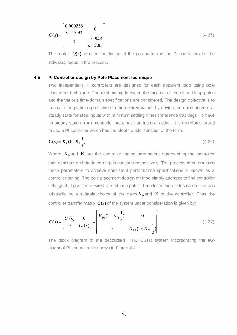
0.009238 013.93( )
0.94302.85
sQ s
s
+=
− −
(4.25)
The matrix ( )Q s is used for design of the parameters of the PI controllers for the
individual loops in the process.
4.5 PI Controller design by Pole Placement technique Two independent PI controllers are designed for each apparent loop using pole
placement technique. The relationship between the location of the closed loop poles
and the various time-domain specifications are considered. The design objective is to
maintain the plant outputs close to the desired values by driving the errors to zero at
steady state for step inputs with minimum settling times (reference tracking). To have
no steady state error a controller must have an integral action. It is therefore natural
to use a PI controller which has the ideal transfer function of the form:
1( ) (1 )P IC s K Ks
= + (4.26)
Where PK and IK are the controller tuning parameters representing the controller
gain constant and the integral gain constant respectively. The process of determining
these parameters to achieve consistent performance specifications is known as a
controller tuning. The pole placement design method simply attempts to find controller
settings that give the desired closed loop poles. The closed loop poles can be chosen
arbitrarily by a suitable choice of the gains PK and IK of the controller. Thus the
controller transfer matrix ( )C s of the system under consideration is given by:
1 11
22 2
1(1 ) 0( ) 0( )
0 ( ) 10 (1 )
P I
P I
K KC s sC sC s K K
s
+ = = +
(4.27)
The block diagram of the decoupled TITO CSTR system incorporating the two
diagonal PI controllers is shown in Figure 4.4.
93

∑ ( )R s ( )Y s+
−
1 1
2 2
10.009238* (1 )0
13.9310.947* (1 )
02.85
P I
P I
K Ks
s
K Ks
s
+
+
− +
−
( )E s
( ) ( )C s Q s
Figure 4.4: Block diagram of the decoupled closed loop system.
From Figure 4.4, the following can be derived.
( ) ( ) ( ) ( ), and ( ) ( ) ( )Y s C s Q s E s E s R s Y s= = − Therefore,
( ) ( ) ( ) ( ) ( ) ( ) ( )Y s C s Q s R s C s Q s Y s= − (4.28)
From Equation (4.28) the expression for the outputs may be written as:
1 1 11 1 1 11 1
2 2 22 2 2 22 2
( ) ( ) ( ) ( ) ( ) ( ) ( )( ) ( ) ( ) ( ) ( ) ( ) ( )
Y s C s Q s R s C s Q s Y sY s C s Q s R s C s Q s Y s
= −= −
(4.29)
Solving for the output 1( )Y s by inserting 11( )Q s and 1( )C s from Equation (4.22) for
11( )Q s and (4.27) for 1( )C s gives:
1 1 11 12
1 1 1
0.009238( )( ) ( )(13.93 0.00923 ) 0.009238
P P I
P P I
K s K KY s R ss s K K K
+=
+ + + (4.30)
Similarly, it can be shown that using Equations (4.24) and (4.27);
2 2 22 22
2 2 2
0.947( )( ) ( )( 2.85 0.947 ) ( 0.947 )
P P I
P P I
K s K KY s R ss s K K K
− +=
+ − − + − (4.31)
Equations (4.30 and (4.31) are the expressions for the outputs from the two separate
non-interacting loops developed with the help of two PI controllers.
4.5.1 PI Controller design for the concentration loop Consider the Equation (4.30) for the concentration control. This closed loop system is
of a second order and its characteristic polynomial equation is: 2
1 1 1(13.93 0.00923 ) 0.009238 0P P Is s K K K+ + + = (4.32)
Thus, the closed loop system poles can be given arbitrary values by choosing the
parameters 1PK and I1K properly. The procedure is to re-parameterize the
characteristic equation to be of the desired standard dimensionless form: 2 22 0n ns sζω ω+ + = (4.33)
94

To achieve this, the relationship between the location of the closed loop poles and the
various time domain specifications are considered. Assuming that the desired poles
are characterised by their relative dampingζ and their frequency nω and identifying
the coefficients of the powers of the variable s in the polynomials (4.32) and (4.33),
the controller parameters can be found as:
1
2
1 1
2 13.930.009328
0.009238
nP
nP I
K
K K
ζω
ω
−=
= (4.34)
where nω and ζ are the un-damped natural frequency and damping factor
respectively. The parameter nω determines the speed of response and ζ determines
the shape of response (damping). It is necessary to specify the values of nω and ζ
The specifications for system’s step response that are often used are the percentage
overshoot and the settling time. If the performance specifications for the
concentration control are such that the settling time should be 0.2 1sT≤ ≤ (minutes)
and an overshoot of 5% 15%pM≤ ≤ and the frequency of oscillation in the step
response 12 /d rad sω ≤ are selected then the poles can be placed in the locations
that ensures good response, hence the controller settings 1PK and I1K can be
calculated with ease. The objective is to determine the region in the s-pane where the
closed loop poles must lie in order to satisfy the performance specifications. Since the
system is under damped, the closed loop poles are complex conjugates, therefore
only the one of the poles is considered. The values for the overshoot and settling time
are related to the damping ratio and the un-damped natural frequency. The overshoot
is controlled by the damping coefficient whereby low overshoot implies high damping
and vice versa.
The relationship between the settling time and the closed loop poles is given by:
1 11
4 4 4, Re[ ] Re[ ]Re[ ]s n s
n s
T p T pp T
ζωζω
= = − ⇒ = ⇔ = (4.35)
Where 1p is one of the closed loop poles. Thus, a settling time specification imposes
a limit on the real part of the complex conjugate closed loop poles. Since there is an
inverse relationship between the settling time and the real part of the pole, that
means that increasing the settling time reduces the absolute value of the real part of
the closed loop pole and vice versa. Imposing the upper and lower limits of the
95

settling time guarantees the position upon which the poles must lie. From the
specifications therefore the constraints on the real part require that the closed loop
poles must be:
max 1
min 1
41 Re[ ] 4
40.2 Re[ ] 20
ss
ss
T pT
T pT
−
−
−= ⇒ = = −
−= ⇒ = = −
(4.36)
Therefore the closed loop poles must lie in the region between 4− and -20 on the real
part of the s-plane. The percentage overshoot is only a function of the damping. The
angle that the closed loop pole makes relative to the negative real axis is also a
function of the damping ratio. For any given percent overshoot, the damping ratio and
the angle can be computed from the formulae (Ogata, K., 1990):
2
-1
2 2
(ln )100% , =cos ( )
(ln )100%
P
P
M
Mζ β ζπ
=+
(4.37)
Where the percentage overshoot is PM and β is the angle in the clockwise direction
from a negative real axis. Thus, from the specifications provided
max
min
15% 0.5169 58.9
5% 0.6901 46.4P
P
MM
ζ β
ζ β
= ⇒ = ⇒ =
= ⇒ = ⇒ =
(4.38)
Thus, for each allowed value of the overshoot, constraints on the damping ratio and
the angle can be imposed. This implies that the constraints on the damping ratio and
the angle are as given by Equation (4.39).
0.6901 0.516946.4 58.9
ζ
β
≥ ≥
≤ ≤ (4.39)
The relationship between the real and the imaginary parts of the closed loop pole is
given by the tangent of the angle and therefore the real and the imaginary parts of 1p
must satisfy the expression:
1
1
Im[ ]tan(46.4 ) 1.0501 1.6577 tan 58.9Re[ ]
pp
= ≤ ≤ =
The damped frequency of oscillation is directly a specification on the imaginary part of
the closed loop pole 1p and the relationship is given by:
211 Im[ ]d n pω ω ζ= − = (4.40)
The final overall requirements on the locations of the closed loop poles are
determined by the consideration that all the constraints specified are satisfied.
Choosing a pole at 8.8 11.8j− + gives the settling time to be 0.453minutes as from
96

equation (4.32). This is within the acceptable specification range. The angle of the
radial line through this pole is 1tan 11.83 / 8.83 53.37− = so that the damping ratio is
0.598ζ = . This yields an overshoot of 9.58% . The next design specification is to
determine nω in order to finish the requirements of the second order system. The
settling time and the frequency of oscillation are related by the equation:
4 0.453sn
Tζω
≈ =
This implies that 14.77 /n rad sω = .
Similarly it can be calculated from 2
21 14.77 /
1d
d n n rad sωω ω ζ ωζ
= − ⇒ = =−
Thus from Equation (4.34) the values of the unknown controller parameters are
calculated as:
1
2 2
11
2 13.93 (2*0.598*14.77) 13.93 4000.009238 0.009238
14.77 58.9780.009238 0.009238*400
nP
nI
P
K
KK
ζω
ω
− −= = =
= = = (4.41)
The flow chart of the procedure for the selection of the poles adopted is illustrated in
Figure 4.5.
97

Concentration control transfer function in terms of the controller parameters
Compare the coefficients of the like powers of s
Start
Desired pole location specification
Closed loop characteristic polynomial
Desired dimensionless characteristic polynomial in terms of natural frequency and damping
Solve to find the relationship between the values of the controller parameters and
time response specifications
End
Simulate the closed loop system for the Concentration tracking control performance
determination
MIMO CSTR decoupled system
YES
YES
NOCheck fulfillment of the closed loop specifications
Figure 4.5: Flow diagram of the summary of the pole selection procedure.
Thus the designed controller settings achieve tracking control of the concentration set
point as depicted by the time domain responses of the Figure 4.8 below.
4.5.2 PI Controller design for the temperature loop Similar procedure is used for the design of the second loop PI controller settings as
described below.
Consider the Equation (4.31) for the temperature control, then the closed loop system
is of second order and its characteristic equation is: 2
2 2 2( 2.85 0.947 ) ( 0.947 ) 0P P Is s K K K+ − − + − = (4.42)
Thus, the closed loop system poles can also be given arbitrary values by choosing
the parameters 2PK and I2K of the second PI controller settings. The procedure
adopted is the same as the one for the concentration control. First is to re-
parameterize the characteristic equation in terms of the desired standard
dimensionless form: 98

2 22 0n ns sζω ω+ + = (4.43)
The relationship between the location of the closed loop poles and the various time
domain specifications are considered. The controller parameters can be found as:
2
2
22
2 2.850.947
0.947
nP
nI
P
K
KK
ζω
ω
+=
−
=−
(4.44)
If the performance specifications for the temperature control are such that the settling
time should be 0.2 1sT≤ ≤ (minutes) and an overshoot of 25% , the poles can be
placed in the arbitrary locations that ensure good temperature tracking and hence the
controller settings 2PK and I2K can be calculated using Equations (4.35-4.37). The
problem is then to determine the region in the s-pane where the closed loop poles
must lie in order to satisfy the performance specifications. With a choice of a settling
time of 0.5minutes which is within the specification range implies that the real part of
the pole must be at:
2 2 20.5 Re[ ] 4 / 4 / 0.5 8s sT p T= ⇒ = − = − = −
For a 25% overshoot, this implies that the damping ratio can be calculated from the
Equation (4.39) as:
22
2 22 2
(ln ) (ln 0.25)100% 0.403(0.25)(ln )
100%
P
P
M
Mζππ
= = =++
(4.45)
The imaginary part of the pole is then calculated from the expression:
112
1
Im[ ]tan( ) cos ( ) tan 66.2 Im[ ] 18.2Re[ ]
p pp
β ζ−= = = ⇒ = (4.46)
Therefore placing the second pole at the point 8.0 18.2j− + ensures the desired
overshoot and the damping ratio are achieved. The next design specification is to
determine nω as:
4 40.5 19.85 /0.403*0.5s n
n
T rad sωζω
≈ = ⇒ = = (4.47)
Thus from Equation (4.44) the values of the unknown controller parameters are
calculated as:
2
2 2
21
2 2.85 (2*0.403*19.85) 2.85 19.90.947 0.947
19.85 20.90.947 0.947*( 19.9)
nP
nI
P
K
KK
ζω
ω
+ += = = −
− −
= = =− − −
(4.48)
99

The flow chart of the procedure for the selection of the poles for the temperature
control is the same as the one given in Figure 4.5. Thus the designed controllers
setting for the proportional gain constant of 2 19.9PK = − and the integral gain constant
of 2 20.9IK = achieve tracking control of the temperature set point.
4.6 Simulated Results Simulation results are used to verify the performance of these control laws. The
Simulink block diagram and time response characteristics of the closed loop MIMO
CSTR designed using dynamic decoupling technique in which the interaction within
the loops are compensated and then two SISO PI controllers are tuned using pole
placement techniques to achieve various set-point tracking for the concentration
control and temperature control are illustrated below.
Figure 4.6: Dynamic decoupling control implemented in Simulink
Figure 4.6 represents the closed loop block diagram of the dynamic decoupling
control scheme of the CSTR process implemented in the Simulink environment.
4.6.1 Concentration loop simulated results The designed controller settings achieve tracking control of the concentration set
point are used to simulate the concentration control loop as depicted by the time
domain response of the Figure 4.7.
100

Figure 4.7: Set-point tracking concentration response.
The set-points for the concentration control is varied from 0.0762 /mol l to0.13 /mol l ,
then from to 0.13 /mol l to 0.1 /mol l with time. Figure 4.8 shows the tracking
characteristics.
4.6.1.1 Investigation of performance for variations in concentration set-point Several other variations in the set-point are investigated to evaluate the time
response performance indices as illustrated by the following figures.
Figure 4.8: response of 0.02 /mol l
Figure 4.9: response of 0.04 /mol l
Figure 4.10: response of 0.06 /mol l
Figure 4.11: response of 0.10 /mol l .
0 0.5 1 1.5 2 2.5 3 3.5 4 4.5 5
0.08
0.09
0.1
0.11
0.12
0.13
0.14
X: 1.26Y: 0.1355
Time [min]
Con
cent
ratio
n[m
ol/L
]
Closed loop response of the nonlinear CSTR process under the dynamic decoupling control
ysp1=0.0762ysp2=0.13ysp3=0.1Mp=10.2%ts=0.311mintr=0.127min
SetpointTracking concentration response
0 0.5 1 1.5 2 2.5 3 3.5 4 4.5 50.01
0.02
0.03
0.04
0.05
0.06
0.07
0.08
0.09
ysp1=0.0762ysp2=0.02ysp3=0.08
X: 0.7Y: 0.01355
Time [min]
Con
cent
ratio
n[m
ol/L
]
Closed loop response of the nonlinear CSTR process under the dynamic decoupling
SetpointTracking concentration response
0 0.5 1 1.5 2 2.5 3 3.5 4 4.5 5
0.04
0.045
0.05
0.055
0.06
0.065
0.07
0.075
0.08
0.085
ysp1=0.0762ysp2=0.04ysp3=0.08
X: 0.7Y: 0.03585
Time [min]
Con
cent
ratio
n[m
ol/L
]
Closed loop response of the nonlinear CSTR process under the dynamic decoupling
SetpointTracking concentration response
0 0.5 1 1.5 2 2.5 3 3.5 4 4.5 50.055
0.06
0.065
0.07
0.075
0.08
0.085
ysp1=0.0762ysp2=0.06ysp3=0.08
X: 0.7Y: 0.05816
Time [min]
Con
cent
ratio
n[m
ol/L
]
Closed loop response of the nonlinear CSTR process under the dynamic decoupling
SetpointTracking concentration response
0 0.5 1 1.5 2 2.5 3 3.5 4 4.5 50.075
0.08
0.085
0.09
0.095
0.1
0.105
ysp1=0.0762ysp2=0.10ysp3=0.08
X: 0.7Y: 0.1028
Time [min]
Con
cent
ratio
n[m
ol/L
]
Closed loop response of the nonlinear CSTR process under the dynamic decoupling
SetpointTracking concentration response
101

Figure 4.12: response of 0.12 /mol l
Figure 4.13: response of 0.14 /mol l .
Table 4.1: Analysis of the different set-points influence over the concentration response performance indicators
Set-point value
Rise time (sec)rt Settling time
(sec)st
Peak over shoot
PM (%)
Steady state error
(%)sse
0.02 Moles/litre. 7.62 27.18 9.58 0 0.04 Moles/litre 7.62 27.18 9.58 0 0.06 Moles/litre 7.62 27.18 9.58 0 0.08 Moles/litre 7.62 27.18 9.58 0 0.1Moles/litre 7.62 27.18 9.58 0 0.12 Moles/litre 7.62 27.18 9.58 0 0.14 Moles/litre 7.62 27.18 9.58 0
Table 4.1 gives the various performance indices for concentration response when the
set-point is varied. The investigation derived is that the indices remains constant
throughout the set-point variations hence this shows that the dynamic decoupling
control design is good irrespective of the set-point variations. Frequency response
analysis using Bode plot is also investigated for the decoupled concentration control
performance. This is illustrated in Figure 4.14.
Figure 4.14 Frequency response analyses for the concentration control
0 0.5 1 1.5 2 2.5 3 3.5 4 4.5 5
0.08
0.09
0.1
0.11
0.12
0.13
ysp1=0.0762ysp2=0.12ysp3=0.08
X: 0.7Y: 0.1251
Time [min]
Con
cent
ratio
n[m
ol/L
]
Closed loop response of the nonlinear CSTR process under the dynamic decoupling
SetpointTracking concentration response
0 0.5 1 1.5 2 2.5 3 3.5 4 4.5 5
0.08
0.09
0.1
0.11
0.12
0.13
0.14
0.15
0.16
ysp1=0.0762ysp2=0.14ysp3=0.08
X: 0.7Y: 0.1474
Time [min]
Con
cent
ratio
n[m
ol/L
]
Closed loop response of the nonlinear CSTR process under the dynamic decoupling
SetpointTracking concentration response
102

The figure shows the open loop gain and the open loop phase plots for the decoupled
concentration control system. The closed loop gain margin is infinity and the phase
margin indicated is 60 degrees implying that the closed loop concentration control
system is stable.
4.6.1.2 Investigation of the process performance for disturbances in the concentration control loop Similarly, the effects of disturbances are investigated. The disturbances are injected
to the concentration output as well as to the control input as illustrated in the Simulink
block of Figure 4.15.
Figure 4.15 Dynamic decoupling controls subject to disturbances at the output 1( )y
and the interaction junction 1( )u
Figure 4.16: Response under
31 mol/le− noise
Figure 4.17: Response under
34 mol/le− noise
0 0.5 1 1.5 2 2.5 3 3.5 4 4.5 5
0.08
0.09
0.1
0.11
0.12
0.13
0.14
ysp1=0.0762ysp2=0.13ysp3=0.10noise of +/-1e-3 mol/L
X: 0.7Y: 0.136
Time [min]
Con
cent
ratio
n[m
ol/L
]
Closed loop response of the nonlinear CSTR process under the dynamic decoupling c
SetpointTracking concentration response with noise on y1
0 0.5 1 1.5 2 2.5 3 3.5 4 4.5 5
0.08
0.09
0.1
0.11
0.12
0.13
0.14
Time [min]
Con
cent
ratio
n[m
ol/L
]
Closed loop response of the nonlinear CSTR process under the dynamic decoupling control
ysp1=0.0762ysp2=0.13ysp3=0.10noise of +/-4e-3 mol/L
SetpointTracking concentration response with noise on y1
103
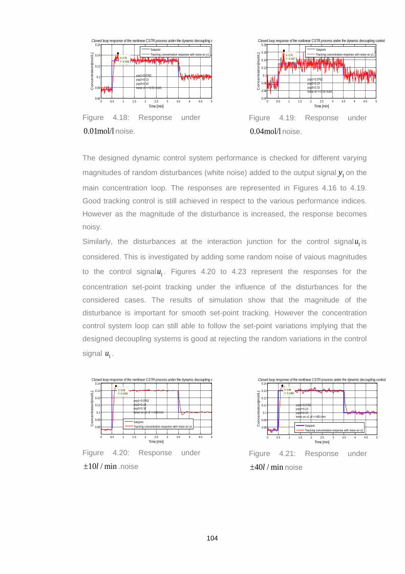
Figure 4.18: Response under
0.01mol/l noise.
Figure 4.19: Response under
0.04mol/l noise.
The designed dynamic control system performance is checked for different varying
magnitudes of random disturbances (white noise) added to the output signal 1y on the
main concentration loop. The responses are represented in Figures 4.16 to 4.19.
Good tracking control is still achieved in respect to the various performance indices.
However as the magnitude of the disturbance is increased, the response becomes
noisy.
Similarly, the disturbances at the interaction junction for the control signal 1u is
considered. This is investigated by adding some random noise of vaious magnitudes
to the control signal 1u . Figures 4.20 to 4.23 represent the responses for the
concentration set-point tracking under the influence of the disturbances for the
considered cases. The results of simulation show that the magnitude of the
disturbance is important for smooth set-point tracking. However the concentration
control system loop can still able to follow the set-point variations implying that the
designed decoupling systems is good at rejecting the random variations in the control
signal 1u .
Figure 4.20: Response under
10 / minl± .noise
Figure 4.21: Response under
40 / minl± noise
0 0.5 1 1.5 2 2.5 3 3.5 4 4.5 50.06
0.08
0.1
0.12
0.14
0.16
ysp1=0.0762ysp2=0.13ysp3=0.10noise of +/-0.01 mol/L
X: 0.76Y: 0.1431
Time [min]
Co
nce
ntr
atio
n[m
ol/L
]
Closed loop response of the nonlinear CSTR process under the dynamic decoupling c
SetpointTracking concentration response with noise on y1
0 0.5 1 1.5 2 2.5 3 3.5 4 4.5 50.04
0.06
0.08
0.1
0.12
0.14
0.16
0.18
ysp1=0.0762ysp2=0.13ysp3=0.10noise of +/-0.04 mol/L
X: 0.76Y: 0.1637
Time [min]
Co
nce
ntr
atio
n[m
ol/L
]
Closed loop response of the nonlinear CSTR process under the dynamic decoupling control
SetpointTracking concentration response with noise on y1
0 0.5 1 1.5 2 2.5 3 3.5 4 4.5 5
0.08
0.09
0.1
0.11
0.12
0.13
0.14
X: 0.68Y: 0.1363
Time [min]
Con
cent
ratio
n[m
ol/L
]
Closed loop response of the nonlinear CSTR process under the dynamic decoupling c
ysp1=0.0762ysp2=0.13ysp3=0.10noise on u1 of +/-10L/min
SetpointTracking concentration response with noise on u1
0 0.5 1 1.5 2 2.5 3 3.5 4 4.5 5
0.08
0.09
0.1
0.11
0.12
0.13
0.14
X: 0.68Y: 0.1369
Time [min]
Co
nce
ntr
atio
n[m
ol/L
]
Closed loop response of the nonlinear CSTR process under the dynamic decoupling control
ysp1=0.0762ysp2=0.13ysp3=0.10noise on u1 of +/-40L/min
SetpointTracking concentration response with noise on u1
104

Figure 4.22: Response under
80 / minl± .noise.
Figure 4.23: Response under
100 / minl± noise.
Similarly, the performances of the temperature control loop signal 2y when the
disturbances are in 1y and 1u are investigated. This is important because of the
interactions that exist in the closed loop system. Figures 4.24-4.27 are the graphs for
the responses of the temperature control loop signal 2y when there are disturbances
on 1y of different magnitudes.
Figure 4.24: Temperature response
under 31 mol/le−± .noise on 1y
Figure 4.25: Temperature response
under 34 mol/le−± .noise on 1y .
Figure 4.26: Temperature response
under 0.01mol/l± .noise on 1y .
Figure 4.27: Temperature response
under 0.04mol/l± .noise on 1y .
The results from Figures 4.24-4.27 show that there is very little influence of the
disturbance effect on 1y to the temperature control loop signal 2y . This implies that the
decoupling control design is good. Next, the investigation on the influence of the
0 0.5 1 1.5 2 2.5 3 3.5 4 4.5 50.06
0.08
0.1
0.12
0.14
0.16
ysp1=0.0762ysp2=0.13ysp3=0.10noise on u1 of +/-80L/min
X: 0.66Y: 0.1405
Time [min]
Co
nce
ntr
atio
n[m
ol/L
]
Closed loop response of the nonlinear CSTR process under the dynamic decoupling co
SetpointTracking concentration response with noise on u1
0 0.5 1 1.5 2 2.5 3 3.5 4 4.5 50.06
0.08
0.1
0.12
0.14
0.16
X: 0.66Y: 0.1428
Time [min]
Co
nce
ntr
atio
n[m
ol/L
]
Closed loop response of the nonlinear CSTR process under the dynamic decoupling control
ysp1=0.0762ysp2=0.13ysp3=0.10noise on u1 of +/-100L/min
SetpointTracking concentration response with noise on u1
0 0.5 1 1.5 2 2.5 3 3.5 4 4.5 5440
445
450
455
460
ysp1=445ysp2=455ysp3=445noise of +/-1e-3 mol/L on y1
X: 0.62Y: 459.1
Time [min]
Tem
pera
ture
[K]
Closed loop response of the nonlinear CSTR process under the dynamic decoupling co
SetpointTracking temperature response with noise on y1
0 0.5 1 1.5 2 2.5 3 3.5 4 4.5 5440
445
450
455
460
Time [min]
Te
mp
era
ture
[K]
Closed loop response of the nonlinear CSTR process under the dynamic decoupling co
ysp1=445ysp2=455ysp3=445noise of +/-4e-3 mol/L on y1
SetpointTracking temperature response with noise on y1
0 0.5 1 1.5 2 2.5 3 3.5 4 4.5 5440
445
450
455
460
Time [min]
Tem
pera
ture
[K]
Closed loop response of the nonlinear CSTR process under the dynamic decoupling control
ysp1=445ysp2=455ysp3=445noise of +/-0.01 mol/L on y1
SetpointTracking temperature response with noise on y1
0 0.5 1 1.5 2 2.5 3 3.5 4 4.5 5440
445
450
455
460
ysp1=445ysp2=455ysp3=445noise of +/-0.04 mol/L on y1
X: 0.63Y: 459
Time [min]
Tem
pera
ture
[K]
Closed loop response of the nonlinear CSTR process under the dynamic decoupling control
SetpointTracking temperature response with noise on y1
105

effect of disturbance on 1u to the temperature control loop signal 2y .is done. Figures
4.28-4.31 are the graphs of the responses of the temperature control loop signal 2y
when there are disturbances of different magnitudes on 1u .
Figure 4.28: Temperature response
under 10 / minl± .noise on 1u
Figure 4.29: Temperature response
under 40 / minl± .noise on 1u
Figure 4.30: Temperature response
under 80 / minl± .noise on 1u
Figure 4.31: Temperature response
under 100 / minl± noise on 1u
From these responses of Figures 4.28-4.31, it can be seen that as the magnitude of
the disturbance 1u increase, the response on 2y becomes noisy. This implies that
there are still some elements of interactions in the system.
4.6.2 Investigation of the process performance in the temperature control loop Similarly, simulation to investigate the process performance in the temperature
control loop is performed. The same procedure adopted for the concentration control
is used. First, the control algorithm derived earlier is used to simulate the temperature
control loop for set-point tracking. Figure 4.32 presents the result of simulation
0 0.5 1 1.5 2 2.5 3 3.5 4 4.5 5440
445
450
455
460
ysp1=445ysp2=455noise on u1 of +/-10l/min
X: 0.61Y: 458.9
Time [min]
Te
mp
era
ture
[K]
Closed loop response of the nonlinear CSTR process under the dynamic decoupling con
SetpointTracking temperature response with noise on u1
0 0.5 1 1.5 2 2.5 3 3.5 4 4.5 5440
445
450
455
460
ysp1=445ysp2=455noise on u1 of +/-40l/min
X: 0.63Y: 458.8
Time [min]
Te
mp
era
ture
[K]
Closed loop response of the nonlinear CSTR process under the dynamic decoupling c
SetpointTracking temperature response with noise on u1
0 0.5 1 1.5 2 2.5 3 3.5 4 4.5 5435
440
445
450
455
460
X: 0.65Y: 458.6
Time [min]
Te
mp
era
ture
[K]
Closed loop response of the nonlinear CSTR process under the dynamic decoupling control
ysp1=445ysp2=455noise on u1 of +/-80l/min
SetpointTracking temperature response with noise on u1
0 0.5 1 1.5 2 2.5 3 3.5 4 4.5 5435
440
445
450
455
460
X: 0.65Y: 458.7
Time [min]
Te
mp
era
ture
[K]
Closed loop response of the nonlinear CSTR process under the dynamic decoupling control
ysp1=445ysp2=455noise on u1 of +/-100l/min
SetpointTracking temperature response with noise on u1
106

Figure 4.32: Set-point tracking temperature response
The set-points for the temperature control loop is varied from 444.7K to 460K , then
from 460K to 444.7K with time. A part from high percentage overshoot, the other
performance indices are good, hence successful temperature set-point tracking is
achieved with this control law. Several other variations in set-points are investigated
to calculate the changes in the time response performance indices as illustrated by
the following Figures 4.33 to 4.38.
4.6.2.1 Investigation of the process performance for variations in the temperature set-point
The variation of set-points magnitude influence over the temperature response
performance indices is investigated. This is varied when the concentration loop’s set
point is maintained at 0.0762 /mol l to 0.13 /mol l , then from to 0.13 /mol l to
0.1 /mol l with time.
Figure 4.33: Temperature set-point
tracking at 465K .
Figure 4.34: Temperature set-point
tracking at 460K .
0 0.5 1 1.5 2 2.5 3 3.5 4 4.5 5440
445
450
455
460
X: 0.63Y: 459
Time [min]
Tem
pera
ture
[K]
Closed loop response of the nonlinear CSTR process under the dynamic decoupling control
ysp1=444.7ysp2=455
SetpointSet-point tracking temperature response
0 0.5 1 1.5 2 2.5 3 3.5 4 4.5 5435
440
445
450
455
460
465
470
475
ysp1=444.7ysp2=465
X: 0.63Y: 473
Time [min]
Tem
pera
ture
[K]
Closed loop response of the nonlinear CSTR process under the dynamic decoupling co
SetpointSet-point tracking temperature response
0 0.5 1 1.5 2 2.5 3 3.5 4 4.5 5435
440
445
450
455
460
465
470
ysp1=444.7ysp2=460
X: 0.63Y: 466
Time [min]
Tem
pera
ture
[K]
Closed loop response of the nonlinear CSTR process under the dynamic decoupling control
SetpointTracking temperature response
107

Figure 4.35: Temperature set-point
tracking at 450K .
Figure 4.36: Temperature set-point
tracking at 446K .
Figure 4.37: Temperature set-point
tracking at 440K .
Figure 4.38: Temperature set-point
tracking at 435K
The results show that a part from high percentage overshoots; the other performance
indices are good, hence successful temperature set-point tracking is achieved with
this control law.
Table 4.2: Analysis of the different set-points influence over the temperature response performance indicators.
Set-point value
Rise time (sec)rt Settling time
(sec)st
Peak over shoot
PM (%)
Steady state error
(%)sse
435K. 2.79 30 28.2 0 440K 2.79 30 28.2 0 446K 2.79 30 28.2 0 450K 2.79 30 28.2 0 455K 2.79 30 28.2 0 460K 2.79 30 28.2 0 465K 2.79 30 28.2 0
The investigation shows that the performance indices such as rise time, settling time
peak overshoot, steady state error remains the same no matter the value of set-point.
This further shows that the dynamic decoupling control design for the temperature
loop is good irrespective of the set-point value.
4.6.2.2 Investigation of the process performance for disturbances in the temperature control loop
Next, the effects of disturbances are investigated for the temperature control loop. The
procedure adopted is the same as that for the concentration control loop. The disturbances
0 0.5 1 1.5 2 2.5 3 3.5 4 4.5 5442
444
446
448
450
452
454
ysp1=444.7ysp2=450
X: 0.63Y: 452
Time [min]
Tem
pera
ture
[K]
Closed loop response of the nonlinear CSTR process under the dynamic decoupling co
SetpointTracking temperature response
0 0.5 1 1.5 2 2.5 3 3.5 4 4.5 5444
444.5
445
445.5
446
446.5
ysp1=444.7ysp2=446
X: 0.63Y: 446.4
Time [min]
Tem
pera
ture
[K]
Closed loop response of the nonlinear CSTR process under the dynamic decoupling co
SetpointTracking temperature response
0 0.5 1 1.5 2 2.5 3 3.5 4 4.5 5436
438
440
442
444
446
448
ysp1=444.7ysp2=440
X: 0.63Y: 438
Time [min]
Tem
pera
ture
[K]
Closed loop response of the nonlinear CSTR process under the dynamic decoupling control
SetpointTracking temperature response
0 0.5 1 1.5 2 2.5 3 3.5 4 4.5 5430
435
440
445
450
ysp1=444.7ysp2=435
X: 0.63Y: 431
Time [min]
Tem
pera
ture
[K]
Closed loop response of the nonlinear CSTR process under the dynamic decoupling control
SetpointTracking temperature response
108

are injected to the main temperature control loop at the output 2y as well as to the control
inputs 2u . The effects of the disturbances at 2y are as illustrated on the responses as
represented in Figures 4.39 to 4.42 for the main temperature control loop and at 2u in
Figures 4.43 to 4.46 for the control input 2u .
Figure 4.39: Temperature response
under 4K± .noise.
Figure 4.40: Temperature response
under 8K± noise
Figure 4.41: Temperature response
under 10K± noise
Figure 4.42: Temperature response
under 20K± noise
The results of simulation shows that the magnitudes of the disturbance is important
for smooth set-point tracking. However the temperature control system can still track
the set-point variations implying that the designed decoupling systems is good.
Similarly, the disturbances at the interaction junction for the control signal 2u is
considered. The is investigation is done by adding some random noise of various
magnitudes to the control signal 2u . Figures 4.43 to 4.46 represent the responses for
the temperature set-point tracking under the disturbances for the considered cases.
The results of simulation shows that the effects of this kind of the disturbance does
not quite affect the set-point tracking. The temperature control system can still track
the set-point variations implying that the designed decoupling systems is good at
rejecting the random variations in the control signal 2u .although the responses
become noisy as the magnitude of this disturbance is increased
0 0.5 1 1.5 2 2.5 3 3.5 4 4.5 5435
440
445
450
455
460
465
ysp1=444.7ysp2=455noise +/- 4K
X: 0.61Y: 460.7
Time [min]
Tem
pera
ture
[K]
Closed loop response of the nonlinear CSTR process under the dynamic decoupling co
SetpointTracking temperature response with noise
0 0.5 1 1.5 2 2.5 3 3.5 4 4.5 5435
440
445
450
455
460
465
ysp1=444.7ysp2=455noise +/- 8K
X: 0.61Y: 462.8
Time [min]
Tem
pera
ture
[K]
Closed loop response of the nonlinear CSTR process under the dynamic decoupling co
SetpointTracking temperature response with noise
0 0.5 1 1.5 2 2.5 3 3.5 4 4.5 5435
440
445
450
455
460
465
470
ysp1=444.7ysp2=455noise +/- 10K
X: 0.61Y: 464.4
Time [min]
Tem
pera
ture
[K]
Closed loop response of the nonlinear CSTR process under the dynamic decoupling control
SetpointTracking temperature response with noise
0 0.5 1 1.5 2 2.5 3 3.5 4 4.5 5430
435
440
445
450
455
460
465
470
475
ysp1=444.7ysp2=455noise +/- 20K
X: 0.61Y: 466.6
Time [min]
Tem
pera
ture
[K]
Closed loop response of the nonlinear CSTR process under the dynamic decoupling control
SetpointTracking temperature response with noise
109

Figure 4.43: Temperature response
under 10 / minl± noise on 2u .
Figure 4.44: Temperature response
under 40 / minl± noise on 2u
Figure 4.45: Temperature response
under 80 / minl± noise on 2u .
Figure 4.46: Temperature response
under 100 / minl± noise on 2u
4.6.2.3 Investigation of the process performance in the concentration loop for disturbances in the temperature control loop
Lastly, the behaviour of the concentration loop when the set-point is changing in 2y is
investigated. The graphs of this case are illustrated below. Lastly, the behaviour of
the concentration loop when there are disturbances on 2y and the control signal 2u .is
investigated.
Figure 4.47: Concentration response
under 4K± noise on 2y .
Figure 4.48: Concentration response
under 8K± noise on 2y
0 0.5 1 1.5 2 2.5 3 3.5 4 4.5 5440
445
450
455
460
ysp1=444.7ysp2=455noise +/-10l/min
X: 0.62Y: 458.9
Time [min]
Tem
pera
ture
[K]
Closed loop response of the nonlinear CSTR process under the dynamic decoupling co
SetpointTracking temperature response with noise
0 0.5 1 1.5 2 2.5 3 3.5 4 4.5 5435
440
445
450
455
460
ysp1=444.7ysp2=455noise +/-40l/min
X: 0.61Y: 458.4
Time [min]
Tem
pera
ture
[K]
Closed loop response of the nonlinear CSTR process under the dynamic decoupling c
SetpointTracking temperature response with noise
0 0.5 1 1.5 2 2.5 3 3.5 4 4.5 5435
440
445
450
455
460
ysp1=444.7ysp2=455noise +/-80l/min
X: 0.61Y: 458.4
Time [min]
Tem
pera
ture
[K]
Closed loop response of the nonlinear CSTR process under the dynamic decoupling control
SetpointTracking temperature response with noise
0 0.5 1 1.5 2 2.5 3 3.5 4 4.5 5435
440
445
450
455
460
ysp1=444.7ysp2=455noise +/-100l/min
X: 0.61Y: 458.2
Time [min]
Tem
pera
ture
[K]
Closed loop response of the nonlinear CSTR process under the dynamic decoupling control
SetpointTracking temperature response with noise
0 0.5 1 1.5 2 2.5 3 3.5 4 4.5 5
0.08
0.09
0.1
0.11
0.12
0.13
0.14
X: 0.7Y: 0.1362
Time [min]
Co
nce
ntr
atio
n[m
ol/L
]
Closed loop response of the nonlinear CSTR process under the dynamic decoupling contr
ysp1=0.0762ysp2=0.13ysp3=0.10noise on y2 of +/-4K
SetpointTracking concentration response with noise on y2
0 0.5 1 1.5 2 2.5 3 3.5 4 4.5 5
0.08
0.09
0.1
0.11
0.12
0.13
0.14
X: 0.7Y: 0.1362
Time [min]
Co
nce
ntr
atio
n[m
ol/L
]
Closed loop response of the nonlinear CSTR process under the dynamic decoupling control
ysp1=0.0762ysp2=0.13ysp3=0.10noise on y2 of +/-8K
SetpointTracking concentration response with noise on y2
110

Figure 4.49: Concentration response
under 10K± noise on 2y .
Figure 4.50: Concentration response
under 20K± noise on 2y
The graphs of these cases are illustrated in the following. Figures 4.47 to 4.50 are the
concentration behaviour for changes in 2y . Investigation is done on the responses of
Figures 4.47 to 4.50 shows the influences of the disturbances on 2y to the
concentration performance 1y for the considered cases
Figure 4.51: Concentration
response under 10 / minl± noise on
2u .
Figure 4.52: Concentration
response under 40 / minl± noise on
2u
Figure 4.53: Concentration
response under 80 / minl± noise on
2u .
Figure 4.54: Concentration
response under 100 / minl± noise
on 2u
0 0.5 1 1.5 2 2.5 3 3.5 4 4.5 5
0.08
0.09
0.1
0.11
0.12
0.13
0.14
ysp1=0.0762ysp2=0.13ysp3=0.10noise on y2 of +/-10K
X: 0.7Y: 0.1362
Time [min]
Co
nce
ntr
atio
n[m
ol/L
]
Closed loop response of the nonlinear CSTR process under the dynamic decoupling contro
SetpointTracking concentration response with noise on y2
0 0.5 1 1.5 2 2.5 3 3.5 4 4.5 5
0.08
0.09
0.1
0.11
0.12
0.13
0.14
X: 0.7Y: 0.1362
Time [min]
Co
nce
ntr
atio
n[m
ol/L
]
Closed loop response of the nonlinear CSTR process under the dynamic decoupling control
ysp1=0.0762ysp2=0.13ysp3=0.10noise on y2 of +/-20K
SetpointTracking concentration response with noise on y2
0 0.5 1 1.5 2 2.5 3 3.5 4 4.5 5
0.08
0.09
0.1
0.11
0.12
0.13
0.14
X: 0.7Y: 0.1363
Time [min]
Co
nce
ntr
atio
n[m
ol/L
]
Closed loop response of the nonlinear CSTR process under the dynamic decoupling co
ysp1=0.0762ysp2=0.13ysp3=0.10noise on u2 of +/-10L/min
SetpointTracking concentration response with noise on u2
0 0.5 1 1.5 2 2.5 3 3.5 4 4.5 5
0.08
0.09
0.1
0.11
0.12
0.13
0.14
X: 0.7Y: 0.1365
Time [min]
Co
nce
ntr
atio
n[m
ol/L
]
Closed loop response of the nonlinear CSTR process under the dynamic decoupling cont
ysp1=0.0762ysp2=0.13ysp3=0.10noise on u2 of +/-40L/min
SetpointTracking concentration response with noise on u2
0 0.5 1 1.5 2 2.5 3 3.5 4 4.5 5
0.08
0.09
0.1
0.11
0.12
0.13
0.14
X: 0.7Y: 0.1368
Time [min]
Co
nce
ntr
atio
n[m
ol/L
]
Closed loop response of the nonlinear CSTR process under the dynamic decoupling control
ysp1=0.0762ysp2=0.13ysp3=0.10noise on u2 of +/-80L/min
SetpointTracking concentration response with noise on u2
0 0.5 1 1.5 2 2.5 3 3.5 4 4.5 5
0.08
0.09
0.1
0.11
0.12
0.13
0.14
ysp1=0.0762ysp2=0.13ysp3=0.10noise on u2 of +/-100L/min
X: 0.7Y: 0.1371
Time [min]
Co
nce
ntr
atio
n[m
ol/L
]
Closed loop response of the nonlinear CSTR process under the dynamic decoupling control
SetpointTracking concentration response with noise on u2
111

It is shown that the responses on 1y do not change. This measured by changing the
magnitude of the disturbance on 2y and then monitoring the responses of 1y .
Therefore this confirms that the decoupling control design is good. Next, the
disturbance effect on 1y when noise is added on the control signal 2u is investigated.
Figures 4.51 to 4.54 are the concentration behaviour for changes in control signal 2u
Figures 4.51 to 4.54 represent the responses for the concentration set-point tracking
under the disturbances for the considered cases. The results from the simulation
shows that the effects of this kind of the disturbance does not quite affect the set-
point tracking performance of the concentration loop. The concentration control
system can still track the set-point variations implying that the designed decoupling
systems is good at rejecting the random variations in the control signal 2u although
the responses become sluggish as the magnitude of this disturbance is increased.
Appendix D provides The file that simulates the dynamic decoupling control
response of the closed loop MIMO CSTR model for various magnitudes of the set-
point step changes, as well as disturbances at the outputs (y1),y(2) and the
interaction junctions (u1) and (u2). The Simulink closed loop model to be simulated is
dyn_dec_2015 and is presented in appendix F.
4.6.3 Discussion of the Results Simulation results are used to verify the performance of the control laws to find
whether the effective set-point tracking control and disturbance effect minimisation for
the output variables can be achieved. The concentration closed loop simulation study
is first investigated for set-point tracking capability. This is done by varying the set-
points for the concentration from 0.0762 /mol l to 0.13 /mol l , and then from
to 0.13 /mol l to 0.1 /mol l with time and the responses verified the set-point tracking
capability of the designed control scheme. Several other variations in set-points are
investigated for the time response performance indices as documented in this
chapter. Good tracking control is still achieved.
Similarly, the effects of disturbances are investigated. The process performance is
analysed for different varying magnitudes of random disturbances (white noise)
added to the main concentration control loop. Good tracking control is still achieved.
However as the magnitude of the disturbance is increased, the concentration step
response becomes noisy. Similarly, the influence of the disturbances at the
interactions point is considered. This is investigated by adding some some random
noise of vaious magnitudes to the control signal. The responses for the concentration
112

set-point tracking with these disturbances for the considered cases show that the
magnitude of the disturbance is important for smooth set-point tracking. However the
concentration control system is still able to track the set-point variations implying that
the designed decoupling systems is good at rejecting the random variations.
Similarly, the performances of the temperature control loop signal 2y when the
disturbances are in 1y and 1u are investigated. This is important because of the
interactions that exist in the closed loop system. The results show that there is very
little influence of the disturbance effect on 1y to the temperature control loop signal 2y .
This implies that the decoupling control design is good. Next, the investigation on the
influence of the effect of disturbance on 1u to the temperature control loop signal 2y .is
also done. It is found that as the magnitude of the disturbance 1u increase, the
response on 2y becomes sluggish and noisy. This implies that there are still some
elements of interactions in the system.
The next simulation investigation performed is on the control performance on the
temperature control loop. The same procedure adopted for the concentration control
is used. First, the control algorithm derived earlier is used to simulate the temperature
control loop for set-point tracking. The set-point is varied from 444.7K to 455K , then
from 445K to 444.7K with time. A part from the high percentage overshoot, the other
performance indices are good, hence successful temperature set-point tracking is
achieved with this control law. Several other variations in set-points are investigated
too. Then, the effects of disturbances are investigated for the temperature control
loop. The procedure adopted is the same as that for the concentration control loop.
The results of simulation shows that the magnitudes of the disturbance is important
for smooth set-point tracking. However the temperature control system is able to track
the set-point variations in the presence of the noise disturbances implying that the
designed decoupling systems is good.
Analysis is done if the behaviour of one loop influences the behaviour of the other
loop. If not influenced then the designed decoupling control is good. This is on the
basis of introducing disturbances in one of the loops and simulating the whole system
to see if the behaviour of the other loop changes. The results of the analyses show
that this kind of decoupling control design is good.
4.7 Conclusion
Difficulties caused by the interacting loops for the MIMO systems are the major
obstacle to the design of controllers for such systems. Interactions occur when there 113

are coupling between the control variables and between the process variables
thereby affecting the states of the controlled variables. To address the problem of
loop interactions in the 2 2x MIMO CSTR process under study at one of the operating
point, a simple dynamic decoupling mechanism is designed to compensate for the
loop interactions. After this two SISO PI controllers for the resulting decoupled system
are designed directly and independently using pole placement technique to tune the
individual loops for tracking control of the output variables namely, the reactor
concentration and the reactor temperature. The results of simulation studies show
that the dynamic decoupling control scheme together with the SISO PI control
algorithms are capable of achieving effective set-point tracking control in the
presence of noise disturbances, implying that the designed decoupling systems is
good.
In the following chapter, decentralized controller design method is presented for the
2 2x MIMO CSTR process under study. In order to design decentralized diagonal
controllers, input output pairing is performed based on the Relative Gain Array (RGA)
technique, and then Internal Model Control PID controller tuning is developed.
114

CHAPTER FIVE DECENTRALIZED CONTROLLER DESIGN FOR THE CSTR
5.1 Introduction
In this chapter, the design of a decentralized controller for the linearized 2 2x MIMO
CSTR model at the given operating point is presented. The decentralized controller
design is based on the judicious choice of single loop parings that reduces the effects
of process interactions based on the Relative Gain Array (RGA) method proposed by
(Bristol, 1966), and on the Inverse model based (IMC) PID controller tuning of the
individual paired diagonal loops. The preliminary theory of the method is presented,
and then the details of the design procedure are described. The closed loop system is
tested by simulation in the Matlab/Simulink environment in terms of the performance
specifications to show the suitability of the control strategy.
The chapter is organized as follows: In section 5.2 the approach of the decentralized
control design is presented with the motivation for the need of the control. Section 4.3
presents the derivation procedure for the RGA for the linearized 2 2x MIMO CSTR
model. Section 4.4 applies the general theory of the Inverse Model Control (IMC)
adopted for the linear PID control design. In section 4.5, the IMC-based feedback PID
controller design is presented. Section 4.6 presents the simulation of the closed loop
system. Section 4.7 discusses the obtained results from the simulation, and finally
section 4.8 gives the conclusion of the chapter.
5.2 Decentralized control approach
In spite of the advancement in the controller design methodologies for the
multivariable processes, the decentralized controllers are still popular in chemical
industries because of: the ease to which the technique is implemented, the simplicity
of operation, and easiness in the controller parameters tuning. Decentralized control
of multivariable plants is based on suitable decomposition of the control system into
single input single output (SISO) control loops. The main obstacle to decentralize the
control design for MIMO systems is the interactions that exist between the control
loops. Controller design is based on two steps; judicious choice of single loop
parings, and the controller tuning in the individual paired loops. For the design of
decentralized controllers, input-output pairing of the variables is performed based on
the Relative Gain Array (RGA) method proposed by (Bristol, 1966). The method
provides two types of useful information for the multivariable controller design; the
measure of the process interactions and the recommendations about the best pairing
such that the effects of the interactions are reduced. The method however requires
115

knowledge of the steady state gains, but not the process dynamics. The main idea
around RGA is to assess the effect of the interactions if a controller is designed for
each output variable on a specific input variable. It determines how the controlled and
the manipulated variables should be coupled to yield control loops with minimal
interactions. It is a matrix of the gains which measures the steady state effects of
coupling. The RGA method is defined and explained in the following subsection:
5.3 The Relative Gain Array (RGA) For an nxn process, each component in the RGA matrix is the fraction of the open
loop gain of the particular loop in the case with all other loops opened, to the closed
loop gain of that loop with all other loops closed. Mathematically each element in the
matrix is described by Equation (5.1) as:
ij
open-loop gain between and λ
closed-loop gain between and
( / )
( / )
; 1, and 1,
i j
i j
i j
i j
u
y
y u
y u
y u
y u
i N j N=
∂ ∂=
∂ ∂
= =
(5.1)
where N is the number of the loops in the process. The subscript u denotes constant
values for all control variables except ju (i.e., all loops open), while subscript y
indicates that all outputs except iy are kept constant by the control loops (i.e., all loops
are closed). i jλ is a dimensionless quantity. The relative-gain array matrix is then
given by:
11 12 1
21 22 2
1 2
....
...... .. .... ..
....
N
N
N N NN
λ λ λ
λ λ λ
λ λ λ
Λ =
(5.2)
Entries of Λ satisfy the following two properties:
1
1 for 1, 2,......,N
iji
j Nλ=
= =∑ Summation in a column
1
1 for 1, 2,......,N
ijj
i Nλ=
= =∑ Summation in a row
For the considered 2 2x process, the matrix transfer function is of the process is of the
form:
11 12
21 22
( ) ( )( )
( ) ( )G s G s
G sG s G s
=
(5.3)
Under steady state conditions Equation (5.3) is called the steady state process gain
matrix as:
116

11 12 11 12
21 22 21 22
(0) (0)(0)
(0) (0)G G K K
GG G K K
= =
(5.4)
The RGA of the steady state gain matrix (0)G , (Skogestad and Postlethwaite, 2005)
is then defined as:
11 12 1
21 22
(0).* ( (0) )TG Gλ λ
λ λ−Λ = =
(5.5)
Where 1( (0) )TG − is the transpose of 1(0)G − . The operator '* ' in Equation (5.5) denotes
element by element multiplication.
The corresponding relative-gains can be computed as follows
11 12 11 11
21 22 11 11
1
1
λ λ λ λ
λ λ λ λ
−=
−Λ
=
Where, 11 2211 22 12 11 21
12 21 11 22 12 21
11 22
1, 1
1
K KK K K K K KK K
λ λ λ λ λ= = = − =−−
=
With regards to the steady state gains, the RGA matrix is obtained as:
11 22 12 21
11 22 12 21 11 22 12 22
21 12 11 22
11 22 12 21 11 22 12 21
K K K K
K K K K K K K K
K K K K
K K K K K K K K
−
− −=
−
− −
Λ
(5.6)
The recommended parings corresponds to the , 1, and 1,ij i N j Nλ = = which have the
largest positive values that are closest to one. The RGA element of one indicates that
for this pairing, the other control loops do not affect the current one and this is thus
the ideal pairing. A RGA element of 0 means that the corresponding input does not
affect the output directly at all. Pairings which correspond to values of ijλ which are
negative should not be chosen. Thus, for the 2 2x CSTR model under consideration
where the manipulated variables are the process feed flow rate and process coolant
flow rate respectively, while the controlled variables are the reactor concentration and
the reactor temperature, the steady state gain matrix is:
0.0015 0.0027(0)
0.6063 0.7457G
−=
−
, and evaluating its RGA yields
2.2577 3.25773.2577 2.2577−
Λ =−
(5.7)
Given that loops are not be formed with relative gains which are negative to ensure
closed loop stability, this implies that a perfect pairing for independent single loops
117

should be 1 2y u− and 2 1-y u for the purposes of the decentralized control. This means
that the pairing should be such that:
1 12 11 2
2 22 21 1
( ) ( ) ( ) ( )( ) ( ) ( ) ( )
Y s G s G s U sY s G s G s U s
=
(5.8)
The steady state input-output relation for the recommended pairing should then be:
1 2
2 1
(0) ( )0.0027 0.0015(0) ( )0.7454 0.6063
Y U sY U s
− = −
(5.9)
The RGA pairing rule does not consider the stability of the resulting control structure.
Therefore, it is necessary to check the resulting control structure stability and which is
done according to the Niederlinski index (Niederlinski, 1971). The Niederlinski Index
is calculated from the full gain matrix of the steady-state and is defined as:
(0)(0)ii
i
GNI
G=∏
Here (0)G implies the determinant of the full gain matrix of the steady-state and
11 22(0) (0) (0)iii
G G G=∏
[(0.00270)(6063)] [( 0.7454)( 0.0015)] 0.3169(0.0027)(0.6063)
NI − − −= = (5.10)
Since 0NI for the recommended pairing, the multivariable decentralized control
system under consideration may be integrally stable. Thus, the effluent concentration
should be controlled by the coolant flow rate while the reactor temperature is to be
controlled by the feed flow rate. This is based on the RGA matrix of Equation (5.9).
This implies that two independent diagonal controllers can be designed while
disregarding the coupling between the two input pairs. After that an interaction
measure is designed to factor in the off-diagonal elements effects on the stability and
performance. Figure 5.1 represents the block diagram for the decentralized control
that is developed.
118

Controller (Linear PID)
Nonlinear CSTR Process
Controller (Linear PID)
1 ( )spY s
2 ( )spY s
2 ( )CG s2 ( )Y s
1( )E s
2 ( )E s
2 ( )U s
1( )U s+
+
−
−1( )Y s
1( )CG s
Figure 5.1: The decentralized control block diagram for the MIMO CSTR.
In this case, the difference between 2 (s)spY and 2 ( )Y s (the errors in output 2) is used
to adjust the input for the concentration control (input 1 of the CSTR) using a linear
controller 2 ( )CG s . Similarly, the difference between 1(s)spY and 1( )Y s (the errors in
output 1) is used to adjust the input for the temperature control (input 2 of the CSTR)
using a linear controller 1( )CG s as illustrated in Figure 5.1. Ignoring the off-diagonal
elements, first, the diagonal controllers are designed in line with the theory for the
Inverse Model Control (IMC). Appendix G provides the PID controller settings based
on IMC.
5.4 IMC-based PID feedback control design theory
IMC-based PID feedback control design procedure that makes use of the model
inverse for control system philosophy as proposed in (Chien and Fruehauf, 1990;
Bequette, B.W. 2003) is applied to design the two independent PID controllers. This
is explained using the following two block diagrams in Figures 5.2 and 5.3.
+
-( )PG s
++
( )CG s( )Y s( )U s( )E s( )R s
( )d sProcessController
Figure 5.2: Classical feedback control scheme
119

+
-
( )PG s
( )PG s+
+
+-
( )q s
( )Y s
( )Y s( )U s( )E s( )R s
( )d sProcessController
( ) ( )Y s Y s−
( )q s
Figure 5.3: Inverse model control scheme
The IMC controller is designed based on Figure 5.3. The model of the process ( )PG s
and the output ( )U s of the controller are required in order to calculate the model
output ( )Y s . The response of the model is subtracted from the actual response of the
process and the error ( ) ( )Y s Y s− is applied to the IMC controller ( )q s as an input.
Figure 5.2 is the block diagram for the conventional feedback control. Using the
limiting case that based on the block diagram reduction techniques, it can be shown
that the two block diagrams (Figures 5.2 and 5.3) are identical if CG (s) and q(s)
satisfy the relation
( )( )1 ( ) ( )C
P
q sG sG s q s
=−
. (5.11)
Thus any IMC controller ( )q s is equivalent to a standard feedback controller ( )CG s and
vice versa.
The design procedure is summarized in the following steps:
• The IMC controller transfer functions, ( )q s which including a filter ( )f s is
determined. The controller ( )q s may be half proper or even improper to result in
the desired PID controller derivative action. For good set-point tracking, a filter
with the following form is generally used 1( )
( 1)zf s
sγ=
+where γ is the adjustable
filter factor similar to the closed loop time constant to vary the closed loop
system’s speed of response and z is the order of the filter.
• The IMC-based PID controller parameters are determined by using the
transformation: ( )( )
1 ( ) ( )CP
q sG s
G s q s=
− where ( )PG s is the plant model.
120

• Express the transformation in the standard PID form and determine the controller
tuning parameters , ,I DPK τ τ where PK is the proportional gain constant, Iτ is the
integral time constant and Dτ is the derivative time constant.
• Perform closed loop simulations. Adjust the value of γ as a trade-off between
performance and robustness.
5.4.1 IMC-based PID feedback control design for the concentration loop
The relationship between the effluent concentrations to the coolant flow rate 1 2( )y u−
in transfer function form is:
12 2 2
0.04672 0.00266( )
5.99 17.58 0.0569 0.34073 1G s
s s s s=
+ + + +=
(5.12)
This transfer function is of the form
12 2 21 1 1
1( )2 1K
G ss sτ ζ τ
=+ +
Where 1K represents the system’s steady state gain and 1τ
represents the system time constant.
According to the proposal by (Chien and Fruehauf, 1990; Bequette, 2003); the IMC
controller can be designed based on the inverse of the process model with a low pass
filter ( )f s placed in series Therefore the IMC controller transfer function for the
concentration control loop as illustrated in Figure 5.1 is derived as: 2 2
1 1 1 112 12
11
2 1 1( ) ( ) ( )
( 1)s s
s G s f sK s
q τ ζ τγ
− + += =
+ (5.13)
Where 12 ( )q s is the IMC controller transfer function for the concentration loop.
Assuming Figure 5.3 is used for the derivation, then the equivalent standard feedback
controller after some transformation is thus;
1212
12 12
2 2 2 2
1 1 1 1 1 1 1 1
1 1
2 21 1 1
12 2
1 1 12 2
1 1 1 1
1
1
1
1 1 1 1
( )
1 ( ) ( )
2 1 2 2 1
2
2 1 1( 1)2 1 1
2 1 ( 1)
( )1 [( )( )]
C
q sG
G s q s
s s s s
K K
s sK s
K s ss s K s
s
s sτ ζ τ ζ τ τ ζ τ
γ γ ζ τ
τ ζ τγ
τ ζ ττ ζ τ γ
=−
+ + + +=
+ ++
+ ++ + +
= =−
=
(5.14)
The general transfer function for an ideal PID controller is of the form 2
12 12 12
11(1 )( ) I D I
C P D PI I
s sG K s K
s ss τ τ τ
ττ τ
+ += + + =
(5.15)
Rearranging Equation (5.14) in the form of the Equation (5.15) to find how the model
parameters and 1γ are related to the PID controller parameters, the following IMC-
based PID controller relationships are found: 121

2 2
1 1 1 1 1
1 1
2
121 1
2 2 1
2
1I D IP
I
s s
K
s sK
s sζ τ τ ζ τ
γ ζ τ
τ τ ττ
+ ++ + = (5.16)
Expressing the like terms in terms of 1 1K ,τ and γ or the controller parameters then
Equation (5.17) is derived.
121 1
1 1
1 1 1 12 2 2 2
12 2
1 1 1
1 1 1
2 ;
2 2
2 2
P
I I
I D I I D
DI
KK
s ss s
ζ τγ
τ ζ τ τ ζ τ
τ τ τ τ τ τ
τ τ τττ ζ τ ζ
→ =
= → =
= → =
= = =
(5.17)
From Equation (5.12) it is found that the various process model parameters are:
1
1
11
0.00266
0.0569 0.2385
0.340730.71432
2
K
τ
ζτ
=
= =
= =
(5.18)
The PID controller tuning parameters designed as per Equations (5.17) and (5.18)
are the derived, as follows,
1 112
1 1
1
1
1
2426.98
0.340728 2.935
0.15562
10.3
5
P
I I
D
KK
K
ζ τγ
τ
ττ
ζ
γ
= =
= ⇒ =
= =
= =
(5.19)
With calculation of the PID controller representing the loop 1 2y u− , the concentration
loop controller design process is completed.
5.4.2 IMC-based PID feedback control design for the temperature loop
Next the relationship between the reaction temperatures to the feed flow rate
2 1( )y u− transfer function form is considered for the second PID controller design:
21 2 2
0.947 10.66 0.6063( 0.08885 1)( )
5.99 17.58 0.0569 0.34073 1s s
G ss s s s− + − +
= =+ + + +
(5.20)
Equation (5.20) shows that the transfer function has a right hand (RH) zero at
1/ 0.08885s = .This will result in an inverse response in the process transfer function.
The process model zeros becomes the controller poles, if the model inverse is
applied for the control system design, and may result in an unstable controller. It is
therefore recommended that this zero be factored out before using the model inverse 122

for the controller design. The proposed control design procedure is in the following
steps:
• The process model is factored into non-invertible and invertible portions using
an all-pass factorization as follows:
21 21 21 2
0.6063( 0.08885 1)( ) ( ) ( )
0.0569 0.34073 1s
G s G s G ss s+ −
− += =
+ +
(5.21)
Where 21 ( )G s− contains the invertible elements and 21 ( )G s+ contains the noninvertible
elements such that;
221 2 2 2
2 2
0.6063( )
0.0569 0.34073 1 2 2 1s
KG s
s s sτ ζ τ− = =+ + + +
And 21 ( ) 0.08885 1 1G s s sβ+ = − + = − +
where 2K is the system’s steady state gain and β gives the time constant of the
noninvertible element.
• The idealized controller constructed from the invertible elements plus filter is
then of the form:
•
2 21 2 2 2
21 212 2
2
2
2 1 1( ) ( ) ( )
( 1)
0.0569 0.34073 1 1 =
0.6063 ( 1)
P
s sq s G s f s
K s
s ss
τ ζ τγ
γ
−−
+ += =
+
+ +
+
(5.22)
• The PID equivalent is then found by the transformation as in Equation (5.14):
21 2121
21 21 21 21 21
2 22 2 2
2 22 2
2 2 22 2
2 2 2 2
2
2
( )1 ( ) 1 ( ) ( )
2 1 1( 1)
2 1 11
2 1 ( 1)
( ) ( )( ) ( )
1 [( )( )( )]
C
q qG s
G s q G s G s q
s sK s
K s ss
s s K s
s ss s
τ ζ τγ
τ ζ τβ
τ ζ τ γ
− +
= =− −
+ ++
+ +− +
+ + +
=
=−
(5.23)
Following the procedure described in Bequette (2003); the IMC-based PID controller
design and implementation parameters to yield good set-point tracking are as follows:
2 221
2 2
2 2 2
2
22
2( )
2
2
P
I
D
KK
ζ τβ γ
τ ζ τ
ττ
ζ
=+
=
=
(5.24)
From Equation (5.20), by comparing the denominator polynomial to the standard
second order dimensionless Equation, 2 22 n ns sζω ω+ + and assuming that 1/nω τ= ,
the model parameters are:
123

2
2
2
0.6063
0.088850.2385
0.71432
K
β
τ
ζ
=
= −
=
=
(5.25)
Using Equations (5.24) and (5.25) the PID controller tuning parameters for the
second loop are found as follows:
21
2
2
2
2(0.71432)(0.2385)1.606
0.6063( 0.08885 0.4)2(0.71432)(0.2385) 0.3407
0.23850.1608
2(0.74132)0.45
P
I
D
K
τ
τ
γ
= =− +
= =
= =
=
(5.26)
After the design of the individual diagonal decentralized controllers for each
independent loop, two detuning factors, each for an individual loop and which are
equivalent to the interaction measures of the off-diagonal matrices of the process are
factored into the controller tuning parameters to compensate for the interactions. A
detuning factor F of typical values varying between 2 and 5 (Luyben, 1986) is
normally chosen to adjust the proportional controller gain constant so that
* /P PK K F= and the integral time constant adjusted to *I I Fτ τ= , so that the effects
of the interactions are minimised The stability of each loop is determined by the
detuning factor F the and the bigger the magnitude of F , the more stable the
system is. However the detuned closed loop system’s response becomes more
sluggish to set-point changes and disturbances, therefore the detuning factor serves
as a compromise between stability and performance.
5.5 Simulation results
Simulation results are used to show the performance of the designed controllers. First
the performances with independent designed diagonal controllers are tested. Figures
5.4 and 5.5 show the Simulink block diagrams used to implement the two feedback
PID decentralized diagonal controllers for the 2 2x MIMO CSTR process under study
as a first step in the implementation of the closed loop control for the 2 2x MIMO
CSTR process by ignoring the off-diagonal elements. The design procedure adopted
is by using IMC-based PID feedback control that makes use of the model inverse for
control system philosophy to design the two independent diagonal PID controllers.
124

Figure 5.4: Fully decentralized closed loop control scheme for the concentration
Figure 5.5: Fully decentralized closed loop control scheme for the temperature
5.5.1 Concentration loop transition behaviour Figure 5.6 show the time response for set-point tracking characteristic of the
concentration for varying set-point values. The set-point is varied in steps from
0.0762mol/l to 0.13mol/l,and then to 0.06mol/l , as illustrated. The PID controller
tuning parameters of Equation 5.19 are used. As can be seen in Figure 5.6, the
concentration response tracking capabilities for the designed decentralized controller
are good. Calculated indices such as the peak overshoot, Peak time, settling time,
steady state error and rise time for the designed controller are then obtained for a
number of set-point values as illustrated in Table 5.1. These are for the Figures 5.7-
5.11. A maximum overshoot of 5.5263% is attained with 0% steady state error for a
maximum set-point of 0.08mol/l
125

Figure 5.6: Decentralized concentration set-point tracking
Figure 5.7: Set-point tracking for
0.08mol/l
Figure 5.8: Set-point tracking for 0.1mol/l
Figure 5.9: Set-point tracking for
0.12mol/l
Figure 5.10: Set-point tracking for0.14mol/l
Table 5.1: Performance indices for the concentration control loop
Set-point
value Settling time
(sec)st
Peak over shoot
PM (%)
Peak time(sec)st
Steady state error
(%)sse
0.08mol/l 78.534 5.5263 60.534 0 0.1mol/l 79.534 5.4622 62.544 0 0.12mol/l 78.534 5.4794 59.568 0 0.14mol/l 78.534 5.3291 59.01 0
0 0.5 1 1.5 2 2.5 3 3.5 4 4.5 50.04
0.06
0.08
0.1
0.12
0.14
ysp1=0.0762ysp2=0.13ysp3=0.06
X: 1.517Y: 0.1327
Time [min]
Con
cent
ratio
n[m
ol/L
]
Decentralized concentration response for the CSTR process
Tracking concentration responseSetpoint
0 0.5 1 1.5 2 2.5 3 3.5 4 4.5 50.076
0.077
0.078
0.079
0.08
0.081
0.082
0.083
0.084
X: 1.009Y: 0.08021
Time [min]
Con
cent
ratio
n[m
ol/L
]
Decentralized concentration response for the CSTR process
ysp1=0.08mol/L
Tracking concentration responseSetpoint
0 0.5 1 1.5 2 2.5 3 3.5 4 4.5 50.075
0.08
0.085
0.09
0.095
0.1
0.105
ysp1=0.1mol/L
X: 1.042Y: 0.1013
Time [min]
Con
cent
ratio
n[m
ol/L
]
Decentralized concentration response for the CSTR process
Tracking concentration responseSetpoint
0 0.5 1 1.5 2 2.5 3 3.5 4 4.5 5
0.08
0.09
0.1
0.11
0.12
0.13
ysp1=0.12mol/L
X: 0.9928Y: 0.1224
Time [min]
Con
cent
ratio
n[m
ol/L
]
Decentralized concentration response for the CSTR process
Tracking concentration responseSetpoint
0 0.5 1 1.5 2 2.5 3 3.5 4 4.5 50.06
0.08
0.1
0.12
0.14
0.16
X: 0.9635Y: 0.1434
Time [min]
Con
cent
ratio
n[m
ol/L
]
Decentralized concentration response for the CSTR process
ysp1=0.14mol/L
Tracking concentration responseSetpoint
126
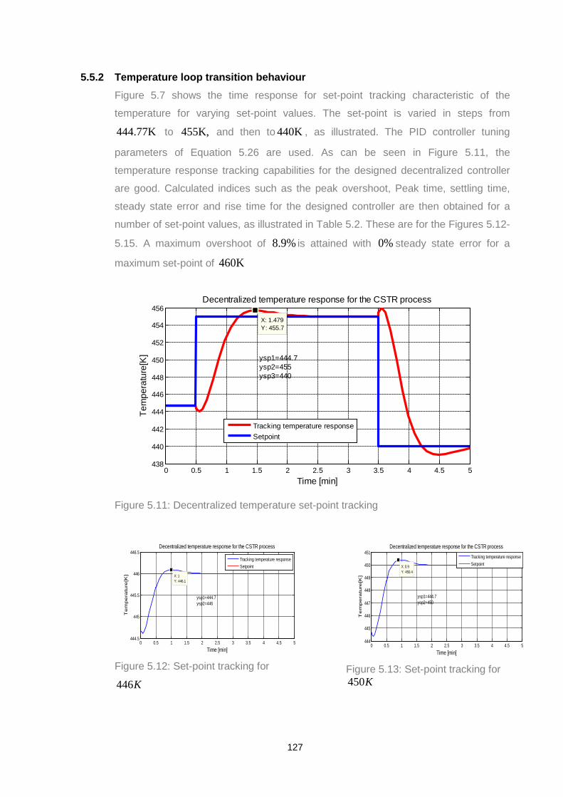
5.5.2 Temperature loop transition behaviour Figure 5.7 shows the time response for set-point tracking characteristic of the
temperature for varying set-point values. The set-point is varied in steps from
444.77K to 455K, and then to 440K , as illustrated. The PID controller tuning
parameters of Equation 5.26 are used. As can be seen in Figure 5.11, the
temperature response tracking capabilities for the designed decentralized controller
are good. Calculated indices such as the peak overshoot, Peak time, settling time,
steady state error and rise time for the designed controller are then obtained for a
number of set-point values, as illustrated in Table 5.2. These are for the Figures 5.12-
5.15. A maximum overshoot of 8.9% is attained with 0% steady state error for a
maximum set-point of 460K
Figure 5.11: Decentralized temperature set-point tracking
Figure 5.12: Set-point tracking for
446K
Figure 5.13: Set-point tracking for450K
0 0.5 1 1.5 2 2.5 3 3.5 4 4.5 5438
440
442
444
446
448
450
452
454
456
ysp1=444.7ysp2=455ysp3=440
X: 1.479Y: 455.7
Time [min]
Tem
pera
ture
[K]
Decentralized temperature response for the CSTR process
Tracking temperature responseSetpoint
0 0.5 1 1.5 2 2.5 3 3.5 4 4.5 5444.5
445
445.5
446
446.5
ysp1=444.7ysp2=446
X: 1Y: 446.1
Time [min]
Te
mp
era
ture
[K]
Decentralized temperature response for the CSTR process
Tracking temperature responseSetpoint
0 0.5 1 1.5 2 2.5 3 3.5 4 4.5 5444
445
446
447
448
449
450
451
ysp1=444.7ysp2=450
X: 0.9Y: 450.4
Time [min]
Te
mp
era
ture
[K]
Decentralized temperature response for the CSTR processTracking temperature responseSetpoint
127
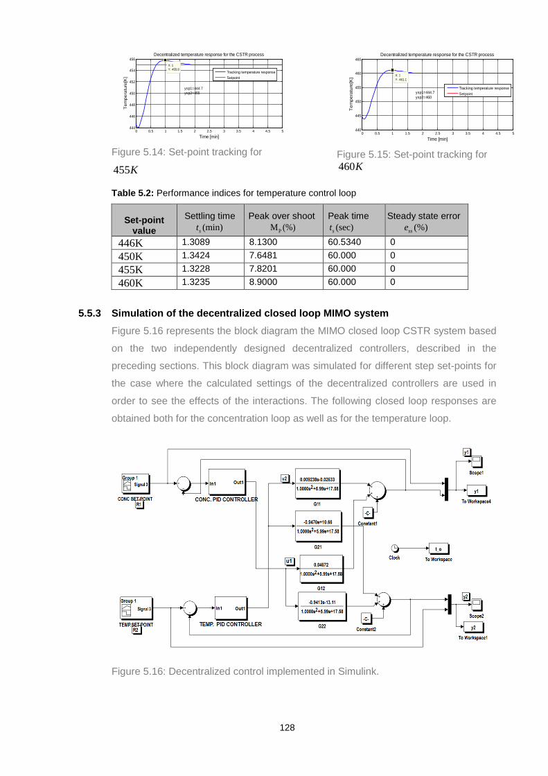
Figure 5.14: Set-point tracking for
455K
Figure 5.15: Set-point tracking for460K
Table 5.2: Performance indices for temperature control loop
Set-point
value Settling time
(min)st
Peak over shoot
PM (%)
Peak time(sec)st
Steady state error
(%)sse
446K 1.3089 8.1300 60.5340 0 450K 1.3424 7.6481 60.000 0 455K 1.3228 7.8201 60.000 0 460K 1.3235 8.9000 60.000 0
5.5.3 Simulation of the decentralized closed loop MIMO system Figure 5.16 represents the block diagram the MIMO closed loop CSTR system based
on the two independently designed decentralized controllers, described in the
preceding sections. This block diagram was simulated for different step set-points for
the case where the calculated settings of the decentralized controllers are used in
order to see the effects of the interactions. The following closed loop responses are
obtained both for the concentration loop as well as for the temperature loop.
Figure 5.16: Decentralized control implemented in Simulink.
0 0.5 1 1.5 2 2.5 3 3.5 4 4.5 5444
446
448
450
452
454
456
X: 1Y: 455.8
Time [min]
Tem
pera
ture
[K]
Decentralized temperature response for the CSTR process
ysp1=444.7ysp2=455
Tracking temperature responseSetpoint
0 0.5 1 1.5 2 2.5 3 3.5 4 4.5 5440
445
450
455
460
465
X: 1Y: 461.1
Time [min]
Tem
pera
ture
[K]
Decentralized temperature response for the CSTR process
ysp1=444.7ysp2=460
Tracking temperature responseSetpoint
128

Figure 5.17: Concentration set-point tracking under decentralized control
Figure 5.18: Temperature set-point tracking under the decentralized control
Figures 5.17 and 5.18 are the responses of the concentration control loop and the
temperature control loop respectively for the MIMO system. The set-point tracking
response capabilities for both outputs are achieved though the responses are
sluggish. It takes the concentration loop to reach the steady state value of 0.13mol/l
in 15.99minutes whereas the temperature loop’s steady state value of 455K is
reached after a time of13.62minutes.
Investigations on the influences over the process output step response for various
magnitudes of disturbances are also investigated for the developed scheme and
presented in the following subsection.
0 50 100 1500.04
0.06
0.08
0.1
0.12
0.14
X: 15.99Y: 0.13
Time [min]
Con
cent
ratio
n[m
ol/L
]
MIMO Closed loop decentralized concentration control without detuning
X: 101.2Y: 0.06
Set-pointConcentration loop tracking response
0 50 100 150440
445
450
455
460
X: 13.62Y: 455
Time [min]
Tem
pera
ture
[K]
X: 88.84Y: 445
MIMO closed loop decentralized control without detuning
Temperature loop tracking responseSet-point
129

5.5.4 Investigation on the disturbance influence on the concentration output 1y
Figure 5.19 is the block diagram of the closed loop system with disturbance at the
concentration output 1y
Figure 5.19: Closed loop control with disturbances at the concentration output 1y
Figure 5.20: Response under
31 mol/le−± noise
Figure 5.21: Response under
34 mol/le−± noise
Figure 5.22: Response under
0.01mol/l± noise
Figure 5.23: Response under
0.04mol/l± noise
The designed decentralized control system performance is checked for different
varying magnitudes of random disturbances (white noise) added to the output signal
0 50 100 1500.04
0.06
0.08
0.1
0.12
0.14
ysp1=0.0762mol/Lysp2=0.13mol/Lysp3=0.06mol/Lnoise=+/-1e-3mol/l
X: 11.3Y: 0.1301
Time [min]
Con
cent
ratio
n[m
ol/L
]
MIMO Closed loop decentralized concentration loop without detuning
X: 89.3Y: 0.0605
SetpointConcentration loop tracking response with noise
0 50 100 1500.04
0.06
0.08
0.1
0.12
0.14
X: 8.7Y: 0.1302
Time [min]
Con
cent
ratio
n[m
ol/L
]
MIMO Closed loop decentralized concentration loop without detuning
ysp1=0.0762mol/Lysp2=0.13mol/Lysp3=0.06mol/Lnoise=+/-4e-3mol/l
X: 89.1Y: 0.0603
SetpointConcentration loop tracking response with noise
0 50 100 1500.04
0.06
0.08
0.1
0.12
0.14
0.16
ysp1=0.0762mol/Lysp2=0.13mol/Lysp3=0.06mol/Lnoise=+/-0.01mol/l
X: 8.6Y: 0.1387
Time [min]
Con
cent
ratio
n[m
ol/L
]
MIMO Closed loop decentralized concentration loop without detuning
X: 98.4Y: 0.07184
SetpointConcentration loop tracking response with noise
0 50 100 1500.02
0.04
0.06
0.08
0.1
0.12
0.14
0.16
0.18
ysp1=0.0762mol/Lysp2=0.13mol/Lysp3=0.06mol/Lnoise=+/-0.04mol/l
X: 16.62Y: 0.158
Time [min]
Con
cent
ratio
n[m
ol/L
]
MIMO Closed loop decentralized concentration loop without detuning
X: 92.1Y: 0.02933
SetpointConcentration loop tracking response with noise
130

1y on the main concentration loop. The responses are represented in Figures 5.20 to
5.23. Good tracking control is still achieved. However as the magnitude of the
disturbance is increased, the response becomes noisy.
Figures 5.24-5.27 are the responses that shows the influences on the output
temperature as a result of the disturbances on the concentration loop 1y
Figure 5.24: Response under
0.01mol/l± noise
Figure 5.25: Temperature response
under 34 mol/le−± noise on 1y
Figure 5.26: Temperature response
under 0.01mol/l± noise on 1y
Figure 5.27: Temperature response
under 0.04mol/l± noise on 1y
Similarly, it can be seen that the disturbance at the concentration output influences
the second loop (temperature loop) too, but the magnitude of the effect is smaller
between the loops. Decentrarized control scheme can not eliminate completely the
efeects of the loop interactions. The results of simulation shows that the magnitude of
the disturbance is important for smooth set-point tracking. However the temperature
control system is still able to track the set-point variations implying that the designed
decentralized systems is good even in the presence of the random disturbances, but
full independence of the control loops can not be achieved.
0 50 100 150444
446
448
450
452
454
456
458
460
X: 13.9Y: 455
Time [min]
Tem
pera
ture
[K]
MIMO Closed loop decentralized concentration loop without detuning factor
ysp1=444.7ysp2=455noise on y1=+/-1e-3mol/l
X: 96.3Y: 444.7
Temperature loop tracking response with noiseSetpoint
0 50 100 150444
446
448
450
452
454
456
458
460
X: 11.6Y: 455
Time [min]
Tem
pera
ture
[K]
MIMO Closed loop decentralized concentration loop without detuning
ysp1=444.7ysp2=455noise on y1=+/-4e-3mol/l
X: 92.2Y: 444.7
Temperature loop tracking response with noiseSetpoint
0 50 100 150442
444
446
448
450
452
454
456
458
460
X: 10.05Y: 455
Time [min]
Tem
pera
ture
[K]
MIMO Closed loop decentralized concentration loop without detuning
ysp1=444.7ysp2=455noise on y1=+/-0.01mol/l
X: 91.5Y: 444.7
Temperature loop tracking response with noiseSetpoint
0 50 100 150440
445
450
455
460
465
ysp1=444.7ysp2=455noise on y1=+/-0.04mol/l
X: 7.6Y: 455.2
Time [min]
Tem
pera
ture
[K]
MIMO Closed loop decentralized concentration loop without detuning
X: 92.7Y: 442.9
Temperature loop tracking response with noiseSetpoint
131

5.5.5 Investigation on the disturbance interference over the temperature output 2y Figure 5.28 is the block diagram of the closed loop MIMO system with disturbance on
the temperature output 2y . The same type of experiments as in point 5.5.4 are
performed.
Figure 5.28: Closed loop control with disturbances on 2y output.
The responses are represented in Figures 5.29 to 5.32. Good tracking control but
sluggish responses are still achieved. However as the magnitude of the disturbance
is increased, the response becomes noisy.
Figure 5.29: Temperature response
under 4K noise±
Figure 5.30: Temperature response
under 8K noise±
Figure 5.31: Temperature response
under 10K noise±
Figure 5.32: Temperature response
under 20K noise±
0 50 100 150442
444
446
448
450
452
454
456
458
460
X: 16.68Y: 455.8
Time [min]
Tem
pera
ture
[K]
MIMO Closed loop decentralized concentration loop without detuning
ysp1=444.7ysp2=455noise=+/-4K
X: 92.1Y: 443.9
Temperature loop tracking response with noiseSetpoint
0 50 100 150442
444
446
448
450
452
454
456
458
460
X: 16.6Y: 457
Time [min]
Tem
pera
ture
[K]
MIMO Closed loop decentralized concentration loop without detuning
ysp1=444.7ysp2=455noise=+/-8K
X: 92.1Y: 442.6
Temperature loop tracking response with noiseSetpoint
0 50 100 150440
445
450
455
460
465
X: 16.6Y: 457.9
Time [min]
Tem
pera
ture
[K]
MIMO Closed loop decentralized concentration loop without detuning
ysp1=444.7ysp2=455noise=+/-10K
X: 92.1Y: 441.8
Temperature loop tracking response with noiseSetpoint
0 50 100 150440
445
450
455
460
465
ysp1=444.7ysp2=455noise=+/-20K
X: 16.6Y: 459
Time [min]
Tem
pera
ture
[K]
MIMO Closed loop decentralized concentration loop without detuning
X: 92.13Y: 440.6
Temperature loop tracking response with noiseSetpoint
132
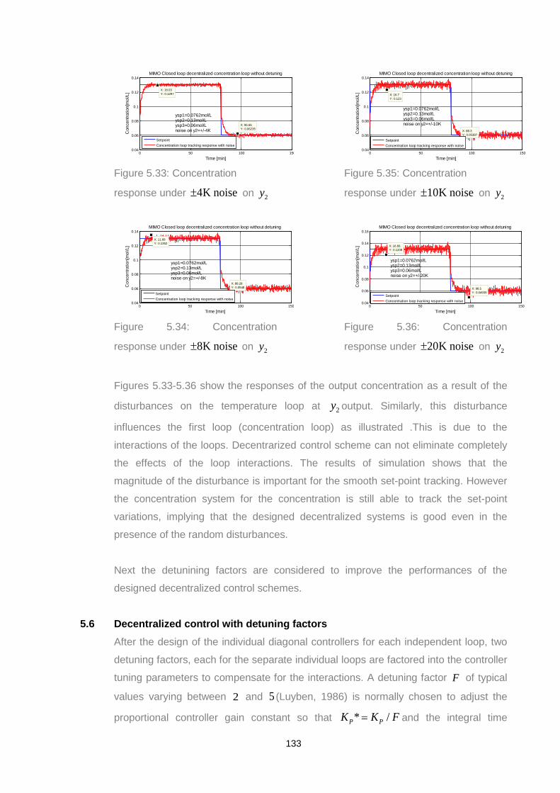
Figure 5.33: Concentration
response under 4K noise± on 2y
Figure 5.34: Concentration
response under 8K noise± on 2y
Figure 5.35: Concentration
response under 10K noise± on 2y
Figure 5.36: Concentration
response under 20K noise± on 2y
Figures 5.33-5.36 show the responses of the output concentration as a result of the
disturbances on the temperature loop at 2y output. Similarly, this disturbance
influences the first loop (concentration loop) as illustrated .This is due to the
interactions of the loops. Decentrarized control scheme can not eliminate completely
the effects of the loop interactions. The results of simulation shows that the
magnitude of the disturbance is important for the smooth set-point tracking. However
the concentration system for the concentration is still able to track the set-point
variations, implying that the designed decentralized systems is good even in the
presence of the random disturbances.
Next the detunining factors are considered to improve the performances of the
designed decentralized control schemes.
5.6 Decentralized control with detuning factors After the design of the individual diagonal controllers for each independent loop, two
detuning factors, each for the separate individual loops are factored into the controller
tuning parameters to compensate for the interactions. A detuning factor F of typical
values varying between 2 and 5 (Luyben, 1986) is normally chosen to adjust the
proportional controller gain constant so that * /P PK K F= and the integral time
0 50 100 1500.04
0.06
0.08
0.1
0.12
0.14
ysp1=0.0762mol/Lysp2=0.13mol/Lysp3=0.06mol/Lnoise on y2=+/-4K
X: 18.03Y: 0.1297
Time [min]
Con
cent
ratio
n[m
ol/L
]
MIMO Closed loop decentralized concentration loop without detuning
X: 96.66Y: 0.06235
SetpointConcentration loop tracking response with noise
0 50 100 1500.04
0.06
0.08
0.1
0.12
0.14
ysp1=0.0762mol/Lysp2=0.13mol/Lysp3=0.06mol/Lnoise on y2=+/-8K
X: 11.68Y: 0.1352
Time [min]
Con
cent
ratio
n[m
ol/L
]
MIMO Closed loop decentralized concentration loop without detuning
X: 88.28Y: 0.0548
SetpointConcentration loop tracking response with noise
0 50 100 1500.04
0.06
0.08
0.1
0.12
0.14
ysp1=0.0762mol/Lysp2=0.13mol/Lysp3=0.06mol/Lnoise on y2=+/-10K
X: 88.3Y: 0.05387
Time [min]
Con
cent
ratio
n[m
ol/L
]
MIMO Closed loop decentralized concentration loop without detuning
X: 16.7Y: 0.123
SetpointConcentration loop tracking response with noise
0 50 100 1500.04
0.06
0.08
0.1
0.12
0.14
0.16
X: 16.66Y: 0.1208
Time [min]
Con
cent
ratio
n[m
ol/L
]
MIMO Closed loop decentralized concentration loop without detuning
ysp1=0.0762mol/Lysp2=0.13mol/Lysp3=0.06mol/Lnoise on y2=+/-20K
X: 98.5Y: 0.04939
SetpointConcentration loop tracking response with noise
133

constant adjusted so that *I I Fτ τ= so that the effects of the interactions are
minimised The stability of each loop is determined by the detuning factor F , and the
bigger the magnitude of F , the more stable the system is. However the result is a
closed loop system whose response becomes more sluggish to the set-point changes
and the disturbance influences, therefore the detuning factor serves as a compromise
between the performance and the stability of the system.
For the designed controllers, it is found that the concentration control with a detuning
factor of 1 2F = gives the best performance for:
12 12 1* / 426.98 / 2 213.49P PK K F= = = ,and
12 12 1* 0.340728(2) 0.681456I I Fτ τ= = = .
Similarly, for the temperature control loop a detuning factor 2 1.4F = of gives the best
performance:
21 21 2* / 1.556 /1.4 1.11143P PK K F= = = , and
12 12 2* 0.340728(1.4) 0.4770192I I Fτ τ= = = .
The corresponding closed loop responses for the detuned loops are illustrated in
Figures 5.37 and 5.38 for the concentration control and the temperature control
respectively.
Figure 5.37: Concentration closed response using the detuning factor
0 5 10 15 20 25 30 35 40 45 500.04
0.06
0.08
0.1
0.12
0.14
ysp1=0.0762mol/Lysp2=0.13mol/Lysp3=0.06mol/L
X: 9.014Y: 0.13
Time [min]
Con
cent
ratio
n[m
ol/L
]
MIMO Closed loop decentralized concentration loop with detuning factor
X: 35.22Y: 0.06
SetpointConcentration loop tracking response
134

Figure 5.38: Temperature loop closed response using the detuning factor
Figures 5.37 and 5.38 are the responses of the concentration control loop and the
temperature control loop respectively for the MIMO system with independent detuning
factors. The set-point tracking response capabilities for both the outputs are achieved
though the responses are sluggish. It takes the concentration loop to reach the
steady state value of 0.13mol/l in 9minutes whereas the temperature loop’s steady
state value of 455K is reached after the same time of. 9minutes This is a significant
improvement when compared to the responses without detuning factors presented in
the preceding section.
5.6.1 Comparison of closed loop performance between decentralized control with and without detuning factors A comparison is made between the responses of the decentralized control under
detuning and without detuning factors in terms of performance specifications in order
to see which system performs better and why. Table 5.3 gives the various
specifications for both the concentration and the temperature responses
Figure 5.39: Comparison for the concentration response without and with the detuning factor
0 5 10 15 20 25 30 35 40 45 50442
444
446
448
450
452
454
456
458
460
X: 9.014Y: 455
Time [min]
Tem
pera
ture
[K]
MIMO Closed loop decentralized concentration loop with detuning factor
ysp1=444.7ysp2=455ysp3=444.7
X: 33.37Y: 444.7
X: 1.008Y: 442.7
Temperature loop tracking responseSet-point
0 5 10 15 20 25 30 35 40 45 500.06
0.07
0.08
0.09
0.1
0.11
0.12
0.13
X: 10.4Y: 0.13
Time [min]
Con
cent
ratio
n[m
ol/L
]
Response of the closed loop CSTR process under the decentralized control with/ and without detuning
X: 10.4Y: 0.13
X: 16.9Y: 0.13
SetpointConcentration responseConcentration response under detuning
135

Figure 5.40: Comparison for the temperature response without and with the detuning
factor
Table 5.2: Performance indices for the concentration and the temperature with and without detuning
Approach
Set-point
value Settling time
(min)st
Peak over shoot
PM (%)
Peak time(min)pt
Steady
state error
(%)sse
Decentralized control
0.13mol/l 15.4 0 15.4 0 455K 9.0 0 9.0 0
Decentralized control with detuning factor
0.13mol/l 13 0 13 0 455K 8.0 0 8.0 0
The investigation is done for the concentration tracking response to step changes in
set-point from 0.0762mol/l then to 0.13mol/l, then to 0.06mol/l , as illustrated in
Figure 5.39. From the Figure 5.39, it can be seen that the concentration performance
with detuning factor outperforms the one without detuning when a comparison is
made in terms of speed of response and the time it takes to reach the steady state
value. However the response is still sluggish. Similar analysis is done for the
temperature control response for to step changes in set-point from 444.77K to 455K
and then to 444.77K and it is seen from Figure 5.40, that the temperature response
under detuned decentralized control is much faster in terms of the speed of response
to reach the steady state. It is therefore concluded that the detuning factors
incorporated have enhanced the performance of the system.
Responses to various magnitudes of disturbances are also investigated for the
schemes developed with the help of the detuning factors and the performances of the
various loops are as illustrated in the following.
0 5 10 15 20 25 30 35 40 45 50440
445
450
455
460
465
ysp=455
X: 14.5Y: 455
Time [min]
Tem
pera
ture
[K]
Response of the closed loop CSTR process under the decentralized control with/without detuning
X: 9.5Y: 455
Decentralized temperature responseSetpointDecentralized temperature response with detuning
136

5.6.2 Investigation on the disturbance interference in the decentralized system with
detuning factor over the concentration output 1y This investigation is done to show that the influence of the interaction is reduced if the
detuning factor is used. This is checked for different varying magnitudes of random
disturbances (white noise) added to the output signal 1y on the main concentration
loop. The responses are represented in Figures 5.41 to 5.44 are responses of the
concentration output signal 1y .when the magnitude of the disturbance on 1y is varied
in the range of 31e−± moles/litre to 0.04 moles/litre. As can be seen in the responses,
the effect of noise is drastically reduced. Set-point tracking controlled is achieved.
Figure 5.41: Response under
31 mol/le−± noise
Figure 5.42: Response under
34 mol/le−± noise
Figure 5.43: Response under
0.01mol/l± noise
Figure 5.44: Response under
0.04mol/l± noise
Figures 5.45 to 5.48 are responses of the temperature output signal 2y .when the
magnitude of the disturbance on 1y is varied in the range of 31e−± moles/litre to 0.04±
moles/litre. This is to show that the influence of the interactions is significantly
reduced as a result of the detuning factor used. As can be seen in the responses, the
effect of noise is drastically reduced. Smooth temperature set-point tracking
controlled is achieved.
0 5 10 15 20 25 30 35 40 45 500.04
0.06
0.08
0.1
0.12
0.14
X: 8.6Y: 0.1302
Time [min]
Con
cent
ratio
n[m
ol/L
]
MIMO Closed loop decentralized concentration loop with detuning factor
ysp1=0.0762mol/Lysp2=0.13mol/Lysp3=0.06mol/Lnoise=+/-1e-3mol/l
Concentration loop tracking response with noiseSetpoint
0 5 10 15 20 25 30 35 40 45 500.04
0.06
0.08
0.1
0.12
0.14
X: 7.3Y: 0.1304
Time [min]
Con
cent
ratio
n[m
ol/L
]
MIMO Closed loop decentralized concentration loop with detuning factor
ysp1=0.0762mol/Lysp2=0.13mol/Lysp3=0.06mol/Lnoise=+/-4e-3mol/l
Concentration loop tracking response with noiseSetpoint
0 5 10 15 20 25 30 35 40 45 500.04
0.06
0.08
0.1
0.12
0.14
X: 5.4Y: 0.1303
Time [min]
Co
nce
ntr
atio
n[m
ol/L
]
MIMO Closed loop decentralized concentration loop with detuning factor
ysp1=0.0762mol/Lysp2=0.13mol/Lysp3=0.06mol/Lnoise=+/-0.01mol/l
Concentration loop tracking response with noiseSetpoint
0 5 10 15 20 25 30 35 40 45 500.04
0.06
0.08
0.1
0.12
0.14
0.16
X: 8.68Y: 0.1402
Time [min]
Con
cent
ratio
n[m
ol/L
]
MIMO Closed loop decentralized concentration loop with detuning factor
ysp1=0.0762mol/Lysp2=0.13mol/Lysp3=0.06mol/Lnoise=+/-0.04mol/l
Concentration loop tracking response with noiseSetpoint
137

Figure 5.45: Response under
0.01mol/l± noise on 1y
Figure 5.46: Response under
0.04mol/l± noise on 1y
Figure 5.47: Response under
0.01mol/l± noise on 1y
Figure 5.48: Response under
0.04mol/l± noise on 1y
Next, the influence of disturbances on 2y is investigated.
5.6.3 Investigation on the disturbance interference in the decentralized system with
detuning factor over the temperature output 2y Figures 5.49 to 5.52 are responses of the temperature output signal 2y .when the
magnitude of the disturbance on 2y is varied in the range of 4K± to 20K± . Set-point
tracking control is achieved but the responses are sluggish. Similarly, the magnitude
of the disturbance has significant effect on the shape of response.
Figure 5.49: Response under
4K noise±
Figure 5.50: Response under
8K noise±
0 5 10 15 20 25 30 35 40 45 50440
445
450
455
460
465
X: 9.9Y: 455
Time [min]
Te
mp
era
ture
[K]
MIMO Closed loop decentralized concentration loop with detuning factor
ysp1=444.7ysp2=455noise on y1=+/-1e-3mol/l
SetpointTemperature loop tracking response with noise
0 5 10 15 20 25 30 35 40 45 50440
445
450
455
460
465
X: 8.9Y: 455
Time [min]
Te
mp
era
ture
[K]
MIMO Closed loop decentralized concentration loop with detuning factor
ysp1=444.7ysp2=455noise on y1=+/-4e-3mol/l
SetpointTemperature loop tracking response with noise
0 5 10 15 20 25 30 35 40 45 50440
445
450
455
460
465
ysp1=444.7ysp2=455noise on y1=+/-0.01mol/l
X: 7.6Y: 455
Time [min]
Te
mp
era
ture
[K]
MIMO Closed loop decentralized concentration loop with detuning factor
SetpointTemperature loop tracking response with noise
0 5 10 15 20 25 30 35 40 45 50440
445
450
455
460
465
X: 6.3Y: 455.2
Time [min]
Tem
pera
ture
[K]
MIMO Closed loop decentralized concentration loop with detuning factor
ysp1=444.7ysp2=455noise on y1=+/-0.04mol/l
SetpointTemperature loop tracking response with noise
0 5 10 15 20 25 30 35 40 45 50440
445
450
455
460
465
ysp1=444.7ysp2=455noise=+/-4K
X: 8.667Y: 458
Time [min]
Te
mp
era
ture
[K]
MIMO Closed loop decentralized concentration loop with detuning factor
SetpointTemperature loop tracking response with noise
0 5 10 15 20 25 30 35 40 45 50435
440
445
450
455
460
465
ysp1=444.7ysp2=455noise=+/-8K
X: 8.643Y: 462.2
Time [min]
Te
mp
era
ture
[K]
MIMO Closed loop decentralized concentration loop with detuning factor
SetpointTemperature loop tracking response with noise
138

Figure 5.51: Response under
10K noise±
Figure 5.53: Response under
10K noise±
Figure 5.55: Response under
10K noise±
Figure 5.52: Response under
20K noise±
Figure 5.54: Response under
20K noise±
Figure 5.56: Response under
20K noise±
Similarly, Figures 5.53-5.56 are responses of the concentration loop to see the
influence of the interactions as a result of disturbances on the temperature loop. From
the figures, it is noted that the influence is not much if the detuning factor is used.
Good concentration set-point tracking is still achieved.
Appendix E1 presents the file that simulates the diagonal decentralized closed loop
system response for various magnitudes of the set-point step changes, as well as
disturbances at the output (y1) and the interaction junction (u1). The Simulink closed
loop models to be simulated are diag_decent_temp’ and 'decentconc_2015' These are
provided in appendix F. Appendix E2 provides the file that simulates the decentralized
control response of the closed loop MIMO CSTR with and without detuning, for
various magnitudes of set-point step changes as well as disturbances. The Simulink
closed loop model to be simulated is decent1_2015 The model is provided in appendix F.
0 5 10 15 20 25 30 35 40 45 50430
435
440
445
450
455
460
465
470
ysp1=444.7ysp2=455noise=+/-10K
X: 8.627Y: 465.3
Time [min]
Te
mp
era
ture
[K]
MIMO Closed loop decentralized concentration loop with detuning factor
SetpointTemperature loop tracking response with noise
0 5 10 15 20 25 30 35 40 45 500.04
0.06
0.08
0.1
0.12
0.14
X: 6.249Y: 0.1307
Time [min]
Con
cent
ratio
n[m
ol/L
]
MIMO Closed loop decentralized concentration loop with detuning factor
ysp1=0.0762mol/Lysp2=0.13mol/Lysp3=0.06mol/Lnoise on y2=+/-4K
Concentration loop tracking response with noiseSetpoint
0 5 10 15 20 25 30 35 40 45 500.04
0.06
0.08
0.1
0.12
0.14
X: 6.353Y: 0.136
Time [min]
Co
nce
ntr
atio
n[m
ol/L
]
MIMO Closed loop decentralized concentration loop with detuning factor
ysp1=0.0762mol/Lysp2=0.13mol/Lysp3=0.06mol/Lnoise on y2=+/-8K
Concentration loop tracking response with noiseSetpoint
0 5 10 15 20 25 30 35 40 45 50420
430
440
450
460
470
480
X: 8.631Y: 476
Time [min]
Te
mp
era
ture
[K]
MIMO Closed loop decentralized concentration loop with detuning factor
ysp1=444.7ysp2=455noise=+/-20K
SetpointTemperature loop tracking response with noise
0 5 10 15 20 25 30 35 40 45 500.04
0.06
0.08
0.1
0.12
0.14
0.16
ysp1=0.0762mol/Lysp2=0.13mol/Lysp3=0.06mol/Lnoise on y2=+/-10K
X: 6.4Y: 0.1398
Time [min]
Co
nce
ntr
atio
n[m
ol/L
]
MIMO Closed loop decentralized concentration loop with detuning factor
Concentration loop tracking response with noiseSetpoint
0 5 10 15 20 25 30 35 40 45 500.02
0.04
0.06
0.08
0.1
0.12
0.14
0.16
ysp1=0.0762mol/Lysp2=0.13mol/Lysp3=0.06mol/Lnoise on y2=+/-20K
X: 6.4Y: 0.1505
Time [min]
Con
cent
ratio
n[m
ol/L
]
MIMO Closed loop decentralized concentration loop with detuning factor
Concentration loop tracking response with noiseSetpoint
139

5.7 Discussion of the Results Simulation studies are used to verify the performance of the designed decentralized
controllers. First the performances with independent designed diagonal controllers
are tested as a first step in the implementation of the closed loop control of the 2 2xMIMO CSTR process by ignoring the off-diagonal elements. The design procedure
adopted is by using IMC-based PID feedback control Good set-point tracking
capabilities for the proposed decentralized controller is achieved for the outputs
(concentration and temperature). Lastly, the closed loop system with the off-diagonal
elements is considered using the designed decentralized controllers used so as to
see the effects of the interactions. The set-point tracking response capabilities for
both outputs are achieved though the responses obtained are sluggish.
Investigations on the influences over the process output step response for various
magnitudes of disturbances are also investigated by varying magnitudes of random
disturbances (white noise) added to the outputs Good tracking control is still achieved
though, as the magnitude of the disturbance is increased, the response becomes
noisy. Similarly, the disturbance influences due to intearctions on the loops are also
investigated and it is found that. the magnitude of the effect is smaller between the
loops implying that the designed decentralized systems is good even in the presence
of the random disturbances. Decentrarized control scheme can not eliminate
completely the efeects of the loop interactions. The results of simulation shows that
the magnitude of the disturbance is important for smooth set-point tracking. Next the
detunining factors are considered to better the performances of the designed
decentralized control schemes. A detuning factor serves as a compromise between
performance and stability of the process. It is found by comparison that there is a
significant improvement in the performances without detuning factors in the designed
decentralized control system. The investigation is also done for responses to various
magnitudes of disturbances. This investigation is done to show that the influence of
the interaction is reduced if the detuning factor is used and, it is found the effect of
noise is drastically reduced. Good concentration set-point tracking is still achieved.
5.8 Concluding remarks on the developed decentralized design method.
The design and implementation of decentralized PID controller for the MIMO CSTR
system are performed. For the design of the controllers, pairing among the input-
output variables is done using the RGA analysis. The results of this analysis required
that the concentration be controlled by the coolant flow rate while the temperature to
be controlled by the feed flow rate for minimum interaction and for optimal tracking
140

response. Then two SISO PID controllers are designed directly for the diagonal
transfer functions of the process model and independently using internal model
control (IMC) principles to tune the diagonal loops for tracking control of the output
variables namely, concentration and temperature. After the independent tuning of the
individual loops, a detuning factor for each individual loop is proposed to compensate
for the off-diagonal matrix transfer function interactions Simulation results
demonstrate the effectiveness of the proposed control law in achieving tracking
control with good disturbance rejection capabilities.
The next method developed for the control of the MIMO CSTR process is the
input/output feedback nonlinear linearizing controller design method as presented in
Chapter six
141

CHAPTER SIX INPUT/OUTPUT FEEDBACK LINEARIZATION CONTROLLER DESIGN FOR
THE CSTR PROCESS
6.1 Introduction
This chapter discusses the input/output feedback linearization controller design
strategy applicable to the nonlinear Multi-Input Multi-Output (MIMO) control of the
reactor temperature and concentration in a CSTR process. Input/output Feedback
linearization technique is a control design methodology that uses feedback signal to
cancel the inherent nonlinear dynamics in a system and to create a linear differential
relation between the output and a newly defined synthetic input. The most
fundamental property of a linear system from the control point of view is the validity of
the principle of superposition. The outputs of such systems are proportional to the
inputs. Systems with this property are governed by linear differential equations. It is
on the account of the superposition property that it can be guaranteed that the linear
system designed to perform satisfactorily when excited by a standard test signal, will
exhibit satisfactory output behaviour under any operating condition. This is not true
with the nonlinear systems because they do not obey the superposition principle. The
nonlinearity applies to more real-world systems, because all real control systems are
nonlinear. It is on this context that many different approaches have been proposed for
the analysis and control design for nonlinear systems. One of these approaches is
the feedback linearization technique.
The chapter is structured in the following sections: In section 6.2 the preliminary
theory of the feedback linearization method is presented. Section 6.3 presents the
details of the design of the input/output feedback linearization control schemes for the
linearized 2 2x MIMO CSTR process. Section 6.4 presents the linear PI control design
strategy applied to aid the input/output feedback linearization control schemes..
Section 6.5 presents the simulation of the closed loop linearized system in the
Matlab/Simulink environment in terms of the performance specifications. Section 6.6
discusses the obtained results. Section 6.7, a comparison with the other conventional
methods developed in Chapters 4 and 5 for the control of the nonlinear MIMO CSTR
process is made and finally section 6.8 concludes the chapter.
6.2 Feedback linearization control schemes There is no general technique that can be used for the design of a nonlinear
controller. However there are many alternatives and complementary techniques, that
142

can be applied to the solutions of certain classes of nonlinear control problems. In this
section, feedback linearization nonlinear control design technique is developed. Feedback linearization is a strategy used for nonlinear control design that
algebraically converts the nonlinear system characteristics to full or partial linear
systems in order for linear control methods to be used. The approach is quite different
from the conventional (Jacobian) linearization technique because the feedback
linearization is realized using exact state conversion and feedback, instead of the
linear approximations of the characteristics. The conventional concept of linearization
implies the approximation of the nonlinear system using a linear counterpart in the
neighbourhood of a steady state operating point. In comparison to the conventional
method, the novelty of this method is that linearization is valid for larger operating
space rather than single operating point. There are basically two distinct strategies for
of feedback linearization can be identified. These are: input/output feedback
linearization and I/O feedback linearization (Hedrick and Girard, 2005). In both cases
the idea is to find feedback and coordinate transformations in order that the resulting
system becomes linear in some way.
The I/O feedback linearization technique is used in this work, The I/O feedback
linearization technique’s objective is to find a linear input-output behaviour of the
resulting system so that any linear control methodology may be applied for the
controller design. Equations (3.12) and (3.13) presented earlier may be re-written as
follows:
( ) ( )
( )(0) o
c
f x g x u u
y h xx x
qx
q= + =
=
=
(6.1)
The case considered is for a system where the number of inputs variables is the
same as the number of output variables, therefore dimension vectors l m= where: xis the n -vector of the state variables; u is the m -vector of the manipulated input
variables; y is the m -vector of the controlled output variables; ( )f x is the n -vector
of the nonlinear functions; ( )g x is the nxm -matrix of the nonlinear functions; ( )h x is
the l -vector of the nonlinear functions and (0) ox x= is the vector of initial state. The
model of Equation (6.1) is called the control affine, since the control input signal uappears linearly in the state space equation. This model can be modified as much as
required in order to satisfy more complex nonlinear processes encountered like those
with disturbances and/or time delays.
143

6.3 I/O Feedback linearization control design technique Input/output controller design by feedback linearization is a control technique where
the controlled output ( )y h x= of the dynamic system is differentiated until the physical
input u appears in the thr derivative of the controlled output (Slotine and Li, 1991). A
key concept of the feedback linearization theory for nonlinear control affine systems is
the relative degree feature r . If r , is less than n , then there will be internal dynamics
in the system. If, r n= , then Input/output and Input/State linearization are the same.
The relative degree r is the number of times the output y has to be differentiated in
order to have at least one component of the control vector in it. Consider a scalar
function h and a vector field f . The Lie derivative of h with respect to f denoted by
fL h is given by
( )( ) ( )f
h xL h x f x
x∂
=∂
and the Lie derivative of h with respect to g denoted by gL h is
given by ( )( ) ( )g
h xL h x g x
x∂
=∂
. The idea of using the Lie derivative formulation is to
determine a control methodology that renders a linear deferential equation from the
virtual input v to the output y . This concept of feedback linearization theory can also
be applied for MIMO systems. By diffentiating the nonlinear Equation of (6.1), for
every component of the output vector, the following is achieved.
1
( ) ( ) , 1, ..,.m
f i gj i jj
iy L h x L h u i i=
= + =∑ (6.2)
The key point is that if, 1 ( ) 0irgj f iL L h x− = for all j , then the input vector u does not
appear explicitly in Equation (6.2) and further differentiation is continued until, for
some integer r n≤
( ) ( 1)
1
( ) ( ) , 1,......,i i i
mr r r
i f i gj f i jj
y L h x L L h x u i l−
=
= + =∑ (6.3)
such that ( 1) ( ) 0irgj f iL L h x− ≠ , for at least one parameter j in the neighbourhood of the
steady state point ox . The procedure is repeated for every output iy and results in a
number of l equations expressed in Equation (6.4):
111 1
( )1
( )
( ). ( ) .( )
.mi
rf
rf l m
r
rm
L h x uB x
L h x u
y
y
= +
(6.4)
Where ( )B x is a lxm matrix expressed as:
144

1 11 11 1 1
1 1
. .. . . .
( ). . . .
. .l l
r rg f gm f
r rf l gm f lgl
L L h L L h
B x
L L h L L h
− −
− −
=
(6.5)
The ( )B x matrix realized is known as a decoupling matrix for the multi-input multi-
output system. When this matrix is non-singular then the vector u of the control signal
can be expressed in Equation (6.5): 1
11
1 1
( )..
( ) ( )..
( )l
rf
rmf l
vL h x
u B x B x
vL h x
− −= − +
(6.6)
The vector [ ]1 . . Tmv v is the vector for the synthetic (virtual) set of inputs or the
synthetic controls that the control designer defines. The characteristics of the new
controls are then obtained by substitution of Equation (6.6) in Equation (6.4) to obtain:
1( )11
( )
..
..m
r
rmm
vy
vy
=
(6.7)
The transformed system of Equation (6.7) is called a decoupling control law and
shows a linear MIMO decoupled relationship. As can be seen, the transformation
leads to a linearized system in the form of integrators. Thus, the system in Equation
(6.4) possesses relative degrees ( )1 2, , ..... mr r r at ox and the scalar value r which is equal
to 1 2 ..... mr r r+ + + is termed as the total relative degree of the system at ox . The order
of relative degree for the system allows for the verification whether a nonlinear
system can be input/output linearized (Isidori, A., 1991; Slotine and Hedrick, 1993).
After performing the input/output linearization, the characteristics of the nonlinear
system is split into external input/output portion and an internal (unobservable)
portion as demonstrated by (Slotine and Li, 1991). Because the external portion
comprises of a linear relation between the output y and the synthetic input v , any
linear controller design methods can be used to design a controller with the help of
control implemented through the synthetic input v so that the output tracks any given
set point trajectory assuming the internal dynamics remain bounded). The control law
involving tracking of a desired output is then obtained in the form: ( 1)
1 1..... nd o nv y k e k e k e −
−= − − − + (6.8)
145

Where, the reference or desired output signal is dy and the tracking error is
( ) ( ) ( )de t y t y t= − . The exponentially convergent tracking error is then achieved. The ik
constants are chosen so that the roots of the polynomial 11 ........n n
n os k s k−−+ + + are
placed in the left hand side of the complex plane.
6.4 I/Output Feedback linearization control design for the CSTR process The block diagram of the arrangement for the considered case of the CSTR process
is illustrated in Figure 6.1.
Linear Pl controller
1( )v t
Nonlinear Linearizing control by input/
output linearization
1( )x t
1( )y t
2 ( )v t2 ( )u t 2 ( )y t
1( )u t
+
2 ( )y t
1( )e t
2 ( )e t
1desiredy
−
+−
2desiredyLinear PI controller
1( )y t
2 ( )x t
MIMO Nonlinear CSTR system
Figure 6.1: Input-output feedback linearization control structure
As illustrated in Figure 6.1, the system comprises of three parts namely, linear
controllers (two), the nonlinear linearizing controller using input/output linearization
methodology that maps the nonlinear system to a linear and decoupled system and
lastly the nonlinear plant model. In order to design of the controllers, 1v and 2v are
chosen in a way so that a stable MIMO closed loop system results and the desired
set-points are achieved. Two different controllers, one for each output are then
designed.
Application of the described above input/output linearization and linear controller
design for the considered CSTR is described below. Substitution of q with 1u and cq
with 2u also AOC with 1x and T with 2x , the CSTR model Equations, (3.12) and (3.13)
can be modified to the standard state space affine form as:
11 1 1 1 2( ) exp( / )AO o
ux C x k x a x
V= − − − (6.9)
12 2 2 1 1 2 3 2 2 24( ) exp( / ) (1 exp( / )( )O CO
ux T x a x a x a u a x T x
V= − − − + − − − (6.10)
146

Where, 1 /a E R= , 2
( ) ,o
p
H ka
Cρ−∆
= 3 ,c pc
p
Ca
C V
ρ
ρ= and 4
p
hAacρ
−= , and [ ] [ ]
1 2 T T
A Tx x x C= =
denotes the state vector as well as the output vector while 1 2[ ] [ ]c
T Tu u u q q= = denotes
the input vector. Equations (6.9) and (6.10) can be written in the standard affine form
as:
1 11 1
22 2 21 1 22
1 1
1 1 2 1 2
1 2 1 2 1 2
1 1
2 2 2 2
( , ) ( , )
( , ) ( , ) ( , )
(
(
))
x f x x g x x u
x f x x g x x u g x x u
x x
y x x
y hh
+
= + +
=
=
== =
(6.11)
Where,
1 1 1 2
2 2 1 1 2
11 1
21 2
22 3 2
2 2 4 2
1 2
1 2
( ) exp( / )
( , ) exp( / )
1( ) ( )
1( ) ( )
( ) ( )
(1 exp( / ))
, o
AO
O
CO
x x k x a x
f x x a x a x
g x C xV
g x T xV
g x a T x
u u a u
f = − −
= −
= −
= −
= −
= − −
(6.12)
Here, 2 2 4 2(1 exp( / ))u u a u= − − from which the control input can be deduced as:
2 2 2 4 2
2 4 2
2 4 2
ln ln ln / )
ln /
/ ln
u u u a u
u a u
u a u
= − +
=
=
(6.13)
The output vector is 1 2( ) [ ] [ ]AT Ty h x x x C T= = = and for the application of the
input/output feedback linearization technique, this output must be differentiated
several for the input parameters to appear in the outputs or their derivatives. Thus,
( ) ( )( ) ( ) and ( ) ( )( ) ( )f g
h x h xL h x f x L h x g xx x
∂ ∂= =∂ ∂
, from which,
147

1 11 1 1 1 1 2 1 1 2
1
1 22 1 2 2 1 2 2 1 2
2
1 111 1 1 11 1 2 11 1 2
1
1 112 1 1 12 1 2 12 1 2
1
2 221 2 2 21
2
( )( ) ( , ) ( , )( )
( )( ) ( , ) ( , )( )( )( ) ( , ) g ( , )
( )( )( ) ( , ) g ( , )
( )( )( )
( )
f
f
g
g
g
h xL h x f x x f x xx
h xL h x f x x f x xx
h xL h x g x x x xx
h xL h x g x x x xx
h xL h x gx
∂= =
∂∂
= =∂∂
= =∂∂
= =∂∂
=∂ 1 2 21 1 2
1 222 2 2 22 1 2 22 1 2
2
( , ) g ( , )
( )( ) ( , ) g ( , )( )g
x x x x
h xL h x g x x x xx
=
∂= =
∂
(6.14)
Then,
11 1 1
22 1 1
1 1 11 1 12 11 1
2 2 21 1 22 12 2
( ) ( ) ( )( ) ( ) ( )
f g g
f g g
uL h x L h x L h xy xL h x L h x L h xy x u
= +
=
1
2
1 1 1 2 11 1 2 12 1 2
2 2 1 2 21 1 2 22 1 2
( ) ( ) ( )( ) ( ) ( )
, , ,, , ,
uy f x x x xy f x x x x
g x g xg x g x u
= +
(6.15)
This implies that:
22
1 1 11 1 1
2 2 21 1 2
1 1 2 1
1 1 2 2
( , ) ; 1
( , ) ; 1
y x f g u v
y x f g u gu v
x x r
x x r
= + =
= + =
= =
= + =
(6.16)
Thus, the total degree of this system is 2 and the following are obtained.
3 2
1
11 1 2 12 1 2
21 1 2 21 1 2 2
0( ) ( )( )
( ) ( )( )
( ), ,, , ( )
CO
AO
O
x xB x
x xa T x
C xg x g x Vg x g x T x
V
=
−
−
= −
, and,
11 1 2 1
22 2 1 1 2 23 2
1
1
2
0exp( / )exp( / )
( )
o
CO
AO
O
uy k x a xy a x a x
a T x
C xvVvT x u
V
− −= +
− −−
−
= −
(6.17)
From Equation (6.17) it implies that the two nonlinear linearizing controllers resulting
from the input-output linearization are:
[ ][ ]
1 1 1 11
11 1
1 1 2
1
( ) ( ) ( )( )
exp( / )( ) /
f
g
o
AO
v x L x v xu
L xk x a x
C x V− −
=− −
=−
(6.18)
and,
[ ] [ ][ ]
2 2 2 21 2 12
22 2
2 12 1 1 2 22 4 2
3 2
( ) ( )
( )
exp( / ) ( ) /; / ln
( )
f g
g
O
CO
v L x L x uu
L x
v a x a x T x V uu a u
a T x
− −=
− −− − −= =
−
(6.19)
148

Equations (6.18) and (6.19) represent the components of the vector of the nonlinear
control sent to the CSTR process. Additional linear controllers are then necessary to
be designed. The reason is that the nonlinear control depends on the parameters of
the process, which normally are non-stationary; also various disturbances can
influence the process. These are two causes that can make the system non stable
and the linearization not fulfilled. To overcome such possibility an additional linear
control is needed to make the closed loop system stable and to improve its
performance.
6.5 Linear PI controller design The linear controller part is then designed. The procedure for the design by pole
placement used is as summarised in the following. On the basis of Equation (6.17) it
can then be written as:
1 1 1 1
2 2 2 2
( ) ( )( ) ( )
y v sY s V sy v sY s V s= → == → =
(6.20)
Then if the linear controls 1v and 2v are determined using PI controllers, the equations
governing them would be:
1 11 1 1 12 1 10
2 21 2 2 22 2 20
( ) ( )
( ) ( )
t
sp sp
t
sp sp
v k y y k y y dt
v k y y k y y dt
= − + −
= − + −
∫
∫ (6.21)
Assuming that the desired output’s rate of change is specified as;
11 1 1 1 12 1 11 01
2 221 2 2 22 2 2
0
( ) ( )
( ) ( )
t
sp spsp
tsp
sp sp
k y y k y y dty vy v
k y y k y y dt
− + −
= = − + −
∫
∫
(6.22)
where 11 12 21, ,k k k and 22k are the linear PI controller tuning parameters. The goal is to
make 11
22
sp
sp
yyyy
=
by choosing v appropriately, then the input-output linearized
closed loop system results when:
11 1 1 12 1 101
221 2 2 22 2 2
0
( ) ( )
( ) ( )
t
sp sp
t
sp sp
k y y k y y dyy
k y y k y y d
τ
τ
− + −
= − + −
∫
∫
(6.23)
The linearized system is represented by the following transfer functions:
149

11
1
22
2
( ) 1( )( )( ) 1( )( )
C
C
Y sG sV s sY sG sV s s
= =
= = (6.24)
Equation (6.24) is applied for the closed loop transfer functions derivation as:
11
1
22
2
( )( )( )
( )( )( )
C CLsp
C CLsp
Y sG sY sY sG s
Y s
=
= (6.25)
Where 1C CLG and 2C CLG are the individual closed loop transfer functions. These
transfer functions are derived for the considered cases as follows:
6.5.1 Linear PI controller design for the concentration loop
+
-12
11( ) kk ss
+1( )Y s
1 1( ) ( )sY s V s=1 1( ) ( )spY s Y s−1 ( )spY sLinearized system
PI Controller
1s
Figure 6.2: Desired closed loop Input-output feedback linearization for concentration
First, the concentration loop is considered. Figure 6.2 is the desired closed loop
Input-output feedback linearized control structure for the concentration control, where
the linearized part transfer function is given by the Equation 1
1
( ) 1( )
Y sV s s
= ; hence with the
help of Figure 6.2, the derived closed loop transfer function is.
11 1212 2111 11 122 2
12 11 121 11 1211 2
1( )( )( ) 11 ( )sp
k s kkkY s k s ks s sk s k s kY s s k s kk s s s
++ +
= = =+ + + ++ +
This closed loop transfer function is then presented in the form:
150

1 11 122
1 11 12
1 12 2
1 1 1
11 11 1 11 12 2
1112 12
( )( )
2 1 1
21 1where, , or, , 2
sp
Y s k s kY s s k s k
ss s
k k kk k
τ ζτ τ ζ
ζτ ζτ τ
+=
+ +
+=
+ +
= = = =
(6.26)
1 2 1 2, , and τ τ ζ ζ are the time constants and damping parameters that determine the
shape of the step responses for concentration and temperature respectively. If the
roots of the characteristic equation: 211 12s k s k+ + are appropriately selected, then
asymptotic tracking of the desired closed loop response can be realised. According to
Slotine and Li, (1990); Henson and Seborg, (1991) the controller tuning parameters
11,k and 12k may be selected to provide the required closed loop response. To
guarantee smaller overshoots, the conditions 211 124k k≥ .and 2
21 224k k≥ should be
fulfilled. The problem is then to find the appropriate parameters 11,k and 12k .
According to Wilson (2014), the algorithm for appropriate values of 11,k and 12k is as
follows:
1. Choose the appropriate values of the damping factors. For tight control, with little
overshoot, 1 3ζ ≈ or higher.is recommended.
2. Specify the time scale by choosing appropriate values of time constant 1τ . Often it
is convenient to specify the rise time.
3. From the specified values of 1ζ and 1,τ the scalar values of parameters are
evaluated for each output. From Equation (6.26) therefore,
2, 2111 12 2
1 1
2 2112
1 1
1 1
2 14 ( )
2 1( ) 0 2 1 0
1 0.707 is selected2
k k ζτ ζ
ζ ζτ ς
ζ ζ
≥ → ≥
− ≥ → − ≥
≥ → ≥
(6.27)
From Equation (6.26), assuming that the specific transient controller requirements for
the damping factor should be1.2and the time constant to be 0.3min, as per Equation
(6.27), the controller tuning parameters for the concentration loop are calculated as
follows:
151

1
111
1
12 2 2
2 2(1.2) 80.3
1 1 11.11(0.3)
k
k
ςτ
τ
= = =
= = = (6.28)
Thus the PI controller tuning parameters designed as per Equations (6.27) and (6.28)
are implemented for the concentration control loop: The designed controlled system’s
performance is discussed at the end of this chapter.
6.5.2 Linear PI controller design for the temperature loop Similarly, the temperature closed loop is considered. Figure 6.3 is the desired closed
loop I/O feedback linearization control structure for the temperature control, where the
linearized part transfer function is given by the Equation 2
2
( ) 1( )
Y sV s s
= ;
+
-22
21( ) kk ss
+2 ( )Y s
2 2( ) ( )sY s V s=2 2( ) ( )spY s Y s−2 ( )spY sLinearized system
PI Controller
1s
Figure 6.3: Desired closed loop Input-output feedback linearization for temperature
Hence with the help of Figure 6.3, the transfer function of the closed loop is derived.
21 2222 2212 21 222 2
22 21 222 21 2221 2
1( )( )( ) 11 ( )sp
k s kkkY s k s ks s sk s k s kY s s k s kk s s s
++ +
= = =+ + + ++ +
This closed loop transfer function can be presented in the form:
2 21 222
2 21 22
( )( )sp
Y s k s kY s s k s k
+=
+ +
2 22 2
2 2 2
2 11
ss sτ ζ
τ τ ζ+
=+ +
21 22 21 22 2
2 222 22
21 1where, , or, , 2
k k kk k
ζτ ζτ τ
= = = = (6.29)
Here, 2ζ and 2τ ,are the time constant and damping parameter that determine the
shape of the step responses for the temperature. If the roots of the characteristic
equation s 221 22s k s k+ + , are appropriately selected, then asymptotic tracking of the
desired closed loop response can be realized. According to Slotine and Li, (1990); 152

Henson and Seborg, (1991) the controller tuning parameters 21k and 22k can be
selected to provide the response of the desired closed loop. To guarantee smaller
overshoots, the conditions 221 224k k≥ should be fulfilled. The problem is then to find the
appropriate parameters 21k and 22k . According to Wilson (2014), the algorithm for
appropriate values of 21k and 22k is as follows:
1. Choose the appropriate values of the damping factors. For tight control, with little
overshoot, 2 3ζ ≈ or higher.is recommended.
2. Specify the time scale by choosing appropriate values of time constant 2τ . Often it
is convenient to specify the rise time
3. From the specified values of 2ζ and 2τ , the scalar values of parameters are
evaluated for each output. From equation (6.29) therefore,
2, 2221 22 2
2 2
2 2222
2 2
2 2
2 14 ( )
2 1( ) 0 2 1 0
1 1.1 is selected2
k k ζτ ζ
ζ ζτ ς
ζ ζ
≥ → ≥
− ≥ → − ≥
≥ → =
(6.30)
Similarly, the controller tuning parameters for the temperature control loop are
subsequently calculated by choosing the damping factor 2ζ and time constant 2τ that
ensures that the condition 221 224k k≥ is fulfilled. From equation (6.29), assuming that
the specific transient controller requirements for the damping factor should be1.1and
the time constant to be 0.14 min, then:
221
2
22 2 22
2 2(1.1) 290.075
1 1 51(0.14)
k
k
ςτ
τ
= = =
= = = (6.31)
Thus the PI controller tuning parameters are designed as per equations (6.30) and
(6.31). The controller is for the temperature control loop:
6.6 Simulation results Simulation results are used to show the performance of the designed controllers. The
Simulink block diagrams used to implement this control scheme are illustrated in the
following figures.
153

Figure 6.4: Simulink CSTR process model.
Figure 6.5: Control structure using input-output feedback linearization
Figure 6.4 is the Simulink block diagram for the nonlinear CSTR process model used
for the design of the I/O feedback linearization control algorithm. Figure 6.5 illustrates
the Simulink block diagram of the complete set-up consisting of the linear controllers,
the nonlinear linearizing controller and the CSTR model implemented in the Simulink
environment. Then Figure 6.6 is the Simulink block diagram for the nonlinear
linearizing controller implemented with the help of Equations (6.18) and (6.19) derived
earlier.
154

Figure 6.6: Simulink block for the I/O feedback linearization controller
The set-point tracking performance capabilities for both outputs with different values
of magnitudes are tested based on simulations of the closed loop system of Figure
6.5 under various set-point and disturbance situations. The results of the simulations
are presented as follows.
6.6.1.1 Concentration loop results from simulation for various set-points Figure 6.7 presents the time response for set-point tracking characteristics for the
concentration control for varying set-points. The PI controller tuning parameters of
Equation (6.29) are used. The set-point is varied in steps from 0.0762mol/l to
0.13mol/l, then to 0.06mol/l , as illustrated. Analysis of this plot for various time
response indices indicates that the rise time is 0.9 min, the settling time of 1.98min,
the percentage overshoot is10.5947% , the time to peak overshoot is 0.56 min, and
steady state error of 0% . This therefore implies that the simulated response tracking
capabilities for the designed concentration control loop by the I/O feedback
linearization methodology is good.
155

Figure 6.7: Input-output feedback linearization controlled concentration set-point
tracking
Simulations are also performed for different set-point conditions. Figures 6.8 to 6.13
show the concentration responses for the set-point tracking when the magnitudes are
varied as 0.08mol/l , 0.09mol/l , 0.10mol/l , 0.11mol/l , 0.12mol/l and 0.13mol/l , then
in Table 6.1 the various time response specifications are compared. From Table 6.1,
it is deduced that the simulated responses for various set-points have good tracking
capability for the input-output feedback linearizing control of the concentration loop of
the MIMO system.
Figure 6.8: Response for a set-
point of 0.08 /mol l
Figure 6.9: Response for a set-
point of 0.09 /mol l
Figure 6.10: Response for a set-
point of 0.1 /mol l
Figure 6.11: Response for a set-
point of 0.11 /mol l
0 0.5 1 1.5 2 2.5 3 3.5 4 4.5 50.04
0.06
0.08
0.1
0.12
0.14
ysp1=0.0762mol/Lysp2=0.13mol/Lysp3=0.06mol/L
X: 1.04Y: 0.1356
Time [min]
Con
cent
ratio
n[m
ol/L
]
Closed loop response of the nonlinear CSTR process under the feedback linearization control
SetpointConcentration loop tracking response
0 0.5 1 1.5 2 2.5 3 3.5 4 4.5 50.076
0.077
0.078
0.079
0.08
0.081
0.082
0.083
ysp1=0.0762mol/Lysp2=0.08mol/L
X: 0.58Y: 0.0804
Time [min]
Tem
pera
ture
[K]
Closed loop response of the nonlinear CSTR process under the feedback linearization c
SetpointNonlinear I/O linearized temperature response
0 0.5 1 1.5 2 2.5 3 3.5 4 4.5 50.076
0.078
0.08
0.082
0.084
0.086
0.088
0.09
0.092
ysp1=0.0762mol/Lysp2=0.09mol/L
X: 0.56Y: 0.09145
Time [min]
Tem
pera
ture
[K]
Closed loop response of the nonlinear CSTR process under the feedback linearization co
SetpointNonlinear I/O linearized temperature response
0 0.5 1 1.5 2 2.5 3 3.5 4 4.5 50.075
0.08
0.085
0.09
0.095
0.1
0.105
ysp1=0.0762mol/Lysp2=0.01mol/L
X: 0.56Y: 0.1025
Time [min]
Tem
pera
ture
[K]
Closed loop response of the nonlinear CSTR process under the feedback linearization control
SetpointNonlinear I/O linearized temperature response
0 0.5 1 1.5 2 2.5 3 3.5 4 4.5 50.075
0.08
0.085
0.09
0.095
0.1
0.105
0.11
0.115
X: 0.56Y: 0.1136
Time [min]
Tem
pera
ture
[K]
Closed loop response of the nonlinear CSTR process under the feedback linearization control
ysp1=0.0762mol/Lysp2=0.011mol/L
SetpointNonlinear I/O linearized temperature response
156

Figure 6.12: Response for a set-
point of 0.12 /mol l
Figure 6.13: Response for a set-
point of 0.13 /mol l .
Table 6.1: Performance indices for the concentration control loop using I/O linearization-based control
Set-point value Settling time
(min)st
Rise time(min)rt
Peak over shoot
PM (%)
Peak time(min)st
Steady state error
(%)sse
0.08mol/l 1.9800 0.900 10.5263 056 0 0.09mol/l 1.9800 0.900 10.5075 0.56 0 0.10mol/l 1.9800 0.900 10.5042 0.56 0 0.11mol/l 1.9800 0.900 10.6508 0.56 0
0.12mol/l 1.9800 0.900 10.5022 0.56 0
0.13mol/l 1.9800 0.900 10.5947 0.56 0
As can be seen Table 6.1, the maximum peak overshoot of 10.65081% is attained
with 0% steady state error. This implies that the designed control is good at tacking
the set-point values. Next the influence of disturbances is investigated.
6.6.1.2 Investigation of the process performance for a disturbance on concentration control loop The designed I/O feedback linearization control system’s performance is checked for
different magnitudes of random disturbances (white noise) added to the output signal
1y on the main concentration loop. The responses are represented in the following
Figures 6.14-6.17.
Figure 6.14: Concentration
response under 31 mol/le−±
disturbance magnitude
Figure 6.15: Concentration
response under 34 mol/le−±
disturbance magnitude
0 0.5 1 1.5 2 2.5 3 3.5 4 4.5 5
0.08
0.09
0.1
0.11
0.12
0.13
X: 0.56Y: 0.1246
Time [min]
Tem
pera
ture
[K]
Closed loop response of the nonlinear CSTR process under the feedback linearization c
ysp1=0.0762mol/Lysp2=0.012mol/L
SetpointNonlinear I/O linearized temperature response
0 0.5 1 1.5 2 2.5 3 3.5 4 4.5 5
0.08
0.09
0.1
0.11
0.12
0.13
0.14
ysp1=0.0762mol/Lysp2=0.012mol/L
X: 0.56Y: 0.1357
Time [min]
Con
cent
ratio
n[m
ol/L
]
Closed loop response of the nonlinear CSTR process under the feedback linearization control
SetpointConcentration loop tracking response
0 0.5 1 1.5 2 2.5 3 3.5 4 4.5 5
0.08
0.09
0.1
0.11
0.12
0.13
0.14
ysp1=0.0762mol/Lysp2=0.13mol/Lnoise=+/-1e-3mol/l
X: 0.56Y: 0.1356
Time [min]
Con
cent
ratio
n[m
ol/L
]
Closed loop concentration response with noise under the feedback linearization contr
SetpointConcentration loop tracking response with noise
0 0.5 1 1.5 2 2.5 3 3.5 4 4.5 5
0.08
0.09
0.1
0.11
0.12
0.13
0.14
ysp1=0.0762mol/Lysp2=0.13mol/Lnoise=+/-4e-3mol/l
X: 0.56Y: 0.1354
Time [min]
Con
cent
ratio
n[m
ol/L
]
Closed loop concentration response with noise under the feedback linearization control
SetpointConcentration loop tracking response with noise
157

Figure 6.16: Concentration
response under 0.01mol/l±
disturbance magnitude
Figure 6.17: Concentration
response under 0.04mol/l±
disturbance magnitude
The responses from the simulations including the disturbances suggest that good
tracking control is still achieved. However, as the magnitude of the disturbance is
increased, the response becomes noisy and therefore the performance is degraded.
Simulation of the temperature loop output signal is also investigated when the
disturbance is on the 1y output. These are illustrated in Figures 6.18-6.22 below.
Figure 6.18: Temperature response
under 31 mol/le−± disturbance
magnitude
Figure 6.19: Temperature response
under 34 mol/le−± disturbance
magnitude
Figure 6.20: Temperature response
under 0.01mol/l± disturbance
magnitude
Figure 6.21: Temperature response
under 0.04mol/l± disturbance
magnitude
0 0.5 1 1.5 2 2.5 3 3.5 4 4.5 5
0.08
0.09
0.1
0.11
0.12
0.13
0.14
0.15
0.16
ysp1=0.0762mol/Lysp2=0.13mol/Lnoise=+/-0.01mol/l
X: 0.61Y: 0.1418
Time [min]
Con
cent
ratio
n[m
ol/L
]
Closed loop concentration response with noise under the feedback linearization con
SetpointConcentration loop tracking response with noise
0 0.5 1 1.5 2 2.5 3 3.5 4 4.5 50.06
0.08
0.1
0.12
0.14
0.16
0.18
X: 0.76Y: 0.165
Time [min]
Con
cent
ratio
n[m
ol/L
]
Closed loop concentration response with noise under the feedback linearization control
ysp1=0.0762mol/Lysp2=0.13mol/Lnoise=+/-0.04mol/l
SetpointConcentration loop tracking response with noise
0 0.5 1 1.5 2 2.5 3 3.5 4 4.5 5440
445
450
455
460
ysp1=444.7ysp2=455noise on y1=+/-1e-3mol/l
X: 0.95Y: 456.2
Time [min]
Tem
pera
ture
[K]
Closed loop response of the nonlinear CSTR process under the feedback linearization c
Temperature loop tracking response with noiseSetpoint
0 0.5 1 1.5 2 2.5 3 3.5 4 4.5 5440
445
450
455
460
ysp1=444.7ysp2=455noise on y1=+/-4e-3mol/l
X: 0.92Y: 456.2
Time [min]
Te
mp
era
ture
[K]
Closed loop response of the nonlinear CSTR process under the feedback linearization co
Temperature loop tracking response with noiseSetpoint
0 0.5 1 1.5 2 2.5 3 3.5 4 4.5 5440
445
450
455
460
X: 0.95Y: 456.3
Time [min]
Tem
pera
ture
[K]
Closed loop response of the nonlinear CSTR process under the feedback linearization control
ysp1=444.7ysp2=455noise on y1=+/-0.01mol/l
Temperature loop tracking response with noiseSetpoint
0 0.5 1 1.5 2 2.5 3 3.5 4 4.5 5440
445
450
455
460
X: 0.94Y: 456.4
Time [min]
Te
mp
era
ture
[K]
Closed loop response of the nonlinear CSTR process under the feedback linearization control
ysp1=444.7ysp2=455noise on y1=+/-0.04mol/l
Temperature loop tracking response with noiseSetpoint
158

The responses from the simulations show that the influence of disturbances on 1y is
very minimal in the temperature control loop 2y though the magnitude of such
disturbances has an effect on the performance of the system as can be seen in
Figure 6.21.
6.6.2.1 Temperature loop results from simulation for various set-points Next, the temperature control loop’s performance is checked for set-point tracking
using I/O feedback linearization control with the help of the control law developed in
Equation (6.13) for the PI controller tuning parameters. This is checked for different
set-point values in terms of the various performance indices such as the peak
overshoot, peak time, settling time, steady state error, and rise time. Figures 6.22-
6.25 are the set-point tracking characteristics. The set-point values tested are varied
as, 447K 450K , 455K and 460K .
Figure 6.22: Response for 447K set
point
Figure 6.23: Response for 450Kset point
Figure 6.24: Response for 455Kset point
Figure 6.25: Response for 460Kset point
Table 6.2 summarises the various performance characteristics for the temperature
control loop with the I/O feedback linearizing control. The results show that even
though set-point tracking for the temperature control loop is achieved, the inverse
response as a result of the zero in the transfer function of the process is much
evident and the performance is sluggish and depends on the set-point.
0 0.5 1 1.5 2 2.5 3 3.5 4 4.5 5436
438
440
442
444
446
448
450
ysp1=444.7ysp2=447
X: 1.2Y: 449.2
Time [min]
Tem
pera
ture
[K]
Closed loop response of the nonlinear CSTR process under the feedback linearization co
Nonlinear I/O linearized temperature responseSetpoint
0 0.5 1 1.5 2 2.5 3 3.5 4 4.5 5438
440
442
444
446
448
450
452
ysp1=444.7ysp2=450
X: 1.06Y: 451.2
Time [min]
Tem
pera
ture
[K]
Closed loop response of the nonlinear CSTR process under the feedback linearization cNonlinear I/O linearized temperature responseSetpoint
0 0.5 1 1.5 2 2.5 3 3.5 4 4.5 5440
442
444
446
448
450
452
454
456
458
ysp1=444.7ysp2=455
X: 0.89Y: 456.1
Time [min]
Tem
pera
ture
[K]
Closed loop response of the nonlinear CSTR process under the feedback linearization control
Nonlinear I/O linearized temperature responseSetpoint
0 0.5 1 1.5 2 2.5 3 3.5 4 4.5 5440
445
450
455
460
465
ysp1=444.7ysp2=460
X: 0.89Y: 461.7
Time [min]
Tem
pera
ture
[K]
Closed loop response of the nonlinear CSTR process under the feedback linearization control
Nonlinear I/O linearized temperature responseSetpoint
159

Table 6.2: Performance indices for the temperature control loop using I/O linearizing control
Set-point value Settling time
(min)st
Rise time(min)rt
Peak over shoot
PM (%)
Peak time(min)st
Steady state error
(%)sse
447K 2.5000 0.800 56.603 1.2 0 450K 2.0000 0.800 22.621 1.06 0 455K 1.6800 0.680 10.68 0.89 0 460K 1.6800 0.620 10.11 0.89 0
The performance indices vary and are not constant. This could be due to the lack of
robustness in the controller design since the fixed PI controller has only limited tuning
parameters. Further analysis of this design is thus needed in order to improve of the
performance of this loop. Next an investigation on the system’s response to
disturbances is carried out as, outlined in the following.
6.6.2.2 Investigation of process performance for a disturbance on the temperature control loop The designed I/O feedback linearization control system’s performance is checked for
different magnitudes of random disturbances (white noise) added to the output signal
2y on the main temperature loop. The responses are represented in the following
Figures 6.26-6.29.
Figure 6.26: Response under a
disturbance magnitude 0.4K±
Figure 6.27: Response under a
disturbance magnitude 1K±
Figure 6.28: Response under a
disturbance magnitude 2K±
Figure 6.29: Response under a
disturbance magnitude 4K±
0 0.5 1 1.5 2 2.5 3 3.5 4 4.5 5440
442
444
446
448
450
452
454
456
458
ysp1=444.7ysp2=455noise=+/-0.4K
X: 1Y: 456.3
Time [min]
Tem
pera
ture
[K]
Closed loop response of the nonlinear CSTR process under the feedback linearization c
Temperature loop tracking response with noiseSetpoint
0 0.5 1 1.5 2 2.5 3 3.5 4 4.5 5440
442
444
446
448
450
452
454
456
458
ysp1=444.7ysp2=455noise=+/-1K
X: 0.97Y: 456.6
Time [min]
Tem
pera
ture
[K]
Closed loop response of the nonlinear CSTR process under the feedback linearization c
Temperature loop tracking response with noiseSetpoint
0 0.5 1 1.5 2 2.5 3 3.5 4 4.5 5360
380
400
420
440
460
ysp1=444.7ysp2=455noise=+/-2K
X: 0.76Y: 456.6
Time [min]
Tem
pera
ture
[K]
Closed loop response of the nonlinear CSTR process under the feedback linearization control
X: 4.79Y: 361.5
Temperature loop tracking response with noiseSetpoint
0 0.5 1 1.5 2 2.5 3 3.5 4 4.5 5420
440
460
480
500
520
540
ysp1=444.7ysp2=455noise=+/-4KX: 1
Y: 455
Time [min]
Tem
pera
ture
[K]
Closed loop response of the nonlinear CSTR process under the feedback linearization control
X: 1.51Y: 520.3 Temperature loop tracking response with noise
Setpoint
160

The effects of disturbance in this case have significant contribution in the
performance degradation of this particular control loop. The disturbance magnitudes
are varied in the ranges 0.4K± , 1K± , 2K± , 4K± , as illustrated. The responses are
more sluggish and the disturbance changes tend to make the system less stable
thereby forcing a break down in the response of the system resulting in instability as
can be seen in Figures 6.28 and 6.29 for the disturbance magnitudes of 2K± , 4K± ,
and therefore the designed fixed PI controller for this loop is not able to prevent the
temperature runaway effectively. Therefore further analysis of the design is needed.
Next, the influence of this disturbance on the concentration control output is
investigated because of the interaction relationships that exist between the two
control loops. Figures 6.30-6.33 are the diagrams of the simulations 1y of when the
disturbance is on 2y
Figure 6.30: Concentration
response under a disturbance
magnitude 0.4K±
Figure 6.31 Concentration
response under a disturbance
magnitude 1K±
Figure 6.32: Concentration
response under a disturbance
magnitude 2K±
Figure 6.33: Concentration
response under a disturbance
magnitude 4K±
Analysis of Figures 6.30-6.33 shows that the concentration responses for set point
tracking are perfect. This implies that when the disturbance is on the temperature 2y ,
0 0.5 1 1.5 2 2.5 3 3.5 4 4.5 5
0.08
0.09
0.1
0.11
0.12
0.13
0.14
X: 0.61Y: 0.1356
Time [min]
Co
nce
ntr
atio
n[m
ol/L
]
Closed loop concentration response with noise under the feedback linearization contro
ysp1=0.0762mol/Lysp2=0.013mol/Lnoise on y2=+/-0.4K
SetpointConcentration loop tracking response with noise
0 0.5 1 1.5 2 2.5 3 3.5 4 4.5 5
0.08
0.09
0.1
0.11
0.12
0.13
0.14
X: 0.54Y: 0.1356
Time [min]
Con
cent
ratio
n[m
ol/L
]
Closed loop concentration response with noise under the feedback linearization contro
ysp1=0.0762mol/Lysp2=0.013mol/Lnoise on y2=+/-1K
SetpointConcentration loop tracking response with noise
0 0.5 1 1.5 2 2.5 3 3.5 4 4.5 5
0.08
0.09
0.1
0.11
0.12
0.13
0.14
X: 0.58Y: 0.1356
Time [min]
Co
nce
ntr
atio
n[m
ol/L
]
Closed loop concentration response with noise under the feedback linearization control
ysp1=0.0762mol/Lysp2=0.013mol/Lnoise on y2=+/-2K
SetpointConcentration loop tracking response with noise
0 0.5 1 1.5 2 2.5 3 3.5 4 4.5 5
0.08
0.09
0.1
0.11
0.12
0.13
0.14
X: 0.59Y: 0.1356
Time [min]
Con
cent
ratio
n[m
ol/L
]
Closed loop concentration response with noise under the feedback linearization control
ysp1=0.0762mol/Lysp2=0.013mol/Lnoise on y2=+/-4K
SetpointConcentration loop tracking response with noise
161

there is no effect on the concentration loop 1y .Good set point tracking control for 1y is
achieved.
6.7 Discussion of the Results Simulation results are used to show the performance of the designed controllers
based on the I/O feedback linearizing control law and the independent PI controllers
designed based on the pole placement principles. First, the set-point tracking
performance capabilities for the concentration control loop with different values of the
magnitudes are tested. Analysis of various time response indices indicates that the
simulated response tracking capabilities for the designed concentration control loop is
good. The designed I/O feedback linearization control system’s performance is
checked for different varying magnitudes of random disturbances (white noise)
perturbed to the concentration loop and the simulated responses with disturbances
suggest good tracking control though the magnitude of the disturbance matters
because higher magnitudes of disturbances causes the performance to be degraded.
Simulation of the temperature loop output signal is also investigated when the
disturbance is on the concentration loop output. The responses from the simulations
indicate that the effect of disturbances on the concentration loop output is very
minimal in the temperature control loop though the magnitude of such disturbances
has an influence on the performance of the system.
Next, the temperature control loop’s performance is also analysed This is checked for
different set-point values in terms of the various performance indices The results
show that even though set-point tracking for the temperature control loop is achieved,
the inverse response due to the zero in the transfer function of the process is much
evident and the performance is sluggish and depends on the magnitude of the set-
point. The performance indices vary and are not constant. This could be due to the
fact that the PI controller design in the loop is with only limited tuning parameters. It
further suggests that a temperature upset is a difficult disturbance to control with this
technique. Further analysis of the design is thus needed for the improvement of the
loop performance. In terms of performance due to the effects to disturbances, it is
shown that the effects have significant contribution in the performance degradation of
this particular control loop. The result is a sluggish and less stable, forcing a break
down in the response. Therefore further analysis of the design is needed. The
performance of concentration control output is investigated for the influence of the
disturbance of the temperature control loop. This is done on the basis of the
interaction relationships that exist between the two control loops. Analysis shows that
the concentration responses for set point tracking are perfect. This implies that when 162

the disturbance is on the temperature loop, there is no effect on the concentration
loop. Good set point tracking control for the concentration control is achieved.
6.8 Concluding remarks on the I/O feedback linearization method designed The design and simulation of the input-output feedback linearization control design for
the nonlinear MIMO CSTR system are investigated. This control technique uses
feedback signal to cancel the inherent nonlinear dynamics in a system by creating
linear differential relationship between the system’s outputs and the newly proposed
synthetic inputs. The nonlinear controller is first designed on the basis of the input-
output linearization to control the concentration and the reactor temperature in a
CSTR process. Then two linear PI controllers for the respective loops are
independently designed using the pole-placement techniques. Finally closed loop
simulations are performed to verify the suitability of the proposed controllers.
Moreover, the suitability is checked with noisy disturbances on the control loops. The
results of this analysis show the suitability of the proposed control law in achieving
set-point tracking for the concentration control as well as for the reactor temperature
control. Similarly, the proposed control exhibits satisfactory performance in the
presence of disturbances with limited magnitudes.
Chapter seven that follows introduces an approach to block diagram transformation
between the Matlab/Simulink environments to Beckhoff Twin3.1 environment for real-
time implementation based on number of the philosophies of the IEC 61499 standard
163

CHAPTER SEVEN FUNCTION BLOCK TRANSFORMATION FROM MATLAB/SIMULINK TO BECKHOFF TwinCAT 3 FOR REAL-TIME SIMULATION AND CONTROL
7.1 Introduction
The chapter presents a methodology for transforming the developed continuous time
controller blocks as well as the complete closed loop systems application from
Matlab/Simulink environment to the Beckhoff Embedded PC-based PLC automation
software using the capabilities of TwinCAT 3.1 simulation environment for real-time
control. Real-time control specializes in the development of hardware and software
algorithms for integrating a closed loop control system application that has a tight
time window to gather data, process that data and update the system. In this chapter
the concepts of real-time control is used for the simulation of the nonlinear
multivariable CSTR process in real-time. The Beckhoff CX5020 Programmable Logic
Controller is used for the closed loop real-time control system simulation to show the
effectiveness of the control laws developed in Chapters 4, 5 and 6. TwinCAT 3.1
software allows for the control set up by programming in Matlab/Simulink and then
downloading to TwinCAT 3.1 runtime simulation environments for real-time
implementation. The communication between the embedded PC and the Beckhoff
CX5020 PLC is ensured by the EtherCAT communication protocol which is an open
real-time Ethernet developed by Beckhoff.
The chapter is structured as follows: In section 7.2, the background of the TwinCAT
3.1 software as a tool for real time control is presented. In section 7.3 the
methodology for integration of TwinCAT 3.1 with Matlab/Simulink software is
presented. In section 7.4 the steps for TwinCAT module generation from a Simulink
model is outlined in order to implement real-time control simulations of the developed
control algorithms. Section 7.5 presents closed loop control transformations from
Matlab/Simulink to TwinCAT 3.1 and results of real-time simulations. In section 7.6,
discussions of the results from the simulations are presented. Section 7.7 gives the
conclusion of the chapter.
7.2 The Beckhoff TwinCAT 3.1 Software for Automation Technology (Overview) The Windows Control and Automation Technology (TwinCAT 3.1) is new PC-based
PLC automation software developed by Beckhoff automation that enables control
engineers to model and simulate complex, distributed control applications in real-
time. It partly supports the IEC 61499 standard in terms of interoperability concept.
The software turns almost any PC-based system into a real-time control with multiple
PLC’s and/or runtime systems. In support to interoperability between different
164

platforms, this new software supports the development of control applications in
Matlab/Simulink environment and generates executable PLC code based on the
models applied to it. The TwinCAT 3.1 software is divided into TWO components,
namely the extended automation Engineering components (XAE) and the extended
automation Runtime components (XAR). The Engineering components enable the
Configuration, Programming and Debugging of applications. This engineering
environment is called the PLC control. The runtime environment consists of further
components that are used for execution of the created control modules and
algorithms in real-time. This runtime system is called the System Manager. Any
Windows programs can access TwinCAT data via Microsoft interfaces. The software
supports IEC 61131 programming languages, object-oriented programming, C/C++
and Matlab/Simulink among other languages thereby enabling interoperability with
other software vendors. Where support for Matlab/Simulink is concerned, a Simulink
block is available in the TwinCAT interface for Matlab/Simulink that establishes an
Automation Device Specification (ADS) connection to the real-time variables. No
specific Beckhoff modules or other modifications to the original model are required to
create Matlab/Simulink modules. The Matlab and Simulink coders generate C++
code, which is then compiled in a TwinCAT 3.1 module. The use of this new software
reduces programming time and various new functionalities are available. The
architecture of TwinCAT 3.1.1 software, (Beckhoff.com, 2015) is as illustrated in
Figure 7.1.where the various blocks functionalities are subsequently explained.
Figure 7.1: TwinCAT 3.1 eXtended Automation (http://www.beckhoff.com/english.,2015)
7.2.1 The Beckhoff TwinCAT 3.1.1 Software Automation Engineering platform In the Engineering platform components, the major highlights are: the Integration of
software tools in the Microsoft Visual studio 2010 or higher version as the
165

development environment. This environment in addition to the Integrated TwinCAT
System Manager is all that is needed to configure, parameterize, program and to
fault-find the automation devices, Programming can be done according to IEC 61131-
3 standard languages, or the usage of C and C++ for real-time programming, and/or
linkage to Matlab/Simulink or other options for links to third party Software-tools.
Figure 7.2 (Beckhoff.com, 2015) illustrates the block diagram of the set-up
Figure 7.2: TwinCAT 3.1. Engineering platform (http://www.beckhoff.com/english.,2015)
7.2.2 The Beckhoff TwinCAT 3.1.1 Software Automation Runtime This platform offers a real-time environment, where TwinCAT modules can be loaded,
executed and administered. The generated modules can be called cyclically from
tasks or by other modules (generated by using C/C++ or out of the Matlab/Simulink
environment). The TwinCAT 3.1 runtime environment can be used to distribute
functional units such as human machine interface (HMI), programmable logic
controllers (PLC) runtimes or motion control (MC) to dedicated cores. All the real-time
components are encapsulated in modules which are managed by the runtime system.
TwinCAT 3.1 uses the concepts from the Component Object Model (COM) to define
the characteristics and behavior of the modules. TwinCAT COM (TcCOM) allows
modules implemented in different languages to interact seamlessly in the real-time
context. The block diagram of a Modular TwinCAT 3.1 runtime platform is as
illustrated in Figure 7.3.
166

Figure.7.3: Modular TwinCAT 3.1. Runtime platform (http://www.beckhoff.com/english.,2015)
7.2.3 Overview of the Programmable Logic Controller (PLC) The PLCs are embedded computers built specifically for industrial environment and
used for the automation of industrial processes. They form the backbone of most
present day industrial automation. A PLC is a computer based controller which
continuously checks the state of input devices in a system and makes decisions for
the actions to be taken. Based upon programs in the system, the state of the output
devices is then controlled. This implies that PLCs are examples of real-time systems
since the outputs must are activated as a result of the input conditions within bounded
time spans. Generally, the PLC consists of Central Processing Unit (CPU), the
memory units (both the Random Access Memory (RAM) and the Read Only Memory
(ROM), the power supply unit and other auxiliary devices including I/O units. The
heart of the PLC is the CPU unit. This unit comprises microprocessor(s) which is used
for the execution of arithmetic and logical operations, connection to local area
networks, interfacing the computer and other peripherals. The CPU executes
programs by checking the states of the input unit and outputs information through the
output unit for the external field devices. The output unit is used to communicate
between the CPU of the PLC and the external field devices where the PLC provides
the signals for control. Present day PLCs have become very attractive for controlling
real-time industrial processes mainly because they are increasingly more versatile in
terms of performance and standardization. The real-time control software is written in
more languages and the embedded operating system can run more applications
which are some of the requirements of the IEC 61499 standard. The Beckhoff
CX5020 PLC is one such real-time control software that meets the requirements for
real-time control. This thesis has utilized the Beckhoff CX5020 PLC for the
implementation of the closed loop real-time control for the CSTR process. The novelty
of this PLC is discussed in the following. 167

7.2.3.1 The Beckhoff CX5020 PLC This PLC is an embedded PC from the CX5000 series-based PLCs developed by
Beckhoff Automation Inc., and is packaged with all of the necessary communication
and I/O options to make it a fully functional PLC. Because of the modular structure, it
allows for flexible extension and modification and consists of independent modules
that can be freely added and removed from the system. The Beckhoff CX5020 is
based on a 1.6 GHz Intel Atom Z530 processor (CPU), 1 GB of RAM and a flashcard
serving as persistent memory. It is Beckhoff proprietary software that makes it
operates as a PLC or for implementation of other Control projects depending on
TwinCAT runtime environment. There is also an integrated uninterrupted power
supply (UPS) embedded within it to provide emergency power for around two
seconds and allows a secure shutdown of the device in case of power failure. The
Z530 features hyper threading technology, i.e. it has two virtual CPU cores for more
effective execution of the software (Beckhoff.com, 2015). The extended operating
temperature range between -25 and +60 °C enables application in climatically
demanding situations. The block diagram of the Beckhoff CX5020 PLC is illustrated in
Figure 7.4.
Figure 7.4: Beckhoff CX5020 PLC (www.beckhoff.com/CX5000)
The CX5020 is DIN rail mountable with durable and compact magnetic housing,
fanless (without rotating components), embedded PC with direct connection for
Beckhoff Bus Terminals or EtherCAT terminals. Table 7.1 gives the technical
datasheet for the CX5020 PLC.
168

Table 7.1: Embedded CX5020 PLC Technical data sheet (www.beckhoff.com/CX5000) Technical data CX5020-x1xx Processor processor Intel® Atom™ Z530, 1.6 GHz clock frequency
(TC3: 40) Flash memory 128 MB Compact Flash card (optionally extendable) Internal main memory 512 MB RAM (optionally 1 GB installed ex-factory) Persistent memory integrated 1-second UPS (1 MB on Compact Flash card) Interfaces 2 x RJ45, 10/100/1000 Mbit/s, DVI-D, 4 x USB 2.0, 1 x
optional interface Diagnostics LED 1 x power, 1 x TC status, 1 x flash access, 2 x bus status Clock internal battery-backed clock for time and date (battery
exchangeable) Operating system Microsoft Windows CE 6 or Microsoft Windows Embedded
Standard 2009 Control software TwinCAT 2 PLC runtime or TwinCAT 2 NC PTP runtime Power supply 24 V DC (-15 %/+20 %) Current supply E-bus/K-bus 2 A Max. power loss 12.5 W (including the system interfaces) Dimensions(W x H x D) 100 mm x 106 mm x 92 mm Operating/storage temperature -25…+60 °C/-40…+85 °C Relative humidity 95 %, no condensation Vibration/shock resistance conforms to EN 60068-2-6/EN 60068-2-27 EMC immunity/emission conforms to EN 61000-6-2/EN 61000-6-4 Protection class IP 20 TC3 performance class performance class 40
In addition to the technical data sheet there are quite a variety of PLC versions of
CX5020 and these depend on the plant to be controlled as well as the communication
protocol to be used to link the controller to the plant.
7.2.3.2 The Beckhoff CX5020 PLC Communication with Ethernet for real-time control To be able to control a synthetic model from the Matlab/Simulink environment with a
PLC, a communication connection is required to interface the PLC and the embedded
PC. The communication protocol Ethernet/IP is used. The block diagram of such an
arrangement is shown in Figure 7.5.
Embedded PC
TwinCAT 3.1 development environment
Matlab/Simulink development environment
Ethernet communication protocol
Beckhoff CX-5020 PLC
Simulink model transformation to TwinCAT3.1
Figure 7.5: Real-time control communication with Ethernet
169

In this case, the CX5020 PLC acts as a real-time platform for execution of the
applications downloaded from the TwinCAT 3.1 development environment through
the Ethernet communication platform. Through this connection, real-time
communication between the Matlab/Simulink, the TwinCAT 3.1 developed algorithms
and the PLC is provided.
7.3 Matlab/Simulink Integration with TwinCAT 3.1
To use control programs and controllers designed in Matlab/Simulink with real
machine after successful tests in simulation, the developed algorithms can be
programmed in real-time capable languages like C++ or PLC code. For example,
Matlab/Simulink software is capable of generating codes from the Simulink models to
the various targets by using the Embedded Simulink Coder (formerly “Real-Time
Workshop). With the Simulink Embedded Coder and the supplementary software from
Beckhoff automation, called the TwinCAT 3.1 Target for Matlab/Simulink (TE1400),
makes it possible for the generation of C++ code which is then encapsulated in a
standard TwinCAT 3.1 module format. This code may be instantiated or loaded into
the TwinCAT 3.1 development platform. The TE1400 software acts as the interface
for the automatic generation of real-time capable modules, which can be executed on
the TwinCAT 3.1 runtime environment. In general, to enable full transformation from
Matlab/Simulink to TwinCAT 3.1, two licences must be available (TwinCAT 3.1 Target
for Matlab/Simulink and TwinCAT 3.1 Interface for Matlab/Simulink). The TwinCAT
3.1 offers system target files of Matlab/Simulink coder to be used on the TwinCAT 3.1
target. It allows for the generation of the TwinCAT 3.1 runtime modules. The
TwinCAT 3.1 Interface Matlab/Simulink enables for the communication interface
between Matlab/Simulink and the TwinCAT 3.1 runtime. It provides for the real-time
parameter acquisition and visualisation. Both the hardware simulation and the
controller simulation are made possible by this TwinCAT 3.1 Interface for
Matlab/Simulink. The real-time capable module is termed the TwinCAT Component
Object Model (TcCOM). This module can be imported in the TwinCAT 3.1
environment and contains the input and output of the Simulink model. TcCOM
facilitates the implementation of modules from different languages to interact with
easiness in the real-time context. The block diagram of Figure 7.6 represents the
transformation procedure between Matlab/Simulink to TwinCAT 3.1.
170

Importing the module to the TwinCAT 3.1 environment
Publishing the module
Matlab/Simulink TwinCAT 3.1
TcCOM Module
Figure 7.6: TcCOM module operation
The transformation between the two platforms (Matlab/Simulink and TwinCAT 3.1)
can be explained as follows.
In the Simulink platform, the build process for the model is started by first generating
the code for the TwinCAT target platform. Once the code generation for the model is
completed the TcCOM modules set of information are published. The module is
imported to the TwinCAT 3.1 target platform (RT) implying the publish procedure
completed successfully for TwinCAT Real-Time environment. After starting the TwinCAT
3.1 runtime, the module is executed in real-time and can thus be integrated into a real
machine controller. The TwinCAT 3.1 has the capability for visual presentation and
navigation of the Simulink block diagrams that include the monitoring of the
parameters and signals values and/or the capability of modification at run-time
without change to the original model (interoperability).
7.4 Steps for TwinCAT module generation from a Simulink model The following is a general procedure for the steps involved in transforming the model
developed in the Matlab/Simulink environment to a TwinCAT function block module
for real-time control simulation.
1. The Simulink model is opened in the main Simulink platform and the model
explorer tab is started under the view menu. Beneath the explorer pop-up window,
the model configuration is selected, upon which the generation code tub is
activated. This will result in another pop-up window containing the system target
files. Then the TwinCAT.tlc file for the TwinCAT target is selected. The model
explorer pop-up window is then closed.
2. The code generation process is then started via the Simulink through menu, tool,
code generation, and build in that order. The building process then starts and the
progress can be monitored on the Matlab workspace.
171

On completion of the build process, all the model files required for transformation are
ready and can be used in the TwinCAT platform. Thus, the generated TwinCAT
module can be used. The following steps are then applied for the TwinCAT
environment.
3. The TwinCAT Engineering platform (XAE) is opened. The visual studio platform
will pop-up asking for the creation of a new TwinCAT project. Upon activating this
tab, the solution explorer windows will pop-up. In the solution explorer, the node
“System” when expanded, a selection of “Add an item-TcCOM objects” is
activated. This leads to the selection of the generated Simulink module with its
default settings to append to this task. A task is then added to this module. In the
context menu of. To check this, selection of the object node of the module and
opening the tab “Context”. The resulting table contains the object ID and the
object name of the task. Now the configuration of the model is completed and can
be activated on the target system.
4. Upon selection of the target system, the configuration is activated for executing of
the Simulink generated module on the target system.
5. Activating the configuration on the target system, the TwinCAT system is started
and the target status icon changes its colour from blue to green implying the
system is running real-time.
6. If the block diagram tab is selected, the block diagram “online” status can be
monitored.
Figures 7.7 to 7.16; presents snapshots of the procedures adopted for Simulink block
transformation to the TwinCAT function blocks.
Figure 7.7: Snapshot of the Code generation in Simulink platform
172

Figure 7.8: Snapshot of the model building in Simulink platform
Figure 7.9: Snapshot of the Code generated in Simulink platform
Figure 7.10: Snapshot of the TwinCAT Microsoft visual studio platform
173

Figure 7.11: Snapshot for creating new TwinCAT project in the visual studio platform
Figure 7.12: Snapshot for adding new TcCOM object
Figure 7.13: Snapshot for test running TcCOM object
174

Figure 7.14: Snapshot for linking the TcCOM object to the local PLC
Figure 7.15: Snapshot for linking the TcCOM object to the task
Figure 7.16: Snapshot of the TwinCAT project in Microsoft visual studio platform
175

In the following, results from the block diagram transformation between the
Matlab/Simulink environments to Beckhoff TwinCAT 3.1 environment for the real-time
implementation of the developed algorithms of Chapters4, 5, and 6 is presented
7.5 Closed loop control transformations and results of real-time simulations The main aim of this chapter is to show how the closed loop control systems for the
2 2x MIMO CSTR process developed in Chapters 4, 5, and 6 could be transformed to
TwinCAT 3.1 software environment and then to be deployed to the Beckhoff CX5020
PLC for real-time execution of the control applications under various set point
conditions and/or disturbances. Simulation results are used to show the performance
of the designed controllers in real-time situations. First the performances of the
decoupling controllers are tested. Then the performances of the decentralized
controllers are presented, followed by the input-output linearization controller, and
finally a comparison of the methods is presented.
7.5.1 Dynamic decoupling control simulation in Real-time environment In line with the steps listed in section 7.4 above, the control algorithms of the dynamic
decoupling developed in Chapter 4 are used for real-time implementation by
downloading the algorithms closed loop system to the Beckhoff CX5020 PLC for real-
time execution to verify the effectiveness of the control schemes under real-time
environment. The following are the real-time simulation results from the experiments
investigated.
7.5.1.1 Model transformation and set-point tracking control for the decoupling closed loop system with the decoupling controllers Figure 7.17 shows the transformed Simulink closed loop MIMO CSTR process under
dynamic control to the corresponding TwinCAT 3 function blocks (modules). The
transformation technique shows that the data and parameter connection are the
same in these two platforms and therefore there is a one to one correspondence of
function blocks between Simulink and TwinCAT 3.1.
176

Figure 7.17: Transformed Simulink closed loop model under dynamic decoupling to
TwinCAT 3 function blocks
Next, investigations are made for set point tracking for both the concentration and the
temperature responses respectively. Figures 7.18-7.23 are the various step
responses for the concentration set-point tracking control when the set point is varied
from 0.08moles/litre to 0.13 moles/litre.
Figure 7.18: Concentration tracking of a set-point of 0.08moles/litre
Figure 7.19: Concentration tracking of a set-point of 0.09 moles/litre
177

Figure 7.20: Concentration tracking of a set-point of 0.1moles/litre
Figure 7.21 Concentration tracking of a set-point of 0.11moles/litre
Figure 7.22: Concentration tracking of a set-point of 0.12 moles/litre
178

Figure 7.23 Concentration tracking of a set-point of 0.13moles/litre
Analyses of the obtained figures, further confirms that the designed dynamic
decoupling controller settings achieve tracking control of the concentration set point in
real-time situation and therefore the control design is good.
7.5.2.1 Investigation of the process performance for a disturbance on the concentration control loop Next, the effects of disturbances are investigated for the concentration control loop in
real-time. The procedure adopted is the same as that for the concentration control
loop in Chapter 4. The difference is that this time the investigation is done on a real-
time platform. The disturbances are injected to the main concentration control loop at
the output 1y as well as to the control inputs 1u The TwinCAT functional block diagram
with a disturbance at the output 1y is llustrated in Figure 7.24. Figures 7.25-7.32 are
the responses when the effects of the disturbances are at 1y .
179

Figure 7.24: TwinCAT 3 dynamic function blocks module for the CSTR closed loop
with decoupled control system with disturbance on 1y
The set-point selected for the investigation is 0.13moles/litre.
Figure 7.25: Set-point tracking under 31e−± moles/litre disturbance on 1y
180

Figure 7.26: Set-point tracking under 34e−± moles/litre disturbance on 1y
Figure 7.27: Set-point tracking under 0.01± moles/litre disturbance on 1y
Figure 7.28: Set-point tracking under 0.04± moles/litre disturbance on 1y
181

As can be seen from the responses, good tracking control is still achieved. However
as the magnitude of the disturbance is increased, the response becomes noisy. This
correlates very well with the findings reported in Chapter 4. Next, the effect of
disturbances on 1u is considered.
Figure 7.29 Concentration Set-point tracking under 10± litres/min disturbance on 1u
Figure 7.30: Concentration Set-point tracking under 40± litres/min disturbance on 1u
182

Figure 7.31: Concentration Set-point tracking under 80± litres/min disturbance on 1u
Figure 7.32: Concentration Set-point tracking under 100± litres/min disturbance on 1u
Figures 7.33 to 7.36 represent the responses for the concentration set-point tracking
under the influence of the disturbances on 1u for the considered cases. The results of
the real-time simulation show that the magnitude of the disturbance is important for
smooth set-point tracking. However the concentration control system is still capable of
tracking the set-point variations implying that the designed decoupling systems is
good at rejecting the random variations in the control signal 1u when the CSTR
closed loop system is run on real-time.
Similarly, the performances of the concentration control loop signal 1y real-time when
the disturbances are in 2u and 2y are investigated. Figures 7.33-7.36 are the graphs
183

of the responses of the concentration control loop signal 1y when there are
disturbances of different magnitudes on 2y .
Figure 7.33: Concentration Set-point tracking under 4K± disturbance on 2y
Figure 7.34: Concentration Set-point tracking under 8K± disturbance on 2y
Figure 7.35: Concentration Set-point tracking under 10K± disturbance on 2y
184

Figure 7.36: Concentration Set-point tracking under 20K± disturbance on 2y
From the real-time simulations, as represented by Figures 7.33-7.36, disturbances on
the output 2y have negligible effect on the concentration real-time set-point tracking.
Good results are achieved. Similarly, the performances of the concentration control
loop signal 1y in real-time when the disturbances are in 2u are investigated. Figures
7.37-7.40 show the graphs of the responses of the concentration control loop signal
1y when there are disturbances of different magnitudes on 2u .
Figure 7.37: Concentration Set-point tracking under 10± litres/min disturbance on 2u
185

Figure 7.38: Concentration Set-point tracking under 40± litres/min disturbance on 2u
Figure 7.39: Concentration Set-point tracking under 80± litres/min disturbance on 2u
Figure 7.40: Concentration Set-point tracking under 100± litres/min disturbance on 2u
Next the results for temperature loop real-time simulation are presented in the section
that follows.
186

7.5.2.2 Temperature loop results from simulation for various set-points and disturbances The variation of set-points magnitude influence over the temperature response
performance indices is investigated. The set-point is varied from 450K to 465K in
steps of5K The responses are illustrated in Figures 7.41-7.44 below.
Figure 7.41: Temperature Set-point of 450K tracking
Figure 7.42: Temperature Set-point of 455K tracking
187
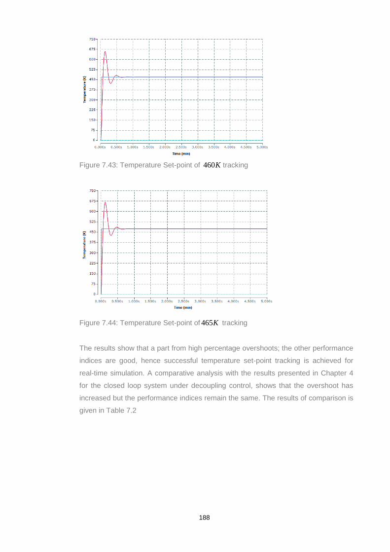
Figure 7.43: Temperature Set-point of 460K tracking
Figure 7.44: Temperature Set-point of 465K tracking
The results show that a part from high percentage overshoots; the other performance
indices are good, hence successful temperature set-point tracking is achieved for
real-time simulation. A comparative analysis with the results presented in Chapter 4
for the closed loop system under decoupling control, shows that the overshoot has
increased but the performance indices remain the same. The results of comparison is
given in Table 7.2
188

Table 7.2: Comparison between the performance indicators of the closed loop concentration and temperature responses under the Matlab/Simulink and the TwinCAT PLC real-time for various magnitudes
closed loop concentration performance indices Matlab/Simulink TwinCAT PLC real-time
Set-point value Rise time (sec)rt Settling time(sec)st
Peak over shoot
PM (%)
Steady state error
(%)sse
Rise time(sec)rt
Settling time(sec)st
Peak over shoot
PM (%)
Steady state error
(%)sse
0.02 Moles/litre. 7.62 27.18 9.58 0 4.25 33 11.0 0 0.04 Moles/litre 7.62 27.18 9.58 0 4.25 33 11.0 0 0.06 Moles/litre 7.62 27.18 9.58 0 4.25 33 11.0 0 0.08 Moles/litre 7.62 27.18 9.58 0 4.25 33 11.0 0 0.1Moles/litre 7.62 27.18 9.58 0 4.25 33 11.0 0 0.12 Moles/litre 7.62 27.18 9.58 0 4.25 33 11.0 0 0.14 Moles/litre 7.62 27.18 9.58 0 4.25 33 11.0 0
closed loop temperature performance indices
Matlab/Simulink TwinCAT PLC real-time Set-point value Rise time (sec)rt Settling time
(sec)st
Peak over shoot
PM (%)
Steady state error
(%)sse
Rise time(sec)rt
Settling time(sec)st
Peak over shoot
PM (%)
Steady state error
(%)sse
435K. 2.79 30 28.2 0 2.79 30 41.9 0 440K 2.79 30 28.2 0 2.79 30 41.9 0 446K 2.79 30 28.2 0 2.79 30 41.9 0 450K 2.79 30 28.2 0 2.79 30 41.9 0 455K 2.79 30 28.2 0 2.79 30 41.9 0 460K 2.79 30 28.2 0 2.79 30 41.9 0 465K 2.79 30 28.2 0 2.79 30 41.9 0
189

Next, the performance of the temperature loop under the influence of the
disturbances on, 1y , 1u and 2u are considered because of the interactions that exist in
the closed loop system. Figures 7.45-7.48 present the temperature responses for
disturbance on 1y . The set-point to be tracked is 450K for all considered
disturbances
Figure 7.45: Temperature Set-point tracking under 31e−± mole/litre disturbance on 1y
Figure 7.46: Temperature Set-point tracking under 34e−± mole/litre disturbance on 1y
190

Figure 7.47: Temperature Set-point tracking under 0.01± mole/litre disturbance on 1y
Figure 7.48: Temperature Set-point tracking under 0.04± mole/litre disturbance on 1y
Good set-point tracking control is realised in real-time. The disturbance on 1y do not
degrade the performance of the temperature loop 2y . Similarly, the performances of
the temperature control loop signal 2( )y when the disturbances are in the junction 1u
are investigated. Figures 7.49-7.52 show the graphs of the responses of the
temperature control loop signal 2y when there are disturbances on 1u of different
magnitudes.
191

Figure 7.49: Temperature Set-point tracking under 10± litres/min disturbance on 1u
Figure 7.50: Temperature Set-point tracking under 40± litres/min disturbance on 1u
Figure 7.51: Temperature Set-point tracking under 80± litres/min disturbance on 1u
192

Figure 7.52: Temperature Set-point tracking under 100± litres/min disturbance on 1u
Figures 7.49-7.52 present the graphs of the real-time responses of the temperature
control loop signal 2y when there are disturbances on 1u of different magnitudes.
Good tracking response is achieved.
Next the disurbance on the temperature loop effects over the temperature loop real-
time behaviour is presented in the section that follows. The first investigation done is
when the disturbance is on the main loop output signal 2y
The responses of Figures 7.53-7.56 show the set point tracking performance of the
temperature for various settings of the disturbance magnitudes.
Figure 7.53: Temperature Set-point tracking under 4K± disturbance on 2y
193

Figure 7.54: Temperature Set-point tracking under 8K± disturbance on 2y
Figure 7.55: Temperature Set-point tracking under 10K± disturbance on 2y
Figure 7.56: Temperature Set-point tracking under 20K± disturbance on 2y
194

Good set-point tracking in real-time control is still achieved. However as the
magnitude of the disturbance is increased, the response becomes noisy.
Similar investigation is done for disturbances on the control signal 2u and the real-
time responses as a result of real time simulations are illustrated in Figures 7.57-7.60
below.
Figure 7.57: Temperature Set-point tracking under 10± litres/min disturbance on 2u
Figure 7.58: Temperature Set-point tracking under 40± litres/min disturbance on 2u
195

Figure 7.59: Temperature Set-point tracking under 80± litres/min disturbance on 2u
Figure 7.60: Temperature Set-point tracking under 100± litres/min disturbance on 2u
Very little effect of disturbance is observed in the performance characteristics of the
temperature tracking response during the real-time simulation. Good tracking
capability is observed. The only limitation is the percentage overshoot.
7.5.3 Decentralized control simulation in Real-time Based on the transformation algorithm listed in section 7.4 above, the algorithms of
the decentralized control methodology developed in Chapter 5 are used for real-time
implementation by downloading the algorithms to the Beckhoff CX5020 PLC for real-
time execution to verify the effectiveness of the control schemes under real-time
environment.
196

7.5.3.1 Model transformation and set-point tracking control for the decentralized closed loop system Figure 7.61: shows the transformed Simulink closed loop MIMO CSTR process under
decentralized control to the corresponding TwinCAT 3 function blocks (modules). The
transformation technique shows that the data and parameter connection are the
same in these two platforms and therefore there is a one to one correspondence of
function blocks between Simulink and TwinCAT platforms.
Figure 7.61: Transformed Simulink decentralized closed loop control system to
TwinCAT 3 function blocks
Next, investigations are made of set point tracking control for both the concentration
and the temperature respectively. Figures 7.62-7.66 present the various step
responses for the concentration set-point tracking when the set point is varied from
0.09 moles/litre to 0.13 moles/litre
Figure 7.62: Concentration set-point of 0.09 moles/litre tracking
197

Figure 7.63: Concentration set-point of 0.1moles/litre tracking
Figure 7.64: Concentration set-point of 0.11moles/litre tracking
Figure 7.65: Concentration set-point of 0.12 moles/litre tracking
198

Figure 7.66: Concentration set-point of 0.13moles/litre tracking
Analyses of the obtained transition behaviours, further confirms that the designed
decentralized controller settings achieve tracking control of the concentration set
point in real-time and therefore the control design is good. As can be seen the set-
point tracking response capabilities for the concentration outputs at different set-point
settings are achieved, though the responses are sluggish. Investigations on the
influences of various magnitudes of disturbances over the process output step
response in real-time are also performed for the developed scheme and presented in
the following subsection
7.5.3.2 Investigation of the process performance for a disturbance on concentration control loop. Next, the effects of disturbances are investigated for the concentration control loop in
real time. The procedure adopted is the same as that for the concentration control
loop in Chapter 5. The difference is that, this time the investigation is done on a real-
time platform. The disturbances are injected to the main concentration control loop at
the outputs 1y . Figures 7.67-7.70 show the real-time responses of the concentration
when the disturbances are at 1y . The set-point is 0.13moles/litre.
199

Figure 7.67: Concentration Set-point tracking under 31e−± moles/litre disturbance on 1y
Figure 7.68: Concentration Set-point tracking under 34e−± moles/litre disturbance on
1y
Figure 7.69: Concentration Set-point tracking under 0.01± moles/litre disturbance on
1y
200

Figure 7.70: Concentration Set-point tracking under 0.04± moles/litre disturbance on
1y
Good tracking control is still achieved in the real-time simulation results. However as
the magnitude of the disturbance is increased, the response becomes noisy as was
investigated in Chapter5.
Next, the effects of the disturbances acting on the temperature output 2y are
investigated. Figures 7.71-7.74 show the real-time responses.
Figure 7.71: Concentration Set-point tracking under 4K± disturbance on 2y
201

Figure 7.72: Concentration Set-point tracking under 8K± disturbance on 2y
Figure 7.73: Concentration Set-point tracking under 10K± disturbance on 2y
Figure 7.74: Concentration Set-point tracking under 20K± disturbance on 2y
202

Decentrarized control scheme can not eliminate completely the effects of the loop
interactions. The results of real-time simulation shows that the magnitude of the
disturbance is important for the smooth set-point tracking. However the concentration
system for the concentration response under real-time simulations is still able to track
the set-point variations, implying that the designed decentralized systems can
achieve its main requirement but needs further improvement.
7.5.3.3 Temperature loop results from simulation for various set-points and disturbances The variation of set-points magnitude influence over the temperature response
performance indices is investigated. The set-point is varied from 450K to 465K in
steps of5K . The responses are illustrated in Figures 7.75-7.78 below.
Figure 7.75: Temperature Set-point of 450K tracking
Figure 7.76: Temperature Set-point of 455K tracking.
203

Figure 7.77: Temperature Set-point of 460K tracking
Figure 7.78: Temperature Set-point of 465K tracking
The results show that a part from the sluggish responses; successful temperature set-
point tracking under real-time simulation is obtained.
Next, the effects of disturbances are investigated for the temperature control loop in
real-time. The procedure adopted is the same as that for the temperature control loop
investigated in Chapter 5. The difference is that, this time the investigation is done on
real-time platform. Figures 7.79-7.82 present real-time temperature the responses
when the actions of the disturbances are at 2y .
204

Figure 7.79: Temperature Set-point tracking under 4K± disturbance on 2y
Figure 7.80: Temperature Set-point tracking under 8K± disturbance on 2y
Figure 7.81: Temperature Set-point tracking under 10K± disturbance on 2y
205

Figure 7.82: Temperature Set-point tracking under 20K± disturbance on 2y
The results of simulation show that the magnitude of the disturbance is important for
the smooth set-point tracking. However the real-time simulation results for the
temperature show the capability to track the set-point variations, implying that the
designed decentralized systems is good even in the presence of the random
disturbances. Figures 7.83-7.86 are the temperature responses when the actions of
the disturbances are at concentration output 1y .
Figure 7.83: Temperature Set-point tracking under 31e−± moles/litre disturbance on 2y
206

Figure 7.84: Temperature Set-point tracking under 34e−± moles/litre disturbance on 1y
Figure 7.85: Temperature Set-point tracking under 0.01± moles/litre disturbance on 1y
Figure 7.86: Temperature Set-point tracking under 0.04± moles/litre disturbance on 1y
207

Good set-point tracking control is realised in real-time. The disturbance effects at 1y
do not degrade on the performance of the temperature loop apart from the sluggish
response. The decentralized control in this case performs well.
A comparative analysis with the results presented in Chapter 5 for the closed loop
system under decentralized control, shows that the overshoot has reduced to but the
time it takes to settle has increased. The results of comparison are given in Table 7.3.
208
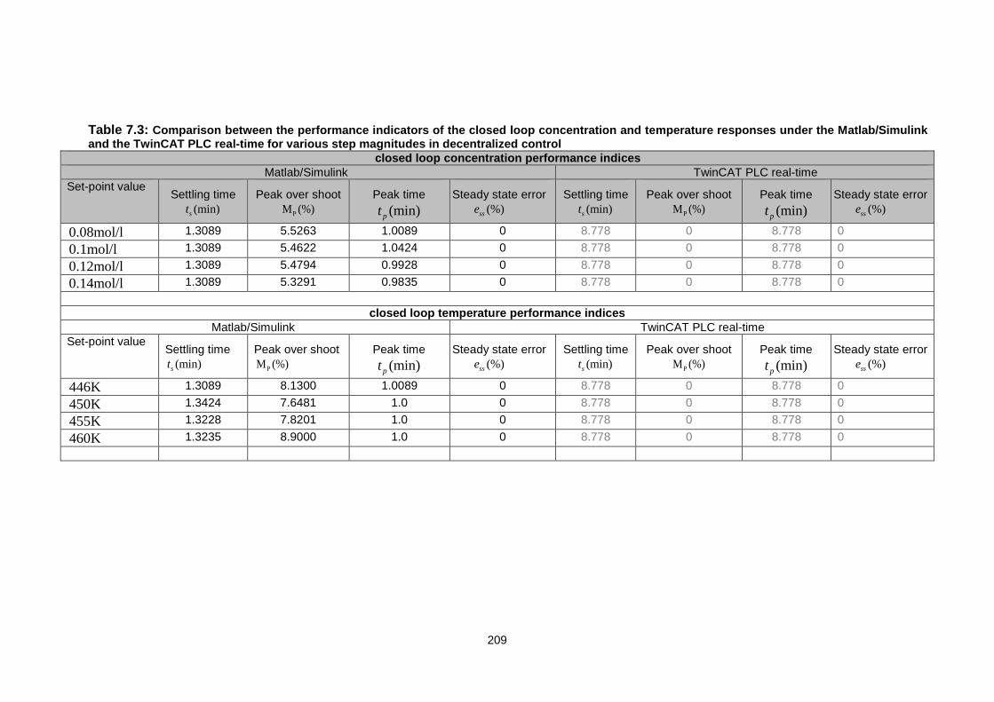
Table 7.3: Comparison between the performance indicators of the closed loop concentration and temperature responses under the Matlab/Simulink and the TwinCAT PLC real-time for various step magnitudes in decentralized control
closed loop concentration performance indices Matlab/Simulink TwinCAT PLC real-time
Set-point value Settling time
(min)st Peak over shoot
PM (%)
Peak time (min)pt
Steady state error
(%)sse
Settling time(min)st
Peak over shootPM (%)
Peak time (min)pt
Steady state error
(%)sse
0.08mol/l 1.3089 5.5263 1.0089 0 8.778 0 8.778 0 0.1mol/l 1.3089 5.4622 1.0424 0 8.778 0 8.778 0 0.12mol/l 1.3089 5.4794 0.9928 0 8.778 0 8.778 0 0.14mol/l 1.3089 5.3291 0.9835 0 8.778 0 8.778 0
closed loop temperature performance indices
Matlab/Simulink TwinCAT PLC real-time Set-point value
Settling time(min)st
Peak over shootPM (%)
Peak time (min)pt
Steady state error
(%)sse
Settling time(min)st
Peak over shootPM (%)
Peak time (min)pt
Steady state error
(%)sse
446K 1.3089 8.1300 1.0089 0 8.778 0 8.778 0 450K 1.3424 7.6481 1.0 0 8.778 0 8.778 0 455K 1.3228 7.8201 1.0 0 8.778 0 8.778 0 460K 1.3235 8.9000 1.0 0 8.778 0 8.778 0
209

7.5.4 Input-Output feedback linearization control simulation in Real-time Based on the transformation algorithm in section 7.4 above, the algorithms of the
Input-Output control methodology developed in Chapter 6 are used for real-time
implementation. This is done by downloading the algorithms to the Beckhoff CX5020
PLC for real-time execution to verify the effectiveness of the control schemes under
real-time environment. The following are the real-time simulation results from the
experiments investigated.
7.5.4.1 Model transformation and set-point tracking control for the input-output feedback linearization closed loop system Figure 7.87: shows the transformed Simulink closed loop MIMO CSTR process under
the I/O feedback linearization control to the corresponding TwinCAT 3 function blocks
(modules). The transformation technique shows that the data and parameter
connection are the same in these two platforms and therefore there is a one to one
correspondence of function blocks between Simulink and TwinCAT platforms.
Figure 7.87: Transformed Simulink Input-Output linearized closed loop to TwinCAT 3
function blocks.
Investigations are done for real-time set point tracking control for both the
concentration and the temperature responses. Figures 7.88-7.93 show the various
step responses for the concentration under the I/O linearized closed loop when the
set point is varied from 0.08moles/litre to 0.13 moles/litre.
210

Figure 7.88: Concentration Set-point of 0.08moles/litre tracking
Figure 7.89: Concentration Set-point of 0.09 moles/litre tracking
Figure 7.90: Concentration Set-point of 0.1moles/litre tracking
211
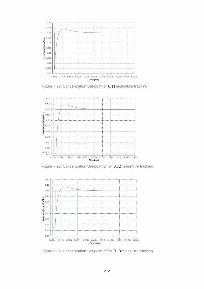
Figure 7.91: Concentration Set-point of 0.11moles/litre tracking
Figure 7.92: Concentration Set-point of for 0.12 moles/litre tracking
Figure 7.93: Concentration Set-point of for 0.13moles/litre tracking
212

Analyses of the concentration real-time behaviour, further confirms that the designed
I/O feedback linearization controller settings achieve good tracking control of the
concentration set point in real-time situation, and therefore the control design is good.
The influences over the real-time process output step response of various
magnitudes of disturbances are also investigated for the developed scheme for the
concentration control loop. The procedure adopted is the same as that for the
concentration control loop in Chapter 6. The difference is that, this time the
investigation is done on a real-time platform. The disturbances are injected to the
main concentration control loop at the outputs 1y .
7.5.4.2 Investigation of the concentration real-time performance for a disturbance on
the concentration output 1y
Figures 7.94-7.97 are the responses when the effects of the disturbances are at 1y
Analyses of the responses, further confirms that the designed I/O feedback
linearization controller settings achieve good tracking control of the concentration set
point in real-time situation as well as rejecting disturbances and therefore the I/O
feedback linearization control design for the concentration loop is good though the
magnitude of disturbance results in a noisy response.
Figure 7.94: Concentration Set-point tracking for 31e−± moles/litre disturbance on 1y
213

Figure 7.95: Concentration Set-point tracking for 34e−± moles/litre disturbance on 1y
Figure 7.96: Concentration Set-point tracking for 0.01± moles/litre disturbance on 1y
Figure 7.97: Concentration Set-point tracking for 0.04± moles/litre disturbance on 1y
214

In appendix C, the algorithm that simulates the nonlinear linearizing feedback control
response of the closed loop MIMO CSTR model for various magnitudes of set-point
step changes, as well as disturbances at the outputs (y1) and (y2) is provided. The
Simulink closed loop model to be simulated is li_2015.and provided in appendix F.
A comparative analysis with the results presented in Chapter 6 for the closed loop
system under I/O feedback linearization control, shows that the various performance
indicators are almost similar. The results of comparison are given in Table 7.4.
215

Table 7.4: Comparison between the performance indicators of the closed loop concentration responses under the Matlab/Simulink and the TwinCAT PLC real-time for various step magnitudes in I/O feedback linearization control
closed loop concentration performance indices Matlab/Simulink TwinCAT PLC real-time
Set-point
value Settling
Time (min)st
Rise time(min)rt
Peak over
shoot PM (%)
Peak time (min)st
Steady state
error (%)sse
Settling
Time (min)st
Rise time(min)rt
Peak over
shoot PM (%)
Peak time (min)st
Steady state
error (%)sse
0.08mol/l 1.9800 0.900 10.5263 056 0 2.1 0.3 10.0 0.6 0 0.09mol/l 1.9800 0.900 10.5075 0.56 0 2.1 0.3 10.0 0.6 0 0.10mol/l 1.9800 0.900 10.5042 0.56 0 2.1 0.3 10.0 0.6 0 0.11mol/l 1.9800 0.900 10.6508 0.56 0 2.1 0.3 10.0 0.6 0
0.12mol/l 1.9800 0.900 10.5022 0.56 0 2.1 0.3 10.0 0.6 0
0.13mol/l 1.9800 0.900 10.5947 0.56 0 2.1 0.3 10.0 0.6 0
216

7.6 Discussion of the Results from the simulations Based on the steps required for model transformation the between the
Matlab/Simulink to the TwinCAT 3 functional blocks, the algorithms of the control
design methodologies developed in Chapters 4. 5 and 6, simulation results are used
to verify the suitability of the control to find whether the effective set-point tracking
control and disturbance effect minimisation for the output variables can be achieved
in real-time using the transformed Simulink blocks to the TwinCAT 3 functional
blocks, then downloaded to the Beckhoff CX5020 PLC for real-time execution. Good
set-point tracking control is achieved for the MIMO closed loop CSTR process for the
considered cases of the dynamic decoupling and decentralized control. Similarly, the
effects of disturbances are investigated. The CSTR process performance under the
input-output feedback linearization transformed TwinCAT functional modules
achieved good set-point tracking with these disturbances minimization for the
concentration control loop under all the cases considered. In the case of the
temperature control loop developed, the objective for real-time control for the
particular loop is not achieved at the moment. This implies that further investigation
on the control design for this particular loop should be done.
7.7 Conclusion The simulation results from the investigation done between Simulink and TwinCAT 3
software platforms in the case of the model transformation and closed loop simulation
of the process for the considered cases have shown the suitability and the potentials
of merging the Matlab/Simulink control function blocks into the TwinCAT 3.1 function
blocks in real-time .The merits derived from such integration implies that the existing
software and software components can be re-used This is in line with one of the IEC
6144 standard requirements such as portability and interoperability. Similarly, the
simplification of programming applications is greatly achieved. The investigation has
also shown that the integration the of Matlab/Simulink models running in the TwinCAT
3.1 PLC do not need any modification, hence confirming that the TwinCAT 3.1
development platform can be used for the design and implementation of controllers
from different platforms.
217

CHAPTER EIGHT CONCLUSION, DELIVERABLES, APPLICATIONS AND FUTURE WORK
8.1 Introduction This research focuses on the control design strategies for the Continuous Stirred
Tank Reactor (CSTR) process. To control such a process a careful design strategy is
required because of the nonlinearities, loop interaction and the potentially unstable
dynamics. In these systems, linear control methods alone may not perform
satisfactorily. The thesis describes the developed methods for the design and
implementation of the closed loop system in the Beckhoff PLC Twin CAT 3.1 real-time
(Beckhoff Automation) and Matlab/Simulink (www.mathworks.com) environment are
used to test the effectiveness of the developed models and methods in realizing the
thesis objectives. Comparative performance analyses using the two platforms
(Matlab/Simulink and TwinCAT 3.1) such as configurability and decentralization
assessment are carried out. The main research questions formulated were:
• Whether linear or nonlinear methods for design of controllers for the MIMO
nonlinear CSTR processes could contribute to better performance of the closed
loop system for various process conditions, as changing set point and
disturbances
• The capability of the software TwinCAT 3.1 to be applied for programming of the
developed decentralized distributed closed loop systems and to perform real-time
simulation and lastly,
• The capability of the real-time Twin CAT 3.1 environment to assure the same
results of the closed loop systems through real-time simulation in comparison with
the situation in Matlab/Simulink environment.
Three different controller design approaches (dynamic decoupling control,
Dentralized and I/O feedback linearization) are investigated. Simulations are used to
demonstrate the suitability of the closed loop control systems in line with the
functional block programming concepts. It is envisaged that the thesis contributions
will provide a platform for understanding the concepts of the TwinCAT 3.1 software
environment and its application to practical distributed control systems. The
developed guide for the model transformation between the two environments
(Matlab/Simulink and TwinCAT 3.1) for modelling, data analysis and real-time
simulation can be very useful for further research investigations or engineering
project implementation in industry.
The simulation results from the investigations done between Simulink and TwinCAT 3
software platforms in regard to the model transformation and control of the closed
loop process for all the considered cases have shown the suitability and the
potentials of merging the Matlab/Simulink control function blocks into the TwinCAT
218

3.1 function blocks in real-time. The merits derived from such integration imply that
the existing software and software components can be re-used. This is in line with the
IEC 6144 standard requirements such as portability and interoperability. Similarly, the
simplification of programming applications is greatly achieved. The investigation has
also shown that the integration the of Matlab/Simulink models running in the TwinCAT
3.1 PLC do not need any modification, hence confirming that the TwinCAT 3.1
development platform can be used for the design and implementation of controllers
from different vendor platforms.
In this chapter, section 8.2 describes the problems solved in this thesis. In section 8.3
the thesis deliverables are discussed while section 8.4 lists the software algorithms
developed in this thesis. In section 8.5, the applications relevant to the deliverables of
the thesis are discussed. Section 8.6 and 8.7 presents future research work and the
author’s publication respectively. Section 8.8 gives the conclusion of the chapter.
8.2 Problems solved in the thesis These problems can be divided into two main groups:
• Design-based
• Implementation-based.
8.2.1 Design-based Sub-problem1: Formulation of the mathematical model for the MIMO nonlinear CSTR
plant
Sub-problem 2: Development of methods for linearization of the nonlinear Multi-Input
Multi-Output (MIMO) CSTR process and methods for analysing the stability of the
system
Sub-problem 3: Development of methods for the analysis and design of linear
controllers using dynamic decoupling techniques relevant to the MIMO nonlinear
CSTR plant model.
Sub-problem 4: Development of methods for the analysis and design of linear
controllers using decentralized control techniques relevant to the MIMO nonlinear
CSTR plant model.
Sub-problem 5: Development of methods for the analysis and design of nonlinear
controllers using I/O feedback linearization techniques relevant to the MIMO
nonlinear CSTR plant model.
8.2.2 Implementation-based sub-problem. Sub-problem1: Development of a software model of the nonlinear MIMO CSTR. This
is done in the Matlab/Simulink platform and investigation by simulations
219

Sub-problem 2: Performance of simulations for the developed decoupled closed loop
control system in the Matlab/Simulink environment
Sub-problem: 3 Simulations for the developed decentralized closed loop control
system in the Matlab/Simulink environment for various cases of set-points and
disturbances.
Sub-problem: 4 Simulations of the developed closed loop input/output feedback
linearized control system in the Matlab/Simulink environment for various cases of set-
points and disturbances.
Sub-problem: 5.Transformation of the developed software for simulation of the closed
loop systems from the Matlab/Simulink platform to the TwinCAT 3 simulation
environment (Function blocks).
Sub-problem: 6 .Perform simulations in real-time for the closed loop systems in the
TwinCAT PLC platform thereby demonstrating the effectiveness of the transformation.
8.3. The thesis deliverables The deliverables of this thesis are as follows:
8.3.1 Comprehensive Literature review. The review on the relevant aspects of the areas of concern to this research is done
A review of the existing literature for the CSTR modelling and the control design is
presented and a review on the IEC 61499 standard and the distributed control in
process industry is done. Several control strategies and problems are reviewed
based on the model-based control concepts. Successful application of these control
strategies has been reported with good results. Similarly a number of the review
papers on the new IEC 61499 standard as well as its real time applicability are
reviewed and discussed. The feasibility to integrate the concepts of the
Matlab/Simulink transformation to the Functional block programming environment of
TwinCAT 3.1, and utilize them to design and implement nonlinear controllers for the
CSTR nonlinear plant are also reviewed.
8.3.2 Mathematical modelling of the nonlinear MIMO CSTR in the Matlab/Simulink platform. The CSTR process is derived based on the first principles and simulation studies are
performed. The CSTR dynamics mathematical model is formulated based on the
assumption that the model represents the ideal case, where the feed flow and the
coolant flow rates respectively are the considered the inputs and the product
concentration and the temperature respectively are the monitored outputs. The
simulation results demonstrate that the CSTR process exhibits highly nonlinear
dynamic behaviour because of the coupling and the inter-relationships of the states, 220

the exponential dependence of each state on the reactor temperature, as well as the
reaction rate being an exponential function of the temperature.
8.3.3 Design of the dynamic decoupling controller for the MIMO CSTR process Difficulties caused by the interacting loops for the MIMO systems are the major
obstacle to the controllers designed for such systems. Interactions occur when there
are coupling between the control variables and between the process variables
thereby affecting the states of the controlled variables. To address the problem of
loop interactions a simple dynamic decoupling mechanism is designed. After this two
SISO PI controllers are designed directly for the resulting decoupled system and
independently by applying pole placement technique to tune the individual loops for
tracking control of the output variables. The results of simulation studies show that
the dynamic decoupling control scheme together with the Single-Input Single-Output
(SISO) PI control algorithms are capable of achieving effective set-point tracking
control in the situation where noise disturbances are present, implying that the
designed decoupling systems is robust towards the disturbances (from the point of
view of stability).
8.3.4 Design of the decentralized control for the MIMO CSTR process The design, implementation and simulation of the decentralized internal model
controller (IMC)-based PID for the MIMO CSTR system are performed. For the design
of the controllers, pairing among the input-output variables is done using the Relative
Gain Array (RGA) analysis. Then two SISO PID controllers are designed directly for
the diagonal transfer functions for the developed closed loop control system that
consists of the process model and independently using internal model controller. After
the independent tuning of the individual loops, a detuning factor for each individual
loop is proposed to compensate for the off-diagonal matrix transfer function
interactions. Simulation results show the suitability of the developed control law in
achieving tracking control with good disturbance rejection capabilities.
8.3.5 Design of the I/O feedback nonlinear linearized control for the MIMO CSTR process This control technique applies a feedback signal to remove the inherent nonlinear
characteristics in a system by creating linear differential relationship between the
system’s outputs and the newly defined synthetic inputs. The nonlinear linearizing
controller, for controlling the concentration and reactor temperature is first designed.
Then two linear PI controllers for the respective loops are independently designed
using the pole-placement techniques. Finally closed loop simulations are performed
221

to show the suitability of the developed controllers. Moreover, the performance is
checked with noisy disturbances on the control loops. The results of this analysis
show the suitability of the developed control law in achieving set-point tracking
control. The proposed control exhibits satisfactory performance in the presence of
disturbances with limited magnitudes.
8.3.6 Development of transformation procedure for the developed software from the Matlab/Simulink environment to Beckhoff TwinCAT 3 real-time environment for real-time simulation. An algorithm detailing the steps of the software transformation from the
Matlab/Simulink platform to the TwinCAT 3 real-time environment is developed. It can
be used as a guide for further research investigations. The real-time simulation
results using the Beckhoff PLC in which the transformed to software platforms is
downloaded have shown the suitability and the potentials of merging the
Matlab/Simulink works into the TwinCAT 3.1 platform .The derived benefits of such
integration implies that the interoperability and portability of software components is
possible. This is in line with one of the IEC 61499 standard requirements. Similarly,
the simplification of the programming applications is greatly achieved. The
investigation has also verified the possibility of integrating the Matlab/Simulink models
to run in the PLC without any alteration to the model, hence implying that the
TwinCAT 3 development platform can be used for the design and implementation of
controllers from different platforms
8.6 Future work Further investigations on how the methods and algorithms can be developed to use
of both for the hardware simulation and the controller simulation in real-time is
necessary so that real-time distributed control for the process can be achieved.
8.4 Developed software. The methods and algorithms developed in the thesis and which are used for
development of Matlab/Simulink software investigations and simulations of the
various models developed are as given in Tables 8.1 for the Matlab script files and in
Table 8.2 for the Simulink models.
Table8.1: Matlab m-files developed for the thesis
Script file
Appendix Function
openloop_cstr.m. Appendix A1 Presents the function file for the MIMO CSTR process with the parameter values that are used for the development of different models.
222

in Simulink openloop_cstrsim.m Appendix A2 The main file for the CSTR process model for
simulating the function openloop_cstr.m for various magnitudes of perturbations over the initial steady state conditions by a plus or minus 10% from the nominal values.
linearize_mod.m APPENDIX B Script file for the linearization of the CSTR process model by finding the Jacobian matrices, the state space matrices and the transfer functions of the state space model
Conc_code_li_2015.m
APPENDIX C This algorithm simulates the nonlinear linearizing feedback control response of the closed loop MIMO CSTR model for various magnitudes of set-point step changes, as well as disturbances at the outputs (y1) and (y2). The Simulink closed loop model to be simulated is li_2015.
dyn_conc_code) APPENDIX D This file simulates the dynamic decoupling control response of the closed loop MIMO CSTR model for various magnitudes of the set-point step changes, as well as disturbances at the outputs (y1),y(2) and the interaction junctions (u1) and (u2). The Simulink closed loop model to be simulated is dyn_dec_2015.
decentsim.m APPENDIX E1 This file simulates the diagonal decentralized closed loop response of the system for various values of the set-point changes, as well as disturbances at the output (y1) and the interaction junction (u1). The Simulink closed loop models to be simulated are diag_decent_temp’ and 'decentconc_2015'.
conc_code_4.m APPENDIX E2 This file simulates the decentralized control response of the closed loop MIMO CSTR with and without detuning, for various magnitudes of set-point step changes as well as disturbances. The Simulink closed loop model to be simulated is decent1_2015.
Table 8.2: Simulink models developed in the thesis
Simulink models Appendix Function decent_2015. Model of MIMO closed
loop decentralized control Model for the MIMO closed loop system under decentralized control
dyn_dec_2015 Model of MIMO closed loop dynamic decoupling control
The MIMO closed loop under dynamic decoupling control
decen1_2015 Model of MIMO closed loop decentralized control incorporating the detuning
The closed loop MIMO system under decentralized control incorporating the detuning
li_2015 Model of MIMO closed loop I/O feedback linearization control
The MIMO closed loop system under I/O feedback linearization control
openloop_cstr_mod Model of MIMO open loop CSTR system
The open loop CSTR process
diag_decent_temp Model of diagonal temperature closed loop control
The temperature diagonal closed loop control system
decenconc_2015 Model of diagonal concentration closed loop control
The concentration diagonal closed loop control system
223

The methods and algorithms developed in the thesis and which are used for
development of TwinCAT software investigations and simulations of the various
models developed are as given in Table 8.3 for the Matlab script files, Table 8.2 for
the Simulink models, Table 8.3 the Simulink models for TwinCAT 3 transformation
and Table 8.4 the generated TwinCAT function blocks.
Table 8.3: Simulink models transformed to TwinCAT 3 functional blocks
Simulink models for TwinCAT 3 transformation
Appendix Function
dyn_dec_2015_ds1 Model of MIMO closed loop dynamic decoupling control (Appendix F1)
Transform the MIMO closed loop control by dynamic decoupling to equivalent TwinCAT 3 functional blocks
decen1_2015_twin Model of MIMO closed loop decentralized control(Appendix F2)
Transform the closed loop MIMO by decentralized block to equivalent TwinCAT 3 functional blocks
li_2015_c Model of MIMO closed loop I/O feedback linearization l(Appendix F2)
Simulates the closed loop MIMO control by I/O feedback linearization to equivalent TwinCAT 3 functional blocks
Table8.4: TwinCAT 3 models developed Simulink models for TwinCAT 3 transformation
Appendix Function
dyn_dec_2015.tcm Model of MIMO closed loop dynamic decoupling control (Appendix. G1)
Transform the MIMO closed loop control by dynamic decoupling to equivalent TwinCAT 3 functional blocks
decen1_2015.tcm Model of MIMO closed loop decentralized control (Appendix. G2)
Transform the closed loop MIMO by decentralized block to equivalent TwinCAT 3 functional blocks
li_2015_c.tcm Model of MIMO closed loop I/O feedback linearization l (Appendix. G3)
Simulates the closed loop MIMO control by I/O feedback linearization to equivalent TwinCAT 3 functional blocks
8.5 Application of the results from this thesis. The methods and algorithms resulting from this thesis can form a cornerstone for:
• Further research investigations or engineering project implementation in industry
• Use as a guide or algorithm for the transformation of the developed software from
Matlab/Simulink environment to the TwinCAT 3.1 simulation environment
• Educational and training institutions in the field of engineering and real-time
automation
224

8.7 Publications
• Muga, J., R. Tzoneva, S. Krishnamurthy (2016). Design, implementation, and
real-time simulation of a controller-based decoupled CSTR MIMO closed loop
system. International Journal of Electrical Engineering & Technology (IJEET), v.
7, Iss. 3, pp. 126-144
• Muga, J., R. Tzoneva (2016) Decentralized controller design and PLC
implementation for the TITO CSTR process, Journal of the South African Institute
of Electrical Engineering (under review)
• Muga J., R. Tzoneva (2015) Design, implementation, and performance
comparison of linear and nonlinear control strategies for the TITO CSTR
process, Control Engineering and Technology (under review)
• Muga, J., R. Tzoneva (2014). Design and Implementation of IEC 61499
Standard-based Neural Networks Nonlinear controllers Using Functional Block
Programming In Distributed Control Platform. A celebration of Research
excellence at Cape Peninsula University of Technology. pp. 60 Research day
27th November, 2014 poster exhibition
8.8 Conclusion This chapter presents an overview of the thesis deliverables, developed methods and
software, the areas applicable to the thesis deliverable, the possible future work to
improve on the thesis and the publications resulting from the investigations.
225

REFERENCES
Allgower F. & Doyle. F.J. 1997. Nonlinear process control–which way to the Promised Land. 5th international conference on chemical process control, 93: 24-45. Alvarez-Ramírez, J. 1991. Stability of a class of uncertain continuous stirred chemical reactors with a nonlinear feedback. Chemical Engineering Science, 49(11): 1743–1748. Anitha, P.M. & Subbulekshmi., D. 2011. RNGA algorithm of nonlinear chemical reactor. 2011 International Conference on Emerging Trends in Electrical and Computer Technology. Antonelli, R. & Astolfi, A. 2003. Continuous stirred tank reactors: easy to stabilize? Automatica, 33: 1817–1827. Alsafi, Y. & Vyatkin, V. Ontology-based reconfiguration agent for intelligent mechatronic systems in flexible manufacturing. Robotics and Computer-Integrated Manufacturing, 26: 381–391. Aris, R. & Amundson, N.R. 2000. An analysis of chemical reactor stability and control—I. Chemical Engineering Science, 7(8): 121–131. B., V., Ponnusamy, L. & K., T. 2015. Design and optimization of multivariable controller for CSTR system. 2015 International Conference on Robotics, Automation, Control and Embedded Systems (RACE), (Article number: 7097271). Bakosova, M. & Vasickaninova, A. 2009. Simulation Of Robust Stabilization Of A Chemical Reactor. ECMS 2009 Proceedings edited by J. Otamendi, A. Bargiela, J. L. Montes, L. M. Doncel Pedrera: 570–576. Balakotaiah, V., & Luss, D. 1981. Analysis of the Multiplicity Patterns of a CSTR. Chem. Eng. Comm. 13: 111. Bansode, P. & Jadhav, S.P. 2015. Decoupling based predictive control analysis of a continuous stirred tank reactor. 2015 International Conference on Industrial Instrumentation and Control (ICIC): 816–820. Bartolini, G., Pisano, A. & Usai, E. 2009. On the second-order sliding mode control of nonlinear systems with uncertain control direction. Automatica, 45: 2982–2985. Benenati, R.F. 1973. Process modeling, simulation and control for chemical engineers, William L. Luyben, McGraw-Hill, New York, 1973. 558 pp. Journal of Polymer Science: Polymer Letters Edition J. Polym. Sci. B Polym. Lett. Ed.: 289–290. Bequette, B.W. 2003. Nonlinear control of chemical processes: a review. Industrial & Engineering Chemistry Research Ind. Eng. Chem. Res., 30: 1391–1413. Black, G. & Vyatkin, V. 2010. Intelligent Component-based Automation of Baggage Handling Systems with IEC 61499. IEEE Transactions on Automation Science and Engineering. 7(2): 337-351 Bristol, E. 1966. On a new measure of interaction for multivariable process control. IEEE Transactions on Automatic Control IEEE Trans. Automat. Contr., 11: 133–134. Cai, W.-J., Ni, W., He, M.-J. & Ni, C.-Y. 2008. Normalized Decoupling MIMO Process Control System Design. Industrial & Engineering Chemistry Research Ind. Eng. Chem. Res., 47: 7347–7356.
226

Campanelli, S., Foglia, P. & Prete, C.A. 2015. An architecture to integrate IEC 61131-3 systems in an IEC 61499 distributed solution. Computers in Industry, 72: 47–67. Chen, J., Yang, W., Luo, A.U. & Wu, X. 2013. The Multi-Point Temperature Decoupling Control Method and its Realization. AMM Applied Mechanics and Materials, 321(324): 2237–2240. Chen, Z.-F. & Zhang, Y. 2014. Robust control of a class of non-affine nonlinear systems by state and output feedback. Journal of Central South University J. Cent. South Univ., 21(4): 1322–1328. Chen, Z., Zhang, Y., Yang, L., Zeng, Q. & Liu, Z. 2012. Robust Output Tracking Control of a Class of Highly Uncertain Non-affine Nonlinear Systems. International Journal of Advancements in Computing Technology IJACT, 4(21): 607–614. Chen, M., Ge, S.S. & Ren, B. 2011. Adaptive tracking control of uncertain MIMO nonlinear systems with input constraints. Automatica, 47(3): 452–465. Chou, Y.-S. & King, C.-Y. 1996. Two-degree-of-freedom controllers for multivariable model-matching systems: Application to a continuous stirred tank reactor (CSTR). Optimal Control Applications and Methods Optim. Control Appl. Meth., 17: 3–27. Chi, T.C. & Chyi, S-D., 2001. Robust controller design for a class of nonlinear uncertain chemical processes. Journal of Process control. 11: 469-482. Copot, D., Ionescu, C., Hernandez, A., Thybaut, J. & Keyser, R.D. 2015. Development of a control strategy for efficient operation of a CSTR reactor. 2015 19th International Conference on System Theory, Control and Computing (ICSTCC): 717–722. Czeczot, J., 2006. Balance-based adaptive control methodology and its application to the non-isothermal CSTR, Chemical Engineering and Processing 45: 359–371 Dai, W. & Vyatkin, V. 2010. Redesign distributed IEC 61131-3 PLC system in IEC 61499 function blocks. 2010 IEEE 15th Conference on Emerging Technologies & Factory Automation (ETFA 2010). Dai, W. & Vyatkin, V. 2010. On migration from PLCs to IEC 61499: Addressing the data handling issues. 2010 8th IEEE International Conference on Industrial Informatics. Desoer, C. & Wang, Y.-T. 1980. Foundations of feedback theory for nonlinear dynamical systems. IEEE Trans. Circuits Syst. IEEE Transactions on Circuits and Systems, 27(2): 104–123. Dubinin, V., Vyatkin, V., & Pfeiffer, T. 2005. 'Engineering of Validatable Automation Systems Based on an Extension of UML Combined With Function Blocks of IEC 61499. IEEE International Conference on Robotics and Automation. Proceedings of ICRA 2005, Barcelona. 4007-4012. Enqvist, M. & Ljung, L. 2004. Estimating nonlinear systems in a neighborhood of LTI-approximants. Proceedings of the 41st IEEE Conference on Decision and Control, 2002.: 639–644. Fruehauf, P.S., Chien, I.-L. & Lauritsen, M.D. 1990. Simplified IMC-PID tuning rules. ISA Transactions, 86(33): 43–59. Fu, Y. & Chai, T. 2011. Robust self-tuning PI decoupling control of uncertain multivariable systems. Int. J. Adapt. Control Signal Process. International Journal of Adaptive Control and
227

Signal Processing, 26(4): 316–332. Gagnon, E., Pomerleau, A. & Desbiens, A. 1998. Simplified, ideal or inverted decoupling? ISA Transactions, 37: 265–276. Ganesh, P. & Chidambaram, M. 2010. Multivariable controller tuning for non-square systems by genetic algorithm. Proceedings of 2005 International Conference on Intelligent Sensing and Information Processing, 24(1): 17–22. Gao, J., & Budman, H.M. 2005 Design of robust gain-scheduled PI controllers for nonlinear processes. Journal of Process Control 15: 807–817. Garelli, F., Mantz, R. & Battista, H.D. 2006. Limiting interactions in decentralized control of MIMO systems. Journal of Process Control, 16(5): 473–483. Garrido, J., Vázquez, F. & Morilla, F. 2014. Multivariable PID control by decoupling. International Journal of Systems Science: 1–19. Ghosh, A. & Das, S. 2012. Decoupled periodic compensation for multi-channel output gain margin improvement of continuous-time MIMO plants. IET Control Theory & Applications IET Control Theory Appl., 6(11): 1735–1740. G., L. & Ray, G. 2014. A Set of Stabilizing PID Controllers for Multi input-Multi output Systems. International Journal of Control and Automation IJCA, 7(4): 175–190. Grosdidier, P. & Morari, M. 1987. Interaction measures for systems under decentralized control. Automatica, 22: 309–319. Golubitsky, M. & Keyfitz, B.L. 1980. A qualitative study of the steady-state solutions for continuous flow stirred tank chemical reactor. Society for Industrial and Applied Mathematics. 11(2) Guay, M., Dier, R., Hahn, J. & Mclellan, P. 2005. Effect of process nonlinearity on linear quadratic regulator performance. Journal of Process Control, 15: 113–124. Hadisujoto, B., Refai, R., Chen, D. & Moon, T.J. 2010. Dynamic Thermal Model of PEM Fuel Cells for MIMO Control Design. ASME 2010 Dynamic Systems and Control Conference, Volume 1, 1. Hahn, J., Mönnigmann, M. & Marquardt, W. 2004. A method for robustness analysis of controlled nonlinear systems. Chemical Engineering Science, 59: 4325–4338. Hammer, J. 2014. State feedback control of nonlinear systems: a simple approach. International Journal of Control, 87(1): 143–160. Hanisch, H.M., Lobov, A., Martinez Lastra, J.L., Tuokko, R., & Vyatkin, V. 2006. Formal Validation of Intelligent Automated Production Systems towards Industrial Applications. International Journal of Manufacturing Technology and Management.8(1):75-86 Henson, M.A. & Seborg, D.E. 1990. Input-output linearization of general nonlinear processes. AIChE Journal AIChE J., 36: 1753–1757. Holobloc, Inc,-Resources for the new generation. (www.holobloc.com) Hovd, M. & Skogestad, S. 1994. Improved independent design of robust decentralized controllers. Journal of Process Control, 3(1): 43–51.
228

Hu, W., Cai, W.-J. & Xiao, G. 2010. Decentralized Control System Design for MIMO Processes with Integrators/Differentiators. Industrial & Engineering Chemistry Research Ind. Eng. Chem. Res., 49(24): 12521–12528. Jevtović, B.T. & Mataušek, M.R. 2010. PID controller design of TITO system based on ideal decoupler. Journal of Process Control, 20: 869–876. Jiao, X., Yan-Ping, Q., Wan-Cheng, W. & Xiao-Xiao, J. 2015. A nonlinear control method of multi-input multi-output nonlinear non-minimum phase system. 2015 34th Chinese Control Conference (CCC): 748–753. Jin, Q.-B., Wang, Y.-F., Wang, Q., Liu, Q. & Tian, Y.-Q. 2014. Reflexive Decoupling Control Based on Singular Value Decomposition for Multivariable System with Time Delays. J. Chem. Eng. Japan / JCEJ J. Chem. Eng. Japan jcej Journal Of Chemical Engineering Of Japan, 47(1): 69–77. Jones, R. & Tham, M. 2006. Reducing Interactions in Decentralized Control Schemes. 2006 SICE-ICASE International Joint Conference. Jouili, K., Charfeddine, S. & Jerbi, H. 2008. An Advanced Geometric Approach of Input-Output Linearization for Nonlinear Control of a CSTR. 2008 Second UKSIM European Symposium on Computer Modeling and Simulation: 353–358. Jyothi, S.N., Aravind, S. & Chidambaram, M., 2001. Design on PI/PID Controllers for Systems with a Zero. Indian Chem. Eng., 43: 288-293. Isidori, A. Nonlinear Control Systems, 3rd edition, Springer Verlag, London, 1995. Kaldmäe, A. & Moog, C.H. 2015. Disturbance Decoupling of Time Delay Systems. Asian Journal of Control. Kamala, N., Thyagarajan, T. & Renganathan, S. 2012. Multivariable control of nonlinear process using soft computing techniques. Journal of Advances in Information Technology JAIT, 3(1): 48–56. Kravaris, C. & Kantor, J.C. 1990. Geometric methods for nonlinear process control. 1. Background. Industrial & Engineering Chemistry Research Ind. Eng. Chem. Res., 29: 2295–2310. Kravaris, C. & Kantor, J.C. 1990. Geometric methods for nonlinear process control. 2. Controller synthesis. Industrial & Engineering Chemistry Research Ind. Eng. Chem. Res., 29(12): 2310–2323. Kruger, K. & Basson, A. 2013. Multi-agent Systems vs IEC 61499 for Holonic Resource Control in Reconfigurable Systems. Procedia CIRP, (7): 503–508. Kumar, N. & Khanduja, N. 2012. Mathematical modeling and simulation of CSTR using MIT rule. 2012 IEEE 5th India International Conference on Power Electronics (IICPE). Kurniawan, E., Cao, Z. & Man, Z. 2013. Design of decentralized repetitive control of linear MIMO system. 2013 IEEE 8th Conference on Industrial Electronics and Applications (ICIEA), 12(5): 427–432. Kwon, H.-Y. & Choi, H.-L. 2014. Gain scheduling control of nonlinear systems based on approximate input-output linearization. International Journal of Control, Automation and Systems Int. J. Control Autom. Syst., 12(5): 1131–1137.
229

Lee, I.H., Choi, J.W. & Kim, M.S. 2011. Studies on the heating capacity control of a multi-type heat pump system applying a multi-input multi-output (MIMO) method. International Journal of Refrigeration, 34(2): 416–428. Lengare, M., Chile, R. & Waghmare, L. 2012. Design of decentralized controllers for MIMO processes. Computers & Electrical Engineering, 38(1): 140–147. Li, D.-J., Zhang, J., Cui, Y. & Liu, L. 2012. Intelligent control of nonlinear systems with application to chemical reactor recycle. Neural Comput & Applic Neural Computing and Applications, 23(5): 1495–1502. Liu, R.-J., Liu, G.-P. & Wu, M. 2012. A novel decoupling control method for multivariable systems with disturbances. Proceedings of 2012 UKACC International Conference on Control: 76–80. Liu, Y.-J. & Wang, W. 2011. Adaptive output feedback control of uncertain nonlinear systems based on dynamic surface control technique. International Journal of Robust and Nonlinear Control Int. J. Robust Nonlinear Control, 30(6): 945–958. Luyben, W.L. 1986. Simple method for tuning SISO controllers in multivariable systems. Industrial & Engineering Chemistry Process Design and Development Ind. Eng. Chem. Proc. Des. Dev., 25: 654–660. Mulubika, C. & Basson, A. H. 2013. Comparison of IEC 61499 and Agent Based Control for a Reconfigurable Manufacturing Subsystem. International Conference on Competitive Manufacturing (COMA): Maghade, D. & Patre, B. 2012. Decentralized PI/PID controllers based on gain and phase margin specifications for TITO processes. ISA Transactions, 51: 550–558. Manikandan, R., Vinodha, R., Lincoln, S.A. & Prakash, J. 2014. Design and simulation of model based controllers for 2x2 CSTR process. 2014 International Conference on Green Computing Communication and Electrical Engineering (ICGCCEE): 1–6. Marinescu, B. 2010. Output feedback pole placement for linear time-varying systems with application to the control of nonlinear systems. Automatica, 46: 1524–1530. Mehta, U. & Majhi, S. 2011. On-line relay test for automatic tuning of PI controllers for stable processes. Transactions of the Institute of Measurement and Control, 34(7): 903–913. Mohamed, B., Bachir, D., Abdellah, M. & Mohammed, C. 2012. Journal of the Korean Mathematical Society. Journal of the Korean Mathematical Society, 49(3): 641–658. Nordfeldt, P. & Hägglund, T. 2006. Decoupler and PID controller design of TITO systems. Journal of Process Control, 16: 923–936. Nunes, D.C., Pinto, J.E.M.G., Fonseca, D.G.V., Maitelli, A.L. & Araújo, F.M.U. 2014. Relay Based PID Auto-tuning Applied to a Multivariable Level Control System. Proceedings of the 11th International Conference on Informatics in Control, Automation and Robotics, 1(1-2). Patil, S., Sorouri, M. & Vyatkin, V. 2012. Formal Verification of Intelligent Mechatronic Systems with Decentralized Control Logic. IEEE Conference on Emerging Technologies and Factory Automation, ETFA. Krakow, Poland Pottman, M. & Seborg, D.E. 1992. Identification of non-linear processes using reciprocal multiquadric functions. Journal of Process Control, 2: 189–203.
230

Pu, Y. & Yu-Hong, W. 2015. Explicit model predictive control of CSTR system based on PWA model. 2015 34th Chinese Control Conference (CCC): 2304–2308. Rajapandiyan, C. & Chidambaram, M. 2012. Controller Design for MIMO Processes Based on Simple Decoupled Equivalent Transfer Functions and Simplified Decoupler. Industrial & Engineering Chemistry Research Ind. Eng. Chem. Res., 51(38): 12398–12410. Rehan, M., Tahir, F., Iqbal, N. & Mustafa, G. 2008. Modeling, simulation and decentralized control of a nonlinear coupled tank system. 2008 Second International Conference on Electrical Engineering. Rehman, O.U. & Petersen, I.R. 2015. Using Inverse Nonlinearities in Robust Output Feedback Guaranteed Cost Control of Nonlinear Systems. IEEE Transactions on Automatic Control IEEE Trans. Automat. Contr., 60(4): 1139–1144. Rosinova, D. 2012. Decentralized Robust Control of MIMO Systems: Quadruple Tank Case Study. 9th IFAC Symposium Advances in Control Education. Rockwell Automation/Holobloc, Inc (http://www.fb61499.com/tools.html). Russo, L.P. & Bequette, B.W. 1995. Impact of process design on the multiplicity behavior of a jacketed exothermic CSTR. AIChE Journal AIChE J., Vol. 41(1): 135–147. Sahoo, N., Panigrahi, B., Dash, P. & Panda, G. 2002. Application of a multivariable feedback linearization scheme for STATCOM control. Electric Power Systems Research, 62(2): 81–91. Saey, P., De Landtsheer, T., Hauspie, W., Jos Knockaert, & Deconinck, G. 2014. Using an industrial hardware target for Matlab generated real-time code to control a torsional drive system. Onderzoeksgroep Energie & Automatisering (E&A), 1-10. Schweickhardt, T. & Allgower, F. 2005. Linear modelling error and steady-state behaviour of nonlinear dynamical systems. In Proc. 44th IEEE Conf. Decision Control: 8150-8155, Seville, Spain Seborg, D.E. 1994. A perspective on advanced strategies for process control. MIC Modeling, Identification and Control: A Norwegian Research Bulletin: 179–189. Shen, Y., Li, S., Li, N. & Cai, W.-J. 2011. Partial Decoupling Control for Multivariable Processes. Industrial & Engineering Chemistry Research Ind. Eng. Chem. Res., 50(12): 7380–7387. Sorouri, M., Patil, S. & Vyatkin, V. 2012. Distributed Control Patterns for Intelligent Mechatronic Systems. IEEE Conference on Industrial Informatics, 2012, Beijing, July 24-26 Sujatha, V. & Panda, R.C. 2013. Control configuration selection for multi input multi output processes. Journal of Process Control, 23(10): 1567–1574. Tavakoli, S., Griffin, I. & Fleming, P.J. 2006. Tuning of decentralised PI (PID) controllers for TITO processes. Control Engineering Practice, 14: 1069–1080. Toh, W.K. & Rangaiah, G.P. 2002. A Methodology for Autotuning of Multivariable Systems. Industrial & Engineering Chemistry Research Ind. Eng. Chem. Res., 41(18): 4605–4615. Ulrich, S. & Sasiadek, J.Z. 2013. Decentralized simple adaptive control of nonlinear systems. Int. J. Adapt. Control Signal Process. International Journal of Adaptive Control and Signal Processing, 28: 750–763.
231

Uppal, A., Ray, W. & Poore, A. 1974. On the dynamic behavior of continuous stirred tank reactors. Chemical Engineering Science, 29: 967–985. Vinodha, R., Abraham Lincoln, S. & Prakash, S. 2010. Multiple Model and Neural based Adaptive Multi-loop Controller for a CSTR Process. International journal of Electrical and Computing engineering. 5(4) 251-256. Vojtesek, J., Novak, J. & Dostal, P. 2005. Effect of External Linear Model's Order on Adaptive Control of CSTR. Applied Simulation and Modelling: 591–598. Vu, T.N.L. & Lee, M. 2010. Independent design of multi-loop PI/PID controllers for interacting multivariable processes. Journal of Process Control, 20(8): 922–933. Vyatkin V., 2006. Modelling and execution of reactive function block systems with Condition/Event nets. 4th IEEE Conference on Industrial Informatics (INDIN'06), Proceedings, Singapore Vyatkin, V., Christensen, J., Lastra, J.M. & Auinger, F. 2006. OOONEIDA: an open, object-oriented knowledge economy for intelligent distributed automation. IEEE International Conference on Industrial Informatics, 2003. INDIN 2003. Proceedings. Vyatkin, V. & Hanisch, H.M., 2005. Re-use in Formal Modeling and Verification of Distributed Control Systems. 10th IEEE Conference on Emerging Technologies and Factory Automation (ETFA'05), Catania, Italy, September, 2005 Vyatkin, V. & Hanisch, H. M. 2003. Verification of Distributed Control Systems in Intelligent Manufacturing', Journal of International Manufacturing. 14(1): 123-136 Vyatkin, V. & Hanisch, H.M. 2001. Formal-modeling and Verification in the Software Engineering Framework of IEC61499: a way to self-verifying systems, 8th IEEE Conference on Emerging Technologies in Factory Automation, Proceedings ETFA'01, Nice, France, September, 2001 Wang, J., Li, H. & Wang, J. 2005. Nonlinear PI control of a class of nonlinear singularly perturbed systems. IEE Proceedings - Control Theory and Applications, 152(5): 560–566. Vyatkin, V, Hanisch, H.-M., Pang, C. & Yang, J. 2009. Application of Closed-Loop Modelling in Integrated Component Design and Validation of Manufacturing Automation. IEEE Transactions on Systems, Man and Cybernetics Part C: 39(1) 17-28. Wang, Y., Zhou, D. & Gao, F. 2007. Robust fault-tolerant control of a class of non-minimum phase nonlinear processes. Journal of Process Control, 17: 523–537. Xiong, Q. & Cai, W.-J. 2006. Effective transfer function method for decentralized control system design of multi-input multi-output processes. Journal of Process Control, 16(8): 773–784. Xudong, Y. 2005. Adaptive output-feedback control of nonlinear systems with unknown nonlinearities. Automatica, 41: 1367–1374. Zhai, J. & Qian, C. 2011. Global control of nonlinear systems with uncertain output function using homogeneous domination approach. Int. J. Robust. Nonlinear Control International Journal of Robust and Nonlinear Control, 22(14): 1543–1561. Yang, J. & Vyatkin, V. 2008. Design and Validation of Distributed Control with Decentralized Intelligence in Process Industries: A Survey. 6th IEEE Conference on Industrial Informatics, (INDIN’08), Seoul, Korea, July 2008.
232

Yang, C.-H. & Vyatkin, V. 2012. Transformation of Simulink models to IEC 61499 Function Blocks for verification of distributed control systems. Control Engineering Practice: 1259–1269. Zhang, L., Sui, S., Li, Y. & Tong, S. 2015. Adaptive fuzzy output feedback tracking control with prescribed performance for chemical reactor of MIMO nonlinear systems. Nonlinear Dynamics Nonlinear Dyn, 80(1-2): 945–957. Zhang, T. & Guay, M. 2005. Adaptive control of uncertain continuously stirred tank reactors with unknown actuator nonlinearities. ISA Transactions, 44: 55–68. Zhao, D., Zhu, Q. & Dubbeldam, J. 2015. Terminal sliding mode control for continuous stirred tank reactor. Chemical Engineering Research and Design, 9(4): 266–274.
233

APPENDICES
APPENDIX A1: Function files openloop_cstr Present the function file for the MIMO CSTR process with the parameter values that are used for the development of different models in Simulink. function [dydt] = openloop_cstr(t,y)%function file for the CSTR process global u1 u2 %========================================================================== % inputs (2) % feed flowrate (1) % coolant flowrate (2) q=u1; qc=u2; %========================================================================== % states (2) CA = y(1); % the concentration of A in the tank, [mol/L] T = y(2); % the reactor temperature(K) %========================================================================== % parameters CAo = 1.0; % feed concentration (mol/L) V = 100; % cstr volume (L) ko = 7.2e10; % reaction rate constant (min^?1); EoverR =1*10^4; % activation energy term (kelvin) hA = 7e5; % heat transfer term (cal/min.K) Tco = 350.0; % inlet coolant temperature (T) To = 350.0; % feed temperature(K) dH = 2e5; % heat of reaction (cal/mol) rho = 1000; % liguid density (g/L) rhoc= 1000; % liguid coolant density (g/L) Cp = 1.0; % specific heats of liquid (cal/g.K) Cpc = 1.0; % specific heats of coolant (cal/g.K) %========================================================================== % Dynamic balance equations for the open loop multi input-multi output CSTR % dCA/dt dydt(1,1) = q*(CAo - CA)/V - ko*CA*exp(-EoverR/T); % dT/dt dydt(2,1) = q*(To - T)/V+(dH*ko/rho/Cp)*CA*exp(-EoverR/T)+... rhoc*Cpc/rho/Cp/V*qc*(1-exp(-hA/qc/rhoc/Cpc))*(Tco-T); end %==========================================================================
234

APPENDIX A2: Script files openloop_cstrsim The main file for the CSTR process model for simulating the function openloop_cstr for various magnitudes of perturbations over the initial steady state conditions by a plus or minus 10% from the nominal values The file name is openloop_cstrsim %========================================================================== clear all clc global u1 u2 %steady state initial condition for control u1_ss=102;%steady state initial condition for feed flow rate u2_ss=97;%steady state initial condition for coolant flow rate % Integrate the ODE % ========================================================================= %Set the initial condition(s): CA_ss = 0.0762; T_ss = 444.770; x_ss=[CA_ss;T_ss]; % Set the time range: tf = 5;%time of simulation %========================================================================== % Open loop step change (Case:1) u1=u1_ss*1.1; %Perturbation of +10% in feed flow rate from initial condition u2=u2_ss*1.0; %Perturbation of initial condition in coolant flow rate % Integrate the ODE(s): [t1, y1] = ode15s('openloop_cstr', [0 tf], x_ss);% solver % Plot the results: CA_1=y1(:,1);%reactor concentration T_1=y1(:,2);%reactor concentration figure (1) plot(t1,CA_1); xlabel('Time [minutes]') ylabel('Concentration CA of A [mol/L]') grid('on') title('open loop step response curves for concentration') gtext('10% step change in q with qc at steady state') hold on figure (2) plot(t1,T_1); xlabel('Time [minutes]') ylabel('Temperature in tank [K]') grid('on') title('open loop step response curves') gtext('10% step change in q with qc at steady state') hold on %========================================================================== %open loop step change (Case:2) u1=u1_ss/1.1;%Perturbation of -10% in feed flow rate from initial condition u2=u2_ss*1.0;%Perturbation of initial condition in coolant flow rate %Open loop step changes [t2, y2] = ode15s('openloop_cstr', [0 tf], x_ss); CA_2=y2(:,1); T_2=y2(:,2); figure (3) plot(t1,CA_2); xlabel('Time [minutes]') ylabel('Concentration CA of A [mol/L]') grid('on') title('open loop step response curves for concentration') gtext('-10% step change in q with qc at steady state') hold on
235

figure (4) plot(t1,T_2); xlabel('Time [minutes]') ylabel('Temperature in tank [K]') grid('on') title('open loop step response curves') gtext('-10% step change in q with qc at steady state') hold on %========================================================================== % Open loop step changes(case:3) u1=u1_ss*1.0;%Perturbation of -10% in feed flow rate from initial condition u2=u2_ss*1.1;%Perturbation of initial condition in coolant flow rate [t3, y3] = ode15s('openloop_cstr', [0 tf], x_ss); CA_3=y3(:,1); T_3=y3(:,2); figure (5) plot(t1,CA_3); xlabel('Time [minutes]') ylabel('Concentration CA of A [mol/L]') grid('on') title('open loop step response curves for concentration') gtext('10% step change in qc with q at steady state') hold on figure (6) plot(t1,T_3); xlabel('Time [minutes]') ylabel('Temperature in tank [K]') grid('on') title('open loop step response curves') gtext('10% step change in qc with q at steady state') hold on %========================================================================== % Open loop step changes(case:4) u1=u1_ss; %Perturbation of initial condition in feed flow rate u2=u2_ss; %Perturbation of initial condition in coolant flow rate [t4, y4] = ode15s('openloop_cstr', [0 tf], x_ss); CA_4=y4(:,1); T_4=y4(:,2); figure (7) plot(t1,CA_4); xlabel('Time [minutes]') ylabel('Concentration CA of A [mol/L]') grid('on') title('open loop step response curves for concentration') gtext('step change in qc and q at steady state') hold on figure (8) plot(t1,T_4); xlabel('Time [minutes]') ylabel('Temperature in tank [K]') grid('on') title('open loop step response curves') gtext('step change in qc and q at steady state') hold on %========================================================================== %open loop step changes (Case:5) u1=u1_ss*1.0;%Perturbation feed flow rate at steady state u2=u2_ss/1.1;%Perturbation of -10% in coolant flow rate from steady state [t5, y5] = ode15s('openloop_cstr', [0 tf], x_ss); CA_5=y5(:,1); T_5=y5(:,2); % Plot the results: figure (9) plot(t1,CA_5);
236

xlabel('Time [minutes]') ylabel('Concentration CA of A [mol/L]') grid('on') title('open loop step response curves for concentration') gtext('-10% step change in qc with q at steady state') hold on figure (10) plot(t1,T_5); xlabel('Time [minutes]') ylabel('Temperature in tank [K]') grid('on') title('open loop step response curves') gtext('-10% step change in qc with q at steady state') hold on %========================================================================
237

APPENDIX B: Script file linearize_mod.m Script file for the linearization of the CSTR process model by finding the Jacobian matrices, the state space matrices and the transfer functions of the state space model. %========================================================================== %Script file for the linearization of the CSTR process model for simulating %the cstr process by finding the Jacobian matrices and %transfer functions of the state space model. %Julius Ngonga Muga %========================================================================== Clear all; Close all; Clc; syms x1 x2 a1 a2 a3 a4 ko V CAo Tco To u1 u2 real x = [x1 x2]'; u=[u1 u2]'; fx = [-ko*x(1)*exp(-a1/x(2))+(1/V)*(CAo-x(1))*u(1); a2*x(1)*exp(-a1/x(2))+(1/V)*(To-x(2))*u(1)+a3*(Tco-x(2))*u(2)*(1-exp(-a4/u(2)))] gx =x; Avar = jacobian(fx,x) Bvar = jacobian(fx,u) Cvar = jacobian(gx,x) Dvar = jacobian(gx,u) A = subs(Avar,{a1,a2,a3,a4,ko,V,CAo,Tco,To,x1,x2,u1,u2},{9.98e3,1.44e13,0.01,700,7.2e10,100,1.0,350,350,0.0762,444.7,102,97}) p=eig(A) B = subs(Bvar,{a1,a2,a3,a4,ko,V,CAo,Tco,To,x1,x2,u1,u2},{9.98e3,1.44e13,0.01,700,7.2e10,100,1.0,350,350,0.0762,444.7,102,97}) E = subs(Evar,{a1,a2,a3,a4,ko,V,CAo,Tco,To,x1,x2,u1,u2},{9.98e3,1.44e13,0.01,700,7.2e10,100,1.0,350,350,0.0762,444.7,102,97}) C = subs(Cvar,{a1,a2,a3,a4,ko,V,CAo,Tco,To,x1,x2,u1,u2},{9.98e3,1.44e13,0.01,700,7.2e10,100,1.0,350,350,0.0762,444.7,102,97}) p=eig(A) D = subs(Dvar,{a1,a2,a3,a4,ko,V,CAo,Tco,To,x1,x2,u1,u2},{9.98e3,1.44e13,0.01,700,7.2e10,100,1.0,350,350,0.0762,444.7,102,97}) Bmat=[B]; Dmat=[D]; [num1,den1]=ss2tf(A,Bmat,C,Dmat,1); [num2,den2]=ss2tf(A,Bmat,C,Dmat,2); g1=num1(1,1:3); g11=tf(g1,den1) g3=num1(2,1:3); g21=tf(g3,den1) g5=num2(1,1:3); g12=tf(g5,den2) g7=num2(2,1:3); g22=tf(g7,den2) g=[g11 g12;g21 g22]; [gr,infor]=reduce(g,'Algorithm','balance','order',2) figure(1) bode(g,'b-',gr,'r--') title('Additive Error method'); legend('Original','Reduced'); %==========================================================================
238

APPENDIX C: Script file conc_code_3.m This algorithm simulates the nonlinear linearizing feedback control response of the closed loop MIMO CSTR model for various magnitudes of set-point step changes, as well as disturbances at the outputs (y1) and (y2). The Simulink closed loop model to be simulated is li_2015. %========================================================================== %This algorithm simulates the nonlinear linearizing feedback control %response characteristics of the closed loop MIMO CSTR model for various %magnitudes of step changes as well as disturbances at the outputs (y1) and (y2). The Simulink closed loop model to be simulated is li_2015. %Julius Ngonga Muga %========================================================================== clear all, close all, clc li_2015% Call the Simulink model for the I/O linearization of the MIMO Cstr process sim('li_2015') %Simulate the model %kp1=8;kp2=29;ki1=11.1;ki2=52;%PI controller tuning parameter values for %the model %ysp1=0.0762mol/L;ysp2=0.13mol/L;ysp3=0.06mol/L.%setpoint values %noise on y1=+/-1e-3;+/-4e-3;+/-0.01;+/-0.04; %noise on y2=+/-04;+/-1;+/-2;+/-4; figure(1) plot(t,y1)%plot the concentration response for various set point conditions grid on xlabel('Time [min]','FontSize',12); ylabel('Concentration[mol/L]', 'FontSize',12); title('Closed loop concentration response with noise under the feedback linearization control','FontSize',12'); gtext({'ysp1=0.0762mol/L','ysp2=0.13mol/L','ysp3=0.06mol/L'},'FontSize',12'); legend('Set point','Concentration loop tracking response') %legend('Setpoint','Concentration loop tracking response with noise') %gtext({'ysp1=0.0762mol/L','ysp2=0.13mol/L','noise on y1=+/-0.04mol/l'},'FontSize',12') %gtext({'ysp1=0.0762mol/L','ysp2=0.13mol/L','ysp3=0.06mol/L','noise on y2=+/-4K'}) %========================================================================== hold on figure(2) plot(t,y2) grid on xlabel('Time [min]','FontSize',12); ylabel('Temperature[K]', 'FontSize',12); title('Closed loop response of the nonlinear CSTR process under the feedback linearization control','FontSize',12'); legend('Setpoint','Temperature loop tracking response') gtext({'ysp1=444.7','ysp2=455'},'FontSize',12') % gtext({'ysp1=444.7','ysp2=455','noise=+/-0.4K'},'FontSize',12') %gtext({'ysp1=444.7','ysp2=455','noise on y1=+/-0.04mol/l'},'FontSize',12') hold on %==========================================================================
239

APPENDIX D: Script file dyn_conc_code.m This file simulates the dynamic decoupling control response of the closed loop MIMO CSTR model for various magnitudes of the set-point step changes, as well as disturbances at the outputs (y1),y(2) and the interaction junctions (u1) and (u2). The Simulink closed loop model to be simulated is dyn_dec_2015. %========================================================================== %This algorithm simulates the dynamic decoupling control response %characteristics of the closed loop MIMO CSTR model for various magnitudes %of step changes as well as disturbances at the outputs (y1),y(2) and the %interaction junctions (u1) and (u2). The Simulink closed loop model to be %simulated is dyn_dec_2015. %Julius Ngonga Muga %========================================================================== dyn_dec_2015 sim('dyn_dec_2015') figure(1) plot(TIME,CONC) xlabel('Time [min]','FontSize',12); ylabel('Concentration[mol/L]', 'FontSize',12); title('Closed loop response of the nonlinear CSTR process under the dynamic decoupling control','FontSize',12'); grid on gtext({'ysp1=0.0762','ysp2=0.13','ysp3=0.1'}) %gtext({'ysp1=0.0762','ysp2=0.13','ysp3=0.10','noise of +/-0.04 mol/L'}) %gtext({'ysp1=0.0762','ysp2=0.13','ysp3=0.10','noise on y2 of +/-4K'}) %gtext({'ysp1=0.0762','ysp2=0.13','ysp3=0.10','noise on u2 of +/-80L/min'}) %legend('Setpoint', 'Tracking concentration response with noise on y2',12) %legend('Setpoint', 'Tracking concentration response with noise on y1',12) %legend('Setpoint', 'Tracking concentration response with noise on u2',12) legend('Setpoint', 'decoupling tracking concentration response',12) hold on %========================================================================== figure(2) plot(TIME,TEMP) xlabel('Time [min]','FontSize',12); ylabel('Temperature[K]', 'FontSize',12); grid on title('Closed loop response of the nonlinear CSTR process under the dynamic decoupling control','FontSize',12'); %gtext({'ysp1=445','ysp2=455','ysp3=445','noise of +/-0.04 mol/L on y1'}) %gtext({'ysp1=445','ysp2=455','noise on u2 of +/-100l/min'}) %gtext({'ysp1=0.0762','ysp2=0.14','ysp3=0.10','noise of +/-1e-3 mol/L on y1'}) legend('Setpoint', 'decouling tracking temperature response',12) %legend('Setpoint', 'Tracking temperature response with noise on y1',12) legend('Setpoint', 'Tracking temperature response with noise on u2',12) %==========================================================================
240

APPENDIX E1: Script file diag_decentsim.m This file simulates the diagonal decentralized closed loop system response for various magnitudes of the set-point step changes, as well as disturbances at the output (y1) and the interaction junction (u1). The Simulink closed loop models to be simulated are diag_decent_temp’ and 'decentconc_2015'. %========================================================================== %This algorithm simulates the diagonal decentralized control response characteristics of the closed loop MIMO CSTR model for various magnitudes of step changes as well as disturbances at the output (y1) and the interaction junction (u1). The Simulink closed loop models to be simulated are ‘diag_decent_temp’ and 'decentconc_2015'. %Julius Ngonga Muga %========================================================================== close all; clc kp2=1.606; taui2=0.3407; tauD2=0.1556 diag_decent_temp sim('diag_decent_temp') figure(1) plot(t, y2) grid on xlabel('Time [min]','FontSize',12); ylabel('Temperature[K]', 'FontSize',12); title('Decentralized digaonal control temperature response for the CSTR process','FontSize',12') gtext({'ysp1=444.7','ysp2=460'}) %gtext({'ysp1=444.7','ysp2=455','ysp3=440'}) %gtext({'ysp1=444.7','ysp2=455','noise +/-40l/min'}) legend('Tracking temperature response','Setpoint',12) %legend('Setpoint', 'Tracking temperature response with noise',12) %========================================================================== kp1=426.98; taui1=0.3407; tauD1=0.167; hold on decentconc_2015 sim('decentconc_2015') figure(2) plot(T,CONC) grid on xlabel('Time [min]','FontSize',12); ylabel('Concentration[mol/L]', 'FontSize',12); title('Decentralized concentration response for the CSTR process','FontSize',12''); gtext({'ysp1=0.0762','ysp2=0.13','ysp3=0.06'}) %gtext({'ysp1=0.14mol/L'}) %gtext({'ysp1=0.0762','ysp2=0.14','ysp3=0.08','noise of+/-0.04mol/L'}) %gtext({'ysp1=0.0762','ysp2=0.14','ysp3=0.08','noise on u1 of +/-80L/min'}) %legend('Setpoint', 'Nonlinear linearized concentration response',12) legend('Tracking concentration response','Setpoint',12) %==========================================================================
241
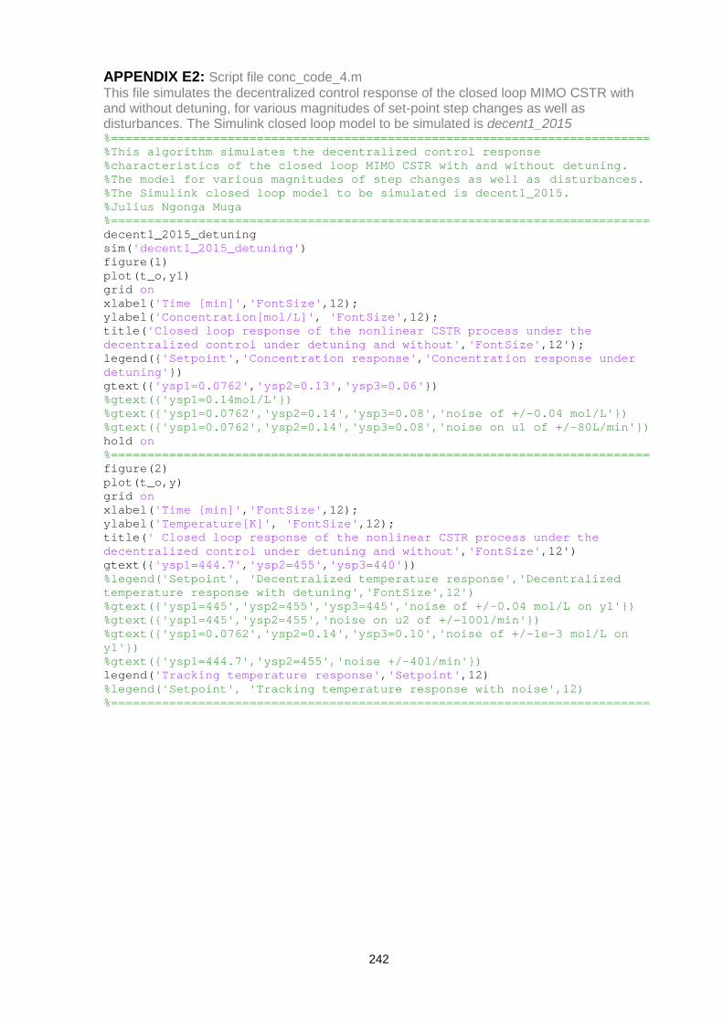
APPENDIX E2: Script file conc_code_4.m This file simulates the decentralized control response of the closed loop MIMO CSTR with and without detuning, for various magnitudes of set-point step changes as well as disturbances. The Simulink closed loop model to be simulated is decent1_2015 %========================================================================== %This algorithm simulates the decentralized control response %characteristics of the closed loop MIMO CSTR with and without detuning. %The model for various magnitudes of step changes as well as disturbances. %The Simulink closed loop model to be simulated is decent1_2015. %Julius Ngonga Muga %========================================================================== decent1_2015_detuning sim('decent1_2015_detuning') figure(1) plot(t_o,y1) grid on xlabel('Time [min]','FontSize',12); ylabel('Concentration[mol/L]', 'FontSize',12); title('Closed loop response of the nonlinear CSTR process under the decentralized control under detuning and without','FontSize',12'); legend({'Setpoint','Concentration response','Concentration response under detuning'}) gtext({'ysp1=0.0762','ysp2=0.13','ysp3=0.06'}) %gtext({'ysp1=0.14mol/L'}) %gtext({'ysp1=0.0762','ysp2=0.14','ysp3=0.08','noise of +/-0.04 mol/L'}) %gtext({'ysp1=0.0762','ysp2=0.14','ysp3=0.08','noise on u1 of +/-80L/min'}) hold on %========================================================================== figure(2) plot(t_o,y) grid on xlabel('Time [min]','FontSize',12); ylabel('Temperature[K]', 'FontSize',12); title(' Closed loop response of the nonlinear CSTR process under the decentralized control under detuning and without','FontSize',12') gtext({'ysp1=444.7','ysp2=455','ysp3=440'}) %legend('Setpoint', 'Decentralized temperature response','Decentralized temperature response with detuning','FontSize',12') %gtext({'ysp1=445','ysp2=455','ysp3=445','noise of +/-0.04 mol/L on y1'}) %gtext({'ysp1=445','ysp2=455','noise on u2 of +/-100l/min'}) %gtext({'ysp1=0.0762','ysp2=0.14','ysp3=0.10','noise of +/-1e-3 mol/L on y1'}) %gtext({'ysp1=444.7','ysp2=455','noise +/-40l/min'}) legend('Tracking temperature response','Setpoint',12) %legend('Setpoint', 'Tracking temperature response with noise',12) %==========================================================================
242

APPENDIX F: Simulink models developed for the thesis These are the Simulink models developed for the thesis
decent_2015. Model of MIMO closed
loop decentralized control Model of the MIMO closed loop system under decentralized control
dyn_dec_2015 Model of MIMO closed loop dynamic decoupling control
The MIMO closed loop under dynamic decoupling control
decen1_2015 Model of MIMO closed loop decentralized control incorporating the detuning
The closed loop MIMO system under decentralized control incorporating the detuning
li_2015 Model of MIMO closed loop I/O feedback linearization control
The closed loop MIMO system under I/O feedback linearization control
openloop_cstr_mod Model of MIMO open loop CSTR system
The open loop CSTR process
diag_decent_temp Model of diagonal temperature closed loop control
The temperature diagonal closed loop control system
decenconc_2015 Model of diagonal concentration closed loop control
The concentration diagonal closed loop control system
243

APPENDIX G: TwinCAT models developed for the thesis APPENDIX G1: TwinCAT model under dynamic control
APPENDIX G2: TwinCAT model under dynamic control with disturbances
244

APPENDIX G3: TwinCAT model under decentralized control
APPENDIX G4: TwinCAT model under I/O feedback linearization control
245

APPENDIX H1: Beckhoff PLC CX-5020
APPENDIX H2: Beckhoff PLC CX-5020 technical data
246

APPENDIX I: PID CONTROLLER SETTINGS BASED ON IMC
Dec 2015
247