Deposition and Removal of Fugitive Dust in the AridSouthwestern United States: Measurements and ModelResults

Vic Etyemezian, Sean Ahonen, and Djordje NikolicDivision of Atmospheric Sciences, Desert Research Institute, Las Vegas, Nevada

John Gillies and Hampden KuhnsDivision of Atmospheric Sciences, Desert Research Institute, Reno, Nevada

Dale GilletteAir Resources Laboratory (MD-81), Applied Modeling Research Branch, Research Triangle Park,North Carolina

John VeranthDepartment of Pharmacology and Toxicology, University of Utah, Salt Lake City, Utah

ABSTRACTThis work was motivated by the need to better reconcileemission factors for fugitive dust with the amount ofgeologic material found on ambient filter samples. Thedeposition of particulate matter with aerodynamic diam-eter less than or equal to 10 �m (PM10), generated bytravel over an unpaved road, over the first 100 m oftransport downwind of the road was examined at Ft. Bliss,near El Paso, TX. The field conditions, typical for warmdays in the arid southwestern United States, representedsparsely vegetated terrain under neutral to unstable atmo-spheric conditions. Emission fluxes of PM10 dust wereobtained from towers downwind of the unpaved road at7, 50, and 100 m. The horizontal flux measurements atthe 7 m and 100 m towers indicated that PM10 depositionto the vegetation and ground was too small to measure.The data indicated, with 95% confidence, that the loss ofPM10 between the source of emission at the unpaved

road, represented by the 7 m tower, and a point 100 m

downwind was less than 9.5%. A Gaussian model was

used to simulate the plume. Values of the vertical stan-

dard deviation �z and the deposition velocity Vd were

similar to the U.S. Environmental Protection Agency

(EPA) ISC3 model. For the field conditions, the model

predicted that removal of PM10 unpaved road dust by

deposition over the distance between the point of emis-

sion and 100 m downwind would be less than 5%. How-

ever, the model results also indicated that particles larger

than 10 �m (aerodynamic diameter) would deposit more

appreciably. The model was consistent with changes ob-

served in size distributions between 7 m and 100 m down-

wind, which were measured with optical particle

counters. The Gaussian model predictions were also com-

pared with another study conducted over rough terrain

and stable atmospheric conditions. Under such condi-

tions, measured PM10 removal rates over 95 m of down-

wind transport were reported to be between 86% and

89%, whereas the Gaussian model predicted only a 30%

removal. One explanation for the large discrepancy be-

tween measurements and model results was the possibil-

ity that under the conditions of the study, the dust plume

was comparable in vertical extent to the roughness ele-

ments, thereby violating one of the model assumptions.

Results of the field study reported here and the previous

work over rough terrain bound the extent of particle

deposition expected to occur under most unpaved road

emission scenarios.

IMPLICATIONSThis work was motivated by the well-documented dis-agreement between estimates of road and other geologicaldust obtained by emissions inventory methods and theactual amount of inorganic minerals observed on filter sam-ples at ambient monitoring sites. This study provides abasis for modeling the magnitude of PM10 dust removal bydeposition close to the emission source. The analysis fo-cuses on emissions from unpaved roads, though the resultsmay be pertinent to other sources of fugitive dust.

TECHNICAL PAPER ISSN 1047-3289 J. Air & Waste Manage. Assoc. 54:1099–1111

Copyright 2004 Air & Waste Management Association

Volume 54 September 2004 Journal of the Air & Waste Management Association 1099

INTRODUCTIONFugitive dust is emitted from an unpaved road when avehicle passes and disturbs the surface, raising a cloud ofdust that begins to travel downwind. Initially, the cloud isdense; with travel downwind, the cloud is dispersed byturbulent eddies in the atmosphere. Particles suspendedin the cloud can be removed by gravitational settling, byinteraction with the ground surface, terrain anomalies(e.g., buildings, boulders, etc.), or vegetative cover in thedownwind fetch of the unpaved road.

Watson and Chow1 documented the discrepancy be-tween emission inventories for particulate matter withaerodynamic diameter less than or equal to 10 �m (PM10)fugitive dust and the source attribution of ambient filtersamples. Their analysis indicated that the amount of geo-logically derived PM10 found in the air is smaller thanwould be expected based on emission inventories anddispersion models. Countess2 summarized 11 shortcom-ings in the current treatment of fugitive dust emissions.One of the recommendations made by Countess2 was toupgrade existing models with “sub-models” to accountfor the removal of particles near the source. Based on theanalysis of PM10 concentrations downwind of an un-paved road, Watson and Chow1 hypothesized that coarseparticles in the PM10 range deposit rapidly within the firstseveral hundred meters downwind of the road. That anal-ysis did not consider the vertical dispersion of PM with

distance downwind, resulting in a great overestimate ofthe effect of near-source deposition.

In this paper, the results of the Ft. Bliss measurementsof the near-source removal of PM10 dust emitted from anunpaved road are presented and compared with predic-tions from a simple dispersion model. These data providean estimate of the fraction of PM10 fugitive dust emissionsfrom unpaved roads that is regionally transportable. Re-sults of the Ft. Bliss study are also compared with theearlier measurements of Veranth et al.,3 which were ob-tained under significantly different terrain and atmo-spheric stability conditions.

BACKGROUNDFigure 1 schematically illustrates the progression of a dustplume emitted behind a vehicle and advected downwindover a vegetative cover. In the region (A) where the dustcloud first meets the vegetation, dust particles may beremoved by individual vegetation elements. Some workin the area of particle removal by windbreaks may beapplicable to this “impact zone,”4 although the specificformulation would have to be adjusted for vegetativecovers with a long fetch (as opposed to a windbreak thatis only several meters deep).

Very far downwind (region C in the figure), the dustplume approaches a steady vertical concentration profilethat is nearly invariant with transport distance. In

Figure 1. Development of a dust plume downwind of an unpaved road.

Etyemezian et al.

1100 Journal of the Air & Waste Management Association Volume 54 September 2004

between the “impact zone” and “far downwind” lies the“near-source” region, where the concentration profile ofdust particles is changing with transport distance; specif-ically, the dust plume is expanding in the vertical direc-tion.

Whereas deposition serves to permanently removeparticles from the airstream, turbulent dispersion causesparticles to dynamically redistribute through the mixedlayer in the atmosphere. Dispersion causes pockets of airwith comparatively high concentrations of particles to bediluted with pockets of air that have lower concentra-tions.

Vertical dispersion is commonly quantified as a dis-persion coefficient multiplied by a concentration gradi-ent. The amount of particles crossing a horizontal plane isgiven by an equation of the following form:

Fz�z� � �Kzz�z��C�z

(1)

where Fz (g/m2/s) is the vertical flux of particles at a heightz and is equal to the vertical (z-direction) dispersion co-efficient Kzz (m2/s) multiplied by the negative of the ver-tical concentration gradient (g/m4). Similar equations areused to describe dispersion in the two horizontal direc-tions with the coefficients Kxx and Kyy, which may beclose in magnitude to one another but can be quite dif-ferent from Kzz. Dispersion parallel to the road may beignored if the source is continuous in time and approxi-mated by an infinitely long line (e.g., a long road).

In the surface layer (nominally �50 m aboveground), where the flux of momentum to the ground isconstant with height, Kzz can be directly measured withmeteorological instrumentation. At greater heights, mea-surements are more difficult, and the functional form ofKzz is inferred from wind tunnel tests, theory, or numer-ical simulations.5–7

An alternative method for modeling diffusion is tospecify the physical degree of the spread of a plume as afunction of downwind distance and atmospheric stabil-ity. This is the approach used by a number of Gaussianplume models, including the ISC3.8 The concentration ofan airborne species is assumed to be normally distributedin each of the three ordinal directions, with standarddeviations of �x, �y, and �z. For a continuous line source,dispersion in the horizontal plane can be ignored. Theparameter �z has been specified by a number of authorsincluding Gifford,9 Klug,10 Turner,11 and Martin.12

The ISC3 model uses the formulation of Turner.11 TheGaussian approach is useful because of its simplicity inimplementation. However, it has its limitations, mostnotably, that the assumption of a normally distributed

concentration profile may be too simple to adequatelyaccount for the range of land use and atmospheric con-ditions that can be encountered.

Alternative methods for quantifying turbulent disper-sion are available from the literature,7,13,14 some of whichmay be more accurate than the simple mixing-length orGaussian models. Venkatram7 argues that eq 1 is flawedbecause it does not account for changes in air density withheight. That is, eq 1 does not reflect the fact that therequirement of zero net flux in the vertical direction canbe satisfied physically by a constant mixing ratio, even ifthere exists a concentration gradient in the vertical direc-tion. Du and Venkatram13 propose a method to specifythe vertical dispersion based on the friction velocity u*

and the Monin–Obukhov length L, rather than strictlyfrom the stability class. Schopflocker and Sullivan14 en-courage the use of two probability density functions (pdf)to specify the vertical distribution of concentration in-stead of a single pdf, as is done in Gaussian plume formu-lations. These authors suggest that two pdfs are requiredto represent both the high-level concentration distribu-tions in the “thin sheets” that are formed in turbulentdiffusion as well as the distribution of low-level concen-trations found outside the sheets.

Dry deposition of particles is frequently modeledanalogous to resistance in an electrical circuit.4,15–17 Mostof the models developed to study dry deposition of sulfateand other pollutants from the atmosphere are derived forthe well-mixed conditions of region C in Figure 1. Theflux to the ground is assumed to be equal to the concen-tration measured at a given height multiplied by a trans-fer coefficient, which is also dependent on height. Thetransfer coefficient is called the deposition velocity and isgiven by the symbol Vd (m/sec). Thus, according to theresistance model

Fdep � C(z)Vd(z) (2)

where Fdep is the vertical flux of material to the ground(g/m2/s) and C(z) is the height-dependent concentration.The deposition velocity is given as the inverse of threeresistances in series, that is:

vd�z� �1

ra�z� � rb � rc(3)

where ra is the resistance to aerodynamic transportthrough the surface layer and is dependent on the heightz above the surface; rb is the resistance to transportthrough the “quasi-laminar sublayer;” and rc is the resis-tance to collection on the surface or vegetative elements(the subscripts a, b, and c are unrelated to the regions in

Etyemezian et al.

Volume 54 September 2004 Journal of the Air & Waste Management Association 1101

Figure 1). This model for deposition is built on the as-sumption that close to the ground, that is, from the top ofthe surface layer down, the flux of a depositing species isconstant with height. Related to the assumption of con-stant flux, the model also assumes that the concentrationprofile through the surface and quasi-laminar layers is notchanging significantly over time. This corresponds strictlyonly to region C in Figure 1, though it may also holdapproximately for region B.

In addition to turbulent transport through the sur-face and quasi-laminar layers, particles are also influencedby gravity. This effect can be embodied in the resistancemodel by assuming that gravitational settling representsanother resistor (rg) acting in parallel with those in eq 3.Using the more familiar settling velocity vg (� 1/rg),which is a well-known function of the particle size,18 thedeposition velocity can be expressed as

vd�z� �1

ra�z� � rb � ra�z�rbvg� vg. (4)

Note that in arriving at eq 4, we have assumed that thesurface resistance to deposition, rc, is very small for parti-cles in the size range of interest (aerodynamic diametersless than 10 �m). That is, once a particle impacts on acollector, it sticks to that collector and is permanentlyremoved from the atmosphere. Deviations from this idealare not considered here, but are addressed by oth-ers.15,19,20 For stable and unstable atmospheric condi-tions, the aerodynamic resistance ra is given by the U.S.Environmental Protection Agency (EPA)8 based on thework of Byun and Dennis.21 ra is dependent on the fric-tion velocity u*, the roughness length z0, the Monin–Obukhov length scale L, and a reference zr. The quasi-laminar resistance rb is a function of the particle Schmidtnumber, Stokes number, and the flow friction velocity(u*).8,22 The Schmidt number accounts for Brownian mo-tion whereas the Stokes number accounts for inertial im-paction, which is the usually dominant pathway for dep-osition of particles with diameters of 1–10 �m. Thismodel for dry deposition requires that the airflow param-eters u*, z0, and L are known.

METHODSField Measurements

From April 11 through April 24, 2002, field experimentswere performed at an unpaved road on the open range ofFt. Bliss, a military facility near El Paso, TX. The experi-mental procedure was-based on an upwind/downwindtechnique that has been used by other investigators (e.g.,Gillies et al.23 and Cowherd24). Three towers were set upcollinearly and perpendicular to a 1000-m section of

unpaved road (Figure 2), which was oriented in a north–south direction. Historical meteorological data indicatedthat winds at this time of year were predominantly fromthe west. Brief rain occurred during the study period butthe soil surface dried rapidly due to springtime wind andsun. During all tests reported here, the unpaved road wasdry and the soil moisture content for at least the topseveral centimeters was near zero.

Tower 1, at 7 m downwind, had measurement posi-tions spaced logarithmically at 0.76, 1.28, 2.66, and5.17 m above ground level (AGL). Tower 2, at 50 m down-wind, had measurement positions at 1.25, 2.6, 5.7, and12.2 m AGL. Tower 3, at 100 m downwind, had the samemeasurement positions as Tower 2, with an additionalsampling location at 0.4 m AGL. One hundred meters waschosen as the maximum practical downwind distance forplacing the furthest tower. This was to ensure that thedust plume originating at the unpaved road, which ex-pands in the vertical direction as it advects horizontally,would be mostly contained within the height of the12.2-m tall tower. Four anemometers, one wind vane, andone temperature probe were mounted on Tower 3 tocharacterize the local meteorological conditions. PM10

dust concentrations were measured simultaneously at allof the tower measurement positions with DustTrak mon-itors (Model 8520, TSI, Inc., Shoreview, MN). The Dust-Trak is a rugged portable instrument that uses particlelight scattering to infer PM concentrations. The DustTrakwas chosen because it operates over a wide range of par-ticle concentrations spanning 0.001–100 mg/m3 and pro-vides the fast-response measurements (1 Hz) needed todetect individual road dust plumes. The flow rate at theinstrument inlet is 1.7 lpm; for the data presented here,the instrument has been equipped with a nominal PM10

inlet provided by the manufacturer. The instrument iscalibrated by the manufacturer with the respirable frac-tion of an Arizona Road Dust standard (ISO 12103–1, A1)to relate light scattering intensity at 90° with respect tothe incident laser light to aerosol mass concentrations inmg/m3. The ISO 12103–1, A1 standard consists of primar-ily silica particles (70%) that are provided with someparticle size specifications. By volume, the standard con-sists of 1–3% particles with diameters less than 1 �m,36–44% with diameters less than 4 �m, 83–88% withdiameters less than 7 �m, and 97–100% with diametersless than 10 �m.

Niu et al.25 found that in comparing data from fourDustTraks collocated in an indoor environment, the in-terinstrument variability was a reasonable 3%. Severalauthors have also reported that DustTrak measurementscorrelate well with filter-based measurements of dieselexhaust,26 ambient urban particulate matter,27 and in-door airborne particles,25 though in all cases, investigators

Etyemezian et al.

1102 Journal of the Air & Waste Management Association Volume 54 September 2004

noted that the DustTrak deviated from filter-basedmeasurements by a factor that depends on the nature ofthe aerosol measured. One shortcoming of using a neph-elometer-style instrument is that light scattering responseto changes in mass concentration can depend strongly onparticle composition as well as particle size. Based onmanufacturer specifications for the DustTrak, the greatestchange in light scattering per unit mass for silica aerosolsoccurs for particles with a diameter of around 0.4 �m. Theinstrument is less sensitive to changes in mass concentra-tion of smaller or larger particles. For 10-�m particles,light scattering sensitivity to changes in mass concentra-tion is approximately a factor of 50 less than for 0.4-�mparticles. This suggests that two different values measuredby the DustTrak may not necessarily translate into pro-portional differences in actual PM10 mass concentration,especially if the two measurements represent airborneparticles that are either substantially different in compo-sition or in particle size distribution. We note that thispotential source of uncertainty should not be of greatconcern for the results presented in this study because theDustTraks are used to provide only a relative measure ofPM10 flux between the three towers downwind of theunpaved road, the composition of the aerosol measuredby all instruments used is constant, and the particle sizedistribution does not change appreciably over the

distance spanned by the three towers (see Results andDiscussion).

During the course of the study, four GRIMM model1.108 particle size analyzers (GRIMM Tech. Inc., Atlanta,GA) were deployed at various locations and different mea-surement periods to provide information on the particlesize characteristics of the emitted dust. The GRIMM 1.108is an optical particle counter with 15 particle size bins thatcover the range of particles with diameters between 0.3�m and 20 �m. To estimate aerodynamic particle diam-eters from the “optical” diameters measured by theGRIMM, we invoke the assumption of spherical particlesand the approximation that the density of all particles isequal to that of silica with the following formula:

Djaero � Dj

opt�pCC�Djopt� (5)

where Djaero is the estimated representative aerodynamic

diameter for bin j, p is the specific density of particles (2.6for silica), CC is the Cunningham slip correction factor,and Dj

opt is the geometric mean of the minimum andmaximum “optical” diameter associated with bin j andgiven by the formula

Djopt � exp�ln�Dj

min� � ln�Djmax�

2 � (6)

Figure 2. Schematic of equipment setup at Ft. Bliss during the April 2002 field campaign. The vertical and horizontal components are drawn on differentscales. Dimensions are in meters.

Etyemezian et al.

Volume 54 September 2004 Journal of the Air & Waste Management Association 1103

where Djmin and Dj

max are the nominal smallest and larg-est diameters in bin j according to the manufacturer of theinstrument.

The data stream from the DustTraks, GRIMMs, andmeteorological instruments were collected in 1-s intervalson a PC located at the base of each tower. Analysis of theDustTrak data indicated that baseline drift over the courseof a day, generally less than 50 �g/m3, did not affect allinstruments equally. Thus, a baseline for each instrumentwas calculated approximately every 20 min over thecourse of the day from background concentrations mea-sured during periods when there were no dust emissionsfrom the unpaved road.

PM10 emissions were created by having a number oftest vehicles travel back and forth along the test section ofthe road. The test vehicles traveled at set speeds of 16, 24,32, 40, 48, 56, 64, 72, and 81 km/hr. Not all vehiclesattained the highest speeds for safety considerations. Af-ter two passes (one heading south and one returningnorth) at the same speed, the vehicle speed was increasedincrementally to the highest attainable value and thendecreased incrementally to the minimum value. This cy-cle was then repeated as time allowed. Test vehiclespaused for approximately 1 1⁄2 min between passes toallow for the dust plume to clear all three downwindtowers.

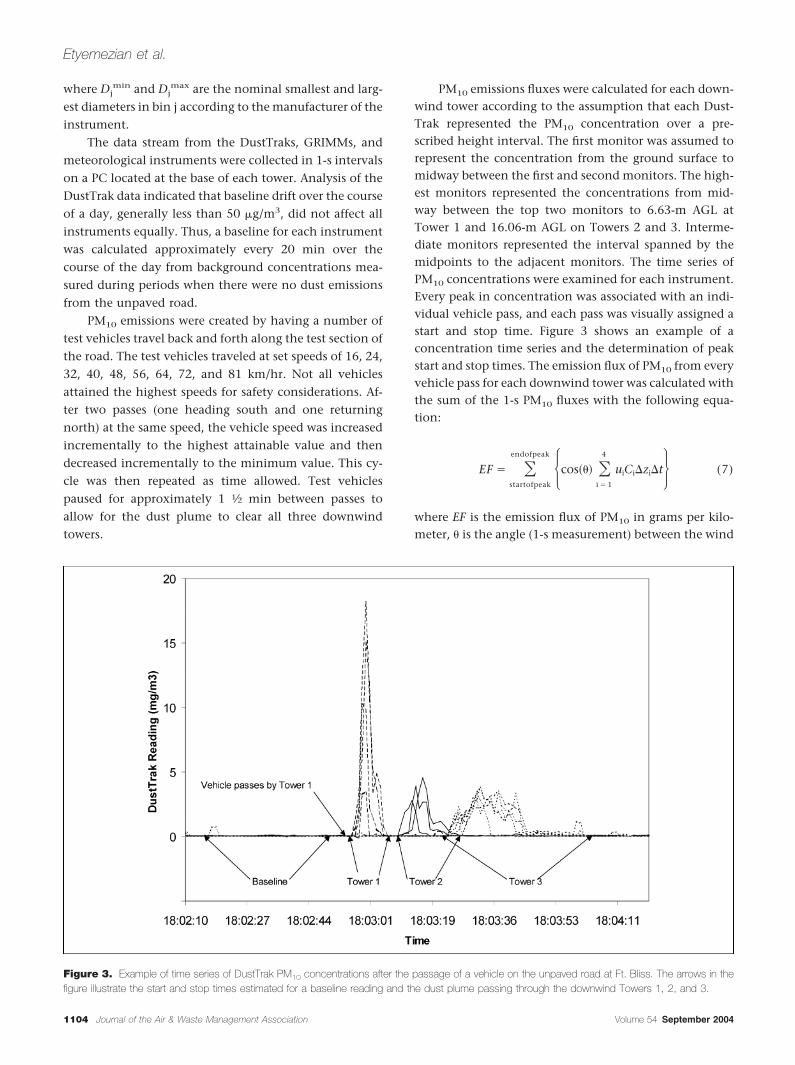
PM10 emissions fluxes were calculated for each down-wind tower according to the assumption that each Dust-Trak represented the PM10 concentration over a pre-scribed height interval. The first monitor was assumed torepresent the concentration from the ground surface tomidway between the first and second monitors. The high-est monitors represented the concentrations from mid-way between the top two monitors to 6.63-m AGL atTower 1 and 16.06-m AGL on Towers 2 and 3. Interme-diate monitors represented the interval spanned by themidpoints to the adjacent monitors. The time series ofPM10 concentrations were examined for each instrument.Every peak in concentration was associated with an indi-vidual vehicle pass, and each pass was visually assigned astart and stop time. Figure 3 shows an example of aconcentration time series and the determination of peakstart and stop times. The emission flux of PM10 from everyvehicle pass for each downwind tower was calculated withthe sum of the 1-s PM10 fluxes with the following equa-tion:

EF � �startofpeak

endofpeak �cos��� �i � 1

4

uiCi�zi�t� (7)

where EF is the emission flux of PM10 in grams per kilo-meter, � is the angle (1-s measurement) between the wind

Figure 3. Example of time series of DustTrak PM10 concentrations after the passage of a vehicle on the unpaved road at Ft. Bliss. The arrows in thefigure illustrate the start and stop times estimated for a baseline reading and the dust plume passing through the downwind Towers 1, 2, and 3.

Etyemezian et al.

1104 Journal of the Air & Waste Management Association Volume 54 September 2004

direction and a line perpendicular to the road, i is one ofthe four positions (five for Tower 3) of the monitors onthe tower, ui is the average wind speed in m/sec over theinterval represented by the ith monitor, Ci is the baseline-corrected PM10 concentration in mg/m3 as measured bythe ith monitor over the period �t, �z in m is the verticalinterval represented by the ith monitor, �t is 1 s.

The unpaved road at Ft. Bliss was 1 km in length andoriented in the north–south direction, with the threetowers lined perpendicular to and east of the road. Eventhough the angle between the wind vector and the roadwas accounted for by the cos (�) term in eq 7, when windsdid not have a strong westerly component, the dustplume generated by passing vehicles did not travel in thedirection of the towers. Only when the 30-s, vector-aver-aged wind direction fell in the quadrant spanned by thenorthwest and southwest vectors was the correspondingvehicle pass considered valid. The averaging time waschosen to be 30 s because this is roughly how long it takesthe plume to travel from the unpaved road to the 100 mdownwind tower. When applying eq 7, 1-s values of winddirection were used.

The wind speed and direction were measured only atthe far downwind tower (Tower 3). Therefore, to use eq 7,it was necessary to use wind speeds and directions mea-sured at Tower 3 for Tower 1 and Tower 2. The possibilityof introducing errors by this method was examined. Thehorizontal PM10 fluxes were calculated for Tower 3 onlyand averaged over the test vehicle speed. This procedurewas performed twice—once with wind data that corre-sponded to the time of the passing of the dust plume andonce with wind data that was retarded by 30 s. For exam-ple, the flux at 13:30:00 was calculated with wind datameasured at 13:30:00 and also with wind data measuredat 13:29:30. The purpose of this exercise was to subject theflux calculations for Tower 3 to the same uncertaintiesthat the data from Tower 1 and Tower 2 would be expe-riencing. In comparing the two resulting sets of horizon-tal fluxes, no significant differences were found (slope �

1.01, R2 � 0.98, n � 53, intercept was forced to 0), indi-cating that the use of Tower 3 wind direction and windspeed to calculate horizontal fluxes of PM10 at Tower 1and Tower 2 would not introduce biases.

The friction velocity and aerodynamic roughnesslength (u* and z0, respectively) were estimated by assum-ing that the wind profile was logarithmic:

u�z� �

u*

ln� zz0� (8)

where is the von Karman constant and equals 0.4. Toobtain meaningful estimates of the bulk quantities u* and

z0, data were averaged over 15-min intervals to obtain thevertical distribution of wind speeds. The final value of0.005 m obtained for z0 lies between those expected for“level desert” (0.001 m) and “lawn” (0.01 m).18 Figure 4shows the distribution of u* values that occurred over thecourse of the field study. Ninety-five percent of the valuesof u* fell between 10 and 50 cm/sec, with values between30 and 40 cm/sec occurring most frequently (35%).

The experiments at Ft. Bliss examined the downwindplume from a vehicle that traversed an unpaved road. Thetime series of the concentration measured at the down-wind towers reflects the influence of a moving pointsource (see Figure 3). To compare the Ft. Bliss data withthe continuous line source models, the concentrationtime series was integrated for each vehicle pass and eachlocation on the tower, that is:

Cint,k �peakstart

peakend

Ckdt (9)

where Cint,k is the integral of the concentration Ck attower location k. Although the location of the particlemonitoring instruments (DustTraks) varied slightly fromone tower to the next, all towers were equipped with onemonitor at a height of 1.26 m. Thus, the integrated con-centrations for each individual pass and at each height ona tower were normalized by the integrated concentrationat 1.26 m for that tower. The concentration profile fromeach of 116 passes was placed in a category according tothe value of the friction velocity, u*, associated with thatpass. The normalized concentration profiles were thenaveraged within each friction velocity category. Therewere four categories in all for u*, corresponding to binscentered at 0.2, 0.3, 0.4, and 0.5 m/sec. For example,all concentration profiles with a u* between 0.15 and

Figure 4. Frequency distribution and cumulative distribution of frictionvelocity u* for the 116 15-min intervals corresponding to periods whentesting was ongoing at Ft. Bliss. Values are based on a roughness length,z0, equal to 0.005 m.

Etyemezian et al.

Volume 54 September 2004 Journal of the Air & Waste Management Association 1105

0.25 m/sec were lumped together under the category u* �

0.2 m/sec.The data from the described fieldwork were collected

under neutral to unstable atmospheric conditions in asparsely vegetated desert with sand dunes 0.1–0.3 m highon generally level terrain. For comparison, a similar dataset was collected by Veranth et al.3 under a stable atmo-sphere and over a substantially rougher terrain. A briefdescription of that work is given below, and the reader isreferred to the original article3 for further details. Thefieldwork was conducted in collaboration with the MockUrban Setting Test (MUST) at the Dugway ProvingGround, Tooele County, UT. An array of cargo containers,2.5 m high � 2.4 m wide � 12.2 m long, was locatednominally downwind of an unpaved road. The array con-sisted of 10 rows of cargo containers, spaced 6.4 m apart,with the long side oriented parallel to the road. Each rowwas 12 columns deep in the downwind direction with aspace of 13.4 m between adjacent containers. This con-figuration resulted in a roughness height, z0, estimatedfrom sonic anemometer data, of 0.71 m, correspondingapproximately to a low-density residential area.

DustTraks and sonic anemometers were placed ontowers located along the cargo array center line at 3 and95 m downwind of the unpaved road. At the 3 m down-wind tower, DustTraks were placed at 0.9, 1.7, and 3.7 mabove grade and a 3-D sonic anemometer was located at1.6 m above grade. At the 95 m tower, DustTraks wereplaced at heights of 1.8, 4.6, 9.1, and 18.3 m and 2-daysonic anemometers were placed at heights of 4, 8, 16, and32 m. PM10 dust was generated by driving a pickup truckback and forth on the unpaved road for a total of 44 trips.Tests were performed between 1:00 and 2:30 AM Moun-tain Daylight time on September 26, 2001. Analysis ofsonic anemometry data gave a Monin–Obukhov length,L, of 310 m upwind of the container array and 1525 m inthe center of the array, indicating that the atmospherewas well within the stable range in both cases. For theperiod of the experiment, winds were within 45° of theline perpendicular to the unpaved road.

Modeling ApproachA class of dispersion models that are known collectively asGaussian plume models and that include the ISC3 short-term model8 is built on the approximation that a plumedispersing in the atmosphere assumes a shape similar to anormal distribution. These models work best for sourcesthat are high above the ground, where dispersion in thevertical direction does not vary greatly with height. Thatis, the vertical dispersion can be assumed symmetricalabout a horizontal plane located at the height of thesource. The applicability and limitations of Gaussianapproaches to dispersion modeling have been considered

by other investigators (e.g., Seinfeld and Pandis18), and anin-depth discussion is omitted here. Following the formu-lation described by the EPA,8 the basic equation for theground-level concentration C (�g/m3) downwind of aground-level continuous line source of nonreactive mate-rial is:

C�zr� � �2�

Qus�z

exp��0.5�zr

�z�2� (10)

where Q is the line source emission rate (g/s/m), �z is thestandard deviation of vertical concentration distribution,us is mean wind speed at the release height, zr is a refer-ence height, which is taken to be the larger of 1 m and20 � z0.8 The dispersion parameter �z is dependent on thedownwind distance x and is given by the following equa-tion:

�z � a(x0 � x)b (11)

The parameters a and b, given by Turner,11 are deter-mined by the atmospheric stability and the distancedownwind of the source.

When a vehicle passes over a road, the plume gener-ated behind the vehicle has a discrete height in the ver-tical direction. This distance is a measure of the initialdepth of the plume and is different from the plume re-lease height. To account for the fact that the dust plumeis initially dispersed by the turbulent wake of the vehicle,a “virtual” distance x0 is added to the value of x in eq 11.The virtual distance x0 is calculated by solving the equa-tion for the initial value �z0. Because �z is the standarddeviation of the concentration in the vertical directionassuming a normal distribution, then 95% of the plume isinitially below the height 2��z0. Therefore, we may ap-proximately define �z0 as half the initial height of theplume generated by turbulence in the wake of a vehicle. Aseries of experiments performed during the same fieldcampaign that has been described here were aimed atestimating the initial dust plume height behind a vehiclemoving on an unpaved road.28 Particle monitors and asonic anemometer were mounted on a tower 3 m down-wind of the road. Analysis of the plume height and theturbulent wake behind the vehicles indicated that for carsand small trucks, the initial plume was generally confinedto less than 2 m above the ground. Based on these data, avalue of 1 m was chosen to represent an approximationfor �z0 for all vehicles tested.

Dry deposition can be accounted for by numericallyintegrating the removal rate using the deposition velocity

Etyemezian et al.

1106 Journal of the Air & Waste Management Association Volume 54 September 2004

(described in an earlier section) over the distance down-wind of the source. If the removal by deposition is slowcompared with the rate of dispersion, then it is a reason-able approximation to apply the fractional removal ateach step to the entire concentration profile. In practice,this is only valid during neutral to unstable conditionsand only when the deposition velocity is not too large.Other options are available for more accurate representa-tion of the effect of deposition, and the ISC3 model ac-commodates their use. One such option allows for a mod-ification to the Gaussian profile to address the fact thatparticles are removed at the ground and not uniformlyfrom the entire vertical profile. In this work, no correctionfor the effect of deposition on the plume shape has beeninvoked.

This type of formulation for the dispersion and dep-osition of a pollutant is based on deposition to a horizon-tal surface from above that surface. It does not apply toflows where dispersion and deposition within the rough-ness elements are the dominant forms of transport (e.g.,“impact zone” in Figure 1).

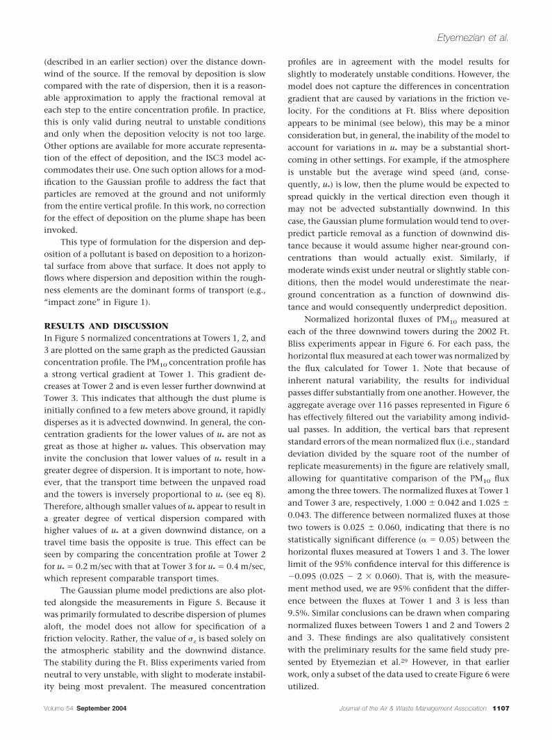
RESULTS AND DISCUSSIONIn Figure 5 normalized concentrations at Towers 1, 2, and3 are plotted on the same graph as the predicted Gaussianconcentration profile. The PM10 concentration profile hasa strong vertical gradient at Tower 1. This gradient de-creases at Tower 2 and is even lesser further downwind atTower 3. This indicates that although the dust plume isinitially confined to a few meters above ground, it rapidlydisperses as it is advected downwind. In general, the con-centration gradients for the lower values of u* are not asgreat as those at higher u* values. This observation mayinvite the conclusion that lower values of u* result in agreater degree of dispersion. It is important to note, how-ever, that the transport time between the unpaved roadand the towers is inversely proportional to u* (see eq 8).Therefore, although smaller values of u* appear to result ina greater degree of vertical dispersion compared withhigher values of u* at a given downwind distance, on atravel time basis the opposite is true. This effect can beseen by comparing the concentration profile at Tower 2for u* � 0.2 m/sec with that at Tower 3 for u* � 0.4 m/sec,which represent comparable transport times.

The Gaussian plume model predictions are also plot-ted alongside the measurements in Figure 5. Because itwas primarily formulated to describe dispersion of plumesaloft, the model does not allow for specification of afriction velocity. Rather, the value of �z is based solely onthe atmospheric stability and the downwind distance.The stability during the Ft. Bliss experiments varied fromneutral to very unstable, with slight to moderate instabil-ity being most prevalent. The measured concentration

profiles are in agreement with the model results forslightly to moderately unstable conditions. However, themodel does not capture the differences in concentrationgradient that are caused by variations in the friction ve-locity. For the conditions at Ft. Bliss where depositionappears to be minimal (see below), this may be a minorconsideration but, in general, the inability of the model toaccount for variations in u* may be a substantial short-coming in other settings. For example, if the atmosphereis unstable but the average wind speed (and, conse-quently, u*) is low, then the plume would be expected tospread quickly in the vertical direction even though itmay not be advected substantially downwind. In thiscase, the Gaussian plume formulation would tend to over-predict particle removal as a function of downwind dis-tance because it would assume higher near-ground con-centrations than would actually exist. Similarly, ifmoderate winds exist under neutral or slightly stable con-ditions, then the model would underestimate the near-ground concentration as a function of downwind dis-tance and would consequently underpredict deposition.

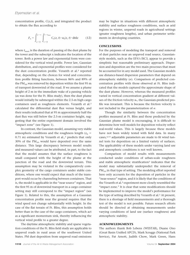
Normalized horizontal fluxes of PM10 measured ateach of the three downwind towers during the 2002 Ft.Bliss experiments appear in Figure 6. For each pass, thehorizontal flux measured at each tower was normalized bythe flux calculated for Tower 1. Note that because ofinherent natural variability, the results for individualpasses differ substantially from one another. However, theaggregate average over 116 passes represented in Figure 6has effectively filtered out the variability among individ-ual passes. In addition, the vertical bars that representstandard errors of the mean normalized flux (i.e., standarddeviation divided by the square root of the number ofreplicate measurements) in the figure are relatively small,allowing for quantitative comparison of the PM10 fluxamong the three towers. The normalized fluxes at Tower 1and Tower 3 are, respectively, 1.000 � 0.042 and 1.025 �

0.043. The difference between normalized fluxes at thosetwo towers is 0.025 � 0.060, indicating that there is nostatistically significant difference (� � 0.05) between thehorizontal fluxes measured at Towers 1 and 3. The lowerlimit of the 95% confidence interval for this difference is�0.095 (0.025 � 2 � 0.060). That is, with the measure-ment method used, we are 95% confident that the differ-ence between the fluxes at Tower 1 and 3 is less than9.5%. Similar conclusions can be drawn when comparingnormalized fluxes between Towers 1 and 2 and Towers 2and 3. These findings are also qualitatively consistentwith the preliminary results for the same field study pre-sented by Etyemezian et al.29 However, in that earlierwork, only a subset of the data used to create Figure 6 wereutilized.

Etyemezian et al.

Volume 54 September 2004 Journal of the Air & Waste Management Association 1107

This point can be further supported by examining theparticle size distributions measured at Towers 1 and 3.Figure 7 shows the ratio of particle concentrations mea-sured at the same height (2.66 m) on both towers. Thefigure represents data from 137 individual passes wheremeasured particle concentrations were significantly abovebackground levels (i.e., greater than background concen-tration plus three standard deviations) at both Tower 1and Tower 3. Note that in the earlier work of Etyemezianet al.29 this criterion was not in place, and the data in thecorresponding figure are slightly different from thoseshown in the present paper. The x-axis shows the

estimated mean geometric diameter for the size bin mea-sured (see eqs 5 and 6).

Because the smallest size bin shown, represented byparticles with diameters of 3.9 �m, is not expected todeposit to any appreciable extent, concentrations of allother size bins were normalized by that of 3.9-�m parti-cles. Thus, the y-axis in the figure corresponds to thefraction of particles in the stated size bin that remains insuspension 100 m downwind of the unpaved road. Ingeneral, the removal rate of particles increases with diam-eter; this is consistent with the expectation that the dep-osition velocity vd also increases with diameter. Figure 7

Figure 5. Concentration profiles normalized to measured and modeled concentration at 1.26 m above ground level at (a) Tower 1, 7 m downwind ofunpaved road; (b) Tower 2, 50 m downwind; and (c) Tower 3, 100 m downwind. The y-axis in (a) differs from that in (b) and (c).

Etyemezian et al.

1108 Journal of the Air & Waste Management Association Volume 54 September 2004

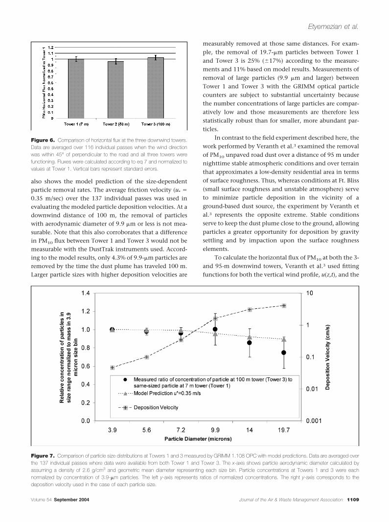
also shows the model prediction of the size-dependentparticle removal rates. The average friction velocity (u* �

0.35 m/sec) over the 137 individual passes was used inevaluating the modeled particle deposition velocities. At adownwind distance of 100 m, the removal of particleswith aerodynamic diameter of 9.9 �m or less is not mea-surable. Note that this also corroborates that a differencein PM10 flux between Tower 1 and Tower 3 would not bemeasurable with the DustTrak instruments used. Accord-ing to the model results, only 4.3% of 9.9-�m particles areremoved by the time the dust plume has traveled 100 m.Larger particle sizes with higher deposition velocities are

measurably removed at those same distances. For exam-ple, the removal of 19.7-�m particles between Tower 1and Tower 3 is 25% (�17%) according to the measure-ments and 11% based on model results. Measurements ofremoval of large particles (9.9 �m and larger) betweenTower 1 and Tower 3 with the GRIMM optical particlecounters are subject to substantial uncertainty becausethe number concentrations of large particles are compar-atively low and those measurements are therefore lessstatistically robust than for smaller, more abundant par-ticles.

In contrast to the field experiment described here, thework performed by Veranth et al.3 examined the removalof PM10 unpaved road dust over a distance of 95 m undernighttime stable atmospheric conditions and over terrainthat approximates a low-density residential area in termsof surface roughness. Thus, whereas conditions at Ft. Bliss(small surface roughness and unstable atmosphere) serveto minimize particle deposition in the vicinity of aground-based dust source, the experiment by Veranth etal.3 represents the opposite extreme. Stable conditionsserve to keep the dust plume close to the ground, allowingparticles a greater opportunity for deposition by gravitysettling and by impaction upon the surface roughnesselements.

To calculate the horizontal flux of PM10 at both the 3-and 95-m downwind towers, Veranth et al.3 used fittingfunctions for both the vertical wind profile, u(z,t), and the

Figure 6. Comparison of horizontal flux at the three downwind towers.Data are averaged over 116 individual passes when the wind directionwas within 45° of perpendicular to the road and all three towers werefunctioning. Fluxes were calculated according to eq 7 and normalized tovalues at Tower 1. Vertical bars represent standard errors.

Figure 7. Comparison of particle size distributions at Towers 1 and 3 measured by GRIMM 1.108 OPC with model predictions. Data are averaged overthe 137 individual passes where data were available from both Tower 1 and Tower 3. The x-axis shows particle aerodynamic diameter calculated byassuming a density of 2.6 g/cm3 and geometric mean diameter representing each size bin. Particle concentrations at Towers 1 and 3 were eachnormalized by concentration of 3.9-�m particles. The left y-axis represents ratios of normalized concentrations. The right y-axis corresponds to thedeposition velocity used in the case of each particle size.

Etyemezian et al.

Volume 54 September 2004 Journal of the Air & Waste Management Association 1109

concentration profile, C(z,t), and integrated the productto obtain the flux according to

Fx �z � 0

z � � t � 0

t � tmax

Cx�z, t� � ux�z, t� � dtdz (12)

where tmax is the duration of passing of the dust plume bythe tower and the subscript x indicates the location of thetower. Both a power law and exponential form were con-sidered for the vertical wind profile. Power law, Gaussiandistribution, and exponential profiles were considered forthe dust concentration profile. Veranth et al.3 reportedthat, depending on the choices for wind and concentra-tion profile fitting functions, between 86% and 89% ofthe PM10 was removed by deposition within the first 95 mof transport downwind of the road. If we assume a plumeheight of 2 m in the immediate wake of a passing vehicle(as was done for the Ft. Bliss study), then the dust plumewould initially be submerged within the 2.5-m high cargocontainers used as roughness elements. Veranth et al.3

calculated the differential dust flux versus height, andtheir results indicated that at 95 m approximately half thedust flux was still below the 2.5-m container height, sug-gesting that the entire experiment domain involved the“impact zone” (see Figure 1).

In contrast, the Gaussian model, assuming very stableatmospheric conditions and the roughness length (z0 �

0.71 m) estimated by Veranth et al.,3 predicts that only30% of the PM10 would have deposited over the samedistance. This large discrepancy between model resultsand measured values can be attributed, in part, to the factthat the model assumes that the surface roughness issmall compared with the height of the plume at thejunction of the road and the downwind terrain. Thisassumption may be violated in the comparatively com-plex geometry of the cargo containers under stable con-ditions, where one would expect that much of the trans-port would occur by channeling between containers. Thatis, the model is applicable in the “near source” region, andthe first 95 m of downwind transport in a cargo containersetting may still correspond to the “impact region” (seeFigure 1). Related to this, the assumption of a Gaussianconcentration profile near the ground requires that thewind speed not change substantially with height. In thecase of the flat terrain of Ft. Bliss, this assumption holdsbetter than in the case of the cargo containers, which actas a significant momentum sink, thereby influencing thevertical wind profile to a greater degree.

The daytime atmospheric stability and sparse vegeta-tion conditions of the Ft. Bliss field study are applicable tounpaved roads in rural areas of the southwest UnitedStates. PM dust deposition from unpaved road emissions

may be higher in situations with different atmosphericstability and surface roughness conditions, such as aridregions in winter, unpaved roads in agricultural settings(greater roughness lengths), and urban perimeter settle-ments in developing countries.

CONCLUSIONSFor the purposes of modeling the transport and removalof dust particles near an unpaved road source, Gaussian-style models, such as the EPA’s ISC3, appear to provide asimplistic but reasonable preliminary approach. Disper-sion and deposition are the two main processes that mustbe accounted for in any model used. The Gaussian modelsuse distance-based dispersion parameters that depend onatmospheric stability (�). Comparison of predicted con-centration profiles with those observed at Ft. Bliss indi-cated that the models captured the approximate shape ofthe dust plume. However, whereas the measured profilesvaried in vertical concentration gradient at different val-ues of the friction velocity u*, the Gaussian-predicted pro-file was invariant. This is because the friction velocity isnot included in the parameterization of �.

Though the similarity between the concentrationprofiles measured at Ft. Bliss and those predicted by theGaussian plume model is encouraging, it is difficult todetermine how well models for deposition velocity reflectreal-world values. This is largely because these modelshave not been widely tested with field data. In manycases,4,15 adjustable parameters are made to fit wind tun-nel tests for deposition on a limited variety of surfaces.The applicability of these models under varying land useand atmospheric conditions is not well known.

Comparison of model results with measurementsconducted under conditions of urban-scale roughnessand stable atmospheric stratification3 indicates that themodel may substantially underpredict the removal ofPM10 in that type of setting. The modeling effort reportedhere only accounts for the deposition of particles in the“near-source” region, and it is likely that the conditions ofthe Veranth et al.3 experiment more closely resembled the“impact zone.” It is clear that some modifications shouldbe implemented to improve the model’s performance forthe type of setting described by Veranth et al.3 At present,there is a shortage of field measurements and a thoroughtest of the model is not possible. Future research effortsshould be directed at obtaining measurements undervarying conditions of land use (surface roughness) andatmospheric stability.

ACKNOWLEDGMENTSThe authors thank Bob Lebens (WESTAR), Duane Ono(Great Basin Unified APCD), Mark Scruggs (National ParkService), Pat Arnott, Judith Chow, Mark Green, Hans

Etyemezian et al.

1110 Journal of the Air & Waste Management Association Volume 54 September 2004

Moosmuller, Ravi Varma, John Walker (Desert ResearchInstitute), Marc Pitchford (NOAA), Geary Schwemmerand Dave Miller (NASA), Raed Laban, Gauri Seshadri (Uni-versity of Utah), Clyde Durham (Ft. Bliss), and ThompsonPace (EPA) for contributing to the completion of this workthrough equipment loans, comments on the manuscript,and assistance in data analysis. This work was funded bythe WESTAR Council and DoD SERDP Grants CP1190 andCP1191. Field testing was made possible through the co-operation of the United States Army at Ft. Bliss.

REFERENCES1. Watson, J.G.; Chow, J. Reconciling Urban Fugitive Dust Emissions Inven-

tory and Ambient Source Contribution Estimates: Summary of CurrentKnowledge and Needed Research. DRI Document No. 6110.4F; U.S. Envi-ronmental Protection Agency, Desert Research Institute: Reno, NV,2000.

2. Countess, R. Methodology for Estimating Fugitive Windblown and Me-chanically Resuspended Road Dust Emissions Applicable for Regional ScaleAir Quality Modeling; Western Governors Association by Countess En-vironmental: Westlake Village, CA, 2001.

3. Veranth, J.M.; Seshadri, G; Pardyjak, E. Vehicle-Generated FugitiveDust Transport: Analytic Models and Field Study; Atmos. Environ.2003, 37, 2295–2303.

4. Raupach, M.R.; Wood, N.; Dorr, G; Leys, J.F.; Cleugh, H.A. The En-trapment of Particles by Windbreaks; Atmos. Environ. 2001, 35, 3373–3383.

5. Lamb, R.G.; Duran, D.R. Eddy Diffusivities Derived from a NumericalModel of the Convective Boundary Layer; Nuovo. Cimento. 1977, 1c,1–17.

6. Shir, C.C. A preliminary Numerical Study of Atmospheric TurbulentFlows in the Idealized Planetary Boundary Layer; J. Atmos. Sci. 1973,30, 1327–1339.

7. Venkatram, A. The Parametrization of the Vertical Dispersion of AScalar in the Atmospheric Boundary Layer; Atmos. Env. 1993, 27A,1963–1966.

8. U.S. EPA. User’s Guide for the Industrial Source Complex (ISC3) DispersionModels Volume II: Description of Model Algorithms; U.S. EnvironmentalProtection Agency, Office of Air Quality Planning and Standards:Emissions, Monitoring, and Analysis Division: Research Triangle Park,NC, 1995.

9. Gifford, F.A. Use of Routine Meteorological Observations for Estimat-ing Atmospheric Dispersion; Nucl. Safety 1961, 2, 47–51.

10. Klug, W. A Method for Determining Diffusion Conditions for Synop-tic Observations; Staub. Reinhalt. Luft. 1969, 29, 14–20.

11. Turner, D.B. Workbook of Atmospheric Dispersion Estimates. PHS Publi-cation No 999-AP-26; U.S. Department of Helath, Education and Wel-fare, National Air Pollution Control Administration: Cincinnati, OH,1970.

12. Martin, D.O.; Comment on the Change of Concentration StandardDeviations with Distance; J. Air Pollut. Control Assoc. 1976, 26, 145–146.

13. Du, S.; Venkatram, A. A Parametrization of Verical Dispersion ofGround-Level Releases; J. Appl. Meteorol. 1997, 36, 1004–1015.

14. Schopflocher, T.P.; Sullivan, P.J. A Mixture Model for the PDF of aDiffusing Scalar in a Turbulent Flow; Atmos. Environ. 2002, 36, 4405–4417.

15. Slinn, W.G.N. Predictions for Particle Depositions to Vegetative Can-opies; Atmos. Environ. 1982, 16, 1785–1794.

16. Wu, Y.L.; Davidson, C.I.; Dolske, D.A.; Sherwood, S.I. Dry Depositionof Atmospheric Contaminants: The Relative Importance of Aerody-namic, Boundary Layer, and Surface Resistances; Aerosol Sci. & Technol.1992a, 16, 65–81.

17. Etyemezian, V.; Davidson, C.I.; Finger, S.; Striegel, M.; Barabas, N.;Chow, J. Vertical Gradients of Pollutant Concentrations and Deposi-

tion Fluxes on a Tall Limestone Building; J. Am. Inst. Conservat. 1997,37, 187–210.

18. Seinfeld, J.H.; Pandis, S.N. Atmospheric Chemistry and Physics: From AirPollution to Climate Change. Wiley Interscience: New York, 1997.

19. Willeke, K.; Xu, M. Impaction and Rebound of Particles from Surfaces.J. Aerosol Sci. 1992, 23 (Suppl.), S15–S18.

20. Wu, Y.L.; Davidson, C.I.; Lindberg, S.E.; Russell, A.G. Resuspension ofParticulate Chemical Species at Forested Sites; Environ. Sci. & Technol.1992b, 26, 2428–2435.

21. Byun, D.W.; Dennis, R. Design Artifacts in Eulerian Air Quality Mod-els: Evaluation of the Effects of Layer Thickness and Vertical ProfileCorrection on Surface Ozone Concentrations; Atmos. Environ. 1995,29, 105–126.

22. Pleim, J., Venkatram, A.; Yamartino, R. ADOM/TADAP Model Develop-ment Program, Volume 4. The Dry Deposition Module. Ontario Ministryof the Environment: Rexdale, Ontario, 1984.

23. Gillies, J.A.; Watson, J.G.; Rogers, C.F.; Dubois, D.; Chow, J.C.; Lang-ston, R.; Sweet, J.. Long-term efficiencies of dust suppressants to re-duce PM10 emissions from unpaved roads; J. Air & Waste Manage.Assoc. 1999, 49, 3–16.

24. Cowherd, C. Profiling Data for Open Fugitive Dust Sources; Prepared forU. S. Environmental Protection Agency, Emissions Factor and Inven-tory Group, Office of Air Quality Planning and Standards, RTP, NC, byMidwest Research Institute: Kansas City, MO, 1999.

25. Niu, J.; Lu, B.M.K.; Tung, T.C.W. Instrumentation Issue in Indoor AirQuality Measurements: The Case with Respirable Suspended Particu-lates; Indoor Built Environ. 2002, 11, 162–170.

26. Moosmuller, H.; Arnott, W.P.; Rogers, C.F.; Bowen, J.L.; Gillies, J.A.;Pierson, W.R.; Collins, J.F.; Durbin, T.D.; Norbeck, J.M. Time ResolvedCharacterization of Diesel Particulate Emissions. 1. Instruments forParticle Mass Measurement; Environ. Sci. Technol. 2001, 35, 781–787.

27. Chung, A.; Chang, D.P.Y.; Kleeman, M.J.; Perry, K.D.; Cahill, T.A.;Dutcher, D.; McDougall, E.M.; Stroud, K. Comparison of Real-TimeInstruments Used to Monitor Airborne Particulate Matter; J. Air &Waste Manage. Assoc. 2001, 51, 109–120.

28. Etyemezian, V.; Gillies, J.; Kuhns, H.; Nikolic, D.; Watson, J.; Veranth,J.; Labban, R.; Seshadri, G.; Gillett, D. Field Testing and Evaluation ofDust Deposition and Removal Mechanisms: Final Report; Report Preparedfor WESTAR Council, Lake Oswego, OR, by DRI: Las Vegas, NV, 2003.

29. Etyemezian, V.; Gillette, D.; Gillies, J.; Kuhns, H.; Nikolic, D.; Veranth,J.; Watson, J. PM10 Emissions Factors for Unpaved Roads: Correctionfor Near-Field Deposition; PM AAAR 2003: Atmospheric Sciences, Expo-sure, Health and Welfare Effects, Policy. Presented at the AmericanAssociation for Aerosol Research, Pittsburgh, PA, March 31 throughApril 4, 2003.

About the AuthorsVic Etyemezian is associate research professor at theDesert Research Institute (DRI) in Las Vegas, NV. JohnGillies and Hampden Kuhns are associate research profes-sors in the Division of Atmospheric Sciences at the DRI inReno, NV. Dale Gillette is a physical scientist at Air Re-sources Laboratory, NOAA, in Research Triangle Park, NC.Sean Ahonen and Djordje Nikolic are research affiliates atDRI in Las Vegas, NV. John Veranth is a research assistantprofessor at the Department of Pharmacology and Toxicol-ogy at the University of Utah, Salt Lake City, UT. Addresscorrespondence to: Vic Etyemezian, Division of Atmo-spheric Sciences, DRI, 755 E. Flamingo Rd., Las Vegas, NV89119; phone: (702) 895-0569; e-mail: vic@dri.edu.

Etyemezian et al.

Volume 54 September 2004 Journal of the Air & Waste Management Association 1111