Dental Ecometrics as a Proxy of Paleoenvironment ...
312
Dental Ecometrics as a Proxy of Paleoenvironment Reconstruction in the Miocene of South America by Jackson Ples Spradley Department of Evolutionary Anthropology Duke University Date:_______________________ Approved: ___________________________ Richard F. Kay, Supervisor ___________________________ Blythe A. Williams ___________________________ James D. Pampush ___________________________ V. Louise Roth ___________________________ Doug M. Boyer Dissertation submitted in partial fulfillment of the requirements for the degree of Doctor of Philosophy in the Department of Evolutionary Anthropology in the Graduate School of Duke University 2017
-
Upload
khangminh22 -
Category
Documents
-
view
0 -
download
0
Transcript of Dental Ecometrics as a Proxy of Paleoenvironment ...

Dental Ecometrics as a Proxy of Paleoenvironment Reconstruction in the Miocene of
South America
by
Jackson Ples Spradley
Department of Evolutionary Anthropology
Duke University
Date:_______________________
Approved:
___________________________
Richard F. Kay, Supervisor
___________________________
Blythe A. Williams
___________________________
James D. Pampush
___________________________
V. Louise Roth
___________________________
Doug M. Boyer
Dissertation submitted in partial fulfillment of
the requirements for the degree of Doctor of Philosophy
in the Department of
Evolutionary Anthropology in the Graduate School
of Duke University
2017
ABSTRACT
Dental Ecometrics as a Proxy of Paleoenvironment Reconstruction in the Miocene of
South America
by
Jackson Ples Spradley
Department of Evolutionary Anthropology
Duke University
Date:_______________________
Approved:
___________________________
Richard F. Kay, Supervisor
___________________________
Blythe A. Williams
___________________________
James D. Pampush
___________________________
V. Louise Roth
___________________________
Doug M. Boyer
An abstract of a dissertation submitted in partial
fulfillment of the requirements for the degree
of Doctor of Philosophy in the Department of
Evolutionary Anthropology in the Graduate School of
Duke University
2017

Copyright by
Jackson Ples Spradley
2017

iv
Abstract
In this dissertation I compile modern mammalian faunal lists, as well as
ecomorphological measurements on living marsupials and rodents, to relate the
diversity of small mammals, specifically the distributions of their dental topographies,
to the climates in which they are found. The emphasis of this dissertation is to
demonstrate the potential of distributions of dental topography metrics as proxies for
the reconstruction of paleoenvironments in the Miocene of South America.
In Chapter 2, I compile complete, non-volant mammalian species lists for 85
localities across South America as well as 17 localities across Australia and New Guinea.
Climatic and habitat variables were also recorded at each locality using GIS spatial data.
Additionally, basic ecological data was collected for each species, including: diet, body
size, and mode of locomotion. Niche indices that describe the relative numbers of
different ecologies were calculated for each locality. These indices then served as the
predictor values in a handful of regression models, including regression trees, random
forests, and Gaussian process regression. The Australian/New Guinean localities were
used as a geographically and phylogenetically independent for the purposes of testing
the models derived from South America.
As for the dental ecomorphological analysis, I use three separate measures of
dental topography, each of which measures a different component of dental topography;
relief (the Relief Index, or RFI), complexity (orientation patch count rotated, OPCR), and
v
sharpness (Dirichlet normal energy, DNE). Together, these metrics quantify the shape of
the tooth surface without regard for tooth size. They also do not depend on homologous
features on the tooth surface for comparative analysis, allowing a broad taxonomic
sample as I present here. After a methodological study of DNE in Chapter 3, I present
correlative studies of dental topography and dietary ecology in marsupials and rodents
in Chapters 4 and 5, respectively. Finally, using the same localities from Chapter 2, I
analyze the distributions of dental topography metrics as they relate to climate and
habitat.
Results suggest that sharpness and relief are positively correlated with a higher
amount of tough foods—such as leaves or insects—in the diet of marsupials, and that
relief is positively correlated with grass-eating in rodents. The distributions of all three
metrics show some utility when used as a proxy for climatic variables, though the
distributions of RFI in marsupials and OPCR in rodents demonstrate the best
correlations.
Overall, this dissertation suggests that dental topography can be used to
discriminate dietary categories in a wide variety of mammalian groups, and that the
distributions of dental ecometrics can be used as proxies for paleoenvironment
reconstruction. This may eliminate the need to reconstruct behavior in individual taxa in
order to construct ecological indices for fossil mammalian communities, thus offering a
more direct avenue to reconstructing past environments.

Dedication
“Nature never did betray the heart that loved her.”
-William Wordsworth
To my mother and father, Patti and Ples Spradley, for their passing on to me the joy of
understanding, and encouraging in me a love and appreciation of the Natural World.
“You give but little when you give of your possessions. It is when you give of yourself that you
truly give.”
-Khalil Gibran
To my wife, Sara, for her unceasing love, support, and companionship during this
journey of intellectual and personal growth.

vii
Table of Contents
Abstract ......................................................................................................................................... iv
List of Tables ...............................................................................................................................xiv
List of Figures ........................................................................................................................... xvii
Acknowledgements ................................................................................................................... xxi
1. Introduction ............................................................................................................................... 1
1.1 Historical Context ............................................................................................................. 2
1.2 Modern Methods .............................................................................................................. 2
1.3 Dental Topography Metrics ............................................................................................ 8
1.4 Ecometrics of Small Mammal Cheek Teeth ................................................................ 12
1.5 Vagaries of the Fossil Record ........................................................................................ 14
1.6 Outline of Chapters ........................................................................................................ 17
2. Past Life Regression: Mammalian Faunas, Ecological Indices, and Machine-Learning
Regression for the Purpose of Paleoenvironment Reconstruction in the Miocene of South
America ........................................................................................................................................ 21
2.1 Background ..................................................................................................................... 23
2.1.1 Regression Methods of Paleoecological Reconstruction ...................................... 28
2.1.1.1 Multivariate Linear Regression ........................................................................ 28
2.1.1.2 Regression Tree Analysis .................................................................................. 29
2.1.1.3 Random Forests .................................................................................................. 31
2.1.1.4 Gaussian Process Regression ............................................................................ 35
2.1.2 Paleoecological Reconstruction ............................................................................... 36
viii
2.1.2.1 La Venta Paleogeography ................................................................................. 37
2.1.2.2 Santa Cruz Paleogeography ............................................................................. 38
2.2 Materials and Methods .................................................................................................. 40
2.3 Results .............................................................................................................................. 47
2.3.1 Spatial Autocorrelation ............................................................................................. 47
2.3.2 South American extant faunas ................................................................................. 47
2.3.3 Australian extant faunas........................................................................................... 56
2.3.3 Paleoclimatic Reconstructions ................................................................................. 60
2.3.3.1 The Monkey Beds of La Venta ......................................................................... 60
2.3.3.2 Santa Cruz Faunal Levels 1-7 ........................................................................... 61
2.4 Discussion ........................................................................................................................ 62
2.4.1 Performance of regression techniques in South American data ......................... 63
2.4.2 Results from modern localities ................................................................................ 65
2.4.2.1 Mean annual precipitation (MAP) ................................................................... 65
2.4.2.2 Mean annual temperature (MAT) ................................................................... 66
2.4.2.3 Temperature seasonality ................................................................................... 67
2.4.2.4 Precipitation seasonality ................................................................................... 68
2.4.2.5 Net primary productivity (NPP)...................................................................... 69
2.4.2.6 Canopy height .................................................................................................... 71
2.4.2.7 Australian comparison ...................................................................................... 71
2.4.2 Paleoenvironment reconstructions ......................................................................... 72
2.4.3.1 The Monkey Beds of La Venta ......................................................................... 72

ix
2.4.3.2 Santa Cruz Faunal Levels 1-7 ........................................................................... 74
2.5 Summary and Conclusions ........................................................................................... 74
3. Smooth Operator: The effects of different 3D mesh retriangulation protocols on the
computation of Dirichlet normal energy ................................................................................. 77
3.1 Background ..................................................................................................................... 80
3.1.1 Scanning and reconstruction ................................................................................... 82
3.1.2 Segmentation .............................................................................................................. 84
3.1.3 Retriangulation .......................................................................................................... 85
3.1.4 Analysis ...................................................................................................................... 88
3.1.5 The Utility of a Hemisphere ..................................................................................... 89
3.2 Materials and Methods .................................................................................................. 91
3.2.1 Production of Virtual Hemispheres ........................................................................ 91
3.2.2 Scanning and Segmenting of Physical Hemisphere ............................................. 92
3.2.3 Test of Different Retriangulation Protocols ........................................................... 93
3.2.4 Primate Molar Occlusal Surfaces ............................................................................ 96
3.2.5 Comparison of Published Methods ........................................................................ 96
3.3 Results .............................................................................................................................. 97
3.3.1 The Virtual Hemisphere ........................................................................................... 97
3.3.1.1 Avizo Smoothing ............................................................................................... 98
3.3.1.2 Laplacian Smoothing ......................................................................................... 99
3.3.1.3 Implicit Fairing ................................................................................................. 101
3.3.1.4 Face Count and Boundary Exclusion ............................................................ 101
3.3.2 Analysis of Occlusal Surfaces ................................................................................ 103

x
3.3.2.1 Comparison of Published Methods ............................................................... 105
3.4 Discussion ...................................................................................................................... 108
3.4.1 Effects of Different Smoothing Protocols ............................................................. 108
3.4.2 Effects of Different Face Counts and Boundary Exclusion on DNE ................ 112
3.4.3 Comparing Results from Previously Published Protocols ................................ 116
3.4.4 Considerations When Designing a Retriangulation Protocol for Tooth Surfaces
............................................................................................................................................. 119
3.5 Conclusions ................................................................................................................... 120
4. Dental Topography in Marsupials: Proxies for Dietary Ecology and Environmental
Reconstruction ........................................................................................................................... 122
4.1 Introduction ................................................................................................................... 122
4.1.1 Measuring Tooth Shape .......................................................................................... 123
4.1.1.1 Relief Index (RFI) ............................................................................................. 124
4.1.1.2 Orientation Patch Count Rotated (OPCR) .................................................... 125
4.1.1.3 Dirichlet Normal Energy (DNE) .................................................................... 127
4.1.2 Predictions ................................................................................................................ 128
4.2 Materials and Methods ................................................................................................ 130
4.2.1 Sample Preparation ................................................................................................. 130
4.2.2 Statistical Analyses .................................................................................................. 135
4.2.3 Distributions of Ecometrics as Climatic Proxies ................................................. 136
4.2.3.1 Exclusion of Range ........................................................................................... 138
4.3 Results ............................................................................................................................ 138
4.3.1 Dental Topography and Dietary Ecology ............................................................ 138

xi
4.3.1.1 Correlations Among Topographic Variables ............................................... 138
4.3.1.2 Phylogenetic ANOVAs ................................................................................... 144
4.3.1.3 Discriminant Function Analysis .................................................................... 147
4.3.2 Dental Topography and Environmental Reconstruction .................................. 148
4.4 Discussion ...................................................................................................................... 154
4.4.1 Issues of Defining Dietary Categories .................................................................. 155
4.4.1.1 Excluding Dactylopsila and Sarcophilus .......................................................... 156
4.4.2 Correlations Among DNE, RFI, and OPCR ......................................................... 157
4.4.3 Differences Among Dietary Groups ..................................................................... 158
4.4.3.1 OPCR ................................................................................................................. 159
4.4.3.2 RFI ...................................................................................................................... 161
4.4.3.3 DNE .................................................................................................................... 165
4.4.3.4 Dental Topography Metrics as Predictors of Diet ....................................... 167
4.4.4 Ecometric Distributions .......................................................................................... 167
4.4.4.1 Ecometric Means .............................................................................................. 167
4.4.4.2 Ecometric Coefficients of Variation ............................................................... 169
4.4.4.3 Ecometric Skew ................................................................................................ 173
4.4.4.4 Using Marsupial Ecometric Distributions as Environmental Proxies ...... 175
4.5 Conclusions ................................................................................................................... 177
5. Dental Topography in South American Rodents: Proxies for Dietary Ecology and
Environmental Reconstruction ............................................................................................... 180
5.1 Introduction ................................................................................................................... 180
5.1.1 Rodent Dental Ecomorphology ............................................................................. 181
xii
5.1.1 Rodent Ecometric Distributions as an Environmental Proxy ........................... 186
5.2 Materials and Methods ................................................................................................ 188
5.2.1 Topography and Dietary Ecology ......................................................................... 188
5.2.2 Ecometric Distributions .......................................................................................... 195
5.3 Results ............................................................................................................................ 195
5.3.1 Dental Topography and Dietary Ecology ............................................................ 195
5.3.1.1 Correlations between Dental Topography Metrics ..................................... 195
5.3.1.2 Phylogenetically-corrected ANOVAs ........................................................... 196
5.3.1.3 Discriminant Function Analysis .................................................................... 200
5.3.2 Ecometric Distributions and Climate ................................................................... 203
5.3.2.1 Ecometric Means .............................................................................................. 203
5.3.2.2 Ecometric Ranges ............................................................................................. 205
5.3.2.3 Ecometric Coefficients of Variation ............................................................... 207
5.3.2.3 Ecometric Skewness ......................................................................................... 209
5.3.3 Machine-learning Regression Techniques ........................................................... 209
5.4 Discussion ...................................................................................................................... 215
5.4.1 Dental Topography and Dietary Ecology ............................................................ 217
5.4.1.1 Dirichlet Normal Energy (DNE) .................................................................... 217
5.4.1.2 Relief Index (RFI) ............................................................................................. 220
5.4.1.3 Orientation Patch Count Rotated (OPCR) .................................................... 222
5.4.1.4 Dental Topography as a Discriminator of Rodent Dietary Ecologies ...... 224
5.4.2 Rodent Dental Topography Distributions as Environmental Proxies ............. 225

xiii
5.4.2.1 DNE .................................................................................................................... 226
5.4.2.2 RFI ...................................................................................................................... 229
5.4.2.3 OPCR ................................................................................................................. 231
5.4.2.4 Tropical Mammal Distributions ..................................................................... 240
5.4.3 Combining Ecometrics and Regression Techniques .......................................... 241
5.5 Conclusions ................................................................................................................... 243
6. Summary ................................................................................................................................ 244
6.1 Summary of Results ..................................................................................................... 245
6.1.1 Conclusions .............................................................................................................. 251
6.1.2 Species Sampling ..................................................................................................... 252
6.2 Future Directions .......................................................................................................... 253
Biography ................................................................................................................................... 291
xiv
List of Tables
Table 1: Definitions of the ecological categories used in this study .................................... 43
Table 2: Root mean squared error (RMSE) and mean absolute error (MAE) for each of
the bioclimatic variables across the South American localities, using each of the
regression techniques, included in this study ......................................................................... 48
Table 3: Root mean squared error (RMSE) and mean absolute error (MAE) for each of
the climatic variables across the Australian localities, using each of the regression
techniques, included in this study. ........................................................................................... 57
Table 4: Estimations of climatic variables in the Miocene of La Venta using the
regression methods included in this study. ............................................................................ 61
Table 5: Estimations of climatic variables in the Miocene of Santa Cruz using the
regression methods included in this study, exclusively with the South American data
set. ................................................................................................................................................. 62
Table 6: Changing values of DNE on a rubber ball versus the number of smoothing
iterations performed in Avizo to which the surface mesh is subjected. ............................. 98
Table 7: DNE on a rubber ball versus the number of Laplacian smoothing steps
performed in MeshLab to which the surface mesh is subjected. ......................................... 99
Table 8: Percent change in DNE from the original unsmoothed surface with increasing
number of smoothing steps performed in Avizo (first column) ........................................ 103
Table 9: DNE values for both the scanned rubber ball hemisphere and a surface mesh of
an Alouatta lower first molar after undergoing various retriangulation protocols used in
previous studies incorporating measurement of DNE. ....................................................... 105
Table 10: The absolute value difference of DNE between previously published protocols
on five different tooth surfaces ............................................................................................... 118
Table 11: Dental topography metrics and dietary category for each species included in
this study .................................................................................................................................... 131
Table 12: Results from ANOVA tests for comparisons between dental topography
metrics. ....................................................................................................................................... 139
Table 13: Phylogenetically-corrected ANOVA table for dietary group means of DNE. 146
xv
Table 14: Phylogenetically-corrected ANOVA table for dietary group means of RFI .... 146
Table 15: Phylogenetically-corrected ANOVA table for dietary group means of OPCR.
..................................................................................................................................................... 147
Table 16: Distribution statistics of DNE, OPCR, and RFI for 17 localities across Australia
and Papua New Guinea. .......................................................................................................... 149
Table 17: ANOVA statistics from the test of effect of bioclimatic variables on the mean of
DNE, OPCR, and RFI at each Australian and New Guinean locality. .............................. 151
Table 18: ANOVA statistics from the test of effect of bioclimatic variables on the
coefficients of variation of DNE, OPCR, and RFI distributions. ........................................ 152
Table 19: ANOVA statistics for the test of effect of climatic variables on the skew of
DNE, OPCR, and RFI distributions ........................................................................................ 153
Table 20: Means of DNE, RFI, OPCR, and M2 area for every species included in this
study. .......................................................................................................................................... 189
Table 21: Results from correlation analyses between dental topography metrics. .......... 195
Table 22: Phylogenetically-corrected ANOVA for test of effect of diet on DNE in South
American rodents. ..................................................................................................................... 198
Table 23: Phylogenetically-corrected ANOVA for test of effect of diet on RFI in South
American rodents. ..................................................................................................................... 198
Table 24: Phylogenetically-corrected ANOVA for test of effect of diet on OPCR in South
American rodents. ..................................................................................................................... 199
Table 25: Summary statistics from phylogenetically-corrected post-hoc Tukey’s Honest
Significant Differences tests ..................................................................................................... 199
Table 26: Results from discriminant function analysis (DFA) performed using dental
topography metrics in combination with M2 area, for the complete rodent dataset. ...... 201
Table 27: Summary statistics of correlation analyses between means of distributions of
DNE, RFI, and OPCR across South American localities and six variables of climate and
habitat. ........................................................................................................................................ 203

xvi
Table 28: Summary statistics of correlation analyses between ranges of distributions of
DNE, RFI, and OPCR across South American localities and six variables of climate and
habitat. ........................................................................................................................................ 205
Table 29: Summary statistics of correlation analyses between coefficients of variation
(CoV) of distributions of DNE, RFI, and OPCR across South American localities and six
variables of climate and habitat. ............................................................................................. 207
Table 30: Mean Absolute Error (MAE) and Root Mean Squared Error (RMSE) for the
estimations of bioclimatic variables using different regression techniques. .................... 209
Table 31: Results of Mann-Whitney U-test for comparisons between cricetid and
echimyid plant-dominated omnivores .................................................................................. 223
Table 32: DNE values for hemispheres simplified to various face counts, and smoothed
to different levels in Avizo, as well as calculated with different boundary exclusion
criteria ......................................................................................................................................... 255
Table 33: Ecological information for marsupial and rodent species included in Chapters
4 and 5, respectively. ................................................................................................................ 259
xvii
List of Figures
Figure 1: I Illustrative regression tree constructed using hypothetical data. In each box
there are three numbers ............................................................................................................. 30
Figure 2: Overview of the procession of the random forest algorithm from the original
data set to predicting new data. ................................................................................................ 33
Figure 3: Example of a single tree from a random forest analysis ....................................... 34
Figure 4: Map of South American illustrating the faunal localities used in this study. .... 42
Figure 5: Actual MAT (x-axis) and predicted MAT (y-axis) values for the test dataset. .. 50
Figure 6: Actual MAP (x-axis) and predicted MAP (y-axis) values for the test dataset ... 51
Figure 7: Actual temperature seasonality (x-axis) and predicted temperature seasonality
(y-axis) values for the test dataset ............................................................................................ 52
Figure 8: Actual precipitation seasonality (x-axis) and predicted precipitation seasonality
(y-axis) values for the test dataset ............................................................................................ 53
Figure 9: Actual NPP (x-axis) and predicted NPP (y-axis) values for the test dataset. NPP
as a metric is discussed in the text. ........................................................................................... 54
Figure 10: Actual canopy height (x-axis) and predicted canopy (y-axis) values for the test
dataset ........................................................................................................................................... 55
Figure 11: Map of Australian faunal localities used as a test data set in this study. ......... 56
Figure 12: Actual MAT (x-axis) and predicted MAT (y-axis) values for the Australian
dataset. .......................................................................................................................................... 59
Figure 13: Actual MAP (x-axis) and predicted MAP (y-axis) values for the Australian
dataset ........................................................................................................................................... 60
Figure 14: NPP versus Frugivore Index for the South American dataset ........................... 69
Figure 15: Workflow for quantifying surface topography of a dental specimen. .............. 82
Figure 16: Workflows for previously published retriangulation protocols used to
generate tooth surfaces ............................................................................................................... 97

xviii
Figure 17: Bivariate plot of DNE as a function of the number of smoothing iterations in
Avizo ............................................................................................................................................. 99
Figure 18: Bivariate plot of DNE as a function of the number of Laplacian smoothing
steps as performed in MeshLab .............................................................................................. 100
Figure 19: Bivariate plot of DNE as a function of the number of faces in a virtual
hemisphere created in R. .......................................................................................................... 102
Figure 20: Bivariate plot of the percent change in DNE values from the original surface
mesh after undergoing the number of smoothing iterations as indicated on the abscissa.
..................................................................................................................................................... 104
Figure 21: A) One-way- plot of DNE as a function of the type of smoothing method
employed on an unsmoothed surface scan of a rubber ball. B) One-way plot of DNE as a
function of the smoothing method on an unsmoothed surface scan of an Alouatta palliata
lower first molar ........................................................................................................................ 107
Figure 22: Illustration of the creation of artifacts on the surface reconstruction of DU-LP-
41. ................................................................................................................................................ 110
Figure 23: Illustration of the effect of increasing the number of faces on the surface
reconstruction of a howling monkey (Alouatta palliata) lower first molar. ....................... 115
Figure 24: Illustration of the 3D surface area (top) and 2D planometric area (bottom
right) that compose the ratio of RFI........................................................................................ 125
Figure 25: Pyramids of different face counts reflecting the effect of face count on the
measurement of OPCR ............................................................................................................. 127
Figure 26: Phylogenetic tree of all marsupial species included in this study. Colors on
tips represent dietary categories assigned to each species .................................................. 134
Figure 27: Map of mammalian localities used in this study of distribution of ecometrics
and environment. ...................................................................................................................... 137
Figure 28: Bivariate plot of DNE as a function of RFI. ......................................................... 140
Figure 29: Bivariate plot of OPCR as a function of RFI. ...................................................... 141
Figure 30: Bivariate plot of DNE as a function of OPCR ..................................................... 142
xix
Figure 31: Principal components analysis including the three dental topography metrics
and the natural log of M2 area ................................................................................................. 143
Figure 32: Quantile plots of species means for each of the three dental topography
metrics ........................................................................................................................................ 145
Figure 33: Bivariate plots of means of RFI, OPCR, and DNE against MAP, temperature
seasonality, and canopy height ............................................................................................... 152
Figure 34: 3D surfaces of the M2s of three species from three different dietary categories.
..................................................................................................................................................... 159
Figure 35: 3D surfaces of three didelphid marsupials with corresponding RFI and DNE
values .......................................................................................................................................... 164
Figure 36: Quantile plots representing the RFI values of the arboreal folivores and
terrestrial browsers in my sample, demonstrating the difference between the two groups
(p = 0.069). ................................................................................................................................... 165
Figure 37: Bivariate plots of the coefficient of variations of distributions of RFI against
MAP, NPP, and canopy height ............................................................................................... 170
Figure 38: Densities plots of RFI in two localities................................................................. 171
Figure 39: Bivariate plot of RFI CoV and species richness .................................................. 171
Figure 40: Bivariate plots of RFI skew (y-axis) and four climatic/habitat variables ........ 175
Figure 41: Density plots of RFI and DNE from three different localities, with associated
MAP values for each ................................................................................................................. 177
Figure 42: Phylogenetic tree of all rodent species included in this study. ........................ 192
Figure 43: Linear regressions of dental topography metrics against one another. .......... 196
Figure 44: Oneway bivariate plots of A) DNE; B) RFI; and C) OPCR by diet. ................. 198
Figure 45: Principal components analysis of DNE, RFI, and OPCR demonstrating
separation of dietary categories in morphospace ................................................................. 202
Figure 46: Actual mean annual temperature (MAT) (x-axis) and predicted MAT (y-axis)
values for the test dataset using rodent dental topography metric distributions as the
predictor variables .................................................................................................................... 211
xx
Figure 47: Actual temperature seasonality (x-axis) and predicted temperature seasonality
(y-axis) values for the test dataset. ......................................................................................... 212
Figure 48: Actual mean annual precipitation (MAP) in millimeters per year (x-axis) and
predicted MAP (y-axis) values for the test dataset. ............................................................. 213
Figure 49: Actual canopy height in meters (x-axis) and predicted canopy height (y-axis)
values for the test dataset. ........................................................................................................ 214
Figure 50: Actual net primary productivity (NPP) (x-axis) and predicted NPP (y-axis)
values for the test dataset. ........................................................................................................ 215
Figure 51: 3D reconstructions of rodent lower M2s illustrating the measurement of DNE,
RFI, and OPCR .......................................................................................................................... 217
Figure 52: Linear regression of the natural log of M2 area and DNE. ................................ 219
Figure 53: Bivariate plots of statistically significant relationships between DNE
distribution statistics and environmental variables ............................................................. 227
Figure 54: Bivariate plots of statistically significant relationships between RFI
distribution statistics and environmental variables. ............................................................ 230
Figure 55: Bivariate plots of statistically significant relationships between OPCR mean
and A) MAT; B) Temperature seasonality; and C) MAP. ................................................... 233
Figure 56: Linear regression of latitude and the mean of OPCR. ....................................... 234
Figure 57: Bivariate plots of statistically significant relationships between OPCR mean
and A) MAT; B) Temperature seasonality; C) MAP; D) Canopy height; and E) NPP. ... 235
Figure 58: Bivariate plots of statistically significant relationships between OPCR
coefficient of variation and A) MAT; B) Temperature seasonality; C) MAP; D) Canopy
height; and E) NPP. ................................................................................................................... 236
Figure 59: Principal components analysis (PCA) plot of the 85 South American localities
segregated by the distribution statistics of DNE, RFI, and OPCR ..................................... 240

xxi
Acknowledgements
First and foremost I would like to thank my Ph.D. advisor, Dr. Richard Kay, for his
guidance and mentorship. I cannot imagine going through this process with anyone else. The
passion and good humor that he brings to his work every single day is inspiring, and he has
served as a role model for my career and in my personal life. From conducting research to
teaching Human Body, it has truly been a pleasure.
I would also like to thank my committee members, beginning with Dr. Blythe Williams.
Without a doubt, Dr. Williams has been akin to my co-advisor, not just because of her proximity
to my own office, but because she is always there for a conversation or for a quick piece of advice.
I have had the pleasure to get to know her very well over these past five years and it is no stretch
to say that she is among my favorite people.
Thank you as well to Dr. JD Pampush, without whom this dissertation would not have
happened. In the brief amount of time we spent together I have become a better researcher and a
better professional, and so much of that is because of his willingness to lend his assistance with
any part of any project.
To Dr. Doug Boyer, who has lent me so much of his time and his lab space so that I could
complete this dissertation. He is also one of the most thoughtful researchers I know and his
attention to detail has made this dissertation all the better.
And to Dr. Louise Roth, with whom I have had a number of insightful conversations, and
whose mammalogy course was a big inspiration behind the fixation I now have with wanting to
include more and more mammalian species in my research.
An enormous thank you to my good friend, Bryan Glazer, for his assistance with the
modeling approaches used in the second chapter of this dissertation. This became a lynchpin of
my entire project and this dissertation would not have been possible without him.
I would also like to thank the museum curators that allowed me access to the specimens I
used in Chapters 4 and 5, including: Jake Esselstyn (LSUMZ), Robert Voss (AMNH), Sandy
Ingleby (Australian Museum), and Darrin Lunde (USNM).
Finally, I would like to acknowledge funding support from the National Science
Foundation (NSF Grant 1349741 to RF Kay).
1
1. Introduction
In this dissertation, I examine the relationships between niche distributions of
South American mammalian communities and six bioclimatic variables, including
precipitation, temperature, seasonality (in terms of temperature and precipitation),
primary productivity, and canopy height. Since previous analyses have primarily used
traditional linear regression, I also use this opportunity to test a number of different
regression techniques that have become popular in the ecological literature since the
early 2000s. Using training data and a randomly selected test data set, estimations from
all techniques are compared for accuracy—that is, the degree to which they are
correlated with and can serve as proxies for the climate variables. Having demonstrated
a relationship between mammal species richness and climate variables, I then move on
to establishing a relationship between morphology and ecology in two groups of small
mammals (marsupials and rodents). This is followed by a use of the morphometric
distributions as proxies for environment using the same regression techniques—
multivariate linear regression, regression trees, Random Forests, and Gaussian process
regression—introduced in Chapter 2. The value of this approach is that the potential
source of error in paleoenvironment reconstruction introduced by the accuracy of
behavioral reconstructions of individual fossil taxa, and instead distributions of
quantitative measurements themselves can be used.
2
1.1 Historical Context
The relationship of organisms’ form and the nature of their behavior and
preferred habitat has been one of the cornerstones of naturalism for millennia, long
before even the contributions of Darwin’s Origin. In his text History of Animals, published
in the fourth century BCE, Aristotle recorded the distinguishing features of animals,
while also noting that groups of animals with similar features tended to behave in
similar ways, and that certain features indicated the kinds of habitats those organisms
preferred. Such qualitative observations laid the foundation of zoology, and his scala
naturae provided the primary way of thinking of the relationship between organisms for
almost two thousand years after his death. While the naturalists of the 18th and 19th
centuries eventually freed zoology from some of its anthropocentric underpinnings, the
idea that an organism’s form is indicative of its environment, at least indirectly, was
retained.
1.2 Modern Methods
The field of paleoecology is generally synthetic in its approach, and at its
broadest scale includes information from disciplines such as paleobotany,
sedimentology, geochemistry, taphonomy, and paleontology, to name a few (Gingerich,
1989; Lowe and Walker, 1984). This study, however, will focus primarily on creating
models based on modern mammalian communities and then ground-truthing them for
application to the fossil record. Modern mammalian communities serve as valuable
3
study tools for understanding the ecology of extinct faunas due to the principle of
convergence. Animals that play the same ecological role (Hutchinson 1965) tend to have
similar adaptive responses, an observation that has been made since even the earliest
naturalists (Huston, 1994). If we assume that animals in the past faced similar challenges
as today, then it stands to reason that we can reconstruct their ecological roles (Sepkoski
and Ruse, 2009).
The potential for inferring paleoecological information from fossilized mammal
teeth is particularly high for several reasons: 1) mammals represent the dominant class
of tetrapods in the Cenozoic (thus are readily available), thereby giving us a chance to
study evolutionary trends in the most recent and abundant fossil records (Vrba, 1992); 2)
their bones are relatively dense as compared to other types of organisms (e.g., birds) and
are more likely to be preserved in the fossil record (Janis, 1993); 3) the most frequently
preserved skeletal element (the dentition) is also the most taxonomically diagnostic and
strongly ecologically correlated in terms of size and diet; and 4) analysis of mammalian
species richness, community structure, and ecomorphology have been demonstrated to
be highly correlated with habitat types and climate (Andrews et al., 1979; Fleming, 1973;
Janis, 1993; Kay and Madden, 1997; Kay et al., 1997; Kay et al., 2012a; Louys et al., 2015;
Vrba, 1992). From the paleontology literature, these studies are often discussed in the
context of finding faunal proxies of climate that can be easily recovered from the fossil
4
record. These proxies include species richness (Kay and Madden, 1997; Kay et al., 1997)
and niche metrics (Andrews et al., 1979; Gingerich, 1989; Kay and Madden, 1997).
That mammal species occupying similar habitats have convergent adaptations is
one of the foundational blocks of Darwin’s work (Darwin, 1859), and this serves as the
theoretical basis for the use of niche metrics as a method of paleoecology (Hutchinson
1965). This premise is validated by the strong correlation between aspects of phenotype
and environment as documented by countless studies designed to test it (Anthony and
Kay, 1993; Boyer, 2008; Boyer et al., 2013; Crompton and Lumsden, 1970; Ross and Kirk,
2007). While this implies an adaptive link between form and function (Kay and Cartmill
1977), it is not dismissive or at odds with the reservations of Gould and Lewontin
(1979)—who suggested that not all morphology is adaptive—since such research is
extremely circumscribed in how it defines morphological candidates for adaptation (e.g.,
Kay and Cartmill 1977, Kay et al. 2004; Boyer et al. 2013). While there have been a
multitude of paleoecological methods that incorporate ecomorphology (Reed, 2013), this
study will focus on two of the broadest and most popular; community structure and
ecometrics.
While it was Harrison (1962) and Fleming (1973) who established that
mammalian communities vary predictably with latitude, Andrews et al. (1979)
demonstrated that even when latitude was held constant, mammalian community
structure is significantly correlated with habitat type. When both latitude and habitat

5
type are similar, mammalian niche structure is “remarkably constant” (Andrews et al.
1979). In this context, community structure is the number and types of niches
(ecological roles) that are available and filled in any given habitat. Previous studies of
community structure and paleoecology, (e.g. Andrews et al. 1979, Kay and Madden
1997, and Vizcaino et al. 2010), have observed the relative abundance of arboreal vs.
terrestrial species, frugivores vs. folivores, herbivores vs. carninvores, and the
distribution of large and small body sizes in modern communities. These observations
are the variables used to create indices (both separate and composite) to search for
consistent relationships with habitat type. These indices are also considered to be taxon-
free (Damuth et al., 1992; Reed, 2013) because they describe what the species is doing,
i.e. the niche, and thus can be used to compare communities of extinct species
irrespective of phylogenetic relationships. This claim is not without controversy,
however. For instance, the concepts of ‘niche conservatism’ (Wiens and Graham, 2005)
or ‘phylogenetic inertia’ (Blomberg and Garland, 2002)—i.e. the tendency of taxa to
retain ancestral ecological traits—would suggest that no ecological analysis would be
free of phylogeny. Andrews and Hixson (2014) have argued that no paleoecological
method has been completely successful in being taxon-free since every regression and
comparison is made within taxonomic groupings, though they assert that community
level analysis is the most resistant to effects of phylogeny. Another potential
confounding factor is the effect of processes that affect large-scale differences in

6
community structure (Whittaker, 1972). For example, because of a climatic or geographic
barrier, if only a few mammalian families ever make it to a particular geographic region
where they would be ecologically suited, then the community structure will reflect the
phylogenetic constraints of those families (Ricklefs 2004).
While analysis of community structure is concerned primarily with relative
proportions of various ecologies (Andrews and Hixson 2014), the ecometric approach
takes quantitative measurements of ecologically relevant morphological traits (Eronen et
al., 2010a). This ecometric approach is therefore related to the previously discussed
analysis but contributes quantitative data that can be measured in individuals,
populations, species, communities or metacommunities (Eronen et al. 2010a). This has
the added benefit of being able to record morphological variation in climate change
across multiple taxonomic levels—e.g. the niche structure of rodents, primates, or
marsupials—in individual localities, even when the difference in overall community
structure between localities is negligible (Reed 2013). So far, such ecometric studies of
mammals have been limited to comparisons of body size distribution in relation to
climate (Ashton et al. 2000; Blackburn et al. 1999; Secord et al. 2012) tooth structure and
precipitation (Eronen et al., 2010b; Fortelius et al., 2002; Liu et al., 2012) as well as
calcaneal morphology, “gear ratios” and climate (Polly 2010). The results from these
studies suggest that there is utility in using quantitative methods for reconstructing
paleoclimate and environment.

7
An example of the ecometric approach is seen in the evolution of high crowned
cheek teeth (i.e. “hypsodonty”). Trends towards hypsodonty are regarded an adaptive
response to abrasive and/or fibrous foods (Janis and Fortelius 1988; Jernvall and
Fortelius 2002; MacFadden 2000; Williams and Kay, 2001; Van Valen 1960) and are
considered ecologically informative because these abrasive/tough foods are found in
abundance in open, dry (or seasonal) environments (Damuth and Janis, 2011; Eronen et
al. 2010b; Janis and Fortelius 1988; Jernvall and Fortelius 2002). These studies have
generally used large-bodied ungulates as their subjects of study (though Williams and
Kay [2001] also included rodents in their analysis), and for this reason are unable to
discern finer scale differences in environments, particularly within the same latitudinal
zones (Eronen et al. 2010a; Liu et al. 2012).
An apparent issue with using body size in any paleontological context is the
problem of body mass prediction in fossil organisms. Complete skeletons are
exceedingly rare in the fossil record, and therefore body mass prediction equations
(BMPE) are often focused on specific skeletal elements. The most commonly used
element has been teeth (Beard et al., 1996; Conroy, 1987; Gingerich, 1977; Gingerich et
al., 1982; Kay and Simons, 1980). However, other studies have used other skeletal
elements such as: craniofacial elements (Martin 1981; Cartelle and Hartwig, 1996;
Steudel, 1980), the femur (Cartelle and Hartwig, 1996), and the ankle bones (Dagosto
and Terranova 1992; Yapuncich et al., 2015). The potential pitfalls of body mass

8
prediction in fossils are numerous. First, BMPE’s are only appropriate when the fossil
for which mass is to be estimated is of a known phylogenetic affiliation (Smith, 2002).
For example, even within one order (Primates), using a cercopithecoid-derived BMPE to
estimate the mass of a fossil ape could produce an estimate that is more representative of
monkeys than it is of apes, because of the phylogenetic specificity of the scaling
relationship of the proxy used. The unresolved phylogenetic affiliation of many fossils
can present uncertainty as to which taxon-specific model to use. Moreover, the small
sample size of fossils introduces another problem. The sample mean is only an estimate
of the species mean, and with very small sample sizes (as is often the case in the fossil
record) the confidence interval for that estimate can be large (Smith, 2002).
1.3 Dental Topography Metrics
To overcome the problem of body size reconstruction, I use dental topography
metrics that have been shown to be independent of size. Quantification of whole tooth
surfaces has taken a number of forms in the past two decades (Reed, 1997; Jernvall and
Selanne, 1999; Ungar and M’Kirera, 2003; Dennis et al., 2004); of these I include three
recent methods: orientation patch count rotated (OPCR) (Evans et al., 2007; Evans and
Jernvall, 2009), relief index (RFI) (M’Kirera and Ungar, 2003; Boyer, 2008), and Dirichlet
normal energy (DNE) (Bunn et al., 2011; Winchester et al., 2014). Each of these metrics
takes advantage of tooth surface scans that can be translated into 3D meshes that
comprise polygonal—in the case of my study, triangular—faces. These meshes can be
9
standardized across different species—even in broad taxonomic samples such as I use
here—by maintaining equivalent relative resolution between scans and by making the
absolute number of faces used to reconstruct the 3D surfaces equivalent across all scans.
These surfaces can then be modified to remove any defects or noise introduced by the
scanning process—a potential source of error that I explore in the context of DNE in
Chapter 3 (Spradley et al., 2017)—resulting in a 3D reconstructions of tooth surfaces that
can be quantified using these established metrics.
The dental metrics are described in greater detail in the following chapters, but I
will provide a brief of explanation of each here. Introduced by Evans et al. (2007),
orientation patch count (OPC) seeks to quantify the complexity of a surface by counting
the number of “patches” on that surface. If the surface is reconstructed using triangular
faces, each patch is a group of at least three adjacent faces that all lie in the same plane of
slope orientation, typically defined within 45° vectors around the central vertical axis of
the tooth (analogous to the four cardinal and four intercardinal directions found on a
compass). The seams between patches are then assumed to be analogous to “breakage
sites” or cutting crests (Lucas, 2004; Evans et al., 2007), which aid the tooth in the
breakdown of food. Thus, the number of patches is correlated with the number of seams
between patches, which are assumed to be cutting edges on the tooth surface. A
derivation of OPC, OPCR (Evans and Jernvall, 2009), was later developed that helped
solve the issue associated with the arbitrary orientation of the tooth or tooth row during

10
analysis, which affects the measurement of patches. Evans and Jernvall (2009)
demonstrated that OPCR is positively correlated with herbivory in rodents and
carnivorans, suggesting its broad taxonomic potential, though results from OPCR in
rodents (Evans and Jernvall, 2009) and primates (Ledogar et al., 2013; Winchester et al.,
2014) are weaker, suggesting further separation of herbivorous diets may be
problematic.
M’Kirera and Ungar (2003) demonstrated in African hominoids that a relief
index (RFI)—a ratio of the surface area of the 3D occlusal surface to the 2D planometric
area created by the “footprint” of that tooth—is related to the diet of species.
Specifically, they showed that the tall crown and high crests and/or cusps of the
folivorous Gorilla gorilla distinguished it from the more frugivorous Pan troglogdytes.
Boyer (2008) modified the approach of M’Kirera and Ungar (2003) and expanded his
analysis to include 19 different genera from across Euarchonta, and his results indicated
that this pattern was generalizable to this broader taxonomic sample as well. Among the
benefits of RFI include; 1) it is an easy to understand and easy to illustrate metric; 2) it
has a demonstrated relationship with tooth wear (Pampush et al., 2016b); and 3) it is
relatively resistant to noise on the surface introduced by the process of scanning (Boyer,
2008). Additionally, RFI is a good proxy for hypsodonty, an important adaptation in
mammalian tooth morphology that is discussed further below.

11
The most recently developed of the three metrics, DNE is best described as a
measure of the curvature of a surface (Winchester et al., 2014; Spradley et al., 2017). DNE
begins with the calculation of an “energy value” for each face (i.e. each triangle) on the
surface, and this energy value is associated with normal vectors assigned to each vertex
(Bunn et al., 2011). At each vertex we can find a normal vector emanating from that
point. The direction of each ‘vertex normal’ is the average of the normal from each face
affixed to the vertex, and if we follow these normal vectors emanating from vertices out
a specified distance, we can then draw another triangle from the ends of these vectors,
and measure the area of this resultant triangle. The difference in size between the
projected triangle’s area, and surface polygon triangle’s area results in the Dirichlet
energy density (DED) of the face. Large differences (in either direction) between the
projected triangle and the surface polygon triangle result in high DED. Faces on a curvy
surface will produce a greater difference between resultant triangles, and in turn
contribute to the overall measure of DNE (see Pampush et al., 2016a for detailed figures
illustrating these concepts). Ledogar et al. (2013) and Winchester et al. (2014)
demonstrated that DNE is a good discriminator of dietary ecology in platyrrhine
primates (Ledogar et al., 2011; Winchester et al., 2014) and strepsirrhine primates
(Winchester et al., 2014). DNE may also reflect changes in dental topography that allow
the tooth to maintain functional efficiency and prolong the functional life of the tooth as
it wears (Pampush et al. 2016b). All of these previously published studies of DNE point

12
to its promise as a metric with broad-scale utility for discriminating tooth complexity in
relation to diet.
1.4 Ecometrics of Small Mammal Cheek Teeth
As might be ascertained above, the vast majority of previous ecometric studies
have focused on large mammals. This discrepancy is likely due to two reasons: 1) the
sampling bias of large mammals in the fossil record; and 2) the abundance of large
mammalian taxa in the savannahs of East Africa, an area of intense study in hominin
evolution. While these taxa have been useful for studies of hominin paleoecology, they
do not present much utility for discerning differences in the forested habitats that likely
played an essential role in the evolution of early primates, and indeed other forest-
dwelling primate clades. Additionally, such studies may be extended to other
mammalian clades have evolved in association with changing environments, in ways
that are both similar and dissimilar to primates.
For this purpose, small mammals intuitively serve as a more viable option.
Small arborealists are dependent on the productivity and/or complexity of the
vegetation, which are themselves dependent on various aspects of the climate (Kay and
Madden, 1997). Terrestrial forms are in turn dependent on the types and complexity of
ground cover, which is often dependent on climate (Louys et al., 2011). Additionally,
unlike the large herbivores of the savannah, small mammals have relatively small
geographic ranges, making them ideal candidates for proxies in response to localized
13
changes in climate and environment (Montuire et al., 2006; van Dam, 2006). Small body
sizes also typically translate to high metabolic rates, resulting in higher rates of heat and
water loss, making them more susceptible to small-scale changes in climate and
environment (Pearson 1947; Churchfield, 1990). Finally, non-volant small mammals do
not migrate, and must adapt to any seasonal changes in their environment; thus we
would expect to see differences in niche structure related to seasonality.
A significant obstacle to using small mammals in this way is that their
preservation in the fossil record is relatively poor when compared to large mammals, as
evidenced by taphonomic studies of faunal composition and bone preservation
(Behrensmeyer et al., 1992; Kidwell and Flessa, 1996). However, due to their high
hardness relative to other parts of the skeleton (Newbrun and Pigman, 1960; Lucas et al.,
2013), teeth are differentially preserved in the fossil record, especially those of small
mammals. In fact, many small mammalian genera are known only from their dentitions.
This implies that any study interested in reconstructing broad-scale community
ecologies in these small mammals should focus on teeth first, as this would be the most
broadly applicable. Fortunately, teeth are also highly informative as to diet. Despite their
phylogenetic signal (Crompton, 1971; Fox, 1975; Read, 1975; Luo et al., 2001; Woodburne
et al., 2003), teeth are, in a sense, where the “rubber meets the road,” a focal point of the
interaction between an organism and its environment. It is of no surprise then, that tooth
morphology is intimately related to the types of foods and food materials consumed by
14
the organism (Crompton and Lumsden, 1970; Kay, 1975; Evans and Sanson, 2003). This
close relationship allows paleontologists to reconstruct dietary ecology in extinct
mammal species based on relationships established in modern mammalian samples, and
forms the backbone for a great deal of paleoecological studies. In addition, the ubiquity
of small mammal teeth in the Cenozoic fossil record (particularly rodents after the
Eocene) creates a great potential for their use in reconstructing climate on a continental
or even global scale (Montuire et al., 2006; van Dam, 2006).
1.5 Vagaries of the Fossil Record
Any attempt of a faunal-level analysis in the fossil record is necessarily fraught
with a number of assumptions inherent in the fossil record including: temporal
resolution (time-averaging), spatial resolution, and taphonomy will affect the
composition of a faunal list. The degree to which these have an effect on such an analysis
is dependent on the quality (both taphonomic and stratigraphic) of the fossil record and
the research question.
A problem that has been discussed frequently in the literature, is that of time-
averaging. Briefly, time-averaging is “the process by which organic remains from
different time-intervals come to be preserved together” (Kidwell and Behrensmeyer,
1993, p.4). While every geological record is time-averaged at some scale, it is typically
only discussed in relation to its effect on paleoecological analyses. Time-averaging can
affect faunal lists in two very distinct ways: overcompleteness and incompleteness

15
(Flessa et al., 1993; Kidwell and Flessa, 1996). Overcompleteness is generally a result of
stratigraphic mixing, wherein the resolution of the geologic record is coarser than the
turnover of the fauna (Kidwell and Flessa, 1996). This lends itself to the compilation of
species lists that represent two or more temporally distinct faunas that may be from
distinctly different environments, and thus an overestimate of the richness of the fauna.
In the context of this study, this would confuse the interpretation of results in a fairly
predictable way; namely, that higher richness would make the reconstruction of the
environment seem wetter, warmer, and more productive than it was, since in South
America richness is positively correlated with precipitation and temperature (Kay and
Madden, 1997; Kay et al., 1997).
The degree to which time-averaging affects any specific fossil fauna is difficult to
quantify (see Croft [2013] for a critique of the definition of the Santa Cruz formation
fauna), though there are methods by which previous studies have sought to control for
the effect of potential ‘incompleteness’. One common method is rarefaction analysis, in
which species richness is assessed as a function of the number of samples from the fauna
(Hurlbert, 1971; Heck et al., 1975; Stucky, 1990). This leads to a rarefaction curve (Stucky,
1990) that gives a confidence interval for the “true” species richness (or other features of
the community, such as morphological diversity) of the community and an asymptote
by which an estimate for a level of sampling that is likely to give a stable estimate of the
richness (Foote, 1992). This method has been employed for a number of fossil faunas,

16
including the Miocene fauna of the Santa Cruz formation (Croft, 2013) and the Eocene
fauna of the Willwood formation (Chew, 2009)
A field biologist recording the species present at a particular site is able, however
precisely, to control the area sampled. This allows for other factors regarding the
environment to be controlled, or at least included in an ecological analysis; including
habitat heterogeneity, elevation, and potentially even high-resolution data for the
environment like plant diversity, soil pH, and canopy height. In the fossil record,
however, this sort of precision is impossible. Animals that die in or near bodies of water
can be subject to post-mortem transport, eventually depositing downstream. Once
discovered, this process can lead to faunal lists that overestimate the richness of the
community. While this can be hard to quantify, research on bone assemblages in modern
mammalian communities can give an indication as to the likelihood of transport. From
field experiments with purposefully placed bones, it is deemed unlikely that
downstream transport affects the composition of bone assemblages—and therefore fossil
assemblages (Behrensmeyer, 1982; Behrensmeyer et al., 1992; Kidwell and Flessa, 1996).
Ultimately, this dissertation is meant to be a “proof of concept” for the potential
of using dental ecometric distributions as proxies of environment. To avoid many of the
potential pitfalls described above, I will apply the above-mentioned models derived
from extant assemblages to two fossil faunae that are heavily sampled and temporally
narrowly constrained: the Monkey Beds stratigraphic interval of La Venta, Colombia
17
and Faunal Levels (FL) 1-7 of the Santa Cruz Formation in southern Argentina. Both
fossil localities represent especially rich deposits of mammalian fossils, and complete
faunal lists have been published for each (the Monkey Beds: Kay and Madden, 1997;
Santa Cruz FL 1-7: Kay et al., 2012b). The paleogeography of these two sites is described
in further detail in Chapter 2, but both of these deposits are from the Early and Middle
Miocene of South America. As such, there are three clades of relatively smaller bodied
mammals that predominate in these faunas; Primates, Rodentia, and Marsupialia
(Patterson and Pascual, 1968; Kay and Madden, 1997; Kay et al., 2012b). In the context of
dental ecomorphology, the latter two are much less well understood than the first, and
thus are the primary focus of this dissertation.
1.6 Outline of Chapters
With the discussion in the previous sections in mind, the guiding question of this
dissertation is as follows: can the distributions of dental ecometrics in small mammals be
used to reconstruct climate and habitat in the Miocene fossil record of South America?
To answer this question, I approach it in three successive steps. To begin, I attempt to
establish the relationship between the distribution of ecologies within mammalian
communities and six bioclimatic variables, including precipitation, temperature,
seasonality (in both temperature and precipitation), primary productivity, and canopy
height. Since previous analyses have primarily used traditional linear regression, I also
use this opportunity to test a number of additional regression techniques that have
18
gained currency in the ecological literature since the early 2000s. Using training data and
a randomly selected test dataset, models are produced from each regression technique
with accompanying error metrics to assess the performance of these models. I end this
chapter by applying these models to the above-mentioned Miocene fossil localities in
South America. Estimations from all techniques are compared with one another and
previous paleoecological reconstructions for these sites (Kay and Madden, 1997; Kay et
al., 2012b).
Having demonstrated a relationship between the diversity/richness and climate,
I then move on to establishing a relationship between dental topography and ecology in
two small mammal taxa—marsupials and rodents—that are important to the faunal
diversity of the Miocene in South America. In this study I will focus on three metrics of
dental topography: DNE, RFI, and OPCR. DNE being the most novel of the three and
the least standardized, I use Chapter 3 to establish a protocol that justifies decisions
made regarding the downsampling and smoothing—together termed as
“retriangulation”—of 3D meshes representing scanned tooth surfaces.
In Chapter 4, I examine how dental topography in marsupial species relates to
their dietary ecology. As mentioned above, marsupials are very diverse in the Miocene
of South America; however, the diversity of extant marsupials in South America is more
limited, so in order to capture the diversity that we find in the South American fossil
record, I include data from extant Australian diprotodontids, paramelids, and dasyurids

19
in my study. Starting with CT scans of tooth surfaces, I measure the three dental
topography metrics and use phylogenetically-corrected one-way ANOVAs to test for the
effect of diet on these metrics. Post-hoc tests are also used to identify significantly
different means of dietary groups. I conclude this chapter by combining the dental
topography metrics for all marsupial species (or at least all species sampled in this
study) found at a number of modern mammalian localities from across Australia and
New Guinea. The distributions of these dental ecometrics—namely statistics associated
with distributions including the means, ranges, coefficients of variation, and skewness—
are correlated with the same six bioclimatic variables in Chapter 2. This analysis is
intended to show the utility of the distributions of dental ecometrics as proxies of
climate and habitat.
Chapter 5 includes a similar analysis to Chapter 4, except with the other
mammalian group of interest, the rodents. South America represents the ideal continent
for broad-scale analyses of rodent morphological diversity, as this continent has the
most ecologically diverse community of rodents in the world (Kay and Hoekstra, 2008).
In a sample including caviomorph, sigmodontine, and sciurid rodents, I once again
correlate dental topography metrics with dietary ecology using phylogenetically-
corrected methods. Additionally, I use the distributions of these metrics across the South
American localities included in Chapter 2 to study how rodent dental topography can be
used as a proxy of climate and habitat. Using this large collection of localities also allows

20
me to apply the same regression techniques used in Chapter 2 to directly compare the
use of distributions of quantitative measurements in a single taxon to qualitative indices
of entire faunas as potential proxies of environment. In combination with Chapter 4, this
analysis is intended to demonstrate that the distributions of ecometrics can be used as
climatic proxies in place of qualitative indices. This circumvents the need to reconstruct
behavior in the fossil record—a potential source of error—and instead provides a proxy
that relies on measurements that can be taken directly from the fossil themselves.
I conclude this dissertation with a brief summary of my results as well as a
discussion as to how well the question above was answered. I also outline future
directions for related projects and how these studies may help us to better understand
mammalian evolution in the context of changing environments in the Miocene of South
America.
21
2. Past Life Regression: Mammalian Faunas, Ecological
Indices, and Machine-Learning Regression for the Purpose of
Paleoenvironment Reconstruction in the Miocene of South
America
Reconstructing paleoenvironments has long been considered a vital component
of understanding the biology of extinct organisms, as well as the patterns that guide the
evolutionary pathways of species and higher-level taxa. However, the ability for
researchers to reconstruct past environments is necessarily limited by the available lines
of evidence; including geochemical indicators of the environment (Wilson, 1974; Hayes
et al., 1990; Kohn, 2010; Cerling et al., 2011), the adaptations of the organisms present in
a fossil assemblage (Andrews and Van Couvering, 1975), and the ecological diversity of
the assemblage (Fleming, 1973; Andrews et al., 1979; Kay and Madden, 1997; Kay et al.,
2012a). For the purposes of this study, I focus on this latter form of evidence, ecological
diversity. That is, the number and types of ecological niches (Hutchinson, 1957) filled
within any given faunal community. This study proposes a novel approach for
paleoecology reconstruction in utilizing two machine-learning algorithms—the random
forest (RF) and Gaussian process regression (GPR)—which are applied to faunal
diversity and climate data from several extant Central and South American localities to
produce a paleoecology prediction model. In order to gauge the predictive power of the
generated models, the models were used to estimate climate parameters at several
extant Australian and New Guinean sites based on their faunal assemblages.

22
Australia/New Guinea serves as an ideal test for my data for two primary reasons: 1)
due to the relative geographic isolation of the Australian continent and New Guinea, the
mammalian fauna there is phylogenetically distinct from that of South America, and
thus similar ecologies and morphologies between the two faunas are almost certainly
due to convergence rather than shared descent; and 2) Australia, with the addition of
New Guinea, is a large continent with a great diversity of climates and habitats, much
like South America.
Having demonstrated the accuracy of my model for estimating modern climate
parameters in phylogenetically distinct faunas, I use the model to reconstruct
paleoclimatic variables in two well-sampled Miocene faunas from South America, the
Santa Cruz fauna from Argentina and the La Venta fauna from Colombia. The former is
an unusually well sampled (from the perspective of species richness and fossil
completeness) Early Miocene fauna from the far southern tip of South America. The
latter is the only Middle Miocene neotropical locality for which I have a relatively
complete sample of well-preserved mammal taxa. For both formations, I am restricting
my analysis to specific complete levels that have previously been identified as
approximating a contemporary fauna, faunal levels 1-7 (FL1-7) of the Santa Cruz
formation (Kay et al., 2012b) and the Monkey Beds of the Honda Group in La Venta
(Kay and Madden, 1997). These retrodictions are compared to those from more

23
traditional linear regression and regression tree models, as applied to the modern and
extinct faunas.
2.1 Background
That mammal species occupying similar habitats have convergent adaptations is
one of the foundational blocks of natural philosophy, including Cuvier (Gould, 1982)
and Darwin (Darwin, 1859), and serves as the theoretical basis for the use of ecological
diversity as an avenue for understanding and reconstructing paleoecology. Referred to
by CS Elton in 1927 as ecological “vicars”, Darwin, Elton, and others envisioned species
as filling roles (or niches) within an ecosystem, roles that would be present and filled in
similar environments regardless of the taxonomic affiliation of the species that are
actually present; just as the duties of a village vicar would be performed regardless of
what individual actually assumed the role. While the metaphor can only go so far, when
describing the niche structure of a community it nevertheless becomes useful to describe
species not by name but rather by what they do (e.g. how large are they, what do they
eat, what part of the environment they inhabit, etc.). This premise is validated by the
strong correlation between aspects of phenotype and environment as documented by
countless studies designed to test this relationship (e.g., Anthony and Kay, 1993; Boyer,
2008; Boyer et al., 2013; Crompton and Lumsden, 1970; Ross and Kirk, 2007). While this
implies an adaptive link between form and function (Kay and Cartmill, 1977), it is not
dismissive or at odds with the reservations of Gould and Lewontin (1979) who
24
suggested that not all morphology is adaptive, since such research is extremely
circumscribed in how it defines aspects of morphology that can be candidates for
adaptive processes (e.g., Kay and Cartmill 1977, Kay et al. 2004; Seiffert et al. 2009; Boyer
et al. 2013).
The link between form and function allowed for studies such as the seminal
work of Andrews et al. (1979) that sought to identify patterns in the distributions and
frequencies of various niches within mammalian communities, particularly as they
relate to the general structure of the environments they inhabit. While it was Harrison
(1962) and Fleming (1973) who established that mammalian communities vary
predictably with latitude, Andrews et al. (1979) demonstrated that even when latitude
was held constant, mammalian community structure is significantly correlated with
habitat type. And when both latitude and habitat type are similar, mammalian niche
structure is “remarkably constant” (Andrews et al. 1979). Other studies have gone on to
show that niche structure covaries predictably with precipitation (Kay et al., 1997). The
former approach of Andrews et al. (1979), for reconstructing the habitat type reveals a
potential flaw of the approach of Kay et al. (1997); namely, focusing on a specific climate
variable fails to consider that a climate variable (such as precipitation) is related to
community structure only in that it is also correlated with a certain habitat type. In other
words, by using community structure to reconstruct a single climate variable like
rainfall, I am potentially losing track of the important matter of describing the habitat in
25
which these animals lived. On the other hand, using quantitative variables eliminates
the need to subjectively characterize a habitat into one category or another. To reconcile
these two approaches, I include a number of different climatic variables (temperature,
precipitation, and seasonality) as well as two quantitative variables directly associated
with the habitat (canopy height and net primary productivity). Combined, these
variables can give a suitable description of the habitat without relying on somewhat
subjective qualitative descriptions of habitat.
In the context of paleoclimate reconstruction, it is thus advocated that the
distribution of niches within a mammalian fauna can serve as a proxy for habitat
structure or climate, as has been done in a number of previous studies (e.g., Andrews et
al., 1979; Gingerich, 1989; Vizcaino et al., 2010; Kay et al., 2012a; 2012b). Such studies are
limited by a multitude of factors, specifically related to the difficulties inherent to
sampling, both in living faunas and in the fossil record. In relation to living faunas, an
incomplete sampling effort can lead to the exclusion of rare species from a faunal list. It
can also be difficult to give an accurate estimation of the general climate or habitat,
depending on the length of the observation. Therefore, I include only data from long-
term field studies from biological field stations. Such stations collect data on the fauna
present as well as track various climatic variables (e.g., precipitation, temperature, etc.)
over decades, providing an approximation for the ecosystem that is robust to aberrant
seasons or years.
26
Similar issues arise when defining a fossil fauna in both space and time. When
recording the species in a modern mammalian community, one can control the size of
the area sampled, and be confident that all species are contemporaneous, i.e., not time
averaged. With a fossil fauna, however, assumptions must be made as to the fidelity of
the fossil assemblage as compared to the prehistoric life assemblage. Taphonomic
studies in mammals suggest a bias against recovery of small mammals in bone
assemblages (Behrensmeyer and Dechant-Boaz, 1980; Damuth, 1982; Sept, 1994). As an
illustrative example, Behrensmeyer and Dechant-Boaz (1980) found that only 60% and
21% of small (<1kg) herbivores and carnivores, respectively, that were recorded in a six-
year study of a mammalian community were also recorded in the bone assemblage. That
is compared to large mammals (>15kg), of which 95-100% were also recorded in the bone
assemblage.
A second commonly mentioned obstacle to assessing fossil community
structure—time averaging—may be the solution to the first. Time averaging is the
process by which distinct events appear to be synchronous in the geological record in
part because the processes associated with burial are generally slower than population
turnover (Walker and Bambach, 1971). Time averaging potentially creates over-
completeness—i.e. oversampling of a fauna that results in an over-estimation of the total
number of species—in an assemblage instead of under-completeness (Kowaleski, 1996).
While the ways in which time-averaging can affect a fossil assemblage are varied and

27
distinct (Kidwell and Flessa, 1996), in the context of this study the biggest concern is that
a single fossil assemblage, by being a sampling of extinct species from an interval of time
(versus a single time slice, as in a modern fauna) might encompass an interval of
environmental change, thereby blunting the environmental signal of the data. However,
such extreme cases are rare (Kidwell and Flessa, 1996) and are typically recognized by
incongruences within a geological context (e.g., unconformities). When temporal
resolution is constrained, time-averaging allows for even rare species within a fossil
assemblage to be recorded, thus providing a presumably complete inventory of the
fossil community.
Finally, Croft (2013) warned that in the context of paleoecological analyses, the
area sampled whilst compiling faunal lists for extant communities must be considered in
relation to the presumed area of the fossil locality. This is based on the reasoning that
ecological diversity within a community will have a positive correlation with the area
sampled. While this is certainly true, as Croft (2013) himself notes, this is an inherently
difficult task and the degree to which it affects the results of such analyses is a relative
unknown. In addition, estimates for the area sampled are frequently excluded from
published faunal lists. Therefore, I exclude this variable from my analyses, and can only
conjecture as to its influence on my results.
28
2.1.1 Regression Methods of Paleoecological Reconstruction
While the long history of paleoecology necessarily makes it impossible to review
all available methods, I focus here on several techniques that take advantage of
regression statistics for prediction—or more appropriately, retrodiction. Until recently,
studies seeking to reconstruct past habitat and climate from the mammalian fossil record
have used linear regression models and Principal Components analyses using variables
drawn from those regression analyses (Andrews et al., 1979; Kay and Madden, 1997;
Kay et al., 2012a, 2012b). This study tests the applicability and accuracy of newer, more
computationally complex regression techniques that have been used in the ecology
literature. These techniques include regression tree analysis, random forests, and
Gaussian process regression.
Beginning with a dataset of modern South American mammalian localities, I test
each of the methods described below for their accuracy and predictive power, as applied
to test samples from South America and Australia/New Guinea. My objective is to assess
the potential of machine-learning algorithms for paleoecological reconstruction, and
compare their performance to previously published regression techniques.
2.1.1.1 Multivariate Linear Regression
Kay and Madden (1997) and Kay et al. (2012b) use a multivariate linear
regression… (to do what?). First performing a PCA of the ecological variables included
in their study, they then use the first principal component axis (PC1) as an independent
29
variable in a simple bivariate correlation. A linear regression performed on this
correlation then provides a simple linear model for reconstruction (in the case of Kay et
al. [2012b], the Santa Cruz faunal levels 1-7). While I do not include all the ecological
indices Kay and Madden (1997) and Kay et al. (2012b) employed, I include this
multivariate approach in my study for comparison, and generally refer to it as “linear
regression”.
2.1.1.2 Regression Tree Analysis
While traditional regression techniques assume some specified relationship
between the predictor variable(s) and the response variable (e.g. a straight line,
quadratic, etc.), regression tree analysis (RTA) builds a series of rules for partitioning the
data into homogenous subsets based on values of the predictor variables. This series is
best illustrated as nodes, branches, and leaves—hence the “tree.” At each node, the best
predictor variable is chosen from all other predictor variables to split the data into its
largest homogenous groups, these groups are then further split—i.e. “recursive
partitioning”—using other predictor variables until the data can no longer be split. Each
leaf then is a cell that carries all data points that have the same partitioning course. The
resultant tree can then be used to predict new values in an efficient, easy to understand
(and illustrate) manner (see Figure 1 for an illustrative example using hypothetical data).
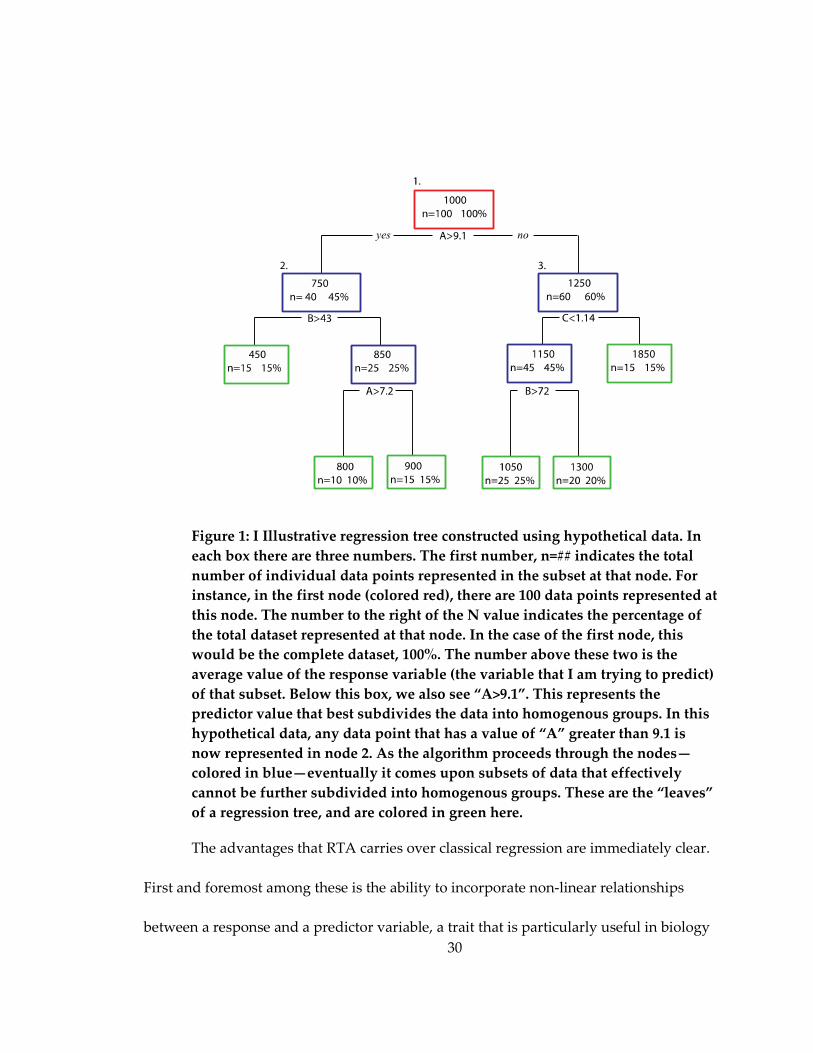
30
Figure 1: I Illustrative regression tree constructed using hypothetical data. In
each box there are three numbers. The first number, n=## indicates the total
number of individual data points represented in the subset at that node. For
instance, in the first node (colored red), there are 100 data points represented at
this node. The number to the right of the N value indicates the percentage of
the total dataset represented at that node. In the case of the first node, this
would be the complete dataset, 100%. The number above these two is the
average value of the response variable (the variable that I am trying to predict)
of that subset. Below this box, we also see “A>9.1”. This represents the
predictor value that best subdivides the data into homogenous groups. In this
hypothetical data, any data point that has a value of “A” greater than 9.1 is
now represented in node 2. As the algorithm proceeds through the nodes—
colored in blue—eventually it comes upon subsets of data that effectively
cannot be further subdivided into homogenous groups. These are the “leaves”
of a regression tree, and are colored in green here.
The advantages that RTA carries over classical regression are immediately clear.
First and foremost among these is the ability to incorporate non-linear relationships
between a response and a predictor variable, a trait that is particularly useful in biology

31
wherein complicated, non-linear relationships are common (Moore et al., 1991; Kay and
Madden, 1997). In addition, the simplistic output of the tree allows for the relative
importance of the various predictors on the distribution of the data to be clearly shown,
providing insight into the spatial influence of the predictors (Iverson and Prasad, 1998;
De’ath and Farbricius, 2000).
However, RTA is not without its disadvantages, even when compared to
conventional regression. First, any linear functions that happen to be included in the
analysis are only approximated, and because of the nature of RTA these linear functions
tend to be binned in a manner that oversimplifies the linear relationship, leading to a
“coarseness” of the RTA output. Those values that lie close to the boundary of two bins
are more likely to be misidentified. Additionally, results from RTA are highly dependent
on the input data, can be unstable with small changes to the input data producing highly
divergent trees. While this can be overcome with an appropriately large dataset,
particularly one in which the variables are normally distributed, such a dataset is
frequently hard to obtain in ecology.
2.1.1.3 Random Forests
Introduced by Breimann (2001), RF is a machine-learning approach based heavily
on RTA. RF analysis works in the following steps (Liaw and Wiener, 2002):
1. The original data is bootstrapped into a specified number of re-sampled data
sets.

32
2. Regression trees are produced for each bootstrapped sample with an alteration to
the node partitioning. Node partitioning is performed on a random sampled
subset of the resampled predictor variables, and the best predictor is chosen
among that subset.
3. New predictions are made through aggregating and averaging all the trees of the
bootstrapped samples. Data is predicted by averaging the predictions of all the
trees of the bootstrapped samples.
While the result from any given tree may differ dramatically from that of another tree,
the high number of trees that are typically grown in RF—≥1000, hence the “forest”—
allows it to effectively construct the best fit of the data irrespective of minor
perturbations within and amongst individual trees. This is further illustrated in Figures
2 and 3.

33
Figure 2: Overview of the procession of the random forest algorithm from the
original data set to predicting new data.
One of the complaints frequently leveled at RF is its apparent lack of
interpretability, that it is a “black box” (Cutler et al., 2007). This criticism stems from the
fact that RF lacks the illustrative efficiency of more traditional regression techniques.
Instead of producing one tree, RF predicts “out-of-bag” observations by calculating the
average of hundreds (or even thousands) of fully-grown, bootstrapped trees, meaning
that the relationship between variables is impossible to demonstrate. This is also true for
Original Data Set
Bootstrapping (ntree
subsets)
Subset 1
Subset 2
Subset ntree
Regression Tree
Regression Tree
Regression Tree
mTRY
predictor variables are randomly
sampled at each node of the regression
trees
Aggregate Tree
New data is predicted by
aggregating the predictions of all
the regression trees
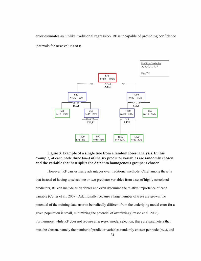
34
error estimates as, unlike traditional regression, RF is incapable of providing confidence
intervals for new values of y.
Figure 3: Example of a single tree from a random forest analysis. In this
example, at each node three (mtry) of the six predictor variables are randomly chosen
and the variable that best splits the data into homogenous groups is chosen.
However, RF carries many advantages over traditional methods. Chief among these is
that instead of having to select one or two predictor variables from a set of highly correlated
predictors, RF can include all variables and even determine the relative importance of each
variable (Cutler et al., 2007). Additionally, because a large number of trees are grown, the
potential of the training data error to be radically different from the underlying model error for a
given population is small, minimizing the potential of overfitting (Prasad et al. 2006).
Furthermore, while RF does not require an a priori model selection, there are parameters that
must be chosen, namely the number of predictor variables randomly chosen per node (mtry), and

35
the number of trees (ntree). Though the chosen values of these parameters can influence the results
(i.e. the predictive accuracy of the RF model), this effect has been shown to be relatively
negligible (Briemann, 2001; Liaw and Wiener, 2002; Cutler et al. 2007).
2.1.1.4 Gaussian Process Regression
GPR can be differentiated from standard linear regression in that rather than
producing a model (typically a straight line) that seeks to capture the relationship and
variance of the dataset as a whole—and thus provide a simple equation that describes
the general relationship between the independent variable(s) and the dependent
variable—it instead can model the covariance of a vector between only two points
(Rasmussen, 2006). It is, in essence, a model of interpolation; wherein the estimation of a
new data point that lies in between two observed data points has a smaller confidence
interval (that is, it can be estimated with greater confidence and lower error) than would
a new data point that lies between two observances that are more distant to one another.
This is done through the formation of a Gaussian, or normal, distribution for the
potential function that connects two known data points. If the observed data clusters in
close proximity, then the distribution that represents the likely feature-space of a
function that connects those two points will be narrower.
In other words, in simple linear regression, the uncertainty is standardized for all
new estimations. In GPR the uncertainty of predictions is dynamic, changing depending
on the richness and proximity of observed data. GPR has been demonstrated to be an

36
effective predictive model for non-linear relationships between continuous variables,
including in species distribution mapping (Weir and Pettit, 2000; Verrelst et al., 2012).
The mathematics of GPR is explained in further detail in Appendix B, which
represents a collaborative document created in conjunction with Bryan Glazer, whose
knowledge and expertise in this modeling technique contributed greatly to its
application in this study.
2.1.2 Paleoecological Reconstruction
While the above methods have been used previously in ecological literature (e.g.,
Okubo & Levin, 1980; Dunning et al., 1995; Monestiez et al., 2005; Rigby et al., 2010;
Verrelst et al., 2012) they have yet to be applied to the fossil record for the purposes of
environmental/climatic reconstruction. Heretofore, linear regression has been the
favored method due to its simplicity of output, application, and interpretation (Andrews
et al., 1979; Kay and Madden, 1997; Kay et al., 2012b). Here, I test these other regression
methods along with the more conventional linear regression in order to explore their
potential in paleoenvironmental reconstruction. Additionally, I apply these methods to
two well-sampled fossil localities in South America, the La Venta and Santa Cruz
Miocene faunas. The reconstructions derived from the different methods are
subsequently compared among one another and—where possible—to previously
37
published reconstructions (e.g., papers with the older reconstructions). Brief descriptions
of each of these fossil localities are presented below.
2.1.2.1 La Venta Paleogeography
The La Venta faunal list used in this study comes from the Monkey Beds of the
Honda Group in the Magdalena river valley in Colombia. The Honda Group, at about
5°N latitude, attains a thickness of 1150m (Guerrero, 1996) and is constrained by
radiometric and paleomagnetic evidence to a period beginning at approximately 13.5ma
and ending at approximately 11.8m (Flynn et al., 1996; Guerrero, 1996; Madden et al.,
1996). The Monkey Beds comprise a richly fossiliferous layer of the Honda Group with a
thickness of approximately 14.8m (Guerrero, 1996; Kay and Madden, 1997).
Magnetostratigraphic evidence limits the time interval of the Monkey Beds to ~15,000
years from between 13-12.85ma (Flynn et al., 1996; Kay and Madden, 1997).
In the mid-Miocene, the La Venta region was situated within 5 degrees of the
equator on a peninsula in northern South America, bordered to the west by the Pacific
Ocean and to the north and east by the Caribbean Sea (Whitmore and Stewart, 1965;
Duque-Caro, 1990; Hoorn et al., 1995; Kay and Madden, 1997). Fossil vertebrate evidence
from amphibians and reptiles, suggests low elevation (<100m) in the middle Miocene La
Venta. This conclusion stands in contrast to the region today, which is largely
dominated by the Colombian Andes—though the actual fossil locality lies in the

38
Magdalena river valley (approximately 500m in elevation) between the Central and
Eastern Cordilleras (Kay and Madden, 1997).
Previous paleoecological reconstructions at La Venta (Kay and Madden, 1996;
Kay and Madden, 1997) have suggested a forested environment within a complex
system of meandering rivers, with a mean average rainfall of between 1500-2000
mm/year. Seasonality was estimated to be an insignificant component of the middle
Miocene at La Venta (Guerrero, 1996; Kay and Madden, 1997).
The mammalian fauna from La Venta, Colombia remains the only well-sampled
Tertiary tropical paleofauna known from South America. As such it offers a rare
window into the understanding of the evolution of South American tropical
communities. Kay and Madden (1997) reconstructed the rainfall at La Venta to be
between 1500-2000 mm/year, and posited that the habitat was marked by heterogeneity
in both ground cover and the distribution of river systems. Croft (2001) came to a similar
conclusion using cenogram analysis. The conclusions of Kay and Madden (1997) were
drawn from least squares and polynomial regressions involving ecological indices
obtained from 18 extant mammalian communities (all of which are included in this
study, as well).
2.1.2.2 Santa Cruz Paleogeography
The Santa Cruz Formation (SCF) in southern Argentina is an exposure of early
Miocene deposits stretching from the Atlantic coast of Patagonia in east to the Andes in
39
the west, and is found between 50.3° and 51.6°S latitude. The SCF lies in approximately
the same latitude today as it did in the early Miocene.
The fauna that I analyze here is found in the southern part of the SCF on and
near the Atlantic coast near Monte León. Tauber (1994) identified several fossil layers
(FL) 1-7 in this region, concluding that levels were successively younger from north to
south. Tephrostratigraphic correlations reported by Perkins et al. (2012) established that
these levels are very close in age, spanning a period of about 100,000 years (~17.5-17.4
ma). Based on this information, Kay et al. (2012b) chose to treat FL 1-7 as a single
paleofauna, as I do here.
Previous paleoecological analyses of the FL 1-7 of the SCF indicate a mosaic
environment of open grasslands and patches of forests, with a high degree of
temperature seasonality, rainfall of approximately 1000-1500 mm/year, and mean annual
temperatures >14°C (Vizcaino et al., 2012). This reconstruction was based on a variety of
different sources and techniques, including paleosol records indicating fluvial deposits
(Matheos and Raigemborn, 2012), paleofloral records (Brea et al., 2012), the presence of
both terrestrial and arboreal ecologies in the mammalian fauna (Degrange et al., 2012;
Prevosti et al., 2012; Bargo et al., 2012; Candela et al., 2012), the presence of a species of
frog (Fernicola and Albino, 2012), the presence of a single primate species (Kay et al.,
2012c), and community level analyses similar to what I present in this study (Kay et al.,
2012b).

40
The faunal levels 1-7 of the SCF—considered by Kay et al. (2012a; 2012b) to be
essentially a contemporaneous fauna—represent another of the most well sampled fossil
mammalian localities in South America. Unlike La Venta however, the SCF is of a much
higher latitude and thus presents us with a chance to compare results between two
localities that should have significantly different estimates for climate. Additionally,
work by Vizcaino et al. (2010) and Kay et al. (2012a; 2012b) uses many of the same
techniques and ecological indices as this dissertation. The primary differences between
this paper and those previous studies is threefold: 1) Kay et al. (2012b) uses 25 modern
localities to create their regression models; 2) Regression techniques are limited to linear
regression; and 3) Climate variables were limited to just temperature and rainfall, no
habitat variables were incorporated. Thus, I compare my results from GPR, RF, and RTA
to these previous estimates and interpret those differences in the context of the
paleoenvironment of the SCF.
2.2 Materials and Methods
Faunal lists for a total of 85 localities across Central and South America (Figure
2.4), as well as 14 localities from across Australia (Figure 2.11) , were compiled from the
literature (see supplemental documents for references) as well as the Information Center
for the Environment (ICE) Biological Inventories of the World’s Protected Areas
(http://www.ice.ucdavis.edu/bioinventory/bioinventory. html). ICE is an online archive of the
world’s national parks, and features mammalian faunal lists for each of the archived

41
parks. Because this study is concerned with community structure and depends on the
listed community being more or less complete, only faunal lists that were recorded by
ICE as being either “complete” or “essentially complete” were included in this study.
While it is likely that a few species go unrecorded in these lists, this procedure provides
a more reliable representation of any given fauna at a locality than does the use of
distribution maps (Spradley et al., 2015).

42
Figure 4: Map of South American illustrating the faunal localities used in this
study.
For each locality, the presence or absence of 617 species of non-volant mammals
was recorded. In addition, basic ecological information for each species was compiled
from the literature (see supplemental documents for references). This information
includes average body size, primary diet, and preferred locomotion. The identification

43
of any of these variables in the fossil record is problematic and is not as precise as their
identification in living species. Thus, I follow Kay and Madden (1997) and Kay et al.
(2012) for the categorization of ecological variables. These are summarized in Table 1. In
addition, I include a predator/prey ratio, calculated as the number of faunivores divided
by primary consumers with a body mass between 500g-500kg.
Table 1: Definitions of the ecological categories used in this study. Each
species was assigned a number from each variable.
Body Mass
Category
Definition Locomotor
Category
Definition
1 10-100g 1 Large terrestrial (>1kg)
2 100g-1kg 2 Small terrestrial (<1kg)
3 1-10kg 3 Arboreal (including gliding)
4 10-100kg 4 Arboreal/Terrestrial
(Scansorial)
5 100-500kg 5 Semi-aquatic
6 >500kg 6 Fossorial (including semi-
fossorial)
Dietary Category Definition
1 Vertebrate Prey
2 Ants and termites
3 Insects (with
some fruit)

44
4 Fruit (with some
animals)
5 Small seeds of
grasses (and
other plants or
insects)
6 Fruit with leaves
7 Leaves (browse)
8 Stems and leaves
of grasses (graze)
9 Tree gums (with
fruit/insects)
After assigning every species an appropriate category, a series of indices were
used to describe the relative abundance of a specific ecology (or ecologies) within each
mammalian community (Kay and Madden, 1997). These indices include the Arboreality
Index (AI: the relative number of arboreal and scansorial species to the total number of
species in a fauna), the Frugivore Index (FI), the Grazing Index (GI), and the Browsing
Index (BI). These indices serve as my primary variables of interest in relation to climatic
variables (see below). Faunal lists, along with ecological information for each species, are
presented in the supplementary documents.
Spatial maps for six bioclimatic variables were downloaded from WorldClim.org.
These spatial maps are produced from data collected at weather stations across the
continent and represent averages of 20-50 years. Areas between weather stations are
filled in with interpolated data. In addition, spatial maps for net primary productivity
45
(NPP) and canopy height were downloaded from the Numerical Terradynamic
Simulation Group (NTSG; http://www.ntsg.umt.edu/project/mod17) and the NASA
Spatial Data Access Tool (SDAT: http://webmap.ornl.gov/wcsdown/wcsdown.jsp?dg_
id=10023_1), respectively. These spatial maps were then uploaded into QGIS® (Open
Source Geospatial Foundation, 2007) and the values for each variable were recorded for
each locality at their associated GPS coordinates using the “point sampling” plugin in
QGIS. Bioclimatic variables for each locality are presented in a supplementary table.
Following Kay and Madden (1997) and Kay et al. (2012b), the localities’ first
Principal Component (PC1) scores from a Principal Components Analysis (PCA)
comprising the ecological indices included in this study, as well as latitude and elevation
were used in a linear regression. The PC1 scores were plotted against each climatic
variable. A least-squares regression was fit to each plot and the subsequent linear
equation was obtained, which in turn was used to predict climatic variables for the other
localities in the test dataset (including the fossil localities). Spatial autocorrelation in
both the species predictor variables and the environmental target variables was
calculated and visualized using a Mantel correlogram (Legendre, 2011).
While choosing the values for the pertinent parameters for the two machine
learning algorithms included in this study—RF and GPR—the recommendations of
previous literature were followed when available (Liaw and Wiener, 2002; Stitson et al.,
46
1999). For RF, mtry was set to 4, representative of p/3, where p is the number of predictor
variables (Liaw and Wiener, 2002), and ntree was set to 1000, the default for RF.
To compare regression techniques, I obtained two metrics that measure the
average error between predicted and observed values in predictive modeling; root mean
squared error (RMSE) and mean absolute error (MAE). MAE is simply the average
difference between the estimate and the observed value for a given data point. RMSE is
a similar measurement, but instead squares the difference between an estimate and the
observed value, and then takes the square root. These differences are then averaged
across all estimations. Compared to MAE, RMSE is more sensitive to outliers—i.e.
predictions that are extremely different than the observed value. While MAE is more
commonly used in other studies incorporating predictive models given its simplicity,
RMSE is preferred by others for its sensitivity (Chai and Draxler, 2014).
All statistical analyses were performed in the open-source statistical software, R.
The “rpart” package (Therneau et al, 2015) was utilized for RTA and the
“randomForest” package (Liaw and Wiener, 2002) utilized for RF. The “gGPRlot2” and
“forestFloor” (Welling et al., 2016) packages were used to visualize the results from
these analyses.
47
2.3 Results
2.3.1 Spatial Autocorrelation
No statistically significant autocorrelation among the climatic variables across
the South American localities was found using Mantel’s rM statistic. This indicates
general independence between my localities, but as a conservative measure any
potential spatial autocorrelation between closely associated localities in my dataset was
accounted for in the models by including latitude and longitude as predictor variables.
2.3.2 South American extant faunas
Results from the models obtained from the training data as applied to the test
data are presented in Table 2. For the multivariate linear regression, the first principal
component (PC1) explained 46.2% of the variance. Plotting the PC1 scores against the
climatic variables resulted in strong correlations with temperature (R2= 0.68),
precipitation (R2= 0.50), and temperature seasonality (R2= 0.59). These correlation
coefficients are weaker for net primary productivity (R2= 0.36) and canopy height (R2=
0.32), though still statistically significant (p < 0.001). The relationship of PC1 scores and
precipitation seasonality was not statistically significant (p = 0.54).
To quantify the error from these predictions, both root mean squared error
(RMSE) and mean absolute error (MAE) are presented. Generally, linear regression (LR)
outperforms regression trees, but is surpassed in predictive performance by both
random forests (RF) and Gaussian process regression (GPR). RF has significantly lower
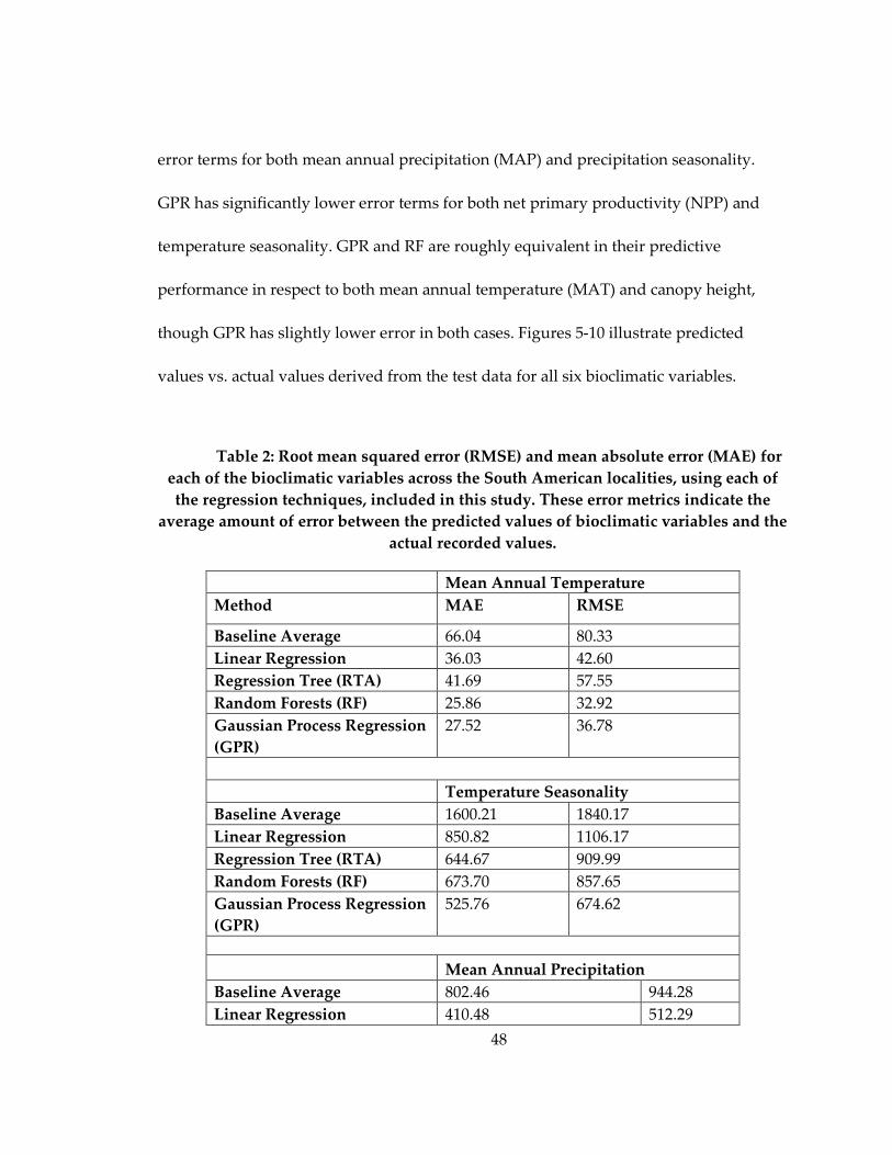
48
error terms for both mean annual precipitation (MAP) and precipitation seasonality.
GPR has significantly lower error terms for both net primary productivity (NPP) and
temperature seasonality. GPR and RF are roughly equivalent in their predictive
performance in respect to both mean annual temperature (MAT) and canopy height,
though GPR has slightly lower error in both cases. Figures 5-10 illustrate predicted
values vs. actual values derived from the test data for all six bioclimatic variables.
Table 2: Root mean squared error (RMSE) and mean absolute error (MAE) for
each of the bioclimatic variables across the South American localities, using each of
the regression techniques, included in this study. These error metrics indicate the
average amount of error between the predicted values of bioclimatic variables and the
actual recorded values.
Mean Annual Temperature
Method MAE RMSE
Baseline Average 66.04 80.33
Linear Regression 36.03 42.60
Regression Tree (RTA) 41.69 57.55
Random Forests (RF) 25.86 32.92
Gaussian Process Regression
(GPR)
27.52 36.78
Temperature Seasonality
Baseline Average 1600.21 1840.17
Linear Regression 850.82 1106.17
Regression Tree (RTA) 644.67 909.99
Random Forests (RF) 673.70 857.65
Gaussian Process Regression
(GPR)
525.76 674.62
Mean Annual Precipitation
Baseline Average 802.46 944.28
Linear Regression 410.48 512.29
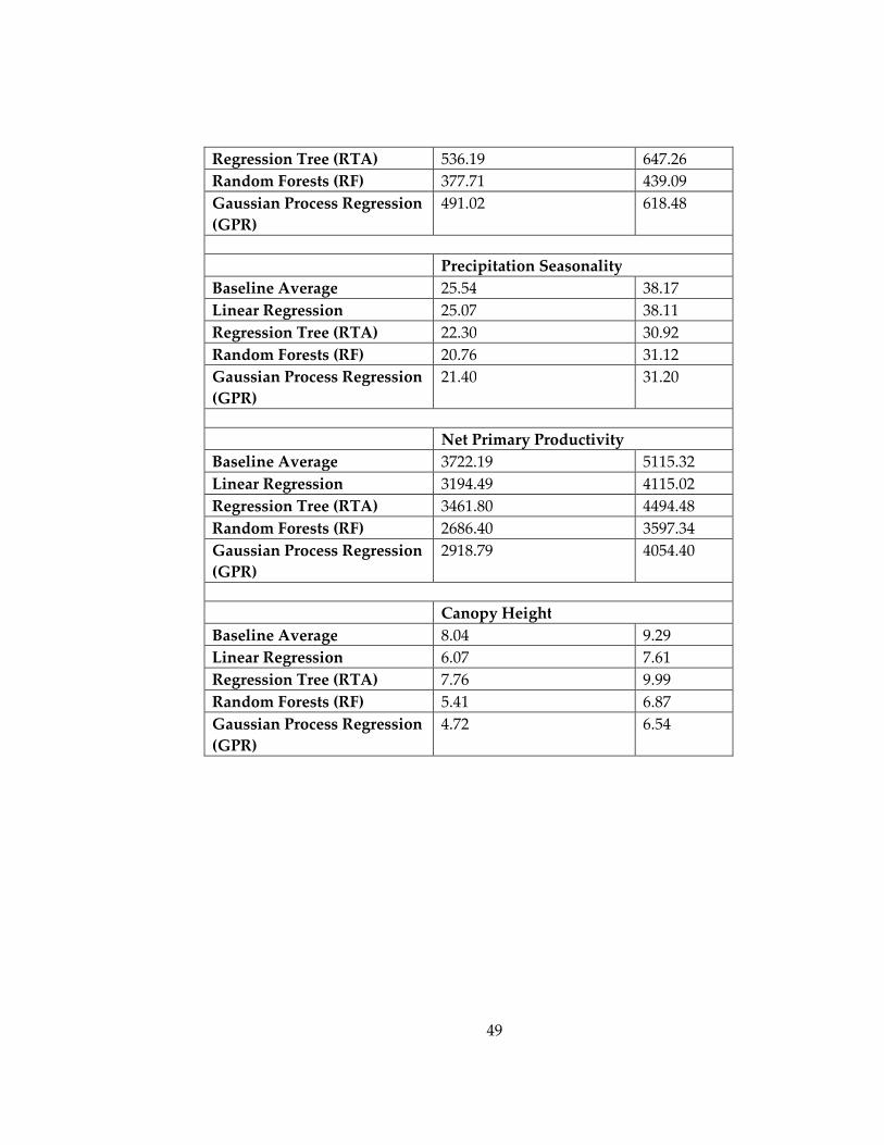
49
Regression Tree (RTA) 536.19 647.26
Random Forests (RF) 377.71 439.09
Gaussian Process Regression
(GPR)
491.02 618.48
Precipitation Seasonality
Baseline Average 25.54 38.17
Linear Regression 25.07 38.11
Regression Tree (RTA) 22.30 30.92
Random Forests (RF) 20.76 31.12
Gaussian Process Regression
(GPR)
21.40 31.20
Net Primary Productivity
Baseline Average 3722.19 5115.32
Linear Regression 3194.49 4115.02
Regression Tree (RTA) 3461.80 4494.48
Random Forests (RF) 2686.40 3597.34
Gaussian Process Regression
(GPR)
2918.79 4054.40
Canopy Height
Baseline Average 8.04 9.29
Linear Regression 6.07 7.61
Regression Tree (RTA) 7.76 9.99
Random Forests (RF) 5.41 6.87
Gaussian Process Regression
(GPR)
4.72 6.54
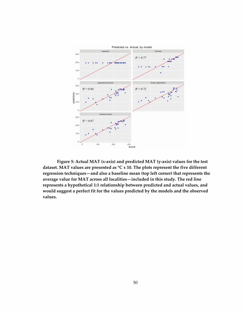
50
Figure 5: Actual MAT (x-axis) and predicted MAT (y-axis) values for the test
dataset. MAT values are presented as °C x 10. The plots represent the five different
regression techniques—and also a baseline mean (top left corner) that represents the
average value for MAT across all localities—included in this study. The red line
represents a hypothetical 1:1 relationship between predicted and actual values, and
would suggest a perfect fit for the values predicted by the models and the observed
values.
baseline full.tree
gaussian.process linear.regression
random.forest
0
100
200
300
0
100
200
300
0
100
200
300
0 100 200 300
actual
pre
dic
tions
Predicted vs. Actual, by model
R2 = 0.77
R2 = 0.72R2 = 0.84
R2 = 0.87
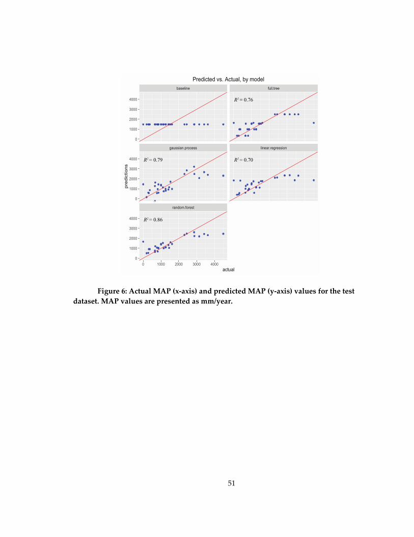
51
Figure 6: Actual MAP (x-axis) and predicted MAP (y-axis) values for the test
dataset. MAP values are presented as mm/year.
baseline full.tree
gaussian.process linear.regression
random.forest
0
1000
2000
3000
4000
0
1000
2000
3000
4000
0
1000
2000
3000
4000
0 1000 2000 3000 4000
actual
pre
dic
tio
ns
Predicted vs. Actual, by model
R2 = 0.76
R2 = 0.70R2 = 0.79
R2 = 0.86
52
Figure 7: Actual temperature seasonality (x-axis) and predicted temperature
seasonality (y-axis) values for the test dataset. Temperature seasonality is presented as
the standard deviation of the MAT multiplied by 100.
baseline full.tree
gaussian.process linear.regression
random.forest
0
2000
4000
6000
0
2000
4000
6000
0
2000
4000
6000
0 2000 4000 6000
actual
pre
dic
tio
ns
Predicted vs. Actual, by model
R2 = 0.86
R2 = 0.63R2 = 0.86
R2 = 0.86
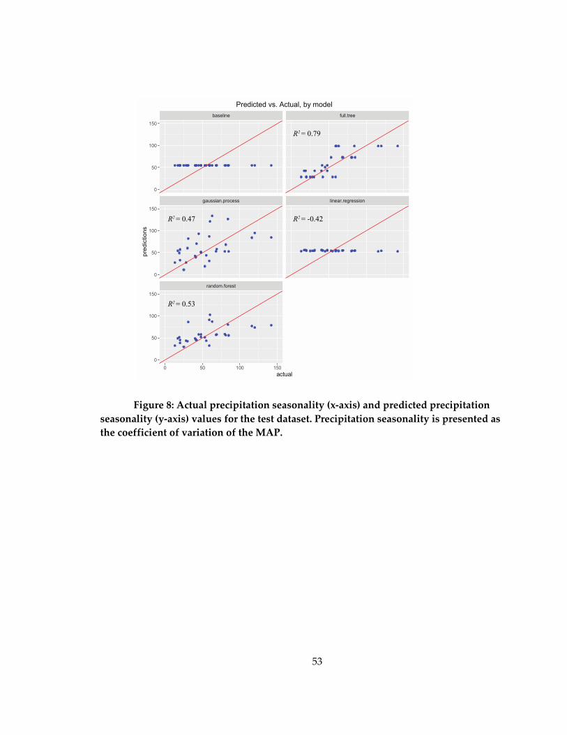
53
Figure 8: Actual precipitation seasonality (x-axis) and predicted precipitation
seasonality (y-axis) values for the test dataset. Precipitation seasonality is presented as
the coefficient of variation of the MAP.
baseline full.tree
gaussian.process linear.regression
random.forest
0
50
100
150
0
50
100
150
0
50
100
150
0 50 100 150
actual
pre
dic
tio
ns
Predicted vs. Actual, by model
R2 = 0.79
R2 = 0.47 R2 = -0.42
R2 = 0.53
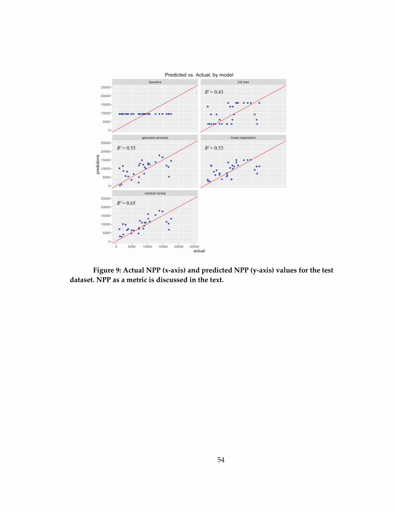
54
Figure 9: Actual NPP (x-axis) and predicted NPP (y-axis) values for the test
dataset. NPP as a metric is discussed in the text.
baseline full.tree
gaussian.process linear.regression
random.forest
0
5000
10000
15000
20000
25000
0
5000
10000
15000
20000
25000
0
5000
10000
15000
20000
25000
0 5000 10000 15000 20000 25000
actual
pre
dic
tions
Predicted vs. Actual, by model
R2 = 0.43
R2 = 0.53R2 = 0.55
R2 = 0.65
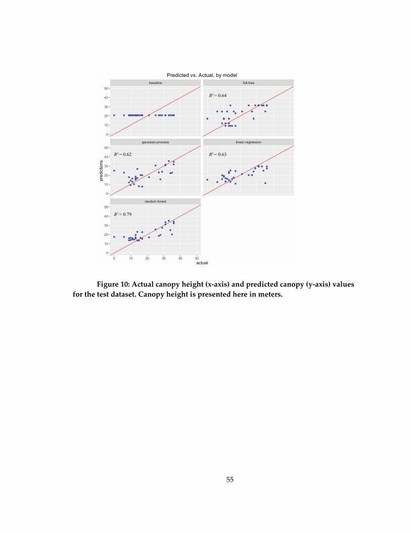
55
Figure 10: Actual canopy height (x-axis) and predicted canopy (y-axis) values
for the test dataset. Canopy height is presented here in meters.
baseline full.tree
gaussian.process linear.regression
random.forest
0
10
20
30
40
50
0
10
20
30
40
50
0
10
20
30
40
50
0 10 20 30 40 50
actual
pre
dic
tion
s
Predicted vs. Actual, by model
R2 = 0.63R2 = 0.62
R2 = 0.79
R2 = 0.64
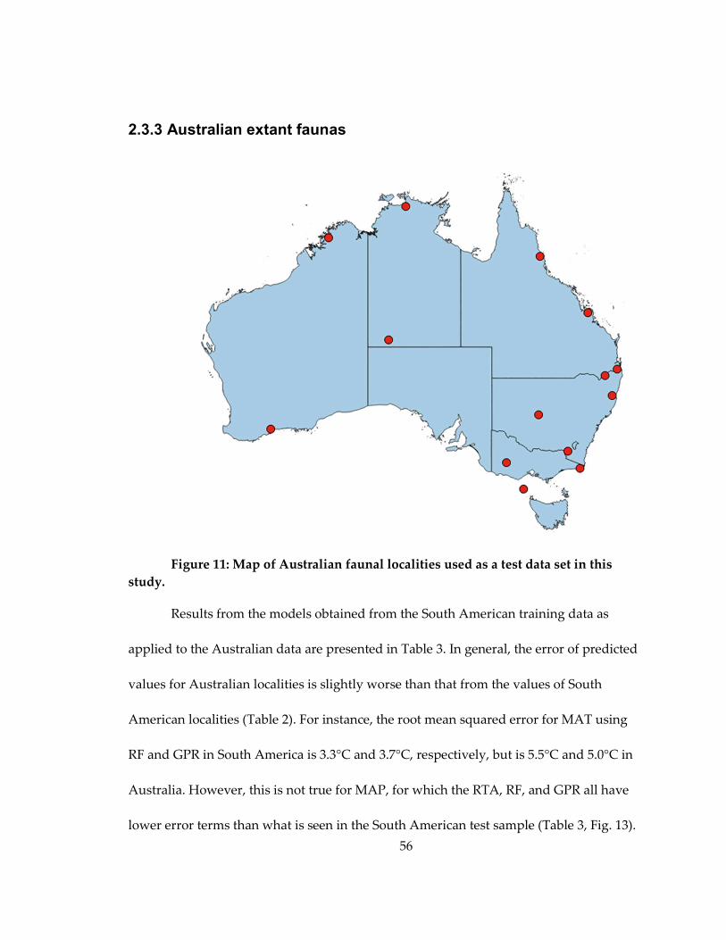
56
2.3.3 Australian extant faunas
Figure 11: Map of Australian faunal localities used as a test data set in this
study.
Results from the models obtained from the South American training data as
applied to the Australian data are presented in Table 3. In general, the error of predicted
values for Australian localities is slightly worse than that from the values of South
American localities (Table 2). For instance, the root mean squared error for MAT using
RF and GPR in South America is 3.3°C and 3.7°C, respectively, but is 5.5°C and 5.0°C in
Australia. However, this is not true for MAP, for which the RTA, RF, and GPR all have
lower error terms than what is seen in the South American test sample (Table 3, Fig. 13).
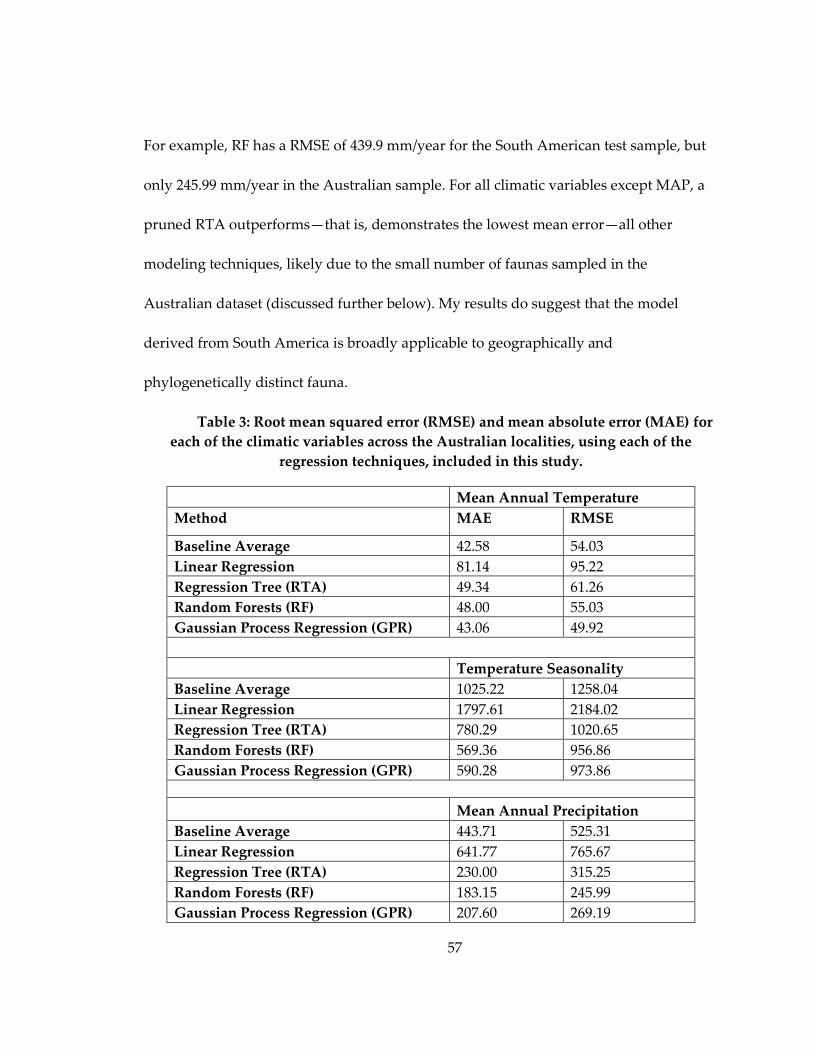
57
For example, RF has a RMSE of 439.9 mm/year for the South American test sample, but
only 245.99 mm/year in the Australian sample. For all climatic variables except MAP, a
pruned RTA outperforms—that is, demonstrates the lowest mean error—all other
modeling techniques, likely due to the small number of faunas sampled in the
Australian dataset (discussed further below). My results do suggest that the model
derived from South America is broadly applicable to geographically and
phylogenetically distinct fauna.
Table 3: Root mean squared error (RMSE) and mean absolute error (MAE) for
each of the climatic variables across the Australian localities, using each of the
regression techniques, included in this study.
Mean Annual Temperature
Method MAE RMSE
Baseline Average 42.58 54.03
Linear Regression 81.14 95.22
Regression Tree (RTA) 49.34 61.26
Random Forests (RF) 48.00 55.03
Gaussian Process Regression (GPR) 43.06 49.92
Temperature Seasonality
Baseline Average 1025.22 1258.04
Linear Regression 1797.61 2184.02
Regression Tree (RTA) 780.29 1020.65
Random Forests (RF) 569.36 956.86
Gaussian Process Regression (GPR) 590.28 973.86
Mean Annual Precipitation
Baseline Average 443.71 525.31
Linear Regression 641.77 765.67
Regression Tree (RTA) 230.00 315.25
Random Forests (RF) 183.15 245.99
Gaussian Process Regression (GPR) 207.60 269.19
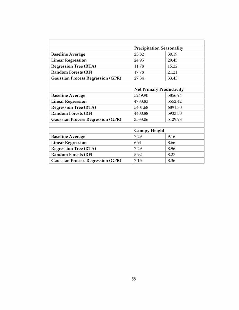
58
Precipitation Seasonality
Baseline Average 23.82 30.19
Linear Regression 24.95 29.45
Regression Tree (RTA) 11.78 15.22
Random Forests (RF) 17.78 21.21
Gaussian Process Regression (GPR) 27.34 33.43
Net Primary Productivity
Baseline Average 5249.90 5856.94
Linear Regression 4783.83 5552.42
Regression Tree (RTA) 5401.68 6891.30
Random Forests (RF) 4400.88 5933.50
Gaussian Process Regression (GPR) 3533.06 5129.98
Canopy Height
Baseline Average 7.29 9.16
Linear Regression 6.91 8.66
Regression Tree (RTA) 7.29 8.96
Random Forests (RF) 5.92 8.27
Gaussian Process Regression (GPR) 7.15 8.36
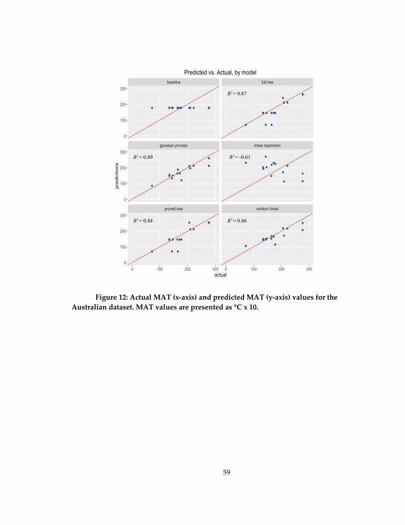
59
Figure 12: Actual MAT (x-axis) and predicted MAT (y-axis) values for the
Australian dataset. MAT values are presented as °C x 10.
baseline full.tree
gaussian.process linear.regression
pruned.tree random.forest
0
100
200
300
0
100
200
300
0
100
200
300
0 100 200 300 0 100 200 300
actual
pre
dic
tio
ns
Predicted vs. Actual, by model
R2 = 0.87
R2 = 0.89 R2 = -0.61
R2 = 0.84 R2 = 0.86

60
Figure 13: Actual MAP (x-axis) and predicted MAP (y-axis) values for the
Australian dataset. MAP values are presented as mm/year.
2.3.3 Paleoclimatic Reconstructions
2.3.3.1 The Monkey Beds of La Venta
Table 4 summarizes the estimations of climate and habitat from each of my
models for the Monkey Beds. All models suggest rainfall between 1500-2000 mm/year,
though the two machine-learning algorithm models suggest slightly higher predictions,
in the vicinity of 2000 mm/year. With the exception of the multivariate linear regression
baseline full.tree
gaussian.process linear.regression
pruned.tree random.forest
0
1000
2000
3000
4000
0
1000
2000
3000
4000
0
1000
2000
3000
4000
0 1000 2000 3000 4000 0 1000 2000 3000 4000
actual
pre
dic
tio
ns
Predicted vs. Actual, by model
R2 = 0.82
R2 = 0.88 R2 = 0.13
R2 = 0.79 R2 = 0.93
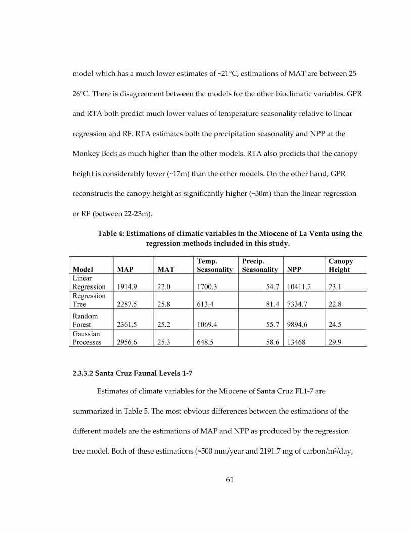
61
model which has a much lower estimates of ~21°C, estimations of MAT are between 25-
26°C. There is disagreement between the models for the other bioclimatic variables. GPR
and RTA both predict much lower values of temperature seasonality relative to linear
regression and RF. RTA estimates both the precipitation seasonality and NPP at the
Monkey Beds as much higher than the other models. RTA also predicts that the canopy
height is considerably lower (~17m) than the other models. On the other hand, GPR
reconstructs the canopy height as significantly higher (~30m) than the linear regression
or RF (between 22-23m).
Table 4: Estimations of climatic variables in the Miocene of La Venta using the
regression methods included in this study.
Model MAP MAT
Temp.
Seasonality
Precip.
Seasonality NPP
Canopy
Height
Linear
Regression 1914.9 22.0 1700.3 54.7 10411.2 23.1
Regression
Tree 2287.5 25.8 613.4 81.4 7334.7 22.8
Random
Forest 2361.5 25.2 1069.4 55.7 9894.6 24.5
Gaussian
Processes 2956.6 25.3 648.5 58.6 13468 29.9
2.3.3.2 Santa Cruz Faunal Levels 1-7
Estimates of climate variables for the Miocene of Santa Cruz FL1-7 are
summarized in Table 5. The most obvious differences between the estimations of the
different models are the estimations of MAP and NPP as produced by the regression
tree model. Both of these estimations (~500 mm/year and 2191.7 mg of carbon/m2/day,

62
respectively) are considerably lower than the other models, which predict that rainfall
was between ~1050 mm/year and 1690 mm/year, and NPP was between ~6000 and 8600
mg of carbon/m2/day. Temperature seasonality is also reconstructed as much higher in
the regression tree model. In other words, the regression tree model is reconstructing the
climate in the Miocene of Santa Cruz FL 1-7 to be much drier, seasonal, and less
productive than the reconstructions from the other models. Otherwise, there is general
agreement between the models, and results suggest that the climate was considerably
drier, cooler, and more seasonal than that of the Monkey Beds of La Venta, as well as the
habitat having lower productivity and a shorter canopy height.
Table 5: Estimations of climatic variables in the Miocene of Santa Cruz using the
regression methods included in this study, exclusively with the South American data
set.
Model MAP MAT
Temp.
Seasonality
Precip.
Seasonality NPP
Canopy
Height
Linear
Regression 1056.5 14.9 3226.4 57.2 6264.4 16.2
Regression
Tree 499.0 17.4 4118.5 34.3 2191.7 22.5
Random
Forest 1268.8 16.6 3166.1 42.9 6598.9 21.04
Gaussian
Processes 1689.9 15.1 3641.4 16.9 8681.3 24
2.4 Discussion
The relationship between the community structure of a mammalian fauna and
environment is undoubtedly complex, and it is impossible to take every potential
confounding variable into consideration. Previous studies of paleoenvironment
63
reconstruction have acknowledged this complexity, but have otherwise sought to
establish linear relationships that can provide simple, easy to interpret estimations from
the fossil record. However, advances in computational power has allowed incorporation
of many more variables with more complex, non-linear relationships unlike least-
squares regression. Given the importance of applying all available evidence to
reconstruct paleoclimates and paleoenvironments, I seek to test the efficacy of
sophisticated regression techniques on the estimation of climate variables. These
methods allow researchers to include several uncertainty parameters (discussed in the
introduction) and allow for narrower error ranges for any given, novel data point. This
is partly due to the fact that simplifying assumptions inherent to techniques like linear
regression are not necessary in these approaches.
2.4.1 Performance of regression techniques in South American data
My results show a consistent improvement in accuracy for the two machine-
learning algorithms, random forests (RF) and Gaussian process regression (GPR), over
all other included methods. These two methods clearly benefit from the ability to apply
data learning to the model, and thus account for the variation of the data. This is
opposed to linear regression, which only fits a best-fit line to the data. A posterior
distribution allows GPR to more accurately account for non-linear relationships between
predictor variables and the response variable (Williams, 1997; Cutler et al., 2007), while
random bagging allows RF to test a large number of potential tree-like models before

64
deciding upon which produces the best fit. There are, however, important a priori
decisions in each technique before running the analyses, each of which will have
significant effects on the results. These can be summarized as follows:
1. The percentage split of data randomly chosen for either the training or testing
dataset.
2. The covariance function used in the GPR model and its free parameters.
3. The number of response variables chosen in each bagging attempt (RF).
Ultimately the first decision is arbitrarily chosen, though intuitively one would
be best served by choosing a majority of the data for the training set. The compromise
lies in choosing enough of the data to have a meaningful effect on the trained model so
that it essentially captures the variation of the entire dataset, but also having enough of
the data set aside for testing so that interpretations from the results are meaningful. In
general, previous studies have chosen a threshold of 70-80% for the training dataset
(Cutler et al., 2007), and my choice of 70% is thus in keeping with previous studies. The
second decision on the other hand is again chosen a priori on the basis of the structure of
the data. Given that I am working with multidimensional regression, the recommended
kernel function is the ANOVA function (Hoffman et al., 2008).
Finally in regards to the number of response variables (mtry) randomly chosen at
each node during RF modeling, setting mtry too high results in overfitting the data—
discussed further in relation to regression trees below—while setting mtry too low also
65
results in a significant decrease in performance. The current standard, used here, is to
take the square root of the total number of predictor variables (Briemann, 2001: Liaw
and Wiener, 2002).
Interestingly, regression trees do not perform as well as least-squares regression
in the majority of the response variables included in this study. This is likely due to the
fact that the output of the regression tree is binning the data too broadly, resulting in
estimations that fit into a limited number of bins. Each bin has its own mean, so the
result is that the estimations are themselves limited to just a handful of means
equivalent to the number of bins. The relatively few number of bins may be related to
the relatively small number of localities in this study (<100), which is significantly less
than other similar studies (>300) that have used regression tree analysis in relation to
communities and environment (De’ath and Fabricius, 2000; De’ath, 2002). While a larger
tree could potentially fix this problem, the standard protocol for determining tree size in
previous studies is to choose the tree that has the smallest mean square error (De’ath,
2002), in a process known as “pruning”.
2.4.2 Results from modern localities
2.4.2.1 Mean annual precipitation (MAP)
An interesting aspect of my results is that the localities with particularly high
MAP (>2500mm/year) are consistently underestimated, regardless of which regression
model is used. This suggests two things: 1) the various ecological indices used do not
66
have a linear relationship with MAP, particularly at higher values, as has been
suggested by previous studies (Kay et al., 1997; Spradley et al., 2015); and 2) the amount
of data available for localities of such high MAP is limited, such that even the machine-
learning based models only have a few data points with which to extrapolate (or
interpolate). This difficulty is acknowledged by previous studies of mammalian
community structure (e.g., Andrews et al., 1979; Kay and Madden, 1997; Kay et al.,
1997). In the context of the fossil record, it makes environments with extreme amounts of
rainfall difficult to identify, and it is likely only through indicator species (such as
aquatic forms) that such an environment can be identified (Kay et al., 1997). It is also
worth noting that in predicting MAP, the linear regression technique of Kay et al.
(2012b) performed better than any other technique. This was the only climatic variable in
which the linear regression outperformed either of the machine-learning approaches.
2.4.2.2 Mean annual temperature (MAT)
In general, MAT is estimated with high accuracy in modern South American
faunal localities, particularly by GPR and RF. In fact, in my results GPR and RF display a
low amount of error for almost all MAT values for the entire test dataset. The only
exceptions are two localities, the Ulla Ulla National Reserve in Bolivia and the Lauca
National Park in Chile, which happen to correspond to the two localities with the
highest elevation in my study, at ~5000m and ~4500m respectively. 89.4% of the localities
in this study are found at altitudes below 1500m, so the inability of the models to
67
accurately estimate the climate variables at high altitudes should come as no surprise, as
high altitudes produce much different physiological demands on the organisms
(Lenfant, 1973; Monge and León-Velarde, 1991). In general, my results suggest that
mammalian community ecological indices are closely related to temperature. This bears
close resemblance to plant communities, amongst which diversity and richness have
also been shown to have a positive correlation with temperature (see Pausas and Austin,
2001 for review of studies of plant species richness), and is also in agreement with the
energy-water hypothesis of species richness of Hawkins et al. (2003).
2.4.2.3 Temperature seasonality
Discarding the pruned regression tree, the regression models, and GPR in
particular, predict temperature seasonality very accurately. This result is consistent with
similar studies that found temperature seasonality to be a good predictor of animal
species richness (Danell et al., 1996; Andrews and O’Brien, 2000; Hawkins et al., 2003;
Hurlbert and Haskell, 2003). Temperature seasonality has a particularly strong
relationship with latitude relative to the other climatic variables, and thus may be a key
driver of the latitudinal gradient of species richness. In a review of species richness and
climate, Hawkins et al. (2003) noted that lower temperatures not only drive plant
productivity down by limiting energy for photosynthesis, but they also create higher
metabolic demands on the fauna. Both factors are likely limiting the ecological richness
of the mammalian fauna in these localities. Kay et al. (2012b) previously suggested that
68
many ecological niches in these highly seasonal environments might be filled by migrant
avian species that can disperse during seasons of low plant productivity. This
hypothesis is supported by the findings of Aizen and Ezcurra (1998), who noted that
seed dispersal in temperate forests is accounted for by just a few bird species, many of
them migratory. Therefore, a seasonally productive environment may not carry a strong
mammalian faunal signal. Regardless, my results suggest that temperature seasonality
can be accurately predicted using ecological indices, with the best performing variables
being the Frugivore Index, the Arboreality Index, and the Grazing Index.
2.4.2.4 Precipitation seasonality
Seasonality in precipitation displays a much more complex relationship with
mammalian faunas. This is illustrated by the fact that RF performs only slightly better
than the baseline (the average precipitation seasonality value from across all 85
localities), and GPR even performs slightly worse. Unlike temperature seasonality,
precipitation seasonality does not have a consistent relationship with any other climatic
variable included in this study. This suggests that it might be more dependent on local
geography than temperature, or reflective of short-term climatic events, which occurred
during the decades of the BioClim data collection. That this result stands in contrast with
that from temperature seasonality may suggest that precipitation seasonality in and of
itself is not as limiting to plant productivity (and thus faunal richness) as is temperature
seasonality. While these potential causes of this poor relationship are purely speculative,

69
the fact remains that based on my results, precipitation seasonality would be difficult—if
not impossible—to predict accurately based purely on mammalian niche structure.
2.4.2.5 Net primary productivity (NPP)
As it is the most direct measure of the potential amount of resources available to
herbivores, NPP should have a strong correlative relationship with many of my
ecological indices. However, results from my models suggest that it is nevertheless a
difficult variable to predict using those same indices. This is perhaps best illustrated by a
simple bivariate plot of NPP and the Frugivore Index (Figure 14), showing that the
relationship between these two variables is extremely poor (R2=.04).
Figure 14: NPP versus Frugivore Index for the South American dataset. Solid
red line represents least-squares regression (R2=.049).

70
This is a surprising result considering that NPP is supposedly an indirect
measure of the metabolism of plants as they absorb carbon dioxide during the
production of sugars and starches during photosynthesis (specifically, NPP is the
difference between CO2 taken in during photosynthesis and CO2 released during
respiration and is measured in grams of carbon per square meter per day). Higher NPP
values would suggest that plants are converting more and more carbon dioxide into
energy; energy that would presumably be available to the mammalian fauna for
consumption (Kay et al., 1997). We might expect, then, that primary consumers in the
community should be particularly species rich in an environment with high NPP. That
we do not find such a relationship may be indicative of three things: 1) NPP is a poor
predictor of plant species richness, such that NPP is being driven by a relatively small
number of plant species with high abundance (and thus ecological diversity in the
mammalian fauna is similarly low); 2) methods used to measure NPP (NASA’s
Moderate Resolution Imaging Spectroradiometer, or MODIS) are inexact for the level of
resolution that is present in the other variables included in this study; or 3) mammalian
species richness is not inherently linked to NPP. Once again, regardless of the cause,
NPP would appear to be a difficult variable to predict accurately from the mammalian
fauna alone.

71
2.4.2.6 Canopy height
Results from my regression models suggest that both GPR and RF are capable of
predicting canopy height accurately to within less than five meters. This, unsurprisingly,
is being driven by the arboreality index and the browsing index, two indices that
directly (or at least indirectly) measure the richness of arboreal species in the
community. This is in accordance with Louys et al. (2015), which found that tree cover
(likely related to canopy height) had a positive correlation with similar ecological
indices. That these variables may be able to be reconstructed in the fossil record suggests
the potential to reconstruct fine scale differences in paleoenvironments, and in
combination with geochemical traces in the fossil record (Cerling et al., 2011) can allow
paleontologists to study the effects of such differences on the evolution of different
arboreal clades.
2.4.2.7 Australian comparison
In order to compare my results from South America to another continent, I also
include data on a number of environmentally diverse localities from across Australia
and New Guinea. One interesting result from this dataset is that the regression tree, and
particularly the pruned regression tree performs well, especially regarding the mixed
results from these same models in the South American dataset. This is likely because of
the small number of localities from Australia and the binning effect that limited the
regression trees’ accuracy in South America are actually manifested as a positive effect

72
on the accuracy in Australia. I would suggest that including a greater number of
localities from Australia-New Guinea might decrease the accuracy of the regression tree
and would be more comparable to the results from South America.
In general, however, my results do suggest that models derived from the South
American data can be used to predict the climate variables in Australian localities. This
in turn suggests that the patterns we see in South America are generalizable to other
continents, and are not just a regional phenomenon of the South American continent,
and also increases my confidence in extrapolating my findings to the SA fossil record.
2.4.2 Paleoenvironment reconstructions
Finally, I applied these models to two well-sampled Miocene faunas from the
South American fossil record. One from the Santa Cruz Formation of southern
Argentina, and the other from the Monkey Beds of the Honda Group in La Venta,
Colombia. In addition to being well sampled, the two faunas are different from one
another in apparent diversity and ecological makeup (see: Kay and Madden, 1997; Kay
et al., 2012) making them an ideal test of my modeling techniques.
2.4.3.1 The Monkey Beds of La Venta
My own estimates of rainfall for La Venta exceed those of Kay and Madden
(1997) and suggest rainfall in the range of 2000-2500 mm/year, with the lowest estimate
suggesting rainfall in the range of 1800-2000 mm/year. In general, the reconstructed
climatic variables suggest an environment that is much more likely to be characterized

73
as a tropical rainforest, with high average temperatures (>25°C), high NPP, and a
relatively tall canopy (>23m). These estimates most closely resemble other lowland
Amazon sites in my dataset, such as those in Brazil, Peru, or Venezuela. This
reconstruction differs substantially from Kay and Madden (1997), and suggests an
environment much more like the modern environments from a similar geography. This
is also in accordance with other modern localities that have a similarly high number of
primates (Spradley et al., 2015), which tend to have high canopies and uninterrupted
ground cover (i.e. heavily forested with very few breaks in the canopy).
However, my estimations for temperature seasonality for La Venta are
substantially higher than most modern tropical lowland localities in the Amazon (the
same can be said of precipitation seasonality, though as mentioned above, the difficulty I
had in accurately predicting precipitation seasonality with my models gives us pause in
claiming anything definitive about this variable in the fossil record). This high
seasonality may help to explain the conclusions of Kay and Madden (1997) and Croft
(2001) that the La Venta fauna seems to have inhabited a significantly different
environment compared to modern tropical environments at similar latitudes and
geography, and may still suggest a habitat unlike that of the modern Orinoco and
Amazon Basin. This may be related to the uplift of the Eastern Cordillera of the
Colombian Andes, which has been dated to approximately the same period as the La
Venta fauna (Barke and Lamb, 2006) or even earlier (Horton et al., 2010), and has been
74
suggested as a major driver of environmental change in the Miocene of this region
(Hoorn et al., 1995). On the other hand, other studies have suggested that this uplift is
considerably younger than the La Venta fauna (Guerrero, 1996).
2.4.3.2 Santa Cruz Faunal Levels 1-7
Kay et al. (2012b) summarizes the climate of the SCF as a markedly seasonal
environment with rainfall >1000 mm/year and a MAT of >14°C. Unsurprisingly, given
the considerable overlap in my methods with those of Kay et al. (2012b), their estimates
are generally in line my results derived from GPR, RF, and linear regression of PC1,
providing further evidence for these paleoclimatic reconstructions. There is considerable
difference, however, with the results from RTA, which has a significantly lower estimate
for MAP and NPP. Given the difficulties I encountered with RTA in the extant dataset,
however, I believe that it is safe to dismiss these particularly low estimates from RTA as
spurious.
2.5 Summary and Conclusions
My results suggest that ecological information from the mammalian fauna can be
successfully used to predict (or reconstruct) several bioclimatic variables in the Miocene
of South America beyond precipitation as has been previously demonstrated (Kay and
Madden, 1997; Kay et al., 2012b). Among the six bioclimatic variables included in this
study, MAT, MAP, temperature seasonality, and canopy height were the most
accurately predicted by my regression models. Precipitation seasonality and NPP are

75
more difficult to reconstruct accurately, presumably because both of these variables have
considerably more complex relationships with the local geography and/or other
historical factors.
Additionally, of the regression models that I include in this study, I demonstrate
that two machine-learning approaches—random forests and Gaussian process
regression—consistently show high levels of accuracy in predicting my bioclimatic
variables in a test dataset. The tradeoff that comes with this accuracy is the lack of
interpretability and clarity of the model(s). Unlike a least-squares linear regression or a
regression tree, neither RF nor GPR have an illustrative output of the structure of the
model, be it a figure or even an equation. This presents a problem for the utility of these
methods for future studies, particularly when combined with the fact that these
machine-learning approaches work best with larger datasets. Given that faunal lists
derived from species distribution maps are, at best, unreliable (Spradley et al., 2015), this
requires a great deal of data compilation on the part of the researcher. As a way of
accommodating these issues with the fact that machine-learning methods do seem to be
more accurate, I suggest including a more conventional approach along with RF or GPR.
This can allow readers to appreciate the general pattern/direction of the relationships in
the data, while also presenting results from RF or GPR.
As a manner of testing the general applicability of my results, I used my South
American-based models to predict bioclimatic variables in localities from Australia/New
76
Guinea. The patterns that we see in South American faunas are also found in the
geographically and phylogenetically distinct faunas of Australia, providing support for
application of my models to the fossil record.
The reconstructions of two Miocene mammalian faunal localities in South
America from my results suggest that the La Venta locality had more annual
precipitation than previously estimated (Kay and Madden, 1997), as well as a warm
climate and tall forest canopy. This generally conforms to the kinds of environments that
are common in tropical forests of similar latitudes today, though I also reconstruct the
temperature seasonality to be much greater in the Miocene at La Venta than those same
modern tropical localities. This may explain the somewhat strange composition of the La
Venta fauna as noted by Kay and Madden (1997), who noted that there is an
“extraordinarily high number of browsing species…compared with modern faunas…”
(p. 179). Regarding the Santa Cruz formation, my results generally conform to those of
Kay et al. (2012b), suggesting a highly seasonal environment with rainfall of
approximately 1000-1500 mm/year. My results also suggest a considerably tall canopy
height (>20m), which would help to explain the high number of arboreal species present
in this fauna.
77
3. Smooth Operator: The effects of different 3D mesh
retriangulation protocols on the computation of Dirichlet
normal energy
Disclaimer: This chapter was published before submission of this dissertation, and
represents a collaborative effort between my co-authors and me. The citation for this
article is as follows:
Spradley JP, Pampush JD, Morse PE, and Kay RF. 2017. Smooth Operator: The effects of
different 3D mesh retriangulation protocols on the computation of Dirichlet
normal energy. American Journal of Physical Anthropology 163(1): 94-109.
Developments in 3D scanning and image processing technologies over the past
15 years have enabled the digital reconstruction of tooth surface topography (Ungar and
Williamson, 2000; Ungar and M’Kirera, 2003; Boyer, 2008; Ungar and Bunn, 2009;
Winchester et al., 2014; Allen et al., 2015). When combined with new software tools for
the analysis of surface topography and surface complexity, these approaches add a
novel quantitative component to the study of occlusal surfaces. Prevalent among these
new surface scan-based measures are Orientation Patch Count Rotated (OPCR, Evans et
al., 2007; Evans and Jernvall, 2009), Relief Index (RFI; Boyer, 2008), and Dirichlet Normal
Energy (DNE; Bunn et al., 2011).
The application of these metrics has been primarily restricted to lower molar
occlusal surfaces, and has an advantage over previous approaches that require
measurements between biologically corresponding landmarks. Freedom from the
constraints of identifying these landmarks allows more flexibility in contrasting tooth

78
morphologies amongst disparate taxa. As with landmark-based datasets, these new
measures likely contain functional information about the masticatory performance of
teeth, as evidenced by the systematic variation among species with different dietary
habits, irrespective of taxonomic propinquity (Evans et al., 2007; Boyer, 2008; Bunn et al.,
2011; Winchester et al., 2014; Allen et al., 2015). Implementation of these new measures
relies on segmented 3D meshes of tooth crown surfaces, which—thanks in large part to
online digital archives like MorphoSource (Boyer et al., in press) are becoming more
widely available (see also: Skinner et al., 2013; Copes et al., 2016). Before these analytical
tools are applied to digital 3D surfaces, 3D models are typically simplified and
smoothed to improve data consistency, to remove potential artifacts produced during
scanning, and to reduce data size, with the goal of retaining an accurate and biologically
meaningful representation of surface morphology.
DNE is an integral measure of the collective ‘sharpness’ of a surface (Winchester,
2016; Pampush et al., 2016a). As such, it has the advantage of being unaffected by
differences in the size of a structure, or its orientation (unlike RFI, which relies on a ratio
of two area measurements and will differ depending on the orientation of the tooth
relative to a somewhat arbitrary defined occlusal plane; or OPCR, whose aggregate
‘face-count’ is also dependent on specimen orientation). But DNE is also more sensitive
to jagged artifacts produced in surface reconstruction and processing than are RFI and
OPCR. Previous work has addressed methodological issues surrounding the impacts of

79
mesh preparation (and tooth orientation) on the latter two metrics (Boyer, 2008; Evans
and Janis, 2014), but no published work addresses these issues in regards to DNE. Up
until now, there have been two outstanding issues with DNE’s implementation, both
likely arising from confusion regarding mesh preparation. First, published DNE analysis
has only been performed by a narrow set of researchers connected to a small number of
research groups including: Boyer & Winchester (e.g., Bunn et al., 2011; Ledogar et al.,
2013; Winchester et al., 2014; Prufrock et al., 2016; Winchester, 2016) and Pampush &
Kay (e.g., Pampush et al., 2016a,b; this study) suggesting that the method has remained
somewhat inaccessible. Second, every study utilizing DNE has used a slightly different
protocol to produce and analyze 3D meshes, raising concerns about the comparability
and repeatability of results (Pampush et al. 2016b). Development of a generalized
protocol to prepare 3D meshes for DNE analysis is an essential process that allows for
greater methodological transparency and improved clarity of results and their
interpretations. The goal of this work is twofold: [1] to make the process of DNE
estimation on dental surfaces less opaque and therefore more accessible to researchers;
and [2] to inform mesh preparation and processing decisions. For readers unfamiliar
with the calculation of DNE or the acquisition and manipulation of scan data to produce
3D surfaces, we present a background section that outlines the various steps in this
process. Those familiar with the process may find it convenient to skip to the section
entitled “The Utility of a Hemisphere,” wherein we present a justification for using a

80
simple geometric shape as a control, in better understanding the effects of protocol
alteration on the topographic metric DNE.
3.1 Background
First used in morphological studies of teeth by Bunn et al. (2011), Dirichlet
Normal Energy (DNE) is an application of differential calculus to surface geometry.
DNE is the integral of the squared normal of a gradient—or the measure of variability—
of a function. In the context of morphology, Bunn et al. (2011: p. 249) put it simply:
“DNE measures the deviation of a surface from being planar.” The DNE of a flat plane is
zero, and DNE increases as a function of surface irregularity, with particularly large
increases in value associated with sharp crests or steep crevices. DNE has been used as a
measure of molar surface topography in extant primates with interspecific variation
found to correspond with primate dietary categories (Bunn et al., 2011; Winchester et al.,
2014). As with OPCR and RFI, one of the benefits of applying DNE in studies of
homologous organs (such as a lower first molar) is that it is not reliant on establishing
inter-specimen landmark correspondence, allowing researchers to draw comparisons
among species with vastly different molar structures. Moreover, as noted above, because
DNE simply measures the relative curvature of a surface, it has the benefit of being
unaffected by surface size and orientation. This provides researchers with a more
complete quantitative metric of the entire tooth surface, adding a new dimension to, and
potentially building upon, previous studies of tooth morphology.

81
Prior studies have focused primarily on demonstrating the utility of DNE through
showing differences in average DNE values of unworn molars among Euarchonta
(Dermoptera, Scandentia, and Euprimates) with different diets (Bunn et al., 2011;
Winchester et al., 2014). The typical workflow for measuring DNE and other surface
topography metrics from these studies is summarized in Figure 15 along with some
terminological clarification. To date, studies that have relied on surfaces generated from
a set of polygons connecting points in a 3D point cloud—hereafter referred to as a
mesh—for dental topographic analyses have used technical terms inconsistently when
describing mesh preparation. Therefore, we offer some operational definitions aimed at
distinguishing and clarifying the description of the steps involved in creating digital
surfaces from physical specimens. We identify four fundamental phases in the process
of generating measurements of surface topography for a physical specimen (1. Scanning
and reconstruction, 2. Segmentation, 3. Retriangulation, and 4. Analysis [Fig. 1]) which are
described in detail below.
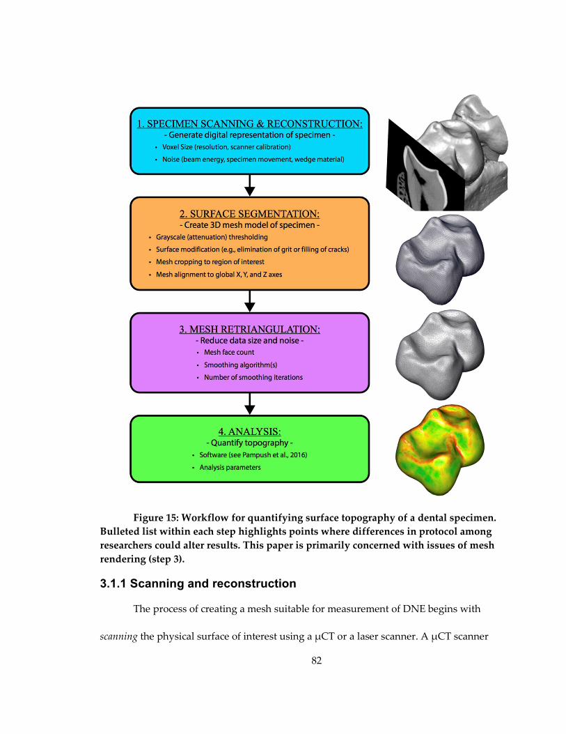
82
Figure 15: Workflow for quantifying surface topography of a dental specimen.
Bulleted list within each step highlights points where differences in protocol among
researchers could alter results. This paper is primarily concerned with issues of mesh
rendering (step 3).
3.1.1 Scanning and reconstruction
The process of creating a mesh suitable for measurement of DNE begins with
scanning the physical surface of interest using a μCT or a laser scanner. A μCT scanner

83
operates by generating X-rays that are transmitted through a rotating sample to a
detector on the opposite side in order to acquire a series of projection images. These
images capture the relative attenuation of the X-rays passing through the studied
sample (Elliot and Dover, 1982; Feldkamp et al., 1984). Generating lower energy X-rays,
or passing them through a sample of high density, means much of the X-ray energy will
be absorbed before it reaches the detector (high attenuation). Conversely, increasing the
X-ray energy or using a less dense sample will result in more of the X-rays reaching the
detector (lower attenuation). When maintained at a constant energy level and passed
through a rotating sample, a μCT generates a series of projection images that indicate
the amount of X-ray energy that was not absorbed or deflected by the sample at each
orientation. A laser scanner on the other hand creates a cloud of points by reflecting a
targeted laser off of a surface, recording evenly spaced positional data (Ungar and
Williamson, 2000). Reconstruction is the process of taking the original scanner projections
and creating a series of images or volume that can then be loaded as a group into a
reconstruction and visualization software program such as Avizo/Amira 8.1 (FEI
Visualization Sciences Group, Berlin, Germany) or VG Studio Max. There are
conventional algorithms for reconstruction, with the convolution/back-projection
formula summarized by Feldkamp et al. (1984) being the most commonly used in cone-
beam scanners. Reconstruction is unique to CT scanning, and is typically not needed
when using a laser scanner. Thus researchers using a laser scanner will skip this step

84
The precision of this process is expressed in voxel size (voxels are ‘volumetric elements,’
a 3D analogy to the 2D pixels that comprise a computer screen) and is governed by
scanner design, the size of the sample, the distance of the sample from the energy source
and detector, and other instrument specific settings during the scan. Noise and artifacts
are introduced to the scan data through a variety of sources, including specimen
movement, beam scattering, energy filtering of the beam by the sample, beam energy
artifacts, and geometric indistinctness.
3.1.2 Segmentation
The process of creating a 3D mesh from the reconstructed image stack or volume
is referred to as segmentation. Performed in Avizo and similar programs, segmentation
seeks to differentiate the specimen/surface of interest from the other components of the
scanned sample (for instance the air, matrix or other material surrounding it during
scanning). Tools exist in Avizo that limit the range of pixel grayscale values—an
expression of the material attenuation from the sample—that are viewable during
analysis, aiding researchers in isolating the desired material. However, the potential for
human error or misinterpretation of the data at hand can add uncertainty to this process.
This is true of fossil specimens in particular, when the attenuation from the specimen
can be close to the attenuation from the matrix in which it was preserved. However,
Boyer (2008) reports that visual assessment of appropriate grayscale threshold values is
likely sufficient.
85
3.1.3 Retriangulation
After segmentation, surface data for quantitative topographic analysis is saved in
a polygon file format, or “PLY” file. PLY files allow for three-dimensional data to be
saved as an object made of simple, planar polygons by incorporating two matrices: one
describing the x-y-z coordinates of the points that compose the mesh, and the other
describing the links between those points to form faces. It is worth noting that though
PLY files are used in DNE analysis, there are many other commonly used file formats
that are capable of representing the same type of 3D data, (e.g., STL, OBJ, OFF).
However, the currently available software programs capable of analyzing DNE
(MorphoTester and molaR, see below) specifically require triangular PLY files as input, as
the underlying algorithm is reliant on the triangular structure of the faces.
Retriangulation refers to further processing of these files (e.g., smoothing,
simplifying, and cropping, discussed in greater detail below). Retriangulation is a
necessary step meant to offset surface noise captured during scanning and
segmentation. There are already established protocols for minimizing error introduced
during initial scanning, reconstruction, and segmentation (Boyer, 2008; Winchester et al.,
2014; Pampush et al., 2016a). However, issues related to the effects of mesh
retriangulation remain under-described.
Studies making use of 3D data must employ retriangulation protocols with the
goal of faithfully retaining the geometry of features considered biologically relevant
86
while simultaneously reducing file size and eliminating localized variation arising from
noise during scanning, segmentation, and reconstruction (Schumaker, 1993; Desbrun et
al., 1999; Dyn et al., 2000). Surface smoothing is the primary way this is achieved. Avizo
has an internal smoothing function that reduces mesh surface irregularity by averaging
the position of mesh vertices with those of their neighbors (with the exception of points
on the mesh boundary, which are only averaged to neighboring boundary vertices). This
function has been employed—to a varying extent—in all previously published studies
measuring DNE (Bunn et al., 2011; Winchester et al., 2014; Prufrock et al., 2016; Pampush
et al. 2016a). Additional downstream smoothing of Avizo-smoothed surfaces has been
employed inconsistently in different projects (see Fig. 2), including the varying use of
‘Laplacian smoothing’ (Prufrock et al., 2016) and ‘implicit fairing smoothing’ (Bunn et
al., 2011; Winchester et al., 2014; Prufrock et al., 2016).
Another critical retriangulation step that must balance manageable file size with
surface detail representation is the simplification of a surface to a target face count. On
one hand, too few faces may result in the loss of relevant surface detail,1 particularly
after smoothing; on the other hand, too many faces can result in unmanageable files
sizes and significantly slower computational speed, potentially without the reward of
greater resolution. Unlike simple geometric shapes (such as a hemisphere), a
1 The exact definition of what constitutes “relevant surface detail” may change depending on the
hypothesis or research question being examined.

87
mammalian cheek-tooth does not have an a priori theoretical limit for DNE. Instead, the
scale-dependent complexity of biological surfaces potentially allows for a scan of
sufficiently high resolution to capture a nearly indefinite number of surface features
revealed through higher and higher surface magnifications, limited only by the
scanner’s upper limit of resolution. In the context of DNE, this is likely to result in
higher and higher values as the fine scale complexity of the surface is revealed,
plateauing as the scanner resolution limit is approached. There is also a plateau for the
number of faces that can be used to represent a surface topography, beyond which the
adding of more faces will not capture any additional features (and will not contribute to
DNE). This is also related to scanning resolution (see above) though it is a distinctly
separate issue, and one that we briefly address in this paper. In the case of scanner
resolution and DNE, we do not tackle this relationship, but rather control for resolution
by using scans with approximately the same resolution (voxel size, measured in
microns).
Finally, retriangulation includes the user-directed cropping of surface meshes to
some consistent boundary. In the case of dental surfaces, the cemento-enamel junction
has frequently been employed as the boundary to which surfaces are cropped by hand
in software like Avizo (Bunn et al., 2011; Winchester et al., 2014, Prufrock et al., 2016).
These boundaries can be erroneously interpreted during DNE analysis as sharp edges.
DNE calculation therefore includes a “boundary exclusion” criterion that mitigates the

88
effects of boundary faces by excluding them from the analysis result (see Pampush et al.,
2016b). There are two options for boundary exclusion in molaR: 1) excluding just the
triangular faces that have two vertices, and therefore a triangle leg (i.e., an edge), on the
mesh boundary; or 2) excluding any faces that have even one vertex on the mesh
boundary. This second, more conservative option excludes a larger number of faces
from the total mesh DNE, potentially controlling for meaninglessly high DNE
estimations resulting from the behavior of vertices on the mesh boundary.
3.1.4 Analysis
Analysis is the final quantification of surface topography from a retriangulated
3D mesh saved as a PLY file. Several different software platforms currently exist for
calculating DNE on a surface mesh: MorphoTester, a Python-based, open-source
application (Winchester, 2016), Teether a MATLAB code available from Yaron Lipman
(Bunn et al., 2011), and an open-source R package “molaR” (Pampush et al., 2016b),
though only MorphoTester and molaR are hosted online for public download.
In this study, we focus on retriangulation procedures that have been employed
in previous studies using DNE with the goal of quantifying and describing their effects
on the estimation of DNE. We investigate each of the following: 1) choice of smoothing
algorithm(s), and number of iterations for which each is implemented; 2) the number of
faces comprising the 3D mesh after simplifying; and 3) the boundary exclusion criterion
89
used during the DNE calculation. To do so we analyze digital surfaces of simple
hemispheres (discussed below) and occlusal surfaces of howling monkey molar teeth.
3.1.5 The Utility of a Hemisphere
Here we compare the effects of different surface retriangulation treatments on a
simple shape (a hemisphere) that has a theoretical DNE value that can be easily
calculated, and use this as a guide for understanding the effects of mesh processing on
occlusal surfaces. The theoretical DNE value for a perfectly smooth hemisphere is:
Equation 1
Therefore a hemisphere has a DNE value of 12.566 (rounded).2 For a more
thorough explanation of the DNE calculation on a hemisphere, see Pampush et al.
(2016b).
Our use of a hemisphere as a simple model unintentionally raises an important
question as to the nature and value of shape descriptors as metrics: namely, how is a
metric (such as DNE) best calibrated? One goal of metrics like DNE, RFI, and OPCR is to
provide a new means of capturing tooth morphology differences among species.
Although—as noted above—signal noise is a potentially important source of error with
scanned surfaces, and retriangulation is required to limit the amount of noise that can
2 As can be appreciated from inspection of Eq. (5), all hemispheres will have a DNE value of ~12.566 (4π)
regardless of the length of the radius.
DNE = 2
r2× 2πr
2

90
affect the measurement. Therefore, one means of arriving on DNE calibration is to
choose a retriangulation procedure which most accentuates the DNE disparity among
dental morphologies associated with differing diets. Such an approach may have
practicality when the primary goal is to use DNE as a pattern recognition tool in the
fossil record. However, if the goal is to better understand dietary adaptations of occlusal
surfaces, then aiming to maximize DNE disparity among dentitions of pre-assigned diet
categories is fraught with tautological issues. We believe that the more conservative
approach to calibration—and one which allows for the use of DNE as a new tool in
examining dietary adaptation—is to study a surface devoid of a presumed functional
role, and one which can be calculated a priori, which is not the case for tooth crown
surfaces.
The approach taken here to calibrating the retriangulation protocol is to evaluate
how accurately the DNE of the resultant surface matches the mathematically expected
DNE, without any concern to interpretation of its meaning. By this philosophy, the only
surface retriangulation needed is that which will remove any “noise” that impedes an
accurate, stable measurement of the surface’s DNE. Stability, in this sense, is defined as
an asymptote in the relationship between DNE and any given step within a
retriangulation protocol. If the functional groups we choose to define (i.e., dietary
groups) are reflected in the surface topography of teeth, then they should naturally
segregate from appropriately calculated DNE values. If they do not, then the functional
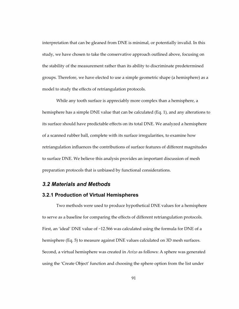
91
interpretation that can be gleaned from DNE is minimal, or potentially invalid. In this
study, we have chosen to take the conservative approach outlined above, focusing on
the stability of the measurement rather than its ability to discriminate predetermined
groups. Therefore, we have elected to use a simple geometric shape (a hemisphere) as a
model to study the effects of retriangulation protocols.
While any tooth surface is appreciably more complex than a hemisphere, a
hemisphere has a simple DNE value that can be calculated (Eq. 1), and any alterations to
its surface should have predictable effects on its total DNE. We analyzed a hemisphere
of a scanned rubber ball, complete with its surface irregularities, to examine how
retriangulation influences the contributions of surface features of different magnitudes
to surface DNE. We believe this analysis provides an important discussion of mesh
preparation protocols that is unbiased by functional considerations.
3.2 Materials and Methods
3.2.1 Production of Virtual Hemispheres
Two methods were used to produce hypothetical DNE values for a hemisphere
to serve as a baseline for comparing the effects of different retriangulation protocols.
First, an ‘ideal’ DNE value of ~12.566 was calculated using the formula for DNE of a
hemisphere (Eq. 5) to measure against DNE values calculated on 3D mesh surfaces.
Second, a virtual hemisphere was created in Avizo as follows: A sphere was generated
using the ‘Create Object’ function and choosing the sphere option from the list under
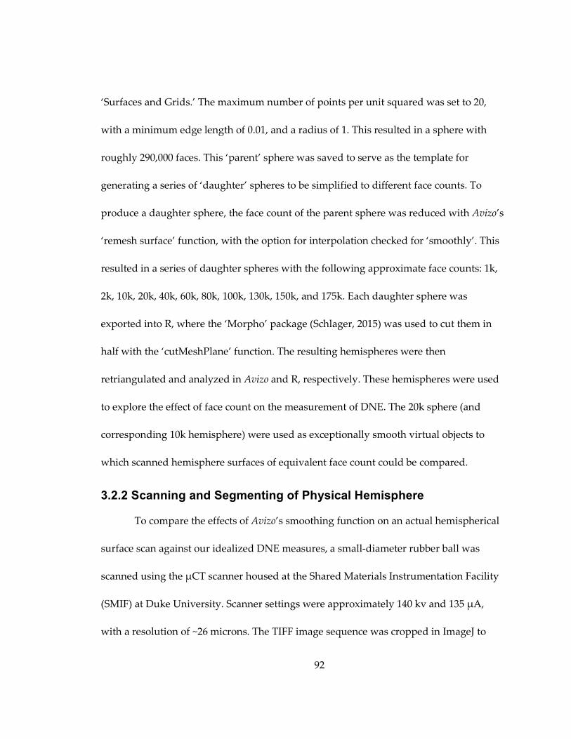
92
‘Surfaces and Grids.’ The maximum number of points per unit squared was set to 20,
with a minimum edge length of 0.01, and a radius of 1. This resulted in a sphere with
roughly 290,000 faces. This ‘parent’ sphere was saved to serve as the template for
generating a series of ‘daughter’ spheres to be simplified to different face counts. To
produce a daughter sphere, the face count of the parent sphere was reduced with Avizo’s
‘remesh surface’ function, with the option for interpolation checked for ‘smoothly’. This
resulted in a series of daughter spheres with the following approximate face counts: 1k,
2k, 10k, 20k, 40k, 60k, 80k, 100k, 130k, 150k, and 175k. Each daughter sphere was
exported into R, where the ‘Morpho’ package (Schlager, 2015) was used to cut them in
half with the ‘cutMeshPlane’ function. The resulting hemispheres were then
retriangulated and analyzed in Avizo and R, respectively. These hemispheres were used
to explore the effect of face count on the measurement of DNE. The 20k sphere (and
corresponding 10k hemisphere) were used as exceptionally smooth virtual objects to
which scanned hemisphere surfaces of equivalent face count could be compared.
3.2.2 Scanning and Segmenting of Physical Hemisphere
To compare the effects of Avizo’s smoothing function on an actual hemispherical
surface scan against our idealized DNE measures, a small-diameter rubber ball was
scanned using the μCT scanner housed at the Shared Materials Instrumentation Facility
(SMIF) at Duke University. Scanner settings were approximately 140 kv and 135 μA,
with a resolution of ~26 microns. The TIFF image sequence was cropped in ImageJ to

93
represent a single hemisphere (half of the original ball). This cropped image stack was
uploaded into Avizo.
Segmentation of 3D surface files in Avizo is done with the “Edit New Label Field”
dialog. Through using the histogram of greyscale values in the image stack provided by
Avizo, the portion of the range of gray shades corresponding to the material attenuation
of the rubber ball was selected using the “magic wand” tool. The threshold was refined
so that only the surface of interest was selected, and extraneous material (air and
packing material) was excluded. Once the selection appeared to accurately represent the
object, it was added to a material and the “Generate Surface” module was applied with
“No smoothing” selected. The resulting surface was an unsmoothed and un-simplified
(beyond the parameters of the initial scan) digital model of half of the rubber ball.
3.2.3 Test of Different Retriangulation Protocols
Using the Avizo “Smooth Surface” module, the raw surface representing a
hemisphere of the scanned rubber ball was iteratively smoothed to differing degrees to
produce variably smoothed surfaces. The smoothing function was performed in
intervals of twenty on the raw surface mesh, evenly spaced from 20-200 iterations to
generate ten new surfaces meshes. The lambda parameter—associated with “lambda-
connectedness,” a parameter that helps the smoothing algorithm decide a threshold for
connecting two points (Chen and Adjei, 2009)—of each operation was kept at the default

94
value of 0.6. Each smoothed surface mesh was saved as a Stanford PLY file for analysis
in molaR.
Some studies that calculated DNE have employed other forms of smoothing after
smoothing in Avizo, including ‘implicit mesh fairing’ (Bunn et al., 2011; Winchester et al.,
2014; Prufrock et al., 2016) and MeshLab’s Laplacian smoothing algorithm (Prufrock et
al., 2016). These additional smoothing methods are both theoretically founded on the
Laplace operator, a differential operator that captures the rate of change across a spatial
gradient, which in 3D surface analysis is approximated using the eigenvectors of the
surface mesh (Taubin, 1995). Approximating the Laplace operator describes the mesh as
a series of changing spherical radii, and these smoothing algorithms seek to reduce the
amount of local radial change while maintaining large-scale topography, with the effect
of producing a more even and consistent local curvature (a method very distinct from
Avizo’s smoothing method, see above). The protocol of Prufrock et al. (2016) calls for one
such smoothing step performed in MeshLab with the “Laplacian Smoothing” function.
To assess the effect of Laplacian smoothing on the measure of DNE we performed
different levels of Laplacian smoothing (from 1-200 iterations) on the scanned rubber
ball hemisphere, resulting in 13 new surface meshes. An alternative approach to fairing
smoothing—‘implicit fairing’ (Desbrun et al., 1999)—was employed by the original
studies involving DNE, which utilized the now-unsupported MATLAB application
Teether (Bunn et al., 2011; Winchester et al., 2014). Other studies using older versions of

95
the MorphoTester software (e.g., Prufrock et al., 2016) also include this implicit fairing
step, as it was formerly integrated by default into all MorphoTester DNE analyses (see
Pampush et al., 2016b; Winchester 2016). As a means to assess differences in topographic
measures produced by the addition of an implicit fairing smoothing step, we used
MorphoTester version 1.1.2 to output implicit faired PLY meshes with three smoothing
iterations and a step size of 0.1 (consistent with published studies). The PLY files were
imported into R for topographic analysis in molaR (Pampush et al., 2016b). DNE was
calculated for each 3D mesh using molaR’s batch function. These values were plotted
against the number of smoothing iterations to illustrate their relationships.
To observe the effect of changing face count, the 11 hemispheres resulting from
bisecting the virtual ‘daughter’ spheres (described above) were analyzed. These
hemispheres had face counts ranging from approximately 500 to 100,000 faces. Each
simplified hemisphere was smoothed identically using Avizo’s “Smooth Surface”
function with a lambda of 0.6. DNE was calculated on the full set of simplified
hemispheres three times: after each surface had been smoothed with 1, 25, and 100
iterations. Since the number of faces located on the mesh boundary is directly related to
the total number of faces of the mesh, the same hemispheres were analyzed and
compared using both DNE boundary exclusion criteria.

96
3.2.4 Primate Molar Occlusal Surfaces
To test the applicability of our results with the hemispheres to primate dental
surfaces, we analyzed 3D meshes representing the occlusal surfaces of first upper and
lower molars of the Costa Rican mantled howling monkey (Alouatta palliata) from the
Glander collection at Duke University (Glander, 1975). Individual M1s were segmented
from whole skulls, scanned at ~195 kv and 215 μA, with a scanning resolution of
approximately 60 microns. These specimens represent seven different individuals at
different wear stages and were subjected to the same series of sampling, smoothing, and
statistical treatments as the rubber ball hemisphere (described above).
3.2.5 Comparison of Published Methods
Finally, we compared the retriangulation protocols of previously published
research that calculated DNE, specifically those of Bunn et al. (2011), Winchester et al.
(2014), Prufrock et al. (2016), and Pampush et al. (2016a). The un-smoothed, segmented
meshes of both the rubber ball and a single, unworn tooth (specimen DU-LP-33)
included in the other analyses (see above) were processed according to the protocols of
each of the four studies (Fig. 2), as well as a fifth treatment that included only 100
iterations of smoothing in Avizo. DNE was then calculated on each mesh in molaR using
the default boundary exclusion criterion.
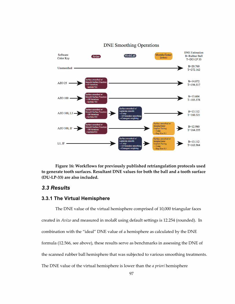
97
Figure 16: Workflows for previously published retriangulation protocols used
to generate tooth surfaces. Resultant DNE values for both the ball and a tooth surface
(DU-LP-33) are also included.
3.3 Results
3.3.1 The Virtual Hemisphere
The DNE value of the virtual hemisphere comprised of 10,000 triangular faces
created in Avizo and measured in molaR using default settings is 12.254 (rounded). In
combination with the “ideal” DNE value of a hemisphere as calculated by the DNE
formula (12.566, see above), these results serve as benchmarks in assessing the DNE of
the scanned rubber ball hemisphere that was subjected to various smoothing treatments.
The DNE value of the virtual hemisphere is lower than the a priori hemisphere

98
calculation for two reasons: [1] The virtual hemisphere calculation includes boundary
exclusion that was not accounted for in the ideal calculation of hemisphere DNE (Eq. 5).
This causes the surface to be slightly ‘flatter’ via trimming a ring of faces off the bottom
edge. [2] The ~10,000 PLY-face count slightly simplifies the curvature of the surface,
wherein a larger number of faces would capture more of the subtle curvature of the
hemisphere.
3.3.1.1 Avizo Smoothing
Table 6: Changing values of DNE on a rubber ball versus the number of
smoothing iterations performed in Avizo to which the surface mesh is subjected.
# Iterations
0
20
40
60
80
100
DNE
22.987
14.275
14.547
14.433
14.384
14.368
# Iterations
120
140
160
180
200
DNE
14.371
14.386
14.409
14.438
14.472
Results from the scanned ball show that the DNE value approaches those of the
theoretical and 10,000-face virtual hemispheres after ~20 Avizo smoothing iterations
(Table 6, Fig. 17). The apparent discrepancy between the values of the scanned surface
and those of the virtual hemispheres is likely the result of real surface features and is
elaborated upon below.
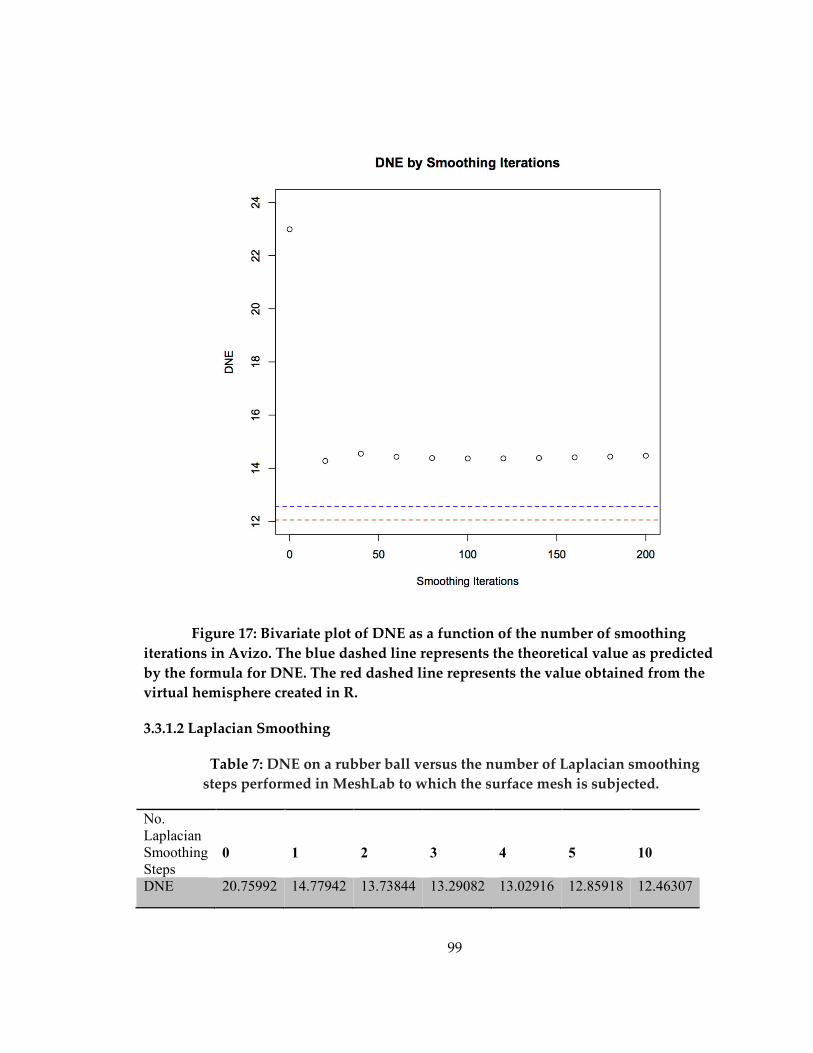
99
Figure 17: Bivariate plot of DNE as a function of the number of smoothing
iterations in Avizo. The blue dashed line represents the theoretical value as predicted
by the formula for DNE. The red dashed line represents the value obtained from the
virtual hemisphere created in R.
3.3.1.2 Laplacian Smoothing
Table 7: DNE on a rubber ball versus the number of Laplacian smoothing
steps performed in MeshLab to which the surface mesh is subjected.
No.
Laplacian
Smoothing
Steps
0
1
2
3
4
5
10
DNE 20.75992 14.77942 13.73844 13.29082 13.02916 12.85918 12.46307

100
No. of
Laplacian
Smoothing
Steps
15
20
25
50
100
150
200
DNE 12.28782 12.17280 12.08384 11.77686 11.38361 11.09786 10.87233
Beginning with the unsmoothed hemisphere created through scanning a rubber
ball, Laplacian smoothing considerably decreased DNE values. This effect was
particularly dramatic after several steps of smoothing (Table 7, Fig. 18), and resulted in
the DNE value falling below both the theoretical value for a perfectly smooth unit
hemisphere, and the value calculated from the virtually created hemisphere, contrary to
expectations for a surface containing obvious and fairly large irregularities.
Figure 18: Bivariate plot of DNE as a function of the number of Laplacian
smoothing steps as performed in MeshLab. The blue dashed line represents the
theoretical value as predicted by the formula for each measurement. The red dashed
line represents the value obtained from the virtual hemisphere created in R. Inset

101
figures (corresponding data points labeled with numbers) are 3D figures created in
molaR that illustrate the effect of Laplacian smoothing in eliminating surface
features. Hotter colors refer to regions of greater surface DNE.
3.3.1.3 Implicit Fairing
The results of three iterations of implicit fairing in MorphoTester bear a close
resemblance to those of the Laplacian smoothing performed in MeshLab, consistent with
the underlying algorithmic similarity of these two smoothing functions. DNE values
obtained after performing these methods are presented in Table 9 (labeled as ‘IF’).
3.3.1.4 Face Count and Boundary Exclusion
DNE results from virtual hemispheres of varied number of faces (generated from
the original ‘parent’ sphere in Avizo and subsequently bisected in R), as well as the two
mesh boundary exclusion criteria, are presented in Figure 19 and Appendix A. The
degree to which face count affects DNE is influenced by the number of smoothing
iterations performed in Avizo. Varying the number of faces on surface meshes smoothed
more than once (Fig. 19B,C) has a greater effect on DNE values than does varying face
count on a surface mesh that has been smoothed only minimally (Fig. 19A). In addition,
DNE values for meshes that were analyzed with the boundary exclusion criterion to
include faces which have at least one vertex on the boundary (i.e., the
BoundaryDiscard=“vertex” argument in molaR, Fig. 19, blue circles) are consistently
lower and track the expected DNE value of a hemisphere more closely than those with
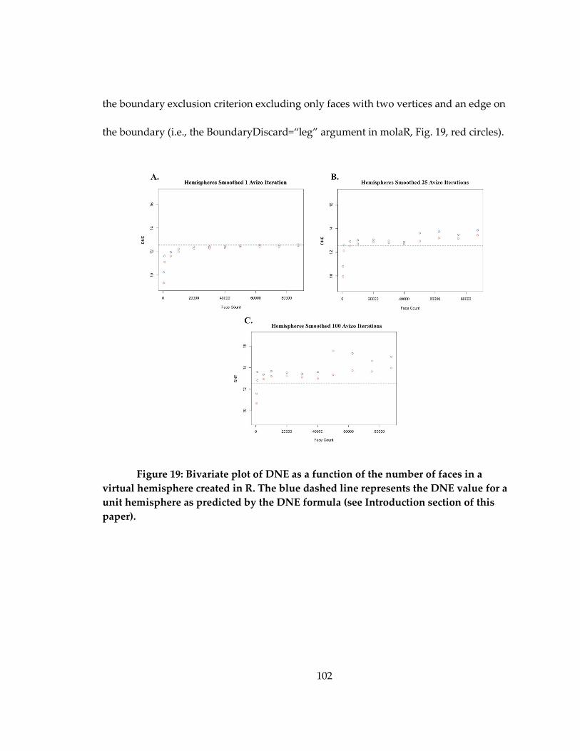
102
the boundary exclusion criterion excluding only faces with two vertices and an edge on
the boundary (i.e., the BoundaryDiscard=“leg” argument in molaR, Fig. 19, red circles).
Figure 19: Bivariate plot of DNE as a function of the number of faces in a
virtual hemisphere created in R. The blue dashed line represents the DNE value for a
unit hemisphere as predicted by the DNE formula (see Introduction section of this
paper).
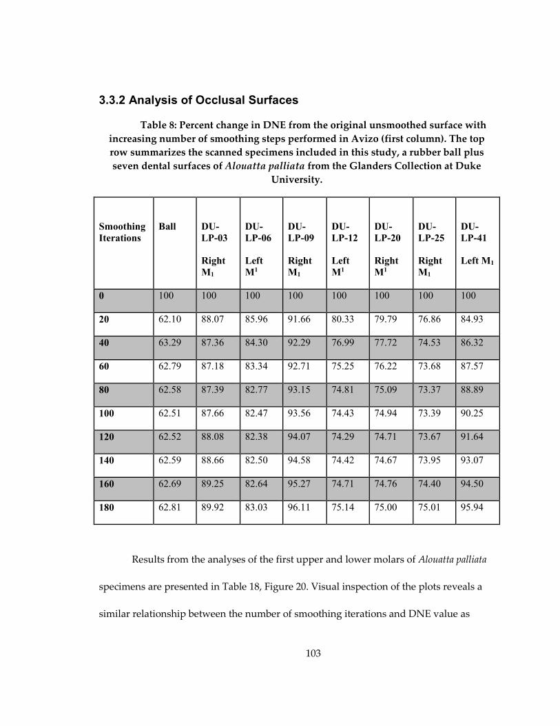
103
3.3.2 Analysis of Occlusal Surfaces
Table 8: Percent change in DNE from the original unsmoothed surface with
increasing number of smoothing steps performed in Avizo (first column). The top
row summarizes the scanned specimens included in this study, a rubber ball plus
seven dental surfaces of Alouatta palliata from the Glanders Collection at Duke
University.
Smoothing
Iterations
Ball
DU-
LP-03
Right
M1
DU-
LP-06
Left
M1
DU-
LP-09
Right
M1
DU-
LP-12
Left
M1
DU-
LP-20
Right
M1
DU-
LP-25
Right
M1
DU-
LP-41
Left M1
0 100 100 100 100 100 100 100 100
20 62.10 88.07 85.96 91.66 80.33 79.79 76.86 84.93
40 63.29 87.36 84.30 92.29 76.99 77.72 74.53 86.32
60 62.79 87.18 83.34 92.71 75.25 76.22 73.68 87.57
80 62.58 87.39 82.77 93.15 74.81 75.09 73.37 88.89
100 62.51 87.66 82.47 93.56 74.43 74.94 73.39 90.25
120 62.52 88.08 82.38 94.07 74.29 74.71 73.67 91.64
140 62.59 88.66 82.50 94.58 74.42 74.67 73.95 93.07
160 62.69 89.25 82.64 95.27 74.71 74.76 74.40 94.50
180 62.81 89.92 83.03 96.11 75.14 75.00 75.01 95.94
Results from the analyses of the first upper and lower molars of Alouatta palliata
specimens are presented in Table 18, Figure 20. Visual inspection of the plots reveals a
similar relationship between the number of smoothing iterations and DNE value as
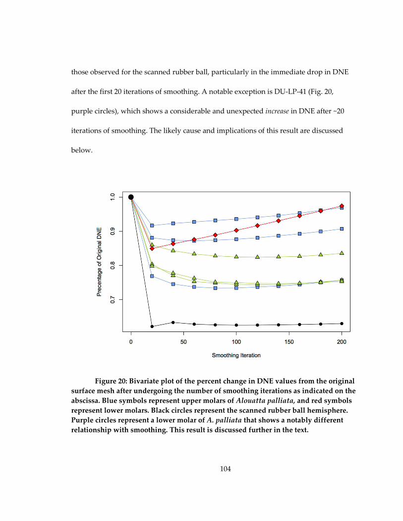
104
those observed for the scanned rubber ball, particularly in the immediate drop in DNE
after the first 20 iterations of smoothing. A notable exception is DU-LP-41 (Fig. 20,
purple circles), which shows a considerable and unexpected increase in DNE after ~20
iterations of smoothing. The likely cause and implications of this result are discussed
below.
Figure 20: Bivariate plot of the percent change in DNE values from the original
surface mesh after undergoing the number of smoothing iterations as indicated on the
abscissa. Blue symbols represent upper molars of Alouatta palliata, and red symbols
represent lower molars. Black circles represent the scanned rubber ball hemisphere.
Purple circles represent a lower molar of A. palliata that shows a notably different
relationship with smoothing. This result is discussed further in the text.
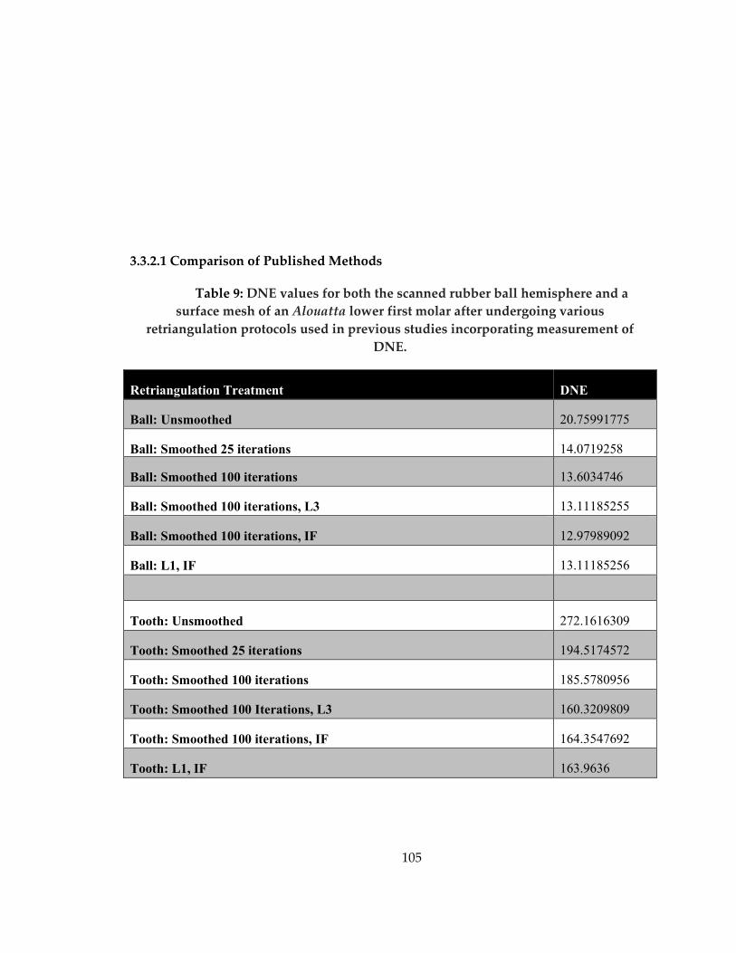
105
3.3.2.1 Comparison of Published Methods
Table 9: DNE values for both the scanned rubber ball hemisphere and a
surface mesh of an Alouatta lower first molar after undergoing various
retriangulation protocols used in previous studies incorporating measurement of
DNE.
Retriangulation Treatment DNE
Ball: Unsmoothed 20.75991775
Ball: Smoothed 25 iterations 14.0719258
Ball: Smoothed 100 iterations 13.6034746
Ball: Smoothed 100 iterations, L3 13.11185255
Ball: Smoothed 100 iterations, IF 12.97989092
Ball: L1, IF 13.11185256
Tooth: Unsmoothed 272.1616309
Tooth: Smoothed 25 iterations 194.5174572
Tooth: Smoothed 100 iterations 185.5780956
Tooth: Smoothed 100 Iterations, L3 160.3209809
Tooth: Smoothed 100 iterations, IF 164.3547692
Tooth: L1, IF 163.9636

106
Values of DNE measured on the scanned rubber ball processed using five
different previously published protocols (as well as the original, unsmoothed surface)
are presented in Table 9 and illustrated in Figure 21A. All methods show a similar
decrease in DNE from the unsmoothed surface, though there is variation in the degree of
DNE deflation among the retriangulation protocols. A consistent pattern emerges in the
DNE values calculated for the Alouatta tooth surface (DU-LP-33; Fig. 21B) following each
retriangulation protocol.
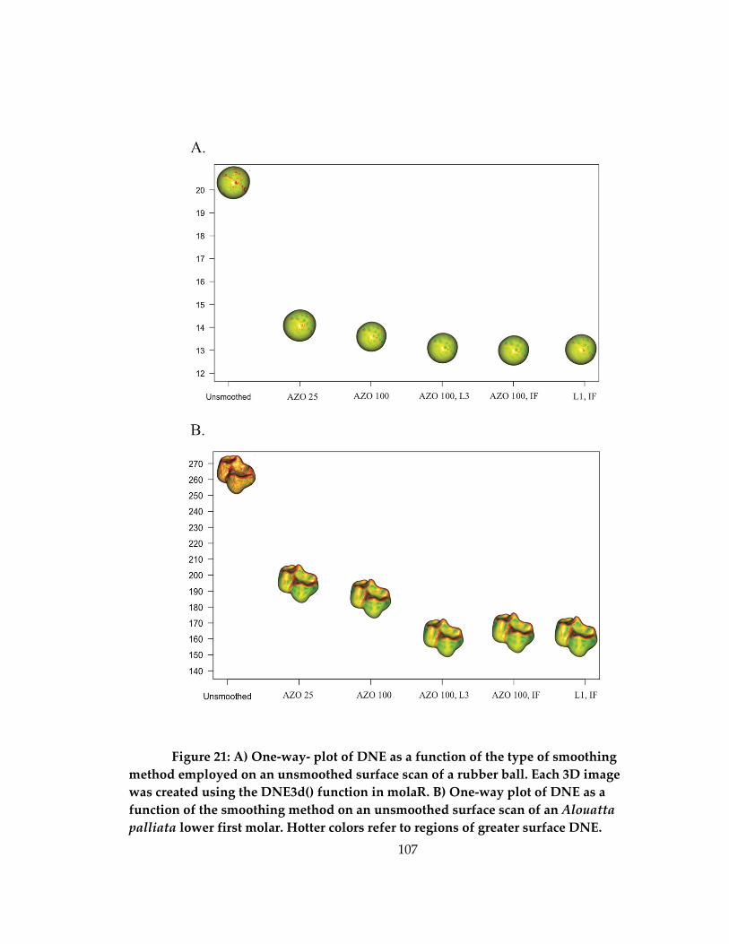
107
Figure 21: A) One-way- plot of DNE as a function of the type of smoothing
method employed on an unsmoothed surface scan of a rubber ball. Each 3D image
was created using the DNE3d() function in molaR. B) One-way plot of DNE as a
function of the smoothing method on an unsmoothed surface scan of an Alouatta
palliata lower first molar. Hotter colors refer to regions of greater surface DNE.

108
3.4 Discussion
Given the number of different protocols for retriangulation and analyzing 3D
meshes of tooth crowns, we seek here to make protocols associated with retriangulation
less opaque by presenting the effects of various retriangulation decisions on DNE.
3.4.1 Effects of Different Smoothing Protocols
The smoothing method employed in Avizo (and similar programs) treats local
topography as a scalar field, generates a set of distances between neighboring vertices,
and then seeks to minimize these distances. Collectively this typically has the effect of
flattening small irregularities on the surface. After approximately 20 iterations of
smoothing in Avizo, DNE values remain generally consistent regardless of continued
smoothing performed in Avizo. There is a consistent discrepancy between the DNE
calculated for the rubber ball surface and the DNE of both the hand-calculated ideal
hemisphere and the molaR estimate of DNE from a virtual hemisphere of 10k faces
created in Avizo. This discrepancy is explained by surface irregularities from scarring,
and a dimple produced during the manufacturing process. That the process of scanning,
segmenting and retriangulation captured the dimple feature suggests that such a
protocol faithfully captures fine details on the surface. Further smoothing, particularly
with implicit fairing, tends to eliminate the effect of these features on the total DNE of
the surface. In other words, over-zealous smoothing has the potential to obliterate real
surface features. It is difficult to speculate as to the potential importance of this
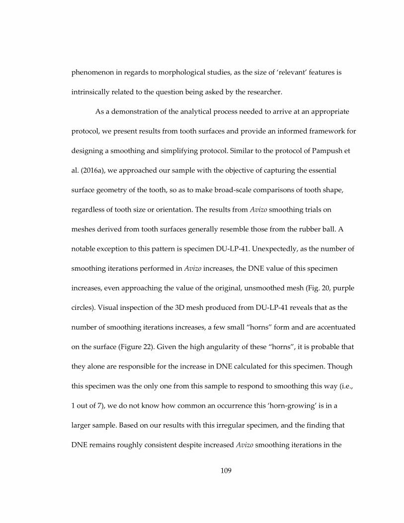
109
phenomenon in regards to morphological studies, as the size of ‘relevant’ features is
intrinsically related to the question being asked by the researcher.
As a demonstration of the analytical process needed to arrive at an appropriate
protocol, we present results from tooth surfaces and provide an informed framework for
designing a smoothing and simplifying protocol. Similar to the protocol of Pampush et
al. (2016a), we approached our sample with the objective of capturing the essential
surface geometry of the tooth, so as to make broad-scale comparisons of tooth shape,
regardless of tooth size or orientation. The results from Avizo smoothing trials on
meshes derived from tooth surfaces generally resemble those from the rubber ball. A
notable exception to this pattern is specimen DU-LP-41. Unexpectedly, as the number of
smoothing iterations performed in Avizo increases, the DNE value of this specimen
increases, even approaching the value of the original, unsmoothed mesh (Fig. 20, purple
circles). Visual inspection of the 3D mesh produced from DU-LP-41 reveals that as the
number of smoothing iterations increases, a few small “horns” form and are accentuated
on the surface (Figure 22). Given the high angularity of these “horns”, it is probable that
they alone are responsible for the increase in DNE calculated for this specimen. Though
this specimen was the only one from this sample to respond to smoothing this way (i.e.,
1 out of 7), we do not know how common an occurrence this ‘horn-growing’ is in a
larger sample. Based on our results with this irregular specimen, and the finding that
DNE remains roughly consistent despite increased Avizo smoothing iterations in the
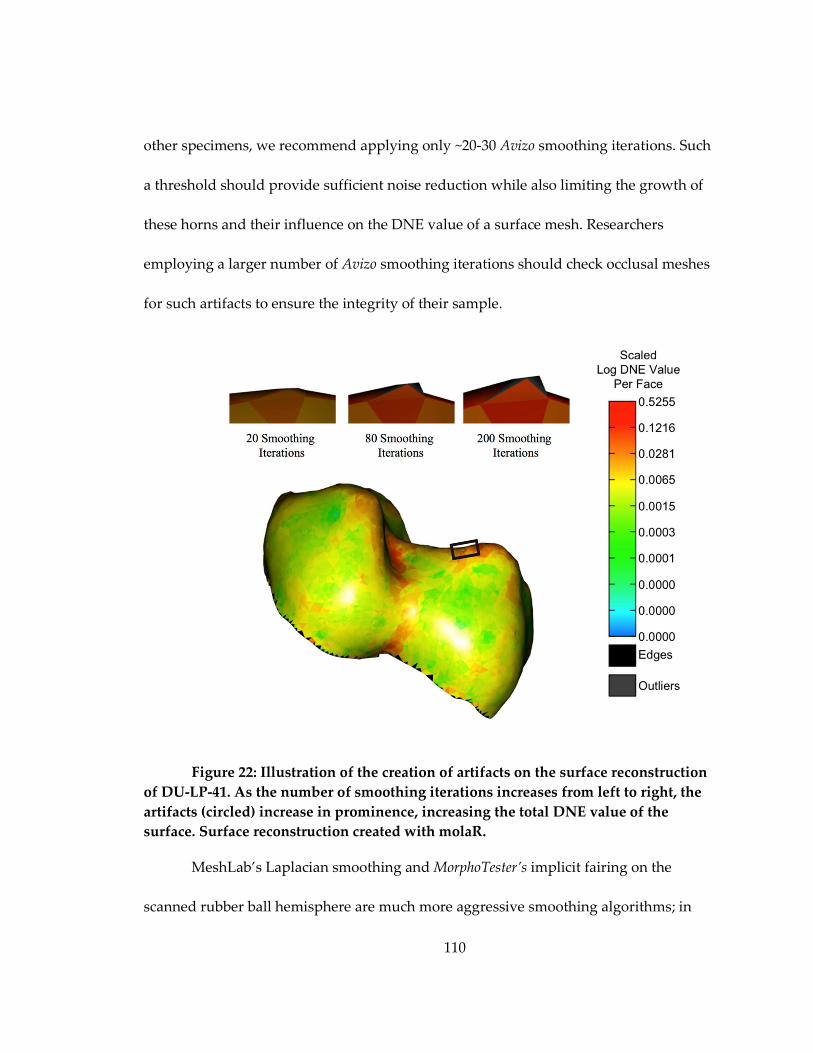
110
other specimens, we recommend applying only ~20-30 Avizo smoothing iterations. Such
a threshold should provide sufficient noise reduction while also limiting the growth of
these horns and their influence on the DNE value of a surface mesh. Researchers
employing a larger number of Avizo smoothing iterations should check occlusal meshes
for such artifacts to ensure the integrity of their sample.
Figure 22: Illustration of the creation of artifacts on the surface reconstruction
of DU-LP-41. As the number of smoothing iterations increases from left to right, the
artifacts (circled) increase in prominence, increasing the total DNE value of the
surface. Surface reconstruction created with molaR.
MeshLab’s Laplacian smoothing and MorphoTester’s implicit fairing on the
scanned rubber ball hemisphere are much more aggressive smoothing algorithms; in

111
fact there exists a point at which a 3D mesh can have much of its topographic resolution
obliterated. Implicit fairing may result in the loss of biologically relevant surface detail.
We find that as the number of mesh fairing smoothing steps (Laplacian or implicit)
increases, the DNE value for the rubber ball eventually falls below the theoretical value
of a unit hemisphere—a result not observed with Avizo smoothing. This suggests a high
potential for distortion of the mesh when a smoothing protocol includes Laplacian or
implicit fairing smoothing. Indeed, if one regards the difference between the theoretical
DNE value of an ideal hemisphere (blue line, Fig. 18) and the molaR DNE estimate of a
nearly smooth virtual hemisphere of 10k faces created in Avizo (red line, Fig. 18) as an
acceptable (and perhaps inevitable) amount of error incurred during analysis, then it
should be noted that even a single step of either Laplacian or implicit fairing
smoothing—applied to a surface already smoothed with Avizo—reduces the DNE value
of the rubber ball surface by an amount larger than this analytical error (i.e., the
differences between the molaR DNE estimate, and the theoretical DNE value of a
hemisphere). This observation underscores the aggressive nature of these smoothing
algorithms.
In comparing the effects of the smoothing protocol on the hemisphere vs. the
tooth surface, there were differences in relative magnitude of DNE decrease, but not in
the pattern of decrease. That is to say, the hemisphere demonstrated a greater percent
decrease in DNE than did the tooth surface, but both showed an initial precipitous

112
decrease in DNE followed by little change in DNE with increased smoothing iterations
in Avizo. By comparing these dramatically different surfaces that produced such similar
patterns, it can be inferred that DNE change with smoothing is consistent regardless of
the surface. Our results indicate that more complex surfaces are likely to show relatively
smaller decreases with smoothing. This is likely to reflect the relationship of noise from
the scan as it relates to the magnitude of the features on the surface. Given identical scan
parameters, noise should be approximately consistent from scan to scan. Therefore, the
relative size of the features—in the case of this study, either a small dimple on a
hemisphere or the crests and cusps of a tooth—is going to either enhance or diminish the
effect noise has on the overall DNE of the surface. This concept likely explains why in
our results, the hemisphere—for which noise is contributing a greater relative
proportion of the DNE prior to smoothing—shows a relatively larger decrease in DNE
with smoothing than does the tooth surface. Stepping back, the comparison of these
smoothing analyses highlights the importance of the tradeoff inherent during
smoothing, namely between the elimination of noise and the distortion of important
surface features. These effects are particularly important to consider when measuring
DNE, because it is sensitive to small changes in curvature on a surface.
3.4.2 Effects of Different Face Counts and Boundary Exclusion on DNE
Another potential source of variation when retriangulating meshes to calculate
DNE or other topographic measures is alterations made to the number of triangular

113
faces that compose the mesh. This is of particular concern with regard to teeth with
relatively small but functionally significant features, which may lose meaningful
resolution with too small a face count. As Figure 19 illustrates, the number of faces does
indeed affect the values of DNE, and it is also apparent that too few faces can distort the
surface (in this case, away from the value of an ideal hemisphere predicted by the DNE
formula). As illustrated in Figure 23, too few faces can result in a tooth surface mesh that
is only a rudimentary representation of the original surface (Fig. 23A), while too many
faces can capture features in the mesh that may be on the original surface, but may be
extraneous to the essential surface geometry of a tooth, such as microfeatures on the
occlusal surface (Fig. 23C, D). This is relevant, as small but jagged surface features—
whether they are artifacts or actual surface features—can have a much more significant
contribution to the overall DNE of a surface than large areas free from jaggedness. It
should be noted that the relevance of these features is wholly dependent on the research
question, but no published studies using DNE so far have prioritized the contribution of
surficial microfeatures to overall tooth crown DNE. The amount of smoothing
performed in Avizo also affects DNE in meshes of different face counts (Fig. 19),
underscoring the importance of establishing a consistent protocol of both mesh
smoothing and simplification if DNE results are to be combined among broad
taxonomic groups, and/or across studies. A conservative approach to smoothing as
advocated here is more likely to be appropriate for a greater range of tooth

114
morphologies than a more intense smoothing protocol. A second consideration is the
tradeoff between processing speed and data richness. Figure 19 shows that the
theoretical value of DNE can be attained on a simple hemispherical mesh comprised of
between 10,000 and 15,000 faces. A similar plateau is not seen in the results from the
tooth surface, which is a consequence of the scale-dependent complexity of the tooth
surface (discussed in the Background) and the upper limit in our computer processing
ability. Provided the processing ability is available, it is likely that DNE would
consistently increase with face count on a given tooth scan until it meets the limit
imposed on it by the initial scanning resolution. That said, DNE processing speed in
molaR and MorphoTester is greatly slowed by the number of faces, and system memory
limits tend to prevent DNE calculation on meshes with more than 125,000 faces (unless
there is access to a cluster for processing). While there may be specific questions or
interest in DNE best addressed using meshes with a large number of faces, for the
purposes of gross dietary differentiation among extant primate taxa, simplifying meshes
to 10,000 faces—as has been done in past studies—appears to be a reasonable and
appropriate threshold. This approach seems to capture biologically meaningful signal,
without over-burdening the analysis tools.
115
Figure 23: Illustration of the effect of increasing the number of faces on the
surface reconstruction of a howling monkey (Alouatta palliata) lower first molar. The
number of faces for each surface is as follows: A) 1000; B) 10,000; C) 50,000; D) 100,000.
The boundary exclusion criterion chosen during analysis also has a significant
effect on DNE values. Unsurprisingly, when faces that have at least one vertex on the
boundary are excluded, DNE values are lower than when boundary exclusion is limited
to only those faces that have an entire leg (i.e., two vertices) on the boundary. The
motivation for boundary exclusion during DNE calculation is that faces on the boundary
are much more likely to possess erratically oriented vertex normals (which are
fundamental to the mechanics of the DNE estimation in both MorphoTester and molaR),
owing to the lack of adjacent faces (Pampush et al., 2016b). If the boundary faces are
included, this can result in a DNE estimation where portions of the boundary are

116
erroneously interpreted as a sharp ridge. A higher number of faces and greater Avizo
smoothing iterations appears to result in more erratic vertex normals along the mesh
boundary, contributing to higher DNE values (Fig. 19). This effect is best countered by a
boundary exclusion criterion that removes all faces from the calculation that have at
least one vertex on the boundary, ensuring that the DNE calculation does not treat the
boundary as a sharp ridge. However, while this effect is clear on the simple surface of a
hemisphere, it is not obvious that complex occlusal surfaces with a larger number of
faces subjected to higher amounts of smoothing suffer from these boundary issues. This
is likely because the raw level of complexity on these surfaces swamps the DNE
contribution from a few faces possessing extreme vertex normals. Regardless, a more
exclusive approach to the mesh boundary is more likely to remove these problem faces.
3.4.3 Comparing Results from Previously Published Protocols
Despite the methodological challenges associated with smoothing and the
measurement of DNE, the metric has enormous potential as a tool in the study of the
ecomorphology of mammalian dentitions. This potential has already been demonstrated
in primates (Bunn et al., 2011; Winchester et al., 2014; Pampush et al., 2016a) and rodents
(Prufrock et al., 2016). In this context, it is important to note that a tooth surface, unlike a
hemisphere, does not have an a priori value of DNE that we can expect to approach with
an optimal retriangulation protocol (i.e., a calibration guide). That these studies used
different protocols does not take away from the validity of their findings—particularly

117
for how DNE relates to other factors/metrics—for as we have argued here, the most
important aspect of any study that requires image processing of CT scans is internal
consistency. Still, our results from the comparative analysis of the smoothing methods
used in previously published studies of DNE suggest that DNE values should not be
combined from studies using differing retriangulation protocols. Table 10 presents the
differences in DNE among five different tooth surfaces retriangulated using different
previously published protocols. The average DNE difference between a protocol that
includes only smoothing in Avizo and one that includes Laplacian smoothing or implicit
fairing is roughly 18 to 25 (or approximately 10-15%), depending on the comparison.
Comparing this disparity with the results from Winchester et al. (2014), in which the
mean difference between frugivores and folivores amongst their platyrrhine sample was
25.77, it is clear that any researcher looking to compile DNE measurements across
studies (and particularly across research groups) must take care to ensure that all
surfaces were given the same retriangulation treatment. The easiest way to rapidly
account for discrepancies between retriangulation protocols is for researchers to publish
their raw segmented surface meshes (pre-retriangulation) in online repositories such as
MorphoSource (Boyer et al., in press) for reanalysis, as has been done already by some
researchers (e.g., Boyer, 2008; Bunn et al., 2011; Winchester et al., 2014; Prufrock et al.,
2016; Pampush et al., 2016a). Posting mesh surface data (or even better, the
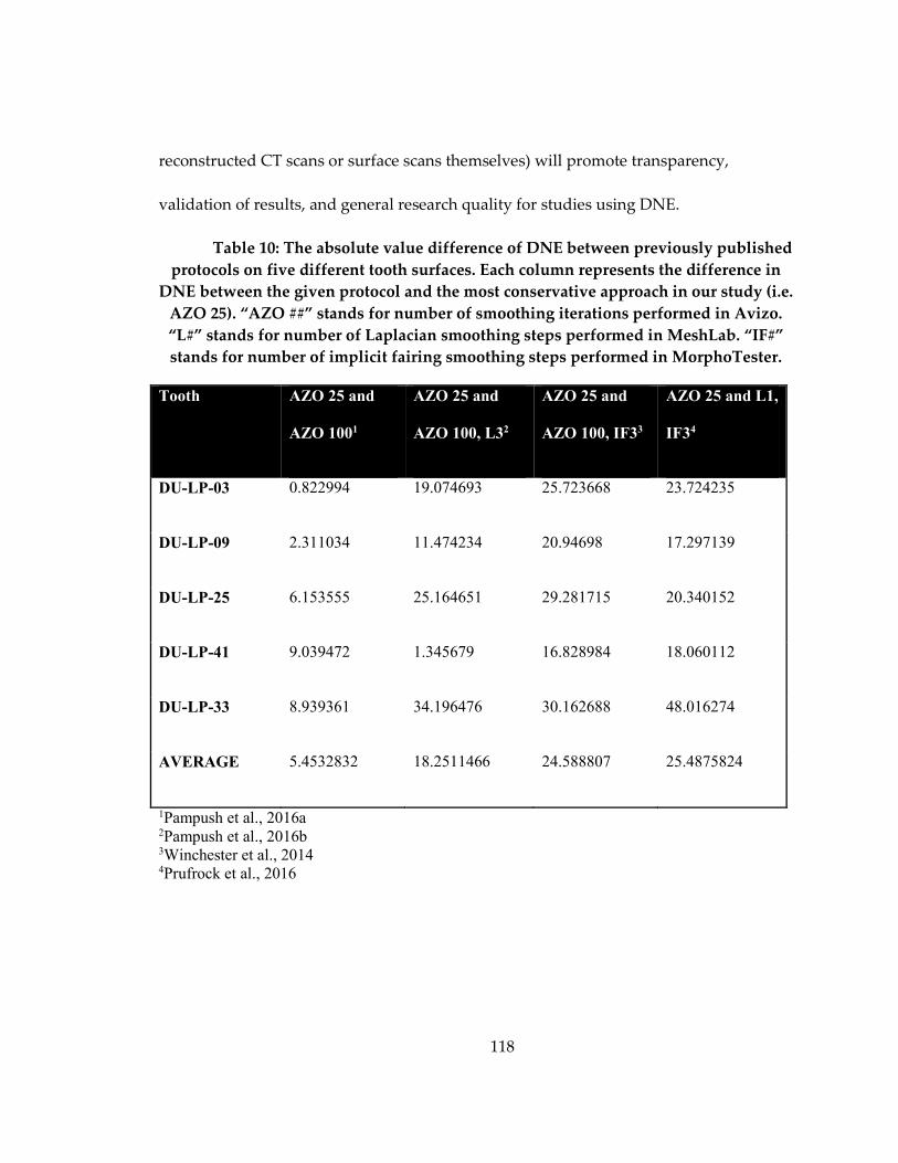
118
reconstructed CT scans or surface scans themselves) will promote transparency,
validation of results, and general research quality for studies using DNE.
Table 10: The absolute value difference of DNE between previously published
protocols on five different tooth surfaces. Each column represents the difference in
DNE between the given protocol and the most conservative approach in our study (i.e.
AZO 25). “AZO ##” stands for number of smoothing iterations performed in Avizo.
“L#” stands for number of Laplacian smoothing steps performed in MeshLab. “IF#”
stands for number of implicit fairing smoothing steps performed in MorphoTester.
Tooth AZO 25 and
AZO 1001
AZO 25 and
AZO 100, L32
AZO 25 and
AZO 100, IF33
AZO 25 and L1,
IF34
DU-LP-03 0.822994 19.074693 25.723668 23.724235
DU-LP-09 2.311034 11.474234 20.94698 17.297139
DU-LP-25 6.153555 25.164651 29.281715 20.340152
DU-LP-41 9.039472 1.345679 16.828984 18.060112
DU-LP-33 8.939361 34.196476 30.162688 48.016274
AVERAGE 5.4532832 18.2511466 24.588807 25.4875824
1Pampush et al., 2016a 2Pampush et al., 2016b 3Winchester et al., 2014 4Prufrock et al., 2016
119
3.4.4 Considerations When Designing a Retriangulation Protocol for Tooth Surfaces
The combined information from our results suggests that a conservative
approach to smoothing generally limits the complications and irregularities associated
with mesh retriangulation. For our sample hemisphere and teeth, 25 iterations of
smoothing in Avizo performed on a mesh simplified to 10,000 faces reduces the
likelihood of irregularities in the 3D mesh that became especially apparent in our results
with ~40 or greater iterations. Similar ‘horn’ artifacts to those produced with Avizo
through over-smoothing are observed on tooth DU-LP-41 after only a few iterations (5
or more) of Laplace operator-based smoothing algorithms. The error introduced by these
artifacts can have a significant effect on the estimation of DNE. Additionally, more
aggressive smoothing algorithms (including “Laplacian smoothing” in MeshLab, or
“implicit fairing smoothing” in MorphoTester) may eliminate real topographic
information or potentially contribute to the formation of false topography. We also
demonstrate that excluding all faces with any vertices on the mesh boundary (boundary
exclusion criterion in molaR set to “vertex”) improves the consistency of DNE results.
Though we caution against use of mesh fairing smoothing algorithms, we do not
challenge the findings of previous studies incorporating such techniques. This stance is
informed by the fact that there is no easily calculable “true” value of DNE for a tooth, as
there is for a hemisphere. Yet, our analysis of different published protocols performed
120
on the same surface produced a range of DNE values greater than the differences that
separate morphological or dietary groupings among primates (Bunn et al., 2011;
Winchester et al., 2014). We suggest that because of this potential pitfall, researchers take
great care in only combining results from prior studies that have equivalent
retriangulation protocols, as combining results from studies with different protocols
may lead to erroneous conclusions.
3.5 Conclusions
Dirichlet Normal Energy (DNE) was calculated for PLY files of an ideal
hemisphere, a bisected scanned rubber ball, and dental occlusal surfaces of Alouatta
palliata (as an example of a medium-sized primate) and subjected to a variety of
retriangulation protocols, including different smoothing algorithms, different amounts
of smoothing, and different face counts. The simple geometry of the hemisphere
provides a well-understood “ideal” benchmark to compare with results of the effects of
variation in retriangulation steps in a way that a complex surface like a tooth crown
cannot. The secondary, informed examination of dental occlusal surfaces allows us to
extrapolate these results further. Based on our results, for future 3D surface
retriangulation with the aim of calculating DNE, we recommend:
• Avoiding Laplace operator-based smoothing algorithms, or excessive smoothing
iterations

121
• A boundary exclusion criterion that excludes all mesh faces on the surface
boundary from the final surface DNE (the BoundaryDiscard=“vertex” argument
in molaR).
• Consistency with retriangulation protocol across all surface meshes included in a
study.
• Avoiding the combination of results from prior studies using different
retriangulation protocols.
We also demonstrate here a framework for decision-making in regards to
retriangulation protocol that can be applied to most research questions. A conservative
approach to smoothing such as we demonstrate in this paper (i.e. a minimal number of
smoothing iterations and the use of less aggressive smoothing algorithms) is more likely
to eliminate scanning noise, while capturing the essential surface geometry of the tooth
surface and retaining the fine scale features, without causing many of the potential
pitfalls associated with retriangulation. Higher face counts are able to capture the
complexity of the tooth surface in greater detail, but do so at the expense of
computational power. Finally, we strongly advocate that researchers publish un-
processed, segmented PLY files in online archives in addition to the retriangulated PLY
meshes used for analyses.

122
4. Dental Topography in Marsupials: Proxies for Dietary
Ecology and Environmental Reconstruction
4.1 Introduction
Having diverged from placental mammals well over 100 million years ago, the
metatheria clade is extremely diverse, and are represented in a set of ecologies that
spans almost the entire range of placental diversity (major exceptions being the lack of
marine and flying forms) (Szalay, 2006; Ungar, 2010). Metatherians constitute a major
component of the fauna for the entire Cenozoic in South America, Australia (as they still
do today), and Antarctica (Simpson, 1950; 1961; Keast, 1977; Chornogubsky et al., 2009).
For this reason, there is a great amount of potential for their use as an environmental
proxy on these continents. However, such an approach requires a foundational dataset
of ecometrics—measurements from ecologically relevant morphological features—from
a broad taxonomic and ecologically diverse sample. If the ecologies of mammals can be
reconstructed reliably, then there is evidence that the distribution of ecologies within
any given fauna may be used to reconstruct the environment or climate that that fauna
inhabits (Andrews et al., 1979; Kay and Madden, 1997; Kay et al. 2012). Given the
abundance of teeth in the mammalian fossil record, deciphering how dentitions relate to
dietary ecology has been a major focus of the mammalian paleoecological literature
(Owen, 1871; Simpson, 1933; Kay, 1975; Walker et al., 1978; Anthony and Kay, 1992;
MacFadden, 2000; Williams and Kay, 2001; Boyer, 2008; Lucas et al., 2008; Damuth and
Janis, 2011).

123
Broad-scale ecomorphological studies of marsupials are scarce for several
reasons, chief among them is that the methods that have been used for placental groups
cannot be easily applied to a clade as evolutionarily distinct as the marsupials.
Ecomorphological studies typically rely on homologous structures that can be identified
and measured in all the included taxa—such as specific tooth crests (e.g., Kay and
Covert, 1984)—and thus marsupials are typically excluded from such studies. However,
a number of homology-free metrics of tooth surfaces have opened the door for analyzing
and comparing taxa with greater morphological disparity. I present here a study of three
dental topography metrics—Relief Index (RFI), Orientation Patch Count Rotated
(OPCR), and Dirichlet Normal Energy (DNE)—as they relate to the dietary ecology of
marsupials. I demonstrate that these metrics do indeed relate to diet in marsupials and
can be used to reliably infer dietary ecology. I also demonstrate the potential for the
metatherian community niche structure to serve as a proxy for reconstructing past
climates and environments.
4.1.1 Measuring Tooth Shape
In a general sense, dental topography metrics allow for the treatment of the tooth
surface as a geometric surface, quantitatively assessing the features of that surface. This
gives these metrics a couple notable advantages over landmark-based metrics: 1) As
suggested above, comparisons of highly divergent dentitions often lack obviously
homologous features that can be juxtaposed in a biologically meaningful manner; and 2)
124
Researcher subjectivity in deciding the exact definition of certain landmarks—or
qualitative trait scores—is reduced, thereby reducing inter-observer error. However, the
precise attributes of the surface that the metrics evaluate differ significantly, potentially
resulting in drastically different interpretations. Before proceeding, I provide a brief
description of each topographic metric included in this study.
4.1.1.1 Relief Index (RFI)
Introduced conceptually by Ungar and M’kirera (2003) and further refined into
the utilized metric in this study by Boyer (2008), relief index (RFI) is most simply
described as a ratio of the 3D surface area of the tooth crown to its 2D-projected
planometric footprint (illustrated in Figure 24). In Figure 24, we see that the 2D
planometric area is representative of the silhouette of the tooth if a light were to be
shown downward perpendicularly to the occlusal surface. Boyer (2008) demonstrated
the usefulness of RFI in distinguishing dietary categories amongst prosimian primates as
well as other euarchontan taxa (Scandentia and Dermoptera). RFI also has been
demonstrated to be relatively robust to minor changes in tooth morphology that occur
naturally as the teeth wear (Boyer, 2008), giving it greater potential utility in the fossil
record, for which worn teeth constitute a significant component. Though studies
incorporating RFI have mostly concentrated on primates, the inclusion of a few
euarchontan taxa, Cynocephalus and Tupaia, in Boyer (2008), suggests that it is capable of
distinguishing diets in non-primate taxa as well.
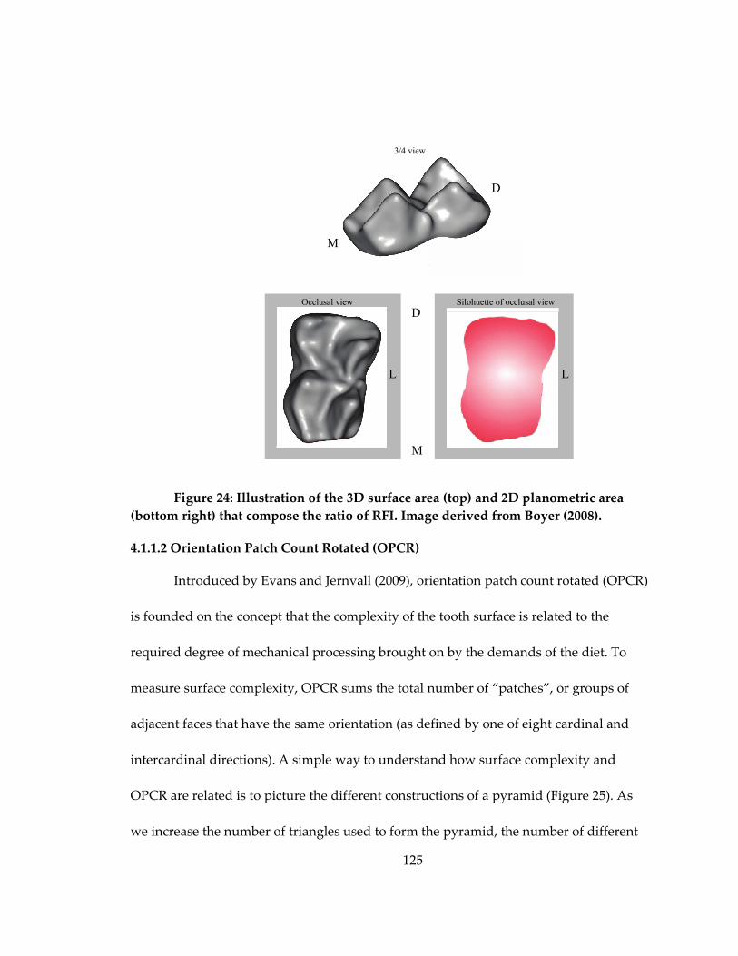
125
Figure 24: Illustration of the 3D surface area (top) and 2D planometric area
(bottom right) that compose the ratio of RFI. Image derived from Boyer (2008).
4.1.1.2 Orientation Patch Count Rotated (OPCR)
Introduced by Evans and Jernvall (2009), orientation patch count rotated (OPCR)
is founded on the concept that the complexity of the tooth surface is related to the
required degree of mechanical processing brought on by the demands of the diet. To
measure surface complexity, OPCR sums the total number of “patches”, or groups of
adjacent faces that have the same orientation (as defined by one of eight cardinal and
intercardinal directions). A simple way to understand how surface complexity and
OPCR are related is to picture the different constructions of a pyramid (Figure 25). As
we increase the number of triangles used to form the pyramid, the number of different
M
D
M
D
L L
3/4 view
Occlusal view Silohuette of occlusal view
126
planes that make up that pyramid increases, and thus the complexity of the pyramid
increases. OPCR is simply the sum of differently oriented planes that make up a 3D
surface.
A modification of the original orientation patch count (OPC) (Evans et al., 2007),
OPCR is a means to compensate for a problem associated with OPC in which the
number of patches is sensitive to the orientation of the tooth. This is done by rotating the
tooth surface eight times—each time by 5.625° for a total of 45°--and OPC is measured
for each orientation. The average of these eight different OPC values is then the recorded
OPCR value. OPCR has demonstrated an ability to distinguish faunivorous from
herbivorous taxa (Evans et al., 2007; Evans and Jernvall, 2009), and has been used to
infer changes in diet in horse evolution (Evans and Janis, 2014). It has also been
suggested to reflect the ‘toughness’ of primate dietary items (Bunn et al., 2011; Ledogar
et al., 2013), the most commonly accepted definition of which is generally the amount of
energy needed to propagate a crack (Ashby, 1992; Lucas, 2004; Williams et al., 2005;
Berthaume, 2017).
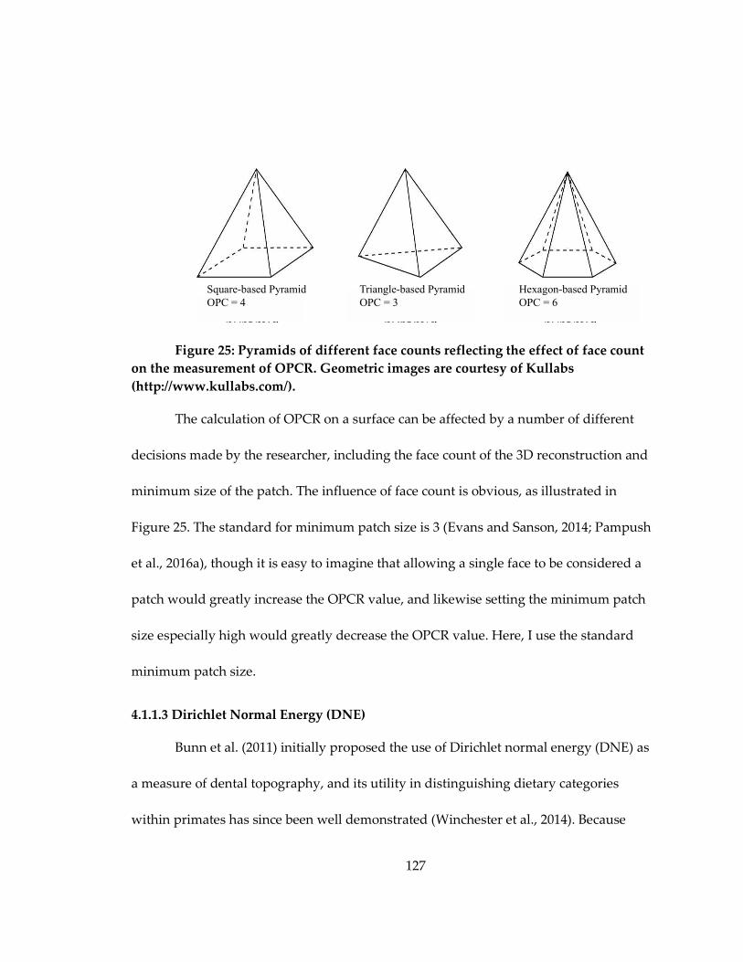
127
Figure 25: Pyramids of different face counts reflecting the effect of face count
on the measurement of OPCR. Geometric images are courtesy of Kullabs
(http://www.kullabs.com/).
The calculation of OPCR on a surface can be affected by a number of different
decisions made by the researcher, including the face count of the 3D reconstruction and
minimum size of the patch. The influence of face count is obvious, as illustrated in
Figure 25. The standard for minimum patch size is 3 (Evans and Sanson, 2014; Pampush
et al., 2016a), though it is easy to imagine that allowing a single face to be considered a
patch would greatly increase the OPCR value, and likewise setting the minimum patch
size especially high would greatly decrease the OPCR value. Here, I use the standard
minimum patch size.
4.1.1.3 Dirichlet Normal Energy (DNE)
Bunn et al. (2011) initially proposed the use of Dirichlet normal energy (DNE) as
a measure of dental topography, and its utility in distinguishing dietary categories
within primates has since been well demonstrated (Winchester et al., 2014). Because
Square-based Pyramid
OPC = 4
Triangle-based Pyramid
OPC = 3
Hexagon-based Pyramid
OPC = 6
128
DNE is discussed in great detail in Chapter 3, I will provide only a brief summary here.
In essence, DNE provides a measure of the sum curvature of the surface, with sharper
features contributing more DNE than more rounded features. Winchester et al. (2014)
noted the strong positive correlation between DNE and the Shearing Quotient (Kay and
Covert, 1984), and indeed DNE can be thought of as an inclusive, automated way of
measuring shearing on a tooth surface. Primarily, DNE has been used in the study of
primate teeth, though recent work by Prufrock et al. (2016) has included primitive
rodents and preliminary studies suggest its utility to distinguish dietary categories in
marsupials (Spradley and Kay, 2016).
4.1.2 Predictions
Given that tooth shape is generally constrained by the functional requirements of
food properties (Kay, 1975; Evans and Sanson, 2003), I expect my results to generally
mirror those from a similarly ecologically-broad clade like Primates. Indeed, Kay and
Hylander (1978) found that, within in a limited sample of phalangeriform marsupials,
dental shearing correlated with diet in a manner similar to the patterns observed in
primates. Thus, I predict folivorous and insectivorous marsupials to have the highest
values of RFI, OPCR, and DNE, as these two diets have been suggested to have the
highest degree of tough food items. Kay (1975) suggested that folivores and insectivores
are not easily distinguished except by body (and tooth) size. Since these metrics do not
include any measure of tooth size, I do not expect to see significantly different values of
129
any metric between these two dietary categories. Additionally, frugivorous marsupials
should have significantly lower values for all three metrics, as has been demonstrated in
primates (Winchester et al., 2014).
True faunivory is rare in primates—limited to a few genera, including Tarsius,
Arctocebus, and Loris—and in fact there are no large vertebrate prey specialists as I find
amongst the marsupials (e.g. Sarcophilus, Thylacinus, etc.). It is thus hard to predict how
DNE will behave or even if it will be useful. Nevertheless, given the high protoconid
and/or paraconid cusp(s) of the carnassial teeth of marsupial carnivores, we might
expect that faunivores will have higher DNE and RFI values than frugivores.
Evans et al. (2007) and Evans and Jervnall (2009) explored faunivory using the
OPCR metric. They report that carnivorous species have significantly lower OPCR
values, and suggest that the relatively easily digested proteins and fats within meat did
not require the same tooth surface complexity as the more difficult to digest fibrous
dietary components of herbivorous species. Thus, I predict that the faunivorous species
in my sample will demonstrate similarly lower OPCR values.
Ultimately, dental topography should have a strong relationship with food
material properties. Though a more in-depth exploration of this interaction is beyond
the scope of this study, I expect gross differences in food material properties across taxa
to generally align with traditionally used heuristic dietary categories, enabling the use of
diet categories as a stand-in for the more difficult to measure material properties. With

130
this caveat in mind, the employed dental topography metrics are expected to be
predictive of diet category within the marsupials studied here.
4.2 Materials and Methods
4.2.1 Sample Preparation
To investigate the relationship between dental topography and dietary ecology, I
scanned and segmented the lower second molars of 135 individual specimens
representing 43 genera, and 59 species of marsupials (Table 1). To capture the wide
ecological variety of marsupials present in the fossil record of South America, it was
necessary to sample both South American and Australian/New Guinean extant
marsupials. Specimens were obtained from the American Museum of Natural History,
the National Museum of Natural History, and the Australian Museum in Sydney, and
include both skeletal material and epoxy casts poured from molds of teeth. Cast fidelity
was examined by comparing scans of casted and original dentitions for a subset of
specimens. The complete sample of species, along with a phylogenetic tree topology, is
depicted in Figure 26. Primary dietary categories were assigned to each species
according to MammalDIET, an online archive of dietary information (Kissling et al.,
2014). This resource was supplemented and cross-referenced with sources from the
primary literature, including taxonomic and ecological reference volumes (Gardner,
2008; Flannery, 1995). The sources for these characterizations are summarized in

131
Appendix C. These dietary categories are necessarily broad owing to the often imprecise
nature of the dietary information.
Table 11: Dental topography metrics and dietary category for each species
included in this study. All values represent means for multiple individuals (when
available).
Family Species Diet DNE RFI OPC
R
M2
Area
Acrobatidae Acrobates
pygmaeus Frugivore 205.54 0.38 72.5 0.69
Potoridae Aepyprymnus
rufescens Browsing 249.19 0.43 92.6 29.43
Dasyuridae Antechinus
minimus Insectivore 308.93 0.62 79.4 3.66
Potoridae Bettongia gaimardi Browsing 187.88 0.49 67.5 21.16
Caenolestidae Caenolestes
fuliginosus Insectivore 326.01 0.58 77.1 2.59
Didelphidae Caluromys
derbianus Frugivore 212.98 0.52 67.6 2.67
Didelphidae Caluromys lanatus Frugivore 161.42 0.57 51.6 4.60
Burramyidae Cercartetus
caudatus Frugivore 190.97 0.48 62.2 1.58
Didelphidae Chironectes
minimus Faunivore 240.37 0.62 69.5 14.09
Petauridae Dactylopsila
palpator Insectivore 137.74 0.43 53.6 7.16
Petauridae Dactylopsila
trivirgata Insectivore 182.30 0.45 78.4 7.73
Dasyuridae Dasykaluta
rosamondae Insectivore 283.68 0.61 67.2 9.65
Dasyuridae Dasyurus
hallucatus Insectivore 213.91 0.58 62.6 10.81
Macropodidae Dendrolagus
lumholtzi Folivore 182.65 0.56 64.2 28.80
Didelphidae Didelphis
albiventris Frugivore 162.69 0.50 50.5 14.32
Macropodidae Dorcopsis hageni Browsing 230.37 0.63 65.9 24.94
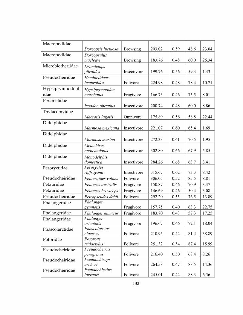
132
Macropodidae Dorcopsis luctuosa Browsing 203.02 0.59 48.6 23.04
Macropodidae Dorcopsulus
macleayi Browsing 183.76 0.48 60.0 26.34
Microbiotheriidae Dromiciops
gliroides Insectivore 199.76 0.56 59.3 1.43
Pseudocheiridae Hemibelideus
lemuroides Folivore 224.98 0.48 78.4 10.71
Hypsiprymnodont
idae Hypsiprymnodon
moschatus Frugivore 166.73 0.46 75.5 8.01
Peramelidae Isoodon obesulus Insectivore 200.74 0.48 60.0 8.86
Thylacomyidae Macrotis lagotis Omnivore 175.89 0.56 58.8 22.44
Didelphidae Marmosa mexicana Insectivore 221.07 0.60 65.4 1.69
Didelphidae
Marmosa murina Insectivore 272.33 0.61 70.5 1.95
Didelphidae Metachirus
nudicaudatus Insectivore 302.80 0.66 67.9 5.85
Didelphidae Monodelphis
domestica Insectivore 284.26 0.68 63.7 3.41
Peroryctidae Peroryctes
raffrayana Insectivore 315.67 0.62 73.3 8.42
Pseudocheiridae Petauroides volans Folivore 306.05 0.52 85.5 8.81
Petauridae Petaurus australis Frugivore 150.87 0.46 70.9 3.37
Petauridae Petaurus breviceps Frugivore 146.69 0.46 50.4 3.08
Pseudocheiridae Petropseudes dahli Folivore 292.20 0.55 76.5 13.89
Phalangeridae Phalanger
gymnotis Frugivore 157.75 0.40 63.3 22.75
Phalangeridae Phalanger mimicus Frugivore 183.70 0.43 57.3 17.25
Phalangeridae Phalanger
orientalis Frugivore 196.67 0.46 72.1 18.04
Phascolarctidae Phascolarctos
cinereus Folivore 210.95 0.42 81.4 38.89
Potoridae Potorous
tridactylus Folivore 251.32 0.54 87.4 15.99
Pseudocheiridae Pseudocheirus
peregrinus Folivore 216.40 0.50 68.4 8.26
Pseudocheiridae Pseudochirops
archeri Folivore 264.58 0.47 88.5 14.36
Pseudocheiridae Pseudochirulus
larvatus Folivore 245.01 0.42 88.3 6.56
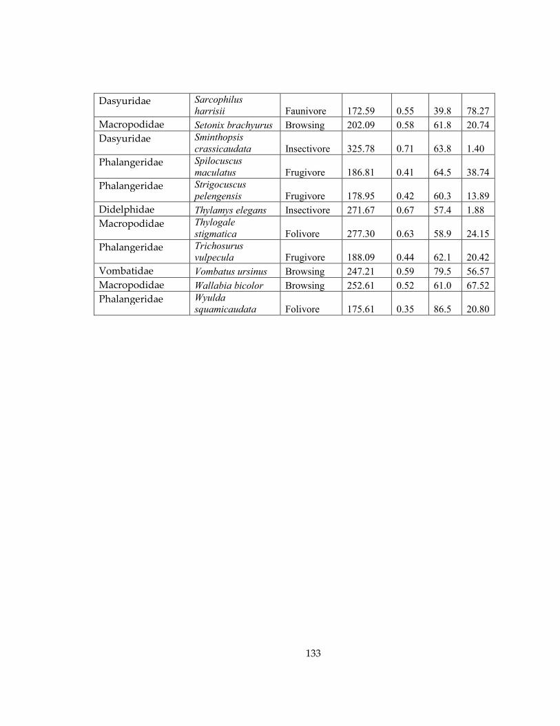
133
Dasyuridae Sarcophilus
harrisii Faunivore 172.59 0.55 39.8 78.27
Macropodidae Setonix brachyurus Browsing 202.09 0.58 61.8 20.74
Dasyuridae Sminthopsis
crassicaudata Insectivore 325.78 0.71 63.8 1.40
Phalangeridae Spilocuscus
maculatus Frugivore 186.81 0.41 64.5 38.74
Phalangeridae Strigocuscus
pelengensis Frugivore 178.95 0.42 60.3 13.89
Didelphidae Thylamys elegans Insectivore 271.67 0.67 57.4 1.88
Macropodidae Thylogale
stigmatica Folivore 277.30 0.63 58.9 24.15
Phalangeridae Trichosurus
vulpecula Frugivore 188.09 0.44 62.1 20.42
Vombatidae Vombatus ursinus Browsing 247.21 0.59 79.5 56.57
Macropodidae Wallabia bicolor Browsing 252.61 0.52 61.0 67.52
Phalangeridae Wyulda
squamicaudata Folivore 175.61 0.35 86.5 20.80
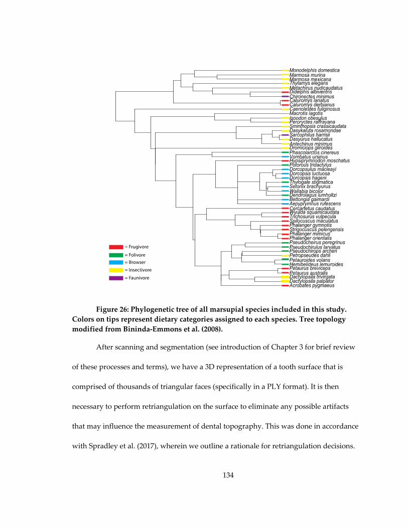
134
Figure 26: Phylogenetic tree of all marsupial species included in this study.
Colors on tips represent dietary categories assigned to each species. Tree topology
modified from Bininda-Emmons et al. (2008).
After scanning and segmentation (see introduction of Chapter 3 for brief review
of these processes and terms), we have a 3D representation of a tooth surface that is
comprised of thousands of triangular faces (specifically in a PLY format). It is then
necessary to perform retriangulation on the surface to eliminate any possible artifacts
that may influence the measurement of dental topography. This was done in accordance
with Spradley et al. (2017), wherein we outline a rationale for retriangulation decisions.
135
Ultimately, I chose to downsample all PLY files to 10,000 faces and smooth the 3D mesh
via 25 smoothing iterations performed in Avizo® (FEI Visualization Sciences Group,
Berlin, Germany). This fairly conservative retriangulation protocol ensures that the effect
of smoothing artifacts is minimized whilst maintaining the essential geometry of the
tooth surface, which is a concern when more aggressive smoothing algorithms are
employed (Spradley et al., 2017). Nevertheless, artifacts were identified on a limited
number of surfaces in my sample, and to eliminate these they were deleted and the
resultant ‘holes’ were filled using Geomagic® (3D Systems, Inc., Rock Hill, SC). After all
PLY files were retriangulated, the resultant files were uploaded to the open-source
statistical software R via the package “molaR” (Pampush et al., 2016a). The boundary
exclusion criterion of molaR was set to “vertex”, and DNE, RFI, and OPCR were
calculated for each tooth surface. Linear measurements of the maximum mesiodistal
length and buccolingual width were also taken for each tooth, and this was used as an
approximation of the molar area. Because molar area was not normally distributed, the
area of each molar was natural-log transformed.
4.2.2 Statistical Analyses
With the exception of phylogenetically informed analyses, all statistical tests
were performed with an alpha level of 0.05, and a modified Bonferroni correction, using
the open-source statistical software R. My Bonferroni correction follows that of
Cheverud (2001), which controls for covariation in the data and is more rigorous than

136
simply accounting for the number of tests being performed. In order to discern how
these different metrics might relate to one another, a Principal Components Analysis
(PCA) was performed using all three metrics. To account for effects of phylogenetic
relatedness among species, mean species values were compiled and a phylogenetic
ANOVA was performed using the R package ‘phytools’. Pairwise comparison tests were
then undertaken using a phylogenetically-corrected Tukey’s Honestly Significant
Difference (HSD) test using the R package ‘caper’. Finally, a discriminant function
analysis (DFA) was performed to test the ability of these metrics to successfully
reconstruct diet with a given dental topography.
4.2.3 Distributions of Ecometrics as Climatic Proxies
Having established that these metrics are ecologically informative in my
marsupial sample, I seek to demonstrate that the distributions of these ecometrics
(ecologically relevant metrics; see Eronen et al., 2010) within communities of marsupials
can be used as proxies for variables of climate and habitat. The six variables of interest
presented here are the same six from Chapter 2: MAT, MAP, temperature seasonality,
precipitation seasonality, NPP, and canopy height. Faunal lists were compiled using the
UC-Davis ICE “Biological Inventories of the World’s Protected Areas”
(http://www.ice.ucdavis.edu/bioinventory/bioinventory.html) and supplemented with
primary sources of published faunal lists (Bulmer and Menzies, 1972; Helgen, 2007;
Mamu, 2008). Species means for DNE, RFI, and OPCR were recorded for each species in
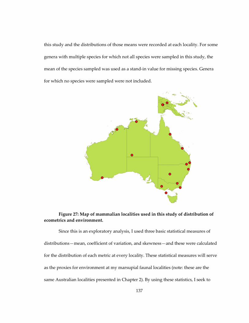
137
this study and the distributions of those means were recorded at each locality. For some
genera with multiple species for which not all species were sampled in this study, the
mean of the species sampled was used as a stand-in value for missing species. Genera
for which no species were sampled were not included.
Figure 27: Map of mammalian localities used in this study of distribution of
ecometrics and environment.
Since this is an exploratory analysis, I used three basic statistical measures of
distributions—mean, coefficient of variation, and skewness—and these were calculated
for the distribution of each metric at every locality. These statistical measures will serve
as the proxies for environment at my marsupial faunal localities (note: these are the
same Australian localities presented in Chapter 2). By using these statistics, I seek to
138
explore the potential of distributions of ecometrics to be used in place of distributions of
known ecologies—as in Chapter 2 of this dissertation. Because the reconstruction of
behavior in the fossil record is problematic, this method would skip this step and
instead rely only on quantitative measurements that can be directly taken from fossil
teeth.
4.2.3.1 Exclusion of Range
I decided to exclude the use of range. This decision was made after analysis of all
variables suggested that ranges do not have significant relationships with my
bioclimatic variables. Before moving forward, it is important that I first explain these
results in the context of my dataset. First of all, the ranges of these ecometrics are not
were overly broad, and not informative. A majority of localities having high ranges of
DNE, OPCR, and RFI. Exploring the data, this is likely because most localities have at
least one insectivore (typically high values of DNE, OPCR, and RFI) and at least one
frugivore (typically low values of each). Thus, the ranges are fairly consistent from one
locality to the next regardless of the actual shape of the distribution.
4.3 Results
4.3.1 Dental Topography and Dietary Ecology
4.3.1.1 Correlations Among Topographic Variables
Summary statistics for correlation analyses between dental topography metrics
are presented in Table 12. Least-squares regressions between each pair of variables are
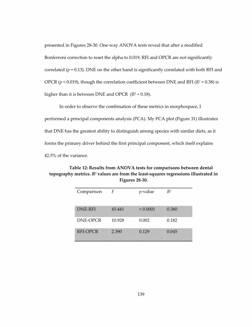
139
presented in Figures 28-30. One-way ANOVA tests reveal that after a modified
Bonferroni correction to reset the alpha to 0.019, RFI and OPCR are not significantly
correlated (p = 0.13). DNE on the other hand is significantly correlated with both RFI and
OPCR (p < 0.019), though the correlation coefficient between DNE and RFI (R2 = 0.38) is
higher than it is between DNE and OPCR (R2 = 0.18).
In order to observe the combination of these metrics in morphospace, I
performed a principal components analysis (PCA). My PCA plot (Figure 31) illustrates
that DNE has the greatest ability to distinguish among species with similar diets, as it
forms the primary driver behind the first principal component, which itself explains
42.5% of the variance.
Table 12: Results from ANOVA tests for comparisons between dental
topography metrics. R2 values are from the least-squares regressions illustrated in
Figures 28-30.
Comparison F p-value R2
DNE-RFI 45.441 < 0.0001 0.380
DNE-OPCR 10.928 0.002 0.182
RFI-OPCR 2.390 0.129 0.045
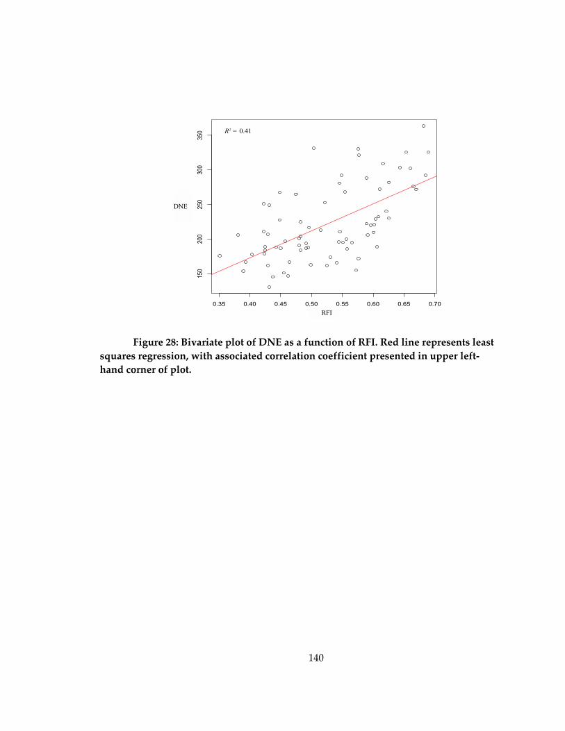
140
Figure 28: Bivariate plot of DNE as a function of RFI. Red line represents least
squares regression, with associated correlation coefficient presented in upper left-
hand corner of plot.
0.35 0.40 0.45 0.50 0.55 0.60 0.65 0.70
150
200
250
300
350
dat$RFI
dat$
DN
E
RFI
DNE
R2 = 0.41
RFI
DNE
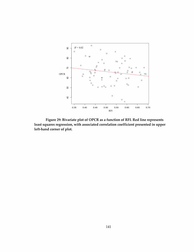
141
Figure 29: Bivariate plot of OPCR as a function of RFI. Red line represents
least squares regression, with associated correlation coefficient presented in upper
left-hand corner of plot.
0.35 0.40 0.45 0.50 0.55 0.60 0.65 0.70
4050
6070
8090
dat$RFI
dat$
OP
CR
RFI
OPCR
R2 = 0.15R2 = 0.02
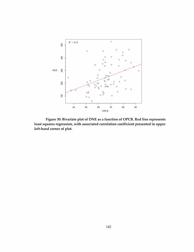
142
Figure 30: Bivariate plot of DNE as a function of OPCR. Red line represents
least squares regression, with associated correlation coefficient presented in upper
left-hand corner of plot.
40 50 60 70 80 90
15
02
00
25
03
00
35
0
dat$OPCR
da
t$D
NE
DNE
OPCR
R2 = 0.15

143
Figure 31: Principal components analysis including the three dental
topography metrics and the natural log of M2 area. The symbol key is as follows: Red
diamonds = frugivores; Blue circles = browsers; Green x’s = folivores; Yellow triangles
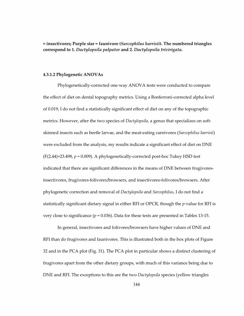
144
= insectivores; Purple star = faunivore (Sarcophilus harrisii). The numbered triangles
correspond to 1. Dactylopsila palpator and 2. Dactylopsila trivirigata.
4.3.1.2 Phylogenetic ANOVAs
Phylogenetically-corrected one-way ANOVA tests were conducted to compare
the effect of diet on dental topography metrics. Using a Bonferroni-corrected alpha level
of 0.019, I do not find a statistically significant effect of diet on any of the topographic
metrics. However, after the two species of Dactylopsila, a genus that specializes on soft-
skinned insects such as beetle larvae, and the meat-eating carnivores (Sarcophilus harrisii)
were excluded from the analysis, my results indicate a significant effect of diet on DNE
(F(2,44)=23.498, p = 0.009). A phylogenetically-corrected post-hoc Tukey HSD test
indicated that there are significant differences in the means of DNE between frugivores-
insectivores, frugivores-folivores/browsers, and insectivores-folivores/browsers. After
phylogenetic correction and removal of Dactylopsila and Sarcophilus, I do not find a
statistically significant dietary signal in either RFI or OPCR, though the p-value for RFI is
very close to significance (p = 0.036). Data for these tests are presented in Tables 13-15.
In general, insectivores and folivores/browsers have higher values of DNE and
RFI than do frugivores and faunivores. This is illustrated both in the box plots of Figure
32 and in the PCA plot (Fig. 31). The PCA plot in particular shows a distinct clustering of
frugivores apart from the other dietary groups, with much of this variance being due to
DNE and RFI. The exceptions to this are the two Dactylopsila species (yellow triangles
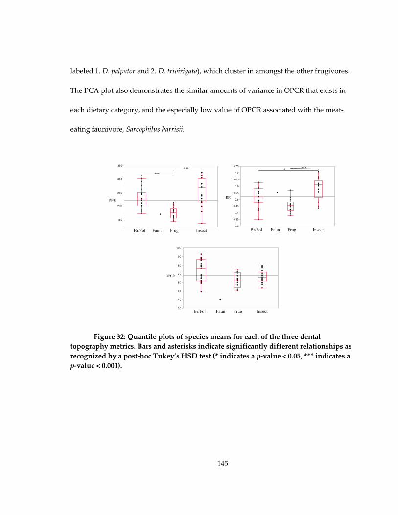
145
labeled 1. D. palpator and 2. D. trivirigata), which cluster in amongst the other frugivores.
The PCA plot also demonstrates the similar amounts of variance in OPCR that exists in
each dietary category, and the especially low value of OPCR associated with the meat-
eating faunivore, Sarcophilus harrisii.
Figure 32: Quantile plots of species means for each of the three dental
topography metrics. Bars and asterisks indicate significantly different relationships as
recognized by a post-hoc Tukey’s HSD test (* indicates a p-value < 0.05, *** indicates a
p-value < 0.001).
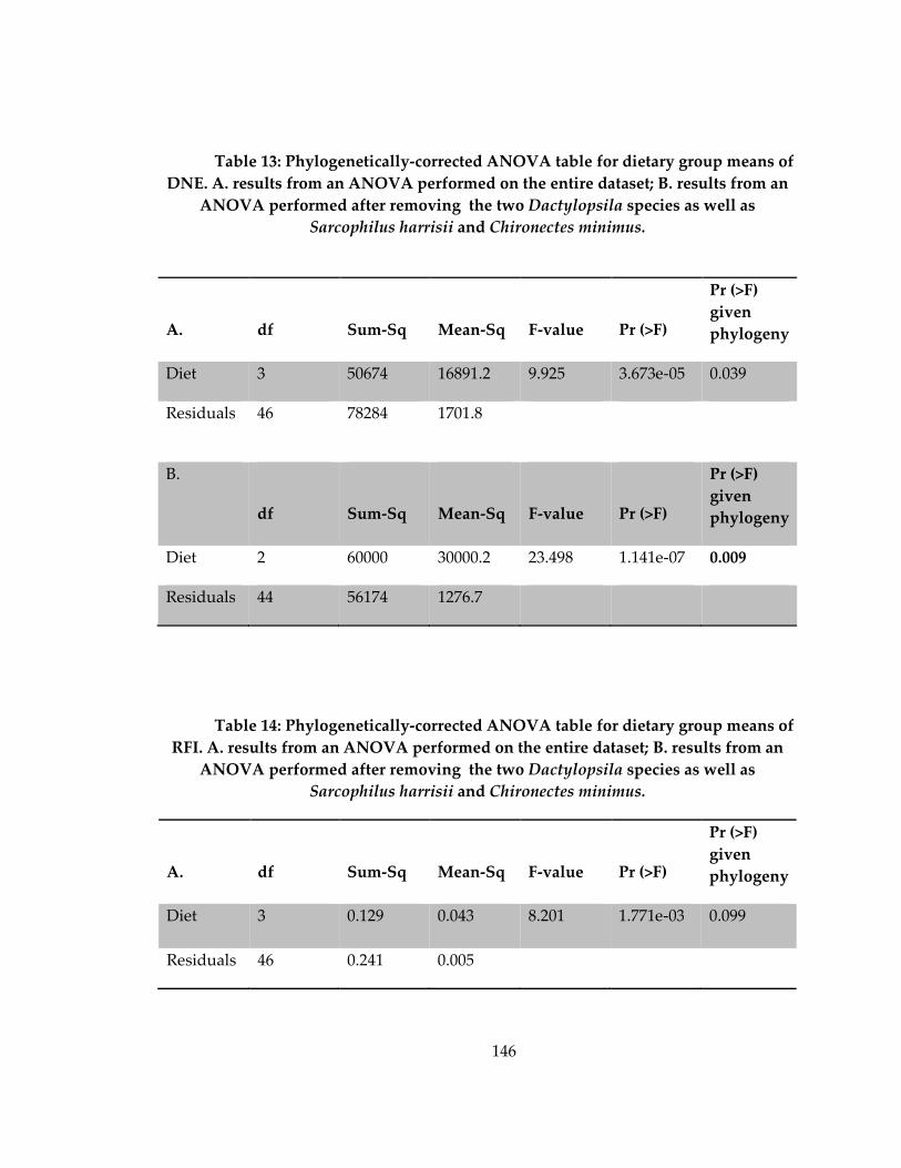
146
Table 13: Phylogenetically-corrected ANOVA table for dietary group means of
DNE. A. results from an ANOVA performed on the entire dataset; B. results from an
ANOVA performed after removing the two Dactylopsila species as well as
Sarcophilus harrisii and Chironectes minimus.
A.
df
Sum-Sq
Mean-Sq
F-value
Pr (>F)
Pr (>F)
given
phylogeny
Diet 3 50674 16891.2 9.925 3.673e-05 0.039
Residuals 46 78284 1701.8
B.
df
Sum-Sq
Mean-Sq
F-value
Pr (>F)
Pr (>F)
given
phylogeny
Diet 2 60000 30000.2 23.498 1.141e-07 0.009
Residuals 44 56174 1276.7
Table 14: Phylogenetically-corrected ANOVA table for dietary group means of
RFI. A. results from an ANOVA performed on the entire dataset; B. results from an
ANOVA performed after removing the two Dactylopsila species as well as
Sarcophilus harrisii and Chironectes minimus.
A.
df
Sum-Sq
Mean-Sq
F-value
Pr (>F)
Pr (>F)
given
phylogeny
Diet 3 0.129 0.043 8.201 1.771e-03 0.099
Residuals 46 0.241 0.005
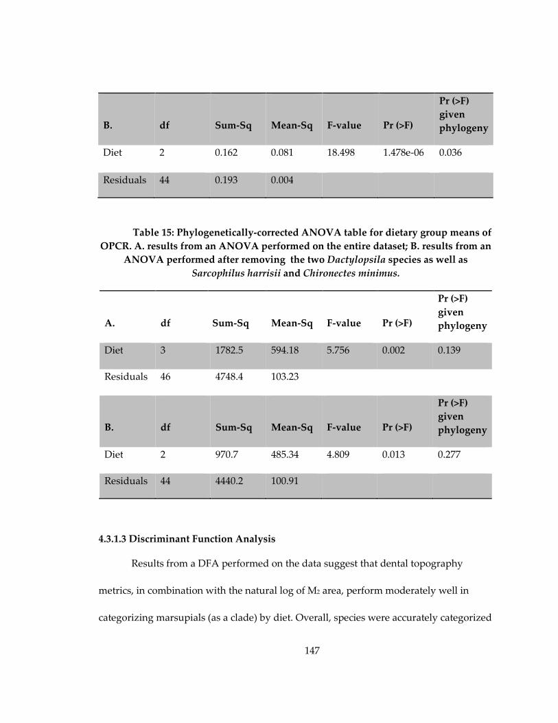
147
B.
df
Sum-Sq
Mean-Sq
F-value
Pr (>F)
Pr (>F)
given
phylogeny
Diet 2 0.162 0.081 18.498 1.478e-06 0.036
Residuals 44 0.193 0.004
Table 15: Phylogenetically-corrected ANOVA table for dietary group means of
OPCR. A. results from an ANOVA performed on the entire dataset; B. results from an
ANOVA performed after removing the two Dactylopsila species as well as
Sarcophilus harrisii and Chironectes minimus.
A.
df
Sum-Sq
Mean-Sq
F-value
Pr (>F)
Pr (>F)
given
phylogeny
Diet 3 1782.5 594.18 5.756 0.002 0.139
Residuals 46 4748.4 103.23
B.
df
Sum-Sq
Mean-Sq
F-value
Pr (>F)
Pr (>F)
given
phylogeny
Diet 2 970.7 485.34 4.809 0.013 0.277
Residuals 44 4440.2 100.91
4.3.1.3 Discriminant Function Analysis
Results from a DFA performed on the data suggest that dental topography
metrics, in combination with the natural log of M2 area, perform moderately well in
categorizing marsupials (as a clade) by diet. Overall, species were accurately categorized
148
74.6% of the time. Taking a closer look at the results, I find that browsers/folivores and
insectivores are categorized at much higher rates (83.8% and 72.7%, respectively) when
compared to frugivores, for which the DFA is performing at a rate nearly equivalent to
random chance (62.5%).
Experimenting with pairs of topographic measures (each model including the
natural log of molar area), I do not find any significant differences between models.
DFAs performed on individual topographic variables—in conjunction with molar area—
reveal that DNE has slightly more discriminatory power (76.1%) than either RFI (70.1%)
or OPCR (62.7%). This pattern holds for all dietary categories. RFI was more successful
at discriminating frugivores than OPCR (37.5% and 6.3%, respectively), though both had
equivalent rates of discrimination for browsers/folivores and insectivores.
Performing a DFA on species belonging to Diprotodontia alone slightly improve
accuracy, with species correctly allocated at an overall rate of 77.8%. Frugivores in this
sample were classified correctly 100% of the time, and the accuracy of classifying
browsers and folivores was also increased to 89%. Non-diprotodont marsupials, taken
alone, show a much lower accuracy in classification at 61%, with only insectivores being
correctly identified at all (84.6%).
4.3.2 Dental Topography and Environmental Reconstruction
See Table 16 for the complete distribution of all three statistics for the ecometrics
at each Australian and New Guinean locality. My results (shown in Table 17) show that
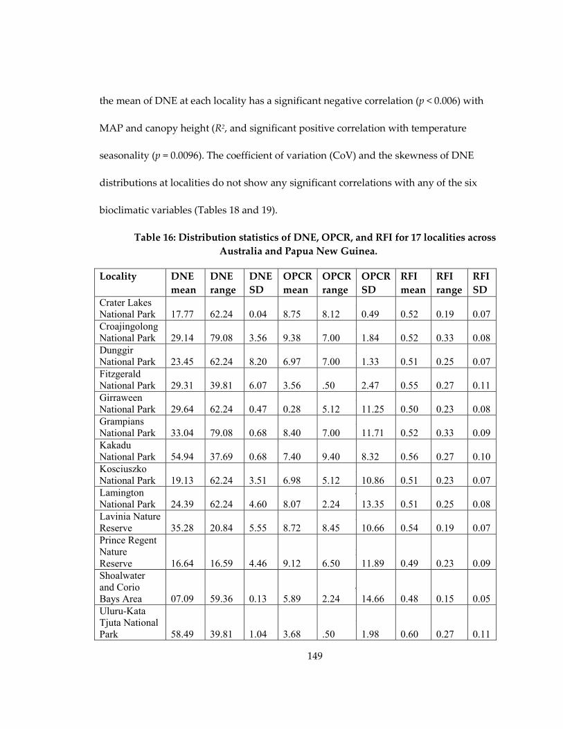
149
the mean of DNE at each locality has a significant negative correlation (p < 0.006) with
MAP and canopy height (R2, and significant positive correlation with temperature
seasonality (p = 0.0096). The coefficient of variation (CoV) and the skewness of DNE
distributions at localities do not show any significant correlations with any of the six
bioclimatic variables (Tables 18 and 19).
Table 16: Distribution statistics of DNE, OPCR, and RFI for 17 localities across
Australia and Papua New Guinea.
Locality
DNE
mean
DNE
range
DNE
SD
OPCR
mean
OPCR
range
OPCR
SD
RFI
mean
RFI
range
RFI
SD Crater Lakes
National Park
2
17.77
1
62.24 0.04
6
8.75
3
8.12
1
0.49 0.52 0.19 0.07
Croajingolong
National Park
2
29.14
1
79.08 3.56
6
9.38
3
7.00
1
1.84 0.52 0.33 0.08
Dunggir
National Park
2
23.45
1
62.24 8.20
6
6.97
3
7.00
1
1.33 0.51 0.25 0.07
Fitzgerald
National Park
2
29.31
1
39.81 6.07
6
3.56
7
.50 2.47 0.55 0.27 0.11
Girraween
National Park
2
29.64
1
62.24 0.47
7
0.28
3
5.12 11.25 0.50 0.23 0.08
Grampians
National Park
2
33.04
1
79.08 0.68
6
8.40
3
7.00 11.71 0.52 0.33 0.09
Kakadu
National Park
2
54.94
1
37.69 0.68
6
7.40
1
9.40 8.32 0.56 0.27 0.10
Kosciuszko
National Park
2
19.13
1
62.24 3.51
6
6.98
3
5.12 10.86 0.51 0.23 0.07
Lamington
National Park
2
24.39
1
62.24 4.60
6
8.07
4
2.24 13.35 0.51 0.25 0.08
Lavinia Nature
Reserve
2
35.28
1
20.84 5.55
6
8.72
2
8.45 10.66 0.54 0.19 0.07
Prince Regent
Nature
Reserve
2
16.64
1
16.59 4.46
6
9.12
2
6.50 11.89 0.49 0.23 0.09
Shoalwater
and Corio
Bays Area
2
07.09
1
59.36 0.13
6
5.89
4
2.24 14.66 0.48 0.15 0.05
Uluru-Kata
Tjuta National
Park
2
58.49
1
39.81 1.04
6
3.68
7
.50 1.98 0.60 0.27 0.11
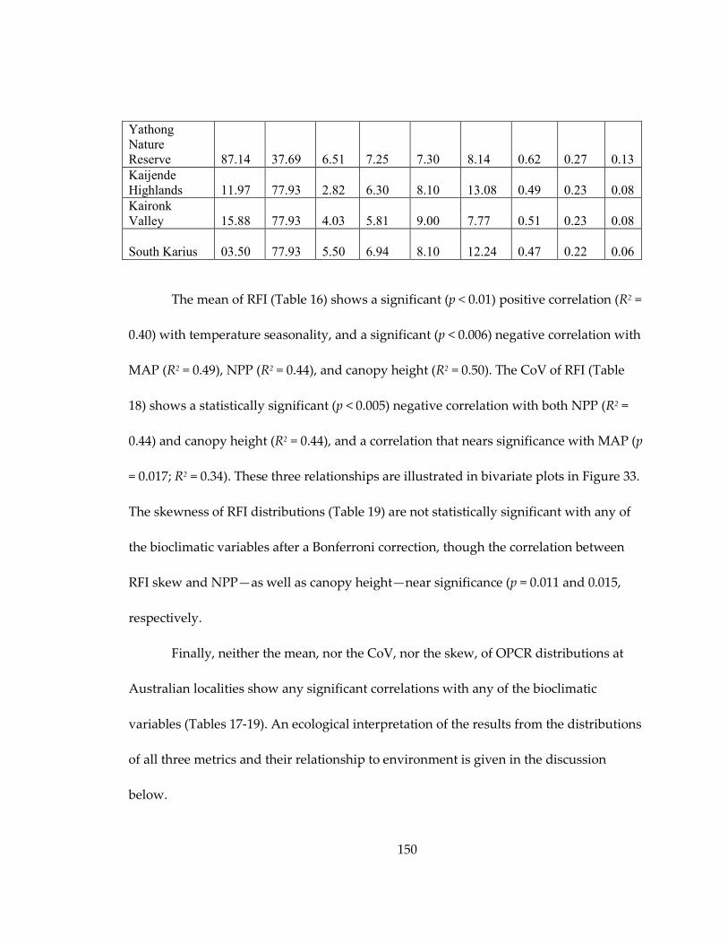
150
Yathong
Nature
Reserve
2
87.14
1
37.69 6.51
6
7.25
1
7.30 8.14 0.62 0.27 0.13
Kaijende
Highlands
2
11.97
1
77.93 2.82
6
6.30
3
8.10 13.08 0.49 0.23 0.08
Kaironk
Valley
2
15.88
1
77.93 4.03
6
5.81
2
9.00 7.77 0.51 0.23 0.08
South Karius
2
03.50
1
77.93 5.50
6
6.94
3
8.10 12.24 0.47 0.22 0.06
The mean of RFI (Table 16) shows a significant (p < 0.01) positive correlation (R2 =
0.40) with temperature seasonality, and a significant (p < 0.006) negative correlation with
MAP (R2 = 0.49), NPP (R2 = 0.44), and canopy height (R2 = 0.50). The CoV of RFI (Table
18) shows a statistically significant (p < 0.005) negative correlation with both NPP (R2 =
0.44) and canopy height (R2 = 0.44), and a correlation that nears significance with MAP (p
= 0.017; R2 = 0.34). These three relationships are illustrated in bivariate plots in Figure 33.
The skewness of RFI distributions (Table 19) are not statistically significant with any of
the bioclimatic variables after a Bonferroni correction, though the correlation between
RFI skew and NPP—as well as canopy height—near significance (p = 0.011 and 0.015,
respectively.
Finally, neither the mean, nor the CoV, nor the skew, of OPCR distributions at
Australian localities show any significant correlations with any of the bioclimatic
variables (Tables 17-19). An ecological interpretation of the results from the distributions
of all three metrics and their relationship to environment is given in the discussion
below.
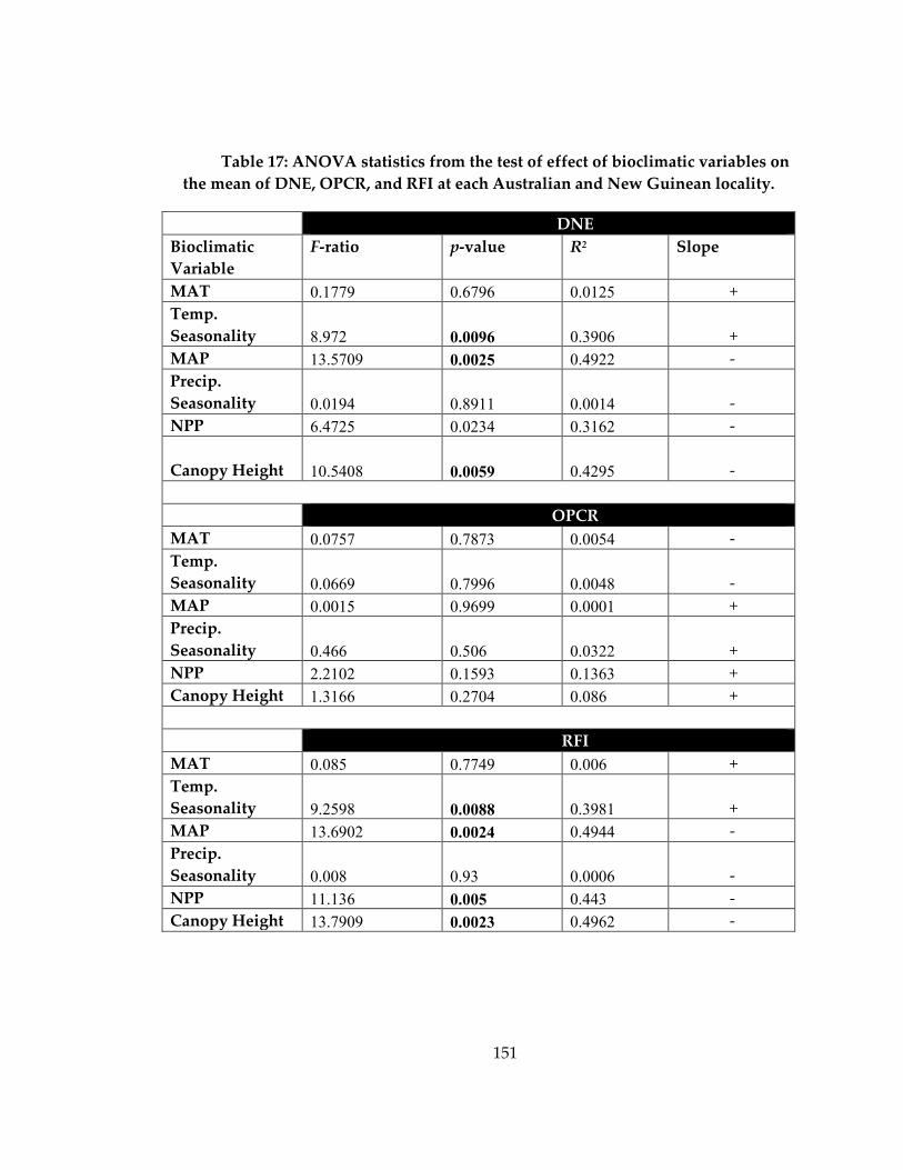
151
Table 17: ANOVA statistics from the test of effect of bioclimatic variables on
the mean of DNE, OPCR, and RFI at each Australian and New Guinean locality.
DNE
Bioclimatic
Variable
F-ratio p-value R2 Slope
MAT 0.1779 0.6796 0.0125 +
Temp.
Seasonality 8.972 0.0096 0.3906
+
MAP 13.5709 0.0025 0.4922 -
Precip.
Seasonality 0.0194 0.8911 0.0014
-
NPP 6.4725 0.0234 0.3162 -
Canopy Height 10.5408 0.0059 0.4295
-
OPCR
MAT 0.0757 0.7873 0.0054 -
Temp.
Seasonality 0.0669 0.7996 0.0048
-
MAP 0.0015 0.9699 0.0001 +
Precip.
Seasonality 0.466 0.506 0.0322
+
NPP 2.2102 0.1593 0.1363 +
Canopy Height 1.3166 0.2704 0.086 +
RFI
MAT 0.085 0.7749 0.006 +
Temp.
Seasonality 9.2598 0.0088 0.3981
+
MAP 13.6902 0.0024 0.4944 -
Precip.
Seasonality 0.008 0.93 0.0006
-
NPP 11.136 0.005 0.443 -
Canopy Height 13.7909 0.0023 0.4962 -
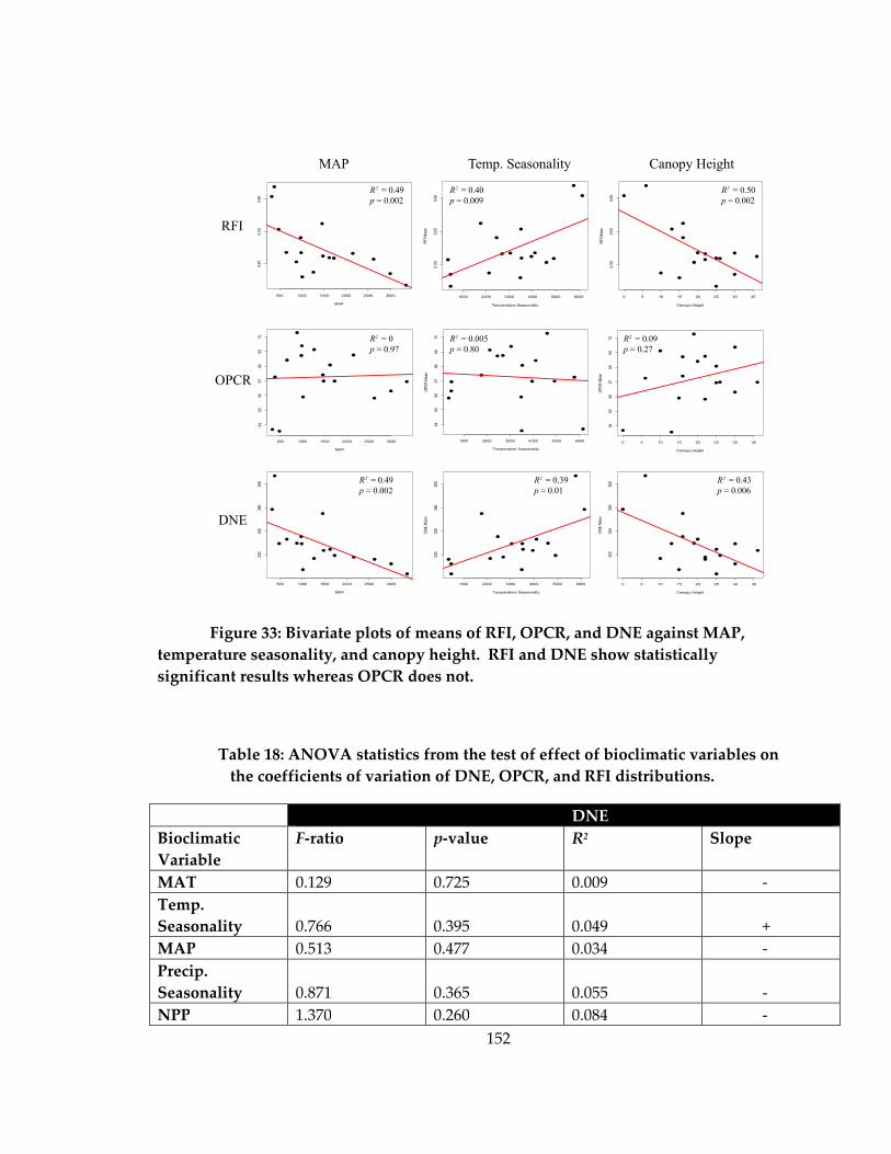
152
Figure 33: Bivariate plots of means of RFI, OPCR, and DNE against MAP,
temperature seasonality, and canopy height. RFI and DNE show statistically
significant results whereas OPCR does not.
Table 18: ANOVA statistics from the test of effect of bioclimatic variables on
the coefficients of variation of DNE, OPCR, and RFI distributions.
DNE
Bioclimatic
Variable
F-ratio p-value R2 Slope
MAT 0.129 0.725 0.009 -
Temp.
Seasonality 0.766 0.395 0.049
+
MAP 0.513 0.477 0.034 -
Precip.
Seasonality 0.871 0.365 0.055
-
NPP 1.370 0.260 0.084 -
0 5 10 15 20 25 30 35
0.50
0.5
50
.60
Canopy Height
RF
I Mea
n
1000 2000 3000 4000 5000 6000
0.50
0.5
50
.60
Temperature Seasonality
RF
I Mea
n
500 1000 1500 2000 2500 3000
0.50
0.55
0.60
MAP
RF
I Mea
nRFI
MAP Temp. Seasonality Canopy Height
500 1000 1500 2000 2500 3000
6465
666
768
6970
MAP
OP
CR
Mea
n
1000 2000 3000 4000 5000 6000
6465
6667
6869
70
Temperature Seasonality
OP
CR
Mea
n
0 5 10 15 20 25 30 35
6465
6667
6869
70
Canopy Height
OP
CR
Mea
n
OPCR
500 1000 1500 2000 2500 3000
220
240
260
280
MAP
DN
E M
eanDNE
1000 2000 3000 4000 5000 6000
220
240
260
280
Temperature Seasonality
DN
E M
ean
0 5 10 15 20 25 30 35
220
240
260
280
Canopy Height
DN
E M
ean
R2 = 0.39
p = 0.01
R2 = 0.49
p = 0.002
R2 = 0.43
p = 0.006
R2 = 0
p = 0.97
R2 = 0.005
p = 0.80
R2 = 0.09
p = 0.27
R2 = 0.49
p = 0.002
R2 = 0.40
p = 0.009
R2 = 0.50
p = 0.002
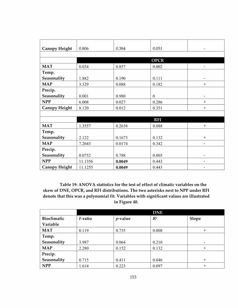
153
Canopy Height 0.806 0.384 0.051
-
OPCR
MAT 0.034 0.857 0.002 -
Temp.
Seasonality 1.882 0.190 0.111
-
MAP 3.329 0.088 0.182 +
Precip.
Seasonality 0.001 0.980 0
-
NPP 6.008 0.027 0.286 +
Canopy Height 8.120 0.012 0.351 +
RFI
MAT 1.3557 0.2638 0.088 +
Temp.
Seasonality 2.122 0.1673 0.132
+
MAP 7.2643 0.0174 0.342 -
Precip.
Seasonality 0.0752 0.788 0.005
-
NPP 11.1356 0.0049 0.443 -
Canopy Height 11.1255 0.0049 0.443 -
Table 19: ANOVA statistics for the test of effect of climatic variables on the
skew of DNE, OPCR, and RFI distributions. The two asterisks next to NPP under RFI
denote that this was a polynomial fit. Variables with significant values are illustrated
in Figure 40.
DNE
Bioclimatic
Variable
F-ratio p-value R2 Slope
MAT 0.119 0.735 0.008 +
Temp.
Seasonality 3.987 0.064 0.210
-
MAP 2.280 0.152 0.132 +
Precip.
Seasonality 0.715 0.411 0.046
+
NPP 1.614 0.223 0.097 +
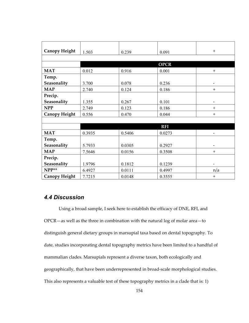
154
Canopy Height 1.503 0.239 0.091
+
OPCR
MAT 0.012 0.916 0.001 +
Temp.
Seasonality 3.700 0.078 0.236
-
MAP 2.740 0.124 0.186 +
Precip.
Seasonality 1.355 0.267 0.101
-
NPP 2.749 0.123 0.186 +
Canopy Height 0.556 0.470 0.044 +
RFI
MAT 0.3935 0.5406 0.0273 -
Temp.
Seasonality 5.7933 0.0305 0.2927
-
MAP 7.5646 0.0156 0.3508 +
Precip.
Seasonality 1.9796 0.1812 0.1239
-
NPP** 6.4927 0.0111 0.4997 n/a
Canopy Height 7.7215 0.0148 0.3555 +
4.4 Discussion
Using a broad sample, I seek here to establish the efficacy of DNE, RFI, and
OPCR—as well as the three in combination with the natural log of molar area—to
distinguish general dietary groups in marsupial taxa based on dental topography. To
date, studies incorporating dental topography metrics have been limited to a handful of
mammalian clades. Marsupials represent a diverse taxon, both ecologically and
geographically, that have been underrepresented in broad-scale morphological studies.
This also represents a valuable test of these topography metrics in a clade that is: 1)

155
phylogenetically distinct from any other in previous topographic studies; and 2)
phylogenetically and ecologically diverse, giving us the chance to test the limits of these
metrics as to how broad a sample they can be applied.
My results provide positive evidence in marsupials for the trends that have been
observed in DNE in primates (Boyer, 2008; Ledogar et al., 2013; Winchester et al., 2014).
DNE exhibits significant differences among dietary groups and in several significant
pairwise comparisons. Results from OPCR and RFI suggest less discriminatory power,
which is consistent with other studies incorporating similar techniques (Winchester et
al., 2014; Pineda-Munoz et al., 2016).
4.4.1 Issues of Defining Dietary Categories
As with any ecomorphological study, the a priori placement of species into
ecological categories presents some philosophical and functional issues. Specifically, in
relation to diet, these issues tend to focus around the summary of a species’ entire diet
into a convenient umbrella term (e.g. frugivore, folivore, insectivore, etc.). The obvious
problem with this practice is that mammalian species rarely have diets that can be so
succinctly summarized, though this is as detailed as one can frequently expect to be in
the fossil record. By categorizing diets in broad terms, we are likely going to encounter
noise in the data that could be explained with greater resolution of species’ diets.
Another issue that specifically arises when discussing dietary categories in the
context of dental morphology is that these categories are often constructed because of
156
the supposed similar material properties of the foods that compose any given category.
Bearing in mind that tooth morphologies have been demonstrated to reflect dietary
preference, this results in studies of dental morphology and dietary ecology that begin
with a priori groupings that may bias the construction of the analysis and interpretation
of the results.
4.4.1.1 Excluding Dactylopsila and Sarcophilus
The rationale to exclude the genera Dactylopsila and Sarcophilus from the
discriminant function analyses was generally motivated by their status as evolutionary
outliers in this data set. Sarcophilus harrisii is the only meat-eating hypercarnivore in my
dataset—all others include large amounts of insects amongst their prey—and as such
was difficult for the model to classify. Additionally, given the distinctive morphology of
the carnassial molar, it is unlikely that any knowledgeable morphologist would have
difficulty ascertaining the diet of a species with such a tooth. Dactylopsila represents a
unique ecological niche in my dataset, one that includes tree gouging and the extraction
of soft-bodied insects, such as grubs. This is not unlike the strepsirrhine primate
Daubentonia (Cartmill, 1974)—the aye-aye—which was also excluded from the dental
topographic analysis of primates by Winchester et al. (2014). This specialization on soft-
bodied insects is reflected in the dentition of Dactylopsila—and indeed Daubentonia—as
both these genera have very low crowned, bunodont molars that resemble those of
frugivores.
157
4.4.2 Correlations Among DNE, RFI, and OPCR
My results show that of the three measures, only DNE and RFI seem to show a
significant correlation (p < 0.019, R2 ≅ 0.38). This should not come as a surprise, as both
metrics have been shown to have a close relationship with shearing (Boyer, 2008;
Winchester et al., 2014). The discrepancy between the two metrics is likely due to the
very fact that one metric, DNE, is more directly affected by the length and sharpness of
these features—as mentioned in the introduction, the sharper the feature, the more it
contributes to the total DNE of a surface. RFI on the other hand, because it is a simple
ratio of the 3D surface area of the tooth to the 2D footprint area, is not likely to be
affected by such small-scale differences like sharpness. The effects that these differences
have in the discernment of dietary groups in marsupials is discussed in detail further
below.
DNE and OPCR—as well as RFI and OPCR—do not have colinear relationships
in my marsupial sample, despite these measures all having been proposed as proxies of
dental shearing efficiency (cf., Bunn et al., 2011; Evans and Janis, 2014; Evans et al., 2007;
Winchester et al., 2014). This incongruent behavior among measurements purported to
be signals of dietary behavior was also noted by Pampush et al. (2016b). I interpret this
as a reflection of the enhanced ability of DNE, relative to RFI or OPCR, to capture the
parts of the marsupial tooth that have the most mechanical efficiency during
mastication—including cusps and crests—and, importantly, is sensitive to both the edge
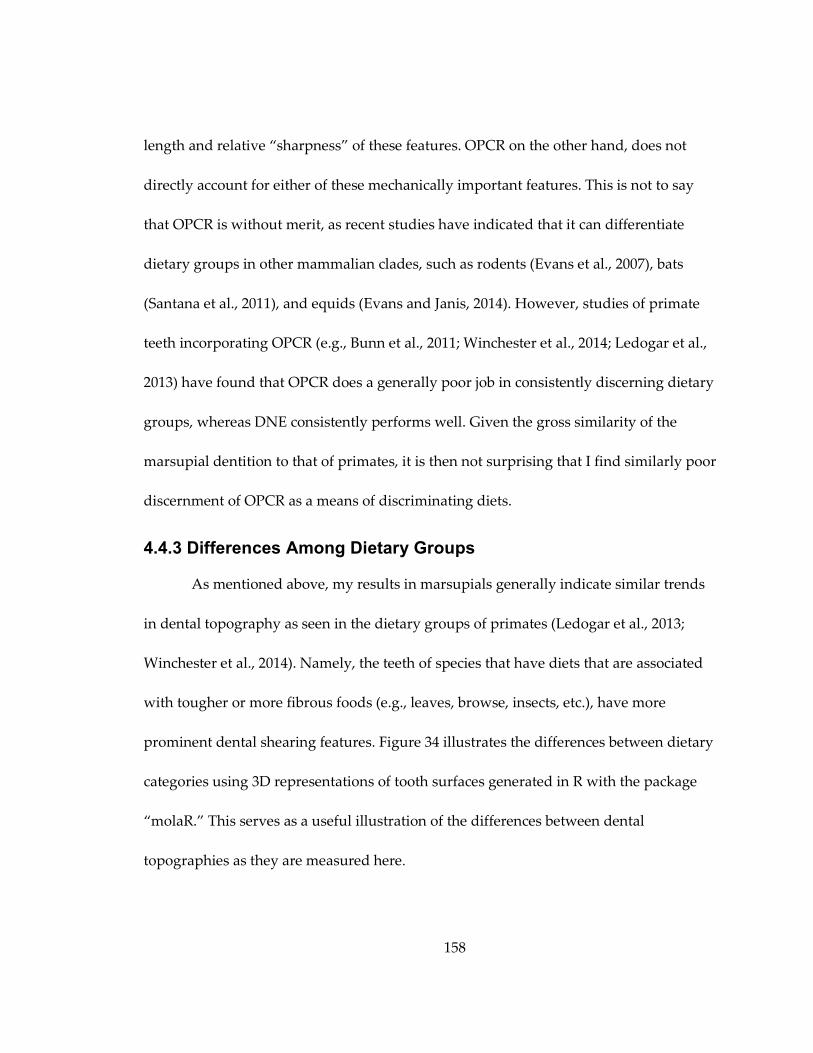
158
length and relative “sharpness” of these features. OPCR on the other hand, does not
directly account for either of these mechanically important features. This is not to say
that OPCR is without merit, as recent studies have indicated that it can differentiate
dietary groups in other mammalian clades, such as rodents (Evans et al., 2007), bats
(Santana et al., 2011), and equids (Evans and Janis, 2014). However, studies of primate
teeth incorporating OPCR (e.g., Bunn et al., 2011; Winchester et al., 2014; Ledogar et al.,
2013) have found that OPCR does a generally poor job in consistently discerning dietary
groups, whereas DNE consistently performs well. Given the gross similarity of the
marsupial dentition to that of primates, it is then not surprising that I find similarly poor
discernment of OPCR as a means of discriminating diets.
4.4.3 Differences Among Dietary Groups
As mentioned above, my results in marsupials generally indicate similar trends
in dental topography as seen in the dietary groups of primates (Ledogar et al., 2013;
Winchester et al., 2014). Namely, the teeth of species that have diets that are associated
with tougher or more fibrous foods (e.g., leaves, browse, insects, etc.), have more
prominent dental shearing features. Figure 34 illustrates the differences between dietary
categories using 3D representations of tooth surfaces generated in R with the package
“molaR.” This serves as a useful illustration of the differences between dental
topographies as they are measured here.
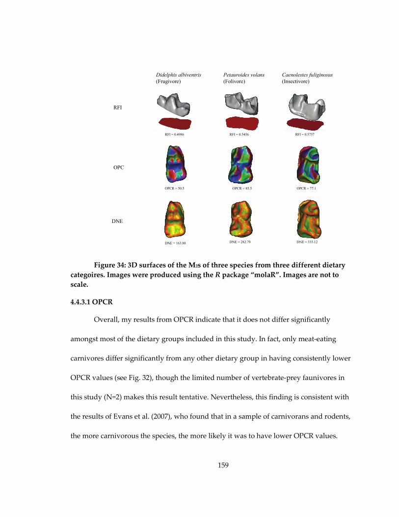
159
Figure 34: 3D surfaces of the M2s of three species from three different dietary
categoires. Images were produced using the R package “molaR”. Images are not to
scale.
4.4.3.1 OPCR
Overall, my results from OPCR indicate that it does not differ significantly
amongst most of the dietary groups included in this study. In fact, only meat-eating
carnivores differ significantly from any other dietary group in having consistently lower
OPCR values (see Fig. 32), though the limited number of vertebrate-prey faunivores in
this study (N=2) makes this result tentative. Nevertheless, this finding is consistent with
the results of Evans et al. (2007), who found that in a sample of carnivorans and rodents,
the more carnivorous the species, the more likely it was to have lower OPCR values.
Caenolestes fuliginosus
(Insectivore)
Petauroides volans
(Folivore)
Didelphis albiventris
(Frugivore)
RFI
DNE
OPC
RFI = 0.4986 RFI = 0.5456
OPCR = 50.5
DNE = 163.88
OPCR = 85.5 OPCR = 77.1
RFI = 0.5757
DNE = 282.79 DNE = 333.12
160
Evans et al. (2007) interpreted this result as a reflection of the relatively high
digestability of vertebrate tissue when compared to plant material or even chitinous
insect exoskeletons, an argument that mirrors the study of Kay and Hylander (1978)
which looked specifically at the shearing crests of primates and phalangeriform
marsupials. Evans et al. (2007) reason that if the complexity of the tooth surface—as
measured by the number of differently oriented patches—is seen as an adaptation to the
mechanical stresses of the ingested food, then the greater the complexity, the greater the
ability to break down fibrous materials. That my results show meat-eating carnivores
have the least complex tooth surfaces is consistent with this observation.
Nevertheless, the similarity in OPCR scores of folivores and frugivores is a
surprising result that is not in line with the supposed aim of the metric, nor with
previous studies that have considered differences in tooth morphology between these
dietary groups (e.g., Kay, 1975; Rosenberger, 1982; Kay and Covert, 1984; Anthony and
Kay, 1993). Generally, fruit-bearing trees that are adapted for the consumption of their
fruit as a means of seed dispersal through the consumer’s feces, have soft pericarps with
relatively few physical properties to hinder its processing and consumption, a fact that
has been demonstrated many times in studies of food mechanical properties (Lucas and
Luke, 1984; Kinsey and Norconk, 1990; Kunzek et al., 1999; Vogel et al., 2008; Berthaume,
2016). This in contrast to leaves, which serve as a plant’s principal sites of
photosynthesis and transpiration, and are vital to the plant’s homeostasis. Thus, in order
161
to discourage predation, leaves typically have defense mechanisms that make their
consumption difficult, or even dangerous, to the consumer. While over the course of
evolution these defenses have taken a myriad of forms, of particular interest to studies
of dental morphology is the toughness of leaves (e.g., Kay, 1975; Lucas and Pereira, 1990;
Coley and Barone, 1996; Berthaume, 2016). This toughness is associated with more
complicated occlusal surfaces in general (e.g., M’Kirera and Ungar, 2003; Lucas, 2004;
Bunn and Ungar, 2009; Evans et al., 2007; Boyer, 2008; Winchester et al., 2014), and
specifically with higher cusps and more prominent shearing crests (Kay and Hiiemae,
1974; Rosenberger and Kinzey, 1976; Kay, 1977; Teaford and Ungar, 2006; Winchester et
al., 2014). Nevertheless, my results from marsupials—in combination with results from
primates (Ledogar et al., 2013; Winchester et al., 2014)—make it clear that OPCR is
unable to consistently pick up these visually obvious differences in tooth shape. It is
possible that my use of dietary categories based on food types rather than food
mechanical properties is at fault for this lack of correlation, as undoubtedly there is
overlap between the material properties of certain kinds of fruits and leaves (Strait, 1997;
Berthaume, 2016). Unfortunately, the testing of food material properties for such a broad
taxonomic sample is beyond the scope of this paper.
4.4.3.2 RFI
Similar to OPCR, my results indicate that diet (as I categorize it) does not have a
statistically significant relationship with RFI in a non-phylogenetically-corrected
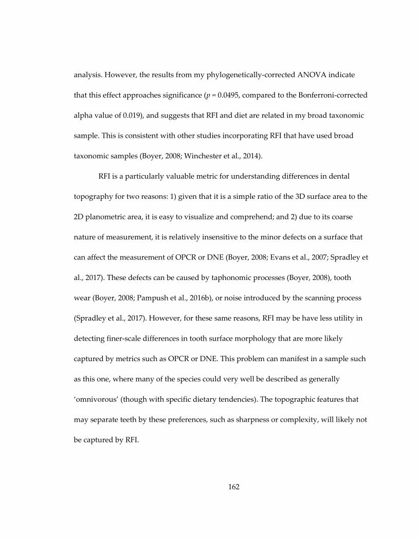
162
analysis. However, the results from my phylogenetically-corrected ANOVA indicate
that this effect approaches significance (p = 0.0495, compared to the Bonferroni-corrected
alpha value of 0.019), and suggests that RFI and diet are related in my broad taxonomic
sample. This is consistent with other studies incorporating RFI that have used broad
taxonomic samples (Boyer, 2008; Winchester et al., 2014).
RFI is a particularly valuable metric for understanding differences in dental
topography for two reasons: 1) given that it is a simple ratio of the 3D surface area to the
2D planometric area, it is easy to visualize and comprehend; and 2) due to its coarse
nature of measurement, it is relatively insensitive to the minor defects on a surface that
can affect the measurement of OPCR or DNE (Boyer, 2008; Evans et al., 2007; Spradley et
al., 2017). These defects can be caused by taphonomic processes (Boyer, 2008), tooth
wear (Boyer, 2008; Pampush et al., 2016b), or noise introduced by the scanning process
(Spradley et al., 2017). However, for these same reasons, RFI may be have less utility in
detecting finer-scale differences in tooth surface morphology that are more likely
captured by metrics such as OPCR or DNE. This problem can manifest in a sample such
as this one, where many of the species could very well be described as generally
‘omnivorous’ (though with specific dietary tendencies). The topographic features that
may separate teeth by these preferences, such as sharpness or complexity, will likely not
be captured by RFI.

163
The coarse nature of RFI likely explains the significant but weak relationship RFI
has with diet in my results. While my frugivore and insectivore categories were
significantly different from one another, no other pair was significantly different when
incorporating Bonferonni correction for the alpha level. Unlike DNE (discussed below),
there is considerable overlap between the frugivores and folivores in my sample, which
is likely indicative of the fact that many marsupial frugivores consume leaves and vice
versa (Kay and Hylander, 1978), and that the differences in dental topography are more
likely to be captured in the qualities of the features rather than by their presence or
absence.
Visual inspection of some of the tooth surfaces in my sample (Fig. 35) show the
similarity of tooth surfaces within a specific marsupial clade, Didelphidae. The
American didelphids show very similar gross tooth morphology despite diversity in
dietary preference. This similarity confounds the signal within RFI, but these surfaces
can be differentiated by DNE.
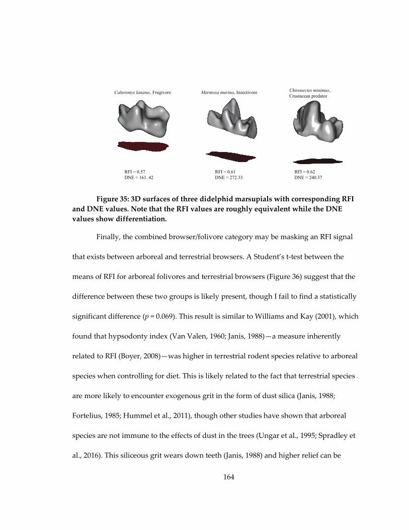
164
Figure 35: 3D surfaces of three didelphid marsupials with corresponding RFI
and DNE values. Note that the RFI values are roughly equivalent while the DNE
values show differentiation.
Finally, the combined browser/folivore category may be masking an RFI signal
that exists between arboreal and terrestrial browsers. A Student’s t-test between the
means of RFI for arboreal folivores and terrestrial browsers (Figure 36) suggest that the
difference between these two groups is likely present, though I fail to find a statistically
significant difference (p = 0.069). This result is similar to Williams and Kay (2001), which
found that hypsodonty index (Van Valen, 1960; Janis, 1988)—a measure inherently
related to RFI (Boyer, 2008)—was higher in terrestrial rodent species relative to arboreal
species when controlling for diet. This is likely related to the fact that terrestrial species
are more likely to encounter exogenous grit in the form of dust silica (Janis, 1988;
Fortelius, 1985; Hummel et al., 2011), though other studies have shown that arboreal
species are not immune to the effects of dust in the trees (Ungar et al., 1995; Spradley et
al., 2016). This siliceous grit wears down teeth (Janis, 1988) and higher relief can be
Caluromys lanatus, Frugivore
RFI = 0.57
DNE = 161. 42
Marmosa murina, Insectivore
RFI = 0.61
DNE = 272.33
Chironectes minimus,
Crustacean predator
RFI = 0.62
DNE = 240.37
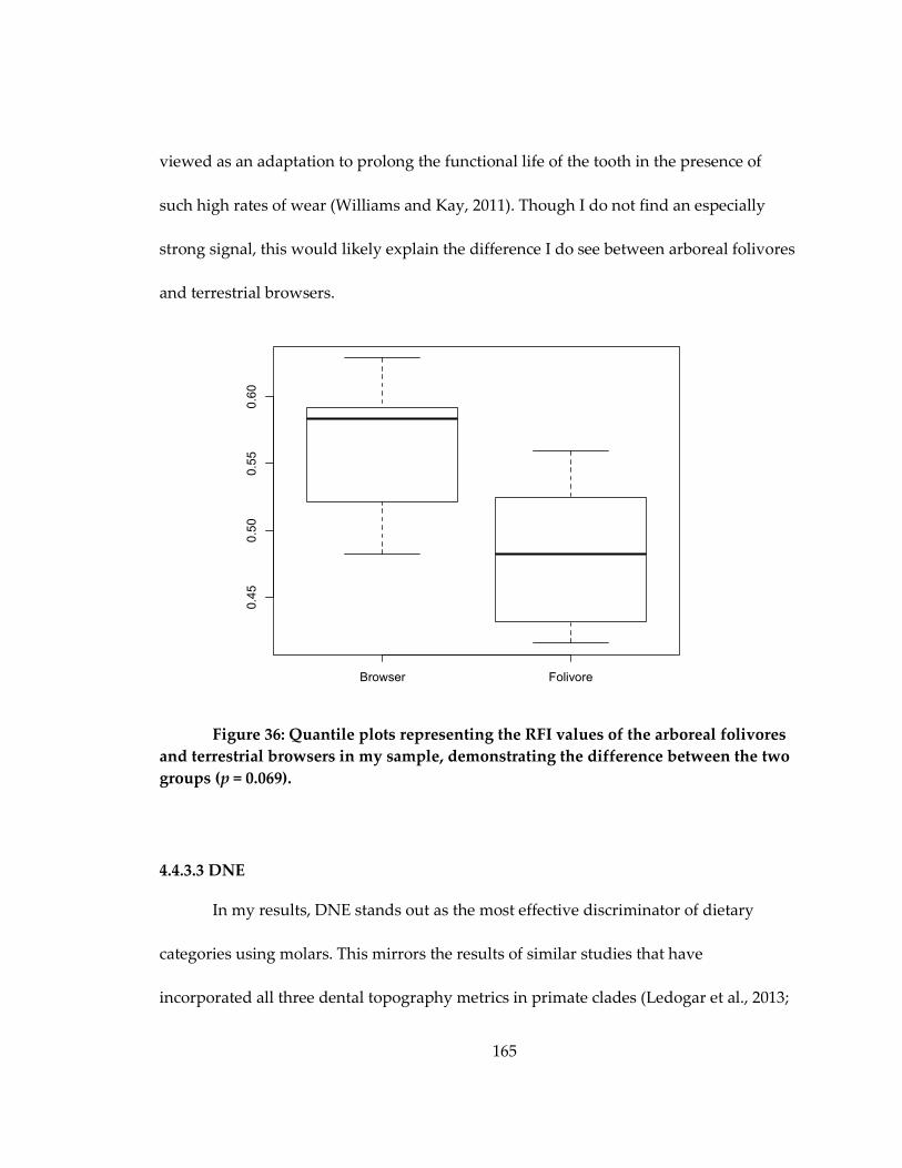
165
viewed as an adaptation to prolong the functional life of the tooth in the presence of
such high rates of wear (Williams and Kay, 2011). Though I do not find an especially
strong signal, this would likely explain the difference I do see between arboreal folivores
and terrestrial browsers.
Figure 36: Quantile plots representing the RFI values of the arboreal folivores
and terrestrial browsers in my sample, demonstrating the difference between the two
groups (p = 0.069).
4.4.3.3 DNE
In my results, DNE stands out as the most effective discriminator of dietary
categories using molars. This mirrors the results of similar studies that have
incorporated all three dental topography metrics in primate clades (Ledogar et al., 2013;
Browser Folivore
0.4
50
.50
0.5
50
.60
166
Winchester et al., 2014), which also found DNE to be the most effective. The importance
of shearing (or sharp) features on the marsupial dentition in discriminating dietary
categories was also noted by Kay and Hylander (1978), who focused on a sample of
phalangeroid marsupials as well as examples from various primate clades. Using
multivariate analysis, they found that folivorous primate species were more distinctly
differentiated from frugivorous species based on shearing and cusp height than were
phalangeroid marsupials. They noted that that many phalangeroid marsupials also had
a greater amount of shearing in the premolars—often manifested as a serrated blade-like
lower premolar—that may amount to lesser shearing demand placed on the molars.
Nevertheless, the shearing of their phalangeroid sample had a clear relationship with
dietary preference.
Expanding this analysis to include a much broader array of marsupial species
and diets, as I have here, we see that this pattern largely holds. Insectivorous species,
like South American Caenolestes fuliginosus or Australian Sminthopsis crassicaudata, have
some of the highest DNE values in my sample, likely reflecting the tough chitinous
exoskeletons of the insects they consume. The high degree of overlap between
insectivorous and browsing/folivorous species is in agreement with other studies that
have shown that shearing/sharpness is generally equivalent between folivorous and
insectivorous primates (e.g. Kay, 1975; Winchester et al., 2014).
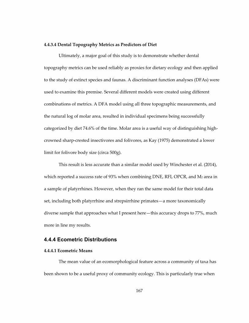
167
4.4.3.4 Dental Topography Metrics as Predictors of Diet
Ultimately, a major goal of this study is to demonstrate whether dental
topography metrics can be used reliably as proxies for dietary ecology and then applied
to the study of extinct species and faunas. A discriminant function analyses (DFAs) were
used to examine this premise. Several different models were created using different
combinations of metrics. A DFA model using all three topographic measurements, and
the natural log of molar area, resulted in individual specimens being successfully
categorized by diet 74.6% of the time. Molar area is a useful way of distinguishing high-
crowned sharp-crested insectivores and folivores, as Kay (1975) demonstrated a lower
limit for folivore body size (circa 500g).
This result is less accurate than a similar model used by Winchester et al. (2014),
which reported a success rate of 93% when combining DNE, RFI, OPCR, and M2 area in
a sample of platyrrhines. However, when they ran the same model for their total data
set, including both platyrrhine and strepsirrhine primates—a more taxonomically
diverse sample that approaches what I present here—this accuracy drops to 77%, much
more in line my results.
4.4.4 Ecometric Distributions
4.4.4.1 Ecometric Means
The mean value of an ecomorphological feature across a community of taxa has
been shown to be a useful proxy of community ecology. This is particularly true when

168
the relationship between the morphology and ecology is known, allowing for an
interpretation between the average value of the ecomorphological measurement and the
preponderance of any given ecology within a community. A classic example of this is
the average value of hypsodonty with a community of ungulate or rodent mammals.
Higher tooth crowns have been demonstrated to be positively correlated with increased
amounts of grazing in these mammalian clades (Janis, 1988; Williams and Kay, 2001). In
the context of an ecometric distribution, a higher mean hypsodonty value in a
community of mammals would suggest a higher relative proportion of grazing
mammals in that community. Indeed, the mean hypsodonty has been demonstrated to
correlate with drier, more seasonal environments (Williams and Kay, 2001; Madden,
2014).
Interestingly, only the means of DNE and RFI have significant relationships with
any of the bioclimatic variables, and both metrics correlate significantly with the same
three variables—MAP, temperature seasonality, and canopy height (Tables 17; Figure
33). Both DNE and RFI have positive relationships with temperature seasonality and
negative relationships with MAP and canopy height. In this context, and in light of my
results from Chapter 2, this would suggest a greater number of frugivores—lower RFI
and DNE (Figure 32)—in wetter, less seasonal environments with taller canopies. This is
not only consistent with the results from Chapter 2, but also with results of other
qualitative analyses of mammalian faunas (Andrews et al., 1979; Kay and Cartmill, 1997;
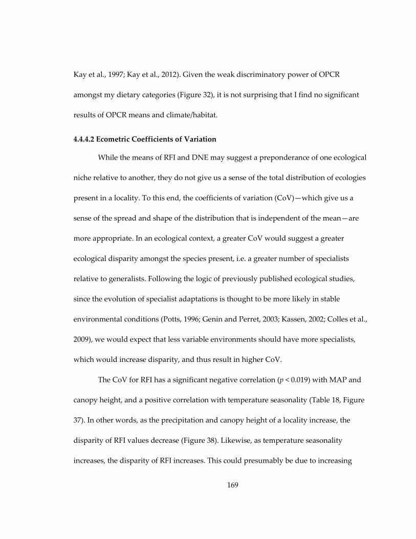
169
Kay et al., 1997; Kay et al., 2012). Given the weak discriminatory power of OPCR
amongst my dietary categories (Figure 32), it is not surprising that I find no significant
results of OPCR means and climate/habitat.
4.4.4.2 Ecometric Coefficients of Variation
While the means of RFI and DNE may suggest a preponderance of one ecological
niche relative to another, they do not give us a sense of the total distribution of ecologies
present in a locality. To this end, the coefficients of variation (CoV)—which give us a
sense of the spread and shape of the distribution that is independent of the mean—are
more appropriate. In an ecological context, a greater CoV would suggest a greater
ecological disparity amongst the species present, i.e. a greater number of specialists
relative to generalists. Following the logic of previously published ecological studies,
since the evolution of specialist adaptations is thought to be more likely in stable
environmental conditions (Potts, 1996; Genin and Perret, 2003; Kassen, 2002; Colles et al.,
2009), we would expect that less variable environments should have more specialists,
which would increase disparity, and thus result in higher CoV.
The CoV for RFI has a significant negative correlation (p < 0.019) with MAP and
canopy height, and a positive correlation with temperature seasonality (Table 18, Figure
37). In other words, as the precipitation and canopy height of a locality increase, the
disparity of RFI values decrease (Figure 38). Likewise, as temperature seasonality
increases, the disparity of RFI increases. This could presumably be due to increasing
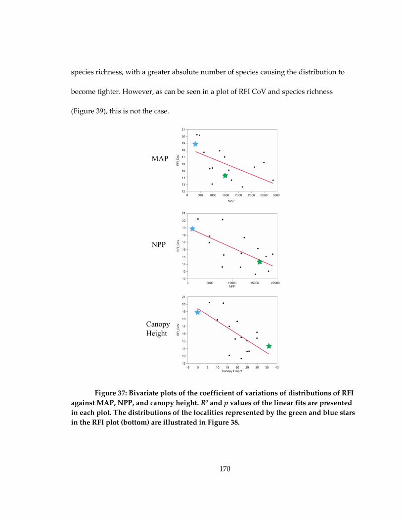
170
species richness, with a greater absolute number of species causing the distribution to
become tighter. However, as can be seen in a plot of RFI CoV and species richness
(Figure 39), this is not the case.
Figure 37: Bivariate plots of the coefficient of variations of distributions of RFI
against MAP, NPP, and canopy height. R2 and p values of the linear fits are presented
in each plot. The distributions of the localities represented by the green and blue stars
in the RFI plot (bottom) are illustrated in Figure 38.
171
Figure 38: Densities plots of RFI in two localities. The green curve represents
the South Karius field site in Papua New Guinea, the blue curve represents the
Uluru-Kata Tjuta National Park. The standard deviation of the green curve is less
than that of the blue curve (see Figure 37).
Figure 39: Bivariate plot of RFI CoV and species richness. The R2 and p-value
demonstrate the weakness of this relationship, suggesting that species richness is not
driving disparity in RFI across localities.
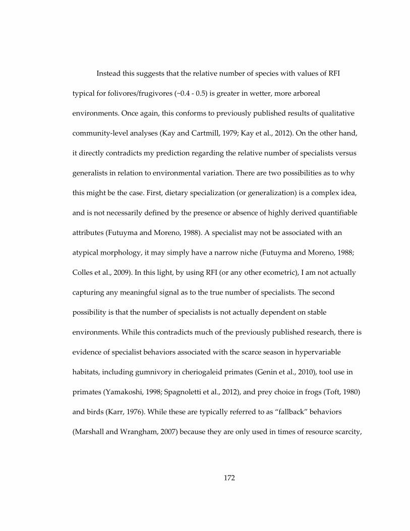
172
Instead this suggests that the relative number of species with values of RFI
typical for folivores/frugivores (~0.4 - 0.5) is greater in wetter, more arboreal
environments. Once again, this conforms to previously published results of qualitative
community-level analyses (Kay and Cartmill, 1979; Kay et al., 2012). On the other hand,
it directly contradicts my prediction regarding the relative number of specialists versus
generalists in relation to environmental variation. There are two possibilities as to why
this might be the case. First, dietary specialization (or generalization) is a complex idea,
and is not necessarily defined by the presence or absence of highly derived quantifiable
attributes (Futuyma and Moreno, 1988). A specialist may not be associated with an
atypical morphology, it may simply have a narrow niche (Futuyma and Moreno, 1988;
Colles et al., 2009). In this light, by using RFI (or any other ecometric), I am not actually
capturing any meaningful signal as to the true number of specialists. The second
possibility is that the number of specialists is not actually dependent on stable
environments. While this contradicts much of the previously published research, there is
evidence of specialist behaviors associated with the scarce season in hypervariable
habitats, including gumnivory in cheriogaleid primates (Genin et al., 2010), tool use in
primates (Yamakoshi, 1998; Spagnoletti et al., 2012), and prey choice in frogs (Toft, 1980)
and birds (Karr, 1976). While these are typically referred to as “fallback” behaviors
(Marshall and Wrangham, 2007) because they are only used in times of resource scarcity,

173
they may nonetheless produce unusual morphologies, driving the disparity of my
distributions and increasing the CoV.
Interestingly, I do not find significant results in the context of DNE. This is
surprising given that in my ecomorphological analyses above, DNE demonstrates the
strongest correlation with diet (Table 13). However, the CoV of DNE does not have a
significant correlation with any of my bioclimatic variables, and in fact does not even
have correlation that might be described as “approaching” significance (p < 0.10).
Finally, the CoV of OPCR does not have a significant correlation with
climate/habitat. Considering that OPCR does not have a clear relationship with diet in
my marsupial sample, I would expect the that the distributions of OPCR would not
elucidate any particularly informative content related to the relative proportions of
ecologies in a fauna. Instead, what I find is a fairly consistent pattern of roughly
equivalent CoVs across different habitats, confirming my expectations.
4.4.4.3 Ecometric Skew
Related to CoV, I can also look at the skewness of my distributions across
localities. In its most general definition, skewness is a measure of the asymmetry of a
distribution, i.e. the length of the “tail” of a distribution. In an ecological context
skewness can intuitively be thought of as the presence of specialists, i.e. species with a
narrow niche breadth when compared to other species (Colles et al., 2009). While the
skew of a distribution (of DNE, RFI, OPCR, etc.) is unlikely to give us a complete picture

174
of the total number of specialists in an environment—after all, median values of RFI and
DNE do not necessarily exclude the possibility that the species is a specialist (e.g. the
koala, a specialist of eucalyptus leaves)—it nevertheless may be informative as an
indicator of relative numbers of distinct dietary specializations. In the context of my
dietary ecology study, I would expect that more seasonal, less productive environments
should have a negative skew—that is, a higher mean value of both RFI and DNE with a
longer tail to the left of the distribution, suggesting fewer low-crowned, rounded cusped
molars—than wetter, more productive, aseasonal environments.
Results for RFI match these predictions (Table 19). Positive skew (i.e. a longer tail
to the right) is associated with wetter and more arboreal habitats, while negative skew is
associated with drier, more seasonal environments. RFI skew appears to have a non-
linear relationship with NPP (Figure 40), with the skew approaching zero at the
localities with the highest NPP in my sample. Similar to the results from CoV, DNE
skew fails to show significant correlations with any climatic/habitat variables (Table 19).
Likewise, OPCR skew fails to show any statistically significant correlations with
environmental variables.
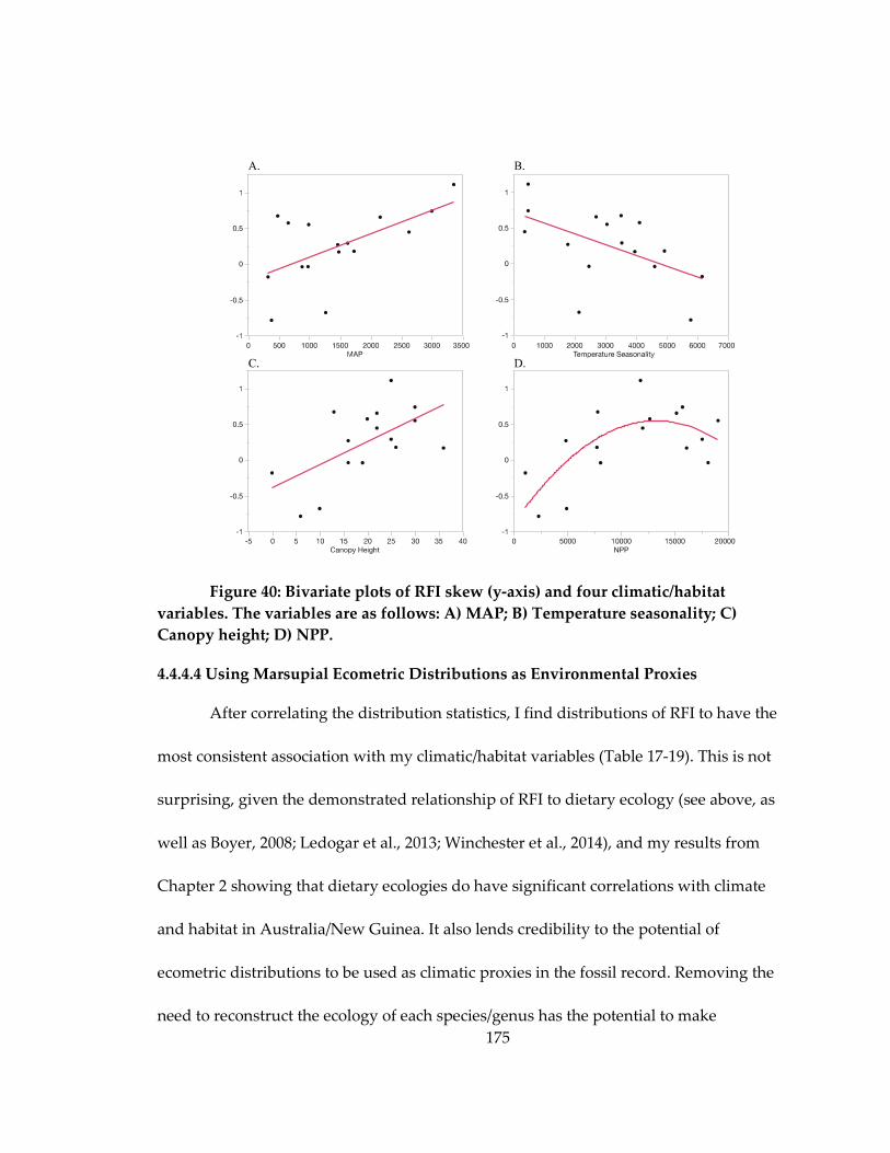
175
Figure 40: Bivariate plots of RFI skew (y-axis) and four climatic/habitat
variables. The variables are as follows: A) MAP; B) Temperature seasonality; C)
Canopy height; D) NPP.
4.4.4.4 Using Marsupial Ecometric Distributions as Environmental Proxies
After correlating the distribution statistics, I find distributions of RFI to have the
most consistent association with my climatic/habitat variables (Table 17-19). This is not
surprising, given the demonstrated relationship of RFI to dietary ecology (see above, as
well as Boyer, 2008; Ledogar et al., 2013; Winchester et al., 2014), and my results from
Chapter 2 showing that dietary ecologies do have significant correlations with climate
and habitat in Australia/New Guinea. It also lends credibility to the potential of
ecometric distributions to be used as climatic proxies in the fossil record. Removing the
need to reconstruct the ecology of each species/genus has the potential to make
176
community-level paleoecological analyses more broadly applicable and quicker to
perform. The mean, CoV, and skew work best for predicting climatic/habitat variables,
whereas the range does not correlate well with any of these variables.
The lack of significant correlations amongst the summary statistics of DNE
distribution is surprising. DNE apparently has a significant relationship with dietary
ecology in marsupials (see above), but unlike RFI this does not seem to translate into
distributions that reflect the results from Chapter 2. Looking at three DNE and RFI
density plots from localities of differing amounts of rainfall (Figure 41), we see that the
differences in the shape of these distributions, while present, is more subtle than what
we see in RFI. This slight tendency towards similarity in DNE distributions is likely the
reason I do not find significant correlations. It is possible that more complete sampling
of the marsupial faunas at these localities may make these correlations significant.
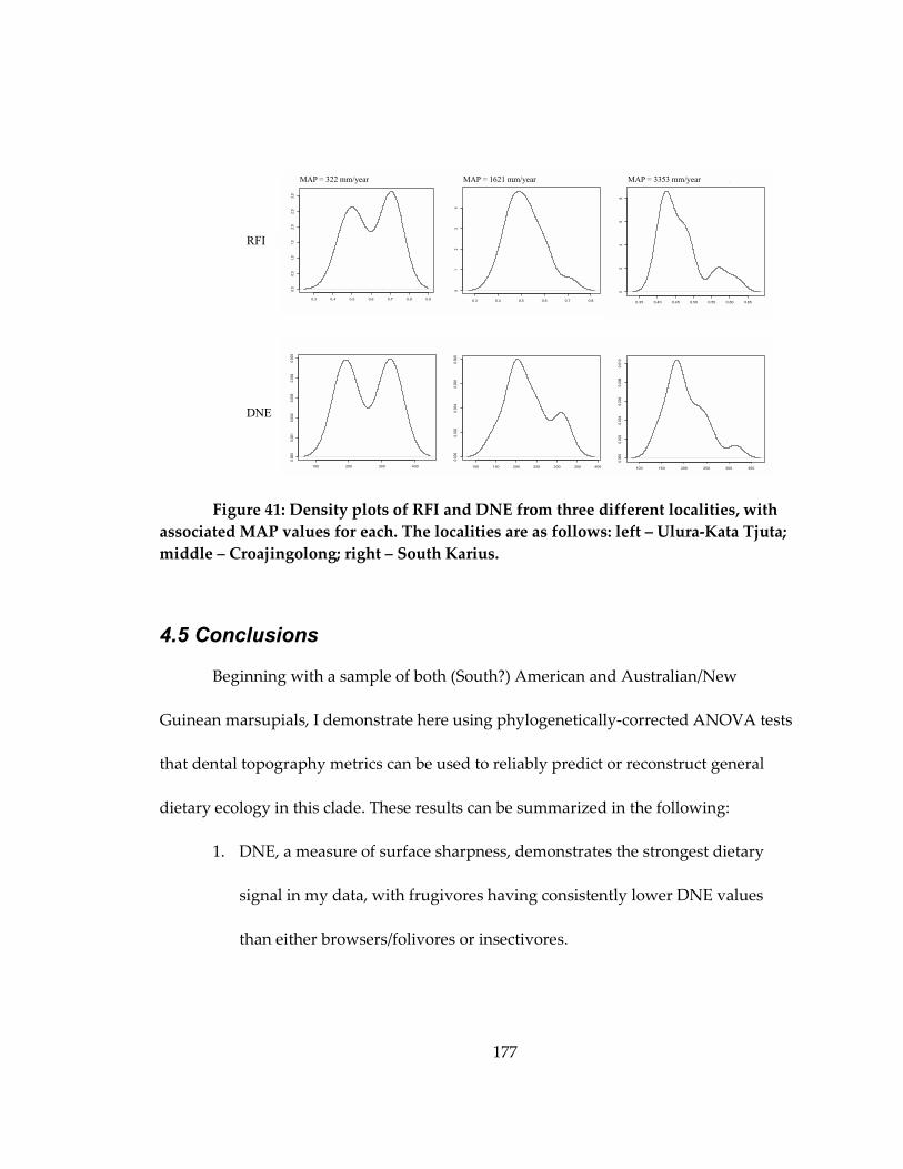
177
Figure 41: Density plots of RFI and DNE from three different localities, with
associated MAP values for each. The localities are as follows: left – Ulura-Kata Tjuta;
middle – Croajingolong; right – South Karius.
4.5 Conclusions
Beginning with a sample of both (South?) American and Australian/New
Guinean marsupials, I demonstrate here using phylogenetically-corrected ANOVA tests
that dental topography metrics can be used to reliably predict or reconstruct general
dietary ecology in this clade. These results can be summarized in the following:
1. DNE, a measure of surface sharpness, demonstrates the strongest dietary
signal in my data, with frugivores having consistently lower DNE values
than either browsers/folivores or insectivores.
0.3 0.4 0.5 0.6 0.7 0.8 0.9
0.0
0.5
1.0
1.5
2.0
2.5
3.0
density.default(x = uluru$RFI)
N = 10 Bandwidth = 0.06475
Den
sity
0.3 0.4 0.5 0.6 0.7 0.8
01
23
4
density.default(x = croa$RFI)
N = 19 Bandwidth = 0.03644
De
nsi
ty
0.35 0.40 0.45 0.50 0.55 0.60 0.65
02
46
8
density.default(x = karius$RFI)
N = 17 Bandwidth = 0.02172
De
nsi
ty
MAP = 322 mm/year MAP = 1621 mm/year MAP = 3353 mm/year
RFI
100 200 300 400
0.00
00.
001
0.0
02
0.0
030.
004
0.0
05
density.default(x = uluru$DNE)
N = 10 Bandwidth = 40.34
De
nsi
ty
100 150 200 250 300 350 400
0.00
00.
002
0.00
40.
006
0.00
8
density.default(x = croa$DNE)
N = 19 Bandwidth = 22.29
Den
sity
100 150 200 250 300 350
0.00
00.
002
0.00
40.
006
0.00
80.
010
density.default(x = karius$DNE)
N = 17 Bandwidth = 18.11
Den
sity
DNE

178
2. RFI, or surface relief, also shows a statistically significant relationship with
diet. Lower relief is associated with frugivores, while browsers/folivores and
insectivores have higher relief.
3. OPCR, a measurement of surface complexity, does not correlate well with
diet, and amongst the dietary categories included in my study only
significantly differentiates faunivores specializing in vertebrate prey from
other dietary groups.
A discriminant function analysis performed using all three metrics, in
combination with the natural log of molar area, resulted in individual specimens being
correctly segregated by dietary group at a rate significantly better than random chance
(~75%).
Having demonstrated the utility of these metrics in reconstructing individual
species’ dietary ecologies, I also explored the utility of the distributions of these metrics
within a locality as a proxy for a number of climatic and habitat variables at that locality.
Four summary statistic of distributions were used: mean, range, coefficient of variation,
and skew. Climatic and habitat variables included precipitation, temperature,
seasonality, productivity, and canopy height. My results from theses correlation
analyses are summarized as follows:
1. The means of RFI and DNE both have statistically significant correlations
with precipitation (negative correlation), temperature seasonality (positive),
179
and canopy height (negative). The mean of OPCR does not have a significant
correlation with any variable.
2. The range of RFI, DNE, and OPCR does not correlate well with any
climatic/habitat variable.
3. The coefficient of variation for RFI has significant correlation with
precipitation, temperature seasonality, and canopy height. The same is not
true for the coefficient of variation for DNE or OPCR.
4. Positive skew in RFI was associated with wetter, more productive habitats
with greater canopy height, and negative skew was associated with drier,
more seasonal climates.
In conclusion, dental topography metrics demonstrate potential to not only
distinguish diet in disparate taxa, but their distributions may have some utility as
proxies for climate and habitat in paleoecological reconstructions. This may eliminate
the need to make often problematic assumptions about diet in fossil taxa.
180
5. Dental Topography in South American Rodents: Proxies for
Dietary Ecology and Environmental Reconstruction
5.1 Introduction
Living rodents represent the most speciose order of mammals on the planet, with
2277 recognized species—over 40% of all recognized mammal species (Wilson and
Reeder, 2005)—and can be found on every continent except Antarctica. They occupy
every terrestrial habitat (Kay and Hoekstra, 2008) and span a wide range of ecological
niches. The largest living rodent, the South American capybara (Hydrochoerus spp.) can
weigh up to 65kg—the largest fossil rodent, Josephoartigasia monesi from Uruguay
weighed approximately 1000kg—while the smallest, the pygmy mouse (Mus minutoides)
is a mere 7g (Hautier and Cox, 2015; Kay and Hoekstra, 2008). So successful were the
early rodents, that after their initial appearance in the fossil record of Laurasia at the end
of the Paleocene (55-60mya) (Meng et al., 1994; Kay and Hoekstra, 2008), they could
already be found on every continent except Australia and Antarctica by the mid-Eocene
(Antoine et al., 2011). They would later be one of the few terrestrial mammalian clades to
cross “Wallace’s Line” into Australia without the aid of introduction by human
colonists, at approximately 10 Mya (Rowe et al., 2008).
This rapid radiation and diversification has since led to their near ubiquity in
terrestrial mammalian fossil localities from the Cenozoic (Kay and Hoekstra, 2008). This
has fostered intense interest in rodents as a potential source of evidence for the
reconstruction of past climates and environments (Montuire et al., 1997; Aguilar et al.,
181
1999; Legendre et al., 2005; Montuire et al., 2006). These efforts have primarily focused
on species richness within specific living rodent families with known climatic
distributions. Clade-specific species richness can be estimated for fossil sites and climate
reconstructions are done using a regressive model derived from modern clade
distributions. While such an approach has proven effective in reconstructing
Quarternary period climates (Montuire et al., 2006), they are limited in their scope for
two reasons. First, sympatric species identification in the fossil record is inherently
difficult, especially for a diverse small mammal clade like the rodents (Gingerich, 1974),
making estimates species richness circumspect. Second, such studies are limited both
spatially and temporally by the families that are chosen for the analyses. In this study, I
seek to broaden the applicability of these types of analyses by using the distribution of
ecomorphology in rodent dentitions from a continent-wide sample of rodent
communities.
5.1.1 Rodent Dental Ecomorphology
Prior to analyzing the rodent ecometric distributions in relation to
environments—as I did for marsupials in Chapter 4—it first must be demonstrated that
the metrics of interest are functionally related to the species’ ecologies. Since the rodent
fossil record is largely represented by jaws and isolated teeth, the dentition (feeding
ecology) will once again be my study focus. Rodent molar morphology is highly derived
and unlike that of the primitive therian tribosphenic molar pattern. Further, the clade

182
spans a wide range in dietary ecologies (Hillson, 1986). Many taxa have complicated
series of cusps, lophs, and ridges aligned buccolingually, so that when the jaw is moved
back and forth these ridges of enamel cut against one another (Hillson, 1986). Due to the
wide diversity of rodent molars, broad-scale analyses of dental ecomorphology in
rodents has been limited to just a few studies (Williams and Kay, 2001; Evans et al., 2007;
Samuels, 2009; Croft et al., 2011), and two of these studied focused solely on linear
measurements of the incisors (Samuels, 2009; Croft et al., 2011)—though Samuels (2009)
also included a broader analysis of skull morphology as it relates to dietary ecology.
Most taxonomically-broad studies of rodent molar morphology have instead focused on
the distinguishing characteristics of molars in determining taxonomic placement or
phylogenetic relationships (Tullberg 1899; Simpson, 1945; Schaub, 1958; Wood, 1965;
Lazzari et al., 2008a; Lazzari et al., 2008b; Vucetich et al., 2015). In this study, I will
instead try to correlate dietary ecology with molar morphology by using the same dental
topography metrics from Chapter 4; DNE, RFI, and OPCR. The methodological
descriptions of these metrics have been presented in detail in previous chapters (number
them here).
Some previously published literature suggests that these dental topographic
metrics may be informative for rodent occlusal surfaces. The utility of OPC, a measure of
dental complexity, was originally demonstrated with an analysis of rodents (as well as
carnivorans) (Evans et al., 2007; Evans and Jernvall, 2009). In their results, Evans et al.

183
(2007) demonstrated that complexity values increase for entire cheek-tooth rows with
increasing herbivory. This was interpreted as an increased ability of the tooth row to
break down high-fiber plant materials. Having also demonstrated the same pattern
within carnivorans, Evans et al. (2007) claim that these disparate morphologies are
subject to the same functional constraints. By expanding on their analysis with more
dental topography metrics as well as a broader taxonomic sample of rodents (Evans et
al. used only muroids, the rats and mice), I seek to explore whether such functional
constraints apply to individual teeth within the tooth row, and if there are other
functional constraints beyond just surface complexity.
Surface relief has also been studied in rodents, at least to the extent that relative
surface relief can be equated with relative hypsodonty (Boyer, 2008). Hypsodonty, or
high-crowned teeth, has been hypothesized as an adaptation to prolong the functional
life of the tooth when the physical properties of the food ingested (Fortelius, 1985; Janis
1988) or exogenous grit in the environment (Ungar et al., 1995; Fortelius and Solounias,
2000; Lucas et al., 2013) subjects the organism to intense tooth wear. Williams and Kay
(2001) present correlations between hypsodonty, diet, and substrate preference in a
taxonomically-broad sample of South American rodents (not unlike the sample I use in
this study). Their results suggest that hyposdonty and diet are significantly correlated,
specifically that hypsodonty was positively correlated with abrasive diets. This pattern

184
has also been observed in ungulates (Janis, 1988; Williams and Kay, 2001; Lucas et al.,
2013).
Studies of molar sharpness (analogous to DNE) in rodents have been limited.
Black (1963) differentiated North American squirrels on the basis of sharpness of their
molar lophs—as well as their relative hypsodonty—and concluded that tree squirrels
generally have more rounded features than do ground squirrels. This was interpreted by
Black (1963) to reflect the high amounts of grass that is consumed by ground squirrels
relative to arboreal and scansorial sciurids. Prufrock et al. (2016) also included some
extinct taxa of rodents—ischyromyids, which presumably resembled modern squirrels
(Korth, 1994)—and measured DNE on the M2. In these ischyromyid species, DNE values
were relatively low, approximately the same as frugivorous platyrrhine primates from
the dataset of Winchester et al. (2014). However, Prufrock et al. (2016) did not include
any comparative dataset of living squirrels with known ecologies, so the precise
relationship between DNE and diet in sciurids remains speculative.
Combining the above information into a coherent set of predictions for my own
data set, I lean towards the hypothesis of Evans and Sanson (2003), namely that
functional constraints on the mammalian dentition result in shape similarities that are
ideal for the processing of certain food materials, despite differences in historical or
developmental constraints (Gould, 1989). In this context, I would expect my results from
the rodent sample to mirror those from the marsupial sample in Chapter 4; more
185
abrasive, tougher (high fiber) diets such as grass, leaves, or insects should correlate with
higher values of complexity, relief, and sharpness. Likewise, I expect that frugivorous
species, such as some of the South American pacas (Myoprocta), should have the lowest
values of all three metrics, since frugivory is associated with less exaggerated surface
features (Kay, 1975; Winchester et al., 2014; Chapter 4 of this dissertation). There are also
a large number of rodent species that can be described as “seed-predators.” The
difficulty of this category in the context of predicting dental morphology is that the
mechanical properties of seeds are variable, ranging from hard and brittle (Agrawal et
al. 1997; Lucas, 2004) to tough and crush resistant (Ayres, 1989; Kinzey and Norconk,
1993; Norconk and Veres, 2011). In other words, while bite force is likely high regardless
of the type of seed, the amount of chewing effort will differ significantly between those
seeds that are more likely to propagate a crack versus those that resist cracking (Lucas,
2004). This difference in chewing effort is likely to be reflected in the dental morphology,
though without proper data as to what rodents are eating what types of seeds, it is
impossible to differentiate amongst them. Therefore, I include the seed predators in
amongst the “plant-dominated omnivores” in my sample.
I limit this analysis to South American rodents, as the diversity and
morphological disparity of rodents is higher in South America than it is on any other
continent, and rodents have made up an important constituent of South American
mammalian faunas since the Oligocene (Vucetich et al., 2015). Living South American
186
rodents comprise three clades; the caviomorphs, the sigmodontines, and the sciurids. Of
these three groups, the molecular (Poux et al., 2006) and fossil evidence (Vucetich et al.,
2015) suggest that only the caviomorphs reached South America before the joining of
North and South America via the Panamanian isthmus—though genetic data indicate
that the ancestors of at least one genus of Amazonian squirrel, Sciurillus, may have made
it to the continent before this event (Mercer and Roth, 2003). The sciurids and the
sigmodontines on the other hand made it to South America only (relatively) recently,
with the latter group subsequently radiating into almost 400 species in the course of
approximately 5 million years (Engel et al., 1998; Smith and Patton, 1999). Comparing
this to the caviomorphs, of which there are only 240 species found in South America
today (Upham and Patterson, 2015), it is clear that evolutionary history may have played
an important role in the morphological disparity of different clades of rodents. To
account for these potential differences, I make phylogenetic corrections in my analyses
as well as perform separate analyses on both caviomorphs and the non-caviomorphs
(sciurids and sigmodontines).
5.1.1 Rodent Ecometric Distributions as an Environmental Proxy
As mentioned above, a major objective of this study is to explore the potential of
rodent ecometrics as proxies for climate and habitat in the fossil record. Given their
ubiquity after their appearance in the Eocene, rodents have tremendous potential in this
respect. Beyond the studies discussed above, Kay et al. (1999) also observed that the

187
percentage of sigmodontine rodents that could be classified as hypsodont increased with
temperature seasonality and decreased with rainfall and higher average temperatures.
While the mechanisms that drive these distributions will not necessarily be addressed
directly in this paper, I seek to test, refine, and expand on the brief analysis of Kay et al.
(1999) to include more ecometrics, more climatic variables, and more detailed statistics
of distributions. I predict that ecometrics that reflect more abrasive diets in the first part
of this paper (if such results are found) should have a greater impact on the distributions
in more arid, more seasonal, and less productive habitats. Much like in Chapter 4,
summary statistics of distributions—mean, range, skew, and coefficient of variation—
will be regressed against climatic and habitat variables across the South American
localities. The utility and possible ecological interpretations of results are discussed in
Chapter 4 as well as in the discussion of this paper.
In addition, I seek to include the same regression techniques in Chapter 2,
including multivariate linear regression and the machine-learning algorithms;
regression trees, random forests, and Gaussian process regression. Rather than the using
the ecological indices as my predictor variables, I will include the aforementioned
distribution statistics as predictors (with the bioclimatic variables being the response
variables which I am trying to estimate). This last section will thus represent multiple
parts of this dissertation in a single analysis, and will give us some notion of how well
188
the use of modern techniques in both data collection and model production can improve
the accuracy of paleoenvironmental reconstruction.
5.2 Materials and Methods
5.2.1 Topography and Dietary Ecology
To investigate the relationship between dental topography and dietary ecology
in South American rodents, I scanned and segmented the lower M2s of 80 individual
specimens representing 59 different South American rodent species (35 genera) (Table
20), including both caviomorph and sigmodontine species. Specimens were obtained
from the National Museum of Natural History (NMNH), the Louisiana State University
Museum of Natural History (LSUMZ), and the University of Florida Museum of Natural
History (FLMNH), and include both skeletal material and epoxy casts poured from
molds taken from skulls. A subset of dentitions were both directly scanned, and casted
to assess the accuracy of surface reconstructions from casts. The complete sample of
species, along with a phylogenetic tree topology, is presented in Figure 42. Primary
dietary categories were assigned to each species according to MammalDIET, an online
archive of dietary information (Kissling et al., 2014), and supplemented with primary
sources (Patton et al., 2015). These sources are summarized along with those from the
marsupial sample in Appendix C. These dietary categories are necessarily low
resolution, and the consequences of this low resolution is further elaborated upon in the
discussion. In this study I recognize five different dietary categories: frugivore, folivore,

189
grazers, plant dominated omnivores—including putative fungivorous and
gramnivorous species—and animal dominated omnivores, including insectivores (Evans
et al., 2007). Species classified in the latter two categories inhabit very broad dietary
niches, but can be distinguished by the relative amounts of insects in the diets (Evans et
al., 2007). An ANOVA test separating the identified seed-predators in my sample from
the other species considered “plant-dominted omnivores” (PDO) suggests that the
differences between the means of these two groups is not significant for DNE (p = 0.77),
RFI (p = 0.51), or OPCR (p = 0.60). Therefore, seed-predators were left in the PDO
category for further analyses.
Table 20: Means of DNE, RFI, OPCR, and M2 area for every species included in
this study.
Family Species N Diet DNE RFI OPCR M2
Area
Cricetidae Abrothrix jelskii 1 PDO 148.55 0.54 119.00 3.01
Cricetidae Akodon aerosus 2 PDO 134.84 0.39 87.00 0.82
Cricetidae Akodon mollis 1 PDO 195.28 0.61 78.38 2.29
Cricetidae Akodon orophilus 1 PDO 139.46 0.41 96.88 2.55
Cricetidae Akodon subfuscus 1 PDO 153.14 0.52 79.00 1.92
Cricetidae Akodon torques 1 PDO 192.54 0.57 112.38 2.68
Caviidae Cavia tschudii 2 Grass 477.99 0.69 160.19 11.42
Echimyidae Clyomys laticeps 1 PDO 307.13 0.58 151.62 13.66
Erethizontidae Coendou prehensilis 2 Folivore 284.94 0.41 274.75 35.34
Erethizontidae Coendou rothschildi 1 Folivore 311.02 0.54 120.12 32.73
Cuniculidae Cuniculus paca 1 Frugivore 270.74 0.59 202.88 54.81
Echimyidae Dactylomys dactylinus 2 Folivore 567.73 0.43 175.31 31.68
Dasyproctidae Dasyprocta fuliginosa 2 Frugivore 377.23 0.61 215.00 25.50
Dasyproctidae Dasyprocta punctata 2 Frugivore 305.90 0.57 202.75 41.50
Echimyidae Diplomys labilis 1 Frugivore 517.14 0.54 165.75 12.84
Caviidae Dolichotis salinicola 1 Grass 252.55 0.71 113.50 12.04
Caviidae Galea musteloides 2 Grass 303.83 0.64 174.38 12.28
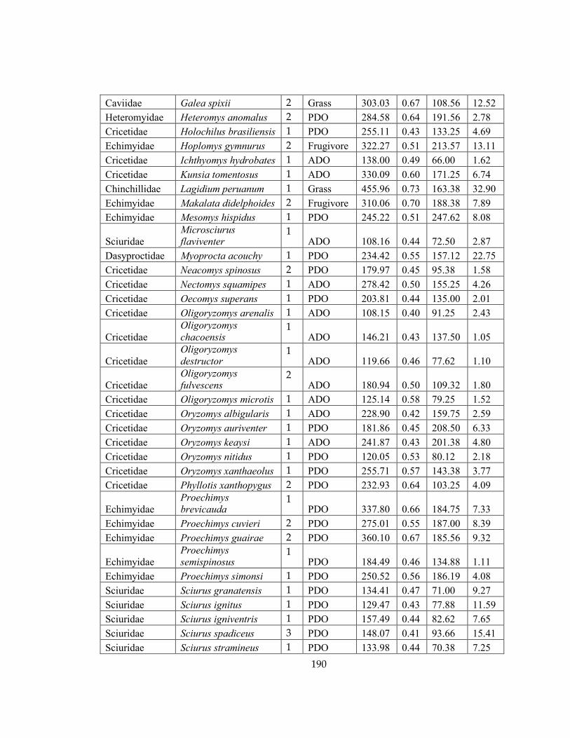
190
Caviidae Galea spixii 2 Grass 303.03 0.67 108.56 12.52
Heteromyidae Heteromys anomalus 2 PDO 284.58 0.64 191.56 2.78
Cricetidae Holochilus brasiliensis 1 PDO 255.11 0.43 133.25 4.69
Echimyidae Hoplomys gymnurus 2 Frugivore 322.27 0.51 213.57 13.11
Cricetidae Ichthyomys hydrobates 1 ADO 138.00 0.49 66.00 1.62
Cricetidae Kunsia tomentosus 1 ADO 330.09 0.60 171.25 6.74
Chinchillidae Lagidium peruanum 1 Grass 455.96 0.73 163.38 32.90
Echimyidae Makalata didelphoides 2 Frugivore 310.06 0.70 188.38 7.89
Echimyidae Mesomys hispidus 1 PDO 245.22 0.51 247.62 8.08
Sciuridae
Microsciurus
flaviventer 1
ADO 108.16 0.44 72.50 2.87
Dasyproctidae Myoprocta acouchy 1 PDO 234.42 0.55 157.12 22.75
Cricetidae Neacomys spinosus 2 PDO 179.97 0.45 95.38 1.58
Cricetidae Nectomys squamipes 1 ADO 278.42 0.50 155.25 4.26
Cricetidae Oecomys superans 1 PDO 203.81 0.44 135.00 2.01
Cricetidae Oligoryzomys arenalis 1 ADO 108.15 0.40 91.25 2.43
Cricetidae
Oligoryzomys
chacoensis 1
ADO 146.21 0.43 137.50 1.05
Cricetidae
Oligoryzomys
destructor 1
ADO 119.66 0.46 77.62 1.10
Cricetidae
Oligoryzomys
fulvescens 2
ADO 180.94 0.50 109.32 1.80
Cricetidae Oligoryzomys microtis 1 ADO 125.14 0.58 79.25 1.52
Cricetidae Oryzomys albigularis 1 ADO 228.90 0.42 159.75 2.59
Cricetidae Oryzomys auriventer 1 PDO 181.86 0.45 208.50 6.33
Cricetidae Oryzomys keaysi 1 ADO 241.87 0.43 201.38 4.80
Cricetidae Oryzomys nitidus 1 PDO 120.05 0.53 80.12 2.18
Cricetidae Oryzomys xanthaeolus 1 PDO 255.71 0.57 143.38 3.77
Cricetidae Phyllotis xanthopygus 2 PDO 232.93 0.64 103.25 4.09
Echimyidae
Proechimys
brevicauda 1
PDO 337.80 0.66 184.75 7.33
Echimyidae Proechimys cuvieri 2 PDO 275.01 0.55 187.00 8.39
Echimyidae Proechimys guairae 2 PDO 360.10 0.67 185.56 9.32
Echimyidae
Proechimys
semispinosus 1
PDO 184.49 0.46 134.88 1.11
Echimyidae Proechimys simonsi 1 PDO 250.52 0.56 186.19 4.08
Sciuridae Sciurus granatensis 1 PDO 134.41 0.47 71.00 9.27
Sciuridae Sciurus ignitus 1 PDO 129.47 0.43 77.88 11.59
Sciuridae Sciurus igniventris 1 PDO 157.49 0.44 82.62 7.65
Sciuridae Sciurus spadiceus 3 PDO 148.07 0.41 93.66 15.41
Sciuridae Sciurus stramineus 1 PDO 133.98 0.44 70.38 7.25

191
Cricetidae Thomasomys aureus 1 ADO 271.28 0.52 112.25 3.30
Cricetidae Thomasomys cinereus 1 ADO 208.90 0.35 141.88 3.95
Echimyidae
Thrichomys
apereoides 2
PDO 260.37 0.51 119.69 8.19
Cricetidae
Zygodontomys
brevicauda 3
PDO 208.29 0.69 104.94 1.66

192
Figure 42: Phylogenetic tree of all rodent species included in this study. Tree
topology derived from Bininda-Emmons et al. (2008).
After scanning and segmentation, it is necessary to perform retriangulation on
surfaces in order to eliminate any possible artifacts that may influence the measurement
Thomasomys aureusThomasomys cinereus
Akodon mollisAkodon orophilusAkodon subfuscusAkodon torquesAkodon aerosusAbrothrix jelskiiPhyllotis xanthopygus
Kunsia tomentosus
Holochilus brasiliensis
Neacomys spinosus
Nectomys squamipes
Oecomys superans
Oligoryzomys arenalisOligoryzomys chacoensis
Oligoryzomys destructorOligoryzomys fulvescens
Oligoryzomys microtis
Oryzomys albigularisOryzomys auriventerOryzomys keaysi
Oryzomys nitidusOryzomys xanthaeolus
Zygodontomys brevicauda
Ichthyomys hydrobatesHeteromys anomalusCavia tschudiiGalea musteloidesGalea spixii
Myoprocta acouchyDasyprocta punctataDasyprocta fuliginosa
Thrichomys apereoides
Hoplomys gymnurus
Proechimys simonsi
Proechimys brevicauda
Proechimys cuvieri
Proechimys semispinosus
Proechimys guairae
Clyomys laticeps
Makalata didelphoidesDiplomys labilis
Dactylomys dactylinus
Mesomys hispidus
Dolichotis salinicola
Cuniculus paca
Coendou prehensilisCoendou rothschildi
Lagidium peruanum
Sciurus granatensisSciurus stramineusSciurus igniventrisSciurus spadiceusSciurus ignitusMicrosciurus flaviventer
= Plant-dominated omnivore
= Animal-dominated omnivore
= Folivore
= Frugivore
= Grazer
193
of dental topography. This was done in accordance with Spradley et al. (2017), which
outlines proper decision making with regards to retriangulation. Ultimately, I chose to
downsample all PLY files to 10,000 faces and smooth the 3D mesh via 25 smoothing
iterations performed in Avizo (FEI Visualization Sciences Group, Berlin, Germany).
Once again, artifacts were produced on a limited number of surfaces in my sample, and
to fix these they were deleted and the resultant hole was filled using Geomagic.
After all PLY files were retriangulated, the resultant files uploaded to R via the
package “molaR.” DNE, RFI, and OPCR were recorded for each tooth surface. A data
limit problem was encountered in relation to the measurement of OPCR on many of the
surfaces. This problem was identified as being related to the high walls of the molars
that many rodents possess. In brief, these walls are recorded as especially large patches
in OPCR, and such large patches create memory issues as the computer attempts to
handle large amounts of information at once while running the analysis. In order to
overcome this obstacle, I cropped the tooth surfaces in Avizo for the DNE and OPCR
analyses. Given the wide disparity of rodent molar morphology, it is difficult to
standardize a cropping procedure using precise terminology. Howerver, surfaces were
cropped in such a way that preserved all potentially functionally relevant features on
the occlusal surface, while eliminating as much of the presumably non-functioning walls
as possible. Cropping was done at the same level as the deepest point on the occlusal
surface; which is similar to previous cropping procedures (Winchester et al., 2014;
194
Prufrock et al., 2017). It has been demonstrated that cropping teeth does not significantly
affect the measurement of DNE and OPCR, as it does for RFI (Prufrock et al., 2017). This
is because the walls of the tooth do not contribute significantly to the measurement of
either DNE or OPCR, as the flat walls are not overly sharp or complex.
Correlations between topopgraphy metrics were performed using linear
regression. A Shapiro-Wilks test performed for each metric failed to reject the hypothesis
that RFI and OPCR are normally distributed in my sample (p > 0.017), but a test
performed for DNE did reject the null hypothesis (p < 0.01), suggesting non-normality
for DNE in my sample. In order to test for the effect of diet on dental topography, mean
species values were compiled and a phylogenetic ANOVA—which is robust to
skewness and small sample sizes (Khan and Rayner, 2003)—was performed on these
means. A phylogenetically-corrected post-hoc Tukey’s Honestly Significant Differences
(HSD) test was then used to test for differences between pairs of dietary categories. In
order to understand how diet and the topography metrics interact, a principal
components analysis was performed on the three metrics and analyzed visually. Finally,
a discriminant function analysis (DFA) was performed to test the ability of the dental
topography metrics to successfully bin taxa by diet category. All analyses were
performed in the open-source statistical software R.
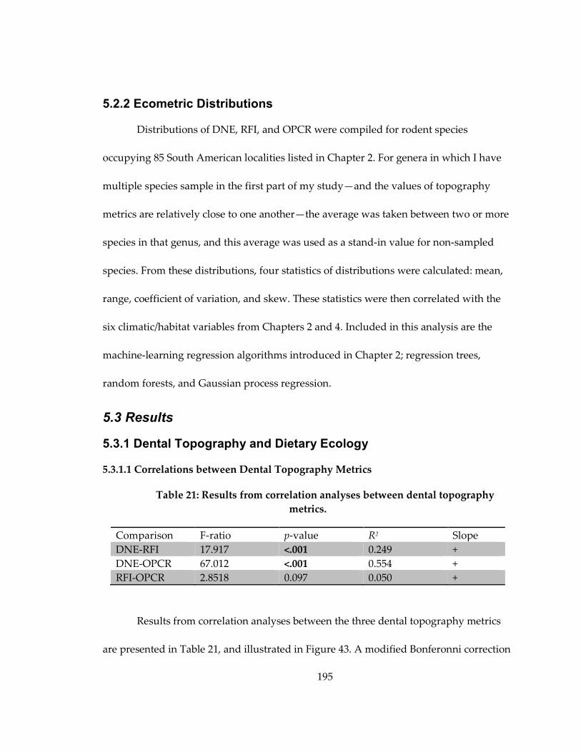
195
5.2.2 Ecometric Distributions
Distributions of DNE, RFI, and OPCR were compiled for rodent species
occupying 85 South American localities listed in Chapter 2. For genera in which I have
multiple species sample in the first part of my study—and the values of topography
metrics are relatively close to one another—the average was taken between two or more
species in that genus, and this average was used as a stand-in value for non-sampled
species. From these distributions, four statistics of distributions were calculated: mean,
range, coefficient of variation, and skew. These statistics were then correlated with the
six climatic/habitat variables from Chapters 2 and 4. Included in this analysis are the
machine-learning regression algorithms introduced in Chapter 2; regression trees,
random forests, and Gaussian process regression.
5.3 Results
5.3.1 Dental Topography and Dietary Ecology
5.3.1.1 Correlations between Dental Topography Metrics
Table 21: Results from correlation analyses between dental topography
metrics.
Comparison F-ratio p-value R2 Slope
DNE-RFI 17.917 <.001 0.249 +
DNE-OPCR 67.012 <.001 0.554 +
RFI-OPCR 2.8518 0.097 0.050 +
Results from correlation analyses between the three dental topography metrics
are presented in Table 21, and illustrated in Figure 43. A modified Bonferonni correction

196
was used for the alpha level, resulting in an alpha level of 0.019. My results indicate that
DNE has a significant positive correlation with both RFI and OPCR, while RFI and
OPCR do not demonstrate a significant correlation with one another. There are two
notable outliers for DNE values that are far above the expected values for my
regressions, Dactylomys dactylinus and Diplomys labilis. The significance of these outliers
is discussed in detail below.
Figure 43: Linear regressions of dental topography metrics against one another.
A. DNE-RFI; B. DNE-OPCR; C. RFI-OPCR.
5.3.1.2 Phylogenetically-corrected ANOVAs
Results from phylogenetically-corrected ANOVA tests are presented in Tables
22-24. My results indicate no significant correlations between diet and any of the dental
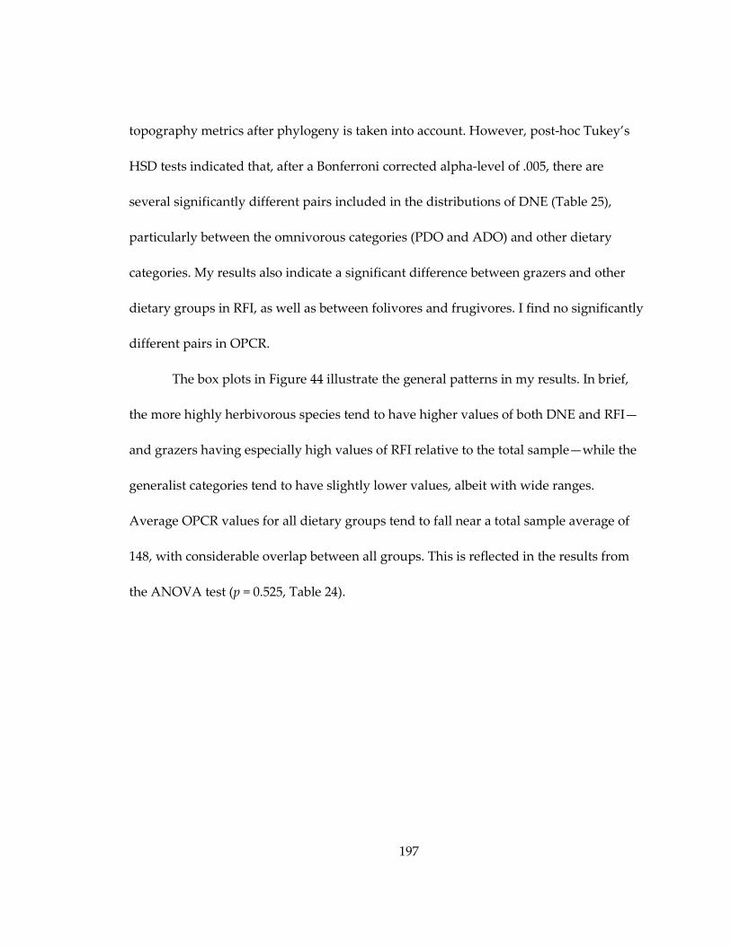
197
topography metrics after phylogeny is taken into account. However, post-hoc Tukey’s
HSD tests indicated that, after a Bonferroni corrected alpha-level of .005, there are
several significantly different pairs included in the distributions of DNE (Table 25),
particularly between the omnivorous categories (PDO and ADO) and other dietary
categories. My results also indicate a significant difference between grazers and other
dietary groups in RFI, as well as between folivores and frugivores. I find no significantly
different pairs in OPCR.
The box plots in Figure 44 illustrate the general patterns in my results. In brief,
the more highly herbivorous species tend to have higher values of both DNE and RFI—
and grazers having especially high values of RFI relative to the total sample—while the
generalist categories tend to have slightly lower values, albeit with wide ranges.
Average OPCR values for all dietary groups tend to fall near a total sample average of
148, with considerable overlap between all groups. This is reflected in the results from
the ANOVA test (p = 0.525, Table 24).
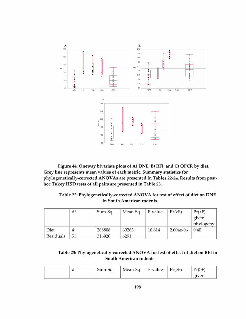
198
Figure 44: Oneway bivariate plots of A) DNE; B) RFI; and C) OPCR by diet.
Grey line represents mean values of each metric. Summary statistics for
phylogenetically-corrected ANOVAs are presented in Tables 22-24. Results from post-
hoc Tukey HSD tests of all pairs are presented in Table 25.
Table 22: Phylogenetically-corrected ANOVA for test of effect of diet on DNE
in South American rodents.
df Sum-Sq Mean-Sq F-value Pr(>F) Pr(>F)
given
phylogeny
Diet 4 268808 69263 10.814 2.004e-06 0.40
Residuals 51 316920 6291
Table 23: Phylogenetically-corrected ANOVA for test of effect of diet on RFI in
South American rodents.
df Sum-Sq Mean-Sq F-value Pr(>F) Pr(>F)
given

199
phylogeny
Diet 4 0.205 0.051 8.4695 2.553e-05 0.198
Residuals 51 0.308 0.006
Table 24: Phylogenetically-corrected ANOVA for test of effect of diet on OPCR
in South American rodents.
df Sum-Sq Mean-Sq F-value Pr(>F) Pr(>F)
given
phylogeny
Diet 4 36380 9095 4.421 0.004 0.525
Residuals 51 104930 2057.5
Table 25: Summary statistics from phylogenetically-corrected post-hoc Tukey’s
Honest Significant Differences tests. Bolded numbers indicate statistical significance
(alpha level = 0.005). Dietary abbreviations: Fol = folivore; Frug = frugivore; Grass =
grazing; ADO = animal dominated omnivore; PDO = plant dominated omnivore.
DNE RFI OPCR
Diff. Std.
Err
Diff.
p-
value
Diff. Std.
Err
Diff.
p-
value
Diff. Std.Err
Diff.
p-
value
Fol-ADO 196.69 50.49 0.001 0.011 0.054 0.262 68.89 29.05 0.256
Fol-PDO 179.46 46.81 0.033 0.061 0.051 0.064 61.85 27.05 0.146
Grass-
ADO
167.46 41.48 0.044 0.177 0.044 <.001 22.83 23.87 0.287
Frug-ADO 159.35 38.91 0.044 0.113 0.041 0.070 76.89 22.39 0.330
Grass-
PDO
150.24 38.17 0.002 0.127 0.041 <.001 15.79 21.96 0.328
Frug-PDO 142.12 35.35 <.001 0.063 0.038 0.451 69.85 20.34 0.134
Fol-Frug 37.34 55.74 0.049 0.124 0.059 0.017 7.99 32.07 0.659
Fol-Grass 29.22 57.57 0.449 0.188 0.061 0.002 46.06 33.13 0.056
PDO-ADO 17.23 26.31 0.947 0.011 0.028 0.212 7.037 15.14 0.688
Grass-
Frug
8.12 47.73 0.396 0.064 0.051 0.035 54.05 27.47 0.066

200
5.3.1.3 Discriminant Function Analysis
Several discriminant function analyses (DFAs) were performed on the dataset to
test the predictive capabilities of these metrics in categorizing species by diet (Table 26).
Results from a DFA performed on the data suggest that dental topography metrics, in
combination with the natural log of M2 area, perform moderately well in characterizing
rodent tooth surfaces by dietary category. Individual specimens were correctly
categorized at a rate of ~59%, and a chi-squared test indicated that the predicted diets
were not independent of the actual dietary categories (p < 0.001). In other words, the
DFA did not perform at random chance, which would be a rate of 20% accuracy (100%
divided by 5 groups = 20%). Different combinations of topography metrics in the
model—i.e., subtracting one or more metrics from the DFA model—results in lower
accuracy rates. Results also suggest that those species belonging to certain dietary
groups—including PDO (82.5%), grazers (62.5%), and frugivores (60%)—were more
consistently placed the correct dietary category by the DFA than folivores (40%) or ADO
(6.7%).
I also segregated the data by taxonomy, performing separate DFAs for
caviomorph rodents and non-caviomorph rodents. The DFA for caviomorph rodents
performed approximately as well (~58%) as that from the complete rodent dataset. The
DFA from the non-caviomorph—comprised of both sigmodontine and sciurid rodents—
performed slightly better (~66%) than either of these other models, though the non-
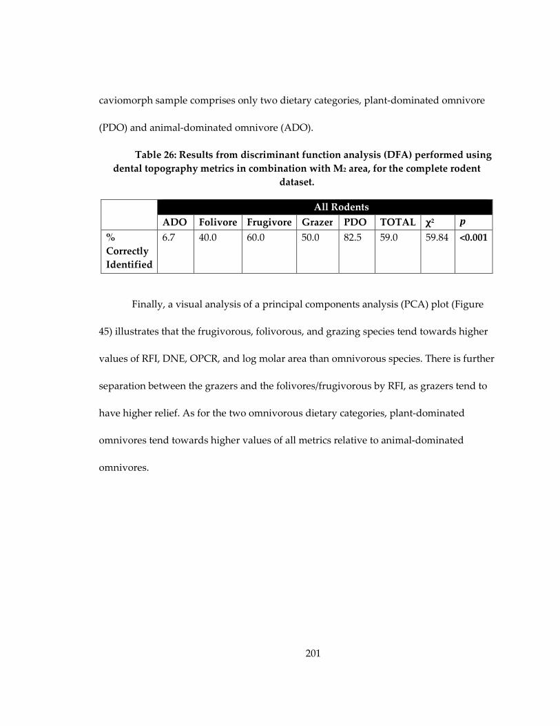
201
caviomorph sample comprises only two dietary categories, plant-dominated omnivore
(PDO) and animal-dominated omnivore (ADO).
Table 26: Results from discriminant function analysis (DFA) performed using
dental topography metrics in combination with M2 area, for the complete rodent
dataset.
All Rodents
ADO Folivore Frugivore Grazer PDO TOTAL χ2 p
%
Correctly
Identified
6.7 40.0 60.0 50.0 82.5 59.0 59.84 <0.001
Finally, a visual analysis of a principal components analysis (PCA) plot (Figure
45) illustrates that the frugivorous, folivorous, and grazing species tend towards higher
values of RFI, DNE, OPCR, and log molar area than omnivorous species. There is further
separation between the grazers and the folivores/frugivorous by RFI, as grazers tend to
have higher relief. As for the two omnivorous dietary categories, plant-dominated
omnivores tend towards higher values of all metrics relative to animal-dominated
omnivores.
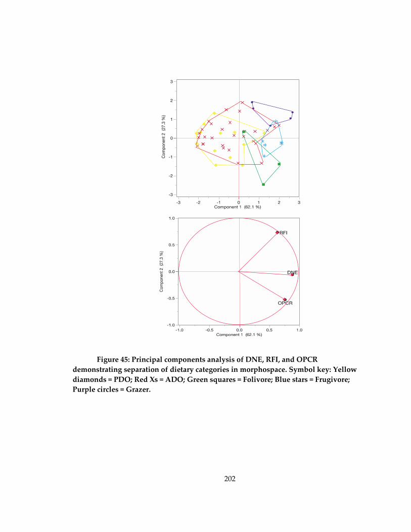
202
Figure 45: Principal components analysis of DNE, RFI, and OPCR
demonstrating separation of dietary categories in morphospace. Symbol key: Yellow
diamonds = PDO; Red Xs = ADO; Green squares = Folivore; Blue stars = Frugivore;
Purple circles = Grazer.
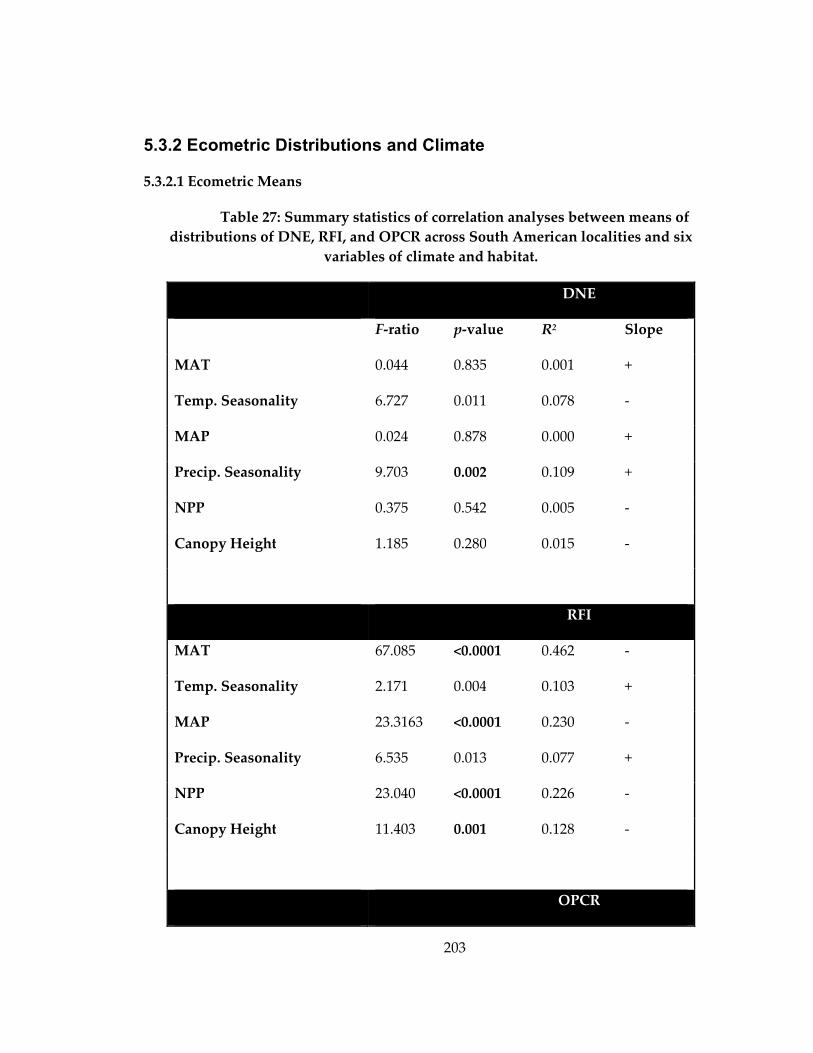
203
5.3.2 Ecometric Distributions and Climate
5.3.2.1 Ecometric Means
Table 27: Summary statistics of correlation analyses between means of
distributions of DNE, RFI, and OPCR across South American localities and six
variables of climate and habitat.
DNE
F-ratio p-value R2 Slope
MAT 0.044 0.835 0.001 +
Temp. Seasonality 6.727 0.011 0.078 -
MAP 0.024 0.878 0.000 +
Precip. Seasonality 9.703 0.002 0.109 +
NPP 0.375 0.542 0.005 -
Canopy Height 1.185 0.280 0.015 -
RFI
MAT 67.085 <0.0001 0.462 -
Temp. Seasonality 2.171 0.004 0.103 +
MAP 23.3163 <0.0001 0.230 -
Precip. Seasonality 6.535 0.013 0.077 +
NPP 23.040 <0.0001 0.226 -
Canopy Height 11.403 0.001 0.128 -
OPCR
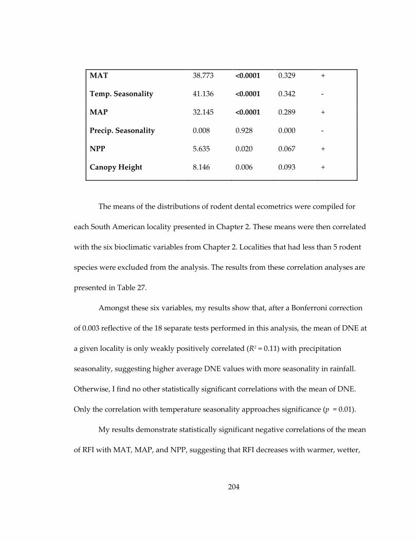
204
MAT 38.773 <0.0001 0.329 +
Temp. Seasonality 41.136 <0.0001 0.342 -
MAP 32.145 <0.0001 0.289 +
Precip. Seasonality 0.008 0.928 0.000 -
NPP 5.635 0.020 0.067 +
Canopy Height 8.146 0.006 0.093 +
The means of the distributions of rodent dental ecometrics were compiled for
each South American locality presented in Chapter 2. These means were then correlated
with the six bioclimatic variables from Chapter 2. Localities that had less than 5 rodent
species were excluded from the analysis. The results from these correlation analyses are
presented in Table 27.
Amongst these six variables, my results show that, after a Bonferroni correction
of 0.003 reflective of the 18 separate tests performed in this analysis, the mean of DNE at
a given locality is only weakly positively correlated (R2 = 0.11) with precipitation
seasonality, suggesting higher average DNE values with more seasonality in rainfall.
Otherwise, I find no other statistically significant correlations with the mean of DNE.
Only the correlation with temperature seasonality approaches significance (p = 0.01).
My results demonstrate statistically significant negative correlations of the mean
of RFI with MAT, MAP, and NPP, suggesting that RFI decreases with warmer, wetter,

205
and more productive environments. Of these three correlations, the mean of RFI has the
strongest relationship with MAT (R2 = 0.42).
The mean of OPCR has statistically significant positive correlations with both
MAT and MAP, and a significant negative correlation with temperature seasonality. In
other words, the average rodent OPCR value increases with warmer and wetter
environments, and decreases significantly in more seasonal environments.
5.3.2.2 Ecometric Ranges
Results from correlation analyses of the ranges of my three dental topography
metrics and climate are presented in Table 28. Statistical significance is once again based
on a Bonferroni corrected alpha value of 0.003. My results indicate that the range of DNE
has a statistically significant positive correlation with both NPP and canopy height. The
range of RFI only shows a statistically significant negative association with temperature
seasonality.
My results suggest that the range of OPCR is the most informative of the three
metrics. The range of OPCR has a significant positive relationship with MAT, MAP,
NPP, and canopy height, and a negative correlation with temperature seasonality (Table
28).
Table 28: Summary statistics of correlation analyses between ranges of
distributions of DNE, RFI, and OPCR across South American localities and six
variables of climate and habitat.
DNE

206
F-ratio p-value R2 Slope
MAT 4.954 0.029 0.060 -
Temp. Seasonality 0.012 0.918 0.000 -
MAP 0.556 0.458 0.007 +
Precip. Seasonality 0.184 0.669 0.002 -
NPP 2.025 0.159 0.025 +
Canopy Height 3.988 0.049 0.049 +
RFI
MAT 0.636 0.428 0.008 +
Temp. Seasonality 2.1636 0.145 0.021 -
MAP 0.117 0.733 0.002 -
Precip. Seasonality 9.029 0.004 0.105 +
NPP 2.803 0.098 0.035 -
Canopy Height 0.059 0.808 0.001 -
OPCR
MAT 41.115 <0.0001 0.345 +
Temp. Seasonality 15.031 0.0002 0.162 -
MAP 20.800 <0.0001 0.211 +
Precip. Seasonality 0.507 0.479 0.006 +
NPP 10.036 0.002 0.114 +
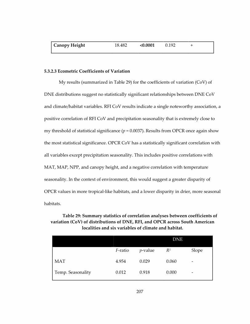
207
Canopy Height 18.482 <0.0001 0.192 +
5.3.2.3 Ecometric Coefficients of Variation
My results (summarized in Table 29) for the coefficients of variation (CoV) of
DNE distributions suggest no statistically significant relationships between DNE CoV
and climate/habitat variables. RFI CoV results indicate a single noteworthy association, a
positive correlation of RFI CoV and precipitation seasonality that is extremely close to
my threshold of statistical significance (p = 0.0037). Results from OPCR once again show
the most statistical significance. OPCR CoV has a statistically significant correlation with
all variables except precipitation seasonality. This includes positive correlations with
MAT, MAP, NPP, and canopy height, and a negative correlation with temperature
seasonality. In the context of environment, this would suggest a greater disparity of
OPCR values in more tropical-like habitats, and a lower disparity in drier, more seasonal
habitats.
Table 29: Summary statistics of correlation analyses between coefficients of
variation (CoV) of distributions of DNE, RFI, and OPCR across South American
localities and six variables of climate and habitat.
DNE
F-ratio p-value R2 Slope
MAT 4.954 0.029 0.060 -
Temp. Seasonality 0.012 0.918 0.000 -
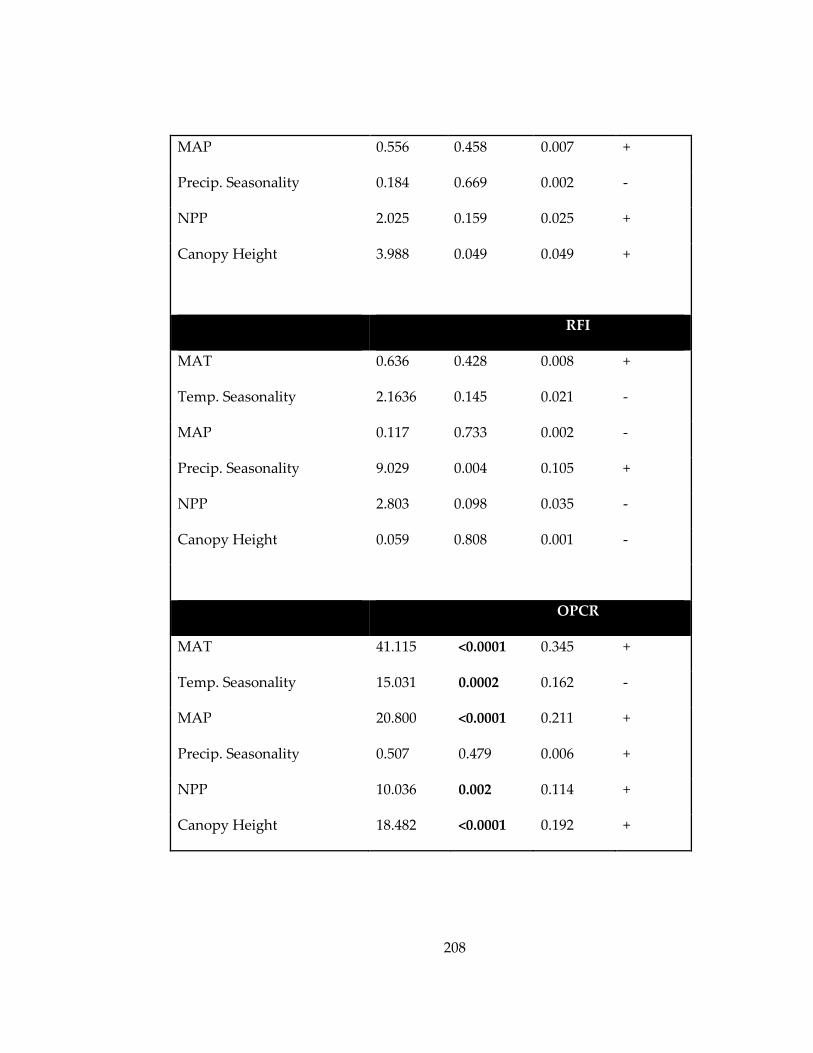
208
MAP 0.556 0.458 0.007 +
Precip. Seasonality 0.184 0.669 0.002 -
NPP 2.025 0.159 0.025 +
Canopy Height 3.988 0.049 0.049 +
RFI
MAT 0.636 0.428 0.008 +
Temp. Seasonality 2.1636 0.145 0.021 -
MAP 0.117 0.733 0.002 -
Precip. Seasonality 9.029 0.004 0.105 +
NPP 2.803 0.098 0.035 -
Canopy Height 0.059 0.808 0.001 -
OPCR
MAT 41.115 <0.0001 0.345 +
Temp. Seasonality 15.031 0.0002 0.162 -
MAP 20.800 <0.0001 0.211 +
Precip. Seasonality 0.507 0.479 0.006 +
NPP 10.036 0.002 0.114 +
Canopy Height 18.482 <0.0001 0.192 +

209
5.3.2.3 Ecometric Skewness
I find no statistically significant relationships between the skewness of the
distributions of my dental topography metrics and the bioclimatic variables included in
this study.
5.3.3 Machine-learning Regression Techniques
Mean absolute error (MAE) and root mean squared error (RMSE)—error metrics
that demonstrated the average difference between predicted and actual observations—
for the six bioclimatic variables across the different regression techniques are presented
in Table 30. MAE and RMSE differ for each bioclimatic variable because they are
presented in the same units as those variables. The three machine-learning regression
methods—regression tree (RTA), random forests (RF), and Gaussian process regression
(GPR)—generally have lower error metrics than multivariate linear regression. Bivariate
plots of the estimated bioclimatic variables versus the actual values of these variables are
presented in Figure 46-50. R2 values in these plots give a measurement of the fit between
estimations and observations. The highest R2 values are found in the estimations of
MAP, including regression tree (R2 = 0.90), Gaussian process regression (R2 = 0.74), and
random forests (R2 = 0.89).
Table 30: Mean Absolute Error (MAE) and Root Mean Squared Error (RMSE)
for the estimations of bioclimatic variables using different regression techniques.
Mean Annual Temperature
Method MAE RMSE
Baseline Average 50.03 60.61
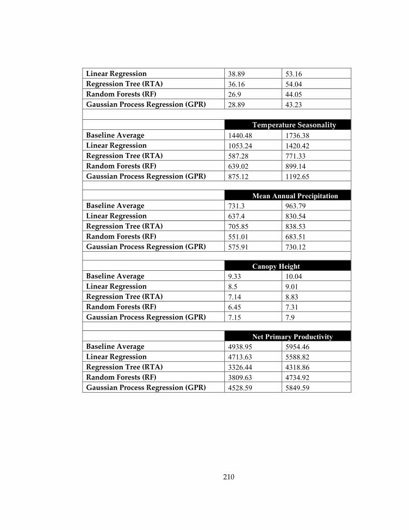
210
Linear Regression 38.89 53.16
Regression Tree (RTA) 36.16 54.04
Random Forests (RF) 26.9 44.05
Gaussian Process Regression (GPR) 28.89 43.23
Temperature Seasonality
Baseline Average 1440.48 1736.38
Linear Regression 1053.24 1420.42
Regression Tree (RTA) 587.28 771.33
Random Forests (RF) 639.02 899.14
Gaussian Process Regression (GPR) 875.12 1192.65
Mean Annual Precipitation
Baseline Average 731.3 963.79
Linear Regression 637.4 830.54
Regression Tree (RTA) 705.85 838.53
Random Forests (RF) 551.01 683.51
Gaussian Process Regression (GPR) 575.91 730.12
Canopy Height
Baseline Average 9.33 10.04
Linear Regression 8.5 9.01
Regression Tree (RTA) 7.14 8.83
Random Forests (RF) 6.45 7.31
Gaussian Process Regression (GPR) 7.15 7.9
Net Primary Productivity
Baseline Average 4938.95 5954.46
Linear Regression 4713.63 5588.82
Regression Tree (RTA) 3326.44 4318.86
Random Forests (RF) 3809.63 4734.92
Gaussian Process Regression (GPR) 4528.59 5849.59
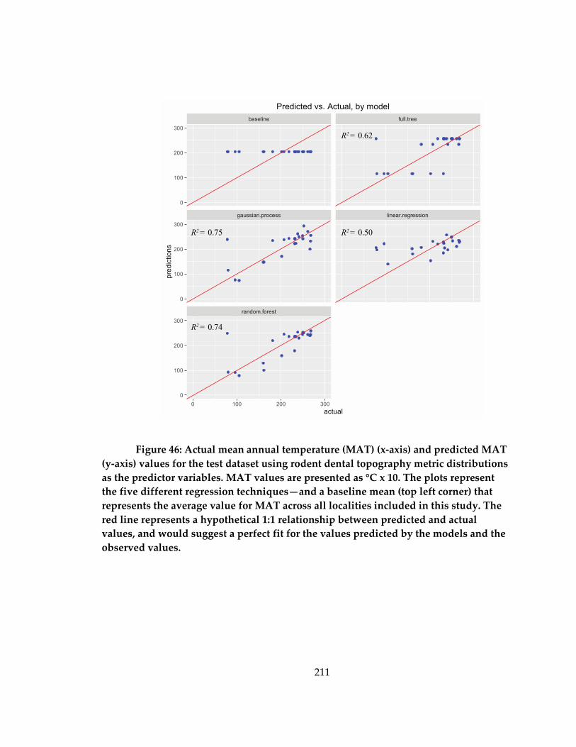
211
Figure 46: Actual mean annual temperature (MAT) (x-axis) and predicted MAT
(y-axis) values for the test dataset using rodent dental topography metric distributions
as the predictor variables. MAT values are presented as °C x 10. The plots represent
the five different regression techniques—and a baseline mean (top left corner) that
represents the average value for MAT across all localities included in this study. The
red line represents a hypothetical 1:1 relationship between predicted and actual
values, and would suggest a perfect fit for the values predicted by the models and the
observed values.
baseline full.tree
gaussian.process linear.regression
random.forest
0
100
200
300
0
100
200
300
0
100
200
300
0 100 200 300
actual
pre
dic
tion
s
Predicted vs. Actual, by model
R2 = 0.50
R2 = 0.62
R2 = 0.75
R2 = 0.74
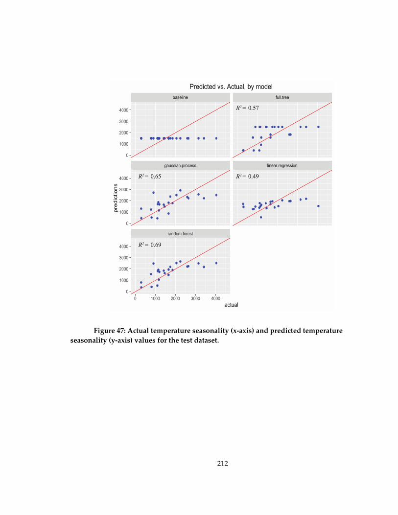
212
Figure 47: Actual temperature seasonality (x-axis) and predicted temperature
seasonality (y-axis) values for the test dataset.
baseline full.tree
gaussian.process linear.regression
random.forest
0
1000
2000
3000
4000
0
1000
2000
3000
4000
0
1000
2000
3000
4000
0 1000 2000 3000 4000
actual
pre
dic
tion
s
Predicted vs. Actual, by model
R2 = 0.49
R2 = 0.57
R2 = 0.65
R2 = 0.69
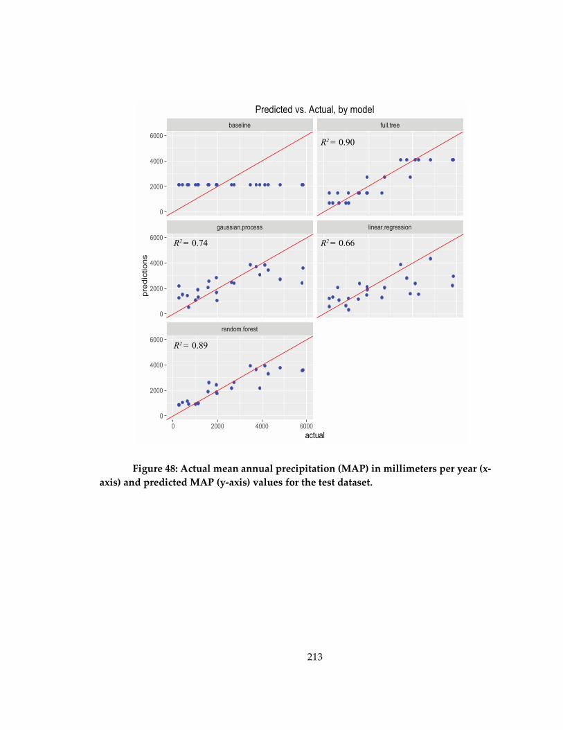
213
Figure 48: Actual mean annual precipitation (MAP) in millimeters per year (x-
axis) and predicted MAP (y-axis) values for the test dataset.
baseline full.tree
gaussian.process linear.regression
random.forest
0
2000
4000
6000
0
2000
4000
6000
0
2000
4000
6000
0 2000 4000 6000
actual
pre
dic
tion
s
Predicted vs. Actual, by model
R2 = 0.66
R2 = 0.90
R2 = 0.89
R2 = 0.74
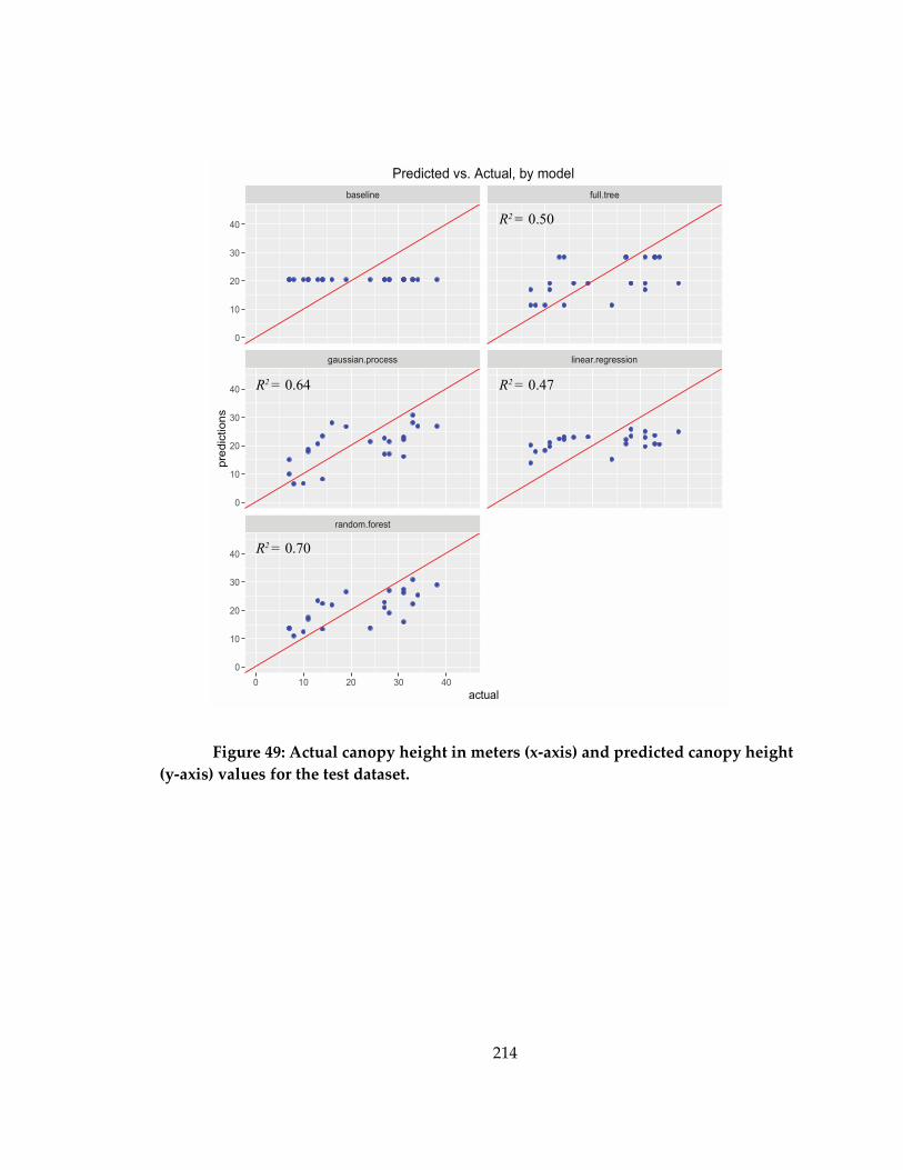
214
Figure 49: Actual canopy height in meters (x-axis) and predicted canopy height
(y-axis) values for the test dataset.
baseline full.tree
gaussian.process linear.regression
random.forest
0
10
20
30
40
0
10
20
30
40
0
10
20
30
40
0 10 20 30 40
actual
pre
dic
tion
s
Predicted vs. Actual, by model
R2 = 0.47
R2 = 0.50
R2 = 0.64
R2 = 0.70
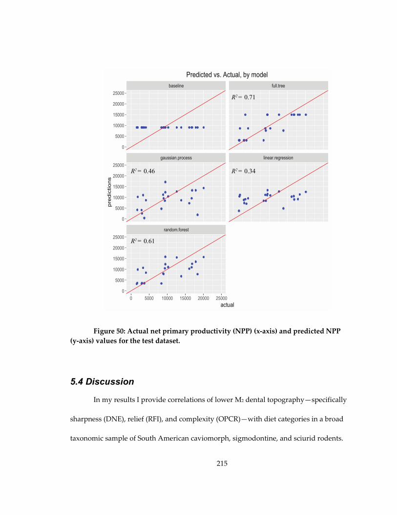
215
Figure 50: Actual net primary productivity (NPP) (x-axis) and predicted NPP
(y-axis) values for the test dataset.
5.4 Discussion
In my results I provide correlations of lower M2 dental topography—specifically
sharpness (DNE), relief (RFI), and complexity (OPCR)—with diet categories in a broad
taxonomic sample of South American caviomorph, sigmodontine, and sciurid rodents.
baseline full.tree
gaussian.process linear.regression
random.forest
0
5000
10000
15000
20000
25000
0
5000
10000
15000
20000
25000
0
5000
10000
15000
20000
25000
0 5000 10000 15000 20000 25000
actual
pre
dic
tio
ns
Predicted vs. Actual, by model
R2 = 0.34
R2 = 0.71
R2 = 0.46
R2 = 0.61

216
In the introduction I stated that I expected rodent molars, despite their vastly different
gross morphology compared to primates or marsupials, to nevertheless abide by the
same functional constraints of the teeth of these clades. This expectation was built on the
hypothesis of Evans and Sanson (2003) that there exists ideal tooth shapes and
configurations for the breaking down of specific categories of food materials. Though
Evans and Sanson (2003) discussed this hypothesis primarily in the context of the
tribosphenic molar, Evans et al. (2007) demonstrated that similar constraints were acting
on the tooth rows of both rodents and carnivorans. Thus, the null hypothesis is that
rodent molar topography shows similar patterns to what see in primates (Boyer, 2008;
Winchester et al., 2014) and marsupials (Chapter 4), namely that an increase in
sharpness, relief, and complexity should be associated with diets consisting of tougher
food materials.
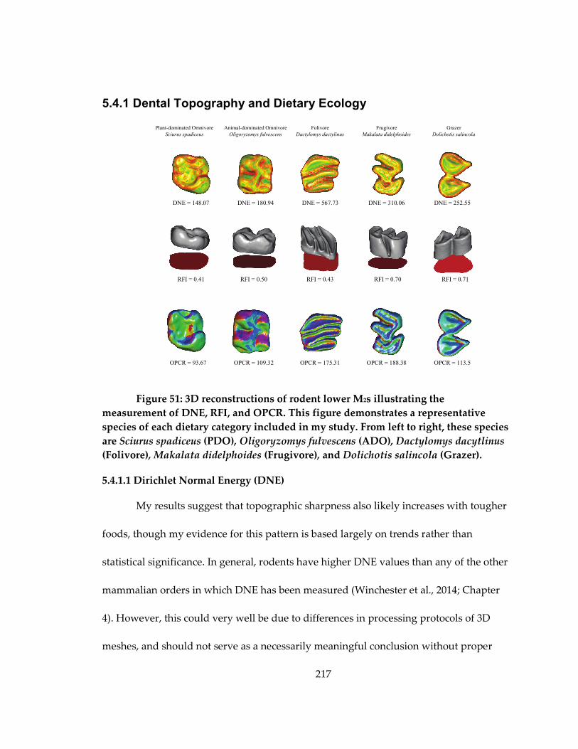
217
5.4.1 Dental Topography and Dietary Ecology
Figure 51: 3D reconstructions of rodent lower M2s illustrating the
measurement of DNE, RFI, and OPCR. This figure demonstrates a representative
species of each dietary category included in my study. From left to right, these species
are Sciurus spadiceus (PDO), Oligoryzomys fulvescens (ADO), Dactylomys dacytlinus
(Folivore), Makalata didelphoides (Frugivore), and Dolichotis salincola (Grazer).
5.4.1.1 Dirichlet Normal Energy (DNE)
My results suggest that topographic sharpness also likely increases with tougher
foods, though my evidence for this pattern is based largely on trends rather than
statistical significance. In general, rodents have higher DNE values than any of the other
mammalian orders in which DNE has been measured (Winchester et al., 2014; Chapter
4). However, this could very well be due to differences in processing protocols of 3D
meshes, and should not serve as a necessarily meaningful conclusion without proper
Folivore
Dactylomys dactylinus
Frugivore
Makalata didelphoides
Grazer
Dolichotis salincola
Plant-dominated Omnivore
Sciurus spadiceus
Animal-dominated Omnivore
Oligoryzomys fulvescens
DNE = 148.07
RFI = 0.41
OPCR = 93.67
DNE = 180.94
RFI = 0.50
OPCR = 109.32
DNE = 567.73
RFI = 0.43
OPCR = 175.31
DNE = 310.06
RFI = 0.70
OPCR = 188.38
DNE = 252.55
RFI = 0.71
OPCR = 113.5
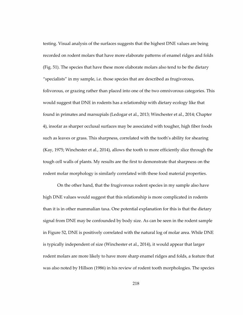
218
testing. Visual analysis of the surfaces suggests that the highest DNE values are being
recorded on rodent molars that have more elaborate patterns of enamel ridges and folds
(Fig. 51). The species that have these more elaborate molars also tend to be the dietary
“specialists” in my sample, i.e. those species that are described as frugivorous,
folivorous, or grazing rather than placed into one of the two omnivorous categories. This
would suggest that DNE in rodents has a relationship with dietary ecology like that
found in primates and marsupials (Ledogar et al., 2013; Winchester et al., 2014; Chapter
4), insofar as sharper occlusal surfaces may be associated with tougher, high fiber foods
such as leaves or grass. This sharpness, correlated with the tooth’s ability for shearing
(Kay, 1975; Winchester et al., 2014), allows the tooth to more efficiently slice through the
tough cell walls of plants. My results are the first to demonstrate that sharpness on the
rodent molar morphology is similarly correlated with these food material properties.
On the other hand, that the frugivorous rodent species in my sample also have
high DNE values would suggest that this relationship is more complicated in rodents
than it is in other mammalian taxa. One potential explanation for this is that the dietary
signal from DNE may be confounded by body size. As can be seen in the rodent sample
in Figure 52, DNE is positively correlated with the natural log of molar area. While DNE
is typically independent of size (Winchester et al., 2014), it would appear that larger
rodent molars are more likely to have more sharp enamel ridges and folds, a feature that
was also noted by Hillson (1986) in his review of rodent tooth morphologies. The species
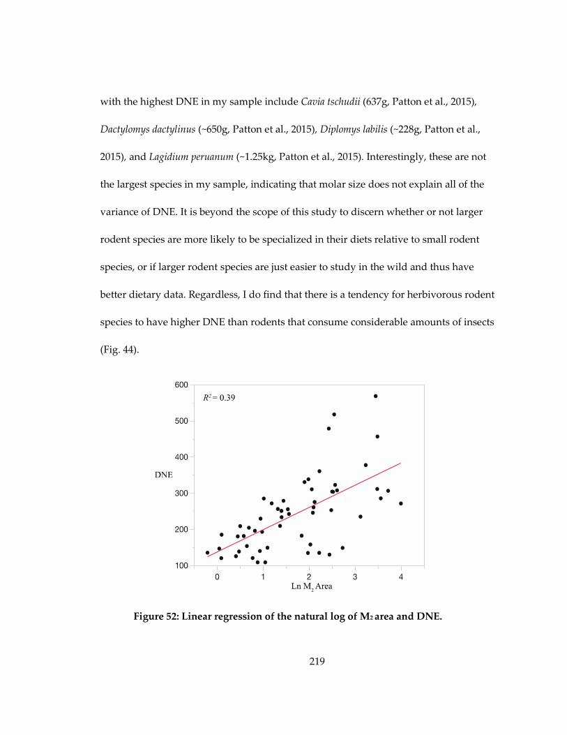
219
with the highest DNE in my sample include Cavia tschudii (637g, Patton et al., 2015),
Dactylomys dactylinus (~650g, Patton et al., 2015), Diplomys labilis (~228g, Patton et al.,
2015), and Lagidium peruanum (~1.25kg, Patton et al., 2015). Interestingly, these are not
the largest species in my sample, indicating that molar size does not explain all of the
variance of DNE. It is beyond the scope of this study to discern whether or not larger
rodent species are more likely to be specialized in their diets relative to small rodent
species, or if larger rodent species are just easier to study in the wild and thus have
better dietary data. Regardless, I do find that there is a tendency for herbivorous rodent
species to have higher DNE than rodents that consume considerable amounts of insects
(Fig. 44).
Figure 52: Linear regression of the natural log of M2 area and DNE.

220
5.4.1.2 Relief Index (RFI)
Of the three dental topography metrics, RFI demonstrates the best correlation
with diet after correcting for phylogeny (p = 0.198). My results from RFI suggest a
similar trend as DNE of herbivorous rodents having higher values. The exception to this
is that frugivorous rodents have RFI values that are more in line with animal-dominated
omnivores and in the lower end of plant-dominated omnivores. This matches my
expectation based on previous results from previously published studies of rodents
(Williams and Kay, 2001), as well as other mammalian taxa (Janis, 1988; Williams and
Kay, 2001; Ungar and M’Kirera, 2003; Boyer 2008; Winchester et al., 2014; Chapter 4).
Based on the interpretations of these previous studies, this would suggest that
frugivorous rodents likely do not experience the same levels of wear as folivores and
grazers.
Williams and Kay (2001) found that grazing South American rodents had
considerably higher hypsodont indices—a measure analogous to RFI—than either
folivorous or frugivorous species. My results are generally in agreement with those of
Williams and Kay (2001), with grazing species having the highest mean RFI (0.688) of
any dietary group in my study. Williams and Kay (2001) interpreted their result as an
adaptation to rapid tooth wear due to either the abrasive nature of phytoliths in grass,
221
the exogenous grit commonly associated with consuming fine particles of dirt adhering
to grass, or a combination of the two.
Beyond the distinguishing of grazing rodents from other species, RFI is generally
poor at discriminating diet, as there is considerable overlap in RFI between the other
dietary groups (Figure 44). However, Williams and Kay (2001) also found that
terrestriality was a significant factor in the evolution of rodent hypsodonty, suggesting
that exogenous grit may be a primary driver of hypsodonty in rodents and other
mammals. In order to test this possibility in my dataset, I first classified every rodent
species as either terrestrial or arboreal/semi-arboreal (including scansorial). Following
Williams and Kay (2001), the grazers were dropped from the dataset, as they may
confound any signal because of their already abrasive diet. After removing grazers and
controlling for phylogeny, I do not find a significant correlation between terrestriality
and RFI (p = 0.27). This is surprising, given that Williams and Kay (2001) found a
significant correlation in their sample of South American rodents, which is very similar
to my own. A potential explanation for this discrepancy is that RFI is not precisely
equivalent to a measure like hypsodonty index. Hypsodonty index is typically measured
as the ratio of tooth crown height over tooth width or length (Van Valen, 1960; Janis,
1980). RFI more completely captures the relief of the whole surface by measuring the 3D
surface area (Boyer, 2008). Thus, the hypsodonty signal distinguishing terrestrial and
222
arboreal rodents detected by Williams and Kay (2001) may be getting lost in the
contributions from other occlusal features that compose the RFI metric.
5.4.1.3 Orientation Patch Count Rotated (OPCR)
Dental complexity, or OPCR, is also not significantly correlated with diet in my
sample. This is particularly surprising as previously published studies have found that
complexity in the rodent tooth row (Evans et al., 2007) and complexity in individual
lower teeth (Evans and Jernvall 2009) are significantly correlated with diet. They use
dietary categories that are very similar to my own—including animal-dominated
omnivore (ADO), plant-dominated omnivore (PDO), and herbivore. Here I separate
‘herbivore’ into folivore, frugivore, and grazer.
There are a couple likely explanations for results relative to those of the other
two studies; 1) my separation of their “herbivore” category into multiple different
categories made the dietary signal of OPCR weaker; or 2) my inclusion of a phylogenetic
correction. In order to test whether our separation of the herbivorous “specialists” into
different categories affected my results, I combined these specialists—i.e., frugivores,
folivores, and grazers—into a single herbivore group. A phylogenetically-corrected
ANOVA performed on this dataset did not indicate a significant effect of diet on OPCR
(p = 0.41). The other potential explanation for my lack of a significant correlation is that
rodent occlusal morphology carries with it a strong phylogenetic signal. As a brief test of
whether the distributions of rodent topographies are equivalent within dietary
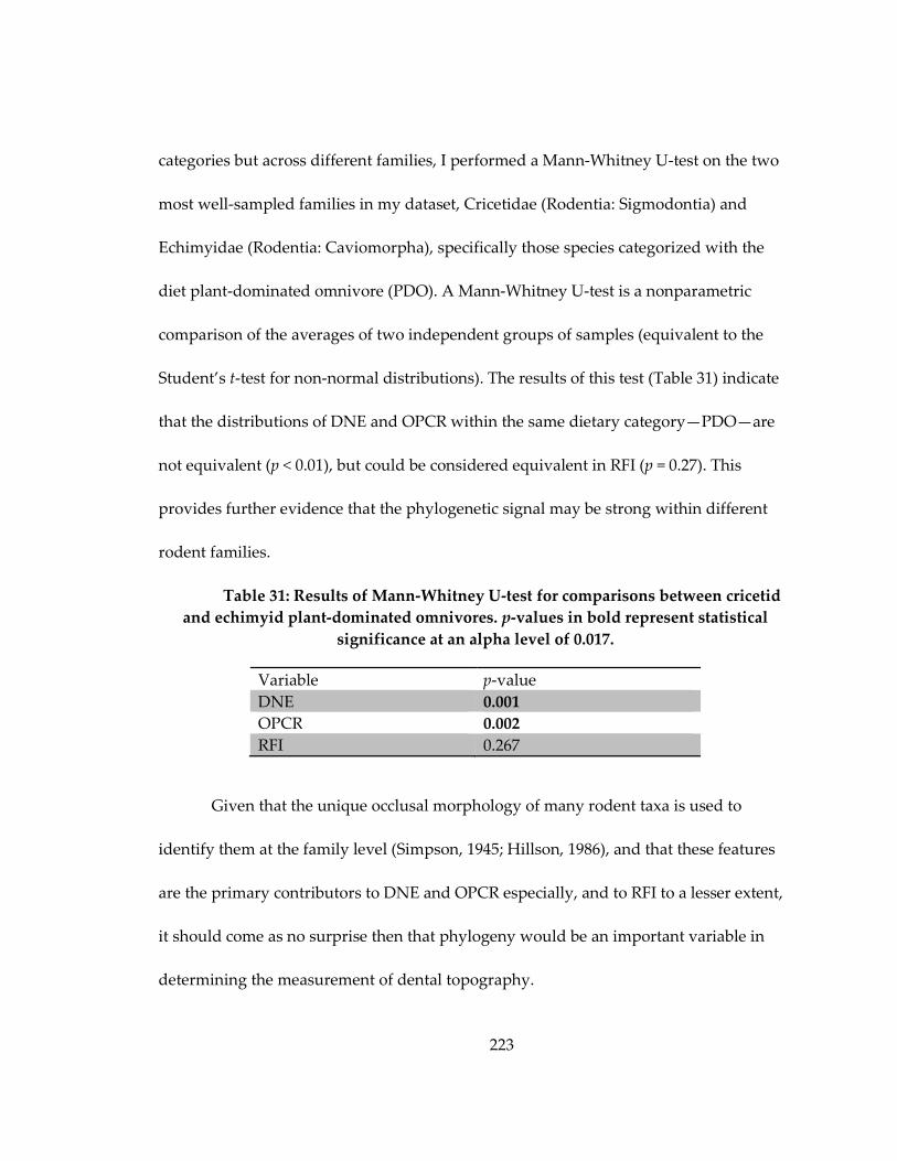
223
categories but across different families, I performed a Mann-Whitney U-test on the two
most well-sampled families in my dataset, Cricetidae (Rodentia: Sigmodontia) and
Echimyidae (Rodentia: Caviomorpha), specifically those species categorized with the
diet plant-dominated omnivore (PDO). A Mann-Whitney U-test is a nonparametric
comparison of the averages of two independent groups of samples (equivalent to the
Student’s t-test for non-normal distributions). The results of this test (Table 31) indicate
that the distributions of DNE and OPCR within the same dietary category—PDO—are
not equivalent (p < 0.01), but could be considered equivalent in RFI (p = 0.27). This
provides further evidence that the phylogenetic signal may be strong within different
rodent families.
Table 31: Results of Mann-Whitney U-test for comparisons between cricetid
and echimyid plant-dominated omnivores. p-values in bold represent statistical
significance at an alpha level of 0.017.
Variable p-value
DNE 0.001
OPCR 0.002
RFI 0.267
Given that the unique occlusal morphology of many rodent taxa is used to
identify them at the family level (Simpson, 1945; Hillson, 1986), and that these features
are the primary contributors to DNE and OPCR especially, and to RFI to a lesser extent,
it should come as no surprise then that phylogeny would be an important variable in
determining the measurement of dental topography.
224
5.4.1.4 Dental Topography as a Discriminator of Rodent Dietary Ecologies
In short, my results discussed above suggest that dental topography is generally
a poor discriminator of dietary ecology in South American rodents. A discriminant
function analysis (DFA) performed with all three metrics and the natural log of molar
area results in individual specimens being correctly categorized by diet 59% of the time.
While this is significantly better than random chance (20%), this is nevertheless a low
percentage, particularly when compared to similar tests on primates (Winchester et al.,
2014) and marsupials (Chapter 4). This begs the question as to why rodent occlusal
morphology does not demonstrate the same patterns as primates and marsupials. The
most obvious answer to this question would be to look towards the defining
characteristic of all rodents, the ever-growing, hypselodont incisors in both the upper
and lower jaw. These incisors serve as remarkably efficient and flexible tools for rodents
across a broad array of ecological niches (Van Valen, 2004). Croft et al. (2011)
demonstrated that upper incisor morphology in herbivorous caviomorph rodents could
be used as an effective discriminator of dietary ecology. In combination with my results
from the molars, this might suggest that the incisor toolkit provided to the rodents may
have released their molars from the functional constraints that have maintained the
general tribosphenic molar shape in other mammalian clades that nevertheless occupy
similar niches as modern rodents. The other potential explanation is that the molars are

225
suited for processing the material they masticate after the incisors have processed the
food. That is, the cheek-teeth are adapted to handle incisor-processed materials.
On the other hand, there is a strong possibility that the lack of dietary signal in
my results is not due to a true biological phenomenon, but rather is due to the
particularly coarse resolution of the dietary data available for the majority of rodent
species in my sample. Unlike Croft et al. (2011), I included species for which wild diet
data is not extensive. These poorly studied species—primarily the various species of rats
and mice that are near ubiquitous in South American ecosystems—largely make up my
omnivorous categories; both of which demonstrate considerable overlap with other
dietary categories, especially in DNE and OPCR (Fig. 44). There is potential that more
discrete classification of diet in these rodents in these categories may elucidate a
relationship between molar topography and diet. Of course, this potential is dependent
on the acquisition of behavioral data of notoriously difficult-to-study mammals, many of
which are found in remote, inaccessible forests.
5.4.2 Rodent Dental Topography Distributions as Environmental Proxies
I proceed to the distributions of these topography metrics as potential proxies of
climate and habitat. Tables 28-30 summarize the results from correlation analyses of
bioclimatic variables and the means, ranges, and coefficients of variation of the dental
topography metrics. I do not present results from analyses of skewness as I did not find
any significant correlations.

226
5.4.2.1 DNE
Of the three metrics, my results suggest that the distributions of DNE are the
least informative for estimating climate and habitat. The handful of significant
relationships between DNE distribution statistics and environment are illustrated in
Figure 53. Of the four climatic variables (MAT, MAP, temperature seasonality,
precipitation seasonality) and the two habitat variables (NPP and canopy height), the
mean of DNE only shows one significant correlation, a positive correlation with
precipitation seasonality (Table 28). Based on the trends that are illustrated in Fig. 44,
this would suggest a greater number of folivores, frugivores, and/or grazers with
precipitation seasonality. Considering the nature of seasonal environments, this would
likely reflect an increase in the number of grazing rodents. However, given the
uncertainty of my results in linking molar DNE to diet, as well as the difficulty in
estimating precipitation seasonality (see Chapter 2), I cannot rule out the possibility that
this is a spurious result. That the mean of DNE has no other statistically significant
association with any other variable only contributes further to the dubiousness of this
result.
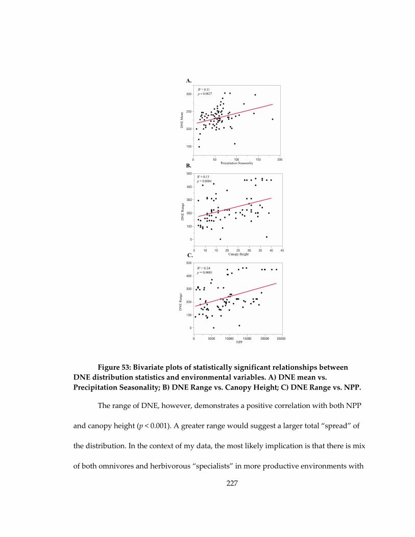
227
Figure 53: Bivariate plots of statistically significant relationships between
DNE distribution statistics and environmental variables. A) DNE mean vs.
Precipitation Seasonality; B) DNE Range vs. Canopy Height; C) DNE Range vs. NPP.
The range of DNE, however, demonstrates a positive correlation with both NPP
and canopy height (p < 0.001). A greater range would suggest a larger total “spread” of
the distribution. In the context of my data, the most likely implication is that there is mix
of both omnivores and herbivorous “specialists” in more productive environments with

228
greater canopy height. Since grazers are unlikely to be affected by canopy height, we can
assume that this reflects a greater number of frugivores and/or folivores, both of which
have generally higher average DNE values in my sample. The correlation of DNE range
and MAP is also very close to statistical significance (p = 0.004, compared to a
Bonferroni-corrected alpha value of 0.003), suggesting that DNE range is associated with
the presence of tropical forests, and the weakness of these correlations—none of the
correlation coefficients (R2) for these significant correlations rise above 0.163—is likely
due to the fact that grazing rodents, indicative of grasslands (Kay et al., 1999), also have
high DNE values. This in turn is creating high ranges in open, highly seasonal
environments.
Finally, my results indicate that the coefficient of variation (CoV) of DNE
distributions has no significant correlation with any of six variables of climate and
habitat. As discussed in Chapter 4, CoV in the context of my study, can be interpreted as
a measure of the average disparity (Gould, 1991) in dental topography at a given
locality. More so than range and mean, CoV is robust to the presence of just one species
with a high DNE value. For this reason, my finding that DNE CoV is not significantly
correlated with any of the climate or habitat variables indicates that the distribution of
DNE is not a useful proxy of environment. This is ultimately unsurprising given that
DNE was a poor predictor of dietary ecology in my results, as well.
229
5.4.2.2 RFI
My results from the distributions of RFI, when viewed through the lens of my
ecomorphological study, suggest that the presence or absence of grazing rodents is
largely driving the significant correlations that I find. Grazers have significantly higher
RFI values than do any other dietary category, and I find that the mean of RFI has a
significantly negative correlation with MAT, MAP, NPP, and canopy height (Table 28).
Additionally, the mean of RFI nears significance for a positive correlation with
temperature seasonality (p = 0.004). Further, RFI range has a significant positive
correlation with temperature seasonality (Table 29). All of these results are indicative of
a trend towards higher RFI values in drier, seasonal grasslands that dominate the
southern third of South America. These results agree with those of Kay et al. (1999), who
found a correlation between the percentage of hypsodont rodent species and MAP,
MAT, seasonal temperature amplitude (similar to my use of temperature seasonality),
and mean temperature of coldest month. Kay et al. (1999) also found negative
correlations with MAP and MAT, and a positive correlation with seasonal temperature
amplitude. The discrepancy between RFI and the hypsodonty index is discussed in
further detail above, but my results would suggest that hypsodonty index may serve as
the better proxy for environment, as it is not affected by occlusal features that are
heavily influenced by phylogeny.

230
Figure 54: Bivariate plots of statistically significant relationships between RFI
distribution statistics and environmental variables. A) RFI mean vs. MAT; B) RFI
mean vs. MAP; C) RFI mean vs. Canopy Height; D) RFI mean vs. NPP; E) RFI range
vs. Temperature Seasonality.
The CoV of RFI does not show any significant correlations with any of the
environmental variables, pointing to RFI being more informative in identifying the
presence of grazing species, which in turn can lead one to assume a more open, seasonal
231
environment (or not). Similar studies have shown how the presence of other mammalian
orders, for which living representatives have known environmental tolerances or
preferences, can be used as environmental proxies (Kay et al., 1997; Vizcaíno et al., 2006).
In conclusion, much like DNE, the dearth of significant correlations with environmental
variables is reflective of my failure to find strong evidence of RFI’s ecomorphological
relationship to diet in rodents.
5.4.2.3 OPCR
Whereas the distributions of RFI and DNE do not show much potential as
proxies for environment, my results from the analyses of OPCR suggest that this may
not be the case for tooth complexity. Quite surprisingly, given the generally poor
performance of OPCR as an ecomorphological discriminator in primates and
marsupials—see above, as well as Chapter 4 and Winchester et al. (2014)—I find that the
distributions of OPCR have significant correlations with environment regardless of
which distribution statistic is used. I will discuss my results in the context of each
statistic below.
The mean of OPCR shows a significant increase with MAT and MAP, and a
decrease with temperature seasonality. Additionally, the positive correlations for both
NPP and canopy height are also close to my alpha value (p = 0.02 and p = 0.006,
respectively). The only variable that it does not correlate well with is precipitation
seasonality, which I demonstrated in Chapter 2 to be generally difficult to model. Based
232
on my ecomorphological results in the first section of this paper, it is clear that an
ecological interpretation of these analyses is complicated. I found no significantly
different dietary pairs in my post-hoc tests in regards to OPCR—though the frugivores
in my sample appear to have a mean that is slightly higher than other dietary groups
(Fig. 44)—which makes it difficult to assume which dietary niches are driving these
correlations. However, viewing my results in combination with those of the OPC/OPCR
studies of Evans et al. (2007) and Evans and Jernvall (2009), this would suggest a greater
number of highly herbivorous species in more tropical-like environments. The strongest
correlation in my results is that with temperature seasonality and MAT (R2 = 0.34 and
0.32, respectively), suggesting a strong latitudinal gradient in our data. In fact, a
correlation of the mean of OPCR and latitude shows a significant positive correlation (p
< 0.001), though the lower correlation coefficient indicates that latitude does not explain
all the variation in my data (Fig. 56, R2 = 0.27).

233
Figure 55: Bivariate plots of statistically significant relationships between
OPCR mean and A) MAT; B) Temperature seasonality; and C) MAP.
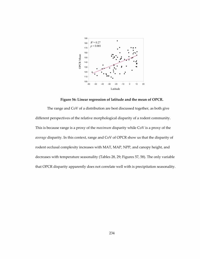
234
Figure 56: Linear regression of latitude and the mean of OPCR.
The range and CoV of a distribution are best discussed together, as both give
different perspectives of the relative morphological disparity of a rodent community.
This is because range is a proxy of the maximum disparity while CoV is a proxy of the
average disparity. In this context, range and CoV of OPCR show us that the disparity of
rodent occlusal complexity increases with MAT, MAP, NPP, and canopy height, and
decreases with temperature seasonality (Tables 28, 29; Figures 57, 58). The only variable
that OPCR disparity apparently does not correlate well with is precipitation seasonality.
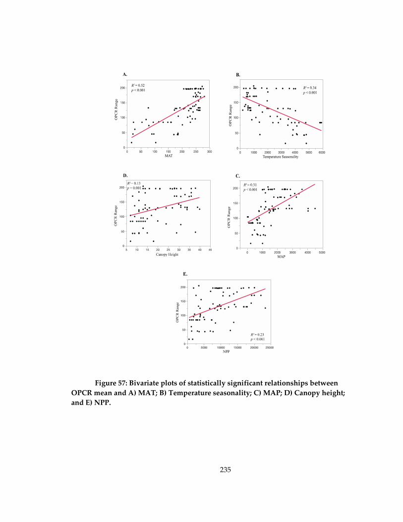
235
Figure 57: Bivariate plots of statistically significant relationships between
OPCR mean and A) MAT; B) Temperature seasonality; C) MAP; D) Canopy height;
and E) NPP.
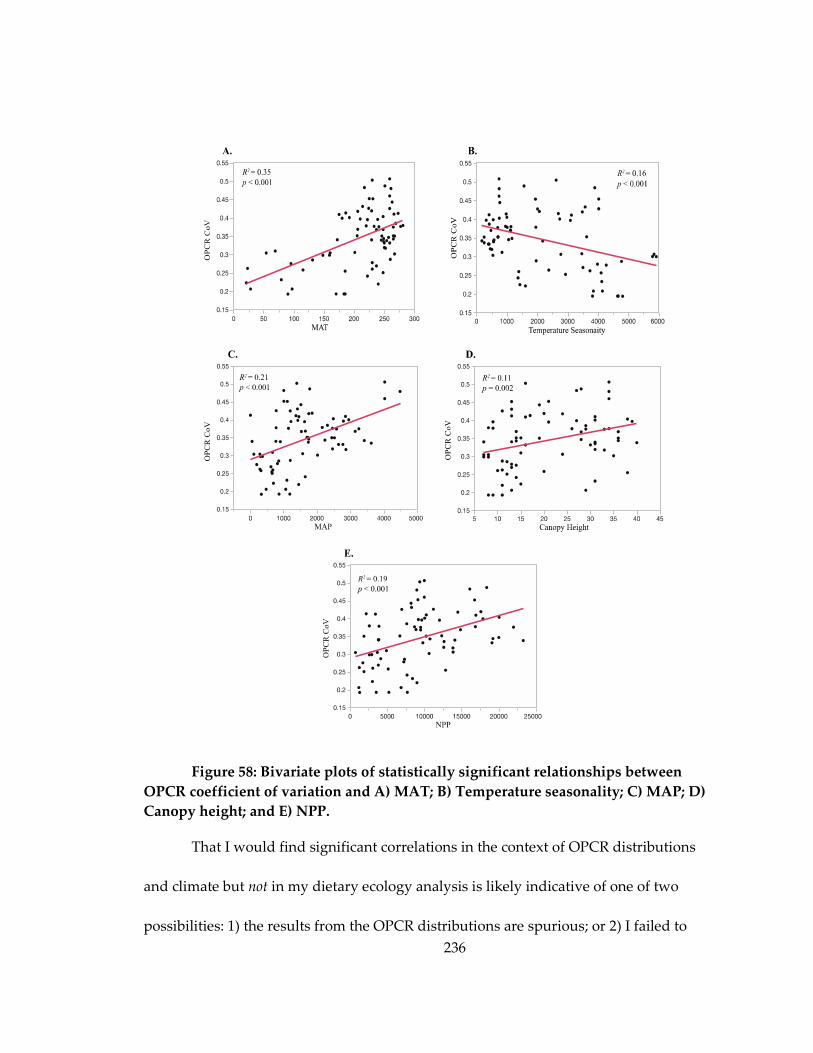
236
Figure 58: Bivariate plots of statistically significant relationships between
OPCR coefficient of variation and A) MAT; B) Temperature seasonality; C) MAP; D)
Canopy height; and E) NPP.
That I would find significant correlations in the context of OPCR distributions
and climate but not in my dietary ecology analysis is likely indicative of one of two
possibilities: 1) the results from the OPCR distributions are spurious; or 2) I failed to

237
detect a dietary signal in OPCR due to coarse data on diet in rodents. I introduced the
first possibility in the discussion of DNE above, pointing to the fact that the small
number of significant correlations associated with the distributions of DNE could be due
to chance. However, the large number of significant correlations in association with
OPCR, and the fact these correlations are consistent regardless of the type of
distributions statistic analyzed, suggests that this is almost certainly not the case for
OPCR. The more likely explanation is that OPCR does in fact have a relationship with
diet that I was unable to pick up in my ecomorphological analysis. This latter
explanation would seemingly provide support to the conclusions of Evans et al. (2007)
and Evans and Jernvall (2009), but it is nevertheless intriguing that I was unable to find
significant correlations despite using very similar dietary categories as these two studies.
One reason for this may be that I have a much broader taxonomic sample than Evans et
al. (2007), who sampled rodents only from the superfamily Muroidea, whereas I have
representatives from three different suborders; Hystricomorpha (the caviomorphs in my
sample), Sciuromorpha (the sciurids), and Myomorpha (the sigmodontine rats and
mice). As discussed above, it may be that occlusal topography carries with it a strong
phylogenetic signal. On the other hand, many of these rodent families are sympatric,
and likely avoid competition through niche separation. This introduces the possibility
that the phylogenetic signal and the ecological signal may be intertwined, as specific
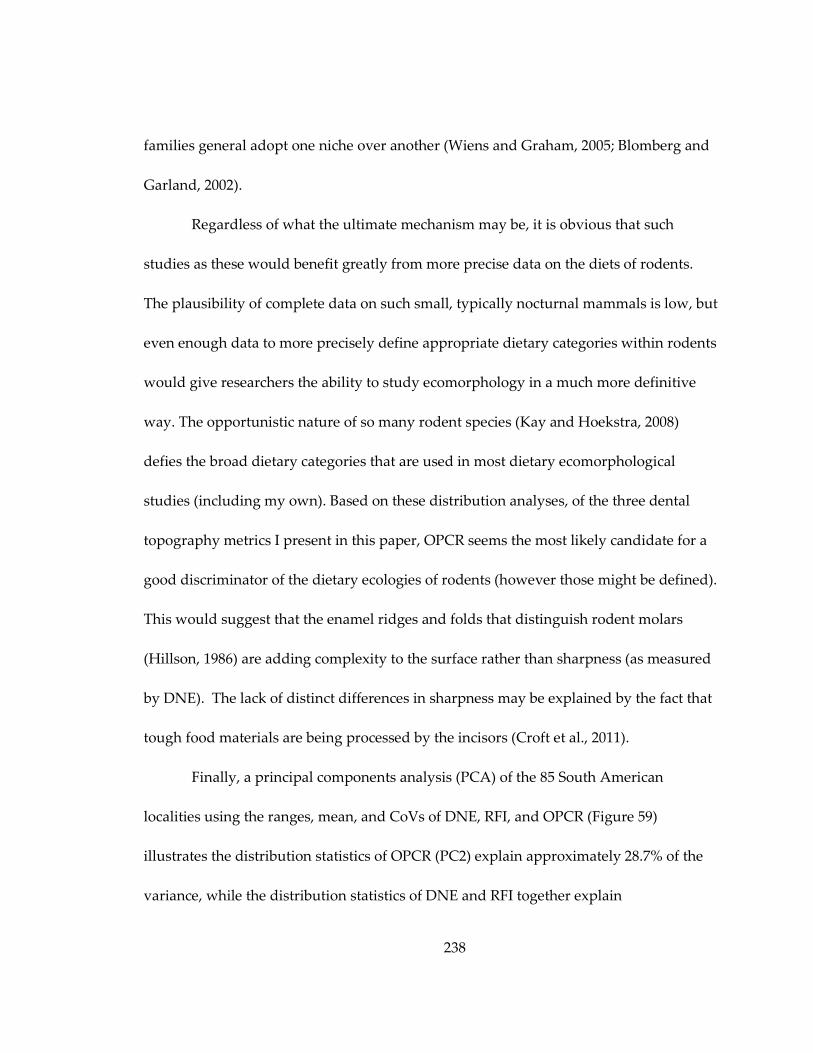
238
families general adopt one niche over another (Wiens and Graham, 2005; Blomberg and
Garland, 2002).
Regardless of what the ultimate mechanism may be, it is obvious that such
studies as these would benefit greatly from more precise data on the diets of rodents.
The plausibility of complete data on such small, typically nocturnal mammals is low, but
even enough data to more precisely define appropriate dietary categories within rodents
would give researchers the ability to study ecomorphology in a much more definitive
way. The opportunistic nature of so many rodent species (Kay and Hoekstra, 2008)
defies the broad dietary categories that are used in most dietary ecomorphological
studies (including my own). Based on these distribution analyses, of the three dental
topography metrics I present in this paper, OPCR seems the most likely candidate for a
good discriminator of the dietary ecologies of rodents (however those might be defined).
This would suggest that the enamel ridges and folds that distinguish rodent molars
(Hillson, 1986) are adding complexity to the surface rather than sharpness (as measured
by DNE). The lack of distinct differences in sharpness may be explained by the fact that
tough food materials are being processed by the incisors (Croft et al., 2011).
Finally, a principal components analysis (PCA) of the 85 South American
localities using the ranges, mean, and CoVs of DNE, RFI, and OPCR (Figure 59)
illustrates the distribution statistics of OPCR (PC2) explain approximately 28.7% of the
variance, while the distribution statistics of DNE and RFI together explain

239
approximately 30% of the variance. The distributions of OPCR are particularly effective
at segregating the tropical localities (green diamonds)—i.e., localities within 23.43°N and
23.43°S latitude—and subtropical localities (red x’s). In fact, on the second component
axis, those subtropical localities that cluster with the majority of the tropical localities are
the five subtropical sites that have the highest mean annual precipitation and net
primary productivity.
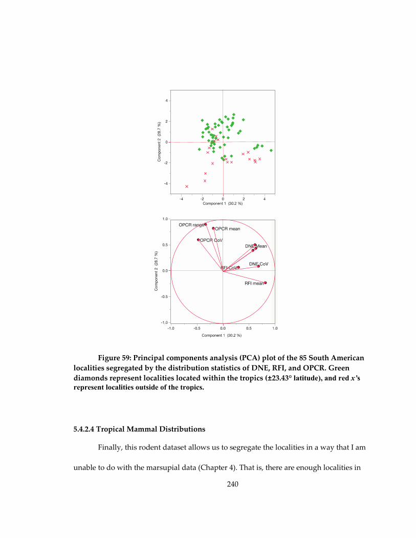
240
Figure 59: Principal components analysis (PCA) plot of the 85 South American
localities segregated by the distribution statistics of DNE, RFI, and OPCR. Green
diamonds represent localities located within the tropics (±23.43° latitude), and red x’s
represent localities outside of the tropics.
5.4.2.4 Tropical Mammal Distributions
Finally, this rodent dataset allows us to segregate the localities in a way that I am
unable to do with the marsupial data (Chapter 4). That is, there are enough localities in
241
this dataset to do analyses that are wholly confined to the tropics. After running
analyses equivalent to those above in the wholly tropical dataset (and excluding sites of
elevation >1500m), I find no significant correlations between distributions of any of the
ecometrics and environment. This once again speaks to the generalist nature of rodents,
suggesting that dietary niche is a much harder notion to define in rodents.
5.4.3 Combining Ecometrics and Regression Techniques
Rodents are near ubiquitous in mammalian fossil records for much of the
Cenozoic after their appearance in the early Eocene (Antoine et al., 2011)—and there is
particularly great potential in their use as environmental and climatic proxies (Montuire
et al., 1997; Kay et al., 1999; Aguilar et al., 1999; Montuire et al., 2006). Another analysis
that is made possible by the size of this rodent dataset is a revisit of the regression
methods used in Chapter 2. For this purpose I include the means, ranges, and CoVs of
DNE, RFI, and OPCR to estimate five bioclimate variables (all of the variables included
in Chapter 2 except precipitation seasonality, which from my results clearly does not
model well). The error metrics—mean absolute error (MAE) and root mean squared
error (RMSE)—of these analyses are presented in Table 30 and the correlations of
estimated values and actual observed values are illustrated in Figures 46-50.
In general, my results (Table 30) from using these distributions of dental
topography are comparable to the results from Chapter 2 in which I use ecological
indices of entire mammalian faunas, though the error terms are slightly higher for the

242
rodent distributions. Much like my findings in Chapter 2, the non-parametric regression
methods—including regression tree analysis (RTA), random forests (RF), and Gaussian
process regression (GPR)—show lower MAE and RMSE than the multivariate linear
regression. This is reflected in the correlation coefficients of estimated vs. observed
values. The two exceptions to the comparability of the results from rodent dental
topography distributions and ecological indices are the high error terms for GPR for
temperature seasonality and NPP. Because the output of GPR is not readily illustrated, it
is difficult to explain these results, particularly because the other regression techniques
do not show such high error.
That the use of rodent dental topography distributions performs approximately
as well as a large number of ecological indices associated with entire mammalian faunas
is remarkable. In the context of paleoenvironment reconstruction (the ultimate focus of
this dissertation), using distributions of quantitative measurements taken directly from
teeth would allow researchers to bypass the assumptions that have to be made in using
ecological indices; namely that behavioral reconstructions of extinct species are accurate
(e.g. Kay and Madden, 1997; Croft, 2001; Kay et al., 2012). This is not to say that such
behavioral reconstructions are misguided or poorly done, but they do nevertheless
introduce a possible source of error, as well as delay paleoenvironmental reconstructions
until every species has been studied.
243
5.5 Conclusions
Using three dental topography metrics of occlusal sharpness (Dirichlet normal
energy; DNE), relief (relief index; RFI), and complexity (orientation patch count rotated;
OPCR), and the natural log of molar area, I attempt to correlate dental topography of
lower M2s and dietary ecology in a broad taxonomic sample of South American rodents.
My results from these analyses suggest that rodent dental topography is not generally a
good discriminator of rodent diets, as phylogenetically-corrected ANOVAs reveal no
statistically significant relationships. However, post-hoc tests reveal some noteworthy
trends in my sample when corrected for the effects of phylogeny:
1. Grazing rodents tend to have much higher dental relief (mean RFI = 0.69)
relative to rodents inhabiting other ecological niches (p < 0.001).
2. Herbivorous rodent species—frugivores, folivores, and grazers—tend
towards higher DNE values than more omnivorous species. Visual inspection
of these molars suggests that this increase in sharpness is being driven by the
presence of long ridges of enamel on the occlusal surface relative to the more
omnivorous species in my sample.
A discriminant function analysis also reveals that using all three metrics in
conjunction with the natural log of molar area results in a predictive model that
performs significantly better than chance.
244
I also include a correlative analysis of the distributions of these metrics across a
large number of localities in South America, specifically with regard to a number of
variables associated with climate and habitat. This analysis reveals that the distribution
of OPCR has the strongest association with environment. I postulate that this signifies a
potential ecological signal of OPCR that I was unable to detect in the ecomorphological
analyses, though more precise dietary data is likely the only avenue to confirm this
hypothesis. My results also indicate that disparity in rodent dental topography increases
with wetter, warmer, more productive conditions. Finally, I also use the distribution
statistics from this analysis in conjunction with sophisticated regression techniques—
including machine-learning algorithms—to demonstrate that such distributions can be
used in place of qualitative ecological indices, such as I use in Chapter 2.
6. Summary
Several important outcomes of this dissertation are:

245
1) I find that dental topography metrics are correlated with dietary ecology in
small South American and Australian marsupial and rodent species, extending previous
published findings for primates; and
2) When the distributions of the dental ecomorphology metrics are compiled for
extant South American and Australian communities of rodents they provide a powerful
proxy for climate and habitat.
The first finding is important because these orders were important contributors
to mammalian faunal diversity in the Miocene of South America and therefore open a
window for the study of extinct species. The value of the second finding is that the
utilization of distributions of quantitative measurements obviates the need for precise
reconstruction of behavior in extinct species, a potential source of error in any
paleoecological analysis. As long as a measurement is demonstrated to be ecologically
relevant, then the distribution of that measurement within a community of species can
potentially be used as a summary of the ecological niches filled within a given
ecosystem.
6.1 Summary of Results
In Chapter 2, I begin with a review of community-level paleoenvironment
reconstruction using mammals and the various statistical approaches that have been
employed to do so. Using data compiled from long-term field studies of extant small
246
South American and Australian/New Guinean marsupials and South American rodents,
I compile a complete species-level dataset of non-volant mammals from 85 localities
from across South America. Long-term field sites of relatively small size were preferred
in this list for two reasons; 1) faunal lists compiled from overlapping species distribution
maps were deemed to be too unreliable, particularly in the tropics of South America
where regional species richness is extraordinarily high and demarcation of species
ranges is poorly documented; and 2) short-term field studies may fail to observe rare
species that are nonetheless important to the ecosystem. Both of these points are
particularly problematic for small mammal species, which can be difficult to observe
and study in the wild.
The ecologies of each species each faunal list were compiled and expressed as
ecological indices to quantitatively describe the niche space of the community, i.e. the
types and relative number of niches filled within any given community. Different niche
measurements that may be related to the environment at that locality, include, for
example, the relative number of arboreal species, frugivorous species, and grazing
species, and the ratio of predators to prey species. Using these indices as my predictor
variables and six bioclimatic variables—precipitation (MAP), temperature (MAT),
temperature seasonality, precipitation seasonality, net primary productivity (NPP),
canopy height—as my response variables, I produced a number of regression models
from the South American communities. The regression techniques include machine-

247
learning algorithms—regression trees, random forests, and Gaussian process
regression—that can allow non-linear relationships to be modeled more accurately. The
models were based on the South American faunas. To test the general applicability of
models derived from South American localities, I estimate climate variables in
Australian and New Guinean localities. Australia/New Guinea was chosen as a test
region because it represents a geographically and phylogenetically distinct region from
South America that spans a similar range of latitude and a similarly broad ecological
spectrum. My results indicate that ecological indices from the South American model
can be used to estimate climate variables, and that the machine-learning algorithms are
particularly powerful tools of analysis.
I conclude this chapter by applying the findings from the extant communities to
the reconstruction of the bioclimatic variables in two particularly well known Miocene
fossil communities in South America; the Middle Miocene ‘Monkey Beds Fauna’ of La
Venta, Colombia and the Early Miocene Faunal Levels 1-7 in the Santa Cruz Formation
of Argentina. My estimations are generally in line with previous paleoecological
analyses of these two deposits. This represents the first time that such algorithms have
been used for this purpose.
In Chapter 3, I lay a methodological foundation for the type of data collection
and analysis I use in Chapters 4 and 5. This is because in Chapters 4 and 5, I examine the
correlation between dental topography and dietary ecology utilizing three specific
248
metrics of dental topography; Dirichlet normal energy (DNE), orientation patch count
rotated (OPCR), and relief index (RFI), each of which is taken from 3D meshes
representing the occlusal surfaces of teeth. These 3D meshes are produced from microCT
scans taken of skulls, mandibles, and/or epoxy dental casts, and the digitial preparation
of these meshes—namely downsampling the number of faces that represent the surface
and smoothing that surface—can have a significant impact on the values of these
metrics. These effects have been previously studied in regards to both OPCR and RFI,
but not as well in regards to DNE. Therefore, Chapter 3 presents a brief analysis of the
effect of downsampling and smoothing—together termed “retriangulation”—on the
measurement of DNE. As DNE is essentially a measure of the sharpness of a surface,
smoothing in particular has the potential to drastically alter this measurement. Starting
with a simple hemisphere, the easiest geometric shape on which to measure DNE, I test
how retriangulation affects DNE values. My results indicate that the degree of
smoothing is inversely related to the values of DNE, and that the inclusion of more
‘aggressive’ smoothing algorithms—as has been done in some previously published
studies incorporating DNE—exacerbates this effect. Downsampling—i.e. decreasing the
number of triangular faces used to represent the surface, a necessary step for
computation—has a less dramatic effect, and my results suggest that a surface with
10,000 faces will have approximately the same DNE value as one with 20,000 or 30,000
faces. Given that current software programs are not typically able to handle surfaces of
249
20,000 or more faces, I propose that using 10,000 faces is a reasonable standard going
forward as it represents a sufficient compromise between faithfulness of surface
representation and computational speed. These conclusions guide my protocol decisions
for the next two chapters.
In Chapter 4, I explore the relationship between the above-mentioned dental
topography and the dietary ecology in South American and Australian/New Guinean
marsupials. This chapter anticipates the application of my results to the pre-Interchange
Miocene faunas of South America when marsupials were especially diverse and filled
many niches now occupied by Carnivora. I employ a phylogenetically-corrected one-
way ANOVA to test for the effect of diet on the mean values of DNE, OPCR, and RFI.
Results from this test suggest that, after controlling for phylogeny, diet has a significant
effect on DNE (p < 0.01). RFI has a correlation that is trending towards significance (p =
0.036, with a Bonferroni-corrected alpha level of 0.019). OPCR does not have a
significant relationship with diet in my marsupial sample. Post-hoc tests suggest that
frugivores have significantly lower values in DNE and RFI relative to other dietary
categories. A discriminant function analysis correctly identified dietary groups at a rate
of ~75%, and a principal components analysis suggests that M2s with higher RFI and
higher DNE are related to dietary ecologies associated with tougher food materials
(particularly folivores and insectivores). Having demonstrated that dental topography is
informative in marsupials’ dietary ecology, I move on to compile the distributions of

250
dental topography metrics in faunas from across Australia and New Guinea. I calculate
the mean, range, coefficient of variation, and skewness of the distribution of each metric
in 17 marsupial faunas and correlate these statistics with the same six bioclimatic
variables in Chapter 2. ANOVAs performed on these correlations revealed that the
distributions of RFI had the most significant correlations with environment, including
MAP, NPP, and canopy height. The mean and coefficient of variation of RFI together
suggest that these results are associated with a greater number of arboreal frugivores in
wetter, more productive habitats with taller canopies. This suggest that the distribution
of a topographic measurement alone can give similar information as ecological indices.
In Chapter 5, I perform an equivalent analysis to Chapter 4, except with a
taxonomically-broad sample of South American rodents, including caviomorphs
(Rodentia: Hystricognathi: Caviomorpha), sciurids (Rodentia: Sciuromorpha: Sciuridae),
and sigmodontines (Rodentia: Muroidea: Cricetidae). Rodents are especially specious on
the South American continent—both in the Miocene and today—and the sample I
present in Chapter 5 samples most of this diversity. For rodents, unlike for marsupials,
DNE does not seem to correspond as well to dietary ecology in rodents. RFI is especially
high in grazing species, but otherwise does not differentiate will between diets. Similar
to the results in marsupials, OPCR does not seem to correlate well with diet. However,
analyzing the distributions of these metrics across the South American localities
presented in Chapter 2, we see that the distribution of OPCR has a surprisingly

251
significant association with environment. I believe that this likely reflects a dietary signal
in OPCR that is lost in the necessarily coarse dietary categories (on account of the poor
quality of dietary information) used in the rodent analyses. The large number of
localities in this chapter also allowed me to use the machine-learning regression
techniques I present in Chapter 2, and the error metrics associated with using rodent
dental ecometrics in place of whole-fauna ecological indices are reasonably close to what
I found with the ecological indices. I conclude this chapter by discussing the significance
of using rodent dental topography distributions to reconstruct climate and habitat.
6.1.1 Conclusions
Viewing these results in concert, it is clear that community structure is at least in
part driven by environment, and as such, the structure can be used to estimate specific
aspects of the environment, now and in the past. This has been demonstrated in
previous studies, though I demonstrate the power of machine-learning algorithms,
which can minimize the error in these estimations. Random forests and Gaussian
process regression models seem especially effective at minimizing error relative to other
techniques. I also demonstrate that by utilizing ecologically relevant morphology—in
this case dental topography—we can construct distributions that serve as useful proxies
for the abundance and disparity of niches filled within a faunal system. The dental
topography metrics that I utilize here—OPCR, DNE, and RFI—are particularly useful as
they do not rely on the identification of homologous landmarks, and instead can

252
quantify whole tooth surfaces. This can allow paleoecologists to collect large amounts of
useful data in extinct species that are frequently only represented by isolated teeth or
jaws. While the scanning of surfaces can be time-consuming and costly, online archives
of 3D surfaces are making data more readily available. This increases the feasibility of
this kind of community-level analysis.
6.1.2 Species Sampling
As with any study, even a brief retrospective can elucidate the way my study
design could be improved. An obvious place to begin would be with the sampling
protocol of living faunas and dental specimens, as it would be ideal to 1) increase the
number of specimens per species, to ensure that species averages are accurate
representations of the true species mean; and 2) obtain a more complete sample of
Australian/New Guinean marsupials and South American rodents. Though given the
restrictions on time and resources the sample is fairly exhaustive, where are several
major holes in the data set. For instance, I was unable to obtain any usable specimens of
the rodent family Octodontidae, which is restricted to the southwest of the South
American continent. This is in large part due to the difficulty in obtaining access to
specimens of particularly rare species, as well as time and financial constraints related to
CT scanning.
253
6.2 Future Directions
The obvious next step for this line of research is the application to the fossil
record, namely the fossil localities that are mentioned explicitly throughout my chapters;
La Venta and the Santa Cruz. This requires the scanning of the marsupial and rodent
fossil teeth from these localities. While obtaining fossil specimens is frequently a difficult
task, original specimens from these two localities are housed in several museums in the
United States and readily accessible collections in Argentina, and there are a number of
casts housed at Duke University. Given the results of Chapter 5, I would expect that the
regressions using ecometric distributions as predictor variables should mirror those of
regressions using ecological indices, and in turn mirror the conclusions of previous
paleoecological analyses at these sites. However, this would serve as a valuable first
application for this method beyond the proof-of-concept approach of this dissertation.
Related to this is the inclusion of other types of morphological data in the models
for better representation of niche structure at a locality. One obvious approach is to
measure morphologies associated with locomotion. A commonly preserved postcranial
element in the fossil record is the calcaneus, and research has suggested that locomotion
in mammals can be reconstructed using simple ratios of linear measurements in the
calcaneus (Polly, 2010). Likewise, articular facets on the other ankle bone, the astragalus,
can be used to represent body size more accurately than molar size (Yapuncich et al.,

254
2015). Ultimately, direct measurements of fossils can potential replace ecological indices
entirely for the purposes of paleoenvironmental reconstruction.
Additionally, the inclusion of a similar analysis of primate distributions might
provide the ability to discern finer scale differences in tropical habitats, as primates have
their greatest species richness in the topics. Based on previously published data on the
dental topography of primates, the easiest datasets to complete would be that for the
platyrrhines—only the callitrichines have not been broadly sampled and I have already
have geographic/climatic data for a good deal of faunas that include primates in South
America—and/or the strepsirrhines of Madagascar.
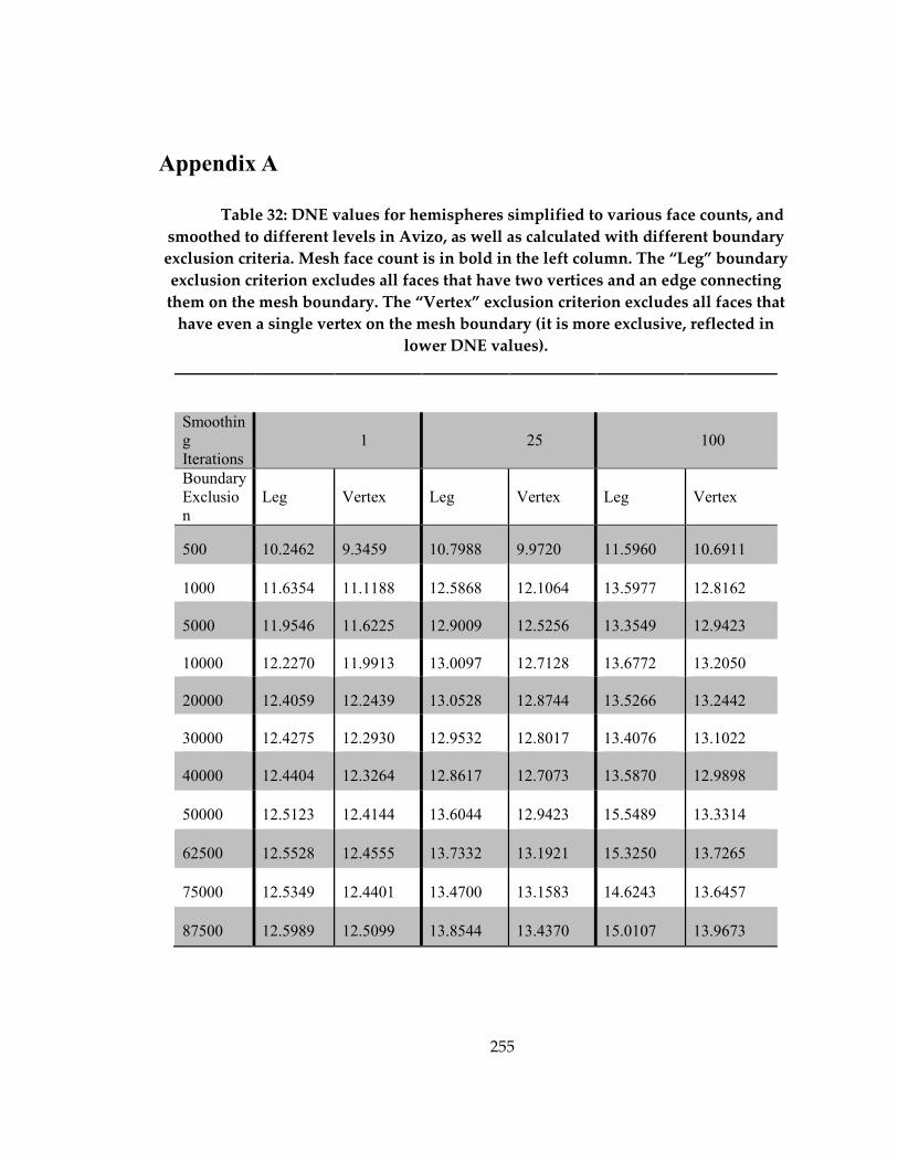
255
Appendix A
Table 32: DNE values for hemispheres simplified to various face counts, and
smoothed to different levels in Avizo, as well as calculated with different boundary
exclusion criteria. Mesh face count is in bold in the left column. The “Leg” boundary
exclusion criterion excludes all faces that have two vertices and an edge connecting
them on the mesh boundary. The “Vertex” exclusion criterion excludes all faces that
have even a single vertex on the mesh boundary (it is more exclusive, reflected in
lower DNE values).
Smoothin
g
Iterations
1 25 100
Boundary
Exclusio
n
Leg Vertex Leg Vertex Leg Vertex
500 10.2462 9.3459 10.7988 9.9720 11.5960 10.6911
1000 11.6354 11.1188 12.5868 12.1064 13.5977 12.8162
5000 11.9546 11.6225 12.9009 12.5256 13.3549 12.9423
10000 12.2270 11.9913 13.0097 12.7128 13.6772 13.2050
20000 12.4059 12.2439 13.0528 12.8744 13.5266 13.2442
30000 12.4275 12.2930 12.9532 12.8017 13.4076 13.1022
40000 12.4404 12.3264 12.8617 12.7073 13.5870 12.9898
50000 12.5123 12.4144 13.6044 12.9423 15.5489 13.3314
62500 12.5528 12.4555 13.7332 13.1921 15.3250 13.7265
75000 12.5349 12.4401 13.4700 13.1583 14.6243 13.6457
87500 12.5989 12.5099 13.8544 13.4370 15.0107 13.9673

256
Appendix B
Gaussian process regression (GPR) is a non-linear, non-parametric, Bayesian
regression technique. Originally developed as “kriging” in the field of geostatistics, GPR
has not seen wide application in ecology or paleoecology (Golding, 2016), but is
nonetheless useful in these applications because of its expressiveness and flexibility.
GPR can be viewed as an extension of simple linear regression.
Equation 2
���� = �⊺�, = ���� + �
Here, xΤw is a dot product between a transposed vector of dependent variables,
xΤ, and their associated weights, w. The error term ε is modeled as a Gaussian
distribution. Thus, the likelihood function (i.e., fit of model to the data given the
weights) is given as:
Equation 3
�|�, �� = � ��|�� , ���
���, � ~ ����⊺�, ���
where σε is the variance of the error term.
Further, the distribution of the linear regression coefficients or weights (w) is
given a multivariate Gaussian distribution:
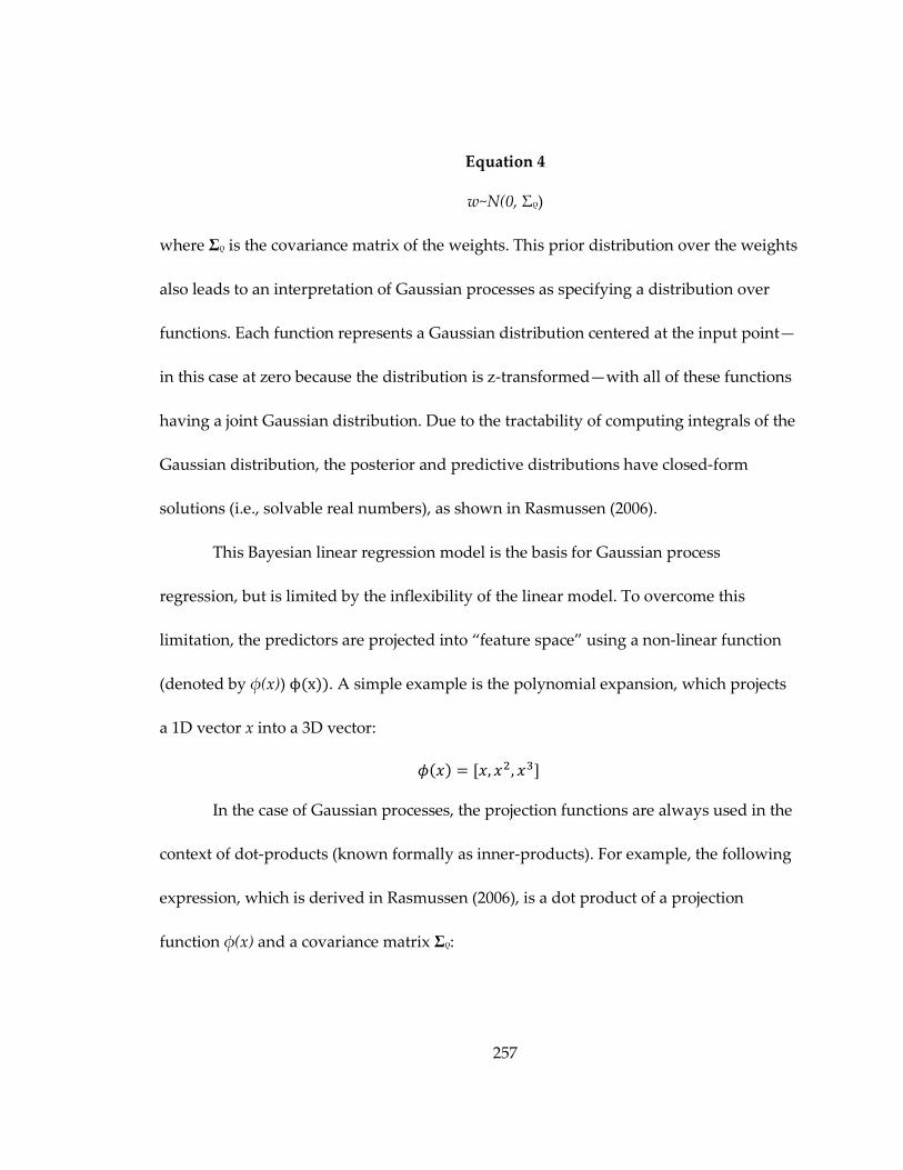
257
Equation 4
w~N(0, Σρ)
where Σρ is the covariance matrix of the weights. This prior distribution over the weights
also leads to an interpretation of Gaussian processes as specifying a distribution over
functions. Each function represents a Gaussian distribution centered at the input point—
in this case at zero because the distribution is z-transformed—with all of these functions
having a joint Gaussian distribution. Due to the tractability of computing integrals of the
Gaussian distribution, the posterior and predictive distributions have closed-form
solutions (i.e., solvable real numbers), as shown in Rasmussen (2006).
This Bayesian linear regression model is the basis for Gaussian process
regression, but is limited by the inflexibility of the linear model. To overcome this
limitation, the predictors are projected into “feature space” using a non-linear function
(denoted by ϕ(x)) ϕ�x��. A simple example is the polynomial expansion, which projects
a 1D vector x into a 3D vector:
���� = [�, ��, ��]
In the case of Gaussian processes, the projection functions are always used in the
context of dot-products (known formally as inner-products). For example, the following
expression, which is derived in Rasmussen (2006), is a dot product of a projection
function ϕ(x) and a covariance matrix Σρ:
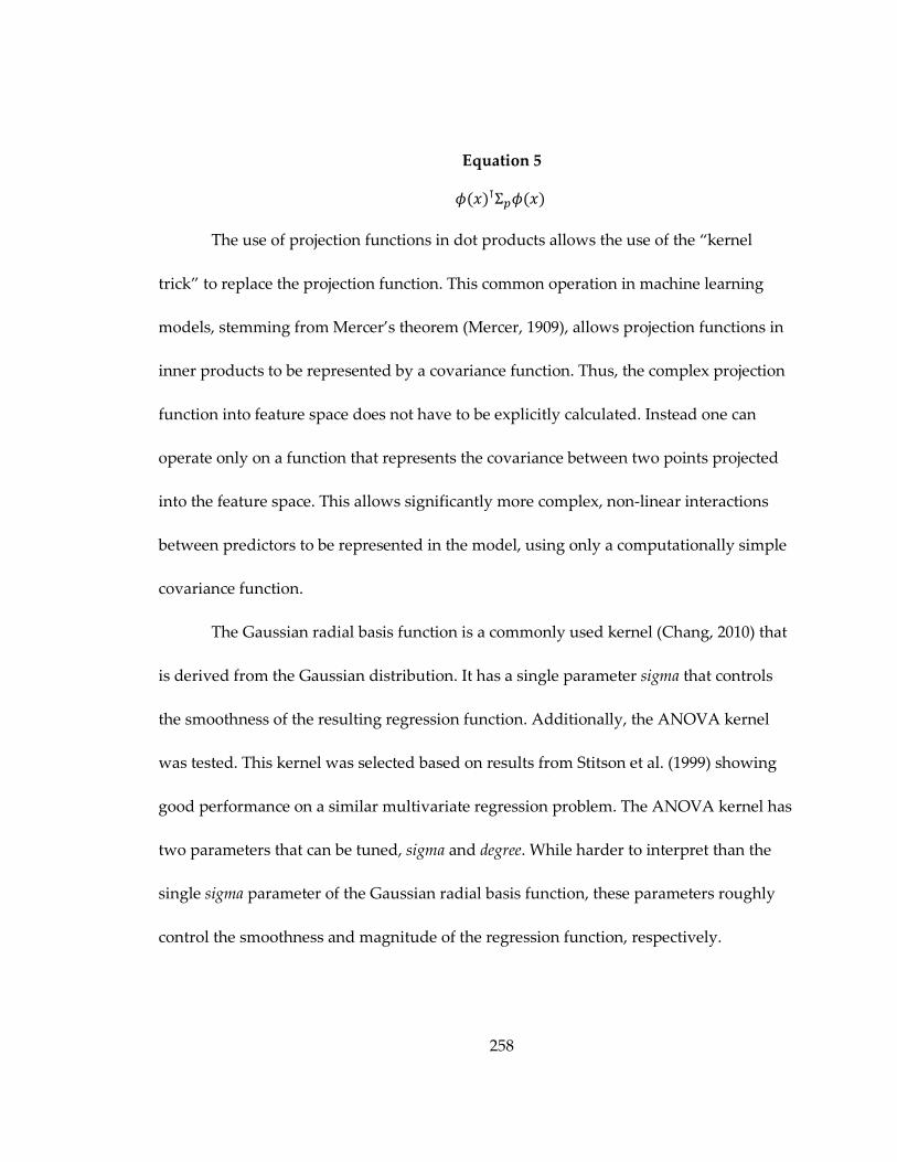
258
Equation 5
����⊺Σ!����
The use of projection functions in dot products allows the use of the “kernel
trick” to replace the projection function. This common operation in machine learning
models, stemming from Mercer’s theorem (Mercer, 1909), allows projection functions in
inner products to be represented by a covariance function. Thus, the complex projection
function into feature space does not have to be explicitly calculated. Instead one can
operate only on a function that represents the covariance between two points projected
into the feature space. This allows significantly more complex, non-linear interactions
between predictors to be represented in the model, using only a computationally simple
covariance function.
The Gaussian radial basis function is a commonly used kernel (Chang, 2010) that
is derived from the Gaussian distribution. It has a single parameter sigma that controls
the smoothness of the resulting regression function. Additionally, the ANOVA kernel
was tested. This kernel was selected based on results from Stitson et al. (1999) showing
good performance on a similar multivariate regression problem. The ANOVA kernel has
two parameters that can be tuned, sigma and degree. While harder to interpret than the
single sigma parameter of the Gaussian radial basis function, these parameters roughly
control the smoothness and magnitude of the regression function, respectively.
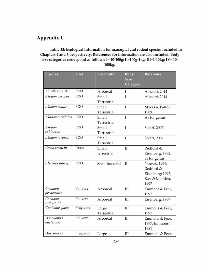
259
Appendix C
Table 33: Ecological information for marsupial and rodent species included in
Chapters 4 and 5, respectively. References for information are also included. Body
size categories correspond as follows: I= 10-100g; II=100g-1kg; III=1-10kg; IV= 10-
100kg.
Species Diet Locomotion Body
Size
Category
Reference
Abrothrix jelskii PDO Arboreal I Alhajeri, 2014
Akodon aerosus PDO Small
Terrestrial
I Alhajeri, 2014
Akodon mollis PDO Small
Terrestrial
I Myers & Patton,
1989
Akodon orophilus PDO Small
Terrestrial
I As for genus
Akodon
subfuscus PDO Small
Terrestrial
I Solari, 2007
Akodon torques PDO Small
Terrestrial
I Solari, 2007
Cavia tschudii Grass Small
terrestrial
II Redford &
Eisenberg, 1992;
as for genus
Clyomys laticeps PDO Semi-fossorial II Nowak, 1991;
Redford &
Eisenberg; 1992;
Kay & Madden,
1997
Coendou
prehensilis Folivore Arboreal III Emmons & Feer,
1997
Coendou
rothschildi Folivore Arboreal III Eisenberg, 1989
Cuniculus paca Frugivore Large
Terrestrial
III Emmons & Feer,
1997
Dactylomys
dactylinus Folivore Arboreal II Emmons & Feer,
1997; Emmons,
1981
Dasyprocta Frugivore Large III Emmons & Feer,
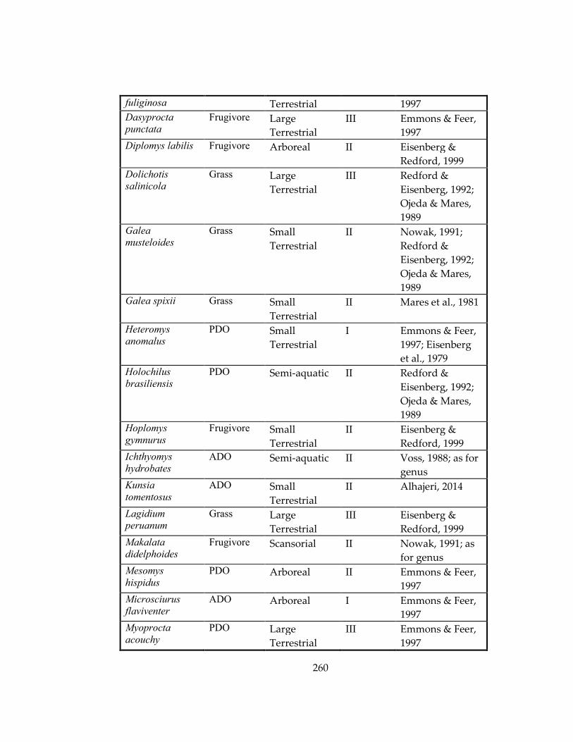
260
fuliginosa Terrestrial 1997
Dasyprocta
punctata Frugivore Large
Terrestrial
III Emmons & Feer,
1997
Diplomys labilis Frugivore Arboreal II Eisenberg &
Redford, 1999
Dolichotis
salinicola Grass Large
Terrestrial
III Redford &
Eisenberg, 1992;
Ojeda & Mares,
1989
Galea
musteloides Grass Small
Terrestrial
II Nowak, 1991;
Redford &
Eisenberg, 1992;
Ojeda & Mares,
1989 Galea spixii Grass Small
Terrestrial
II Mares et al., 1981
Heteromys
anomalus PDO Small
Terrestrial
I Emmons & Feer,
1997; Eisenberg
et al., 1979
Holochilus
brasiliensis PDO Semi-aquatic II Redford &
Eisenberg, 1992;
Ojeda & Mares,
1989
Hoplomys
gymnurus Frugivore Small
Terrestrial
II Eisenberg &
Redford, 1999
Ichthyomys
hydrobates ADO Semi-aquatic II Voss, 1988; as for
genus
Kunsia
tomentosus ADO Small
Terrestrial
II Alhajeri, 2014
Lagidium
peruanum Grass Large
Terrestrial
III Eisenberg &
Redford, 1999
Makalata
didelphoides Frugivore Scansorial II Nowak, 1991; as
for genus
Mesomys
hispidus PDO Arboreal II Emmons & Feer,
1997
Microsciurus
flaviventer ADO Arboreal I Emmons & Feer,
1997
Myoprocta
acouchy PDO Large
Terrestrial
III Emmons & Feer,
1997
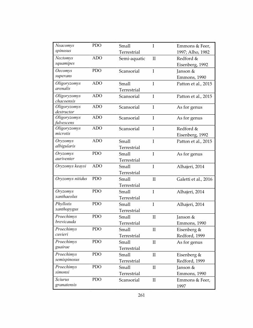
261
Neacomys
spinosus PDO Small
Terrestrial
I Emmons & Feer,
1997; Alho, 1982 Nectomys
squamipes ADO Semi-aquatic II Redford &
Eisenberg, 1992
Oecomys
superans PDO Scansorial I Janson &
Emmons, 1990
Oligoryzomys
arenalis ADO Small
Terrestrial
I Patton et al., 2015
Oligoryzomys
chacoensis ADO Scansorial I Patton et al., 2015
Oligoryzomys
destructor ADO Scansorial I As for genus
Oligoryzomys
fulvescens ADO Scansorial I As for genus
Oligoryzomys
microtis ADO Scansorial I Redford &
Eisenberg, 1992
Oryzomys
albigularis ADO Small
Terrestrial
I Patton et al., 2015
Oryzomys
auriventer PDO Small
Terrestrial
I As for genus
Oryzomys keaysi ADO Small
Terrestrial
I Alhajeri, 2014
Oryzomys nitidus PDO Small
Terrestrial
II Galetti et al., 2016
Oryzomys
xanthaeolus PDO Small
Terrestrial
I Alhajeri, 2014
Phyllotis
xanthopygus PDO Small
Terrestrial
I Alhajeri, 2014
Proechimys
brevicauda PDO Small
Terrestrial
II Janson &
Emmons, 1990
Proechimys
cuvieri PDO Small
Terrestrial
II Eisenberg &
Redford, 1999
Proechimys
guairae PDO Small
Terrestrial
II As for genus
Proechimys
semispinosus PDO Small
Terrestrial
II Eisenberg &
Redford, 1999
Proechimys
simonsi PDO Small
Terrestrial
II Janson &
Emmons, 1990 Sciurus
granatensis PDO Scansorial II Emmons & Feer,
1997
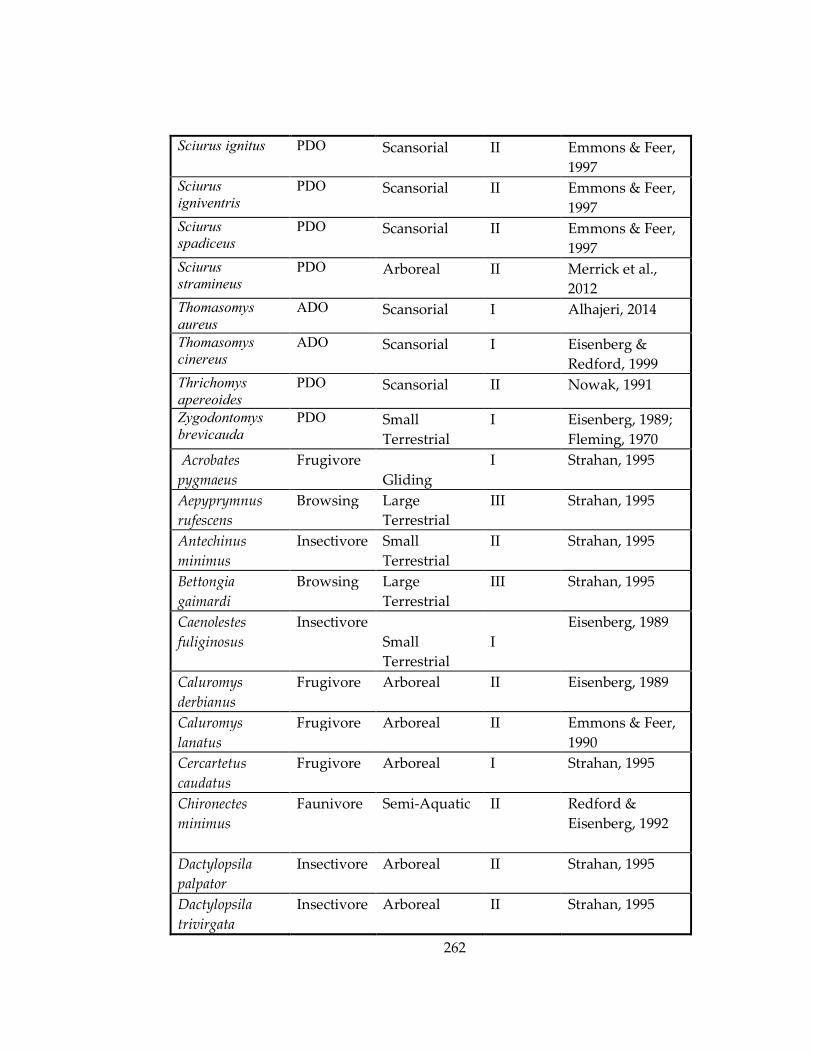
262
Sciurus ignitus PDO Scansorial II Emmons & Feer,
1997 Sciurus
igniventris PDO Scansorial II Emmons & Feer,
1997
Sciurus
spadiceus PDO Scansorial II Emmons & Feer,
1997
Sciurus
stramineus PDO Arboreal II Merrick et al.,
2012
Thomasomys
aureus ADO Scansorial I Alhajeri, 2014
Thomasomys
cinereus ADO Scansorial I Eisenberg &
Redford, 1999
Thrichomys
apereoides PDO Scansorial II Nowak, 1991
Zygodontomys
brevicauda PDO Small
Terrestrial
I Eisenberg, 1989;
Fleming, 1970
Acrobates
pygmaeus
Frugivore
Gliding
I Strahan, 1995
Aepyprymnus
rufescens
Browsing Large
Terrestrial
III Strahan, 1995
Antechinus
minimus
Insectivore Small
Terrestrial
II Strahan, 1995
Bettongia
gaimardi
Browsing Large
Terrestrial
III Strahan, 1995
Caenolestes
fuliginosus
Insectivore
Small
Terrestrial
I
Eisenberg, 1989
Caluromys
derbianus
Frugivore Arboreal II Eisenberg, 1989
Caluromys
lanatus
Frugivore Arboreal II Emmons & Feer,
1990
Cercartetus
caudatus
Frugivore Arboreal I Strahan, 1995
Chironectes
minimus
Faunivore Semi-Aquatic II Redford &
Eisenberg, 1992
Dactylopsila
palpator
Insectivore Arboreal II Strahan, 1995
Dactylopsila
trivirgata
Insectivore Arboreal II Strahan, 1995

263
Dasykaluta
rosamondae
Insectivore Small
Terrestrial
I Flannery, 1995
Dasyurus
hallucatus
Insectivore Scansorial II Strahan, 1995
Dendrolagus
lumholtzi
Folivore Scansorial III Strahan, 1995
Didelphis
albiventris
Frugivore Scansorial III Emmons & Feer,
1997; Ojeda &
Mares, 1989
Dorcopsis hageni Browsing Large
Terrestrial
III Flannery, 1995
Dorcopsis
luctuosa
Browsing Large
Terrestrial
III Flannery, 1995
Dorcopsulus
macleayi
Browsing Large
Terrestrial
III Flannery, 1995
Dromiciops
gliroides
Insectivore Arboreal I Fonturbel et al.,
2012
Hemibelideus
lemuroides
Folivore Arboreal II Strahan, 1995
Hypsiprymnodon
moschatus
Frugivore Small
Terrestrial
II Strahan, 1995
Isoodon obesulus Insectivore Small
Terrestrial
II Strahan, 1995
Macrotis lagotis Omnivore Semi-
Fossorial
III Strahan, 1995
Marmosa
mexicana
Insectivore
Scansorial
I Emmons & Feer,
1997
Marmosa murina Insectivore
Arboreal
I Emmons & Feer,
1997
Metachirus
nudicaudatus
Insectivore
Small
Terrestrial
II Emmons & Feer,
1997; Redford &
Eisenberg, 1992
Monodelphis
domestica
Insectivore
Small
Terrestrial
I Emmons & Feer,
1997; Redford &
Eisenberg, 1992;
Streilein, 1982
Peroryctes
raffrayana
Insectivore Small
Terrestrial
II Flannery, 1995
Petauroides Folivore III Strahan, 1995
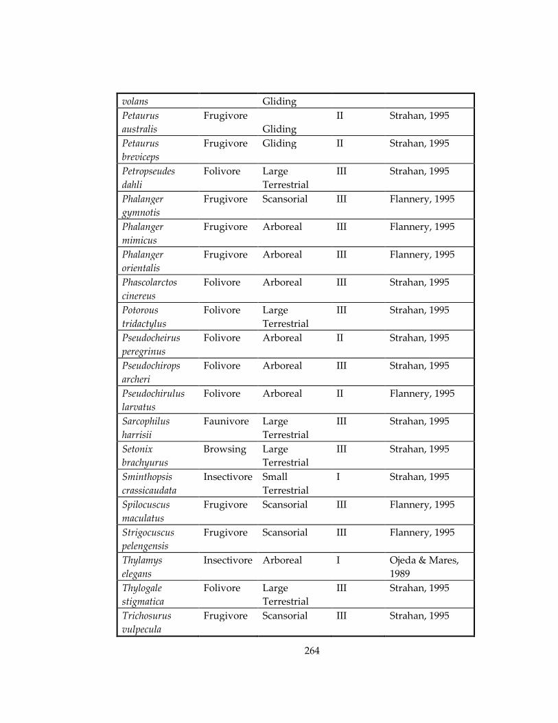
264
volans Gliding
Petaurus
australis
Frugivore
Gliding
II Strahan, 1995
Petaurus
breviceps
Frugivore Gliding II Strahan, 1995
Petropseudes
dahli
Folivore Large
Terrestrial
III Strahan, 1995
Phalanger
gymnotis
Frugivore Scansorial III Flannery, 1995
Phalanger
mimicus
Frugivore Arboreal III Flannery, 1995
Phalanger
orientalis
Frugivore Arboreal III Flannery, 1995
Phascolarctos
cinereus
Folivore Arboreal III Strahan, 1995
Potorous
tridactylus
Folivore Large
Terrestrial
III Strahan, 1995
Pseudocheirus
peregrinus
Folivore Arboreal II Strahan, 1995
Pseudochirops
archeri
Folivore Arboreal III Strahan, 1995
Pseudochirulus
larvatus
Folivore Arboreal II Flannery, 1995
Sarcophilus
harrisii
Faunivore Large
Terrestrial
III Strahan, 1995
Setonix
brachyurus
Browsing Large
Terrestrial
III Strahan, 1995
Sminthopsis
crassicaudata
Insectivore Small
Terrestrial
I Strahan, 1995
Spilocuscus
maculatus
Frugivore Scansorial III Flannery, 1995
Strigocuscus
pelengensis
Frugivore Scansorial III Flannery, 1995
Thylamys
elegans
Insectivore Arboreal I Ojeda & Mares,
1989
Thylogale
stigmatica
Folivore Large
Terrestrial
III Strahan, 1995
Trichosurus
vulpecula
Frugivore Scansorial III Strahan, 1995

265
Vombatus
ursinus
Browsing Large
Terrestrial
IV Strahan, 1995
Wallabia bicolor Browsing Large
Terrestrial
IV Strahan, 1995
Wyulda
squamicaudata
Folivore Scansorial III Strahan, 1995

266
References
Aguilar J-P, Escarguel G, and Michaux J. 1999. A succession of Miocene rodent
assemblages from fissure fillings in southern France: palaeoenvironmental
interpretation and comparison with Spain. Palaeogeography, Palaeoclimatology,
Palaeoecology 145: 215-230.
Aizen MA and Ezcurra C. 1998. High incidence of plant-animal mutualisms in the
woody flora of the temperate forest of southern South America: biogeographical
origin and present ecological significance. Ecologica Austral 8: 217-236.
Alhajeri B. 2014. Adaptation, Diversification, and Desert Ecology of the Most Diverse
Order of Mammals (Mammalia, Rodentia). Electronic Theses, Treatises and
Dissertations. Paper 8930.
Alho CJR. 1982. Brazilian rodents: their habitats and habits. Pymatuning Laboratory of
Ecology, University of Pittsburgh Special Publication Series 6: 143-166.
Allen KL, Cooke SB, Gonzales LA, and Kay, RF. 2015. Dietary inference from upper and
lower molar morphology in platyrrhine primates. PloS ONE 10(3): e0118732.
Andrews P, Lord JM, and Nesbit-Evans EM. 1979. Patterns of ecological diversity in
fossil and modern mammalian faunas. Biological Journal of the Linnean Society
11:177-205.
Andrews P and Hixson H. 2014. Taxon-free methods of palaeoecology. Annales
Zoologici Fennici: 269-284.
Andrews P and O’Brien EM. 2000. Climate, vegetation, and predictable gradients in
mammal species richness in southern Africa. Journal of Zoology 251:205-231.
Andrews P and Van Couvering JAH. 1975. Palaeoenvironments in the East African
Miocene. Approaches to Primate Paleobiology 5: 62-103.
Anthony MRL, and Kay RF. 1993. Tooth form and diet in ateline and alouattine
primates: reflections on the comparative method. American Journal of Science
283A:356-382.

267
Antoine PO, Marivaux L, Croft DA, Billet G, Ganerød M, Jaramillo C, Martin T,
Orliac MJ, Tejada J, Altamirano AJ, and Duranthon F. 2011. Middle Eocene
rodents from Peruvian Amazonia reveal the pattern and timing of caviomorph
origins and biogeography. Proceedings of the Royal Society: Biological Sciences:
279(1732): 1319-1326.
Ashby M. 1992. Materials selection in mechanical design. Oxford: Pregamon Press.
Ashton KG, Tracy MC, and de Queiroz A. 2000. Is Bergmann’s rule valid for mammals?.
The American Naturalist 156(4): 390-415.
Barke R and Lamb S. 2006. Late Cenozoic uplift of the Eastern Cordillera, Bolivian
Andes. Earth and Planetary Science Letters 249: 350-367.
Beard KC, Tong Y, Dawson MR, Wang J, and Huang X. 1996. Earliest complete dentition
of an anthropoid primate from the Late Middle Eocene of Shanxi Province,
China. Science 272: 82-85.
Behrensmeyer AK. 1982. Time resolution in fluvial vertebrate assemblages. Paleobiology
8(3): 211-227.
Behrensmeyer AK and Dechant-Boaz DE. The recent bones of Amboseli Park, Kenya, in
relation to East African paleoecology. Fossils in the making: vertebrate taphonomy
and paleoecology, pp. 72-92. University of Chicago Press, Chicago.
Behrensmeyer AK, Hook RW, Badgley CE, Boy JA, Chapman RE, Dodson P, Gastaldo
RA, Graham RW, Martin LD, Olsen PE, and Spicer RA. 1992. Paleoenvironmental
contexts and taphonomic nodes. In Terrestrial ecosystems through time: evolutionary
paleoecology of terrestrial plants and animals, pp. 15-136. University of Chicago
Press.
Berthaume MA. 2016. Food mechanical properties and dietary ecology. American
Journal of Physical Anthropology 159: S79-S104.
Black CC. 1963. A review of the North American Tertiary Sciuridae. Museum of
Comparative Zoology, Harvard Univesity Bulletin 130(3): 305-322.
Blackburn TM, Gaston KJ, and Loder N. 1999. Geographic gradients in body size: a
clarification of Bergmann’s rule. Diversity and Distributions 5(4): 165-174.

268
Blomberg SP and Garland T. 2002. Tempo and mode in evolution: phylogenetic inertia,
adaptation and comparative methods. Journal of Evolutionary Biology 15(6): 899-
910.
Borcard D, Gillet F, and Legendre P. 2011. Numerical Ecology With R, pp. 232-236.
Boyer DM. 2008. Relief Index of second mandibular molars is a correlate of diet among
prosimian primates and other euarchontan mammals. Journal of Human
Evolution 55:1118-1137.
Boyer DM, Seiffert ER, Gladman JT, and Bloch JI. 2013. Evolution and allometry of
calcaneal elongation in living and extinct primates. PloS one 8(7):e67792.
Brieman L. 2001. Random forests. Machine Learning 45(1): 5-32.
Bunn JM, Boyer DM, Lipman Y, St. Clair EM, Jernvall J, and Daubechies I. 2011.
Comparing Dirichlet normal surface energy of tooth crowns, a new technique of
moalr shape quantification for dietary inference, with previous methods in
isolation and in combination. American Journal of Physical Anthropology 145:
247-261.
Bunn JM, Ungar PS. 2009. Dental topography and diets of four old world
monkey species. American Journal of Primatology 71:466–477.
Cartelle C and Hartwig WC. 1996. A new extinct primate among the Pleistocene
megafauna of Bahia, Brazil. Proceedings of the National Academy of Sciences
USA 93: 6405-6409.
Cartmill M. 1974. Daubentonia, Dactylopsila, woodpeckers and klinorhynchy. In Prosimian
Biology (Martin RD, Doyle GA, Walker AC, eds.). Gerald Duckworth and Co.
Ltd., London, pp. 655-670.
Cerling TE, Wynn JG, Andanje SA, Bird MI, Korir DK, Levin NE, Mace W, Macharia
AN, Quade J, and Remien CH. 2011. Woody cover and hominin environments in
the past 6 million years. Nature 476: 51-56.
Chai T and Draxler RR. 2014. Root mean squared error (RMSE) or mean absolute error
(MAE)?—Arguments against avoiding RMSE in the literature. Geoscientific
Model Development 7: 1247-1250.

269
Chang YW, Hsieh CJ, Chang KW, Ringgaard M, and Lin CJ. 2010. Training and testing
low-degree Polynomial Data Mappings via Linear SVM. Journal of Machine
Learning Research 1471-1490.
Cheverud JM. 2001. A simple correction for multiple comparisons in interval mapping
genome scans. Heredity 87: 52-58.
Chew AE. 2009. Paleoecology of the early Eocene Willwood mammal fauna from the
central Bighorn Basin, Wyoming. Paleobiology 35(1): 13-31.
Chornogubsky L, Goin FJ, and Reguero M. 2009. A reassessment of Antarctic
polydolopid marsupials (middle Eocene, La Meseta Formation). Antarctic
Science 21(3): 285-297.
Churchfield S. 1990. The natural history of shrews. Cornell University Press.
Coley PD and Barone JA. 1996. Herbivory and plant defenses in tropical forests. Annual
Review of Ecology and Systematics 27: 305-335.
Colles A, Liow LH, and Prinzing A. 2009. Are specialists at risk under environmental
change? Neoecological, paleoecological and phylogenetic approaches. Ecology
Letters 12: 849-863.
Copes LE, Lucas LM, Thostenson JO, Hoekstra HE, and Boyer DM. 2016. A collection of
non-human primate computed tomography scans housed in MorphoSource, a
repository for 3D data. Scientific Data 3.
Conroy GC. 1987. Problems of body-weight estimation in fossil primates. International
Journal of Primatology 8(2): 115-137.
Croft DA. 2001. Cenozoic environmental change in South America as indicated by
mammalian body size distributions (cenograms). Diversity and Distributions 7:
271-287.
Croft DA. 2013. What constitutes a fossil mammal community in the early Miocene
Santa Cruz Formation?. Journal of Vertebrate Paleontology 33(2): 401-409.
Croft DA, Niemi K, and Franco A. 2011. Incisor morphology reflects diet in
caviomorph rodents. Journal of Mammalogy 92(4): 871-879.
270
Crompton AW. 1971. The origin of the tribosphenic molar. Early Mammals 50: 65-87.
Crompton AW, and Lumsden AGS. 1970. Functional significance of the therian molar
pattern. Nature 227:197-199.
Cutler DR, Edwards TC, Beard KH, Cutler A, Hess KT, Gibson J, and Lawler JJ. 2007.
Random forests for classification in ecology. Ecology 88(11): 2783-2792.
Dagosto M and Terranova CJ. 1992. Estimating the body size of Eocene primates: a
comparison of results from dental postcranial variables. International Journal of
Primatology 13(3): 307-344.
Damuth J. 1982. Analysis of the preservation of community structure in assemblages of
fossil mammals. Paleobiology 8(4): 434-446.
Damuth JD, Jablonski D, Harris JA, Potts R, Stucky RK, Sues HD, and Weishampel DB.
1992. Taxon-free characterization of animal communities. In Terrestrial ecosystems
through time: evolutionary paleoecology of terrestrial plants and animals, pp. 183-203.
Damuth JD and Janis CM. 2011. On the relationship between hypsodonty and feeding
ecology in ungulate mammals, and its utility in palaeoecology. Biological
Reviews 86(3): 733-758.
Danell K, Lundberg P, and Niemela P. 1996. Species richness in mammalian herbivores:
patterns in the boreal zone. Ecography 19:404-409.
Darwin C. 1859. The Origin of Species, Sixth Edition (1872). London: reprinted by D.
Appleton and Company.
De’ath G. 2002. Multivariate regression trees: a new technique for modeling species-
environment relationships. Ecology 83(4): 1105-1117.
De’ath G and Fabricius KE. 2000. Classification and regression trees: a powerful yet
simple technique for ecological data analysis. Ecology 81(11): 3178-3192.
Desbrun M, Meyer M, Schröder P, and Burr AH. 1999. Implicit fairing of
irregular meshes using diffusion and curvature flow. SIGGRAPH 99 (Conf.
Proc.): 317-324.

271
Dennis JC, Ungar PS, Teaford MF, and Glander KE. 2004. Dental topography and molar
wear in Alouatta palliata from Costa Rica. American Journal of Physical
Anthropology 125: 152-161.
Dunning J, Stewart D, Danielson B, Noon B, Root T, Lamberson R, and Stevens E. 1995.
Spatially explicit population models: current forms and future uses. Ecological
Applications 5: 3-11.
Duque-Caro H. 1990. Neogene stratigraphy, paleoceanography and paleobiogeography
in northwest South America and the evolution of the Panama Seaway.
Palaeogeography, Palaeoclimatology, Palaeoecology 77: 203-234.
Eisenberg JF. 1989. Mammals of the Neotropics, vol. 1. The northern neotropics: Panama,
Colombia, Venezuela, Guyana, Suriname, French Guiana. The University of Chicago
Press: London.
Eisenberg JF, O’Connell MA, and August PV. 1979. Density, productivity, and
distribution of mammals in two Venezuelan habitats. In Vertebrate ecology in the
northern Neotropics (JF Eisenberg, ed.), Smithsonian Institute Press: Washington,
D.C. pp. 187-207.
Eisenberg JF and Redford KH. 1999. Mammals of the Neotropics, vol. 2. The central
Neotropics: Ecuador, Peru, Bolivia, Brazil. The University of Chicago Press: London.
Elton CS. 2001. Animal Ecology. University of Chicago Press: Chicago, IL.
Emmons LH. 1981. Morphological, ecological, and behavioral adaptations for arboreal
browsing in Dactylomys dactylinus (Rodentia, Echimyidae). Journal of
Mammalogy 62(1): 183-189.
Emmons LH and Feer F. 1997. Neotropical rainforest mammals. A field guide, 2.
Engel SR, Hogan KM, Taylor JF, and Davis SK. 1998. Molecular systematics and
paleobiogeography of the South American sigmodontine rodents. Molecular
Biology and Evolution 15(1): 35-49.
Eronen JT, Polly PD, Fred M, Damuth J, Frank DC, Mosbrugger V, Scheidegger C,
Stenseth NC, and Fortelius M. 2010a. Ecometrics: the traits that bind the past and
present together. Integrative zoology 5(2): 88-101.

272
Eronen JT, Puolamäki K, Liu L, Lintulaakso K, Damuth J, Janis CM, and Fortelius M.
2010b. Precipitation and large herbivorous mammals II: application to fossil data.
Evolutionary Ecology Research 12(2): 235-248.
Evans AR and Janis CM. 2014. The evolution of high dental complexity in the horse
lineage. Annales Zoologici Fennici 51: 73-79.
Evans AR and Jernvall J. 2009. Patterns and constraints in carnivorans and rodent dental
complexity and tooth size. Journal of Vertebrate Paleontology 29: 92.
Evans AR and Sanson GD. 2003. The tooth of perfection: functional and spatial
constraints on mammalian tooth shape. Biological Journal of the Linnean
Society 78: 173-191.
Evans AR, Wilson GP, Fortelius M, and Jernvall J. 2007. High-level similarity of
dentitions in carnivorans and rodents. Nature 445: 78-81.
Feldkamp LA, Davis LC, and Kress JW. 1984. Practical cone-beam algorithm. Journal of
the Optical Society of America A 1(6): 612-619.
Flannery TF. 1995. Mammals of New Guinea. Reed, 1995.
Fleming TH. 1970. Notes on the rodent faunas of two Panamanian forests. Journal of
Mammalogy 51(3): 473-490.
Fleming TH. 1973. Numbers of mammalian species in north and central american forest
communities. Ecology 54:555-563.
Flessa KW, Cutler AH, and Meldahl KH. 1993. Time and taphonomy: quantitative
estimates of time-averaging and stratigraphic disorder in a shallow marine
habitat. Paleobiology 19(2): 266-286.
Flynn JJ, Guerrero J, and Swisher CC. 1996. Geochronology of the Honda Group. In
Vertebrate Paleontology in the Neotropics: The Miocene Fauna of La Venta, Colombia
(Kay RF, Madden RH, Cifelli RL, and Flynn JJ, eds.). Smithsonian Institution
Press: Washington, D.C.
Foote M. 1992. Rarefaction analysis of morphological and taxonomic diversity.
Paleobiology 18(1): 1-16.
273
Fonturbel FE, Franco M, Rodriguez-Cabal MA, Rivarola MD, and Amico GC. 2012.
Ecological consistency across space: a synthesis of the ecological aspects of
Dromiciops gliroides in Argentina and Chile. Naturwissenschaften 99(11): 873-881.
Fortelius M. 1985. Ungulate cheek teeth: Developmental, functional, and
evolutionary interrelations. Acta Zoologica Fennica 180: 1-76.
Fortelius M, Eronen J, Jernvall J, Liu L, Pushkina D, Rinne J, Tesakov A, Vislobokova I,
Zhang Z, and Zhou L. 2002. Fossil mammals resolve regional patterns of
Eurasian climate change over 20 million years. Evolutionary Ecology Research
4(7): 1005-1016.
Fortelius M and Solounias N. 2000. Functional characterization of ungulate
molars using the abrasion-attrition wear gradient: a new method for
reconstructing paleodiets. American Museum Novitates: 1-36.
Fox RC. 1975. Molar structure and function in the early Cretaceous mammal
Pappotherium: evolutionary implications for Mesozoic Theria. Canadian Journal
of Earth Sciences 12: 412-442.
Futuyma DJ and Moreno G. 1988. The evolution of ecological specialization. Annual
Review of Ecological Systems 19207-19233.
Galetti M, Rodarte RR, Neves CL, Moreira M, and Costa-Pereira R. 2016. Trophic niche
differentiation in rodents and marsupials revealed by stable isotopes. PloS one
11(4): e0152494.
Gardner AL, ed. 2008. Mammals of South America, volume 1: marsupials, xenarthrans,
shrews, and bats. Chicago: University of Chicago Press.
Genin FGS, Masters JC, and Ganzhorn JU. 2010. Gummivory in cheirogaleids: primitive
retention or adaptation to hypervariable environments?. In The Evolution of
Exudativory in Primates, Springer: New York. pp. 123-140.3.
Gingerich PD. 1974. Size variability of the teeth in living mammals and the
diagnosis of closely related sympatric fossil species. Journal of Paleontology
48(5): 895-903.

274
Gingerich PD. 1977. Correlation of tooth size and body size in living hominoid primates,
with a note on the relative brain size in Aegyptopithecus and Proconsul. American
Journal of Physical Anthropology 47: 395-398.
Gingerich PD. 1989. New earliest Wasatchian mammalian fauna from the Eocene of
northwestern Wyoming: composition and diversity in a rarely sampled high-floodplain
assemblage. No. 56 GIN.
Gingerich PD, Smith BH, and Rosenberg K. 1982. Allometric scaling in the dentition of
primates and prediction of body weight from tooth size in fossils. American
Journal of Physical Anthropology 58: 81-100.
Golding N and Purse BV. 2016. Fast and flexible Bayesian species distribution modelling
using Gaussian processes. Methods Ecol Evol, 7: 598–608.
Gould SJ. 1982. The Stinkstones of Oeningen. Natural History 91(6): 6-13.
Gould SJ. 1989. A developmental constraint in Cerion, with comments on the
definition and interpretation of constraint in evolution. Evolution 43: 516-539.
Gould SJ. 1991. The disparity of Burgess Shale arthropod fauna and the limits of
cladistic analysis: why we must strive to quantify morphospace.
Paleobiology17(4): 411-423.
Gould SJ, and Lewontin RC. 1979. The spandrels of San Marco and the Panglossian
paradigm: a critique of the adaptationist programme. Proceedings of the Royal
Society of London B: Biological Sciences 205(1161):581-598.
Guerrero J. 1996. Stratigraphy, sedimentary environments, and the Miocene uplift of the
Colombian Andes. In Vertebrate Paleontology in the Neotropics: The Miocene Fauna of
La Venta, Colombia (Kay RF, Madden RH, Cifelli RL, and Flynn JJ, eds.).
Smithsonian Institution Press: Washington, D.C.
Harrison JL. 1962. The distribution of feeding habits among animals in a tropical rain
forest. Journal of Animal Ecology 34:53-64.
Hautier L and Cox PG. 2015. Rodentia: a model order?. In Evolution of the Rodents
Advances in Phylogeny, Functional Morphology and Development (Cox PG and
Hautier L, eds.). Cambridge University Press: Cambridge.
275
Hawkins BA, Field R, Cornell HV, Currie DJ, Guegan JF, Kaufman DM, Kerr JT,
Mittelbach GG, Oberdorff T, O’Brien EM, Porter EE. Energy, water, and broad-
scale geographic patterns of species richness. Ecology 84(12): 3105-3117.
Hayes JM, Freeman KH, Popp BN, and Hoham CH. 1990. Compound-specific isotopic
analyses: a novel tool for reconstruction of ancient biogeochemical processes.
Organic Geochemistry 16(4): 1115-1128.
Heck KL, van Belle G, and Simberloff D. 1975. Explicit calculation of the rarefaction
diversity measurement and the determination of sufficient sample size. Ecology
56(6): 1459-1461.
Helgen KM. 2007. The mammal fauna of the Kaijende Highlands, Enga Province, Papua
New Guinea. In A Rapid Biodiversity Assessment of the Kaijende Highlands, Enga
Province, Papua New Guinea, pp. 52-68. Conservation International.
Hillson S. 1986. Teeth. Cambridge University Press: Cambridge.
Hoffman T, Schölkopf B, and Smola AJ. 2008. Kernel methods in machine learning. The
Annals of Statistics: 1171-1220.
Hoorn C, Guerrero J, Sarmiento GA, and Lorente MA. 1995. Andean tectonics as a cause
for changing drainage patterns in Miocene northern South America. Geology
23(5): 237-240.
Horton BK, Parra M, Saylor JE, Nie J, Mora A, Torres V, Stockli DF, and Strecker MR.
2010. Resolving uplift of the northern Andes using detrital zircon age signatures.
GSA Today 20(7): 4-10.
Hummel J, Findeisen E, Sudekum K-H, Ruf I, Kaiser TM, Bucher M, Clauss M, and
Codron D. 2011. Biological Sciences 278(1712): 1742-1747.
Hurlbert SH. 1971. The nonconcept of species diversity: a critique and alternative
parameters. Ecology 52(4): 577-586.
Huston MA. 1994. Biological diversity: the coexistence of species. Cambridge University
Press.
Hutchinson GE. 1965. The ecological theater and the evolutionary play. Yale University Press.

276
Iverson L and Prasad A. 1998. Estimating regional plant biodiversity with GIS
modelling. Diversity and Distributions 4(2): 49-61.
Janis CM. 1988. An estimation of tooth volume and hypsodonty indices in
ungulate mammals, and the correlation of these factors with dietary preference.
In Teeth Revisited: Proceedings of the VIIth International Symposium on Dental
Morphology, Memoires du Museum national d’histoire Naturelle (Serie C) 53 (Russell
DE, Santoro JP, and Signogneau-Russell D, eds.). pp. 367-387. Editions du
Museum: Paris.
Janis CM. 1993. Tertiary mammal evolution in the context of changing climates,
vegetation, and tectonic events. Annual Review of Ecology and Systematics: 467-
500.
Janis CM and Fortelius M. 1988. On the means whereby mammals achieve increased
functional durability of their dentitions, with special reference to limiting factors.
Biological Reviews 63(2): 197-230.
Janson CH and Emmons LH. 1990. Ecological structure of the nonflying mammal
community at Cocha Cashu biological station, Manu National Park, Peru. Four
neotropical rainforests: 314-338.
Jernvall J and Fortelius M. 2002. Common mammls drive the evolutionary increase of
hypsodonty in the Neogene. Nature 417(6888): 538-540.
Jernvall J and Selanne L. 1999. Laser confocal microscopy and geographic information
systems in the study of dental morphology. Palaeontologia Electronica 2: 1-18.
Karatzoglou A, Smola A, Hornik K, Zeileis Achim 2004. kernlab - An S4 Package for
Kernel Methods in R. Journal of Statistical Software 11(9): 1-20.
Kassen R. 2002. The experimental evolution of specialists, generalists, and the
maintenance of diversity. Evolutionary Biology 15(2): 173-190.
Kay EH and Hoekstra HE. 2008. Rodents. Current Biology 18(10): R406-R410.
Kay RF. 1975. The functional adaptations of primate molar teeth. American Journal of
Physical Anthropology 43: 195-216.
Kay RF. 1977. The evolution of molar occlusion in the Cercopithecidae and early

277
early catarrhines. American Journal of Physical Anthropology 46: 327-352.
Kay RF and Cartmill M. 1977. Cranial morphology and adaptations of Palaechthon
nacimienti and other Paromomyidae (Plesiadapoidea, ? Primates), with a
description of a new genus and species. Journal of Human Evolution
6(1):19IN533-3253.
Kay RF and Covert HH. 1984. Anatomy and behaviour of extinct primates. In Food
acquisition and processing in primates, pp. 467-508. Springer US.
Kay RF and Hiiemae KM. 1974. Jaw movement and tooth use in recent and fossil
primates. American Journal of Physical Anthropology 40: 227-256.
Kay RF and Madden RH. 1996. Paleogeography and paleoecology. In Vertebrate
Paleontology in the Neotropics: The Miocene Fauna of La Venta, Colombia (Kay RF,
Madden RH, Cifelli RL, and Flynn JJ, eds.). Smithsonian Institution Press:
Washington, D.C.
Kay RF and Madden RH. 1997. Mammals and rainfall: paleoecology of the middle
Miocene at La Venta (Colombia, South America). Journal of Human Evolution
32:161-199.
Kay RF, Madden RH, Vucetich MG, Carlini AA, Mazzoni MM, Ré GH, Heizler
M, and Sandeman H. 1999. Revised age of the Casamayoran South American
Land Mammals “Age”—climatic and biotic implications. Proceedings of the
National Academy of the USA 96: 13236-13240.
Kay RF and Simons EL. 1980. The ecology of oligocene African anthropoidea.
International Journal of Primatology 1(1): 21-37.
Kay RF, Madden RH, Van Schaik C, and Higdon D. 1997. Primate species richness is
determined by plant productivity: implications for conservation. Proceedings of
the National Academy of Sciences of the United States of America 94: 13023-
13027.
Kay RF, Schmitt D, Vinyard CJ, Perry JM, Shigehara N, Takai M, and Egi N. 2004. The
paleobiology of Amphipithecidae, south Asian late Eocene primates. Journal of
Human Evolution 46(1): 3-25.

278
Kay RF, Vizcaíno SF, and Bargo MS. 2012a. The paleoenviroinment and paleoecology of
the coastal Miocene Santa Cruz Formation (late Early Miocene, Argentina).
Journal of Vertebrate Paleontology 32(6):119.
Kay RF, Vizcaíno SF, and Bargo MS. 2012b. A review of the paleoenvironment and
paleoecology of the Miocene Santa Cruz Formation. In: Vizcaíno SF, Kay RF, and
Bargo MS, editors. Early Miocene Paleobiology in Patagonia: High-Latitude
Paleocommunities of the Santa Cruz Formation. Cambridge, UK: Cambridge
University Press. p 331-364.
Keast A. 1977. Historical biogeography of the marsupials. In The biology of marsupials, pp.
69-95. Macmillan Education UK.
Khan A and Rayner GD. 2003. Robustness to non-normality of common tests for
the many-sample location problem. Journal of Applied Mathematics and
Decision Sciences 7(4): 187-206.
Kidwell SM and Behrensmeyer AK, eds. 1993. Taphonomic approaches to time resolution in
fossil assemblages: Short courses in Paleontology 6, 302 pp.
Kidwell SM and Flessa KW. 1996. The quality of the fossil record: populations, species,
and communities 1. Annual Review of Earth and Planetary Sciences 24(1): 433-
464.
Kinzey WG and Norconk MA. 1990. Hardness as a basis of fruit choice in two sympatric
primates. American Journal of Physical Anthropology 81: 5-15.
Kissling WD, Dalby L, Fløjgaard C, Lenoir J, Sandel B, Sandom C, Trøjelsgaard
K, and Svenning JC. 2014. Establishing macroecological trait datasets:
digitalization, extrapolation, and validation of diet preferences in terrestrial
mammals world-wide. Ecology and Evolution 4(14): 2913-2930.
Kohn MJ. 2010. Carbon isotope compositions of terrestrial C3 plants as indicators of
(paleo) ecology and (paleo) climate. Proceedings of the National Academy of Sciences
107(46): 19691-19695.
Korth WW. 1994. The Tertiary Record of Rodents in North America. Plenum Press:
New York.
279
Kowaleski M. 1996. Time-averaging, overcompleteness, and the geological record. The
Journal of Geology: 317-326.
Kunzek H, Kabbert R, Gloyna D. 1999. Aspects of material science in food processing:
changes in plant cell walls of fruits and vegetables. Zeitschrift Fur Leb und –
Forsch a 208: 233-250.
Lazzari V, Charles C, Tafforeau P, Vianey-Liaud M, Aguilar J-P, Jaeger J,
Michaux J, and Viriot L. 2008a. Mosaic convergence of rodent dentitions. PLoS
ONE 3(10): e3607.
Lazzari V, Tafforeau P, Aguilar JP, and Michaux J. 2008b. Topographic maps
applied to comparative molar morphology: the case of murine and cricetine
dental plans (Rodentia, Muroidea). Paleobiology 34(1): 46-64.
Ledogar JA, Winchester JM, St. Clair EM, and Boyer DM. 2013. Diet and dental
topography in pitheciine seed predators. American Journal of Physical
Anthropology 150: 107-121.
Legendre S, Montuire S, Maridet O, and Escarguel G. 2005. Rodents and climate:
a new model for estimating past temperatures. Earth and Planetary Science
Letters 234: 408-420.
Lenfant C. 1973. High altitude adaptation in mammals. American Zoologist 13(2): 447-
456.
Liaw A and Wiener M. 2002. Classification and regresion by randomForest. R news 2(3):
18-22.
Liu L, Puolamäki K, Eronen JT, Ataabadi MM, Hernesniemi E, and Fortelius M. 2012.
Dental functional traits of mammals resolve productivity in terrestrial
ecosystems past and present. Proceedings of the Royal Society of London B:
Biological Sciences: rspb20120211.
Louys J, Meloro C, Elton S, Ditchfield P, and Bishop LC. 2011. Mammal community
structure correlates with arboreal heterogeneity in faunally and geographically
diverse habitats: implications for community convergence. Global Ecology and
Biogeography 20: 717-729.

280
Louys J, Meloro C, Elton S, Ditchfield P, and Bishop LC. 2015. Analytical framework for
reconstructing environmental variables from mammal community structure.
Journal of Human Evoltion 78:1-11.
Lowe JJ and Walker MJ. 1984. Reconstructing Quarternary Environments. Longmans,
London, 389 pp.
Lucas PW. 2004. Dental functional morphology: how teeth work. New York: Cambridge
University Press. 371pp.
Lucas PW, Constantino P, Wood B, and Lawn B. 2008. Dental enamel as a dietary
indicator in mammals. BioEssays 30(4): 374-385.
Lucas PW and Luke DA. 1984. Chewing it over: basic principles of food breakdown.
Eds. Chivers DA, Wood BA, Bilsborough A. New York, NY: Plenum Press. p.
283-301.
Lucas PW, Omar R, Al-Fadhalah K, Almusllam AS, Henry AG, Michael S,
Arockia Thai L, Watzke J, Strait DS, and Atkins AG. 2013. Mechanisms and
causes of wear in tooth enamel: implications for hominin diets. Journal of the
Royal Society Interface 10(80): 20120923.
Lucas PW and Pereira B. 1990. Estimation of the fracture toughness of leaves. Functional
Ecology 4: 819.
Luo Z-X, Cifelli RL, and Kielan-Jaworowska Z. 2001. Dual origin of tribosphenic
mammals. Nature 409(6816): 53.
MacFadden BJ. 2000. Cenozoic mammalian herbivores from the Americas:
reconstructing ancient diets and terrestrial communities. Annual Review of
Ecology and Systematics: 33-59.
Madden RH, Guerrero J, Kay RF, Flynn JJ, Swisher CC, and Walton AH. 1996. The
Laventan Stage and Age. In Vertebrate Paleontology in the Neotropics: The Miocene
Fauna of La Venta, Colombia (Kay RF, Madden RH, Cifelli RL, and Flynn JJ, eds.).
Smithsonian Institution Press: Washington, D.C.
Mamu T. 2008. Environmental impact study of terrestrial mammals for the PNG LNG
Project, Papua New Guinea. In Terrestrial biodiversity analysis of the upstream
project area, Annex 03: 1-57. Papua New Guinea Liquefied Natural Gas Project.

281
Mares MA, Ojeda RA, and Kosco MP. 1981. Observations on the distribution and
ecology of the mammals of Salta Province, Argentina. Carnegie Museum of
Natural History.
Marshall AJ and Wrangham RW. 2007. Evolutionary consequences of fallback foods.
International Journal of Primatology 28: 1219-1235.
Martin RA. 1981. On extinct hominid population densities. Journal of Human Evolution
10(5): 427-428.
Mercer, J. (1909), "Functions of positive and negative type and their connection with the
theory of integral equations", Philosophical Transactions of the Royal Society A,
209 (441–458): 415–446.
Mercer JM and Roth VL. 2003. The effects of Cenozoic global change on squirrel
phylogeny. Science 299: 1568.
Meng J, Wyss AR, Dawson MR, and Zhai R. 1994. Primitive fossil rodent from
Inner Mongolia and its implications for mammalian phylogeny. Nature 370: 134-
136.
Merrick MJ, Koprowski JL, and Gwinn RN. 2012. Sciurus stramineus (Rodentia:
Sciuridae). Mammalian Species: 44-50.
M’Kirera F and Ungar PS. 2003. Occlusal relief changes with molar wear in Pan
troglodytes troglodytes and Gorilla gorilla gorilla. American Journal of Primatology
60: 31-41.
Monestiez P, Dubroca L, Bonnin E, Durbec JP, and Guinet C. 2005. Comparison of model
based geostatistical methods in ecology: application to fin whale spatial
distribution in northwestern Mediterranean Sea. In Geostatistics Banff 2004, pp.
777-786. Springer Netherlands.
Monge C and Leon-Velarde F. 1991. Physiological adaptation to high altitude: oxygen
transport in mammals and birds. Physiology Review 71(4): 1135-1172.
Montuire S, Maridet O, and Legendre S. 2006. Late Miocene-Early Pliocene temperature
estimates in Europe using rodents. Palaeogeogrpahy, Palaeoclimatology,
Palaeoecology 238(1): 247-262.

282
Montuire S, Michaux J, Legendre S, Aguilar J-P. 1997. Rodents and climate: 1. A
model for estimating past temperatures using arvicolids (Mammalia: Rodentia).
Palaeogeography, Palaeoclimatology, Palaeoecology 128: 187-206.
Moore DE, Lees BG, and Davey SM. 1991. A new method for predicting vegetation
distributions using decision tree analysis in a geographic information system.
Journal of Environmental Management 15:59-71.
Myers P and Patton JL. 1989. A new species of Akodon from the cloud forests of eastern
Cochabamba Department, Bolivia (Rodentia: Sigmodontinae). Occasional Papers
of the Museum of Zoology, The University of Michigan, No. 720.
Newbrun E and Pigman W. 1960. The hardness of enamel and dentine. Australian
Dental Journal 5(4): 210-217.
Nowak RM. 1991. Walker’s Mammals of the World, 5th Edition. Johns Hopkins University
Press: Baltimore.
Ojeda RA and Mares MA. 1989. A biogeographic analysis of the mammals of Salta
Province, Argentina: patterns of species assemblage in the Neotropics. No. 27.
Texas Tech University Press.
Okubo A and Levin SA. 1980. Diffusion and ecological problems. New York: Springer.
Owen R. 1871. Monograph of the fossil Mammalia of the Mesozoic formations.
Palaeontographical Society of London, vol. for 1871.
Pampush JD, Winchester JM, Morse PE, Vining AQ, Boyer DM, and Kay RF. 2016a.
Introducing molaR: a new R package for quantitative topographic analysis of
teeth (and other topographic surfaces). Journal of Mammalian Evolution doi:
10.1007/s10914-016-9326-0.
Pampush JD, Spradley JP, Morse PE, Harrington AR, Allen KL, Boyer DM, and Kay RF.
2016b. Wear and its effects on dental topography measures in howling monkeys
(Alouatta palliata). American Journal of Physical Anthropology 161(4): 705-721.
Patterson B and Pascual R. 1968. The fossil mammal fauna of South America. The
Quarterly Review of Biology 43(4): 409-451.
283
Patton JL, Pardiñas UFJ, and D’Elía, eds. 2015. Mammals of South America: Volume
2 Rodents. The University of Chicago Press: Chicago.
Pausas JG and Austin MP. 2001. Patterns of plant species richness in relation to different
environments: an appraisal. Journal of Vegetatation Science 12(2): 153-166.
Pearson OP. 1947. The rate of metabolism of some small mammals. Ecology 28(2): 127-
145.
Pineda-Munoz S, Lazagabaster IA, Alroy J, and Evans AR. 2016. Inferring diet from
dental morphology in terrestrial mammals. Methods in Ecology and Evolution.
doi: 10.1111/2041-210X.12691.
Polly PD. 2010. Tiptoeing through the trophics: geographic variation in carnivoran
locomotor ecomorphology in relation to environment. Carnivoran evolution:
new views on phylogeny, form, and function: 374-401.
Poux C, Chebret P, Huchon D, de Jong WW, and Douzery EJ. 2006. Arrival and
diversification of caviomorph rodents and platyrrhine primates in South
America. Systematic Biology 55(2): 228-244.
Potts R. 1996. Evolution and climate variability. Science 273: 922-923.
Prasad AM, Iverson LR, and Liaw A. 2006. Newer classification and regression tree
techniques: bagging and random forests for ecological prediction. Ecosystems 9:
181-199.
Prufrock KA, Boyer DM, and Silcox MT. 2016. The first major primate extinction: an
evaluation of paleoecological dynamics of North American stem primates using
a homology free measure of tooth shape. American Journal of Physical
Anthropology.
Rasmussen CE and Williams CKI. 2006. Gaussian Processes for Machine Learning.
Read DW. 1975. Hominid teeth and hominid phylogeny. American Journal of Physical
Anthropology 42(1); 105-125.
Redford KH and Eisenberg JF. 1992. Mammals of the Neotropics, Vol. 2. The Southern
Cone: Chile, Argentina, Uruguay, Paraguay. University of Chicago Press: Chicago.

284
Reed DNO. 1997. Contour mapping as a new method for interpreting diet from tooth
morphology. American Journal of Physical Anthropology 102(s24): 194.
Reed KE. 2013. Mutliproxy paleoecology: reconstructing evolutionary context in
paleoanthropology. In A companion to paleoanthropology (DR Begun, ed.), pp. 204-
225. Wiley-Blackwell, Oxford.
Ricklefs RE. 2004. A comprehensive framework for global patterns in biodiversity.
Ecology Letters 7(1): 1-15.
Rigby P, Pizarro O, and Williams SB. 2010. Towards adaptive benthic habitat mapping
using gaussian process classification. Journal of Field Robotics 27(6): 741-758.
Rosenberger AL. 1992. Evolution of feeding niches in New World monkeys. American
Journal of Physical Anthropology 88(4): 525-562.
Rosenberger AL and Kinzey WG. 1976. Functional patterns of molar occlusion in
platyrrhine primates. American Journal of Physical Anthropology 45: 281-297.
Ross CF and Kirk EC. 2007. Evolution of eye size and shape in primates. Journal of
Human Evolution 52(3): 294-313.
Rowe KC, Reno ML, Richmond DM, Adkins RM, and Steppan SJ. 2008. Pliocene
colonization and adaptive radiations in Australia and New Guinea
(Sahul): Multilocus systematics of the old endemic rodents (Muroidea: Murinae).
Molecular Phylogenetics and Evolution 47: 84-101.
Samuels JX. 2009. Cranial morphology and dietary habits of rodents. Zoological
Journal of the Linnean Society 156: 864-888.
Santana SE, Strait S, and Dumont ER. 2011. The better to eat you with: functional
correlates of tooth structure in bats. Functional Ecology 25(4): 839-847.
Schaub S. 1958. Simplicidentata. In Traite de Paleontologie (Piveteau J, ed.) 6(2):
659-818. Masson et Cie.: Paris.
Schlager S. 2015. Morpho: Calculations and visualisations related to geometric
morphometrics. https://cran.r.project.org/web/packages/Morpho/index.html
Version=2.3.1.1.

285
Secord R, Bloch JI, Chester SGB, Boyer DM, Wood AR, Wing SL, Kraus MJ, McInerney
FA, and Krigbaum J. 2012. Evolution of the earliest horses driven by climate
change in the Paleocene-Eocene Thermal Maximum. Science 335(6071): 959-962.
Seiffert ER, Perry JM, Simons EL, and Boyer DM. 2009. Convergent evolution of
anthropoid-like adaptations in Eocene adapiform primates. Nature 461(7267):
1118-1121.
Sepkoski D and Ruse M (Eds.). 2009. The paleobiological revolution: essays on the growth of
modern paleontology. University of Chicago Press.
Sept JM. 1994. Bone distribution in a semi-arid riverine habitat in eastern Zaire:
Implications for the interpretation of faunal assemblages at early archaeological
sites. Journal of Archaeological Science 21(2): 217-235.
Simpson GG. 1933. The ‘Plagiaulacoid’ Type of Mammalian Dentition, A Study of
Convergence. Journal of Mammalogy 14(2): 97-107.
Simpson GG. 1945. The principles of classification and a classification of
mammals. Bulletin of the American Museum of Natural History 85.
Simpson GG. 1950. History of the fauna of Latin America. American Scientist 38(3): 361-
389.
Simpson GG. 1961. Historical zoogeography of Australian mammals. Evolution: 431-446.
Smith MF and Patton JL. 1999. Phylogenetic relationships and the radiation of
sigmodontine rodents in South America: evidence from cytochrome b. Journal of
Mammalian Evolution 6(2): 89-128.
Smith RJ. 2002. Estimation of body mass in paleontology. Journal of Human Evolution
43(2): 271-287.
Solari S. 2007. Trophic relationships within a highland rodent assemblage from Manu
National Park, Cusco, Peru. The Quintessential Naturalist: Honoring the Life and
Legacy of Oliver P. Pearson 134: 225.
Spradley JP, Glander KE, and Kay RF. 2016. Dust in the wind: How climate variables
and volcanic dust affect rates of tooth wear in Central American howling
monkeys. American Journal of Physical Anthroplogy 159(2): 201-222.

286
Spradley JP and Kay RF. 2016. Homology-free dental topography measures can
distinguish dietary categories in marsupials. Society of Vertebrate Paleontology,
Annual Meeting: 230.
Spradley JP, Pampush JD, Morse PE, and Kay RF. 2017. Smooth operator: The effects of
different 3D mesh retriangulation protocols on the computation of Dirichlet
normal energy. American Journal of Physical Anthropology.
Spradley JP, Williams BA, and Kay RF. 2015. Environmental variables affecting primate
richness in the Neotropics. American Journal of Physical Anthropology 156(S60):
294.
Steudel K. 1980. New estimates of early hominid body size. American Journal of
Physical Anthropology 52: 63-70.
Stitson M, Gammerman A, Vapnik V, Vovk V, Watkins C, and Wetson J. 1999. Support
vector regression with ANOVA decomposition kernels. In Advances in kernel
methods—Support vector learning, pp. 285-292.
Strahan R. 1995. Mammals of Australia. Smithsonian Institute Press.
Strait SG. 1997. Tooth use and the physical properties of food. Evolutionary
Anthropology: Issues, News, and Reviews 5(6): 199-211.
Streilein KE. 1982. Behavior, ecology, and distribution of South American marsupials.
Special Publication of the Pymatuning Laboratory of Ecology 6: 231-250.
Stucky R. 1990. Evolution of land mammal diversity in North America during the
Cenozoic. Current Mammalogy: 375-432.
Szalay FS. 2006. Evolutionary history of the marsupials and an analysis of osteological
characters. Cambridge University Press, Cambridge.
Taubin G. 1995. Estimating the tensor of curvature from a surface of polyhedral
approximation. In Proc. 5th International Conference on Computer Vision: 902-
907.
287
Teaford MF and Ungar PS. 2006. Dental adaptations of African apes. In Handbook of
Paleoanthropology, Volume 1: principles, methods, and approaches (Henke W, Rothe
W, Tattersal I, eds.). Heidelberg: Springer. pp. 1107-1132.
Therneau T, Atkinson B, and Ripley B. 2015. Package ‘rpart’. 3-1.
Toft CA. 1980. Feeding ecology of thirteen syntopic species of anurans in a seasonal
tropical environment. Oecologia 45: 131-141.
Ungar PS. 2004. Dental topography and diets of Australopithecus afarensis and early
Homo. Journal of Human Evolution 46: 605-622.
Ungar PS. 2010. Monotremata and Marsupalia. In Mammal teeth: origin, evolution, and
diversity, pp. 129-143. JHU Press.
Ungar PS, Bunn JM. 2008. Primate dental topographic analysis and functional
morphology. In: Irish JD, Nelson GC, editors. Technique and Application in Dental
Anthropology. New York: Cambridge University Press. p 253–265.
Ungar PS and M’Kirera F. 2003. A solution to the worn tooth conundrum in primate
functional anatomy. Proceedings of the National Academy of Sciences of the
United States of America 100: 3874-3877.
Ungar PS, Teaford MF, Glander KE, and Pastor RF. 1995. Dust accumulation in the
canopy: a potential cause of dental microwear in primates. American Journal of
Physical Anthropology 97(2): 93-99.
Ungar PS, Williamson MD. 2000. Exploring the effects of tooth wear on
functional morphology: a preliminary study using dental topographic analysis.
Palaeontologica Electronica 3(1): 1-18.
van Dam JA. 2006. Geographic and temporal patterns in the late Neogene (12-3 Ma)
aridification of Europe: the use of small mammals as paleoprecipitation proxies.
Palaeogeography, Palaeoclimatology, Palaeoecology 238(1): 190-218.
Van Valen L. 1960. A functional index of hypsodonty. Evolution: 531-532.
Van Valen L. 2004. Adaptation and the origin of rodents. Bulletin of the American
Museum of Natural History 285: 110-119.

288
Verrelst J, Alonso L, Camps-Valls G, Delegido J, and Moreno J. 2012. Retrieval of
vegetation biophysical parameters using Gaussian process techniques. IEEE
Transactions on Geoscience and Remote Sensing 50(5): 1832-1843.
Vizcaíno SF, Bargo MS, Kay RF, Fariña RA, Di Giacomo M, Perry JM, Prevosti FJ, Toledo
N, Cassini GH, and Fernicola JC. 2010. A baseline paleoecological study for the
Santa Cruz Formation (late-early Miocene) at the Atlantic coast of Patagonia,
Argentina. Palaeogeography, Palaeoclimatology, Palaeoecology 292(3): 507-519.
Vizcaíno SF, Bargo MS, Kay RF, and Milne N. 2006. The armadillos (Mammalia,
Xenarthra, Dasypodidae) of the Santa Cruz Formation (early-middle Miocene):
An approach to their paleobiology. Palaeogeography, Palaeoclimatology,
Palaeoecology 237: 255-269.
Vizcaíno SF, Kay RF, and Bargo MS, eds. 2012. Early Miocene Paleobiology in Patagonia:
High-Latitude Paleocommunities of the Santa Cruz Formation. Cambridge University
Press.
Vogel ER, van Woerden JT, Lucas PW, Utami Atmoko SS, van Schaik CP, Dominy NJ.
2008. Functional ecology and evolution of hominoid molar enamel thickness: Pan
troglodytes schweinfurthii and Pongo pygmaeus wurmbii. Journal of Human
Evolution 55: 60-74.
Voss RS. 1988. Systematics and ecology of Ichthyomys rodents (Muroidea): patterns of
morphological evolution in a small adaptive radiation. Bulletin of the American
Museum of Natural History 188: 260-463.
Vrba ES. 1992. Mammals as a key to evolutionary theory. Journal of Mammalogy 73(1):
1-28.
Vucetich M, Arnal M, Deschamps C, Pérez M, and Vieytes E. 2015. A brief history of
caviomorph rodents as told by the fossil record. Biology of caviomorph rodents:
diversity and evolution. Buenos Aires: SAREM Series A.
Walker A, Hoeck HN, and Perez L. 1978. Microwear of mammalian teeth as an indicator
of diet. Science 201(4359): 908-910.
Walker KR and Bambach RK. 1971. The significance of fossil assemblages from fine-
grained sediments: Time-averaged communities. Geological Society of America
Abstracts with Programs 3: 783-784.

289
Wasserman L. 2005. All of Statistics, pp. 363-364.
Welling SH, Refsgaard HH, Brockhoff PB, and Clemmensen LH. 2016. Forest Floor
Visualizations of Random Forests. arXiv preprint arXiv:1605.09196.
Whitmore FC and Stewart RH. 1965. Miocene mammals and Central American seaways.
Science 148: 180-185.
Whittaker RH. 1972. Evolution and measurement of species diversity. Taxon: 213-251.
Wiens JJ and Graham CH. 2005. Niche conservatism: integrating evolution, ecology, and
conservation biology. Annual Review of Ecology, Evolution, and Systematics 36:
519-539.
Williams CK. 1998. Prediction with Gaussian processes: From linear regression to
linear prediction and beyond. In Learning in graphical models, pp. 599-621.
Springer Netherlands.
Williams SH and Kay RF. 2001. A comparative test of adaptive explanations for
hypsodonty in ungulates and rodents. Journal of Mammalian Evolution 8(3): 207-
229.
Williams SH, Wright BW, Truong VD, Daubert CR, and Vinyard CJ. 2005. Mechanical
properties of foods used in experimental studies of primate masticatory function.
American Journal of Primatology 67: 329-346.
Wilson JL. 1974. Characteristics of carbonate platform margins. American
Association of Petroleum Geologists Bulletin 58: 810-824.
Wilson DE and Reeder DM, eds. 2005. Mammal species of the world: a taxonomic and
Geographic reference. JHU Press.
Winchester JM. (2016) MorphoTester: An open source application for
morphological topographic analysis. PLoS ONE vol 11(2):
e0147649.doi:10.1371/journal.pone.0147649.
Winchester JM, Boyer DM, St. Clair EM, Gosselin-Ildari AD, Cooke SB, and Ledogar JA.
2014. Dental topography of platyrrhines and prosimians: convergence and
contrasts. American Journal of Physical Anthropology 153: 29-44.

290
Wood AE. 1965. Grades and clades among rodents. Evolution: 115-130.
Woodburne MO, Rich TH, and Springer MS. 2003. The evolution of tribospheny and the
antiquity of mammalian clades. Molecular Phylogenetics and Evolution 28(2):
360-385.
Yapuncich GS, Gladman JT, and Boyer DM. 2015. Predicting euarchontan body mass: a
comparison of tarsal and dental variables. American Journal of Physical
Anthropology 157(3): 472-506.
Zuccotti LF, Williamson MD, Limp WF, and Ungar PS. 1998. Modeling primate occlusal
topography using geographic information systems technology. American Journal
Physical Anthropology 107:137-142.

291
Biography
Jackson Spradley was born in Little Rock, Arkansas on February 15th, 1990 to
Patricia and Ples Spradley. Having spent his entire childhood growing up on a farm in
central Arkansas, he attended the University of Arkansas in Fayetteville beginning in
August 2008. In May 2012 he graduated summa cum laude with a Bachelor of Arts
degree in Anthropology and a minor in Arabic language. He also wrote a honors thesis
with Dr. Peter Ungar entitled “Intra-tooth variation in dental microwear in Macropus
rufus”.
He then moved on to begin his Ph.D. with Dr. Richard Kay in August 2012.
Whilst working on his Ph.D., Jackson published two first author papers including: “Dust
in the Wind: How climate variables and volcanic ash affect molar wear rates in Central
American howling monkeys” in the American Journal of Physical Anthropology in 2016;
and “Smooth Operator: The effects of different 3D mesh retriangulation protocols on the
computation of Dirichlet normal energy” also in the American Journal of Physical
Anthropology in 2017. He has won several awards from Duke University Graduate
School, including the Summer Research Fellowship and the International Travel Award.
He will be joining the faculty of the Department of Biology and Marine Biology
at the University of North Carolina-Wilmington in August 2017.