Data Quality Check: Methods & Procedures
63
HAL Id: hal-03609712 https://hal.archives-ouvertes.fr/hal-03609712 Submitted on 15 Mar 2022 HAL is a multi-disciplinary open access archive for the deposit and dissemination of sci- entific research documents, whether they are pub- lished or not. The documents may come from teaching and research institutions in France or abroad, or from public or private research centers. L’archive ouverte pluridisciplinaire HAL, est destinée au dépôt et à la diffusion de documents scientifiques de niveau recherche, publiés ou non, émanant des établissements d’enseignement et de recherche français ou étrangers, des laboratoires publics ou privés. Copyright Data Quality Check: Methods & Procedures Martin Charlton, Paul Harris, Alberto Caimo, Conor Cahalane To cite this version: Martin Charlton, Paul Harris, Alberto Caimo, Conor Cahalane. Data Quality Check: Methods & Procedures. [Research Report] ESPON. 2014. hal-03609712
-
Upload
khangminh22 -
Category
Documents
-
view
0 -
download
0
Transcript of Data Quality Check: Methods & Procedures

HAL Id: hal-03609712https://hal.archives-ouvertes.fr/hal-03609712
Submitted on 15 Mar 2022
HAL is a multi-disciplinary open accessarchive for the deposit and dissemination of sci-entific research documents, whether they are pub-lished or not. The documents may come fromteaching and research institutions in France orabroad, or from public or private research centers.
L’archive ouverte pluridisciplinaire HAL, estdestinée au dépôt et à la diffusion de documentsscientifiques de niveau recherche, publiés ou non,émanant des établissements d’enseignement et derecherche français ou étrangers, des laboratoirespublics ou privés.
Copyright
Data Quality Check: Methods & ProceduresMartin Charlton, Paul Harris, Alberto Caimo, Conor Cahalane
To cite this version:Martin Charlton, Paul Harris, Alberto Caimo, Conor Cahalane. Data Quality Check: Methods &Procedures. [Research Report] ESPON. 2014. �hal-03609712�

i
Data Quality Check: Methods & Procedures
CONTENT
The outcome of this report is a targeted
review of existing outlier-detection tools in
the field of statistics, data mining and
spatial analysis, and an examination how
they can assist in the detection of
errors/outliers in the ESPON Database for
improved quality control.
This methodological review has a clear
focus on spatial analysis with respect to
outlier-detection; and is complemented by
worked examples on an ESPON-type data
set, where chosen techniques are
demonstrated. Worked examples are coded
using open-source software so that the
applied techniques are easily transferable.
June 2014
62 pages

ii
AUTHORS
Martin Charlton
Paul Harris
Alberto Caimo
Conor Cahalane
National Centre for Geocomputation National University of Ireland, Maynooth
Maynooth Co Kildare IRELAND
Email: [email protected]

iii
TABLE OF CONTENT
Section Title Page 1 Introduction 1
2 Exceptional values: types and identification 2 2.1 Logical input errors 2 2.2 Aspatial statistical outliers: identification in univariate to
multivariate data sets
2
2.3 Spatial statistical outliers: identification in univariate data
sets
3
2.4 The use of statistical models and residual data in outlier
identification
4
2.5 The identification of spatial clusters 5 2.6 Summary: MAUP, temporal data and data imputation 5
2.7 Further reading 6 3 Data check control file 8
3.1 Introduction 8 3.2 Control file organisation 8 3.3 In practice 10
4 Data check system 11 4.1 General order of operation 11
4.2 Reading Excel spreadsheets 12 4.3 Pre-processing data 15 4.4 Reading geometry data from shapefiles 16
4.5 Implementation in the data check 17 5 Available data checks 19
5.1 Univariate summaries 19 5.2 Univariate checks 19 5.3 Bivariate checks 19
5.4 Multivariate checks 20 5.5 Spatial checks 21
5.6 Missing values 22 5.7 Visualisations: Plots 22 5.8 Visualisations: Maps 22
6 Data checks in practice 24 6.1 Reflections on the data check process 24
6.2 Helping the suppliers: the report 25 7 Installation 26 8 Further developments 27
References 28
Appendices 1 ESatDOR data check control file 30 2 SeGI data check control file 33
3 SEMIGRA sex ratio data check 35 4 SEMIGRA labour market data check 36
5 EU LUPA data check 37 6 Data_Check_Main_Template.R 38
7 Data_Check_Functions.R 39

1
1 INTRODUCTION The ESPON Database should be as free from errors as possible. It follows from this that detecting errors is an important activity in both data entry and data
checking. This technical report is to examine how mathematical, statistical and spatial analysis tools can be applied to the ESPON Database in order to find
‘logical input errors’ and ‘statistical outliers’. In both cases, ‘exceptional values’ can arise but it is not always clear if such values relate to input errors or true values that are statistically-outlying. In this respect, reliably determining the
nature of an exceptional value is important, especially as input errors should be treated differently to statistical outliers. For example, input errors are usually
corrected or removed, whilst suspected outliers are usually flagged for further scrutiny.
The outcome of this report is a targeted review of existing outlier-detection tools in the field of statistics, data mining and spatial analysis, and an examination
how they can assist in the detection of errors/outliers in the ESPON Database for improved quality control. This methodological review has a clear focus on
spatial analysis with respect to outlier-detection; and is complemented by worked examples on an ESPON-type data set, where chosen techniques are demonstrated. Worked examples are coded using open-source software so that
the applied techniques are easily transferable. The list of techniques that are applied should not be considered as exhaustive, but form a cross-section of
useful techniques which are appropriate for ESPON Database. A related aim of this report is to examine the effects of the Modifiable Areal Unit
Problem (MAUP) with respect to error/outlier identification. This follows previous research by NCG for the ESPON 2006 project on this topic (ESPON 2006).
We describe the software that has been developed in the R1 language, its operation, and how it was used in practice. Appendices contain the R code in its
entirety.
1 Other researchers have proposed R as well: http://www.ilr.uni-
bonn.de/agpo/rsrch/capri-rd/docs/d2.3.5.pdf

2
2 EXCEPTIONAL VALUES: TYPES AND IDENTIFICATION
2.1 Logical input errors Logical input errors can arise for a number of reasons. For example, the wrong NUTS2 code could be specified; incorrect data values could be input; data could
be repeated exactly but assigned to different variables; data could be displaced within or between columns; data could be swapped within or between columns.
In general, the identification of an input error will follow some logical, mathematical approach. For example, if a land use class could only take a positive integer value from 1 to 9 say, then an input error of say, -2, 4.5 or 10
would be easily identified.
An input error may also be identified statistically. For example, if the number 27 is inadvertently entered as 72 for a region’s unemployment rate, the value 72 may lie in the extreme tail of this variable’s distribution and as such, is
statistically-outlying. A difficulty here would be to distinguish between an input error of 72 and a true value of 72.
In this respect, when dealing with errors/outliers, most input errors can be either be corrected or removed, whilst most outliers should be flagged as: (i)
suspected outliers and (ii) potential (undetected) input errors. Flagged observations would then require further scrutiny, which should ascertain whether
the observation should be: (a) replaced; (b) removed; or if specifically an outlier, (c) retained or possibly down-weighted in some way (so as to provide some robust model fit or statistic of the data).
2.2 Aspatial statistical outliers: identification in univariate to
multivariate data sets A simple, graphical tool for the detection of outliers in univariate data sets is the boxplot (e.g. Frigge et al. 1989). Central to the creation of the boxplot is the
inter-quartile range (Q3-Q1) around the median value Q2. Commonly, at the upper end of the distribution, the inner fence is defined as the value given by
Q2+1.5(Q3-Q1) and the outer fence as the value given by Q2+3(Q3-Q1); and there are corresponding values for the lower end of the distribution. Observations whose values lie between the inner and outer fences are usually
referred to as outside and those whose values lie beyond the outer fence are usually referred to as far out. In either case, such observations can be flagged
as outlying, however most attention should be placed on observations that lie beyond the outer fence. In this report, we not only demonstrate the use of the
standard boxplot but also an adjusted boxplot for skewed distributions (Hubert and Vandervieren 2008). For bivariate data sets, a simple extension of the boxplot, the bagplot (Rousseeuw et al. 1999) can be constructed.
To detect outliers in multivariate data sets, we first demonstrate a technique
where outliers are observations that have a large squared Mahalanobis Distance
2 NUTS stands for “nomenclature of territorial units for statistics”.

3
(MD2), where the MD itself is estimated in a robust manner (Filzmoser et al. 2005). MDs are used as they take into account the covariance matrix from
which the shape and size of the multivariate data set can be quantified. In this outlier detection technique, robust MD2 values are related to some pre-
determined (upper) quantile of a chi-square distribution (e.g. the 97.5th percentile), where large robust MD2 values lie above this pre-determined threshold. Furthermore, to address subjectivity in choosing the threshold, the
technique automatically adjusts the pre-determined threshold (downwards or upwards) via simulation reflecting specific properties of the sample data. The
technique (called here RMD2-AQ-outlier) is applied incorporating useful graphical displays of suspected outliers.
We also demonstrate two further multivariate techniques that each use principal component analysis (PCA) to reduce the dimensions of the multivariate data set,
where in the resultant transformed space, outliers may be more readily observable. Of the many PCA-based techniques for outlier detection that have been proposed (e.g. see Rousseeuw et al. 2006; Daszykowski et al. 2007;
Filzmoser et al. 2008), we demonstrate: (a) the ‘sign’ approach of Locantore et al. (1999) (call this technique, PCA-outlier-1) and (b) the ‘PCOut’ approach of
Filzmoser et al. (2008) (call this technique, PCA-outlier-2). Both techniques are computationally fast and thus suited to large, high dimensional data sets (see
the comparisons given in Filzmoser et al. 2008).
2.3 Spatial statistical outliers: identification in univariate data sets Commonly outlier detection techniques ignore any spatial element to the data. Data not observed as an outlier when an aspatial technique is used, may nevertheless be a spatial outlier. Therefore it is important to consider spatial
aspects if false negatives (i.e. outliers undetected by an aspatial technique) are to be avoided. In this respect, we demonstrate a technique of Hawkins (1980)
to detect spatial outliers in univariate data sets3. This technique has much in common with the more recent techniques of Lui et al (2001); Kou et al. (2005).
For this technique, all observations iz x are suspected a priori as spatial
outliers, where iz x is a spatial outlier if
2
1
221 critlli sNmzN x
(1)
3 We only present a technique to identify spatial outliers in a univariate sense.
Extensions to bivariate and multivariate spatial data sets are not considered here.
However our current research in this area concerns the development of geographically
weighted PCA techniques with respect to outlier identification (see Charlton et al. 2010),
which should allow the identification of multivariate spatial outliers in the ESPON
database.

4
Here, ni ,,1 ; x is spatial location; N is the number of neighbouring values of
iz x ; lm is the local mean; 2
ls is the average variance for equivalently sized
neighbourhoods across the sample area (i.e. the average local variance) and 2
1crit is a critical value of the chi-squared distribution for 1 degree of freedom.
As there is no objective function for cross-validation, then neighbourhood definitions (for the local mean and variances) are chosen subjectively for this
test statistic. In this report, the local mean and variances are found using a geographically weighted approach (see sections 2.4 and 2.5), with 95%, 99%
and 99.9% critical levels chosen as appropriate cut-offs.
2.4 The use of statistical models and residual data in outlier
identification In a statistical analysis, it is common to identify outliers via large (positive or
negative) prediction errors (or residuals) from some predictive model fit. Observations that are poorly predicted produce large residuals when compared with the actual data, and are therefore deemed as outlying. The key drawback
to this approach is the need to specify a model in the first place, where different models may produce different outlying observations. However if several
prediction models are applied, then it is reasonable to expect that the most influential outlying observations should be repeatedly identified. In this respect, we first identify outliers (in a univariate sense) simply using the
key component of expression 1, where a spatial outlier relates to a large
(absolute) value of the error li mz x . Here our prediction model is simply the
one chosen to find the local mean lm , which in this case is some simple spatial
predictor using geographical weights (which we shall call the local mean predictor, LM). The widely-used inverse distance weighting model would be one
example of such an LM model. Furthermore, we also identify outliers (via residual data) using univariate and
multivariate regressions in both aspatial and spatial forms. In particular we apply: (a) standard multiple linear regression (MLR) models, (b) attribute-space
local regression (LR) models (see Loader 2004) and (c) geographic-space local regression models (Fotheringham et al. 2002) (i.e. geographically weighted
regression, GWR). Here LR accounts for nonstationarity and nonlinearity in attribute-space, whilst GWR accounts for nonstationary and nonlinearity in geographic-space. Both LR and GWR are nonparametric in design. The
conventional MLR model assumes stationarity and linearity in both attribute- and geographic-space; and is parametric in design. Consequently, each of the three
regression forms will identify outliers (or possibly groups of outliers, see section 2.5) according to their particular specification (or set of modelling assumptions). The investigation of residual data plays a central role in the formulation of a
robust regression model, where the influence of outlying data on the regression fit is reduced (e.g. see Faraway 2004, p98-106; Cruz Ortiz et al. 2006). MLR,
LR (see Loader 2004) and GWR (Fotheringham et al. 2002, p73-82; Harris et al. 2010) all have robust forms. Commonly, a robust regression will identify outliers as observations with large standardised (or studentised) residuals via a
leave-one-out approach. However, in this report we only identify outliers simply, via the raw residuals and without the benefit of a leave-one-out fit.

5
2.5 The identification of spatial clusters A group of observations identified as outliers may actually be spatially clustered with a substantive reason for their ‘unusualness’ (i.e. false positives are to be avoided as well). In this respect, it is worthwhile applying techniques that
identify local (or regional) changes in the spatial process according to some key moment or relationship4.
Furthermore, seemingly significant clusters can be sometimes be attributable to
only a few (influential and outlying) observations; so although the local techniques described below are not specifically designed to identify spatial outliers, they sometimes do so. Indeed, a corresponding robust form of the
given local technique would out of necessity identify spatial outliers in order to reduce their influence.
Thus in the first instance, local summary univariate and bivariate statistics are calculated and investigated. In particular, we assess changes in the mean,
standard deviation and correlation across space, where these (spatial) moments are all found in a geographically weighted form (Fotheringham et al. 2002)5. For
the multivariate case, GWR can be applied, which complements a local correlation analysis when investigating relationship-change across space.
From a spatial autocorrelation viewpoint, a local version of Moran’s I (Anselin 1995) is used. Positive spatial autocorrelation exists when neighbouring spatial
units tend to have similar values of a variable; whilst negative spatial autocorrelation exists when they do not. Local Moran’s I is only used to investigate univariate data, but the statistic could be adapted to investigate
cross-autocorrelation in bivariate and multivariate data sets.
2.6 Summary: MAUP, temporal outliers and data imputation We have presented a typology of techniques where variables are analysed singly or in combination; and aspatially or spatially. Underlying all of these techniques
is the spatial structure of the reporting units, where results can be influenced not only by the level of spatial aggregation used but also by the spatial configuration
of the reporting units (i.e. a MAUP; e.g. see Wong 1996). In this report we demonstrate the consequences of the MAUP for outlier identification via a worked example, where outlier-detection techniques are applied at different
NUTS levels (NUTS level 3 through to NUTS level 0).
4 Brunsdon and Charlton (2010) assess the effectiveness of multiple hypothesis testing
for detecting clusters of geographical anomalies. These tests would complement the
techniques demonstrated from this section of the report.
5 Robust forms of geographically weighted summary statistics (GWSS) can be found in
Brunsdon et al. (2002) and in Harris and Brunsdon (2010).

6
We have not addressed the identification of temporal (or by extension, spatio-
temporal) outliers. This is not an oversight, as ESPON time series data is not expected to be of a sufficient length for an outlier detection technique to be
reliably applied. Instead it should suffice that the aspatial/spatial detection methods demonstrated here can be repeated at different time intervals. The consequences of the reporting units changing over time (i.e. another MAUP) are
addressed elsewhere in ESPON database project.
As already discussed, once an input error has been identified the observation can either be corrected or removed (i.e. replaced with the missing value notation, NA6). On the other hand, suspected outliers (which may be an input
error) can (after some additional scrutiny) be: (a) replaced; (b) removed (i.e. replaced by NA); or if indeed an outlier, (c) retained or possibly down-weighted
in some way. This entails that some form of imputation or prediction of missing valued data will be required, and here the chosen regression models of section 2.4 may be of value.
2.7 Further reading This report provides a brief overview to subject of error or outlier identification with respect to the task of identifying outliers in the ESPON Database. There is an extensive literature on outlier detection, where the following reading list may
be useful.
An evaluation of aspatial techniques to detect input errors and true outliers (here known as data editing), together with imputation techniques, for large scale survey data can be found in Charlton (2004).
This and related articles arose from the EUREDIT project7. Related articles include: an outlier identification technique for multivariate data by
Béguin and Hulliger (2004); a robust regression technique for data edits by Chambers et al. (2004); and a classification and regression tree technique for data edits by Petrakos et al. (2004).
An aspatial Bayesian technique that both edits and imputes data in a multivariate context can be found in Ghosh-Dastidar and Schafer (2003).
Reviews of aspatial outlier identification techniques from univariate to multivariate data sets can be found in Reimann et al. (2005); Rousseeuw et al. (2006); Daszykowski et al. (2007); Morgenthaler (2007).
Further aspatial outlier identification techniques for multivariate data sets can found in Hoo et al. (2002); Jackson and Chen (2004), where the
former article also imputes data. Imputation (aspatial) techniques can be found in Plaia and Bondi (2006);
Vanden Branden and Verboven (2009), where the former article focuses
on time series data.
6 NA is the missing data indicator used in the R statistical computing package (see
section 4). 7 See http://www.cs.york.ac.uk/euredit/. The project website was still active as of
1/12/09.

7
Alternative spatial outlier identification techniques can be found in D’Alimonte and Cornford (2007); Ainsworth and Dean (2008); Meiklit et
al. (2009).
8
3 DATA CHECK CONTROL FILE
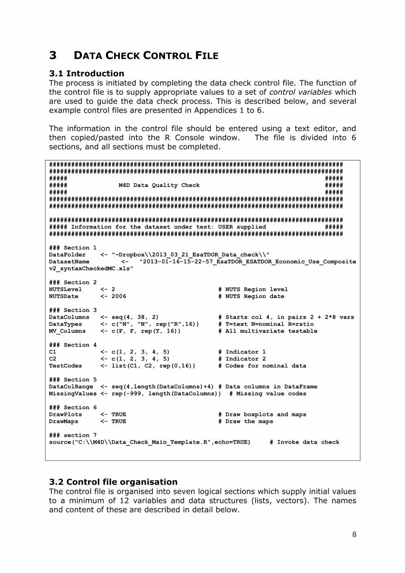
3.1 Introduction The process is initiated by completing the data check control file. The function of the control file is to supply appropriate values to a set of control variables which
are used to guide the data check process. This is described below, and several example control files are presented in Appendices 1 to 6.
The information in the control file should be entered using a text editor, and then copied/pasted into the R Console window. The file is divided into 6
sections, and all sections must be completed. ################################################################################
################################################################################
##### #####
##### M4D Data Quality Check #####
##### #####
################################################################################
################################################################################
################################################################################
##### Information for the dataset under test: USER supplied #####
################################################################################
### Section 1
DataFolder <- "~Dropbox\\2013_03_21_EsaTDOR_Data_check\\"
DatasetName <- "2013-01-16-15-22-57_EsaTDOR_ESATDOR_Economic_Use_Composite
v2_syntaxCheckedMC.xls"
### Section 2
NUTSLevel <- 2 # NUTS Region level
NUTSDate <- 2006 # NUTS Region date
### Section 3
DataColumns <- seq(4, 38, 2) # Starts col 4, in pairs 2 + 2*8 vars
DataTypes <- c("N", "N", rep("R",16)) # T=text N=nominal R=ratio
MV_Columns <- c(F, F, rep(T, 16)) # All multivariate testable
### Section 4
C1 <- c(1, 2, 3, 4, 5) # Indicator 1
C2 <- c(1, 2, 3, 4, 5) # Indicator 2
TestCodes <- list(C1, C2, rep(0,16)) # Codes for nominal data
### Section 5
DataColRange <- seq(4,length(DataColumns)+4) # Data columns in DataFrame
MissingValues <- rep(-999, length(DataColumns)) # Missing value codes
### Section 6
DrawPlots <- TRUE # Draw boxplots and maps
DrawMaps <- TRUE # Draw the maps
### section 7
source("C:\\M4D\\Data_Check_Main_Template.R",echo=TRUE) # Invoke data check
3.2 Control file organisation The control file is organised into seven logical sections which supply initial values
to a minimum of 12 variables and data structures (lists, vectors). The names and content of these are described in detail below.

9
3.2.1: Section 1: Dataset Identification DataSetFolder: a string which contains the full pathname of the folder in which
the Excel spreadsheet is located. This string must be terminated with the folder separator. This can either be '/' or '\\'.
DatasetName: a string which contains the name of the dataset, including its filetype. In the current version of the software, only .xls spreadsheets can be handled.
3.2.2: Section 2: Spatial binding information
NUTSLevel: a single value to denote the NUTS level for the data. This may be 0, 1, 2, 3, or 'X'. The 'X' is used when combined NUTS2/3 data are
present. NUTSDate: the year for which the NUTS units are required, The current
implementation supports 2003, 2006 or 2010. In some datasets data was available for several NUTS levels, with complete
coverage at each level. If this is the case, the dataset should be split into separate files, one level only.
3.2.3: Section 3: Data Location and Type
DataColumns: indexing for the columns that contain data for the data check in the worksheet Data. Columns occur in pairs, the first contains the data for
each indicator, the second contains an index to the source of the data in the Source worksheet. The R function seq() can be used. In the example above seq(4, 38, 2) generates the vector of indices: 4 6 8 10 12 14 16
18 20 22 24 26 28 30 32 34 36 38 DataTypes: a vector of data type indicators. This must be the same length as
the vector of DataColumns. The allowable types are 'R': ratios/counts, 'N': categorical numeric values, 'T': text. This information is used to guide the type of missing values analysis that takes place.
MV_Columns: a vector of logical values indicating which columns can be subjected to testing for multivariate outliers. It should be the same length
as the DataColumns and DataTypes vectors. Allowable values are T and F.
3.2.4: Section 4: Coding for nominal data types
Cn: a vector of allowable code values for variables of DataType 'N'. These
values are specified in the Indicator worksheet. TestCodes: a list of vectors of allowable code values or 0 if the corresponding
variable is ratio or text. The list should have as many members as there
are elements in DataColumns.
3.2.5: Section 5: Dataset size and Missing Values DataColRange: index vector for the data columns in the data frame to be used
for the data check. The column ranges normally starts a 4 (the first three columns contain the NUTS code, the NUTS name, and the NUTS level. In
the example given, the index vector contains the values: 4 5 6 7 8 9 10 11 12 13 14 15 16 17 18 19 20 21 22, and is the same length as DataColumns. The R function seq(start.col,
length(DataColumns)+start.col) can be used.

10
MissingValues: Some data suppliers include missing value codes. These are recoded internally to NA. In the example given -999 was used as a
missing value code for each variable. The R function rep(value,N) can be used to create a vector of N missing values – N should be the length of
the DataColumns vector.
3.2.6: Section 6: Graphics
DrawPlots: some of the data check functions produce graphic output. These
graphics can be omitted by specifying FALSE or F for this control variable. DrawMaps: some of the data check functions produce map output. These
graphics can be omitted by specifying FALSE or F for this control variable
3.2.7: Section 7: Invocation
The final line in the control file invokes the data check process for the specified file. Output is in graphical Windows and to the R Console.
source("C:\\M4D\\Data_Check_Main_Template.R",echo=TRUE)
For debugging purposes the argument echo=TRUE can be used.
3.3 In practice In spite of the existence of documentation with detailed instructions from the Lead Partner on the ways to organise data for the upload, there were many
variations which we encountered in practice. This prevented the use of some of the more advanced checks, and auxiliary software was used to compute Moran's
I for some of the data check reports8.
8 http://geodacenter.asu.edu/ - GeoDa has some useful and robust functions for dealing
with the computation of Moran's I, both global and local versions

11
4 DATA CHECK SYSTEM
4.1: General Order of Operation: Data_Check_Main_Template.R Once the control file has been completed and its contents executed in the R Console (this can either be done by cut/paste from the Text Editor window to the
R Console, or by the menu option of File/Source R Code…, then the code in the file C:\M4D\Data_Check_Main_Template.R will be executed. This accomplished
a number of high level tasks:
1. Initialisation: create global folder and dataset names
2. Read the appropriate NUTS boundaries (by level and date) into a Spatial Polygons Data Frame
3. Read the worksheets in the Excel spreadsheet into separate data frames 4. Check for unique variable names 5. ** Undertake an analysis of missing data
6. Check for invalid NUTS codes 7. Check for regions in the NUTS data which are omitted from the Data
worksheet 8. Create a Spatial Polygons Data Frame with complete cases only (for
spatial checking)
9. Univariate variable summaries a. Frequency tabulation for nominal data
b. Five number summaries for ratio data 10.Bivariate variable summaries
a. Crosstabulation for nominal data
11.Plot variables a. Univariate histograms for ratio data
b. Univariate boxplots for ratio data c. Univariate barplots for nominal data d. Univariate maps
e. Bivariate bagplots 12.** Univariate Outlier check
13.** Spatial Outlier check 14.** Multivariate Outlier check 15.Outlier report
Function Action
LoadLibraries Load the require R packages for the operation of the data check
PrintBanner Printer a header on the output
M4D_Folders Return a single object containing the various folder pathnames
loadPolyShapefile Read the NUTS geometries into a Spatial Polygons Data Frame (SPDF)
GetNUTSCodes Read the current NUTS codes from index file
GetData Return an object containing the four worksheets (Dataset, Indicator, Source, Data) from the Excel spreadsheet
Dataset.Info Print summary details of the dataset
Indicator.Info Printer summary metadata on each

12
indicator
Data.Unique.Name.Check Check for duplicate indicator names
UnpackDataWorksheet Extract and reshape the data for the
quality check
Reshaped.Data.Unique.Name.Check Check for duplicate names in the reshaped
data
Update.Missing.Value.Codes Convert missing data codes from values in
Indicator worksheet to NA
Missing.Value.Analysis Summary information on missing data in
the indicator data
MergeNUTSNames Add in region names from the NUTS code
index
Print.Invalid.NUTS.Codes Print any invalid NUTS codes found in the
data
Omitted Create a list of omitted NUTS regions
Print.Omitted Print regions in the shapefile not in the Data
SubsetSPDF Remove omitted regions from the SPDF
MissingRecords Find the NAs in the Data
CleanSPDF Remove records with incomplete data
summary.Check.variables Summaries for SPDF variables
summary.Check.univariate Summaries for Data variables
Summary.Check.bivariate Summary bivariate checks
UniveriateExplore Univariate outlier analysis
SpatialExplore Spatial outlier analysis
MultivariateExplore Multivariate outlier analysis
4.2 Reading ESPON Database Excel spreadsheets into R data
frames
There are several different ways of reading a Microsoft Excel spreadsheet into an R data frame. Tow commonly used libraries are RODBC and gdata. There are
other libraries, but our experience using ESPON data is that these two are preferable9.
RODBC is very flexible. It will read Access databases as well as Exel
spreadsheets, but there are some known problems10 . Because the driver uses the first few lines of each column to determine the data type for the output data frame, it will often select 'Numeric'', even if there are non-numeric entries. If a
column is declared as Text, any numeric entries will be set to NA. At the time of writing there is no convenient workaround for this.
An alternative is provided by the gdata library. This requires that Perl has been installed, and that the path to the Perl executable is in the PATH environment
variable on Windows systems11.
9 http://www.r-bloggers.com/read-excel-files-from-r/ 10 See http://cran.r-project.org/web/packages/RODBC/vignettes/RODBC.pdf section 7 11 ActiveState Perl is easily installed from http://www.perl.org/get.html. See also
http://www.activestate.com/activeperl/downloads
13
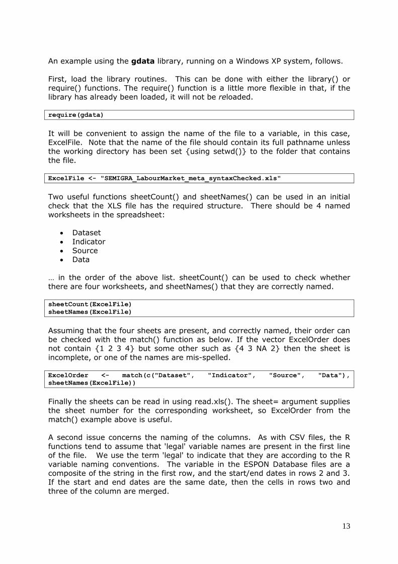
An example using the gdata library, running on a Windows XP system, follows.
First, load the library routines. This can be done with either the library() or
require() functions. The require() function is a little more flexible in that, if the library has already been loaded, it will not be reloaded. require(gdata)
It will be convenient to assign the name of the file to a variable, in this case, ExcelFile. Note that the name of the file should contain its full pathname unless the working directory has been set {using setwd()} to the folder that contains
the file. ExcelFile <- "SEMIGRA_LabourMarket_meta_syntaxChecked.xls"
Two useful functions sheetCount() and sheetNames() can be used in an initial
check that the XLS file has the required structure. There should be 4 named worksheets in the spreadsheet:
Dataset
Indicator Source Data
… in the order of the above list. sheetCount() can be used to check whether
there are four worksheets, and sheetNames() that they are correctly named. sheetCount(ExcelFile)
sheetNames(ExcelFile)
Assuming that the four sheets are present, and correctly named, their order can be checked with the match() function as below. If the vector ExcelOrder does not contain {1 2 3 4} but some other such as {4 3 NA 2} then the sheet is
incomplete, or one of the names are mis-spelled. ExcelOrder <- match(c("Dataset", "Indicator", "Source", "Data"),
sheetNames(ExcelFile))
Finally the sheets can be read in using read.xls(). The sheet= argument supplies the sheet number for the corresponding worksheet, so ExcelOrder from the
match() example above is useful. A second issue concerns the naming of the columns. As with CSV files, the R
functions tend to assume that 'legal' variable names are present in the first line of the file. We use the term 'legal' to indicate that they are according to the R
variable naming conventions. The variable in the ESPON Database files are a composite of the string in the first row, and the start/end dates in rows 2 and 3. If the start and end dates are the same date, then the cells in rows two and
three of the column are merged.

14
The existence of the merged cells can make the output from these input functions unpredictable, and all cells should be unmerged prior to analysis.
Example input calls are below.
Excel.Dataset <- read.xls(ExcelFile, sheet=ExcelOrder[1], header=FALSE)
Excel.Indicator <- read.xls(ExcelFile, sheet=ExcelOrder[2], header=FALSE)
Excel.Source <- read.xls(ExcelFile, sheet=ExcelOrder[3], header=FALSE)
Excel.Data <- read.xls(ExcelFile, sheet=ExcelOrder[4], header=FALSE)
The first few lines of each worksheet as read into R are below: > head(Excel.Dataset,5)
V1 V2 V3 V4
1 Dataset information NA
2 Name Population Structure NA
3 Project SEMIGRA NA
4 Upload date 2012-01-22 NA
5 Metadata date 2011-07-04 NA
Notice that there is an extra column in the spreadsheet, named V4 by read.xls(). It should be checked for content, since a data entry error might have moved one
row across by one column. > head(Excel.Indicator)
V1 V2
1 Indicator Identification
2 Code Name
3 Typology_Gendergap Typology of gender differences on the labour market
4 Core False
5 NAT Type TS
6 Theme economyFinanceAndTrade
V3 V4 V5 V6
1 NA NA NA
2 Abstract NA NA NA
3 Typology of gender differences in economic activity in regional perspective NA NA NA
4 NA NA NA
5 NA NA NA
6 NA NA NA
There are an extra three columns present in this worksheet – again, they should be checked for content.
> head(Excel.Source)
V1 V2 V3 V4
1 Source Reference NA
2 Label 1 NA
3 Date 2012-07-04 NA
4 Copyright © Leibniz-Institut für Länderkunde NA
5 Provider Name Leibniz-Institut für Länderkunde NA
6 URI www.ifl-leipzig.de NA
The head() and summary() functions are useful to obtaining a quick first look at
the data. It will be noted that the NUTS codes for the data are in lowercase. The column names appear in row three of the data, with the exception of the data
columns, where the name is qualified by start and end data as described above. The source columns identify the lineage of the data, the labels in row three are
not unique.

15
> head(Excel.Data)
V1 V2 V3 V4
1 see ch.3.Cluster 5 of the Specifications
2
3 Unit code Name Object type Version
4 at11 Burgenland (AT) NUTS2 2006
5 at12 Niederösterreich NUTS2 2006
6 at13 Wien NUTS2 2006
V5 V6 V7 V8 V9 V10
1 Typology_Gendergap Typology_IndustryStructure GenderGap_15-24
2 2009 2009 2008
3 source source source
4 Cluster 1 1 Cluster 1 1 --19.15 1
5 Cluster 1 1 Cluster 1 1 --15.89 1
6 Cluster 2 1 Cluster 2 1 --3.92 1
V11 V12 V13 V14 V15 V16
1 GenderGap_25-34 GenderGap_35-44 WF_Agriculture
2 2009 2009 2009
3 source source source
4 --8.12 1 --11.95 1 6.74 1
5 --13.72 1 --9.43 1 7.26 1
6 --14.07 1 --9.50 1 0.38 1
V17 V18 V19 V20 V21 V22 V23
1 WF_IndustryConstruction WF_TTA WF_PublicServices WF_OtherServices
2 2009 2009 2009 2009
3 source source source
4 25.09 1 27.83 1 23.46 1 16.88
5 24.02 1 26.57 1 23.54 1 18.60
6 16.01 1 26.48 1 24.76 1 32.39
V24
1
2
3 source
4 1
5 1
6 1
4.3 Pre-processing the data for checking The data frame can be rationalised to remove the columns which are not to be
checked, and then to add suitable row and column names. # [1]
Data.Check <- Excel.Data[4:nrow(Excel_Data),c(1,2,seq(3,23,2)]
# [2]
varBase <- Excel.Data[1, seq(3,23,2)])
varStDt <- Excel.Data[2, seq(3,23,2)])
varEnDt <- Excel.Data[3, seq(3,23,2)])
varName <- paste(varBase,varStDt,varEnDt,sep="")
varName <- gsub("-","_",varName)
varName <- gsub(" ","_",varName)
# [3]
rownames(Data.Check) <- toupper(Data.Check[,1])
colnames(Data.Check) <- c("Unit_code","Name",varName)
The actions in the preceding box result in the data frame which is suitable for further processing. Action [1] extracts the subset of the data frame for processing – rows 4 to the
end, and columns 1, 2, 3 and every second column thereafter.

16
Action [2] extracts the indicator names from the first row of the spreadsheet, the start dates from the second row, and the end dates from the third row, and
concatenates them into a single string. Any characters which are not allowable in a R variable name are replaced by underscores.
Action [3] assigns row and column names. The row names can be used to index the data frame, and the column names index the individual; columns. The row
names that we used in the data check are the NUTS codes, which are converted to uppercase. The column names are created from the variable names from
|Action [2].
4.4 Reading geometry data from shapefiles
The spatial extensions to R allow for the input, processing, and output of
shapefiles. The ESRI shapefile12 has emerged as a de facto standard for the exchange of spatial data. The shapefile, in spite of its name consists of at least three separate files, with the extensions .shp, .shx, and .dbf, and a common
prefix name.. ESRI refer to the .shp file as the "Main File" – this contains the geometry data. The .shx file is known as the Index File, and is used to index the
individual object records in the Main File. The .dbf file is a table of attribute data and has the following characteristics:
There is one record per shape feature (object) The record is order the same as the record order in the Main File
There can be other files, notable a file of projection information (.prj). For the
NUTS geometry data used in the Database project, the following projection definition is used:
PROJCS["ETRS_1989_LAEA",
GEOGCS["GCS_ETRS_1989",
DATUM["D_ETRS_1989",
SPHEROID["GRS_1980",6378137.0,298.257222101]],
PRIMEM["Greenwich",0.0],
UNIT["Degree",0.0174532925199433]],
PROJECTION["Lambert_Azimuthal_Equal_Area"],
PARAMETER["False_Easting",4321000.0],
PARAMETER["False_Northing",3210000.0],
PARAMETER["Central_Meridian",10.0],
PARAMETER["Latitude_Of_Origin",52.0],
UNIT["Meter",1.0]]
The underlying projection is a Lambert Azimuthal Equal Area projection, with an
origin at 52N, 10W (near the town of Sehlem in Germany). The projection units are meters, and the false eastin and northing parameters ensure that all
coordinate measurements are positive. The datum for the projection is based on
12 http://www.esri.com/library/whitepapers/pdfs/shapefile.pdf

17
the GRS 80 (Geodetic Reference System) spheroid13 used in the European Terrestrial Reference System 198014.
Several functions exists to read ESRI shapefiles, among them are
readShapePoly() from the maptools library, and readOGR() from the rgdal library. There are advantages and drawbacks to using either function. The readShapePoly() function will return an error if it is used to read a non-polygon
shapefile; it will not read the projection file, so the Coordinate Reference System string as to be attached by the user in the R code. By contract readOGR() will
read any shapefile without checking to see what the type is, it will read and store the projection information if this is present in the shapefile.
4.5 Implementation in the data check
The geometry information is located in a folder whose name is assigned to a global variable in the R code. In a typical Windows application this is
c:\M4D\NUTS_ETRS_1989_LAEA. There is no reason why this location may not be a
networked drive, or the URL to cloud storage. The individual shapefiles are named using a common convention
NUTSn_yyyy.shp
… where n is the NUTS level (0, 1, 2, 3, X) and yyyy refers to the year (2003, 2006, 2010). Other shapefiles can be added to the repository. In this implementation NUTS level X is used to refer to the combined NUTS 2/3
geometries, in order to keep the NUTS level code to a single character.
To read NUTS3_2006.shp using either the maptools or rgdal functions, the following is appropriate: require(maptools)
SPDF.1 <- readShapePoly("C:\\M4D\\NUTS_ETRS_1989_LAEA\\NUTS3_2006.shp")
proj4string(SPDF.1) <- "+proj=laea +lat_0=52 +lon_0=10 +x_0=4321000
+y_0=3210000 +ellps=GRS80 +units=m +no_defs"
require(rgdal)
SPDF.2 <- readOGR("C:\\M4D\\NUTS_ETRS_1989_LAEA","NUTS3_2006")
A Spatial Polygons Data Frame (SPDF) is a single object which contains, inter alia, the geometry and attribute information. The objects inside the SPDF object
are known as slots. > slotNames(SPDF.2)
[1] "data" "polygons" "plotOrder" "bbox" "proj4string"
The attribute data is located in the data object, the geometry in the polygons object. The bbox object contains the coordinates of the bounding box:
13 Geodetic Reference System 1980, Bulletin Géodésique, (54)3, 1980. Republished (with
corrections) in Moritz, H., 2000, Geodetic Reference System 1980, J. Geod., 74(1), 128–
162 14 http://etrs89.ensg.ign.fr/

18
> bbox(SPDF.2)
min max
x -2823914 10026125
y -3076145 5415982
The attribute data is fairly minimal, but does contain the NUTS codes and NUTS levels:
> head(SPDF.2@data)
OBJECTID_1 OBJECTID NUTS_ID STAT_LEVL_ AREA LEN Shape_Leng Shape_Le_1 Shape_Area
0 463 463 IS001 3 0 0 4.814391 299120.0 1047327456
1 464 464 FI133 3 0 0 11.247582 783542.7 21584072176
2 465 465 FI1A1 3 0 0 9.442749 638978.5 5456649618
3 466 466 NO062 3 0 0 49.584899 3074302.0 22296592101
4 467 467 NO073 3 0 0 113.311666 6023597.7 48565287828
5 468 468 NO072 3 0 0 86.592704 4839567.6 25820053059
The variable NUTS_ID contains the NUTS code, and the variable STAT_LEVL_
contains the NUTS level.
To merge the data from the imported Database spreadsheet, the following can be used: SPDF.Order <- match(SPDF.2$NUTS_ID,rownames(Data.Check))
SPDF.2a <- SPDF.2
SPDF.2a@data <- data.frame(cbind(SPDF.2a@data, Data.Check[SPDF.Order,]))
Several of the spatial functions require the removal of the regions which have missing data (coded as NA). If the variable of interest is Test, then creating a
subset of the SPDF with only the non-missing data can be achieved with: SPDF.3a <- SPDF.2a[!is.na(SPDF.2a$Test),]

19
5 AVAILABLE DATA CHECKS The actuality of the data checks proved to be more complex than was ever envisaged in Phase I of the Database project. The control file drives the check
process, and the DataTypes vector, together with the TestCodes list provide the information as to which method will be used at each stage of the analysis.
5.1 Univariate summaries The initial assessment of the data begins with a series of univariate summaries.
These provide an initial 'quick-look', to answer questions such as (i) do the percentages fall between 0 and 100 (ii) are the counts positive (iii) are there any
missing values (iv) are there any obviously anomalous values (v) do the categories in the frequency tables for the nominal data match the values in the metadata (vi) are the distributions noticeably skew [long right tail, so the mean
differs from the median] (vii) are the original values positive?
Ratio Compute 6-number summary (extremes, quartiles, median, mean)
Nominal
Frequency table of values, and list of values found Ordinal
Compute 6-number summary (extremes, quartiles, median, mean) Count
Compute 6-number summary (extremes, quartiles, median, mean)
This initial assessment can be augmented with visualisations of the data – in
practice boxplots and histograms have proved to be most useful. The great variation in physical size of the NUTS regions means that identifying anomalous values is not always possible visually.
5.2 Univariate Checks The checking begins by taking each variable in turn. The values in the DataTypes variable (assigned in the Control File) direct the nature of the check. For ratio data, the system checks for the existence of boxplot outliers – these
are anomalous in terms of the definition of the boxplot. An outlier in boxplot terms is one whose value is more than 1.5 times the interquartile range. The
NUTS codes and names are listed in the output together with the anomalous values.
Ordinal and count data are checked to see whether their values belong to the set of positive integers. The values are also checked to see whether they have any
inadvertent fractional parts where they are not stored exactly as an integer in the Excel spreadsheet. The upper value of an ordinal variable should not be greater than the number of observations. Any regions which are anomalous are
listed.

20
Nominal data require reference to the TestCodes lists in the Control File. TestCodes is a list of either 0 for non-categorical variables or a vector of
allowable values (extracted from the metadata in the Indicator worksheet15)
Ratio Check for boxplot outliers
Nominal
Check codes in the Data against codes supplied in the control file Ordinal
Check that data values are positive integers and in range Count
Check that data values are positive integers
Count data gives rise to some challenges. The variation in the underlying
support for the data means that count data are not standardised – each value has not arisen on an equal footing, so we cannot treat the values as comparable.
5.3 Bivariate Checks For the ratio variables we can compute a correlation matrix. This might seem
unnecessary – it's a useful diagnostic tool to determine whether any variables have been entered twice (the correlation will be 1) or whether, in choosing variables, two have been selected which are essentially measurements of the
same underlying characteristic.
The bagplot is a two-dimensional extension of the boxplot. The output is a plot showing both the non-outlying and outlying values. The IDs of the outlying values are also listed in the output object, and can be identified for printing.
What we observe as an outlier here is a combination of values that is unusual, not necessary from values which are themselves unusual when taken one at a
time.
Ratio
Compute correlation coefficients and p-values Bagplot Outliers
The correlation matrix can be augmented by a scatterplot matrix – although
once the number of variables exceeds about 15, the individual plots themselves become almost too small to see on the computer screen.
5.4 Multivariate Checks If there are sufficient variables of ratio type in the dataset, then a trawl for
multivariate outliers becomes possible. In the work carried out prior to 2011 the dataset used was a time series of GDP values at NUTS2/3. An ad hoc method
was developed in the form of a circulating regression: the values for time period
15 In future versions of the software, consideration should be given to extracting these
data from the metadata directly

21
t would be regressing on the values for the other n-1 time periods in a multiple regression, and the residuals checked for unusual high or low values. With n
time periods, there would be n regressions, and n sets of residuals. A region which was anomalous on a majority of these might be flagged for checking.
There are a number of issues of multi-collinearity and multiple testing which would indicate that it would identify too many false positives.
In practice none of the data from the suppliers allowed the possibility of using the circulating regression technique.
Given sufficient data, we can transform the original variables, say n of them, into n principal components. The component scores can then be examined for
univariate, and bivariate outliers using the methods outlined above. We restrict the search to components whose eigenvalues are greater than 1 to minimise the
possibility of identifying false positives. A second technique is the computation of Mahalanobis distances to some
multivariate centroid. The Mahalanobis distance is a generalisation of the Euclidean distance which takes into account the correlation structure in the data.
The mean vector can be used as the position of the multivariate centroid. The output is a vector of distances, which can then be treated as a single variable,
and examined for outliers as above.
Circulating regression
Circulating Robust regression Principal Component outliers
Mahalanobis outliers These checks are useful, not that they identify anomalous individual values, but
that they identify potentially anomalous combinations of values on the candidate variables. This does pre-suppose that the candidate set has some thematic
coherence.
5.5 Spatial Checks The original version of the software, developed on GDP time series for NUTS2/3 regions included a version of a test named after Hawkins, which would identify spatial outliers. A spatial outlier is one that is unusual when compared with the
values in its neighbours. It was surprising to discover that the test is not mentioned in Professor Hawkins monograph on outlier detection16. An
alternative is provided by the Local Moran statistic, which will identify values which are either locally high or low in comparison with their neighbours.
Local Moran Outliers Hawkins' test
The Hawkins test requires further development.
16 Hawkins, DM, 1980, Identification of Outliers, London: Chapman and Hall

22
5.6 Missing values Any regions with missing values on one or more variables are listed for further checking. We also check to whether data is missing on all variables. A heatmap can be a useful tool in giving an overall 'quick-look' as to the global pattern ob
missing data. The missing data pattern can sometimes give some clues as to the process that generated the missing data17. Large quantities of missing data
would give rise to a request for confirmation that the data are in fact missing and not omitted by oversight.
5.7 Plots Two modes of visualisation are useful additional tools. For the univariate ratio data columns boxplots provide a helpful visual summary of the presence or otherwise of anomalous values in the data. The barplot when used with the table
function again provides a useful visual summary of the categories in a nominal variable (with the table function to provide the frequency information).
Univariate
Ratio
Boxplot Nominal
Barplot Bivariate
Scatterplot matrix Bagplots for selected pairs of variables
Treemaps might be useful ways of summarising the pattern of values, visually, in a crosstabulation of two or more categorical variables – they either help to
identify an unusual combination of categories or allow a check on the presence or otherwise of the valid values which represent each category.
5.8 Maps The data values for many of the datasets refer to individual NUTS regions. Mapping the values, either as choropleth maps for ratio data, and area class
maps for categorical data, provides a quick visual summary of the patterns.
Ratio Choropleth maps (10 categories)
Nominal
Plot of data categories
One of the issues with mapping the data is the variation in the physical size of the NUTS regions. If the more distant overseas regions are included, this
problem is magnified. In future assessment, consideration might be given to the use of a population cartogram as the basis – areas with larger populations are
more prominent than areas with smaller populations. An alternative would be to create a cartogram where the areas are also approximately the same size.
17 Enders, CK, 2010, Applied Missing Data Analysis, New York: Guilford Press

23
Software for creating cartograms exists both as an extension to ArcGIS18 and through the ScapeToad website19. The reshaped set of zones then allows each
data value to visualised on an equal footing.
Both the visual display described in 5.7 and 5.8 are essentially ephemeral displays, they are of less use in presenting the results of the analysis in the output report for the data supplier. However, as diagnostic tools they are useful
is helping to identify some of the initial characteristics of the data set.
18 http://arcscripts.esri.com/details.asp?dbid=15638 and
https://uknow.drew.edu/confluence/display/DREWGIS/ArcMap+-+Cartograms+Tutorial 19 http://scapetoad.choros.ch/

24
6 DATA CHECKS IN PRACTICE
6.1 Reflections on the data check process In practice we found that the data supplied by the projects was very different from that which we had envisaged. A "one-size-fits-all" system that we had
developed for the ESPON 2013 Database project required radical overhaul and re-organisation. The "exceptions to the exceptions" that we encountered as
enumerated below.
6.1.1 Missing data
There was inconsistency in the presentation of missing data. Sometimes a numeric code was used, such as -999, other times we encountered alphameric
codes which as "n/r".
For some studies, data was not present for all NUTS regions. Some studies omitted these regions entirely, others coded every variable as missing.
6.2.2 Non-integer counts
In a number of cases projects supply count data – these should be positive integers, yet we occasionally encountered fractional values where rounding had either been omitted or forgotten. Excel will display a rounded value to a number
stored with a fractional part.
6.2.3 Duplicated data We checked to see whether any rows appeared to be duplicated. In one case
every NUTS2 region in Denmark was included twice in the data. Again, with the user of Excel, this is easy to overlook.
6.2.4 Internal inconsistencies
In one case a series of indicators were supplied, together with an additional indicator which was their sum. The summations were checked – for one
example, the difference was 7.2 percentage points for a value of 24.2%. Either the summation column was correct, in which case individual indicator values were incorrect, or the summation was faulty.
6.2.5 Phantom worksheets
The spreadsheets are supposed to contain four separate worksheets: Dataset, Indicator, Source and Data. In one case we discovered an extra hidden
worksheet, named SPSS, which could not be seen in when the spreadsheet was opened in Excel, but was clearly visible to the R software.
6.2.6 Multivariate checks
In several cases there was insufficient data to allow a multivariate check, of the data was so disparate as to make this meaningless. Additionally the existing of
missing data meant that addinfg additional variables into the multivariate set would have result in a series depletion of the number of regions with sufficiently complete data.

25
6.2.7 Faulty computation Notwithstanding the prior semantic and syntaxic checks carried out on the
metadata we identified one example were the computation of the indicator was faulty. In another case a commonly used demographic indicator was inverted.
6.2.8 Errors in the metadata
We are very aware that many working under the ESPON programme do not have English as a first language. There were occasional errors in the metadata to
which we drew attention. Occasional uncommon English uses appeared in the metadata, and we requested clarification.
6.2.9 Mixed NUTS2/3 data
One project included regions at NUTS 2 for some countries, and NUTS3 for others. We created a new geometry file, and a new geometry code, "X" for these data.
6.2 Helping the suppliers: the report Rather than a bland printout/listing from the data check software, we decided to
arrange our reports in logical sections, with some initial identification from the metadata, a logical organisation of the anomalies that we had found, and a final
section with some recommendations for checking and, if necessary, altering the data that was submitted.

26
Example report section
We noted in one case that many of the indicators had presented apparently anomalous values in the right tail of the distribution. This is not unknown in
socio-economic data. We requested, nevertheless, that the supplier checked the values.

27
7 INSTALLATION The implementation of the data check assumes that the code and any associated shapefiles and lookup tables will be stored in the folder C:\M4D. A batch file
(LoadDataCheckCodes.bat) is used to copy the code and data files from the software development folder to C:\M4D. Within the software development folder
are the following files and folders: Data_Check_Main_template.R high level data check functions
DataCheckFunctions.R low level data check functions TERCO_Data_Check.R example control file
SpatialData\NUTS_Info folder of NUTS lookup tables SpatialData\NUTS_ETRS_1989_LAEA folder of shapefiles
The batch file creates the M4D folder if it is not present, and copies the files. @ECHO OFF
CLS
Echo ****************************************
Echo ****************************************
Echo *** Copying M4D Data Check Functions ***
Echo *** == Destination folder c:\M4D == ***
Echo ****************************************
echo ****************************************
IF EXIST C:\M4D GOTO M4DPRESENT
@ECHO *** C:\M4D folder does not exist. Creating new version...
MKDIR C:\M4D
@ECHO *** C:\M4D created
:M4DPRESENT
@ECHO *** C:\M4D folder already exists
@ECHO *** Copying R files...
COPY Data_Check_Main_template.R C:\M4D
COPY DataCheckFunctions.R C:\M4D
COPY TERCO_Data_Check.R C:\M4D\Example_Control_file.R
@ECHO *** Copying NUTS lookup tables...
XCOPY Spatial_Data\NUTS_Info C:\M4D\NUTS_Info /E /I /Q /R /Y
@ECHO *** Copying NUTS shapefiles
XCOPY Spatial_Data\NUTS_ETRS_1989_LAEA C:\M4D\NUTS_ETRS_1989_LAEA /E /I /Q /R /Y
ECHO **********************************************
ECHO **********************************************
ECHO *** M4D Data Check Function Copy Completed ***
ECHO **********************************************
ECHO **********************************************
PAUSE
ECHO ON

28
8 FURTHER DEVELOPMENTS This technical report provides an introduction to the detection of logical input errors and statistical outliers (i.e. exceptional values) for ESPON Database
datasets. Some important aspatial and spatial techniques have been introduced and demonstrated within the R statistical computing environment.
The field of robust statistics and outlier detection is extremely large and diverse, and as such can not be comprehensively reviewed within the terms of reference
of this report. However, outlier detection techniques applicable (or designed for) spatial data sets are not as developed as those for aspatial applications.
Robust versions of geographically weighted summary statistics (GWSS),
geographically weighted regression (GWR) and geographically weighted principal component analysis (GWPCA) are of interest, as they allow the detection of outliers in both univariate and multivariate spatial data sets, without being
influenced by the non-normal nature of the data.
Further developments in the detection methodology might include a selection of the robust geographically weighted techniques that we are currently working on. An improved version of Hawkins’ spatial outlier test is also under development,
as is a robust version of the local Moran’s I statistic (with respect to outlier identification).

29
REFERENCES Ainsworth LM, Dean CB (2008) Detection of local and global outliers in mapping studies. Environmetrics 19, 21-37.
Anselin L. (1995) Local indicators of spatial association. Geographical Analysis 27, 93 -115.
Béguin C, Hulliger B (2004) Multivariate outlier detection in incomplete survey data: the epidemic algorithm and transformed rank correlations. Journal of the Royal Statistical Society, Series A 167(2), 275-294.
Brunsdon C, Fotheringham AS, Charlton ME (2002) Geographically weighted summary statistics - a framework for localised exploratory data analysis.
Computers, Environment and Urban Systems 26, 501-524.
Brunsdon C, Charlton ME (2010) An assessment of the effectiveness of multiple
hypothesis testing for geographical anomaly detection. Submitted to Environment and Planning B
Chambers R, Hentges A, Zhao X (2004) Robust automatic methods for outlier
and error detection. Journal of the Royal Statistical Society, Series A 167(2), 323-339.
Charlton ME, Brunsdon C, Demšar U, Harris P, Fotheringham AS (2010) Principal component analysis: from global to local. In preparation.
Charlton S (2004) Evaluating automatic edit and imputation methods, and the
EUREDIT Project. Journal of the Royal Statistical Society, Series A 167(2), 199-207.
Cruz Ortiz M, Sarabia LA, Herrero A (2006) Robust regression techniques: A useful alternative for the detection of outlier data in chemical analysis. Talanta 70, 499-512.
D’Alimonte D, Cornford D (2007) Outlier detection with partial information: application to emergency mapping. Stochastic Environmental Research and Risk
Assessment 22, 613-620.
Daszykowski M, Kaczmarek K, Vander Heyden Y, Walczak B (2007) Robust statistics in data analysis – a review Basic concepts. Chemometrics and
Intelligent Laboratory Systems 85, 203-219.
ESPON (2006) 3.4.3 The modifiable areas unit problem – Final Report
http://www.espon.eu/mmp/online/website/content/projects/261/431/file_4970/
Faraway J (2004) Linear models with R. Chapman & Hall/CRC, Boca Raton/FL
Filzmoser P, Garrett R, Reimann C (2005) Multivariate outlier detection in
exploration geochemistry. Computers & Geosciences 31, 579-587.
Filzmoser P, Maronna R, Werner M (2008) Outlier identification in high
dimensions. Computational Statistics and Data Analysis 52, 1694-1711.
Fotheringham AS, Brunsdon C, Charlton ME (2002) Geographically Weighted Regression - the analysis of spatially varying relationships. Wiley, Chichester.
Frigge M, Hoaglin DC, Iglewicz B (1989) Some implementations of the Boxplot. The American Statistician 43, 50–54.
Ghosh-Dastidar B, Schafer JL (2003) Multiple edit/multiple imputation for multivariate continuous data. Journal of the American Statistical Association

30
98(464), 807-817.
Harris P, Brunsdon C (2010) Exploring spatial variation and spatial relationships
in a freshwater acidification critical load data set for Great Britain using geographically weighted summary statistics. Computers & Geosciences 36, 54-
70.
Harris P, Fotheringham AS, Juggins S (2010) Robust Geographically Weighed Regression: A Technique for Quantifying Spatial Relationships Between
Freshwater Acidification Critical Loads and Catchment Attributes. To appear in the Annals of the Association of American Geographers.
Hawkins RM (1980) Identification of Outliers. Chapman & Hall, London.
Hoo KA, Tvarlapati KJ, Piovoso MJ, Hajare R (2002) A method of robust multivariate outlier replacement. Computers and Chemical Engineering 26, 17-
39.
Hubert M, Vandervieren E (2008) An adjusted boxplot for skewed distributions.
Computational Statistics and Data Analysis 52, 5186-5201.
Ihaka R, Gentleman R (1996) R: A language for data analysis and graphics. Journal of Computational and Graphical Statistics 5, 299-314.
Jackson DA, Chen Y (2004) Robust principal component analysis and outlier detection with ecological data. Environmetrics 15, 129-139.
Kou Y, Lu C-T, Chen D (2006) Spatial Weighted Outlier Detection. In proceedings of the 2006 SIAM International Conference on Data Mining No. 614
2006.
Liu H, Jezek K, O’Kelly M (2001) Detecting outliers in irregularly distributed spatial data sets by locally adaptive and robust statistical analysis and GIS.
International Journal of Geographical Information Science 15(8), 721-741
Loader C (2004) Smoothing: Local Regression Techniques. In Gentle J, Härdle
W, Mori Y (eds) Handbook of Computational Statistics. Springer-Verlag, Heidelberg.
Locantore N, Marron J, Simpson D, Tripoli N, Zhang J, Cohen K (1999) Robust principal
components for functional data. Test 8, 1–73.
Meklit T, Van Meirvenne M, Verstraete S, Bonroy J, Tack F (2009) Combining
marginal and spatial outliers identification to optimize the mapping of the regional geochemical baseline concentration of soil heavy metals. Geoderma 148, 413-420.
Morgenthaler S (2007) A survey of robust statistics. Statistical Methods & Applications 15, 271-293.
Petrakos G, Conversano C, Farmakis G, Mola F, Siciliano R, Stavropoulos P (2004) New ways of specifying data edits. Journal of the Royal Statistical Society, Series A 167(2), 249-274.
Plaia A, Bondi A (2006) Single imputation method of missing values in environmental pollution data sets. Atmospheric Environment 40, 7316-7330.
Reimann C, Filzmoser P, Garrett R (2005) Background and threshold: critical comparison of methods of determination. Science of the Total Environment 346, 1-16.

31
Rousseeuw PJ, Ruts I, Tukey JW (1999) The Bagplot: A Bivariate Boxplot. The American Statistician 53, 382–387.
Rousseeuw PJ, Debruyne M, Engelen S, Hubert M (2006) Robust and outlier detection in chemometrics. Critical Reviews in Analytical Chemistry 36, 221-242.
Vanden Branden K, Verboven S (2009) Robust data imputation. Computational Biology and Chemistry 33, 7-13.
Wong D (1996) Aggregation effects in geo-referenced data. In Arlinghaus SL
(ed) Practical Handbook of Spatial Statistics. CRC Press, Boca Raton, FL.

32
APPENDIX 1
ESaTDOR Data Check Control File (21/3/2013) ################################################################################
################################################################################
##### #####
##### M4D Data Quality Check #####
##### #####
################################################################################
################################################################################
################################################################################
##### Information for the dataset under test: USER supplied #####
################################################################################
DataFolder <- "~Dropbox\\2013_03_21_EsaTDOR_Data_check\\"
DatasetName <- "2013-01-16-15-22-57_EsaTDOR_ESATDOR_Economic_Use_Composite
v2_syntaxCheckedMC.xls"
NUTSLevel <- 2 # NUTS Region level
NUTSDate <- 2006 # NUTS Region date
DataColumns <- seq(4, 38, 2) # Starts col 4, in pairs 2 + 2*8 vars
DataTypes <- c("N", "N", rep("R",16)) # T=text N=nominal R=ratio
MV_Columns <- c(F, F, rep(T, 16)) # All multivariate testable
C1 <- c(1, 2, 3, 4, 5) # Indicator 1
C2 <- c(1, 2, 3, 4, 5) # Indicator 2
TestCodes <- list(C1, C2, rep(0,16)) # Codes for nominal data
DataColRange <- seq(4,length(DataColumns)+4) # Data columns in DataFrame
MissingValues <- rep(-999, length(DataColumns)) # Missing value codes
DrawPlots <- TRUE # Draw boxplots and maps
DrawMaps <- TRUE # Draw the maps
################################################################################
# #
# Data check begins here #
# Latest data check functions: to copy these double click on #
# ~Dropbox\00ESPON_M4D\Database_Quality_Check\Live\LoadDataCheckCodes.bat #
# #
################################################################################
source("C:\\M4D\\Data_Check_Main_Template.R",echo=TRUE) # Invoke data check
################################################################################
# #
# Bespoke tests #
# #
################################################################################
TestData <- DQCmData[!is.na(DQCmData$E09SHIPBUI20012009),] # get the rows
with data
dim(TestData)
colnames(TestData)
# [1] "UnitCode" "Level" "Year"
# [4] "marine_compo_eco_120012009" "marine_compo_eco_220012009" "E09TOT20092009"
# [7] "E09SHIPBUI20012009" "E09TRADSEC20012009" "E09TRANSP20012009"
#[10] "E09TOURISM20012009" "E09FISHERI20012009" "E09OTHER20012009"
#[13] "E09OILGAS20012009" "P_09TOT20092009"
"P_09SHIPBUI20012009"
#[16] "P_09TRADSEC20012009" "P_09TRANSP20012009"
"P_09TOURISM20012009"
#[19] "P_09FISHERI20012009" "P_09OTHER20012009"
"P_09OILGAS20012009"

33
not.integer <- which(TestData$E09TOT20092009 %% 1 > 0) # non integer counts
TestData[not.integer,c(1,6)] # list them
not.integer <- which(TestData$E09TOT20092009 %% 1 > 0)
TestData[not.integer,1]
#
# TestData[,14] is the sum of the cols 15:21 - check the summation
#
px <- TestData[,15] +TestData[,16] + TestData[,17] +TestData[,18] +TestData[,19]
+TestData[,20] +TestData[,21]
pt <- rowSums(TestData[,15:21])
x <- TestData$P_09TOT20092009 - pt # compare wtih actual sum
big <- which(abs(x) > .1) # which are the big ones
cbind(TestData[big,c(1,14)], pt[big], x[big]) # list the table
mvdata <- TestData[,15:21]
pcs <- princomp(mvdata,cor=T,scores=T)
# > pcs$sdev^2 / sum(pcs$sdev^2)
# Comp.1 Comp.2 Comp.3 Comp.4 Comp.5 Comp.6 Comp.7
# 0.24929559 0.19683055 0.15896476 0.12046032 0.10538623 0.08982176 0.07924078
# .25 .45 .61 .73 .83 .91 .99
pcs$loadings
> pcs$loadings
## Loadings:
## Comp.1 Comp.2 Comp.3 Comp.4 Comp.5 Comp.6 Comp.7
## P_09SHIPBUI20012009 -0.663 -0.134 0.494 0.528
## P_09TRADSEC20012009 0.577 -0.429 0.378 0.576
## P_09TRANSP20012009 0.390 -0.182 -0.569 -0.201 0.338 -0.564 0.136
## P_09TOURISM20012009 -0.288 0.172 -0.663 -0.447 -0.199 0.402 -0.218
## P_09FISHERI20012009 -0.203 -0.370 -0.437 0.765 -0.205
## P_09OTHER20012009 0.603 -0.180 -0.767
## P_09OILGAS20012009 -0.136 -0.597 0.175 -0.383 -0.587 -0.312
pcs.scores <- pcs$scores
boxplot(pcs.scores) # hmmm - some outliers
#
# Bagplot to look at the first couple of components - accounts for about
# 45% of the variance
#
bagplot(pcs$scores[,1],pcs$scores[,2]) # compare the first two
#
# print the results of the mutlivariate analysis
#
# Names can be got from http://http://nuts.geovocab.org/id/NO04.html
k <- which(pcs$scores[,1] > 3 | pcs$scores[,2] < -2.5) # outliers
as.data.frame(cbind(as.character(TestData[k,1]),pcs$scores[k,1:2]))
# NUTS Comp.1 Comp.2 Name
# 165 IS00 -2.62080242231774 -2.7997695388609 sland
# 172 ITD3 4.08584331110513 0.3810196487946 Veneto
# 173 ITD4 4.40887180192335 -0.2562404548776 Friuli-Venezia Giulia
# 174 ITD5 4.38184283329398 0.1497851513156 Emilia-Romagna
# 208 NO04 0.45951451096980 -6.8260406244667 Agder og Rogaland
# 209 NO05 0.92418754519894 -5.0458479442180 Vestlandet
# 238 RO22 0.76849593144108 -3.2802554172067 Sud-Est
# 245 SE21 3.41048199666645 0.4252567502375 Smland med arna
# 318 UKM6 -3.37228171738626 -5.7277554506111 Highlands and Islands

34
MVNutsCode <- TestData[k,1]
MVNutsCode
which(NUTSCodes[,1] %in% MVNutsCode)
NUTSCodes[which(NUTSCodes[,1] %in% MVNutsCode),]
# Code Name Level
#1123 ITD3 Veneto 2
#1131 ITD4 Friuli-Venezia Giulia 2
#1136 ITD5 Emilia-Romagna 2
#1488 RO22 Sud-Est 2
#1533 SE21 Smland med arna 2
#1763 UKM6 Highlands and Islands 2
################################################################################
# #
# End of data check template #
# #
################################################################################

35
APPENDIX 2
SeGI Data Check Control File (22/3/2013) ################################################################################
################################################################################
##### #####
##### M4D Data Quality Check #####
##### #####
################################################################################
################################################################################
################################################################################
##### Information for the dataset under test: USER supplied #####
################################################################################
DataFolder <- "~Dropbox\\00ESPON_M4D (1)\\2013_03_22_SEGI_Data_Check\\"
DatasetName <- "2012-11-05-14-03-19_SeGi_I-
6ESPONindicatorsSeGI_syntaxCheckedMC.xls"
NUTSLevel <- 2 # NUTS Region level
NUTSDate <- 2006 # NUTS Region date
DataColumns <- seq(4, 104, 2) # Starts col 4, in pairs
DataTypes <- rep("R",length(DataColumns)) # All ratios
MV_Columns <- rep(T, length(DataColumns)) # All multivariate testable
#C1 <- c(1, 2, 3, 4, 5) # Indicator 1
#C2 <- c(1, 2, 3, 4, 5) # Indicator 1
TestCodes <- list(rep(0, length(DataColumns))) # Codes for nominal data
DataColRange <- seq(4,length(DataColumns)+4) # Data columns in DataFrame
MissingValues <- rep("n/a", length(DataColumns)) # Missing value codes
DrawMaps <- FALSE
DrawPlots <- FALSE
################################################################################
# #
# Data check begins here #
# Latest data check functions: to copy these double click on #
# ~Dropbox\00ESPON_M4D\Database_QWuality_Check\Live\LoadDataCheckCodes.bat #
# #
################################################################################
source("C:\\M4D\\Data_Check_Main_Template.R",echo=TRUE) # Invoke data check
################################################################################
# #
# End of data check template #
# #
################################################################################
library(VIM)
matrixplot(as.data.frame(DQCmData[,4:54]),main="Missing Values Analysis")
x <- function(i){junk <-
is.na(DQCmData[,i]);as.data.frame(cbind(as.character(DQCmData[junk,1]),DQCmData[jun
k,i]))}
v <- colnames(DQCmData)
kk <- 55; x(kk);v[kk]
alldata <- c(15, 27, 28, 32, 33, 34, 41, 42, 43, 44)
somedata <- c(6, 7, 9, 10, 11, 12, 13, 14, 16, 20, 21, 23, 24, 25, 29, 30, 31, 50,
51, 52)
mostdata <- sort(c(alldata,somedata))
pc.data <- DQCmData[,alldata]

36
pcs <- princomp(pc.data,cor=T,scores=T)
pcs$sdev^2/sum(pcs$sdev^2)
# Comp.1 Comp.2 Comp.3 Comp.4 Comp.5 Comp.6 Comp.7
Comp.8 Comp.9 Comp.10
#0.24647463 0.16778182 0.13843203 0.11163209 0.09727827 0.06804657 0.06035619
0.04353280 0.03872245 0.02774315
bagplot(pcs$scores[,1],pcs$scores[,2])
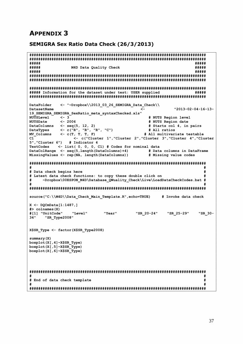
37
APPENDIX 3
SEMIGRA Sex Ratio Data Check (26/3/2013) ################################################################################
################################################################################
##### #####
##### M4D Data Quality Check #####
##### #####
################################################################################
################################################################################
################################################################################
##### Information for the dataset under test: USER supplied #####
################################################################################
DataFolder <- "~Dropbox\\2013_03_26_SEMIGRA_Data_Check\\
DatasetName <- "2013-02-04-16-13-
19_SEMIGRA_SEMIGRA_SexRatio_meta_syntaxChecked.xls"
NUTSLevel <- 3 # NUTS Region level
NUTSDate <- 2006 # NUTS Region date
DataColumns <- seq(5, 12, 2) # Starts col 4, in pairs
DataTypes <- c("R", "R", "R", "C") # All ratios
MV_Columns <- c(T, T, T, F) # All multivariate testable
C1 <- c("Cluster 1","Cluster 2","Cluster 3","Cluster 4","Cluster
5","Cluster 6") # Indicator 4
TestCodes <- list( 0, 0, 0, C1) # Codes for nominal data
DataColRange <- seq(5,length(DataColumns)+4) # Data columns in DataFrame
MissingValues <- rep(NA, length(DataColumns)) # Missing value codes
################################################################################
# #
# Data check begins here #
# Latest data check functions: to copy these double click on #
# ~Dropbox\00ESPON_M4D\Database_QWuality_Check\Live\LoadDataCheckCodes.bat #
# #
################################################################################
source("C:\\M4D\\Data_Check_Main_Template.R",echo=TRUE) # Invoke data check
X <- DQCmData[1:1487,]
#> colnames(X)
#[1] "UnitCode" "Level" "Year" "SR_20-24" "SR_25-29" "SR_30-
34" "SR_Type2008"
X$SR_Type <- factor(X$SR_Type2008)
summary(X)
boxplot(X[,4]~X$SR_Type)
boxplot(X[,5]~X$SR_Type)
boxplot(X[,6]~X$SR_Type)
################################################################################
# #
# End of data check template #
# #
################################################################################

38
APPENDIX 4
SEMIGRA Labour Market Data Check (26/3/2013) ################################################################################
################################################################################
##### #####
##### M4D Data Quality Check #####
##### #####
################################################################################
################################################################################
################################################################################
##### Information for the dataset under test: USER supplied #####
################################################################################
DataFolder <- "~Dropbox\\2013_03_26_SEMIGRA_Data_Check\\"
DatasetName <- "2013-02-04-18-08-
10_SEMIGRA_SEMIGRA_LabourMarket_meta_syntaxChecked.xls"
NUTSLevel <- 2 # NUTS Region level
NUTSDate <- 2006 # NUTS Region date
DataColumns <- seq(5, 24, 2) # Starts col 4, in pairs
DataTypes <- c("T", "T", rep("R",8)) # All ratios
MV_Columns <- rep(F, F, T, T, T, T, T, T, T, T) # All multivariate
testable
C1 <- c("Cluster 1","Cluster 2","Cluster 3","Cluster 4","Cluster
5","Cluster 6","Underemployment","Extreme values","Not analysed") # Indicator 1
C2 <- c("Cluster 1","Cluster 2","Cluster 3","Cluster 4","Agriculture
dominant","Industry dominant","Service sector dominant","Public sector
dominant","Financial sector dominant","Not analysed") # Indicator 1
TestCodes <- list(C1, C2, 0, 0, 0, 0, 0, 0, 0, 0) # Codes for nominal data
DataColRange <- seq(4,length(DataColumns)+4) # Data columns in DataFrame
MissingValues <- rep(NA, length(DataColumns)) # Missing value codes
DrawPlots <- TRUE
DrawMaps <- TRUE
################################################################################
# #
# Data check begins here #
# Latest data check functions: to copy these double click on #
# ~Dropbox\00ESPON_M4D\Database_Quality_Check\Live\LoadDataCheckCodes.bat #
# #
################################################################################
source("C:\\M4D\\Data_Check_Main_Template.R",echo=TRUE) # Invoke data check
################################################################################
# #
# End of data check template #
# #
################################################################################
Typology_Gendergap
Typology_IndustryStructure
GenderGap_15-24
GenderGap_25-34
GenderGap_35-44
WF_Agriculture
WF_IndustryConstruction
WF_TTA
WF_PublicServices
WF_OtherServices

39
APPENDIX 5
EU LUPA Data Check
################################################################################
################################################################################
##### #####
##### M4D Data Quality Check #####
##### #####
################################################################################
################################################################################
################################################################################
##### Information for the dataset under test: USER supplied #####
################################################################################
DataFolder <- "~ Dropbox\\2014_01_08_EU_LUPA_LandUse_DataCheck\\"
DatasetName <- "2014-01-08-19-55-38_EU LUPA_eu-
lupa_land_change_syntaxChecked_v2_syntaxChecked.xls"
NUTSLevel <- "X" # NUTS Region level (X =
NUTS2/3
NUTSDate <- 2006 # NUTS Region date
DataColumns <- c(4,6,8) # Starts col 4, in pairs
DataTypes <- c(rep("R",3)) # All ratios
MV_Columns <- c(T, T, F) # All multivariate testable
TestCodes <- list(0, 0, 0) # Codes for nominal data
DataColRange <- seq(4,length(DataColumns)+4) # Data columns in DataFrame
MissingValues <- rep(NA, length(DataColumns)) # Missing value codes
################################################################################
# #
# Data check begins here #
# Latest data check functions: to copy these double click on #
# ~Dropbox\00ESPON_M4D\Database_Quality_Check\Live\LoadDataCheckCodes.bat #
# #
################################################################################
source("C:\\M4D\\Data_Check_Main_Template.R",echo=TRUE) # Invoke data check
################################################################################
# #
# End of data check template #
# #
################################################################################
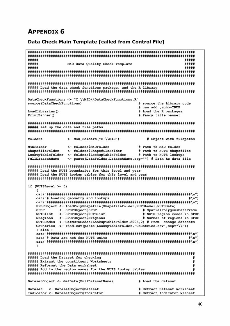
40
APPENDIX 6
Data Check Main Template [called from Control File] ################################################################################
################################################################################
##### #####
##### M4D Data Quality Check Template #####
##### #####
################################################################################
################################################################################
################################################################################
##### Load the data check functions package, and the R library
################################################################################
DataCheckFunctions <- "C:\\M4D\\DataCheckFunctions.R"
source(DataCheckFunctions) # source the Library code
# can add ,echo=TRUE
LoadLibraries() # Load the R packages
PrintBanner() # fancy title banner
################################################################################
##### set up the data and file paths
################################################################################
folders <- M4D_Folders("C:\\M4D") # Object with filepaths
M4DFolder <- folders$M4DFolder # Path to M4D folder
ShapefileFolder <- folders$ShapefileFolder # Path to NUTS shapefiles
LookupTableFolder <- folders$LookupTableFolder # Path to NUTS lookups
FullDatasetName <- paste(DataFolder,DatasetName,sep="") # Path to data file
################################################################################
##### Load the NUTS boundaries for this level and year
##### Load the NUTS Lookup tables for this level and year
################################################################################
if (NUTSLevel >= 0)
{
cat("#####################################################################\n")
cat("# Loading geometry and lookups #\n")
cat("#####################################################################\n")
SPDFObject <- loadPolyShapefile(ShapefileFolder,NUTSLevel,NUTSDate)
SPDF <- SPDFObject$SPDF # SpatialPolygonsDataFrame
NUTSlist <- SPDFObject$NUTSlist # NUTS region codes in SPDF
Nregions <- SPDFObject$Nregions # Number of regions in SPDF
NUTSCodes <- GetNUTSCodes(LookupTableFolder,2006,2) # From change datasets
Countries <- read.csv(paste(LookupTableFolder,"Countries.csv",sep="\\"))
} else {
cat("#####################################################################\n")
cat("# Data are not for NUTS units #\n")
cat("#####################################################################\n")
}
################################################################################
##### Load the Dataset for checking #
##### Extract the constituent Worksheets #
##### Reformat the Data worksheet #
##### Add in the region names for the NUTS lookup tables #
################################################################################
DatasetObject <- GetData(FullDatasetName) # Load the dataset
Dataset <- DatasetObject$Dataset # Extract Dataset worksheet
Indicator <- DatasetObject$Indicator # Extract Indicator w/sheet

41
Source <- DatasetObject$Source # Extract Source worksheet
Data <- DatasetObject$Data # Extract Data worksheet
Dataset.Info(Dataset) # print data details
Indicator.Info(Indicator) # print summary metadata
Data.Unique.Name.Check(Data) # Check Duplicate Names
DQC.out <- UnpackDataWorksheet(Data,DataColumns) # Reshape for analysis
DQCrData <- DQC.out$DQC # Reshaped data
DQCVnames <- DQC.out$Vnames # Variables
DQCMVnames <- DQCVnames[MV_Columns] # Multivariate columns
Reshaped.Data.Unique.Name.Check(DQCVnames) # check duplicate names
DQCmData <- Update.Missing.Value.Codes(DQCrData,MissingValues) # conv to NA
Missing.Value.Analysis(DQCmData) # check incomplete cases
################################################################################
##### Data are not for any NUTS units #
################################################################################
DQCData <- MergeNUTSNames(DQCmData,NUTSCodes) # Add in names from MUTS
lookup
nv <- length(DQCVnames) # number of variables
invalidNUTScodes <- which(is.na(DQCData[,3+nv+1])) # NUTS codes not in lookup
#Check.Invalid.NUTS.Codes(DQCData,invalidNUTScodes,Countries)
Print.Invalid.NUTS.Codes(DQCData,invalidNUTScodes,Countries) # list the crap
################################################################################
##### Determine NTS regions in the SPDF are *not* in the data #
##### Print a list of the omitted regions #
##### Subset the SPDF appropriately #
################################################################################
OmittedRegions <- Omitted(NUTSlist,DQCData[,1]) # Which regions are missing
PrintOmitted(NUTSCodes,OmittedRegions) # Print the regions in the
# shapefile which are not
SPDF.DQC <- SubsetSPDF(SPDF,OmittedRegions) # in the test dataset
################################################################################
##### Determine NUTS regions in the DQC data that have missing data #
##### Print the records #
##### Create a 'clean' subset for the spatial and multivariate tests #
################################################################################
cat("\n\nMissing Data (records with NA check\n")
MissingDataRecords <- MissingRecords(DQCData,DataColRange) # Find NAs in data
if (length(MissingDataRecords) > 0) {
cat("\n*** Records with missing data\n")
DQCData[MissingDataRecords,c(1,DataColRange,12)] # Print names
} else {
cat("\n*** There are NO records with missing data\n")
}
if (length(MissingDataRecords) > 0){
DQCData.nomissing <- DQCData[-MissingDataRecords,] # Remove missing
} else
DQCData.nomissing <- DQCData
SPDF.nomissing <- CleanSPDF(SPDF,DQCData.nomissing) # Clean SPDF
################################################################################
##### Exploratory analysis first #
##### Nominal: frequency tabulation and histogram #
##### valid category check #
##### Ordinal: summary statistics #
##### Ratio: summary statistics #
##### #
##### Then... check plots next - barplots for nominal, boxplots for ratio #
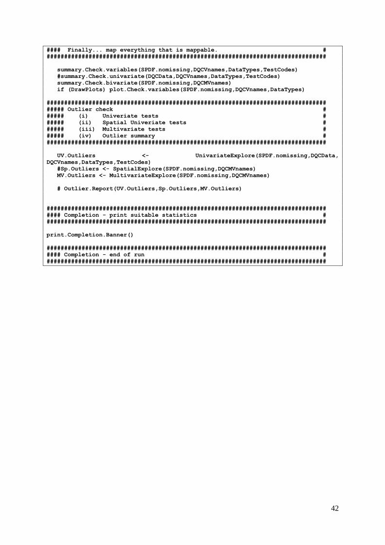
42
#### Finally... map everything that is mappable. #
################################################################################
summary.Check.variables(SPDF.nomissing,DQCVnames,DataTypes,TestCodes)
#summary.Check.univariate(DQCData,DQCVnames,DataTypes,TestCodes)
summary.Check.bivariate(SPDF.nomissing,DQCMVnames)
if (DrawPlots) plot.Check.variables(SPDF.nomissing,DQCVnames,DataTypes)
################################################################################
##### Outlier check #
##### (i) Univeriate tests #
##### (ii) Spatial Univeriate tests #
##### (iii) Multivariate tests #
##### (iv) Outlier summary #
################################################################################
UV.Outliers <- UnivariateExplore(SPDF.nomissing,DQCData,
DQCVnames,DataTypes,TestCodes)
#Sp.Outliers <- SpatialExplore(SPDF.nomissing,DQCMVnames)
MV.Outliers <- MultivariateExplore(SPDF.nomissing,DQCMVnames)
# Outlier.Report(UV.Outliers,Sp.Outliers,MV.Outliers)
################################################################################
#### Completion - print suitable statistics #
################################################################################
print.Completion.Banner()
################################################################################
#### Completion - end of run #
################################################################################

43
APPENDIX 7
Data_Check_Functions.R ########################################################################
########################################################################
#### ####
#### M4D Data Check Functions ####
#### ####
#### Authors: Paul Harris ####
#### Martin Charlton ####
#### Alberto Caimo ####
#### ####
#### Version NCG.2012.11.28a ####
#### ####
#### Contact: Martin Charlton ####
#### National Centre for Geocomputation ####
#### National University of Ireland Maynooth ####
#### Maynooth, County Kildare, IRELAND ####
#### ####
#### email: [email protected] ####
#### ####
########################################################################
########################################################################
########################################################################
# Housekeeping #
########################################################################
#
# Return folder paths for various users
#
M4D_Folders <- function(folder){
#Dropbox <- switch(user,
# martin.office = "C:\\Documents and Settings\\mcharlton.NUIM\\My
Documents\\My Dropbox",
# martin.fujitsu = "C:\\Documents and Settings\\mcharlton\\My
Documents\\Dropbox",
# martin.laptop = "C:\\Users\\mcharlton\\Dropbox",
# alberto.laptop = "C:\\Users\\acaimo\\Dropbox"
# )
# M4DFolder <- paste(Dropbox,"\\00ESPON_M4D",sep="")
# ShapefileFolder <-
paste(M4DFolder,"\\Spatial_Data\\NUTS_ETRS_1989_LAEA",sep="")
# LookupTableFolder <- paste(M4DFolder,"\\Spatial_Data\\NUTS_Info",sep="")
M4DFolder <- folder
ShapefileFolder <- paste(M4DFolder,"\\NUTS_ETRS_1989_LAEA",sep="")
LookupTableFolder <- paste(M4DFolder,"\\NUTS_Info",sep="")
return(list(M4DFolder=M4DFolder,
ShapefileFolder=ShapefileFolder,
LookupTableFolder=LookupTableFolder))
}
#
# Banner for the output
#
PrintBanner <- function(){
cat("+===============================================================+\n")
cat("+===============================================================+\n")
cat("### ###\n")
cat("### M4D: Data Quality Check ###\n")
cat("### ###\n")
cat("### National Centre for Geocomputation ###\n")
cat("### National University of Ireland Maynooth ###\n")
cat("### Maynooth, Co Kildare, Ireland ###\n")

44
cat("### ###\n")
cat("+===============================================================+\n")
cat("+===============================================================+\n")
cat("Run on: ",date(),"\n\n")
}
#
# Banner for end of run
#
print.Completion.Banner <- function(){
cat("+===============================================================+\n")
cat("### M4D: Data Quality Check ###\n")
cat("### Completed at: ", date()," ###\n")
cat("+===============================================================+\n")
}
########################################################################
# General purpose and setup routines #
########################################################################
#
# LoadLibraries()
#
# Load the required libraries
#
LoadLibraries <- function(){
library(RODBC) # to import data from excel
library(MASS) # this has parallel coordinates plots, rlm
library(maptools) # spatial data handling libraries
library(spdep) # localmoran in here
library(forecast) # auto.arima stuff in here
library(spgwr) # gw.cov in here
library(DMwR) # Talgo's outlier.ranking routines
library(RColorBrewer) # Cindy Brewer's palettes
library(aplpack) # this has bagplots
}
#
# Country level color palette
#
LoadEUColorPalette <- function(){
#
# Color palette
#
c( 24,214,236,558, 32,
553, 59,504, 54, 41,
620,151,412,146,143,
385,611,654,494, 51,
258,614,124,434,615,
29,594, 31,462,450,
120,122,609, 88)
}
#
# Reminder of the Brewer Color Palettes which are available
#
PlotBrewerPalettes <- function(){
display.brewer.all(n=NULL, type="all", select=NULL, exact.n=TRUE)
}
#
# Re-insert the omitted items back in the right order
# weeded.list is the logical vector without the omits
# omits is the vector of omitted indices
#
rebuild.list <- function(weeded.list, omits){
n <- length(weeded.list) + length(omits)
final.list <- rep(NA,1,n)
k <- 0
final.list[omits] <- FALSE
for (i in 1:n){
if (is.na(final.list[i])){

45
k <- k + 1
final.list[i] <- weeded.list[k]
}
}
final.list
}
#
# pause():
# Pause an interactive script
#
pause <- function () {
if (interactive())
readline("Hit <enter> to continue...")
invisible()
}
#######################################################################
# Dataset manipulation and setup routines #
#######################################################################
#
# GetData()
# Function to read an M4D Excel Spreadsheet
# Arguments:
# Excel.Spreadsheet: path to an Excel (.xls) spreadsheet
#
# Requires: library(RODBC)
#
GetData <- function(Excel.Spreadsheet){
id <- odbcConnectExcel(Excel.Spreadsheet) # file handle
Dataset <- sqlFetch(id,"Dataset") # Read the Dataset description
Indicator <- sqlFetch(id,"Indicator") # Read the metadata
Source <- sqlFetch(id,"Source") # Read sources
Data <- sqlFetch(id,"Data") # Read the Data worksheet
close(id)
return(list(Dataset=Dataset,Indicator=Indicator,Source=Source,Data=Data))
}
#
# GetNUTSCodes(year)
# Function to read the NUTS codes for a given
# Arguments:
# Year: year required
#
# Requires: library(RODBC)
#
GetNUTSCodes <- function(filepath,year,NUTSLevel){
filename <- paste(filepath,"\\NUTS_",year,"_Codes.xls",sep="")
id <- odbcConnectExcel(filename) # file handle
Lookup <- sqlFetch(id,"Lookup") # Read the NUTS codes and names
close(id)
#
# Now copy NUTS codes code NUTSLevel (Level in Col 7, Name in Col 10,
# Code in Col 1)
# Lookup[which(Lookup[,7] == NUTSLevel),c(1,2,7)]
colnames(Lookup)[10] <- "Name"
Lookup[which(Lookup[,7] == NUTSLevel),c(1,10,7)]
}
#
# MergeNUTSNames - add in the names to the data frame - names come from the
# GetNUTSCodes lookup tables (Excel spreadsheets)
#
MergeNUTSNames <- function(DQCData,NUTSCodes){
data.frame(DQCData, NUTSCodes[match(DQCData[,"UnitCode"], NUTSCodes[,"Code"]),])
}
#
# Create a variable name from the indicator name
# and date information in the spreadsheet
# NA and null are omitted to keep the variable
# name short
#

46
# is.crap : auxiliary function to test for NA, NULL
# or blank fields
# Probably should have a more polite name
#
is.crap <- function(x) {is.na(x) | is.null(x) | x == "" | x == " "}
#
create.variable.name <- function(a,b,c){
if (is.crap(b) & is.crap(c)) a # both missing
else if (is.crap(b)) paste(a,c,sep="") # first date missing
else if (is.crap(c)) paste(a,b,sep="") # second date missing
else paste(a,b,c,sep="") # neither missing
}
#
# UnpackDataWorksheet
#
UnpackDataWorksheet <- function(DataWorksheet,DataColumns){
N.Data <- dim(DataWorksheet)[1] # Worksheet length
NV <- length(DataColumns) # Number of variables to extract
cnames <- rep("",NV) # Array for column names
dnames <- colnames(DataWorksheet)
Data.for.checking <- as.data.frame(Data[3:N.Data,c(1:3,DataColumns)])
for (i in 1:NV){
VarCol <- DataColumns[i]
# cnames[i] <-
paste(dnames[VarCol],DataWorksheet[1,VarCol],DataWorksheet[2,VarCol],sep=".")
cnames[i] <-
create.variable.name(dnames[VarCol],DataWorksheet[1,VarCol],DataWorksheet[2,VarCol]
)
}
colnames(Data.for.checking) <- c("UnitCode","Level","Year",cnames)
return(list(DQC=Data.for.checking,Vnames=cnames))
}
#
# Omitted Regions
#
Omitted <- function(NUTSRegions,CheckDataRegions){
setdiff(NUTSRegions,CheckDataRegions)
}
PrintOmitted <- function(NUTSCodes,OmittedRegions){
cat("\n\nMISSING REGIONS in the Data for Checking\n")
if (length(OmittedRegions) > 0) {
cat("Regions in the NUTS list not in the data for checking\n")
print(NUTSCodes[which(NUTSCodes[,1] %in% OmittedRegions),])
cat("\nRegions in the Shapefile not in the data for checking\n")
print(OmittedRegions)
} else {
cat("\n*** There are no omitted regions\n\n")
}
}
#######################################################################
# Missing Data handlers #
#######################################################################
#
# MissingRecords
#
MissingRecords <- function(DQCData,DataColRange){
N <- dim(DQCData)[1]
MissingData <- which(is.na(DQCData[,DataColRange]))
MissingData[MissingData <= N]
}
#
# Function ValidCodes()
#
# Arguments:
# x: vector of nominal data to be checked
# ValidCodeList: list of allowable codes for x
#
ValidCodes <- function(x,ValidCodeList){

47
x %in% ValidCodeList
}
#
# Function Data.Unique.Name.Check(Data)
# Check for unique column names in spreadsheet as it comes in
#
# Arguments:
# Data: worksheet Data from spreasheet
#
Data.Unique.Name.Check <- function(Data) {
cat("\n\n")
cat("+===============================================================+\n")
cat("### Check for duplicated column names in original spreadsheet ###\n")
cat("+===============================================================+\n")
Column.Names <- colnames(Data)
Duplicate.List <- which(duplicated(Column.Names))
if (length(Duplicate.List) > 0) {
cat("***The following names are duplicated in the column header\n")
Column.Names[Duplicate.List]
cat("\n\n")
} else {
cat("***There are no duplicated column names\n\n")
}
}
#
# Function Data.Unique.Name.Check(Data)
# Check for unique column names in spreadsheet as it comes in
#
# Arguments:
# Data: worksheet Data from spreasheet
#
Reshaped.Data.Unique.Name.Check <- function(NameList) {
cat("\n\n")
cat("+===============================================================+\n")
cat("## Check for duplicated column names in worksheet for checking ##\n")
cat("+===============================================================+\n")
Duplicate.List <- which(duplicated(NameList))
if (length(Duplicate.List) > 0) {
cat("***The following column names are duplicated...\n")
NameList[Duplicate.List]
cat("\n\n")
} else {
cat("***There are no duplicated column names\n\n")
}
}
#######################################################################
# Missing Value Handlers #
#######################################################################
#
# Update.Missing.Value.Codes
#
# Update the supplied missing value codes for each column as NA
#
# Arguments:
# DQCData: data frame for update
# MissingValues: vector missing value codes
#
Update.Missing.Value.Codes <- function (DQCData,MissingValues) {
nv <- length(MissingValues)
DQCTest <- DQCData
if (nv > 0) {
for (i in 1:nv) {
DQCTest[which(DQCTest[,i+3] == MissingValues[i]),i+3] <- NA
}
}
DQCTest
}

48
#
# Missing.Value.Analysis
#
Missing.Value.Analysis <- function(DQCTest) {
nr <- dim(DQCTest)[1] # number of rows
nv <- dim(DQCTest)[2] # number of columns
vn <- colnames(DQCTest) # column headers
cat("\n\n")
cat("+===============================================================+\n")
cat("### Missing Value analysis ###\n")
cat("+===============================================================+\n")
cat("\n***Missing value counts and percentages\n")
for (i in 4:nv) {
nm <- which(is.na(DQCTest[,i])) # find Missing
km <- length(nm) # number missing
kpct <- round(100 * (km / nr),2) # percent missing
cat(paste("Indicator ",vn[i],": ",km," (",kpct,"%)\n",sep=""))
}
complete <- which(complete.cases(DQCTest[,4:nv])) # complete cases
nc <- length(complete) # number of complete cases
cat("\nTotal observations: ",nr,", of which ",nc," have ALL data present\n")
incomplete <- which(!complete.cases(DQCTest[,4:nv]))
nt <- nv - 3
all.missing <- rep(nr,FALSE)
if (length(incomplete) > 0) {
cat("\n*** Zones with missing observations\n")
cat(" ===================================\n")
for (i in 1:nr) {
s <- rowSums(is.na(DQCTest[i,4:nv]))
if (s > 0){
cntry <- which(Countries[,1]==substr(DQCTest[i,1],1,2))
if (length(cntry) > 0) {
cdata <- Countries[as.integer(cntry),2:3]
} else {
cdata <- c("Unknown code","Unknown")
}
country.name <- unlist(cdata[1])
country.status <- unlist(cdata[2])
# print(cdata)
cat(paste(DQCTest[i,1],", (",s,") ",
country.name,": ",
country.status," \n",sep=""))
}
}
}
}
Print.Completely.Missing.Cases <- function(D,incomplete){
cat("\n\n*** Completely Missing Cases ***\n")
if(length(incomplete) > 0) {
cat("\n*** All indicators missing for:\n")
D[incomplete,"UnitCode"]
} else {
cat("\n*** No cases with all indicators missing ***\n")
}
}
#######################################################################
# Shapefile handling service routines #
#######################################################################
#
# Load shapefile
#
loadPolyShapefile <- function(filepath,NUTSlevel,year){
filename <- paste(filepath,"\\NUTS",NUTSlevel,"_",year,".shp",sep="")
# print(filename)

49
SPDF <- readShapePoly(filename,
proj4string=CRS("+proj=laea +lat_0=52 +lon_0=10 +x_0=4321000 +y_0=3210000
+ellps=GRS80 +units=m +no_defs "))
NUTSlist <- sort(SPDF@data$NUTS_ID)
Nregions <- length(NUTSlist)
return(list(SPDF=SPDF,NUTSlist=NUTSlist,Nregions=Nregions))
}
#
# Update.SPDF.COlumns
# Adjust DQCData column positions to allow for SPDF
# items after merge of DQCData and SPDF@data
#
#Update.SPDF.Columns <- function(DQCCols,year){
# switch (year,
# 1996 = Offset <- 0,
# 2003 = Offset <- 8,
# 2006 = Offset <- 9,
# 2010 = Offset <- 6)
# DQCCols + Offset
#}
#
# Subset the Shapefile on the region name
#
SubsetSPDF <- function(SPDF,OmittedRegions){
valid.regions <- ! SPDF@data$NUTS_ID %in% OmittedRegions
SPDF[valid.regions,]
}
#
# Clean SPDF for spatial and multivariate tests
#
CleanSPDF <- function(SPDF,DQCData.nomissing){
Records.nomissing <- dim(DQCData.nomissing)[1]
SPDF2 <- SPDF
if (Records.nomissing > 0) {
CleanRegions <- SPDF@data$NUTS_ID %in% DQCData.nomissing[,1]
SPDF2 <- SPDF[CleanRegions,]
SPDF2@data <- MergeDataWithSPDF(SPDF2,DQCData.nomissing,"UnitCode")
}
return(SPDF2)
}
#
# Create neighbour list from the subsetted data
#
SPDF.listw <- function(SPDF){
nb2listw(poly2nb(SPDF)) # Create neighbour list from nb-ed polygons
}
#
# Match the data frame from UnpackDataWorksheet with the SPDF from
# loadPolyShapefile
# See
# http://stackoverflow.com/questions/3650636/how-to-attach-a-simple-data-frame-to-
a-spatialpolygondataframe-in-r
# x must be a data frame
#
MergeDataWithSPDF <- function(SPDF,x,Code){
SPDF@data <- data.frame(SPDF@data, x[match(SPDF@data[,"NUTS_ID"], x[,Code]),
])
}
#
#######################################################################
# Metadata service routines #
#######################################################################
Dataset.Info <- function(Dataset){
Dataset.name <- as.character(Dataset[1,2])
Project <- as.character(Dataset[2,2])
Abstract <- as.character(Dataset[5,2])
URI <- as.character(Dataset[7,2])

50
cat("+===============================================================+\n")
cat("### Dataset identification ###\n")
cat("+===============================================================+\n")
cat("Dataset name: ",Dataset.name,"\n")
cat("Project: ",Project,"\n")
cat("Abstract: ",Abstract,"\n")
cat("Unique Resource Identifier ",URI,"\n")
cat("\n")
}
Indicator.Info <- function(Indicator){
vnames <- Indicator[which(Indicator[,1]=="Code")+1,1]
datatypes <- Indicator[which(Indicator[,1]=="Data type"),3]
values <- as.character(Indicator[which(Indicator[,1]=="Unit of
measure"),3])
start.dates <- as.numeric(Indicator[which(Indicator[,1]=="Temporal
Extent")+1,2])
finish.dates <- as.numeric(Indicator[which(Indicator[,1]=="Temporal
Extent")+1,3])
z <- cbind(as.character(vnames),as.character(datatypes),as.character(values))
z <- rbind(c("Indicator Name","Data Type","Data Values"),z)
cat("+===============================================================+\n")
cat("### Summary information from the metadata ###\n")
cat("+===============================================================+\n")
write.table(format(z,justify="left"),row.names=F,col.names=F,quote=F)
cat("\n")
}
#######################################################################
# Outlier check service routines #
#######################################################################
#
# Function PositiveInteger
#
PositiveInteger <- function(x){
x == floor(x) & x >= 0
}
#
# Function BoxplotTest
#
BoxplotTest <- function(x){
bp <- boxplot.stats(x,coef=1.5)
x >= bp$stats[1] & x <= bp$stats[5]
}
#
# HawkinsTest
#
# Requires: library(spgwr)
#
HawkinsTest <- function(x,coords){
x.spdf <- x
coordinates(x.spdf) <- coords # create data frame
bw <- 0.1 # local bandwidth (10% of data)
chi5pct <- 3.84146 # test distributed as chi square
with 1df
gwss <- gw.cov(x.spdf, data=x, adapt=bw) # locally weighted summary
statistics
local.mean <- gwss$SDF$mean.V1 # locally weighted mean
local.variance <- gwss$SDF$sd.V1^2 # locally weighted variance
local.N <- bw * length(x) # local sample size
local.alv <- mean(local.variance) # average local variance
Hawkins <- (local.N*(x - local.mean)^2)/((local.N+1)*local.alv) # test
statistic
Hawkins > chi5pct # significant test result
}
#

51
# Local Moran test
# Anselin, L. 1995. Local indicators of spatial association, Geographical Analysis,
27, 93–115
# Getis, A. and Ord, J. K. 1996 Local spatial statistics: an overview. In P.
Longley and M. Batty (eds)
# Spatial analysis: modelling in a GIS environment (Cambridge: Geoinformation
International), 261–277.
#
# SPDF must 'clean' - no missing data
#
Local.Moran.Outliers <- function(SPDF,MVCols,p.threshold=0.05){
# First generate the neighbour lists, and the weights matrix
# Allow for zero neighboured objects
print(MVCols)
neighbour.list <- poly2nb(SPDF) # build neighbour list
spatial.weights.matrix <- nb2listw(neighbour.list,zero.policy=TRUE)
#
N <- dim(SPDF@data)[1] # number of observations
M <- length(MVCols) # number of variables
evidence <- array(FALSE,c(N,M+1))
deviates <- array(0,c(N,5)) # weight of evidence
rownames(evidence) <- seq(1,N)
colnames(evidence) <- seq(1,M+1)
k <- 0
for (i in MVCols) { # test each variable in turn
deviates <- as.matrix(localmoran(SPDF@data[,i],spatial.weights.matrix))
k <- k + 1
rownames(deviates) <- seq(1,N)
# str(deviates)
# str(evidence)
evidence[,k] <- deviates[,"Pr(z > 0)"] > p.threshold # Pr(Z > 0)
}
evidence[,M+1] <- rowSums(evidence[,1:M]) / M # weight of evidence
return(evidence)
}
#######################################################################
### ###
### Multivariate Methods ###
### ###
#######################################################################
#
# RunningRegression(x)
# Regress each column of x on the others and compute the
# proportion of standardised residuals greater
# than a user supplied threshold
#
CirculatingRegression <- function(x,thresh=3){
N <- dim(x)[1]
M <- dim(x)[2]
resid.tests <- matrix(0,N,M)
for (i in 1:M) {
response <- x[,i]
predictors <- as.matrix(x[,-i])
m1 <- lm(response~predictors)
resid.tests[,i] <- abs(rstandard(m1)) > thresh
}
rowSums(resid.tests) / M
}
#
# Robust version: use Boxplot Test
#
CirculatingRobustRegression <- function(x,thresh=3){
N <- dim(x)[1]
M <- dim(x)[2]
resid.tests <- matrix(0,N,M)
for (i in 1:M) {
response <- x[,i]
predictors <- as.matrix(x[,-i])

52
rlm.res <- rlm(response~predictors)$resid
resid.tests[,i] <- BoxplotTest(rlm.res)
}
rowSums(resid.tests) / M
}
#
# Component scores - summarise a large body of variables
# Areas with score > thresh on component 1 are potential
# outliers
#
test_PCA <- function(x,thresh=3){
princomp(x,cor=T,scores=T)$scores[,1] <= thresh
}
#
# Mahalonobis distances
#
Mahalanobis.Distances <- function(x){
mahalanobis(x,colMeans(x),cov(x))
}
#
# Mahalanobis plot
#
Mahalanobis.Plot <- function(MD2,bw=0.5,title){
plot(density(MD2,bw=bw),main=title); rug(MD2)
}
#
# Mahalanobis.Outliers
#
Mahalanobis.Outliers <- function(x,threshold){
Mahalanobis.Distances(x) < threshold
}
#
# Torgo's routines
# http://www.liaad.up.pt/~ltorgo/DataMiningWithR/
#
Torgo.Probabilities <- function(x){
inter.object.distances <- daisy(x)
outliers.ranking(inter.object.distances)$prob.outliers
}
#
# Torgo Outliers
#
Torgo.Outliers <- function(x,threshold=0.8){
Torgo.Probabilities(x) <= threshold
}
#
# Bagplot Test for two variables
#
bagplot.test <- function(v1,v2){
N <- length(v1) # length of data vectors
bagplot.test.result <- rep(TRUE,N) # Initialise output
z <- compute.bagplot(v1,v2) # compute bagplot
out <- z$pxy.outlier # extract the outliers
Nout <- dim(out)[1] # Any outliers?
if (Nout >= 1) { # Yes: which are they?
outliers <- which((v1 %in% out[,1]) & (v2 %in% out[,2]))
bagplot.test.result[outliers] <- FALSE # Update the output
}
bagplot.test.result # return the result vector
}
#
# Bagplot.Analysis
#
# Computes the bagplot statistics for every pairing of the variables
# in a matrix and returns a outlier score (1=OK, <1 possibly an outlier)
#
Bagplot.Analysis <- function(x){
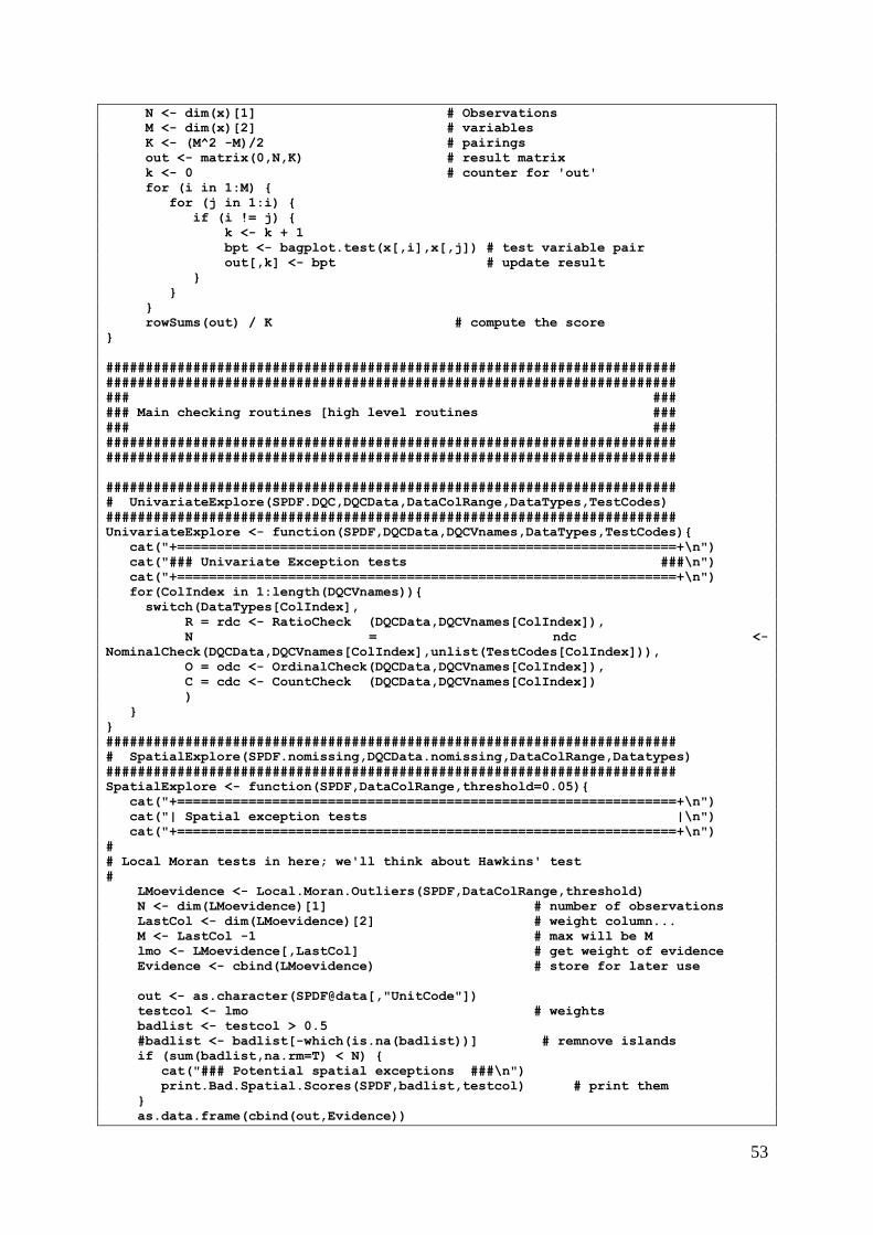
53
N <- dim(x)[1] # Observations
M <- dim(x)[2] # variables
K <- (M^2 -M)/2 # pairings
out <- matrix(0,N,K) # result matrix
k <- 0 # counter for 'out'
for (i in 1:M) {
for (j in 1:i) {
if (i != j) {
k <- k + 1
bpt <- bagplot.test(x[,i],x[,j]) # test variable pair
out[,k] <- bpt # update result
}
}
}
rowSums(out) / K # compute the score
}
########################################################################
########################################################################
### ###
### Main checking routines [high level routines ###
### ###
########################################################################
########################################################################
########################################################################
# UnivariateExplore(SPDF.DQC,DQCData,DataColRange,DataTypes,TestCodes)
########################################################################
UnivariateExplore <- function(SPDF,DQCData,DQCVnames,DataTypes,TestCodes){
cat("+===============================================================+\n")
cat("### Univariate Exception tests ###\n")
cat("+===============================================================+\n")
for(ColIndex in 1:length(DQCVnames)){
switch(DataTypes[ColIndex],
R = rdc <- RatioCheck (DQCData,DQCVnames[ColIndex]),
N = ndc <-
NominalCheck(DQCData,DQCVnames[ColIndex],unlist(TestCodes[ColIndex])),
O = odc <- OrdinalCheck(DQCData,DQCVnames[ColIndex]),
C = cdc <- CountCheck (DQCData,DQCVnames[ColIndex])
)
}
}
########################################################################
# SpatialExplore(SPDF.nomissing,DQCData.nomissing,DataColRange,Datatypes)
########################################################################
SpatialExplore <- function(SPDF,DataColRange,threshold=0.05){
cat("+===============================================================+\n")
cat("| Spatial exception tests |\n")
cat("+===============================================================+\n")
#
# Local Moran tests in here; we'll think about Hawkins' test
#
LMoevidence <- Local.Moran.Outliers(SPDF,DataColRange,threshold)
N <- dim(LMoevidence)[1] # number of observations
LastCol <- dim(LMoevidence)[2] # weight column...
M <- LastCol -1 # max will be M
lmo <- LMoevidence[,LastCol] # get weight of evidence
Evidence <- cbind(LMoevidence) # store for later use
out <- as.character(SPDF@data[,"UnitCode"])
testcol <- lmo # weights
badlist <- testcol > 0.5
#badlist <- badlist[-which(is.na(badlist))] # remnove islands
if (sum(badlist,na.rm=T) < N) {
cat("### Potential spatial exceptions ###\n")
print.Bad.Spatial.Scores(SPDF,badlist,testcol) # print them
}
as.data.frame(cbind(out,Evidence))

54
# to return to NUTS code sort order
xx <- as.data.frame(Sp.Outliers[order(Sp.Outliers[,1]),])
}
########################################################################
# MultivariateExplore(SPDF.nomissing,DQCData.nomissing,MV_Cols)
########################################################################
MultivariateExplore <- function(SPDF,MVCols){
cat("+===============================================================+\n")
cat("### Multivariate Exception tests ###\n")
cat("+===============================================================+\n")
#
# Circulating regression residuals
# PCA with boxplots on first component
# Mahalanobis distances - try with thresh 20 at first
#
N <- length(SPDF@data[,1])
ntests <- 5
CiR.evidence <- 1 - CirculatingRegression(SPDF@data[,MVCols])
RbR.evidence <- CirculatingRobustRegression(SPDF@data[,MVCols])
PCA.evidence <- test_PCA(SPDF@data[,MVCols])
Mah.evidence <- Mahalanobis.Outliers(SPDF@data[,MVCols],20)
Biv.evidence <- Bagplot.Analysis(SPDF@data[,MVCols])
Evidence <-
cbind(CiR.evidence,RbR.evidence,PCA.evidence,Mah.evidence,Biv.evidence)
out <- as.character(SPDF@data[,"UnitCode"])
testcol <- rowSums(Evidence) # total the scores
badlist <- testcol >= ntests / 1.5 # any less than 5
if (sum(badlist) < N) {
cat("### Potential multivariate exceptions ###\n")
print.Bad.Spatial.Scores(SPDF,badlist,testcol) # print them
}
as.data.frame(cbind(out,Evidence))
}
########################################################################
### Main checking routines [high level routines ###
########################################################################
#
# Function NominalCheck(x)
#
# [tests]
# (a) Consistency check - does the codelist agree
#
NominalCheck <- function(x,ColIndex,CodeList){
cat("Nominal data check for Indicator: ",ColIndex,"\n")
cat("Valid codes: ",CodeList,"\n")
cat("\nFrequency Tabulation\n")
print(table(x[,ColIndex])) # Frequency tabulation
vc <- ValidCodes(x[,ColIndex],CodeList) # Valid code check
n.invalid <- length(which(vc==0)) # List any invalid codes
if (n.invalid > 0){
#NUTSCode <- as.character(DQCData[which(vc==F),1])
#BadCode <- DQCData[which(vc==F),ColIndex]
#cat("Regions with invalid codes\n")
#print(cbind(NUTSCode,BadCode) )
cat("\nAnomalous data values found...\n")
print.Bad.Data.Values(DQCData,vc,ColIndex)
}
cat("-------------------------------------------------------------------\n")
return(vc) # Return vector of T/F
}

55
#
# Function OrdinalCheck(x)
#
OrdinalCheck <- function(x,ColIndex){
cat("Ordinal Data Check for Indicator: ",ColIndex,"\n")
IsPositiveInteger <- PositiveInteger(x[,ColIndex])
n.invalid <- length(which(IsPositiveInteger==0)) # List any invalid codes
if (n.invalid > 0){
#NUTSCode <- as.character(DQCData[which(IsPositiveInteger==F),1])
#BadCode <- DQCData[which(IsPositiveInteger==F),ColIndex]
#cat("Regions with invalid ranks\n")
#print(cbind(NUTSCode,BadCode) )
cat("\nNon postive-integer data values found...\n")
print.Bad.Data.Values(DQCData,IsPositiveInteger,ColIndex)
}
cat("-------------------------------------------------------------------\n")
return(IsPositiveInteger)
}
#
# Function CountCheck(x)
#
CountCheck <- function(x,ColIndex){
cat("Count Data Check for Indicator: ",ColIndex,"\n")
IsPositiveInteger <- PositiveInteger(x[,ColIndex])
n.invalid <- length(which(IsPositiveInteger==0)) # List any invalid codes
if (n.invalid > 0){
#NUTSCode <- as.character(DQCData[which(IsPositiveInteger==F),1])
#BadCode <- DQCData[which(IsPositiveInteger==F),ColIndex]
#cat("Regions with non-positive integer data\n")
#print(cbind(NUTSCode,BadCode) )
cat("\nNon postive-integer data values found...\n")
print.Bad.Data.Values(DQCData,IsPositiveInteger,ColIndex)
}
cat("-------------------------------------------------------------------\n")
return(IsPositiveInteger)
}
#
# Function RatioCheck(x)
#
RatioCheck <- function(x,ColIndex){
cat("Ratio Data Check for Indicator: ",ColIndex,"\n")
StatOutlier <- BoxplotTest(x[,ColIndex])
n.invalid <- length(which(StatOutlier==0)) # List potential outliers
if (n.invalid > 0){
#NUTSCode <- as.character(DQCData[which(StatOutlier==F),1])
#BadCode <- DQCData[which(StatOutlier==F),ColIndex]
cat("\nRegions with unusual boxplot data\n")
#print(cbind(NUTSCode,BadCode) )
print.Bad.Data.Values(DQCData,StatOutlier,ColIndex)
}
cat("-------------------------------------------------------------------\n")
}
################################################################################
################################################################################
##### #####
##### Summary functions for the ESPON Data Quality Check #####
##### #####
################################################################################
################################################################################
summary.Check.variables <- function(SPDF,DQCVnames,DataTypes,TestCodes){
cat("+===============================================================+\n")
cat("### Exporatory data summaries ###\n")
cat("+===============================================================+\n")
for (i in 1:length(DQCVnames)){

56
cat("Variable: ",DQCVnames[i],"\n")
cat("Data Type: ",DataTypes[i],"\n")
switch(DataTypes[i],
R = {ss <- summary(SPDF@data[,DQCVnames[i]]) # summary for ratio
data
print(ss)
},
N = {tt <- table(as.factor(SPDF@data[,DQCVnames[i]]))
print(tt)
cat("Categories found are: ",
levels(as.factor(SPDF@data[,DQCVnames[i]])),"\n")
},
O = summary(SPDF@data[,DQCVnames[i]]),
C = summary(SPDF@data[,DQCVnames[i]])
)
cat("-----------------------------------------------------------------\n")
}
cat("\nCompleted\n\n")
}
#
# cor.prob(X)
# correlation matrix of X with correlations in the lower triangle
# and signficance probabilities in the upper triangle
#
# Due to Bill Venables, [email protected],
# 04 Jan 2000 15:05:39
#
cor.prob <- function(X, dfr = nrow(X) - 2) {
R <- cor(X)
above <- row(R) < col(R)
r2 <- R[above]^2
Fstat <- r2 * dfr / (1 - r2)
R[above] <- 1 - pf(Fstat, 1, dfr)
R
}
################################################################################
### Bivariate summaries for ratio variables ####
################################################################################
summary.Check.bivariate <- function(SPDF,MVnames){
cat("+===============================================================+\n")
cat("### Bivariate data summaries ###\n")
cat("+===============================================================+\n")
cat("\nBivariate correlations and p-values\n")
cat("Correlations in the lower triangle and p-values in the upper\n")
print(cor.prob(SPDF@data[,MVnames]))
cat("-----------------------------------------------------------------\n")
}
################################################################################
################################################################################
##### #####
##### Plotting functions for the ESPON Data Quality Check #####
##### #####
################################################################################
################################################################################
#
# Check plots for nominal and ratio data using spplot
# needs the RColorBrewer library
#
# For boxplots, barcharts and maps, plot 4 per display window
# Pairwise plot uses single window only
#
plot.Check.variables <- function(SPDF,varlist,vartypes){
#
# Start with boxplots for the ratio variables: requires RColorBrewer
#

57
X11()
par(mfrow=c(2,2))
for (plotvar in varlist[which(vartypes == "R")]){ # ratio variables only
boxplot(SPDF@data[,plotvar],main=plotvar) # boxplots
pause()
}
par(mfrow=c(1,1))
#
# Next, barcharts for the nominal variables
#
X11()
par(mfrow=c(2,2))
for (plotvar in varlist[which(vartypes == "N")]){ # nominal variables only
barplot(table(SPDF@data[,plotvar]),main=plotvar,xlab="Code") #
barcharts
pause()
}
par(mfrow=c(1,1))
#
# Pairwise plot of the ratio variables
X11()
pairs(SPDF@data[,varlist[which(vartypes == "R")]], main="Pairwise Plots")
pause()
#
# Plot check plots of the ratio variables
#
X11()
for (i in 1:length(varlist)){
if (vartypes[i] %in% c("N","R")){ # ratio/nominal variables
plotvar <- varlist[i] # get the name
datatype <- vartypes[i] # get the type
p.obj <- plot.SPDF.data(SPDF,plotvar,datatype) # create the object
switch.val <- i %% 4
if (i == length(varlist) || switch.val == 0) {AddToPlot <- FALSE} else
{AddToPlot <- TRUE}
switch (switch.val+1,
print(p.obj,position=c(0.5, 0.0, 1.0, 0.5),more=AddToPlot),
print(p.obj,position=c(0.0, 0.5, 0.5, 1.0),more=AddToPlot),
print(p.obj,position=c(0.5, 0.5, 1.0, 1.0),more=AddToPlot),
print(p.obj,position=c(0.0, 0.0, 0.5, 0.5),more=AddToPlot)
)
if (!AddToPlot) {pause()}
} # end if
} # end for
par(mfrow=c(1,1))
#
}
#
# Plot a variable from the SPDF data frame into a trellis plot object
# Nominal data - coerce the data to a factor
# Ratio data plot against 10 classes with a general purpose colour ramp
# from RColorBrewer
#
plot.SPDF.data <- function(SPDF,plotvar,type){
print(paste(plotvar,type))
switch(type,
R =
spplot(SPDF,plotvar,main=as.character(plotvar),col.regions=brewer.pal(11,"Spectral"
),cuts=10),
N = {SPDF2 <- SPDF
SPDF2@data[,plotvar] <- as.factor(SPDF2@data[,plotvar])
labeltext <- as.numeric(levels(SPDF2@data[,plotvar]))
nlabels <- length(labeltext)
labelat <- seq(1,nlabels)
spplot(SPDF2,plotvar,main=plotvar,col.regions=brewer.pal(nlabels,"Set1"),cuts=nlabe
ls-1)

58
}
)
}
###############################################################################
#### ####
#### Reporting routines ####
#### ####
###############################################################################
#
# print.Bad.Spatial.Values()
# SPDF - spatial polygons data frame
# badlist: anomalous entries are FALSE
# testcol: column which has been tested
#
print.Bad.Spatial.Values <- function(SPDF,badlist,testcol){
Values <- SPDF@data[!badlist,testcol]
NUTSCode <- as.character(SPDF@data[!badlist,"UnitCode"])
NUTSName <- as.character(SPDF@data[!badlist,"Name"])
outtable <- cbind(NUTSCode,Values,NUTSName)
outtable <- rbind(c("NUTSCode","Value","NUTS Region Name"),outtable)
write.table(format(outtable,justify="left"),row.names=F,col.names=F,quote=F)
}
#
# print.Bad.Spatial.Scores()
# SPDF - spatial polygons data frame
# badlist: anomalous entries are FALSE
# testcol: column which has been tested
#
print.Bad.Spatial.Scores <- function(SPDF,badlist,testcol){
Values <- testcol[!badlist]
NUTSCode <- as.character(SPDF@data[!badlist,"UnitCode"])
NUTSName <- as.character(SPDF@data[!badlist,"Name"])
outtable <- cbind(NUTSCode,Values,NUTSName)
outtable <- rbind(c("NUTSCode","Value","NUTS Region Name"),outtable)
write.table(format(outtable,justify="left"),row.names=F,col.names=F,quote=F)
}
#
# print.Bad.Data.Values()
# X: data.frame
# badlist: anomalous entries are FALSE
# testcol: column which has been tested
#
print.Bad.Data.Values <- function(X,badlist,testcol){
Values <- X[!badlist,testcol]
NUTSCode <- as.character(X[!badlist,"UnitCode"])
NUTSName <- as.character(X[!badlist,"Name"])
outtable <- cbind(NUTSCode,Values,NUTSName)
outtable <- rbind(c("NUTSCode","Value","NUTS Region Name"),outtable)
write.table(format(outtable,justify="left"),row.names=F,col.names=F,quote=F)
}
#
#
#
Print.Invalid.NUTS.Codes <- function(DQCData,invalidNUTScodes,Countries){
n.inv <- length(invalidNUTScodes)
if (n.inv > 0) {
InvalidStuff <- DQCData[invalidNUTScodes,c(1,2,3,nv+4,nv+5,nv+6)]
InvalidStuff[,4] <- "No NUTS lookup code"
InvalidStuff[,5] <- "Unknown NUTS country"
InvalidStuff[,6] <- "Unknown"
}
cat("\n\nRegions with Unknown NUTS codes for this level and date\n")
cat( "=======================================================\n")
if (n.inv == 0) {
cat("\n*** All NUTS codes in these data appear to be valid\n\n")
} else {

59
xc <- substr(InvalidStuff[,1],1,2)
for (i in 1:n.inv) {
xp <- which(Countries[,1] == xc[i])
if (length(xp) > 0) InvalidStuff[i,5] <-
paste(Countries[xp,2],Countries[xp,3],sep=", ")
}
}
print(InvalidStuff[,c(1,2,3,5)])
}