a genealogy of ISIS and the dynamism of Salafi - Enlighten ...
Upload
khangminh22Category
view
1download
0
GA no. 671657
D5.1
Report on Application Dynamism
Document type: Report
Dissemination level: ReportWork package: WP5
Editor: Lubomır Rıha (IT4I-VSB)Contributing partners: IT4I-VSB, ICHEC-NUIG, GNS, TUM, TUDReviewer: Daniel Molka (TUD), Michael Gerndt (TUM)Version: 1.0
Ref. Ares(2017)1064112 - 28/02/2017
READEX D5.1-Deliverable
Document history
Version Date Author/Editor Description
0.1 27/01/17
Lubomır Rıha, Jan Zapletal, Martin Beseda,Ondrej Vysocky, Vojtech Nikl (IT4I-VSB)Michael Lysaght, Venkatesh Kannan (ICHEC-NUIG),
1st Draft
0.2 14/01/17
Lubomır Rıha, Jan Zapletal, Martin Beseda,Ondrej Vysocky, Vojtech Nikl (IT4I-VSB)Michael Lysaght, Venkatesh Kannan (ICHEC-NUIG),
2nd Draft
0.3 22/01/17
Lubomır Rıha, Jan Zapletal, Martin Beseda,Ondrej Vysocky, Vojtech Nikl (IT4I-VSB)Michael Lysaght, Venkatesh Kannan (ICHEC-NUIG),Kai Diethelm (GNS)
3rd Draft
1.0 28/02/17
Lubomır Rıha, Jan Zapletal, Martin Beseda,Ondrej Vysocky, Vojtech Nikl (IT4I-VSB)Michael Lysaght, Venkatesh Kannan (ICHEC-NUIG),Kai Diethelm (GNS)
Final version
H2020-FETHPC-2014 2

Contents
1 Introduction 4
2 Overview of Dynamism Metrics 5
2.1 Investigation of Computational Intensity . . . . . . . . . . . . . . . . . . . . . 7
2.2 Investigation of Parallel I/O . . . . . . . . . . . . . . . . . . . . . . . . . . . . 10
3 Overview of Tuning Parameters 12
4 Methodology for Dynamism Analysis 14
4.1 Manual Dynamism Evaluation with MERIC . . . . . . . . . . . . . . . . . . . 14
5 Metodology for Dynamism Reporting 19
5.1 RADAR . . . . . . . . . . . . . . . . . . . . . . . . . . . . . . . . . . . . . . . 19
5.2 RADAR Generator for MERIC . . . . . . . . . . . . . . . . . . . . . . . . . . 19
6 Results – Intra-Phase Dynamism 24
6.1 Intel Math Kernel Library Sparse BLAS routines . . . . . . . . . . . . . . . . 24
6.2 ESPRESO . . . . . . . . . . . . . . . . . . . . . . . . . . . . . . . . . . . . . . 26
6.3 Indeed . . . . . . . . . . . . . . . . . . . . . . . . . . . . . . . . . . . . . . . . 37
6.4 MiniMD . . . . . . . . . . . . . . . . . . . . . . . . . . . . . . . . . . . . . . . 42
6.5 OpenFOAM . . . . . . . . . . . . . . . . . . . . . . . . . . . . . . . . . . . . . 49
6.6 ProxyApps 1 - AMG2013 . . . . . . . . . . . . . . . . . . . . . . . . . . . . . 54
6.7 ProxyApps 2 - Kripke . . . . . . . . . . . . . . . . . . . . . . . . . . . . . . . 62
6.8 ProxyApps 3 - LULESH . . . . . . . . . . . . . . . . . . . . . . . . . . . . . . 72
6.9 ProxyApps 4 - MCB . . . . . . . . . . . . . . . . . . . . . . . . . . . . . . . . 86
7 Results – Inter-Phase Dynamism 95
7.1 MCB . . . . . . . . . . . . . . . . . . . . . . . . . . . . . . . . . . . . . . . . . 95
7.2 MiniMD . . . . . . . . . . . . . . . . . . . . . . . . . . . . . . . . . . . . . . . 98
7.3 Indeed . . . . . . . . . . . . . . . . . . . . . . . . . . . . . . . . . . . . . . . . 100
8 Summary 103
3

READEX D5.1-Deliverable
1 Introduction
The energy consumption of supercomputers is one of the critical problems for the upcomingExascale supercomputing era. The awareness of power and energy consumption is requiredon both software and hardware side. This report presents the evaluation of basic kernels,several more complex proxy applications from ProxyApps package and a set of full fledgeapplications, such as ESPRESO FEM library with FETI based solvers, molecular dynamicscode MiniMD and sheet metal forming simulation software Indeed and well known open-source CFD package OpenFOAM.
Section 2 introduces crucial metrics used for detection and evaluation of the dynamic behav-ior of applications. These are the execution time, the computational intensity and energyconsumption.
The selected tuning parameters from three different domains: (1) hardware parameters, (2)runtime system parameters and (3) application parameters are described in Section 3. Thelist of parameters is not final and more will be investigated in the second half of the project.
In order to evaluate the dynamic behavior of any parallel application we have developedMERIC, a tool for semi-automatic energy consumption evaluation. By semi-automatic wemean that the regions of the code that user want to evaluate must be annotated manually,but the rest of the evaluation process is automatic. In the current version the MERIC usesexhaustive parameters space search. This tool is introduced in Section 4.
Section 5 describes the RADAR report and the automatic report generator. This is used forreporting the dynamic savings in this document.
Sections 6 and 7 present the achieved energy savings for selected applications for intra-phaseand inter-phase dynamism, respectively. The applications range from basic BLAS kernels toreal world applications. The evaluation is using various tuning parameters including hard-ware, system software, and application parameters. The effect of both types of tuning: (1)static tuning (when the tuning parameter is fixed for the whole phase) and (2) dynamic tuning(when the tuning parameter changes for particular kernels of this phase) were examined.
Finally Section 8 concludes the document with an overview of the achieved savings of allapplications and final discussion.
H2020-FETHPC-2014 4
READEX D5.1-Deliverable
2 Overview of Dynamism Metrics
The READEX tool suite will tune hardware, system software and application tuning pa-rameters as described in D4.1 [10]. In order to apply the best configurations for the tuningparameters during run-time application tuning (RAT) that are computed during design timeanalysis (DTA), the dynamism present in an application has to be first analysed and quanti-fied using dynamism metrics during DTA. To achieve this, experiments are performed duringwhich the application is run to obtain measurements for the different dynamism metrics toquantify the dynamism present in the application. Additionally, these tools also evaluate thepotential savings using objective values (such as energy consumed and execution time) thatindicate the result of run-time tuning.
The dynamism metrics that are presently measured and used in the READEX project are:
1. Execution time.
2. Energy consumed.
3. Computational intensity.
Among these three metrics, the semantics of execution time and energy consumed are straight-forward. Variation in the execution time and energy consumed by regions in an applicationduring its execution is an indication of different resource requirements. The execution timeand energy consumed are also used in an objective function that will be measured to quantifythe result or potential gain of tuning an application using the READEX tool suite. The com-putational intensity is a metric that is used to model the behaviour of an application based onthe workload imposed by it on the CPU and the memory. Presently, computational intensityis calculated using the following formula and is analogous to the operational intensity usedin the roofline model [16].
Computational Intensity = Total number of instructions executedTotal number of L3 cache misses .
Computational intensity can directly dictate the tuning of two hardware parameters: CPUcore frequency and CPU uncore frequency. A low computational intensity may indicatean application that is more memory intensive, which results in increased L3 cache misses.Since this would cause increased traffic between the L3 cache and the main memory, it willbe desirable to increase the uncore frequency. On the other hand, a high computationalintensity may indicate an application that is more computation intensive. In this case, it willbe desirable to increase the frequency of the CPU cores.
In the context of the READEX project, an application is termed to exhibit the following twotypes of dynamism:
• Inter-phase dynamism: This is when each phase of a phase region in the applicationexhibits different characteristics. This results in different values for the measured ob-jective values and thus may require different configurations to be applied for the tuningparameters.
H2020-FETHPC-2014 5
READEX D5.1-Deliverable
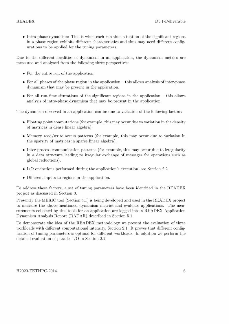
• Intra-phase dynamism: This is when each run-time situation of the significant regionsin a phase region exhibits different characteristics and thus may need different config-urations to be applied for the tuning parameters.
Due to the different localities of dynamism in an application, the dynamism metrics aremeasured and analysed from the following three perspectives:
• For the entire run of the application.
• For all phases of the phase region in the application – this allows analysis of inter-phasedynamism that may be present in the application.
• For all run-time situtations of the significant regions in the application – this allowsanalysis of intra-phase dynamism that may be present in the application.
The dynamism observed in an application can be due to variation of the following factors:
• Floating point computations (for example, this may occur due to variation in the densityof matrices in dense linear algebra).
• Memory read/write access patterns (for example, this may occur due to variation inthe sparsity of matrices in sparse linear algebra).
• Inter-process communication patterns (for example, this may occur due to irregularityin a data structure leading to irregular exchange of messages for operations such asglobal reductions).
• I/O operations performed during the application’s execution, see Section 2.2.
• Different inputs to regions in the application.
To address these factors, a set of tuning parameters have been identified in the READEXproject as discussed in Section 3.
Presently the MERIC tool (Section 4.1) is being developed and used in the READEX projectto measure the above-mentioned dynamism metrics and evaluate applications. The mea-surements collected by this tools for an application are logged into a READEX ApplicationDynamism Analysis Report (RADAR) described in Section 5.1.
To demonstrate the idea of the READEX methodology we present the evaluation of threeworkloads with different computational intensity, Section 2.1. It proves that different config-uration of tuning parameters is optimal for different workloads. In addition we perform thedetailed evaluation of parallel I/O in Section 2.2.
H2020-FETHPC-2014 6

READEX D5.1-Deliverable
2.1 Investigation of Computational Intensity
The computational intensity (CI) is one of the key metrics to evaluate the dynamism. If anapplication has a low CI, the application is memory bound (such as Matrix-Vector Multipli-cation - GEMV) and high CPU frequency cannot be utilized as the data in caches cannotbe reused. On the other hand, for high arithmetical intensity (such as Matrix-Matrix vectormultiplication - GEMM) the memory traffic is significantly lower and a CPU running at highfrequency can be fully utilized.
The goal of this section is to demonstrate how the energy consumption for operations withdifferent compute intensity (DGEMV - low CI; DGEMM - higher CI; compute only kernel -very high CI) is affected by the CPU core and uncore frequencies. Please note that in thissection we use two MPI processes per node and one MPI process per socket. This way weeliminate the NUMA effect. For this experiment the best configuration for all three functionsis to use all cores, i.e. 12 OpenMP threads.
Table 2.1 shows that with increasing CI the effect of the uncore frequency becomes lessimportant, see figures bellow, and the optimal setting is decreased from 2.5 GHz to 1.2 GHz.On the other hand the optimal core frequency should be high (2.5 GHz) for applications withhigh CI and it is decreasing with lower CI. It can be also observed that core frequency tuningis most efficient for kernels high CI.
Finally we can observe, that the highest static energy savings, 12.5%, have been achieved bycompute bound codes while memory bounded code achieved only 5.6%.
Energy consumption evaluation
Workload typeDefaultsettings
Defaultvalues
Best staticconfiguration
StaticSavings
DGEMV12 threads,3.0GHz UCF,2.5GHz CF
2085.47 J12 threads,2.5GHz UCF,1.8GHz CF
117.17 J(5.62%)
DGEMM12 threads,3.0GHz UCF,2.5GHz CF
1995.29 J12 threads,1.5GHz UCF,2.1GHz CF
206.98 J(10.37%)
Compute only12 threads,3.0GHz UCF,2.5GHz CF
1666.32 J12 threads,1.2GHz UCF,2.5GHz CF
212.51 J(12.75%)
Table 1: Evaluation of the kernels with various compute intensity (DGEMV - low CI,DGEMM - higher CI, and compute only - the highest CI). Note: CF - CPU core frequency,UCF - CPU uncore frequency, threads - number of OpenMP threads.
H2020-FETHPC-2014 7

READEX D5.1-Deliverable
1.2 1.4 1.6 1.8 2 2.2 2.4 2.6
2,000
2,200
2,400
2,600
2,800
3,000
3,200
3,400
( 2.5GHz UCF, 1.80GHz CF: 1968.30J )
Core freq [GHz]
Energy
consumption
[J]
Low CI - DGEMV - 12 OpenMP threads
Uncore freq [GHz]1.21.51.82.12.53.0
Uncore freq [GHz]Core freq [GHz] 1.2 1.5 1.8 2.1 2.5 3.0
1.2 2,464.45 2,256.16 2,202.93 2,257.76 2,367.74 2,526.651.5 2,556.83 2,203.36 2,061.39 2,026.45 2,080.01 2,213.781.8 2,736.55 2,319.69 2,081.53 1,971.79 1,968.3 2,047.272.1 2,994.96 2,551.26 2,233.03 2,053.46 1,985.7 2,011.272.5 3,432.98 2,883.56 2,531.54 2,301.16 2,146.5 2,085.47
H2020-FETHPC-2014 8

READEX D5.1-Deliverable
1.2 1.4 1.6 1.8 2 2.2 2.4 2.6
1,800
2,000
2,200
2,400
2,600
( 1.5GHz UCF, 2.10GHz CF: 1788.31J )
Frequency [GHz CF]
Energy
consumption
[J]
Higher CI - DGEMM - 12 OpenMP threads
Uncore freq [GHz]1.21.51.82.12.53.0
Uncore freq [GHz UCF]Core freq [GHz] 1.2 1.5 1.8 2.1 2.5 3.0
1.2 2,117.08 2,140.04 2,182.8 2,242.67 2,364.48 2,540.921.5 1,902.38 1,901.92 1,937.77 1,983.77 2,079.23 2,225.041.8 1,812.5 1,794.7 1,807.14 1,846.06 1,926.4 2,050.862.1 1,840.92 1,788.31 1,789.54 1,815.26 1,887.52 1,996.092.5 1,975.04 1,865.36 1,847.54 1,856.24 1,921.72 1,995.29
H2020-FETHPC-2014 9

READEX D5.1-Deliverable
1.2 1.4 1.6 1.8 2 2.2 2.4 2.6
1,400
1,600
1,800
2,000
2,200
2,400
( 1.2GHz UCF, 2.50GHz CF: 1453.81J )
Core freq [GHz]
Energy
consumption
[J]
High CI - compute only - 12 OpenMP threads
Uncore freq [GHz]1.21.51.82.12.53.0
Uncore freq [GHz UCF]Core freq [GHz] 1.2 1.5 1.8 2.1 2.5 3.0
1.2 1,986.81 1,968.58 2,043.81 2,088.83 2,204.84 2,413.441.5 1,683.44 1,717.64 1,772.68 1,778.7 1,877.02 2,002.641.8 1,520.23 1,546.89 1,583.61 1,661.61 1,761.28 1,818.922.1 1,479.83 1,489.49 1,520.81 1,545.45 1,607.07 1,724.812.5 1,453.81 1,504.91 1,506.23 1,580.08 1,583.42 1,666.32
2.2 Investigation of Parallel I/O
To evaluate multithreaded (OpenMP) parallel I/O we have developed a benchmark whichreads the sparse matrix from file. Matrices are obtained from the SuiteSparse Matrix Col-lection [4] and are stored in the Matrix Market format. The parallelization is done usingOpenMP. The following results show the optimal setup for reading large amount of datafrom network file system on Taurus machine.
H2020-FETHPC-2014 10

READEX D5.1-Deliverable
Energy consumption evaluation
Workload typeDefaultsettings
Defaultvalues
Best staticconfiguration
StaticSavings
Parallel I/O12 threads,3.0GHz UCF,2.5GHz CF
12397 J4 threads,2.1GHz UCF,2.5GHz CF
6996 J(56.43%)
Table 2: Evaluation of the parallel I/O. Note: CF - CPU core frequency, UCF - CPU uncorefrequency, threads - number of OpenMP threads.
0 2 4 6 8 10 12 14 16 18 20 22 24 26
0.6
0.8
1
1.2
1.4
1.6
·104
4 threads, 2.1GHz UCF, 2.5GHz CF: 5401J )
Number of OpenMP threads [-]
Energy
consumption
[J]
1.2GHz(core)
1.5GHz(core)
1.8GHz(core)
2.1GHz(core)
2.5GHz(core)
Threads [-]\Core freq [GHz] 1.2 1.5 1.8 2.1 2.5
2 10,877 8,717 7,371 6,767 5,6904 9,803 8,492 7,233 6,802 5,4018 9,939 8,869 7,461 6,791 6,45512 10,621 9,536 8,168 7,165 6,83318 14,621 12,130 10,690 10,521 10,32624 15,755 14,087 13,263 12,693 12,657
Table 3: The heat map presenting the optimal setting for the parallel I/O benchmark. Theuncore frequency for this visualization is set to 2.1GHz which is the best setting.
H2020-FETHPC-2014 11
READEX D5.1-Deliverable
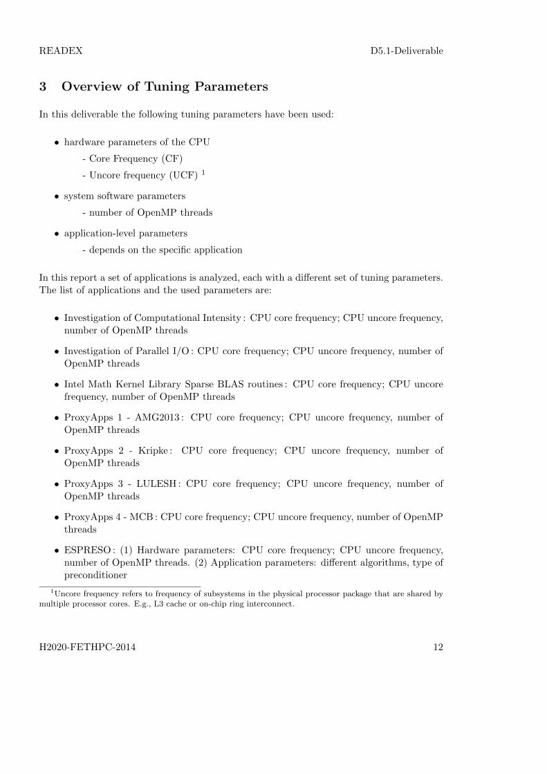
3 Overview of Tuning Parameters
In this deliverable the following tuning parameters have been used:
• hardware parameters of the CPU
- Core Frequency (CF)
- Uncore frequency (UCF) 1
• system software parameters
- number of OpenMP threads
• application-level parameters
- depends on the specific application
In this report a set of applications is analyzed, each with a different set of tuning parameters.The list of applications and the used parameters are:
• Investigation of Computational Intensity : CPU core frequency; CPU uncore frequency,number of OpenMP threads
• Investigation of Parallel I/O : CPU core frequency; CPU uncore frequency, number ofOpenMP threads
• Intel Math Kernel Library Sparse BLAS routines : CPU core frequency; CPU uncorefrequency, number of OpenMP threads
• ProxyApps 1 - AMG2013 : CPU core frequency; CPU uncore frequency, number ofOpenMP threads
• ProxyApps 2 - Kripke : CPU core frequency; CPU uncore frequency, number ofOpenMP threads
• ProxyApps 3 - LULESH : CPU core frequency; CPU uncore frequency, number ofOpenMP threads
• ProxyApps 4 - MCB : CPU core frequency; CPU uncore frequency, number of OpenMPthreads
• ESPRESO : (1) Hardware parameters: CPU core frequency; CPU uncore frequency,number of OpenMP threads. (2) Application parameters: different algorithms, type ofpreconditioner
1Uncore frequency refers to frequency of subsystems in the physical processor package that are shared bymultiple processor cores. E.g., L3 cache or on-chip ring interconnect.
H2020-FETHPC-2014 12

READEX D5.1-Deliverable
• OpenFOAM : CPU core frequency; CPU uncore frequency (Note: MPI only application,no threading)
• Indeed : CPU core frequency; CPU uncore frequency
• MiniMD : CPU core frequency; CPU uncore frequency, number of OpenMP threads
H2020-FETHPC-2014 13

READEX D5.1-Deliverable
4 Methodology for Dynamism Analysis
Detecting the dynamism of an application is the initial step of the READEX approach. Thetuning potential of an application is determined by measuring its intra-phase and inter-phasedynamism. The tuning potential analysis is described in deliverable D2.1 [8] in more detail.
4.1 Manual Dynamism Evaluation with MERIC
MERIC is a C++ dynamic library that measures energy consumption and runtime of an-notated regions inside a user application. It also can change the tuning parameters duringthe runtime. By running the code with different settings of the tuning parameters, we an-alyze possibilities for energy savings. Subsequently, the optimal configurations are appliedby changing the tuning parameters during the application runtime. MERIC wraps a listof libraries, that provide access to different hardware knobs and registers, operating systemand runtime system variables, i.e. tuning parameters, in order to read or modify their values.
The library is easy to use, all a user needs to do is to initialize the MERIC. After that itis possible to insert so called probes, that wrap potentially significant regions of the analyzedcode. Besides storing the measurement results, the user should not notice any changes inapplication behavior.
The main motivation for the development of this tool was to simplify the evaluation ofvarious applications which includes a large number of measurements. MERIC automatesenergy measurements of applications for various system parameters (frequency, number ofthreads, compiler, application parameters, etc.). It also allows to split the application codeinto parts, that may require different settings to show energy savings.
4.1.1 MERIC features
• Environment settingsDuring the MERIC initialization and at each region start and end the CPU frequency,uncore frequency and number of OpenMP threads are set. To do so, MERIC uses theOpenMP runtime API and the cpufreq and x86 adapt libraries.
• HDEEMThe key MERIC feature is energy measurement using HDEEM. HDEEM provides en-ergy consumption measurement in two different ways, and in MERIC it is possible tochoose which one the user wants to use by setting the MERIC CONTINUAL parame-ter. In one mode, the energy consumed from the point that HDEEM was initialised istaken from the HDEEM Stats structure (a data structure used by the HDEEM libraryto provide measurement information to the user application). In this mode we read thestructure at each region start and end. This solution is straightforward, however thereis a delay of approximately 4ms associated with every read from HDEEM API. Toavoid the delay, we take advantage of the fact that during the measurement HDEEM
H2020-FETHPC-2014 14

READEX D5.1-Deliverable
stores energy samples in its internal memory. In this case the MERIC only needs torecord timestamps at the beginning and the end of each region instead of calling theHDEEM API. This results in a very small overhead of MERIC instrumentation duringthe application runtime because all samples are transferred from HDEEM memory atthe end of the application runtime. The energy is subsequently calculated from thesamples based on the recorded timestamps.
• Intel Running Average Power LimitContemporary Intel processors support energy consumption measurements via the Run-ning Average Power Limit (RAPL) interface. MERIC uses the RAPL counters to allowenergy measurements on machines without the HDEEM infrastructure as well as tocompare them with HDEEM measurements. RAPL counters are read by the x86 adaptlibrary.
• Hardware performance countersTo provide more information about the instrumented regions of the application, weuse the perf event and PAPI libraries, which provide access to hardware performancecounters.
• Computational intensityMERIC also measures the computational intensity based on performance counters mea-sured by the perf event or PAPI library. This is a key metric for dynamism detectionas described in Section 2.
4.1.2 MERIC requirements
The MERIC tool relies on the following:
• Machine instrumented with HDEEM or x86 adapt library for accessing RAPL counters
• Compiler with C++14 standard support
• PAPI and perf event for accessing hardware counters
4.1.3 Workflow
1. Identification of significant regionsFirst, the user has to analyze its application using a profiler tool (such as Allinea MAP)and find the significant regions in order to cover the most consuming functions in termof time, MPI communication or I/O.
2. Insertion of MERIC probesTo use MERIC the user has to initialize the library and then insert the probes to an-notate the regions. At first the functions MERIC Init() and MERIC Close() should
H2020-FETHPC-2014 15

READEX D5.1-Deliverable
be inserted in the main function of the code. These functions should be inserted di-rectly after MPI Init() and before MPI Finalize(), respectively if MPI is used. Thenevery significant region should be wrapped by the MERIC MeasureStart(”NAME”) andMERIC MeasureStop() functions, where NAME is a user defined name of the region.These start and stop functions are called the probes. The stop function does not haveany input parameters, because it ends the region that has been started most recently.
3. Compilation of MERIC and a user codeMERIC is compiled using the Waf [11] compilation tool . Waf is a Python-basedframework for configuring, compiling and installing applications. Because there is lackof general knowledge about Waf, the code repository contains also a Makefile, thatprovides several Waf compilation commands. To compile a user application, it mustbe linked with the MERIC library (with its MPI or non-MPI version) and with otherlibraries, that MERIC wraps and the user want to use.
4. Setting MERIC parametersMERIC has almost no influence on the application’s runtime. The instrumented appli-cation should be run as usual. MERIC is controlled using the following environmentalvariables:
• MERIC FREQUENCYAfter the MERIC initialization the CPU frequency is set to this value. The pa-rameter should be in 0.1GHz steps.
• MERIC UNCORE FREQUENCYOn Intel Haswell processors the frequency of the uncore (i.e., the compenents thatare shared by all cores) can also be adjusted in 0.1GHz steps.
• MERIC NUM THREADSNumber of OpenMP threads, that will be used by the application.
• MERIC MODEMERIC works in four basic modes. In the default mode the energy consumptionis provided by HDEEM. Because this library is only available on Taurus in TUDresden, it is also possible not to use HDEEM, but to work with the Intel RAPLcounters instead. Another possibility is to use both, to compare the output values,or simply run the code without energy measurements.
• MERIC COUNTERSFor each region it is also possible to access hardware performance counters viaperf event or PAPI library.
• MERIC OUTPUT DIRName of the output directory.
• MERIC OUTPUT FILENAMEName of the output .csv file, that contains energy data.
• MERIC CONTINUALSet MERIC to read energy consumption directly (with HDEEM internal delay) at
H2020-FETHPC-2014 16

READEX D5.1-Deliverable
each region start and end (MERIC CONTINUAL=0) or from samples stored inthe HDEEM internal memory at the end of execution (MERIC CONTINUAL=1).
• MERIC DETAILEDIf set, energy consumption is not only measured for the whole node, but for eachCPU and DRAM as well.
• MERIC AGGREGATESetting for the MPI version. If set, measurement results are gathered at one MPIprocess, that stores only minimum, maximum and average values over all MPIprocesses.
• MERIC REGION OPTIONSFile with each region runtime settings.
Detailed description of all parameters can be found in the MERIC README file.
5. Running complete energy measurementNow it is possible to run a test to measure all the possible settings. To do so, in thetest directory there is a template of the batch script. The batch script consists ofthree parts. At the beginning of the script there are settings that should be consistentfor all runs of the code (e.g., MERIC output format). After that, there are loops forevery parameter, setting it to one of the possible values. And in the last part, the usermust set the variable MERIC OUTPUT FILENAME, that should be composed of eachparameter value and run the code.
6. Processing the resultsWhen the MERIC regions are defined and its parameters are set, we may run the code.The results are stored in two directories. The first one contains the information howoften the measurement was performed with a given setting. The second directory isfilled with the measurement results, that are stored in .csv file format. These files areanalyzed with the RADAR, that produces a detailed report where results are visualizedin graphs and logged in tables. RADAR also gives information about the best staticand dynamic settings of the measured code.
7. Dynamic tuningMERIC can enforce specific configuration for each significant region from a JSON for-matted configuration file (details are described in the MERIC README file). Theuser may set this file using the MERIC environment variable. MERIC sets the envi-ronment during runtime for each region to its required settings and therefore performsthe dynamic tuning.
4.1.4 MERIC repository
The MERIC repository contains not only the library, but also a small set of test applications,that already have several annotated regions. These examples show the potential user how
H2020-FETHPC-2014 17

READEX D5.1-Deliverable
to use MERIC and test whether everything is ready to use. The test directory also con-tains a script to print and/or set all MERIC environment variables and a complete energymeasurement template of a batch script as mentioned in Section 4.1.3 item 5.
H2020-FETHPC-2014 18

READEX D5.1-Deliverable
5 Metodology for Dynamism Reporting
5.1 RADAR
READEX Application Dynamism Analysis Report (RADAR) represents a brief measurementresults of dynamism metrics of different runs of an application. The report depicts graphicalrepresentations of the energy consumption with respect to a set of tuning parameters. Italso contains different sets of graphical comparisons of static and dynamic significant energysavings across the regions for different hardware tuning parameter configurations.
5.2 RADAR Generator for MERIC
When the significant regions are annotated with MERIC probes we run the application forall combinations of the selected tuning parameters. Subsequently, the measurement resultsare analyzed with the RADAR report generator tool.
The report generator is a Python based tool which visualizes the MERIC measurements inform of the Latex/PDF document. The goal is to present results in easily readable formatusing aggregated tables, 2D plots and heat-maps. The report generator not only visualizesthe measured results, but more importantly it also evaluates the energy consumption usingboth HDEEM or RAPL, runtime and arithmetical intensity for each significant region. Thisanalysis detects an optimal configuration of tuning parameters for each significant region andcalculates the potential energy savings.
The energy savings are calculated for both static and dynamic tuning. In case of statictuning we evaluate the energy consumption of the entire application and find the singleoptimal configuration. For the dynamic tuning we evaluate each of the significant regionsindependently and calculate the additional savings over the static tuning. All the savings arethen acumulated to report a single value for static savings and a single value for dynamicsavings.
Optimal configurations for each significant region are then saved to the JSON configurationfile which is used by a MERIC instrumented application for dynamic tuning.
The RADAR reports in this document always present the results for tuning for two objectivefunctions: (1) minimal energy consumption and (2) minimal runtime. This clearly show howdifferent are the optimal settings for these two objective functions.
5.2.1 Report elements
Overall application evaluation is the basic overview of the behavior of the entire appli-cation also called the main region. This listing contains the default configuration of tuningparameters, the optimal configuration for the entire application and static and dynamic sav-ings. An example is given in Table 4.
H2020-FETHPC-2014 19

READEX D5.1-Deliverable
Overall application evaluation
Defaultsettings
Defaultvalues
Best staticconfiguration
StaticSavings
DynamicSavings
Energy consump-tion [J],Blade summary
24 MPI proc ,1 thread,3.0GHz UCF,2.5GHz CF
10515.1 J
24 MPI proc ,1 thread,1.3GHz UCF,1.4GHz CF
3355.32 J(31.91%)
63.87 J of7159.78 J(0.89%)
Runtime of applica-tion [s]
24 MPI proc1 thread,3.0GHz UCF,2.5GHz CF
45.16 s
24 MPI procs,,1 thread,3.0GHz UCF,2.5GHz CF
0.00 s(0.00%)
0.19 s of45.16 s(0.42%)
Table 4: Example of overall application evaluation
Intra-Phase Dynamic Tuning Evaluation contains the optimal configuration of the tun-ing parameters for each significant region. All regions in this section are considered to benested regions of the main region. Therefore as the default configuration we take the bestconfiguration for the main region, i.e. the configuration that provides the best static savings.An example is given in Table 5.
Intra-Phase Dynamism EvaluationBlade summary, Energy consumption [J]
Region % of 1 phaseBest static
configurationValue
Best dynamicconfiguration
ValueDynamicsavings
LTimes 19.82
24 MPI proc ,1 thread,1.3GHz UCF,1.4GHz CF
589.78 J
24 MPI proc ,1 thread,1.2GHz UCF,1.2GHz CF
576.29 J13.49 J(2.29%)
Source 19.32
24 MPI proc ,1 thread,1.3GHz UCF,1.4GHz CF
574.96 J
24 MPI proc ,1 thread,1.2GHz UCF,1.2GHz CF
562.34 J12.62 J(2.20%)
LPlusTimes 19.88
24 MPI proc ,1 thread,1.3GHz UCF,1.4GHz CF
591.50 J
24 MPI proc ,1 thread,1.2GHz UCF,1.2GHz CF
582.50 J9.00 J(1.52%)
Scattering 19.62
24 MPI proc ,1 thread,1.3GHz UCF,1.4GHz CF
583.76 J
24 MPI proc ,1 thread,1.2GHz UCF,1.2GHz CF
570.57 J13.19 J(2.26%)
H2020-FETHPC-2014 20

READEX D5.1-Deliverable
Sweep 21.36
24 MPI proc ,1 thread,1.3GHz UCF,1.4GHz CF
635.47 J
24 MPI proc ,1 thread,1.4GHz UCF,1.3GHz CF
619.88 J15.58 J(2.45%)
Total values for statictuning for significant re-gions
589.78 + 574.96 + 591.50 + 583.76 + 635.47 = 2975.45 J
Total savings for dy-namic tuning for signifi-cant regions
13.49 + 12.62 + 9.00 + 13.19 + 15.58 = 63.87 J of2975.45 J (2.15%)
Dynamic savings for ap-plication runtime
63.87 J of 7159.78 J (0.89%)
Table 5: Example of the overview table of the optimal set-tings for the significant regions.
Phase ID 1 2 3 4 5
Default Energy consumption [J] 624.35 49.83 59.68 62.89 63.35% per 1 phase 91.54 37.38 39.10 39.17 38.61
Per phase optimal settings
2.0 GHzUCF,
2.5 GHzCF
2.1 GHzUCF,
1.7 GHzCF
2.2 GHzUCF,
1.7 GHzCF
2.1 GHzUCF,
1.7 GHzCF
2.5 GHzUCF,
1.7 GHzCF
Dynamic savings [J] 14.63 1.37 3.76 4.78 5.51Dynamic savings [%] 2.34 2.74 6.30 7.61 8.70
Table 6: Example of the inter-phase evaluation per significantregion for 5 phases
Inter-Phase Dynamic Tuning Evaluation contains optimal configurations and dynamicsavings detected for significant regions per phase of the phase region. By default the mainregion is used as the phase region but this can be changed by the user to any other significantregion. Please note that the phase region can be either the main region itself or anotherregion nested in the main region. The evaluated significant regions must be nested in thephase region.
This evaluation is useful for solvers based on iterative methods (e.g. Conjugate Gradients),where we’re interested mostly in profiling the steps of the iterations itself.
An example can be seen in Table 6 and results are shown in section 7.
2D plots are used in the report to visualize the dependence between some of the parameterssset, e.g. core frequency, number of threads and energy consumed. A simple plot can be seenin Figure 1.
H2020-FETHPC-2014 21

READEX D5.1-Deliverable
1.2 1.25 1.3 1.35 1.4 1.45 1.5 1.55 1.65.08
5.09
5.09
5.09
5.09
5.09
( 3.0 GHz UCF, 1.6 GHz CF: 5.08s) )
Core freq [GHz]
Runtimeof
function[s]
1 thread
Uncore freq [Ghz]2.62.83.0
Figure 1: Example of a plot representing the behavior of an application for various of coreand uncore frequencies.
Heat-maps have exactly the same purpose and are used in the same way as plots. They wereintroduced in RADAR report generator, because for some data sets the relations betweenquantities are easily visible this way. An example can be seen in Table 7.
Uncore freq [GHz]Core freq [GHz] 2.6 2.8 3.0
1.2 5.0923 5.0922 5.09341.4 5.0923 5.0867 5.06671.6 5.0897 5.0653 5.0245
Table 7: Heat map example generated by the RADAR report generator
5.2.2 Using the RADAR report generator
All the necessary settings are done (and described in detail) in the config.py file. Af-ter customizing the settings, the generation of the report itself is performed by the scriptprintFullReport.py. Then, the file results.tex is created in the folder with data (i.e. thepath assigned in config.py to the variable rootfolder). The file is subsequently compiledwith pdflatex or lualatex, the later one being the better choice because of its dynamicallyallocated memory, which prevents crashing during compilation when there are plenty of dataprocessed.
H2020-FETHPC-2014 22

READEX D5.1-Deliverable
The compilation creates many files when drawing plots named like data*.csv. When youcompile with flag --shell-escape, they are removed automatically at the end of the com-pilation.
Finally, you can see examples of reports generated by this tool in the Results section (e.g.,Section 6.2.2).
H2020-FETHPC-2014 23

READEX D5.1-Deliverable
6 Results – Intra-Phase Dynamism
In this section we present energy savings that were achieved by both static and dynamictuning of the selected applications. We present two types of evaluations (1) the intra-phasedynamism, see sections 6.1–6.9, and (2) the inter-phase dynamism which has been detectedonly for a subset of the evaluated applications, see Section 7.
6.1 Intel Math Kernel Library Sparse BLAS routines
This section deals with the energy consumption evaluation of selected Sparse BLAS Level2 and 3 routines. We have investigated the following routines from the Intel Math KernelLibrary (MKL) [3] version 2017.
• Sparse Matrix-Vector Multiplication in IJV/COO format,
• Sparse Matrix-Vector Multiplication in CSR format,
• Sparse Matrix-Matrix Multiplication in CSR format,
• Sparse Matrix-Matrix Addition in CSR format,
These belong to the most frequently used operations in HPC applications. For benchmarkingwe have used the University Florida set of matrices [1] and the MERIC library for the energyand time measurements.
The measured characteristics illustrate a different energy consumption for different BLASroutines, as some operations are more memory-bound and others are more compute-bound.We also show that some of the routines suffer significantly from the NUMA effect and shouldbe executed on single CPU socket only.
Table 6.1 shows measurements where default number of CPU cores have been set to 24therefore both sockets of the node have been used. We can see that most of the routines haveoptimal number of cores smaller than 12 and therefore using only 1 CPU socket. We can seethat significant savings up to 66% can be achieved in this case. Table 6.1 shows result of thesame experiment but in this case running on one CPU socket only (no NUMA effect). In thiscase the savings are between 2.7% – 12.3%.
The optimal uncore frequency in both tests has been between 2.1 GHz and 2.5 GHz (defaultvalue is 3.0 GHz). Matrix with higher number of non-zero values (road central) requires alsohigher uncore frequency. The range of CPU core frequency is between 1.5 GHz and 2.5 GHz(default value is 2.5 GHz). The sparse matrix-vector multiplication for CSR sparse matrixformat is the only routine that runs more efficiently on rather low core frequencies 1.5–1.8GHz, while the remaining operations take advantage of higher one. We can also observe, thatmatrix with higher number of non-zero values becomes more memory bound (optimum is onhigher uncore frequency and lower core frequency).
H2020-FETHPC-2014 24

READEX D5.1-Deliverable
Matrix name Rows Cols Nonzero Nonzero [%] Method Th. CF UCF Savings [%]
road central 14,081,816 14,081,816 33,866,826 1.71E-07
SpMV CSR 12 1.5 2.1 41.42SpMV COO 24 2.5 2.5 4.21SpMM CSR 12 2.1 2.5 18.5
Sp Mat Add CSR 8 1.8 2.5 21.17
sls 1,748,122 62,729 6,804,304 6.21E-05
SpMV CSR 18 1.5 2.1 45.22SpMV COO 8 2.5 2.1 7.35SpMM CSR 6 2.5 2.1 22.83
Sp Mat Add CSR 6 2.5 2.1 29.30
TSOPF RS b2052 c1 25,626 25,626 6,761,100 1.03E-02
SpMV CSR 12 1.8 2.1 66.19SpMV COO 6 2.5 2.1 7.24SpMM CSR 24 2.1 1.8 7.83
Sp Mat Add CSR 8 2.5 2.1 31.66
Table 8: The MKL sparse routines evaluation with NUMA effect (running on 2 CPU sockets)using 3 representative matrices (1 node, 6–24 threads, savings compared to 3GHz core,2.5GHz uncore, 24 threads). Note: Th. – threads; CF – CPU core frequency in GHz; UCF– CPU uncore frequency in GHz.
Matrix name Rows Cols Nonzero Nonzero [%] Method Th. CF UCF Savings [%]
road central 14,081,816 14,081,816 33,866,826 1.71E-07
SpMV CSR 12 1.5 2.1 12.29SpMV COO 6 2.5 2.5 4.21SpMM CSR 12 2.1 2.5 3.12
Sp Mat Add CSR 8 1.8 2.5 6.41
sls 1,748,122 62,729 6,804,304 6.21E-05
SpMV CSR 12 1.8 2.1 11.44SpMV COO 8 2.5 2.1 6.10SpMM CSR 6 2.5 2.1 2.72
Sp Mat Add CSR 6 2.5 2.1 9.94
TSOPF RS b2052 c1 25,626 25,626 6,761,100 1.03E-02
SpMV CSR 12 1.8 2.1 5.21SpMV COO 6 2.5 2.1 7.39SpMM CSR 12 2.5 1.5 9.75
Sp Mat Add CSR 8 2.5 2.1 5.56
Table 9: The MKL sparse routines evaluation without NUMA effect (running on 1 CPUsocket) using 3 representative matrices (1 node, 6–24 threads, savings compared to 3GHzcore, 2.5GHz uncore, 12 threads). Note: Th. – threads; CF – CPU core frequency in GHz;UCF – CPU uncore frequency in GHz.
H2020-FETHPC-2014 25

READEX D5.1-Deliverable
6.2 ESPRESO
For many years, the Finite Element Tearing and Interconnecting method (FETI) [6], [7]has been successfully used in the engineering community for solving very large problemsarising from the discretization of partial differential equations. In such an approach theoriginal structure is decomposed into several non-overlapping subdomains. Mutual continuityof primal variables between neighboring subdomains is enforced afterwards by dual variables,i.e., Lagrange multipliers (LM). They are usually obtained iteratively by one of the Krylovsubspace methods, then the primal solution is evaluated locally for each subdomain.
In 2006 Dostal et al. [5] introduced a new variant of an algorithm called Total FETI (orTFETI) in which Dirichlet boundary condition is enforced also by LM.
The HTFETI method is a variant of hybrid FETI methods introduced by Klawonn andRheinbach [9] for FETI and FETI-DP. In the original approach a number of subdomains isgathered into clusters. This can be seen as a three-level domain decomposition approach.Each cluster consists of a number of subdomains and for these, a FETI-DP system is set up.The clusters are then solved by a traditional FETI approach using projections to treat thenon trivial kernels. In contrast, in HTFETI, a TFETI approach is used for the subdomainsin each cluster and the FETI approach with projections is used for clusters.
The main advantage of HTFETI is its ability to solve problems decomposed into a very largenumber of subdomains [14]. We have ran tests with over 21 million subdomains organized into17,576 clusters. This means two things: (i) an extremely large problem can be solved (over120 billion DOF); (ii) moderate size problems (up to few billion DOF) can be decomposedinto very small subdomains which improves memory, computational and numerical efficiency.
6.2.1 ESPRESO Library
The ESPRESO library is a combination of Finite Element (FEM) and Boundary Element(BEM) tools and TFETI/HTFETI solvers. It supports FEM and BEM (uses BEM4I library)discretization for Advection-diffusion equation, Stokes flow and Structural mechanics. Realengineering problems are imported from Ansys Workbench or OpenFOAM. A C API allowsESPRESO to be used as a solver library for third party applications. For large scale testslibrary also contains a multiblock benchmark generator. The postprocessing and vizual-ization is based on the VTK library and Paraview including Paraview Catalyst for inSituvizualization.
The ESPRESO solver is a parallel linear solver, which includes a highly efficient MPI commu-nication layer [12] designed for massively parallel machines with thousands of compute nodes.The parallelization inside a node is done using OpenMP. Three versions of the solver are beingdeveloped: (i) ESPRESO CPU uses sparse matrices and sparse direct solvers to process thesystem matrices; (ii) ESPRESO MIC is an Intel Xeon Phi accelerated version, which workswith both sparse and dense representation of system matrices; and (iii) ESPRESO GPU isa GPU accelerated version, which supports dense structures only [13]. Support for sparsestructures using cuSolver is under development.
H2020-FETHPC-2014 26

READEX D5.1-Deliverable
All versions can solve both symmetric (conjugate gradient (CG) solver) and nonsymmetricsystems (GMRES and BiCGStab).
Hardware Tuning Parameters: The dynamism of the ESPRESO library has been evalu-ated using the following hardware parameters:
• CPU Core frequency
• Number of OpenMP threads
• CPU Uncore frequency
6.2.2 Application Tuning Parameters
Preconditioners: The ESPRESO solver supports several preconditioners, that can be dy-namically switched during the runtime of the iterative solver. The list of preconditioners thatare evaluated are:
• Lumped preconditioner - uses sparse BLAS2 - matrix-vector multiplication,
• Dirichlet preconditioner - uses dense BLAS2 - matrix-vector multiplication.
The order of the list is based on the numerical efficiency (from the worst to the best) whichalso corresponds to their computational demand (from low to high). From the nature ofthe FETI method the (ii) weight function and (iii) the lumped preconditioners are alwaysavailable and we do not need to calculate them at additional cost. However the (iv) Dirichletpreconditioner needs to be calculated if required, which potentially increases the preprocessingtime and the energy consumption.
Stiffness Matrix Processing: In FETI a stiffness matrix is a sparse matrix which in ageneral approach is processed by a SParse Direct Solver (SPDS). In particular each stiffnessmatrix is factorized once during the preprocessing and then in each iteration a forward andbackward substitutions (the solve routine of the SPDS) are called.
H2020-FETHPC-2014 27

READEX D5.1-Deliverable
Figure 2: Diagram of the significant regions in the ESPRESO library as used for thedynamic savings evaluation in this section. The orange regions are called just once periteration and therefore are used only for intra-phase dynamism evaluation. White regions areignored because there are other significant regions nested in them. The green regions denotesthe iterative solver (conjugate gradient (CG)) and provides an opportunity for inter-phasedynamism. The regions with names highlighted in bold are called only if Hybrid Total FETIis used.
ESPRESO contains an alternative method based on the Local Schur Complement method(LSC) for stiffness matrix processing originally developed for GPGPU and Intel Xeon Phiaccelerators, see [13]. In this method the preprocessing is more expensive as we have tocalculate the LSC for each subdomain using SPDS. However the iterative FETI solver thanuses dense matrix-vector multiplication using LSCs instead of more expensive solve routineof the SPDS. So the following methods will be evaluated:
H2020-FETHPC-2014 28

READEX D5.1-Deliverable
• Sparse Direct Solver (SPDS) - is using the solve routine (in this case the Intel MKLPARDISO solver is used),
• Local Schur Complement (LSC) - is using the dense BLAS 2 matrix-vector multiplica-tion.
We can calculate both (i) factorization of the stiffness matrices and (ii) the local Schurcomplements during the preprocessing stage and than ESPRESO can dynamically switchbetween these two methods during the runtime.
FETI Method: The ESPRESO solver contains two FETI methods: Total FETI (two levelmethod - better numerical behavioral, but limited parallel scalability) and Hybrid Total FETI(three level method with worse numerical behavior, but very good parallel scalability). Asof now the dynamic switching between these two methods in not implemented, however withcertain effort this can be implemented into ESPRESO. So the dynamism for the followingFETI methods can be evaluated:
• Total FETI method
• Hybrid Total FETI method
6.2.3 RADAR Reports for ESPRESO
In this section we present a series of experiments, that have been executed with the ESPRESOlibrary. For all runs the significant regions shown in Figure 2 have been used for measure-ments.
6.2.3.1 Configuration 0: 1 node with 1 MPI process; 2 to 24 OpenMP threads
• Method: Hybrid Total FETI
• Preconditioner: Dirichlet (dense)
• Stiffness matrix processing: PARDISO Sparse Direct Solver (sparse)
• Decomposition: 1x1x1 cluster; 8x8x8 subdomains per cluster; 11x11x11 elements persubdomain
H2020-FETHPC-2014 29
READEX D5.1-Deliverable
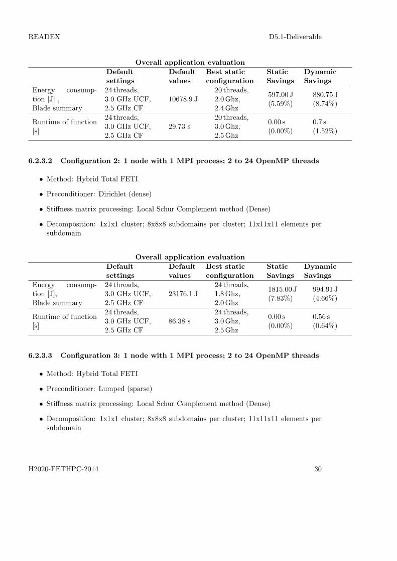
Overall application evaluation
Defaultsettings
Defaultvalues
Best staticconfiguration
StaticSavings
DynamicSavings
Energy consump-tion [J] ,Blade summary
24 threads,3.0 GHz UCF,2.5 GHz CF
10678.9 J20 threads,2.0Ghz,2.4Ghz
597.00 J(5.59%)
880.75 J(8.74%)
Runtime of function[s]
24 threads,3.0 GHz UCF,2.5 GHz CF
29.73 s20 threads,3.0Ghz,2.5Ghz
0.00 s(0.00%)
0.7 s(1.52%)
6.2.3.2 Configuration 2: 1 node with 1 MPI process; 2 to 24 OpenMP threads
• Method: Hybrid Total FETI
• Preconditioner: Dirichlet (dense)
• Stiffness matrix processing: Local Schur Complement method (Dense)
• Decomposition: 1x1x1 cluster; 8x8x8 subdomains per cluster; 11x11x11 elements persubdomain
Overall application evaluation
Defaultsettings
Defaultvalues
Best staticconfiguration
StaticSavings
DynamicSavings
Energy consump-tion [J],Blade summary
24 threads,3.0 GHz UCF,2.5 GHz CF
23176.1 J24 threads,1.8Ghz,2.0Ghz
1815.00 J(7.83%)
994.91 J(4.66%)
Runtime of function[s]
24 threads,3.0 GHz UCF,2.5 GHz CF
86.38 s24 threads,3.0Ghz,2.5Ghz
0.00 s(0.00%)
0.56 s(0.64%)
6.2.3.3 Configuration 3: 1 node with 1 MPI process; 2 to 24 OpenMP threads
• Method: Hybrid Total FETI
• Preconditioner: Lumped (sparse)
• Stiffness matrix processing: Local Schur Complement method (Dense)
• Decomposition: 1x1x1 cluster; 8x8x8 subdomains per cluster; 11x11x11 elements persubdomain
H2020-FETHPC-2014 30

READEX D5.1-Deliverable
Overall application evaluation
Defaultsettings
Defaultvalues
Best staticconfiguration
StaticSavings
DynamicSavings
Energy consump-tion [J],Blade summary
24 threads,3.0 GHz UCF,2.5 GHz CF
20508.9 J24 threads,2.0Ghz,2.2Ghz
1589.70 J(7.75%)
1017.92 J(5.38%)
Runtime of function[s]
24 threads,3.0 GHz UCF,2.5 GHz CF
86.38 s24 threads,3.0Ghz,2.5Ghz
0.00 s(0.00%)
0.54 s(0.74%)
6.2.3.4 Configuration 1: 1 node with 1 MPI process; 2 to 24 OpenMP threadsFor this experiment we provide more detailed report as it has achieved the most significantstatic and dynamic savings.
• Method: Hybrid Total FETI
• Preconditioner: Lumped (sparse)
• Stiffness matrix processing: PARDISO Sparse Direct Solver (sparse)
• Decomposition: 1x1x1 cluster; 8x8x8 subdomains per cluster; 11x11x11 elements persubdomain
Overall application evaluation
Defaultsettings
Defaultvalues
Best staticconfiguration
StaticSavings
DynamicSavings
Energy consump-tion [J] ,Blade summary
24 threads,3.0GHz UCF,2.5GHz CF
6265.18 J18 threads,1.8GHz UCF,2.5GHz CF
771.63 J(12.32%)
499.2 J of5493.6 J(9.09%)
Runtime of function[s],Job info - hdeem
24 threads,3.0GHz UCF,2.5GHz CF
29.55 s22 threads,3.0GHz UCF,2.5GHz CF
0.01 s(0.04%)
0.82 s of29.54 s(2.76%)
H2020-FETHPC-2014 31

READEX D5.1-Deliverable
1.2 1.4 1.6 1.8 2 2.2 2.4 2.6
5,500
6,000
6,500
7,000
7,500
8,000
8,500
9,000
( 1.8GHz UCF, 2.50GHz CF: 5493.55J )
Core freq [GHz]
Energy
consumption
[J]
18 threads
Uncore freq [GHz]1.21.41.61.82.02.22.42.62.83.0
Uncore freq [GHz UCF]Core freq [GHz] 1.2 1.4 1.6 1.8 2.0 2.2 2.4 2.6 2.8 3.0
1.2 7,774.33 7,577.13 7,620.86 7,712.41 7,638.19 7,887.51 8,017.52 8,224.55 8,457.63 8,713.341.4 7,014.96 7,006.61 6,951.7 6,989.9 7,013.88 7,100.78 7,353.77 7,538.7 7,540.17 7,808.451.6 6,657.43 6,585.3 6,497.84 6,405.66 6,448.15 6,626.3 6,742.37 6,790.9 6,955.32 7,114.61.8 6,387.41 6,286.4 6,195.08 6,068.22 6,093.49 6,158.65 6,244.49 6,354.23 6,412.18 6,693.562 6,303.9 6,177.23 5,979.14 5,892.41 5,862.35 5,941.4 6,094.83 6,116.72 6,337.78 6,405.452.2 6,130.89 5,908.28 5,771.2 5,729.32 5,695.97 5,732.87 5,822.58 5,901.66 6,020.53 6,124.22.4 6,219.49 5,866.82 5,718.77 5,548.09 5,590.74 5,644.12 5,679.25 5,750.53 5,840.8 5,940.32.5 6,201.34 5,870.99 5,678.56 5,493.55 5,544.76 5,507.07 5,567.86 5,711.89 5,834.93 5,909.88
H2020-FETHPC-2014 32

READEX D5.1-Deliverable
1.2 1.4 1.6 1.8 2 2.2 2.4 2.6
30
35
40
45
50
55
60
( 3.0GHz UCF, 2.50GHz CF: 29.54s )
Core freq [GHz]
Runtimeoffunction[s]
22 threads
Uncore freq [GHz]1.21.41.61.82.02.22.42.62.83.0
Uncore freq [GHz UCF]Core freq [GHz] 1.2 1.4 1.6 1.8 2.0 2.2 2.4 2.6 2.8 3.0
1.2 60.727 58.527 56.92 55.813 55.095 54.454 53.975 53.517 53.023 52.9531.4 54.553 52.357 50.638 49.499 48.44 48.232 48.128 47.066 46.746 45.9751.6 49.634 48.031 46.226 44.984 44.163 44.134 42.875 42.999 42.153 41.5511.8 46.755 44.614 42.516 40.89 40.118 40.101 39.405 38.555 38.611 38.0672 44.359 41.281 39.536 38.114 37.025 36.431 36.352 35.646 35.404 35.0052.2 41.544 39.015 37.503 36.214 35.329 34.505 33.865 33.714 32.878 32.7792.4 39.773 37.102 35.515 33.968 33.053 32.318 31.931 31.36 31.106 30.6342.5 38.339 35.518 34.437 33.109 32.481 31.425 30.983 30.433 29.862 29.536
Intra-Phase Dynamism EvaluationBlade summary, Energy consumption [J]
Region % of 1 phaseBest staticconfiguration
ValueBest dynamicconfiguration
ValueDynamicsavings
Assembler–AssembleStiffMat
14.3218 threads,1.8GHz UCF,2.5GHz CF
733.73 J20 threads,2.0GHz UCF,2.5GHz CF
731.22 J2.51 J(0.34%)
Assembler–Assemble-B1
2.2318 threads,1.8GHz UCF,2.5GHz CF
114.30 J2 threads,2.2GHz UCF,2.5GHz CF
94.15 J20.15 J(17.63%)
Cluster–CreateF0-FactF0
0.1718 threads,1.8GHz UCF,2.5GHz CF
8.71 J6 threads,1.6GHz UCF,2.5GHz CF
6.90 J1.80 J(20.73%)
H2020-FETHPC-2014 33

READEX D5.1-Deliverable
Assembler–SaveResults
3.1018 threads,1.8GHz UCF,2.5GHz CF
158.81 J2 threads,1.2GHz UCF,2.5GHz CF
147.66 J11.16 J(7.03%)
Assembler-K Regular-ization
5.4318 threads,1.8GHz UCF,2.5GHz CF
278.39 J2 threads,1.8GHz UCF,2.5GHz CF
231.38 J47.01 J(16.89%)
Cluster–CreateSa-SolveF0vG0
2.2218 threads,1.8GHz UCF,2.5GHz CF
113.87 J6 threads,2.0GHz UCF,2.5GHz CF
97.46 J16.41 J(14.41%)
Create -GGT Inv
0.2818 threads,1.8GHz UCF,2.5GHz CF
14.23 J2 threads,1.2GHz UCF,2.5GHz CF
8.92 J5.31 J(37.34%)
Cluster–Kfactorization
12.8418 threads,1.8GHz UCF,2.5GHz CF
658.07 J24 threads,2.0GHz UCF,2.4GHz CF
629.62 J28.45 J(4.32%)
Assembler–SaveMeshtoVTK
6.3618 threads,1.8GHz UCF,2.5GHz CF
325.69 J2 threads,1.2GHz UCF,2.5GHz CF
296.66 J29.03 J(8.91%)
Cluster–CreateSa-SaFactorization
1.9518 threads,1.8GHz UCF,2.5GHz CF
99.93 J4 threads,2.2GHz UCF,2.5GHz CF
80.85 J19.08 J(19.09%)
Cluster–SetClusterPC
1.4618 threads,1.8GHz UCF,2.5GHz CF
74.70 J20 threads,2.0GHz UCF,2.5GHz CF
74.54 J0.16 J(0.22%)
Assembler–PrepareMesh
12.5318 threads,1.8GHz UCF,2.5GHz CF
641.88 J22 threads,1.8GHz UCF,2.5GHz CF
639.39 J2.49 J(0.39%)
Assembler–SolverSolve
30.7918 threads,1.8GHz UCF,2.5GHz CF
1578.06 J10 threads,2.2GHz UCF,2.5GHz CF
1289.85 J288.21 J(18.26%)
Assembler–Assemble-B0
0.2618 threads,1.8GHz UCF,2.5GHz CF
13.28 J24 threads,2.0GHz UCF,2.5GHz CF
12.51 J0.77 J(5.81%)
Cluster–CreateG1-perCluster
0.4718 threads,1.8GHz UCF,2.5GHz CF
24.20 J14 threads,2.2GHz UCF,2.5GHz CF
22.32 J1.88 J(7.76%)
Cluster–CreateF0-AssembleF0
5.4318 threads,1.8GHz UCF,2.5GHz CF
278.22 J24 threads,2.2GHz UCF,2.2GHz CF
254.98 J23.24 J(8.35%)
Cluster–CreateSa-SaReg
0.1718 threads,1.8GHz UCF,2.5GHz CF
8.59 J8 threads,2.0GHz UCF,2.5GHz CF
7.03 J1.56 J(18.15%)
H2020-FETHPC-2014 34

READEX D5.1-Deliverable
Total value for statictuning for significant re-gions
733.73 + 114.30 + 8.71 + 158.81 + 278.39 + 113.87 +14.23 + 658.07 + 325.69 + 99.93 + 74.70 + 641.88 +1578.06 + 13.28 + 24.20 + 278.22 + 8.59 = 5124.66 J
Total savings for dy-namic tuning for signifi-cant regions
2.51 + 20.15 + 1.80 + 11.16 + 47.01 + 16.41 + 5.31 +28.45 + 29.03 + 19.08 + 0.16 + 2.49 + 288.21 + 0.77+ 1.88 + 23.24 + 1.56 = 499.22 J of 5124.66 J (9.74%)
Dynamic savings for ap-plication runtime
499.22 J of 5493.55 J (9.09%)
Total value after savings 4994.33 J (79.72% of 6265.18 J)
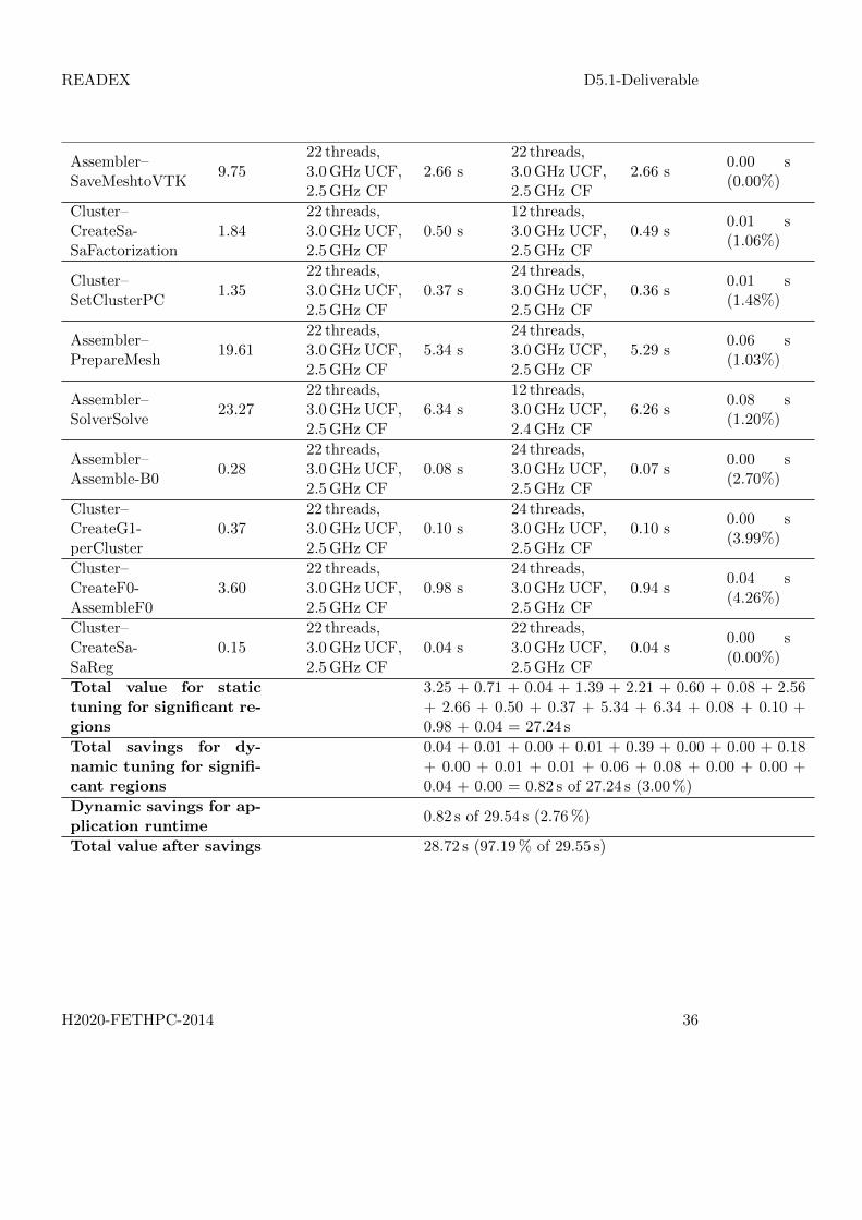
Intra-Phase Dynamism EvaluationRuntime of function [s]
Region % of 1 phaseBest static
configurationValue
Best dynamicconfiguration
ValueDynamicsavings
Assembler–AssembleStiffMat
11.9122 threads,3.0GHz UCF,2.5GHz CF
3.25 s24 threads,3.0GHz UCF,2.5GHz CF
3.21 s0.04 s(1.23%)
Assembler–Assemble-B1
2.6022 threads,3.0GHz UCF,2.5GHz CF
0.71 s16 threads,3.0GHz UCF,2.5GHz CF
0.70 s0.01 s(1.63%)
Cluster–CreateF0-FactF0
0.1622 threads,3.0GHz UCF,2.5GHz CF
0.04 s22 threads,2.8GHz UCF,2.5GHz CF
0.04 s0.00 s(2.03%)
Assembler–SaveResults
5.1022 threads,3.0GHz UCF,2.5GHz CF
1.39 s12 threads,2.4GHz UCF,2.5GHz CF
1.38 s0.01 s(0.75%)
Assembler-K Regular-ization
8.1222 threads,3.0GHz UCF,2.5GHz CF
2.21 s2 threads,3.0GHz UCF,2.5GHz CF
1.82 s0.39 s(17.53%)
Cluster–CreateSa-SolveF0vG0
2.2022 threads,3.0GHz UCF,2.5GHz CF
0.60 s18 threads,3.0GHz UCF,2.5GHz CF
0.60 s0.00 s(0.13%)
Create -GGT Inv
0.2922 threads,3.0GHz UCF,2.5GHz CF
0.08 s6 threads,3.0GHz UCF,2.5GHz CF
0.08 s0.00 s(0.39%)
Cluster–Kfactorization
9.4022 threads,3.0GHz UCF,2.5GHz CF
2.56 s24 threads,3.0GHz UCF,2.5GHz CF
2.39 s0.18 s(6.84%)
H2020-FETHPC-2014 35
READEX D5.1-Deliverable
Assembler–SaveMeshtoVTK
9.7522 threads,3.0GHz UCF,2.5GHz CF
2.66 s22 threads,3.0GHz UCF,2.5GHz CF
2.66 s0.00 s(0.00%)
Cluster–CreateSa-SaFactorization
1.8422 threads,3.0GHz UCF,2.5GHz CF
0.50 s12 threads,3.0GHz UCF,2.5GHz CF
0.49 s0.01 s(1.06%)
Cluster–SetClusterPC
1.3522 threads,3.0GHz UCF,2.5GHz CF
0.37 s24 threads,3.0GHz UCF,2.5GHz CF
0.36 s0.01 s(1.48%)
Assembler–PrepareMesh
19.6122 threads,3.0GHz UCF,2.5GHz CF
5.34 s24 threads,3.0GHz UCF,2.5GHz CF
5.29 s0.06 s(1.03%)
Assembler–SolverSolve
23.2722 threads,3.0GHz UCF,2.5GHz CF
6.34 s12 threads,3.0GHz UCF,2.4GHz CF
6.26 s0.08 s(1.20%)
Assembler–Assemble-B0
0.2822 threads,3.0GHz UCF,2.5GHz CF
0.08 s24 threads,3.0GHz UCF,2.5GHz CF
0.07 s0.00 s(2.70%)
Cluster–CreateG1-perCluster
0.3722 threads,3.0GHz UCF,2.5GHz CF
0.10 s24 threads,3.0GHz UCF,2.5GHz CF
0.10 s0.00 s(3.99%)
Cluster–CreateF0-AssembleF0
3.6022 threads,3.0GHz UCF,2.5GHz CF
0.98 s24 threads,3.0GHz UCF,2.5GHz CF
0.94 s0.04 s(4.26%)
Cluster–CreateSa-SaReg
0.1522 threads,3.0GHz UCF,2.5GHz CF
0.04 s22 threads,3.0GHz UCF,2.5GHz CF
0.04 s0.00 s(0.00%)
Total value for statictuning for significant re-gions
3.25 + 0.71 + 0.04 + 1.39 + 2.21 + 0.60 + 0.08 + 2.56+ 2.66 + 0.50 + 0.37 + 5.34 + 6.34 + 0.08 + 0.10 +0.98 + 0.04 = 27.24 s
Total savings for dy-namic tuning for signifi-cant regions
0.04 + 0.01 + 0.00 + 0.01 + 0.39 + 0.00 + 0.00 + 0.18+ 0.00 + 0.01 + 0.01 + 0.06 + 0.08 + 0.00 + 0.00 +0.04 + 0.00 = 0.82 s of 27.24 s (3.00%)
Dynamic savings for ap-plication runtime
0.82 s of 29.54 s (2.76%)
Total value after savings 28.72 s (97.19% of 29.55 s)
H2020-FETHPC-2014 36

READEX D5.1-Deliverable
6.3 Indeed
Indeed is a commercial finite element software package that has been especially designed forthe simulation of sheet metal forming processes. The REDAEX consortium member GNS isthe owner of this product and is responsible for its development, maintenance and marketing.Most of Indeed’s users are based in the automotive industry or its suppliers.
In contrast to most of its competitors, Indeed makes use of an implicit time integrationmethod. As a result, its computational cost is relatively high, but on the other hand it canprovide a very high degree of accuracy of the numerical solutions. Indeed is available in twoversions, a shared memory version based on an OpenMP parallelization and a distributedmemory version based on a hybrid OpenMP and MPI approach.
The READEX-related analysis of Indeed has been performed jointly by GNS and TUMunchen. The work has so far concentrated on the OpenMP version because it is moreimportant from the perspective of the users.
Following a detection of the significant regions, Indeed has been instrumented with theMERIC system and numerous measurements have been started. At the time of writing thisdocument, not all of these experiments were finished, but nevertheless a number of resultscan already be reported.
Specifically, we have started with an investigation of the potential energy savings with statictuning measures based on changes in the number of OpenMP threads, the core frequencyand the uncore frequency.
From those plots and the underlying figures, it is evident that it is always advisable to choosethe highest possible core frequency. The optimal choice of uncore frequency and number ofthreads depends on the objective function with respect to which the user attempts to optimizethe program run’s environment settings. For example, using a large number of threads issensible when optimizing for runtime, but not when optimizing (purely) with respect to theenergy requirements. Similarly, a high uncore frequency is usually advantageous from theruntime point of view but not from the energy perspective. In practice, one is frequentlyinterested in a compromise between these two objective functions; a suitable approach toachieve this goal is provided by the energy delay product EDP1, i.e. the product of run timeand required energy. When using this objective function, it turns out that it makes sense touse many threads but only a medium high uncore frequency. A quantitative assessment ofthe tuning potential that can be realized in this manner is given in Table 12.
The analysis of Indeed’s dynamic tuning potential is currently in progress and not finishedyet. The results will be reported later.
The future steps in this connection will also include similar investigations based on othertypes of input data sets that might exhibit a different behaviour.
H2020-FETHPC-2014 37

READEX D5.1-Deliverable
Figure 3: Energy requirements of example Indeed run for various choices of core frequencyand number of threads. The plots indicate the results for an uncore frequency of 1.5 GHz(top left), 2.0 GHz (top right), 2.5 GHz (bottom left) and 3.0 GHz (bottom right).
H2020-FETHPC-2014 38

READEX D5.1-Deliverable
Figure 4: Run time requirements of example Indeed run for various choices of core frequencyand number of threads. The plots indicate the results for an uncore frequency of 1.5 GHz(top left), 2.0 GHz (top right), 2.5 GHz (bottom left) and 3.0 GHz (bottom right).
H2020-FETHPC-2014 39

READEX D5.1-Deliverable
Figure 5: Energy delay product (EDP1) requirements of example Indeed run for variouschoices of core frequency and number of threads. The plots indicate the results for an uncorefrequency of 1.5 GHz (top left), 2.0 GHz (top right), 2.5 GHz (bottom left) and 3.0 GHz(bottom right).
H2020-FETHPC-2014 40

READEX D5.1-Deliverable
Tuning Energy [J] Runtime [s] EDP1 [MJs]objective Optimal settings (improvement) (improvement) (improvement)
None 24 Threads(Default 2.5 GHz core freq. 171967 772 132Parameters) 3.0 GHz uncore freq.
12 ThreadsEnergy 2.5 GHz core freq. 141751 871 123
2.0 GHz uncore freq. (17.6%) (−12.8%) (6.8%)
20 ThreadsRuntime 2.5 GHz core freq. 160538 762 122
3.0 GHz uncore freq. (6.6%) (1.3%) (7.6%)
20 ThreadsEDP1 2.5 GHz core freq. 151200 764 115
2.5 GHz uncore freq. (12.1%) (1.0%) (12.9%)
Table 12: Static tuning potential for Indeed.
H2020-FETHPC-2014 41

READEX D5.1-Deliverable
6.4 MiniMD
MiniMD is a parallel molecular dynamics (MD) simulation package written in C++ and isbased on many of the same algorithm concepts of LAMMPS parallel MD code, but is muchsimpler. The self-contained application performs parallel molecular dynamics simulation ofa Lennard-Jones or a EAM system and gives timing information.
MiniMD consists of less than 5,000 lines of code and uses spatial decomposition MD, whereindividual processors in a cluster own subsets of the simulation box. The application usesneighbour lists for the force calculation. The input to miniMD, which is provided as a file,includes a problem size, atom density, temperature in the box, timestep size for the simulation,number of timesteps to perform, and particle interation cut-off distance.
6.4.1 Instrumentation with MERIC
To instrument the miniMD application with MERIC, we identified the phase region to bethe for-loop in the Integrate::run() function in integrate.cpp. The for-loop iterates forthe number of timesteps provided as input to the application. Within this for-loop, the threeregions that we instrumented are the calls to functions borders(), build() and compute().Thus for analysis, we instrumented the for-loop as phase region with MERIC, while the threeregions were instrumented as significant regions.
6.4.2 Results
We conducted the two experiments, one with the Lennard-Jones and another with EAMsystems, by varying the processor core and uncore frequencies. The results from using theLennard-Jones system are summarised in Section 6.4.2.1, while those from using the EAMsystem are presented in Section 6.4.2.2. The inter-phase dynamism observed and the associ-ated results of tuning are reported in Section 7.2. Further, we observe from these experimentsthat the significant regions that contribute to the energy consumption and execution timeare build() and compute functions.
6.4.2.1 Experiment 1 This experiment was conducted using the Lennard-Jones systemconfiguration of miniMD with the input file in.lj.miniMD that is available in the applicationfolder with the application run for 100 iterations and reneighbouring of atoms performed onceevery 20 iterations. The core and uncore frequencies were varied in steps of 0.2 GHz. Weobserve that while static tuning results in saving around 21% of energy, there are no dynamicsavings reported for the energy consumption and execution time.
H2020-FETHPC-2014 42

READEX D5.1-Deliverable
Overall application evaluation
Defaultsettings
Defaultvalues
Best staticconfiguration
StaticSavings
DynamicSavings
Energy consump-tion [J] (Samples),Blade summary
1 th,3.0GHz UCF,2.5GHz CF
1348.27 J1 th,1.2GHz UCF,2.5GHz CF
288.95 J(21.43%)
0.00 J of1059.32 J(0.00%)
Runtime of function[s],Job info - hdeem
1 th,3.0GHz UCF,2.5GHz CF
9.69 s1 th,3.0GHz UCF,2.5GHz CF
0.00 s(0.00%)
0.00 sof 9.69 s(0.00%)
1.2 1.4 1.6 1.8 2 2.2 2.4 2.6
1,000
1,200
1,400
1,600
1,800
2,000
2,200
2,400
2,600
( 1.2GHz UCF, 2.50GHz CF: 1059.32J )
Core freq [GHz]
Energy
consumption
[J](Samples)
1 thread
Uncore freq [GHz]1.21.41.61.82.02.22.42.62.83.0
Uncore freq [GHz]Core freq [GHz] 1.2 1.4 1.6 1.8 2.0 2.2 2.4 2.6 2.8 3.0
1.3 1,888.99 1,929.84 1,962.73 2,009.72 2,061.49 2,131.48 2,237.87 2,291.71 2,389.63 2,484.211.5 1,653.81 1,680.75 1,712.4 1,756.5 1,815.37 1,867.59 1,923.6 2,000.78 2,080.96 2,172.351.7 1,472.38 1,494.71 1,523.82 1,556.46 1,605.55 1,652.25 1,730.88 1,785.18 1,877.01 1,920.051.9 1,336.63 1,355.74 1,379.6 1,423.11 1,447.66 1,498.09 1,549.65 1,602.05 1,682.81 1,730.742.1 1,224.64 1,255.05 1,261.31 1,289.55 1,320.5 1,362.35 1,412.43 1,472.32 1,538.84 1,576.282.3 1,139.03 1,147.07 1,163.44 1,197.83 1,219.15 1,254.94 1,295.33 1,349.15 1,399.41 1,458.062.5 1,059.32 1,076.93 1,083.04 1,110.74 1,134.39 1,185.37 1,221.75 1,252.1 1,315.25 1,348.27
H2020-FETHPC-2014 43

READEX D5.1-Deliverable
1.2 1.4 1.6 1.8 2 2.2 2.4 2.6
10
12
14
16
18
( 3.0GHz UCF, 2.50GHz CF: 9.69s )
Core freq [GHz]
Runtimeof
function[s]
1 thread
Uncore freq [GHz]1.21.41.61.82.02.22.42.62.83.0
Uncore freq [GHz]Core freq [GHz] 1.2 1.4 1.6 1.8 2.0 2.2 2.4 2.6 2.8 3.0
1.3 18.685 18.703 18.546 18.494 18.44 18.429 18.675 18.376 18.374 18.3531.5 16.322 16.219 16.139 16.112 16.059 16.107 16.012 15.981 15.96 16.0361.7 14.47 14.365 14.304 14.235 14.22 14.186 14.353 14.128 14.318 14.1181.9 13.03 12.919 12.864 12.854 12.751 12.742 12.694 12.682 12.66 12.6532.1 11.874 11.883 11.698 11.621 11.58 11.571 11.529 11.606 11.615 11.4732.3 10.911 10.799 10.715 10.66 10.615 10.584 10.561 10.536 10.534 10.5042.5 10.117 10.016 9.906 9.85 9.798 9.853 9.894 9.731 9.85 9.688
Intra-Phase Dynamism EvaluationBlade summary, Energy consumption [J]
Region % of 1 phaseBest staticconfiguration
ValueBest dynamicconfiguration
ValueDynamicsavings
Build 13.571 th,1.2GHz UCF,2.5GHz CF
1.34 J1 th,1.2GHz UCF,2.5GHz CF
1.34 J0.00 J(0.00%)
Borders 0.181 th,1.2GHz UCF,2.5GHz CF
0.02 J1 th,2.2GHz UCF,2.5GHz CF
0.01 J0.00 J(18.83%)
Compute 86.251 th,1.2GHz UCF,2.5GHz CF
8.54 J1 th,1.2GHz UCF,2.5GHz CF
8.54 J0.00 J(0.00%)
H2020-FETHPC-2014 44

READEX D5.1-Deliverable
Total value for statictuning for significant re-gions
1.34 + 0.02 + 8.54 = 9.91 J
Total savings for dy-namic tuning for signifi-cant regions
0.00 + 0.00 + 0.00 = 0.00 J of 9.91 J (0.03%)
Dynamic savings for ap-plication runtime
0.00 J of 1059.32 J (0.00%)
Total value after savings 1059.32 J (78.57% of 1348.27 J)
Intra-Phase Dynamism EvaluationJob info - hdeem, Runtime of function [s]
Region % of 1 phaseBest staticconfiguration
ValueBest dynamicconfiguration
ValueDynamicsavings
Build 13.891 th,3.0GHz UCF,2.5GHz CF
0.01 s1 th,3.0GHz UCF,2.5GHz CF
0.01 s0.00 s(0.00%)
Borders 0.121 th,3.0GHz UCF,2.5GHz CF
0.00 s1 th,3.0GHz UCF,2.5GHz CF
0.00 s0.00 s(0.00%)
Compute 85.991 th,3.0GHz UCF,2.5GHz CF
0.08 s1 th,3.0GHz UCF,2.5GHz CF
0.08 s0.00 s(0.00%)
Total value for statictuning for significant re-gions
0.01 + 0.00 + 0.08 = 0.09 s
Total savings for dy-namic tuning for signifi-cant regions
0.00 + 0.00 + 0.00 = 0.00 s of 0.09 s (0.00%)
Dynamic savings for ap-plication runtime
0.00 s of 9.69 s (0.00%)
Total value after savings 9.69 s (100.00% of 9.69 s)
6.4.2.2 Experiment 2 This experiment was conducted using the EAM system configu-ration of miniMD with the input file in.eam.miniMD that is available in the application folderwith the application run for 100 iterations and reneighbouring of atoms performed once every20 iterations. The core and uncore frequencies were varied in steps of 0.2 GHz. We observethat while static tuning results in saving around 22% of energy, there are no dynamic savingsreported for the energy consumption and execution time.
H2020-FETHPC-2014 45

READEX D5.1-Deliverable
Overall application evaluation
Defaultsettings
Defaultvalues
Best staticconfiguration
StaticSavings
DynamicSavings
Energy consump-tion [J] (Samples),Blade summary
1 th,3.0GHz UCF,2.5GHz CF
2565.29 J1 th,1.2GHz UCF,2.5GHz CF
574.81 J(22.41%)
0.00 J of1990.48 J(0.00%)
Runtime of function[s],Job info - hdeem
1 th,3.0GHz UCF,2.5GHz CF
18.28 s1 th,3.0GHz UCF,2.5GHz CF
0.00 s(0.00%)
0.00 s of18.28 s(0.00%)
1.2 1.4 1.6 1.8 2 2.2 2.4 2.6
2,000
2,500
3,000
3,500
4,000
4,500
( 1.2GHz UCF, 2.50GHz CF: 1990.48J )
Core freq [GHz]
Energy
consumption
[J](Samples)
1 thread
Uncore freq [GHz]1.21.41.61.82.02.22.42.62.83.0
Uncore freq [GHz]Core freq [GHz] 1.2 1.4 1.6 1.8 2.0 2.2 2.4 2.6 2.8 3.0
1.3 3,632.17 3,680.32 3,746.07 3,844.45 3,943.41 4,055.09 4,197.78 4,346.98 4,522.45 4,694.481.5 3,157.15 3,213.13 3,259.76 3,350.18 3,425.36 3,535.88 3,650.1 3,778.52 3,928.76 4,099.131.7 2,805.57 2,856.72 2,908.73 2,980.48 3,050.93 3,147.65 3,259.53 3,371.93 3,526.74 3,647.381.9 2,538.64 2,581.08 2,627.83 2,687.8 2,757.72 2,833.8 2,947.94 3,039.34 3,155.44 3,279.842.1 2,314.35 2,348.43 2,392.8 2,438.77 2,504.02 2,573.81 2,656.13 2,757.06 2,864.99 2,977.32.3 2,129.61 2,165.26 2,203.31 2,246.53 2,302.75 2,370.86 2,443.55 2,532.71 2,624.84 2,730.22.5 1,990.48 2,011.18 2,050.7 2,100.27 2,149.23 2,201.92 2,277.96 2,365.57 2,461.13 2,565.29
H2020-FETHPC-2014 46

READEX D5.1-Deliverable
1.2 1.4 1.6 1.8 2 2.2 2.4 2.6
18
20
22
24
26
28
30
32
34
36
( 3.0GHz UCF, 2.50GHz CF: 18.28s )
Core freq [GHz]
Runtimeof
function[s]
1 thread
Uncore freq [GHz]1.21.41.61.82.02.22.42.62.83.0
Uncore freq [GHz]Core freq [GHz] 1.2 1.4 1.6 1.8 2.0 2.2 2.4 2.6 2.8 3.0
1.3 35.377 35.11 34.998 34.949 34.891 34.863 34.842 34.824 34.772 34.7591.5 30.615 30.657 30.418 30.359 30.31 30.265 30.236 30.211 30.221 30.1881.7 27.117 26.994 26.919 26.857 26.791 26.757 26.74 26.714 26.856 26.71.9 24.368 24.252 24.143 24.081 24.028 23.982 24.106 23.94 23.934 23.92.1 22.145 22.014 21.921 21.833 21.791 21.755 21.723 21.699 21.69 21.6562.3 20.292 20.18 20.071 20.006 19.95 19.902 19.871 19.847 19.827 19.8152.5 18.757 18.636 18.53 18.498 18.406 18.355 18.336 18.309 18.281 18.277
Intra-Phase Dynamism EvaluationBlade summary, Energy consumption [J]
Region % of 1 phaseBest staticconfiguration
ValueBest dynamicconfiguration
ValueDynamicsavings
Borders 0.091 th,1.2GHz UCF,2.5GHz CF
0.02 J1 th,2.4GHz UCF,2.5GHz CF
0.01 J0.00 J(19.90%)
Build 11.071 th,1.2GHz UCF,2.5GHz CF
2.13 J1 th,1.2GHz UCF,2.5GHz CF
2.13 J0.00 J(0.00%)
Compute 88.831 th,1.2GHz UCF,2.5GHz CF
17.13 J1 th,1.2GHz UCF,2.5GHz CF
17.13 J0.00 J(0.00%)
H2020-FETHPC-2014 47

READEX D5.1-Deliverable
Total value for statictuning for significant re-gions
0.02 + 2.13 + 17.13 = 19.28 J
Total savings for dy-namic tuning for signifi-cant regions
0.00 + 0.00 + 0.00 = 0.00 J of 19.28 J (0.02%)
Dynamic savings for ap-plication runtime
0.00 J of 1990.48 J (0.00%)
Total value after savings 1990.48 J (77.59% of 2565.29 J)
Intra-Phase Dynamism EvaluationJob info - hdeem, Runtime of function [s]
Region % of 1 phaseBest staticconfiguration
ValueBest dynamicconfiguration
ValueDynamicsavings
Borders 0.061 th,3.0GHz UCF,2.5GHz CF
0.00 s1 th,3.0GHz UCF,2.5GHz CF
0.00 s0.00 s(0.00%)
Build 11.181 th,3.0GHz UCF,2.5GHz CF
0.02 s1 th,3.0GHz UCF,2.5GHz CF
0.02 s0.00 s(0.00%)
Compute 88.761 th,3.0GHz UCF,2.5GHz CF
0.16 s1 th,3.0GHz UCF,2.5GHz CF
0.16 s0.00 s(0.00%)
Total value for statictuning for significant re-gions
0.00 + 0.02 + 0.16 = 0.18 s
Total savings for dy-namic tuning for signifi-cant regions
0.00 + 0.00 + 0.00 = 0.00 s of 0.18 s (0.00%)
Dynamic savings for ap-plication runtime
0.00 s of 18.28 s (0.00%)
Total value after savings 18.28 s (100.00% of 18.28 s)
H2020-FETHPC-2014 48

READEX D5.1-Deliverable
6.5 OpenFOAM
OpenFOAM is an abbreviation for Open source Field Operation And Manipulation. It isan open source C++ toolbox for computational fluid dynamics (CFD). OpenFOAM does nothave a generic solver applicable to all cases, but there is a long list of solvers each for specificclass of problems. Solvers are categorized into several categories, e.g. compressible and incom-pressible flow, multiphase flow, combustion, particle-tracking flows heat transfer and manymore. Besides the solvers, OpenFOAM has a set of pre-/post-processing features in meshing,physical modeling or numerical methods. More information about the OpenFOAM softwarecan be found at www.openfoam.com.
6.5.1 Instrumentation with MERIC
For the OpenFOAM investigation we have selected the simpleFoam application, the steady-state solver for incompressible flows with turbulence modeling.
The application was split into following parts: the initialization, iterative solver for pressure,velocity and turbulence problems and the part for saving the results to the output file.The initialization part was split into more fine grained regions according to division in thesimpleFoam source code.
6.5.2 Results
We ran a test with the OpenFOAM application simpleFoam on the test example motorBike,that is part of the OpenFOAM repository. The experiment were done on one single node with24 MPI processes, that were used to decompose the domain using the simple decompositionmethod for decomposition into 6× 2× 2 blocks of 48× 20× 20 elements.
The simpleFoam application were set to use GAMG solver for pEqn region and PBiCGsolver for UEqn, transport and turbulence regions. The results were written twice during theruntime into binary uncompressed format.
The core and uncore frequencies ranged between 1.2 - 2.5 GHz and 1.2 - 3.0 GHz, respectively,with the step size of 0.2 GHz. The test were ran five times to reduce measurement oscillationsmainly due to network traffic. RADAR reports an average values across these measurements.
Since the most time consuming regions, the GAMG and PBiCG solvers, perform similarsparse BLAS operations the optimal configuration is either identical or very similar. Due tothis reason the most of the saving can be achieved by static tuning, 15.9%, while only theremaining regions provide some potential for dynamic savings. Since the runtime of remainingregions is only 14.5% the overall dynamic savings are only 1.7%.
H2020-FETHPC-2014 49

READEX D5.1-Deliverable
Overall application evaluation
Defaultsettings
Defaultvalues
Best staticconfiguration
StaticSavings
DynamicSavings
Energy consump-tion [J],Blade summary
3.0GHz UCF,2.5GHz CF
14231.30J
2.0GHz UCF,1.6GHz CF
2264.94 J(15.92%)
207.54 Jof11966.36 J(1.73%)
Runtime of function[s],Job info - hdeem
3.0GHz UCF,2.5GHz CF
56.45 s2.6GHz UCF,2.4GHz CF
0.37 s(0.66%)
2.36 s of56.08 s(4.20%)
1.2 1.4 1.6 1.8 2 2.2 2.4 2.6
1.2
1.25
1.3
1.35
1.4
1.45
1.5
1.55
·104
( 2.0GHz UCF, 1.60GHz CF: 11929.60J )
Core freq [GHz]
Energy
consumption
[J]
Total Application summary for:24 MPI processes
Uncore freq [GHz]1.21.41.61.82.02.22.42.62.83.0
Uncore freq [GHz]Core freq [GHz] 1.2 1.4 1.6 1.8 2.0 2.2 2.4 2.6 2.8 3.0
1.2 13,200.02 12,717.1 12,621.78 12,410.62 12,380.68 12,507.38 12,774.16 13,108.6 13,604.2 14,040.81.4 13,161.9 12,597.78 12,125.18 12,065.52 12,074.54 12,173.36 12,312.24 12,802.26 13,095.84 13,450.81.6 13,320.66 12,640.76 12,256.22 12,033.62 11,966.36 11,992.7 12,372.04 12,579.22 13,126.44 13,370.241.8 13,878.04 13,082.66 12,700.92 12,457.08 12,373.86 12,445.98 12,574.6 12,831.82 13,081.62 13,296.042 14,218.58 13,327.12 12,902.62 12,544.82 12,456.82 12,494.8 12,680.32 13,038.86 13,207.38 13,474.82.2 14,625.62 13,849.58 13,240.14 12,851 12,760.98 12,802.24 12,993.44 13,260.38 13,497.6 13,767.622.4 15,083.2 14,412.62 13,568.68 13,447.18 12,973.38 13,238.6 13,332.7 13,388.7 13,777.68 14,030.662.5 15,554.96 14,465.2 13,991 13,553.84 13,300.24 13,354.46 13,472.36 14,179.16 14,083.06 14,231.3
H2020-FETHPC-2014 50

READEX D5.1-Deliverable
1.2 1.4 1.6 1.8 2 2.2 2.4 2.6
55
60
65
70
75
80
85
( 2.2GHz UCF, 2.40GHz CF: 55.43s )
Core freq [GHz]
Runtimeof
function[s]
Total Application summary for:24 MPI processes
Uncore freq [GHz]1.21.41.61.82.02.22.42.62.83.0
Uncore freq [GHz]Core freq [GHz] 1.2 1.4 1.6 1.8 2.0 2.2 2.4 2.6 2.8 3.0
1.2 84.976 80.339 79.028 74.925 72.716 71.654 71.226 70.598 71.485 72.8391.4 82.421 77.248 71.714 70.108 68.613 67.333 65.866 67.414 66.378 66.3051.6 81.434 75.465 71.304 67.975 65.964 64.097 65.142 63.646 65.33 64.4991.8 79.927 73.333 69.946 66.98 65.096 63.895 62.421 61.626 60.613 60.0352 77.398 70.564 67.241 63.494 62.111 60.541 59.925 60.035 58.424 58.6172.2 76.263 71.037 66.391 62.403 60.939 60.121 59.311 58.759 57.863 57.9922.4 74.449 71.009 64.141 63.308 58.418 59.89 58.406 56.076 56.27 56.4612.5 75.975 68.4 65.549 61.872 59.241 58.514 57.273 58.729 57.091 56.447
Intra-Phase Dynamism EvaluationBlade summary, Energy consumption [J]
Region % of 1 phaseBest static
configurationValue
Best dynamicconfiguration
ValueDynamicsavings
init-createTime
0.032.0GHz UCF,1.6GHz CF
3.35 J1.4GHz UCF,1.4GHz CF
2.64 J0.71 J(21.06%)
init-createFields
4.282.0GHz UCF,1.6GHz CF
506.91 J2.4GHz UCF,2.0GHz CF
474.80 J32.11 J(6.33%)
H2020-FETHPC-2014 51

READEX D5.1-Deliverable
init-createMesh
2.262.0GHz UCF,1.6GHz CF
267.33 J1.4GHz UCF,1.4GHz CF
194.38 J72.96 J(27.29%)
UEqn 40.712.0GHz UCF,1.6GHz CF
4820.82 J2.2GHz UCF,1.6GHz CF
4810.03 J10.80 J(0.22%)
pEqn 19.152.0GHz UCF,1.6GHz CF
2268.19 J2.0GHz UCF,1.6GHz CF
2268.19 J0.00 J(0.00%)
trans-portAnd-Turbulence
25.702.0GHz UCF,1.6GHz CF
3042.91 J2.0GHz UCF,1.6GHz CF
3042.91 J0.00 J(0.00%)
write 7.882.0GHz UCF,1.6GHz CF
932.59 J1.2GHz UCF,1.4GHz CF
841.62 J90.97 J(9.75%)
Total value for statictuning for significant re-gions
3.35 + 506.91 + 267.33 + 4820.82 + 2268.19 + 3042.91+ 932.59 = 11842.12 J
Total savings for dy-namic tuning for signifi-cant regions
0.71 + 32.11 + 72.96 + 10.80 + 0.00 + 0.00 + 90.97 =207.54 J of 11842.12 J (1.75%)
Dynamic savings for ap-plication runtime
207.54 J of 11966.36 J (1.73%)
Total value after savings 11758.82 J (82.63% of 14231.30 J)
Intra-Phase Dynamism EvaluationRuntime of function [s]
Region % of 1 phaseBest static
configurationValue
Best dynamicconfiguration
ValueDynamicsavings
init-createTime
0.052.6GHz UCF,2.4GHz CF
0.03 s1.4GHz UCF,1.4GHz CF
0.02 s0.01 s(29.14%)
init-createFields
5.222.6GHz UCF,2.4GHz CF
2.88 s2.4GHz UCF,2.0GHz CF
2.77 s0.10 s(3.54%)
init-createMesh
3.612.6GHz UCF,2.4GHz CF
1.99 s1.4GHz UCF,1.4GHz CF
1.66 s0.33 s(16.49%)
UEqn 36.852.6GHz UCF,2.4GHz CF
20.31 s3.0GHz UCF,2.5GHz CF
19.71 s0.60 s(2.97%)
pEqn 16.522.6GHz UCF,2.4GHz CF
9.11 s3.0GHz UCF,2.5GHz CF
8.84 s0.27 s(2.94%)
trans-portAnd-Turbulence
22.952.6GHz UCF,2.4GHz CF
12.65 s3.0GHz UCF,2.5GHz CF
12.28 s0.37 s(2.92%)
write 14.802.6GHz UCF,2.4GHz CF
8.16 s2.0GHz UCF,2.4GHz CF
7.48 s0.68 s(8.33%)
H2020-FETHPC-2014 52

READEX D5.1-Deliverable
Total value for statictuning for significant re-gions
0.03 + 2.88 + 1.99 + 20.31 + 9.11 + 12.65 + 8.16 =55.11 s
Total savings for dy-namic tuning for signifi-cant regions
0.01 + 0.10 + 0.33 + 0.60 + 0.27 + 0.37 + 0.68 = 2.36 sof 55.11 s (4.28%)
Dynamic savings for ap-plication runtime
2.36 s of 56.08 s (4.20%)
Total value after savings 53.72 s (95.17% of 56.45 s)
H2020-FETHPC-2014 53

READEX D5.1-Deliverable
6.6 ProxyApps 1 - AMG2013
AMG2013 is a parallel algebraic multigrid solver for linear systems arising from problems onunstructured grids. It has been derived directly from the BoomerAMG solver in the hyprelibrary, a large linear solver library that is being developed in the Center for Applied ScientificComputing (CASC) at LLNL. The driver provided in the benchmark can build various testproblems. The default problem is a Laplace type problem on an unstructured domain withvarious jumps and an anisotropy in one part. Further, the application allows to solve aLaplace type problem on a structured grid by a finite difference scheme with either a 7-pointor 27-point stencil, or a problem with jumping coefficients.
AMG2013 is written in ISO-C. It is an SPMD code which uses MPI as well as OpenMP.Parallelism is achieved by data decomposition. The driver provided with AMG2013 achievesthis decomposition by simply subdividing the grid into logical P x Q x R (in 3D) chunks ofequal size. The benchmark was designed to test parallel weak scaling efficiency.
AMG2013 is a highly synchronous code. The communications and computations patternsexhibit the surface-to-volume relationship common to many parallel scientific codes. Hence,parallel efficiency is largely determined by the size of the data ’chunks’ mentioned above, andthe speed of communications and computations on the machine. AMG2013 is also memory-access bound, doing only about 1-2 computations per memory access, so memory-accessspeeds will also have a large impact on performance.
For more information on the package and download links we refer the reader to https://code-sign.llnl.gov/amg2013.php.
6.6.1 Instrumentation with MERIC
For the testing purposes we concentrated on the default problem solved by AMG2013, namelythe Laplace type problem on an unstructured grid solved by a conjugate gradient schemepreconditioned by the algebraic multigrid approach.
To instrument the code with MERIC we first profiled the application in Allinea Map. Thereare three significant regions suitable for MERIC. Firstly, we insert the probes around thepreparatory phase including the set up of the system matrices and the creation of datadecomposition and communication patterns. The preconditioned conjugate gradient (PCG)method is set up in the method HYPRE_PCGSetup. The PCG itself is called in HYPRE_PCGSolve
which contains individual iterations. This region can thus be evaluated on the per-iterationbasis by RADAR.
To keep the runtime of the MERIC evaluation reasonable, the size of the problem was chosensuch that the single simulation took tens of seconds on a single Taurus node. Specifically, wecall the program by
srun -n $MPI_PROCS ./amg2013.exe -P PX PY PZ -r RX RY RZ
H2020-FETHPC-2014 54

READEX D5.1-Deliverable
with MPI_PROCS denoting the number of MPI processes distributed in each direction by theparameters PX, PY, PZ with
MPI_PROCS = PX · PY · PZ.
The remaining parameters define the size of the problem. Specifically for the default Laplaceproblem, the parameters RX, RY, RZ define the number of refinements of the initial gridcomprising of 384 degrees of freedom.
6.6.2 Results
For the reports we used two configurations of AMG2013. Firstly, we instrumented a sym-metric decomposition of the computational domain with PX=PY=PZ=2 and thus MPI_PROCS=8.The number of OpenMP threads ranged between 1–3 per process and were bound to themaster thread by OMP_PROC_BIND=close to avoid NUMA effects. The core and uncore fre-quencies ranged between 1.3–2.5 GHz and 1.2–3.0 GHz, respectively, with the step size of0.1 GHz. Secondly, since we only run on a single node, we ran the program with a single MPIprocess and the number of OpenMP threads ranging from 2 to 24 with the step size equalto 2 (again with close binding to the master thread). Due to a large number of runs, in thiscase the core and uncore frequencies ranged between the same extremal values, but with thestep size of 0.2 GHz. All configurations were ran five times, RADAR reports represent anaverage run, i.e., both energy and time measurements are averaged across the five instancesto remedy possible oscillations.
6.6.2.1 MPI_PROCS=8, PX=PY=PZ=2, RX=RY=RZ=20
Overall application evaluation
Defaultsettings
Defaultvalues
Best staticconfiguration
StaticSavings
DynamicSavings
Energy consump-tion [J],Blade summary
3 threads,3.0GHz UCF,2.5GHz CF
4422.48 J3 threads,2.1GHz UCF,2.4GHz CF
288.79 J(6.53%)
119.28 Jof4133.69 J(2.89%)
Runtime of function[s],Job info - hdeem
3 threads,3.0GHz UCF,2.5GHz CF
16.32 s3 threads,3.0GHz UCF,2.5GHz CF
0.00 s(0.00%)
0.00 s of16.32 s(0.01%)
H2020-FETHPC-2014 55

READEX D5.1-Deliverable
1.2 1.4 1.6 1.8 2 2.2 2.4 2.6
4,200
4,400
4,600
4,800
5,000
5,200
5,400
( 2.1GHz UCF, 2.40GHz CF: 4133.69 J )
Core freq [GHz]
Energy
consumption
[J]
Total Application Summary for:3 threads
Uncore freq [GHz]1.21.31.41.51.61.71.81.92.02.12.22.32.42.52.62.72.82.93.0
Uncore freq [GHz]Core freq [GHz] 1.2 1.3 1.4 1.5 1.6 1.7 1.8 1.9 2.0 2.1 2.2 2.3 2.4 2.5 2.6 2.7 2.8 2.9 3.0
1.3 4,903 4,849 4,812 4,792 4,792 4,778 4,791 4,805 4,822 4,856 4,914 4,956 5,024 5,092 5,143 5,198 5,287 5,366 5,4281.4 4,761 4,695 4,641 4,622 4,610 4,609 4,615 4,632 4,647 4,663 4,710 4,755 4,816 4,880 4,937 5,001 5,076 5,142 5,2141.5 4,647 4,574 4,520 4,483 4,471 4,457 4,459 4,472 4,497 4,509 4,551 4,600 4,654 4,711 4,761 4,811 4,885 4,953 5,0221.6 4,544 4,455 4,401 4,362 4,335 4,325 4,318 4,323 4,337 4,359 4,396 4,440 4,491 4,545 4,590 4,646 4,713 4,773 4,8361.7 4,474 4,386 4,321 4,282 4,247 4,231 4,220 4,223 4,228 4,241 4,275 4,328 4,375 4,418 4,476 4,521 4,577 4,640 4,7021.8 4,474 4,386 4,310 4,263 4,230 4,198 4,205 4,196 4,193 4,202 4,242 4,281 4,330 4,378 4,427 4,473 4,541 4,588 4,6431.9 4,534 4,433 4,353 4,299 4,256 4,230 4,212 4,203 4,210 4,211 4,243 4,285 4,331 4,376 4,421 4,468 4,515 4,572 4,6232 4,534 4,431 4,356 4,288 4,238 4,205 4,190 4,178 4,177 4,177 4,202 4,241 4,284 4,322 4,360 4,391 4,446 4,514 4,5652.1 4,546 4,433 4,347 4,283 4,233 4,194 4,170 4,161 4,154 4,155 4,178 4,212 4,252 4,284 4,328 4,363 4,414 4,475 4,5262.2 4,553 4,453 4,362 4,287 4,242 4,197 4,166 4,157 4,148 4,142 4,164 4,198 4,234 4,263 4,308 4,354 4,397 4,447 4,5012.3 4,588 4,471 4,385 4,315 4,249 4,210 4,173 4,153 4,151 4,140 4,157 4,193 4,230 4,256 4,301 4,331 4,375 4,417 4,4552.4 4,601 4,483 4,399 4,316 4,257 4,211 4,177 4,151 4,137 4,134 4,144 4,176 4,218 4,245 4,282 4,316 4,361 4,410 4,4632.5 4,655 4,544 4,445 4,364 4,298 4,241 4,208 4,189 4,177 4,164 4,175 4,200 4,230 4,261 4,296 4,320 4,361 4,404 4,422
H2020-FETHPC-2014 56

READEX D5.1-Deliverable
1.2 1.4 1.6 1.8 2 2.2 2.4 2.6
16
18
20
22
24
26
28
30
( 3.0GHz UCF, 2.50GHz CF: 16.32 s )
Core freq [GHz]
Runtimeof
function[s]
Total Application Summary for:3 threads
Uncore freq [GHz]1.21.31.41.51.61.71.81.92.02.12.22.32.42.52.62.72.82.93.0
Uncore freq [GHz]Core freq [GHz] 1.2 1.3 1.4 1.5 1.6 1.7 1.8 1.9 2.0 2.1 2.2 2.3 2.4 2.5 2.6 2.7 2.8 2.9 3.0
1.3 30.2 29.5 29 28.7 28.4 28 27.8 27.6 27.4 27.2 27.2 27 27 26.9 26.8 26.7 26.7 26.7 26.61.4 28.8 28.1 27.5 27.1 26.7 26.5 26.2 26 25.8 25.6 25.5 25.4 25.3 25.3 25.2 25.2 25.2 25.1 251.5 27.5 26.8 26.2 25.7 25.4 25 24.8 24.6 24.5 24.3 24.2 24.1 24 23.9 23.8 23.8 23.7 23.7 23.71.6 26.6 25.7 25.1 24.7 24.3 24 23.7 23.4 23.3 23.1 23 22.9 22.8 22.7 22.6 22.6 22.6 22.5 22.41.7 25.7 24.9 24.2 23.8 23.3 23 22.7 22.5 22.2 22 21.9 21.9 21.8 21.7 21.6 21.6 21.5 21.5 21.41.8 24.9 24.1 23.4 22.9 22.5 22.1 21.9 21.6 21.4 21.2 21.1 21 20.9 20.8 20.7 20.7 20.6 20.5 20.51.9 24.2 23.4 22.7 22.2 21.7 21.4 21.1 20.8 20.6 20.4 20.2 20.2 20.1 20 19.9 19.9 19.8 19.7 19.72 23.6 22.8 22.2 21.6 21.1 20.7 20.4 20.1 19.9 19.7 19.5 19.4 19.3 19.2 19.2 19.1 19 19 192.1 23.1 22.2 21.6 21 20.5 20.1 19.8 19.5 19.3 19.1 18.9 18.8 18.7 18.6 18.5 18.5 18.4 18.4 18.32.2 22.6 21.8 21.1 20.4 20 19.6 19.2 19 18.7 18.5 18.4 18.2 18.1 18 17.9 17.9 17.8 17.8 17.82.3 22.1 21.3 20.6 20.1 19.5 19.1 18.8 18.5 18.2 18 17.8 17.7 17.6 17.5 17.5 17.4 17.3 17.3 17.22.4 21.7 20.9 20.2 19.6 19.1 18.7 18.3 18 17.8 17.6 17.4 17.3 17.2 17.1 17 16.9 16.9 16.8 16.82.5 21.3 20.5 19.8 19.2 18.7 18.3 17.9 17.6 17.4 17.1 17 16.8 16.7 16.7 16.6 16.5 16.4 16.4 16.3
Intra-Phase Dynamism EvaluationBlade summary, Energy consumption [J]
Region % of 1 phaseBest static
configurationValue
Best dynamicconfiguration
ValueDynamicsavings
HYPRE -PCGSetup
57.213 threads,2.1GHz UCF,2.4GHz CF
2252.82 J3 threads,1.7GHz UCF,2.5GHz CF
2237.68 J15.14 J(0.67%)
H2020-FETHPC-2014 57

READEX D5.1-Deliverable
set up matrix 8.963 threads,2.1GHz UCF,2.4GHz CF
352.99 J1 threads,2.1GHz UCF,2.4GHz CF
349.29 J3.70 J(1.05%)
hypre PCG-Solve iter
33.833 threads,2.1GHz UCF,2.4GHz CF
1332.25 J3 threads,2.1GHz UCF,1.7GHz CF
1231.81 J100.44 J(7.54%)
Total value for statictuning for significant re-gions
2252.82 + 352.99 + 1332.25 = 3938.06 J
Total savings for dy-namic tuning for signifi-cant regions
15.14 + 3.70 + 100.44 = 119.28 J of 3938.06 J (3.03%)
Dynamic savings for ap-plication runtime
119.28 J of 4133.69 J (2.89%)
Intra-Phase Dynamism EvaluationRuntime of function [s]
Region % of 1 phaseBest static
configurationValue
Best dynamicconfiguration
ValueDynamicsavings
HYPRE -PCGSetup
61.473 threads,3.0GHz UCF,2.5GHz CF
9.60 s3 threads,3.0GHz UCF,2.5GHz CF
9.60 s0.00 s(0.00%)
set up matrix 11.013 threads,3.0GHz UCF,2.5GHz CF
1.72 s1 threads,3.0GHz UCF,2.5GHz CF
1.72 s0.00 s(0.09%)
hypre PCG-Solve iter
27.523 threads,3.0GHz UCF,2.5GHz CF
4.30 s3 threads,3.0GHz UCF,2.5GHz CF
4.30 s0.00 s(0.00%)
Total value for statictuning for significant re-gions
9.60 + 1.72 + 4.30 = 15.62 s
Total savings for dy-namic tuning for signifi-cant regions
0.00 + 0.00 + 0.00 = 0.00 s of 15.62 s (0.01%)
Dynamic savings for ap-plication runtime
0.00 s of 16.32 s (0.01%)
6.6.2.2 MPI_PROCS=1, PX=PY=PZ=1, RX=RY=RZ=20
H2020-FETHPC-2014 58

READEX D5.1-Deliverable
Overall application evaluation
Defaultsettings
Defaultvalues
Best staticconfiguration
StaticSavings
DynamicSavings
Runtime of function[s],Job info - hdeem
24 threads,3.0GHz UCF,2.5GHz CF
6.50 s14 threads,3.0GHz UCF,2.5GHz CF
0.65 s(9.99%)
0.01 sof 5.85 s(0.09%)
Energy consump-tion [J],Blade summary
24 threads,3.0GHz UCF,2.5GHz CF
1268.24 J10 threads,2.0GHz UCF,2.5GHz CF
325.46 J(25.66%)
26.41 J of942.77 J(2.80%)
1.2 1.4 1.6 1.8 2 2.2 2.4 2.6
6
7
8
9
10
11
( 3.0GHz UCF, 2.50GHz CF: 5.85 s )
Core freq [GHz]
Runtimeof
function[s]
Total Application Summary for:14 threads
Uncore freq [GHz]1.21.41.61.82.02.22.42.62.83.0
Uncore freq [GHz]Core freq [GHz] 1.2 1.4 1.6 1.8 2.0 2.2 2.4 2.6 2.8 3.0
1.3 11.132 10.646 10.296 10.044 9.856 9.691 9.608 9.527 9.451 9.3911.5 10.283 9.688 9.319 9.029 8.854 8.697 8.594 8.495 8.449 8.3781.7 9.602 9.026 8.616 8.313 8.099 7.956 7.841 7.755 7.691 7.6021.9 9.102 8.504 8.068 7.763 7.528 7.375 7.263 7.162 7.066 7.0292.1 8.693 8.089 7.896 7.31 7.069 6.919 6.783 6.685 6.623 6.5652.3 8.353 7.749 7.313 6.975 6.732 6.541 6.406 6.315 6.24 6.1742.5 8.099 7.477 7.029 6.677 6.457 6.236 6.1 6.001 5.923 5.853
H2020-FETHPC-2014 59

READEX D5.1-Deliverable
1.2 1.4 1.6 1.8 2 2.2 2.4 2.6900
1,000
1,100
1,200
1,300
1,400
1,500
( 2.0GHz UCF, 2.50GHz CF: 942.77 J )
Core freq [GHz]
Energy
consumption
[J]
Total Application Summary for:10 threads
Uncore freq [GHz]1.21.41.61.82.02.22.42.62.83.0
Uncore freq [GHz]Core freq [GHz] 1.2 1.4 1.6 1.8 2.0 2.2 2.4 2.6 2.8 3.0
1.3 1,310.7 1,283.7 1,275.1 1,276.2 1,286 1,312.8 1,345.4 1,381.9 1,425.5 1,469.31.5 1,215.8 1,183.1 1,168.5 1,167.5 1,173.2 1,187 1,218.6 1,248.5 1,285.3 1,329.51.7 1,146.3 1,111.3 1,088.3 1,081.6 1,088.3 1,100.2 1,122.5 1,153 1,183.6 1,221.91.9 1,117.5 1,073.3 1,046.3 1,036.4 1,039.4 1,048.3 1,068.2 1,092.8 1,118.9 1,155.12.1 1,087.9 1,038.3 1,015.8 996.5 991.9 1,002.7 1,010.8 1,040.5 1,061.1 1,0952.3 1,070.7 1,016.4 986.1 966.7 965.4 967.3 984.1 1,005.5 1,026.1 1,051.52.5 1,064.1 1,007 969.2 954.8 942.8 947 957.5 977.9 995.5 1,019.2
Intra-Phase Dynamism EvaluationRuntime of function [s]
Region % of 1 phaseBest static
configurationValue
Best dynamicconfiguration
ValueDynamicsavings
set up matrix 26.4014 threads,3.0GHz UCF,2.5GHz CF
1.47 s12 threads,3.0GHz UCF,2.5GHz CF
1.46 s0.01 s(0.37%)
HYPRE -PCGSetup
52.9614 threads,3.0GHz UCF,2.5GHz CF
2.94 s14 threads,3.0GHz UCF,2.5GHz CF
2.94 s0.00 s(0.00%)
H2020-FETHPC-2014 60

READEX D5.1-Deliverable
hypre PCG-Solve iter
20.6314 threads,3.0GHz UCF,2.5GHz CF
1.15 s14 threads,3.0GHz UCF,2.5GHz CF
1.15 s0.00 s(0.00%)
Total value for statictuning for significant re-gions
1.47 + 2.94 + 1.15 = 5.56 s
Total savings for dy-namic tuning for signifi-cant regions
0.01 + 0.00 + 0.00 = 0.01 s of 5.56 s (0.10%)
Dynamic savings for ap-plication runtime
0.01 s of 5.85 s (0.09%)
Intra-Phase Dynamism EvaluationBlade summary, Energy consumption [J]
Region % of 1 phaseBest static
configurationValue
Best dynamicconfiguration
ValueDynamicsavings
set up matrix 21.3810 threads,2.0GHz UCF,2.5GHz CF
191.13 J6 threads,2.2GHz UCF,2.5GHz CF
188.31 J2.82 J(1.48%)
HYPRE -PCGSetup
50.3510 threads,2.0GHz UCF,2.5GHz CF
450.19 J10 threads,2.0GHz UCF,2.5GHz CF
450.19 J0.00 J(0.00%)
hypre PCG-Solve iter
28.2710 threads,2.0GHz UCF,2.5GHz CF
252.78 J16 threads,2.0GHz UCF,1.7GHz CF
229.20 J23.59 J(9.33%)
Total value for statictuning for significant re-gions
191.13 + 450.19 + 252.78 = 894.11 J
Total savings for dy-namic tuning for signifi-cant regions
2.82 + 0.00 + 23.59 = 26.41 J of 894.11 J (2.95%)
Dynamic savings for ap-plication runtime
26.41 J of 942.77 J (2.80%)
H2020-FETHPC-2014 61

READEX D5.1-Deliverable
6.7 ProxyApps 2 - Kripke
Kripke is a simple, scalable, 3D Sn deterministic particle transport code. Its primary pur-pose is to research how data layout, programming paradigms and architectures effect theimplementation and performance of Sn transport. A main goal of Kripke is investigatinghow different data-layouts affects instruction, thread and task level parallelism, and what theimplications are on overall solver performance.
Kripkie supports storage of angular fluxes (Psi) using all six striding orders (or nestings) ofDirections (D), Groups (G), and Zones (Z), and provides computational kernels specificallywritten for each of these nestings. Most Sn transport codes are designed around one ofthese nestings, which is an inflexibility that leads to software engineering compromises whenporting to new architectures and programming paradigms. Early research has found thatthe problem dimensions and the scaling (number of threads and MPI tasks) can make aprofound difference in the performance of each of these nestings. To our knowledge this isa capability unique to Kripke, and should provide key insight into how data-layout effectsSn performance. An asynchronous MPI-based parallel sweep algorithm is provided, whichemploys the concepts of Group Sets (GS) and Zone Sets (ZS), Direction Sets (DS), borrowedfrom the Texas A&M code PDT.
For more information on the package and download links we refer the reader to https://code-sign.llnl.gov/kripke.php.
6.7.1 Instrumentation with MERIC
We used Allinea Map to identify the most runtime significant parts of the code. Allinearevealed 5 main kernels, each taking 5–30 % of the runtime, see the RADAR reports belowfor details. Each of these kernels was wrapped by a single MERIC region. Since they arecalled quite infrequently, the overhead caused by MERIC is negligible.
Kripke achieves its parallelism by MPI, OpenMP, or their combination. Both the numberof MPI processes and OpenMP threads are arbitrary. The OpenMP implementation (bothin the pure and hybrid code) seems to be inefficient and is roughly ten times slower thanthe pure MPI implementation. This is mainly caused by (i) the #pragma omp parallel for
pragmas used in the innermost for loops, thus increasing the threading overhead, and (ii)also by big chunks of sequential code in between the OpenMP parallel regions (Amdahl’slaw). From the energy scaling point of view, the OpenMP implementation was also poor,saving only a few percent of energy at best. Therefore, only the MPI parallelization with 24processes per node, which performed and scaled very well on a single node, was tested.
In particular, the Kripke benchmark was called as:
mpirun -np 24 -bind-to core -map-by core ./kripke
--procs PX PY PZ --niter I --nest NEST --zones ZX ZY ZZ
[--groups G] [--legendre L] [--dset D].
H2020-FETHPC-2014 62

READEX D5.1-Deliverable
In the above example, the parameters PX, PY, PZ denote the number of MPI processes in eachdirection with the restriction
PX · PY · PZ = 24.
During our experiments we found out that for the best performance all these argumentsshould be even. The number I denotes the number of iterations, NEST stands for the chosennesting sequence as described at the beginning of Section 6.7. The greatest energy savingswere achieved for the GZD variant. The parameters ZX, ZY, ZZ further define the number ofzones in each direction. It was found out that biggest static savings can be achieved witha lower number of zones, while more significant dynamic savings are possible with highervalues. The numeric value G denotes the number of energy groups. Again, lower value seemsto lead to better static savings. For the second instrumented run we dropped the --groups
argument and chose additional ones. Firstly, the value L denotes the Legendre expansionorder. Secondly, the parameter D, which has to be a multiple of 8, defines the number ofdirection sets. Higher values lead to higher dynamic savings.
6.7.2 Results
For the reports we defined two sets or application arguments, as seen in Sections 6.7.2.1 and6.7.2.2. The parameters were chosen such that they lead to significant static and dynamicenergy savings, respectively. All configurations were ran five times, where the RADAR reportsrepresent an average run.
6.7.2.1 PX=PY=2, PZ=6, I=1000, NEST=GZD, ZX=ZY=ZZ=4, G=8
Overall application evaluation
Defaultsettings
Defaultvalues
Best staticconfiguration
StaticSavings
DynamicSavings
Energy consump-tion [J] (Statsstructure),Blade summary
24MPI proc,1 thread,3.0GHz UCF,2.5GHz CF
10608.08 J
24MPI proc,1 thread,1.2GHz UCF,1.6GHz CF
2987.48 J(28.16%)
118.74 Jof7620.60 J(1.56%)
Runtime of function[s],Job info - hdeem
24MPI proc,1 thread,3.0GHz UCF,2.5GHz CF
45.66 s
24MPI proc,1 thread,3.0GHz UCF,2.5GHz CF
0.00 s(0.00%)
0.22 s of45.66 s(0.47%)
H2020-FETHPC-2014 63

READEX D5.1-Deliverable
1.2 1.4 1.6 1.8 2 2.2 2.4 2.6
0.75
0.8
0.85
0.9
0.95
1
1.05
·104
( 1.2GHz UCF, 1.60GHz CF: 7620.60 J )
Core freq [GHz]
Energy
consumption
[J]
Total Application Summary for:24 MPI proc, 1 thread
Uncore freq [GHz]1.21.31.41.51.61.71.81.92.02.12.22.32.42.52.62.72.82.93.0
Uncore freq [GHz]Core freq [GHz] 1.2 1.3 1.4 1.5 1.6 1.7 1.8 1.9 2.0 2.1 2.2 2.3 2.4 2.5 2.6 2.7 2.8 2.9 3.0
1.2 7,688 7,673 7,730 7,748 7,827 7,866 7,951 8,002 8,088 8,154 8,199 8,318 8,451 8,556 8,638 8,780 8,925 9,050 9,1811.3 7,642 7,658 7,707 7,771 7,773 7,827 7,910 7,925 8,035 8,103 8,200 8,294 8,377 8,506 8,604 8,709 8,872 8,996 9,1171.4 7,651 7,651 7,693 7,741 7,791 7,839 7,908 7,966 8,045 8,100 8,227 8,295 8,396 8,507 8,602 8,729 8,874 9,002 9,1101.5 7,664 7,674 7,714 7,760 7,795 7,880 7,909 7,957 8,044 8,109 8,181 8,270 8,349 8,492 8,585 8,703 8,850 8,951 9,0851.6 7,621 7,674 7,708 7,749 7,800 7,854 7,911 7,955 8,011 8,120 8,231 8,303 8,394 8,486 8,622 8,707 8,845 8,981 9,1121.7 7,731 7,754 7,764 7,806 7,868 7,922 7,963 8,016 8,100 8,173 8,240 8,354 8,443 8,545 8,646 8,769 8,904 8,993 9,1231.8 7,840 7,878 7,905 7,939 7,965 8,032 8,078 8,142 8,223 8,292 8,377 8,443 8,511 8,665 8,765 8,875 8,993 9,109 9,2471.9 8,272 8,298 8,337 8,374 8,407 8,473 8,517 8,552 8,645 8,713 8,804 8,874 8,965 9,050 9,174 9,306 9,434 9,506 9,6322 8,421 8,453 8,467 8,527 8,560 8,608 8,648 8,721 8,775 8,843 8,927 9,015 9,084 9,182 9,306 9,397 9,527 9,633 9,7592.1 8,601 8,600 8,626 8,677 8,726 8,771 8,819 8,880 8,934 8,985 9,060 9,127 9,243 9,327 9,434 9,534 9,667 9,782 9,9152.2 8,794 8,770 8,811 8,868 8,912 8,949 8,999 9,043 9,078 9,142 9,192 9,285 9,409 9,470 9,596 9,689 9,793 9,903 10,0362.3 8,980 8,986 9,003 9,058 9,072 9,096 9,163 9,216 9,258 9,330 9,387 9,489 9,569 9,632 9,712 9,804 9,926 10,071 10,1632.4 9,200 9,205 9,231 9,245 9,285 9,337 9,386 9,422 9,431 9,486 9,545 9,635 9,731 9,804 9,935 10,046 10,127 10,258 10,3822.5 9,446 9,453 9,468 9,495 9,539 9,528 9,542 9,600 9,662 9,717 9,775 9,862 9,945 10,038 10,130 10,244 10,353 10,494 10,608
H2020-FETHPC-2014 64

READEX D5.1-Deliverable
1.2 1.4 1.6 1.8 2 2.2 2.4 2.645
46
47
48
49
50
51
52
53
54
55
( 3.0GHz UCF, 2.50GHz CF: 45.66 s )
Core freq [GHz]
Runtimeof
function[s]
Total Application Summary for:24 MPI proc, 1 thread
Uncore freq [GHz]1.21.31.41.51.61.71.81.92.02.12.22.32.42.52.62.72.82.93.0
Uncore freq [GHz]Core freq [GHz] 1.2 1.3 1.4 1.5 1.6 1.7 1.8 1.9 2.0 2.1 2.2 2.3 2.4 2.5 2.6 2.7 2.8 2.9 3.0
1.2 54.27 54.05 54.04 53.79 53.93 53.75 53.86 53.72 53.76 53.66 53.44 53.55 53.63 53.53 53.35 53.45 53.45 53.47 53.41.3 53.13 52.93 52.91 52.94 52.6 52.57 52.68 52.29 52.54 52.46 52.44 52.43 52.31 52.34 52.23 52.15 52.3 52.25 52.171.4 52.22 51.93 51.89 51.92 51.83 51.66 51.66 51.63 51.7 51.59 51.81 51.57 51.56 51.54 51.39 51.42 51.43 51.43 51.361.5 51.45 51.2 51.09 51.02 50.86 50.99 50.83 50.71 50.78 50.68 50.65 50.58 50.42 50.6 50.45 50.44 50.45 50.42 50.411.6 50.49 50.54 50.39 50.35 50.32 50.2 50.14 50.13 50.06 50.21 50.28 50.07 50.13 50.08 50.12 49.93 49.95 50.09 50.031.7 50.21 50.09 49.89 49.86 49.8 49.76 49.67 49.67 49.66 49.62 49.52 49.57 49.5 49.46 49.35 49.45 49.47 49.27 49.241.8 49.57 49.58 49.49 49.4 49.25 49.34 49.2 49.17 49.2 49.02 49 48.94 48.83 49 48.88 48.82 48.74 48.73 48.811.9 49.19 49.09 49.03 48.92 48.81 48.82 48.69 48.52 48.62 48.58 48.63 48.52 48.46 48.4 48.44 48.55 48.51 48.23 48.252 48.73 48.69 48.48 48.52 48.41 48.32 48.23 48.25 48.16 48.11 48.08 48.11 47.97 47.9 47.94 47.82 47.89 47.77 47.782.1 48.48 48.27 48.11 48.07 48.06 47.97 47.88 47.85 47.81 47.72 47.64 47.48 47.52 47.46 47.45 47.41 47.48 47.42 47.472.2 48.17 47.83 47.77 47.77 47.7 47.58 47.5 47.44 47.29 47.25 47.12 47.14 47.23 47.06 47.08 46.97 46.95 46.87 46.872.3 47.77 47.59 47.45 47.47 47.34 47.15 47.14 47.07 46.96 46.96 46.81 46.85 46.74 46.61 46.47 46.39 46.41 46.43 46.272.4 47.45 47.33 47.22 47.03 46.95 46.9 46.83 46.65 46.4 46.36 46.26 46.24 46.18 46.05 46.13 46.13 46.04 46.03 45.992.5 47.2 47.01 46.86 46.76 46.66 46.41 46.21 46.16 46.1 46.02 45.84 45.86 45.83 45.79 45.71 45.69 45.68 45.72 45.66
Intra-Phase Dynamism EvaluationBlade summary, Energy consumption [J]
Region % of 1 phaseBest static
configurationValue
Best dynamicconfiguration
ValueDynamicsavings
LPlusTimes 19.95
24MPI proc,1 thread,1.2GHz UCF,1.6GHz CF
639.79 J
24MPI proc,1 thread,1.2GHz UCF,1.2GHz CF
614.22 J25.57 J(4.00%)
H2020-FETHPC-2014 65

READEX D5.1-Deliverable
LTimes 19.79
24MPI proc,1 thread,1.2GHz UCF,1.6GHz CF
634.59 J
24MPI proc,1 thread,1.3GHz UCF,1.2GHz CF
612.41 J22.18 J(3.50%)
Source 19.36
24MPI proc,1 thread,1.2GHz UCF,1.6GHz CF
621.00 J
24MPI proc,1 thread,1.3GHz UCF,1.2GHz CF
597.48 J23.52 J(3.79%)
Scattering 19.56
24MPI proc,1 thread,1.2GHz UCF,1.6GHz CF
627.43 J
24MPI proc,1 thread,1.3GHz UCF,1.2GHz CF
603.15 J24.28 J(3.87%)
Sweep 21.34
24MPI proc,1 thread,1.2GHz UCF,1.6GHz CF
684.46 J
24MPI proc,1 thread,1.3GHz UCF,1.2GHz CF
661.26 J23.20 J(3.39%)
Total value for statictuning for significant re-gions
639.79 + 634.59 + 621.00 + 627.43 + 684.46 = 3207.25 J
Total savings for dy-namic tuning for signifi-cant regions
25.57 + 22.18 + 23.52 + 24.28 + 23.20 = 118.74 J of3207.25 J (3.70%)
Dynamic savings for ap-plication runtime
118.74 J of 7620.60 J (1.56%)
Intra-Phase Dynamism EvaluationRuntime of function [s]
Region % of 1 phaseBest static
configurationValue
Best dynamicconfiguration
ValueDynamicsavings
LPlusTimes 19.88
24MPI proc,1 thread,3.0GHz UCF,2.5GHz CF
4.06 s
24MPI proc,1 thread,2.9GHz UCF,2.5GHz CF
4.05 s0.01 s(0.20%)
LTimes 19.82
24MPI proc,1 thread,3.0GHz UCF,2.5GHz CF
4.05 s
24MPI proc,1 thread,2.9GHz UCF,2.5GHz CF
4.03 s0.02 s(0.39%)
Source 19.74
24MPI proc,1 thread,3.0GHz UCF,2.5GHz CF
4.03 s
24MPI proc,1 thread,2.9GHz UCF,2.5GHz CF
4.00 s0.03 s(0.77%)
H2020-FETHPC-2014 66

READEX D5.1-Deliverable
Scattering 19.71
24MPI proc,1 thread,3.0GHz UCF,2.5GHz CF
4.02 s
24MPI proc,1 thread,2.9GHz UCF,2.5GHz CF
3.99 s0.04 s(0.93%)
Sweep 20.85
24MPI proc,1 thread,3.0GHz UCF,2.5GHz CF
4.26 s
24MPI proc,1 thread,2.7GHz UCF,2.5GHz CF
4.13 s0.12 s(2.89%)
Total value for statictuning for significant re-gions
4.06 + 4.05 + 4.03 + 4.02 + 4.26 = 20.41 s
Total savings for dy-namic tuning for signifi-cant regions
0.01 + 0.02 + 0.03 + 0.04 + 0.12 = 0.22 s of 20.41 s(1.05%)
Dynamic savings for ap-plication runtime
0.22 s of 45.66 s (0.47%)
6.7.2.2 PX=PY=2, PZ=6, I=30, NEST=GZD, ZX=ZY=ZZ=32, L=8, D=32
Overall application evaluation
Defaultsettings
Defaultvalues
Best staticconfiguration
StaticSavings
DynamicSavings
Energy consump-tion [J] ,Blade summary
24MPI proc,1 thread,3.0GHz UCF,2.5GHz CF
14732.36J
24MPI proc,1 thread,1.7GHz UCF,1.7GHz CF
1860.50 J(12.63%)
906.50 Jof12871.86 J(7.04%)
Runtime of function[s],Job info - hdeem
24MPI proc,1 thread,3.0GHz UCF,2.5GHz CF
49.64 s
24MPI proc,1 thread,3.0GHz UCF,2.5GHz CF
0.00 s(0.00%)
0.04 s of49.64 s(0.09%)
H2020-FETHPC-2014 67
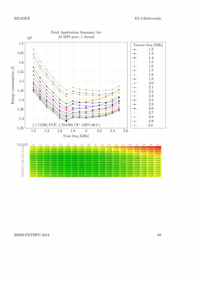
READEX D5.1-Deliverable
1.2 1.4 1.6 1.8 2 2.2 2.4 2.61.25
1.3
1.35
1.4
1.45
1.5
1.55
1.6
1.65
1.7
·104
( 1.7GHz UCF, 1.70GHz CF: 12871.86 J )
Core freq [GHz]
Energy
consumption
[J]
Total Application Summary for:24 MPI proc, 1 thread
Uncore freq [GHz]1.21.31.41.51.61.71.81.92.02.12.22.32.42.52.62.72.82.93.0
Uncore freq [GHz]Core freq [GHz] 1.2 1.3 1.4 1.5 1.6 1.7 1.8 1.9 2.0 2.1 2.2 2.3 2.4 2.5 2.6 2.7 2.8 2.9 3.0
1.2 14,859 14,680 14,548 14,475 14,445 14,462 14,500 14,576 14,687 14,810 14,950 15,118 15,329 15,546 15,742 15,960 16,248 16,431 16,7031.3 14,497 14,290 14,148 14,046 14,001 14,025 14,062 14,115 14,194 14,307 14,450 14,602 14,765 14,966 15,181 15,399 15,652 15,816 16,0661.4 14,167 13,948 13,780 13,673 13,617 13,613 13,653 13,693 13,787 13,885 14,015 14,187 14,346 14,525 14,714 14,966 15,238 15,369 15,6191.5 13,967 13,712 13,525 13,429 13,364 13,363 13,397 13,447 13,501 13,598 13,709 13,841 14,028 14,202 14,387 14,598 14,812 14,946 15,1791.6 13,666 13,426 13,243 13,102 13,026 13,024 13,060 13,108 13,165 13,232 13,366 13,512 13,643 13,820 14,013 14,207 14,425 14,546 14,7751.7 13,532 13,293 13,129 12,982 12,892 12,872 12,884 12,917 12,993 13,071 13,170 13,299 13,442 13,610 13,789 13,992 14,199 14,314 14,5291.8 13,809 13,528 13,333 13,192 13,078 13,052 13,049 13,097 13,144 13,221 13,324 13,446 13,591 13,775 13,938 14,126 14,346 14,458 14,6641.9 13,857 13,554 13,350 13,182 13,092 13,063 13,057 13,074 13,107 13,180 13,269 13,402 13,560 13,714 13,877 14,074 14,275 14,376 14,5682 13,887 13,589 13,348 13,180 13,085 13,043 13,038 13,035 13,073 13,137 13,269 13,386 13,539 13,680 13,861 14,055 14,261 14,359 14,5372.1 13,966 13,652 13,419 13,257 13,140 13,083 13,074 13,094 13,117 13,155 13,258 13,354 13,469 13,648 13,837 14,026 14,219 14,313 14,4982.2 14,063 13,727 13,486 13,314 13,178 13,121 13,097 13,122 13,147 13,170 13,267 13,392 13,540 13,699 13,858 14,044 14,223 14,276 14,4722.3 14,157 13,821 13,543 13,353 13,245 13,152 13,159 13,160 13,190 13,205 13,284 13,445 13,576 13,705 13,865 14,047 14,213 14,324 14,5312.4 14,367 14,012 13,707 13,532 13,394 13,320 13,289 13,286 13,319 13,350 13,399 13,509 13,635 13,767 13,903 14,105 14,259 14,356 14,5582.5 14,548 14,161 13,904 13,705 13,565 13,451 13,419 13,442 13,481 13,494 13,550 13,662 13,805 13,963 14,113 14,293 14,409 14,549 14,732
H2020-FETHPC-2014 68

READEX D5.1-Deliverable
1.2 1.4 1.6 1.8 2 2.2 2.4 2.6
50
55
60
65
70
75
80
85
90
95
( 3.0GHz UCF, 2.50GHz CF: 49.64 s )
Core freq [GHz]
Runtimeof
function[s]
Total Application Summary for:24 MPI proc, 1 thread
Uncore freq [GHz]1.21.31.41.51.61.71.81.92.02.12.22.32.42.52.62.72.82.93.0
Uncore freq [GHz]Core freq [GHz] 1.2 1.3 1.4 1.5 1.6 1.7 1.8 1.9 2.0 2.1 2.2 2.3 2.4 2.5 2.6 2.7 2.8 2.9 3.0
1.2 91.25 89.1 87.31 85.97 84.91 84.18 83.61 83.24 82.85 82.67 82.29 82.2 82.11 81.98 81.82 81.77 81.79 81.67 81.621.3 86.59 84.42 82.65 81.19 80.13 79.43 78.86 78.31 77.99 77.66 77.45 77.31 77.17 77.06 76.95 76.83 76.78 76.71 76.751.4 82.66 80.44 78.61 77.2 76.12 75.28 74.75 74.13 73.8 73.46 73.22 73.19 73.04 72.86 72.78 72.78 72.76 72.69 72.61.5 79.31 77.07 75.19 73.76 72.67 71.92 71.31 70.83 70.37 69.99 69.75 69.57 69.5 69.39 69.3 69.22 69.14 69.02 691.6 76.26 74.03 72.25 70.7 69.58 68.8 68.26 67.73 67.3 66.92 66.68 66.54 66.28 66.19 66.17 66.08 66.05 65.9 65.831.7 73.65 71.41 69.66 68.15 67.01 66.2 65.58 65.02 64.63 64.28 63.98 63.82 63.66 63.56 63.48 63.34 63.26 63.14 63.141.8 71.35 69.08 67.24 65.78 64.56 63.78 63.12 62.67 62.23 61.82 61.58 61.4 61.26 61.19 61.05 60.96 60.98 60.88 60.821.9 69.3 67.02 65.18 63.56 62.46 61.69 61.06 60.56 60.08 59.69 59.37 59.23 59.16 59.05 58.89 58.82 58.77 58.66 58.642 67.47 65.22 63.28 61.75 60.63 59.82 59.21 58.65 58.19 57.73 57.58 57.31 57.25 57.08 57 56.93 56.85 56.77 56.782.1 65.76 63.5 61.62 60.14 59.02 58.15 57.49 56.96 56.48 56.04 55.78 55.62 55.4 55.36 55.31 55.22 55.16 55.13 55.092.2 64.26 61.96 60.11 58.63 57.44 56.62 55.87 55.37 54.88 54.5 54.26 54.09 53.96 53.88 53.76 53.67 53.57 53.56 53.492.3 62.86 60.56 58.68 57.2 56.05 55.07 54.46 53.93 53.44 53 52.75 52.62 52.54 52.4 52.33 52.24 52.17 52.14 52.12.4 61.67 59.39 57.46 55.95 54.79 53.94 53.28 52.67 52.24 51.73 51.44 51.32 51.26 51.13 51.01 51.01 50.9 50.86 50.752.5 60.5 58.17 56.32 54.81 53.66 52.71 52.13 51.57 51.05 50.61 50.29 50.09 50 49.9 49.77 49.72 49.79 49.68 49.64
Intra-Phase Dynamism EvaluationBlade summary, Energy consumption [J]
Region % of 1 phaseBest static
configurationValue
Best dynamicconfiguration
ValueDynamicsavings
Source 0.15
24MPI proc,1 thread,1.7GHz UCF,1.7GHz CF
19.50 J
24MPI proc,1 thread,1.2GHz UCF,1.2GHz CF
17.83 J1.66 J(8.54%)
H2020-FETHPC-2014 69

READEX D5.1-Deliverable
LTimes 57.29
24MPI proc,1 thread,1.7GHz UCF,1.7GHz CF
7264.09 J
24MPI proc,1 thread,1.2GHz UCF,2.3GHz CF
6652.07 J612.02 J(8.43%)
Scattering 24.08
24MPI proc,1 thread,1.7GHz UCF,1.7GHz CF
3053.29 J
24MPI proc,1 thread,1.9GHz UCF,1.2GHz CF
2869.10 J184.19 J(6.03%)
LPlusTimes 14.01
24MPI proc,1 thread,1.7GHz UCF,1.7GHz CF
1776.89 J
24MPI proc,1 thread,2.1GHz UCF,1.6GHz CF
1681.94 J94.95 J(5.34%)
Sweep 4.47
24MPI proc,1 thread,1.7GHz UCF,1.7GHz CF
566.36 J
24MPI proc,1 thread,1.8GHz UCF,2.3GHz CF
552.68 J13.68 J(2.41%)
Total value for statictuning for significant re-gions
19.50 + 7264.09 + 3053.29 + 1776.89 + 566.36 =12680.12 J
Total savings for dy-namic tuning for signifi-cant regions
1.66 + 612.02 + 184.19 + 94.95 + 13.68 = 906.50 J of12680.12 J (7.15%)
Dynamic savings for ap-plication runtime
906.50 J of 12871.86 J (7.04%)
Intra-Phase Dynamism EvaluationRuntime of function [s]
Region % of 1 phaseBest static
configurationValue
Best dynamicconfiguration
ValueDynamicsavings
Source 0.24
24MPI proc,1 thread,3.0GHz UCF,2.5GHz CF
0.12 s
24MPI proc,1 thread,2.1GHz UCF,2.3GHz CF
0.11 s0.00 s(1.63%)
LTimes 53.48
24MPI proc,1 thread,3.0GHz UCF,2.5GHz CF
26.04 s
24MPI proc,1 thread,3.0GHz UCF,2.5GHz CF
26.04 s0.00 s(0.00%)
Scattering 28.08
24MPI proc,1 thread,3.0GHz UCF,2.5GHz CF
13.67 s
24MPI proc,1 thread,3.0GHz UCF,2.3GHz CF
13.64 s0.03 s(0.24%)
H2020-FETHPC-2014 70

READEX D5.1-Deliverable
LPlusTimes 13.81
24MPI proc,1 thread,3.0GHz UCF,2.5GHz CF
6.72 s
24MPI proc,1 thread,3.0GHz UCF,2.4GHz CF
6.72 s0.00 s(0.04%)
Sweep 4.40
24MPI proc,1 thread,3.0GHz UCF,2.5GHz CF
2.14 s
24MPI proc,1 thread,2.9GHz UCF,2.5GHz CF
2.14 s0.01 s(0.27%)
Total value for statictuning for significant re-gions
0.12 + 26.04 + 13.67 + 6.72 + 2.14 = 48.69 s
Total savings for dy-namic tuning for signifi-cant regions
0.00 + 0.00 + 0.03 + 0.00 + 0.01 = 0.04 s of 48.69 s(0.09%)
Dynamic savings for ap-plication runtime
0.04 s of 49.64 s (0.09%)
H2020-FETHPC-2014 71

READEX D5.1-Deliverable
6.8 ProxyApps 3 - LULESH
The Shock Hydrodynamics Challenge Problem was originally defined and implemented byLLNL as one of five challenge problems in the DARPA UHPC program and has since becomea widely studied proxy application in DOE co-design efforts for exascale. It has been portedto a number of programming models and optimized for a number of advanced platforms.
Computer simulations of a wide variety of science and engineering problems require modelinghydrodynamics, which describes the motion of materials relative to each other when subjectto forces. Many important simulation problems of interest to DOE involve complex multi-material systems that undergo large deformations. LULESH is a highly simplified application,hard-coded to only solve a simple Sedov blast problem with analytic answers but representsthe numerical algorithms, data motion, and programming style typical in scientific C or C++based applications.
LULESH represents a typical hydrocode, like ALE3D. LULESH approximates the hydrody-namics equations discretely by partitioning the spatial problem domain into a collection ofvolumetric elements defined by a mesh. A node on the mesh is a point where mesh linesintersect. LULESH is built on the concept of an unstructured hex mesh. Instead, indirectionarrays that define mesh relationships are used. The default test case for LULESH appearsto be a regular cartesian mesh, but this is for simplicity only - it is important to retain theunstructured data structures as they are representative of what a more complex geometrywill require. When modifying LULESH it is important to not take advantage of this or othersimplifications in the application.
For more information on the package and download links we refer the reader to https://code-sign.llnl.gov/lulesh.php.
6.8.1 Instrumentation with MERIC
To identify significant parts of the code, the Allinea Map tool was used to profile LULESH.Allinea revealed 14 kernels that took at least 1 % of the whole runtime in at least one of thetested runs, see Section 6.8.2 for a detailed list of these functions in the RADAR reports.Each kernel was then wrapped by a MERIC region.
LULESH was tested on a single node of the Taurus supercomputer. The MPI, OpenMPand hybrid implementations are provided, with the restriction that the total number of MPIprocesses has to be a cube (i.e. 1, 8, 27, . . . ). Two settings were chosen for the instrumentedruns, namely with 1 MPI process, 24 OpenMP threads with no explicit MPI binding and 8MPI processes, 3 OpenMP threads with MPI processes bound to every third core.
For both settings the environment variable KMP_AFFINITY was set to compact to avoidNUMA effects. We found out that employing fewer than 24 threads on a single node iscounter-productive, mainly due to the rather high static power consumption of the node.Performance-wise, both settings are very similar, on a single node we recommend the pure
H2020-FETHPC-2014 72

READEX D5.1-Deliverable
OpenMP parallelization due to potential MPI binding problems when testing with differentMPI implementations.
For the testing the program was called as
mpirun -n $MPI_PROCS ./lulesh2.0 -s $S -i $I -b $B
with MPI_PROCS, I and S denoting the number of MPI processes, maximal number of itera-tions, and the size of the domain, respectively, and B affecting the load balancing. Duringexperiments we have found out that the parameter S has the most significant impact onruntime and power consumption. The best static energy savings were obtained with powersof two, while primes lead to the best dynamic savings. The parameter B has not proven tohave a significant impact on the energy consumption, which might be caused by the fact thatwe only ran the program on a single node and the MPI communication overhead was notsignificant.
6.8.2 Results
We tested the application with the parameters -s 32 -i 20 and -s 97 -b 7 -i 20 whichresulted in the best static and dynamic savings, respectively, out of all testing runs. Allconfigurations were ran five times, RADAR reports represent an average run. The generatedreports are provided below.
6.8.2.1 MPI_PROCS=1, S=32, I=20, B=20
Overall application evaluation
Defaultsettings
Defaultvalues
Best staticconfiguration
StaticSavings
DynamicSavings
Energy consump-tion [J],Blade summary
1MPI proc,24 threads,3.0GHz UCF,2.5GHz CF
13307.00 J
1MPI proc,24 threads,1.2GHz UCF,1.3GHz CF
3790.04 J(28.48%)
52.40 J of9516.96 J(0.55%)
Runtime of function[s],Job info - hdeem
1MPI proc,24 threads,3.0GHz UCF,2.5GHz CF
58.36 s
1MPI proc,24 threads,3.0GHz UCF,2.5GHz CF
0.00 s(0.00%)
0.07 s of58.36 s(0.11%)
H2020-FETHPC-2014 73

READEX D5.1-Deliverable
1.2 1.4 1.6 1.8 2 2.2 2.4 2.6
0.95
1
1.05
1.1
1.15
1.2
1.25
1.3
1.35
·104
( 1.2GHz UCF, 1.30GHz CF: 9516.96 J )
Core freq [GHz]
Energy
consumption
[J]
Total Application Summary for:1 MPI proc, 24 threads
Uncore freq [GHz]1.21.31.41.51.61.71.81.92.02.12.22.32.42.52.62.72.82.93.0
Uncore freq [GHz]Core freq [GHz] 1.2 1.3 1.4 1.5 1.6 1.7 1.8 1.9 2.0 2.1 2.2 2.3 2.4 2.5 2.6 2.7 2.8 2.9 3.0
1.2 9,534 9,545 9,621 9,689 9,790 9,832 9,928 10,018 10,093 10,208 10,303 10,440 10,562 10,720 10,873 11,022 11,187 11,327 11,5131.3 9,517 9,552 9,607 9,646 9,731 9,790 9,900 9,987 10,096 10,186 10,285 10,406 10,570 10,693 10,855 10,979 11,137 11,312 11,4821.4 9,520 9,573 9,619 9,676 9,742 9,803 9,895 9,972 10,100 10,221 10,317 10,430 10,561 10,708 10,829 10,963 11,120 11,307 11,4721.5 9,552 9,599 9,658 9,678 9,757 9,804 9,907 9,999 10,107 10,204 10,324 10,458 10,518 10,676 10,800 10,967 11,139 11,264 11,4731.6 9,543 9,577 9,600 9,684 9,747 9,817 9,896 9,998 10,055 10,175 10,322 10,425 10,557 10,639 10,809 10,935 11,124 11,288 11,4531.7 9,643 9,668 9,727 9,781 9,838 9,908 10,018 10,083 10,150 10,293 10,373 10,498 10,638 10,768 10,876 11,031 11,198 11,319 11,5021.8 10,041 10,069 10,123 10,186 10,223 10,291 10,376 10,444 10,566 10,684 10,800 10,915 11,030 11,176 11,293 11,410 11,582 11,715 11,8661.9 10,360 10,385 10,422 10,478 10,534 10,629 10,677 10,766 10,852 10,982 11,069 11,179 11,300 11,421 11,557 11,714 11,853 11,991 12,1672 10,532 10,553 10,579 10,668 10,725 10,785 10,866 10,942 11,045 11,158 11,260 11,355 11,452 11,616 11,746 11,868 12,016 12,141 12,3352.1 10,727 10,773 10,817 10,887 10,941 11,024 11,100 11,172 11,254 11,342 11,443 11,557 11,640 11,749 11,919 12,026 12,138 12,331 12,4732.2 10,969 11,022 11,053 11,120 11,145 11,224 11,319 11,380 11,441 11,520 11,632 11,723 11,868 11,960 12,114 12,223 12,356 12,544 12,6762.3 11,220 11,270 11,310 11,367 11,420 11,464 11,538 11,586 11,678 11,719 11,857 11,921 12,014 12,177 12,281 12,413 12,563 12,718 12,8262.4 11,478 11,519 11,577 11,630 11,646 11,698 11,734 11,822 11,912 11,977 12,064 12,174 12,264 12,396 12,517 12,652 12,787 12,905 13,0722.5 11,752 11,784 11,832 11,892 11,876 11,924 11,999 12,057 12,175 12,249 12,314 12,421 12,485 12,628 12,791 12,857 13,007 13,163 13,307
H2020-FETHPC-2014 74

READEX D5.1-Deliverable
1.2 1.4 1.6 1.8 2 2.2 2.4 2.6
58
60
62
64
66
68
70
( 3.0GHz UCF, 2.50GHz CF: 58.36 s )
Core freq [GHz]
Runtimeof
function[s]
Total Application Summary for:1 MPI proc, 24 threads
Uncore freq [GHz]1.21.31.41.51.61.71.81.92.02.12.22.32.42.52.62.72.82.93.0
Uncore freq [GHz]Core freq [GHz] 1.2 1.3 1.4 1.5 1.6 1.7 1.8 1.9 2.0 2.1 2.2 2.3 2.4 2.5 2.6 2.7 2.8 2.9 3.0
1.2 69.4 68.9 68.9 68.8 68.8 68.6 68.6 68.5 68.3 68.4 68.2 68.2 68.1 68.3 68.2 68.2 68.2 68.1 681.3 67.9 67.8 67.6 67.3 67.4 67.2 67.3 67.3 67.2 67.1 67 66.9 67.1 67 67 66.9 66.8 66.9 66.81.4 66.7 66.6 66.4 66.3 66.2 66.1 66 65.9 66 66.1 66 66 65.9 65.9 65.9 65.8 65.7 65.7 65.71.5 65.7 65.6 65.5 65.2 65.1 64.8 65 64.9 64.9 64.7 64.9 65 64.5 64.7 64.5 64.5 64.6 64.5 64.61.6 64.7 64.6 64.3 64.3 64.3 64.2 64.1 64.2 63.9 63.9 64 64 64 63.7 63.9 63.7 63.8 63.8 63.81.7 64.2 63.9 63.8 63.7 63.5 63.5 63.6 63.4 63.2 63.3 63.2 63.3 63.3 63.2 63.1 63.2 63.1 62.9 63.11.8 63.5 63.3 63.2 63.1 62.9 62.8 62.8 62.6 62.7 62.6 62.6 62.7 62.6 62.6 62.6 62.4 62.4 62.2 62.21.9 62.9 62.7 62.5 62.4 62.2 62.4 62.1 62.1 62 62.1 62 62 61.9 61.8 61.8 61.9 61.8 61.7 61.82 62.3 62.1 61.9 62 61.9 61.7 61.7 61.6 61.5 61.6 61.6 61.4 61.3 61.4 61.3 61.3 61.3 61 61.22.1 61.7 61.7 61.5 61.5 61.4 61.3 61.3 61.1 61.1 61 60.9 60.9 60.9 60.6 60.7 60.6 60.5 60.6 60.52.2 61.4 61.4 61.1 61 60.9 60.8 60.8 60.6 60.5 60.3 60.3 60.1 60.3 60.1 60.1 60.1 60 60 59.92.3 60.9 60.9 60.7 60.6 60.5 60.3 60.2 60 60 59.8 59.9 59.8 59.6 59.7 59.6 59.5 59.5 59.4 59.32.4 60.6 60.5 60.4 60.3 60.1 59.8 59.6 59.6 59.4 59.4 59.3 59.2 59.2 59.1 59 59 58.9 58.9 58.82.5 60.3 60.2 60 60 59.6 59.3 59.3 59.2 59.3 59.1 58.9 58.9 58.7 58.6 58.7 58.5 58.5 58.4 58.4
Intra-Phase Dynamism EvaluationBlade summary, Energy consumption [J]
Region % of 1 phaseBest static
configurationValue
Best dynamicconfiguration
ValueDynamicsavings
H2020-FETHPC-2014 75

READEX D5.1-Deliverable
CalcLa-grangeEle-ments
0.36
1MPI proc,24 threads,1.2GHz UCF,1.3GHz CF
13.56 J
1MPI proc,24 threads,1.3GHz UCF,1.2GHz CF
13.07 J0.49 J(3.58%)
EvalE-OSForElems -parallel-Pragma
10.99
1MPI proc,24 threads,1.2GHz UCF,1.3GHz CF
417.84 J
1MPI proc,24 threads,1.2GHz UCF,1.2GHz CF
413.17 J4.67 J(1.12%)
CalcCourant-Constraint-ForElems
3.41
1MPI proc,24 threads,1.2GHz UCF,1.3GHz CF
129.78 J
1MPI proc,24 threads,1.2GHz UCF,1.2GHz CF
129.70 J0.07 J(0.06%)
CalcEnergy-ForElems4
10.99
1MPI proc,24 threads,1.2GHz UCF,1.3GHz CF
417.97 J
1MPI proc,24 threads,1.2GHz UCF,1.2GHz CF
412.18 J5.80 J(1.39%)
CalcSound-Speed-ForElems
3.45
1MPI proc,24 threads,1.2GHz UCF,1.3GHz CF
131.16 J
1MPI proc,24 threads,1.2GHz UCF,1.2GHz CF
128.94 J2.22 J(1.69%)
CalcEnergy-ForElems1
10.90
1MPI proc,24 threads,1.2GHz UCF,1.3GHz CF
414.64 J
1MPI proc,24 threads,1.2GHz UCF,1.2GHz CF
409.35 J5.29 J(1.28%)
CalcEnergy-ForElems3
10.93
1MPI proc,24 threads,1.2GHz UCF,1.3GHz CF
415.80 J
1MPI proc,24 threads,1.2GHz UCF,1.2GHz CF
409.49 J6.31 J(1.52%)
CalcFBHour-glassForce-ForElems
0.45
1MPI proc,24 threads,1.2GHz UCF,1.3GHz CF
17.25 J
1MPI proc,24 threads,1.7GHz UCF,1.2GHz CF
16.92 J0.33 J(1.90%)
Integrat-eStress-ForElems
0.36
1MPI proc,24 threads,1.2GHz UCF,1.3GHz CF
13.59 J
1MPI proc,24 threads,1.3GHz UCF,1.3GHz CF
13.06 J0.53 J(3.93%)
CalcEnergy-ForElems2
10.97
1MPI proc,24 threads,1.2GHz UCF,1.3GHz CF
417.19 J
1MPI proc,24 threads,1.2GHz UCF,1.2GHz CF
413.11 J4.08 J(0.98%)
H2020-FETHPC-2014 76
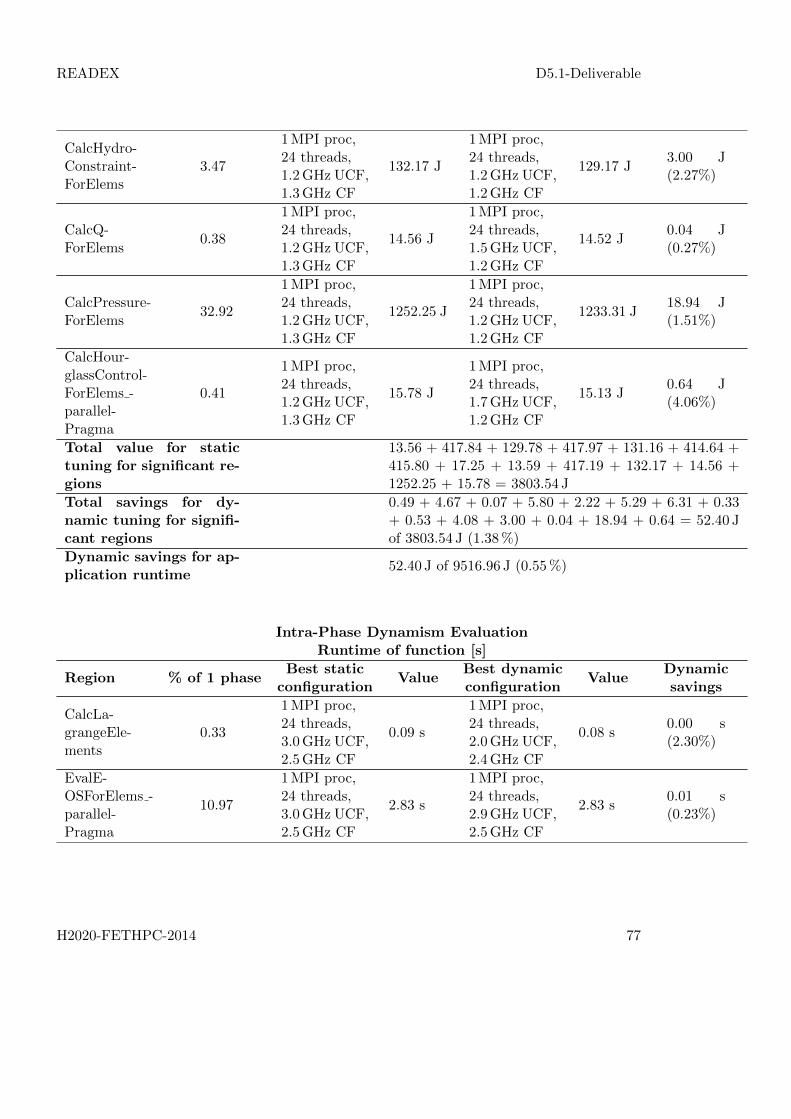
READEX D5.1-Deliverable
CalcHydro-Constraint-ForElems
3.47
1MPI proc,24 threads,1.2GHz UCF,1.3GHz CF
132.17 J
1MPI proc,24 threads,1.2GHz UCF,1.2GHz CF
129.17 J3.00 J(2.27%)
CalcQ-ForElems
0.38
1MPI proc,24 threads,1.2GHz UCF,1.3GHz CF
14.56 J
1MPI proc,24 threads,1.5GHz UCF,1.2GHz CF
14.52 J0.04 J(0.27%)
CalcPressure-ForElems
32.92
1MPI proc,24 threads,1.2GHz UCF,1.3GHz CF
1252.25 J
1MPI proc,24 threads,1.2GHz UCF,1.2GHz CF
1233.31 J18.94 J(1.51%)
CalcHour-glassControl-ForElems -parallel-Pragma
0.41
1MPI proc,24 threads,1.2GHz UCF,1.3GHz CF
15.78 J
1MPI proc,24 threads,1.7GHz UCF,1.2GHz CF
15.13 J0.64 J(4.06%)
Total value for statictuning for significant re-gions
13.56 + 417.84 + 129.78 + 417.97 + 131.16 + 414.64 +415.80 + 17.25 + 13.59 + 417.19 + 132.17 + 14.56 +1252.25 + 15.78 = 3803.54 J
Total savings for dy-namic tuning for signifi-cant regions
0.49 + 4.67 + 0.07 + 5.80 + 2.22 + 5.29 + 6.31 + 0.33+ 0.53 + 4.08 + 3.00 + 0.04 + 18.94 + 0.64 = 52.40 Jof 3803.54 J (1.38%)
Dynamic savings for ap-plication runtime
52.40 J of 9516.96 J (0.55%)
Intra-Phase Dynamism EvaluationRuntime of function [s]
Region % of 1 phaseBest static
configurationValue
Best dynamicconfiguration
ValueDynamicsavings
CalcLa-grangeEle-ments
0.33
1MPI proc,24 threads,3.0GHz UCF,2.5GHz CF
0.09 s
1MPI proc,24 threads,2.0GHz UCF,2.4GHz CF
0.08 s0.00 s(2.30%)
EvalE-OSForElems -parallel-Pragma
10.97
1MPI proc,24 threads,3.0GHz UCF,2.5GHz CF
2.83 s
1MPI proc,24 threads,2.9GHz UCF,2.5GHz CF
2.83 s0.01 s(0.23%)
H2020-FETHPC-2014 77

READEX D5.1-Deliverable
CalcCourant-Constraint-ForElems
3.44
1MPI proc,24 threads,3.0GHz UCF,2.5GHz CF
0.89 s
1MPI proc,24 threads,3.0GHz UCF,2.5GHz CF
0.89 s0.00 s(0.00%)
CalcEnergy-ForElems4
10.98
1MPI proc,24 threads,3.0GHz UCF,2.5GHz CF
2.83 s
1MPI proc,24 threads,2.8GHz UCF,2.5GHz CF
2.82 s0.01 s(0.31%)
CalcSound-Speed-ForElems
3.44
1MPI proc,24 threads,3.0GHz UCF,2.5GHz CF
0.89 s
1MPI proc,24 threads,2.7GHz UCF,2.5GHz CF
0.88 s0.00 s(0.33%)
CalcEnergy-ForElems1
10.99
1MPI proc,24 threads,3.0GHz UCF,2.5GHz CF
2.84 s
1MPI proc,24 threads,2.9GHz UCF,2.5GHz CF
2.82 s0.01 s(0.42%)
CalcEnergy-ForElems3
11.01
1MPI proc,24 threads,3.0GHz UCF,2.5GHz CF
2.84 s
1MPI proc,24 threads,2.7GHz UCF,2.5GHz CF
2.83 s0.01 s(0.24%)
CalcFBHour-glassForce-ForElems
0.40
1MPI proc,24 threads,3.0GHz UCF,2.5GHz CF
0.10 s
1MPI proc,24 threads,2.8GHz UCF,2.5GHz CF
0.10 s0.00 s(1.43%)
Integrat-eStress-ForElems
0.34
1MPI proc,24 threads,3.0GHz UCF,2.5GHz CF
0.09 s
1MPI proc,24 threads,2.6GHz UCF,2.4GHz CF
0.08 s0.00 s(4.06%)
CalcEnergy-ForElems2
10.99
1MPI proc,24 threads,3.0GHz UCF,2.5GHz CF
2.84 s
1MPI proc,24 threads,2.8GHz UCF,2.5GHz CF
2.83 s0.00 s(0.15%)
CalcHydro-Constraint-ForElems
3.47
1MPI proc,24 threads,3.0GHz UCF,2.5GHz CF
0.90 s
1MPI proc,24 threads,2.7GHz UCF,2.5GHz CF
0.89 s0.01 s(1.21%)
CalcQ-ForElems
0.36
1MPI proc,24 threads,3.0GHz UCF,2.5GHz CF
0.09 s
1MPI proc,24 threads,2.9GHz UCF,2.4GHz CF
0.09 s0.00 s(5.10%)
H2020-FETHPC-2014 78

READEX D5.1-Deliverable
CalcPressure-ForElems
32.91
1MPI proc,24 threads,3.0GHz UCF,2.5GHz CF
8.49 s
1MPI proc,24 threads,3.0GHz UCF,2.5GHz CF
8.49 s0.00 s(0.00%)
CalcHour-glassControl-ForElems -parallel-Pragma
0.36
1MPI proc,24 threads,3.0GHz UCF,2.5GHz CF
0.09 s
1MPI proc,24 threads,3.0GHz UCF,2.3GHz CF
0.09 s0.00 s(1.56%)
Total value for statictuning for significant re-gions
0.09 + 2.83 + 0.89 + 2.83 + 0.89 + 2.84 + 2.84 + 0.10+ 0.09 + 2.84 + 0.90 + 0.09 + 8.49 + 0.09 = 25.81 s
Total savings for dy-namic tuning for signifi-cant regions
0.00 + 0.01 + 0.00 + 0.01 + 0.00 + 0.01 + 0.01 + 0.00+ 0.00 + 0.00 + 0.01 + 0.00 + 0.00 + 0.00 = 0.07 s of25.81 s (0.25%)
Dynamic savings for ap-plication runtime
0.07 s of 58.36 s (0.11%)
6.8.2.2 MPI_PROCS=8, S=97, I=20, B=7
Overall application evaluation
Defaultsettings
Defaultvalues
Best staticconfiguration
StaticSavings
DynamicSavings
Energy consump-tion [J],Blade summary
8MPI proc,3 threads,3.0GHz UCF,2.5GHz CF
13636.90 J
8MPI proc,3 threads,1.2GHz UCF,1.6GHz CF
3519.32 J(25.81%)
124.38 Jof10117.58 J(1.23%)
Runtime of function[s],Job info - hdeem
8MPI proc,3 threads,3.0GHz UCF,2.5GHz CF
58.05 s
8MPI proc,3 threads,3.0GHz UCF,2.5GHz CF
0.00 s(0.00%)
0.06 s of58.05 s(0.10%)
H2020-FETHPC-2014 79

READEX D5.1-Deliverable
1.2 1.4 1.6 1.8 2 2.2 2.4 2.6
1
1.05
1.1
1.15
1.2
1.25
1.3
1.35
·104
( 1.2GHz UCF, 1.60GHz CF: 10117.58 J )
Core freq [GHz]
Energy
consumption
[J]
Total Application Summary for:8 MPI proc, 3 threads
Uncore freq [GHz]1.21.31.41.51.61.71.81.92.02.12.22.32.42.52.62.72.82.93.0
Uncore freq [GHz]Core freq [GHz] 1.2 1.3 1.4 1.5 1.6 1.7 1.8 1.9 2.0 2.1 2.2 2.3 2.4 2.5 2.6 2.7 2.8 2.9 3.0
1.2 10,241 10,287 10,327 10,415 10,506 10,532 10,666 10,680 10,820 10,870 10,974 11,154 11,274 11,428 11,596 11,714 11,933 12,045 12,2361.3 10,214 10,210 10,275 10,342 10,399 10,449 10,528 10,600 10,685 10,787 10,920 11,078 11,182 11,371 11,553 11,696 11,852 11,975 12,1651.4 10,130 10,195 10,247 10,306 10,362 10,398 10,486 10,566 10,648 10,764 10,873 11,023 11,159 11,269 11,408 11,582 11,743 11,940 12,0831.5 10,142 10,142 10,180 10,267 10,315 10,384 10,452 10,511 10,633 10,754 10,846 10,955 11,105 11,280 11,375 11,558 11,754 11,868 12,0461.6 10,118 10,148 10,160 10,233 10,292 10,378 10,451 10,510 10,588 10,703 10,799 10,949 11,074 11,229 11,354 11,503 11,673 11,842 12,0241.7 10,166 10,174 10,210 10,268 10,348 10,393 10,488 10,572 10,645 10,733 10,821 10,972 11,104 11,222 11,403 11,571 11,720 11,863 12,0311.8 10,416 10,464 10,477 10,546 10,577 10,653 10,745 10,825 10,892 11,021 11,121 11,211 11,375 11,500 11,652 11,786 11,975 12,133 12,3201.9 10,764 10,791 10,831 10,883 10,961 11,018 11,072 11,133 11,213 11,301 11,412 11,545 11,672 11,801 11,976 12,099 12,256 12,433 12,5892 10,925 10,950 10,984 11,025 11,083 11,144 11,227 11,272 11,353 11,460 11,581 11,697 11,826 11,954 12,106 12,214 12,389 12,523 12,6722.1 11,089 11,113 11,161 11,211 11,287 11,301 11,374 11,466 11,535 11,610 11,715 11,840 11,976 12,088 12,224 12,372 12,508 12,664 12,8312.2 11,285 11,293 11,345 11,399 11,464 11,509 11,575 11,671 11,747 11,786 11,867 12,006 12,146 12,279 12,394 12,567 12,716 12,821 13,0162.3 11,511 11,529 11,545 11,583 11,646 11,724 11,756 11,837 11,903 11,928 12,020 12,177 12,266 12,363 12,545 12,667 12,849 12,958 13,1492.4 11,737 11,777 11,831 11,903 11,926 11,952 12,005 12,037 12,100 12,210 12,308 12,391 12,554 12,643 12,755 12,919 13,052 13,235 13,3542.5 12,066 11,993 12,036 12,110 12,119 12,174 12,210 12,318 12,354 12,440 12,549 12,643 12,775 12,898 13,078 13,260 13,382 13,479 13,637
H2020-FETHPC-2014 80
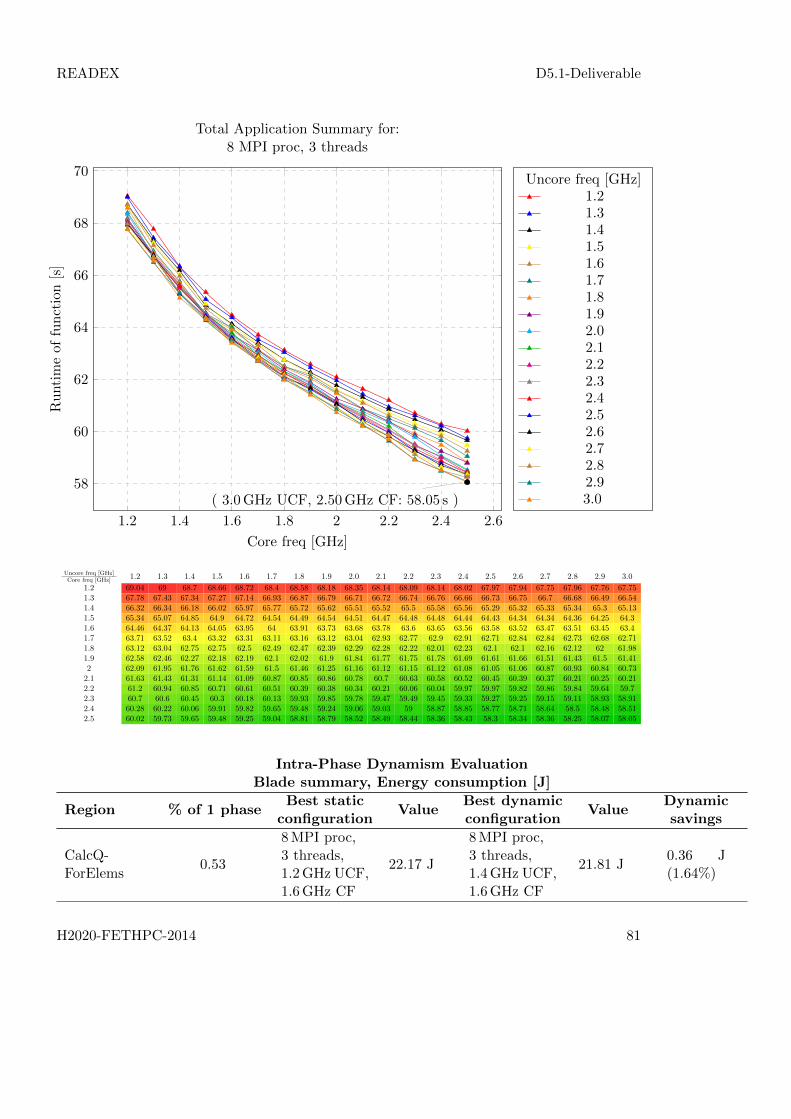
READEX D5.1-Deliverable
1.2 1.4 1.6 1.8 2 2.2 2.4 2.6
58
60
62
64
66
68
70
( 3.0GHz UCF, 2.50GHz CF: 58.05 s )
Core freq [GHz]
Runtimeof
function[s]
Total Application Summary for:8 MPI proc, 3 threads
Uncore freq [GHz]1.21.31.41.51.61.71.81.92.02.12.22.32.42.52.62.72.82.93.0
Uncore freq [GHz]Core freq [GHz] 1.2 1.3 1.4 1.5 1.6 1.7 1.8 1.9 2.0 2.1 2.2 2.3 2.4 2.5 2.6 2.7 2.8 2.9 3.0
1.2 69.04 69 68.7 68.66 68.72 68.4 68.58 68.18 68.35 68.14 68.09 68.14 68.02 67.97 67.94 67.75 67.96 67.76 67.751.3 67.78 67.43 67.34 67.27 67.14 66.93 66.87 66.79 66.71 66.72 66.74 66.76 66.66 66.73 66.75 66.7 66.68 66.49 66.541.4 66.32 66.34 66.18 66.02 65.97 65.77 65.72 65.62 65.51 65.52 65.5 65.58 65.56 65.29 65.32 65.33 65.34 65.3 65.131.5 65.34 65.07 64.85 64.9 64.72 64.54 64.49 64.54 64.51 64.47 64.48 64.48 64.44 64.43 64.34 64.34 64.36 64.25 64.31.6 64.46 64.37 64.13 64.05 63.95 64 63.91 63.73 63.68 63.78 63.6 63.65 63.56 63.58 63.52 63.47 63.51 63.45 63.41.7 63.71 63.52 63.4 63.32 63.31 63.11 63.16 63.12 63.04 62.93 62.77 62.9 62.91 62.71 62.84 62.84 62.73 62.68 62.711.8 63.12 63.04 62.75 62.75 62.5 62.49 62.47 62.39 62.29 62.28 62.22 62.01 62.23 62.1 62.1 62.16 62.12 62 61.981.9 62.58 62.46 62.27 62.18 62.19 62.1 62.02 61.9 61.84 61.77 61.75 61.78 61.69 61.61 61.66 61.51 61.43 61.5 61.412 62.09 61.95 61.76 61.62 61.59 61.5 61.46 61.25 61.16 61.12 61.15 61.12 61.08 61.05 61.06 60.87 60.93 60.84 60.732.1 61.63 61.43 61.31 61.14 61.09 60.87 60.85 60.86 60.78 60.7 60.63 60.58 60.52 60.45 60.39 60.37 60.21 60.25 60.212.2 61.2 60.94 60.85 60.71 60.61 60.51 60.39 60.38 60.34 60.21 60.06 60.04 59.97 59.97 59.82 59.86 59.84 59.64 59.72.3 60.7 60.6 60.45 60.3 60.18 60.13 59.93 59.85 59.78 59.47 59.49 59.45 59.33 59.27 59.25 59.15 59.11 58.93 58.912.4 60.28 60.22 60.06 59.91 59.82 59.65 59.48 59.24 59.06 59.03 59 58.87 58.85 58.77 58.71 58.64 58.5 58.48 58.512.5 60.02 59.73 59.65 59.48 59.25 59.04 58.81 58.79 58.52 58.49 58.44 58.36 58.43 58.3 58.34 58.36 58.25 58.07 58.05
Intra-Phase Dynamism EvaluationBlade summary, Energy consumption [J]
Region % of 1 phaseBest static
configurationValue
Best dynamicconfiguration
ValueDynamicsavings
CalcQ-ForElems
0.53
8MPI proc,3 threads,1.2GHz UCF,1.6GHz CF
22.17 J
8MPI proc,3 threads,1.4GHz UCF,1.6GHz CF
21.81 J0.36 J(1.64%)
H2020-FETHPC-2014 81

READEX D5.1-Deliverable
CalcEnergy-ForElems1
10.78
8MPI proc,3 threads,1.2GHz UCF,1.6GHz CF
453.05 J
8MPI proc,3 threads,1.2GHz UCF,1.2GHz CF
439.60 J13.45 J(2.97%)
Integrat-eStress-ForElems
0.64
8MPI proc,3 threads,1.2GHz UCF,1.6GHz CF
27.04 J
8MPI proc,3 threads,1.5GHz UCF,1.7GHz CF
26.32 J0.72 J(2.67%)
CalcEnergy-ForElems4
10.86
8MPI proc,3 threads,1.2GHz UCF,1.6GHz CF
456.21 J
8MPI proc,3 threads,1.2GHz UCF,1.2GHz CF
442.49 J13.72 J(3.01%)
EvalE-OSForElems -parallel-Pragma
10.91
8MPI proc,3 threads,1.2GHz UCF,1.6GHz CF
458.32 J
8MPI proc,3 threads,1.3GHz UCF,1.2GHz CF
444.67 J13.65 J(2.98%)
CalcSound-Speed-ForElems
3.40
8MPI proc,3 threads,1.2GHz UCF,1.6GHz CF
142.79 J
8MPI proc,3 threads,1.2GHz UCF,1.2GHz CF
138.04 J4.75 J(3.32%)
CalcEnergy-ForElems3
10.86
8MPI proc,3 threads,1.2GHz UCF,1.6GHz CF
456.33 J
8MPI proc,3 threads,1.2GHz UCF,1.2GHz CF
441.44 J14.89 J(3.26%)
CalcEnergy-ForElems2
10.81
8MPI proc,3 threads,1.2GHz UCF,1.6GHz CF
454.41 J
8MPI proc,3 threads,1.2GHz UCF,1.2GHz CF
440.31 J14.10 J(3.10%)
CalcLa-grangeEle-ments
0.52
8MPI proc,3 threads,1.2GHz UCF,1.6GHz CF
21.94 J
8MPI proc,3 threads,1.3GHz UCF,1.7GHz CF
21.39 J0.55 J(2.50%)
CalcPressure-ForElems
32.39
8MPI proc,3 threads,1.2GHz UCF,1.6GHz CF
1361.06 J
8MPI proc,3 threads,1.2GHz UCF,1.2GHz CF
1324.79 J36.27 J(2.67%)
CalcHydro-Constraint-ForElems
3.40
8MPI proc,3 threads,1.2GHz UCF,1.6GHz CF
142.79 J
8MPI proc,3 threads,1.2GHz UCF,1.2GHz CF
138.25 J4.54 J(3.18%)
H2020-FETHPC-2014 82

READEX D5.1-Deliverable
CalcFBHour-glassForce-ForElems
0.77
8MPI proc,3 threads,1.2GHz UCF,1.6GHz CF
32.49 J
8MPI proc,3 threads,1.4GHz UCF,1.7GHz CF
30.93 J1.56 J(4.80%)
CalcHour-glassControl-ForElems -parallel-Pragma
0.72
8MPI proc,3 threads,1.2GHz UCF,1.6GHz CF
30.11 J
8MPI proc,3 threads,1.6GHz UCF,1.7GHz CF
29.13 J0.98 J(3.27%)
CalcCourant-Constraint-ForElems
3.40
8MPI proc,3 threads,1.2GHz UCF,1.6GHz CF
143.03 J
8MPI proc,3 threads,1.2GHz UCF,1.2GHz CF
138.19 J4.83 J(3.38%)
Total value for statictuning for significant re-gions
22.17 + 453.05 + 27.04 + 456.21 + 458.32 + 142.79 +456.33 + 454.41 + 21.94 + 1361.06 + 142.79 + 32.49 +30.11 + 143.03 = 4201.72 J
Total savings for dy-namic tuning for signifi-cant regions
0.36 + 13.45 + 0.72 + 13.72 + 13.65 + 4.75 + 14.89 +14.10 + 0.55 + 36.27 + 4.54 + 1.56 + 0.98 + 4.83 =124.38 J of 4201.72 J (2.96%)
Dynamic savings for ap-plication runtime
124.38 J of 10117.58 J (1.23%)
Intra-Phase Dynamism EvaluationRuntime of function [s]
Region % of 1 phaseBest static
configurationValue
Best dynamicconfiguration
ValueDynamicsavings
CalcQ-ForElems
0.45
8MPI proc,3 threads,3.0GHz UCF,2.5GHz CF
0.12 s
8MPI proc,3 threads,2.7GHz UCF,2.5GHz CF
0.11 s0.00 s(2.71%)
CalcEnergy-ForElems1
10.90
8MPI proc,3 threads,3.0GHz UCF,2.5GHz CF
2.81 s
8MPI proc,3 threads,2.4GHz UCF,2.5GHz CF
2.81 s0.00 s(0.11%)
Integrat-eStress-ForElems
0.48
8MPI proc,3 threads,3.0GHz UCF,2.5GHz CF
0.12 s
8MPI proc,3 threads,3.0GHz UCF,2.5GHz CF
0.12 s0.00 s(0.00%)
H2020-FETHPC-2014 83

READEX D5.1-Deliverable
CalcEnergy-ForElems4
10.90
8MPI proc,3 threads,3.0GHz UCF,2.5GHz CF
2.81 s
8MPI proc,3 threads,2.8GHz UCF,2.4GHz CF
2.81 s0.00 s(0.02%)
EvalE-OSForElems -parallel-Pragma
10.95
8MPI proc,3 threads,3.0GHz UCF,2.5GHz CF
2.82 s
8MPI proc,3 threads,2.9GHz UCF,2.5GHz CF
2.81 s0.01 s(0.36%)
CalcSound-Speed-ForElems
3.42
8MPI proc,3 threads,3.0GHz UCF,2.5GHz CF
0.88 s
8MPI proc,3 threads,3.0GHz UCF,2.5GHz CF
0.88 s0.00 s(0.00%)
CalcEnergy-ForElems3
10.91
8MPI proc,3 threads,3.0GHz UCF,2.5GHz CF
2.81 s
8MPI proc,3 threads,2.9GHz UCF,2.5GHz CF
2.80 s0.02 s(0.54%)
CalcEnergy-ForElems2
10.89
8MPI proc,3 threads,3.0GHz UCF,2.5GHz CF
2.81 s
8MPI proc,3 threads,2.8GHz UCF,2.5GHz CF
2.80 s0.00 s(0.14%)
CalcLa-grangeEle-ments
0.44
8MPI proc,3 threads,3.0GHz UCF,2.5GHz CF
0.11 s
8MPI proc,3 threads,2.5GHz UCF,2.5GHz CF
0.11 s0.00 s(3.04%)
CalcPressure-ForElems
32.71
8MPI proc,3 threads,3.0GHz UCF,2.5GHz CF
8.43 s
8MPI proc,3 threads,2.7GHz UCF,2.5GHz CF
8.42 s0.01 s(0.07%)
CalcHydro-Constraint-ForElems
3.45
8MPI proc,3 threads,3.0GHz UCF,2.5GHz CF
0.89 s
8MPI proc,3 threads,2.5GHz UCF,2.4GHz CF
0.88 s0.01 s(0.99%)
CalcFBHour-glassForce-ForElems
0.54
8MPI proc,3 threads,3.0GHz UCF,2.5GHz CF
0.14 s
8MPI proc,3 threads,2.8GHz UCF,2.5GHz CF
0.14 s0.00 s(0.80%)
CalcHour-glassControl-ForElems -parallel-Pragma
0.53
8MPI proc,3 threads,3.0GHz UCF,2.5GHz CF
0.14 s
8MPI proc,3 threads,2.9GHz UCF,2.5GHz CF
0.14 s0.00 s(0.16%)
H2020-FETHPC-2014 84

READEX D5.1-Deliverable
CalcCourant-Constraint-ForElems
3.43
8MPI proc,3 threads,3.0GHz UCF,2.5GHz CF
0.88 s
8MPI proc,3 threads,2.7GHz UCF,2.3GHz CF
0.88 s0.01 s(0.59%)
Total value for statictuning for significant re-gions
0.12 + 2.81 + 0.12 + 2.81 + 2.82 + 0.88 + 2.81 + 2.81+ 0.11 + 8.43 + 0.89 + 0.14 + 0.14 + 0.88 = 25.77 s
Total savings for dy-namic tuning for signifi-cant regions
0.00 + 0.00 + 0.00 + 0.00 + 0.01 + 0.00 + 0.02 + 0.00+ 0.00 + 0.01 + 0.01 + 0.00 + 0.00 + 0.01 = 0.06 s of25.77 s (0.24%)
Dynamic savings for ap-plication runtime
0.06 s of 58.05 s (0.10%)
H2020-FETHPC-2014 85

READEX D5.1-Deliverable
6.9 ProxyApps 4 - MCB
The Monte Carlo Benchmark (MCB) is intended for use in exploring the computationalperformance of Monte Carlo algorithms on parallel architectures. It models the solutionof a simple heuristic transport equation using a Monte Carlo technique. The MCB employstypical features of Monte Carlo algorithms such as particle creation, particle tracking, tallyingparticle information, and particle destruction. Particles are also traded among processorsusing MPI calls.
The heuristic transport equation models the behavior of particles that are born, travel witha constant velocity, scatter, and are absorbed. Its implementation in MCB ignores a numberof effects that are important in real world problems. The particles in the MCB simulation donot interact with material by depositing energy, do not use physical cross sections, and donot model real transport effects such as frequency dependent properties or material motioncorrections. The MCB is implemented on a simple orthogonal grid. Because of these limita-tions, the MCB is solely intended to serve as a benchmark and is not intended to model realphysics.
The MCB is designed to confirm correct hybrid MPI + OpenMP performance, single CPUperformance, and parallel scaling on new computers. It achieves parallelism through domaindecomposition and threading. Domain decomposition means that the physical space simu-lated by the code is cut up into distinct sections (domains), each of which is simulated bya different MPI process. When particles hit the boundary of a domain, they are buffered.The buffers are sent using a non-blocking MPI call to the processor simulating the domainon the other side of the boundary. OpenMP threads can be used within an MPI task tocooperatively track the particles in its domain.
For more information on the package and download links we refer the reader to https://code-sign.llnl.gov/mcb.php.
6.9.1 Instrumentation with MERIC
Before inserting MERIC regions, the MCB app was profiled by Allinea Map. The advance
function and the functions it calls do most of the work in MCB. Inside of this function weidentified several significant regions. The first one comprises calls to the functions setUp
and get_source_photons preparing data for the subsequent simulation. The computation-ally most intensive part is included in the function advancePhotonList. This function alsoincludes the above mentioned non-blocking MPI calls representing a good candidate for asignificant region. However, this part of the code is not accessed by all MPI processes thesame number of times, which implies that it is not possible to insert a global MPI barrierbefore and after the MPI send/receive calls without further changes in the code. Thus, formeasurements with MERIC we could not further separate the advancePhotonList functioninto the computation and communication phases. This results in two MERIC regions, firstone including both preparatory functions setUp and get_source_photons, and the secondone for the computationally intensive advancePhotonList. All these functions are called in
H2020-FETHPC-2014 86

READEX D5.1-Deliverable
MPI_PROCS 1 2 4PX 1 1 2PY 1 2 2
OMP_THREADS 24 12 6
Default consumption [J] 2325 3439 5880Static savings [J] 96 (4.13 %) 163 (4.75 %) 365 (6.21 %)
Dynamic savings [J] 32 (1.42 %) 50 (1.51 %) 119 (2.15 %)Total savings [J] 128 (5.51 %) 213 (6.19 %) 484 (8.23 %)
Table 31: Energy savings for various settings, part 1.
every time step. The time stepping is thus denoted as an iteration region for visualizationpurposes.
Testing runs were chosen such that the runtime of a single simulation is reasonable, i.e., tensof seconds. In particular, the program MCBenchmark.exe was called as
srun -n $MPI_PROCS ./MCBenchmark.exe
--nMpiTasksX=$MPI_X
--nMpiTasksY=$MPI_Y
--nCores=$OMP_THREADS
--nThreadCore=1
--numParticles=8000000
with the parameters MPI_PROCS, PX, PY, MCB_OMP_THREADS denoting the number of MPI pro-cesses, number of subdomains in x and y axes, and number of OpenMP threads, respectively.Each MPI process is assigned a single subdomain, i.e., it must hold
MPI_PROCS = PX · PY.
The experiments were performed on a single Taurus node and in every instance all availablecores were utilized. The tuning parameters thus included core and uncore frequencies, numberof MPI processes and OpenMP threads, such that
MPI_PROCS · OMP_THREADS = 24.
To overcome NUMA effects, in particular for the case with a single MPI process and 24OpenMP threads, the environment variable OMP_PROC_BIND was set to close.
6.9.2 Results
In Tables 31 and 32 we present possible energy savings for different configurations by tuningthe core and uncore frequencies. First three rows describe the configuration of MCB asdescribed in the previous section. The following row corresponds to the energy consumed
H2020-FETHPC-2014 87

READEX D5.1-Deliverable
MPI_PROCS 6 12 24PX 2 3 4PY 3 4 6
OMP_THREADS 4 2 1
Default consumption [J] 8539 13259 18681Static savings [J] 444 (5.20 %) 573 (4.32 %) 636 (3.40 %)
Dynamic savings [J] 210 (2.59 %) 306 (2.41 %) 753 (4.18 %)Total savings [J] 654 (7.66 %) 879 (6.63 %) 1389 (7.44 %)
Table 32: Energy savings for various settings, part 2.
by the program running in the default configuration, i.e., 2.5 GHz and 3.0 GHz for coreand uncore frequencies, respectively. Tuning these frequencies for the whole runtime of theprogram leads to the static savings summarized in the next row. Dynamic tuning, i.e., tuningfor every significant region independently results in further savings, note that the value inpercent corresponds to savings with respect to the static optimum. In the last row we presenttotal savings achieved by both static and dynamic tuning of the parameters.
We present the results obtained by MERIC and visualized by RADAR for two configurations,namely the runs with a single MPI process and 24 OpenMP threads and the other extremewith 24 MPI processes and a single OpenMP thread per process. All configurations were ranfive times, RADAR reports represent an average run. It can be clearly seen that the behaviourchanges dynamically both between the two significant regions and the two configurations. Inparticular, the methods setUp and get_source_photons cease to be compute bound in thelatter setting. Moreover, the energy consumption also differs for the first and subsequentiterations, see Section 7.1. This gives some room both for intra- and inter-phase tuning.
6.9.2.1 MPI_PROCS=1, PX=PY=1, OMP_THREADS=24
Overall application evaluation
Defaultsettings
Defaultvalues
Best staticconfiguration
StaticSavings
Dy-namicSavings
Runtime of function[s],Job info - hdeem
3.0GHz UCF,2.5GHz CF
9.63 s3.0GHz UCF,2.5GHz CF
0.00 s(0.00%)
0.01 sof 9.63 s(0.12%)
Energy consump-tion [J],Blade summary
3.0GHz UCF,2.5GHz CF
2325.22 J2.1GHz UCF,2.3GHz CF
96.04 J(4.13%)
31.73 J of2229.17 J(1.42%)
H2020-FETHPC-2014 88

READEX D5.1-Deliverable
1.2 1.4 1.6 1.8 2 2.2 2.4 2.6
10
12
14
16
18
( 3.0GHz UCF, 2.50GHz CF: 9.63 s )
Core freq [GHz]
Runtimeof
function[s]
Total Application Summary for:24 threads
Uncore freq [GHz]1.21.31.41.51.61.71.81.92.02.12.22.32.42.52.62.72.82.93.0
Uncore freq [GHz]Core freq [GHz] 1.2 1.3 1.4 1.5 1.6 1.7 1.8 1.9 2.0 2.1 2.2 2.3 2.4 2.5 2.6 2.7 2.8 2.9 3.0
1.3 18.65 18.21 17.91 17.59 17.39 17.15 16.94 16.69 16.57 16.35 16.26 16.12 16.02 15.93 15.84 15.85 15.76 15.77 15.621.4 17.68 17.32 17.09 16.64 16.37 16.17 15.86 15.76 15.62 15.41 15.33 15.28 15.16 15.06 15.04 14.91 14.91 14.81 14.751.5 16.97 16.55 16.2 15.84 15.55 15.35 15.14 14.95 14.85 14.68 14.54 14.42 14.34 14.28 14.15 14.08 14.07 13.98 13.921.6 16.27 15.8 15.46 15.12 14.92 14.68 14.45 14.22 14.07 13.93 13.86 13.75 13.66 13.57 13.6 13.42 13.39 13.33 13.251.7 15.6 15.17 14.93 14.51 14.35 14.02 13.87 13.74 13.48 13.33 13.21 13.15 13.02 12.94 12.91 12.8 12.74 12.7 12.661.8 15.04 14.55 14.23 13.92 13.66 13.47 13.28 13.13 13.08 12.85 12.79 12.69 12.58 12.5 12.44 12.39 12.3 12.22 12.181.9 14.67 14.14 13.77 13.49 13.24 13.03 12.88 12.71 12.6 12.46 12.35 12.28 12.15 12.05 12.05 11.89 11.79 11.73 11.72 14.26 13.75 13.38 13.08 12.83 12.6 12.41 12.29 12.17 11.99 11.89 11.8 11.78 11.64 11.57 11.44 11.38 11.31 11.272.1 13.91 13.43 12.99 12.71 12.47 12.29 12 11.83 11.75 11.57 11.46 11.37 11.31 11.18 11.14 11.1 10.99 10.91 10.842.2 13.5 13.03 12.7 12.36 12.1 11.81 11.65 11.49 11.37 11.26 11.21 11.05 10.94 10.96 10.79 10.73 10.66 10.6 10.562.3 13.27 12.83 12.42 12.1 11.81 11.59 11.33 11.16 11.03 10.89 10.85 10.72 10.63 10.52 10.46 10.4 10.35 10.29 10.272.4 13.03 12.6 12.23 11.86 11.55 11.28 11.1 10.91 10.75 10.64 10.53 10.44 10.33 10.26 10.19 10.1 10.07 9.99 9.952.5 12.77 12.34 11.95 11.61 11.32 11.08 10.81 10.58 10.49 10.34 10.2 10.09 10.03 9.98 9.91 9.82 9.74 9.7 9.63
H2020-FETHPC-2014 89

READEX D5.1-Deliverable
1.2 1.4 1.6 1.8 2 2.2 2.4 2.6
2,200
2,300
2,400
2,500
2,600
2,700
2,800
2,900
( 2.1GHz UCF, 2.30GHz CF: 2229.17 J )
Core freq [GHz]
Energy
consumption
[J]
Total Application Summary for:24 threads
Uncore freq [GHz]1.21.31.41.51.61.71.81.92.02.12.22.32.42.52.62.72.82.93.0
Uncore freq [GHz]Core freq [GHz] 1.2 1.3 1.4 1.5 1.6 1.7 1.8 1.9 2.0 2.1 2.2 2.3 2.4 2.5 2.6 2.7 2.8 2.9 3.0
1.3 2,733 2,694 2,674 2,652 2,645 2,639 2,646 2,642 2,650 2,644 2,659 2,671 2,690 2,718 2,745 2,788 2,816 2,858 2,8791.4 2,633 2,601 2,590 2,551 2,533 2,528 2,504 2,519 2,532 2,529 2,545 2,572 2,595 2,619 2,652 2,671 2,709 2,727 2,7581.5 2,572 2,535 2,507 2,476 2,454 2,446 2,437 2,443 2,454 2,457 2,464 2,480 2,497 2,521 2,535 2,570 2,609 2,631 2,6551.6 2,496 2,450 2,421 2,394 2,383 2,378 2,367 2,358 2,356 2,358 2,380 2,392 2,405 2,425 2,477 2,482 2,510 2,531 2,5501.7 2,439 2,398 2,384 2,340 2,336 2,308 2,307 2,312 2,296 2,297 2,309 2,331 2,338 2,357 2,386 2,404 2,428 2,456 2,4831.8 2,473 2,422 2,391 2,362 2,338 2,334 2,327 2,323 2,340 2,326 2,348 2,360 2,370 2,386 2,408 2,437 2,452 2,472 2,5001.9 2,488 2,424 2,385 2,359 2,338 2,324 2,321 2,314 2,319 2,319 2,327 2,343 2,348 2,363 2,394 2,399 2,413 2,435 2,4632 2,473 2,412 2,371 2,342 2,320 2,302 2,288 2,289 2,290 2,283 2,290 2,302 2,328 2,333 2,352 2,361 2,381 2,401 2,4232.1 2,467 2,408 2,357 2,330 2,307 2,296 2,266 2,256 2,263 2,256 2,261 2,273 2,288 2,294 2,318 2,346 2,353 2,372 2,3862.2 2,454 2,394 2,357 2,318 2,291 2,260 2,252 2,243 2,246 2,248 2,266 2,264 2,270 2,305 2,302 2,322 2,337 2,354 2,3722.3 2,468 2,412 2,358 2,321 2,290 2,271 2,245 2,233 2,232 2,229 2,247 2,249 2,260 2,267 2,284 2,304 2,322 2,339 2,3632.4 2,487 2,428 2,381 2,334 2,298 2,270 2,257 2,243 2,234 2,234 2,240 2,248 2,252 2,267 2,283 2,295 2,319 2,329 2,3482.5 2,500 2,440 2,390 2,347 2,314 2,288 2,258 2,235 2,242 2,234 2,231 2,234 2,248 2,264 2,279 2,288 2,300 2,318 2,325
Job info - hdeem, Runtime of function [s]
Region % of 1 phase Def set. Def val. Optim set. Optim val. Savings
advance 40.623.0GHz UCF,2.5GHz CF
3.75 s2.8GHz UCF,2.5GHz CF
3.73 s0.01 s(0.31%)
setUp 59.383.0GHz UCF,2.5GHz CF
5.48 s3.0GHz UCF,2.5GHz CF
5.48 s0.00 s(0.00%)
Total value for statictuning for significant re-gions
3.75 + 5.48 = 9.22 s
H2020-FETHPC-2014 90

READEX D5.1-Deliverable
Total savings for dy-namic tuning for signifi-cant regions
0.01 + 0.00 = 0.01 s of 9.22 s (0.13%)
Dynamic savings for ap-plication runtime
0.01 s of 9.63 s (0.12%)
Intra-Phase Dynamism EvaluationBlade summary, Energy consumption [J]
Region % of 1 phaseBest static
configurationValue
Best dynamicconfiguration
ValueDynamicsavings
advance 44.922.1GHz UCF,2.3GHz CF
958.43 J1.5GHz UCF,2.3GHz CF
937.92 J20.51 J(2.14%)
setUp 55.082.1GHz UCF,2.3GHz CF
1175.06 J2.3GHz UCF,2.5GHz CF
1163.84 J11.22 J(0.95%)
Total value for statictuning for significant re-gions
958.43 + 1175.06 = 2133.49 J
Total savings for dy-namic tuning for signifi-cant regions
20.51 + 11.22 = 31.73 J of 2133.49 J (1.49%)
Dynamic savings for ap-plication runtime
31.73 J of 2229.17 J (1.42%)
6.9.2.2 MPI_PROCS=24, PX=4, PY=6, OMP_THREADS=1
Overall application evaluation
Defaultsettings
Defaultvalues
Best staticconfiguration
StaticSavings
Dy-namicSavings
Energy consump-tion [J],Blade summary
3.0GHz UCF,2.5GHz CF
18680.76 J2.3GHz UCF,2.3GHz CF
635.98 J(3.40%)
753.48 Jof18044.78 J(4.18%)
Runtime of function[s],Job info - hdeem
3.0GHz UCF,2.5GHz CF
78.90 s3.0GHz UCF,2.5GHz CF
0.00 s(0.00%)
0.00 s of78.90 s(0.00%)
H2020-FETHPC-2014 91
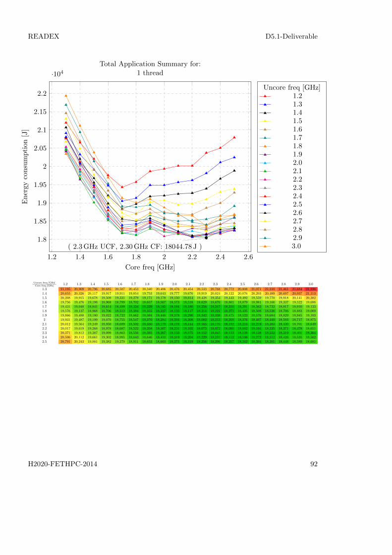
READEX D5.1-Deliverable
1.2 1.4 1.6 1.8 2 2.2 2.4 2.6
1.8
1.85
1.9
1.95
2
2.05
2.1
2.15
2.2
·104
( 2.3GHz UCF, 2.30GHz CF: 18044.78 J )
Core freq [GHz]
Energyconsumption
[J]
Total Application Summary for:1 thread
Uncore freq [GHz]1.21.31.41.51.61.71.81.92.02.12.22.32.42.52.62.72.82.93.0
Uncore freq [GHz]Core freq [GHz] 1.2 1.3 1.4 1.5 1.6 1.7 1.8 1.9 2.0 2.1 2.2 2.3 2.4 2.5 2.6 2.7 2.8 2.9 3.0
1.3 21,195 20,909 20,796 20,685 20,507 20,453 20,340 20,406 20,476 20,454 20,533 20,768 20,772 20,808 21,071 21,310 21,461 21,684 21,9361.4 20,655 20,326 20,117 19,917 19,911 19,854 19,753 19,643 19,777 19,676 19,919 20,024 20,122 20,076 20,203 20,489 20,697 20,937 21,1131.5 20,208 19,915 19,678 19,509 19,331 19,279 19,171 19,178 19,150 19,014 19,428 19,354 19,443 19,492 19,559 19,770 19,918 20,141 20,3821.6 19,756 19,476 19,198 18,968 18,799 18,702 18,657 18,567 18,573 18,518 18,629 18,676 18,801 18,879 18,981 19,160 19,337 19,522 19,6981.7 19,431 19,048 18,841 18,614 18,499 18,334 18,229 18,165 18,184 18,180 18,256 18,247 18,310 18,391 18,563 18,733 18,817 18,910 19,1331.8 19,576 19,137 18,968 18,706 18,512 18,384 18,355 18,227 18,133 18,117 18,214 18,221 18,271 18,425 18,508 18,526 18,706 18,883 19,0091.9 19,866 19,488 19,180 19,022 18,722 18,662 18,504 18,446 18,378 18,290 18,342 18,338 18,475 18,523 18,576 18,684 18,829 18,945 19,1032 19,931 19,487 19,199 19,070 18,755 18,547 18,370 18,284 18,204 18,208 18,082 18,213 18,268 18,376 18,407 18,440 18,593 18,717 18,8752.1 20,012 19,564 19,249 18,950 18,699 18,502 18,350 18,179 18,178 18,144 18,165 18,176 18,182 18,215 18,219 18,383 18,430 18,701 18,6492.2 20,017 19,619 19,268 18,978 18,687 18,522 18,358 18,307 18,231 18,102 18,073 18,072 18,090 18,062 18,104 18,335 18,371 18,478 18,6512.3 20,371 19,812 19,387 19,099 18,862 18,556 18,395 18,267 18,133 18,075 18,152 18,045 18,133 18,128 18,138 18,232 18,319 18,401 18,3642.4 20,506 20,112 19,661 19,302 18,995 18,643 18,646 18,410 18,319 18,204 18,229 18,216 18,152 18,186 18,272 18,312 18,426 18,535 18,5622.5 20,791 20,243 19,881 19,382 19,279 18,911 18,653 18,603 18,375 18,319 18,256 18,299 18,257 18,242 18,304 18,381 18,448 18,589 18,681
H2020-FETHPC-2014 92

READEX D5.1-Deliverable
1.2 1.4 1.6 1.8 2 2.2 2.4 2.6
80
90
100
110
120
130
140
150
( 3.0GHz UCF, 2.50GHz CF: 78.90 s )
Core freq [GHz]
Runtimeof
function[s]
Total Application Summary for:1 thread
Uncore freq [GHz]1.21.31.41.51.61.71.81.92.02.12.22.32.42.52.62.72.82.93.0
Uncore freq [GHz]Core freq [GHz] 1.2 1.3 1.4 1.5 1.6 1.7 1.8 1.9 2.0 2.1 2.2 2.3 2.4 2.5 2.6 2.7 2.8 2.9 3.0
1.3 148.6 145.6 143.7 141.8 139.4 137.9 136.1 135.1 134.4 132.9 132 131.9 130.4 129.2 129 128.8 128 127.4 126.81.4 141.8 138.4 136.1 133.6 132.5 130.9 129.3 127.4 127 125.1 125.4 124.6 123.8 122 121.3 121.4 120.9 120.6 119.81.5 135.5 132.6 130.1 128 125.9 124.6 122.8 121.8 120.6 118.4 119.8 117.9 117.2 116.1 114.9 114.9 114.2 113.6 113.51.6 130.3 127.5 124.9 122.5 120.5 118.9 117.6 116 115 113.6 113.2 112.1 111.6 110.8 110 109.6 109.2 108.7 108.31.7 125.4 122.1 119.9 117.7 116 114 112.5 111.1 110.2 109.2 108.6 107.4 106.5 105.8 105.5 105.1 104.2 103.3 103.21.8 121.3 117.8 116 113.5 111.4 109.9 108.9 107.2 105.9 104.7 104.2 103.2 102.3 102 101.4 100.3 99.9 99.5 98.81.9 117 114 111.5 109.8 107.4 106.2 104.4 103.3 102.2 100.9 100.2 99.2 98.8 98 97.2 96.8 96.2 95.7 95.32 114.2 110.9 108.5 107.1 104.6 102.7 100.8 99.8 98.4 97.7 96.1 95.8 95.2 94.7 93.9 92.9 92.7 92.2 91.82.1 111.2 108 105.6 103.3 101.4 99.5 98 96.5 95.6 94.6 93.9 93 92.1 91.3 90.4 90.3 89.5 89.6 88.22.2 108 105.1 102.6 100.4 98.3 96.7 95.2 94.1 93.1 91.7 90.8 89.9 89.1 88.1 87.4 87.6 86.8 86.1 862.3 106.5 103 100.2 98.1 96.2 94 92.6 91.3 90 88.9 88.6 87.2 86.9 86 85.2 84.8 84.1 83.6 82.52.4 104 101.2 98.2 96 93.9 91.5 91 89.1 88 86.8 86.2 85.3 84.2 83.6 83.2 82.4 82 81.6 80.92.5 102 98.6 96.2 93.4 92.3 90 88.1 87.2 85.6 84.5 83.6 83.1 82.2 81.4 80.9 80.2 79.7 79.5 78.9
H2020-FETHPC-2014 93

READEX D5.1-Deliverable
Intra-Phase Dynamism EvaluationBlade summary, Energy consumption [J]
Region % of 1 phaseBest static
configurationValue
Best dynamicconfiguration
ValueDynamicsavings
setUp 30.562.3GHz UCF,2.3GHz CF
5383.30 J2.9GHz UCF,1.7GHz CF
4773.10 J610.20 J(11.34%)
advance 69.442.3GHz UCF,2.3GHz CF
12233.56 J1.8GHz UCF,2.5GHz CF
12090.29 J143.28 J(1.17%)
Total value for statictuning for significant re-gions
5383.30 + 12233.56 = 17616.86 J
Total savings for dy-namic tuning for signifi-cant regions
610.20 + 143.28 = 753.48 J of 17616.86 J (4.28%)
Dynamic savings for ap-plication runtime
753.48 J of 18044.78 J (4.18%)
Job info - hdeem, Runtime of function [s]
Region % of 1 phase Def set. Def val. Optim set. Optim val. Savings
setUp 31.083.0GHz UCF,2.5GHz CF
23.93 s3.0GHz UCF,2.5GHz CF
23.93 s0.00 s(0.00%)
advance 68.923.0GHz UCF,2.5GHz CF
53.07 s3.0GHz UCF,2.5GHz CF
53.07 s0.00 s(0.00%)
Total value for statictuning for significant re-gions
23.93 + 53.07 = 77.00 s
Total savings for dy-namic tuning for signifi-cant regions
0.00 + 0.00 = 0.00 s of 77.00 s (0.00%)
Dynamic savings for ap-plication runtime
0.00 s of 78.90 s (0.00%)
H2020-FETHPC-2014 94

READEX D5.1-Deliverable
7 Results – Inter-Phase Dynamism
The previous sections provided energy and time measurements focusing on the possible intra-phase dynamism, i.e., dynamism between different significant regions. In this section wewould thus like to focus on the inter-phase dynamism, where the same region exhibits differentbehaviour in different phases (iterations, time-steps, etc.). Not all applications studied abovedemonstrate such behaviour. For example PCG iterations used in Espreso or AMG2013usually behave similarly regardless on the iteration number. This may change with thetransition, e.g., to (restarted) GMRES, which iteratively builds a Hessenberg system to besolved. In the rest of this section we restrict our attention to a subset of applications studiedin Section 6.
7.1 MCB
From the results presented in Section 6.9.2 one can deduce that the nature of the individualsignificant regions, i.e., the set-up and photon advancing, is rather different. While advancingthe photons seems to be more or less compute bound (at least for our settings on a singleTaurus node), the set-up phase prefers a higher uncore frequency and lower core frequency.However, this is not entirely true for the first couple of time-steps. From the tables inSection 7.1.1, we can see that in the first time-step the set-up phase takes over 90 % of boththe energy consumption and the runtime. This ratio drops down in the subsequent time-steps to less than 40 %. The optimal core and uncore frequencies thus differ and such tuningleads to further dynamic savings with respect to the best static scenario. The inter-phasedynamism with more MPI processes is presented in Section 7.1.2.
7.1.1 MPI_PROCS=1, PX=PY=1, OMP_THREADS=24
advancePhotonList - average program start
Phase ID 1 2 3 4 5
Default Energy consumption(Samples) [J]
57.69 83.48 92.95 97.67 100.72
% per 1 phase 8.46 62.62 60.90 60.83 61.39
Per phase optimal settings
1.2 GHzUCF,
2.3 GHzCF
1.3 GHzUCF,
2.5 GHzCF
1.5 GHzUCF,
2.3 GHzCF
1.5 GHzUCF,
2.3 GHzCF
1.5 GHzUCF,
2.3 GHzCF
Dynamic savings [J] 2.92 2.71 2.14 2.07 2.08Dynamic savings [%] 5.05 3.25 2.31 2.12 2.07
H2020-FETHPC-2014 95

READEX D5.1-Deliverable
Phase ID 6 7 8 9 10
Default Energy consumption(Samples) [J]
102.69 104.23 105.37 106.33 107.29
% per 1 phase 61.83 62.29 62.60 62.89 63.10
Per phase optimal settings
1.5 GHzUCF,
2.3 GHzCF
1.5 GHzUCF,
2.3 GHzCF
1.5 GHzUCF,
2.3 GHzCF
1.5 GHzUCF,
2.3 GHzCF
1.5 GHzUCF,
2.3 GHzCF
Dynamic savings [J] 2.09 1.82 1.96 1.97 1.98Dynamic savings [%] 2.03 1.75 1.86 1.85 1.85
setUp + get source photons - average program start
Phase ID 1 2 3 4 5
Default Energy consumption(Samples) [J]
624.35 49.83 59.68 62.89 63.35
% per 1 phase 91.54 37.38 39.10 39.17 38.61
Per phase optimal settings
2.0 GHzUCF,
2.5 GHzCF
2.1 GHzUCF,
1.7 GHzCF
2.2 GHzUCF,
1.7 GHzCF
2.1 GHzUCF,
1.7 GHzCF
2.5 GHzUCF,
1.7 GHzCF
Dynamic savings [J] 14.63 1.37 3.76 4.78 5.51Dynamic savings [%] 2.34 2.74 6.30 7.61 8.70
Phase ID 6 7 8 9 10
Default Energy consumption(Samples) [J]
63.40 63.10 62.96 62.75 62.74
% per 1 phase 38.17 37.71 37.40 37.11 36.90
Per phase optimal settings
2.5 GHzUCF,
1.7 GHzCF
2.5 GHzUCF,
1.7 GHzCF
2.5 GHzUCF,
1.7 GHzCF
2.5 GHzUCF,
1.7 GHzCF
2.5 GHzUCF,
1.7 GHzCF
Dynamic savings [J] 6.22 6.65 6.86 7.09 7.34Dynamic savings [%] 9.81 10.54 10.89 11.30 11.70
7.1.2 MPI_PROCS=24, PX=4, PY=6, OMP_THREADS=1
advancePhotonList - average program start
Phase ID 1 2 3 4 5
Default Energy consumption[J]
741.88 1084.73 1208.26 1265.27 1296.45
% per 1 phase 80.87 76.40 70.14 68.18 68.25
Per phase optimal settings
1.5 GHzUCF,
2.5 GHzCF
1.8 GHzUCF,
2.5 GHzCF
1.8 GHzUCF,
2.5 GHzCF
1.8 GHzUCF,
2.5 GHzCF
1.8 GHzUCF,
2.5 GHzCF
Dynamic savings [J] 32.76 24.38 16.15 14.12 11.17Dynamic savings [%] 4.42 2.25 1.34 1.12 0.86
H2020-FETHPC-2014 96

READEX D5.1-Deliverable
Phase ID 6 7 8 9 10
Default Energy consumption[J]
1313.10 1323.57 1330.75 1333.10 1336.46
% per 1 phase 68.13 67.86 67.65 67.52 67.42
Per phase optimal settings
1.9 GHzUCF,
2.3 GHzCF
1.9 GHzUCF,
2.3 GHzCF
1.9 GHzUCF,
2.3 GHzCF
1.9 GHzUCF,
2.3 GHzCF
1.9 GHzUCF,
2.3 GHzCF
Dynamic savings [J] 11.04 10.50 10.44 10.61 10.83Dynamic savings [%] 0.84 0.79 0.78 0.80 0.81
setUp + get source photons - average program start
Phase ID 1 2 3 4 5
Default Energy consumption[J]
175.49 335.05 514.33 590.44 603.19
% per 1 phase 19.13 23.60 29.86 31.82 31.75
Per phase optimal settings
1.7 GHzUCF,
2.5 GHzCF
2.6 GHzUCF,
1.7 GHzCF
2.9 GHzUCF,
1.7 GHzCF
2.6 GHzUCF,
1.6 GHzCF
2.8 GHzUCF,
1.7 GHzCF
Dynamic savings [J] 4.71 28.49 78.50 92.89 84.14Dynamic savings [%] 2.69 8.50 15.26 15.73 13.95
Phase ID 6 7 8 9 10
Default Energy consumption[J]
614.35 626.84 636.44 641.34 645.83
% per 1 phase 31.87 32.14 32.35 32.48 32.58
Per phase optimal settings
2.5 GHzUCF,
1.7 GHzCF
2.5 GHzUCF,
1.7 GHzCF
2.5 GHzUCF,
1.7 GHzCF
2.5 GHzUCF,
1.7 GHzCF
2.5 GHzUCF,
1.7 GHzCF
Dynamic savings [J] 74.42 75.38 76.27 76.31 76.38Dynamic savings [%] 12.11 12.02 11.98 11.90 11.83
H2020-FETHPC-2014 97

READEX D5.1-Deliverable
7.2 MiniMD
The phase region in miniMD, which is the for-loop in function Integrate::run(), wasalso analysed for inter-phase dynamism by the MERIC tool with the results summarised inRADAR. Since the regions build() and compute() were observed to be significant, the inter-phase dynamism analysis results are summarized in Section 7.2.1. Though the experimentwas performed for 100 phases (iterations of the for-loop), the results are presented onlypresented for the first 20 phases for brevity. We observe that these results are similar for theremaining phases in the experiment results.
From the results in Section 7.2.1 we observe that once every 20 phases, the build() regioncontributes around 75% of the energy consumption and the execution time, while it is neg-ligible during the other phases. Consequently, once every 20 phases the compute() regioncontributes only around 25% of the energy consumption and the execution time, while it con-tributes around 100% during the other phases. This periodicity (once every 20 phases) in thedynamism is associated to one of the input parameters to miniMD – reneighbouring atomsonce every N steps/iterations. In the inputs for the experiments reported here, this reneigh-bouring of atoms is performed once every 20 steps/iterations. This results in the inter-phasedynamism of energy consumption and execution time that is observed in miniMD.
However, we also observe that the optimal configurations for the processor core and uncorefrequencies in response for the observed dynamism are the same as the best configurationsidentified from static tuning. As a result, even though we observe inter-phase dynamism inminiMD, it does not result in any significant dynamic savings for energy consumption andexecution time.
7.2.1 Experiment 1
Build - average program start
Phase ID 1 2 ... 19 20
Default Energy con-sumption [J]
- - - - 26.89
% per 1 phase - - - - 74.83
Per phase optimalsettings
- - - -
1 thread,1.2 GHzUCF,
2.5 GHzCF
Dynamic savings [J] - - - - 0.00Dynamic savings [%] - - - - 0.00
Total sum of values from dynamic savings from all phases
Energy consumption [J] (Samples)134.43 J → 134.43 J (savings 0.00%)Runtime of function [s]1.30 s → 1.30 s (savings 0.00%)
H2020-FETHPC-2014 98

READEX D5.1-Deliverable
Compute - average program start
Phase ID 1 2 3 4 5
Default Energy con-sumption [J]
7.56 7.57 7.56 7.58 7.64
% per 1 phase 100.00 100.00 100.00 100.00 100.00
Per phase optimalsettings
1 thread,1.2 GHzUCF,
2.5 GHzCF
1 thread,1.2 GHzUCF,
2.5 GHzCF
1 thread,1.2 GHzUCF,
2.5 GHzCF
1 thread,1.2 GHzUCF,
2.5 GHzCF
1 thread,1.2 GHzUCF,
2.5 GHzCF
Dynamic savings [J] 0.00 0.00 0.00 0.00 0.00Dynamic savings [%] 0.00 0.00 0.00 0.00 0.00
Phase ID 6 7 8 9 10
Default Energy con-sumption [J]
7.57 7.56 7.65 7.94 7.97
% per 1 phase 100.00 100.00 100.00 100.00 100.00
Per phase optimalsettings
1 thread,1.2 GHzUCF,
2.5 GHzCF
1 thread,1.2 GHzUCF,
2.5 GHzCF
1 thread,1.2 GHzUCF,
2.5 GHzCF
1 thread,1.2 GHzUCF,
2.5 GHzCF
1 thread,1.2 GHzUCF,
2.5 GHzCF
Dynamic savings [J] 0.00 0.00 0.00 0.00 0.00Dynamic savings [%] 0.00 0.00 0.00 0.00 0.00
Phase ID 11 12 13 14 15
Default Energy con-sumption [J]
8.19 8.26 8.29 8.33 8.37
% per 1 phase 100.00 100.00 100.00 100.00 100.00
Per phase optimalsettings
1 thread,1.2 GHzUCF,
2.5 GHzCF
1 thread,1.2 GHzUCF,
2.5 GHzCF
1 thread,1.2 GHzUCF,
2.5 GHzCF
1 thread,1.2 GHzUCF,
2.5 GHzCF
1 thread,1.2 GHzUCF,
2.5 GHzCF
Dynamic savings [J] 0.00 0.00 0.00 0.00 0.00Dynamic savings [%] 0.00 0.00 0.00 0.00 0.00
Phase ID 16 17 18 19 20
Default Energy con-sumption [J]
8.41 8.44 8.46 8.50 8.68
% per 1 phase 100.00 100.00 100.00 100.00 24.17
Per phase optimalsettings
1 thread,1.2 GHzUCF,
2.5 GHzCF
1 thread,1.2 GHzUCF,
2.5 GHzCF
1 thread,1.2 GHzUCF,
2.5 GHzCF
1 thread,1.2 GHzUCF,
2.5 GHzCF
1 thread,1.2 GHzUCF,
2.5 GHzCF
Dynamic savings [J] 0.00 0.00 0.00 0.00 0.00Dynamic savings [%] 0.00 0.00 0.00 0.00 0.00
Total sum of values from dynamic savings from all phases
Energy consumption [J] (Samples)854.43 J → 853.76 J (savings 0.08%)Runtime of function [s]7.90 s → 7.90 s (savings 0.00%)
H2020-FETHPC-2014 99

READEX D5.1-Deliverable
7.3 Indeed
The forming simulation code Indeed has also been investigated with respect to its inter-phasedynamism. Due to the nature of Indeed as a finite element program with an implicit timeintegration method, this investigation has turned out to provide interesting insight into thequestion of inter-phase dynamism from a rather abstract point of view.
Specifically, the first attempts to analyze Indeed’s inter-phase dynamism were based on theobservation that the code simulates a process that runs over a certain period of time by cuttingthe process time into a number of small time increments and by looking at the process onetime step after the other. Therefore it seemed to be quite natural to assume that each phasecorresponds to one such time step. The analysis of the run time and energy requirementsthen produced, for a typical input data sets, results such as those indicated in Figure 6.
Figure 6: Inter-phase dynamism of Indeed: Run time vs. number of time step.
However, the above mentioned structure of Indeed implies that, within each iteration of thetime stepping loop, further loops are nested (see Figure 7), and the number of iterations thatthese inner loops perform vary strongly from time step to time step, depending on what isphysically happening in the real process during each time step. On the other hand, whathappens within each iteration of the innermost loop shows much less variation from oneinstance to the next.
This behavior is indicated in Figure 8. In this figure we show the run time that each inneriteration takes. The graph shows one remarkable very high spike whose origin is not yetclear and is presently under investigation. Apart from that, the variation is much smallerthan in Figure 6, and seems to indicate a clear upward trend upon which some mild noise issuperimposed.
H2020-FETHPC-2014 100

READEX D5.1-Deliverable
Start of computation
New tools?
Initial movements
Assembly ofequation system
Solution ofequation system
Recovery computation
Equilibrium reached?
Change ofcontact?
End ofprocess?
yes
no
yes
no
yes
End of computation
no
yes
no
Equ
ilib
rium
loop
Co
nta
ct lo
op
Tim
e lo
op
Figure 7: Structure of Indeed code.
This upward trend can easily be traced back to Indeed’s adaptive mesh refinement feature.In fact, if one divides the run time per iteration by the number of currently active finiteelements, one obtains the results indicated in Figure 9. Here we again see the single strongspike apart from which the amount of time per element remains almost constant over thecourse of the inner iterations, especially during the second half of the programs runtime.
The conclusions that need to be drawn from this significant difference in the results dependingon the precise definition of the concept of the phase are currently under discussion.
H2020-FETHPC-2014 101

READEX D5.1-Deliverable
Figure 8: Inter-phase dynamism of Indeed: Normalized runtime vs. number of inner iterationstep.
Figure 9: Inter-phase dynamism of Indeed: Normalized runtime divided by number of ele-ments vs. number of inner iteration step.
H2020-FETHPC-2014 102

READEX D5.1-Deliverable
8 Summary
In this repot we present evaluation of (1) key sparse BLAS routines from the Intel MKL library(2) OpenMP parallel I/O (3) a set of proxy-apps (AMG2013, Kripke, LULESH and MCB)and (4) selected full fledge applications (ESPRESO, MiniMD, Indeed) and the potentialenergy savings due to dynamic tuning of the selected hardware parameters.
We have implemented a parallel I/O benchmark, that reads sparse matrices stored in IJV/-COO format from file. The evaluation of this benchmark shows, that parallel I/O within asingle compute node does not scale to more that 4 OpenMP threads. From the frequencypoint of view, to maximize the energy efficiency of the I/O the CPU core frequency has tohigh, 2.5 GHz, while the uncore frequency should be 2.1 GHz. When compared to defaultsettings (24 threads, 2.5 GHz core frequency and 3.0 Ghz uncore frequency) the savings areas high as 56%. This significant potential for dynamic tuning should be taken into accountin every application that contains heavy I/O workload.
Our experiments with variation of the computation intensity show that with increasing CIthe effect of the uncore frequency becomes less important and optimal setting is decreasesfrom 2.5 GHz to 1.2 GHz. On the other hand, the optimal core frequency should be high(2.5 GHz) for applications with high CI and it is decreasing with lower CI. It can be alsoobserved that core frequency tuning is the most efficient for kernels with high CI. Finally wecan observe, that the highest static energy savings, 12.5%, have been achieved by computebound codes while memory bounded kernel achieved only 5.6%.
We have also presented the energy consumption evaluation of selected sparse BLAS routinesfrom the Intel MKL library. The measured characteristics illustrate a different energy con-sumption for different sparse BLAS routines and different sparse matrices. We also showthat some of the routines suffer significantly from the NUMA effect and should be executedon a single CPU socket. The significant savings up to 66% can be achieved in case whenNUMA effect is active. The result of the same experiment but in this case running on oneCPU socket only (no NUMA effect) shows reduced savings to 2.7% – 12.3%.
In the case of the ProxyApps suite we have selected applications that support hybrid paral-lelization (MPI+OpenMP). By changing the core and uncore frequencies and the number ofOpenMP threads we were able to achieve the static/dynamic savings summarized in Table 43.Although the main purpose of these applications is to provide simple benchmarks and thecodes are usually rather short, they are able to deliver significant static savings (up to over25 %) over all instrumented regions. On the other hand, since none of the programs containsany extensive I/O regions and they were tested on a single node of the Taurus supercom-puter, the further dynamic savings (maximum reached by Kripke is 7 %, otherwise mostlybelow 3 %) are quite unsatisfactory. The situation may change when testing on a reasonablenumber of nodes, where the applications may become communication bound. However, theexhaustive search algorithm (sweeping over all combinations of tuning parameters) wouldhave to be replaced by a more efficient minimization algorithm. A more detailed outputcausing some I/O overhead would lead to higher dynamism as well.
H2020-FETHPC-2014 103

READEX D5.1-Deliverable
Application Static savings [%] Dynam. savings [%] Total Savings [%]
Parallel OpenMP I/O 56 — 56
Dense BLAS - DGEMV - without NUMA 5.6 — 5.6Dense BLAS - DGEMM - without NUMA 10.4 — 10.4Compute only kernel 12.8 — 12.8
Sparse BLAS Routines - without NUMA 3.1-12.3 — 3.1 – 12.3Sparse BLAS Routines - with NUMA 4.2-66.2 — 4.2 – 66.2
ProxyApps 1 - AMG2013, configuration 1 6.53 2.89 9.23ProxyApps 1 - AMG2013, configuration 2 25.66 2.80 27.74
ProxyApps 2 - Kripke, configuration 1 28.16 1.56 29.28ProxyApps 2 - Kripke, configuration 2 12.63 7.04 18.78
ProxyApps 3 - LULESH, configuration 1 28.58 0.55 28.88ProxyApps 3 - LULESH, configuration 2 25.81 1.23 26.72
ProxyApps 4 - MCB, configuration 1 4.13 1.42 5.51ProxyApps 4 - MCB, configuration 2 3.40 4.18 7.44
ESPRESO - configuration 0 5.6 8.7 14.3ESPRESO - configuration 1 12.3 9.1 21.4ESPRESO - configuration 2 7.8 4.7 12.5ESPRESO - configuration 3 7.8 5.4 13.1
OpenFOAM (Motorbike benchmark) 15.9 1.8 17.7
Indeed 17.6 to be evaluated 17.6
MiniMD 21.92 0.00 21.92
Table 43: Overview of the static and dynamic energy savings achieved by the applicationsselected for this report.
The ESPRESO library contains both FEM preprocessing tools and sparse iterative solversbased on FETI method. We have annotated more than 20 regions, which includes all typesof operations including I/O, communication, sparse BLAS and dense BLAS. The testsalso focus on the variation of the arithmetical intensity in form of sparse and dense datastructures. Two key kernels of the FETI iterative solver (i) the F operator and (ii) thepreconditioner can be represented by both dense and sparse matrices providing differenttype of workload. The results show that static savings are 5.6–12.3% and dynamic savings4.7–9.1%. The highest total savings for ESPRESO are 21.4% as a combination of 12.3%static savings and 9.1% dynamic savings.
H2020-FETHPC-2014 104

READEX D5.1-Deliverable
The investigation of Indeed has shown a relatively high static tuning potential. Moreover,the tools developed within the READEX project have also been successfully used to detect asignificant amount of intra-phase and inter-phase dynamism in Indeed. Therefore we expectto find a substantial dynamic tuning potential in the code. At the moment, the READEXteam is actively discussing possible ways that can be used to realize this potential.
In case of the OpenFOAM application a simpleFoam solver was used on the motorBikebenchmark, that is part of the OpenFOAM repository. The experiment were done on onesingle node with 24 MPI processes. The simpleFoam was set to use GAMG solver andPBiCG solvers. The results were written twice during the runtime into binary uncompressedformat. Since the most time consuming regions, the GAMG and PBiCG solvers, performsimilar sparse BLAS operations the optimal configuration for these regions is either identicalor very similar. Due to this reason the most of the saving can be achieved by static tuning,15.9%, while only the remaining regions provide some potential for dynamic savings. Sincethe runtime of remaining regions is only 14.5% the overall dynamic savings are only 1.7%.
H2020-FETHPC-2014 105

READEX D5.1-Deliverable
References
[1] The university of florida sparse matrix collection.
[2] David H. Bailey. The NAS Parallel Benchmarks. In David Padua, editor, Encyclopediaof Parallel Computing, pages 1254–1259. Springer, New York, 2011.
[3] Intel corp. Intel math kernel library (mkl).
[4] Timothy A. Davis and Yifan Hu. The university of florida sparse matrix collection. ACMTrans. Math. Softw., 38(1):1:1–1:25, December 2011.
[5] Zdenek Dostal, David Horak, and Radek Kucera. Total FETI-an easier implementablevariant of the FETI method for numerical solution of elliptic PDE. Communications inNumerical Methods in Engineering, 22(12):1155–1162, jun 2006.
[6] C. Farhat, J. Mandel, and F-X. Roux. Optimal convergence properties of the FETI do-main decomposition method. Computer Methods in Applied Mechanics and Engineering,115:365–385, 1994.
[7] Pierre Gosselet and Christian Rey. Non-overlapping domain decomposition methods instructural mechanics. Archives of Computational Methods in Engineering, 13(4):515–572,2006.
[8] Per Gunnar Kjeldsberg, Michael Gerndt, Mohammed Sourouri, and Anamika Chowd-hury. D2.1 analysis of tuning potential and scenario identification. Technical report,NTNU, TUM, 2016.
[9] A. Klawonn and O. Rheinbach. Highly scalable parallel domain decomposition methodswith an application to biomechanics. ZAMM, 90(1):5–32, jan 2010.
[10] Michael Lysaght, Kashif Iqbal, Joseph Schuchart, Andreas Gocht, Michael Gerndt,Anamika Chowdhury, Madhura Kumaraswamy, Per Gunnar Kjeldsberg, Magnus Jahre,Mohammed Sourouri, David Horak, Lubomir Riha, Radim Sojka, Jakub Kruzik, KaiDiethelm, and Othman Bouizi. D4.1: Concepts for the READEX tool suite. Technicalreport, ICHEC, TUD, TUM, NTNU, IT4I, Intel, gns, 2016.
[11] Thomas Nagy. The waf book.
[12] L. Riha, T. Brzobohaty, A. Markopoulos, M. Jarosova, T. Kozubek, D. Horak, andV. Hapla. Implementation of the efficient communication layer for the highly paralleltotal feti and hybrid total feti solvers. Parallel Computing, 2016.
[13] L. Riha, T. Brzobohaty, A. Markopoulos, T. Kozubek, O. Meca, O. Schenk, and W. Van-roose. Efficient implementation of total feti solver for graphic processing units using schurcomplement. Lecture Notes in Computer Science, 9611:85–100, 2016.
H2020-FETHPC-2014 106

READEX D5.1-Deliverable
[14] Lubomir Riha, Tomas Brzobohaty, Alexandros Markopoulos, Ondrej Meca, and TomasKozubek. Massively parallel hybrid total feti (htfeti) solver. In Proceedings of the Plat-form for Advanced Scientific Computing Conference, PASC ’16, New York, NY, USA,2016. ACM.
[15] P. Saviankou, M. Knobloch, A. Visser, and B. Mohr. Cube v4: From performance reportexplorer to performance analysis tool. Procedia Computer Science, 51:1343–1352, 2015.
[16] Samuel Williams, Andrew Waterman, and David Patterson. Roofline: An insightfulvisual performance model for multicore architectures. Commun. ACM, 52(4):65–76,April 2009.
H2020-FETHPC-2014 107
Copyright © 2022 FDOKUMEN