1

Crossing the hurdle:

the determinants of individual scientific performance

A. Baccini, L. Barabesi, M. Cioni, C. Pisani

Department of Economics and Statistics - University of Siena

An original cross-sectional dataset referring to a medium-sized Italian university is

implemented in order to analyze the determinants of scientific research production at

individual level. The dataset includes 942 permanent researchers of various scientific sectors

for a three-year time-span (2008-2010). Three different indicators - based on the number of

publications and/or citations - are considered as response variables. The corresponding

distributions are highly skewed and display an excess of zero-valued observations. In this

setting, the goodness-of-fit of several Poisson mixture regression models are explored by

assuming an extensive set of explanatory variables. As to the personal observable

characteristics of the researchers, the results emphasize the age effect and the gender

productivity gap - as previously documented by existing studies. Analogously, the analysis

confirm that productivity is strongly affected by the publication and citation practices adopted

in different scientific disciplines. The empirical evidence on the connection between teaching

and research activities suggests that no univocal substitution or complementarity thesis can be

claimed: a major teaching load does not affect the odds to be a non-active researcher and does

not significantly reduce the number of publications for active researchers. In addition, new

evidence emerges on the effect of researchers administrative tasks - which seem to be

negatively related with researcher’s productivity - and on the composition of departments.

Researchers’ productivity is apparently enhanced by operating in department filled with more

administrative and technical staff, and it is not significantly affected by the composition of the

department in terms of senior/junior researchers.

Keywords: Academic research productivity; Scientist productivity; Poisson mixture

distributions; Hurdle models; Zero-Inflated models; Sichel model; Waring model; Gender

productivity gap; Age effect.

Acknowledgments

We would like to thank Sonia Boldrini from the Evaluation Committee of the University of

Siena for her valuable assistance in data harvesting and database building. In addition, we

would like to express our gratitude to two anonymous referees for their comments which have

led to a truly improved version of the paper.

2

1. Introduction

During the past thirty years, there has been a growing interest in the role of academic

research activity and in its contribution to economic growth and social development. One of

the least studied and most puzzling feature of this debate is the question of individual

scientific productivity. Researcher’s activity is basically a multi-output activity, producing

outcomes as research, teaching and others products (newspapers articles, medical protocols,

etc.) with a relevant impact on society. This idea is so widespread that in the national research

assessment exercises - as an example in the British Research Excellence Framework 2014 -

information is collected on all these different activities in order to evaluate not only the

quality of research produced by universities, but even their multifaceted societal impact. At

the best of our knowledge, no study addresses the question of the determinants of researchers’

overall production, even if many papers solely focus on one dimension of their multi-output

activities.

The idea that scientific publications represent the essence of the research activity is

widely accepted (Wooton 2013). In this respect, two different streams of literature have been

developed. The first stream is focused on describing the laws underlying the frequency

distribution of researcher’s publications - following the tradition started by Lotka (1926). The

second stream deals with the determinants of individual productivity. These works aim to

define the factors affecting research productivity by using tools as correlation analysis or

regression modelling.

A common feature of this literature consists in considering the number of publications

of a researcher as a proxy for quantifying her/his productivity. The main drawback of this

indicator stems on the fact that each publication counts for one: a short paper addressing a

limited issue counts as a seminal paper. So, the holy grail of scientometric research is the

construction of indicators addressing - at the same time - the issue of productivity and quality

of scientific work also at a researcher level (van Leeuwen et al. 2003). To this aim, the most-

used strategy in empirical research consists in the substitution of the notion of “research

quality” with the notion of “scientific impact” (as defined in Martin and Irvine 1983) which

can be more easily handled using citation data. A first possible approach may be based on

counting a subset of the publications of a researcher, such as the highly-cited papers or those

published in “top” journals - so defined in reference to the impact factor or to other similar

indicators. A different approach aims to obtain composite indicators of productivity and

3

impact of a researcher considering her/his published articles as well as the citations they

received. Among them, the most widespread indicator is the h-index (Hirsch 2005).

The aim of this article is to contribute to the debate on the determinants of individual

scientific production by stressing the attention on two original issues. The first issue deals

with the adoption of regression models able to properly handle the specific nature of the data.

Three standard different indicators, based on the number of publications and/or their citations,

are considered as response variables. They are integer-valued and display highly-skewed

distributions which are in addition zero-inflated, i.e. an excess of zeroes is present. Many

existing papers dealing with modelling the determinants of scientific production do not

specifically account the skewed and zero-inflated nature of the data (Carayol and Matt 2004,

2006; Lissoni et al. 2011; Rivera-Huerta et al. 2011). In order to address the skew distribution

of research output - and eventually acknowledging the presence of zero excess - quantile

regression may be adopted (Kelchtermans and Veugelers 2011). In the present paper, an

alternative approach, based on appropriate GLM models expressly conceived for count data

with zero excesses, is proposed. Quite surprisingly some of these models, even if well-

established in other disciplines, have been neglected in the framework of the analysis of

production process of academic research. The second issue focuses on the joint use of an

extensive set of explanatory variables, which have been considered by adopting separate

analyses in the previous literature. Indeed, the proposed models consider as possible

determinants of the researcher’s individual academic productivity: (i) some personal

observable characteristics, such as gender and age; (ii) some individual career features, such

as academic position, seniority, typology of labour contract; (iii) the scientific field in which

the scholar works; (iv) her/his teaching and administrative tasks; (v) her/his departmental

working context. These ideas are carried out on a large original dataset referred to a set of

about one thousand scholars belonging to a medium-sized Italian university.

The remainder of the paper is subdivided into four sections. In Section 2, the main

literature addressing the issues of researcher’s production is surveyed. In Section 3, the data

and the methodologies adopted are illustrated. In Section 4, the main results of our empirical

analysis are presented and discussed. Finally, in Section 5 the conclusions are drawn.

4

2. Literature review

Two alternative approaches have been considered in the analysis of scientific

production: the first focuses on the laws underlying the frequency distribution of the number

of publications (or citations), while the second aims to identify the determinants of scientific

performance. The first approach dates back to the 1920s, particularly to the publication of

Lotka’s seminal article (1926). Lotka investigated the frequency distribution of scientific

productivity of chemists and physicists showing that “...the number (of authors) making n

contributions is about l/n2 of those making one; and the proportion of all contributors, that

make a single contribution, is about 60%...”. This kind of approach has survived until the

recent attempts to create theoretical models able to foresee the future pattern of the production

of a scholar given her/his past performance (e.g. Wang et al. 2013 and the bibliography cited

thereon).

Alternative explanations of the Lotka findings and - more generally - of the highly-

skewed nature of scientific production of scholars have been proposed. The simplest one -

highly criticized for example by Allison and Stewart (1974) and by David (1994) - is the so-

called “sacred-spark hypothesis”, i.e. the differences in productivity reflect unequal and

predetermined capabilities of researchers. In the late 1960s, a so called “Matthew-effect

hypothesis” was advanced by Merton (1968). Merton highlighted that well-known researchers

receive more recognition for their work than less known researchers. Subsequently, this

hypothesis was generalized by Cole and Cole (1973) to be valid not only for recognition, but

even for scientific productivity. In this form, this hypothesis was called “cumulative

advantage hypothesis”. The idea is that recognition received early in researchers’ career may

be reinforced over time as it would enable easier access to research resources - this issue

means that any advantage will be cumulative (Defazio et al. 2009). This kind of explanation

exclusively focuses on the social structure in which scholars are embedded and work.

A second approach addresses the academic research production aiming to identify the

determinants of scientific productivity. In these works the sacred-spark and the Mattew-effect

hypotheses are considered as residual or unexplained components of a roughly defined

production function addressing all the relevant explanatory variables. This explanatory

approach has been applied both to the individual level of analysis - where the survey unit is

the researcher - and to the aggregate level - where the survey unit is the research unit - e.g.

department, laboratory, university. A complete review of the elements that a broad and

5

growing applied literature considers as possible explanatory variables of individual and

aggregate scientific productivity is not the aim of our work. Nevertheless, it can be suggested

a possible twofold categorization, which separates individual determinants, referring to each

scholar’s characteristics, and collective determinants, relating to the features of the

organization in which she/he is working.

A first group of individual determinants properly refers to the personal characteristics of

a researcher, such as gender and age. Regarding the role of gender in scientific publication

performance, at least starting from Cole and Zuckerman (1984), the gender differences in

productivity among academic scientists is considered as a puzzle to be solved (Levin and

Stephan 1998; Xie and Shauman 2003; Fox 2005; Leahey 2006; Fox et al. 2011). Mairesse

and Pezzoni (2013) revisit the gender gap in scientific production, offering a critical review of

the empirical evidence throughout the analysis of the issues influencing women scientific

productivity (family engagements, marital status and policies in favour of women,

institutional specificities, discipline specificities, etc.). Abramo et al. (2009) document

differences in productivity between men and women, but highlight a progressive reduction of

the performance gap over time for Italian scientists at least in hard sciences and life sciences.

Similar conclusions are achieved by van Arensbergen et al. (2012) who suggest that - even if

men outperform women in terms of scientific production in the older generations - the

gendered differences are disappearing in the younger generations.

The so called age-effect is considered a well-consolidated issue in literature. Many

studies document a decrease of research production as age increases (Diamond 1984, 1986);

others find that publication activity tends to augment in the early career, reaches a peak, and

then decreases (Zuckerman and Merton 1972; Weiss and Lillard 1982; Levin and Stephan

1991); while others find a productivity curve with two peaks (Bayer and Dutton 1977). These

relationships have to be taken with caution, since it is difficult to distinguish between age

effect and cohort effect. Indeed, the latter can be associated - for example - with a progression

of knowledge or a different availability of resources, as discussed by Stephan (1996, 2012).

At the aggregate level of analysis, a study on the Italian National Research Council highlights

a negative relationship between age and research productivity indicators (Bonaccorsi and

Daraio 2003), while the results by Carayol and Matt (2004) suggest an “inversed-U shape”

relationship between laboratories productivity and age. In contrast, a lack of significant

relationship between age and publication rate within the faculties of the University of Vienna

is claimed by Wallner et al. (2003).

6

A second group of individual determinants refer to the career features. As to the effects

of seniority and career progress, the role of tenure and position are ambiguous. On one hand,

an improvement in the professional status of the researcher can positively affect research

performance, since - for example - she/he can have easier access to funding or attract talented

young students/scientists in her/his research team (the so-called “status effect”). On the other

hand, once a career progress has been obtained, the incentives to production can be reduced.

The relationship between seniority or career progress and research performance is nearly

universally addressed in this literature. Among others, Fabel et al. (2008) find a negative

effect of career age on publications for full professors, while Rivera-Huerta et al. (2011)

consider career years as a control variable in modelling individual research output.

The scientific field in which the scholar works is considered as a determinant of

productivity since it is well known that publishing activities and citation patterns vary among

scientific disciplines. These differences - as emphasized by Anania and Caruso (2013) - are

particularly relevant in many areas of Social Sciences and Humanities, where scientific

productivity and citation practices typically yield fewer citations per paper. Two strategies are

used for tackling this problem. The first strategy tends to limit the analysis on researchers

working in homogeneous scientific fields (see e.g. Lissoni et al. 2011; Pezzoni at al. 2012).

The second strategy aims to model the research performance of scientists from heterogeneous

areas including control variables for the researcher scientific discipline - defined according to

some available classification (see e.g. Carayol and Matt 2006; Rivera-Huerta et al. 2011).

The researcher’s teaching activities and administrative tasks are also considered

determinants of productivity. The main question addressed by literature is if the engagement

in these activities may crowd out research. According to some authors (Fox 1992; Taylor et

al. 2006), these activities conflict since the more productive researchers spend less time for

teaching and students in general. A substitutive relationship of this kind is also documented

by a paper on French professors in Economics (Kossi et al. 2013). Contrasting results are

conveyed by Fabel et. al (2008) showing that higher teaching loads in terms of class sizes do

not deteriorate research productivity of business economists in Germany and Switzerland, and

by Kelchtermans and Veugelers (2011) highlighting that alternative activities have very small

and mostly insignificant effects on research output for scientists employed at the KU Leuven.

However, as suggested by Stephan (1996), given the collaborative nature of science,

individual determinants solely represent a part of the drivers of scientific production. Thus,

determinants relating to the organization in which the researcher operates have to be

7

considered. Allison and Long (1990) highlight the role of prestigious departments in

encouraging individual scientific productivity. The composition of laboratories or

departments in terms of type of researchers (full professors, assistant professors, PhD

students, etc.) and their average age are also considered in the literature (Carayol and Matt

2006), as well as the quality of colleagues’ production (Mairesse and Turner 2006; Lissoni et

al. 2011;), and the fundraising ability (Carayol and Matt 2006). At the aggregate level of

analysis, some scholars concentrate on the organization size, showing a positive size effect on

laboratory productivity (Cainelli et al. 2006; Fabel et al. 2008); others find that small-sized

departments are more productive (Carayol and Matt 2004, 2006) while others focus on the

effects of the composition and average age of the research unit (Bonaccorsi and Daraio 2003).

On one side, senior researchers may enhance the productivity of the younger due to co-author

works or informal contacts. On the other side, the younger can act as incentives to stimulate

the research activities of the older (Carayol and Matt 2004, 2006).

3. Material and methods

3.1. Data

In order to address the issues raised in the previous section, our analysis is based on a

large original dataset implemented by using either internal administrative sources or external

sources. The data refer to the University of Siena. Established in 1240, it is one of the oldest

publicly-funded universities in Italy. It is a medium-sized university with about 17,000

students covering 8 scientific areas: Arts and Humanities, Economics, Engineering, Law,

Mathematical, Physical and Natural Sciences, Medicine and Surgery, Pharmacy, Political

Sciences. The dataset is composed by 942 individual records referred to permanent

researchers of the University of Siena. For each researcher, we collected information dealing

with personal characteristics, research activity, teaching activity, administrative tasks and

departmental affiliation. The data concerning personal characteristics and departmental

affiliation refer to December 31st 2010. The data regarding research and teaching activities, as

well as administrative tasks, refer to the three-year period 2008-2010. The choice of a three

year time-span is due to the costly nature of manual collection of disperse administrative data,

and to the growing difficulties of finding comparative and complete information in

administrative files when further years are considered. A three-year period is a time-span

8

sufficient to capture the normal activity of scholars. It permits to avoid yearly anomalies that

could have arisen in reference to researchers’ activities such as organizational breaks affecting

the number of students or of thesis supervised. A three-year period also permits to avoid

accidental conditions such as sabbatical or health leave, maternity, etc., which could have

arisen by examining a single year. Finally, it also permits to avoid accidental zeroes for the

response variables - arising by delays in data recording in the bibliographic archives

considered or by a long time-lapse from submission to publication in peer-reviewed journals.

3.1.1 Response variables

In order to quantify publication production, three different response variables are

considered:

i. number of publications in Anagrafe.UNISI, denoted by repository. The

Anagrafe.UNISI is the institutional research repository of the University of Siena. It is used

by researchers in order to record all their research outputs. It is therefore filled with a broad

range of outputs from scientific publications to teaching materials and informative articles -

such as newspapers and magazine articles. It is worthwhile to note that not all the research

outputs recorded in repository are peer-reviewed, and that the researchers are responsible for

registering and classifying their outputs. The response variable repository is constructed by

counting - for each scholar - the number of authored or co-authored scientific outputs,

recorded in the repository during the period 2008-2010 and classified as articles, books,

chapters in books and conference proceedings;

ii. number of publications in Scopus, the bibliographic database developed by Elsevier

(http://www.scopus.com), denoted by scopus. This response variable is the number of

authored or co-authored publications registered in the Scopus database in the period 2008-

2010. In order to get this information for each researcher, the last and first names and the

affiliation were queried in the Scopus Author search. If the author’s name was not unique, the

results were refined to ensure that the correct publications were attributed to the researcher

checking for the curriculum vitae and the list of publications available on the researcher

personal web site. The database was accessed in July 2011;

iii. h-index score, described by the variable h_index. This index - introduced by Hirsh

(2005) - combines the author’s article count and citation count into a single value. According

to Hirsch (2005 p.16572), the h-index “... gives an estimate of the importance, significance,

and broad impact of a scientist’s cumulative research contributions ...”. The value of the h-

9

index was extracted from the Scopus database and refers to December 31st, 2010. The

database was accessed in July 2011 using the same procedure adopted for the variable scopus.

The use of the two response variables repository and scopus is motivated by the

recognized differences in publication patterns among different disciplines. In many

disciplines such as Italian Literature or Law, research outputs traditionally consist of books,

chapter in books and articles in national language. Scopus database does not cover at all, or

covers very partially, these research outputs. As a consequence, data on research activities of

social scientists and art-and-humanities scholars tend to be systematically undervalued by the

variable scopus. Therefore, the institutional repository - containing a wider set of research

outputs - allows to quantify the research production of these scholars more properly. Indeed,

the response variable repository also considers data on the so-called national literature (Hicks,

2004).

Finally, the use of the three different measures of research outcome is supported by the

values of the correlation coefficients computed on the data (0.53, 0.42 and 0.71 respectively

for repository and scopus, repository and h_index and scopus and h_index).

3.1.2 Explanatory variables

The explanatory variables are collected from internal administrative files. Among the

variables describing researcher personal characteristics, the variable gender is the first

considered. The database also includes the variable age, i.e. the age of the researcher at

December 31st, 2010. The variable tenure is the number of years since a researcher got a

permanent position in the Italian university system. The variable position gives the

professional role in the University of Siena at December 31st, 2010. Three different permanent

positions are defined in the Italian university systems: “ricercatore universitario” (assistant

professor), “professore associato” (associate professor) and “professore ordinario” (full

professor). The recruitment and career promotion system, from assistant professor to associate

or full professor, and from associate to full professor, are ruled by national laws and based - at

least on principle - on scientific productivity. Research and teaching activities, as well as

wages, are centrally defined by national legislation. Researchers do not bargain for wages and

academic duties on an individual level. Indeed, the publicly-funded Italian university system

is centralized and researchers of all ranks are considered civil servants, employed by the

10

government through a selection made by commissions of senior peers (for a more detailed

analysis on this issue, see Lissoni et al. 2011, 257-263 and Pezzoni et al. 2012, 708-209).

Italian researchers can choose between full-time or part-time academic positions. Part-

time researchers have a teaching load of about one-half with respect to full-time researchers.

It is mandatory that researchers involved in private practice, such as, for example, lawyers,

engineers or architects, have a part-time contract. The wage for a part-time academic contract

is about one-half of a full-time contract. The variable full-time differentiates researchers with

full-time and part-time contracts at December 31st, 2010.

It must be pointed out that researchers in our database represent a single population, as

they are affected by the same rules for hiring, career and academic duties, regardless of the

discipline to which they belong to. Therefore, the adoption of separate regression analysis for

the different disciplines in order to model their different publishing activities and citation

practices, seems a forced strategy. Thus, we prefer to include the discipline in the model as a

factor. To this purpose, the variable erc is constructed by manually reclassifying the scientific

disciplines, as defined in the Italian academic system, into the European Research Council

sectors: Life Sciences (LS), Physical and Engineering Sciences (PE), and Social Sciences and

Humanities (SH).

Prin projects - acronym of “Progetti di Ricerca di Interesse Nazionale” - are three-year

research projects granted by the Italian Ministry of University and Research and represent the

unique universal research funding system for basic research in Italy. They are assigned on a

competitive basis and open to all disciplines. Each project is evaluated by peer reviewers.

Projects receiving positive evaluation are grouped according to the scientific fields and ranked

on the basis of the evaluation given by peers. Given the shortage of funding, a small minority

of the positively evaluated projects are effectively funded. The dummy variable prin indicates

if a researcher has been involved at least in one positive-evaluated Prin project during the

period 2008-2010. Therefore, it can be considered a proxy of the engagement of a researcher

in active searching for funding, and of the ability to write well-evaluated project proposal.

Hence, it is not a proxy of the financial resources available for scholars’ research, since a

positive evaluated project is not necessarily funded.

In order to tackle the question if teaching and research are complementary or conflicting

activities, we gathered information on researchers teaching activity through three variables.

The variable teaching is the average number of teaching hours per month during the period

2008-2010, computed excluding months on leave. The variable thesis is the number of

11

bachelor and master dissertations supervised by each researcher in the period 2008-2010,

while the variable students is the average number of students attending lectures in the same

period. Similarly, we would assess if the time devoted to the governance could badly affect

the individual productivity. To this purpose, we introduce the variable

presence_faculty_meeting, i.e. the proportion of faculty meetings attended by a researcher

during the period 2008-2010. As the number of faculty meetings is the same for each scholar

belonging to the same Faculty, this variable can be considered as a rough proxy of the

diligence of a researcher to face institutional duties.

Finally, we wonder if research productivity is affected by the research context and,

particularly, by the characteristics of the departmental staff, i.e. the so-called “departmental

effect”. In order to contemplate the department composition, we include two variables,

denoted by more_junior_ratio and taw_ratio. The former variable is researcher-specific and

represents the ratio between the number of researchers in more junior ranks and the number of

researcher in the same or more senior ranks. Thus, for all the assistant professors in a given

department, the variable is the ratio between PhD students and research fellows and the

overall number of assistant professors, associate professors and full professors, while for the

associate professors the variable is the ratio between PhD students, research fellows and

assistant professors, and the overall number of associate professors and full professors.

Finally, for full professors, the variable is the ratio between PhD students, research fellows,

assistant and associate professors, and the number of full professors. The taw_ratio variable is

department-specific and represents the ratio of the number of non-research staff units to the

number of permanent researchers. The non-research staff of a department includes technical

and administrative workers. It is worth noting that the experimental science departments,

where the staff is involved in the laboratory activities and in the management of well-funded

research projects, present the highest values of this ratio.

Table 1 reports the definition of the explanatory and response variables adopted in the

analysis, as well as some corresponding descriptive statistics, while Table 2 reports the

correlation matrix of the quantitative explanatory variables.

TABLE 1 ABOUT HERE

TABLE 2 ABOUT HERE

12

3.2 Method

From Table 1, it is at once apparent that the distributions of the three response variables

show the presence of a remarkable number of zeroes and a high level of skewness. When

dealing with modelling skewed count data with an excess of zeroes, it is well known that the

usual Poisson (P) regression can be inappropriate (see e.g. Schubert and Telcs 1989). Indeed,

the data tend to exhibit over-dispersion, i.e. a larger variance than that predicted by the mean

and a large number of zero counts. Therefore, Poisson regression can be considered as a

benchmark. In order to address over-dispersion, the Negative Binomial (NB) regression can

be alternatively used (see e.g. Rao 1980). However, when the major source of over-dispersion

is related to an excess of zero counts, more flexible count data models - such as zero-inflated,

hurdle models or more general mixture models - have to be adopted.

Actually, in what follows, several Poisson mixture models are considered, starting from

zero-inflated and hurdle Poisson and Negative Binomial models. Since the Negative Binomial

can be expressed as a Poisson mixture model - where the mixturing distribution is a Gamma

law - these models have indeed a common base. Subsequently, we also consider two general

Poisson mixture models by adopting the Sichel and Waring laws. Hence, the common

rationale underlying our approach stems on the use of the Poisson law as the primary

distribution. For a detailed discussion on this topic, see the classical monograph by Johnson et

al. (2005: 351-373). For a recent discussion on more advanced Poisson mixture and

compound Poisson models, see e.g. Barabesi and Pratelli (2014) and Marcheselli et al.

(2008).

3.2.1 Zero-inflated models

Let us assume that Y be the random variable representing the response variable and that

nYY ,,1 be a sample of n stochastically independent counts. Under the zero-inflated models,

the response variable is modelled as a mixture of a Dirac mass at zero and an integer-valued

distribution - usually referred to as the count component. Thus, if represents a unknown

parameter vector, the response variable Y has an integer-valued distribution ),;( zkf , with

probability )(1 xp , where z and x denote suitable covariate vectors), which is inflated by

zeroes with probability )(xp . More precisely, if iz and ix denote the value of the covariate

vectors for the i-th individual, the probability function of the random variable iY is given by

13

),;0())(1()(),0( iiiiii zfxpxpzxYP

and

,2,1),,;())(1(),( kzkfxpzxkYP iiiii .

In the following, two regression models are actually considered: a logistic regression

managing “inflated” zero counts and a log-linear regression managing the remaining zero and

non-zero counts, i.e.

T

i

i

i xxp

xp

)(1

)(log

and

T

iii zzY )(Elog ,

where and denote parameter vectors to be estimated. Among zero-inflated models, the

most widely applied one is arguably the Zero-Inflated Poisson (ZIP) model (see e.g. Lambert

1992; Bohning et al. 1999; Hall 2000; Dalrymple et al. 2003; Rathbun and Fei 2006) where

the count component is assumed to display a Poisson distribution. However, count data may

exhibit a high variability precluding the use of a Poisson distribution. In such a case, a

Negative Binomial distribution can be assumed to describe the count component of the model,

giving rise to the Zero-Inflated Negative Binomial (ZINB) model (see e.g. Rose et al. 2006;

Minami et al. 2007; Zhang et al. 2012).

3.2.2 Hurdle models

The hurdle models, originally introduced by Mullahy (1986), are two-component

models: the first component is constituted by a Dirac distribution at zero, while the second

component - i.e. the count component - is a truncated integer-valued distribution modelling

strictly positive counts. Thus, the probability function of the random variable iY is given by

)()0( iii xpxYP

and

,2,1,),;0(1

),;())(1(),(

k

zf

zkfxpzxkYP

i

iiiii

.

14

Similarly to the framework of zero-inflated models, )( ixp and )(E ii zY are generally

modelled by means of the logit and log-linear regression, respectively. In this setting, the

Hurdle Poisson (HP) model postulates that the count component has a truncated Poisson

distribution. Alternatively, when dealing with a marked data variability, the count component

can be modelled by means of a truncated Negative Binomial distribution giving rise to the

Hurdle Negative Binomial (HNB) model (Dalrymple at al. 2003; Zhang et al. 2012).

It is worth noting that - even if the hurdle model may apparently resemble the zero-inflated

model, since they are essentially a mixture of a Dirac mass at zero with a count distribution -

their interpretation is rather different. Indeed, hurdle models assume that zero counts can

solely arise with probability )( ixp , while under zero-inflated models )( ixp represents the

probability of getting “excess zeroes”. More precisely, in the last case, zero counts may be

obtained from the Dirac distribution as well as from the count component.

3.2.3 Mixture models

Loosely speaking, mixture models arise when considering a probability distribution

whose parameters are in turn allowed to vary according to a further distribution, the so-called

mixing distribution. More precisely, if );( izkf denotes the probability function characterized

by the parameter corresponding to the primary distribution and );( g denotes the

probability density function corresponding to the mixing distribution depending on the vector

of parameters , the mixture probability function of the random variable iY is given by

,1,0,);();()( kdgzkfzkYP iii .

In such a case, over-dispersion may be handled by adopting a specific model. This issue leads

to the theory of mixtures of Poisson distributions (Johnson et al. 2005). Indeed, the Poisson

distribution is assumed to be the primary distribution - owing to its simplicity and intuitive

appeal - while the mixing distribution is selected in order to be flexible enough for describing

the main features of the data (Burrell and Fenton 1993). Among these models, the

Generalized Waring Regression (GWR) model (see e.g. Irwin 1968; Schubert and Glänzel

1984, Burrell 2005 and the extended methodology proposed by Rodríguez-Avi et al. 2009) is

obtained when the gamma product-ratio distribution is adopted as mixing distribution (Sibuya

1979). Under this model, the probability function of the random variable iY is given by

15

,1,0,!)(

)()(

)()()(

)()()(

k

kkha

khka

ha

hazkYP

i

i

i

iii

where h and are unknown parameters, with 0h and 10 , while hzYa iii /)(E)1(

and - similarly to the zero-inflated and hurdle models - the log-linear function

T

iii zzY )(Elog is adopted.

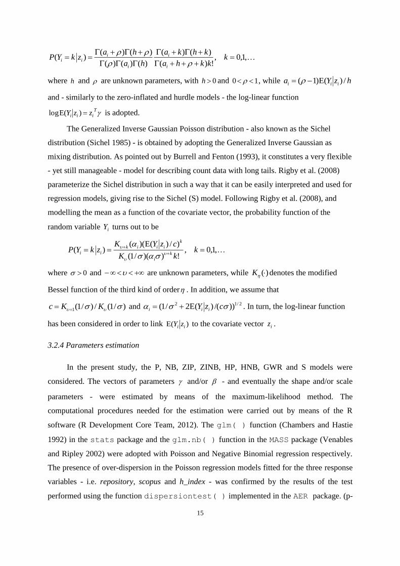
The Generalized Inverse Gaussian Poisson distribution - also known as the Sichel

distribution (Sichel 1985) - is obtained by adopting the Generalized Inverse Gaussian as

mixing distribution. As pointed out by Burrell and Fenton (1993), it constitutes a very flexible

- yet still manageable - model for describing count data with long tails. Rigby et al. (2008)

parameterize the Sichel distribution in such a way that it can be easily interpreted and used for

regression models, giving rise to the Sichel (S) model. Following Rigby et al. (2008), and

modelling the mean as a function of the covariate vector, the probability function of the

random variable iY turns out to be

,1,0,!))(/1(

)/)(E)(()(

k

kK

czYKzkYP

k

i

k

iiik

ii

where 0 and are unknown parameters, while )(K denotes the modified

Bessel function of the third kind of order . In addition, we assume that

)/1(/)/1(1 KKc and 2/12 ))/()(E2/1( czY iii . In turn, the log-linear function

has been considered in order to link )(E ii zY to the covariate vector iz .

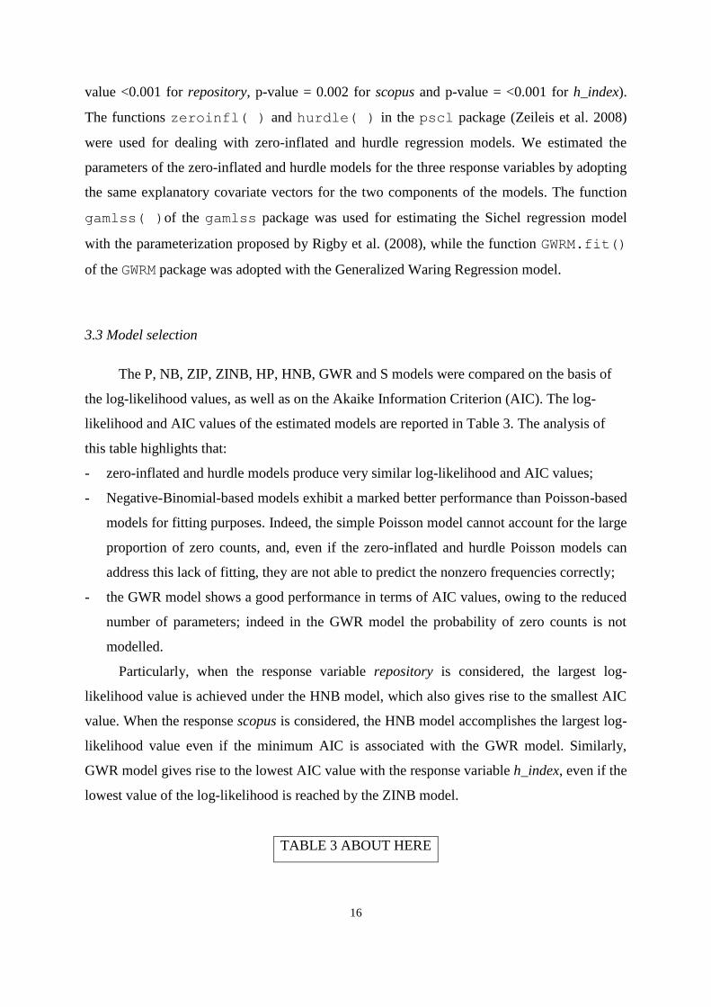
3.2.4 Parameters estimation

In the present study, the P, NB, ZIP, ZINB, HP, HNB, GWR and S models were

considered. The vectors of parameters and/or - and eventually the shape and/or scale

parameters - were estimated by means of the maximum-likelihood method. The

computational procedures needed for the estimation were carried out by means of the R

software (R Development Core Team, 2012). The glm( ) function (Chambers and Hastie

1992) in the stats package and the glm.nb( ) function in the MASS package (Venables

and Ripley 2002) were adopted with Poisson and Negative Binomial regression respectively.

The presence of over-dispersion in the Poisson regression models fitted for the three response

variables - i.e. repository, scopus and h_index - was confirmed by the results of the test

performed using the function dispersiontest( ) implemented in the AER package. (p-

16

value <0.001 for repository, p-value = 0.002 for scopus and p-value = <0.001 for h_index).

The functions zeroinfl( ) and hurdle( ) in the pscl package (Zeileis et al. 2008)

were used for dealing with zero-inflated and hurdle regression models. We estimated the

parameters of the zero-inflated and hurdle models for the three response variables by adopting

the same explanatory covariate vectors for the two components of the models. The function

gamlss( )of the gamlss package was used for estimating the Sichel regression model

with the parameterization proposed by Rigby et al. (2008), while the function GWRM.fit()

of the GWRM package was adopted with the Generalized Waring Regression model.

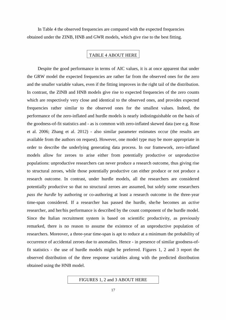
3.3 Model selection

The P, NB, ZIP, ZINB, HP, HNB, GWR and S models were compared on the basis of

the log-likelihood values, as well as on the Akaike Information Criterion (AIC). The log-

likelihood and AIC values of the estimated models are reported in Table 3. The analysis of

this table highlights that:

- zero-inflated and hurdle models produce very similar log-likelihood and AIC values;

- Negative-Binomial-based models exhibit a marked better performance than Poisson-based

models for fitting purposes. Indeed, the simple Poisson model cannot account for the large

proportion of zero counts, and, even if the zero-inflated and hurdle Poisson models can

address this lack of fitting, they are not able to predict the nonzero frequencies correctly;

- the GWR model shows a good performance in terms of AIC values, owing to the reduced

number of parameters; indeed in the GWR model the probability of zero counts is not

modelled.

Particularly, when the response variable repository is considered, the largest log-

likelihood value is achieved under the HNB model, which also gives rise to the smallest AIC

value. When the response scopus is considered, the HNB model accomplishes the largest log-

likelihood value even if the minimum AIC is associated with the GWR model. Similarly,

GWR model gives rise to the lowest AIC value with the response variable h_index, even if the

lowest value of the log-likelihood is reached by the ZINB model.

TABLE 3 ABOUT HERE

17

In Table 4 the observed frequencies are compared with the expected frequencies

obtained under the ZINB, HNB and GWR models, which give rise to the best fitting.

TABLE 4 ABOUT HERE

Despite the good performance in terms of AIC values, it is at once apparent that under

the GRW model the expected frequencies are rather far from the observed ones for the zero

and the smaller variable values, even if the fitting improves in the right tail of the distribution.

In contrast, the ZINB and HNB models give rise to expected frequencies of the zero counts

which are respectively very close and identical to the observed ones, and provides expected

frequencies rather similar to the observed ones for the smallest values. Indeed, the

performance of the zero-inflated and hurdle models is nearly indistinguishable on the basis of

the goodness-of-fit statistics and - as is common with zero-inflated skewed data (see e.g. Rose

et al. 2006; Zhang et al. 2012) - also similar parameter estimates occur (the results are

available from the authors on request). However, one model type may be more appropriate in

order to describe the underlying generating data process. In our framework, zero-inflated

models allow for zeroes to arise either from potentially productive or unproductive

populations: unproductive researchers can never produce a research outcome, thus giving rise

to structural zeroes, while those potentially productive can either produce or not produce a

research outcome. In contrast, under hurdle models, all the researchers are considered

potentially productive so that no structural zeroes are assumed, but solely some researchers

pass the hurdle by authoring or co-authoring at least a research outcome in the three-year

time-span considered. If a researcher has passed the hurdle, she/he becomes an active

researcher, and her/his performance is described by the count component of the hurdle model.

Since the Italian recruitment system is based on scientific productivity, as previously

remarked, there is no reason to assume the existence of an unproductive population of

researchers. Moreover, a three-year time-span is apt to reduce at a minimum the probability of

occurrence of accidental zeroes due to anomalies. Hence - in presence of similar goodness-of-

fit statistics - the use of hurdle models might be preferred. Figures 1, 2 and 3 report the

observed distribution of the three response variables along with the predicted distribution

obtained using the HNB model.

FIGURES 1, 2 and 3 ABOUT HERE

18

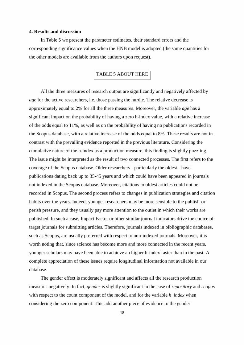
4. Results and discussion

In Table 5 we present the parameter estimates, their standard errors and the

corresponding significance values when the HNB model is adopted (the same quantities for

the other models are available from the authors upon request).

TABLE 5 ABOUT HERE

All the three measures of research output are significantly and negatively affected by

age for the active researchers, i.e. those passing the hurdle. The relative decrease is

approximately equal to 2% for all the three measures. Moreover, the variable age has a

significant impact on the probability of having a zero h-index value, with a relative increase

of the odds equal to 11%, as well as on the probability of having no publications recorded in

the Scopus database, with a relative increase of the odds equal to 8%. These results are not in

contrast with the prevailing evidence reported in the previous literature. Considering the

cumulative nature of the h-index as a production measure, this finding is slightly puzzling.

The issue might be interpreted as the result of two connected processes. The first refers to the

coverage of the Scopus database. Older researchers - particularly the oldest - have

publications dating back up to 35-45 years and which could have been appeared in journals

not indexed in the Scopus database. Moreover, citations to oldest articles could not be

recorded in Scopus. The second process refers to changes in publication strategies and citation

habits over the years. Indeed, younger researchers may be more sensible to the publish-or-

perish pressure, and they usually pay more attention to the outlet in which their works are

published. In such a case, Impact Factor or other similar journal indicators drive the choice of

target journals for submitting articles. Therefore, journals indexed in bibliographic databases,

such as Scopus, are usually preferred with respect to non-indexed journals. Moreover, it is

worth noting that, since science has become more and more connected in the recent years,

younger scholars may have been able to achieve an higher h-index faster than in the past. A

complete appreciation of these issues require longitudinal information not available in our

database.

The gender effect is moderately significant and affects all the research production

measures negatively. In fact, gender is slightly significant in the case of repository and scopus

with respect to the count component of the model, and for the variable h_index when

considering the zero component. This add another piece of evidence to the gender

19

productivity gap, suggesting that women face ceteris paribus more difficulties than men in

publishing. In turn, the not-longitudinal nature of our data does not permit to explore further

this topic as done for example by Mairesse and Pezzoni (2013).

As to the academic position, its effect is significant for all the response variables. In

particular, referring to the model count component, the number of publications and h-index

value of the active researchers decrease for associate professors and assistant professors with

respect to full professors (relative decrease respectively equal to 23% and 48%). Moreover, as

evidenced by the zero component of the model, the academic position has a marked effect on

the probability to be a non-active researcher. Indeed, when the variable h_index is considered,

the increases of the odds of having a zero value for associate professors and assistant

professors are approximately equal to 4% and 20% with respect to full professors. In turn,

similar results hold for the variable scopus, while for the variable repository the effect is

weakly significant on the odds only for assistant professors. The effect of position on research

productivity can be related to the still-surviving hierarchical organization of the university

which allows for full professors to act as both coordinators of national and international

projects - which generally give rise to many co-authored publications - and supervisors for

PhD students and junior researchers - who can stimulate their production. It should be

pointed out that, especially when the h-index value is considered, there might be a reverse

explicative process between academic position and research output: an higher academic

position should be determined by the life-long scientific production activity. This

interpretation is coherent with the organizational characteristics of the Italian university

system, in which promotions are mainly based on research activities. Moreover, this

interpretation is also supported by the results by Lissoni et al. (2011) who proved that in Italy

promotion is affected by the quantity of past publications.

As expected, the scientific sector of activity significantly impacts on research

performance: the researchers who have passed the hurdle and belong to the Life Sciences

sector show a higher level of production than those belonging to the Social Sciences and

Humanities sector. This result also holds for the Physical and Engineering Sciences sector for

the h_index variable. Analogously, in the zero component part of the models, the odds of the

non-active status is significantly smaller for the researchers of the Life Sciences sector. In

particular, the relative increase of the odds of having a zero value for the researchers

belonging to the Social Sciences and Humanities sector with respect to those belonging to

Life Sciences sector is equal to 1.8% for repository, to 127% for scopus, and to 185% for

20

h_index; while the relative increase is about 2% for all the three variables when the Physical

and Engineering Sciences sector is considered. However, such results should be cautiously

interpreted owing to the different coverage of the Scopus database, as well as to the different

publication and citation patterns in the sectors (Iglesias and Pecharroman 2007). As is well

known, the Scopus database has a weaker coverage for Social Sciences and Humanities,

especially for non-English language countries, such as Italy. In the Social Sciences and

Humanities sector, research results are communicated to the academic community mainly by

means of books and chapters in books. Therefore, for this sector, the bibliographic databases,

such as Scopus, are largely incomplete in terms of publications and citations (Hicks 2004). It

is also worth remembering that co-authorship patterns are very different across scientific

sectors. It can be argued that for sectors where articles have usually dozens of authors, the

probability to be non-active is lower than in other sectors - such as Social Sciences and

Humanities - where groups of co-authors are very small and single authorship often prevails.

We also performed the regression analysis separately on the three datasets obtained by

considering the different ERC sectors (Social Sciences and Humanities, Life Sciences, and

Physical and Engineering Sciences). The corresponding results per discipline (available from

the authors upon request) do not reveal marked different patterns with respect to those

performed on the complete dataset.

As to the connection between teaching and research activities, when the zero component

of the model is considered, a major teaching load in terms of teaching hours, number of

students and thesis supervised does not affect the odds to be a non-active researcher. Indeed,

our findings tend to reject the hypothesis that the odds to be non-active is affected by the

crowding out effect between teaching and publications. Analogous conclusions have been

achieved - using a completely different approach - by Kelchtermans and Veugelers (2011).

However, if active researchers are considered, it is worth noting that, concerning the

three explanatory variables adopted to proxy teaching tasks (i.e. teaching, thesis and

students), only students weakly significantly affects the research performance in terms of a

weak decrease in the number of publication in the Scopus and h-index value, (relative

decreases respectively equal to 0.3% and 0.2%. On the contrary, when the number of

publications in the repository is considered, there is a weak evidence that the variable students

positively, although moderately, influences the research output (relative increase equal to

0.2%); and a strong evidence that the number of thesis increases the number of publications,

with a relative increase equal to 3.4%. It may be argued that the results achieved in the thesis

21

can be used by supervisors to produce a research outcome suitable to appear in the repository

- which, it is worth to remember, includes any type of publication - but not in peer-reviewed

journals indexed by the Scopus database. Our results, differently from previous analyses (Fox

1992; Taylor et al. 2006; Kossi et al. 2013), suggest that neither substitution nor

complementarity simple hypotheses seem to adequately represent the multifaceted relation

among research and teaching activities.

As to the connection between the administrative duties of a researcher and her/his

research activities, we found that the participation to Faculty meetings has a significant

negative effect on the number of publications in the Scopus database for active researchers.

Moreover, it increases the odds of having zero h-index value, while significantly reduces the

odds of having zero publications on the research repository. These results seem to suggest that

researchers productivity is negatively affected by bureaucratic and administrative tasks - a

topic not covered in previous literature and deserving more scrutiny.

A positive evaluation received for the Prin projects significantly increases (i) the

expected output of active researchers, as highlighted by the positive coefficient estimates in

the count component of the model; and (ii) the probability of passing the hurdle, as shown by

the negative sign of the estimates in the zero part of the model. Also in this case we are not

able to interpret causally these results. In fact we cannot exclude that more productive

researchers may be more likely to obtain positive evaluation.

As for the labour contract of researchers, a part-time contract significantly increases the

probability to be non-active, with the most marked effect when the variable h_index is

considered. However, it is worth noting that, among the active researchers, a part-time

contract does not significantly affect the research performance. About this mixed evidence, it

is possible to conjecture that some part-time-researchers are engaged in scientific research and

achieved results similar to those of their full-time colleagues; others are devoted mainly to

private practice outside university, and therefore they are non-active researchers.

As to the features of the department a researcher belongs to, it is worth noting that the

relative number of researchers in more junior ranks and researchers in the same or more

senior ranks does not seem to impact the odds to be non-active for repository and scopus,

while it does for h_index. The same variable seems to have a significant positive effect for the

h_index variable and a moderately significant negative effect for the scopus variable when

active researchers are considered. These results suggest another puzzling question about the

relation between the composition of departments and researchers’ productivity (Carayol and

22

Matt 2006; Stephan 2012). A possible but not exhaustive conjecture is that the presence of

productive junior researchers widen the citation network of senior researchers improving the

number of citations received by the latters and thus affecting their h-index value.

The composition of the department, in terms of the ratio of the number of non-research

staff units to the number of permanent researchers, affects both the odds to be non-active and

the value of the production indicators, thus evidencing a positive effect of staff availability on

scientific productivity. In particular, an increase in the ratio between technical and

administrative workers and researchers (taw_ratio) has a significant positive effect on the

production of active researchers when repository or h_index variables are considered, with a

relative increase approximately equal to 56% and to 45% respectively. It also has a significant

effect on the reduction of the odds to be a non-active researcher, with a relative decrease of

the odds equal to 74% for repository and 86% for h-index. It is worthwhile to remember that

departmental staff consists of administrative personnel and specialized technicians directly

involved in research activities coordinated by academic staff. This is particularly true in

experimental sciences departments. Thus, on one hand we can suppose that administrative

staff conveniently help a researcher in administrative and bureaucratic tasks connected with

teaching and with the management of projects and research activities. On the other hand, we

can suppose that the contribution of technical workers could be particularly relevant for those

scholars working in experimental sciences departments where laboratory activities are the

core of scientific research.

5. Conclusions

This article contributes to the stream of literature investigating the individual

determinants of researcher performance. We analyse original data referring to a medium-sized

Italian university which employs 942 researchers covering many scientific fields in Life

Sciences, Physical and Engineering Sciences and Social Sciences and Humanities. All the

researchers have a permanent position in the university and obey the same rules defined at a

national level for recruitment, career, didactic charges, administrative duties and wages. Data

refers to a three-year time-span (2008-2010).

With respect to previous literature, we adopt eight regression models to manage skewed

count data with an excess of zero-valued observations, which are often the main features of

the response variables adopted to quantify research production. Among these models, the

Hurdle Negative Binomial exhibits a good fitting and appears to be reasonably coherent with

23

the underlying generating data process. This model can be interpreted as follows: all the

researchers are considered as potentially productive; when a researcher passes the hurdle by

writing a paper and becoming active in the time period considered, her/his performance is

described by the count component of the model. Moreover, the odds to be non-active is

modelled by the zero component of the model. In order to highlight the determinants of a

researcher production, we introduced an extensive set of explanatory variables, which, to the

best of our knowledge, were not jointly explored by previous literature in an unique

framework. A first result, widely known in literature, is that the different publication and

citation practices adopted in different research fields have a strong impact on productivity of

active researcher and on the odds to be non-active. This strong evidence suggests to consider

a research priority the investigation of the processes giving rise to these sectorial differences,

which are substantially unexplained in our model .

Results regarding personal observable characteristics of researchers confirm the

evidences of previous studies. In particular, our data add evidence to the gender productivity

puzzle and to the age-effect in publication activity. Academic position positively influences

researcher’s productivity, while seniority tends to have a negative effect. The evidence of our

analysis does not allow to draw a clear-cut conclusion about the relation between teaching and

research activities. A major teaching load does not affect the odds to be a non-active

researcher and it does not reduce significantly the number publications for active researchers.

The number of thesis supervised increases the number of publications in the repository. This

evidence suggests that no univocal substitution or complementarity hypothesis can be

claimed. Also in this case an in-deep analysis of factual evidence and underlying processes is

straightforward to gain a better understanding of the phenomena.

On the contrary, a clear result emerges about administrative tasks. These appear to

negatively affect research productivity, especially when research outcomes filtered by a

reviewing process are considered. To the best of our knowledge, this is a new piece of

evidence that deserves further scrutiny. Our data also allowed to analyse the effect of the

departmental working context on productivity. A first clear result is that operating in a

department filled with more administrative and technical staff enhances productivity. On the

contrary, mixed evidences emerge when the composition of the department in terms of

senior/junior researchers is considered.

24

However, we caution against generalizations of our results since the adopted database

include scientists working in a single university and we are aware that more general country-

level investigation on the main determinants of scientific production should be undertaken.

We believe that further research is needed in order to create improved measures of the effort

devoted to institutional duties and university governance and to better understand if and how

these activities could affect scientific production. Similarly, additional proxies for the

teaching load have to be exploited. To this purpose, future research could surely benefit from

the availability of information concerning researcher’s final outputs (publications, patents,

products, etc.), but also projects, scientific areas, teaching and administrative and institutional

activities. Indeed, the evaluation of the effects of administrative and teaching tasks on

scientific output is mandatory to verify if current incentive policies for stimulating research

production are effective.

25

References

Abramo, G., D’Angelo, C.A., Caprasecca, A. (2009). Gender differences in research

productivity: a bibliometric analysis of the Italian academic system. Scientometrics, 79, 517-

539.

Allison, P.D., Long J.S. (1990). Departmental effects on scientific productivity. American

Sociological Review, 55, 469-478.

Allison, P.D., Stewart, J.A. (1974). Productivity differences among scientists: evidence for

accumulative advantage. American Sociological Review, 39, 596-606.

Anania, G., Caruso, A. (2013). Two simple new bibliometric indexes to better evaluate

research in disciplines where publications typically receive less citations. Scientometrics, 96,

617-631.

Barabesi, L., Pratelli, L. (2014). Discussion of “On simulation and properties of the stable

law” by L. Devroye and L. James. Statistical Methods & Applications, DOI 10.1007/s10260-

014-0263-x.

Bayer, A.E., Dutton, J.E. (1977). Career age and research professional activities of academic

scientists. Journal of Higher education, 48, 259-282.

Böhning, D., Dietz, E., Schlattmann, P., Mendonça, L., Kirchner, U. (1999). The zero-inflated

Poisson model and the decayed, missing and filled teeth index in dental epidemiology.

Journal of the Royal Statistical Society Series A, 162, 195-209.

Bonaccorsi, A., Daraio, C. (2003). Age effects in scientific productivity. The case of the

Italian National Research Council (CNR). Scientometrics, 58, 49-90.

Burrell, Q.L. (2005). The use of the generalized Waring process in modelling informetric

data. Scientometrics, 64, 247-270.

Burrell, Q.L., Fenton, M.R. (1993). Yes, the GIGP really does work -- and is workable!.

Journal of the American Society for Information Science, 44, 61-69.

Cainelli, G., de Felice, A., Lamonarca, M., Zoboli, R. (2006). The publications of Italian

economists in ECONLIT: quantitative assessment and implications for research evaluation.

Economia Politica, 23, 385-423.

Carayol, N., Matt, M. (2004). Does research organization influence academic production?

Laboratory level evidence from a large European university. Research Policy, 33, 1081-1102.

Carayol, N., Matt, M. (2006). Individual and collective determinants of academic scientists’

productivity. Information Economics and Policy, 18, 55-72.

26

Chambers, J.M., Hastie, T.J. (Eds) (1992). Statistical Models in S. Chapman & Hall, London.

Cole, J.R., Cole, S. (1973). Social Stratification in Science. University of Chicago Press,

Chicago.

Cole, J.R., Zuckerman, H. (1984). The productivity puzzle: persistence and change in patterns

of publication of men and women scientists. In: Steinkempt, M.W., Maehr, M.L. (Eds),

Advances in Motivation and Achievement. JAI Press, Greenwich, Conn., 217-258.

Dalrymple, M.L., Hudson, I.L., Ford, R.P.K. (2003). Finite mixture, zero-inflated Poisson and

hurdle models with application to SIDS. Computational Statistics & Data Analysis, 41, 491-

504.

David, P. (1994). Positive feedbacks and research productivity in science: reopening another

black box. In: Grandstrand, O. (Ed), Economics and Technology. Elsevier, Amsterdam, pp.

65-85.

Defazio, D., Lockett, A., Wright, M. (2009). Funding incentives, collaborative dynamics and

scientific productivity: evidence from the EU framework program. Research Policy, 38, 293-

305.

Diamond, A.M. (1984). An economic-model of the life-cycle research productivity of

scientists. Scientometrics, 6, 189-196.

Diamond, A.M. (1986). The life-cycle research productivity of mathematicians and scientists.

The Journal of Gerontology, 41, 520-525.

Fabel, O., Hein, M., Hofmeister, R. (2008). Research productivity in business economics: an

investigation of Austrian, German and Swiss universities. German Economic Review, 9, 506-

531.

Fox, M.F. (1992). Research, teaching and publication productivity: mutuality versus

competition in academia. Sociology of Education, 65, 293-305.

Fox, M.F. (2005). Gender, family characteristics, and publication productivity among

scientists. Social Studies of Science, 35, 131-150.

Fox, M.F., Fonseca, C., Bao, J. (2011). Work and family conflict in academic science:

Patterns and predictors among women and men in research universities. Social Studies of

Science, 41, 715-735.

Hall, D.B. (2000). Zero-inflated Poisson and binomial regression with random effects: a case

study. Biometrics, 56, 1030-1039.

27

Hicks, D. (2004). The four literatures of social science, in: Moed, F.H., Glaenzel, W.,

Schmoch, U. (Eds), Handbook of Quantitative Science and Technology Research. Kluwer

Academic Publishers, Dordrecht, Boston and London, pp. 473-496.

Hirsch, J.E. (2005). An index to quantify an individual’s scientific research output.

Proceedings of the National Academy of Sciences of the United States of America, 102,

16569-16572.

Iglesias, J.E., Pecharroman, C. (2007). Scaling the h-index for different scientific ISI fields.

Scientometrics, 73, 303-320.

Irwin, J.O. (1968). The generalized Waring distribution applied to accident theory. Journal of

the Royal Statistical Society. Series A (General), 131, 205-225.

Johnson, N.L., Kemp, A.W., Kotz, S. (2005). Univariate discrete distributions, 3rd

edn.,Wiley, New York.

Kelchtermans, K., Veugelers, R. (2011). The great divide in scientific productivity: why the

average scientist does not exist. Industrial and Corporate Change, 20, 295-336.

Kossi, Y., Lesueur, J.Y., Sabatier, M. (2013). Publish or teach? The role of the scientific

environment on academics multitasking. Groupe d’Analyse et de Théorie Économique Lyon-

St Étienne, GATE WP 1315.

Lambert, D. (1992). Zero-inflated Poisson regression, with an application to defects in

manufacturing. Technometrics, 34, 1-17.

Leahey, E. (2006). Gender differences in productivity: research specialization as a missing

link. Gender & Society, 20, 754-780.

Levin, S., Stephan, P.E. (1991). Research productivity over the life cycle: evidence for

academic scientists. American Economic Review, 81, 114-132.

Levin, S., Stephan, P.E. (1998). Gender differences in the rewards to publishing in academe:

science in the 1970s. Sex Roles, 38, 1041-1064.

Lissoni, F., Mairesse, J., Montobbio, F., Pezzoni, M. (2011). Scientific productivity and

academic promotion: a study on French and Italian physicists. Industrial and Corporate

Change, 20, 253-294.

Lotka, A.J. (1926). The frequency distribution of scientific productivity. Journal of the

Washington Academy of Science, 16, 317-323.

Mairesse J., Pezzoni M. (2013). Does gender affect scientific productivity? A critical review

of the empirical evidence and a panel data econometric analysis for French physicists.

Presented to AFSE Meeting, Aix en Provence, 26 June 2013.

28

Mairesse, J., Turner, L. (2006). Measurement and explanation of the intensity of co-

publication in scientific research: an analysis at the laboratory level. In: Antonelli, C., Foray,

D., Hall, B.H., Steinmueller, W.E. (Eds), New Frontiers in the Economics of Innovation and

New Technology: Essays in Honour of Paul A. David. Edward Elgar, Cheltenham and

Northampton, 255-295.

Marcheselli, M., Baccini, A., Barabesi, L. (2008). Parameter estimation for the discrete stable

family. Communications in Statistics - Theory and Methods, 37, 815-830.

Martin, B.R., Irvine, J. (1983). Assessing basic research: some partial indicators of scientific

progress in radio astronomy. Research Policy, 12, 61-90.

Merton, R. (1968). The Matthew effect in science. Science, 159, 56-63.

Minami, M., Lennert-Cody, C.E., Gao, W., Román-Verdesoto, M. (2007). Modeling shark

bycatch: the zero-inflated negative binomial regression model with smoothing. Fisheries

Research, 84, 210-221.

Mullahy, J. (1986). Specification and testing of some modified count data models. Journal of

Econometrics, 33, 341-365.

Pezzoni, M., Sterzi, V., Lissoni, F. (2012). Career progress in centralized academic systems:

social capital and institutions in France and Italy. Research Policy, 41, 704-719.

R Core Team (2012). R: a language and environment for statistical computing. R Foundation

for Statistical Computing, Vienna, Austria. ISBN 3-900051-07-0, from http://www.R-

project.org/.

Rao, I.K.R. (1980). The Distribution of Scientific Productivity and Social Change. Journal of

the American Society for Information Science, 31, 111-122.

Rathbun, S.L., Fei, S. (2006). A spatial zero-inflated Poisson regression model for oak

regeneration. Environmental and Ecological Statistics, 13, 409-426.

Rigby, R.A., Stasinopoulos, D.M., Akantziliotou, C. (2008). A framework for modelling

overdispersed count data, including the Poisson-shifted generalized inverse Gaussian

distribution. Computational Statistics and Data Analysis 53, 381-393.

Rivera-Huerta, R., Dutrénit, G., Ekboir, J.M., Sampedro, J.L., Vera-Cruz, A.O. (2011). Do

linkages between farmers and academic researchers influence researcher productivity? The

Mexican case. Research Policy, 40, 932-942.

Rodríguez-Avi, J., Conde-Sánchez, A., Sáez-Castillo, A.J., Olmo-Jiménez, M.J. and

Martínez-Rodríguez, A.M., (2009). A generalized Waring regression model for count data.

Computational Statistics and Data Analysis, 53, 3717-3725.

29

Rose, C.E., Martin, S.W., Wannemuehler, K.A., Plikaytis, B.D. (2006). On the use of zero-

inflated and hurdle models for modeling vaccine adverse event count data. Journal of

Biopharmaceutical Statistics, 16, 463-481.

Schubert, A., Glanzel, W. (1984). A dynamic Look at a class of skew distributions. A model

with scientometric applications. Scientometrics, 6, 149-167.

Schubert,A., Telcs, A. (1989). Estimation of the publication potential in 50 U.S. states and in

the District of Columbia based on the frequency distribution of scientific productivity.

Journal of the American Society for Information Science, 40, 291–297.

Sibuya, M. (1979). Generalized hypergeometric, digamma and trigamma distributions. Annals

of the Institute of Statistical Mathematics, 31, 373-390.

Sichel, H.S. (1985). A bibliometric distribution which really works. Journal of the American

Society for Information Science, 36, 314-321.

Stephan, P.E. (1996). The economics of science. Journal of Economic Literature, 34, 1199-

1235.

Stephan, P.E. (2012). How Economics Shapes Science. Harvard University Press, Cambridge,

Mass.

Taylor, S.W., Fender, B.F., Burke, K.G. (2006). Unraveling the academic productivity of

economists: the opportunity costs of teaching and service. Southern Economic Journal, 72,

846-859.

van Arensbergen, P., van der Weijden, I., van den Besselaar, P. (2012). Gender differences in

scientific productivity: a persisting phenomenon? Scientometrics, 93, 857-868.

van Leeuwen, T.N., Visser, M.S., Moed, H.F., Nederhof, T.J., van Raan, A.F.J. (2003). The

Holy Grail of science policy: exploring and combining bibliometric tools in search of

scientific excellence. Scientometrics, 57, 257-280.

Venables, W.N., Ripley, B.D. (2002). Modern Applied Statistics with S. Springer-Verlag,

New York.

Wallner, B., Fieder, M., Iber, K. (2003). Age profile, personnel costs and scientific

productivity at the University of Vienna. Scientometrics, 58, 143-153.

Wang, D., Song, C., Barabási, A.L. (2013). Quantifying long-term scientific impact. Science,

342, 127-132.

Weiss, Y., Lillard, L.A. (1982). Output variability, academic labor contracts, and waiting

times for promotion. Research in Labor Economics, 5, 157-188.

30

Wooton, R. (2013). A simple, generalizable method for measuring individual research

productivity and its use in the long-term analysis of departmental performance, including

between-country comparisons. Health Research Policy and Systems, 11, 1-14.

Xie, Y., Shauman, K.A. (2003). Women in Science: Career Processes and Outcomes. Harvard

University Press, Cambridge, Mass.

Zeileis, A., Kleiber, C., Jackman, S. (2008). Regression models for count data in R. Journal

of Statistical Software, 27, 1-25.

Zhang, X., Lei, Y., Cai, D., Liu, F. (2012). Predicting tree recruitment with negative binomial

mixture models. Forest Ecology and Management, 270, 209-215.

Zuckerman, H.A., Merton, R.K. (1972). Age, aging, and age structure in science, in: Riley,

M.R., Johnson, M., Foner, A. (Eds), A Sociology of Age Stratification: Aging and Society.

Russell Sage Foundation, New York, 292-356.

31

Fig. 1 The observed distribution of the number of publications in the research repository of

the University of Siena along with the predicted distribution obtained using the HNB model.

Values greater than 40 are omitted for improving readability

Fig. 2 The observed distribution of the number of publications in Scopus along with the

predicted distribution obtained using the HNB model. Values greater than 40 are omitted for

improving readability

Fig. 3 The observed distribution of the h-index value along with the predicted distribution

obtained using the HNB model. Values greater than 40 are omitted for improving readability

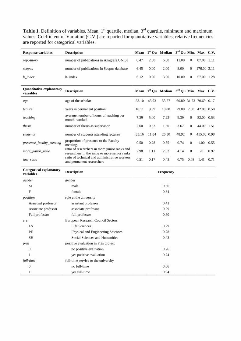
Table 1. Definition of variables. Mean, 1st quartile, median, 3

rd quartile, minimum and maximum

values, Coefficient of Variation (C.V.) are reported for quantitative variables; relative frequencies

are reported for categorical variables.

Response variables Description Mean 1st Qu Median 3rd Qu Min. Max. C.V.

repository number of publications in Anagrafe.UNISI 8.47 2.00 6.00 11.00 0 87.00 1.11

scopus number of publications in Scopus database 6.45 0.00 2.00 8.00 0 176.00 2.11

h_index h- index 6.12 0.00 3.00 10.00 0 57.00 1.28

Quantitative explanatory

variables Description Mean 1st Qu Median 3rd Qu Min. Max. C.V.

age age of the scholar 53.10 45.93 53.77 60.80 31.72 70.69 0.17

tenure years in permanent position 18.11 9.99 18.00 29.00 2.00 42.00 0.58

teaching average number of hours of teaching per

month worked 7.39 5.00 7.22 9.39 0 52.00 0.53

thesis number of thesis as supervisor 2.60 0.33 1.30 3.67 0 44.00 1.51

students number of students attending lectures 35.16 11.54 26.50 48.92 0 415.00 0.98

presence_faculty_meeting proportion of presence to the Faculty

meeting 0.50 0.28 0.55 0.74 0 1.00 0.55

more_junior_ratio ratio of researchers in more junior ranks and

researchers in the same or more senior ranks 2.98 1.11 2.02 4.14 0 20 0.97

taw_ratio ratio of technical and administrative workers

and permanent researchers 0.51 0.17 0.43 0.75 0.08 1.41 0.71

Categorical explanatory

variables Description

Frequency

gender gender

M male 0.66

F female 0.34

position role at the university

Assistant professor assistant professor 0.41

Associate professor associate professor 0.29

Full professor full professor 0.30

erc European Research Council Sectors

LS Life Sciences 0.29

PE Physical and Engineering Sciences 0.28

SH Social Sciences and Humanities 0.43

prin positive evaluation in Prin project

0 no positive evaluation 0.26

1 yes positive evaluation 0.74

full-time full-time service to the university

0 no full-time 0.06

1 yes full-time 0.94

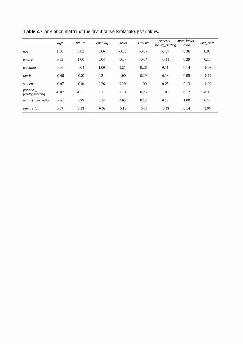
Table 2. Correlation matrix of the quantitative explanatory variables.

age tenure teaching thesis students

presence_

faculty_meeting

more_junior_

ratio taw_ratio

age 1.00 0.83 0.06 -0.06 -0.07 -0.07 0.36 0.07

tenure 0.83 1.00 0.04 -0.07 -0.04 -0.11 0.29 0.13

teaching 0.06 0.04 1.00 0.21 0.26 0.11 0.14 -0.08

thesis -0.06 -0.07 0.21 1.00 0.29 0.13 0.05 -0.19

students -0.07 -0.04 0.26 0.29 1.00 0.25 0.13 -0.09

presence_

faculty_meeting -0.07 -0.11 0.11 0.13 0.25 1.00 0.12 -0.13

more_junior_ratio 0.36 0.29 0.14 0.05 0.13 0.12 1.00 0.14

taw_ratio 0.07 0.13 -0.08 -0.19 -0.09 -0.13 0.14 1.00

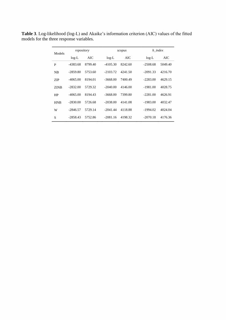
Table 3. Log-likelihood (log-L) and Akaike’s information criterion (AIC) values of the fitted

models for the three response variables.

Models repository scopus h_index

log-L AIC log-L AIC log-L AIC

P -4383.68 8799.40 -4105.30 8242.60 -2508.68 5049.40

NB -2859.80 5753.60 -2103.72 4241.50 -2091.33 4216.70

ZIP -4065.00 8194.01 -3668.00 7400.49 -2283.00 4629.15

ZINB -2832.00 5729.32 -2040.00 4146.00 -1981.00 4028.75

HP -4065.00 8194.43 -3668.00 7399.80 -2281.00 4626.91

HNB -2830.00 5726.68 -2038.00 4141.08 -1983.00 4032.47

W -2846.57 5729.14 -2041.44 4118.88 -1994.02 4024.04

S -2858.43 5752.86 -2081.16 4198.32 -2070.18 4176.36

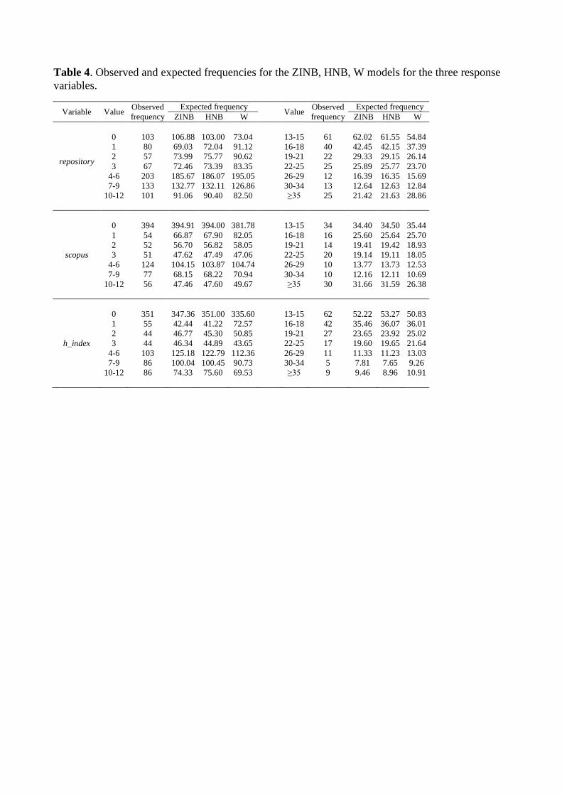
Table 4. Observed and expected frequencies for the ZINB, HNB, W models for the three response

variables.

Variable Value Observed

frequency

Expected frequency Value

Observed

frequency

Expected frequency

ZINB HNB W

ZINB HNB W

repository

0 103 106.88 103.00 73.04

13-15 61 62.02 61.55 54.84

1 80 69.03 72.04 91.12

16-18 40 42.45 42.15 37.39

2 57 73.99 75.77 90.62

19-21 22 29.33 29.15 26.14

3 67 72.46 73.39 83.35

22-25 25 25.89 25.77 23.70

4-6 203 185.67 186.07 195.05

26-29 12 16.39 16.35 15.69

7-9 133 132.77 132.11 126.86

30-34 13 12.64 12.63 12.84

10-12 101 91.06 90.40 82.50

≥35 25 21.42 21.63 28.86

scopus

0 394 394.91 394.00 381.78

13-15 34 34.40 34.50 35.44

1 54 66.87 67.90 82.05

16-18 16 25.60 25.64 25.70

2 52 56.70 56.82 58.05

19-21 14 19.41 19.42 18.93

3 51 47.62 47.49 47.06

22-25 20 19.14 19.11 18.05

4-6 124 104.15 103.87 104.74

26-29 10 13.77 13.73 12.53

7-9 77 68.15 68.22 70.94

30-34 10 12.16 12.11 10.69

10-12 56 47.46 47.60 49.67

≥35 30 31.66 31.59 26.38

h_index

0 351 347.36 351.00 335.60

13-15 62 52.22 53.27 50.83

1 55 42.44 41.22 72.57

16-18 42 35.46 36.07 36.01

2 44 46.77 45.30 50.85

19-21 27 23.65 23.92 25.02

3 44 46.34 44.89 43.65

22-25 17 19.60 19.65 21.64

4-6 103 125.18 122.79 112.36

26-29 11 11.33 11.23 13.03

7-9 86 100.04 100.45 90.73

30-34 5 7.81 7.65 9.26

10-12 86 74.33 75.60 69.53

≥35 9 9.46 8.96 10.91

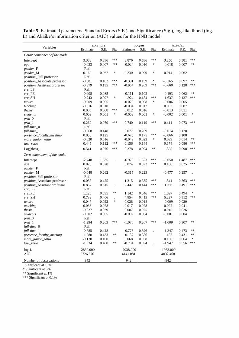
Table 5. Estimated parameters, Standard Errors (S.E.) and Significance (Sig.), log-likelihood (log-

L) and Akaike’s information criterion (AIC) values for the HNB model.

Variables repository scopus h_index

Estimate S.E. Sig. Estimate S.E. Sig. Estimate S.E. Sig.

Count component of the model

Intercept 3.388 0.396 *** 3.876 0.596 *** 3.250 0.381 ***

age -0.023 0.007 *** -0.024 0.010 * -0.018 0.007 **

gender_F Ref.

gender_M 0.160 0.067 * 0.230 0.099 * 0.014 0.062

position_Full professor Ref.

position_Associate professor -0.381 0.102 *** -0.391 0.159 * -0.265 0.097 **

position_Assistant professor -0.879 0.135 *** -0.954 0.209 *** -0.660 0.128 ***

erc_LS Ref.

erc_PE -0.008 0.085

-0.111 0.102

-0.193 0.062 **

erc_SH -0.243 0.097 * -1.924 0.184 *** -1.637 0.127 ***

tenure -0.009 0.005

-0.020 0.008 * -0.006 0.005

teaching -0.016 0.010

-0.004 0.012

0.002 0.007

thesis 0.033 0.008 *** 0.012 0.016

-0.013 0.011

students 0.002 0.001 * -0.003 0.001 * -0.002 0.001 *

prin_0 Ref.

prin_1 0.269 0.079 *** 0.740 0.119 *** 0.411 0.073 ***

full-time_0 Ref.

full-time_1 -0.068 0.148

0.077 0.209

-0.014 0.128

presence_faculty_meeting 0.058 0.125

-0.675 0.175 *** -0.066 0.108

more_junior_ratio -0.020 0.016

-0.049 0.023 * 0.039 0.014 **

taw_ratio 0.445 0.112 *** 0.156 0.144

0.374 0.086 ***

Log(theta) 0.541 0.076 *** 0.278 0.094 ** 1.355 0.098 ***

Zero component of the model

Intercept -2.748 1.535 . -6.973 1.323 *** -9.050 1.487 ***

age 0.028 0.028

0.074 0.022 *** 0.106 0.025 ***

gender_F Ref.

gender_M -0.048 0.262

-0.315 0.223

-0.477 0.257 .

position_Full professor Ref.

position_Associate professor 0.086 0.425

1.315 0.335 *** 1.541 0.363 ***

position_Assistant professor 0.857 0.515 . 2.447 0.444 *** 3.036 0.491 ***

erc_LS Ref.

erc_PE 1.126 0.395 ** 1.142 0.346 *** 1.097 0.494 *

erc_SH 0.732 0.406 . 4.854 0.415 *** 5.227 0.512 ***

tenure 0.047 0.022 * 0.028 0.018

-0.009 0.020

teaching 0.033 0.028

0.017 0.028

0.022 0.041

thesis -0.027 0.039

0.007 0.025

0.015 0.026

students -0.002 0.005

-0.002 0.004

-0.001 0.004

prin_0 Ref.

prin_1 -1.294 0.263 *** -1.070 0.267 *** -1.009 0.307 **

full-time_0 Ref.

full-time_1 -0.685 0.428

-0.773 0.396 . -1.347 0.473 **

presence_faculty_meeting -1.280 0.433 ** -0.157 0.386

1.187 0.431 **

more_junior_ratio -0.170 0.100 . 0.068 0.058

0.156 0.064 *

taw_ratio -1.334 0.488 ** -0.734 0.394 . -1.947 0.556 ***

log-L -2830.000

-2038.000

-1983.000

AIC 5726.676

4141.081

4032.468

Number of observations 942 942 942

. Significant at 10%

* Significant at 5%

** Significant at 1%

*** Significant at 0.1%

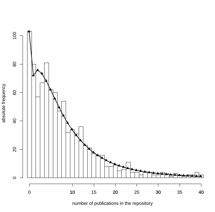
number of publications in the repository

abso

lute

freq

uenc

y

0 10 20 30 40

020

4060

8010

0

10 15 20 25 30 35 40

number of publications in Scopus

abso

lute

freq

uenc

y

0 10 20 30 40

010

020

030

040

0

5 10 15 20 25 30 35 40

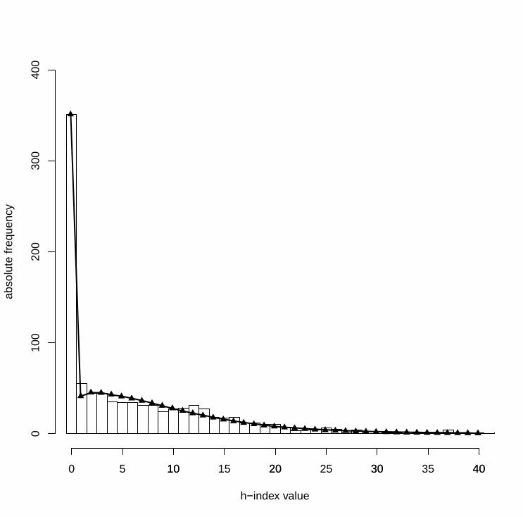
h−index value

abso

lute

freq

uenc

y

0 10 20 30 40

010

020

030

040

0

5 10 15 20 25 30 35 40