Continuous Top-k Spatial-Keyword Search on Dynamic Objects

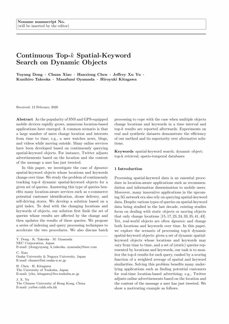
Noname manuscript No.(will be inserted by the editor)

Continuous Top-k Spatial-KeywordSearch on Dynamic Objects

Yuyang Dong · Chuan Xiao · Hanxiong Chen · Jeffrey Xu Yu ·Kunihiro Takeoka · Masafumi Oyamada · Hiroyuki Kitagawa

Received: 12 February 2020

Abstract As the popularity of SNS and GPS-equipped

mobile devices rapidly grows, numerous location-based

applications have emerged. A common scenario is that

a large number of users change location and interests

from time to time; e.g., a user watches news, blogs,

and videos while moving outside. Many online services

have been developed based on continuously querying

spatial-keyword objects. For instance, Twitter adjusts

advertisements based on the location and the content

of the message a user has just tweeted.

In this paper, we investigate the case of dynamic

spatial-keyword objects whose locations and keywords

change over time. We study the problem of continuously

tracking top-k dynamic spatial-keyword objects for a

given set of queries. Answering this type of queries ben-

efits many location-aware services such as e-commerce

potential customer identification, drone delivery, and

self-driving stores. We develop a solution based on a

grid index. To deal with the changing locations and

keywords of objects, our solution first finds the set of

queries whose results are affected by the change and

then updates the results of these queries. We propose

a series of indexing and query processing techniques to

accelerate the two procedures. We also discuss batch

Y. Dong · K. Takeoka · M. OyamadaNEC Corporation, JapanE-mail: {dongyuyang, k takeoka, oyamada}@nec.com

C. XiaoOsaka University & Nagoya University, JapanE-mail: [email protected]

H. Chen · H. KitagawaThe University of Tsukuba, JapanE-mail: {chx, kitagawa}@cs.tsukuba.ac.jp

J. X. YuThe Chinese University of Hong Kong, ChinaE-mail: [email protected]

processing to cope with the case when multiple objects

change locations and keywords in a time interval and

top-k results are reported afterwards. Experiments on

real and synthetic datasets demonstrate the efficiency

of our method and its superiority over alternative solu-

tions.

Keywords spatial-keyword search; dynamic object;

top-k retrieval; spatio-temporal databases

1 Introduction

Processing spatial-keyword data is an essential proce-

dure in location-aware applications such as recommen-

dation and information dissemination to mobile users.

Moreover, many innovative applications in the upcom-ing 5G network era also rely on querying spatial-keyword

data. Despite various types of queries on spatial-keyword

data being studied in the last decade, existing studies

focus on dealing with static objects or moving objects

that only change locations [15, 17, 23, 24, 33, 35, 41, 43].

Yet, real-world objects are often dynamic and change

both locations and keywords over time. In this paper,

we explore the scenario of processing top-k dynamic

spatial-keyword objects: given a set of dynamic spatial-

keyword objects whose locations and keywords may

vary from time to time, and a set of (static) queries rep-

resented by locations and keywords, our task is to mon-

itor the top-k results for each query, ranked by a scoring

function of a weighted average of spatial and keyword

similarities. Solving this problem benefits many under-

lying applications such as finding potential customers

for real-time location-based advertising; e.g., Twitter

adjusts online advertisements based on the location and

the content of the message a user has just tweeted. We

show a motivating example as follows.

Fig. 1: Potential customer identification for e-

commerce.

Consider an e-commerce instance in Fig. 1. A hip-

hop cloth store, a sushi restaurant, and an Apple Store

are registered as queries. Three users (objects) are using

mobile phones. Suppose we search for top-1 results; i.e,

the system identifies top-1 users as potential customers

w.r.t. the three shops. At time t0, Bob is watching a

hip-hop music video, Amy is searching for Apple, and

Jack is reading news on Apple. Bob becomes the top-1

result of the hip-hop store, as he is the only user that

matches keyword hip-hop. Both Amy and Jack are as-

sociated with keyword Apple, but Amy is closer to the

Apple Store and becomes the top-1 result. Nobody is

associated with keyword sushi. So the top-1 result for

the sushi restaurant is empty. At time t1, Bob is mov-

ing northeast and starts to watch an eating show about

sushi. So his keywords become hip-hop and sushi (we

assume previous keywords do not immediately disap-pear in this example). Amy moves away from the Apple

Store and searches for steak. So her keywords become

Apple and steak. Jack is staying and still reading news

on Apple. The system keeps Bob at the top-1 result of

the hip-hop store and recognizes him as the new top-1

of the sushi restaurant. Since Jack becomes closer than

Amy to the Apple Store, he replaces Amy as the top-1

result of the Apple Store.

Besides, since we target the scenario of monitoring

dynamic spatial-keyword objects, our solution is poten-

tially useful for the following IoT applications: (1) Asset

tracking: We consider moving assets (e.g., shared vehi-

cles), whose status is modeled in keywords (e.g, carry-

ing goods, needing refueling, and engaging a mechani-

cal problem). Companies track their assets and provide

service when necessary. (2) Location and medication

watch: Patients or elderly people, while moving, wear

equipment that monitors health status (e.g., nausea,

chest pain, and shortness of breath). Health centers

keep watch and rescue nearby ones in an emergency.

(3) Wildlife tracking: Similar to location and medica-

tion watch, but the objects are wild animals. Keywords

are used to describe gender, age group, and health sta-

tus. Investigators may track the herd for population

and migration studies.

To the best of our knowledge, this is the first work

targeting the case when objects change both spatial and

textual attributes. For real-time applications, the key

issue is to efficiently update top-k results for the queries

whenever an object updates its state. It is noteworthy

to mention that our problem can be extended from the

location-based publish/subscribe model by allowing ob-

jects (messages) to update in a free manner, including

moving and/or insertion/deletion of keywords. Exist-

ing work in this category decides whether an object is

interested by a query (subscription) by utilizing a de-

cay factor CIQ [6] or a sliding window [31]. Albeit in a

stream, the objects considered in these studies are es-

sentially static once they appear, i.e., they never move

or change keywords. Their techniques were also devel-

oped specifically for the decay factor or sliding window.

Simply adapting these methods for our problem does

not deliver sufficient efficient query processing. Our ex-

periments show that adaptation of these methods spend

more than 60 seconds to process a batch of 1,000 object

updates on a dataset of 250K queries, hence difficult to

keep up with the pace of frequent update in real-time

applications. Another line of related work is answering

reverse k nearest neighbors (RkNN) for spatial-keyword

data, because the roles of objects and queries can be

swapped, and then finding top-k results for the queries

is equivalent to finding RkNN for the objects. However,

existing methods in this category (e.g., [14,19,20]) only

deal with the static case and do not apply to the con-

tinuous search in our problem. Next we summarize the

challenges of this problem and our solution.

The first challenge originates from the large number

of queries. It is prohibitive to check every query and re-

compute top-k results. On the other hand, the number

of affected queries (i.e., the queries that change any

top-k result) is usually very small once an object update

occurs. This challenge is akin to that in location-aware

publish/subscribe systems. Both CIQ and SKYPE uti-

lize an inverted index for keywords and a quadtree for

spatial information to identify the queries (referred to

as subscriptions in [6, 31]) affected by an object up-

date (referred to as messages in [6, 31]). However, CIQand SKYPE have to traverse the quadtree and compute

score upperbounds to determine whether a cell can be

skipped, hence resulting in considerable cell access. In

addition, both methods index single keywords in the in-

verted index, yet it is common that an object has only

frequent keywords in our problem setting, thereby re-

2

sulting in access to long postings lists in the inverted

index and hence significant overhead.

To address the first challenge, we index objects and

queries in a grid index and propose the notions of cell-

cell links (CC links) and l-signatures. CC links model

the cells in a grid as a directed graph. Whenever an

object update occurs, through the outgoing CC links

of the cell of the new location, we can quickly identify

the cells that need look-up and avoid accessing the cells

that can be pruned. l-signatures are combinations of l

keywords. Despite the existence of frequent keywords,

the frequencies of their combinations are often signifi-

cantly smaller. By indexing l-signatures of queries and

selecting a good set of l-signatures from the updated

object, the cost of inverted index access can be remark-

ably reduced.

The second challenge is to compute the top-k results

of the affected queries. Since the update of an object

may cause the object to move out of the top-k results

of some queries (e.g., when an object moves away from

a query), it is time-consuming to refill the top-k of

these queries from scratch. Most related studies adopt a

buffering strategy to store a list of non-top-k objects for

each query, e.g., the kmax buffering [39]. The buffered

objects are used when a top-k refilling is needed. Such

object-based buffering is inefficient for our problem be-

cause a reordering of the objects in the buffer is required

whenever an update occurs.

To address the second challenge, we first propose to

leverage the upper and lower bounds of scores of the

objects in a cell. The key observation is that the score

bounds of the objects in a cell do not change frequently.

To improve the performance, we also observe that the

new top-k result of a query is either the updated ob-

ject or the (k + 1)-th result prior to the update. Thus,

on top of the score bounds, we propose a method that

maintains a list of cells for each query such that (k+1)-

th object of the query is guaranteed to reside in one of

these cells. We derive the condition of these cells and

address the issue of the list update.

We extend our method to batch processing, i.e.,

multiple objects change state in an time interval. By

taking into account of sharing computation for multiple

objects, the technique can be used to handle the case

when top-k results are supposed to be reported once

a batch. In addition, the initialization of top-k results

and the update of queries are discussed. We conduct

experiments on real and synthetic datasets. The results

demonstrate that the proposed techniques are effective

in reducing query processing time and contribute to a

substantial overall speed-up over alternative solutions,

hence reducing the average query processing time to

milliseconds.

Our contributions are summarized as follows.

– We study a new type of queries to continuously

search top-k results for dynamic spatial-keyword ob-

jects that may change locations and keywords over

time.

– We propose a query processing method that com-

prises an affected query finder and a top-k refiller

to address the technical challenges of the studied

problem. We devise a series of data structures and

algorithms for the two components.

– We extend our method to handle the case of batch

processing.

– We conduct extensive experiments. The results demon-

strate the effectiveness of the components of our

method and the superiority of our method over al-

ternative solutions in speed.

Compared to the preliminary version of this pa-

per [11], we made the following improvements:

– For affected query finder, we propose data struc-

tures (CC links and l-signatures) tailored to our

problem to speed up query processing.

– For top-k refiller, we improve the cell list mainte-

nance policy and the list update algorithm which

employs a lazy update strategy for efficiency.

– We extend our method to batch processing and dis-

cuss initialization and query updates.

– We conduct substantially more experiments (scal-

ability, batch processing, etc.) to evaluate the new

techniques and compare with the method proposed

in [11].

The rest of the paper is organized as follows. Sec-

tion 2 reviews related work. Section 3 introduces prelim-

inaries and defines the problem. Section 4 provides the

overview of our solution. Sections 5 and 6 present the

algorithms of finding affect queries finder and refilling

top-k. The extension to batch processing is covered by

Section 7. The initialization and the update of queries

are discussed in Section 8. Experimental results are re-

ported in Section 9. Section 10 concludes the paper.

2 Related Work

Location-aware publish/subscribe. In location-aware

publish/subscribe systems, users register their interests

as continuous queries into the system, and then new

streaming objects are delivered to relevant users. Key-

word Boolean matching was studied in [5,18,32], spatial

range query was studied in [8], and the case of scor-

ing function combining spatial and keyword similari-

ties were considered in [6, 31]. The major difference in

3

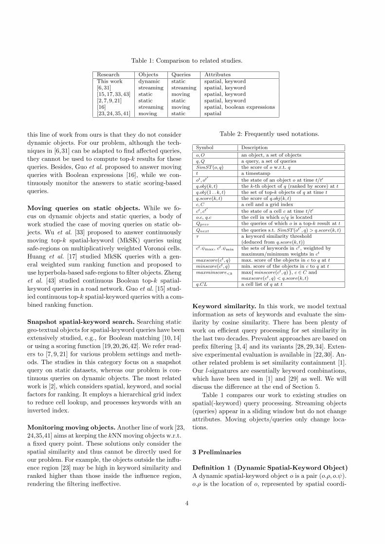
Table 1: Comparison to related studies.

Research Objects Queries AttributesThis work dynamic static spatial, keyword[6, 31] streaming streaming spatial, keyword[15,17,33,43] static moving spatial, keyword[2, 7, 9, 21] static static spatial, keyword[16] streaming moving spatial, boolean expressions[23,24,35,41] moving static spatial

this line of work from ours is that they do not consider

dynamic objects. For our problem, although the tech-

niques in [6,31] can be adapted to find affected queries,

they cannot be used to compute top-k results for these

queries. Besides, Guo et al. proposed to answer moving

queries with Boolean expressions [16], while we con-

tinuously monitor the answers to static scoring-based

queries.

Moving queries on static objects. While we fo-

cus on dynamic objects and static queries, a body of

work studied the case of moving queries on static ob-

jects. Wu et al. [33] proposed to answer continuously

moving top-k spatial-keyword (MkSK) queries using

safe-regions on multiplicatively weighted Voronoi cells.

Huang et al. [17] studied MkSK queries with a gen-

eral weighted sum ranking function and proposed to

use hyperbola-based safe-regions to filter objects. Zheng

et al. [43] studied continuous Boolean top-k spatial-

keyword queries in a road network. Guo et al. [15] stud-

ied continuous top-k spatial-keyword queries with a com-

bined ranking function.

Snapshot spatial-keyword search. Searching static

geo-textual objects for spatial-keyword queries have been

extensively studied, e.g., for Boolean matching [10, 14]

or using a scoring function [19,20,26,42]. We refer read-

ers to [7, 9, 21] for various problem settings and meth-

ods. The studies in this category focus on a snapshot

query on static datasets, whereas our problem is con-

tinuous queries on dynamic objects. The most related

work is [2], which considers spatial, keyword, and social

factors for ranking. It employs a hierarchical grid index

to reduce cell lookup, and processes keywords with an

inverted index.

Monitoring moving objects. Another line of work [23,

24,35,41] aims at keeping the kNN moving objects w.r.t.

a fixed query point. These solutions only consider the

spatial similarity and thus cannot be directly used for

our problem. For example, the objects outside the influ-

ence region [23] may be high in keyword similarity and

ranked higher than those inside the influence region,

rendering the filtering ineffective.

Table 2: Frequently used notations.

Symbol Description

o,O an object, a set of objectsq,Q a query, a set of queriesSimST (o, q) the score of o w.r.t. qt a timestamp

ot, ot′

the state of an object o at time t/t′

q.obj(k, t) the k-th object of q (ranked by score) at tq.obj(1 . . k, t) the set of top-k objects of q at time tq.score(k, t) the score of q.obj(k, t)c, C a cell and a grid index

ct, ct′

the state of a cell c at time t/t′

o.c, q.c the cell in which o/q is locatedQprev the queries of which o is a top-k result at t

Qnext the queries s.t. SimST (ot′, q) > q.score(k, t)

τ a keyword similarity threshold(deduced from q.score(k, t))

ct.ψmax, ct.ψmin the sets of keywords in ct, weighted bymaximum/minimum weights in ct

maxscore(ct, q) max. score of the objects in c to q at tminscore(ct, q) min. score of the objects in c to q at tmaxminscore<k max{minscore(ct, q) }, c ∈ C and

maxscore(ct, q) < q.score(k, t)q.CL a cell list of q at t

Keyword similarity. In this work, we model textual

information as sets of keywords and evaluate the sim-

ilarity by cosine similarity. There has been plenty of

work on efficient query processing for set similarity in

the last two decades. Prevalent approaches are based on

prefix filtering [3, 4] and its variants [28, 29, 34]. Exten-

sive experimental evaluation is available in [22,30]. An-

other related problem is set similarity containment [1].

Our l-signatures are essentially keyword combinations,

which have been used in [1] and [29] as well. We will

discuss the difference at the end of Section 5.

Table 1 compares our work to existing studies on

spatial(-keyword) query processing. Streaming objects

(queries) appear in a sliding window but do not change

attributes. Moving objects/queries only change loca-

tions.

3 Preliminaries

Definition 1 (Dynamic Spatial-Keyword Object)

A dynamic spatial-keyword object o is a pair (o.ρ, o.ψ).

o.ρ is the location of o, represented by spatial coordi-

4

nates. o.ψ keeps track of the keywords of o, represented

by a set. Both o.ρ and o.ψ are dynamic and change over

time.

Definition 2 (Spatial-Keyword Query) A spatial-

keyword query q is a triplet (q.ρ, q.ψ, q.α), where q.ρ

is a location, q.ψ is a set of keywords, and q.α is a

parameter to balance spatial and keyword similarities.

The three parameters are all static.

Example 1 In Fig. 1, we regard users as objects and

shops as queries. At time t0, there are three objects:

(o1.ρ, o1.ψ), (o2.ρ, o2.ψ), and (o3.ρ, o3.ψ), for Amy, Bob,

and Jack, respectively. o1.ψ = { Apple }. o2.ψ = { hip-hop }.o3.ψ = { Apple }. At time t1, o1 and o2 are updated

to (o1.ρ′, o1.ψ

′) and (o1.ρ′, o2.ψ

′), respectively, where

o1.ψ′ = { Apple, steak } and o2.ψ

′ = { hip-hop, sushi }.The three shops are represented by three queries q1, q2,

and q3. q1.ψ = { hip-hop }. q2.ψ = { sushi }. q3.ψ =

{ Apple }.

For brevity, we call a dynamic spatial-keyword ob-

ject an object, and a spatial-keyword query a query. Our

scoring function 1 is defined as follows.

Definition 3 (Spatial-Keyword Similarity) Given

an object o and a query q, their spatial-keyword simi-

larity is

SimST (o, q) = q.α · SimS(o.ρ, q.ρ) (1)

+ (1− q.α) · SimT (o.ψ, q.ψ). (2)

For simplicity, we call SimST (o, q) the score of o w.r.t.

q, and the score of o when context is clear. It is a

weighted average of spatial similarity SimS and key-word (textual) similarity SimT . SimS is calculated by

the normalized Euclidean similarity:

SimS(o.ρ, q.ρ) = 1− Dist(o.ρ, q.ρ)

maxDist, (3)

where Dist(·, ·) measures the Euclidean distance and

maxDist is the maximum Euclidean distance in the

space. SimT is calculated using the keywords in o.ψ

and q.ψ:

SimT (o.ψ, q.ψ) =∑

w∈o.ψ∩q.ψ

wt(o.ψ,w) · wt(q.ψ,w),

(4)

where wt(o.ψ,w) (or wt(q.ψ,w)) denotes the weight of

keyword w in o.ψ (or q.ψ). As such, SimT exactly cap-

tures the cosine similarity between o.ψ and q.ψ. We

consider the following weighting scheme: the weights of

the keywords in an object or a query are normalized

1 This scoring function is also used in [31].

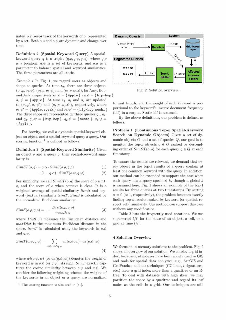
Fig. 2: Solution overview.

to unit length, and the weight of each keyword is pro-

portional to the keyword’s inverse document frequency

(idf) in a corpus. Static idf is assumed.

By the above definitions, our problem is defined as

follows.

Problem 1 (Continuous Top-k Spatial-Keyword

Search on Dynamic Objects) Given a set of dy-

namic objects O and a set of queries Q, our goal is to

monitor the top-k objects o ∈ O ranked by descend-

ing order of SimST (o, q) for each query q ∈ Q at each

timestamp.

To ensure the results are relevant, we demand that ev-

ery object in the top-k results of a query contain at

least one common keyword with the query. In addition,

our method can be extended to support the case when

each query has a query-specified k, though a global k

is assumed here. Fig. 1 shows an example of the top-1

results for three queries at two timestamps. By setting

α = 0 (or 1, respectively), the problem becomes exactly

finding top-k results ranked by keyword (or spatial, re-

spectively) similarity. Our method can support this case

without any modification.

Table 2 lists the frequently used notations. We use

superscript t/t′ for the state of an object, a cell, or a

grid at time t/t′.

4 Solution Overview

We focus on in-memory solutions to the problem. Fig. 2

shows an overview of our solution. We employ a grid in-

dex, because grid indexes have been widely used in GIS

and tools for spatial data analytics, e.g., ArcGIS and

GeoPandas, and our techniques (CC links, l-signatures,

etc.) favor a grid index more than a quadtree or an R-

tree. To deal with datasets with high skew, we may

partition the space by a quadtree and regard its leaf

nodes as the cells in a grid. Our techniques are still

5

applicable because they do not rely on how the space

is partitioned. Besides, our method does not rely on a

global k. It is easy to support the case when the k val-

ues vary across queries. In the grid, an object or a query

is indexed in the cell in which it is located. We assume

that in the initial state, there have already been a set

of objects and a set of queries, and the top-k results

of the queries have been computed. Since our focus is

to solve the dynamic case of the problem, we leave the

details of initialization to Section 8. When the state of

an object changes, the grid index is updated. Then we

update the top-k results for queries. Two modules are

designed for efficient query processing: (1) an affected

query finder that finds the set of affected queries (by

“affected”, we mean at least one top-k object of this

query is replaced or changes its similarity w.r.t. the

query), and (2) a top-k refiller that updates top-k

results of these affected queries.

5 Affected Query Finder

When a new state of an object is received, the affected

query finder finds the affected queries whose top-k re-

sults or their scores need to be updated. Given ot and

ot′, the states of an object o at two contiguous times-

tamps t and t′, the change from ot to ot′

affects two sets

of queries:

– Qprev: the set of queries such that o is a top-k result

of q at t.

– Qnext: the set of queries such that SimST (ot′, q) >

q.score(k, t).

Qprev refers to the queries to which ot potentially moves

out of top-k, while Qnext refers to the queries to which

ot′

is guaranteed to be a top-k result. They may overlap

because o may stay as a top-k result despite the change

of state. It is easy to see that the other queries in Q can

be safely excluded.

To compute Qprev, we assume that the top-k re-

sults of all the queries at t have been correctly com-

puted. Hence, an object-query map (implemented as an

inverted index) can be employed to map o to a list of

queries of which o is a top-k result. The map is updated

whenever a top-k result of a query changes. Comput-

ing Qnext is much more challenging. A sequential scan

of Q is too time-consuming for real applications. We

propose a method of computing Qnext composed of the

following two procedures: (1) exploiting the grid index

to find out the cells that may contain a query in Qnext;

and (2) for each cell in (1), identifying the queries that

share a necessary number of keywords with o using an

efficient search algorithm. Two data structures, cell-cell

link and l-signatures, are developed to handle the two

procedures. Next we introduce them respectively.

5.1 Cell-Cell Links

Since the keyword similarity SimT is no greater than 1

and the minimum distance between two cells is static,

it is easy to derive a score upperbound for a query lo-

cated in a different cell from ot′’s. CIQ and SKYPE index

queries in a quadtree and exploit this bound. By com-

paring the bound with the score of the k-th object at

t, unpromising cells (i.e., those too far from ot′

to have

a bound over the k-th object’s score) can be pruned by

traversing the quadtree. However, when adapting CIQor SKYPE for our problem, index access could be ex-

pensive because the pruning at the first few depths of

the quadtree is less effective, meaning that we have to

go deeper in the quadtree and access quite a number of

cells. Moreover, even if a cell can be pruned, we only

get aware of this after comparing the score bound with

the smallest k-th object’s score in this cell. Such com-

parison is invoked many times and significantly affects

the performance. Seeing this inefficiency, we seek a so-

lution to finding Qnext by answering the question: can

we avoid the comparison so that the unpromising cells

are not even accessed?

Given ot′.c, the cell in which ot

′is located, our ba-

sic idea is to store at ot′.c a set of links that directly

point to the cells having at least one possible query in

Qnext. In doing so, we can quickly identify these cells

and circumvent the access to the unpromising ones. We

call these links cell-cell links and CC links for short.In this sense, the cells in the grid are the vertices of

a directed graph, and there is an edge from ot′.c to a

cell c if c potentially has a query in Qnext. For the sake

of efficiency, the update to the CC links needs to be

infrequent.

Based on this idea, we first derive the upperbound of

score across cells. Given ot′.c and q.c (the cell in which

q is located), by Eq. 1, we have an upperbound of score

of ot′

and q, assuming the keyword similarity is 1:

UBSimST (ot′ .c,q.c) = q.α ·UBSimS(ot′ .c,q.c)+1−q.α. (5)

UBSimS(ot′ .c,q.c) is the upperbound of spatial similarity

between ot′.c and q.c: UBSimS(ot′ .c,q.c) = 1−minD(ot

′.c,q.c)

maxDist ,

where minD(ot′.c, q.c) is the minimum distance from

ot′.c to q.c. Comparing UBSimST (ot′ .c,q.c) and q.score(k, t),

we have:

Lemma 1 Consider an object ot′and a query q ∈ Qnext.

UBSimS(ot′ .c,q.c) >q.score(k,t)+q.α−1

q.α .

6

Algorithm 1: AQF(ot, ot′)

Input : the states of o at t and t′

Output : affected queries Qprev and Qnext1 Qprev ← the queries in the object-query map of o;

2 foreach c connected by an outgoing CC link of ot′.c

do

3 Qnext ← Qnext ∪ GetQueryIn(c, ot′);

4 return Qprev , Qnext

Proof By the definition ofQnext, we have SimST (ot′, q)

> q.score(k, t). Because UBSimST (ot′ .c,q.c) is the score

upperbound of ot′and q, UBSimST (ot′ .c,q.c) > q.score(k, t).

By Eq. 5, q.α ·UBSimS(ot′ .c,q.c)+1−q.α > q.score(k, t).

Therefore, UBSimS(ot′ .c,q.c) >q.score(k,t)+q.α−1

q.α . ut

The lemma means that a cell c has a query in Qnext,

only if it is close enough to ot′.c. For each cell c, it

is obvious that only the query yielding the minimumq.score(k,t)+q.α−1

q.α has to be considered. We connected

the cells that satisfy the condition in Lemma 1 by CC

links, each of which is an edge from ot′.c to c. It can

be seen that only when the minimum q.score(k,t)+q.α−1q.α

of a cell changes, the incoming CC links of this cell are

updated. Hence we can achieve the goal of infrequent

update.

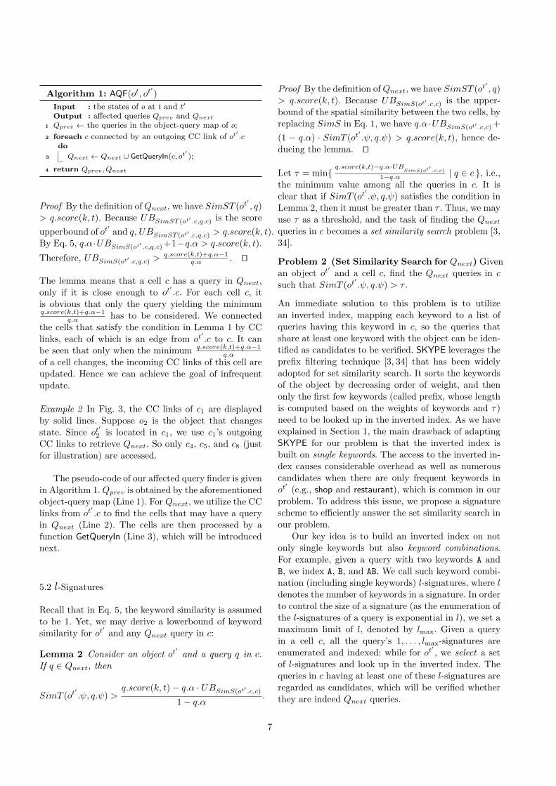
Example 2 In Fig. 3, the CC links of c1 are displayed

by solid lines. Suppose o2 is the object that changes

state. Since ot′

2 is located in c1, we use c1’s outgoing

CC links to retrieve Qnext. So only c4, c5, and c8 (just

for illustration) are accessed.

The pseudo-code of our affected query finder is given

in Algorithm 1.Qprev is obtained by the aforementioned

object-query map (Line 1). For Qnext, we utilize the CC

links from ot′.c to find the cells that may have a query

in Qnext (Line 2). The cells are then processed by a

function GetQueryIn (Line 3), which will be introduced

next.

5.2 l-Signatures

Recall that in Eq. 5, the keyword similarity is assumed

to be 1. Yet, we may derive a lowerbound of keyword

similarity for ot′

and any Qnext query in c:

Lemma 2 Consider an object ot′and a query q in c.

If q ∈ Qnext, then

SimT (ot′.ψ, q.ψ) >

q.score(k, t)− q.α · UBSimS(ot′ .c,c)1− q.α

.

Proof By the definition ofQnext, we have SimST (ot′, q)

> q.score(k, t). Because UBSimS(ot′ .c,c) is the upper-

bound of the spatial similarity between the two cells, by

replacing SimS in Eq. 1, we have q.α ·UBSimS(ot′ .c,c) +

(1 − q.α) · SimT (ot′.ψ, q.ψ) > q.score(k, t), hence de-

ducing the lemma. ut

Let τ = min{q.score(k,t)−q.α·UB

SimS(ot′.c,c)

1−q.α | q ∈ c }, i.e.,

the minimum value among all the queries in c. It is

clear that if SimT (ot′.ψ, q.ψ) satisfies the condition in

Lemma 2, then it must be greater than τ . Thus, we may

use τ as a threshold, and the task of finding the Qnextqueries in c becomes a set similarity search problem [3,

34].

Problem 2 (Set Similarity Search for Qnext) Given

an object ot′

and a cell c, find the Qnext queries in c

such that SimT (ot′.ψ, q.ψ) > τ .

An immediate solution to this problem is to utilize

an inverted index, mapping each keyword to a list of

queries having this keyword in c, so the queries that

share at least one keyword with the object can be iden-

tified as candidates to be verified. SKYPE leverages the

prefix filtering technique [3, 34] that has been widely

adopted for set similarity search. It sorts the keywords

of the object by decreasing order of weight, and then

only the first few keywords (called prefix, whose length

is computed based on the weights of keywords and τ)

need to be looked up in the inverted index. As we have

explained in Section 1, the main drawback of adapting

SKYPE for our problem is that the inverted index is

built on single keywords. The access to the inverted in-

dex causes considerable overhead as well as numerous

candidates when there are only frequent keywords in

ot′

(e.g., shop and restaurant), which is common in our

problem. To address this issue, we propose a signature

scheme to efficiently answer the set similarity search in

our problem.

Our key idea is to build an inverted index on not

only single keywords but also keyword combinations.

For example, given a query with two keywords A and

B, we index A, B, and AB. We call such keyword combi-

nation (including single keywords) l-signatures, where l

denotes the number of keywords in a signature. In order

to control the size of a signature (as the enumeration of

the l-signatures of a query is exponential in l), we set a

maximum limit of l, denoted by lmax. Given a query

in a cell c, all the query’s 1, . . . , lmax-signatures are

enumerated and indexed; while for ot′, we select a set

of l-signatures and look up in the inverted index. The

queries in c having at least one of these l-signatures are

regarded as candidates, which will be verified whether

they are indeed Qnext queries.

7

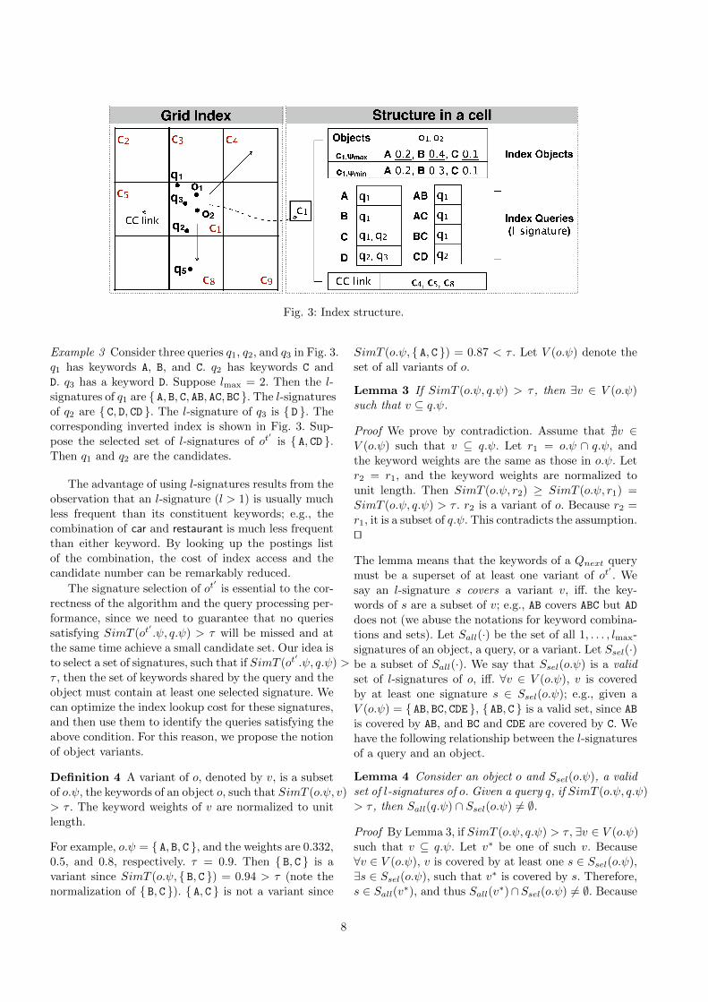
Fig. 3: Index structure.

Example 3 Consider three queries q1, q2, and q3 in Fig. 3.

q1 has keywords A, B, and C. q2 has keywords C and

D. q3 has a keyword D. Suppose lmax = 2. Then the l-

signatures of q1 are { A, B, C, AB, AC, BC }. The l-signatures

of q2 are { C, D, CD }. The l-signature of q3 is { D }. The

corresponding inverted index is shown in Fig. 3. Sup-

pose the selected set of l-signatures of ot′

is { A, CD }.Then q1 and q2 are the candidates.

The advantage of using l-signatures results from the

observation that an l-signature (l > 1) is usually much

less frequent than its constituent keywords; e.g., the

combination of car and restaurant is much less frequent

than either keyword. By looking up the postings list

of the combination, the cost of index access and the

candidate number can be remarkably reduced.

The signature selection of ot′

is essential to the cor-

rectness of the algorithm and the query processing per-

formance, since we need to guarantee that no queries

satisfying SimT (ot′.ψ, q.ψ) > τ will be missed and at

the same time achieve a small candidate set. Our idea is

to select a set of signatures, such that if SimT (ot′.ψ, q.ψ) >

τ , then the set of keywords shared by the query and the

object must contain at least one selected signature. We

can optimize the index lookup cost for these signatures,

and then use them to identify the queries satisfying the

above condition. For this reason, we propose the notion

of object variants.

Definition 4 A variant of o, denoted by v, is a subset

of o.ψ, the keywords of an object o, such that SimT (o.ψ, v)

> τ . The keyword weights of v are normalized to unit

length.

For example, o.ψ = { A, B, C }, and the weights are 0.332,

0.5, and 0.8, respectively. τ = 0.9. Then { B, C } is a

variant since SimT (o.ψ, { B, C }) = 0.94 > τ (note the

normalization of { B, C }). { A, C } is not a variant since

SimT (o.ψ, { A, C }) = 0.87 < τ . Let V (o.ψ) denote the

set of all variants of o.

Lemma 3 If SimT (o.ψ, q.ψ) > τ , then ∃v ∈ V (o.ψ)

such that v ⊆ q.ψ.

Proof We prove by contradiction. Assume that @v ∈V (o.ψ) such that v ⊆ q.ψ. Let r1 = o.ψ ∩ q.ψ, and

the keyword weights are the same as those in o.ψ. Let

r2 = r1, and the keyword weights are normalized to

unit length. Then SimT (o.ψ, r2) ≥ SimT (o.ψ, r1) =

SimT (o.ψ, q.ψ) > τ . r2 is a variant of o. Because r2 =

r1, it is a subset of q.ψ. This contradicts the assumption.

ut

The lemma means that the keywords of a Qnext query

must be a superset of at least one variant of ot′. We

say an l-signature s covers a variant v, iff. the key-

words of s are a subset of v; e.g., AB covers ABC but AD

does not (we abuse the notations for keyword combina-

tions and sets). Let Sall(·) be the set of all 1, . . . , lmax-

signatures of an object, a query, or a variant. Let Ssel(·)be a subset of Sall(·). We say that Ssel(o.ψ) is a valid

set of l-signatures of o, iff. ∀v ∈ V (o.ψ), v is covered

by at least one signature s ∈ Ssel(o.ψ); e.g., given a

V (o.ψ) = { AB, BC, CDE }, { AB, C } is a valid set, since AB

is covered by AB, and BC and CDE are covered by C. We

have the following relationship between the l-signatures

of a query and an object.

Lemma 4 Consider an object o and Ssel(o.ψ), a valid

set of l-signatures of o. Given a query q, if SimT (o.ψ, q.ψ)

> τ , then Sall(q.ψ) ∩ Ssel(o.ψ) 6= ∅.

Proof By Lemma 3, if SimT (o.ψ, q.ψ) > τ , ∃v ∈ V (o.ψ)

such that v ⊆ q.ψ. Let v∗ be one of such v. Because

∀v ∈ V (o.ψ), v is covered by at least one s ∈ Ssel(o.ψ),

∃s ∈ Ssel(o.ψ), such that v∗ is covered by s. Therefore,

s ∈ Sall(v∗), and thus Sall(v∗)∩Ssel(o.ψ) 6= ∅. Because

8

v∗ ⊆ q.ψ, Sall(v∗) ⊆ Sall(q.ψ). Therefore, Sall(q.ψ) ∩

Ssel(o.ψ) ⊇ Sall(v∗) ∩ Ssel(o) 6= ∅. ut

By this lemma, we can select a valid set of l-signatures

for ot′. It is guaranteed that any Qnext query must share

at least one of these selected signatures. For the sake of

efficiency, we need to minimize the cost of the selected

signatures. The lengths of postings lists in the inverted

index are used here to measure the cost. Then the l-

signature selection problem is defined below.

Problem 3 (l-signature Selection) Let |Ls| denote

the length of the postings list of a signature s in the

inverted index. Given an object o and a threshold τ ,

the l-signature selection problem is to select Ssel(o.ψ), a

valid set of l-signatures for o, such that∑s∈Ssel(o.ψ)

|Ls|is minimized.

It is easy to see that the l-signature selection prob-

lem is exactly a minimum weighted set cover problem.

Hence it is NP-hard and can be solved by a greedy algo-

rithm with an approximation ratio ofO(ln|V (o.ψ)|) [40].

Given variants V (o.ψ) and all the l-signatures of o,

the greedy algorithm picks signatures in the order of

decreasing benefit-to-cost ratio. The benefit of an l-

signature is the number of variants that it covers in

the uncovered part of V (o.ψ). The time complexity

of the greedy algorithm is O(|Sall(o.ψ)| · |V (o.ψ)|) =

O((|o.ψ|lmax

)· (2|o.ψ| − 1)). |o.ψ| is usually small in real ap-

plications, and we can choose a small lmax to control the

enumeration cost of Sall(o.ψ). Since it is difficult to es-

timate the number of selected signatures by the greedy

algorithm, we will choose lmax through empirical study

rather than using a cost model.

Enumerating variants. Prior to running the greedy al-

gorithm, a technical challenge is to compute V (o.ψ).

One may notice that we only need to cover the mini-

mal variants (i.e., the variant such that we cannot re-

move any keyword from it and still make a variant) in

V (o.ψ) instead of all. However, the minimality check is

costly. We take a compromise to quickly find a subset

of V (o.ψ) and still guarantee the selected l-signatures

cover V (o.ψ): First, we sort the keywords of o.ψ by de-

creasing order of weights, and pick keywords one by

one until we get a variant. It can be seen that the num-

ber of picked keywords is the minimum number of key-

words of a variant. So we only enumerate subsets of o.ψ

whose sizes are no smaller than this number. By enu-

merating subsets of o.ψ in increasing order of size, we

can stop when reaching a size such that all the subsets

of this size are variants. Let V ′(o.ψ) denote the set of

variants we have enumerated. We replace V (o.ψ) with

V ′(o.ψ) and run the greedy algorithm. The returned l-

signatures are guaranteed to cover V (o.ψ), because any

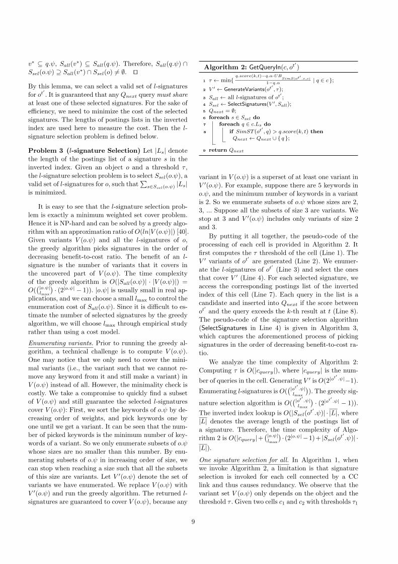
Algorithm 2: GetQueryIn(c, ot′)

1 τ ← min{q.score(k,t)−q.α·UB

SimS(ot′.c,c)

1−q.α | q ∈ c };2 V ′ ← GenerateVariants(ot

′, τ);

3 Sall ← all l-signatures of ot′;

4 Ssel ← SelectSignatures(V ′, Sall);5 Qnext = ∅;6 foreach s ∈ Ssel do7 foreach q ∈ c.Ls do

8 if SimST (ot′, q) > q.score(k, t) then

Qnext ← Qnext ∪ { q };

9 return Qnext

variant in V (o.ψ) is a superset of at least one variant in

V ′(o.ψ). For example, suppose there are 5 keywords in

o.ψ, and the minimum number of keywords in a variant

is 2. So we enumerate subsets of o.ψ whose sizes are 2,

3, ... Suppose all the subsets of size 3 are variants. We

stop at 3 and V ′(o.ψ) includes only variants of size 2

and 3.

By putting it all together, the pseudo-code of the

processing of each cell is provided in Algorithm 2. It

first computes the τ threshold of the cell (Line 1). The

V ′ variants of ot′

are generated (Line 2). We enumer-

ate the l-signatures of ot′

(Line 3) and select the ones

that cover V ′ (Line 4). For each selected signature, we

access the corresponding postings list of the inverted

index of this cell (Line 7). Each query in the list is a

candidate and inserted into Qnext if the score between

ot′

and the query exceeds the k-th result at t (Line 8).

The pseudo-code of the signature selection algorithm

(SelectSignatures in Line 4) is given in Algorithm 3,

which captures the aforementioned process of picking

signatures in the order of decreasing benefit-to-cost ra-

tio.

We analyze the time complexity of Algorithm 2:

Computing τ is O(|cquery|), where |cquery| is the num-

ber of queries in the cell. Generating V ′ is O(2|ot′ .ψ|−1).

Enumerating l-signatures is O((|ot′ .ψ|lmax

)). The greedy sig-

nature selection algorithm is O((|ot′ .ψ|lmax

)· (2|ot

′.ψ| − 1)).

The inverted index lookup is O(|Ssel(ot′.ψ)| · |L|, where

|L| denotes the average length of the postings list of

a signature. Therefore, the time complexity of Algo-

rithm 2 is O(|cquery|+(|o.ψ|lmax

)· (2|o.ψ|−1)+ |Ssel(ot

′.ψ)| ·

|L|).

One signature selection for all. In Algorithm 1, when

we invoke Algorithm 2, a limitation is that signature

selection is invoked for each cell connected by a CC

link and thus causes redundancy. We observe that the

variant set V (o.ψ) only depends on the object and the

threshold τ . Given two cells c1 and c2 with thresholds τ1

9

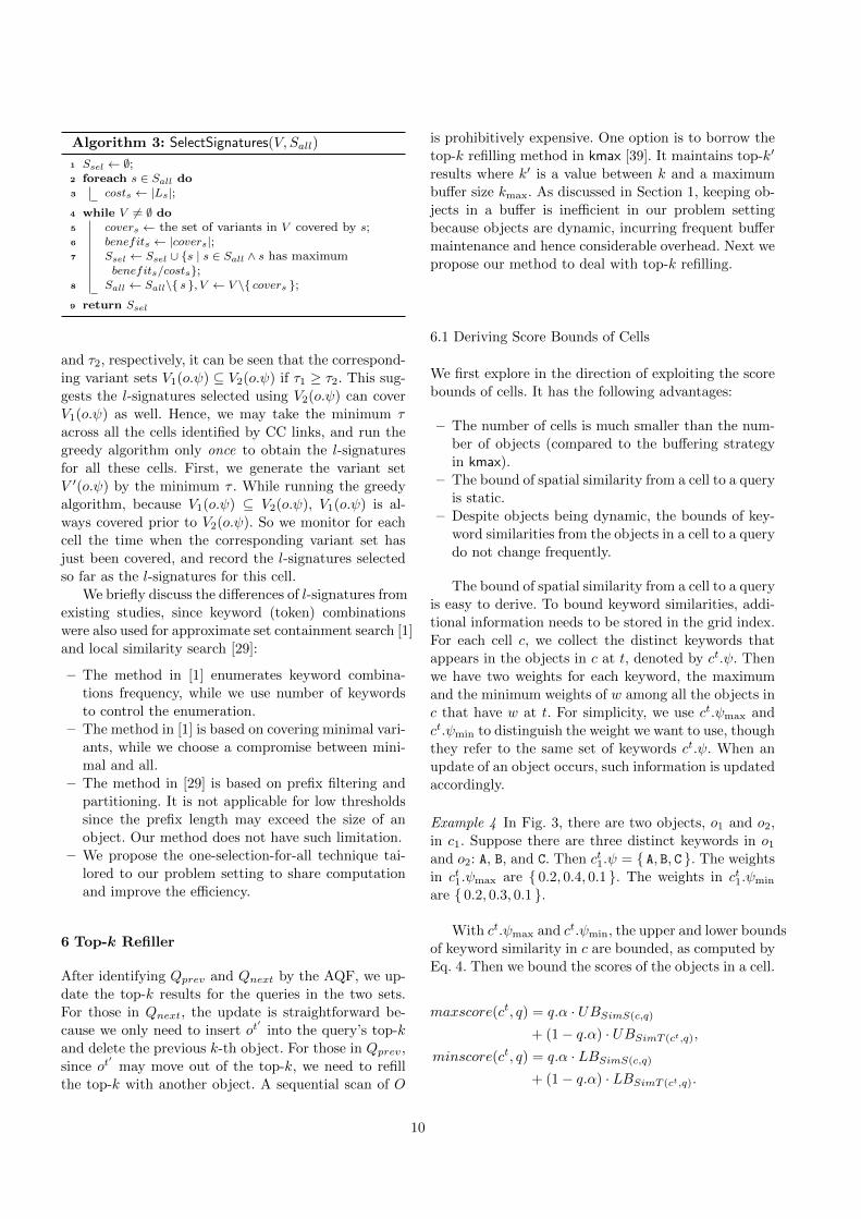
Algorithm 3: SelectSignatures(V, Sall)

1 Ssel ← ∅;2 foreach s ∈ Sall do3 costs ← |Ls|;

4 while V 6= ∅ do5 covers ← the set of variants in V covered by s;6 benefits ← |covers|;7 Ssel ← Ssel ∪ {s | s ∈ Sall ∧ s has maximum

benefits/costs};8 Sall ← Sall\{ s }, V ← V \{ covers };

9 return Ssel

and τ2, respectively, it can be seen that the correspond-

ing variant sets V1(o.ψ) ⊆ V2(o.ψ) if τ1 ≥ τ2. This sug-

gests the l-signatures selected using V2(o.ψ) can cover

V1(o.ψ) as well. Hence, we may take the minimum τ

across all the cells identified by CC links, and run the

greedy algorithm only once to obtain the l-signatures

for all these cells. First, we generate the variant set

V ′(o.ψ) by the minimum τ . While running the greedy

algorithm, because V1(o.ψ) ⊆ V2(o.ψ), V1(o.ψ) is al-

ways covered prior to V2(o.ψ). So we monitor for each

cell the time when the corresponding variant set has

just been covered, and record the l-signatures selected

so far as the l-signatures for this cell.

We briefly discuss the differences of l-signatures from

existing studies, since keyword (token) combinations

were also used for approximate set containment search [1]

and local similarity search [29]:

– The method in [1] enumerates keyword combina-

tions frequency, while we use number of keywords

to control the enumeration.

– The method in [1] is based on covering minimal vari-

ants, while we choose a compromise between mini-

mal and all.

– The method in [29] is based on prefix filtering and

partitioning. It is not applicable for low thresholds

since the prefix length may exceed the size of an

object. Our method does not have such limitation.

– We propose the one-selection-for-all technique tai-

lored to our problem setting to share computation

and improve the efficiency.

6 Top-k Refiller

After identifying Qprev and Qnext by the AQF, we up-

date the top-k results for the queries in the two sets.

For those in Qnext, the update is straightforward be-

cause we only need to insert ot′

into the query’s top-k

and delete the previous k-th object. For those in Qprev,

since ot′

may move out of the top-k, we need to refill

the top-k with another object. A sequential scan of O

is prohibitively expensive. One option is to borrow the

top-k refilling method in kmax [39]. It maintains top-k′

results where k′ is a value between k and a maximum

buffer size kmax. As discussed in Section 1, keeping ob-

jects in a buffer is inefficient in our problem setting

because objects are dynamic, incurring frequent buffer

maintenance and hence considerable overhead. Next we

propose our method to deal with top-k refilling.

6.1 Deriving Score Bounds of Cells

We first explore in the direction of exploiting the score

bounds of cells. It has the following advantages:

– The number of cells is much smaller than the num-

ber of objects (compared to the buffering strategy

in kmax).

– The bound of spatial similarity from a cell to a query

is static.

– Despite objects being dynamic, the bounds of key-

word similarities from the objects in a cell to a query

do not change frequently.

The bound of spatial similarity from a cell to a query

is easy to derive. To bound keyword similarities, addi-

tional information needs to be stored in the grid index.

For each cell c, we collect the distinct keywords that

appears in the objects in c at t, denoted by ct.ψ. Then

we have two weights for each keyword, the maximum

and the minimum weights of w among all the objects in

c that have w at t. For simplicity, we use ct.ψmax and

ct.ψmin to distinguish the weight we want to use, though

they refer to the same set of keywords ct.ψ. When an

update of an object occurs, such information is updated

accordingly.

Example 4 In Fig. 3, there are two objects, o1 and o2,

in c1. Suppose there are three distinct keywords in o1and o2: A, B, and C. Then ct1.ψ = { A, B, C }. The weights

in ct1.ψmax are { 0.2, 0.4, 0.1 }. The weights in ct1.ψmin

are { 0.2, 0.3, 0.1 }.

With ct.ψmax and ct.ψmin, the upper and lower bounds

of keyword similarity in c are bounded, as computed by

Eq. 4. Then we bound the scores of the objects in a cell.

maxscore(ct, q) = q.α · UBSimS(c,q)+ (1− q.α) · UBSimT (ct,q),

minscore(ct, q) = q.α · LBSimS(c,q)+ (1− q.α) · LBSimT (ct,q).

10

UBSimS and LBSimS are upper and lower bounds of

spatial similarity, respectively:

UBSimS(c,q) = 1− minD(c, q.ρ)

maxDist,

LBSimS(c,q) = 1− maxD(c, q.ρ)

maxDist,

where minD(c, q.ρ) and maxD(c, q.ρ) denote the min-

imum and the maximum distances from a cell to the

query location, respectively. UBSimT and LBSimT are

upper and lower bounds of keyword similarity, respec-

tively:

UBSimT (ct,q) = SimT (ct.ψmax, q.ψ),

LBSimT (ct,q) = min{wt(ct.ψmin, w) · wt(q.ψ,w)

| w ∈ ct.ψmin ∩ q.ψ }.

Note that these bounds are tight bounds because ob-

jects may reside on cell boundaries and contain the

same keywords (and weights) as ct.ψmax or ct.ψmin.

6.2 Maintaining Cell Lists

One may design an algorithm to leverage the derived

score bounds for pruning, yet a caveat is that a sequen-

tially scan of all the cells in the grid should be avoided.

To this end, we notice that when ot changes to ot′, at

most one object in the top-k of q changes. Moreover,

we have the following observation.

Observation 1 Consider an old state ot and a new

state ot′of an object. For any q ∈ Qprev, q.o(1 . . k, t′)

\ q.obj(1 . . k, t) = { o } or { q.obj(k + 1, t) }.

q.obj(k+1, t) is the (k+1)-th result of q at time t. The

observation indicates that we only need to compare ot′

and q.obj(k + 1, t), and pick the one with the higher

score as the new top-k result of q. Based on this obser-

vation, we are able to exploit the score bounds in a more

effective way by maintaining a cell list (CL) for each q

such that the (k + 1)-th object of q at t is guaranteed

to reside in one of these cells 2. We have:

Lemma 5 If minscore(ct, q) > q.score(k, t), q.obj(k+

1, t) 6∈ ct.

Proof Because minscore(ct, q) > q.score(k, t), we have

∀oi ∈ ct, SimST (oti, q) > q.score(k, t) ≥ q.score(k +

1, t). Therefore, q.obj(k + 1, t) 6∈ ct. ut

2 One may want to keep only the (k+1)-th object, but thisobject may change state while q is outside both Qprev andQnext, hence difficult to track.

Letmaxminscore<k(Ct, q) = max{minscore(ct, q) |c ∈ C∧maxscore(ct, q) < q.score(k, t) }; i.e., we collect

the cells whosemaxscore values are less than q.score(k, t),

and pick the the maximum of their minscore values.

Lemma 6 Ifmaxscore(ct, q) < maxminscore<k(Ct, q),

then q.obj(k + 1, t) 6∈ ct.

Proof We prove by contradiction: assume q.obj(k+1, t) ∈ct. Let c∗ be the cell that yields maxminscore<k(Ct, q);

i.e.,maxminscore<k(Ct, q) = minscore(c∗t

, q). Because

maxscore(ct, q) < maxminscore<k(Ct, q),maxscore(ct, q)

< minscore(c∗t

, q). Because maxscore and minscore

are scores’ upper and lower bounds, respectively, and

q.obj(k+1, t) ∈ ct, we have ∃o′ ∈ c∗t , s.t. SimST (o′t, q) >

q.score(k + 1, t). By the definition of maxminscore<k,

maxscore(c∗t

, q) < q.score(k, t). Therefore, SimST (o′t, q)

< q.score(k, t), meaning that SimST (o′t, q) ≤ q.score(k+

1, t). This contradicts SimST (o′t, q) > q.score(k+1, t).

ut

Intuitively, the two lemmata state that if a cell whose

score bounds are too high or too low, then the (k+ 1)-

th result is not in it. So by taking the complement of

these cells in the grid, we are guaranteed to include the

(k + 1)-th result’s cell:

Corollary 1 Consider a set of cells

C ′ = {c ∈ C | minscore(ct, q) ≤ q.score(k, t)∧ maxscore(ct, q) ≥ maxminscore<k(Ct, q)}.

∃c ∈ C ′, s.t., q.obj(k + 1, t) ∈ ct.

Proof We prove by contradiction. If @c ∈ C ′, s.t., q.obj(k+

1, t) ∈ ct, by the definition of C ′, the cell that has

q.obj(k+1, t), denoted by c′, satisfies minscore(c′t, q) >

q.score(k, t) ormaxscore(c′t, q) < maxminscore<k(Ct, q).

This either contradicts Lemma 5 or Lemma 6. ut

Although it is sufficient to fetch the (k + 1)-th re-

sult with only C ′ in Corollary 1, we also store the cells

having the top-1, . . . , k results. This is to simplify the

update of CL (introduced later). As such, we define the

(k + 1)-CL of q:

Definition 5 ((k+1)-CL) The (k+1)-CL of a query q

with a timestamp t is defined as {c ∈ C | maxscore(ct, q)≥ maxminscore<k(Ct, q)}.

Compared to Corollary 1, we remove the condition on

minscore. In the rest of this section, we mean (k + 1)-

CL when CL is mentioned, and we use q.CL to denote

the CL of q. Since we will use a lazy update strategy,

the corresponding timestamp is recorded along with the

CL, denoted by q.CL.t.

11

1 0

…

SimST score w.r.t q

c5 c1c2 c6

maxminscore<k(ct,q)

cn

maxscore(cn,q)minscore(cn,q)

cell maxscore minscore

c5 0.78 0.72

c2 0.65 …

c1 … …

c6 … …

Time t

q.CL on t

time cell

… …

t0 …

… c8

t …

!C

cell maxscore minscore

c5 0.78 0.72

c2 0.65 …

c8 … …

c6 … …

q.CL on t0Union c!

update

1 0SimST score w.r.t q

c5c1

c2c8

maxminscore<k(ct0,q)Time t0

c6

c8

…

q.score(k,t)

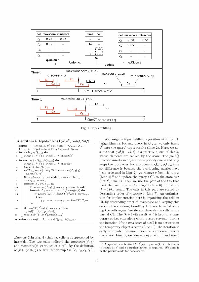
Fig. 4: top-k refilling.

Algorithm 4: TopKRefiller-CL(ot, ot′, OutQ, InQ)

Input : the states of o at t and t′, Qprev, QnextOutput : top-k results for q ∈ Qprev ∪Qnext

1 for each q ∈ Qnext do2 q.obj(1 . . k, t′)← q.obj(1 . . k, t).push(o);

3 foreach q ∈ {Qprev\Qnext} do4 q.obj(1 . . k, t′)← q.obj(1 . . k, t).pop(o);5 UpdateCL(q.CL, q, t);6 q.CL≤k ← { c | c ∈ q.CL ∧minscore(ct, q) ≤

q.score(k, t) };7 Sort q.CL≤k by descending maxscore(ct, q);8 scorek+1 ← −∞;9 foreach c ∈ q.CL≤k do

10 if maxscore(ct, q) ≤ scorek+1 then break;11 foreach o′ ∈ c such that o′ 6= q.obj(k, t) do12 if q.score(k, t) ≥ SimST (o′t, q) > scorek+1

then13 ok+1 ← o′, scorek+1 ← SimST (o′t, q);

14 if SimST (ot′, q) ≥ scorek+1 then

q.obj(1 . . k, t′).push(o);15 else q.obj(1 . . k, t′).push(ok+1);

16 return { q.obj(1 . . k, t′) | q ∈ Qprev ∪Qnext }

Example 5 In Fig. 4 (time t), cells are represented by

intervals. The two ends indicate the maxscore(ct, q)

and minscore(ct, q) values of a cell. By the definition

of (k+1)-CL, q.CL with timestamp t is { c5, c2, c1, c6 }.

We design a top-k refilling algorithm utilizing CL

(Algorithm 4). For any query in Qnext, we only insert

ot′

into the query’ top-k results (Line 2). Here, we as-

sume that q.obj(1 . . k, t) is a priority queue of size k,

whose elements are ranked by the score. The push()

function inserts an object to the priority queue and only

keeps the top-k ones. For any query in Qprev\Qnext (the

set difference is because the overlapping queries have

been processed in Line 2), we remove o from the top-k

(Line 4) 3 and update the query’s CL to the state at t

(not t′, Line 5). Then we use the part of the CL that

meet the condition in Corollary 1 (Line 6) to find the

(k + 1)-th result. The cells in this part are sorted by

descending order of maxscore (Line 7). An optimiza-

tion for implementation here is organizing the cells in

CL by descending order of maxscore and keeping this

order when checking Corollary 1, hence to avoid sort-

ing the cells again. We iterate through the cells in the

partial CL. The (k + 1)-th result at t is kept in a tem-

porary object ok+1 along with its score scorek+1 during

the iteration. If the maxscore of a cell is no better than

the temporary object’s score (Line 10), the iteration is

early terminated because unseen cells are even lower in

maxscore. Finally, we compare ok+1 with o and insert

3 A special case is SimST (ot′, q) = q.score(k, t). o is the k-

th result at t′ and no further action is required. We omit itin the pseudo-code for conciseness.

12

the one with the higher score to the top-k results of q

(Lines 14 – 15).

Example 6 We consider a query q in Qprev\Qnext. In

Fig. 4, the cell list of q with timestamp t includes c5, c2,

c1, and c6. Since c5 violates the condition in Corollary 1

(minscore(ct, q) ≤ q.score(k, t)), we only access c2, c1,

and c6 to retrieve the (k + 1)-th result at t. Then it

is compared with ot′. The one with the higher score is

refilled to the top-k of q at t′.

We analyze the time complexity of Algorithm 4 by

assuming that a priority queue operation (push/pop)

runs in O(1) time: Processing Qnext is O(|Qnext|). For

the queries in Qprev\Qnext, each query runs in O(|C|+|q.CL| · |cobj |)-time. O(|C|) is the worst-case complexity

of updating a CL; O(|q.CL| · |cobj |) is the complexity of

the remaining process, where |cobj | denotes the average

number of objects in a cell. Therefore, the time com-

plexity of Algorithm 4 is O(|Qnext|) + |Qprev\Qnext| ·(|C|+ |q.CL| · |cobj |).

6.3 Cell List Update

An important step in Algorithm 4 is the update of CL

(Line 5), as we need to guarantee the CL has all the

cells satisfying the condition in Definition 5. A naive

way of update is to scan all the cells to make a CL

from scratch, but this essentially reduces the algorithm

to a sequential scan of all the cells. An efficient way is

to find the cells to be inserted or deleted from the exist-

ing CL. The challenge is that the CL’s timestamp (say,

t0) prior to the update could be very old compared to

t. Nonetheless, by Definition 5, the cells in the CL are

determined by maxscore, minscore, and q.score(k, t).

maxscore and minscore depend only on the keywords

that appear in the cell. We may keep track of the cells

whose c.ψmax or c.ψmin change, along with the times-

tamp at which the change happens. The new CL can

be computed using the old CL and the set of the cells

that change c.ψmax or c.ψmin during time interval (t0, t].

Let ∆C denote this set. We describe our solution to CL

update.

The key idea is to compute maxminscore<k(Ct, q),

so the inserted/deleted cells can be determined by com-

paring theirmaxscore values withmaxminscore<k(Ct, q).

To this end, we derive the following lemma.

Lemma 7 Consider q.CL, a cell list to be updated,

whose timestamp is t0. Let C∪ = q.CL∪∆C . We have:

if maxminscore<k(Ct∪, q) ≥ maxminscore<k(Ct0 , q),

then maxminscore<k(Ct, q) = maxmins(Ct∪, q).

Proof By the definition of maxminscore<k, ∀C ′ ⊆ C,

we havemaxminscore<k(Ct, q) ≥ maxminscore<k(C ′t, q).

Because C∪ ⊆ C, we have maxminscore<k(Ct, q) ≥maxminscore<k(Ct∪, q). So, if maxminscore<k(Ct, q)

6= maxminscore<k(Ct∪, q), thenmaxminscore<k(Ct, q)

> maxminscore<k(Ct∪, q). We assume this is true and

prove by contradiction. In this case, ∃c′ ∈ C\C∪, s.t.,

maxscore(c′t, q) > maxminscore<k(Ct∪, q). So because

maxminscore<k(Ct∪, q)≥ maxminscore<k(Ct0 , q), and

any cell in C\C∪ does not changemaxscore orminscore

during (t0, t], maxscore(c′t, q) = maxscore(c′t0 , q) >

maxminscore<k(Ct0 , q). This means c′ ∈ q.CL and

thus c′ ∈ C∪, which contradicts c′ ∈ C\C∪. ut

The lemma reveals under which condition we can make

the new CL using the old CL and ∆C . First, we up-

date the maxscore and minscore values of the cells

in q.CL and ∆C for timestamp t, and compute the

value of maxminscore<k(Ct∪, q) using these maxscore

and minscore values and q.score(k, t). Then we check if

maxminscore<k(Ct∪, q) is greater than or equal to that

of the old CL, i.e., maxminscore<k(Ct0 , q).

– If so,maxminscore<k(Ct, q) = maxminscore<k(Ct∪, q).

All the cells to be inserted or deleted must belong

to C∪. This is because the set of cells such that

maxscore(ct, q) ≥ maxminscore<k(Ct0 , q) is a su-

perset of the set of cells such that maxscore(ct, q) ≥maxminscore<k(Ct∪, q) = maxminscore<k(Ct, q),

and the former set is stored in C∪. Thus, the new

CL can be made using only C∪.

– Otherwise, we scan all the cells of the grid to make

the new CL.

The pseudo-code of the above process is captured

by Algorithm 5. Lines 1 – 4 update maxscore and

minscore in C∪ and compute maxminscore<k(Ct∪, q).

Lines 5 – 9 make the new CL using the cells in C∪only; i.e., inserting or deleting a cell after comparing

its maxscore with maxminscore<k(Ct∪, q). Lines 11 –

13 make the new CL by scanning all the cells in the

grid. The timestamp of the CL is updated to t eventu-

ally (Line 14). The time complexity of the algorithm is

O(|∆C | + |C∪|) if we only use the cells in C∪ to make

the new CL, or O(|C|) if we scan all the cells in the

grid.

Example 7 In Fig. 4, we assume that the old q.CL with

timestamp t0 is { c5, c2, c8, c6 }.maxminscore<k(Ct0 , q)

is given by minscore(ct06 , q). Suppose ∆C = { c1, c8 }.So C∪ = { c5, c2, c8, c6, c1 }. maxminscore<k(Ct∪, q) is

given by minscore(ct1, q). Since maxminscore<k(Ct∪, q)

> maxminscore<k(Ct0 , q), we havemaxminscore<k(Ct, q)

= maxminscore<k(Ct∪, q). So only the cells in C∪ are

considered to compute the new CL. We compare their

maxscore(ct, q) values with maxminscore<k(Ct, q). c8is deleted and c1 is inserted. After the update, the new

CL is { c5, c2, c1, c6 }.

13

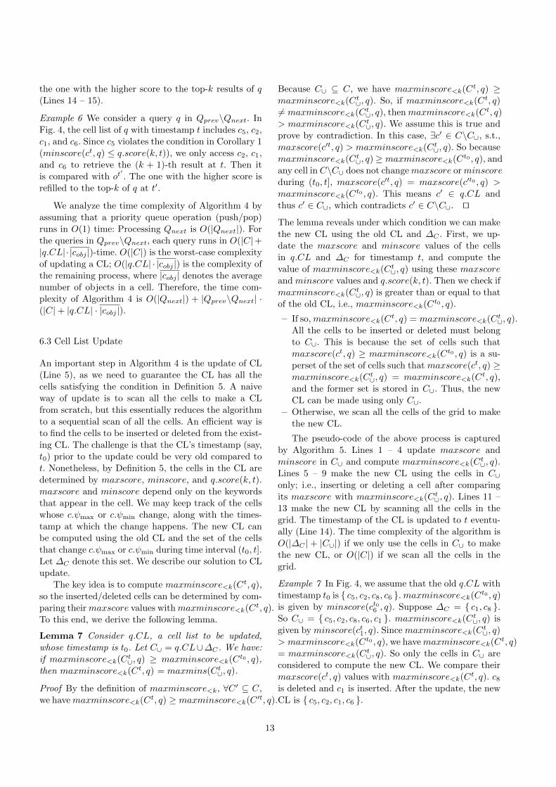
Algorithm 5: UpdateCL(q.CL, q, t)

1 ∆C ← the cells that change c.ψmax or c.ψmin in(q.CL.t, t];

2 foreach c ∈ ∆C do

3 Compute maxscore(ct, q) and minscore(ct, q);

4 C∪ ← q.CL ∪∆C , γ ← maxminscore<k(Ct∪, q);5 if γ ≥ maxminscore<k(Cq.CL.t, q) then

6 foreach c ∈ q.CL do7 if maxscore(ct, q) < γ then q.CL.delete(c);

8 foreach c ∈ ∆C\q.CL do9 if maxscore(ct, q) ≥ γ then q.CL.insert(c);

10 else11 q.CL.clear(), γ ← maxminscore<k(Ct, q);12 foreach c ∈ C do13 if maxscore(ct, q) ≥ γ then q.CL.insert(c);

14 q.CL.t← t;

7 Batch Processing

We assume that multiple objects change states during

time interval (t, t′]. Let Ot,t′

denote this set of objects.

Given the top-k results of each query at t, our task is

to compute the top-k results at t′.

7.1 Affected Query Finder

We first modify the definitions of Qprev and Qnext:

– Qprev: the multiset of queries such that ∃o ∈ Ot,t′ ,o is a top-k result of q at t.

– Qnext: the multiset of queries such that ∃o ∈ Ot,t′ ,SimST (ot

′, q) > q.score(k, t).

We define the occurrence of a query q in Qprev or Qnextas the number of objects in ∈ Ot,t′ satisfying the above

condition.

It is easy to see that the top-k results are not af-

fected if a query is in neither Qprev nor Qnext. The

computation of Qprev is straightforward. We scan the

objects in Ot,t′

and fetch Qprev queries by the object-

query map. To find Qnext queries, we scan the objects

in Ot,t′

and use CC links to identify the cells that need

look-up. An important observation is that objects may

share keywords and computation can be shared when

invoking Algorithm 2. Consider a cell c identified by

CC links from multiple objects in Ot,t′. Each object o

yields its own keyword similarity threshold. We gen-

erate the l-signature set Sall and the variant set V ′

for each object. Since these l-signature sets and vari-

ant sets may overlap, we take them together as the in-

put of the signature selection algorithm. While running

the signature selection, we monitor the time when the

variant set of an object has been covered, and record

the l-signatures selected so far. This resembles the one-

signature-selection-for-all technique described in Sec-

tion 5.2. Besides, the two techniques can work together.

As such, only one run of signature selection outputs

the l-signatures for all the Ot,t′

objects and all the cells

identified by CC links.

7.2 Top-k Refiller

Since Qprev and Qnext are multisets and may overlap,

for each query q, we count its occurrences in Qprev and

Qnext to determine what objects need to be refilled to

top-k. Let ∆q denote the difference of q’s occurrences

in Qprev and Qnext. If ∆q ≤ 0, the processing is simi-

lar to Qprev queries in the case of single object update:

we pop out the Qprev objects (i.e., the Ot,t′

objects

which are q’s top-k results at t), and push into q’s top-

k the Qnext objects (i.e., the Ot,t′

objects such that

SimST (ot′, q) > q.score(k, t)). If ∆q > 0, the process-

ing is similar to Qnext queries in the case of single object

update. The Qprev objects are popped out first. The CL

of q has to include the 2k-th object at t, because ∆q

can be up to k. To this end, maxminscore<k(Ct, q) is

replaced by kminscore<k(Ct, q), which is k-th largest

minscore(ct, q) of the cells in C such thatmaxscore(ct, q)

< q.score(k, t). Definition 5 is replaced by (2k)-CL. The

related lemmata, corollary, and algorithms are modi-

fied accordingly. Then we use the (2k)-CL to fetch the

(k+1)-th to 2k-th objects of q at t. They are compared

with the Qprev objects and the better ones are pushed

into q’s top-k, along with the Qnext objects.

8 Initialization and Query Updates

Initialization. We first create a grid index on the ob-

jects. The initialization of top-k results for each query

is a snapshot spatial-keyword search. We do not adopt

existing methods (surveyed in Section 2) as they ei-

ther target different problem settings or use different

indexes. Our method maintains a list of temporary top-

k results (initialized as empty). By starting from the

query’s cell, it iterates cells by a breadth-first search.

The objects in each cell are checked whether they out-

perform any temporary top-k result. This is repeated

until we reach the cells that are too far to make a score

better than the current k-th one. After obtaining top-

k results, the query is indexed in the grid. We create

an object-query map for each object and a cell list for

each query. Then we create the inverted index and CC

links for each cell, and compute the keyword similarity

threshold τ .

14

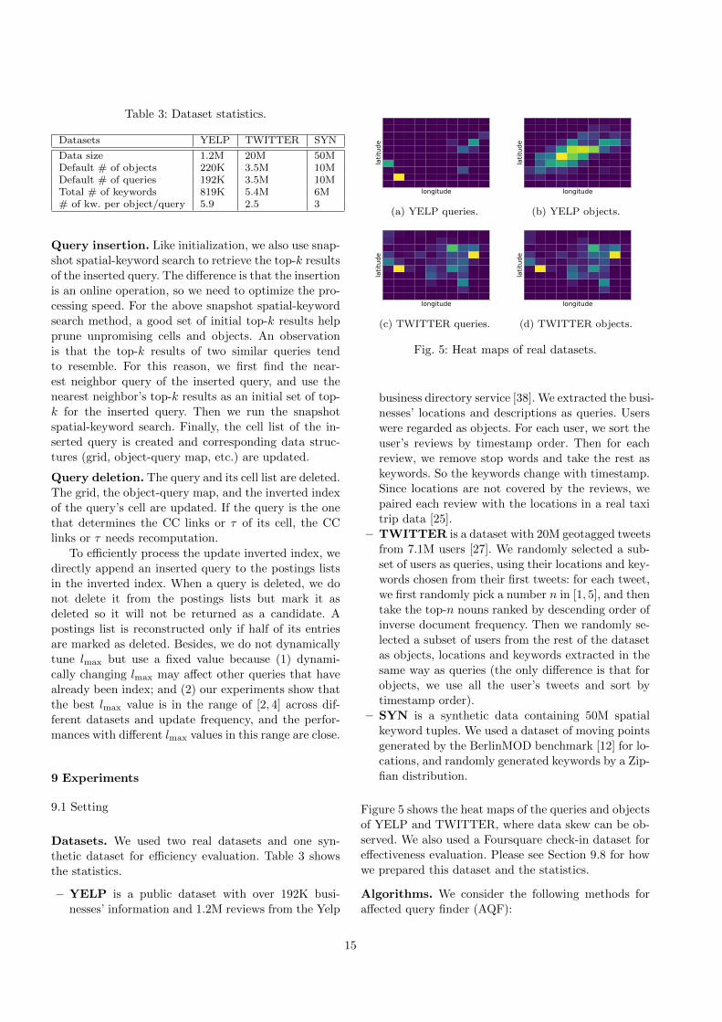
Table 3: Dataset statistics.

Datasets YELP TWITTER SYN

Data size 1.2M 20M 50MDefault # of objects 220K 3.5M 10MDefault # of queries 192K 3.5M 10MTotal # of keywords 819K 5.4M 6M# of kw. per object/query 5.9 2.5 3

Query insertion. Like initialization, we also use snap-

shot spatial-keyword search to retrieve the top-k results

of the inserted query. The difference is that the insertion

is an online operation, so we need to optimize the pro-

cessing speed. For the above snapshot spatial-keyword

search method, a good set of initial top-k results help

prune unpromising cells and objects. An observation

is that the top-k results of two similar queries tend

to resemble. For this reason, we first find the near-

est neighbor query of the inserted query, and use the

nearest neighbor’s top-k results as an initial set of top-

k for the inserted query. Then we run the snapshot

spatial-keyword search. Finally, the cell list of the in-

serted query is created and corresponding data struc-

tures (grid, object-query map, etc.) are updated.

Query deletion. The query and its cell list are deleted.

The grid, the object-query map, and the inverted index

of the query’s cell are updated. If the query is the one

that determines the CC links or τ of its cell, the CC

links or τ needs recomputation.

To efficiently process the update inverted index, we

directly append an inserted query to the postings lists

in the inverted index. When a query is deleted, we do

not delete it from the postings lists but mark it as

deleted so it will not be returned as a candidate. Apostings list is reconstructed only if half of its entries

are marked as deleted. Besides, we do not dynamically

tune lmax but use a fixed value because (1) dynami-

cally changing lmax may affect other queries that have

already been index; and (2) our experiments show that

the best lmax value is in the range of [2, 4] across dif-

ferent datasets and update frequency, and the perfor-

mances with different lmax values in this range are close.

9 Experiments

9.1 Setting

Datasets. We used two real datasets and one syn-

thetic dataset for efficiency evaluation. Table 3 shows

the statistics.

– YELP is a public dataset with over 192K busi-

nesses’ information and 1.2M reviews from the Yelp

longitude

latitud

e

(a) YELP queries.

longitude

latitud

e

(b) YELP objects.

longitude

latitud

e

(c) TWITTER queries.

longitude

latitud

e

(d) TWITTER objects.

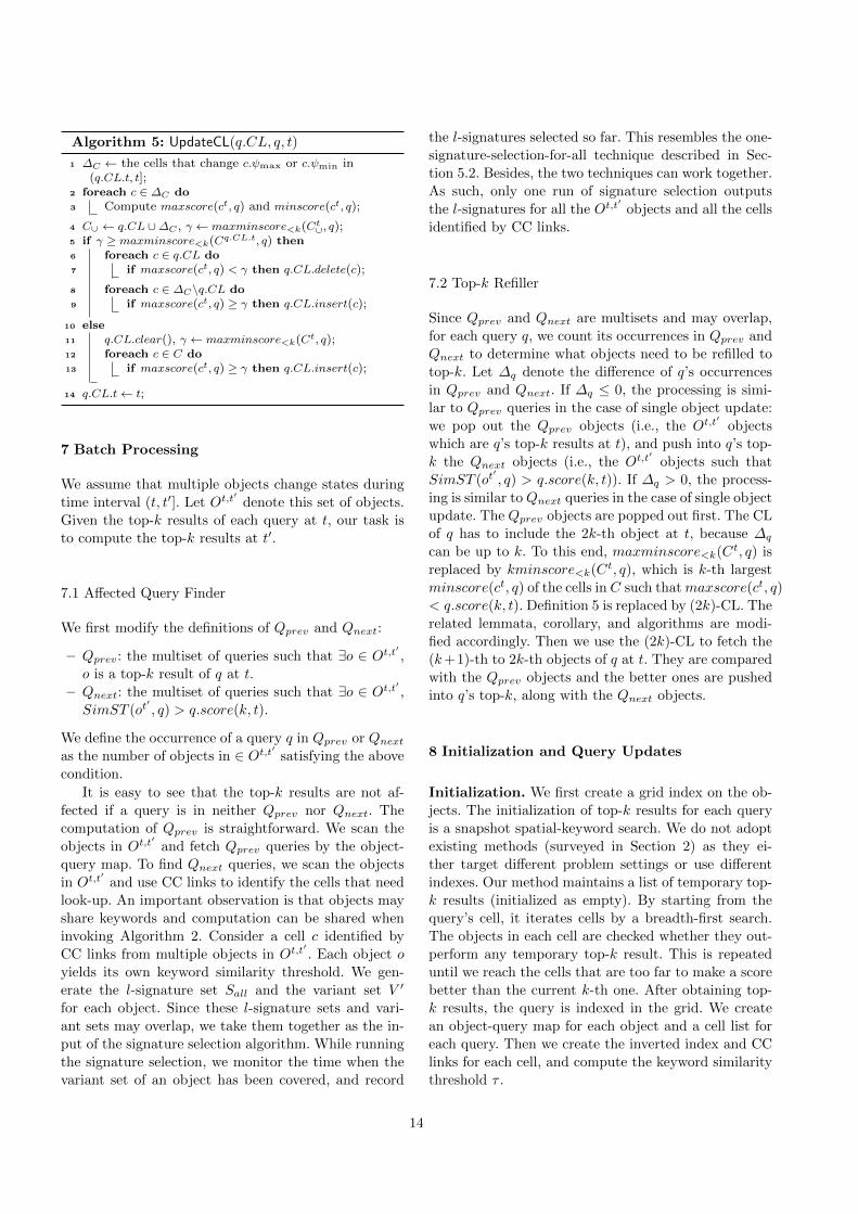
Fig. 5: Heat maps of real datasets.

business directory service [38]. We extracted the busi-

nesses’ locations and descriptions as queries. Users

were regarded as objects. For each user, we sort the

user’s reviews by timestamp order. Then for each

review, we remove stop words and take the rest as

keywords. So the keywords change with timestamp.

Since locations are not covered by the reviews, we

paired each review with the locations in a real taxi

trip data [25].

– TWITTER is a dataset with 20M geotagged tweets

from 7.1M users [27]. We randomly selected a sub-

set of users as queries, using their locations and key-

words chosen from their first tweets: for each tweet,

we first randomly pick a number n in [1, 5], and then

take the top-n nouns ranked by descending order of

inverse document frequency. Then we randomly se-

lected a subset of users from the rest of the dataset

as objects, locations and keywords extracted in the

same way as queries (the only difference is that for

objects, we use all the user’s tweets and sort by

timestamp order).

– SYN is a synthetic data containing 50M spatial

keyword tuples. We used a dataset of moving points

generated by the BerlinMOD benchmark [12] for lo-

cations, and randomly generated keywords by a Zip-

fian distribution.

Figure 5 shows the heat maps of the queries and objects

of YELP and TWITTER, where data skew can be ob-

served. We also used a Foursquare check-in dataset for

effectiveness evaluation. Please see Section 9.8 for how

we prepared this dataset and the statistics.

Algorithms. We consider the following methods for

affected query finder (AQF):

15

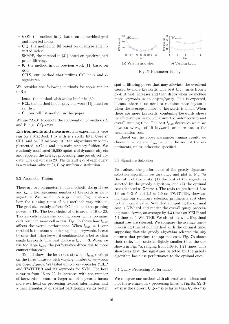
– GSKI, the method in [2] based on hierarchical grid

and inverted index.

– CIQ, the method in [6] based on quadtree and in-

verted index.

– SKYPE, the method in [31] based on quadtree and

prefix filtering.

– IC, the method in our previous work [11] based on

grid.

– CCLS, our method that utilizes CC links and l-

signatures.

We consider the following methods for top-k refiller

(TR):

– kmax, the method with kmax buffer in [39].

– PCL, the method in our previous work [11] based on

cell list.

– CL, our cell list method in this paper.

We use “A-B” to denote the combination of methods A

and B, e.g., CIQ-kmax.

Environments and measures. The experiments were

run on a MacBook Pro with a 2.2GHz Intel Core i7

CPU and 64GB memory. All the algorithms were im-

plemented in C++ and in a main memory fashion. We

randomly monitored 10,000 updates of dynamic objects

and reported the average processing time per object up-

date. The default k is 20. The default q.α of each query

is a random value in [0, 1] by uniform distribution.

9.2 Parameter Tuning

There are two parameters in our methods: the grid size

and lmax, the maximum number of keywords in an l-signature. We use an n × n grid here. Fig. 6a shows

how the running times of our methods vary with n.

The grid size mainly affects CC links and the pruning

power in TR. The best choice of n is around 16 to 20.

Too few cells reduce the pruning power, while too many

cells result in more cell access. Fig. 6b shows how lmax

affects the overall performance. When lmax = 1, our

method is the same as indexing single keywords. It can

be seen that using keyword combinations is better than

single keywords. The best choice is lmax = 3. When we

use too large lmax, the performance drops due to more

enumeration cost.

Table 4 shows the best (fastest) n and lmax settings

on the three datasets with varying number of keywords

per object/query. We tested up to 5 keywords for YELP

and TWITTER and 20 keywords for SYN. The best

n varies from 16 to 22. It increases with the number

of keywords, because a larger set of keywords incurs

more overhead on processing textual information, and

a finer granularity of spatial partitioning yields better

50

100

150

10 12 14 16 18 20 22 24 26

CP

U t

ime

(ms)

n

YELPTWITTER

(a) Varying grid size.

10

20

30

40

1 2 3 4 5

CP

U t

ime

(ms)

lmax

YELPTWITTER

(b) Varying lmax.

Fig. 6: Parameter tuning.

spatial filtering power that may alleviate the overhead

caused by more keywords. The best lmax varies from 1

to 4. It first increases and then drops when we include

more keywords in an object/query. This is expected,

because there is no need to combine more keywords

when the average number of keywords is small. When

there are more keywords, combining keywords shows

its effectiveness in reducing inverted index lookup and

overall running time. The best lmax decreases when we

have an average of 15 keywords or more due to the

enumeration cost.

Based on the above parameter tuning result, we

choose n = 20 and lmax = 3 in the rest of the ex-

periments, unless otherwise specified.

9.3 Signature Selection

To evaluate the performance of the greedy signature

selection algorithm, we vary lmax and plot in Fig. 7a

the ratio of two costs: (1) the cost of the signatures

selected by the greedy algorithm, and (2) the optimal

cost (denoted as Optimal). The ratio ranges from 1.3 to

1.6 on YELP and 1.5 to 1.9 on TWITTER, showcas-

ing that our signature selection produces a cost close

to the optimal value. Note that computing the optimal

cost is NP-hard and render the overall query process-

ing much slower, on average by 4.3 times on YELP and

5.1 times on TWITTER. We also study what if optimal

signatures are selected. We compare the average query

processing time of our method with the optimal time,

supposing that the greedy algorithm selected the sig-

natures that produce the optimal cost. Fig. 7b shows

their ratio. The ratio is slightly smaller than the one

shown in Fig. 7a, ranging from 1.08 to 1.21 times. This

showcases that the signatures selected by the greedy

algorithm has close performance to the optimal ones.

9.4 Query Processing Performance

We compare our method with alternative solutions and

plot the average query processing times in Fig. 8a. GSKI-kmax is the slowest. CIQ-kmax is faster than GSKI-kmax

16

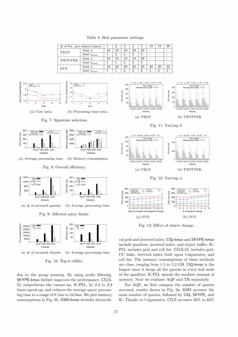
Table 4: Best parameter settings.

# of kw. per object/query 1 2 3 4 5 10 15 20

YELPbest n 16 16 18 20 20 - - -best lmax 1 2 3 3 3 - - -

TWITTERbest n 18 18 18 18 20 - - -best lmax 1 1 3 3 3 - - -

SYNbest n 18 20 20 20 20 20 20 22best lmax 1 1 2 2 2 4 3 3

1.2

1.6

2

2.4

1 2 3 4 5Co

st

(Gre

ed

y/O

ptim

al)

lmax

YELPTWITTER

(a) Cost ratio.

1

1.1

1.2

1.3

1.4

1 2 3 4 5CP

U tim

e (

Gre

edy/O

ptim

al)

lmax

YELPTWITTER

(b) Processing time ratio.

Fig. 7: Signature selection.

0

150

300

450

600

YELP TWITTER SYN

CP

U t

ime

(m

s)

Datasets

GSKI-kmaxCIQ-kmax

SKYPE-kmax

IC-PCLCCLS-CL

(a) Average processing time.

2000

4000

6000

8000

YELP TWITTER SYN

Me

mo

ry u

sa

ge

(M

B)

Datasets

GSKI-kmaxCIQ-kmax

SKYPE-kmax

IC-PCLCCLS-CL

(b) Memory consumption.

Fig. 8: Overall efficiency.

4000

8000

12000

16000

YELP TWITTER SYN

# o

f a

cce

sse

d q

ue

rie

s

Datasets

GSKICIQ

SKYPEIC

CCLS

(a) # of accessed queries.

0

100

200

300

400

YELP TWITTER SYN

CP

U t

ime

(m

s)

Datasets

GSKICIQ

SKYPEIC

CCLS

(b) Average processing time.

Fig. 9: Affected query finder.

0

50000

100000

150000

200000

250000

YELP TWITTER SYN

# o

f a

cce

sse

d o

bje

cts

Datasets

kmaxPCL

CL

(a) # of accessed objects.

50

100

150

200

YELP TWITTER SYN

CP

U t

ime

(m

s)

Datasets

kmaxPCL

CL

(b) Average processing time.

Fig. 10: Top-k refiller.

due to the group pruning. By using prefix filtering,

SKYPE-kmax further improves the performance. CCLS-

CL outperforms the runner-up, IC-PCL, by 2.4 to 3.3

times speed-up, and reduces the average query process-

ing time to a range of 8.1ms to 34.0ms. We plot memory

consumptions in Fig. 8b. GSKI-kmax includes hierarchi-

50

100

150

200

250

12345 12345 12345 12345 12345

k = 10 k = 20 k = 30 k = 40 k = 50

CP

U t

ime

(m

s)

Methods

Top-k refillerAffected query finder

(a) YELP.

0

100

200

300

400

12345 12345 12345 12345 12345

k = 10 k = 20 k = 30 k = 40 k = 50

CP

U t

ime

(m

s)

Methods


(b) TWITTER.

Fig. 11: Varying k.

50

100

150

200

250

12345 12345 12345 12345 12345

α = 0 α=0.25 α=0.5 α=0.75 α=1

CP

U t

ime

(m

s)

Methods


(a) YELP.

0

200

400

12345 12345 12345 12345 12345

α = 0 α=0.25 α=0.5 α=0.75 α=1

CP

U t

ime

(m

s)

Methods


(b) TWITTER.

Fig. 12: Varying α.

0

200

400

600

800

1:9 2:8 3:7 4:6 5:5 6:4 7:3 8:2 9:1

CP

U t

ime

(m

s)

Ratio of location and keyword change

GSKI-kmaxCIQ-kmaxSKYPE-kmax

IC-PCLCCLS-CL

(a) SYN.

0

200

400

600

800

1 2 3 4 5 6 7 8 9 10

CP

U t

ime

(m

s)

# of keyword change


IC-PCLCCLS-CL

(b) SYN.

Fig. 13: Effect of object change.

cal grid and inverted index. CIQ-kmax and SKYPE-kmaxinclude quadtree, inverted index, and object buffer. IC-

PCL includes grid and cell list. CCLS-CL includes grid,

CC links, inverted index built upon l-signatures, and

cell list. The memory consumptions of these methods

are close, ranging from 1.5 to 5.2 GB. CIQ-kmax is the

largest since it keeps all the queries in every leaf node

of the quadtree. IC-PCL spends the smallest amount of

memory. Next we evaluate AQF and TR separately.

For AQF, we first compare the number of queries

accessed, results shown in Fig. 9a. GSKI accesses the

most number of queries, followed by CIQ, SKYPE, and

IC. Thanks to l-signatures, CCLS accesses 50% to 62%

17

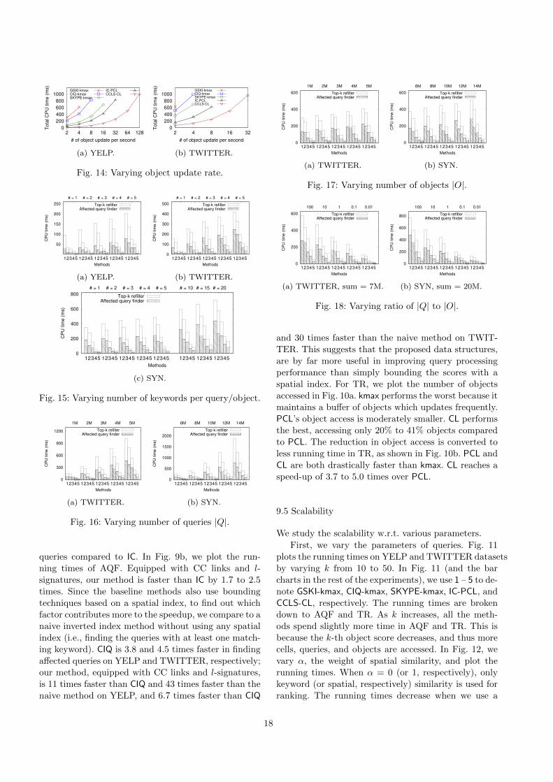
0

200

400

600

800

1000

2 4 8 16 32 64 128

To

tal C

PU

tim

e (

ms)

# of object update per second


IC-PCLCCLS-CL

(a) YELP.

0

200

400

600

800

1000

2 4 8 16 32

To

tal C

PU

tim

e (

ms)

# of object update per second

GSKI-kmaxCIQ-kmaxSKYPE-kmaxIC-PCLCCLS-CL

(b) TWITTER.

Fig. 14: Varying object update rate.

50

100

150

200

250

12345 12345 12345 12345 12345

# = 1 # = 2 # = 3 # = 4 # = 5

CP

U t

ime

(m

s)

Methods


(a) YELP.

0

100

200

300

400

500

12345 12345 12345 12345 12345

# = 1 # = 2 # = 3 # = 4 # = 5

CP

U t

ime

(m

s)

Methods


(b) TWITTER.

0

200

400

600

800

12345 12345 12345 12345 12345 12345 12345 12345

# = 1 # = 2 # = 3 # = 4 # = 5 # = 10 # = 15 # = 20

CP

U t

ime

(m

s)

Methods


(c) SYN.

Fig. 15: Varying number of keywords per query/object.

0

300

600

900

1200

12345 12345 12345 12345 12345

1M 2M 3M 4M 5M

CP

U t

ime

(m

s)

Methods


(a) TWITTER.

0

500

1000

1500

2000

12345 12345 12345 12345 12345

6M 8M 10M 12M 14M

CP

U t

ime

(m

s)

Methods


(b) SYN.

Fig. 16: Varying number of queries |Q|.

queries compared to IC. In Fig. 9b, we plot the run-

ning times of AQF. Equipped with CC links and l-

signatures, our method is faster than IC by 1.7 to 2.5

times. Since the baseline methods also use bounding

techniques based on a spatial index, to find out which

factor contributes more to the speedup, we compare to a

naive inverted index method without using any spatial

index (i.e., finding the queries with at least one match-

ing keyword). CIQ is 3.8 and 4.5 times faster in finding

affected queries on YELP and TWITTER, respectively;

our method, equipped with CC links and l-signatures,

is 11 times faster than CIQ and 43 times faster than the

naive method on YELP, and 6.7 times faster than CIQ

0

200

400

600

12345 12345 12345 12345 12345

1M 2M 3M 4M 5M

CP

U t

ime

(m

s)

Methods


(a) TWITTER.

0

200

400

600

12345 12345 12345 12345 12345

6M 8M 10M 12M 14M

CP

U t

ime

(m

s)

Methods


(b) SYN.

Fig. 17: Varying number of objects |O|.

0

200

400

600

12345 12345 12345 12345 12345

100 10 1 0.1 0.01

CP

U t

ime

(m

s)

Methods


(a) TWITTER, sum = 7M.

0

200

400

600

800

12345 12345 12345 12345 12345

100 10 1 0.1 0.01

CP

U t

ime

(m

s)

Methods


(b) SYN, sum = 20M.

Fig. 18: Varying ratio of |Q| to |O|.

and 30 times faster than the naive method on TWIT-

TER. This suggests that the proposed data structures,

are by far more useful in improving query processing

performance than simply bounding the scores with a

spatial index. For TR, we plot the number of objects

accessed in Fig. 10a. kmax performs the worst because it

maintains a buffer of objects which updates frequently.

PCL’s object access is moderately smaller. CL performs

the best, accessing only 20% to 41% objects compared

to PCL. The reduction in object access is converted to

less running time in TR, as shown in Fig. 10b. PCL and

CL are both drastically faster than kmax. CL reaches a

speed-up of 3.7 to 5.0 times over PCL.

9.5 Scalability

We study the scalability w.r.t. various parameters.

First, we vary the parameters of queries. Fig. 11

plots the running times on YELP and TWITTER datasets

by varying k from 10 to 50. In Fig. 11 (and the bar

charts in the rest of the experiments), we use 1 – 5 to de-

note GSKI-kmax, CIQ-kmax, SKYPE-kmax, IC-PCL, and

CCLS-CL, respectively. The running times are broken

down to AQF and TR. As k increases, all the meth-

ods spend slightly more time in AQF and TR. This is

because the k-th object score decreases, and thus more

cells, queries, and objects are accessed. In Fig. 12, we

vary α, the weight of spatial similarity, and plot the

running times. When α = 0 (or 1, respectively), only

keyword (or spatial, respectively) similarity is used for

ranking. The running times decrease when we use a

18

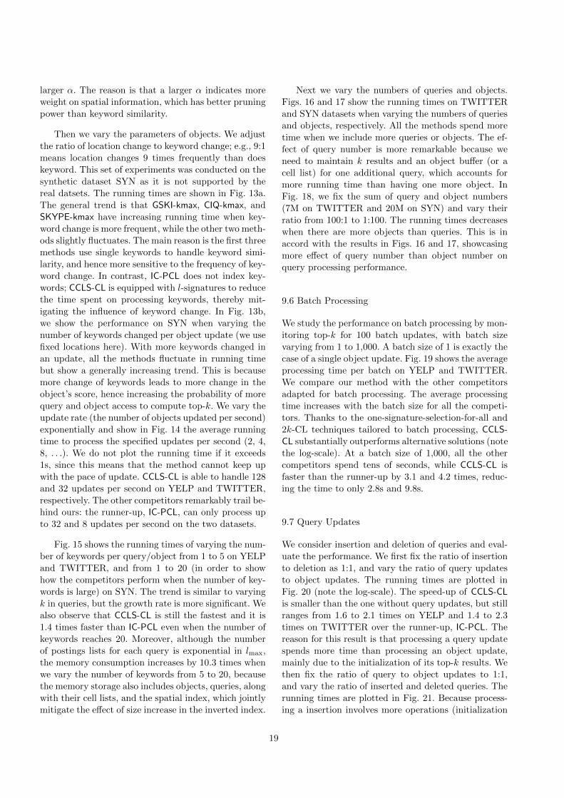
larger α. The reason is that a larger α indicates more

weight on spatial information, which has better pruning

power than keyword similarity.

Then we vary the parameters of objects. We adjust

the ratio of location change to keyword change; e.g., 9:1

means location changes 9 times frequently than does

keyword. This set of experiments was conducted on the

synthetic dataset SYN as it is not supported by the

real datsets. The running times are shown in Fig. 13a.

The general trend is that GSKI-kmax, CIQ-kmax, and

SKYPE-kmax have increasing running time when key-

word change is more frequent, while the other two meth-

ods slightly fluctuates. The main reason is the first three

methods use single keywords to handle keyword simi-

larity, and hence more sensitive to the frequency of key-

word change. In contrast, IC-PCL does not index key-

words; CCLS-CL is equipped with l-signatures to reduce

the time spent on processing keywords, thereby mit-

igating the influence of keyword change. In Fig. 13b,

we show the performance on SYN when varying the

number of keywords changed per object update (we use

fixed locations here). With more keywords changed in

an update, all the methods fluctuate in running time

but show a generally increasing trend. This is because

more change of keywords leads to more change in the

object’s score, hence increasing the probability of more

query and object access to compute top-k. We vary the

update rate (the number of objects updated per second)

exponentially and show in Fig. 14 the average running

time to process the specified updates per second (2, 4,

8, . . .). We do not plot the running time if it exceeds

1s, since this means that the method cannot keep up

with the pace of update. CCLS-CL is able to handle 128

and 32 updates per second on YELP and TWITTER,

respectively. The other competitors remarkably trail be-

hind ours: the runner-up, IC-PCL, can only process up

to 32 and 8 updates per second on the two datasets.

Fig. 15 shows the running times of varying the num-

ber of keywords per query/object from 1 to 5 on YELP

and TWITTER, and from 1 to 20 (in order to show

how the competitors perform when the number of key-

words is large) on SYN. The trend is similar to varying

k in queries, but the growth rate is more significant. We

also observe that CCLS-CL is still the fastest and it is

1.4 times faster than IC-PCL even when the number of

keywords reaches 20. Moreover, although the number

of postings lists for each query is exponential in lmax,

the memory consumption increases by 10.3 times when

we vary the number of keywords from 5 to 20, because

the memory storage also includes objects, queries, along

with their cell lists, and the spatial index, which jointly

mitigate the effect of size increase in the inverted index.

Next we vary the numbers of queries and objects.

Figs. 16 and 17 show the running times on TWITTER

and SYN datasets when varying the numbers of queries

and objects, respectively. All the methods spend more

time when we include more queries or objects. The ef-

fect of query number is more remarkable because we

need to maintain k results and an object buffer (or a

cell list) for one additional query, which accounts for

more running time than having one more object. In

Fig. 18, we fix the sum of query and object numbers

(7M on TWITTER and 20M on SYN) and vary their

ratio from 100:1 to 1:100. The running times decreases

when there are more objects than queries. This is in

accord with the results in Figs. 16 and 17, showcasing

more effect of query number than object number on

query processing performance.

9.6 Batch Processing

We study the performance on batch processing by mon-

itoring top-k for 100 batch updates, with batch size

varying from 1 to 1,000. A batch size of 1 is exactly the

case of a single object update. Fig. 19 shows the average

processing time per batch on YELP and TWITTER.

We compare our method with the other competitors

adapted for batch processing. The average processing

time increases with the batch size for all the competi-

tors. Thanks to the one-signature-selection-for-all and

2k-CL techniques tailored to batch processing, CCLS-

CL substantially outperforms alternative solutions (note

the log-scale). At a batch size of 1,000, all the other

competitors spend tens of seconds, while CCLS-CL is

faster than the runner-up by 3.1 and 4.2 times, reduc-

ing the time to only 2.8s and 9.8s.

9.7 Query Updates

We consider insertion and deletion of queries and eval-

uate the performance. We first fix the ratio of insertion

to deletion as 1:1, and vary the ratio of query updates

to object updates. The running times are plotted in

Fig. 20 (note the log-scale). The speed-up of CCLS-CLis smaller than the one without query updates, but still

ranges from 1.6 to 2.1 times on YELP and 1.4 to 2.3

times on TWITTER over the runner-up, IC-PCL. The

reason for this result is that processing a query update

spends more time than processing an object update,

mainly due to the initialization of its top-k results. We

then fix the ratio of query to object updates to 1:1,

and vary the ratio of inserted and deleted queries. The

running times are plotted in Fig. 21. Because process-

ing a insertion involves more operations (initialization

19

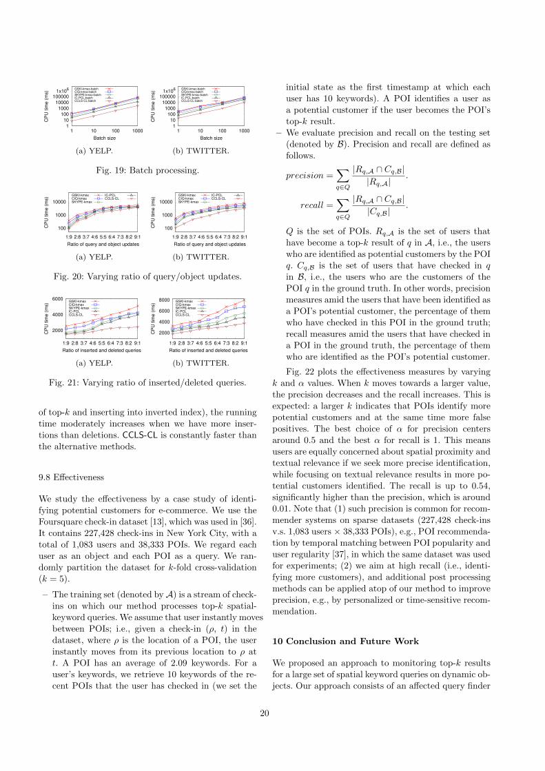
1

10

100

1000

10000

100000 1x10

6

1 10 100 1000

CP

U t

ime

(m

s)

Batch size

GSKI-kmax-batchCIQ-kmax-batchSKYPE-kmax-batchIC-PCL-batchCCLS-CL-batch

(a) YELP.

1

10

100

1000

10000

100000 1x10

6

1 10 100 1000

CP

U t

ime

(m

s)

Batch size

GSKI-kmax-batchCIQ-kmax-batchSKYPE-kmax-batchIC-PCL-batchCCLS-CL-batch

(b) TWITTER.

Fig. 19: Batch processing.

100

1000

10000

1:9 2:8 3:7 4:6 5:5 6:4 7:3 8:2 9:1

CP

U t

ime

(m

s)

Ratio of query and object updates


IC-PCLCCLS-CL

(a) YELP.

100

1000

10000

1:9 2:8 3:7 4:6 5:5 6:4 7:3 8:2 9:1

CP

U t

ime

(m

s)

Ratio of query and object updates


IC-PCLCCLS-CL

(b) TWITTER.

Fig. 20: Varying ratio of query/object updates.

2000

4000

6000

1:9 2:8 3:7 4:6 5:5 6:4 7:3 8:2 9:1

CP

U t

ime

(m

s)

Ratio of inserted and deleted queries


(a) YELP.

2000

4000

6000

8000

1:9 2:8 3:7 4:6 5:5 6:4 7:3 8:2 9:1

CP

U t

ime

(m

s)

Ratio of inserted and deleted queries


(b) TWITTER.

Fig. 21: Varying ratio of inserted/deleted queries.

of top-k and inserting into inverted index), the running

time moderately increases when we have more inser-

tions than deletions. CCLS-CL is constantly faster than

the alternative methods.

9.8 Effectiveness

We study the effectiveness by a case study of identi-

fying potential customers for e-commerce. We use the

Foursquare check-in dataset [13], which was used in [36].

It contains 227,428 check-ins in New York City, with a

total of 1,083 users and 38,333 POIs. We regard each

user as an object and each POI as a query. We ran-

domly partition the dataset for k-fold cross-validation

(k = 5).

– The training set (denoted byA) is a stream of check-

ins on which our method processes top-k spatial-

keyword queries. We assume that user instantly moves

between POIs; i.e., given a check-in (ρ, t) in the

dataset, where ρ is the location of a POI, the user

instantly moves from its previous location to ρ at

t. A POI has an average of 2.09 keywords. For a

user’s keywords, we retrieve 10 keywords of the re-

cent POIs that the user has checked in (we set the

initial state as the first timestamp at which each

user has 10 keywords). A POI identifies a user as

a potential customer if the user becomes the POI’s

top-k result.

– We evaluate precision and recall on the testing set

(denoted by B). Precision and recall are defined as

follows.

precision =∑q∈Q

|Rq,A ∩ Cq,B||Rq,A|

.

recall =∑q∈Q

|Rq,A ∩ Cq,B||Cq,B|

.

Q is the set of POIs. Rq,A is the set of users that

have become a top-k result of q in A, i.e., the users

who are identified as potential customers by the POI

q. Cq,B is the set of users that have checked in q

in B, i.e., the users who are the customers of the

POI q in the ground truth. In other words, precision

measures amid the users that have been identified as

a POI’s potential customer, the percentage of them

who have checked in this POI in the ground truth;

recall measures amid the users that have checked in

a POI in the ground truth, the percentage of them

who are identified as the POI’s potential customer.

Fig. 22 plots the effectiveness measures by varying

k and α values. When k moves towards a larger value,

the precision decreases and the recall increases. This is

expected: a larger k indicates that POIs identify more

potential customers and at the same time more false

positives. The best choice of α for precision centers

around 0.5 and the best α for recall is 1. This means

users are equally concerned about spatial proximity and

textual relevance if we seek more precise identification,

while focusing on textual relevance results in more po-

tential customers identified. The recall is up to 0.54,

significantly higher than the precision, which is around

0.01. Note that (1) such precision is common for recom-

mender systems on sparse datasets (227,428 check-ins

v.s. 1,083 users × 38,333 POIs), e.g., POI recommenda-

tion by temporal matching between POI popularity and

user regularity [37], in which the same dataset was used

for experiments; (2) we aim at high recall (i.e., identi-

fying more customers), and additional post processing

methods can be applied atop of our method to improve

precision, e.g., by personalized or time-sensitive recom-

mendation.

10 Conclusion and Future Work

We proposed an approach to monitoring top-k results

for a large set of spatial keyword queries on dynamic ob-

jects. Our approach consists of an affected query finder

20

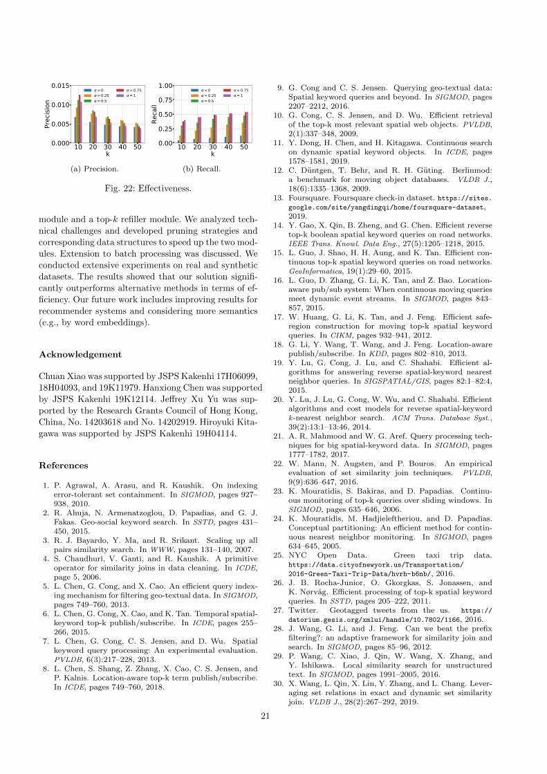
10 20 30 40 50k

0.000

0.005

0.010

0.015

Prec

ision

α=0α=0.25α=0.5

α=0.75α=1

(a) Precision.

10 20 30 40 50k

0.00

0.25

0.50

0.75

1.00

Recall

α=0α=0.25α=0.5

α=0.75α=1

(b) Recall.

Fig. 22: Effectiveness.

module and a top-k refiller module. We analyzed tech-

nical challenges and developed pruning strategies and

corresponding data structures to speed up the two mod-

ules. Extension to batch processing was discussed. We

conducted extensive experiments on real and synthetic

datasets. The results showed that our solution signifi-

cantly outperforms alternative methods in terms of ef-

ficiency. Our future work includes improving results for

recommender systems and considering more semantics

(e.g., by word embeddings).

Acknowledgement

Chuan Xiao was supported by JSPS Kakenhi 17H06099,

18H04093, and 19K11979. Hanxiong Chen was supported

by JSPS Kakenhi 19K12114. Jeffrey Xu Yu was sup-

ported by the Research Grants Council of Hong Kong,

China, No. 14203618 and No. 14202919. Hiroyuki Kita-

gawa was supported by JSPS Kakenhi 19H04114.

References

1. P. Agrawal, A. Arasu, and R. Kaushik. On indexingerror-tolerant set containment. In SIGMOD, pages 927–938, 2010.

2. R. Ahuja, N. Armenatzoglou, D. Papadias, and G. J.Fakas. Geo-social keyword search. In SSTD, pages 431–450, 2015.

3. R. J. Bayardo, Y. Ma, and R. Srikant. Scaling up allpairs similarity search. In WWW, pages 131–140, 2007.

4. S. Chaudhuri, V. Ganti, and R. Kaushik. A primitiveoperator for similarity joins in data cleaning. In ICDE,page 5, 2006.

5. L. Chen, G. Cong, and X. Cao. An efficient query index-ing mechanism for filtering geo-textual data. In SIGMOD,pages 749–760, 2013.

6. L. Chen, G. Cong, X. Cao, and K. Tan. Temporal spatial-keyword top-k publish/subscribe. In ICDE, pages 255–266, 2015.

7. L. Chen, G. Cong, C. S. Jensen, and D. Wu. Spatialkeyword query processing: An experimental evaluation.PVLDB, 6(3):217–228, 2013.

8. L. Chen, S. Shang, Z. Zhang, X. Cao, C. S. Jensen, andP. Kalnis. Location-aware top-k term publish/subscribe.In ICDE, pages 749–760, 2018.

9. G. Cong and C. S. Jensen. Querying geo-textual data:Spatial keyword queries and beyond. In SIGMOD, pages2207–2212, 2016.

10. G. Cong, C. S. Jensen, and D. Wu. Efficient retrievalof the top-k most relevant spatial web objects. PVLDB,2(1):337–348, 2009.

11. Y. Dong, H. Chen, and H. Kitagawa. Continuous searchon dynamic spatial keyword objects. In ICDE, pages1578–1581, 2019.

12. C. Duntgen, T. Behr, and R. H. Guting. Berlinmod:a benchmark for moving object databases. VLDB J.,18(6):1335–1368, 2009.

13. Foursquare. Foursquare check-in dataset. https://sites.google.com/site/yangdingqi/home/foursquare-dataset,2019.

14. Y. Gao, X. Qin, B. Zheng, and G. Chen. Efficient reversetop-k boolean spatial keyword queries on road networks.IEEE Trans. Knowl. Data Eng., 27(5):1205–1218, 2015.

15. L. Guo, J. Shao, H. H. Aung, and K. Tan. Efficient con-tinuous top-k spatial keyword queries on road networks.GeoInformatica, 19(1):29–60, 2015.

16. L. Guo, D. Zhang, G. Li, K. Tan, and Z. Bao. Location-aware pub/sub system: When continuous moving queriesmeet dynamic event streams. In SIGMOD, pages 843–857, 2015.

17. W. Huang, G. Li, K. Tan, and J. Feng. Efficient safe-region construction for moving top-k spatial keywordqueries. In CIKM, pages 932–941, 2012.

18. G. Li, Y. Wang, T. Wang, and J. Feng. Location-awarepublish/subscribe. In KDD, pages 802–810, 2013.

19. Y. Lu, G. Cong, J. Lu, and C. Shahabi. Efficient al-gorithms for answering reverse spatial-keyword nearestneighbor queries. In SIGSPATIAL/GIS, pages 82:1–82:4,2015.

20. Y. Lu, J. Lu, G. Cong, W. Wu, and C. Shahabi. Efficientalgorithms and cost models for reverse spatial-keywordk-nearest neighbor search. ACM Trans. Database Syst.,39(2):13:1–13:46, 2014.

21. A. R. Mahmood and W. G. Aref. Query processing tech-niques for big spatial-keyword data. In SIGMOD, pages1777–1782, 2017.

22. W. Mann, N. Augsten, and P. Bouros. An empiricalevaluation of set similarity join techniques. PVLDB,9(9):636–647, 2016.

23. K. Mouratidis, S. Bakiras, and D. Papadias. Continu-ous monitoring of top-k queries over sliding windows. InSIGMOD, pages 635–646, 2006.

24. K. Mouratidis, M. Hadjieleftheriou, and D. Papadias.Conceptual partitioning: An efficient method for contin-uous nearest neighbor monitoring. In SIGMOD, pages634–645, 2005.

25. NYC Open Data. Green taxi trip data.https://data.cityofnewyork.us/Transportation/

2016-Green-Taxi-Trip-Data/hvrh-b6nb/, 2016.26. J. B. Rocha-Junior, O. Gkorgkas, S. Jonassen, and

K. Nørvag. Efficient processing of top-k spatial keywordqueries. In SSTD, pages 205–222, 2011.

27. Twitter. Geotagged tweets from the us. https://

datorium.gesis.org/xmlui/handle/10.7802/1166, 2016.28. J. Wang, G. Li, and J. Feng. Can we beat the prefix

filtering?: an adaptive framework for similarity join andsearch. In SIGMOD, pages 85–96, 2012.

29. P. Wang, C. Xiao, J. Qin, W. Wang, X. Zhang, andY. Ishikawa. Local similarity search for unstructuredtext. In SIGMOD, pages 1991–2005, 2016.

30. X. Wang, L. Qin, X. Lin, Y. Zhang, and L. Chang. Lever-aging set relations in exact and dynamic set similarityjoin. VLDB J., 28(2):267–292, 2019.

21

31. X. Wang, Y. Zhang, W. Zhang, X. Lin, and Z. Huang.SKYPE: top-k spatial-keyword publish/subscribe oversliding window. PVLDB, 9(7):588–599, 2016.

32. X. Wang, Y. Zhang, W. Zhang, X. Lin, andW. Wang. Ap-tree: efficiently support location-awarepublish/subscribe. VLDB J., 24(6):823–848, 2015.

33. D. Wu, M. L. Yiu, and C. S. Jensen. Moving spatial key-word queries: Formulation, methods, and analysis. ACMTrans. Database Syst., 38(1):7:1–7:47, 2013.

34. C. Xiao, W. Wang, X. Lin, J. X. Yu, and G. Wang. Ef-ficient similarity joins for near-duplicate detection. ACM

Trans. Database Syst., 36(3):15:1–15:41.35. X. Xiong, M. F. Mokbel, and W. G. Aref. SEA-

CNN: scalable processing of continuous k-nearest neigh-bor queries in spatio-temporal databases. In ICDE, pages643–654, 2005.

36. D. Yang, D. Zhang, V. W. Zheng, and Z. Yu. Modelinguser activity preference by leveraging user spatial tem-poral characteristics in lbsns. IEEE Trans. Systems, Man,and Cybernetics: Systems, 45(1):129–142, 2015.

37. Z. Yao, Y. Fu, B. Liu, Y. Liu, and H. Xiong. POI recom-mendation: A temporal matching between POI popular-ity and user regularity. In ICDM, pages 549–558, 2016.

38. Yelp. Yelp dataset. https://www.yelp.com/dataset, 2019.39. K. Yi, H. Yu, J. Yang, G. Xia, and Y. Chen. Efficient

maintenance of materialized top-k views. In ICDE, pages189–200, 2003.

40. N. E. Young. Greedy set-cover algorithms. In Encyclope-

dia of Algorithms. 2008.41. X. Yu, K. Q. Pu, and N. Koudas. Monitoring k-nearest

neighbor queries over moving objects. In ICDE, pages631–642, 2005.

42. J. Zhao, Y. Gao, G. Chen, C. S. Jensen, R. Chen, andD. Cai. Reverse top-k geo-social keyword queries in roadnetworks. In ICDE, pages 387–398, 2017.

43. B. Zheng, K. Zheng, X. Xiao, H. Su, H. Yin, X. Zhou,and G. Li. Keyword-aware continuous knn query on roadnetworks. In ICDE, pages 871–882, 2016.

22

Continuous Top-k Spatial-Keyword Search on Dynamic Objects

Documents

Transcript of Continuous Top-k Spatial-Keyword Search on Dynamic Objects