Chapter1: Introduction
67
DR. Muna M. Mustafa Chapter1:Introduction 1 Chapter1: Introduction 1.1 REPRESENTATION OF NUMBERS ON A COMPUTER (Decimal and binary representation) Numbers can be represented in various forms. The familiar decimal system (base 10) uses ten digits 0, 1, ... , 9. A number is written by a sequence of digits that correspond to multiples of powers of 10. As shown in Fig. 1-1, the first digit to the left of the decimal point corresponds to 10 0 . The digit next to it on the left corresponds to 10 1 , the next digit to the left to 10 2 , and so on. In the same way, the first digit to the right of the decimal point corresponds to 10 -1 , the next digit to the right to 10 -2 , and so on. Fig. 1-1: Representation of the number 60,724.3125 in the decimal system (base 10). In general, however, a number can be represented using other bases. A form that can be easily implemented in computers is the binary (base 2) system. In the binary system, a number is represented by using the two digits 0 and 1. A number is then written as a sequence of zeros and ones that correspond to multiples of powers of 2. The first digit to the left of the decimal point corresponds to 2 0 . The digit next to it on the left corresponds to 2 1 , the next digit to the left to 2 2 , and so on. In the same way, the first digit to the right of the decimal point corresponds to r 1 , the next digit to the right to r 2 , and so on. The first ten digits 1, 2, 3, . . . , 10 in base 10 and their representation in base 2 are shown in Fig. 1-2. The representation of the number 19.625 in the binary system is shown in Fig. 1-3. Figure 1-2: Representation of numbers in decimal and binary forms.
-
Upload
khangminh22 -
Category
Documents
-
view
5 -
download
0
Transcript of Chapter1: Introduction

DR. Muna M. Mustafa Chapter1:Introduction
1
Chapter1: Introduction 1.1 REPRESENTATION OF NUMBERS ON A COMPUTER
(Decimal and binary representation) Numbers can be represented in various forms. The familiar decimal system (base 10) uses ten digits
0, 1, ... , 9. A number is written by a sequence of digits that correspond to multiples of powers of 10. As
shown in Fig. 1-1, the first digit to the left of the decimal point corresponds to 100. The digit next to it on the
left corresponds to 101 , the next digit to the left to 10
2 , and so on. In the same way, the first digit to the right
of the decimal point corresponds to 10-1
, the next digit to the right to 10-2
, and so on.
Fig. 1-1: Representation of the number 60,724.3125 in the decimal system (base 10).
In general, however, a number can be represented using other bases. A form that can be easily implemented
in computers is the binary (base 2) system. In the binary system, a number is represented by using the two
digits 0 and 1. A number is then written as a sequence of zeros and ones that correspond to multiples of
powers of 2. The first digit to the left of the decimal point corresponds to 20. The digit next to it on the left
corresponds to 21, the next digit to the left to 2
2, and so on. In the same way, the first digit to the right of the
decimal point corresponds to r1, the next digit to the right to r
2, and so on. The first ten digits 1, 2, 3, . . . , 10
in base 10 and their representation in base 2 are shown in Fig. 1-2. The representation of the number 19.625
in the binary system is shown in Fig. 1-3.
Figure 1-2: Representation of numbers in decimal and binary forms.

DR. Muna M. Mustafa Chapter1:Introduction
2
Figure 1-3: Representation of the number 19.625 in the binary system (base 2).
Another example is shown in Fig. 1-4, where the number 60,724.3125 is written in binary form.
Figure 1-4: Representation of the number 60,724.3125 in the binary system (base 2).
Computers store and process numbers in binary (base 2) form. Each binary digit (one or zero) is called a bit
(for binary digit). Binary arithmetic is used by computers because modem transistors can be used as
extremely fast switches. Therefore, a network of these may be used to represent strings of numbers with the
"1" referring to the switch being in the "on" position and "O" referring to the "off' position. Various
operations are then performed on these sequences of ones and zeros.
1.1.2 Floating point representation To accommodate large and small numbers, real numbers are written in floating point representation.
Decimal floating point representation (also called scientific notation) has the form:
d.ddddd × l0P (1. 1)
One digit is written to the left of the decimal point, and the rest of the significant digits are written to the
right of the decimal point. The number d.dddddd is called the mantissa. Two examples are:
6519.23 written as 6.51923 x 10³
0.00000391 written as 3.91 x 10⁻⁶
The power of 10, p, represents the number's order of magnitude, provided the preceding number is smaller
than 5. Otherwise, the number is said to be of the order of p + 1. Thus, the number 3.91 x 10⁻⁶
is of the order
of 10-6
, 0( 10-6
) , and the number 6.51923 x 10³ is of the order of 10
4(written as 0(10
4) ). Binary floating
point representation has the form:
1. bbbbbb x 2bbb
(b is a decimal digit) (1. 2)
In this form, the mantissa is . bbbbbb , and the power of 2 is called the exponent. Both the mantissa and the
exponent are written in a binary form. The form in Eq. (1. 2) is obtained by normalizing the number (when it
is written in the decimal form) with respect to the largest power of 2 that is smaller than the number itself.
For example, to write the number 50 in binary floating point representation, the number is divided (and
multiplied) by 25 = 32 (which is the largest power of 2 that is smaller than 50):

DR. Muna M. Mustafa Chapter1:Introduction
3
1.2 ERRORS IN NUMERICAL SOLUTIONS Numerical solutions can be very accurate but in general are not exact. Two kinds of errors are
introduced when numerical methods are used for solving a problem. One kind, which was mentioned in the
previous section, occurs because of the way that digital computers store numbers and execute numerical
operations. These errors are labeled round-off errors. The second kind of errors is introduced by the
numerical method that is used for the solution. These errors are labeled truncation errors. Numerical methods
use approximations for solving problems. The errors introduced by the approximations are the truncation
errors. Together, the two errors constitute the total error of the numerical solution, which is the difference
(can be defined in various ways) between the true (exact) solution (which is usually unknown) and the
approximate numerical solution. Round-off, truncation, and total errors are discussed in the following three
subsections.
1.2.1 Round-Off Errors Numbers are represented on a computer by a finite number of bits . Consequently, real numbers that
have a mantissa longer than the number of bits that are available for representing them have to be shortened.
This requirement applies to irrational numbers that have to be represented in a finite form in any system, to
finite numbers that are too long, and to finite numbers in decimal form that cannot be represented exactly in
binary form. A number can be shortened either by chopping off, or discarding, the extra digits or by
rounding. In chopping, the digits in the mantissa beyond the length that can be stored are simply left out. In
rounding, the last digit that is stored is rounded.
As a simple illustration, consider the number 2/3. (For simplicity, decimal format is used in the
illustration. In the computer, chopping and rounding are done in the binary format.) In decimal form with
four significant digits, 2/3 can be written as 0.6666 or as 0.6667. In the former instance, the actual number
has been chopped off, whereas in the latter instance, the actual number has been rounded. Either way, such
chopping and rounding of real numbers lead to errors in numerical computations, especially when many
operations are performed. This type of numerical error (regardless of whether it is due to chopping or
rounding) is known as round-off error. Example 1-1 shows the difference between chopping and rounding.
Example 1-1: Round-off errors Consider the two nearly equal numbers p = 9890.9 and q = 9887. l . Use decimal floating point
representation (scientific notation) with three significant digits in the mantissa to calculate the difference
between the two numbers, (p - q) . Do the calculation first by using chopping and then by using rounding.
SOLUTION
In decimal floating point representation, the two numbers are:
p = 9.8909 x 10³ and q = 9.8871 x 10
3
If only three significant digits are allowed in the mantissa, the numbers have to be shortened. If chopping is
used, the numbers become:
p = 9.890 x 10³ and q = 9.887 x 10
3
Using these values in the subtraction gives:
p- q = 9.890 x 10³ - 9.887 x 10
3 = 0.003 x 10
3 = 3

DR. Muna M. Mustafa Chapter1:Introduction
4
If rounding is used, the numbers become:
p = 9.891 x 10³ and q = 9.887 x 10
3 (q is the same as before)
Using these values in the subtraction gives:
p- q = 9.891 x 10³ - 9.887 x 10
3 = 0.004 x 10
3 = 4
The true (exact) difference between the numbers is 3.8. These results show that, in the present problem,
rounding gives a value closer to the true answer.
The magnitude of round-off errors depends on the magnitude of the numbers that are involved since, as
explained in the previous section, the interval between the numbers that can be represented on a computer
depends on their magnitude. Round-off errors are likely to occur when the numbers that are involved in the
calculations differ significantly in their magnitude and when two numbers that are nearly identical are
subtracted from each other.
For example, consider the quadratic equation:
x2 - 100.000lx + 0.01 = 0 (1.3)
for which the exact solutions are x1 = 100 and x2 = 0.0001. The solutions can be calculated with the
quadratic formula:
x1 = √
and x2=
√
(1.4)
Using MATLAB (Command Window) to calculate x1 and x2 gives:
>> format long
>> a = 1; b = -100.0001; c = 0.01;
>> root = sqrt(b^2 - 4*a*c)
root =
99.999899999999997
>> x1 = (-b + root)/(2*a)
xl =
100
>> x2 = (-b - root)/(2*a)
x2 =
1.000000000033197e-004
The value that is calculated by MATLAB for x2 is not exact due to round-off errors. The round-off error
occurs in the numerator in the expression for x2 • Since b is negative, the numerator involves subtraction of
two numbers that are nearly equal.
Another example of round-off errors is shown in Example 1-2.
Example 1-2: Round-off errors Consider the function:
( ) (√ √ ) (1.5)
(a) Use MATLAB to calculate the value of f(x) for the following three values of x:
x = 10, x = 1000 , and x = 100000 .
(b) Use the decimal format with six significant digits to calculate f(x) for the values of x in part (a). Compare
the results with the values in part (a).
SOLUTION
(a)
>> format long g
>> x = [10 1000 100000] ;
>> Fx = x.*(sqrt(x) - sqrt(x-1))
Fx =
1.6227766016838 15.8153431255776 158.114278298171
(b) Using decimal format with six significant digits in Eq. (1.5) gives the following values for f(x):

DR. Muna M. Mustafa Chapter1:Introduction
5
( ) (√ √ ) ( )
This value agrees with the value from part (a), when the latter is rounded to six significant digits.
( ) (√ √ ) = 1000(31.6228-31.6070) = 15.8
When rounded to six significant digits, the value in part (a) is 15.8153.
( ) (√ √ )= 100000(316.228-316.226) = 200
When rounded to six significant digits, the value in part (a) is 158.114.
The results show that the rounding error due to the use of six significant digits increases as x increases and
the relative difference between √ and √ decreases.
1.2.2 Truncation Errors Truncation errors occur when the numerical methods used for solving a mathematical problem use an
approximate mathematical procedure. A simple example is the numerical evaluation of sin(x), which can be
done by using Taylor's series expansion :
(1.6)
The value of sin (
) can be determined exactly with Eq. (1.6) if an infinite number of terms are used. The
value can be approximated by using only a finite number of terms. The difference between the true (exact)
value and an approximate value is the truncation error, denoted by ETR
. For example, if only the first term is
used:
sin (
) =
= 0.5235988 , E
TR = 0.5 - 0.5235988 = -0.0235988
If two terms of the Taylor's series are used:
sin (
) =
= 0.4996742 , E
TR = 0.5 - 0.4996742 = 0.0003258
Another example of truncation error that is probably familiar to the reader is the approximate calculation of
derivatives. The value of the derivative of a function f(x) at a point x1 can be approximated by the
expression: ( )
|
( ) ( )
(1.7)
where x2 is a point near x1 • The difference between the value of the true derivative and the value that is
calculated with Eq. (1.7) is called a truncation error. The truncation error is dependent on the specific
numerical method or algorithm used to solve a problem. Details on truncation errors are discussed as various
numerical methods are presented. The truncation error is independent of round-off error; it exists even when
the mathematical operations themselves are exact.
1.2.3 Absolute and Relative Errors If XE is the exact or true value of a quantity and XA is its approximate value, then |XE– XA| is called the
absolute error Ea. Therefore absolute error:
Ea = |XE – XA | (1.8)
and relative error is defined by:
(1.9)
provided XE or XE is not too close to zero. The percentage relative error is:
(1.10)
Significant digits: The concept of a significant figure, or digit, has been developed to formally define the
reliability of a numerical value. The significant digits of a number are those that can be used with
confidence.

DR. Muna M. Mustafa Chapter1:Introduction
6
If XE is the exact or true value and XA is an approximation to XE, then XA is said to approximate XE to t
significant digits if t is the largest non-negative integer for which:
|
| (1.10)
Example 1-3: If XE = e (base of the natural algorithm = 2.7182818) is approximated by XA = 2.71828, what is the
significant number of digits to which XA approximates XE?
Solution:
|
|
Hence XA approximates XE to 6 significant digits.
Example 1-4: Let the exact or true value = 20/3 and the approximate value = 6.666.
Solution: The absolute error is 0.000666... = 2/3000.
The relative error is (2/3000)/ (20/3) = 1/10000.
The number of significant digits is 4.
Example 1-5: Given the number is approximated using n = 4 decimal digits.
(a) Determine the relative error due to chopping and express it as a per cent.
(b) Determine the relative error due to rounding and express it as a per cent.
Solution:
Example 1-6: If the number = 4 tan
–1(1) is approximated using 4 decimal digits, find the percentage relative error due to,
(a) chopping (b) rounding.
Solution:

DR. Muna M. Mustafa Chapter1:Introduction
7
1.3 PROBLEMS Problems to be solved by hand
Solve the following problems by hand. When needed, use a calculator or write a MATLAB script file to
carry out the calculations.
1. Convert the binary number 1010100 to decimal format.
2. Consider the function ( )
.
a) Use the decimal format with six significant digits (apply rounding at each step) to calculate
(using a calculator) f(x) for x = 0.007 .
b) Use MATLAB (format long) to calculate the value of f(x). Consider this to be the true value,
and calculate the true relative error, due to rounding, in the value of f(x) that was obtained in
part (a).
3. Consider the function ( ) √
.
a) Use the decimal format with six significant digits (apply rounding at each step) to calculate
(using a calculator) f(x) for x = 0.001 .
b) Use MATLAB (format long) to calculate the value of f(x). Consider this to be the true value,
and calculate the true relative error, due to rounding, in the value of f(x) that was obtained in
part (a).

DR. Muna M. Mustafa Chapter2: Solving Nonlinear Equations
8
Chapter2: Solving Nonlinear Equations 2.1 BACKGROUND
Equations need to be solved in all areas of science and engineering. An equation of one variable can
be written in the form:
f(x) = 0 (2.1)
A solution to the equation (also called a root of the equation) is a numerical value of x that satisfies the
equation. Graphically, as shown in Fig. 2-1, the solution is the point where the function f(x) crosses or
touches the x-axis. An equation might have no solution or can have one or several (possibly many) roots.
When the equation is simple, the value of x can be determined analytically. This is the case when x can be
written explicitly by applying mathematical operations, or when a known formula (such as the formula for
solving a quadratic equation) can be used to determine the exact value of x. In many situations, however, it
is impossible to determine the root of an equation analytically.
Figure 2-1: Illustration of equations with no, one, or several solutions.
Overview of approaches in solving equations numerically
The process of solving an equation numerically is different from the procedure used to find an
analytical solution. An analytical solution is obtained by deriving an expression that has an exact numerical
value. A numerical solution is obtained in a process that starts by finding an approximate solution and is
followed by a numerical procedure in which a better (more accurate) solution is determined.
An initial numerical solution of an equation f(x) = 0 can be estimated by plotting f(x) versus x and
looking for the point where the graph crosses the x-axis.
It is also possible to write and execute a computer program that looks for a domain that contains a
solution. Such a program looks for a solution by evaluating f(x) at different values of x. It starts at one value
of x and then changes the value of x in small increments. A change in the sign of f(x) indicates that there is a
root within the last increment. In most cases, when the equation that is solved is related to an application in
science or engineering, the range of x that includes the solution can be estimated and used in the initial plot
of f(x), or for a numerical search of a small domain that contains a solution. When an equation has more than
one root, a numerical solution is obtained one root at a time.
The methods used for solving equations numerically can be divided into two groups: bracketing methods and
open methods.
In bracketing methods, illustrated in Fig. 2-2, an interval that includes the solution is identified. By
definition, the endpoints of the interval are the upper bound and lower bound of the solution. Then, by using
a numerical scheme, the size of the interval is successively reduced until the distance between the endpoints
is less than the desired accuracy of the solution. In open methods, illustrated in Fig. 2-3, an initial estimate
(one point) for the solution is assumed. The value of this initial guess for the solution should be close to the
actual solution. Then, by using a numerical scheme, better (more accurate) values for the solution are
calculated. Bracketing methods always converge to the solution. Open methods are usually more efficient
but sometimes might not yield the solution.

DR. Muna M. Mustafa Chapter2: Solving Nonlinear Equations
9
Figure 2-2: Illustration of a bracketing method.
Figure 2-3: Illustration of an open method.
2.2 ESTIMATION OF ERRORS IN NUMERICAL SOLUTIONS Since numerical solutions are not exact, some criterion has to be applied in order to determine
whether an estimated solution is accurate enough. Several measures can be used to estimate the accuracy of
an approximate solution. The decision as to which measure to use depends on the application and has to be
made by the person solving the equation. Let xrs be the true (exact) solution such that f(xrs) = 0, and let xNs be
a numerically approximated solution such that f(xNs) = E (where E is a small number). Four measures that
can be considered for estimating the error are:

DR. Muna M. Mustafa Chapter2: Solving Nonlinear Equations
10
2.2.1 True error The true error is the difference between the true solution, Xrs and a numerical solution, XNs:
TrueError = Xrs-X Ns (2.2)
Unfortunately, however, the true error cannot be calculated because the true solution is generally not known.
2.2.2 Tolerance in f(x): Instead of considering the error in the solution, it is possible to consider the deviation of f(xNs) from zero
(the value of f(x) at xrs is obviously zero). The tolerance in f(x) is defined as the absolute value of the
difference between f(xrs) and f(xNs):
Tolerancelnf = | | | | | | (2.3)
The tolerance in f(x) then is the absolute value of the function at xNs·
2.2.3 Tolerance in the solution: A tolerance is the maximum amount by which the true solution can deviate from an approximate
numerical solution. A tolerance is useful for estimating the error when bracketing methods are used for
determining the numerical solution. In this case, if it is known that the solution is within the domain [a, b] ,
then the numerical solution can be taken as the midpoint between a and b:
(2.4)
plus or minus a tolerance that is equal to half the distance between a and b:
Tolerance
(2.5)
2.2.4 Relative error: If xNs is an estimated numerical solution, then the True Relative Error is given by:
TrueRelativeError = |
| (2.6)
This True Relative Error cannot be calculated since the true solution xrs is not known. Instead, it is possible
to calculate an Estimated Relative Error when two numerical estimates for the solution are known. This is
the case when numerical solutions are calculated iteratively, where in each new iteration a more accurate
solution is calculated. If
is the estimated numerical solution in the last iteration and
is the
estimated numerical solution in the preceding iteration, then an Estimated Relative Error can be defined by:
Estimated Relative Error=|
| (2.7)
When the estimated numerical solutions are close to the true solution it is anticipated that the difference
is small compared to the value of
, and the Estimated Relative Error is approximately the
same as the True Relative Error.
2.3 Root-finding algorithms Theorem: If the function f(x) is defined and continuous in the range [a,b] and function changes sign at the
ends of the interval that is f (a) f (b) < 0 then there is at least one single root in the range [a,b].

DR. Muna M. Mustafa Chapter2: Solving Nonlinear Equations
11
If the function does not change the sign between two points, there may not be or there may exist roots for
this equation between the two points.
Root-finding strategy
Plot the function (the plot provides an initial guess, and indication of potential problems).
Isolate single roots in separate intervals (bracketing).
Select an initial guess.
Iteratively refine the initial guess with a root-finding algorithm, i.e. generate the sequence :
{ }
EXAMPLE 2.1
Find the largest root of f (x) = x6 − x − 1 = 0.
x -2 -1 0 1 2 3 4
f(x) 65 1 -1 -1 61 725 4091
It is obvious that the largest root of this equation is in the interval [1.2].
2.4 BISECTION METHOD The bisection method is a bracketing method for finding a numerical solution of an equation of the
form f(x) = 0 when it is known that within a given interval [a, b], f(x) is continuous and the equation has a
solution. When this is the case, f(x) will have opposite signs at the endpoints of the interval. As shown in
Fig. 2-4, if f(x) is continuous and has a solution between the points x = a and x = b , then either f(a) > 0 and
f(b) < 0 or f(a) < 0 and f(b) > 0. In other words, if there is a solution between x=a and x = b, then f(a)f(b)< 0.
Figure 2-4: Solution of f(x) = 0 between x =a and x = b.

DR. Muna M. Mustafa Chapter2: Solving Nonlinear Equations
12
Algorithm for the bisection method 1. Choose the first interval by finding points a and b such that a solution exists between them. This means
that f(a) and f(b) have different signs such that f(a)f(b) < 0. The points can be determined by examining the
plot of f(x) versus x.
2. Calculate the first estimate of the numerical solution by:
3. Determine whether the true solution is between a and xNS1 or between xNs1 and b. This is done by checking
the sign of the product f(a) · f( ) :
If f(a) · f( ) < 0, the true solution is between a and ·
If f(a) · f( ) > 0, the true solution is between and b.
4. Select the subinterval that contains the true solution (a to , or to b) as the new interval [a, b], and
go back to step 2.
Steps 2 through 4 are repeated until a specified tolerance or error bound is attained.
When should the bisection process be stopped? Ideally, the bisection process should be stopped when the true solution is obtained. This means that
the value of is such that f( ) = 0. In reality, as discussed in Section 2.1, this true solution generally
cannot be found computationally. In practice, therefore, the process is stopped when the estimated error,
according to one of the measures listed in Section 2.2, is smaller than some predetermined value. The choice
of termination criteria may depend on the problem that is actually solved.
Additional notes on the bisection method • The method always converges to an answer, provided a root was trapped in the interval [a, b] to begin with.
• The method may fail when the function is tangent to the axis and does not cross the x-axis at f(x) = 0.
• The method converges slowly relative to other methods.
EXAMPLE 2.2
Find the largest root of f (x) = x6 − x − 1 = 0 accurate to within = 0.001.
Solution With a graph, it is easy to check that 1 < α < 2. We choose a = 1, b =2; then f(a) = −1, f (b) = 61,
and the requirement f (a) f (b) < 0 is satisfied. The results from Bisect are shown in the table. The entry n
indicates the iteration number n.
Example 2.3 Show that f (x) = x
3 + 4x
2 − 10 = 0 has a root in [1, 2], and use the Bisection method to
determine an approximation to the root that is accurate to at least within10−4
.
Solution Because f (1) = −5 and f (2) = 14, the Intermediate Value Theorem ensures that this continuous
function has a root in [1, 2].
For the first iteration of the Bisection method we use the fact that at the midpoint of [1,2] we have f (1.5) =
2.375 > 0. This indicates that we should select the interval [1,1.5] for our second iteration. Then we find that
f (1.25) = −1.796875 so our new interval becomes [1.25, 1.5], whose midpoint is 1.375. Continuing in this

DR. Muna M. Mustafa Chapter2: Solving Nonlinear Equations
13
manner gives the values in the following table. After 13 iterations, p13 = 1.365112305 approximates the root
p with an error:
| p − p13| < |b14 − a14| = |1.365234375 − 1.365112305| = 0.000122070.
Since |a14| < | p|, we have | p − p13|/| p| <|b14 − a14|/|a14|≤ 9.0 × 10⁻⁵
,
so the approximation is correct to at least within 10
−4. The correct value of p to nine decimal places is p =
1.365230013. Note that p9 is closer to p than is the final approximation p13. You might suspect this is true
because |f ( p9)| < |f ( p13)|, but we cannot be sure of this unless the true answer is known.
Example 2.4 Use the Bisection method to find a root of the equation x3 – 4x – 8.95 = 0 accurate to three
decimal places using the Bisection method.
Solution
Here, f (x) = x3 – 4x – 8.95 = 0
f (2) = 23 – 4(2) – 8.95 = – 8.95 < 0
f (3) = 33 – 4(3) – 8.95 = 6.05 > 0
Hence, a root lies between 2 and 3.
Hence, we have a = 2 and b = 3. The results of the algorithm for Bisection method are shown in Table.
n a b b-
f(
0 2 3 2.5 0.5 -3.324999999999999
1 2.5 3 2.75 0.25 0.846875000000001
2 2.5 2.75 2.625 0.125 -1.362109374999999
3 2.625 2.75 2.6875 0.0625 -0.289111328124999
4 2.71875 0.03125 0.270916748046876
5 2.703125 0.015625 -0.011077117919921
6 2.7109375 0.007812 0.129423427581788
7 2.7070312 0.003906 0.059049236774445
8 2.7050781 0.001953 0.023955102264882
9 2.7041016 0.000976 0.006431255675853
10 2.7036133 0.000488 -0.002324864896945
11 2.7038574 0.000244 0.002052711902071
12 2.7037354 0.000122 -0.000136197363826
13 2.7037964 0.000061 0.000958227051843
Hence the root is 2.703 accurate to three decimal places.

DR. Muna M. Mustafa Chapter2: Solving Nonlinear Equations
14
2.5 FALS POSITION METHOD The false position method (also called regula falsi and linear interpolation methods) is a bracketing
method for finding a numerical solution of an equation of the form f(x) = 0 when it is known that, within a
given interval [a, b], f(x) is continuous and the equation has a solution. As illustrated in Fig. 2-5, the solution
starts by finding an initial interval [a1, b1] that brackets the solution. The values of the function at the
endpoints are f(a1) and f(b1). The endpoints are then connected by a straight line, and the first estimate of the
numerical solution, xNs1, is the point where the straight line crosses the x-axis. This is in contrast to the
bisection method, where the midpoint of the interval was taken as the solution. For the second iteration a
new interval, [a2, b2] is defined. The new interval is a subsection of the first interval that contains the
solution. It is either [a1, ] ( a1 is assigned to a2, and to b2) or [ , b1] ( is assigned to a2, and
b1 to b2 ). The endpoints of the second interval are next connected with a straight line, and the point where
this new line crosses the x-axis is the second estimate of the solution, xNs2. For the third iteration, a new
subinterval [a3, b3] is selected, and the iterations continue in the same way until the numerical solution is
deemed accurate enough.
Figure 2-5: False position method
For a given interval [a, b], the equation of a straight line that connects point (b, f(b)) to point (a, f(a)) is given
by:
(2.8)
The point xNS where the line intersects the x-axis is determined by substituting y=0 in Eq. (2.8), and solving
the equation for x :
(2.9)
The procedure (or algorithm) for finding a solution with the regula falsi method is almost the same as that
for the bisection method.
Algorithm for the regula falsi method 1. Choose the first interval by finding points a and b such that a solution exists between them. This means
that f(a) and f(b) have different signs such that f(a)f(b) < 0. The points can be determined by looking at a
plot of f(x) versus x.
2. Calculate the first estimate of the numerical solution by using Eq. (2.9).
3. Determine whether the actual solution is between a and or between and b. This is done by
checking the sign of the product f(a) · f( ):
If f(a) · f( ) < 0, the solution is between a and ·
If f(a) · f( ) > 0, the solution is between and b.
4. Select the subinterval that contains the solution (a to , or to b) as the new interval [a, b] , and go
back to step 2.
Steps 2 through 4 are repeated until a specified tolerance or error bound is attained.

DR. Muna M. Mustafa Chapter2: Solving Nonlinear Equations
15
When should the iterations be stopped? The iterations are stopped when the estimated error, according to one of the measures listed in
Section 2 .2, is smaller than some predetermined value.
Additional notes on the regula falsi method • The method always converges to an answer, provided a root is initially trapped in the interval [a, b] .
• Frequently, as in the case shown in Fig. 2-5, the function in the interval [a, b] is either concave up or
concave down. In this case, one of the endpoints of the interval stays the same in all the iterations, while the
other endpoint advances toward the root. In other words, the numerical solution advances toward the root
only from one side. The convergence toward the solution could be faster if the other endpoint would also
"move" toward the root. Several modifications have been introduced to the regula falsi method that make the
subinterval in successive iterations approach the root from both sides.
Example 2.5
Using the False Position method, find a root of the function f (x) = ex – 3x
2 to an accuracy of 5 digits. The
root is known to lie between 0.5 and 1.0.
Solution
We apply the method of False Position with a = 0.5 and b = 1.0 and equation (2.2) which is:
The calculations based on the method of False Position are shown in the following Table:
The relative error after the fifth step is
The root is 0.91 accurate to five digits. Example 2.6
Using the method of False Position, find a real root of the equation x4 – 11x + 8 = 0 accurate to four decimal
places.
Solution
Here f (x) = x4 – 11x + 8 = 0
f (1) = 14 – 11(1) + 8 = – 2 < 0
f (2) = 24 – 11(2) + 8 = 2 > 0
Therefore, a root of f (x) = 0 lies between 1 and 2.We apply the method of False Position with a = 1and b =2.
The calculations based on the method of False Position are summarized in the following Table :

DR. Muna M. Mustafa Chapter2: Solving Nonlinear Equations
16
The relative error after the seventh step is
Hence, the root is 1.8918 accurate to four decimal places.
2.6 NEWTON'S METHOD Newton's method (also called the Newton-Raphson method) is a scheme for finding a numerical
solution of an equation of the form f(x) = 0 where f(x) is continuous and differentiable and the equation is
known to have a solution near a given point. The method is illustrated in Fig. 2.6.
Figure 2-6: Newton's method.
The solution process starts by choosing point x1 as the first estimate of the solution. The second estimate x2
is obtained by taking the tangent line to f(x) at the point (x1, f(x1)) and finding the intersection point of the
tangent line with the x-axis. The next estimate x3 is the intersection of the tangent line to f(x) at the point (x2,
f(x2)) with the x-axis, and so on. Mathematically, for the first iteration, the slope, f '(x1), of the tangent at
point (x1, f(x1)) is given by:
(2.10)
Solving Eq. (2.10) for x2 gives:
(2.11)
Equation (2 .11) can be generalized for determining the "next" solution xi+1 from the present solution xi:
(2.12)
Equation (2.12) is the general iteration formula for Newton's method. It is called an iteration formula
because the solution is found by repeated application of Eq. (2.12) for each successive value of i.
Algorithm for Newton's method 1. Choose a point xi as an initial guess of the solution.
2. For i = 1, 2, . . . , until the error is smaller than a specified value, calculate xi+1 by using Eq. (2.12).

DR. Muna M. Mustafa Chapter2: Solving Nonlinear Equations
17
When are the iterations stopped? Ideally, the iterations should be stopped when an exact solution is obtained. This means that the
value of x is such that f(x) = 0. Generally, as discussed in Section 2.1, this exact solution cannot be found
computationally. In practice therefore, the iterations are stopped when an estimated error is smaller than
some predetermined value. A tolerance in the solution, as in the bisection method, cannot be calculated since
bounds are not known. Two error estimates that are typically used with Newton's method are:
Estimated relative error: The iterations are stopped when the estimated relative error is smaller than a
specified value ε:
|
|
Tolerance in f(x): The iterations are stopped when the absolute value of f(x;) is smaller than some number
δ:
| |
Notes on Newton's method • The method, when successful, works well and converges fast. When it does not converge, it is usually
because the starting point is not close enough to the solution. Convergence problems typically occur when
the value of f '(x) is close to zero in the vicinity of the solution (where f(x) = 0). It is possible to show that
Newton's method converges if the function f(x) and its first and second derivatives f '(x) and f "(x) are all
continuous, if f '(x) is not zero at the solution, and if the starting value x1 is near the actual solution.
Illustrations of two cases where Newton's method does not converge (i.e., diverges) are shown in Fig. 2-7.
Figure 2-7: Cases where Newton's method diverges.
• A function f '(x), which is the derivative of the function f(x), has to be substituted in the iteration formula,
Eq. (2.12). In many cases, it is simple to write the derivative, but sometimes it can be difficult to determine.
When an expression for the derivative is not available, it might be possible to determine the slope
numerically or to find a solution by using the secant method (Section 2.7), which is somewhat similar to
Newton's method but does not require an expression for the derivative.
Example 2.7
Find the solution of the equation 8-4.5(x- sinx) = 0 by using Newton's method in the following two ways:
(a) Using a nonprogrammable calculator, calculate the first two iterations on paper using six significant
figures.
(b) Use MATLAB with 0.0001 for the maximum relative error and 10 for the maximum number of
iterations.
In both parts, use x = 2 as the initial guess of the solution.
Solution: In the present problem, f(x) = 8 - 4.5(x-sinx) and f '(x) = -4.5(1 -cosx) .
(a) To start the iterations, f(x) and f '(x) are substituted in Eq. (2.12):
(2.13)

DR. Muna M. Mustafa Chapter2: Solving Nonlinear Equations
18
In the first iteration, i = 1 and x1 = 2, and Eq. (2.13) gives:
=2.485172
for the second iteration, i = 2 and x2 = 2.485172, and Eq. (2.13) gives:
=2.430987
(b) (Exc)
Example2.8 Consider f (x) ≡ x6 − x − 1 = 0 for its positive root α. An initial guess x0 can be generated
from a graph of y = f (x). The iteration is given by:
n≥ 0
We use an initial guess of x0 = 1.5.
The column “xn − xn−1” is an estimate of the error α − xn−1; justification is given later.
As seen from the output, the convergence is very rapid. The iterate x6 is accurate to the machine
precision of around 16 decimal digits. This is the typical behavior seen with Newton’s method for most
problems, but not all.
Example 2.9:
Use Newton-Raphson method to find the real root near 2 of the equation x4 – 11x + 8 =0 accurate to
five decimal places.
Solution:
Here f (x) = x4 – 11x + 8
f'(x) = 4x3 – 11
x0 = 2
and f (x0) = f (2) = 24 – 11(2) + 8 = 2
f '(x0) = f'(2) = 4(2)3 – 11 = 21
Therefore,

DR. Muna M. Mustafa Chapter2: Solving Nonlinear Equations
19
Hence the root of the equation is 1.89188.
Example 2.10
Using Newton-Raphson method, find a root of the function f (x) = ex – 3x
2 to an accuracy of 5 digits. The
root is known to lie between 0.5 and 1.0. Take the starting value of x as x0 = 1.0.
Solution:
Start at x0 = 1.0 and prepare a table as shown in Table 2.8, where f (x) = ex – 3x
2 and f'(x) = e
x – 6x. The
relative error
|
|
The Newton-Raphson iteration method is given by
Example 2.11:
Evaluate √ to five decimal places by Newton-Raphson iterative method.
Solution:
Let x = √ then x2 – 29 = 0.
We consider f (x) = x2 – 29 = 0 and f'(x) = 2x
The Newton-Raphson iteration formula gives
Now f (5) = 25 – 29 = –4 < 0 and f (6) = 36 – 29 = 7 > 0.
Hence, a root of f (x) = 0 lies between 5 and 6.
Taking x0 = 5.3, Equation (E.1) gives
Since x2 = x3 up to five decimal places, √ = 5.38516.

DR. Muna M. Mustafa Chapter2: Solving Nonlinear Equations
20
2.7 SECANT METHOD The secant method is a scheme for finding a numerical solution of an equation of the form f(x) = 0.
The method uses two points in the neighborhood of the solution to determine a new estimate for the solution
(Fig. 2-8). The two points (marked as x1 and x2 in the figure) are used to define a straight line (secant line),
and the point where the line intersects the x-axis (marked as x3 in the figure) is the new estimate for the
solution. As shown, the two points can be on one side of the solution
Figure 2-8: The secant method.
The slope of the secant line is given by:
(2.14)
which can be solved for x3 :
(2.15)
Once point x3 is determined, it is used together with point x2 to calculate the next estimate of the solution, x4.
Equation (2.15) can be generalized to an iteration formula in which a new estimate of the solution xi+ 1 is
determined from the previous two solutions xi and xi-1.
(2.16)
Figure 2-9 illustrates the iteration process with the secant method.
Figure 2-9: Secant method.
Example 2.12
Find a real root of cos x – 3x + 5 = 0. Correct to four decimal places using the secant method.
Solution
Here f (x) = cos x – 3x + 5 = 0
f (0) = cos 0 – 3(0) + 5 = 6 > 0

DR. Muna M. Mustafa Chapter2: Solving Nonlinear Equations
21
Therefore, a root of f (x) = 0 lies between 0 and /2. We apply the method of False position with a = 0 and b
= /2. The calculations based on the method of False Position are shown in Table:
The relative error after the third step is
The root is 1.6427 accurate to four decimal places.
Example 2.13
Find a root of the equation x3 – 8x – 5 = 0 using the secant method.
Solution:
f (x) = x3 – 8x – 5 = 0
f (3) = 33 – 8(3) – 5 = – 2
f (4) = 43 – 8(4) – 5 = – 27
Therefore one root lies between 3 and 4. Let the initial approximations be x0 = 3, and x1= 3.5. Then, x2 is
given by:
The calculations are summarized in the above Table
Hence, a root is 3.1004 correct up to five significant figures.
Example 2.14
Determine a root of the equation sin x + 3 cos x – 2 = 0 using the secant method. The initial
approximations x0 and x1 are 0 and 1.5.
Solution:
The formula for x2 is given by:

DR. Muna M. Mustafa Chapter2: Solving Nonlinear Equations
22
The calculations are summarized in the above Table .
f( f( f(
0 -2.33914 1.5 -0.79029 0.83785149 0.75039082
1.5 -0.79029 0.83785149 0.75039082 1.160351166 0.113995951
0.83785149 0.75039082 1.160351166 0.113995951 1.2181197917 -0.025315908
1.160351166 0.113995951 1.2181197917 -0.025315908 1.2076220119 0.000503735
1.2181197917 -0.025315908 1.2076220119 0.000503735 1.2078268211 0.000002099
1.2076220119 0.000503735 1.2078268211 0.000002099 1.2078276783 -0.000000000
1.2078268211 0.000002099 1.2078276783 -0.000000000
Hence, a root is 1.2078 correct up to five significant figures.
2.8 FIXED-POINT ITERATION METHOD Fixed-point iteration is a method for solving an equation of the form f(x) = 0. The method is carried
out by rewriting the equation in the form:
x = g(x) (2.17)
Obviously, when x is the solution of f(x) = 0, the left side and the right side of Eq. (2.17) are equal. This is
illustrated graphically by plotting y = x and y = g( x), as shown in Fig. 2-10.
Figure 2-10: Fixed-point iteration method.
The point of intersection of the two plots, called the fixed point, is the solution. The numerical value of the
solution is determined by an iterative process. It starts by taking a value of x near the fixed point as the first
guess for the solution and substituting it in g(x). The value of g(x) that is obtained is the new (second)
estimate for the solution. The second value is then substituted back in g(x), which then gives the third
estimate of the solution. The iteration formula is thus given by:
(2.18)
The function g(x) is called the iteration function.
• When the method works, the values of x that are obtained are successive iterations that progressively
converge toward the solution. Two such cases are illustrated graphically in Fig. 2-11. The solution process
starts by choosing point x1 on the x-axis and drawing a vertical line that intersects the curve y = g(x) at point
g(x1). Since x2 = g(x1), a horizontal line is drawn from point (x1, g(x1)) toward the line y = x. The
intersection point gives the location of x2 . From x2 a vertical line is drawn toward the curve y = g(x). The
intersection point is now (x2, g(x2)), and g(x2) is also the value of x3. From point (x2, g(x2)) a horizontal line
is drawn again toward y = x, and the intersection point gives the location of x3 . As the process continues
the intersection points converge toward the fixed point, or the true solution xrs.

DR. Muna M. Mustafa Chapter2: Solving Nonlinear Equations
23
Figure 2-11: Convergence of the fixed-point iteration method.
• It is possible, however, that the iterations will not converge toward the fixed point, but rather diverge away.
This is shown in Fig. 2-12. The figure shows that even though the starting point is close to the solution, the
subsequent points are moving farther away from the solution.
Figure 2-12: Divergence of the fixed-point iteration method.
• Sometimes, the form f(x) = 0 does not lend itself to deriving an iteration formula of the form x = g(x) . In
such a case, one can always add and subtract x to f ( x) to obtain x + f ( x) - x = 0. The last equation can be
rewritten in the form that can be used in the fixed-point iteration method:
x = x+ f(x) = g(x)
Choosing the appropriate iteration function g(x) For a given equation f(x) = 0, the iteration function is not unique since it is possible to change the
equation into the form x = g(x) in different ways. This means that several iteration functions g(x) can be
written for the same equation. A g(x) that should be used in Eq. (2.18) for the iteration process is one for
which the iterations converge toward the solution. There might be more than one form that can be used, or it
may be that none of the forms are appropriate so that the fixed-point iteration method cannot be used to
solve the equation. In cases where there are multiple solutions, one iteration function may yield one root,
while a different function yields other roots. Actually, it is possible to determine ahead of time if the
iterations converge or diverge for a specific g( x) .
The fixed-point iteration method converges if, in the neighborhood of the fixed point, the derivative of
g(x) has an absolute value that is smaller than 1:
| | (2.19)

DR. Muna M. Mustafa Chapter2: Solving Nonlinear Equations
24
As an example, consider the equation:
xe0.5x
+ l.2x - 5 = 0 (2.20)
A plot of the function f(x) = xe0.5x
+ l.2x- 5 (see Fig. 2-13) shows that the equation has a solution between x=
1 and x= 2 .
Figure 2-13: A plot of f(x) = xexl2 + l.2x - 5.
Equation (2 .20) can be rewritten in the form x= g ( x) in different ways. Three possibilities are discussed
next.
Case a:
In this case
and
The values of g'(x) at points x= 1 and x= 2 , which are in the neighborhood of the solution, are:
= -2.0609
= -4.5305
Case b:
In this case
and
The value of g'(x) at points x= 1 and x= 2 , which are in the neighborhood of the solution, are:
= -0.5079
= -0.4426
Case c:
In this case,
and
The value of g'(x) at points x= 1 and x= 2 , which are in the neighborhood of the solution, are:
= -1.8802
= -0.9197
These results show that the iteration function g(x) from Case b is the one that should be used since, in this
case, | | and| | .
Substituting g(x) from Case b in Eq. (2.18) gives:
Starting with x1 = 1, the first few iterations are:
= 1.755173 ,
= 1.386928

DR. Muna M. Mustafa Chapter2: Solving Nonlinear Equations
25
= 1.56219 ,
= 1.477601
= 1.518177 ,
= 1.498654
As expected, the values calculated in the iterations are converging toward the actual solution, which is x =
1.5050. On the contrary, if the function g(x) from Case a is used in the iteration, the first few iterations are:
= 2.792732
= -5.23667
= 4.4849
= -31.0262
In this case, the iterations give values that diverge from the solution.
When should the iterations be stopped?
The true error (the difference between the true solution and the estimated solution) cannot be calculated
since the true solution in general is not known. As with Newton's method, the iterations can be stopped
either when the relative error or the tolerance in f(x) is smaller than some predetermined value .
Example 2.15
Find a real root of x3 – 2x – 3 = 0, correct to three decimal places using the Successive Approximation
method.
Solution:
Here f (x) = x3 – 2x – 3 = 0 (E.1)
Also f (1) = 13 – 2(1) – 3 = – 4 < 0
and f (2) = 23 – 2(2) – 3 = 1 > 0
Therefore, root of Eq.(E.1) lies between 1 and 2. Since f (1) < f (2), we can take the initial approximation
x0 = 1. Now, Eq. (E.1) can be rewritten as
x3 = 2x + 3
or x = (2x + 3)1/3
= (x)
The successive approximations of the root are given by
x1 = (x0) = (2x0 + 3)1/3
= [2(1) + 3]1/3
= 1.709975947
x2 = (x1) = (2x1 + 3)1/3
= [2(1.709975947) + 3]1/3
= 1.858562875
x3 = (x2) = (2x2 + 3)1/3
= [2(1.858562875) + 3]1/3
= 1.88680851
x4 = (x3) = (2x3 + 3)1/3
= [2(1.88680851) + 3]1/3
= 1.892083126
x5 = (x4) = (2x4 + 3)1/3
= [2(1.892083126) + 3]1/3
= 1.89306486
Hence, the real roots of f (x) = 0 is 1.893 correct to three decimal places.
Example 2.16
Find a real root of cos x – 3x + 5 = 0. Correct to four decimal places using the fixed point method.
Solution:
Here, we have
f (x) = cos x – 3x + 5= 0 (E.1)
f (0) = cos(0) – 3(0) + 5 = 5 > 0
f ( /2) = cos( /2) – 3( /2) + 5 = –3 /2 + 5 < 0
Also f (0) f ( /2) < 0
Hence, a root of f (x) = 0 lies between 0 and /2.

DR. Muna M. Mustafa Chapter2: Solving Nonlinear Equations
26
The given Eq. (E.1) can be written as:
Hence, the successive approximation method applies.
2.9 Use of MATLAB Built - in Functions for Solving NONLINEAR
EQUATIONS MATLAB has two built-in functions for solving equations with one variable. The fzero command
can be used to find a root of any equation, and the roots command can be used for finding the roots of a
polynomial.
2.9.1 The fzero Command The fzero command can be used to solve an equation (in the form f(x) = 0) with one variable. The
user needs to know approximately where the solution is, or if there are multiple solutions, which one is
desired. The form of the command is:
• x is the solution, which is a scalar. A value of x near to where the function crosses the axis.

DR. Muna M. Mustafa Chapter2: Solving Nonlinear Equations
27
• function is the function whose root is desired. It can be entered in three different ways:
1. The simplest way is to enter the mathematical expression as a string.
2. The function is first written as a user-defined function, and then the function handle is entered.
3. The function is written as an anonymous function, and then its name (which is the name of the handle) is
entered.
• The function has to be written in a standard form. For example, if the function to be solved is xe -x = 0.2, it
has to be written as
f(x) = xe-x
-0.2 = 0. If this function is entered into the fzero command as a string, it is typed as:
'x*exp (-x) -0. 2'.
• When a function is entered as a string, it cannot include predefined variables. For example, if the function
to be entered is f(x) = xe-x
-0.2 , it is not possible to first define b=0. 2 and then enter:
'x*exp (-x) -b'.
• x0 can be a scalar or a two-element vector. If it is entered as a scalar, it has to be a value of x near the point
where the function crosses the x-axis. If x0 is entered as a vector, the two elements have to be points on
opposite sides of the solution . When a function has more than one solution, each solution can be determined
separately by using the fzero function and entering values for x0 that are near each of the solutions. Usage of
the fzero command is illustrated next for solving the equation 8 - 4.5(x- sinx). The function f(x) = 8 - 4.5(x-
sinx) is first defined as an anonymous function named FUN. Then the name FUN is entered as an input
argument in the function fzero.
2.9.2 The roots Command
The roots command can be used to find the roots of a polynomial. The form of the command is:
2.10 PROBLEMS 1. Determine the root of f (x) = x – 2e
-x by:
(a) Using the bisection method. Start with a= 0 and b= 1, and carry out the first three iterations.
(b) Using the secant method. Start with the two points, x1 = 0 and x2 = 1, and carry out the first three
iterations.
(c) Using Newton's method. Start at x1 = 1 and carry out the first three iterations.
2. Determine the fourth root of 200 by finding the numerical solution of the equation x4- 200 = 0. Use
Newton's method. Start at x = 8 and carry out the first five iterations.
3. Determine the positive root of the polynomial x3 + 0.6x
2 + 5 .6 x-4.8 .
(a) Plot the polynomial and choose a point near the root for the first estimate of the solution. Using
Newton's method, determine the approximate solution in the first four iterations.

DR. Muna M. Mustafa Chapter2: Solving Nonlinear Equations
28
(b) From the plot in part (a), choose two points near the root to start the solution process with the secant
method. Determine the approximate solution in the first four iterations.
4. The equation x3 -x -e
x - 2 = 0 has a root between x = 2 and x = 3.
(a) Write four different iteration functions for solving the equation using the fixed-point iteration method.
(b) Determine which g(x) from part (a) could be used according to the condition in Eq. (2.19).
(c) Carry out the first five iterations using the g(x) determined in part (b), starting with x = 2.
5. Use the Bisection method to compute the root of ex – 3x = 0 correct to three decimal places in the interval
(1.5, 1.6).
6. Use the Bisection method to find a root of the equation x3 – 4x – 9 = 0 in the interval (2, 3), accurate to
four decimal places.
7. Use the method of False Position to find a root correct to three decimal places of the function x3 – 4x – 9
= 0.
8. A root of f (x) = x3 – 10x
2 + 5 = 0 lies close to x = 0.7. Determine this root with the Newton-Raphson
method to five decimal accuracy.
9. A root of f (x) = x3 – x
2 – 5 = 0 lies in the interval (2, 3). Determine this root with the Newton-Raphson
method for four decimal places.
10. Use the fixed point method to find a root of the equation ex – 3x = 0 in the interval
(0, 1) accurate to four decimal places.
11. Use the method of Successive Approximation to determine a solution accurate to within 10–2
for x4 – 3x
2
– 3 = 0 on [1, 2]. Use x0 = 1.

DR. Muna M. Mustafa Chapter 3: Solving a System of Linear Equations
29
Chapter 3: Solving a System of Linear Equations 3.1 BACKGROUND
Systems of linear equations that have to be solved simultaneously arise in problems that include
several (possibly many) variables that are dependent on each other. Such problems occur not only in
engineering and science, but in virtually any discipline (business, statistics, economics, etc.). A system of
two (or three) equations with two (or three) unknowns can be solved manually by substitution or other
mathematical methods (e.g., Cramer's rule ). Solving a system in this way is practically impossible as the
number of equations (and unknowns) increases beyond three.
3. 1. 1 Overview of Numerical Methods for Solving a System of Linear Algebraic Equations
The general form of a system of n linear algebraic equations is:
} (3.1)
The matrix form of the equations is shown in Fig. 3-1.
Figure 3-1: A system of n linear algebraic equations.
Two types of numerical methods, direct and iterative, are used for solving systems of linear algebraic
equations. In direct methods, the solution is calculated by performing arithmetic operations with the
equations. In iterative methods, an initial approximate solution is assumed and then used in an iterative
process for obtaining successively more accurate solutions.
Direct methods In direct methods, the system of equations that is initially given in the general form, Eqs. (3.1), is
manipulated to an equivalent system of equations that can be easily solved. Three systems of equations that
can be easily solved are the upper triangular, lower triangular, and diagonal forms. The upper triangular form
is shown in Eqs. (3.2),
}
(3.2)
and is written in a matrix form for a system of four equations in Fig. 3-2.
Figure 3-2: A system of four equations in upper triangular form.

DR. Muna M. Mustafa Chapter 3: Solving a System of Linear Equations
30
The system in this form has all zero coefficients below the diagonal and is solved by a procedure called back
substitution. It starts with the last equation, which is solved for xn. The value of xn is then substituted in the
next-to-the-last equation, which is solved for xn-1. The process continues in the same manner all the way up
to the first equation. In the case of four equations, the solution is given by:
( )
and ( )
For a system of n equations in upper triangular form, a general formula for the solution using back
substitution is:
∑
(3.3)
In Section 3.2 the upper triangular form and back substitution are used in the Gauss elimination method.
Exc: Write a program for Eq. (3.3).
3.2 GAUSS ELIMINATION METHOD The Gauss elimination method is a procedure for solving a system of linear equations. In this
procedure, a system of equations that is given in a general form is manipulated to be in upper triangular
form, which is then solved by using back substitution (see Section 3.1.1). For a set of four equations with
four unknowns the general form is given by: ( ) ( ) ( ) ( )
} (3.4)
The matrix form of the system is shown in Fig. 3-3.
Figure 3-3: Matrix form of a system of four equations.
In the Gauss elimination method, the system of equations is manipulated into an equivalent system of
equations that has the form:
Figure 3-4: Matrix form of the equivalent system.
In general, various mathematical manipulations can be used for converting a system of equations
from the general form displayed in Eqs. (4.10) to the upper triangular form. One in particular, the Gauss
elimination method, is described next. The procedure can be easily programmed in a computer code.

DR. Muna M. Mustafa Chapter 3: Solving a System of Linear Equations
31
Gauss elimination procedure (forward elimination) The Gauss elimination procedure is first illustrated for a system of four equations with four
unknowns. The starting point is the set of equations that is given by Eqs. (3.4). Converting the system of
equations to the upper triangular form is done in steps.
Step 1: In the first step, the first equation is unchanged, and the terms that include the variable x1 in all the
other equations are eliminated. This is done one equation at a time by using the first equation, which is
called the pivot equation. The coefficient a11 is called the pivot coefficient, or the pivot element. To
eliminate the term ai1x1 in Eq. (3.4b), the pivot equation, Eq. (3.4a), is multiplied by
, and then the
equation is subtracted from Eq. (3.4b):
It should be emphasized here that the pivot equation, Eq. (3.4a), itself is not changed. The matrix form of the
equations after this operation is shown in Fig. 3-5.
Figure 3-5: Matrix form of the system after eliminating a21·
Next, the term a31x1 in Eq. (3.4c) is eliminated. The pivot equation, Eq. (3.4a), is multiplied by
and then is subtracted from Eq. (3.4c):
The matrix form of the equations after this operation is shown in Fig. 3-6.
Figure 3-6: Matrix form of the system after eliminating a31·

DR. Muna M. Mustafa Chapter 3: Solving a System of Linear Equations
32
Next, the term a41x1 in Eq. (3.4d) is eliminated. The pivot equation, Eq. (3.4a), is multiplied by
and then is subtracted from Eq. (4.3d):
This is the end of Step 1. The system of equations now has the following form:
( )
( )
( )
( )}
(3.5)
The matrix form of the equations after this operation is shown in Fig. 3-7. Note that the result of the
elimination operation is to reduce the first column entries, except a11 (the pivot element), to zero.
Figure 3-7: Matrix form of the system after eliminating a41·
Step 2: In this step, Eqs. (3.5a) and (3.5b) are not changed, and the terms that include the variable x2 in Eqs.
(3.5c) and (3.5d) are eliminated. In this step, Eq. (3.5b) is the pivot equation, and the coefficient a'22 is the
pivot coefficient. To eliminate the term a'32x2 in Eq. (3.5c), the pivot equation, Eq. (3.5b), is multiplied by
and then is subtracted from Eq. (3.5c):
The matrix form of the equations after this operation is shown in Fig. 3-8.
Figure 3-8: Matrix form of the system after eliminating a32•

DR. Muna M. Mustafa Chapter 3: Solving a System of Linear Equations
33
Next, the term a'42x2 in Eq. (3.5d) is eliminated. The pivot equation, Eq. (3.5b), is multiplied by
and then is subtracted from Eq. (3.5d):
The matrix form of the equations after this operation is shown in Fig. 3-9.
Figure 3-9: Matrix form of the system after eliminating a42•
This is the end of Step 2. The system of equations now has the following form:
( )
( )
( )
( )}
(3.6)
Step 3: In this step, Eqs. (3.6a), (3.6b), and (3.6c) are not changed, and the term that includes the variable x3
in Eq. (3.6d) is eliminated. In this step, Eq. (3.6c) is the pivot equation, and the coefficient a"33 is the pivot
coefficient . To eliminate the term a"43x3 in Eq. (3.6d), the pivot equation is multiplied by
and
then is subtracted from Eq. (3.6d):
This is the end of Step 3. The system of equations is now in an upper triangular form:
( )
( )
( )
( ) }
(3.7)
The matrix form of the equations is shown in Fig. 3-10. Once transformed to upper triangular form, the
equations can be easily solved by using back substitution.

DR. Muna M. Mustafa Chapter 3: Solving a System of Linear Equations
34
Figure 3-10: Matrix form of the system after eliminating a43 •
The three steps of the Gauss elimination process are illustrated together in Fig. 3-11.
Figure 3-11: Gauss elimination procedure.
Example 3-1: Solve the following system of four equations using the Gauss elimination method.
4x1-2x2- 3x3+6x4 = 12
-6x1 +7 x2 +6.5x3 -6x4 = -6.5
x1 +7.5x2 +6.25x3 +5.5x4 = 1 6
-12x1 +22x2+ 15.5x3- x4 = 17
SOLUTION: The solution follows the steps presented in the previous pages.
Step 1: The first equation is the pivot equation, and 4 is the pivot coefficient.
Multiply the pivot equation by m21 = (-6)/ 4 = -1.5 and subtract it from the second equation:
Multiply the pivot equation by m31= ( 1I4) =0 .25 and subtract it from the third equation:
Multiply the pivot equation by m41=(-12)/4 = -3 and subtract it from the fourth equation:

DR. Muna M. Mustafa Chapter 3: Solving a System of Linear Equations
35
At the end of Step 1, the four equations have the form:
4x1 - 2x2 - 3x3 + 6x4 = 12
4x2 + 2x3 + 3x4 = 11.5
8x2 + 7 x3 + 4x4 = 13
16x2 + 6.5x3 + 17x4 = 53
Step 2: The second equation is the pivot equation, and 4 is the pivot coefficient. Multiply the pivot equation
by m32 = 8/ 4 = 2 and subtract it from the third equation:
Multiply the pivot equation by m42 = 16/4 = 4 and subtract it from the fourth equation:
At the end of Step 2, the four equations have the form:
4x1- 2x2- 3x3+6x4 = 12
4x2 + 2x3 + 3x4 = 11.5
3x3 - 2x4 = -10
- l.5x3 + 5x4 = 7
Step 3: The third equation is the pivot equation, and 3 is the pivot coefficient. Multiply the pivot equation by
m43 = (-1.5)/ 3 = -0.5 and subtract it from the fourth equation:
At the end of Step 3, the four equations have the form:
4x1- 2x2- 3x3+6x4 = 12
4x2 + 2x3 + 3x4 = 11.5
3x3 - 2x4 = -10
4x4 = 2
Once the equations are in this form, the solution can be determined by back substitution. The value of x4 is
determined by solving the fourth equation:
x4 = 2/4 = 0.5
Next, x4 is substituted in the third equation, which is solved for x3 :
( )
Next, x4 and x3 are substituted in the second equation, which is solved for x2:
( ) ( )
Lastly, x4, x3 and x2 are substituted in the first equation, which is solved for x1 :
( ) ( ) ( )

DR. Muna M. Mustafa Chapter 3: Solving a System of Linear Equations
36
3.2.1 Potential Difficulties When Applying the Gauss Elimination Method
The pivot element is zero
Since the pivot row is divided by the pivot element, a problem will arise during the execution of the
Gauss elimination procedure if the value of the pivot element is equal to zero. As shown in the next section,
this situation can be corrected by changing the order of the rows. In a procedure called pivoting, the pivot
row that has the zero pivot element is exchanged with another row that has a nonzero pivot element.
The pivot element is small relative to the other terms in the pivot row
Significant errors due to rounding can occur when the pivot element is small relative to other
elements in the pivot row. This is illustrated by the following example.
Consider the following system of simultaneous equations for the unknowns x1 and x2:
0.0003x1 + 12.34x2 = 12.343
0.432l xl + x2 = 5.321
(3.8)
The exact solution of the system is x1 = 10 and x2 = 1. The error due to rounding is illustrated by solving the
system using Gaussian elimination on a machine with limited precision so that only four significant figures
are retained with rounding. When the first equation of Eqs. (3.8) is entered, the constant on the right-hand
side is rounded to 12.34.
The solution starts by using the first equation as the pivot equation and a11= 0.0003 as the pivot coefficient.
In the first step, the pivot equation is multiplied by m21= 0.4321/0.0003 = 1440. With four significant figures
and rounding, this operation gives:
(1440)(0.0003x1 + 12.34x2) = 1440 ( 12.34)
or:
0.4320x1 + 17770x2 = 17770
The result is next subtracted from the second equation in Eqs. (3.8):
After this operation, the system is:
0.0003x1 + 12.34x2 = 12.34
0.0001x1 - 17770x2 = -17760
Note that the a21 element is not zero but a very small number. Next, the value of x2 is calculated from the
second equation:
Then x2 is substituted in the first equation, which is solved for x1:
( )
The solution that is obtained for x1 is obviously incorrect. The incorrect value is obtained because the
magnitude of all is small when compared to the magnitude of a12. Consequently, a relatively small error (due
to round-off arising from the finite precision of a computing machine) in the value of x2 can lead to a large
error in the value of x1 . The problem can be easily remedied by exchanging the order of the two equations in
Eqs. (3.8):
0.432l x1 +x2 = 5.321
0.0003x1 + 12.34x2 = 12.343
(3.9)

DR. Muna M. Mustafa Chapter 3: Solving a System of Linear Equations
37
Now, as the first equation is used as the pivot equation, the pivot coefficient is all= 0.4321. In the first step,
the pivot equation is multiplied by m21 = 0.0003/0.4321 = 0.0006943. With four significant figures and
rounding this operation gives:
(0.0006943)(0.4321x1 + x2) = 0.0006943 (5.321)
or:
0.0003x1 + 0.0006943x2 = 0.003694
The result is next subtracted from the second equation in Eqs. (3.9):
After this operation, the system is:
0.4321x1 + x2 = 5.321
0x1 + 12.34x2 = 12.34
Next, the value of x2 is calculated from the second equation:
Then x2 is substituted in the first equation that is solved for x1:
The solution that is obtained now is the exact solution.
In general, a more accurate solution is obtained when the equations are arranged (and rearranged every time
a new pivot equation is used) such that the pivot equation has the largest possible pivot element. This is
explained in more detail in the next section.
Round-off errors can also be significant when solving large systems of equations even when all the
coefficients in the pivot row are of the same order of magnitude. This can be caused by a large number of
operations (multiplication, division, addition, and subtraction) associated with large systems.
3.3 GAUSS ELIMINATION WITH PIVOTING
In the Gauss elimination procedure, the pivot equation is divided by the pivot coefficient. This,
however, cannot be done if the pivot coefficient is zero. For example, for the following system of three
equations:
0x1 + 2x2 + 3x3 = 46
4x1 - 3x2 + 2x3 = 16
2x1 + 4x2 - 3x3 = 12
the procedure starts by taking the first equation as the pivot equation and the coefficient of x1, which is 0, as
the pivot coefficient. To eliminate the term 4x1 in the second equation, the pivot equation is supposed to be
multiplied by 4/0 and then subtracted from the second equation. Obviously, this is not possible when the
pivot element is equal to zero. The division by zero can be avoided if the order in which the equations are
written is changed such that in the first equation the first coefficient is not zero. For example, in the system
above, this can be done by exchanging the first two equations.
In the general Gauss elimination procedure, an equation (or a row) can be used as the pivot equation
(pivot row) only if the pivot coefficient (pivot element) is not zero. If the pivot element is zero, the equation
(i.e., the row) is exchanged with one of the equations (rows) that are below, which has a nonzero pivot
coefficient. This exchange of rows, illustrated in Fig. 3-12, is called pivoting.

DR. Muna M. Mustafa Chapter 3: Solving a System of Linear Equations
38
Figure 3-12: Illustration of pivoting.
Additional comments about pivoting
• If during the Gauss elimination procedure a pivot equation has a pivot element that is equal to zero, then if
the system of equations that is being solved has a solution, an equation with a nonzero element in the pivot
position can always be found.
• The numerical calculations are less prone to error and will have fewer round-off errors if the pivot element
has a larger numerical absolute value compared to the other elements in the same row. Consequently, among
all the equations that can be exchanged to be the pivot equation, it is better to select the equation whose pivot
element has the largest absolute numerical value. Moreover, it is good to employ pivoting for the purpose of
having a pivot equation with the pivot element that has a largest absolute numerical value at all times (even
when pivoting is not necessary).
3.4 LU DECOMPOSITION METHOD Background
The Gauss elimination method consists of two parts. The first part is the elimination procedure in
which a system of linear equations that is given in a general form, [a][x] = [b], is transformed into an
equivalent system of equations [a'][x] = [b'] in which the matrix of coefficients [a'] is upper triangular. In the
second part, the equivalent system is solved by using back substitution. The elimination procedure requires
many mathematical operations and significantly more computing time than the back substitution
calculations. During the elimination procedure, the matrix of coefficients [a] and the vector [b] are both
changed. This means that if there is a need to solve systems of equations that have the same left-hand-side
terms (same coefficient matrix [a]) but different right-hand-side constants (different vectors [ b] ), the
elimination procedure has to be carried out for each [ b] again. Ideally, it would be better if the operations on
the matrix of coefficients [a] were dissociated from those on the vector of constants [ b] . In this way, the
elimination procedure with [a] is done only once and then is used for solving systems of equations with
different vectors [ b] .

DR. Muna M. Mustafa Chapter 3: Solving a System of Linear Equations
39
One option for solving various systems of equations [a][x] = [b] that have the same coefficient
matrices [a] but different constant vectors [ b] is to first calculate the inverse of the matrix [a] . Once the
inverse matrix [a]-1
is known, the solution can be calculated by: [x] = [a]-1
[b] .
Calculating the inverse of a matrix, however, requires many mathematical operations, and is
computationally inefficient. A more efficient method of solution for this case is the LU decomposition
method. In the LU decomposition method, the operations with the matrix [a] are done without using, or
changing, the vector [ b] , which is used only in the substitution part of the solution. The LU decomposition
method can be used for solving a single system of linear equations, but it is especially advantageous for
solving systems that have the same coefficient matrices [a] but different constant vectors [ b] .
The LU decomposition method
The LU decomposition method is a method for solving a system of linear equations [a] [ x] = [ b] .
In this method the matrix of coefficients [a] is decomposed (factored) into a product of two matrices [L] and
[U]:
[a] = [L][U] (3.10)
where the matrix [L] is a lower triangular matrix and [U] is an upper triangular matrix. With this
decomposition, the system of equations to be solved has the form:
[L][U][x] = [b] (3.11)
To solve this equation, the product [U][x] is defined as:
[U][x] = [y] (3.12)
and is substituted in Eq. (3.11) to give:
[L][y] = [b] (3.13)
Now, the solution [x] is obtained in two steps. First, Eq. (3.13) is solved for [y]. Then, the solution [y] is
substituted in Eq. (3.12), and that equation is solved for [x]. Since the matrix [ L] is a lower triangular
matrix, the solution [y] in Eq. ( 3.13) is obtained by using the forward substitution method. Once [y] is
known and is substituted in Eq. (3.12), this equation is solved by using back substitution, since [ U] is an
upper triangular matrix. For a given matrix [a] several methods can be used to determine the corresponding
[L] and [U]. One of them are related to the Gauss elimination method are described next.
3.4.1 LU Decomposition Using the Gauss Elimination Procedure When the Gauss elimination procedure is applied to a matrix [a], the elements of the matrices [ L]
and [U] are actually calculated. The upper triangular matrix [U] is the matrix of coefficients [a] that is
obtained at the end of the procedure, as shown in Figs. 3-4 and 3- 11. The lower triangular matrix [L] is not
written explicitly during the procedure, but the elements that make up the matrix are actually calculated
along the way. The elements of [L] on the diagonal are all 1, and the elements below the diagonal are the
multipliers mij that multiply the pivot equation when it is used to eliminate the elements below the pivot
coefficient. For the case of a system of four equations, the matrix of coefficients [a] is ( 4 x 4) , and the
decomposition has the form:
A numerical example illustrating LU decomposition is given next. It uses the information in the solution of
Example 3- 1, where a system of four equations is solved by using the Gauss elimination method. The
matrix [a] can be written from the given set of equations in the problem statement, and the matrix [U] can
be written from the set of equations at the end of step 3 (page 35). The matrix [ L] can be written by using
the multipliers that are calculated in the solution. The decomposition has the form:

DR. Muna M. Mustafa Chapter 3: Solving a System of Linear Equations
40
3.5 ITERATIVE METHODS A system of linear equations can also be solved by using an iterative approach. The process, in
principle, is the same as in the fixed-point iteration method used for solving a single nonlinear equation. In
an iterative process for solving a system of equations, the equations are written in an explicit form in which
each unknown is written in terms of the other unknown. The explicit form for a system of four equations is
illustrated in Fig. 3-13.
Figure 3-13: Standard (a) and explicit (b) forms of a system of four equations.
The solution process starts by assuming initial values for the unknowns (first estimated solution). In the first
iteration, the first assumed solution is substituted on the right-hand side of the equations, and the new values
that are calculated for the unknowns are the second estimated solution. In the second iteration, the second
solution is substituted back in the equations to give new values for the unknowns, which are the third
estimated solution. The iterations continue in the same manner, and when the method does work, the
solutions that are obtained as successive iterations converge toward the actual solution. For a system with n
equations, the explicit equations for the [xj] unknowns are:
( ∑
) (3.14)
Condition for convergence For a system of n equations [a][x] = [b], a sufficient condition for convergence is that in each row of
the matrix of coefficients [a] the absolute value of the diagonal element is greater than the sum of the
absolute values of the off-diagonal elements.
| | ∑ | | (3.15)
This condition is sufficient but not necessary for convergence when the iteration method is used. When
condition ( 3.15) is satisfied, the matrix [a] is classified as diagonally dominant, and the iteration process
converges toward the solution. The solution, however, might converge even when Eq. ( 3.15) is not satisfied.
Two specific iterative methods for executing the iterations, the Jacobi and Gauss-Seidel methods, are
presented next. The difference between the two methods is in the way that the new calculated values of the
unknowns are used.
3. 5. 1 Jacobi Iterative Method
In the Jacobi method, an initial (first) value is assumed for each of the unknowns ( )
( )
( )
. If
no information is available regarding the approximate values of the unknown, the initial value of all the
unknowns can be assumed to be zero. The second estimate of the solution ( )
( )
( )
is calculated by
substituting the first estimate in the right-hand side ofEqs. (3.14):

DR. Muna M. Mustafa Chapter 3: Solving a System of Linear Equations
41
( )
( ∑
( )
)
In general, the ( k + 1) th estimate of the solution is calculated from the ( k) th estimate by:
( )
( ∑
( )
)
The iterations continue until the differences between the values that are obtained in successive iterations are
small. The iterations can be stopped when the absolute value of the estimated relative error of all the
unknowns is smaller than some predetermined value:
| ( )
( )
( )
|
Example 3.3 Solve the following equations by Jacobi’s method.
15x + 3y – 2z = 85
2x + 10y + z = 51
x – 2y + 8z = 5
Solution In the above equations: |15| > |3| + |–2|
|10| > |2| + |1|
|8| > |1| + |–2|
then Jacobi’s method is applicable. We rewrite the given equations as follows:
Let the initial approximations be:
x0 = y
0 = z
0 = 0
Iteration 1:
Iteration 2:

DR. Muna M. Mustafa Chapter 3: Solving a System of Linear Equations
42
Iteration 3:
Iteration 4:
Iteration 5:
Iteration 6:

DR. Muna M. Mustafa Chapter 3: Solving a System of Linear Equations
43
Iteration 7:
Example 3.2:Use the Jacobi iterative scheme to obtain the solutions of the system of equations correct to
three decimal places.
x + 2y + z = 0
3x + y – z = 0
x – y + 4z = 3
Solution
Rearrange the equations in such a way that all the diagonal terms are dominant.
3x + y – z = 0
x + 2y + z = 0
x – y + 4z = 3
Computing for x, y and z we get:
x = (z – y)/3
y = (–x – z)/2
z = (3 + y – x)/4
The iterative equation can be written as:
The initial vector is not specified in the problem. Hence we choose
x(0)
= y(0)
= z(0)
= 1
Then, the first iteration gives:
similarly, second iteration yields:

DR. Muna M. Mustafa Chapter 3: Solving a System of Linear Equations
44
Subsequent iterations result in the following:
so to three decimal places the approximate solution:
x = 0.333 y = –0.444 z = 0.555
3. 5. 2 Gauss-Seidel Iterative Method In the Gauss-Seidel method, initial (first) values are assumed for the unknowns x2, x3, ..., xn (all of the
unknowns except x1). If no information is available regarding the approximate value of the unknowns, the
initial value of all the unknowns can be assumed to be zero. The first assumed values of the unknowns are
substituted in Eq. (3.14) with i = 1 to calculate the value of x1 . Next, Eq. (3.14) with i = 2 is used for
calculating a new value for x2 . This is followed by using Eq. (3.14) with i = 3 for calculating a new value
for x3. The process continues until i = n, which is the end of the first iteration. Then, the second iteration
starts with i = 1 where a new value for x1 is calculated, and so on. In the Gauss-Seidel method, the current
values of the unknowns are used for calculating the new value of the next unknown. In other words, as a new
value of an unknown is calculated, it is immediately used for the next application of Eq. (3.14). (In the
Jacobi method, the values of the unknowns obtained in one iteration are used as a complete set for
calculating the new values of the unknowns in the next iteration. The values of the unknowns are not
updated in the middle of the iteration.) Applying Eq. (3.14) to the Gauss-Seidel method gives the iteration
formula:
( )
( ∑
( ) )
( )
( ∑
( ) ∑
( ) )
( )
( ∑
( ) ) }
(3.16)
Example 3.3: Solve the following equations by Gauss-Seidal method.
8x + 2y – 2z = 8
x – 8y + 3z = –4
2x + y + 9z = 12
Solution
In the above equations:
|8| > |2| + | –2|
| –8| > |1| + |3|
|9| > |2| + |1|
So, the conditions of convergence are satisfied and we can apply Gauss-Seidal method. Then we rewrite the
given equations as follows:

DR. Muna M. Mustafa Chapter 3: Solving a System of Linear Equations
45
Let the initial approximations be:
x0 = y0 = z0 = 0
Iteration 1:
Iteration 2:
Iteration 3:
Iteration 4:
Iteration 5:

DR. Muna M. Mustafa Chapter 3: Solving a System of Linear Equations
46
Iteration 6:
Example 3.4: Using the Gauss-Seidal method solve the system of equations correct to three decimal places.
x + 2y + z = 0
3x + y – z = 0
x – y + 4z = 3
Solution
Rearranging the given equations to give dominant diagonal elements, we obtain
3x + y – z = 0
x + 2y + z = 0
x – y + 4z = 3 (E.1)
Equation (E.1) can be rewritten as
x = (z – y)/3
y = –(x + z)/2
z = (3 + x + y)/4 (E.2)
Writing Eq.(E.2) in the form of Gauss-Seidal iterative scheme, we get:
We start with the initial value
x(0) = y(0) = z(0) = 1
The iteration scheme gives:
The second iteration gives:
Subsequent iterations result in:

DR. Muna M. Mustafa Chapter 3: Solving a System of Linear Equations
47
Hence, the approximate solution is as follows:
x = 0.333, y = –0.444, z = 0.555
3.6 USE OF MATLAB Built IN FUNCTIONS FOR SOLVING A SYSTEM
OF LINEAR EQUATIONS MATLAB has mathematical operations and built-in functions that can be used for solving a system
of linear equations and for carrying out other matrix operations that are described in this chapter.
3.6.1 Solving a System of Equations Using MATLAB's Left and Right Division Left division \ : Left division can be used to solve a system of n equations written in matrix form
[a][x]=[b], where [a] is the (n x n ) matrix of coefficients, [x] is an ( n x 1) column vector of the unknowns,
and [ b] is an (n x 1) column vector of constants.
x=a\b
For example, the solution of the system of equations in Example 3-1 is calculated by (Command Window):
Right division / : Right division is used to solve a system of n equations written in matrix form [x][a] = [b],
where [a] is the (n x n ) matrix of coefficients, [ x] is a ( 1 x n ) row vector of the unknowns, and [ b] is a ( 1
x n) row vector of constants.
x=b/a
For example, the solution of the system of equations in Example 3-1 is calculated by (Command Window):
Notice that the matrix [a] used in the right division calculation is the transpose of the matrix used in the left
division calculation.
3.6.2 Solving a System of Equations Using MATLAB Inverse Operation

DR. Muna M. Mustafa Chapter 3: Solving a System of Linear Equations
48
In MATLAB, the inverse of a matrix [a] can be calculated either by raising the matrix to the power
of -1 or by using the inv( a ) function. Once the inverse is calculated, the solution is obtained by multiplying
the vector [ b] by the inverse. This is demonstrated for the solution of the system in Example 4-1.
3.7 Problems 1. Solve the following system of equations using the Gauss elimination method:
2x1 +x2 -x3 = 1
x1+ 2x2+ x3 = 8
-x1 +x2- x3 = -5
2. Consider the following system of two linear equations:
0.0003x1 + l.566x2 = l.569
0.3454x1 -2.436x2 = 1.018
(a) Solve the system with the Gauss elimination method using rounding with four significant figures.
(b) Switch the order of the equations, and solve the system with the Gauss elimination method using
rounding with four significant figures.
Check the answers by substituting the solution back in the equations.
3. Solve the following set of simultaneous linear equations using the Jacobi’s method.
a. 2x – y + 5z = 15
2x + y + z = 7
x + 3y + z = 10
b. 20x + y – 2z = 17
3x + 20y – z = –18
2x – 3y + 20z = 25
c. 5x + 2y + z = 12
x + 4y + 2z = 15
x + 2y + 5z = 20
4. Solve the following system of simultaneous linear equations using the Gauss-Seidal method.
a. 4x – 3y + 5z = 34
2x – y – z = 6
z + y + 4z = 15
b. 2x – y + 5z = 15
2x + y + z = 7
x + 3y + z = 10
c. 15x + 3y – 2z = 85
2x + 10y + z = 51
x – 2y + 8z = 5

DR. Muna M. Mustafa Chapter 3: Solving a System of Linear Equations
49
5. Determine the LU decomposition of the matrix [
] using the Gauss elimination
procedure.
6. Carry out the first three iterations of the solution of the following system of equations using the
Gauss-Seidel iterative method. For the first guess of the solution, take the value of all the unknowns
to be zero.
8x1 + 2x2 + 3x3 = 51
2x1+5x2+x3 = 23
-3x1+x2+6x3 = 20

DR. Muna M. Mustafa Chapter 4: Curve Fitting and Interpolation
50
Chapter4: Curve Fitting and Interpolation Limits processes are the basis of calculus. For example, the derivative
f'(x)=
( ) ( )
is the limit of the difference quotient where both the numerator and the denominator go to zero. A Taylor
series illustrates another type of limit process. In this case an infinite number of terms is added together by
taking the limit of certain partial sums. An important application is their use to represent the elementary
functions: sin(x), cos(x), ex, ln(x),etc. Table(4.1) gives several of the common Taylor series expansions.
Table(4.1): Taylor Series Expansions for Some Common Function
Sin(x)=x-
+
-
+… for all x
Cos(x)=1-
+
-
+… for all x
ex=1+
+
+
+… for all x
ln(1+x)=x-
+
-
+…
tan-1
(x)=
+…
(1+x)p=
( )
( )( )
for | |
We want to learn how a finite sum can be used to obtain a good approximations to an infinite sum. For
illustration we shall use the exponential series in table(4.1) to compute the number e=e1. Here we choose
x=1 and use the series:

DR. Muna M. Mustafa Chapter 4: Curve Fitting and Interpolation
51
Table(4.2): Partial Sums Sn Used to Determine e
n
0 1
1 2
2 2.5
3 2.666 666 666
4 2.708 333 333
5 2.716 666 666
6 2.718 055 555
7 2.718 253 968
8 2.718 278 769
9 2.718 281 525
10 2.718 281 180
11 2.718 281 826
12 2.718 281 182
13 2.718 281828
14 2.718 281 828
15 2.718 281 828
Theorem(4.1): (Taylor Polynomial Approximation)
Assume that and is a fixed value. If ,then:
f(x)=PN(x)+EN(x) (4.1)
where PN(x) is a polynomial that can be used to approximate f(x):

DR. Muna M. Mustafa Chapter 4: Curve Fitting and Interpolation
52
f(x) ( ) ∑ ( )( )
( )
(4.2)
The error term EN(x) has the form:
EN(x)= ( )( )
( ) ( )
(4.3)
for some value c=c(x) that lies between x and x0.
Example(4.1): Show why 15 terms are all that are needed to obtain the 13-digit approximation
e=2.718 281 828 459 in table(4.2).
P15(x)=
(4.4)
setting x=1 in (4.4) gives the partial sum S15=P15(1)
E15(x)= ( )( )
Since x0=0 and x=1 then 0<c<1
which implies that ec<e
1
|E15(x)|=| ( )( )
|
Exercises:
1. Let f(x)=sin(x) and apply theorem(4.1)
a. Use x0=0 and find P5(x), P7(x), and P9(x).
b. Show that if |x| 1 then the approximation
sin(x)
has the error bound | ( )|
.
c. Use
and find P5(x), which involves powers of (x-
).
2. (a) Find a Taylor polynomial of degree N=5 for ( )
expanded about x0=0.
(b) Find the error term E5(x) for the polynomial part(a).

DR. Muna M. Mustafa Chapter 4: Curve Fitting and Interpolation
53
4.1 Introduction to Interpolation
We saw how a Taylor polynomial can be used to approximate the function f(x). The information
needed to construct the Taylor polynomial is the value of f and its derivatives at x0. A short coming is that
the higher-order derivatives must be known, and often they are either not available or they are hard to
compute.
Suppose that the function y=f(x) is known at N+1 points (x0,y0),(x1,y1),…,(xN,yN), where the values xk are
spread out over the interval [a,b] and satisfy. In the construction, only the numerical values xk and yk are
needed.
and yk=f(xk)
A polynomial p(x) of degree N will be constructed that passes through these N+1 points.
4.2 Lagrange Approximation
Interpolation means to estimate a missing function value by taking a weighted average of known
function values at neighboring points. Linear interpolation uses a line segment that passes through two
points. The slope between (x0,y0) and (x1,y1) is m=(y1-y0)/(x1-x0), and the point-slope formula for the line
y=m(x-x0)+y0 can be rearranged as:
y=P(x)=y0+(y1-y0)
(4.5)
when formula (4.5) is expanded, the result is a polynomial of degree 1. Evaluation of P(x) at x0 and x1,
respectively:
P(x0)=y0+(y1-y0)(0)=y0
P(x1)=y0+(y1-y0)(1)=y1
The French mathematician Joseph Louis Lagrange used a slightly different method to find this
polynomial. He noticed that it could be written as:
y=P1(x)=
(4.6)
Each term on the right side of (4.6) involves a linear factor; hence the sum is a polynomial of degree 1.
The quotient in (4.6) are denoted by

DR. Muna M. Mustafa Chapter 4: Curve Fitting and Interpolation
54
( )
and ( )
(4.7)
Computation reveals that ( ) , ( ) , ( ) , and ( ) so that the
polynomial P1(x) in (4.6) also passes through the two given pints. The terms ( ) and ( ) are
called Lagrange coefficient polynomials. Using this notation, (4.6) can be written in summation form:
P1(x)=∑ (4.8)
Example(4.2): Consider the graph y=f(x)=cos(x) over [0,1.2].
a. Use the nodes x0=0, and x1=1.2 to construct a linear interpolation polynomial P1(x).
b. Use the nodes x0=0.2, and x1=1 to construct a linear interpolation polynomialQ1(x).
Using (4.6) with the abscissas x0=0, and x1=1.2 and the ordinates y0=cos(0)=1 and y1=cos(1.2)=0.362 358
P1(x)=1
=-0.833 333(x-1.2)+0.301 965(x-0)
When the nodes x0=0.2, and x1=1 with y0=cos(0.2)=0.980 067 and y1=cos(1)=0.540 302 are used, the results
is:
Q1(x)=
=-1.225 083(x-1)+0.675 378(x-0.2)
The generalization of(1.8) is the construction of a polynomial PN(x) of degree at most N that passes
through the N+1 points (x0,y0),(x1,y1),…,(xN,yN) and has the form:
PN(x)=∑ (4.9)
where LN,k is the Lagrange coefficient polynomial based on these nodes
LN,k=( ) ( )( ) ( )
( ) ( )( ) ( ) (4.10)

DR. Muna M. Mustafa Chapter 4: Curve Fitting and Interpolation
55
Example(4.3): Consider y=f(x)=cos(x) over [0,1.2]
a. Use the three nodes x0=0,x1=0.6 and x2=1.2 to construct a quadratic interpolation polynomial P2(x).
b. Use the four nodes x0=0,x1=0.4,x2=0.8 and x3=1.2 to construct a cubic interpolation polynomial
P3(x).
a.
xi 0 0.6 1.2
yi=cos(xi) 1 0.825 336 0.362 358
P2(x)= ( )( )
( )( )
( )( )
( )( )
( )( )
( )( )
=1.388 889(x-0.6)(x-1.2)-2.292 599x(x-1.2)+0.503275x(x-0.6)
b.
P3(x)= ( )( )( )
( )( )( )
( )( )( )
( )( )( )
( )( )( )
( )( )( )
+ ( )( )( )
( )( )( )
= -2.604 167(x-0.4)(x-0.8)(x-1.2)+7.195 789x(x-0.8)(x-1.2)
-5.443 021x(x-0.4)(x-1.2)+0.943 641x(x-0.4)(x-0.8)
Exercises: Find Lagrange polynomials that approximate f(x)=x3.
a. Find the linear interpolation polynomial P1(x) using the nodes x0=-1 and x1=0
b. Find the quadratic interpolation polynomial P2(x) using x0=-1, x1=0 and x2=1.
xi 0 0.4 0.8 1.2
yi=cos(xi) 1 0.921 061 0.696 707 0.362 358

DR. Muna M. Mustafa Chapter 4: Curve Fitting and Interpolation
56
c. Find the cubic interpolation polynomial P3(x) using x0=-1, x1=0 x2=1 and x3=2.
d. Find the linear interpolation polynomial P1(x) using the nodes x0=1 and x1=2.
4.2.1 Error Terms and Error Bounds:
Theorem(4.2): (Lagrange Polynomial Approximation)
Assume that and that are N+1 nodes. If , then :
f(x)=PN(x)+EN(x) (4.11)
where PN(x) is a polynomial that can be used to approximate f(x)
f(x)=PN(x)=∑ ( ) (4.12)
The error term EN(x) has the form:
EN(X)=( )( ) ( ) ( )( )
( ) (4.13)
for some value c=c(x) that lies in the interval [a,b].
Theorem (4.3): (Error Bounds for Lagrange Interpolation, Equally Spaced Nodes)
Assume that f(x) is defined on [a,b], which contains equally spaced nodes xk=x0+hk. Additionally, assume
that f(x) and derivatives of f (x), up to order N+1, are continuous and bounded on the special subintervals
[x0,x1], [x0,x2], and [x0,x3], respectively; that is:
| ( )( )| (4.14)
for N=1,2,3. The error terms (4.13) corresponding to the cases N=1,2, and 3 have the following useful bounds
on their magnitude:
| ( )|
(4.15)
| ( )|
√ (4.16)
| ( )|
(4.17)
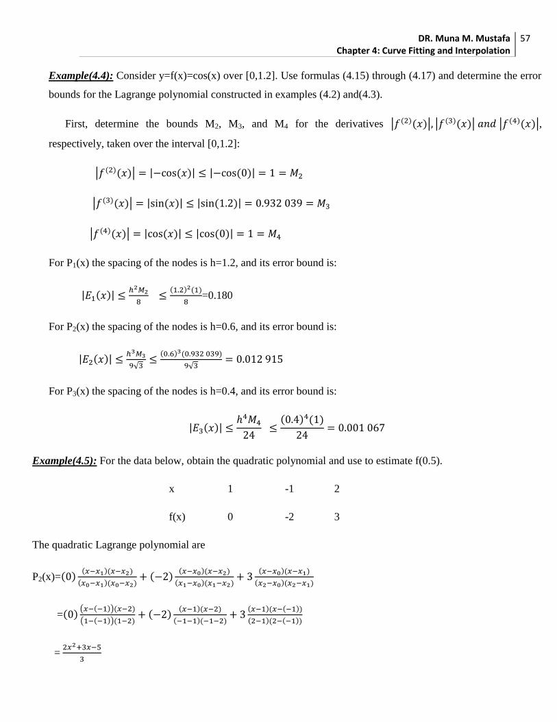
DR. Muna M. Mustafa Chapter 4: Curve Fitting and Interpolation
57
Example(4.4): Consider y=f(x)=cos(x) over [0,1.2]. Use formulas (4.15) through (4.17) and determine the error
bounds for the Lagrange polynomial constructed in examples (4.2) and(4.3).
First, determine the bounds M2, M3, and M4 for the derivatives | ( )( )| | ( )( )| | ( )( )|,
respectively, taken over the interval [0,1.2]:
| ( )( )| | ( )| | ( )|
| ( )( )| | ( )| | ( )|
| ( )( )| | ( )| | ( )|
For P1(x) the spacing of the nodes is h=1.2, and its error bound is:
| ( )|
( ) ( )
=0.180
For P2(x) the spacing of the nodes is h=0.6, and its error bound is:
| ( )|
√
( ) ( )
√
For P3(x) the spacing of the nodes is h=0.4, and its error bound is:
| ( )|
( ) ( )
Example(4.5): For the data below, obtain the quadratic polynomial and use to estimate f(0.5).
x 1 -1 2
f(x) 0 -2 3
The quadratic Lagrange polynomial are
P2(x)=( )( )( )
( )( ) ( )
( )( )
( )( )
( )( )
( )( )
=( )( ( ))( )
( ( ))( ) ( )
( )( )
( )( )
( )( ( ))
( )( ( ))
=

DR. Muna M. Mustafa Chapter 4: Curve Fitting and Interpolation
58
hence P2(0.5)=-1.
Exercises:
1. Consider the Lagrange coefficient polynomial L2,k(x) that are used for quadratic interpolation at the nodes
x0,x1, and x2. Define g(x)=L2,0(x)+L2,1(x)+L2,2(x)-1.
a. Show that g is a polynomial of degree 2.
b. Show that g(xk)=0 for k=0,1,2.
2. Consider the function f(x)=sin(x) on the interval [0,1]. Use theorem(4.3) to determine the step size h so that:
a. linear Lagrange interpolation has an accuracy of 10-6
.
b. quadratic Lagrange interpolation has an accuracy of 10-6
.
c. cubic Lagrange interpolation has an accuracy of 10-6
.
4.3 Divided Difference Interpolation
The Lagrange interpolation polynomial is useful for analysis, but is not the ideal formula for evaluating the
polynomial. Here the groundwork is laid for the development of efficient form of the unique interpolating
polynomial Pn.
a. by simplifying the construction.
b. by reducing effort required to evaluate the polynomial.
Definition(4.1):
Define ( ) ( )
(4.18)
is the first-order divided difference of f at x=xi
and
(4.19)
is the second-divided difference of f at x=xi.
and the recursive rule for constructing k-order divided differences is
(4.20)
and is used to construct the divided differences in table (4.3)

DR. Muna M. Mustafa Chapter 4: Curve Fitting and Interpolation
59
Table(4.3): Divided Differences Table
xi f(xi) f[xi,xi+1] f[xi,xi+1,xi+2] f[xi,xi+1,xi+2,xi+3]
x0 f0
f[x0,x1]
x1 f1 f[x0,x1,x2]
f[x0,x1,x2,x3]
f[x1,x2]
x2 f2 f[x1,x2,x3]
f[x2,x3]
x3 f3
Theorem(4.4): (Newton Polynomial)
Suppose that x0,x1,…,xN are N+1 distinct numbers in [a,b]. There exists a unique polynomial PN(x) of
degree at most N with the property that:
f(xj)=PN(xj) for j=0,1,…,N
The Newton form of this polynomial is:
PN(x)=a0+a1(x-x0)+…+aN(x-x0)(x-x1)…(x-xN-1) (4.21)
where ak=f[x0,x1,…,xk], for k=0,1,…,N.
Example(4.6): Repeating example(4.5) using the polynomial form (4.21) requires a divided difference table.
xi fi f[xi,xi+1] f[xi,xi+1,xi+2]
1 0
1
-1 -2
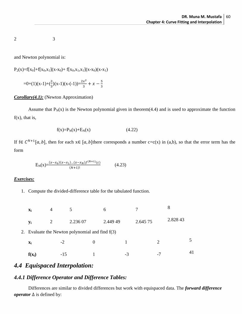
DR. Muna M. Mustafa Chapter 4: Curve Fitting and Interpolation
60
2 3
and Newton polynomial is:
P2(x)=f[x0]+f[x0,x1](x-x0)+ f[x0,x1,x1](x-x0)(x-x1)
=0+(1)(x-1)+(
)(x-1)(x-(-1))=
Corollary(4.1): (Newton Approximation)
Assume that PN(x) is the Newton polynomial given in theorem(4.4) and is used to approximate the function
f(x), that is,
f(x)=PN(x)+EN(x) (4.22)
If f , then for each x there corresponds a number c=c(x) in (a,b), so that the error term has the
form
EN(x)=( )( ) ( ) ( )( )
( ) (4.23)
Exercises:
1. Compute the divided-difference table for the tabulated function.
xi 4 5 6 7 8
yi 2 2.236 07 2.449 49 2.645 75 2.828 43
2. Evaluate the Newton polynomial and find f(3)
xi -2 0 1 2 5
f(xi) -15 1 -3 -7 41
4.4 Equispaced Interpolation:
4.4.1 Difference Operator and Difference Tables:
Differences are similar to divided differences but work with equispaced data. The forward difference
operator is defined by:

DR. Muna M. Mustafa Chapter 4: Curve Fitting and Interpolation
61
0f(x)=f(x) (4.24)
f(x)= 1f(x)=f(x+h)-f(x) (4.25)
kf(x)= ( k-1
f(x))= k-1( f(x))
= k-1f(x+h)- k-1
f(x) (4.26)
The k are conveniently displayed in a difference table(4.4)
Table(4.4): A Table of Forward Differences
x f(x) f(x) 2f(x) 3
f(x)
x0 f(x0)
f0
x1 f(x1) 2f0
f1 3f0
x2 f(x2) 2f1
f2
x3 f(x3)
Example(4.7): The polynomial P3(x)=x3-6x
2+11x-3 gives rise to the following difference table at x=2, 4, 6,
8, 10.
x P3(x) P3(x) 2P3(x) 3
P3(x)
2 3
6
4 9 48
54 48
6 63 96
150 48
8 213 144 294

DR. Muna M. Mustafa Chapter 4: Curve Fitting and Interpolation
62
10 507
4.4.2 Backward Difference Operator :
Define 0f(x)=f(x) ( 4.27)
f(x)= 1f(x)=f(x)-f(x-h) (4.28)
kf(x)= k-1
f(x)- k-1f(x-h) , k 1 (4.29)
Table(4.5): A Table of Backward Differences
x f(x) f(x) 2f(x) 3
f(x)
x0 y0
f1
x1 y1 2f2
f2 3f3
x2 y2 2f3
f3
x3 y3
4.4.3 Shift Operator: E
E0f(x)=f(x) (4.30)
Ef(x)=E1f(x)=f(x+h) (4.31)
E-1
f(x)=f(x-h) (4.32)
Ekf(x)=f(x+kh)=E(E
k-1f(x)), k= 1, 2,… (4.33)
E shifts the data point a number of intervals to the left or right.
There are many relationships between the three difference operators, of which two will be useful for
the ensuing discussion:

DR. Muna M. Mustafa Chapter 4: Curve Fitting and Interpolation
63
( ) ( ) ( ) ( ) ( ) ( ) ( )
(4.34)
and ( ) ( ) ( ) ( ) ( ) ( ) ( )
( ) (4.35)
4.4.4 Forward Difference Polynomial:
Assume that the nodes x0, x1, …, xn are in ascending order and may be described by an index j and an
interval h,
xj=x0+jh, j=0,1,…,n (4.36)
j is the number of intervals between the data point xj and the origin x0. For a real number t,
x=x0+th, 0≤t≤n (4.37)
If t {0,1,…,n}, x corresponds to a data point. Otherwise x corresponds to a point lying between two
adjacent data points.
f(x)=f(x0+th)=Etf(x0)=(1+Δ)
tf(x0)
=[ ( )
( )( )
] ( )
then Pn(x)=f0+tΔf0+ ( )
( )( ) ( )
(4.38)
which is the Newton-Gregory forward difference polynomial.
Example(4.8): Construct a difference table for the function f where f(0.5)=1, f(0.6)=2 and f(0.7)=5, and use
quadratic interpolation to estimate f(0.53).
The difference table is:
x f(x) f(x) 2f(x)
0.5 1
1
0.6 2 2
0.7 5

DR. Muna M. Mustafa Chapter 4: Curve Fitting and Interpolation
64
the quadratic polynomial P2(x)=f0+tΔf0+
t(t-1)Δ
2f0
at x=0.53 , t=
, h=0.1, we choose x0=0.5
→t=
=0.3
and f(0.53)≈P2(0.53)=1+0.3(1)+(0.3)(0.3-1)(2)/2!=1+0.3-0.105=1.195
An alternative form of Pn uses the backward difference operator
Pn(x)=Pn(x0+th)= ( )
( ) ( )
(4.39)
Example(4.9): Repeat example(4.8) using the backward formula(4.39) to find f(0.63).
The difference table is identical to that of example(4.8)
x f(x) f(x) 2f(x)
0.5 1
1
0.6 2 2
0.7 5
The quadratic polynomial P2(x2+th)=f2+t f2+
t(t+1) 2
f2
since t=
=
=-0.7 and f(0.63)≈P2(0.63)=5-3*0.7+
(-0.7)(-0.7+1)(2)=2.69
Exercises:
1. Construct a difference table for the data
x 0 0.2 0.4 0.6 0.8 1
f(x) 0.55 0.82 1.15 1.54 1.99 2.5
and use to find f(0.23) and f(0.995).
4.5 Curve Fitting

DR. Muna M. Mustafa Chapter 4: Curve Fitting and Interpolation
65
4.5.1 Least Squares Approximation:
Let Yi represent an experimental value, and let yi be a value from the equation yi=axi+b where xi is a
particular value of the variable assumed free of error. We wish to determine the best values for a and b so that the
y's predict the function values that correspond to x-values. Let ei=Yi-yi. The least-squares criterion requires that:
S=
=∑
∑ ( )
be a minimum. N is the number of x,Y-pairs. We reach the
minimum by proper choice of the parameters a and b, so they are the " variables" of the problem. At a minimum for
S, the two partial derivatives ⁄
⁄ will be both zero, that is:
∑ ( )( )
∑ ( )( )
,
Dividing each of these equations by -2 and expanding the summation, we get:
∑
∑ ∑
∑ ∑ } (4.40)
All the summations in(4.40) are from i=1 to i=N. Solving these equations gives
a= ∑ ∑ ∑
∑ (∑ )
(4.41)
b=∑ ∑
∑ ∑
∑ (∑ )
(4.42)
Example(4.10): Find the least-squares line for the data point given in the following table:
x -1 0 1 2 3 4 5 6
y 10 9 7 5 4 3 0 -1
N=8, ∑ =20, ∑ =92, ∑ =37, ∑ =25
from equations(4.41) and (4.42), we get:
a=-1.6071429, b=8.6428571
and y=-1.6071429x+8.6428571
4.5.2 The Power Fit y=AxM

DR. Muna M. Mustafa Chapter 4: Curve Fitting and Interpolation
66
Some situations involve f(x)=AxM
, where M is a Known constant. In this cases there is only one parameter
A to be determined.
Theorem(4.5): (Power Fit)
Suppose that {(xk,yk)}, k=1,…,N are N points, where the abscissas are distinct. The coefficient A of the
least-squares power curve y=AxM
is given by
A=(∑
)
(∑
)⁄ (4.43)
Example(4.11): Find the constant g in the relation d=
using the following table:
t 0.2 0.4 0.6 0.8 1.0
d 0.196 0.785 1.7665 3.1405 4.9075
Here M=2, N=5, ∑ =7.6868 , ∑
=1.5664
and the coefficient A=7.6868/1.5664=4.9073, so we get g=2A=9.7146.
4.5.3 Data Linearization Method for y=CeAx
:
Suppose that we are given points (x1,y1),…,(xN,yN) and want to fit an exponential curve of the form
y=CeAx
(4.44)
The first step is to take the logarithm of both sides:
ln(y)=Ax+ln(C) (4.45)
Then introduce the change of variables:
Y=ln(y), X=x , and B=ln(C) (4.46)
This results in a linear relation between the new variables X and Y

DR. Muna M. Mustafa Chapter 4: Curve Fitting and Interpolation
67
Y=AX+B (4.47)
Example(4.12): Use the data linearization method and find the exponential fit y=CeAx
for the five points (0,1.5),
(1,2.5), (2,3.5), (3,5), and (4,7.5).
x 0 1 2 3 4
y 1.5 2.5 3.5 5 7.5
∑ ∑ ∑ ∑ ∑ ∑ and N=5
therefore we have a=0.3912023, b=0.457367
then C is obtained with the calculation C=e0.457367
=1.57991
and y=1.57991e0.3912023x
Exercises:
1. Find the least-squares line for the data
x -6 -2 0 2 6
y 7 5 3 2 0
2. Find the power fits y=Ax2 and y=Bx
3 for the following data:
x 0.5 0.8 1.1 1.8 4
y 7.1 4.4 3.2 1.9 0.9
3. For the given data find the least-squares curve f(x)=CeAx
x -1 0 1 2 3
y 6.62 3.94 2.17 1.35 0.89