CALIFA, the Calar Alto Legacy Integral Field Area survey: I. Survey presentation
33
Astronomy & Astrophysics manuscript no. sanchez c ESO 2011 November 7, 2011 CALIFA, the Calar Alto Legacy Integral Field Area survey: I. Survey presentation ? S.F. S´ anchez 1 , R.C. Kennicutt 2 , A. Gil de Paz 3 , G. van de Ven 4 , J.M. V´ ılchez 5 , L. Wisotzki 6 , C. J. Walcher 6 , D. Mast 5,1 , J. A. L. Aguerri 9,28 , S. Albiol-P´ erez 20 , A. Alonso-Herrero 12 , J. Alves 22 , J. Bakos 9,28 , T. Bart´ akov´ a 34 , J. Bland-Hawthorn 7 , A. Boselli 19 , D. J. Bomans 25 , A. Castillo-Morales 3 , C. Cortijo-Ferrero 5 , A. de Lorenzo-C´ aceres 9,28 , A. del Olmo 5 , R.-J. Dettmar 25 , A. D´ ıaz 10 , S. Ellis 8,7 , J. Falc´ on-Barroso 9,28 , H. Flores 31 , A. Gallazzi 14 , B. Garc´ ıa-Lorenzo 9,28 , R. Gonz´ alez Delgado 5 , N. Gruel 24 , T. Haines 26 , C. Hao 32 , B. Husemann 6 , J. Igl´ esias-P´ aramo 5,1 , K. Jahnke 4 , B. Johnson 30 , B. Jungwiert 16,33 , V. Kalinova 4 , C. Kehrig 6 , D. Kupko 6 , ´ A. R. L ´ opez-S´ anchez 8,23 , M. Lyubenova 4 , R.A. Marino 1,3 , E. M´ armol-Queralt´ o 1,3 , I. M´ arquez 5 , J. Masegosa 5 , S. Meidt 4 , J. Mendez-Abreu 9,28 , A. Monreal-Ibero 5 , C. Montijo 5 , A. M. Mour˜ ao 17 , G. Palacios-Navarro 21 , P. Papaderos 15 , A. Pasquali 29 , R. Peletier 11 , E. P´ erez 5 , I. P´ erez 27 , A. Quirrenbach 13 , M. Rela ˜ no 27 , F. F. Rosales-Ortega 10,1 , M. M. Roth 6 , T. Ruiz-Lara 27 , P. S´ anchez-Bl´ azquez 10 , C. Sengupta 1,5 , R. Singh 4 , V. Stanishev 17 , S.C. Trager 11 , A. Vazdekis 9,28 , K. Viironen 1,24 , V. Wild 18 , S. Zibetti 14 , and B. Ziegler 22 (Affiliations can be found after the references) Received —– ; accepted —- ABSTRACT The final product of galaxy evolution through cosmic time is the population of galaxies in the Local Universe. These galaxies are also those that can be studied in most detail, thus providing a stringent benchmark for our understanding of galaxy evolution. Through the huge success of spectroscopic single-fiber, statistical surveys of the Local Universe in the last decade, it has become clear, however, that an authoritative observational description of galaxies will involve measuring their spatially resolved properties over their full optical extent (covering D25) for a statistically significant sample. We present here the Calar Alto Legacy Integral Field Area (CALIFA) survey, which has been designed to provide a first step in this direction. We summarize the survey goals and design, including sample selection and observational strategy. We also showcase the data taken during the first observing runs (June/July 2010) and outline the reduction pipeline, quality control schemes and general characteristics of the reduced data. This survey is obtaining spatially resolved spectroscopic information of a diameter selected sample of ∼600 galaxies in the Local Universe (0.005< z <0.03). CALIFA has been designed to allow the building of two-dimensional maps of the following quantities: (a) stellar populations: ages and metallicities; (b) ionized gas: distribution, excitation mechanism and chemical abundances; and (c) kinematic properties: both from stellar and ionized gas components. CALIFA uses the PPAK Integral Field Unit (IFU), with a hexagonal field-of-view of ∼1.3u t 0 , with a 100% covering factor by adopting a three-pointing dithering scheme. The optical wavelength range is covered from 3700 to 7000 Å, using two overlapping setups (V500 and V1200), with different resolutions: R∼850 and R∼1650, respectively. CALIFA is a legacy survey, intended for the community. The reduced data will be released, once the quality has been guaranteed. The analyzed data fulfill the expectations of the original observing proposal, on the basis of a set of quality checks and exploratory analysis: (i) the final datacubes reach a 3σ limiting surface brightness depth of ∼ 23.0 mag/arcsec 2 for the V500 grating data (∼22.8 mag/arcsec 2 for V1200); (ii) about ∼70% of the covered field-of-view is above this 3σ limit; (iii) the data have a blue-to-red relative flux calibration within a few percent in most of the wavelength range; (iv) the absolute flux calibration is accurate within ∼8% with respect to SDSS; (v) the measured spectral resolution is ∼85 km s -1 for V1200 (∼150 km s -1 for V500); (vi) the estimated accuracy of the wavelength calibration is ∼5 km s -1 for the V1200 data (∼10 km s -1 for the V500 data); (vii) the aperture matched CALIFA and SDSS spectra are qualitatively and quantitatively similar. Finally, we show that we are able to carry out all measurements indicated above, recovering the properties of the stellar populations, the ionized gas and the kinematics of both components. The associated maps illustrate the spatial variation of these parameters across the field, reemphasizing the redshift dependence of single aperture spectroscopic measurements. We conclude from this first look at the data that CALIFA will be an important resource for archaeological studies of galaxies in the Local Universe. Key words. techniques: spectroscopic – galaxies: abundances – stars: formation – galaxies: ISM – galaxies: stellar content 1. Introduction Our understanding of the Universe and its constituents comes from large surveys such as the 2dFGRS (Folkes et al. 1999), ? Based on observations collected at the Centro Astron´ omico Hispano Alem´ an (CAHA) at Calar Alto, operated jointly by the Max- Planck-Institut f¨ ur Astronomie and the Instituto de Astrof´ ısica de Andaluc´ ıa (CSIC). SDSS (York et al. 2000), GEMS (Rix et al. 2004), VVDS (Le F` evre et al. 2004), and COSMOS (Scoville et al. 2007a), to name but a few. Such surveys have not only constrained the evolu- tion of global quantities such as the cosmic star formation rate, but also enabled us to link these with the properties of individ- ual galaxies – morphological types, stellar masses, metallicities, etc. Compared to previous approaches, the major advantages of this recent generation of surveys are: (1) the large number of ob- 1 arXiv:1111.0962v2 [astro-ph.CO] 4 Nov 2011
-
Upload
independent -
Category
Documents
-
view
1 -
download
0
Transcript of CALIFA, the Calar Alto Legacy Integral Field Area survey: I. Survey presentation
Astronomy & Astrophysics manuscript no. sanchez c© ESO 2011November 7, 2011
CALIFA, the Calar Alto Legacy Integral Field Area survey:I. Survey presentation?
S.F. Sanchez1, R.C. Kennicutt2, A. Gil de Paz3, G. van de Ven4, J.M. Vılchez5, L. Wisotzki6, C. J. Walcher6, D.Mast5,1, J. A. L. Aguerri9,28, S. Albiol-Perez20, A. Alonso-Herrero12, J. Alves22, J. Bakos9,28, T. Bartakova34, J.
Bland-Hawthorn7, A. Boselli19, D. J. Bomans25, A. Castillo-Morales3, C. Cortijo-Ferrero5, A. de Lorenzo-Caceres9,28,A. del Olmo5, R.-J. Dettmar25, A. Dıaz10, S. Ellis8,7, J. Falcon-Barroso9,28, H. Flores31, A. Gallazzi14, B.
Garcıa-Lorenzo9,28, R. Gonzalez Delgado5, N. Gruel24, T. Haines26, C. Hao32, B. Husemann6, J. Iglesias-Paramo5,1, K.Jahnke4, B. Johnson30, B. Jungwiert16,33, V. Kalinova4, C. Kehrig6, D. Kupko6, A. R. Lopez-Sanchez8,23, M.
Lyubenova4, R.A. Marino1,3, E. Marmol-Queralto1,3, I. Marquez5, J. Masegosa5, S. Meidt4, J. Mendez-Abreu9,28, A.Monreal-Ibero5, C. Montijo5, A. M. Mourao17, G. Palacios-Navarro21, P. Papaderos15, A. Pasquali29, R. Peletier11, E.
Perez5, I. Perez27, A. Quirrenbach13, M. Relano27, F. F. Rosales-Ortega10,1, M. M. Roth6, T. Ruiz-Lara27, P.Sanchez-Blazquez10, C. Sengupta1,5, R. Singh4, V. Stanishev17, S.C. Trager11, A. Vazdekis9,28, K. Viironen1,24, V.
Wild18, S. Zibetti14, and B. Ziegler22
(Affiliations can be found after the references)
Received —– ; accepted —-
ABSTRACT
The final product of galaxy evolution through cosmic time is the population of galaxies in the Local Universe. These galaxies are also thosethat can be studied in most detail, thus providing a stringent benchmark for our understanding of galaxy evolution. Through the huge successof spectroscopic single-fiber, statistical surveys of the Local Universe in the last decade, it has become clear, however, that an authoritativeobservational description of galaxies will involve measuring their spatially resolved properties over their full optical extent (covering D25) for astatistically significant sample. We present here the Calar Alto Legacy Integral Field Area (CALIFA) survey, which has been designed to provide afirst step in this direction. We summarize the survey goals and design, including sample selection and observational strategy. We also showcase thedata taken during the first observing runs (June/July 2010) and outline the reduction pipeline, quality control schemes and general characteristicsof the reduced data.This survey is obtaining spatially resolved spectroscopic information of a diameter selected sample of ∼600 galaxies in the Local Universe(0.005< z <0.03). CALIFA has been designed to allow the building of two-dimensional maps of the following quantities: (a) stellar populations:ages and metallicities; (b) ionized gas: distribution, excitation mechanism and chemical abundances; and (c) kinematic properties: both from stellarand ionized gas components. CALIFA uses the PPAK Integral Field Unit (IFU), with a hexagonal field-of-view of ∼1.3ut′, with a 100% coveringfactor by adopting a three-pointing dithering scheme. The optical wavelength range is covered from 3700 to 7000 Å, using two overlapping setups(V500 and V1200), with different resolutions: R∼850 and R∼1650, respectively. CALIFA is a legacy survey, intended for the community. Thereduced data will be released, once the quality has been guaranteed.The analyzed data fulfill the expectations of the original observing proposal, on the basis of a set of quality checks and exploratory analysis: (i)the final datacubes reach a 3σ limiting surface brightness depth of ∼ 23.0 mag/arcsec2 for the V500 grating data (∼22.8 mag/arcsec2 for V1200);(ii) about ∼70% of the covered field-of-view is above this 3σ limit; (iii) the data have a blue-to-red relative flux calibration within a few percent inmost of the wavelength range; (iv) the absolute flux calibration is accurate within ∼8% with respect to SDSS; (v) the measured spectral resolutionis ∼85 km s−1 for V1200 (∼150 km s−1 for V500); (vi) the estimated accuracy of the wavelength calibration is ∼5 km s−1 for the V1200 data(∼10 km s−1 for the V500 data); (vii) the aperture matched CALIFA and SDSS spectra are qualitatively and quantitatively similar. Finally, weshow that we are able to carry out all measurements indicated above, recovering the properties of the stellar populations, the ionized gas and thekinematics of both components. The associated maps illustrate the spatial variation of these parameters across the field, reemphasizing the redshiftdependence of single aperture spectroscopic measurements. We conclude from this first look at the data that CALIFA will be an important resourcefor archaeological studies of galaxies in the Local Universe.
Key words. techniques: spectroscopic – galaxies: abundances – stars: formation – galaxies: ISM – galaxies: stellar content
1. Introduction
Our understanding of the Universe and its constituents comesfrom large surveys such as the 2dFGRS (Folkes et al. 1999),
? Based on observations collected at the Centro AstronomicoHispano Aleman (CAHA) at Calar Alto, operated jointly by the Max-Planck-Institut fur Astronomie and the Instituto de Astrofısica deAndalucıa (CSIC).
SDSS (York et al. 2000), GEMS (Rix et al. 2004), VVDS (LeFevre et al. 2004), and COSMOS (Scoville et al. 2007a), to namebut a few. Such surveys have not only constrained the evolu-tion of global quantities such as the cosmic star formation rate,but also enabled us to link these with the properties of individ-ual galaxies – morphological types, stellar masses, metallicities,etc. Compared to previous approaches, the major advantages ofthis recent generation of surveys are: (1) the large number of ob-
1
arX
iv:1
111.
0962
v2 [
astr
o-ph
.CO
] 4
Nov
201
1
S.F. Sanchez et al.: CALIFA, the Calar Alto Legacy Integral Field Area survey:
jects sampled, allowing for meaningful statistical analysis to beperformed on an unprecedented scale; (2) the possibility to con-struct large comparison/control samples for each subset of galax-ies; (3) a broad coverage of galaxy subtypes and environmentalconditions, allowing for the derivation of universal conclusions;and (4) the homogeneity of the data acquisition, reduction and(in some cases) analysis.
On the other hand, the cost of these surveys, in terms of tele-scope time, person-power, and time scales involved, is also un-precedented in astronomy. The user of such data products hasnot necessarily been involved in any step of designing or con-ducting the survey, but nevertheless takes advantage of the databy exploiting them according to her/his scientific interests. Thisnew approach to observational astronomy is also changing ourperception of the scientific rationale behind a new survey: whileit is clear that certain planned scientific applications are key de-terminants to the design of the observations and ‘drive’ the sur-vey, the survey data should, at the same time, allow for a broadrange of scientific exploitation. This aspect is now often called asurvey’s legacy value.
Current technology generally leads to surveys either in theimaging or in the spectroscopic domain. While imaging surveysprovide two-dimensional coverage, the information content of aphotometric Spectral Energy Distribution (SED) is limited. Thisremains true for the new generation of multi-band photometricsurveys such as COMBO-17 (Wolf et al. 2003), ALHAMBRA(Moles et al. 2008), the planned PAU project (Benıtez et al.2009), COSMOS (Scoville et al. 2007b) or the LUS survey1,which are geared towards better precision in redshift, mean agesand stellar masses, but are nevertheless unable to measure in-dividual spectral lines and thus emission line ratios or internalradial velocity differences. Spectroscopic surveys such as SDSSor zCOSMOS (Lilly et al. 2007), on the other hand, do providemore detailed astrophysical information, but they are generallylimited to one spectrum per galaxy. One thus misses all informa-tion on the radial distribution of galaxy properties and on all de-tails of the kinematics. Even when attempting to describe galax-ies by their integrated properties only, this state of affairs alsoleads to aperture losses that are difficult to control. For example,the 3′′ diameter of the fiber used in the SDSS corresponds to dif-ferent physical scales at different redshifts, with limited possibil-ities to correct for these aperture effects (e.g., Kewley et al. 2005;Ellis et al. 2005). The most popular method is to compare resultsof a fit to the photometry of the whole galaxy with the photomet-ric fit corresponding to the area of the fiber only (Gomez et al.2003; Brinchmann et al. 2004). Even more severely, Zibetti et al.(2009) have recently shown that spatially resolved stellar popu-lation analysis may lead to corrections of up to 40% for the stel-lar mass of a galaxy, when compared to integrated light studies.
An observational technique combining the advantages ofimaging and spectroscopy (albeit with usually quite small fieldof view) is Integral Field Spectroscopy (IFS). This technique al-lows us to study both the integrated and spatially resolved spec-troscopic properties of galaxies. IFS has the potential to pro-vide observational evidence to constrain many outstanding ques-tions of baryonic physics which are key to our understanding ofgalaxy evolution and, therefore, cosmology. Some of these are(1) the importance and consequences of merging, major and mi-nor; (2) internal dynamical processes, such as bars, spiral arms,stellar migration; (3) environmental effects, such as tidal forces,stripping; (4) AGN feedback; (5) occurrence, spatial and tempo-ral extent and trigger of star formation. Spatially resolved spec-
1 http://www.inaoep.mx/∼gtc-lus/
troscopic properties of a statistical sample of nearby galaxies isthe dataset required to address these questions.
However, so far, IFS has rarely been used in a ‘survey mode’to investigate sizeable samples. Among the few exceptions thereis, most notably, the SAURON survey (de Zeeuw et al. 2002),focused on the study of the central regions of 72 nearby early-type galaxies and bulges of spirals, and its extension ATLAS3D
(260 early-type galaxies at z < 0.01; Cappellari et al. 2011).Others are the on-going PINGS project (Rosales-Ortega et al.2010) at the CAHA 3.5m of a dozen of very nearby galaxies(∼10 Mpc) and the currently ongoing study of 70 (U)LIRGS atz < 0.26 using different IFUs (Arribas et al. 2008). Finally, theVIRUS-P instrument is currently used to carry out two small IFSsurveys, namely VENGA (30 spiral galaxies, Blanc et al. 2010)and VIXENS2 (15 starbursts). All these datasets are clearlyfocused on specific science questions, adopting correspond-ingly optimized sample selection criteria and also observingstrategies. For example, at the redshifts of the galaxies in theATLAS3D sample SAURON has a field of view of 30′′ × 40′′, or < 7 × 9 kpc, thus does not cover the outer parts of thesegalaxies.
On completion, CALIFA will be the largest and the mostcomprehensive wide-field IFU survey of galaxies carried out todate. It will thus provide an invaluable bridge between largesingle aperture surveys and more detailed studies of individualgalaxies. With CALIFA we will fix observational properties ofgalaxies in the Local Universe, which will have a potential im-pact in the interpretation of observed properties at higher redshift(e.g. Epinat et al. 2010).
CALIFA is an ongoing survey, which has been granted with210 dark nights by the Calar Alto Executive Committee, span-ning through 6 semesters. The gathering of the data started inJune/July 2010, and after a technical problem with the telescope,it was resumed in March 2011. This technical problem, fullyrepaired, has not affected the quality of the CALIFA data.About 20 galaxies are observed per month. As mentioned above,there will be consecutive data releases of the fully reduceddatasets, once certain milestones/number of observed galaxiesare reached. The first one is planned for late 2012, when a totalnumber of 100 galaxies is completed (ie., observed, reduced andquality of the data tested). The current status of data acquisitioncan be obtained from the CALIFA webpage3.
In this article we present the main characteristics of the sur-vey, starting from the design requirements in Section 2. Section3 describes the sample selection criteria, and the main character-istics of the CALIFA mother sample. In Section 4 we describethe observing strategy, in particular the observations performedduring the first CALIFA runs. The data reduction is described indetail in Section 5, and some of the first quality tests performedon the data are presented in Section 6. The exploratory analy-sis performed on these first datasets, obtained in 2010, to verifythat we will be able to reach our science goals are presented inSection 7. A summary and conclusion of the results is presentedin Section 8.
2. Design drivers
CALIFA has been designed to increase our knowledge of thebaryonic physics of galaxy evolution. We intend to characterizeobservationally the local galaxy population with the followingkey points in mind:
2 http://www.as.utexas.edu/∼alh/vixens.html3 http://www.caha.es/CALIFA/
2
S.F. Sanchez et al.: CALIFA, the Calar Alto Legacy Integral Field Area survey:
– Sample covering a substantial fraction of the galaxy lumi-nosity function.
– Large enough sample to allow statistically significant con-clusions for all classes of galaxies represented in the survey.
– Characterization of galaxies over their full spatial extent(covering in most cases the R25 radius) , i.e. avoiding aper-ture biases and harnessing the additional power of 2D reso-lution (gradients, sub-structures: bars, spiral arms...).
– Measurement of gas ionization mechanisms: star formation,shocks, AGN.
– Measurement of ionized gas oxygen and nitrogen abun-dances.
– Measurement of stellar population properties: ages, mass-to-light ratios, metallicities, and (to a limited extent) abundancepatterns.
– Measurement of galaxy kinematics in gas and stars, i.e. ve-locity fields for all galaxies and velocity dispersions for themore massive ones.
A careful assessment of these, partially competing, driversand of the practical limits imposed by the instrument, the ob-servatory and the timescale has led to the following key charac-teristics of the survey: (i) Sample: ∼600 galaxies of any kind inthe Local Universe, covering the full color-magnitude diagramdown to MB ∼ −18 mag, selected from the SDSS to allow gooda-priori characterization of the targets; (ii) Instrument: PPAKIFU of the Potsdam Multi-Aperture Spectrograph (PMAS) in-strument at the 3.5m telescope of CAHA, with one of the largestfields-of-view for this kind of instruments (>1 arcmin2); (iii)Grating setups: two overlapping setups, one in the red (3750–7000 Å, R∼850, for ionized gas measurements and stellar popu-lations) and one in the blue (3700–4700 Å, R∼1650, for detailedstellar populations and for stellar and gas kinematics); and (iii)Exposure times: 1800s in the blue and 900s in the red.
3. The CALIFA galaxy sample
We now briefly describe how the sample has been constructed.We limit this section to some fundamental considerations thatare important for understanding the potential and limitations ofthe survey. In a later paper we will present a detailed character-ization of the sample and the distribution of galaxy properties,including comparisons to other studies and the galaxy popula-tion as a whole.
The guiding principle for building the CALIFA galaxy sam-ple followed from the broad set of scientific aims outlined inthe previous section, i.e. the sample should cover a wide rangeof important galaxy properties such as morphological types, lu-minosities, stellar masses, and colours. Further constraints wereadded due to technical and observational boundary conditions,such as observing all galaxies with the same spectroscopic setupto make scheduling as flexible as possible. As detailed below, asmall set of selection criteria was employed to define a sampleof 937 possible target galaxies, the so-called “CALIFA mothersample”. From this mother sample, the galaxies are drawn asactual targets only according to their visibility, i.e. in a quasi-random fashion, so that the final catalog of CALIFA galaxieswill be a slightly sparsely sampled (∼2/3) subset of the mothersample.
The CALIFA mother sample was initially selected from theSDSS DR7 photometric catalog (Abazajian et al. 2009), whichensures the availability of good quality multi-band photometry,and in many cases (but not all, cf. below) nuclear spectra. TheCALIFA footprint is thus largely identical to that of the SDSS
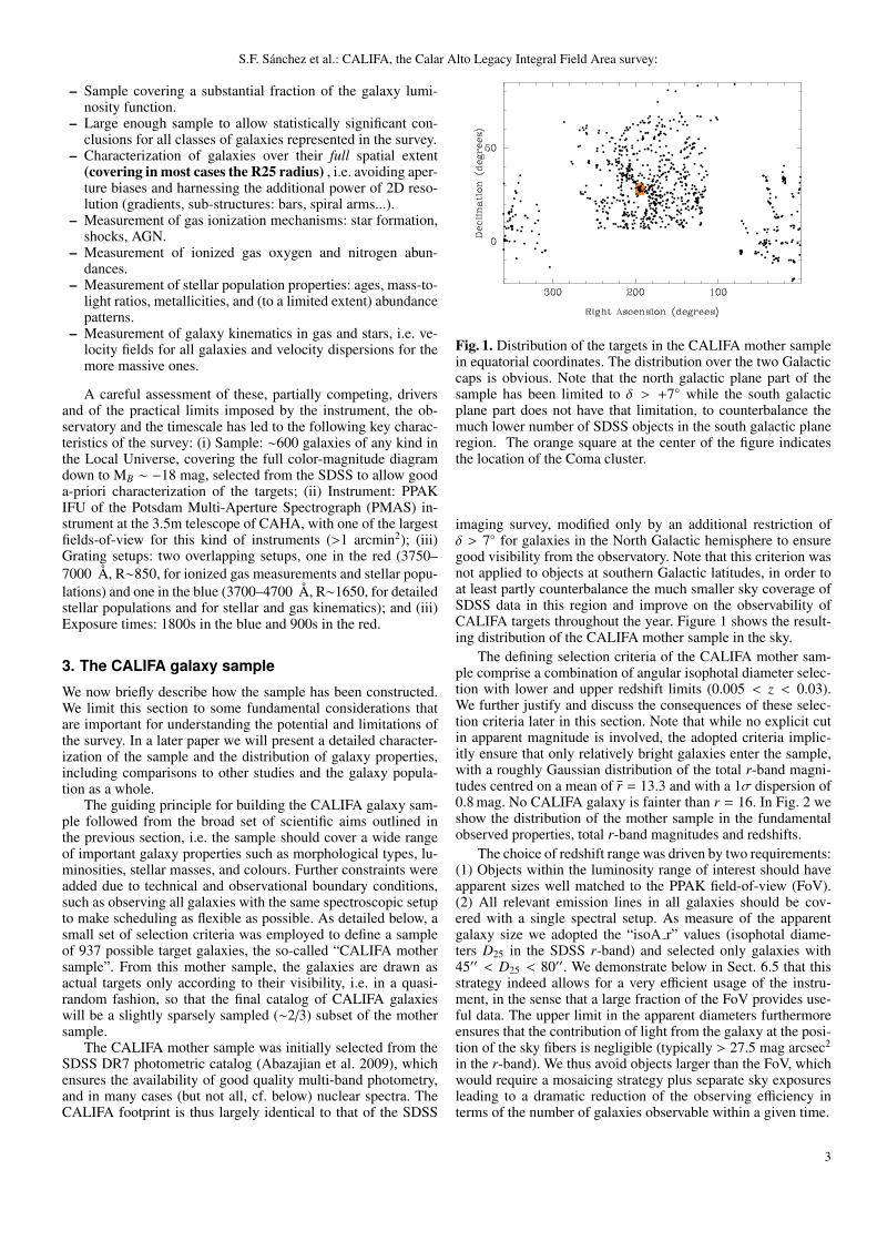
Fig. 1. Distribution of the targets in the CALIFA mother samplein equatorial coordinates. The distribution over the two Galacticcaps is obvious. Note that the north galactic plane part of thesample has been limited to δ > +7◦ while the south galacticplane part does not have that limitation, to counterbalance themuch lower number of SDSS objects in the south galactic planeregion. The orange square at the center of the figure indicatesthe location of the Coma cluster.
imaging survey, modified only by an additional restriction ofδ > 7◦ for galaxies in the North Galactic hemisphere to ensuregood visibility from the observatory. Note that this criterion wasnot applied to objects at southern Galactic latitudes, in order toat least partly counterbalance the much smaller sky coverage ofSDSS data in this region and improve on the observability ofCALIFA targets throughout the year. Figure 1 shows the result-ing distribution of the CALIFA mother sample in the sky.
The defining selection criteria of the CALIFA mother sam-ple comprise a combination of angular isophotal diameter selec-tion with lower and upper redshift limits (0.005 < z < 0.03).We further justify and discuss the consequences of these selec-tion criteria later in this section. Note that while no explicit cutin apparent magnitude is involved, the adopted criteria implic-itly ensure that only relatively bright galaxies enter the sample,with a roughly Gaussian distribution of the total r-band magni-tudes centred on a mean of r = 13.3 and with a 1σ dispersion of0.8 mag. No CALIFA galaxy is fainter than r = 16. In Fig. 2 weshow the distribution of the mother sample in the fundamentalobserved properties, total r-band magnitudes and redshifts.
The choice of redshift range was driven by two requirements:(1) Objects within the luminosity range of interest should haveapparent sizes well matched to the PPAK field-of-view (FoV).(2) All relevant emission lines in all galaxies should be cov-ered with a single spectral setup. As measure of the apparentgalaxy size we adopted the “isoA r” values (isophotal diame-ters D25 in the SDSS r-band) and selected only galaxies with45′′ < D25 < 80′′. We demonstrate below in Sect. 6.5 that thisstrategy indeed allows for a very efficient usage of the instru-ment, in the sense that a large fraction of the FoV provides use-ful data. The upper limit in the apparent diameters furthermoreensures that the contribution of light from the galaxy at the posi-tion of the sky fibers is negligible (typically > 27.5 mag arcsec2
in the r-band). We thus avoid objects larger than the FoV, whichwould require a mosaicing strategy plus separate sky exposuresleading to a dramatic reduction of the observing efficiency interms of the number of galaxies observable within a given time.
3

S.F. Sanchez et al.: CALIFA, the Calar Alto Legacy Integral Field Area survey:
Not all galaxies in the SDSS photometric catalog obeyingour isophotal diameter criterion have spectra – and therefore red-shifts – in the SDSS spectroscopic database, which is knownto become increasingly incomplete for total magnitudes brighterthat r ∼ 14. In order to (as much as possible) overcome such anundesirable bias against bright galaxies, we supplemented theSDSS redshifts with information accessed through the SIMBADdatabase at CDS, which in turn is a compilation of a large varietyof observations and redshift catalogs. Hence, there are SDSS-based spectra and redshifts for ∼60% of the CALIFA galax-ies, while for the remainder we have only the redshift informa-tion provided by SIMBAD. As the latter is also not 100% com-plete, there could be a few galaxies within the CALIFA foot-print without redshift measurements and, therefore, outside ofthe CALIFA mother sample. It is difficult to quantify this in-completeness, but it is unlikely to be more than a few percent,and probably much less.
Our decision to construct a diameter-selected sample hasseveral practical advantages, besides the obvious benefit of effi-ciently using the instrumental field-of-view. Another advantagehas already been mentioned: for the adopted redshift range, thedistribution of apparent galaxy magnitudes naturally favours rel-atively bright systems, and in fact there was no need to define anadditional faint flux limit to the survey (see Fig. 2). Furthermore,the range in absolute magnitudes is considerably broadened dueto the factor of 6 between lowest and highest redshifts, so that theCALIFA sample encompasses an interval of > 7 mag in intrinsicluminosities. In fact, the low-redshift cutoff was mainly intro-duced in order to limit the luminosity range and avoid swampingthe sample with dwarf galaxies, which – given the limitation to600 galaxies in total – were considered to be outside the mainscientific interest of the CALIFA project.
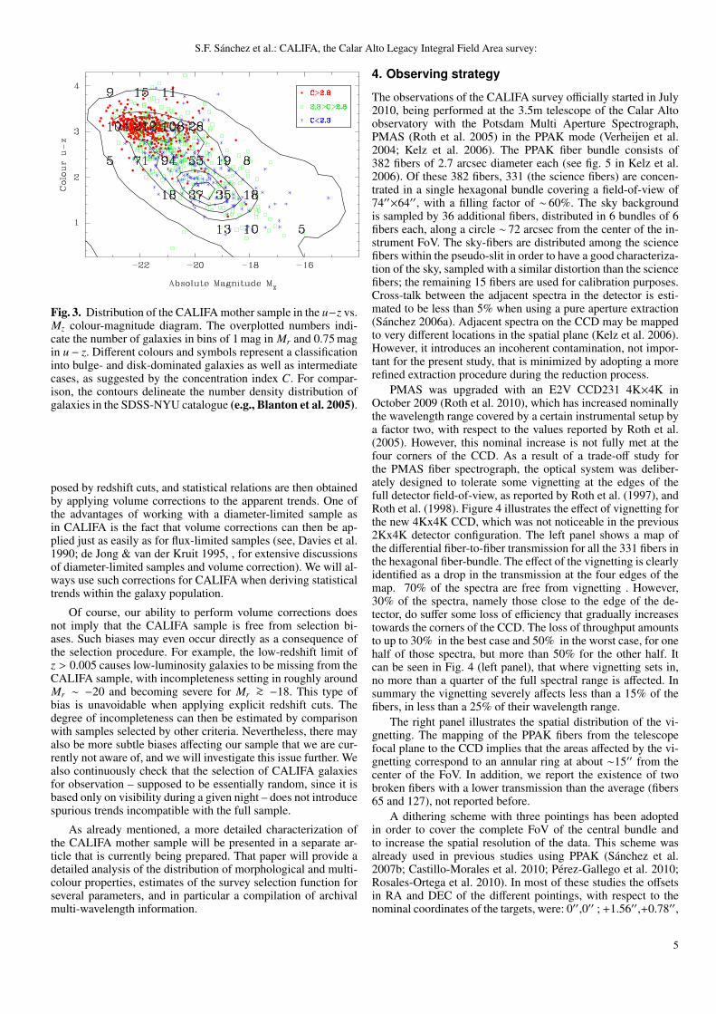
Together with the wide range in luminosities comes a broadcoverage of galaxy colours, and the CALIFA sample includessubstantial numbers of galaxies in all populated areas of thecolour-magnitude diagram, from the red sequence through thegreen valley to the blue cloud (which is of course effectivelytruncated at its faint end due to the low-redshift limit). Thisbroad colour distribution is illustrated in Fig. 3, where we com-pare the u − z vs. Mz relation of galaxies in the CALIFA mothersample with the corresponding distribution in the SDSS-NYUcatalog (e.g. Blanton et al. 2005). While there are (and shouldbe) differences in the details of the distribution – which can bequantified, see below –, it is immediately clear that CALIFAat least qualitatively represents a wide range of galaxy types.Figure 3 also provides the number of CALIFA objects per bin inMz and u− z (recall, however, that the observed sample size willbe smaller by a factor ∼ 2/3). These numbers show that therewill be sufficient statistics in several bins to make robust state-ments about typical galaxy properties, for early-type as well aslate-type galaxies. In fact, these were the numbers that drove theoverall time request for CALIFA to enable a total sample size of600 galaxies.
The broad representation of galaxy properties in the CALIFAsample is also reflected in the distribution of morphologicaltypes. While a thorough characterization of the sample in termsof morphology and structural properties will be the subject ofa future paper, a qualitative impression can be obtained alreadyfrom rather simple diagnostics. It has been demonstrated in thepast (Strateva et al. 2001) that bulge- and disk-dominated sys-tems can be reasonably well distinguished by their concentrationindices, defined as the ratio C of the r90 and r50 Petrosian radiiprovided by the SDSS photometric catalog. Typically, a value ofC >∼ 2.8 requires the presence of a substantial bulge, whereas
Fig. 2. Apparent r-band magnitude and redshift distribution ofthe CALIFA mother sample.
C <∼ 2.3 is indicative of an exponential disk. In Fig. 3 we codedthe symbols into three groups, including a class of transition oruncertain objects with 2.3 < C < 2.8. Their different distribu-tions in the colour-magnitude diagram is immediately apparent.
Clearly, the majority of CALIFA galaxies (∼ 2/3) have sub-stantial disk components, including irregulars and interactinggalaxies, and are more or less actively forming stars. The fi-nal sample of ∼ 400 of such galaxies will clearly exceed anyprevious IFU study by a large factor. Interestingly, the ominous“green valley” intermediate to star-forming and passive galaxiesis well covered by the sample.
On the other hand, CALIFA will also provide IFU data forsome 200 bulge-dominated, morphologically early-type galax-ies, most of which – as expected – cluster very stronglyalong the red sequence. While the successful ATLAS3D project(Cappellari et al. 2011) has already observed an even somewhatlarger number of early-type galaxies, CALIFA will complementthe insights from ATLAS3D due to its much larger spectral cov-erage (∼ 6×) and FoV, which will allow the study of the outerregions of early-type galaxies.
In terms of environment, the CALIFA sample is clearly dom-inated by field galaxies. It will effectively include galaxy popu-lations in groups, but much denser environments will be poorlysampled. A rough estimate of the total number of galaxy clustersin the sample can be obtained from the counts by Baillard et al.(2011), leading to a maximum of 10 clusters that will, at leastpartially, be covered by CALIFA. Fortunately, the Coma clusterat z ' 0.023 is fully covered by the CALIFA footprint and red-shift range (cf. Fig. 1). Therefore, there will be some (limited)ability to study the environmental dependence of galaxy proper-ties.
Any sample of galaxies faces the question about its abilityto represent, in a statistically well-defined way, the propertiesof the galaxy population as a whole. In some cases, e.g. in theATLAS3D project, it has been possible to construct and observestrictly volume-limited samples for which this relation can be di-rectly made, but this is not a viable approach for a more genericsurvey covering a wide range of luminosities. Many surveysare simply flux-limited (such as the SDSS main galaxy sam-ple), possibly supplemented by an additional volume limit im-
4
S.F. Sanchez et al.: CALIFA, the Calar Alto Legacy Integral Field Area survey:
Fig. 3. Distribution of the CALIFA mother sample in the u−z vs.Mz colour-magnitude diagram. The overplotted numbers indi-cate the number of galaxies in bins of 1 mag in Mr and 0.75 magin u − z. Different colours and symbols represent a classificationinto bulge- and disk-dominated galaxies as well as intermediatecases, as suggested by the concentration index C. For compar-ison, the contours delineate the number density distribution ofgalaxies in the SDSS-NYU catalogue (e.g., Blanton et al. 2005).
posed by redshift cuts, and statistical relations are then obtainedby applying volume corrections to the apparent trends. One ofthe advantages of working with a diameter-limited sample asin CALIFA is the fact that volume corrections can then be ap-plied just as easily as for flux-limited samples (see, Davies et al.1990; de Jong & van der Kruit 1995, , for extensive discussionsof diameter-limited samples and volume correction). We will al-ways use such corrections for CALIFA when deriving statisticaltrends within the galaxy population.
Of course, our ability to perform volume corrections doesnot imply that the CALIFA sample is free from selection bi-ases. Such biases may even occur directly as a consequence ofthe selection procedure. For example, the low-redshift limit ofz > 0.005 causes low-luminosity galaxies to be missing from theCALIFA sample, with incompleteness setting in roughly aroundMr ∼ −20 and becoming severe for Mr >∼ −18. This type ofbias is unavoidable when applying explicit redshift cuts. Thedegree of incompleteness can then be estimated by comparisonwith samples selected by other criteria. Nevertheless, there mayalso be more subtle biases affecting our sample that we are cur-rently not aware of, and we will investigate this issue further. Wealso continuously check that the selection of CALIFA galaxiesfor observation – supposed to be essentially random, since it isbased only on visibility during a given night – does not introducespurious trends incompatible with the full sample.
As already mentioned, a more detailed characterization ofthe CALIFA mother sample will be presented in a separate ar-ticle that is currently being prepared. That paper will provide adetailed analysis of the distribution of morphological and multi-colour properties, estimates of the survey selection function forseveral parameters, and in particular a compilation of archivalmulti-wavelength information.
4. Observing strategy
The observations of the CALIFA survey officially started in July2010, being performed at the 3.5m telescope of the Calar Altoobservatory with the Potsdam Multi Aperture Spectrograph,PMAS (Roth et al. 2005) in the PPAK mode (Verheijen et al.2004; Kelz et al. 2006). The PPAK fiber bundle consists of382 fibers of 2.7 arcsec diameter each (see fig. 5 in Kelz et al.2006). Of these 382 fibers, 331 (the science fibers) are concen-trated in a single hexagonal bundle covering a field-of-view of74′′×64′′, with a filling factor of ∼ 60%. The sky backgroundis sampled by 36 additional fibers, distributed in 6 bundles of 6fibers each, along a circle ∼ 72 arcsec from the center of the in-strument FoV. The sky-fibers are distributed among the sciencefibers within the pseudo-slit in order to have a good characteriza-tion of the sky, sampled with a similar distortion than the sciencefibers; the remaining 15 fibers are used for calibration purposes.Cross-talk between the adjacent spectra in the detector is esti-mated to be less than 5% when using a pure aperture extraction(Sanchez 2006a). Adjacent spectra on the CCD may be mappedto very different locations in the spatial plane (Kelz et al. 2006).However, it introduces an incoherent contamination, not impor-tant for the present study, that is minimized by adopting a morerefined extraction procedure during the reduction process.
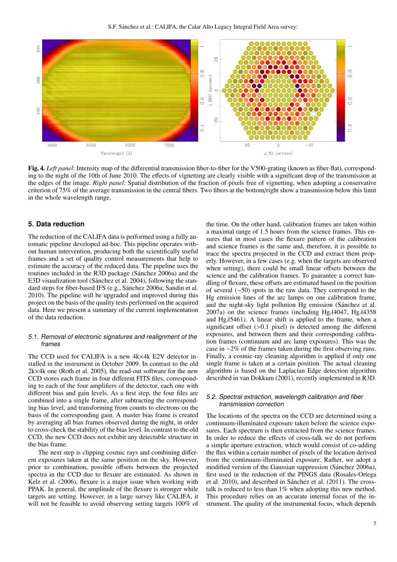
PMAS was upgraded with an E2V CCD231 4K×4K inOctober 2009 (Roth et al. 2010), which has increased nominallythe wavelength range covered by a certain instrumental setup bya factor two, with respect to the values reported by Roth et al.(2005). However, this nominal increase is not fully met at thefour corners of the CCD. As a result of a trade-off study forthe PMAS fiber spectrograph, the optical system was deliber-ately designed to tolerate some vignetting at the edges of thefull detector field-of-view, as reported by Roth et al. (1997), andRoth et al. (1998). Figure 4 illustrates the effect of vignetting forthe new 4Kx4K CCD, which was not noticeable in the previous2Kx4K detector configuration. The left panel shows a map ofthe differential fiber-to-fiber transmission for all the 331 fibers inthe hexagonal fiber-bundle. The effect of the vignetting is clearlyidentified as a drop in the transmission at the four edges of themap. 70% of the spectra are free from vignetting . However,30% of the spectra, namely those close to the edge of the de-tector, do suffer some loss of efficiency that gradually increasestowards the corners of the CCD. The loss of throughput amountsto up to 30% in the best case and 50% in the worst case, for onehalf of those spectra, but more than 50% for the other half. Itcan be seen in Fig. 4 (left panel), that where vignetting sets in,no more than a quarter of the full spectral range is affected. Insummary the vignetting severely affects less than a 15% of thefibers, in less than a 25% of their wavelength range.
The right panel illustrates the spatial distribution of the vi-gnetting. The mapping of the PPAK fibers from the telescopefocal plane to the CCD implies that the areas affected by the vi-gnetting correspond to an annular ring at about ∼15′′ from thecenter of the FoV. In addition, we report the existence of twobroken fibers with a lower transmission than the average (fibers65 and 127), not reported before.
A dithering scheme with three pointings has been adoptedin order to cover the complete FoV of the central bundle andto increase the spatial resolution of the data. This scheme wasalready used in previous studies using PPAK (Sanchez et al.2007b; Castillo-Morales et al. 2010; Perez-Gallego et al. 2010;Rosales-Ortega et al. 2010). In most of these studies the offsetsin RA and DEC of the different pointings, with respect to thenominal coordinates of the targets, were: 0′′,0′′ ; +1.56′′,+0.78′′,
5
S.F. Sanchez et al.: CALIFA, the Calar Alto Legacy Integral Field Area survey:
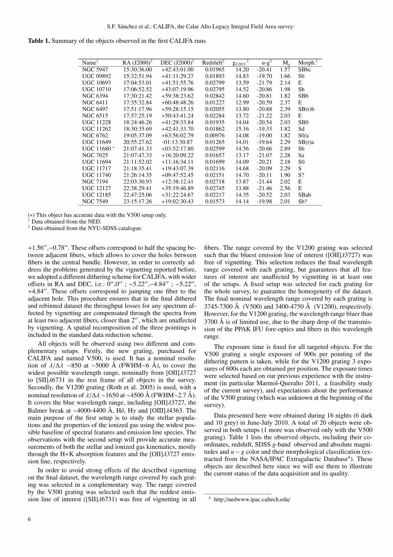
Table 1. Summary of the objects observed in the first CALIFA runs
Name1 RA (J2000)2 DEC (J2000)2 Redshift2 gS DS S2 u-g2 Mg Morph.1
NGC 5947 15:30:36.00 +42:43:01.00 0.01965 14.20 -20.41 1.57 SBbcUGC 09892 15:32:51.94 +41:11:29.27 0.01893 14.83 -19.70 1.66 SbUGC 10693 17:04:53.01 +41:51:55.76 0.02799 13.59 -21.79 2.14 EUGC 10710 17:06:52.52 +43:07:19.96 0.02795 14.52 -20.86 1.98 SbNGC 6394 17:30:21.42 +59:38:23.62 0.02842 14.60 -20.81 1.82 SBbNGC 6411 17:35:32.84 +60:48:48.26 0.01227 12.99 -20.59 2.37 ENGC 6497 17:51:17.96 +59:28:15.15 0.02055 13.80 -20.88 2.39 SB(r)bNGC 6515 17:57:25.19 +50:43:41.24 0.02284 13.72 -21.22 2.03 EUGC 11228 18:24:46.26 +41:29:33.84 0.01935 14.04 -20.54 2.03 SB0UGC 11262 18:30:35.69 +42:41:33.70 0.01862 15.16 -19.33 1.82 SdNGC 6762 19:05:37.09 +63:56:02.79 0.00976 14.08 -19.00 1.82 S0/aUGC 11649 20:55:27.62 -01:13:30.87 0.01265 14.01 -19.64 2.29 SB(r)aUGC 11680 ∗ 21:07:41.33 +03:52:17.80 0.02599 14.56 -20.66 2.89 SbNGC 7025 21:07:47.33 +16:20:09.22 0.01657 13.17 -21.07 2.28 SaUGC 11694 21:11:52.02 +11:16:34.11 0.01699 14.09 -20.21 2.18 S0UGC 11717 21:18:35.41 +19:43:07.39 0.02116 14.68 -20.09 2.29 SUGC 11740 21:26:14.35 +09:47:52.45 0.02151 14.70 -20.11 1.90 S?NGC 7194 22:03:30.93 +12:38:12.41 0.02718 13.87 -21.44 2.02 EUGC 12127 22:38:29.41 +35:19:46.89 0.02745 13.88 -21.46 2.56 EUGC 12185 22:47:25.06 +31:22:24.67 0.02217 14.35 -20.52 2.03 SBabNGC 7549 23:15:17.26 +19:02:30.43 0.01573 14.14 -19.98 2.01 Sb?
(∗) This object has accurate data with the V500 setup only.1 Data obtained from the NED.2 Data obtained from the NYU-SDSS catalogue.
+1.56′′,−0.78′′. These offsets correspond to half the spacing be-tween adjacent fibers, which allows to cover the holes betweenfibers in the central bundle. However, in order to correctly ad-dress the problems generated by the vignetting reported before,we adopted a different dithering scheme for CALIFA, with wideroffsets in RA and DEC, i.e.: 0′′,0′′ ; −5.22′′,−4.84′′ ; −5.22′′,+4.84′′. These offsets correspond to jumping one fiber to theadjacent hole. This procedure ensures that in the final ditheredand rebinned dataset the throughput losses for any spectrum af-fected by vignetting are compensated through the spectra fromat least two adjacent fibers, closer than 2′′, which are unaffectedby vignetting. A spatial recomposition of the three pointings isincluded in the standard data reduction scheme.
All objects will be observed using two different and com-plementary setups. Firstly, the new grating, purchased forCALIFA and named V500, is used. It has a nominal resolu-tion of λ/∆λ ∼850 at ∼5000 Å (FWHM∼6 Å), to cover thewidest possible wavelength range, nominally from [OII]λ3727to [SII]λ6731 in the rest frame of all objects in the survey.Secondly, the V1200 grating (Roth et al. 2005) is used, with anominal resolution of λ/∆λ ∼1650 at ∼4500 Å (FWHM∼2.7 Å).It covers the blue wavelength range, including [OII]λ3727, theBalmer break at ∼4000-4400 Å, Hδ, Hγ and [OIII]λ4363. Themain purpose of the first setup is to study the stellar popula-tions and the properties of the ionized gas using the widest pos-sible baseline of spectral features and emission line species. Theobservations with the second setup will provide accurate mea-surements of both the stellar and ionized gas kinematics, mostlythrough the H+K absorption features and the [OII]λ3727 emis-sion line, respectively.
In order to avoid strong effects of the described vignettingon the final dataset, the wavelength range covered by each grat-ing was selected in a complementary way. The range coveredby the V500 grating was selected such that the reddest emis-sion line of interest ([SII]λ6731) was free of vignetting in all
fibers. The range covered by the V1200 grating was selectedsuch that the bluest emission line of interest ([OII]λ3727) wasfree of vignetting. This selection reduces the final wavelengthrange covered with each grating, but guarantees that all fea-tures of interest are unaffected by vignetting in at least oneof the setups. A fixed setup was selected for each grating forthe whole survey, to guarantee the homogeneity of the dataset.The final nominal wavelength range covered by each grating is3745-7300 Å (V500) and 3400-4750 Å (V1200), respectively.However, for the V1200 grating, the wavelength range bluer than3700 Å is of limited use, due to the sharp drop of the transmis-sion of the PPAK IFU fore-optics and fibers in this wavelengthrange.
The exposure time is fixed for all targeted objects. For theV500 grating a single exposure of 900s per pointing of thedithering pattern is taken, while for the V1200 grating 3 expo-sures of 600s each are obtained per position. The exposure timeswere selected based on our previous experience with the instru-ment (in particular Marmol-Queralto 2011, a feasibility studyof the current survey), and expectations about the performanceof the V500 grating (which was unknown at the beginning of thesurvey).
Data presented here were obtained during 16 nights (6 darkand 10 grey) in June-July 2010. A total of 20 objects were ob-served in both setups (1 more was observed only with the V500grating). Table 1 lists the observed objects, including their co-ordinates, redshift, SDSS g-band observed and absolute magni-tudes and u − g color and their morphological classification (ex-tracted from the NASA/IPAC Extragalactic Database4). Theseobjects are described here since we will use them to illustratethe current status of the data acquisition and its quality.
4 http://nedwww.ipac.caltech.edu/
6
S.F. Sanchez et al.: CALIFA, the Calar Alto Legacy Integral Field Area survey:
Fig. 4. Left panel: Intensity map of the differential transmission fiber-to-fiber for the V500-grating (known as fiber-flat), correspond-ing to the night of the 10th of June 2010. The effects of vignetting are clearly visible with a significant drop of the transmission atthe edges of the image. Right panel: Spatial distribution of the fraction of pixels free of vignetting, when adopting a conservativecriterion of 75% of the average transmission in the central fibers. Two fibers at the bottom/right show a transmission below this limitin the whole wavelength range.
5. Data reduction
The reduction of the CALIFA data is performed using a fully au-tomatic pipeline developed ad-hoc. This pipeline operates with-out human intervention, producing both the scientifically usefulframes and a set of quality control measurements that help toestimate the accuracy of the reduced data. The pipeline uses theroutines included in the R3D package (Sanchez 2006a) and theE3D visualization tool (Sanchez et al. 2004), following the stan-dard steps for fiber-based IFS (e.g., Sanchez 2006a; Sandin et al.2010). The pipeline will be upgraded and improved during thisproject on the basis of the quality tests performed on the acquireddata. Here we present a summary of the current implementationof the data reduction.
5.1. Removal of electronic signatures and realignment of theframes
The CCD used for CALIFA is a new 4k×4k E2V detector in-stalled in the instrument in October 2009. In contrast to the old2k×4k one (Roth et al. 2005), the read-out software for the newCCD stores each frame in four different FITS files, correspond-ing to each of the four amplifiers of the detector, each one withdifferent bias and gain levels. As a first step, the four files arecombined into a single frame, after subtracting the correspond-ing bias level, and transforming from counts to electrons on thebasis of the corresponding gain. A master bias frame is createdby averaging all bias frames observed during the night, in orderto cross-check the stability of the bias level. In contrast to the oldCCD, the new CCD does not exhibit any detectable structure inthe bias frame.
The next step is clipping cosmic rays and combining differ-ent exposures taken at the same position on the sky. However,prior to combination, possible offsets between the projectedspectra in the CCD due to flexure are estimated. As shown inKelz et al. (2006), flexure is a major issue when working withPPAK. In general, the amplitude of the flexure is stronger whiletargets are setting. However, in a large survey like CALIFA, itwill not be feasible to avoid observing setting targets 100% of
the time. On the other hand, calibration frames are taken withina maximal range of 1.5 hours from the science frames. This en-sures that in most cases the flexure pattern of the calibrationand science frames is the same and, therefore, it is possible totrace the spectra projected in the CCD and extract them prop-erly. However, in a few cases (e.g. when the targets are observedwhen setting), there could be small linear offsets between thescience and the calibration frames. To guarantee a correct han-dling of flexure, these offsets are estimated based on the positionof several (∼50) spots in the raw data. They correspond to theHg emission lines of the arc lamps on one calibration frame,and the night-sky light pollution Hg emission (Sanchez et al.2007a) on the science frames (including Hgλ4047, Hgλ4358and Hgλ5461). A linear shift is applied to the frame, when asignificant offset (>0.1 pixel) is detected among the differentexposures, and between them and their corresponding calibra-tion frames (continuum and arc lamp exposures). This was thecase in ∼2% of the frames taken during the first observing runs.Finally, a cosmic-ray cleaning algorithm is applied if only onesingle frame is taken at a certain position. The actual cleaningalgorithm is based on the Laplacian Edge detection algorithmdescribed in van Dokkum (2001), recently implemented in R3D.
5.2. Spectral extraction, wavelength calibration and fibertransmission correction
The locations of the spectra on the CCD are determined using acontinuum-illuminated exposure taken before the science expo-sures. Each spectrum is then extracted from the science frames.In order to reduce the effects of cross-talk we do not performa simple aperture extraction, which would consist of co-addingthe flux within a certain number of pixels of the location derivedfrom the continuum-illuminated exposure. Rather, we adopt amodified version of the Gaussian suppression (Sanchez 2006a),first used in the reduction of the PINGS data (Rosales-Ortegaet al. 2010), and described in Sanchez et al. (2011). The cross-talk is reduced to less than 1% when adopting this new method.This procedure relies on an accurate internal focus of the in-strument. The quality of the instrumental focus, which depends
7
S.F. Sanchez et al.: CALIFA, the Calar Alto Legacy Integral Field Area survey:
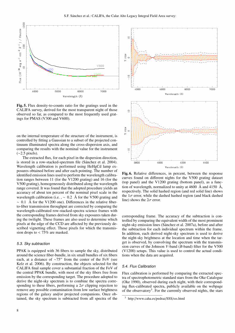
Fig. 5. Flux density-to-counts ratio for the gratings used in theCALIFA survey, derived for the most transparent night of thoseobserved so far, as compared to the most frequently used grat-ings for PMAS (V300 and V600).
on the internal temperature of the structure of the instrument, iscontrolled by fitting a Gaussian to a subset of the projected con-tinuum illuminated spectra along the cross-dispersion axis, andcomparing the results with the nominal value for the instrument(∼2.5 pixels).
The extracted flux, for each pixel in the dispersion direction,is stored in a row-stacked-spectrum file (Sanchez et al. 2004).Wavelength calibration is performed using HeHgCd lamp ex-posures obtained before and after each pointing. The number ofidentified emission lines used to perform the wavelength calibra-tion ranges between 11 (for the V1200 grating) and 16 (for theV500 grating), homogeneously distributed along the wavelengthrange covered. It was found that the adopted procedure yields anaccuracy of about ten percent of the nominal pixel scale in thewavelength calibration (i.e. , ∼ 0.2 Å for the V500 grating and∼ 0.1 Å for the V1200 one). Differences in the relative fiber-to-fiber transmission throughput are corrected by comparing thewavelength-calibrated row-stacked-spectra science frames withthe corresponding frames derived from sky exposures taken dur-ing the twilight. These frames are also used to determine whichpixels at the edge of the CCD are affected by the previously de-scribed vignetting effect. Those pixels for which the transmis-sion drops to < 75% are masked.
5.3. Sky subtraction
PPAK is equipped with 36 fibers to sample the sky, distributedaround the science fiber-bundle, in six small bundles of six fiberseach, at a distance of ∼75′′ from the center of the FoV (seeKelz et al. 2006). By construction, the objects selected for theCALIFA final sample cover a substantial fraction of the FoV ofthe central PPAK bundle, with most of the sky fibers free fromemission by the corresponding target. The procedure adopted toderive the night-sky spectrum is to combine the spectra corre-sponding to these fibers, performing a 2σ clipping rejection toremove any possible contamination from low surface brightnessregions of the galaxy and/or projected companions. Once ob-tained, the sky spectrum is subtracted from all spectra of the
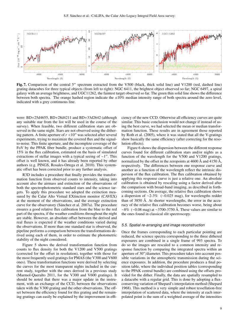
Fig. 6. Relative differences, in percent, between the responsecurves found on different nights for the V500 grating dataset(top panel) and the V1200 grating (bottom panel), as a func-tion of wavelength, normalized to unity at 4600 Å and 4150 Å,respectively. The solid hashed region (and red solid line) showsthe 1σ error, while the dashed hashed region (and black dashedline) shows the 2σ error.
corresponding frame. The accuracy of the subtraction is con-trolled by comparing the equivalent width of the most prominentnight-sky emission lines (Sanchez et al. 2007a), before and afterthe subtraction for each individual spectrum within the frame.In addition, each derived night-sky spectrum is used to derivethe night-sky brightness at the location and time when the tar-get is observed, by convolving the spectrum with the transmis-sion curves of the Johnson V-band (B-band) filter for the V500(V1200) setups. This value is used to control the actual condi-tions when the data are acquired.
5.4. Flux Calibration
Flux calibration is performed by comparing the extracted spec-tra of spectrophotometric standard stars from the Oke Catalogue(Oke 1990), observed during each night, with their correspond-ing flux-calibrated spectra, publicly available on the webpageof the observatory5. For the currently observed nights, the stars
5 http://www.caha.es/pedraz/SSS/sss.html
8
S.F. Sanchez et al.: CALIFA, the Calar Alto Legacy Integral Field Area survey:
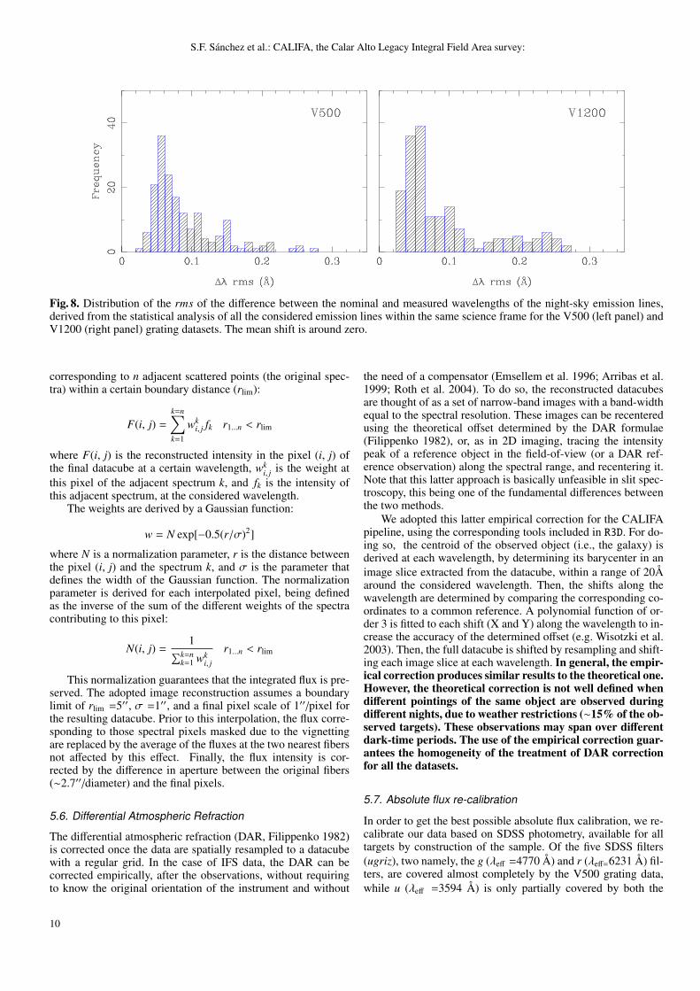
Fig. 7. Comparison of the central 5′′ spectrum extracted from the V500 (black, thick solid line) and V1200 (red, dashed line)grating datacubes for three typical objects (from left to right): NGC 6411, the brightest object observed so far; NGC 6497, a spiralgalaxy with an average brightness, and UGC11262, the faintest target observed so far. The green thin solid line shows the differencebetween both spectra. The orange hashed region indicate the ±10% median intensity range of both spectra around the zero level,indicated with a grey continuous line.
were: BD+25d4655, BD+28d4211 and BD+33d2642 (althoughany suitable star from the list will be used in the course of thesurvey). When feasible, two different calibration stars are ob-served in the same night. Stars are not observed using the dither-ing pattern. A finite aperture of r <10′′ was selected after severalexperiments, trying to maximize the covered flux and the signal-to-noise. This finite aperture, and the incomplete coverage of theFoV by the PPAK fiber bundle, produce a systematic offset of15% in the flux calibration, estimated on the basis of simulatedextractions of stellar images with a typical seeing of ∼1′′. Thisoffset is well known, and it has already been reported by otherauthors (e.g. PINGS, Rosales-Ortega et al. 2010). This system-atic offset has been corrected prior to any further analysis.
R3D includes a procedure that finally provides the transfor-mation function from observed counts to intensity, taking intoaccount also the airmass and extinction of the observations ofboth the spectrophotometric standard stars and the science tar-gets. To apply this procedure we adopted the extinction mea-sured by the Calar Alto Vistual EXtinction monitor (CAVEX)at the moment of the observations, and the average extinctioncurve for the observatory (Sanchez et al. 2007a). The procedureensures a good relative flux calibration from the blue to the redpart of the spectra, if the weather conditions throughout the nightare stable. However, an absolute offset between the derived andreal fluxes is expected if the weather conditions varied duringthe observations. If more than one standard star is observed, thepipeline performs a comparison between the transformations de-rived using each of them, in order to estimate the photometricstability of the night considered.
Figure 5 shows the derived transformation function fromcounts to flux density for both the V1200 and V500 gratings(corrected for the offset in resolution), together with those forthe most frequently used gratings for PMAS (the V300 and V600ones). These transformation functions were derived by selectingthe curves for the most transparent nights included in the cur-rent study, together with the ones derived in a previous study(Marmol-Queralto 2011, for the V300 and V600 gratings). Itshould be noted that there was a major update in the instru-ment, with an exchange of the CCD, between the observationstaken with the V300 grating and the other observations. The off-set between the efficiency found for this grating and the remain-ing gratings can easily be explained by the improvement in effi-
ciency of the new CCD. Otherwise all efficiency curves are quitesimilar. This basic conclusion would not change if instead of us-ing the best curve, we had selected the mean or median transfor-mation function. These results are in agreement those reportedby Roth et al. (2005), where it was stated that all the V-gratingsshow basically the same efficiency (after correcting for the reso-lution effects).
Figure 6 shows the dispersion between the different responsecurves found for different calibration stars and/or nights as afunction of the wavelength for the V500 and V1200 gratings,normalized by the offset in the zeropoints at 4600 Å and 4150 Å,respectively. The differences between one response curve andanother as a function of the wavelength reflect the intrinsic dis-persion of the flux calibration. The flux calibration obtained byapplying this response curve is just a relative one. An absolutecalibration is obtained by rescaling using a factor derived afterthe comparison with broad-band imaging, as described in forth-coming sections. On average, the relative flux calibration showsa dispersion of ∼2-3% (∼0.025 mag), for wavelengths redderthan of 3850 Å. At shorter wavelengths, the error in the accu-racy of the relative flux calibration becomes worse, being about∼8% (∼0.08 mag) at ∼3700-3750 Å. These values are similar tothe ones found in classical slit spectroscopy.
5.5. Spatial re-arranging and image reconstruction
Once the frames corresponding to each particular pointing arereduced, the science spectra corresponding to the three ditheredexposures are combined in a single frame of 993 spectra. Todo so the images are rescaled to a common intensity and re-sponse function by comparing the integrated spectra within anaperture of 30′′/diameter. This procedure takes into account pos-sible variations in the atmospheric transmission during the sci-ence exposures. In addition, the procedure produces a final po-sition table, where the individual position tables (correspondingto the PPAK central bundle) are combined using the offsets pro-vided for the dither. Finally, the data are spatially resampled toa datacube with a regular grid. This is done by adopting a flux-conserving variation of Shepard’s interpolation method (Shepard1968). This method is a very simple and robust tessellation-freeinterpolation of scattered data, where the intensity at each inter-polated point is the sum of a weighted average of the intensities
9
S.F. Sanchez et al.: CALIFA, the Calar Alto Legacy Integral Field Area survey:
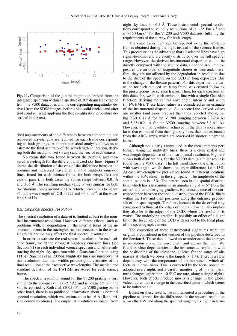
Fig. 8. Distribution of the rms of the difference between the nominal and measured wavelengths of the night-sky emission lines,derived from the statistical analysis of all the considered emission lines within the same science frame for the V500 (left panel) andV1200 (right panel) grating datasets. The mean shift is around zero.
corresponding to n adjacent scattered points (the original spec-tra) within a certain boundary distance (rlim):
F(i, j) =
k=n∑k=1
wki, j fk r1...n < rlim
where F(i, j) is the reconstructed intensity in the pixel (i, j) ofthe final datacube at a certain wavelength, wk
i, j is the weight atthis pixel of the adjacent spectrum k, and fk is the intensity ofthis adjacent spectrum, at the considered wavelength.
The weights are derived by a Gaussian function:
w = N exp[−0.5(r/σ)2]
where N is a normalization parameter, r is the distance betweenthe pixel (i, j) and the spectrum k, and σ is the parameter thatdefines the width of the Gaussian function. The normalizationparameter is derived for each interpolated pixel, being definedas the inverse of the sum of the different weights of the spectracontributing to this pixel:
N(i, j) =1∑k=n
k=1 wki, j
r1...n < rlim
This normalization guarantees that the integrated flux is pre-served. The adopted image reconstruction assumes a boundarylimit of rlim =5′′, σ =1′′, and a final pixel scale of 1′′/pixel forthe resulting datacube. Prior to this interpolation, the flux corre-sponding to those spectral pixels masked due to the vignettingare replaced by the average of the fluxes at the two nearest fibersnot affected by this effect. Finally, the flux intensity is cor-rected by the difference in aperture between the original fibers(∼2.7′′/diameter) and the final pixels.
5.6. Differential Atmospheric Refraction
The differential atmospheric refraction (DAR, Filippenko 1982)is corrected once the data are spatially resampled to a datacubewith a regular grid. In the case of IFS data, the DAR can becorrected empirically, after the observations, without requiringto know the original orientation of the instrument and without
the need of a compensator (Emsellem et al. 1996; Arribas et al.1999; Roth et al. 2004). To do so, the reconstructed datacubesare thought of as a set of narrow-band images with a band-widthequal to the spectral resolution. These images can be recenteredusing the theoretical offset determined by the DAR formulae(Filippenko 1982), or, as in 2D imaging, tracing the intensitypeak of a reference object in the field-of-view (or a DAR ref-erence observation) along the spectral range, and recentering it.Note that this latter approach is basically unfeasible in slit spec-troscopy, this being one of the fundamental differences betweenthe two methods.
We adopted this latter empirical correction for the CALIFApipeline, using the corresponding tools included in R3D. For do-ing so, the centroid of the observed object (i.e., the galaxy) isderived at each wavelength, by determining its barycenter in animage slice extracted from the datacube, within a range of 20Åaround the considered wavelength. Then, the shifts along thewavelength are determined by comparing the corresponding co-ordinates to a common reference. A polynomial function of or-der 3 is fitted to each shift (X and Y) along the wavelength to in-crease the accuracy of the determined offset (e.g. Wisotzki et al.2003). Then, the full datacube is shifted by resampling and shift-ing each image slice at each wavelength. In general, the empir-ical correction produces similar results to the theoretical one.However, the theoretical correction is not well defined whendifferent pointings of the same object are observed duringdifferent nights, due to weather restrictions (∼15% of the ob-served targets). These observations may span over differentdark-time periods. The use of the empirical correction guar-antees the homogeneity of the treatment of DAR correctionfor all the datasets.
5.7. Absolute flux re-calibration
In order to get the best possible absolute flux calibration, we re-calibrate our data based on SDSS photometry, available for alltargets by construction of the sample. Of the five SDSS filters(ugriz), two namely, the g (λeff =4770 Å) and r (λeff=6231 Å) fil-ters, are covered almost completely by the V500 grating data,while u (λeff =3594 Å) is only partially covered by both the
10

S.F. Sanchez et al.: CALIFA, the Calar Alto Legacy Integral Field Area survey:
Fig. 9. Left panel: The distribution of the FWHM of the instrumental dispersion derived from the analysis of the emission lineswithin the arc-lamp frames at different wavelengths and different positions within the FoV, for the V1200 data. Right panel: Thespatial distribution of the average FWHM of the instrumental dispersion, derived from the same arc lines.
V500 and V1200 grating data. Therefore, we use the V500 grat-ing data and the g and r band SDSS images to perform a primaryflux recalibration.
To perform the primary recalibration, we measure the countsof each galaxy in the SDSS image inside a 30′′ diameter aper-ture. These counts are converted to flux density following thecounts-to-magnitude prescription in the SDSS documentation6.The accuracy of this photometry was cross-checked by obtain-ing the magnitudes of any detected star in each field, using thesame procedure, and comparing them with the values listed inthe SDSS DR6 photometric catalogue. We obtained less than0.05 magnitude dispersion for the stars with g < 17.5 mag. Oncewe ensure the accuracy of this photometry, we extract the spec-trophotometry from the reduced datacubes corresponding to theV500 grating setup, coadding the flux of individual spectra in-side a 30′′ diameter aperture and convolving this spectrum withthe SDSS g and r filter passbands (ADPS database, Moro &Munari 2000). Using these two data pairs, a scaling solution isfound, by adopting the average of the flux ratio in both bands.
Once the V500 datacube has been recalibrated, a newscaling solution for the V1200 data is derived by comparing the5′′ aperture extracted spectra around the central position of eachobject from these cubes with those extracted from the originalreduced V1200 data. In this case, a low-order polynomicalfunction is fitted to the ratio between both spectra within thecommon wavelength range (∼3745-4770 Å). The result of thispolynomial fitting is then applied to the V1200 data, to matchthem to the V500 ones. Figure 7 shows the central apertureextracted spectra for both setups together with the difference be-tween them (5′′/diameter), for three typical targets. It illustratesthe agreement between both datasets, once the recalibrationprocedure has been applied. The V1200 spectra have beenconvolved with a Gaussian function to compensate for thedifference in resolution, for the purpose of this figure only. Thetypical difference between the spectra is ∼10% of the average.The strongest differences are located at the wavelengths of themore significant spectral features (absorption and/or emissionlines).
6 http://www.sdss.org/dr6/algorithms/fluxcal.html
We conclude that the current version of the pipeline, which op-erates automatically, is able to reduce the data, producing the re-quired data cubes to perform early experiments and estimationsof their quality. The pipeline will be continuously upgraded, pro-ducing different versions of the data, on the basis of the resultsof the different foreseen quality controls, prior to releasing thedata to the community. In the next section we describe the earlytests implemented to estimate the quality of the data. In somecases these tests have already induced slight modifications in thepipeline, as we will describe below in detail.
6. Quality of the data
In parallel to the reduction of the data, the pipeline performs a setof automatic tests, which are stored during the reduction process,creating a set of tables and figures. These allow the CALIFAteam to check the quality of the data and to identify possibleproblems in the data reduction. In this section we present thebasic results of the currently implemented quality controls onthe data acquired so far. We expect the quality control to becomemore comprehensive with time.
6.1. Accuracy of the wavelength calibration
In general, the wavelength solution is found with an accuracy ofthe order of 10-15% of the nominal pixel scale, i.e., the rms ofthe fit with the low order polynomial function is ∼0.2-0.3 Å forthe V500 grating and ∼0.1-0.2 Å for the V1200 grating.
In order to obtain an independent estimate of the accuracyof the wavelength calibration of the science frames, we comparethe nominal and recovered wavelengths of the most prominentnight-sky emission lines in each individual spectrum prior to thesky subtraction. The central wavelength of these lines was deter-mined by fitting a Gaussian function to each line. This providesus with 331 estimations of the relative offsets between both val-ues for each considered night-sky line. For the V500 grating weuse the HgIλ5461, [OI]λ5577, NaDλ5893 and [OI]λ6300 lines,while for the V1200 grating we use the HgIλ4046 and HgIλ4358ones. Only measurements derived using emission lines with asignal-to-noise higher than 10 are considered. Finally, a few hun-
11
S.F. Sanchez et al.: CALIFA, the Calar Alto Legacy Integral Field Area survey:
Fig. 11. Comparison of the g-band magnitude derived from theintegrated spectrum within an aperture of 30′′ diameter extractedfrom the V500 datacubes and the corresponding magnitudes de-rived from the SDSS images, before (blue solid circles) and after(red solid squares) applying the flux recalibration procedure de-scribed in the text.
dred measurements of the differences between the nominal andrecovered wavelengths are retained for each frame correspond-ing to both gratings. A simple statistical analysis allows us toestimate the final accuracy of the wavelength calibration, deriv-ing both the median offset (if any) and the rms of each dataset.
No mean shift was found between the nominal and mea-sured wavelength for the different analyzed sky lines. Figure 8shows the distribution of the rms of the difference between thenominal and measured wavelengths of the night-sky emissionlines, found for each science frame, for both setups (left andcentral panel). In both cases the values range between 0.01 Åand 0.35 Å. The resulting median value is very similar for bothdistributions, being around ∼0.1 Å, which corresponds to ∼8 kms−1 at the wavelength of [OII]λ3727 and ∼3 km s−1, at the wave-length of Hα.
6.2. Empirical spectral resolution
The spectral resolution of a dataset is limited at best to the nom-inal instrumental resolution. However, different effects, such asproblems with, or degradation in, the internal focus of the in-strument, errors in the tracing/extraction process or in the wave-length calibration may affect the final spectral resolution.
In order to estimate the real spectral resolution for each sci-ence frame, we fit the strongest night-sky emission lines (seeSection 6.1) in each individual science spectrum and before sub-tracting the night-sky spectrum with a Gaussian function usingFIT3D (Sanchez et al. 2006b). Night-sky lines are unresolved atour resolution, thus their widths provide good estimates of thefinal resolution at their respective wavelengths. The median andstandard deviation of the FWHMs are stored for each scienceframe.
The spectral resolution found for the V1200 grating is verysimilar to the nominal value (∼2.7 Å), and is consistent with thevalues reported by Roth et al. (2005). For the V500 grating on theother hand, there is no published information about its nominalspectral resolution, which was estimated to be ∼6 Å (Roth, pri-vate communications). The empirical resolution estimated from
night-sky lines is ∼6.5 Å. These instrumental spectral resolu-tions correspond to velocity resolutions of σ ∼85 km s−1 andσ ∼150 km s−1 for the V1200 and V500 datasets, fulfilling therequirements of the survey, for both setups.
The same experiment can be repeated using the arc-lampframes obtained during the night instead of the science frames.This procedure has the advantage that all selected lines have highsignal-to-noise, and are evenly distributed over the full spectralrange. However, the derived instrumental dispersion cannot bedirectly compared with the science data, since the arc-lamp ex-posures are an order of magnitude shorter in time and, there-fore, they are not affected by the degradation in resolution dueto the drift of the spectra on the CCD in long exposures (dueto the change of the flexure pattern). For this experiment, a dat-acube for each reduced arc lamp frame was created followingthe prescriptions for science frames. Then, for each spectrum ofthis datacube, we fit each emission line with a single Gaussianfunction, deriving the central wavelength, intensity and width(in FWHMs). These latter values are considered as an estimateof the instrumental dispersion. As expected the derived valuesare smaller (and more precise) than thos reported above, be-ing 2.30±0.11 Å for the V1200 (ranging between 2.2-2.4 Å)and 5.65±0.21 Å for the V500 (ranging between 5.3-6.1 Å).However, the final resolution achieved in the data is more simi-lar to that estimated from the night-sky lines, than that estimatedfrom the ARC-lamps, which are observed in shorter integrationtimes.
Although not clearly appreciated in the measurements per-formed using the night-sky lines, there is a clear spatial andwavelength dependence of the instrumental resolution. Figure 9shows both distributions, for the V1200 data (a similar result isfound for the V500 data). The left panel shows the distributionwith wavelength, which shows the larger difference, i.e. ∼13%.At each wavelength we plot values found at different locationswithin the FoV, shown in the right-panel. The amplitude of thespatial pattern is ∼5%. The pattern seen in the spatial distribu-tion, which has a maximum in an annular ring at ∼15′′ from thecenter, and an underlying gradient, is a consequence of the cor-respondence between the spatial distribution of the PPAK fiberswithin the FoV and their positions along the entrance pseudo-slit of the spectrograph. The fibers located in the described ringcorrespond to those at the edges of the pseudo-slit. This impliesthey also lie at the edges of the CCD, where the resolution isworse. The underlying gradient is possibly an effect of a slighttilt of the focal plane of the CCD with respect to the focal planeof the spectrograph camera.
The correction of these instrumental signatures were notoriginally considered in the version of the pipeline described inthe Section 5. These data allowed us to understand the changesin resolution along the wavelength and across the field. Wefound no clear dependencies of the instrumental resolution withthe positioning of the telescope, at least for the range of air-masses at which we observe the targets (< 1.4). There is a cleardependency with the temperature of the instrument, which af-fects its internal focus. This is corrected by the focus procedureadopted every night, and a careful monitoring of this tempera-ture (changes larger than ∼0.5◦ C are rare, along a single night).However, both effects produce mostly a change in the globalvalue, rather than a change in the described pattern, which seemsto be rather stable.
Based on these results, we implemented a procedure in thepipeline to correct for the differences in the spectral resolutionacross the FoV and along the spectral range by fixing it (in terms
12
S.F. Sanchez et al.: CALIFA, the Calar Alto Legacy Integral Field Area survey:
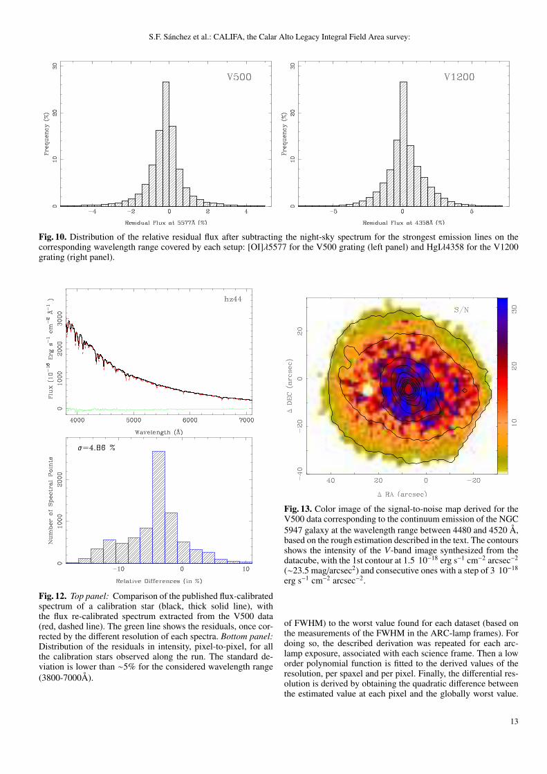
Fig. 10. Distribution of the relative residual flux after subtracting the night-sky spectrum for the strongest emission lines on thecorresponding wavelength range covered by each setup: [OI]λ5577 for the V500 grating (left panel) and HgIλ4358 for the V1200grating (right panel).
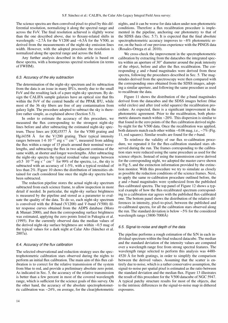
Fig. 12. Top panel: Comparison of the published flux-calibratedspectrum of a calibration star (black, thick solid line), withthe flux re-calibrated spectrum extracted from the V500 data(red, dashed line). The green line shows the residuals, once cor-rected by the different resolution of each spectra. Bottom panel:Distribution of the residuals in intensity, pixel-to-pixel, for allthe calibration stars observed along the run. The standard de-viation is lower than ∼5% for the considered wavelength range(3800-7000Å).
Fig. 13. Color image of the signal-to-noise map derived for theV500 data corresponding to the continuum emission of the NGC5947 galaxy at the wavelength range between 4480 and 4520 Å,based on the rough estimation described in the text. The contoursshows the intensity of the V-band image synthesized from thedatacube, with the 1st contour at 1.5 10−18 erg s−1 cm−2 arcsec−2
(∼23.5 mag/arcsec2) and consecutive ones with a step of 3 10−18
erg s−1 cm−2 arcsec−2.
of FWHM) to the worst value found for each dataset (based onthe measurements of the FWHM in the ARC-lamp frames). Fordoing so, the described derivation was repeated for each arc-lamp exposure, associated with each science frame. Then a loworder polynomial function is fitted to the derived values of theresolution, per spaxel and per pixel. Finally, the differential res-olution is derived by obtaining the quadratic difference betweenthe estimated value at each pixel and the globally worst value.
13
S.F. Sanchez et al.: CALIFA, the Calar Alto Legacy Integral Field Area survey:
The science spectra are then convolved pixel-to-pixel by this dif-ferential resolution, normalizing it along the spectral range andacross the FoV. The final resolution achieved is slightly worsethan the one described above, due to flexure-related shifts inwavelength: ∼2.7Å for the V1200 and ∼6.5Å for the V500, asderived from the measurements of the night-sky emission lineswidth. However, with the adopted procedure the resolution isnormalized along the spectral range and across the field.
Any further analysis described in this article is based onthese spectra, with a homogeneous spectral resolution (in termsof FWHM).
6.3. Accuracy of the sky subtraction
The determination of the night-sky spectrum and its subtractionfrom the data is an issue in many IFUs, mostly due to the smallFoV and the resulting lack of a pure night-sky spectrum. By de-sign the CALIFA sample galaxies have an optical size that fitswithin the FoV of the central bundle of the PPAK IFU, whilemost of the 36 sky fibers are free of any contamination fromgalaxy light. The procedure adopted to subtract the sky is there-fore rather simple, as explained above (Section 5.3).
In order to estimate the accuracy of this procedure, wemeasured the flux corresponding to the strongest night-skylines before and after subtracting the estimated night-sky spec-trum. These lines are [OI]λ5577 Å for the V500 grating andHgλ4358 Å for the V1200 grating. Their typical intensityranges between 1-6 10−17 erg s−1 cm−2, measured from addingthe flux within a range of 15 pixels around their nominal wave-lengths, and subtracting the flux in two adjacent continua of thesame width, at shorter and longer wavelengths. After subtractingthe night-sky spectra the typical residual value ranges between±0.5 10−16 erg s−1 cm−2 for 99% of the spectra, i.e., the sky issubtracted with an accuracy of 1-5%, with a typical residual ofless than 2%. Figure 10 shows the distribution of intensities ob-tained for each considered line once the night-sky spectra havebeen subtracted.
The reduction pipeline stores the actual night-sky spectrumsubtracted from each science frame, to allow inspection in moredetail if needed. In particular, the night-sky surface brightnessis measured by the pipeline and stored as a parameter to eval-uate the quality of the data. To do so, each night-sky spectrumis convolved with the B-band (V1200) and V-band (V500) fil-ter response curves obtained from the ADPS database (Moro& Munari 2000), and then the corresponding surface brightnesswas estimated, applying the zero points listed in Fukugita et al.(1995). For the currently observed data the median values ofthe derived night-sky surface brightness are within ∼0.5 mag ofthe typical values for a dark night at Calar Alto (Sanchez et al.2007a).
6.4. Accuracy of the flux calibration
The selected observational and reduction strategy uses the spec-trophotometric calibration stars observed during the nights toperform an initial flux calibration. The main aim of this flux cal-ibration is to correct for the relative transmission of the systemfrom blue to red, and provide a preliminary absolute zero point.As indicated in Sec. 5, the accuracy of the relative transmissionis better than a few percent in most of the covered wavelengthrange, which is sufficient for the science goals of this survey. Onthe other hand, the accuracy of the absolute spectrophotomet-ric calibration was ∼24%, on average, for the clear/photometric
nights, and it can be worse for data taken under non-photometricconditions. Therefore a flux recalibration procedure is imple-mented in the pipeline, anchoring our photometry to that ofthe SDSS data (Sec. 5.7). It is expected that the final absolutespectrophotometric accuracy improves to ∼8% photometric er-ror, on the basis of our previous experience with the PINGS data(Rosales-Ortega et al. 2010).
We cross-check the improvement in the spectrophotometriccalibration by extracting from the datacubes the integrated spec-tra within an aperture of 30′′ diameter around the peak intensityof the object, before and after the flux recalibration. The cor-responding g and r-band magnitudes were derived from thesespectra, following the procedures described in Sec. 5. The mag-nitudes derived from the spectroscopy were then compared withthe corresponding ones obtained from the SDSS images, adopt-ing a similar aperture, and following the same procedure as usedto recalibrate the data.
Figure 11 shows the distribution of the g-band magnitudesderived from the datacubes and the SDSS images before (bluesolid circles) and after (red solid squares) the recalibration pro-cedure. As expected, there is a significant improvement in thephotometric agreement. Prior to the recalibration, both photo-metric datasets match within ∼20%. This dispersion is similar tothat found in the zero points of the flux calibration derived night-by-night for the V500 data. Once the recalibration was applied,both datasets match each other within ∼0.06 mag, i.e., ∼7% (Fig.11, red squares). Similar results are found for the r-band.
To reinforce the validity of our flux re-calibration proce-dure, we repeated it for the flux-calibration standard stars ob-served during the run. The frames corresponding to the calibra-tion stars were reduced using the same procedure as used for thescience objects. Instead of using the transmission curve derivedfor the corresponding night, we adopted the master curve shownin Fig 5, and the extinction information provided by the extinc-tion monitor. With this procedure we try to simulate as closelyas possible the reduction conditions of the science frames. Next,to apply the same re-calibration procedure outlined before, theg and r-band magnitudes were synthesized from the publishedflux-calibrated spectra. The top panel of Figure 12 shows a typ-ical example of how the flux-recalibrated spectrum correspond-ing to a calibration star agrees with the published flux-calibratedone. The bottom panel shows the distribution of the relative dif-ferences in intensity, pixel-to-pixel, between the published andre-calibrated spectra, for all the calibration stars observed alongthe run. The standard deviation is below ∼5% for the consideredwavelength range (3800-7000Å)
6.5. Signal-to-noise and depth of the data
The pipeline performs a rough estimation of the S/N in each in-dividual spectrum within the final reduced datacube. The medianand the standard deviation of the intensity values are computedover a wavelength range free from strong spectral features. Thewavelength range selected to perform this analysis was 4480-4520 Å for both gratings, in order to simplify the comparisonbetween the derived values. Assuming that the scatter is en-tirely due to noise, which is a rather conservative assumption, thesignal-to-noise per spatial pixel is estimated as the ratio betweenthe standard deviation and the median flux. Figure 13 illustratesthe result of this procedure for the V500 datacube of NGC 5947.A typical patchy structure results for most of the objects, dueto the intrinsic differences in the signal-to-noise map in ditheredexposures.
14
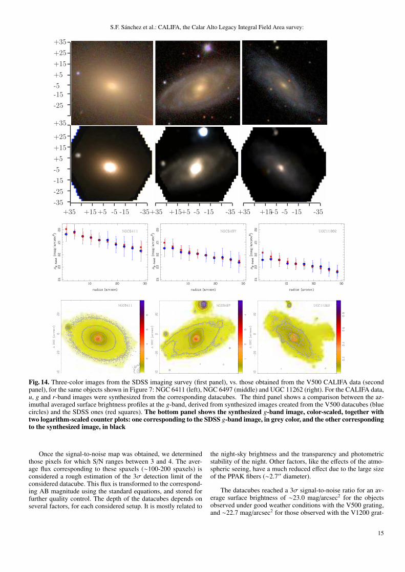
S.F. Sanchez et al.: CALIFA, the Calar Alto Legacy Integral Field Area survey:
-35
-25
-15
-5
+5
+15
+25
+35
-25
-15-5
+5
+15
+25
+35
+35 +15+5 -5 -15 -35+35 +15+5 -5 -15 -35 +35 +15+5 -5 -15 -35
Fig. 14. Three-color images from the SDSS imaging survey (first panel), vs. those obtained from the V500 CALIFA data (secondpanel), for the same objects shown in Figure 7: NGC 6411 (left), NGC 6497 (middle) and UGC 11262 (right). For the CALIFA data,u, g and r-band images were synthesized from the corresponding datacubes. The third panel shows a comparison between the az-imuthal averaged surface brightness profiles at the g-band, derived from synthesized images created from the V500 datacubes (bluecircles) and the SDSS ones (red squares). The bottom panel shows the synthesized g-band image, color-scaled, together withtwo logarithm-scaled counter plots: one corresponding to the SDSS g-band image, in grey color, and the other correspondingto the synthesized image, in black
Once the signal-to-noise map was obtained, we determinedthose pixels for which S/N ranges between 3 and 4. The aver-age flux corresponding to these spaxels (∼100-200 spaxels) isconsidered a rough estimation of the 3σ detection limit of theconsidered datacube. This flux is transformed to the correspond-ing AB magnitude using the standard equations, and stored forfurther quality control. The depth of the datacubes depends onseveral factors, for each considered setup. It is mostly related to
the night-sky brightness and the transparency and photometricstability of the night. Other factors, like the effects of the atmo-spheric seeing, have a much reduced effect due to the large sizeof the PPAK fibers (∼2.7′′ diameter).
The datacubes reached a 3σ signal-to-noise ratio for an av-erage surface brightness of ∼23.0 mag/arcsec2 for the objectsobserved under good weather conditions with the V500 grating,and ∼22.7 mag/arcsec2 for those observed with the V1200 grat-
15
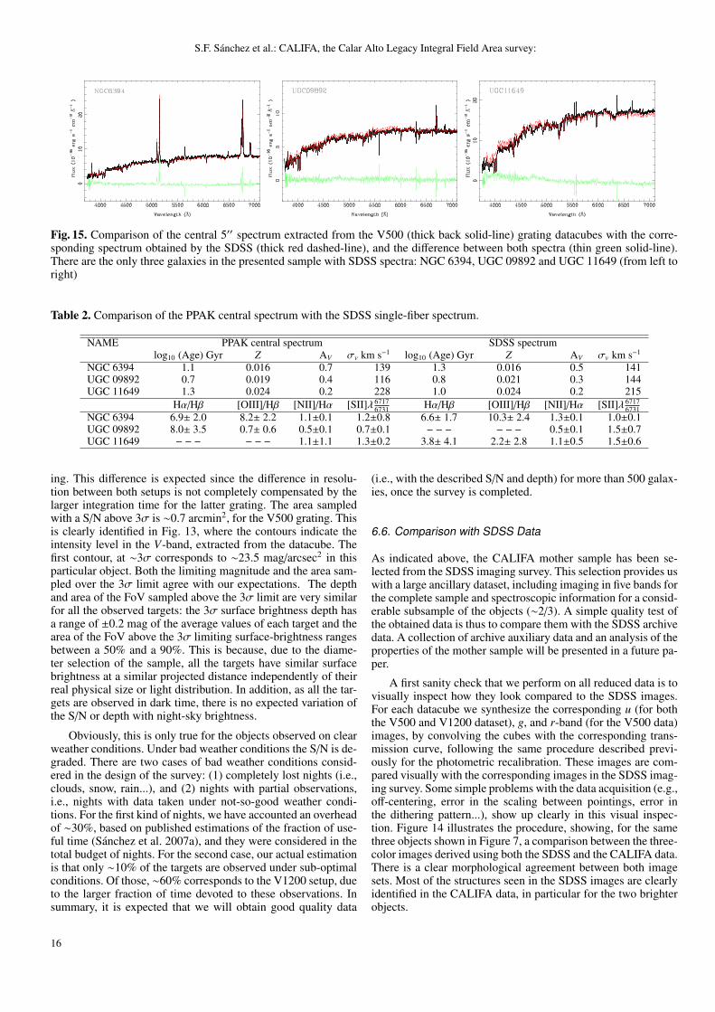
S.F. Sanchez et al.: CALIFA, the Calar Alto Legacy Integral Field Area survey:
Fig. 15. Comparison of the central 5′′ spectrum extracted from the V500 (thick back solid-line) grating datacubes with the corre-sponding spectrum obtained by the SDSS (thick red dashed-line), and the difference between both spectra (thin green solid-line).There are the only three galaxies in the presented sample with SDSS spectra: NGC 6394, UGC 09892 and UGC 11649 (from left toright)
Table 2. Comparison of the PPAK central spectrum with the SDSS single-fiber spectrum.
NAME PPAK central spectrum SDSS spectrumlog10 (Age) Gyr Z AV σv km s−1 log10 (Age) Gyr Z AV σv km s−1
NGC 6394 1.1 0.016 0.7 139 1.3 0.016 0.5 141UGC 09892 0.7 0.019 0.4 116 0.8 0.021 0.3 144UGC 11649 1.3 0.024 0.2 228 1.0 0.024 0.2 215
Hα/Hβ [OIII]/Hβ [NII]/Hα [SII]λ 67176731 Hα/Hβ [OIII]/Hβ [NII]/Hα [SII]λ 6717
6731NGC 6394 6.9± 2.0 8.2± 2.2 1.1±0.1 1.2±0.8 6.6± 1.7 10.3± 2.4 1.3±0.1 1.0±0.1UGC 09892 8.0± 3.5 0.7± 0.6 0.5±0.1 0.7±0.1 − − − − − − 0.5±0.1 1.5±0.7UGC 11649 − − − − − − 1.1±1.1 1.3±0.2 3.8± 4.1 2.2± 2.8 1.1±0.5 1.5±0.6
ing. This difference is expected since the difference in resolu-tion between both setups is not completely compensated by thelarger integration time for the latter grating. The area sampledwith a S/N above 3σ is ∼0.7 arcmin2, for the V500 grating. Thisis clearly identified in Fig. 13, where the contours indicate theintensity level in the V-band, extracted from the datacube. Thefirst contour, at ∼3σ corresponds to ∼23.5 mag/arcsec2 in thisparticular object. Both the limiting magnitude and the area sam-pled over the 3σ limit agree with our expectations. The depthand area of the FoV sampled above the 3σ limit are very similarfor all the observed targets: the 3σ surface brightness depth hasa range of ±0.2 mag of the average values of each target and thearea of the FoV above the 3σ limiting surface-brightness rangesbetween a 50% and a 90%. This is because, due to the diame-ter selection of the sample, all the targets have similar surfacebrightness at a similar projected distance independently of theirreal physical size or light distribution. In addition, as all the tar-gets are observed in dark time, there is no expected variation ofthe S/N or depth with night-sky brightness.
Obviously, this is only true for the objects observed on clearweather conditions. Under bad weather conditions the S/N is de-graded. There are two cases of bad weather conditions consid-ered in the design of the survey: (1) completely lost nights (i.e.,clouds, snow, rain...), and (2) nights with partial observations,i.e., nights with data taken under not-so-good weather condi-tions. For the first kind of nights, we have accounted an overheadof ∼30%, based on published estimations of the fraction of use-ful time (Sanchez et al. 2007a), and they were considered in thetotal budget of nights. For the second case, our actual estimationis that only ∼10% of the targets are observed under sub-optimalconditions. Of those, ∼60% corresponds to the V1200 setup, dueto the larger fraction of time devoted to these observations. Insummary, it is expected that we will obtain good quality data
(i.e., with the described S/N and depth) for more than 500 galax-ies, once the survey is completed.
6.6. Comparison with SDSS Data
As indicated above, the CALIFA mother sample has been se-lected from the SDSS imaging survey. This selection provides uswith a large ancillary dataset, including imaging in five bands forthe complete sample and spectroscopic information for a consid-erable subsample of the objects (∼2/3). A simple quality test ofthe obtained data is thus to compare them with the SDSS archivedata. A collection of archive auxiliary data and an analysis of theproperties of the mother sample will be presented in a future pa-per.
A first sanity check that we perform on all reduced data is tovisually inspect how they look compared to the SDSS images.For each datacube we synthesize the corresponding u (for boththe V500 and V1200 dataset), g, and r-band (for the V500 data)images, by convolving the cubes with the corresponding trans-mission curve, following the same procedure described previ-ously for the photometric recalibration. These images are com-pared visually with the corresponding images in the SDSS imag-ing survey. Some simple problems with the data acquisition (e.g.,off-centering, error in the scaling between pointings, error inthe dithering pattern...), show up clearly in this visual inspec-tion. Figure 14 illustrates the procedure, showing, for the samethree objects shown in Figure 7, a comparison between the three-color images derived using both the SDSS and the CALIFA data.There is a clear morphological agreement between both imagesets. Most of the structures seen in the SDSS images are clearlyidentified in the CALIFA data, in particular for the two brighterobjects.
16
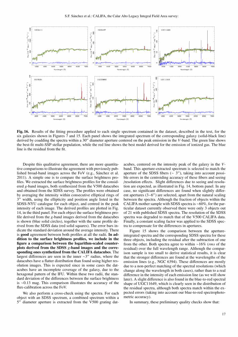
S.F. Sanchez et al.: CALIFA, the Calar Alto Legacy Integral Field Area survey:
Fig. 16. Results of the fitting procedure applied to each single spectrum contained in the dataset, described in the text, for thesix galaxies shown in Figures 7 and 15. Each panel shows the integrated spectrum of the corresponding galaxy (solid-black line)derived by coadding the spectra within a 30′′ diameter aperture centered on the peak emission in the V-band. The green line showsthe best-fit multi-SSP stellar population, while the red line shows the best model derived for the emission of ionized gas. The blueline is the residual from the fit.
Despite this qualitative agreement, there are more quantita-tive comparisons to illustrate the agreement with previously pub-lished broad-band images across the FoV (e.g., Sanchez et al.2011). A simple one is to compare the surface brightness pro-files. We extracted the surface brightness profiles for the consid-ered g-band images, both synthesized from the V500 datacubesand obtained from the SDSS survey. The profiles were obtainedby averaging the intensity within consecutive elliptical rings of3′′ width, using the ellipticity and position angle listed in theSDSS-NYU catalogue for each object, and centred in the peakintensity of each image. The derived profiles are plotted in Fig.14, in the third panel. For each object the surface brightness pro-file derived from the g-band images derived from the datacubesis shown (blue solid circles), together with the same profile de-rived from the SDSS data (red solid squares). The error bars in-dicate the standard deviation around the average intensity. Thereis good agreement between both profiles at all the radii. In ad-dition to the surface brightness profiles, we include in thefigure a comparison between the logarithm-scaled counter-plots derived from the SDSS g-band images and the corre-sponding ones synthetized from the CALIFA datacubes. Thelargest differences are seen in the inner ∼3′′ radius, where thedatacubes have a flatter distribution than found using higher res-olution images. This is expected since in some cases the dat-acubes have an incomplete coverage of the galaxy, due to thehexagonal pattern of the IFU. Within these two radii, the stan-dard deviation of the differences between the surface brightnessis ∼0.13 mag. This comparison illustrates the accuracy of theflux-calibration across the FoV.
We also perform a cross-check using the spectra. For eachobject with an SDSS spectrum, a combined spectrum within a5′′ diameter aperture is extracted from the V500 grating dat-
acubes, centered on the intensity peak of the galaxy in the V-band. This aperture-extracted spectrum is selected to match theaperture of the SDSS fibers (∼ 3′′), taking into account possi-ble errors in the centroiding accuracy of these fibers and seeing/resolution effects. Slight differences due to seeing and resolu-tion are expected, as illustrated in Fig. 14, bottom panel. In anycase, no significant differences are found when slightly differ-ent apertures (3−6′′) are selected, apart from the natural scalingbetween the spectra. Although the fraction of objects within theCALIFA mother sample with SDSS spectra is ∼60%, for the par-ticular dataset currently observed there were only 3 objects outof 21 with published SDSS spectra. The resolution of the SDSSspectra was degraded to match that of the V500 CALIFA data.Finally, a constant scaling factor was applied to the SDSS spec-tra to compensate for the differences in apertures.
Figure 15 shows the comparison between the aperture-integrated spectra and the corresponding SDSS spectra for thesethree objects, including the residual after the subtraction of onefrom the other. Both spectra agree to within ∼16% (rms of theresidual) over the full wavelength range. Although the compar-ison sample is too small to derive statistical results, it is clearthat the stronger differences are found at the wavelengths of theemission lines (e.g., NGC 6394). These differences are mostlydue to a non-perfect matching of the spectral resolutions (whichchange along the wavelength in both cases), rather than to a realdifference in the intensity of each emission line (as we will showlater). A slight difference is also found in the blue-to-red spectralshape of UGC11649, which is clearly seen in the distribution ofthe residual spectra, although both spectra match within the ex-pected errors (taking into account our blue-to-red spectrophoto-metric accuracy).
In summary, these preliminary quality checks show that:
17
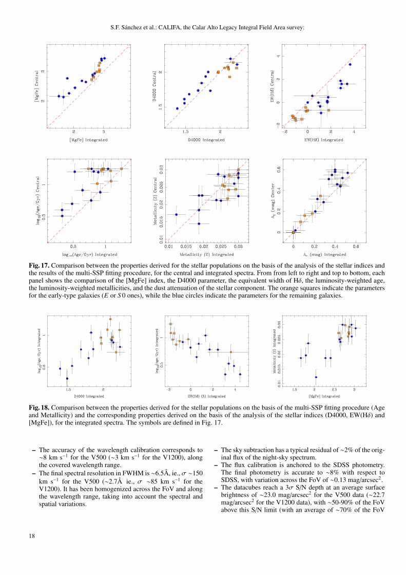
S.F. Sanchez et al.: CALIFA, the Calar Alto Legacy Integral Field Area survey:
Fig. 17. Comparison between the properties derived for the stellar populations on the basis of the analysis of the stellar indices andthe results of the multi-SSP fitting procedure, for the central and integrated spectra. From from left to right and top to bottom, eachpanel shows the comparison of the [MgFe] index, the D4000 parameter, the equivalent width of Hδ, the luminosity-weighted age,the luminosity-weighted metallicities, and the dust attenuation of the stellar component. The orange squares indicate the parametersfor the early-type galaxies (E or S 0 ones), while the blue circles indicate the parameters for the remaining galaxies.
Fig. 18. Comparison between the properties derived for the stellar populations on the basis of the multi-SSP fitting procedure (Ageand Metallicity) and the corresponding properties derived on the basis of the analysis of the stellar indices (D4000, EW(Hδ) and[MgFe]), for the integrated spectra. The symbols are defined in Fig. 17.
– The accuracy of the wavelength calibration corresponds to∼8 km s−1 for the V500 (∼3 km s−1 for the V1200), alongthe covered wavelength range.
– The final spectral resolution in FWHM is ∼6.5Å, ie., σ ∼150km s−1 for the V500 (∼2.7Å ie., σ ∼85 km s−1 for theV1200). It has been homogenized across the FoV and alongthe wavelength range, taking into account the spectral andspatial variations.
– The sky subtraction has a typical residual of ∼2% of the orig-inal flux of the night-sky spectrum.
– The flux calibration is anchored to the SDSS photometry.The final photometry is accurate to ∼8% with respect toSDSS, with variation across the FoV of ∼0.13 mag/arcsec2.
– The datacubes reach a 3σ S/N depth at an average surfacebrightness of ∼23.0 mag/arcsec2 for the V500 data (∼22.7mag/arcsec2 for the V1200 data), with ∼50-90% of the FoVabove this S/N limit (with an average of ∼70% of the FoV
18
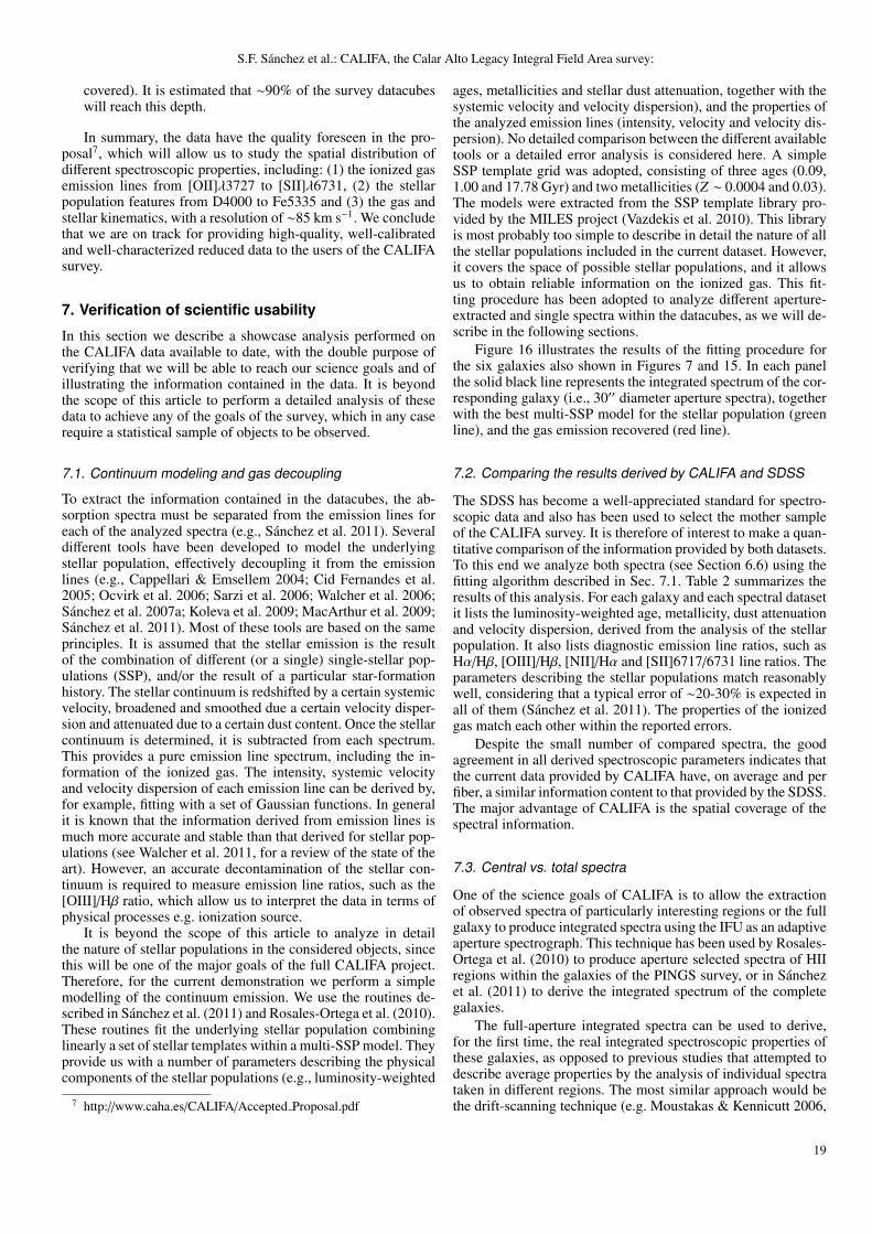
S.F. Sanchez et al.: CALIFA, the Calar Alto Legacy Integral Field Area survey:
covered). It is estimated that ∼90% of the survey datacubeswill reach this depth.
In summary, the data have the quality foreseen in the pro-posal7, which will allow us to study the spatial distribution ofdifferent spectroscopic properties, including: (1) the ionized gasemission lines from [OII]λ3727 to [SII]λ6731, (2) the stellarpopulation features from D4000 to Fe5335 and (3) the gas andstellar kinematics, with a resolution of ∼85 km s−1. We concludethat we are on track for providing high-quality, well-calibratedand well-characterized reduced data to the users of the CALIFAsurvey.
7. Verification of scientific usability
In this section we describe a showcase analysis performed onthe CALIFA data available to date, with the double purpose ofverifying that we will be able to reach our science goals and ofillustrating the information contained in the data. It is beyondthe scope of this article to perform a detailed analysis of thesedata to achieve any of the goals of the survey, which in any caserequire a statistical sample of objects to be observed.
7.1. Continuum modeling and gas decoupling
To extract the information contained in the datacubes, the ab-sorption spectra must be separated from the emission lines foreach of the analyzed spectra (e.g., Sanchez et al. 2011). Severaldifferent tools have been developed to model the underlyingstellar population, effectively decoupling it from the emissionlines (e.g., Cappellari & Emsellem 2004; Cid Fernandes et al.2005; Ocvirk et al. 2006; Sarzi et al. 2006; Walcher et al. 2006;Sanchez et al. 2007a; Koleva et al. 2009; MacArthur et al. 2009;Sanchez et al. 2011). Most of these tools are based on the sameprinciples. It is assumed that the stellar emission is the resultof the combination of different (or a single) single-stellar pop-ulations (SSP), and/or the result of a particular star-formationhistory. The stellar continuum is redshifted by a certain systemicvelocity, broadened and smoothed due a certain velocity disper-sion and attenuated due to a certain dust content. Once the stellarcontinuum is determined, it is subtracted from each spectrum.This provides a pure emission line spectrum, including the in-formation of the ionized gas. The intensity, systemic velocityand velocity dispersion of each emission line can be derived by,for example, fitting with a set of Gaussian functions. In generalit is known that the information derived from emission lines ismuch more accurate and stable than that derived for stellar pop-ulations (see Walcher et al. 2011, for a review of the state of theart). However, an accurate decontamination of the stellar con-tinuum is required to measure emission line ratios, such as the[OIII]/Hβ ratio, which allow us to interpret the data in terms ofphysical processes e.g. ionization source.
It is beyond the scope of this article to analyze in detailthe nature of stellar populations in the considered objects, sincethis will be one of the major goals of the full CALIFA project.Therefore, for the current demonstration we perform a simplemodelling of the continuum emission. We use the routines de-scribed in Sanchez et al. (2011) and Rosales-Ortega et al. (2010).These routines fit the underlying stellar population combininglinearly a set of stellar templates within a multi-SSP model. Theyprovide us with a number of parameters describing the physicalcomponents of the stellar populations (e.g., luminosity-weighted
7 http://www.caha.es/CALIFA/Accepted Proposal.pdf
ages, metallicities and stellar dust attenuation, together with thesystemic velocity and velocity dispersion), and the properties ofthe analyzed emission lines (intensity, velocity and velocity dis-persion). No detailed comparison between the different availabletools or a detailed error analysis is considered here. A simpleSSP template grid was adopted, consisting of three ages (0.09,1.00 and 17.78 Gyr) and two metallicities (Z ∼ 0.0004 and 0.03).The models were extracted from the SSP template library pro-vided by the MILES project (Vazdekis et al. 2010). This libraryis most probably too simple to describe in detail the nature of allthe stellar populations included in the current dataset. However,it covers the space of possible stellar populations, and it allowsus to obtain reliable information on the ionized gas. This fit-ting procedure has been adopted to analyze different aperture-extracted and single spectra within the datacubes, as we will de-scribe in the following sections.
Figure 16 illustrates the results of the fitting procedure forthe six galaxies also shown in Figures 7 and 15. In each panelthe solid black line represents the integrated spectrum of the cor-responding galaxy (i.e., 30′′ diameter aperture spectra), togetherwith the best multi-SSP model for the stellar population (greenline), and the gas emission recovered (red line).
7.2. Comparing the results derived by CALIFA and SDSS
The SDSS has become a well-appreciated standard for spectro-scopic data and also has been used to select the mother sampleof the CALIFA survey. It is therefore of interest to make a quan-titative comparison of the information provided by both datasets.To this end we analyze both spectra (see Section 6.6) using thefitting algorithm described in Sec. 7.1. Table 2 summarizes theresults of this analysis. For each galaxy and each spectral datasetit lists the luminosity-weighted age, metallicity, dust attenuationand velocity dispersion, derived from the analysis of the stellarpopulation. It also lists diagnostic emission line ratios, such asHα/Hβ, [OIII]/Hβ, [NII]/Hα and [SII]6717/6731 line ratios. Theparameters describing the stellar populations match reasonablywell, considering that a typical error of ∼20-30% is expected inall of them (Sanchez et al. 2011). The properties of the ionizedgas match each other within the reported errors.
Despite the small number of compared spectra, the goodagreement in all derived spectroscopic parameters indicates thatthe current data provided by CALIFA have, on average and perfiber, a similar information content to that provided by the SDSS.The major advantage of CALIFA is the spatial coverage of thespectral information.
7.3. Central vs. total spectra
One of the science goals of CALIFA is to allow the extractionof observed spectra of particularly interesting regions or the fullgalaxy to produce integrated spectra using the IFU as an adaptiveaperture spectrograph. This technique has been used by Rosales-Ortega et al. (2010) to produce aperture selected spectra of HIIregions within the galaxies of the PINGS survey, or in Sanchezet al. (2011) to derive the integrated spectrum of the completegalaxies.
The full-aperture integrated spectra can be used to derive,for the first time, the real integrated spectroscopic properties ofthese galaxies, as opposed to previous studies that attempted todescribe average properties by the analysis of individual spectrataken in different regions. The most similar approach would bethe drift-scanning technique (e.g. Moustakas & Kennicutt 2006,
19

S.F. Sanchez et al.: CALIFA, the Calar Alto Legacy Integral Field Area survey:
Fig. 19. Comparison between the gas parameters derived for the central and integrated spectra using the fitting procedure describedin the text. From from left to right and top to bottom each panel shows the comparison between the Hα flux, and the Hα/Hβ,[OII]λ3727/Hβ, [SII]λ6717/[SII]λ6731, [NII]λ6584/Hα and [OIII]λ5007/Hβ line ratios. Only values with a S/N>3 for both spectrahave been included in each plot.
and part of the ancillary data of the SINGS survey), although inthose studies the fraction of the galaxy covered by the spectrawas smaller than that of CALIFA. Another advantage of an IFUwith respect to the drift-scan technique is that the former allowsa comparison between the integrated and the spatially resolvedproperties of the galaxy, or the integrated spectra of particularregions.
In this section we analyze two spectra derived for eachgalaxy for different apertures, using the V500-grating dataset.One is a 5′′ diameter aperture spectrum, centered on the peakintensity in the V-band. This spectrum is representative of thecentral region of each galaxy, and is similar to the one obtainedby the SDSS survey (see Section 6.6). The other is a 30′′ di-ameter aperture spectrum, an aperture that contains most fibersabove the 5σ detection limit for each galaxy. The latter spectrumis representative of the integrated properties of each galaxy. Bothspectra have similar S/N (∼40, at ∼5000 Å). This is due to thefact that the central spectrum samples areas of much higher S/N,despite its smaller aperture, while the total spectrum samples ar-eas of lower S/N, but with a larger aperture. On average, the5′′ aperture contains 10% of the flux encircled by the 30′′ aper-ture. We applied the above fitting technique described in Sec. 7.1to both spectra, deriving the main properties of both the stellarpopulation and the ionized gas. An example of typical integratedspectra, and their modelling, was already shown in Fig. 16.
7.3.1. Stellar Populations
Gradients and, more generally, spatial variations of stellar popu-lation properties have been observed in galaxies, both early types
(e.g. Kuntschner et al. 2006) and late types (e.g MacArthur et al.2004). CALIFA will allow the mapping of these variations forthe first time over a statistically representative sample of galax-ies, unbiased in terms of morphology and mass/luminosity. Thedetailed modeling required to this goal is beyond the scope ofthis paper and will be presented in forthcoming dedicated works.Here we just illustrate the potential of the dataset using eithermodel-independent measurements, such as the spectral indices,or the output of the simple fitting technique described in Sec.7.1.
It is known (e.g. Trager et al. 2000; Gallazzi et al. 2005) thatspectral indices can be used to infer stellar population parame-ters such as age, metallicity and α enhancement. They providerobust, model-independent, information, complementary to thatprovided by fitting the full spectrum with SSP templates as de-scribed in Sec. 7.1. For the current analysis, we have explored theD4000 index (i.e. the 4000 Å break) and the Hδ index (whichrepresents the equivalent width of the Hδ line), as tracers of stel-lar age, and [MgFe] as a tracer of stellar metallicity. For this laterindex, we adopted the formula:
[MgFe] =√
Mgb (0.72Fe5270 + 0.28Fe5335)
The indices were measured for both the central and inte-grated spectra, once decontaminated by the ionized gas emissionand normalized to the standard Lick/IDS resolution, using thescripts included in FIT3D, described in Sanchez et al. (2007b).
Figure 17 shows a comparison of the properties derived forthe underlying stellar populations for both spectral apertures. Itincludes the results from the analysis of the indices, i.e., the age-sensitive D4000 and Hδ indices and the metal-sensitive [MgFe]
20

S.F. Sanchez et al.: CALIFA, the Calar Alto Legacy Integral Field Area survey:
Table 3. Summary of the physical properties derived from the analysis of the ionized gas for the integrated and central spectrum ofeach galaxy.
Integrated spectrumNAME Spec. Type AV SFRHα SFR[OII] log(U) 12+log(O/H) Electron Density
(mag) M� yr−1 M� yr−1 cm−3
NGC 5947 SF 1.2 ± 0.1 3.8 ± 0.1 3.8 ± 0.8 -3.5 ± 0.2 8.7 ± 0.1 —-UGC 09892 SF 1.3 ± 0.2 2.3 ± 0.1 3.9 ± 0.8 -3.7 ± 0.4 8.7 ± 0.3 —-
NGC 6394 SF/AGN 2.1 ± 0.2 12.1 ± 0.1 14.1 ± 2.8 -3.2 ± 0.3 8.6 ± 0.1 214 ± 64NGC 6497 SF/AGN 1.5 ± 0.2 3.7 ± 0.1 3.4 ± 0.7 -3.5 ± 0.4 8.7 ± 0.1 —-
UGC 11262 SF 1.5 ± 0.2 1.8 ± 0.1 1.4 ± 0.3 -3.3 ± 0.7 8.6 ± 0.2 145 ± 43NGC 6762 AGN 1.5 ± 0.2 —- —- —- —- —-
UGC 11680 AGN 3.3 ± 0.2 —- —- -3.0 ± 0.5 —- —-UGC 11694 SF 0.0 ± 0.5 0.3 ± 0.1 0.2 ± 0.1 -2.9 ± 0.7 8.6 ± 0.4 —-UGC 11717 AGN 3.3 ± 0.4 —- —- -3.6 ± 0.2 —- 4571± 1371UGC 11740 SF 1.8 ± 0.2 3.5 ± 0.1 5.1 ± 1.0 -3.5 ± 0.5 8.6 ± 0.2 525 ± 157UGC 12185 SF/AGN 2.8 ± 0.4 6.2 ± 0.1 22.1 ±15.0 -3.6 ± 0.6 8.6 ± 0.2 —-
NGC 7549 SF 2.4 ± 0.1 10.8 ± 0.1 10.3 ± 0.1 -3.7 ± 0.2 8.7 ± 0.1 —-Central Spectrum
NAME Spec. Type AV SFRHα SFR[OII] log(U) 12+log(O/H) Electron Density(mag) M� yr−1 M� yr−1 cm−3
NGC 5947 SF/AGN 1.5 ± 0.1 0.4 ± 0.2 0.2 ± 0.1 -3.2 ± 0.3 8.7 ± 0.1 —-UGC 09892 SF/AGN 2.6 ± 0.3 0.2 ± 0.2 0.4 ± 0.2 -3.8 ± 0.6 8.7 ± 0.3 2512± 754UGC 10710 SF/AGN 4.5 ± 0.9 3.9 ± 0.1 23.2 ±13.9 -3.8 ± 0.6 8.6 ± 0.5 —-
NGC 6394 AGN 2.9 ± 0.3 —- —- -2.8 ± 0.1 —- 309 ± 93NGC 6497 AGN 1.8 ± 0.9 —- —- -3.4 ± 0.4 —- —-
UGC 11262 SF/AGN 2.7 ± 0.4 0.1 ± 0.2 0.2 ± 0.2 -3.7 ± 1.1 8.7 ± 0.4 575 ± 173NGC 6762 AGN 2.4 ± 0.5 —- —- -3.3 ± 0.1 —- 234 ± 70
UGC 11680 AGN 2.3 ± 0.2 —- —- -2.5 ± 0.1 —- —-UGC 11694 AGN 3.1 ± 0.5 —- —- -3.3 ± 0.2 —- 316 ± 95UGC 11717 AGN 4.9 ± 0.7 —- —- -3.4 ± 0.1 —- —-UGC 11740 SF/AGN 2.8 ± 0.6 0.1 ± 0.2 0.5 ± 0.2 -3.7 ± 0.5 8.6 ± 0.3 34 ± 10
NGC 7549 SF/AGN 2.6 ± 0.2 0.4 ± 0.2 0.3 ± 0.2 -3.4 ± 0.3 8.6 ± 0.2 —-
index, and the physical parameters luminosity-weighted age,metallicity and dust attenuation, estimated by fitting SSP tem-plates to the full spectrum. The galaxy UGC11262 has been ex-cluded due to its lower S/N level in the continuum due to tech-nical problems during the observations. These problems affectthe shape of the continuum and therefore the parameters derivedby the fitting procedure, although they affect neither the stellarindices nor the parameters of the emission lines.
Fig. 17 shows the correlations between central (within 5 arc-sec) and total integrated indices. Red dashed lines are used todisplay the one-to-one correlation and guide the eye. For all in-dices we find tight correlations between central and total val-ues. However, we find systematic offsets with respect to the one-to-one line, which indicate gradients: in particular, for the stel-lar population indices, i) [MgFe] central is always significantlyhigher than total, thus indicating negative metallicity gradients inall galaxies; ii) Hδ is typically stronger in the integrated spectrathan in the central ones, thus indicating that young stellar popu-lations are mainly found in the outskirts of galaxies; iii) D4000has typically flatter radial distribution, with some indication forpositive (age) gradients for the oldest galaxies (those with thestrongest D4000), and vice versa for the younger ones.
Similar trends are appreciated in the parameters derived fromthe SSP fitting procedure. On average the central stellar popula-tions are slightly older than the integrated ones, and they suffera stronger or equal dust attenuation. The metallicity shows noclear trend, with values randomly distributed around the one-to-one relation. Maybe the selected library template, with onlytwo extreme metallicities in the grid, is not good enough to
sample this parameter properly, which is better represented bythe [MgFe] index. Differences are also appreciated among thedifferent galaxy types. The stellar component of the early-typegalaxies (E or S0) is, in all the cases, dominated by old (>7 Gyr,high D4000 and low Hδ values) and metal rich (Z >0.025, hight[MgFe] values) populations. In addition, very low dust attenua-tion is found in both the integrated and central spectra (Av <0.5mag, with a mean value of ∼0.2 mag). On the other hand, thelate-type galaxies show a wider variety of properties in their stel-lar populations.
The information provided by the indices and the SSP anal-ysis is complementary, but leads to similar conclusions, in gen-eral. Figure 18 shows a comparison between each stellar popu-lation index and its corresponding parameter derived by the SSPanalysis, for the integrated spectra (similar results are found forthe central spectra). As expected there is a clear correlation be-tween the age-sensitive indices (D4000 and Hδ) and the lumi-nosity weighted ages, on one hand, and a weaker trend betweenthe [MgFe] and the luminosity weighted metallicity, on the otherhand. The larger scatter in this relation is most probably due toan incorrect sampling of the metallicities in the over-simplisticstellar population library grid adopted for the current analysis.
Although a more detailed analysis is required to understandthe described trends, these preliminary results seem very encour-aging, illustrating the kind of studies that can be done when ap-plying more refined analysis techniques over the full CALIFAsample.
21
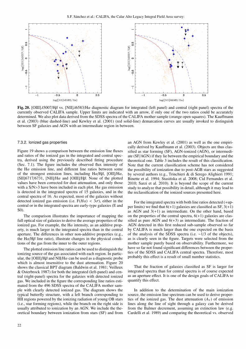
S.F. Sanchez et al.: CALIFA, the Calar Alto Legacy Integral Field Area survey:
Fig. 20. [OIII]λ5007/Hβ vs. [NII]λ6583/Hα diagnostic diagram for integrated (left panel) and central (right panel) spectra of thecurrently observed CALIFA sample. Upper limits are indicated with an arrow, if only one of the two ratios could be accuratelydetermined. We also plot data derived from the SDSS spectra of the CALIFA mother sample (orange open squares). The Kauffmannet al. (2003) (blue dashed-line) and Kewley et al. (2001) (red solid-line) demarcation curves are usually invoked to distinguishbetween SF galaxies and AGN with an intermediate region in between.
7.3.2. Ionized gas properties
Figure 19 shows a comparison between the emission line fluxesand ratios of the ionized gas in the integrated and central spec-tra, derived using the previously described fitting procedure(Sec. 7.1). The figure includes the observed flux intensity ofthe Hα emission line, and different line ratios between someof the strongest emission lines, including Hα/Hβ, [OII]/Hα,[SII]6717/6731, [NII]/Hα and [OIII]/Hβ. None of the plottedvalues have been corrected for dust attenuation, and only thosewith a S/N>3 have been included in each plot. Hα gas emissionis detected in the integrated spectra of 15 galaxies, and in thecentral spectra of 16. As expected, most of the galaxies withoutdetected ionized gas emission (i.e. F(Hα) < 3σ), either in thecentral or in the integrated spectra are early-type galaxies (E andS0).
The comparison illustrates the importance of mapping thefull optical size of galaxies to derive the average properties of theionized gas. For example, the Hα intensity, as an additive prop-erty, is much larger in the integrated spectra than in the centralaperture. The differences in other non-additive properties (e.g.,the Hα/Hβ line ratio), illustrate changes in the physical condi-tions of the gas from the inner to the outer regions.
The plotted emission line ratios can be used to distinguish theionizing source of the gas associated with each region. In partic-ular, the [OIII]/Hβ and NII/Hα can be used as a diagnostic probewhich is almost insensitive to the dust attenuation. Figure 20shows the classical BPT diagram (Baldwin et al. 1981; Veilleux& Osterbrock 1987) for both the integrated (left-panel) and cen-tral (right-panel) spectra for the galaxies with detected ionizedgas. We included in the figure the corresponding line ratios esti-mated from the 496 SDSS spectra of the CALIFA mother sam-ple with clearly detected ionized gas. The diagram shows thetypical butterfly structure, with a left branch corresponding toHII regions powered by the ionizing radiation of young OB stars(i.e., star forming regions), while the branch on the right side isusually attributed to ionization by an AGN. We include the the-oretical boundary between ionization from stars (SF) and from
an AGN from Kewley et al. (2001) as well as the one empiri-cally derived by Kauffmann et al. (2003). Objects are thus clas-sified as star forming (SF), AGN-ionized (AGN), or intermedi-ate (SF/AGN) if they lie between the empirical boundary and thetheoretical one. Table 3 includes the result of this classification.Note that the current classification scheme has not consideredthe possibility of ionization due to post-AGB stars as suggestedby several authors (e.g., Trinchieri & di Serego Alighieri 1991;Binette et al. 1994; Stasinska et al. 2008; Cid Fernandes et al.2010; Sarzi et al. 2010). It is beyond the scope of the currentstudy to analyze that possibility in detail, although it may lead tothe reclassification of the ionized sources presented here.
For the integrated spectra with both line ratios detected (+up-per limits) we find that 6(+1) galaxies are classified as SF, 3(+1)as AGN and 3(+1) as intermediate. On the other hand, basedon the properties of the central spectra, 6(+1) galaxies are clas-sified as pure AGN and 6(+3) as intermediate. The fraction ofAGN detected in this first reduced sub-sample observed so farby CALIFA is much larger than the one expected on the basisof the analysis of the SDSS spectra (i.e. ∼1/3 of the objects),as is clearly seen in the figure. Targets were selected from themother sample purely based on observability. Furthermore, wehave so far not found significant differences between the proper-ties of the SDSS and CALIFA central spectra. Therefore, mostprobably this effect is a result of small number statistics.
That the fraction of galaxies classified as SF is larger forintegrated spectra than for central spectra is of course expectedas an aperture effect. It is one of the design goals of CALIFA toquantify this effect.
In addition to the determination of the main ionizationsource, the emission line spectrum can be used to derive proper-ties of the ionized gas. The dust attenuation (AV ) of emissionlines along the line of sight through a galaxy can be derivedfrom the Balmer decrement, assuming an extinction law (e.g.Cardelli et al. 1989) and comparing the theoretical vs. observed
22
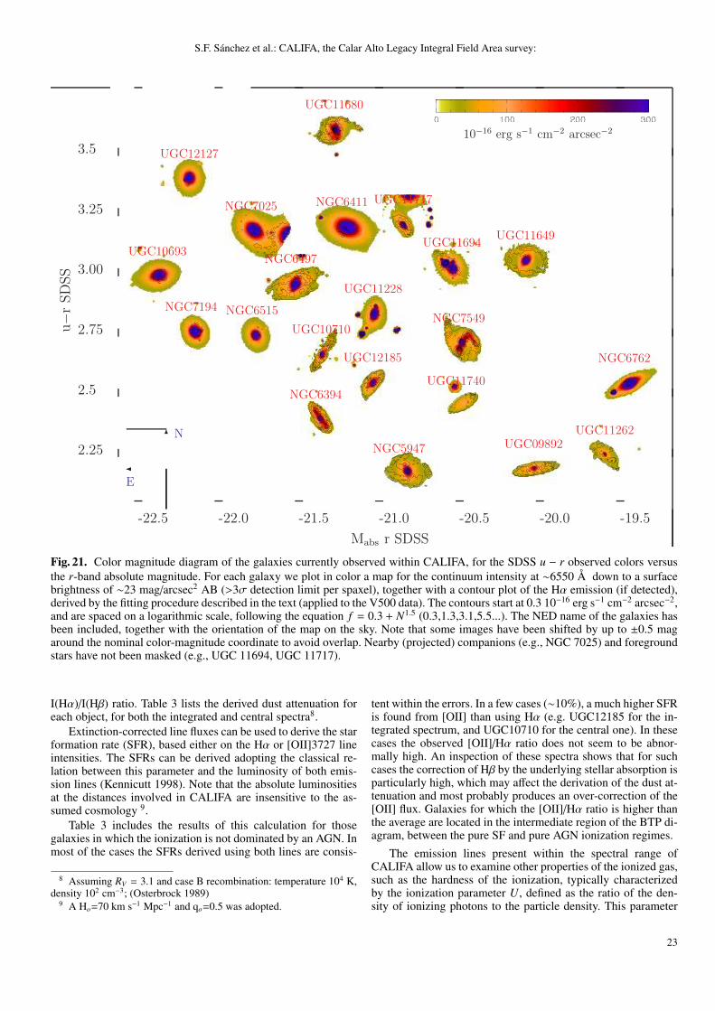
S.F. Sanchez et al.: CALIFA, the Calar Alto Legacy Integral Field Area survey:
-22.5 -22.0 -21.5 -21.0 -20.5 -20.0 -19.5
2.25
2.5
2.75
3.00
3.25
3.5
u−r
SDSS
Mabs r SDSS
UGC11717NGC6411
UGC09892
UGC10693
NGC7194
UGC10710
NGC6394
NGC6497
NGC6515
UGC11262
NGC6762
UGC11649
UGC11680
NGC7025
UGC11694
UGC11740
UGC12127
UGC11228
UGC12185
NGC7549
NGC5947
10−16 erg s−1 cm−2 arcsec−2
�
??
E
N
Fig. 21. Color magnitude diagram of the galaxies currently observed within CALIFA, for the SDSS u − r observed colors versusthe r-band absolute magnitude. For each galaxy we plot in color a map for the continuum intensity at ∼6550 Å down to a surfacebrightness of ∼23 mag/arcsec2 AB (>3σ detection limit per spaxel), together with a contour plot of the Hα emission (if detected),derived by the fitting procedure described in the text (applied to the V500 data). The contours start at 0.3 10−16 erg s−1 cm−2 arcsec−2,and are spaced on a logarithmic scale, following the equation f = 0.3 + N1.5 (0.3,1.3,3.1,5.5...). The NED name of the galaxies hasbeen included, together with the orientation of the map on the sky. Note that some images have been shifted by up to ±0.5 magaround the nominal color-magnitude coordinate to avoid overlap. Nearby (projected) companions (e.g., NGC 7025) and foregroundstars have not been masked (e.g., UGC 11694, UGC 11717).
I(Hα)/I(Hβ) ratio. Table 3 lists the derived dust attenuation foreach object, for both the integrated and central spectra8.
Extinction-corrected line fluxes can be used to derive the starformation rate (SFR), based either on the Hα or [OII]3727 lineintensities. The SFRs can be derived adopting the classical re-lation between this parameter and the luminosity of both emis-sion lines (Kennicutt 1998). Note that the absolute luminositiesat the distances involved in CALIFA are insensitive to the as-sumed cosmology 9.
Table 3 includes the results of this calculation for thosegalaxies in which the ionization is not dominated by an AGN. Inmost of the cases the SFRs derived using both lines are consis-
8 Assuming RV = 3.1 and case B recombination: temperature 104 K,density 102 cm−3; (Osterbrock 1989)
9 A Ho=70 km s−1 Mpc−1 and qo=0.5 was adopted.
tent within the errors. In a few cases (∼10%), a much higher SFRis found from [OII] than using Hα (e.g. UGC12185 for the in-tegrated spectrum, and UGC10710 for the central one). In thesecases the observed [OII]/Hα ratio does not seem to be abnor-mally high. An inspection of these spectra shows that for suchcases the correction of Hβ by the underlying stellar absorption isparticularly high, which may affect the derivation of the dust at-tenuation and most probably produces an over-correction of the[OII] flux. Galaxies for which the [OII]/Hα ratio is higher thanthe average are located in the intermediate region of the BTP di-agram, between the pure SF and pure AGN ionization regimes.
The emission lines present within the spectral range ofCALIFA allow us to examine other properties of the ionized gas,such as the hardness of the ionization, typically characterizedby the ionization parameter U, defined as the ratio of the den-sity of ionizing photons to the particle density. This parameter
23
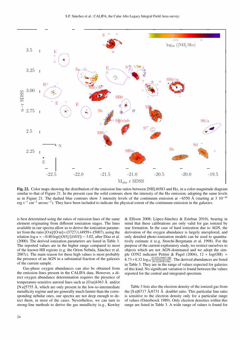
S.F. Sanchez et al.: CALIFA, the Calar Alto Legacy Integral Field Area survey:
-22.5 -22.0 -21.5 -21.0 -20.5 -20.0 -19.5
2.25
2.5
2.75
3.00
3.25
3.5
u−r
SDSS
Mabs r SDSS
SE
Sb
E
E
Sb
SBb
SB(r)b
E
Sd
S0/a
SB(r)a
S
Sa
?
S?
E
SB0
SB(s)ab
SBc
SBbc
log10 ([NII]/Hα)
�
??
E
N
Fig. 22. Color maps showing the distribution of the emission line ratios between [NII]λ6583 and Hα, in a color-magnitude diagramsimilar to that of Figure 21. In the present case the solid contours show the intensity of the Hα emission, adopting the same levelsas in Figure 21. The dashed blue contours show 3 intensity levels of the continuum emission at ∼6550 Å (starting at 3 10−16
erg s−1 cm−2 arcsec−2). They have been included to indicate the physical extent of the continuum emission in the galaxies.
is best determined using the ratios of emission lines of the sameelement originating from different ionization stages. The linesavailable in our spectra allow us to derive the ionization parame-ter from the ratio [O ii]/[O iii]=λ3727/(λ4959+λ5007), using therelation log u = −0.80 log([OII]/[OIII])− 3.02, after Dıaz et al.(2000). The derived ionization parameters are listed in Table 3.The reported values are in the higher range compared to mostof the known HII regions (e.g. the Orion Nebula, Sanchez et al.2007c). The main reason for these high values is most probablythe presence of an AGN in a substantial fraction of the galaxiesof the current sample.
Gas-phase oxygen abundances can also be obtained fromthe emission lines present in the CALIFA data. However, a di-rect oxygen abundance determination requires the presence oftemperature-sensitive auroral lines such as [O iii]4363 Å and/or[N ii]5755 Å, which are only present in the low-to-intermediatemetallicity regime and are generally much fainter than the corre-sponding nebular ones, our spectra are not deep enough to de-tect them, in most of the cases. Nevertheless, we can turn tostrong-line methods to derive the gas metallicity (e.g., Kewley
& Ellison 2008; Lopez-Sanchez & Esteban 2010), bearing inmind that these calibrations are only valid for gas ionized bystar formation. In the case of hard ionization due to AGN, thederivation of the oxygen abundance is largely unexplored, andonly detailed photo-ionization models can be used to quantita-tively estimate it (e.g. Storchi-Bergmann et al. 1998). For thepurpose of the current exploratory study, we restrict ourselves toobjects which are not AGN-dominated and we adopt the sim-ple O3N2 indicator Pettini & Pagel (2004), 12 + log(OH) =
8.73+0.32 log10[O III]λ5007/Hβ[N II]λ6583/Hα . The derived abundances are listed
in Table 3. They are in the range of values expected for galaxiesof this kind. No significant variation is found between the valuesreported for the central and integrated spectrum.
Table 3 lists also the electron density of the ionized gas fromthe [S ii]6717 Å/6731 Å doublet ratio. This particular line ratiois sensitive to the electron density only for a particular rangeof values (Osterbrock 1989). Only electron densities within thisrange are listed in Table 3. A wide range of values is found for
24
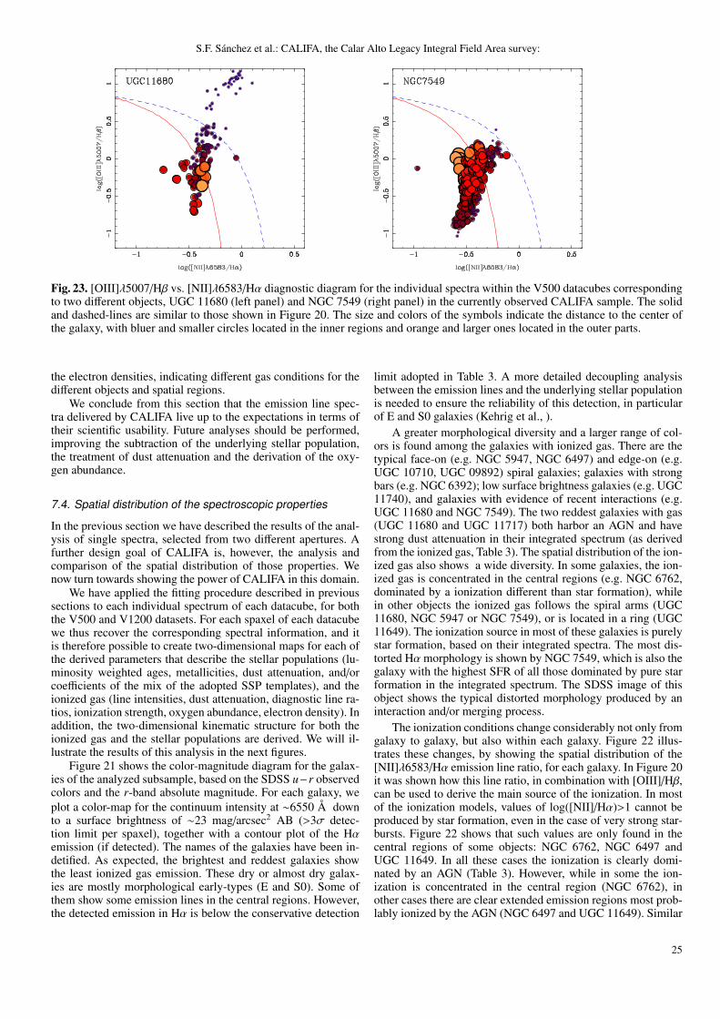
S.F. Sanchez et al.: CALIFA, the Calar Alto Legacy Integral Field Area survey:
Fig. 23. [OIII]λ5007/Hβ vs. [NII]λ6583/Hα diagnostic diagram for the individual spectra within the V500 datacubes correspondingto two different objects, UGC 11680 (left panel) and NGC 7549 (right panel) in the currently observed CALIFA sample. The solidand dashed-lines are similar to those shown in Figure 20. The size and colors of the symbols indicate the distance to the center ofthe galaxy, with bluer and smaller circles located in the inner regions and orange and larger ones located in the outer parts.
the electron densities, indicating different gas conditions for thedifferent objects and spatial regions.
We conclude from this section that the emission line spec-tra delivered by CALIFA live up to the expectations in terms oftheir scientific usability. Future analyses should be performed,improving the subtraction of the underlying stellar population,the treatment of dust attenuation and the derivation of the oxy-gen abundance.
7.4. Spatial distribution of the spectroscopic properties
In the previous section we have described the results of the anal-ysis of single spectra, selected from two different apertures. Afurther design goal of CALIFA is, however, the analysis andcomparison of the spatial distribution of those properties. Wenow turn towards showing the power of CALIFA in this domain.
We have applied the fitting procedure described in previoussections to each individual spectrum of each datacube, for boththe V500 and V1200 datasets. For each spaxel of each datacubewe thus recover the corresponding spectral information, and itis therefore possible to create two-dimensional maps for each ofthe derived parameters that describe the stellar populations (lu-minosity weighted ages, metallicities, dust attenuation, and/orcoefficients of the mix of the adopted SSP templates), and theionized gas (line intensities, dust attenuation, diagnostic line ra-tios, ionization strength, oxygen abundance, electron density). Inaddition, the two-dimensional kinematic structure for both theionized gas and the stellar populations are derived. We will il-lustrate the results of this analysis in the next figures.
Figure 21 shows the color-magnitude diagram for the galax-ies of the analyzed subsample, based on the SDSS u−r observedcolors and the r-band absolute magnitude. For each galaxy, weplot a color-map for the continuum intensity at ∼6550 Å downto a surface brightness of ∼23 mag/arcsec2 AB (>3σ detec-tion limit per spaxel), together with a contour plot of the Hαemission (if detected). The names of the galaxies have been in-detified. As expected, the brightest and reddest galaxies showthe least ionized gas emission. These dry or almost dry galax-ies are mostly morphological early-types (E and S0). Some ofthem show some emission lines in the central regions. However,the detected emission in Hα is below the conservative detection
limit adopted in Table 3. A more detailed decoupling analysisbetween the emission lines and the underlying stellar populationis needed to ensure the reliability of this detection, in particularof E and S0 galaxies (Kehrig et al., ).
A greater morphological diversity and a larger range of col-ors is found among the galaxies with ionized gas. There are thetypical face-on (e.g. NGC 5947, NGC 6497) and edge-on (e.g.UGC 10710, UGC 09892) spiral galaxies; galaxies with strongbars (e.g. NGC 6392); low surface brightness galaxies (e.g. UGC11740), and galaxies with evidence of recent interactions (e.g.UGC 11680 and NGC 7549). The two reddest galaxies with gas(UGC 11680 and UGC 11717) both harbor an AGN and havestrong dust attenuation in their integrated spectrum (as derivedfrom the ionized gas, Table 3). The spatial distribution of the ion-ized gas also shows a wide diversity. In some galaxies, the ion-ized gas is concentrated in the central regions (e.g. NGC 6762,dominated by a ionization different than star formation), whilein other objects the ionized gas follows the spiral arms (UGC11680, NGC 5947 or NGC 7549), or is located in a ring (UGC11649). The ionization source in most of these galaxies is purelystar formation, based on their integrated spectra. The most dis-torted Hα morphology is shown by NGC 7549, which is also thegalaxy with the highest SFR of all those dominated by pure starformation in the integrated spectrum. The SDSS image of thisobject shows the typical distorted morphology produced by aninteraction and/or merging process.
The ionization conditions change considerably not only fromgalaxy to galaxy, but also within each galaxy. Figure 22 illus-trates these changes, by showing the spatial distribution of the[NII]λ6583/Hα emission line ratio, for each galaxy. In Figure 20it was shown how this line ratio, in combination with [OIII]/Hβ,can be used to derive the main source of the ionization. In mostof the ionization models, values of log([NII]/Hα)>1 cannot beproduced by star formation, even in the case of very strong star-bursts. Figure 22 shows that such values are only found in thecentral regions of some objects: NGC 6762, NGC 6497 andUGC 11649. In all these cases the ionization is clearly domi-nated by an AGN (Table 3). However, while in some the ion-ization is concentrated in the central region (NGC 6762), inother cases there are clear extended emission regions most prob-lably ionized by the AGN (NGC 6497 and UGC 11649). Similar
25
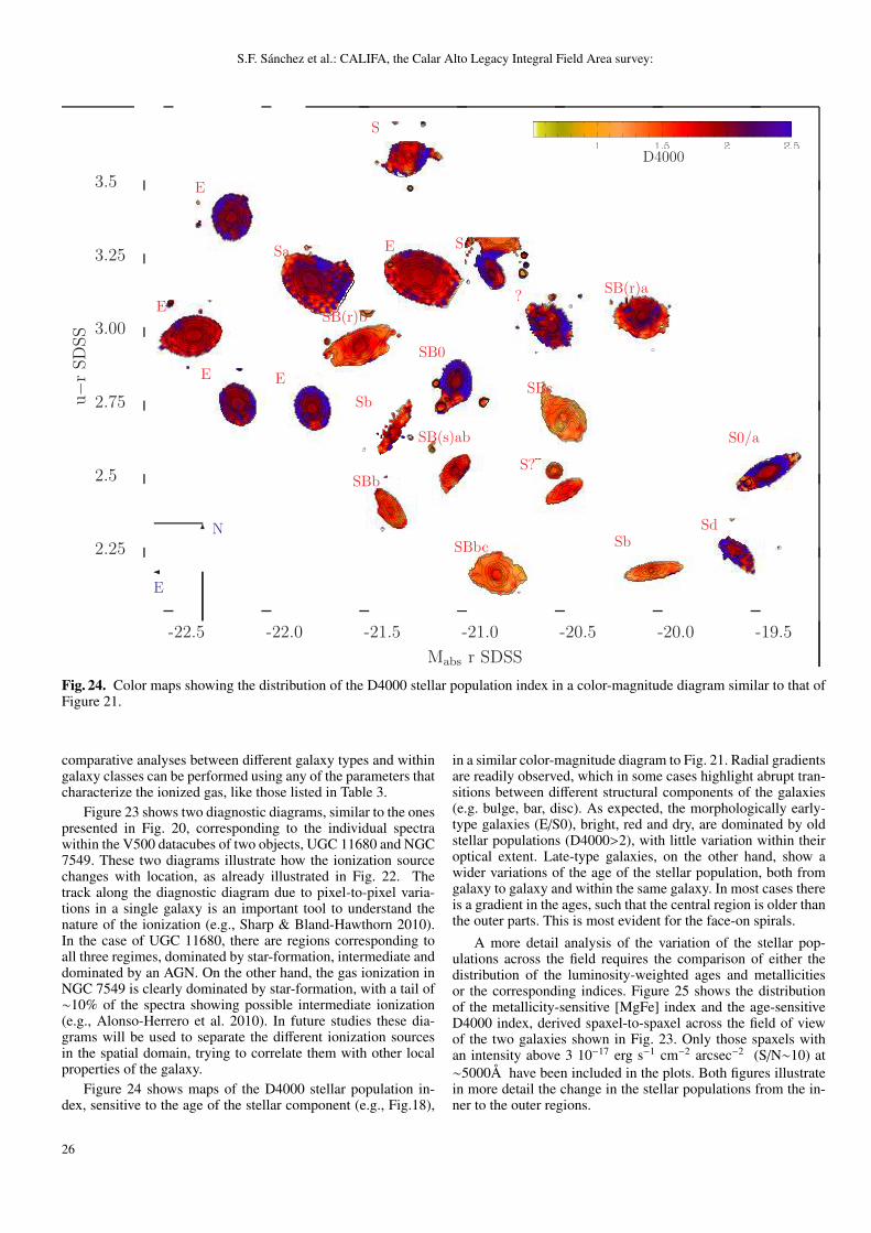
S.F. Sanchez et al.: CALIFA, the Calar Alto Legacy Integral Field Area survey:
-22.5 -22.0 -21.5 -21.0 -20.5 -20.0 -19.5
2.25
2.5
2.75
3.00
3.25
3.5
u−r
SDSS
Mabs r SDSS
SE
Sb
E
E
Sb
SBb
SB(r)b
E
Sd
S0/a
SB(r)a
S
Sa
?
S?
E
SB0
SB(s)ab
SBc
SBbc
D4000
�
??
E
N
Fig. 24. Color maps showing the distribution of the D4000 stellar population index in a color-magnitude diagram similar to that ofFigure 21.
comparative analyses between different galaxy types and withingalaxy classes can be performed using any of the parameters thatcharacterize the ionized gas, like those listed in Table 3.
Figure 23 shows two diagnostic diagrams, similar to the onespresented in Fig. 20, corresponding to the individual spectrawithin the V500 datacubes of two objects, UGC 11680 and NGC7549. These two diagrams illustrate how the ionization sourcechanges with location, as already illustrated in Fig. 22. Thetrack along the diagnostic diagram due to pixel-to-pixel varia-tions in a single galaxy is an important tool to understand thenature of the ionization (e.g., Sharp & Bland-Hawthorn 2010).In the case of UGC 11680, there are regions corresponding toall three regimes, dominated by star-formation, intermediate anddominated by an AGN. On the other hand, the gas ionization inNGC 7549 is clearly dominated by star-formation, with a tail of∼10% of the spectra showing possible intermediate ionization(e.g., Alonso-Herrero et al. 2010). In future studies these dia-grams will be used to separate the different ionization sourcesin the spatial domain, trying to correlate them with other localproperties of the galaxy.
Figure 24 shows maps of the D4000 stellar population in-dex, sensitive to the age of the stellar component (e.g., Fig.18),
in a similar color-magnitude diagram to Fig. 21. Radial gradientsare readily observed, which in some cases highlight abrupt tran-sitions between different structural components of the galaxies(e.g. bulge, bar, disc). As expected, the morphologically early-type galaxies (E/S0), bright, red and dry, are dominated by oldstellar populations (D4000>2), with little variation within theiroptical extent. Late-type galaxies, on the other hand, show awider variations of the age of the stellar population, both fromgalaxy to galaxy and within the same galaxy. In most cases thereis a gradient in the ages, such that the central region is older thanthe outer parts. This is most evident for the face-on spirals.
A more detail analysis of the variation of the stellar pop-ulations across the field requires the comparison of either thedistribution of the luminosity-weighted ages and metallicitiesor the corresponding indices. Figure 25 shows the distributionof the metallicity-sensitive [MgFe] index and the age-sensitiveD4000 index, derived spaxel-to-spaxel across the field of viewof the two galaxies shown in Fig. 23. Only those spaxels withan intensity above 3 10−17 erg s−1 cm−2 arcsec−2 (S/N∼10) at∼5000Å have been included in the plots. Both figures illustratein more detail the change in the stellar populations from the in-ner to the outer regions.
26
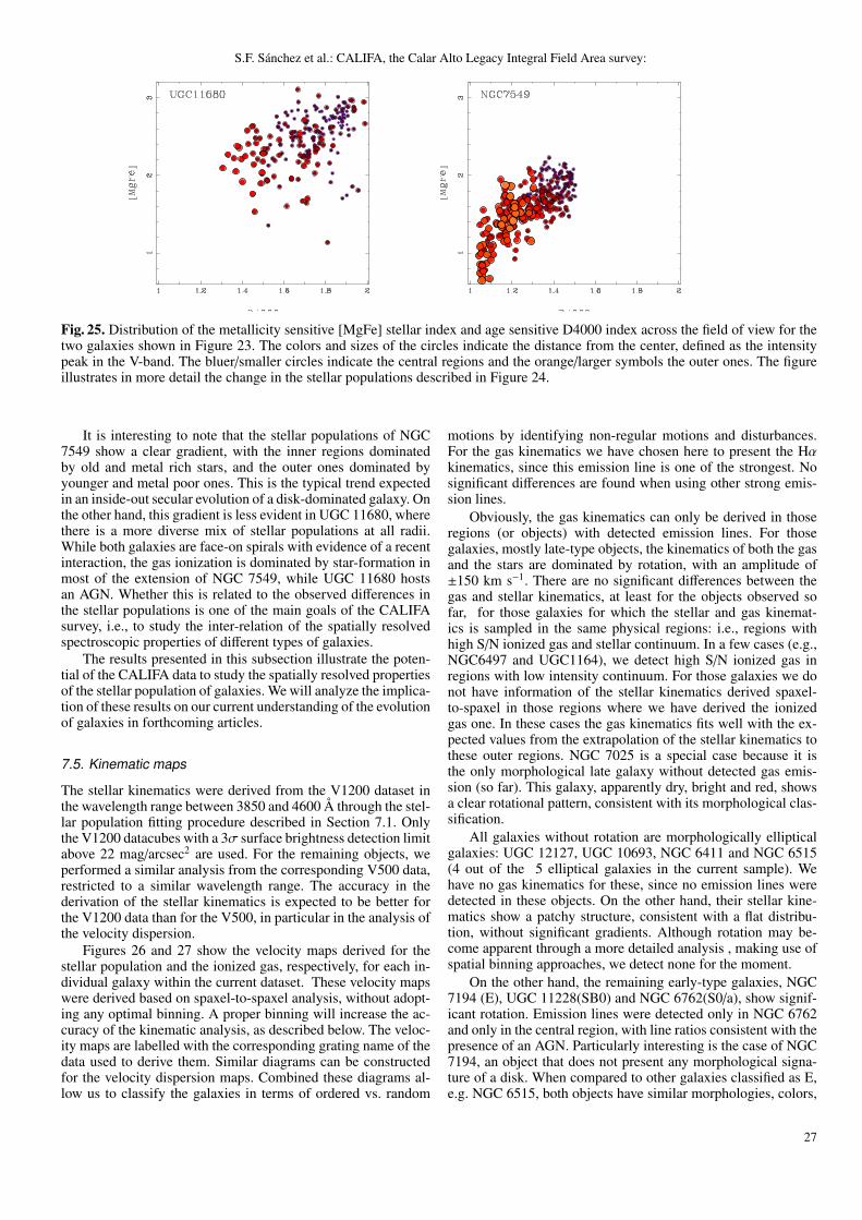
S.F. Sanchez et al.: CALIFA, the Calar Alto Legacy Integral Field Area survey:
Fig. 25. Distribution of the metallicity sensitive [MgFe] stellar index and age sensitive D4000 index across the field of view for thetwo galaxies shown in Figure 23. The colors and sizes of the circles indicate the distance from the center, defined as the intensitypeak in the V-band. The bluer/smaller circles indicate the central regions and the orange/larger symbols the outer ones. The figureillustrates in more detail the change in the stellar populations described in Figure 24.
It is interesting to note that the stellar populations of NGC7549 show a clear gradient, with the inner regions dominatedby old and metal rich stars, and the outer ones dominated byyounger and metal poor ones. This is the typical trend expectedin an inside-out secular evolution of a disk-dominated galaxy. Onthe other hand, this gradient is less evident in UGC 11680, wherethere is a more diverse mix of stellar populations at all radii.While both galaxies are face-on spirals with evidence of a recentinteraction, the gas ionization is dominated by star-formation inmost of the extension of NGC 7549, while UGC 11680 hostsan AGN. Whether this is related to the observed differences inthe stellar populations is one of the main goals of the CALIFAsurvey, i.e., to study the inter-relation of the spatially resolvedspectroscopic properties of different types of galaxies.
The results presented in this subsection illustrate the poten-tial of the CALIFA data to study the spatially resolved propertiesof the stellar population of galaxies. We will analyze the implica-tion of these results on our current understanding of the evolutionof galaxies in forthcoming articles.
7.5. Kinematic maps
The stellar kinematics were derived from the V1200 dataset inthe wavelength range between 3850 and 4600 Å through the stel-lar population fitting procedure described in Section 7.1. Onlythe V1200 datacubes with a 3σ surface brightness detection limitabove 22 mag/arcsec2 are used. For the remaining objects, weperformed a similar analysis from the corresponding V500 data,restricted to a similar wavelength range. The accuracy in thederivation of the stellar kinematics is expected to be better forthe V1200 data than for the V500, in particular in the analysis ofthe velocity dispersion.
Figures 26 and 27 show the velocity maps derived for thestellar population and the ionized gas, respectively, for each in-dividual galaxy within the current dataset. These velocity mapswere derived based on spaxel-to-spaxel analysis, without adopt-ing any optimal binning. A proper binning will increase the ac-curacy of the kinematic analysis, as described below. The veloc-ity maps are labelled with the corresponding grating name of thedata used to derive them. Similar diagrams can be constructedfor the velocity dispersion maps. Combined these diagrams al-low us to classify the galaxies in terms of ordered vs. random
motions by identifying non-regular motions and disturbances.For the gas kinematics we have chosen here to present the Hαkinematics, since this emission line is one of the strongest. Nosignificant differences are found when using other strong emis-sion lines.
Obviously, the gas kinematics can only be derived in thoseregions (or objects) with detected emission lines. For thosegalaxies, mostly late-type objects, the kinematics of both the gasand the stars are dominated by rotation, with an amplitude of±150 km s−1. There are no significant differences between thegas and stellar kinematics, at least for the objects observed sofar, for those galaxies for which the stellar and gas kinemat-ics is sampled in the same physical regions: i.e., regions withhigh S/N ionized gas and stellar continuum. In a few cases (e.g.,NGC6497 and UGC1164), we detect high S/N ionized gas inregions with low intensity continuum. For those galaxies we donot have information of the stellar kinematics derived spaxel-to-spaxel in those regions where we have derived the ionizedgas one. In these cases the gas kinematics fits well with the ex-pected values from the extrapolation of the stellar kinematics tothese outer regions. NGC 7025 is a special case because it isthe only morphological late galaxy without detected gas emis-sion (so far). This galaxy, apparently dry, bright and red, showsa clear rotational pattern, consistent with its morphological clas-sification.
All galaxies without rotation are morphologically ellipticalgalaxies: UGC 12127, UGC 10693, NGC 6411 and NGC 6515(4 out of the 5 elliptical galaxies in the current sample). Wehave no gas kinematics for these, since no emission lines weredetected in these objects. On the other hand, their stellar kine-matics show a patchy structure, consistent with a flat distribu-tion, without significant gradients. Although rotation may be-come apparent through a more detailed analysis , making use ofspatial binning approaches, we detect none for the moment.
On the other hand, the remaining early-type galaxies, NGC7194 (E), UGC 11228(SB0) and NGC 6762(S0/a), show signif-icant rotation. Emission lines were detected only in NGC 6762and only in the central region, with line ratios consistent with thepresence of an AGN. Particularly interesting is the case of NGC7194, an object that does not present any morphological signa-ture of a disk. When compared to other galaxies classified as E,e.g. NGC 6515, both objects have similar morphologies, colors,
27
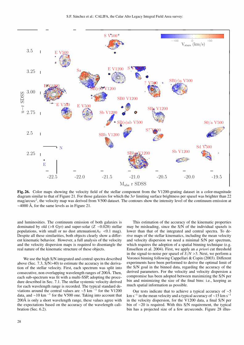
S.F. Sanchez et al.: CALIFA, the Calar Alto Legacy Integral Field Area survey:
-22.5 -22.0 -21.5 -21.0 -20.5 -20.0 -19.5
2.25
2.5
2.75
3.00
3.25
3.5
u−r
SDSS
Mabs r SDSS
S V1200E V1200
Sb V1200
E V1200
E V500
Sb V1200
SBb V1200
SB(r)b V1200
E V500
Sd V500
S0/a V500
SB(r)a V500
S V500
Sa
? V500
S? V500
E V500
SB0 V1200
SB(s)ab V500
SBc V1200
SBbc V1200
Vstars (km/s)
�
??
E
N
Fig. 26. Color maps showing the velocity field of the stellar component from the V1200-grating dataset in a color-magnitudediagram similar to that of Figure 21. For those galaxies for which the 3σ limiting surface brightness per spaxel was brighter than 22mag/arcsec2, the velocity map was derived from V500 dataset. The contours show the intensity level of the continuum emission at∼4000 Å, for the same levels as in Figure 21.
and luminosities. The continuum emission of both galaxies isdominated by old (>8 Gyr) and super-solar (Z ∼0.028) stellarpopulations, with small or no dust attenuation(AV <0.1 mag).Despite all these similarities, both objects clearly show a differ-ent kinematic behavior. However, a full analysis of the velocityand the velocity dispersion maps is required to disentangle thereal nature of the kinematic structure of these objects.
We use the high S/N integrated and central spectra describedabove (Sec. 7.3, S/N>40) to estimate the accuracy in the deriva-tion of the stellar velocity. First, each spectrum was split intoconsecutive, non overlapping wavelength ranges of 200Å. Then,each sub-spectrum was fit with a multi-SSP, adopting the proce-dure described in Sec. 7.1. The stellar systemic velocity derivedfor each wavelength range is recorded. The typical standard de-viations around the central values are ∼5 km −1 for the V1200data, and ∼10 km −1 for the V500 one. Taking into account that200Å is only a short wavelength range, these values agree withthe expectations based on the accuracy of the wavelength cali-bration (Sec. 6.2).
This estimation of the accuracy of the kinematic propertiesmay be misleading, since the S/N of the individual spaxels islower than that of the integrated and central spectra. To de-rive maps of the stellar kinematics, including the mean velocityand velocity dispersion we need a minimal S/N per spectrum,which requires the adoption of a spatial binning technique (e.g.Emsellem et al. 2004). First, we apply an a priori cut thresholdin the signal-to-noise per spaxel of S/N >3. Next, we perform aVoronoi binning following Cappellari & Copin (2003). Differentexperiments have been performed to derive the optimal limit ofthe S/N goal in the binned data, regarding the accuracy of thederived parameters. For the velocity and velocity dispersion acompromise has been adopted between maximizing the S/N perbin and minimizing the size of the final bins: i.e., keeping asmuch spatial information as possible.
Our tests indicate that to achieve a typical accuracy of ∼5km s−1 in the mean velocity and a typical accuracy of ∼15 km s−1
in the velocity dispersion, for the V1200 data, a final S/N perbin of ∼20 is required. With this S/N requirement, the typicalbin has a projected size of a few arcseconds. Figure 28 illus-
28
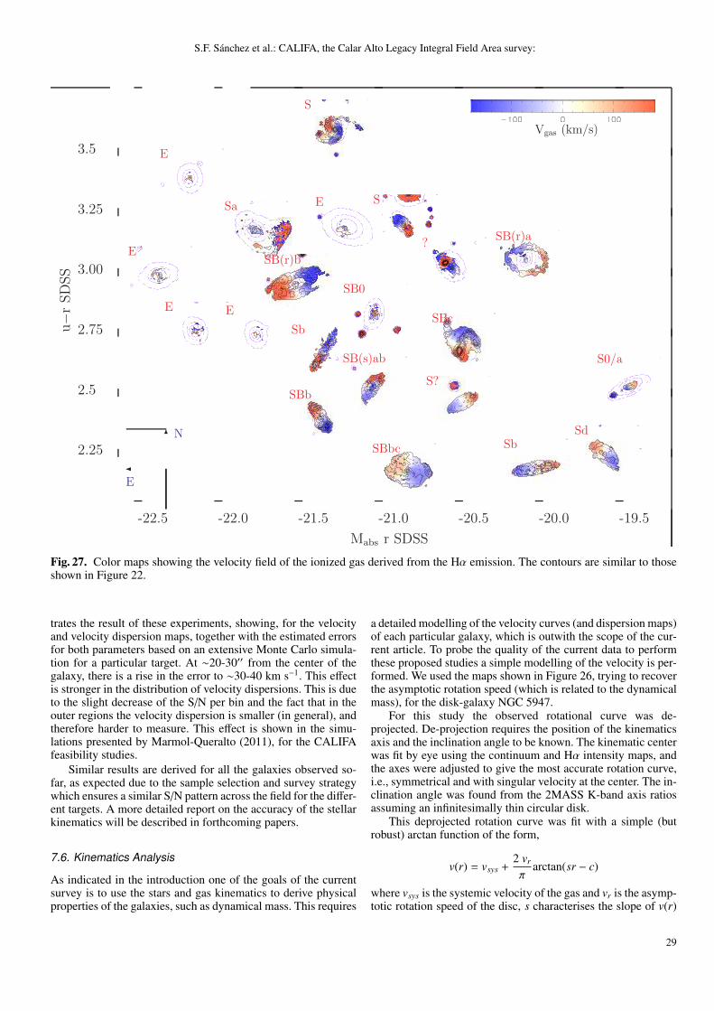
S.F. Sanchez et al.: CALIFA, the Calar Alto Legacy Integral Field Area survey:
-22.5 -22.0 -21.5 -21.0 -20.5 -20.0 -19.5
2.25
2.5
2.75
3.00
3.25
3.5
u−r
SDSS
Mabs r SDSS
SE
Sb
E
E
Sb
SBb
SB(r)b
E
Sd
S0/a
SB(r)a
S
Sa
?
S?
E
SB0
SB(s)ab
SBc
SBbc
Vgas (km/s)
�
??
E
N
Fig. 27. Color maps showing the velocity field of the ionized gas derived from the Hα emission. The contours are similar to thoseshown in Figure 22.
trates the result of these experiments, showing, for the velocityand velocity dispersion maps, together with the estimated errorsfor both parameters based on an extensive Monte Carlo simula-tion for a particular target. At ∼20-30′′ from the center of thegalaxy, there is a rise in the error to ∼30-40 km s−1. This effectis stronger in the distribution of velocity dispersions. This is dueto the slight decrease of the S/N per bin and the fact that in theouter regions the velocity dispersion is smaller (in general), andtherefore harder to measure. This effect is shown in the simu-lations presented by Marmol-Queralto (2011), for the CALIFAfeasibility studies.
Similar results are derived for all the galaxies observed so-far, as expected due to the sample selection and survey strategywhich ensures a similar S/N pattern across the field for the differ-ent targets. A more detailed report on the accuracy of the stellarkinematics will be described in forthcoming papers.
7.6. Kinematics Analysis
As indicated in the introduction one of the goals of the currentsurvey is to use the stars and gas kinematics to derive physicalproperties of the galaxies, such as dynamical mass. This requires
a detailed modelling of the velocity curves (and dispersion maps)of each particular galaxy, which is outwith the scope of the cur-rent article. To probe the quality of the current data to performthese proposed studies a simple modelling of the velocity is per-formed. We used the maps shown in Figure 26, trying to recoverthe asymptotic rotation speed (which is related to the dynamicalmass), for the disk-galaxy NGC 5947.
For this study the observed rotational curve was de-projected. De-projection requires the position of the kinematicsaxis and the inclination angle to be known. The kinematic centerwas fit by eye using the continuum and Hα intensity maps, andthe axes were adjusted to give the most accurate rotation curve,i.e., symmetrical and with singular velocity at the center. The in-clination angle was found from the 2MASS K-band axis ratiosassuming an infinitesimally thin circular disk.
This deprojected rotation curve was fit with a simple (butrobust) arctan function of the form,
v(r) = vsys +2 vr
πarctan(sr − c)
where vsys is the systemic velocity of the gas and vr is the asymp-totic rotation speed of the disc, s characterises the slope of v(r)
29
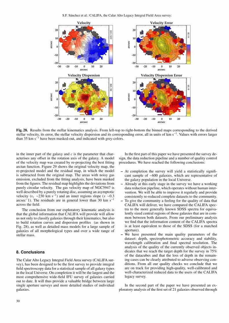
S.F. Sanchez et al.: CALIFA, the Calar Alto Legacy Integral Field Area survey:
Velocity
-30 -20 -10 0 10 20arcsec
-20
-10
0
10
20
arc
sec
-11
5 /
11
5
Velocity Error
-30 -20 -10 0 10 20arcsec
-20
-10
0
10
20
arc
sec
0 /
35
Velocity Dispersion
-30 -20 -10 0 10 20arcsec
-20
-10
0
10
20
arc
sec
30
/ 1
50
Velocity Dispersion Error
-30 -20 -10 0 10 20arcsec
-20
-10
0
10
20
arc
sec
0 /
35
Fig. 28. Results from the stellar kinematics analysis. From left-top to right-bottom the binned maps corresponding to the derivedstellar velocity, its error, the stellar velocity dispersion and its corresponding error, all in units of km s−1. Values with errors largerthan 35 km s−1 have been masked-out, and indicated with grey-colors.
in the inner part of the galaxy and c is the parameter that char-acterises any offset in the rotation axis of the galaxy. A modelof the velocity map was created by re-projecting the best fittingarctan function. Figure 29 shows the original velocity map, there-projected model and the residual map, in which the modelis subtracted from the original map. The areas with noisy gasemission, excluded from the fitting analysis, have been maskedfrom the figures. The residual map highlights the deviations frompurely circular velocity. The gas velocity map of NGC5947 iswell described by a purely rotating disc, assuming an asymptoticvelocity (vr ∼230 km s−1) and an inner regions slope (s ∼0.3arcsec−1). The residuals are in general lower than 30 km s−1
across the field.The conclusion from our exploratory kinematic analysis is
that the global information that CALIFA will provide will allowus not only to classify galaxies through their kinematics, but alsoto build rotation curves and dispersion profiles (as shown inFig. 28), as well as detailed mass models for a large sample ofgalaxies of all morphological types and over a wide range ofstellar mass.
8. Conclusions
The Calar Alto Legacy Integral Field Area survey (CALIFA sur-vey), has been designed to be the first survey to provide integralfield spectroscopy data for a statistical sample of all galaxy typesin the local Universe. On completion it will be the largest and themost comprehensive wide-field IFU survey of galaxies carriedout to date. It will thus provide a valuable bridge between largesingle aperture surveys and more detailed studies of individualgalaxies.
In the first part of this paper we have presented the survey de-sign, the data reduction pipeline and a number of quality controlprocedures. We have reached the following conclusions:
– At completion the survey will yield a statistically signifi-cant sample of ∼600 galaxies, which are representative ofthe galaxy population in the local Universe.
– Already at this early stage in the survey we have a workingdata reduction pipeline, which operates without human inter-vention. We will be able to improve it regularly and provideconsistently re-reduced complete datasets to the community.
– To give the community a feeling for the quality of data thatCALIFA will deliver, we have compared the CALIFA spec-tra to the more generally known SDSS spectra for equiva-lently sized central regions of those galaxies that are in com-mon between both datasets. From our preliminary analysiswe find that the information content of the CALIFA spectrais at least equivalent to those of the SDSS (for a matchedaperture).
– We have presented the main quality parameters of thedataset: depth, spectrophotometric accuracy and stability,wavelength calibration and final spectral resolution. Theanalysis of the quality of the currently observed objects in-dicates that we reach the target depth for the survey in 75%of the datacubes and that the loss of depth in the remain-ing cases can be clearly attributed to adverse observing con-ditions. From all our quality checks we conclude that weare on track for providing high-quality, well-calibrated andwell-characterized reduced data to the users of the CALIFAlegacy survey.
In the second part of the paper we have presented an ex-ploratory analysis of the first set of 21 galaxies observed through
30
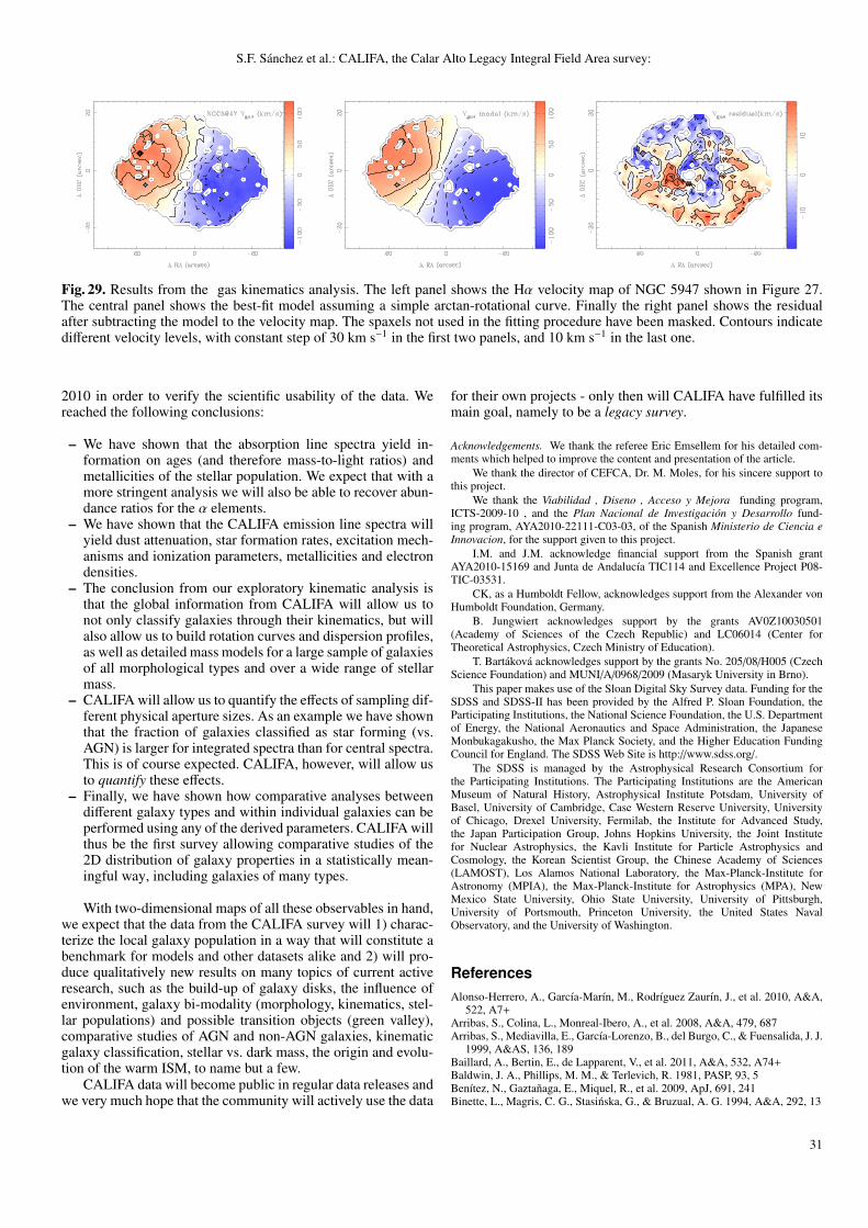
S.F. Sanchez et al.: CALIFA, the Calar Alto Legacy Integral Field Area survey:
Fig. 29. Results from the gas kinematics analysis. The left panel shows the Hα velocity map of NGC 5947 shown in Figure 27.The central panel shows the best-fit model assuming a simple arctan-rotational curve. Finally the right panel shows the residualafter subtracting the model to the velocity map. The spaxels not used in the fitting procedure have been masked. Contours indicatedifferent velocity levels, with constant step of 30 km s−1 in the first two panels, and 10 km s−1 in the last one.
2010 in order to verify the scientific usability of the data. Wereached the following conclusions:
– We have shown that the absorption line spectra yield in-formation on ages (and therefore mass-to-light ratios) andmetallicities of the stellar population. We expect that with amore stringent analysis we will also be able to recover abun-dance ratios for the α elements.
– We have shown that the CALIFA emission line spectra willyield dust attenuation, star formation rates, excitation mech-anisms and ionization parameters, metallicities and electrondensities.
– The conclusion from our exploratory kinematic analysis isthat the global information from CALIFA will allow us tonot only classify galaxies through their kinematics, but willalso allow us to build rotation curves and dispersion profiles,as well as detailed mass models for a large sample of galaxiesof all morphological types and over a wide range of stellarmass.
– CALIFA will allow us to quantify the effects of sampling dif-ferent physical aperture sizes. As an example we have shownthat the fraction of galaxies classified as star forming (vs.AGN) is larger for integrated spectra than for central spectra.This is of course expected. CALIFA, however, will allow usto quantify these effects.
– Finally, we have shown how comparative analyses betweendifferent galaxy types and within individual galaxies can beperformed using any of the derived parameters. CALIFA willthus be the first survey allowing comparative studies of the2D distribution of galaxy properties in a statistically mean-ingful way, including galaxies of many types.
With two-dimensional maps of all these observables in hand,we expect that the data from the CALIFA survey will 1) charac-terize the local galaxy population in a way that will constitute abenchmark for models and other datasets alike and 2) will pro-duce qualitatively new results on many topics of current activeresearch, such as the build-up of galaxy disks, the influence ofenvironment, galaxy bi-modality (morphology, kinematics, stel-lar populations) and possible transition objects (green valley),comparative studies of AGN and non-AGN galaxies, kinematicgalaxy classification, stellar vs. dark mass, the origin and evolu-tion of the warm ISM, to name but a few.
CALIFA data will become public in regular data releases andwe very much hope that the community will actively use the data
for their own projects - only then will CALIFA have fulfilled itsmain goal, namely to be a legacy survey.
Acknowledgements. We thank the referee Eric Emsellem for his detailed com-ments which helped to improve the content and presentation of the article.
We thank the director of CEFCA, Dr. M. Moles, for his sincere support tothis project.
We thank the Viabilidad , Diseno , Acceso y Mejora funding program,ICTS-2009-10 , and the Plan Nacional de Investigacion y Desarrollo fund-ing program, AYA2010-22111-C03-03, of the Spanish Ministerio de Ciencia eInnovacion, for the support given to this project.
I.M. and J.M. acknowledge financial support from the Spanish grantAYA2010-15169 and Junta de Andalucıa TIC114 and Excellence Project P08-TIC-03531.
CK, as a Humboldt Fellow, acknowledges support from the Alexander vonHumboldt Foundation, Germany.
B. Jungwiert acknowledges support by the grants AV0Z10030501(Academy of Sciences of the Czech Republic) and LC06014 (Center forTheoretical Astrophysics, Czech Ministry of Education).
T. Bartakova acknowledges support by the grants No. 205/08/H005 (CzechScience Foundation) and MUNI/A/0968/2009 (Masaryk University in Brno).
This paper makes use of the Sloan Digital Sky Survey data. Funding for theSDSS and SDSS-II has been provided by the Alfred P. Sloan Foundation, theParticipating Institutions, the National Science Foundation, the U.S. Departmentof Energy, the National Aeronautics and Space Administration, the JapaneseMonbukagakusho, the Max Planck Society, and the Higher Education FundingCouncil for England. The SDSS Web Site is http://www.sdss.org/.
The SDSS is managed by the Astrophysical Research Consortium forthe Participating Institutions. The Participating Institutions are the AmericanMuseum of Natural History, Astrophysical Institute Potsdam, University ofBasel, University of Cambridge, Case Western Reserve University, Universityof Chicago, Drexel University, Fermilab, the Institute for Advanced Study,the Japan Participation Group, Johns Hopkins University, the Joint Institutefor Nuclear Astrophysics, the Kavli Institute for Particle Astrophysics andCosmology, the Korean Scientist Group, the Chinese Academy of Sciences(LAMOST), Los Alamos National Laboratory, the Max-Planck-Institute forAstronomy (MPIA), the Max-Planck-Institute for Astrophysics (MPA), NewMexico State University, Ohio State University, University of Pittsburgh,University of Portsmouth, Princeton University, the United States NavalObservatory, and the University of Washington.
ReferencesAlonso-Herrero, A., Garcıa-Marın, M., Rodrıguez Zaurın, J., et al. 2010, A&A,
522, A7+Arribas, S., Colina, L., Monreal-Ibero, A., et al. 2008, A&A, 479, 687Arribas, S., Mediavilla, E., Garcıa-Lorenzo, B., del Burgo, C., & Fuensalida, J. J.
1999, A&AS, 136, 189Baillard, A., Bertin, E., de Lapparent, V., et al. 2011, A&A, 532, A74+Baldwin, J. A., Phillips, M. M., & Terlevich, R. 1981, PASP, 93, 5Benıtez, N., Gaztanaga, E., Miquel, R., et al. 2009, ApJ, 691, 241Binette, L., Magris, C. G., Stasinska, G., & Bruzual, A. G. 1994, A&A, 292, 13
31
S.F. Sanchez et al.: CALIFA, the Calar Alto Legacy Integral Field Area survey:
Blanc, G. A., Gebhardt, K., Heiderman, A., et al. 2010, in Astronomical Societyof the Pacific Conference Series, Vol. 432, Astronomical Society of thePacific Conference Series, ed. L. M. Stanford, J. D. Green, L. Hao, & Y. Mao,180
Blanton, M. R., Schlegel, D. J., Strauss, M. A., et al. 2005, AJ, 129, 2562Brinchmann, J., Charlot, S., White, S. D. M., et al. 2004, MNRAS, 351, 1151Cappellari, M. & Copin, Y. 2003, MNRAS, 342, 345Cappellari, M. & Emsellem, E. 2004, PASP, 116, 138Cappellari, M., Emsellem, E., Krajnovic, D., et al. 2011, MNRAS, 413, 813Cardelli, J. A., Clayton, G. C., & Mathis, J. S. 1989, ApJ, 345, 245Castillo-Morales, A., Gallego, J., Perez-Gallego, J., et al. 2010, MNRAS, 1804Cid Fernandes, R., Mateus, A., Sodre, L., Stasinska, G., & Gomes, J. M. 2005,
MNRAS, 358, 363Cid Fernandes, R., Stasinska, G., Schlickmann, M. S., et al. 2010, MNRAS, 403,
1036Davies, J. I., Phillipps, S., & Disney, M. J. 1990, MNRAS, 244, 385de Jong, R. S. & van der Kruit, P. C. 1995, VizieR Online Data Catalog, 4106,
60451de Zeeuw, P. T., Bureau, M., Emsellem, E., et al. 2002, MNRAS, 329, 513Dıaz, A. I., Castellanos, M., Terlevich, E., & Luisa Garcıa-Vargas, M. 2000,
MNRAS, 318, 462Ellis, S. C., Driver, S. P., Allen, P. D., et al. 2005, MNRAS, 363, 1257Emsellem, E., Bacon, R., Monnet, G., & Poulain, P. 1996, A&A, 312, 777Emsellem, E., Cappellari, M., Peletier, R. F., et al. 2004, MNRAS, 352, 721Epinat, B., Amram, P., Balkowski, C., & Marcelin, M. 2010, MNRAS, 401, 2113Filippenko, A. V. 1982, PASP, 94, 715Folkes, S., Ronen, S., Price, I., et al. 1999, MNRAS, 308, 459Gallazzi, A., Charlot, S., Brinchmann, J., White, S. D. M., & Tremonti, C. A.
2005, MNRAS, 362, 41Gomez, P. L., Nichol, R. C., Miller, C. J., et al. 2003, ApJ, 584, 210Kauffmann, G., Heckman, T. M., Tremonti, C., et al. 2003, MNRAS, 346, 1055Kelz, A., Verheijen, M. A. W., Roth, M. M., et al. 2006, PASP, 118, 129Kennicutt, Jr., R. C. 1998, ApJ, 498, 541Kewley, L. J., Dopita, M. A., Sutherland, R. S., Heisler, C. A., & Trevena, J.
2001, ApJ, 556, 121Kewley, L. J. & Ellison, S. L. 2008, ApJ, 681, 1183Kewley, L. J., Jansen, R. A., & Geller, M. J. 2005, PASP, 117, 227Koleva, M., Prugniel, P., Bouchard, A., & Wu, Y. 2009, A&A, 501, 1269Kuntschner, H., Emsellem, E., Bacon, R., et al. 2006, MNRAS, 369, 497Le Fevre, O., Vettolani, G., Paltani, S., et al. 2004, A&A, 428, 1043Lilly, S. J., Le Fevre, O., Renzini, A., et al. 2007, ApJS, 172, 70Lopez-Sanchez, A. R. & Esteban, C. 2010, A&A, 517, A85+MacArthur, L. A., Courteau, S., Bell, E., & Holtzman, J. A. 2004, ApJS, 152,
175MacArthur, L. A., Gonzalez, J. J., & Courteau, S. 2009, MNRAS, 395, 28Marmol-Queralto, E., e. 2011, A&A, 1, 1Moles, M., Benıtez, N., Aguerri, J. A. L., et al. 2008, AJ, 136, 1325Moro, D. & Munari, U. 2000, A&AS, 147, 361Moustakas, J. & Kennicutt, Jr., R. C. 2006, ApJS, 164, 81Ocvirk, P., Pichon, C., Lancon, A., & Thiebaut, E. 2006, MNRAS, 365, 46Oke, J. B. 1990, AJ, 99, 1621Osterbrock, D. E. 1989, Astrophysics of gaseous nebulae and active galactic
nuclei (University Science Books)Perez-Gallego, J., Guzman, R., Castillo-Morales, A., et al. 2010, MNRAS, 402,
1397Pettini, M. & Pagel, B. E. J. 2004, MNRAS, 348, L59Rix, H., Barden, M., Beckwith, S. V. W., et al. 2004, ApJS, 152, 163Rosales-Ortega, F. F., Kennicutt, R. C., Sanchez, S. F., et al. 2010, MNRAS, 405,
735Roth, M. M., Bauer, S.-M., Dionies, F., et al. 1998, in Presented at the
Society of Photo-Optical Instrumentation Engineers (SPIE) Conference, Vol.3355, Society of Photo-Optical Instrumentation Engineers (SPIE) ConferenceSeries, ed. S. D’Odorico, 798–809
Roth, M. M., Becker, T., Kelz, A., & Schmoll, J. 2004, ApJ, 603, 531Roth, M. M., Fechner, T., Wolter, D., et al. 2010, in Society of Photo-Optical
Instrumentation Engineers (SPIE) Conference Series, Vol. 7742, Society ofPhoto-Optical Instrumentation Engineers (SPIE) Conference Series
Roth, M. M., Kelz, A., Fechner, T., et al. 2005, PASP, 117, 620Roth, M. M., Seydack, M., Bauer, S.-M., & Laux, U. 1997, in Presented at the
Society of Photo-Optical Instrumentation Engineers (SPIE) Conference, Vol.2871, Society of Photo-Optical Instrumentation Engineers (SPIE) ConferenceSeries, ed. A. L. Ardeberg, 1235–1245
Sanchez, S. F. 2006a, Astronomische Nachrichten, 327, 850Sanchez, S. F., Aceituno, J., Thiele, U., Perez-Ramırez, D., & Alves, J. 2007a,
PASP, 119, 1186Sanchez, S. F., Cardiel, N., Verheijen, M. A. W., et al. 2007c, A&A, 465, 207Sanchez, S. F., Cardiel, N., Verheijen, M. A. W., Pedraz, S., & Covone, G. 2007b,
MNRAS, 376, 125
Sanchez, S. F., Garcıa-Lorenzo, B., Jahnke, K., et al. 2006b, New A Rev., 49,501
Sanchez, S. F., Jahnke, K., Wisotzki, L., et al. 2004, ApJ, 614, 586Sanchez, S. F., Rosales-Ortega, F. F., Kennicutt, R. C., et al. 2011, MNRAS, 410,
313Sandin, C., Becker, T., Roth, M. M., et al. 2010, A&A, 515, 35Sarzi, M., Falcon-Barroso, J., Davies, R. L., et al. 2006, MNRAS, 366, 1151Sarzi, M., Shields, J. C., Schawinski, K., et al. 2010, MNRAS, 402, 2187Scoville, N., Aussel, H., Brusa, M., et al. 2007a, ApJS, 172, 1Scoville, N., Aussel, H., Brusa, M., et al. 2007b, ApJS, 172, 1Sharp, R. G. & Bland-Hawthorn, J. 2010, ApJ, 711, 818Shepard, D. 1968, Proceedings of the 1968 ACM National Conference, 1, 517Stasinska, G., Vale Asari, N., Cid Fernandes, R., et al. 2008, MNRAS, 391, L29Storchi-Bergmann, T., Schmitt, H. R., Calzetti, D., & Kinney, A. L. 1998, AJ,
115, 909Strateva, I., Ivezic, Z., Knapp, G. R., et al. 2001, AJ, 122, 1861Trager, S. C., Faber, S. M., Worthey, G., & Gonzalez, J. J. 2000, AJ, 119, 1645Trinchieri, G. & di Serego Alighieri, S. 1991, AJ, 101, 1647van Dokkum, P. G. 2001, PASP, 113, 1420Vazdekis, A., Sanchez-Blazquez, P., Falcon-Barroso, J., et al. 2010, MNRAS,
404, 1639Veilleux, S. & Osterbrock, D. E. 1987, ApJS, 63, 295Verheijen, M. A. W., Bershady, M. A., Andersen, D. R., et al. 2004,
Astronomische Nachrichten, 325, 151Walcher, C. J., Boker, T., Charlot, S., et al. 2006, ApJ, 649, 692Walcher, J., Groves, B., Budavari, T., & Dale, D. 2011, Ap&SS, 331, 1Wisotzki, L., Becker, T., Christensen, L., et al. 2003, A&A, 408, 455Wolf, C., Meisenheimer, K., Rix, H., et al. 2003, A&A, 401, 73York, D. G., Adelman, J., Anderson, Jr., J. E., et al. 2000, AJ, 120, 1579Zibetti, S., Charlot, S., & Rix, H. 2009, MNRAS, 400, 1181
32
S.F. Sanchez et al.: CALIFA, the Calar Alto Legacy Integral Field Area survey:
1 Centro Astronomico Hispano Aleman, Calar Alto, (CSIC-MPG),C/Jesus Durban Remon 2-2, E-04004 Almeria, Spain e-mail:[email protected].
2 Institute of Astronomy, University of Cambridge, Madingley Road,Cambridge CB3 0HA, UK.
3 Departamento de Astrofısica y CC. de la Atmosfera, UniversidadComplutense de Madrid, Madrid 28040, Spain.
4 Max Planck Institute for Astronomy, Konigstuhl 17, D-69117Heidelberg, Germany.
5 Instituto de Astrofısica de Andalucıa (CSIC), Camino Bajo deHuetor, s/n, E-18008, Granada.
6 Leibniz-Institut fur Astrophysik Potsdam (AIP), An der Sternwarte16, D-14482 Potsdam, Germany.
7 Sydney Institute for Astronomy, School of Physics A28, Universityof Sydney, NSW 2006, Australia .
8 Australian Astronomical Observatory, PO BOX 296, Epping, NSW1710, Australia
9 Instituto de Astrofısica de Canarias (IAC), Glorieta de laAstronomıa S/N, La Laguna, S/C de Tenerife, Spain.
10 Departamento de Fisica Teorica, Universidad Autonoma de Madrid,Cantoblanco, 28049, Madrid, Spain.
11 Kapteyn Astronomical Institute, University of Groningen, NL-9700AV, Groningen, Netherlands.
12 Instituto de Fısica de Cantabria, CSIC-UC, Avenida de los CastrosS/N, 39005 Santander, Spain
13 ZAH, Landessternwarte, Konigstuhl 12, D-69117, Heidelberg,Germany.
14 Dark Cosmology Centre, Niels Bohr Institute, University ofCopenhagen, Juliane Maries Vej 30, DK-2100 Copenhagen,Denmark.
15 Centro de Astrofısica da Universidade do Porto, Rua das Esteral,4150-762, porto, Portugal.
16 Astronomical Institute of the Academy of Sciences of the CzechRepublic, v.v.i., Bocni II 1401, 14131 Prague, Czech Republic.
17 CENTRA - Centro Multidisciplinar de Astrofısica, InstitutoSuperior Tecnico, Av. Rovisco Pais 1, 1049-001 Lisbon, Portugal.
18 SUPA, Institute for Astronomy, University of Edinburgh, RoyalObservatory, Blackford Hill, Edinburgh EH9 3HJ, UK.
19 Laboratoire d’Astropysique de Marseille, UMR6110 CNRS, 38 rueF. Joliot-Curie, F-13388 Marseille, France.
20 Department of Systems Engineering and Computing, University ofZaragoza, Teruel 44003, Spain.
21 Department of Electronic Engineeing and Communications,University of Zaragoza, Teruel 44003, Spain.
22 University of Vienna, Turkenschanzstrasse 17, 1180 Vienna,Austria.
23 Department of Physics and Astronomy, Macquarie University, NSW2109, Australia.
24 Centro de Estudios de Fısica del Cosmos de Aragon (CEFCA), C/G. Pizarro, 1, Teruel, Spain.
25 Astronomical Institute of the Ruhr-University BochumUniversitaetsstr. 150, 44801 Bochum, Germany.
26 Department of Physics, University of Missouri-Kansas City, KansasCity, MO 64110, USA.
27 Dep. Fsica Terica y del Cosmos, Campus de Fuentenueva,Universidad de Granada, 18071, Granada, Spain.
28 Depto. Astrofsica, Universidad de La Laguna (ULL), E-38206 LaLaguna, Tenerife, Spain.
29 Astronomisches Rechen Institut, Zentrum fuer Astronomie derUniversitaet Heidelberg, Moenchhofstrasse 12 - 14, 69120Heidelberg, Germany.
30 Institut d’Astrophysique de Paris, CNRS, 98 bis Boulevard Arago,75014 Paris, France.
31 Laboratoire GEPI, Observatoire de Paris, CNRS-UMR8111, Univ.Paris-Diderot 5 place Jules Janssen, 92195 Meudon, France
32 Tianjin Astrophysics Center, Tianjin Normal University, Tianjin300387, China.
33 Astronomical Institute, Faculty of Mathematics and Physics,Charles University in Prague, Ke Karlovu 3, CZ-121 16 Prague,Czech Republic
34 Dept. of Theoretical Physics and Astrophysics, Faculty of Science,Masaryk University, Kotlarska 2, CZ-611 37 Brno, Czech Republic 33