Boolean models of the lac operon in E. coli - Clemson University

Boolean models of the lac operon in E. coli

Matthew Macauley Clemson University

Gene expression �  Gene expression is a process that takes gene info and creates a functional

gene product (e.g., a protein).

�  Some genes code for proteins. Others (e.g., rRNA, tRNA) code for functional RNA.

�  Gene Expression is a 2-step process: 1)  transcription of genes (messenger RNA synthesis)

2)  translation of genes (protein synthesis)

�  DNA consists of bases A, C, G, T.

�  RNA consists of bases A, C, G, U.

�  Proteins are long chains of amino acids.

�  Gene expression is used by all known life forms.

Transcription

•  Transcription occurs inside the cell nucleus. •  A helicase enzyme binds to and “unzips” DNA to read it. •  DNA is copied into mRNA. •  Segments of RNA not needed for protein coding are removed. •  The RNA then leaves the cell nucleus.

Translation

•  During translation, the mRNA is read by ribosomes. •  Each triple of RNA bases codes for an amino acid. •  The result is a protein: a long chain of amino acids. •  Proteins fold into a 3-D shape which determine their function

Gene expression �  The expression level is the rate at which a gene is being expressed.

�  Housekeeping genes are continuously expressed, as they are essential for basic life processes.

�  Regulated genes are expressed only under certain outside factors (environmental, physiological, etc.). Expression is controlled by the cell.

�  It is easiest to control gene regulation by affecting transcription.

�  One way to block repression is for repressor proteins bind to the DNA or RNA.

�  Goal: Understand the complex cell behaviors of gene regulation, which is the process of turning on/off certain genes depending on the requirements of the organism.

The lac operon in E. coli �  An operon is a region of DNA that contains a cluster of genes that are

transcribed together.

�  E. coli is a bacterium in the gut of mammals and birds. Its genome has been sequenced and its physiology is well-understood.

�  The lactose (lac) operon controls the transport and metabolism of lactose in Escherichia coli.

�  The lac operon was discovered by Francois Jacob and Jacques Monod in 1961, which earned them the Nobel Prize.

�  The lac operon was the first operon discovered and is the most widely studied mechanism of gene regulation.

�  The lac operon is used as a “test system” for models of gene regulation.

�  DNA replication and gene expression were all studied in E. coli before they were studied in eukaryotic cells.

Lactose and β−galactosidase �  When a host consumes milk, E. coli is exposed to lactose (milk sugar).

�  Lactose consists of one glucose sugar linked to one galactose sugar.

�  If both glucose and lactose are available, then glucose is the preferred energy source.

�  Before lactose can used as energy, the β−galactosidase enzyme is needed to break it down.

�  β−galactosidase is encoded by the LacZ gene on the lac operon.

�  β−galactosidase also catalyzes lactose into allolactose.

Transporter protein �  To bring lactose into the cell, a transport protein, called lac permease, is

required.

�  This protein is encoded by the LacY gene on the lac operon.

�  If lactose is not present, then neither of the following are produced: 1)  β−galactosidase (LacZ gene)

2)  lac permease (LacY gene)

�  In this case, the lac operon is OFF.

The lac operon

with lactose and no gluclose

�  Lactose is brought into the cell by the lac permease transporter protein

�  β−galactosidase breaks up lactose into glucose and galactose..

�  β−galactosidase also converts lactose into allolactose.

�  Allolactose binds to the lac repressor protein, preventing it from binding to the operator region of the genome.

�  Transcription begins: mRNA encoding the lac genes is produced.

�  Lac proteins are produced, and more lactose is brought into the cell. (The operon is ON.)

�  Eventually, all lactose is used up, so there will be no more allolactose.

�  The lac repressor can now bind to the operator, so mRNA transcription stops. (The operon has turned itself OFF.)

An ODE lac operon model �  M: mRNA

�  B: β−galactosidase

�  A: allolactose

�  P: transporter protein

�  L: lactose

Downsides of an ODE model �  Very mathematically advanced.

�  Too hard to solve explicitly. Numerical methods are needed.

�  MANY experimentally determined “rate constants” (I count 18…)

�  Often, these rate constants aren’t known even up to orders of magnitude.

A Boolean approach �  Let’s assume everything is “Boolean” (0 or 1):

o  Gene products are either present or absent

o  Enzyme concentrations are either high or low.

o  The operon is either ON or OFF.

�  mRNA is transcribed (M=1) if there is no external glucose (G=0), and either internal lactose (L=1) or external lactose (Le=1) are present.

�  The LacY and LacZ gene products (E=1) will be produced if mRNA is available (M=1).

�  Lactose will be present in the cell if there is no external glucose (Ge=0), and either of the following holds:

ü  External lactose is present (Le=1) and lac permease (E=1) is available.

ü  Internal lactose is present (L=1), but β−galactosidase is absent (E=0).

xM (t +1) = fM (t +1) =Ge ∧(L(t)∨Le )

xE (t +1) = fE (t +1) =M (t)

xL (t +1) = fL (t +1) =Ge ∧ (Le ∧E(t))∨(L(t)∧E(t))⎡⎣

⎤⎦

Comments on the Boolean model �  We have two “types” of Boolean quantities:

o  mRNA (M), lac gene products (E), and internal lactose (L) are variables.

o  External glucose (Ge) and lactose (Le) are parameters (constants).

�  Variables and parameters are drawn as nodes.

�  Interactions can be drawn as signed edges.

�  A signed graph called the wiring diagram describes the dependencies of the variables.

�  Time is discrete: t = 0, 1, 2, ….

�  Assume that the variables are updated synchronously.

xM (t +1) = fM (t +1) =Ge ∧(L(t)∨Le )xE (t +1) = fE (t +1) =M (t)

xL (t +1) = fL (t +1) =Ge ∧ (Le ∧E(t))∨(L(t)∧E(t))⎡⎣

⎤⎦

How to analyze a Boolean model �  At the bare minimum, we should expect:

o  Lactose absent => operon OFF.

o  Lactose present, glucose absent => operon ON.

o  Lactose and glucose present => operon OFF.

�  The state space (or phase space) is the directed graph (V, T), where

�  We’ll draw the state space for all four choices of the parameters:

o  (Le, Ge) = (0, 0). We hope to end up in a fixed point (0,0,0).






xL (t +1) = fL (t +1) =Ge ∧ (Le ∧E(t))∨(L(t)∧E(t))#$

%&

T = (x, f (x)) : x ∈V{ }V = (xM , xE, xL ) : xi ∈ {0,1}{ }

How to analyze a Boolean model �  We can plot the state space using the software: Analysis of Dynamical

Algebraic Models (ADAM), at adam.plantsimlab.org.

�  First, we need to convert our logical functions into polynomials.

�  Here is the relationship between Boolean logic and polynomial algebra:

Boolean operations logical form polynomial form

o  AND

o  OR

o  NOT

•  Also, everything is done modulo 2, so 1+1=0, and x2=x, and thus x(x+1)=0.




%&

z = x∧ yz = x∨ yz = x

z = xyz = x + y+ xyz =1+ x



%&



%&

State space when (Ge, Le) = (0, 1). The operon is ON.



%&

State space when (Ge, Le) = (0, 0). The operon is OFF.



%&


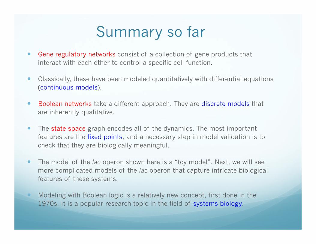
Summary so far �  Gene regulatory networks consist of a collection of gene products that

interact with each other to control a specific cell function.

�  Classically, these have been modeled quantitatively with differential equations (continuous models).

�  Boolean networks take a different approach. They are discrete models that are inherently qualitative.

�  The state space graph encodes all of the dynamics. The most important features are the fixed points, and a necessary step in model validation is to check that they are biologically meaningful.

�  The model of the lac operon shown here is a “toy model”. Next, we will see more complicated models of the lac operon that capture intricate biological features of these systems.

�  Modeling with Boolean logic is a relatively new concept, first done in the 1970s. It is a popular research topic in the field of systems biology.

A more refined model

�  Our model only used 3 variables: mRNA (M), enzymes (E), and lactose (L).

�  Let’s propose a new model with 5 variables:

�  M: mRNA



�  L: intracellular lactose

�  P: lac permease (transporter protein)

�  Assumptions �  Translation and transcription require one unit of time.

�  Protein and mRNA degradation require one unit of time

�  Lactose metabolism require one unit of time

�  Extracellular lactose is always available.

�  Extracellular glucose is always unavailable.

fM = AfB =MfA = A∨(L∧B)

fL = P∨(L∧B)fP =M

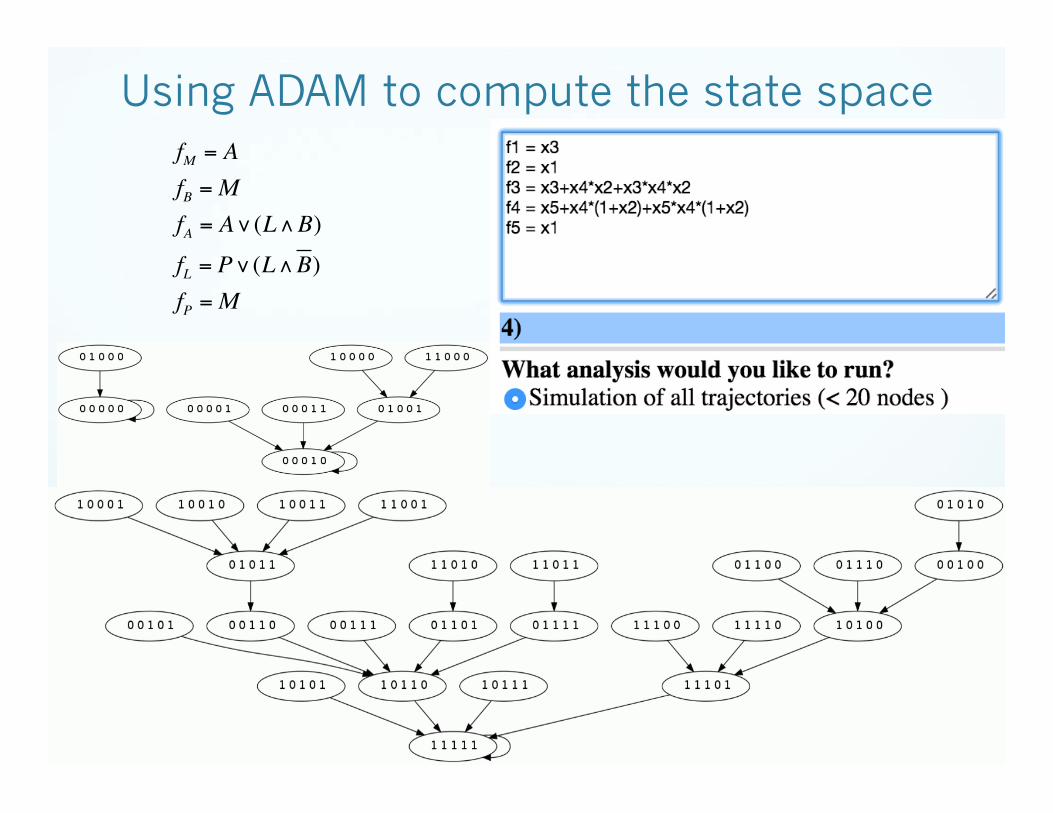
Using ADAM to compute the state space fM = A

fB =MfA = A∨(L∧B)


Problems with our refined model

�  Model variables:

�  M: mRNA




�  P: lac permease (transporter protein)

�  Problems:

�  The fixed point (M,B,A,L,P) = (0,0,0,0,0) should not happen with lactose present but not glucose. [though let’s try to justify this...]

�  The fixed point (M,B,A,L,P) = (0,0,0,1,0) is not biologically feasible: it would describe a scenario where the bacterium does not metabolize intracellular lactose.

�  Conclusion: The model fails the initial testing and validation, and is in need of modification. (Homework!)

fM = AfB =MfA = A∨(L∧B)


Catabolite repression

�  We haven’t yet discussed the cellular mechanism that turns the lac operon OFF when both glucose and lactose are present. This is done by catabolite repression.

�  The lac operon promoter region has 2 binding sites: �  One for RNA polymerase (this “unzips” and reads the DNA)

�  One for the CAP-cAMP complex. This is a complex of two molecules: catabolite activator protein (CAP), and the cyclic AMP receptor protein (cAMP, or crp).

�  Binding of the CAP-cAMP complex is required for transcription for the lac operon.

�  Intracellular glucose causes the cAMP concentration to decrease.

�  When cAMP levels get too low, so do CAP-cAMP complex levels.

�  Without the CAP-cAMP complex, the promoter is inactivated, and the lac operon is OFF.

Lac operon gene regulatory network

A more refined model �  Variables:

�  M: mRNA

�  P: lac permease


�  C: catabolite activator protein (CAP)

�  R: repressor protein (LacI)


�  Am: at least med. allolactose


�  Lm: at least med. levels of intracellular lactose

�  Assumptions:

�  Transcription and translation require 1 unit of time.

�  Degradation of all mRNA and proteins occur in 1 time-step.

�  High levels of lactose or allolactose at any time t imply (at least) medium levels for the next time-step t+1.

fM = R∧CfP =MfB =M

fC =Ge

fR = A∧AmfA = L∧BfAm = A∨L∨LmfL =Ge ∧P∧LefLm =Ge ∧(L∨Le )

A more refined model �  This 9-variable model is about as big as ADAM can render a state

space.

�  In fact, it doesn’t work using the “Open Polynomial Dynamical System (oPDS)” option (variables + parameters).

�  Instead, it works under “Polynomial Dynamical System (PDS)”, if we manually enter numbers for the parameters.

�  Here’s a sample piece of the state space:


fC =Ge


What if the state space is too big? �  The previous 9-variable model is about as big as ADAM can handle.

�  However, many gene regulatory networks are much bigger.

�  A Boolean network model (2006) of T helper cell differentiation has 23 nodes, and thus a state space of size 223 = 8,388,608.

�  A Boolean network model (2003) of the segment polarity genes in Drosophila melanogaster (fruit fly) has 60 nodes, and a state space of size 260 ≈1.15 × 1018.

�  There are many more examples…

�  For these systems, we need to be able to analyze them without constructing the entire state space.

�  Our first goals is to find the fixed points. This amounts to solving a system of equations:


fC =Ge


fx 1 = x 1fx 2 = x 2!

fx n = x n

!

"

##

$

##

How to find the fixed points �  Let’s rename variables:

�  Writing each function in polynomial form, and then for each i=1,…,9 yields the following system:

�  We need to solve this for all 4 combinations:

fM = R∧C =MfP =M = PfB =M = B

fC =Ge =C

fR = A∧Am = RfA = L∧B = AfAm = A∨L∨Lm = AmfL =Ge ∧P∧Le = AmfLm =Ge ∧(L∨Le ) = Lm

x 1+x 4 x 5+x4 = 0x 1+x2 = 0x 1+x3 = 0x 4+(Ge +1) = 0x 5+x 6 x 7+x6 + x7 +1= 0x 6+x3x8 = 0x 6+x 7+x 8+x 9+x 8 x 9+x 6 x 8+x 6 x 9+x6x8x9 = 0x 8+x2Le(Ge +1) = 0x 9+(Ge +1)(x8 + x8Le + Le ) = 0

!

"

######

$

######

(M,P,B,C,R,A,Am,L,Lm ) = (x1, x2, x3, x4, x5, x6, x7, x8, x9 )

fxi = xi

(Ge,Le ) = (0, 0), (0,1), (1, 0), (1,1)

How to find the fixed points �  Let’s first consider the case when

�  We can solve the system by typing the following commands into Sage (https://cloud.sagemath.com/), the free open-source mathematical software:

� 

(Ge,Le ) = (1,1)

What those Sage commands mean Let’s go over what the following commands mean:

Ø  P.<x1,x2,x3,x4,x5,x6,x7,x8,x9> = PolynomialRing(GF(2),9,order=‘lex’);§  Define P to be the polynomial ring over 9 variables, x1,…,x9.

§  GF(2)={0,1} because the coefficients are binary.

§  order=‘lex’ specifies a monomial order. More on this later.

Ø  Le=1; Ge=1; print "Le =", Le; print "Ge =", Ge;§  This defines two constants and prints them.

Ø  I = ideal(x1+x4*x5+x4, x1+x2, x1+x3, x4+(Ge+1), x5+x6*x7+x6+x7+1, x6+x3*x8, x6+x7+x8+x9+x8*x9+x6*x8+x6*x9+x6*x8*x9, x8+Le*(Ge+1)*x2, x9+(Ge+1)*(Le+x8+Le*x8)); I

§  Defines I to be the ideal generated by those following 9 polynomials, i.e.,

Ø  B = I.groebner_basis(); B§  Define B to be the Gröbner basis of I w.r.t. the lex monomial order. (More on

this later)

(Ge,Le ) = (1,1)

I = p1 f1 +!+ pk fk : pk ∈ P{ }

What does a Gröbner basis tell us? The output of B = I.groebner_basis(); B is the following:

[x1, x2, x3, x4, x5+1, x6, x7, x8, x9]

This is short-hand for the following system of equations:

This simple system has the same set of solutions as the much more complicated system we started with:

x1 = 0, x2 = 0, x3 = 0, x4 = 0, x5 +1= 0, x6 = 0, x7 = 0, x8 = 0, x9 = 0{ }


!

"

######

$

######

Gröbner bases vs. Gaussian elimination ²  Gröbner bases are a generalization of Gaussian elimination, but for

systems of polynomials (instead of systems of linear equations)

²  In both cases: §  The input is a complicated system that we wish to solve.

§  The output is a simple system that we can easily solve by inspection.

²  Consider the following example: §  Input: The 2x2 system of linear equations

§  Gaussian elimination yields the following:

§  This is just the much simpler system

with the same solution!

1 23 8

11

!

"##

$

%&&→ 1 2

0 21−2

!

"##

$

%&&→ 1 0

0 23−2

!

"##

$

%&&→ 1 0

0 13−1

!

"##

$

%&&

x + 2y =13x +8y =1

!"#

$#

x + 0y = 30x + y = −1

"#$

%$

Back-substitution & Gaussian elimination

²  We don’t necessarily need to do Gaussian elimination until the matrix is the identity. As long as it is upper-triangular, we can back-substitute and solve by hand.

²  For example:

²  Similarly, when Sage outputs a Gröbner basis, it will be in “upper-triangular form”, and we can solve the system easily by back-substituting.

²  We’ll do an example right away. For this part of the class, you can think of Gröbner bases as a mysterious “black box” that does what we want.

²  We’ll study them in more detail shortly, and understand what’s going on behind the scenes.

x + z = 2y− z = 80 = 0

"

#$

%$$

Gröbner bases: an example

²  Let’s use Sage to solve the following system:

²  From this, we get an “upper-triangular” system:

²  This is something we can solve by hand.

x2 + y2 + z2 =1

x2 − y+z2 = 0x − z = 0

"

#$$

%$$

x − z = 0

y− 2z2 = 0

z4 + .5z2 −.25= 0

"

#$$

%$$

Gröbner bases: an example (cont.)

²  To solve the reduced system:

§  Solve for z in Eq. 3:

§  Plug z into Eq. 2 and solve for y:

§  Plug y & z into Eq. 1 and solve for x:

²  Thus, we get 2 solutions to the original system:

x − z = 0

y− 2z2 = 0

z4 + .5z2 −.25= 0

"

#$$

%$$z = ± −1+ 5

4

y = 2z2 = −1+ 52

x = z = ± −1+ 54 x2 + y2 + z2 =1

x2 − y+z2 = 0x − z = 0

"

#$$

%$$

(x1, y1, z1) =−1+ 54

, −1+ 52

, −1+ 54

"

#$$

%

&'' (x2, y2, z2 ) = −

−1+ 54

, −1+ 52

,− −1+ 54

"

#$$

%

&''

Returning to the lac operon �  We have 9 variables:

�  Writing each function in polynomial form, we need to solve the system for each i=1,…,9, which is the following:

�  We need to solve this for all 4 combinations: (we already did (1,1)).

fM = R∧C =MfP =M = PfB =M = B

fC =Ge =C

fR = A∧Am = RfA = L∧B = AfAm = A∨L∨Lm = AmfL =Ge ∧P∧Le = AmfLm =Ge ∧(L∨Le ) = Lm


!

"

######

$

######


fxi = xi

(Ge,Le ) = (0, 0), (0,1), (1, 0), (1,1)

Returning to the lac operon �  Again, we use variables

and parameters

�  Here is the output from Sage:

� 


(Ge,Le ) = (0, 0)

(M,P,B,C,R,A,Am,L,Lm ) = (x1, x2, x3, x4, x5, x6, x7, x8, x9 ) = (0, 0, 0,1,1, 0, 0, 0, 0)


and parameters


� 


(Ge,Le ) = (1, 0)

(M,P,B,C,R,A,Am,L,Lm ) = (x1, x2, x3, x4, x5, x6, x7, x8, x9 ) = (0, 0, 0, 0,1, 0, 0, 0, 0)


and parameters


� 


(Ge,Le ) = (0,1)

(M,P,B,C,R,A,Am,L,Lm ) = (x1, x2, x3, x4, x5, x6, x7, x8, x9 ) = (1,1,1,1, 0,1,1,1,1)

Fixed point analysis of the lac operon Using the variables

we got the following fixed points for each choice of parameters

�  Input:

Fixed point:

�  Input:

Fixed point:

�  Input:

Fixed point:

�  Input:

Fixed point:

All of these fixed points make biological sense!


(Ge,Le )

(x1, x2, x3, x4, x5, x6, x7, x8, x9 ) = (1,1,1,1, 0,1,1,1,1)

(Ge,Le ) = (0, 0)

(Ge,Le ) = (1, 0)

(Ge,Le ) = (1,1)

(Ge,Le ) = (0,1)

(x1, x2, x3, x4, x5, x6, x7, x8, x9 ) = (0, 0, 0, 0,1, 0, 0, 0, 0)

(x1, x2, x3, x4, x5, x6, x7, x8, x9 ) = (0, 0, 0,1,1, 0, 0, 0, 0)

(x1, x2, x3, x4, x5, x6, x7, x8, x9 ) = (0, 0, 0, 0,1, 0, 0, 0, 0)

Boolean models of the lac operon in E. coli - Clemson University

Documents

Transcript of Boolean models of the lac operon in E. coli - Clemson University