B.A.(H) Economics-4th Semester-2018.pdf - Deshbandhu ...

w This question paper contains 15 printed pages]

Roll No. I I I I I I I I I I I I S. No. of Question Paper 4405

Unique Paper Code

Name of the Paper

Name of the Course

Semester

12271401

Intermedi~te Microeconomics-II

:- B.A. (Hons.) Economics CBCS

IV

L1.J . .

::'J L\BRARY -k

,(..

'~h , ~' l'(Si · f":'_(: ·.

1 Ne-N v Duration : 3 Hours . Maximum Marks: 75

(Wri_te your Roll No. on the top-immediately on receipt of this question paper.)

Note : Answers may be, written either in English or in Hindi; but the same medium should be

used throughout the paper.

R:t11oft : ~ >fFf--q5, cn.r ~ ~ m ~ ~ ~ cqJ1SfJ '# . ~1f\l1Q.;· 8fctd "B~ ~

cf>T i:rr~ ~ m "ITT1T- -cllfoQ, I r

The question paper is divided into tw~ Sections

Attempt four questions in all, s_electing two questions from Section A and two from Section B.

1.

Use bf simple calculator is permitted.

~ Sl:?195i GT ~ -q fq~ i I

~ f~cilch{ ~ m c;fi" " ~ c;lf~~' GT Wf 3f 3m GT Wf ~ -ii "B·1

m~ cfic?icfici2.< cfi ~ cfft &1:Jl-ifct i 1

Section A ( ~ 3l)

(a) · son (A and B) and two g;ood (X and Y) pure exchange economy, In a two per

the ordinal utility functions of the consumers A and B are given as :

X Y ) 2.1n X + ~In YA and U8 (X8 ,Y 8 ) = min (XB, YB),

UA ( A' A = ... A ~

P.T.O.

( 2 ) 4405

where XA, X8 , YA' Y 8 are the consun1ption of X and Y by consumers A and B

respectively. A is endowed with (10, 0) whereas B is endowed with (0, 1 0).

(i) If A and B trade with each other using the competitive mechanism. Write the market

clearing equation for X and thereby find· the general equilibrium price ratio and

allocation ?

(ii) Is the competitive equilibrium allocation equitable ? Why or why not ?

(iii) Is the competitive mechanism equilibrium allocation fair ? Why or why not ?

(iv) If the initial endowment were interchanged between A and B, then write the market

clearing equation for Y and thereby find the competitive mechanism equilibrium price

ratio and allocation ? Does · any agent. envy the other ?

(b) Is it possible to have a Pareto ·efficient allocation that is not equilibrium in a 2x2

exchange economy ? If yes, under what conditions ? Show in an Edgeworth box.1 2+6.5 . .

( 3l) ~ fqf:14~ 3l~ -q ~ oqfcRi (A cf~ B) ~ zj ~ .(X cf~ Y) %·1 ~~;m A °CT9.TT B -~ shl--lctl-61cfi d9<4

2lfilcil 1:nm f1Ciljfll{ -~ Tfq: ·% :

1 3 UA (XA, YA) = 41n XA + 4 ln YA ·cf~ UB (X8 ,)\) = min (XB, YB),

~ XA, Xs, Y~, Ys shl--1~1: A a~ B &RT X a~ Y ~3TI "q;T ~~ %1 A aj

ffl-q4cil (10, 0) NU ~~fch . B cf>1 fll--4~dl (0, 10) &RT . ~~1kfl 11m %- I .

(i) ~ A a~ B !-l@¼m (f;if" cf>T. 39<4"'1'1 ~ ~ ~ ~ ~ ~~ 6ql91{

~ %, a) x ~ ~ -~,~R flJ..tl~TI'tR f!l--l1cfi{o1 f<1f@4 a~ B11i 1.-<.1 figci1 ~ - &lj91ci . ~ 3-11<~~1 f1cfilf<:14 I

(ii) cp.:JT . !-lfaflfm ~tl<?H ~1ci21 ~14fi'lci t? cFTT _3l~ ~ -;,m ?

(iii) cF1T !,1@~"'1,n cf5f fitl<?Ff 6Uci21 ~~ t? cFIT 3l~ cFIT -;,m ?

· (iv) ~ A a~ B cfi" ~ >fTU% ftl--44dl cf>T 3001-~ ~ lFTT zj, cTT

y cfi" ~ ~l~R fffil~TI~ ffl-ilcfi{OI faf@Q. a~~~ !,lfctflfm ~ firt(vH ~ ~j9kl 3W ~1ci21 f1cfilfci4 1 cflfT ~ m oqfcA ~ oqfcki ~ ~ {©di % I, .

(cf) <Fill "Q,cf) 11Rir cfi~l<'1 d-1142..:i zj<qq i -;:;it fcn 2 X 2 fqf.-J'-l <l 3=1\l.lcl\CH:11H ii ijgcl'l . 1 m? ~ m:a1 fcf>, ~ ~ 7 "Q,cf) ~~c112f ~ -q r~@l$41 ,

2.

( 3 ) 4405

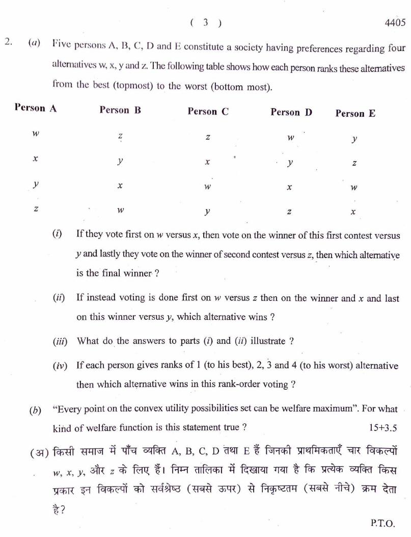
(a ) Five persons A, B, C, D and E constitute a society having preferences regarding four

alternatives w, x, y and z. The fo llowing table shows how each person ranks these alternatives

from the best (topn1ost) to the worst (bottom most).

Person A Person B Person C Person D Person E

w

X

y

z

z z w y

y X y z

X w X w

w y z X

(i) If they vote first on w versus x, then vote on the winner of this first contest versus

y and lastly they vote on the winner of second contest versus z, then which altemati';e

is the · final winner ?

(ii) If instead voting is done first on w versus z then on the winner and x and last

on this winner versus y, which alternative wins ?

(iii) What do _ the answers to parts (i) and (ii) illustrate ?

(iv) If each person gives ranks of 1 (to his best), 2, 3 and 4 (to his worst) alternative

then which alternative wins in this rank-order voting?

(b) "Every point on the convex utility possibilities set can be welfare maximum". For what

kind of welfare-function is this statement true ? 15+3.5

( 3l) fchftl fP--11(:ij ~ "qfq o!.ffc@ A, B, C, D (f~ E i f\JFF=hl >fl~P-Fhctlt!' ~ fetch~

w, x, y , 3ffi z cf> ~ i I f.:p:;, ctif<--Jcfil ~ fc;@l~I ~ % ~ Sf~cfi &ffc@ ~

>t chl{ ~ fetch ~ cn1 "BcT~ (ffl ~) ft f--1<1162.ctq (ffl ~) snll ~

%" ? P.T.O.

w

X

y

z

(i)

( 4 ) 4405

oQfcfff B 6'4Pc@ C ~Rm D &-lfcfct E

z z w y

y X y z

X w X w

~ w y z X

~ ~ w _cl~ x it 1-kl<;H ffi %, d<:9~"91(\ dHcfi fc:l'5-lc11 cl~ Y °B l.id<;H

ffi %, 3W 3=@ it ~ >1falf1r1a1 # . fcii'5-lc11 ~ z it J.Jc1<;H ffi %, "ill

~: ~·H-11 f-~ fq'5P-il mrTf?

(ii) ~ ~'3-11~ ~ ~ ·w cl~ z it it fchB1 ~ # ~ . iia~H · ~ ~

%, ~ ~ ~ ~ ftj'5-lc11 cl~ x ~ J.Jc1<;H fch"7.fl ~ %, ~ 3lcf ~

~ ftj~c11 cl~ y ~ ~ 4d<;H ~ "'3-lTill elf ch1+81 fqcfi~ ~: fq'114)

mrTI?

(iii) <qf11 ' (i) cl~ ' <q"[ll (ii) cf;" ~ cFTT ~ .i?

(iv) ~ Sffllcfi &1Fc@ fiaji1J.J fqcfif9 cfi1 tcn" 1, fiR 2, 3 cf~ f•·FfitS2..ctJ.J fqcfi~

cfll 4 tcf> ~ . % elf ~ 't:n-snll J.Jct~H it ~1HI fcF-h~ \JlltP 11?

· (Gf) a--1ctl~< 39lf1fJ1a1 zj~ ~ cfi ~fllch ~ l:f\ cr04IOI 3TI~cfictl-i m ficfictl

t-1 ~ cfi0!-11°1 'chl,\l lf>~H ~ -~ ~ cf>~ ~ i? I

3. (a) A beekeeper chooses the number of hives 'H; to keep. Each hive produces one kilogram

(kg) of honey which s'ells at a price of Rs. 60 per kg. The ·marginal cost of holding

'H' hives is : MC = 20 + 8H. The hives are located next to an apple orchard.

The orchard owner benefits (without paying) from the bees because bees pollinate

the trees and bees from one hive 'pollinate one acre ·of apple trees. The cost of artificial

pollination is Rs. 24 per acre of apple trees.

(i) . How many beehives 'If will the beekeeper maintain ?

(ii) Is this the economically efficient number of beeh· ? E 1

• 1ves . xp ain.

( 5 ) 4405

(iii) What changes would lead to a socially effcient operation ?

(iv) How much subsidy should be given to the beekeeper for inducing him to produce

socially efficient number of beehives ?

(b) Consider a plant th~t manufactures dynamite 'd'and a nearby farm producing tomatoes' t' •

The cost of production of dynamite is :

1 T _Cd (d, n) = -;_d2 + (n - 2)2

where 'd' is the amount of dynamite produced ·and 'n' is the intensity of use of a nitrogen

· in the production process. The side product associated with use of th~ nitrogen is ammonia

- a fertilizer that is released into the air. Such· fertilizer promotes growth of tomatoes

making the production on the farm cheaper. In ·µarticular the higher the intensity ' n ' the

,lower the farmers -cost : T Ct (t, n) = 1½ t2 + 2t - .nt.

The prices of tomatoes and dynamite · ~re Pd = Pt = Rs.1

(i) Find the level of production of dynamite 'd' and intensity 'n' that maximizes

the profit of the dyn<;1mite manufacturer. What is the maximal .level of profit ? . (ii) Given the intensity 'n ' from (i) find the optimal level 9f production of tomatoes

't' and' the profit of the farmer.

(iii) Find the joint profit of the dynamite manufacturer and the farmer.

(iv) · Economists say' that the positive extemality is associated with too little activity, compared

to the efficient outcome. Are your findings in this problem confirming this

statement ? . 9+9.5

( 31) ~ ll!jl-lcf&l Yl<:1cfi ~ 'cnl . ~~I 'H' 11a1 % I ~~cfi ~ ~ f cfi~!-Hl-l ~ cnr ~clf 1~1 ct><m % f'Jf~chl cnl11~ 60 ~ >Jfu f<ti<:11m11 · % 1 ~~4~1 q1c11 cffr 4Jl-lict <:11l ld . MC = 20 + 8H % I ™ ~ ~ ~ ciPO-tj ~ . ~-lfffi i I qJfl-tj

cnT l-ll f(1i:h ll~l.ifct©~I ~ ffi~ m1-0 cfi{dl % cflfifcfi ~"ch" llql-i~l cf>T ~ ~ Q.cb-$ ~~ ct ~ -q Y_{l ' l01 ffl i1 ~ UT~ WT 9{1'1°1 c6"B "cfi1" <11'1d

24 mcf Q.cfi~ % I Rs.· P.T.O.

( 6 ) 4405

(i) ll~l-4ct@l 91cicfi fcha~ ~ ffl WTJ?

(ii) cFfT ~ "cfil' B&ql 3ID$.n- ~ "B cfi~lfl B&-tl % ? 6ql§41 ch1f~ lf I

(iii) chl+g 9Rctct1 ~ Bll-llf~cfi ~ - "B cfi~lfl B-tjlf!'i cf>1 mt, ~? I

(iv) ll~l-lct@l 91cicfi cfiT Bll-llf~cfi ~ "B cfi~IM llql-lfcf©'41 ~ ~ cfiT "3~-(l~i

cfiB %g fcha1l 3ID$.n- B~P-rn1 ( Bf~it) ~ fl =q1fo~ ?

(~) ~ Sl4'ill-11$d. 'd' d(lll~cfi 3W dBch +it~lch ~ 1:nTlf ~ fq-tjl{ ct>lf~4 I '51£Hll41$2.

cn1 <11 JI ct % : T C (d n) = ~d2 + (n - 2)2

d ' I . .

~ 'd' sl<J'ill-11$2. cfiT l=fBIT % 3W 'n' 'il$c1hH cfiT dlc;4cil % ~ slll'ill-41$2. 60ll~.:i

"B ~ ~ %1 'il$4)Zi11 ~ ~~ d-11-Tif141 iftur d(lll~ % "ZiiT ~ ~ % 3lR

~ "B fuT ~ -i1 ~ ~ cfiT ~ 2.l-112.{ ~ d0ll~1 _cf>l . q($1ctl % 3m 1-np:J

cilJlct cfiT cf>l'.J ffl %, ~ clR ~ 'n' cfiT · e1l~a·1 ~ d-ljBI{ fchBH "cfi1" "ffilTa'

~ ' 1 cfill ~ Q- : T (\ (t, n) = 1 t 2 + 2t - nt.

Pd = Pt = Rs. 1 s 14--lll-11$2. 3W 2.l-112.{ cfiT ct>l l-la i I .

(i) '514.'"11141$2. cfiT d(lll~ 3W· 'n' cf>1 alc;4a1 f1cfilf<14 ~ 1n: '514'"11141$2. d0ll~ch

cf)l "ffi~ ~ 3TT~ -mm %1

(ii) 'ri' cfiT ctl~ctl 3fTR (i) ~ 6tjBR % cTT 2.l-112.{ ·cf>T $ts2.dl--f _d(lll~.-J fchcHI m1TI

3ffi fchBH cf>T ffi<q fchct1I m11T? .

(iii) -sl411l-11$2.-d(lll~cfi , afu: fchBH cf>T fi~ ffi<q f1cf>lf<14 I

(iv) . ~~~llff5P-ll cnl cfi~.-JI % fcf> $ts2.dl-l qfi:011it cn1 gZVHI "B BchRl,l-lch ~

'cnll d011~1 "ch" ~~ ~ % I ~ q41.-J "cf>l ~ ~ qTffi ~ . f!AflIT ~

~ - R&titt ~ %?

4. (a) Ann (A) and Bobby (B) share an apartment. They spend some of their income on

private goods separately and some of their incomes on public good like TV. A's utility

function is : U A(XA, G) = G114X1~14and B's utility function is : UB(X8, G) == G112XB

112'

where XA and X8 are the quantities con~umed of private goods. by Ann and BobbY

and G is the size of the public good, where, G . gA + g8

, the contribution of A

( 7 ) 4405

and B for buying TV. Both Ann and Bobby have income of (WA and w8

respectively)

Rs. 2000 each per month. Price of public good is given as, p G = JOO and price

of private good is given as, Px CC: l.P G reflects the marginal cost of public good.

(1) Write the conditions for the provision ~f the Pareto efficient amount of public good

assuming both Ann and Bobby can pool their resources.

(iz) Find the optimum ,size of G for the proyision of the public good assuming XA = x8

.

(b) There are two types of workers in the labour market, high ability workers and low

ability workers. Let e)ducation be a signal to the firms and firms pay each type of worker

according to their marginc:\l product. A successful signal causes high ability workers to

receive WH and low ability workets to receive WL. In particular, the cost of acquiring

education_ 'C' for workers is Rs 15,000, WH ~ Rs. 40,000 and WL = Rs. 20,000. P is the proportion of high ability workers.

(i) If th~re is a pooling equilibrium in the model, what should be the proportion of

high ability worker, p.

(ii) What kind of equilibrium will occur if the ·cost of ~cquiring education is less than

Rs.15,O00, assuming P as above ? 9.5+9

(3T) 1t-l cfl!JT, ~ .i::(qi) J.JcfiH if WI!! um 'ti it ~ 3=fm cfiT ~ WI f.r;,ft ~,a:j'i

"TR 3T<:¥f-3IB11 ~ ~ i a2TT ~ _cqJTf Bl&ZiiRcfi ~ ~ ~ fen" 2.c:1lcflZJ111

~ cni° 3qlf1filctl - lh<-"H U A(XA, G) = G_114x 1314 a2TT ~ .cf>T 344lrldl lh~H U8

(X , G) =Gl/2xBI/2, % ~ XA a2TT . XB sfil--1!?1: ~ a2TT ~ IDU ~tjrr cfiT ,rzjt f.r,ft ct½l,ci: t ~ G Bl4"1f1cfi q½j, cfiT am % 0211 G= gA + gs, % I ll.'l_

. ~ c!);n cpl l--llf+ich 3-w:f ( sfil--1!(.I w A a2TT Ws) Rs. 2,000 % I filcfZiif1ch ~ Gl':IT om f.fJit 9½J, ·cfill c/>liia Px = L Po B1cM•1ct> ~ cfill cf>1 chll--lct PG = 100

ffl l--ll.-d cilJ Id ~~llal % I -A- ~ ~ TTr-JT q;- >ffc:f~ ~ -w fc1f@~ 7lR ~

"Blcl~f1ch ~ q')I '-i'(C.I <t~_l<--1 .,,_,,,.....,.,. ~ ~ ~, (1) ~ ~ c!);n ffl W"RI cfill ~cf>?_dl 1'1~1 <;1'11<1 l'i

P.T.O.

( 8 ) 4405

(ii) xA = A8 ~ ~ ftlctZilPtcf> ~ ~ . mer~ ~ ~ G cflT ct1~ 1<1 3TicnR

~ chl f-31 l( I

(~) ~ ~!Zill{ ~ ~ !,fcf>R ~ ~ i, ~ a_:p:ffif qJzq ~fYch (f~ ~ aF@T ~

~ 1 llR <11f~i¾ fuan ~ -~ ~ ~ -fi~a t- -a~ ~ !,lf4cf> m ~

~fYcf> "cf>T ffi!-11~ ac=q1<; ct 3-tjftl{ :!l 1a11 cf>{al t- 1 ~ "Blflff fi~a ~ ~ cTTB ~fYchl "cf>T _ WH .(f~ cn1i a_:p:rcn cTTB ~ft.tch1 ch1 WL >ITC<f ,cf>B ~ chl{UT

~ t-1 fc4!fll':i ~ "B ~fYch2i ~ ~ fu&n 'C' ~ cf>8" aj- <11_llci 15,000

m t-, . W H = Rs. 40,000, WL = Rs. 20,000 CT~ ~ ~ a_:p:rcn qJzq ~fYch1 cfi1

~j41ci t, . (i) 3ffi !-l'f:s<1 ~ ~ch<__a1 .(~) fitl<--H t-, "ill ~ 8I1=fci1 cTTB chl4chat'1TI ctT

6tj41d, ~ cFlT m1lf I (ii) ~ - fuan ~ cf>B aj- fill.Id . 15,000 ffl-"B ~ t, ~ ~ ~ cfi1 ·

Btl<-1--i m1lT * ~ "cf>T aq{faf@a aj- (fW l=lft ~ ~ 1

Section B ( ~ ~)

5. (a) Mr. Gnash, ·who will distribute Rs. 4 between two -people A and B, asks them to

· simultaneously write any whole number between O and 4 o_n a piece of paper. If _the

sum of the two numbers is at ·most 4 then both will get the numbers of rupees they

have written. If the sum exceeds 4 and both have written the Sfime nun1ber then both

will get Rs. 2 else the one who has written the smaller number will get the number of

rupees he has writtei:i and the other will get 4 minus this an1oul).t. · Determine the best

response of each player to each of.the other player 's actions; plot th~m in a dot-circle

best response diagram; and·_ thus find the Nash equilibria of this game.

(b) Consider the following _game:

PlayerB

L R

Player A u 2,4 1,0

D 0,1 4,5

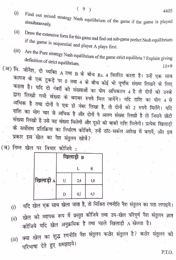
( 9 ) 4405 (i) Find out mixed t · I d s rategy Nash equilibrium of the game if the game 1s P aye simultaneously. ·

(ii) D raw tbe extensive fonn for this game and find out sub-game perfect Nash equilibrium if the game · · 1 · . 1s sequentia and player A plays first.

(l_.ii) Are the Pure strategy Nash equilibrium of the game strict equilibria? Explain giving definition of strict equilibrium. 10+9

(~)TT{. '3fl~~T, ~ cl.If<@ A {12:!f B ~ .jtq Rs. 4 fcrnfl:ct cfil:ctT % I ~ ~ rrr:1.1 chPl\lf * ~ ~ ."CR o -a?.TI 4 ~ .jtq ~ ~ ~ mf f(1@~ ~ ~ ch~ctl i I ~ ·;1_ ~ cfft · m;m ~ 7l1TT 3if'tlchdY 4 ·i "ill ~ cfl1 ~ &RT f<1©1 Tftft B~I ~ <sHI~{ m ~ Zitl4~ I ~ urn cfil "lft11 ,4 "B an~_ i cl~~ ~ 1lcfi m ~ mi, -at~ cfl1 2 · m r~#i~ 1 ~ ~ .cfil "lWf ~ "B ~~ i 3W ~ ~ ~ mf WI"@ i "ill f~B~ ~ 4&:f1 f(1@1 i ~ ~ m r~8~n 3W ~ cf)l ~ -Dfu r~€\Jn 1 ~~ch f{§aci1~1

.~ fiaj-d~ -~fufsh~I -cfiT ~~ ct>lf\Jf~, ~ sll-~chci 3TI& it ffl, 3W ~ ~cbR ~ -~ cfiT ~ fig~H ffi?

(~) f.:p:;, ~ ~ fc;j-tjl{ chlf\Jf4 : f@(1fsl B .

L R

ffit&ii:S1 A u 2,4 1,0 •

,

D . · 0 i 4,5 , '

( 10 ) 4405

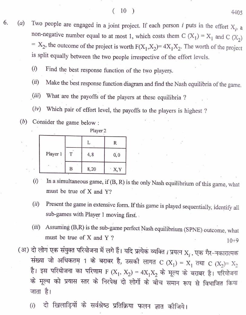
6. (a) Two people are engaged in a joint project. If each person i puts in the effort Xi, a non-negative number equal to at most 1, which costs them C (X 1) = X 1 and C (X2) = X2, the outcome of the project is worth F(X1,X2)= 4X1X2. The worth of the project is split equally between the two people irrespective of the effort levels.

(i) Find th~ best response function of the two pl.ayer$.

(ii) Make the best response function diagram and find the Nash equilibria of the game. '

(iii) What · are the payoffs of the players at these equilibria ?

(iv) Which pair of effort level, the payoffs to the players is highest ?

( b) Consider the game . below : Player2

L R

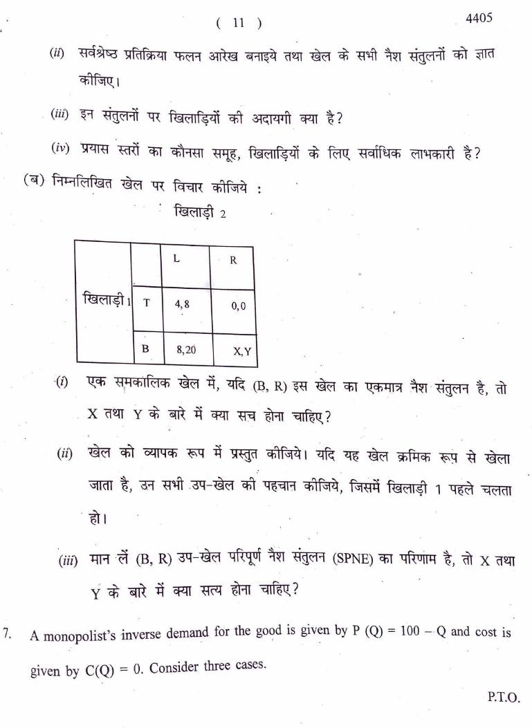
Player l · T 4,8 0,0

B 8,20 · X,Y

(i) · Iri a simultaneous game, if (B, R) is the only Nash equilibrium of this game, what must be true of X and Y?

(ii) Present the game in extensive form. If this game is played sequentially, identify all sub-games with ·Player 1 moving first . .

(iii) Assuming (B,R) is the sub-game perfect ~ash equilibrium (SPNE) outcome, what must be true of X and Y ·7 10+9

( ~) ~ ~ ~ :ri~cR1 4RlflZ:iHl -ij ~-% 1 ~ ~~cf> ~Fc@ t sP-1c-1 xi,~ %-+=hRl,Ach -8@1 ~ ~~cfici~ 1 cf> (SHlq{ i, dfFhl c?tl~la C (X1) = X1 -a:~ C (X2)= X2 i I ~ 4Rlf1Zl111 cfil 4R0lll-l F (X1, X2) = 4X1X2 ~ ~ ~ q{lq{ t° I qfQ:<-il\JHT

cf> ~ cfiT ~41fi ~ cf> R{qa_, ~ ffl ~ ~ Bl-111 ~ "B fq~ fcnm "Z:if@T i1 (i) ~ f@c?tlf-$~1 ~ ~~ ~faf~-41 tfie11 ~ c:hlf\J\~ 1

( 11 ) 4405

(ii) "B'cf~ ~fctfsfil{I ~ ~ ~11~~ cf~ ffi ct "B~ ~ Bgjl;n cf1l We{

cti"tf\l\Q. t

- (iii) ~ Btlfl-TI -q"{ f©t11f~lfi cfi1 3-t<!_ll{Jf\ cp:fT i?

(iv) ™ ~ "q=i1 ~Hf\\ ~' f©t1tf~lfi ~ IB"Q. ft~ "ffi~ i? (~) f1t..qf(1f©ct ffi -q"{ fc(-q\{ cf>if\J\(t :

f@t114) 2

L R

f©fll~l 1 T 4,8 0,0

B 8,20 X,Y

{i) ~ flt-tchlf<1ch ffi it, ~ .(8, R) ~ ffi cfil l(cfil-\15\ ~ --81(11 i, 'at _ X cf~ Y ~ ~ - it cf<.TT ~ ffi =qlf~Q,?

(ii) ~ cfil o41qcfi ~ it ~ cf>1f \J\(t , ~ ~ ~ snf~ch ~ "B ~ ~ t, ~ "Bm -~-~ chl q~=q11 cf>1f\J\~, f\J\fli=l f©t11~, , ~ =ct~a, -m I

(iii) ~ ·~ (B, R) ~-i@ ~ ~l tigfl"I (SPNE) cfll qf(oj14 't ~ X Q'ifl

y cfi ~ ~ ~ ~ ffi =qtf~Q,?

7. A monopolist's inverse demand for the go~d is given by P (Q) = 100 - Q and cost is

given by C(Q) = 0. Consider three cases.

P.T.O.

( 12 ) 4405

Case-1

Suppose that monopolist can perfectly price discriminate ~mong the consumers.

(i) What is monopolist's profit in that case .?

(ii) Is the allocation Pareto efficient ?

(iii) Calculate the consumer surplus ? .

Case-2

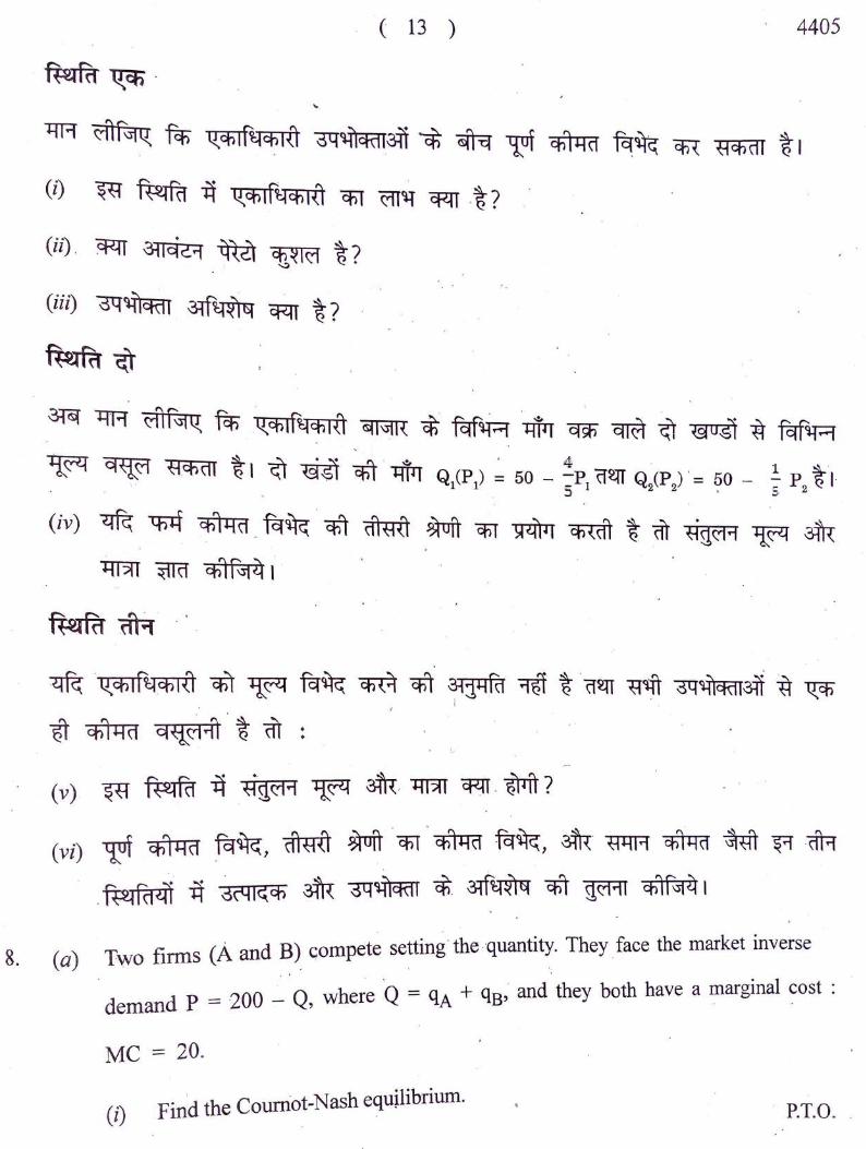
Now suppose that Monopolist can charge different prices on two segments of the market

with differefit demand curves. The demand.son two segments are :

(iv) Find out equilibrium price and quantity if the firm practices third degree price discrimination.

Case- 3

If the MonopoFst is not _allowed to price discriminate and has to charge a single price

from all consumers.

(v) What would be. the equilibrium price arid quantity in' this case ?

( vi) Compare producer's and consumer's surplus in the three cases:· perfect price discrimination,

third degree price · discrimination and uniform price .. 19

~ Q.chlf~ ~ ~ fc~q{ld l'.TTlT ·p (Q) = 100 - Q NU ~ lT{ i 3ffi ~

C(Q) = O &ffi ~ ~ % I ~ ~ l:f"{ fq-ql{ cf>lf'51~ I

8.

( 13 ) , 4405

im <11f'l1q: fen ~~~l{l ~~;m cr; ~ ~ chll-ict ~~ ~ ~chctl % 1

(i) ~ ~ -q ~~ cf>l ffi'q ~ -%?

(ii) · cp:JT ~ici2..-1 ~ 66,~1(1 % ?

(iii) ~- an'~ cp:[T %? .

fum{~

~ l=rR ("tlf'51q: fen" -~~ ~1'111{ cf; M~ .-tjm cfsf> cflB ~ @Oil ~ fcrr~ . .

~ q~(1 ~.cfictl % I ~ ~ cf>l . lTill Q (P) ~ 50 - ~p "(f~ Q (P )'= 50 - ~ P i ·1-. . , _ 11 51 22 . 5, 2

(iv) ~ ~ chll-ict _ fq~ . cf>1 dh-1D wrft cf>T ~ cfi"till i 'ill fiu~H ~ 3fu: i:tf5IT ~ chlf'l1ll I

. ---"-'- . ~ ·l(ch1P·-1ch1D cfiT ~ fcf~ ~ cfft ~jl-ifct ~ i ·(f~ ~cm ~~an ~ ~ ' I . m cnll-ict q~~11 · % m :

L,

(v) ~ ~ -q fi·g,(1'i ~ 3m:. lITTfl cf<:rT · mrfr?

(vi) irif ctil4ct fcl~, dl-m'.l ~ ·Cf;[ · q;')1-1a fcl~, 3l"R· W:rR q;')1-1a ~ ~ .<f!R

-~ 'B d011~ch 3W ~mcml ct. *~ cfft tl~HI chif\J\ll I

(A. d B) rompete setting· the -quantity. They face the market inverse (a) Two firms an . "' . , ·

· · · · h · 'Q = q + q · and they both have a marginal cost : demand p = 200 - Q, w ere . A s, . . .

MC= 20.

(i) Find the Courriot-Nash equilibrium. . P.T.O . .

( 14 ) 4405

(ii) H ow would the equilibrium charige if the government decides to subsidise Firm A

with 12 per unit making MCA= 8 whereas, .~CB = 20,

(iii) · How would the equilibrium quantities and prices change if there were three identical

firms with MC .= 20 ?

(b) Consider Hotelling's model where two petrol stations labeled A and Bare located along

a street length of 1 km. Assume that consumers are uniformly distributed along the street . . length. Each consumer has a transportation cost equal to 2d, where 'd' is the distance . . .

traveled back to one's-house after filling up petrol. Suppose that A is located at 1/4

of a km and B is located at 1 km. Assume that production is _costless.

(i) . Determine the demand fµnctions QA and Q8 for the two petrol stations .

. (ii) If the two petrol stations compete in prices (PA and_P8) and settle at Nash equilibrium,

will they charge the same price for petrol ? ,

(iii) What will be the profits of th.e two P~trol s~at'io_ns ? · , 7+12

( 3l) ~ ~ (A cf~ B) lITTff f.:rmftf ~ cf> ~ ~fctf9~ ~ i I ~ ~l'l1R o!J&>l'.l

'tj;Tr ~ Bll=t11 ~ %1 P · 200 - Q, ~ qA + q8 c1~ ~ ~ ~ Bll-lia

eP Id t° : MC = 20

(i)

(ii) -8gci~ "B, -~ ~cfiR qftctd-1 W1TI ·* fRcf>R 1f>lt A cn) >ffu ~ 12 cfi1

3llf~ ft~lttctl ( flf~-5,) ~ cfiT f101tt cfi{ctl t d~ MC A = 8 'l1~fch MCB

= 20 m ~ ti

4405

( 15 ) 4405

(iii) • ...~ ,,,.-rr;:r -q;it ~gi:-H 1iT5l1 ()-11\ cf>ll-ictl ~ fcITT:r m 9Rctct--i mm "lfR ill1 ~--(:1..,I I

t f~+=h7 fi7J4Hi Br"@ MC = 20 % ?

(~) &l2.f<1JI J.il:Si:-1 ~ fqijl{ cf>lf~~ ~ AG~ B <TT ~ R.~11 1 fc8:IT ~ ~&cf>

~ W«f t, 1=fR ~lf~q_ ~ ~~ ~ ~ "B B~ch 1:f\ fqctftct %1 >{c-ltcf>

"3l=f<qfc@T ctr qfQ:q~'i ~ 2d ~ ~{I~{ t, ~ 'd' ~ ~ ~ ~ cR cllq~

'3lR ctr ~1 i, "J.iR (17f~q_ ~ A 1/4 M -q"{ ~%"ff~ B 1 ~ -q"{ ft.2m ' ' '

i1 -q:m i:rR ~ .dclll~'i ffi1Tcf -ma %1

u) m ~ e~H"i ~ ~ lTTTT ·l:f)&f QA 3th: QB Rmftf ct>lF~~ ,

eti) ~ m ~ e~H ct>lJ.iJi (P~ a~ PB) ·"B >1Fa~m ~ i ~ ~ cf>

firt<:-1-1 it ~ ~ t, "ill cp:fT ~ ~ ~ ~ ~ m ct>ll4ct 9~2i~ ?

(iii) m ~ e:~111 cfll ffi~l cp:fT mm?

15 3,500

_· . ~ This question · paper contains 8+~ nted pages]

Roll N.o.

S. No. of Question Paper 4622 0 . <S·\

l/.j ( \ <

a -·LIBRARY \·i,\ * ~. I

·Unique Paper co4e 12271 C . . . Name of the Paper ics II

Name of the Course B.A. (H) Econo•mics CBCS .

_ Semes,ter IV .

Du.ration : 3 Hours -Maximum Marks : 75

(Write your · Roi£ ?-Jo. on the_ top immediately on receipt of this question paper.)

•· .

Note:- Answers may -be ·:written either· in ·E:nglish or in Hindi; ..

but the same medium should _be used through~ut the

paper.

.,

~ ~,r"'~; <1Fcfi1 ~\TT ~ <:fil -i:tl~ ~ m ~ . =cufuCJ: t I. .

. .

Attempt All questions, .sel~~ting · any· two parts from each question. \

ri m ~, ~ <f\f~l{ I ·

Stf4fh ~ ~ ~ - w-~ ~ ~ ·e)r~l{,

P.T.O.

I.

( 2 )

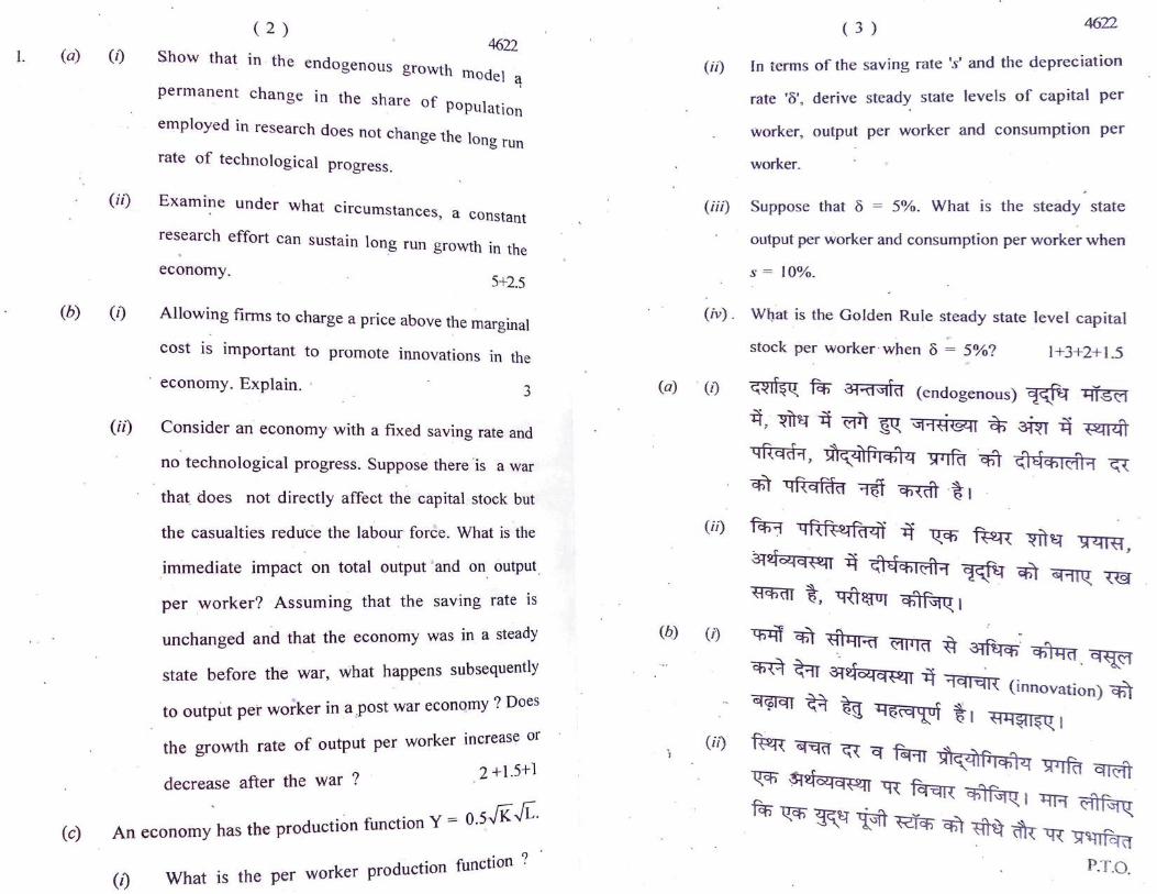
(a) (1) Show that in . the d en ogenous growth m d

4622

(b)

(c)

o el a permanent change in the share of . ,

population employed in research does not change th l

e ong run rate of technological progress.

( ii) E . xam1~e under what circumstances a c

(z)

(ii)

, onstant

res.earch effort can sustain lon_g run growth in the

economy. 5+2.5

Allowing firms to charge a price above t?e marginal

cost is important to promote innovations in the

economy. Explain. · 3

Consider an economy with a fixed saving rate and

no technological progress. Suppose there is a war

that. does not directly affect the capital stock but

the casualties reduc·e the labour force. What is the

im·mediate impact on total output 'and on_ output _

per worker? Assuming that the saving rate is

unchanged and that the economy was in a steady

state before the war, what happens subsequently

· • · t onomy ? Does to output per worker m a ,pos war ec ·

· e or the growth rate of output per worker mcreas

decrease after the war ? 2 + I.5+1

· . ~ · v = o s✓K ✓L-An economy has the production iunct1on .

(,)

. . ?

What is the per worker production function .

(a)

(b)

( 3 ) 46Z2

(i,) In terms of the saving rate 's' and the depreciation

rate '8', derive steady state levels of capital per

worker, output per worker and consumption per

worker.

(iii) Suppose that 8 = 5%. What is the steady state

output per worker and consumption per worker when

s = 10%.

(iv). What _is the Golden Rule steady state level capital

stock per worker · when 8 ~ 5%? 1+3+2+1.5

(ii)

(i)

(ii)

101 cf.@ '91: ~ ~ ~ ffl t..:~1sualtks) ~

~ ~4~112:@ ~ m ~ t-1 ~ ~ 9

~ '\~ ~~ ~ 1l'qlqcf<:lT%° ? ~

~ ~ ~ ~ ~ ~~fo:~fcta waT t" 'c1~

Nl it~ ~l64c(~ ~ (stead~_ state)

it.~. ~ fcn ~ ~ ~ -gm ~ ~ ~ <FlT ~'qlq ~ %- ? ~ ~ ~ cnl

~ ~ ~ ~ ~ ~ i ?:TT cfi1i m i ?

Jq,fii 3f46qq~l if ~ ~ Y = 0 . S✓K ✓L %° 1

"5lfu ~ 30Hc!,'1 · ~ cf<TT • -%- ? ·

lii) ~ ~ ·s· cl ~ cfi1 WB ~ ·o· ~ ~ ~ >ffu

~~, >lfu ~~q>ffu ~~$T

if> f ~:i::tc!~i (steady state) cTT'0 «R 0'§1"1 c:hlf\J\Q, I

(iii)

(fr)

(a) (r)

"BR alf\JJQ, fcn 8 = s¾ ~ s = 10¾ mm >lfu

~ ~q>fIB~"3'CfiWT"&i~

~ ~ cf<TT -@,- ?

~ 8 = 5% -%- en >ffu ~ ~ ~ cfi1 f-qfufq

~ (golden ru le) ~ «=R 'cf<1T irTf ?

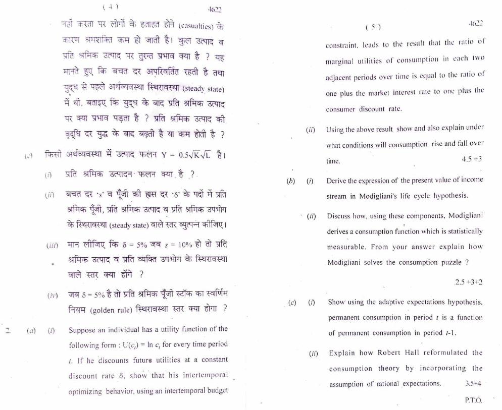
Suppose an ind ividual has a util ity funct ion of the

following form : U(ci) = In c1 for every time period

t. If he discoun ts future uti lities at a constant

dis count rat e 8, sh o.;.,, · that hi s intertem pora I

optimizing behavior, using an intertemporal budget

( 5 )

the resttlt th at the rat io or constraint. k ads to

. . . 1· . ·u111p ti o 11 in cnc h two margin al util111 cs o cons

adjacent pe riods over time is equal to the rat io of

. . t , to 01w plus the one plus th e market tntcreSl I a t: •

consumer di scount rate.

(ii) Us ing the above result show and also explain under

what conditions will consumption ri se and fa ll over

time. 4.5 +3

(h) (i) Derive the ewress ion of the present va lue of income

stream in Mod igliani's life cycle hypothes is.

. (c)

· (ii) Discuss how, using these components. Modigliani

(i)

I

derives a consumption fun ction which is statisti ca ll y '

measurable. From your answe r expl a in how

Modigliani solves the consumption puzz le ?

.2.5 +3+2

Show using the adaptive expectations hypothes is,

permanent consumption in period t is a fun ction

of permanent consumption in period t-1.

(ii) Ex p lain how Robei't Ha l I reformul ated th e

consumption the ory by inco rpora t ing the

assumption of rational expectati ons. 3.5+4 ·

P.T.O.

(a) (i)

(ii)

( 6 ) 4622

~ ~,f'1iQ_ fcf> q ollFc@ cfiT ~ ~ .

~ cfllcilC4M ~ U(c,) = Jn c, %" I ?:JR 9Q ~

cfiT d941fildl 1R ~ ~ & "B ~ (discount)

cfTTZffi %", "fil ~~ll~Q_ fcn ~3f<::Wl (i1-1tertemporal)

~ 1,rftrar'4l ~ 3l'tlf.l ~ - 3Fm:arcrf-q

~~a'-i1cfl<01 (optimization) oljq~R in qRulli-f¼~q

~ 3m:R ·(adjacent)~ ll ~ cfll ~141-it

d94lfildl~ cflT ~ (t +~~-~)cf

(I +·°31:f~cfil"~(discount)cnl~) in"lfUJ ~in~m1ft,

3qgcR1 qR0 11i-t cfl1 ~Wllldl °B ~~ll~Q_ q Bl-l~l~Q_ <

-Fcn m r~rnin -ij ~<qflJ ~ * "BT~ ~ . ' .

cl tlmll

(b) (j) lftfafici4111 cift ~...:~ qftcfl<_,,q11 ll awl-

. ~ in qdl-111 ~ %TI ~ 69t-i~ cf>jf-i!Q_ I

(ii) i.nfofia4111 ~ ~ cffl- ft~14a1 ~-fcnB m

--~ ~ ~$1 1:fiffi ~~ ~-~ ~ '3ft fcfl Bif&-icf>l4 ~ -« l-1191l4 %, ~ . fcjtj+.11

<:fllf-iill I a:rCR ~ -« el-!~l~Q. Fc.n- Jflfofia<-1111

~ m 6"Cl'lWT ~ cf>) ~a~1a % 1

(c) (I) 3ij~ci1~Tici (adaptive)™1:JRcfi'ffl<t)- ·mW-Ml

~ ~ fcf> 3lcITTl ,-q ~ ~ -, ~ 1-1 ~ ~ ~ cfil ~ mm i,

3. (a)

' . (b)

(c)

(i,)

(1)

( 7 ) 4622

fl4~1$Q. fcn ~ ~ ~ fcfiB ~ acti.d,1a

(rational) SIMl~lldTI cnl fl41fq62. ~ ~mrr ~ ~'tlRf cfiT _ 9,14_:;iUI fcfi<:IT I

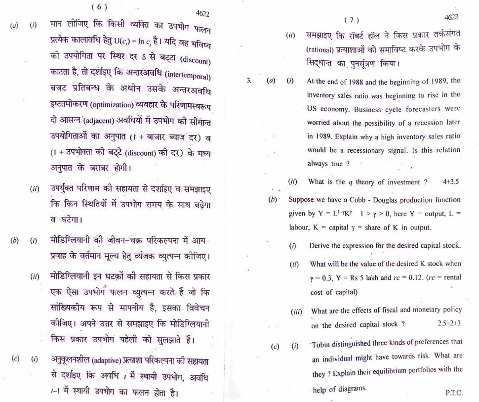
At,lhe end of 1988 and the beginning of I 989, the

inventory sales ratio was beginning to rise in the

· US economy. Business cycle forecasters were

worried about the possibility of a recession later

in l 989 .. Explain why a high inventory sales ratio

would be a recessionary signal. Is this relation

always true ?

(ii) What is the q theory of investment ? 4+3.5

Suppose we have a Cobb - Douglas production function

given by Y = L1-YKY I > y > 0, here Y = output, L =

labour, K = capital y = share. of K in output.

(1) Derive the expression for the desired capital stock .

(ii) What will be the value of the desired K stock when

y = 0.3, Y. = Rs 5 lakh and re= 0. 12. (re= rental

cost of capital)

(iii)

(1)

What are the effects of fiscal and monetary policy "' on the desired capital stock ? 2.5+2+3

·Tobin distin~uished three kinds of preferences that

an individual might have towards risk. What are

h ? E 1a·1n their equilibrium portfolios with the t ey . xp .

help of diagrams. P.T.O.

(ii)

' (a) (i)

( 8 ) 4622

Explain from the above anal'ysis ho~ the ag . - giegate

money demand can be derived in the portfolio

balance model when an individL1al d. ,versifies . between bonds and money.

3 +4.5

1988 ~~if _cl 1989 ~ -~ ~ ~-~

~ (inventory sales ratio) US ec;onomy it~

~~I clll91-l-~,~ ~fcl?-lc!c@I 1989_~ 3™

~ 'B ~ cfi1 ~ ch7 ffll: ftjf~ct ~, '

f!Y$11~Q_ fen" Wen-~ ~ ~ cfi1 ~

. cp.:n ~I cp:fT ~ ~~ ~ ~ mctl t?

(b) 1=fR e1"1f\JJQ. fen-~ 1TTB y = L1 -YKY ~ ~ -rr:n

~ ~-Sl lcif! 3~1c;1 ~ %- ~ I > y > 0,

Y = ~, L = 5>Tli, K = ,tm (l~ y =~if K cfil . .

3Wf %- I

(i) cTI~ (desired)"F,"0cfl%g~ &JN;:;:i ~l

(ii) ~ y = 0.3, Y = 5 ~ ~- (1~ re = 0.12 m "ill ~ K ~ cnr 1=fR "cplT m11T ? (re = rental

cost of capital) ~ cfiT fcfi-ll-41 · ffiTfcl I

4 .

(c) (,)

(ii)

(a) (i)

( 9 ) 4622

I~~ \lflf@~ ~ "Slfu fcpm "&tfc@ '&) m-;, ~ ifi wcqq 3-"W-.:rG°AT (preferences) ~ i::f'af

fcl~ fcn7-ll I ~ cPTI- cPTI % ? ~ WTd flt¼lc!fill

cITffi ~ - :qf-cll!l (portfolios) ct11 3:nr@l cfi"T

fiH'--lc11 "f1 fi~~l$Q_ I

3qqcR1 fq~c_~qo1 cn1 fi~W-kll "B ~ fcn ~ olJfcfa ~-u'f (bond s) cf 13,~ ~;i i::f't-7.l

fcrfcrmcfi{UI (diversification) cfi"«TT t "Qm wm'f it .~-~ fi1,c-H i::ffw (portfolio balance

model) it "BBlJ ~ 1WT ~ m og~.:.:i cn1 ~ ~ t, ' A dramatic rethinking of monetary policy took

place, based on inflation targeting rather than on

money growth targeting'. What were the reasons

for this ?

(ii) Explain, using the Taylor rule, how the economy

adjusts when, first - ·inflation is above target and

second-when unemployment is above the natural

rate ? · 4 .5+3

(b) (i) Examine the view that debt financed govt. spending

keeps economic activity unchanged. What are the

limitations of this argument ?

(ii) 'The higher the. rat io of debt to GDP. the larger

the potent ial fo r catastrophi c debt dynamics'.

Explain. 4 -t 3.5

P. LO_

(c) (,)

(ii)

( 10 ) 4622

Distingu ish between nominal price rigidity and real

price rigidi ty in the context of the New Keynesia~

macroeconomic mo'dels.

Taking the case of a monopolistic firm, explain with

a diagram how .a firm's decision not to cut price,

inspite of a fall in demand, due to menu costs can

have adverse effect on the society. 3+4.5

(a) (i) ·ti1facfi -;:ftfu cnl, ~ e1~ (inflation

targeting) ~ ~ 1R 13?J cfi1" <Kf''tl ~ C1~

(money growth targeting) ~ 3lT't-llftl ~

6ilcfiff4-lcfi (dramatic) 9/ifcf=ql{ (rethinking)~ I'

~"9mcp:Jfcf.iRUT~/

(ii) "lffi ~ "cfi1 fll:tlllctl "B fll'..J~l$Q_ fcn 3l~

~ m fll-fllllf\lfct mm t ~, ~, ~ am "ci'~ -u ~ m a.m ~, ~ ~il~Jn:tl

~ Sll~@cfi -«R "B ~ "ITT J

(b) (1) ~-~ (debt financed) fi(cfiFU o!flf "B ~

Jl@fqfiT "cfi"T «R Ji9fh~R@ ~ %°, ~ mR cfiT

Tffi~ chl NI Q_ I ~ .(fcfi cfi1" cf<lf ~ i /

(ii) '"5lf01-G DP ~ flfc:Rr a:ff'tlcn m1Tl, SI t_vP-i~

(catastrophic) ~ Jl@chl (debt dynamics) cfil"

~ "3fAT m a:rf'tlcfi ~ I fll-i $il~ l{ I

5.

(c) (1)

(ii)

( 11 ) 4622

-;,cr-ch~lll (New keynesian) fi14f62:- 3-i\!:f~l if5il <-t

~~"fR'l{-q~~-~cf cll«ifctcfi

~-~ if> l=J't:zf 3FcR ~ chlf\llQ_ I

~~~i:mif>~c8~~~ {©lfi.151 cfi1 fll:tl"1<'11 B fll'..l$il$Q_ fcn "lWl "B fiRlcl2-

~ ~lclZi[<; cfITlm-"9";{ ffiTTffi * cfiRUf ~ ~ 1" cnB cfiT i:m cnT ~' ~ 1TI: Slfct~ci

~'ll]q sIB ~ l I

(a) (1) Explain how asset price bubble affects the financial

system and what measures should the central bank

take to resolve the problem.

(ii) Discuss how collateral reduces the problem of

asymmetric information. 5+2.5

(b) (i) Explain the process of determination of equilibrium

in the housing market in the short run.

(c)

(ii) What are the factors that determine the position

of the demand curve for housing in the short run ?

(iii) . When will the long run equilibrium of the housing

industry be reached in a non-growing economy ?

(1)

(ii)

3 +3 +1.5

Explain with an example that an economy with a

higher average inflation rate has more scope to use

monetary policy to fi ght a recession.

Why w~rs typica lly br ing about large budget

deficits ? 4 +3.5

P.T.O.

4622

(a) (1)

( 12 )

M$1 l$l/: fcf> -qfo:-tUi fo-ct,l4d ~'¥\ (asset price .

bubble) fcITT:r !,lcfiR fcnfl"-1 o;:;f cfi1' )l''ilfcrn qi,@ .

~ Giil ~ ~4¼1 if; f.-Rlcfi{UI ~ &J,il"-1 ~ · :cn1 ~ cfic!.4 «3R . ·cuf~Q. ? ·

(ii) ·3=iYl1d (collateral) ~ ~cfil{ 3-R4l4f~a ~"91i

cfi1" {41-lfltl cfil~~ cfi{dl %-, ~~Befit fq~-q1 cbif\llQ. I

(b) . (i) 3-tlctlftl4 ~1-511< "B <1tlchlf{ 'B ftl D..t lct~l it R~ cn1" '!,lf9h4·1 · cf>1 ft4$1 1~Q. -1

(i0 d·flc=41ft1 ~ - l=firT ~ ·cn1 ~ cnT (1~cf> I~

"B ~-c611~ chl{6fi ~~ ~ ~ ? .

(iii) ~ ~ al~, f'1ift?i ~'q ~ m w. t-, "B d-f l~I ft1 d~lf!J 1 "B c)ttcfi lc.1 f 1 BIJ..lllcH~ ~ ~~.mrj)-? 1

(c) (I) . ~ dc!,IQ{OI cfTT ft~llkti . ~ ft l4 ~l$Q. fcfi" d=a61d{ . !

fl-h1fa ~ ffl a1~ -q ~ ~ ~ .

(ii)

-~ 4,f1cn ffl ~ d9~41 "cf>1" · alf~ 1'511~~1 %1 ',

~~ 3w:T ~ ~ ~ ~\Jl2 ~ cITT ~ ~ . ' I tt t ? } 1!. j ., \

12

--t . , I . ,

3,500~

I

This question paper contains 16+8 printed pages · ~ (b + 11 Tables A~~h~

•t _. . ... ,. ... ,,._ h"'

~::::;;::::_,.._.. __ __,.-r--,----r--ir-::~~~ -j· ,..-... , ....., . ._. I

. S. No. of Question Paper 4665

Unique Paper Code

Name 9f the Paper

Name of the ·co.urse

Semester

12271403 WB f{ . .\ r~Y

Introduct~ry Econometrics· _ t~ x _,,:1,,,1..,.:1,.,1t...--, • -

B.A. (Honours) Economics-'-'· .-..,~ . \

·N

Duration: 3 Hours Maximum Marks: 75 _

. . ' ~

· (Write your Roll No. on the top immediately on receipt of this question paper.)

c~ m-~ ~ ~ m ~ -~ TPJ; T¾mftf ~ ~ 3TtRT ~ 19h~ich R1f@Q, 1)

Note :- _ Answers may be .written eit~er in English or in Hindi;

· but the same medium should be u_sed throughout the

paper . .

R:cqun :-~-~--q-5f cfTT ~ ~D'lll m ~ fcfiB1 ~ ~ . .

# e.lf-51((; ~Fcfi1 -~m ~ . cflT 1'.ll~ -~ m ~ · -6fiful( I The question paper consists of seven questions.

Attempt any five questions.

Each question- carries 15 marks.

Use of simple non-programmable calculator is ·allowed.

Statistic~l tables are attached· for your reference.

~-"Cf;f ~ m r cf>T ti fcfi~1 _'QTq fic41<1i° cfi -aw <:.lf~l( I

· ~tilcfi m 1s afcn- ~ <:h<ct, ~1

fi=(t1 itt -Sll!-114 cl;0:fi82.-l cf) . d44l'I . cffr ~j4@ ~ ~ % I 3U9~ ~cq ~ ft;m: Bif&-1cnl ~ 51~1951 cfi 3rcf -q cfl' -rr:fi" ~I

P.T.O.

1.

( 2 ) 4665

State whether the following statements aFe true or false. Give

reasons for your answer :

(I) . If the regression model

. + B3X3; + ut, is estimated using the met~od of ordinary

least squares, the sum of the estimated residuals (e;) •

is zero.

(ii) For the two-variable regression model, Yt =B 1 + B 2X;

+ ut, if the OLS residuals (e1) are plotted agains~ time

(t) and a distinct pattern is observed, then it is an

indication of heteroscedasticity.

(iii) · If the p-value for a test statistic is greater · than the

chosen level of significance a, the!\ we reject H0 at

(iv)

a. level of significance.

In the regression model Yi =B 1 _ + B 2Xi + ui, some

variation in the values of the explanatory variable (X)

is necessary for estimation of the · regression coefficients.

(v) The model : Y =. B 1 =+ B2X, is a mathematical model

I

but not an econometric model. 5x3=15 I I

I I

( 3 ) 4665

f1Yf(_"jf©a ~ "Bm ~ ~ l"fffif ~ I altA ~ ct

~ cfiRUT e.1fsiJQ. :

(i)

(ii)

"lf~ 11 f cfll-i:r;f "Bf~ Yi =B1 + B2X 2i

+ B3X3i + ui, cfiT d-lj/-111 arr.~.~. rcIT'tl "B

f1cf>IC1I Tf(TT % m d-l :j/-11 f1 ct ~clf¼i~ (e,) cfiT "lfT1l

~ - %1

-~-~ i;i _fcPP·H i:rr~: yt =B1 + B2Xt + UI'

cfi ~ 3i7R 3TI.~.-q:B. &lclf"¼l62. (et) cfTT ~

(t) cfi ~ ~ ~ ~ ~ ~ \lf@T %,

m ~ %2.D:?l-sf-R.fo2.1 (Heteroscedasticity) cfiT ~

~%1

(iii) ~ ~ "9fl-arur Bif@llcfll cfi -~ 'TT-l--fR ,:=;p-1f1a

~ cfi a "B 3ff'tfcf> %, m Qt.f ~ cfi" a «R

~ H0 cfi1 ~fctlcf>i:C -~ i 1

(iv) SI fc:P i'-11 ~ - Y B ~ "11'-::),1 i = I+ B2Xi + ui, ~ f91S2.1cfi{OI

• ~ (X) cfi ~ # ~ f"F@T Slfc:Pll=H ~Uiicfi cfi"

~ cfi" ~ 3-iicf~.!-lcfi % I

(v) . ~ : y = '31·+ B2X, ~ Jifulalll t-ff-s(1 t (9fch9

~ . 3l~f'-·kll'4 t-ff-s(1 -;,m i I

P.T.O.

( 4 ) • 4665

2_ (a) The following auxiliary regression results were obtained

using OLS residuals (e;) of the original regression model,

Yi =B1 + B2X2i + ui,

e~ = -25 + 19.57 Xi - 10.54 Xr l

R 2 = 0.1423 n = 80

(i) Perform White's General Heteroscedasticity Test at

I 0% level of significance. State the null and

alternative hypotheses clearly. Do you find

evidence of heterosc·edasticity ?

- .

(ii) Are the OLS estimators still unbiased and best

in the presence of heteroscedasticity ? 5

(b) The h~pothesis H0 : µ = 75 is tested ag_ainst the

alternative hypothesis H1 : µ < 75 using a random sample

of size 25 from a normally distributed population with

cr = 9 using a I%. level of significance :

(1) Calculate the probability of Type II error if the

true µ = 72.

(iI) Wi11 the probability of Type II error be larger if _

a I 0% level of significance is used, instead ? 5

(c) Discuss any five consequences of multicollinearity. 5

( 5 ) 4665

'3TT.~.~. ~qf~l62. (ei) cfiT _ 3941~1 cfl"@ ~

f;p:-r1fc.1f&1a fH~l~cfi s;if,1'IJ..j1 qRo,,J..j ~ ~ ~ :

_ e'f = - 25 + 19.57 Xi - 10.54 Xr

R 2 = 0.1423 n = 80

(1) 10% ~ ~ ~ ~ ~ cf}l ~FHci

~2.D~sf,R.ff12.l (Heteroscedasticity) m q;lf'51 Q_ I

~ (null) 3ffi ~?1-ifMcfi ~jJ..jl1"i cfiT ~

~ it ~rn$Q. 1 ~ ~ %2.<1~sfRffl2.1 cfiT

>fl1TUT ·p·kldl % ?

(ii) ~ an.~.iJ:B. 3-l1cne-i1cnar %2.<1~:sfRFB2.1 cn1"

~ ~ '1ft f.:rm:ra_, am ~ ~ i?

( "&) 1lf~~"'i"T. HO : µ = 7 5 ~"ch"f~"ch" 1lfrcn .. ~"'i"T

H1 : µ < 75 "cfi" f€lt11'-h fiP-11.;qa: fqctRct '5FH-i©4,

(cr = ·9) "B ~ l!l~f1:£§ch ~ ( 3Wfil{ 25) cf>T 3941'1

cR 1 % ~ cfi" _«R cf>T "CJfta.,ur fcf?:IT \lfRT %- I

(i) ~ -:::rf:r ~ II ~I~ ~ I ri~ cfil" TfUAT chl f '5-1 q:

7:JR ."Bm µ. = 72 %1

P.T.O.

( 6 ) 4665

(i i) cp:rr~ II We qfr ~~ ~m~

i~~~-10%~ 911 '> m 39£il 1!

~ ~ t )

(TJ) i.t (;21chtfe1~ll:2.1 (Multicolli~earity) ~ ~ ~ . .

qRuo i?i -q{ ~ cf>lf-:iiQ, I

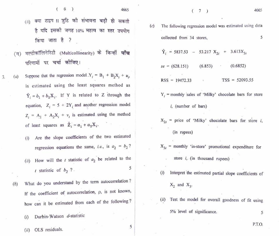
.,_ (a) Suppose that the regression model .Yi = B1 + B2Xi + ui,

is estimated using the least squares method as

Y i = b1

+ b2Xi. If '! is related to Z ·through the

equation, z . = 5 + 2Y and another regression model I I, .

Zi = ~ 1 + A2Xi + vi is estimated using the method

of least squares as zi = al + azXi.

(1) Are the slope coefficients of the two estimated

regression equations the same, i.e., is a2 = b2 ?

(ii) How will the t statistic of a2 be related to the

t statistic of b2 ? -5 I

(b) What do you understand by the term autocorrelation?

If the coefficient o~ autocorrelation, p, is not known,

how ca~ it be estimated from each of the following?

(1) Durbin-Watson d-statistic

(it) OLS residuals . 5

( 7 ) 4665

(c) The following regression model was estimated using data

collected from 34 stores, 5

Yi = 5837.53 - 53.211 x 2i + 3.613X3;

se = (628.151) (6.853) (0.6852)

RSS = 19472.33 TSS 52093.55

Yi = monthly ·sales of 'Milky' chocolate bars for store

i, (number of bars)

X2i = price of 'Milky' chocolate bars for store i,

(in rupees)

X3; = monthly 'in-store' promotional expenditure for

store i, (in thousand rupees)

(i) Interpret ·the estimated partial slope coefficients of

(ii) Test the model for overall goodness of fit using

5% 'level of significance. 5

P.T.O.

' ( . 8 ) 4665 ,

(en) l'.lR a,f\ill!. fcn sifaJ1i11 ~ v . = B1 + s2x. + u. 1

. I I I'

qiT ~ an.~.~ - fcrf,q qiT 394lJI cR WlT!IT

l"fm % ~ 'fcn ~ ·% Yi= bl+ .b2Xi I "l-fR (1lf'51(J:

fcfi y ftl-tlch< 01 zi = 5 + 2vi cfi' i:rr~ 'B z 'B

~~f't,TTf t 3=ll< -q:cfi ~~ 11fcrrpl-;, i:rf~

Z; = A, + A2X; + V; cfiT -3l":J,llR 3TT-~-~

fcrf~ IDU WTf<TT 7rn -m ~ % zi = al + a2Xi I

(1) cp:fT ~ 61:j,l-ilf.-ic:1 ~f~Pll-11 fP-tlch< 0n cfi' ~

~ WTT1 t ~ a2 = b2?

(il) a2 cfiT it ~ ~ >fcfiR b2 cfi' it ~ I

'B oomf wn· ? !

(~) ~ ~:~-~~ (Autocorr-elation) 'B _cf<ll fll-1$d

t ? <lR ~:~-~~ (Autocorrelation) cfiT 'T1fTch", .

p, ~ -;,m t" "ITT ~ ~ "B ~ ~ ~ 3fjl-fA

~ - WTr1T \lfT "Bcfim t- ?

( 9 ) 4665

(Tf) 34 ~ 'B ~ ~ ~ W qi1 394141 ~

~ f1t..-if<--iforn SlfaJll-H ~ cfil ~ ~

y . = 5837.53 - 53.217 X2; + 3.613X3; i

l=fAcfi ~ = (628.151) (6.853) (0.6852)

'31R:-~-~- = 19472.33 it."Q"Jf."Q"Jf• = 52093.55

Y . = ~ -~ ~ 'Milky' tj'fcf,ci2 ~ cITT l-llfflcf, I I

X2i = ~i cfi' ~ 'Mill<y' -tjlchci2 ~ cfi1 cfi1l=@

, (~ "B) .

• x 3i = ~i cfi' ~ l-llfflch '~-~' ~ ~

(~ ~ ~)

(1) · x 2 3lT< x 3 cfi' ~jl-l1f1a ~ ~ 101icti1

cfi1 ell I &11 cf>l f '1i Q_ I

(ii) 5%, 'fITT: cf> ~ cfiT 3qifp I ~ ~ cfft

fil{0l¢11 cf> ~ ~ cfiT 1:J"U~ cf>jf~q_ I

P.T.O.

( 10 ) 4665

4. (a) Consider the following regression results for 45 countries

for the year 2011-20 I 2, (the !-ratios are given in

brackets):

FDii = 21.045 + 0.0545 GDP; + 1.864 GOV _lNDEXi

t = (1.232) (0.744) (1.005) R2 = 0.9667 • !

where

FDI = Foreign Direct Investment (billion dollars)

GDP = Gross Domestic Product (billion dollars)

GOV INDEX = Governance Index (a higher value

indicates better governance)

(i) Is there evidence of multicollinearity ? Explain your '

0 answer.

(ii.) Discuss any two methods that can be used to

deal with the issue of multicollinearity. 5

(b) The following regression was estimated using data from

a sample of 15 houses (standard errors are giv~n in

brackets) :

Yi = 200.091 + 16.186 X; + 3.853D;

Se = (4.354) (2.578) (1.241)

(c)

( 11 ) 4(,65

Y; = assessed value of a house (in Rs. lakhs)

X; = size of the house (in hundreds of square feet)

D; = 0 for house i, 'if it does not face a park

= I for house i, if it faces a park

(z) Interpret the estimated coefficient of Di' . (ii) Test whether the presence of a park in front of

the house increases the assessed value of the

house, using the p-value approach and a 5% level

of significance. 5

A researcher postulates that the car density (number ',

of cars per thousand population), Y, in a city depends

on the bus density (number of buses per thousand

population), X. He runs the regression model, Y; = B1

+ B2X; +· u; for a cross-section of ·128 cities in India

and finds evidence of heteroscedasticity.

(z) How would the model be re-estimated if it is

assumed that error variance is proportional · to the

• I f cr2 rec1proca o X;, that is, E(ur) = - ? Show that

x. l

the transformed error term is homoscedastic.

P.T.O.

( 12 ) %65

(ii' Can we compare R2 of the original model a d

, n the

transformed model ? Explain your answer 5

(cf>) q1Sf 2011-2012 cfi' 45 ~ cfi' ~ f;yf~f©q ~

qf<ollJ.il 11\ fcRm chlf'>llQ,, ·Ct ~ ~ -q 1

' ~ -71"({ t :·

FDii = 21.045 + 0.0545 GDP; + 1.861 GOV _INDEX. I

t = (1.232) (0.744) (1.005) R2 = 0.9667 1

GOV _INDEX = Sl~llfi1 ½:i-.lchlch (~ 1:JR 'tl~lifl1

cnJ zyJ@T %) I I

. I

(Multicollinearity) <!iT "ll1ll"l !

(ii) fcn;m w fcrrw:rr i:n: ~ ch1f"1Q, fJHchT ~

~~fiG~f©chdl .(Multicollinearity) ~ ~ ~ •

R4c.~ cf1 ~ ~ "fl .flcfidl ~I

I

I

( 13 ) 4665

f;:i&.1faf@kf 6l4'141 cf>T ~ ffJ lili l Tf<:TT

y_ = 200.091 + 16.186 xi+ 3.853D, l

"BRcn ~ = (4.35~) (2.578) (1.241)

Y. = ~ ~ cf>T 3Wficl ~ ("ffi<§l' ~ if) 1

x . = -~ cf>T ~ (~ch-$1 cf1f ~ if) 1 . '

· D . = 0 ~ cl"{ "Cffcff c6 -~ -;,m % . I

(1) D; cfi" -:}1j,J-11Rd lJUTTch"' cff)- [email protected] chlf'>llQ, I

(ii) , 1TT-i:JA" (p-~ ~f~cf>jUj ~ 5% ~ cnl

3~'41'1 ~ ~ ~ chif,jjQ, fen ~ eR cfi'

m1R ~ "tff<t cfiT ~ eR _cfi' ~ cfil

~ % ?

c-rr) ~ m~ ~ i fen ~ if cnR eFRq Ccfiro

cfiT ~ ~ ~ ~), Y, ~ eFRq X

"Cf\ R"R cITTffl % (~ ~ ~ cff)- ~) I

P.T.O.

( 14 ) 4665

~ m«f ~ olll4cfi Sl@Hf~ ~ 128 ~ cfi'T

3fR ~l{l~sfefo2.1 (Heteroscedasticity) cfiT w=rJ1ll' 1TTffl

{1) ~ cnT ~ ~ 31j/HHa cITT) fcn<TT ~

~ ~ l=JRT ~ fcf; ~ fqtj{Ui X; ~ 69;&-iG

~ ~ g I fa cfi ~~l ~<§TTTT t, al ~rf ~ cr2

E(ur) = x. ? f¾@l~Q_ fen (C\qiaRa ~ "tJ"{ i

(ii) cf<:IT ~ ~ ~ aw (C\4,a<a, ~ ~

• R2 'cfiT ~ ~ ~ f ? ~ ~

fP-1$11~~ I

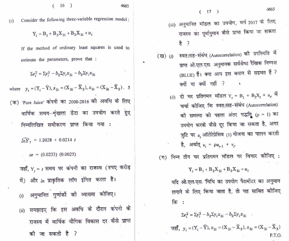
5. (a) Using annual time-series data for the company 'Pure

Juice' for the period 2000-2016, the following equation

was Gbtained

lnY t = 1.2028 + 0.0214 t

se = (0.0233) (0.0025)

(b)

( 15 ) 4665

where Y1

= revenue of the company in Rs. crores at

" time t and In indicates natural log.

(1) Interpret the estimated coefficients.

(i1) Explain how the annual compound growth rate in

(iii)

(1)

(ii)

revenues of the company duriog the period can

be obtained ?

Using the estimated model, how ·can the forecast

revenue for the year 2017 be obtained ? 5

In the presence of autocorrelation, the OLS

estimators obtained ai;,e Best Linear Unbiased

Estimators (BLUE). Do you agree with the

statement ? Why or why not ?

In the two variable regression ·model,

Y, = B1 + ~ + ur discuss ·how the problem of

autocorrelation can be remedied using First Difference

Method (p = 1) if the disturbance term u1

follows

AR(l) scheme, that is, ut = put-I + vt'. 5

P.T.O.

( 16 ) 4€>65

(c) Consider the following three-variable regression model .

If the method of ordinary least squares IS used to I

estimate the parameters. prove that :

(cfi') 'Pure Juice ' ~ cfil 2000-2016 cfiT arcTT'tl ~ ~

qjf~ch -~-i~ ~ cfil d9lil 41 'ch"m ~

R'"1faPm, fil-f1cn< □, m1-0 fcfi<:rr TPTI

Zni\ = 1.2028 + 0.0214 t

. se = (0.0233) (0.0025)

~, Y1= t ~ "CR~ cfiT <1'51t4 (~ -~

if) 3TR ln ~,q,fctch ~ ~ ~ i I

(il) ff~$11~Q, Ft> ~ a:rcrf'~ ~ -ey{R ~ ~

{1'51t4 'ij qlftifch 41fi,ch fqcf,jfi ~ cR) m1-0

cfft '3lT ff ch <11 % ?

( 17 ) 4()65

(iii) d-l:j,41f1a ~ cfil 39li'Pi, qq 20 17 ct ~

~ cfiT iclfj4H ~ m1-0 ~ ~ m

t- ?

("©') (1) ~=~-~'tl. (Autocorrelation) cf>1' ~ ~

W1-0 311.~."Q;B. d-lj4Hcfi 'BciWSo ~ R'&faJ

(BLUE) % I ~ 3lr1 ~ ~ 'B ~ % ?

cfllT ?:fl cfllT -;,m ? · t

(ii) ~ ~ s.ifc'Pll-11 1-ITw Y 1 = 8 1 + B2X1 + u1, ~

~ cf>tf\l\Q, fcn" ~=~-~'tl (Autocorrelation)

'cfi1 -84{--41 'cfi1 ~ ~ ~ (p = I) 'cfil

o9lf1Ji ~ 'cfi'B ~ ~ ~ ~ t", WR

We ~ u1

3-IT2!1~foc1 (I)~ 'cfil 1lR11 ctmft

t", 3l~ ut = put-I + vr

~ 31l.~.~- tfcn'tl cfil 39lf1Ji ~<1l-f12.< 'cfil ~

~ ~ ~ ~ ~ t m ~ ~ cnlf'11 Q,

fq,

~' Yi = (Yi - Y), Xzi = (X 2i - X2), x 3i = (X3i - X. 3)

P.T.O.

( J 8 ) 4665

6. (a) It is known that the variance of scores of all high

school students in a science test is 150. A ,,sample of

scores o~ 20 high school students who took the science

test this year yielded a variance of 170. Test, at 5%

Iev_el of significance, if the variance of scores ·of the

high school students who took the science test this

year is difffrent from 150. State the underlying

(b)

(c)

assumptions, if any. 5

Consider the three-variable model, Y; = B1 + B2x2; +

B3X

3; + B4X4; + U;- Let b2 be the OLS estimator of

. .

the slope coefficient B2.

(1) Derive variance of b2, i.e. var(b2), m tenns of

Variance Inflation Factor (VIF).

(ii) When X2 is regressed on X3 and X4, R~

obtained from this auxiliary regr,ession is 0.9217.

Does it necessarily imply high variance of b2?

Explain. 5

Based on a sample of si~e 20, the following regression

line was estimated us1·nP the I h d 9

east-squares met o ,

In addition, X = 21:(Xi - X) 2 = 20 and · the standard

error of regression was estimated to be equal to I.

I . I

( 19 ) 4665

Construct a 95% confidence interval estimate of the true

population mean of Y for X0 == . 15. Do you expect

the confidence interval to be wider if a similar interval

is estimated for x0

== 2 ? Explain your answe_r. 5

~ ~ ~ cfi1 fqtj(11 (Variance) 150 "%- I · 20

~ fq'E)j~lj ~ ~ ~ ~ cfi1 lJ:-fl ~ ~

~ 'B"R1 ~ cfil" 1Rta:n #t m ~, 110 cfi1 lJ:-fl

fqtj(11 ~ -%-1 5% w ~ ~ 1l\ ~ ch7f~Q,

~ Ql~%°'t1 ~ ~ -~ ~ cfi1 fq=q(11, ~

~ -~ cfil" ~ cfil" 1RTa:TT #t W ~' 150 "B ~ %1

(~) ·<fR ~ ~ -in: fcR.JR"[\ . ct>I 'JI~, Y; == B1 + B2X2;

+ B3X3; + B4X4; + U; I i:JA1 fcn b2, B2 ~ ~

cfi1 . 3TI-~-~- ~ %_1

(i) b2, ~ fqtj(11 ~~ var(b2), -aj,-·variance Inflation

Factor (VIF) ~ - -~ ~ chif\lJQ, ~

(ii) ~ -X2 cf)1' X3 3W X4 ~ - sifcPiil14a ~ ~

% "ffi' ~ ,(-iQlllc.h sifct~1~1 °B ~ R~ 0.9il7.

% I ~ ~ 3-llfW'4c.h ~ "B (b2) - -ij ~

fqtjci1 cfil WTTf ~ i ? '8G$il$Q, I

P.T.O.

7.

( 20 ) 4665

( Tf) 3llcfiT{ 20 cf) ~ ~ cf) 3TI'tITT °91: I R9 >lfct~ p:r,,

Bil cfil ~ 3TI-~-"Q;B- fcff~ °B ~Pillfr ~

~ ~-m~, X = 2I(Xi - X)2 = 20 , 3TR >lfc:Pllfl

cffr i:fRcfi ~ , # ~ 6ij/-11f..rn cff)- TftIT 1

y cfiT ~ ~ ~ ~ cf> 95% fq~qlf{ ~

qiT RliTUf i:h1f'31Q. ~ X0 = 15 %°1 ~ 3lTtT fq~tjlff

~cfil~~fflc8~~f~

~ 3HHIC1 x0 = 2 ~ fum_ 6ij/llf.:1e:1 ~

(a) The following hvo regression models were estimated

using annual time-series data for the period 1990-2012

for a certain country (standard errors are mentioned in

the parentheses) :

Model A: lnY t = 2. 18 + 0.34 lnX21 -0.5 I lnX31

+ 0,.15 lnX41 + 0.09 lnX51

se = (0.156) (0.083) (Q.110) (0.099) _ (0.101)

R2 = 0.9823

(b)

( 21 ) 4665

Model B : ZnY t F _ 2.03 + 0.45 lnX21

- 0.377 lnX31

se = (0. I I 6) (0.025)

R2 = 0.9801

where Y 1 = demand for cheese (in kg)

X2 = disposable income (in Rs. '000)

X3 = price of cheese (in Rs. per kg)

X4 pnce of butter (in Rs. per kg)

(0.063)

X5 price of peanut-butter (in Rs. per kg)

Which model wottld you choose ? Test the relevant

hypotheses at the 5% level of significance and state

your conclusion clearly. 5

For the regression model : Yi = B2Xi + ui, derive the

OLS estimator of 8 2. Show that it is an unbiased

estimator. Clearly, state the assumptions required to

prove its unbiasedness. 5

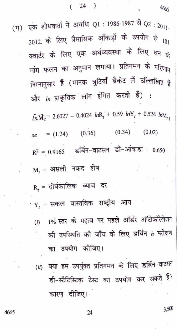
(c) A researcher estimated the demand function for money

for an economy for IO I quarters using quarterly data

for the period QI : 1986-1987 to Q2 : 2011-2012. The .. • •

regression results are as follows (standard errors are

P.T.O.

( 22 ) 4665 I

. d . th brackets and In indicates natural log): mentt0ne m e

lnMt= 2.6027 _ 0.4024 lnR1

+ ·0.59 lnY1 + 0.524 lnM1_1 1

se = ( 1.24) (0.36) (0.34) (0.02)

R2 == 0_9165 Durbin-Watson d-statistic = 0.650

M == real · cash balances I

R = long-term interest rate t .

y 1

= aggregate real national · income

. I

(i) Use burbin's h-test to check for the presence of

first order autocorrelation at 1 % level of

significance. \

(ii} Can we use Durbin-Watson d-statistic test for the I

above regres~ion ? Give reasons. 5

(cfi) fcnm ~ ~ ~ 1990-2012 clft ~'tl ~ ~ I

q1f6fcfi ~-~~ ~ cn1 39-47'1 ~ ~

f1~fcif@c1 ~ S1fct,11-F1 ~ cnl 3TTfR c?t'lllll

~A: lnY t = 2.18 + 0.34 /~X21 -0.5 l /nX31 + 0.15 lnX41 + 0.09 lnXs1

, se = (0.156) (0.083) (0.110) (0 .099) (0.101)

R2 = 0.9823

( 23 ) 4665

~ B : lnY t = 2.03 + 0.45 /nX 21 - 0.377 lnX31

se = (0.116) (0.025) (0.063)

R2 = o.9801

X4 = l4ct©1 cfi1 cfft+m (~ Wd ~ ~)

«R in: S11 zj n, cfi ~ :J}-11.:n cfil "tfft a,,ur en, f '51 q_ -3lR

3l'R f16cfitSf cfil ~ ~ 'B ~c11$Q, I

(~) S1fcP11--11 ~ : Y; = B2X; + u;, ~ ~ B2 cfil

3TI-~-~- '1-lji--!Hcfi 1TT1-0 ch7f-:iiQ, I f~©i$4 fen ~

~ R&18-1 31ji--111cfi i I -~ ~~ ~

cfiB ~ wnr_ arn'am 1--11;.qc11-m . cf)1 . ~ctl~Q, I

P.T.O.

(Tf)

4665

( 24 ) A 466s

~ "fflffl ";t 3lc!fq QI : 1986-1987 it Q2 : 20t 1_

2012. cfi Wl1!. ~1•11f.8i:f> 6tii:f>9l cfi :aqi.flrr il io1

qqld{ ~ ~ ~ 3l~ ~ ~ ~ ct

~ Cfic?H cnl ~jGH (!1'11411 ~f(Pll41 ~ ~

f1i:.-tljl!-iR ~ ( l9Hi:f> ~ ~ jf dffufGHJ f

3W In ~1q;facn . ffi1T ~ cfi(ctl ~) :

lnMt = 2.6027 - 0.4024 lnR1 + :p.59 -lnY1 + 0.524 lnM . ~I

se = (1.24) (0.36) (0.34) (0.02)

R2 = o.9165 sf41-ct12~1 tT--3-ticfisl = 0.650

(i) lo/~' ~ -~ 4t&A "9\ ~ am ~T2lch21~8~11

cfft ~ cfft ~ ~ Wl1!, sfcif1 h ~~

cn1 aq.li"1,, cnl f'51 ~ 1

(ii) cfllT ~ :aqic@ Slf(t'IWI cfi ~ :gfi;{1-c112M I

"it-R.fc:fgcf> ~ cnT d91421'1 cITT: ffl ~? / . .

cfiR~J G1f'51~.1 · .

24 3,500

Table A.3 Standard Normal Curve Areas

<l><.z) = P(Z :s z)

Standard nonnal density cu1Ve / .

0 z.

z .oo .01 .02 .03 .04 .OS .06 .(17 • .08 .09

-3.4 . 0003 · .0003 .0003 .0003 .0003 .0003 .0003 .0003 .0003 .0002 -3.3 .0005 .0005 .0005 .0004 .0004 .0004 .0004 .0004 .000~ .0003 -3.2 .0007 · .0007 .0006 .0006 .0006 .0006 .0006 .0005 .0005 .0005 -3.1 .0010 .0009 .0009 .()009 .0008 .0008 .0008 .0008 .0007 .0007 - 3.0 .0013 .0013 .0013 _()()12 .0012 .001 I .0()11 .0011 .0010 .0010 -2.9 .0019 .0018 .0017 .0017 .0016 .00 I 6 .0015 .0()15 .0014 .0014 -2.8 .()()26 .0025 .0024 .0023 .0023 .0022 .0021 .002J .0020 .0019 -27 .0035 .0034 .0033 .0032 .0031 .0030 .0029 .0028 .0027 .0026 -2.6 .0047 .0045 ,()()44 .0043 .0<)41 .0040 .0039 ,0{)38 .0037 .0036 -1.5 · .0062 .0060 . .0059 .0057 .0055 ;0054 .0052 ··.0051 .0049 .0048 -2.4 .0082 .0080 .0078 .0075 . 0()73 .0071 . t0069 .0068 .0066 .0064 -? 3 -· .0107 .0104 . . 0102 .0099 .0096 .0094 .0091 .0089 , .0087 .0084 -2.2 .0139 .0136 .0132 .0129 .0125 .0122 .0119 .0116 .Ol13 .0110 -2.1 .0179 .0174 .0170 .0166 .0162 .0158 .0154 .015-0 .Ol46 .0143 -2.Q .0228 .0222 .0217 .0212 .0207 .0202 .0197 .0192 .0188. .0183

• -L9 .0287 .0281 .0274 .0268 .0262 .0256 .0250 .0244 .0239 .0233 -1.8 .03:59 .0352 .0344 .0336 r .0329 .0322 .0314 .0307 .0301 .0294 -1.7 .0446 .0436 .0427 .0418 .0409 .0401 .0392 .0384 .0375 .0367 -1.6 .0548 .0537 .0526 .0516 ·.0505 · .0495 .0485 .0475 .0465 .0455 -1.5 .0668 .0655 .0643 .()630 .0618 .0606 .0594 .0582 .0571 .0559 -1.4 .0808 .0793 .0778 .0764 .0749 .0735 .0722 .0708 .0694 .0681 -1.3 .0968 .0951 . .0934 .0918 .0901 .0885 .0869 .0853 .0838 .0823 -1.2 .11.$1 .1131 .1112 .1093 .I075 .1056 .1038 .1020 .1003 .0985 . -1.1 .1357 .1335 .1314 .1292 .1271 :125 I .1230 .1210 .l 190 .1170 -1.0 .1587 .1562 .1539 .1515 · .1492 .1469 .1446 .1423 .1401 .1379 -0.9 .1841 .1&14 .1788 .1762 .1736 .1711 .1685 .1660 .1635 . 16l l -0.8 .2119 .2090 . .2061 .2033 .2005 .1977 .1949 .1922 .1894 .1867 -0.7 .2420 .2389 .2358 .2327 .2296 .2266 .2236 .2206 . . 2177 .2148 -0.6 .2743 .2709 .2676 .2643 .2611 .2578 .2S46 .2514 .2483 .2451 -0.5 .3085 .3050 .3015 .2981 .2946 .2912 .2877 .2843 .2810 .2776 .. -0.4 .3446 .3409 .3372 .3336 . 3300 .3264 .3228 . . 3192 ·.3156 .3121 -0.3 .3821. .3783 .3745 .3707 .3669 .3632 .3594 .3557 .3520 · .3482 -0.2 .4207 .4168 .4129 .4090 .4052 .4013 .3974 .3936 .3897 .3&59 -0.l .4602 .4562 .4522 .4483 .. 4443 .4404 .4364 ,4325 .4286 .4247 -o.o .5000 · .4960 .4920 .4880 .4840 .4801 .4761 .4721 .4681 .4641

(continued)

Table A.3 Standard Normal Curve Areas (cont.) <l>(z) = P(Z :s z)

z .00 .01 .02 .03 .04 .05 .06 .07 .08 .09

0.0 .5000 .5040 .5080 .5120 .5160 · .5199 .5239 .5279 .5319 .5359 0.1 .5398 .5438 .5478 .5517 .5557 .5596 .5636 .5675 .5714 .5753 0.2 .5793 .5832 .5871 .5910 .5948 .5987 .6026 .6064 .6103 . . 6141 0.3 .6179 .6217 .6255 .6293 .6331 .6368 .6406 .6443 .6480 .6517 0.4 .6554 .6591 .6628 .6664 .6700 .6736 .6772 .6808 .6844 .6879

0.5 .6915 .6950 .69&5 .7019 .7054 .7088 .7123 .7157 .7190 .7224 0.6 .7257 .7291 .7324 .7357 .7389 .7422 .7454 .7486 .7517 .7549 0.7 .7580 .7611 .7642 .7673 ' .7704 .7734 · .7764 .7794 .7823 .7852 0.8 .7881 .7910 .7939 .7967 .7995 .8023 .8051 · .8078 .8106 .8133 0.9 .8159 .8186 .8212 .8238 .8264 .8289 .8315 .8340 .8365 .8389

1.0 . .8413 .8438 .8461 .8485 .8508 .8531 .8554 .8577 .8599 .8621 1.1 .8643 .8655 .8686 .8708 .8729 .8749 .8770 .8790 .8810- .8830 1.2 .8849 .. 8869 .8888 .8907 .8925 .,8944 .8962 .8980 ·.8997 .9015 1.3 .9032 .9049 .9066 .9082 .9099 .9115 .9131 .9147 .9162 .9177 1.4 .9192 .9207 .9222 .9236 .9251 .. 9265 .9278 .9292 .9306 .9319

1.5 .9332 ' .9345 .9357 .9370 .9382 .9394 .9406 · .9418 .9429 .9441 · 1.6 .9452 .9463 .9474 .9484 .9495 .9505 . . 9515 .9525 .9535 .9545 1.7 .9554 .9564 .9573 .9582 .9591 .9599 .9608 .9616 .9625 .9633 1.8 .9641 ·.9649 .9656 .9664 .9671 .9678 .9686 .9693 .9699 .9706 1.9 .9713 .9719 .9726 .9732 .9738 .9744 .9750 .9756 .9761 .9767

2.0 .9772 .9778 .9783 .9788 .9793 .9798 .9803 .9808 .9812 .9817 2.1 .9821 .9826 .9830 .9834 .9838 .9842 .9846 .9850 .9854 .9857 2.2 .9861 .9864 ~ .9868 .9871 .9875 .9878 .9881 .9884 .9887 .9890 2.3 .. 9893 .9896 .9898 .9901 .9904 .9906 .9909 .9911 .9913 .9916 2.4 .9918 .9920 .9922 .9925 . . . 9927 .9929 .9931 .9932 .9934 .9936

2.5 .9938 .9940 .9941 .9943 .9945 .9946 .9948 .9949 .9951 .9952 2.6 .9953 .9955 .9956- .9957 .9959 .9960 .9961 .9962 .9963 .9964 2.7 .9965 .9966 .9967 .9968 .9969 .9970 .9971 .9972 .9973 .9974

I.

2.8 .9974 .9975 .9976 .9977 .9977 .9978 .9979 .9979 , .9980 .9981 ' 2.9 .9981 .9982 .9982 .9983 .9984 .9984 .9985 .9985 .9986 .9986

3.0 .9987 .9987 .9987 .9988 .9988 .9989 .9989 .9989 .9990 .9990 3.1 .9990 .9991 .9991 .9991 .9992 .9992 .9992 .9992 .9993 .9993

3.2 .9993 .9993 .9994 .9994 .9994 .9994 .9994 .9995 .9995 .9995 3.3 .9995 .9995 .9995 .9996 .9996 .9996 .9996 .9996 .9996 .9997 3.4 .9997 · . . 9997 .9997 .9997 .9997 .9997 .9997 .9997 .9997 .9998

Tab le A.8 t Curve Tail Areas

I Cl, !vl: Ar-:..i t0 th ..:

"' 11 gh1 ul,

1 /

u t

l ,, 2 3 4 5 ' 6 7 8 9 10 I I 12 13 14 15 16 17 18

0.0 .500 .500 .500 .500 .500 .500 .500 .500 .500 .500 .500 .500 .500 .500 .500 .500 .500 .500

0.1 .468 .465 .463 .463 .462 . .462 .462 .461 .461 .461 .461 .461 .46 1 .46 1 .46 1 .461 .461 .46 1

0.2 .43 7 .-UO ·.427 .426 .425 .424 .424 .423 .423 .423 .423 .422 .422 .422 .422 .422 .422 .422

0.3 .407 .396 .392 .390 .388 .387 .386 .386 .386 .385 .385 .385 .384 .384 .384 .384 .384 .3 84

0.4 .379 .364 .358 .355 .353 .352 .351 . .350 .349 .349 .348 .348 .348 .347 .347 .347 .347 .34 7

0.5 .352 .333 .326 .322 .319 .3 I 7 .316 .315 .315 .314 .313 .3 l 3 .313 .312 .312 .312 .312 .312

0.6. .328 .305 .295 .290 .287 .285 .284 .283 .282 .281 .280 .280 .279 .279 .279 .278 .278 .278

0.7 .306 .278 :267 .261 .258 .255 .253 .252 .251 .250 .249 .249 .248 .247 .247 .247 .247 .246

0.8 .285 .254 .24 1 .234 .230 .227 .225 .223 .222 .221 .220 .220 .219 .218 .21 8 .218 .217 .217

0.9 .267 ,232 .217 .210 .205 .201 . 199 .197 .196 .195 .194 .193 .192 .191· .191 . 191 .190 . . 190

1.0 .250 .211 .196 .I 87 -.182 .178 .175 .173 .172 .170 .169 .169 .168 .167 .167 .166 .166 .165

1.1 .235 .193 .176 .167 .162 .157 :154 .152 .150 .149 .147 . /.46 .146 .144 .144 . 144 .143 . . 143

1.2 .221 .177 . 158 .148 .142 . 138 .135 .132 .130 .129 .128 .127 .126 .124 .124 .124 .123 .123

1.3 .209 .162 .142 .132 .125 .121 .117 .115 .113 · .111 .110 .109 .108 . 107 .107 . 106 .105 .105 1.4 .197 .148 .128 .117 .! 10 .106 .102 ·.100 .098 .096 .095 ·. 093 .092 .-:091 .091 .090 .090 .089 1.5 .187 .136 .115 .104 .097 .092 .089 .086 .084 .082 .081 .080 .079 .077 .q77 .077 .076 .075

1.6 .178 '.125 .104 .092 .085 .080 .077 .074 .072 .070 .069 .068 .067 .065 .065 .065 .064 .064 1.7 .169 .116 .094 .082 .075 .070 .065 .064 .062 .060 .059 .057 .056 .055 .055 .054 .054 .053 1.8 .161 .107 .085 .073 :066 .061 .057 .055 .053 .051 .050 .049 .048 .046 .046 " .045 .045 .044 1.9 . \ 54 .099 .077 .065 .058 .053 .050 .047 .045 .043 .042 .041 .040 .038 .038 .038 .037 .037 2.0 .148 .092 .070 .058 .051 . . 046 .043 .040 .038 .037 .035 .034 .033 .032 .032 .03l .03l .03()

2.1 . 141 .085 .063 .052 .045 .040 .037 .034 .033 .031 .030 .029 .028 .027 .027 .026 .025 .025

2.2 .1 36 .079 .058 .046 .040 .035 .032 .029 .028 .026 .025 .024 .023 .022 .022 .021 .021 .021

2.3 . 131 .074 . . 052 .041 .035 .031 .. . 027 .025 .023 .022 .021 .020 .019 .018 .018 .018 .017 .017

... 2.4 .126 .069 .048 .037 .031 .027 .024 .022 .020 .019 .018 .017 .016 .015 .015 .014 .014 .01 4

2.5 ' .121 .065 .044 .033 .027 .023 .020 .018 .017 .016 .015 .014 .on .012 .012 .012 .011 .01 l

2.6 .117 .061 .040 :030 .024 .020 .018 .016 .014 .013 .012 .012 .011 .0 10 .010 .010 .009 .009

2.7 .I .113 .057 .037 .027 .021 .018 .015 .014 .012 J) 11 .010 .010 .009 .008 .008 .008 .008 .007

2.8 .109 .054 .034 .024 .019 .016 .013 .012 .010 .009 .009 .008 .008 .007 .007 .006 . . 006 .006

2.9 .106 .051 .03 l .022 .017 .014 .OJ 1 .010 .009 .008 .007 .007 .006 .005 .005 .005 .005 .005

3.0 .102 .048 .029 .020 .015 .012 .010 .009 .007 .007 ~ .006 .006 .005 .004 .004 .004 .004 .004

3.1 .099 .045 .027 .. 018 .013 .0-11 .009 .007 .006 .006 .005 .005 .004 .004 · .004 .003 .003 .003

3.2 .096 .043 .025 .016 .0)2 .009 .008 .006 .005 .005 .004 .004 .003 .003 .003 .003 .003 .002

3.3 .094 .040 .023 .015 .011 .008 .007 .005 .005' .004 .004 .003 .003 .002 .002 .002 .002 .002

3.4 .09 1 .038 .021 .014 .010 .007 .006 _ .005 .004 .003 .003 .003 .002 .002 .002 .OQ2 .002 .002

3.5 .089 .036 .020 .012 .009 .006 .005 .004 .003 . . 003 .002 .002 .002 .002 .002 .001 .001 .001

3.6 .086 .035 .018 .011 .008 .006 .004 .004 .003 .002 .002 .002 .002 .001 .001 .001 .001 .001

3.7 .084 .033 .0 17 .010 .007 .005 · .004 .003 .002 .002 .002 .002 .001 .001 .001 .001 .001 .00 1

3.8 .082 .031 .OJ 6 .010 .006 .004 .003 .003 .002 .002 .001 .001 .001 .001 .001 .001 .001 .001

3.9 .080 .030 .015 .009 .006 .004 .003 .002 .002 .001 .001 .001 .001 _ .001 . . 001 .001 .001 .001

4.0 .078 .029 .014 .008 .005 .004 .003 .002 .002 .001 .001 .001 .001 .001 .001 .001 .000 .000

(continued)

Table A.8 t Curve Ta il Areas (cont.)

19 20 21

t curve ~ / ·'

/

0

Arca to the

right oft

•I t

22 23 24 25 26 27 28 29 30 35 40 60 120 oc(= z)

0.0 .500 .500 .500 .500 .500 .500 .500 .500 .500 .500 .500 .500 .500 .500 .500 .S00 .500 0.1 .461 .461 .461 .461 .461 .461 .461 .461 · .461 .461 .461 .46 1 .460 .460 .460 .460 .460 0.2 .422 .422 .422 .422 .422 .422 .422 .422 .421 .421 .421 .421 .421 .42 1 .421 .421 .421 0,3 .3 84 .384 .384 .383 .383 .383 .383 .383 .383 I .383 .383 .383 .383 .383 .383 .382 .382 0.4 .347 .347 .347 .347 .346 .346 .346 .346 .346 .346 .346 .346 .346 .346 .345 .345 .345 O.~ .311 .311 .311 . .311 .311 .311 .311 .311 .311 .310 .310 .3 10 .310 .310 .309 .309 .309

0.6 .278 .278 .278 .277 .277 .277 .277 .277 .277 .277 .277 .277 .276 .276 .275 .275 .274 0.7 .246 .246 .246 .246 .245 .245 .245 .245 .245 .245 .245 .245 .244 .244 .243 .243 · .242 0.8 .217 .217 .216 .2·16 .216 .216 .216 .215 .215 .215 .215 .215 .215 .2 I 4 .2 13 .2 I 3 .212 0.9 .190 .189 .189 .189 .189 .189 .188 .188 .188 .188 .188 .188 .187 .187 .186 .1 85 .184 1.0 .165 .165 .164 .164 .164 .164 .163 .163 .163 .163 .163 .163 .162 ' .162 .1 6 1 .160 .159 1.1 1.2 1.3 1.4 1.5

1.6 1.7 1.8 1.9 2.0

2.1 2.2 2.3 2.4 2.5

2.6 2.7 2.8 2.9 3.0

3.1 3.2 ,

.143 .142 .142 .142 .141 .J 41 .141 .141 .141 .140 .140 .140 .139 .139 .138 .137

.122 .122 .122 .121 .121 .121 .121 .120 .120 .120 .120 .120 .119 .119 .117 .1 16 ' .105 .104 .104 .104 .103 .103 .103 .103 .102 .102 .102 .102 .101 .IOI .099 .098

.089 .089 .088 .088 .087 .087 .087 .087 .086 .086 .086 .086 .Q85 .085 .083 .082

.075 .075 .074 .074 .074 .073 .073 .073 .073 .072 .072 .072 .071 .071 .069 .068

.063 .063 .062 .062 .062 .061 .061 .061 .061 .060 .060 .060 .059 .059 .057 .056 .053 .052 .052 .052 .05 I .05 I .05 I ·.051 .050 .050 .050 .050 .049 .048 .047 .046 .044 .043 .043 .043 .042 .042 .Q42 .042 .042 .041 .041 .041 .040 .040 .038 .037 .036 .036 .036 .035 .035 .035 .035 .034 .034 .034 .034 .034 .033 .032 .03 1 .030 .030 .030 .029 .029 .029 .028 .028 .028 .028 .028 .027 .027 .027 .026 .025 .024

.025 .024 .024 .024 .023 .023 .023 .023 .023 .022 .022 .022 .022 .021 .020 .0 19

.020 .020 .020 .019 .019 .019 .019 .018 .018 .018 .018 .018 .017 .017 .016 .015

.016 .016 .016 .016 . . 015 .015 .015 .015 .015 .015 .014 .014 .014 .013 .01 2 .0 12

.013 .013 .013 .013 .012 .012 .012 .012 .012 .012 .012 .011 .011 .01 1 .010 .009

.011 .011 .010 .010 .010 .010 .010 ·.010 .009 .009 .009 .609 .009 .008 .008 .007

.009 .009 .008 .008 .008 .008 .008 .008 .007 .007 .007 .007 .007 .007 .006 .005

.007 .007 .007 .007 .006 .006 .006 .006 .006 ·.006 .006 .006 .005 .005 .004 .004

.006 .006 .005 , .005 .005 .005 .005 .005 .005 .005 .005 .004 .004 .004 .003 .003

.005 .004 .004 .004 .004 .004 .004 .004 .004 .... 004 .004 .00~ .003 .003 .003 .002

.004 .004 .003 .003 .003 .003 .003 .003 .003 .003 .003 .003 .002 .002 .002 .002

.003 .003 .003 .003 .003 .002 .002 .002 .002 .002 .002 .002 .002 .002 .00 1 .001

.002 .002 .002 .002 .002 .002 .002 .002 .002 .002 .002 .002 .001 .001 .001 .001

.136

.115

.097

.081

.067

.055 .045 .036 .029 ,023

.018

.01 4

.01 I

.008

.006

.005

.003

.003

.002

.00 1

.001

.00 1 3.3 .002 .002 .002 .002 .002 .001 .001 .001 .001 .001 .001 .001 .001 .00 1 .001 .001 .000 3.4 . . 002 .001 .001 .001 . .001 .001 .001 .001 .001 .001 .001 .001 .001 .001 .001 .000 .000 3.5 .001 .001 .001 .001 .001 .001 .001 .001 .001 .001 · .001 .001 .001 .001 .000 .000 .000

3.6 .001 .001 .001 .001 .001 .001 .001 .001 .001 .001 .001 .001 .000 .000 .000 .000 .000 3.7 .001 .001 . . 001 .001 .001 .001 .001 .001 .000 · .000 .000 .000 .000 .000 .000 .000 .000 3.8 .001 .0O'l .001 .000 .000 .000 .000 .000 .000 .000 .000 .000 .000 · .000 .000 .000 .000 3.9 .000 .000 .000 .000 .000 .000 .000 .000 .000 .000 .000 .000 .000 .000 .000 .000 .000 4.0 .000 .000 .000 .000 .000 .000 .000 .000 .000 .000 .000 .000 .000 .000 .000 .000 .000

f,. F{E:AS UNUt:H THE STANDARDIZED NORMAL DrSTRIBUTION

Example

Pr (0 ~ z~ 1.96) = 0.4750

Pr(Z ::: 1.96) = 0.5 - 0.4750 = 0.025

0

z .00 .01 .02 .03 .04 .05 .06

0.0 .0000 .0040 .0080 .0120 .0160 ~0199 .0239

0.1 .0398 .0438 .0478 .0517 .0557 .0596 .063e

0.2 .0793 .0832 .0871 .0910 .0948 .0987 .1026

0.3 .1179 .1217 .1255 .1293 . . 1331 .1368 .1406

d.4 .1554 .1591 .1628 -.1664 .1700 .1736 .1772

0.5 · .1915 .1950 .1985 .2019 .2054 .2088 .2123

0.6 .2257 .2291 .2324 .2357 .2389 .2422 .2454

0.7 .2580 .2611 .2642 .2673 .2704 .2734 .2764

0.8 .2881 .2910 .2939 .2967 .2995 .3023 . . 3051

0.9 .3159 .3186 .3212 .3238 .3264 .3289 .3315

1.0 .3413 .3438 .3461 .3485 .3508 .3531- .3554

1.1 .3643 .3665 .3686 .3708 .3729 .3749 · .3770

1.2 .3849 , .. 3869 .3888 .3907 .3925 .3944 .3962 1.3 . .4032 :4049 . .4066 .4082 .4099 .4115 .4131

1.4 .4192 .4207 .4222 .4236 .4251 .4265 .4279

1.5 .4332 .4345 .4357 .4370 .4382 .4394 .4406

1.6 .4452 .4463 .4474 .4484 .4495 .4505 .4515 1.7 .4454 .. . 4564 .4573 .4582 .4591 .4599 .460'8

1.8 .4641 .4649 .4656 .4664 .4671 .4678 .4686

1.9 .4713 · .4719 .4726 .4732 .4738 .4744 .4750

2.0 .4772 · .4778 .4783 .4788 .4793 .4798 .4803 ·

2.1 .4821 .4826 .4830 .4834 .4838 .4842 .4846

2.2 .486·1 .4864 .4868 .4871 .4875 .4878 .4881 ·

2.3 .4893 .4896 .4898 .4901 .4904 .4906 .4909

,2.4 .4918 .4920 .4922 .4925 .4927 .4929 .4931

2.5 .4938 . .4940 .4941 .4943 .4945 .4946 .4948

2.6 .4953 .4955 .4956 .4957 .4959 .4960 .4961

2.7 .4965 .4966 .4967 .4968 .4969 .4970 .4971

2.8 .4974 ·.4975 .4976 .4977 .4977 .4978 .4979

2.9 .4981 .4982 .4982 .4983 .4984 .4984 .4985

3.0 .4987 .4987 .4987 .4988 .4988 .4989 .4989 •

0.4750

z 1.96

.07 .08 .09

.0279 .0319 .0359

.0675 .0714 .0753

.1064 .1103 .1141

.1443 .1480 .1517

.1808 .1844 .1879

.2157 .2190 .2224

.2486 .2517 .2549

.2794 .2823 .2852

.3078 .3106 .3133

.3340 .3365 .3389

.3577 .3599 .3&21

.3790 .3810 .3830

.3980 .3997 .4015

.4147 .4162 .4177

.4292 .4306 .4319

.4418 .4429 .4441

.4525 .4535 .4545 .4616 .4625 .4633 .4693 .4699 .4706 .4756 .4761 .4767 .4808 .4812 .4817

.4850 .4854 .4857

.4884 .4887 .4890

.4911 .4913 .4916

.4932 .4934 .4936

.4949 .4951 .4952

.4962 .4963 .4964

.4972 .4973 .4974

.4979 .4980 .4981

.4985 .4986 .4986

.4989 . .4990 .4990

PERCENTAGE POINTS OF THE t DISTRIBUTION

Example

Pr ( t > 2.086) = 0.025

Pr(t > 1.725) = 0.05 for df = 20 ·

Pr( \tl > 1.725) = 0.10

0.05

~ -=--------.L..----'---'-----t

0 1.725

~ 0.25 0.10 0.05 0.025 0.01 0.005 0.001

0.50 0.20 0.10 0.05 0.02 0.010 0.002 .

1 1.000 3.078 6.314 12.706 31.821 63.657 318.31

2 0.816 1.886 2.92~ 4.303 6.965 9.925 22.327

3 0.765 1.638 2.353 3.182 4.541 5.841 10.214

4 0.741 1.533 2.132 2.776 3.747 4.604 7.173

5 0.727 1.476 2.015 2.-571 3.365 . 4.032 5.893

6 -0.718 1.440 1.943 2.447 3.143 3.707 5.208

7 0.711 1.415 1.895 2.365 2.998 ·3.499 4.785

8 0.706 1.397 1.860 2.306 2.896 . 3.355 4.501

9 0.703 . 1.383 1.833 2.-262 2.821 3.250 4.297

10 0.700 1.372 1.812· 2.228 2.764 3.169 4.144

11 0.697 1.363 · 1.796 2.201 2.718 3.106 4.025

12 0.695 1.356 1.782 2.179 2.681 3.055 3.930 13 0.694 1.350 1.771 2.160 2.650 3.012 3.852 14 0.692 1.345 1.761 2.145 2.624 2_. 977 3.787

15 0.691 1.341 1.753 2.131 2.602 2.947 3.733 16 0.690 1.337 ,1. 746 2 .-120 . 2.583 2.~21 3.686 17 0.689 1.333 1.740 2.110 2.567 2.898 3.646 18 0.688 .1.330 . 1.734 · 2.101 2.552 2.878 3.61 19 · 0.688 1.328 1.729 2,09·3 .2.539 2.861 3.579

0

20 0.687 1.325 1.725 2.086 2.528 2.845 3.552 21 · 0.686 1.323 1.721 2.080 2.518 2.831 3~527 22 0.686 1.321 1.717 2.074 2.508 2.819 3.505 23 0.685 1.319 1.714 2.069 2.500 2.807 3.485 24 0.685 1.318 1.711 ·2.064 2.492 2.797 ·3.457

25 0.684 1.316 1.708 2.060 2.485 2.787 3.450 26 0.684 1.315 1.706 2.056 2.479 2.779 3.435 -27 0.684 1.314 1.703 2.052 2.473 2.771' 3.421 28 0.683 1.313 1.701 2.048 2.467 2.763 3.408 29 0.683 1.311 1.699 2.045 2.462 2.756 3.396

30 0.683 1.310 1.697 2.042 2.457 2.750 3.385 ·, 40 0.681 1.303 1.684 2.021 2.423 2.704 3.307 60 0.679 1.296 1.671 2.000 2.390 2.660 3.232

120 0.677 1.289 1.658 1.980 2.358 2.617 3.160 00 0.674 . 1.282 1.645 1.960 2.326 2.576 3.090

- AGE POINTS OF THE F DISTRIBUTION

l;PPER p[Ac;tNT

E..umpJt

Pr(F ::, 1.59) "' 0.25

M f > 2.42) - 0.10

Pr(F ::, 3.i4) = 0.05

Pr(F > 5.26) - 0.01

ford .f. N1 "' 10

and N2 = q V 0 •

I I - f 3.14 5.26 d.f. for

denom-

_------------~d~.f-~fo~r~n~ume~r~a1~or~N~1=:--;:-~~-~ ~--:r -;7 inator

d.!." or /! d.f. for numerator N,

200 500 00 I Pr N2

dtnom · L-------~--..:.:..=~~----:---:8--:--.---;-~~---- 30 40 so so 100 120

rnafor 3 4 5 6 7 9 10 11 . 12 15 20 24

~ ~ 2

gn

2

3

4

5

6

7 ·

8

9

, 8 20 8 58 B 82 8.98 9.10 9.19 9.26 9.32

2 5 5.83 7

.50

· . . 0 59 40 59 90 60 20

. 10 39.90 49.50 53.60 55.80 57 .20 58.20 sa.9 · - · . -9.36 9.41 9.49

so.so 60.70 61 .20

21 6.00 225.00 230.00 234.00 237.00 239.00 241 .00 242.00

.05 161.00 200.00

.25 2.57 3.00 3.15 3.23 3.28 3.31 3.34 3.35 3.31 3.38 243.00 244.00 246.00

.10 8.53 9.00 9.16 9.24 9.29 9.33 9.3S ,~:!~ 1!:!~ 9.39

.05 18.50 19.00 1920 19.20 19.30 19.30 19.40 19.40

.01 • 98.50 99.00 99.20 -99.20 99.30 99.30 99.40 99 .40 99.40 99.40

2 5 .10 .05 .01

.25

.10

.05

.01

25 .10

05 .01

.25

.10

.OS .-01

.25

.10

.05

.01

.25

.10

.05

.01

.25

.10

.05

.01

2.02 5.54

10.10 34 10

1.81 4.54

7.71 21 .20

1.69 4.06

6.61 16.30

1.62

3.78

5.99

13.70

1.57

3.59

5.59

12.20

1.54

3.46

5.32

11 .30

1.51

3:36 5.12

10.60

2.28 5.46 9.55

30.80

2.00

4.32

6.94 18.00

1.85

3.78 S-.79

13.30

1.76

3.46 5.14

10.90

1.70

3.26

4.74 9.55

1.66

3.11

4.46 8.65

1.62

3.01

4.26

8.02

2.36 · 5.39 9.28

29.50

2.05 4.19

6.59 16.70

1.88 3.62

5.41

12.10

1.78 ,

3.29

4,76 I

9.78

1-72 3.07

4.35

8.45

1.67

2.92

4.07

7.59

1.63

2.81

3.86

6.99

2.39 5.34

9.12 28.70

2.06

4.11

6.39 16.00

1.89

3.52

5.19

11.40

1.79

3.18

4.53

9.15

1.72

2.96

4.12

7.85

1.66 2.81

3.B4

7.01

1.63

2.69

3.63

6.42

2.41 ?.42

5.31 5.28

9.01 8.94

28.20 27.90

2.07 2.08

4.05 4.01

·6.26 6.16

15.50 15.20

1.89 1.89

3.45 3.40

5.05 4.95

11.00 10.70

1.79 1.78

3.11 3.05

4.39 4.28

8.75 8.47

1.71 1.71

2.88 2.83

3.97 3.87

7.46 7.19

1.66 1.65

2.73 2.67

3.69 3.58

6.63 ~.37

1.62 1.61 -

2.61 2.55

3.48 3.37

6.06 5.BO

2.43 2.44 2.44 2.44

5.27 5.25 5.2<1 5.23

8.89 8.85 8.81 8.79

27.70 27 .50 27.30 27.20

2.08 ·2.08 2.08 2.08

3.98 3.95 3.94 3.92

6.09 6.04 6.00 5.96

15.00 14.80 14.70 14.50

· 1.89 1.B9 1.89 1.89

3.37 3.34 3.32 3.30

4.88 4.B2 4.77 4.74

10.50 10.30 10.20 .10.10

1.78

3.01

4.21

8,26

1.70

2.78 3.79

6.99

1.64 2.62

3.50

6.18

1.60 2.51

3.29

5.61

1.78 1.77 1.77

2.98 2.96 2.94

415 4.10 4.06

8.10 7.98 7.87

1.70 1.69 1.69

2.75 2.72 · 270

3.73 3.68 3.64

6.84 6,72 6.62

1.64 1.63 1.63

2.59 2.56 2.54

3.44 · 3.39 3.35

6.03 5 91 5.81

1.60 1 .59 1.59

2.47 . 2.44 2.42

3.23 3.18 3.14

5.47 5.35 526

3.39 3.39 3.41

9.40 9.41 9.42

19.40 19.40 19.40

99.40 99.40 99.40

2.45 2.45 2.46

5.22 5.22 5.20

8.76 ,. 8.74 , 8.70

27.10 27.101

26.,90

2.08 2.08 2.08

3.91 a.90 3.87

5.94 5.91 . 5.86

14.40 14.40 14.20

1.89 . 1.89 1.89

328 3.27 · 324

4.71 4.68 4.62

9.96 .9.89 9.72

1.n 1.n 1.1s

2.92 2.90 2.87

4.03 400 3.94

7.79 7.72 7.56

1.69 1.68 1.68

2.68 2.67 263

3.60 3.57 3.51

6.54 6.47 6.31

1.63 1.62 1.62

2.52 2.50 2.46

3.31 3.28 3.22

5.73 ~-67 - 5.52

1.58 1,58 1.57

2.40 2.38 2.34

3.10 3.07 3.01

5.18 5.11 4.96

8 9.63 9.67 9.71 9.74 9.76 63.00 9·5 62 80

61.70 62.QO I 62.30 62.50 62,70 ' .

9.80

63.10 253.00

9.82 9.84 ~-&5 .25

63.20 63.30 63.30 .10

248.00 249.00 250.00 251.00 252.00 252.00 253.00 254.00 254.0Q 254.00 .05

3.43 3.43 3.44 . . 3.45 3.45 .. 3.46. . 3.47 3.47 3.48 3.48 3.48 .25

9.44 9.45 9.46 9.47 · 9.47 9.47 9.48 9.48 9.49 9.49 9~49 .10

19.40 19.50 19.50 19.50 19.50 19.50 19.50 19.50 19.50 19.50 19.50 ·.05

99.40 99.50 99.50 99.50 99.50 99.50 99.50 99.50 99.50 99.50 99.50 .01

I 2.46 2.46

5.1.8 5.18

8.66 8.64

26.70 26.60

2.08 2.08

3.84 3.83

5.80 5.77'

14.00 13.90

1.88 1.88

3.21 3.19

4.56 4.53

9.55 9.47

1.76 1.75

2.84 2.82

3.87 3.84

7.40 7.31

1.67 1.6'7

2.59 . 2.58

3.44 3.41

6.16 6.07

1.61 1.60

2:42 • 2.40

3.15 3.12 .

5.36 . 5.28

1.56 1.56

2.30 2.28

2.94 2,90

4.81 4.73

2.47 2.47

5.17 5.16

8,62 · 8.59

26.50 26.40

2.08 208

3.82 3.80

5.75 5.72

13.80 13.70

1.88 1.88

3.17 3.16

4.50 4.46

9.38 9,2!!

1.75 2.B0

3.81

7.23

166

2.56

3.3B

5.99

J.60 2.38 3.08

5.20

1.55

2.25

2.86 4,65

1.75

2.78

3.77

7.14

1.66

2.54

3.34

5.91

1.59 2.36 3.04

5.12

1.55

2.23

2.83

4.57

2.47 2.47 2.47. 2.47 2.47 2.47 . 2.47 .25

5.15 5.15 5.14 5.14 5.14 5.14 5 .13 .10

8.58 8.57 8.55 8.55 8.54 8 .53 8.53 .05

26.40 26.30 26.20 26.20 26.20 26.10 26.10 .01

2.08 2.08 2.08 2.08 2.08 2.08 2.08 .25

3.8o 3.79 3.78 3.7a 3 .n 3.76 3.76 .10

5,70 5.69 • 5.66 5.66 5.65 5.64 I 5.63 .05

13.70 13.70 13.60 13.60 13.SO 13.50 13.50 .01

1.88 1.87 1.87 - 1.87 1.87· 1.87 1.87 .25

3.15 3.14 3.13- 3.12 3 .12 3.11 3 .10 .10

4.44 4.43 4.41 · 4.40 4.39 4.37 4.36 .05

9.24 9.20 9.13 9.11 9.08 9.04 9.02 .01

l .75 1.74 1.74 1.74 1.74 1.74 1J4 .25

2.77 2.76 2.75 2.74 2.73 2.73 2.72 :10

3.75 3.74 3.71 3.70 3.69 3.68 ~.67 .05

7.09 7.06 6.99 6.97 6 .93 6.90 6.88 .01

1.66 1.65 1.65 1.65 1.65 1.65 1.65 .25

2.52 2.51 2 .50 2.49 2.48 2.48 2 .47 .10

3.32 3.30 3.27 3.27 3.25 3.24 3.23 .OS

5.86 5.82 . 5.75 5.74 5.70 5.57 5.65 .01

1.59 1.59 1.58 1.58 1.58 1.58 1.58 .25

2.35 2.34 2.32 2.32 2.31 2.30 2.29 .10

!:~~ :-~~ :·:; 2.97 2.95 2.94 2.93 .05

. . 4.95 4.91 4.88 4.86 .01

;:~ ~ -:~ ; -~: 1.53 1.53 1.53 1.53 .25

2.80 2.79 2.76 2.18 2.17 2.17 2.1 6 :10

2

3

4

5

6

7

8

9

4.52 4.48 4 42 2.75 2.73 2 .72 2 .71 .05

, .. ·· .__:_ __ . ___ 4

·_40 __ 4_-36 ___ 4_._33-~ 4;.3~1~ .0:l:..J~ --

d.f.fo< oenominator'.

N-i

10

11

12

13

14

15

16

17

18

19

20

UPPER PERCENTAGE POINTS

Pr

.25

.10

.05

.01

.25

.10

.05

.01

.25

.10

.os

.01

.25 · .10

.os

.01

.25

.10

05 .01

.25

. 10

.05

.01

.25

.10

.05

.01

.2S

.10

.05

.01 .

.25

.10 05 .01

.25

.1 0

.05

.01

.25

.10

05 .01

1.49 3.29

4.~6 10.00

1.47 3.23 4.64

9.65

1.46 3.18 4.75 9.33

1.45

,3.14

4.67 9.07

1.44 3.10 4.60 8.86

1.43 3.01 4.54 8.68

1.42 3.05

4.49 8.53

1.42

3.03 4.45 8.40

1.41 3.01

4.41 829

1.41 2.99 4.38 8.18

1.40

2.97 4.35 8.10

2

1.60 2.92 4.10 7.56

1.58 2 .86 3.98 7.21

1.56 2.81 3.89 6.93

1.55 2.76 3.81 6.70

1.53 2.73 3.74 6.51

1.52 2.70 3.68 6.36

1.51 2.67 3.63 6.23

1.51

2 .64 3.59

6.11

1.50 2.62 3.55 6.01

1.49 2.61 3.52 5.93

1.49 2.59 3.49 5.85

3

1.60 2.73 3.71 6.55

1.~ -2.66 3.59 • .6.22

1.56 2.61 3.49 5.95

1.55 2.56 3.41 5.74

1.53 2.52 3.34 5.56

1.5_2 2.4_9 3.29 5.42

1.51 2.46

3 .24 5 .29

1.50 2.44 3.20 5.18

1.49 2.42 3.16 5.09

1.49 2.40 3.13 5.01

1.48 2.38 3.10 4.94

OF THE F DISTRIBUTION (CONTINUED)

4

1.59 2.61 3 .48 5.99

1.57 2.54 3.36

5.67

1.55 2.48 3.26 5 .41

1.53 2.43 3.18 5.21

1.52 2.39 3.11 5.04

1.51 2 .36 3.06 4.89

1.50 2.33 3.01

.4.77

1.49 2.31 2.96 4.67

1.48

2.29 2.93 4.58

1.47 2 .27 2 .90 4.50

1.46

2.25 2.87 4.43

d.f. for numerator N1

5 6 7

1.59 1.SS t57 2.52 2.46 2.41 3,33 3.22 3.14 5.64 5,.39 5.20

l .56 1.55 1.54 2.45 2.39 2.34 a.20 ·3.09 3.01· 5.32 5.07 4.89

1.54 1.53 1.52 2.39 2.33 2.28 3.11 3.00 2.91 5.06 4.82 4.64

1.52 1.51 1.50 2.35 2.28 2.23 3.03 2.92 2.B3 4.86 4.62 4.44

1.51 1.50 1.49 2.31 2.24 2.19 2.96 2.85 2.76 4.69 4.46 4.28

1.49 1.48 1 .47 2.27 2.21 2.16 2.90 2.79 2.71 4.56 4.32 4.14

1.48 1.47 1.46 2.24 2 .18 2.13 2.B5 2.74 2.66 4.44 4.20 4.03

1.47 1.46 1.45 2 .22 2.15 2.10 2.81 2.70, 2.61 4.34 4.10 3.93

8

1.56 2.38 3.07 5.06

1.53 2.30 2.95 4.74

1.51 2.24 2.85 4.50

1.49 2.20 2.77

4.30

1.48 2.15 2.70 4.14

1.46 2.12 2.64 4.00

1.45 2.09 2.59 3.89

1.44 2.06 2.55 3.79

9

1.56 2.35 3.02 4.94

1.53

~.27 2.90 4.63

1.51 2.21 2.80

4.39

1.49 2.16

2.71 4.19

1.47 2 .12

2.65 4.03

1.46 2.09 2.59 3.89

1.44 2.06 2.54 3.78

1.43 2.03 2.49 3.68

1.46 2.20 2.77 4.25

1.45 2.13 2.66 4.01

1.44 1.43 1.42

1.46 2.18 2.74 4.17

1.45 2. 16 2.71 4.10

1.44 2.11

2.63 3.94

1.44

2.09 2.60 3.87

2.08 2.04 2.00 2.58 2.51 2.46 3.84 3.71 3.60

1.43 1.42 1.41 2.06 2.02 1.98 2.54 2.48 2.42 3.77 3.63 3.52

1.43 1.42 1.41 2.04 2.00 1.96 2.51 2.45 2.39 3.70 3.56 3.46

10

1.55 2.32

2.98 4.85

1.52 2.25 2.85 4.54

1.50 2.19 2.75 4,30

1.48

2.14 2.67 4.10

1.46 2.10 2.60 3.94

1.45 2.06 2.54 3.80

1.44

2.03 2.49 3.69

1.43 2.00

2.45

3.59

11

1.55 2.30 2.94 4.77

1.52 2.23 2.82 4.46

1.50 2.17 2.72 4.22

1.47 2.12 2.63 4.02

1'.46 2.08 2.57 3.B6

1.44 2.04 2:51 3.73

1.44 201

2.46 3.62

1.42 1.98

2.41

3.52

ts

1.54 1.53 2.28 2.24 z_9f; 2-85 4.71 4,56

,.51 1.so 2.21. 2,17 2.19 2.72 4.40 4.25

1.49' 1.48 2.15 2.10 2.69 2.62 4.16 4.01

1.47 1.46 2.10' 2.05 2.60 2.53 3.96 3.82

1.45 1.44 2.05 2.0·1 2.53 2.46 3.80 3.66

1.44 1.43 2.02 1.97 2.48 2.40 3.67 3.52

1.43 1.41 1.99 1.94 2.42 2.35 3.55 3.41

1.41 1.40

1.96 1.91 2.38 2.31 3.46 3.31

1.42 1.41 1.40

. 20

1,52 2.20 2.77 4.41

1.49 2.12 2.65 4.10

• 1.47 2.06 2.54 3.86

1.45 2.01 2.46 3.66

1.43 1.96 2.39 3.51

1.41 1.92 2.33 3.37

1.40 1.89 2.28 3.26

1.39 1.86 2.23 3.16

1.38

d.f. for numerator N1

24 30 40 50 60 100 120

1.52 1.51 1.51 1.50 1.50 1.49 1.49 2.18 2.16 2.13 2.12 ·2.11 2.09 2.08 2.74 2.70 2.66 2.64 2.62 2 .59 2.58 4.33 4.25 4.17 4.12 4.08 4.01 4.00

1.49 1.48 1.47 1 .47 1.47 1.46 1 .46 2.10 2.08 2.05 2.04 2.03 2.00 2.00 2.61 2.57 2.53 2.51 M9 2.46 2.4S 4.02 3.94 3.86 3.81 3.78 3.71 3.69

1.4S 1.45. 1.45 1.44 1.44 1.43 1.43 2.04 2.01 1.99 1.97 1.96 1.94 1. 93 2.51 2.47 2.43 , 2.40 2.38 2.35 2.34 3.78 3.70 3.62 3.57· 3.54 3.47 3.45

1.44 1.43 1.42 1.42 1.42 1.41 1.41 1.98 1.96 1.93 1.92 1.90 1.88 1 .88 2.42 2.38 2.34 2.31 2.30 2 .26 2.25 3.59 3.51 3.43 3.38 3.34 3.27 3.25

1.42 1.41 1.41 1.40 1.40 1.39 1.39 1.94 1.91 1.89 1.87' 1.86 1.83 1.83 2.35 2.31 2.27 2.24 2.22 2.19 2 .18 3.43 3.35 3.27 3,22 3.18 3.11 3.09

1.41 1.40 ~ .39 · 1 .39 1.38 ~ .38 1.37 1.90 1.87 1.85 1.83 1.82 1. 7_9 1. 79 2.29 2.25 2.20 2.18 2.16 2.12 2.11 3.29 3.21 3.13 3.08 3.05 2.98 2 .96

1.39 1.38 1.37 1.37 1.36 1.36 1.35 1.87 1.84 1.81 1.79 1.78 1.76 1.75 2.24 2.19 2.15 2.12 2.11 I 2.07 2.06 3.18 3.10 3.02 2.97 2.93 2.86 2.84

1.38 1.37 1.36 1 .35 1 .35 1.34 1. 34 1.~ 1.81 1.78 1.76 . 1.75 1.73 1.72 2.19 . 2.15 2.10 .2.08 2.06 2.02 2.01 3.08 3.00 2.92 2.87 2.83 2.76 2.75

1.37 1.36 1.35 1.34 1.34 1.33 1.33 1.81 1.78 1.75 1.74 1.72 1.70 1.69

200

1.49 2.07 2.56 3 .96

1.46 1.99

2.43 3.66

1.43 1.92 2.32 3 .41

1.40 1.86 2.23 3.22

1.39 1.82 2.16 3.06

1.37 1.77 2.10 2.92

1.35 1.74 2 04 2.81

1.34 1.71 1.99 2.71

1.32 1.68

500

1.48 2 .06 2.55 3.93

1.45 1.98 2.42 3.62

1.42 1.91 2.31 3.38

1 .40 1.85 2 .22 3.19

1.38 1.80 2.14 3.03

1.36 1.76 2.08 2.89

1.34 1.73 2.02 2.78

1.33 1.69 1.97 2.68

1.32 1.67 1.9B 1.96 1,g3

2.41 2.37 2.34 3.51 . 3.43 3.37.

1.39

1.89 . 2.27 3.23

1.84 2.19 3.08

2.15 2.11 2.06 2.04 2.02 1.98 1.97 3.00 2.92 2.84 2.78 2.75 2.68 2 .66

1.95 .• 2.62

1.93 2.59

1.41 1.96 2.38 3.43

1.40 1.40 1.94 1.91 2·34 2.31 3.36 3.30

1.39 1 39

1.92 1.89

1.38 1.37 1 .36 1.35 1.34 1.33 1.33 1.32 1.32 1.31 1.66 1.81 1.79 1.76 1.73 1.71 1.70 1.67 1.67 1.65 2.23 2.16 2.11 2:07 2.03 2.00 1.98 1.94 1.93 1.91 3.15 3.00 2.92 2.84 2.76 2.71 2.67 2.60 2.58 2.55

1.37 1.36 1 .35 1.34 1 .33 1.33 1.32 1.31 1.31 1.30 t.84 1.79 1.77 1.74 1.71 1.69 1.68 1.65 1.64 1.63

1.31 1.64 1.89 2.51

1.40

1.94 2.35 3.37

2.31 2.28 3.29 3.23

20 2.12 2.08 2.04 1.99 1.97 1.95 1 .91 1.90 1.88 ; :09 __ 2 __ 9_4 __ 2_.8_s __ 2_.1_8 __ 2_.s_9 __ 2_.6_4 _ _ 2_.s_, __ 2_._s 4 __ 2_.s_2 _ _ 2_.48_

1.30 1.62 1.86 2.44 ---

00

1.4'8 2 .06 2.54 3,91

1.45 1.97 2.40 3.60

1.42 1.90 2 .30 3.36

1.40 1.85 2.21 3.17

1.38 1.80 2.1 3 3.00

1.36 1.76 2.07 2.87

1.34 1.72 2 .01 2.75

1.33 1.~9 1.96 2.65

1.32

1.66 1 92 2.57

1.30 1.63 1.88 2.49

1.29 1.61 1.84 2 .42

Pr

2 5 .10 .05 .01

.25

.10. ·.

.05

.01

.25

.10

.05

.01

.25 .1 0 .05 .01

.25

.10

.05

.01

.25 10 .05 .01

.25

.10 05 .01

.25 .10 .05 .0 1

25 .1 0 .05 .01

.25

.10

.05

.o, .25 .to .05 o,

. d.f. fo< ,,denoln

ioalOf

Nr

10

11

12

13

14

15

16

t7

18

19

20

d . .f. fol denominator ~

UPPER PERCENTAGE P.OINTS OF THE FDISTAIBUTION (CONTINUED) d .l. for denominatOf

22

24

26

28

30

40

60

120

200

00

• Pr

d .l. ro, numerator N,

2 3 4 5 6

·25 1.40 1.48 1.47

· 10 2 .95 2.56 2 .35

.os 4.30 3.44 3.05

.01 7.95 5. 72 4.82

1.45 2.22 2.82 4.31

1.44·

2.19

1.44 2.T3 2.66

1.42

2.06 2.55 3.76

.25 l .39 1.47 1.46

· 1 O 2.93 2 .54 2.33

-05 4.26 3.40 3 .01

.Ol 7.82 5.61 4.72

.25 1.38 1.46 1.45

.10 2.91 2.52 2.31

.05 4.23 3.37 2.98

.Q1 7. 72 5.53 4.64

.25 1.36 1.46 1 .45

· 1 O 2 .89 2 .50 229

.os 4.20 3.34 2.95

.01 7.64 5.45 4 .57

.25 1.38 1.45 1.44

.10 2.88 2.49 2 .28

.Os 4.17 3.32 2.92

.01 7.56 5.39. 4 .51

.25 1.36 1.44 1.42

.10 2.84 2.44 2.23

.05 4.08 323 2.84

.01 7.31° 5.18 4.31

.25 1.35 1.42 1.41

.10 2 .79 2.39 2.18

.05 4.00 3.15 2.76

.01 7.08 4.98 4.13-

.25 1.34 1.40 1.39

.10 2.75 2.35 2 .13

.05 · 3 .92 3.07 2 .68

.01 6.85 4.79 3.95

25 1.33 1.39 1.38

·.1 0 2.73 2 .33 2 .11

.05 3.89 3.04 2 .65

.01 6.76 4.71 3.88

.25 1.32 1.39 1.37

.10 2 .71 2.30 2 .08

.OS 3.84 3.00 2.60

.01 6.63 4.61 3.78

2 .78

4.22

1.44 2.17 2.74 4.14

1.43 2.16 2.71 4.07

1.42

2.14 2.69 4.02

1.40 2.09

2.61 3.83

1.38 2.04 2.53 3.65

1.37 1.99

2.45 3.48

1.36 1.97

2.42 3.41

1.35 1.94

2.37 3.32

3.99

1.43 2.10 2.62 3 .90

1.42 2.08

2.59 3.82

1.41 2.06 2.56 3.75

1.41 2.05

2.53 3.70

1.39 2.00

2.45 · 3.5i

1.37 1.95

2.37 3.34

1.35

-1.90

2.29

3.17

1.34 1.88

2.26 3 .11

1.33 1.85 2.2f 3'.02

1.41 2.04

2.51 3.67

1.41 2.01 2.47

3,59

1.40_ . 2 .00

2.45 3.53

1.39 1.98 2.42 3.47

1.37 1.93 2.34. 3.29·

1.35 1.87 2 .25 3.12

1.33

1.82 2.17

2.96

1.32

1.80

2.14 2.89

1.31

1.77 2.10 2.80

7

1.41 2.01 2.46 3.59

1.40

1.98 2.42 3 .50

1.39 1.96

2.39 3.42

1.39 1.94 2.36 3.36

1.38 1.93 2.33 3.30

1.36 1.87 2.25 3.12

1.33 1.82 2.17 2.95

1.31 1.77 2.09

2.79

1.31

1.75

2.06 2.73

1.29

1.72

2 .01 2 .64

8

1.40 1.97 2 .40

3.45

1.39

1.94

2.36 3.36

1.38 1.92

2 .32 3:29

1.38 1.90 2 .29 3.23

1.37 1.88

2.27 3.17

1.35 1.83

2.18 2 .99

1.32 1.77 2.10

2 .82

1.30 1.72

2.02 2 .66

1.29

1.70

1.98 2.60

1.28

1.67 1.94 2.St

J.f. ior numerak>< Ni

9 10 11

SO 60 100 120 200 500 00 Pr Nz

~ ... 3~?~~4~0-~~--=-~::--:-::~--:-:--~~~;--;:11- -20 1.31 1.30 1.30 1.30 1.29 1.29 1,?8 .25

15 1.33 1.32 f.~ 1.65 1.64 1.61 1.60 1.59 1.56 1.57 .10

~ 1.39 1.39 1 38 1.36

1.93 1.90 1:00 ~-37 1.01

2.34 2.30 2.26 .86 2.15

3.35 3.26 3. 18 2.23 2.96

1.38 1 3 3

·12 5 · 8 1.37 136 1.3

1.91 1.88 1 85 . 1.78

2.30 2 25 . 1·83 11 · 2.21 2 18 2.

3.26 3.17 3.09 3:03 z.6._9

1.37 1 .37 1.36 1 35 . 1.34

1.00 1.86 1_84 1:01

1.76

2.27 2.22 2.18 2. 15 2.07

3.18 3.09 3.02 2.96 2.81

•1_37 qs 1.35 i.34 1.33

1.87 1.84 1.81 1.79 1.74 '

2.24 2.19 2. ;5 2_ 12 2.04

3, 12 3.03 ' 2.9q 2.90 2.75

1.36

1.85 2.21 ·

3.07

1.34 1.79

2:12

2.89

1.31 1.74 2 .04 2.72

129 1.68 1.96

2.56

1.28

1.66

1.93

2.50

l .27

1.63 1.88 2.41

1.35 1.82 2.16

2.98

1.33 1.76

2.08 2 .. ao 1.30

1.71 1.99 2.63

1.28 1.65

1.91 2 .47

1.27 1.63 1.88 2.41

1.25 1.60 1.83 2.32

1.35 1.79 2.13 2.91

1.32 1.73 2.04 .

2.73

1.29

1.68

1.95 2.56

1.27 1.62

1.87 2.40

1.26

1.60

1.84 2.34

1.24

1.57 1.79 2.25

1,34 1.32

1.77 t .72

2.09 2.01

2.84 2.70

1.31 1.30 1.7l 1.66

2.00 1.92

2.66 i52

1.29 127

1.66 1.IJO 1.92 1.84

2.50 2.35

1.26 1\24

1.50 · 1.55

1.83 1.75

2 .34 2.19

1.25 1.23

1.57 1.52

1.80 1.72

227 2.13

1.24 1.22

1.55 1.49

1.75 1.67

2.18 2.04

1.34

1.73 1.70 1

· 1.91 1.89 1.85 1.84 1.82 1.80 1.78 .05

1.7~ 2.03 1.98 1.94 2.53 2.50 2.42 2.40 2.36 2.33 2 .31 .01

2-

0 2.75

2-67 2

'58

26 128 127 1.27 1.26 .25

2 83 31 1.30 1 .29 129 , .

1:33 1.32 1

· 1_62 1_61 , .sa· 1.s1 1.s6 1.54 1.53 .10

1;73 1.70. 1

·67

-~:: 1_86 1.84 1.80 1.79 1.n 1.75 1.73 .OS

· 3 l.98 1.94

2.44 2.40 2.33 2.31 227 2.24 2.21 .Ot

2.0 2 66 2.58 2.49

2,7! . 1.30 1.29 1.28 1,2.8 1.26 1.26 1.26 1.25 1.25 .. 25

1 32 1.31 1 1.59 1 .58 1.55 1.54 1.53 1.51 1.50 .10

. 1 1.68 1

·65 1

·6

1.82 1.80 1.76 1.75 1.73 1.71 1.69 ,05

: :;9 1.95

~: ; ::; 2.36 2.33 2 .25 2.23 2.19 2.16 2.13 .01

2·66

~::: l .ZB 128 1.27 1.27 1.26 1.25 1 .25 1.24 1.24 .25

1.31 ·1 63 1.59 1.57 ._ 1.56 1.53 1.52 1.50 1.49. 1.48 .10

1.69 1

-66

. . 1.79 1.77 1.73 1.71 1.69 1.67 1.65 .05

1 91 1 87 1,82 2.06 0

1.96 · .2:44 2.35 2.30 2.26, 2.19, 2.17 2 .13 2.09 . 1

2.60 2.52 1.28 . 1.27 1.26 1.26 1.25 1.24 1.24 123 1.23 .25

1.3o

1·: 1_61 1_57 1·_55 1.s4 1.51 1.so 1.48 1.47 1.46 .10

1·67 ~:as 1_84 1_79 1 .16 1 .74 1.10 1.68 1.66 1.6'4 1.62 .05

1·93

2.47 2.39 2.30 2.25 2 .21 2 .13 2 .11 2 .07 2 .03 2.01 .01

2.55

1 26 1.25 1.24 1.23 1.22 1.21 1.21 1.20 1.19 1.19 .25 1

·

28 . 1.51 1.48 1.47 1.43 1.42 1.41 1.39 1.38 .10

1 61 1.57 1.54

1:84 1.79 1.74 1.69 1.66 1.64 1.59 1.58 1.55 \ .53 1.51 .05

2.37 2.29 2.20 2.11 2 .06 2.02 1.94 1.92 1.87 1.83 1.80 .01

1.25 1.24 1.22 1.21 1.20 -1.19 1.17 1.17 1.16 1.15 1.15 .25

1.54 1.51 1.48 1.44 1.41 1.40 1.36 1.35 f.33 1.31 1.29 .10

1.75 uo 1.65 1.59 .1.56 1.53 1.4~ 1.47 1.44 1.41 1.39

2.20 2 .12 2.03 1.94 1.8B 1.84. 1.75 1.73 1.68 1.63 1.60

1.22 .1.21 1.19 1.18 1.17 1.16 · t .14 1.13 1.12- 1.11 1.10

1.48 1.45 1.41 1.37 1.34 1.32 1.27 1.26 1.24 1.21 1.19

1.66 1.61 1.55 1.50 1.46 1.43 1.37 1.35 1.32 1.28 1.25

2.03 1.95 1.86 1.76 1.70 1.66 1.56 1.53 1.48 1.42 1.38

1.21 1.20 1.18 1.16 1.14 1.12 1.11 1.10 1.09 1.08 1.06

1.46 1.42 1.38 1.34 1.31 1.28 1.24· 1.22 1.20 1.17 1.14

.05

.01

.25

.1 0

.05

.01

. 25

4'!2

28

30

40

60

200

1.62 1.57 1.52 1.46 1.41 1.39 1.32 1.29 1.26 1.22 1.19

1.97 1.89 1.79 1.69 1.63 , .sa 1.48 1.44 ,.39 1.33 1.28 .Ol l l .19 1.18 '1.16 1.14 1.13 1.12 1.09 1.08 1 .07 1.04 1.00 .25

l.42

1.38 1·.34 1.30 1.26 1.24 1.18 1.17 1.13 1.08 l.00 .10

l.S7 1.52 i .46 1.39 1.35 1.32 1.24 1.22 1.17 1.11 1.00 .05

1·88

1.79 1.70 1.59 1.52 1.47 1.36 1.32 1.25 1.1 5 f .00 .01

·--------------------

.10

.OS

UPPER PERCENTAG EPOINTSOF

. THE x.2 DISTRIBUTION

Example

Pr(x2 > 10.85) "' 0.95

Pr(x2 > 23.83) = 0.25 ford.f. = 20 _Pt (x2 > 31.4l) = o.os

x2 Q 10.&5

Degr~~

23.83 31.41

of Freedom .995 .025 .010 .005

.990 .900 .2.5-0 .100 .050 .975 .950 .750 .500 \

392704 X 10-10 157088 X 10-9 . .0158 2.7055 3 .8415 5.0239 6 .6349 • 7 .879'-

2 .0100 982069 X 1 o-9 393214 X 10-B .1015 .4549 1.3233 9.2 103 __ 10.:j96€

3 .0201 .0506 .2107 2.7726 4.6052 5.991'5 7 .3778

.0717 .1026 .5754 1.3863 11.3449 12.8381

4 .1148 ,5844 6.2514 7.8147 9.3484

.2070 .2158 .3518 1.2125 2.3660 4.1084 11.1433 13.2767 14,8602 .297t .4844 1.0636 5.3853 7.7794 9.4877

5 .7107 1.9226 3.3567 16:749€

.41 17 .5543 9.2364 11 .0705 12.8325 15.0863

6 .6757 .8312 1.1455 1.6103 2.6746 · 4.3515 . 6.6257 16.8119 18.5476

.8721 10.6446 12.5916 14.4494

7 .9893 · 1.2373 1.6354 2.2041 t3:4545 5.3481 7.8408 18.4753 ' 20.2777

1.2390 ,1.6899 2.8331 9.0372 12.0170 14.0671 16.0128

8 1.3444 2.1674 4.2549 6,3458 15.5073 17.5346 20'.0992 ·21.esso

1.6465 2.1797 2.7326 3.4895 5.0706 . 7.3441 10.2188 13.3616 ·23.5893 . 9 1.7349 2.0879

14.6837· 16.9190 19.0228 ·21.6660 2.70Q4 3.3251 4.1682 5.8988 8.3428 11.3887

10 2.1559 2.5582 15.9871 18.30?0 20.4831 23.2093. . . ~5.1882

3.2470 4.8652 9.3418 12.5489 11 2 .6032

3.9403 6.7372 21.9200 24.7250 26.7569 3.0535 3.8158 4.5748 5.5778 7.5841 10.3410 13.7007 17.2750 19.6751

12 3.0738 26.2170 28.2995

3.5706 4.4038 5.2260 6.3038 8.4384 11 .3403 14.8454 18.~494 21.0261 23.3367 -

13 3.5650 27.6883 29.8 194

4.1069 5.0087 5.8919 7.0415 9.2991 12.3398 15.9839 19.8119 22.3621 24.7356

14 4.0747 29.141 3 31.3193

4.6604 5.6287 6.5706 7.7895 10.1653 13.3393 17.1170 21.0642 23.6848 26.1190

J 15 4.6009 5.2294 24.9958 27.4884 30.5779 32.8013

6.2621 7.2609 8.5468 11.0365 14.3389 18.2451 22.3072

16 5 .1422 5.8122 6.9077 7.9616 9.3122 11.9122 15.3385 19.3688 23.5418 . 26.29_62 28 .B454 31.9999 :M.267~

17 5.6972 6.4078 7.5642 8.6718 10.0852 12.7919 16.3381 20.4887 24.7690 27.5871 30.1910 33.4087 35.71ES

,a 6 .2648 7.0149 8.2308 . 9.3905 10.8649 '13.6753 17.3379 21.6049 25.9894 28.8693 31:5264 34.8053 37.1564

19 6.8 440 ?.6327 8.9066 · 10.1170 11 .6509 14.5620 Hl.3376 22.7178 27.2036 30.1435 32.8523 36.1908 38.5822

20 7.4339 8 .2604 9.5908 10.8508 12.4426 15.4516 19.3374 23.8277 28.4120 31.4104 34.1696 37.566-2 39.996'8

21 B.0337 8.8972 10.2829 11.5913 13.2396 16.3444 20 .3372 24.9348 29.6151 32.6705 35.4789 38.9321 41 .4010

22 8 .6427 9.5425 10.9823 12.3380 14.0415 17.2396 21 .3370 26.0393 30.8133 33.9244 36.7807 40.2894 42.7956

23 9.2604 10.1957 11 .6885 13.0905 14.8479 18.1373 22.3369 27.1413 32.0069 35.1725 38.0757 41.6384 44.1812

24 9.8862 10.8564 12.4011 13.8484 15.0587 19.037-2 23.3367 28.2412 33.rn63 36.4151 :39.3641 42.9798 45.558:.

25 10 .5197 11 .5240 13.1197 14.6114 16.4734 19.9393 .24.3366 29.3389 34.3816 37.6525 40.6465 44.3141 46.9278

26 11 .1603 12.1981 13.8439 15.3791 17.2919 20.8434 25.3364 .30.4345 · 35.5631 · 38.8852 41.9232 45.6417 48.2899

27 11 .8076 12.8786 14.5733 16.1513 18.1138 21.7494 26.3363 31.5284 36.7412 40.1133 43.1944 46.9630 49.6449

28 12.4613 13.5648 15.3079 16.9279 18.9392 22.6572 27.3363 32.6205 37.9159 41 .3372 44.4607 48.2782 50.9933

29 · 13.1211 14.2565 16.0471 17.7083 19.7677 23.5666 28.3362 33.710"9 39.0875 42.5569 45.7222 49.5879 52.3356

30 13.7867 14.9535 16.7908 18.4926 ~0 .5992 24.4776 29.3360 34.7998 40.2560 43.7729 46.9792 50.8922 53.6720

40 20 .7065 22.1643 24.4331 26.5093 29.0505 33.6603 39.3354 45.6160 51.8050 55.7585 59.3417 63.6907 66.7659

50 27.9907 29.7067 32.3574 34.7642 37.6886 42.9421 49 .3349 56.3336 63.1671 67.5048 71.4202 76.1 539 79:"4900

60 35.5346 37.4848 40.4817 43.1879 46.4589 · 52.2938 59.3347 66.9814 74.3970 79.0819 83.2976 88.3794 91.9517

?O 43.2752 45 4418 48.7576 51,7393 55.3290 61.6983 69.3344 77.5766 85.5271 57.1532 60.3915 64.2778 71.1445

90.5312 95.0231 100.425 104.215

80 5 1.1720 53.5400 79.3343 88.1303 96.5782 101 .879 106.629 112.329 116.321

90 59.1963 61.7541 65 .6466 69.1260 73.2912 80.6247 89 .3342 ' 98.6499 107.565 113.145 12°4 .1 16 82.3581

118.136 128.299

100· 67.3276 70.0648 74.2219 77.9295 90.1332 99.3341 109.141 118.498 124.342 129.561 135.807 140 .169 -----

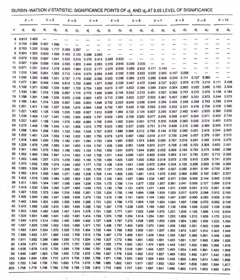
DURBIN- WATSON d STATISTIC: SIGNIFICANCE POINTS OF dL AND du AT 0.05 LEVEL OF SIGNIFICANCE

k' = 2 k' =3 k' =4 k'=5 k' = 6 k'= 7 1<'=8 k' =9 k' = 10

n dv dv du du du du du du du du

6 0.610 1.400

7 0.700 1.356 0.467 1.896

8 o.763 1.332 0.559 un o.368 2.201

9 0.824 1.320 0.629 1.699 0.455 2.128 0.296 2.588 -= 10 0.879 1.320 0.697 1.641 0.525 2.016 0.376 2.414 0.243 2.822

11 0.927 1.324 0.658 1.604 0.595 1.928 0.444 2.283 0.316 2.645 0.203 3.005 12 0.971 1.331 0.812 1.579 0.658 1.864 0.512 2.177 0.379 2.506 0.268 2.832 0.171 3.149 13 1.010 1.340 0.861 1.562 0.715 1.816 0.574 2.094 0.445 2.390 0.328 2.692 0.230 2.985 0.147 3.266

14 1.045 1.350 0.905 1.551 0.767 1.779 0.632 2.030 0.505 2.296 0.389 2.572 0.286 2.848 0.200 3.111 0.127 3.360

15 1.077 1.361 0.946 1.543 0.814 1.750 0.685 1.977 0.562 2.220 0.447 2.472 0.343 2.7.27 0.21,i,1 2 .979 0.175 3.216 0.111 3.438 16 · 1.106 1.371 0.982 1.539 0.857 1.728 0.734 1.935 0.615 2.157 0.502 2.388 0.398 2.624 0.304 2.860 0.222 3.090 0.155 3.304

17 1.133 1.381 1.015 1.536 0.897 1.710 0.779 1.900 0.664 2.104 0.554 2.318 0.451 2.537 0.356 2.757 0.272 2.975 0.198 3.184

18 1.158 1.391 1.046 1.535 0.933 .1.696 0.820 1.872 0.710 2.060 0.603 2.257 0.502 2.461 0.407 2.667 0.321 2.873 0.244 3.073

19 1.180 1 .. 401 1.074 1.536 0.967 1.685 0.859 1.848 0.752 2.023 0.649 2.206 0.549 2.396 0.456 2.589 0.369 2.783 0.290 2.974 20 1.201 1.411 1.100 1.537 0.998 1.676 0.894 1.828 0.792 1.991 0.692 2.162 0.595 2.339 0.502. 2.521 0.416 2.704 0.336 2-885

21 1.221 1.420 1.125 1.538 1.026 1.669 0.927 1.812 0.829 1.964 0.732 2.124 0.637 2.290 0.547 2.460 0.461 2.633 0.380 2.806

22 1.239 1.429 1.147 1.541 1.053 1,664 0,"958 1.797 0.863 1.940 0.769 2.090 0.677 2.246 0.588 2.407 0.504 2.571 0.424 2.734

23 1.257 1.437 1.168 1.543 1.078 1.660 0.986 1.785 0.895 1.920 0.804 2.061 0.715 2.208 0.628 2.360 0.545 2.514 0.465 2.670 24 1.273 1.446 1.188 1.546 1.101 1.656 1.013 1.775 0.925 1.902 0.837 2.035 0.751 2.1:74 0.666 2.318 0.584 2.464 0.506 2.613 25 1.288 1.454 1.206 1.550 1.123 1.654 1.038 1.767 0.953 1.886 0.868 2.012 0.784 2.144 0.702 2.280 0.621 2.419 0.544 2.560 26 1.302 1.461 1.224 1.553 1.143 1.652 1.062 1.759 0.979 1.873 0.897 1.992 0.816 2.117 0.735 2.246 0.657 2.379 0.581 2.513 27 1.316 1.469 1.240 1.556 1.162 1.651 ' 1.084 1.753 1.004 1.861 0.925 1.974 0.845 2.093 0.767 2.216 0.691 2.342 0.616 2.470 28 1.~28 1.476 1.255 1.560 1.181 1.650 1.104 1.747 1.028 1.850 0.951 1.958 0.874 2.071 0.798 2.188 0.723 2.309 0.650 2.431 29 1.341 1.483 1.270 1.563 1.198 1.650 1.124 1.743 1.050 1.841 0.975 1.944 0.900 2.052 0.826 2.164 0.753 2.278 0.682 2.396

30 1.352 1.489 1.284 1.567 1.214 1.650 1.143 1.739 1.071 1.833 0.998 1.931 0.926 2.034 0.854 2.141 0.782 2.251 0.712 2.363

31 1.363 1.496 1.297 1.570 1.229 1.650 1.160 1.735 1.090 1.825 1.020 1.920 0.950 2.018 0.879 2.120 0.810 2.226 0.741 2.333 32 1.373 1.502 1.309 1.574 1.244 1.650 1.177 1.732 1.109 1.819 1.041 1.909 0.972 2.004 0.904 2.102 0.836 2.203 0.769 2.306 33 1,383 1.508 1.321 1.577 1.258 1.651 1.193 1.730 1.127 -1.813 1.061 1.900 0.994 1.991 0.927 2.085 0.8~1 2.181 0.795 2.281

34 1.393 1.514 1.333 1.580 1.271 1.652 1.208 1.728 1.144 1.808 1.080 1.891 1.015 1.979 0.950 2.069 0.885 2.162 0.821 2.257

35 1.402 1.519 1.343 1.584 1.283 1.653 1.222 1.726 1.160 1.803 1.097 1.884 1.034 1.967 0.971 2.054 0.908 2.144 0.845 2.236

36 1.411 1.525 1.354 1.587 1.295 1.654 1.236 1.724 1.175 1.7,99 1.114 1.877 1.053 1.957 . 0.991 2.041 0.930 2.127 0.868 2.216 37 1.419 1.530 1.364 1.590 1.307 1.655 1.249 1.723 1.190 1-.795 ·1.131 1.870 1.071 1.948 1.011 2.029 0.951 2.112 0.891 2.198 38 1.427 1.535 1.373 1.594 1.318 1.6&6 1.261 1.722 1.204 1.792 1.146 1.864 1.088 1.939 1.029 2.017 0.970 2.098 , 0.912 2.180

39 1.435 1.540 1.382 1.597 1.328 1.658 1.273 1.722 1.218 1.789 1.161 1.859 1.104 1.932 1.047 2.007 0.990 2.085 0.932 2.164

40 1.442 1.544 1.391 1.600 1.338 1.659 1.285 1.721 1.230 1.786 1.175 1.854 1.120 1.924 1.064 1.997 1.008 2.072 0.952 2.149

45 1.475 1.566 1.430 1.615 1.383 1.666 1.336 1.720 1.287 1.776 1.238 1.835 1.189 1.895 1.139 1.958 1.089 2.022· 1.038 2.088

50 1.503 1.585 1.462 1.628 1.421 1.674 1.378 1.721 1.335 1.771 1.291 1.822 1.246 1.875 1.201 1.930 1.156 1.986 1.110 2.044

55 1.528 1.601 1.490 1.641 1.452 1.681 1.414 1.724 1.374 1.768 1.334 1.814 1.294 1.861 1.253 1.909 1.212 1.959 1.170 2.010 60 1.549 -1.616 1.514 1.652 1.480 1.689 1.444 1.727 1.408 1.767 1,372 1.808 1.335 1.850 1.298 1.894 1.260 1.939 1.222 1.984

65 1.567 1.629 1.536 1.662 1.503 1.696 1.471 1.731 1.438 1.767 1.404 1.805 1.370 1.843 1.336 1.882 1.301 1.923 1.266 1.964

10 1.583 1.641 1.554 1.612 1.52s~ 1.103 1.494 1.735 1.464 1.768 1.433 1.002 1.401 1.837 1.369 1.873 1.337 1.910 1.305 1.948

75 1.598 1.652 1.571 1.680. 1.543 1.709 1.515 1.739 l.487 1.770 1.458 1.801 1.428 1.834 1.399 1.867 1..369 1.901 1.339 1.935

80 1.611 1.662 1.586 1.688 1.560 1.715 1.534 1.743 1.507 1.772 1.480 1.801 1.453 1.831 1.425 ' 1.861 1.397 1.893 1.369 1.925

85 1.624 1.671 1.600 1.696 1.575 1.721 1.550 1.747 1.525 1.774 1.500 1.801 1.474 1.829 1.448 1.857 1.422 1.886 1.396 1.916 90 1.635 1.679 1.612 1.703 1.589 1.726 1.566 1.751 1.542 1.776 1.518 1,801 1.494 1.827 1.469 1.854 1.445 1.881 1.420 1.909

95 1.645 1.687 1.623 1.709 1.602 1.732 1.579 1.755 1.557 1.778 1.535 1.802 1.512 1.827 1.489 1.852 1.465 1.877 1.442 1.903

100 1.654 1.694 1.634 1.715 ,.613 1.736 1.592 1.758 1.571 1.780 1.550 1.803 1.528 1.826 1.506 1.850 1.484 1.874 1.462 1.898

150 1.720 1.746 1.706 1.760 1.693 1.774 1.679 1.788 1.665 1.802 1.651 1.817 1.637 1.832 1.622 1.847 1.608 1.862 1.594 1.877

200 1.758 1.778 1.748 1.789· 1.738 1.799 •1.728 1.810 1.718 1.820 1.707 1.831 1.697 1.841 1.686 1.852 1.675 1.863 1.665 1.874

B.A.(H) Economics-4th Semester-2018.pdf - Deshbandhu ...

Documents

Transcript of B.A.(H) Economics-4th Semester-2018.pdf - Deshbandhu ...