New Jersey Institute of Technology New Jersey Institute of Technology

Digital Commons @ NJIT Digital Commons @ NJIT

Theses Electronic Theses and Dissertations

Fall 12-31-1991

Analytical methodology for ATM control panel design Analytical methodology for ATM control panel design

Donald C. Johnson New Jersey Institute of Technology

Follow this and additional works at: https://digitalcommons.njit.edu/theses

Part of the Industrial Engineering Commons

Recommended Citation Recommended Citation Johnson, Donald C., "Analytical methodology for ATM control panel design" (1991). Theses. 1285. https://digitalcommons.njit.edu/theses/1285

This Thesis is brought to you for free and open access by the Electronic Theses and Dissertations at Digital Commons @ NJIT. It has been accepted for inclusion in Theses by an authorized administrator of Digital Commons @ NJIT. For more information, please contact digitalcommons@njit.edu.

Copyright Warning & Restrictions

The copyright law of the United States (Title 17, United States Code) governs the making of photocopies or other

reproductions of copyrighted material.

Under certain conditions specified in the law, libraries and archives are authorized to furnish a photocopy or other

reproduction. One of these specified conditions is that the photocopy or reproduction is not to be “used for any

purpose other than private study, scholarship, or research.” If a, user makes a request for, or later uses, a photocopy or reproduction for purposes in excess of “fair use” that user

may be liable for copyright infringement,

This institution reserves the right to refuse to accept a copying order if, in its judgment, fulfillment of the order

would involve violation of copyright law.

Please Note: The author retains the copyright while the New Jersey Institute of Technology reserves the right to

distribute this thesis or dissertation

Printing note: If you do not wish to print this page, then select “Pages from: first page # to: last page #” on the print dialog screen

The Van Houten library has removed some of the personal information and all signatures from the approval page and biographical sketches of theses and dissertations in order to protect the identity of NJIT graduates and faculty.

ABSTRACT

Analytical Methodology for ATM

Control Panel Design

by

Donald C. Johnson

This thesis presents a methodology for control panel design and layout

along with a case study of an automated teller machine (ATM). A predictive

model of human endurance and fatigue is developed from anthropometric,

biomechanical and kinematics research. The layout problem is formulated to

assign controls to locations to minimize the fatigue imposed on an operator

performing a known set of tasks. A family of optimal and near-optimal layouts

are found using conventional algorithms. The final hardware design refinements

are suggested by human factors concerns. Ergonomic guidelines are also

proposed for software aspects of the design. The methods and guidelines can

provide hardware and software designers with useful insights into some human-

machine interface considerations.

ANALYTICAL METHODOLOGY FOR ATM

CONTROL PANEL DESIGN

by

Donald C. Johnson

A ThesisSubmitted to the Faculty of the Graduate Division of the

New Jersey Institute of TechnologyM Partial Fulfillment of the Requirements for the Degree of

Master of Science in Industrial EngineeringDepartment of Mechanical and Industrial EngineeringDivision of Industrial and Management Engineering

December 1991

Copyright © 1991 by Donald C. Johnson

ALL RIGHTS RESERVED

APPROVAL PAGE

Analytical Methodology

for ATM Control Panel Design

by

Donald C. Johnson

Dr. Suebsak Nanthavanij, ThesorAssistant Professor, Division of Industrial and Management Engineering,Department of Mechanical and Industrial Engineering.

Dr. Layek Abdel-Malek, Committee MemberAssociate Chairperson and Professor, Division of Industrial and ManagementEngineering, Department of Mechanical and Industrial Engineering.

Dr. Howard Gage, Comm' ittee MemberAssociate Professor, Division of Industrial and Management Engineering,Department of Mechanical and Industrial Engineering.

BIOGRAPHICAL SKETCH

Author: Donald. C. Johnson

Degree: Master of Science in Industrial Engineering

Date: December, 1991

Undergraduate and Graduate Education:

Master of Science in Industrial Engineering, New Jersey

Institute of Technology, Newark, NJ, 1991.

Bachelor of Science in Industrial Engineering, New

Jersey Institute of Technology, Newark, NJ, 1988.

Major: Industrial Engineering

Professional Positions held:

Chief Engineer, United States Electronics Corp,

Springfield, NJ, 1988-91.

Engineering Supervisor, Cosmo Plastics Company, Long

Branch, NJ, 1977-84.

ACKNOWLEDGEMENT

The author wishes to express his sincere gratitude to Professor Suebsak

Nanthavanij for his expert assistance, valued guidance, and patient support as

advisor.

Special thanks to Professors Layek Abdel-Malek and Howard Gage for

serving as members of the committee, and to Professor Ian Fisher for his technical

assistance.

The author also wishes to acknowledge the other members of the faculty and

staff of the Department of Industrial and Management Engineering and the

Graduate Division at New Jersey Institute of Technology for their support and

assistance during graduate studies.

The author is grateful to the State of New Jersey for the Garden State

Graduate Fellowship award, the proceeds of which served to enable the author to

continue his education and attain his degree goals.

TABLE OF CONTENTS

LIST OF TABLES ix

LIST OF FIGURES xi

1 INTRODUCTION 1

1.1 The General Layout Problem 11.2 Automated Teller Machine Case Study 21.3 Sequence of the Discussion 9

2 LITERATURE REVIEW 12

2.1 Ergonomic Design of Workplaces 122.2 Subjective Layout Techniques 122.3 Heuristic Techniques 13

2.3.1 Logical Evaluation Techniques 142.3.2 Link Analysis Model 16

2.4 Quantitative Techniques 192.4.1 Categories of the Layout Problem 192.4.2 Quadratic Assignment Problem 222.4.3 Special Cases of the Location Problem 242.4.4 Linear Programming Problem 252.4.5 Stochastic Modeling 262.4.6 Markov Activity Models 26

2.5 Human Factors Research 282.5.1 Physical Workplace Dimensions 282.5.2 Controls and Displays 30

2.5.2.1 Keyboards and Keypads 322.5.2.2 Video Display Terminals 362.5.2.3 Character Displays 372.5.2.4 Video Display Viewing Angle 38

2.6 Ergonomics and Biomechanics Research 402.7 Analysis of Manipulator Systems 432.8 Software Ergonomics 43

2.8.1 Response Time 442.8.2 Computer Dialogues 45

2.9 Human Anthropometry and Capabilities 472.10 Automated Teller Machine Studies 48

3 PRELIMINARIES 50

3.1 Overview of Workstation Design 50

vi

3.2 Hardware Control Specifications 523.2.1 Control Accessibility 523.2.2 Ease of Use 533.2.3 Freedom from Errors 53

3.3 Human Factors in Button Selection 543.3.1 Control Physical Parameters 543.3.2 Coding and Labeling 563.3.3 Feedback Characteristics 573.3.4 Standardization 573.3.5 Stereotypes 58

3.4 Control Proximities 583.5 Input Error Rates 583.6 Stochastic Model 60

3.6.1 Classification of States 603.6.2 Steady-state Probabilities 633.6.3 Semi-Markov Process 673.6.4 Goal Programming 67

3.7 Ergonomic Design Factors 693.7.1 Design Population 693.7.2 User Base Skill Level 713.7.3 Defining the Control Panel 783.7.4 Accessibility of Controls 79

3.8 Finding the Optimal Layout 803.8.1 Complexity of the Layout Problem 813.8.2 Types of Assignment Costs 82

3.8.2.1 Motion Costs 823.8.2.2 Position Costs 86

3.8.3 Biomechanical Analysis 883.8.3.1 Human Work Endurance 883.8.3.2 Biomechanical Joint Analysis 90

3.8.4 Arm Kinematic Analysis 913.8.4.1 Forward Kinematics 913.8.4.2 Inverse Kinematics 92

3.9 Determining Optimal Control Location 933.10 Determining Endurance Time Penalty 933.11 Optimization Methods 95

3.11.1 Linear Programming Solution 963.11.2 Linear Assignment Model 973.11.3. Linear Assignment Solution 98

4 METHODOLOGY 104

4.1 Operational Analysis 1054.2 ATM Transaction Models 112

4.2.1 Case I - Ideal Case 112

vii

4.2.2 Case II - Human Error Model 1144.2.3 Case III - Multitransaction Model 1164.2.4 Transaction Conditional Probabilities 118

4.3 ATM Stochastic Models 1204.3.1 Transition Probabilities 1204.3.2 Composite Transition Diagrams 1264.3.3. Composite Transition Matrices 1294.3.4 Steady-State Solution 132

4.4 Arm Kinematics 1344.4.1 Simple Manipulators 1354.4.2 Multiple Link Manipulators 1384.4.3 Inverse Kinematics (Joint Solution) 1414.4.4 Denavit-Hartenberg Algorithm 143

4.5 Formulation of Linear Assignment Model 1454.6 Numerical Arm Solution 146

5 CASE STUDY - ATM CONTROL PANEL DESIGN 148

5.1 Problem Definition 1485.3 Predictive Model of Endurance Time 157

5.3.1 Effect of Force on Endurance 1575.3.2 Effect of Elbow Angle on MVC Force 1605.3.3 Estimating Endurance Time 160

5.4 Linear Assignment Model Formulation 1645.5 Solution of Assignment Model 1705.6 Layout Recommendations 170

5.7 Software Ergonomics 1745.7.1 Video Screen Layout 1745.7.2 Design Simplification 1745.7.3 Social Amenities 1755.7.4 Implicit Input Requests 1755.7.5 Entry Error Handling and Logging 1765.7.6 Global and Local Patterns 1775.7.7 System Default Strategies 1775.7.8 Response-Based Defaults 1785.7.9 Evolutionary Interface 1785.7.10 Multilevel ATM Interface Design 179

6 CONCLUSIONS AND RECOMMENDATIONS 185

BIBLIOGRAPHY 188

APPENDIX 196

viii

LIST OF TABLES

Table Page

3.1 Recommended Physical Parameters for Push-Buttons for Various Modesof Operation 55

3.2 Recommended Physical Parameters for Push-Buttons for SelectedApplications 55

3.3 Expected Keystrokes and Predicted Task Error Rates for ATM KeyingActivities 61

3.4 Sample One-Step Markov Transition Matrix 65

3.5 Markov Transition Matrix after 256th Multiplication 65

3.6 ATM Usage by Selected Demographic Factors 72

3.7 Selected U.S. Population Statistics 74

3.8 Bayesian Analysis of ATM User Population 75

3.9 Motion Costs for Equally-Spaced Controls on a Control Panel of NFeasible Locations 84

3.10 Distance Cost Matrix for 3.0-inch Equally-Spaced Controls on a 12-Control Panel 85

4.1 Input/Output Objects List for Typical ATM 106

4.2 Activity Elements List for Typical ATM 106

4.3 Task Elements and Loci for ATM Transaction Types 110

4.4 Distribution of ATM Activities by Transaction Type 111

4.5 Conditional Probabilities and Distribution of Two Transactions 119

4.6 One-Step Transition Matrix for ATM Withdrawals 124

4.7 One-Step Transition Matrix for ATM Deposits 124

4.8 One-Step Transition Matrices for ATM Transfers 125

4.9 One-Step Transition Matrix for ATM Inquiries 125

4.10 Composite Transition Matrix - Case I 130

4.11 Composite Transition Matrix - Case II 130

ix

4.12 Composite Transition Matrix - Case III 131

4.13 Steady-State Solutions for ATM Models 133

5.1 Computer Solution of Joint Angles 155

5.2 Probability Distribution of Multiple Visits and Expected Visits to EachNode 167

5.3 Location Parameters and Assignment Cost Matrix for Case III 168

LIST OF FIGURES

Figure Page

1.1 Layout for IBM Automated Teller Machines 6

1.2 Layout for NCR Automated Teller Machines 7

2.1 Relationship Chart for Link Analysis 18

2.2 Operational Guide to Layout Problems, Part 1 20

2.3 Operational Guide to Layout Problems, Part 2 21

2.4 Activity Sequence Generator .27

2.5 Workspace Arrangement Guide for Seated Operations 29

2.6 Preferred Dimensions for Standing Workplaces 31

2.7 Numeric Keypad Layouts 33

2.8 Display Legends for Function Keys 35

2.9 Preferred Viewing Angles 39

2.10 Muscular Strength and Endurance Time 42

3.1 Selected Anthropometric Data for Design Population 70

3.2 ATM User Population by Age and Sex 76

3.3 ATM User Population by Education and Income 77

3.4 Three Control Arrangements with Identical Motion Costs 87

3.5 Force Available at Various Elbow Configurations 89

3.6 Computer Solution of Assignment Problem by ASGN 103

4.1 Typical ATM Session Flowchart 108

4.2 Forced Exit ATM Session Flowchart 109

4.3 ATM Activity Sequences (Case I) 113

4.4 ATM Activity Sequences (Case II) 115

xi

4.5 ATM Activity Sequences (Case III) 117

4.6 ATM Transition Diagram (Case I) 122

4.7 ATM Transition Diagram (Case II) 127

4.8 ATM Transition Diagram (Case III) 128

4.9 Coordinate Frames for Simple Manipulator 136

4.10 Link Coordinate Systems for Six-Joint PUMA Arm 140

4.11 Transformation Matrices for Six-Joint PUMA Arm 140

4.12 Two-Link Articulated Ann 142

5.1 Heights of 5th Percentile Female Stewardesses 149

5.2 Link Lengths for 5th Percentile Females 149

5.3 Reference Planes for Standing Operator 151

5.4 Control Panel Dimensions 153

5.5 Range of Motion for Upper Body 154

5.6 Endurance Time and Percentage of MVC 159

5.7 Endurance Time and Percentage of MVC 159

5.8 Graph of Isometric Force vs. Elbow Angle 161

5.9 Available Force (A) at Selected Joint Angles (f) 163

5.10 Relative Force (R) at Selected Joint Angles (f) 163

5.11 Predicted Endurance Times and Fatigue Rates 165

5.12 Forced Exit ATM Session Flowchart 166

5.13 Layout for ATM Control Panel #1 171

5.14 Layout for ATM Control Panel #2 171

5.15 Layout for ATM Control Panel #3 172

5.16 Layout for ATM Control Panel #4 172

xii

5.17 Preferred Layout for ATM Control Panel 173

5.18 Default ATM Top Level Menu Provided to All Users 180

5.19 Individualized ATM Top Level Menu 180

5.20 Flowchart for an Adaptive User Proficiency System 184

CHAPTER 1 INTRODUCTION

1.1 The General Layout Problem

In general, several approaches have been used in designing and planning

the layouts of various types of facilities. Several qualitative and quantitative

techniques traditionally employed in general layout problems are considered. In

general, subjective techniques based on heuristics yield suboptimal results, while

optimization methods such as quadratic assignment or goal programming give

exact solutions, but are too computationally complex for use on practical

problems.

It is conjectured that many control panel layout problems are of a class

that allows optimization by special methods. When transportation costs are

insignificant, less complex linear optimization algorithms can find an optimal

arrangement of controls. The proposed objective function assigns controls to

locations within a user's reach envelope, with the goal of minimizing the level of

fatigue experienced by the human operator.

A methodology is presented whereby a set of costs is developed as a

function of the human body's positions in performing a given set of tasks. The

costs are determined from the well known relationship between endurance time

and the fraction of a muscle's maximum voluntary contraction (MVC) imposed

by the task (Caldwell, 1964). As MVC varies with body configuration, the

endurance time can be predicted for any point in the range of motion.

1

From anthropometric data and kinematic analysis, the specific configuration -

hence endurance time - is predicted for each feasible control location.

A series of optimal layouts are found and the final hardware design

refinements are suggested by human factors and other considerations. Other

ergonomic guidelines are proposed for the software aspect of the design. The

developed guidelines can help provide hardware and software designers with

useful insights into some practical human-machine interface design

considerations.

1.2 Automated Teller Machine Case Study

An automated teller machine (ATM) is a computerized device comprised

of mechanical and electronic components which permits users to conduct simple

banking and other financial transactions. Without the need for the assistance of a

human teller, the users, who are members of the general public, can make

deposits, withdrawals, transfers, and account queries at any time during or

outside of the regular business hours of the financial institution.

Originally, the ATM machine was introduced to solve the problem of ever-

increasing costs to financial institutions for processing some routine transactions

and delivering services to consumers. Over the past decade, the trend in the

banking industry has been to install ATMs in increasing numbers in order to

reduce the necessity of using human tellers for those transactions. Successful

implementation of this strategy will relieve customer-contact personnel of menial

2

paper shuffling tasks and allow tellers and other platform personnel to provide

other services or perform complicated transactions.

In recent years, ATMs have come into very wide use, with 75,000 units

installed in the United States, representing a capital investment of more than $4

billion, and annual operating and maintenance expenses of over $300 million.

However, the utilization rate of currently installed ATMs (14%) has fallen far

short of the system's potential productivity of one transaction per minute

(Haynes, 1990).

Although the locations of ATMs are typically at the banks, either indoors

(in a bank lobby) or outdoors (through-the-wall), they are also frequently found

in shopping malls or supermarkets in a stand-alone island. Furthermore, "drive-

thru" ATMs which can be operated from the driver's seat of an automobile are

available in some areas.

Currently, there are several types of ATMs in use due to different

manufacturers. Among the approximately eight ATM manufacturers, the largest

three, namely Diebold, International Business Machines (IBM), and National

Cash Register Company (NCR), account for the majority of the installed base.

Depending on the manufacturer and type, the cost of a single remote ATM unit

usually ranges between $30,000 and $67,000 (plus installation and repair or

maintenance contracts). The costs of computer and network communication

services and in-house or third party loading and unloading services are additional.

3

There are several computerized banking systems in existence today. The

two largest networks, Cirrus Systems, Inc., a division of MasterCard and Plus

Systems Inc. together serve a total of 425 million card holders (Seidenberg, 1990).

The hardware and software configurations of the actual ATM terminals

belonging to the competing communications networks appear functionally to be

nearly identical. Of the 75,000 machines, 92.8% are on-line - connected to the

network of mainframes - and have access to customer banking records (van der

Velde, 1982).

While the designs and features of ATMs can vary depending on the

manufacturer, certain basic component parts are commonly found on all ATMs.

They are as follows:

* Input devices

- Magnetic card readers

- Push buttons

- Keypads and Keyboards

- Touch sensitive screens

* Output devices

- Cathode Ray Tubes (CRTs)

- Electroluminescent Displays (ELDs)

- Light Emitting Diode (LED) displays

* Dispensing and intake devices

- Cash dispensing mechanism

- Receipt printing and dispensing mechanism

- Deposit acceptance chute or mechanism

4

* Convenience features

- Storage area for deposit envelopes

- Pen for filling out deposits

- Writing area

It is likely that an ATM user will encounter several types of machines in

the normal course of travels within a relatively small radius. There are two main

reasons for this. First, the distribution of ATM types appears to be uniform,

rather than geographically stratified, meaning that a wide variety of machines are

found in a limited area. Second, a primary purpose of ATMs is to permit banking

transactions to be performed anywhere, and ATM usage patterns indicate that a

significant portion of transactions occur at "foreign" locations. Consequently, it

is expected that a typical user will frequently use, at these foreign locations, a

variety of ATMs with different designs from any of the several manufacturers.

An initial cursory examination of several different ATM models indicates

that control designs, layouts and operating procedures for different ATM models

show little or no standardization. The physical layout, types of controls and

displays, and the operating software for these units are found to vary widely

between models and manufacturers. Figures 1.1 and 1.2 depict typical layouts for

some major ATM models.

With the recent widespread proliferation of ATMs, there has apparently

not been a comparable increase in ergonomically efficient hardware and software

designs.

5

6

Figure 1.1 Layout for IBM Automated Teller Machines.

Figure 1.2 Layout for NCR Automated Teller Machines.

7

The users of ATM machines often find that their productivity level, as well

as their satisfaction, is adversely affected by poor workplace design and layout,

inconsistent operating procedures, confusing screen displays, and intolerant data

entry and error handling procedures. In order to attain the highest utilization

rate of the entire ATM system, the performance of operators at all levels must be

maximized. Through a proper ergonomic design, performance degradation can

be reduced, resulting in higher ATM system utilization, better operator

performance rates, and an increase in satisfaction (Haynes, 1990).

The purpose of this thesis is to develop a set of design guidelines for

ATMs' hardware and software interfaces by incorporating ergonomic principles.

Included in this work are methods for selecting and implementing practical

routines to provide optimal or near-optimal layout of ATM control panels,

keyboards, and screen displays. In addition, dialog scripts, data entry techniques,

fault-tolerant error handling routines, and other practical techniques for

improving the software determined aspects of the human-machine interface will

be addressed.

With emphasis on physiological, perceptual and cognitive psychological

factors, certain quantitative methods are discussed on how to evaluate human-

machine interfaces in order to measurably enhance their user friendliness. The

developed guidelines can be applied to a variety of human-machine interface

design problems.

In the course of studying the ergonomic design of ATMs, various

interdisciplinary qualitative and quantitative techniques of analysis and

8

optimization are employed. It is anticipated that the methods used and results

achieved may find wider application in the design and analysis of other types of

control panels and work environments in general.

1.3 Sequence of the Discussion

The discussion of the ATM layout procedure that follows will be

organized according to the following sequence. First, the ATM layout problem is

defined, starting with determination of the expected user population, typical

activity sequences, transaction distributions, and other overall system functional

specifications.

Next, the overall workstation size and shape is selected based on the

practical requirements and the anthropometry of the user population. The

problem is reduced to a finite set of feasible control sites, and a basic set of

controls is selected in accordance with general ergonomic guidelines.

From the given initial workstation envelope, layouts are defined using

various techniques. Several conventional methods for facilities and control panel

layout are discussed, such as experimental trial, link analysis, CORELAP, etc. are

discussed. The design objective of these methods is generally to minimize the total

motion cost, which is defined as the sum of individual inter-control distances (or

travel times) in performing a given function.

9

A methodology is developed which involves the determination of a set of

costs as a function of the human body's positions in performing a set of tasks.

From the expected probabilities for each type of transaction, and knowing the

type of control needed for each transaction, the system is modeled as a stochastic

process. By using simple calculations, the limiting behavior - or steady-state

condition - of the system is found. From the steady-state solution, an indication

of the percentage of time spent by the operator in manipulating each control can

be found.

Using established principles of biomechanics, the position cost factor is

developed. For each feasible control location, position costs as defined in terms

of reduced work capacity will be computed. The sets of joint angles required to

reach each point are computed by the technique of inverse kinematics. Given

each location's joint angles, and from anthropometric and biomechanics data, a

corresponding position cost is derived in terms of predicted endurance reduction.

Once the position cost coefficients are determined, suitable methods are

used to find the optimal control assignment. The optimal arrangement is that

which minimizes the sum of position costs in performing a specific set of activity

sequences.

After the control assignments are made and the hardware design is

complete, the emphasis shifts to the software component. Recommendations are

offered for providing an efficient operator interface. Types of screen displays and

dialog scripts are discussed. A discussion follows concerning the concept of a

flexible interface which can adapt to the needs of the user.

10

Finally, a case study of an ATM design is presented. Intermediate

numerical solutions are found using the proposed techniques, and a final design

recommendation is proposed.

11

CHAPTER 2 LITERATURE REVIEW

An analysis of techniques for the design and layout of ATMs suggests that

several subject areas be explored. Specifically, literature references are

concentrated into the following general areas: systems analysis, workplace and

control panel layout, human engineering and biomechanics, operations research,

and robotics.

2.1 Ergonomic Design of Workplaces

There has been extensive work done in the area of ergonomic design of

workplaces and control panels (Van Cott & Kinkade, 1972; Woodson, 1981;

Rodgers et al., 1986). Very few specific reports on the design of ATMs are found

in the literature; nevertheless, several studies in related design issues do exist.

They are either in the areas of general layout or endeavor to solve specific layout

problems in some complex environment, such as an air traffic control center.

2.2 Subjective Layout Techniques

In many cases, control panel designs have been developed solely on the

basis of subjective opinion rather than an objective methodology. In the

experimental studies of control console design of Morant (1954), a four-step

12

technique is employed. The procedure, called the "Method of Experimental

Trials," can be described as follows. Initially, a mock-up of the workplace to be

studied is constructed. Then, appropriate subjects from the user population are

selected to perform suitable tasks. Observations of the performance and results

are collected in terms of speed, accuracy, etc. Finally, the quality of the console

design is determined from the results. A study showing the comparison of four

different designs, gives users and evaluators the opportunity to rank them with

"preference rankings" from 1 to 4 (Siegel and Brown, 1958). Although some

successful layouts have been developed, results have been inconsistent using this

technique.

2..3 Heuristic Techniques

Heuristic and quasi-quantitative solutions to the layout problem are found

in the literature. Nugent et al. (1968) give an experimental comparison of four

techniques for the assignment of facilities to locations. They discuss the

difficulties in finding an optimal solution and give examples of the computational

efficiencies of various methods of solving problems of small to moderate

complexity. A method for assessing the theoretical lower bounds in quadratic

assignment problems is proposed by Francis and White (1974). A heuristic to

find the approximate solution to the assignment problem is provided by West

(1983). Abdel-Malek and Li (1990) used inverse kinematics and an extension of

the Traveling Salesman algorithm (Held and Karp, 1970) to find the optimal

sequencing of robot tasks in automated work cells.

13

The computer-aided design of facility and workplace layout based on the

inter-element relationships between components is the subject of ALDEP,

CORELAP (Lee and Moore, 1967), and CRAFT (Francis and White, 1974).

Other computerized techniques include WOLAP (Rabideau and Luk, 1975),

PLANET (Apple, 1977), and DISCON (Drezner, 1980). Entire factories and

industrial buildings are laid out based on the strength of the associations between

functions of the departments comprising them. The cost functions generally are

computed from a weighted sum of the center distances between workplace

elements. More recent techniques in workplace layout are described in

McCormick and Wrennall (1985).

2.3.1 Logical Evaluation Techniques

Bonney and Williams (1977) developed a computer software program,

CAPABLE (Control And Panel Analysis By Logical Evaluation), to solve certain

simplified control panel layout problems. The problem formulation involves

positioning n controls into m available locations, where n is not greater than m, in

order to maximize or minimize some objective function. In an example, an

objective function is defined to minimize the total distance traveled or time taken

to perform a predefined set of tasks. The program enumerates and evaluates all

feasible solutions and eventually finds the optimum configuration. However, as

the number of controls and locations increases, so does the complexity of the

problem in terms of the number of feasible solutions.

14

Two situations can occur in the control layout problem. First, the number

of controls (n) can precisely match the number of feasible locations (m). In this

case where n = m, the number of feasible solutions will be n!. The other case is

when the number of controls is less than the number of feasible locations (n < m).

In this instance, the number of solutions will be m! / (m-n)! It is apparent that,

even in greatly simplified problems where n and m are relatively small, optimal

solutions may be extremely difficult to obtain by totally enumerating using this

algorithm.

Formal techniques for systems analysis and design by breaking down into

and processing the elements in the form of lists were described by Phillips (1987).

For the operation being studied, the elements are contained in one of two lists -

verbs (actions or activities), and nouns (objects or locations) manipulated or

visited during operation. Monte Carlo type operational simulations of actions

and activities have been applied in order to analyze stochastic systems and to

determine statistical results (Metropolis and Ulam, 1949).

There have been attempts to measure quantitatively the accessibility of

controls for human operators. By objective evaluation, judgements can be made

based on comparisons of various layouts. Banks and Boone (1981) introduced

the concept of an "Accessibility Index" as a method for quantifying control

accessibility. The index takes into account the operator's reach envelope and the

frequency of use of the particular control.

15

2.3.2 Link Analysis Model

Link analysis is a systematic procedure for studying and planning human-

machine and machine-machine systems based on the strength of links between

components. The term link refers to "any connection between a man and a

machine or between one man and another" (Van Cott and Kincade, 1972). The

purpose of link analysis is to optimize the links contained within a system. Link

analysis techniques have been employed by Champanis (1959) to assist in the

redesign of workplaces in a shipboard combat intelligence center. McCormick

(1970) also employed link analysis techniques in the studying of eye movements of

pilots. The research led to the increased standardization of arrangements of

aircraft instrument panels. Applications of link analysis procedures in control

panel layout problems are described in Cullinane (1977). Examples are given of

charting and computerized methods for designing the layout of facilities for a

computer center.

Link values are established between workplace elements according to the

relative frequency of the operator going from one element to another,

communication frequencies, and relative importance. Alternative designs are

considered by rearranging their locations, redrawing, and recomputing the link

values for evaluation (Kantowitz and Sorkin 1983).

A four step procedure is followed in performing a link analysis as follows

(Cullinane, 1977):

16

1. Using symbols, develop a diagram showing all interactions between

people and equipment.

2. Examine all relationships and establish link values.

3. Develop a preliminary link diagram.

4. Refine the link diagram and state the final layout.

A relationship chart as shown in Figure 2.1 is created to show the

interrelationships of workplace activities. The symbols A, E, I, 0, U, and X,

entered in the upper triangles describe the link strengths according to the

following:

A: Absolutely essential for the two activities to be located close together.

E: Essential for the two activities to be close together.

I: Important that the two activities be close together.

0: Ordinary closeness is acceptable for the two activities.

U: Unimportant if the two activities are placed close together, or a link

does not exist.

X: It is undesirable for the two activities to be placed together.

17

Figure 2.1 Relationship Chart for Link Analysis (Adapted from. Cullinane,1977).

18

2.4 Quantitative Techniques

Other, less subjective approaches to the layout of control panels and other

general layouts have been addressed. An examination of the layout problem in

perspective and a methodology for selecting which analytical tools to employ is

given in Vollmann and Buffa (1966). An operational guide to the analysis of

layout problems is presented as shown in Figures 2.2 and 2.3.

Nedungadi and Kazerouinian (1989) suggests that certain problems may

be decomposed, or split into smaller subproblems to facilitate solution. That is,

given the set of controls used by each member, heuristic rules are applied and

each set optimized. Then, individual results are recombined to obtain a global

"pseudo-optimal" which may approximate the exact optimal solution.

2.4.1 Categories of the Layout Problem

Hendy (1989) suggests that there are three basic categories of the layout

problem. Category I problems are of such large scale that they are beyond

human perception. Examples include the locating of departments within a large

facility and the locating of buildings within a geographical area. Category II

problems are of moderate scale and within the range of human perception; for

example, the layout of a factory department or an office. Category III problems

are of small scale and within the immediate range of perception. The layout of

operator workstations and instrument panels fall into the realm of

19

20

Figure 2.2 Operational Guide to Layout Problems, Part 1. (Adapted fromVollmann and Buffa, 1966).

21

Figure 13 Operational Guide to Layout Problems, Part 2. (Adapted fromVollmann and Buffa, 1966).

category III problems. Although in individual situations this may not be the case.

In general, category I problems are those in which the costs of transportation

from location to location are critical in the decision process; and category III

problems are those in which transportation is less significant.

2.4.2 Quadratic Assignment Problem

The problem of assigning m facilities to n locations has been formulated as

a quadratic assignment problem, or QAP (Koopmans and Beckmann, 1957). The

basic form of the quadratic assignment problem is to find the values of xij which

minimizes the total cost of all assignments, where:

c.• = the cost per unit time associated withassigning work center i to location j.

dij the distance from location i to location j,appropriately adjusted to measure the costof travel from location i to location j.

fij = the work flow from work center i to workcenter j.

Si = the set whose elements are the locations towhich work center i may be assigned.

The assumption is made that m is not greater than n, or, for the sake of

generality, that m = n since (n m) dummy work centers can be introduced.

The general format of the quadratic programming model is stated as

follows (Hillier and Connors, 1966):

22

subject to,

Where:

23

The case of infeasible assignments is avoided by assigning a very large

number to cij whenever j is not an element of Si. Since the goal of the objective

function is to minimize Z, infeasible assignments will not be included in the final

solution unless the solution itself is infeasible.

There are several quadratic assignment algorithms reported in the

literature. Gilmore (1962) and Lawler (1963) present algorithms to find optimal

assignments, however their complexity is such that they are computationally

feasible for small scale problems (n < 15). Several suboptimal QAP algorithms

are available and two versions are submitted by Hillier and Connors (1966). One

algorithm deals with the general quadratic assignment problem, and the second

deals with the special case in which travel costs are proportional to the

rectangular distances between them. The complexities of these algorithms are,

respectively, ns and n4. Other algorithms can find the exact solution to the

assignment problem with orders of complexity of n 3 (Lawler, 1976) and n 2 log n

(Karp, 1980). Finding exact solutions to larger scale problems by these methods

may still be cost-prohibitive for n > 15 (West, 1983).

It has been shown (Hitchings, 1968) that assignment costs follow a normal

distribution even in QAP problems as small as n = 5. Nanda and Weingarten

(1974) suggest that a formula can be used to calculate the statistical parameters of

all n! assignment costs without the need for enumerating each one. A heuristic

method for assessing the efficiencies of QAP solutions is proposed, based on their

percentiles in the normal distribution (Khaopravetch and Nanda, 1990).

2.4.3 Special Cases of the Location Problem

Hillier and Connors (1966) identify two special cases of the facilities

location problem.

1. Independent work centers are assigned to heterogeneous locations.For example, the m work centers are unrelated in that no work flowsoccur between them, and cost is entirely unaffected by their relativeproximities.

2. Interrelated work centers are assigned to homogeneous locations.Cost is determined by the relative proximities of the respective workcenters, rather than the locations to which they are assigned.

24

In problems of the first type, costs of work flows are insignificant or

nonexistent and the problem can be formulated and solved as a linear assignment

problem. It is conjectured that the ATM and certain other control layout

problems belonging to Category III (Hendy 1989) can be modeled as a special

case (of independent work centers), and solved by linear programming or linear

assignment methods.

2.4A Linear Programming Problem

A solution to the layout problem based on modeling and solving by linear

programming, was found by Freund and Sadosky (1967), who optimized the

assignment of 8 control devices into 8 feasible locations. The objective function in

this problem was defined as the Utility Cost Rating, and was computed by

multiplying the frequency by the accuracy of response. The results show that

solution of these problems can be accomplished by several linear programming

algorithms. Formulation and solution as a simplex problem was attempted, but

the structure of constraints was found to be too complex to be efficiently

implemented. Instead, it is recommended that either the transportation algorithm

or the assignment algorithm be used (McCormick, 1970).

25

2.4_5 Stochastic Modeling

Methods of studying systems by stochastic modeling are abundant in the

literature. The basic elements of probability theory and some of its applications

are discussed in Cramer (1955). The mathematical basis of various operations

research techniques in optimization of stochastic systems are given in Saaty

(1959). Analytical techniques and solution methods for specific types of

stochastic model applications are discussed in Bhat (1984).

2.4.6 Markov Activity Models

A finite number of states and discrete sequences of events can be modeled

using an Activity Sequence Generator. The analysis of the sequencing of control

activities by their expected sequence of actions was described by Miller et al.

(1981). An event-based Markov activity sequence generator was constructed in

order to study the tracking behavior and capture times for eye-to-target

situations. In a typical Activity Sequence Generator diagram (Figure 2.4), the

circles represent the different states of the system (nodes), and the directed paths

(arcs) represent internodal transitions between states. The number on each arc

denotes the probability of transition from source to destination node, given that

the system has entered the source node (Miller et al., 1981).

26

Figure 2.4 Activity Sequence Generator (Adapted from Miller, Jagacinski,Nalavade, and Johnson, 1981).

27

2.5 Human Factors Research

Purely quantitative methods which solve the layout problem by time or

motion minimization are suitable for many applications, such as facilities and

department layouts. However, these techniques often do not address the human

factors concerns which may dominate in the class of problems of which control

panel and other small scale category III layout problems are a member (see

Section 2.4.1).

Recommendations for equipment and workplace design have been

addressed in the ergonomics and human factors literature. A thorough treatment

of the subject and presentation of a set of guidelines for the ergonomic design of

equipment is the subject of Van Cott and Kinkade (1972), Rodgers et al. (1986),

and Konz (1990). Comprehensive sets of design heuristics based on scientific

research have been developed.

2.5.1 Physical Workplace Dimensions

Workplace arrangement guides presented in the literature are used in

determining the preliminary physical layout and dimensions of the workplace.

The "Human Engineering Guide for Army Material" (Department of Defense,

1981) includes a workspace arrangement guide showing optimal manual control

locations for seated operations as shown in Figure 2.5. Recommendations for

desired dimensions and shapes for standing workplaces are reported by Woodson

et al. (1972). The preferred locations for primary and secondary visual displays,

28

Figure 2.5 Workspace Arrangement Guide for Seated Operations (Reproducedfrom MIL-HDBK-759A, U.S. Department of Defense, 1981).

29

keyboards and other operating controls have been defined, with an example of a

suggested workplace for a standing operator as given in Figure 2.6. Konz (1990)

lists fourteen guidelines for the physical design of general purpose workplaces.

2.5.2 Controls and Displays

Control and display guidelines are available to assist in the selection and

specification of controls and displays for operator workstations based on the

functions to be performed. The literature in the human factors area also contains

numerous references concerning recommended control design. Certain

ergonomic physical design parameters such as control type, size, shape, color,

spacing, operating force requirement, displacement, feedback properties, etc, have

been determined for several specific types of typical controls such as individual

push-buttons, keyboards and keypads (Tillmann and Tillmann, 1991).

Ergonomic aspects of push-button switch operators are discussed in

Moore (1975). Various types of buttons used in several different applications and

methods of operation are covered. In one example it is suggested that buttons for

one finger operation should be a minimum of 13 mm (0.5 inches) in diameter with

separation of at least one diameter.

The use of arrayed touch screens to simulate full-scope control panels is

discussed in the literature. Reason (1989) describes a powerplant application in

which six CRTs in a 10-foot space replaced a 24-section bank of conventional

controls and instruments. In aircraft flight decks, multiple CRTs and

30

31

Figure 2.6 Preferred Dimensions for Standing Workplaces (Adapted fromWoodson et al., 1972).

sophisticated control display software are being introduced to the "glass cockpits"

of the latest generation airliners such as Boeing 747-400 and 777 (Hughes, 1989;

Scott, 1991).

2.5.2.1 Keyboards and Keypads

For alphabetic and numeric entries, several buttons are grouped together

into keyboards or keypads. The subject of much study, numeric keyset designs

typically follow one of two major patterns. The touch telephone numeric keyset

has the lowest numbers at the top, while the adding machine numeric keyset has

the lowest numbers at the bottom as shown in Figure 2.7. Recommendations

regarding the design of push-button keyset are given by Lutz and Chapanis

(1955), and Deininger (1960). They state that in most applications the adding

machine layout is preferred, since the most frequently keyed numbers are at closer

position to the operator.

In both alphanumeric keyboards or numeric keypads, Alden et al. (1972)

recommend that key centers should be 19 mm (0.75 in.) apart, and that the key

tops should be 12 mm (0.47 in.) square. The force needed to activate the key

should be from 0.3 to 0.75 N (1.0 to 2.5 oz.). Additionally, the vertical key

displacement may range from 1.3 to 6.4 mm (0.05 in. to 0.25 in.). Membrane

keyboards and keypads, suitable for occasional and low frequency applications,

are typically flat and have very short displacement, although full-travel raised

membrane keyboards are reportedly now available (Bishop, 1980).

32

Figure 23 Numeric Keypad Layouts (Adapted from Lutz and Chapanis, 1955).

33

Special function keys can provide significantly improved operator

performance for advanced users. Function keys can be either hard wired and

predefined, or programmable and changeable. Hard wired function keys are

simple to implement, but can restrict future upgrades to the system. On the other

hand, programmable function keys have the advantage of flexibility; functions

can be added or reassigned by changing the software. However, system users,

particularly novices, can become confused and irritated if continuity is sacrificed

in favor of innovations or "enhancements" of dubious value (Morland, 1983).

In any case where function keys are adopted, they must be clearly

identified, either by permanent markings or by nonconfusing screen display

legends. Some examples of typical implementations of hard wired and

programmable function keys legends are given in Figure 2.8. Improved designs

incorporating generally accepted ergonomic principles (Kantowitz and Sorkin,

1983) are also given in Figure 2.8.

34

35

Figure 2.8 Display Legends for Function Keys.

2.5_2_2 Video Display Terminals

Basic design rules for video display terminals (VDTs) are available. First,

the VDT display color is considered. The human eye sensitivity is greatest for

light with a wavelength of around 555 nanometers (nm). Therefore, a green (550

nm) display color is preferred over an amber (600 nm) color, according to

Willeges and Willeges (1982).

After the display color is established, the optimal spacing between pixels

can be found. The pixel diameter (d) is found according to the formula:

d= 1.22 X, V / D (2.5)

where:

d = pixel diameter

= wavelength of light

V = viewing distance (eye to display surface)

D = eye diameter (from anthropometric data)

In a typical case with light of 550 nanometer (nm) wavelength, a viewing

distance of 500 mm, and an eye diameter of 0.6771 mm, the formula in Equation

2.5 gives the preferred pixel diameter of 0.54 mm (Willeges and Willeges, 1982).

36

2.5.2.3 Character Displays

The preferred specifications for the characters displayed on VDTs have

been reported. Minimum character height should be 3.0 mm, width should be 2.1

mm, and stroke - or thickness of lines forming the characters - should be 0.45 mm.

The characters ideally should be spaced 0.9 mm apart, with 3.0 mm to 4.5 mm

(100 to 150 percent of character height) between lines (Willeges and Willeges,

1982).

Konz (1990) reports that character text displayed on VDTs is more

readable if the lines are double-spaced and unjustified (ragged right). Reading

speeds are found to be improved by a factor of 11 percent over single-spaced text

and lines with flush margins.

Tullis (1983) recommends four rules for formatting VDT screen menus:

Minimize frame density - fill no more than 25 percent of the available

screen positions with characters.

2. Provide spacing between items with blank spacing double-space text

and separate groups by 3 to 5 spaces.

3. Group related items together.

4. Minimize layout complexity - left justify words, right justify numbers

on the decimal, and display lists either alphabetized or in priority

order.

37

2.5.2.4 Video Display Viewing Angle

The literature references describe the preferred viewing angles of visual

displays with respect to a "standard" or "normal" line of sight. Van Cott and

Kinkade (1972) propose that primary displays be located within 15 degrees of the

normal line of sight (10 degrees below the horizontal). Woodson (1972) and

Woodson (1981) suggests that visual targets be placed between 10 degrees above

and 20 degrees below the normal line of sight (declined 10 degrees below

horizontal). The military standard for equipment design defines the normal line

of sight as 15 degrees below the horizontal, with preferred viewing angles between

+15 and -15 degrees of that line (U.S. Department of Defense, 1981). Another

recommendation for "optimal eye rotation" (McCormick and Sanders, 1982) is

within 15 degrees above or below the normal sight line (declined 15 degrees below

horizontal). Experimental determination of preferred line of sight (Hill and

Kroemer, 1986) confirms that (at 1.00 m) the normal viewing angle should be 30.1

degrees below the horizontal anthropometrically defined Frankfurt plane (Figure

2.9).

38

39

Figure 2.9 Preferred Viewing Angles (Adapted from Van Cott and Kinkade,1972; Woodson, 1972; Woodson, 1981; U.S. Department of Defense, 1981;McCormick and Sanders, 1982; and Hill and Kroemer, 1986).

2.6 Ergonomics and Biomechanics Research

The problem of determining workplace design standards from the

viewpoints of biomechanics and human work endurance has been addressed in

the literature. The biomechanical basis of ergonomics is the subject of Tichauer

(1978).

Experimental work on muscle fatigue and endurance versus the workload

levels was done by Rohmert (1960), and confirmed by Hayward (1975). The

relationship between work endurance and level of applied muscular stress was

stated by Simonson and Lind (1971) and Morton (1987). They report that

endurance time for an activity can be stated as a function of the percentage of the

activity's maximum muscular capacity.

Caldwell (1962) conducted experimental studies to determine the effects of

various body positions on the maximum force applicable to a hand control. The

results show that body postures and joint angles are major factors in the

production of usable muscle forces. Various anthropometric studies by Parker

and West (1973) and Roebuck et al., (1975) have provided much detailed data

regarding the human body and its muscular strength and endurance capabilities.

Wiker et al., (1989) discuss the effects of nonpreferred arm locations on human

movement, reach, and positioning capabilities. They conclude that the significant

posture-based decrements in performance were found to be independent of the

strength capabilities of the individual subjects studied.

40

Strength is defined as "the maximal force muscles can exert isometrically in

a single voluntary effort" (Kroemer, 1970). In isometric exertion, the length of

the muscles is kept constant during the period of muscle contraction. When the

muscle lengths do not change, the body segments remain motionless and a static

condition exists. Static measurements of human strength are limited to a period

of less than 10 seconds to eliminate the effects of muscular fatigue.

The experiments of E. A. Mueller in the 1930's show that the endurance

time depends on what fraction of the exertable force is required. This relationship

is also demonstrated by Caldwell (1962) and Caldwell (1964). Figure 2.10 depicts

the nonlinear relationship between time and functional strength. While maximal

strength (by definition) can be maintained for only 10 to 15 seconds, less that 15

to 20 percent of total strength can be maintained for an "indefinite" period

(Kroemer, 1970). Experimental studies of physiological responses and endurance

times have been performed for lifting with leg muscles (Genaidy and Asfour,

1989; Genaidy, et al., 1990), and for prolonged arm lifting (Asfour, et al., 1991);

showing that responses over short durations were not significantly different from

those over longer durations.

Human biomechanical models are developed by Chaffin (1969), in which

forces and torques are calculated for a three-link representation of the human

arm. The validity of techniques for modeling worker strengths is confirmed by

Chaffin, et al., (1987). The biomechanical model of the human aim, and arm

movement capabilities are presented by Wiker, et al., (1989). A computerized 3-D

biomechanical model is used to predict static strength and to determine the

segment of the population able to perform a given task (Chaffin and Erig, 1991).

41

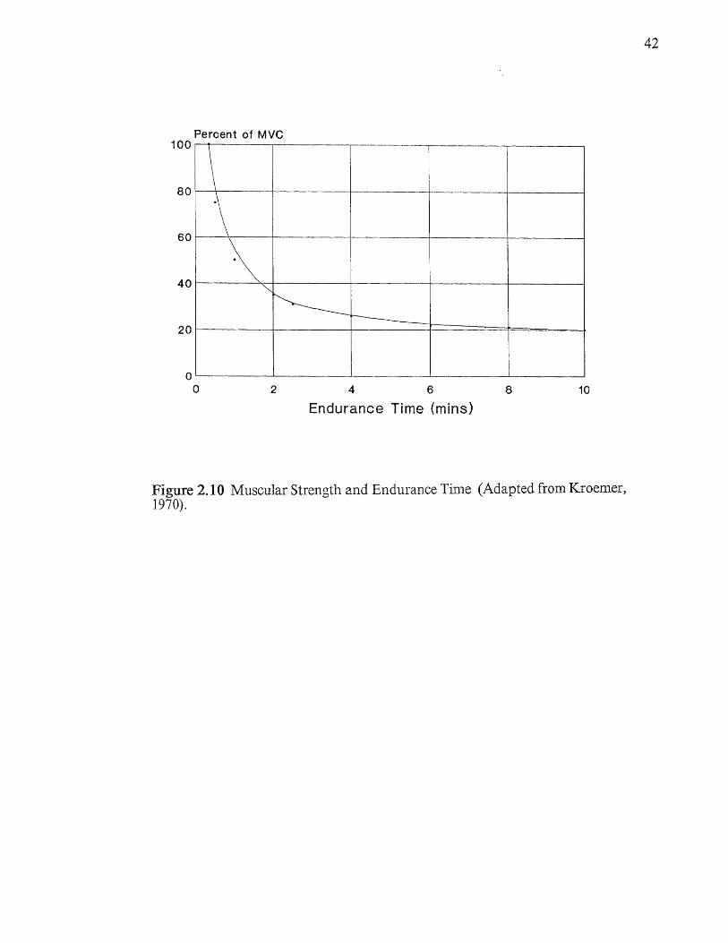
Figure 2. 10 Muscular Strength and Endurance Time (Adapted from Kroemer,1970).

42

23 Analysis of Manipulator Systems

A strictly mechanical analog to the human operator is a robotic

manipulator system. A method of representing coordinate systems for multiple

link manipulators is described by Denavit and Hartenberg (1955), in which a 4 x 4

homogeneous transformation matrix is established to represent each link's

coordinate system with respect to the previous link's coordinate system, beginning

at the base and continuing until the end effector is reached. The description of

robot coordinate systems and transformations and generalized techniques of

solution are attempted by Paul (1981) and Paul (1982). The mathematical

analysis of the robot arm based upon direct and inverse kinematics and dynamics

is given by Lee (1982). A simplified solution method for specific robot

configurations such as the six degree-of-freedom PUMA robot is included.

Improved methods for solving the general inverse kinematics problem are given

by Goldenberg (1985). Other techniques and simplified algorithms for motion

planning and control for certain robots are described by Schwartz and Sharir

(1988).

2.8 Software Ergonomics

Software design guidelines are available to detail how computer software

should interact with human operators. The topic of software ergonomics is

widely addressed and covered in literature from the fields of computer science and

human factors. A comprehensive set of human factors guidelines for the design

43

of computer terminal interfaces is provided in Morland (1983). Strategies for

assigning system defaults are proposed and the new concept of statistically

generated default values is discussed. The advantages and disadvantages of

predefined and programmable special function keys are described.

2.8.1 Response Time

A very important factor in the human-machine interface is the response

time. Response time is defined by Martin (1973) as "the interval between the

operator's pressing the last key in the input operation, and the terminal's

displaying the first character of the response." Desired response times for human-

computer interactions are given by Miller (1968). While a response time of more

than 15 seconds (common in data communications) is acceptable in

noninteractive mode, and between 4 and 15 seconds may be tolerable, it is

preferred to have a maximum of 3 seconds, and ideally below 2 seconds.

Conversely, it is suggested that a response time that is too short (less that

0.1 seconds) can also be psychologically bad, and built-in delays of 1 to 1.5

seconds are sometimes implemented, but artificial delays are not often needed on

real world systems involving telecommunication (Martin, 1973).

It is also imperative that the standard deviation of response times on a

system not be too high (Martin, 1973). Consider, for example, two systems with

an identical mean response time of 2.5 seconds. If the first and second systems

have standard deviation of response times of 0.5 and 3.0 seconds, respectively, it is

44

conceivable that an operator of the second system will occasionally have to wait

10 seconds, when he is accustomed to waiting only 3 seconds. This variability can

cause the operator to become anxious and even wonder if the machine is working

properly.

2.8.2 Computer Dialogues

The design of human-computer dialogues is addressed by Martin (1973).

The human-computer conversation is comprised of several pairs of transactions

consisting of a statement or question, followed by a response. All transactions

are either operator-initiated or computer-initiated interchanges. The structure of

screen conversation in human-machine interfaces is discussed and number of

distinct display techniques are illustrated. The first eight methods listed below are

operator-initiated, and the remainder are computer-initiated techniques.

1. Simple query - no conversation

2. Mnemonic techniques - memorizing logical codes

3. English-language input - parsing technique

4. Program-like statements - high level language

5. Action code systems - action prefix / function key

6. Multiple action codes per entry - multi-function

7. Screen edit - building up a record on the screen

8. Scroll technique - multiple screen edit

9. Simple instruction - one request at a time

10.Multiple instructions - several requests

45

11.Menu selection - choose 1 item

12.Multiscreen menu - (go to next screen)

13.Telephone-directory - choose from alphabetic list

14.Multipart menu - several menus on one screen

15.Multianswer menu - several answers on one menu

16.Displayed formats - enter date (mm/dd/yy)?

17.Variable-length multiple entry - (date: )

18.Multiple-format - choice of (mm/dd/yy), (mm-dd-yy)

19.Form-filling - fill in blanks (_ -_ _ _ _ _ _ )

20. Overwriting - accept default data or type over it

The choice of which method to use in designing a human-computer

interface depends on the job requirements and skill level of the anticipated users.

Although more than one technique will sometimes be used on one system, it is

desirable that all methods for a given user be similar so as to lessen confusion.

For the operator-originated interactions, the free-form techniques of input

(methods 1, 2, 3, 4, 7 and 8) are most suitable for expert or experienced users. For

inexperienced to moderately advanced users, the action code methods (techniques

5 and 6) are preferred.

For computer-initiated interactions, the more complicated input displays

(methods 16 through 20) may give satisfactory results with expert users.

Intermediate to advanced users can effectively use the advanced menu types of

techniques 12 through 15. Simple menu selection (technique 11) is generally

46

recommended for novice users, although productivity is lowered for all groups

using this technique (Martin, 1973).

The screen interface should be laid out to match stereotypical

expectations, consistent throughout, with predefined input, menu and message

areas. Complete feedback should be provided at all times, indicating the status of

the system, and suggested actions in lieu of tersely worded error messages.

2_9 Human Anthropometry and Capabilities

Human size and capability data is reported in Van Cott and Kinkade

(1972), Parker and West (1973), NASA (1978), and Rodgers et al. (1986). Tables

and charts are provided showing physical dimensions, movement range, and

human cognitive and perceptual skills for various subject populations. Modeling

the human operator in performing computer data entry procedures is the subject

of Willeges and Willeges (1982). Expected error rates for data entry operators of

varied skill levels are reported by Rodgers et al. (1986). Concepts specifically

related to keyboarding are covered in Montgomery (1982).

Research in operator proficiency analysis for operators of varying skill

levels has been performed. Gilb (1977) discusses estimated input error rates for

various entry lengths and states that, with arbitrary four-digit numbers and no

defaults, errors were experienced at the rate of 10 per 1000 entries. In another

laboratory study of error rates for keyboarding, Rodgers et al. (1986) reports on

average rates for raw and self-corrected errors for both experienced and

47

inexperienced operators. It is stated that experienced operators made from 1 to 4

errors per hundred, that 70 percent of raw errors were self-corrected, and that

inexperienced operators typically had error rates of five to ten times those of

experienced operators.

Much information can be found by analyzing the user's individual keying

pattern. Weinberg (1965) discovered that by timing keystrokes and combinations

of keystrokes, a timing signature can be found to indicate the proficiency and

possible even the identity of a user. In addition, changes in keying times during

input (blips) can be used to discover errors or poorly designed procedures (alb,

1977).

2.10 Automated Teller Machine Studies

Research with respect to Automated Teller Machine usage is reported in

literature devoted to banking and finance. Studies have been performed to find

the distribution of transaction types, to track weekly ATM usage, and to

determine the characteristic transaction patterns of typical users of ATMs (van

der Velde, 1982). An analytical approach to determine ATM system and

transaction costs is given by Martin and Clark (1982). An assessment of the

productivity of current ATM systems is given by Haynes (1990), who reports that,

after considering all costs, a typical ATM transaction can theoretically cost the

financial institution as little as $0.07, while the same transaction executed by a live

teller costs $1.15. In addition, studies have shown that the typical ATM system is

48

used by only 33% of potential users, and that system utilization factor is only

14%.

Other research on the demographic characteristics of the population of

expected ATM users is reported in the literature. It is suggested that there are

three categories of ATM users: non-users, inactive users, and active users, based

on the number of ATM transactions per month. Non-users are defined as

banking customers who never have, and, unless no alternative exists, never will

use an ATM. Inactive customers make casual use of ATMs up to 2 times per

month. Active users perform more than 2 transactions per month (Taube, 1988).

According to Haynes (1990), non-users have no ATM activity, inactive users

average 1 transaction per month, while active users can average 20 or more. The

segmentation of the three classes of the banking represents an extreme example of

the Pareto principle, since as much as 90 percent of the activity is generated by 1

percent of the users.

Bayes' theorem is applicable to the problem of estimating the probabilities

of individuals being in one of the three categories - given that they belong to one

of the population subgroups (Drake, 1967). The probability of belonging to each

user class is reported in the literature for several demographic groups (Taube,

1988). The additional data to perform Bayesian analysis - population

distributions by age, sex, level of education, and income level - are reported by the

U.S. Bureau of the Census (1990).

49

CHAPTER 3 PRELIMINARIES

3.1 Overview of Workstation Design

The objective of workplace design is to provide a human operator a

workplace in which one can efficiently and effectively perform with a minimum

level of fatigue and discomfort. There are many guidelines to consider in the

design of workplaces. Konz (1990) describes fourteen guidelines for the physical

design of general purpose workplaces. The workstation guidelines are as follows:

1. Avoidance of static loads and fixed work postures.

2. Reduction of cumulative trauma disorders.

3. Setting of the work height.

4. Providing proper seating.

5. Use of both foot and hand operations.

6. Use of gravity assists.

7. Conservation of momentum.

8. Use of two-hand motions.

9. Use of parallel motions.

10. Use of rowing motions.

11. Define elbow pivot motions.

12. Design for the preferred hand.

13. Keeping arm motions in the normal work area.

14. Design for the user population.

50

The ergonomic design guidelines stated by Konz apply to the industrial

workplace in general. However, the ATM workstation problem has certain

characteristics, such as short duration, non-repetitive tasks, etc., which will

require some guidelines to be emphasized while others could be discounted. Of

the fourteen guidelines; numbers three, and eleven through fourteen will be

stressed. Of greater importance in the ATM design problem, they can be directly

applied to the problem of interest.

* Setting of the work height

* Primary use of elbow pivot motions

* Using the preferred hand

* Keeping arm motions within the normal work area

* Let the small woman reach; let the large man fit

These considerations will all be addressed in the physical workplace design

that follows. The selection and physical layout of a workplace can be achieved by

developing a set of techniques for describing a hypothetical design, reducing the

designs to a manageable number, analyzing and quantifying them, and finally

selecting the optimal design from the subset using heuristics and other tools from

the field of operations research.

In systems analysis, it is helpful if a large and complex problem can be

divided into smaller and simpler components. Similarly, when considering the

human-machine interface in a computer-related device such as an ATM, we can

logically partition the overall design problem into hardware and software

51

elements. The hardware elements include the control buttons, keyboard, display,

and other components and their arrangements.

3.2 Hardware Control Specifications

In studying the hardware elements of a control panel, there are several

design parameters to be considered. The first concern is the design of the control

itself. It is well established that the type, size, shape, and spacing of a control

device are important constituents in the overall ergonomic design. By specifying

the appropriate control which is properly sized and spaced for human operators,

improvement of the final design in terms of high operation rates and low error

rates can be achieved. The operational requirements for a control include:

* Accessibility

* Ease of Use

* Freedom from Errors

3.2.1 Control Accessibility

Attention should be paid to the location of the control buttons with

respect to the operator. The spatial position of each control plays a major role in

the ergonomic efficiency of the overall design. A control button which is

improperly placed within the work envelope can increase cost of operation in

52

terms of higher operation time and operator fatigue. The placement of individual

or panels of buttons should take into account anthropometric data and the

position taken by the operator in performing the task.

3.2.2 Ease of Use

All control buttons must be chosen and spaced with the objective of easy

and efficient operation. The size, key travel distance, and operating force of the

button are to be considered. The manner of operation is considered including

frequency of operation and possible hindrances to the operator (such as

operation while wearing gloves).

3.2.3 Freedom from Errors

In the operation of push-buttons two primary error types can be

committed. Type I, or selection errors occur when the wrong button is depressed

when another was desired. The type II category of errors are inadvertent

operation errors, in which a key was accidentally hit when no other was desired.

Errors of the first type are typically caused by misidentification due to

inadequate coding or labeling, although inadequate physical layout may

contribute as well. Errors of the second type, inadvertent operation, are almost

always the result of improper placement of controls. Accidental multiple

53

operation can be caused by lack of input confirmation (feedback), a slow

response time, or a too rapid key repeat rate.

3.3 Human Factors in Button Selection

In designing and selecting push-buttons, several human factors concerns

are to be considered.

* Physical parameters

* Coding and Labeling

* Feedback

* Panel Design

* Panel Position

* Standardization

* Stereotypes

3.3.1 Control Physical Parameters

The physical parameters of control buttons include size, shape, separation,

operating force, displacement, and feedback. The recommended guidelines for

physical parameters vary based on type of application and how the button is to be

operated. A list of the push-button design recommendations is given in Tables

3.1 and 3.2.

54

Table 11 Recommended Physical Parameters for Push-Buttons for VariousModes of Operation.

Mode ofOperation

DiameterMin

Key Travel Resistance SeparationMin Max Min Max Min Preferred

One Finger Random 1.3 cm 0.3 cm 0.6 cm 283 g 1133 g 1.3 cm 5.0 cm

One Finger Sequential 1.3 cm 0.3 cm 0.6 cm 283 g 1133 g 0.6 cm 1.3 cm

Different Fingers 1.3 cm 0.3 cm 0.6 cm 140 g 560 g 0.6 cm 1.3 cm

Thumb 1.9 cm 0.3 cm 3.8 cm 283 g 2272 g 2.5 cm 15.0 cm

Adapted from Alden et al. (1972), and Moore (1975).

Table 3.2 Recommended Physical Parameters for Push-Buttons for SelectedApplications.

Type ofApplication

DiameterMin

Key Travel Resistance SeparationMin Max Min Max Min Preferred

Industrial Push Button 1.9 cm 0.6 cm 3.8 cm 283 g 2272 g 2.5 cm 5.0 cm

Car Dashboard Switch 1.3 cm 0.6 cm 1.3 cm 283 g 1133 g 1.3 cm 2.5 cm

Calculator Keypad 1.3 cm 0.3 cm 0.3 cm 100 g 200 g 3.0 cm 3.0 cm

Typewriter Keyboard 1.3 cm 0.08 cm 0.47 cm 26 g 152 g 0.6 cm 0.6 cm

Adapted from Alden et al. (1972), and Moore (1975).

55

From these guidelines, specific requirements for each application must be

considered in order to select appropriate design specifications. For example, it is

suggested that if gloves are worn, separation of buttons must be increased from a

minimum of 25 mm to 50 or even 100 mm apart (Moore, 1975)

13.2 Coding and Labeling

Coding is the feature of a display or control which enhances its

identification to the human operator. Coding features are incorporated into the

design in symbolic form (words), representative form (pictures), or physical form

(color, etc). Among the guidelines for coding of push-buttons are the following

factors:

* Detectability

* Discriminability

* Compatibility

* Symbolic Association

* Standardization

The requirements for detectability and discriminability can be met by

providing adequate size, color, and labels. Compatibility with human

expectations is achieved by using spatial, movement, or stimulus/response

combinations which are consistent with the functional characteristics of the

desired action. Symbolic association adds to compatibility by using common

symbols which are associated with the control's function. Standardization of

56

coding is important since different individuals will often be interpreting the

coding methods used in different versions of similar equipment.

3.3.3 Feedback Characteristics

Feedback is the property of a push-button which provides the operator

with the immediate results of his or her actions. The information often originates

directly from the action of the button itself in the form of a tactile or audible

click. Additionally or alternately, the system can electronically provide feedback

by either generating a beep, rapidly changing the visual displays to the operator,

or both.

13.4 Standardization

In the ideal case, coding, layout and locations will follow established

standards. In reality, however, this standardization is limited at best. In

machines which perform similar functions and operated by the same user

population, lack of standardization is frequently observed. For example, a

calculator keypad and telephone touch tone keypad follow entirely different

layout schemes. An accountant who is skilled at using the calculator keypad

arrangement may, when unconsciously dialing, reach wrong phone numbers. It

would obviously be preferable if standards were established and adopted by

manufacturers of similar equipment.

57

3.3.5 Stereotypes

Population stereotypes for push-button design and coding should be

followed whenever possible. In cases where designs violate existing stereotypes, it

is necessary to provide careful instruction and training to overcome situations

where the same stimuli requires different responses. Using stereotypical

expectation will serve to reduce both operator training times and error rates.

14 Control Proximities

The manner of operation of a particular set of tasks will determine the

relative positions of control buttons within the workplace. For example, certain

related controls can be located adjacent to each other and unrelated ones apart

based on their function. Logical placement of controls with respect to each other

can result in reduced travel distance, hence lower time and motion costs.

3.5 Input Error Rates

It cannot be assumed that human data entry procedures will proceed

flawlessly. Even in performing simple keying tasks, it has been found that the

level of experience has a drastic effect on error rates. It is believed that the

inexperienced operators make five to ten times as many errors as experienced

ones. Laboratory studies have shown that the percentage of raw errors made by

experienced operators are typically between 1 and 4 percent, with an average of

58

2.2 percent. An reasonable estimate of the raw error percentage for novice users

(the worst case) is thus given by:

(0.022) x 5 = 0.11 (raw keying error rate) (3.1)

Given that an estimated 70 percent of raw errors are self-corrected

(Rodgers et al., 1986), an inexperienced user population would have a net error

percentage (uncorrected error percentage) given by:

(0.011) x 0.3 = 0.033 (net keying error rate). (3.2)

As a result, and assuming independence of activities, the novice error rate

for the task consisting of keypad input of a four-digit Personal Identification

Number (PIN) can be estimated according to:

(4) x 0.033 = 0.132 (keypad task error rate). (3.3)

According to industry statistics, the average ATM transaction amount to

be entered at the keypad is $66.06 (Van der Velde, 1982). Since the decimal points

are omitted, and both cents places are entered, the average ATM data entry task

requires an expected number of 4.7 keystrokes. The predicted numeric entry error

rate is given by:

59

(4.7) x 0.033 = 0.155 (data entry task error rate). (3.4)

All other ATM keying activities can be analyzed in a similar manner,

resulting in the task error rate predictions as shown in Table 3.3.

3.6 Stochastic Model

A system may be described which can at any time be in one of a set of

mutually exclusive states, and undergoes changes of state according to a set of

probabilistic rules. The set of random variables X(t) which depend upon a

parameter t (usually denoting time) is said to define a stochastic process. For

each set of t's there is a corresponding probability distribution of the associated

variables. If the t's are discrete, the corresponding random variables are denoted

by (X 1 , X2 , ...). In the simplest case a sequence of possible outcome states

(events) E 1 , E2 , ... of an experiment are strictly independent.

3.6.1 Classification of States

It is possible to classify and characterize the states of an experiment

according to the probability of returning to a state after t transitions (Hillier and

Lieberman, 1986; Winston, 1987).

* A state E. is said to be recurrent if it is certain that the system will return

to it.

60

* A state to which a return is uncertain is said to be transient.

Table 13 Expected Keystrokes and Predicted Task Error Rates for ATMKeying Activities (Adapted from Rodgers et al., 1986).

Keying Activity TaskLocus

Expected ValuesNumber ofKeystrokes

Task ErrorProbability

Enter PIN Number KeyPad 4 0.132

Choose Transaction FunctKey 1 0.033

Enter Account FunctKey 1 0.033

Enter Amount KeyPad 4.7 0.155

Another Transaction FunctKey 1 0.033

Enter Account FunctKey 1 0.033

Enter Amount Keypad 4.7 0.155

61

* A state from which a transition can result in the system never returning to

that state is called null.

* A state is periodic if a return is possible only in k, 2k, ... steps (where k is

an integer greater than 1).

* A state which is neither periodic nor null is called an ergodic state.

There is a weak dependence in which a probability is associated with each

pair of events - the conditional probability of occurrence of event E j , given that

event Ej has occurred, or element pij = P( Ej|Ei ). In this weak dependent

situation, the sequence of trials of an experiment results in outcomes E 1 , E2 ,

and the "transition" probability ( element p ij) is the probability of outcome E j ,

given that outcome Ei occurred in the previous trial.

If the probability of any series of outcomes can be determined from the

absolute probabilities vector a j(n) after n transitions and transition probabilities,

such a system is described by a Markov chain. A Markov chain in which all states

Ej can (eventually) be reached from any other state E i is called irreducible. An

irreducible Markov chain in which all states are ergodic is called an ergodic

Markov chain.

If the probabilities of matrix Pij are dependent on a continuous parameter

such as time, the process which can be described by the Markov chain is called a

Markov process. The key property of a Markov process is that the probability of

62

the state at any given moment is dependent only upon the immediately preceding

state. Information from other previous states has no effect on the outcome of a

new state. The system is then said to be memoryless.

3.6.2 Steady-state Probabilities

It is of particular interest to find the long-run behavior of stochastic

systems. As the number of transitions increases, the absolute probabilities

become independent of the initial conditions. After a very large number of

transitions, the absolute probability distribution will approach a value reflecting

the percentage of time the system resides in each state.

The limiting distribution, or steady state solution can be obtained by either

analytical or numerical solution methods. The exact limiting distribution for an

irreducible ergodic Markov chain can be found by means of the algebraic solution

of a system of simultaneous equations as follows (Hillier and Lieberman, 1986):

Develop the set of equations:

63

where:

First, one redundant equation is eliminated from the first set of equations.

The selection is made arbitrarily. After solving simultaneously, the solution

yields the limit (as n approaches infinity) of πj(n), which is the steady state

solution vector πj.

The reciprocal of each element in the steady state It vector is equal to the

expected recurrence time, in number of transitions (on the average) that pass

between re-visits to a given node (Hillier and Lieberman, 1986).

A valid numerical solution can also be found by repeatedly multiplying the

one-step transition probability matrix by itself - in effect, raising the matrix to a

high numbered power. For example, consider the one-step Markov transition

matrix as shown in Table 3.4. After each successive multiplication, the similarity

between the rows of the transition matrix becomes more apparent. Eventually,

for example at an arbitrarily high value of n = 256 iterations, the row vectors

comprising matrix Pij(n) approach the point of being identical, coinciding with the

steady state vector π j found analytically. In the example problem, the repeated

squaring results in the P ij(256) matrix as shown in Table 3.5.

In practice, the numerical technique can be easily employed manually for

small-scale problems, and by matrix multiplication computer software programs

for larger scale problems. In practice, the algorithm is incorporated into a

computer program and set up to automatically terminate processing when the

steady state solution is found to a desired level of precision (See Appendix C).

64

Table 3.4 Sample One-Step Markov Transition Matrix (Adapted from Bhat,1984)

0 1 2 3 4

0 .13 .34 .35 .15 .03

1 .02 .24 .42 .26 .06(1)

P = 2 .00 .07 .38 .42 .13

3 .00 .03 .15 .53 .29

4 .00 .00 .05 .29 .66

Table 3.5 Markov Transition Matrix after 256th Multiplication (Adapted fromBhat, 1984)

0 1 2 3 4

0 .001 .03 .152 .406 .41

1 .001 .03 .152 .406 .41(256)

P = 2 .001 .03 .152 .406 .41

3 .001 .03 .152 .406 .41

4 .001 .03 .152 .406 .41

65

The steps of the proposed algorithm are as follows:

1. Enter the transition matrix P

ij

, tolerance T, and maximum number

of iterations N.

2. Multiply the matrix Pij by itself. Increment iteration counter n.

3. Compute the range Rj , the difference between the smallest and

largest values in each column j.

4. If Rj is less than T for all j, the program terminates and displays:

matrix Pij(k) where k = 2(n); and approximate steady-state vector H

where πj is the mean of the entries in each column of matrix P ij(k).

5. If Rj is greater than T for any j, and iteration count n < N, go back

to step 2 and continue.

6. If n = N, terminate the program and display a message that the

iteration limit has been reached.

If the routine reaches the iteration limit and stops, the value of N can be

increased and the program re-started. It is possible that even after a large number

of iterations (say, in the instance of a 10x 10 matrix, 256 iterations), the row

vectors may still not converge. This could possibly be a result of too low a

threshold, an instability due to excessive accumulation of rounding errors, or an

error in model formulation. In this case the program terminates and displays an

appropriate warning message.

66

16.3 Semi-Markov Process

When a stochastic system can reside in one or more of the states for a

variable length of time, the problem can be more accurately defined as a semi-

Markov chain. In order to adequately describe the situation, the time that the

system spends in each of the system states during a given transition must be

known. This value will be comprised of a mean (mean sojourn time) and variance

(Bhat, 1984).

By redefining the problem as a semi-Markov chain, an exact steady-state

solution can be found, but the procedure is more complicated. There are

computer software packages, such as Markovl, available for personal computers,

which can find numerical solutions for the steady-state vectors of Markov as well

as semi-Markov chains (Grassmann, 1990). Semi-Markov analysis may be

required in some instances. In problems where extreme variability in sojourn

times exists between nodes, or when very accurate prediction of long-run state

probabilities is needed, semi-Markov models may be formulated and solved using

special techniques (Howard, 1971).

3.6.4 Goal Programming

Goal programming is a concept in which several incommensurable

objectives are considered in order to reach the best combination of all goals

(Charnes and Cooper, 1961). In the goal programming model, some goals may be

67

reached only at the expense of other goals. Since it may not be possible to

optimize all goals, the individual goals are weighted and the higher ranked goals

are given greater consideration (Lee, Moore and Taylor, 1985).

Goal programming models are formulated like linear programs, with the

same type of limitations, assumptions and conditions, and can be solved by using

a variation of the simplex method. Formulating a goal programming model as a

linear program requires the introduction of two new deviational variables (d i+

and di-) that reflect how much a given goal differs from (overutilizes or

underutilizes) a goal objective. A numerical priority variable (P i ) is established

for each goal in the problem based on the relative priority of achieving the goal.

The objective function in a goal program is to minimize Z, the sum of each

product of goal deviational variable and goal priority value (Lee, Moore and

Taylor, 1985).

68

3.7 Ergonomic Design Factors

33.1 Design Population

Workstations which are used by an individual or a homogeneous group of

people can be designed and optimized for the intended user base. Multiperson

workstations for use by a heterogeneous population should be designed to

include a certain portion of the population, rather than the mean of the entire

population. For example, a control which is set to be within the reach of the 50th

percentile reach limit will be out of reach of 50% of the population. Konz (1990)

states this guideline as "Let the small woman reach; let the large man fit."

Restating this principle, use the 5th percentile female as a lower limit, and the

95th percentile male as the upper limit in determining physical workstation design

parameters.

In the ATM problem, fit is of less consequence than reach, therefore the

design population will be defined as the 5th percentile females. In this case, 95

percent of females (and over 95 percent of males) will be able to reach all

components in the designed workspace. The body dimensions for the design

population are given in the diagram in Figure 3.1.

69

No. Dimension 5%ile Mean 95%ile

949 Waist height 93.1 100.7 108.1(36.7) (39.6) (42.6)

249 Crotch height 67.7 74.4 81.3(26.7) (29.3) (32.0)

215 Calf height 28.7 33.1 37.5(11.3) (13.(1) (14.8)

103 Biacromial breadth 33.4 36.1 38.8(13.1) (14.2) (15.3)

946 Waist front 30.4 33.7 37.1(12.0) (13.3) (14.6)

735 Scye circumference 34.1 37.8 41.9(13.4) (14.9) (16.5)

178 Buttock circumference 86.0 95.1 106.6(33.9) (37.4) (42.0)

312 Elbow rest height 19.2 22.9 27.1(7.6) (9.0) (10.7)

856 Thigh clearance 10.4 12.5 14.9(4.1) (4.9) (5.9)

381 Forearm-hand lengthb 39.7 42.8 45.9(15.6) '(16.9) (18.1)

200 Buttock-popliteal length 43.7 47.9 52.7(17.2) (18.9) (20.7)

a Data given in centimeters with inches in parentheses.

Figure 3.1 Selected Anthropometric Data for Design Population (Adapted fromNASA, 1978; Kantowitz and Sorkin, 1983).

70

3.7.2 User Base Skill Level

It may be assumed that the population of users of ATMs will follow a

specific distribution with regard to skill level. The factors in describing the user.

population include frequency of ATM use, age of user, education level, and

income level.

ATM research, Taube (1988), reports that active ATM users belong to

certain demographic classifications and that ATM usage can be classified into

three categories: nonusers, who have no ATM usage; inactive users, who use their

card two times a month or less; and active users, who use ATMs more than twice

a month. A study of ATM usage patterns showed that only about 36% of the

ATM card holders are active users, which confirms the industry accepted 33%

value. A study at a large commercial bank in the western United States, which

has over 1,300 ATMs showed that one-half to two-thirds of ATM users fall into

the category of infrequent users, perhaps using ATMs only in an emergency

(Haynes, 1990.)

The typical active users are characterized as males in the 18 to 34 age range

with at least some college education, who are likely to use credit cards, and have

above-average incomes. The probability of ATM usage as a function of several

demographic factors is given in Table 3.6.

71

Table 3.6 ATM Usage by Selected Demographic Factors.

Demographic FactorNon-

User %InactiveUser %

ActiveUser 0/0

Sex Male 47.16 21.98 30.88Female 65.66 21.42 13.92

Age 18 - 24 48.83 21.42 23.4825 - 34 47.23 27.54 25.2335 - 44 59.76 23.69 16.5545 - 54 67.34 20.27 12.3955 - 64 71.04 19.92 9.0465 & over 86.25 9.35 4.40

Education Grade School 96.61 3.39 0.00High School 68.23 20.79 10.98Some College 57.44 23.59 18.97College Graduate 52.28 24.13 23.59College Graduate + 53.72 22.96 23.32

Annual Under $5,000 62.69 22.81 14.50Income 5,000 - 9,999 41.78 16.71 41.51

10,000 - 14,999 74.74 13.40 11.8615,000 - 24,999 63.66 25.16 11.1825,000 - 34,999 56.95 26.61 16.4435,000 - 44,999 54.33 25.67 20.0045,000 - 59,999 77.27 18.18 4.5560,000 and over 60.73 19.02 20.25 1

Notes:

1. Nonusers: No reported ATM Usage

2. Inactive Users: 2 Accesses or less per month.

3. Active Users: More than 2 accesses per month.

4. Low-Income Active Users are primarily college students whoexpect to be only temporarily in this income range.

5. Source: Taube (1988).

72

It is assumed here that the ATM user population is a subset drawn at

random from the overall population, the breakdown of the ATM user population

is determined by combining these results with vital statistical data on the general

public. According to 1988 figures (U.S. Bureau of the Census, 1988), the median

age of individuals is 32.3 years, and the median family income is $30,853 per year

for a total of 65,133,000 families. Additional data on the composition of the

general U.S. population is as shown in Table 3.7.

Using the data on ATM usage probabilities and population demographic

data, a Bayesian analysis is performed to determine an approximation of the

distribution of the ATM user population by selected factors (Drake, 1967). For

example, the probability that an active ATM user is female, P(F|A), is estimated

according to Equation 3.9.

P(F|A) = P(F) P(A|F) / [ P(F) P(A|F) + P(M) P(A|M) ] (3.9)

The complete summary of the results of this analysis are given in Table 3.8, and

shown graphically in Figures 3.2 and 3.3. From the results, it may be presumed

that the ATM user base is somewhat reflective of the general population in terms

of physical and experience characteristics, and that the design population should

be defined accordingly.

73

Table 3.7 Selected U.S. Population Statistics (Based on 1980 Census Data).

Demographic FactorNumber(millions)

Percentof Total

Sex Male 71.90 47.42Female 79.70 52.58

Age 18 - 24 26.70 14.6625 - 34 43.70 24.0035 - 44 35.30 19.3845 - 54 24.80 13.6255 - 64 21.20 11.6465 & over 30.40 16.69

Education Grade School 36.80 23.70High School 61.80 38.90Some College 26.40 17.00College Graduate 27.90 18.00College Graduate + 3.60 2.30

Annual Under $5,000 2.88 4.42Income 5,000 - 9,999 4.79 7.35

10,000 - 14,999 5.87 9.0215,000 - 24,999 12.18 18.7025,000 - 34,999 11.39 17.4935,000 - 44,999 9.33 14.3245,000 - 59,999 8.82 13.5460,000 and over 9.88 15.17

Notes:

1. Education data reflects highest level achieved by adults(18 years and older).

2. Source: U.S. Bureau of the Census (1988).

74

Table 3.8 Bayesian Analysis of ATM User Population.

Observed Data Computed

Demographic Factor XiProb(Xi)

Prob(N I Xi)

Prob(I I Xi)

Prob(A I Xi)

Prob(Xi I N)

Prob(Xi I I)

Prob(Xi I A)

Sex Male 1 0.474 0.472 0.220 0.309 0.393 0.481 0.667Female 2 0.526 0.657 0.214 0.139 0.607 0.519 0.333

Age 18 - 24 3 0.147 0.488 0.277 0.235 0.116 0.185 0.21325 - 34 4 0.240 0.472 0.275 0.252 0.183 0.302 0.37435 - 44 5 0.194 0.598 0.237 0.166 0.187 0.210 0.19845 - 54 6 0.136 0.673 0.203 0.124 0.148 0.126 0.10455 - 64 7 0.116 0.710 0.199 0.090 0.134 0.106 0.06565 & over 8 0.167 0.863 0.094 0.044 0.232 0.071 0.045

Edu- Grade School 9 0.237 0.966 0.034 0.000 0.328 0.045 0.000cation High School 10 0.389 0.682 0.208 0.110 0.380 0.455 0.348

Some College 11 0.170 0.574 0.236 0.190 0.140 0.226 0.263College Grad 12 0.180 0.523 0.241 0.236 0.135 0.244 0.346College Grad+ 13 0.023 0.537 0.230 0.233 0.018 0.030 0.044

Annual Under $5,000 14 0.044 0.627 0.228 0.145 0.045 0.046 0.039Income 5,000 - 9,999 15 0.074 0.418 0.167 0.415 0.050 0.056 0.187

10,000 - 14,999 16 0.090 0.747 0.134 0.119 0.109 0.055 0.06615,000 - 24,999 17 0.187 0.637 0.252 0.112 0.192 0.216 0.12825,000 - 34,999 18 0.175 0.570 0.266 0.164 0.161 0.213 0.17735,000 - 44,999 19 0.143 0.543 0.257 0.200 0.126 0.168 0.17645,000 - 59,999 20 0.135 0.773 0.182 0.046 0.169 0.113 0.03860,000 and over 21 0.152 0.607 0.190 0.203 0.149 0.132 0.189

Notes:

1. N = Nonusers: No recorded ATM Usage

2. I = Inactive Users: 2 Accesses or less per month.

3. A = Active Users: More than 2 accesses per month

4. Observed Data for Prob(Xi) from U. S. Bureau of the Census (1988)

5. Observed Data for Prob(N I Xi), (I I Xi), (A I Xi) from Taube (1988)

75

Figure 3.2 ATM User Population by Age and Sex.

76

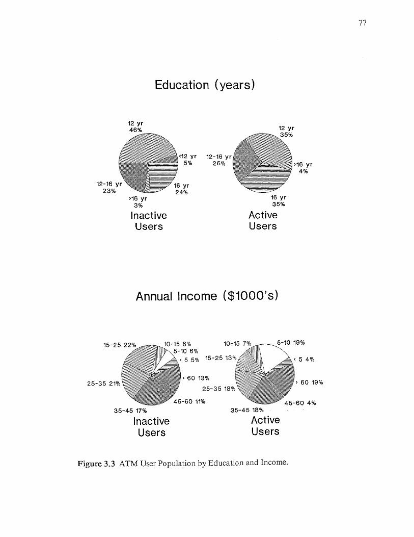
Figure 3.3 ATM User Population by Education and Income.

77

3.7.3 Defining the Control Panel

The set Si is defined as the set of locations on the control panel whose

characteristics (size, proximity to operator, etc.) are compatible with the

requirements of control or display i. With a continuous solution space, the

control panel layout problem is too complex to solve, as S = infinity, with an

infinite number of feasible locations included in the control panel analysis.

We can, fortunately, simplify the problem, since for ergonomic reasons the

control spacings and sizes must be relatively large. Literature in the area of

human factors recommends physical parameters for buttons and keypads for

various modes of operation. Since the ATM user population is comprised of

members of the general public, we will assume that strong keyboarding skills will

not normally be present. Therefore, the most likely technique of use is believed to

be a one finger random operation. In this application, it is suggested that the

push-button diameter should be a minimum of 0.5 in.; and that spacing between

push-buttons should be at least 0.5 in., with 2.0 inches spacing preferred (Moore,

1975). In the case of keyboards and keypads, the key centers should ideally be 19

millimeters (0.75 in.) apart. The key tops should be 12 mm (0.5 in.) square

(Alden et al., 1972). The controls should be spaced no closer than the

recommended 2.0 in. and be at least 0.5 inches in diameter. A keypad of 12 such

keys arranged in 4 rows and 3 columns can be made to fit into a control panel

space of 8.125 sq. in. The adherence to this guideline will significantly reduce the

complexity of the layout problem.

78

A special case of the layout problem defines the set of all locations as

points on a rectangular lattice. In the ATM problem, by restricting the feasible

object locations (Si) to the intersections of a 3.0 x 3.0 inch planar grid, the

problem can be discretized and made in some sense finite. Given a finite number

of feasible locations, the problem can be modeled as a discrete optimization

problem once suitable cost coefficients are developed.

Another assumption used in the model is that space is allocated in

increments of 9 sq. in. for each of the control panel elements. Thus, by

eliminating the effect of irregular areas and the possibility of overlapping of

adjacent controls, the problem is greatly simplified. This assumption can be

justified by observing that nearly all ATM control panel elements in the field fit

inside the 9 sq. in. envelope.

3.7.4 Accessibility of Controls

Although the goodness of a particular control location can be highly

subjective in nature, there has been at least one attempt to quantitatively measure

the accessibility of controls for human operators. Banks and Boone (1981)

introduced the concept of an "Accessibility Index" as a method for quantifying

control accessibility. The index takes into consideration the reach envelope of the

operator, the frequency of use of the particular control, and the control position

with respect to the operator. The accessibility index (I) is computed according to

Equation 3.8:

79

Where:

r = the correlation coefficient between the distance from the

operator and the ranked frequency of use of the control.

n = the number of controls outside of the reach envelope.

N = the total number of controls.

s = the number of operators under study.

F = the rank of each control outside the reach envelope.

f = the rank of each control within the reach envelope.

The accessibility indices for various control panel configurations can be

computed and the results compared. Or, the problem could be formulated to find

the configuration which yields the optimal value of I, when the control locations

are allowed to vary.

1.8 Finding the Optimal Layout

Generally, the workspace, and consequently the set of feasible control

button locations, will be given as part of the problem definition. Once a feasible

work area is defined, an attempt is usually made to determine the set of control

locations which provide a lowest-cost solution. A linear programming problem

can be formulated in which the optimal solution minimizes the sum of all the costs

80

of assigning each required control to a feasible location, while not violating any

constraints.

3.8.1 Complexity of the Layout Problem

When assigning m facilities to a finite number of locations n, the number

of possible layouts is finite. Enumerating each of the feasible arrangements is

possible but computationally practical for only the smallest problems, since the

number of layouts is n!. A formulation of the problem as a special case of the

quadratic assignment problem, using a branch and bound solution is given by

Lawler (1963). Although more efficient than total enumeration, the algorithm is

probably not computationally feasible for n much larger than 15 (Gilmore, 1962).

Other algorithms are available to find the exact assignment solution with orders

of complexity of n 3 (Lawler, 1976) and n 2 log n (Karp, 1980). Finding exact

solutions to larger scale problems by these methods may still be cost-prohibitive

for n > 15 (West, 1983).

CRAFT (Computerized Relative Allocation of Facilities Technique) is a

heuristic deterministic improvement technique (Nugent, et al., 1967). The

algorithm improves upon a given solution by evaluating the effect on the cost

function of all possible two-department exchanges, and choosing the exchange

yielding the greatest improvement. The algorithm continues until no further

improving exchanges are possible. In the worst case, the number of exchanges to

evaluate is n(n - 1)/2.

81

18.2 Types of Assignment Costs

The individual assignment cost coefficients in general layout problems can

be divided into two basic types. First, the motion costs generally reflect the cost

of motion in terms of distance or time costs in moving between feasible locations.

For example, the costs of transporting goods between feasible warehouse

locations are motion costs. Second, the position costs - independent of motion -

represent the costs incurred by an object or component simply being in a given

location. For example, the costs of renting space in various feasible cities are

position costs, since they are incurred even with no motion. Position costs for a

human operator are biomechanical in nature and can be derived by employing a

combination of anthropometric, biomechanical, and kinematic analyses.

18.2.1 Motion Costs

The typical problem in the assignment of facilities to locations is to place

the facilities in a functional layout so as to minimize the total material handling

cost or flow among the facilities. As formulated, the problem is to assign n

equally-sized facilities to n homogeneous fixed locations within a prescribed area

so as to minimize the cost function:

82

where:

83

fij = the flow of material between the ith and

the jth facility ( = 0 for i = j),

dkr = the distance between the kth location and

rth location ( = 0 for k r).

In many instances coefficients for the cost of motion are derived from a

linear function of distance from any location in a control panel to any other

control location. In this case motion costs can readily be obtained from the

feasible workspace. Given the separation distance (D) between controls, and the

diameter (d) of the control, the rectilinear spacing (s) between actuation points

(control centers) is simply: s = D + d . If each location (a and b) is defined as a

set of Cartesian coordinates (X a , Y a ) and (X b , Y b ) such as a = (1,3) and b =

(4,7), the shortest direct (straight-line) distance between them is given by:

D = [ [ s (Xb-X a ) ] 2 + [ s (Y b-Y a ) ] 2 ] 0 . 5 (3.10)

If the values for D and d are taken from the ergonomically recommended

guidelines (Moore, 1975), namely D min = 2.0 inches, and d min = 1.0 inches, then

the value for spacing will be s = 3.0 inches. The distances between each point and

each other point in the control panel are computed from Equation 3.10 as shown

in Table 3.9.

For example, with a control panel with 12 feasible locations, arranged in

three rows of four columns, with 3.0 x 3.0 inch spacing, the distance matrix is

given in Table 3.10.

Table 3.9 Motion Costs for Equally-Spaced Controls on a Control Panel of NFeasible Locations.

ToFrom 1 2 ... n ...

1 0.00 3.00 ... D(1,n) . . . D(1,N)

2 3.00 0.00 D(2,n) . . . D(2,N)

n D(n,1) ... 0.00 ... D(n,N)

N D(N,1) ... ... D(N,n) ... 0.00

Notes:

1. All motion is bidirectionally equivalent.

2. Motion costs are directly proportional to straight-line distancesbetween points (Xa,Ya) and (Xb,Yb).

3. All N feasible locations are on a planar grid.

4. Grid spacing (s x s) is 3.00 x 3.00 inches.

5. D(a,b) j[ s(Xb-Xa)]^2 + s(Yb-Ya)]^2 r0.5

84

Table 3.10 Distance Cost Matrix for 3.0-inch Equally-Spaced Controls on a 12-Control Panel.

LocationTo 1 2 3 4 5 6 7 8 9 10 11 12

From r 1 1 1 1 2 2 2 2 3 3 3 3r c 1 2 3 4 1 2 3 4 1 2 3 4

1 1 1 0.0 3.0 6.0 9.0 3.0 4.2 6.7 9.5 6.0 6.7 8.5 10.8

2 1 2 3.0 0.0 3.0 6.0 4.2 3.0 4.2 6.7 6.7 6.0 6.7 8.5

3 1 3 6.0 3.0 0.0 3.0 6.7 4.2 3.0 4.2 8.5 6.7 6.0 6.7

4 1 4 9.0 6.0 3.0 0.0 9.5 6.7 4.2 3.0 10.8 8.5 6.7 6.0

5 2 1 3.0 4.2 6.7 9.5 0.0 3.0 6.0 9.0 3.0 4.2 6.7 9.5

6 2 2 4.2 3.0 4.2 6.7 3.0 0.0 3.0 6.0 4.2 3.0 4.2 6.7

7 2 3 6.7 4.2 3.0 4.2 6.0 3.0 0.0 3.0 6.7 4.2 3.0 4.2

8 2 4 9.5 6.7 4.2 3.0- 9.0 6.0 3.0 0.0 9.5 6.7 4.2 3.0

9 3 1 6.0 6.7 8.5 10.8 3.0 4.2 6.7 9.5 0.0 3.0 6.0 9.0

10 3 2 6.7 6.0 6.7 8.5 4.2 3.0 4.2 6.7 3.0 0.0 3.0 6.0

11 3 3 8.5 6.7 6.0 6.7 6.7 4.2 3.0 4.2 6.0 3.0 0.0 3.0

12 3 4 10.8 8.5 6.7 6.0 9.5 6.7 4.2 3.0 9.0 6.0 3.0 0.0

Notes:

1. All motion is bidirectionally equivalent

2. Motion costs are straight-line distances (in inches)

3. All 12 locations are on a 3 row x 4 column planar grid

4. Grid spacing (s x s) is 3.00 x 3.00 inches

85

3.8/.2 Position Costs

An alternate cost factor to be considered is the position cost - a static

function independent of motion or materials flows - of a facility i being assigned

to a particular location j. This cost, (cii ) analogous to the fixed cost incurred in

renting the space required for a facility, may in many problems be more

significant than motion cost. It is possible that, for small-scale layouts such as the

control panel problem, the motions may be of such short distance that motion

costs may be ignored. In this instance, the cost of placing the human body in a

given position may be of great consequence.

For example, a group of controls which must be frequently operated can

be placed in close proximity to each other and achieve minimal cost from the

motion point of view. However, unless the position cost is minimized, the

arrangement can be very costly in terms of the stress inflicted on the body in

reaching to each control's position. Consider the three arrangements of controls

in Figure 3.4. Assume that the operator's task requires that switches A, B, C, and

D are operated in succession, and that joystick E is used to control an industrial

process for a ten minute period. In each case, the motion costs for performing the

given set of tasks are identical. However, the position costs will vary because the

operators will use different sets of body configurations and will as a result

experience different levels of biomechanical stress. It is apparent in this example

that, in terms of overall cost, arrangements (a) and (b) are both inferior to

arrangement (c). Assessment of the goodness of these arrangements may be made

by determining quantitatively the biomechanical stress imposed by each

alternative.

86

(a) Poor - Centroid of controls at extreme upper left positionin user's reach envelope. Position costs are excessive.

87

(b) Poor - Centroid of controls at extreme lower right positionin user's reach envelope. Position costs are excessive.

(c) Good - Centroid of controls is at optimal position withinuser's reach envelope. Position costs are minimized.

Figure 3.4 Three Control Arrangements with Identical Motion Costs.

3.8.3 Biomechanical Analysis

From reports on the anthropometric studies (NASA, 1978), it has been

determined that, within the range of motion, the force available in a body element

has a definite relationship to that element's joint angle (a). Experimental studies

of elbow angle versus force resulted in the data given in Figure 3.5.

Shown graphically, the results indicate that the maximum available force is

present at approximately 90 degrees of elbow angle. At this point (α *), it is

evident that the joint is at an optimal configuration for performing work.

3.8.3.1 Human Work Endurance

Much work has been done in the field of human work endurance. Among

those studies in the area of fatigue and work endurance, it has been repeatedly

shown that the endurance time (T e )) is related to the degree of stress encountered

by the joint, muscle or body member, expressed as a percentage of the maximum

total capacity of that member (Simonson and Lind, 1971; Morton, 1987).

Experimental evidence of the relation between muscle fatigue,

consequently endurance, and the level of imposed workload was provided by

Rohmert (1960), and confirmed by Simonson & Lind (1971) and Hayward (1975).

It was found that, for example, at a required force exertion level (R) of R = 25%

of maximum voluntary strength, usually measured as the muscle's maximum

voluntary contraction (MVC), the subject had an endurance time T e of about

88

Figure 15 Force Available at Various Elbow Configurations (Adapted fromRodgers et al., 1986).

89

four minutes, while at R 50% of maximum voluntary strength, the T e value

reduces to only 1 minute.

Theoretically, as the exerted force approaches the total available force, the

performance, measured in terms of endurance time rapidly degrades and T e

approaches zero. The level of muscular contraction at which fatigue becomes a

prohibiting factor in performing a required function is called the "threshold of

fatigue," and is given the symbol P 1 , expressed as a percentage of the maximum

voluntary contraction of the muscle (Bigland, Ritchie & Woods, 1984). As the

force demands are reduced, as P 1 approaches zero, the fatigue factor tends to

vanish and endurance time goes to infinity. Morton (1987) developed a model to

link fatigue and endurance in static work and found that P 1 < 0.1 yielded a good

fit to the experimental data already obtained.

3.8.3.2 Biomechanical Joint Analysis

For a human operator, each joint involved in the control operation will

have, accordingly, a relationship between the available force and the joint angle.

In the static case, the optimal joint angle is defined as that angle for which the

available force is at a maximum. This information can be either presented as data

to a computer program, or expressed graphically for use later.

Since more than one joint is involved in reaching a control location, each

point in space may have multiple (feasible and infeasible) solutions with respect to

joint angles. It is therefore necessary to apply techniques to obtain local optimal

90

solutions. The assumption is made that the global optimum will correspond to

the set of local optimal solutions. (Nedungadi & Kazerouinian, 1989). Therefore,

if each joint involved in reaching a point in space is set to its optimal condition,

and there is independence between each joint, then the total configuration should

be optimal.

3.8.4 Arm Kinematic Analysis

Similar to the human arm in many respects is the robot manipulator arm.

The end-effector is the most extreme member at the end of the chain of connected

joints, and is analogous to the human finger or hand. In the field of robotics, the

study of arm kinematics deals with the geometry of robot arm motion with

respect to a fixed-reference coordinate system. The kinematics problem can be

divided into two subproblems - forward kinematics and inverse kinematics

problems.

3.8.4.1 Forward Kinematics

The forward (or direct) kinematics problem is solved in order to determine

the position and orientation of a robot's manipulator with respect to a standard

reference coordinate system. The positions are derived from the angular

orientations of the set of joints comprising the whole configuration and the

lengths of the links involved. By direct kinematic analysis, any end-effector

position can be predicted from the given set of joint angles and link lengths. The

91

development of the formulas for computing the forward kinematics arm solution

is detailed in the Appendix.

By applying forward kinematics on the vector of optimal joint angles, we

can find an optimal end-effector position. By perturbing the joint angle vectors to

the limits of their optimal conditions, and re-solving, a space or envelope of

control locations can be developed which will theoretically provide a maximum

endurance time (T e*). The control envelope in the ideal case will have an T e* =

infinity, in which case any control within the Tee:

space can presumably be

operated for a long duration without serious detrimental effects from the

viewpoint of fatigue. In the practical case, however, the Te* will have the

longest finite endurance time during which work may be performed. It is

therefore desirable to assign only those controls with the longest duration

requirements to the Te*

3.8.4.2 Inverse Kinematics

It is useful to be able to determine the set of joint angles needed to reach a

given coordinate in space. By solving the inverse kinematic problem, a set of

feasible joint angles is found. Various techniques of solution are available. The

formulas used in the actual method of solution are described in detail in the

Appendix.

92

3.9 Determining Optimal Control Location

Given the set of joint angles, each proposed control location can be

evaluated in terms of endurance time degradation. To accomplish this,

information including force requirements, control positions, and the

configuration of the joint in question are analyzed to determine an estimate of the

predicted endurance time for each joint.

When this procedure is repeated for each joint involved in the activity, the

results can be combined to arrive at a total penalty cost. For each feasible point

in the control area, a total penalty value can be determined. The objective is to

minimize the total endurance penalty cost for the entire activity. After analysis,

the results can be given in a tabular form, shown graphically, or provided as input

data to optimization programs.

3.10 Determining Endurance Time Penalty

Biomechanical penalty costs are developed based on reduced endurance

times or increased discomfort levels due to the suboptimal joint configuration

needed to reach the control location in question. For control locations outside of

the Te* layout, some quantitative estimate of the penalty cost is needed. One

approach for developing appropriate cost coefficients is to express the endurance

time (Te ) as a function of the position in space of the end-effector.

93

If the end-effector position is known, as is the case with a fixed control

panel, the joint angles required to reach that position can also be determined.

This can be accomplished by applying techniques of inverse kinematics. The

problem in inverse kinematics is to calculate the joint angle vector given the

position and orientation of the end-effector. Solving the problem in inverse

kinematics will yield a number of solutions which are used to determine a feasible

set of joint angles needed to reach a given point in space. Each feasible control

location in the workspace can be analyzed and a corresponding joint angle vector,

or solution set, developed.

In conjunction with the biomechanical principles, each of the joint angle

vectors is compared with the data derived from biomechanics research. For each

element of the joint angle vectors (1), 9, S), an estimate of the endurance time (T)

is made. The theoretical endurance time (T ` ) for the entire joint angle vector,

hence the control location, is the minimum of the set of individual element

endurance times according to:

Another approach is to determine the optimal joint configuration by

studying each individual joint and optimizing it independently. From the

solution set(s), a primary configuration is selected. The rationale for the selection

may be to optimize the largest joints first, enumerate and (by exhaustive search)

evaluate all combinations of feasible solutions. Alternately, techniques such as

shortest route, or dynamic programming may be employed to find the optimal

combinations more directly.

94

3.11 Optimization Methods

The endurance time reductions, or relative penalty costs, can be used as

cost coefficients in appropriate optimization algorithms. Once a primary

(presumably feasible) configuration has been selected, the values of all joint angles

(αi ) are compared with the previously found optimal joint angles (α i* ). The

deviation ( βi ) is the absolute value of the difference between actual and optimal.

The cost of choosing a sub-optimal a i is given by the penalty function

P i = f ( β i , F). The penalty is a function of the force applied and the deviation

from optimality. This function will possibly vary from joint to joint, and

probably be non-linear in nature. The function may be developed on a case-by-

case basis for use as the need arises.

To compute the total penalty cost for control location i, the program

algorithm will use: control i's Cartesian spatial coordinates (x i , yi , z i); primary

configuration (α s , α e , αw ); deviation from optimal ( β s , βe , βw ); and penalty

cost (P5 Pe ,Pw , The total cost (C i ) is the result of the addition of the individual

penalty costs from the individual joints comprising the configuration. Although

this approach would probably yield good solutions by classical non-linear

optimization techniques, the problem can be modeled as a linear assignment

problem and solution found using simpler methods.

95

3.11.1 Linear Programming Solution

One of the simplest types of mathematical models in operations research is

the linear programming (LP) model. The mathematical formulation of an LP

problem consists of three parts. First, a set of decision variables which reflects the

value of each unknown input component of the solution. Second, a set of

constraints limiting the values of the decision variables based on some externally

imposed restriction. Third, an objective function, with decision variables and a

corresponding set of cost (or benefit) coefficients reflecting the loss or gain

associated with employing a given unit of decision variable in the final solution.

The solution of LP models can be achieved analytically by use of the

simplex algorithm. However, since a linear program with N constraints will have

on the average 2N iterations, a 5 constraint problem may require a time-

consuming 10 iterations (Lee, Moore and Taylor, 1985). Therefore computer

implementation of the simplex or dual-simplex algorithm is needed for all but the

most simple LP problems. Small scale problems (up to 50 constraints and 100

variables) can be solved relatively quickly using the simplex computer program

listed in the Appendix (Taha, 1986). The program can also be modified to

increase this limit by changing the DIMENSION statement in the first line,

however the program is not efficient to use above 200 variables. Problems of a

larger scale (200 to 1500 constraints and/or variables) can be better solved using

commercially available software packages. Programs such as LINDO (Lindo

Systems Inc.), LP88 (Eastern Software Products), XPRESS-MP (MathPro Inc.),

and others are available for a variety of popular computer hardware

configurations including the Macintosh, IBM PC, AT, and 386 (Swain, 1990).

96

3.11.2 Linear Assignment Model

The classic linear assignment problem is a special case of the linear

programming transportation model in which a number of facilities (workers, jobs,

departments, etc.) are assigned to several destinations (machines, workspaces,

etc.). The objective is to assign the jobs to the machines to achieve the lowest

total cost, while not violating any constraints. For example, only one job can be

performed per machine and only one machine is allowed per job.

The assignment problem is expressed mathematically as follows: A given

job i, ( i = 1, 2, ... , m) can be assigned to a machine j, ( j = 1, 2, ... , n) at an

assignment cost c ij. If there are more machines than jobs (m < n), or more jobs

than machines (m > n), it is necessary to balance the problem by adding either

fictitious jobs or fictitious machines. Let xij represent the event of assigning job i

to machine j. If x ij = 1, then the jth job is assigned to the ith machine; while if x ij

= 0, then the jth job is not assigned to the ith machine. The objective function is

thus:

97

subject to:

While this problem can be solved by standard linear programming

methods, the simple structure and special nature of the assignment problem lends

itself to an special method of solution. A solution algorithm called the Hungarian

method (after the Hungarian mathematician Dr. Konig) has advantages in

computational efficiency over standard linear programming and transportation

methods. (Saaty, 1959; Lee, Moore, and Taylor, 1985).

3_11.3_ Linear Assignment Solution

The first step in the algorithm is to develop a table of opportunity costs,

reflecting the costs in choosing one course of action over another. It can be

shown that the addition or subtraction of a constant to any row or column in the

cost matrix c•• does not affect the optimal solution of the assignment model.

Consequently, the elements of each row (or column) in the matrix can be reduced

by the smallest element in that row (or column) without changing the solution. In

a simple example (Taha, 1987), the assignment costs have been determined and

are as given in the cost matrix below.

98

Each row is reduced by the minimum of each entry in the row (pi) giving a new

cost matrix C'ij.

Each column is then reduced by the minimum or each entry in the column (qi)

giving a new cost matrix C"ij.

99

In this simple case, n zero elements can be found which satisfy both a row

and column as shown in Cij* The marked entries indicate the feasible and

optimal assignments which can be made, so that if c ij* = 0 and marked, then

decision variable xij = 1. The optimal assignment ( x 11 =1, x 23=1, x 32=1 ) has a

total cost of ( 5 + 12 + 13) = 30, which is equivalent to p 1 + p 2 + p 3 + q 3.

In slightly more complex problems, the solution may not be obtained

immediately. Further steps and iterations may be required, and additional rules

are introduced into the algorithm. In the example below (Taha, 1987), the cost

matrix is given as:

The reduction of each row by p i and column by qj gives cost matrix Cij :

100

Since a feasible assignment of zero elements cannot be made at this point,

the minimum number of horizontal and vertical lines is drawn through rows and

columns so that all zeros are crossed out. The application of this rule is shown

below:

The next step is to subtract the smallest uncrossed element in C" ij (= 1 in

this example) from each uncrossed element and added to each element at the

intersection of two lines. The resulting cost matrix C ij* with optimal assignments

as marked is shown below.

101

The optimal assignment (x 11 = 1, x23 = 1, x32 = 1, and x44 = 1) has a total

cost of( 1 + 10 + 5 + 5 ) 21.

In this simple example, the optimal solution is found in only one iteration.

However, it is not always possible to arrive at a solution this quickly. In the event

that the optimal solutions are not obtained, the line drawing portion of the

procedure is again repeated until a feasible and optimal assignment is reached.

In some cases, analysis of the final tableau yields more than one optimal

set of assignments. If multiple optimal solutions are found, the choice of which

solution set to use is arbitrary and can be based on heuristics or other factors.

Assignment problems of a larger scale are most efficiently solved on a

computer in one of two ways. The problem can be modeled as a standard linear

transportation program and solved with general purpose LP software, such as

LINDO; or preferably, a more efficient program can be used which deals with the

special nature of the assignment problem, such as ASGN (Erikson and Hall). The

ASGN computer solution of the above problem is accomplished in less than 1

second, as shown in the printout in Figure 3.6.

102

COMPUTER MODELS FOR MANAGEMENT SCIENCEASSIGNMENT MODEL

START TIME: 08 - 06 - 1991 - 19:07:48

-=*=- INFORMATION ENTERED -=*=-

TOTAL NUMBER OF ROWS 4TOTAL NUMBER OF COLUMNS 4PROBLEM TYPE

MINIMIZATION

PAYOFF VALUES

C1 C2 C3 C4R1 1.000 4.000 6.000

3.000R2 9.000 7.000 10.000

9.000R3 4.000 5.000 11.000

7.000R4 8.000 7.000 8.000

5.000

-=*=- RESULTS -=*=-

ROW ASSIGNMENTS

C1 C2 C3 C4

R1 A - - -R2 - - A -R3 - A - -R4 - - - A

TOTAL PAYOFF : 21

END TIME: 08 - 06 - 1991 - 19:07:49

END OF ANALYSIS

103

Figure 16 Computer Solution of Assignment Problem by ASGN.

CHAPTER 4 METHODOLOGY

The proposed methodology for ATM control panel design is comprised of

several steps as outlined below.

I . Problem definition - Functional specifications for the problem include

operational analysis, activity sequences, and determination of user population.

2. Preliminary panel definition. - Based on operational requirements,

anthropometry of user population, and other ergonomic guidelines; a selection is

made of the overall workstation size and shape, specific types of controls, and a

basic set of feasible control sites.

3. Determination of position cost - Given a set of tasks, probabilities for

various transactions, and their associated controls, the system is modeled as a

stochastic process and the limiting behavior is found. From kinematics and

biomechanics, a position cost in terms of fatigue rate is developed.

4. Model formulation - Develop a linear assignment problem to find the

optimal arrangement which minimizes the sum of position costs in performing the

specific set of activity sequences.

5. Solution - Find the optimal solution(s) and make a final selection based

on heuristic guidelines for the design of hardware and software human-machine

interfaces.

104

4.1 Operational Analysis

A typical ATM session consists of one or more of the following activities,

which will be abbreviated as follows:

1. Withdrawal from Checking Account (CW)

2. Deposit to Checking (CD)

3. Withdrawal from Savings Account (SW)

4. Deposit to Savings Account (SD)

5. Withdrawal from Bank Credit Card (BW)

6. Transfer Between Accounts (TR)

7. Balance Inquiry (IN)

For each of these ATM activities, the selection and sequencing of activity

elements (i.e., tasks and objects) are determined by the operational requirement

specifications. From the set of requirement specifications, two lists, as shown in

Tables 4.1 and 4.2, are created (Phillips, 1987).

1. Input/Output Objects List: the set of all physical OBJECTS (loci) needed

for the activity.

2. Activity Elements List: the TASKS (verbs) and their associated

OBJECTS (nouns) manipulated or used in performing a given Activity.

105

Table 4. 1 Input/Output Objects List for Typical ATM.

ObjectID Name (Locus) NounA ATM Card Slot CARDSLOT

B Numeric Keypad KEYPAD

C Function Keys FUNCTKEY

D Deposit Slot -DEPOSSLOT

E Receipt Dispenser RECPTSLOT

F Cash Dispenser CASHSLOT

Table 4.2 Activity Elements List for Typical ATM.

No. Activity Element Verb Noun1 Insert ATM Card INSERT CARDSLOT

2 Enter PIN number ENTER KEYPAD

3 Choose Transaction PRESS FUNCTKEY

4 Enter Account PRESS FUNCTKEY

5 Enter Amount ENTER KEYPAD

6 'Enter Account PRESS FUNCTKEY

7 Insert Deposit INSERT DEPOSSLOT

8 Receive Cash TAKE CASHSLOT

9 Receive Receipt TAKE RECPTSLOT

10 Retrieve ATM Card TAKE CARDSLOT

106

The sequence of operations for any specific ATM session will ultimately

be determined by the combination of hardware and software provided to the user.

In addition, sequences may vary slightly within a single ATM system, depending

on the particular requirements of the

customer. Figures 4.1 and 4.2 depict two flowcharts for standard and forced exit

ATM sessions as observed in the field. The activities and their corresponding

control positions of a typical ATM session are also given in Table 4.3.

In order to arrive at a typical ATM session, weights must be applied to

each of the feasible transaction types according to their frequency-of-use

distribution. In a study of weekly ATM usage, (van der Velde, 1982) a total of

1646 transactions were observed, The data collected in this study were analyzed,

resulting in a transaction mix as shown in Table 4.4.

107

Figure 4.1 Typical ATM Session Flowchart.

108

Figure 4.2 Forced Exit ATM Session Flowchart.

109

Table 4.3 Task Elements and Loci for ATM Transaction Types.

TaskNo.

TaskElement

ObjectID Locus

IncludedTransactions

1 Insert ATM Card A CardSlot all

2 'Enter PIN Number B KeyPad all

3 Choose Transaction C FunctKey all

4 Enter Account C FunctKey all

5 Enter Amount B KeyPad all exc. TR IN

6 Enter Account C FunctKey TR

7 Insert Deposit D DeposSlot CD SD

8 Receive Cash F CashSlot CW SW BW

9 Receive Receipt E RecptSlot all

10 Retrieve ATM Card A CardSlot all

110

Table 4.4 Distribution of ATM Activities by Transaction Type

ActivityNo. (i) Abbrev. Transaction

ObservedFrequency

(n)

RelativeFrequency

P(i)=n/N1 CW Withdrawal from Checking 760 0.462

2 CD Deposit to Checking 189 0.115

3 SW Withdrawal from Savings 131 0.080

4 SD Deposit to Savings 25 0.015

5 BW Withdrawal from Bank Card 8 0.005

6 TR Transfer Between Accounts 97 0.059

7 IN Balance Inquiry 436 0.265

Notes:

1. Frequency data based on sample size of N = 1646 ATM transactions

2. Source: van der Velde (1982)

111

4.2 ATM Transaction Models

Three models for ATM transaction sequences are considered. For Case I,

the simplest and ideal case, it is assumed that no operational errors occur and that

only one transaction occurs per ATM session. A more realistic case, Case II,

incorporates human errors, but allows only a single transaction per session. Case

III is the most realistic situation in which both error probabilities are considered

and multiple transactions per ATM session are permitted.

4.2.1 Case I - Ideal Case

In the first and simplest case, tasks are performed in accordance with a

pre-defined sequence of activities as shown in Figure 4.3. The possibility of errors

is ignored and only one transaction is allowed per session. The activity sequence

diagrams are arranged with activities on the nodes and connecting arrows or arcs

showing the normal sequences for each type of transaction. The distribution of

transaction types is obtained from the typical transaction mix from Table 4.4.

112

Notes

1. Activities on nodes

2. 1 - Insert card 2 Enter PIN 3 - Enter transaction type4 - Choose account 5 Enter Amount 6 . _- Insert Deposit7 - Get Receipt 8 • Get Cash 9 - Take ATM card

3. One transaction allowed per session

4. All activities are performed without errors

Figure 4.3 ATM Activity Sequences (Case I).

113

4_2.2 Case II - Human Error Model

In the Case II model, the likelihood of human error is introduced (Figure

4.4). The probabilities of certain errors, such as in entering a PIN number or in

selecting a function, are derived from the task error rates of Table 3.3. For

example, the probability of correct PIN number entry is 0.868, and for function

key selection the probability of correct entry is 0.967.

The probabilities for other types of errors can also be estimated. For

example, on some machines with horizontal card slots, the ATM card must be

inserted with the magnetic stripe down and on the right. Despite (or perhaps

because of) the labels on the card slot, incorrect insertion frequently occurs, since

three of the four physically possible card orientations are invalid. In the absence

of actual card input error statistics, this parameter will be estimated, although it is

recommended that any further studies in this area should include the additional

research and experimentation to verify the assumptions stated herein. A

reasonable estimate is that ATM cards will be correctly inserted the first time in at

best 90 percent of sessions..

114

Notes

1. Activities on nodes

2. 1 - Insert card 2 - Enter PIN 3 - Enter transaction type4 - Choose account 5 - Enter Amount 6 - Insert Deposit7 - Get Receipt 8 - Get Cash 9 - Take ATM card

3. One transaction allowed per session

4. All transactions are completed once started

5. Probability of ATM card inserted incorrectly - 0.10

6. Probability of incorrect PIN number entry 0.132

7. Probability of incorrect numeric entry - 0.155

8. Probability of incorrect function selection - 0.033

115

Figure 4.4 ATM Activity Sequences (Case II).

4.2.3 Case III - Multitransaction Model

In this combined model, the situation is covered in which more than one

transaction is allowed in an ATM session (Figure 4.5). The conditional

probabilities for multiple transactions can be estimated. The probability of

transactions canceled once begun can be estimated from the total transactions

completed divided by the total of all transactions started. Since the actual data

was not obtainable, it will be assumed for the purpose of calculation that all

transactions are completed once started and that no cancellations or other

abnormal events are encountered. Those parties with access to ATM transaction

records could conduct further research which may yield a more accurate estimate

of transaction completion rates. This could be achieved by examining records of

all transactions or by analyzing a statistically valid sample.

116

Notes

1. Activities on nodes

2. 1 • Insert card 2 - Enter PIN 3 - Enter transaction type4 - Choose account 5 • Enter Amount 6 ■ Insert Deposit7 - Get Receipt 8 - Get Cash 9 - Take ATM card

3. Multiple transactions ( n - 1 or n - 2 ) allowed per session

4. All transactions are completed once started

5. Probability of ATM card inserted incorrectly • 0.10

6. Probability of incorrect PIN number entry ■ 0.132

7. Probability of incorrect numeric entry - 0.155

8. Probability of incorrect function selection - 0.033

9. Conditional probabilities for multiple transactions canbe estimated

10. Probability of n > 2 transactions is negligible ( > 0.02 )

117

Figure 4.5 ATM Activity Sequences (Case III).

4.2.4 Transaction Conditional Probabilities

The likelihood of having a multiple transaction is dependent upon the

nature of the first transaction. Transactions involving deposits and inquiries

often are followed by another transaction. Many ATM systems, however,

automatically end the session after a cash withdrawal, therefore, in such a "forced

exit" system the sequence of any withdrawal followed by a deposit or any other

transaction is infeasible (See Figure 4.2).

The sequence of transactions in a multiple transaction session can also be

estimated. For example, some typical sequences consist of a deposit or an

inquiry, followed by a withdrawal from the same account, or an inquiry followed

by a deposit to the same account. A less common sequence would be to have two

of the same transactions in sequence, for example checking deposit followed by

another checking deposit. Also, a withdrawal transaction can be assumed to

terminate the session.

If the first transaction in the ATM session is i I, the conditional probability

of having another transaction (i 2 ) following in the same session can be

determined. Given the first transaction (i 1 ) and n = 2, the probability

distributions for the second transaction (i 2 ) have been estimated according to

Table 4.5.

118

Table 4.5 Conditional Probabilities and Distribution of Two Transactions.

First Trans-action (i1)

ProbabilityP(n=2|l=i1)

Second Transaction (i2) SeeNote #CW CD SW SD BW TR IN

CW 0.000 0.000 0.000 0.000 0.000 0.000 0.000 0.000 (2)

CD 0.200 0.600 0.000 0.020 0.000 0.020 0.060 0.300 (3)

SW 0.000 0.000 0.000 0.000 0.000 0.000 0.000 0.000 (2)

SD 0.200 0.020 0.000 0.600 0.000 0.020 0.060 0.300 (3)

BW 0.000 0.000 0.000 0.000 0.000 0.000 0.000 0.000 (2)

TR 0.200 0.460 0.115 0.080 0.015 0.005 0.060 0.265 (4)

IN 0.500 0.460 0.115 0.080 0.015 0.005 0.060 0.265 (4)

Notes:

1. Probability of occurrence of similar transactions (e.g. CD & SD) in sequence is nil.

2. Multiple transactions following withdrawals are infeasible in forced exit system.

3. Deposit transaction followed by any withdrawal has probability of 0.6, inquiry0.3, transfer 0.06, deposit to alternate account 0.02.

4. Following inquiry or transfer, standard transaction distribution patternis assumed to be in effect (data from Van der Velde, 1982).

119

4.3 ATM Stochastic Models

The activities of the ATM control panel operation model can be thought

of as a stochastic process, or random chance process X(t), with the set of user

operation activities defined as the sample space S for a random experiment in

time. The n elements of the sample space are states within the sample space and,

for reasons of simplification, are discrete and countable in number.

In the case of the ATM machine problem, the number of possible discrete

activities in a transaction session is finite. Since a one-to-one correspondence

exists between the task and the object used in performing the activity, we will

define the state space as comprised of the set of spatial positions assumed by the

user's hand in operating an ATM. The size of the state space (S) can then

determined by the number of objects or control positions (p), rather than the

number of activities (n). Since the expected sequence of operation of each of the

p controls is presumably known, probabilities can theoretically be assigned to the

operation of each control, based on the last control used.

Given a small and arbitrary time interval Δt, it is possible to state all of the

relationships between control functions in the form of an n x n stochastic matrix.

4.3.1 Transition Probabilities

The ATM transition probabilities, obtained by studying actual usage

patterns, will most likely vary depending on the particular model of ATM and the

120

controlling software programs. A typical ATM model will be used for illustrative

purposes and solved as a case study. Although the results for a given model will

not necessarily apply universally, the same basic techniques can be employed to

find a solution for any other specific ATM configuration.

Based on the activity sequences and weighting of each type of transaction,

a transition diagram can be developed. In the diagram for Case I (Figure 4.6),

nodes indicate the sites of activities and the directed arcs indicate valid branch

paths connecting activities. The values along each arc denote, for each source

node i, the probabilities of performing the destination activity on node j, given

that the source activity has occurred. Since all ATM sessions begin with a

common starting point (the insertion of the ATM card), we can, by studying the

resulting activity sequence generator, obtain important and useful control layout

design information.

Since it can be reasonably assumed that the relationships between control

functions stay unchanged over time and are independent of prior events, the

system is said to exhibit the properties of both stationarity and lack of memory.

A stochastic process exhibiting both properties has the characteristic known as

first-order dependence. In other words, the conditional distribution of X(t) is

dependent only upon X(t n ) which is the most recently determined value of the

state of the process.

121

Figure 4_6 ATM Transition Diagram (Case I).

122

This type of dependence is called Markov-dependence, and a Markov

dependent system is referred to as Markovian. As a consequence of the Markov-

dependence of the process, we can define the one-step transition matrix as P, and

the elements of P as p ij , where i is the location state at time period t, and j is the

location state at time period ( t + Δt). Each element p ij represents the probability

that, in a single time period (epoch), the system moves from state i to state j. The

one-step transition probability matrices (Markov chains) for the four transaction

types are given in Tables 4.6 through 4.9.

123

Table 4.6 One-Step Transition Matrix for ATM Withdrawals.

Locus ObjectA B C D E F

CardSlot A 0.000 1.000 0.000 0.000 - 0.000

KeyPad B 0.000 0.000 0.500 0.000 - 0.500

FunctKey C 0.000 1.000 0.000 0.000 - 0.000

DeposSlot D - - - - - -

RecptSlot E 1.000 0.000 0.000 0.000 - 0.000

CashDisp F 0.000 0.000 1.000 0.000 - 0.000

Table 4.7 One-Step Transition Matrix for ATM Deposits.

Locus ObjectA B C D E F

CardSlot A 0.000 1.000 0.000 0.000 0.000 -

KeyPad B 0.000 0.000 0.500 0.500 0.000 -

FunctKey C 0.000 1.000 0.000 0.000 0.000 -

DeposSlot D 0.000 0.000 0.000 0.000 1.000 -

RecptSlot E 1.000 0.000 0.000 0.000 0.000 -

CashDisp F - - - - - -

124

Table 4.8 One-Step Transition Matrices for ATM Transfers.

Locus ObjectA B C D E F

CardSlot A 0.000 1.000 0.000 - 0.000 -

KeyPad B 0.000 0.000 0.500 - 0.500 -

FunctKey C 0.000 1.000 0.000 - 0.000 -

DeposSlot D - - - - - -

RecptSlot E 1.000 0.000 0.000 - 0.000 -

CashDisp F - - - - - -

Table 4.9 One-Step Transition Matrix for ATM Inquiries.

Locus ObjectA B C D E F

CardSlot A 0.000 1.000 0.000 - 0.000 -

KeyPad B 0.000 0.000 1.000 - 0.000 -

FunctKey C 0.000 0.000 0.000 - 1.000 -

DeposSlot D - - - - -

RecptSlot E 1.000 0.000 0.000 - 0.000 -

CashDisp F - - - - - -

125

4.3.2 Composite Transition Diagrams

A composite transition diagram is developed for each of the three models

describing the probabilities of transition from each node to every other nodes and

incorporate weighting factors derived from the transaction mix as previously

defined. The numbers adjacent to the arcs show the number of transitions (in

thousands) from the source node to the destination node, given that a simulated

1000 visits were made to the source node.

For the second case, the model formulation is revised slightly. An

additional keypad node (B') is added to represent the re-visit to the keypad to

enter a numeric amount. The rest of the formulation is as in Case I. The

transition diagram for the Case II model is given in Figure 4.7.

In Case III, the multiple transaction model, three more nodes have been

added. To allow for multiple transaction re-visits, an additional keypad node

(B"), a function key node (C'), and a receipt slot node (E') are introduced. The

transition diagram for the Case III model is shown in Figure 4.8.

126

Figure 43 ATM Transition Diagram (Case II).

127

Figure 4.8 ATM Transition Diagram (Case III).

128

129

4.3.3. Composite Transition Matrices

The one-step transition matrix for the composite ATM session can be

developed directly from the transition diagrams of Figures 4.6 thru 4.8. The listed

values are the conditional probabilities for each arc, calculated according to:

Pij = Fij / Ti(4.1)

where:

Pij = probability of transition from node i to j

Fij = frequency of transactions from node i to j

Ni = total number of transactions leaving node i

Using the values for the Case I model (Figure 4.6) as an example, a one-

step transition matrix (Markov chain) is constructed, as shown in Table 4.10. The

same technique is repeated for Cases II and III, with the resulting transition

matrices given in Tables 4.11 and 4.12.

Table 4A0 Composite Transition Matrix - Case I.

Locus ObjectA B C D E F

CardSlot A 0.000 1.000 0.000 0.000 0.000 0.000

KeyPad B 0.000 0.000 0.576 0.075 0.035 0.314

FunctKey C 0.000 0.735 0.000 0.000 0.265 0.000

DeposSlot D 0.000 0.000 0.000 0.000 1.000 0.000

RecptSlot E 1,000 0.000 0.000 0.000 0.000 0.000

CashDisp F 0.000 0.000 0.000 0.000 1.000 0.000

Table 4.11 Composite Transition Matrix - Case II.

Locus ObjectA B B' C D E F

CardSlot A 0.100 0.900 0.000 0.000 0.000 0.000 0.000

KeyPad B 0.000 0.132 0.000 0.868 0.000 0.000 0.000

KeyPad-1 B' 0.000 0.000 0.132 0.000 0.154 0.071 0.643

FunctKey C 0.000 0.000 0.711 0.033 0.000 0.256 0.000

DeposSlot D 0.000 0.000 0.000 0.000 0.000 1.000 0.000

RecptSlot E 1.000 0.000 0.000 0.000 0.000 0.000 0.000

CashDisp F 0.000 0.000 0.000 0.000 0.000 1.000 0.000

130

Table 4.12 Composite Transition Matrix - Case III.

ObjectA B B' B" C C' D E E' F

A 0.100 0.900 0.000 0.000 0.000 0.000 0.000 0.000 0.000 0.000

B 0.000 0.132 0.000 0.000 0.868 0.000 0.000 0.000 0.000 0.000

B' 0.000 0.000 0.132 0.000 0.000 0.000 0.154 0.014 0.057 0.643

B" 0.000 0.000 0.000 0.132 0.000 0.000 0.154 0.000 0.071 0.643

C 0.000 0.000 0.711 0.000 0.033 0.000 0.000 0.128 0.128 0.000

C' 0.000 0.000 0.000 0.711 0.000 0.033 0.000 0.000 0.256 0.000

D 0.000 0.000 0.000 0.000 0.000 0.000 0.000 0.200 0.800 0.000

E 0.000 0.000 0.000 0.000 0.000 1.000 0.000 0.000 0.000 0.000

E' 1.000 0.000 0.000 0.000 0.000 0.000 0.000 0.000 0.000 0.000

F 0.000 0.000 0.000 0.000 0.000 0.000 0.000 0.000 1.000 0.000

Legend

A CardSlot C' FunctKey-1B Keypad-0 D DeposSlotB' Keypad-1 E RecptSlot-0B" Keypad-2 E' RecptSlot-1C FunctKey-0 F CashDisp

131

4.3.4 Steady-State Solution

If a stochastic system is Markovian, stationary, and well behaved, or

ergodic (i.e. does not have absorbing states from which the system cannot exit), a

steady-state solution can be found. The steady-state solution of a Markov chain

is an n-element vector with describes the percentage of time the system can be

observed in each of the n states, over the long run. The steady-state solution for

the ATM problem can be obtained by analyzing the composite one-step

transition matrix (Table 4.12) using either numerical or algebraic techniques. A

sample calculation demonstrating the method of determining a steady-state

solution is presented in the Appendix.

The steady-state solutions for the Markov chains of each separate

transaction type and for the composite cases were determined. The results were

computed numerically by raising each n x n stochastic matrix to a high-numbered

power, and then multiplying the transpose of any state probability vector (a 1 x n

stochastic vector), by the result. In this case, 256 iterations were sufficient to

reach convergence, and the computations could be performed in a reasonable

amount of time (less than 30 minutes for the example shown in the Appendix).

The steady-state solutions for the individual transaction types, and a weighted

solution based on transaction mix are given in Table 4.13. The steady-state

solution vectors for the composite matrices in Tables 4.10 through 4.12,

representing Cases I, II, and III, are also given in Table 4.13.

132

Table 4A3 Steady-State Solutions for ATM Models.

Steady-State VectorA

CardSlotB

KeyPadC

FnctKeyD

DepoSlotE

RcptSlotF

CashDispModel Case

Individual Withdrawal 0.0000 0.4000 0.4000 0.0000 0.0000 0.2000

Deposit 0.3330 0.0000 0.3333 0.3333 0.0000 0.0000

Transfer 0.1999 0.3999 0.1999 0.0000 0.1999 0.0000

Inquiry 0.2500 0.2500 0.2500 0.0000 0.2500 0.0000

WeightedAverage

0.1810 0.3550 0.1780 0.0490 0.1720 0.0750

Composite Case I 0.1853 0.3198 0.1854 0.0241 0.1843 0.1010

Case II 0.1909 0.3435 0.1777 0.0224 0.1718 0.0936

Case III 0.1725 0.3333 0.1886 0.0238 0.1824 0.0993

133

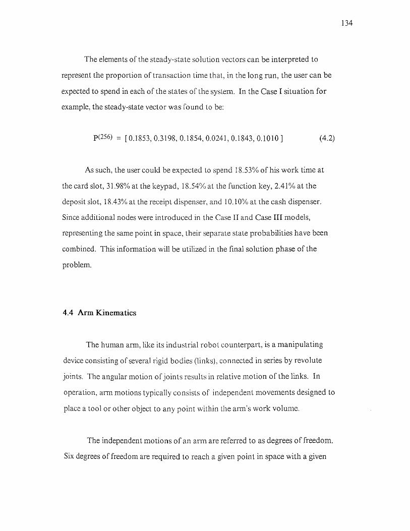
The elements of the steady-state solution vectors can be interpreted to

represent the proportion of transaction time that, in the long run, the user can be

expected to spend in each of the states of the system. In the Case I situation for

example, the steady-state vector was found to be:

p(256) = [ 0.1853, 0.3198, 0.1854, 0.0241, 0.1843, 0.1010 ] (4.2)

As such, the user could be expected to spend 18.53% of his work time at

the card slot, 31.98% at the keypad, 18.54% at the function key, 2.41% at the

deposit slot, 18.43% at the receipt dispenser, and 10.10% at the cash dispenser.

Since additional nodes were introduced in the Case If and Case III models,

representing the same point in space, their separate state probabilities have been

combined. This information will be utilized in the final solution phase of the

problem.

4.4 Arm Kinematics

The human arm, like its industrial robot counterpart, is a manipulating

device consisting of several rigid bodies (links), connected in series by revolute

joints. The angular motion of joints results in relative motion of the links. In

operation, arm motions typically consists of independent movements designed to

place a tool or other object to any point within the arm's work volume.

The independent motions of an am. are referred to as degrees of freedom.

Six degrees of freedom are required to reach a given point in space with a given

134

orientation. The human arm has exactly six degrees of freedom: two in the

shoulder, one at the elbow, and three at the wrist (Paul, 1981). If we disregard the

requirement for arbitrary wrist orientation and affix the end effector to the end of

the arm, only three degrees of freedom are needed. The procedure for finding the

joint solution for a simple three degree of freedom arm is described in the

Appendix.

4.4.1 Simple Manipulators

The approach to describing the location of arm links with respect to a

fixed reference point requires the use of vector and matrix algebra. A 3 x 3

rotation matrix is defined as a transformation matrix to map the rotated

coordinate system to a reference coordinate system with the same origin. In order

to accommodate translation and scaling, a fourth component or coordinate is

introduced. If the vector O = (p x , p y , pz )T is used to represent the position of

the endpoint in 3-D space, then vector P = (wp x , wp y , Wp z )T are homogeneous

coordinates encompassing rotation and translation (Lee, 1982). By matrix

multiplication, the result of combinations of rotations and translations can be

determined. From Paul (1982), using the coordinate frames shown in Figure 4.9,

the general form of the 4 x 4 transformation matrix is given by Equation 4.3.

135

Figure 43 Coordinate Frames for Simple Manipulator (From Paul, 1981).

136

Given:

the combination is

RPY(φ z φy φx ) =

137

Referring to the coordinate frames in Figure 4.9, the base is the origin of

frame R, whose location is presumably known relative to a universe frame U. The

location of the end effector relative to the universe frame can be determined by

the transform: UT E = UTR • RTH • HT E . Also, the same point in space can be

found from UTE = UTP • PTE . The desired transform that identifies the location

of the end effector (hand frame H) with respect to the robot base (robot frame R)

is RT H , and may be found by:

Due to the special nature of robot transformation matrices, inversion can

be accomplished by use of a specialized techniques. If the elements of a 4 x 4

homogeneous transform T are:

The inverse of T is found very simply by rearranging elements and

computing three dot products (Paul, 1982):

where,

4.4.2 Multiple Link Manipulators

In order to analyze the typical system comprised of multiple links, the

relationships between links must be described. In order to describe the

translational and rotational relationships between the adjacent links, Denavit and

138

Hartenberg (1955) introduced an algorithm (D-H method) for establishing

coordinate systems for each link. The details of the eleven step D-H procedure

are given in Section 4.4.4. Using the D-H representation, a 4 x 4 homogeneous

transformation matrix is established to represent each link's coordinate system

with respect to the previous link's coordinate system. The labeling of the links

typically begins at the base and continues until the end effector is reached.

Once the D-H coordinate system has been established for each link, a

homogeneous transformation matrix (Ai i-1 ) can be found to describe the ith

coordinate frame with respect to the (i-1)th frame (Lee, 1982). The homogeneous

matrix (Ti 0) specifies the position of the end point of link i with respect to the base

coordinate system. This matrix can be found for any link i in the system by chain

multiplication of D-H transformation matrices for adjacent links 0 to i according

to:

For example, given a manipulator with six joints, such as the PUMA arm

(shown in Figure 4.10), the coordinate transformation matrices are developed

(Figure 4.11). By direct kinematics the arm solution T = A 60 , was found (Lee,

1982).

139

The steps in the solution are given in the Appendix.

Figure 4A0 Link Coordinate Systems for Six-Joint PUMA Arm (adapted fromLee, 1982).

140

Figure 4.11 Transformation Matrices for Six-Joint PUMA Aim (Adapted fromLee, 1982).

4.4.3 Inverse Kinematics (Joint Solution)

Since the arm is usually comprised of links of fixed-length, the motion is

achieved by varying the joint angles. To control the position of the end effector

in space, the inverse kinematic solution must be found. The geometric approach

is used to find the joint angle vector (θ = θ 1 , θ2 , ... θ i )T (Paul, 1981). The

procedure is to first find a position vector pointing from the shoulder to the wrist.

This is then used to derive the solution for the other joints. The generalized

solution method is given in Paul (1981), however, it is relatively complicated.

Other simplified approaches can be used in specific cases, such as the solution

provided by Lee (1982) for the six-joint PUMA robot.

The direct kinematics problem is always solvable; that is, the position and

orientation of the end effector can always be computed. However, the inverse

problem is not always solvable, since the configuration of the manipulator may

not allow all points in space to be reached. In addition, a single unique solution

does not exist for systems with more than one joint. Given a two-link articulated

arm, the solution algorithm finds that α 2 and α 3 can each be positive or negative

in sign (Lee, 1982). This results in the four configurations as shown in Figure

4.12.

The first two configurations, in which α 2 and α 3 have different signs, are

immediately dismissed because they imply that the links are disconnected. The

last two configurations, however, are feasible as long as none of the angles violate

any of the manipulator's joint constraints (Paul, 1981).

141

Figure 4.12 Two-Link Articulated Arm (Paul, 1982).

142

143

In comparison with a robot manipulator, the likelihood of multiple

configurations in the human arm is less, since human ranges of motion are usually

limited to only positive angles, while robot manipulator ranges are less restrictive.

4.4.4 Denavit-Hartenberg Algorithm

The method of representing coordinate systems for multiple link

manipulators, described by Denavit and Hartenberg (1955), uses matrices to

describe adjacent link coordinate systems with respect each other. The

representation of a rigid link depends on four parameters associated with each

link as follows:

θi= the joint angle from the xi-1 axis to the xi axis about the zi-i axis

(using the right-hand rule).

di= the distance from the origin of the (i- 1)th coordinate frame to the

intersection of the zi-1 axis with the xi axis along the zi-1 axis.

ai= the offset distance from the intersection of the z i-1 axis with the xi

axis to the origin of the ith frame along the x i axis (shortest distance

between the zi-1 and zi axes).

αi= the offset angle from the zi-1 to the zi axis about the xi axis (using

the right-hand rule).

For rotary joints, di, ai, and ai are the joint parameters which remain

constant, while θ i is the joint variable that changes when link i moves. Given a

manipulator with n degrees of freedom, the D-H algorithm establishes coordinate

systems for each link in the manipulator. The links are numbered starting at the

base and ending at the end effector, and the relationship between adjacent links

are represented by 4 x 4 homogeneous transformation matrices. The steps of the

algorithm are numbered D1 through D11 as follows (Lee, 1982):

Dl.

Establish the base coordinate system. Establish a right-hand

orthonormal coordinate system (x0 , y0 , z0 ) at the supporting base with

the z0 axis lying along the axis of motion of joint 1.

D2. Initialize and loop. For each i, i = 1,... n, perform steps D3 to D6.

D3. Establish joint axis. Align the zi axis with the axis of motion (rotary or

sliding) of joint i+1.

D4. Establish the origin of the ith coordinate system. Locate the origin of

the ith coordinate system at the intersection of the z i and z i-1 axes or at

the intersection of common normals between the z i and z i-1 and the z i

axis.

D5. Establish xi axis. Establish xi = (zi-1 x zi )/||zi-1 xzi|| or along the

common normal between the z i-1 and zi axes when they are parallel.

D6. Establish yi axis. Assign yi = (zi x xi )/||zix xi|| to complete the right-

hand coordinate system. Extend the z i and xi axes if necessary for

steps D8 to D11.

144

D7. Find joint and link parameters. For each i, i = 1 ,...n , perform steps D8

to D11.

D8. Find di, the distance from the origin of the (i-1)th coordinate system to

the intersection of the z i-1 axis and the xi axis along the zi-1 axis.

D9. Find ai, the distance from the intersection of the z i-1 axis and the xi

axis to the origin of the ith coordinate system along the x i axis.

D10. Find 0, the angle of rotation from the xi-1 axis to the xi axis about the

zi-1 axis.

D11. Find a, the angle of rotation from the z i-1 axis to the zi axis about the

xi axis.

4.5 Formulation of Linear Assignment Model

The steady-state solution set for a control function activity is first used to

determine the frequency of use for a given control. Each activity in ATM

operation requires a predictable number of operations or tasks (Tn ), for example

a cash withdrawal from checking requires 7 tasks. Therefore, knowing the

distribution of transaction types, the expected number of ATM tasks, E(T),

required to perform one transaction is found according to equation 4.9.

145

146

where,

E(T) = expected number of ATM tasks

n = number of operations

Pi = probability of transaction type i

Ti = number of tasks used in performing operation i

4_6 Numerical Arm Solution

The numerical solution of arm and shoulder joint angles given spatial

coordinates for the control panel problem is found by computer with the aid of

the MATHCAD software package. The algorithm used is an implementation of

the Levenberg-Marquardt (L-M) method, a quasi-Newtonian variation of the

gradient method (Anderson, 1989). At each step, an estimate is made of the first

partial derivatives of the error function f(x) with respect to the variable to be

solved, creating a Jacobian matrix J. Next, the matrix function J -s = -f(x) is

solved for the step vector s, where s is the vector of unknown variables. If the step

vector can be found, then (x + s) becomes the new value of x.

In the event that this calculation fails because the matrix J cannot be

inverted, an additional condition is added - to minimize the quantity

where D is a vector of weight factors computed from the norms of matrix J. The

algorithm terminates when any of the following conditions is met:

1. It is no longer possible to significantly reduce the value of the norm of

the error vector, relative to the tolerance level (TOL) currently set

within the program.

2. The value of s becomes relatively close to zero (closer than the larger of

TOL and TOL - |x' ).

3. The program exceeds the limit of the number of calculations without

returning an answer. The function is determined to be non-converging

in nature.

147

CHAPTER 5 CASE STUDY - ATM CONTROL PANEL DESIGN

A practical case study is presented in which, given a set of parameters and

assumptions, an efficient layout of ATM control panel can be designed, based on

the objective of minimizing the fatigue rate.

5.1 Problem Definition

The problem is described according to the following seven step procedure

as follows:

1. The user population is determined and basic design parameters are

defined. The design population has been determined to be right-

handed 5th percentile females. From the anthropometric data,

(NASA, 1978; Rodgers, 1986), the shoulder height is 132.9 cm (52.3

in.), and eye height is 151.4 cm (59.6 in.) as shown in Figure 5.1. The

shoulder width (w) is 39 cm (15.36 in.) (NASA, 1978). The upper arm

length (lateral epicondyle to acromion) (A) is 34.1 cm (13.4 in.), and

the lower arm length (lateral epicondyle to fist, plus half of the hand

length) (B) is 44.0 cm (17.32 in.) as shown in Figure 5.2.

148

Measurement cm in.

A Height 161.0 63.39

B Shoulder Height 132.9 52.32

C Eye Height 151.4 59.61

Anthropometric data on 5th percentilefemale stewardesses (NASA, 1978).

Figure 5.1 Heights of 5th Percentile Female Stewardesses (Adapted fromNASA, 1978).

Link cm in.

A Shoulder Breadth 39.0 15.36

B Upper Arm Length 34.1 13.43

C Elbow to Fist 34.8 13.70

D Half Hand Length 9.2 3.62

Anthropometric data on 5th percentilefemale stewardesses (NASA, 1978).

Figure 5.2 Link Lengths for 5th Percentile Females (Adapted from NASA,1978; and Rodgers, 1986).

149

150

2. A spatial coordinates system is defined with the shoulder as the point

of reference origin as shown in Figure 5-3. With respect to a standing

operator the x-axis is horizontal from left to right, the y-axis is forward

and back, and the z-axis is vertical. In agreement with the "right-hand

rule," the sign conventions are: positive x is to the right, positive y is

forward, and positive z is up.

3. The rotation angles for the shoulder-arm configuration are defined as

shown in Figure 5.3. The angle of rotation of the upper arm in the y-z

plane is called the shoulder forward flexion angle and given variable A.

The angle of rotation of the elbow (4) is called the elbow flexion to

extension angle. The rotation angle (6) of the upper arm in the x-y

plane (the plane of the chest) is called the shoulder horizontal flexion

angle.

4. The range of feasible panel coordinate values is defined (See Figure

5.4). The x value is defined as the horizontal distance from the center

of the right shoulder joint to the point on the control panel. In this

problem the x coordinate will vary from -21.68, rounded to(-21), to

+6.32, rounded to (+6). The y value is defined as the distance from the

center of the shoulder joint in a direction normal to the plane of the

control panel. With a simple vertical planar control panel, the y

coordinates will be fixed at +18 inches. The z value is defined as the

vertical distance from the center of the shoulder joint to the point on

the control panel. In this problem the z coordinate can range in value

from -11 inches to +12 inches.

Figure 5.3 Reference Planes for Standing Operator.

151

152

5. The procedure begins with an initial set of coordinates representing a

point in the feasible control panel. The first point to be examined is the

extreme upper left corner position. The coordinates of this point are

(-21, 18, 12).

6. To facilitate the solution on computer by numerical methods, a set of

initial seed values for the joint angles are chosen. In this case, the

values used will be the approximate midrange joint angles for each

joint's range of motion (Figure 5.5). The seed values are (in radians):

= 1.5, = 1.3, and 8 = 1.1.

7. The transformation equations for each coordinate and the constraint

equations for each joint are entered as part of the problem. The

computer program is then directed to find the solution (if possible) to

within the level of precision (TOL) desired. The program then displays

the solution vector (V) in both radians and degrees, and the ERR value

(E) is checked to verify the results. Table 5.1 shows the output from

computer solution of the ATM example problem.

Figure 5.4 Control Panel Dimensions.

153

154

Figure 5.5 Range of Motion for Upper Body. Mean Values - Individual Rangesmay Vary. (Adapted from Rodgers, et al., 1986).

Table 5.1 Computer Solution of Joint Angles.

Loc.No.

Spatial Coordinates Joint Angles (radians)x y z THETA PHI DELTA

1 -21 18 12 2.277 0.399 0.5192 -18 18 12 1.973 0.837 0.5883 -15 18 12 1.764 1.096 0.6754 -12 18 12 1.591 1.284 0.7855 -9 18 12 1.446 1.423 0.9276 -6 18 12 1.332 1.52 1.1077 -3 18 12 1.257 1.578 1.3268 0 18 12 1.231 1.597 1.5719 3 18 12 1.257 1.578 1.816

10 6 18 12 _ 1.332 1.52. 2.03411 -21 18 9 2.097 0.667 0.40512 -18 18 9 1.917 0.91 0.44213 -15 18 9 1.63 1.243 0.5414 -12 18 9 1.446 1.423 0.64415 -9 18 9 1.283 1.559 0.78516 -6 18 9 1.147 1.655 0.98317 -3 18 9 1.054 1.714 1.24918 0 18 9 1.02 1.733 1.57119 3 18 9 1.054 1.714 1.89320 6 18 9 1.147 1.655 2.15921 -21 18 6 1.993 0.81 0.27822 -18 18 6 1.745 1.118 0.32223 -15 18 6 1.53 1.344 0.38124 -12 18 6 1.332 1.52 0.46425 -9 18 6 1.147 1.655 0.58826 -6 18 6 0.984 1.753 0.78527 -3 18 6 0.861 1.812 1.10728 0 18 6 0.813 1.832 1.57129 3 18 6 0.861 1.812 2.03430 6 18 6 0.984 1.753 2.356

155

Table 5A (continued) Computer Solution of Joint Angles.

Loc.No.

Spatial Coordinates Joint Angles (radians)x y z THETA PHI DELTA

31 -21 18 3 1.934 0.888 0.14232 -18 18 3 1.688 1.181 0.16533 -15 18 3 1.467 1.403 0.19734 -12 18 3 1.257 1.578 0.24535 -9 18 3 1.054 1.714 0.32236 -6 18 3 0.861 1.812 0.46437 -3 18 3 0.696 1.873 0.78538 0 18 3 0.616 1.893 1.57139 3 18 3 0.696 1.873 2.35640 6 18 3 0.861 1.812 2.67841 -21 18 0 1.915 0.912 042 -18 18 0 1.669 1.202 043 -15 18 0 1.446 1.423 044 -12 18 0 1.231 1.597 045 -9 18 0 1.02 1.733 046 -6 18 0 0.813 1.832 047 -3 18 0 0.616 1.893 048 0 18 0 0.436 1.914 1.149 3 18 0 0.616 1.893 3.14250 6 18 0 0.813 1.832 3.142

Angles for remaining locations found by symmetry

156

5.3 Predictive Model of Endurance Time

Endurance is defined as the ability to continue to exert force over time.

The amount of isometric work a person can accomplish is limited more by

endurance than by strength. It is useful to be able to predict the endurance time

of a particular activity without resorting to experimentation. If the task can be

described in terms of body member configurations (joint angles and link lengths),

an estimate of the endurance time in this configuration can be made.

5.3.1 Effect of Force on Endurance

It has been shown and there is widespread agreement that the human

endurance time is a function of the amount of force required in a given activity.

An activity which uses a high percentage of the member's maximum voluntary

contraction (MVC) will have a very short endurance time, while a much less

demanding task can have an almost indefinite endurance time. Kroemer (1970),

Roebuck et al. (1975), and others provide data (Figure 5.6) which show the

functional relationship between endurance time and the percentage of MVC

applied. The experimental data indicates that the relationship of endurance time

and strength appears to be exponential in nature.

An exponential regression equation is proposed as follows:

157

The validity of the regression equation can be verified by various methods.

Plotting the experimental data and the expected values from regression (Figure

5.7), it becomes apparent that the curve of the experimental data (F) is a good fit

to the regression curve (G) with r2 = 0.863.

158

159

Figure 5.6 Endurance Time and Percentage of MVC (Adapted from Kroemer,1970, and Roebuck et al., 1975).

Figure 5.7 Endurance Time and Percentage of MVC - Plot of Regression Line

5.12 Effect of Elbow Angle on MVC Force

The change in isometric strength (F) compared to elbow angle (0) has been

determined experimentally (Knapik, Wright, and Mardsley, 1983). The data were

collected on male subjects performing tasks requiring flexion and extension and

show the percentage of MVC (P) at six elbow angles from 30 to 120 degrees,

According to the graph (Figure 5.8), the maximum force is available with the

elbow at an angle of 90 degrees, with a rapid falloff on either side of the curve.

5.13 Estimating Endurance Time

The endurance time for a given joint angle is predicted for a specific task

by first determining the force requirements (F R) demanded by the activity. In a

simple example, assume that the workplace task dictates that the elbow is

required to apply a force of FR = 8 pounds. Next, the theoretical maximum force

available (FA) is determined from anthropometric data on the population under

study. In this example, assume that F A = 40 pounds MVC at the optimal angle.

Then, the amount of force (A) actually available at the specified joint angle is

adjusted to compensate for the reduction due to the angle effect according to the

expression:

160

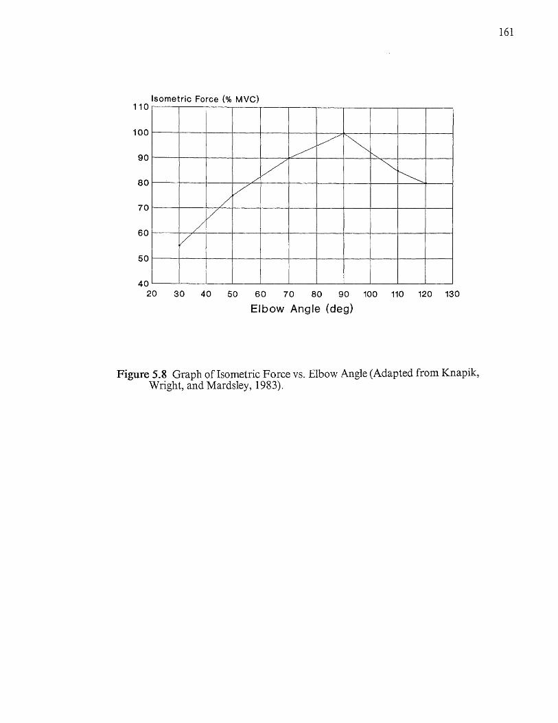
Figure 5.8 Graph of Isometric Force vs. Elbow Angle (Adapted from Knapik,Wright, and Mardsley, 1983).

161

162

Then, the required force (R) is expressed as a proportion to the actual available

MVC by:

Finally, the regression equation (Equation 5.2) is rearranged to express the

endurance time (t) as a function of the required force (R).

The approximate endurance times have been calculated for the six joint

angles for which experimental data are available. Figures 5.9 and 5.10 show,

respectively, the actual maximum available force (A), and the relative force as a

percent of MVC, for selected joint angles. A predicted endurance time (T) is

computed for the selected joint angles. Trials in which the required force (R) is a

greater fraction of MVC are expected to have shorter endurance times.

The aforementioned technique is repeated for each feasible spatial location

with its corresponding set of joint angles. The values for which experimental data

are not available can be approximated by using linear interpolation between the

available data points. In the general case a table can be is constructed showing in

each cell the predicted endurance time (T) for various force demand levels. In

practice, however, the task requirements (e.g. 8 lbs.) will dictate which of the cell

entries are to be used in a linear assignment problem.

Figure 5.9 Available Force (A) at Selected Joint Angles (0) (Adapted fromKnapik, Wright, and Mardsley, 1983).

163

Figure 5.10 Relative Force (R) at Selected Joint Angles (0) (Adapted fromKnapik, Wright, and Mardsley, 1983).

We can define the fatigue rate as the rate in a given activity cycle at which

the limit of endurance is approached. The fatigue rate value (F) is derived from

the predicted endurance times for a given activity, and is computed by taking the

reciprocal of endurance time. For each location on the ATM control panel, a

predicted endurance time and fatigue rate for the given force demand level is

given in Figure 5.11.

5_4 Linear Assignment Model Formulation

In order to minimize the total cost per ATM session (in terms of fatigue

rate) the expected cost of assigning each node (control) to every feasible spatial

location is calculated. The expected number of visits to a given node varies

depending on the type of transaction and likelihood of multiple transactions per

session. For Case III, the expected number of visits to each node is first estimated

for each transaction type by examination of the system flowchart of Figure 5.12,

multiple transaction probabilities, and transaction mix. The resulting probability

distribution for multiple visits and the expected number of visits to each node (per

ATM session) are given in Table 5.2.

Once the expected number of visits to each node for each type of

transaction is determined, an assignment tableau is constructed which contains

the cost of assigning each control to each location. The initial assignment matrix

(Tableau 0) is given in Table 5.3.

164

Figure 5.11 Predicted Endurance Times and Fatigue Rates Based on 5thPercentile Female and an 8-Pound Force Demand.

165

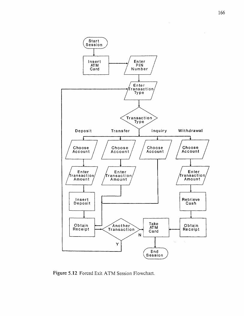
Figure 5A2 Forced Exit ATM Session Flowchart.

166

Table 5.2 Probability Distribution of Multiple Visits and Expected Visits toEach Node per ATM Session.

Node nCase I Case II Case III

P(n) E(n) P(n) E(n) P(n) E(n)Cardslot 0 0 0 0

1 1 1 0.9 1.1 0.9 1.12 0 0.1 0.1

Keypad 0 0 0 01 0.265 1.735 0.868 1.132 0.868 1.1322 0.735 0.132 0.132

Keypad-1 0 1 0.256 0.2561 0 0 0.646 0.842 0.646 0.8422 0 0.098 0.098

Keypad-2 0 1 1 0.831 0 0 0 0 0.148 0.1922 0 0 0.022

DeposSlot 0 0.87 0.87 0.871 0.13 0.13 0.13 0.13 0.108 0.1522 0 0 0.022

RecptSlot 0 0 0 01 1 1 1 1 1 12 0 0 0

RecptSlot-1 0 1 1 0.831 0 0 0 0 0.17 0.172 0 0 0

CashDisp 0 0.455 0.455 0.4551 0.545 0.545 0.545 0.545 0.545 0.5452 0 0 0

167

Table 5.3 Location Parameters and Assignment Cost Matrix for Case III.

Assignment Cost ( Cij )Location Parameters 1= 1 1= 2 1=3 i= 4 1= 5 1=6

Loc.j

EndurTime

FatigueRate

CardSlot

KeyPad

FunctnKey

DepositSlot

ReceiptSlot

CashDisp

1 1.28 0.781 0.859 1.692 1.891 0.119 0.914 0.4262 2.6 0.385 0.423 0.833 0.931 0.058 0.450 0.2103 3.31 0.302 0.332 0.654 0.731 0.046 0.353 0.1654 4.02 0.249 0.274 0.539 0.602 0.038 0.291 0.1365 4.73 0.211 0.233 0.458 0.512 0.032 0.247 0.1156 5.82 0.172 0.189 0.372 0.416 0.026 0.201 0.0947 7.38 0.136 0.149 0.293 0.328 0.021 0.159 0.0748 6.08 0.164 0.181 0.356 0.398 0.025 0.192 0.0909 7.38 0.136 0.149 0.293 0.328 0.021 0.159 0.074

10 5.82 0.172 0.189 0.372 0.416 0.026 0.201 0.09411 2.15 0.465 0.512 1.007 1.126 0.071 0.544 0.25312 2.8 0.357 0.393 0.774 0.865 0.054 0.418 0.19513 3.88 0.258 0.284 0.558 0.624 0.039 0.302 0.14014 4.73 0.211 0.233 0.458 0.512 0.032 0.247 0.11515 7.3 0.137 0.151 0.297 0.332 0.021 0.160 0.07516 4.89 0.204 0.225 0.443 0.495 0.031 0.239 0.11117 4.33 0.231 0.254 0.500 0.559 0.035 0.270 0.12618 4.2 0.238 0.262 0.516 0.576 0.036 0.279 0.13019 4.33 0.231 0.254 0.500 0.559 0.035 0.270 0.12620 4.89 0.204 0.225 0.443 0.495 0.031 0.239 0.11121 2.52 0.397 0.437 0.860 0.961 0.060 0.464 0.21622 3.39 0.295 0.324 0.639 0.714 0.045 0.345 0.16123 4.28 0.234 0.257 0.506 0.566 0.036 0.273 0.12724 5.82 0.172 0.189 0.372 0.416 0.026 0.201 0.09425 4.89 0.204 0.225 0.443 0.495 0.031 0.239 0.11126 4.08 0.245 0.270 0.531 0.593 0.037 0.287 0.13427 3.77 0.265 0.292 0.575 0.642 0.040 0.310 0.14528 3.68 0.272 0.299 0.589 0.658 0.041 0.318 0.14829 3.77 0.265 0.292 0.575 0.642 0.040 0.310 0.14530 4.08 0.245 0.270 0.531 0.593 0.037 0.287 0.134

Notes

1. Fatigue Rate = Reciprocal of Endurance Time

2. Cij = (Fatigue Rate at Location j) x (Frequency of Use of Control i)

168

Table 5.3 (Continued) Location Parameters and Assignment Cost Matrix forCase III.

Assignment Cost ( Cij )Location Parameters i = 1 i=2 i=3 1=4 i=5 1=6

Loc.j

EndurTime

FatigueRate

CardSlot

KeyPad

FunctnKey

DepositSlot

ReceiptSlot

CashDisp

31 2.74 0.365 0.401 0.791 0.884 0.055 0.427 0.19932 3.63 0.275 0.303 0.597 0.667 0.042 0.322 0.15033 4.6 0.217 0.239 0.471 0.526 0.033 0.254 0.11834 7.38 0.136 0.149 0.293 0.328 0.021 0.159 0.07435 4.33 0.231 0.254 0.500 0.559 0.035 0.270 0.12636 3.77 0.265 0.292 0.575 0.642 0.040 0.310 0.14537 3.51 0.285 0.313 0.617 0.690 0.043 0.333 0.15538 3.44 0.291 0.320 0.630 0.704 0.044 0.340 0.15839 3.23 0.310 0.341 0.671 0.750 0.047 0.362 0.16940 3.77 0.265 0.292 0.575 0.642 0.040 0.310 0.14541 2.8 0.357 0.393 0.774 0.865 0.054 0.418 0.19542 3.72 0.269 0.296 0.582 0.651 0.041 0.315 0.14743 4.73 0.211 0.233 0.458 0.512 0.032 0.247 0.11544 6.08 0.164 0.181 0.356 0.398 0.025 0.192 0.09045 4.2 0.238 0.262 0.516 0.576 0.036 0.279 0.13046 3.68 0.272 0.299 0.589 0.658 0.041 0.318 0.14847 3.44 0.291 0.320 0.630 0.704 0.044 0.340 0.15848 3.36 0.298 0.327 0.645 0.721 0.045 0.348 0.16249 3.44 0.291 0.320 0.630 0.704 0.044 0.340 0.15850 3.68 0.272 0.299 0.589 0.658 0.041 0.318 0.148

Notes

1. Fatigue Rate = Reciprocal of Endurance Time

2. Cij = (Fatigue Rate at Location j) x (Frequency of Use of Control i)

169

5.5 Solution of Assignment Model

The computer solution of the assignment model is found using an

adaptation of the Hungarian algorithm (as outlined in Section 3.11), implemented

in the IBM PC software program ASSIGN1. The data from the assignment cost

matrix (Tableau 0) is entered into the program, and after several iterations an

optimal tableau is found. The results of the computation can be found in the

Appendix.

5.6 Layout Recommendations

An analysis of the results yields multiple optimal and near-optimal

solutions to the minimization assignment problem. From these solution sets

several layouts (Figures 5.13 through 5.16) can be described in which the total

fatigue rates will be minimal. The choice of which (if any) solution should be

implemented will be based upon heuristics and other considerations. In this case

study, the selected layout is as shown in Figure 5.17. The rationale for this

selection is that the keypad and function keys are ideally located near to the eye

level and adjacent to the CRT display.

170

1 2 3 4 5 6 7

KeyPad

8

RecSlot

9

CardSlot

10

11 12 13 14 15

FunctKey

16 17 18 19 20

21 22 23 24 25 26 27 28 29 30

31 32 33 34

CashDisp

35 36 37 38 39 40

41 42 43 44

DepSlot

45 46 47 48 49 50

Total Cost of Assignment: 1.14

Figure 5.13 Layout for ATM Control Panel #1.

1 2 3 4 5 6 7

KeyPad

8

FunctKey

9

RecSlot

10

11 12 13 14 15

CardSlot

16 17 18 19 20

21 22 23 24 25 26 27 28 29 30

31 32 33 34

Cash35

Disp

36 37 38 39 40

41 42 43 44

DepSlot

45 46 47 48 49 50

Total Cost of Assignment: 1.14

171

Figure 5A4 Layout for ATM Control Panel #2.

6 8

RecSlot

32

18131211

2821 2322

39383731 3632 33

49484741 42 43

9

CardSlot

19

29

7

KeyPad

17

FunctKey

27

34

CashSlot

44

DepSlot

35

45 1 46

1 2 3

_

4 5 6 7

FunctKey

8

RecSlot

9

CardSlot

10

11 12 13 14 15

KeyPad

16 17 18 19 20

21 22 23 24 25 26 27 28 29 30

31 32 33 34

CashDisp

35 36 37 38 39 40

41 42 43 44

DepSlot

45 46 47 48 49 50

172

Total Cost of Assignment: 1.14

Figure 5.15 Layout for ATM Control Panel #3.

Total Cost of Assignment: 1.367

10

20

30

40

50

Figure 5.16 Layout for ATM Control Panel #4.

7

RecSlot

82 3 4 65

173

10

18

FunctKey

28

11

21

13

23

12

22

14

24

19

KeyPad

29

20

30

5049

9

CardSlot

31 1 32 33 34

DepSlot

35 36 37 38 39 40

CashDisp

41 1 42 1 43 44 1 45 46 1 47 1 48

Total Cost of Assignment: 1.55

Figure 5A7 Preferred Layout for ATM Control Panel.

5.7 Software Ergonomics

5.7.1 Video Screen Layout

Mental workload requirements for a particular task are directly related to

the design of the human-machine interface. With a poor interface design, the

point of information overload may possibly be approached for some members of

the user base. Human information processing capabilities are often unnecessarily

overtaxed by presenting a user with too much, unneeded, or confusing

information. In contrast, efficient design will substantively improve performance

for the entire user population.

5.7.2 Design Simplification

One of the fundamental tenets of effective screen design is simplicity.

Providing the user with an interface that presents the required information and

obtains the desired response objectives is the responsibility of programmers. Just

as nature abhors a vacuum, programmers seem to abhor presenting blank space

on a display screen. Given a screen capable of displaying many characters, the

tendency of programmers is to fill it just because it is there (Morland, 1983). This

is exhibited in several ATM system dialog screens. It has been shown that most

transactions will proceed faster if the amount of (superfluous) infomation

displayed on the screen is minimized. (Morland, 1983).

174

5.7.3 Social Amenities

Computers frequently are met by the public with resistance, apprehension

or even fear. Programmers, sensitive to this, often overcompensate by liberally

including social amenities in their systems. There is an tendency to include

phrases such as "PLEASE," "IF YOU WANT," and "DO YOU WISH" in dialog

screens. Although it is important that computers appear not to be rude, it is

recommended that these social amenity phrases be systematically eliminated in

the interest of improving clarity (Morland, 1983).

Pseudopersonal dialogs are also commonly found in ATM as well as other

software designs. It is recommended that designers should not attempt to be too

friendly, so that displaying "GOOD AFTERNOON, JOHN DOE" - which serves

no useful purpose other than exhibiting that the time of day and identity of the

user is known to the system - and similar phrases should be avoided.

5.7.4 Implicit Input Requests

Systems designed for use by the general public should be designed to be as

explicit as necessary about what the user should do at each stage of the

transaction. However, on the screens specifically requesting input, the fact that

the computer is requesting input can be made implicit instead of explicit without

introducing adverse effects. For example, the relatively verbose messages:

175

"PLEASE SELECT THE TYPE OF TRANSACTION THAT YOU WISH,"

and

"WHAT IS THE AMOUNT OF YOUR DESIRED TRANSACTION?"

can be replaced by:

"TYPE OF TRANSACTION:"

and

"AMOUNT."

The result can be a less cluttered screen with improved operator performance.

5.7_5 Entry Error Handling and Logging

Data entry errors can never be eliminated. The goal instead is to minimize

the consequences of user errors that occur. The ability to undo a mistake is a

desirable feature. Users should be given the opportunity to self-correct their

keyboarding errors with one or more clearly labeled keys for: cursor back,

backspace, redo, or cancel. The error control strategy must, wherever possible,

give clear indication of an error as soon as it is detected, and preferably

recommend a suggested remedy. Automatic error logging is essential in accurate

detection of user errors made in performing various functions and their types, and

the collection of error statistics will aid in the evaluation of operator skill levels

and in the diagnosis of human-machine interface problems.

176

5.7.6 Global and Local Patterns

From the historical distribution of ATM transaction types, it is apparent

that some transactions occur with greater frequency than others. However, a

particular institution may find from study of historical records of ATM sessions

that their transaction mix may differ from the industry standards. Certain

transaction types such as cash deposit to checking account may in some cases be

found to occur more often than cash withdrawal from checking. System defaults

should therefore be adjusted to reflect the transaction pattern in the local area

specifically under study.

5.7.7 System Default Strategies

System default entries represent an attempt by the software system

designers to anticipate the answers a user will give to some or all of the system's

queries. A system may have (at one extreme) no defaults at all, in which the user

must enter all data required; and (at the other extreme) "entry-by-exception", in

which the system supplies all of its own answers and the user enters data only

when on-screen defaults are incomplete or inaccurate (Martin, 1973).

Default entries are usually established by the system designer or

development team when the system is created.

Morland (1983) suggests that default values can be assigned based on three

factors:

177

1. How universal are the default responses?

2. How stable are they?

3. How context dependent are they?

Theoretically, a large number of separate default sets can be defined: systemwide,

site-dependent, group-dependent, or even individual user.

5.7.8 Response -Based Defaults

Although it is recognized that defaults should be held constant as much as

possible, Morland (1983) advocates the evolution of default values on the basis of

a continuous statistical analysis of user responses. The responses for the entire

user base can be compiled and interpreted by either the host computer or satellite

processors. The system would start with an initial default set. After observing a

sufficient number of user responses, the default set would be revised when a more

statistically significant response pattern is found. Several important control

parameters must be established, such as the threshold frequency of a given

response required to trigger a change in default (Morland, 1983).

5.7.9 Evolutionary Interface

An evolutionary interface can be designed for the ATM in which the

manual analysis and assignment of user defaults completely unnecessary. An

artificially intelligent multilevel system could continually monitor and collect data

178

on the user's pattern of accesses to the system, and alter the interface presentation

sequences according to a set of established rules.

For example, consider a user who most frequently uses an ATM for cash

withdrawals of $100.00 from his checking, and never performs transfers between

accounts. Such a user could eventually have his top level menu screen evolve

from the system default menu (Figure 5.19) to the menu shown in Figure 5.20. At

any time the user could, if desired, access any other non-displayed options by

requesting "other" from the menu. If menu option "other" is selected and some

other type of transaction is chosen a significant number of times, then the user's

default menu would adapt accordingly.

5.7.10 Multilevel ATM Interface Design

ATM Systems should be designed to accommodate users with different

experience levels within the user population. This strategy will permit a wide

variety of users to use the system efficiently. Once a user has gained access to the

system, by inserting his card and entering a valid personal identification number

(PIN), his identity is known with absolute certainty.

179

Figure 5.18 Default ATM Top Level Menu Provided to All Users.

180

Figure 5.19 Individualized ATM Top Level Menu Based on User TransactionPatterns.

With the system default, novice users are given the standard user interface,

using the techniques referred to as numbers 9 and 11 by Martin (1973), and

generous help capabilities. Users identified as more advanced can be offered

more condensed screens, combined screen cues, and abbreviated input fields (such

as in techniques 12 through 15). Expert users could be provided with even more

advanced features, typeahead, or even command language (techniques 4, 5, and

16 through 20).

For example, consider the common input sequence of entering a PIN

number, such as # 5151, then selecting to make a cash withdrawal from the

checking account in the amount of 100 dollars. The transaction sequence is as

follows:

Enter PIN number 5 1 5 1 <ENTER>

(wait for validation and menu display)

Choose Transaction Type 1 <ENTER>

(wait for next menu)

Choose Account 1 <ENTER>

(wait for next menu)

Enter Amount ($100.00) 10000 <ENTER>

(transaction is completed)

The normal ATM transaction sequence to achieve this result requires fifteen

keystrokes, three pauses, and three queries for additional input.

181

A command line interface could be set up for more advanced users to

perform the same transaction more quickly and efficiently. In constructing the

command line, the first four digits represents the PIN number, the fifth digit is the

transaction type (1 = cash withdrawal from checking), and 100 is the amount of

$100.00. The command line transaction sequence is as follows:

Enter PIN number 5 1 5 1 1 1 0 0 <ENTER>

(transaction is completed)

A user employing the command line interface accomplishes the same

transaction in only nine keystrokes, with no pauses or queries for additional

input.

The command line entry system would process this input from the

recognized expert user and, once validated, handle the entire transaction faster

and without the need for additional dialogs.

The approach of altering the presentation or merging several screens into

one, while somewhat more difficult to implement, can be worthwhile if the

distribution of skill levels within the user base is characterized as "bathtub-

shaped". For example, a user population following this distribution contains

relatively few average users, and a large number of novice and advanced users. It

is very likely that the distribution of ATM user skill levels falls into this category,

since many users can learn and develop proficiency quickly, while a large number

apparently do not. As a result, many transaction are performed by persons at

each end of the proficiency spectrum.

182

The user's "expert rating" can be assigned a numerical value according to

his ATM performance over time, possibly based on time per screen, time per

transaction, user response time, total errors, number of canceled transactions, or

keying signature (Gilb, 1977).

A great deal of information can be determined by analyzing the user's

individual keying pattern. Weinberg (1965) discovered that by timing keystrokes

and combinations of keystrokes, a timing signature can be found to indicate the

proficiency and possible even the identity of a user. In addition, changes in

keying times during input (blips) can be used to discover errors or poorly

designed procedures (Gilb, 1977).

The logic of a proposed quasi-intelligent system is as shown in the

flowchart in Figure 5.20. For example, a user who typically completes an ATM

session quickly and with few errors could have his proficiency rating

automatically revised to better utilize his demonstrated ability, while a user who

makes many errors or often sees the "need more time?" prompt could have his

rating modified to give him a more helpful interface. Changes in the user's

proficiency levels (either up or down) would be detected by the system and the

interface modified accordingly. With automatic logging, a self-maintaining

system could be devised which would be completely transparent to the user and

therefore require no intervention from either the user or the system operator.

183

Notes

1. X • Number of errors in previous 10 transactions

2. Y • Cumulative errors divided by total transactions

184

Figure 5.20 Flowchart for an Adaptive User Proficiency System.

CHAPTER 6 CONCLUSIONS AND RECOMMENDATIONS

In solving the ATM layout problem this thesis utilized methods which

yielded satisfactory solutions from the ergonomic point of view. The resulting

system designs should prove workable in practice as long as the underlying

assumptions made in this thesis are valid. The concepts and methods employed

are believed to be valid when applied not only to the ATM problem, but to

similar problems in human-machine interface design in which position costs

dominate and motion costs are of minor importance.

The methods of determining joint configurations from points in space are

well established, and most of the underlying assumptions made in the endurance

model formulations are based on recognized principles of ergonomics and

biomechanics. The heuristic design guidelines provided by the human factors

profession are helpful in specifying and designing an ergonomic workplace.

The specific layout, although believed to be optimal, may in some cases be

found infeasible for reasons of physical or mechanical impracticality. For

example, the internal dimensions behind the panel of a cash dispensing

mechanism may prohibit its installation in a given location. The detailed

information needed to ascertain this and incorporate this situation into the model

was unobtainable. If necessary, however, the model could be reformulated the

problem with the physical limitation constraints and the problem solving

procedure repeated.

185

Some basic simplifying assumptions are made in the formulation of cost

coefficients. The first is that the optimization of the elbow joint is the most

critical in determining endurance times and fatigue rates. The justification for this

assumption is based on the relative muscle sizes of the limbs involved in upper

body work activities. Future research may test the validity of this assumption,

and if it is found that other biomechanical effects are significant, other cost

coefficients could be developed accordingly.

Other assumptions are that individual body parts are independent of each

other, that the endurance times for each body element can be separately

determined, and that the fatigue-inducing effort affecting one part does not

necessarily affect the other parts of the body. These assumptions may also be

tested by experimentation. Tests of human endurance in simulated workplace

conditions can be developed that will show if the independence assumption is

valid. It is recommended that any further studies in this area should include the

additional research and experimentation to verify the assumptions stated herein.

The ergonomic design guidelines employed for the physical workplace

provide an ergonomically efficient standing workstation for the design population

(5th percentile female) and an ergonomically acceptable workstation for the

majority of the anticipated user base.

The combination of kinematic analysis and prediction of human fatigue

rates may, when combined with the appropriate anthropometric data, be used to

develop quantitative reach envelopes for general populations, a segment of the

186

population, or even individuals. Also, quantitative assessments of existing

layouts and comparisons between competing design proposals can be made.

The implementation of adaptive human-machine interfaces is strongly

recommended. Instead of relying on fixed position controls, a designer, given the

design population's anthropometric, biomechanical, movement, mental

processing and perceptual capabilities, can develop an adaptive interface which

responds to the user's requirements. The control panel layouts can be efficiently

designed by software programs such as the expert systems currently used to

design machine and motor control panels (Blickley, 1988).

In the ideal case, a control panel could be comprised of an array of touch

sensitive screens, such as is found in power plant simulators (Reason, 1988), or in

the "glass cockpits" of new generation airliners such as the Boeing 777 (Scott,

1991). With such a system an optimal custom interface can - at least theoretically

- be provided to each user. Control and display types, sizes, locations, and

complexities can be determined by system software, based on the situation at

hand and the requirements of the user, so as to maximize the overall ergonomic

efficiency of the system.

187

BIBLIOGRAPHY

Abdel-Malek, L. L. and Z. Li. "The Application of Inverse Kinematics in theOptimum Sequencing of Robot Tasks." International Journal ofProduction Research. 28(1): 75-90. 1990.

Alden, D. G., R. W. Daniels and A. T. Kanarick. "Keyboard Design andOperation: A Review of the Major Issues." Human Factors. 14: 275-293.1972.

Ambrosino, G. "Adaptive Tracking Control of Industrial Robots." Journal ofDynamic Systems Measurement and Control. 110: 215-220. September1988.

Anderson, R. B. MathCAD User's Manual Student Edition Version 2.0.Reading, MA: Addison-Wesley, 1989.

Asfour, S. S., M. Tritar, and A. M. Genaidy. "Endurance Time and PhysiologicalResponses to Prolonged Arm Lifting." Ergonomics. 34(3): 335-342. 1991.

Avis, D. "A Survey of Heuristics for the Weighted Matching Problem."Networks. 13: 475-493. 1983.

Avis, D. and C. W. Lai. "The Probabilistic Analysis of a Heuristic for theAssignment Problem." SIAM Journal on Computing. 17(4): 732-741.August 1988.

Banks, W. W. and M. P. Boone. "Method For Quantifying ControlAccessibility." Human Factors. 23: 299-303. June 1981.

Benhabib, B. "Optimal Continuous Path Planning for Seven Degree of FreedomRobots." Journal of Engineering Industry. 108: 213-218. August 1986.

Bhat, U. N. Elements of Applied Stochastic Processes, 2nd ed. New York: JohnWiley and Sons, 1984.

Bishop, A. "Membrane Keyboards Adopting Raised Keys." Electronics. 44.August 14, 1980.

Blickley, G. J. "Control Panel Design Made Easy with Software." ControlEngineering. 35: 68-70. June 1988.

Bonney, M. C. and R. W. Williams. "CAPABLE: A Computer Program toLayout Controls and Panels." Ergonomics. 20: 297-316. 1977.

Caldwell, L. S. "Body Stabilization and the Strength of Arm Extension." HumanFactors. 4(3):125-130. March 1962.

. "The Load-Endurance Relationship for a Static Manual Response."Human Factors. 6(1):71-79. January 1964.

188

189

. "Body Position and the Strength and Endurance of Manual Pull."Human Factors. 6(7):479-484. July 1964.

Chapanis, A. Research Techniques in Human Engineering. Baltimore: JohnsHopkins Press, 1953.

Chaffin, D. B. "A Computerized Biomechanical Model - Development of andUse in Studying Gross Body Actions." Journal of Biomechanics. 2: 429-441. 1969.

Chaffin, D. B. and M. Erig. "Three-Dimensional Biomechanical Static StrengthPrediction Model Sensitivity to Postural and AnthropometricInaccuracies." IIE Transactions. 23: 215-227. September 1991.

Chaffin, D. B., A. Freivalds and S. M. Evans. "On the Validity of an IsometricBiomechanical of Worker Strengths." IIE Transactions. 19: 280-288.September, 1987.

Charnes, A. and W. W. Cooper. Management Models and IndustrialApplications of Linear Programming. New York: John Wiley and Sons,1961.

Cockton, G. "Interaction Ergonomics, Control and Separation: Open Problemsin User Interface Management." Information Software Technology. 29:176-191. May 1987.

Cramer, H. The Elements of Probability Theory and Its Applications. NewYork: John Wiley and Sons, 1955.

Cullinane, T. P. "Minimizing Cost and Effort in Performing a Link Analysis."Human Factors 19: 151-156. 1977.

Deininger, R. L. "Human Factors Engineering Studies of the Design and Use ofPush-Button Telephone Sets." Bell Systems Technical Journal, 39: 995-1012. July 1960.

Denavit, J. and R. S. Hartenberg. "A Kinematic Notation for Lower-PairMechanisms Based on Matrices." Journal of Applied Mechanics. 215-221.June 1955.

Downing, J. V. and M. S. Sanders. "Effects of Panel Arrangement and Locus ofAttention on Performance." Human Factors. 29: 551-62. October 1987.

Drake, A. W. Fundamentals of Applied Probability Theory, McGraw-Hill Seriesin Probability and Statistics. New York: McGraw-Hill; 1967.

Drezner, Z. "DISCON: A New Method for the Layout Problem." OperationsResearch. 28: 1375-1384. 1980.

Erikson, W. J. and 0. P. Hall, Jr. Computer Models for Management Science,2nd ed. Reading, MA: Addison-Wesley, 1986.

Francis, R. L. and J. A. White. Facility Layout and Location: An AnalyticalApproach. Englewood Cliffs, NJ: Prentice-Hall, 1974.

Freund, L. E. and T. L. Sadosky. "Linear Programming Applied to Optimizationof Instrument Panel and Workplace Layout." Human Factors. 9: 295-300. 1967.

Gavett, J. W. and N. V. Plyter. "The Optimal Assignment of Facilities toLocations by Branch and Bound." Operations Research. 14:210-232.1966.

Genaidy, A. M. and S. S. Asfour. "Effects of Frequency and Load of Lift onEndurance Time." Ergonomics. 32: 51-57. 1989.

Genaidy, A. M., T. M. Khalil, S. S. Asfour and R. C. Duncan. "HumanPhysiological Capabilities for Prolonged manual Lifting Tasks." IIETransactions. 23(3): 270-280. 1990.

Gilb, T. and G. Weinberg. Humanized Input. Winthrop Computer SystemsSeries. Cambridge, MA: Winthrop Publishers, 1977.

Gilmore, P. C. "Optimal and Suboptimal Algorithms for the QuadraticAssignment Problem." Journal of Society of Industrial and AppliedMathematics. 10:305-313. 1962.

Goldenberg, A. A. and D. L. Lawrence. "A Generalized Solution to the InverseKinematics of Robotic Manipulators." Journal of Dynamic SystemsMeasurement and Control. 107: 103-106. March 1985.

. "A New Approach to Kinematic Control of Robot Manipulators."Journal of Dynamic Systems Measurement and Control. 109: 97-103.June 1987.

Grassmann, W. K. "Review of Markov 1." OR/MS Today. 17(6): 32-35.December 1990.

Haynes, R. M. "The ATM at Age Twenty: A Productivity Paradox." NationalProductivity Review. 9: 273-281. 1990.

Held, M. and R. Karp. "The Traveling Salesman Problem and MinimumSpanning Trees." Operations Research. 18(6): 1126-1138. 1970.

Hendy, K. C. "A Model for Human-Machine-Human Interaction in WorkspaceLayout Problems." Human Factors. 31:593-610. October 1989.

Hill, S. G. and K. H. E. Kroemer. "Preferred Declination of the Line of Sight."Human Factors. 28(2): 127-134. April 1986.

Hillier, F. S. "Quantitative Tools for Plant Layout Analysis." Journal ofIndustrial Engineering. 14:33-40. 1963.

190

Hillier, F. S. and M. M. Connors. "Quadratic Assignment Problem Algorithmsand the Location of Indivisible Facilities." Management Science. 13:42-57. 1966.

Hillier, F. S. and G. Lieberman. Introduction to Operations Research, 4th ed.Oakland: Holden-Day, 1986.

Hitchings, G. G. "The Application of Optimizing Techniques and StatisticalControl Theory to a Generalized Layout." Institute of Science andTechnology, University of Wales. Technical Note EPTN3. January 1968.

Howard, R. A. Dynamic Probabilistic Systems, Volume II, Semi-Markov andDecision Processes. New York: John Wiley and Sons, 1971.

Hughes, D. "Glass Cockpit Study Reveals Human Factors Problems." AviationWeek and Space Technology. 131:32-36. August 7, 1989.

Kantowitz, B. H. and R. D. Sorkin. Human Factors: Understanding People-System Relationships. New York: John Wiley & Sons, 1983.

Karp, R. M. "An Algorithm to Solve the m x n Assignment Problem in ExpectedTime O(mn log n)." Networks. 10: 143-152. 1980.

Khaopravetch, K., and R. Nanda. "Assessing Solution Efficiency for QuadraticAssignment Problems." Industrial Engineering. 22: 51-53. April 1990.

Konz, S. Work Design: Industrial Ergonomics, 3rd ed. Worthington, OH:Publishing Horizons, 1990.

Koopmans, T. C. and M. J. Beckmann. "Assignment Problems and the Locationof Economic Activities." Econometrica. 25: 53-76. 1957.

Kroemer, E. H. Eberhard. "Human Strength: Terminology, Measurement andInterpretation of Data." Human Factors. 12: 297-313. June 1970.

Lawler, E. L. "The Quadratic Assignment Problem." Management Science.13:42-57. 1963.

. Combinatorial Optimization: Networks and Matroids. New York: Holt,Rinehart and Winston, 1976.

Ledgard, H. and A. Singer. Directions in Human Factors for Interactive Systems.New York: Springer Verlag, 1981.

Lee, C. S. G. "Robot Arm Kinematics, Dynamics and Control." Computer. 15:62-80. December 1982.

Lee, R. C. and J. M. Moore. "CORELAP - Computerized Relationship LayoutPlanning." Journal of Industrial Engineering. 18: 195-200. 1967.

Lee, S. M., L. J. Moore, and B. W. Taylor. Management Science, 2nd ed.Dubuque, Iowa: Wm. C. Brown, 1985.

191

Lisboa, J. J. "Quantification of Human Error and Common-Mode Failures inMan/Machine Systems." IEEE Transactions Energy Conversion. 3: 292-9.June 1988.

Lutz, M. C. and A. Chapanis. "Expected Location of Digits and Letters on Ten-Button Keysets." Journal of Applied Psychology. 39(5): 314-17. 1955.

Martin, J. Design of Man-Computer Dialogues. Prentice-Hall: EnglewoodCliffs, 1973

Martin, S. and D. Clark. "Moving to ATMs - An Analytical Approach". TheMagazine of Bank Administration. 28-33. December 1982.

Mathsoft, Inc. MathCAD Version 2.0. Mathsoft Publishing Co. 1989.

McCormick, E. J. and M. S. Sanders. Human Factors in Engineering and Design,5th ed. New York: McGraw-Hill, 1982.

McCormick, M. J. and W. Wrennall. "A Step Beyond Computer-Aided Layout."Industrial Engineering. 17: 40-42. May 1985.

Metropolis, N. and S. Ulam. "The Monte Carlo Method." Journal of theAmerican Statistical Association. 44: 335-341. 1949.

Miller, R. A., R. J. Jagacinski, R. B. Nalavade, and W. W. Johnson. "Plans andthe Structure of Target Acquisition Behavior." Proceedings of the HumanFactors Society. 25: 571-575. 1981.

Miller, R. B. "Response Time in Man-Computer Conversational Transactions."Proceedings of the National Computer Conference. Montvale, NJ: AFIPSPress, 268-277. 1968.

Montgomery, E. B. "Bringing Manual Input into the 20th Century; NewKeyboard Concepts." Computer. 15: 11-19. March 1982.

Moore, T. G. "Industrial Push Buttons." Applied Ergonomics. 6: 33-38. 1975.

Morland, D. V. "Human Factors Guidelines for Terminal Interface Design."Communications of the ACM. 26: 484-494. July 1983.

NASA. Anthropometric Source Book - Volume I: Anthropometric Data forDesigners; Volume II: A Handbook of Anthropometric Data; Volume III:Annotated Bibliography of Anthropometry. Yellow Springs, OH:National Aeronautics and Space Administration Scientific and TechnicalInformation Office. 1978.

Nemeth, S. E. and K. E. Blache. "Ergonomic Evaluation of Two-Hand ControlLocation." Human Factors. 24: 567-571. October 1982.

Norman, D. A. "Commentary: Human Error and the Design of ComputerSystems." Communications of the ACM, 33: 4-7. January 1990.

192

Nugent, C. E., T. E. Vollmann, and J. Ruml. "An Experimental Comparison ofTechniques for the Assignment of Facilities to Locations." OperationsResearch, 16: 150-173. 1968.

Parker, J.F., Jr. and V. R. West, eds. Bioastronautics Data Book, 2nd ed. NASASP-3006. Washington, D.C.: U.S. Government Printing Office, 1973.

Paul, R. Robot Manipulators: Mathematics, Programming and Control.Cambridge, MA: MIT Press, 1981.

. Robot Manipulators. Cambridge MA: MIT Press, 1982.

Phillips, Mark D. "The Quantification of Operational Suitability." Computer.20: 63-71. February, 1987.

Red, W. E. "Robot Path Planning in 3-Dimensions Using the Direct Subspace."Journal of Dynamic Systems Measurement and Control. 109: 238-244.September 1987.

Reason, J. "Six CRT Touch Screens Simulate a Full-Scope Control Panel."Power. 133: 29-31. July 1989.

Rodgers, S. H., ed. The Ergonomics Group Health and EnvironmentLaboratories, Eastman Kodak Company. Ergonomic Design for Peopleat Work: A Source Book for Human Factors. New York: Van NostrandReinhold, 1986.

Roebuck, J. A. Jr., K. H. E. Kroemer, and W. G. Thomson. EngineeringAnthropometry Methods. New York: John Wiley and Sons, 1975.

Saaty, T. Mathematical Methods of Operations Research. New York: McGraw-Hill, 1959.

Schwartz, J. T. and M. Sharir. "A Survey of Motion Planning and RelatedGeometric Algorithms." Artificial Intelligence. 37: 157-169. December1988.

Scott, W. B. "777's Flight Deck Reflects Strong Operations Influence." AviationWeek and Space Technology. 134: 52-58. June 3, 1991.

Seidenberg, J. P. "Cirrus and Plus Announce August Date for Start of TerminalDuality." Card News. 5:4-5. July 16, 1990.

Sharir, M. "Algorithmic Motion Planning in Robotics." Computer. 22:9-20.March 1989.

Siegel, A. I., J. J. Wolf, and J. Pilitis. "A New Method for the Scientific Layout ofWorkspaces." Applied Ergonomics. 13(2): 87-90. 1982

Swain, J. "Linear Programming: Software Survey." OR/MS Today. 17(5).October 1990.

193

Taha, H. A. Operations Research, 4th ed. New York: Macmillan, 1987.

Taube, P. M. "The Influence of Selected Factors on the Frequency of ATMUsage." Journal of Retail Banking. 10. 41-52. Spring 1988.

Tichauer, E. R. Biomechanical Basis of Ergonomics. New York: WileyInterscience, 1978.

Tillmann, P. and Tillmann, B. Human Factors Essentials - An Ergonomics Guidefor Designers, Engineers, Scientists, and Managers. New York: McGraw-Hill, 1991.

Tullis, T. "The Formatting of Alphanumeric Displays." Human Factors. 25(6):657-82. 1983.

U.S. Bureau of the Census. Statistical Abstract of the United States: 1990 (110thedition). Washington: U.S. Department of Commerce, GovernmentPrinting Office. 1990.

U.S. Department of Defense. Human Engineering Design Criteria for MilitarySystems, Equipment and Facilities. Washington: U.S. GovernmentPrinting Office. DOD Military Standard MIL-STD-1472C. 1981.

U.S. Department of Defense. Human Engineering Guide for Army Material.Washington: U.S. Government Printing Office. DOD Military HandbookMIL-HDBK-759A. 1981.

Van Cott, H. P. and R. G. Kinkade, eds. Human Engineering Guide toEquipment Design. New York: John Wiley, 1972.

Van der Velde, M. "ATMs: The Product, Placement and Pricing." BankManagement. 24-28. November 1986.

. "EFT Transactions: Growth and Direction." Magazine of BankAdministration. 36-38. December 1982.

. "Two New Models Tell How Much an ATM Transaction Really Costs."The Magazine of Bank Administration. 34-40. November 1986

Vollmann, T. E. and E. S. Buffa. "The Facilities Layout Problem in Perspective."Management Science. 12:450-468. 1966.

West, D. H. "Algorithm 608 - Approximate Solution to the QuadraticAssignment Problem." ACM Transactions on Mathematical Software.9(4): 461-466. 1983.

Wiker, S. F., G. D. Langolf, and D. B. Chaffin. "Arm Posture and HumanMovement Capability." Human Factors. 31(4): 421-441. 1989.

Willeges, R. C. and B. H. Willeges. "Modeling the Human Operator inComputer-Based Data Entry." Human Factors. 24: 285-99. 1982.

194

195

. "User Considerations in Computer-Based Interfaces." Human Factors.24: 421-441. 1982.

Winston, W. Operations Research: Applications and Algorithms. Boston:PWS-Kent, 1987.

Woodson, W. E., M. P. Ranc Jr., and D. W. Conover. "Design of IndustrialWorkplaces" Chapter 9 in Van Cott and Kinkade. 381-418. 1972.

Woodson, W. E. Human Factors Design Handbook: Information andGuidelines for the Design of Systems, Facilities, and Products for HumanUse. New York: McGraw-Hill, 1981.

Appendix A. Solution to Joint Problem for 5th Percentile Female -Numerical Solution and General Method for Kinematic Solution toManipulator Problem.

1. Upper and lower arm link lengths of 5th percentile femalesubject (from Rodgers, 1983).

a := 13.43 b := 17.32

2. Panel coordinates for a given point being analyzed:

x := -21 y := 18 z := 12

3. Define units for angular measurements:

rad a 1 deg := π/180.rad

4. Determine initial conditions for seed values frommid-range of feasible range of motion (Rodgers, 1983).

θ := 1.5 φ := 1.3 δ := 1.1

5. Solve the problem and find the set of joint angles:

Given

6. Transformation equations for each coordinate:

b.cos(θ).cos(φ).cos(δ) - b. sin(θ)-sin(φ)-cos(δ) + a.cos(θ).cos(δ) ≈ x

b.sin(θ).cos(φ) + b.cos(θ)-sin(φ) + a-sin(δ) ≈ y

-b . cos(θ).cos(φ).sin(δ) + b.sin(θ)-sin(φ).sin(δ) - a.cos(θ).sin(δ) ≈ z

7. Motion constraints for each joint, in radians (Rodgers, 1983).

-1.047-rad < θ < 3.14.rad

0.rad < φ < 2.62.rad

0.rad < δ < 2.27.rad

8. The computer program's algorithm then finds the solutionvector (V), and error vector values (ERR) as follows:

V := Find(θ,φ,δ)

E := ERR

9. Since a numerical solution method is used, the resultsare verified by checking the magnitude of the error. If thevalue of ERR is sufficiently small (ERR < 0.01), the answeris considered acceptable.

E = 7.105-10 (well within acceptable limits)

Appendix B. Computation of Predicted Endurance Times for SelectedJoint Configurations.

1. Given the relationship between force (F) and endurancetime (t), (from Kroemer, 1970; Kroemer, et al., 1975).

i := 1 ..9

Fi:=ti:=

100 .35,75 .5050 1

F - % MVC Applied 35 231 2.5

t - Endurance Time 26 421 621 820 10

Percent Minutes

2. Define the regression equation:

a := 100 b := -1 c := 20

b.ti

Gi := a•e + c

3. For the available extension forces at elbow angles(Adapted from Knapik, Wright, and Mardsley, 1983).

i := 1 ..6 φi:= Pi :=

30 5550 7570 9090 100'110 85120 80

Degrees Minutes

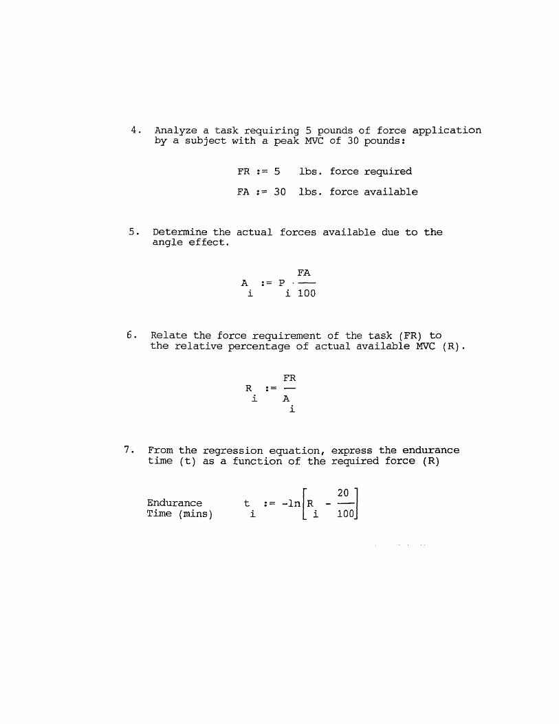
4. Analyze a task requiring 5 pounds of force applicationby a subject with a peak MVC of 30 pounds:

FR := 5 lbs. force required

FA := 30 lbs. force available

5. Determine the actual forces available due to theangle effect.

Ai:= Pi• FA/100

6. Relate the force requirement of the task (FR) tothe relative percentage of actual available MVC (R).

Ri:= FR/Ai

7. From the regression equation, express the endurancetime (t) as a function of the required force (R)

EnduranceTime (mins) t

i := -ln[Ri - 20/100]

8. Compute the predicted endurance times for each joint angle.

Trial

i

JointAngle

0'i

Availablemax Force

Ai

Req'd Force(% of MVC)

R .100i

PredictedEndurance time

Ti

1 30 16.5 30.3 2.32 50 22.5 22.2 3.83 70 27 18.5 61.34 90 30 16.7 68.55 110 25.5 19.6 49.56 120 24 20.8 4.8

Degrees Pounds Percent Minutes

Appendix C. Computation of Steady-State Probabilities from One-StepTransition Matrix - (Numerical Example from Case II Model).

Transition Matrix - (Example from Case II).

- .1 .9 0 0 0 0 00 .132 0 .868 0 0

0 0 .132 0 .154 .071 .643P := 0 0 .711 .033 0 .256 0

0 0 0 0 0 1 0

1 0 0 0 0 0 0

0 0 0 0 0 1 0

- 0.01 0.209 0 0.781 0 0 0

0 0.017 0.617 0.143 0 0.222 02 0.071 0 0.017 0 0.02 0.806 0.085

P = 0.256 0 0.117 0.001 0.109 0.059 0.457

1 0 0 0 0 0 0

0.1 0.9 0 0 0 0 0

1 0 0 0 0 0 0_

0.001 0.037 0.555 0.207 0 0.2 0

0.222 0.002 0.183 0.02 0.095 0.08 0.3973 0.813 0.064 0.002 0 0.003 0.106 0.011

P = 0.085 0.23 0.016 0 0.018 0.575 0.075

0.1 0.9 0 0 0 0 0

0.01 0.209 0 0.781 0 0 0

0.1 0.9 0 0 0 0 0_

- 0.2 0.006 0.221 0.039 0.086 0.092 0.357 -

0.103 0.2 0.038 0.003 0.028 0.51 0.1184 0.188 0.741 0 0.055 0 0.014 0.001

P = 0.584 0.106 0.002 0.2 0.003 0.095 0.01

0.01 0.209 0 0.781 0 0 00.001 0.037 0.555 0.207 0 0.2 0

0.01 0.209 0 0.781 0 0 01

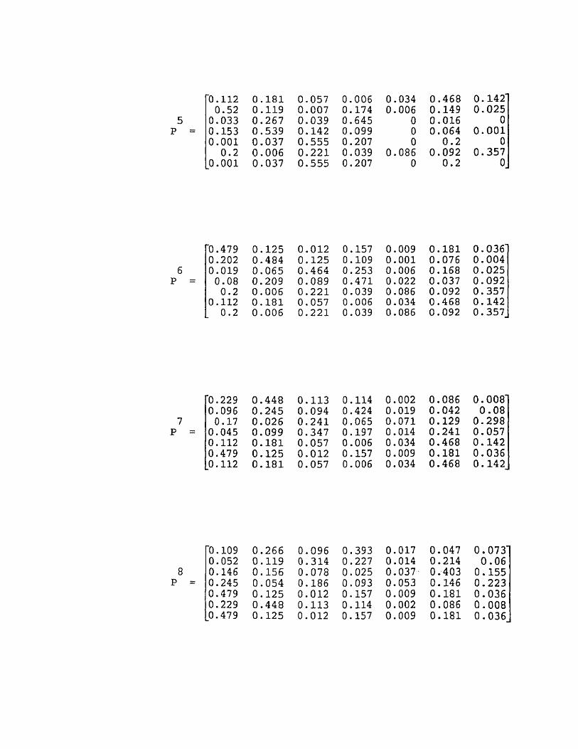
-0.112 0.181 0.057 0.006 0.034 0.468 0.1420.52 0.119 0.007 0.174 0.006 0.149 0.025

5 0.033 0.267 0.039 0.645 0 0.016 0P = 0.153 0.539 0.142 0.099 0 0.064 0.001

0.001 0.037 0.555 0.207 0 0.2 00.2 0.006 0.221 0.039 0.086 0.092 0.357

0.001 0.037 0.555 0.207 0 0.2 0

0.479 0.125 0.012 0.157 0.009 0.181 0.036 -

0.202 0.484 0.125 0.109 0.001 0.076 0.0046 0.019 0.065 0.464 0.253 0.006 0.168 0.025P = 0.08 0.209 0.089 0.471 0.022 0.037 0.092

0.2 0.006 0.221 0.039 0.086 0.092 0.3570.112 0.181 0.057 0.006 0.034 0.468 0.1420.2 0.006 0.221 0.039 0.086 0.092 0.357

0.229 0.448 0.113 0.114 0.002 0.086 0.008 -

0.096 0.245 0.094 0.424 0.019 0.042 0.087 0.17 0.026 0.241 0.065 0.071 0.129 0.298P = 0.045 0.099 0.347 0.197 0.014 0.241 0.057

0.112 0.181 0.057 0.006 0.034 0.468 0.1420.479 0.125 0.012 0.157 0.009 0.181 0.0360.112 0.181 0.057 0.006 0.034 0.468 0.142

-0.109 0.266 0.096 0.393 0.017 0.047 0.07310.052 0.119 0.314 0.227 0.014 0.214 0.06 '

8 0.146 0.156 0.078 0.025 0.037 0.403 0.155P = 0.245 0.054 0.186 0.093 0.053 0.146 0.223

0.479 0.125 0.012 0.157 0.009 0.181 0.0360.229 0.448 0.113 0.114 0.002 0.086 0.008 '

0.479 0.125 0.012 0.157 0.009 0.181 0.036

0.19 0.129 0.18 0.161 0.031 0.178 0.130.198 0.194 0.134 0.112 0.027 0.219 0.114

16 0.226 0.275 0.122 0.173 0.011 0.145 0.048P = 0.245 0.206 0.092 0.182 0.02 0.174 0.082

0.162 0.239 0.136 0.259 0.02 0.101 0.0820.117 0.178 0.202 0.216 0.021 0.178 0.088

0.239 0.136_0.162 0.259 0.02 0.101 0.082 _

0.189 0.203 0.146 0.186 0.022 0.164 0.09-

0.183 0.196 0.152 0.182 0.023 0.17 0.09532 0.194 0.192 0.146 0.166 0.024 0.18 0.098

P 0.19 0.189 0.149 0.175 0.024 0.175 0.0980.201 0.201 0.136 0.172 0.022 0.175 0.0930.195 0.207 0.14 0.18 0.021 0.169 0.0870.201 0.201 0.136 0.172 0.022 0.175 0.093_

0.191 0.198 0.146 0.178 0.022 0.172 0.094-

0.191 0.198 0.146 0.178 0.022 0.172 0.09464 0.191 0.198 0.145 0.178 0.022 0.172 0.093

P = 0.191 0.198 0.145 0.178 0.022 0.172 0.0940.191 0.198 0.146 0.178 0.022 0.172 0.0930.191 0.198 0.146 0.178 0.022 0.172 0.0940.191 0.198 0.146 0.178 0.022 0.172 0.093_

0.191 0.198 0.146 0.178 0.022 0.172 0.094-

0.191 0.198 0.146 0.178 0.022 0.172 0.094128 0.191 0.198 0.146 0.178 0.022 0.172 0.094

= 0.191 0.198 0.146 0.178 0.022e 0.172 0.0940.191 0.198 0.146 0.178 0.022 0.172 0.0940.191 0.198 0.146 0.178 0.022 0.172 0.0940.191 0.198 0.146 0.178 0.022 0.172 0.094 _

Appendix D. Solution to Joint Angle Problem for 6-Jointed Manipulator(from Lee, 1982).

Appendix E. Computer Program for Solving Simplex LinearProgramming Problems (Adapted from Taha, 1987).

DIMENSION A(50,100), B(50), CJ(100), NXI(50),*KODE(50),C(50,100),D(100),IN(50), IS(50,2)IIM=50IIN=100

C SIMPLEX PROGRAM FOR LINEAR PROGRAMMINGINTEGER GE,EQDATA MIN/3HMIN/, MAX/3HMAX/,GE/2HGE/,LE/2HLE/, EQ/2HEQ/

61 FORMAT (A4, 1013)63 FORMAT (16E5.0)64 FORMAT (1H1, 20X, 'PROBLEM—',A4,1H(,A3,1H))65 FORMAT (/' ITERATION NO.', 12)66 FORMAT (124, 9110)67 FORMAT (10X, 3H X(, 12, IH), 10F10.2, 2X, F10.2)71 FORMAT(//' *** OPTIMUM TABLEAU (ITERATION #', 12,') ***')72 FORMAT(/' UNBOUNDED SOLUTION -- X(',I2, 1 ) CANNOT BE MADE BASIC')73 FORMAT (10X, ' X( 0)', 10F10.2, 2X, F10.2)74 FORMAT (' NO FEASIBLE SOLUTION SINCE ARTIF. VAR. X(',I2,* ') IS BASIC AND POSITIVE')

75 FORMAT (' OBJ COEFF',10F10.2, 2X, F10.2)80 FORMAT(//'DO YOU NEED INSTRUCTIONS (TYPE 1=YES OR O=NO)')85 FORMAT('DATA MUST BE ENTERED AS FOLLOWS:'/

*'LINE 1: PROBLEM NAME, # CONSTRS, # VARS, # UNRESTRICTED VARS'/* 1 (IF NO UNRESTRICTED VARS, YOU MUST TYPE 0 "ZERO")'/*'LINE 2: MAX OR MIN, OBJ COEFFS'/*'FOLLOWING LINES: CONSTR TYPE(GE,LE OR EQ), CONSTR COEFFS, RHS'/*'LAST LINE: INDICES OF UNRESTRICTED VARS. (IF NONE, DELETE LINE)'/* 1/

* 'EXAMPLE'/' MAXIMIZE Z = 2X1 + 4X3 + 5X4'/'SUBJECT TO '/* I X1 + X2 — 3X3 — 2X4 <= l'/* 5X1 + 7X2 + 2X3 — X4 = 8'/* ' 9X1 + X2 + 6X >= 9'/* X1,X2 UNRESTR, X3 >=0'/* 'INPUT DATA ARE:'/* "'EXAMPLE",3,4,2 <HIT RETURN>'/* "'MAX",2,0,4,5 <HIT RETURN>'/* "'LE",1,1,-3,-2,1 <HIT RETURN>'/* "'EQ",5,7,2,-1,8 <HIT RETURN>'/* "'GE",9,1,0,6,9 <HIT RETURN>'/* ' 1,2 <HIT RETURN>'/*'

87 FORMAT(/'NOTE: VALUE OF "M" FOR ARTIFICIAL VARS IS "1E4". ․ )90 FORMAT(/' DATA SET IS NOW COMPLETE'//)95 FORMAT('DO YOU WANT TO PRINT ALL TABLEAUS (TYPE 1=YES OR O=NO)')

500 FORMAT(5X,'ORIGINAL X(',I2,') = X(',I2,') X(',I2,') = ',F10.4)

510 FORMAT(5X,'ORIGINAL X(',I2,') = X(',I2,') = F10.4)520 FORMAT(/ '*** INITIAL TABLEAU *** I )530 FORMAT('THE UNRESTR VARS RESULTED IN THE FOLLOWING SUBSTITUTION:')540 FORMAT(//'DO YOU WANT TO RUN A NEW PROBLEM (TYPE 1=YES OR O=NO)')550 FORMAT(/'PLS ENTER DATA NOW')560 FORMAT(//'*** OPTIMAL SOLUTION ***'/'OBJECTIVE VALUE = ',F10.4)580 FORMAT(' X(',I2,') = ', F10.4)

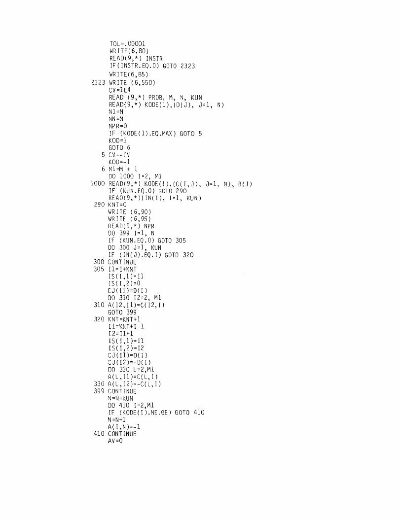
TOL=.00001WRITE(6,80)READ(9,*) INSTRIF(INSTR.EQ.0) GOTO 2323WRITE(6,85)

2323 WRITE (6,550)CV=1E4READ (9,*) PROB, M, N, KUNREAD(9,*) KODE(1),(D(J), J=1, N)N1=NNN =NNPR=0IF (KODE(1).EQ.MAX) GOTO 5KOD=1GOTO 6

5 CV=-CVK00=-1

6 M1=M + 1DO 1000 1=2, M1

1000 READ(9,*) KODE(I),(C(I,J), J=1, N), B(I)IF (KUN.EQ.0) GOTO 290READ(9,*)(IN(I), 1=1, KUN)

290 KNT=OWRITE (6,90)WRITE (6,95)READ(9,*) NPRDO 399 I-1, NIF (KUN.EQ.0) GOTO 305DO 300 J=1, KUNIF (IN(J).EQ.I) GOTO 320

300 CONTINUE305 I1=I+KNT

IS(I,1)=I1IS(1,2)=0CJ(I1)=D(I)DO 310 12=2, M1

310 A(I2,I1)=C(12,I)GOTO 399

320 KNT=KNT+1I1=KNT+I-112=11+1IS(I,1)=I1IS(I,2)=I2CJ(I1)=D(I)CJ(I2)=-D(I)DO 330 L=2,M1A(L,I1)=C(L,I)

330 A(L,12)=-C(L,I)399 CONTINUE

N=N+KUNDO 410 I=2,M1IF (KODE(I).NE.GE) GOTO 410N=N+1A(I,N)=-1

410 CONTINUEAV=0

DO 420 1=2,M1N=N+1A(I,N)=1NXI(I)=NIF (KODE(I).EQ.LE) GOTO 420AV=1CJ(N)=CV

420 CONTINUE2222 ITER=O

IF (KUN.EQ.0) GOTO 3333WRITE (6,530)DO 690 I =1, N1IF (IS(I,2).EQ.0) GOTO 600IF (IS(I,1).EQ.IS(I,2)) GOTO 600WRITE (6,500) I,IS(I,2),IS(I,1)GOTO 690

600 WRITE(6,510)I, IS(I,1)690 CONTINUE3333 IF (AV.EQ.1) WRITE (6,87)

WRITE(6,64) PROB, KODE(1)WRITE (6,520)

C PRINT TABLEAUIF (ITER.EQ.0) GOTO 4444IF (NPR.EQ.0) GOTO 55

1212 WRITE(6,65) ITER4444 N1=1

N2=643 IF (N2-N) 45,45,4444 N2=N45 IF (ITER.EQ.0) WRITE(6,75) (CJ(J), J=N1, N2)

WRITE(6,66) (J, J=N1,N2)WRITE(6,73)(A(1,J), J=N1, N2), B(1)DO 48 1=2, M1

48 WRITE(6,67) NXI(I), (A(I,J), J=N1, N2), B(I)IF (N2-N) 52,55,55

52 N1=N1+6N2=N2+6GOTO 43

55 CONTINUEIF (NPR.NE.2) GOTO 21WRITE (6,560) B(1)DO 800 J=1,NND(J)=0DO 800 1=2, MlK=NXI(I)IF (K.EQ.IS(J,1)) D(J)=B(I)

800 IF (K.EQ.IS(J,2)) D(J)=-B(I)DO 810 J=1, NNIF (KUN.EQ.0) WRITE (6,580) J, 0(J)IF(KUN.GT.O.AND.IS (J,2).EQ.0) WRITE(6,510) J,IS(J,1), D(J)IF (KUN.GT.O.AND.IS (J,2).NE.0) WRITE(6,500) J,IS(J,2),IS(J,1),D(J)

810 CONTINUEGOTO 1

C COMPUTE Z AND ZC21 DO 25 J=1,N

A(1,J)=0.DO 24 1=2, MlK=NXI(1)

24 A( 1 ,J)=A(1,J)+CJ(K)*A(I,J)25 A(1,J)=A(1,j)-CJ(J)

B(1)=0.DO 28 1=2, M1K=NXI(I)

28 B(1)=B(1)+CJ(K)*B(I)

C DETERMINE PIVOT COLUMNZCM=A(1,1)JM=1DO 109 J=2,NIF (KOD.EQ.1) GOTO 106

105 IF (A(1,J)-ZCM) 107, 109, 109106 IF (A(1,J)-ZCM) 109, 109, 107107 ZCM=A(1,J)

JM-J109 CONTINUE

C CHECK FOR OPTIMALCK=KOD*ZCMIF (CK.GT.TOL) GOTO 131

123 DO 124 1=2, M1K=NXI(I)IF (CJ(K).NE.CV) GOTO 124IF (B(I).LE.TOL) GOTO 124WRITE(6,74) KGOTO 1

124 CONTINUEWRITE(6,71) ITERNPR=2GOTO 4444

C DETERMINE PIVOT ROW131 XM=1.OE38

IM=0DO 139 1=2, M1IF (A(I,JM)) 139,139,135

135 XX=B(I)/A(I,JM)IF (XX-XM) 137,139,139

137 XM=XXIM=I

139 CONTINUEIF (IM) 141,141,151

141 WRITE(6,72) JMGOTO 1

C PERFORM PIVOT OPERATION151 XX=A(IM,JM)

B(IM)=B(IM)/XXITER=ITER+1DO 154 J=1,N

154 A(IM,J)=A(IM,J)/XXDO 161 I=1, M1IF (I-IM) 157,161,157

157 XX=A(I,JM)B(I)=B(I)-XX*B(IM)DO 160 J=1,N

160 A(I,J)=A(1,J)-XX*A(IM,J)161 CONTINUE

NXI(IM)= JMIF (NPR.EQ.1)GOTO 1212GOTO 21

DO 700 J=1,IINA(I,J)=0CJ(J)=0

700 C(I,J)=0ITER=0GOTO 2323END

Appendix F. Linear Assignment Tableaus for ATM Control PanelProblem.

Control i1

Card Slot

2KeyPad

3Functn

Key

4Deposit

Slot

5Receipt

Slot

6CashDisp

Loc.j1 0.8594 1.6922 1.8914 0.1188 0.9141 0.42582 0.4231 0.8331 0.9312 0.0585 0.4500 0.20963 0.3323 0.6544 0.7314 0.0459 0.3535 0.16474 0.2736 0.5388 0.6022 0.0378 0.2910 0.13565 0.2326 0.4579 0.5118 0.0321 0.2474 0.11526 0.1890 0.3722 0.4160 0.0261 0.2010 0.09367 0.1491 0.2935 0.3280 0.0206 0.1585 0.07388 0.1809 0.3563 0.3982 0.0250 0.1924 0.08969 0.1491 0.2935 0.3280 0.0206 0.1585 0.0738

10 0.1890 0.3722 0.4160 0.0261 0.2010 0.093611 0.5116 1.0074 1.1260 0.0707 0.5442 0.253512 0.3929 0.7736 0.8646 0.0543 0.4179 0.194613 0.2835 0.5582 0.6240 0.0392 0.3015 0.140514 0.2326 0.4579 0.5118 0.0321 0.2474 0.115215 0.1507 0.2967 0.3316 0.0208 0.1603 0.074716 0.2249 0.4429 0.4951 0.0311 0.2393 0.111517 0.2540 0.5002 0.5591 0.0351 0.2702 0.125918 0.2619 0.5157 0.5764 0.0362 0.2786 0.129819 0.2540 0.5002 0.5591 0.0351 0.2702 0.125920 0.2249 0.4429 0.4951 0.0311 0.2393 0.111521 0.4365 0.8595 0.9607 0.0603 0.4643 0.216322 0.3245 0.6389 0.7142 0.0448 0.3451 0.160823 0.2570 0.5061 0.5657 0.0355 0.2734 0.127324 0.1890 0.3722 0.4160 0.0261 0.2010 0.093625 0.2249 0.4429 0.4951 0.0311 0.2393 0.1115

Notes

1. Control Dummyl thru Dummy44 = 7 thru i 50) not shown.

2. Unit assignment costs for Dummyl thru Dummy44 are zero.

Control i1

CardSlot

2KeyPad

3Functn

Key

4Deposit

Slot

5Receipt

Slot

6CashDisp

Loc.No.26 0.2696 0.5309 0.5934 0.0373 0.2868 0.133627 0.2918 0.5745 0.6422 0.0403 0.3103 0.144628 0.2989 0.5886 0.6579 0.0413 0.3179 0.148129 0.2918 0.5745 0.6422 0.0403 0.3103 0.144630 0.2696 0.5309 0.5934 0.0373 0.2868 0.133631 0.4015 0.7905 0.8836 0.0555 0.4270 0.198932 0.3030 0.5967 0.6669 0.0419 0.3223 0.150133 0.2391 0.4709 0.5263 0.0330 0.2543 0.118534 0.1491 0.2935 0.3280 0.0206 0.1585 0.073835 0.2540 0.5002 0.5591 0.0351 0.2702 0.125936 0.2918 0.5745 0.6422 0.0403 0.3103 0.144637 0.3134 0.6171 0.6897 0.0433 0.3333 0.155338 0.3198 0.6297 0.7038 0.0442 0.3401 0.158439 0.3406 0.6706 0.7495 0.0471 0.3622 0.168740 0.2918 0.5745 0.6422 0.0403 0.3103 0.144641 0.3929 0.7736 0.8646 0.0543 0.4179 0.194642 0.2957 0.5823 0.6508 0.0409 0.3145 0.146543 0.2326 0.4579 0.5118 0.0321 0.2474 0.115244 0.1809 0.3563 0.3982 0.0250 0.1924 0.089645 0.2619 0.5157 0.5764 0.0362 0.2786 0.129846 0.2989 0.5886 0.6579 0.0413 0.3179 0.148147 0.3198 0.6297 0.7038 0.0442 0.3401 0.158448 0.3274 0.6446 0.7205 0.0452 0.3482 0.162249 0.3198 0.6297 0.7038 0.0442 0.3401 0.158450 0.2989 0.5886 0.6579 0.0413 0.3179 0.1481

Notes

1. Control Dummy1 thru Dummy44 (i = 7 thru i = 50) not shown.

2. Unit assignment costs for Dummyl thru Dummy44 are zero.