Análisis e Implementación de Algoritmo BLAST-Like para ...

ESCUELA TECNICA SUPERIOR DEINGENIERIA INFORMATICA

GRADO EN INGENIERIA INFORMATICA

Analisis e Implementacion de AlgoritmoBLAST-Like para arquitecturas MIC

Analysis and Implementation of aBLAST-like Algorithm for MIC

Architectures

Realizado por

D. Felipe Sulser Larraz

Tutorizado por

Dr. D. Sergio Galvez Rojas

Departamento

Lenguajes y Ciencias de la Computacion

UNIVERSIDAD DE MALAGA

MALAGA, Junio 2016

Fecha defensa:

El Secretario del Tribunal

Analysis and Implementation of a BLAST-like

Algorithm for MIC Architectures

Felipe Sulser Larraz

Spanish Abstract

El alineamiento de secuencias esta ganando importancia de manera incremental en

el ambito de la bioinformatica. Con el auge de los coprocesadores, es importante

adaptar los algoritmos de alineamiento de secuencias a las nuevas arquitecturas de

coprocesadores. La paralelizacion de estos programas usando tecnologıa SIMD ya

se ha logrado anteriormente de manera eficiente, por ejemplo SWIPE, creado por

Rognes en 2011.

El coprocesador Intel Xeon Phi proporciona una arquitectura solida, que puede ser

usada para maximizar la velocidad en el alineamiento de secuencias. Es por lo tanto

importante desarrollar algoritmos que sean capaces de usar el coprocesador con el

fin de maximizar el throughput.

En este trabajo, se describe y se analiza una nueva solucion e implementacion lla-

mada BLPhi. Este nuevo programa trata de reducir el tiempo de ejecucion usando

un metodo de filtrado. Ademas, aprovecha la arquitectura del coprocesador Intel

Xeon Phi y proporciona una solucion paralela al alineamiento de secuencias usando

tecnologıa SIMD.

Mientras que los metodos de alineamiento exactos, como el de Smith-Waterman, son

demasiados sensibles para la busqueda en bases de datos, BLPhi usa una tecnica

de filtrado que puede ser adaptada para cualquier longitud de secuencia. Esto le

proporciona al usuario la capacidad de adaptar la busqueda a sus necesidades y

puede, por ejemplo, hacerla mas restrictiva.

Tambien se proporciona un analisis del presente estado del arte en metodos de

alineamiento. Se realizan analisis y comparativas de tiempo y de precision para ver

el potencial que tiene BLPHi en comparacion con sus competidores.

Palabras clave— Bioinformatica, Intel Xeon Phi, SIMD, Alineamiento

3

English Abstract

Sequence alignment is becoming increasingly important in our current day and age,

and with the rise of coprocessors, it is important to adapt sequence alignment al-

gorithms to the new architecture. Parallelization using SIMD technology has previ-

ously been achieved that implement alignment algorithms efficiently such as SWIPE,

described by Rognes in 2011.

The Intel Xeon Phi provides a solid architecture which can be used and exploited

to maximize the speed in sequence alignment. It is therefore important, to develop

algorithms that are able to use efficiently the coprocessor to maximize throughput.

A different approach and implementation is described and benchmarked. The new

program, called BLPhi, aims to reduce execution time by using a filtering method.

BLPhi takes advantage of the architecture of the Intel Xeon Phi and provides a

parallel solution to sequence alignment using SIMD technology.

While exact alignment methods such as the Smith-Waterman are too sensitive for

database searching, BLPhi uses a filtering technique that can be adapted to any

length given. This gives the user the ability to adapt the search for his needs and

may, perhaps, make the search more restrictive.

An analysis with current state of the art alignment methods is also presented. We

perform speed and accuracy analysis to see the potential that BLPhi has among its

competitors.

Keywords— Bioinformatics, Intel Xeon Phi, SIMD, Alignment

4

Contents

1 Introduction 7

1.1 Motivation . . . . . . . . . . . . . . . . . . . . . . . . . . . . . . . . . 7

1.2 Objective . . . . . . . . . . . . . . . . . . . . . . . . . . . . . . . . . 7

1.3 A Brief Introduction to Bioinformatics . . . . . . . . . . . . . . . . . 8

1.4 State of the Art Local Alignment Algorithms . . . . . . . . . . . . . . 10

1.5 BLAST . . . . . . . . . . . . . . . . . . . . . . . . . . . . . . . . . . 11

1.5.1 Background . . . . . . . . . . . . . . . . . . . . . . . . . . . . 11

1.5.2 Scoring matrices . . . . . . . . . . . . . . . . . . . . . . . . . 12

1.5.3 Pre-processing algorithms . . . . . . . . . . . . . . . . . . . . 13

1.5.4 Heuristic . . . . . . . . . . . . . . . . . . . . . . . . . . . . . . 13

1.5.5 Algorithm steps . . . . . . . . . . . . . . . . . . . . . . . . . . 15

1.6 About the Intel Xeon Phi . . . . . . . . . . . . . . . . . . . . . . . . 16

1.6.1 Technical specifications . . . . . . . . . . . . . . . . . . . . . . 17

1.6.2 Vector Processing Unit . . . . . . . . . . . . . . . . . . . . . . 17

2 First steps with the Intel Xeon Phi 19

2.1 Intel C/C++ Compiler (ICC) . . . . . . . . . . . . . . . . . . . . . . 19

2.1.1 Offloading to the Xeon Phi . . . . . . . . . . . . . . . . . . . . 20

2.1.2 OpenMP . . . . . . . . . . . . . . . . . . . . . . . . . . . . . . 21

2.2 MIC Program Architecture . . . . . . . . . . . . . . . . . . . . . . . . 22

2.2.1 General Structure . . . . . . . . . . . . . . . . . . . . . . . . . 22

2.2.2 Parallelization . . . . . . . . . . . . . . . . . . . . . . . . . . . 23

2.2.3 Vectorization . . . . . . . . . . . . . . . . . . . . . . . . . . . 30

2.3 Simple examples using the Xeon Phi . . . . . . . . . . . . . . . . . . 33

3 Implementation of the BLAST-like algorithm 39

3.1 Structure of the Algorithm . . . . . . . . . . . . . . . . . . . . . . . . 39

3.2 Filtering . . . . . . . . . . . . . . . . . . . . . . . . . . . . . . . . . . 41

3.2.1 Filtering using a reduced alphabet . . . . . . . . . . . . . . . . 43

3.3 Efficient Implementation of the Filtering . . . . . . . . . . . . . . . . 45

3.3.1 Parallelization of the Filtering . . . . . . . . . . . . . . . . . . 45

3.3.2 Vectorization of the Filtering . . . . . . . . . . . . . . . . . . 46

3.4 Efficient Smith-Waterman . . . . . . . . . . . . . . . . . . . . . . . . 48

5

4 Results 52

4.1 Filtering Efficiency . . . . . . . . . . . . . . . . . . . . . . . . . . . . 52

4.2 Time Efficiency . . . . . . . . . . . . . . . . . . . . . . . . . . . . . . 53

4.2.1 Time Efficiency Between Filters . . . . . . . . . . . . . . . . . 53

4.2.2 Comparing Time Efficiency with Naive Smith-Waterman . . . 55

4.2.3 Comparing Time Efficiency with Other Algorithms . . . . . . 56

4.3 Algorithm Accuracy . . . . . . . . . . . . . . . . . . . . . . . . . . . 57

4.3.1 Comparing Accuracy with Other Algorithms . . . . . . . . . . 57

5 Conclusions 61

5.1 Future Upgrades and Extensions . . . . . . . . . . . . . . . . . . . . . 62

6 Conclusiones 64

6.1 Conclusiones . . . . . . . . . . . . . . . . . . . . . . . . . . . . . . . . 64

6.2 Futuras mejoras y extensiones . . . . . . . . . . . . . . . . . . . . . . 65

References 66

A User documentation 69

B Developer documentation 73

C Tables 83

Chapter 0 6

Chapter 1

Introduction

1.1 Motivation

In order to maximize performance in new computer designs, the current trend in

hardware design relies on the strategy of adding more cores to do multiple things

at once. Whether we consider CPU cores or GPU cores, the growth in the number

of cores is exponential. This increase in computing throughput opens new doors for

several research fields such as bioinformatics.

In particular, for the local alignment of biomolecular sequences (ADN, ARN or pro-

tein sequences), we require a high computational power due to the complexity of the

algorithms. For instance, the Smith-Waterman algorithm retrieves the optimal local

alignment with quadratic time and space complexity. It is therefore a requirement

to minimize execution time for these local alignment algorithms so that they become

practical and useful.

As a consequence, if we wish to adapt local alignment algorithms to the current

trend in computing, we have to optimize them for many-core machines, machines

that have more than 4-8 cores and have Simple Instruction Multiple Data (SIMD)

support.

Using the ideas from Rognes, 2011 [1], our objective is to develop a BLAST-like

algorithm [2] that reduces the execution latency by adapting it for many-core ma-

chines.

1.2 Objective

The main objective of this project is to develop a many-core optimized search al-

gorithm that will take advantage of the underlying architecture. The goal is to

7

find heuristics that are able to exploit the hardware and allow a high-throughput

sequencing.

Secondary objectives are also regarded as important. Objectives such as the study of

the current state of the art programs for local sequence alignment such as variants

of the Smith-Waterman algorithm. Also, the study of the state of the art MIC

technology is important due to the fact that it is a new technology and there is not

much information available for these technologies.

Another objective is the study of the behaviour of the proposed algorithm, BLPhi.

Analyzing the flexibility and performance of the algorithm is important in order to

compare it with other alignment methods such as BLAST.

Because of the lack of available resources for MIC application development, we have

considered the inclusion of another objective. We provide an incremental explana-

tion of the technologies involved in a MIC application, as well as examples using the

previously explained technologies. This guide should act as an introductory lesson

for anyone who would like to learn the technologies.

1.3 A Brief Introduction to Bioinformatics

Having a deep knowledge in the field of bioinformatics is not a mandatory requisite

in order to understand this thesis. Therefore, this section will provide a simple

introductory step to the basics of bioinformatics and why it is important.

The information is presented in a simplified way so that the reader can understand

the underlying motivations in sequence alignment and other bioinformatics applica-

tions.

Historical perspective

Since the discovery of the structure of DNA by Watson and Crick [3] and the discov-

ery of the protein sequence of insulin by Sanger [4], computers became essential in

molecular biology. Comparing multiple sequences of amino acids manually turned

to be impractical and thus, the use of computers was fundamental.

When the first genome was sequenced in 1977 by Sanger, these sequences have been

decoded and stored in databases. Comparing genes within a species can determine

the similarities or relations between protein functions. Also, comparing genes be-

tween different species, can show relations between species. However, this enormous

amount of data, often containing billions of base pairs or amino acids, makes a

manual DNA analysis impractical.

Chapter 1 8

The first methods used for sequencing are called chain termination sequencing or

Sanger sequencing. The method requires a single stranded DNA template, a DNA

polymerase, a DNA primer, normal deoxynucleosidetrophosphates (dNTPs) and di-

deoxynucleosidetriphosphates (ddNTPs). The method exploited the fact that the

ddNTP’s lack of hydroxyl on the third carbon group will avoid the growth of the

DNA polymerase which needs the hydroxyl to keep growing. Although an effective

method, it lacked the quality of being able to automate the process.

Next-Generation Sequencing are a group of sequencing methods that appeared af-

ter the Sanger sequencing method in order to allow a much quicker and cheaper

sequencing method. These methods include techniques such as pyrosequencing and

Ion semiconductor sequencing.

Alignment

Once we have a genome, we want to use the information gathered in the genomic

database to obtain other information such as species similarity or protein function

comparison. To do so, we will need to compare the similarities of the sequences.

This technique is called sequence alignment.

Depending on the type of similarity, there are two types of alignments:

• A global alignment attempts to align every residue in every sequence. This

technique is useful when the overall structure of the sequences are similar and

of equal size. Algorithms such as the Needleman-Wunsch algorithm which is

a dynamic programming algorithm.

• Local alignments, on the other hand, are more useful for sequences that

contain regions of similarity. The alignment in local alignment is based on local

regions rather than the global structure of the sequence. The Smith-Waterman

algorithm is a local alignment method also based on dynamic programming.

We can also divide the alignment methods depending on the quantity of sequences

we want to align. A pairwise sequence alignment is used to align two biological

sequences, whereas a multiple sequence alignment or MSA is the alignment of three

or more biological sequences of similar length.

Another division can be made regarding the exactness of the method. Exact methods

find the optimal alignment for the sequences. On the other hand, heuristic methods

provide a near-optimal alignment. The latter methods usually perform much faster,

as a trade-off for precision.

9 Chapter 1

Figure 1.1: Type of alignment algorithms.

1.4 State of the Art Local Alignment Algorithms

Exact methods

The current trend for exact methods is to optimize existing algorithms such as the

Smith-Waterman algorithm. This algorithm is able to find the optimal local align-

ment in quadratic time and linear space complexity. Although a quadratic time

might not be a feasible approach when working with large protein or nucleotide

database, recent implementations focus on taking advantage of computing paral-

lelization and thus reduce the execution time.

A fast approach using parallelization with SIMD technology has previously been

described by Farrar in 2007 [5] proposes a parallelized algorithm using SIMD in-

structions. The implementation uses a vectorized pattern for being able to execute

several instructions at a time. More recently, Rognes has create an inter-sequence

SIMD parallelisation that is able to perform several alignments at the same time

using vectorization in 2011 [1]. This last technique claims to be over six times more

rapid than Farrar’s approach.

Recently, the trend has shifted towards the use of coprocessors to perform the align-

ments. Rucci et al. have proposed a parallel and vectorized approach of the Smith-

Waterman algorithm that is also energy-aware using the Intel Xeon Phi coprocessor.

The program proposed by them is called SWIMM [6] and is able to reach speeds up

to three times faster than the inter-sequence method used by Rognes.

Chapter 1 10

Heuristic methods

Heuristic methods such as the FASTA (not to be confused with the file format) have

slowly lost importance and the main trend for heuristic method is the BLAST family

of algorithms. Different BLAST programs exist to tackle different problems such

as the Gapped BLAST and PSI-BLAST (Position-specific iterated BLAST). For

all these variants of the original BLAST, the main goal is to achieve faster speeds.

Parallelized implementations such as the MPI-BLAST described by Darling et al.

in 2003 [7] provide the tools necessary to create a distributed computational system

to execute BLAST on a large scale.

More recently, commercial BLAST programs have emerged such as Paracel BLAST

that provide a scalable BLAST platform [8]. This allows the creation of large clusters

of computation focused on the execution of sequence alignment.

1.5 BLAST

The program developed in this thesis is a BLAST-like algorithm that performs a

heuristic, local pairwise sequence alignment. Therefore it is of great importance

to know what the BLAST algorithm is and how it works. While the current

BLAST program is a suite of programs that contains many other features such

as pre-processing tools and graphical outputs, we are more interested in the orig-

inal heuristic behind the main BLAST algorithm rather than the whole suite of

programs.

BLAST works for nucleotide alignment and protein alignment. However, the imple-

mentation developed in the thesis, works on ungapped protein sequences. Therefore

all future references of BLAST will be based on the protein BLAST program or

BLASTP without gap extension.

1.5.1 Background

BLAST stands for Basic Local Alignment Search Tool and it is a heuristic, local

pairwise sequence alignment algorithm. This means that the algorithm provides a

near-optimal alignment for the given scoring matrices and the parameters. It com-

putes a similarity between regions, rather than a global alignment and the alignment

is computed between pairs of sequences.

The algorithm was designed by Stephen Altschul, Warren Gish, Webb Miller, Eugene

Myers and David Lipman [2]. Since then, it has become one of the most widely

used programs in bioinformatics for sequence searching. It addresses a fundamental

problem in bioinformatics research. Using a heuristic method, BLAST is much faster

11 Chapter 1

than other exact sequence alignments algorithms. The tradeoff between efficiency

and exactness is advantageous since it still provides solid results, not losing any

significant accuracy.

For any executions of BLAST, it requires the following inputs:

• Input sequences — usually in FASTA format.

• Weight matrix — like the PAM or BLOSUM matrices. This matrix is used

to weigh the scores between matches, gaps and differences.

• A prior formatted database of sequences.

The output of the execution can be delivered in several formats such as plain text,

HTML and XML. The results are in a graphical and explicit format showing the

hits found and the score that the sequence has obtained.

1.5.2 Scoring matrices

One of the input that BLAST needs is a scoring matrix or substitution matrix.

A scoring matrix has the objective of matching the most similar elements of two

sequences. The score of each pair of amino acids in the matrix is obtained by taking

into account the similarity of both amino acids and the possibility of mutation over

a period of evolutionary time.

The simplest scoring matrix would be an identity matrix where we only consider

each amino acid similar if matched with itself. Such a scoring matrix, will succed

if we try to align very similar sequences, but will fail to align somewhat related

sequences but with some differences.

A family of scoring matrices is the BLOSUM (BLock SUbstitution Matrix) family.

Each entry in a BLOSUM matrix is computed by looking at blocks of sequences

found on multiple protein alignments. An example of the BLOSUM62 matrix is

shown in the Figure 1.2.

Figure 1.2: BLOSUM62 matrix.

Chapter 1 12

1.5.3 Pre-processing algorithms

Apart from the main algorithm of BLAST, the suite offers several other filtering

options that can be used to obtain a better result and perhaps more accuracy.

Low Complexity Regions (LCR)

At the start of the execution of BLAST, a low complexity region filtering is usually

computed.

A low complexity region in a sequence is a region where there is a low variety

of amino acids. These regions usually carry a low amount of information. On

eukaryotic proteins for example, this is usually the case, and in order to obtain a

good result it is necessary to filter these low complexity regions [9].

SEG

BLAST eliminates low complexity regions using the SEG algorithm. This algorithm

uses a sliding window of size 12 to determine subsequences that contain potential

low complexity regions. The process goes as follows:

• Input of SEG is a protein sequence in FASTA format.

• Using a sliding window of size 12 we scan the sequence.

• If the subsequence contains less information than a certain threshold, we mark

the subsequence with ’X’.

To know how much information is carried in the subsequence we use the notion of

entropy. For example, if we have 20 characters randomly distributed, the information

carried by a character k would be log(p(k)) where p(k) is the probability of the

character.

1.5.4 Heuristic

The main difference between BLAST and other exact methods resides in the use of

a heuristic in order to accelerate the alignment process. On an exact algorithm such

as the Smith-Waterman, we will have to compare pairwise all the query sequences

with all the database sequences. This means that for m database sequences and n

query sequences we will perform mn executions of the Smith-Waterman alignment

algorithm. What BLAST tries to accomplish with an heuristic is to reduce the

number of comparisons done. The main core of the alignment algorithm can be also

a Smith-Waterman algorithm, however the number of comparisons executed will be

diminished due to the heuristic approach.

13 Chapter 1

The filtering process of the heuristic begins by making a k-letter word list of the

query sequence. For example, if k = 3 we list the words of length 3 in the protein

sequence sequentially (for nucleotides, usually k = 11). The words are constructed

by using a sliding window of three characters. Example shown in Figure 1.3.

Figure 1.3: Establishing the k-letter list.

After obtaining the list, we compare each word to the sequences in the database.

The comparison tries to find for each pair the T-value between the word and the

sequence. The T-value is the maximum score that is obtained between the word

and the sequence using a scoring matrix such as the BLOSUM62. An example is

shown in Figure 1.4 of the initial step for the calculation of the t-value.

Figure 1.4: Obtaining the t-value.

Then, the T-value is obtained by extending the query word in both directions reach-

ing to a maximum. When the extension starts to decrease the score value we stop.

This will be considered its T-value.

We call the alignments whose score is above a threshold value (usually 18 for BLAST)

High Scoring Segment Pairs (HSPs). These HSPs will be stored in an index and

will be later used to execute the local alignment algorithm.

To analyze how a high score is likely to exist by chance or randomness, a statistical

model of random sequences is needed. If we consider both sequences subject and

query sequences long enough, we may assume that the sum of these random variables

follows a normal distribution due to the central limit theorem. Therefore, in the limit

Chapter 1 14

of large sequence lengths m and n, the statistics for the HSP scores are characterized

by two parameters λ and K.

For each alignment of HSPs reported, an E-value [2] (Expected value) is computed

as follows for score S:

E = Kmne−λS (1.1)

This value will calculate the expected number of HSPs with score equal or greater

than S. This formula makes sense, the number of HSPs decrements exponentially

with score a higher score S. The parameters K and λ are scales for the search space

and the scoring system used respectively.

Now that we know the expected number of HSPs, we want to know the number of

random HSPs with score equal or greater than S. This expected value is described

by a Poisson distribution. The probability of finding at least one random HSP is

P = 1− e−E (1.2)

Where E is the E-value and P is called P-value.

Using these metrics, we are able to provice a statistical proof of how accurate the

heuristic will be and to analyze the random HSPs that will appear by using the

k-letter word list method.

1.5.5 Algorithm steps

The general BLAST algorithm is divided in four main steps. Although more modern

BLAST’s contain more steps, its main core can be separated in four different steps.

In the first step, we want to filter low complexity regions and in general, subse-

quences that carry low information. This can be accomplished by using the previ-

ously explained SEG algorithm. Performing a good low complexity region filtering

will generally result in an output that is more significant; however it is an optional

step.

In the second step we perform an exact word match. This is, for a query subsequence

of length k, we look for sequences in the database that contain the exact same

subsequence. We will store these matches includingt their location in the sequence.

All the matches will be called words.

In the third step, we generate the high scoring pairs or HSPs. For each word

previously obtained, we perform the following steps:

• We extend the word to the left, until the score that the match would obtain

using a scoring matrix starts to decrease. We stop on the highest value.

15 Chapter 1

• We extend the word to the left right until the score that the match would

obtain using a scoring matrix starts to decrease. We stop on the highest

value.

• The resulting segment is called HSP.

In the last step we perform a statistical significance check. Using the previously

defined P-value and E-value, we can determine if the amount of HSPs make sense

for the given input. We may compare the results obtained with the P-value. Since

the P-value estimates the quantity of random HSPs, we can verify if our results are

signficant or not.

1.6 About the Intel Xeon Phi

The main computing engine for the implemented program will be an Intel Xeon Phi

coprocessor. A coprocessor acts as task offloader to a CPU. A typical plattform

is diagrammed in Figure 1.5. Multiple of such platforms can be joined together in

order to form a supercomputer or a cluster.

Figure 1.5: Processor and Coprocessor platform

The main difference between a processor and a coprocessor is that a coprocessor

cannot act as a processor. Processors are cache coherent and also share RAM

with other processors. On the other hand, coprocessors are cache coherent SMP’s

(Symmetric Multiprocessors) that connect to other devices via the PCI bus and are

not cache coherent between other coprocessors or processors in the same system.

Chapter 1 16

1.6.1 Technical specifications

The specific coprocessor used for this task is the Intel Xeon Phi SC31S1P and its

technical specifications are:

• 57 Cores running at 1.1 GHz.

• In-order cores support 64-bit x86 instructions with unique SIMD capabilities

of 512 bits.

• 8 GB of DDR5 RAM

• Cache coherence in the entire coprocessor.

• Cores interconnected by a bidirectional ring.

• Each core has a 512 KB L2 cache. Total L2 cache size is over 25 MB.

• The coprocessor runs its own OS (Linux).

• Passive refrigeration (No fan).

• 270 W of TDP (Thermal Design Power).

Table: Technical specifications of the Xeon Phi

Clock Frequency 1.1 GHZ Code

Number of Cores 57 Cores

Memory Size 8GB GDDR5

Peak Memory Bandwidth 352 GB/s

Operating System Linux

Thermal Design Power 270 W

1.6.2 Vector Processing Unit

One of the main characteristics of the Xeon Phi coprocessor is its vector process-

ing unit or VPU. The coprocessor is designed with strong support for vector level

parallelism with features such as 512 bit registers, hardware prefetching and a high

memory bandwidth.

One of they key aspects of optimizing code using a coprocessor is learning to use

its VPU. Despite the number of cores, the computing strength of the coprocessor

resides on its SIMD registers.

Each core of the Xeon Phi coprocessor has a SIMD 512 bit wide VPU with a new

instruction set called KNC (Knight’s Corner). This VPU can be used to process 16

single precision elements per clock cycle. If we take into account the 57 cores each

coprocessor has, we can process up to 912 single precision elements per clock cycle.

As we can see in Fig. 1.6, each core executes 4 threads. Therefore it is a key aspect

to use the VPU and not leave it idle. Without vectorization, the Xeon Phi would

17 Chapter 1

not be as fast as it is. The computational strength of the Xeon Phi comes from its

vector processing unit.

Figure 1.6: Inside an Intel Xeon Phi core

Source: www.eetimes.com

Chapter 1 18

Chapter 2

First steps with the Intel Xeon Phi

On this chapter we will introduce the basics of the technologies used for the de-

velopment of the program. Because the available information and documentation

about the technologies of the MIC architecture is relatively scarce, a simple tuto-

rial is also included. This simple and progressive tutorial is oriented for those who

want to learn how to develop software on a coprocessor following a MIC program

architecture.

2.1 Intel C/C++ Compiler (ICC)

The Intel C/C++ Compiler (ICC) is a proprietary compiler owned by the Intel

company. This compiler generates optimized code for Intel architectures such as the

IA-32 or Intel 64. This compiler is essential when using a Xeon Phi coprocessor to

generate code because other compilers such as the GNU Compiler Collection (GCC)

do not generate KNC instructions, or lack the technologies that ICC has in order to

communicate with the coprocessor.

The ICC also has the capability of auto-vectorization and auto-parallelization. Auto-

vectorization is enabled by default and auto-parallelization can be enabled when

compiling with the -parallel flag.

Another important feature in the ICC is the possibility of generating a vectorization

report or parallelization report. These reports can be generated using the compila-

tion parameters -vec-report 1 and -par report-1 respectively.

ICC is optimized to computers using processors that support Intel architectures.

The code generated by it minimizes the stalls and minimizes the cycles. Several

tools and technologies are also included in the compiler:

• Cilk Plus extends the C language and enables the programmer to use high-level

sentences to generate parallel code.

19

• Intel Threading Building Blocks (TBB), similar to Cilk Plus, is a library that

can generate high-level paralellism using C code.The advantages of using this

library are that it generates flow graphs of the concurrent version of the pro-

gram, it is open source and works with several compilers.

• Intel Compiler’s Offload allows the programmer to transfer memory and ex-

ecute fragments of code in a coprocessor. All of the transfer is done using C

pragmas. This can also be used with Cilk Plus.

2.1.1 Offloading to the Xeon Phi

The offloading feature in the ICC allows the application to be partially executed on

a coprocessor or any MIC architecture.

In a program that includes offloading, execution begins on the host and, based

on used-defined statements, some sections of the program can be offloaded to the

coprocessor. A key feature of offloading is that the resulting binary program runs

whether or not a coprocessor is present in the system.

When to choose an Offload model vs. a Native execution is an important decision.

Generally speaking, an Offload model is the right approach when the program cannot

be made highly parallel consistently throughout its execution.

Overall, we should use an Offload model for:

• Large programs with high and focused hotspots such as a matrix multiplication

work best using an Offload model.

• Programs that require several I/O operations and are memory intensive work

also best using an Offload model.

How to offload

The main offload mechanism works using pragmas. This method uses a non-shared

memory model. This means, that the memory that the host processor can access

will not be shared with the coprocessor. However the cores in the coprocessor will

share the memory. The advantage of using a non-shared memory model is that it

allows the programmer to control the data movement very precisely.

If we want to offload dynamic data, a non-shared memory model would not be an

appropriate solution and we would have to use a shared virtual memory model used

in Cilk. However, we will focus on the non-shared model.

Chapter 2 20

Example 2.1: Simple offloading of a function

// function_a is executed by the host

function_a ();

#pragma offload target(mic : target_id)

{

// function_b is executed by the coprocessor

function_b ();

}

// function_c is executed by the host

function_c ();

Asynchronous offload

By default, the offload pragma directive causes the host processor’s thread that

encounters it to wait until the coprocessor completes the offload. It is possible to

execute an asynchronous offload, which enables the host processor to continue its

execution without waiting.

To specify an asynchronous offload, we use the signal clause in the offload pragma.

Example 2.2: Asynchronous offload

char vSignal;

// function_a is executed by the host

function_a ();

#pragma offload target(mic : target_id) signal (& vSignal)

{

// function_b is executed asynchronously

function_b ();

}

// function_c is executed by the host without waiting for

coprocessor to finish

function_c ();

...

//this makes the CPU thread to wait until coprocessor has finished

its execution

#pragma offload_wait (& signal_var)

2.1.2 OpenMP

OpenMP is a set of compiler directives for Fortran and C/C++ compilers that can be

used to specify high-level parallelism. The main strength of these directives is that

the programmer can ignore the directives while working in a sequential program.

Then, when a compiler recognizes the OpenMP directives, they are interpreted and

21 Chapter 2

give direction on how to create parallel tasks in order to increase speed in the

execution of a program.

Why use OpenMP?

The traditional way of developing a parallel program would be to use threads such

as the POSIX Threads (pthreads). Using pthreads allows the programmer to have

an extremely fine-grained control over the thread management such as creating and

joining the threads. However, pthreads is a very low-level API and it forces the

programmer to develop the program taking in consideration the parallelism since

the beginning.

On the contrary, OpenMP is much higher level and portable. The programmer

can focus on the development of the sequential program and afterwards introduce

OpenMP directives to make it parallel. Therefore, the tradeoff of using OpenMP

vs. using pthreads is between allowing a faster and simple program development or

having more control over the threads themselves.

An additional benefit of using OpenMP with a coprocessor is that it works with

the host’s CPU cores and with the coprocessor’s cores. This parallelism cannot be

achieved with a GPU.

Example 2.3: for-loop executed in parallel

int i;

//This simple directive , makes the for -loop parallel

#pragma omp parallel for

for(i = 1; i < n; i++){ //i is private by default

b[i] = ( a[i] + a[i-1] ) / 2.0;

}

2.2 MIC Program Architecture

Although there are several combinations of technologies available when developing

programs on the Xeon Phi, we will focus on specific technologies and learn how to

apply them on examples.

2.2.1 General Structure

In general, a MIC program can be offloaded or run natively on the coprocessor.

Since offloading is simply enabled by changing a compiler flag (-mmic) let us focus

on the former.

Chapter 2 22

Ideally, the general offloading program structure will consist of the following work

flow:

1. The host CPU runs the program and executes I/O heavy code.

2. Before the execution of a computational heavy loop or code we offload the task

to the coprocessor using Offloading.

3. Once the execution is on the coprocessor the CPU can still be executing code

or can be stalled.

4. The coprocessor then spawns threads and executes the code in parallel using

OpenMP.

5. Each thread then executes its task using the VPU running vectorized code.

Figure 2.1: Example of a program using offload for two tasks.

2.2.2 Parallelization

Parallelization is achieved using OpenMP. Using directives we are able to parallelize

the code. This section is dedicated to explain some important OpenMP directives

with simple examples. For a full and thorough guide of all the directives with, please

consult the OpenMP API specification at www.openmp.org .

Work-Sharing Directives

#pragma omp p a r a l l e l [ c l a u s e l i s t ]

code b lock

23 Chapter 2

www.openmp.org

This directive spawns a team of threads and starts the parallel execution of code block.

The clauses are:

• if(expression) — condition to spawn threads.

• num threads(integer) — number of threads to spawn.

• private (list of variables) — variables that will be private for each thread. By

default every variable is shared.

• reduction(operation:variable) — specifies that one or more variables that are

variables are subject to a reduction operation at the end of the region. E.g.

cumulative value.

#pragma omp for [ c l a u s e l i s t ]

f o r l o o p

This directive specifies how the threads spawned will execute the for-loop. The

clauses will specify how the for loop is divided, the order of execution and the

shared and private variables available for each thread.

• private(list of variables) — variables that will be private for each thread. By

default, every variable is shared.

• schedule(type) — Depends on each type:

– static divides the loop into equal-sized chunks for each thread. By de-

fault, it is the division between the number of iterations and the number

of threads.

– dynamic uses a work queue to give each thread a chunk of the for-loop.

When they are finished, it queues up until assigned another chunk.

– auto the decision of scheduling is delegated to the compiler.

• nowait — if enabled, threads do not synchronize at the end of the parallel

loop.

#pragma omp s e c t i o n s [ c l a u s e l i s t ]

{#pragma omp s e c t i o n

code b lock

#pragma omp s e c t i o n

code b lock

. . .

code b lock

}

This directive will distribute the threads among all the sections included inside the

sections block.

Chapter 2 24

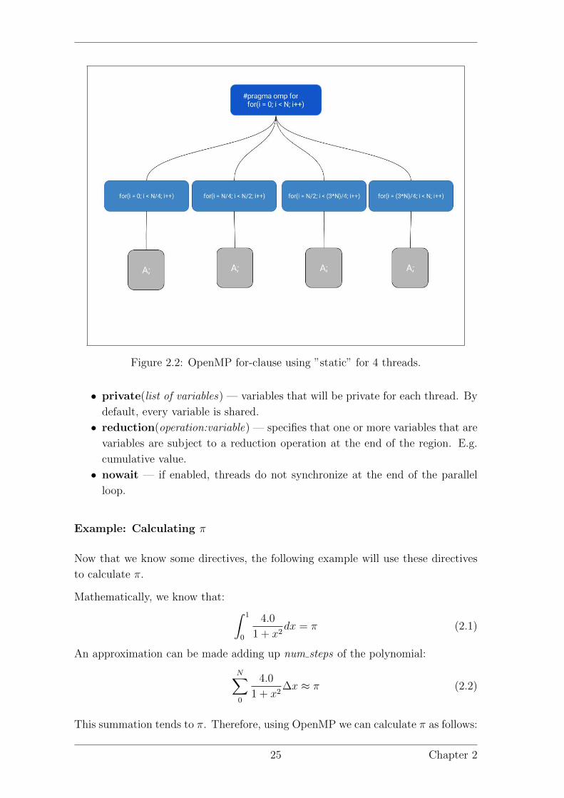
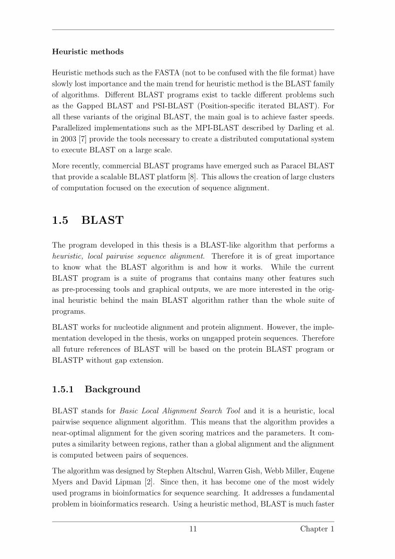
Figure 2.2: OpenMP for-clause using ”static” for 4 threads.

• private(list of variables) — variables that will be private for each thread. By

default, every variable is shared.

• reduction(operation:variable) — specifies that one or more variables that are

variables are subject to a reduction operation at the end of the region. E.g.

cumulative value.

• nowait — if enabled, threads do not synchronize at the end of the parallel

loop.

Example: Calculating π

Now that we know some directives, the following example will use these directives

to calculate π.

Mathematically, we know that: ∫ 1

0

4.0

1 + x2dx = π (2.1)

An approximation can be made adding up num steps of the polynomial:

N∑0

4.0

1 + x2∆x ≈ π (2.2)

This summation tends to π. Therefore, using OpenMP we can calculate π as follows:

25 Chapter 2

Example 2.4: Approximating pi

double j = 0 ;

double sum = 0 . 0 ;

double f a c t o r = 1 .0/ num steps ;

int i = 0 ;

//we spawn 8 threads

#pragma omp p a r a l l e l p r i va t e ( i , x ) num threads (8 )

{//The f o r loop g e t s d i v i d ed in t o e q u a l l y s i z e d chunks and ”

sum” , w i l l be reduced

#pragma omp for r educt ion (+:sum) schedu le ( stat ic )

for ( i = 0 ; i < num steps ; i++){j = i ∗ f a c t o r ; // in inc r ea s in g s t e p s between 0 and 1

sum = sum+4.0 /(1.0+ j ∗ j ) ;}

}double pi = f a c t o r ∗sum ;

p r i n t f ( ” p i = %f \n” , p i ) ;

Example: Sections

The following example would be executed by two threads. Even if we spawn more

threads, the other threads will not have any work load since there are only two

sections.

Example 2.5: Simple section task-dividing

#pragma omp s e c t i o n s

{#pragma omp s e c t i o n

{p r i n t f ( ” id=%d\n” , omp get thread num ( ) ) ;

}#pragma omp s e c t i o n

{p r i n t f ( ” id=%d \n” , omp get thread num ( ) ) ;

}}

Chapter 2 26

Synchronization Directives

Apart from spawning threads, we also need to orchestrate the threads and organize

them so we could establish critical sections, conditions and atomicity.

There are two types of synchronization, implicit and explicit. The implicit synchro-

nization exists at the beginning and end of the parallel directive. However, users

can also explicitly manage synchronization.

#pragma omp c r i t i c a l

code b lock

The critical directive restricts the execution of the code block to a single thread at

a time.

Figure 2.3: OpenMP for-clausewith a critical region.

#pragma omp atomic [ read | wr i t e | update | capture ]

statement ;

Atomic ensures that a specific variable is accessed atomically. Depending on the

clause, the statement can be:

• read — variable assignment (v = x;).

• write — assignment to expression (x = expr;).

27 Chapter 2

• update — expressions mentioned above and other expressions such as x++;.

• capture — any expression


The barrier directive specifies a point in the code where each thread must wait un-

till all threads in the execution arrive at the barrier. In other APIs (e.g. POSIX

threads) this is usually called a join.

#pragma omp f l u s h

code b lock

Flushing will make each thread that accesses the block of code memory-consistent.

#pragma omp ordered

code b lock

The ordered directive forces the execution of the block of code in an ordered way.

Example: π revisited

Following the previous example of the approximation of π, we can now solve the

same problem but introducing a critical zone, so that the sum is performed inside

the loop. We no longer need to use the reduce clause.

Example 2.6: Approximating pi using a critical region

double j = 0 ;

double sum = 0 . 0 ;

double f a c t o r = 1 .0/ num steps ;

int i = 0 ;

double aux = 0 . 0 ;

//we spawn 8 threads

#pragma omp p a r a l l e l p r i va t e ( i , j , aux ) num threads (8 )

{//The f o r loop g e t s d i v i d ed in t o e q u a l l y s i z e d chunks

#pragma omp for schedu le ( stat ic )

for ( i = 0 ; i < num steps ; i++){j = i ∗ f a c t o r ; // In inc r ea s in g s t e p s between 0 and 1

aux = sum+4.0 /(1.0+ j ∗ j ) ;// t h i s ensures t ha t on ly one thread acce s s e s t h i s

sentence

Chapter 2 28


sum = sum+aux ;

}}double pi = f a c t o r ∗sum ;

p r i n t f ( ” p i = %f \n” , p i ) ;

Example: Barriers

An example using a barrier would be the following. Suppose we have a function

that we wish to execute in parallel. With OpenMP we spawn a number of threads.

But how can we add a barrier in the middle of the function?

Example 2.7: Using a barrier to join threads

void worker ( ) {int t i d = omp get thread num ( ) ;

p r i n t f ( ”Thread %u s t a r t i n g \n” , t i d ) ;

// s imu la t e execu t ion o f a t a s k wi th s l e e p

s l e e p ( t i d ) ;

p r i n t f ( ”Thread %u has f i n i s h e d the execut ion o f the task \n” ,

t i d ) ;

// t h i s makes the thread to await u n t i l they are a l l j o ined

#pragma omp ba r r i e r

p r i n t f ( ”Thread %u has been j o in ed with a l l the threads \n” ,

t i d ) ;

}

int main ( ) {// t h i s spawns 4 threads f o r the execu t i on o f the func t i on

#pragma omp p a r a l l e l num threads (4 )

worker ( ) ;

return 0 ;

}

29 Chapter 2

2.2.3 Vectorization

In order to obtain the maximum throughput in our program, we need to vectorize

the code. Although Intel’s compiler can auto-vectorize the code, it is always recom-

mended to vectorize the critical and inner loops of the programs that may eventually

cause a bottleneck.

The decision of which part of the code is to be vectorized can be taken using the

following methods:

• We can consider vectorizing all the possible code from the host CPU code to

the co processor’s tasks. This method is not recommended due to the amount

of work needed to vectorize all the code.

• Using the auto vectorization report, we can see which loops and parts of the

code have not been vectorized by Intel’s auto vectorization and try to vectorize

them.

• We may vectorize the code that takes the most execution time. For each block

of code or loop, we can measure the execution time. Begin vectorizing the

most time consuming loops or blocks of code until the program meets the

maximum execution time.

Intrinsics

In order to simplify the process of vectorizing the code, Intel provides a set of

intrinsic functions that can help to write vectorized code.

An intrinsic function is a function that does not get called. Instead, the code of

the function is inserted inline by the compiler as the machine instructions to be

outputted by the function. We should regard intrinsic functions as a wrapper of

assembly language statements.

The benefit of using intrinsics for vectorization is that we can write efficient assembly

code by using high level functions, instead of assembly. In this project we will work

with the KNC instructions for the x86 instruction set architecture. We are not using

AVX-512 since it has not been released yet.

The following list includes several intrinsic data types and functions used in the

program. For more information about these functions please see: Intel intrinsics

guide.

Intrinsic data types

When working on the 512 bits SIMD registers of the Xeon Phi, we need to work with

special data types able to store 512 bits of information. The compiler automatically

Chapter 2 30

https://software.intel.com/sites/landingpage/IntrinsicsGuide/

https://software.intel.com/sites/landingpage/IntrinsicsGuide/

alignes the data types to a 64-byte boundary on the stack. If we want to align other

variables such as int, double, arrays or structures we can use the declspec align(64)

modifiers. For structures or arrays, it is important to know that the alignment only

affects the structure and the size. Every member of the structure or array will not

be aligned. If you want to align each member it is mandatory to specify it as in the

following example.

Example 2.8: Aligned structure

// t h i s s t r u c t u r e w i l l be a l i gn ed to a 16 by t e boundary

struct d e c l s p e c ( a l i g n (16) ) mystructure {d e c l s p e c ( a l i g n (16) ) int v1 ;

d e c l s p e c ( a l i g n (16) ) short v2 ;

d e c l s p e c ( a l i g n (16) ) int v3 ;

} ;

• m512 — This data type represents the contents of a 512 bit register used

by the SIMD intrinsics. It can hold sixteen 32-bit floating point values.

• m512d — This data type can hold eight 64-bit double precision floating

point values. The “d” in the end denotes double precision.

• m512i — This data type can hold integer values. For example, it can hold

sixty four 8 bit integer values, thirty two 16 bit integers or eight 64 bit integer

values. The “i” in the end denotes integer.

Intrinsic load functions

These functions are used to load data into the SIMD registers.

m512i mm512 load epi32 (void const ∗ , mem address )

This intrinsic loads 512 bits from const into mem address. The 512 bits must be

composed of 16 packed 32-bit integers.

m512i mm512 ext load epi32 (void const ∗ mt ,

MM UPCONV EPI32 ENUM conv , MMBROADCAST32 ENUM bc , int hint

)

This intrinsic loads 1, 4 or 16 elements of type and size determined by conv. The

amount of elements loaded depends on bc:

• MM BROADCAST32 NONE — means that it loads 16 elements.

• MM BROADCAST 1X16 — will load 1 element.

• MM BROADCAST 4X16 — will load 4 elements.

conv can be:

31 Chapter 2

• MM UPCONV EPI32 NONE — no conversion is applied.

• MM UPCONV EPI32 UINT8 — converts an uint8 data to a uint32 data.

• MM UPCONV EPI32 SINT8 — converts an sint8 data to a uint32 data.

• MM UPCONV EPI32 UINT16 — converts an uint16 data to a uint32 data.

• MM UPCONV EPI32 SINT16 — converts an sint16 data to a uint32 data.

Intrinsic arithmetic and comparison functions

These functions are used to apply operations on the data or between SIMD registers.

m512i mm512 setzero epi32 ( )

This function will return a m512 vector with all values set to zero.

m512i mm512 max epi32 ( m512i a , m512i b)

This function will compare 32-bit integers in a with b and will return the vector

containing the maximum values for each pair of 32-bit integers.

m512i mm512 add epi32 ( m512i a , m512i b)

This function adds 32-bit integers from a with b and returns the vector containing

the added pairs of 32-bit integers.

m512i mm512 sub epi32 ( m512i a , m512i b)

This function subtracts 32-bit integers from a with b and returns the vector con-

taining the subtracted pairs of 32-bit integers.

mmask16 mm512 cmpeq epi32 mask ( m512i a , m512i b)

This function compares 32-bit integers in a and b for equality. The results will be

stored in a mask that will contain 16 bits. For each integer compared, if the bit is

set to 1 it will mean the values in a and b were equal. Zero otherwise.

int mm512 mask2int ( mmask16 k1 )

Converts the bit mask into a 16-bit integer.

Chapter 2 32

2.3 Simple examples using the Xeon Phi

Now that we have seen the general structure of a program using a coprocessor and

the technologies involved, it is time to show some examples. The steps followed in

the process of explaining the example will be:

1. Naive solution

2. Offload the task

3. Parallelize the code

4. Vectorize

First example

For the first example program, we want to compute a fast array addition between

two int arrays. For this example, we consider the length of the array to be 16.

To begin, we start by implementing a simple loop that computes the sum of the

elements.

i n t 3 2 t x [ 1 6 ] = random array ( ) ;

i n t 3 2 t y [ 1 6 ] = random array ( ) ;

i n t 3 2 t z [ 1 6 ] ;

int j ;

for ( j = 0 ; j < n I t e r ; j++){//do mu l t i p l i c a t i o n here

int k ;

for ( k = 0 ; k < 16 ; k++){// S t ra i gh t f o rward naive s o l u t i o n

z [ k ] = x [ k]+y [ k ] ;

}}

After implementing the naive approach, we want to delegate the task of computing

the addition to our coprocessor. Now we offload the task to the coprocessor. To

offload the data, we need to use the in modifier from the offload pragma. This will

tell the compiler which data imported needs allocation in the co processor’s memory

and which will need to be copied back to the host’s memory.



i n t 3 2 t z [ 1 6 ] ;

//We o f f l o a d i t to the mic number 1

#pragma o f f l o a d ta r g e t (mic : 1 ) \in ( x : l ength (16) ) \in ( y : l ength (16) ) \

33 Chapter 2

inout ( z : l ength (16) )

{// t h i s code i s executed by the coprocessor number 1

int j ;


int k ;

for ( k = 0 ; k < 16 ; k++){z [ k ] = x [ k]+y [ k ] ;

}}

}// t h i s e x i t s the b l o c k o f code executed by the coprocessor

Now that the main task is delegated to the coprocessor, we can proceed to use its

many-core design by using OpenMP. We can now spawn threads.



i n t 3 2 t z [ 1 6 ] ;


#pragma o f f l o a d ta r g e t (mic : 1 ) \in ( x : l ength (16) ) \in ( y : l ength (16) ) \inout ( z : l ength (16) )

#pragma omp p a r a l l e l num threads (5 ) //we spawn 5 threads

{// t h i s code i s executed by the coprocessor number 1

int j ;

// t h i s w i l l d i v i d e the loop in chunks . When a thread has

f i n i s h e d i t s t a s k i t g e t s queued again and awai t s new

t a s k s .

#pragma omp for schedu le ( dynamic )


int k ;

for ( k = 0 ; k < 16 ; k++){z [ k ] = x [ k]+y [ k ] ;

}}

}// t h i s e x i t s the b l o c k o f code executed by the coprocessor

However, instead of using OpenMP we could perhaps vectorize the code. We could

also use vectorization in a loop if the array was longer.

Chapter 2 34



i n t 3 2 t z [ 1 6 ] ;


#pragma o f f l o a d ta r g e t (mic : 1 ) \in ( x : l ength (16) ) \in ( y : l ength (16) ) \inout ( z : l ength (16) )

{m512i datos = mm512 load epi32 ( ( m512i ∗) x ) ;m512i datos2 = mm512 load epi32 ( ( m512i ∗) y ) ;m512i datos3 ;

//We add a l l the va l u e s wi th a s i n g l e i n s t r u c t i o n

datos3 = mm512 add epi32 ( datos , datos2 ) ;

//We s t o r e the r e s u l t

mm512 store epi32 ( ( m512i ∗) z , datos3 ) ;}// t h i s e x i t s the b l o c k o f code executed by the coprocessor

Fast 8x8 matrix multiplication

For the second example, we want to implement a fast 8x8 matrix multiplication.

In order to start, we should first write the naive solution, this is, the function that

multiplies the matrices.

// i n i t i a l i z e the matr ices to a random matrix o f doub le

double A[ 6 4 ] = random 8x8 matrix ( ) ;

double B[ 6 4 ] = random 8x8 matrix ( ) ;

double C[ 6 4 ] ;

double sum ;

int i , j , k ;

for ( i = 0 ; i <= 8 ; i++) {for ( j = 0 ; j <= 8 ; j++) {

sum = 0 ;

for ( k = 0 ; k <= 8 ; k++) {sum = sum + A[ i ∗8+k ] ∗ B[ k∗8+ j ] ;

}C[ i ∗8+ j ] = sum ;

}}

Now that we have the main loop of the program, we can proceed to offload it to the

coprocessor. To offload data, we need to use the in modifier, and for the output, the

inout. This will tell the compiler which data imported needs to be allocated in the

35 Chapter 2

co processor’s memory and which will need to be copied back to the host’s memory.




double C[ 6 4 ] ;

double sum ;

#pragma o f f l o a d ta r g e t (mic : 1 ) \in (A: l ength (64) ) \in (B: l ength (64) ) \inout (C: l ength (64) )

{// t h i s code i s executed in the coprocessor

int i , j , k ;

for ( i = 0 ; i <= 8 ; i++) {for ( j = 0 ; j <= 8 ; j++) {

sum = 0 ;


}C[ i ∗8+ j ] = sum ;

}}

}//end o f the b l o c k o f s ta tements executed by the coprocessor

The computational heavy loop will now be executed on the coprocessor. However,

it will only be executed in one core using one thread. We can use OpenMP now to

spawn several threads.




double C[ 6 4 ] ;

double sum ;


#pragma omp p a r a l l e l num threads (20) //we spawn 20 threads

{int i , j , k ;

//We d i v i d e the loop in chunks . when a thread has f i n i s h e d i t s

t a s k i t g e t s queued again and awai t s f o r new tasks , because

o f the dynamic schedu l e .

Chapter 2 36


for ( i = 0 ; i <= 8 ; i++) {for ( j = 0 ; j <= 8 ; j++) {

sum = 0 ;


}C[ i ∗8+ j ] = sum ;

}}

}//end o f the b l o c k o f s ta tements executed by the coproces sor

We may want now to vectorize the inner loop. To do so we need to load the data

into 512 bits-wide SIMD registers, execute the vectorized loop and then store the

data to an array.

d e c l s p e c ( a l i g n (64) ) double A[ 6 4 ] = random 8x8 matrix ( ) ;

d e c l s p e c ( a l i g n (64) ) double B[ 6 4 ] = random 8x8 matrix ( ) ;

d e c l s p e c ( a l i g n (64) ) double C[ 6 4 ] ;

double sum ;


#pragma omp p a r a l l e l num threads (20) //we spawn 20 threads

{int i ;

// We load a l l rows here f o r matrix B

m512d row1 = mm512 load pd(&B[ 0 ] ) ;

m512d row2 = mm512 load pd(&B[ 8 ] ) ;

m512d row3 = mm512 load pd(&B[ 1 6 ] ) ;

m512d row4 = mm512 load pd(&B[ 2 4 ] ) ;

m512d row5 = mm512 load pd(&B[ 3 2 ] ) ;

m512d row6 = mm512 load pd(&B[ 4 0 ] ) ;

m512d row7 = mm512 load pd(&B[ 4 8 ] ) ;

m512d row8 = mm512 load pd(&B[ 5 6 ] ) ;


for ( i =0; i <8; i++) {// Set1 pd s e t s the brod v a r i a b l e s to A[8∗ i + k ]

repea ted as many t imes as a 64 b i t f l o a t i n g po in t

va lue f i t s in 512 b i t s .

m512d brod1 = mm512 set1 pd (A[8∗ i +0]) ;



37 Chapter 2






//Here we proceed to mu l t i p l y e lements by whole rows

m512d rowreg1 = mm512 add pd (

mm512 add pd (

mm512 mul pd ( brod1 , row1 ) ,

mm512 mul pd ( brod2 , row2 ) ) ,

mm512 add pd (


mm512 mul pd ( brod4 , row4 ) ) ) ;

m512d rowreg2 = mm512 add pd (

mm512 add pd (


mm512 mul pd ( brod6 , row6 ) ) ,

mm512 add pd (


mm512 mul pd ( brod8 , row8 ) ) ) ;

m512d row = mm512 add pd ( rowreg1 , rowreg2 ) ;

mm512 store pd(&C[8∗ i ] , row ) ;

}}//end o f the b l o c k o f s ta tements executed by the coprocessor

As we can see from the examples, designing an application using this architecture

always follows the same steps. Once we are able to apply these steps, the conversion

becomes feasible to do. However, vectorization sometimes is not trivial and may

require rethinking the structure of the problem. In order to skip this step we could

use auto vectorization or vectorizing only a subset of the problem.

Chapter 2 38

Chapter 3

Implementation of the BLAST-like

algorithm

On this chapter we will explain the BLAST-like program called “BLPhi”(BLAST-

Like for the Xeon Phi) from now on. This algorithm performs a filter using heuristic

methods. This reduces the number of comparisons made. Afterwards a vectorized

Smith-Waterman alignment is computed with the reduced number of comparisons.

3.1 Structure of the Algorithm

This section is an introduction to the BLPhi program. We will briefly describe all

the steps that are taken in the execution of the program. Further explanations and

descriptions are in the following sections.

BLPhi relies on an heuristic to reduce the number of comparisons made. This

heuristic will receive the name of filtering. The algorithm can be divided into the

following steps:

• Preprocessing — We load the data structures to memory and create new data

structures.

• Filtering — We filter the sequences so that we reduce the number of compar-

isons made.

• Alignment — We perform the Smith-Waterman method and compute the

alignments.

Preprocessing

At the beginning of the execution, we have to read the query file and the database

from files. We need to load the data structures into memory.

39

Also, other data structures need to be pre-computed that will be used later. An

example of this is the data structure used for the vectorized filtering. This data

structure is explained later in the “Vectorized filtering” section.

Filtering

The filtering step reduces the number of comparisons to be made. Without any

reduction, for q query sequences and m database sequences the number of com-

parisons is q · m. This has a high cost since every comparison is done using the

Smith-Waterman algorithm, which has a quadratic complexity in time as described

by Gotoh 1982 [10]. We, therefore want to reduce the number of comparison reduced

in order to reduce execution time.

To implement the filtering, we use the k-mer of length of for each query sequence

and database sequence to find equal subsequences.

Alignment

After the filtering step, we will still need to align several pairs of sequences. We use

a vectorized and parallelized approach of the Smith-Waterman algorithm as defined

by Rognes, 2011 [1]. The implementation, however, is a variant of the SWIMM

program described in Rucci et al. 2015 [6] for the Xeon Phi.

Figure 3.1: The structure of the algorithm

Chapter 3 40

3.2 Filtering

To filter, we use a sliding window technique that will find identical subsequences of

length 4. Filtering will allow use to reduce the number of sequences to be aligned,

therefore reducing execution time. However, there is a trade off with this gain

in speed. Since the filtering technique is based on a heuristic principle, we might

not align relevant sequences and perhaps skip them. It is important that, when

designing this heuristic method, we keep in mind the accuracy and effectiveness of

the algorithm. We must reduce execution time while providing an accurate solution

to the problem.

Simple Filter

There are several variants of this technique and the first one will only find one

identical subsequence of length 4. The process goes as follows:

• For each query sequence, we generate its k-mer of length 4.

• For each database sequence, we generate its k-mer of length 4.

• If a substring of length 4 of the query equals a substring of length 4 of the

database we consider it a hit. We add it to the pair of sequences to be compared

and we jump to the next pair of sequences.

• Else, we continue.

Algorithm 1 Filtering algorithm

1: procedure filter(Q,DB)

2: ASSIGN ← Zeroes() . Returned matrix is 1 if pair to be compared

3: foreach q ∈ Q do

4: ∆← Kmer(q, 4) . We generate the k-mer

5: foreach δ ∈ δ do

6: foreach db ∈ DB do

7: Γ← Kmer(db, 4) . We generate the k-mer

8: foreach γ ∈ Γ do

9: if δ == γ then

10: ASSIGN(q, db)← 1

11: goto 6 . Move on to the next pair

12: end if

13: end for

14: end for

15: end for

16: end for

17: return ASSIGN

18: end procedure

41 Chapter 3

The filtering heuristic specified in the psuedocode provides a threshold of similarity

for both sequences to be required prior to the alignment. This method will therefore

reduce the quantity of comparisons made.

Using the previous described filter, we are still comparing many sequences. The

condition of having a common subsequence of size 4 becomes too weak for longer

database sequences, since they may not be similar to the query sequence. Also,

there is the problem of random matches.

Let us consider how many random sequences will be matched using k-mer of length

4.

For the SWISS-PROT [11] protein database, there are 551193 of sequences. Also,

the average sequence length in SWISS-PROT is 357 amino acids long and the me-

dian is 292 amino acids long. There are 23 amino acids. Then, for each sequence

of 357 amino acids, the k-mer size of length 4 is 354. The probability of a random

subsequence of 4 is 3.573× 10−6. However, if we consider there are 354 subsequences

of size 4 per sequence and there are a total of 551193 sequences in the database, the

number of random subsequences that can be matched is an average of 697.26 in the

entire database.

We may, therefore, change the algorithm and perform a more restrictive filtering by

following two distinct paths:

• We can change the k-mer length to a higher number, so that the number of

random matches decreases.

• We can consider that we need more than one common subsequence per pair.

We call this solution n-matches filtering.

n-matches Filter

As we have previously seen for the simple filter, we still are aligning too many

sequences. The simple filter can be convenient if we want a broad solution, but

generally, we are only interested in the sequences with relevant similarity.

Using a certain threshold n, we can now create a filter that takes into account more

than one common subsequence between pairs of sequences. This will make the filter

more restrictive, and thus, only the sequences with a high similarity will be aligned

to the query.

Chapter 3 42

Algorithm 2 n-matches Filtering algorithm

1: procedure filter(Q,DB, threshold)

2: ASSIGN ← Zeroes() . Returned matrix is 1 if pair to be compared

3: foreach q ∈ Q do

4: ∆← Kmer(q, 4) . We generate the k-mer

5: i← 0

6: foreach δ ∈∆ do

7: foreach db ∈ DB do

8: i← 0

9: Γ← Kmer(db, 4) . We generate the k-mer

10: foreach γ ∈ Γ do

11: if δ == γ then . Hit, sum it up

12: i← i+ 1

13: if i ≥ threshold then

14: ASSIGN(q, db)← 1

15: goto 7 . Move on to the next pair

16: end if

17: end if

18: end for

19: end for

20: end for

21: end for

22: return ASSIGN

23: end procedure

As we can see from the pseudo code specification, the changes made are minimal.

The main difference is that we only assign the alignment if a certain threshold value

is met.

3.2.1 Filtering using a reduced alphabet

As explained previously, we can improve the filtering following two paths, changing

the k-mer length and considering more than one common subsequence per pair.

If we change the k-mer length to a higher value, however, we will limit the results.

For example, using k-mer of length 8, the probability of a random subsequence of

length 8 (supposing a uniform distribution) will be 1.276× 10−11. We have decreased

the probability by 5 orders of magnitude. Because of the average length of a protein

sequence, this probability can be considered a too restrictive threshold for filtering.

However, we may still use a k-mer of length of 8 if we are able to reduce the alphabet.

The reduction proposed here reduces the current alphabet of 23 amino acids to 16.

43 Chapter 3

Table 3.1: Probability of each amino acid in SWISS-PROT

Ala(A) 8.26% Gln (Q) 3.93% Leu (L) 6.59%

Arg (R) 5.53% Glu (E) 6.74% Lys (K) 5.83%

Thr (T) 5.34% Asn (N) 4.06% Gly (G) 7.08%

Met (M) 2.41% Trp (W) 1.09% Asp (D) 5.46%

His (H) 2.27% Phe (F) 3.86% Tyr (Y) 2.92%

Cys (C) 1.37% Ile (I) 5.94% Pro (P) 4.72%

Val (V) 6.87% Asx (B) 0.00%

Xaa (X) 0.00% Glx (Z) 0.00%

The benefits are the following:

1. The filter will not be too restrictive anymore.

2. 16 amino acids can be encoded in 4 bits, which can be fitted into a single byte.

This can reduce execution time and memory in the filtering process.

The reduction of the alphabet requires merging several amino acids into a single let-

ter that will represent both amino acids. This will result in a loss of information that

the sequence contains. However, the reduction will only be used during the filtering

process. The actual alignment will be performed with the complete sequence.

Reducing the number of amino acids can potentially lead us to a great improvement

in the performance, because with a single comparison of a bye, we are comparing

two amino acids, although if we find a match, it might not be as significant as a

match between the original two sequences.

For the purpose of reducing the number of bases, we need to find a metric to define

the least significant bases or the ones that affect the least in the results of a match.

We may reduce the number of amino acids in the alphabet following two different

ideas:

Statistical reduction

Upon observation of the database of sequences we are working with, we could analyze

the sequences to find the least frequent amino acids and merge them into one. For

the SWISS-PROT database, the probabilities for each of the amino acids is shown

in Table 3.1.

The process therefore will be the following:

1. Merge the amino acid with least probability with the second one with least

probability.

2. Calculate the new probability for the merged amino acids and assign them a

new letter.

Chapter 3 44

3. Repeat until we have 16 letters.

Biological similarity reduction

A different approach can be taken if we consider biological similarity between pro-

teins. The likelihood of two proteins being similar is related to their biological

similarity.

The amino acids, can be classified into the following groups:

• Aliphatic — Leu, Ala, Gly, Val, Le, Pro

• Acidic — Glu, Asp

• Small Hydroxy — Ser, Thr

• Basic — Lys, Arg, His

• Aromatic — Phe, Tyr, Trp

• Amide — Asn, Gln

• Sulfur — Met, Cys

We do not include Asx, Glx and Xaa because they represent a mix of two proteins

that cannot be told apart.

Using this idea, we could merge the groups that have the least frequency in SWISS-

PROT so that we end up with 16 amino acids.

The idea of a reduced alphabet filtering fits well with the Xeon Phi coprocessor

because we are fitting two amino acids in a single byte. This means, that the

throughput, if implemented correctly, will increase significantly in comparison with

the other filtering methods.

3.3 Efficient Implementation of the Filtering

For this section we are considering the n-matches Filtering algorithm. For a detailed

explanation of the filtering functions please use Appendix 2.

As seen from the pseudocode specifications of the algorithm, a naive implementation

would result in a slow filtering. The use of a coprocessor for the filtering will improve

its throughput using offloading with parallelization and vectorization.

3.3.1 Parallelization of the Filtering

Once the filtering code is offloaded to the coprocessor, we can proceed to parallelize

the code. The parallelization will be done using OpenMP. This will allow to keep

45 Chapter 3

the main structure of the algorithm intact while still being able to parallelize the

code.

Example 3.1: Parallelizing using OpenMP

//we offload the data structures to the coprocessor

#pragma offload target(mic:mic_no)\

inout(assigned:length(n) )\

in(a:length(m) )\

...

#pragma omp parallel num_threads(NUM_THREADS) //spawn the threads

{

for(i = 0; i < query_sequences_count; i++){

// threads compute the following loop in parallel

#pragma omp for schedule(dynamic) nowait

for(j = 0; j < length[i]-3;j++){

//more code

}

}

}

As we can see from the code, the parallelization is done on a query subsequence

level. This means that the each thread is assigned the block of computation that

belongs to the loop for the subsequence of the query.

3.3.2 Vectorization of the Filtering

To maximize throughput, we need to use vectorization in the inner loop of the

filtering in order to make this comparison faster. However, a problem arises due to

the structure of the SIMD registers. If we want to fully exploit the registers, we

must fill them completely with data. Because they are 512 bit registers, this means

that for each comparison, we need to have 64 characters in the registers. If the

size of the remaining sequence is lower than 64, however, we can pad the data with

random bits.

To make the process of loading the blocks of 64 bytes faster, we create a new data

structure for each sequence in the database.

The process goes as follows:

1. Divide the sequence in blocks of 4 characters.

2. If the final block does not contain 4 characters, discard.

3. Remove the first character of the sequence.

4. Repeat 4 times (because we created blocks of 4 characters).

5. If final data structure is not multiple of 64, add padding until multiple.

Chapter 3 46

Because we simply cannot just shift a character when comparing arrays using intrin-

sics (due to the alignment), this new data structure allows to perform all comparisons

of subsequences of size 4. It is created so that every new comparison uses the next

chunk of 64 bytes of data. While we are in the loop comparing, we do not need to

copy or align any memory.

Figure 3.2: Example of the creation of the datastructure.

After the creation of this data structure, to filter we simply follow these steps:

1. For each sequence in the query.

2. For each block of 4 character of the query sequence, replicate this block 16

times (64 bytes or 512 bits).

3. For each sequence in the database, generate the new datastructure proposed

and compare with the 64 bytes of the query.

47 Chapter 3

Figure 3.3: Example of the comparison between blocks of 64 bytes.

After we obtain the comparison, the vectorized comparison will return a mask of

16 bits. If the i-th bit equals to 1 this means that we have a match for the i-th

subsequence. Since we have a mask we need to count the number of matches we

have found. In order to maximize efficiency we use the Hamming distance to count

the number of 1’s found in the mask. An efficient implementation of the Hamming

distance avoids using a loop to iterate over all the bits. However, the probability of

finding two hits in a single comparison is low.

3.4 Efficient Smith-Waterman

In order to achieve the most performance, even after filtering, we need to have a

fast implementation of the local alignment algorithm.

The original Smith-Waterman algorithm uses dynamic programming to construct a

maximum similarity score matrix that is computed as follows:

Chapter 3 48

H(i, 0) = 0, 0 ≤ i ≤ m

H(0, j) = 0, 0 ≤ j ≤ n

H(i, j) = max

0

H(i− 1, j − 1) + s(ai, bj), Match/Mismatch

maxk≥1{H(i− k, j) +Wk}, Deletion

maxl≥1{H(i, j − l) +Wl Insertion

, 1 ≤ i ≤ m, 1 ≤ j ≤ n

Where:

• a, b are amino acid sequences.

• m is the length of sequence a.

• n is the length of sequence b.

• s(ai, bj) is the value of the scoring matrix s.

• H(i, j) is the maximum similarity score matrix between a1..i and b1..j.

• Wi is the gap cost.

There exists several vectorized implementations of the Smith-Waterman algorithm.

Authors like Wozniak have proposed the use of vectorization in 1997 [12]. Further-

more, Farrar proposed in 2007 a fast vectorization using SSE intrinsics [5]. The

main core of the algorithm is composed by several intrinsics that use vectorization

to work with the rows of the dynamic programming matrix that is created in the

algorithm. Example 3.2 shows the main core of the algorithm were the matrix is be-

ing updated. Generally, for all the SIMD implementations of the Smith-Waterman

algorithm they all follow the same nomenclature.

• vCur is the matrix cell currently being calculated.

• vPrev is the previous cell.

• vH is the previous row.

• vScore represents a scoring matrix.

• vE and vF is the score vector for the alignments that end in gap in the query

sequence.

• vF is the score vector for the alignments that end in gap in the database

sequence.

49 Chapter 3

Example 3.2: Core of SW in SSE intrinsics

vCur = _mm_adds_epi16(vH[j-1],vSub);

vCur = _mm_max_epi16(vCur ,vF[j]);

vCur = _mm_max_epi16(vCur ,vE[j]);

vS = _mm_max_epi16(vS ,vCur);

vF[i] = _mm_subs_epi16(vF[i],vGe);

vE[j] = _mm_subs_epi16(vE[j],vGe);

vAux = _mm_subs_epi16(vCur ,vGe);

vF[i] = _mm_max_epi16(vF[i],vAux);

vE[j] = _mm_max_epi16(vE[j],vAux);

vH[j-1] = vPrev;

vPrev = vCur;

However, since we are working on a Xeon Phi coprocessor, we cannot use SSE. We

need a KNC architecture intrinsic implementation of the Smith-Waterman algorithm

that uses the underlying architecture of the Xeon Phi efficiently in order to perform

the alignments.

The following code is the structure of the main core of the algorithm using KNC

instructions. The instructions are similar than the ones used for the SSE implemen-

tation, however we are working with 512-bit wide SIMD registers instead of 128-bit

wide registers.

Example 3.3: Smith-Waterman using KNC intrinsics

vCur = _mm512_add_epi32(vH[j-1],vSub);

vCur = _mm512_max_epi32(vCur ,vF[i]);

vCur = _mm512_max_epi32(vCur ,vE[j]);

vCur = _mm512_max_epi32(vS ,vCur);

vS = _mm512_max_epi32(vS ,vCur);

vF[i] = _mm512_sub_epi32(vF[i],vGe);

vE[j] = _mm512_sub_epi32(vE[j],vGe);

vAux = _mm512_sub_epi32(vCur ,vGe);

vF[i] = _mm512_max_epi32(vF[i],vAux);

vE[j] = _mm512_max_epi32(vE[j],vAux);

vH[j-1] = vPrev;

vPrev = vCur;

An important feature of this implementation is that it contains inter-sequence SIMD

parallelization [1]. This means that we effectively align several sequence in a sin-

gle cycle using SIMD technology. However, to do so, we need to create the data

structures to work with this alignment.

Prior to the execution of the Smith-Waterman algorithm, we create the vectorized

data structures that contain all the data needed to align the sequences. This data

structure is called Chunked Database in the code provided.

The Chunked Database will format the sequences in a special way. First, we can

Chapter 3 50

divide the database into several chunks if desired. Then, each chunk of sequences

will divide the sequences into blocks of 16 sequences. This is done like this so that

we will be able to use these blocks for vectorization. This pre-formatting will allow

for a fast Smith-Waterman in the next steps. For more information about this, see

the appendix about “developer documentation”.

Figure 3.4: The creation of the datastructures

For the code implemented, we have used the version of Rucci et al. from 2015 [6].

This implementation written in C uses the previously explained KNC intrinsics as

the core of the algorithm.

51 Chapter 3

Chapter 4

Results

In this chapter we will focus on the performance of BLPhi. We will analyze if the

results given are valid and accurate and also if the execution time is low and feasible

for use. It is important to know where the implemented method excels and where

it fails. Finding its strengths and weaknesses is important for such an algorithm

because it will find the best use for it.

To do so, the comparisons will be divided in three sections : Filtering comparisons,

time comparisons and accuracy comparisons. The comparisons will be done between

the different methods of filtering proposed or between BLPhi and other algorithms

such as BLAST.

4.1 Filtering Efficiency

In order to analyze the performance of BLPhi, we will have to see the efficiency of

the filtering method. The overall performance will be directly affected by how many

sequences will be filtered out.

The number of sequences to be filtered out depends entirely on the threshold value

for BLPhi. For example, if we set a value of t = 1 this means that we filter all

sequences that do not contain at least one subsequence of length 4. The higher the

threshold, the more sequences will be filtered out.

Another important question would be to consider the quantity of sequences that

should be filtered out. Finding the correct threshold will provide a fast filtering of

sequences while still providing accurate results. It is because of this, that a feasible

approach would be to set the value of threshold to t. So that after filtering with t

we only consider one tenth of the original database, or a 10%.

Figure 4.1 compares the different filtering thresholds. It uses four protein sequences

as query and compares them with the SWISS-PROT database. As we can see, for

52

Figure 4.1: Difference between threshold values

a low value of threshold, the number of comparisons still made is too high and

therefore needs to be reduced. On the other hand, for large values of threshold, we

filter out too many sequences and we may lose relevant information in the process.

We can see that for the value of threshold 3, it yields the best result. It reduces the

amount of comparisons made while not removing important sequences that may be

relevant to the query sequences.

Also noticeable is that for longer sequences, the filtering with low threshold performs

worse. This is due to the increased likelihood of having a subsequence equal of length

4. The shortest query sequence is the one that yields a better filtering result.

4.2 Time Efficiency

Minimizing execution time in an alignment algorithm is crucial. For exact and

heuristic methods, we want a fast implementation of the algorithm so that we can

use it for real tasks. It is therefore a priority to reduce the execution time of the

program.

4.2.1 Time Efficiency Between Filters

For the first comparison we are considering the difference in execution time between

the vectorized filter and the non vectorized filter. We want to analyze how the

filtering behaves by changing the input size.

The input size will be changed in the form of quantity of query sequences. This

means that we will compare the executions of both filters with 1,2,4,8,16 query

sequences and analyze the growth.

53 Chapter 4

The sequences have been chosen so that their average length is close to the average

length of the SWISS-PROT database, which is 357. Also, three measurements have

been taken for each of the tests so that the result will be the average of the three.

The execution of the program can be divided in the following steps:

• Load query sequences — On this step we load the fasta file containing the

query sequences into memory.

• Load database sequences — On this step we load the database file con-

taining the database into memory.

• Create shifted copy — This step is only done in the vectorized version. It

creates a new data structure for the database needed to perform the vectorized

comparisons.

• Filter offload loading — This step is done in the beginning of the offloading.

It is the process of copying all the memory required from the host CPU into

the coprocessor’s memory.

• Filter execution — This step performs the filtering and decides which se-

quences will be compared using the k-mer technique described before. This

section does not include the previous step of offloading the memory into the

coprocessor.

• Preprocessing Smith-Waterman — This step is executed prior to the al-

ingment. In here we create the data structures necessary for the alignment

execution.

• Smith-Waterman — In this step we perform the alignment between the

sequences that have not been filtered out.

The sum of all the times, the total execution time, for both of the filtering approaches

can be seen in Figure 4.2. A break down of all the steps for both algorithms is

available in Appendix C.

Figure 4.2: Vectorized and non-vectorized filter execution.

As we can see in Fig 4.2, the non-vectorized approach is not scalable. The vectorized

Chapter 4 54

approach has lower execution times for all the cases. The execution time for the

vectorized approach has a linear growth.

It is also interesting to observe that there is no increase in time between 4 sequences

and 8 sequences, for the vectorized method. This is due to the amount of calculations

needed to perform and the overhead. We can see that the overhead, when comparing

8 sequences, is completely compensated with the amount of time gained by filtering.

Therefore, the execution time does not increase.

4.2.2 Comparing Time Efficiency with Naive Smith-Waterman

In order to see the raw efficiency of the filtering, we propose a comparison using

a naive Smith-Waterman implementation. The naive implementation is a straight-

forward solution of the dynamic programming approach without taking any consid-

erations of time or space efficiency.

Due to the slowness of the naive implementation, a new database has been built

selecting every tenth sequence of the original SWISS-PROT database.

Figure 4.3: Comparing Time Efficiency with naive SW

As seen in the Figure 4.3, the filter helps to boost performance for the slow naive

Smith-Waterman implementation. Although the filter for threshold length of 1 still

takes a long execution time, for higher values of threshold, the filter vastly decreases

execution time due to the decrease in number of alignments.

55 Chapter 4

4.2.3 Comparing Time Efficiency with Other Algorithms

The algorithms compared on this test will be:

• BLASTP

• Vectorized Smith-Waterman

• BLPhi (Threshold=1)



For the test, the input size will be changed in the form of quantity of query sequences.

This means that we will compare the executions with 1,2,4,8,16,32 query sequences.

The sequences have been chosen so that their average length is close to the average

length of the SWISS-PROT database, which is 357. Also, three measurements have

been taken for each of the tests so that the result will be the average of the three.

Figure 4.4: Comparing Time Efficiency with Other Algorithms

We can see in Figure 4.4 that for a small number of query sequences, the overhead

that the filter introduces makes it slower than other algorithms. However, for a

larger number of query sequences, the execution time tends to be lower than the

other algorithms, as can be seen for 32 sequences.

Also, a larger threshold value for BLPhi will filter out more sequences and therefore

will run faster.

Chapter 4 56

4.3 Algorithm Accuracy

Accuracy is an important factor for alignment algorithms. The output of the algo-

rithm should contain all the hits that are similar to the query sequence. However, we

need to establish a limit of the quantity of the sequences we want to consider. The

original BLAST algorithm introduces the concept of bit score as a scoring system

for the sequences that uses a scoring matrix. In the Smith-Waterman method, the

score is assigned by the scoring matrix. Our goal is to assign the highest score to

the most similar sequences and also include the scores for the potential sequences

that are still similar.

4.3.1 Comparing Accuracy with Other Algorithms

The following comparisons are done using the BLOSUM45 matrix. We will consider

the following algorithms:

• BLASTP

• Smith-Waterman

• BLPhi (threshold = 1)



Suppose Pn is a sequence of length n. Then:

• BLASTP with Pn gives hn−BLAST hits.

• SW with Pn gives hn−SW hits.

• BLPhi with Pn gives hn−BLPhi hits.

Suppose Rn is a random sequence of length n. Then:

• BLAST with Rn gives rn−BLAST hits.

• SW with Rn gives rn−SW hits.

• BLPhi with Rn gives rn−BLPhi hits.

First comparison

For the first comparison, we are taking into account the number of hits reported in

the output of each algorithm. The test is done using four different query sequences.

Also, a random sequence with the same length is also generated. This random

sequence will be used to estimate the number of random matches that can potentially

happen.

With this test we want to show that:

57 Chapter 4

• The number of hits reported by BLPhi is similar to the other algorithms.

• The number of random hits reported by BLPhi is low. This means that the

algorithm is accurate. rn−BLPhi � hn−BLPhi.

Figure 4.5: Comparing Accuracy among methods (logarithmic scale)

As we can see in Figure 4.5, the number of random hits for the BLPhi algorithm

tends to be low. This is because, since we are filtering out sequences, we are perform-

ing the Smith-Waterman algorithm with a subset of sequences. Although it may

happen that we discard a potential candidate because we are using a high thresh-

old, generally if two sequences are similar, they will contain identical subsequences

of length of four.

Also, the number of real hits reported by BLPhi is similar in quantity to the other

algorithms. This is showing that the results reported by BLPhi, although using an

heuristic, are accurate.

Second comparison

For the following comparison we will focus on the difference between the hits reported

by BLPhi (hn−BLPhi) and BLAST (hn−BLAST ). We want to show that the difference

on accuracy appears only in cases where the score is low.

In this comparison we will use four different query sequences: P00762.1, P01008.1,

P02232.2 and P14942.2. The scoring matrix will be BLOSUM45. We will divide

the scores obtained by BLPhi into different intervals, and we will see that most of

them are low scoring sequences.

As we can see in Figure 4.6 the majority of sequences are given a low score between

0 and 50. This means that, if BLAST behaves similarly, the random hits for BLPHI

rn−BLPhi will be distributed similarly than the random ones in BLAST and therefore,

it will be accurate.

Chapter 4 58

Figure 4.6: BLPhi score range by percentage

Figure 4.7: BLAST vs. BLPHi(t=1) hits in percentage

59 Chapter 4

Figure 4.7 calculates the difference between hits reported by BLPhi and BLAST.

For each query sequence we plot the difference, which is 100(1 − hn−BLPhi

hn−BLAST). For

the sequence P02232.2 the accuracy is low. This happens because of the length of

the sequence. This sequence is the shortest of all (144 amino acids). Therefore,

the value from which we consider that a sequence is a hit might be set too low for

BLPHi and therefore we discard many sequences.

The comparison is done using the value of 1 for the filter threshold. Figure 4.8 shows

how the different threshold values distribute the scores. Generally, larger values of

threshold tend to create more significant sequences because we filter the low scoring

sequences.

Figure 4.8: Different threshold values for BLPhi for sequence P00762.1

Chapter 4 60

Chapter 5

Conclusions

In this thesis we have provided an introduction of the current state of bioinformatics

and the current state of the art in coprocessor technology.

The following chapter, about coprocessor architecture and programming is, not only

an explanation or a shallow view of the technologies, but it is intended to serve as a

guide for a beginner in these new technologies. It will allow the reader to obtain the

understanding and skills required to take the first steps developing applications and

software for a MIC architecture. This part is regarded as essential due to the lack

of resources available. By providing this guide, we hope to increase the quantity of

learning resources available for these technologies and making it more accessible to

future students.

The algorithm proposed, BLPhi, is an alignment method that uses a filtering heuris-

tic. Using the coprocessor as the computing core with parallelization and vectoriza-

tion, it is able to provide an accurate and fast alignment.

Different filtering options are presented like the reduced alphabet encoding, which

reduces the amino acids to 16 bases and filtering with threshold. The variable

threshold lets the user to manually change the amount of sequences filtered.

Efficiency conclusions

The analysis done on the algorithm has shown that it works best with a large

number of query sequences. On the long run, the overhead introduced by the filtering

becomes acceptable due to the overall reduction in execution time.

Although other alignment algorithms such as BLAST still outperform BLPhi for

small query sizes, the increase in time for BLPhi tends to be lower than BLAST.

Also, for executions with higher values of threshold, the increase in performance is

significant, and it can reach faster speeds than BLAST.

61

Accuracy for the BLPhi has been shown to be good. It is similar to the accuracy of

other algorithms such as BLAST or Smith-Waterman. This proves to be essential

for the algorithm because a lower accuracy rate may make the algorithm useless.

In conclusion, the new algorithm provides a new alternative for protein sequence

alignment. With a fast execution and accuracy, the implementation based on the

Intel Xeon Phi is an innovative approach.

5.1 Future Upgrades and Extensions

Although the main goal for the proposed algorithm has been met, which is to provide

an alignment algorithm optimized for the coprocessor platform, there is still work

to be done. There are features or analyses that have not been done due to time

constraints or because they were not the main focus of the thesis.

Future Upgrades

The main focus for the filtering method was to make a threshold filter that was

parallel and vectorized and could be used on the coprocessor. Although the reduced

encoding method is also included, this part could be extended. The reduced encoding

is interesting because it merges several amino acids into a single one. Therefore, we

are creating a relation between amino acids. Also, this method can potentially yield

a high throughput because we can encode two amino acids in a single byte. Further

improvement of this encoding method could be done to achieve a high throughput.

Another feasible upgrade would be to implement all offload calls asynchronously.

As mentioned before, it is possible to make offloading in an asynchronous way. By

doing it like that, we can reduce the transfer times from the data structures and

maximize throughput. However doing it would also mean to study and analyze the

possible synchronization issues that might occur with the asynchronous model.

Extensions

A possible extension for the proposed work would be to add global alignment meth-

ods to the analyses or hybrid methods. This would provide a general view of how

BLPhi performs compared with different techniques.

A second extension would be to implement a multiple offload architecture. By being

able to perform multiple offloads at the same time, we could work with several

coprocessors and achieve a higher throughput. This would mean that we would

have to divide the comparisons and filtering into several chunks of data and offload

them separately into different coprocessors.

Chapter 5 62

Currently, BLPhi only works with protein sequences. However, another extension

could change this and make it able to align nucleotide sequences as well. This would

allow the algorithm to work with several other databases. Changing this would make

necessary to rethink the subsequence length for the filtering, since the nucleotide

alphabet is more limited.

Another extension would be to calculate the Smith-Waterman alignments at the

same time the hits are generated. If we use an asynchronous offload mode, we could

potentially achieve this feature that would allow to minimize execution time.

At last, an extension that would provide us more control over the parallelization

would be to use threads instead of using OpenMP. Although losing the simplicity,

it could potentially allow a better parallelization scheme.

63 Chapter 5

Chapter 6

Conclusiones

6.1 Conclusiones

Al comienzo de este trabajo se ha proporcionado una introduccion del actual estado

de la bioinformatica y del presente estado del arte en tecnologıa de coprocesadores.

Se continua con un capıtulo dedicado al estudio de la arquitectura de aplicaciones

para coprocesadores. Este capıtulo no solo proporciona una breve vista e intro-

duccion a las tecnologıas usadas, sino que sirve de guıa para empezar a usar estas

tecnologıas. Esta guıa es una parte esencial del trabajo debido a la falta de recur-

sos disponibles sobre la programacion con coprocesadores. Esperamos incrementar

la accesibilidad y la cantidad de recursos disponibles creando esta guıa de progra-

macion.

El algoritmo propuesto, BLPhi, es un metodo de alineamiento de secuencias que

usa una heurıstica de filtrado. Este metodo, usando un coprocesador como central

de computo, junto con una paralelizacion y vectorizacion del algoritmo, es capaz de

obtener un alineamiento preciso y de manera rapida.

Las diferentes opciones de filtrado proporcionan variedad de uso. Opciones como el

filtro usando el alfabeto reducido, que reducen el numero de aminoacidos a 16 bases

y otras tecnicas como el filtrado con umbral, proporcionan al usuario una forma de

limitar el numero de secuencias filtradas.

Conclusiones sobre la eficiencia

En el analisis, se muestra que la mejor forma de funcionamiento de BLPhi es un

con numero elevado de secuencias de busqueda (query sequences). Esto es debido a

que, con un incremento en el numero de secuencias, se iguala el coste de ejecutar el

algoritmo con el decremento en tiempo obtenido.

64

Pese a que otros algoritmos de alineamiento sean mas eficientes para un numero

menor de secuencias, como BLAST, con un incremento de secuencias, el crecimiento

en tiempo de BLPhi es menos pronunciado. Ademas, con un umbral mayor del

filtrado, los tiempos se reducen, pudiendo incluso superar a BLAST.

La precision de BLPhi se ha mostrado que es buena. Es similar a la de otros

algoritmos como BLAST o Smith-Waterman. Esto es algo esencial para el algoritmo,

ya que valores bajos de precision hacen que el algoritmo no tenga ningun uso.

En conclusion, el algoritmo propuesto proporciona una nueva alternativa al alin-

eamiento de secuencias de proteinas. Con una ejecucion rapida y precisa, la imple-

mentacion basada en la arquitectura del coprocesador Inel Xeon Phi es innovadora.

6.2 Futuras mejoras y extensiones

En el trabajo se propuesto un algoritmo de alineamiento optimizado para su uso

en un coprocesador. Sin embargo aun queda trabajo por realizar. El hecho de no

incluir algunas extensiones o mejoras puede deberse a la falta de tiempo o a que no

ha sido el tema central del trabajo.

Mejoras Futuras

La principal tarea del filtrado de secuencias ha sido en obtener un algoritmo opti-

mizado para su uso en el coprocesador. Pese a que tambıen se incluya el metodo

por reduccion del alfabeto, este podrıa ser extendido. Este metodo resulta intere-

sante debido a que une varios aminoacidos creando relaciones entre estos. Ademas,

al trabajar con 16 aminoacidos, somos capaces de representar dos aminoacidos en

un unico byte. El aumento de eficiencia de este metodo serıa considerable si se

implementa correctamente.

Otra posible mejora serıa la de realizar el “offloading” de manera asıncrona. Como

se menciona en el trabajo, existe una forma de realizar la llamada de “offloading”

asıncronamente. Si esto se implementara, permitirıa reducir los tiempos de trans-

ferencia de memoria y por lo tanto maximizar la eficiencia. Sin embargo tambien

habrıa que analizar los posibles problemas de sincronizacion que pueden occurir

usando un modelo asıncrono.

Extensiones

Una posible extension futura serıa la de anadir algoritmos de alineamiento global a

las comparativas. De este modo, se tendrıa una vista global de como BLPhi compite

contra sus rivales.

65 Chapter 6

Otra posible extension serıa la de implementar una arquitectura que permitiera

multiples llamadas de “offloading”. De esta manera se podrıa dividir la carga del

computo y distribuirlas en varios coprocesadores. Esto implicarıa que habrıa que

dividir el alineamiento y el filtrado en bloques de datos y realizar el “offloading” de

manera separada para diferentes coprocesadores.

Actualmente, BLPhi solo funciona con secuencias de proteinas. Anadiendo una

extension que permita la ejecucion del algoritmo con secuencias de nucleotidos serıa

algo ventajoso ya que ampliarıa el uso del algoritmo. Sin embargo, este cambio

implicarıa replantearse la longitud de la ventana del filtro, ya que el alfabeto de

nucleotidos es mas reducido.

Otra extension serıa la de calcular el alineamiento de Smith-Waterman a la vez que

se van generando los “hits”. Su usamos un modo de offload asıncrono, se podrıa

lograr este objetivo que minimizarıa los tiempos de ejecucion.

Por ultimo, una extension que permite un mayor control de la paralelizacion serıa

la de usar threads en vez de OpenMP. Aunque se perderıa la simplicidad que trae

OpenMP, permitirıa un mejor esquema de paralelizacion.

Chapter 6 66

References

[1] Torbjørn Rognes. “Faster Smith-Waterman database searches with inter-sequence

SIMD parallelisation”. In: BMC Bioinformatics 12.1 (2011), pp. 1–11. issn:

1471-2105. doi: 10.1186/1471-2105-12-221. url: http://dx.doi.org/10.

1186/1471-2105-12-221.

[2] S. F. Altschul et al. “Basic local alignment search tool”. In: J. Mol. Biol. 215.3

(Oct. 1990), pp. 403–410.

[3] J. D. Watson and F. H. Crick. “The structure of DNA”. In: Cold Spring Harb.

Symp. Quant. Biol. 18 (1953), pp. 123–131.

[4] F. Sanger and H. Tuppy. “The amino-acid sequence in the phenylalanyl chain

of insulin. I. The identification of lower peptides from partial hydrolysates”.

In: Biochem. J. 49.4 (Sept. 1951), pp. 463–481.

[5] Michael Farrar. “Striped Smith–Waterman speeds database searches six times

over other SIMD implementations”. In: Bioinformatics 23.2 (2007), pp. 156–

161.

[6] Enzo Rucci et al. “An energy-aware performance analysis of SWIMM: Smith–Waterman

implementation on Intel’s Multicore and Manycore architectures”. In: Con-

currency and Computation: Practice and Experience 27.18 (2015). cpe.3598,

pp. 5517–5537. issn: 1532-0634. doi: 10.1002/cpe.3598. url: http://dx.

doi.org/10.1002/cpe.3598.

[7] Aaron Darling, Lucas Carey, and Wu-chun Feng. “The design, implementa-

tion, and evaluation of mpiBLAST”. In: The HPC Revolution 2003 (Oct.

2003).

[8] Paracel BLAST. http://www.paracel.com/. Accessed: 2016-06-09.

[9] Macarena Toll-Riera et al. “Role of Low-Complexity Sequences in the Forma-

tion of Novel Protein Coding Sequences”. In: Molecular Biology and Evolution

(2011). doi: 10.1093/molbev/msr263. eprint: http://mbe.oxfordjournals.

org/content/early/2011/12/08/molbev.msr263.full.pdf+html. url:

http://mbe.oxfordjournals.org/content/early/2011/12/08/molbev.

msr263.abstract.

67

http://dx.doi.org/10.1186/1471-2105-12-221

http://dx.doi.org/10.1186/1471-2105-12-221

http://dx.doi.org/10.1186/1471-2105-12-221

http://dx.doi.org/10.1002/cpe.3598



http://www.paracel.com/

http://dx.doi.org/10.1093/molbev/msr263

http://mbe.oxfordjournals.org/content/early/2011/12/08/molbev.msr263.full.pdf+html

http://mbe.oxfordjournals.org/content/early/2011/12/08/molbev.msr263.full.pdf+html

http://mbe.oxfordjournals.org/content/early/2011/12/08/molbev.msr263.abstract

http://mbe.oxfordjournals.org/content/early/2011/12/08/molbev.msr263.abstract

[10] Osamu Gotoh. “An improved algorithm for matching biological sequences”.

In: Journal of molecular biology 162.3 (1982), pp. 705–708.

[11] A. Bairoch and R. Apweiler. “The SWISS-PROT protein sequence data bank

and its supplement TrEMBL.” In: Nucleic acids research 25.1 (Jan. 1997),

pp. 31–36. issn: 0305-1048. url: http://view.ncbi.nlm.nih.gov/pubmed/

9016499.

[12] A. Wozniak. “Using video-oriented instructions to speed up sequence compar-

ison”. In: Computer applications in the biosciences : CABIOS 13.2 (1997),

pp. 145–150. doi: 10 . 1093 / bioinformatics / 13 . 2 . 145. eprint: http :

//bioinformatics.oxfordjournals.org/content/13/2/145.full.pdf+

html. url: http://bioinformatics.oxfordjournals.org/content/13/2/

145.abstract.

Chapter 68

http://view.ncbi.nlm.nih.gov/pubmed/9016499

http://view.ncbi.nlm.nih.gov/pubmed/9016499

http://dx.doi.org/10.1093/bioinformatics/13.2.145

http://bioinformatics.oxfordjournals.org/content/13/2/145.full.pdf+html



http://bioinformatics.oxfordjournals.org/content/13/2/145.abstract

http://bioinformatics.oxfordjournals.org/content/13/2/145.abstract

Appendix A

User documentation

This appendix provides the documentation needed to execute the program from a

users perspective. The input files and all the input parameters and flags will be

described here. Also the output of each mode is described.

Creating the Database

Before any execution, it is required that we convert any FASTA database into a

binary formatted file. This will allow us to efficiently execute any query to the

database without the need to parse the FASTA file every time.

To format the database, we need to provide the FASTA file that contains the

database and an output name:

./BLPhi -m makedb -f <database_name >. fasta -o <output_name >

The result of this execution will create 3 files located on the path where the program

was executed:

• A “.bin” file that contains the database data structures in a binary format.

• A “.stats” file containing three numbers. The first being the number of se-

quences in the database, the second the total linear length in bytes and the last

is the longest title size. This information will be useful for further executions

of the program so that they do not have to be re-calculated.

• A “.title” file containing all the headers of the sequences ordered as in the

datastructure. The order is defined by the length of the sequence the header

represents, ordered in an ascending order.

69

Vectorized Smith-Waterman Only

The program can also execute a Vectorized Smith-Waterman. This mode is used

mostly to compare the results with a filtered execution. The algorithm here imple-

mented is a version of SWIPE [1] called SWIMM, defined by Enzo Rucci et al. 2015

[6].

If we want to use this mode, we first need to create the database. The steps for the

creation of the database are explained in the previous section.

In order to establish the maximum chunk size, we can set this using the−b parameter

and then a number indicating the size in kilobytes.

By default, the number of threads used for the Xeon Phi is 200. However, we can

change this value using the −n parameter flag.

To execute the vectorized Smith-Waterman algorithm use:

./ BLPhi -m search -q <query_fasta_file > -f <formatted_db_file > [-b

<size > -n <num_threads >]

The output will contain the following information:

• The number of chunks of the database.

• The database size.

• The gap open penalty and gap extend penalty cost.

• The query file name.

• For each query sequence, its descriptor, its length and a list of all the matching

database sequences and the score.

• The execution time.

Non-Vectorized Filtered Execution

For this mode, the parameters are the same as the previous one. However, in this

mode we filter out all the sequences that do not have a common subsequence of 4

amino acids.

Currently, the filtering for multi-block databases divided in chunks is not included.

Although a working, non vectorized prototype function has been developed and

included in the code, called filter sequences multiple db, it is not possible to use this

function yet because this was not the main objective.

To execute the algorithm using this mode we set the −x flag:

./ BLPhi -m search -q <query_fasta_file > -f <formatted_db_file > -x

[-n <num_threads >]

Chapter A 70


• The percentage of comparisons filtered.

• Time used in filtering.






Vectorized Filter Execution

This mode executes the vectorized filtering and then computes the vectorized Smith-

Waterman.

Currently, the filtering for multi-block databases divided in chunks is not included.

Although a working, non vectorized prototype function has been developed and

included in the code, called filter sequences multiple db, it is not possible to use this

function yet because this was not the main objective.

To execute the algorithm using this mode we set the −x flag and the −z flag:

./BLPhi -m search -q <query_fasta_file > -f <formatted_db_file > -x -

z [-n <num_threads >]


• The percentage of comparisons filtered.

• Time used in filtering.






More parameters

A list of all possible input parameter and flags is shown here to allow the user to

execute the program in any possible way.

• -m <mode>— Allows for the search mode and the database creation mode.

<mode>can be search or makedb.

71 Chapter A

• -q <query >— Specifies the path and the name of the query file to be used

for the search.

• - f <file >— Specifies the path and th ename of the database file to be used.

• -b <size >— Size in kilobytes that each chunk of database will have.

• -n <threads >— This will allow the user to control the number of threads

that will be spawned on the coprocessor.

• -x — This enables the Filtered mode, and executed the BLPhi with filter.

– -z — This executes the vectorized filter of BLPhi.

– -l — This value is the threshold for the filter. By default its set to 1 so

that we only need to find a subsequence of length 4 to call it a hit.

Chapter A 72

Appendix B

Developer documentation

This appendix provides the documentation needed to execute the program from a

developers perspective. The data structures needed in order to execute and under-

stand the functions will be explained here as well as the output of the functions.

Compilation

In order to compile the code, we need to have the OpenMP libraries for the Intel

compiler.

The following call to the compiler compiles the program:

icc -qopenmp -g -O3 -MMD -MP *.c

If working with an IDE like Eclipse, it is necessary to reference and include the

OpenMP libraries or else the project will not compile.

Pre-processing functions

These functions parse the FASTA files and are located in preprocess.c.

Creating the Database

void convert_db (char * input_filename , char * out_filename);

This function, takes a FASTA file located in input filename and creates three files:

<out filename>.stats, <out filename>.bin and <out filename>.title.

• <out filename>.stats contains three values. The first being the number of

sequences in the database, the second the total linear length in bytes and

73

the last is the longest title size. This information will be useful for further

executions of the program so that they do not have to be re-calculated.

• <out filename>.bin contains the binary structure of the database. It contains

two datastructures:

– The first is an array of type uint16 t* and as long as the database length

(first number in the .stats file). An unsigned 16 bit number is enough

for the length of any protein sequence, being the longest possible 65.535

long. To obtain this datastructure use fread.

– Second we have the linear data structure of type char *. The length of

this array is the second number in the .stats file. Use fread as well.

• <out filename>.title contains the header of all sequences in the same order as

in the binary data structure. The order is “smallest first”.

Reading the Database

These functions read the binary data structure of the database and the FASTA

query file and loads them into memory.

Load query sequences

void l oad que ry s equence s (char ∗ que r i e s f i l e name ,

struct query data ∗∗ que ry r e t ) ;

This function takes a FASTA file located in queries filename and returns the data

structures by reference.

The returned structure contains the following values:

typedef struct query data {char∗ q seq ;

char∗∗ query headers ;

uint16 t∗ que ry s eq l en ;

uint64 t query sequences count ;

uint64 t l i n l e n t o t a l ;

uint32 t∗ que ry s eq d i sp ;

}Query ;

• q seq is a pointer to an array that contains all the query sequences. Its size is

lin len total.

• query headers is an array containing all the sequences headers. Its length is

query sequences count.

Chapter B 74

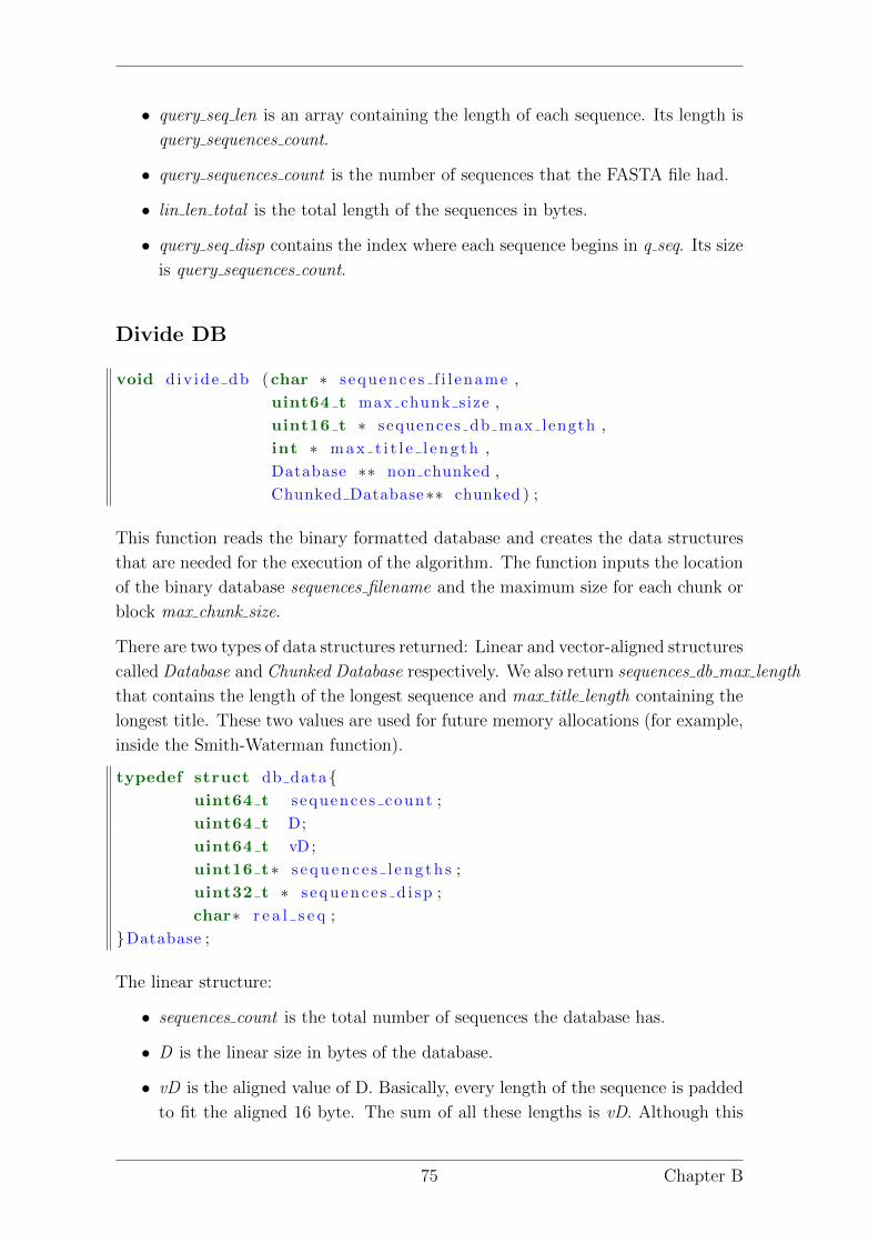
• query seq len is an array containing the length of each sequence. Its length is

query sequences count.

• query sequences count is the number of sequences that the FASTA file had.

• lin len total is the total length of the sequences in bytes.

• query seq disp contains the index where each sequence begins in q seq. Its size

is query sequences count.

Divide DB

void d iv ide db (char ∗ s equence s f i l ename ,

uint64 t max chunk size ,

uint16 t ∗ sequences db max length ,

int ∗ max t i t l e l eng th ,

Database ∗∗ non chunked ,

Chunked Database∗∗ chunked ) ;

This function reads the binary formatted database and creates the data structures

that are needed for the execution of the algorithm. The function inputs the location

of the binary database sequences filename and the maximum size for each chunk or

block max chunk size.

There are two types of data structures returned: Linear and vector-aligned structures

called Database and Chunked Database respectively. We also return sequences db max length

that contains the length of the longest sequence and max title length containing the

longest title. These two values are used for future memory allocations (for example,

inside the Smith-Waterman function).

typedef struct db data{uint64 t sequences count ;

uint64 t D;

uint64 t vD;

uint16 t∗ s equenc e s l eng th s ;

uint32 t ∗ s equence s d i sp ;

char∗ r e a l s e q ;

}Database ;

The linear structure:

• sequences count is the total number of sequences the database has.

• D is the linear size in bytes of the database.

• vD is the aligned value of D. Basically, every length of the sequence is padded

to fit the aligned 16 byte. The sum of all these lengths is vD. Although this

75 Chapter B

is an aligned value, it is included in this data structure due to further uses in

other functions.

• sequences lengths is the length of each sequence. The size of this array is

sequences count.

• sequences disp is the index where each sequence begins in the linear structure

real seq. The size of this array is sequences count.

• real seq is the linear structure of the database. Its size is D.

Figure B.1: Example of the structure of the non aligned data structures.

The vector aligned structured are a special type of data which we will work with.

These structures are used in the vectorized Smith-Waterman and are designed to

work with inter-sequence parallelisation as described in Rognes, 2011 [1]. Currently,

since the main algorithm is a variation from SWIMM [6], it parallelises up to vec-

tor length sequences simultaneously. This can be adjusted by changing a macro with

the same name. By default, it is set to 16.

typedef struct chunked db data{uint64 t vec t s equence s db count ;

char ∗∗ chunk b ;

uint32 t chunk count ;

uint32 t ∗ chunk vect sequences db count ;

uint16 t ∗∗ chunk n ;

uint32 t ∗∗ chunk b disp ;

Chapter B 76

uint64 t ∗ chunk vD ;

}Chunked Database ;

• vect sequences db count is the number of sequences the database contained

divided by 16 (vector length).

• chunk b contains the database for each chunk of database created. Therefore,

its size is chunk count. The division of the database depends on the parameter

“−b” passed to the program.

• chunk vect sequences db count contains vect sequences count for each of the

chunks created. Its size is chunk count.

• chunk vD contains the value of vD for each block. Its length is chunk count.

• chunk n contains the lengths of each sequence per block. Its size is chunk count.

• chunk b disp contains the index that identifies each sequence in chunk b. Note

that the length is aligned to a 16 byte boundary. Its size is chunk count.

To explain this further, let’s analyze the creation of the vectorized length array for

no chunk. Since we will group vector length (by default 16) sequences, we will select

the longest length of these sequences to represent their length. Therefore, since our

array is ordered in an ascending order, we select, every vector length sequences, the

last of the group. However, in order to fit these sequences in our registers, we can

make them multiple of 4, therefore we round them up to the nearest multiple of 4.

This process is explained in more detail in Fig. B.2.

For the rest of the data structures, their construction follow the same pattern.

If we consider more than one chunk, we will have a pointer pointing to the data

structures described for each chunk. For example, if we have two chunks chunk n

will be a pointer pointing at two of the explained vectorized length array.

Encoding Functions

The encoding reduces the alphabet of amino acids to a 16 character alphabet so that

we can fit two characters in a single byte. The functions are located in Conversor.c.

There are two functions, one for query and another for database. Since they work

in the same way only one will be explained.

void change encoding query (

char∗ query seq ,

uint64 t query count ,

uint32 t∗ query disp ,

uint64 t Q,

uint16 t∗ query l engths ,

77 Chapter B

Figure B.2: Example of the creation of the vectorized length array for one chunk.

Figure B.3: Example of the creation of the vectorized shift array for one chunk.

Assignment a ,

unsigned char∗∗ pt r que ry s eq r ed ,

uint64 t∗ ptr Q red ,

uint32 t ∗∗ pt r que ry d i sp r ed ,

uint16 t ∗∗ p t r qu e r y l e ng th s r ed

) ;

Although it has several arguments, the arguments are basically two Query structs

and Assignment. One if the Query struct is for the input and the other will be

output.

• Assignment is a structure that contains the replacements we have decided to

make in the alphabet. So that every 23 of the amino acids has an assigned

replacement, which can be the same amino acid (identity) or a different one

Chapter B 78

(swap).

• The input Query struct is composed by query seq, query count, query disp, Q

and query lengths. These contain the previously parsed query file using the

load query sequences function.

• The returned reduced query sequences is located in ptr query seq red.

• ptr Q red contains the total length of the reduced query sequences in bytes.

• ptr query disp red contains the index of each sequence.

• ptr query lengths red contains the length of each sequence in nibbles (or amino

acid count).

Figure B.4: Example of how we reduce the query considering we swap C to Y.

Filtering Functions

These functions are the ones used for the sequence filtering. There are two main

functions. They are located in preprocess.c and heuristic.c. Although there are

several types of filtering, the most complete example is explained.

void c r e a t e sh i f t ed copy nopad (char∗ seq ,

uint64 t D,

uint64 t seq count db ,

uint32 t∗ s h i f t ,

uint16 t∗ len ,

char∗∗ p t r s h i f t e d s e q ,

int ∗∗ pt r ex t en s i on ,

int ∗∗ p t r s h i f t ,

uint64 t ∗ t o t a l l i n e a r

) ;

This function takes the database and creates a data structures as explained in the

thesis in chapter 2. This new structure is important because if we want to use vec-

torization for sequence comparison, we need to consider every comparison possible

between the two sequences. Therefore, from the original sequence, we create 4 copies

of the original shifted by one character each. Also padding is added to the end to

79 Chapter B

ensure they are all multiple of 64 (this will improve the performance when loaded

into a 512 bit SIMD register).

• The input is defined by seq, D, seq count db, shift and len, which act as a

Query struct.

• ptr shifted seq will point to the new data structure.

• ptr extension defines the new length per sequence. Its size is seq count db.

• ptr shift contains the index that marks the beginning of each sequence. Its

size is seq count db.

• total linear contains the total length of ptr shifted seq in bytes. This will be

used in other functions in order to allocate the right amount of memory.

void f i l t e r s e q u e n c e s s h i f t e d t h r e s h o l d v e c t o r i z e d (char ∗query sequences ,

char∗∗ query headers ,

char∗∗ seq headers ,

unsigned short int ∗ query sequence s l eng ths ,

unsigned int query sequences count ,

unsigned long int Q,

unsigned int ∗ query disp ,

char∗ seq db ,

unsigned long int D,

unsigned short int ∗ s eq l en db ,

unsigned long int seq count db ,

unsigned int ∗ seq d i sp db ,

int ∗∗ pt r a s s i gned ,

double∗ e lapsed t ime ,

unsigned long int ∗ to ta l done ,

char∗ sh i f t ed copy ,

int ∗ extens ion ,

int ∗ s h i f t e d s h i f t ,

unsigned long int s h i f t e d l i n e a r ,

int th r e sho ld

) ;

This function filters the number of comparisons that will be made. Although there

exists other filtering functions, I will describe the vectorized one. However, all the

filtering functions have the same arguments. Only the internal algorithm is what

changes.

The threshold parameter sets the filtering limit. For each query-subject pair, if we

find more than threshold sub sequences of length 4 we consider it as a hit.

• The input is defined by a Query struct and a Database struct:

Chapter B 80

– The Query struct is defined by query sequences, query headers, query sequences lengths,

Q and query sequences count. It also includes the shifted copy obtained

from the function create shifted copy nopad.

– The Database struct is defined by seq headers, seq db, D, seq len db,

seq count db and seq disp db.

• The threshold parameters lets us decide what we consider as a hit. For each

query-subject pair, if we find more or equal than threshold sub sequences of

length 4 we may consider it as a hit.

• ptr assigned is a linear matrix of size query sequences countseq count db. If

the (i, j) value is 0, then we do not compute the alignment for query i and

subject j. We only compute the alignment if the value is greater or equal than

threshold.

• total done contains the count of the comparisons that will be made.

Smith-Waterman Functions

This function is the vectorized implementation of the Smith-Waterman algorithm.

It is a variation from the SWIMM program [6] that uses a inter-sequence paralleliza-

tion.

It is located in blastcore.c.

void smith waterman vector ized (Query∗ query ,

Chunked Database∗ db ,

char ∗ submat ,

int open gap ,

int extend gap ,

int num threads ,

int ∗ s co re s ,

double ∗ workTime ) ;

• The inputs are the following:

– Query contains the structures that defines a query file (previously ex-

plained).

– A Chunked Database struct that contains all the structures that defines

a chunked database.

– A scoring matrix submat. This can be BLOSUM or PAM.

– The cost of opening a gap open gap.

– The cost of extending a gap extend gap

81 Chapter B

– The number of threads that will be executed on the Xeon Phi num threads.

• scores is an array containing the numeric score for each alignment.

• workTime is the elapsed time in seconds.

• query length threshold is a threshold that defines the maximum length of each

sequence considered. By default it is set to the longest sequence.

Chapter B 82

Appendix C

Tables

Filtering Efficiency

Filtering comparison with different threshold values

Method P00762.1 P01008.1 P02232.2 P14942.2

BLPhi (t=1) 296562 406839 252308 307274

BLPhi (t=2) 145824 272657 107821 153593

BLPhi (t=3) 68388 170854 44923 72126

BLPhi (t=4) 31990 104966 18795 33321

Time comparison between Filters

Execution comparison for 1 sequence

Execution step Non-Vectorized Vectorized

Time(s) Time(%) Time(s) Time(%)

Load Query Sequence 0.001 0 % 0.004 0 %

Load db Sequence 0.313 1.6 % 0.4 4.1 %

Create shifted copy - - 0.141 1.4 %

Filter offload load 1.019 5.3 % 4.536 56.5 %

Filter execution 16.64 85.8% 3.033 31.1 %

Preprocessing SW 0.301 1.6 % 0.385 3.9 %

SW 1.131 5.8 % 1.253 12.8 %

Total 19.405 100 % 9.752 100 %

83

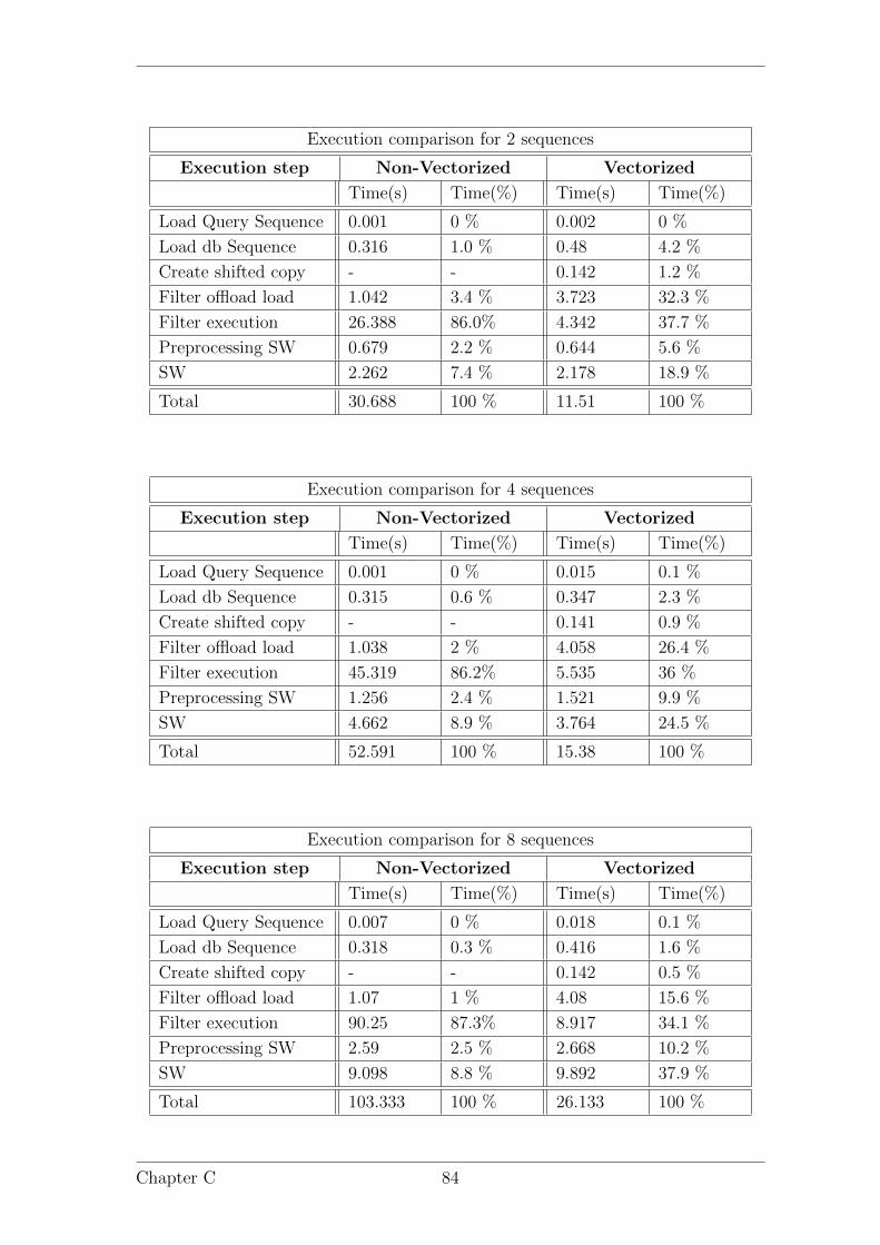
Execution comparison for 2 sequences



Load Query Sequence 0.001 0 % 0.002 0 %

Load db Sequence 0.316 1.0 % 0.48 4.2 %





SW 2.262 7.4 % 2.178 18.9 %

Total 30.688 100 % 11.51 100 %




Load Query Sequence 0.001 0 % 0.015 0.1 %

Load db Sequence 0.315 0.6 % 0.347 2.3 %


Filter offload load 1.038 2 % 4.058 26.4 %

Filter execution 45.319 86.2% 5.535 36 %


SW 4.662 8.9 % 3.764 24.5 %

Total 52.591 100 % 15.38 100 %





Load db Sequence 0.318 0.3 % 0.416 1.6 %


Filter offload load 1.07 1 % 4.08 15.6 %



SW 9.098 8.8 % 9.892 37.9 %

Total 103.333 100 % 26.133 100 %

Chapter C 84





Load db Sequence 0.340 0.2 % 0.481 1.1 %




Preprocessing SW 4.016 2 % 4.965 11.1 %

SW 19.646 9.5 % 19.171 42.9 %

Total 205.882 100 % 44.695 100 %

85 Chapter C

Time comparison with naive Smith-Waterman

Execution comparison with naive SW and filtering

Method 1 Seq 2 Seq 4 Seq

No Filter 37.523 73.413 150.75

BLPhi (t=1) 26.533 54.016 106.84

BLPhi (t=2) 0.713 1.883 2.51

BLPhi (t=3) 0.703 1.211 2.129

Time comparison with Other Algorithms

Execution comparison with Other Algorithms

Method 1 Seq 2 Seq 4 Seq 8 Seq 16 Seq 32 Seq

BLASTP 6.688 7.589 12.355 21.477 40.359 75.214

SW 5.857 7.701 15.412 27.904 61.213 115.123

BLPhi (t=1) 11.621 16.35 25.642 44.961 60.897 90.257

BLPhi (t=2) 10.982 14.965 23.674 39.370 56.21 81.257

BLPhi (t=3) 10.403 14.181 21.091 35.712 50.12 75.212

Chapter C 86

Accuracy comparison with Other Algorithms

Hit accuracy comparison with Other Algorithms

Sequence SW BLAST BLPhi

(t=1)

BLPhi

(t=2)

BLPhi

(t=3)

P00762.1 750 510 746 737 733

Random

(length=246)

2 2 2 1 1

P01008.1 310 253 305 291 265

Random

(length=464)

7 7 7 6 5

P14942.2 193 87 129 95 58

Random

(length=222)

2 5 2 1 1

P02232.2 49 53 48 40 32

Random

(length=144)

6 2 6 3 0

P03435.1 274 176 274 263 236

Random

(length=567)

9 8 9 8 8

87 Chapter 6

Análisis e Implementación de Algoritmo BLAST-Like para ...

Documents

Transcript of Análisis e Implementación de Algoritmo BLAST-Like para ...